Modeling Ozark Caves with Structure-from-Motion ...
143
University of Arkansas, Fayeeville ScholarWorks@UARK eses and Dissertations 8-2017 Modeling Ozark Caves with Structure-from- Motion Photogrammetry: An Assessment of Stand-Alone Photogrammetry for 3-Dimensional Cave Survey Joseph H. Jordan University of Arkansas, Fayeeville Follow this and additional works at: hp://scholarworks.uark.edu/etd Part of the Spatial Science Commons is esis is brought to you for free and open access by ScholarWorks@UARK. It has been accepted for inclusion in eses and Dissertations by an authorized administrator of ScholarWorks@UARK. For more information, please contact [email protected], [email protected]. Recommended Citation Jordan, Joseph H., "Modeling Ozark Caves with Structure-from-Motion Photogrammetry: An Assessment of Stand-Alone Photogrammetry for 3-Dimensional Cave Survey" (2017). eses and Dissertations. 2406. hp://scholarworks.uark.edu/etd/2406
-
Upload
khangminh22 -
Category
Documents
-
view
1 -
download
0
Transcript of Modeling Ozark Caves with Structure-from-Motion ...

University of Arkansas, FayettevilleScholarWorks@UARK
Theses and Dissertations
8-2017
Modeling Ozark Caves with Structure-from-Motion Photogrammetry: An Assessment ofStand-Alone Photogrammetry for 3-DimensionalCave SurveyJoseph H. JordanUniversity of Arkansas, Fayetteville
Follow this and additional works at: http://scholarworks.uark.edu/etd
Part of the Spatial Science Commons
This Thesis is brought to you for free and open access by ScholarWorks@UARK. It has been accepted for inclusion in Theses and Dissertations by anauthorized administrator of ScholarWorks@UARK. For more information, please contact [email protected], [email protected].
Recommended CitationJordan, Joseph H., "Modeling Ozark Caves with Structure-from-Motion Photogrammetry: An Assessment of Stand-AlonePhotogrammetry for 3-Dimensional Cave Survey" (2017). Theses and Dissertations. 2406.http://scholarworks.uark.edu/etd/2406
Modeling Ozark Caves with Structure-from-Motion Photogrammetry:
An Assessment of Stand-Alone Photogrammetry for 3-Dimensional Cave Survey
A thesis submitted in partial fulfillment
of the requirements for the degree of
Master of Science in Geography
by
Joseph Jordan
Arkansas Tech University
Bachelor of Science in Geology, 2015
August 2017
University of Arkansas
This thesis is approved for recommendation to the Graduate Council.
Dr. Jackson Cothren
Thesis Director
Dr. Mathew Covington Dr. W. Fred Limp
Committee Member Committee Member

Abstract
Nearly all aspects of karst science and management begin with a map. Yet despite this
fact, cave survey is largely conducted in the same archaic way that is has been for years - with a
compass, tape measure, and a sketchpad. Traditional cave survey can establish accurate survey
lines quickly. However, passage walls, ledges, profiles, and cross-sections are time intensive and
ultimately rely on the sketcher’s experience at interpretively hand drawing these features
between survey stations.
This project endeavors to experiment with photogrammetry as a method of improving on
traditional cave survey, while also avoiding some of the major pitfalls of terrestrial laser
scanning. The proposed method allows for the creation of 3D models which capture cave wall
geometry, important cave formations, as well as providing the ability to create cross sections
anywhere desired. The interactive 3D cave models are produced cheaply, with equipment that
can be operated in extremely confined, harsh conditions, by unpaid volunteers with little to no
technical training.
While the rapid advancement of photogrammetric software has led to its use in many 3D
modeling applications, there is only a sparse body of research examining the use of
photogrammetry as a standalone method for surveying caves. The proposed methodology uses a
GoPro camera and a 1000 lumen portable floodlight to capture still images down the length of
cave passages. The procedure goes against several traditional rules of thumb, both operating in
the dark with a moving light source, as well as utilizing a wide angle, fish eye lens, to capture
scene information that is not perpendicular to the camera's field of view. Images are later
processed into 3D models using Agisoft’s PhotoScan.

Four caves were modeled using the method, with varying levels of success. The best
results occurred in dry confined passages, while passages greater than 9 meters (30ft) in width,
or those with a great deal of standing water in the floor, produced large holes. An additional
experiment occurred in the University of Arkansas utility tunnel.

Acknowledgments
There is a long list of people who made this project possible. First and for most, I would
like to express my deep gratitude to my committee members Dr. Mathew Covington, Dr. Fred
Limp, and especially to my advisor Dr. Jack Cothren, for their continued support and guidance
throughout the research.
Also of paramount importance were the cave owners and park/plant managers, most of
which did not know me well at the time, but none the less were excited to be a part of this
experimental research. Specifically, I would like to thank Rita Smith, Faron Usrey, Caven Clark,
Brian Culpepper, and Doug Moore, who were all key in helping to grant me access to each of the
various study sites.
I am incredibly grateful to the University of Arkansas and the Center for Advanced
Spatial Technology for the software and resources used. I would like to specifically
acknowledge Vance Green at CAST, for introducing me to photogrammetry and the ins and outs
of PhotoScan and Unity game engine. A huge thankyou also, to Dr. Jason Tullis, for giving me
access to the Sirius server at CAST which was used to process all the models.
A special thanks to my grandparents Jackie and Eric Lewis-leaning who bought the
GoPro and Floodlight used in the project, at a time when my student budget was very tight.
This page would not be complete without also acknowledging Charla New and Kayla
Sapkota for getting me into “productive” caving and cave surveying in the first place.
I owe a great deal to all of the friends, family, and teachers that have pushed and
encouraged me throughout my education.
Finally, I would like to thank God as my source for everything--and for the opportunity
and the ability to take on this adventure.

Table of Contents
1. Introduction ............................................................................................................................. 1
1.1 Traditional Cave Survey ..................................................................................................... 2
1.2 TLS vs CRP for the Creation of 3D Models ..................................................................... 5
1.3 Brief History of Photogrammetry ...................................................................................... 7
1.4 Overview of Cave Survey Accuracy Standards ................................................................ 9
1.5 Study Area ......................................................................................................................... 13
2. Literature Review ................................................................................................................... 15
2.1 TLS for Cave Survey......................................................................................................... 15
2.2 Integration of TLS and CRP for Cave Survey ............................................................... 18
2.3 CRP and TLS for applications outside of Cave Survey ................................................. 21
2.4 CRP as Standalone Method for Cave Survey ................................................................. 23
3. Statement of the Problem ....................................................................................................... 24
3.1 Research Questions ........................................................................................................... 25
4. Materials and Methods .......................................................................................................... 26
4.1 Study Design ...................................................................................................................... 26
4.2 Image Acquisition .............................................................................................................. 29
4.3 Model Construction........................................................................................................... 33
4.4 Exporting Models to Useful End Products ..................................................................... 36
4.5 Control Target Survey and Georeferencing Models ...................................................... 38
4.6 Accuracy Assessment ........................................................................................................ 40
5. Results/Discussion ................................................................................................................... 42
5.1 Aspen Cave......................................................................................................................... 42
5.2 Birch Cave .......................................................................................................................... 45
5.2.1 Chunk 1......................................................................................................................... 46
5.2.2 Chunk 2......................................................................................................................... 49
5.2.3 Chunk 3......................................................................................................................... 49
5.2.4 Chunk 4......................................................................................................................... 50
5.2.5 Chunk 5......................................................................................................................... 51
5.2.6 Chunk 6......................................................................................................................... 52
5.2.7 Chunk 7......................................................................................................................... 52
5.2.8 Georeferencing the model ............................................................................................ 54

5.2.9 Accuracy Assessment ................................................................................................... 57
5.3 Cedar Cave......................................................................................................................... 59
5.4 Dogwood Cave ................................................................................................................... 64
5.5 University of Arkansas Utility Tunnels ........................................................................... 71
6. Conclusion ............................................................................................................................... 75
6.1 Research Question ............................................................................................................. 75
6.2 Real World Applications .................................................................................................. 77
6.3 Future Research Areas ..................................................................................................... 78
References .................................................................................................................................... 80
Appendix A: PhotoScan Processing Reports ................................................................................ 84

Table of Figures
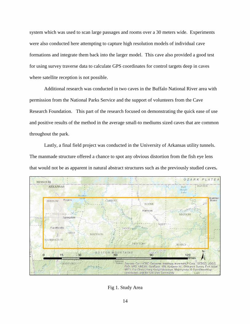
Fig 1. Study Area .......................................................................................................................... 14
Fig 2. GoPro Survey Rig ............................................................................................................... 30
Fig 3. Aspen Cave viewed as 3D PDF .......................................................................................... 43
Fig 4. 2D map created from orthomosaic based on X-Y extent of the 3D model ........................ 44
Fig 5. Exterior of cave .................................................................................................................. 47
Fig 6. Screen capture of the cave entrance with mossy rocks scattered along the creek bed and
“keep out” faintly visible on the rock face. ................................................................................... 47
Fig 7. Close up showing detailed model of tight crawlway into the cave. ................................... 48
Fig 8. Screen capture showing thin connection between exterior and interior portions of the cave
model............................................................................................................................................. 48
Fig 9. (Left) Illustrating missing left and right walls as the cave opened up into the expansive
room. (Right) Plan view of Chunk 2 with cave entrance at bottom of screen capture. ................ 49
Fig 10. (Left) Illustrating missing left and right walls in the middle of the large room. (Right)
Plan view of Chunk 3 with the top portion representing further in cave and bottom portion closer
to the cave entrance. ...................................................................................................................... 50
Fig 11. Shows marked improvement in the completeness of chunk 4 as the cave tapers off
towards a linear passage. (Right) Plan view of chunk 4 with top part representing the beginning
of linear passage. ........................................................................................................................... 51
Fig 12. (Left) This chunk of linear passage was very successful, besides the holes visible in the
plan view of the model. (Right) Plan view of chunk 5. ................................................................ 51
Fig 13. (Left) Screen capture looking down passage through chunk 6. (Right) Plan view of chunk
6..................................................................................................................................................... 52
Fig 14. (Left) Screen capture looking down passage through chunk 6 towards large column.
(Right) Plan view of chunk 7. ....................................................................................................... 53
Fig 15. High resolution model of cave column processed independently in its own chunk. ....... 54
Fig 16. Control Points ................................................................................................................... 55
Fig 17. Hole in the top of small room with elevated ceiling height............................................. 61
Fig 18. Crawling passage approaching two-way fork. ................................................................. 62
Fig 19. Traditional compass and tape survey overlaid over plan view of 3D photogrammetric
model............................................................................................................................................. 63
Fig 20. Reclassified Orthomosaic showing weak area with little data. ....................................... 65
Fig 21. Screen capture where the ceiling of the cave has been removed to show poor image
overlap through the bend. Images 5507-5510 were highlighted in red to show some of the worst
image overlap through the abrupt turn in the passage. Note that image 5509 was removed
because it was poorly focused creating a gap in the photos just before the bend. ........................ 65
Fig 22. Screen capture of model with ceiling removed to show holes in the floor in areas where
there was standing water. .............................................................................................................. 66
Fig 23. Unity game engine allowed for easy inspection of all parts of the mesh, allowing the user
to easily move forwards, backwards, left, right, up, or down, inside the model while
simultaneously changing the look direction of the camera. .......................................................... 67
Fig 24. Cave exploration simulation created in Unity. ................................................................ 68

Fig 25. Workflow designed using Esri’s model builder which automatically processes an
orthomosaic into a 2D footprint map. Orthomosaics that have been georeferenced allow for the
generation of maps with proper scale and orientation. Cross sections from the 3D model can
then be placed around the map to add information on the cave’s interior features. ..................... 69
Fig 26. Original 1994 compass and tape survey by W.Pierce and K. McCormick at top,
photogrammetric survey in middle, and newer 2016 compass and Disto survey by Kayla Sapkota
and Joseph Jordan on bottom. Sketching and cartography was completed independently by
Kayla Sapkota to ensure there was no bias introduced from the author. ...................................... 70
Fig 27. Severely distorted vertical support in the utility tunnel. .................................................. 71
Fig 28. View looking down model created with still images ....................................................... 73
Fig 29. Model generated with individual frames split from continuous GoPro video. ............... 75

List of Tables
Table 1 BCRA Accuracy Standards for Survey Line .............................................................. 12
Table 2 BCRA Accuracy Standards for Cave Passage Detail ................................................ 13
Table 3 Control Point Quality ................................................................................................... 56
Table 4. Survey Traverse Data .................................................................................................. 57
Table 5. Left-Right Measurements Comparison...................................................................... 58

1
1. Introduction
In the age of Google Maps, GPS, and Landsat, there are few places on the planet that
remain unknown. One of the final frontiers of exploration remains underneath our feet, where a
small 1 by 1 meter hole in the ground may give way into a 50 meter drop, filled with glistening
flowstone waterfalls, quiet pools, and unique cave adapted creatures not found anywhere else in
the world. Karst features serve as a window into the subsurface, providing us the opportunity to
study geology, speleogenesis, groundwater, as well as a plethora of rare, delicate, biological
resources.
These discoveries, however, are not nearly as significant without a frame of
reference. The first step in managing any natural resource, including caves, should be
ascertaining the locations and spatial extent of that resource. In many ways the fundamental
building block for all karst research is the cave survey.
From communicating the location of a colony of rare bat species to biologists, to
planning the rescue of a lost or injured person, to understanding the movement of polluted water
through the subsurface, and preventing the construction of highways and buildings only a few
meters above structurally unsound caverns, a map is required. At the most fundamental level,
cave maps are how we distinguish the passages that have been rediscovered “for the first time”, a
dozen times, from the new passages and rooms where truly no person has ever set foot before.
This project will explore the way cave surveys are conducted currently, and ways they
could be improved with modern technology using three dimensional models. Specifically, the
research will assess the practicality of photogrammetry as a quick, inexpensive, method for the
average cave survey volunteer to survey or at least document caves. The project also aims to
assess the accuracy of the method in comparison to traditional methods.

2
1.1 Traditional Cave Survey
Currently, cave survey methods involve using manual time consuming methods. The
archaic tools used, typically include a tape measure, transit compass/clinometer, and a hand
drawn paper map that is later scanned into a digital format. Survey stations are set up throughout
the cave within line of site of each other and the distance, azimuth, and clinometer numbers are
measured between stations. Azimuth and clinometer measurements are measured from the first
station to the station deeper into the cave (the front site reading), then usually double checked
with a back-shot in the reverse direction. The completed network of stations with azimuths,
inclinations, and distances is called a traverse. At each station along the traverse, the left, right,
up, down (LRUD) measurements are taken. Distance and bearing information help the sketcher
draw an accurate to-scale map of the survey line with all the survey stations. Clinometer data
and floor to ceiling measurements help the sketcher to draw cross sections and profiles. Lastly,
LRUD data allows the sketcher to interpretively draw in formations and passage walls in relation
to the survey line. Some sketches are done only to a relative scale, but most are done to-scale on
graph paper with proper orientation using a protractor.
Traditional cave survey is capable of quickly establishing survey lines which are
acceptably accurate for the application. Often a Sunnto clinometer/compass is used. Some
cavers also use the Disto-X, a specially modified Disto laser rangefinder upgraded to measure
distance, azimuth, and inclination, all at once with the click of a button. Whatever equipment is
chosen, it is likely that it is not as precise as the total stations most above ground surveyors are
familiar with. Many cave surveys must be completed with handheld equipment in highly
confined cave passages where the surveyor may not be able to sit up out of the prone position,
much less set up a large professional tripod based total station.

3
Even the best surveys using these handheld tools will result in some degree of error in
each shot. There are several methods of mathematically checking the survey for quality by
calculating loop closure error. The survey can then be adjusted by redistributing the error evenly
throughout the survey.
The fastest traverse method is called an open traverse. This is a series of survey shots
with no loops and where no or only one GPS point is known. With this method mathematical
checks are impossible. All other traverse methods provide the ability for a quality check to be
performed.
Probably the most common method of creating a mathematically checkable survey occurs
where the passage of a cave naturally creates a loop that closes on itself. Since the traverse starts
at a station, progresses throughout the loop and eventually ends back at the same station, all
changes in the X, Y, and Z coordinates between stations in the loop should theoretically sum to
zero. This is because, at this point, the cave surveyor has moved no more north than they have
south and no more east than west. (McCormac, 2004). This sum of changes will never actually
be zero. If the survey data is plotted, the ends of the survey loop will not actually connect
perfectly. This disparity is called the loop closure error, and is essential in determining the
quality of the traverse, and its precision with respect to the total length of the survey.
It should be noted however that the ability to complete a survey loop does not require that
the physical cave passage loops back on itself. Even in a completely linear passage, a survey
loop can still be created by starting at the last station in the survey and beginning a new traverse
in the reverse direction back to the first station, using all new stations.
A traverse does not actually even have to close geometrically for mathematical checks to
be possible. In some cases where a cave or tunnel has two entrances, a linear traverse can be

4
mathematically closed between two known GPS points. In this case, the traverse, if plotted, will
result in a final point which will not exactly match up with the second GPS coordinate. The
difference between this GPS coordinate and the final coordinates calculated from the traverse
represent the loop closure errors in the X, Y, and Z directions. In two dimensions, total loop
closure error can be calculated with basic Pythagorean theorem (Mcormac, 2004). McCormac
further indicates that in a loop with geometric closure, precision is then described by the total
loop closure error divided by the perimeter of the figure created by the traverse. This idea can
also be adapted into a 3D version of total loop closure error. In this case, the total closure error
will be defined as Eclosure, and can be calculated with the 3D version of the Pythagorean Theorem
Eclosure = √(Ex2+Ey
2+Ez2), where Ex,
Ey, and Ez represent the error in each coordinate direction.
For traverses that do not close, perimeter can be replaced with survey length giving the equation
precision= Eclosure / Survey Length.
If the precision of the survey is acceptable, and there are no obvious blunders in the data, these
errors can be distributed throughout the survey to minimize their effect using several adjustment
methods such as the least squares adjustment method.
The traverse method for establishing cave survey lines is a mature and effective one.
However, acquiring details about the passage walls, profiles, and cross-sections is time intensive
and ultimately relies on the sketcher’s experience at interpreting and hand drawing the trend of
the cave walls between survey stations. Because of this, a cave sketch done by two different
sketchers on the same day, though similar, will never be the same. In the widely-recognized
cave survey book, On Station, author George Dasher said that “More cave passage has been
resurveyed because of poor sketch than for any other reason.” (Dasher, 1994). Because of the
time it takes, cross sections are typically only drawn at certain intervals or at key areas. One

5
final downside of free hand sketching is that the full glory of spectacular formations is typically
reduced to a basic 2-dimensional symbol from the legend.
1.2 TLS vs CRP for the Creation of 3D Models
3D models created from terrestrial laser scanning (TLS) and close range photogrammetry
(CRP) offer an alternative solution or at least a valuable supplement to traditional cave survey.
Three dimensional scanned models are often both faster to produce than a sketch, and more
informative. The models can provide cross sections anywhere, they capture unique flowstone
formations and columns in the caves interior, and all this information is captured in a manner
which is non-subjective, unbiased, and scientifically repeatable.
TLS is now widely recognized as a mature, reliable method to scan caves. Highly
accurate LIDAR systems utilize infrared remote sensors capable of scanning hundreds of
thousands to even a million points a second in total darkness. Onboard computers calculate the
range to each point in the tiny fraction of a second flight time that it takes for each laser to travel
to the target and back. This technology for the moment however, is incredibly expensive. Most
TLS systems currently range from $20,000 for units like the Faro Focus to over $120,000 for
Leica Scan Stations. Some other notable manufactures include Riegl, Trimble, and
Zoller+Frohlich GmbH, all of which have multiple models of terrestrial LIDAR units suitable for
scanning caves. TLS devices, besides being expensive, also often require extensive training, are
too valuable and susceptible to damage to risk operating in wild cave environments, and are very
limited in mobility. Most models designed by the manufactures mentioned above are tripod
based units, weighing 20-40 pounds, also requiring large power sources (Idrees & Pradhan,
2016). The final products created from laser scans are accurate, but often lack color and texture
quality. It should be noted however, that new developments suggest great future potential for

6
TLS in cave survey including newly emerging devices such as Teladynes VLP-16 “Puck”, a
100meter range LIDAR scanner that scans 300,000 points per second and weighs less than 2
pounds. The device costs $8,000, significantly less than the systems mentioned above. In 2016
Leica also released a similar handheld TLS scanner called the BLK 360. This device gathers
360,000 points per second with a range of 60 meters and only weighs 2 pounds. The BLK360
costs just under $16,000, which is much more affordable compared to most other TLS devices
(Higgins,2016).
Close range photogrammetry is defined by photogrammetric operations that are
conducted from less than a meter all the way up to 300 meters from the target (Mathews, 2008).
“Close” in this sense is a relative term describing the short distance compared to aerial
photogrammetry which commonly uses images taken at high altitudes from the scene. While
CRP is a bit more challenging to work with in the total darkness of cave passages, it is cheaper,
has better color resolution, and only requires equipment that is tough, waterproof, and easily
transported through tight cave passages. The method is robust and versatile with the capability
to work within the minimum distances of most TLS equipment. The method even be used under
water where most TLS systems, besides special bathymetric LIDAR’s, fail to function. In
addition to this, it takes little to no training to equip the average cave survey volunteer to acquire
a set of overlapping images of a passage. Later, all that is required is one designated
experienced person who has the adequate knowledge to process the photos into 3D models using
photogrammetric software. It is the opinion of the author, that while the market is flooded with
new highly impressive TLS designs, photogrammetry has been overlooked as a much cheaper,
more practical method of basic cave survey and documentation, which is primarily conducted in
harsh space-limited environments, by unpaid volunteers in their spare time.

7
1.3 Brief History of Photogrammetry
Since the middle to late 1800s photogrammetry has been practiced as a method of
obtaining reliable information about physical objects using photographic images. In 1909
Eduard Dolezal founded the International Society for Photogrammetry (Ghosh, 1992). Later on,
in response to the first two world wars, photogrammetry rapidly developed as a reconnaissance
tool. Photogrammetry began as more along the lines of what we would think of as “aerial image
analysis”, using stereographic aerial imagery spread apart on a page to create a parallax. With
specialized stereogram glasses, this provided the ability to view landscapes and objects in the flat
image in 3D. During WWII, this allowed image analysts to detect rocket sites and other military
structures which were not as apparent in 2D photographs (Howard and Rogers, 2012). After the
war, civilian applications developed in geological surveys, mapping, and forestry. In the 1970s,
photogrammetry shifted away from physical hard copy photographs towards processing digital
images on a computer screen (Cooper, 1998). Soft copy photogrammetry, as it is now called
today, has progressed to the point where we are now able to make fully 3 dimensional models on
a computer simply by processing a collection of overlapping digital images.
In the past, it was critical that soft copy photogrammetrists use metric cameras and avoid
moving light sources, shadows in the imagery, and off-nadir shots (Matthews 2008). While
these are still good guidelines to follow, the technology has evolved to the point where many of
these limitations are no longer strict requirements. Additionally, proper image matching and
scaling in traditional soft copy photogrammetry required the use of specialized scale frames and
networks of carefully pre-placed and pre-surveyed photogrammetric target control points.
(Westoby, Brasington, Glasser, Hambrey, & Reynolds, 2012).

8
These targets had to be manually identified in photos along with other common points in
the images to facilitate the “re-sectioning” process, where camera positions and orientations are
calculated. (Westoby, et al. 2012). Alternatively, if control points were not set up, every camera
pose and position had to be measured and known as the photos were taken. (Westoby, et al.
2012).
Today with advances in the technology including the development of structure-from
motion (SfM) methods, no control information of any kind is required to construct a
photogrammetric model. This method uses a highly redundant self-calibrating bundle
adjustment to approximate image positions and scene geometry automatically and
simultaneously, simply from the overlapping image pairs (Westoby, et al. 2012).
Rather than manually creating and selecting control targets and other common points
within the input photographs, the software automatically identifies and matches thousands of
common points, termed “key points” in the input photos. These key points are identified and
grouped into features through the use of object recognition algorithms such as the Scale Invariant
Feature Transform (SIFT) operator created by Dr. David G. Lowe. SIFT uses identified key
points to extract features which are “invariant to image scaling and rotation and partially
invariant to changes in illumination and 3D camera view point” (Lingua, Marenchino, & Nex,
2009).
Using SIFT or several other similar algorithms, the key points are linked and encoded
as tracks. Tracks relate the 3D coordinates of a point in the scene to the corresponding 2D
coordinates in the input images. The aligned photos are then used to estimate camera pose, then
target object geometry is calculated to produce point cloud layout of the three-dimensional scene
(Furukawa, 2013).

9
Although this process is much faster and less tedious, models derived from the SfM
approach at first lack scale and orientation. While they may be correct within the relative “image
space” coordinate system of the model, for many applications the next step is to align this image
space to a real-world object-space coordinate system using a 3D similarity transformation
(Westoby 2012). To transform the model from the relative space to an absolute coordinate
system there must be at least three recognizable points in the model, of which precise real world
coordinates are known. This can be done post hoc, by surveying distinct natural objects in the
scene, or a priori using a small network of high contrast control targets.
1.4 Overview of Cave Survey Accuracy Standards
A major goal of this project will be to assess the accuracy of photogrammetry as a survey
method. To make any claim that the proposed method has or does not have “acceptable
accuracy”, it is important to first investigate what the currently held standards and expectations
for cave surveys are. Traditional surveys have been conducted much the same way for the past
60 years. A bulletin from the 1962 National Speleological Society states that a transit and steel
tape survey should have all points within a circle of error with a radius of 0.14% as long as the
survey line. (Schwinge, 1962). For a 1000 meter survey, that leaves an acceptable loop closure
error of 1.4 meters at most. Modern cave survey standards in the United States tend to be vague
and vary largely upon the specifications for the survey given by the cave owner. As an
American system has not yet been created, often a widely-recognized survey grading system
created by the British Cave Research Association is used as a framework to evaluate the quality
of survey products. The hierarchical BCRA system is illustrated in tables 1 and 2 on the next
page.

10
The accuracy of these surveys hinges on the precise reading of angles with as little error
as possible. Many attempts have been made to assess the accuracy of cave survey techniques
over the years but this is often a difficult question to answer because there is no perfect control
with which to compare to. Much of the literature concerned with assessing cave survey accuracy
is not totally conclusive and simply presents a statistical analysis of standard deviation and other
measures of central tendency for survey loop closure adjustments. (Thrun, 2009). However, in a
recent study of the accuracy of a large collection of surveys conducted in West Virginia, it was
found that no survey met the BCRA grade 5 standards (Thrun, 2009).
Accuracy, as described in this paper, will be defined as a measure of how close a position
or measurement is to its true value. This should not be confused with precision, which refers to
the closeness of results to each other with regards to repeated attempts to measure the same
position or distance. It should also be noted that there are different types of accuracy and errors
in the realm of geospatial science and cave surveying. A model must first be evaluated based on
its relative or “point to point” accuracy within the image space. This type of accuracy is
concerned with comparing the distance between two or more recognizable points in the virtual
model versus the same distance between those points in real life (“Positional Accuracy,” 2003).
Relative accuracy can also be used to assess the difference between a point cloud model
generated through the use two different methods such as TLS and photogrammetry. In this case
relative differences between the point clouds can be described through the Hausdorf Distance.
The Hausdorf Distance measures the degree of mismatch between two point clouds by taking
each point in the first point cloud and finding the point that is furthest away from it in the second
point cloud and vice versa the in opposite direction. The maximum distance between any point
in the first point cloud from any point in the second cloud is then said to be the Hausdorf

11
Distance. (Huttenlocher, Klanderman, & Rucklidge, 1993). The results of this operation cannot
determine whether a method is “more” or “less” accurate than another, but can determine how
much the model or point cloud deviates from another which is generally assumed to be more
accurate.
To the contrary, absolute accuracy is a measure of how accurately an object is positioned
with respect to its true position in an absolute reference frame. For this type of accuracy
assessment to occur, the relative image space coordinate system must be aligned to a real-world
coordinate system using a 3D similarity transformation. (“Positional Accuracy,” 2003).
Just as there are different kinds of accuracy, there are also different types of errors.
Systematic error is error which has a non-zero mean. It is constantly biased by the same amount
in one direction and accumulates over time. An example would be an uncalibrated Suunto
compass transit which always shoots 1 degree off in a specific direction. Systematic errors start
off small and negligible for small surveys but become enormous on long surveys (Thrun, 2009).
Fortunately, if the cause of the error can be recognized, it is often very easy to fix. Random error
on the other hand, consists of small errors in measurements which are not biased to a direction
and are directly related to the precision limitations of the measurement instrument. All
measurements besides counting have some degree of random error. (Thrun, 2009). If these
errors are small, they tend to balance out over a survey and can be modeled with a normal
(Gaussian) curve. (Thrun, 2009). The most important kind of error to avoid in cave survey is
large random errors called “blunders.” Writing down a number incorrectly, or reading the wrong
side of a clinometer, among several other things can cause serious blunders that can drastically
throw off a survey.

12
Table 1 BCRA Accuracy Standards for Survey Line
Grade 1 Sketch of low accuracy where no measurements have been made.
Grade 2 May be used, if necessary, to describe a sketch that is intermediate in
accuracy between Grade 1 & 3.
Grade 3 A rough magnetic survey. Horizontal & vertical angles measured to ±2.5º;
distances measured to ±50 cm; station position error less than 50cm.
Grade 4 May be used, if necessary, to describe a survey that fails to attain all the
requirements of Grade 5 but is more accurate than a Grade 3 survey.
Grade 5 A Magnetic survey. Horizontal and vertical angles measured to ±1º;
distances should be observed and recorded to the nearest centimeter and
station positions identified to less than 10cm.
Grade 6 A magnetic survey that is more accurate than grade 5. A Grade 6 survey
requires the compass to be used at the limit of possible accuracy, i.e.
accurate to ±0.5º; clinometer readings must be to the same accuracy.
Station position error must be less than ±2.5 cm, which will require the
use of tripods at all stations or other fixed station markers.
Grade X A survey that is based primarily on the use of a theodolite or total station
instead of a compass, (see notes 6 and 10 below) A Grade X survey must
include on the drawing notes descriptions of the instruments and
techniques used, together with an estimate of the probable accuracy of the
survey compared with Grade 3, 5 or 6 surveys.

13
1.5 Study Area
This study takes place in several caves throughout the Ozark Plateau Region in Northern
Arkansas. This region is dominated by limestone and dolomite formations, chiefly the karstic
Boone formation which consists of interbedded limestone and chert. It is the presence of this
thick carbonate formation which facilitates karst development, hosting 78% of the caves found in
the Buffalo River National Park. (Hudson, Turner, & Bitting, 2011).
The first experimental pilot study took place in a small cave located in Bentonville, AR.
This cave provided an opportunity to conduct the very first cave experiment and determine
whether the idea of using photographic images from a GoPro camera to model a cave would
work at all. Two trips were made to this cave which worked as an initial testing ground for
various hardware and software methods and settings.
The next part of the study took place in Searcy County, AR where the method was
utilized in a cave with much larger rooms and passages. This cave has an interesting history and
is so large that it was surveyed by the Department of Defense with intentions of using it as a
possible nuclear fallout shelter. This part of the work focused on the limits of the proposed
Table 2 BCRA Accuracy Standards for Cave Passage Detail
Class A All passage details based on memory.
Class B Passage details estimated and recorded in the cave.
Class C Measurements of detail made at survey stations only.
Class D Measurements of detail made at survey stations and wherever else needed
to show significant changes in passage dimensions.
14
system which was used to scan large passages and rooms over a 30 meters wide. Experiments
were also conducted here attempting to capture high resolution models of individual cave
formations and integrate them back into the larger model. This cave also provided a good test
for using survey traverse data to calculate GPS coordinates for control targets deep in caves
where satellite reception is not possible.
Additional research was conducted in two caves in the Buffalo National River area with
permission from the National Parks Service and the support of volunteers from the Cave
Research Foundation. This part of the research focused on demonstrating the quick ease of use
and positive results of the method in the average small-to mediums sized caves that are common
throughout the park.
Lastly, a final field project was conducted in the University of Arkansas utility tunnels.
The manmade structure offered a chance to spot any obvious distortion from the fish eye lens
that would not be as apparent in natural abstract structures such as the previously studied caves.
Fig 1. Study Area

15
2. Literature Review
A large body of research exists that describes the use of TLS systems as a method to
survey caves. There are also abundant instances where photogrammetry has been integrated with
TLS for cave survey. Outside of cave survey, photogrammetry is often used as a stand-alone
method for many applications, as well as being integrated with TLS for finished products.
However, there has been only sparse research experimenting with the use of photogrammetry as
a completely independent low cost means for basic cave survey and documentation.
2.1 TLS for Cave Survey
The following list of works is in no way meant to be exhaustive as there has been an
enormous amount of research into using TLS for cave survey.
One of the first attempts on record began in 1988 where researchers used one of the first
TLS scanners, the Minolta VI scanner, to model Altamira Cave in Cantabria, Spain. The project
took over 10 years to complete due to the difficulty of using the scanner which had only about a
meter range, and a large amount of the work that had to be done manually (Idrees & Pradhan,
2016).
About decade later in 1999, a group of researchers out of the United Kingdom used an
automated TLS system designed by Measurement Devices Limited to survey the rock shelter of
Cap Blanc in southwest France. This Autoscanning Laser System (ALS) consisted of a tripod
with an automated rotating mount carrying a Leica Disto laser range finder. The team completed
two scans of the rock shelter which had a resolution of 2cm (Brown, Chalmers, Saigol, Green, &
D’errico, 2001).

16
One of the first TLS cave mapping projects to be conducted in the U.S was at Chapel’s
cave in southwestern Oregon. This project used the Cyrax 2400 scanner and is one of the first
projects that tested the feasibility of TLS for cave survey. After the model was created, highly
accurate horizontal and vertical cross-sections were extracted. (Idrees & Pradhan, 2016).
Moving forward, more TLS survey research was published in 2009 regarding work done
in Wonderwork Cave, which represents one of the only TLS cave scans conducted in Africa.
Wonderwork cave is a very large dolomite solution cavity located in the Northern Cape Province
of South Africa. The cave was scanned with a Leica HDS 3000 primarily to set up a framework
for archaeological research at the site. The scan took only three days of field work and
comprehensively mapped all the cave walls and excavation sites. (Rüther, et al., 2009).
Also published in 2009, was a project which used a Riegl LMS-Z420I to model
Dachstein South Face cave in Austria. This research was distinct in that, instead of a historical
preservation motivation, it focused on studying water storage capacity of the cavities and
structural geology of the mountain. Another distinguishing feature was the more extreme and
wild nature of the cave. While TLS surveys are typically done in easier horizontal “walk-
through” caves, this project pioneered laser scanning in complex partially vertical survey
environments. Part of the logistics included transporting the scanner through tight spaces as well
as with researchers down a 60-meter rappel all with dripping water from overhead (Buchroithner
& Gaisecker, 2009).
Two years later, another team in Austria studied Marchnhohle cave using the z+f Imager
5006i terrestrial laser scanner to create very high resolution (1.66mm) scans of the cave. These
scans were significant to studying speleogensis and micro to macro cave morphology features

17
that are not normally recorded in a traditional cave survey (Roncat, Dublyansky, SpöTl, &
Dorninger, 2011).
Also published in 2011 is work by Aaron Addison in the historic longest cave system in
the world--Mammoth Cave in Kentucky. Addison successfully scanned a 4km section of the
cave merging 135 different point clouds made up of a total of 18 million data points. The point
cloud was later reduced to 500,000 points for visualization as most software currently cannot
handle such a large dataset. As a part of the discussion of the research, several limitations were
mentioned regarding using laser scanning in the cave. It was noted that the project was difficult
to complete due to the high humidity which caused condensation on the equipment, thermal
gradient from the airflow into the cave causing out of range values for the temperature
compensators on the device, sand and rock fragments getting into mechanical components such
as tripod legs and mounting instruments, as well as the normal hazards of equipment getting
dropped and broken in the wild cave environment. Addison also discussed the issues with
getting the scanner to scan large vertical sections in mammoth dome where the scanner had
difficulty sighting the high angle survey stations. Lastly, Addison mentions the limited
mobility of the system which weighs 18kg and is a highly fragile sensor. The project was
completed using the readily available power supply along the caves tour trail, but had this not
been available, the device would have required two 12-volt auto type batteries to power it,
exacerbating the weight and logistical awkwardness of transporting the already cumbersome
equipment. Despite the limitations this research went far in proving the maturity of TLS and its
feasibility for scanning very long cave systems (Addison, 2011).
Research published in 2012, discusses the use of a FARO Photon 20/120 to scan
Eisriesenwelt the largest ice cave in the world. Due to global warming, the ice is beginning to

18
melt in the cave. While there is some intrinsic value in preserving the landmark, it also serves as
an important tourist attraction, drawing around 150,000 people a year to journey through the 42
kilometers of tangled icy corridors and massive halls. The “World of Ice Giants” as it is also
called was scanned to quantify the amount of existing surface ice to be used as a baseline to
monitor future ice loss. The research also has the potential to identify areas prone to hazard.
Lastly, a complete fly through of the cave captured the amazing icy cavern for posterity (Milius
& Petters, 2012).
2.2 Integration of TLS and CRP for Cave Survey
It is widely recognized that both TLS and CRP have their advantages and disadvantages.
As such, there is a large body of research discussing the integration of the color and texture
quality of photogrammetry with the accuracy of TLS for photorealistic cave surveys.
A project that first pioneered this idea occurred Baiame Cave in New South Wales,
Australia. The work, which was published in 2004, developed a workflow for creating a high
resolution realistic model through the combined us of a Riegl LMS-Z210i scanner and an
inexpensive Nikon coolpix digital camera. For this project, control points were first surveyed
with a total station and used to automatically register the texture information from the
photogrammetry to the accurate 3D geometry of the laser scan. While the scans were taken in
Australia at the site, they were processed independently by a team in Canada. The final model of
the cave and its various aboriginal rock art and cave paintings were captured for posterity as well
as research on prehistoric living (El-Hakim, Fryer, & Picard, 2004).
A very similar workflow was used in 2009 in two caves in Spain: Las Caldas and Peña de
Candamo. This was one of the first of many 3D cave modeling projects that would be conducted
in Spain. This research utilized the same multi sensor approach where control points where first

19
surveyed with a total station and then used to combine scans from a Trimble GS200 scanner with
images from several digital cameras. This research used convergent images taken with the
traditional rules of photogrammetry, independent high resolution close-up images of the cave
texture, and panoramic images using a fish eye lens to provide 360 degree panoramic images of
the cave. The method used in the Spanish caves was particularly useful for capturing the
abundant delicate Paleolithic art forms—but the researchers also recognized the potential use for
studying cave morphology and speleogensis. The authors also discuss future possibility for
improvement with the software utilizing the Scale Invariant Feature Transform (SIFT) algorithm
(González-Aguilera, Muñoz-Nieto, Gómez-Lahoz, Herrero-Pascual, & Gutierrez-Alonso, 2009).
In 2010, also in Spain, Parpalló Cave was scanned using a joint photogrammetric and
TLS process. This cave is one of the oldest known and most important international world
heritage sites. The laser scan data was acquired with a FARO LS 880HE scanner with a range of
75 m and a resolution of up to 3mm. This point cloud was registered with the photogrammetric
point cloud using artificial white spherical targets provided by the manufacturer. This greatly
improved on the existing 2D hand drawn sketch which was later determined to have poor metric
accuracy when compared with the data from the TLS survey (Lerma, Navarro, Cabrelles, &
Villaverde, 2010).
In the same year, research was published regarding the modeling of the Bronze Age Cave
Les Fraux in Perigord, France. The cave is one of the most studied caves in Europe containing
numerous artifacts and engravings. This team used a network of reference GPS points outside the
cave, along with surveyed spheres and coded targets to register the photogrammetric model with
the TLS model. A FARO Photon 80 and 120 were used for the laser scan, and a Canon EOS 5D
with 28 and 85 mm lenses was the primary camera for acquiring images for the photogrammetric

20
model. This camera was equipped with a flash ring to collect imagery in the darker parts of the
cave. For this project, texturing had to be conducted manually as an automated method of
identifying corresponding points in the images was not yet readily available (Grussenmeyer,
Landes, Alby, & Carozza, 2010).
A similar approach to the above examples was used in research published in 2011
discussing the modeling of two more Spanish caves Buxu Cave, and La Loja cave. These two
caves were surveyed using a Nikon D80 Camera, Canon 500D, and a Trimble GX. The authors
of the paper emphasized the importance of cataloguing Paleolithic art and integrating them in a
GIS for better management. The authors also discussed the advantages of capturing these places
and presenting them virtually for the many people with disabilities who cannot visit the caves
themselves (Gonzalez-Aguilera et al., 2011).
In 2013 more research was published at another Spanish location, Can Sadurní cave. For
the Can Sadurní project, control targets were first surveyed with a Leica TCR 705 total station.
After this, large scale structures such as storage silos and a combustion structure were surveyed
using photogrammetry. The cave itself was scanned with a Reigel 420i sensor and combined
with texture information from photographic images to create a photorealistic model. The team
noted the difficulty of acquiring images with good radiometric quality and suggested that a
structured light system could resolve the problem in future research. The project successfully
created a spatial frame with which to incorporate with a GIS for continued archeological
excavation. The model also helped in analyzing the stratigraphy of the cave and the gradual
process of sedimentation that infilled the cave (Núñez, Buill, & Edo, 2013).
Another study done in 2013 studied the Gomantong caves in Malaysia. The Gomontong
caves are comprised of two caves Simed Hitam (Black Cave) and Simid Puteh (White Cave).

21
Because the publically available ASTER digital elevation model had pretty low spatial
resolution, the researchers used aerial drone based photogrammetry on a Gate Wing X100 UAV
to model the mountain side containing the caves. After this was complete, a Faro Focus 3D
scanner was used to scan the caves. The model took 69 scans and produced over 5 billion data
points. The model was integrated with traditional cave survey techniques to create highly
accurate plan view surveys of the caves. It was also useful for establishing volume densities for
the caves, and establishing the greater volume density in Simed Hitam. Researchers were
interested in why there was such a large difference in volume densities for the caves, as Simed
Hitam has a much higher volume density than what would be expected from natural hydrologic
processes. It is believed that the biology of each cave played a significant role in the differing
morphologies of the caves, as Simed Hitam has much larger swift and bat populations. The
activities of these animals as well as the increased amount of guano may have played a part in
quicker erosion and weathering of the cavity. Additionally, researchers noted that the scan was
such good resolution that individual animals and nests could be identified. The authors hope to
develop an automatic algorithm in the future that automatically acquires bio inventory count data
by species (McFarlane et al., 2013).
2.3 CRP and TLS for applications outside of Cave Survey
Photogrammetry has been used by itself for cultural heritage preservation for many years.
One such example was research published in 2005 were researchers photogrammetrically
modeled aboriginal pictographs and petroglyphs. This was especially useful for capturing the
pictographs as they represent art that is painted onto a 3-dimensional rock surface, not a flat
planar surface. Furthermore, the research proved that the operation could be conducted with

22
satisfactory results using nothing but a cheap Nikon Coolpix 3100 three-megapixel camera
(Chandler & Fryer, 2005).
Other interesting uses for photogrammetry include modeling steep mountain terrain. This
idea was mentioned in 2011 by N. Kolecka. This research project involved modeling the steep
western slopes of the Kóscielec Mountain with a Nikon D80 SLR 10 MP camera. The
photogrammetry was compared to a TLS which were found to have similar results. The final
product demonstrated the significance of photogrammetrically derived digital terrain models in
creating detailed representations of the steep rock faces to be utilized for planning rock climbing
routes. The author also discusses potential uses in tourism, engineering, geomorphology, and
studying rock fall and avalanche hazards (Kolecka, 2011).
Another alternative use for photogrammetry is in modeling historical architecture. One
example would be the Beufort Castle in Lebanon, where researchers tied together several
hundred photos from a variety of cameras to model the castle. Some of the images were oblique
photos taken by helicopter using the CIPA 3x3 rules as a guideline. The result of the project was
a 3D virtual re-creation of part of the castle, created from both modern and historical images that
included parts that are now destroyed or buried (Grussenmeyer & Jasmine, 2003).
Similar work was published a year later by the same author, concerning several more
case studies in France such as modeling the Gallo-Roman Theatre of Mandeure using a
combination of TLS and dense stereo image matching as well as Engelbourg Castle with a
similar methodology. In the discussion of these two projects the authors said the slow scanning
speed and small field of view of the Trimble GX TLS made it not suitable for covering the large
study site. The 2-meter minimum scanning distance also added limitations for scanning between

23
some of the dense collections of ruined buildings. The TLS point cloud was then completed by
integrating it with a photogrammetric one (Grussenmeyer et al., 2012).
Recently, in 2014, Yang Liu and Julian Kang from Texas A&M University experimented
with photogrammetry as completely independent method of surveying the interior of buildings.
They divided the first floor of the target building into 20 sections which were scanned with a
Canon EOS Rebel T3I SLR camera mounted to a tripod with a panoramic head. Sticky notes
were used to efficiently image the rooms with the right amount of overlap between photos. The
researchers found that the model had an average difference of -.43% in comparison to the CAD
drawing provided by the University. The final results portrayed the features of the interior of the
building very well and at an acceptable level of accuracy considering the low budget nature of
the research, and that TLS was not used.
2.4 CRP as Standalone Method for Cave Survey
In Le Grotte De Castellana Spain, researchers tested both the TLS method, and an
independent photogrammetric method with a Nikon D100 camera and found that both methods
had pros and cons—the TLS method had more accurate geometry, while the photogrammetry
had better color and texture resolution (Caprioli, Minchilli, Scognamiglioi, & Strisciuglio, 2003).
A couple of the same researchers who mapped Baime cave in 2004, as mentioned in the
previous chapter on integrated TLS and CRP surveys, also went back and mapped the same cave
a year later to experiment with using photogrammetry alone to model the cave. The researcher’s
first surveyed photogrammetric targets with a total station then used a 6 Megapixel Kodak
DCS460 and a 3 Mega pixel Nikon Coolpix camera for image capture. The images were then
processed in Leica Photogrammetry Suite. The authors noted that by using the digital cameras
alone, much of the field work logistics were made easier as they didn’t need to carry the

24
previously used bulky scanner and its power supply. The main concern for digital image
correlation in the project was whether there would be enough texture on the surface for
automatic generation of the key points. This remains an issue for using photogrammetry as a
stand-alone method in caves with homogenous wall texture and geometry. Overall, no firm
conclusions could be drawn as to which method better characterized the cave (Fryer 2005).
Recently in 2012 another low budget, photogrammetry project was conducted in El Niño
Cave in Spain. The researchers used a Nikon D90 to model a panel section of a cave with
numerous Paleolithic paintings mostly of animals. While the final results were not quite as
accurate as a laser scan, the authors felt that the product appropriately accomplished the needs of
the project to document and archive the rock art (Moreno & Garate, 2012).
3. Statement of the Problem
Cave survey is vitally important to karst science and management. Yet while survey
methods have evolved rapidly above ground, cave survey remains much the same. Hand drawn
surveys take time, skill, and are limited in what they can capture and how precisely they can
capture it. 3D modeling using LIDAR scanners offers a whole new way of capturing entire
environments with great detail and accuracy, but also brings its own set of challenges. If
traditional survey seems archaic, LIDAR can seem rather impractical and “over the top.” While
LIDAR could be the way of the future, it currently involves the use of incredibly bulky and
expensive devices that are not built to work in confined passages, or when partially submerged in
mud and water. While large tour caves are currently being scanned with TLS systems, this
methodology is not yet practical for the average cave survey volunteer in the average cave.
Advances in digital photogrammetry offer the opportunity to study a new method of obtaining 3-
dimensional cave models. The methodology discussed in this paper is designed to improve on

25
the limited capabilities of traditional survey, and provide similar results to laser scanning, while
using equipment that is inexpensive, rugged, and easy to use. This thesis project will test and
evaluate the use of fisheye lens photogrammetry as a survey method in caves, a research area
that is not well documented in the fields of photogrammetric and karst science.
3.1 Research Questions
Two major research questions will be addressed. Firstly, under what if any conditions
can pure stand-alone photogrammetry be used to create interpretable 3D models of interior cave
structures? There must be an emphasis on the word interpretable here, as it is likely that almost
any set of related overlapping images will produce something in Photoscan. In this case,
successful interpretable models should be largely complete, aesthetically attractive, and must
correctly represent the environment in such a way that the viewer can understand the general
layout of the cave. The study will explore the effects of cave size, water, and mazy or sinuous
caves on the quality of the finished model. Various capture methods, camera settings, and
processing parameters will also be explored.
A secondary question will be to establish whether or not models created using the
proposed method are acceptably accurate with respect to the application of cave survey, and
compared to the currently held standards and expectations for traditional cave survey. Part of
answering this question will involve comparing 2D maps derived from photogrammetry to
traditional survey maps. After models are georeferenced, real world measurements will be
compared to measurements in the virtual model. Finally, the error values in the PhotoScan
processing reports of each model with be evaluated to determine the precision of both the
photogrammetric method, and any control networks used to georeferenced the models.

26
4. Materials and Methods
4.1 Study Design
The first objective of this study was to ascertain under what if any conditions can pure
photogrammetry be used to create useful interpretable 3D models of cave structures. For this
research to occur, there was first a brief study of the photogrammetric process in general. After
this study was complete a very rough experiment was conducted to provide a “proof of concept”
and see if overlapping images from a GoPro camera taken in a dark cave would in fact create a
model at all. While the first attempt failed, modifications were made to the software, hardware,
and methodology until the first successful cave model was produced. Gradually, this
methodology was tweaked and tested in several different caves of varying sizes and
characteristics. These caves were given the aliases “Aspen”, “Birch”, “Cedar”, and “Dogwood”
to protect their true names and locations.
Photogrammetry was chosen over other cheap 3D modeling techniques such as using a
modified Xbox Kinnect for several reasons. The GoPro is both more portable and more rugged
than the modified Xbox Kinnect system which is not waterproof and requires being connected to
a laptop computer during its operation. Photogrammetry also allowed for the creation of full
color textured models as opposed to the often-lower quality color and texture information in
models from the Kinnect’s RGB camera. Photogrammetry also uses regular images, without any
changes to the programming of the GoPro Camera. Google Tango was also briefly considered,
but was dismissed do to its limitations in only being available on a few android phone and tablet
models.
While Autodesk 360 Recap was used in the first experiments, Agisoft PhotoScan quickly
became the software package of choice for the project. 360 Recap from Autodesk, offered an

27
initial user-friendly method of making photogrammetric models from input photos, but was
essentially a “black box” with very few options for controlling how the images were aligned and
processed. PhotoScan allowed for camera based calibration, complete control over every step in
the processing, a wide variety of post processing tools, the ability to georeference models and
export them to a wide variety of formats, and the ability to process the data in “chunks.”
PhotoScan was also chosen over Pix4D, from Pix4D Inc., due to the substantial price difference,
as well as PhotoScan’s reputation for being better used for convergent photogrammetry as
opposed to the parallel stereo photogrammetry that Pix4D excels at.
The camera chosen for the project was a GoPro camera which has a wide angle fisheye
lens. While this camera inevitably creates more distortion than a conventional camera with a
standard lens, it also allows for the simultaneous capture of cave floor, left and right walls, and
ceiling all at once with a large amount of overlap between photos. Conventional cameras excel
at modeling a wall, or a ceiling, or the ground, and when pointed directly perpendicular to these
targets can provide highly accurate measurements. However, these cameras require a much
higher quantity of photos to achieve the overlap required to model a tunnel or cave passage
environment. It is likely that the nature of the wide angel fisheye lens, as well as the relatively
new support added for this style of lens in software like PhotoScan, is what made this project
possible (Higgins, 2015).
Initial tests used a bright helmet mounted headlamp but it was quickly realized that an
even brighter light was needed. There are many bright spotlights on the market, but instead a
floodlight was chosen so that the large amount of light would be spread evenly across the
environment instead of being concentrated in one area. A water-resistant portable rechargeable
floodlight was chosen so that it could be used in cave environments.

28
While the successful construction of several cave models was exciting, it was important
to ensure that such models were easy to manipulate, navigate, explore, and share with others
effectively. Several end products were tested such as interactive 3D PDFs, Unity Game Engine
(Unity Technologies) models, Fly throughs and rotating models generated with ESRI’s
ArcScene, as well as more classic 2D maps based on the X-Y extent of the model. Viewing of
the models in virtual reality was also considered but was not pursued in this project.
The secondary objective of the research was to examine the meaningful quantitative
information that could be retrieved out of georeferenced models and assess the accuracy of that
information. Obtaining GPS coordinates for ground control points presented a new challenge in
cave environments which have no satellite signal. The term “GPS” is used in this paper in the
place of the more correct term “GNSS” due to its more widespread familiarity among cavers and
karst scientists. Two different methods were developed for georeferencing the models. The
first, a quick and dirty method for small caves, involved simply surveying three control targets
around the entrance area of the cave. The second method was more intensive involving the use
of trigonometry and cave survey line traverse data to calculate the coordinates of control targets
throughout the cave.
An additional challenge was found in attempting to assess the accuracy of cave models
and how closely they represented the true cave. To do this, measurements in the model were
compared to real life in-cave measurements. 2D maps were also extracted from the model and
compared with cave survey maps constructed with traditional survey methodology. While these
products were similar, it was hard to say that either one was more correct than the other, or that
either one accurately represented the highly abstract shape and structure of the caves.
Unfortunately a LIDAR unit could not be acquired to compare the photogrammetric point cloud

29
to a TLS point cloud. So that any distortion from the fisheye lens would be more recognizable,
the method was also utilized in manmade tunnel.
4.2 Image Acquisition
The method used to acquire images of cave passages was non-invasive involving the use
of a simple “survey rig” which consisted of a GoProHero3+ Black Edition camera securely
mounted to a 1000 lumen Husky cordless rechargeable floodlight, with an attached Iphone 6
connected to the GoPro via Wi-Fi. A GoPro handlebar mount was used to attach the GoPro to
the floodlight, while Velcro command strips secured the iPhone 6 to the back of the floodlight.
This survey rig was a vast improvement over the initial experiments which used only a GoPro
and Princeton Apex headlamp mounted to a caving helmet.

30
The Husky rechargeable floodlight was
chosen due to its inexpensive price ($50),
tough waterproof resistant housing, cordless
portable nature, as well as its ability to
illuminate cave passages far better and more
evenly than spotlights of similar brightness.
The floodlight was able to produce
1000lumens for about 3 hours, which was far
longer than necessary to take the images of
each cave.
The Iphone 6 was cased in a LifeProof
case and mounted to the back of the floodlight
for live feedback to make sure images were
clear and consistent overlap was achieved
between shots. Live feedback and camera
settings were controlled on the iPhone using
GoPros “capture” app via a WiFi connection
with the camera.
The camera used throughout the project was the GoProHero3+Black edition. This was a
relatively inexpensive camera purchased for around $350. According to GoPro’s website, when
shot on 12MP wide setting, the camera has a 122.6 degree field of view (“Hero3+ Black Edition
Field of View Information”). The EXIF data from the camera indicates that it has an estimated
3mm focal length, which can be viewed as roughly equivalent to a 17.2 mm lens on a 35mm
Fig 2. GoPro Survey Rig

31
camera. The cameras aperture (f-stop) is fixed at f/2.8. Lastly, ISO and exposure time (shutter
speed) settings are variable and automatically controlled for the best results by the camera.
Some obvious advantages to this camera, besides the price, include the easy mounting
options which allowed for its attachment to the floodlight, as well as the extreme ruggedness of
the device. This camera, while attached to the survey rig, was easily fit through tight spaces,
smacked against rocks, and pulled through muddy cave passages with little concern. The camera
is fitted with a wide angle fisheye lens which brought both pros and cons. There is undoubtedly
greater distortion using a fisheye lens especially around the edges of each photos compared to
the lenses found in more traditional DSLR (digital single-lens reflex camera.) However, the
12MP resolution, coupled with PhotoScan’s automatic camera calibration technology, largely
mitigated the effects of this distortion. The upside of this lens was its ability to capture more of
the environment with each individual image, allowing for better image overlap and more
information about how objects in the scene are connected. While DSLR style cameras work well
for capturing a wall or ceiling by itself, the wide-angle fisheye lens was chosen for its advantages
in capturing entire “tunnel” environments where it can gather information on the floor, left wall,
right wall, and ceiling all simultaneously without ever directly looking at any of them. While it
may be possible achieve similar tunnel photogrammetry models with a DSLR camera, it would
most likely take a great deal more photos and would likely be far more challenging to perform
image matching on the larger set of photos taken with the sensor pointed in widely varying
directions (Higgins, 2015).
The fixed f-stop of the camera was also an advantage in that it insured that the
aperture size remained consistent throughout the data collection. Keeping the sensor size
constant is an important photogrammetric rule of thumb. While the maximum limit of the ISO

32
setting can be adjusted, the both ISO setting and the shutter speed are automatically controlled by
the camera to achieve the most optimal results. While it would be nice if these settings could be
manually controlled, the automatically chosen settings worked well for the purposes of this
system which was designed to be used by the average cave survey volunteer who may or may
not have extensive photography knowledge.
It should be noted that there was some experimentation with both time lapse photography
which allowed for the automatic capture of photos every few seconds, as well as the use of video
walk throughs of caves. Videos were split into hundreds of individual frames which allowed for
an extremely quick capture of long passages with guaranteed overlap between frames. This
video methodology was proven valid as a quick and method of data capture which sacrificed
quality for speed.
The primary image capture setting in this research however, was the 12MP wide single
photo method which took more time, but resulted in higher quality images and models.
The capture procedure used was highly unconventional in comparison to traditional
photogrammetry where camera shots are always taken perpendicular to the target and a moving
light source is never used. As it would be impractical to scan the left wall, right wall, ceiling,
and floor, independently, and furthermore improbable that the software could recognize and tie
the four scans taken at right angles to each other together, this study approached the problem a
different way. For all the models created in this research the GoPro was transported largely
parallel to its targets, progressing down the center of passages to acquire depth information by
moving through the area. This procedure does not fit into either the parallel or convergent
classifications for traditional stereo photogrammetry. This idea combines structure from motion
(SfM) methodology with Simultaneous Localization and Mapping (SLAM), a computer vision

33
concept largely studied in autonomous robotics and self-driving cars (Urban & Hinz, 2016). The
idea is very similar to the way humans process the dimensions of a hallway and localize
themselves and their progress as they move through it. While the wide-angle fisheye lens
introduces some distortion, it also better facilitates the SfM SLAM photogrammetry approach
allowing the camera to have some limited peripheral view of the walls, ceiling, and floor, all
while remaining pointed in the forward direction down the center line of the passage.
Some experimentation occurred with taking side shots and ceiling facing shots with little
success. A method of capturing large rooms was attempted by walking around the perimeter of
the room while facing the camera such that it was pointed at an imaginary object in the center of
the room. This technique was also not very successful, probably due to the challenge of getting
the light to reach the other side of the room. For cave formations and other points of interest in
cave models, like columns, images were taken from all angles of the feature which was
processed as its own “chunk” and then integrated with the larger model. The utilization of
“chunks” is further discussed below.
4.3 Model Construction
Initial experiments used Autodesk 360 Recap which is a simple free online software
program which allows users to upload images to the website to be processed into models. This
worked great for the first few tries but was essentially a “black box” in that there was no control
over how the model was processed. Due to the highly-limited nature of 360 Recap, PhotoScan
was quickly adopted as the software of choice for model construction. The PhotoScan software
can be purchased at anywhere from $59-179 for the standard version, and $549-$3,499 for the
professional version. While the standard version is all that is needed to simply create cave

34
models, the professional version is required for more advanced functions such as the use of
control points to create georeferenced 3D models and orthomosaics.
All models were processed using PhotoScan version 1.2.3 except for the utility tunnel
models which were processed in version 1.2.6. Finished models were later viewed in versions
1.2.6 and 1.3 so that more recently developed features such as the ruler measuring tool could be
utilized. Created by the Russian company Agisoft, PhotoScan offers an interactive software
program which allows the user to control every aspect of each step in the processing. PhotoScan
stood out over other software such as Pix4D due to its inexpensive price, user friendly menus,
and reputation for being good at modeling images taken using convergent photogrammetry as
opposed to parallel photogrammetry.
To speed up the processing time, models were built and stored on the Sirius server at
CAST. This provided more physical memory (25 Gigs of Ram) as well as enabling processes to
be controlled and monitored remotely from the author’s iPhone. Even with the extra memory, it
was necessary to create cave models in “chunks” which were later aligned and merged together
to form complete cave models. Model construction followed the standard PhotoScan workflow:
add photos, align photos, build dense cloud, build mesh, build texture (Agisoft, 2016). After
settings were chosen, the pipeline was typically executed in the proper order automatically using
the batch process tool. There was some light experimentation with using python code to
automate batch processing and store a record of provenance and all settings and parameters used.
However, this idea was eventually dismissed as being outside the scope of the research.
Before processing, photos were first divided into chunks and imported into PhotoScan.
Each chunk was processed independently using the same sequential workflow and then
aggregated into one model at the end of the processing.

35
Photo alignment was set to high accuracy, pair preselection disabled, with a default key
point limit of 40,000 and a default tie point limit of 4,000. A mask was not used. It is during
this alignment process that the software automatically detects the make and model obtained from
the EXIF data and makes the appropriate calibrations based on the collection of images and the
specifications of the specific camera used to capture them.
The dense point clouds for most models were created using the “medium” quality setting
as dense point clouds created with the quality set to “high” often used up 100% of the available
physical memory leading to very long processing times, and in some cases, failure to process.
Depth filtering varied between moderate and aggressive to retain the most points while filtering
noise out from outlier points and floating model pieces not attached to the main model. Depth
maps were not stored for reuse.
For creation of the mesh the surface type was set to arbitrary, which is recommended for
closed structures such as buildings or caves (Agisoft, 2016). The mesh models were created
using the dense cloud as the source data, using the default medium face count. Interpolation was
enabled with point classes set to “all”.
Texture was created using the generic mapping mode from all cameras with the blending
mode set to Mosaic. Texture size and counts were set to the defaults and color correction was not
used.
Individual chunks were aligned using the camera based method, high accuracy setting,
and default point limit of 40,000. Images were not preselected. After alignment, both the dense
clouds and models were merged together. Occasionally the area where two chunks were fused
together was noticeable. One possible method of getting rid of this is to merge just the point

36
clouds, then build the mesh for the entire merged point cloud. This however, almost always
required more physical memory than one was available and resulted in a failure to process.
Lastly, most models required some post processing that could not be automated. The
gradual selection tool was first used to get rid most of the extra floating pieces around the model.
After this, any extra unwanted pieces of the model were removed using the rectangle selection
tool. This tool also served as a quick means of creating temporary cross section views of the
model.
4.4 Exporting Models to Useful End Products
Cave models created and viewed in PhotoScan are no doubt useful and informative by
themselves. Finished structures can be rotated and viewed from every angle with the ability to
zoom in on areas of interest. While it is possible to view the interior of models in PhotoScan,
navigating and exploring the inside of the caves proved to be somewhat awkward and frustrating.
Additionally, these products are difficult to share with people who do not have PhotoScan. For
this reason numerous exportable end products were evaluated.
Accessing the file, “export model” menu in PhotoScan allows the user to export the
model in a wide variety of file formats. Models were often first exported to 3D PDF, which
allowed for them to be easily shared and viewed by anyone with a recent version of adobe
reader. These 3D PDF files typically only take up a 60-160 megabytes. The somewhat compact
nature of this data could potentially allow for 3D PDFs to be stored in a cave database alongside
more traditional 2D maps, cave entrance photos, and other data.
To view cave structures in ArcScene, they were first exported from PhotoScan as VRML
(.wrl) files. These files were then imported to ArcScene using the Import 3D files tool which
outputs to a multipatch feature class. Models first appear without any color and must be replaced

37
using the editor toolbar. After replacement with the same model, the model will show up in
color, allowing the original no-color model to be deleted. The camera was the re-centered on the
new model using the center on target tool. Using the animation toolbar in conjunction with the
fly function, fly virtual fly though videos of the cave were recorded. The animation toolbar was
also used to create videos of caves spinning 360 degrees as if they were spinning on a turntable.
The Unity game engine provided the most interactive and immersive environment for
viewing the caves. The game engine can be downloaded for free, and finished game applications
can be shared easily. Unity allows for the user to utilize the arrow keys on the keyboard to fly
through the model at their own pace, stopping and turning around or going down a different
passageway as they choose. This proved to be the most useful way to explore models and to
examine areas where the mesh was incomplete or of poor quality.
To do this, a .3DS file was exported from PhotoScan and imported as an asset to Unity.
Basic flat terrain was created long with a directional light in the sky to provide some exterior
light around the cave. A first-person controller was equipped with a flashlight which allowed for
a cave exploration simulation to be made where the user could walk around the dark cave in first
person with only the small light to see.
In order to share the caves in a more traditional 2D map view, ArcMap was used to create
2D footprint maps. Using PhotoScan, the orthomosaics were first built, georeferenced if survey
data was available, and then exported to .tif format. A model was designed in ESRI’s model
builder which automatically takes the orthomosaic, reclassifies all non-zero pixel values to “1”,
converts from raster to vector, uses a positive buffer to buffer out any internal holes, and finishes
with an equal and opposite negative buffer to return the outside boundary of the cave to its
original extent. The result of this is a 2D footprint map of the cave’s extent in the X-Y plane.

38
Cross sections were then made from the 3D model and added to various locations on the
footprint map. If the orthomosaic was georeferenced before it was exported, a north arrow and
scale was added.
Along with these final products, final reports were generated within PhotoScan which
include detailed information on calibration coefficients, camera residuals, RMSE of the point
clouds, as well as a breakdown of errors in the control network.
4.5 Control Target Survey and Georeferencing Models
Photogrammetric models initially only possess a very rough scale based on the focal
length of the camera. To get meaningful and accurate information such as measurements of
passage dimensions, areas, volumes, locations, and orientations, models must be georeferenced.
To do this, X,Y,Z coordinates must be entered at various unique points in the model. While early
attempts used distinct natural cave features, or objects like water bottles for targets, it was found
that the printable coded targets found within the Agisoft software worked best. The targets are
easy to spot and are all slightly different so that each target represents a different unique marker
number in the software. The coding of the targets allowed the software to scan and detect all the
targets without the user having to manually find and click the center of each one. Ideally, control
targets should be placed evenly across the surface of the photogrammetric survey area, and then
simply surveyed with GPS equipment. Clusters, or linear placement of control points is not
recommended. However, in this case, the highly linear nature of caves and tunnels made this
distribution of targets unavoidable. An additional challenge was surveying control targets while
inside caves where there is no GPS satellite reception. Several methods were developed for
georeferencing underground models despite the lack of GPS availability.

39
The first method was a quick and dirty one where 3 targets where placed around the
entrance of the cave and surveyed to give a rough idea of location and distances in the model.
The second method used a traverse to create a traditional cave survey line from one
external GPS coordinate at the cave entrance, to multiple internal survey stations throughout the
cave. All External GPS coordinates were obtained using a highly accurate Leica GS15 with a
CS15 Controller and a GS15 Pillar Tripod. The rapid static method was used throughout the
research to obtain data in the Arkansas State Plane North coordinate system. It should be noted
however, that the accuracy of the initial GPS point only effects absolute accuracy and the quality
of coordinate locations, while lengths, widths, heights, and volumes of cave passages rely
entirely on the accuracy of the traverse data. Cave dimensions and volumes can be obtained with
only data from a traverse, simply setting the GPS point to some coordinates in the general
vicinity of the cave, or even (0,0,0). A change in the initial coordinate will shift all other control
points in the same direction by the same amount.
To calculate the (X,Y,Z) coordinates of all survey stations along the survey line,
distances, azimuth, and clinometer data were used with the following equations inside of a
Microsoft Excel document. These equations are similar to the standard equations used to convert
spherical coordinates to Cartesian coordinates but are adapted to work with a degrees from the
horizontal component instead of a degrees from the vertical component. The equations were
derived by the author and tested with trial and error for validity. Because the sine of an angle is
equal to the cosine of its compliment, the resulting set of derived equations represents the exact
same set of standard equations used to transform from spherical to Cartesian coordinates except
that all trigonometric functions have been replaced with their cofunction.

40
ΔX= [R*cos(ζ)]*cos(α) (1)
ΔY= [R*cos(ζ)]*sin(α) (2)
ΔZ= R*sin(ζ) (3)
In these equations, the delta values represent the change in X, Y, and Z coordinates from
the first station to the second survey station, which are calculated from the azimuth value in
radians, α, the zenith value in radians, ζ, and the true distance between the stations in meters, R.
Cave survey data is typically taken in azimuth degrees, vertical degrees from horizontal,
and feet between stations. All coordinates were taken in the state plane Arkansas North (meters)
coordinate system, so all distances measured in feet were first converted to meters. Excel works
in radians mode only, so all azimuth degrees and degrees from horizontal were first converted to
their equivalents in radians before they could be used in the above equations.
4.6 Accuracy Assessment
Once models were created and georeferenced, some measure of quality and correctness
needed to take place. To start with, footprint maps from the 3D models were overlaid and
visually compared to any existing cave survey maps. This process was done in Microsoft Word,
where the white paper background of the cave sketch could be made transparent leaving only the
sketch of the cave. The both graphics were manually sized and positioned for the best possible
fit and examined for similarity. This allowed for a basic visual assessment but no quantitative
assessment in accuracy. Additionally, even if one quantified the exact deviation between the
photogrammetrically derived map, and the hand drawn map, one could not actually say that one
is more correct than the other anyway. The best control to compare to would be a LIDAR scan,
but this equipment was not available for the project.

41
A more quantitative approach was taken in Davis Creek cave, where left and right
dimensions at survey stations where measured inside the georeferenced model and compared to
LRUD data acquired in the cave. While this cave was meant to be the “flagship” cave of the
project in terms of assessing the quality of georeferenced cave models, the large passage widths
ended up pushing the limits of the system resulting in many holes in the side walls and ceiling.
Regardless, the comparison in passage width measurements derived from the virtual model and
widths measurements measured in real life were compared simply noting where the distance left
or right of the station could not be properly measured due to a hole in the model on the side wall
at that particular location.
As previously mentioned, it is difficult to assess whether an abstract structure like a cave
is really modeled correctly because there is no perfect representation with which to compare it.
Nearing the end of the research, a manmade tunnel was also modeled. Whereas it was nearly
impossible for the eye to detect distortions in the cave images, bent and warped vertical support
beams were quickly recognized in the tunnel images allowing for a test to be done to see how the
PhotoScan software would handle these distortions. The trend of the tunnel was straight
compared to the natural unpredictable cave passages, which meant that any deviation from this
straight line would represent error in the model. While the trend was in the X-Y plane was very
consistent and predictable, some slight complexity was added by the floor which slopes gently
towards a central drain followed by an upward slope.
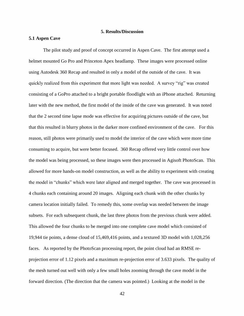
42
5. Results/Discussion
5.1 Aspen Cave
The pilot study and proof of concept occurred in Aspen Cave. The first attempt used a
helmet mounted Go Pro and Princeton Apex headlamp. These images were processed online
using Autodesk 360 Recap and resulted in only a model of the outside of the cave. It was
quickly realized from this experiment that more light was needed. A survey “rig” was created
consisting of a GoPro attached to a bright portable floodlight with an iPhone attached. Returning
later with the new method, the first model of the inside of the cave was generated. It was noted
that the 2 second time lapse mode was effective for acquiring pictures outside of the cave, but
that this resulted in blurry photos in the darker more confined environment of the cave. For this
reason, still photos were primarily used to model the interior of the cave which were more time
consuming to acquire, but were better focused. 360 Recap offered very little control over how
the model was being processed, so these images were then processed in Agisoft PhotoScan. This
allowed for more hands-on model construction, as well as the ability to experiment with creating
the model in “chunks” which were later aligned and merged together. The cave was processed in
4 chunks each containing around 20 images. Aligning each chunk with the other chunks by
camera location initially failed. To remedy this, some overlap was needed between the image
subsets. For each subsequent chunk, the last three photos from the previous chunk were added.
This allowed the four chunks to be merged into one complete cave model which consisted of
19,944 tie points, a dense cloud of 15,469,416 points, and a textured 3D model with 1,028,256
faces. As reported by the PhotoScan processing report, the point cloud had an RMSE re-
projection error of 1.12 pixels and a maximum re-projection error of 3.633 pixels. The quality of
the mesh turned out well with only a few small holes zooming through the cave model in the
forward direction. (The direction that the camera was pointed.) Looking at the model in the

43
reverse direction, there were many small holes and black areas representing no data. These
represent shadow areas that the camera could not see while moving through the cave in the
forward direction. Small dark rings were also visible where the chunks were welded together.
To make the model universally shareable, it was exported to 3D pdf format. This exported file
took up 59.7 MB of storage space and allowed for anyone with adobe reader to interactively
view a slightly lower resolution version of the model.
Fig 3. Aspen Cave viewed as 3D PDF
While rotating the cave and viewing its exterior was simple, scrolling through the cave to
the very back was difficult, and as one zoomed to the very back, the model began to disappear.
Because of this, an attempt was made to also create an accompanying traditional 2D cave map
based on an orthomosaic constructed from the X-Y extent of the 3D model. The intent here was
to both present an easy to understand plan view of the cave, as well as various 3D cross section
views of the model. While cross sections can be made anywhere in PhotoScan, this first

44
experiment used the individual chunks leftover from creation of the model as rough cross
sectional views.
Fig 4. 2D map created from orthomosaic based on X-Y extent of the 3D model

45
5.2 Birch Cave
Birch Cave offered an opportunity to study the limits of the methodology in a much
larger cave. Still images were taken around the entrance of the cave, and down the first 150-160
meters of passage to a large column. These images were divided into 7 chunks containing 75 to
144 images per chunk. Each chunk contained around 10 images in common with the previous
chunk to ensure they could be aligned and merged properly. In total, the model took just under
19 hours to process. The finished product consisted of 151,239 tie points, a point cloud of
66,782,453 points, and a model with 4,435,017 faces. According to the PhotoScan processing
report the point cloud had a RMS re-projection error of 2.57 pixels with a maximum re-
projection error of 84.078 pixels. The resolution of the model was listed as 1.64mm/pixel.
While the completed model does represent the general trend of the cave passage, there were
numerous large holes in the side walls and ceilings. Passages exceeding 9-11meters (30-35ft) in
width, especially large rooms over 30 meters (100ft) wide resulted in missing left and right
walls. An attempt was made to capture the large room just after the entrance by moving around
the perimeter of the chamber while pointing the camera towards the center, but there was not
enough light to light up the far walls. Instead a linear path was made through the large room,
attempting to capture as much information on this path as possible as it lead up to a more
confined linear passage. Sections of this more confined linear passage turned out much better
than the large room, but had challenges of their own. While average ceiling height remained
consistent, there were several areas of the ceiling which shot up dramatically. These vertical
features ascending from the main walking passage were difficult to capture. Even with effort
taken to maintain overlap, for the most part, any picture taken with the camera pointed upwards
was not aligned with the rest of the images facing down passage resulting in many holes where

46
the vertical extent of the ceiling could not be imaged. At the end of this passage, a large column
was modeled which turned out complete but was not very high resolution. Because of this, a
separate individual model was created of this feature to capture it in the greatest detail possible.
To share the results of the 3D model universally with others a 3D rotating model and virtual fly
through of the cave was created in ArcScene. However, color could not be added to this model,
possibly do to the large amount of faces in the mesh.
A challenge of this project is to present results which are inherently 3D in the 2D format
of this research paper. Due to the large size of the cave model and the differing characteristics of
each of the 7 chunks used to reconstruct the cave, they will each be discussed separately.
5.2.1 Chunk 1
Chunk 1 modeled an approximately 20 meter by 20 meter area outside of the cave. This
took 144 photos and created a point cloud with over 7 million points. Despite numerous
shadows in the images, the quality of this first exterior model was very good. The creek bed,
trees, survey equipment, and six control targets are clearly visible along with the words “keep
out” on the rock face near the entrance. The purpose of this large entrance area chunk along with
the 6 targets was to allow for georeferencing of the entrance area if georeferencing the rest of the
cave was not possible. In the end only one of these control points was used.

47
Fig 5. Exterior of cave
This first part of the model captures the tight crawlway entrance into the cave and successfully
aligned and merged this thin narrow piece of mesh between the large exterior model and large
interior model much easier than expected.
Fig 6. Screen capture of the cave entrance with mossy rocks scattered along the creek bed and
“keep out” faintly visible on the rock face.

48
Fig 7. Close up showing detailed model of tight crawlway into the cave.
Fig 8. Screen capture showing thin connection between exterior and interior portions of the cave
model.

49
5.2.2 Chunk 2
The second chunk modeled the tight entrance as it gradually descends and opens up into a
large room. 141 images were used to model this section of the cave which produced a point
cloud of about 15.7 million points. A large stalagmite at the end of the chunk was used as the
second control point. While the ceiling and floor turned out well, a significant majority of the
left and right side wall were missing. In this first large room, it was difficult to capture the entire
room in the field of view of the camera. It was also challenging to light up the other side of the
room at such a great distance.
Fig 9. (Left) Illustrating missing left and right walls as the cave opened up into the expansive
room. (Right) Plan view of Chunk 2 with cave entrance at bottom of screen capture.
5.2.3 Chunk 3
Chunk 3 represents the central part of this large chamber. This chunk is an even more
extreme example showing the floor and ceiling along the linear path of the camera, but leaving
out the nearly all of the sidewalls of the cave. This section of the cave was created from 107

50
images which created a point cloud of roughly 11.7 million Points. This section captured a rill
developing across the floor of the cave from water draining towards the entrance.
Fig 10. (Left) Illustrating missing left and right walls in the middle of the large room. (Right)
Plan view of Chunk 3 with the top portion representing further in cave and bottom portion closer
to the cave entrance.
5.2.4 Chunk 4
The fourth section of the model represents the end of the large room as the cave walls
begin to taper off into a more confined linear passage of about 10-11 meters (35 feet) of width.
This section used data from 76 images and created a point cloud of 7.6 million points. This
chunk is much more complete in nature than previous sections modelling the ceiling, left wall,
and boulder covered floor. It is however missing a significant part of the right wall which
extends a good distance from the path of the camera.

51
Fig 11. Shows marked improvement in the completeness of chunk 4 as the cave tapers off
towards a linear passage. (Right) Plan view of chunk 4 with top part representing the beginning
of linear passage.
5.2.5 Chunk 5
Chunk 5 marks a shift from the large beginning chamber unto the first of three sections of
linear passage. This confined passage way had much better results with complete left and right
walls. There were however, several holes in the ceiling due to abrupt changes in ceiling height.
The chunk took only 62 images which generated a point cloud of 6.9 million points.
Fig 12. (Left) This chunk of linear passage was very successful, besides the holes visible in the
plan view of the model. (Right) Plan view of chunk 5.

52
5.2.6 Chunk 6
Chunk 6 was the second section of linear passage. This section used 73 images and
produced 9.2 million points. This chunk was similar in nature to the previous chunk, widely
successful with the creation of the floor and sidewalls, but struggled to model the ceiling in areas
with sudden and dramatic increases in height. This section of the passage begins to be more
airfoil shaped, tapering off quickly to a low ceiling along the left wall of the cave.
Fig 13. (Left) Screen capture looking down passage through chunk 6. (Right) Plan view of chunk
6.
5.2.7 Chunk 7
Chunk 7 was the final chunk of the cave model representing just the first 150-160 meters of
Birch Cave. This final section modeled a beautiful cave column at the end of the chunk. While
the right-hand wall turned out very well, almost all of the left-hand wall was missing as well as
the central part of the chunk. It is unclear why this occurred, however the airfoil shape seen in
the last chunk tapers off even sharper along the left wall here, along with an increased width

53
from about 10.7 meters to 12.2 meters (35ft to around 40ft). The wider passage along with the
more sharply sloping ceiling along the left wall most likely cast a dark shadow along that portion
of the cave wall.
Fig 14. (Left) Screen capture looking down passage through chunk 6 towards large column.
(Right) Plan view of chunk 7.

54
Fig 15. High resolution model of cave column processed independently in its own chunk.
5.2.8 Georeferencing the model
For the model to have proper orientation and scale it had to be georeferenced.
Additionally, spatial reference was important in defining up and down directions in the model so
that it could be rotated naturally in ArcScene. (Initially tilt and roll functions worked but the
yaw function, that is, rotating the model as if on a turntable was not functional. Georeferencing
the cave model was challenging as clearly there was no GPS reception underground, and a
cluster of control points at the entrance would likely do very little to provide accurate spatial
information far down the length of the passage. Because of this, a method was developed which
used a single GPS point at the entrance and a basic survey line traverse throughout the length of
the cave. While there were 11 survey stations along the traverse, only 6 of these stations were

55
selected to be control points, due to their unique, easily recognizable locations. An Excel
spreadsheet was used to calculate the approximate GPS coordinates of each control point along
the survey line. Figure 16 shows the overall distribution of control points throughout the cave.
Fig 16. Control Points
The initial GPS control point at the entrance was taken by a Leica GS15 using the Rapid
Static method. The GPS unit occupied the location for 1 hour and 14 minutes. Unfortunately,
correction via the National Geodetic Survey’s OPUS (Online Positioning User Service) website
failed to correct the resulting RINEX file retrieved from the GPS unit. This may have been due
to the thick tree cover and proximity to the steep hill side in which the cave is located.
Nevertheless, even without post processing, the occupation of more than an hour likely resulted
in a point more than accurate enough for the application. In fact, while the GPS point does affect
the absolute accuracy of locations in the cave, it has no effect on relative accuracy between
control points, which is wholly reliant upon the traverse. Unfortunately, the calculated

56
coordinates of each control point could not be listed in order to protect the cave and respect the
owner’s wishes. Instead however, an analysis of control point coordinate quality is presented in
table 3.
The traverse data was produced by Kayla and Pradeep Sapkota using a Sunnto
clinometer/Compass and a Disto laser range finder. All traverse survey data used to calculate in-
cave GPS coordinates is listed in Table 4. Station D0 represents a vertical offset from the
recorded initial ground GPS point, .9 meters up the central vertical pole of the tripod. Horizontal
and vertical angles were checked with back shots, and redone until they agreed within two
degrees. Distances between stations were precisely measured while LRUDS were estimations,
typically to nearest .15 meters (.5ft). All distances were surveyed in feet, but converted to metric
here to maintain consistency with the rest of this paper. Dashes in the LRUD section of the table
represent stations which were outside of the cave where distance to ceiling and other
measurements were not applicable. Down measurements with an additional number in
parenthesis represent a station located on an object or ledge with the measurement all the way to
the true floor of the cave represented in parenthesis.
Table 3 Control Point Quality
(Values from PhotoScan Processing Report)
GCP X error (m) Y error (m) Z error (m) Total (m)
Point 1 1.47091 -0.125357 -0.292624 1.50496
Point 2 -0.807128 -0.212727 0.930479 1.25
Point 3 -1.26324 0.792292 -0.712222 1.6525
Point 4 -0.479499 0.233919 -0.182537 0.563878
Point 5 -0.0529091 -0.679768 -0.246493 0.261111
Point 6 1.12738 -0.618425 0.5032222 1.38082
Total 0.99285 0.434066 0.548633 1.21456

57
Table 4. Survey Traverse Data
(Survey by Kayla and Pradeep Sapkota)
Station/GCP Distance
(m)
Bear. Angle
(Front/Back)
Vert. Angle
(Front/Back)
Left
(m)
Right
(m)
Up
(m)
Down
(m)
D0 / GCP1 -- -- -- .90
5.34 339.5 /159.0 -10.5/9.5
D1 -- 0.15 -- 0.24
2.12 236.0/55.0 -4.5/5.0
D2 .61 0.15 .91 0
2.14 248.5/68.0 -10.5/10
D3 1.83 2.44 .24 0
(+0.15)
21.82 278.0/99.0 -3.0/4.0
D4 / GCP2 8.23 9.45 1.62 .30
33.59 327.5/148.0 2.5/-2
D5 27.13 8.23 2.29 0
(+.46)
18.38 238.5/59.0 2.0/-3.0
D6 10.06 20.42 2.74 .76
14.66 292.0/113.0 -0.5/-2.0
D7 / GCP3 4.57 6.10 1.98 .91
33.53 294.0/114.0 -1.0/0.0
D8 / GCP4 1.52 9.45 .30 .61
16.11 326.0/147.0 0.0/0.0
D9 / GCP5 8.23 2.74 3.96 .61
16.28 280.0/100.0 3.0/-4.0
D10 2.44 7.92 .46 1.52
20.18 321.0/142.5 0.0/0.5
D11 / GCP6 9.14 2.92 1.92 1.52
5.2.9 Accuracy Assessment
Birch Cave was originally intended to be the “flagship” cave of the research project. It
was hoped that a large 1.5km long model could be constructed, accurately georeferenced, and
then tested for accuracy. Unfortunately, the large size of the cave really pushed the limits of the
method. Even in just the 150-160 meter section that was modeled, a large portion of the cave

58
walls were missing. Because of this, more time was not invested in advancing the model further
into the cave, or improving the survey data used to georeferenced it. Because of the many
missing sidewalls, Birch cave does not represent the optimal situation for comparing real world
measurements to model measurements. None the less, a comparison of left and right
measurements at each station was made between the survey data, and what was measured in the
virtual model. This comparison is listed in Table 5. Here, values in red with an asterisk indicate
that there was a hole in the model at this location which prevented the full extent from survey
station to wall from being measured.
Table 5. Left-Right Measurements Comparison
Station/GCP Virtual Model in
PhotoScan
Real World
Survey Data
Error (m)
Left (m) Right (m) Left (m) Right (m) Left Right
D0 / GCP1 -- -- -- -- -- --
D4 / GCP2 *2.56m 9.48m 8.23m 9.45m -- .03m
D7 / GCP3 6.55m *2.32m 4.57m 6.10m 1.98m --
D8 / GCP4 1.16m 9.42m 1.52m 9.45m .36m .03m
D9 / GCP5 8.26m 3.66m 8.23m 2.74m .03m .92m
D11 / GCP6 *4.97m 2.65m 9.14m 2.92m -- .27m
If the areas where the wall was entirely missing is ignored, 3 out of the 7 left-right
measurements in the virtual model agree almost exactly with the real-world measurements. The
worst discrepancy occurred at station D7 where the left measurement in the virtual model was
1.98 meters in excess compared to the real-world measurement. Referencing table 3, this station
had the worst total error at 1.65 meters. There are several considerations when attempting to
identify the sources of these errors. First, there was limited precision in selecting target locations
with the mouse. While care was taken to select the exact portion of the stalagmite, rock, or other
object that was used as a survey station, there was certainly some small error in selecting the

59
exact location of the survey station on the natural object. Similarly, there was a small degree of
error derived from using the measuring tool within PhotoScan. Care was taken to place the
model in the “top” predefined view looking straight down on the X-Y axis. Even despite this,
the precision of the measuring tool was limited and each time the measurement was taken
resulted in a very close, though slightly different value. Front shots were allowed up to two
degrees difference with back shots. Even an error of two degrees could make a significant
impact on the quality of subsequent control point locations further down the traverse line.
Lastly, it should be noted that often LRUDs are somewhat subjective. The exact angle that a
surveyor points the Disto from the station to the wall may influence the range to the wall slightly.
This is exacerbated further where there are bulges or objects along the wall where left
measurements may vary by a third of a meter or more simply by shooting to one place on the
wall versus another. LRUDs in this cave survey were typically only recorded to the nearest half
foot, meaning that differences of .03m (0.1 ft) in the table are not significant.
5.3 Cedar Cave
At around 77 meters (253ft) of survey length, Cedar Cave was much bigger than the pilot
project in Aspen Cave but also a great deal smaller than the large section modeled in Birch Cave.
It took a total of 296 unique images to model the cave. Some of these images were rear facing
photos (towards the entrance of the cave), which was an experiment to see if both front facing
and rear facing images could be aligned in the same passage way to eliminate data holes when
viewing the cave passage in the opposite direction that the camera traveled through the cave.
Images were first taken from the entrance area towards a two-way split, then down the left side
arm of the cave in the forward direction, then in the reverse direction back towards the junction,
finishing with modeling the right arm of the cave in the forward direction.

60
Initially, there was an attempt to process all 296 images together to build the model all in
one chunk. This resulted in a model of the central part of the cave with the end of both arms of
the cave as well as the entrance area missing. This model of the central portion of the cave
consisted of 142,692 tie points, a dense cloud of 23,414,135 points, and a mesh model with
1,291,670 faces. To remedy the missing pieces three more chunks were created utilizing: 28
images for the left arm, 31 images for the entrance area, and 70 images for the right arm of the
cave. All 4 chunks were easily aligned and merged. Unfortunately, the mesh of the entrance
chunk was closed at the far end where it entered into the main passage. After these sections were
aligned and merged, this mesh divider between the two adjoining sections of cave passage was
manually selected and deleted. The final model was somewhat larger consisting of 219,881 tie
points, 38,476,633 points in the dense cloud, and a mesh model made up of 2,107,132 faces. The
point cloud had an RMS re-projection error of 1.23 pixels with a max re-projection error of 56.58
pixels.
There were very few holes in the model, the most of significant of which were located
holes in the ceiling at locations where the passage bulged out and the ceiling height increased.
Viewing the left arm of the cave in reverse (toward the cave entrance) versus the right arm of the
cave, there were far less black “data shadows” along the cave walls. This lends support to the
method of taking pictures both down cave passages and back in the reverse direction. While this
lead to less black spots when viewed from the other direction, it did not improve the geometry of
the mesh, and added some extra processing time.

61
Fig 17. Hole in the top of small room with elevated ceiling height.
The passages in this cave were about 1.5m by 1.5m (5ft by 5ft) representing the tightest
cave passage studied in the project. Crawling through the cave taking pictures lead to an
interesting observation. In aerial photogrammetry, flying height is an important factor,
determining both the ground resolution, as well as the geographic extent of the ground being
captured in each image. Flying closer to the ground, if flying slow enough, can improve spatial
resolution, but will require taking pictures more frequently per distance traveled, as well as
requiring more transacts back and forth across the target area. On the contrary, during high
altitude image capture, it takes far less photos to capture a large area, though the cost is often a
much coarser spatial resolution. In the case of cave passage photogrammetry, flying height can
be replaced with passage diameter. In the larger open walking passages of Birch Cave, one
could walk for a few steps before snapping another image, while in Cedar cave, crawling a third

62
of a meter forward immediately required another image to maintain overlap and capture changes
in the scene as they occurred.
Fig 18. Crawling passage approaching two-way fork.
Cedar Cave was georeferenced to the Arkansas State plane coordinate system using 3
GPS coordinates around the entrance area. 3D control targets consisted of Nalgene water bottles,
which were surveyed with a Leica GS15 unit in in rapid static configuration. This gave the cave
a rough reference of up, down, north, and the ability to very roughly estimate widths and lengths
inside the cave model. The control network, as listed on the PhotoScan processing report, had an
error of about 1.6 meters in the X and Y directions, and a total error of 2.4 meters.
An existing survey sketch of the cave allowed for a relative test of accuracy to occur.
This compass and tape survey was overlaid over the top of the X-Y extent of the

63
photogrammetric model in Microsoft word. This allowed for the white paper background of the
survey sketch to be made transparent leaving only the sketch of the cave passage walls and other
accompanying information. The two images were scaled and oriented manually for best fit,
revealing a close match, besides some small deviations in the tips of each arm of the passage.
Note that a second connection between the two arms of the passage is observable in the sketch
but not the model. This connection was noted in-cave, but was too small to crawl through and
scan with the camera.
Fig 19. Traditional compass and tape survey overlaid over plan view of 3D photogrammetric
model.

64
5.4 Dogwood Cave
Dogwood cave consists of about 60m (200ft) of sinuous walking passage with a small
stream running along the floor. The entire cave was modeled with 130 images. An additional 88
rear facing images were taken from the back of the cave returning to the entrance, but these
images were never successfully aligned with the rest of the photoset. The model was first run all
as one chunk with the set of 218 total images. However, the resulting model only included the
back half of the cave. Trouble-shooting began with running the first 41 photos in the photoset to
model the entrance area and the passage just after it, which rendered successfully. After this, a
quick glance of the groups of photos that did not align revealed a problematic area in the model.
This problem area was isolated and constructed as its own chunk of just 12 photos. Once this
was complete, the front and rear of the cave were aligned with the middle problematic section,
which was missing a large portion of its floor, but was otherwise intact.
The entire finished model consisted of 219,881 tie points, a dense cloud of 38,476,633
points, and a mesh model of 2,107,132 faces. The point cloud had an RMS re-projection error
of 1.28 pixels, with a max re-projection error of 39.54 pixels.
One of the challenges of creating this model was locating and modeling the trouble area,
a gap between the front and rear chunks were there was not as much data. This weak area can be
seen more easily in Figure 20, where an orthomosaic of the model was created and reclassified to
show only pixels with a non-zero value. This weak area could have been caused by several
things. It should be noted that the passage bends sharply here, and is the first place that the
camera directly crosses over the stream. An analysis of image spacing reveals that poor image
overlap is also likely at fault. The lack of image overlap is illustrated in Figure 21.

65
Fig 20. Reclassified Orthomosaic showing weak area with little data.
Fig 21. Screen capture where the ceiling of the cave has been removed to show poor image
overlap through the bend. Images 5507-5510 were highlighted in red to show some of the worst
image overlap through the abrupt turn in the passage. Note that image 5509 was removed
because it was poorly focused creating a gap in the photos just before the bend.

66
Other issues with this model include a small section of missing walls and ceiling as the
entrance of the cave widens into the main passage, as well as difficulty modeling the floor in
areas where there was a lot of standing water. The largest hole occurred at the back of the cave
where there was a wide pool. These challenging watery areas are illustrated in Figure 22.
Despite these challenges, the rest of the model turned out well capturing both the sinuous
nature of the cave as well as the scalloped nature of the walls, which was not readily apparent in
person when the images were acquired.
Fig 22. Screen capture of model with ceiling removed to show holes in the floor in areas where
there was standing water.
Several end products were created so that the model would be more easily sharable with
others. A 3D PDF was created, along with a video of a virtual fly through of the model in
ArcScene, and a video of the model spinning as if on a turntable, also generated in ArcScene.
This was the first time a color model was successfully rendered in the software by replacing the
3D model with itself using the editor toolbar. The ArcScene fly through of the cave model
allowed for the viewing of all parts of the interior of the cave, including those that were difficult
to view in PhotoScan. However, navigating the interior of the model with this tool was limited,
with only control over the speed of movement and the ability to adjust course slightly up, down,

67
left, or right while flying through the cave in one direction. The model was then imported into
Unity game engine. This software offered by far the best way to interactively fly through each
part of the model allowing the user to look or move around in any direction desired. Figure 23
illustrates the mesh model of the cave as viewed in Unity.
Fig 23. Unity game engine allowed for easy inspection of all parts of the mesh, allowing the user
to easily move forwards, backwards, left, right, up, or down, inside the model while
simultaneously changing the look direction of the camera.
While the main practical use of Unity was the ability to go to and view any part of the
interior of the model with ease, a video game style caving simulation was also created which
allows the user to control a 3D character and walk around the cave. A spotlight was added
projecting from the front of the character to simulate the effect of a flashlight or headlamp in the
dark cave. A screen capture from this caving simulation is shown in Figure 24.

68
Fig 24. Cave exploration simulation created in Unity.
Throughout the project there was an effort to generate not only a 3D model, but also,
simultaneously, a 2D map somewhat similar to what would be produced using traditional cave
survey methods. This method was improved further in the processing of Dogwood cave, where a
model-workflow was designed to automatically take an orthomsaic of the model and output a
map of the caves X-Y footprint. The first experiments with Aspen Cave simply took the
orthomosaic and reclassified pixel values to “1” or no data. This worked okay, but left holes in
the map where the mesh was not complete. This workflow took the process further by
converting the reclassified raster to vector format, buffering outward to remove any internal
holes, then utilizing an equal and opposite negative buffer to return the exterior cave walls to
their original extent. This workflow, and resulting outputs are illustrated in Figure 25.
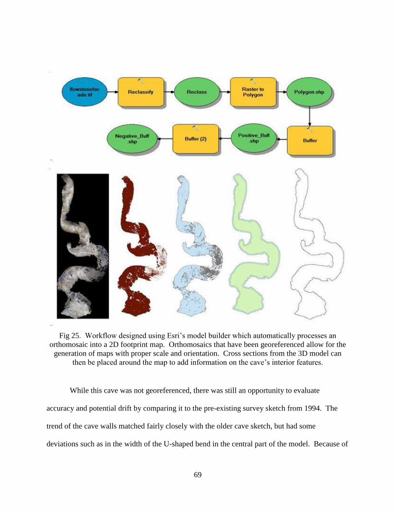
69
Fig 25. Workflow designed using Esri’s model builder which automatically processes an
orthomosaic into a 2D footprint map. Orthomosaics that have been georeferenced allow for the
generation of maps with proper scale and orientation. Cross sections from the 3D model can
then be placed around the map to add information on the cave’s interior features.
While this cave was not georeferenced, there was still an opportunity to evaluate
accuracy and potential drift by comparing it to the pre-existing survey sketch from 1994. The
trend of the cave walls matched fairly closely with the older cave sketch, but had some
deviations such as in the width of the U-shaped bend in the central part of the model. Because of

70
this, the cave was resurveyed in 2016. To avoid any bias, the cave sketch was not drawn by the
author. Analyzing all three representations of the cave quickly reveals that all three characterize
the cave in a highly similar but unique fashion. The 1994 sketch clearly differs in several areas
from the 2016 sketch, which underlines the highly subjective nature of hand drawing the shape
of the walls. Unfortunately, it cannot be said with great confidence whether one representation
or the other is “more correct” only that they all do not agree 100% with each other. A side by
side comparison of the three different cave maps is offered in Figure 26.
Fig 26. Original 1994 compass and tape survey by W.Pierce and K. McCormick at top,
photogrammetric survey in middle, and newer 2016 compass and Disto survey by Kayla Sapkota
and Joseph Jordan on bottom. Sketching and cartography was completed independently by
Kayla Sapkota to ensure there was no bias introduced from the author.

71
5.5 University of Arkansas Utility Tunnels
While not a true natural cave, the university utility tunnels offered a unique opportunity
to test the method in a manmade subterranean structure with a straight line overall trend and
straight vertical supports along the corridor. While minor distortions in natural random cave
wall geometry would be difficult to spot, here, any curved passage or warped support beams
would immediately represent error in the method. Approximately 30m of the tunnel was
modeled with the primary goal of observing any distortion or deviation in the predictable
manmade corridor. Other objectives of the project included comparing several types of control
targets and testing the use of split frames in a video opposed to still images.
It was immediately apparent during image acquisition that there was a large amount of
distortion in the image from the fisheye lens. The vertical support beams looked normal from a
distance but gradually became more and more distorted as the camera approached them. The
severity of this distortion at its greatest is illustrated in Figure 27.
Fig 27. Severely distorted vertical support in the utility tunnel.

72
Luckily this distortion did not carry over into the 3D model. Both the video method and
the still frame method successfully captured the straight-line trend of the tunnel, and rather than
constructing warped vertical beams, these were simply removed by the software, automatically.
Additionally, both models captured the slight downward slope to the drain and the slight upward
slope of the tunnel after the drain, which were nearly imperceptible to the human eye in the
images. Although the overall trend of the structure was good, the quality of the mesh in both
models was undesirable containing numerous holes as well as an “acid eaten” texture to the
surface. This was partially remedied through the use of the PhotoScans “smooth mesh” tool, but
consequently lead to a loss of detail and sharpness, especially notable by a slight distortion in the
two tripod mounted targets set up in the tunnel. Even after the smoothing, pipes and walls in
both models had a mangled appearance. It is likely that the complexity of various supports and
pipes running across the walls made this environment difficult to model as the camera could not
see all the different sides of these objects. The camera also could not image what was behind
these objects leading to periodic holes in the side walls of the corridor. Post it notes, tripod
mounted targets, and printable coded targets from PhotoScan were all tested in this model.
Unfortunately, the post it notes were placed on the vertical supports which were automatically
removed from the model, so these could not be evaluated. The tripod mounted targets offered
good 3D targets, but were distorted by the mesh smoothing tool. Coded targets worked the best,
and it was discovered that the software can scan for and detect these targets automatically even
before the photo alignment step. Six of these markers were placed on the floor, while two of
them were placed on the wall. Though all six floor targets were detected and clearly modeled in
both the video frame and still image tests, only one of the side wall targets was detected in the
video frame test. This target was severely distorted.

73
The last part of this experiment plotted the same section of passage captured with still
photos vs a video split into individual frames and evaluated the models on several different
aspects. The video was made using the 1080p 60 fps setting with low light mode turned on.
With still images, the corridor took 81 images to model, which were all processed in one
chunk. Because these two models were processed in Agisoft version 1.2.6, details were recorded
on the exact time each step took to process. For this first model, total processing time was about
1 hour and 35 min. The finished model consisted of 42,542 tie points, 9,479,861 points in the
dense cloud, and a mesh model containing 631,989 faces. RMS re-projection error was 1.49
pixels, while max re-projection error was 55.32 pixels. The effective overlap value for the model
was 2.74. The plan view of the model looks correct with a few small floating chunks of mesh
along the left side. It took around 15-20 min to take the 81 photos. A screen capture looking
down the model is presented in Figure 28.
Fig 28. View looking down model created with still images

74
The other was created using 200 individual video frames. Despite the larger number of
images, this model processed faster with an overall processing time of 1 hour and 9 minutes. At
58,758 the model had more tie points, but less than half of the number of total points and faces at
just 4,083,041 and 257,741 respectively. According to the Agisoft report the model had less re-
projection error at an RMSE re-projection of 1.23 pixels, and a maximum re-projection error of
25.19 pixels. This model also, as expected, had a higher effective overlap value of 3.21. Despite
this however, this model contained more error visually, with several significant bulges along the
exterior of the left wall, most severe of which is in the central part of the model. Internally, the
quality of the mesh was similar, with a much lighter appearance to the textured mesh model most
likely due to the low light mode that was used during video capture. The video frames seem to
be lower resolution, less in focus than the still photos, and lack the EXIF data containing camera
specification used in the calibration process. All of this was accomplished however at a fraction
of the time, only a two to three minutes of steadily walking down the passage in video mode. It
is also important to consider that consistent movement speed was easy walking down the tunnel,
but would be more difficult in many cave environments. It’s likely that there would be a great
deal of excess video footage (and frames) through highly confined passages or those containing
difficult obstacles. A screen capture looking through the tunnel model generated with the video
method is presented in Figure 29. More detailed information on each cave model as well as a
plan view of the models can be found in the appendix.

75
Fig 29. Model generated with individual frames split from continuous GoPro video.
6. Conclusion
6.1 Research Question
The first objective of this research was to ascertain under what if any conditions can pure
stand-alone photogrammetry be used to create interpretable 3D models of interior cave
structures? This study concludes that using a bright floodlight and still images from a wide angle
fisheye lens camera can in fact produce interpretable 3D models of underground cave structures.
The use of split frames from a video camera was also established as a comparable method,
allowing a faster scanning speed and greater image overlap at the cost of lower resolution and
possibly lower accuracy. The most successful environmental conditions were those where the
lowest part of the floor, the width of the walls, and the vertical extent of the ceiling were clearly
illuminated and unobstructed by any interior features. The methodology worked best in cave
passages less than 10.6 meters (35 feet) wide, with consistent ceiling height, minimal standing

76
water on the floor, and no complex structures lining the side walls. Agisoft PhotoScan was the
software of choice for producing the models utilizing the ability to isolate tricky areas in
individual chunks and later merge then together into complete cave models. Disabling pair pre-
selection among several other processing settings and parameters were critical to the successful
construction of the models.
A secondary goal of the research was to evaluate the accuracy of the generated models
with respect to currently held cave survey accuracy standards. Plan views of the 3D models
agreed for the most part with traditional cave sketches. Although there were some small
deviations between the cave sketch of Dogwood Cave and the corresponding 3D model, the two
sketches of this cave from different years also did not agree completely with each other.
The accuracy of measurements made in the model depends heavily on the quality of the
control network used to georeference it. In this case of Birch Cave, real world measurements
typically agreed with measurements in the virtual model within a meter. As reported by the
PhotoScan report, the control network had a total error of 1.2 meters. The RMSE projection
error was typically between 1-2 pixels, while the max re-projection error ranged from 25.19 to
84.07 pixels in the largest model in Birch Cave. In reference to the BCRA cave accuracy
standards, the survey line used achieves Grade 4 accuracy, where all angles agree within 2
degrees, distances were measured with the Disto which is accurate to 1.5875 mm(1/16 of an
inch), and exact station locations in the model were definable within a radius of a few
centimeters. The highest rating for cave passage detail is Class D and is defined by
“measurements of detail made at survey stations and wherever else needed to show significant
changes in passage dimensions” (“BCRA Survey Grades”, 2002). Since in this case every vertex
in the cave walls was measured by the software, the method used technically surpasses Class D

77
in accuracy. However, this assumes that the photogrammetrically derived measurements
between stations and at all critical points of change in the model are to the same accuracy. In
either case, the cave wall geometry constructed by the photogrammetric method largely agrees
with traditional cave sketches where cave walls were interpretively drawn between stations as
the caver eye-balled them. It can be said that the result of the photogrammetric method at the
very least achieves a similar accuracy to that of the human, hand drawn interpretations of the
cave.
6.2 Real World Applications
The methodology discussed in this paper allows for cave survey to move beyond the 2D
sketch map to capture the entirety of subterranean structures, and any notable features they
contain. Accurate scale and orientation still relies on a survey line traverse, but eliminates the
need to hand sketch cave walls, ledges, profiles, cross sections, and internal features.
It is the opinion of the author that in its present highly experimental state, the proposed
methodology should not replace traditional cave survey, but that it is a valuable supplement to it.
Photogrammetric models, under ideal conditions, capture more of the cave than a 2D map can
and do so using inexpensive, cave friendly equipment that is easy to use. Finished models can be
used to study speleogensis as well as cave morphology especially in the analysis of the size and
location of scallops. These models can be converted into caving simulations and virtual tours
that can be used for education and outreach to people who are not willing or able to physically
travel to or explore the caves. With further research and advancement in the technology, this
system could also be used as an effective low budget strategy for the modeling of mining
operations, municipal storm water drainage systems (MS4s), and utility tunnels.

78
6.3 Future Research Areas
Numerous ideas and questions came about as a result of the experiments discussed in this
paper. Though these were out of the scope of this paper, they may represent important topics for
future studies.
In theory, the wide angle fisheye lens is a huge part of what makes this method possible,
as each picture captures much more information about the environment than a conventional
frame camera. However, this is speculative and yet to be proven. An imitation of this research
with a variety of camera types would be beneficial in establishing concrete evidence supporting
the degree to which camera and lens type matter for the application of capturing 3D tunnels and
passageways. It is possible that different cameras, settings, and light rigs could achieve better
results than those achieved in this project.
The accuracy assessment of traverse data and control networks is not critically important,
because these are widely used and mature methods that are used both in traditional and
photogrammetric cave survey. More important, is an assessment of the geometry of the cave
walls generated by the photogrammetric method, and how close they represent the walls in
reality. In this research, photogrammetric models were roughly compared to the hand drawn
cave maps that were available. The problem is that those hand drawn cave maps used as a
control cannot be proven to be any more accurate than the models. A better assessment of
relative accuracy would be to directly compare the CRP method to a TLS survey and analyze the
point clouds and any deviation in terms of their Hausdorf distance.
In retrospect, after this work was completed, it was noted that the PhotoScan camera
calibration parameters were set to the “frame” setting instead of “fisheye.” It would be valuable,

79
in future research, to examine various calibration methods and models and examine whether or
not they lead to significant changes in the final products and their accuracy.
The only equipment needed to repeat this method is a light source and a GoPro camera.
The simplicity in this system is significant in that it could potentially be mounted to a small
unmanned remote control vehicle for the exploration and 3D mapping of tight passages that are
too tight for humans. With enough light, the method should theoretically work the same
underwater, allowing for a remote control submersible vehicle to explore sumps and flooded
cave passages. Finally, the same could be done with a quadcopter or other UAV system for use
in 3D modeling large vertical pits.

80
References
Addison A., (2011). LiDAR at Mammoth Cave. Civil Engineering Surveyor, (April 2011) 22-
25
Agisoft LLC. (2016). Agisoft PhotoScan User Manual; Professional Edition version 1.2
BCRA Survey Grades. (2002, November 10). Retrieved from http://bcra.org.uk/surveying/
Brown, K. R., Chalmers, A., Saigol, T., Green, C., & D’errico, F. (2001). An Automated Laser
Scan Survey of the Upper Paleolithic Rock Shelter of Cap Blanc. Journal of
Archaeological Science, 28(3), 283-289.
Buchroithner, M. F., & Gaisecker, T. (2009). Terrestrial Laser Scanning for the Visualization of
a Complex Dome in an Extreme Alpine Cave System. Photogrammetrie - Fernerkundung
- Geoinformation, 2009(4), 329–339. https://doi.org/10.1127/1432-8364/2009/0025
Caprioli, M., Minchilli, M., Scognamiglio, A., & Strisciuglio, G. (2003). Using photogrammetry
and laser scanning in surveying monumental heritage: le Grotte di Castellana.
International Archives of Photogrammetry Remote Sensing and Spatial Information
Sciences, 34(5/W12), 107–110.
Chandler, J. H., & Fryer, J. G. (2005). Recording aboriginal rock art using cheap digital cameras
and digital photogrammetry. Retrieved from
https://dspace.lboro.ac.uk/dspace/handle/2134/2240
Cooper, S. E., (1998). Softcopy Photogrammetry and the Development of Field Methodologies
Applied to the Recording and Analysis of Rock Art (Masters Thesis). University of
Arkansas Special Collection Storage. (T 1998 C664 Archival Copy)
Dasher, G. R. (1994). On Station: A Complete Handbook for Surveying and Mapping Caves.
Huntsville (AL): National Speleological Society. 240 p. Quote excerpt from p. 42.
El-Hakim, S. F., Fryer, J. G., & Picard, M. (2004). Modelling and Visualization of Aboriginal
Rock Art in the Baiame Cave. International Archives of Photogrammetry and Remote
Sensing, 35(5), 990–995.
Furukawa, Y. (2013). Multi-view Stereo: A Tutorial. Foundations in Computer Graphics and
Vision, 9(1-2), 3-14.
Ghosh, S. K., (1981). History of Photogrammetry -Analytical Methods and Instruments. XVIIth
ISPRS Congress Proceedings--Technical Commission VI: Economic, Professional and
Educational Aspects of Photogrammetry and Remote Sensing, 29, 311-327.
González-Aguilera, D., Muñoz-Nieto, A., Gómez-Lahoz, J., Herrero-Pascual, J., & Gutierrez-
Alonso, G. (2009). 3D Digital Surveying and Modelling of Cave Geometry: Application
to Paleolithic Rock Art. Sensors, 9(2), 1108–1127. https://doi.org/10.3390/s90201108
González-Aguilera, D., Muñoz-Nieto, A., Picon-Cabrera, I., Gomez-Lahoz, J., Herrero-Pascual,
J., Mancera-Taboada, J., & Rodriguez-Gonzálvez, P. (2011). Application of non-

81
destructive techniques to the recording and modelling of palaeolithic rock art. INTECH
Open Access Publisher. Retrieved from http://cdn.intechweb.org/pdfs/15812.pdf
Grussenmeyer, P., & Jasmine, J. (2003). The Restoration of Beaufort Castle (South-Lebanon): A
3D Restitution According to Historical Documentation. In XIXth CIPA International
Symposium, (pp. 322–327). Retrieved from https://halshs.archives-ouvertes.fr/halshs-
00264004/
Grussenmeyer, P., Landes, T., Alby, E., Carozza, L., (2010). High Resolution 3D Recording and
Modelling of the Bronze Age Cave “Les Fraux” in Perigord (France). International
Archives of Photogrammetry, Remote Sensing, and Spatial Information Sciences, Vol
38(5) 262-267.
Grussenmeyer, P., Alby, E., Landes, T., Koehl, M., Guillemin, S., Hullo, J., & Smigiel, E.
(2012). Recording Approach of Heritage Sites Based on Merging Point Clouds from
High Resolution Photogrammetry and Terrestrial Laser Scanning. Int. Arch.
Photogramm. Remote Sens. Spat. Inf. Sci, 34, 553–558.
Hero 3+ Black Edition Field of View Information. (n.d.). Retrieved from
https://gopro.com/support/articles/hero3-field-of-view-fov-information
Higgins, Sean. (2015, March 04). Fisheye Lenses Make the Impossible Possible. Retrieved from
http://www.spar3d.com/blogs/the-other-dimension/vol13no9-fisheye-lenses-make-the-
impossible-possible/
Higgins, Sean (2016, November 16). Meet Leicas 16k LiDAR scanner, the BLK360. Retrieved
from http://www.spar3d.com/news/lidar/meet-leicas-16k-scanner-blk360/
Howard, I. P., Brian, R., J. (2012). Perceiving in Depth, Volume 2: Stereoscopic Vision. New
York, NY: Oxford University Press.
Hudson, M. R., Turner, K. J., & Bitting, C. (2011). Geologic Framework of Karst Features in
Western Buffalo National River, Northern Arkansas. US Geological Survey Karst
Interest Group Proceedings, Fayetteville, Arkansas, April 26–29, 2011, 16-17.
Huttenlocher, D., Klanderman, G. A., & Rucklidge, W. J., (1993). Comparing Distances Using
the Hausdorff Distance. IEEE Transactions on Pattern Analysis and Machine
Intelligence, 15(9) 850-862.
Idrees, O.M., & Pradhan B., (2016). A Decade of Modern Cave Surveying with Terrestrial Laser
Scanning. A Review of Sensors, Method, and Application Development. International
Journal of Speleology, 45(1) ,71-88. Tampa, FL ISSN 0392-6672.
Kolecka, N., (2011). Photo-based 3D Scanning vs. Laser Scanning-Competitive Data
Acquisition Methods for Digital Terrain Modelling of Steep Mountain Slopes. ISPRS -
International Archives of the Photogrammetry, Remote Sensing and Spatial Information
Sciences, 38(-4/W19) 203-208.
Lerma, J. L., Navarro S., Cabrelles, M., & Villaverde, V. (2010). Terrestrial Laser Scanning and
Close Range Photogrammetry for 3D Archaeological Documentation: the Upper
Palaeolithic Cave of Parpalló as a Case Study. Journal of Archaeological Science, 37,
499-507.

82
Lingua, A., Marenchino, D., & Nex, F. (2009). Performance Analysis of the SIFT Operator for
Automatic Feature Extraction and Matching in Photogrammetric Applications. Sensors,
9(05), 3745-3766.
McCormac, Jack. (2004) Surveying. Hoboken, NJ: Wiley.
McFarlane, D. A., Buchroithner, M., Lundberg, J., Petters, C., Roberts, W., & Van Rentergen, G.
(2013). Integrated three-dimensional laser scanning and autonomous drone surface-
photogrammetry at Gomantong caves, Sabah, Malaysia. In Proceedings of the 16th
International Congress of Speleology, Brno (Vol. 1, pp. 317–319). Retrieved from
https://www.researchgate.net/profile/Manfred_Buchroithner/publication/261097340_Go
mantong_Congress_Paper_2013/links/00b7d5332d8cf3bd16000000.pdf
Milius, J., & Petters, C. (2012). Eisriesenwelt–From laser scanning to photo-realistic 3D model
of the biggest ice cave on Earth. In GI-Forum (pp. 513-523).
Moreno, A., G., & Garate, D., 2012. Low-Cost Photogrammetry and 3D scanning: the
Documentation of Paleolithic Parietal Art in El Niño Cave. CAA2012 Proceedings of the
40th Conference in Computer Applications and Quantitative Methods in
Archaeology, Southampton, United Kingdom, 26-30 March 2012, p. 344-348.
Núñez, M. A., Buill, F., & Edo, M. (2013). 3D model of the Can Sadurní cave. Journal of
Archaeological Science, 40(12), 4420–4428. https://doi.org/10.1016/j.jas.2013.07.006
Matthews, N., A. (2008). Aerial and Close-Range Photogrammetric Technology: Providing
Resource documentation, Interpretation, and Preservation. Technical Note 428. U.S
Department of Interior, Bureau of Land Management, National Operations Center,
Colorado. P42.
Positional Accuracy. (2003, February 24). Retrieved from
http://www.gitta.info/MetaDataQual/en/html/PositAccurac_learningObject1.html
Roncat, A., Dublyansky, Y., SpöTl, C., & Dorninger, P. (2011). Full-3D Surveying of Caves: A
Case Study of Märchenhöhle (Austria). cogeo@oeaw-giscience.
https://doi.org/10.5242/iamg.2011.0074
Rüther, H., Chazan, M., Schroeder, R., Neeser, R., Held, C., Walker, S. J., & Horwitz, L. K.
(2009). Laser scanning for conservation and research of African cultural heritage sites:
the case study of Wonderwerk Cave, South Africa. Journal of Archaeological Science,
36(9), 1847–1856. https://doi.org/10.1016/j.jas.2009.04.012
Schwinge, H. T., (1962). The Accuracy of Cave Survey. Bulletin of the National Speleological
Society, 24, 40-47
Thrun, R., (2000). A Statistical Study of Survey Errors and Closure Adjustments. 2000 NSS
convention. Revised in 2009.
Urban, S., & Hinz, S. (2016). MultiCol-SLAM-A Modular Real-Time Multi-Camera SLAM
System. arXiv Preprint arXiv:1610.07336. Retrieved from
https://arxiv.org/abs/1610.07336

83
Westoby, M. J., Brasington, J., Glasser, N. F., Hambrey, M. J., & Reynolds, J. M. (2012).
‘Structure-from-Motion’photogrammetry: A low-cost, effective tool for geoscience
applications. Geomorphology, 179, 300-314.

84
Appendix A: PhotoScan Processing Reports

85

86

87

88

89

90

91

92

93

94

95

96

97
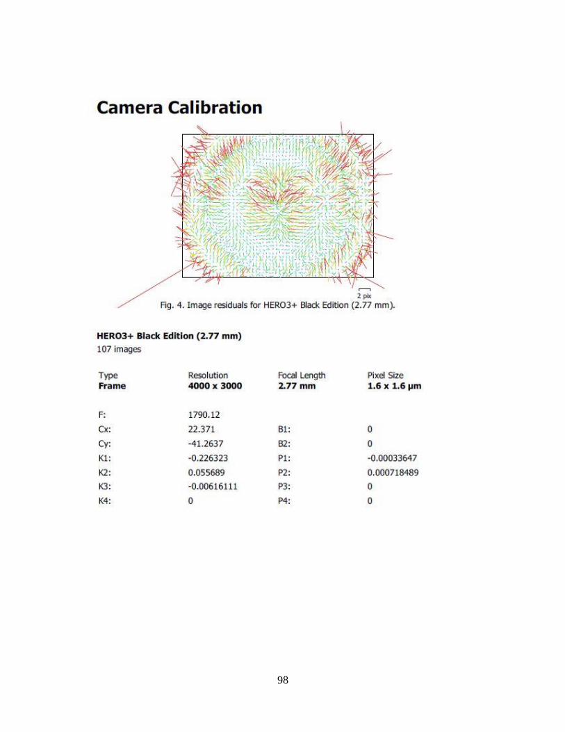
98
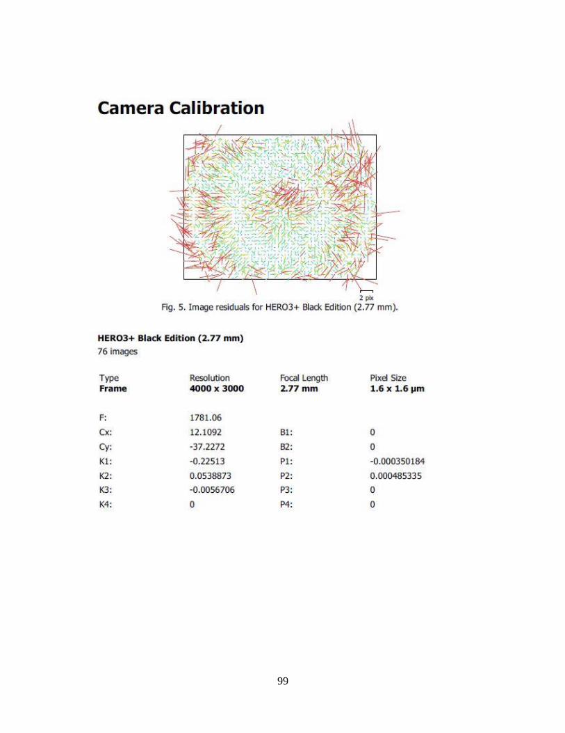
99

100

101

102

103

104

105

106

107
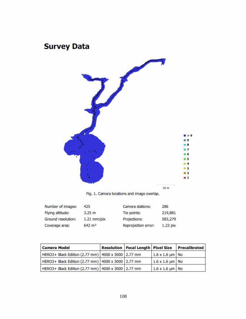
108

109
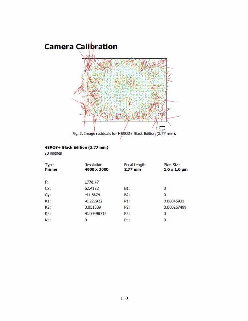
110

111
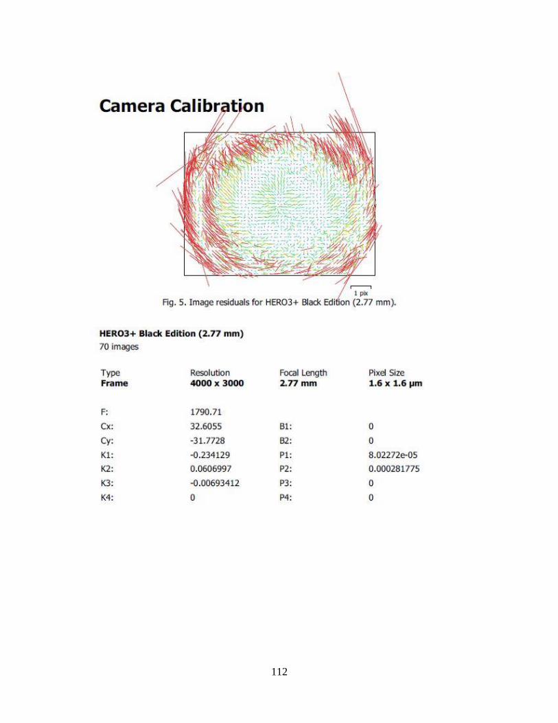
112

113

114

115

116

117

118

119

120

121

122

123
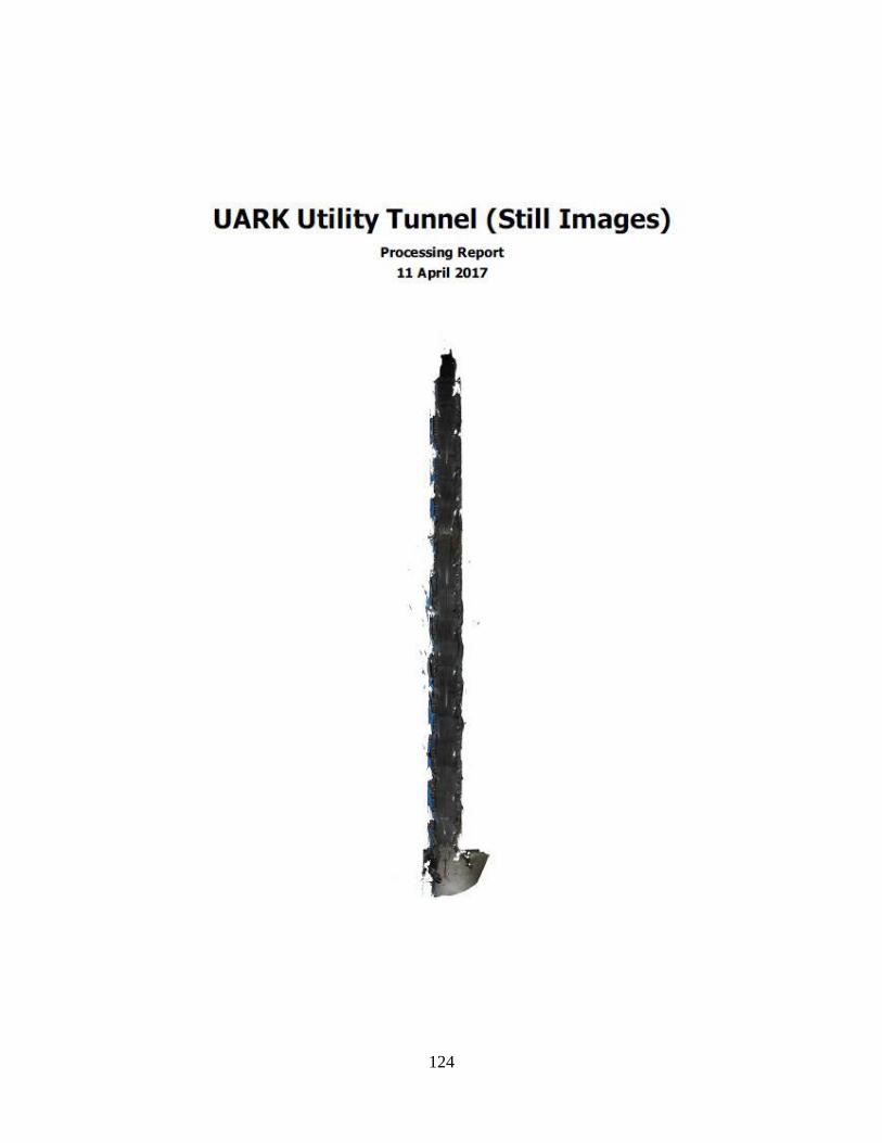
124
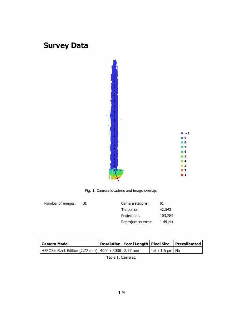
125

126

127

128

129

130

131
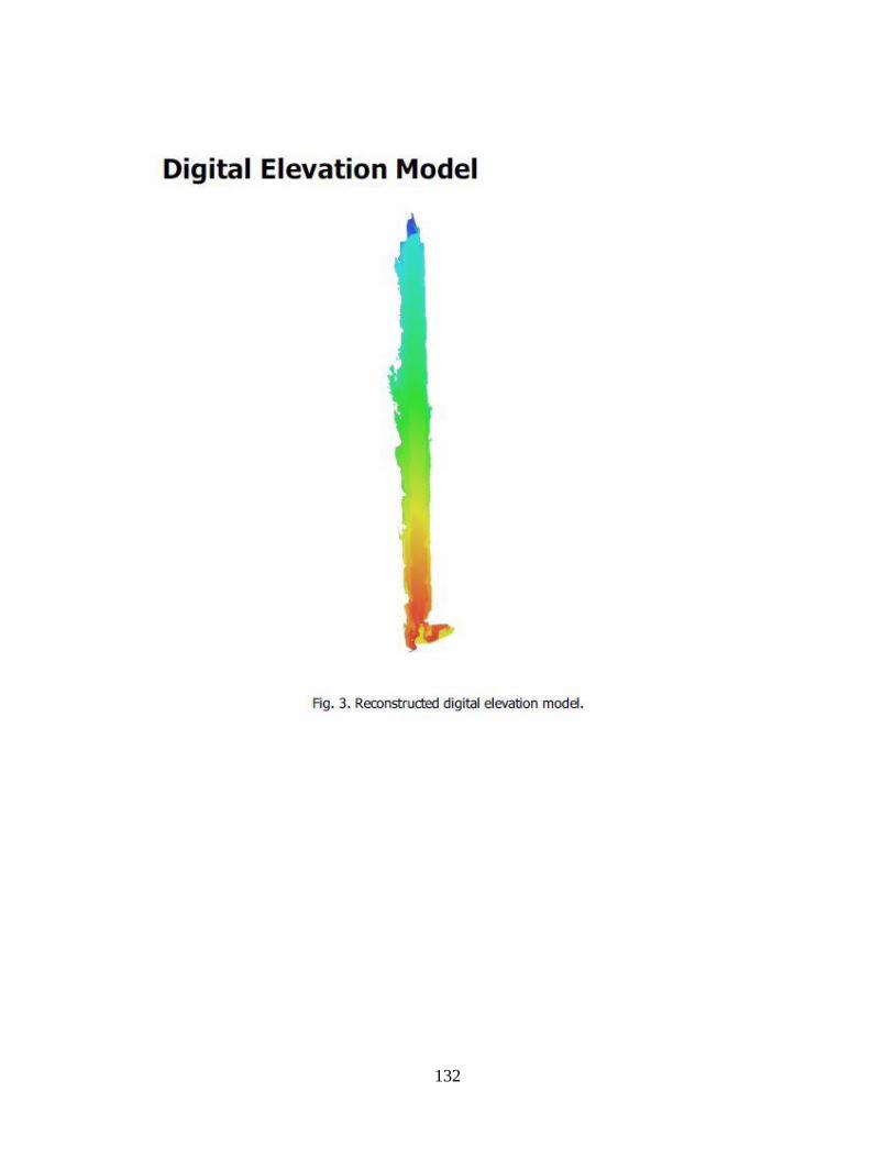
132

133