Modeling of the Kinetics of Alkali Metal Fusion

3678 Ind. Eng. Chem. Res. 1995,34, 3678-3687

Modeling of the Kinetics of Alkali Fusion

Juha Lehtonen? Tapio Salmi,*ft Antti Vuori,f Heikki Haario? and Paula Nousiained Laboratory of Industrial Chemistry, Abo Akademi, FIN-20500 Turku, Finland, Kemira Agro Oy, Espoo Research Centre, FIN-02271 Espoo, Finland, and Department of Mathematics, University of Helsinki, FIN-00100 Helsinki. Finland

Alkali fusion is applied to substitute a sulfonic acid group with a hydroxyl group in a substituted aromatic ring. Beside the main reaction, also side reactions appear, because the substituents in the aromatic ring are eliminated and the aromatic rings are polymerized. A kinetic model for the main and the side reactions in alkali fusion of a substituted aminobenzenesulfonic acid was developed. The substitution reaction of sulfonic acid with a hydroxyl group, the elimination of sulfonic acid and amino groups, the dealkylation reactions, and the polymerization reactions were included in the kinetic model. The system consisted of the main reaction and of 27 side reactions. The number of adjustable constants in the kinetic model was reduced by assuming that the reactivity of any functional group in the aromatic ring is not affected by the other substituents. The reactions could then be described with eight kinetic parameters only. The kinetic data were obtained from isothermal experiments carried out in a batchwise operating laboratory reactor at the temperature range of 220-270 "C. The kinetic parameters were estimated from the experimental data using nonlinear regression analysis. The model agreed well with the experimental data, which implies that the proposed reaction scheme is suitable for the description of alkali fusion and that the assumption concerning the reactivities of the functional groups is reasonable.

Introduction Alkali fusion is used for the production of substituted

alkyl phenols from the corresponding sulfonic acids. The reaction takes places in the melt of sodiudpotassium hydroxide. The overall reaction can be written as follows

S03M OM

where M denotes Na or K. If the aromatic ring has other substituents, like alkyl and amino groups, side reactions appear: the substituents are abstracted in the melt phase. The aromatic rings can also polymerize in the melt phase. The side reactions are illustrated below: pH R'

- products with fewer substituents _ _ (2)

S03H

(3)

where R and R' denote alkyl groups. The melt phase in the alkali fusion consists mainly

of KOH and NaOH. KOH is added to NaOH because of the high melting point of NaOH (360 "C). The KOH- NaOH system has an eutecticum at 185 "C. The composition of the eutectic melt is 39 mol % NaOH and

' Ab0 Akademi. * Kemira Agro. P University of Helsinki.

61 mol % KOH. Industrially the alkali fusion is carried out at temperatures of 200-400 "C. The reaction mixture contains typically a large excess of the alkali: the molar ratio between alkali and aromatic compounds varies between 2:l and 1O:l. The excess of alkali is used to suppress the side reactions (Wedemeyer, 1976).

The mechanism of the main reaction (1) is known to be a bimolecular nucleophilic substitution (sN2). The reaction mechanism can be described with consecutive steps:

Despite the fact that alkali fusion represents an old technology-the first process was commercialized at the end of 19th century-the studies of the kinetics of this reaction are very scarce. Cerveny et al. (1978) investigated alkali fusion kinetics of sodium 3-amino-4- methylbenzolsulfonate in a laboratory reactor. The kinetic data were described qualitatively, and the side reactions were discarded.

The objective of the present work was to determine the kinetics of the main and the side reactions in the alkali fusion of a substituted aminobenzenesulfonic acid, to develop the rate equations, and to estimate the kinetic parameters in order to use the kinetic model for the optimization of the reaction conditions.

Experimental Methods

The alkali fusion kinetics was determined with isothermal experiments carried out in a closed laboratory reactor (Hastelloy B, 100 mL) at 220,230,240,250,260, and 270 "C. The molar ratio between the aromatic reactant and the NaOH-KOH melt was 1:7. The alkali

0 1995 American Chemical Society

Ind. Eng. Chem. Res., Vol. 34, No. 11, 1995 3679

V2

iJ

1

I

0" S03M

L q2 0 = MOH rF-1 18 P =H20 Q = M 2 S 0 3

R = M2C03 SO,M

s =polymer

Figure 1. Reaction scheme for the alkali fusion (M = Na or K, R, R = alkyl groups).

melt contained 70 mol % KOH and 30 mol % NaOH. For each temperature five batches were prepared, and the whole batch was taken to analysis. The reaction times of the batches were 1, 6, 18, 30, and 68 h, respectively. The reaction was interrupted by cooling the mixture to 100 "C. Water was added into the alkali melt to dissolve the sulfite formed and to dilute the mixture. The cooled solution was filtrated and the liquid phase was analyzed with high pressure liquid chromatography (HPLC) equipped with a reversed phase column and an W detector. An external standard was used to calibrate the HPLC analysis. Mass spectroscopy (MS, chemical ionization) was used to identify the product compounds. The concentrations of the dominating aromatic compounds could be registered with HPLC, whereas the amount of polymeric material (tar) was estimated from the total mass balance of the aromatic compounds. The polymers were assumed to consist of dimers only. The loss of the material during

the analysis was confirmed to be negligible by performing a blank experiment at 25 "C.

Stoichiometry and Kinetics Six types of chemical reactions appear in alkali

fusion: the main reaction, i.e., substitution of the sulfonic acid group with a hydroxyl group, as well as five side reactions, i.e., elimination of the sulfonic group, dealkylation of the alkyl groups (R and R ) , elimination of the amino group, and polymerization of the aromatic rings. The reactions of the aromatic ring are illustrated in Figure 1, and the reaction types are summarized in Table 1. Most of the chemical reactions proceed in the upper left corner of the reaction scheme (Figure 1): the desired product is E, and the most important monomeric byproduct is F, whereas some B exists already in the initial solution. Reactions 1 and 2 (Table 1) are considered as bimolecular reactions between the aromatic compound and hydroxide. These reactions give alkali

3680 Ind. Eng. Chem. Res., Vol. 34, No. 11, 1995

Table 1. Reaction Categories R R

1. substitution of -S03H with -OH 2. elimination of -SOsH 3. dealkylation of R 4. dealkylation of R 5. elimination of -NH2 6. polymerization (tar formation)

metal sulfite, which precipitates immediately forming a solid phase. Reactions 1 and 2 (Table 1) can formally be written as

R R

S03M

? OM

?

S03M

Dealkylation of R from the amino group in the reaction scheme of Figure 1 is regarded as a monomolecular thermal decomposition. The overall stoichiometry is given by

R R eNHR'+ H2 - ($"' + HR' (7)

SO3M SO3M

The decomposition is enhanced above a critical temperature, at which there is a sufficient amount of energy for the cleavage of the bond between R and the nitrogen atom. At lower temperatures a different reaction mechanism prevails: the hydroxyl group acts catalytically in the reaction, and alkoxides are formed as reaction products. For the sake of simplicity we assume, how- ever, that the reaction obeys first order kinetics.

The dealkylation of R, reaction 4, can be treated as a consecutive process consisting of two steps. The reaction proceeds via a carboxylate ion. The hydroxide ions participate in the reaction also. For the case in which R is a methyl group, the reaction can be written as

+MOH+HzO - GHRf+ 3H2 (8)

The carboxyl group is eliminated in a subsequent reaction step. The reaction step can formally be written as

COOM

@"R +MOH - aNHR' + M2CO3 + 0.5H2 (9)

The reaction is regarded as a second order reaction and the steady-state approximation is applied to the intermediate.

The eliminations of the amino groups are considered first order reactions, because they are monomolecular thermal decomposition reactions. The reaction stoichiometry is given by

OM OM

It was also assumed that all oxygen liberated in reaction 6 and all hydrogen formed in reactions 8 and 9 react instantaneously, giving water. The formation of water was not included in the kinetic model.

Based on the above reasoning the rate equations for reactions 1-25 can be written as shown in Chart 1.

R14 = '14'K

R15 = k15cAc0

R16 = 'l&ECO

R17 = k17cf10

= k18cBc0

R l 9 = k 1 9 c F c o

R20 = k20C$O

R 2 1 = k21ciVlco

R22 = k22cI3

R23 = k23cF

R24 = '24'G

R25 = '25'I-I

The polymerization reactions can be regarded as bimolecular processes between all aromatic compounds in the system. Principally the polymers can contain dimers, trimers, etc., but here we adapted the simplified concept that dimers were the dominating compounds among the polymers. If all possible dimerizations between the monomers are included, the rate equation for the tar formation becomes

i.e., there exist 120 dimerization reactions between 14 aromatic monomers. Experimental observations, how- ever, suggest that the polymerization processes are strongest in the beginning of the experiment, which implies that mainly the starting compounds participate in the polymerization. According to studies with differential scanning calorimetry the main products (E and F) are virtually stable at the temperature range used. Therefore we included only the bimolecular reactions between A and B in the tar formation kinetics. Fur- thermore, it was assumed that the rate constants of the three dimerization reactions are equal. Thus only the terms &SA2, kta$B2, and k t d A c B (k tar = k26) were included in the final model.

Basically the proposed reaction scheme consists of 25 reactions (Figure 1) with 25 kinetic constants and of 3 polymerization reactions with 1 rate constant. In order to simplify the system and to limit the number of adjustable kinetic parameters, the principle of a constant reactivity of a functional group was introduced. This implies that the reactivity of a functional group is independent of the other substituents in the aromatic


The initial conditions of (42) and (43) are ci = Coi and 6 = 0 at t = 0.

The combination of the rate equations and the stoichiometry gives the generation rates of the compounds:

ring. This hypothesis limits the number of rate constants to six according to the equations below:

k’l = k l = k , = k3 = k,; k’, = k5 = k6 = k7 = k8; k ’ , = k , = k = k = k = k = k

10 11 12 13 14; k‘, = k, , = k, , = k18 = k,, = k2, = k Z l ; k’, = k2, = k 2 3 = k24 = k 2 5 ; k’, = k27

A special treatment was applied to reaction 17 in the reaction scheme (Figure 1): because the intermediate for reaction type 4 was detected only for reaction 17, this reaction was excluded from the remaining reactions in this category.

The temperature dependencies of the rate constants were determined from Arrhenius’ law:

E,IRT k =Ae- (37) To suppress the strong correlation between the frequency factor (A) and the activation energy (Ea), a transformed_ temperature was introduced: 110 = 1pT - 1/T, where T is the average temperature of the experiments.

Reactor Model

The reactor was considered to be a batch reactor, where the mass of the liquid decreases continuously because of the crystallization of the sulfite formed in reactions 1 and 2. The crystallization was presumed to occur instantaneously, which implies that the crystallization rate equals the sulfite formation rate. The concentrations in the liquid phase were defined as the amount of substance per mass of liquid; i.e., ci = nib. Consequently, the mass balance of compound i is written as

dn,ldt = riml (38)

When the concentration is inserted in the left-hand side, eq 38 becomes, after differentiation and rearrangement,

(39)

The change of the liquid phase mass (md is connected to the formation of sulfite; thus the multiplication of (38) with the molar mass of alkali metal sulfite (Mso3) gives the mass change

(40)

The total mass of the liquid and solid phases is constant: mo = ml+ mso3, where mo is the initial mass.

Introduction of a dimensionless quantity 6 = mso$ mo gives, finally,

1 dd- ~so3Mso, ---

1 - d d t (41)

The total balance implies that dmlldt = -dmso$dt; Le., ml-l dmlldt = -(1 - 61-l d6/dt, which is inserted in (39). The whole system is now described with balance eqs 42 and 43.

dci Ci dd -- -ri+-- dt 1 - 6 d t

dd - = (1 - d)rso3Mso, dt

(42)

(43)

ri = Cvipj (44) j

where vu denotes the stoichiometric coefficient of compound i in the reaction j . The stoichiometric matrix is given in the Appendix. After performing multiplication 44 and insertion of the generation in eq 42, we obtained the final forms of the mass balances.

For the reaction intermediates in the reaction group 4 the application of the steady-state hypothesis

(45) rB‘ = kPSICAcOH - k P S f l B c O H =

gives the concentration of the reaction intermediate:

Differentiation of the expression gives

dcBj kpsl dc, dt kps2 dt

- ---- (46)

Application of this principle to the intermediate gives analogously

G m 2 - &E kKAR,16 dt --

dt

(47)

(48)

(49)

(51)

(52)

(53)

Kinetic Model at Individual Temperatures The rate constants were estimated from the isother-

mal experiments separately at each temperature. The following objective function was used in the minimization of the residual sum of squares:

Q = C t=l [ ( c ~ , ~ - ~ ’ 1 , ~ ) ~ + ( ~ 2 , ~ - ~ ’ 2 , ~ ) ’ + ... + m

(C,,$ - C’,,t)21 (54)

where ci and c’: denote the experimentally observed and the predicted concentrations. The mass balance, i.e., differential eqs 42 and 43, were solved with a fourth order semiimplicit Runge-Kutta method, a Rosen- brock-Wanner method (Gottwald and Wanner, 1981)


1.2

E 1 0

E E 0.8

.- L

240 C mollkg 1.6 1

F -.- s -.-.-.-.-.-.-.-.-.- .-.

--

1.2

e 1 .B E E 0.8

8

L

8 0.6

0.4

0.2

0 vh

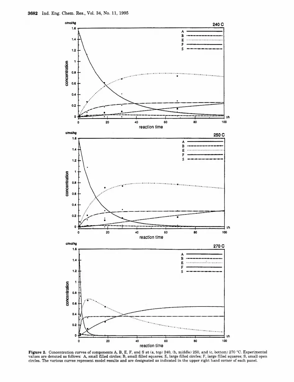
Figure 2. Concentration curves of components A, B, E, F, and S a t (a, top) 240, (b, middle) 250, and (c, bottom) 270 "C. Experimental values are denoted as follows: A, small filled circles; B, small filled squares; E, large filled circles; F, large filled squares; S, small open circles. The various curves represent model results and are designated as indicated in the upper right hand corner of each panel.


1

0.8

0.6

Table 2. Rate Constants at 220 "C, at 230 "C, at 240 "C, a t 250 "C, a t 260 "C, a t 270 "C,

Q = 0.000 36 Q = 0.034 30 Q = 0.027 84 Q = 0.141 08 Q = 0.092 01 Q = 0.010 36 U/% U/% ul% U/% U/% U/%

0.000 518 1.6 0.001 325 7.7 0.003 324 2.8 0.005 092 6.9 0.011 043 6.6 0.033 130 3.6 0.000 148 13.8 0.000 401 65.2 0.000 884 22.2 0.001 552 40.1 0.002 987 29.0 0.008 792 16.8

--

--

a-

1

0.001 035 6.0 0.002 848 28.1 0.002 743 12.3 0.003 512 21.3 0.006 288 11.1 0.022 453 5.9 0.001 165 18.3 0 0 0.001 582 28.0 0 0 0.001 099 59.1 0.003 840 32.2 0.000 778 5.8 0.002 957 19.0 0.009414 6.8 0.018 513 13.2 0.047 290 9.9 0.181 15 4.7 0.111 88 large 1.0069 large 0.009 977 large 0.256 27 large 0.617 88 large 1.0461 large 9.7606 large 7.7566 large 0.879 57 large 1.1750 large 2.6938 large 4.6676 large

26,27,28

5

9

0.2 -- ...............................................

+/-

~.......................................................................................,.,........ 0 .- I I I I , v h

0 20 40 60 80 100

reaction time Figure 3. Consumption contributions of A at 260 "C. The reaction numbers are indicated above each curve.

during the course of the estimation. The minimization of the objective function was carried out with the Levenberg-Marquardt (Marquardt, 1963) method using the software of Vajda and Valko (1985). Some parameter estimations and the evaluation of the sensitivity of the objective function (Q) with respect to the kinetic parameters were performed with the regression software of Haario (1994).

The estimation was initiated with the determination of the rate constants of the dominating reactions, i.e., K'1, K'3, and K'6. After obtaining sufficiently good values for these parameters, the remaining rate constants were estimated. Rate constant k'4 as well as rate constants l z ~ l - k w 2 and KKARQ - k ~ 7 were approximated to zero. The values of the rate constants and the estimation statistics are displayed in Table 2.

These values of the rate constants were then used to simulate the progress of the reaction at the experimental temperatures. The concentration curves of components A, B, E, F, and S are shown in Figure 2a-c. The other components are not shown here because of their very low concentrations.

The comparison between the simulated curves and the experiments reveals that the model reproduces well the experimental data. The small deviations depend on the uncertainties in the chemical analysis. The most prominent systematic deviation appears in the concentration of component F. This may be due to the different routes leading to the formation of F.

Contribution Analysis In order to penetrate the formation routes of the

products and the consumption routes of the main

reagent (A), the principles of contribution analysis were used. The contribution of reaction j to the generation of component i is given by Nemeth et al. (1987).

(55 )

where Rj is the rate of reaction j . Differentiation of (55) gives

dQLj. - v z J R j -- dt (56)

The relative contribution of reaction j to the formation of component i is defined as

p=- ' N

(57)

CQL k = l

where N is the total number of reactions contributing to the formation of i.

The corresponding consumption contribution is defined by

Q,

CQik 1: = - '' N

k = l

(58)

In the present case the contribution of a reaction to the


w1 00

1

0.8

0.6

0.4

0.2

t

0 1 I I I m 0 20 40 60 80 100

reaction time Figure 4. Formation contributions of F at 260 "C. The reaction numbers are indicated above each curve.

consumption of A is given by

Iij =

QA.i

QA,I + QA,5 + QA,9 + QA,15 + QA,26 + QA,27 + Q i , 2 8

(59)

Furthermore, the analysis gives the formation con- where j gets the values 1, 5, 9, 15, 26, 27, and 28.

tribution of compound F:

(60)

where j gets the values 2 and 10. The values of contributions 59 and 60 were obtained

by solving numerically eq 56 after the determination of the rate constants. The consumption contributions of A at 260 "C are shown in Figure 3. The contribution of reaction 15 was not included in the figure because its rate constant was practically nil. The figure reveals that the contribution of the main reaction increases during the progress of alkali metal fusion, whereas the importance of the tar formation (the polymerization) diminishes as the reaction proceeds. This effect is fortified with an increasing temperature. The contribution of reactions 5 and 9 are minor and virtually constant during the experiment. The contribution analysis for the formation of F at 260 "C is presented in Figure 4. In the beginning of the experiment both reaction paths give an equal contribution to the formation of F. As the experiment proceeds, the contribution of reaction 10 increases. In practice reaction path 2 dominates totally in the beginning of the experiment. The rate model was not able to fully recognize this fact, which caused the deviations between the experimentally observed and the simulated concentrations of F.

Temperature Dependences of the Kinetic Parameters

Different methods were tested in the determination of the temperature dependence, i.e., the Arrhenius

Llnear regresslon

F

ilm1 .O.m ., 0 . m 0.mOl

-

-8

:f i

c "---. 5 -

-8

1 f l I l K

Figure 5. Linear plot for kl .

parameters, of the kinetic constants. The rate constants obtained from the separate regression runs at different temperatures were estimated with linear regression (In k' vs l/@), with nonlinear regression using equal weights and with weighting the constants originating from the lowest temperatures. The objective function was

(61)

where k'j denote the rate constants determined at each temperature (Table 2) and k'j denotes the model predic- tion, i.e., the Arrhenius law (37).

Furthermore, the Arrhenius parameters were determined directly by fitting all of the data together in the original model and applying the law of Arrhenius t o each rate constant.

Already preliminary tests indicated that nonlinear regression with equally weighted rate constants is unsuitable, because it is totally dominated by the rate constants at the highest experimental temperatures. This resulted in a poor fit at the lowest temperatures. Therefore this approach was abandoned at an early stage.

The simple logarithmic plot gives an illustration, whether the kinetic parameter obeys the law of Arrhe- nius. The linear plot for the main reaction is presented in Figure 5. As can be seen from the figure, the main reaction (5) follows Arrhenius law satisfactorily well. Analogously, the rate constants for the most important


0 20 40 60 80 100

reaction time

0.6

0.6

0.4

0.2

0

Y I E ........................... F s -.-.-.-.-.-.-.-.-.-

.............

.-.-.-.-.-.-.-

I I I I vh 0 20 40 60 80 100

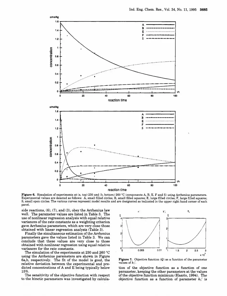
reaction time Figure 6. Simulation of experiments a t (a, top) 230 and (b, bottom) 260 "C (components A, B, E, F and S) using Arrhenius parameters. Experimental values are denoted as follows: A, small filled circles; B, small filled squares; E, large filled circles; F, large filled squares; S, small open circles. The various curves represent model results and are designated as indicated in the upper right hand corner of each panel.

side reactions, (61, (7), and (31, obey the Arrhenius law well. The parameter values are listed in Table 3. The use of nonlinear regression analysis with equal relative variances of the rate constants as a weighting criterion gave Arrhenius parameters, which are very close those obtained with linear regression analysis (Table 3).

Finally the simultaneous estimation of the Arrhenius parameters gave the values listed in Table 3. We can conclude that these values are very close to those obtained with nonlinear regression using equal relative variances for the rate constants.

The simulation of the experiments at 230 and 260 "C using the Arrhenius parameters are shown in Figure 6a,b, respectively. The fit of the model is good, the relative deviation between the experimental and predicted concentrations of A and E being typically below 15%.

The sensitivity of the objective function with respect to the kinetic parameters was investigated by calcula-

A

P

0' ' 01 I 0 0.005 0.01 1 1.5 2 2.5 3

10'

Figure 7. Objective function (8) as a function of the parameter vaIues of K1'.

tion of the objective function as a function of one parameter, keeping the other parameters at the values of the objective function minimum (Haario, 1994). The objective function as a function of parameter kl' is


plotted in Figure 7. It can be seen from Figure 7 that the objective function has a sharp minimum, which implies that the parameter is well identified. Analo- gously, by drawing the corresponding plots for parameters k2' and k3' we could observe that also these parameters are well identified.

Optimal Yield The yield of the desired product (E) was defined as

cEml E-- ' - cA,OmO

i.e.,

(62)

(63)

The yield of E was simulated at different temperatures by using the kinetic parameters listed in Table 2. The yield curves are presented in Figure 8. The simulations revealed that the highest yield of E (41.7%) is obtained at 250 "C with a reaction time of 34 h. Above this temperature the maximal yield is lower because of the increased importance of the polymerization reactions.

Conclusions The kinetic model developed for the main and the side

reactions in the alkali fusion of a substituted aminobenzenesulfonic acid (Figure 1, eqs 11-35) was able to describe the experimental data (Figure 2) obtained at 220-270 "C. The essential feature in the kinetic model is the independence of the reactivity of any functional group on the other substituents in the aromatic ring. This simplification reduced the number of adjustable kinetic parameters to a reasonable level but preserved the main characteristics of the kinetic model. The Arrhenius parameters of the kinetic constants were estimated with different techniques (Table 3). The linear regression was considered as a initial step in the parameter estimation and the values obtained from the linear regression were used as initial values in the

Table 3. Arrhenius Parameters for Rate Constants k'i (i = 1, 2, 3, 5, 6) and ki (i = 17 and KARS)

Al(kdmo1 h)) E./(kJ/mol)

k'i linear regressn 2.01 x 1015 175 nonlinear regressn re1 var 1.11 x 173 simultaneous estimn 2.47 x 1014 166

linear regressn 2.50 x 1014 172 nonlinear regressn re1 var 1.51 x 1014 170 simultaneous estimn 3.96 x 1007 103

linear regressn 2.34 x loz1 231 nonlinear regressn re1 var 1.50 x loz1 229 simultaneous estimn 6.63 x lozo 225

linear regressn 1.51 x lo1@ 188 nonlinear regressn re1 var 1.23 x lo1@ 187 simultaneous estimn 3.17 109 102

k'z

k 6

k 17

AI(vh) Ea/( kJ/mol)

k'3 linear regressn 1.26 1009 114

simultaneous estimn 9.71 x 10l6 195 nonlinear regressn re1 var 6.94 x loo7 102

linear regressn 5.93 35.3 k'5

nonlinear regressn re1 var 1.00 28.6 simultaneous estimn 1.17 40.1

A Ea/( kJ/mol )

k w 3 linear regressn 4.40 x 1013 135 nonlinear regressn re1 var 8.66 x 1013 138 simultaneous estimn 7.69 1014 147

further estimations. The final estimation step was the simultaneous determination of all Arrhenius parameters. The estimation method had a vital effect on the reliability of the model. The Arrhenius plots of the rate constants of the most important reactions (1-3, Table 1; Figure 5 ) showed that these constants obey the Arrhenius law. The experimental data were well re- produced with the model involving the Arrhenius parameters (Figure 6). The kinetic model revealed that there exist an optimal reaction time and optimal tem-

o.6 t ....... ....................... .---u"c-_. ................ ~. ~ ...---.--..- .--_ . . . .

0 20 40 60 80 100

reaction time Figure 8. Yield of E at 220-270 "C. Curves correspond to the various temperatures as indicated in the upper right hand corner.


i component index j reaction index

1 liquid phase - mean value Abbreviations

A, B, ..., S M alkali metal ion R alkyl group R alkyl group

reaction components

Derature for maximizing the yield of the desired product [Figure 8).

Notation A

C

E, Zij

k , k' m M n

Q Qi

r

R R t

T

W

Y

frequency factor concentration (mol/kg) activation energy relative contribution rate constant

mass molar mass amount of substance

objective function contribution generation rate of a compound

reaction rate general gas constant

time temperature weight factor

yield

Greek Letters

6 dimensionless mass, eq 41 e transformed temperature V stoichiometric coefficient V stoichiometric matrix

0

Subscripts and Superscripts

0 initial value

standard deviation of a parameter

Literature Cited Cerveny, L.; Minar, L.; Marhoul, A.; Ruzicka, V. Untersuchung

der Herstellung von 3-Amino-4-Metylpheno1, Sbornik, Vys. Sk. chem.-technol. Praze, 1978, C25, 25-36.

Gottwald, B. A.; Wanner, G. A. A reliable Rosenbrock integrator for stiff differential equations. Computing 1981,26, 355-360.

Haario, H. 1994 MODEST-software for parameter estimation, Profmath Oy, Helsinki, 1994.

Marquardt, D. W. An algorithm for least squares estimation on nonlinear parameters. SZAM J. 1963,11, 431.

Nemeth, A.; Benedek, P.; Vaczi, P. A Combined Sensitivity and Contribution Analysis for Construction the Reaction Mechanism in Modelling Chemical reactors. Proceedings of the XVZZZ Congress: Use of Computers in Chemical Engineering, Apr 26- 30, 1987; Giardini Naxos: Sicily, 1987; pp 204-209.

Vajda, S.; Valko, P. Reproche-Regression Program for Chemical Engineers, Manual; Laboratory for Chemical Cybernetics, Eot- vos Lorand University: Budapest, 1985.

Wedemeyer, K.-F. Die Sulfonsaure-Gruppe. In Methoden der Organishen Chernie, 4th ed.; Muller, E., Georg Thieme Verlag: Stuttgart, Germany, 1976; pp 202-229.

Received for review May 30, 1995 Accepted June 6 , 1995@

IE940535Z

@ Abstract published in Advance ACS Abstracts, September 15, 1995.

Modeling of the Kinetics of Alkali Metal Fusion

Documents

Transcript of Modeling of the Kinetics of Alkali Metal Fusion