HAL Id: hal-02985539https://hal.univ-lorraine.fr/hal-02985539

Submitted on 4 Dec 2020

HAL is a multi-disciplinary open accessarchive for the deposit and dissemination of sci-entific research documents, whether they are pub-lished or not. The documents may come fromteaching and research institutions in France orabroad, or from public or private research centers.

L’archive ouverte pluridisciplinaire HAL, estdestinée au dépôt et à la diffusion de documentsscientifiques de niveau recherche, publiés ou non,émanant des établissements d’enseignement et derecherche français ou étrangers, des laboratoirespublics ou privés.

Distributed under a Creative Commons Attribution - NonCommercial - NoDerivatives| 4.0International License

Modeling of the austenite decomposition kinetics in alow-alloyed steel enriched in carbon and nitrogen

K. Jeyabalan, S.D. Catteau, J. Teixeira, G. Geandier, B. Denand, J. Dulcy, S.Denis, G Michel, M. Courteaux

To cite this version:K. Jeyabalan, S.D. Catteau, J. Teixeira, G. Geandier, B. Denand, et al.. Modeling of the austenitedecomposition kinetics in a low-alloyed steel enriched in carbon and nitrogen. Materialia, Elsevier,2020, 9, pp.100582. �10.1016/j.mtla.2019.100582�. �hal-02985539�

1

Modeling of the austenite decomposition kinetics in a low-alloyed steel enriched in carbon and nitrogen

K. Jeyabalan1,2,3,!, S.D. Catteau4 , J. Teixeira1,2, G. Geandier1,2, B. Denand1,2, J. Dulcy1,

S. Denis1,2, G Michel3, M. Courteaux5 1Institut Jean Lamour, UMR 7198 CNRS – Univ. Lorraine, Nancy, France, 2Laboratory of Excellence

“Design of Alloy Metals for Low-mass Structures” (DAMAS), Univ. Lorraine, 3IRT-M2P, Metz,4Ascometal Creas France 5PSA Peugeot-Citroën, Centre Technique de Belchamp, France.

Abstract A model predicting the effect of carbon (0.1-0.7%mC) and nitrogen (0.3-0.4%mN) enrichment of a low-alloyed steel (23MnCrMo5) on its austenite decomposition kinetics during cooling is introduced here. Its practical purpose concerns the simulation of microstructure evolutions after surface treatments of carburizing, nitriding or carbonitriding. Effects of nitrogen in solid solution in austenite are considered for the first time. Regarding the carbon, previous approaches from literature which estimate IT C curves displacements along time and temperature axes are adapted. Phase transformation kinetics are predicted from phenomenological rules (JMAK, Koistinen-Marburger). However, the number of empirical model parameters is reduced to a minimum thanks to thermodynamic calculations. JMAK kinetic parameters have to be established in one single reference steel composition. The model gathers, in one comprehensive framework, several phenomena which are generally considered separately, such as, e.g., the austenite stabilization after the proeutectoid ferrite transformation (by carbon enrichment) or after the bainite transformation. The kinetics simulations and the predicted final microstructures are critically compared to a large set of experiments carried out on dilatometry samples with different homogeneous C/N composition and samples with composition gradients. After carbonitriding, microstructure and hardness profiles differ strongly from the classical case of carburizing. This highlights the consequences of the previously reported, unexpected acceleration of the austenite decomposition when it has been enriched in nitrogen. Keywords Carburizing; Nitriding; Carbonitriding; Low alloyed steel; Phase transformation kinetics;

1! Introduction Thermochemical surface treatments are the most common method to improve wear, impact strength, and fatigue properties in gear applications. Carbonitriding treatment, which is the purpose of the present study, involves two stages. First, the piece is enriched in carbon and nitrogen by diffusion in austenite phase field. Then, the piece is quenched to obtain adequate gradients of microstructures and mechanical properties. It is crucial to have at the surface a hardened structure which exhibits high hardness and compressive residual stresses. A preliminary industrial study [1] has shown that carbonitriding of gearwheels followed by gas quench can impart simultaneously high toughness and fatigue resistance. These preliminary results demonstrate the relevance of such treatments for industrial applications. Nevertheless, the variation of different parameters (carbon and nitrogen concentration at the surface, gradients of composition in the case, cooling conditions) makes complicated to understand the

! Corresponding author. Institut Jean Lamour - SI2M, 2, allée André Guinier BP 50840, F-54011 Nancy Cedex, France. Tel: +33 3 72 74 26 90 E-mail address: karthikeyan.jeyabalan@univ-lorraine.fr (K. Jeyabalan)

2

mechanisms responsible for the improvement of the mechanical properties. Hence, optimal treatment parameters are difficult to define for this new process. This reason initiated several studies: the first one was focused on the microstructural evolutions after carbonitriding [2–5] considering 23MnCrMo5 steel. It addressed, in particular, the influence of nitrogen on the austenite decomposition. A second experimental and modeling study considered the carbonitriding thermochemical process of enrichment [6]. Currently, the efforts are focused on the experimental study and the prediction of the residual stresses. It requires the understanding and prediction of the coupled evolutions of temperatures, phase transformation kinetics and stresses/strains [7]. In this framework, the purpose of this present study is to develop first a calculation model able to predict, from the knowledge of the carbon and nitrogen concentration profiles and the temperature evolutions on cooling, the profiles of microstructures and hardness in carbonitrided pieces. As far as we know, very few authors [8,9] have taken into account both the effect of carbon and nitrogen in a phase transformation kinetics model. However, the authors did not give details on the determination of different model parameters, and no experimental validation of this metallurgical model is shown. Thus, this article starts by summarizing the experimental basis of the model regarding the effects of carbon and nitrogen on kinetics and microstructures. Then, the model and the detailed determination of its parameters are presented, with emphasis on the specific effects of carbon and nitrogen. Validation of the model is established on the prediction of phase transformation kinetics during continuous cooling at a constant cooling rate of a chemically homogeneous specimen. Finally, the obtained model is applied to calculate profiles of phase amounts and hardness inside samples with carbon and nitrogen composition gradients resulting from carburizing, nitriding or carbonitriding treatments. The results are compared with measurements done on both types of samples, homogeneous and heterogeneous.

2! Experimental analysis of kinetics and microstructures This section summarizes previous studies [2–5] regarding the influence of carbon and/or nitrogen enrichments on the austenite decomposition in terms of kinetics, microstructures, and hardness. The purpose is to highlight which features must be predicted by the model.

2.1! Enrichment treatments, experimental techniques The base material of this study is a 23MnCrMo5 steel, (0.246C–1.21Mn–1.31Cr–0.237Si–0.184Ni %m). The samples were 30 mm in length, either tubular (4 and 3 mm outer and inner diameter) or lamellar (thickness 0.5 mm, width 10 mm). They were enriched homogeneously in carbon in austenite phase field and/or in nitrogen in austenite + CrN phase field by cracking methane and ammonia molecules respectively at the surface of the samples. Treatments were performed at 900°C during up to 5 h, at atmospheric pressure in an in house thermobalance furnace which allows in situ monitoring of mass increase and in situ gas chromatography. Methods developed for the control of carbon and nitrogen concentration in solid solution were based on thermodynamic analyses of gas/solid reaction detailed in [2]. Homogeneity of carbon and nitrogen concentration was assessed by using a Jeol JXA- 8530F electron probe micro- analyzer (EPMA). Table 1 summarizes carbon and nitrogen contents of investigated steels. The N steels underwent some decarburizing. After each enrichment treatment, the obtained concentrations in carbon and nitrogen were not exactly the same in N and C+N samples. This is why the ranges of concentration are indicated.

3

Table 1. Carbon and nitrogen contents of investigated steels.

Steel Enrichment %mC ±0.04

%mN ±0.07

!" (°C) #$ (°C) %$ (°C)

I Initial 0.23 - - 550 ± 25 385

C Carburized 0.57 - 675 500 ± 25 260

N Nitrided 0.07-0.13* 0.27-0.39 - 400 - 500

**

C+N Carbonitrided 0.59-0.68 0.31-0.41 - 205 *Nitrided steel underwent decarburization during enrichment **Hardenability was too low to determine the &'. As expected from thermodynamics, CrN nitrides precipitated during the enrichment treatments in N and C+N steels. Indeed, the solubility limit of nitrogen in austenite at 900°C is 0.08 %mN, (according to Thermocalc®-TCFE7 database). Their mass fraction, which was measured by HEXRD, ranges between 0.3 and 0.6%m, depending on the considered sample. Their size distribution widely ranges from ca. 30 nm to 1 µm. Micro-sized CrN nitrides precipitated at the grain boundaries. Smaller ones precipitated inside the austenite grains. They may come from temporary super-saturation during the enrichment treatments. Phase transformation kinetics were studied in situ under isothermal conditions by dilatometry and also in situ by HEXRD in the case of bainite transformation. After the isothermal treatments (IT) and fast cooling, microstructures were observed by SEM and TEM, and the hardness was measured (at room temperature).

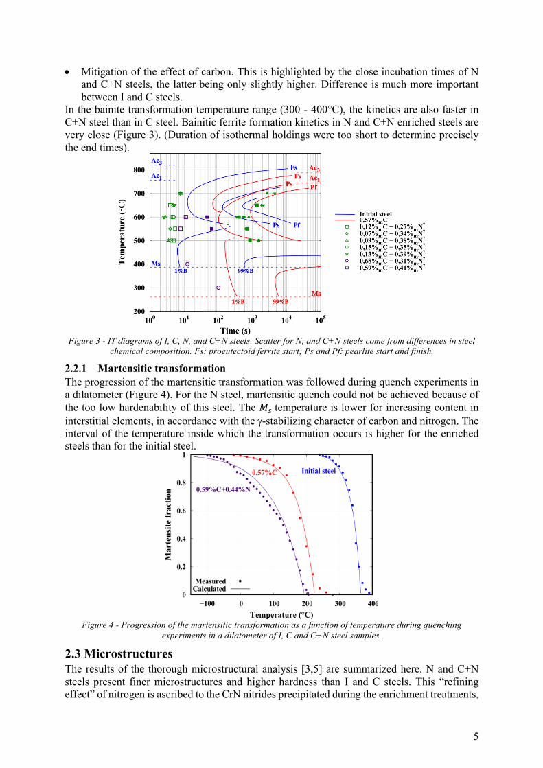
2.2! Austenite decomposition kinetics Isothermal kinetics have been determined in the temperature range ()*+- &'+for the different compositions shown in Table 1. As an example, Figure 1 and Figure 2 show isothermal kinetics measured respectively at 600°C (this temperature is higher than ,' for all compositions) and 400°C (temperature between ,' and &'). (Figures show also calculated results that will be discussed later on section 5.1) In addition, all the kinetics results are synthetized on the IT diagrams of I, C, N, and C+N steels shown in Figure 3.

4

Figure 1 - Kinetics of austenite decomposition measured by dilatometry at 600°C for initial steel, C enriched steel (0.57%mC), N enriched steel (0.09%mC - 0.38%mN) and C+N enriched steel (0.59%mC - 0.41%mN).

Comparison between calculations (solid lines) and experiments (dots). a) represents kinetics with larger timescale b) shows kinetics with smaller timescale. Zoom on first stages in the insert.

Figure 2 - Kinetics of austenite decomposition measured by in situ X-ray diffraction at 400°C for initial steel, C

enriched steel (0.57%mC), N enriched steel (0.12%mC - 0.26%mN) and C+N enriched steel (0.65%mC - 0.25%mN). Comparison between calculations (solid lines) and experiments (dots), (Calculated

fraction of N and C+N enriched steels are overlapped). Zoom on first stages in the insert.

From this experimental knowledge, the main kinetics features that have to be predicted have been identified. Regarding the steels without nitrogen, one has to predict: •! The slowing down effect of the carbon, due to its austenite-stabilizing character that appears

when comparing the I and C steels. •! The only exception concerns the pearlite when it is formed under the Hultgren temperature

(-.) at 600-650°C, that is without being preceded by proeutectoid ferrite. The “Single Pearlite,” as designated here, forms faster than when the proeutectoid ferrite precedes it.

•! At -+> -., the kinetics follows two stages, proeutectoid ferrite followed by pearlite. •! The bainite transformation is incomplete in a temperature range around 100°C below ,',

due to mechanical and chemical composition stabilization effects. Regarding nitrogen-enriched steels, the primary trend is a strong acceleration of the kinetics compared to steels without nitrogen. This “accelerating effect” of nitrogen (despite its "-stabilizing character) is ascribed to the CrN nitrides, like for the refinement of the microstructure [3,5]. In more detail, one can notice at -+> ,': •! The short incubation times, which implies that the nitrogen-enriched steels have a poor

hardenability. For the C+N steel, the end times are also shorter than for the C steel. Nevertheless, the end times for N steel are higher than for C+N steel.

5

•! Mitigation of the effect of carbon. This is highlighted by the close incubation times of N and C+N steels, the latter being only slightly higher. Difference is much more important between I and C steels.

In the bainite transformation temperature range (300 - 400°C), the kinetics are also faster in C+N steel than in C steel. Bainitic ferrite formation kinetics in N and C+N enriched steels are very close (Figure 3). (Duration of isothermal holdings were too short to determine precisely the end times).

Figure 3 - IT diagrams of I, C, N, and C+N steels. Scatter for N, and C+N steels come from differences in steel

chemical composition. Fs: proeutectoid ferrite start; Ps and Pf: pearlite start and finish.

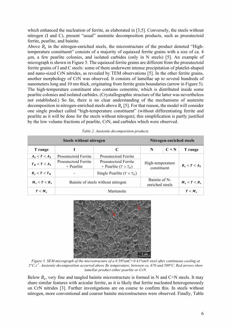
2.2.1! Martensitic transformation The progression of the martensitic transformation was followed during quench experiments in a dilatometer (Figure 4). For the N steel, martensitic quench could not be achieved because of the too low hardenability of this steel. The &'+temperature is lower for increasing content in interstitial elements, in accordance with the "-stabilizing character of carbon and nitrogen. The interval of the temperature inside which the transformation occurs is higher for the enriched steels than for the initial steel.

Figure 4 - Progression of the martensitic transformation as a function of temperature during quenching

experiments in a dilatometer of I, C and C+N steel samples.

2.3 Microstructures The results of the thorough microstructural analysis [3,5] are summarized here. N and C+N steels present finer microstructures and higher hardness than I and C steels. This “refining effect” of nitrogen is ascribed to the CrN nitrides precipitated during the enrichment treatments,

6

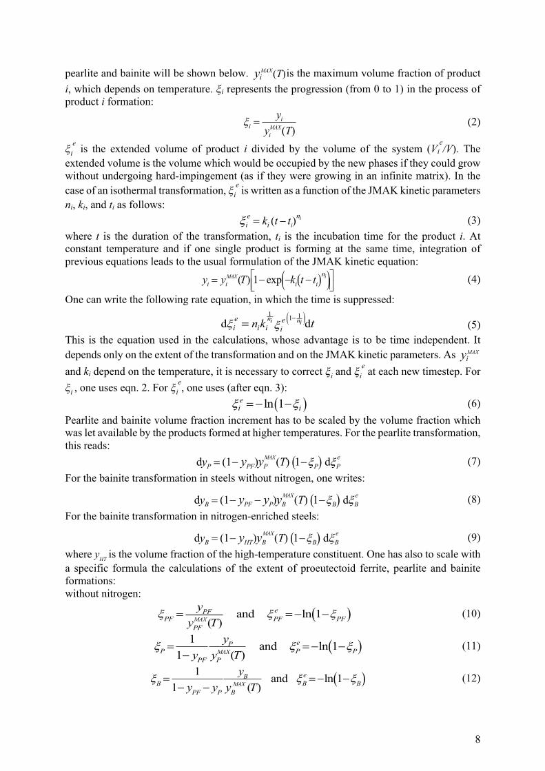
which enhanced the nucleation of ferrite, as elaborated in [3,5]. Conversely, the steels without nitrogen (I and C), present “usual” austenite decomposition products, such as proeutectoid ferrite, pearlite, and bainite. Above ,' in the nitrogen-enriched steels, the microstructure of the product denoted “High-temperature constituent” consists of a majority of equiaxed ferrite grains with a size of ca. 4 µm, a few pearlite colonies, and isolated carbides (only in N steels) [5]. An example of micrograph is shown in Figure 5. The equiaxed ferrite grains are different from the proeutectoid ferrite grains of I and C steels: some of them underwent intense precipitation of platelet-shaped and nano-sized CrN nitrides, as revealed by TEM observations [5]. In the other ferrite grains, another morphology of CrN was observed. It consists of lamellae up to several hundreds of nanometers long and 10 nm thick, originating from ferrite grain boundaries (arrow in Figure 5). The high-temperature constituent also contains cementite, which is distributed inside some pearlite colonies and isolated carbides. (Crystallographic structure of the latter was nevertheless not established.) So far, there is no clear understanding of the mechanisms of austenite decomposition in nitrogen-enriched steels above ,' [5]. For that reason, the model will consider one single product called “high-temperature constituent” (without differentiating ferrite and pearlite as it will be done for the steels without nitrogen); this simplification is partly justified by the low volume fractions of pearlite, CrN, and carbides which were observed.

Table 2. Austenite decomposition products.

Steels without nitrogen Nitrogen-enriched steels

T range I C N C + N T range /0 < 2 < /3 Proeutectoid Ferrite Proeutectoid Ferrite

High-temperature constituent 45 < 2 < /3 26 < 2 < /0 Proeutectoid Ferrite

+ Pearlite Proeutectoid Ferrite + Pearlite (- > -.)

45 < 2 < 26 - Single Pearlite (- < -.)

95 < 2 < 45 Bainite of steels without nitrogen Bainite of N-enriched steels 95 < 2 < 45

2 < 95 Martensite 2 < 95

Figure 5. SEM micrograph of the microstructure of a 0.59%mC+0.41%mN steel after continuous cooling at

2°C.s-1. Austenite decomposition occurred above Bs temperature, between ca. 670 and 580°C. Red arrows show lamellar product either pearlite or CrN.

Below ,', very fine and tangled bainite microstructure is formed in N and C+N steels. It may share similar features with acicular ferrite, as it is likely that ferrite nucleated heterogeneously on CrN nitrides [3]. Further investigations are on course to confirm this. In steels without nitrogen, more conventional and coarser bainite microstructures were observed. Finally, Table

7

2 shows the products of the austenite decomposition which are considered in the model. A clear distinction is made between the steels with or without nitrogen because they present very different microstructures [3, 4]. Microstructural analyses were completed with hardness measurement as a function of the IT temperature, i.e., microstructure formation temperature (Figure 6). For any given temperature, increased hardness is obtained for I, C, N and C+N steels (except at 650°C). The main observation is the higher hardnesses in N and C+N steels. It comes in large part from the refinement of the microstructure, especially the intra-granular CrN nitrides precipitated inside the equiaxed ferrite grains above ,' [4] and the fine and tangled bainite formed below ,' [3]. This effect of refined microstructures is more significant than the strengthening due to the higher content in interstitials. Indeed, the C+N steel exhibits much higher hardness than the C steel, despite close overall content in interstitials. Moreover, N and C steels exhibit similar hardness, despite higher content of interstitials in C steel. The hardness associated with each product has been calculated with empirical functions as a function of transformation temperature and steel composition.

Figure 6. Vickers microhardness measurements (load 100 g, at room temperature) after IT vs. IT temperature, for I, C, N, and C+N steels. ITs with incomplete transformations (T > Ae1 range or bainite range close to Bs)

are not represented. Dashed and continuous lines: empirical functions employed in the model.

3! Model The model, which has been developed in [4], predicts the fraction of either constituents (pearlite, bainite, high-temperature constituent) or phases (austenite, proeutectoid ferrite and martensite). It is based on previous models of austenite decomposition kinetics [10–13]. The approach consists first in establishing a model predicting the global kinetics in the initial steel under isothermal conditions. The kinetics under anisothermal conditions are then predicted by making an additivity assumption. The effect of carbon content on the isothermal kinetics is modeled following the approach introduced by Mey et al. [10,11], which was derived from Kirkaldy’s model for IT diagrams predictions [14]. A new approach will be introduced regarding the effects of nitrogen.

3.1! Diffusion dependent phase transformations In order to calculate the progression of (time-dependent) diffusive phase transformations, a differential formulation of the Johnson-Mehl-Avrami-Kolmogorov (JMAK) equation is used [15–19], [20]:

( )d ( ) 1 dMAX ei i iiy Ty ! != " (1)

where i denotes either the proeutectoid ferrite in steels without nitrogen or the high-temperature constituent in nitrogen-enriched steels. yi is the volume fraction of product i. The equations for

8

pearlite and bainite will be shown below. ( )MAXi Ty is the maximum volume fraction of product

i, which depends on temperature. #i represents the progression (from 0 to 1) in the process of product i formation:

( )MAXi

ii

yy T

! = (2)

#ie is the extended volume of product i divided by the volume of the system (Vi

e/V). The

extended volume is the volume which would be occupied by the new phases if they could grow without undergoing hard-impingement (as if they were growing in an infinite matrix). In the case of an isothermal transformation, #i

e is written as a function of the JMAK kinetic parameters ni, ki, and ti as follows:

( ) iine

i ik t t! "= (3) where t is the duration of the transformation, ti is the incubation time for the product i. At constant temperature and if one single product is forming at the same time, integration of previous equations leads to the usual formulation of the JMAK kinetic equation:

( )( )( ) 1 exp iMAXi i i i

ny y T k t t! "= # # #$ %& ' (4)

One can write the following rate equation, in which the time is suppressed:

(5) This is the equation used in the calculations, whose advantage is to be time independent. It depends only on the extent of the transformation and on the JMAK kinetic parameters. As MAX

iy

and ki depend on the temperature, it is necessary to correct #i and #ie at each new timestep. For

#i , one uses eqn. 2. For #ie, one uses (after eqn. 3):

( )ln 1ei i! != " " (6)

Pearlite and bainite volume fraction increment has to be scaled by the volume fraction which was let available by the products formed at higher temperatures. For the pearlite transformation, this reads:

( )d (1 ) ( ) 1 dMAX ePFP PP Py Ty y ! != " " (7)

For the bainite transformation in steels without nitrogen, one writes:

( )d (1 ) ( ) 1 dMAX ePF P BB B By Ty y y ! != " " " (8)

For the bainite transformation in nitrogen-enriched steels:

( )d (1 ) ( ) 1 dMAX eHTB B B By Ty y ! != " " (9)

where yHT is the volume fraction of the high-temperature constituent. One has also to scale with a specific formula the calculations of the extent of proeutectoid ferrite, pearlite and bainite formations: without nitrogen:

( ) and ln 1( )MAXPF

PF PF PFP

e

F

yy T

! ! != =" " (10)

( )1 and ln 11 ( )MAX

ePP P P

PF P

yy y T

! ! != =" ""

(11)

( )

1 and ln 11 ( )MAX

eBB B B

PF P B

yy y y T

! ! != =" "" "

(12)

( )1 11d dn ni iei i

eiin k t!! "=

9

with nitrogen:

( )

1 and ln 11 ( )MAX

eBB B

BHTB

yy y T

! ! != =" ""

(13)

For proeutectoid ferrite, ( )MAX

PFy T is the equilibrium volume fraction. For pearlite, ( )MAX

Py T is always equal to 1 (but its equilibrium overall fraction is equal to 1 ( )MAX

PFy T! above the Hultgren temperature). For bainite, ( )MAX

By T allows taking account of an incomplete transformation, as it will be detailed in Section 4.3.2. In our approach, the kinetic parameters are extracted from experimentally determined isothermal kinetics, as will be seen in the following. This implicitly assumes the additivity hypothesis, which was deeply discussed in the literature [17,21–24]. Under anisothermal conditions, the calculation of the phase transformations progression is preceded by the calculation of the incubation time [25,26]. The incubation time is calculated with the sum of Scheil [27], which is also based on the additivity hypothesis:

( )j

i jj

tS f

Tt!

= " (14)

where ∆tj is the increment of time at timestep j, and ti is the incubation time of the isothermal transformation, which depends on temperature. The transformation starts when the sum reaches the value of 1. In order to calculate the incubation of the bainite transformation, Fernandes [25] proposed to introduce a correction factor f, which takes account of a deviation to the additivity assumption for the bainite. In the present study, a value f = 0 is taken, which means that the incubation of bainite is independent of the higher-temperature constituents. This assumption gave the best agreement between simulations and experiments. Thus, the calculation includes a first step dedicated to the calculation of the incubation time and a second step dedicated to the progression of the different transformations. For simplicity, it is assumed that one single product can be formed at the same time. The domains of transformation for each product are separated by equilibrium or characteristic temperatures, (see Table 2).

3.2! Martensitic phase transformation The progression of the martensitic transformation is described by the Koistinen Marburger’s law: without nitrogen:

( ) ( )1 1 Ms TM PF P By y y y e !" "= " " " "# $% & (15)

with nitrogen: ( ) ( )1 1HT

Ms TM By y y e !" "= " " "# $% & (16)

where yM is the volume fraction of martensite, &'+the martensite start temperature, $ a parameter which is determined experimentally.

3.3! Accounting of a carbon concentration variation in steels without nitrogen

In order to take account of the variations of austenite decomposition kinetics when the carbon concentration is modified, Mey [10] developed an approach based on the calculation of the displacement of isothermal kinetics curves with respect to a reference steel (the I steel in the present case). These displacements depend on the undercooling. They are defined as:

0, ,

, 0,

i ii

i

ttt

D ! !!

!

"= (17)

10

where ti,# is the time necessary to form a fraction # of product i (proeutectoid ferrite, pearlite, bainite, HT constituent). t0

i,# is the time related to the initial steel. The calculation of Di,# is based on the model introduced by Kirkaldy in order to calculate IT diagrams as a function of the steel composition. The rules of variations are detailed in [14]. Because in our case, only the carbon concentration varies, simplified displacement relationships are obtained:

303

,3

1PFAe TDAe T!

" #$= $% &$' (

(18)

30

1,

1

1 PAe TDAe T!

" #$= $% &$' (

(19)

2

0

, 0

''

2.34 200% 3.8% 19% 12.34 200% 3.8% 19%

eff

s m m mB

s m m m

oo

B T C Cr MID

B T C Cr MI!

" #" #$ + + += $% &% & % &$ + + +' ( ' (

(20)

with: ( )2 35% 2.5% 0.9% 1.7% 4% 2.6

2(1 ) 203 3

d

(1 )

'eff

m m m m mC Mn Ni Cr M

x x

x o x

x x

eI

! + + + + "

"

"

= # (21)

where %mCeff is an effective carbon concentration, which will be defined later (see Section 4.3.3) and %mC0 is the initial carbon content of the steel. For proeutectoid ferrite, the displacement is the same whatever the progression of the transformation (DPF,# = DPF). Regarding pearlite, the displacement is equal to zero because we will assume (see Section 4.2.2.3) that the (): temperature does not depend on the carbon concentration ((): = ():<). As for bainite, the coefficients associated with the carbon concentration in eqns. 20 and 21 have been adjusted on the basis of our own experiments. The validation of these modifications will be discussed in Section 5.1.2. The DPF,# parameters allow to recalculate the times of transformation start for proeutectoid ferrite and bainite when the carbon concentration is modified:

( )0,1%1i i it t D= + (22)

Hence, 1% is taken as a reference to determine the start of the austenite transformation. Regarding the kinetic coefficients, it is assumed that ni does not vary with the carbon concentration (i.e., the mechanisms are not modified). As for the ki parameter, it reads [10]:

( )0

,1 i

ii

in

kkD !

=+

(23)

3.4! Effect of the nitrogen The approach used to predict the influence of the carbon concentration on the austenite decomposition kinetics cannot be adapted to the case of an enrichment with nitrogen, for the considered steel. The nitrogen enriched steels have faster kinetics (as shown in Figure 1) due to the precipitation of CrN nitrides during the enrichment treatments. The model presented above for the effect of carbon could only be used to predict a possible slow-down of the kinetics by the nitrogen in solid solution in the austenite. Many questions remain to be solved regarding the mechanisms of the phase transformations in the presence of nitrogen. More observations are necessary in order to serve as a basis for modeling with a more physical basis. Hence a more straightforward approach for the modeling has been followed. Two temperature domains have been separated: above and below ,'. In the high-temperature range, the global kinetics of one single product termed as “high-temperature constituent” is described. It is denoted HT, and its

11

isothermal kinetics is described according to the eqn. 1. In the temperature range of bainite, the isothermal kinetics is described with the eqn. 9. The influence of the carbon and nitrogen concentrations is described empirically in both temperature ranges. The anisothermal simulations are still based on an additivity hypothesis for the incubation and the progression of the transformations. As for the martensitic transformation, it is described with the Koistinen-Marburger relationship. The model separates so far two distinct situations: either the steel is enriched with nitrogen or not. When simulating cooling of samples with carbon and nitrogen concentration gradients (in Section 6), a threshold of nitrogen concentration will be set in order to separate both cases. This limit is taken as the solubility limit of nitrogen in austenite at 900°C, 0.08 %m N, (according to Thermocalc® - TCFE7 database). Indeed, beyond this limit, the precipitation of CrN nitrides during the enrichment treatments becomes possible thermodynamically. In the range, 0 - 0.08 %m N, the nitrogen is expected to remain in solid solution during the enrichments. The possible slowing down effect due to the austenite-stabilizing character of nitrogen is neglected, because of these low nitrogen concentrations.

4! Model parameters This section presents how the data were established and formulated for each product of the austenite decomposition (characteristic temperatures, maximum fractions, incubation periods, hardnesses) as well as various hypotheses and extrapolations. In steels without nitrogen (I and C), the parameters come in part from a thermodynamic basis. A more empirical approach is followed for the steels enriched in nitrogen (N and C+N).

4.1! Kinetic parameters 4.1.1! Steels without nitrogen In steels without nitrogen, the determination of the JMAK kinetic parameters ni, ki, and ti were done classically from the exploitation of the experimental isothermal kinetics of the I steel. If the carbon concentration is different from the one of the I steel (0.246%mC), the model presented in Section 3.3 calculates the modified kinetic parameters, ki, and ti. One exception concerns the “single pearlite” (i.e., not preceded by proeutectoid ferrite), whose JMAK parameters came from the exploitation of the experiments done on the C steel because in I steel, pearlite is always preceded by proeutectoid ferrite. In two particular cases, the analysis of the isothermal kinetics had to be adapted: •! For a ferrite-pearlite transformation, the successive proeutectoid ferrite and pearlite kinetics

had to be deconvoluted [25]. For simplicity, the overlap between both kinetics was neglected. Both kinetics could nevertheless be appropriately described with the JMAK equation.

•! In the case of the bainite transformation in steels without nitrogen, most of the experimental kinetics could not be adequately described by the JMAK equation. Indeed, in many cases, the bainite transformation kinetics exhibited two-stage kinetics, fast, followed by a slow-down (as shown in Figure 2 for C steel). The first stage is well described by the JMAK equation, but the overall kinetics shows an overestimation of the bainite amount in the second stage. The coefficients nB, and kB of the I steel were determined by considering only the first stage and experimental values of yMAX have been used (see Section 3.1). Nevertheless, for the model, it is most important to describe properly the domain where the phase transformation kinetics is faster, in order to obtain a good precision in the simulations of cooling treatments.

12

4.1.2! Steels enriched with nitrogen For the steels enriched with nitrogen, the JMAK parameters were determined in the same manner. No significant variation of ti with the steel composition was observed. The parameter nHT was considered as constant as a function of temperature and steel composition. Indeed, the morphology of the high-temperature constituent remained identical in the set of tested conditions. In the high-temperature domain, significantly faster kinetics were determined in steels enriched in nitrogen, compared to steels enriched in carbon + nitrogen. In order to take this trend into account, the kinetic parameter HTk is modified empirically as a function of the carbon concentration of the steel, according to the following formula:

0ln ln (T) 1.5(% 0.1)HT HT mk k C= ! ! (24) where 0

HTk is the kinetic coefficient determined for the steel enriched in nitrogen, which has a carbon content of 0.1 %m. No significant variation of HTk could be associated with the nitrogen content. The JMAK parameters of the bainite transformation in nitrogen-enriched steels are assumed to be constant as a function of carbon and nitrogen concentrations. Indeed, from the experiments, it was not possible to establish a correlation with the kinetics.

4.2! Ferrite and pearlite transformations In this temperature range, some parameters of the model (namely ()*, ():, =>?@ABand -.) come from thermodynamic calculations.

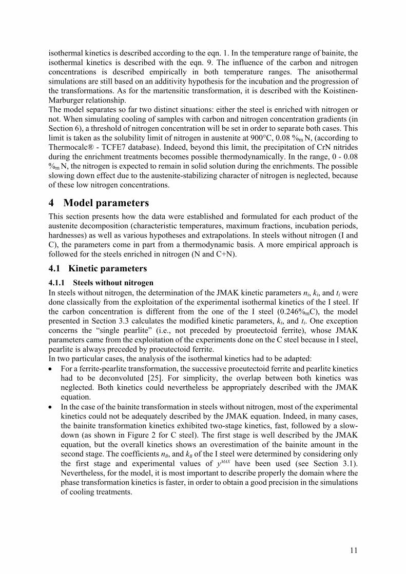
4.2.1! Proeutectoid ferrite in steels without nitrogen For the kinetics calculations (eqn. 18), ()* equilibrium temperature (including its extrapolation below ():) is used. The extrapolated ()* line was calculated by considering a metastable equili-brium between ferrite and austenite. Thermocalc® and TCFE7 thermodynamic database were used. The ()* line is plotted in the isopleth curve of the studied steel, in Figure 7).

4.2.2! Ferrite-pearlite transformation in steels without nitrogen 4.2.2.1! Transition from proeutectoid ferrite to pearlite It is generally admitted that the pearlite starts to form when the austenite becomes super-saturated by the carbon rejected by the growing proeutectoid ferrite. According to Hultgren’s extrapolation [28], the solubility limit corresponds to the extrapolation of the (CD line ("/"+% boundary) below ():. The (CD line and its extrapolation below (): are plotted in the isopleth curve (Figure 7a). The dots represent the carbon concentration in the austenite at the transition, which was estimated with the following mass balance (Phase’s mass fraction assumed equal to the volume fraction):

,max% % %PF PFm m mC CC y y! != + (25)

Where %mC is the C concentration,%mC! the C mass concentration in phase! ( PFy or y! ), y!

the volume fraction of phase! . One assumes that% 0.PFmC = PFy was measured by image

analysis of optical micrographs taken at the end of the ITs. It can be seen that the carbon concentration in austenite largely exceeded the extrapolated equilibrium (CD line for all the experiments. This is a significant discrepancy with the equilibrium assumption, which was already reported in the case of alloyed steels [29]. Besides the equilibrium, two other frequent assumptions are the paraequilibrium (PE) and the local equilibrium with no partition (LENP), according to which the cementite grows without partition of the substitutional elements. The corresponding solubility limits, which are denoted (CD>E and (CDFEG>, are plotted in Figure 7. (The method of calculation is detailed in [30,31]). Both curves are closer to the experimental points than the (CD line. Hence, it is likely that in I and C

13

steels, the ferrite-pearlite transformation occurs with a limited partition of the alloying elements. Neither curves describe accurately all the experimental points. They are in close agreement with the (CDFEG> curve for the I steel, while those of the C steel are closer to the (CD>E curve. Nevertheless, for the C steel, the measured volume fractions of proeutectoid ferrite (4 and 9%) were quite low, leading to significant uncertainties in the mass balance. This is why the (CDFEG>curve is used in the model. Maximum fraction of proeutectoid ferrite will be calculated as follows:

,max

%1%

MAX mPF

m

CyC!= " (26)

with ,max%mC! being given by the (CDFEG>curve.

4.2.2.2! Hultgren temperature Below the Hultgren temperature (-.), the austenite decomposes directly to pearlite. As the (CDFEG> curve is taken as a reference, this happens at -. = 671°C in the C steel according to the model. (One would obtain -.+= 636°C with the (CD>E curve). The experimental -. temperature of the C steel actually ranges between 600 and 625°C, according to the microstructural observations. This discrepancy is significant, but it will have limited consequences on the simulations, as will be shown in Section 5.

4.2.2.3! (): temperature and eutectoid composition The (): temperature was chosen in accordance with the selection of the equilibrium ()* line for the onset of the proeutectoid ferrite and the (CDFEG> line for the cementite. Intersection of both curves yields “eutectoid” temperature and composition of respectively 720°C and 0.68%mC. This is in accordance with the absence of pearlite transformation at T ≥ 725°C in both I and C steels, and also with the hypo-eutectoid behavior of the C steel. If the austenite composition exceeds the eutectoid composition of 0.68%mC, hyper-eutectoid behavior (proeutectoid cementite followed by pearlite) should be considered, which is not accounted for by the model. Nevertheless, such carbon concentrations will not occur experimentally, in the samples with concentration gradients as will be seen in Section 6.

Figure 7. a) Isopleth diagram of the investigated steels; Ae3 lines for different overall nitrogen contents. b)

Proeutectoid ferrite fraction vs. temperature according to the experiment in the initial steel and comparison with thermodynamic calculations.

4.2.3! High-temperature constituent in steels enriched with nitrogen In the case of steels enriched with nitrogen, a “high-temperature” constituent is considered, instead of proeutectoid ferrite and/or pearlite (see Section 2.2). As it consists mostly of ferrite, it is considered like the proeutectoid ferrite of the steels without nitrogen. The ()* temperature was calculated according to the thermodynamic equilibrium. It was tabulated as a function of carbon and nitrogen concentration (up to 0.45%m N in solid solution

14

in austenite). (See Figure 7). In these calculations, a fixed concentration of N in " was imposed. The ()* temperature is defined as the temperature below which the ferrite starts to be present at equilibrium. In all the calculations, the presence of CrN phase is predicted by the equilibrium. Its mass fraction depends on the considered temperature, the overall carbon concentration and the imposed nitrogen concentration in austenite. The maximum fraction of the high-temperature constituent is considered as constant and equal to 1 in the temperature range from+(): to ,' ( MAX

HTy = 1). Indeed, the complete transformation

was observed in the presence of nitrogen, for the IT temperatures considered experimentally.

4.3! Bainite transformation For the bainite transformation, more empirical relationships had to be used. 4.3.1! Bainite start temperature The variation of the ,' temperature as a function of the carbon content is supposed to be linear, per the empirical relationship introduced by Steven and Haynes [32]. The proportionality constant was determined from the experimental data regarding ,' for I and C steels. Hence, the variation of ,' reads (with respect to the initial steel):

( )0185 % %S meff

mC CB = !" ! (27)

where %meffC is an effective carbon concentration which will be defined later (in Section 4.3.3)

and 0%mC is the initial steel carbon content, 0.246%m C. The ,' temperature of the steels enriched with nitrogen could not be established with as much precision as for the carbon steels. Due to the lack of experimental data, this temperature is assumed to be constant whatever the nitrogen content and it is fixed to 475°C. 4.3.2! Maximum fraction of bainite At temperature close to ,', the bainite transformation is incomplete, and the model takes as a parameter the maximum fraction of bainite, MAX

By . An empirical approach was followed. The experimental curve giving ( )MAX

By T was established for the I steel. It was found that translating this master curve along the temperature axis (towards lower temperatures) allowed to represent accurately the experimental points for the C steel. Thus, for a particular steel composition in carbon, the approach consists of translating the master ( )MAX

By T curve with an offset which is proportional to the carbon content. Regarding the steels enriched in nitrogen, the bainite transformation is assumed complete, due to the lack of experimental data.

4.3.3! Accounting of the “local” enrichment in carbon The formation of proeutectoid ferrite leads to the carbon enrichment of the austenite. The model takes into account the effect of this change of composition on the kinetics of bainite formation, as proposed by Louin et al., [13]. The mass balance estimates the effective carbon concentration in austenite following the proeutectoid ferrite formation:

% % %PF Pm

fm

fm

F eC y yC C!= + (28) where%mC is the carbon content in the steel, yPF the fraction of formed proeutectoid ferrite, and yγ the austenite fraction. For simplicity, a carbon concentration equal to zero is assumed in proeutectoid ferrite. The model of accounting of carbon composition variation presented in Section 3.3 will be used to modify the calculation of the kinetics (tB and kB, eqns. 20-23), ,' (eqn. 27), and &' (eqn. 29) as a function of % eff

mC .

15

In steels enriched with nitrogen, the possible carbon enrichment of austenite due to a high-temperature partial transformation is presently not taken into account. Further experimental knowledge should be necessary.

4.4! Martensitic transformation The variation of the &' temperature is calculated as a function of the variation of carbon content in austenite with respect to the initial steel, by using the following empirical relationship, which was established on the basis of the measurements done in the initial steel and the C steel (enriched to 0.57%m C).

( )0429 % %S meff

mC CM = !" ! (29)

It can be noticed that via the parameter %meffC , the effect of a variation of the local carbon

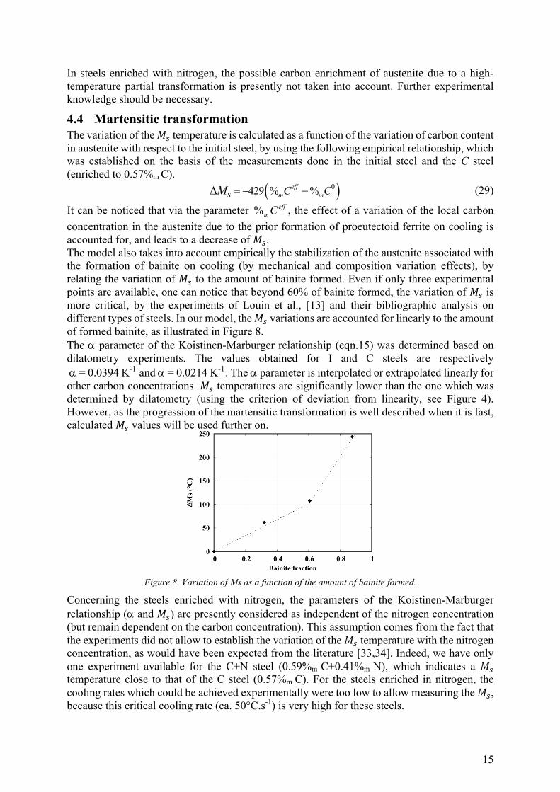
concentration in the austenite due to the prior formation of proeutectoid ferrite on cooling is accounted for, and leads to a decrease of &'. The model also takes into account empirically the stabilization of the austenite associated with the formation of bainite on cooling (by mechanical and composition variation effects), by relating the variation of &' to the amount of bainite formed. Even if only three experimental points are available, one can notice that beyond 60% of bainite formed, the variation of &' is more critical, by the experiments of Louin et al., [13] and their bibliographic analysis on different types of steels. In our model, the &' variations are accounted for linearly to the amount of formed bainite, as illustrated in Figure 8. The $ parameter of the Koistinen-Marburger relationship (eqn.15) was determined based on dilatometry experiments. The values obtained for I and C steels are respectively +$+=+0.0394+K-1+and $+=+0.0214+K-1. The $ parameter is interpolated or extrapolated linearly for other carbon concentrations. &' temperatures are significantly lower than the one which was determined by dilatometry (using the criterion of deviation from linearity, see Figure 4). However, as the progression of the martensitic transformation is well described when it is fast, calculated &' values will be used further on.

Figure 8. Variation of Ms as a function of the amount of bainite formed.

Concerning the steels enriched with nitrogen, the parameters of the Koistinen-Marburger relationship ($ and &') are presently considered as independent of the nitrogen concentration (but remain dependent on the carbon concentration). This assumption comes from the fact that the experiments did not allow to establish the variation of the &' temperature with the nitrogen concentration, as would have been expected from the literature [33,34]. Indeed, we have only one experiment available for the C+N steel (0.59%m C+0.41%m N), which indicates a &' temperature close to that of the C steel (0.57%m C). For the steels enriched in nitrogen, the cooling rates which could be achieved experimentally were too low to allow measuring the &', because this critical cooling rate (ca. 50°C.s-1) is very high for these steels.

16

4.5! Hardness The calculation of the hardness is done by considering that the final hardness results from a mixture rule on the hardness of the austenite decomposition products formed on cooling [25]:

( ) ( ),i

ij j i jj

iHv y Hv on Hv T= !" (30)

where ∆yij represents the increase of product i fraction during timestep j and Hvij, its hardness (at room temperature) corresponding to the temperature of timestep j. Figure 6 shows the evolutions of hardness as a function of formation temperature for the different products, which are used in the calculations. Hardness of proeutectoid ferrite and pearlite products are taken from previous work [35] on steel with a composition similar to the initial steel of present study. The hardness of bainite as a function of formation temperature comes from measurements in I steel and C steel, enriched to 0.57%m C. The effect of the carbon content has been taken into account on the hardness of bainite and martensite, for which it is the most significant. For bainite, a relationship similar to the one adopted by Mey [10] was established from the measurements taken in the I steel and the C steel:

00 225(% %( ) )m meff

B BHv Hv C CT= + ! (31) where 0

BHv corresponds to the bainite hardness of initial steel (0.246%m C) and %m Ceff is the C content in austenite at the beginning of the bainitic transformation. The hardness of martensite is calculated as a function of the carbon content by using the empirical relationship of Krauss [36], whose parameters were adapted to our measurements:

2 381 1737% 612(% 428(%) )m m meff eff

MeffHv C C C= + ! ! (32)

For the steels enriched with nitrogen, an empirical approach is used, based on the hardness measurements for both N and C+N steels (Figure 6). The hardness of high-temperature constituent and bainite depends on the transformation temperature and the carbon concentration [33,34]. No correlation was found with the nitrogen concentration. The following empirical rules, which are plotted in Figure 6 are employed:

1.757 1448.5 257(% 0.1)mHT T CHv = ! + + ! (33) 0.3842 801.7 257(% 0.63)mB TH Cv = ! + + ! (34)

where T is in °C. In the absence of hardness measurements for the bainite in N steel, the same offset proportional to the carbon concentration as in the high-temperature range is applied. Regarding the hardness of martensite in the steels enriched with nitrogen, the only available experiment was used to add a term dependent on the nitrogen concentration in the empirical formula of Krauss.

2 381 1737% 612% 428% 500%m m m mMHv C C C N= + ! ! + (35) One reminds that in nitrogen-enriched steels, we do not introduce an effective carbon concentration which would result from the carbon rejected by the HT constituent, due to the lack of experimental knowledge.

5! Results for homogeneous samples The model has been implemented in the FE code Zebulon [37], for future simulations coupled to mechanical calculations. In order to check the whole model and the complete set of input data, isothermal kinetics have firstly been calculated in homogeneous specimens with different carbon and nitrogen compositions and compared to experiments even if in some cases, model parameters have been adjusted directly from these experiments. Then, the experimental validation of the calculated kinetics during continuous cooling as well as final microstructures and hardnesses were performed and discussed, still considering homogeneous specimens. The volume fractions of the different phases (proeutectoid ferrite, martensite) and constituents

17

(pearlite, bainite, HT constituent) were determined experimentally[4] from image analysis of optical or SEM micrographs and the interpretation of dilatometry curves.

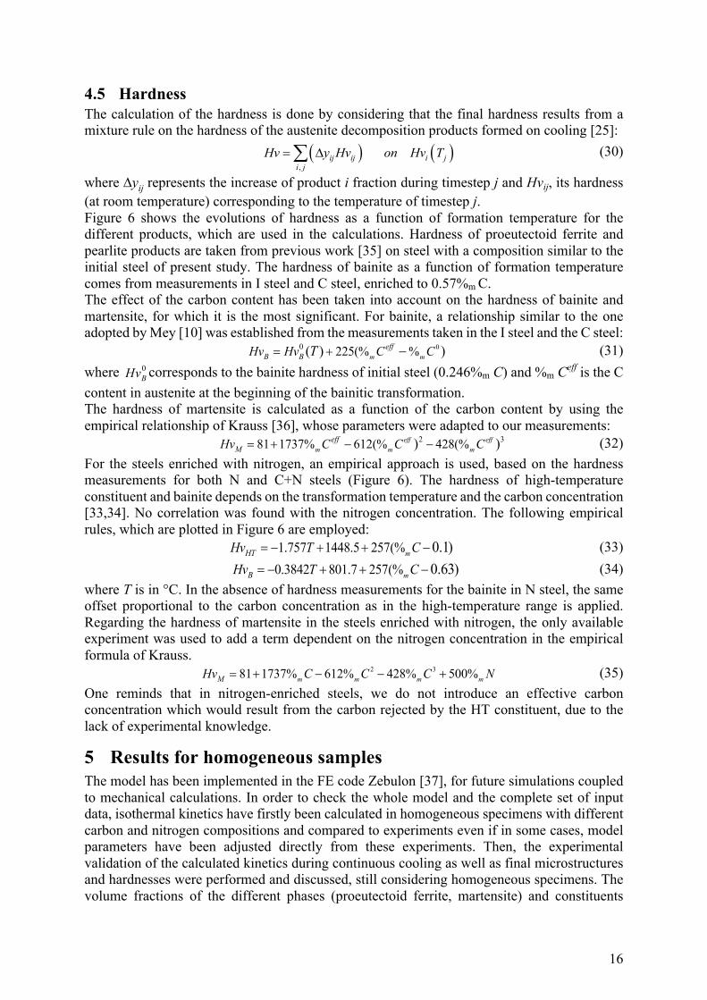
5.1! Isothermal kinetics 5.1.1! Initial steel For the I steel, two examples of comparisons between calculated and experimental isothermal kinetics have already been shown in Figure 1 and Figure 2. The JMAK parameters were directly established on the basis of these experiments, and the precision was good whatever the IT temperature, as mentioned in Section 4.1.1. One can mention that in the bainite domain, assuming a constant value of the parameter nB (despite some scatter) did not lead to significant discrepancies. Figure 9 shows the fraction of the respective decomposition products at the end of the isothermal treatments (IT) as a function of the IT temperature. The calculated fractions of proeutectoid ferrite, MAX

PFy are in accordance with the experimental values in the ferrite-pearlite domain. This confirms the selection made in Section 4.2.2 regarding the Hultgren’s extrapolation based on the (CDFEG> line. The maximum fractions of bainite are expectedly in close agreement with the experiment, as the ( )MAX

PFy T curve was established empirically for the I steel. The hardnesses calculated at the end of the ITs are in good agreement with the experiments in the ferrite-pearlite temperature range. This confirms the choice of the data which were used for the ferrite-pearlite microstructures, which came from previous studies [35]. Bainite hardnesses come directly from the experiment in the I steel. In the case of incomplete transformation, the hardness calculations take into account the formation of martensite during the cooling to room temperature. This explains the high hardnesses calculated in the bainite range at IT temperatures close to ,'. For the proeutectoid ferrite transformation at 750°C, the calculation overestimates the hardness, which is due to an overestimated hardness of the martensite. At 550°C, the hardness is also largely overestimated. This IT temperature is located inside the transition between ferrite-pearlite and bainite domains (see the IT diagram in Figure 3). It was observed experimentally that the kinetics and the proportion of the products depend strongly on the exact IT temperature. These discrepancies will have little influence on the simulations under anisothermal conditions, as the kinetics are slow in this temperature range, as will be seen in Section 5.2.1.

Figure 9. Fractions of products and hardness at the end of ITs for the initial steel. Comparison between calculations (solid lines) and experiments (dots). The white hardness dots correspond to the cases where

martensite was formed upon final quench (incomplete isothermal transformations).

18

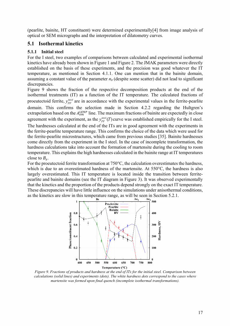
5.1.2! Carburized steel As previously for the I steel, Figure 10 shows the fractions of the different products versus temperature for the different IT temperatures, for the C steel. It can be seen that the amount of proeutectoid ferrite is underestimated by the calculation. These discrepancies come from the choice of the (CDFEG> line for the Hultgren’s extrapolation. In the bainite domain, as expected, the maximum fractions of bainite are correctly predicted, thanks to the empirical approach introduced in Section 4.3.2. Nevertheless, one can notice discrepancies regarding the kinetics, which worsen when the IT temperature gets farther below ,' (Figure 11). At 300°C, and also at 350°C (Figure 11), the incubation period is too short, and the kinetics is too fast at the beginning of the phase transformation. These discrepancies come mostly from the formulae which were used to calculate the displacement of the transformation curves. Analysis of the functions proposed by Kirkaldy shows that for transformation temperatures largely below ,', the times of transformation start are weakly modified. One should also mention that in order to apply the model, one has to extrapolate the C curves of the IT diagram of the I steel below its &' temperature (385°C). Regarding the hardnesses, the calculated values are close to the experiment in the bainite temperature range. This validates the empirical formula introduced in eqn. 31.

Figure 10. Fractions of products and hardness at the end of ITs for the carburized steel. Comparison between

calculations (solid lines) and experiments (dots). The white hardness dots correspond to the cases when martensite was formed upon final quench (incomplete isothermal transformations).

Figure 11. Isothermal kinetics of austenite decomposition at 400, 350 and 300°C in the carburized steel,

calculated and experimental.

19

5.1.3! Nitrided and carbonitrided steels We have chosen to show in Figure 1 and Figure 2 the calculated and measured kinetics for nitrided steel at 600°C and a carbonitrided steel at 400°C respectively. In each case, we have reported the set of experimental curves that correspond to several different samples. The measured isothermal kinetics differ from one sample to another, mainly due to the discrepancies in sample compositions (see Table 1). In the model, the kinetic parameters were established at each temperature in order to represent at best “mean” kinetics. Also, for the bainite transformation, discrepancies at the end of the transformation are due to our assumption of a complete transformation.

5.2! Continuous cooling kinetics The phase transformation kinetics were determined experimentally by dilatometry during continuous cooling at different constant cooling rates, as well as the final microstructures and hardnesses. The detail of these experiments as well as their exploitation and analysis are presented in [4]. The results presented here are focused on the comparisons between the simulations and the experiments.

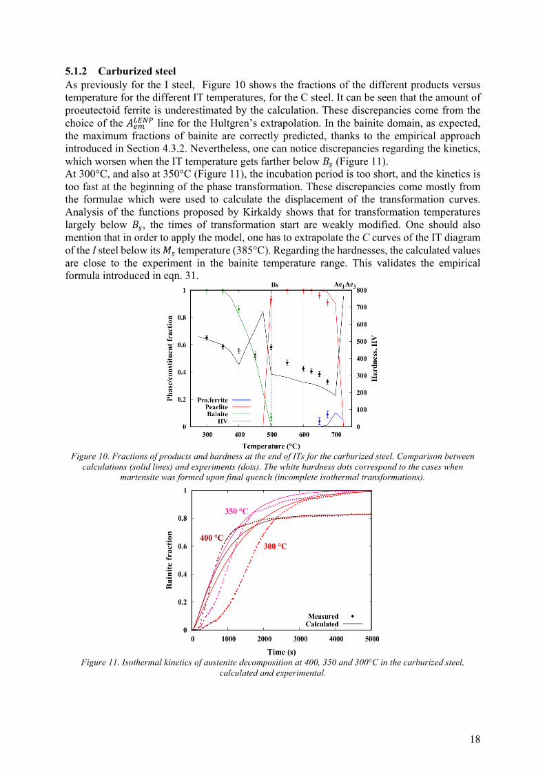
5.2.1! Initial steel Figure 12a compares the experimental and simulated kinetics for cooling at 0.5°C.s-1. The model predicts the start of the proeutectoid ferrite transformation accurately. Nevertheless, the predicted proeutectoid ferrite transformation kinetics is too slow below 700°C. Thus, the final amount of proeutectoid ferrite is underestimated. According to the microstructural observations, there is no pearlite at the end of the cooling, whereas the calculation predicts an amount of 9%. In the bainite domain, the model predicts the start of the transformation and the kinetics appropriately. The final calculated amount of bainite (20%) is comparable to the experiment (14%). Hence, the model predicts satisfactorily the effect of the austenite enrichment in carbon (to 0.52%m) by the prior ferritic transformation, despite the underestimation of the proeutectoid ferrite amount. The start of the martensitic transformation is strongly affected by the prior formation of proeutectoid ferrite and bainite: experimentally the start of the martensitic transformation is estimated to occur at 230°C.

Figure 12. Experimental and calculated kinetics of austenite decomposition during continuous cooling at a)

0.5°C.s-1 and b) 10°C.s-1 in the initial steel.

For the 10°C.s-1 cooling rate (Figure 12b) leading to bainite and martensitic transformations, the calculation underestimates the rate of the bainite transformation. This may be ascribed to the additivity hypothesis, which is not fully justified to estimate the bainite transformation progression during anisothermal treatments (see e.g. [38]). It also seems that the calculation overestimates the decrease of &' with the bainite fraction. Nevertheless, the final amount of phases is correctly predicted (Figure 13).

20

Figure 13. Fractions of products and hardness at room temperature for different cooling rates for the initial

steel; calculated (continuous lines) and experimental (points).

Figure 13 gives a synthesis of all the results showing the fractions of the different products (at room temperature) as a function of the cooling rate as well as the associated hardness. As expected, fractions of proeutectoid ferrite and pearlite are higher at lower cooling rates. Increasing the cooling rate makes increase successively the final fraction of bainite and then martensite. Except for the proeutectoid ferrite proportion at 0.5°C.s-1, the difference between the simulation and the experiment does not exceed 10%. The discrepancies regarding the hardness do not exceed 50 HV, except in the case of a fully martensitic transformation (cooling at 50°C.s-1). This discrepancy comes from the empirical relationship relating the hardness of martensite and its composition in carbon following the approach of Krauss (eqn. 32). Our formula results from a compromise between different experiments. 5.2.2! Carburized steel For a 2°C.s-1 cooling rate (Figure 14), calculation predicts a mostly martensitic transformation with the formation of a small amount of bainite. Progression of martensite is well described, but no bainite was detected experimentally.

Figure 14. Experimental and calculated kinetics of austenite decomposition during continuous cooling at 2°C.s-1

in the carburized steel.

Synthesis of the results is shown in Figure 15. For both cooling rates considered experimentally, 0.5 and 2°C.s-1, the differences between the calculations and the experiments are limited. Compared to the I steel, the higher carbon concentration reduced the proportions of

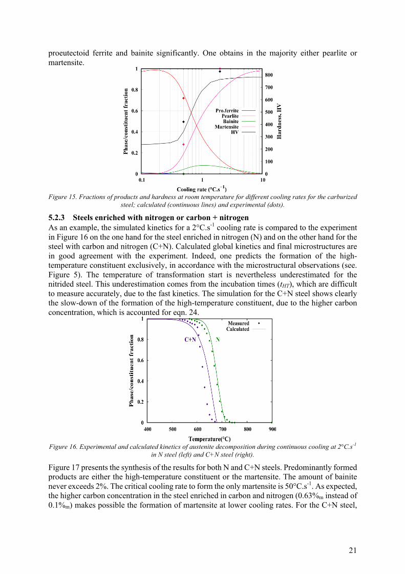
21

proeutectoid ferrite and bainite significantly. One obtains in the majority either pearlite or martensite.

Figure 15. Fractions of products and hardness at room temperature for different cooling rates for the carburized

steel; calculated (continuous lines) and experimental (dots).

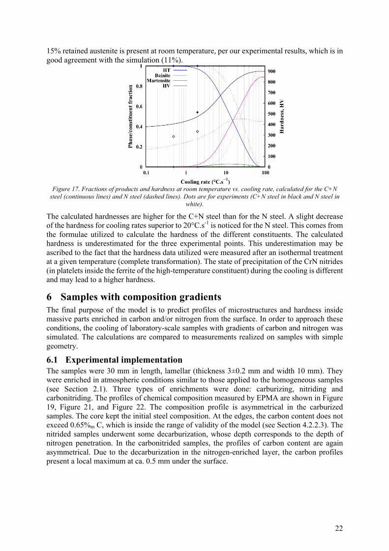
5.2.3! Steels enriched with nitrogen or carbon + nitrogen As an example, the simulated kinetics for a 2°C.s-1 cooling rate is compared to the experiment in Figure 16 on the one hand for the steel enriched in nitrogen (N) and on the other hand for the steel with carbon and nitrogen (C+N). Calculated global kinetics and final microstructures are in good agreement with the experiment. Indeed, one predicts the formation of the high-temperature constituent exclusively, in accordance with the microstructural observations (see. Figure 5). The temperature of transformation start is nevertheless underestimated for the nitrided steel. This underestimation comes from the incubation times (tHT), which are difficult to measure accurately, due to the fast kinetics. The simulation for the C+N steel shows clearly the slow-down of the formation of the high-temperature constituent, due to the higher carbon concentration, which is accounted for eqn. 24.

Figure 16. Experimental and calculated kinetics of austenite decomposition during continuous cooling at 2°C.s-1

in N steel (left) and C+N steel (right).

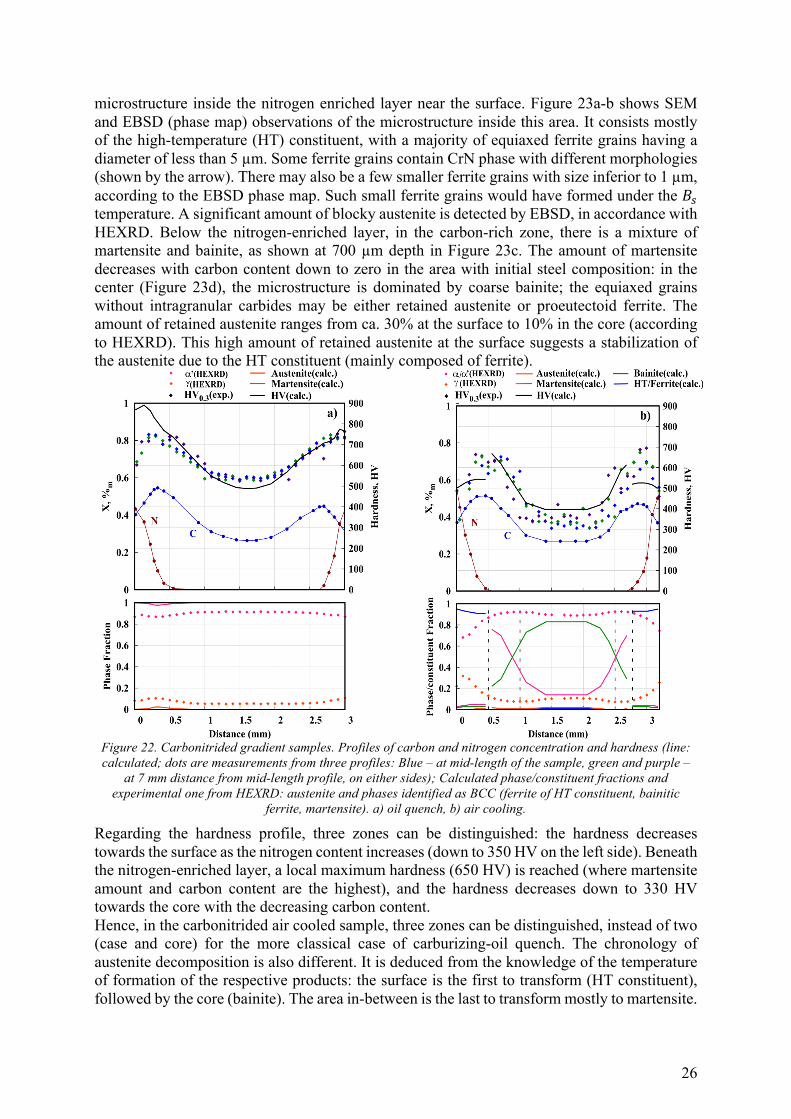
Figure 17 presents the synthesis of the results for both N and C+N steels. Predominantly formed products are either the high-temperature constituent or the martensite. The amount of bainite never exceeds 2%. The critical cooling rate to form the only martensite is 50°C.s-1. As expected, the higher carbon concentration in the steel enriched in carbon and nitrogen (0.63%m instead of 0.1%m) makes possible the formation of martensite at lower cooling rates. For the C+N steel,

22

15% retained austenite is present at room temperature, per our experimental results, which is in good agreement with the simulation (11%).

Figure 17. Fractions of products and hardness at room temperature vs. cooling rate, calculated for the C+N

steel (continuous lines) and N steel (dashed lines). Dots are for experiments (C+N steel in black and N steel in white).

The calculated hardnesses are higher for the C+N steel than for the N steel. A slight decrease of the hardness for cooling rates superior to 20°C.s-1 is noticed for the N steel. This comes from the formulae utilized to calculate the hardness of the different constituents. The calculated hardness is underestimated for the three experimental points. This underestimation may be ascribed to the fact that the hardness data utilized were measured after an isothermal treatment at a given temperature (complete transformation). The state of precipitation of the CrN nitrides (in platelets inside the ferrite of the high-temperature constituent) during the cooling is different and may lead to a higher hardness.

6! Samples with composition gradients The final purpose of the model is to predict profiles of microstructures and hardness inside massive parts enriched in carbon and/or nitrogen from the surface. In order to approach these conditions, the cooling of laboratory-scale samples with gradients of carbon and nitrogen was simulated. The calculations are compared to measurements realized on samples with simple geometry.

6.1! Experimental implementation The samples were 30 mm in length, lamellar (thickness 3±0.2 mm and width 10 mm). They were enriched in atmospheric conditions similar to those applied to the homogeneous samples (see Section 2.1). Three types of enrichments were done: carburizing, nitriding and carbonitriding. The profiles of chemical composition measured by EPMA are shown in Figure 19, Figure 21, and Figure 22. The composition profile is asymmetrical in the carburized samples. The core kept the initial steel composition. At the edges, the carbon content does not exceed 0.65%m C, which is inside the range of validity of the model (see Section 4.2.2.3). The nitrided samples underwent some decarburization, whose depth corresponds to the depth of nitrogen penetration. In the carbonitrided samples, the profiles of carbon content are again asymmetrical. Due to the decarburization in the nitrogen-enriched layer, the carbon profiles present a local maximum at ca. 0.5 mm under the surface.

23

Figure 18 - Evolutions of the temperature over time of a sample quenched in oil and cooled in calm air. The

curves correspond to the average of the thermocouple measurements placed at the center and on the surface of the sample (at mid-height).

Two cooling conditions (see Figure 18) to ambient temperature were applied after the enrichments: oil quench and calm air cooling for carbonitrided samples, whereas only oil quench was applied for carburized and nitrided sample. Temperature evolutions were measured with thermocouples located at the surface and the core of a non-enriched initial steel sample [4]. According to these measurements, the temperature is supposed to be homogeneous in the whole volume of samples for both coolings. Recorded temperature evolutions served as input data to perform the simulations. The cooling rate was not constant, contrary to the continuous cooling experiments presented in previous sections. After the cooling, three Vickers hardness (HV0.3) profiles were measured through the thickness of each sample: one at mid-length of the sample, the two others on both sides of the latter and spaced out by 7 mm. The microstructure was observed by SEM and the amounts of phases were determined by high energy X-ray diffraction (HEXRD). Experimental conditions for HEXRD are the same as described in detail in [3]. Phase’s mass fractions are determined from Rietveld analysis of HEXRD diagrams. Two crystallographic systems are considered: cubic face centered (FCC) for austenite and cubic centered (BCC) indifferently for ferrite and martensite, because the martensitic lattice never exhibited quantifiable tetragonality. CrN and cementite phases are not considered because of their low fractions.

6.2! Carburizing - Oil Quenched In the carburized oil quenched sample, the microstructure consists mostly of martensite, with amounts of retained austenite inferior to 10%m throughout the thickness, according to SEM observations and HEXRD (Figure 19). Calculation predicts of a fully martensitic microstructure along almost the entire thickness of the sample. A small amount of retained austenite is predicted near the edges because of the higher carbon content (maximum 0.65%m C at the surface) These predictions are in good agreement with the experimental values from HEXRD with nevertheless an underestimation of the amount of retained austenite. This could be attributed to some stabilization of the austenite due to low cooling rates in the martensitic domain (see Figure 14) which is not taken into account in the model presently. The comparison between calculated and measured hardness shows a good agreement.

24

Figure 19. Carburized – oil quenched gradient sample. Profiles of carbon concentration and hardness (line:

calculated; dots are measurements from three profiles: Blue – at mid-length of the sample, green and purple – at 7 mm distance from mid-length profile, on either sides); Calculated martensite and austenite fractions and

experimental austenite and martensite fractions from HEXRD.

6.3! Nitriding - Oil Quench Concerning the nitrided oil quenched sample, experimentally the microstructure consists of a mixture of bainite and martensite in the nitrogen-enriched layer (Figure 20), and mostly martensite in the non-enriched area (0.245%mC). The hardness is uniform in the non-enriched area, and it slightly increases with the nitrogen content towards the surface of the specimen. This increase of hardness is much smaller as compared to carburized steel mainly because of a decrease in carbon content and the presence of bainite. Hence, it is shown that nitriding is less efficient than carburizing in terms of surface hardening.

Figure 20. SEM micrograph of the nitrided oil-quenched sample at 100 µm from the edge of the sample.

25

Figure 21. Nitrided – oil quenched gradient sample. Profiles of carbon, nitrogen concentration and hardness (line: calculated; dots are measurements from three profiles: Blue – at mid-length of the sample, green and

purple – at 7 mm distance from mid-length profile, on either sides); Calculated martensite and austenite fractions.

The simulation predicts an entirely martensitic microstructure along the thickness, which is in agreement with the microstructure observations beneath the nitrogen-enriched layer. Conversely, in the nitrogen-enriched layers, the proportion of bainite is underestimated. This discrepancy is ascribed to the sensitivity of the model to the cooling rate, due to the fast phase transformation kinetics in the presence of nitrogen. A small variation of the input cooling curve can modify notably the predicted microstructures and as mentioned above the actual cooling rate of the experiment is not known with precision. The predicted hardness in the nitrogen-enriched layer is lower than the experiment. This difference is probably due to the formula giving the hardness of martensite containing C and N, which probably underestimates the effect of nitrogen.

6.4! Carbonitriding - Oil quenched and Air cooled In the carbonitrided oil quenched sample, the microstructure consists of martensite and retained austenite, with amount inferior to 7%m, according to HEXRD. The hardness variations are correlated with the profile of carbon composition, with a local maximum at ca. 250 µm under the surface, where the carbon content is maximum, and the nitrogen content is close to zero. There is no apparent influence of the nitrogen content profile on the hardness. The simulation (Figure 22a) underestimates the amount of retained austenite through the thickness (maximum calculated value is 3%), like in the carburized sample. Below the nitrogen-enriched layers, the shape of the calculated hardness profile is in good agreement with the experiment. In the nitrogen-enriched layers, the simulation predicts an increasing hardness towards the edge, while the experiment shows the opposite trend. This difference could be linked to the formula giving the hardness of martensite containing C and N, as seen in the nitrided sample. Carbonitriding air cooled sample presents exciting features, which differ from the classical case of carburizing treatment followed by oil quench. The most significant difference regards the

26

microstructure inside the nitrogen enriched layer near the surface. Figure 23a-b shows SEM and EBSD (phase map) observations of the microstructure inside this area. It consists mostly of the high-temperature (HT) constituent, with a majority of equiaxed ferrite grains having a diameter of less than 5 µm. Some ferrite grains contain CrN phase with different morphologies (shown by the arrow). There may also be a few smaller ferrite grains with size inferior to 1 µm, according to the EBSD phase map. Such small ferrite grains would have formed under the ,' temperature. A significant amount of blocky austenite is detected by EBSD, in accordance with HEXRD. Below the nitrogen-enriched layer, in the carbon-rich zone, there is a mixture of martensite and bainite, as shown at 700 µm depth in Figure 23c. The amount of martensite decreases with carbon content down to zero in the area with initial steel composition: in the center (Figure 23d), the microstructure is dominated by coarse bainite; the equiaxed grains without intragranular carbides may be either retained austenite or proeutectoid ferrite. The amount of retained austenite ranges from ca. 30% at the surface to 10% in the core (according to HEXRD). This high amount of retained austenite at the surface suggests a stabilization of the austenite due to the HT constituent (mainly composed of ferrite).

Figure 22. Carbonitrided gradient samples. Profiles of carbon and nitrogen concentration and hardness (line: calculated; dots are measurements from three profiles: Blue – at mid-length of the sample, green and purple –

at 7 mm distance from mid-length profile, on either sides); Calculated phase/constituent fractions and experimental one from HEXRD: austenite and phases identified as BCC (ferrite of HT constituent, bainitic

ferrite, martensite). a) oil quench, b) air cooling.

Regarding the hardness profile, three zones can be distinguished: the hardness decreases towards the surface as the nitrogen content increases (down to 350 HV on the left side). Beneath the nitrogen-enriched layer, a local maximum hardness (650 HV) is reached (where martensite amount and carbon content are the highest), and the hardness decreases down to 330 HV towards the core with the decreasing carbon content. Hence, in the carbonitrided air cooled sample, three zones can be distinguished, instead of two (case and core) for the more classical case of carburizing-oil quench. The chronology of austenite decomposition is also different. It is deduced from the knowledge of the temperature of formation of the respective products: the surface is the first to transform (HT constituent), followed by the core (bainite). The area in-between is the last to transform mostly to martensite.

27

In the carburizing oil quenched sample, the austenite transformation to martensite starts in the core, and it ends in the case.

Figure 23. a) SEM and b) EBSD based phase identification (where pink is BCC - “HT constituent” or

bainitic ferrite and yellow is FCC - Austenite) of the microstructure in the carbonitrided air-cooled sample at 100 µm from the edge of the sample. The arrows A, B and C show intragranular, platelet shaped and lamellar

CrN inside ferrite. Bright spots are either CrN from enrichment treatment, MnSiN2 or cementite. SEM micrographs c) at 700 µm from the edge of the sample d) at the core of the sample.

Below the nitrogen-enriched layer, in the carbon-rich region (~>0.5%m), the calculated amount of martensite and bainite is in agreement with the experimental observations. In the core, mainly bainitic microstructure is predicted, which is also in good agreement with the microstructural observation. The model nevertheless does not predict retained austenite in the core, probably because the austenite stabilization on slow cooling is not accounted for in present version (see Section 6.2). In the nitrogen-enriched layer, the calculation predicts the formation of the high-temperature constituent in accordance with the experiment, but the amount is overestimated, and the calculation does not predict retained austenite. As discussed above for the nitrided sample, the difficulties are related to the fast phase transformation kinetics in the presence of nitrogen. This reduces the precision of the isothermal kinetics, which serve as input data for the model and can lead to too fast predicted kinetics for the HT constituent. Also, possible stabilization of austenite is not accounted for HT constituent (mostly ferrite). The calculated hardness profile is satisfactory as far as the global shape is concerned. In agreement with the measurements, the calculated hardness profile shows a decrease in the nitrogen-enriched layer, but with a sharper transition than the experimental one. It can be explained mostly by the underestimation of the hardness in the nitrogen-enriched layer that we attribute to the effect of the cooling on the hardness of the HT constituent. This underestimation also comes from the too low predicted austenite fraction. Final cause of discrepancies is the sensitivity of the model to the cooling rate in presence of nitrogen, as illustrated in Figure 17. In the core (0.245%mC), the hardness is slightly overestimated mostly because the model does not predict the formation of austenite. Below the nitrogen-enriched layer, the hardness is correctly predicted.

28

Despite the mentioned discrepancies regarding the microstructure predictions, the simulation achieves to predict and understand the key features of this sample: the presence of three zones associated with a distinct microstructural state: high-temperature constituents in the nitrogen-enriched layer, mostly martensite in the carbon-rich layer underneath and bainite-martensite mixture in the core. The model also predicts the hardness “peak” under the surface.

7! Conclusion From kinetic and microstructural data obtained experimentally in isothermal conditions on homogeneously C and N enriched specimen, it has been possible to develop a global model able to predict the phase transformation kinetics under anisothermal conditions as well as the microstructures and the final hardness, by taking into account variations in carbon and nitrogen content in the austenite. The developed metallurgical model is based on the works of Fernandes [25] and is based on the principle of additivity. The kinetics of isothermal transformations are described by Johnson-Mehl-Avrami-Kolmogorov laws. The incubation periods under anisothermal conditions are predicted with Scheil’s method. The progression of the martensitic transformation is described with the Koistinen-Marburger law. Also, the calculation of the hardness associated with the microstructure obtained at the end of the cooling comes from a mixture rule between the different products (proeutectoid ferrite, pearlite, bainite…) that takes into account the formation temperature of the products. The initial identification of the model parameters (equilibrium temperatures, equilibrium phase amounts, ,' and &' characteristic temperatures, kinetic parameters…) is based on measurements realized with the initial steel and thermodynamic data. The accounting of carbon content variations in the austenite is inspired by the approach developed by Mey [10]. It consists of calculating displacements of IT curves along time and temperature axes by using the equations of Kirkaldy. These displacements are mainly linked to carbon content dependent undercooling. The thermodynamic approach has been established to predict the equilibrium temperatures (*, (:, and -. as well as the maximum fractions of proeutectoid ferrite. A modification of the additivity principle has also been introduced to take into account the effects of austenite stabilization during cooling on the kinetics of bainite transformation and the &' temperature. The model has first been validated under isothermal and anisothermal conditions on the initial steel and the carburized steel. For the initial steel, the calculations are in accordance with the experiments, as the model is built upon data coming from the latter. For the carburized steel, there are some discrepancies, especially for the bainite transformation for which the displacements cannot be calculated precisely, even by modifying the empirical parameters of Kirkaldy’s equations. Due to the complex phase transformation mechanisms in the austenite enriched with nitrogen, a simple approach has been set up by describing only two domains of time-dependent transformations: one for the high-temperature constituent, the other one for bainite. The model parameters have been established on the basis of our experimental results. In view of the numerous simplifying hypotheses, the comparisons between simulations and experiments for the anisothermal kinetics in nitrided and carbonitrided homogeneous samples are satisfactory. Calculations on samples with carbon and carbon+nitrogen concentration gradients gave as a well satisfactory agreement between measured and simulated hardness profiles. In the case of oil quenches, the microstructures are fully martensitic. In the case of the cooling in the air of the carbonitrided sample, due to the fast phase transformation kinetics, the nitrogen-enriched layer contains mostly the high-temperature constituent, with an associated hardness which can be lower than underneath, where carbon-enriched martensite is formed. Hence, the hardness profile of the carbonitrided gradient sample exhibits a sharp local maximum beneath the nitrogen-enriched layer, which differs strongly from the classical case of carburizing. Even if

29

there are discrepancies with experiments, the metallurgical model presented in this work helps to understand the complex microstructure and hardness profiles arising in the specimen with C and N gradients by describing the chronology of the phase transformations taking into account the local compositions and the cooling rates. This model will be an essential tool to predict the residual stresses in future work. Acknowledgments The authors are grateful to IRT M2P for financial support. Special thanks to the colleagues of Institut Jean Lamour, Mrs. Christine Gendarme for the conduction on chemical microanalyses, Mrs. Sandrine Mathieu, and Mr. Erwan Etienne for assisting on microstructural analyses. We are grateful to the European Synchrotron Radiation Facility (ESRF) for the provision of beamtime at beamline ID11. References [1] PSA Peugeot Citroën, Impact resistance and fatigue resistance of enriched gears with the

different processes., Internal report, 2010. [2] S.D. Catteau, S. Denis, J. Teixeira, J. Dulcy, M. Dehmas, A. Redjaïmia, M. Courteaux,

Effects of Carbon and Nitrogen on Isothermal Transformations of Austenite in a Low Alloyed Steel, Eur. Conf. Heat Treat. 21st IFHTSE Congr. (2014) 153–161. doi:10.1016/j.jallcom.2015.11.007.

[3] S.D. Catteau, H.P. Van Landeghem, J. Teixeira, J. Dulcy, M. Dehmas, S. Denis, A. Redjaïmia, M. Courteaux, Carbon and nitrogen effects on microstructure and kinetics associated with bainitic transformation in a low-alloyed steel, J. Alloys Compd. 658 (2016) 832–838. doi:10.1016/j.jallcom.2015.11.007.

[4] S.D. Catteau, Effets du Carbone et de l’Azote sur les Cinétiques de Décomposition de l’Austénite dans un Acier Faiblement Allié - Étude Expérimentale et Modélisation, Thèse Université de Lorraine, 2017. http://www.theses.fr/2017LORR0390.

[5] V. Landeghem, S.D. Catteau, M. H.P.Dehmas, J. Dulcy, A. Redjaïmia, J. Teixeira, S. Denis, M. Courteaux, Isothermal decomposition of carbon and nitrogen-enriched austenite in 23MnCrMo5 low-alloy steel, Acta Mater. 148 (2018) 363–373. doi:10.1016/j.actamat.2018.02.008.

[6] W. Dal’Maz Silva, Mise au point de la carbonitruration gazeuse des alliages 16NiCrMo13 et 23MnCrMo5$: modélisation et procédés, Thèse Université de Lorraine, 2017. http://www.theses.fr/2017LORR0158.

[7] S. Denis, P. Archambault, E. Gautier, A. Simon, G. Beck, Prediction of Residual Stress and Distortion of Ferrous and Non-Ferrous Metals: Current Status and Future Developments, J. Mater. Eng. Perform. 11 (2002) 92–102. doi:10.1361/105994902770344457.

[8] C.C. Liu, D.Y. Ju, T. Inoue, A numerical modeling of metallo-thermo-mechanical behavior in both carburized and carbonitrided quenching processes, Isij Int. 42 (2002) 1125–1134. doi:10.2355/isijinternational.42.1125.

[9] H.S. R. Mukai, T. Matsumoto, D. Ju, T. Suzuki, Modeling of numerical simulation and experimental verification for carburizing-nitriding quenching process, Trans. Nonferrous Met. Soc. China. 16 (2006) s566–s571. doi:10.1016/S1003-6326(06)60257-4.

[10] A. Mey, Prévision par Calcul des Cinétiques de Transformation de Phases et des Contraintes Internes lors du Traitement Thermique d’Aciers Cémentés, Thèse Institut National Polytechnique de Lorraine, 1997.

30

[11] S. Denis, P. Archambault, C. Aubry, A. Mey, J.-C. Louin, A. Simon, Modelling of phase transformation kinetics in steels and coupling with heat treatment residual stress predictions, J. Phys. IV. 9 (1999) 323–332. doi:10.1051/jp4:1999933.

[12] Michaël VEAUX, Etude expérimentale et prévisions par le calcul des cinétiques de transformation de phases, des contraintes résiduelles et des déformations lors de la transformation bainitique, Thèse Institut National Polytechnique de Lorraine, 2003. http://www.theses.fr/2003INPL050N.

[13] Jean-Charles LOUIN, Effets d’hétérogénéités de teneur en carbone sur les cinétiques de transformations de phase et sur la genèse des contraintes internes lors du refroidissement d’aciers, Thèse Institut National Polytechnique de Lorraine, 2003.

[14] J.S. Kirkaldy, D. Venugopalan, Prediction Of Microstructure And Hardenability In Low Alloy Steels, Phase Transform. Ferr. Alloy. (1983) 125–148.

[15] A. Johnson. William, A. Mehl, Reaction kinetics in processes of nucleation and growth, Trans. Aime. 135 (1939) 396–415.

[16] M. Avrami, Kinetics of phase change. I: General theory, J. Chem. Phys. 7 (1939) 1103–1112. doi:10.1063/1.1750380.

[17] M. Avrami, Kinetics of phase change. II Transformation-time relations for random distribution of nuclei, J. Chem. Phys. 8 (1940) 212–224. doi:10.1063/1.1750631.

[18] M. Avrami, Granulation, Phase Change, and Microstructure Kinetics of Phase Change. III, J. Chem. Phys. 9 (1941) 177–184. doi:10.1063/1.1750872.

[19] A.N. Kolmogorov, On the statistical theory of metal solidification, Izv. Akad. Nauk SSSR. Math. Ser. 3 (1937) 355–359.

[20] M. Jung, M. Kang, Y.K. Lee, Finite-element simulation of quenching incorporating improved transformation kinetics in a plain medium-carbon steel, Acta Mater. 60 (2012) 525–536. doi:10.1016/j.actamat.2011.10.007.

[21] J.W. Cahn, Transformation kinetics during continuous cooling, Acta Metall. 4 (1956) 572–575.

[22] R.G. Kamat, E.B. Hawbolt, L.C. Brown, J.K. Brimacombe, The Principle of Additivity and the Proeutectoid Ferrite Transformation, Metall. Trans. A. 23 (1992) 2469–2480. doi:10.14288/1.0078583.

[23] M. Lusk, H.J. Jou, On the rule of additivity in phase transformation kinetics, Metall. Mater. Trans. A Phys. Metall. Mater. Sci. 28 (1997) 287–291. doi:10.1007/s11661-997-0131-5.

[24] Y.T. Zhu, T.C. Lowe, Application of, and precautions for the use of, the rule of additivity in phase transformation, Metall. Mater. Trans. B Process Metall. Mater. Process. Sci. 31 (2000) 675–682. doi:10.1007/s11663-000-0106-z.

[25] F.M. Braz Fernandes, Modélisation et Calcul de l’Évolution de la Température et de la Microstructure au cours du Refroidissement Continu des Aciers, Thèse Institut National Polytechnique de Lorraine, 1985.

[26] S. Denis, D. Farias, A. Simon, Mathematical Model Coupling Phase Transformations and Temperature Evolutions in Steels, ISIJ Int. 32 (1992) 316–325. doi:10.2355/isijinternational.32.316.

[27] E. Scheil, Anlaufzeit der Austenitumwandlung, Arch. Fur Das Eisenhuttenwes. 8 (1935) 565–567.

[28] A. Hultgren, A metallographic study on tungsten steels, J. Wiley. (1920). [29] M. Hillert, Comments on kinetics model of isothermal pearlite formation in a 0.4C–

1.6Mn steel, Scr. Mater. 50 (2003) 171–173. doi:10.1016/j.scriptamat.2003.09.014. [30] D.E. Coates, Diffusion-Controlled Precipitate Growth in Ternary Systems I, Metall.

Trans. 3 (1972) 1203–1212. [31] Z.Q. Liu, G. Miyamoto, Z.G. Yang, T. Furuhara, Direct measurement of carbon

31

enrichment during austenite to ferrite transformation in hypoeutectoid Fe-2Mn-C alloys, Acta Mater. 61 (2013) 3120–3129. doi:10.1016/j.actamat.2013.02.003.

[32] W. Steven, A.. Haynes, The Temperature of Formation of Martensite and Bainite in Low-Alloy Steels, J. Iron Steel Institue. (1956) 349–359.

[33] I. Bell, W.S. Owen, The Thermodynomics of the Martensite Transformation in lron-Carbon ond lron-Nitrogen, Trans. Metall. Soc. AIME. 239 (1967) 1940–1949.

[34] T. Bell, Martensite Transformation Start Temperature in Iron-Nitrogen Alloys, J. Iron Steel Inst. 206 (1968) 1017–1021.

[35] S. Denis, E. Gautier, Calcul des Cinétiques de Transformations de Phases en Refroidissement Continu par un Modèle “TTT” et un Modèle “TRC” pour un Acier 27MC5R, Internal report, 1994.

[36] G. Krauss, Martensite in steel: strength and structure, Mater. Sci. Eng. A. 273–275 (2002) 40–57. doi:10.1016/s0921-5093(99)00288-9.

[37] J. Besson, R. Leriche, R. Foerch, G. Cailletaud, Object-Oriented Programming Applied to the Finite Element Method Part II. Application to Material Behaviors, Rev. Eur. Des Éléments Finis. 7 (1998) 567–588. doi:10.1080/12506559.1998.10511322.

[38] T. Jia, M. Militzer, Z.Y. Liu, General Method of Phase Transformation Modeling in Advanced High Strength Steels, ISIJ Int. 50 (2010) 583–590. doi:10.2355/isijinternational.50.583.