Modeling Fish Biomass Structure at Near Pristine

Coral Reefs and Degradation by Fishing

Abhinav Singh

School of Physics, Georgia Institute of Technology

abhinav.singh@gatech.edu

Hao Wang

Department of Mathematical and Statistical Sciences, University of Alberta

hao8@ualberta.ca

Wendy Morrison

School of Biology, Georgia Institute of Technology

wendymorrison@gatech.edu

Howard Weiss

School of Mathematics, Georgia Institute of Technology

weiss@math.gatech.edu

1

Abstract

Until recently, the only examples of inverted biomass pyramids have been in

freshwater and marine planktonic communities. In 2002 and 2008 investigators

documented inverted biomass pyramids for nearly pristine coral reef ecosystems

within the NW Hawaiian islands and the Line Islands, where apex predator

abundance comprises up to 85% of the fish biomass. We build a new refuge

based predator-prey model to study the fish biomass structure at coral reefs

and investigate the effect of fishing on biomass pyramids. Utilizing realistic

life history parameters of coral reef fish, our model exhibits a stable inverted

biomass pyramid. Since the predators and prey are not well mixed, our model

does not incorporate homogeneous mixing and the inverted biomass pyramid is

a consequence of the refuge. Understanding predator-prey dynamics in nearly

pristine conditions provides a more realistic historical framework for comparison

with fished reefs. Finally, we show that fishing transforms the inverted biomass

pyramid to be bottom heavy.

1 Introduction

An inverted biomass pyramid has increasing biomass along trophic levels (Odum

and Odum, 1971). Inverted biomass pyramids in ecology are highly counter-

intuitive and appear to be exceedingly rare. Inverted biomass pyramids have

only been observed in aquatic planktonic communities (Odum and Odum, 1971;

Gasol et al., 1997; Del Giorgio et al., 1999; Moustaka-Gouni et al., 2006; Buck

et al., 1996). Odum (Odum and Odum, 1971) hypothesized that the high turn-

over rate and the metabolism of phytoplankton can produce inverted biomass

pyramids. Other hypotheses include the low turn-over rate of predators (Cho

2

and Azam, 1990; Del Giorgio et al., 1999) and the influx of organic matter

which act as food for heterotrophic predators (Del Giorgio et al., 1999).

Recently, inverted biomass pyramids have also been observed at coral reefs

where up to 85% of the fish biomass was composed of apex predators (Friedlan-

der and DeMartini, 2002; Sandin et al., 2008). Historical observations suggest

that this high abundance of predators was common (Sandin et al., 2008) (Jack-

son 1997 and referenced therein) and such reefs can be considered ‘nearly pris-

tine’ (Knowlton and Jackson, 2008), and thus provide a baseline for studying

natural reefs. The coral cover at these pristine reefs is far more extensive and

healthier than at conventional reefs, and these reefs seem to be either resistant

or resilient to ocean warming and rising acidity (Knowlton and Jackson, 2008;

Sandin et al., 2008).

The high predator biomass at these ‘nearly pristine’ reefs is in sharp con-

trast to most reefs, where the prey biomass substantially dominates the total

fish biomass (Sandin et al., 2008). The mechanisms causing inverted biomass

pyramids in planktonic communities and coral reefs are clearly different. The

former relies upon homogeneous mixing which is clearly not present in coral

reefs with many holes (as the refuge) for prey to hide.

Some ecologists believe that refuges provide a general mechanism for inter-

preting ecological patterns (Hawkins et al., 1993). Previous experimental and

theoretical studies of prey refuges have demonstrated how refuges increase the

abundance of prey and add stability to the system (Huffaker, 1958) Berryman

and Hawkins 2006). Few studies have analyzed the impact of refuges on preda-

tor abundances (see (Persson and Eklov, 1995) for an analysis of how refuges

impact predator growth), and none have addressed how refuges affect preda-

tor to prey biomass ratios. We study the influence of refuges on prey growth,

3

predator feeding behavior, and predator and prey biomass in this manuscript.

Investigations into the importance of shelter for coral reef fish abundance

have found mixed results. Robertson et al. (1981) monitored the abundance

of reef fish after physically removing half of the patch reef. He found that the

abundance of a small herbivorous damselfish on the remaining reef increased

by up to 1.63 times the original density, suggesting that shelter was not limit-

ing. Conversely, Shulman (Shulman, 1984) found that the presence of shelter

increases the recruitment and survival of small herbivorous fish. Similarly, Hol-

brook and Schmitt (Holbrook and Schmitt, 2002) used infra-red photography

at night to document the predation of small reef fish that were located near

or outside the coral shelter. Extremely high mortality of coral reef fish (up to

60%) has been documented during settlement (Doherty and Sale, 1986) and

during the days directly after settlement (Almany and Webster, 2006). This is

followed by a reduction in mortality as time passes (Doherty and Sale, 1986)

Shulman and Ogden 1987). This suggests that mortality during and directly af-

ter settlement may be a population bottleneck for reef species (Doherty et al.,

2004). Doherty and Sale (Doherty and Sale, 1986) showed that providing a

cage during this time decreased predation on sedentary reef species, though

they were unable to quantify natural mortality due to confounding factors.

Mathematical modeling can provide insights into some of the fundamental

open questions about the biomass structure at coral reefs. Classical predator-

prey models, including Holling type models, assume that predators and prey are

well mixed, i.e., all prey are accessible to the predators. This is not the case at

coral reefs where small fish find ‘refuge’ from predators in coral holes where large

predators cannot enter (Hixon and Beets, 1993). Thus, a population model

assuming homogeneous mixing between predators and prey is not appropriate

4

to study the fish biomass structure at coral reefs. An appropriate model must

include a prey refuge and its associated functional response of predation due

to the refuge.

In our recently published work Wang et al. (Wang et al., 2009), we used

mathematical modeling to investigate the theoretical conditions necessary for

the creation of inverted biomass pyramids, but we did not test the ideas with

actual predator and prey life history parameters. In addition, we developed a

family of predator-prey models (RPP model) that explicitly incorporate a ‘prey

refuge’, where the refuge size influences predator hunting patterns (predation

response). We showed that refuges provide a new general mechanism in ecol-

ogy to create an inverted biomass pyramid that does not require mass action

interactions between predators and prey.

This study is an extension as well as a modification of Wang et al. (Wang

et al., 2009)’s work by modeling the coral reef inverted biomass pyramids with

realistic life-history parameters specific for coral reef fish. Our new refuge-

based predator-prey model exhibits a stable inverted biomass pyramid and

thus provides a mechanism to explain the recently observed inverted biomass

pyramid at nearly pristine reefs. We end this paper by using the parameterized

model to investigate the impact of fishing on the biomass ratio.

2 Derivation of the Model

Guided by field observations at pristine coral reefs, we derive a model for the

biomass of coral reef fishes using a pair of differential equations. Following

Sandin et al. (Sandin et al., 2008), we classify reef fishes as prey or predators.

We model prey when they are large enough to be visualized by the divers on the

5

survey and are a possible source of food for the apex predators (i.e. past the

high mortality experienced during recruitment). We include herbivores, and

planktivores within our prey categories, and include the top predators within

our predator category. We currently have not incorporated the carnivores (i.e.

small predators) into the model as they consume mainly small invertebrates

(Sandin et al. 2008) and thus have minimal impact on the abundance of prey

fishes.

Prey fish eat plankton and algae and hide from predators in coral holes (Pala,

2007; Sandin et al., 2008; Hixon and Beets, 1993; Caley and St John, 1996). We

assume that prey biomass grows logistically and (per capita predator) predation

rate depends on prey biomass and availability of coral holes to hide. Predators

grow by eating prey fish and die a natural death at pristine reefs. Prey fish find

‘refuge’ in coral holes and rarely venture out of the holes at Kingman (Pala,

2007). Therefore, the availability of hiding space for prey in coral holes affects

predator hunting patterns and thus the biomass pyramid. We define the ‘refuge

size’ as the maximum prey biomass which can sustainably hide in coral holes,

i.e. the coral-specific prey carrying capacity in presence of predators (Daily and

Ehrlich, 1992). We distinguish the refuge size from the prey carrying capacity

in absence of predators (K); the prey will not be forced to stay inside the holes

when the predators are absent and the reef can support a much greater prey

biomass. We assume that the refuge size is an increasing function of coral cover

at pristine reefs. The equations describing such a community are

6

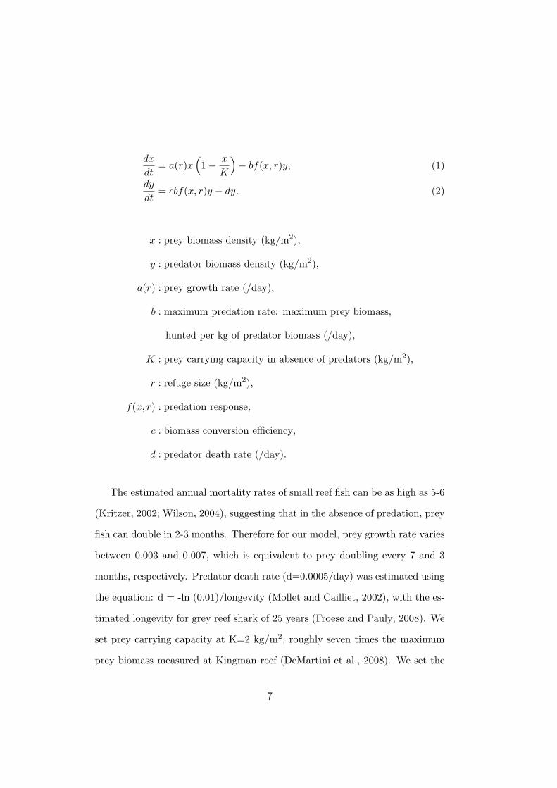
dx

dt= a(r)x

(1− x

K

)− bf(x, r)y, (1)

dy

dt= cbf(x, r)y − dy. (2)

x : prey biomass density (kg/m2),

y : predator biomass density (kg/m2),

a(r) : prey growth rate (/day),

b : maximum predation rate: maximum prey biomass,

hunted per kg of predator biomass (/day),

K : prey carrying capacity in absence of predators (kg/m2),

r : refuge size (kg/m2),

f(x, r) : predation response,

c : biomass conversion efficiency,

d : predator death rate (/day).

The estimated annual mortality rates of small reef fish can be as high as 5-6

(Kritzer, 2002; Wilson, 2004), suggesting that in the absence of predation, prey

fish can double in 2-3 months. Therefore for our model, prey growth rate varies

between 0.003 and 0.007, which is equivalent to prey doubling every 7 and 3

months, respectively. Predator death rate (d=0.0005/day) was estimated using

the equation: d = -ln (0.01)/longevity (Mollet and Cailliet, 2002), with the es-

timated longevity for grey reef shark of 25 years (Froese and Pauly, 2008). We

set prey carrying capacity at K=2 kg/m2, roughly seven times the maximum

prey biomass measured at Kingman reef (DeMartini et al., 2008). We set the

7

biomass conversion efficiency (c) to 0.15, a reasonable estimate given that con-

version efficiencies are higher in marine versus terrestrial environments (Barnes

and Hughes, 1999). Predation rates of 12% predator body weight per day have

been documented for smaller sedentary predators (Sweatman, 1984), suggesting

that rates for active predators would be higher. We therefore set the maximum

predation, b=0.24/day.

Wang et al. (Wang et al., 2009) developed the family of refuge-modulated

predator prey models (RPP Type I, II and III) to explicitly include the multiple

effects of refuge on the feeding behavior of predators. The effects of a refuge

can be included by the generalized predation response function

f(x, r) =1

1 + e−ξ[x−(2−i)r] , (3)

i = 1, 2 and 3,

The choice of i depends on the environment under consideration. Adding a

refuge to the ecosystem could conceviably either decrease the prey available to

the predators (i = 1; RPP is Type I), have no impact on the number of prey

available (i = 2; RPP is Type II), or increase the number of prey available to

predators (i = 3, RPP is Type III). The predation response function f(x, r) at

coral reefs should have the following properties. It should be a monotonically

increasing function of prey biomass. When the prey biomass is less than the

refuge size, it should be small. When prey biomass approaches refuge size, it

should rapidly increase and as prey biomass greatly exceeds the refuge size, the

predators become satiated and the response function approaches a constant;

8

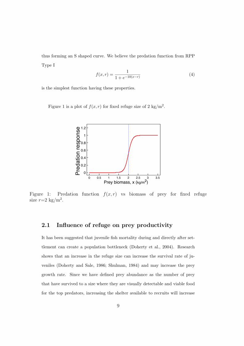
thus forming an S shaped curve. We believe the predation function from RPP

Type I

f(x, r) =1

1 + e−10(x−r) (4)

is the simplest function having these properties.

Figure 1 is a plot of f(x, r) for fixed refuge size of 2 kg/m2.

0 0.5 1 1.5 2 2.5 3 3.50

0.2

0.4

0.6

0.8

1

1.2

Prey biomass, x (kg/m2)

Pred

atio

n re

spon

se

Figure 1: Predation function f(x, r) vs biomass of prey for fixed refugesize r=2 kg/m2.

2.1 Influence of refuge on prey productivity

It has been suggested that juvenile fish mortality during and directly after set-

tlement can create a population bottleneck (Doherty et al., 2004). Research

shows that an increase in the refuge size can increase the survival rate of ju-

veniles (Doherty and Sale, 1986; Shulman, 1984) and may increase the prey

growth rate. Since we have defined prey abundance as the number of prey

that have survived to a size where they are visually detectable and viable food

for the top predators, increasing the shelter available to recruits will increase

9

the number of fish that become available prey. This idea is similar to the idea

of recruitment within fisheries science where fish are considered recruits when

they have reached a size where they can be captured by the fishery. For this

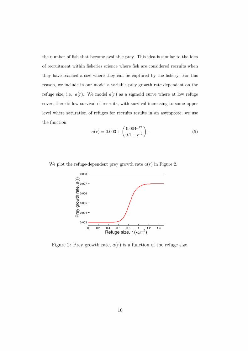
reason, we include in our model a variable prey growth rate dependent on the

refuge size, i.e. a(r). We model a(r) as a sigmoid curve where at low refuge

cover, there is low survival of recruits, with survival increasing to some upper

level where saturation of refuges for recruits results in an asymptote; we use

the function

a(r) = 0.003 +(

0.004r12

0.1 + r12

). (5)

We plot the refuge-dependent prey growth rate a(r) in Figure 2.

0 0.2 0.4 0.6 0.8 1 1.2 1.4

0.003

0.004

0.005

0.006

0.007

0.008

Pre

y gr

owth

rate

, a(r

)

Refuge size, r (kg/m2)

Figure 2: Prey growth rate, a(r) is a function of the refuge size.

10

The following equations describe the complete model:

dx

dt=(

0.003 +0.004r12

0.1 + r12

)x(

1− x

K

)− by

1 + e−10(x− r), (6)

dy

dt= c

by

1 + e−10(x− r)− dy. (7)

3 Results

The system of differential equations has three equilibrium points. The unstable

equilibrium point, x = 0, y = 0 corresponds to a reef with no fish. The

equilibrium point x = K, y = 0 corresponds to the absence of predators and

is rarely seen in reefs. The third and the most interesting equilibrium point,

which we call the interior equilibrium point is

x∗(r) = r − 110

ln(bc

d− 1), (8)

y∗(r) =a(r)cd

x∗(

1− x∗

K

). (9)

This equilibrium point is locally attractive for the refuge size between 0.65-

0.9 kg/m2. The predator-prey biomass ratio at the third equilibrium point

isy∗(r)x∗(r)

=a(r)cd

(1 +

110K

ln(bc

d− 1)− r

K

). (10)

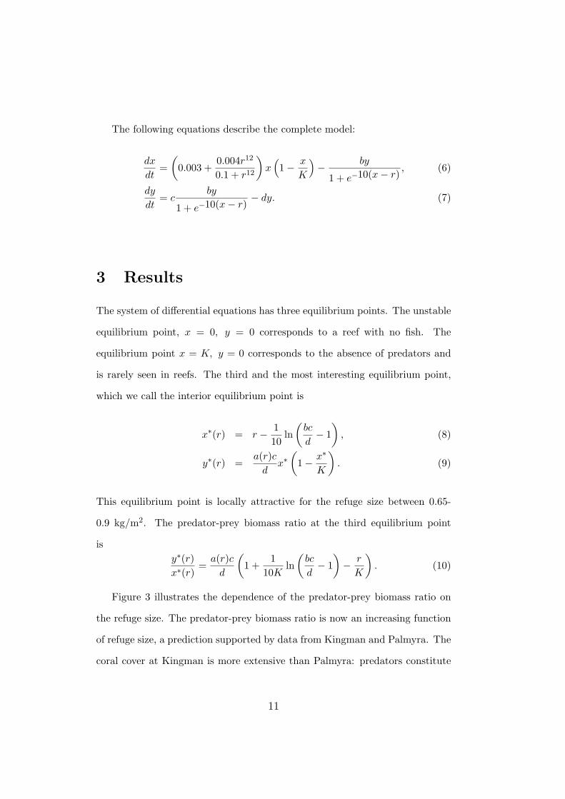
Figure 3 illustrates the dependence of the predator-prey biomass ratio on

the refuge size. The predator-prey biomass ratio is now an increasing function

of refuge size, a prediction supported by data from Kingman and Palmyra. The

coral cover at Kingman is more extensive than Palmyra: predators constitute

11

85% of the fish biomass at Kingman while they constitute only 66% of the fish

biomass at Palmyra (Sandin et al., 2008).

0.6 0.65 0.7 0.75 0.8 0.85 0.9 0.950.6

0.8

1

1.2

1.4

Pre

dato

r:Pre

y B

iom

ass

Rat

io

Refuge size, r (kg/m2)

Figure 3: The biomass pyramid is inverted and the predator:prey biomass ratio is anincreasing function of refuge size.

4 Effects of Fishing

It is believed that fishing can dramatically change the biomass ratio; the fish

biomass pyramid becomes bottom heavy at reefs with fishing (Sandin et al.,

2008; Kennedy, 2008). We add fishing to our model and show that sufficiently

high fishing pressure will destroy the inverted pyramid. Destruction of the in-

verted pyramid in presence of predator fishing is direct, but we show that prey

fishing alone will also destroy the inverted biomass pyramid.

As an illustrative example, we assume that predator fishing rate is proportional

to the predator biomass and prey fishing is similar to predator hunting. We

understand that this is not the only form of prey fishing and thus we further

12

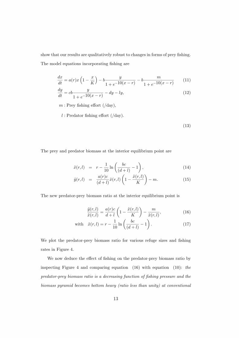
show that our results are qualitatively robust to changes in forms of prey fishing.

The model equations incorporating fishing are

dx

dt= a(r)x

(1− x

K

)− b

y

1 + e−10(x− r)− b

m

1 + e−10(x− r)(11)

dy

dt= cb

y

1 + e−10(x− r)− dy − ly, (12)

m : Prey fishing effort (/day),

l : Predator fishing effort (/day).

(13)

The prey and predator biomass at the interior equilibrium point are

x(r, l) = r − 110

ln(

bc

(d+ l)− 1), (14)

y(r, l) =a(r)c

(d+ l)x(r, l)

(1− x(r, l)

K

)−m. (15)

The new predator-prey biomass ratio at the interior equilibrium point is

y(r, l)x(r, l)

=a(r)cd+ l

(1− x(r, l)

K

)− m

x(r, l), (16)

with x(r, l) = r − 110

ln(

bc

(d+ l)− 1). (17)

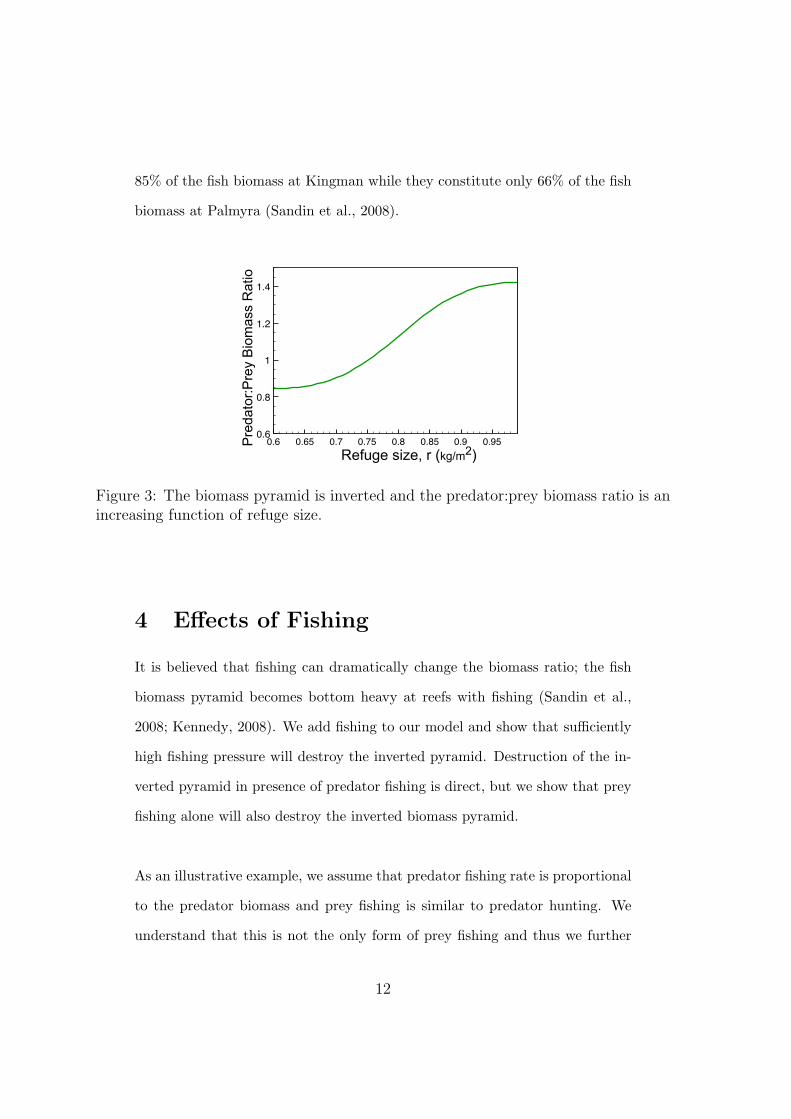
We plot the predator-prey biomass ratio for various refuge sizes and fishing

rates in Figure 4.

We now deduce the effect of fishing on the predator-prey biomass ratio by

inspecting Figure 4 and comparing equation (16) with equation (10): the

predator-prey biomass ratio is a decreasing function of fishing pressure and the

biomass pyramid becomes bottom heavy (ratio less than unity) at conventional

13

0.75 0.8 0.85 0.9 0.95 10

0.5

1

1.5

2No prey fishingPrey fishing, m=0.30m=0.32

Pre

dato

r:Pre

y B

iom

ass

Rat

io

Refuge size, r (kg/m2)

No predator fishing

0.6 0.65 0.7 0.75 0.8 0.85 0.90

0.5

1

1.5

2No fishingPrey fishing, m=0.02m=0.05

Pre

dato

r:Pre

y B

iom

ass

Rat

io

Refuge size, r (kg/m2)

Predator fishing=0.0002/day

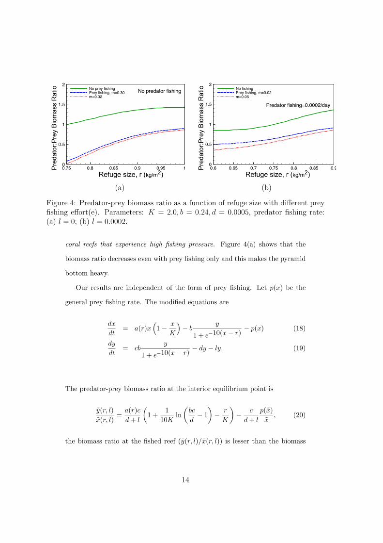
(a) (b)

Figure 4: Predator-prey biomass ratio as a function of refuge size with different preyfishing effort(e). Parameters: K = 2.0, b = 0.24, d = 0.0005, predator fishing rate:(a) l = 0; (b) l = 0.0002.

coral reefs that experience high fishing pressure. Figure 4(a) shows that the

biomass ratio decreases even with prey fishing only and this makes the pyramid

bottom heavy.

Our results are independent of the form of prey fishing. Let p(x) be the

general prey fishing rate. The modified equations are

dx

dt= a(r)x

(1− x

K

)− b

y

1 + e−10(x− r)− p(x) (18)

dy

dt= cb

y

1 + e−10(x− r)− dy − ly. (19)

The predator-prey biomass ratio at the interior equilibrium point is

y(r, l)x(r, l)

=a(r)cd+ l

(1 +

110K

ln(bc

d− 1)− r

K

)− c

d+ l

p(x)x

, (20)

the biomass ratio at the fished reef (y(r, l)/x(r, l)) is lesser than the biomass

14

ratio at a reef without fishing (y∗(r)/x∗(r))

y(r, l)x(r, l)

≤ a(r)cd

(1 +

110K

ln(bc

d− 1)− r

K

)=y∗(r)x∗(r)

. (21)

As a result of fishing, the predator-prey biomass ratio is less than the

biomass ratio at reefs without fishing. This result is robust under different

forms of fishing.

As another example of prey fishing, if the prey fishing rate is proportional

to prey biomass, p(x) = vx, the predator-prey biomass ratio

y(r, l)x(r, l)

=a(r)cd+ l

(1 +

110K

ln(bc

d− 1)− r

K

)− c

d+ lv. (22)

This is less than the biomass ratio for the model without fishing in Equa-

tion (10) and high fishing pressure will destroy the inverted biomass pyramid.

5 Discussion

In this manuscript, we model the fish biomass structure in near pristine coral

reef ecosystems and our model displays a stable inverted biomass pyramid. We

show how the presence of refuge can influence the inverted biomass pyramid

through the modification of prey growth rate and predator response function.

Our model confirms previous suggestions that high prey growth rate and low

predator growth rate are necessary for inverted biomass pyramids (Odum and

15

Odum, 1971; Del Giorgio et al., 1999; Cho and Azam, 1990). Both conditions

are satisfied at ‘nearly pristine’ reefs where apex predators such as sharks can

live up to 20 years and reproduce rarely (Smith et al., 1998) and smaller prey

fish can reproduce at least three times a year (Srinivasan and Jones, 2006).

In addition, we show that sufficiently high fishing pressure will destroy the

inverted biomass pyramid.

By incorporating realistic parameter values, we show that inverted biomass

pyramids on reefs are possible. Coral holes are essential to our model as prey

fish at pristine reefs take ‘refuge’ in coral holes from predators and were rarely

observed to leave the holes (Sandin et al., 2008). Prey fish also practice‘hot-

bunking’, i.e. if one prey fish left a coral hole, another immediately occupied

that hole (Pala, 2007). Our model assumes that the refuge size influences prey

growth rate. The protection provided to juveniles by the coral cover ends up

boosting the overall supply of prey fish by increasing prey growth rate a(r).

Alternatively, this same concept could be incorporated into the model through

the RPP Type III equation (Wang et al., 2009), but for the parameter values

implemented here, leads to an unrealistic unstable biomass pyramid. If we

assume that prey survival to adult size is dependent on the cover of coral

reef, we find that the predator-prey biomass ratio is an increasing function of

refuge size. This relationship is supported by data from (Sandin et al., 2008)

comparing Palmyra and Kingman.

The predator and prey life-history estimates utilized for this paper are at

the extremes of those measured in the field. For example, the prey growth

rate variation from 0.003 to 0.007 applies to small planktivorous fish. Larger

herbivores (i.e. parrotfish) have much lower growth rate estimates (.0013/day;

Fishbase). However, all available parameter estimates are from the highly im-

16

pacted reefs with low predator abundances. No estimates exist for life history

parameters of coral reef fish at any of the locations with the inverted biomass

structure.

When the fishing pressure is sufficiently strong, the inverted biomass pyra-

mid disappears (see Figure 4). This is consistent with field observations where

reefs with fishing exhibit a non-inverted bottom heavy pyramid (Sandin et al.,

2008). Our model shows that the biomass ratio decreases when either predator

or prey fishing or a combination of both takes place. Further computations,

which we do not present, show that prey fishing alone can have the same effect.

6 Appendix

6.1 Local Stability of equilibrium points

The equations governing the dynamics of predator and prey biomass are de-

scribed by

dx

dt= a(r)x

(1− x

K

)− bf(x, r)y,

dy

dt= cbf(x, r)y − dy.

The equilibrium points are (0, 0), (K, 0) and (x∗, y∗).

x∗ = r − 110

ln(bc

d− 1), (23)

y∗ =a(r)cd

x∗(

1− x∗

K

). (24)

17

We determine the local stability of the equilibrium points by computing the

Jacobian at the equilibrium points. The Jacobian

J =

a(r)− 2a(r) xK − 10by

(e−10(x− r))

(1 + e−10(x− r))2− b

1 + e−10(x− r)

4bcy(e−10(x− r))

(1 + e−10(x− r))2bc

1 + e−10(x− r)− d

.

At (0,0)

J(0, 0) =

a(r) − b

1 + e10r

0bc

1 + e10r − d

.

The eigenvalues of the Jacobian are a(r) and (bc/(1 + e10r)− d). As a(r) ≥ 0,

(0,0) is an unstable equilibrium point (Strogatz, 1994).

At (K,0),

J(K, 0) =

−a(r) − b

1 + e−10(K − r)

0bc

1 + e−10(K − r)− d

and det(J(K, 0)) = −a(r)

(bc

1 + e−10(K − r)− d

)< 0.

As 1 + e−10(K − r) ≤ 2 and bc > 2d, det(J(K, 0)) < 0 . Therefore, (K,0)

is a saddle equilibrium point (Strogatz, 1994).

18

At (x∗, y∗),

x∗(r) = r − 110

ln(bc

d− 1),

y∗(r) =a(r)cd

x∗(

1− x∗

K

),

J(x∗, y∗) =

a(r)− 2a(r)x

∗K − 10by∗

e−10(x∗ − r)

(1 + e−10(x∗ − r))2−b

1 + e−10(x∗ − r)

10bcy∗e−10(x∗ − r)

(1 + e−10(x∗ − r))20

,

det J(x∗, y∗) =10a(r)cx∗(1− x∗/K)( c

d− 1)

b( cd

)2,

Tr(x∗, y∗) = a(r)− 2a(r)x∗

K− 10by∗

e−10(x∗ − r)

(1 + e−10(x∗ − r))2.

The determinant and the trace of the Jacobian are complicated functions of

the parameters and equilibrium predator and prey biomass. Computer assisted

analysis shows that det J(x∗, y∗) ≥ 0 and trJ(x∗, y∗) ≤ 0 when 0.60 ≤ r ≤ 0.99.

Therefore, (x∗, y∗) is an attractive equilibrium point when 0.60 ≤ r ≤ 0.99.

19

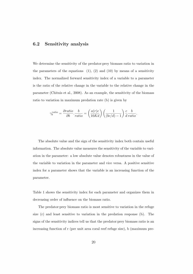
6.2 Sensitivity analysis

We determine the sensitivity of the predator:prey biomass ratio to variation in

the parameters of the equations (1), (2) and (10) by means of a sensitivity

index. The normalized forward sensitivity index of a variable to a parameter

is the ratio of the relative change in the variable to the relative change in the

parameter (Chitnis et al., 2008). As an example, the sensitivity of the biomass

ratio to variation in maximum predation rate (b) is given by

γratiob =∂ratio

∂b.b

ratio=(a(r)c10Kd

)(1

(bc/d)− 1

)c

d

b

ratio.

The absolute value and the sign of the sensitivity index both contain useful

information. The absolute value measures the sensitivity of the variable to vari-

ation in the parameter: a low absolute value denotes robustness in the value of

the variable to variation in the parameter and vice versa. A positive sensitive

index for a parameter shows that the variable is an increasing function of the

parameter.

Table 1 shows the sensitivity index for each parameter and organizes them in

decreasing order of influence on the biomass ratio.

The predator:prey biomass ratio is most sensitive to variation in the refuge

size (r) and least sensitive to variation in the predation response (b). The

signs of the sensitivity indices tell us that the predator:prey biomass ratio is an

increasing function of r (per unit area coral reef refuge size), b (maximum pre-

20

Parameter Sensitivity Indexr 1.55c 0.61d -0.61K 0.11b 0.05

Table 1: Sensitivity indices for parameters in equations (1), (2) and (10). Baselinevalue for parameters:( b = 0.24, c = 0.15, d = 0.0005, K = 2.0, r = 0.9, biomassratio= 1.13).

dation rate), c (biomass conversion efficiency) and K (prey carrying capacity)

and a decreasing function of d (predator death rate).

21

References

Almany, G. and M. Webster. 2006. The predation gauntlet: early post-settlement mortality in reef fishes. Coral reefs, 25:19–22.

Barnes, R. and R. Hughes. 1999. An introduction to marine ecology. BlackwellScientific Publications.

Buck, K., F. Chavez, and L. Campbell. 1996. Basin-wide distributions of livingcarbon components and the inverted trophic pyramid of the central gyre ofthe North Atlantic Ocean, summer 1993. Aquatic Microbial Ecology, 10:283–298.

Caley, M. and J. St John. 1996. Refuge availability structures assemblages oftropical reef fishes. Journal of Animal Ecology, 65:414–428.

Chitnis, N., J. Hyman, and J. Cushing. 2008. Determining Important Pa-rameters in the Spread of Malaria Through the Sensitivity Analysis of aMathematical Model. Bull Math Biol.

Cho, B. and F. Azam. 1990. Biogeochemical significance of bacterial biomassin the ocean’s euphotic zone. Marine ecology progress series. Oldendorf,63:253–259.

Daily, G. and P. Ehrlich. 1992. Population, Sustainability, and earth’s CarryingCapacity. Bioscience, 42:761–771.

Del Giorgio, P., J. Cole, N. Caraco, and R. Peters. 1999. Linking planktonicbiomass and metabolism to net gas fluxes in northern temperate lakes. Ecol-ogy, 80:1422–1431.

DeMartini, E., A. Friedlander, S. Sandin, and E. Sala. 2008. Differences infish-assemblage structure between fished and unfished atolls in the northernLine Islands, central Pacific. Mar Ecol Prog Ser, 365:199–215.

Doherty, P., V. Dufour, R. Galzin, M. Hixon, M. Meekan, and S. Planes. 2004.High mortality during settlement is a population bottleneck for a tropicalsurgeonfish. Ecology, 85:2422–2428.

Doherty, P. and P. Sale. 1986. Predation on juvenile coral reef fishes: anexclusion experiment. Coral reefs, 4:225–234.

Friedlander, A. and E. DeMartini. 2002. Contrasts in density, size, and biomassof reef fishes between the northwestern and the main Hawaiian islands: theeffects of fishing down apex predators. Marine Ecology Progress Series,230:253–264.

22

Froese, R. and D. Pauly. 2008. FishBase. version (06/2008). World Wide Webelectronic publication. www.fishbase.org.

Gasol, J., P. del Giorgio, and C. Duarte. 1997. Biomass distribution in marineplanktonic communities. Limnology and Oceanography, pages 1353–1363.

Hawkins, B., M. Thomas, and M. Hochberg. 1993. Refuge theory and biologicalcontrol. Science, 262:1429–1432.

Hixon, M. and J. Beets. 1993. Predation, prey refuges, and the structure ofcoral-reef fish assemblages. Ecological Monographs, pages 77–101.

Holbrook, S. and R. Schmitt. 2002. Competition for shelter space causesdensity-dependent predation mortality in damselfishes. Ecology, 83:2855–2868.

Huffaker, C. 1958. Experimental studies on Predation: Dispersion factors andpredator-prey oscillations. Hilgardia, 27:343–383.

Kennedy, W. 2008. An Uneasy Eden. National Geographic, pages 144–157.

Knowlton, N. and J. Jackson. 2008. Shifting Baselines, Local Impacts, andGlobal Change on Coral Reefs. PLoS Biol, 6:e54.

Kritzer, J. 2002. Stock Structure, Mortality and Growth of The DecoratedGoby, Istigobius decoratus (Gobiidae), at Lizard Island, Great Barrier Reef.Environmental Biology of Fishes, 63:211–216.

Mollet, H. and G. Cailliet. 2002. Comparative population demography of elas-mobranchs using life history tables, Leslie matrices and stage-based matrixmodels. Marine and Freshwater Research, 53:503–516.

Moustaka-Gouni, M., E. Vardaka, E. Michaloudi, K. Kormas, E. Tryfon, H. Mi-halatou, S. Gkelis, and T. Lanaras. 2006. Plankton food web structure ina eutrophic polymictic lake with a history in toxic cyanobacterial blooms.Limnology and Oceanography, 51:715–727.

Odum, E. and H. Odum. 1971. Fundamentals of ecology.

Pala, C. 2007. Reefs in Trouble: Life on the Mean Reefs. Science, 318:1719.

Persson, L. and P. Eklov. 1995. Prey refuges affecting interactions betweenpiscivorous perch and juvenile perch and roach. Ecology, pages 70–81.

Sandin, S., J. Smith, E. DeMartini, E. Dinsdale, S. Donner, A. Friedlander,T. Konotchick, M. Malay, J. Maragos, D. Obura, et al. 2008. Baselines anddegradation of coral reefs in the northern Line Islands. PLoS ONE, 3.

23

Shulman, M. 1984. Resource limitation and recruitment patterns in a coralreef fish assemblage. Journal of experimental marine biology and ecology,74:85–109.

Smith, S., D. Au, and C. Show. 1998. Intrinsic rebound potentials of 26 speciesof Pacific sharks. Marine & Freshwater Research, 49:663–678.

Srinivasan, M. and G. Jones. 2006. Extended breeding and recruitment periodsof fishes on a low latitude coral reef. Coral Reefs, 25:673–682.

Strogatz, S. 1994. Nonlinear dynamics and chaos. Addison-Wesley Reading,MA.

Sweatman, H. 1984. A field study of the predatory behavior and feeding rate ofa piscivorous coral reef fish, the lizardfish Synodus englemani. Copeia, pages187–194.

Wang, H., W. Morrison, A. Singh, and H. Weiss. 2009. Modeling in-verted biomass pyramids and refuges in ecosystems. Ecological Modelling,220:1376–1382.

Wilson, S. 2004. Growth, mortality and turnover rates of a small detritivorousfish. Marine Ecology Progress Series, 284:253–259.

24