Modeling and simulation of arterial walls with focus on ...
159
Modeling and simulation of arterial walls with focus on damage and residual stresses Von der Fakult¨at f¨ ur Ingenieurwissenschaften, Abteilung Bauwissenschaften der Universit¨at Duisburg-Essen zur Erlangung des akademischen Grades Doktor-Ingenieurin genehmigte Dissertation von Dipl.-Ing. Sarah Brinkhues aus Borken (Westf.) Hauptreferent: Prof. Dr.-Ing. habil. J¨ org Schr¨ oder Korreferent: Prof. Dr. rer. nat. habil. Axel Klawonn Tag der Einreichung: 12. Juli 2012 Tag der m¨ undlichen Pr¨ ufung: 19. Oktober 2012 Fakult¨atf¨ ur Ingenieurwissenschaften, Abteilung Bauwissenschaften der Universit¨at Duisburg-Essen Institut f¨ ur Mechanik Prof. Dr.-Ing. habil. J. Schr¨ oder
-
Upload
khangminh22 -
Category
Documents
-
view
1 -
download
0
Transcript of Modeling and simulation of arterial walls with focus on ...

Modeling and simulation of arterial walls
with focus on damage and residual stresses
Von der Fakultat fur Ingenieurwissenschaften,Abteilung Bauwissenschaftender Universitat Duisburg-Essen
zur Erlangung des akademischen Grades
Doktor-Ingenieurin
genehmigte Dissertation
von
Dipl.-Ing. Sarah Brinkhues
aus Borken (Westf.)
Hauptreferent: Prof. Dr.-Ing. habil. Jorg SchroderKorreferent: Prof. Dr. rer. nat. habil. Axel Klawonn
Tag der Einreichung: 12. Juli 2012Tag der mundlichen Prufung: 19. Oktober 2012
Fakultat fur Ingenieurwissenschaften,Abteilung Bauwissenschaftender Universitat Duisburg-Essen
Institut fur MechanikProf. Dr.-Ing. habil. J. Schroder

Herausgeber:
Prof. Dr.-Ing. habil. J. Schroder
Organisation und Verwaltung:
Prof. Dr.-Ing. habil. J. SchroderInstitut fur MechanikAbteilung BauwissenschaftenFakultat fur IngenieurwissenschaftenUniversitat Duisburg-EssenUniversitatsstraße 1545117 EssenTel.: 0201 / 183 - 2682Fax: 0201 / 183 - 2680
© Sarah BrinkhuesInstitut fur MechanikAbteilung BauwissenschaftenFakultat fur IngenieurwissenschaftenUniversitat Duisburg-EssenUniversitatsstraße 1545117 Essen
Alle Rechte, insbesondere das der Ubersetzung in fremde Sprachen, vorbehalten. OhneGenehmigung des Autors ist es nicht gestattet, dieses Heft ganz oder teilweise auffotomechanischem Wege (Fotokopie, Mikrokopie), elektronischem oder sonstigem Wegezu vervielfaltigen.
ISBN-10 3-9809679-6-4ISBN-13 978-3-9809679-6-9EAN 9783980967969

meinen Eltern

Preface
This work was developed during my time as research associate at the Institute ofMechanics at the University of Duisburg-Essen. Many people have accompanied and sup-ported me on this way and I would like to thank some of them at this point.
First and foremost I thank my doctoral advisor Professor Jorg Schroder for the greatopportunity to obtain my doctorate under his supervision. With his winning characterand his extensive knowledge he captivates people and sparks their interest in mechanics.Jorg has always encouraged me to challenge myself and gave me the required supportand the mechanical background to achieve my goals. Furthermore, I thank Professor AxelKlawonn for the intensive collaboration during the last years and for agreeing to act assecond examiner of this thesis. In particular in the field of applied mathematical methodsin continuum mechanics I could benefit a lot from his knowledge.
Furthermore, I thank Professor Gerhard A. Holzapfel for helpful scientific discussions andfor the provision of experimental data for human arteries. My sincere thanks go to OliverRheinbach for many conversations we had about parallel computing and the correspond-ing simulation results. His continuous and immediate support regarding mathematicalproblems and the handling of the parallel computer system were very helpful for me.
Many thanks go to my colleagues for the comfortable working atmosphere, whichplayed an important role for me: Moritz Bloßfeld, Dominik Brands, Bernhard Eidel,Veronika Jorisch, Matthias Labusch, Petra Lindner-Roulle, Vera Meyer, Tim Ricken,Lisa Scheunemann, Thomas Schmidt, Serdar Serdas, Steffen Specht, Huy Ngoc Minh Thai,and Robin Wojnowski. Special thanks go also to my student assistants Simon Fausten andAnna-Katharina Tielke for the friendly cooperation and their helpful support.
In addition to that, I want to mention some colleagues which have played a crucial roleduring my graduation. First of all I thank Daniel Balzani who was the supervisor of mydiploma thesis and who gave me the first insides into material modeling in biomechanics.I thank him for paving the way for my graduation and for the support he gave me duringthat time. My special thanks are due to Professor Joachim Bluhm for his joy of teaching,for lending an ear to everyone at any time, and for his commitment to the institute.Moreover, I thank Karl Steeger for being full of energy of life, for his sense of humor, andfor his reliance. Special thanks go to a person, which I got to know at the very beginning ofmy studies. Alexander Schwarz accompanied me during my whole time at the university,became my colleague, and as a friend he was always ready to offer me help and advice.
My heartiest thanks go to my friends who gave me the right diversion from this work,different perspectives, and many reasons to smile. Especially I would like to thankEva Albers, Bernhard Breil, Christina Delannay, Ina Graw, Thomas Hahn-Graw, JuliaHeßbruggen, Andrea Kampen, Sandra Risthaus, and Kai Timmermann.
I thank my whole family for their backing, in particular my brother Andreas Brinkhues andhis wife Katja, my cousin Nicole Wesseling-Jatschmann, and certainly my parents Edithand Karl-Heinz Brinkhues. During my whole life my parents gave me the encouragementI needed and their trust in me makes my development easier. My deepest gratitude goesto my partner Marc-Andre Keip who has a clear mind and a warm heart. I thank him forhis technical and above all for his emotional support in all situations of life.
Essen, in October 2012 Sarah Brinkhues


Abstract
The present work deals with the continuum-mechanical modeling and anal-ysis of arterial walls. One focus is on the construction of anisotropic dam-age models that are able to reflect damage effects in arterial tissues undertherapeutic loading. Damage effects are assumed to be a main contributorto the success of a balloon angioplasty, which is a method of treatmentof atherosclerotic arteries. Another main focus is on the elaboration of anumerical model for the incorporation of residual stresses in arterial walls.Residual stresses influence the circumferential stress distribution in sucha way that they prevent large stress gradients in the arterial wall. Thus,a novel approach for the implementation of residual stresses is proposed.All models are adjusted to experimental data and applied to numericalsimulations of patient-specific arterial walls. The quasi-incompressibilityconstraint is ensured by using the Penalty-Method and the Augmented-Lagrange-Method, which are analyzed with respect to their computationalrobustness.
Zusammenfassung
Die vorliegende Arbeit behandelt die kontinuumsmechanische Model-lierung von Arterienwanden. Ein Schwerpunkt liegt in der Konstruk-tion von anisotropen Schadigungsmodellen zur Beschreibung von Schadi-gungseffekten in Arterienwanden, wie sie bei therapeutischen Maßnah-men auftreten. Solche Schadigungseffekte gelten als einer der wesentlichenFaktoren fur eine erfolgreiche Behandlung von atherosklerotisch degener-ierten Arterien mittels Ballonangioplastie. Ein weiterer Schwerpunkt liegtin der Erarbeitung eines numerischen Modells zur Berucksichtigung vonEigenspannungen in Arterienwanden. Eigenspannungen beeinflussen dieSpannungsverteilung in Umfangsrichtung derart, dass sie zu einer Ver-ringerung der Spannungsgradienten in der Arterienwand beitragen. Hier-auf aufbauend wird ein neuer Ansatz zur Implementierung von Eigenspan-nungen vorgeschlagen. Alle Modelle werden an experimentelle Datenangepasst und auf die numerische Simulation von patientenspezifischenArterienwanden angewendet. Die Quasi-Inkompressibilitat des Materialswird zum einen durch die Verwendung einer Penalty-Methode und zumanderen uber einen Augmented-Lagrange Ansatz erfullt. Beide Methodenwerden hinsichtlich ihres Einflusses auf die Robustheit numerischer Simu-lationen untersucht.


Table of contents I
Contents
1 Introduction 1
2 Human arteries: composition and diseases 3
2.1 General composition of a healthy artery . . . . . . . . . . . . . . . . . . . . 4
2.2 Disease of arterial tissue and possible treatments . . . . . . . . . . . . . . . 6
2.3 Mechanical behavior of arterial tissue . . . . . . . . . . . . . . . . . . . . . 9
3 Fundamentals of the continuum mechanics of solids 11
3.1 Kinematical relations . . . . . . . . . . . . . . . . . . . . . . . . . . . . . . 11
3.2 Material time derivatives . . . . . . . . . . . . . . . . . . . . . . . . . . . . 15
3.3 The stress concept . . . . . . . . . . . . . . . . . . . . . . . . . . . . . . . 16
3.4 Balance principles . . . . . . . . . . . . . . . . . . . . . . . . . . . . . . . . 18
3.4.1 Mass balance . . . . . . . . . . . . . . . . . . . . . . . . . . . . . . 18
3.4.2 Balance of linear momentum . . . . . . . . . . . . . . . . . . . . . . 19
3.4.3 Balance of angular momentum . . . . . . . . . . . . . . . . . . . . . 19
3.4.4 Energy balance (1st law of thermodynamics) . . . . . . . . . . . . . 20
3.4.5 Entropy inequality (2nd law of thermodynamics) . . . . . . . . . . . 21
3.5 Basic principles in the framework of material modeling . . . . . . . . . . . 23
3.5.1 Principle of material frame-indifference – Objectivity . . . . . . . . 24
3.5.2 Principle of material symmetry . . . . . . . . . . . . . . . . . . . . 25
3.6 Representation theorems of isotropic and anisotropic tensor functions . . . 26
3.6.1 Representation theorems of isotropic tensor functions . . . . . . . . 26
3.6.2 Representation theorems of anisotropic tensor functions . . . . . . . 28
4 Finite-Element-Method 31
4.1 Boundary value problem . . . . . . . . . . . . . . . . . . . . . . . . . . . . 31
4.2 Weak formulation of the field equations . . . . . . . . . . . . . . . . . . . . 31
4.3 Linearization of the weak forms . . . . . . . . . . . . . . . . . . . . . . . . 32
4.4 Finite element discretization . . . . . . . . . . . . . . . . . . . . . . . . . . 33
5 Material modeling of soft biological tissues 39
5.1 Polyconvex energy functions . . . . . . . . . . . . . . . . . . . . . . . . . . 39
5.1.1 Isotropic polyconvex energy functions . . . . . . . . . . . . . . . . . 40
5.1.2 Transversely isotropic polyconvex energy functions . . . . . . . . . 40
5.2 Incompressibility constraint . . . . . . . . . . . . . . . . . . . . . . . . . . 42

II Table of contents
5.2.1 Kinematic split of the deformation gradient . . . . . . . . . . . . . 42
5.2.2 Penalty-Method . . . . . . . . . . . . . . . . . . . . . . . . . . . . . 44
5.2.3 Augmented-Lagrange-Method . . . . . . . . . . . . . . . . . . . . . 45
6 Identification of material parameter 47
6.1 Adjustment to experimental data . . . . . . . . . . . . . . . . . . . . . . . 47
6.2 Material parameters for the plaque components . . . . . . . . . . . . . . . 50
6.2.1 Identification of plaque parameter . . . . . . . . . . . . . . . . . . . 52
6.2.2 Influence of plaque behavior on arterial wall behavior . . . . . . . . 53
7 An anisotropic damage model for softening hysteresis in arterial walls 57
7.1 A short literature overview of damage in soft biological tissues . . . . . . . 57
7.2 Damage variable, strain equivalence principle and anisotropic damage . . . 59
7.3 Construction principle for damage models . . . . . . . . . . . . . . . . . . 62
7.3.1 Construction principle . . . . . . . . . . . . . . . . . . . . . . . . . 62
7.3.2 Specification of the model for soft biological tissues . . . . . . . . . 65
7.3.3 Algorithmic implementation . . . . . . . . . . . . . . . . . . . . . . 65
7.4 Specific constitutive models . . . . . . . . . . . . . . . . . . . . . . . . . . 69
7.5 Adjustment to experimental data . . . . . . . . . . . . . . . . . . . . . . . 70
7.6 Numerical simulation of an arterial wall . . . . . . . . . . . . . . . . . . . . 73
8 Numerical analysis of the robustness of the Penalty-Method and theAugmented-Lagrange-Method 79
8.1 Constitutive model . . . . . . . . . . . . . . . . . . . . . . . . . . . . . . . 79
8.2 Automatic time stepping . . . . . . . . . . . . . . . . . . . . . . . . . . . . 81
8.3 FEAP and FETI-DP Method . . . . . . . . . . . . . . . . . . . . . . . . . 82
8.4 Simulation of an arterial segment with an axial length of 1 mm . . . . . . . 84
8.5 Simulation of an arterial segment with an axial length of 10 mm . . . . . . 86
9 Incorporation of residual stresses in patient-specific arteries 93
9.1 State of the art in the modeling of residual stresses in arteries . . . . . . . 93
9.2 Numerical simulation of an isotropic two-dimensional ideal tube . . . . . . 96
9.3 Derivation of suitable invariants for the definition of residual stresses infiber-reinforced soft biological tissues . . . . . . . . . . . . . . . . . . . . . 98
9.4 Incorporation of residual stresses . . . . . . . . . . . . . . . . . . . . . . . 99
9.5 Numerical simulations . . . . . . . . . . . . . . . . . . . . . . . . . . . . . 100
9.5.1 Anisotropic two-dimensional ideal tube . . . . . . . . . . . . . . . . 100

Table of contents III
9.5.2 Two-dimensional realistic artery . . . . . . . . . . . . . . . . . . . . 103
9.5.3 Three-dimensional realistic artery . . . . . . . . . . . . . . . . . . . 105
10 Summary and outlook 109
A Notation and calculation rules 111
B Voigt notation of the tangent modulus C 114
C Partial derivatives of the invariants with respect to C 115
References 125


Introduction 1
1 Introduction
In the last decades the field of biomechanics and related issues have emerged as a majorarea of research. It incorporates the study of the structure and the mechanical function-ality of human, animal, and vegetal biomaterials. The goal of biomechanical research isto understand the biophysical phenomena arising in the field of biology and medicine,which affect normal and degenerative processes of the organism. The research is an iter-ative process, where hypotheses are formulated, proved by material models in computersimulations, reformulated, and verified by adjustment to experimental data.
As first biomechanists often Leonardo da Vinci (1452–1519; analysis of movement andanatomy of human joints, muscles, etc.) and Galileo Galilei (1564–1642; study of thestrength of bones) are mentioned. Further pioneers in this field are Rene Descartes (1596–1650), Giovanni A. Borelli (1608–1679), Isaac Newton (1642–1727), Daniel Bernoulli(1700–1782), and Thomas Young (1773–1829), to mention a few. The biomechanical re-search made further progress in the 19th and 20th century, but received a new impetus withthe development of digital computers and the invention of the Finite-Element-Method inthe 1960s as well as the biological discoveries in the 1960s by Linus C. Pauling (1901–1994; structure of proteins), and Francis H. C. Crick (1916–2004; molecular structure ofdeoxyribonucleic, i.e. DNA, together with James D. Watson (born 1928)) among others.A exhaustive historical overview is e.g. given in Fung [1993] and Humphrey [1995, 2003].
This work deals with the continuum-mechanical analysis of soft biological tissues with afocus on the modeling of atherosclerotic arteries. Atherosclerosis is the result of biochemi-cal and mechanical degenerative processes which lead to the formation of plaque depositsand therewith to narrowing of the lumen (the inside space of an artery). Considerableconsequential diseases are among others heart attack or stroke, which are under the mostcommon causes of death in the Western industrial nations. For example, the causes ofdeath statistics of the federal statistical office of Germany states that in the year 2010 themost frequent cause of death in Germany are cardiovascular disease (352 689 of 858 768).
In order to provide a normal blood flow and to prevent the aggravation of the disease andthe development of consequential diseases, the balloon angioplasty is an often used methodof treatment. Here, the degenerated arterial wall is dilated by using a balloon cathetersuch that the lumen is increased. This pronounced therapeutic loading damages the arteryin such a way that irreversible deformations remain, even after the balloon is deflated andremoved from the artery. As a result, the damage in the arterial wall is a contributorto the success of this treatment. Therefore, the first main aim of this work is to modelarterial tissues under therapeutic loading in order to gain more insight into the complexbiomechanical processes arising in dilated, damaged arterial walls. This could also giveinformation about the optimization of such therapeutic interventions. Another importantphenomenon occurring in arteries is the presence of residual stress. Residual stresses areassumed to prevent large stress gradients in the arterial wall by homogenization of thecircumferential stresses. The in-vivo stress distribution is strongly influenced by residualstresses. Thus, the second main goal of this work is to incorporate residual stresses intothe continuum-mechanical model. In order to provide a realistic framework, the materialmodels used in this work are adjusted to experimental data whenever suitable experimentsare available. Otherwise, when such experimental data is not available (for example inthe case of plaque deposits), reasonable parameters are chosen and their influence on

2 Introduction
the overall mechanical behavior is tested. Additionally, realistic arterial cross-sectionsare taken into consideration, which have been obtained from patient-specific data. Sincearterial walls consist of incompressible material, robust computational schemes for theincorporation of the incompressibility constraint are needed. For this purpose numericalmethods based on the Penalty and the Augmented-Lagrange approach are employed.
This work is structured as follows. In Chapter 2 biomechanical foundations of arterialwalls are briefly discussed. Hereby, a deeper view is taken on the composition of arteriesin order to explain their mechanical behavior. Additionally, typical vascular diseases andpossible methods of treatment are mentioned.The continuum-mechanical framework used in this work is explained in Chapter 3. Ashort review of some kinematical variables, measures of stress, the balance principles aswell as of the representation theorems of isotropic and anisotropic tensor functions isgiven. The Finite-Element-Method is introduced in Chapter 4. First, the underlyingnonlinear boundary value problem and the corresponding weak formulation are discussed.Then the needed linearized form is evaluated and the discretization of the domain withfinite elements is explained. Furthermore, details of specific finite elements used in thiswork are provided.For the material modeling of the soft biological tissues polyconvex energy functions will beused. The construction of such functions is discussed in Chapter 5. Furthermore, differ-ent methods for the consideration of the quasi-incompressibility of soft biological tissuesas the Penalty-Method and the Augmented-Lagrange-Method are explained. In order tofind adequate material parameters for the proposed strain-energy functions, a method foradjustment to experimental uniaxial extension tests is discussed in Chapter 6. If no ex-perimental data is available, as for example in case of the plaque components, reasonablematerial parameters have to be chosen. The identification of different sets of parametersfor the plaque and their influence is investigated.A material model for the description of damage of soft biological tissues is proposed inChapter 7. To provide an introduction into this subject a literature overview is given onmaterial damage modeling and experimental findings in this field. Then some fundamen-tals in damage modeling are provided and the stress-strain hysteresis of over-expandedsoft biological tissue is discussed in detail. Based on the principle for the constructionof polyconvex energy functions, a construction principle for damage models as well as itsalgorithmic implementation is presented. Specific anisotropic constitutive models fulfillingthe proposed construction principle are considered and adjusted to experimental data. Ina numerical simulation of a two-dimensional realistic arterial cross-section the applicabil-ity of the anisotropic damage model as well as the working of the proposed algorithm infinite-element simulations are demonstrated.In Chapter 8 the Penalty-Method and the Augmented-Lagrange-Method are investi-gated with respect to their influence on the robustness of the numerical simulation. Here,special attention is paid to a boundary value problem with about a million degrees offreedom, which is solved using an iterative solution strategy.A novel model for the incorporation of residual stresses in arterial walls is introduced inChapter 9. This model is first tested in two-dimensional isotropic and anisotropic idealtubes and later on applied to two- and three-dimensional patient-specific arterial walls.Additionally, the opening of unloaded arterial walls due to the presence of residual stressesis investigated.Chapter 10 provides a summary of this work and some aspects for future developments.

Human arteries: composition and diseases 3
2 Human arteries: composition and diseases
The word artery comes from the Greek and means “the one trailed on the pericardium(heart sac)”. Arteries carry blood away from the heart: the systemic arteries carry theoxygen-rich blood to the whole body, while the pulmonary arteries carry the blood withlow oxygen content to the lungs. In general, there exist two distinct types of systemicarteries: elastic arteries and muscular arteries. Elastic arteries, for example the aorta andthe common carotid and iliac arteries, are located close to the heart and have a largerdiameter. They provide a pulsative, but continuous blood flow by passive contractionduring the diastole1 (windkessel effect). To the muscular type belong, amongst others, thefemoral and renal arteries. They are smaller, peripheral vessels, which regulate the bloodflow to the organs. Transitional arteries, which have both elastic and muscular propertiesare, for example, the internal carotids. For detailed information, the reader is referredto, for example, Humphrey [1995] and Junqueira and Carneiro [2005]. Fig. 2.1 shows aschematic of the human arterial tree.
deep femoral artery
descending (thoracic) aorta
abdominal aorta
superior mesenteric artery
internal iliac artery
external iliac artery
ascending (thoracic) aorta
brachiocephalic trunk
celiac trunk
femoral artery
common iliac artery
left renal arteryright renal artery
inferior mesenteric artery
left common carotid artery
left subclavian artery
arch of aorta
right common carotid artery
right subclavian artery
Figure 2.1: Selection of the most relevant systemic arteries in the human body.
In the following sections the general composition of a healthy artery, possible arterialdiseases, and the mechanical behavior of arteries are discussed. The information on thesetopics are taken mainly from Rhodin [1980], Silver et al. [1989], Fung [1993], Humphrey[1995], Junqueira and Carneiro [2005], and Welsch [2006].
1The diastole is the relaxing phase of the cardiac cycle. Opposed to that, the systole is the contractionphase.

4 Human arteries: composition and diseases
2.1 General composition of a healthy artery
A healthy artery is mainly composed of three layers. From the lumen (the inner side of theartery) to the outer side we identify: (i) the intima, (ii) the media, and (iii) the adventitia,see the schematic illustration of a healthy elastic artery in Fig. 2.2.
membrana elastica interna
stratum subendothelialeendothelium
membrana elastica externa
smooth muscle
tunica externa(adventitia)
tunica media(media)
tunica interna(intima)
Figure 2.2: Composition of a healthy elastic artery, taken from the webpage www.e-visits.de.
Intima (tunica interna). The intima is the innermost layer, which consists mainlyof endothelial cells and a subendothelial membrane (stratum subendotheliale). The flat,elongated endothelial cells are axially oriented and attached to a thin basal membrane.They build a monolayer, the endothelium, which prevents adhesion of blood to the luminalsurface. The subendothelial membrane is composed of extracellular matrix, i.e. connectivetissue2 and an amorphous ground substance with proteoglycans3. The membrane, whichseparates the intima from the adjacent media is called membrana elastica interna. Adifference between muscular and elastic arteries is, that the intima of muscular arteriesis often thinner than the intima of the elastic type. This is due to the more pronouncedsubendothelial layer in elastic arteries. Furthermore, in elastic arteries it cannot easily bedistinguished between the membrana elastica interna and the elastic membranes of themedia, whereas in muscular arteries this membrane is relative thick and clearly defined.
Media (tunica media). The main constituents of the middle layer, the media, are cir-cular smooth muscle cells4 and connective tissue fibers. It is the thickest of the three mainlayers. The boundary between the media and the adventitia is the membrana elasticaexterna. In the middle layer the main differences between muscular and elastic arteriesbecome obvious. While in elastic arteries the media is formed by various concentric fen-estrated elastin lamellae (30–70) and intermediate, axial smooth muscle cells, the mediaof the muscular type is composed of dense, circular smooth muscle layers (up to 40) con-
2Connective tissue is composed of collagen fibers, elastic fibers, and reticular collagen fibers.3Proteoglycans: glycoproteins that have a core protein with covalently fixed glycosaminoglycan chains.4Smooth muscle cells are contractile tissue constituents with a fusiform shape.

Human arteries: composition and diseases 5
nected by gap junctions. The membrana elastica externa in elastic arteries cannot easilybe distinguished from the other lamellae and in muscular arteries it can only be observedclearly in larger arteries. Following the arterial tree from the heart to peripheral musculararteries, the amount of elastic fibers decreases and the amount of smooth muscle cellsincreases.
Adventitia (tunica externa). The outermost layer is the adventitia, which passes intothe adjacent loose connective tissue. It is composed of axially oriented collagen fibrils withadmixed elastic fibers (fibrils and elastin), and fibroblasts. In elastic arteries additionallynerves and the vasa vasorum exist. The vasa vasorum serves the outer parts of the vessel.
Very important constituents in arteries are the fiber proteins collagen and elastin.
Collagen. In collagenous structures, bundles of collagen fibers are present, see Fig. 2.3a.Each collagen fiber consists of collagen fibrils, which in turn are made up of micro-fibrilsinterconnected by proteoglycan filaments (PG), see Fig. 2.3b. A subunit of the micro-fibrilis the tropocollagen, a collagen-molecule interconnect by cross-links (CL) on the molecularlevel. Each tropocollagen is composed of three polypeptide strands twisted together intoa triple helix. Due to its structure, collagen has a high tensile strength and therefore itprovides the arterial wall with rigidity. There exist various classifications of collagen types,which differ in their polymerized form (PF). In arteries mainly collagen of type I (PF:fibrils), type III (PF: fibrils), and type IV (PF: network; in basal membrane) exists.
a)
micro-fibril
collagenfibril
collagenfiber
bundle ofcollagen fibers
b)
PG
Micro-fibrils with proteoglycan-rich matrix
➀ Hole zone, 41 nm➁ Overlap zone, 27 nm
➀ ➁
c)
Packing of molecules
(Collagen molecule)
Triple helix
300 nm➁➀
∼ 68 nm
CL
10.4 nm
Tropocollagen
1.5 nm diameter
Figure 2.3: Composition of collagenous structures. a) Rough division of a collagen fiberbundle, taken from Junqueira and Carneiro [2005], page 61. b),c) Molecular structure of col-lagenous micro-fibrils connected by proteoglycan-rich matrix (PG), cf. Fratzl [2008], page 10and Ross and Pawlina [2006], page 152. The main component is tropocollagen, which is inturn interconnected with cross-links (CL).

6 Human arteries: composition and diseases
Elastin. Elastin is a structural protein consisting of elastic polypeptid chains, which areinterconnected with cross-links. If the elastic fibers are stretched, the molecules are ableto uncoil. By relaxation they recoil spontaneously, see Fig. 2.4. This provides the arterialstructure with elasticity.
stretchCL
elastin molecule
Figure 2.4: Schematic illustration of elastin molecules interconnected with cross-links (CL)in its relaxed and stretched configuration; cf. figure 4-28 in Alberts et al. [2004].
2.2 Disease of arterial tissue and possible treatments
Arteriosclerosis refers to a disease of arteries, in which the vessel wall becomes thickerand hardens. Three forms of appearance of these pathological changes can be differed:(i) atherosclerosis (see detailed explanation below), (ii) Monckeberg’s sclerosis (medialarteriosclerosis, calcium deposits in the media), and (iii) arteriolosclerosis (mostly smallarteries and arterioles are affected). Here, the atherosclerosis has the highest clinical sig-nificance and is therefore treated in this work. For details see the textbooks Lenz [2007],Bocker et al. [2008], and Lullmann-Rauch [2009], which served as the basis for this section.
Atherosclerosis. Atherosclerosis is a chronic and progressive disease primary of theintima, but also of the inner layers of the media. It appears mostly in elastic arteries and inlarger arteries of the muscular type. Here, proliferation of connective tissue, accumulationof collagen fibers and proteoglycans, and deposit of fat (lipid), platelets (thrombocytes)and calcium lead to the formation of atheromatous plaques. As a result the lumen narrows(stenosis) and the blood flow is reduced, see the difference of normal and abnormal bloodflow in Fig. 2.5a and b. By building of lesions in the plaque the blood clots so that athrombus could evolve, which narrows the lumen additionally. The reduced or inhibitedperfusion in turn causes an inadequate blood supply of the organs (ischemia) to the extentperhaps of a necrosis of the tissue, an infarct, or a stroke.
normal blood flow
wallarterial
arterycross-section
abnormalblood flow
plaque
artery
plaque
guide wire
narrowed
catheter
balloon
arterya) b) c)
Figure 2.5: a) Artery with normal blood flow. b) Occluded artery with abnormal blood flow;a and b taken from the web page www.daviddarling.info/images. c) Inflation of a ballooninside an artery, taken from the web page www.csmc.edu.

Human arteries: composition and diseases 7
The pathogenesis of the atherosclerosis is not yet fully understood due to the large amountof concerned factors and cellular interactions. Nevertheless, two central hypotheses exist:
• The Response-to-injury hypothesis was proposed in Ross and Glomset [1973, 1976],see also Ross [1982]. This hypothesis identified the injury of the endothelium by,for example, hypercholesterolemia, biochemical deterioration, or mechanical injuries(supported by hypertension), to be the cause for the disease. The lesion in theendothelium enables platelets and the monocytes (those become macrophages aftermigration into the tissue) to interact with the vessel wall and to release growthfactors. As a result proliferation of smooth muscle cells takes place, which migratefrom the media into the intima and produce extracellular matrix. Additionally, themacrophages accumulate LDL5 and become foam cells. In a histological preparationsfoam cells appear as “fatty streaks”.
• The Lipoprotein-induced-atherosclerosis hypothesis, see Brown and Goldstein [1983],states that the crucial catalyst of atherosclerosis is the oxidative modificationof LDL to oxLDL (oxidized LDL). Due to oxLDL-receptors (scavenger receptor)macrophages absorb oxLDL faster and consequently the transformation to foamcells is faster.
The further pathogenesis of atherosclerosis is equal for both hypotheses. The foam cellsbecome necrotic and their content leaks into the surrounding tissue, building a soft lipid-rich core, the so-called necrotic core. Additionally, a fibrous cap is formed and over timedense calcium inclusions appear. A thrombus (blood clot evolved from intravascular coag-ulation) formation evolves if the fibrous cap breaks open or if an endothelial erosion takesplace. A detailed explanation of the atherogenesis and the complications of atherosclerosisis given in Libby and Ridker [2006].
Atherosclerotic plaques usually grow over a period of many years. Factors contributingto the spread of the atherosclerosis are arterial hypertension, nicotine abuse, diabetesmellitus, hypercholesterolemia, genetic (pre-) disposition, age, and male sex. Adiposity,lack of physical activity, psychosocial stress, and hormonal disorder can be seen as riskfactors of second order. Several of these factors are not influenceable, the others can bereduced by adequate exercises, a dietary change, or lowering the blood pressure by meansof a therapy. However, if the atherosclerosis is in an advanced stadium, invasive treatmentsare necessary in the majority of cases: a bypass surgery, an atherectomy (excision of theatheromatous plaque), or a balloon dilatation (sometimes with stent implantation).
Balloon dilatation/balloon angioplasty. A percutaneous transluminal angioplasty(PTA) is a method of treatment for the dilation of an narrowed vessel in order to re-establish the blood flow. If the dilation takes place through a balloon catheter6, it iscalled a balloon angioplasty. By this minimally invasive treatment the balloon catheteris introduced through the skin and guided to the narrowed vessel. If the narrowed lumenis reached, the balloon is shortly inflated with a pressure of 6 to 20 bar, see Fig. 2.5c.
5LDL: low density lipoprotein. LDL is a transportation protein, which transports cholesterol to thecells of the body. Here cholesterol is needed, for example, to repair the cell wall. In contrast, HDL (highdensity lipoprotein) carries excessive cholesterol to the liver, where it is broken down.
6A balloon catheter is a catheter composed of an empty and collapsed balloon, which is attached ona guide wire.

8 Human arteries: composition and diseases
The inflation is repeated until the arterial lumen has been sufficiently opened. Then, theballoon is deflated and removed. During the procedure angiograms are made in order toensure a successful treatment. Additionally, a stent can be inserted in order to supportthe vessel wall.
The vascular radiologist Charles Dotter discovered the transluminal angioplasty by chancein 1963 when he performed an abdominal aortogram and relieved an occlusive lesion inan iliac artery. Based on this finding he used the technique of multiple catheters withincreasing diameter and treated atherosclerosis in femoral arteries, see Dotter and Judkins[1964]. The cardiologist Andreas Gruntzig developed a double-lumen, polyvinyl ballooncatheter, see Gruntzig [1977], Gruntzig et al. [1978], and enabled a dilation of coronaryarteries. He was the first who performed a balloon angioplasty and therefore he is a pioneerof a nowadays well-established and widely-used treatment. For a historical overview seeDotter [1980] and Landau et al. [1994].
Hypertension. Hypertension means high blood pressure. As a result of hypertension,the extracellular matrix and the smooth muscle cells in the media structurally changeand therefore the media thickens. Hereby, hyperplasia is a higher replication of the cellsand hypertrophy is the increase of the cell size, see section 8.1 in Humphrey [2002]. Asmentioned before, hypertensive people have a higher risk to suffer from atherosclerosis.The JNC 7 (Seventh report of the Joint National Committee on prevention, detection,evaluation and treatment of high blood pressure; Chobanian et al. [2003]) classified theblood pressure into different levels. According to that, a systolic blood pressure up to120 mmHg is normal, a systolic blood pressure of 120-139 mmHg is prehypertensive,and a systolic blood pressure over 140 mmHg is hypertensive, see Table 2.1. Thereby,prehypertensive persons are not yet diseased, but they have an increased chance to sufferfrom hypertension and should prevent the developing of the disease.
BP classification systolic BP [mmHg] diastolic BP [mmHg]normal <120 and <80prehypertensive 120-139 or 80-89stage 1 hypertension 140-159 or 90-99stage 2 hypertension ≥ 160 or ≥ 100
Table 2.1: Classification of hypertension for different blood pressures (BP) of adults, takenfrom Chobanian et al. [2003]; 100 mmHg = 0.13332 bar = 13.332 kPa.
In this work we distinguish between two different loading types: the physiological and thesupra-physiological loading domain.
Physiological loading domain. Arteries, which are under “normal” blood pressure upto approximately 120mmHg (16 kPa) or up to 140mmHg (18.7 kPa) and even higher incase of hypertension, are said to be in the physiological loading domain. In this work theupper limit of the physiological domain of 180mmHg (24 kPa) is taken into account.
Supra-physiological loading domain. High inner pressure not naturally arising inarteries are referred to as supra-physiological or therapeutic, since such pressure arise, forexample, due to a balloon dilation. In this loading domain the artery will be mechanicallydamaged, see Chapter 7.

Human arteries: composition and diseases 9
2.3 Mechanical behavior of arterial tissue
From a mechanical perspective arteries are highly deformable structures composed offibers embedded in a soft matrix material (extracellular matrix; ground substance). Ad-ditionally, arteries are assumed to be quasi-incompressible, see for example Carew et al.[1968], and Chuong and Fung [1984]. There are mainly two families of fibers reinforcingthe artery, which are helically coiled around the artery. The ground substance, which hasa much lower stiffness than the embedded fibers, is assumed to be isotropic and exhibitsa nearly linear stress-strain response.In Roach and Burton [1957] the tension-radius response of elastin-digested, collagen-digested and control samples of human iliac arteries was investigated. The experimentsshow, that the arterial response in the low loading domain is mainly carried by elastin andthat the collagen is the load-carrying material at a higher loading range. At physiologicalpressure, both constituents are responsible for the stress-strain response, where the colla-gen is the dominant factor. In Fischer and Llaurado [1966], Cox [1978], and Nichols andO‘Rourke [1998] the correlation between the mechanical response of arterial tissue andthe collagen and elastin content was investigated. It was shown, that the ratio of colla-gen to elastin effects the stiffness of the arterial wall such that a higher collagen contentindicates a stiffer arterial wall behavior. Thus, the overall highly nonlinear stress-strain re-sponse with the typical (exponential) stiffening effect at higher pressures is a result of thestraightening of the embedded wavy collagen fibers, see, for example, Gupta [2008]. Dueto the arrangement of the elastin and collagen fibers, the arterial wall behaves anisotropic.One of the first works dealing with anisotropy in arterial walls is Patel and Fry [1969].They stated, that arterial walls are cylindrically orthotropic.As mentioned in Section 2.1, arteries are mainly composed of three layers. Due to their dif-ferent composition, they have different mechanical properties and relevance. The intima isrelatively thin in healthy young arteries and therefore their mechanical influence is ratherinsignificant. Arteriosclerotic degenerations lead to a thickening and stiffening of the in-tima with age, thus the influence may become more significant. Furthermore, pathologicalchanges transform parts of the intima into plaque, leading to a total different mechanicalbehavior. Thus, in this work the intima is neglected in healthy parts of the artery andassumed to be a part of the plaque in degenerated arteries. The mechanically most im-portant layers are the media and the adventitia, whereas the media is the load-bearinglayer in the physiological loading range and the adventitia saves the arterial wall fromrupture under higher loadings, see Holzapfel et al. [2000a]. Both layers are anisotropic asmentioned in, for example, von Maltzahn et al. [1984]. Here, bovine carotid arteries areinvestigated and it was stated that the media and the adventitia are stiffer in the axialdirection than in the circumferential direction. Additionally, they observed higher stressvalues in the media compared with that in the adventitia under physiological conditions.At zero stress state Yu et al. [1993] measured the initial Young’s modulus of inner layers(intima and media) and of the outer layer (adventitia) of pig aortas. A higher Young’smodulus was observed in the inner layers. Xie et al. [1995] observed the same in rat aortaby application of a new experimental method. In Holzapfel et al. [2005] the mechanicalbehavior of the individual layers of human coronary arteries are discussed in the frame-work of finite strains. The authors found out that mechanical behavior of all tissues isdifferent. However, it is nonlinear and anisotropic in all cases. The tissue samples of theadventitia are stiffer when tested in the axial direction than in circumferential direction.In contrast, the samples of the media show the exactly opposite behavior. Sommer et al.

10 Human arteries: composition and diseases
[2010] analyzed the influence of axial pre-stretch on the circumferential and axial stress-strain behavior of human common and internal carotid arteries. High axial pre-stretchesresult in a stiffer response.In the physiological range soft biological tissues as arteries behave (perfectly) elastic,see Holzapfel et al. [2000a]. The reviews in Fung [1993], Abe et al. [1996], Liu [1999],Humphrey [2002], and Holzapfel and Ogden [2006] give an overview on experimental find-ings on the material behavior of arteries within the physiological range of deformations.Under supra-physiological (therapeutic) loadings damage effects appear. These effects leadto a softening of the arterial wall and result in hysteresis in the stress-strain response un-der cyclic loading conditions. This topic is discussed in detail in Chapter 7. Another veryimportant issue is the existence of residual stresses in arterial walls. Even in an unloadedstate (when the artery is released from internal pressure), stresses are observed: thesestresses are called residual stresses. This topic is treated in Chapter 9.

Fundamentals of the continuum mechanics of solids 11
3 Fundamentals of the continuum mechanics of solids
The aim of this chapter is to briefly introduce the basic concepts of the continuum me-chanics of solids used in the present work. In order to find more detailed information aboutcontinuum mechanics the reader is referred to, for example, Eringen [1980], Marsden andHughes [1983], Stein and Barthold [1996], Chadwick [1999], Haupt [2000], Holzapfel [2000],Truesdell and Noll [2004], and Wriggers [2008].
3.1 Kinematical relations
In the field of continuum mechanics, the body of interest is modeled as a continuum,whereby the microscopic composition is not taken into account explicitly. We consider amaterial body B as continuum in Euclidean space R3, which consists of a continuous set ofmaterial points P . The boundary of the body is described as ∂B. The undeformed state ofthe body is denoted as reference configuration B0 (material or Lagrangian configuration)and is defined by the position X of the material points P ∈ B0 at time t = t0
X = X(Θ1,Θ2,Θ3) or X = X(Θi) with i = 1, 2, 3 , (3.1)
with the convective coordinates Θi. The convective coordinates can be imagined as linescarved on the body, i.e. when the body deforms the convective coordinates deform as well.The current configuration B (spatial or Eulerian configuration) is the deformed state ofthe body. This state is defined by the position x of the material points P ∈ B at time t
x = x(Θ1,Θ2,Θ3, t) or x = x(Θi, t) with i = 1, 2, 3 . (3.2)
The cartesian coordinates can be written as functions of the convective coordinates: inthe reference position XA = XA(Θ1,Θ2,Θ3) with A = 1, 2, 3 and in the current positionxa = xa(Θ1,Θ2,Θ3) with a = 1, 2, 3. The position of the material points P in terms ofthe orthonormal (cartesian) basis EA and ea, respectively, yields
X = XAEA and x = xa ea . (3.3)
The covariant basis vectors (natural basis) are the tangent vectors on the convectivecoordinates Θi and can be computed by the partial derivative of the position vectors Xand x with respect to Θi. Therefore, the natural basis in the reference position Gi and inthe current position gi is given by
Gi =∂X
∂Θi=∂XA
∂ΘiEA = XA
,i EA and gi =∂x
∂Θi=∂xa
∂Θiea = xa,i ea . (3.4)
The contravariant basis vectors (dual basis) follow from the conditions
Gi ·Gk = δik and gi · gk = δi
k with δik =
1, if i = k0, if i 6= k
. (3.5)
Here, δik is the so-called Kronecker symbol. Therefore, the contravariant basis vectors in
the reference position Gi and in the current position gi can be computed by
Gi =∂Θi
∂X=
∂Θi
∂XAEA and gi =
∂Θi
∂x=∂Θi
∂xaea , (3.6)

12 Fundamentals of the continuum mechanics of solids
with EA = EA and ea = ea. The convective coordinates and the resulting basis vectorsare depicted in Fig. 3.1 for a simple two-dimensional problem.
G2
E2, e2
E1, e1
X
X1
G1
X2
B
x
g2
B0 g1
G2G1 g2
g1Θ1
Θ2 Θ2
Θ1
Figure 3.1: Schematic illustration of the reference configuration and the current configu-ration with convective coordinates and resulting basis vectors of the natural and dual basis.
Motion, deformation and strain. The deformation and motion of a body B is givenby the nonlinear deformation mapping ϕ : B0 7→ B, which transfers the material pointsP from the reference configuration into the current configuration, see Fig. 3.2. At timet ∈ R+ the position of the points X ∈ B0 is mapped onto the current position x ∈ B
ϕ(X, t) : X 7→ x = ϕ(X, t) . (3.7)
Due to the fact that the deformation mapping defines an injective function, deformationinvolving tearing and interpenetration of matter of the body is excluded and the inversedeformation mapping is well defined:
ϕ−1(x, t) : x 7→X = ϕ−1(x, t) . (3.8)
The movement of a point P is described by the displacement vector u(X, t) as the dif-ference between the position vector of the current and the reference configuration
u(X, t) = ϕ(X, t)−X = x−X . (3.9)
In order to describe the deformation process, the so-called transport theorems are used.They describe the mapping from the reference to current configuration of infinitesimalline, area, and volume elements, respectively. One of the most fundamental kinematicquantities is the deformation gradient F , which is a primary measure of deformationdefined by the partial derivative of the spatial position x with respect to the materialposition X,
F (X, t) =∂x
∂X= Gradx = ∇x . (3.10)
Considering eq. (3.9) we get the alternative representation of the deformation gradient
F = Grad[X + u(X, t)] = 1 +Gradu = 1+∇u , (3.11)

Fundamentals of the continuum mechanics of solids 13
∂B
F
Xx
P
E3, e3
E1, e1
E2, e2
B
da
dx
∂B0
dvdX
dA
dV
P B0CofF
detF
x = ϕ(X, t)
Figure 3.2: Schematic illustration of the reference configuration and the current configu-ration with the corresponding geometrical mappings (transport theorems).
with the second-order identity tensor 1. In convective and cartesian coordinates, respec-tively, the expression in eq. (3.10) yields
F =∂x
∂Θi⊗ ∂Θi
∂X= gi ⊗Gi =
∂xa
∂Θi
∂Θi
∂XAea ⊗EA = F a
A ea ⊗EA , (3.12)
and it can be seen that F is a two-point tensor: one base vector is defined with respect tothe Eulerian configuration and the other is defined with respect to the Lagrangian con-figuration. The deformation gradient is a linear operator and transforms an infinitesimalline element in the reference configuration dX into a current infinitesimal line elementdx and the mapping of an infinitesimal line element reads
dx = F dX . (3.13)
From the condition that an inverse mapping exists follows that the deformation mappingis one-to-one. Thus, the deformation gradient F cannot be singular and its inverse exists
F−1 =∂X
∂x=∂X
∂Θi⊗ ∂Θi
∂x= Gi ⊗ gi =
∂XA
∂Θi
∂Θi
∂xaEA ⊗ ea = (F−1)Aa EA ⊗ ea . (3.14)
From this follows that the determinant of the deformation gradient F differs from zero,
detF (X, t) 6= 0 . (3.15)
The mapping of an infinitesimal volume element can be computed by the scalar tripleproduct which is defined as the dot product of one of the vectors with the cross productof the other two. Therefore, an infinitesimal referential volume element can be expressedby dV = (dX1 ×X2) · dX3 and the corresponding current volume by
dv = (dx1 × x2) · dx3 = det
dx1
dx2
dx3
= det
F dX1
F dX2
F dX3
= detF det
dX1
dX2
dX3
, (3.16)

14 Fundamentals of the continuum mechanics of solids
where we have considered eq. (3.13). This leads to the mapping of an infinitesimal volumeelement
dv = detF dV = J dV (3.17)
with the local volumetric deformation measure J = detF = dvdV
called the Jacobiandeterminant. Since interpenetration of the body B is excluded, eq. (3.15) must be furtherlimited and the Jacobian determinant has to fulfill the condition
J = detF (X, t) > 0 . (3.18)
The mapping of an infinitesimal area element is derived by eq. (3.17) consideringeq. (3.13). Here, we compute first
dv = da · dx = JdA · dX = JdV
da · F dX = JdA · dX
(F Tda− JdA) · dX = 0 .
(3.19)
Since dX cannot be zero we obtain the so-called Nanson‘s formula
da = JF−T dA = CofF dA , (3.20)
where an infinitesimal material area element dA = NdA, with the material unit outwardnormal vector N , is mapped to an infinitesimal spatial area element da = nda, withthe spatial unit outward normal vector n. A schematic representation of the transporttheorems is given in Fig. 3.2 and the summarization of the transport theorems is
dx = F dX
da = JF−T dA = CofF dA
dv = detF dV = JdV
. (3.21)
Decomposing the deformation into straining and rigid rotation at a material point, thedeformation gradient can be written in its polar decomposition
F = RU = V R , (3.22)
with the rotation tensor R and the right and left stretch tensors U and V , respectively.The rotation tensor is a proper orthogonal tensor, i.e. R ∈ SO(3) with R−1 = RT .Although the deformation gradient incorporates all information of the deformation at amaterial point, it is not suitable for describing deformation in the sense of alteration ofshape since it is affected by rigid body rotations. The right Cauchy-Green deformationtensor and the left Cauchy-Green deformation tensor (Finger tensor) are defined as
C = F TF = (RU)TRU = U 2 with CAB = δabFaAF
bB , and
b = FF T = (V R)TV R = V 2 with bab = δABF aAF
bB ,
(3.23)

Fundamentals of the continuum mechanics of solids 15
which are free of rigid body rotations. Further deformation measures can be obtained byevaluating half the difference between the square of the norm of the line element in thecurrent placement ds = ||dx|| and the reference placement dS = ||dX||, i.e.
12((ds)2 − (dS)2) = 1
2(dx · dx− dX · dX) . (3.24)
Inserting eq. (3.13) and eq. (3.23) in eq. (3.24) yields the Green-Lagrange strain tensor
E = 12(C − 1) with EAB = 1
2(CAB − δAB) , (3.25)
and usage of the inverse mapping dX = F−1dx yields the Euler-Almansi strain tensor
e = 12(1− b−1) with eab =
12(δab − (b−1)ab) . (3.26)
An alternative notation of the Green-Lagrange strain tensor in terms of the displacementvector u is obtained by eq. (3.25) using eq. (3.11)
E = 12(∇u+∇Tu+∇Tu∇u) . (3.27)
In the so-called geometrically linear theory of solid mechanics the deformations of the bodyare assumed to be small. Therefore, geometric nonlinearities have not to be accounted for.By neglecting all nonlinear contributions in eq. (3.27) or by linearization of the equation,i.e.
LinE = E|X +∆E with ∆E =d
dǫ[E(X + ǫu)]
∣∣∣∣ǫ=0
, (3.28)
with E|X = 0 and the directional derivative, also called Gateaux derivative,∆E = [1
2(∇u+∇Tu+∇Tu∇(ǫu) +∇T (ǫu)∇u)]
∣∣ǫ=0
we get the linear strain tensor
ε = 12(∇u+∇Tu) = sym[∇u] , (3.29)
which is the symmetric part of the displacement gradient.
3.2 Material time derivatives
A material time derivative is the derivative with respect to time holding X fixed, i.e.DξDt
= (∂ξ∂t)|X . For a material field Ξ = Ξ(X, t) and a spatial field ξ = ξ(x(X, t), t) the
material time derivative yields
DΞ
Dt= Ξ =
∂Ξ
∂tand
Dξ
Dt= ξ =
∂ξ
∂t+∂ξ
∂x· ∂x∂t
=∂ξ
∂t+ gradξ · x . (3.30)
Considering the velocity v = ϕ(X, t) and the acceleration a = v = ϕ(X, t) as materialtime derivatives of material fields, we compute
v(X, t) =∂ϕ(X, t)
∂tand a(X, t) =
∂2ϕ(X, t)
∂t2. (3.31)
In contrast, if we consider material time derivatives of spatial fields, i.e. V = ϕ−1(x, t) = 0and A = V = ϕ−1(x, t) = 0, the velocity and the acceleration can be computed by
V =∂ϕ−1(x, t)
∂t+∂ϕ−1(x, t)
∂xx = 0 → x = v(x, t) and
a = v(x, t) =∂v(x, t)
∂t+∂v(x, t)
∂x
∂x
∂t=∂v
∂t+ gradv v =
∂v
∂t+ l v ,
(3.32)

16 Fundamentals of the continuum mechanics of solids
with the spatial velocity gradient l. The material velocity gradient is given by
F =∂x
∂X= Gradx (3.33)
and the relation between the spatial and the material velocity gradient can be derived as
l = gradv =∂x
∂x=
∂x
∂X
∂X
∂x= F F−1 . (3.34)
An additive decomposition of l into a symmetric part d and a skew-symmetric part (spin)w results in
l = d+w with d =1
2(l+ lT ) = sym[l] and w =
1
2(l− lT ) = skew[l] . (3.35)
The material time derivative of the Jacobian determinant is (using eq. (3.34))
J =∂J
∂F:∂F
∂t=∂ detF
∂F: F = detFF−T : F = JF−T : lF = J gradx : 1 = J divx .
(3.36)
3.3 The stress concept
In the following the concept of stresses in the framework of continuum mechanics isdiscussed. Considering a deformable continuum body on which external forces are applied,the field of internal forces acting on infinitesimal surfaces within the body as a reactionto the external forces is called stress.
e1
e2
e3
da
x
a
P
−t
t
−nn
Figure 3.3: Body with cut free internal stress vector t.
Let us consider a cutting surface a, which passes through a material point P , as depictedin Fig. 3.3. The continuum is subjected to external forces f , consisting of external surfaceand body forces. As mechanical reaction to the external loadings, forces are transmittedfrom one segment to the other through the cutting surface, resulting in a force distributionon a small area ∆a, with a normal unit vector n. As ∆a becomes infinitesimally smallthe ratio ∆f/∆a becomes df/da. The resulting vector df/da is defined as the tractionvector given by
t(x, t) = lim∆a→0
∆f
∆a=df
da(3.37)

Fundamentals of the continuum mechanics of solids 17
at the point P associated with a plane with a normal vector n. According to Cauchy’spostulate, the traction vector t persists for all surfaces passing through the point P andhaving the same normal vector n at P . The state of stress at a point in the body is thendefined by all stress vectors t associated with all planes that pass through that point.In order to describe the stress state explicitly, Cauchy’s stress theorem states that thereexists a second-order tensor field σ(x, t), independent of n, such that t is a linear functionof n
t(x, t,n) = σ(x, t)n with ta = σabnb . (3.38)
The Cauchy stress tensor σ, also denoted as true stress, is a pure Eulerian stress tensorand relates the current force in the cutting plane to the current area element. Anotherstress tensor is obtained by multiplying the Cauchy stress tensor σ with the Jacobiandeterminant J . Therefore, the resulting Kirchhoff stress tensor τ is also known as weightedCauchy stress tensor and is given by
τ = Jσ with τab = Jσab . (3.39)
The Lagrangian counterpart of the Eulerian Cauchy theorem can be formulated as
T (X, t,N) = P (X, t)N , (3.40)
with the normal N and the traction vector T associated to the undeformed surface ∂B0,see Fig. 3.4.
da
B
t
n
dA
B0
T
N
CofF
Figure 3.4: Traction vectors T on ∂B0 and t on ∂B.
The referential traction vector T points in the same direction as the traction vector t andit follows for every surface element
T dA = tda . (3.41)
The first Piola-Kirchhoff stress tensor P is obtained from eq. (3.41) by consideringeq. (3.20), eq. (3.38), and eq. (3.40), thus
P = JσF−T with P aA = Jσab(F−1)Ab. (3.42)
The stress tensor P is a two-field tensor obtained by a Piola transformation of σ andrelates the current force in the cutting plane to the referential area element and is alsodenoted as nominal stress. A pure Lagrangian stress tensor, the second Piola-Kirchhoffstress tensor S, can be obtained by a pull-back operation of the Kirchhoff stress tensor
S = F−1τF−T with SAB = (F−1)Aa τab (F−1)Bb . (3.43)
A summary of the above mentioned stress tensors as well as the relations between thedifferent stress measures is given in Table 3.1.

18 Fundamentals of the continuum mechanics of solids
σ = σab τ = τab P = P aA S = SAB
σ Cauchy stress σ 1Jτ 1
JPF T 1
JFSF T
τ Kirchhoff stress Jσ τ PF T FSF T
P 1st Piola-Kirchhoff stress JσF −T τF−T P FS
S 2nd Piola-Kirchhoff stress JF−1σF−T F−1τF−T F−1P S
Table 3.1: Summary of the relations between different stress measures.
3.4 Balance principles
In this section some fundamental principles of continuum mechanics are provided. Thefundamental balance principles discussed here are the mass balance, the balance of linearmomentum, the balance of angular momentum, and the energy balance (also referred toas 1st law of thermodynamics) as well as the entropy inequality (also referred to as 2nd
law of thermodynamics). They are valid for every continuum, since the balance principlesare material-independent, and they have an axiomatic character. That means that theyhave universal validity, but, however, they can not be deduced from other natural laws.In the following the individual axioms, constituents and local forms are discussed briefly.
3.4.1 Mass balance
The conservation of mass is a conservation law, which means that during a motion themass of a body does not change for all times. Therefore, the first global form of the massbalance is given by
m = const. →∫
B0
ρ0 dV =
∫
B
ρ dv and m =d
dt
∫
B
ρ dv = 0 , (3.44)
with the current density ρ and the referential density ρ0. From the second equation ineq. (3.44) with eq. (3.17) it follows that the Jacobian determinant is a volume ratio, i.e.
J =ρ0ρ
∀ X ∈ B0,x ∈ B , (3.45)
which is the first local form of balance of mass. Evaluation of the third equation ineq. (3.44) under consideration of eq. (3.17) and eq. (3.36) leads to the second global formof balance of mass
m =d
dt
∫
B
ρ dv =
∫
B0
(ρJ + ρJ) dV =
∫
B
(ρ+ ρ divx) dv = 0 (3.46)
and the corresponding second local form of balance of mass reads
ρ+ ρ divx = 0 ∀ x ∈ B . (3.47)
It should be noted that a balance equation is not only valid for each local material pointof the body and it is therefore reasonable to formulate a local form of the equation.

Fundamentals of the continuum mechanics of solids 19
3.4.2 Balance of linear momentum
The balance of linear momentum states, that the temporal change of the linear momentumL, also called impulse, equals to the sum of forces K acting on the body B
L = K → d
dt
∫
B
ρ x dv =
∫
B
ρg dv +
∫
∂B
t da . (3.48)
Herein, g is the volume acceleration. Using eq. (3.17), eq. (3.36) and eq. (3.47) the materialtime derivative of L results in
L =d
dt
∫
B
ρ x dv =
∫
B0
[x(ρ+ ρ divx) + ρx] J dV =
∫
B
ρ x dv , (3.49)
and by usage of eq. (3.38) and eq. (A.16) the surface forces can be expressed by
∫
∂B
t da =
∫
∂B
σn da =
∫
B
divσ dv . (3.50)
Therewith, the global form of balance of linear momentum results in∫
B
ρ x dv =
∫
B
ρg dv +
∫
B
divσ dv , (3.51)
and the corresponding local form of balance of linear momentum reads
divσ + ρ(g − x) = 0 ∀ x ∈ B . (3.52)
3.4.3 Balance of angular momentum
The balance of angular momentum states, that the temporal change of the angular mo-mentum h(0), also referred to as moment of momentum, relative to a fixed point x0 equalsto the sum of moments m(0) acting on the body B. With definition of the position vectorr = x− x0 and the velocity at this point r = x− x0 = x the balance equation reads
h(0) = m(0) → d
dt
∫
B
r × ρx dv =∫
B
r × ρg dv +∫
∂B
r × t da . (3.53)
Using equation eq. (3.17), eq. (3.36) and eq. (3.47) and noting that x × ρx = 0 thematerial time derivative of h(0) can be reformulated
h(0) =d
dt
∫
B
r×ρx dv =
∫
B0
[x×ρx+r×ρx+r×x(ρ+ρ divx)]J dV =
∫
B
r×ρx dv . (3.54)
The reformulation of the equation of the moment produced by the surface traction usingCauchy’s theorem eq. (3.38) and the divergence theorem eq. (A.16) yields
∫
∂B
r × t da =
∫
∂B
r × σn da =
∫
B
[r × divσ + ǫ : σT ]dv , (3.55)

20 Fundamentals of the continuum mechanics of solids
with the permutation tensor ǫ, see eq. (A.15). The balance of angular momentum yields
∫
B
r × (divσ + ρ(g − x))dv +
∫
B
ǫ : σT dv = 0 →∫
B
ǫ : σT dv = 0 , (3.56)
using eq. (3.52). This equation is only valid, if the Cauchy stresses σ are symmetric, i.e.
σ = σT ∀ x ∈ B , (3.57)
known as Cauchy’s second equation of motion.
3.4.4 Energy balance (1st law of thermodynamics)
The first fundamental theorem of thermodynamics is the balance of energy. The corre-sponding axiom says that the rate of total energy, which is the sum of internal energyE and the kinetic energy K, equals to the rate of mechanical work W plus the rate ofnon-mechanical work. In case of thermo-mechanics with the thermal power Q we obtain
E + K =W +Q → d
dt
∫
B
eρ dv +d
dt
∫
B
12ρ x · x dv =W +Q , (3.58)
with the specific energy density per unit mass e. Using the equations eq. (3.17), eq. (3.36)and eq. (3.47) the temporal change of the internal and the kinetic energy reads
E =d
dt
∫
B
eρ dv =
∫
B0
(eρ+ e[ρ+ ρ divx])J dV =
∫
B
eρ dv , and
K =d
dt
∫
B
12ρx · x dv = 1
2
∫
B0
(x · x[ρ+ ρ divx] + 2ρx · x)J dV =
∫
B
ρx · x dv ,(3.59)
respectively. Mechanical work is caused by volume and surface forces acting on a body.Using Cauchy’s theorem eq. (3.38), the divergence theorem eq. (A.16), and the equationseq. (3.57), eq. (3.34), eq. (3.35) and eq. (3.52) the rate of mechanical work yields
W =
∫
B
x · ρg dv +∫
∂B
x · t da =∫
B
(x · ρx + σ : d) dv . (3.60)
It should be noticed, that the rate of mechanical work consists of the rate of internalwork Wint =
∫B σ : d dv (internal stress power) and rate of kinetic work
∫B x · ρx dv. The
thermal power is given by
Q =
∫
B
ρ r dv +
∫
∂B
q da =
∫
B
(ρ r − divq) dv , (3.61)
with the heat source per unit mass r supplying energy in form of heat and the heat fluxq(x, t,n) = −q(x, t) · n describing heat entering the body across the surface. Thus, thelocal form of the balance of energy reads
ρ e = σ : d+ ρ r − divq ∀ x ∈ B . (3.62)
Fundamentals of the continuum mechanics of solids 21
With eq. (3.17) and eq. (3.39) the the internal stress power Wint is given by
Wint =
∫
B0
τ : d dV (3.63)
and with eq. (3.34) and E = 12C = F TdF alternative forms of the stress power read
Wint =
∫
B0
τ : (F F−1) dV =
∫
B0
τF−T : F dV =
∫
B0
P : F dV and
Wint =
∫
B0
τ : (F−T EF −1) dV =
∫
B0
F−1τF−T : E dV =
∫
B
S : E dV .
(3.64)
The stress power is the double contraction of a stress tensor and its associated rate ofdeformation. In this context, the quantities (τ ;d), (P ; F ), and (S; E) are so-called workconjugated pairs.
3.4.5 Entropy inequality (2nd law of thermodynamics)
The second fundamental theorem of thermodynamics is the entropy inequality, whichgives information about the direction of an energy transfer within a thermomechanicalprocess. The total rate of entropy production Γ equals to the difference between the rateof total entropy H and the rate of entropy input Q, i.e. Γ = H− Q. The axiom of entropyinequality states that the total rate of entropy production Γ is never negative, thus
H ≥∫
B
1
ϑρ r dv −
∫
∂B
1
ϑq · n da → d
dt
∫
B
ρ η dv ≥∫
B
1
ϑρ r dv −
∫
∂B
1
ϑq · n da , (3.65)
with the specific entropy η = η(x, t), the absolute temperature ϑ = ϑ(x, t) restricted topositive values, the flux of entropy q/ϑ entering the body by conduction and the entropysource r/ϑ entering the body by radiation. With the temporal change of the total entropy
H =d
dt
∫
B
ρ η dv =
∫
B0
(ρ η + η [ρ+ ρ divx])J dV =
∫
B
ρ η dv , (3.66)
the global form of entropy inequality, also called Clausius-Duhem inequality, yields∫
B
ρ η dv ≥∫
B
1
ϑρ r dv −
∫
∂B
1
ϑq · n da , (3.67)
and with the divergence theorem eq. (A.16) the local form can be derived as
ρ η ≥ 1
ϑρ r − div
(qϑ
). (3.68)
Multiplying eq. (3.68) with the absolute temperature ϑ yields the spatial dissipation D.By use of div(q/ϑ) = divq/ϑ− q · gradϑ/ϑ2 and eq. (3.62) D can be written as
D := ρ (ϑ η − e) + σ : d− 1
ϑq · gradϑ ≥ 0. (3.69)

22 Fundamentals of the continuum mechanics of solids
An additive split of the dissipation into an internal part Dint and a conductive part Dcond,i.e. D = Dint + Dcond, and postulation that both parts have to be positive or zero yieldsthe Clausius-Planck inequality and the Fourier inequality
Dint = ρ (ϑ η − e) + σ : d ≥ 0 and Dcond = −1
ϑq · gradϑ ≥ 0. (3.70)
For thermal independent processes Dcond vanishes. Let the Helmholtz free energyψ = e− ϑη be the thermodynamic potential, then after a Legendre transformation appliedon eq. (3.70)1 we get
Dint = σ : d− ρ(˙ψ + ϑη
)≥ 0 . (3.71)
Considering isothermal processes, i.e. for constant temperature (ϑ = const.), the internaldissipation eq. (3.71) reduces to
Dint = σ : d− ρ ˙ψ ≥ 0 . (3.72)
Considering the work-conjugated pairs and using ρ0ψ = ψ the material form of the internaldissipation reads
Dint = S : E − ψ ≥ 0 . (3.73)
If the Helmholtz free energy depends only on a strain tensor (e.g. E), then it is referredto as stored energy and the material time derivative yields ψ = ∂Eψ : E. Thus, we obtain
Dint =(S − ∂ψ
∂E
): E ≥ 0 . (3.74)
In case of a perfectly elastic material, locally no entropy is produced, i.e. Dint = 0, andtherefore, all processes are reversible (no plastic deformation, no damage, etc.). In orderto ensure Dint = 0 for arbitrary E due to the standard argument of rational continuummechanics, we set the term in the parentheses in eq. (3.74) equal to zero and obtain theconstitutive equation for the second Piola-Kirchhoff stresses as
S =∂ψ
∂E= 2
∂ψ
∂C. (3.75)
This relation characterizes a hyperelastic (or Green elastic) material, for which the stressescan be determined from a given stored-energy function, see Truesdell and Noll [2004],page 13. The corresponding standard elasticity tensor for hyperelasticity, see for exampleHolzapfel [2000], is given by
C =∂S
∂E= 2
∂S
∂C= 4
∂2ψ
∂C∂C, (3.76)
which is a symmetric fourth order tensor.
A summary of the balance equations and the entropy inequality is given in Table 3.2.

Fundamentals of the continuum mechanics of solids 23
Conservation of mass: m = 0
m =
∫
B
ρ dv ρ0 = Jρ and ρ+ ρ divx = 0
Balance of linear momentum: L = K
L =
∫
B
ρx dv K =
∫
B
ρg dv +
∫
∂B
t da divσ + ρ(g − x) = 0
Balance of angular momentum: h(0) = m(0)
h(0) =
∫
B
x×ρx dv, m(0)=
∫
B
x×ρg dv +∫
∂B
x×t da ǫ : σT = 0 → σ = σT
Balance of energy: E + K =W +Q
E =
∫
B
eρ dv, W =
∫
B
x · ρg dv +∫
∂B
x · t daeρ = σ : d+ ρr − divq
K =
∫
B
1
2ρx · x dv, Q =
∫
B
ρ r dv −∫
∂B
q · n da
Entropy inequality: H ≥∫
B
rρ
ϑdv −
∫
∂B
q
ϑ· da
H =
∫
B
ρη dv ρ(ϑη − e) + σ : d− q · gradϑϑ≥ 0
Table 3.2: Balance equations and entropy inequality: axiom, constituents and local form.
3.5 Basic principles in the framework of material modeling
The description of material behavior is based on the derivation of mathematical models,the constitutive equations. In Section 3.4 eight field equations (1 from eq. (3.47), 3 fromeq. (3.52), 3 from eq. (3.57), 1 from eq. (3.62)) were derived, which include 23 fieldquantities depending on the position and the time
ϕ|3, ρ
|1,σ
|9, g
|3, ψ
|1, η
|1, ϑ
|1, r
|1, q
|3 → 23 field quantities . (3.77)
Since g and r (four quantities) are given, the resulting quantities have to be computedby the eight field equations and additionally by 11 constitutive equations
f(σ|6, ψ
|1, η
|1, q
|3) → 11 constitutive equations . (3.78)
In order to construct physically reasonable constitutive equations several basic principlesshould be considered: the principle of consistency, the principle of determinism, the prin-ciple of equipresence, the principle of fading memory, the principle of local agency, theprinciple of material frame indifference (also referred to as objectivity), and the principleof material symmetry. A detailed overview concerning this subject is given in e.g. Trues-dell [1969], Truesdell and Toupin [1960], Noll [1974], and Stein and Barthold [1996]. See

24 Fundamentals of the continuum mechanics of solids
also Holzapfel [2000], in which special attention is paid to the principle of material frameindifference. In the present section the principle of material objectivity and the principleof material symmetry are discussed in more detail.
3.5.1 Principle of material frame-indifference – Objectivity
The principle of material frame-indifference or objectivity demands that
“Constitutive equations must be invariant under changes of frame of reference.”And thus: “The response of a material is the same for all observers.”,
see e.g. Truesdell and Noll [2004]. Here, a frame of reference can be regarded as referencesystem. For a change of frame or change of observer from O to O+, the one-to-one mappingof an event in space described by the pair x, t to the corresponding pair x+, t+ isgiven by the Euclidean transformation
x+ = c(t) +Q(t)x ∀ Q(t) ∈ SO(3) and t+ = t− α , (3.79)
where the vector c(t) depends on the choice of origin, α ∈ IR denotes the time shift and theproper orthogonal tensor Q(t) describes proper rotations, i.e. detQ = 1 and QT = Q−1,see Fig. 3.5a. The proper orthogonal group SO(3) is a subgroup of the orthogonal groupO(3), which contains only proper rotations. The orthogonal group contains also improperrotations (reflections and rotoinversions; detQ = ±1). Physical quantities are observerindependent if they transform under an Euclidean transformation as given in Table 3.3.
quantitybasis in the
transformationcurrent conf. reference conf.
Scalar field – – γ+ = γ
Eulerian vector field one – γ+ = Qγ
Eulerian 2nd order tensor two – Γ+ = QΓQT
Lagrangian quantity – two L+ = L
two-point tensor one one T+ = QT
Table 3.3: Objective Euclidean transformations of different arbitrary Eulerian and La-grangian quantities as well as for a two-point tensor.
Nevertheless, not only the physical quantities but also the constitutive equations have tobe objective. In case of the free energy the principle demands that
ψ(F+) = ψ(QF ) = ψ(F ) ∀ Q ∈ SO(3) . (3.80)
The right Cauchy-Green tensor is invariant against rigid body rotations C = U 2, seeeq. (3.23), and considering the deformation gradient we notice that it is a priori objective
F+ =∂x+
∂x
∂x
∂X= QF → C+ = (F T )+F+ = (QF )TQF = F TQTQF = C. (3.81)
Therefore, it seems to be reasonable to formulate the constitutive equations in terms ofthe right Cauchy-Green tensor in the following. Now, the free energy in its reduced form
ψ(C+) = ψ(C) ∀ Q ∈ SO(3) (3.82)
satisfies the principle of material frame-indifference automatically.

Fundamentals of the continuum mechanics of solids 25
3.5.2 Principle of material symmetry
The principle of material symmetry requires that
Constitutive equations have to be invariant with respect to all transformations of thematerial coordinates, which belong to the symmetry group Gk of the underlying material.
Considering a material point X ∈ B0 and transferring it to an alternative referenceconfiguration B∗
0 by an arbitrary rigid body motion Q ∈ Gk yields
X∗ = QTX ∀ Q ∈ Gk , (3.83)
see Fig. 3.5b. Then the current position of each material point can be expressed byx = x(X) or x = x(X∗) and the corresponding deformation gradient and the rightCauchy-Green tensor are given by
F ∗ =∂x
∂X
∂X
∂X∗ = FQ and C∗ = (F ∗)TF ∗ = QTCQ . (3.84)
Concerning the second Piola-Kirchhoff stress tensor S = 2∂Cψ(C) as constitutive equa-tion, the principle of material symmetry requires that
ψ(C) = ψ(QTCQ)
QTS(C)Q = S(QTCQ)
∀ Q ∈ Gk . (3.85)
A material is isotropic, if the symmetry group Gk equals to the full orthogonal group O(3),i.e. the material behavior is in all directions the same and thus a priori invariant withrespect to arbitrary rotations onto the reference configuration.
B+x+
x
B0X
B0X
QT
F
F ∗
x
F+
Q
F
BB
X∗
B∗
0
a) b)
Figure 3.5: Rigid body motion applied to a) the current configuration, and b) the referenceconfiguration.
Let us consider a scalar-valued function h, a vector-valued function h, and a tensor-valuedfunction of second order H as functions of a finite set of vector-valued arguments vi anda finite set of tensor-valued arguments of second order Vj (argument tensors of higher

26 Fundamentals of the continuum mechanics of solids
order are not considered for simplicity). They are isotropic tensor functions, if they areinvariant with respect to rotations of the orthogonal group O(3), i.e.
h(vi,Vj) = h(QTvi,QTVjQ)
h(vi,Vj) = h(QTvi,QTVjQ)
H(vi,Vj) = H(QTvi,QTVjQ)
∀ Q ∈ O(3) . (3.86)
3.6 Representation theorems of isotropic and anisotropic tensor functions
The mathematical description of constitutive equations in continuum mechanics is mainlyassociated to scalar-, vector-, or tensor-valued tensor functions. Such constitutive tensorfunctions can be represented using coordinate-invariant scalar-valued quantities (invari-ants) together with corresponding tensor-valued quantities (tensor generators). Funda-mental works in the framework of the invariant theory are given by e.g. Grace and Young[1903], Elliott [1913], Weyl [1946], Turnbull [1960], Gurevich [1964], and Schur [1968]. Rep-resentation theorems for isotropic tensor functions are proposed and discussed in Wang[1969a,b,c, 1970a,b, 1971], Smith [1970, 1971], and Boehler [1977]. These theorems arethe basis for the description of anisotropic materials by use of structural tensors, i.e. bytensors reflecting the symmetry group of the considered material. Important works onthe concept of structural tensors are, for example, Boehler [1979, 1987a]. In the contextof representations of anisotropic tensor functions the reader is referred to, for example,Spencer [1971], Boehler [1987b], Zheng and Spencer [1993], and Betten [2001]. The in-variant theory in the framework of continuum mechanics is also described in Rivlin andEricksen [1955], Pipkin and Wineman [1963], Wineman and Pipkin [1964], Schroder [1996]and Truesdell and Noll [2004]. The content of this section is based on the works Schroder[1996] and Balzani [2006].
3.6.1 Representation theorems of isotropic tensor functions
In this section we focus on the representation theorems of isotropic tensor functions inthe framework of the invariant theory. The aim of the invariant theory is to determinean invariant system of irreducible invariants. This set of irreducible invariants is the so-called integrity basis, see Schur [1968], from which all other invariants can be deduced. Inthis context, Hilbert’s theorem postulates that for a finite number of vectors and tensorsthere exists a integrity basis consisting of a finite number of invariants, see the proof inGurevich [1964]. The application of the representation theory, saying that each isotropictensor function (cf. eq. (3.86)) can be expressed by a function of a finite set of scalar-valuedinvariants Is and tensor generators hk,Hk, provides
h(vi,Vj) = h(Is), h(vi,Vj) =∑
k
ϕk(Is)hk, and H(vi,Vj) =∑
k
ϕk(Is)Hk, (3.87)
where Is = I1, I2, I3, ..., Ip is the integrity basis consisting of a set of p irreducibleinvariants and ϕk(Is) are scalar-valued functions of the irreducible invariants. For a moredetailed derivation the reader is referred to Korsgaard [1990a,b].
The invariants of the right Cauchy-Green tensor C are defined by the characteristic poly-nomial det[λ1−C] = λ3−I1λ2+ I2λ−I3 = 0 with the eigenvalues λ of C and the second

Fundamentals of the continuum mechanics of solids 27
order identity tensor 1. The Cayley-Hamilton theorem states that every square matrixsatisfies its own characteristic equation, thus
p(C) = C3 − I1C2 + I2C − I31 = 0 , (3.88)
with the set of isotropic principal invariants of the right Cauchy-Green tensor
I1 = trC, I2 =12((trC)2 − trC2) = tr[ cofC], I3 = detC . (3.89)
The resulting isotropic polynomial basis (integrity basis of polynomial invariants) is
Piso = I1, I2, I3 . (3.90)
Now we are able to express the free-energy function ψ as isotropic scalar-valued functionin terms of the principal invariants of the right Cauchy-Green tensor
ψ(C) = ψ(Li|Li ∈ Piso) . (3.91)
Then, the second Piola-Kirchhoff stress tensor S (see eq. (3.75)) as well as the tangentmoduli C (see eq. (3.76)) can be written as isotropic tensor functions
S = 2∂Cψ = 2∑
i
∂ψ
∂Li
∂Li∂C
, (3.92)
and considering the symmetry conditions ∂2ψ∂Li∂Lj
= ∂2ψ∂Lj∂Li
C = 4∑
i
[∑
j
∂2ψ
∂Li∂Lj
∂Li∂C⊗ ∂Lj∂C
+∂ψ
∂Li
∂2Li∂C∂C
], (3.93)
with the invariants Li, Lj ∈ Piso. Insertion of the partial derivatives of the invariants withrespect to C, see Appendix C, in eq. (3.92) yields the explicit expression for the isotropicsecond Piola-Kirchhoff stress tensor
Siso = 2
[(∂ψ
∂I1+∂ψ
∂I2I1
)1− ∂ψ
∂I2C +
∂ψ
∂I3CofC
], (3.94)
with the isotropic tensor generators Hiso = 1,C,CofC. Then, with further insertioninto eq. (3.93) the isotropic tangent modulus is given by
Ciso = 4
[∂2ψ
∂I1∂I11⊗ 1+
∂2ψ
∂I2∂I2I11−C ⊗ I11−C
+∂2ψ
∂I3∂I3CofC ⊗ CofC
+∂2ψ
∂I2∂I1[1⊗ I11−C+ I11−C ⊗ 1]
+∂2ψ
∂I3∂I1[1⊗ CofC + CofC ⊗ 1]
+∂2ψ
∂I3∂I2[CofC ⊗ I11−C + I11−C ⊗ CofC]
+∂ψ
∂I2[1⊗ 1− 1⊠ 1] +
∂ψ
∂I3I3[C
−1 ⊗C−1 −C−1⊠C−1]
],
(3.95)
with (•)⊠ (•) in index notation being (•)AB⊠ (•)CD = (•)AC(•)BD.

28 Fundamentals of the continuum mechanics of solids
3.6.2 Representation theorems of anisotropic tensor functions
Anisotropic materials do not have the same material behavior in all directions. But, theremay be special directions present, along which the physical properties are identical. Forinstance the material properties of a transversely isotropic material are the same in onepreferred direction and perpendicular to that the properties are rotationally-symmetric.Thus, the underlying material symmetry group is given by
Gti = ±1,Q(α,A) with 0 < α < 2π , (3.96)
with α being the angle of rotation around the preferred direction A in the referenceconfiguration. For rotations belonging to this symmetry group the relations in eq. (3.85)hold. The direction-specific behavior can be described by the second-order structuraltensor
M = A⊗A with trM = 1 and ||A|| = 1 , (3.97)
which reflects the symmetry properties of the underlying transversely isotropic material,
M ∗ = QTMQ = M ∀ Q ∈ Gti . (3.98)
Inserting the extended list of argument tensors into eq. (3.85) yields
ψ(C,M) = ψ(QTCQ,M)
QTS(C,M)Q = S(QTCQ,M)
∀ Q ∈ Gti . (3.99)
However, if we not only account for a rotation of the loading but also of the structuraltensor we observe that the response functions remain unaltered, i.e.
ψ(C,M) = ψ(QTCQ,QTMQ)
QTS(C,M)Q = S(QTCQ,QTMQ)
∀ Q ∈ O(3) , (3.100)
see also Fig. 3.6, which is the definition of isotropic tensor functions. Thus, we can derivea finite set of scalar-valued invariants and associated tensor generators, which representthe characteristics of the material. Consequently, the requirement of material symmetryis automatically fulfilled.
nCIIa1
a2nCI
nSII
nCII
nSI
a1
a2
nSII
QTa2
a2
QTa1
nSI
a1a1
QTa2
a2 nCI
QTa1
a) b)
Figure 3.6: Eigenvectors nCI ,nCII of the deformation C and eigenvectors nSI ,nSII ofthe stresses S in a transversely isotropic body: a) due to initial loading, b) after rotationof both loading and structural properties. In the rotated system the principal strains andstresses remain unaltered.

Fundamentals of the continuum mechanics of solids 29
Since the invariants of M (e.g. IM1 = trM = 1) are no expedient invariants for therepresentation, we obtain the mixed invariants of the arguments C and M
J4 = tr[CM ], J5 = tr[C2M ], J6 = det[CM 2], J7 = tr[C2M 2] , (3.101)
see Boehler [1987b]. Note that J4 = J6 and J5 = J7, due to eq. (3.97)3, then the polynomialbasis will be extended for transversely isotropic materials to
Pti(C,M) = I1, I2, I3, J4, J5 , (3.102)
and furthermore the free energy function ψ as will be written as
ψ(C,M) = ψ(Li|Li ∈ Pti(C,M)) . (3.103)
Extending the second Piola-Kirchhoff stress tensor and the tangent moduli to transverseisotropy yields
S = Siso + Sti and C = Ciso + C
ti . (3.104)
with the transversely isotropic second Piola-Kirchhoff stress tensor
Sti = 2
[∂ψ
∂J4M +
∂ψ
∂J5(CM +MC)
]. (3.105)
Let the new set of tensor generators be Hti = 1,C,CofC,M , CM +MC, then thetransversely isotropic tangent modulus appears as
Cti = 4
[∂2ψ
∂J4∂J4M ⊗M +
∂2ψ
∂J5∂J5CM +MC ⊗ CM +MC
+∂2ψ
∂I1∂J4[1⊗M +M ⊗ 1]
+∂2ψ
∂I1∂J5[1⊗ CM +MC+ CM +MC ⊗ 1]
+∂2ψ
∂I2∂I4[I11−C ⊗M +M ⊗ I11−C]
+∂2ψ
∂I2∂J5[I11−C ⊗ CM +MC+ CM +MC ⊗ I11−C]
+∂2ψ
∂I3∂J4[CofC ⊗M +M ⊗ CofC]
+∂2ψ
∂I3∂J5[CofC ⊗ CM +MC+ CM +MC ⊗ CofC]
+∂2ψ
∂J4∂J5[CM +MC ⊗M +M ⊗ CM +MC]
+∂ψ
∂J5[(1⊠M)
34T + (M ⊠ 1)
34T ]
],
(3.106)
with (•)34T in index notation being (•)ABCD
34T = (•)ABDC .


Finite-Element-Method 31
4 Finite-Element-Method
In order to describe mathematically the physical phenomena occurring in materials, thebalance equations are used. These balance equations are given as partial differential equa-tions of field variables. For complex nonlinear problems an analytical (exact) solutionof the problem can not be derived in general. Thus, an approximate solution of partialdifferential equations on arbitrary domains must be taken into account, for example theFinite-Element-Method (FEM). Here, firstly the continuous problem is transformed intoa discrete counterpart, i.e. the domain is discretized by a number of finite elements, andthen the discrete problem is solved using suitable numerical methods. Further informa-tion concerning this subject is given in the standard text books Zienkiewicz and Taylor[1989], Bathe [1996], Belytschko et al. [2000], Hughes [2000], Braess [2001], Zienkiewiczand Taylor [2005], Zienkiewicz et al. [2005], and Wriggers [2008].
4.1 Boundary value problem
In case of thermally independent, quasi-static conditions (x ≈ 0) the nonlinear boundaryvalue problem is characterized by the local balance of linear momentum eq. (3.52) andboundary conditions. Then, the balance of linear momentum in the material setting canbe derived from eq. (3.52) with using eq. (3.44). This gives us the partial differentialequation
DivP + ρ0g = 0 , (4.1)
which is referred to as strong form of equilibrium. Since the boundary value problem isdriven by the displacements u as primary variable, the Dirichlet boundary conditions interms of the displacements and the corresponding Neumann boundary conditions are
u = u on ∂B0u and T = PN = t on ∂B0σ . (4.2)
Here, the surface of the body ∂B0 is divided into a part for prescribed deformations ∂B0uand one part for prescribed stresses ∂B0σ whereby the parts do not overlap
∂B0 = ∂B0u ∪ ∂B0σ with ∂B0u ∩ ∂B0σ = ∅ . (4.3)
4.2 Weak formulation of the field equations
For complex boundary value problems it is in general impossible to derive an analyticalsolution. Therefore, the strong form of equilibrium is converted to a so-called weak form.We use the Galerkin method and multiply eq. (4.1) with an appropriate test function δu,with δu = 0 on ∂B0u, and integrate over the domain B0
G(u, δu) = −∫
B0
(DivP + ρ0g) · δu dV = 0 . (4.4)
Application of the product rule DivP ·δu = Div(P T δu)−P : Gradδu yields the relation
G(u, δu) =
∫
B0
P : Gradδu dV −∫
B0
Div(δuP ) dV −∫
B0
ρ0g · δu dV = 0 . (4.5)

32 Finite-Element-Method
Using the Gauß divergence theorem (eq. (A.16)) and the relation Gradδu = δF leads tothe weak form of equilibrium
G(u, δu) =
∫
B0
P : δF dV
︸ ︷︷ ︸Gint
−
∫
∂B0σ
t · δu dA+
∫
B0
ρ0g · δu dV
︸ ︷︷ ︸Gext
= 0 , (4.6)
with the internal virtual work Gint and the external virtual work Gext. With the relations
P : δF = (FS) : δF = S : sym[F T δF ] ,
δC = (δF )TF + F T δF = 2 sym[F T δF ] ,(4.7)
and δE = 12δC the alternative form of the internal part in terms of the symmetric second
Piola-Kirchhoff stress tensor S is given by
Gint(u, δu) =
∫
B0
S : δE dV =
∫
B0
S : 12δC dV . (4.8)
4.3 Linearization of the weak forms
In order to solve the weak form G(u, δu) the Newton-Raphson iteration method is used,since G(u, δu) is a nonlinear function in u. Therefore, a linearization of the underlyingequations is required. The linearization of the weak form of equilibrium at u = u is givenby
LinG(u, δu,∆u) = G(u, δu) + ∆G(u, δu,∆u) , (4.9)
with the linear increment ∆G(u, δu,∆u). The increment is defined by the directionalderivative of G at u in the direction of an incremental deformation ∆u as
∆G(u, δu,∆u) = DG(u, δu) ·∆u =d
dǫ[G(u+ ǫ∆u, δu)]
∣∣∣∣ǫ=0
. (4.10)
Under consideration of the incremental second Piola-Kirchhoff stress tensor ∆S, the in-cremental right Cauchy-Green tensor ∆C and the increment of δC (see eq. (4.7)2)
∆C = ∆F TF + F T∆F ,
∆S =∂S
∂C: ∆C = 1
2C : ∆C with C = 2∂CS ,
∆δC = δF T∆F +∆F T δF ,
(4.11)
and in case of conservative loads (volume forces ρ0g and traction forces t are independentof the displacements → ∆Gext = 0) the directional derivative of eq. (4.10) is
∆G(u, δu,∆u) = DGint(u, δu) ·∆u =
∫
B0
∆S : 12δC dV +
∫
B0
S : 12∆δC dV
=
∫
B0
12δC : C : 1
2∆C dV
︸ ︷︷ ︸∆Gmaterial
+
∫
B0
S : 12∆δC dV
︸ ︷︷ ︸∆Ggeometric
. (4.12)

Finite-Element-Method 33
Here, the increment of G is divided into a material part ∆Gmaterial and a geometric part∆Ggeometric. Since Gext is independent of u the linearization of the weak form (eq. (4.9))appears with eq. (4.8) and eq. (4.12) as
LinG(u, δu,∆u) =
∫
B0
S : 12δC dV −Gext +∆Gmaterial +∆Ggeometric . (4.13)
4.4 Finite element discretization
In the framework of the Finite-Element-Method partial differential equations are solvedon the discretized domain of a physical body. As shown in Fig. 4.1a for an arbitraryphysical body, the domain in the reference configuration B0 is geometrically subdividedinto a certain number of finite elements.
J
X = X(ξ)
Bh0
Be0
B0
X1
ηη
Ωe ξBe0 ξ
X2
a) b)
Figure 4.1: a) Discretization of the physical domain B0 resulting in an approximate do-main B0h. The approximate domain consists of individual finite elements Be
0. b) Four-nodedquadrilateral element in the parameterized space Ωe and the reference configuration Be
0.
Thus, the body B0 is approximated by a discrete counterpart Bh0 consisting of nelem finiteelements Be0, i.e.
B0 ≈ Bh0 =
nelem⋃
e=1
Be0 . (4.14)
In order to derive a compact formulation a vector-matrix notation will be used for thefollowing finite element formulation, i.e. some second-order tensor fields will be formu-lated in vector form and all present higher-order tensors as matrices signified with squarebrackets. For the symmetric second-order strain tensor C and the second Piola-Kirchhoffstress tensor S this convention results in the equivalent Voigt notation
[C] := [C11, C22, C33, 2C12, 2C23, 2C13]T and [S] := [S11, S22, S33, S12, S23, S13]
T ,(4.15)
respectively. The matrix notation of the fourth-order mechanical moduli C yields
[C] :=
C1111 C1122 C1133 C1112 C1123 C1113
C2222 C2233 C2212 C2223 C2213
C3333 C3312 C3323 C3313
C1212 C1223 C1213
sym. C2323 C2313
C1313
(4.16)
34 Finite-Element-Method
with [C]ij = [C]ji. A more detailed derivation of the appearing matrix entries is given inAppendix B.
For the approximation of the unknown fields the isoparametric concept is taken intoaccount. Here, the main idea is to use the same interpolation (shape) functions NI(ξ) forthe approximation of the geometry
[X] = [X](ξ) =
nnode∑
I=1
NI(ξ)[XI ] , (4.17)
as well as for the unknown displacement fields and its virtual and incremental counterparts
[u] =
nnode∑
I=1
NI [dI ] , [δu] =
nnode∑
I=1
NI [δdI ], and [∆u] =
nnode∑
I=1
NI [∆dI ] . (4.18)
Here, [dI ], [δdI ], and [∆dI ] are the discrete nodal, virtual and incremental displacementsat one of nnode discrete nodal points I of the element. The corresponding interpolationfunction NI at each point I is a function of the natural coordinates ξ = [ξ, η, ζ ]T on anisoparametric space Ωe, which is mapped onto the reference configuration via the Jacobian
J =∂[X]
∂ξ=
∂
∂ξ
nnode∑
I=1
NI [XI ] =
nnode∑
I=1
[XI ]⊗∇ξNI , (4.19)
see Fig. 4.1b. The current position vector of an arbitrary point I is approximated by
[xI ] = [XI ] + [dI ] . (4.20)
The approximation of the virtual and incremental deformation gradient is given as
δF = Grad[δu] =
nnode∑
I=1
[δdI ]⊗GradNI(ξ) , δF aA =
nnode∑
I=1
NI,A δdaI and
∆F = Grad[∆u] =
nnode∑
I=1
[∆dI ]⊗GradNI(ξ) , ∆F aA =
nnode∑
I=1
NI,A ∆daI .
(4.21)
Since the interpolation functions are functions of the natural coordinates ξ, but the bound-ary value problem is defined in physical coordinates X, we make use of the chain ruleand derive for the derivative of the interpolation functions the relation
GradNI(ξ) = ∇XNI =∂NI(ξ)
∂X=∂NI(ξ)
∂ξ
∂ξ
∂X= J−T ∂NI(ξ)
∂ξ= J−T ∇ξNI . (4.22)
The virtual and incremental right Cauchy-Green tensor (eq. (4.11) and eq. (4.7)) areapproximated by
1
2[δC] =
nnode∑
I=1
[BI ][δdI ] and1
2[∆C] =
nnode∑
I=1
[BI ][∆dI ] , (4.23)

Finite-Element-Method 35
where the three-dimensional nodal B-matrices [BI ] are defined as
[BI ] =
F11NI,1 F21NI,1 F31NI,1
F12NI,2 F22NI,2 F32NI,2
F13NI,3 F23NI,3 F33NI,3
F11NI,2 + F12NI,1 F21NI,2 + F22NI,1 F31NI,2 + F32NI,1
F12NI,3 + F13NI,2 F22NI,3 + F23NI,2 F32NI,3 + F33NI,2
F11NI,3 + F13NI,1 F21NI,3 + F23NI,1 F31NI,3 + F33NI,1
, (4.24)
where NI,i = ∂NI/∂Xi. Inserting the above derived relations into eq. (4.6) with Gint
from eq. (4.8) the discretized weak form of equilibrium of an element in the referenceconfiguration is
Ge =
nnode∑
I=1
[δdI ]T
∫
Be0
[BI ]T [S] dV
︸ ︷︷ ︸[rintI ]
−∫
∂Be0σ
NI [t] dA−∫
Be0
NIρ0[g] dV
︸ ︷︷ ︸[rextI ]
= 0 . (4.25)
Here, [rintI ]+[rextI ] := [rI ] denote the residuals associated to node I, consisting of an inter-nal and an external part. The discrete form of the material linear increment ∆Ge,material
(cf. eq. (4.12)) is
∆Ge,material =
nnode∑
I=1
nnode∑
J=1
[δdI ]T
∫
Be0
[BI ]T [C] [BJ ] dV
︸ ︷︷ ︸[kmaterialIJ ]
[∆dJ ] , (4.26)
with the material nodal stiffness matrices [kmaterialIJ ]. And by using the relation
12∆δCAB = 1
2
(δab δF
aA∆F
bB + δab∆F
aAδF
bB
)
= 12
(nnode∑
I=1
NI,A δdaIδab
nnode∑
J=1
NJ,B ∆dbJ +
nnode∑
I=1
NI,A ∆daIδab
nnode∑
J=1
NJ,B δdbJ
)
=
nnode∑
I=1
nnode∑
J=1
NI,A δdaIδabNJ,B ∆dbJ
(4.27)
we obtain the approximation of the geometric linear increment
∆Ge,geometric =
nnode∑
I=1
nnode∑
J=1
δdaIδab
∫
Be0
NI,ANJ,BSAB dV
︸ ︷︷ ︸[kgeometricIJ ]
∆dbJ (4.28)

36 Finite-Element-Method
with the geometric nodal stiffness matrices [kgeometricIJ ]. Combining eq. (4.25), eq. (4.26),and eq. (4.28) we obtain the discrete form of the linearized weak form
LinGe =
nnode∑
I=1
[δdI ]T [rI ] +
nnode∑
I=1
nnode∑
J=1
[δdI ]T [kIJ ][∆dJ ] = 0 , (4.29)
with the complete nodal stiffness matrices [kIJ ] = [kmaterialIJ ] + [kgeometricIJ ]. The elementvector of the virtual and incremental nodal displacements as well as the residual elementvector are given by
[δde] =[[δd1]
T , [δd2]T , [δd3]
T , ..., [δdnnode]T]T
,
[∆de] =[[∆d1]
T , [∆d2]T , [∆d3]
T , ..., [∆dnnode]T]T
, and
[re] =[[r1]
T , [r2]T , [r3]
T , ..., [rnnode]T]T
.
(4.30)
Analogously, the element stiffness matrix is defined as
[ke] =
[k11] [k12] [k13] ... [k1n]
[k21] [k22] [k23] ... [k2n]
[k31] [k32] [k33] ... [k3n]...
......
. . ....
[kn1] [kn2] [kn3] ... [knn]
with n = nnode . (4.31)
The global element stiffness matrix [K], the global virtual and incremental displacements([δD] and [∆D]) as well as the global residual vector [R] can be obtained by an assemblingprocedure over all nelem finite elements of the domain
[K] =nelem
Ae = 1
[ke], [δD] =nelem
Ae = 1
[δde], [∆D] =nelem
Ae = 1
[∆de], [R] =nelem
Ae = 1
[re] . (4.32)
The overall discrete form of 4.29 leads to the system of equations
[δD]T [K][∆D] + [R] = 0 ⇒ [∆D] = −[K]−1[R] , (4.33)
solved by the Newton-Raphson iteration method as mentioned before. Therefore, theglobal nodal displacement vector is updated by D ⇐ D +∆D after each iteration untilthe norm of the residual vector ||R|| is lower than a given tolerance value.
In order to compute the integrals appearing in eq. (4.33) we make use of the Gaussquadrature and compute the volume integrals of a function f(x) by
∫
Be0
f(X) dV =
∫
Ωe
f(ξ) detJ dΩ ≈ngp∑
gp=1
f(ξgp) detJ ωgp (4.34)
considering a number of ngp Gauß points per element, which are characterized by theirlocation ξgp and their weighting factor ωgp.

Finite-Element-Method 37
For specific finite elements used in the following the parameterized space Ωe, the in-terpolation functions NI and the Gauß points with corresponding weights are listed inTable 4.1.
Parameterized space Ωe Interpolation functions Gauß points and weights
1 23
ξΩe
ξ ∈ [−1, 1]
N1 = 12ξ(ξ − 1)
N2 = 12ξ(ξ + 1)
N3 = 1− ξ2
ξ1gp = −√
35, ω1
gp =59
ξ2gp = 0 , ω2gp =
89
ξ3gp =√
35
, ω3gp =
59
24
5
ξ
6
3
1
η
Ωe
ξ ∈ [0, 1]
η ∈ [0, 1]
N1 = λ(2λ− 1)
N2 = ξ(2ξ − 1)
N3 = η(2η − 1)
N4 = 4ξλ
N5 = 4ξη
N6 = 4ηλ (λ = 1− ξ − η)
ξ1gp = (1
6, 16) , ω1
gp =16
ξ2gp = (2
3, 16) , ω2
gp =16
ξ3gp = (1
6, 23) , ω3
gp =16
2
1
4
ζ
5
6
7
810
9
ξ
η
3
Ωe
ξ ∈ [0, 1]
η ∈ [0, 1]
ζ ∈ [0, 1]
N1 = λ(2λ− 1)
N2 = ξ(2ξ − 1)
N3 = η(2η − 1)
N4 = ζ(2ζ − 1)
N5 = 4ξλ, N6 = 4ξη
N7 = 4ηλ, N8 = 4ζλ
N9 = 4ξζ, N10 = 4ηζ
(λ = 1− ξ − η − ζ)
ξ1gp = (α, α, α) , ω1
gp =124
ξ2gp = (β, α, α) , ω2
gp =124
ξ3gp = (α, β, α) , ω3
gp =124
ξ4gp = (α, α, β) , ω4
gp =124
(α = (5 + 3√5)/20 = 0.5854,
β = (5−√5)/20 = 0.1382)
η1
34
5
6
8
2
7
ζ
ξ Ωe
ξ ∈ [−1, 1]
η ∈ [−1, 1]
ζ ∈ [−1, 1]
N1 = 18(1− ξ)(1− η)(1− ζ)
N2 = 18(1 + ξ)(1− η)(1− ζ)
N3 = 18(1 + ξ)(1 + η)(1− ζ)
N4 = 18(1− ξ)(1 + η)(1− ζ)
N5 = 18(1− ξ)(1− η)(1 + ζ)
N6 = 18(1 + ξ)(1− η)(1 + ζ)
N7 = 18(1 + ξ)(1 + η)(1 + ζ)
N8 = 18(1− ξ)(1 + η)(1 + ζ)
ξ1gp = (−1√
3, −1√
3, −1√
3) , ω1
gp = 1
ξ2gp = (−1√
3, 1√
3, −1√
3) , ω2
gp = 1
ξ3gp = (−1√
3, 1√
3, 1√
3) , ω3
gp = 1
ξ4gp = (−1√
3, −1√
3, 1√
3) , ω4
gp = 1
ξ5gp = ( 1√
3, −1√
3, −1√
3) , ω5
gp = 1
ξ6gp = ( 1√
3, 1√
3, −1√
3) , ω6
gp = 1
ξ7gp = ( 1√
3, 1√
3, 1√
3) , ω7
gp = 1
ξ8gp = ( 1√
3, −1√
3, 1√
3) , ω8
gp = 1
Table 4.1: Finite element subspaces, interpolation functions, and Gauß integration.

38 Finite-Element-Method
In order to apply a load in form of a hydrostatic pressure p on the surface of a two-dimensional or three-dimensional element, respectively, a corresponding one-dimensionalor two-dimensional element (see the first two rows in Table 4.1) is needed. Thus, the firstpart of the external virtual work eq. (4.6) changes by replacing t = pn
Gextpressure =
∫
∂B0σ
t · δu dA =
∫
∂B0σ
pn · δu dA (4.35)
and we obtain the disretized form with
Ge,extpressure =
nnode∑
I=1
[δdI ]T
∫
∂B0σ
NI p [n] dA . (4.36)
Since the direction of hydrostatic pressure p changes with time, it is not a conservativeload, thus ∆Gext 6= 0. For a detailed description of the linearization the reader is referredto Zienkiewicz and Taylor [1989] and Bathe [1996].

Material modeling of soft biological tissues 39
5 Material modeling of soft biological tissues
Arteries mainly consist of matrix a material (the ground substance) that is reinforced bytwo families of collagen fibers. Furthermore, they are composed of (thick-walled) layers:the intima, the media and the adventitia, see Section 2.1. As mentioned in Section 2.3 theintima is often neglected in continuum mechanical analyses due to its little mechanical in-fluence. The distinct layers, media and adventitia, have a qualitatively similar mechanicalresponse and therefore they are modeled with the same type of strain-energy function
ψ(C,M(1),M(2)) = ψvol(detC) + ψiso(C) +2∑
a=1
ψti(a)(C,M(a)) . (5.1)
The isotropic part ψiso describes the matrix-material and the superimposed transverselyisotropic energies ψti
(1) and ψti(2) represent one fiber family in the fiber directions A(1) and
A(2), respectively. Following eq. (3.92) with ∂Cψvol = ∂I3ψ
vol CofC the general constitutiveequation for the second Piola-Kirchhoff stress tensor is given by
S = Svol + Siso +
2∑
a=1
Sti(a) with Svol = 2
∂ψvol
∂I3CofC , (5.2)
with Siso from eq. (3.94) and Sti from eq. (3.105). The function ψvol is a penalty func-tion controlling the volumetric behavior and should become large for violations of theincompressibility constraint J = 1. The notion of incompressibility and the correspond-ing treatment within the continuum mechanical framework will be discussed in detail inSection 5.2. For the description of the strain energies in eq. (5.1) polyconvex functions areused and discussed in the next section.
5.1 Polyconvex energy functions
In the last decades, the material behavior of collagenous soft tissues has been describedby use of numerous different material models. In this context, two-dimensional modelshave been proposed by Vaishnav et al. [1973] and Fung et al. [1979]. An extension toa three-dimensional model is given in Chuong and Fung [1983]. Weiss et al. [1996] wereamong the first who applied the use of a structural tensor and the representation the-orems for anisotropic tensor functions to models for collagenous soft. Throughout thiswork we use polyconvex energy functions in order to describe the material behavior ofsoft biological tissues. Such kind of energy functions satisfy the Legendre-Hadamard con-dition, which is a physically reasonable requirement since the condition ensures real wavespeeds and material stability. A proof can be done by investigation of the acoustic ten-sor, which has to be positive definite (i.e. all main minors have to be greater than zero).For more details about polyconvexity the reader is referred to Ball [1976, 1977], Marsdenand Hughes [1983], and Ciarlet [1988]. Further information, especially with respect to theproof of polyconvexity of special energy functions and the derivation of polyconvex en-ergy functions for transverse isotropy and orthotropy see e.g. Hartmann and Neff [2003],Schroder and Neff [2003], Schroder et al. [2005b], and Balzani [2006]. A first polyconvexmodel for the description of the exponential stiffening behavior of soft biological tissueshas been proposed by Holzapfel et al. [2000a]. Further polyconvex models, which are able

40 Material modeling of soft biological tissues
to describe collagenous soft tissues, are for example proposed in Itskov and Aksel [2004],Balzani [2006], and Ehret and Itskov [2007].
5.1.1 Isotropic polyconvex energy functions
There exist a variety of well-known isotropic polyconvex functions, see e.g. Steigmann[2003], Hartmann and Neff [2003], Schroder and Neff [2003], and Mielke [2005]. In thissection only those functions, which are considered in this work, are listed.
The compressible Mooney-Rivlin model, which is polyconvex and coercive, is given by
ψisoMR = η1 I1 + η2 I2 + η3 I3 − δ ln
√I3 , ∀ η1, η2, η3, δ ≥ 0 . (5.3)
Evaluation of the condition of a stress-free reference configuration yields a condition forthe parameter δ, i.e.
S(C = 1) = 2[(η1 + 3η2 − η2 + η3 − 1
2δ)1]= 0 → δ = 2η1 + 4η2 + 2η3 . (5.4)
The isochoric neo-Hookean material model has the form
ψisoNH = c1
(I1
I1/33
− 3
), ∀ c1 > 0 . (5.5)
Here, c1 is a stress-like material parameter. This function has often been used for thedescription of the matrix material in soft biological tissues, for example, in Holzapfelet al. [2000a, 2004a]. In Gundiah et al. [2007] suitable strain energies are investigated forthe description of arterial elastin, which is the main constituent of the ground-matrix,and they found out that the (classical) neo-Hookean model is a satisfactory descriptor.Further information about the modeling of the mechanical response of elastin for arterialtissue is given in Watton et al. [2009].
A penalty term ψvolP can be used in order to satisfy the incompressibility constraint,
ψvolP = ε1
(Iε23 + I−ε23 − 2
), ∀ ε1 > 0, ε2 ≥ 1 , (5.6)
see Schroder and Neff [2003] and Hartmann and Neff [2003] for the proof of polyconvexity.
It should be noticed, that eq. (5.5) and eq. (5.6) fulfill a priori the requirement of astress-free reference configuration.
5.1.2 Transversely isotropic polyconvex energy functions
For the description of transversely isotropic materials the possible polynomial basisPti := I1, I2, I3, J (a)
4 , J(a)5 , was derived in Section 3.6.2, cf. eq. (3.102). Nevertheless,
Merodio and Neff [2006] showed that the fifth invariant J(a)5 is not polyconvex. In Schroder
and Neff [2003] an alternative polyconvex invariant function is given by
K(a)1 := tr[ CofCM(a)] = J
(a)5 − I1J (a)
4 + I2 , (5.7)
which is geometrically motivated. Introducing an alternative structural tensor
D = 1−M(a) , with trD = 2 (5.8)

Material modeling of soft biological tissues 41
yields further alternative polyconvex invariant functions
K(a)2 = tr[C D] = I1 − J (a)
4 and K(a)3 = tr[CofC D] = I1J
(a)4 − J (a)
5 . (5.9)
Now, the alternative polynomial basis used in this work is given by
Pti := I1, I2, I3, J (a)4 , K
(a)i with i = 1, 2, 3 . (5.10)
In order to describe the material behavior of soft biological tissues in the physiologicalloading domain, principles for the construction of anisotropic polyconvex energies, whichautomatically fulfill the condition of a stress-free reference configuration, are derived inBalzani et al. [2006a] and Balzani [2006]. They are briefly repeated in the following. Thefirst construction principle is given by:
Construction Principle 1: Find a polyconvex function P (X) which is zero inthe reference configuration and include this function into any arbitrary convexand monotonically increasing function m, whose first derivative with respect toP vanishes in the origin; then the polyconvex function satisfying the stress-freereference configuration is given by ψ = m(P (X)),
cf. Schroder and Neff [2003], Lemma B.9. As an example, such convex and monotonicallyincreasing functions m are given by
m1 := P k and m2 := cosh(P )− 1 , ∀ P > 0 and k > 1 . (5.11)
This leads to the following case distinction for the polyconvex energy function
ψ =
mi for P > 00 for P ≤ 0
with i = 1, 2 . (5.12)
Additionally, if k is chosen to be greater than 2, the tangent modulus is continuous, seeBalzani [2006]. The (internal) polyconvex functions P have to be zero in the referenceconfiguration (i.e. P (C = 1) = 0) and are given by, e.g.
P1 := J(a)4 − 1, P2 := K
(a)1 − 1, P3 := K
(a)2 − 1, P4 := K
(a)3 − 2 . (5.13)
It should be noticed, that these functions satisfy the energy-free reference configurationdue to the fact that ψ = mi(P = 0) = 0 in the natural state.
Additional polyconvex functions, which fulfill the natural-state condition, are given fol-lowing the second construction principle:
Construction Principle 2: Include any function m(P (X)), obtained by ap-plying Construction Principle 1, into the exponential function g(m) = exp(m),
cf. Balzani et al. [2006a]. With P defined above we find a number of further functions
ψ =
exp(mi(P )) for P > 00 for P ≤ 0
with i = 1, 2 . (5.14)
In this work we make use of functions which fit into these principles.

42 Material modeling of soft biological tissues
In Holzapfel et al. [2000a] a material model was provided that is able to reflect the strongstiffening effect of soft biological tissues at higher loadings due to its exponential character
ψti,HGO1
(a) =k12k2
exp
(k2
⟨J(a)4 − 1
⟩2)− 1
, ∀ k1 > 0, k2 > 0 . (5.15)
The parentheses 〈(•)〉 denote the Macaulay brackets7 filtering out positive values. Thisseems to be reasonable since shortening of the fibers is assumed to generate no stress. Thereason for that is the wavy structure of the collagen fibers, which buckle under compres-sive load and thus are not able to support any compression. Therefore, the anisotropicterm is only activated in case of fiber-extension. The assumption that the collagen fibersare almost entirely responsible for the resistance to stretch in the high loading domain,see Roach and Burton [1957], can be obtained by a convenient choice of the parameterk1 (dimension of stress) and the dimensionless parameter k2. The proof of convexity ofeq. (5.15) is given in Schroder et al. [2005b].
Introducing the isochoric part of J(a)4 into eq. (5.15) yields a further polyconvex function
ψti,HGO2
(a) =k12k2
exp
(k2
⟨J(a)4 I
−1/33 − 1
⟩2)− 1
, ∀ k1 > 0, k2 > 0 . (5.16)
5.2 Incompressibility constraint
In soft biological tissues often incompressible or nearly incompressible material behaviorcan be observed. In material modeling the incompressibility constraint can be enforced bydifferent methods. Among others, there are two methods to be mentioned: the Penalty-Method, which is discussed in Section 5.2.2, and the Augmented-Lagrange-Method de-scribed in Section 5.2.3. These methods are often based on a multiplicative split of thedeformation gradient in a volumetric and a unimodular part, see Section 5.2.1. In thiswork both methods are considered. For a numerical comparison of the two see Chapter 8.
5.2.1 Kinematic split of the deformation gradient
According to Flory [1961] the multiplicative split of the deformation gradient F into apurely deviatoric part F and a volumetric part F vol, can be formulated as
F = F vol F = F F vol with F vol = J1/31 and F = J−1/3F , (5.17)
and the Jacobian determinant, see eq. (3.18). From eq. (5.17) it follows that the Jaco-bian determinant J is the determinant of the volumetric deformation gradient and thedeterminant of the deviatoric term is equal to 1, i.e.
detF vol = (J1/3)3 = J and detF = (J−1/3)3 detF = 1 . (5.18)
This approach has the disadvantage of the incompressibility-locking phenomenon. Thereason for that is, that the deformation gradient is a function of the position and thusthe condition for incompressibility J = detF = 1 must be fulfilled in each point, seeSimo [1998], section 45.
7The Macaulay brackets are defined by 〈(•)〉 = (|(•)| + (•))/2, with (•) ∈ IR. The result differs fromzero only for positive values (•).

Material modeling of soft biological tissues 43
Modified deformation gradient F . In order to avoid incompressibility-locking thedeformation gradient F is replaced by a modified deformation gradient F , according tothe approach of Simo et al. [1985], see also Simo and Taylor [1991], Weiss et al. [1996]and section 45 in Simo [1998]. Therefore, the determinant of the deformation gradientdetF = J is replaced by a volume dilation Θ, which is constant over the element. Thus,the modified deformation gradient arises as
F = Θ1/3 F with detF = Θ → F =
(Θ
J
)1/3
F (5.19)
i.e. the dilational part Θ is an independent field. Then, the associated modified rightCauchy-Green tensor is
C = F T F = Θ2/3C =
(Θ
J
)2/3
C (5.20)
and the stored-energy function is now splitted into one part depending on I1 = trC, onepart depending on I2 = tr[CofC] and one part depending on I3 = detC, i.e.
I1 = trC = Θ2/3 trC =
(Θ
J
)2/3
trC = Θ2/3 I1
I1/33
,
I2 = tr[CofC] = Θ4/3 12
[(trC)2 − trC2
]=
(Θ
J
)4/3
tr[CofC] = Θ4/3 I2
I2/33
,
I3 = detC = Θ2 detC =
(Θ
J
)2
detC = Θ2 .
(5.21)
The stored-energy function can also be decoupled into a deviatoric and a volumetric part
ψ(C) = ψ1(trC) + ψ2(tr[CofC]) + ψ3(detC) = ψdev(C) + ψvol(Θ) . (5.22)
Three-field functional. Since the dilation Θ is an independent field and since the con-dition J = Θ will be enforced by a Lagrange multiplier p, the underlying three-fieldHu-Washizu functional Π can be given as
Π(ϕ,Θ, p) =
∫
B0
(ψdev(C(ϕ)) + ψvol(Θ) + p(J(ϕ)−Θ)
)dV +Πext(ϕ) , (5.23)
with the potential energy of the external loading Πext = Gext, see eq. (4.6). The variationof eq. (5.23) with respect to the independent field variables ϕ, p and Θ yields the threeEuler-Lagrange equations
∂ϕΠ · δϕ =
∫
B0
12δC :
[2∂ψdev
∂C:∂C
∂C+ pJC−1
]dV = 0 ,
∂pΠ δp =
∫
B0
δp (J −Θ) dV = 0 ,
∂ΘΠ δΘ =
∫
B0
δΘ
[∂ψvol
∂Θ− p]dV = 0 .
(5.24)

44 Material modeling of soft biological tissues
The variation with respect to p yields the condition J = Θ, the variation with respect toΘ yields the constitutive equation for the pressure p, i.e. p = ∂Θψ
vol, and the variationwith respect to ϕ yields the balance equation. By association the second Piola-Kirchhoffstresses S, decoupled into a purely pressure-related and a purely deviatoric part, are
S = p J C−1 + 2∂ψdev
∂C:∂C
∂Cwith 2 ∂Cψ
dev = 2 J−2/3DEV[∂Cψ
dev(C)], (5.25)
with the definition DEV[•] = [•]− 13([•] : C)C−1. Now the displacement field is assumed
to be continuous over the discretized domain, whereas Θ and p are only continuous in eachelement. The independent variables Θ and p can be condensed on element level and weget a hybrid formulation, see Simo and Taylor [1991]. Furthermore, if the dilation Θ andthe pressure p are assumed to be constant over the element we obtain a P0-formulation.The dilation can then be computed as volume average by
Θ = Θ =1
V
∫
V
JdV =V
V0and p = p =
1
V
∫
V
∂ΘψvoldV = ∂Θψ
vol(Θ) . (5.26)
Note, that the above P0-formulation gives the same response as the F -approach of Nagte-gaal et al. [1974]. For an extended approach using a five-field formulation see the recentlypublished work Schroder et al. [2011]. A well written overview on the above mentionedmethods is given, for example, in Freischlager [2000].
5.2.2 Penalty-Method
In order to enforce the incompressibility constraint often the Penalty-Method is takeninto account, see e.g. Simo and Taylor [1982]. Incorporation of a penalty functionψvol(Θ) = κǫ Γ(Θ) in the functional eq. (5.23) yields
Π(ϕ,Θ, p) =
∫
B0
[ψdev + κǫ Γ(Θ) + p(J −Θ)
]dV +Πext(ϕ) . (5.27)
The function Γ(Θ) obeys the following conditions:
Γ : IR+ → IR convex ,
Γ(Θ) ≥ 0 ∀ Θ ∈ IR+ ,
Γ(Θ) = 0 iff Θ = 1 .
(5.28)
Following eq. (5.24)3 the Lagrange multiplier p appear as
p := κǫΓ′
(Θ) , (5.29)
and by association, if there exist another volumetric term ψ∗ in addition to the penaltyterm such that ψvol(Θ) = ψ∗(Θ) + κǫ Γ(Θ), the Lagrange multiplier appears as
p := κǫΓ′
(Θ) + ∂Θψ∗ . (5.30)
The penalty parameter κǫ, which has to be greater than 0, has no physical relevance.It should be noticed, that the incompressibility constraint will be fulfilled exactly, i.e. Θconverges to one, only if κǫ converges to infinity. Using high penalty parameters may leadto an ill-conditioning of the global stiffness matrix.

Material modeling of soft biological tissues 45
5.2.3 Augmented-Lagrange-Method
Using the penalty approach mentioned in the previous section the penalty parameter maybecome relatively large to enforce incompressibility. Therefore, the functional in eq. (5.27)is augmented by an additional term, which furthermore enforces incompressibility, in orderto prevent ill-conditioning of the global stiffness matrix. In the context of the augmentedLagrangian solution strategy we refer to Hestenes [1969], Powell [1969], Fortin and Fortin[1985], Glowinski and Le Tallec [1984, 1988, 1989], and Simo and Taylor [1991]. The aug-mentation is performed only on the dilational part Θ and thus the augmented Lagrangianfunctional with the Lagrange multiplier λ follows as
L(ϕ,Θ, p, λ) := Π(ϕ,Θ, p) +
∫
B0
λ h(Θ) dV . (5.31)
Now the pressure p can be computed by p := κǫΓ′(Θ) + λ h′(Θ). The function h(Θ) has
to be a continuously differentiable function with the conditionsh : IR+ → IR ,
h(Θ) = 0 iff Θ = 1 .(5.32)
In this work, the function h(Θ) = Θ−1 is used. For the update of the Lagrange multiplier
λn+1 = λn + κal h(Θn), (5.33)
two different algorithms are used, which are both presented in Simo and Taylor [1991]:i) the Uzawa algorithm, for which the algorithm is given in Table 5.1, and ii) a simulta-neous algorithm., see the algorithm in Table 5.2. Here, κal is a parameter associated tothe Augmented-Lagrange-Method, which has to be chosen in a reasonable manner, andTOL is a tolerance value, which quantifies the maximum deviation of Θ from unity.
Given ϕ and λ from last time step
loop n, while |h(Θn)| > TOL
loop i, while δΠ(ϕin, Θ
in, p
in, λn) 6= 0
Compute Θin
Compute pin = λn h′(Θi
n) + κǫ Γ′(Θi
n)
end loop
Compute λn+1 = λn + κal h(Θn)
end loop
Table 5.1: Algorithmic implementation of the nested iteration (Uzawa algorithm) for atypical time step with ∆t = k+1t − kt, cf. Simo and Taylor [1991]. At the beginning of thesimulation λ is initialized to zero.
In the Uzawa algorithm the iteration of λ is nested within the Newton iteration. Here, foreach value of λ, a nonlinear system is solved using Newton‘s method.

46 Material modeling of soft biological tissues
Given ϕ and λ from last time step
loop i, while |h(Θi)| > TOL and δΠ(ϕi, Θi, pi, λi) 6= 0
Compute Θi
Compute λi = λi−1 + κal h(Θi)
Compute pi = λi h′(Θi) + κǫ Γ′(Θi)
end loop
Table 5.2: Algorithmic implementation of the simultaneous iteration for a typical time stepwith ∆t = k+1t − kt, cf. Simo and Taylor [1991]. At the beginning of the simulation λ isinitialized to zero.
In the simultaneous Augmented-Lagrange-Method the iteration for the Lagrange multi-plier λ is performed simultaneously with the Newton iteration. This can be seen as aninexact Newton method, such that quadratic convergence cannot be expected. In Fig. 5.1such iteration is shown for a typical time step of the numerical example presented inSection 8.4. As can be seen, the convergence is linear as long as the Lagrange multiplier isiterated simultaneously. Once all elements fulfill the condition ||h(Θk)|| < TOL, quadraticconvergence is obtained.
Computing solution at time 1.00000000: Total proportional load 24.000000
Residual norm = 0.714490620000 1.000000000000
number of elements with dabs(h(theta)) .gt. 1.d-3: 322
Residual norm =12.698878000000 17.773331000000
number of elements with dabs(h(theta)) .gt. 1.d-3: 51
Residual norm = 4.407793800000 6.169141600000
number of elements with dabs(h(theta)) .gt. 1.d-3: 8
Residual norm = 1.757445700000 2.459718300000
number of elements with dabs(h(theta)) .gt. 1.d-3: 3
Residual norm = 0.929985650000 1.301606500000
Residual norm = 0.022476203000 0.031457660000
Residual norm = 0.000053131242 0.000074362407
Residual norm = 0.000000025876 0.000000036216
Figure 5.1: Simultaneous Augmented-Lagrange iteration for a typical time step of thenumerical example presented in Section 8.4.

Identification of material parameter 47
6 Identification of material parameter
In order to identify suitable material parameters for a numerical simulation of soft biologi-cal tissues the constitutive model is adjusted to experimental data. The general approachof the adjustment done in this work is explained in Section 6.1. If no sufficient exper-imental data is available, for example in case of the plaque components, the materialparameters have to be chosen in a suitable way. In Section 6.2 the identification of fivedifferent parameter sets for the plaque is shown. In order to analyze the influence of thechoice of parameters a subsequent investigation of the influence of the plaque behavior onthe overall arterial wall behavior is conducted.
6.1 Adjustment to experimental data
The experimental data used in this work was obtained from uniaxial extension tests ofhuman blood vessels. Here, the test strips were separated in circumferential or axial direc-tion, see the schematic illustration in Fig. 6.1a,b. A detailed description of the dissectioninto circumferential and axial strips from human illiac arteries and the mechanical testingis given in Holzapfel et al. [2004b].
tt
A(2)
tt
x1
x3
x2
A(1)
2βf
x2
x1
βf
A(2)A(1)
➁➀
a) b) c)
Figure 6.1: Schematic illustration a) of a segment of a human blood vessel with strips incircumferential (➀) and axial (➁) direction; b) of a strip in circumferential direction with
the preferred directions [A(1)] = [cosβf , − sinβf , 0]T and [A(2)] = [cosβf , sinβf , 0]
T (thefiber angle βf is defined as the angle between the circumferential and the fiber direction); c)of a uniaxial extension in circumferential direction of the specimen.
The preferred directions indicated in Fig. 6.1b are given as
[A(1)] = [cosβf , − sinβf , 0]T and [A(2)] = [cosβf , sinβf , 0]
T , (6.1)
where the fiber angle βf is the angle between the circumferential and the fiber direction,which is taken as a phenomenological (fitting) parameter. Let λ1 be the stretch in the di-rection of the extension (x1) and λ2 the transverse stretch. Then the associated structuraltensors appears as
[M(1)] =
c2 −cs 0
−cs s2 0
0 0 0
and [M(2)] =
c2 cs 0
cs s2 0
0 0 0
, (6.2)

48 Identification of material parameter
with the abbreviations c := cosβf and s := sinβf . Since incompressible material is assumed,the deformation gradient F and the right Cauchy-Green tensor C are of the form
[F ] =
λ1 0 0
0 λ2 0
0 0 λ−11 λ−1
2
and [C] =
λ21 0 0
0 λ22 0
0 0 λ−21 λ−2
2
. (6.3)
In order to account for incompressibility, the volumetric part in eq. (5.1) is set toψvol = p(I3 − 1) and thus the corresponding term in eq. (5.2) yields Svol = 2pCofC, withthe pressure-like Lagrange multiplier p. Note, that the considered problem is symmetricand therefore ψti := ψti
(1) = ψti(2). Then, evaluation of eq. (5.2) with eq. (3.94), eq. (3.105)
and eq. (6.3) yields the S22 component of the second Piola-Kirchhoff stress tensor
S22 = 2
∂ψiso
∂I1+∂ψiso
∂I2
(λ21 + λ−2
1 λ−22
)+
(p+
∂ψiso
∂I3
)λ−22
+2
[∂ψti
∂I1+∂ψti
∂I2
(λ21 + λ−2
1 λ−22
)
+∂ψti
∂I3λ−22 +
∂ψti
∂J(a)4
sin2βf +∂ψti
∂J(a)5
2 λ22 sin2βf
].
(6.4)
The requirement S22 = 0 yields the Lagrange multiplier p and insertion of p into S33 = 0,
S33 = 2
(∂ψiso
∂I1
(1− λ21λ42
)+∂ψiso
∂I2
(λ21 − λ41λ42
)
+2
[∂ψti
∂I1
(1− λ21λ42
)+∂ψti
∂I2
(λ21 − λ41λ42
)
− ∂ψti
∂J(a)4
λ21λ42 sin2βf − 2
∂ψti
∂J(a)5
λ21λ62 sin2βf
])= 0 ,
(6.5)
yields a relation between the stretch quantities λ1 and λ2. In general, the analyticalsolution of eq. (6.5) can not be evaluated and therefore a Newton-scheme is used. Letvalues with the index j−1(•) be values at the last iteration step and values with the indexj(•) be values at the current iteration step, then the linearization of eq. (6.5) is given by
LinS33 =j−1S33 +
∂S33
∂λ2
∣∣∣∣j−1λ2
j∆λ2 = 0 . (6.6)
Within each Newton step the increment j∆λ2 is computed and updated for a series ofnmp experimentally measured stretches λexp1,i with i = 1, . . . ,nmp, i.e.
jλ2,i ⇐ j−1λ2,i +j∆λ2,i until || S33|jλ2 || < ǫ , (6.7)
with the tolerance parameter ǫ, which is close to computer accuracy. In each iterationprocedure the value of the stretch λ1 is given by the experimental stretch value, i.e.λ1,1 = λexp1,i , and the starting value for the stretch λ2 is defined as
0λ2,i :=√C−1
33 λ−21,i , (6.8)

Identification of material parameter 49
wherein the incompressibility constraint detC = 1 is taken into account in order toimprove the efficiency of the iteration. By dint of the achieved second Piola-Kirchhoffstress S11 in the x1-direction, the Cauchy stresses are calculated by σcomp = λ21S11, whichcan be compared with experimental data. Therewith, a relative error results in
r(λ1,i,α) :=|σexp(λ1,i)− σcomp(λ1,i,α)|
max(σexp), (6.9)
with the maximum value of experimental stresses in the considered extension cyclemax(σexp) 6= 0, which is used as a normalization factor, and a vector α, which contains allmaterial parameters involved in the strain-energy function ψ. In Table 6.1 an algorithmicbox for the computation of the relative error r is given.
Do for i = 1, . . . , nmp
(I) Set λ1,i = λexp1,i , initialize C = 1 and set C11 = λ21,i
if i > 1 then C22 = C22/(λ1,i/λ1,i−1) and C33 = C33/(λ1,i/λ1,i−1)
(II) Compute initial value 0λ2,i =√C−1
33 λ−21,i
(III) Do Newton iteration with index j
(i) Compute jS11 = S11|jλ2,i , jS22 = S22|jλ2,i , jS33 = S33|jλ2,i(ii) if ||jS33|| < ǫ, with ǫ close to computer accuracy
then λ2,i =jλ2,i and C22 = λ22,i and C33 = λ−2
1,i λ−22,i and S11 =
jS11
break
else update jλ2,i ⇐ j−1λ2,i +j∆λ2,i and go to (i)
(IV) Compute Cauchy stresses σcomp(λ1,i,α) = λ21,i S11
(V) Compute relative error r(λ1,i,α) :=|σexp(λ1,i)− σcomp(λ1,i,α)|
max(σexp)
Table 6.1: Algorithmic box for the computation of the relative error r as a function ofthe stretch λ1,i at each measuring point i = 1, . . . , nmp and a vector α, which contains allmaterial parameters involved in the strain-energy function ψ.
The objective function of the optimization is given by the resulting total error
r(α) =
ne∑
e=1
√√√√ 1
nmp
nmp∑
i=1
(σexp(λ1,i)− σcomp(λ1,i,α)
max(σexp)
)2
, (6.10)
for a number of ne = 2 experiments, i.e. extension in circumferential and axial direction.In this work an SQP8 algorithm is used for the minimization of eq. (6.10).
8SQP: sequential quadratic programming. The SQP method is a gradient based method. Thethree key steps are (i) the update of the Hessian matrix using the BFGS (Broyden-Fletcher-Goldfarb-Shanno) method at each major iteration, (ii) a QP-subproblem is solved using an active-set strategyat each major point, (iii) a line-search algorithm with a merit function is used, where a small functiondenotes a good agreement of data and the model to be fitted. For a general overview of the SQP methodsee, for example, Gill et al. [1981], Powell [1983], and Fletcher [1987].

50 Identification of material parameter
6.2 Material parameters for the plaque components
Arterial plaque appears as soft lipid pools covered by a fibrous cap, see e.g. Davies [1996].There exist various patient-specific differences in the morphology and the composition ofthe plaque, as can be exemplarily seen in Fig. 6.2a in the different plaque constitution ofeight human stenotic iliac arteries. The four major plaque components of the coronaryplaque are fibrous tissue, fibrofatty tissue, necrotic-core tissue and dense calcified tissue.The fibrous tissue mainly consists of bundles of collagen fibers with little or no lipiddeposits, while the fibrofatty tissue consists of loosely packed collagen fibers with lipidaccumulation. The necrotic-core tissue exhibits a high level of lipid and many necroticcells, remnants of dead lymphocytes and foam cells. The dense calcium is composed ofcompact calcium crystals. For the in-vivo examination of the arterial structure VH IVUS(virtual histology intravascular ultrasound) techniques can be used. Many publicationsdeal with the application of this method, see e.g. Nair et al. [2002], Konig and Klauss[2007], Granada et al. [2007], Nasu et al. [2008], and Garcia-Garcia et al. [2010].
Virtual histology (VH) intravascular ultrasound (IVUS). The IVUS imaging iscatheter based and provides a series of gray-scale cross-sectional images, see Fig. 6.2b.Using this method the degree of diseases in vessels can be identified so that decisions on theneed of medical treatment are facilitated, see for example Bose et al. [2007]. On the basisof these gray-scale images the lumen-media interface and the media-adventitia interfacecan be determined. A spectrum analysis of IVUS radiofrequency data using VH IVUS9
results in a detailed analysis of the four major plaque constituents, such that a color-coded cross-sectional image can be derived, see Fig. 6.2c. For the following analyzes IVUSgray-scale images and the corresponding color-coded VH IVUS images were provided byProf. Erbel and Dr. Bose from the West German Heart Center in Essen. One example ofthe provided IVUS gray-scale images and corresponding color-coded VH IVUS images isgiven in Fig. 6.2b,c. Note that in Fig. 6.2c large necrotic-core tissue was identified withoutevidence of a fibrous cap. On the basis of the VH IVUS images numerical models weregenerated, see for example Balzani et al. [2011] for details.
a) b)transmitter & receiverlumen-intima
interface
external elastic membrane
c)
Figure 6.2: a) Macroscopic view of eight human stenotic iliac arteries (one side of a squareis 1 mm), taken from Holzapfel et al. [2004b]. b) IVUS (intravascular ultrasound) gray-scaleimage and c) corresponding color-coded VH (Virtual Histology) IVUS image, from Prof.Erbel and Dr. Bose (West German Heart Center, Essen).
Literature overview. In the last decades many scientific works investigated the plaqueand plaque-cap properties and especially their influence on plaque rupture. In Richardsonet al. [1989] plaques from patients who died from coronary thrombosis were investigated.
9VH IVUS technology is the proprietary of the Volcano Corporation, California, USA.

Identification of material parameter 51
The plaque rupture occurred in three out of five cases at the junction of the cap. In theother cases the rupture evolves through the cap center. As one critical factor of plaquerupture the stress distribution in the plaque was mentioned. Lee et al. [1991, 1992] studiedthe mechanical behavior of three different types of fibrous caps (cellular, hypocellularand calcified) from atherosclerotic plaques of the human abdominal aorta under dynamicand static imposed uniaxial compression. They stated that the dynamic stiffness of thehypocellular fibrous caps were 1-2 times stiffer than the cellular caps, while the calcifiedcaps were 4-5 times stiffer. Additionally, an increase in stiffness with increasing frequenciesof stress was observed. In a further work in Loree et al. [1994] tensile tests were performedand they found out that the static tensile stiffness is less dependent on the cap-type. Thiswas explained by the existence of fibrous collagen, which is present in each type of capand dominates the mechanical behavior in case of tension. Ruptured and intact caps ofhuman aortas were mechanically tested in Lendon et al. [1991, 1993]. In plaques withpresence of a tear in the cap, the macrophage density was higher, the maximal stress atfracture was significantly lower, and the extension was significantly larger than in intactplaque caps. Experimental tests on human abdominal and iliac arteries were done byTopoleski and Salunke [2000] and Salunke et al. [2001] in order to study the mechanicalbehavior of different plaque types (calcified, fibrous, atheromatous) compared to healthyvessels. They concluded that the behavior of calcified plaques is different from the otherplaque types and healthy arteries. Furthermore, they suggested that dividing the plaqueinto only three categories is not sufficient since in each category different responses areobserved. Finite-Element simulations of atherosclerotic lesions were performed in Huanget al. [2001]. Here, it was shown that the increased biomechanical stresses in the fibrouscap of atherosclerotic plaque leading to plaque rupture is due to the presence of lipid pools,while the impact of calcification is rather low. In contrast to the above mentioned worksHolzapfel et al. [2000b, 2004b] investigated not primarily the mechanical properties of theplaque cap but those of the individual tissue components in the atherosclerotic plaques.Here, the geometry of human iliac arteries with its different components was monitored byuse of hrMRI (high resolution magnetic resonance imaging). By histological analysis eightdifferent tissue types were identified, i.e. the adventitia, the non-diseased media, the non-diseased intima, the diseased fibrotic media and the atherosclerotic plaque (collagenouscap, fluid-like lipid pool, a fibrous part at the medial border, and calcification). Withexception of calcifications and lipid pools all tissue types were mechanically tested byuniaxial extension tests in axial and circumferential direction. The results of Holzapfelet al. [2004b] were used in this work in Chapter 7. Baldewsing et al. [2004] measuredIVUS elastograms, i.e. radial strain images, and used Finite-Element simulations in orderto investigate the influence of plaque material properties, plaque geometry, and catheterposition upon the peak radial strains. A clinical study was made in Rodriguez-Granilloet al. [2006] in order to clarify the role of the plaque composition, which was identifiedby spectral analysis of IVUS radiofrequency data, in the mechanisms of coronary-arteryremodelling.
Nevertheless, there exists only few experimental data with respect to the mechanicalbehavior of the plaque. Due to that and because of the patient-specific differences, it isdifficult to identify material parameters for the plaque components. In the next sectionthe plaque is assumed to be a homogeneous and isotropic material. Physically reasonablematerial parameters are assumed and applied in a numerical simulation in order analyzetheir influence of different material parameters.

52 Identification of material parameter
6.2.1 Identification of plaque parameter
In the following the plaque is assumed to be homogeneous and isotropic. Therefore, thecompressible Mooney-Rivlin model ψiso
MR, see eq. (5.3), is used to describe the plaquebehavior. Following eq. (3.95) the isotropic elasticity tensor in the reference placementcan be obtained by
Ciso(C = 1) = (4η2 + 4η3)1⊗ 1+ (2δ − 4η2 − 4η3)1⊠ 1 . (6.11)
The classical isotropic elastic constitutive tensor in matrix notation is given by
[C] :=
C1111 C1122 C1122 0 0 0C1111 C1122 0 0 0
C1111 0 0 012(C1111 − C1122) 0 0
sym. 12(C1111 − C1122) 0
12(C1111 − C1122)
. (6.12)
The relations between the Ogden-parameters and the isotropic elasticity tensor appear as
4η2 + 4η3 = C1122 and 2δ = C1111 . (6.13)
Furthermore, the expressions of the isotropic moduli in terms of the Lame constants λand µ are given by
C1111 = λ+ 2µ and C1122 = λ . (6.14)
The solution of the equations in eq. (6.13) and eq. (5.4) for the material parameters(η1, η2, η3, δ) ∈ R+ under consideration of eq. (6.14) is given by
η3 = 14ξ C1122 = 1
4ξ λ
δ = 12C1111 = 1
2(λ+ µ)
η2 = 14C1122(1− ξ) = 1
4(λ+ 2µ− (ξ − 2) λ)
η1 = 14(C1111 + (ξ − 2) C1122) = 1
2µ− 1
4λ+ 1
4ξ λ
ξ ∈ [0, 1] . (6.15)
Thus, it is always possible to select a set of positive parameters λ and µ that satisfyeq. (6.15) with (η1, η2, η3, δ) ∈ R+, see Ciarlet [1988] and Schroder and Neff [2003].
In Table 6.2 the identified material parameters (parameter set I-V) for different configu-rations of the constants λ = 2µν/(1− 2ν) and µ are listed.
I II III IV V
λ [kPa] 13036 11950 6518 3259 1086
µ [kPa] 600 550 300 150 50
η1 [kPa] 141 88 20 60 4
η2 [kPa] 160 188 130 15 22
η3 [kPa] 3100 2800 1500 800 250
Table 6.2: Five different sets (I-V) of material parameters for the plaque with ν = 0.478.

Identification of material parameter 53
The constants are chosen is such a way that the plaque behaves quasi-incompressible,i.e. the Poisson’s ratio ν is nearly 0.5. In this section, a Poisson’s ratio of ν = 0.478 isassumed. In order to get a first impression of the material behavior of the plaque underconsideration of the different parameter sets, a uniaxial tension and a compression testwas performed, see Fig. 6.3. It is obvious that the stiffness continuously decreases fromparameter set I to set V.
0
100
200
300
400
1 1.05 1.1 1.15 1.2 1.25
III
IIIIVV
σ11 [kPa]
F11
-500
-400
-300
-200
-100
0
0.75 0.8 0.85 0.9 0.95 1
III
IIIIVV
σ33 [kPa]
F33
u
u
Figure 6.3: Stress-stretch relation of the plaque for the five different sets (I-V) of materialparameters as a result of a) a tension test and b) a compression test.
6.2.2 Influence of plaque behavior on arterial wall behavior
In order to investigate the influence of the plaque behavior under consideration of the fivedifferent parameter sets with respect to the overall arterial wall behavior, a simulation ofa two-dimensional arterial cross-section was performed, cf. also the diploma thesis Tielke[2009]. The patient-specific cross-section (Fig. 6.4b) was identified by an VH IVUS image(Fig. 6.4a) as described in the introduction of this section, and discretized with 6 015quadratic triangular finite elements, see Fig. 6.4c.
a) b) c)
Figure 6.4: a) Patient specific VH IVUS image and b) corresponding two-dimensionalnumerical model of an arterial wall composed of adventitia, media and plaque and c) dis-cretization of the cross-section with 6 015 quadratic triangular finite elements.
Since an artery has a very large dimension in x3-direction (axial) in comparison withthe dimensions in x1- and x2-direction the simulations are conducted under plane strainconditions. As additional Dirichlet boundary conditions three outer boundary nodes are

54 Identification of material parameter
fixed, such that the cross-section is not allowed to move radially and the system is staticallydetermined. The material behavior of the media and the adventitia is modeled with thematerial model
ψ = ψisoMR +
2∑
a=1
ψti,HGO1
(a) , (6.16)
see eq. (5.3) and eq. (5.15) and the material parameters were fitted to experimentaldata10 according to Section 6.1. The resulting parameters are listed in Table 6.3. Thestress-stretch results of the adjusted material model and the experimental data are shownin Fig. 6.5.
c1 c2 c3 k1 k2 βf
[kPa] [kPa] [kPa] [kPa] [-] [ ]
media 14.64 0.15 60.81 6.85 754.01 43.47
adventitia 2.33 6.17 60.64 3.13e-8 147.17 52.29
Table 6.3: Material parameters or the media and the adventitia.
In the simulations the quasi-incompressibility is enforced by using the Augmented-Lagrange-Method, see Section 5.2.3. Here, the nested iteration algorithm was used withκal = 99.0 for media and adventitia and κal = 999.0 in case of the plaque.
b)
a) 0
20
40
60
80
100
120
140
1 1.05 1.1 1.15 1.2 1.25
experimentmodel
media
circumferential ➀axial ➁
σ11 [kPa]
λ [-]
➀
➁
0
10
20
30
40
50
60
70
1 1.05 1.1 1.15 1.2 1.25 1.3 1.35
experimentmodel
adventitia
circumferential ➀axial ➁
σ11 [kPa]
λ [-]
➁
➀
0
0.02
0.04
0.06
0.08
1 1.05 1.1 1.15 1.2 1.25
circumferentialaxial
media
r [-]
λ [-] 0
0.02
0.04
0.06
0.08
1 1.05 1.1 1.15 1.2 1.25 1.3 1.35
circumferentialaxial
adventitia
r [-]
λ [-]
Figure 6.5: Uniaxial extension test: a) stress-stretch response (σ11 [kPa] vs. λ [-]) of theexperiments and the material model for media and adventitia; b) relative error r [-].
10Uniaxial extension tests performed on test strips the media and adventitia of a human abdominalaorta (male, 40 years, primary disease: congestive cardiomyopathy); courtesy of Prof. Holzapfel, TU Graz.

Identification of material parameter 55
A good agreement between the experimental stress-stretch relation and the behavior ofthe material model can be observed. For the media as well as for the adventitia therelative error r is always smaller than 0.08 in axial direction and always smaller than 0.04in circumferential direction, respectively.
In the numerical simulation of the arterial wall an internal hydrostatic pressure followerload of pi = 24 kPa (180 mmHg) is applied stepwise by surface elements in order torepresent the blood pressure. The appearing stress distribution of the Cauchy stressesin x1-direction, i.e. σ11, is depicted in Fig. 6.6 exemplarily for parameter set I and V.Additionally, the distribution of stress in a vertical section through the artery is shown(in the direction of x2 with x1 = 0), which correspond to the circumferential stresses.
200184169153137121106907459432711
-4-20
0 100 200
I
σ11 [kPa]
x1
x2
200184169153137121106907459432711
-4-20
0 100 200
V
σ11 [kPa]
x1
x2
Figure 6.6: Distribution of the Cauchy stresses in x1-direction (σ11) for two parametersets, i.e. set I and V.
The diagram in Fig. 6.7a shows the σ11-distribution for all parameter sets on the righthand side of the artery where the plaque is present.
b) 0
50
100
150
200
250
1 1.2 1.4 1.6 1.8
III
IIIIVV
σ11[kPa]
x2
p m a
c) 0
20
40
60
80
100
I II III IV V
%of
totalσ11-stress
82
18
81
19
71
29
42
58
14
86
I II III IV V
Figure 6.7: σ11 stress distribution in a slice through one side of the artery, where plaquep, media m and adventitia a are present; c) Fraction of the σ11-stress, which are capturedby the plaque (light blue) and by the media/adventitia (gray).

56 Identification of material parameter
A comparison of the particular sets makes obvious, that, if the plaque is relatively stiff(parameter set I), it carries the total load, whereas the adventitia and the media are almoststress-free. The softer the plaque is, the less stress it bears and the more the stresses aretransferred to the media. Since the adventitia is the load carrying layer at higher loadlevels, see Section 2.3, it is always almost stress-free. In set V the plaque has the softestmaterial behavior and is nearly stress-free. In Fig. 6.7b the diagram shows the fractionof the stresses, which is carried by the the plaque and the media/adventitia, respectively.It should be noticed, that although the material behavior of media and adventitia areadjusted to experiments, the stress distribution in the arterial cross-section is totallydifferent, depending on whether the plaque is a rather stiff or a rather soft material.

An anisotropic damage model for softening hysteresis in arterial walls 57
7 An anisotropic damage model for softening hysteresis in ar-terial walls
This chapter deals with the modeling of damage in soft biological tissues. A literaturesurvey of this topic with regard to the experimental observations and the mechanicalmodeling is given in Section 7.1. In Section 7.2 a brief overview of the characteristics ofdamage and of general assumptions concerning the modeling of damage is presented. Inorder to get a more general overview the reader is referred to Lemaitre and Chaboche[1990], Lemaitre [1996], Krajcinovic [1996], de Souza Neto et al. [1998], Skrzypek andGanczarski [1999], and Lemaitre and Desmorat [2005]. In Section 7.3 a novel principle forthe construction of damage models which is able to describe stress-softening hysteresisand remnant strains in the collagen fibers after unloading is proposed. This principle isapplied to specific constitutive models in Section 7.4. The models are then adjusted toexperimental data of cyclic uniaxial extension tests of the media and the adventitia ofa human carotid artery in Section 7.5. In Section 7.6 a circumferential overstretch of asimplified atherosclerotic artery is simulated to demonstrate that the proposed damagemodel is working in finite element calculations. A part of the following results is publishedin the joint works Balzani et al. [2009b, 2012].
7.1 A short literature overview of damage in soft biological tissues
In arterial walls microscopic tissue damage takes place in a supra-physiological load-ing situation, i.e. by an inner pressure much higher than that occurring under normal(physiological) conditions. As a result of such micro-damage the arterial tissues undergosignificant deterioration.
Experimental data. In Castaneda-Zuniga et al. [1980] it is shown that remnant defor-mations occur if a certain load level is exceeded during the overexpansion of the arteriallumen in the consequence of balloon angioplasty. Oktay et al. [1991] and Holzapfel et al.[2000b] observed analogous findings in experimental studies on carotid arteries of dogsand human iliac arteries. In Zollikofer et al. [1984] electron- and light microscopies wereinvestigated in order to study the influence of an overexpansion on the intima, the my-ocytes and the collagen fibers of canine arteries over a period of six month. They discovera repairing of the dilated segments due to proliferation of myocytes and collagen, andintimal hyperplasia. In the study of Castaneda-Zuniga [1985] the main damage result-ing from percutaneous arterial angioplasty was observed in the media. As mentioned inSchulze-Bauer et al. [2002b] the influence of dilation on damage in the adventitia is low,i.e. the adventitia behaves nearly elastically during an overexpansion. The same was ob-served in Sommer et al. [2010], in which furthermore biaxial extension tests of intact andlayer-dissected human carotid arteries at physiological and supra-physiological loadingswere performed and analyzed. Experiments in the form of cyclic extension tests in thesupra-physiological loading range is less explored in the literature. One of the few worksperforming cyclic uniaxial extension tests is Horny et al. [2010]. Here, samples of humanthoracic aorta were investigated. In Weisbecker et al. [2012] additionally layer-specific testwere performed on human thoracic and abdominal aortic samples.

58 An anisotropic damage model for softening hysteresis in arterial walls
Constitutive modeling. A three-dimensional isotropic damage formulation at finitestrains was proposed in Simo [1987], see also Simo and Ju [1987]. Here, a scalar valuedinternal variable (see Section 7.2) was used in order to reflect the discontinuous softeningbehavior of polymers, i.e. the Mullins effect (Mullins [1948]). This technique has also beenapplied in Govindjee and Simo [1991] and de Souza Neto et al. [1994]. An extension tothe modeling of continuous damage was given by Miehe [1995] by using a distinct internalvariable. Another phenomenological model for the description of damage was proposedin Miehe and Keck [2000]. Here, the saturation behavior of filled rubber is investigatedin cyclic deformation processes. In Marckmann et al. [2002] micro-mechanical interpreta-tions of the evolving damage as breakage of links in the material were adopted by a chainmodel in combination with network alteration theory. Here, the alteration of the meanchain length depends on the previous maximum chain stretch ratio. The idea of such net-work alteration was adapted by Horgan et al. [2004] in combination with the Gent modelof rubber elasticity (Gent [1996]), and by Diani et al. [2006], which induced anisotropyby modeling the damage as a function of the maximum stretch in the material directions.Damage induced stress-softening effects combined with remanent deformations were mod-eled in Besdo and Ihlemann [2003] based on the idea of limiting stresses. A pseudo-elasticmodel was investigated previously by Ogden and Roxburgh [1999a,b] to model the Mullinseffect. In the theory of pseudo-elasticity the loading and unloading/reloading paths arecharacterized by different strain-energy functions. In Dorfmann and Ogden [2003] themodel is adopted in order to account for a hysteretic response due to loading, partialand complete unloading, and reloading cycles. By introduction of an additional internalvariable Dorfmann and Ogden [2004] enabled the accumulation of remanent strains. Acomparison of a continuum damage mechanics model used in, for example, Simo [1987],Miehe [1995], and the pseudo-elastic model combined with Gao‘s elastic law (Gao [1997])was done in Guo and Sluys [2006]. For the description of anisotropic damage, internal vari-ables as tensors of second order are introduced, for example, in Simo and Ju [1987], Zhuand Cescetto [1995], Hokanson and Yazdani [1997], and Menzel and Steinmann [2001]; inthe framework of micro-macro approaches see, for example, Steinmann and Carol [1998]and Goktepe and Miehe [2005]. In Schroder et al. [2005a] and Balzani et al. [2007] thedamage is assumed to take effect only in fiber direction, so that a scalar-valued damagevariable could be used to describe the damage. Consequently, damage tensors could beavoided, which yields a more practical approach. Scalar-valued damage variables are alsoused in earlier works for isotropic damage, see, for example, Simo [1987] or Miehe andKeck [2000]. In Rodrıguez et al. [2006] a scalar-valued damage variable is used in order todescribe damage in the matrix. Fiber failure is modeled using a worm-like chain model,see also Rodrıguez et al. [2008]. An individual damage formulation for the matrix and thefibers has also been proposed in, for example, Natali et al. [2003, 2005], Calvo et al. [2007],Alastrue et al. [2007b], Pena et al. [2009], and Pena [2011]. In Gasser and Holzapfel [2007]it is accounted for remanent strains after overstretch by using a finite-plasticity model.The model by Ehret and Itskov [2009] is able to reflect the preconditioning of fibrous softbiological tissues. Furthermore, the Mullins effect was investigated. The recently pub-lished approach by Weisbecker et al. [2012] uses a pseudo-elastic damage model in orderto describe discontinuous softening in aortic arterial tissues, where damage in the fibersand in the matrix material can be accounted for individually. Furthermore, they fittedthe model to experimental data.

An anisotropic damage model for softening hysteresis in arterial walls 59
7.2 Damage variable, strain equivalence principle and anisotropic damage
In solid mechanics damage can be considered as the result of the evolution of micro-cavitiesor micro-cracks resulting in discontinuities. Since we are interested in continuous media,we consider a representative volume element (RVE), which accounts for such damagediscontinuities by using a homogenized (continuous) variable.
Scalar damage variable. A scalar variable for the description of micro-cavities or micro-cracks at small strains was proposed by Kachanov [1958]. Here, a cutting plane of an RVEat a material point M of a damaged body is considered, see Fig. 7.1a.
a)
δA
δAD RVE
x
n
b)
undamaged damaged
ADA
pseudo-undamagedstatestatestate
F = σAF = σA
ε(σ,D) = ε(σ, 0)
F = σA
F F F
Figure 7.1: a) RVE of a damaged body at a material pointM , cf. Lemaitre [1996], page 11;b) One-dimensional effective stress concept as a result of strain equivalence, cf. Skrzypekand Ganczarski [1999], page 10.
The cutting plane is defined by its area δA containing the area of all micro-cavities ormicro-cracks δAD|x, by its normal n and its position along the abscissa x, which is parallelto n. Since we are interested in a representative continuous damage variable of the RVE, alldamage variables D(M,n, x) of each cutting plane are considered and then the maximumis taken into account, i.e.
D(M,n) = supx
[D(M,n, x)] with D(M,n, x) =δAD|xδA
. (7.1)
This results in a damage variable, which is independent of the position x, i.e.D(M,n) = δAD
δA. Two extreme cases are possible: an undamaged material with D = 0
and a completely damaged material with D = 1, i.e. the damage variable varies be-tween zero and one (D ∈ [0, 1]). The remaining (effective, undamaged) area is given byδA = δA− δAD. If the damage parameter does not change with the normal vector orien-tation, the material can be regarded as isotropically damaged. In that case the problemunder consideration reduces to the one-dimensional case and the damage variable is givenby the surface density of micro-defects
D =ADA
with D ∈ [0, 1] . (7.2)
Strain equivalence principle and effective stress concept. The damage variablecan be computed by the effective area using mathematical homogenization techniques,see Voyiadjis and Kattan [2006]. In that case, the shape and size of defects have to be
60 An anisotropic damage model for softening hysteresis in arterial walls
detected. In order to circumvent a difficult detection procedure, Rabotnov [1968] proposedthe effective stress concept, see also the hypothesis of strain equivalence in Lemaitre [1971].As shown in Fig. 7.1b, a one-dimensional volume element is accounted for with cross-section A, which is loaded by a uniaxial stress σ. In the undamaged state, the damagevariable is zero. Then micro-defects arise and D becomes a value greater than zero, thematerial is damaged. It is assumed that this physical state can be transformed to a pseudo-undamaged state without changing the material response, i.e. the strain remains the same(ε = ε). Here, the stress σ is replaced by the effective stress σ, which can be regarded asfictitious undamaged stress acting on the reduced area A
σ =F
A=
F
A− AD=
σ
(1−D)→ σ = (1−D)σ . (7.3)
For a detailed description of this subject see Lemaitre [1996] (pp. 11), Skrzypek andGanczarski [1999] (pp. 10), and Lemaitre and Desmorat [2005] (pp. 3).
Anisotropic damage in soft biological tissues. Soft biological tissues are fiber-reinforced and therefore not isotropic. To account for anisotropic damage, in several worksinternal variables are used as tensors of second or fourth order (see Section 7.1). Eventhough these anisotropic models are able to reflect the material response, the definitionof damage tensors often complicates the material modeling. Therefore, in the presentwork a scalar-valued isotropic damage variable D is used in order to reflect the three-dimensional anisotropy of damage occurring in soft biological tissues by application ofthe (1 − D)-approach directly to the energy function, which is associated to the fibers.The consideration of damage only in the fibers seems to be reasonable since the fiberreinforcements are the main load bearing elements. Incorporation of the (1−D)-approachdirectly to the energy function has been proposed in several works, see Section 7.1.
Damage and saturation effects in arterial walls. As mentioned in Section 2.3healthy elastic arteries exhibit a highly non-linear and anisotropic stress-strain response.In Fig. 7.2a the typical stress-strain response of an arterial strip loaded within a cyclicuniaxial tension test is shown schematically. The cyclic application of the load, i.e. thethree loading cycles up to three different load levels (I, II, III) and the correspondingunloading cycles shows Fig. 7.2b.
The first three cycles (load level I) are called the pre-conditioning. The material softensuntil the path ending in point ➀ is reached. Then, after the pre-conditioning the materialbehaves nearly perfectly elastic as expected due to in-vivo conditions and a physiologicalblood pressure. Loading beyond the elastic domain up to load level II (point ➁), forexample due to a transluminal angioplasty (see Section 2.2), results in stiffness reductiondue to damage and plastic deformations, which remain after unloading. Thus, we followa lower path (A) while unloading, which could be due to deflation of a balloon catheter.In the physiological stress range remanent strains εr,phys = ∆lr,phys/l0 are observed, whichare responsible for a dilation of the arterial lumen. The remanent strains are a resultof the damage (i) directly, since the damage reduces the material stiffness and increasesthe strains in the physiological stress range, and (ii) indirectly, since the damage inducesplastic strains εr,plas = ∆lr,plas/l0. Application of further loading and unloading cycles bya fixed maximum load level (load level II) yields a diminishing softening until the stresshysteresis converges to a ‘saturated’ response curve (point ➂). Only when a higher loadlevel is reached (here the load level III), further softening effects occur (see path untilpoint ➃) and the saturation begins again.

An anisotropic damage model for softening hysteresis in arterial walls 61
a)
σ
A
ε
➁
➀
➂
➃
εr,plas
physiologicalstressrange
I
II
III
εr,phys
t
load
b)
Figure 7.2: Schematic diagram showing a) a cyclic uniaxial stress-strain response (σ,ε = ∆l/l0) of an arterial strip, cf. Holzapfel et al. [2000a]. After pre-conditioning (point➀) the material behaves (perfectly) elastic. Loading beyond the elastic domain up to point➁ results in softening due to damage effects. Further loading and unloading cycles soft-ens the material until it is ‘saturated’ (point ➂). Application of higher load levels (point➃) causes further damage and softening effects. The remanent strains due to elasto-plasticmaterial behavior εr,plas = ∆lr,plas/l0 and remanent strains after two over-expansions at theedge of the physiological stress range εr,phys = ∆lr,phys/l0 are shown. b) Corresponding cyclicapplication of load (loading and unloading cycles) up to three different load levels (I, II, III).
In order to uncover the reason for the damage effects we have to take a closer look atthe main components of an arterial wall, i.e. elastin and collagen. Elastin is the mainconstituent of the ground substance (the matrix material) and in combination with pro-teoglycans it provides the matrix with resilience, see Montes [1996]. As mentioned in Sec-tion 2.3 collagen rather than elastin is the load-bearing component at high strains wheredamage appears. Additionally, comparing the behavior of elastin and collagen fibers, sig-nificantly higher elastic strains are needed to cause a dissipative behavior in elastin, see,for example, Roach and Burton [1957]. In this work we do not account for damage in thematrix since it is assumed to be of secondary importance, see the experimental study ofWeisbecker et al. [2012].
The embedded collagen fibers are the main load-carrying elements in arterial walls. Onthe molecular level the main component of the fibers is tropocollagen interconnected bycross-links, see Section 2.1. If the fibers are elongated in fiber direction the cross-linksare straightened, and by exceeding a certain level (in the supra-physiological domain)the cross-links break, see Fig. 2.3b. A complete failure of the micro-fibril takes place if acertain number of cross-links have collapsed. Thus, the more load is applied, the less fibrilsare intact to resist the load and the more the stiffness of the material is reduced. Orienteddiscontinuous damage takes place in fiber direction, if it is assumed that the cross-linksand therefore the micro-fibrils break due to overstretch and cannot heal themselves. Thereason for continuous damage effects may be a rearrangement of the cross-links, such thatfurther damage appears during a re-loading cycle within the same loading range as theprevious loading cycle. The saturation effect may be a result of the gradual breaking ofall cross-links, which cannot resist the applied maximum load level. If all such cross-linkshave failed then the ‘saturated’ response curve is achieved. Furthermore, if a higher loadlevel is applied, there exist again some cross-links not able to resist the higher stretch.

62 An anisotropic damage model for softening hysteresis in arterial walls
7.3 Construction principle for damage models
According to the construction principles for polyconvex energy functions for the hyperelas-tic regime derived in Balzani et al. [2006a], see also the short replication in Section 5.1.2,a principle for the construction of damage models, which are able to describe stress-softening hysteresis and remnant strains in the collagen fibers after unloading, is given inthis section.
7.3.1 Construction principle
As mentioned before, the breaking of micro-fibrils results in remnant strains in soft bio-logical tissues. The material model should be able to reflect such remnant strains, suchthat the following construction principle has to be taken into account
Consider the modified (internal) energy function P := (1−D) P − c with thedamage variable D ∈ [0, 1[ and polyconvex function P . Then include P into anyarbitrary (external) convex and monotonically increasing function m(P (X)),whose first derivative is zero in the origin,
see Balzani et al. [2012]. Here, the basic idea is to incorporate the (1−D)-term directly intothe inner function P instead of prefixing it. This approach poses the important effect thatby evolution of the damage function D the stress-free configuration is shifted resultingin remanent strains after unloading. In a similar manner this idea was investigated byGovindjee and Simo [1991] and Ogden and Roxburgh [1999b]. A number of seven possiblefunctions P and the corresponding values of the functions in the natural (undamaged)state c, i.e.
c = Pi (C = 1) for i = 1, . . . , 7 , (7.4)
are given in Table 7.1. The value c is subtracted in order to satisfy the condition of aenergy-free reference configuration for the undamaged case.
P1 := J(a)4 P2 := K
(a)1 P3 := K
(a)2 P4 := K
(a)3 (P5 := I1 P6 := I2 P7 := I3)
c 1 1 1 2 3 3 1
Table 7.1: Possible functions P and value of the function P in the natural state c.
Considering the above mentioned construction principle for the investigation of damagedsoft biological tissues the energy functions are of the type
ψ(C, D) := m(P (C, D)) with P := (1−D)ψ0 − c , (7.5)
where the fictitiously undamaged effective energy is defined as ψ0 := P .
With D = Dint and isothermal processes we start from the dissipation inequality, seeeq. (3.73), with E = 1
2C and obtain with the abbreviation m′ := ∂Pm
D =1
2S : C − ψ ≥ 0 with ψ =
∂ψ
∂C: C +
∂ψ
∂DD =
∂ψ
∂C: C −m′ψ0D . (7.6)

An anisotropic damage model for softening hysteresis in arterial walls 63
Insertion of the time derivative of the strain-energy function into the dissipation inequalityyields
D =
(1
2S − ∂ψ
∂C
): C +m′ψ0D ≥ 0 . (7.7)
By application of the standard argument of rational continuum mechanics, cf. Sec-tion 3.4.5, the second Piola-Kirchhoff stress tensor is given by
S = 2∂ψ
∂C= m′(1−D)S0 with S0 := 2
∂ψ0
∂C, (7.8)
cf. eq. (3.75). The reduced dissipation Dred may be represented by the inequality
Dred := m′ψ0D ≥ 0 ⇒ D ≥ 0 . (7.9)
Note, that from eq. (7.9)1 follows that D has to be greater or equal zero in order to en-sure thermodynamic consistency, because the function m is assumed to be monotonicallyincreasing and the energy functions are zero in the reference configuration.
In this work a damage function D is considered, which is assumed to depend on thefictitiously undamaged (effective) energy ψ0 = P , i.e.
D(β(ψ0)) = Ds
[1− exp
(ln(1− rs)
βsβ(ψ0)
)], (7.10)
with Ds ∈ [0, 1[, rs ∈ [0, 1[, βs > 0 is used, cf. Miehe [1995]. The only material parameterin eq. (7.10) is βs, which represents the value of the internal variable β(ψ0) reached at acertain fraction rs of the maximum damage value Ds for a fixed maximum load level, seeFig. 7.3a. In this work a fraction of rs = 0.99 is taken into account. Therefore, βs is thevalue of the internal variable β at a saturated damage value D = 0.99Ds. In Fig. 7.3bit becomes visible that the smaller βs is, the faster the maximum damage value Ds isreached.
a)
D
ββs
Ds
0.99Ds
rs = 0.99
b) 0
0.1
0.2
0.3
0.4
0.5
0.6
0.7
0.8
0.9
1
0 25 50 75 100
β
DDs x
rs = 0.99
500 = βs
200
100
50
Figure 7.3: Relation between the damage variable D, its maximum value Ds and theinternal variable β for a certain value rs = 0.99: a) in general and b) for different values ofthe material parameter βs.
The assumption that evolution of damage is activated in the loading and the reloadingprocesses is taken into account by choosing the internal variable β as follows
β(ψ0) :=⟨β − β ini
⟩with β =
t∫
0
⟨ψ0(s)
⟩ds . (7.11)
64 An anisotropic damage model for softening hysteresis in arterial walls
The variable β ini is the internal variable at an initial damage state, which ensures that thedamage evolution starts at the beginning of the supra-physiological domain and not in thephysiological range of deformations. The time s ∈ IR+ reflects the loading history, whilet ∈ IR+ indicates the current loading situation. The Macaulay brackets7 (page 42) ensure thatno damage evolution takes place while unloading.
The evolution of the internal variable β drives the saturation of the damage function ineq. (7.10), which converges to a maximum value of damage Ds. This maximum value isnot a fixed or predefined value, but rather a function of the same type as eq. (7.10), i.e.
Ds(γ(ψ0)) = D∞
[1− exp
(ln(1− r∞)
γ∞γ(ψ0)
)], (7.12)
with D∞ ∈ [0, 1[, r∞ ∈ [0, 1[ and γ∞ > 0. Analogously, γ∞ represents the value of theinternal variable γ reached at the fraction r∞ of D∞ (in the following we use r∞ = 0.99).The parameter D∞ is fixed and predefined and represents the converging limit for theoverall damage value. Not prefixing the maximal value Ds delivers the advantage to beable to account for (i) increased maximally reachable damage value for increased loadlevels and (ii) an unaltered maximum damage value under fixed maximum load levelsfor cyclic processes. Such behavior is enabled by defining the internal variable as themaximum value of the effective energy reached up to the current state
γ(ψ0) = sups∈[0,t]
⟨ψ0(s)− ψ0
ini
⟩. (7.13)
The parameter ψ0ini is the effective strain energy at the limit of the physiological domain,
i.e. at the initial damage state. In order to enable the evolution of eq. (7.13) the followingsaturation criterion is defined inducing no evolution for φ ≤ 0, i.e.
φ(ψ0) :=⟨ψ0 − ψ0
ini
⟩− γ(ψ0) ≤ 0 . (7.14)
The proposed damage model is mainly driven by two material parameters (i) the param-eter βs describing the damage behavior in the individual cycles and (ii) the parameterγ∞ describing the saturation behavior. These two parameters have to be fitted to experi-mental data. The third parameter D∞ is the maximally reachable damage value, ideallyequal to 1. Due to numerical reasons the adjustment results in values rather close to 1,see Section 7.5.
In order to ensure thermodynamical consistency, the evolution of the proposed damagevariable has to be greater or equal to zero, see eq. (7.9). The evolution of the saturationvariable Ds is obtained by the derivative of eq. (7.12), i.e.
Ds = −D∞
γ∞ln(1− r∞) exp
(ln(1− r∞)
γ∞γ
)γ ≥ 0 . (7.15)
The evolution of the damage variable (eq. (7.10)) is given by
D = Ds
[1− exp
(ln(1− rs)
βsβ
)]− Ds
βsln(1− rs) exp
(ln(1− rs)
βsβ
)β ≥ 0 . (7.16)
Since eq. (7.15) and eq. (7.16) are greater or equal to zero the thermodynamical consis-tency of the damage model derived in consideration of the proposed construction principleis ensured.

An anisotropic damage model for softening hysteresis in arterial walls 65
7.3.2 Specification of the model for soft biological tissues
As mentioned in Section 7.2 micro-damage and the resulting remanent strains are assumedto evolve particularly in the fibers. Therefore, following the construction principle11 de-scribed in the previous section we formulate the transversely isotropic part as
ψti(a) := m(P(a)(C, D(a))) with P(a) = (1−D(a))ψ
ti,0(a) − c , (7.17)
with the effective transversely isotropic strain-energy function ψti,0(a) = P(a). The first part
of the inner function P , i.e. (1 − D(a))P(a), can be taken as the energy stored in themicro-fibrils, which is softened by the damage variable D(a) in the case of over-expansion.Accordingly, the (external) function m reflects the structural response and the interactionof the micro-fibrils. The second Piola-Kirchhoff stress tensor is computed by eq. (5.2),where the latter part is now given by
Sti(a) = m′(1−D(a))S
ti,0(a) , with S
ti,0(a) = 2
∂ψti,0(a)
∂C. (7.18)
In the following, we add a superscript (a) to the quantities whenever it appears reasonablein order to express that they have to be evaluated for each fiber direction a(a).
7.3.3 Algorithmic implementation
In order to implement the proposed model in a finite-element framework the linearizationof the second Piola-Kirchhoff stress tensor
∆S(C, D(a)) =∂Svol
∂C: ∆C +
∂Siso
∂C: ∆C +
2∑
a=1
(∂Sti
(a)
∂C: ∆C +
∂Sti(a)
∂D(a)
∆D(a)
)(7.19)
is required. Here, the specific derivatives are given by
∂Sti(a)
∂D(a)
= −[m′ +m′′(1−D)ψti,0
]S
ti,0(a) and ∆D(a) =
∂D(a)
∂β(a)∆β(a)+
∂D(a)
∂Ds,(a)
∂Ds,(a)
∂γ(a)∆γ(a) ,
(7.20)where we used eq. (7.18)1, eq. (7.10) and eq. (7.12). The insertion of the linearizations ofβ(a) and γ(a) into eq. (7.20)2 yields
∆D(a) =
(∂D(a)
∂β(a)
∂β(a)
∂ψti,0(a)
+∂D(a)
∂Ds,(a)
∂Ds,(a)
∂γ(a)
∂γ(a)
∂ψti,0(a)
)∂ψti,0
(a)
∂C: ∆C . (7.21)
The compact notation of the incremental stress ∆S follows, if we use the propertieseq. (7.18)2 and ∆C = 2∆E, i.e. ∆S = C : ∆E. Here, the elasticity tensor C in the mate-rial description can be additively decoupled into an elastic part Celas and an transverselyisotropic part Cti
(a), which is in turn decoupled into three parts, i.e.
C = Celas +
2∑
a=1
Cti(a) with C
ti(a) = C
eD(a) + C
D(a) + C
Ds
(a) . (7.22)
11It should be noticed, that the construction principle for softening models can be applied to theisotropic part as well.

66 An anisotropic damage model for softening hysteresis in arterial walls
The elastic part Celas is given as the isotropic standard elasticity tensor for hyperelasticity
Celas = C
vol + Ciso = 4
∂2ψvol
∂C∂C+ 4
∂2ψiso
∂C∂C, (7.23)
cf. eq. (3.76). The first part of Cti(a), i.e. the part CeD
(a), is the (standard) damaged trans-versely isotropic elasticity tensor and can be computed by
CeD(a) = m′(1−D(a))C
ti,0(a) +m′′(1−D(a))
2 Sti,0(a) ⊗ S
ti,0(a) , (7.24)
with m′′ := ∂2PPm and the effective transversely isotropic elasticity tensor given by
Cti,0(a) = 4
∂2ψti,0(a)
∂C∂C. (7.25)
The latter parts in eq. (7.22) are the damage-evolution part and the saturation-evolutionpart. In the case that ψti,0
(a) is greater than zero, the damage-evolution part is
CD(a) = −
[m′ +m′′(1−D(a))ψ
ti,0(a)
] ∂D(a)
∂β(a)
∂β(a)
∂ψti,0(a)
Sti,0(a) ⊗ S
ti,0(a) , (7.26)
and zero otherwise. The saturation-evolution part can be computed by
CDs
(a) = −[m′ +m′′(1−D(a))ψ
ti,0(a)
] ∂D(a)
∂Ds,(a)
∂Ds,(a)
∂γ(a)
∂γ(a)
∂ψti,0(a)
Sti,0(a) ⊗ S
ti,0(a) (7.27)
whenever φtrial(a) is greater than zero, and it is zero otherwise. Here, φtrial
(a) is the trial valueof the saturation criterion in the current time step, i.e.
φtrial(a) =
⟨ψti,0(a) − ψ
ti,0ini,(a)
⟩− kγ(a) , (7.28)
using eq. (7.13). This criterion evaluates whether an update of the saturation has to beperformed. The discrete time steps with t ∈ k+1t, kt are considered for the numerical im-plementation. Here, values with the index k+1(•) and k(•) denote values at the current andthe last time step, respectively. In order to obtain a clear notation, the index of the currenttime step is only assigned if necessary. If φtrial
(a) > 0 we have to fulfill φ(a) = 0 (eq. (7.14))and the algorithmic current internal variable of the saturation term is computed by
γ(a) =⟨ψti,0(a) − ψ
ti,0ini,(a)
⟩. (7.29)
Otherwise, if φtrial(a) ≤ 0 it is set equal to the value of the last time step, i.e. γ(a) =
kγ(a).Now, we define the algorithmic current internal variable of the damage term as
β(a) =⟨β(a) − β ini
(a)
⟩with β(a) =
kβ(a) +⟨ψti,0(a) − kψti,0
(a)
⟩. (7.30)
Following eq. (7.10) and eq. (7.30) and considering the derivative of the Macaulay brackets∂X〈X〉 = ∂X [
12(|X|+X)] = 1
2(sign[X ] + 1), with the sign function sign[X ], we obtain
∂D(a)
∂β(a)= −Ds,(a)
ln(1− rs)βs
exp
(ln(1− rs)
βsβ(a)
),
∂β(a)
∂ψti,0(a)
=1
4
[sign
(β(a) − β ini
(a)
)+ 1
][sign
(ψti,0(a) − kψti,0
(a)
)+ 1
],
(7.31)

An anisotropic damage model for softening hysteresis in arterial walls 67
(I) Compute Svol, Siso, Cvol and Ciso
(II) Do for a = 1, 2
(i) Compute effective transversely isotropic strain-energy function ψti,0(a)
(ii) Check initial damage state
if t < (tini − ǫ), then go to (vi)
else a) Read history kψti,0(a) ,
kβ(a),kψti,0
ini,(a),kβ ini
(a)
b) Compute β(a) =kβ(a) +
⟨ψti,0(a) − kψti,0
(a)
⟩
c) if (tini − ǫ) < t < (tini + ǫ), then
set ψti,0ini,(a) = ψti,0
(a) , βini(a) = β(a)
else set from history ψti,0ini,(a) =
kψti,0ini,(a), β
ini(a) =
kβ ini(a)
(iii) Read history kγ(a) and compute maximum damage saturation value
a) Trial criterion φtrial(a) =
⟨ψti,0(a) − ψ
ti,0ini,(a)
⟩− kγ(a)
b) Check algorithmic saturation criterion
if φtrial(a) > ǫ, then set γ(a) =
⟨ψti,0(a) − ψ
ti,0ini,(a)
⟩
else set from history γ(a) =kγ(a)
c) Compute damage saturation value
Ds,(a) = D∞
[1− exp
(ln(1− r∞)
γ∞γ(a)
)]
(iv) Compute internal variable β(a) =⟨β(a) − β ini
(a)
⟩
(v) Compute damage function
D(a) = Ds,(a)
[1− exp
(ln(1− rs)
βsβ(a)
)]
(vi) Compute transversely isotropic stress tensor
a) Compute effective stress tensor Sti,0(a) = 2∂Cψ
ti,0(a)
b) if t > tini, then Sti(a) = m′ (1−D(a)
)S
ti,0(a)
else Sti(a) = m′Sti,0
(a)
(vii) Compute transversely isotropic part of the elasticity tensor
(see Table 7.3)
(III) Compute total stress and elasticity tensors
S = Svol + Siso +
2∑
a=1
Sti(a) and C = C
vol + Ciso +
2∑
a=1
Cti(a)
Table 7.2: Algorithmic box (taken from Balzani et al. [2012]) for the computation ofthe stress and elasticity tensors. The initial values of the history variables at k = 0 are0ψti
(a) =0β(a) =
0ψti,0ini,(a) =
0βini(a) =
0γ(a) = 0, and the tolerance ǫ should be close to com-puter accuracy.

68 An anisotropic damage model for softening hysteresis in arterial walls
respectively. For the complete computation of the total tangent moduli C the derivativesincorporated in eq. (7.27) are needed, which are given by
∂D(a)
∂Ds,(a)
= 1− exp
(ln(1− rs)
βsβ(a)
),
∂Ds,(a)
∂γ(a)= −D∞
ln(1− r∞)
γ∞exp
(ln(1− r∞)
γ∞γ(a)
),
∂γ(a)
∂ψti,0(a)
=1
2
[sign
(ψti,0(a) − ψ
ti,0ini,(a)
)+ 1],
(7.32)
where we used eq. (7.10), eq. (7.12) and eq. (7.29). In Table 7.2 and Table 7.3 an overviewof the algorithm to determine the stress and elasticity tensors is given. Before enteringthe supra-physiological state, the damage variable D(a) is set equal to zero. Only if theupper limit of the physiological domain is reached this damage algorithm is considered.
(i) Compute effective elasticity tensor Cti,0(a) = 4∂2
CCψti,0(a)
(ii) if t > tini, then
a) Compute derivatives from (7.31), (7.32)
D′(a) = ∂β(a)D(a), β ′
(a) = ∂ψti,0(a)β(a),
D′,Ds
(a) = ∂Ds,(a)D(a)
D′s,(a) = ∂γ(a)Ds,(a), γ′(a) = ∂ψti,0
(a)γ(a),
b) Compute parts of the transversely isotropic elasticity tensor
• Cti(a) := CeD
(a) = m′ (1−D(a)
)C
ti,0(a) +m′′(1−D(a))S
ti,0(a) ⊗ S
ti,0(a)
• if(ψti,0(a) − kψti,0
(a)
)> ǫ , then
CD(a) = −
[m′ +m′′(1−D(a))ψ
ti,0(a)
]D′
(a)β′(a)S
ti,0(a) ⊗ S
ti,0(a)
Cti(a) ⇐ Cti
(a) + CD(a)
• if φtrial(a) > ǫ , then
CDs
(a) = −[m′ +m′′(1−D(a))ψ
ti,0(a)
]D
′,Ds
(a) D′s,(a)γ
′(a)S
ti,0(a) ⊗ S
ti,0(a)
Cti(a) ⇐ Cti
(a) + CDs
(a)
else Cti(a) = m′C
ti,0(a) +m′′S
ti,0(a) ⊗ S
ti,0(a)
Table 7.3: Algorithmic box (from Balzani et al. [2012]) for the computation of the trans-versely isotropic elasticity tensor Cti
(a). The tolerance ǫ should be close to computer accuracy.

An anisotropic damage model for softening hysteresis in arterial walls 69
7.4 Specific constitutive models
In this section two specific constitutive models are investigated, which meet the construc-tion principle mentioned in Section 7.3. They are adjusted to experimental data in orderto analyze their ability to capture the behavior of soft biological tissues, in particular ofhuman carotid arteries, under cyclic uniaxial extensions. In general form, the strain-energyfunctions read
ψ(HGO) := ψvol + ψiso +2∑
a=1
ψti,HGO(a) and ψ(BNSH) := ψvol + ψiso +
2∑
a=1
ψti,BNSH(a) . (7.33)
For the isotropic response the neo-Hookean function ψisoNH (eq. (5.5)) is used, and in order
to enforce the incompressibility constraint the function ψvolP is applied, see eq. (5.6).
The first transversely isotropic function is a combination of the function ψti,HGO1
(a)
(eq. (5.15)) and the fiber-dispersion approach presented in Gasser et al. [2006]. Here,an additional scalar parameter κ is introduced, which reflects the variation in dispersionof collagen-fiber orientations in soft biological tissues. Thus, the range of κ characterizesa state between isotropic distribution with equally distributed collagen fibers and idealalignment of collagen fibers. The individual expressions in eq. (7.17) can be identified as
m(P(a)) =k12k2
exp
(k2〈P(a)〉2
)− 1, P(a) = ψti,0
(a) = κI1+(1−3κ)J (a)4 , c = 1 , (7.34)
with the restrictions k1 > 0, k2 > 0 and κ ∈ [0, 1/3]. Now, the first transversely isotropicstrain-energy function is completely given by
ψti,HGO(a) =
k12k2
exp
[k2
⟨(1−D(a))
(κI1 + (1− 3κ)J
(a)4
)− 1⟩2]− 1
. (7.35)
As second function a power function proposed in Balzani et al. [2006a] is combined withthe fiber-dispersion approach and we identify
m(P(a)) = α1〈P(a)〉α2 , P(a) = ψti,0(a) = κI1 +
(1− 3
2κ
)K
(a)3 , c = 2 . (7.36)
Here, the restrictions α1 > 0, α2 > 1 (for smooth tangent moduli α2 > 2), and κ ∈ [0, 2/3]has to be enforced. Now, the complete expression for the second transversely isotropicstrain-energy function is
ψti,BNSH(a) = α1
⟨(1−D(a))
[κI1 +
(1− 3
2κ
)K
(a)3
]− 2
⟩α2
. (7.37)
As mentioned in Section 5.1.2 the anisotropic term of the models is only activated if thefibers are extended, that is when (1−D(a))ψ
ti,0(a) > c.
It should be noticed, that m(P(a)) is convex and monotonically increasing and P is poly-convex and zero in the reference state for both models. Therefore, the two models satisfythe construction principles in the physiological domain before reaching the initial damagestate, see Section 5.1.2, and remain polyconvex in the hyperelastic regime.

70 An anisotropic damage model for softening hysteresis in arterial walls
7.5 Adjustment to experimental data
In the following the models are adjusted to experimental data, which has been obtainedfrom uniaxial extension tests with two strip specimens from the media of a human carotidartery (one in circumferential direction, and the other one in the axial direction, i.e.ne = 2), see Balzani et al. [2012]. The specimens were excised during autopsy and thentested within 24 hours after death. In order to accomplish pre-conditioning, five loadingand unloading cycles were performed prior to testing for each test to achieve repeatablestress-strain curves in the physiological loading domain. Then, uniaxial extension tests in0.9% NaCl solution at 37C were performed with continuous recording of the tensile force,the strip width and the gage length. Details on the customized tensile testing machineare given in Schulze-Bauer et al. [2002b].
Physiological loading domain. In order to adjust the model response in the purelyphysiological domain rather moderate loads were investigated in the first loading cycle.Here, a number of nmp = 49 measuring points for the axial and nmp = 43 measuringpoints for the circumferential tension test were created. Then the two models ψ(HGO) andψ(BNSH) in eq. (7.33) were adjusted to the experimental data using the method mentionedin Section 6.1. The achieved material parameters are given Table 7.4.
c1 k1 k2 α1 α2 κ βf r
[kPa] [kPa] [-] [kPa] [-] [-] [ ] [-]
ψ(HGO) 6.56 1482.38 564.81 - - 0.16 37.03 3.7×10⁻²
ψ(BNSH) 7.54 - - 984.29 2.18 0.055 39.48 3.6×10⁻²
Table 7.4: Material parameters and resulting total error r (eq. (6.10)) of the two models(eq. (7.33)) for the media of a human carotid artery in the physiological loading domain.
The resulting stress-strain response of the two models in comparison to experimental datais shown in Fig. 7.4. Additionally, the relative error r is depicted in Fig. 7.5, in order toshow the accurate match of the models with the experimental data. The relative error r(eq. (6.9)) as well as the total error r (eq. (6.10)), given in Table 7.4, are relatively small.
0
20
40
60
80
100
120
1 1.05 1.1 1.15 1.2 1.25 1.3
experimentmodel
ψ(HGO)
σ11 [kPa]
λ [-]
➀
➁
0
20
40
60
80
100
120
1 1.05 1.1 1.15 1.2 1.25 1.3
experimentmodel
ψ(BNSH)
σ11 [kPa]
λ [-]
➀
➁
Figure 7.4: Comparison of the constitutive model response (ψ(HGO) and ψ(BNSH)) withexperimental data from uniaxial extension tests performed with strip specimens of the mediaof a human carotid artery in circumferential ➀ and axial ➁ directions.

An anisotropic damage model for softening hysteresis in arterial walls 71
0
0.02
0.04
0.06
0.08
0.1
1 1.05 1.1 1.15 1.2 1.25 1.3
circumaxial
ψ(HGO)
r [-]
λ [-]
➀
➁
0
0.02
0.04
0.06
0.08
0.1
1 1.05 1.1 1.15 1.2 1.25 1.3
circumaxial
ψ(BNSH)
r [-]
λ [-]➀
➁
Figure 7.5: Relative error r corresponding to Table 7.4. For the model response the twostrain-energy functions ψ(HGO) and ψ(BNSH) are used.
Supra-physiological loading domain. In the following the comparison of the modelresponse to experimental data obtained from a significantly increased load correspondingto the supra-physiological loading domain is investigated. Cyclic uniaxial extension testsin the circumferential and in the axial direction were performed on the same specimens,see the stress-strain response in 7.6a, where a strong anisotropy as well as a pronouncedsoftening hysteresis is visible.
a) b) 0
100
200
300
400
500
600
700
1 1.1 1.2 1.3 1.4 1.5
circumferentialaxial experiment
σ11 [kPa]
λ [-]
➀
➁
0
100
200
300
400
500
600
700
1 1.1 1.2 1.3 1.4 1.5
circumferentialaxial ψ(HGO)
σ11 [kPa]
λ [-]
➀
➁
Figure 7.6: Cyclic uniaxial extension tests of the media of a human carotid artery in circum-ferential ➀ and axial ➁ directions: a) experimental data, and b) results of the constitutivemodel ψ(HGO) using the material parameters given in Tables 7.4 and 7.5.
For the least-squares fit, two different procedures are taken into account:
i) The (hyperelastic) parameters (Table 7.4) of the constitutive model ψ(HGO) are fixed,and only the damage parameters are adjusted. The resulting material parameters arelisted in Table 7.5.
D∞ γ∞ βs r
[kPa] [kPa] [-] [-]
ψ(HGO) 0.99 6.52 0.37 0.11
Table 7.5: Damage parameters and error measure r for the constitutive model ψ(HGO)
for the media of a human carotid artery in the supra-physiological loading domain. Theadjustment was performed with fixed hyperelastic parameters.

72 An anisotropic damage model for softening hysteresis in arterial walls
The stress-strain response of the proposed model ψ(HGO) is shown in Fig. 7.6b. Quali-tatively and quantitatively the model correlates good with the experimental data and arelatively small error measure r is obtained, see Table 7.5. Nevertheless, a slight overesti-mation of the exponential character is visible.
ii) Suitable bounds for the (hyperelastic) parameters on the basis of the fitted parametersgiven in Table 7.4 are prescribed. Then, the hyperelastic as well as the damage parametersare fitted to the experimental data, see Table 7.6.
c1 k1 k2 α1 α2 κ βf D∞ γ∞ βs r
[kPa] [kPa] [-] [kPa] [-] [-] [ ] [kPa] [kPa] [-] [-]
ψ(HGO) 7.50 1288.97 400.0 - - 0.2 35.06 0.99 6.67 0.001 0.137
ψ(BNSH) 9.02 - - 1400.0 2.20 1e-8 39.87 0.96 17.98 0.06 0.08
Table 7.6: Material parameters and error measure r of the two models ψ(HGO) and ψ(BNSH)
for the media of a human carotid artery in the supra-physiological loading domain. For theadjustment suitable bounds for the (hyperelastic) parameters, based on the results given inTable 7.4, have been considered.
As a result, the hyperelastic response is not as accurately mapped as above. Furthermore, alow sensitivity of the overall mechanical response with respect to changes in βs in the rangeof values close to zero, i.e. for βs < 0.001 was observed, leading to the additional constraintβs ≥ 0.001. The stress-strain response of the models ψ(HGO) and ψ(BNSH) is depictedin Fig. 7.7a and Fig. 7.7b, respectively. The correlation between the experiments andboth models is qualitatively and quantitatively good. This impression is supported by arelatively small error measure r, see Table 7.6. Nevertheless, the correlation is not perfect:using the model ψ(HGO) the exponential character is slightly overestimated, as observed bythe previous adjustment; using the model ψ(BNSH) this characteristic is underestimated.
a) b) 0
100
200
300
400
500
600
700
1 1.1 1.2 1.3 1.4 1.5
circumferentialaxial ψ(HGO)
σ11 [kPa]
λ [-]
➀
➁
0
100
200
300
400
500
600
700
1 1.1 1.2 1.3 1.4 1.5
circumferentialaxial ψ(BNSH)
σ11 [kPa]
λ [-]
➀
➁
Figure 7.7: Cyclic uniaxial tension tests of the media of a human carotid artery in cir-cumferential ➀ and axial ➁ directions: a) results of the constitutive model ψ(HGO), and b)results of the constitutive model ψ(BNSH). The material parameters are given in Table 7.6.
It should be noticed, that the remanent strain present in the fibers after unloading cannot be observed in the Figs. 7.6 and 7.7. This is due to the superposition with the stressesin the matrix material, in which no remanent effects take place.

An anisotropic damage model for softening hysteresis in arterial walls 73
7.6 Numerical simulation of an arterial wall
In this section a numerical example of a two-dimensional cross-section of an artery witha pronounced atherosclerotic plaque is discussed, in order to show the applicability ofthe anisotropic damage model to finite-element simulations. The cross-section of theartery and its components are determined by high-resolution Magnetic Resonance Imag-ing (hrMRI) and histological analysis, see Fig. 7.8a. The identified components are non-diseased intima, fibrous cap, i.e. the fibrotic part at the luminal border, fibrotic intima atthe medial border, calcification, lipid pool, non-diseased media, diseased fibrotic media,and adventitia. The cross-section of the arterial model was developed based on the hrMRIimage and discretized with 6 048 quadratic triangular elements, see Fig. 7.8b. Here, thefibrotic intima at the medial border and the diseased fibrotic media are combined andtreated as fibrotic media. Since the non-diseased intima has secondary importance withrespect to the mechanical behavior we do not account for it in the numerical simulation.
a) b)
adventitia
fibrotic media
lipid pool
calcification
media
fibrous cap
Figure 7.8: a) Human external iliac artery: high-resolution magnetic resonance image,filtered and (manually) segmented, taken from Holzapfel et al. [2004b], page 659. b) Cross-section of the arterial model discretized with 6 048 quadratic triangular finite elements; theconsidered components are adventitia, non-diseased media, fibrotic (diseased) media, fibrouscap, lipid pool, and calcification.
We use the constitutive model ψ(HGO) and the adjusted parameters from Table 7.4 and Ta-ble 7.5 (Section 7.5) for the media. The set of material parameters used for the simulationof the adventitia and the plaque components are listed in Table 7.7.
c1 k1 k2 κ βf D∞ γ∞ βs
[kPa] [kPa] [-] [-] [ ] [kPa] [kPa] [-]
adventitia 4.0 1640.23 115.63 0.097 45.60 0.99 10.84 7.36
fibrotic media 21.12 1951.48 925.37 0.095 25.55 0.99 6.52 0.37
fibrous cap 24.12 4778.44 1023.59 0.12 53.18 0.99 6.52 0.37
calcification 2250.0 – – – – – – –
lipid pool 2.5 – – – – – – –
Table 7.7: Hyperelastic and damage parameters of adventitia and plaque components.

74 An anisotropic damage model for softening hysteresis in arterial walls
For the simulation the parameters rs = r∞ are set to 0.99. The parameters of the functionψvolP (ε1 and ε2) are chosen such that detF = 1± 1%, see Table 7.8. The lower values for
the calcification are due to the assumption that it is not incompressible.
ε1 ε2
[kPa] [-]
adventitia, non-diseased media,50.0 20.0
fibrotic media, fibrous cap
calcification 5.0 2.0
lipid pool 20.0 10.0
Table 7.8: Parameters of the penalty function ψvolP for the different arterial constituents.
The material parameters of the adventitia are adjusted to experimental data of a humancarotid artery. The stress-strain response of the model and the experimental data aredepicted in Fig. 7.9. It can be observed that the model and experimental curves fit well.
b)
a)
0
200
400
600
800
1000
1200
1400
1 1.1 1.2 1.3 1.4
circumferential
experiment
σ11 [kPa]
λ [-]
➀
0
200
400
600
800
1000
1200
1400
1 1.1 1.2 1.3 1.4
axial
experiment
σ11 [kPa]
λ [-]
➁
0
200
400
600
800
1000
1200
1400
1 1.1 1.2 1.3 1.4
circumferential
ψ(HGO)
σ11 [kPa]
λ [-]
➀
0
200
400
600
800
1000
1200
1400
1 1.1 1.2 1.3 1.4
axial
ψ(HGO)
σ11 [kPa]
λ [-]
➁
Figure 7.9: Cyclic uniaxial extension tests of the a) adventitia of a human carotid arteryin circumferential ➀ and axial ➁ direction; b) associated response of the model ψ(HGO).
For the fibrous cap and the fibrotic media cyclic extension tests are available only in thephysiological loading range. Therefore, only the (hyperelastic) parameters are adjustedto experiments from Holzapfel et al. [2004b], see the stress-strain response of the model
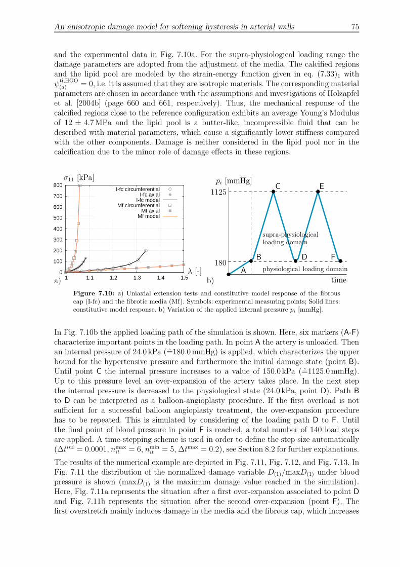
An anisotropic damage model for softening hysteresis in arterial walls 75
and the experimental data in Fig. 7.10a. For the supra-physiological loading range thedamage parameters are adopted from the adjustment of the media. The calcified regionsand the lipid pool are modeled by the strain-energy function given in eq. (7.33)1 withψti,HGO(a) = 0, i.e. it is assumed that they are isotropic materials. The corresponding material
parameters are chosen in accordance with the assumptions and investigations of Holzapfelet al. [2004b] (page 660 and 661, respectively). Thus, the mechanical response of thecalcified regions close to the reference configuration exhibits an average Young’s Modulusof 12 ± 4.7MPa and the lipid pool is a butter-like, incompressible fluid that can bedescribed with material parameters, which cause a significantly lower stiffness comparedwith the other components. Damage is neither considered in the lipid pool nor in thecalcification due to the minor role of damage effects in these regions.
a) b) 0
100
200
300
400
500
600
700
800
1 1.1 1.2 1.3 1.4 1.5
I-fc circumferentialI-fc axial
I-fc modelMf circumferential
Mf axialMf model
σ11 [kPa]
λ [-]
1125
180
C E
B
pi [mmHg]
supra-physiologicalloading domain
physiological loading domain
time
D
A
F
Figure 7.10: a) Uniaxial extension tests and constitutive model response of the fibrouscap (I-fc) and the fibrotic media (Mf). Symbols: experimental measuring points; Solid lines:constitutive model response. b) Variation of the applied internal pressure pi [mmHg].
In Fig. 7.10b the applied loading path of the simulation is shown. Here, six markers (A-F)characterize important points in the loading path. In point A the artery is unloaded. Thenan internal pressure of 24.0 kPa (=180.0mmHg) is applied, which characterizes the upperbound for the hypertensive pressure and furthermore the initial damage state (point B).Until point C the internal pressure increases to a value of 150.0 kPa (=1125.0mmHg).Up to this pressure level an over-expansion of the artery takes place. In the next stepthe internal pressure is decreased to the physiological state (24.0 kPa, point D). Path B
to D can be interpreted as a balloon-angioplasty procedure. If the first overload is notsufficient for a successful balloon angioplasty treatment, the over-expansion procedurehas to be repeated. This is simulated by considering of the loading path D to F. Untilthe final point of blood pressure in point F is reached, a total number of 140 load stepsare applied. A time-stepping scheme is used in order to define the step size automatically(∆tini = 0.0001, nmax
it = 6, nminit = 5, ∆tmax = 0.2), see Section 8.2 for further explanations.
The results of the numerical example are depicted in Fig. 7.11, Fig. 7.12, and Fig. 7.13. InFig. 7.11 the distribution of the normalized damage variable D(1)/maxD(1) under bloodpressure is shown (maxD(1) is the maximum damage value reached in the simulation).Here, Fig. 7.11a represents the situation after a first over-expansion associated to point Dand Fig. 7.11b represents the situation after the second over-expansion (point F). Thefirst overstretch mainly induces damage in the media and the fibrous cap, which increases

76 An anisotropic damage model for softening hysteresis in arterial walls
during the second overstretch and reaches a higher maximum value. Furthermore, a pro-nounced concentration is observable at the interface of the media and the fibrous cap.
0.3000.2790.2570.2360.2140.1930.1710.1500.1290.1070.0860.0640.0430.0210.000
a) b)
D(1)/maxD(1)
Figure 7.11: Distribution of the normalized damage variable D(1)/maxD(1) in an arte-rial cross-section under blood pressure of 24 kPa after a) one over-expansion (point D inFig. 7.10b), and b) after two over-expansions (point F in Fig. 7.10b).
In another numerical simulation axial residual strains of 5% were taken into account inorder to analyze the assumption that they have a considerable influence on the damageevolution. It should be noticed, that circumferential residual strains were not consideredin these simulations. This is a reasonable simplification, since the residual stresses aresignificantly lower compared with the stresses obtained during an arterial over-expansion.Firstly, the distribution of (J
(1)4 )1/2, which is associated to the stretch in the fiber direction,
is taken under consideration in the physiological undamaged configuration at a bloodpressure of 24 kPa (point B), see Fig. 7.12. Comparison of Fig. 7.12a (simulation withoutaxial residual strains) and Fig. 7.12b (simulation with axial residual strains of 5%) makesvisible, that the fiber stretch is higher if residual strains are taken into account. However,the difference is rather low.
1.0501.0461.0411.0371.0331.0291.0241.0201.0161.0111.0071.0030.9990.9940.990
a) b)
√J(1)4
Figure 7.12: Distribution of the stretch (J(1)4 )1/2 in the fiber direction of a loaded but
undamaged artery at internal pressure of 24 kPa (point B in Fig. 7.10b): a) without axialresidual strains and b) with axial residual strains of 5%.

An anisotropic damage model for softening hysteresis in arterial walls 77
Now we again take a look at the normalized damage variable D(1)/maxD(1). In Fig. 7.13the distribution associated to point E is shown, i.e. at the second over-expansion of theartery: again we compare the two cases in which no residual strains are taken into account(Fig. 7.13a) and residual strains of 5% are considered (Fig. 7.13b). Here, the differencebetween the two cases is much more pronounced as observed in Fig. 7.12: the normalizeddamage values are up to four times higher if we apply axial residual strains. Especiallyfrom a medical perspective, this is an interesting result since the rather high damagevalues at the fibrous-cap/media interface could increase the risk of plaque rupture.
0.3000.2790.2570.2360.2140.1930.1710.1500.1290.1070.0860.0640.0430.0210.000
a) b)
D(1)/maxD(1)
Figure 7.13: Distribution of the normalized damage variable D(1)/maxD(1) in an arterialcross-section under blood pressure of 150kPa (point E in Fig. 7.10b): a) without and b) withaxial residual strains of 5%.
In order allow the comparison of Fig. 7.11 and Fig. 7.13 the same maximum damage valueof maxD(1) = 0.0951 has been used for the calculation of the normalized value.


Robustness of the Penalty-Method and the Augmented-Lagrange-Method 79
8 Numerical analysis of the robustness of the Penalty-Methodand the Augmented-Lagrange-Method
In this chapter the numerical robustness and the computational costs of three-dimensionalsimulations is investigated with regard to the use of a pure Penalty approach and withregard to the use of an Augmented-Lagrange approach with a nested or a simultaneousiteration of the Lagrange multiplier. The theory behind the different approaches wasdiscussed in Section 5.2. For a proper comparison between the approaches we will makeuse of an automatic time step size control described in Section 8.2.
In Section 8.1 the constitutive model is described, which is used in the three-dimensionalnumerical simulations. The results of the simulations are discussed in Section 8.4 (1 mmlong arterial segment) and in Section 8.5 (patient-specific 10 mm long arterial segment).Because of the high number of degrees of freedom (more than a million) in case of the sim-ulation of the longer segment, the parallel implementation of FEAP12 and the FETI-DP13
domain decomposition method is used, which is briefly discussed in Section 8.3. A partof the following results is published in Brinkhues et al. [2012].
8.1 Constitutive model
In the three-dimensional simulations that are considered in this section arterial walls areinvestigated, which are composed of media, adventitia and degenerated tissue. The degen-erated tissue consists of plaque and in the numerical simulation in Section 8.4 additionallyof calcified regions and extracellular lipid. The strain-energy function of the underlyingmedia and adventitia material is
ψ = ψisoNH + ψvol
P +2∑
a=1
ψti,HGO2
(a) , (8.1)
see the individual energy functions in eq. (5.5), eq. (5.6), and eq. (5.16). For the identifi-cation of the parameters c1, k1, k2 and βf for the adventitia and the media the materialmodel (eq. (8.1)) is adjusted to experimental data10 (page 54) with the adjustment strategyproposed in Section 6.1. In Table 8.1 the resulting parameters are summarized.
c1 k1 k2 βf penalty augmented[kPa] [kPa] [-] [ ] ε1 [kPa] ε2 [-] ε1 [kPa] ε2 [-]
media 9.23 192.86 2626.84 43.9 360.0 9.0 10.0 4.0
adventitia 7.17 3.68e-3 51.15 54.7 70.0 8.5 10.0 4.0
Table 8.1: Material parameters for the media and the adventitia with penalty parametersε1 and ε2 for the Penalty approach and the Augmented-Lagrange approach.
Since the adjustment is done under the assumption that the material is quasi-incompressible, the incompressibility constraint has to be enforced separately in the nu-merical simulation. Thus, the penalty parameters have to be chosen sufficiently large incase of the Penalty approach, such that detF ≈ 1, see also Table 8.1. The volumetric
12Finite Element Analysis Program, R. L. Taylor, University of California.13Finite Element Tearing and Interconnecting - Dual Primal.

80 Robustness of the Penalty-Method and the Augmented-Lagrange-Method
change produced by the chosen penalty parameters is only known subsequently. Using anAugmented-Lagrange approach lower penalty parameters can be chosen, but an accuratestopping criterion has to be taken into account (i.e. a sufficiently small tolerance valueTOL, see Fig. 5.1 and Fig. 5.2 must be used). Thus, the volumetric change is controlledduring the iteration process by satisfying the element-wise condition | detF − 1| ≤ TOL.
The stress-strain response of the material model in consideration of the adjusted param-eters is shown in Fig. 8.1. Here, it is clearly visible that the experimental data and thematerial model fit very well for the media as well as for the adventitia in both directions,i.e. in axial and circumferential direction. Furthermore, the stress-strain response remainssimilar under consideration of a Penalty approach, displayed in Fig. 8.1a, compared tothe use of an Augmented-Lagrange approach, see Fig. 8.1b.
a) 0
20
40
60
80
100
120
140
1 1.05 1.1 1.15 1.2 1.25
experimentmodel
media
circumferential ➀axial ➁
σ11 [kPa]
λ [-]
➀
➁
0
10
20
30
40
50
60
70
1 1.05 1.1 1.15 1.2 1.25 1.3 1.35
experimentmodel
adventitia
circumferential ➀axial ➁
σ11 [kPa]
λ [-]
➁
➀
b) 0
20
40
60
80
100
120
140
1 1.05 1.1 1.15 1.2 1.25
experimentmodel
mediacircumferential ➀axial ➁
σ11 [kPa]
λ [-]
➀
➁
0
10
20
30
40
50
60
70
1 1.05 1.1 1.15 1.2 1.25 1.3 1.35
experimentmodel
adventitiacircumferential ➀axial ➁
σ11 [kPa]
λ [-]
➁
➀
Figure 8.1: Comparison of the stretch-strain response of the experiments and the materialmodel in a uniaxial extension test (media and adventitia) under consideration of a) a Penaltyapproach and b) an Augmented-Lagrange approach.
For the description of the plaque components the isotropic Mooney-Rivlin strain-energyfunction ψiso
MR (eq. (5.3)) is used. For the extracellular lipid and the calcified regions theisotropic part of the energy function is taken into account. The parameters of the degen-erated tissue are chosen as listed in Table 8.2.
Robustness of the Penalty-Method and the Augmented-Lagrange-Method 81
η1 η2 η3 c1 ε1 ε2[kPa] [kPa] [-] [kPa] [kPa] [-]
plaque 80.0 250.0 2000.0 – – -
calcified regions – – – 6800.0 50.0 10.0
extracellular lipid – – – 700.0 5250.0 10.0
Table 8.2: Material parameters of the degenerated tissue.
Penalty term. The penalty term ψvolP in eq. (8.1) models the incompressibility by pe-
nalizing deviations from the constraint detF = 1. The influence of the penalty parameteron the penalty function is shown in Fig. 8.2. Here, the curve of the penalty function usedfor the Penalty-Method is compared with the curve used in the Augmented-Lagrange-Method. It is clearly visible, that the curve belonging to the Penalty approach is verysteep compared to the one belonging to the Augmented-Lagrange approach.
0
0.5
1
1.5
2
0.98 0.99 1 1.01 1.02
ψvolP
I3
ε1 = 360
ε2 = 9
ε1 = 10
ε2 = 4
Figure 8.2: Comparison of the penalty function ψvolP = ε1(I
ε23 + I−ε2
3 − 2) for the two setsof parameters (Penalty approach and Augmented-Lagrange approach) for the media, seeTable 8.1.
The second derivative of the penalty function is related to the material tangent. Thisderivative with respect to the invariant I3 is given by
∂2ψ
∂2I3= ε1ε2
((ε2 − 1) Iε2−2
3 +ε2 + 1
Iε2+23
), (8.2)
which grows linearly with ε1 and exponentially with ε2. Thus, it may have a bad influenceon the condition number of the stiffness matrix, i.e. the condition number may deteriorate.
8.2 Automatic time stepping
In order to ensure a proper comparison between the different approaches an automatictime stepping scheme is used, where the size of the incremental time steps is controlled. Itshould be noticed, that the notation “time” is used in the sense of a “pseudo” time. Here,the initial time step size ∆tini is chosen. During the simulation the step size is reducedautomatically by ∆t = ∆t·10−1/5, if more than nmax
it Newton iterations are needed. On theother hand, if less than nmin
it Newton iterations are needed, the time step size is increasedby ∆t = ∆t · 101/5. The maximum time step size is bounded from above by ∆tmax.
82 Robustness of the Penalty-Method and the Augmented-Lagrange-Method
Regarding the nested Augmented-Lagrange approach only the number of Newton itera-tions in the first Newton step is considered. Generally, the later Newton steps convergefaster than the first step. In the simultaneous Augmented-Lagrange approach (SAL) theiteration for the Lagrange multiplier is performed simultaneously with the Newton cor-rection. As mentioned in Section 5.2.3 this can be seen as an inexact Newton method.Therefore, the bounds nmax
it and nminit are chosen higher.
8.3 FEAP and FETI-DP Method
The pre- and postprocessing of the computation is done by FEAP12 (page 79), while theFETI-DP13 (page 79) method is used to subdivide the domain and to solve the solutionvector with a parallel solution strategy. Within our parallel solver environment we useMPI14, PETSc15, UMFPACK16 and ACML17.
One global iteration can be divided into the following main steps:
i) FEAP: Computation of element stiffnesses and element right-hand-sides and trans-ferring the computed values by the use of an interface to the FETI-DP solver.
ii) FETI-DP: Decomposition of the whole domain into subdomains, assembling of thesystems of equations for all subdomains, and computation of the solution vector bythe parallel solver.
iii) Transferring the solution vector by the use of an interface to FEAP.
iv) FEAP: Update of the displacement vector.
In this work the classical Newton-Krylov-FETI-DP approach is used. Here, firstly thelinearization is done and thereafter the linearized systems are solved using the FETI-DPdomain decomposition method.
FETI-DP domain decomposition method In Farhat and Roux [1991] FETI domaindecomposition methods were first introduced. In the framework of domain decompositionmethods an approximate inverse is built from solving small problems on subdomainsand a small global problem. For an overview on domain decomposition methods see thetextbooks Smith et al. [1996], Quarteroni and Valli [1999], and Toselli and Widlund [2005].The more recent FETI-DP domain decomposition methods were proposed in Farhat et al.[2000a, 2001] and enhanced in, for example, Klawonn and Widlund [2001, 2002, 2005,2006], Klawonn et al. [2002], Klawonn [2006], Klawonn and Rheinbach [2006, 2007a],Klawonn et al. [2011]. By using FETI methods, large structural-mechanics problems canbe solved on massively parallel machines, see for example Farhat et al. [2000b], Bhardwajet al. [2000], and Klawonn and Rheinbach [2010].
In the framework of FETI-DP methods the considered domain B0 is decomposed intoa number of N nonoverlapping subdomains B0,i, i = 1, . . . , N , with diameter H andboundary ∂B0,i. A graph partitioner (Karypis et al. [2003]) is used in order to define the
14MPI: Message Passing Interface.15PETSc: Portable, Extensible Toolkit for Scientific Computation; Balay et al. [2001, 2004, 1997].16UMFPACK: Unsymmetric MultiFrontal PACKage; Davis [2004].17ACML: AMD Core Math Library released by the american company AMD (Advanced Micro Devices).

Robustness of the Penalty-Method and the Augmented-Lagrange-Method 83
decomposition into unions of finite elements with matching finite-element nodes on theboundaries of neighboring subdomains across the interface
Γ :=⋃
i 6=j∂B0,i ∩ ∂B0,j and Γ =
N⋃
i=1
∂B0,i \ ∂B0 , (8.3)
with ∂B0,i ∩ ∂B0,j . This process does not need access to geometric data since it is a com-pletely algebraic process. After decomposition one or several subdomains can be allottedto each processor.
The linearized subdomain problems, cf. eq. (4.33), are identified for each subdomain B0,iwith the local stiffness matrices K(i), the load vectors f (i), and the local displacementincrement ∆D(i), i.e.
K(i) ∆D(i) = f (i) with i = 1, . . . , N . (8.4)
We distinguish between nonprimal variables with index (•)B and primal variables withindex (•)Π. Furthermore, the nonprimal variables are subdivided into internal variableswith index (•)I and dual variables with index (•)∆. Thus, the local stiffness matrices aregiven by
K(i) =
[K
(i)BB (K
(i)ΠB)
T
K(i)ΠB K
(i)ΠΠ
]with K
(i)BB =
[K
(i)I I (K
(i)∆ I)
T
K(i)∆ I K
(i)∆∆
]. (8.5)
Generally, the N independent local problems in eq. (8.4) lead to discontinuous solutionsacross the subdomain interfaces Γ. In order to enforce continuity of the solution in theprimal variables, a finite-element subassembly is performed
[KBB (KΠB)
T
KΠB KΠΠ
]=
K(1)BB · · · 0 (K
(1)ΠB)
T
.... . .
......
0 · · · K(N)BB (K
(N)ΠB)
T
K(1)ΠB · · · K
(N)ΠB
∑Ni=1K
(i)ΠΠ
. (8.6)
Using a global-to-local map RΠ with entries from 0, 1 and the identity IB applied onthe nonprimal variables, we achieve the partially assembled, global stiffness matrix
K =
[KBB (KΠB)
T
KΠB KΠΠ
]=
[IB 00 (RΠ)
T
] [KBB (KΠB)
T
KΠB KΠΠ
] [IB 00 RΠ
], (8.7)
which is coupled in the primal variables yielding a coarse problem for the method. Anappropriate choice of the primal variables yields a positive definite matrix K. The corre-sponding global load vector and global displacement increment appear as
f =
[fBfΠ
]=
[IB 00 (RΠ)
T
] [fB∑Ni=1 f
(i)Π
]=
f(1)B...
f(N)B
fΠ
and ∆D =
[∆DB
∆DΠ
]. (8.8)
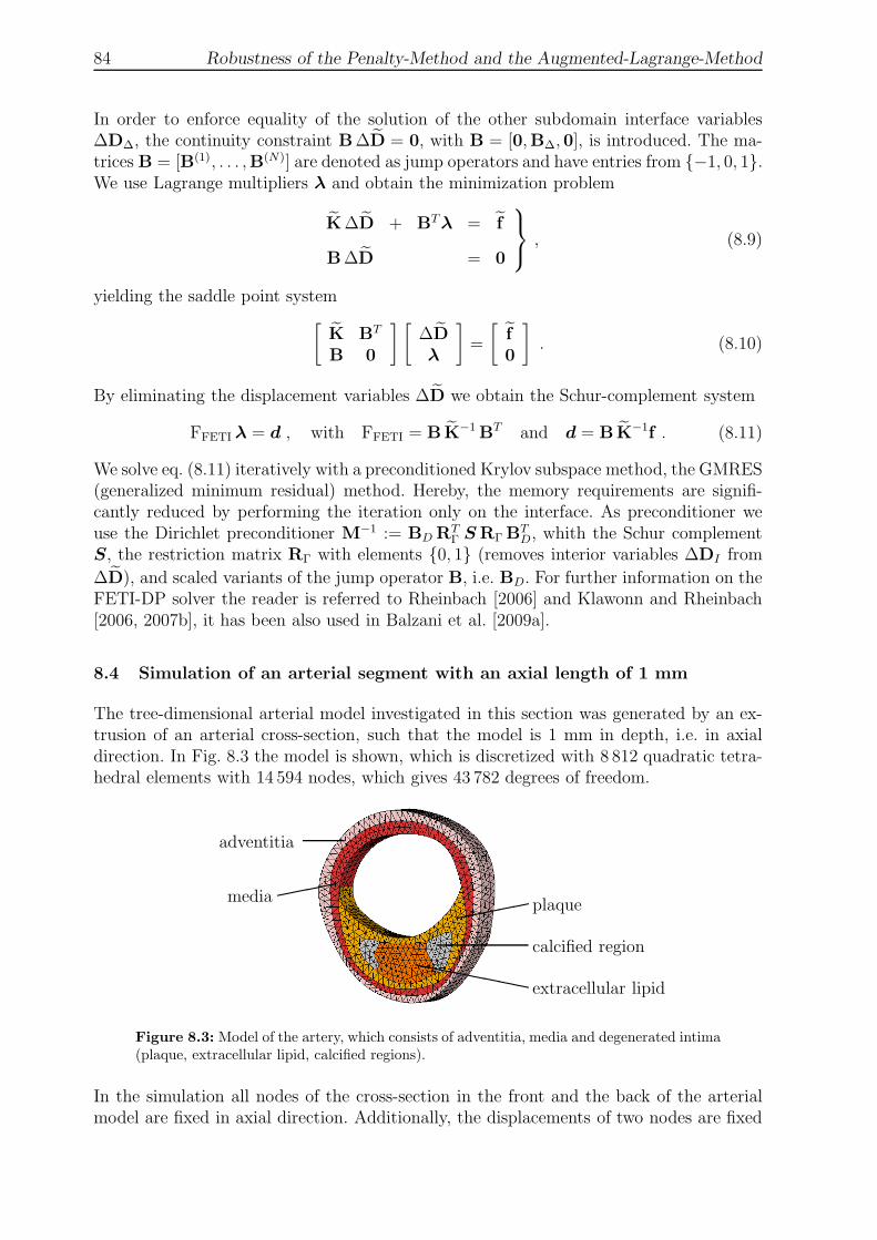
84 Robustness of the Penalty-Method and the Augmented-Lagrange-Method
In order to enforce equality of the solution of the other subdomain interface variables∆D∆, the continuity constraint B∆D = 0, with B = [0,B∆, 0], is introduced. The ma-trices B = [B(1), . . . ,B(N)] are denoted as jump operators and have entries from −1, 0, 1.We use Lagrange multipliers λ and obtain the minimization problem
K∆D + BTλ = f
B∆D = 0
, (8.9)
yielding the saddle point system
[K BT
B 0
] [∆Dλ
]=
[f0
]. (8.10)
By eliminating the displacement variables ∆D we obtain the Schur-complement system
FFETIλ = d , with FFETI = BK−1BT and d = BK−1f . (8.11)
We solve eq. (8.11) iteratively with a preconditioned Krylov subspace method, the GMRES(generalized minimum residual) method. Hereby, the memory requirements are signifi-cantly reduced by performing the iteration only on the interface. As preconditioner weuse the Dirichlet preconditioner M−1 := BDRT
Γ SRΓBTD, whith the Schur complement
S, the restriction matrix RΓ with elements 0, 1 (removes interior variables ∆DI from
∆D), and scaled variants of the jump operator B, i.e. BD. For further information on theFETI-DP solver the reader is referred to Rheinbach [2006] and Klawonn and Rheinbach[2006, 2007b], it has been also used in Balzani et al. [2009a].
8.4 Simulation of an arterial segment with an axial length of 1 mm
The tree-dimensional arterial model investigated in this section was generated by an ex-trusion of an arterial cross-section, such that the model is 1 mm in depth, i.e. in axialdirection. In Fig. 8.3 the model is shown, which is discretized with 8 812 quadratic tetra-hedral elements with 14 594 nodes, which gives 43 782 degrees of freedom.
adventitia
media
plaque
calcified region
```````
extracellular lipid
Figure 8.3: Model of the artery, which consists of adventitia, media and degenerated intima(plaque, extracellular lipid, calcified regions).
In the simulation all nodes of the cross-section in the front and the back of the arterialmodel are fixed in axial direction. Additionally, the displacements of two nodes are fixed

Robustness of the Penalty-Method and the Augmented-Lagrange-Method 85
vertically and the displacements of one node is fixed horizontally. The constitutive modelfor the individual components is described in Section 8.1 and the material parameters arelisted in Table 8.1 and Table 8.2.
For the enforcement of incompressibility the following methods are used andanalyzed regarding the robustness of the simulation: i) the Penalty-Method,ii) the Augmented-Lagrange-Method with a nested iteration (NAL) and an adherenceof the (detF = 1)-condition with a tolerance of ±1% and κal = 999.0, and iii) theAugmented-Lagrange-Method with a simultaneous iteration (SAL) and an adherence ofthe (detF =1)-condition with a tolerance of ±1% and κal = 999.0.
For the automatic time stepping scheme the initial time step size value is ∆tini = 0.001 andthe maximum time step size is ∆tmax = 0.1. For the simulations with the Penalty approachand the nested Augmented-Lagrange-Method the bounds are nmax
it = 9 and nminit = 6
and for the simulation with simultaneous Augmented-Lagrange-Method nmaxit = 11 and
nminit = 8.
The distribution of detF under an inner pressure pi = 24 kPa is shown in Fig. 8.4. Thequasi-incompressibility condition can be regarded as met in a sufficient manner: for thetwo simulations with the Augmented-Lagrange approach the tolerance value is maintainedand also for the simulation with the Penalty approach detF ≈ 1± 0.01.
a)
min = 0.9963max = 1.0119
b)
min = 0.9928max = 1.0099
c)
detF
min = 0.9936max = 1.0096
Figure 8.4: Distribution of the determinant of the deformation gradient detF under aninner pressure pi = 24 kPa using a) the Penalty-Method and using the Augmented-Lagrange-Method with b) a nested iteration and c) a simultaneous iteration.
An evaluation of the numerical simulation with regard to the robustness is given in Fig. 8.5.Here, the diagrams show the time increment, the last absolute residual norm and thenumber of Newton iterations over time. In the simulation with the Penalty-Method moretime steps are needed. It can be stated that during the automatic time stepping schemethe maximum time increment ∆tmax is reached faster when the Augmented-Lagrange-Method is used. Furthermore, in most cases the value of the last residual norm usingan Augmented-Lagrange-Method is below the value using the Penalty-Method. Compar-ison of the two Augmented-Lagrange approaches shows, that more Newton iterations areneeded using the nested iteration compared to the simultaneous iteration. In summary, thehighest robustness of the simulation can be obtained by using the Augmented-Lagrange-Method with a simultaneous iteration.

86 Robustness of the Penalty-Method and the Augmented-Lagrange-Method
a)
0
0.02
0.04
0.06
0.08
0.1
0 0.2 0.4 0.6 0.8 1
timeincrem
ent
time
26 time steps -7.6
-7.4
-7.2
-7
-6.8
-6.6
0 0.2 0.4 0.6 0.8 1
last
absolute
residual
norm
10x
time
5
5.5
6
6.5
7
0 0.2 0.4 0.6 0.8 1
New
toniterations
time
143 iterations
b)
0
0.02
0.04
0.06
0.08
0.1
0 0.2 0.4 0.6 0.8 1
timeincrem
ent
time
15 time steps -7.6
-7.4
-7.2
-7
-6.8
-6.6
0 0.2 0.4 0.6 0.8 1
last
absolute
residual
norm
10x
time
5
10
15
20
25
30
35
40
0 0.2 0.4 0.6 0.8 1
New
toniterations
time
293 iterations
c)
0
0.02
0.04
0.06
0.08
0.1
0 0.2 0.4 0.6 0.8 1
timeincrem
ent
time
19 time steps -7.6
-7.4
-7.2
-7
-6.8
-6.6
0 0.2 0.4 0.6 0.8 1
last
absolute
residual
norm
10x
time
4
5
6
7
8
9
10
11
0 0.2 0.4 0.6 0.8 1
New
toniterations
time
132 iterations
Figure 8.5: Time increment, last absolute residual norm of the time step and numberof Newton iterations over time: a) Penalty-Method; Augmented-Lagrange-Method with b)nested iteration and with c) simultaneous iteration.
8.5 Simulation of an arterial segment with an axial length of 10 mm
The three-dimensional geometry of the artery analyzed in the following numerical simu-lation is based on histological pictures, cf. Brands et al. [2009], Balzani et al. [2011]. Theartery is composed of media, adventitia and of a large inclusion of plaque, see Fig. 8.6.
Figure 8.6: Layered finite element model of the arterial segment discretized using 10-nodedtetrahedral elements: a) complete arterial model, b) blanked adventitia and c) plaque.

Robustness of the Penalty-Method and the Augmented-Lagrange-Method 87
The model is discretized with 305 033 quadratic tetrahedral elements yielding 434 517nodes and therefore 1 303 551 degrees of freedom. Due to such a large number of degreesof freedom, the FETI-DP domain decomposition method is used parallel to the FiniteElement Program FEAP, see Section 8.3. The Newton method stops if a reduction of theabsolute residual norm to a value less than 10−6 or a value less than 10−4 for three consec-utive Newton steps is achieved. In the FETI-DP Krylov iteration the stopping criterion isan absolute residual less than 5 · 10−9. The domain is decomposed into 224 subdomains,see Fig. 8.7.
Figure 8.7: Domain decomposition of the arterial segment into 224 subdomains. For abetter view of the nonoverlapping method the subdomains are dispersed.
The following different methods are used in order to enforce quasi-incompressibility:
• Penalty-Method
• Augmented-Lagrange-Method with the nested iteration and enforcement of the con-dition | detF − 1| ≤ 0.01, i.e. TOL = 1%, and the parameter κal = 499.0
• Augmented-Lagrange-Method with the simultaneous iteration and enforcement ofthe condition | detF − 1| ≤ 0.01, i.e. TOL = 1%, and the parameter κal = 500.0
• Augmented-Lagrange-Method with the simultaneous iteration and enforcement ofthe condition | detF − 1| ≤ 0.001, i.e. TOL = 1‰, and the parameter κal = 1 000.0
For the automatic time stepping scheme the initial time step size value is ∆tini = 0.001and the maximum time step size is ∆tmax = 0.4. For the simulations with the Penaltyapproach and the nested Augmented-Lagrange-Method (NAL) the bounds are nmax
it = 9and nmin
it = 6 and for the simulation with simultaneous Augmented-Lagrange-Method(SAL) nmax
it = 36 and nminit = 18.
The artery is loaded with an internal pressure of pi = 33.331 kPa (≈ 250 mmHg). InFig. 8.8a the range of the determinant of the deformation gradient detF under full load-ing is shown for the different approaches. In the Augmented-Lagrange approaches thepredefined conditions | detF − 1| ≤ 0.01 and | detF − 1| ≤ 0.001, respectively, are met.The solution using the Penalty approach only satisfies | detF − 1| ≤ 0.0209. Additionally,

88 Robustness of the Penalty-Method and the Augmented-Lagrange-Method
Fig. 8.8 shows the distribution of the determinant of the deformation gradient detF . Thedistribution is depicted for the Penalty approach, the NAL, and the SAL approach witha tolerance value of 10−2. The overall distribution is very smooth in case of all threedifferent simulations. Furthermore, due to the equal tolerance value, the two simulations,in which the Augmented-Lagrange-Method are used, exhibit an almost identical distribu-tion. One reason for the difference to the simulation using the Penalty-Method is that itis not possible to explicitly define a tolerance value.
0.99
0.995
1
1.005
1.01
1.015
1.02
1.025detF
penalty NAL, TOL =1% SAL, TOL =1% SAL, TOL =1‰a)
detF
b) c) d)
Figure 8.8: a) Diagram showing the range of the determinant of the deformation gradientfor the different used approaches. The minimum and maximum values (detFmin/detFmax)are as follows: penalty (0.9926/1.0209), NAL with TOL = 0.01 (0.9901/1.0099), SAL withTOL = 0.01 (0.9902/1.01), SAL with TOL = 0.001 (0.9990/1.001); Distribution of thedeterminant of the deformation gradient detF : b) Penalty approach, c) NAL (TOL=10−2),and d) SAL with TOL=10−2.
In Fig. 8.9, Fig. 8.10, Fig. 8.11 and Fig. 8.12 the evaluations of the simulations aredisplayed. The diagrams show the time increment, the last absolute residual norm, thenumber of Newton iterations, and the number of FETI-DP iterations for each approach.Additionally, the main facts are summarized in compact form in Table 8.3. Here, also thetotal costs of the computations are listed, which can roughly be estimated by multiplyingthe number of global Newton steps (summary of all Newton steps needed within thesimulation) with the corresponding average number of (inner) FETI-DP iterations.

Robustness of the Penalty-Method and the Augmented-Lagrange-Method 89
0
0.05
0.1
0.15
0.2
0.25
0.3
0.35
0.4
0 0.5 1 1.5 2 2.5
timeincrem
ent
pseudo time
19 time steps-8
-7.5
-7
-6.5
-6
-5.5
-5
-4.5
-4
0 0.5 1 1.5 2 2.5
last
abs.
residual
norm
10x
pseudo time
5
5.5
6
6.5
7
7.5
8
8.5
9
0 0.5 1 1.5 2 2.5
New
toniterations
pseudo time
112 iterations 50
100
150
200
250
300
350
400
450
0 20 40 60 80 100
FETI-DP
iterations
global Newton iterations
∅ 220.8 iterations
a) b)
c) d)
Figure 8.9: Penalty-Method: a) time increment, b) last absolute residual norm, c) numberof Newton iterations, and d) FETI-DP iterations over time.
0
0.05
0.1
0.15
0.2
0.25
0.3
0.35
0.4
0 0.5 1 1.5 2 2.5
timeincrem
ent
pseudo time
19 time steps-8
-7.5
-7
-6.5
-6
-5.5
-5
-4.5
-4
0 0.5 1 1.5 2 2.5
last
abs.
residual
norm
10x
pseudo time
0
10
20
30
40
50
60
70
0 0.5 1 1.5 2 2.5
New
toniterations
pseudo time
618 iterations 50
100
150
200
250
300
350
400
450
0 100 200 300 400 500 600
FETI-DP
iterations
global Newton iterations
∅ 154.0 iterations
a) b)
c) d)
Figure 8.10: NAL method: a) time increment, b) last absolute residual norm, c) numberof Newton iterations, and d) FETI-DP iterations over time.

90 Robustness of the Penalty-Method and the Augmented-Lagrange-Method
0
0.05
0.1
0.15
0.2
0.25
0.3
0.35
0.4
0 0.5 1 1.5 2 2.5
timeincrem
ent
pseudo time
13 time steps-8
-7.5
-7
-6.5
-6
-5.5
-5
-4.5
-4
0 0.5 1 1.5 2 2.5
last
abs.
residual
norm
10x
pseudo time
4
6
8
10
12
14
16
18
0 0.5 1 1.5 2 2.5
New
toniterations
pseudo time
141 iterations 50
100
150
200
250
300
350
400
450
0 20 40 60 80 100 120 140
FETI-DP
iterations
global Newton iterations
∅ 150.2 iterations
a) b)
c) d)
Figure 8.11: SAL method with TOL = 0.01: a) time increment, b) last absolute residualnorm, c) number of Newton iterations, and d) number of FETI-DP iterations over time.
0
0.05
0.1
0.15
0.2
0.25
0.3
0.35
0.4
0 0.5 1 1.5 2 2.5
timeincrem
ent
pseudo time
13 time steps-8
-7.5
-7
-6.5
-6
-5.5
-5
-4.5
-4
0 0.5 1 1.5 2 2.5
last
abs.
residual
norm
10x
pseudo time
5
10
15
20
25
30
35
40
45
0 0.5 1 1.5 2 2.5
New
toniterations
pseudo time
284 iterations 50
100
150
200
250
300
350
400
450
0 50 100 150 200 250
FETI-DP
iterations
global Newton iterations
∅ 161.4 iterations
a) b)
c) d)
Figure 8.12: SAL method with TOL = 0.001: a) Time increment, b) last absolute residualnorm, c) number of Newton iterations, and d) number of FETI-DP iterations over time.

Robustness of the Penalty-Method and the Augmented-Lagrange-Method 91
If we compare the number of Newton iterations needed in the Penalty-Method inFig. 8.9 with the number needed in the simultaneous Augmented-Lagrange-Method withTOL = 0.01 (see Fig. 8.11) more Newton iterations are needed in the SAL approach dueto the additional Augmented-Lagrange iterations. Nevertheless, the convergence of thenonlinear scheme and the linear iterative solver is much faster in case of the SAL method,so that the total costs are less, see also Table 8.3. The total cost of the nested Augmented-Lagrange approach (Fig. 8.10) is distinctly higher due to the high amount of the Newtoniterations.
In Fig. 8.10c, Fig. 8.11c and Fig. 8.12c it is visible that the number of Newton iterationsbecomes greater during the simulation. A reason for that may be, that only a very smallnumber of finite elements violate the element-wise condition | detF − 1| ≤ TOL in thebeginning of the simulation and this number increases in the course of the simulation.
We can also observe, that the number of FETI-DP iterations becomes greater during thesimulations, see Fig. 8.9d, Fig. 8.10d, Fig. 8.11d and Fig. 8.12d. This may be a resultof the increasing influence of the incompressibility constraint during the simulation. InBalzani et al. [2009a] it was found out that the convergence of the nonlinear iterationscheme as well as the convergence of the iterative linear solver is measurably influencedby the anisotropies resulting from the energy terms of the fibers. Thus, an alternativeexplanation is that the increase of iterations is due to exponential stiffening of the fibers.
Summarizing the above, it can be conducted that the use of the Augmented-Lagrange-Method can significantly improve the properties of the linearized systems appearing in thenonlinear solution scheme. Here, a lower number of iterations is needed for convergenceof the FETI-DP iterative method. Furthermore, larger time steps ∆t can be chosen,such that the convergence of the nonlinear scheme is also improved. Nevertheless, theAugmented-Lagrange approach needs an additional iteration process for the Lagrangemultiplier.
time global Newton ∅ FETI-DP totalsteps iterations iterations costs
penalty 19 112 220.8 24 729.6(min = 170,max = 316)
SAL, TOL = 0.01 13 141 150.2 21 178.2(min 98,max = 217)
NAL, TOL = 0.01 19 618 154.0 95 172.0(min = 98,max = 427)
SAL, TOL = 0.001 13 248 161.4 40 027.2(min = 98,max = 368)
Table 8.3: Comparison of the methods in the framework of the FETI-DP method. TheFinite-Element model has approx. 1.3 million degrees of freedom, see Fig. 8.6. The totalcost can be estimated roughly by multiplying the number of global Newton iterations by theaverage number of FETI-DP iterations. This table is taken from Brinkhues et al. [2012].


Incorporation of residual stresses in patient-specific arteries 93
9 Incorporation of residual stresses in patient-specific arteries
In this chapter a method for the incorporation of residual stresses into a numerical modelfor the simulation of arterial walls is introduced. Section 9.1 gives an overview of thestate of the art in this field of research. The proposed new method, see also Schroder andBrinkhues [2012], is based on the assumption that residual stresses reduce the gradientof the wall stresses in radial direction. An experimental motivation for such an approachis given in, for example, Takamizawa and Hayashi [1987] or Fung [1991]. The idea is touse the local difference of the circumferential stresses with respect to its volume averagefor the estimation of the residual stresses. In Section 9.2 a plausibility check of the newapproach is done by a simple numerical simulation of an isotropic two-dimensional idealtube. Here, the gradients of the circumferential stresses are reduced through the residualstresses. Since arterial walls are anisotropic and exhibit a distinct material behavior infiber direction, suitable stress measures (the fiber stresses) are defined. The associatedinvariants, which are used for the definition of the residual stresses in soft biological tis-sues are derived in Section 9.3. Since an arterial geometry is not rotationally symmetric,the numerical realization of this method is based on a decomposition of the domain intodifferent segments, see Section 9.4. Furthermore, each segment is subdivided into sectorsdepending on how many different fiber reinforced layers the segments consist of (e.g. ad-ventitia and media). Such sectoral division seems to be evident, since the individual layersexhibit different opening angles and therefore a different residual stress distribution, seeHolzapfel et al. [2007], especially figure 6 on page 537. In Section 9.5 numerical simulationsare performed in order to show the suitability of the proposed approach.
9.1 State of the art in the modeling of residual stresses in arteries
Until the early 1980‘s a cylindrical arterial segment, which is not loaded with any externalforce, was assumed to be stress free. This assumption was disproved experimentally byVaishnav and Vossoughi [1983]. They sliced circular rings of bovine and porcine abdominalaortas radially; for a schematic illustration see Fig. 9.1. After the radial sectioning the ringsopened up into a horseshoe leading to the conclusion that the aorta is residually stressedin circumferential direction when it is intact but free from external forces. However, Bergel[1960] seems to be the first who observed this phenomenon.
θ
Figure 9.1: Schematic of longitudinal cut through an artery and resulting opening angle θ.
In Chuong and Fung [1986] it was stated that residual stresses reduce the magnitude of thestresses and the stress gradient of a pressurized artery significantly, see also Fung [1991].Takamizawa and Hayashi [1987] suggested that the residual stresses cause an almost uni-form circumferential strain distribution under physiological pressure; this is called the

94 Incorporation of residual stresses in patient-specific arteries
uniform-strain hypothesis. In Nollert et al. [1992] it is stated that a reduction of the stressgradient at the inner side of the arterial wall may reduce the risk of atherogenesis. Furtherexperimental observations on rat aortas showed that the level of the segmental openingdiffers depending on the position of the segment in the aortic tree, see Liu and Fung[1988]. Thus, the opening angle θ gradually varies from the ascending aorta to the lumbarregion: it starts by 160, follows a curve to 60, tends toward zero before becoming slightlynegative and increases again over 60. Liu and Fung [1989] banded abdominal rat aortasnear the celiac trunk in order to establish hypertension. Then they discussed the changeof the opening angle as a result of hypertension and hypertrophy and found out that achange in blood pressure changes the residual strains and therefore the opening anglesignificantly. They stated that the residual-strain change is stress-modulated. A study onthe circumferential residual stresses in the left ventricle and the trachea is given in Omensand Fung [1990] and Han and Fung [1991], respectively. The zero-stress state of smallblood vessels, which consists of 79–57% smooth muscles, was investigated by Fung andLiu [1992]. Additionally, the effect of several drugs on the microvessels were presented.Experiments on bovine aortas done by Vossoughi et al. [1993] showed that even the cut-ted configuration is not fully stress-free. Additional circumferential cuts caused differentopening angles for the individual arterial layers. Thus, the magnitude of opening of theinner layers increases while those of the outer layers reduces indicating that stresses stillremain after the radial cut. Experiments on human aortas in Schulze-Bauer et al. [2002a]revealed also that residual stresses are not vanishing by a single cut, see also the study ofMatsumoto et al. [2004] on porcine thoracic aortas. Greenwald et al. [1997] investigatedaortas from rats and provided similar results concerning the different opening angles of theindividual layers after mechanical removal of the other layers. Additionally, they showedthat elastase treated (elimination of elastin) specimens offer smaller opening angles whilecollagenase treated (elimination of collagen) and frozen (destruction of smooth musclecells) specimens behave like the untreated control specimens. First studies on human tho-racic and abdominal aortas were done by Saini et al. [1995]. Here, the influence of age, sex,the position along the artery, and atherosclerosis on the opening of sliced arterial ringswas discussed. It was stated that the value of the opening angle increases with increasingdistance from the heart (female: 150–200, male: 200–250). They also observed largeropening angles in aged and atherosclerotic diseased vessels, and in those obtained frommale samples. Three-dimensional residual deformations of intact human abdominal aortaswere shown in Holzapfel et al. [2007]. In this study arterial rings were cut open and thenseparated into three layers. Furthermore, residual deformations on axial strips were in-vestigated. It was stated that, due to the occurrence of the residual deformations in threedimensions, they cannot be described by a single parameter. A review of experimentalmethods for residual-strain measurement was given by Rachev and Greenwald [2003].Chuong and Fung [1986] were probably the first to use a constitutive model to computeresidual stresses. They discussed a procedure for the description of the geometry of anopen artery, whose closed counterpart was regarded as thick-walled cylindrical tube withconstant thickness. This method is known as opening-angle method. Therewith they com-puted the two-dimensional residual stresses in the unloaded closed artery and showedthat the residual stresses enforce compression on the inner side of the vessel wall andtension on the outer side of the vessel wall. Many works are based on the opening-anglemethod to achieve an analytical solution for the residual strains of initially open idealtubes, which were closed by an initial bending. Rachev [1997] derived a mathematical

Incorporation of residual stresses in patient-specific arteries 95
model for the stress-dependent remodeling of a two-layer arterial tube. The assumptionthat the stress and strain values are equal under hypertensive and normotensive condi-tions was taken into account by means of remodeling of the zero-stress configuration bythickening of the layers. They also observed remaining residual stresses in the opened-upconfiguration of a hypertensive artery. Using a one-layer model Chaudhry et al. [1997]showed that circumferential stresses and gradients are reduced significantly at the innerwall. The opening-angle method was also used by Holzapfel for an analytical solution ofthe initial deformation tensor for multilayered arterial tubes. In Holzapfel et al. [2000a]the opening-angle method was applied to a two-layered tube and different material modelswere investigated. Another key objective was to analyze the effect of the residual stressesonto the overall stress distribution in the physiological regime. The high-pressure responseis analyzed in Holzapfel and Gasser [2007]. Pena et al. [2006] applied the opening-anglemethod to more realistic arterial geometries and conducted corresponding finite-elementsimulations. To account for residual stresses, Alastrue et al. [2007a] used a special formof the multiplicative decomposition of the deformation gradient, in which one part corre-sponds to the opening angle experiment. This approach was also investigated by Alastrueet al. [2008], where growth was included, and implemented in a micro-sphere model inAlastrue et al. [2009]. A combination of the opening-angle method and a constrained mix-ture model of vascular growth and remodeling was suggested in Cardamone et al. [2009].Here, the mixture components are the individual constituents of the artery, i.e. elastin,collagen and smooth muscle. One aim of the authors was find the origin of residual stress.For the modeling of growth and remodeling in the framework of constrained mixturemodels see also Alford et al. [2008] and Valentin and Humphrey [2009]. Holzapfel andOgden [2010] accounted for the different behavior of the three main arterial layers andused different opening angles for the individual layers. Additionally, they extended theopening-angle method by accounting for bending and stretching in both circumferentialand axial directions in order to reflect the three-dimensional residual stretch and stressstate. A further extension of the model was done by Bustamante and Holzapfel [2010],which accounted for opening angles depending on axial and radial position, i.e. differentopening angles along the tube. Furthermore, a different set of opening angles for intima,media and adventitia were considered. Stahlhand et al. [2004] used experimental data inorder to derive a residual-strain state. In order to do so, a minimization problem wasderived for an approximate identification of material parameters including the residualstrains. The parameters for the residual strains were presumed in the sense of the opening-angle method. This parameter identification algorithm is used in Olsson et al. [2006] todetermine an initial local deformation tensor, which is able to describe the residual strain,see also Klarbring et al. [2007]. An extension of the model was given by Olsson and Klar-bring [2008], which introduced the evolution of growth. In the recent paper of Chen andEberth [2012] a uniform circumferential stress was obtained by introducing a special classof constitutive functions without considering a residually stressed state. This idea couldbe attractive for the design of engineered blood vessels.In contrast to the above mentioned methods Balzani et al. [2006b, 2007] used a numericalmethod in order to establish a residual-strain state. Here, an initially open artery wasnumerically closed within a displacement-driven procedure. This model is appropriate,but nevertheless numerically extensive. In this work a novel model for the incorporationof residual stresses is proposed. An advantage of this model is that it is suitable for theincorporation of residual stresses in patient-specific three-dimensional arterial models.

96 Incorporation of residual stresses in patient-specific arteries
9.2 Numerical simulation of an isotropic two-dimensional ideal tube
As a plausibility check of the new approach two-dimensional numerical simulations of anisotropic ideal tube are performed. The circular ring has an inner radius r = 1 mm andan outer radius of r = 2 mm and is discretized with 6 100 quadratic triangular elements,see Fig. 9.2a. The material behavior is reflected by the Mooney-Rivlin model ψ = ψiso
MR
introduced in eq. (5.3). The corresponding material parameters are randomly chosen andlisted in Table 9.1. According to the procedure introduced in Section 6.2.1 the Lameconstants are µ = 30 [kPa] and λ = 345 [kPa] and the Poisson’s ratio is ν = 0.46.
c1 c2 c3
[kPa] [kPa] [kPa]
8.75 6.25 80.0
Table 9.1: Material parameters of the isotropic ideal tube.
Under an inner pressure of pi = 16 kPa (120 mmHg) the distribution of the stresses incircumferential direction with the normal vector nϕ
σϕ = σ : (nϕ ⊗ nϕ) (9.1)
arises as depicted in Fig. 9.2b (solid line). The maximum stresses are located at the innersurface (r = 1 mm) and decrease towards the outer surface (r = 2 mm), such that a stressgradient of the circumferential stresses in radial direction can be observed. Accordingto the above mentioned approach this gradient should be reduced as a consequence ofresidual stresses in circumferential direction.
a)
pi
r=1 r=2 [mm]r=0 b)
25
30
35
40
45
50
55
1 1.2 1.4 1.6 1.8 2
without residual stresses with residual stresses (A)with residual stresses (B)
σϕ [kPa]
r [mm]
Figure 9.2: a) Ideal two-dimensional circular ring discretized with 6 100 quadratic trian-gular elements. b) Circumferential stresses σϕ [kPa] plotted over the radius r [mm] withoutand with application of residual stresses at an inner pressure of pi = 16 kPa ≈ 120 mmHg;(A) after the first application of residual stresses and (B) after a further application.
Firstly the average value of the circumferential stresses in radial direction are computed.In this special case for a rotationally symmetric distribution of stress we get
σϕ =1
V
∫
B
σϕ(x) dv . (9.2)

Incorporation of residual stresses in patient-specific arteries 97
It should be noted that eq. (9.2) only holds for this rotationally symmetric stress distri-bution. The difference between the circumferential stresses and the average value is usedto compute the residual stress distribution
σres = ∆σϕ nϕ ⊗ nϕ with ∆σϕ = σϕ − σϕ . (9.3)
After the application of the residual stresses by a stress update σ ⇐ σ − σres the cir-cumferential stresses arise as depicted in Fig. 9.2b (line with circles). If this procedure18
is repeated another time a fully homogeneous stress distribution is obtained as indicatedby line with solid circles in Fig. 9.2b. The stress distribution along the tube before andafter the application of the smoothing-loop are shown in Fig. 9.3a and b.
a)
60.055.751.447.142.938.634.330.025.721.417.112.9
8.64.30.0
pi = 16 kPa
σϕ [kPa]
b)
60.055.751.447.142.938.634.330.025.721.417.112.9
8.64.30.0
pi = 16 kPa
σϕ [kPa]
c)
8.06.95.74.63.42.31.10.0
-1.1-2.3-3.4-4.6-5.7-6.9-8.0
pi = 0 kPa
σϕ [kPa]
d)
60.055.751.447.142.938.634.330.025.721.417.112.9
8.64.30.0
pi = 0 kPa
σϕ [kPa]
Figure 9.3: Stress distribution of circumferential stresses σϕ in an isotropic two-dimensionalcircular ring under an inner pressure of pi = 16 kPa: a) without considering residual stressesand b) after application of the residual stresses. c) Pure residual stress distribution in anunloaded circular ring (pi = 0 kPa) and d) opening of the ring due to residual stresses.
If the circular ring is unloaded to zero internal pressure, i.e. pi = 0 kPa, only the residualstresses remain as depicted in Fig. 9.3c. It is clearly visible that the residual stressesenforce pressure at the inner surface and tension at the outer surface as was expected. Ina further step, the tube is sliced radially. As shown in Fig. 9.3d, the circular ring opensdue to the residual stresses. An opening angle can be observed and the circumferentialstresses are almost zero.
18Each of those applications of residual stresses we call a “smoothing-loop”.

98 Incorporation of residual stresses in patient-specific arteries
9.3 Derivation of suitable invariants for the definition of residual stresses infiber-reinforced soft biological tissues
In patient-specific arteries circumferential stress cannot uniquely be defined. Furthermore,due to the heterogeneous composition of arteries as well as from a biological and physicalpoint of view, the usage of the circumferential stresses is not suitable for the purpose ofdefining residual stresses in fiber reinforced soft biological tissues. Therefore, the definitionof physically and biologically motivated invariants is of crucial importance.
Soft biological tissues are assumed to be quasi-incompressible materials. Generally, in caseof such kinematically constrained materials the true stresses σ are decomposed into devia-toric and hydrostatic parts. Furthermore, fiber-reinforced tissues like arterial walls exhibita distinct behavior in the direction of the fibers. Therefore, the Cauchy stresses are addi-tively decomposed into deviatoric ground stresses σ∗, which depend on the deformation,and reaction stresses σr
σ = σ∗ + σr . (9.4)
The second part of the stresses, σr, is a reaction to the constraints and cannot be computedfrom constitutive equations. For the definition of suitable invariants we assume (in additionto the incompressibility of the material) the (fictive) inextensibility of the fibers. Since thematerial is assumed to be incompressible and inextensible in the current fiber directionsa(1) and a(2), the reaction is composed of a hydrostatic pressure p and tensions T(1) andT(2) in the direction of inextensibility a(1) and a(2), respectively. Thus, the reaction stresstensor σr results from the equilibrium conditions in consideration of the side conditionsof the boundary value problem and arises as
σr = −p 1+ T(1) m(1) + T(2) m(2) . (9.5)
Here, m(1) and m(2) are the structural tensors associated to the preferred directions a(1)
and a(2) in the current placement, i.e.
m(a) = a(a) ⊗ a(a) with a(a) =a(a)
||a(a)||and a(a) = FA(a) for a = 1, 2 . (9.6)
Following eq. (9.5) the expressions trσ∗, σ∗ : m(1) and σ∗ : m(2) are absorbed into thefunctions p, T(1) and T(2) leading to the side conditions on the ground stresses
trσ∗ = 0 , σ∗ : m(1) = 0 and σ∗ : m(2) = 0 . (9.7)
The general idea of this approach is based on Spencer [1972] and Rogers [1987], seealso Schroder [1996]. It should be noticed, that the assumption of inextensible fibers isintended for the motivation of suitable invariants only. This assumption is not taken intoaccount in the constitutive modeling of the arterial behavior. In consideration of eq. (9.5)and eq. (9.7) the projection of the stresses onto the current preferred directions and theevaluation of the volumetric part of the stresses lead to the following three conditions
σ : m(1) = − p + T(1) + T(2) m(2) : m(1) ,
σ : m(2) = − p + T(1) m(1) : m(2) + T(2) ,
1 : σ = − 3 p + T(1) + T(2) ,
(9.8)

Incorporation of residual stresses in patient-specific arteries 99
from which the hydrostatic pressure p and the fiber stresses T(1) and T(2) can be obtained
p =[−(ξ + 1) 1 : σ + σ : m(1) + σ : m(2)
]/[3ξ + 1
],
T(1) =[
(1− ξ) 1 : σ − 2 σ : m(1) + (3 ξ − 1) σ : m(2)
]/ Ξ ,
T(2) =[
(1− ξ) 1 : σ + (3 ξ − 1) σ : m(1) − 2 σ : m(2)
]/ Ξ .
(9.9)
Here, the abbreviations ξ = m(1) : m(2) = cos2 φ and Ξ = 3 ξ2 − 2 ξ − 1 are introduced,where φ denotes the inclination angle between the two current preferred directions.
9.4 Incorporation of residual stresses
The incorporation of residual stresses is based on a decomposition of the domain, whichis carried out in two consecutive steps. First, the arterial cross-section, which consists ofnMAT layers or materials, respectively, is initially decomposed into nSG segments. Then,each segment is further subdivided into nMAT sectors, depending on the number of ma-terials the segments consists of. Considering a two-dimensional arterial cross-section, thenumber of sectors can be specified as
n2DSC = nSG · nMAT . (9.10)
In Fig. 9.4a the decomposition of a two-dimensional arterial cross-section consisting oftwo layers is depicted schematically.
ma
segment
a) b)
Figure 9.4: Schematical illustration of the decomposition of an arterial cross-section, whichconsists of two materials (media m and adventitia a, i.e. nMAT = 2), nSG = 16; a) two-dimensional cross-section decomposed into n2DSC = 32 sectors and b) additional longitudinaldecomposition in nL = 5 parts yielding nSC = 32 · 5 = 160 sectors.
The consideration of three-dimensional numerical simulations requires an additional de-composition in longitudinal direction. Thus, a decomposition in nL longitudinal sectionincreases the number of sectors to nSC = n2D
SC · nL, see Fig. 9.4b.
When the artery is loaded with a physiological internal pressure, the local volume averagevalues of the fiber stresses are computed for each sector19 with the subvolumes Vi, i.e.
Ti
(1) =1
Vi
∫
Bi
T(1)(x) dv and Ti
(2) =1
Vi
∫
Bi
T(2)(x) dv , (9.11)
19These average values provide well-defined values only for (nearly) coaxial preferred directions in eachsector. Thus, the increase of the amount of segments provides more and more suitable values.

100 Incorporation of residual stresses in patient-specific arteries
with i = 1, . . . , nSC and x ∈ Bi. The difference between this mean value and the fiberstresses yields the stresses
∆T(1) = T(1) − Ti
(1) and ∆T(2) = T(2) − Ti
(2) in Bi . (9.12)
These stresses in turn are used for an estimation of the residual stresses
σres = −∆p 1+∆T(1) m(1) +∆T(2) m(2) . (9.13)
Since the residual stresses should not cause changes in volume, ∆p can be computed fromthe condition trσres = 0 and yields
∆p =1
3
(∆T(1) +∆T(2)
). (9.14)
The estimation of the residual stresses is accomplished within an iterative process, asmentioned in the isotropic example in Section 9.2. Here, the so-called smoothing-loops(SL) are applied with a certain amount of the computed residual stresses in eq. (9.13)in a stepwise manner. After that the residual stresses are stored and considered in thefollowing simulations in form of the second Piola-Kirchhoff stress tensor
Sres = JF−1 σres F−T . (9.15)
9.5 Numerical simulations
In this section some numerical simulations are investigated in order to show the suitabilityof the proposed approach. In Section 9.5.1 an anisotropic two-dimensional ideal tube isconsidered. Here, a pitch circle, which consists of only one material, is investigated aswell as a whole circular ring consisting of two materials (media and adventitia). A two-dimensional realistic artery is investigated in Section 9.5.2. The cross-section originatesfrom patient-specific VH IVUS data, see Section 6.2. Finally, three-dimensional parts of apatient-specific arterial wall are simulated in Section 9.5.3. For the media and adventitiawe use the strain-energy function
ψ = ψisoMR +
2∑
a=1
ψti,HGO1
(a) , (9.16)
see eq. (5.3) and eq. (5.15) and the material parameters from Section 6.2.2, Table 6.3. Theplaque is modeled according to Section 6.2.1 where the parameter set IV is used, see Ta-ble 6.2. The condition of quasi-incompressibility is enforced by an augmented Lagrangiansolution strategy, see Section 5.2.3.
9.5.1 Anisotropic two-dimensional ideal tube
This section is subdivided into two parts. In the first part a pitch circle of −5 to 5 isconsidered, which consists purely of media material. Here, the smoothing effect on thegradients of some stress measures as a result of the incorporation of the residual stressesis investigated. In the second part of this section a complete circular ring is considered,which consists of media and adventitia. In this simulation the focus will be on the openingof the circular ring due to residual stresses.

Incorporation of residual stresses in patient-specific arteries 101
Analysis of a pitch circle consisting of media material. The pitch circle, whichconsists only of media material, is discretized with 10 015 triangular elements, see Fig. 9.5.The cross-section is subdivided into n2D
SC = 2 · 1 sectors20 since nMAT = 1. The pitch circleis loaded with an internal pressure of pi = 16.0 kPa and a number of 10 smoothing-loops(SL) is applied with 100%.
pi
Figure 9.5: Pitch circle with boundary conditions, which is discretized with 10 015 quadratictriangular elements. On the right hand side a detail of the mesh is depicted.
In Fig. 9.6a the fiber stress T(1) in the fiber direction a(1) over the radius r is depicted.The different curves show the fiber stress distribution without considering residual stresses(normal) and after application of residual stresses using 2, 5 or 10 SLs. A strong gradientis visible if no residual stresses are considered. The gradient decreases as a consequenceof the application of residual stresses. After 10 SL the distribution is almost linear.
0
40
80
120
160
200
240
280
1 1.2 1.4 1.6 1.8 2
without residual stresses 2 SL 5 SL
10 SL
T(1) [kPa]
r [mm] 0
40
80
120
160
200
240
280
0 1 2 3 4 5 6 7 8 9 10
min T1max T1
T(1)(min/max) [kPa]
SL
a) b)
Figure 9.6: a) Fiber stress T(1) in the direction a(1) over the radius r [mm] in a radial cutwithout and with residual stresses (2, 5, and 10 smoothing-loops (SL)). b) Maximum andminimum value of the fiber stress T(1) in one of the two sectors after each applied SL.
The diagram in Fig. 9.6b shows the minimum and maximum values of the fiber stress T(1)in one of the two sectors after each applied smoothing-loop. It is clearly visible that thedifference of the minimum and maximum values decreases continuously. As a consequencethe stress-gradient in the sector, in which the element is located, decreases.
The distributions of the fiber stresses of the overall pitch circle without considering residualstresses and after application of the residual stresses are depicted in Fig. 9.7. Additionally,
20Note, that the use of only one sector would be sufficient due to the homogeneous material.

102 Incorporation of residual stresses in patient-specific arteries
the distributions of some values in a horizontal slice through the pitch circle at x2 = 0 mmare shown: the fiber stresses T(1), the pressure p, the Cauchy stress σ11 and σ22 as wellas the gradient of the σ22-stresses σ
′22. In this slice the stresses σ11 are equal to the
radial stresses σr and the stresses σ22 are equal to the circumferential stresses σϕ. In thesimulation, in which no residual stresses are considered, the stresses T(1), σ11, σ22, andthe pressure p exhibit a highly exponential character and therefore a strong gradient. Thegradient of the σ22-stresses (σ′
22) is very high at the inner side of the pitch circle. Afterthe application of the residual stresses, the gradients are smoothed such that they thestresses are nearly linear and the gradient σ′
22 is almost zero.
0
50
100
150
200
250
0
5
10
15
-15
-10
-5
0
0
50
100
150
200
1 1.1 1.2 1.3 1.4 1.5 1.6 1.7 1.8 1.9 2 2.1 2.2
-0.2
-0.1
0
0.1
0.2
0.3
200.00
171.43
142.86
114.29
85.71
57.14
28.57
0.00
1 1.1 1.2 1.3 1.4 1.5 1.6 1.7 1.8 1.9 2 2.1 2.2
-0.2
-0.1
0
0.1
0.2
0.3
200.00
171.43
142.86
114.29
85.71
57.14
28.57
0.00
-4000
-2000
0
0
50
100
150
200
250
0
5
10
15
-15
-10
-5
0
-4000
-2000
0
0
50
100
150
200
T(1) [kPa] T(1) [kPa]
T(1) T(1)
p p
σ11=σr σ11
σ22=σϕ σ22
σ′22 σ′
22
Figure 9.7: Distribution of the fiber stresses T(1) [kPa] of the overall pitch circle withoutconsidering residual stresses (left hand side) and after application of the residual stresses(right hand side) and distribution of some values in a horizontal slice through the pitch circleat x2 = 0 mm: the fiber stresses T(1), the pressure p, the Cauchy stresses σ11 and σ22 (whichare equal to the radial stress σr and the circumferential stress σϕ, respectively) as well asthe gradient of the σ22-stresses σ
′
22.

Incorporation of residual stresses in patient-specific arteries 103
Analysis of a circular ring consisting of media and adventitia material. Thecross-section of the circular ring is composed of two materials (nMAT = 2: media and ad-ventitia) and discretized with 6 100 quadratic triangular elements, see Fig. 9.8a. It is de-composed into n2D
SC = 36 · 2 sectors and loaded with an internal pressure of pi = 16.0 kPa.The corresponding distribution of the fiber stresses T(1) over the radius is depicted inFig. 9.8b and in Fig. 9.8c. After application of 2, 5, and 10 smoothing-loops with anamount of 100% the fiber-stress distribution arises as shown in Fig. 9.8b. Since the stressesare smoothed in an appropriate way after 2 smoothing-loops the further simulations areperformed with the residual stresses obtained at this stage of the simulation, see Fig. 9.8d.Here, an almost homogeneous distribution can be observed in the media and in the ad-ventitia, respectively. If the ring is unloaded and then sliced, it opens as a result of theresidual stresses and an opening angel appears, see Fig. 9.8e.
0
50
100
150
200
250
1 1.2 1.4 1.6 1.8 2
without residual stresses 2 SL 5 SL
10 SL
T(1) [kPa]
r [mm]
200.0185.7171.4157.1142.9128.6114.3100.0
85.771.457.142.928.614.3
0.0
pi = 16 kPa
T(1) [kPa]
pi = 16 kPa pi = 0 kPa
a) b)
c) d) e)
Figure 9.8: a) Two-dimensional circular ring discretized with 6 100 quadratic triangularelements, which consists of media and adventitia material. Fiber-stress T(1) under an innerpressure of pi = 16 kPa: b) over radius r [mm] (without residual stresses and after applicationof 2, 5, and 10 smoothing-loops); c) distribution without residual stresses and d) afterapplication of residual stresses. e) Opening due to residual stresses (pi = 0 kPa).
9.5.2 Two-dimensional realistic artery
In this section the simulation of a two-dimensional patient-specific arterial cross-sectionin consideration of residual stresses is discussed. The arterial model is identical to thatin Section 6.2.2, see Fig. 6.4. It is decomposed into n2D
SC = 36 · 2 sectors, even though

104 Incorporation of residual stresses in patient-specific arteries
there exist three materials (adventitia, media, and plaque) nMAT = 2. This is due to thereasonable assumption that the plaque exhibits no fibers (T(1) = T(2) = 0) and thus noresidual stresses. At an internal pressure of pi = 16.0 kPa a number of 13 smoothing-loopsare applied with 10% of magnitude. The fiber stresses T(1) at x2 = 0 mm before and afterthe application of the smoothing-loops arise as depicted in Fig. 9.9.
0
20
40
60
80
100
120
-1.8 -1.7 -1.6 -1.5 -1.4 -1.3 -1.2
without residual stressesafter 13 SL
T(1) [kPa]
r 0
5
10
15
20
25
30
35
1.4 1.45 1.5 1.55 1.6 1.65 1.7 1.75 1.8 1.85
without residual stressesafter 13 SL
T(1) [kPa]
r
Figure 9.9: Fiber stresses T(1) without and with residual stresses (after application of 13smoothing-loops (SL)) in the direction a(1) in a diagram over the radius r [mm] (x2 = 0 mm;left: left hand side of the domain, right: right hand side of the domain without plaque; theorigin of the coordinate system is approximately in the center of the domain).
Throughout the whole procedure the adventitia is almost stress free. However, in themedia the smoothing of the strong gradient as a result of the application of the residualstresses is visible. The smoothing of the stresses can also be seen in Fig. 9.10a. Here, theσ22 stress distribution is displayed.
150.0137.9125.7113.6101.4
89.377.165.052.940.728.616.4
4.3-7.9
-20.0
0
50
100
150
pi = 16 kPa
σ22 [kPa]
150.0137.9125.7113.6101.4
89.377.165.052.940.728.616.4
4.3-7.9
-20.0
0
50
100
150
pi = 16 kPa
σ22 [kPa]
Figure 9.10: Stress distribution of the σ22 stresses without and with residual stresses (lefthand side and right hand side, respectively).
In order to allow for a more quantitative statement about the smoothing of the stressdistribution, we take a look at the stress gradient σ′
22. In Fig. 9.11 the gradients σ′22
corresponding to the σ22 stresses are depicted in the horizontal slice through the artery.It can be observed that the gradients in consideration of residual stresses are two timesto four times lower compared to those without residual stresses.

Incorporation of residual stresses in patient-specific arteries 105
-800
-600
-400
-200
0
200
400
600
800
-1.9 -1.8 -1.7 -1.6 -1.5 -1.4 -1.3
without residual stresseswith residual stresses
σ′22 [kPa
mm]
r -200
-150
-100
-50
0
50
100
1.1 1.2 1.3 1.4 1.5 1.6 1.7 1.8 1.9
without residual stresseswith residual stresses
σ′22 [kPa
mm]
r
Figure 9.11: Diagram of the gradients σ′
22 [kPamm ], which correspond to the σ22 stress. Thegradients are depicted over the current radius r [mm] in a horizontal slice through the artery.
Next, we analyze the behavior of the unloaded artery with residual stresses after a radialcut. In order to do so, a sliced, but geometrically closed cross-section is taken into account.The residual-stress distribution, which has been computed in the previous numerical sim-ulation, is applied on the cross-section. In Fig. 9.12 the result of the simulation is shown.The artery opens due to the residual stresses and an opening angle of θ ≈ 50 arises.
θ ≈ 50
200.0185.7171.4157.1142.9128.6114.3100.0
85.771.457.142.928.614.3
0.0
pi = 0 kPa
σvM [kPa]
Figure 9.12: Distribution of the von Mises stress σvM [kPa] in an opened artery (openingangle θ ≈ 50). The opening is only due to residual stresses as the internal pressure is zero.
The von Mises stresses, defined by σvM =√
3/2 ‖ devσ‖ with devσ = σ − 13trσ 1, are
close to zero in the opened state. However, the stresses are not exactly equal to zero,which is in agreement with the experimental findings of Vossoughi et al. [1993].
9.5.3 Three-dimensional realistic artery
In this section the proposed approach is applied to the incorporation of residual stresses inthree-dimensional simulations of patient-specific arterial walls. We consider a constructionof the arterial geometry based on two sequenced two-dimensional VH IVUS images, see

106 Incorporation of residual stresses in patient-specific arteries
Section 6.2, with a distance of 0.5 mm to each other21. In the first example we consider thegeometry depicted in Fig. 9.13. The model is discretized with 2 725 triangular elementswith quadratic shape functions.
Figure 9.13: Three-dimensional patient-specific arterial model consisting of adventitia (or-ange), media (red), and plaque (yellow). Discretization was done with 2 725 elements.
The geometry is decomposed into nSC = 10 · 2 · 3 = 60 sectors. Since we consider theadventitia and the media for the computation of the residual stresses we have nMAT = 2,as explained in Section 9.5.2. As mentioned in Section 9.4 a segmentation in longitudinaldirection is also needed. Therefore, nL = 3 segments are investigated in this direction.In the simulation the arterial wall is loaded with an internal pressure of pi = 16.0 kPa.Thereafter, a number of seven smoothing-loops is applied, each with an amount of 10%.In Fig. 9.14 the distribution of the σ22 stresses is depicted for the case that no residualstresses are considered and after the application of the smoothing-loops.
σ22 [kPa] σ22 [kPa]
a) b)
Figure 9.14: Distribution of the stresses σ22 [kPa]: a) without considering residual stressesand b) after the application of the smoothing-loops.
It is visible that the residual stresses influence the stress distribution in the physiologicalloading range such that the stresses are smoothed. Nevertheless, in this three-dimensionalsimulation the smoothing is not as pronounced as in the two-dimensional case. The open-ing of the artery as a result of the residual stresses is analyzed in an unloaded but slicedconfiguration, see Fig. 9.15. In the opened state the von Mises stresses are nearly zeroand an opening angle of θ ≈ 30 arises.
21For a detailed discussion of the construction principle the reader is referred to Balzani et al. [2011].

Incorporation of residual stresses in patient-specific arteries 107
X
Y
Z
120.00111.43102.86
94.2985.7177.1468.5760.0051.4342.8634.2925.7117.14
8.570.00
σvM [kPa]
Figure 9.15: Distribution of the von Mises stresses σvM [kPa] in an open artery. Theopening is due to residual stresses.
In two further simulations, the application of the residual stresses is applied on dis-tinct three-dimensional arterial-wall geometries. The segmentation was again done withnSC = 60 sectors. The first model is discretized with 5 620 triangular elements withquadratic shape functions, as shown in Fig. 9.16a.
a)
X
Y
Z
120.00111.43102.86
94.2985.7177.1468.5760.0051.4342.8634.2925.7117.14
8.570.00
b)
σvM [kPa]
c)
X
Y
Z
120.00111.43102.86
94.2985.7177.1468.5760.0051.4342.8634.2925.7117.14
8.570.00d)
σvM [kPa]
Figure 9.16: a/c) Three-dimensional patient-specific arterial models. b/d) Correspondingdistribution of the von Mises stresses σvM [kPa] in the opened artery.
Here, six smoothing-loops are applied with an amount of 10%. Again, the residual stresseslead to an opening of the artery when it is sliced in radial direction, see Fig. 9.16b. InFig. 9.16c the discretization of the second model is shown. Here, 5 452 triangular elementswith quadratic shape functions are used. During this simulation 11 smoothing-loops areapplied with an equal amount of 10%. In Fig. 9.16d the opening of the artery is shown.Comparison of the opening angles of the three simulations shows that the respective anglesare different, which can be explained by the difference in the arterial-wall compositions.


Summary and outlook 109
10 Summary and outlook
This work dealt with the constitutive modeling of soft biological tissues with a focus oni) the construction of suitable damage models for the simulation of degenerated arteriesand ii) the development of a novel model for the incorporation of residual stresses inarterial-wall simulations.
Summary. In order to motivate the work a general overview on the compositionand the mechanics of arterial walls was provided with a special focus on diseases andpossible treatments. It was discussed that atherosclerosis, as one of the most frequentdegenerations of the human vessels, contributes immensely to serious diseases such asheart attack and stroke. The understanding of the mechanisms of the related treatmentsas for example the overexpansion of the vessel using a balloon angioplasty could helpto improve and facilitate corresponding medical therapies. A key to understand themechanical behavior of the human artery is given by continuum mechanics. Therefore,the fundamental continuum-mechanical relations were provided and discussed in detail.Since the typical deformations of the vessel during treatment are rather large, the theoryis provided in the general, non-linear case and the field equations are formulated interms of non-linear deformation and stress measures. Since analytical solutions of theoccurring field equations on any domains under general boundary conditions do notexist, a numerical scheme given by the Finite-Element-Method was used in this work.Thus, some fundamental procedures of the non-linear Finite-Element-Method wereintroduced and discussed in detail. We started with the strong form of the balance oflinear momentum and converted it into a weak formulation using Galerkin’s method.Based on that, a discrete version was derived using discretization with finite elements. Inorder to provide a concise representation of the procedures, vector-matrix notation wasused throughout the derivations.Material models of soft biological tissues are based on suitable energy functions whichdescribe the constitutive response of the underlying material. In this work, we focused onpolyconvex free energies since they guarantee the existence of minimizers and materialstability. The construction of such polyconvex functions was discussed and severalenergies were provided, which are suitable for the description of the physical behaviorof arterial walls. Since the biological tissues which are analyzed in this work do notchange their volume under applied loading we had to employ a suitable method forthe consideration of this incompressibility constraint. The Penalty-Method as well asthe Augmented-Lagrange-Method were explained in detail. Later on, the robustness ofrelated numerical simulations with regard to the incorporation of these two differentmethods was investigated. Here, a special focus was on a boundary value problem withabout a million degrees of freedom describing the structure of a patient-specific arterialsegment with 10 mm in length. In order to solve the arising equations, an iterativesolution strategy (FETI-DP) was used, which is based on domain decomposition. TheFETI-DP domain decomposition method was explained briefly. It was found out, thatthe use of an augmented Lagrange algorithm provides advantages for the nonlinearand the iterative solution in terms of the number of iterations needed for obtainingconvergence of the FETI-DP iterative method and the possibility to apply larger timesteps. Adequate material parameters of the free energy were identified from experimentaluniaxial extension tests by using a least-squares method. Whenever no experimental datawas available reasonable parameters were chosen.

110 Summary and outlook
In order to get an insight into the field of damage mechanics, this work provided a liter-ature overview as well as a detailed discussion of the hysteretic stress-strain behavior ofsoft biological tissues. For the construction of damage models a construction principle wasproposed, which is based on the construction principle of polyconvex energy functions.This principle was applied to some specific constitutive models, which were then adjustedto experimental data. In a two-dimensional simulation of a realistic arterial cross-sectionthe applicability of the anisotropic damage model was shown. As a further aspect axialstrains were taken into consideration. The proposed algorithm worked in the frameworkof finite element simulations and the damage models were able to reflect the experimentalstress-strain behavior accurately.There exist a variety of publications in the scientific literature on the incorporation ofresidual stresses, which were outlined in this work. Many of these works are based on thethe so-called opening angle method, which is, however, restricted to ideal geometries. Inthis work, a novel model was proposed, which is concerned with the numerical implemen-tation of residual stresses in patient-specific geometries. The basic idea of this approach isto reduce the stress gradients in circumferential direction. In an isotropic simulation thiseffect was incorporated by application of residual stresses, which were computed underphysiological loadings. When the residually stressed body was sliced it opened as a resultof the residual stresses. In order to apply the method to fiber-reinforced soft biologicaltissues, first suitable invariants were defined as function of the stresses in the direction ofthe embedded fibers. These fiber stresses were used to compute the residual stresses inparticular segments of the arterial wall. The segmentation was done for two reasons: i) inorder to account for the heterogeneous composition of the arterial wall and ii) in orderto reflect the distinct residual stress behavior in the particular layers. In the performednumerical simulations of an anisotropic ideal tube and of two- and three-dimensionalpatient-specific arterial walls, the expected results were achieved. The stresses in circum-ferential direction exhibited a smoothed distribution under physiological loadings and anopening angle was observed after application of the residual stresses to the unloaded, butsliced arterial walls.
Outlook. Biomechanics is a scientific field, which will always bear new aspects and mo-tivation for further research. Here, only a few aspects related to this work are mentioned:
(i) In order to describe the material behavior of soft biological tissues as accurate aspossible, a focus should be on the micro-mechanical response of the individual com-ponents of the tissue. For this reason material models could be developed, whichreflect the macro-mechanical behavior based on micro-mechanical information. Es-pecially for the modeling of the damage behavior this could give further insight intothe complex structural interactions.
(ii) In order to allow for more realistic simulations, the method for the incorporationof the residual stresses could be applied to larger arterial segments. For such large-scale simulations parallel solution strategy are necessary. Thus, the residual-stressapproach could be implemented in the FETI-DP scheme. In this way the biome-chanical analysis of patient-specific arteries could be improved.

Appendix 111
A Notation and calculation rules
Tensor operations in tensor and index notation
1st-order contraction: c = a · b or c = aibi
a = Ab or ai = Aijbj
A = BC or Aij = BikCkj
2nd-order contraction: c = A : B or c = AijBij
A = A : B or Aij = AijklBkl
dyadic product: A = a⊗ b or Aij = aibj
(A.1)
Arrangement of a matrix
A = Aij =
A11 A12 · · · A1m
A21 A22 · · · A2m
......
. . ....
An1 An2 · · · Anm
← 1st row
← 2nd row
· · ·← nth row
↑ ↑ ↑1st 2nd · · · mth column
Transposed of a matrixAT or (Aij)
T = Aji (A.2)
with (AT )T = A , (A+B)T = AT +BT , (AB)T = BTAT (A.3)
Identity matrix (also 2nd-order identity tensor)
1 = δij =
1 0 · · · 00 1 · · · 0...
.... . .
...0 0 · · · 1
(A.4)
Trace of a matrix (also trace of a 2nd-order tensor)
trA = A : 1 = c or A11 + A22 + . . .+ Ann =n∑
i=1
Aii = c (A.5)
A symmetric matrix is characterized by
A = AT (A.6)
A skew-symmetric matrix is characterized by
A = −AT and trA = 0 (A.7)

112 Appendix
Matrix notations of some 4th-order unity tensors
I = Iijkl =1
2(δikδjl + δilδjk) =
1 0 0 0 0 00 1 0 0 0 00 0 1 0 0 00 0 0 1/2 0 00 0 0 0 1/2 00 0 0 0 0 1/2
(A.8)
I = Iijkl = 1⊗ 1 = δijδkl =
1 1 1 0 0 01 1 1 0 0 01 1 1 0 0 00 0 0 0 0 00 0 0 0 0 00 0 0 0 0 0
(A.9)
I = Iijkl = δikδjl =
1 0 0 0 0 00 1 0 0 0 00 0 1 0 0 00 0 0 1 0 00 0 0 0 1 00 0 0 0 0 1
(A.10)
Gradient of a scalar s, of a vector v, and of a 2nd-order tensor T
grad = ∇ =
∂
∂x∂
∂y∂
∂z
, grad s =
∂s
∂x∂s
∂y∂s
∂z
, gradv =
∂vx∂x
∂vx∂y
∂vx∂z
∂vy∂x
∂vy∂y
∂vy∂z
∂vz∂x
∂vz∂y
∂vz∂z
grad s = ∇s = v or s,i = vi → vector
gradv = ∇v = T or vi,j = Tij → 2nd-order tensor
gradT = ∇T = T or Tij,k = Tijk → 3rd-order tensor
(A.11)
Divergence of a vector v and a 2nd-order tensor T
div v =∂vx∂x
+∂vy∂y
+∂vz∂z
, divT =
∂Txx∂x
+∂Txy∂y
+∂Txz∂z
∂Tyx∂x
+∂Tyy∂y
+∂Tyz∂z
∂Tzx∂x
+∂Tzy∂y
+∂Tzz∂z
div v = gradv : 1 = ∇v : 1 = s or vi,i = s → scalar
divT = gradT : 1 = ∇T : 1 = v or Tij,j = vi → vector(A.12)

Appendix 113
Some calculation rules
div(sv) = v · grad s+ s div v
div(sT ) = T · grad s+ s divT
div(Tv) = (divT T ) · v + T T : gradv
(A.13)
Another tensor operation that is often used is the tensor product of a tensor with a vector.Let A be a tensor and let v be a vector. Then the tensor cross product gives a tensor Cdefined by
C = A× v =⇒ Cij = ekljAikvl , (A.14)
or T = v × v via Tij = ǫijkvk. The permutation symbol eijk is defined as
eijk =
1 if ijk = 123, 231, or 312
−1 if ijk = 321, 132, or 213
0 if any two indices are alike
(A.15)
Divergence theorem (also referred to as Gauß’s theorem)
∫
B
div[v v] dV =
∫
∂B
v v · n dA =
∫
∂B
v v · dA
∫
B
divT dV =
∫
∂B
T · n dA =
∫
∂B
T · dA(A.16)

114 Appendix
B Voigt notation of the tangent modulus C
The arrangement of the 4th-order elasticity tensor C in 9×9 matrix notation based on thevector notation of the stresses [σ] = [σ11, σ22, σ33, σ12, σ23, σ13σ21, σ32, σ31, ] and the strains[ε] = [ε11, ε22, ε33, ε12, ε23, ε13, ε21, ε32, ε31] is given by
[C9×9] =
C1111 C1122 C1133 C1112 C1123 C1113 C1121 C1132 C1131
C2211 C2222 C2233 C2212 C2223 C2213 C2221 C2232 C2231
C3311 C3322 C3333 C3312 C3323 C3313 C3321 C3332 C3331
C1211 C1222 C1233 C1212 C1223 C1213 C1221 C1232 C1231
C2311 C2322 C2333 C2312 C2323 C2313 C2321 C2332 C2331
C1311 C1322 C1333 C1312 C1323 C1313 C1321 C1332 C1331
C2111 C2122 C2133 C2112 C2123 C2113 C2121 C2132 C2131
C3211 C3222 C3233 C3212 C3223 C3213 C3221 C3232 C3231
C3111 C3122 C3133 C3112 C3123 C3113 C3121 C3132 C3131
. (B.1)
Based on the Voigt notation of the stresses [σ] = [σ11, σ22, σ33, σ12, σ23, σ13, ] and thestrains [ε] = [ε11, ε22, ε33, 2ε12, 2ε23, 2ε13, ] the 9 × 9 matrix can be transformed into the6× 6 matrix
[C6×6] =
C1111 C1122 C1133 C11(12) C11(23) C11(13)
C2211 C2222 C2233 C22(12) C22(23) C22(13)
C3311 C3322 C3333 C33(12) C33(23) C33(13)
C(12)11 C(12)22 C(12)33 C(12)(12) C(12)(23) C(12)(13)
C(23)11 C(23)22 C(23)33 C(23)(12) C(23)(23) C(23)(13)
C(13)11 C(13)22 C(13)33 C(13)(12) C(13)(23) C(13)(13)
(B.2)
where C(ij)kl =12(Cijkl+Cjikl), Cij(kl) =
12(Cijkl+Cijlk), and C(ij)(kl) =
12(C(ij)kl+Cij(kl)).
With the symmetries Cijkl = Cjikl = Cijlk = Cklij we get the final representation
[C] =
C1111 C1122 C1133 C1112 C1123 C1113
C2222 C2233 C2212 C2223 C2213
C3333 C3312 C3323 C3313
C1212 C1223 C1213
sym C2323 C2313
C1313
. (B.3)

Appendix 115
C Partial derivatives of the invariants with respect to C
In this appendix some partial derivatives of the invariants with respect to the rightCauchy-Green tensor C are provided. The first derivative of the principal invariants aregiven by
∂I1∂C
=∂ trC
∂C=∂C : 1
∂C= 1 ,
∂I3∂C
=∂ detC
∂C= detCC−1 = CofC ,
∂I2∂C
=∂ tr[ CofC]
∂C=∂detCC−1 : 1
∂C=∂ detCC−1 : 1
∂C
= CofC tr[C−1]− detCC−2 = CofC[tr[C−1]−C−1] .
(C.1)
Using the Cayley-Hamilton theorem multiplied with C−1 we obtain C2 = I1C − I21 +I3C
−1, and with tr[ CofC] = tr[C−1] detC we get CofC = C2 − I1C + I21. Thus wecompute the first derivative of the second invariant alternatively as
∂I2∂C
= C2 tr[C−1]− I1C tr[C−1] + I21 tr[C−1]−C2C−1 + trCCC−1 − I21C−1
= tr[C−1][C2 − I1C + I21− I3C−1]−C + trC1 = trC 1−C .(C.2)
The first derivatives of the mixed invariants are given by
∂J4∂C
=∂ tr[CM ]
∂C=∂CM : 1
∂C= M ,
∂J5∂C
=∂ tr[C2M ]
∂C=∂C2M : 1
∂C= CMT +MTC = CM +MC ,
(C.3)
with the symmetric structural tensor MT = M . The second derivative of the first invari-ant is zero, i.e. ∂CC∂
2I1 = ∂C1 = 0, and the second derivative of the second principalinvariant is given by
∂2I2∂C∂C
=∂trC 1−C
∂C= 1⊗ 1− 1⊠ 1 . (C.4)
with (•)⊠(•) in index notation is defined as (•)AB⊠(•)CD = (•)AC(•)BD. The secondderivative of the third principal invariant is given by
∂2I3∂C∂C
=∂ CofC
∂C=∂ detCC−1
∂C= detCC−1 ⊗C−1 − detCC−1
⊠C−1 . (C.5)
The second derivative of the fourth invariant is zero, i.e. ∂CC∂2J4 = ∂CM = 0, and of
the fifth invariant it is given by
∂2J5∂C∂C
=∂CM +MC
∂C= (1⊠M)
34T + (M ⊠ 1)
34T , (C.6)
with (•)34T in index notation is defined as (•)ABCD
34T = (•)ABDC .


List of figures 117
List of figures
2.1 Selection of the most relevant systemic arteries in the human body. . . . . 3
2.2 Composition of a healthy elastic artery, taken from the webpagewww.e-visits.de. . . . . . . . . . . . . . . . . . . . . . . . . . . . . . . . . . 4
2.3 Composition of collagenous structures. a) Rough division of a collagen fiberbundle, taken from Junqueira and Carneiro [2005], page 61. b),c) Molecularstructure of collagenous micro-fibrils connected by proteoglycan-rich matrix(PG), cf. Fratzl [2008], page 10 and Ross and Pawlina [2006], page 152. Themain component is tropocollagen, which is in turn interconnected withcross-links (CL). . . . . . . . . . . . . . . . . . . . . . . . . . . . . . . . . . 5
2.4 Schematic illustration of elastin molecules interconnected with cross-links(CL) in its relaxed and stretched configuration; cf. figure 4-28 in Albertset al. [2004]. . . . . . . . . . . . . . . . . . . . . . . . . . . . . . . . . . . . 6
2.5 a) Artery with normal blood flow. b) Occluded artery with abnormal bloodflow; a and b taken from the web page www.daviddarling.info/images. c) In-flation of a balloon inside an artery, taken from the web page www.csmc.edu. 6
3.1 Schematic illustration of the reference configuration and the current con-figuration with convective coordinates and resulting basis vectors of thenatural and dual basis. . . . . . . . . . . . . . . . . . . . . . . . . . . . . . 12
3.2 Schematic illustration of the reference configuration and the current config-uration with the corresponding geometrical mappings (transport theorems). 13
3.3 Body with cut free internal stress vector t. . . . . . . . . . . . . . . . . . . 16
3.4 Traction vectors T on ∂B0 and t on ∂B. . . . . . . . . . . . . . . . . . . . 17
3.5 Rigid body motion applied to a) the current configuration, and b) thereference configuration. . . . . . . . . . . . . . . . . . . . . . . . . . . . . . 25
3.6 Eigenvectors nCI ,nCII of the deformation C and eigenvectors nSI ,nSII
of the stresses S in a transversely isotropic body: a) due to initial loading,b) after rotation of both loading and structural properties. In the rotatedsystem the principal strains and stresses remain unaltered. . . . . . . . . . 28
4.1 a) Discretization of the physical domain B0 resulting in an approximatedomain B0h. The approximate domain consists of individual finite elementsBe0. b) Four-noded quadrilateral element in the parameterized space Ωe andthe reference configuration Be0. . . . . . . . . . . . . . . . . . . . . . . . . . 33
5.1 Simultaneous Augmented-Lagrange iteration for a typical time step of thenumerical example presented in Section 8.4. . . . . . . . . . . . . . . . . . 46
6.1 Schematic illustration a) of a segment of a human blood vessel with strips incircumferential (➀) and axial (➁) direction; b) of a strip in circumferentialdirection with the preferred directions [A(1)] = [cosβf , − sinβf , 0]
T and
[A(2)] = [cosβf , sinβf , 0]T (the fiber angle βf is defined as the angle between
the circumferential and the fiber direction); c) of a uniaxial extension incircumferential direction of the specimen. . . . . . . . . . . . . . . . . . . . 47
118 List of figures
6.2 a) Macroscopic view of eight human stenotic iliac arteries (one side of asquare is 1 mm), taken from Holzapfel et al. [2004b]. b) IVUS (intravascularultrasound) gray-scale image and c) corresponding color-coded VH (VirtualHistology) IVUS image, from Prof. Erbel and Dr. Bose (West German HeartCenter, Essen). . . . . . . . . . . . . . . . . . . . . . . . . . . . . . . . . . 50
6.3 Stress-stretch relation of the plaque for the five different sets (I-V) of ma-terial parameters as a result of a) a tension test and b) a compressiontest. . . . . . . . . . . . . . . . . . . . . . . . . . . . . . . . . . . . . . . . 53
6.4 a) Patient specific VH IVUS image and b) corresponding two-dimensionalnumerical model of an arterial wall composed of adventitia, media andplaque and c) discretization of the cross-section with 6 015 quadratic tri-angular finite elements. . . . . . . . . . . . . . . . . . . . . . . . . . . . . . 53
6.5 Uniaxial extension test: a) stress-stretch response (σ11 [kPa] vs. λ [-]) of theexperiments and the material model for media and adventitia; b) relativeerror r [-]. . . . . . . . . . . . . . . . . . . . . . . . . . . . . . . . . . . . . 54
6.6 Distribution of the Cauchy stresses in x1-direction (σ11) for two parametersets, i.e. set I and V. . . . . . . . . . . . . . . . . . . . . . . . . . . . . . . 55
6.7 σ11 stress distribution in a slice through one side of the artery, where plaquep, media m and adventitia a are present; c) Fraction of the σ11-stress,which are captured by the plaque (light blue) and by the media/adventitia(gray). . . . . . . . . . . . . . . . . . . . . . . . . . . . . . . . . . . . . . . 55
7.1 a) RVE of a damaged body at a material point M , cf. Lemaitre [1996],page 11; b) One-dimensional effective stress concept as a result of strainequivalence, cf. Skrzypek and Ganczarski [1999], page 10. . . . . . . . . . . 59
7.2 Schematic diagram showing a) a cyclic uniaxial stress-strain response (σ,ε = ∆l/l0) of an arterial strip, cf. Holzapfel et al. [2000a]. After pre-conditioning (point ➀) the material behaves (perfectly) elastic. Loadingbeyond the elastic domain up to point ➁ results in softening due to dam-age effects. Further loading and unloading cycles softens the material un-til it is ‘saturated’ (point ➂). Application of higher load levels (point ➃)causes further damage and softening effects. The remanent strains due toelasto-plastic material behavior εr,plas = ∆lr,plas/l0 and remanent strainsafter two over-expansions at the edge of the physiological stress rangeεr,phys = ∆lr,phys/l0 are shown. b) Corresponding cyclic application of load(loading and unloading cycles) up to three different load levels (I, II, III). . 61
7.3 Relation between the damage variable D, its maximum value Ds and theinternal variable β for a certain value rs = 0.99: a) in general and b) fordifferent values of the material parameter βs. . . . . . . . . . . . . . . . . . 63
7.4 Comparison of the constitutive model response (ψ(HGO) and ψ(BNSH)) withexperimental data from uniaxial extension tests performed with strip spec-imens of the media of a human carotid artery in circumferential ➀ andaxial ➁ directions. . . . . . . . . . . . . . . . . . . . . . . . . . . . . . . . 70
7.5 Relative error r corresponding to Table 7.4. For the model response thetwo strain-energy functions ψ(HGO) and ψ(BNSH) are used. . . . . . . . . . . 71

List of figures 119
7.6 Cyclic uniaxial extension tests of the media of a human carotid arteryin circumferential ➀ and axial ➁ directions: a) experimental data, andb) results of the constitutive model ψ(HGO) using the material parametersgiven in Tables 7.4 and 7.5. . . . . . . . . . . . . . . . . . . . . . . . . . . 71
7.7 Cyclic uniaxial tension tests of the media of a human carotid artery in cir-cumferential ➀ and axial ➁ directions: a) results of the constitutive modelψ(HGO), and b) results of the constitutive model ψ(BNSH). The material pa-rameters are given in Table 7.6. . . . . . . . . . . . . . . . . . . . . . . . . 72
7.8 a) Human external iliac artery: high-resolution magnetic resonance image,filtered and (manually) segmented, taken from Holzapfel et al. [2004b], page659. b) Cross-section of the arterial model discretized with 6 048 quadratictriangular finite elements; the considered components are adventitia, non-diseased media, fibrotic (diseased) media, fibrous cap, lipid pool, and cal-cification. . . . . . . . . . . . . . . . . . . . . . . . . . . . . . . . . . . . . 73
7.9 Cyclic uniaxial extension tests of the a) adventitia of a human carotidartery in circumferential ➀ and axial ➁ direction; b) associated responseof the model ψ(HGO). . . . . . . . . . . . . . . . . . . . . . . . . . . . . . . 74
7.10 a) Uniaxial extension tests and constitutive model response of the fibrouscap (I-fc) and the fibrotic media (Mf). Symbols: experimental measuringpoints; Solid lines: constitutive model response. b) Variation of the appliedinternal pressure pi [mmHg]. . . . . . . . . . . . . . . . . . . . . . . . . . . 75
7.11 Distribution of the normalized damage variable D(1)/maxD(1) in an arterialcross-section under blood pressure of 24 kPa after a) one over-expansion(point D in Fig. 7.10b), and b) after two over-expansions (point F inFig. 7.10b). . . . . . . . . . . . . . . . . . . . . . . . . . . . . . . . . . . . 76
7.12 Distribution of the stretch (J(1)4 )1/2 in the fiber direction of a loaded but
undamaged artery at internal pressure of 24 kPa (point B in Fig. 7.10b): a)without axial residual strains and b) with axial residual strains of 5%. . . . 76
7.13 Distribution of the normalized damage variable D(1)/maxD(1) in an arterialcross-section under blood pressure of 150 kPa (point E in Fig. 7.10b): a)without and b) with axial residual strains of 5%. . . . . . . . . . . . . . . . 77
8.1 Comparison of the stretch-strain response of the experiments and the mate-rial model in a uniaxial extension test (media and adventitia) under consid-eration of a) a Penalty approach and b) an Augmented-Lagrange approach. 80
8.2 Comparison of the penalty function ψvolP = ε1(I
ε23 + I−ε23 − 2) for the two
sets of parameters (Penalty approach and Augmented-Lagrange approach)for the media, see Table 8.1. . . . . . . . . . . . . . . . . . . . . . . . . . . 81
8.3 Model of the artery, which consists of adventitia, media and degeneratedintima (plaque, extracellular lipid, calcified regions). . . . . . . . . . . . . . 84
8.4 Distribution of the determinant of the deformation gradient detF underan inner pressure pi = 24 kPa using a) the Penalty-Method and using theAugmented-Lagrange-Method with b) a nested iteration and c) a simulta-neous iteration. . . . . . . . . . . . . . . . . . . . . . . . . . . . . . . . . . 85

120 List of figures
8.5 Time increment, last absolute residual norm of the time step and numberof Newton iterations over time: a) Penalty-Method; Augmented-Lagrange-Method with b) nested iteration and with c) simultaneous iteration. . . . . 86
8.6 Layered finite element model of the arterial segment discretized using 10-noded tetrahedral elements: a) complete arterial model, b) blanked adven-titia and c) plaque. . . . . . . . . . . . . . . . . . . . . . . . . . . . . . . . 86
8.7 Domain decomposition of the arterial segment into 224 subdomains. For abetter view of the nonoverlapping method the subdomains are dispersed. . 87
8.8 a) Diagram showing the range of the determinant of the deformation gra-dient for the different used approaches. The minimum and maximum val-ues (detFmin/detFmax) are as follows: penalty (0.9926/1.0209), NAL withTOL = 0.01 (0.9901/1.0099), SAL with TOL = 0.01 (0.9902/1.01), SALwith TOL = 0.001 (0.9990/1.001); Distribution of the determinant of thedeformation gradient detF : b) Penalty approach, c) NAL (TOL=10−2),and d) SAL with TOL=10−2. . . . . . . . . . . . . . . . . . . . . . . . . . 88
8.9 Penalty-Method: a) time increment, b) last absolute residual norm, c) num-ber of Newton iterations, and d) FETI-DP iterations over time. . . . . . . 89
8.10 NAL method: a) time increment, b) last absolute residual norm, c) numberof Newton iterations, and d) FETI-DP iterations over time. . . . . . . . . . 89
8.11 SAL method with TOL = 0.01: a) time increment, b) last absolute resid-ual norm, c) number of Newton iterations, and d) number of FETI-DPiterations over time. . . . . . . . . . . . . . . . . . . . . . . . . . . . . . . . 90
8.12 SAL method with TOL = 0.001: a) Time increment, b) last absolute resid-ual norm, c) number of Newton iterations, and d) number of FETI-DPiterations over time. . . . . . . . . . . . . . . . . . . . . . . . . . . . . . . . 90
9.1 Schematic of longitudinal cut through an artery and resulting opening angle θ. 93
9.2 a) Ideal two-dimensional circular ring discretized with 6 100 quadratic tri-angular elements. b) Circumferential stresses σϕ [kPa] plotted over theradius r [mm] without and with application of residual stresses at an innerpressure of pi = 16 kPa ≈ 120 mmHg; (A) after the first application ofresidual stresses and (B) after a further application. . . . . . . . . . . . . . 96
9.3 Stress distribution of circumferential stresses σϕ in an isotropic two-dimensional circular ring under an inner pressure of pi = 16 kPa: a) with-out considering residual stresses and b) after application of the residualstresses. c) Pure residual stress distribution in an unloaded circular ring(pi = 0 kPa) and d) opening of the ring due to residual stresses. . . . . . . 97
9.4 Schematical illustration of the decomposition of an arterial cross-section,which consists of two materials (media m and adventitia a, i.e. nMAT =2), nSG = 16; a) two-dimensional cross-section decomposed into n2D
SC =32 sectors and b) additional longitudinal decomposition in nL = 5 partsyielding nSC = 32 · 5 = 160 sectors. . . . . . . . . . . . . . . . . . . . . . . 99

List of figures 121
9.5 Pitch circle with boundary conditions, which is discretized with 10 015quadratic triangular elements. On the right hand side a detail of the meshis depicted. . . . . . . . . . . . . . . . . . . . . . . . . . . . . . . . . . . . 101
9.6 a) Fiber stress T(1) in the direction a(1) over the radius r [mm] in a radialcut without and with residual stresses (2, 5, and 10 smoothing-loops (SL)).b) Maximum and minimum value of the fiber stress T(1) in one of the twosectors after each applied SL. . . . . . . . . . . . . . . . . . . . . . . . . . 101
9.7 Distribution of the fiber stresses T(1) [kPa] of the overall pitch circle withoutconsidering residual stresses (left hand side) and after application of theresidual stresses (right hand side) and distribution of some values in ahorizontal slice through the pitch circle at x2 = 0 mm: the fiber stressesT(1), the pressure p, the Cauchy stresses σ11 and σ22 (which are equal tothe radial stress σr and the circumferential stress σϕ, respectively) as wellas the gradient of the σ22-stresses σ
′22. . . . . . . . . . . . . . . . . . . . . . 102
9.8 a) Two-dimensional circular ring discretized with 6 100 quadratic triangularelements, which consists of media and adventitia material. Fiber-stress T(1)under an inner pressure of pi = 16 kPa: b) over radius r [mm] (withoutresidual stresses and after application of 2, 5, and 10 smoothing-loops); c)distribution without residual stresses and d) after application of residualstresses. e) Opening due to residual stresses (pi = 0 kPa). . . . . . . . . . . 103
9.9 Fiber stresses T(1) without and with residual stresses (after application of13 smoothing-loops (SL)) in the direction a(1) in a diagram over the radiusr [mm] (x2 = 0 mm; left: left hand side of the domain, right: right handside of the domain without plaque; the origin of the coordinate system isapproximately in the center of the domain). . . . . . . . . . . . . . . . . . 104
9.10 Stress distribution of the σ22 stresses without and with residual stresses(left hand side and right hand side, respectively). . . . . . . . . . . . . . . 104
9.11 Diagram of the gradients σ′22 [
kPamm
], which correspond to the σ22 stress. Thegradients are depicted over the current radius r [mm] in a horizontal slicethrough the artery. . . . . . . . . . . . . . . . . . . . . . . . . . . . . . . . 105
9.12 Distribution of the von Mises stress σvM [kPa] in an opened artery (openingangle θ ≈ 50). The opening is only due to residual stresses as the internalpressure is zero. . . . . . . . . . . . . . . . . . . . . . . . . . . . . . . . . . 105
9.13 Three-dimensional patient-specific arterial model consisting of adventitia(orange), media (red), and plaque (yellow). Discretization was done with2 725 elements. . . . . . . . . . . . . . . . . . . . . . . . . . . . . . . . . . 106
9.14 Distribution of the stresses σ22 [kPa]: a) without considering residualstresses and b) after the application of the smoothing-loops. . . . . . . . . 106
9.15 Distribution of the von Mises stresses σvM [kPa] in an open artery. Theopening is due to residual stresses. . . . . . . . . . . . . . . . . . . . . . . . 107
9.16 a/c) Three-dimensional patient-specific arterial models. b/d) Correspond-ing distribution of the von Mises stresses σvM [kPa] in the opened artery. . 107


List of tables 123
List of Tables
2.1 Classification of hypertension for different blood pressures (BP) of adults,taken from Chobanian et al. [2003]; 100 mmHg = 0.13332 bar = 13.332 kPa. 8
3.1 Summary of the relations between different stress measures. . . . . . . . . 18
3.2 Balance equations and entropy inequality: axiom, constituents and localform. . . . . . . . . . . . . . . . . . . . . . . . . . . . . . . . . . . . . . . . 23
3.3 Objective Euclidean transformations of different arbitrary Eulerian andLagrangian quantities as well as for a two-point tensor. . . . . . . . . . . . 24
4.1 Finite element subspaces, interpolation functions, and Gauß integration. . . 37
5.1 Algorithmic implementation of the nested iteration (Uzawa algorithm) fora typical time step with ∆t = k+1t− kt, cf. Simo and Taylor [1991]. At thebeginning of the simulation λ is initialized to zero. . . . . . . . . . . . . . . 45
5.2 Algorithmic implementation of the simultaneous iteration for a typical timestep with ∆t = k+1t − kt, cf. Simo and Taylor [1991]. At the beginning ofthe simulation λ is initialized to zero. . . . . . . . . . . . . . . . . . . . . . 46
6.1 Algorithmic box for the computation of the relative error r as a functionof the stretch λ1,i at each measuring point i = 1, . . . , nmp and a vectorα, which contains all material parameters involved in the strain-energyfunction ψ. . . . . . . . . . . . . . . . . . . . . . . . . . . . . . . . . . . . 49
6.2 Five different sets (I-V) of material parameters for the plaque with ν = 0.478. 52
6.3 Material parameters or the media and the adventitia. . . . . . . . . . . . . 54
7.1 Possible functions P and value of the function P in the natural state c. . . 62
7.2 Algorithmic box (taken from Balzani et al. [2012]) for the computation ofthe stress and elasticity tensors. The initial values of the history variablesat k = 0 are 0ψti
(a) =0β(a) =
0ψti,0ini,(a) =
0β ini(a) =
0γ(a) = 0, and the toleranceǫ should be close to computer accuracy. . . . . . . . . . . . . . . . . . . . . 67
7.3 Algorithmic box (from Balzani et al. [2012]) for the computation of thetransversely isotropic elasticity tensor Cti
(a). The tolerance ǫ should be closeto computer accuracy. . . . . . . . . . . . . . . . . . . . . . . . . . . . . . 68
7.4 Material parameters and resulting total error r (eq. (6.10)) of the two mod-els (eq. (7.33)) for the media of a human carotid artery in the physiologicalloading domain. . . . . . . . . . . . . . . . . . . . . . . . . . . . . . . . . . 70
7.5 Damage parameters and error measure r for the constitutive model ψ(HGO)
for the media of a human carotid artery in the supra-physiological loadingdomain. The adjustment was performed with fixed hyperelastic parameters. 71
7.6 Material parameters and error measure r of the two models ψ(HGO) andψ(BNSH) for the media of a human carotid artery in the supra-physiologicalloading domain. For the adjustment suitable bounds for the (hyperelastic)parameters, based on the results given in Table 7.4, have been considered. . 72
7.7 Hyperelastic and damage parameters of adventitia and plaque components. 73

124 List of tables
7.8 Parameters of the penalty function ψvolP for the different arterial constituents. 74
8.1 Material parameters for the media and the adventitia with penalty pa-rameters ε1 and ε2 for the Penalty approach and the Augmented-Lagrangeapproach. . . . . . . . . . . . . . . . . . . . . . . . . . . . . . . . . . . . . 79
8.2 Material parameters of the degenerated tissue. . . . . . . . . . . . . . . . . 81
8.3 Comparison of the methods in the framework of the FETI-DP method.The Finite-Element model has approx. 1.3 million degrees of freedom, seeFig. 8.6. The total cost can be estimated roughly by multiplying the numberof global Newton iterations by the average number of FETI-DP iterations.This table is taken from Brinkhues et al. [2012]. . . . . . . . . . . . . . . . 91
9.1 Material parameters of the isotropic ideal tube. . . . . . . . . . . . . . . . 96

References 125
References
H. Abe, K. Hayashi, and M. Sato, editors. Data book on mechanical properties of livingcells, tissues, and organs. Springer Verlag, New York, 1996.
V. Alastrue, E. Pena, M. Angel, M.A. Martınez, and M. Doblare. Assessing the use of the”opening angle method” to enforce residual stresses in patient-specific arteries. Annalsof Biomedical Engineering, 35:1821–1837, 2007a.
V. Alastrue, J.F. Rodrıguez, B. Calvo, and M. Doblare. Structural damage models forfibrous biological soft tissues. International Journal of Solids and Structures, 44(18-19):5894–5911, 2007b.
V. Alastrue, M.A. Martınez, and M. Doblare. Modelling adaptive volumetric finite growthin patient-specific residually stressed arteries. Journal of Biomechanics, 41:1773–1781,2008.
V. Alastrue, M.A. Martınez, M. Doblare, and A. Menzel. Anisotropic micro-sphere-basedfinite elasticity applied to blood vessel modelling. Journal of the Mechanics and Physicsof Solids, 57:178–203, 2009.
B. Alberts, D. Bray, K. Hopkin, A. Johnson, M. Raff, K. Roberts, and P. Walter. EssentialCell Biology. Garland Science, 2nd edition, 2004.
P.W. Alford, J.D. Humphrey, and L.A. Taber. Growth and remodeling in a thick-walledartery model: effects of spatial variations in wall constituents. Biomechanics and Mod-eling in Mechanobiology, 7(4):245–262, 2008.
S. Balay, V. Eijkhout, W.D. Gropp, L.C. McInnes, and B.F. Smith. Efficient managementof parallelism in object oriented numerical software libraries. In E. Arge, A. M. Bruaset,and H. P. Langtangen, editors, Modern Software Tools in Scientific Computing, pages163–202. Birkhauser Press, 1997.
S. Balay, K. Buschelman, W.D. Gropp, D. Kaushik, M. Knepley, L.C. McInnes, B.F.Smith, and H. Zhang. PETSc home page, 2001.
S. Balay, K. Buschelman, V. Eijkhout, W.D. Gropp, D. Kaushik, M.G. Knepley, L.C.McInnes, B.F. Smith, and H. Zhang. PETSc users manual. Technical Report ANL-95/11 - Revision 2.1.5, Argonne National Laboratory, 2004.
R.A. Baldewsing, C.L. de Korte, J.A. Schaar, F. Mastik, and A.F.W. van der Steen. Fi-nite element modeling and intravascular ultrasound elastography of vulnerable plaques:parameter variation. Ultrasonics, 42:723–729, 2004.
J.M. Ball. Convexity conditions and existence theorems in nonlinear elasticity. Archivefor Rational Mechanics and Analysis, 63:337–403, 1976.
J.M. Ball. Constitutive inequalities and existence theorems in nonlinear elastostatics. InR.J. Knops, editor, Symposium on Non-Well Posed Problems and Logarithmic Convex-ity, volume 316. Springer-Lecture Notes in Mathematics, 1977.

126 References
D. Balzani. Polyconvex anisotropic energies and modeling of damage applied to arterialwalls. Phd-thesis, University Duisburg-Essen, Verlag Gluckauf Essen, 2006.
D. Balzani, P. Neff, J. Schroder, and G.A. Holzapfel. A polyconvex framework for softbiological tissues. Adjustment to experimental data. International Journal of Solidsand Structures, 43:6052–6070, 2006a.
D. Balzani, J. Schroder, and D. Gross. Simulation of discontinuous damage incorporat-ing residual stresses in circumferentially overstretched atherosclerotic arteries. ActaBiomaterialia, 2:609–618, 2006b.
D. Balzani, J. Schroder, and D. Gross. Numerical simulation of residual stresses in arterialwalls. Computational Materials Science, 39:117–123, 2007.
D. Balzani, D. Brands, A. Klawonn, O. Rheinbach, and J. Schroder. On the mechanicalmodeling of anisotropic biological soft tissue and iterative parallel solution strategies.Archive of Applied Mechanics, 80:479–488, 2009a.
D. Balzani, S. Brinkhues, and G.A. Holzapfel. Comparative study of polyconvex strain-energy functions used for the modeling of damage hysteresis in overstretched arterialwalls. In Proceedings of the 7th EUROMECH Solid Mechanics Conference, 2009b.
D. Balzani, D. Bose, D. Brands, R. Erbel, A. Klawonn, O. Rheinbach, and J. Schroder.Parallel simulation of patient-specific atherosclerotic arteries for the enhancement ofintravascular ultrasound diagnostics. Engineering Computations, 2011. In press.
D. Balzani, S. Brinkhues, and G.A. Holzapfel. Constitutive framework for the modelingof damage in soft biological tissues. Computer Methods in Applied Mechanics andEngineering, 213–216:139–151, 2012.
K.J. Bathe. Finite element procedures. Prentice Hall, New Jersey, 1996.
T. Belytschko, W. K. Liu, and B. Moran. Nonlinear Finite Elements for Continua andStructures. John Wiley and Sons, 2000.
D.H. Bergel. The visco-elastic properties of the arterial wall. PhD thesis, University ofLondon, London, 1960.
D. Besdo and J. Ihlemann. A phenomenological constitutive model for rubberlike materialsand its numerical applications. International Journal of Plasticity, 19:1019–1036, 2003.
J. Betten. Kontinuumsmechanik: Elastisches und inelastisches Verhalten isotroper undanisotroper Stoffe. Springer, 2nd edition, 2001.
M. Bhardwaj, D. Day, C. Farhat, M. Lesoinne, K. Pierson, and D. Rixen. Applicationof the FETI method to ASCI problems - scalability results on one thousand processorsand discussion of highly heterogeneous problems. International Journal for NumericalMethods in Engineering, 47:513–535, 2000.
W. Bocker, H. Denk, and P.U. Heitz, editors. Pathologie. Urban & Fischer - Elsevier,Munchen, 4th edition, 2008. ISBN 978-3-437-42382-6.

References 127
J.P. Boehler. On irreducible representations for isotropic scalar functions. Zeitschrift furangewandte Mathematik und Mechanik, 57:323–327, 1977.
J.P. Boehler. A simple derivation of respresentations for non-polynomial constitutiveequations in some cases of anisotropy. Zeitschrift fur angewandte Mathematik undMechanik, 59:157–167, 1979.
J.P. Boehler. Introduction to the invariant formulation of anisotropic constitutive equa-tions. In J. P. Boehler, editor, Applications of Tensor Functions in Solid Mechanics,volume 292 of CISM Courses and Lectures, pages 13–30. Springer, 1987a.
J.P. Boehler. Representations for isotropic and anisotropic non-polynomial tensor func-tions. In J.P. Boehler, editor, Applications of Tensor Functions in Solid Mechanics,Courses and Lectures of CISM, number 292. Springer, 1987b.
D. Bose, C. von Birgelen, and R. Erbel. Intravascular ultrasound for the evaluationof therapies targeting coronary atherosclerosis. Journal of the American College ofCardiology, 49(9):925–932, 2007.
D. Braess. Finite Elements: Theory, Fast Solvers and Applications in Solid Mechanics.Cambridge University Press, Cambridge, 2nd edition, 2001.
D. Brands, J. Schroder, A. Klawonn, O. Rheinbach, D. Bose, and R. Erbel. Numericalsimulations of arterial walls based on IVUS-data. Proceedings in Applied Mathematicsand Mechanics, 9(1):75–78, 2009.
S. Brinkhues, A. Klawonn, O. Rheinbach, and J. Schroder. Augmented lagrange methodsfor quasi-incompressible materials – Applications to soft biological tissue. InternationalJournal for Numerical Methods in Biomedical Engineering, 2012. accepted 6/2012.
M.S. Brown and J.L. Goldstein. Lipoprotein metabolism in the macrophage: implicationsfor cholesterol deposition in atherosclerosis. Annual Reviews of Biochemistry, 52(1):223–261, 1983.
C. Bustamante and G.A. Holzapfel. Methods to compute 3D residual stress distribu-tions in hyperelastic tubes with application to arterial walls. International Journal ofEngineering Science, 48(11):1066–1082, 2010.
B. Calvo, E. Pena, M.A. Martınez, and M.A. Doblare. An uncoupled directional damagemodel for fibered biological soft tissues. International Journal for Numerical Methodsin Engineering, 69:2036–2057, 2007.
L. Cardamone, A. Valentin, J.F. Eberth, and J.D. Humphrey. Origin of axial prestretchand residual stress in arteries. Biomechanics and Modeling in Mechanobiology, 8:431–446, 2009.
T.E. Carew, R.N. Vaishnav, and D.J. Patel. Compressibility of the arterial wall. Circu-lation Research, 23(1):61–68, 1968.
W. Castaneda-Zuniga. Pathophysiology of transluminal angioplasty. In J. Meyer, R. Er-berl, and H.J. Rupprecht, editors, Improvement of myocardial perfusion, pages 138–141.Martinus Nijhof, Boston, 1985.

128 References
W.R. Castaneda-Zuniga, A. Formanek, M. Tadavarthy, Z. Vlodaver, J.E. Edwards, C. Zol-likofer, and K. Amplatz. The mechanism of balloon angioplasty. Radiology, 135:565–571,1980.
P. Chadwick. Continuum mechanics: concise theory and problems. Dover Publications,1999.
H.R. Chaudhry, B. Bukiet, A. Davis, A.B. Ritter, and T. Findley. Residual stresses inoscillating thoracic arteries reduce circumferential stresses and stress gradients. Journalof Biomechanics, 30(1):57–62, 1997.
Y.-C. Chen and J.F. Eberth. Constitutive function, residual stress, and state of uniformstress in arteries. Journal of the Mechanics and Physics of Solids, 60(6):1145–1157,2012.
A.V. Chobanian, G.L. Bakris, H.R. Black, W.C. Cushman, L.A. Green, J.L. Izzo Jr.,D.W. Jones, B.J. Materson, S. Oparil, J.T. Wright Jr., E.J. Roccella, and the NationalHigh Blood Pressure Education Program Coordinating Committee. Seventh report ofthe joint national committee on prevention, detection, evaluation, and treatment ofhigh blood pressure. Hypertension, 42:1206–1252, 2003.
C.J. Chuong and Y.C. Fung. Three-dimensional stress distribution in arteries. Journalof Biomechanical Engineering, 105:268–274, 1983.
C.J. Chuong and Y.C. Fung. Compressibility and constitutive equation of arterial wall inradial compression experiments. Journal of Biomechanics, 17(1):35 – 40, 1984.
C.J. Chuong and Y.C. Fung. On residual stress in arteries. Journal of BiomechanicalEngineering, 108:189–191, 1986.
P.G. Ciarlet. Mathematical Elasticity, Volume 1: Three Dimensional Elasticity. ElsevierScience Publishers B.V., North Holland, 1988.
R.H. Cox. Passive mechanics and connective tissue composition of canine arteries. Amer-ican Journal of Physiology – Heart and Circulatory Physiology, 234:H533–H541, 1978.
M.J. Davies. Stability and instability: two faces of coronary atherosclerosis. The PaulDudley White lecture 1995. Circulation, 94:2013–2020, 1996.
T.A. Davis. A column pre-ordering strategy for the unsymmetric-pattern multifrontalmethod. ACM Transactions on Mathematical Software, 30(2):165–195, June 2004.
E.A. de Souza Neto, D. Peric, and D.R.J. Owen. A phenomenological three-dimensionalrate-independent continuum damage model for highly filled polymers: formulation andcomputational aspects. Journal of the Mechanics and Physics of Solids, 42:1533–1550,1994.
E.A. de Souza Neto, D. Peric, and D.R.J. Owen. Continuum modelling and numericalsimulation of material damage at finite strains. Archive of Computational Methods inEngineering, 5(4):311–384, 1998.

References 129
J. Diani, M. Brieub, and J.M. Vacheran. A damage directional constitutive model formullins effect with permanent set and induced anisotropy. European Journal of Me-chanics, A/Solids, 25:483–496, 2006.
A. Dorfmann and R.W. Ogden. A pseudo-elastic model for loading, partial unloading andreloading of particle-reinforced rubber. International Journal of Solids and Structures,40:2699–2714, 2003.
A. Dorfmann and R.W. Ogden. A constitutive model for the Mullins effect with permanentset in particle-reinforced rubber. International Journal of Solids and Structures, 41:1855–1878, 2004.
C.T. Dotter. Transluminal angioplasty: a long view. Radiology, 135:561–564, 1980.
C.T. Dotter and M. Judkins. Transluminal treatment of arteriosclerotic obstruction:description of a new technic and a preliminary report of its applications. Circulation,30(5):654–70, 1964.
A. Ehret and M. Itskov. A polyconvex hyperelastic model for fiber-reinforced materials inapplication to soft tisues. Journal of the Mechanics and Physics of Solids, 42:8853–9963,2007.
A. Ehret and M. Itskov. Modeling of anisotropic softening phenomena: application to softbiological tissues. International Journal of Plasticity, 25:901–919, 2009.
E.B. Elliott. An introduction to the algebra of quantics. Oxford University Press, 2nd
edition, 1913.
A.C. Eringen. Mechanics of continua. Huntington, New York, Robert E. Krieger Pub-lishing Co., 2nd edition, 1980.
C. Farhat and F.-X. Roux. A method of Finite Element Tearing and Interconnectingand its parallel solution algorithm. International Journal for Numerical Methods inEngineering, 32:1205–1227, 1991.
C. Farhat, M. Lesoinne, and K.H. Pierson. A scalable dual-primal domain decompositionmethod. Numerical Linear Algebra With Applications, 7:687–714, 2000a.
C. Farhat, K.H. Pierson, and M. Lesoinne. The second generation of FETI methodsand their application to the parallel solution of large-scale linear and geometricallynonlinear structural analysis problems. Computer Methods in Applied Mechanics andEngineering, 184:333–374, 2000b.
C. Farhat, M. Lesoinne, P. LeTallec, K.H. Pierson, and D. Rixen. FETI-DP: A dual-primal unified FETI method - part I: A faster alternative to the two-level FETI method.International Journal for Numerical Methods in Engineering, 50:1523–1544, 2001.
G.M. Fischer and J.G. Llaurado. Collagen and elastin content in canine arteries selectedfrom functionally different vascular beds. Circulation Research, 19:394–399, 1966.
R. Fletcher. Practical Methods of Optimization. John Wiley and Sons, 1987.

130 References
P.J. Flory. Thermodynamic relations for high elastic materials. Transaction of the FaradaySociety, 57:1691–1702, 1961.
M. Fortin and A. Fortin. A generalization of Uzawa’s algorithm for the solution of theNavier-Stokes equations. Communications in Applied Numerical Methods, 1(5):205–208,1985.
P. Fratzl. Collagen: structure and mechanics, an introduction. In P. Fratzl, editor, Col-lagen : structure and mechanics, pages 1–13. Springer, 2008.
C. Freischlager. Konzepte zur Formulierung versteifungsfreier Volumenelemente. PhDthesis, University of Karlsruhe, 2000.
Y.C. Fung. What are the residual stresses doing in our blood vessels? Annals of BiomedicalEngineering, 19(3):237–249, 1991.
Y.C. Fung. Biomechanics – Mechanical properties of living tissues. Springer, New York,Berlin, Heidelberg, 1993.
Y.C. Fung and S.Q. Liu. Strain distribution in small blood vessels with zero-stress statetaken into consideration. American Journal of Physiology – Heart and CirculatoryPhysiology, 262:H544–H552, 1992.
Y.C. Fung, K. Fronek, and P. Patitucci. Pseudoelasticity of arteries and the choice of itsmathematical expression. American Journal of Physics, 237:H620–H631, 1979.
Y.C. Gao. Large deformation field near a crack tip in rubber-like material. Theoreticaland Applied Fracture Mechanics, 26(3):155 – 162, 1997.
H.M. Garcia-Garcia, M.A. Costa, and P.W. Serruys. Imaging of coronary atherosclerosis:intravascular ultrasound. European Heart Journal, 3:2456–2469, 2010.
T.C. Gasser and G.A. Holzapfel. Finite element modeling of balloon angioplasty by consid-ering overstretch of remnant non-diseased tissues in lesions. Computational Mechanics,40:47–60, 2007.
T.C. Gasser, R.W. Ogden, and G.A. Holzapfel. Hyperelastic modelling of arterial layerswith distributed collagen fibre orientations. Journal of the Royal Society Interface, 3:15–35, 2006.
A.N. Gent. A new constitutive relation for rubber. Rubber Chemistry and Technology,69:59–61, 1996.
P.E. Gill, W. Murray, and M.H. Wright. Practical optimization. Academic Press, London,1981.
R. Glowinski and P. Le Tallec. Finite element analysis in nonlinear incompressible elas-ticity. In J.T. Oden and G.F. Carey, editors, Finite elements, Vol V: Special Problemsin Solid Mechanics. Prentice-Hall, Englewood Cliffs, NH, 1984.
R. Glowinski and P. Le Tallec. Augmented Lagrangian methods for the solution of varia-tional problems. Springer, Berlin, 1988.

References 131
R. Glowinski and P. Le Tallec. Augmented Lagrangian and operator-splitting methods innonlinear mechanics, volume 9 of SIAM Studies in Applied Mathematics. Society forIndustrial and Applied Mathematics (SIAM), Philadelphia, PA, 1989. ISBN 0-89871-230-0.
S. Goktepe and C. Miehe. A micro-macro approach to rubber-like materials. Part III:The micro-sphere model of anisotropic Mullins-type damage. Journal of the Mechanicsand Physics of Solids, 53(10):2259–2283, 2005.
S. Govindjee and J.C. Simo. A micro-mechanically based continuum damage model forcarbon black-filled rubbers incorporating Mullins’ effect. Journal of the Mechanics andPhysics of Solids, 39:87–112, 1991.
J.H. Grace and A. Young. The algebra of invariants. Cambridge University Press, Cam-bridge, 1903.
J.F. Granada, D. Wallace-Bradley, H.K. Win, C.L. Alviar, A. Builes, E.I. Lev, R. Barrios,D.G. Schulz, A.E. Raizner, and G.L. Kaluza. In vivo plaque characterization using in-travascular ultrasound-virtual histology in a porcine model of complex coronary lesions.Arteriosclerosis, Thrombosis, and Vascular Biology, 27:387–393, 2007.
S.E. Greenwald, J.E. Moore, A. Rachev, T.P.C. Kane, and J.-J. Meister. Experimen-tal investigation of the distribution of residual strains in the artery wall. Journal ofBiomechanical Engineering, 119:438–444, 1997.
A. Gruntzig. Die perkutane transluminale Rekanalisation chronischer Arterienverschlussemit einer neuen Dilatationstechnik. G. Witzstrock, 1977. ISBN 9783879210671.
A. Gruntzig, W. Vetter, B. Meier, U. Kuhlmann, U. Lutolf, and W. Siegenthaler. Treat-ment of renovascular hypertension with percutaneous transluminal dilatation of a renal-artery stenosis. The Lancet, 311(8068):801 – 802, 1978.
N. Gundiah, M.B. Ratcliffe, and L.A. Pruitt. Determination of strain energy function forarterial elastin: experiments using histology and mechanical tests. Journal of Biome-chanics, 40:586–594, 2007.
Z. Guo and L.J. Sluys. Computational modelling of the stress-softening phenomenon ofrubber-like materials under cyclic loading. European Journal of Mechanics, A/Solids,25:877–896, 2006.
H.S. Gupta. Nanoscale deformation mechanisms in collagen. In P. Fratzl, editor, Collagen:Structure and Mechanics, pages 155–173. Springer, 2008.
G.B. Gurevich. Foundations of the theory of algebraic invariants. Nordhoff, 1964.
H.C. Han and Y.C. Fung. Residual strains in porcine and canine trachea. Journal ofBiomechanics, 24:307–315, 1991.
S. Hartmann and P. Neff. Existence theory for a modified polyconvex hyperelastic relationof generalized polynomial-type in the case of nearly-incompressibility. InternationalJournal of Solids and Structures, 40:2767–2791, 2003.

132 References
P. Haupt. Continuum Mechanics and Theory of Materials. Springer, Berlin, Heidelberg,New York, 2000.
M.R. Hestenes. Multiplier and gradient methods. Journal of Optimization Theory andApplications, 4:303–320, 1969.
J. Hokanson and S. Yazdani. A constitutive model of the artery with damage. MechanicsResearch Communications, 24(2):151–159, 1997.
G.A. Holzapfel. Nonlinear solid mechanics: a continuum approach for engineering. JohnWiley & Sons, 2000.
G.A. Holzapfel and T.C. Gasser. Computational stress-deformation analysis of arterialwalls including high-pressure response. International Journal of Cardiology, 116:78–85,2007.
G.A. Holzapfel and R.W. Ogden, editors. Mechanics of biological tissue. Springer-Verlag,Heidelberg, 2006.
G.A. Holzapfel and R.W. Ogden. Modelling the layer-specific 3d residual stresses inarteries, with an application to the human aorta. Journal of the Royal Society Interface,7:787–799, 2010.
G.A. Holzapfel, T.C. Gasser, and R.W. Ogden. A new constitutive framework for arterialwall mechanics and a comparative study of material models. Journal of Elasticity, 61:1–48, 2000a.
G.A. Holzapfel, C.A.J. Schulze-Bauer, and M. Stadler. Mechanics of angioplasty: wall,balloon and stent. In J. Casey and G. Bao, editors, Mechanics in biology, pages 141–156.New York, 2000b.
G.A. Holzapfel, T.C. Gasser, and R.W. Ogden. Comparison of a multi-layer structuralmodel for arterial walls with a fung-type model, and issues of material stability. Journalof Biomechanical Engineering, 126:264–275, 2004a.
G.A. Holzapfel, G. Sommer, and P. Regitnig. Anisotropic mechanical properties of tissuecomponents in human atherosclerotic plaques. Journal of Biomechanical Engineering,126:657–665, 2004b.
G.A. Holzapfel, G. Sommer, T.C. Gasser, and P. Regitnig. Determination of the layerspe-cific mechanical properties of human coronary arteries with non-atherosclerotic intimalthickening, and related constitutive modelling. American Journal of Physiology – Heartand Circulatory Physiology, 289:H2048–H2058., 2005.
G.A. Holzapfel, G. Sommer, M. Auer, P. Regitnig, and R.W. Ogden. Layer-specific 3dresidual deformations of human aortas with non-atherosclerotic intimal thickening. An-nals of Biomedical Engineering, 35(4):530–545, 2007.
C.O. Horgan, R.W. Ogden, and G. Saccomandi. A theory of stress softening of elastomersbased on finite chain extensibility. Proceedings of the Royal Society London A, 460:1737–1754, 2004.
References 133
L. Horny, E. Gultova, H. Chlup, R. Sedlacek, J. Kronek, J. Vesely, and R. Zitny. Mullinseffect in an aorta and limiting extensibility evolution. Bulletin of Applied Mechanics, 6(21):1–5, 2010.
H. Huang, R. Virmani, H. Younis, A.P. Burke, R.D. Kamm, and R.T. Lee. The impact ofcalcification on the biomechanical stability of atherosclerotic plaques. Circulation, 103:1051–1056, 2001.
T.J.R. Hughes. The finite elemente method. Dover Publications, 2000.
J.D. Humphrey. Mechanics of the arterial wall: review and directions. Critical Reviewsin Biomedical Engineering, 23:1–162, 1995.
J.D. Humphrey. Cardiovascular solid mechanics. Cells, tissues, and organs. Springer-Verlag, New York, 2002.
J.D. Humphrey. Review paper: Continuum biomechanics of soft biological tissues. Pro-ceedings of the Royal Society London A, 459(2029):3–46, 2003.
M. Itskov and A. Aksel. A class of orthotropic and transversely isotropic hyperelasticconstitutive models based on a polyconvex strain energy function. International Journalof Solids and Structures, 41:3833–3848, 2004.
L.C.U. Junqueira and J. Carneiro. Histologie. Springer Medizin Verlag Heidelberg, 6th
edition, 2005. ISBN 3-540-21965-X.
L.M. Kachanov. Time of the rupture process under creep conditions. Izvestija Akademiinauk Sojuza Sovetskich Socialisticeskich Respubliki (SSSR) Otdelenie TechniceskichNauk (Moskra), 8:26–31, 1958.
G. Karypis, K. Schloegel, and V. Kumar. ParMETIS - Parallel graph partitioning andsparse matrix ordering. Version 3.1. Technical report, University of Minnesota, Depart-ment of Computer Science and Engineering, August 2003.
A. Klarbring, T. Olsson, and J. Stahlhand. Theory of residual stresses with applicationto an arterial geometry. Archives of Mechanics, 59(4-5):341–364, 2007.
A. Klawonn. FETI domain decomposition methods for second order elliptic partial dif-ferential equations. GAMM-Mitteilungen, 29(2):319–341, 2006.
A. Klawonn and O. Rheinbach. Inexact FETI-DP methods. International Journal forNumerical Methods in Engineering, 69:284–307, 2007a.
A. Klawonn and O. Rheinbach. Robust FETI-DP methods for heterogeneous three di-mensional linear elasticity problems. Computer Methods in Applied Mechanics andEngineering, 196:1400–1414, 2007b.
A. Klawonn and O. Rheinbach. Highly scalable parallel domain decomposition meth-ods with an application to biomechanics. Zeitschrift fur angewandte Mathematik undMechanik, 90(1):5–32, 2010.

134 References
A. Klawonn and O.bra Rheinbach. A parallel implementation of dual-primal FETI meth-ods for three dimensional linear elasticity using a transformation of basis. SIAM Journalon Scientific Computing, 28(5):1886–1906, 2006.
A. Klawonn and O.B. Widlund. Dual and dual-primal FETI methods for elliptic prob-lems with discontinuous coefficients in three dimensions. In Domain decompositionmethods in sciences and engineering (Chiba, 1999), pages 29–39 (electronic). DDM.org,Augsburg, 2001.
A. Klawonn and O.B. Widlund. FETI-DP methods for elliptic problems with discon-tinuous coefficients in three dimensions. In Domain decomposition methods in scienceand engineering (Lyon, 2000), Theory Eng. Appl. Comput. Methods, pages 405–411.Internat. Center Numer. Methods Eng. (CIMNE), Barcelona, 2002.
A. Klawonn and O.B. Widlund. Selecting constraints in dual-primal FETI methods forelasticity in three dimensions. In Domain decomposition methods in science and en-gineering, volume 40 of Lect. Notes Comput. Sci. Eng., pages 67–81. Springer, Berlin,2005.
A. Klawonn and O.B. Widlund. Dual-primal FETI methods for linear elasticity. Com-munications on Pure and Applied Mathematics, 59:1523–1572, 2006.
A. Klawonn, O.B. Widlund, and M. Dryja. Dual-primal FETI methods for three-dimensional elliptic problems with heterogeneous coefficients. SIAM J. Numer. Anal.,40(1):159–179 (electronic), 2002. ISSN 0036-1429. doi: 10.1137/S0036142901388081.
A. Klawonn, P. Neff, O. Rheinbach, and S. Vanis. FETI-DP domain decomposition meth-ods for elasticity with structural changes: P -elasticity. ESAIM Math. Model. Numer.Anal., 45(3):563–602, 2011. ISSN 0764-583X.
A. Konig and V. Klauss. Virtual histology. Heart, 93:977–982, 2007.
J. Korsgaard. On the representation of two-dimensional isotropic functions. InternationalJournal of Engineering Science, 28(7):653–662, 1990a.
J. Korsgaard. On the representation of symmetric tensor-valued isotropic functions. In-ternational Journal of Engineering Science, 28(12):1331–1346, 1990b.
D. Krajcinovic. Damage mechanics. Elsevier Science B.V., North-Holland, 1996.
C. Landau, R.A. Lange, and L.D. Hillis. Percutaneous transluminal coronary angioplasty.New England Journal of Medicine, 330(14):981–993, 1994.
R.T. Lee, A.J. Grodzinsky, E.H. Frank, R.D. Kamm, and F.J. Schoen. Structure-dependent dynamic mechanical behavior of fibrous caps from human atheroscleroticplaques. Circulation, 83:1764–1770, 1991.
R.T. Lee, S.G. Richardson, H.M. Loree, A.J. Grodzinsky, S.A. Gharib, F.J. Schoen, andN. Pandian. Prediction of mechanical properties of human atherosclerotic tissue byhigh-frequency intravascular ultrasound imaging. an in vitro study. Arteriosclerosis,Thrombosis, and Vascular Biology, 12:1–5, 1992.

References 135
J. Lemaitre. Evaluation of dissipation and damage in metals submitted to dynamic load-ing. Proceedings of the First International Conference on Mechanical Behavior of Ma-terials. The Society of Material Science, Kyoto, Japan, 1971.
J. Lemaitre. A course on damage mechanics. Springer, Berlin, Heidelberg, New York, 2nd
edition, 1996.
J. Lemaitre and J.-L. Chaboche. Mechanics of solid materials. Cambridge UniversityPress, 1990.
J. Lemaitre and R. Desmorat. Engineering damage mechanics - Ductile creep, fatigue andbrittle failures. Springer, Berlin, Heidelberg, 2005.
C.L. Lendon, M.J. Davies, G.V.R. Born, and P.D. Richardson. Atherosclerotic plaquecaps are locally weakened when macrophages density is increased. Atherosclerosis, 87(1):87–90, 1991.
C.L. Lendon, M.J. Davies, P.D. Richardson, and G.V.R. Born. Testing of small connectivetissue specimens for the determination of the mechanical behaviour of atheroscleroticplaques. Journal of Biomechanical Engineering, 15(1):27–33, 1993.
T. Lenz. Hypertonie in Klinik und Praxis. Schattauer GmbH, Verlag fur Medizin undNaturwissenschaften, 1st edition, 2007. ISBN 3-7945-2458-6.
P. Libby and P.M. Ridker. Inflammation and atherothrombosis: From population biologyand bench research to clinical practice. Journal of the American College of Cardiology,48:33–46, 2006.
S.Q. Liu. Biomechanical basis of vascular tissue engineering. Critical Reviews in Biomed-ical Engineering, 27:75–148, 1999.
S.Q. Liu and Y.C. Fung. Zero-stress states of arteries. Journal of Biomechanical Engi-neering, 110:82–84, 1988.
S.Q. Liu and Y.C. Fung. Relationship between hypertension, hypertrophy, and openingangle of zero-stress state of arteries following aortic constriction. Journal of Biome-chanical Engineering, 111:325–335, 1989.
H.M. Loree, A.J. Grodzinsky, S.Y. Park, L.J. Gibson, and R.T. Lee. Static circumferentialtangential modulus of human atherosclerotic tissue. Journal of Biomechanics, 27(2):195 – 204, 1994.
R. Lullmann-Rauch. Histologie. Georg Thieme Verlag, Stuttgart, 3rd edition, 2009. ISBN978-3-13-129243-8.
G. Marckmann, E. Verron, L. Gornet, G. Chagnon, P. Charrier, and P. Fort. A theoryof network alteration for the Mullins effect. Journal of the Mechanics and Physics ofSolids, 50:2011–2028, 2002.
J.E. Marsden and T.J.R. Hughes. Mathematical Foundations of Elasticity. Prentice-Hall,1983.

136 References
T. Matsumoto, T. Goto, T. Furukawa, and M. Sato. Residual stress and strain in thelamellar unit of the porcine aorta: experiment and analysis. Journal of Biomechanics,37(6):807–815, 2004.
A. Menzel and P. Steinmann. A theoretical and computational framework for anisotropiccontinuum damage mechanics at large strains. International Journal of Solids andStructures, 38:9505–9523, 2001.
J. Merodio and P. Neff. A note on tensile instabilities and loss of ellipticity for a fiber-reinforced nonlinearly elastic solid. Archive of Applied Mechanics, 58:293–303, 2006.
C. Miehe. Discontinuous and continuous damage evolution in Ogden-type large-strainelastic materials. European Journal of Mechanics, A/Solids, 14:697–720, 1995.
C. Miehe and J. Keck. Superimposed finite elastic-viscoelastic-plastoelastic stress responsewith damage in filled rubbery polymers. Experiments, modelling and algorithmic im-plementation. Journal of the Mechanics and Physics of Solids, 48:323–365, 2000.
A. Mielke. Necessary and sufficient conditions for polyconvexity of isotropic functions.Journal of Convex Analysis, 12:291–314, 2005.
G.S. Montes. Structural biology of the fibres of the collagenous and elastic systems. CellBiology International, 20:15–27, 1996.
L. Mullins. Effect of stretching on the properties of rubber. Rubber Chemistry andTechnology, 21(2):281–300, 1948.
J.C. Nagtegaal, D.M. Parks, and J.R. Rice. On numerically accurate finite element so-lutions in the fully plastic range. Computer Methods in Applied Mechanics and Engi-neering, 4(2):153–177, 1974.
A. Nair, B.D. Kuban, E.M. Tuzcu, P. Schoenhagen, S.E. Nissen, and D.G. Vince. Coro-nary plaque classification with intravascular ultrasound radiofrequency data analysis.Circulation, 106:2200–2206, 2002.
K. Nasu, E. Tsuchikane, O. Katoh, H. Fujita, J.F. Surmely, M. Ehara, Y. Kinoshita,N. Tanaka, T. Matsubara, Y. Asakura, K. Asakura, M. Terashima, and T. Suzuki.Plaque characterisation by virtual histology intravascular ultrasound analysis in pa-tients with type 2 diabetes. Heart, 94(4):429–433, 2008.
A.N. Natali, P.G. Pavan, E.L. Carniel, and C. Dorow. A transversally isotropic elasto-damage constitutive model for the periodontal ligament. Computer Methods in Biome-chanics and Biomedical Engineering, 6:329–336, 2003.
A.N. Natali, P.G. Pavan, E.L. Carniel, M.E. Lucisano, and G. Taglialavoro. Anisotropicelasto-damage constitutive model for the biomechanical analysis of tendons. MedicalEngineering & Physics, 27(3):209–214, 2005.
W.W. Nichols and M.F. O‘Rourke, editors. Mcdonalds’s blood flow in arteries. HodderArnold, London, 4th edition, 1998.
W. Noll. The foundations of mechanics and thermodynamics. Springer, 1974.
References 137
M.U. Nollert, N.J. Panaro, and L.V. McIntire. Regulation of genetic expression in shearstress–stimulated endothelial cellsa. Annals of the New York Academy of Sciences, 665(1):94–104, 1992.
R.W. Ogden and D.G. Roxburgh. An energy-based model of the Mullins effect. InA. Dorfmann and A. Muhr, editors, Proceedings of the First European Conference onConstitutive Models, pages 23–28. A. A. Balkema, Rotterdam, Brookfield, 1999a.
R.W. Ogden and D.G. Roxburgh. A pseudo-elastic model for the Mullins effect in filledrubber. Proceedings of the Royal Society London A, 455:2861–2877, 1999b.
H.S. Oktay, T. Kang, J.D. Humphrey, and G.G. Bishop. Changes in the mechanicalbehavior of arteries following balloon angioplasty. In R.L. Spilker and M.H. Friedman,editors, ASME 1991 Biomechanics Symposium, AMD-Vol. 120. The American Societyof Mechanical Engineers, 1991.
T. Olsson and A. Klarbring. Residual stresses in soft tissue as a consequence of growthand remodeling: application to an arterial geometry. European Journal of Mechanics,A/Solids, 27:959–974, 2008.
T. Olsson, J. Stahlhand, and A. Klarbring. Modeling initial strain distribution in softtissues with application to arteries. Biomechanics and Modeling in Mechanobiology, 5:28–38, 2006.
J.H. Omens and Y.C. Fung. Residual strain in rat left ventricle. Circulation Research, 66(1):37–45, 1990.
D.J. Patel and D.L. Fry. The elastic symmetry of arterial segments in dogs. CirculationResearch, 24:1–8, 1969.
E. Pena. A rate dependent directional damage model for fibred materials: application tosoft biological tissues. Computational Mechanics, 48:407–420, 2011.
E. Pena, M.A. Martinez, B. Calvo, and M. Doblare. On the numerical treatment ofinitial strains in biological soft tissues. International Journal for Numerical Methods inEngineering, 68:836–860, 2006.
E. Pena, J.A. Pena, and M. Doblare. On the Mullins effect and hysteresis of fibered bio-logical materials: a comparison between continuous and discontinuous damage models.International Journal of Solids and Structures, 46:1727–1735, 2009.
A.C. Pipkin and A.S. Wineman. Material symmetry restrictions on non-polynomial con-stitutive equations. Archive for Rational Mechanics and Analysis, 12:420–426, 1963.
M.J.D. Powell. A method for nonlinear constraints in minimization problems. InR. Fletcher, editor, Optimization, pages 283–298. Academic Press, New York, 1969.
M.J.D. Powell. Variable metric methods for constrained optimization. In A. Bachem,M. Grotschel, and B. Korte, editors, Mathematical programming: the state of the art,pages 288–311. Springer Verlag, 1983.
A. Quarteroni and A. Valli. Domain decomposition methods for partial differential equa-tions. Oxford Science Publications, 1999.

138 References
Y.N. Rabotnov. Creep rupture. In Proceedings of the XII international congress on appliedmechanics, Stanford, Californa, pages 342–349, 1968.
A. Rachev. Theoretical study of the effect of stress-dependent remodeling on arterialgeometry under hypertensive conditions. Journal of Biomechanics, 30:819–827, 1997.
A. Rachev and S.E. Greenwald. Residual strains in conduit arteries. Journal of Biome-chanics, 36:661–670, 2003.
O. Rheinbach. Parallel scalable iterative substructuring: robust exact and inexact FETI-DP methods with applications to elasticity. PhD thesis, Department of Mathematics,University of Duisburg-Essen, Essen, Germany, 2006.
J.A.G. Rhodin. Handbook of physiology, section 2: the cardiovascular system, volume II:vascular smooth muscle, chapter Architecture of the Vessel Wall, pages 1–31. AmericanPhysiological Society, 1980. ISBN 9780470650714.
P.D. Richardson, M.J. Davies, and G.V.R. Born. Influence of plaque configuration andstress distribution on fissuring of coronary atherosclerotic plaques. The Lancet, 334(8669):941 – 944, 1989.
R.S. Rivlin and J.L. Ericksen. Stress-deformation relations for isotropic materials. Journalof Rational Mechanics and Analysis, 4:323–425, 1955.
M.R. Roach and A.C. Burton. The reason for the shape of the distensibility curves ofarteries. Canadian Journal of Biochemstry and Physiology, 35:681–690, 1957.
J.F. Rodrıguez, F. Cacho, J.A. Bea, and M. Doblare. A stochastic-structurally based threedimensional finite-strain damage model for fibrous soft tissue. Journal of the Mechanicsand Physics of Solids, 54:864–886, 2006.
J.F. Rodrıguez, V. Alastrue, and M. Doblare. Finite element implementation of a stochas-tic three dimensional finite-strain damage model for fibrous soft tissue. Computer Meth-ods in Applied Mechanics and Engineering, 197(9-12):946–958, 2008.
G.A. Rodriguez-Granillo, P.W. Serruys, H.M. Garcia-Garcia, J. Aoki, M. Valgimigli,C.A.G. van Mieghem, E. McFadden, P.P.T. de Jaegere, and P. de Feyter. Coronaryartery remodelling is related to plaque composition. Heart, 92:388–391, 2006.
T.G. Rogers. Yield criteria, flow rules, and hardening in anisotropic plasticity. In J.P.Boehler, editor, Yielding, damage and failure of anisotropic solids, pages 53–79, 1987.
M.H. Ross and W. Pawlina. Histology: a text and atlas: with correlated cell and molecularbiology. Lippincott Williams & Wilkins, 2006.
R. Ross. The gordon wilson lecture: Atherosclerosis – a response to injury gone awry.Transactions of the American Clinical and Climatological Association, 93:78–86, 1982.
R. Ross and J.A. Glomset. Atherosclerosis and the arterial smooth muscle cell. Stahlbau,180(4093):1332–1339, 1973.
R. Ross and J.A. Glomset. The pathogenesis of atherosclerosis. New England Journal ofMedicine, 295(7):369–377, 1976.

References 139
A. Saini, C. Berry, and S. Greenwald. Effect of age and sex on residual stress in the aorta.Journal of Vascular Research, 32:398–405, 1995.
N.V. Salunke, L.D.T. Topoleski, J.D. Humphrey, and W.J. Mergner. Compressive stress-relaxation of human atherosclerotic plaque. Journal of Biomedical Material Research,55(2):236–241, 2001.
J. Schroder. Theoretische und algorithmische Konzepte zur phanomenologischen Beschrei-bung anisotropen Materialverhaltens. Phd-thesis, Universitat Hannover, Institut furMechanik (Bauwesen), Lehrstuhl I, Bericht Nr.: I-1, 1996.
J. Schroder and S. Brinkhues. A novel numerical scheme for the computation of residualstresses in arterial walls. 2012. In preparation.
J. Schroder and P. Neff. Invariant formulation of hyperelastic transverse isotropy basedon polyconvex free energy functions. International Journal of Solids and Structures,40:401–445, 2003.
J. Schroder, D. Balzani, and D. Gross. Aspects of modeling and computer simulation ofsoft tissues: applications to arterial walls. Material- und Werkstofftechnik, 36:795–801,2005a.
J. Schroder, P. Neff, and D. Balzani. A variational approach for materially stableanisotropic hyperelasticity. International Journal of Solids and Structures, 42(15):4352–4371, 2005b.
J. Schroder, P. Wriggers, and D. Balzani. A new mixed finite element based on differentapproximations of the minors of deformation tensors. Computer Methods in AppliedMechanics and Engineering, 200:3583–3600, 2011.
C.A.J. Schulze-Bauer, M. Auer, and G.A. Holzapfel. Layer-specific residual deformationsof aged human aortas. In 13th Conference of the European Society of Biomechanics,2002a.
C.A.J. Schulze-Bauer, P. Regitnig, and G.A. Holzapfel. Mechanics of the human femoraladventitia including the high-pressure response. American Journal of Physiology –Heart and Circulatory Physiology, 282:H2427–H2440, 2002b.
I. Schur. Vorlesungen uber Invariantentheorie. Springer, 1968.
F.H. Silver, D.L. Christiansen, and C.M. Buntin. Mechanical properties of the aorta: areview. Critical Reviews in Biomedical Engineering, 17(4):323–58, 1989.
F.C. Simo and R.L. Taylor. Quasi-incompressible finite elasticity in principal stretches.continuum basis and numerical algorithms. Computer Methods in Applied Mechanicsand Engineering, 85(3):273–310, 1991.
J.C. Simo. On a fully three-dimensional finite-strain viscoelastic damage model: for-mulation and computational aspects. Computer Methods in Applied Mechanics andEngineering, 60:153–173, 1987.
J.C. Simo. Numerical analysis and simulation of plasticity. In P.G. Ciarlet and J.L. Lions,editors, Handbook of numerical analysis, number 6. Elsevier Science, 1998.

140 References
J.C. Simo and J.W. Ju. Strain- and stress-based continuum damage models, I. formu-lation, II. computational aspects. International Journal of Solids and Structures, 23:821–869, 1987.
J.C. Simo and R.L. Taylor. Penalty function formulations for incompressible nonlinearelastostatics. Computer Methods in Applied Mechanics and Engineering, 35:107–118,1982.
J.C. Simo, R.L. Taylor, and K.S. Pister. Variational and projection methods for thevolume constraint in finite deformation elasto-plasticity. Computer Methods in AppliedMechanics and Engineering, 51:177–208, 1985.
J.J. Skrzypek and A. Ganczarski. Modeling of material damage and failure of structures,theory and applications. Springer, 1999.
B.F. Smith, P.E. Bjørstad, and W. Gropp. Domain decomposition: parallel multilevelmethods for elliptic partial differential equations. Cambridge University Press, 1996.
G.F. Smith. On a fundamental error in two papers of C.-C. Wang “On representationsfor isotropic functions, Parts I and II”. Archive for Rational Mechanics and Analysis,36:161–165, 1970.
G.F. Smith. On isotropic functions of symmetric tensors, skew-symmetric tensors andvectors. International Journal of Engineering Science, 9:899–916, 1971.
G. Sommer, P. Regitnig, L. Koltringer, and G. A. Holzapfel. Biaxial mechanical prop-erties of intact and layer-dissected human carotid arteries at physiological and supra-physiological loadings. American Journal of Physiology – Heart and Circulatory Phys-iology, 298:H898–912, 2010.
A.J.M. Spencer. Theory of invariants. In A.C. Eringen, editor, Continuum Physics,volume I – Mathematics, pages 239–353. Academic Press, New York, 1971.
A.J.M. Spencer. Deformations of fibre-reinforced materials. Oxford University Press,1972.
D.J. Steigmann. Frame-invariant polyconvex strain-energy functions for some anisotropicsolids. Mathematics and Mechanics of Solids, 8:497–506, 2003.
E. Stein and F.-J. Barthold. Elastizitatstheorie. In G. Mehlhorn, editor, Der Ingenieurbau:Grundwissen, number 4. Ernst und Sohn, 1996.
P. Steinmann and I. Carol. A framework for geometrically nonlinear continuum damagemechanics. International Journal of Engineering Science, 36:1793–1814, 1998.
J. Stahlhand, A. Klarbring, and M. Karlsson. Towards in vivo aorta material identificationand stress estimation. Biomechanics and Modeling in Mechanobiology, 2:169–186, 2004.
K. Takamizawa and K. Hayashi. Strain energy density function and uniform strain hy-pothesis for arterial mechanics. Journal of Biomechanics, 20:7–17, 1987.

References 141
A.-K. Tielke. Sensitivity analysis of plaque components within arterial wall simulationsbased on patient specific data. Master’s thesis, Institut fur Mechanik, UniversitatDuisburg-Essen, 2009.
L.D.T. Topoleski and N.V. Salunke. Mechanical behavior of calcified plaques: a summaryof compression and stress-relaxation experiments. Zeitschrift fur Kardiologie, 89:S085–S091, 2000.
A. Toselli and O.B. Widlund. Domain decomposition methods – algorithms and theory,volume 34 of Series in Computational Mathematics. Springer-Verlag, Berlin, Heidelberg,New York, 2005.
C. Truesdell. Rational Thermodynamics. McGraw-Hill, New York, 1969.
C. Truesdell and W. Noll. The Non-Linear Field Theories of Mechanics. Springer, 3rd
edition, 2004.
C. Truesdell and R. Toupin. The classical field theories. In S. Flugge, editor, Encyclopediaof Physics, volume 3, pages 226–793. Springer, 1960.
H.W. Turnbull. The theory of determinants, matrices and invariants. Dover, New York,3rd edition, 1960.
R.N. Vaishnav and J. Vossoughi. Estimation of residual strains in aortic segments. InC.W. Hall, editor, Biomedical Engineering II: Recent Developments. Pergamon Press,New York, 1983.
R.N. Vaishnav, J.T. Young, and D.J. Patel. Distribution of stresses and of strain-energydensity through the wall thickness in a canine aortic segment. Circulation Research,32:577–583, 1973.
A. Valentin and J.D. Humphrey. Evaluation of fundamental hypotheses underlying con-strained mixture models of arterial growth and remodelling. Philosophical Transactionsof the Royal Society A: Mathematical, Physical and Engineering Sciences, 367(1902):3585–3606, 2009.
W.-W. von Maltzahn, R.G. Warriyar, and W. Keitzer. Experimental measurements ofelastic properties of media and adventitia of bovine carotid arteries. Journal of Biome-chanics, 17:839–847, 1984.
J. Vossoughi, Z. Hedjazi, and F.S. Borris. Intimal residual stress and strain in largearteries. In N.A. Langrana, M.H. Friedman, and E.S. Grood, editors, Proceedings ofthe Summer Bioengineering Conference, New York, pages 434–437. American Societyof Mechanical Engineers, 1993.
G.Z. Voyiadjis and P.I. Kattan, editors. Advances in damage mechanics: metals andmaterial matrix composites with an introduction to fabric tensors. Amsterdam, Elsevier,2006.
C.-C. Wang. On a general representation theorem for constitutive relations. Archive forRational Mechanics and Analysis, 33:1–25, 1969a.

142 References
C.-C. Wang. On representations for isotropic functions: part I. Isotropic functions ofsymmetric tensors and vectors. Archive of Rational Mechanics and Analysis, 33:249–267, 1969b.
C.-C. Wang. On representations for isotropic functions: part II. Isotropic functions ofskew-symmetric tensors, symmetric tensors and vectors. Archive of Rational Mechanicsand Analysis, 33:268–287, 1969c.
C.-C. Wang. A new representation theorem for isotropic functions: an answer to ProfessorG.F. Smith’s Criticism of my papers on representations for isotropic functions. Part 1.Scalar-valued isotropic functions. Archive for Rational Mechanics and Analysis, 36:166–197, 1970a.
C.-C. Wang. A new representation theorem for isotropic functions: an answer to ProfessorG. F. Smith’s Criticism of my papers on representations for isotropic functions. Part2. Vector-valued isotropic functions, symmetric tensor-valued isotropic functions, andskew-symmetric tensor-valued isotropic functions. Archive for Rational Mechanics andAnalysis, 36:198–223, 1970b.
C.-C. Wang. Corrigendum to my recent papers on ”Representations for isotropic func-tions”. Archive for Rational Mechanics and Analysis, 43:392–395, 1971.
P.N. Watton, Y. Ventikos, and G.A. Holzapfel. Modelling the mechanical response ofelastin for arterial tissue. Journal of Biomechanics, 42:1320–1325, 2009.
H. Weisbecker, D.M. Pierce, P. Regitnig, and G.A. Holzapfel. Layer-specific damage exper-iments and modeling of human thoracic and abdominal aortas with non-atheroscleroticintimal thickening. Journal of the Mechanical Behavior of Biomedical Materials, 12:93–106, 2012.
J.A. Weiss, B.N. Maker, and S. Govindjee. Finite element implementation of incompress-ible, transversely isotropic hyperelasticity. Computer Methods in Applied Mechanicsand Engineering, 135:107–128, 1996.
U. Welsch. Lehrbuch Histologie: Zytologie, Histologie, Mikroskopische Anatomie. Urban& Fischer - Elsevier, Munchen, 2nd edition, 2006. ISBN 978-3-437-44430-2.
H. Weyl. The classical groups: their invariants and representation. Princeton UniversityPress, Princeton, New Jersey, 1946.
A.S. Wineman and A.C. Pipkin. Material symmetry restrictions on constitutive equations.Archive for Rational Mechanics and Analysis, 17:184–214, 1964.
P. Wriggers. Nonlinear finite element methods. Springer, 2008.
J. Xie, J. Zhou, and Y.C. Fung. Bending of blood vessel wall: stress-strain laws of theintima-media and adventitia layers. Journal of Biomechanical Engineering, 117:136–145, 1995.
Q. Yu, J. Zhou, and Y. C. Fung. Neutral axis location in bending and young’s modulus ofdifferent layers of arterial wall. American Journal of Physiology – Heart and CirculatoryPhysiology, 265:H52–H60, 1993.

References 143
Q.-S. Zheng and A.J.M. Spencer. Tensors which characterize anisotropies. InternationalJournal of Engineering Science, 31(5):679–693, 1993.
Y.Y. Zhu and S. Cescetto. A fully coupled elasto-visco-plastic damage theory foranisotropic materials. International Journal of Solids and Structures, 32:1607–1641,1995.
O.C. Zienkiewicz and R.L. Taylor. The finite element method, volume 1: basic formulationsand linear problems. McGraw Hill, 4th edition, 1989.
O.C. Zienkiewicz and R.L. Taylor. The finite element method for solid and structuralmechanics. Elsevier, 6th edition, 2005.
O.C. Zienkiewicz, R.L. Taylor, and J.Z. Zhu. The finite element method: its basis andfundamentals. Elsevier, 2005.
C.L. Zollikofer, E. Salomonowitz, R. Sibley, J. Chain, W.F. Bruehlmann, W.R. Castaneda-Zuniga, and K. Amplatz. Transluminal angioplasty evaluated by electron microscopy.Radiology, 153:369–374, 1984.


Curriculum Vitae
Der Lebenslauf ist in der Online-Version aus Grunden des Datenschutzes nicht enthalten.


In dieser Schriftenreihe bisher erschienene Berichte:
Nr. 1 (2004) Ein Modell zur Beschreibung finiter anisotroper elasto-plastischerDeformationen unter Berucksichtigung diskreter Rissausbreitung,J. Loblein, Dissertation, 2004.
Nr. 2 (2006) Polyconvex Anisotropic Energies and Modeling of Damage applied toArterial Walls, D. Balzani, Dissertation, 2006.
Nr. 3 (2006) Kontinuumsmechanische Modellierung ferroelektrischer Materialien imRahmen der Invariatentheorie, H. Romanowski, Dissertation, 2006.
Nr. 4 (2007) Mehrskalen-Modellierung polykristalliner Ferroelektrika basierend aufdiskreten Orientierungsverteilungsfunktionen, I. Kurzhofer, Disserta-tion, 2007.
Nr. 5 (2007) Proceedings of the First Seminar on the Mechanics of MultifunctionalMaterials, J. Schroder, D. Lupascu, D. Balzani (Ed.), Tagungsband,2007.
Nr. 6 (2008) Zur Modellierung und Simulation diskreter Rissausbreitungsvorgange,O. Hilgert, Dissertation, 2008.
Nr. 7 (2009) Least-Squares Mixed Finite Elements for Solid Mechanics, A. Schwarz,Dissertation, 2009.
Nr. 8 (2010) Design of Polyconvex Energy Functions for All Anisotropy Classes,V. Ebbing, Dissertation, 2010.
Nr. 9 (2011) Modeling of Electro-Mechanically Coupled Materials on Multiple Scales,M.-A. Keip, Dissertation, 2011.
Nr. 10 (2012) Geometrical Modeling and Numerical Simulation of Heterogeneous Ma-terials, D. Brands, Dissertation, 2012.