S0045-6535(96)00060-4

Chemosphere, Vol. 32, No. 8, pp. 1527-1545, 1996 Copyright © 1996 Elsevier Science Ltd

Printed in Great Britain. All rights reserved 0045-6535/96 $15.00+0.00

M O D E L I N G A N D P R E D I C T I O N BY U S I N G W H I M D E S C R I P T O R S IN Q S A R S T U D I E S : T O X I C I T Y O F H E T E R O G E N E O U S C H E M I C A L S O N DAPHNIA MAGNA

R.Todeschini* (1), M. Vighi (2), 1L Provenzani (1), A. Finizio (3), and P. Gramatica (1).

(1) Department of Environmental Sciences - University of Milan, Via Emanueli, 15 - I - 20126 Milano (Italy).

(2) Institute of Agricultural Entomology - University of Milan, Via Celoria, 2 - I - 20133 Milano (Italy).

(3) Department of Animal, Vegetal and Environmental Sciences, University of Molise, Via Cavour, 50

1-86100 Campobasso (Italy).

(Received in Germany 15 May 1995; accepted 20 December 1995)

ABSTRACT Recently proposed 3-dimensional molecular indices (WHIM: Weighted Holistic Invariant Molecular descriptors), developed to describe the whole molecular structure in terms of size, shape, symmetry and atom distribution, are applied in QSARs for the toxicity of several groups of organic chemicals to Daphnia magna. Models with excellent predictive capability have been obtained for amines, chlorobenzenes, organotin compounds and organophosphorous pesticides. Moreover, a more general model has been produced for the whole, highly heterogeneous, set of 49 compounds. The resulting 7-variable equation accounts for 75% of the variability of the toxic effect, over a range of more than 7 logarithmic units, and the model has been externally validated with success. Some attempts are made here to interpret the toxicological mode of action of the chemicals in function of molecular features described by the indices. Copyright © 1996 Elsevier Science Ltd

INTRODUCTION

The Quantitative Structure-Activity Relationship (QSAR) approach has been widely applied in ecotoxicology and

has proven to be a useful predictive tool, at least within classes of compounds of similar structure. The value and

limitations of this approach have been described in extensive reviews (Hermens, 1989; Calamari and Vighi, 1990).

The practical usefulness of such a predictive instrument for the risk assessment of potentially harmful chemicals

for man and the environment is demonstrated by its inclusion in official evaluation procedures. Since 1986 OECD

proposed the QSAR approach as a tool for the establishment of priority lists for existing chemicals (OECD,

1986), and the procedure is also accepted as a preliminary step for the development of water quality criteria by

the US.EPA (1987), in Germany (Lange, 1991) and in The Netherlands (Slooff, 1992). On the contrary, the

EEC/CSTE (Scientific Advisory Committee on Toxicity and Ecotoxicity) still shows some reluctancy in using

QSAR derived data to establish Water Quality Objectives. (CSTE/EEC, 1994). A computer assisted approach for

setting priorities for existing chemicals on the basis of QSARs has been proposed by Klein et al. (1988).

A number of very reliable models, with excellent predictive capability, has been produced for congeneric or at

least relatively homogeneous classes of chemicals. On the other hand, for practical applications and, in particular,

for the setting of priority lists, there is the need for more general models capable of producing approximate values,

or at least general toxicity trends, for a wide range of chemicals.

1527

1528

A few attempts have been made to produce these kinds of general models, even if some promising results have

been obtained (Devillers et al., 1987; Kamlet et al., 1986; Kamlet et al., 1987; Vighi and Calamari, 1987).

Such general models are in contrast with the tradition of QSARs and in particular with the theoretical bases of the

original Hansch approach (Hansch, 1962) developed for strictly congeneric chemicals (Rekker, 1985). On the

other hand, the aim of a QSAR model is to describe the various aspects of the toxicological mode of action as

either toxicokinetic (uptake, biotransformation, distribution) or toxicodynamic (interaction with the receptor site).

Each component of the toxic mode of action is a function of particular physico-chemical properties or structural

features of the compound (lipophilicity, chemical reactivity, steric patterns etc.) and in each QSAR model similar

molecular features are utilized to describe the behaviour of different classes of toxicants (e.g. log kow for uptake

patterns, steric features for specific "lock and key" enzymatic reactions etc.).

Therefore, ideally, if a suitable set of molecular descriptors could produce a picture reliable enough for all the

different features affecting the toxic effect of a chemical, a model capable of predicting the toxicity of

heterogeneous chemicals could be developed.

In this paper an attempt is made to produce a general model, applicable for highly heterogeneous chemicals,

utilizing new tridimensional molecular indices (WHIM: Weighted Holistic Invariant Molecular descriptors)

recently developed to describe the whole molecular structure in terms of size, shape, symmetry and atom

distribution.

THEORY

In this work the theory of new molecular descriptors, as proposed in previous works (Todeschini et al., 1994;

Todeschini et al., 1995 a; Todeschini et al., 1995 b) has been applied.

WHIM descriptors are built in such a way as to capture the relevant molecular 3-D information regarding the

molecular size, shape, symmetry and atom distribution with respect to some invariant reference frame. The

algorithm consists in performing a Principal Component Analysis (PCA) on the centered molecular coordinates by

using four different weighting schemes. The four weighting schemes are (1) the unweighted case U

(w , = 1 i = l , n , where n is the number of atoms for each compound), (2) the atomic masses M (w , = m,) , (3) the

van der Waals volume V (w, = vdw , ) , and (4) the Mulliken atomic electronegativity E (w , = e ln , ) .

For each weighting scheme, a set of statistical indices is calculated on the atoms projected onto each principal

component t m (m = 1,2,3) as described below.

The first group of descriptors are the eigenvalues ~,1, ~2 and k 3, which are related to the molecular size; the

second group of descriptors is constituted by the eigenvalue proportions 81 , 82 and 8s,, defined as follows:

Z'm m= 1,2,3 (1)

which are related to the molecular shape (because of the closure condition, only two of these are independent).

For example, 8 s =0 indicates a planar molecule (k s =0), whilst 81 =0.5 a n d 8 2 =0.5 indicate a planar

symmetrical molecule like benzene. The third group of descriptors is constituted by the symmetries yp'/2,"/3, calculated from an information content

index as follows:

r ; = - [ --". log: --+no" . ( ! . log~ i ) ] r . - 1 o < r . -< 1 (2) n n n n 1 + y "

1529

where n s is the number of the symmetric atoms plus the atoms in the origin and n a is the number of atoms

without correspondent symmetrical atoms. Small values indicate distance from symmetry; a value equal to 1

indicates symmetry along the considered axis.

Finally, the fourth group of descriptors is constituted by the inverse function of the kurtosis (K), and calculated as

follows:

~ w~t 4 1 = - - O<~qm < 1 l¢.,n -- S4 . ~ j W ~ "lqm Km m= 1,2,3 (3)

This quantity is related to the atom distribution along each axis.

The range of variation of rl is between 0 and 1. In fact, the minimum value of the kurtosis is 1 and is obtained

when the data points assume only two opposite values (-t and t). When an increasing number of data values are

within the extreme values t along a principal axis, the kurtosis value increases (i.e., t: = 1.8 for a uniform

distribution of points, ~: = 3.0 for a normal distribution). When the kurtosis value tends to infinity the

corresponding value tends to zero. Thus, the group of descriptors m can be related to quantity of unfilled space

per projected atom and was called emptiness: the greater the m values, the greater the projected unfilled space.

Derived from the shape descriptors, the acentric factor was defined as o = ~ - ~3, one for each weighting

scheme and ranging between zero (spherical molecules) and one (linear molecules). The four acentric factors are:

¢0 -U 0)-M o - V o)-E.

In many cases the size descriptors can play a significant role in modelling independently of the directions

measured along. For this simple reason, a new group of descriptors of the total dimension of a molecule was

added (Todeschini etal. , 1995 b) to the previous ones as the sum of the eigenvalues along the three principal

directions:

"17 = LI + ~,2 + ~, 3

allowing simpler models.

As for the acentric factors, four total dimensions are obtained, one for each weighting scheme:

x - U x -M x -V x-E .

Molecular descriptors defined above are generalized molecular properties in the context of each weighting

scheme. Their invariance to roto-translation is guaranteed by the initial centering of molecular coordinates, by the

uniqueness of principal components directions and by the kind of defined statistical parameters.

Thus, for each weighting scheme, a total of 13 molecular descriptors (,9, 3 was eliminated), Weighted Holistic

Invariant Molecular (WHIM) indices, can be obtained from each molecular geometry:

~'1 ~2 ~'3 ~1 ~2 71 72 ~'3 111 I"12 '1"13 ¢.0 'E

When only planar compounds are dealt with, only 9 descriptors must be taken into account in modelling:

k! ~-2 8! ~2 7~ 72 rll r12 x

Note that the aeentric factor has been eliminated because, in this case, co = 8.!.

METHODS

Mathematical methods

The minimum energy conformations of all the compounds have been obtained by the molecular mechanics method

of Allinger (MM2) by using the package HyperChem (HyperChem, 1993).

1530

WHIM descriptors have been calculated from the obtained coordinates by using our package WHIM for

WINDOWS/PC, which will be available soon.

Thus each compound is described by 52 WHIM descriptors - 13 for each weighting scheme - plus the molecular

weight (MW). The Selection of the best Subset Variables (VSS method) for modelling has been made by using a

Genetic Algorithm (GA-VSS) approach (Leardi et al., 1992), where the response is obtained by Ordinary Least

Squares regression (OLS), by using our package for variable selection for WINDOWS/PC The variable selection based on the GA is usually performed by maximizing the cross-validated R~v by the leave-

one-out procedure. In this work, the predictive power of the obtained models was also verified by a leave-more-

out procedure (20% and 30% of objects left out at each step,/~0, R20, respectively).

The GA applied to the model selection usually produces a set of best models of different sizes. Then, a final model

selection can be also based on additional criteria: the lowest number of variables, their interpretability and the

nesting of the variables into models of increasing dimensionality are usually additional tools to avoid chance

correlation and selection bias.

In order to interpret the results and to evaluate the role of the different descriptors in explaining the toxic effect of

the various compounds, a Principal Component Analysis (PCA) has been performed. Loadings and scores plots

have been used to analyze the relationships among the variables and the distributions of the samples, respectively.

Toxicity data Acutetoxicity data on Daphnia magna (24 h EC50) for 8 amines, 6 chlorobenzenes, 15 organotin compounds

(Vighi and Calamari, 1987) and 20 organophosphorous pesticides (Vighi et al., 1991) have been taken into

account. All these data represent a homogeneous set, obtained with the same methodology and in the same

experimental conditions. Toxicity tests were performed according to the Acute Immobilization Test proposed by

the OECD (OECD, 1981). The 24 h EC50 were obtained according to the method of Litchfield and Wilcoxon

(1949).

RESULTS AND DISCUSSION

Models for single chemical classes The complete set of data utilized for the calculations (EC50 and molecular descriptors) is reported in the Annex.

Table 1 shows the models obtained for the four single classes of chemical compounds (amines, chlorobenzenes,

organotin and organophosphorous compounds).

Amines (A) In the original paper on the toxicity of amines (Calamari et al., 1980) a satisfactory QSAR equation was not

found, even if a relationship between toxicity and pKa was evident for aliphatic compounds. Using WHIM descriptors, a good 4-dimensional model (/~v = 97.7) has been obtained with shape

( g t - E and 8 .2 -M ) and emptiness ( r l l - U and "q2-E) parameters. None of the four descriptors alone is

significantly correlated with toxicity. In the four variables model, shape and emptiness play a comparable role in

explaining total variability. The available response values are very few (8 compounds) and the exportability of the obtained model must be

further explored in the future. It is not very clear how to relate those parameters to the toxicological mode of

action of amines, which depends mainly on toxicodynamic (chemical reactivity) properties.

1531

TABLE 1 - Models for the different classes o f compounds (A: amines; B: chlorobenzenes; C: organotin compounds; D: organophosphorous compounds) for the prediction o f toxicity and log Kow. Objects is the

number o f considered molecules in the model; Size is the number o f independent variables in the regression model; / ~ and R 2 are the explained variance percentages in prediction and in fitting, respectively; R~0_30 refer to the

leave-more-out procedure where 20 or 30% o f objects were left out at each step.The less favourable value between/~0 and R20 is reported in the table.

Data/Response Objects R2v R 2

R220_3o

! A - Tox 8 97.68 99.70

94.30

A - log Kow 8 97.35 99.77

96.59

B - Tox 6 99.87 99.99

99.87

B - log Kow 6 99.95 99.98

99.94

C - Tox 15 96.96 99.19

95.53

C - log Kow 15 95.65 98.28

95.60

D - Tox 20 85.46 92.05

84.37

D - log Kow 20 89.13 95.07

86.41

Size

Chlorobenzenes (B)

Model variables

Coefficients of the regression equations

v l1-U ~q2-M 8 q - E r l 2 - E

-3.61 3.72 2.95 -2.34

K 2 - V 8 1 - V 8 1 - E y 3 - E

1.52 -27.89 35.78 0.47

3 r l l - U y i - M z - M

15.39 -0.14 0.36

1 ~ - U

2.33

6 K t - U 7 3 - M r h - M r l3 -M ~'2"E "~2-E

0.58 0.28 6.21 4.81 -0.63 21.46

4 ~ , 2 - M l ' l l - V t h - U o - V

1.10 -10.46 -7.82 13.38

5 ~ 2 - M r l l - V r l s - V 8 1 - E Y 2 - E

-5.50 7.21 -5.59 -16.55 0.32

5 • l-U ~ , 2 - V y 3 - V K I - E MW

: -24.49 -1.23 -0.51 0.94 0.02

b 0 = 0.53

b 0 = -5.51

b 0 = -6.27

b 0 = -7.42

b 0 = -9.18

b 0 = 1.42

b 0 = 10.69

b 0 = 8.45

Chlorobenzenes have a non specific toxicological mode of action that can be significantly described with

traditional parameters by means o f a simple relationship with octanol/water partition coefficient (Kow) (Calamari

et al., 1983).

A three-dimensional model using WHIM is able to predict the whole variability o f the dependent variable (R2~ =

99.9) using dimensional ( x - M ) , symmetry ( Y I - M ) and emptiness (rl I - U ) parameters. In particular, the

dimensional descriptor alone explains more than 60% o f the response variability. This is in agreement with the

dependence o f toxicity on Kow, that increases with the dimensional increase due to chlorine addition.

1532

Symmetry parameters (and probably emptiness too) play an important role in explaining differences among

isomers not adequately described by dimension alone. As for amines, the exportability of the obtained model must

be further explored.

Organotin (C)

Precise information of the toxicological mode of action of organotin compounds is not reported in the literature.

This chemical class includes compounds with high biological activity, commonly used as biocides (trisubstituted

compounds) and compounds with lower biological activity (mono, di and tetrasubstituted), with probably a

dissimilar mode of action.

A good QSAR equation (R 2 = 98.0, no value is available in prediction) was obtained with traditional parameters

(log Kow, pKa, molecular connectivity) excluding tetrasubstituted compounds from the calculation (Vighi and

Calamari 1985).

With WHIM an excellent model has been obtained for the whole set of compounds (R~ = 97.0) using dimensional

( ~ - U and ~-2 - E), symmetry (73 - M), shape (gz - E) and emptiness (ql - M and 113 - M ) descriptors.

The dimensional and shape parameters, related to lipophilic properties, are able to explain more than 650 of the

total variability, whereas all other descriptors are not correlated individually with toxicity. The 6 variable equation

contains information related to lipophilic properties and other structural features, producing a very high predictive

capability.

Organophosphorous compounds (D) All organophosphorous insecticides are specific toxicants, inhibitors of aceticholinesterase (AchE). A good QSAR

equation (R 2 = 89.5, no value is available in prediction) was obtained by taking into account the particular

patterns of the mode of action (methabolic oxidation, release of the leaving group) by means of traditional

properties and descriptors (log Kow, IC, molecular connectivity) and non traditional parameters derived from

molecular connectivity capable of describing the electronegativity of the leaving group (Vighi et al., 1991).

With the WHIM descriptors, a 5-dimensional model is obtained with a satisfactory predictive capability (Rfv =

85.5). The variables used are symmetry (3'2-E), shape (S, 2 - M and 8, I - E ) and emptiness

(rll - V and r13 - V).

Only 9,1 - E alone is significantly correlated individually with toxicity; moreover, a two variable equation with

rll - V and 8,1 - E is able to explain more than 55% of the total variability.

The structural and toxicological complexity of this class of compounds makes it difficult to interprete the

relationships between descriptors and activity features. In particular, the complexity of the toxicological mode of

action can explain why, among the various partial models pertaining to single chemical classes, that obtained for

organophosphates is the only one without a predictive capability significantly higher in comparison with the model

described in the original paper (Vighi et al., 1991), which was obtained by using specifically formulated molecular

properties and descriptors, in relation to the particular patterns of mode of action of these compounds.

General models Table 2 shows the 3, 4, 5, 6 and 7-variable models obtained for the whole set of compounds. In some cases,

similar variables, although intercorrelated, appear in the same model (e.g. x - M and x - V) with comparable

otherwise opposite regression coefficients. This means that the significant contribution to the predictive capability

of the model is determined by their difference and not by their individual contributions. This kind of contribution

to predictive capability can often be found by using the GA-VSS method in searching for the best models.

1533

TABLE 2 - General models for the prediction o f toxicity and log Kow. Objects is the number o f considered R2 n2 R 2 . n2 molecules in the model; Size is the number o f independent variables in the regression model; ~ , ~ 0 , ana ~,~j

are the explained variance percents in prediction (with the leave-one-out and the leave-more-out procedure) and in fitting (not adjusted or adjusted to degree o f freedom) respectively.

Data/Response Objects ~v R2

T - Tox (Mod. 1) 49 64.2 68.3

64.0 66.2

T - Tox (Mod.2) 49 68.4 75.9

67.1 73.4

T - Tox (MOd.3) 49 69.8 77.3

67.4 74.6

T - Tox (Mod.4) 49 71.6 79.5

65.4 76.6

T - Tox (MOd.5) 49 74.4 81.7

71.4 78.6

T - log Kow 49 84.2 87.7

80.9

Size Model variables

Coefficients of the regression equations

3 ? ' 2 - M r - M r - V

0.37 0.66 -0.22 b 0 = -0.68

4 y 3 - V r - M r - V MW

0.44 0.75 -0.52 0.01 b 0 = -1.18

5 Y 2 - M Y 3 - V x - M x - V MW

0.22 0.36 0.73 -0.52 0.01 b 0 = -1.40

6 Y3 - U r/3 - M r/3 - E r - M r - V MW

0.44 4.38 -3.27 0.75 -0.55 0.01 b 0 = -1.14

7 z 2 - M Y 3 - V 7 / 3 - M T/3-E r - M r - V MW

0.29 0.37 4.83 -3.42 0.74 -0.58 0.01 b 0 = -1.20

5 Y 3 - V 8 q - E y s - E 0 ) - V x - M

-0.93 -22 .48 0.71 14.37 0.43 b 0 = 5.27

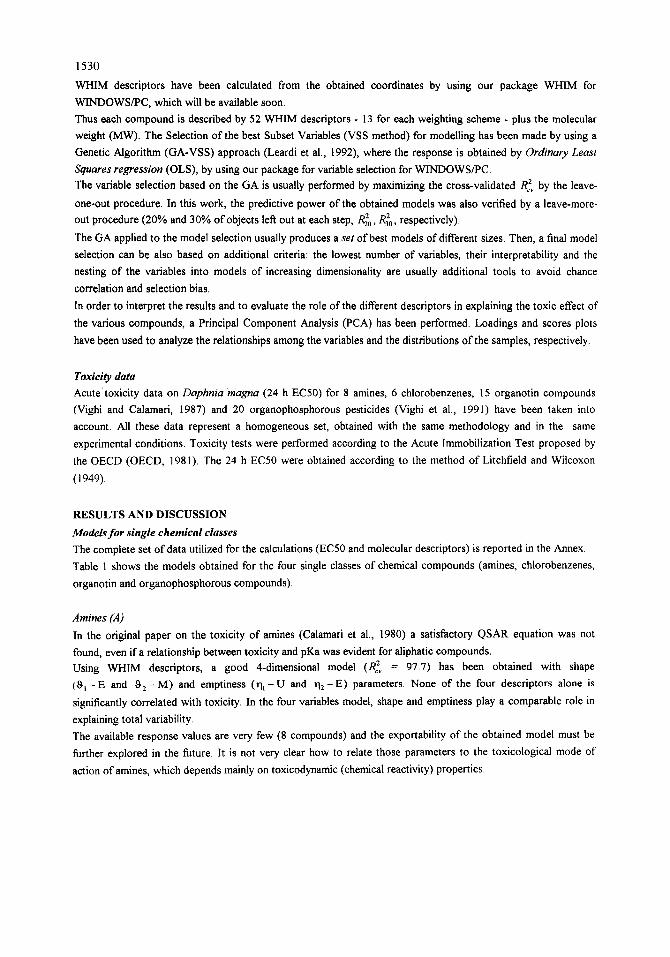
Figure I shows the relationship between experimental and calculated values obtained with the 7-variable model.

From the figure the good predictive capability o f the model is evident. In a set o f extremely heterogeneous

compounds, with toxicity values ranging over about 8 logarithmic orders o f magnitude, 36 out o f 49 compounds

are predicted with an error lower than 1 order o f magnitude and in any case the difference between experimental

and calculated values doesn't exceed 2 orders o f magnitude, without any evident outlier.

In particular, for the different classes o f compounds, the following comments can be made.

Amines All amines show low toxicity values, with a variability within 1 order o f magnitude (observed log I/ECS0 between

-0.35 and 0.6). The model shows a good predictive capability for the position o f this class o f chemicals in relation

to the complete set o f compounds (external variability) but gives a poor explanation o f the variability within the

class (internal variability). The highest differences between predicted and observed values (overestimated for more

than 1.5 logaritmic units) are shown by tert-buthyl and diisopropylamine.

Chlorobenzenes Toxicity ofchlorobenzenes ranges from relatively low to very high values (observed log 1/EC50 between 1.4 and

1534

- 8 '~ ~ amines• E ........ [ ] .......... ...... E ....... /[~ /..." chlorobenzenes

~' 6 ................. , ...-~ .... [] ............... . ...... * organo~n

otganophosphate$ o ........... . ............. .......

4

~ 2 ........... * .....

...... i . ........... . +.... '

0 "J m* .,-' ........ .. "'"" I I

0 2 4 6 8 observed log 1/E050 mmol/I

Figure 1. Comparison between observed toxicity values for the 49 studied compounds and calculated with the 7-variable model. Solid line indicates the theoretical perfect fitting; dotted lines

indicate a difference between observed and calculated of 1 and 2 logarithmic units, respectively.

3.7). The external variability of these compounds is well described by the model; internal variability, relatively

well. The relationship between experimental and calculated toxicity within the class shows an R 2 value of 0.59 and

the internal variability is mainly explained by dimensional parameters and in particular by MW. As previously

mentioned, this is due to the dependence of toxicity on lipophilicity. Negligible or no role is played by symmetry

and emptiness descriptors included in the model.

The maximum difference beween experimental and calculated toxicity is shown by 1,2,4 trichlorobenzene,

overestimated by more than 1.5 logarithmic units. This is due, at least in part, to the higher r values, in

comparison with the 1,2,3 isomer, in contrast with the lower experimental toxicity.

Organotin compounds Toxicity of organotin compounds ranges over more than 4 orders of magnitude (observed log 1/EC50 between

0.27 and 4.6). The model shows a good predictive capability, both for external and internal variability of this class

of chemicals. The relationship between experimental and calculated toxicity shows an R2=0.82 and only one

compound (buthyl SnC12) exceeds the difference of one logarithmic unit between experimental and calculated

figure.

As mentioned before, from a toxicological point view this is a relatively complex group of compounds including

substances with high biological activity utilised as biocides (triorganotin) and substances with low, probably

aspecific toxicity. Therefore all the variables of the model play a significant role in explaining the variability of the

whole group. On the contrary the variability within subclasses can be significantly explained by a reduced numbers of

parameters. For triorganotin compounds in particular, the major role is played by dimensional ( r and MW) and

emptiness parameters, whereas symmetry descriptors have a negligible influence.

1535

Organophosphorous compounds For these compounds the toxic effect ranges over more than 3.5 orders of magnitude (observed log 1/EC50

between 3.3 and 6.9).

The general model has an acceptable predictive capability for the external variability. Only three compounds

(dichlorvos, tetrachlorvinphos and chlorpyriphos methyl) exceed a difference of 1.5 logarithmic unit between

experimental and calculated toxicity. On the contrary, the internal variability is poorly explained. The relationship

between observed and calculated toxicity values within this chemical group shows an R 2 = 0.24.

Apparently, all seven variables of the model make a significant contribution to the predictive capability. All

attempts to divide the class in more homogeneous subclasses with simpler behaviour resulted unsuccessful. The

grouping obtained by applying hierarchical cluster analysis seems to be independent of the main chemical features.

Principal Component Analysis To attempt an interpretation of the results of the model and of the meaning of WHIM descriptors in explaining the

toxic effect, the data have also been analyzed by means of Principal Component Analysis. Thus the Principal

Component Analysis has been performed on the whole data set (49 compounds and 53 variables). The first 6

factors explain about 80% of the total variability. In order to obtain better interpretability, a row varimax rotation

of the first 6 factors has been successively performed and their interpretation is shown in table 3.

Figures 2, 3 and 4 show the trend of toxicity values and the distribution of chemicals in terms of their factor

scores relatively to factors 1, 2, 3, and 5.

As a general trend, toxicity seems to increase with the increase of the dimension of the molecule (high score

values of Factor 1), at least in the dimensional range of the chemicals studied. In correspondence to relatively low

dimensions, toxicity is independent from molecular linearity (Factor 2), increases with emptiness (high score

values of Factor 3 and confirmed also for Factors 4 and 6, not reported here) and decreases with symmetry (low

score values of Factor 5).

Amines and chlorobenzenes are in a region of space where emptiness and symmetry have a low influence on

toxicity. On the contrary, these two factors play a higher role for organotin (in particular tri and tetrasubstituted)

and for organophosphorous compounds. In this last group the most toxic compounds (log 1/EC50 > 6) are in the

part of the plane corresponding to relatively high emptiness. A possible hypothesis to explain the role of emptiness

could be related to the specific mode of action of these compounds, which are enzymatic inhibitors. Higher

emptiness values could indicate a higher accessibility of the active part of the molecule for the reaction with the

enzyme. This kind of molecular descriptors plays a minor role for aspecific toxic compounds, such as amines and

chlorobenzenes.

TABLE 3 - Interpretation of the toxicity effect in terms of the first 6 factors of the Principal Component Analysis.

Factor Explained variance %

32.5

2 21.5

3 10.2

4 7 .4

5 4.2

6 3.5

meanin 8 / variables

size

: linearity

emptiness on 3 rd axis

emptiness on 2 rd axis

simmetry on 2 nd axis

emptiness on 1 st axis

toxicity

increase with size

low dependence from linearity

increase with accessibility

increase with accessibility

decrease with symmetry

increase with accessibility

1536

Oi

0

im

0

-1

-2

Min A

-3 -3 -1.5 0 1.5 3 4.5

Factor I Figure 2. Toxicity contour plot. Lines are the isoresponse curves of log 1/EC50 obtained from factors 1 (size) and

2 (linearity) as independent variables, together with the scores of the 49 studied compounds. A: amines; B: chlorobenzenes; C: organotin; D: organophosphates.

2

1

t ~ I i ,90 o u Ill tL

-1

-2

-3 -3

~,~'~N~] I l_ / / ~ ~ ~ ~ % Min

}t)Y))/DIJ . ,

-1.5 0 1.5 3 4.5

Factor I Figure 3. Toxicity contour plot. Lines are the isoresponse curves of log I/EC50 obtained from factors 1 (size)

and 3 (emptiness) as independent variables, together with the scores of the 49 studied compounds. A: amines; B: chlorobenzenes; C: organotin; D: organophosphates.

1537

1

0

-2

-3 -3 -1.5 0 1.5 3 4.5

Factor I

Figure 4. Toxicity contour plot. Lines are the isoresponse curves of log 1/EC50 obtained from factors 1 (size) and 5 (symmetry) as independent variables, together with the scores of the 49 studied compounds. A: amines; B:

chlorobenzenes; C: organotin; D: organophosphates.

External validation o f the model

In order to perform an external validation of the model, toxicity data for 11 compounds, extremely different in

chemical structure and toxicological properties, have been selected from the literature. Selected figures, ranging

over about 6 orders of magnitude, are comparable with those utilized for the calculation of the model (24 h EC50

obtained with the same test method).

For the toxicity prediction the five obtained general models have been used. To have a better control about the

reliability of the predicted values, the leverage h (Atkinson, 1985) of each external compound, which can be

interpreted as the influence of the object into the model, has been also calculated by the following:

h = x, (XTX) ' ' x, T (4)

where x e is the vector of the descriptors of the external compound and X and X T are the model matrix and the

transpose model matrix, respectively, built from the training set descriptor values. The warning leverage is

calculated by:

h ' = 3 . h = 3 . Z ' h ' ( i = 1, n) n

(5)

where the hii are the leverage values obtained from the hat matrix 1t, calculated by the following:

H = X.(XTX) ~ .X r (6)

1538

A calculated leverage for an external compound greater than the warning leverage indicates that this compound is

not represented by the training set compounds, i.e. the predicted value is extrapolated from the model and the

obtained value must be carefully used (because less reliable). On the contrary, a leverage value lower than the

warning leverage indicates that the compound is represented in the experimental space, i.e. the predicted value is

calculated inside the model (and it is more reliable).

The results of the comparison between predicted and observed values were calculated for all five models. In

Table 4 the leverage values referred to the five models are shown. Cypermethrin is out of warning leverage for

all models, while in the case of endrin and lindane only the 3-dimensional model gives an acceptable leverage

value. In Table 5 the minimum and maximum values obtained from all the models are shown, taking into account

only the models whose leverage is lower than the warning value and in Fig. 5, the calculated ranges of toxicities

are shown together with the experimental values. Picloram and, in minor extent, pentachlorophenol and lindane

appear higly overestimated, while for other compounds an acceptable predictive capability was obtained. The

reason for the behaviour of the outliers is not easy to explain. It could be noted that all the three substances are

highly chlorinated cyclic compounds, showing some possible structural similarity with the more toxic

hexachlorobenzene (included in the original set) and some effective differences not enough described by the

obtained models.

n-OctanolAvater partition coefficients (log Ko~) The same approach has been applied for the prediction of the n-octanol/water partition coefficients (log Kow) In

tables 1 and 2, models to calculate log Kow, that is able in many cases to explain a significant component of the

toxic effect, are also shown

In all the cases, a good predictive capability has been obtained with low-dimensional models, using mainly size

variables: R~v = 97.4, R~ = 99.9, R~v = 95.7, and R~v = 89 1, for amines, chlorobenzenes, organotin compounds,

and organophosphorous compounds, respectively.

In particular, for chlorobenzenes this result has been obtained using only ~ - U descriptor, a result which is also

justified by the small number and congenericity of the considered class.

For the general model an acceptable result was also obtained (R)v = 84.2), with the contribution of different kinds

of variables.

TABLE 4 - Leverage values of the compounds used for external validation of the five models. Figures out of the warning values are in bold.

1 2 3 4 5 6 7 8 9 10 11

Warning leverage .245 .306 .367 .429 .490 Formaldeyde .131 .129 .148 .226 .240 Picloram .094 .075 .132 .127 .187 Benzene .109 .101 .128 .200 .223 2,4-dichlorophenol .086 .064 .112 .124 .176

! Pentachlorophenol .099 .109 .146 .153 .194 Lindane .114 .345 .348 .558 .724 3,4-dichloroaniline .082 .056 .123 127 .198 Endrin .143 .$02 .785 .847 1.09 Disulfoton .086 .175 .182 .309 .317 Azynphos ethyl .153 227 .223 .434 .388 Cypermethrin .483 .683 .685 .792 .777

1539

TABLE 5 - Toxicity prediction for external compounds.Minimum and maximum values obtained with the five models are compared with experimental figures. The range of variability among models and the minimum

difference between predicted and observed values are also reported.

Compound log 1/EC50 References mmoles/l

1 Formaldeyde

2 Picloram

3 Benzene

4 2,4-dichlorophen.

5 Pentachlorophen.

6 Lindane

6 3,4-dichloroanil.

8 Endrin

9 Disulfoton

10 Azynphos ethyl

11 Cypermethrin

Min Max Models Range Min Diff.

-0.3 Jannssen & Persoone, 1993 -1.1 -0.5 3 - 7 0.6 +0.2

0.5 M_ayes & Dill, 1984 3.8 4.5 3 - 7 0.7 +3.3

0.5 Devillers et al., 1987 -0.4 0.2 3 - 7 0.6 -0.3

1.8 Devillers ¢t al., 1987 2.5 3.4 3 - 7 0.9 +0.7

2.5 Devillers ¢t al., 1987 4.4 5.0 3 - 7 0.6 +1.9

2.5 Devillers ¢t al., 1987 4.3 4.3 3 +1.8

2.6 Adema & Vink, 1981 2.0 3.1 3 - 7 1.1 within

3.6 Devillers ¢t al., 1987 3.3 3.3 3 -0.3

4.1 Deviilers ¢t al., 1987 4.4 5.7 3 - 7 1.3 +0.3

5.0 Mayer & Ellersiek, 1986 5.8 7.1 3 - 7 1.3 +0.8

5.3 Stephenson, 1982 none

6

o E E 4

0

0

" - 2 o

i I T - •

I . . I -

I

I i

1

T I I I I , I , I I I , I , I

2 3 4 5 6 7 8 9 10 11 compounds

Figure 5 - Comparison between eperimental toxicity values ( I ) and predicted ranges (bars). Compound numbers are the same of table 4.

CONCLUSIONS

WHIM molecular descriptors have proven to be effective in predicting the toxicity of various classes of

substances that are extremely different in chemical structure and toxicological mode of action.

An excellent predictive capability has been obtained within single chemical classes, in most cases significantly

higher in comparison with QSAR models produced with traditional parameters or descriptors.

Even more interesting is the result obtained with the general model, showing an acceptable predictive QSAR

equation for highly heterogeneous compounds. The external validation confirms, at least in part, the promising

1540

results. Nevertheless, the high leverage values obtained in some cases and the outlier behaviour of some

chlorinated compounds indicate the need for further investigation on a wider set of compounds.

Even if the suitability of these new tridimensional indices for the description of several molecular properties, such

as total surface area, log P, boiling and melting points, and other hiosensors, has been successfully tested

(Todeschini et al., 1994; Todeschini et al., 1995 a; Todeschini et al., 1995 b), the potentiality of this approach has

not yet been fully explored and the real information content of the various parameters is not completely known.

Therefore a satisfactory interpretation of the results on the basis of the toxicological mode of action is extremely

difficult. Nevertheless, at least for some simple classes such as chlorobenzenes, an explanation of the obtained

models seems to be possible and in more complex cases, reasonable hypotheses regarding the meaning of some

descriptors can be proposed. For this purpose, the application of multivariate statistical methods, such as the

Principal Component Analysis, can be very helpful. On the other hand, for the interpretation of the QSAR models

obtained, the WHIM indices, describing precise molecular features (dimension, symmetry, shape, etc.) on a

tridimensional space, are clearly advantageous in comparison with other traditional molecular indices. There are

many examples of QSAR models, obtained with molecular connectivity or information content indices, showing

empirically satisfactory results, but extremely difficult to understand from a toxicological point of view. Therefore

the WHIM approach could be explored as a possible tool for the study of the relationships between structural

molecular features and biological activity. Finally, the suitability of this approach must be evaluated for practical applications in the preliminary

environmental hazard evaluation of unknown chemical substances.

The possibility of applying the model to a range of substances that are highly different in chemical structure and

toxicological mode of action has been proven and externally validated. Moreover the evaluation of leverage values

gives important warning information in order to avoid the mistake of using the model out of the range of

applicability.

The level of predictive capability attained (with differences between observed and predicted results lower than 1

order of magnitude for the majority of compounds, and in any case lower than 2 orders of magnitude, in a

toxicity range of about 8 orders of magnitude) can not produce precise results but can be taken as acceptable at

least for preliminary screening for completely unknown substances. Therefore, the WHIM approach can be

proposed as a useful tool of general applicability for predicting preliminary hazard ranking and for the

formulation of priority lists for potentially dangerous chemicals.

REFERENCES

Atkinson, A.C (1985). Plots, Transformations, and Regression. Clarendon Press, Oxford.

Calamari, D., Da Gasso, R., Galassi, S., Provini, A., and Vighi, M. (1980). Biodegradation and toxicity of selected amines on aquatic organisms. Chemosphere 9, 753-762.

Calamari, D., Galassi, S., Setti, F., and Vighi, M. (1983). Toxicity of selected chlorobenzenes to aquatic organisms. Chemosphere 12, 253-262.

Calamari, D. and Vighi, M. (1990). Quantitative Structure-Activity Relationships in ecotoxicology: value and limitations. Reviews in Environmental Toxicology 4, 1-91

CSTE/EEC (1994). EEC Water Quality Objectives for chemicals dangerous to aquatic environments. Rev. Environ. Contam. Toxicol. 137, 83-110.

Devillers, J., Zakarya, D., Chambon, P., and Chastrette, M., (1987). Utilization des descripteurs moleculaires d'autocorr~lation dans les ~tudes quantitatives du type structure-6cotoxicitr, C.R. Acad. Sc. Paris 304,195

1541

Hansch, C. (1962). A quantitative approach to biochemical structure-activity relationships. Accounts Chem. Res. 2, 232-237.

Hermens, J. (1989). Quantitative structure-activity relationships on environmental pollutants. In: Handbook of environmental chemistry Vol 2E (O. Hutzinger, Ed.). Springer Verlag, Berlin, pp. 111-162

HyperChem - rel.3for Windows (1993). Autodesk, Inc., Sausalito, CA.

Kamlet, M.J., Doherty, R.M, Veith, G.D., Tatt, R.W., and Abraham, M.H. (1986). Solubility properties in polymers and biological media. 7. An analysis of toxicants properties that influence inhibition of bioluminescence in Photobacterium phosphoreum (the Microtox test). Environ. Sci. Technol. 20, 690-696.

Kamlet, M.J., Doherty, R.M., Taft R.W., Abraham, M.H., Veith, G.D., and Abraham, D.J. (1987). Solubility properties in polymers and biological media. 8. An analysis of the factors that influence toxicities of organic nonelectrolytes to the golden arfe fish (Leuciscus idus melanotus). Environ. Sci. Technol. 21, 149-154.

Klein, A.W., Klein, W., Kordel, W., and Weiss, M. (1988). Structure-Activity Relationships for selecting and setting priorities for existing chemicals - A computer assisted approach. Environ Toxicol. Chem. 7, 455-468.

Lange A.W. (1991). The Experience of a National Competent Authority in Hazard Assessment from the Data Provided by Industry and Its Relates to Ecotoxicology. In, Registering New Chemicals in Europe (P.L. Chambers and C.M. Chambers, Eds.). JAPAGA, Ashford, Ireland.

Leardi, R., Boggia, R., and Terrile, M. (1992). Genetic algorithms as a strategy for feature selection, Journal of Chemometrics 6, 267-281.

Litchfield, J. T. and Wilcoxon, F. (1949). A simplified method of evaluating dose-effect experiments. J. Pharmacol. Exp. Theor. 96, 99-118.

OECD (1981). OECD Guidelines for Testing of Chemicals. OECD, Paris

OECD (1986). Produits Chimiques Existants. OECD, Paris

Rekker, R.F. (1985). The principles of congenericity, a frequently overlooked prerequisite in quantitative structure-activity relationships studies. In, QSAR m toxicology and xenobiochemistry, Elsevier, London, pp. 3- 18

Slooff, W. (1992). RIVM Guidance Document no. 719102018 of March 1992 by W. Slooff, National Institute of Public Health and Environmental Protection, Bilthoven, NL.

Todeschini, R., Lasagni, M. and Marengo, E. (1994). New Molecular Descriptors for 2D and 3D Structures. Theory. J. Chemometrics 8, 263-272.

Todeschini, R., Gramatica, P., Provenzani, R., and Marengo, E. (1995). Weighted Holistic Invariant Molecular descriptors. Part 2. Theory development and application on modeling physico-cbemical properties of PolyAromatic Hydrocarbons. Chemometrics and Intelligent Laboratory Systems, 27, 221-229..

Todeschini, R., Gramatica, P. and Provenzani, R. (1995 b). Weighted Holistic Invariant Molecular (WHIM) descriptors. Part 3. Aquatic toxicity of chlorophenols and chlorobenzenes: structure-activity and structure property relationships. Chemometrics and Intelligent Laboratory Systems, in progress.

US.EPA (1987) United States/Environmental Protection AQgency: U.S. Federal Register, 50:30784

Vighi, M., Calamari, D. (1985). QSARs for organotin compounds on Daphnia magna. Chemosphere 14, 1925- 1932.

Vighi, M. and Calamari, D. (1987). A triparametric equation to describe QSARs for heterogeneous chemical substances. Chemosphere 16, 1043-1051.

Vighi M., Masoero Garlanda, M., and Calamari, D. (1991). QSARs for toxicity of organophosphorous pesticides to Daphnia and honeybees. Sci. Tot." Environ. 109/110, 605-622.

1542

ANNEX. To3dcity data (log I/EC50). log Kow and WHIM molecular descriptom for the examined compounds

loll I/ECSO Io~ Kow 21U Z2U Z3U 3IU ,9"2U TIU y2U y~J rllU Amlnei

1 dimethylarnine .0.02 2 diethylamine -0.35 3 diisopropylamine -0.27 4 di-n-butylamine 0.10 5 tert-butylarnine .0.27 6 aniline 0.60 7 cydohe~lamine 0.24 8 morpholine -0.13

Chlorobenzenel 9 monochlombenzene 1.40 10 1.2 dichlorobenzene 2.30 11 1,4 dichlorobenzene 1,96 12 1,2,3 trichlorobenzene 2.73 13 1,2,4 trichlorobenzene 2.15 14 hexachlorobenzene 3.70

Organotln comp, 15 methyl Sn 0 3 0.27 16 but~ Sn 0 3 0,76 17 dimethyl Sn Cl2 0.40 18 dlethyl Sn (312 1.80 16 dibutyl Sn 0 2 2.53 20 diphen'/I Sn (312 2,72 21 kimethyl Sn CI 2.62 22 ~ethytSnCl 3.04 23 bipropyl Sn (31 3.88 24 tributyl Sn CI 4.40 25 bis (tTibutyl)SnO 4.61 26 tdpheny~ Sn CI 4.30 27 tetramethyl Sn 0.65 28 tetrapmpylSn 2.39 29 tebabutylSn 2.37

Organophosph=te= 30 dichlorv~ 5.98 31 monocrotophco 4.20 32 dicmtophos 4~20 33 tet]'achlo(vinphos 5.12 34 chlorfenvinphos 5.70 35 pho6phamidon 4.18 36 parathion-methyl 4.82 37 parathion~yl 5.12 38 fenibothion 6.19 39 chlorpyripho~-methyl 6.81 40 chloq0yriphos~thy( 6.24 41 diazinon 5.37 42 pidmiphos-methyl 6.05 43 iodofenfos 6.44 44 fenthion 464 45 malathion 4.62 46 phorate 4.64 47 dimethoa~ 3,16 48 terbufos 5.20 49 thchlorfon 6.01

I=xtemal compounds 5o formak~hyde 51 pidoram 52 benzene 53 2.4-dichloropbenoi 54 lindane ,55 pe~acf~ompt~,n~ 56 3.4-dichlcxoaniline 57 ec~ldn 58 disulfoton 59 azinphos ethyl 60 cyperme~dn

-0,30 1.78 0.57 0,33 0.66 0.21 0.00 3.32 1.85 0.62 0.50 3.85 0.67 0.43 0.78 0.14 3.75 3.28 2.27 0.59 1.73 3,42 1.24 0.62 0.65 0.24 3.17 1.30 4.24 0.63 2.00 10.52 1.25 0.53 0.86 0.10 395 1.22 0.11 0.58 0.40 1.40 1.39 1.01 0.37 0.37 0.00 3.25 2.50 0.49 0.90 2.06 1.64 0.00 0.56 0.44 0.00 3.46 0.00 0,56 0.79 1.97 1.62 0,90 0.44 0.36 1.70 0.85 2.20 0.50 -0.60 190 1,43 0.45 0.50 0.38 0.00 3.37 2.61 062

2.81 2.33 2.05 0.00 0.53 0.47 3.19 0.00 0.00 0.44 3.53 2.46 2.23 0.00 0.52 0,48 3.58 0.00 0.00 0.48 3.53 2.62 2.06 0,00 0.56 0.44 0.00 0.00 0.00 0.40 4.20 2.82 2.47 0.00 0.51 0.49 0.00 2.54 0.00 0.46 4.20 2.72 2.27 0.00 055 0.45 3,58 3.58 0.00 0.43 6.44 2.97 2.97 0.00 0.50 0.50 0.00 0.00 0.00 046

-3.10 2.39 1.16 1.16 0.51 0.25 3.00 2.00 0.42 0.91 0.38 5.61 1.12 0.83 0.74 0.15 4.09 3.97 0.00 0.48 -3.10 2.94 1.42 1.00 0.55 0.26 0.00 3.48 0.00 0.61 -I.40 3.79 1.70 1.14 0.87 0.26 0.00 2.93 0.00 0.65 1.49 10,18 2.14 1.00 0.76 0.16 4.03 2.65 3.35 0.60 1.90 11.09 2.75 0.30 0.78 0.19 0.00 4.45 0.00 0.59

-2.30 2.46 2.46 1.03 0.41 0.41 2.43 0.19 1.77 053 -I.80 3.87 2.60 1.42 0.49 0.33 4.04 4.18 3.48 0.50 0.93 6.14 4.23 1.41 0,82 0.36 3,65 4.23 3.50 0.46 2,60 9.37 5.00 1.45 0.59 0.32 4.59 3.54 2.60 0.43 2.29 11.67 7.20 5.70 0.47 0.29 3.04 3.78 2.04 0.50 2.65 7.17 6.89 1.87 0.45 0.43 4.15 4.27 3.30 0.46 -2.19 2.14 2.14 2.14 0.33 0.33 2.69 2.69 3.16 0.54 2.04 6.13 4.21 2.49 0.48 0.33 4.18 3.40 3.40 0.39 3.90 7.66 5.93 3.36 0.45 0.35 5.54 3.66 3.77 0.35

1.25 3.71 2.18 1.23 0.52 0.31 4.17 0.00 3.77 0.40 0.15 8.12 1.67 1.39 0.73 0.15 4.25 2.35 2.90 0.57 0.35 7.87 1.52 1.46 0.73 0.14 3.72 2.87 3.07 0.59 4.18 8.13 3.67 0.67 0.65 0.29 4.25 4.81 2.54 0.55 4.17 10.61 5.06 0.60 0.65 0.31 4.25 2.56 1.24 0.52 1.40 8.80 1.95 1.83 0.70 0.16 4.45 2.89 3.23 0.64 2.81 7.11 1.82 1.56 0.68 0.17 4.25 3.78 0.00 0.56 3.51 7.33 2.85 1.73 0.62 0.24 4.25 2.63 2.65 0.49 3.47 8.04 1.99 1.46 0.70 0.17 4.16 2.27 0.00 0.66 4.05 4.86 1.83 1.76 0.57 0.22 3.57 4.37 2.71 0.51 4.75 5.87 3.13 1.44 0.56 0.30 4.32 2.87 3.21 0.42 3.51 9.33 2.70 2.28 0.65 0.19 4.68 3.49 3.62 0.51 2.34 7.25 4.05 1.50 0.57 0.32 3.91 3.92 1,63 0.55 5,37 5.89 2.04 1.70 0.61 0.21 4.39 3.58 0.00 0.51 4.36 9.58 2,30 1.42 0.72 0,17 4.03 3,06 0.00 0.48 2.57 7,05 5.08 1.82 0,54 034 4.24 3.12 2,65 0,40 0.34 8.61 3.13 1.18 0.67 0.24 4.75 4.25 3.47 0.46 -0.47 7.06 1.72 t.05 0.74 0.16 4.10 0.00 3.94 0.57 1.16 8.85 3.00 1.27 0.67 0.23 4.25 3.69 2.01 0.62 1.11 4.31 2.06 1.15 0.57 0.27 2.17 2.91 2.46 0.57

0.53 0.46 0,00 0.53 0.47 1.50 0.00 0.0O 0.49 4.74 2.48 0.00 0.66 0.34 3.27 3.03 0.00 0.50 2.05 2.05 0.00 0.50 0.50 O.OO 0.00 0.00 0.52 3.11 2.13 0.00 0.59 0.41 3.70 1.85 0.00 0.44 2.25 2.21 1.00 0.41 0.40 0.00 2.84 2.58 0.46 3.41 2.70 0.00 0.56 0.44 3.55 3.09 0.00 0.49 3.42 2.08 0,00 0.62 0.38 3.66 3.81 0.00 0.48 4.19 1.69 1.69 0.55 0.22 1.88 0.85 3.35 0.56 12.01 2.31 1.63 0.75 0.15 5.04 4.80 4.98 0.53 16.05 3.48 0.88 0.79 0.17 5.16 4.99 4.79 0.59 18.21 2.23 1.74 0.62 0.10 5.31 5.38 5.55 0.50

ANNEX. Com~nued (2)

1543

:,,]a f~:" ;,ir,r e , l , , v ~ = j , ~ .,I;,~, ~ l , T ~ - I h ~ "le,~ - - :-"Y," m 't {et~ Ir'Fl~ ~e~v, ~,1' I,,]i

1 0.38 0.36 1.10 0.24 0.09 0.77 O. 17 0.00 3.32 2.46 0.56 0.39 O. I I 1.54 0.39 2 0.59 0.45 2.88 0.28 0.10 0.89 0.08 3.38 2.50 0.09 0.57 0.39 0.12 3.49 0.46 3 0.53 0.47 2.60 0.71 0.22 0.74 0.20 2.50 2.27 2.50 0,67 0.47 0.25 3.08 0.96 4 0.49 0.35 8.90 0.71 0,16 0.91 0.07 4.25 1.92 0.61 0.56 0.45 0.13 9.91 0.96 5 0.60 0.44 0.79 0.78 0.71 0.34 0.34 0.00 3.25 3.75 0.38 0.51 0.40 1.12 1.10 6 0.58 0.52 1.08 1.01 0,00 0.52 0.48 2.73 0.00 0.00 0.59 0.51 0.44 1.45 1.23 7 0.47 0.46 1.52 1.05 0.41 0.51 0.35 3.53 0.29 4.22 0.53 0.48 0.37 1.65 1.35 8 0.68 0.48 1.13 1.03 0.13 0.49 0.45 0.35 0,00 0.16 0.66 0.53 0,12 1.57 1.15

9 0.52 0.00 2.88 0.79 0.00 0.78 0.22 2.92 0.00 0.00 0.82 0.37 0.00 2.22 1.35 I0 0,57 0.00 2.41 1.86 0.00 0.56 0.44 2.82 0.00 0,00 0.58 0.75 0.00 2.33 1.72 11 0.52 0.00 5.22 0.61 0.00 0.90 O.lO 0.00 0.00 0.00 0.59 0.28 0.00 3.01 1.24 12 0.47 0.00 3.40 1.88 0.00 0.84 0.36 0.00 3.58 0.00 0.50 0.40 0.00 2.43 2.12 13 0.54 0.00 4.72 1.56 0.00 0,75 0.25 3.58 3.42 0.00 0.56 0.51 0.00 3,04 1.67 14 0.46 0,00 3.95 3.95 0,00 0,50 0,50 0.00 0,00 0,00 0.58 0,58 0,00 3.00 3.00

15 0,35 0.35 1.14 1.14 0.55 0.40 0.40 2.00 0.31 3.00 0.30 0.30 0.13 1.68 1.20 16 0.82 0.34 3.52 0.99 0.92 0.65 0.19 4.09 0.00 2.92 0.22. 0.26 0.44 6.05 0.99 17 0.43 0.34 1.26 0.79 0.45 0.51 0,32 0.00 3.46 0.00 0.33 0.41 0.12 1.76 1.40 18 0.34 0.53 1.44 1.36 0.87 0.42 0.39 0.00 3.85 0.00 0.42 0.39 0,30 2.74 1,94 19 0.31 0.29 3.93 2.17 0.87 0.56 0.31 4.79 4.58 2.86 0.28 0.38 0.22 8.23 2,31 20 0.51 0,08 4.84 2.12 0.78 0.63 0.27 0.00 2.55 0.00 0.33 0,44 0.21 8.95 2.38 21 0.53 0.17 1.12 0.51 0,51 0.52 0.24 3.24 2.69 2.43 0.29 0.14 0.14 1.66 1.88 22 0.50 0.29 2.38 1.03 0.65 0.59 0.25 4.44 3.82 3.28 0.44 0.18 0.21 2.97 2.13 23 0.43 0.26 2.65 2.08 1.41 0.43 0.34 3.02 3.02 4.64 0.25 0,22 0.36 5,05 3.45 24 0.40 0.31 4.64 3.03 1.45 0.51 0.33 3.93 3.53 2.98 0.24 0,20 0.43 8,02 4.36 25 0.56 0.57 7.40 4.02 3.20 0.51 0.26 4.03 2.46 3.20 0.38 0.33 0.35 10.57 6.37 26 0.46 0.39 3.89 3.75 1.66 0.42 0.40 3.16 3.89 3,75 0.31 0.30 0.30 6.04 5.82 27 0.54 0.64 0.58 0.58 0.58 0.33 0.33 3.14 3,16 3.18 0.15 0.18 0.17 1.58 1.58 28 0.38 0.43 3.19 2.16 1.20 0.49 0.33 4.94 4.55 2.94 0.25 0.23 0.26 5.25 3.60 29 0.35 0.39 4.58 3.43 1.84 0.46 0.35 4.60 3.18 3.18 0.24 0.22 0.28 6.81 5,19

30 0.41 0.31 5.29 1.32 0.79 0.72 0.18 4.17 3.52 0.00 0.77 0.53 0.23 4.52 1,54 31 0.45 0.51 7.13 1.13 0,81 0.79 0.12 4.43 3.27 2.75 0.57 0.45 0.24 7.47 1.38 32 036 0.38 7.10 1.17 0.79 0.78 0.13 4.18 3.73 2.55 0.83 0.52 0.31 7.26 1.30 33 0.52 0,31 8.76 3.33 0.34 0.70 0.27 4.39 3.93 0.96 0.59 0.42 0.13 7.93 3.23 34 0.48 0.27 9.84 3.86 0.48 0,69 0.27 4.60 3.67 1.78 0.54 0.44 0.27 10.45 4.29 35 0.46 0.50 6.17 1.75 0.98 0.69 0.20 4.18 3.05 2.03 0.67 0.40 0.31 7.60 1.80 36 0.44 0,28 8.53 1.13 0.72 0.82 0.11 4.52 3.78 0.00 0.59 0,48 0.20 6.64 1.47 37 0.38 0.39 8.42 1.39 1.34 0.76 0.13 4.36 2.36 3.01 0.55 0.23 0.40 7.01 2.25 38 0.44 0.27 8.62 1.35 0.69 0,81 0.13 4,35 3.02 0.00 0.64 0.46 0.19 7.22 1.64 39 0.46 0.52 6.06 2.12 0.58 0.69 0.24 4.10 2.96 0.41 0.53 0.42 0.16 5.18 1.88 40 0.41 0.38 7.42 1.50 .1.14 0.74 0.15 4.58 4.32 3.17 0.62 0.59 0.19 6.58 2.23 41 0.41 0.31 8.88 1.86 1.47 0.67 0.18 5.16 3.03 3.18 0.52 0.34 0.28 8.32 2,18 42 0.55 0.32 6.12 2.65 0.77 0,64 0.28 5.03 3.64 3.24 0.60 0.44 0.21 6.39 3.62 43 0.36 0.31 9.30 2.17 0.45 0.78 0.18 4.25 3.58 0.00 0.64 0.30 0.13 6.48 2.22 44 0.40 0.28 9.06 1.33 0.70 0.82 0.12 4.64 2.73 0.00 0.55 0.38 0.20 8.51 1.88 45 0.46 0.37 4.90 4.01 1.23 0.48 0.40 3.71 3.42 2.97 0,32 0.51 0.33 7,01 4.56 46 0.42 0.29 6.14 1.68 1.15 0.68 0.19 4.75 3.13 3.14 0.43 0.28 0.31 7.93 2.65 47 0.35 0.29 5.82 0.94 0.88 0.76 0.12 3.94 3.77 0.00 0.49 0.38 0.27 7,26 1.38 48 0.43 0.34 6.84 1,68 1.21 0.70 0.17 4.26 3.83 3.08 0.58 0.27 0.34 8,25 2.52 49 047 0.42 3.85 1.34 0.99 0.62 0,22 3.92 2.66 3.11 0.58 0,47 0.48 4,38 1.65

50 0.50 0.00 0.43 0.06 0,00 0.88 0.12 1.50 0.00 0.00 0.74 0.07 0.00 0,43 0.26 51 0.39 0.34 4.79 2.62 0.00 0,64 0.35 3.45 3.70 0.00 0,64 0.61 0.21 3.83 2.36 52 0.52 0.00 1.14 1.14 0.00 0.50 0.50 0.00 0.00 0.00 0.53 0.53 0.00 1.47 1.47 53 0.44 0.00 4.27 1.45 0.00 0,75 0.25 3.70 3.55 0.00 1.03 0.15 0.00 2.84 1.71 54 0.47 0.32 2.89 2.67 1.41 0.41 0.38 0.00 3.91 2,58 0.48 0.56 0.33 2.31 2.21 55 0.42 0.00 4.16 3.39 0.00 0.55 0.45 2.50 3.70 0.00 1.01 0.43 0.00 3.04 2.80 56 0.48 0,00 3.46 1.74 0.00 0.68 0.34 3.86 3.81 0.00 0.23 0.33 0.00 3.09 1.68 57 0.38 0.44 4.11 2.35 2.07 0.48 0.28 4.32 0,00 4.03 0.39 0.40 0.48 4.09 1.89 58 0.38 0.35 8.82 1.72 1.11 0.76 O. 15 5.04 4.90 4.57 0,22 O. 16 0.96 10.84 1.94 59 0.46 0.17 12.20 1.91 1.08 0.80 0.13 5.21 4.99 4.99 0.36 0.12 0.09 15,00 2.84 60 0.43 0.44 19.39 1.91 1.40 0.85 0.84 5.55 5.22 4.95 0.47 0.28 0.21 18.28 1.92

1544

ANNEX. Co¢~nued (31

1 0.22 0.72 0.18 0.00 3.32 2,46 0.62 0.30 0.24 1.74 0.56 0.32 0.66 0.21 0.00 2 0.26 0.83 0.11 3.75 2.22 0.17 0.60 0.48 0~30 3.79 0.66 0.42 0.78 0.14 3.75 3 0.40 0.69 0.22 2,75 1.80 3.57 0.66 0.49 0.34 3.38 1.22 0.61 0.65 0.23 3.17 4 0.33 0.88 O.Og 3.95 3.45 0.17 0,58 0.46 0.23 10.42 1.23 0.52 0.86 0.10 3.95 5 0.78 0.37 0.37 O,O0 3.25 1.92 0.44 0.50 0.33 1.37 1.36 1.02 0.37 0.36 O.O0 6 O.O0 054 0.46 0.00 3.46 0.00 051 0.54 0.44 1.99 1.63 0.00 0.55 0.45 0,00 7 0.61 0.46 0.37 3.55 0.14 1.70 0.50 0.47 0.34 197 1,60 0.89 0.44 0.36 2.44 8 0.28 0.52 0.38 0.00 3.59 2.00 0.62 0.61 0,27 1.81 1.43 0.43 0.49 0.39 O.O0

9 0.00 0.62 0.38 2.29 0.00 0.00 0.42 0.44 O.O0 2.48 1.97 0.00 0.56 0.44 3.58 IO O,O0 0.57 0.43 3.58 O.O0 O.OO 0.53 0.58 0,00 2.62 2.21 0.00 0.54 0.46 3.58 11 O.O0 0.71 0.29 0.00 O.OO 0.00 0.40 0.41 0.00 2.95 1.92 0.00 0.61 0,39 O.OO 12 0.00 0.53 0.47 O.OO 3,58 0.00 0.42 0.45 O.O0 2.67 2,55 0.00 0.51 0,49 0.00 13 O.O0 0.65 0.35 3.42 2.92 O.O0 0.45 0.48 0.00 3.04 2.22 0.00 0.58 0.42 3.58 14 O.O0 0.50 0.50 0.00 O.O0 0.00 0.46 0.46 O.OO 3.20 3.20 O.O0 0.50 0.50 O.OO

15 1.20 0.41 0.29 3.00 2.00 0.00 0.50 0.33 0.33 2.44 1.33 1.33 0.48 0.26 3.00 16 0.84 0.77 0.13 3.49 3.81 0.00 0.58 0.52 0.26 5.98 1.19 0.92 0.74 0.15 3.81 17 1.14 0.41 0.33 0.00 3.46 0.00 0.41 0.59 0.32 2.80 1.59 1.17 0.50 0.29 Q.O0 18 1.01 0.48 0.34 0.00 4.09 0.00 0.55 0.52 0.44 3.70 1.90 1.21 0.54 0.28 0.00 19 0,89 0.72 0.20 4.32 3.53 1.88 0,52 0.34 0.23 9.99 2,26 1.06 0.75 0.17 4.03 20 0.41 0.76 0.20 0.00 4.64 O.O0 0.55 0.48 0.11 10,81 2.86 0.38 0.77 0.20 O.OO 21 1.20 0,37 0.37 2.43 0,10 3.81 0.40 0.40 0.22 2.41 2.41 1.20 0.40 0.40 2,43 22 1.56 0.45 0.32 4.32 4.02 3.28 0.44 0.39 0.49 3.85 2.60 1.50 0.48 0.33 4.04 23 1.53 0,50 0.34 4.23 4.54 2.63 0.41 0.36 0.28 6.08 4.20 1,52 0.52 0.36 3.81 24 1.47 0,58 0.31 4.38 4.30 2.10 0.39 0.34 0.31 9.31 4.99 1.52 0.59 0.32 4.59 25 4.98 0.48 0.29 3,95 4.12 3,28 0.47 0.51 0.55 11.63 7.18 5.69 0.47 0,29 2.95 26 1.55 0.45 0.43 3.75 4.39 3.90 0.44 0,44 0.30 7.10 6.83 1.94 0.45 0.43 4.15 27 1.58 0.33 0.33 3.16 2.17 2.69 0.37 0.44 0.43 2.14 2.14 2,14 0.33 0,33 2.69 28 2.06 0.48 0.33 4.06 4.18 3.26 0.36 0.35 0.40 6.13 4.21 2.49 0.48 0.33 4.18 29 2.86 0.46 0.35 5.19 3.99 3.64 0.33 0,32 0.36 7.66 5.92 3.35 0.45 0.35 5.54

30 1.18 0,62 0.21 3.52 0,00 2.08 0.60 0.33 0.38 3.90 2.00 1.36 0.54 0.28 4.06 31 1.14 0.75 0.14 4.52 2.92 3.95 0.58 0.46 0.40 8.11 1.65 1.39 0.73 0.15 4.39 32 1.17 0.75 0.13 3.07 3.25 2.76 0.60 0.48 0.37 7.89 1.53 1.45 0.73 0.14 4.18 33 0.47 0.68 0.28 3.45 3,79 2.10 0.58 0.43 0,20 8.22 3.62 0.68 0.66 0.29 4.25 34 0.48 0.69 0.28 3.82 4.85 2.35 0.57 0.44 0.24 10.52 4.93 0.62 0.65 0.31 4.38 35 1.42 0.70 0.17 4.42 1.82 3.06 0.62 0,38 0.38 8.45 1.95 1.78 0.69 0.16 4.03 36 1.14 0.72 0.16 4.10 3.60 0.00 0.57 0,46 0.24 7.58 1,83 1.46 0.70 0.17 4.25 37 1.47 0.65 0.21 4.25 3.33 2.83 0.54 0.33 0.41 7.72 2.67 1.81 0.63 0.22 3.48 38 1.07 0.73 0.17 4.46 2.65 O.OO 0.64 0.46 0.23 8.28 2.06 1.38 0.71 0.18 4.41 39 1.13 063 0.23 4.24 4.10 1.19 0.58 0.46 0.24 5.02 1.90 1.65 0.59 0.22 4.46 40 1.30 065 0.22 4,18 2.84 2.65 0.55 0.33 0.42 6.08 2.89 1.55 0.58 0.28 4.86 41 1.90 0.67 0.17 4.05 3.77 2.42 0.53 0.38 0.33 9.06 2.59 2.35 0.65 0.19 456 42 1.13 0.57 0.33 3,09 3.65 3.11 0.54 0~56 0.26 7.20 3.97 1.45 0.57 0.31 4.43 43 1.05 0.66 0.23 3.58 2.79 O.O0 0.54 0.35 0.22 5,81 2.25 1.59 0.60 0.23 3.75 44 1.02 0.75 0.16 4.03 4.70 O.O0 0.49 O,3g 0.22 9.57 2.30 1.38 0.72 0.17 4.29 45 1.51 0.54 0.35 4.84 4.25 3.12 0.38 0.44 0.33 7.53 4.95 1.80 0.53 0.35 4.48 46 1.09 0.68 0.23 4.52 3.47 2.79 0.48 0.39 0.30 8.32 3.01 1,29 0.66 0.24 4.25 47 0.92 0.76 0.14 4.58 O,O0 3.21 0.57 0.32 0.31 7.72 1.63 1.15 0.74 0.16 4.39 48 1.17 0.69 0.21 4.50 4.25 3.83 0.65 0.40 0.35 8.69 2.91 1.38 0.67 0.22 3.83 49 1.00 0.62 0.23 3.92 2.91 2.66 0.58 0.45 0.39 4.30 1.98 1.20 0.57 0.26 3.12

50 O.OO 0.62 0.38 2.00 O.O0 0.00 0.47 0.28 O.OO 0.59 0.41 0.00 0.59 0.41 2.00 51 0.00 0.62 0.38 4,00 3.75 0.00 0.48 0.44 0.18 4.81 2.59 O.OO 0.65 0.35 3.50 52 O.OO 0.50 0.50 0.00 0.00 0.00 0.48 0.48 O.OO 2.02 2.02 O.OO 0.50 0.50 O.O0 53 O.O0 0.62 0.38 3.70 3.70 O.O0 0.42 0.31 O.OO 3.31 2,12 O.O0 0.61 0.39 3.55 54 1.01 0.42 0.40 O.OO 3.73 3.21 0.44 0.48 0,29 2.36 2.30 1.08 0.41 0.40 O.OO 55 O.O0 0,52 0.48 3.09 3.70 O.O0 0.52 0.36 O.OO 3.54 2.93 0.00 0.55 0.45 3.70 56 O.OO 0.65 0.35 3.66 3.81 O.OO 0.35 0.33 0.00 3.62 2.07 0.00 0.64 0.38 3.81 57 1,56 0.56 0.23 4.18 O.OO 4.75 0.55 0.35 0.39 4.43 1.78 1.75 0.56 0.22 4.18 58 1.63 0.75 0.13 5.04 4.80 4.98 0.41 0.29 0.27 11.81 2.28 1.63 0.75 0.15 4.e8 59 0.99 0.81 0.14 5.16 4.99 4.18 0.55 0.26 0.23 15.58 3.37 0.89 0.79 0.17 5.16 60 1.47 0.64 0.09 5.22 5,38 5.38 0.50 0.28 0.31 18.12 2.24 1.76 0.82 0.10 5.14

ANNEX. Con~ued (4)

1545

y2E y3E JTIE rl2E ~73E mU m~4 voV toe rU rM r V rE

I 3.32 2 3.50 3 1.30 4 1.65 5 3.75 6 3.46 7 0.29 8 3.59

0 0.00 10 0.00 I I 0.00 12 3.58 13 3.42 14 0.00

15 2.00 16 3.40 17 2.65 18 3.49 19 3.21 20 3.50 21 0.10 22 3.85 23 4.23 24 3.66 25 3.79 26 4.27 27 3.14 28 3.40 29 3.66

30 0.00 31 3.79 32 3.41 33 2.67 34 3.51 35 2.35 36 3.42 37 2.61 38 3.02 39 3.75 40 3.02 41 4.04 42 3.23 43 3.39 44 4.03 45 3.42 46 2.95 47 0.00 48 3.83 49 3.71

50 O.OO 51 3.03 52 0.00 53 3.70 54 4.17 55 3.09 56 3.81 57 0.05 58 5.04 59 5.16 60 5.22

1.85 0.60 0.38 0.35 0.54 0.71 0.62 1.17 0.58 0.58 0.44 0.69 0.86 0.77 3.93 0.62 0.53 0.47 0.53 0.67 0.60 -0.05 0.57 0.49 0.34 0.81 0.89 0.85 3.27 0.48 0.60 0.45 0.10 0.03 0.11 0.00 0.55 0.58 0.51 0.56 0.52 0.54 2.44 0.50 0.47 0.46 0.24 0.37 0.29 0.35 0.59 0.66 0.44 0.38 0.44 0.43

O.O0 0.45 0.51 0.00 0.53 0.78 0.62 0.00 0.52 0.58 0.00 0.52 0.56 0.57 0.00 0.42 0.49 0.00 0.56 0.90 0.71 0.00 0.46 0.48 0.00 0.51 0.64 0.53 0.00 0.46 0.53 0.00 0.55 0.75 0.65 0.00 0.48 0.48 0.00 0.50 0.50 0.50

0.31 0.01 0.39 0.39 0.26 0.21 0.12 0.00 0.51 0.64 0.3,5 0.63 0.48 0.66 0.00 0.58 0.51 0.37 0.36 0.33 0.14 O.O0 0.64 0.38 0.5,5 0.40 0.22 0.30 2.65 0.59 0.31 0.29 0.69 0.44 0.64 O.O0 0.58 0.52 0.10 0.76 0.53 0.73 3.81 0.52 0.52 0.20 0.24 0.28 0.10 2.13 0.50 0.50 0.30 0.31 0.43 0.21 3.34 0.46 0.43 0.26 0.40 0.20 0.35 3.53 0.42 0.40 0.30 0.50 0.35 0.47 2.13 0.49 0.56 0.57 0.24 0.29 0.26 4.18 0.46 0.45 0.38 0.33 0.24 0.34 2.69 0.54 0.54 0.64 0.00 O.O0 0.00 3.40 0.39 0.36 0.43 0.28 0.30 0.29 3.77 0.35 0.35 0.39 0.25 0.28 0.27

3.31 0.42 0.38 0.36 0.35 0.61 0.46 3.27 0.58 0.50 0.47 0.60 0.70 0.63 2.41 0.60 0.44 0.39 0.59 0.70 0.63 1.68 0.54 0.51 0.29 0.60 0.68 0.64 1.62 0.51 0.47 0.26 0.61 0.66 0.66 3.06 0.63 0.39 0.45 0.55 0.58 0.57 O.OO 0.56 0.46 0.27 0.53 0.75 0.59 4.20 0.49 0.36 0.42 0.47 0.64 0.52 0.00 0.67 0.48 0.27 0.57 0.74 0.62 2.07 0.46 0.47 0.32 0.37 0.63 0.49 3.02 0.43 0.39 0.41 0.42 0.62 0.52 2.89 0.50 0.41 0.34 0.49 0.53 0.51 2.08 0.56 0.54 0.31 0.45 0.58 0.47 O.OO 0.51 0.38 0.30 0.44 0.74 0.56 0.00 0.48 0.41 0.27 0.61 0.75 0.66 2.02 0.30 0.46 0.37 0.41 0.36 0.42 2.22 0.45 0.41 0.31 0.58 0.56 0.59 2.14 0.56 0.34 0.34 0.64 0.65 0.66 2.09 0.61 0.42 0.35 0.58 0.58 0.59 1.95 0.56 0.48 0.44 0.42 0.46 0.48

O.O0 0.65 0.45 0.00 0.53 0.88 0.62 0.00 0.52 0.41 0.34 0.66 0.65 0.62 0.00 0.52 0.52 0.00 0.50 0.50 0.50 0.00 0.51 0.46 0.00 0.59 0.75 0.62 2.84 0.46 0.48 0.34 0.23 0.21 0.23 0.00 0.52 0.50 0.00 0,56 0.55 0.52 0.00 0.55 0.49 0.00 0.62 0.86 0.65 4.46 0.56 0.37 0.44 0.33 0.24 0.35 4.80 0.60 0.37 0.35 0.65 0.66 0.64 4.56 0.56 0.43 0.16 0.74 0.73 0.75 5.22 0.49 0.42 0.4.5 0.74 0.7g 0.78

0.54 2.68 1.43 2.14 2.62 0.66 4.96 3.24 4.22 4.87 0.53 5.28 3.53 4.46 5.20 0.81 12.31 9.77 11.22 12.18 0.09 3.80 2.26 3.00 3.75 0.55 3.70 2.10 2.68 3.62 0.24 4.50 2.08 3.60 4.45 0.37 3.77 2.30 3.00 3.68

0.56 4.39 3.67 3.56 4.45 0.54 4.69 4.27 4.05 4.84 0.61 4.68 5.83 4.25 4.87 0.51 4.99 5.28 4.55 5.23 0.58 4.99 6.28 4,71 5.26 0.50 5.94 7.89 6.01 6.40

0.22 4.72 2.83 4.08 5.10 0.62 7.57 5.42 7.87 8.10 0.29 5.36 2.50 4.30 5.56 0.37 6.63 3.46 5.69 6.81 0.67 13.32 6.97 11.42 13.31 0.74 14.11 7.73 11.71 14.05 0.20 5.94 2.14 4.51 6.02 0.30 7.90 4.06 6.66 7.65 0.39 11.76 6.14 10.04 11.80 0.49 15.82 9.11 13.86 15.81 0.24 24.58 14.62 21.92 24.49 0.33 15.93 9.30 13.41 15.86 0.00 6.41 1.75 4.73 6.43 0.28 12.83 6.55 10.91 12.82 0.25 16.95 9.85 14.87 16.93

0.35 7.12 7.39 7.24 7.26 0.60 11.18 9.07 9.99 11.16 0.59 10.85 9.05 9.74 10.87 0.60 12.47 12.43 11.64 12.52 0.62 16.27 14.19 15.22 16.06 0.55 12.58 8.90 10.82 12.18 0.56 10.49 10.39 9.25 10.87 0.48 11.92 11.16 10.72 12.19 0.59 11.49 10.87 9.93 11.72 0.39 6.45 8.76 8.19 8.58 0.43 10.44 10.07 10.10 10.52 0.48 14.32 10.19 12.49 14.00 0.46 12.80 9.55 11.15 12.62 0.44 9.63 11.93 9.75 9.65 0,62 13.29 11.09 11.39 13,25 0.40 14.85 10.14 13.07 14.28 0.56 12.92 8.66 11.66 12.82 0.63 10.73 7.64 9.56 10.50 0.57 13.12 9.73 11.94 12.96 0.41 7.52 6.18 7.03 7.49

0.59 0.68 0.49 0.69 1.00 0.65 7.22 7+41 6.19 7.40 0.50 4.10 2.28 2.94 4.04 0.61 5.24 5.72 4.54 5.43 0.22 5.46 6.97 5.53 5.73 0.55 6.11 7.54 5.85 6.47 0.64 5.50 5.20 4.77 5.60 0.34 7.56 8.52 7.33 7.96 0.65 15.95 11.65 14.41 15.72 0.74 20.41 15.18 18.63 19.85 0.74 22.18 22.69 21.67 22.12