University of Calgary

PRISM: University of Calgary's Digital Repository

Graduate Studies The Vault: Electronic Theses and Dissertations

2014-05-26

Modeling and Identification of Joint Dynamics Using a

Frequency-Based Method

Mehrpouya, Majid

Mehrpouya, M. (2014). Modeling and Identification of Joint Dynamics Using a Frequency-Based

Method (Unpublished doctoral thesis). University of Calgary, Calgary, AB.

doi:10.11575/PRISM/26938

http://hdl.handle.net/11023/1555

doctoral thesis

University of Calgary graduate students retain copyright ownership and moral rights for their

thesis. You may use this material in any way that is permitted by the Copyright Act or through

licensing that has been assigned to the document. For uses that are not allowable under

copyright legislation or licensing, you are required to seek permission.

Downloaded from PRISM: https://prism.ucalgary.ca

UNIVERSITY OF CALGARY

Modeling and Identification of Joint Dynamics Using a Frequency-Based Method

by

Majid Mehrpouya

A THESIS

SUBMITTED TO THE FACULTY OF GRADUATE STUDIES

IN PARTIAL FULFILMENT OF THE REQUIREMENTS FOR THE

DEGREE OF DOCTOR OF PHILOSOPHY

DEPARTMENT OF MECHANICAL AND MANUFACTURING ENGINEERING

CALGARY, ALBERTA

MAY 2014

© Majid Mehrpouya 2014

ii

Abstract

There is an ever increasing demand for more productivity along with improved accuracy

of goods produced by manufacturing technologies. Traditionally, physical prototypes were tested

and changed in order to improve productivity and obtain the optimal operating conditions, which

imposed a great cost on manufacturers. Nowadays, virtual prototyping technology is being

employed to aid in eliminating costs associated with iterative testing and development processes.

Virtual prototypes facilitate the implementation of simulations, predictions and optimizations

based on the kinematics and dynamics of a machine tool structure, all within a virtual

environment. The creation of such an environment, however, is not a simple endeavor.

Building an accurate virtual model requires thorough knowledge of all constituent

elements of the physical structure, including the joints. Joints play an important role in the

overall dynamics of assembled structures; as much of flexibility and damping in the structures

are originated at the joints. Ignoring joint effects and modeling the joints as rigid connections

result in deviations between the physical structure dynamics and model dynamics. In order to

improve accuracy of model predictions, joint dynamic properties need to be identified and

incorporated into the virtual model. This will allow for a higher fidelity representation of the real

physical system.

Joints are usually complex in geometry and often inaccessible in the assembled structure,

making it difficult for their direct measurements and mathematical modeling. In order to

accurately identify joint dynamics, this study aims at identification of joint dynamics using a

frequency-based method. The overall essence of joint identifications through the frequency-

iii

based approach is the determination of the difference between the measured overall dynamics

and the rigidly coupled substructure dynamics.

The inverse receptance coupling (IRC) method is introduced as the primary identification

technique used in this study. Applications of the IRC method in 2-dimensional (2D) structures is

examined on two physical structures: a lathe machine and a vertical computer numerical control

(CNC) machining centre. On the lathe machine, the joint dynamics of a modular tool are

obtained; and, on the CNC machine, the joint dynamics at the tool / tool-holder / spindle

interfaces are obtained. The joint dynamics at these locations have shown significant effects on

the overall dynamics of the assembled structure. An extension to the IRC method is also

proposed to account for the effects of multiple joints in structures.

The IRC method is also extended to 3-dimensional (3D) structures. A complete joint

model which accounts for the effects of joint’s inertial properties is developed and validated

through finite element (FE) simulation. Experimental tests on a mock test setup of a vertical

CNC machine are performed to assess applicability of the proposed identification method in

actual 3D structures.

The results of this study can be used in constructing a database for various types of joints

in machine tool centers as a function of influential factors on the joint dynamics such as preload,

material and surface contact. Such a database can then be used in the design stage to improve the

correlation between predictions made by the virtual model and the behaviour of the physical

structure.

iv

Acknowledgement

I would like to express my sincere gratitude to my supervisor, Dr. Simon Park, for his

continuous guidance, encouragement, and support during my Ph.D. program. His ideas,

feedbacks, and vision helped me shape my research career. Without his guidance, this

dissertation would not have been possible.

I would like to thank the NSERC CANRIMT Research Grant and Alberta Innovates

Technology Future (AITF) scholarship for the financial support provided for this research.

Heartfelt thanks go to my wife, Paniz, for all her understanding, support and patience

during the work of this thesis. Her love made my journey to finish this thesis easier. My deepest

gratitude goes to my parents and siblings who always had their love and support for me.

I am also thankful to my friends, Ali Sarvi, Majid Tabkhpaz, Mehdi Mahmoodi,

Mohammad Arjmand, for their sincere friendship. I also acknowledge the help and support of my

colleagues in MEDAL: Golam Mostofa, Chaneel Park, Kaushik Parmar, Eldon Graham, Allen

Sandwell, Mohamad Malekian, Amir Kianimanesh, Samira Salimi, Liam Hagel, Will Atkinson,

Matthew Kindree, Jesus Resendiz and Tianjun Xia.

v

Table of Contents

Abstracts ...................................................................................................................................... ii

Acknowledgments ........................................................................................................................ iv

Table of Contents ......................................................................................................................... v

List of Tables ............................................................................................................................... viii

List of Figures and Illustrations ................................................................................................... ix

List of Symbols ............................................................................................................................ xv

Chapter 1. Introduction ............................................................................................................ 1

1.1 Motivation ......................................................................................................................... 6

1.2 Objectives .......................................................................................................................... 10

1.3 Organization ...................................................................................................................... 14

Chapter 2. Literature Review ................................................................................................... 16

2.1 Virtual Prototyping ............................................................................................................ 16

2.2 Different Types of Joint .................................................................................................... 21

2.3 Damping ............................................................................................................................ 26

2.4 Joint Dynamics Modeling ................................................................................................. 34

2.4.1 Nonlinear Joint Models ............................................................................................. 35

2.4.2 Finite Element Models .............................................................................................. 36

2.5 Joint Dynamics Identification ........................................................................................... 38

2.5.1 Iterative Methods ....................................................................................................... 39

2.5.2 Direct Methods .......................................................................................................... 44

2.6 Summary ........................................................................................................................... 48

vi

Chapter 3. Experimental Setup ................................................................................................ 51

3.1 Experimental Modal Analysis ........................................................................................... 51

3.2 Impact Hammer ................................................................................................................. 54

3.3 Accelerometer ................................................................................................................... 56

3.4 Capacitive Sensor .............................................................................................................. 58

3.5 Lathe Machine ................................................................................................................... 59

3.6 FADAL Vertical CNC Machine ....................................................................................... 60

3.7 Summary ........................................................................................................................... 62

Chapter 4. Identification of Joint Dynamics in 2D Structures .............................................. 63

4.1 Receptance Coupling (RC) Method .................................................................................. 65

4.2 Inverse Receptance Coupling (IRC) Method .................................................................... 68

4.3 Numerical Simulation ....................................................................................................... 72

4.4 Identification of Dynamic Properties of a Modular Tool .................................................. 78

4.5 Identification of Joint Dynamics in a Vertical CNC Machine .......................................... 84

4.5.1 FE Model of the Machine Tool, Tool-Holder and Tools .......................................... 86

4.5.2 Joint Identification between Tool and Tool-Holder .................................................. 92

4.5.3 Joint Identification between Tool-Holder and Spindle ............................................. 96

4.6 Summary ........................................................................................................................... 99

Chapter 5. Multiple Joint Dynamics Identification ................................................................ 102

5.1 Extended Inverse Receptance Coupling Method .............................................................. 104

5.1.1 Modeling of the Joint ................................................................................................. 106

5.1.2 Joint Identification ..................................................................................................... 109

5.2 Finite Element Simulations ............................................................................................... 111

vii

5.3 Experimental Results ........................................................................................................ 119

5.3.1 Effects of Different Interfaces on the Joint Dynamics .............................................. 127

5.4 Summary ........................................................................................................................... 130

Chapter 6. Identification of Joint Dynamics in 3D Structures .............................................. 132

6.1 Extended Inverse Receptance Coupling Method .............................................................. 133

6.2 Finite Element Simulations ............................................................................................... 141

6.2.1 Investigation of the Effects of Noise ......................................................................... 144

6.3 Experimental Tests ............................................................................................................ 147

6.3.1 Finite Element Model Updating ................................................................................ 149

6.3.2 Joint Identification ..................................................................................................... 152

6.3.3 Validation of Joint Dynamics .................................................................................... 153

6.4 Discussions on the Applicability of the IRC Method ....................................................... 155

6.5 Summary ........................................................................................................................... 160

Chapter 7. Summary, Limitations and Future Works ........................................................... 162

7.1 Summary ........................................................................................................................... 162

7.2 Novel Contributions .......................................................................................................... 166

7.3 Assumptions and Limitations ............................................................................................ 169

7.4 Future Works ..................................................................................................................... 171

References ................................................................................................................................... 174

viii

List of Tables

Table 4.1 Stiffness and damping values used as the joint in Figure 4.3 ...................................... 73

Table 4.2 Modal parameters obtained from measurements on FADAL 2216 ............................. 89

Table 5.1 Spring and damping constants used in the simulation of the joint .............................. 113

Table 5.2 Design variables boundary for the optimization scheme ............................................. 121

Table 5.3 Comparison of natural frequencies before and after updating ..................................... 122

Table 5.4 Comparison of the natural frequencies obtained from different FRFs ........................ 127

Table 6.1 Dimensions of the blocks used in the simulation ........................................................ 141

Table 6.2 Design variables boundary for the optimization scheme ............................................. 150

Table 7.1 Different configurations and the required measurements ............................................ 165

ix

List of Figures and Illustrations

Figure 1.1 Comparison of the traditional design process and the design process with virtual

prototypes .................................................................................................................. 1

Figure 1.2 Steps of FE analysis of a machine tool ....................................................................... 3

Figure 1.3 Chip thickness variations due to chatter vibrations .................................................... 4

Figure 1.4 Chatter surface on the bottom surface of a hole for a twist drill ................................ 4

Figure 1.5 Effects of unmodeled joints ........................................................................................ 7

Figure 2.1 Finite element model of a high-speed milling machine ............................................. 17

Figure 2.2 Schematic construction of a vertical column milling structure .................................. 18

Figure 2.3 CNC profile-machining center with a moveable column (left), dynamic model of the

tool-side structure (right) .......................................................................................... 19

Figure 2.4 Guideway joint used in machine tools ........................................................................ 22

Figure 2.5 Modeling of the rolling guide with spring elements at ball grooves .......................... 23

Figure 2.6 Modeling of the linear guide ...................................................................................... 23

Figure 2.7 Simulation of bearing interface .................................................................................. 24

Figure 2.8 Ball screw drive axis and the equivalent dynamic model .......................................... 25

Figure 2.9 Simplified FE model of the ball screw and nut and bearings ..................................... 26

Figure 2.10 Two-parameter viscoelastic models: (a) Maxwell model, (b) Kelvin-Voigt model 28

Figure 2.11 Typical hysteresis loop for mechanical damping ..................................................... 29

Figure 2.12 Coulomb friction model ........................................................................................... 30

x

Figure 2.13 Sandwich beam specimen adhered with a partially inserted viscoelastic layer (left),

experimental frequency response of a single beam and sandwich-bonded beams

(right) ........................................................................................................................ 32

Figure 2.14 Plane view of plate showing nodal lines and location of clamping bolts (left),

damping ratio as a function of clamping force (right) .............................................. 32

Figure 2.15 Joint identification techniques .................................................................................. 39

Figure 2.16 Iterative procedure of the IES method ...................................................................... 41

Figure 2.17 Iterative procedure for the RFM ............................................................................... 43

Figure 2.18 Substructures in the uncoupled state ........................................................................ 47

Figure 3.1 (a) Schematic representation of the basic hardware for modal testing, (b) experimental

setup used for modal testing ...................................................................................... 52

Figure 3.2 PCB hammer used in the modal testing ..................................................................... 55

Figure 3.3 Spectrum content of PCB hammer with different tips ............................................... 56

Figure 3.4 Piezoelectric accelerometer ........................................................................................ 57

Figure 3.5 Frequency response of a typical piezoelectric accelerometer .................................... 57

Figure 3.6 (a) Variable distance capacitive displacement sensor, (b) Lion Precision DMT20

sensor ........................................................................................................................ 59

Figure 3.7 Lathe machine used in joint identification ................................................................. 60

Figure 3.8 The FADAL vertical CNC machine ........................................................................... 61

Figure 4.1 Substructures in coupled and uncoupled states .......................................................... 65

Figure 4.2 Overview of the joint identification approach through the IRC method .................... 70

Figure 4.3 Structure with spring-damping elements .................................................................... 73

Figure 4.4 Identified stiffness (left) and damping (right) values for the translational elements . 74

xi

Figure 4.5 Identified stiffness (left) and damping (right) values for the rotational elements ...... 74

Figure 4.6 Structure used for joint identification (top) and validation (bottom) ......................... 75

Figure 4.7 Reconstructed G11,tt for Case B ................................................................................... 75

Figure 4.8 WC shank (120 mm) inserted in the chuck (Sub. A), interchangeable cylinder (Sub.

B) and test devices, including impact hammer, accelerometer and capacitive sensor 79

Figure 4.9 WC shanks and modular tools: (a) 30 mm cutter, (b) 30 mm cylinder and (c) 50 mm

cylinder ...................................................................................................................... 79

Figure 4.10 Experimental process for identification and validation of the joint parameters ....... 80

Figure 4.11 Identified joint FRF: (a) translational hJtt , (b) rotational h

Jrr .................................... 82

Figure 4.12 Comparison between the predicted and measured FRF for the 30 mm blank cylinder

(G11,tt) ........................................................................................................................ 84

Figure 4.13 Comparison between the predicted and measured FRF for the cutter tool (G11,tt) ... 84

Figure 4.14 Two-stage substructural synthesis of the machine tool ............................................ 85

Figure 4.15 Experimental test setup for modal analysis on the three-axis vertical machining

center – FADAL 2216 ............................................................................................... 89

Figure 4.16 Comparisons of the measured responses at the spindle nose with those predicted by

the model for rigid connections and spring connections in X (top) and Y (bottom)

directions ................................................................................................................... 90

Figure 4.17 Schematic of the tool / tool-holder assemblies ......................................................... 92

Figure 4.18 Free-free test setup for the tool / tool-holder combination ....................................... 93

Figure 4.19 Procedure for joint identification and validation between tool and tool-holder ....... 93

Figure 4.20 Joint’s FRF between the tool and the tool-holder: (a) translational FRF httJ, (b)

rotational FRF hrrJ ..................................................................................................... 94

xii

Figure 4.21 Direct FRFs for the 50 mm cylinder / tool-holder assembly (G11_50mm) ................... 95

Figure 4.22 Direct FRFs for the 90 mm tool / tool-holder assembly (G11_90mm) .......................... 95

Figure 4.23 Schematic of spindle and tool / tool-holder assemblies ........................................... 97

Figure 4.24 Procedure for the joint identification and validation between tool-holder and spindle97

Figure 4.25 Joint’s translational FRF between the spindle and the tool-holder (httJ ) ................. 98

Figure 4.26 Direct FRFs at TCP with spindle / holder / tool assembly (G11_90mm) ...................... 99

Figure 5.1 Generic substructures coupled through joint elements ............................................... 104

Figure 5.2 Substructures coupled through the joint element: (a) schematic model, (b) FE model 107

Figure 5.3 (a) FE simulation with the spring and damping elements, (b) FE simulation with the

beam elements ........................................................................................................... 112

Figure 5.4 Identified stiffness values in Figure 5.3(a) ................................................................. 114

Figure 5.5 Identified damping constants in Figure 5.3(a) ............................................................ 114

Figure 5.6 Mode shapes of the assembled structure with B, A1 and spring/damping elements: (a)

32.00 Hz, (b) 160.47 Hz, (c) 308.49 Hz .................................................................... 115

Figure 5.7 Identified joint FRFs for the structure in Figure 5.3(b) with Substructures B and A1 116

Figure 5.8 Reconstructed G11 FRF for the assembled structure in Figure 5.3(b) with

Substructures B and A2 ............................................................................................. 117

Figure 5.9 Mode shapes of the assembled structure with B, A2 and beam elements: (a) 41.48 Hz,

(b) 52.95 Hz, (c) 138.58 Hz, (d) 230.82 Hz .............................................................. 119

Figure 5.10 (a) Substructure B, (b) Substructure A, (c) assembled structure .............................. 121

Figure 5.11 h11 FRF for Substructure A2 before and after updating ............................................ 123

Figure 5.12 Experimental process for identification and validation ............................................ 124

Figure 5.13 Identified joint FRFs in the assembled structure in Figure 5.10(c) .......................... 125

xiii

Figure 5.14 Predicted vs. measured G11 FRFs for the assembled structure of Substructures B and

A2 ............................................................................................................................... 126

Figure 5.15 Experimental setups: (a) nylon nut interface, and (b) elastic interface .................... 128

Figure 5.16 Identified joint’s FRF at location 3 (J3) on the structure with nylon nut interface and

on the structure without interface .............................................................................. 128

Figure 5.17 Comparison of the identified joint’s FRF at location 3 (J3) on the structure with

elastic gasket and on the structure without any interface .......................................... 129

Figure 6.1 Subcomponents in the uncoupled and coupled state .................................................. 133

Figure 6.2 Assembled structure comprised of Substructures A and B and the joint ................... 136

Figure 6.3 The procedure followed in the FE simulation to obtain joint’s FRFs ........................ 142

Figure 6.4 Comparison of the identified and FE FRFs for the joint: a) H1y1yJ, b) H1rz1rz

J ............ 143

Figure 6.5 Comparison of the identified and FE model translational H1z1zJ FRFs for the joint (1%

noise added to the assembled structure’s FRFs) ....................................................... 145

Figure 6.6 Comparison of the identified and FE model rotational H1z1ryJ FRF for the joint (1%

noise added to the assembled structure’s FRFs) ....................................................... 145

Figure 6.7 Condition number for matrix A in Eq. (6.19) ............................................................. 146

Figure 6.8 Experimental setups: (a) Substructure B (b) Substructure A1 and (c) Substructure A2 148

Figure 6.9 Assembled structure in the free-free condition .......................................................... 149

Figure 6.10 Measured and FE FRFs of Substructure B before and after updating ...................... 151

Figure 6.11 Measured and FE FRFs before and after updating for: (a) Substructure A1, (b)

Substructure A2 ......................................................................................................... 151

Figure 6.12 Identified joint’s FRFs: (a) H1y1rzJ and (b) H1z1z

J ..................................................... 153

xiv

Figure 6.13 Comparison of the assembled structure’s FRFs obtained through the RC method

using the identified joint’s FRFs, through measurements and through consideration

of a rigid joint ............................................................................................................ 154

Figure 6.14 Substructures in the uncoupled state ........................................................................ 156

Figure 6.15 A 3D structure with spring/damping elements as the joint ...................................... 159

Figure 6.16 Plane view of the 3D setup in Figure 6.2 ................................................................. 160

xv

List of Symbols

rAij modal constant

A surface area

C capacitance

c damping constant coefficient

cx translational damping

c rotational damping

D loss tangent

dv damping capacity per volume

E1 Young’s modulus

{Fi}S external force vector at point i on Sub. S

{FJ}S internal force vectors at the joint

FCS vector of force and moment at connecting nodes on Sub. S in the

assembled structure

FJ internal force in the joint

fcS vector of force and moment at connecting node on Sub. S

fiJ force vector at point i on joint

fiS force vector at point i on Sub. S

fiS vector of force and moment at internal node on Sub. S

fres restoring force

[Goa] constraints mode influence coefficient matrix

[Goq] dynamics transformation matrix

xvi

Gij assembled structure’s FRFs between points i and j

Ga’a’,zz assembled structure’s FRFs at internal nodes on Sub. A in the z direction

GIIS assembled structure’s FRFs between internal nodes on Sub. S

H (ω) FRF

HJ joint’s FRF matrix

Haa, Hbb FRF between connecting points on Sub. A and Sub. B

Ha’a’, Hb’b’ FRF between internal points on Sub. A and Sub. B

HiiS FRF between internal points on Sub. S

HccS FRF between connecting points on Sub. S

HicS FRF between internal and connecting points on Sub. S

H11J, H22

J joint’s FRFs at locations 1 and 2

h length

hij FRF between point i and j (xi/fj)

httJ translational FRF of the joint

hrrJ rotational FRF of the joint

hJi joint’s FRF at location i

J mass moment of inertia

[Kgg] stiffness matrix of the residue system

[Kjj] reduced superelement stiffness matrix at the external nodes

[Koo] stiffness matrix of internal nodes

[Kaa] stiffness matrix of boundary nodes

[Ktt] physical stiffness matrix

[Kqq] modal stiffness matrix

xvii

Kh Hertzian constant

kl, kc, kq stiffness constant coefficients

kBS axial stiffness of ball screw system

kshaft axial stiffness of the screw shaft

knut axial contact stiffness of the screw shaft and the nut interface

kbearing axial stiffness of the ball screw bearing

kdyn dynamic (modal) stiffness

kx translational stiffness

k rotational stiffness

lij FRF between point i and j (xi/Mj)

l length

MiS moment vector at point i on Sub. S

MiJ moment vector at point i on joint

[Moo] mass matrix of internal nodes

[Maa] mass matrix of boundary nodes

[Mtt] physical mass matrix

[Mqq] modal mass matrix

m mass

N normal force

nij FRF between point i and j (i/fj)

{Po}, {Pa} force vector on internal and boundary nodes

pij FRF between point i and j (i/Mj)

Q contact force

xviii

S (ω) power spectrum

{Uo}, {Ua} displacement vector of internal and boundary nodes

w length

{Xi}S displacement vector at point i on Sub. S

XCS vector of translational and rotational displacement at connecting nodes on

Sub. S in the assembled structure

xiS vector of translational and rotational displacement at internal node on

Sub. S

xiS displacement at location i on Sub. S

xcS vector of translational and rotational displacement at connecting node on

Sub. S

x distance

αij receptance between point i and j

α deformation

Δp changes in the design parameters

[ΔK], [ΔM] changes in the stiffness and mass matrix

ε strain

ε permittivity

η viscoelastic parameter

eigenvalues matrix

λ eigenvalues

μk kinetic friction coefficient

mode shape matrix

xix

{i} ith

mode shape

{a} static constraint mode matrix

σ stress

iS rotation at location i on Sub. S

ω excitation frequency

ωni ith

natural frequency

ζ damping ratio

1

Chapter 1. Introduction

The current goal of manufacturing technologies is the accurate production of parts in the

shortest time and most cost-effective way. Manufacturers can no longer afford the cost and time

involved in the examination of physical prototypes to detect deviations and iteratively redesign,

rebuild and test the design. Instead, virtual prototyping technology is employed to eliminate the

cost of testing and altering physical prototypes [Altintas et al., 2005].

A virtual prototype of a physical structure is a computer simulation model that can

represent the physical model and can be analyzed and tested like a real machine. All the

optimization processes and design variations can be performed on the virtual prototype until the

desired performance is achieved. This provides a big advantage in reducing the cost and time of

manufacturing the optimal design, as depicted in Figure 1.1.

Figure 1.1 Comparison of the traditional design process and the design process with virtual

prototypes [Altintas et al., 2005].

2

Simulation of machine tools can be roughly classified in two categories: rigid body

simulation (RBS) and finite element method (FEM) [Maglie, 2012]. RBS can provide a quick

prediction of the kinematics of a machine tool and study the geometric effects of different

parameters, such as the length of an actuator, on the machine kinematics. Parts are modeled as

rigid components that have their corresponding inertial properties but cannot deform [Altintas et

al., 2005].

Different analysis options, such as kinematic and dynamic analyses, are available within

RBS. Through kinematic analysis, the position, velocity and acceleration of different

components are generated in time using laws of motion. Through dynamic analysis, it is possible

to obtain the positions of different parts as a result of time-dependant forces that are applied to

the structure.

RBS is an easy way to analyze the kinematic behaviour of the machine tool over a

complete range of the workspace and determine load histories of the components or joints

[Weule H., 2002]. However, this analysis does not take the deformation of structural components

of a machine tool into account. In modern machine tools where the majority of structural

components are designed to have lightweight characteristics, the deformation and vibration of

flexible parts play important roles in the behaviour of the overall structure; ignoring these

deformations can result in an unrealistic representative model [Maglie, 2012].

The FEM is used to study the structural behaviour of a machine tool under static,

dynamic and thermal loads [Altintas et al., 2005]. As shown in Figure 1.2, the first step in

building a finite element (FE) model of a machine tool center is the preparation of a computer-

aided design (CAD) model of the machine. A complex CAD model is then fractionized into

3

simple base models to allow for an easier meshing process. Meshed components are connected

through nodes and constraints to build the complete FE model.

Figure 1.2 Steps of FE analysis of a machine tool [Altintas et al., 2005].

Different results can be obtained from the FE model of a machine tool center. These

results include tool center point (TCP) deflection under process loads, structural mode shapes

and frequency response functions (FRFs). The FE model can also be optimized to obtain the

minimum mass, maximum machining precision and optimal operation conditions.

Different factors, such as machining speed, accuracy and productivity, contribute to the

optimal performance of a machine tool. The productivity of a machine tool is governed by its

ability to remove the material at the highest rate. Increasing the material removal rate by

increasing the depth of cut and/or spindle speed can lead to unstable regenerative chatter

vibrations, due to the dynamic flexibility at the tool tip [Altintas, 2000]. In order to increase

productivity of a machine tool, the virtual model of the machine tool should be studied for

avoiding chatter vibration.

4

Vibration of the tool during a cutting process can leave a wavy surface finish on the

workpiece during a revolution. This wavy surface is removed in the succeeding revolution,

which also leaves a wavy surface, as depicted in Figure 1.3. Depending on the phase shift

between the two successive waves, the maximum chip thickness may grow exponentially while

the tool is oscillating at the chatter frequency [Altintas, 2000].

Figure 1.3 Chip thickness variations due to chatter vibrations [Graham et al., 2014].

The produced vibration can lead to increased cutting forces and a poor surface finish,

Figure 1.4. Chatter can be recognized by high noise during the cutting process, chatter marks on

the workpiece and chip appearance [Geurtsen, 2007].

Figure 1.4 Chatter surface on the bottom surface of a hole for a twist drill [Altintas and Weck,

2004].

5

Although reductions in the depth of cut and/or spindle speed may result in avoiding

chatter vibration, they can also lead to a considerable decrease in the productivity of the

machining process. In order to avoid chatter vibration and operate at the highest productivity

rate, chatter stability lobes (CSL) are required before the actual cutting process begins.

Stability lobes define the boundaries of stable cutting operation as functions of the depth

of cut and spindle speed. Therefore, process conditions under which chatter does not occur and

productivity is not sacrificed can be determined. Prediction of such lobes requires the exact

dynamic behaviour of the machine tool. The dynamic behaviour of the structure, particularly

FRFs, can be measured directly on the machine or obtained from virtual models.

In order to build an accurate virtual prototype of a physical machine tool and use the

model in the analysis of the corresponding structures, it is necessary to have a thorough

knowledge of the dynamics of all the constituent elements. These elements include bars, beams,

plates, feed drives, guiding elements and, most importantly, joints. The dynamics of the main

components, such as bars, beams and plates, have been thoroughly studied in the literature; and,

a good knowledge of their behaviour is available [Rao, 2007]. When these components are

attached together through different joints, the assembled structure is significantly affected by the

joint characteristics.

Different components of a machine tool center can be connected through different types

of joints, such as a screw joint, revolute joint, translational joint, adhesive joint and bolted joint.

Joints create discontinuity in the structure and result in a high stress concentration around the

connecting area. As joints increase the flexibility of a structure, they cause changes in the natural

frequencies and mode shapes of the structure. With increased surface contact between different

components, the assembled structure experiences higher damping compared to the individual

6

elements. All these characteristics lead to joint dynamics being an influential factor in the

dynamics of the overall structure and, thus, need to be thoroughly investigated.

1.1 Motivation

The accuracy and efficacy of virtual machine tools are strongly dependent on the joint

characteristics, i.e. the stiffness and damping of the connections between various machine tool

elements. Joint characteristics significantly affect the dynamic stiffness at the tool centre point

(TCP) of a machine tool, which governs the productivity of the process and the quality of the

machined component.

A typical machine tool includes many types of joints, each with different characteristics

that impact the overall machine tool dynamic response. For instance, bolted connections between

structural members, connections between the guide block and the rail, connections between ball

screws and nuts, bearing supports and interface connections between the tool and the tool-holder

and between the tool-holder and the spindle all have varying degrees of influence on the TCP

response.

Joint characteristics for each of these connections and interfaces depend on a variety of

parameters, such as preloads, contact surface conditions, bearing types, friction and damping.

Since about 60% of the total dynamic stiffness and 90% of the total damping in a machine tool

structure originates at the joints [Zhang et al., 2003], these joint characteristics, if not modeled,

often result in deviations between the virtual model and their corresponding physical prototypes,

as illustrated in Figure 1.5.

Several accurate but complex models have been developed to approximate bolted

connections and connections between the guide block and the rail and between ball screws and

7

nuts [Mi et al., 2012; Kim et al., 2007; Lin et al., 2010]. However, these high-fidelity joint

models require several dedicated experiments and detailed FE modeling for the validation of the

joint interfaces, which makes it difficult to extend the models to all such joints in a complete

machine tool. Moreover, regardless of the joint type, damping must always be measured from

experiments and be added to the updated FE model.

Figure 1.5 Effects of unmodeled joints.

Several studies have addressed the identification of the joint dynamics through model

updating techniques [Friswell et al., 1998; Mottershead and Friswell, 1993; Heylen et al., 1998].

Direct FE model updating schemes are based on the updating of the global system matrices and

can result in system models that have no physical meaning [Friswell et al., 1998].

Other sensitivity-based methods [Heylen et al., 1998] require determination of the

sensitivity of a set of modal parameters, i.e. natural frequencies and mode shapes, to the updating

parameters. These methods have iterative schemes and are based on the extraction of modal data,

which may pose challenges due to measurement data being incomplete and corrupted by noise.

8

Moreover, due to the high sensitivity of these methods to the modal data, especially mode

shapes, small deviations in the extracted modal data can result in erroneous identified values.

Difficulties with modal parameter extraction based schemes may be overcome with the

use of response-based methods, such as the receptance coupling (RC) method. The RC method

couples experimentally or analytically obtained FRFs and derives the response of the assembled

structure based on the substructures’ responses. Conversely, the inverse receptance coupling

method (IRC) is proposed to obtain the joint’s FRFs based on the FRFs of the substructures and

the assembled structure. Several studies have addressed identification of the joint dynamics

between the tool and the tool-holder using the IRC method in order to obtain FRFs at the TCP

[Erturk et al., 2006; Park et al., 2003; Park and Chae, 2008; Schmitz, 2000; Schmitz et al., 2001;

Schmitz and Duncan, 2005].

The IRC method has several advantages over the model updating techniques. Since the

responses of structures are directly used in the identification method, the truncation error

associated with considering a limited number of modes to obtain the response of the structure is

eliminated. Moreover, the problem associated with the high sensitivity of the identification

technique to the measurement noise is mitigated.

Most of the existing response-based methods, however, considered only the effects of

stiffness and damping in the joints. Although this assumption may be valid for interfacial joints,

it can result in deviations from the actual behaviour of a joint in cases where the joint’s inertial

properties are comparable to those of the other components. In reality, every element presents

inertial properties in its dynamic behaviour. If these properties are ignored in the modeling, some

deviations may arise in the predicted joint dynamics.

9

A few studies have considered the inertial properties of the joint segment in their

proposed joint models [Liu and Ewins, 2002; Ren and Beards, 1995; Ren and Beards, 1998].

These methods consider two substructures that are coupled through a general continuous joint

element. However, the proposed techniques require the complete FRF matrices of all

substructures and the assembled structure, including translational and rotational FRFs at different

locations. In practice, translational FRFs can be measured easily, but measuring rotational FRFs

is a physical challenge. The limitations in measuring rotational FRFs make these methods more

suitable for the FE environment, where rotational degrees of freedom (RDOF) can be

numerically obtained.

A few strategies have been proposed to indirectly obtain the rotational FRFs from

measurements. The finite difference method [Ozsahin et al., 2011; Schmitz and Duncan, 2005],

for instance, uses two closely located accelerometers to find the rotational FRFs; however, this

method is highly sensitive to small amounts of measurement noise. If the measurement points are

located very close to each other, the order of measurement difference approaches the order of the

measurement error [Ewins, 1984]. A set of over determined linear equations, obtained from

several measurements on the assembled structures, was used in [Celic and Boltezar, 2009] to

obtain the RDOFs. Considering the scarcity of these studies, there is a lack of studies that include

the inertial properties of the joint in the IRC method and relate the joint dynamics to the

translational FRFs of the assembled structure.

There is also an absence of studies on the joint identification in three-dimensional (3D)

structures. Most of the studies in the area of joint identification have been focused on two-

dimensional (2D) structures and have tried to address the identification problems by simplifying

the structures to 2D elements. However, most real structures operate in different directions with

10

different characteristics. These structures cannot be accurately represented by simple 2D

elements; therefore, it is apparent that an applicable identification technique for 3D structures is

needed.

This study presents the modeling and identification of joint dynamics in structures to

have accurate and predictive models for structural dynamics. Due to the advantages of

frequency-based IRC methods over the model updating techniques, the IRC method is used as

the primary methodology for the joint identification purpose in this research. A new

methodology is proposed that accounts for the inertial properties of the joint to relate the joint’s

FRFs to the translational FRFs of the assembled structure. This eliminates the necessity of

measuring rotational FRFs. To address the lack of an applicable joint identification method for

3D structures, a new methodology that considers a complete joint’s FRF matrix in all directions

is also proposed.

1.2 Objectives

The overarching objective of this thesis is the development of a methodology to identify

joint dynamics at different locations of a machine tool center using the measured translational

FRFs on the machine tool. The identified joint’s FRFs, including both translational and rotational

FRFs, can be saved in a database as functions of joint conditions, such as preload, stress and

material. This database can then be used in the analysis of subsequent structures that use a

similar joint in their configuration. These analyses include static deflection of the structure under

loads, dynamics analysis of the structure and chatter stability analysis.

The proposed methodology should be applicable for 2D structures where only two

degrees of freedom (DOFs) in translation and rotation are involved, as well as for 3D structures

11

where all DOFs in translation and rotation are involved. The proposed methodology should also

be capable of considering joint’s inertial properties in the cases where the joint size is

comparable to the rest of the structure.

In order to achieve this goal, specific aims are set and described as follows:

Aim 1: Development of the Inverse Receptance Coupling (IRC) Method

The first aim of this thesis is the development of a methodology through which joint

dynamics can be obtained. Due to the difficulties in measuring rotational FRFs, the proposed

methodology should be able to obtain joint’s FRFs using only the translational FRFs of the

assembled structure.

The IRC method takes the FRFs of the assembled structure and substructures and extracts

the joint’s FRFs. Joint’s FRFs are determined as the difference between the measured assembled

structure’s responses and response of the rigidly coupled substructures. The IRC method

provides an explicit solution for the joint’s FRFs and generates frequency-dependant parameters

for the joint. Having an explicit solution for the joint’s FRF provides a major advantage over

other methodologies that require numerical solutions to obtain joint dynamics. The IRC method

generates the exact parameters for the joint provided that the joint is comprised of only spring

and damping elements. Therefore, the IRC method can be applied on the structures with

interfacial joints, such as tool / tool-holder and tool-holder / spindle interfaces to obtain joint

dynamics at these connections.

Aim 2: Identification of Joint Dynamics in 2D Structures

Some structures can be treated and modeled as 2D components under certain operational

conditions. For instance, a slender milling tool in the cutting process experiences deflection and

12

rotation in the horizontal and longitudinal directions. Aim 2 targets these structures and uses the

results of Aim 1 to address the dynamic behaviour of the joints that are used in the

configurations of such components.

Two actual physical structures are tested throughout this aim to obtain the joint dynamics

properties. The first structure is a lathe machine where the joint dynamics properties for a

modular tool are obtained and the second structure is a vertical CNC machine where the joint

dynamics between the tool and the tool-holder and between the tool-holder and the spindle are

identified. On these structures, the joint’s rotational and translational FRFs in two directions are

obtained. These FRFs minimize the difference between the measured assembled structure’s FRFs

and the reconstructed FRF obtained in consideration of the joint effects. The joint dynamics

properties are obtained at each individual frequency by using only translational FRFs of the

assembled structures and considering frequency-dependant spring-damping elements at the joint.

Aim 3: Identification of Multiple Joint Dynamics

Many components of a machine tool structure are attached at multiple locations. For

instance, plates and beams are usually bolted at multiple locations to ensure a proper

connectivity. Identification of these types of joints is the main scope of Aim 3. The proposed

identification technique should account for the effects of RDOFs and should require only

translational FRFs of the assembled structure. Aim 3 is achieved through the extension of Aim 1

to include multiple joints between two substructures. A joint model comprised of only

translational elements that are placed at each joint location is proposed. The effects of RDOFs

are considered by the couple between every two translational elements that are considered at the

13

joint section. Through this objective, the effects of different factors, such as insertion of

interfacial layer at the joint segment, are also investigated.

Aim 4: Development of the IRC Methodology to Include Joint Inertial Properties

In Aim 1, the identification of joint dynamics is addressed by considering only spring and

damping elements in the joint segment. This assumption makes the proposed method more

applicable when the joint has negligible mass. Aim 4 targets identification of the joint dynamics

in structures with considerable joint size and mass. A joint model is proposed that includes the

complete joint FRFs matrix with consideration of cross FRFs and joint’s inertial properties. The

goal is the development of a methodology that relates the joint’s FRF matrix to the translational

FRFs of the assembled structure and the FRFs of substructures. Through this aim, we will be

able to test real structures with considerable joint size and obtain the joint dynamics using only

translational FRFs of the assembled structure.

Aim 5: Identification of Joint Dynamics in 3D Structures

In actual physical structures, different DOFs, including rotational and translational DOFs,

are coupled in the motion of the structure. In order to analyze such structures and obtain the

accurate prediction of their dynamic response, an identification procedure that is capable of

obtaining the joint’s rotational and translational FRFs is required. Aim 5 addresses the

identification of joint dynamics in 3D structures by proposing a joint model that includes

translational, rotational and cross FRFs. The proposed methodology in Aim 4, which relates the

joint’s FRF matrix to the assembled structure’s FRFs, is employed in Aim 5 to obtain the joint’s

FRFs in all translational and rotational directions. A mock test setup of a machine tool, including

14

column, spindle and spindle housing, is built to investigate the application of Aim 5 on actual

physical structures.

1.3 Organization

This thesis consists of seven chapters. In Chapter 2, overviews of previous studies on

joint identification and virtual prototyping are provided. This chapter covers studies on the

theoretical and FE models of joints as well as studies on the identification of joint dynamics

through response- and modal-based methods. Virtual prototyping with an emphasis on the

development of FE models of machine tool centers are discussed in detail.

Chapter 3 explains the experimental setups that are used in this research. The first and

most important tool in the analysis of the dynamic behaviour of structures is experimental modal

analysis (EMA). The tools needed to perform EMA, including hammers, accelerometers,

displacement sensors and a fast Fourier transform (FFT) analyzer, are discussed. The joint

identification technique is used on two actual structures, a lathe machine and a vertical CNC

machine, which are also described in this chapter.

Chapter 4 discusses the identification of joint dynamics in 2D structures. First, the IRC

method, which is the basis of the identification, is developed. The application of the developed

methodology is investigated on two machine tool structures: the joint dynamics are obtained for

a modular tool on a lathe machine and for the tool / tool-holder / spindle interfaces on a vertical

CNC machine. The FE model of the vertical CNC machine is also discussed.

Chapter 5 expands the identification technique described in Chapter 4 to include the

effects of multiple joints in a structure. The IRC method is extended in order to identify the joint

15

dynamics at each individual joint location in an assembled structure. FE simulations and

experimental tests are performed to investigate the applicability of the proposed method.

In Chapter 6, the identification technique is further enhanced: first, a methodology that

accounts for the joint’s inertial properties is developed; and, the identification methodology is

then expanded to 3D structures where different translational and rotational DOFs are involved.

These advancements are addressed by expanding the IRC method and proposing a complete joint

FRF matrix. The IRC method is formulated in order for the identification technique to obtain a

joint’s FRFs by using only translational FRFs of the assembled structure. Different FE

simulations are performed to study the accuracy of the proposed technique. Experimental tests on

a structure that mimics a CNC machine tool center are performed to investigate applicability of

the proposed technique for real structures.

The last chapter provides a summary of this thesis. Novel scientific contributions of the

thesis and possible future work are outlined. Limitations and assumptions of the proposed

techniques are also discussed.

16

Chapter 2. Literature Review

This thesis proposes an identification technique that can be applied to actual physical

machine tools and obtain the dynamic properties of a joint between different components. These

characteristics can be incorporated into virtual models to improve their accuracy and enhance the

correlation between the model and the actual physical structures.

This chapter covers existing studies on the subject of joint dynamics identification and

discusses their limitations and challenges. The identification technique that is employed

throughout this thesis is also discussed. Virtual prototyping with an emphasis on machine tools is

discussed in Section 2.1. Different machine tool models and their applications are also explained

in this section. In Section 2.2, different types of joints that are typically used in machine tools are

revealed. Since the joints between machine components are the primary source of damping in the

structure, Section 2.3 is dedicated to a discussion on damping. Section 2.4 presents the modeling

of joint dynamics, and Section 2.5 describes joint identification techniques. Two main

identification techniques are compared, and the advantages and disadvantages of each method

are discussed.

2.1 Virtual Prototyping

Virtual prototyping is a cost- and time-effective method for analyzing the performance

and behaviour of actual structures before their construction. Through virtual prototypes, we can

perform all the optimization and design variations processes in order to achieve the desired

design, thereby eliminating several iterations between the design and manufacturing steps that

exists in the conventional development process.

17

Researchers have tried to provide accurate virtual models of different machining centers.

Figure 2.1 shows a finite element (FE) model of a milling machine, including different

components such as the base (a), slide (b), cross rail (c), ram (d), tool (e), table (f), guideway (g),

ball screw (h) and electrical motor (i). In Figure 2.1, detailed FE models of each section were

developed, and the overall model was reduced using the Craig-Bampton method [Bampton and

Craig, 1968] to decrease the number of degrees of freedom (DOFs).

Figure 2.1 Finite element model of a high-speed milling machine [Bianchi et al., 1996].

Although several main components of machine tools, such as the base and column, can

be modeled by solid FE elements, much effort has been put into modeling the connections

between these components. The connection between the linear guideways and the rail in a model

developed in [Bianchi et al., 1996] was modeled with lumped spring-damping elements in the

orthogonal direction to the motion of the guideway.

[Hung et al., 2011] developed a FE model for a vertical milling system by considering

Hertzian contact stiffness for the rolling interfaces and investigated effects of the guideway

18

preload on the overall dynamics of the machine tool. It was shown that the preload on the linear

guides greatly affects the dynamic behaviour and stability of the entire machine system.

The developed FE model is shown in Figure 2.2. The model included a vertical column

and the feeding stage of the spindle head, both of which were made of carbon steel plates. Two

linear rolling guides were secured on the front plate and driven by a ball screw. The sliding

blocks of the linear guide could be preloaded to low, medium and heavy preloads by setting the

oversized steel balls within the ball grooves.

Figure 2.2 Schematic construction of a vertical column milling structure [Hung et al., 2011].

[Zhang et al., 2003] provided a model to perform the dynamic analysis of a computer

numerical control (CNC) profile-machining center with a moveable column. The model included

the hind-bed, saddle, column, headstock, milling head and profile arm, shown in Figure 2.3. In

the proposed model, the bed, column, headstock and profile arm were approximated with

distributed-beam elements. The hind-bed under the movable column was mounted on the

foundation through bolts in the physical structure. In the model, these bolts were modeled with

19

complex spring elements to account for stiffness and damping. The motors, gears and profile

head were modeled with lumped-mass elements.

Figure 2.3 CNC profile-machining center with a moveable column (left), dynamic model of the

tool-side structure (right) [Zhang et al., 2003].

A simplified structural model has been proposed for a double-column machine tool in

order to minimize the manufacturing cost of the machine tool structures under constraints of

machining accuracy, productivity and local deformation [Yoshimura et al., 1984]. [Catania and

Mancinelli, 2011] provided a milling machine tool model by coupling the experimentally

obtained modal model of the machine frame and spindle with the theoretically obtained model of

the tool. The connection between the two components was provided by a rigid joint. Chatter

stability lobes that were obtained from the model were compared to the experimental lobes, in

order to investigate accuracy of the proposed model.

[Zulaika et al., 2011] provided a methodology to design milling machine tool centers

with high productivity and low environmental impact, based on the changes in the modal

stiffness and damping of the machine. It was shown that the dynamic stability of a milling

20

process is dependent on the machine modal vectors, feed direction, effective stiffness and modal

damping. Their design methodology showed effective only if the critical modes in the stability

were associated with the machine itself, rather than with the tool (in case of a long slender tool)

or the workpiece (in case of a thin-walled workpiece).

[Kolar et al., 2011] studied the dynamic properties of a milling machine tool by coupling

the spindle tool system and the machine tool frame. The FE model of the machine frame was

reduced and then coupled to the detailed FE model of the spindle, which was modeled by

consideration of the gyroscopic effects.

Several studies have focused on particular components of a machine tool, such as ball

screws and bearings, to obtain accurate models. [Okwudire and Altintas, 2009; Zaeh and Oertli,

2004] have provided accurate FE models for a ball screw drive. [Cao and Altintas, 2004]

proposed a general model for a spindle-bearing system that consisted of a spindle shaft, angular

contact ball bearings and spindle housing. The spindle and housing were built by Timoshenko’s

beam element with consideration of the effects of gyroscopic moment.

Due to the several movable parts in a machine tool, several studies have investigated

changes in the dynamics of a machine tool center as a result of changes in the location of

different components. The dynamics of a machine tool is highly dependent on the location of

different components. Relocation of the spindle along the column can greatly affect the tool tip

dynamics.

[Zatarain et al., 1998] proposed a methodology by which the precalculated structures

could be coupled together to obtain the dynamics of the entire structure at any position. [Law et

al., 2013b] used a reduced order model of substructures to obtain tool tip frequency response

functions (FRFs) at any position of the spindle. This was achieved by coupling substructures at

21

the contacting interfaces using the constraint equations. These constraints were updated at each

new location of a component.

Bolts, rivets, ball screws and guideways are indispensable parts of a machine tool center.

Inaccurate modeling of these components can result in deviation of the model from its

corresponding actual physical structure. Many studies can be found in the literature with a focus

on the modeling and identification of these components. In the following section, some of these

research works are discussed.

2.2 Different Types of Joint

Bolted joints are widely used in structures to connect different components together.

Bolted joints can provide the majority of damping in structures though a slip mechanism

[Segalman, 2005] in the interface layer. Dynamic characteristics of bolted joints are influenced

by many factors, such as material, appearance, pressure and geometry. Many studies have

investigated the behaviour of bolted joints through experiments and detailed FE models [Gaul

and Nitsche, 2000; Gaul and Nitsche, 2001]. [Oldfield et al., 2005] developed a detailed FE

model of the bolted joint with Jenkins elements [Segalman, 2005] and identified the joint

parameters through the hysteresis loops obtained from the experiments.

Rivet joints have been widely used in aerospace structures and the auto industry. Rivet

joint and bolted joints have similar damping mechanisms, but differ in the interface pressure

distribution, zone of influence and preload. [Mohanty, 2010] studied the damping mechanism in

rivet joints with classic and FE methods. [Walker et al., 2009] experimentally investigated the

effects of joint parameters on the damping of metal plates for rivet and bolted joints. The results

22

showed that rivet joints possess lower damping than an equivalent bolted joint, due to higher

stiffness.

A great deal of effort has been put into accurate identification of the stiffness and

damping elements for the linear guideways and ball screws. [Zhang et al., 2003] provided

dynamic characteristics of a guideway joint, as shown in Figure 2.4, by using the dynamic

fundamental characteristic parameters of the joint surfaces in the unit area. The joint’s normal

and tangential dynamic stiffness and damping were presented as a function of machining

method, the lubricative state of the joint, the material of the joint, the normal pressure in the unit

joint area and the displacement amplitudes at the joint in the normal and tangential directions.

.

Figure 2.4 Guideway joint used in machine tools [Zhang et al., 2003].

[Hung et al., 2011] determined that the contact force between the ball and guideway were

related to the local deformation at the contact point by a Hertzian contact equation:

2/3hKQ (2.1)

where Q is the contact force, is the deformation and Kh is the Hertzian constant as a function of

ball groove and guideway geometry. The normal stiffness is defined as:

3/13/22/1

2

3

2

3

d

dQKK

QK hhn

(2.2)

23

The contact stiffness values are determined based on the contact preloads. The main

bodies of the linear guideway components were modeled by solid elements and connected

through the spring elements at the rolling interfaces, as shown in Figure 2.5.

Figure 2.5 Modeling of the rolling guide with spring elements at ball grooves [Hung et al., 2011].

[Mi et al., 2012] modeled the linear guideway shown in Figure 2.6 with brick elements in

FE software and modeled the rollers through spring elements. The values for the elements were

obtained by comparing the results of the FE model with the experiments.

Figure 2.6 Modeling of the linear guide [Mi et al., 2012].

[Bianchi et al., 1996] provided a numerical model for the static friction of guideways in a

machine tool. The proposed method was based on the experimental measurements performed on

the selected components. The results gave the relation between the friction force and the

velocity.

24

[Dhupia et al., 2007] studied the nonlinear behaviour of a translational guide between the

column and the spindle. He used a nonlinear receptance coupling (RC) method to identify joints’

characteristics. They showed that, although the joint had weak nonlinearities, it significantly

affected the natural frequencies and amplitude of vibration at the natural frequency. The model

that correlated the restoring force to the relative deflection and velocity of the guide was given

as:

xcxkxxkxkxxf cqlres 3),(

(2.3)

where kl, kq, kc, and c are constant coefficients and obtained experimentally by performing a

least-square curve fitting on the measured force at different displacements and velocities. The

restoring force is then used to obtain the transfer function used in the RC method.

[Mi et al., 2012] modeled the bearing effects with spring elements in the radial and axial

directions and extracted the values of these elements based on the geometry of the ball bearings,

as depicted in Figure 2.7.

Figure 2.7 Simulation of bearing interface [Mi et al., 2012].

Ball screws are commonly used as feeding mechanisms in machine tools and carry the

major loads in the feeding direction. Ball screws are made up a circular shaft that sits on two sets

of bearings and a nut that travels along the shaft, as illustrated in Figure 2.8. The axial stiffness

of a ball screw system is expressed as [Mi et al., 2012]:

25

bearingnutshaft

BSkkk

k/1/1/1

1

(2.4)

where kshaft represents the axial stiffness of the screw shaft, knut is the axial contact stiffness of the

interface between the screw shaft and the nut, and kbearing refers to the bearing stiffness.

The contact stiffness at the interface between the shaft and the bearings were represented

by the Hertzian contact model, which related the local deformation at the point of contact

between rolling ball and the raceway to the applied force. The connection between the nut and

the shaft was modeled by spring elements, where the values of the stiffness elements were

obtained by comparing the natural frequencies of the model with the experiments.

Figure 2.8 Ball screw drive axis and the equivalent dynamic model [Mi et al., 2012].

[Hung et al., 2011] modeled the ball screw through a cylindrical shaft and meshed with

three-dimensional (3D) solid elements, as shown in Figure 2.9. For the sake of simplicity, the

rolling interface at the ball groove that connected the ball nut and the screw shaft was modeled

with spring elements. The stiffness value was estimated as 152 N/m.

26

Figure 2.9 Simplified FE model of the ball screw and nut and bearings [Hung et al., 2011].

In this research, we investigate the dynamics properties of modular tools, interfacial joints

between tool and tool-holder, bolted joints and generic continuous joints with considerable

inertial properties. The proposed identification methods in Chapters 4 and 5 obtains frequency-

dependent values for the joint stiffness and damping, while the proposed technique in Chapter 6

extracts the exact joint’s FRFs for a continuous joint element. Presenting joints behaviour with

the corresponding FRFs enables us to find joint modal stiffness, mass, and damping properties

near each individual mode of the structure and use those values in the analysis of structures.

One primary effect of joints is the introduction of damping to the structures. Depending

on the type of joint, material, loading conditions, etc., different damping can be imposed on the

structure. Therefore, next section discusses the damping mechanisms in structures and the

different studies that have tried to model damping in structures.

2.3 Damping

Damping represents the ability of a structure to dissipate the energy and decay the

vibration of the structure at a faster rate. Damping plays a significant role in the vibration

27

amplitude of a structure close to its natural frequencies. If high damping exists in a structure, the

vibration amplitude at the resonant frequency decrease considerably compared to a low damping.

It is sometimes impractical to avoid excitation of a structure at its natural frequencies, due to a

broad bandwidth of excitation sources. Therefore, structures must be designed with high

damping at some particular frequencies.

In machine tools, damping plays a crucial role. Chatter vibration, which is mainly due to

the lack of damping at the tool tip, is a major source of poor surface quality. To avoid chatter

vibrations, it is desirable to manipulate the structure integrity to increase damping between

connecting elements.

Among the common methods to increase damping is the use of a sandwich beam with a

viscoelastic interfacial layer [Park and Choi, 2004]. In such a technique, the structures are

fabricated in layers by means of joints, which provide adequate energy dissipation. The

utilization of piezoelectric actuators in a bolted joint to control the normal force on the contact

interface and improve damping performance has also been used in some applications [Gaul and

Nitsche, 2000].

Many studies have focused on a full understanding of the damping mechanism in the

structures and the methods to improve damping characteristics of the structures. Damping is

usually characterized in three forms: hysteretic damping, viscous damping and coulomb

damping.

Hysteretic damping [de Silva, 2005], which is also referred as material damping or

internal damping, is caused by a variety of different combinations of fundamental mechanisms,

such as local temperature gradients due to non-uniform stresses and material layers micro-slip

[Bert, 1973; De Silva, 2007] .

28

Internal damping is related to the viscoelastic characteristic of the material. In

viscoelastic materials, the relationship between the stress and strain depends on time or

frequency [Martz et al., 1996]. Several mathematical models have been proposed to study the

rheological behaviour of solids in various conditions. Among the proposed models are the

Maxwell model, as shown in Figure 2.10(a), and the Kelvins-Voigt model, as illustrated in

Figure 2.10(b) [Bert, 1973].

(a) (b)

Figure 2.10 Two-parameter viscoelastic models: (a) Maxwell model, (b) Kelvin-Voigt model.

The governing equation for the Kelvin-Voigt model is obtained as [Martz et al., 1996]:

1E (2.5)

where E1 is the Young’s modulus and is the viscoelastic parameter. Under harmonic loading

we will have:

EiEiEiE 1)( (2.6)

where E′ stands for the stiffness properties and E″ stands for the damping properties of the

material.

The governing equation for the Maxwell model is presented as:

1E

(2.7)

Under harmonic loading we will have:

29

EiEE

i

EE

iiiE

221

2

1

21

1

1/

1)(

(2.8)

In the harmonic loading of a linearly viscoelastic material, the relationship between stress

and strain can be related by the loss tangent, which is a measure of the viscoelastic damping in

the material and depends upon the frequency [Martz et al., 1996]. Based on Eq. (2.8), the loss

tangent for the Maxwell model is:

1

)Re(

)Im(tan

E

E

ED (2.9)

The stress-strain relation on a point on a structure in a cyclic excitation shows a

hysteresis loop, as shown in Figure 2.11. The area of the hysteresis loop depicts the dissipated

energy per volume.

Figure 2.11 Typical hysteresis loop for mechanical damping [De Silva, 2007].

For the Kelvin -Voigt model, the damping capacity per volume is defined as:

dd

dd 1

tEdv

(2.10)

For a harmonic excitation we have:

30

t cosmax and tcosmax (2.11)

Therefore, Eq. (2.10) can be converted to:

tttttEdv dsindsincos 2/2

0

2max

/2

0

2max1

(2.12)

The first term in Eq. (2.12), which represents the elastic component, does not contribute

to the damping; hence, its integral is zero. Therefore, the frequency-dependent damping capacity

per volume can be obtained as:

2maxvd

(2.13)

Dry friction or Coulomb damping is commonly used to represent structural damping and

is the primary source of mechanical energy dissipation, due to the relative motion between

components [De Silva, 2007]. Structural damping has more influence on the dynamics of a

structure than internal damping. Coulomb friction is a function of the applied force on the

contact surfaces and the surface characteristics. An idealized Coulomb friction for which the

frictional force remains constant in different directions of motion is shown in Figure 2.12.

Figure 2.12 Coulomb friction model.

The corresponding force equation is given by:

31

)sgn(dNf k (2.14)

where µk is the kinetic friction coefficient, N is the normal force, and sgn( ) shows the direction

of motion.

In joints with high normal force on the interface and rough surfaces, the plastic

deformation is the main source of energy loss. As the normal force decreases, the slip

mechanism takes on a more significant role. Micro-slip [Gaul and Lenz, 1997] is where slip

occurs locally along the frictional joint interfaces, but the rest of the interface is in the stick

region. If the normal force is less than a certain threshold, slip along the entire interface takes

place, which is referred as macro-slip.

[Beards, 1983] has studied the effects of interfacial slip and clamping force on the

maximum energy dissipation due to slip. Dissipated energy due to slip is proportional to the

shear force in the joint and the amount of slip. Under high pressure, the slip is small; and, under

low pressure, the shear force is small. It was shown that, between these two extremes, there is an

optimal combination where the product of shear and slip is maximum.

The use of interfacial layers for increasing damping in structures has been widely studied.

Lap joints are often used in the auto and aerospace industries to connect different components

[Gaul and Nitsche, 2001]. [Park and Choi, 2004] studied flexural vibration characteristics of a

sandwich beam with a partially inserted viscoelastic layer, as shown in Figure 2.13. The effects

of length and thickness of the viscoelastic layer on the system loss factor and resonant

frequencies were studied. It was concluded that the loss factor is largely dependent on the length

of viscoelastic layer and almost independent of its thickness.

32

Figure 2.13 Sandwich beam specimen adhered with a partially inserted viscoelastic layer (left),

experimental frequency response of a single beam and sandwich-bonded beams (right) [Park

and Choi, 2004].

[Beards and Imam, 1978] studied damping in a laminated plate. He investigated the free-

free vibrations of two identical circular plates that were clamped together to form a laminated

plate, as illustrated in Figure 2.14. The results showed that around 1% variation was observed in

the first natural frequency of the structure when the clamping force between two plates was

increased. Clamping forces between 60 and 130 N were applied; and, an optimal clamping force

with a Q factor of 20 was achieved, compared to a Q factor of 1300 found for a solid plate with

no interface.

Figure 2.14 Plane view of plate showing nodal lines and location of clamping bolts (left),

damping ratio as a function of clamping force (right) [Beards and Imam, 1978].

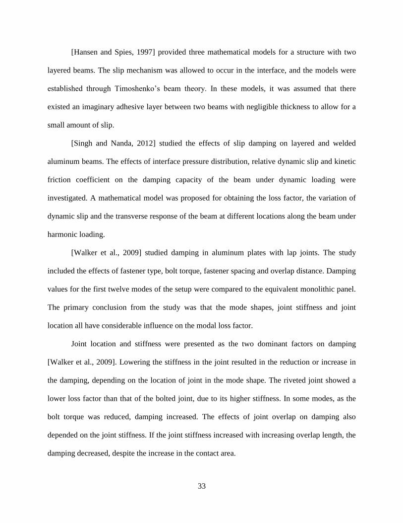
33

[Hansen and Spies, 1997] provided three mathematical models for a structure with two

layered beams. The slip mechanism was allowed to occur in the interface, and the models were

established through Timoshenko’s beam theory. In these models, it was assumed that there

existed an imaginary adhesive layer between two beams with negligible thickness to allow for a

small amount of slip.

[Singh and Nanda, 2012] studied the effects of slip damping on layered and welded

aluminum beams. The effects of interface pressure distribution, relative dynamic slip and kinetic

friction coefficient on the damping capacity of the beam under dynamic loading were

investigated. A mathematical model was proposed for obtaining the loss factor, the variation of

dynamic slip and the transverse response of the beam at different locations along the beam under

harmonic loading.

[Walker et al., 2009] studied damping in aluminum plates with lap joints. The study

included the effects of fastener type, bolt torque, fastener spacing and overlap distance. Damping

values for the first twelve modes of the setup were compared to the equivalent monolithic panel.

The primary conclusion from the study was that the mode shapes, joint stiffness and joint

location all have considerable influence on the modal loss factor.

Joint location and stiffness were presented as the two dominant factors on damping

[Walker et al., 2009]. Lowering the stiffness in the joint resulted in the reduction or increase in

the damping, depending on the location of joint in the mode shape. The riveted joint showed a

lower loss factor than that of the bolted joint, due to its higher stiffness. In some modes, as the

bolt torque was reduced, damping increased. The effects of joint overlap on damping also

depended on the joint stiffness. If the joint stiffness increased with increasing overlap length, the

damping decreased, despite the increase in the contact area.

34

[Hartwigsen et al., 2004] did an experimental analysis on a monolithic beam structure

and a jointed beam structure to quantify the nonlinear effects of a typical shear lap joint. He

concluded that, in general, the natural frequencies of a jointed structure decrease compared to

those of the monolithic structure, as a result of softening stiffness behaviour of the joint section.

The difference between captured FRFs at the same location on two structures showed that

changes in the mode shapes of a structure can occur, depending on the location of the joint.

More interestingly, it was shown that damping was generally higher in the jointed

structure, but was extremely amplitude dependent [Hartwigsen et al., 2004]. At higher vibration

amplitudes, a faster decay was observed in the captured time-domain signal. The applicability of

the Iwan model [Iwan, 1967] in predicting the stiffness and damping properties of the joint

section was also investigated. Iwan model is a parallel arrangement of elements, each composed

of spring and frictional dampers in series that is capable of predicting the micro- and macro-slip

mechanism in the joints.

Regardless of damping model or identification methods, damping should always be

measured experimentally and then be added to the FE model. In this research, damping is

inherently considered in the measured FRFs on the structures. For substructures, when the FE

models are developed, damping is identified through measurements on the substructures and then

added to the corresponding FE models.

2.4 Joint Dynamics Modeling

In this section, different joint models proposed in the literature, including theoretical and

FE models, are reviewed. The first step in a successful identification method is a valid model that

35

can properly reflect the properties of the joint under study. After reviewing the existing models,

two main identification strategies in the modal and frequency domains are discussed.

2.4.1 Nonlinear Joint Models

Different models have been proposed to represent the behaviour of the bolted joints with

particular emphasis on their nonlinear behaviour. [Ahmadian and Jalali, 2007] proposed a

nonlinear model for bolted lap joints to represent micro/macro-slip behaviour. The proposed

parametric model for the bolted lap joint considered linear and nonlinear spring elements and a

viscous damper. An analytical solution for the assembled structure FRFs was derived and the

joint’s parameters were derived by minimizing the error between the predicted and measure

FRFs. To obtain the measured FRFs, a moderate force was applied to induce micro slip

mechanism in the joint.

[Jalali et al., 2007] represented a bolted joint with a linear viscous damper and a cubic

stiffness element. In order to find the joint’s model coefficients, the structure was excited near its

first natural frequency; and, the force-state mapping method [Alhadid and Wright, 1990] was

employed. Hysteresis loops were generated through the model and experiments to confirm

accuracy of the proposed model.

[Iranzad and Ahmadian, 2012] used a thin layer of virtual elastoplastic material to model

the nonlinear stiffness and damping effects of a bolted lap joint. In order to identify the joint

parameters, stiffness at the macro-slip and transition from stick to micro-slip, the nonlinear

response of the structure was measured at different force amplitudes and compared with the

responses obtained from the model.

36

[Song, 2004] used the Iwan beam element [Iwan, 1967] to simulate the nonlinear effects

of a bolted joint on a beam structure. The Iwan model is a network of parallel and series spring-

slider elements to describe the hysteretic behaviour of structures. The Iwan model is capable of

describing the joint motion ranging from micro-slip to macro-slip. In order to obtain the model’s

parameters, a neural network was used for the measured acceleration of the structure. In order to

verify the model, the acceleration of the structure to a different excitation was predicted and

compared with the measured acceleration.

[Wileman et al., 1991] proposed an expression for the calculation of stiffness of a bolted

joint as a function of the joint’s aspect ratio (diameter/length) and material and compared the

results with a FE model.

2.4.2 Finite Element Models

Different studies that focus on the modeling of the joint behaviour in FE environment can

be found in the literature. [Oldfield et al., 2005] studied the dynamic frictional contact properties

of a bolted joint under harmonic loading using FE methods. He used several Jenkins elements

[Iwan, 1967], which consisted of a spring and a Coulomb element connected in series, to

represent the stick-slip mechanism in the joint. The Jenkins element could only provide either a

sticking or total slipping condition. Therefore, a single element could not represent the actual

behaviour of a lap joint in which some parts were in the sticking region and some parts were in

the total slipping region.

Instead, multiple elements were used in parallel, where each element was considered as a

point on the radius of the contact interface. The elements closer to the bolt axis were represented

by a single spring that never underwent sliding, and the elements further away from the bolt axis

37

were represented by Coulomb dampers. The parameters for the joints were obtained by

comparing the hysteresis loop obtained from experiments and the FE model. It was found that

the contact pressure distribution had a critical role on the dynamic performance of the interface.

A uniform pressure distribution caused a large area of the interface to slip [Oldfield et al., 2005].

[Chen and Deng, 2005] studied the micro-slip through FE methods and evaluated the

effects of dry friction on the damping response of a frictional joint. The FE model was compared

with two analytical models for the joint and showed that the FE model had a higher range of

validity compared to the analytical models.

[Richardson et al., 1993] studied a FE model for an adhesive joint. [Iranzad and

Ahmadian, 2012] used a two-dimensional (2D) elasto-plastic layer using a MSC/Nastran

QUAD4 element [MSC/Nastran] to model the interface in a single bolted lap joint. [Hwang and

Stallings, 1994] proposed a detailed FE model for a bolted flange connection. [Lehnhoff and

Wistehuff, 1996] performed an axisymmetric FE model of a bolted joint to investigate the effects

of magnitude and position of the external load and members’ material and thickness on the joint

stiffness.

In this thesis, a frequency-based model, representing a joint’s dynamic properties through

its FRFs, is used. The use of a joint’s FRFs allows for the combination of different FRFs of a

machine component and determination of the FRFs of the assembled structure. The main goal of

an accurate virtual prototype of a machine tool is the provision of an accurate FRF at the tool tip.

Since the majority of joints in a machine tool show weak nonlinearity, the nonlinear effects of

the joints are ignored, and the main focus is on the linear behaviour of the joints.

Two main models are proposed in this thesis. First, a joint model that is capable of

representing interfacial joints, such as the joint between the tool and the tool-holder, is proposed

38

by consideration of the frequency-dependent spring-damping elements. The second model

incorporates inertial properties of the joint and the cross effects between rotational and

translation DOFs in a joint element.

Regardless of the joint model, an identification technique is needed to obtain the joint’s

parameters and coefficients. In the following section, we discuss different joint identification

techniques and the particular method that we used throughout this research.

2.5 Joint Dynamics Identification

The discrepancy between numerical techniques, such as FE methods, and experimentally

measured responses of a structure is due to uncertainties in the FE models, such as joint

properties, boundary conditions and nonlinearity. The main purpose of joint identification is the

estimation of the joint parameters that minimize the difference between the measured and

predicted FRFs. In an attempt to address uncertainties in the joint properties, various techniques

have been proposed, by which the experimental data are integrated with a corresponding joint

model [Collins et al., 1974; Friswell and Penny, 1990].

The identification of joint properties has several applications in the prediction of the

dynamic characteristics of mechanical structures, such as machine tools [Ozsahin et al., 2009;

Park and Chae, 2008; Schmitz, 2000; Schmitz and Duncan, 2005; Y., 1974] and aerospace

structures [O’Donnell and Crawley, 1985; Chapman et al., 1986; Ikegami et al., 1986; Crawley

and Odonnell, 1987]. In machine tool structures, the dynamic characteristics of bolted joints,

welded joints and guiding systems are necessary in order to achieve an accurate model [Altintas

et al., 2005].

39

In aerospace structures, many complex joints influence the overall dynamics of the

structure. These structures cannot simply be treated as continuous systems by ignoring the joint

effects [Ibrahim and Pettit, 2005]. Joint identification techniques serve as a powerful tool that

assists the designer in achieving the desired behaviour for the structures by tuning the stiffness

and damping values.

Given the importance of joints in industrial structures and virtual prototyping, different

methods can be found in the literature regarding indirect identification of joint properties. Many

studies have been conducted on the linear and nonlinear behaviour of different types of joint. In

this section, the joint dynamics identification techniques are divided into two general categories

– direct methods and iterative methods – as illustrated in Figure 2.15. Different techniques are

explained, and their relative advantages and limitations are discussed.

Figure 2.15 Joint identification techniques.

2.5.1 Iterative Methods

Iterative methods introduce changes to the predefined design parameters on an elemental

basis in an FE model. The error model calculates the first-order derivative of the chosen dynamic

properties in the system. This allows the linearization of the formulations and yields to an over-

40

determined linear set of algebraic equations. There are two main iterative methods: the inverse

eigensensitivity method (IES) and the response function method (RFM).

The inverse eigensensitivity (IES) method, also classified as the modal-based technique

[Kim et al., 1991; Liu and Ewins, 2002; Shamine et al., 2000], is a well-established method

among iterative model updating tools. This technique is based on the minimization of the errors

or residuals between the FE models and experimental measurements. These differences are in the

vector format on the right-hand side of Eq. (2.15):

m

nm

n

n

n

mm

n

nmnm

n

n

nn

p

p

pp

pp

pp

pp

1

1

1

1

1

1

1

1

1

1

1

(2.15)

where Δω and Δφ represent the difference between the measured and simulated natural

frequencies and mode shapes, respectively; and, Δω/Δp and Δφ/Δp are the sensitivity of the

model’s natural frequencies and mode shapes to the design parameters Δp, respectively.

The corrections to the model parameters are related to the parameters of the FE model

through a sensitivity (Jacobian) matrix. The sensitivity matrix typically involves the derivatives

of each of the model parameters that need to be updated with respect to the stiffness, damping

and mass parameters.

The flowchart in Figure 2.16 shows the common procedure used in this technique. First,

the modal properties of the actual structure need to be measured. These parameters are also

extracted from the FE model. The differences between these parameters are then fed into Eq.

41

(2.15). Sensitivities of the modal parameters to the design parameters are extracted from the FE

model.

Figure 2.16 Iterative procedure of the IES method.

Based on the results of Eq. (2.15), the variation of the design parameters, i.e. Δp, are

obtained. This variation vector is added to the last design variables to generate the new design

variables as pnew = pold + Δp. At this stage, the convergence of the iterative optimization process

is checked based on the predefined criteria. If a desirable convergence is achieved, the new

design parameters are considered as the joint parameters. Otherwise, the new design parameters

are used in the FE model to start the new iteration until convergence is achieved.

[Shamine et al., 2000] employed this method for experimental identification of the joint

parameters on an actual spindle system. An indirect estimation scheme was proposed to

determine the complete set of eigenvector components corresponding to the joint location. [Li,

2002] reported that such techniques were generally more flexible and versatile than other

identification methods, in that various constraints were readily imposed on the model parameters.

Several other studies have used the IES method to identify the bolted joints in different

structures, where bolted joints were treated as lumped elements [Arruda and Santos, 1993;

42

Mottershead and Friswell, 1993; Mottershead et al., 1996; Pabst and Hagedorn, 1995; Yang and

Park, 1993]. In addition to bolted joints, some complex joints in an automotive structure were

identified using the IES method and a generic element approach [Ahmadian et al., 1996].

One of the major issues regarding the IES method is its high sensitivity to the

eigenvectors and eigenvalues in the model [Ewins, 1984]. All the modes of each substructure are

needed in the coupling method to achieve exact results; and, slight variations in the modal

parameters result in erroneous overall assembled dynamics. Moreover, several transformations

between the modal and physical coordinates impose errors in the calculations, due to the

truncation in the modal modes.

Other difficulty associated with the IES method is obtaining enough measurement points

to assure that the problem becomes over-determined. The unknown parameters are usually more

than the number of possible modal properties that can be extracted from the measurements. The

incompleteness of modal methods falls into two categories. First, it is sometimes impossible to

measure all the DOFs that are considered in the FE model. Second, due to measurement

equipment limitations, it is almost impossible to extract the modal properties of more than a

limited number of modes.

One solution to this problem is the direct use of the response function data, which provide

more data points than the modal data [Mottershead and Stanway, 1986; Ren and Beards, 1995;

Tsai and Chou, 1988; Wang and Liou, 1990]. The basic principle behind the response function

method (RFM), which is also known as the FRF sensitivity method, is the formation of a least-

square problem in which the known matrix is the sensitivity of FRFs to the design variables; and,

the known vector is the difference between the measured and predicted FRFs. In other words:

43

ijn

n

ijij

n

p

p

pp

pp

111

1

11

1

11

(2.16)

where αij is the FRF at point i when the excitation is at point j, and pi are the design parameters.

Figure 2.17 shows the procedure for obtaining the joint parameters through the RFM and

Eq. (2.16). The iteration procedure for the optimization process is the same as the IES method,

but the FRFs are used instead of the modal parameters.

Figure 2.17 Iterative procedure for the RFM.

[Mottershead and Stanway, 1986] used this algorithm for obtaining structural parameters.

However, the proposed algorithm was not practical for cases where measurements were not

possible at certain locations, such as joints. Some other studies tried to combine substructures’

FRFs and joint dependent FRFs of the whole structure to identify the joint properties [Hong and

Lee, 1991; Tsai and Chou, 1988; Wang and Liou, 1991; Yang and Park, 1993].

[Arruda and Santos, 1993; Hwang, 1998] employed the RFM at each discrete frequency,

and the joint properties were estimated for each frequency and averaged using statistical

44

methods. These methods also suffered from ineffectiveness when the FRF measurements at the

joints were not possible.

The iterative methods discussed in this section, i.e. IES and RFM, require high

computational efforts to solve for the sets of equations and suffer from the convergence

problems. They rely on the initial values for the uncertain parameters and, depending on the

initial guess, may result in different values. Sometimes, the values obtained at the end of iteration

procedure may result in the convergence of the solution, but may not yield values with

meaningful physical interpretation. All these issues indicate the necessity of other methods, such

as direct methods.

2.5.2 Direct Methods

The principles of direct updating methods are generally different than iterative

formulations. Direct methods focus on the global system matrices, while iterative model

updating procedures are formulated in respect to the discretized nature of the FE model [Grafe,

1998]. While the unknowns in the iterative methods are sets of individual element correction

factors [Ewins, 1984], the unknowns in the direct methods are the individual elements of mass

and stiffness matrices. Three direct methods – the error matrix method (EMM), equation error

method (EEM) and direct frequency-based method – are discussed in this section.

The error matrix method (EMM) deals directly with mass and stiffness matrices. This

method stems from the general form of the equation of motion for a multiple DOF (MDOF)

system and finds the updated matrices by comparing the equations of motion of the simulated

model with the experimental model.

45

This algorithm generates the updated global system of mass and stiffness matrices by

contemplating single matrix equations [Ewins, 1984; Grafe, 1998]. It first adjusts the system of

mass matrix and uses the resultant matrix to update the stiffness matrix, as expressed in Eqs.

(2.17) and (2.18):

XA

T

XA

A

T

XAAAXA

Mm

MmmImMM

11

(2.17)

which is followed by:

A

T

XXA

A

T

XXAA

T

XXXA

A

T

XXA

T

XXA

KM

MKMM

MKMK

2

(2.18)

where subscript X denotes the measured model and subscript A denotes the analytical model.

Several studies have employed this technique [Baruch, 1978; Berman and Nagy, 1983].

In these studies, the joint’s structural parameters were identified from the complete mode shapes

and eigenvalues, while in other studies, a condensed FE model and incomplete mode shapes

were used [Kim et al., 1989; Yuan and Wu, 1985].

In practical applications, [Lei et al., 2010] used the integrated modal analysis method

along with EMM to obtain the contact stiffness of joints. The proposed method incorporated the

FE method, lumped parameters and modal testing. The whole machine tool was considered as a

lumped parameter model, and the contact stiffnesses of the translational guides were obtained.

Another application of the direct methods in updating the FE model for an aerospace structure

can be found in [Lin, 1991] .

The EMM technique has several limitations, due to the assumption that the measurements

are complete [Grafe, 1998]. Mass and stiffness matrices are also necessary to create the updating

schemes, which are very expensive and difficult to obtain for complex systems [Lee and Hwang,

46

2007]. The accurate extraction of modal parameters is also difficult in closely coupled or heavily

damped modes [Ibrahim and Pettit, 2005]. Moreover, the solutions provided by such technique

are considered as numerical solutions, which may not have physical meaning; and, usually the

connectivity pattern in the system matrices are lost after the updating process [Ewins, 1984].

Another direct algorithm is the equation error method (EEM). In the EEM, the updating

algorithm is based on the equations obtained from the eigendynamic conditions [Ewins, 1984]

with additional constraints, such as the system symmetricity and orthogonality conditions

[Friswell et al., 2001]. The EEM [Kim et al., 1991; Nobari et al., 1995; Yuan and Wu, 1985]

combines FE models with the experimental models to estimate the mass and stiffness matrices

that contain the joint parameters [Chapman et al., 1986; Fengquan and Shiyu, 1996; Yuan and

Wu, 1985]:

KIM

MKTT ,

0

(2.19)

These sets of equations can be rearranged to form a least-square problem to find the

individual unknown elements [Mottershead et al., 1996]:

0

M

KTT

(2.20)

The main drawback of this method is that all the DOFs must be included in the mode

shapes, which requires expansion techniques. This is the main reason why this method is not

often used. Not only are the mode expansion techniques troublesome, but they are also quite

inaccurate in the application of model updating.

To overcome some of the challenges associated with the direct model updating methods,

several researchers have used the direct frequency-based method. The basic principle of the

direct FRF-based joint identification method is the comparison of the dynamic properties of the

47

rigidly attached substructures and the dynamic properties of the assembled structure measured

experimentally. The difference between these two cases is attributed to the joint effects [Ibrahim

and Pettit, 2005]. While the modal-based methods use modal parameters, such as eigenvectors

and natural frequencies, to estimate the joint parameters, the FRF-based methods estimate the

joint parameters directly from the measured FRFs.

In FRF-based methods, the joints are typically modeled with stiffness and damping

elements, and the parameters are identified from the FRFs of the overall system and the

substructures. Although the measurement errors and parameter uncertainties are still a source of

error in this method, the independence of the extraction of modal information for the

substructures and assembled structure is considered an advantage.

The receptance coupling (RC) method, as a subset of FRF-based methods, couples the

experimentally or analytically obtained FRFs of the substructures to generate the assembled

structure’s FRFs [Park et al., 2003; Schmitz, 2000]. Figure 2.18 shows two substructures (A and

B) that are coupled through a joint element comprised of translational and rotational spring-

damping elements.

Conversely, the inverse receptance coupling (IRC) method can be used for the

identification of the joint parameters. In this approach, assembled structure’s FRFs along with

the FRFs obtained from the FE models of substructures are used to generate joint’s FRFs.

Figure 2.18 Substructures in the uncoupled state.

48

There are several studies that used the FRF-based methods for joint identification. [Lee

and Hwang, 2007] used the FRF-based method to estimate joint parameters indirectly by

minimizing the difference between the measured and calculated responses using a gradient-based

optimization technique. [Movahhedy and Gerami, 2006] used the same concept and solved the

objective function using a genetic algorithm (GA) method [Goldberg, 1989].

In practical applications, different studies employed these techniques to identify the

connecting elements in the machining devices between the tool and the tool-holder [Movahhedy

and Gerami, 2006; Ozsahin et al., 2011; Park and Chae, 2008; Schmitz and Duncan, 2005]. The

FRF-based method has also been used on an engine mount system of a passenger car to identify

the hydraulic engine mount stiffness parameters [Lee and Hwang, 2007]. Several other studies

were conducted on simple structures with different configurations and substructures can be found

[Ren and Beards, 1995; Tsai and Chou, 1988; Wang and Liou, 1990; Wang and Liou, 1991;

Yang and Park, 1993]. In all of these studies, the goal was the determination of the properties of

connecting elements from the measured FRFs of the structures.

2.6 Summary

The most significant advantage of direct FRF methods, such as IRC method, over other

methodologies is that they directly employ the measured FRFs from the assembled structure and

do not require extraction of modal parameters. They also generate the responses of the structures,

which is usually the final goal in studying the structures.

One of the challenges associated with such methods is the difficulty in measuring

rotational FRFs of the structures. Measurements of these FRFs need either special equipment or

special experimental setups, which are usually extremely expensive. A few studies proposed

49

finite difference methods [Ozsahin et al., 2009; Schmitz and Duncan, 2005] to indirectly obtain

the rotational FRFs, but these methods were susceptible to measurement errors and were not

reliable. To overcome this challenge, this research uses the proposed method by [Park et al.,

2003] to obtain rotational FRFs using two sets of measurements on the structures.

In order to examine the applicability of the existing FRF-based technique, two machine

tools are tested. The IRC method was first used on a lathe machine to obtain the joint dynamics

of a modular tool. The technique was then employed on a vertical CNC machine to obtain the

joint dynamics between the tool and the tool-holder and between the tool-holder and the spindle.

Another limitation of the existing frequency-based methods is that the joint must be

comprised of stiffness-damping elements. This assumption can lead to an acceptable prediction

of the joint dynamics if the joint inertial properties are negligible compared to the rest of

substructures; otherwise, the identified joint dynamics deviate from the actual behaviour of the

joint.

A general FRF-based method proposed by [Ren and Beards, 1995] and used by [Liu and

Ewins, 2002] considered two substructures that were coupled through a general continuous joint

element with inertial properties. In a numerical simulation, the rotational DOFs were supposed to

be known through measurement or numerical methods, such as FE models [Wang and Liou,

1990]. Difficulties in measuring the rotational DOFs in experimental cases impose a limitation

on the implementation of the proposed methods by [Ren and Beards, 1995] in practice.

In this thesis, we adopt the method proposed by [Ren and Beards, 1995] to account for

the joint’s inertial properties and relate the joint dynamic properties to only the translational

FRFs of the assembled structure. The proposed technique in this thesis enabled us to account for

50

the inertial properties of the joint and overcome difficulties associated with the measurements of

the rotational FRFs.

Most of the existing studies have focused on the identification of joint dynamics in 2D

structures; and, there is lack of proper identification techniques in 3D structures. [Celic and

Boltezar, 2009] used the IRC method to identify the joint properties in a 3D structure. However,

difficulties in the measurement of rotational FRFs put a limitation on the applicability of the

proposed method to real structures.

One of the objectives of this thesis is the development of a methodology through the IRC

method to find rotational and translational joint’s FRFs in all directions in a 3D structure by

using only translational FRFs of the assembled structure. Unlike the majority of the previous

studies, a complete joint FRF matrix, which accounts for the effects of cross FRFs, is proposed

in this thesis. The proposed method also accounts for the effects of a joint’s inertial properties,

which is essential to consider when the joint’s mass and size are comparable to those of other

substructures.

The successful utilization of the proposed methods in our research makes the proposed

methods applicable to the real structures, such as machine tools. It is possible to obtain the joint

properties between the different components of a machine tool, such as the column and base and

the column and spindle housing, through the proposed methodologies. These locations, which

are usually ignored in virtual models, have significant impacts on the dynamics of the entire

structure.

51

Chapter 3. Experimental Setup

This chapter explains the main equipment, algorithms and machines that were used

throughout this research. Modal testing, which is the basis of all the experiments, is first

discussed by explaining the modal analysis principle and the required equipment. The lathe and

vertical computer numerical control (CNC) machine that were tested for joint identification are

also explained.

3.1 Experimental Modal Analysis

Modal analysis is the process of representing a structure in terms of its natural

frequencies, damping ratios and mode shapes. Understanding this information helps to design

structures for vibrations and noise applications. Applications of modal analysis range from the

design of tennis rackets and computers to automotive and aircraft structures [Avitabile, 2001].

Frequency response functions (FRFs) of a structure are extremely useful information that

can be obtained through modal analysis. An FRF is simply the ratio between the output response

of a structure to the input force in the frequency domain. The response can be measured in terms

of displacement (i.e. receptance FRF), velocity (mobility FRF) or acceleration (accelerance FRF)

[Ewins, 1984]. FRFs are obtained by converting time domain signals to the frequency domain

using the fast Fourier transformation (FFT). Therefore, FRFs are presented with a complex

number as:

n

r nrrnr

jrirn

r nrrnr

ijr

ijjj

AH

122

122 22

)(

(3.1)

52

where rAij is the modal constant, ir is the motion of ith

node in the rth

mode, nr is the rth

natural

frequency, and r is the damping ratio at rth

mode.

The magnitude of the FRF shows the ratio between the output response and the input

force, while the phase shows the phase lag between the response and the force. If a structure is

excited at a frequency well below its natural frequency, there is negligible phase difference

between the response and the force. As the excitation frequency approaches the natural

frequency, the response lags the force by 90 degrees; and, above the natural frequency, the

response lags the force by 180 degrees.

In order to perform modal testing, several measuring devices should be available, as

shown in Figure 3.1. These include an excitation source, a sensing mechanism and a data

acquisition and processing mechanism [Maia and Montalvão e Silva, 1997]. For the excitation

source, there is a choice between a shaker or a hammer, depending on the accessibility of the

excitation point and the application of the modal testing. For the sensing mechanism, there is a

large variety of transducers, such as accelerometers, capacitive sensors, fiber optic sensors and

laser sensors. Since the electric signals generated by the transducers are most often very weak,

the signals are passed through conditioning amplifiers.

(a) (b)

Figure 3.1 (a) Schematic representation of the basic hardware for modal testing [Maia and

Montalvão e Silva, 1997], (b) experimental setup used for modal testing.

Data Acqusition

Card

IO Box with

AntiAliasing Filter

TF analysis

SoftwareAccelerometer

Impact Hammer

53

Theoretically, there is no difference between the FRFs obtained with a shaker and

hammer. With a hammer, it is easier to excite the structures at different locations and measure at

one location, i.e. capturing one row of the FRF matrix; whereas, with the shaker, it is easier to

capture one column of the FRF matrix by changing the accelerometer location.

The two other main components of modal analysis are the data acquisition system and the

FFT analyzer. The signals are collected in the time domain at the transducers and impact source

and passed through an anti-aliasing filter to cancel out the high-frequency content. This filter is

basically a low-pass filter that cuts off the noise and high-frequency content.

The next step in the capturing of an FRF is the digitization of the analog signals. This

step is done through an analog-to-digital convertor (ADC). The sampling rate of the signal

controls the resolution in the time and frequency domains. Quantization is associated with the

accuracy of the magnitude of the captured signal [Avitabile, 2001]. In this step, in order to

reduce the effects of leakage, i.e. spreading of the true spectrum components to other

frequencies, windowing is applied to the signals [Avitabile, 2001].

Fourier transformation requires that the sample data have a periodic pattern and contain a

complete representation of the data at all times. When these conditions are not satisfied, leakage

causes a distortion in the frequency content of the signal. In order to mitigate distortion of the

signal in the frequency domain, weighting functions are applied to the signal to better satisfy the

requirements of the FFT.

After applying windows on the time domain signals, the FFT is applied to the input and

the response signals to obtain the linear spectra of these signals in the frequency domain. The

spectra includes the input power spectrum, output power spectrum and cross spectrum between

54

input and output signals. These functions are then averaged and used to obtain the FRFs of the

structure through Eq. (3.2).

)(

)()(

)(

)()(

2

1

xf

xx

ff

fx

S

SH

S

SH

(3.2)

In theory, H1() and H2() are similar; however, in reality, the noise effects cause these

two FRFs to differ. The ratio between these two FRFs is called coherence [Ewins, 1984]. While

the FRF is the ratio between the output spectrum and the input spectrum, the coherence is an

indication of data quality and shows how much noise has affected the data collections.

Coherence ranges between zero and unity, where zero means poor quality and unity means a

clear signal.

CUTPRO® software [CUTPRO] was used in this research as the FFT analyzer along with

a NI9234 data acquisition and signal conditioning unit. The hardware used in this research for

modal analysis including an impact hammer, an accelerometer and a capacitive sensor are

described in the following sections.

3.2 Impact Hammer

A very popular device that is commonly used as an excitation device is an impulse or

impact hammer. An impact hammer consists of a hammer with a force transducer attached to its

head. Contrary to shakers, impact hammers do not require a signal generator; the hammer acts as

the excitation mechanism and is used to impact the structure.

There are several advantages in the utilization of impact hammers instead of shakers.

Impact hammers are capable of exciting structures in a broad range of frequencies. Since they do

55

not need a connecting device, they do not apply any added mass loading to the test structure.

Moreover, an impact hammer is faster to set up than a shaker.

The range of frequencies that is excited by an impact hammer depends on the hammer

mass and the rigidity of the impacting head. Impact hammers range from a miniature hammer to

a sledge hammer. The mass of a hammer along with the velocity of the impact determine the

amplitude of the impact force [Maia and Montalvão e Silva, 1997].

The hammer used in our experiments was a PCB SN2222 type, as shown in Figure 3.2.

This type of hammer included quartz as its sensing element with an integrated circuit

piezoelectric element. The hammer had a mass of 0.16 kg, a sensitivity of 1.86 mV/N and a

resonant frequency at 22 kHz. The connection between the hammer and the data acquisition

system was provided through a BNC connector.

Figure 3.2 PCB hammer used in the modal testing.

The hammer impulse consists of a nearly constant force over a frequency range called a

bandwidth. The impact is capable of exciting all the frequency resonances of a structure within

its bandwidth. The hammer size, length and material and the velocity of the impact determine the

56

amplitude and frequency content of the impulse [Piezotronics]. The primary factor in

determining the frequency content of an impulse is the impact cap. The hammer that was used in

this research was equipped with different caps with different bandwidths. In this research, the

metallic tip was used for the excitation of high frequency ranges and the hard plastic cap was

used for the excitation of medium to high frequency range. Figure 3.3 shows the spectrum of an

impact on a stiff steel mass for the hammer that we used in our experiments with different tips.

Figure 3.3 Spectrum content of PCB hammer with different tips [Piezotronics].

3.3 Accelerometer

The sensing in modal testing is done through transducers. The most commonly used

transducers are piezoelectric transducers, which are used in both sensing the force excitation

(force transducers) and acceleration response (accelerometers). Piezoelectric transducers

generate electric signals proportional to the corresponding physical parameter.

Piezoelectric accelerometers utilize a mass in direct contact with the piezoelectric

component or crystal, as shown in Figure 3.4. When a varying motion is applied to the

accelerometer, the crystal element senses a varying force proportional to the mass and generates

57

an electric charge. Two commonly used piezoelectric crystals are lead zirconate titanate ceramic

(PZT) and quartz [Webster, 1999]. The piezoelectric strain constant of the PZT is about 150

times greater than the quartz, which results the PZT having greater sensitivity than quartz

counterparts.

Figure 3.4 Piezoelectric accelerometer [Webster, 1999].

Figure 3.5 Frequency response of a typical piezoelectric accelerometer [Webster, 1999].

Figure 3.5 demonstrates a typical frequency response of a PZT device. Since piezoelectric

accelerometers have comparatively low mechanical impedances, their effects on the motion of

most structures is negligible. At low frequencies, the response of the accelerometer is limited by

58

the piezoelectric time constant, while the high-frequency response is limited by the mechanical

resonance of the system.

Piezoelectric accelerometers are found in a wide range of specifications. For example, a

shock accelerometer can have a sensitivity of 0.004 pC/g and a natural frequency of 250 kHz,

while a low-level seismic accelerometer may have a sensitivity of 1000 pC/g and a natural

frequency of 7 kHz.

The accelerometer that was used in our experiments was a Kistler type 8278A500 with a

sensitivity of 10 mV/g and an acceleration range of ± 500 g. The bandwidth was 10 kHz, with a

resonant frequency of 40 kHz. This type of accelerometer has a wide frequency and is

lightweight with a ceramic shear sensing element. The accelerometer was mounted on the test

structures using wax or adhesives.

3.4 Capacitive Sensor

Capacitive sensors are commonly used in industrial applications. The basic principle of

capacitive sensors is the detection of changes in the capacitance as a response to physical

variations. Although the applications of capacitive sensors range from humidity to moisture

measurements, these sensors are mainly used for measuring rotational and translational

displacement [Webster, 1999]. Capacitive displacement sensors are in high demand for

displacement measurements due to their high linearity and wide range (from a few centimeters to

a couple of nanometers).

The basic sensing elements of a capacitive displacement sensor are two electrodes that

form a capacitance. The capacitance between the two plates (C) is a function of the distance (x)

59

between the two electrodes, the surface area (A) of the electrodes, and the permittivity () of the

dielectric between the electrodes (8.85×10–12

F/m for air).

A capacitive displacement sensor with two plates at a distance of x apart is shown in

Figure 3.6. The capacitance of this configuration is:

xAxC /)( (3.3)

where x is in meters (m) and A is in m2.

As the moving plate moves away from and close to the fixed plate, the distance between

two plates varies; and, this change is converted to a voltage proportional to the changes in the

capacitance. Figure 3.6 (b) shows the capacitive sensor (Lion Precision DMT20 with a

sensitivity of 80 mV/µm and a sensor bandwidth of 10 kHz) that was used during the

experiments.

(a) (b)

Figure 3.6 (a) Variable distance capacitive displacement sensor [Webster, 1999], (b) Lion

Precision DMT20 sensor.

3.5 Lathe Machine

A standard lathe machine was selected to perform joint identification in a 2D structure

and to investigate the applicability of the proposed technique on a real machine. The lathe was a

Sherline 4100 model with a 90 VDC motor, a 2.75″×6.0″ cross slide, a 15″ steel bed, pulleys, a

60

belt and a faceplate, as shown in Figure 3.7. The 3-jaw chuck was suitable for turning objects up

to 3.5″ in diameter. The spindle could rotate between 70 to 2800 RPM.

In the experiments, one blank shaft was always secured inside the chuck; and, the inverse

receptance coupling (IRC) method was applied to the setup to obtain the translational and

rotational FRFs at the shaft tip. Since the experiments were performed on the shaft tip when it

was inside the chuck, the obtained FRFs included the effects of the boundary conditions between

the tool and the chuck, as well as the machine dynamics and boundary conditions.

Figure 3.7 Lathe machine used in joint identification.

3.6 FADAL Vertical CNC Machine1

One of the machining centers on which the proposed technique in this thesis was applied

was a three-axis FADAL 2216 vertical CNC machine, as shown in Figure 3.8. The main

components of the machine included the base, column, table, cross slides, spindle housing,

spindle and feed drives. The structural components were made of cast iron with a modulus of

elasticity of 89 GPa, a density of 7250 kg/m3 and Poisson’s ratio of 0.25. This machine was

1 The FADAL CNC machine was located in the Manufacturing and Automation Laboratory (MAL) at the

Department of Mechanical Engineering at the University of British Columbia.

61

equipped with an open CNC and a built-in spindle. The table size was 39×16, and the motion

range in the x (longitudinal), y (cross) and z (vertical) axes were 22, 16 and 20, respectively.

Figure 3.8 The FADAL vertical CNC machine (UBC MAL).

The spindle assembly of the CNC machine included the tool, the tool-holder, the spindle

shaft, the spindle cartridge, bearings, spacers, the drive pulley and other accessories, such as nuts

and rotary couplings. The spindle had a standard CAT 40 tool-holder interface and was designed

to operate at up to 15,000 rpm with a 15 kW motor connected to the shaft with a pulley-belt

system.

The feed drive consisted of a ball screw that was attached to the motor shaft through a

coupling. The screw was constrained axially and radially by thrust bearings at the motor. A

62

radial bearing also supported the screw, providing axial freedom and allowing for thermal

expansion [Okwudire and Altintas, 2009]. The rotary motion of the screw was converted to the

translation motion at the nut, which was connected to the table supported by guideways on two

parallel sides.

3.7 Summary

In this chapter, the equipment, algorithms and machines that were employed in this

research were explained. Experimental modal analysis, as the main tool that was utilized for the

analysis of the dynamics of structures, and the required equipment for modal analysis, such as

impact hammer, accelerometers, signal conditioning units and FFT software, were introduced.

Joint identification algorithms were applied on several setups to obtain joint dynamics at

different interfaces. These setups, including a lathe machine and a vertical CNC machine, were

also explained in detail.

The lathe machine and the CNC machine are tested in Chapter 4 to obtain dynamic

properties of modular tools and tool / tool-holder / spindle interfaces. The required FRFs in the

identification algorithm are obtained by performing modal testing on the physical setups at

different locations. In Chapter 5, two thin wall plates that are attached by four bolted joints are

tested through modal analysis to obtain several FRFs required in the identification algorithm. In

Chapter 6, modal tests are applied on 3D cubic blocks to obtain 15 FRFs at different locations on

the assembled structure.

63

Chapter 4. Identification of Joint Dynamics in 2D Structures

Complex structures are comprised of several substructures joined together to form an

assembled structure. Different types of joints, such as welded joints, bolted joints and rivets, are

commonly used in such structures. Much of the flexibility and damping in the structures is due to

the joints in the structures [Ahmadian and Jalali, 2007]. Ignoring joint effects in the design stage

results in considerable deviation from the actual structure.

If the joint dynamics are determined, the overall assembled dynamics can be accurately

predicted by mathematically combining the substructures’ dynamics through the equilibrium and

compatibility conditions at the joint. The accurate dynamics of an assembled structure can be

helpful in preventing chatter vibration and minimizing forced vibrations in machining processes.

It is not possible to develop a joint model that can predict the behaviour of all types of

joints. A joint’s behaviour depends on different conditions, such as prestress, applied torque,

contact surface conditions, friction and residual stress. Each type of joint requires an

investigation to develop an identification technique that is applicable for that specific joint. For

instance, fastener joints are commonly used in machining centers, such as milling machines. This

particular type of joint which comes in different sizes and shapes needs to be accurately

identified and incorporated into the models of the structures.

Regular milling machines commonly use CAT type tool-holders to provide the interface

between the tool and the spindle. The interface dynamic properties between the tool and the

collet can change based on the surfaces area of the connection and the applied torque to the

chuck. The drawbar clamping force between the tool-holder and the spring inside the spindle can

64

also be a contributing factor in the tool tip dynamics. All these types of joints require specific

identification methods that can generate the dynamics properties of the joint.

The receptance coupling (RC) method was first developed to relate the dynamics of

substructures to the dynamics of the assembled structure. The inverse receptance coupling (IRC)

method was then introduced to obtain a joint’s FRFs as a function of the FRFs of the

substructures and the assembled structure. The principle behind the joint identification through

the IRC method is the determination of the difference between the measured overall dynamics

and the rigidly coupled substructure dynamics.

The IRC method obtains a closed-form solution for the joint parameters and uses only

two translational frequency response functions (FRFs) of the assembled structure. The IRC

method overcomes the barrier of identifying joint characteristics even when they cannot directly

be measured. Relying on only two measurements on the assembled structures eliminates the

necessity of performing several measurements that were required in earlier studies to obtain the

translational and rotational FRFs.

The proposed methodology is validated through finite element (FE) simulations. The

methodology is then employed on two actual physical structures, including a lathe machine and a

vertical computer numerical control (CNC) machine. A blank shaft was inserted inside the chuck

of a lathe machine, and the joint between the modular tool and the shank was identified. In order

to avoid measurement of the rotational degrees of freedom (RDOFs), an indirect identification

method is used. The identified joint dynamics is then used to reconstruct the FRFs of another

assembly with the same joint, but different substructures.

The joint dynamics identification in the CNC machine is performed at two locations:

between the tool and the tool-holder, and between the tool-holder and the spindle. A virtual

65

model for the machine tool, including the base, column, headstock and spindle, is first

developed. To build this model, the joints between the various structural components of the

machine are approximated with linear spring and damping elements. The response at the spindle

nose obtained from the virtual machine tool model is then combined with the response of the tool

and tool-holder through the IRC approach to identify the joint characteristics between these

interfaces.

4.1 Receptance Coupling (RC) Method

The RC method enables the combination of the responses of all the components of a

structure obtained from an FE model or measurements and the formulation of the response of the

assembled structure. Unlike the component mode synthesis (CMS) methods, the RC method does

not require extraction of modal parameters [Park et al., 2003]. The FRFs of the substructures are

combined at the equilibrium and compatibility conditions of the joint interface and form the

assembled structure’s FRFs [Ewins, 1984].

Let us consider that Substructures A and B are connected by a joint element, as shown in

Figure 4.1. Points 1 and 4 represent the internal degrees of freedom (DOFs) for each

substructure, which are not involved in the joint interface; and, points 2 and 3 illustrate the DOFs

connected through the joint section. FiS = {fi

S , Mi

S}, (S = A, B, J), represents the vector of force

and moment at location i.

Figure 4.1 Substructures in coupled and uncoupled states.

66

According to Figure 4.1, F1B, F2

B, F3

A and F4

A are the vectors of applied force and

moment on the assembled structure; and, F2J and F3

J are the vectors of internal force and

moment in the joint section at locations 2 and 3. These internal forces and moments are added to

the substructures when formulating the substructures’ FRF matrix in the uncoupled state. The

relation between the displacements and the forces in each substructure can be defined as:

A

A

JA

JA

A

A

A

A

JB

JB

B

B

B

B

B

B

M

f

MM

ff

pnpn

lhlh

pnpn

lhlh

x

x

MM

ff

M

f

pnpn

lhlh

pnpn

lhlh

x

x

4

4

33

33

44444343

44444343

34343333

34343333

4

4

3

3

22

22

1

1

22222121

22222121

12121111

12121111

2

2

1

1

,

(4.1)

where xi and θi represent the translational and rotational displacement vectors at location i. The

receptance components are also defined as hij = xi/fj, lij = xi/Mj, nij = θi/fj and pij = θi/Mj.

The joint segment is assumed to be an element that mainly imposes stiffness and damping

to the structure; therefore, the equilibrium condition at the joint part is:

(4.2)

Using equilibrium conditions, the equation of motion at the joint part can be written as:

(4.3)

where kx, kθ, cx and cθ are the joint’s frequency-dependent translational and rotational spring and

damping parameters.

With the application of the Laplace transformation to Eq. (4.3) and substitution of s = i,

Eq. (4.3) can be rewritten in the frequency domain as:

03

3

2

2

J

J

J

J

M

f

M

f

JBABA

JBA

x

BA

x

Mkc

fxxkxxc

22323

22323

67

(4.4)

where HJ denotes the receptance matrix of the joint as:

(4.5)

where subscripts t and r represent the translational and rotational directions, respectively.

Substitution of Eqs. (4.1) and (4.2) into Eq. (4.4) leads to:

(4.6)

where B = (H22+H33+HJ) and Hij = [hij lij ; nij pij].

Substitution of Eq. (4.6) into Eq. (4.1) leads to the assembled structure’s FRFs based on

the substructures’ FRFs as:

A

A

B

B

A

A

B

B

F

F

F

F

HBHHHBHHHBHHBH

HBHHHBHHHBHHBH

HBHHBHHBHHHBHH

HBHHBHHBHHHBHH

F

F

F

F

GGGG

GGGG

GGGG

GGGG

X

X

X

X

4

3

2

1

34

1

334433

1

343422

1

3421

1

34

34

1

333433

1

333322

1

3321

1

33

34

1

2233

1

2222

1

222221

1

2221

34

1

1233

1

1222

1

121221

1

1211

4

3

2

1

44434241

34333231

24232221

14131211

4

3

2

1

(4.7)

where Gij = [Gij,tt Gij,tr ; Gij,rt Gij,rr] represents the assembled structure’s FRFs and Xi = {xi θi}T is

the displacement vector of the assembled structure.

The assembled response at locations 1 and 2 (i.e. G11 and G12 entities) can be expanded

as:

J

J

JBA

BA

M

fH

xx

2

2

2

2

3

3

1

0

0

0

0

ick

ick

h

hH

xx

J

rr

J

tt

J

A

A

A

A

B

B

B

B

J

J

J

J

M

fHB

M

fHB

M

fHB

M

fHB

M

f

M

f

4

4

34

1

3

3

33

1

2

2

22

1

1

1

21

1

3

3

2

2

68

(4.8)

where

(4.9)

Based on Eq. (4.8), the assembled structure’s dynamics are directly related to the

dynamics of each individual substructure and the joint. This equation generates the exact

assembled structure’s FRFs if the joint is comprised of only spring and damping elements.

In Eq. (4.8), the term Gij,tt is the only assembled structure’s FRF that can be measured

through direct experiments. This term is the ratio between the measured translational

displacement at location i and the applied force at location j. Measurement of the rotational

displacements of the structures and application of only the moment on the structures are both

challenging and usually contaminated by noise, which makes the measurement of Gij,tr and Gij,rr

very difficult.

The IRC method uses Eq. (4.8) and relates the joint’s FRFs, i.e. httJ and hrr

J, to the

assembled structure’s translational FRFs to obtain a symbolic solution for the joint’s FRFs. This

is an advantage for practical applications where rotational FRFs are hard to measure.

4.2 Inverse Receptance Coupling (IRC) Method

The IRC method generates a joint’s FRFs as the difference between the assembled

structure’s FRFs and those of the rigidly coupled substructures. The IRC method is used to

explicitly identify the joint’s FRFs using a symbolic approach. This method derives the rotational

2222

2222

1

1212

1212

1212

1212

,12,12

,12,12

2121

2121

1

1212

1212

1111

1111

,11,11

,11,11

pn

lh

bb

bb

pn

lh

pn

lh

GG

GG

pn

lh

bb

bb

pn

lh

pn

lh

GG

GG

rrrt

trtt

rrrt

trtt

rrrt

trtt

rrrt

trtt

J

rr

J

tt

rrrt

trtt

h

h

pn

lh

pn

lh

bb

bb

0

0

3333

3333

2222

2222

69

and translational joint’s FRFs using the translational FRFs of the assembled structure and the

FRFs of substructures. The IRC method was developed by [Schmitz, 2000] and [Park et al.,

2003].

The joint’s mass properties have recently been added to the FRF matrix by [Park and

Chae, 2008]. The joint FRF matrix is introduced as:

1

2

2

0

0

Jick

mick

hh

hhH

xx

J

rr

J

rt

J

tr

J

tt

J (4.10)

where m and J represent the frequency-dependent mass and moment of inertia of the joint,

respectively.

Cross FRF terms between the translational and rotational DOFs (htrJ, hrt

J) are assumed to

be negligible after introducing mass to the model. Moreover, the equilibrium condition at the

joint section is considered to stay the same as Eq. (4.2). This assumption implies that the forces

in the joint section are equal in magnitude and opposite in direction. Neglecting the cross FRF

terms in the joint matrix can result in deviation from the actual behaviour of a joint if the mass of

the joint is considerable compared to other substructures; therefore, this model is not

recommended for the structures with considerable joint’s inertial properties.

The two remaining FRF terms (httJ, hrr

J) in the joint matrix represent the dynamics of the

joint. These two terms are sought in the IRC method, which can be employed to identify joint

properties based on the experimentally measured response of the assembled structure and the

analytical FE models of the substructures.

Figure 4.2 shows the process of applying the IRC method to extract the dynamic

properties of the joint when the FRFs of Substructure A were identified experimentally and the

FRFs of Substructure B were identified analytically. Substructure A was considered to have a

70

complex geometry that could not be modeled analytically; therefore, its dynamics was obtained

using experimental modal analysis (EMA).

The translational FRF (h33) was measured directly at location 3 on Substructure A;

however, the direct measurement of rotational FRFs at this location was difficult and prone to

noise effects. Therefore, an indirect method was employed to acquire the rotational FRFs (l33,

n33, p33) using two sets of measurements on Substructure A [Park et al., 2003]. Two sets of

measurements on the assembled structure were also taken when Substructure B was attached to

Substructure A to obtain two values of G11,tt and G12,tt.

The IRC method generates the joint properties as the difference between the measured

FRFs of the assembled structure and the FRFs obtained by the coupling of the substructures’

FRFs through a rigid joint.

Figure 4.2 Overview of the joint identification approach through the IRC method.

Expansion of the translational FRFs of the assembled structure in Eq. (4.8) results in:

(4.11)

])()[(1

21121221121211

1

1

,11nblbhhblbh

bbbbh

f

xG

tttrrtrr

trrtrrtt

tt

])()[(1

22121222121212

2

1

,12nblbhhblbh

bbbbh

f

xG

tttrrtrr

trrtrrtt

tt

71

Two explicit parameters of btt and brr are obtained symbolically by simultaneously solving

Eq. (4.11) using MATLABTM

symbolic toolbox [MATLAB]:

221122,11121212,12

22

2

12122212221122,11

2

1212,12

lhlGlhlG

lhlhhhhbhGbhbhGbb

tttt

rtttrtrtttrt

tt

221122,11

2

1212,12

22

2

12122212221122,11121212,12

hhhGhhG

hlllhlhblGblhblGbb

tttt

trtttrtrtttr

rr

(4.12)

The joint’s FRFs are then obtained from Eqs. (4.9) and (4.12) as:

3322

3322

ppbh

hhbh

rr

J

rr

tt

J

tt

(4.13)

Based on Eq. (4.13), the joint’s FRFs can be obtained using the substructures’ FE models

and two translational measurements on the assembled structure. These joint’s FRFs are the

results of the IRC method, which minimize the difference between the calculated and

measured/simulated assembled structure’s FRFs. In the simulation section, the assembled

structure’s FRFs, G11,tt and G12,tt, were obtained from the simulated FE model, while in the

experimental section, these FRFs were obtained from the direct measurements on the assembled

structure.

The IRC method eliminates the dependence on the rotational FRF measurements and

provides an explicit solution for a joint’s FRFs. This capability makes the identification process

faster, since there is no need to measure RDOFs, which is difficult, time-consuming and

sensitive to noise.

A numerical simulation was conducted in the following section to investigate the

effectiveness of the method in identifying the joint’s dynamics properties. The simulation was

done to mimic the identification procedure on an actual case, i.e. only those FRFs that could be

72

measured experimentally on a physical structure were derived from the FE model. Experimental

tests were also conducted on a modular tool and on a CNC machine to further investigate the

applicability of the proposed methodology.

4.3 Numerical Simulations

FE simulations were employed to investigate the applicability of the proposed

methodology. One simulation was performed with rotational and translational spring-damping

elements acting as the joint; and, another simulation was conducted considering a continuous

joint segment as the joint. The purpose of the first simulation was to determine if the proposed

IRC method could generate the exact joint parameters when the joint acted only as stiffness and

damping elements. The purpose of the second simulation was to investigate applicability of the

proposed method in predicting the dynamics of structures with a continuous joint element.

To mimic experimental conditions, only the information that could be obtained from an

actual structure by performing experimental measurements was extracted from the FE models. In

the simulations, Substructure A was treated as a complex structure whose FE model could not be

easily built (Figures 4.3 and 4.6). This substructure was arbitrarily considered to be clamped at

one end. Substructure B represented the part of a structure that had a simple geometry; therefore,

both rotational and translational FRFs were obtained from its FE model.

Substructures A and B were modeled with beam elements having steel properties with a

modulus of elasticity (E) of 200 GPa and a density (ρ) of 7850 kg/m3. The element size for all

substructures was 5 cm. With an element length of 5 cm in the simulation, the discretization error

could be ignored. Proportional damping was considered for all the parts with a damping ratio of

73

0.1. For the first simulation, translational and rotational spring and damping elements were used

to connect two substructures. The corresponding values for the joint are presented in Table 4.1.

Figure 4.3 Structure with spring-damping elements.

Table 4.1 Stiffness and damping values used as the joint in Figure 4.3.

Translational

Stiffness (N/m)

Translational

Damping (N.s/m)

Rotational

Stiffness (N.m/rad)

Rotational

Damping (N.m.s/rad)

2×106 100 8×10

4 80

Two of the assembled structure’s FRFs (i.e. G11,tt and G12,tt) obtained from the FE model

along with the FRFs of substructures were inserted into Eqs. (4.12) and (4.13) to obtain the joint

FRFs (i.e. httJ and hrr

J). From the identified FRFs, the stiffness and damping values were

obtained as httJ

= 1/(kx+icx) and hrrJ

= 1/(kθ+icθ). The identified values are shown in Figures

4.4 and 4.5 for the translational and rotational elements, respectively.

As expected, no deviation existed between the exact joint values and the identified values

through the IRC method. Since no assumptions were considered in the derivation of the IRC

method with only spring and damping elements in the joints, no deviations existed between the

identified parameters and the exact parameters. However, many joints in real structures exhibit a

dynamic behaviour that cannot be approximated with only stiffness and damping elements. To

study the applicability of the proposed IRC method in identifying such joints and using the

identified FRFs in predicting the behaviour of subsequent structures, the second simulation was

conducted.

74

Figure 4.4 Identified stiffness (left) and damping (right) values for the translational elements.

Figure 4.5 Identified stiffness (left) and damping (right) values for the rotational elements.

The second FE simulation had two stages: identification and validation. In the

identification stage, the joint properties were extracted using the proposed methodology. These

identified properties were then used in the validation stage to predict the FRFs of the validation

structure that was comprised of the same joint, but with different substructures. The predicted

FRFs were then compared with the simulated FRFs obtained from the FE model of the validation

structure.

In this simulation, the effect of dilation of one of the substructures was investigated. The

joint properties were identified using the configuration of Case A in Figure 4.6. The length of

Substructure B was then decreased to constitute the validation structure as Case B in Figure 4.6.

Substructure A and the joint remained the same as in the identification structure. The properties

of the joint from the identification stage along with the FE models of the substructures were

75

employed in the RC method to predict the assembled structure’s FRF (G11,tt) in the validation

configurations. The predicted FRF was then compared with the simulated FRF obtained from the

FE model of the assembly.

Figure 4.6 Structure used for joint identification (top) and validation (bottom).

For the IRC method, two sets of assembled structure FRFs (G11,tt, G12,tt) extracted from

Case A and used in Eqs. (4.12) and (4.13) to identify the joint’s FRFs. The substructures’ FRFs

were obtained from the free-free model of substructure B and the clamped-free model of

substructure A. The assembled structure’s FRFs were obtained after connecting the substructures

through the joint element.

Figure 4.7 Reconstructed G11,tt for Case B.

Figure 4.7 shows the comparison between the predicted FRF at the tip of the validation

structure (G11,tt) obtained from the IRC method, the simulated FRF obtained from the FE model

76

of the assembly and the FRF obtained by a rigid connection. Based on Figure 4.7, the proposed

IRC method was able to predict the new structure’s FRF (i.e. case B) acceptably with minor

deviations at high frequencies.

In order to quantify the agreement between the prediction and the simulation, the relative

deviation between two sets was calculated at each frequency; and, the average was taken over the

entire frequency range. While the average deviation from the simulated FRF was 109% in the

prediction of a rigid connection, it decreased to 5% for the IRC prediction. Moreover, both the

natural frequencies and the amplitude of the FRFs were reconstructed accurately.

The joint section in the simulations was a continuous segment with a finite length.

Therefore, its dynamic behaviour could not be characterized with single spring-damping values

in a wide frequency range. Using the IRC method, the frequency-dependent values were

obtained for the joint parameters that minimized the difference between the predicted and

simulated assembled structure’s FRFs at all frequencies.

One possible validation for the identified joint’s FRFs is if they can acceptably predict

the behaviour of a different structure that uses the same joint. This is the main difference

between the receptance-based method proposed in this research and the model updating

techniques. In model updating techniques, a single value is obtained for the model parameter at

the end of the updating procedure. This single value, which is usually selected to have physical

meaning [Friswell et al., 2001], is assigned to the corresponding parameter to minimize the

difference between the predicted and measured natural frequencies or mode shapes that were

used in the optimization scheme. The proposed FRF-based technique finds the joint’s FRFs

instead of a single value for the mass, stiffness and damping and minimizes the difference

between the predicted and measured assembled structure’s FRFs at each individual frequency.

77

The IRC method can obtain exact joint’s parameters if the joint is comprised of only

stiffness and damping elements. However, when a joint has inertial properties, the IRC method

obtains an approximation of the exact joint’s FRF. Therefore, care should be taken when the

proposed IRC method is used on structures with considerable joint inertial properties. In Chapter

6, an extension to the current IRC method is introduced, which enables the IRC method to

accurately obtain the joint’s FRF with consideration of inertial properties. However, the

proposed methodology requires more FRFs of the assembled structure.

The FE simulation discussed in this section revealed the effectiveness of the IRC method

in predicting the joint’s dynamic properties when the joint section had an aspect ratio

(length/diameter) of 2.5 and was 1/6 of the length of Substructure A. Based on different

simulations on the studied structure in this section, when the aspect ratio of the joint was below

5, negligible deviation occurred between the prediction of the two models and the simulated

assembled structure’s FRFs. In addition, when the ratio between the length of the joint and

length of the substructures was less than 1/3, an acceptable correlation was observed between the

predicted and simulated FRFs.

In spite of the limitations, the proposed methodology can be used in actual cases where

the joint part is not long compared to other substructures and mostly serves as a connecting part

between two substructures. The next two sections discuss the proposed IRC method when

employed on two actual physical structures. The first structure was a lathe machine, where the

dynamic properties of a modular tool were identified. The second structure was a vertical CNC

machine, where the dynamic properties of the joint between the tool and the tool-holder and

between the tool-holder and the spindle were identified.

78

4.4 Identification of Dynamic Properties of a Modular Tool

To further validate the proposed methods, a set of experiments was performed on a

physical modular tool used in milling operations. Modular tools are receiving a lot of attention in

the machining industry, since they only require replacement of the cutter sections instead of the

whole tool, minimizing the setup time and costs.

One such modular tool includes a shank, which is inserted into a spindle, and an

interchangeable tool, which is threaded to the shank through a fastener joint. The fastener joints,

which contribute much of the flexibility in the assembled structure, need to be identified in order

to have reliable predictions of the tool tip FRFs. Due to the difficulties in the modeling of this

type of joint, indirect identification methods are sought. Thus, the IRC method can be used to

identify the modular tool’s properties.

The aim of the experiments in this section was the utilization of the identified joint

properties in obtaining the dynamic characteristics of a different assembly that used the same

joint in its configuration. The test setup included two tungsten carbide (WC) cylinder shanks

with lengths of 120 mm and 170 mm, which were inserted 23 mm in the 3-jaw chuck of a lathe

machine, as shown in Figures 4.8 and 4.9. A modulus of elasticity (E) of 405 GPa and a density

(ρ) of 14800 kg/m3 were considered as the material properties for the shanks.

Substructure A was the setup that consisted of the lathe column, holder and inserted

shank; and, Substructure B was the interchangeable tool. Three different interchangeable tools

were used for identification and validation. These tools included two blank steel cylinders with a

diameter of 13 mm and lengths of 30 and 50 mm and a 2-flute cutter with a length of 30 mm, as

shown in Figure 4.9. The tools were made of JIS SCM440 alloy steel with a density (ρ) of 7800

kg/m3, a modulus of elasticity (E) of 205 GPa and a damping ratio of 0.012. The damping ratio

79

was obtained by performing the hammer test on the 50 mm tool with free-free boundary

conditions and applying the curve fitting method on the experimental FRFs.

The fastener joint thread size was M8×1.25, as shown in Figure 4.9. The modular tools

were threaded into the cylindrical shanks for 12 mm to build the assembled structure. The

fastener size was similar for all three modular tools.

Figure 4.8 WC shank (120 mm) inserted in the chuck (Sub. A), interchangeable cylinder (Sub.

B) and test devices, including impact hammer, accelerometer and capacitive sensor.

Figure 4.9 WC shanks and modular tools: (a) 30 mm cutter, (b) 30 mm cylinder and (c) 50 mm

cylinder.

80

The procedure for the identification and validation of joint parameters in the experiments

is shown in the flowchart of Figure 4.10. The assembled structure with 50 mm cylinder was

measured at two locations to obtain assembled structure’s FRFs. These FRFs along with the

FRFs of the 50 mm cylinder in a free-free condition and the measured FRFs at the tip of the

blank shank on Substructure A were used to obtain the joint’s FRFs. Once the joint’s FRFs were

obtained, validation process with the 30 mm cylinder and 30 mm cutter was performed.

Figure 4.10 Experimental process for identification and validation of the joint parameters.

To find two rotational FRFs at the end of the 120 mm WC shank (l33 and p33), only the

170 mm shank was inserted in the chuck; and, two sets of measurements were conducted, one at

the end and the other 50 mm from the shank end. The 120 mm shank was then inserted in the

chuck, and the h33 FRF was measured directly at the shank tip. These three measurements and

the FE model of a 50 mm long shank cylinder were used to indirectly obtain l33 and p33 [Park et

al., 2003]. The information of the tools was used in constructing their FE models and obtaining

the FRFs needed for Substructure B.

81

The FRFs obtained by inserting the 50 mm cylinder into the shank were used to identify

the joint dynamics, and the FRFs obtained from the cutter and the 30 mm tool were used to

validate the identified parameters. These modular tools were attached to the shank through the

fastener joint, and three steel washers were placed between the tools and the shank. To keep the

joint conditions similar for all the experiments, the amount of torque that was applied to fasten

the modular tools to the shank was kept constant for all the structures.

The impact modal tests were performed by exciting the structure with an impulse from an

instrumented force hammer (PCB 2222). The measurements were obtained with a miniature

accelerometer (Kistler 8778A500) with a weight of 0.29 g and a capacitive sensor (Lion

Precision DMT20), as shown in Figure 4.8. Point 1 was at the tip of the modular tools, point 2

was near the fastener, and point 3 was at the end of the carbide shank near the joint.

First, the 50 mm interchangeable cylinder, as shown in Figure 4.9(c), was inserted into

the gauge shank. The joint between the cylinder and the shank was identified using the IRC

method. The IRC method required two sets of the assembled structure’s FRFs. These FRFs were

measured as G11,tt and G12,tt.

The identification method also required the FRFs of Substructure B (i.e. the

interchangeable steel cylinder). This information was obtained from an FE model of cylinders.

The FE cylinder models were divided into ten disk elements of the Timoshenko beam with

corresponding material properties and free-free boundary conditions. Once the FRFs for

Substructures A and B and the assembled structure were available, the IRC method (Eqs. (4.12)

and (4.13)) was employed to identify the joint receptances, i.e. hJtt and h

Jrr.

The identified translational and rotational FRFs are shown in Figure 4.11, respectively.

The waviness of these graphs is the result of the Savitzky–Golay filter [Orfanidis, 1996] on the

82

experimentally obtained FRFs. A 4th

-order Savitzky–Golay filter was applied to the measured

FRFs to smooth the recorded FRFs and avoid magnification of the measurement noise when

dealing with the matrix inversion. Figure 4.11 also shows that the joint did not behave as a single

DOF system. If only one parameter was obtained for the joint’s parameters, there would be only

one mode in the joint’s FRF, indicating a single DOF system.

(a) (b)

Figure 4.11 Identified joint FRF: (a) translational hJtt, (b) rotational h

Jrr.

To validate the identified joint’s FRFs, the 50 mm cylinder (Figure 4.9(c)) was replaced

with the 30 mm cylinder (Figure 4.9(b)) and the 30 mm cutter (Figure 4.9(a)), while the same

torque was applied to fasten the joint. The FRF at the end of each tool was then measured by

applying the impact at the tip the tool and measuring at the same location (G11,tt). The measured

FRFs were then compared with the predicted FRFs obtained by considering the joint’s FRFs. In

order to obtain the predicted FRFs, the identified joint receptances from the IRC method were

inserted into Eq. (4.8) to obtain the assembled structure’s FRFs.

Figures 4.12 and 4.13 show comparisons between the measured and predicted FRFs for

the 30 mm cylinder and cutter, respectively, as well as the assembled FRF obtained by the rigid

connection. The substructure FRFs of the 30 mm cylinder were obtained from the corresponding

FE model. An exact FE model of the complex interchangeable cutter (Figure 4.9(a)) could be

83

obtained by using a three-dimensional scanner and transferring the CAD (computer-aided

design) solid model to FE software. However, in order to develop the FE model of the cutter in

this study, an equivalent diameter was considered for the cutter, which was approximately 65.6%

of the original diameter of the maximum diameter in the FE model [Kops and Vo, 1990]. The

equivalent diameter was considered as the diameter of a solid cylinder that yielded the closest

deflection and dynamic properties of the CAD model.

Based on Figures 4.12 and 4.13, the measured receptances for the two new assemblies

could be predicted acceptably using the IRC method. This showed the ability of the proposed

model in the identification of joint properties. In addition to the natural frequencies at low

frequencies, two modes, around 300 and 340 Hz, were also predicted reasonably well. The

magnitude of the receptance in the predicted plot also showed acceptable agreement with the

measured FRFs at natural frequencies.

Some differences that were observed in the magnitude can be attributed to the inaccuracy

of damping considered in the FE model. Due to the limitations of the proposed techniques, two

closely located modes of the structure were missed at low frequencies, and only one of the

modes was predicted. This could be as a result of the single DOF assumption in the modal

analysis. Based on this assumption, only one mode dominantly contributes to the response of a

structure near a structural mode. Poor recorded coherence at low frequencies (i.e. below 100 Hz)

made the results of this range of frequency inaccurate. One reason for the poor coherence at this

range was the existence of an anti-resonance around 150 Hz, which resulted in a low signal to

noise ratio. The first few structural modes of the assembled structure happened below 500 Hz, as

illustrated in Figures 4.12 and 4.13, showing that structural modes had an important contribution

in the dynamics of the whole structure.

84

Figure 4.12 Predicted and measured FRF for the 30 mm blank cylinder (G11,tt).

Figure 4.13 Predicted and measured FRF for the cutter tool (G11,tt).

In the following section, the IRC method is employed on a CNC machine to find the joint

dynamic properties between the tool and the tool-holder and between the tool-holder and the

spindle. The identified joint properties are then used to improve the tool tip FRFs.

4.5 Identification of Joint Dynamics in a Vertical CNC Machine2

A two-step strategy for the modeling and identification of joints in a machine tool is used

in this section to obtain a predictive structural model, as shown in Figure 4.14. The objective of

this section is the use of the IRC method to identify the joint dynamics properties between each

2 The FE models used in this section were built at Manufacturing Automation Laboratory (MAL) at the University

of British Columbia and published in [Law et al., 2013a].

85

substructure in Figure 4.14 and introduce the identified properties into the complete machine

model to increase the correlation between the dynamic properties predicted by the model and

those of the actual physical structure.

Figure 4.14 Two-stage substructural synthesis of the machine tool [Law et al., 2013a].

This multi-stage substructural synthesis procedure is based on modeling the virtual

machine tool to predict the low-frequency response at the spindle nose, which is subsequently

synthesized with the tool / tool-holder assembly response to obtain the full frequency response

characteristics. The tool / tool-holder assembly response is obtained by synthesizing the response

of the tool (Substructure I, Figure 4.14) with the tool-holder response (Substructure II, Figure

4.14) by including the joint’s FRF between these components. The process of identifying the

86

joint dynamics at this location is done through the IRC method and using the measurements of

the tool / tool-holder assembly in a free-free condition.

Since the response at the spindle nose is available from the virtual machine tool model,

the measurements of rotational and translational FRFs at the spindle nose, which can be

challenging, are no longer necessary. Moreover, the virtual machine tool model enables the

inclusion of the effects of the machine tool structural dynamics on the identified joint dynamics.

4.5.1 FE Models of the Machine Tool, Tool-Holder and Tools

An example of a virtual machine tool model is shown schematically in Figure 4.14. This

virtual model represents a three-axis physical vertical milling machine (FADAL 2216). Each of

the major substructures of the machine under consideration (i.e. spindle and spindle housing,

column, base, cross slide and table) were modeled independently and subsequently synthesized

together with the three individual feed-drive models. FE models for the structural substructures

were generated from their respective CAD models using 10-node solid tetrahedron elements with

a modulus of elasticity of 89 GPa, a density of 7250 kg/m3 and Poisson’s ratio of 0.25. The

spindle, three ball-screw drive models and the tool / tool-holder were modeled with Timoshenko

beam elements. The feed-drive units and the spindle assembly, including the spindle shaft,

cartridge, bearings, drive pulley, nuts and rotary couplings, were modeled as described in [Cao

and Altintas, 2004; Law et al., 2013a].

To simplify the modeling of the connections between the various structural components,

they were idealized as spring elements. Although there existed several fasteners between various

substructures of the machine, such as between the ball-screw nut flange and slides and between

the spindle housing and the spindle assembly connections, only those connections that may

87

contribute towards the overall tool point compliance were modeled as if connected by linear

springs. As such, only the major interfaces between the base and column, between the spindle

housing and the column and between the base and the ground were modeled, while other

connections were assumed to have rigid contact.

Bolted connections were modeled as linear spring (bar) elements with the stiffness as a

function of the material and geometric properties of the fasteners. The spring stiffness for the

bolted connections was expressed as , where A was the nominal cross-sectional

area of the bolt, E was the modulus of elasticity (steel assumed), and l was the length of the bolt.

Bearings when preloaded may be represented by a stiffness value that is usually available

for various bearing types and arrangements from the respective manufacturers’ catalogues. For

each of the three ball-screw feed-drive models in the machine being modeled, the ball-screws

were supported with the help of angular-contact ball bearings with a medium-high preload

setting of ~700 N. For these preload levels, the axial stiffness of the bearings was taken as 135

N/m and the radial stiffness as 95 N/m. With the spindle bearings, the radial stiffness was

taken as 212 N/m and the axial stiffness as 97 N/m for a medium-high preload setting of

~1000 N on the angular-contact ball bearings. Additional details on the modeling of the support

bearings are described in [Cao and Altintas, 2004; Law et al., 2013a].

Detailed modeling of the contact stiffness at the rolling interfaces, which has been treated

in detail elsewhere [Kim et al., 2007; Lin et al., 2010; Mi et al., 2012], is beyond the scope of

this section. These interfaces were idealized as connected by linear spring elements [THK

Global] with the equivalent contact stiffness values obtained from manufacturers’ catalogues.

Joints at these contacting interfaces were idealized as two translational springs perpendicular to

the direction of motion with no resistance, i.e. no spring in the direction of motion.

1 1

1 1

AEk

l

88

For the three-axis vertical machining center (FADAL 2216) each axis had two

guideways, four guide-blocks and one ball-screw nut interface. The equivalent contact stiffness

for each of the three axes for the guide-block and guide-rail interface was assigned as 187 N/m

(THK SVR series) and as 280 N/m for the ball-screw-nut interface (THK SBN series) [Law et

al., 2013a].

Since the spindle assembly was modeled with Timoshenko beam models, with each node

having six DOFs, the tools and tool-holders were also each separately modeled with Timoshenko

beam models to ensure element-type compatibility during substructural synthesis. Each of the FE

models of the tools and tool-holders were all checked for convergence and were subsequently

validated with their physical counterparts by comparing response characteristics (FRFs) in their

unsupported (free-free) configurations.

The material properties assigned for the tools that were made of carbide were a modulus

of elasticity of 550 GPa and a density of 15630 kg/m3. For a tool holder made of steel, the

material properties assigned were a modulus of elasticity of 210 GPa and a density of 7800

kg/m3. Since the joint identification procedure also involved the use of cylinders in place of tools

to identify and validate the joint characteristics, the cylinders that were made of steel were also

modeled with Timoshenko beam elements.

Having modeled the connections between the structural substructures as described above,

the dynamic response was obtained at the spindle nose and was compared with the measured

response on the actual machine. The model response with all structural joints treated as rigid was

also compared against the measured response. The response for the full model was obtained by

carrying out modal analyses for the full models within the FE environment.

89

The test setup on which the experiments were performed is shown in Figure 4.15. An

instrumented impact hammer was used to excite the machine at the spindle nose, and a laser

vibrometer was used to measure the displacement response at the same location. The measured

FRFs were curve fit within CUTPRO® software [CUTPRO] to identify the modal damping

levels. The first few dominant modes of the machine that were measured are listed in Table 4.2,

along with the identified modal parameters. These identified modal parameters (modal damping

levels) were subsequently used to update the model’s predicted response.

Figure 4.15 Experimental test setup for modal analysis on the three-axis vertical machining

center – FADAL 2216 (located at UBC MAL) [Law et al., 2013a].

Table 4.2 Modal parameters obtained from measurements on FADAL 2216.

X direction

Mode # [Hz]

[N/m]

ζ

[%]

1 36 23.1 6.4

2 97 12.5 6

3 130 16.9 4.5

Y direction 1 26 7.5 6

nf dynk

90

Figure 4.16 Comparisons of the measured responses at the spindle nose with those predicted by

the model for rigid connections and spring connections in X (top) and Y (bottom) directions.

The measured FRFs of the spindle nose were compared with the response predicted by

updated model for both the X and Y directions, as shown in Figure 4.16. Comparisons were

limited to the low-frequency regime of up to 400 Hz (i.e. the frequency range influenced by the

structural components). As is evident from Figure 4.16, the model with joints was able to

adequately approximate the natural frequencies of the measured modes with errors ranging from

12% to 16%, with the exception of the second dominant mode in the X direction, for which the

error in approximation was as much as ~42%. The model with joints showed improvement over

the model with rigid connections, for which the errors in predicting frequencies ranged from

14% to 55%. The errors in approximating the dynamic stiffness were high for both models.

91

These errors in the low-frequency modes may partially be attributed to the modeling

simplifications in representing some minor machine components, such as the automatic tool

changer and cabinets, as lumped-mass elements, and to the approximation of the base mounting

pads by linear springs with a potentially overestimated contact stiffness. The true nature of the

contacts between these substructural interfaces is more complex than can be captured with an

idealized spring connection and a detailed high-fidelity model requires complex models of joints

to be included. Although the model predicted response had considerable errors, the model with

joints approximated the measured behaviour better than the rigid model, especially in the case of

frequency matching. As a first level of approximation for subsequent analyses and investigations,

the error levels, although high, are deemed acceptable.

The response at the spindle nose obtained from the validated virtual machine tool model

was combined with the tool / tool-holder response with the IRC approach to obtain the tool

center point (TCP) FRF, as discussed in Section 4.5.2. To avoid measurement of rotational

receptances, which is very challenging, only the translational FRFs of the assembled structures

(i.e. machine tool / spindle/ tool-holder / tool) were used in the identification. For the

substructures, both rotational and translational FRFs were extracted from the FE models and

used in the identification.

The FE model of the tool and the tool-holder and the measured FRFs of the free-free tool

/ tool-holder assembly were first used to find the joint’s dynamic properties between the tool and

the tool-holder. The validated FE model of the machine tool was then employed in the IRC

method to obtain the joint’s dynamic properties between the tool-holder and the spindle using the

measured receptances on the actual physical machine tool structure. The identification of joint

92

dynamics between the tool-holder and the spindle was performed by using the measured

receptances along the tool while the tool / tool-holder assembly was inserted inside the spindle.

4.5.2 Joint Identification between Tool and Tool-Holder

The experimental setup in this section included a CAT40 tool-holder, two cylinders with

lengths of 50 mm and 70 mm and one actual end mill tool with a length of 90 mm, which were

each inserted 30 mm inside the tool-holder, as demonstrated in Figure 4.17. These components

were all modeled with Timoshenko beam elements in the FE environment. The translational and

rotational FRFs at locations H44 and H45 on the tool-holder were obtained from its FE model. The

cylinders/tool FRFs (H11, H12, H22, H13 and H23) were also obtained from their corresponding FE

models.

Figure 4.17 Schematic of the tool / tool-holder assemblies.

The measurements on the tool / tool-holder assembly were performed at locations 1 and 2

on the assembled structure, as shown in Figure 4.18, with the tool-holder in a free-free

configuration, i.e. with unsupported conditions.

93

Figure 4.18 Free-free test setup for the tool / tool-holder combination.

The procedure to identify and verify the joint dynamics between the tool and the tool-

holder is shown in the flowchart in Figure 4.19. The flowchart depicts the identification

procedure that was conducted on the 70 mm cylinder and the validation step, which was

performed on the 90 mm end mill tool and the 50 mm cylinder.

Figure 4.19 Procedure for joint identification and validation between tool and tool-holder.

94

The identification step included two measurements at locations 1 and 2 (Figures 4.17 and

4.18) on the 70 mm cylinder, with the tool / tool-holder in the free-free conditions. These

measurements determined the assembled structure’s FRFs, G11,tt and G12,tt. This information,

along with the FRFs of the tool-holder (H44 and H45) and the FRFs of the cylinder (H11, H12, H13,

H22, H23 and H33) were inserted into Eq. (4.13) to find the joint’s translational and rotational

FRFs between the blank shank and the tool-holder. The identified joint FRFs are shown in Figure

4.20 for the translational FRF (httJ ) and the rotational FRF (hrr

J ).

The structural modes of the joint were observed to be between 5 kHz and 6 kHz. This

indicated that, if the dynamics of a structure that used this tool / tool-holder setup is sought

around these frequencies (i.e. 1-10 kHz), the effects of the joint between the tool-holder and the

tool should be considered.

(a) (b)

Figure 4.20 Joint’s FRF between the tool and the tool-holder: (a) translational FRF httJ, (b)

rotational FRF hrrJ .

The identified joint’s FRFs between the tool and the tool-holder were then used in the

construction and validation steps, as depicted in Figure 4.19. In the construction step, the

identified joint FRFs were used to reconstruct the assembled structures’ FRFs for the 50 mm

cylinders and the 90 mm end mill tool. For this purpose, the joint’s FRFs, the FRFs of the tool-

95

holder and the FRFs of each individual cylinder/tool that were obtained from the corresponding

FE models were inserted into Eq. (4.11).

To investigate the potential improvements in the assembled structure’s FRFs resulting

from the joint’s FRFs, the reconstructed FRFs for the 50 mm cylinder and 90 mm end mill tool

were compared with the measured FRFs on the corresponding free-free assemblies. To obtain the

measured FRFs, the 90 mm end mill and the 50 mm cylinder were inserted inside the collet; and

the setup was put in free-free boundary conditions, as shown in Figure 4.18. The assembled

structure was then impacted and measured at the tip to obtain the translational FRF (G11,tt).

Comparisons between the measured and reconstructed assembled structure’s FRFs, as

well as for the substructures being rigidly coupled, are shown in Figures 4.21 and 4.22 for the 50

mm cylinder / tool-holder assembly (G11_50mm) and the 90 mm end mill / tool-holder assembly

(G11_90mm), respectively.

Figure 4.21 Direct FRFs for the 50 mm cylinder / tool-holder assembly (G11_50mm).

Figure 4.22 Direct FRFs for the 90 mm tool / tool-holder assembly (G11_90mm).

96

Based on Figures 4.21 and 4.22, considerable improvement in the prediction of the tool /

tool-holder assembly was achieved with the identified joint dynamics compared to the rigid joint

connection. The error in the prediction of the first two consecutive natural frequencies improved

from 24.0% and 9.7% in the rigid joint assumption to 5.0% and 2.1% in the reconstructed FRF in

Figure 4.22.

Although a considerable improvement in the tool / tool-holder assembled structure’s

FRFs was achieved by considering the joint dynamics between the tool and the tool-holder, the

joint between the tool-holder and the spindle could also affect the overall tool tip FRFs. When

the tool / tool-holder assembly was inserted inside the spindle, the interface between the tool-

holder and the spindle influenced the dynamics at the TCP. Identification of the joint dynamics at

this interface is discussed in the next subsection.

4.5.3 Joint Identification between Tool-Holder and Spindle

Two substructures were considered in this section, as shown schematically in Figure

4.23: a FADAL 2216 machine tool, including spindle housing, spindle, column and base; and,

the tool / tool-holder assemblies. The reconstructed FRFs for the tool / tool-holder assemblies

obtained in Section 4.5.2 were used in this section as the FRFs for the tool / tool-holder

substructure. The FRFs for the machine tool were obtained from the virtual model. Having a

validated virtual model of the machine tool center reduced the need to perform several

measurements at the spindle nose, which were required in earlier studies to obtain translational

and rotational FRFs [Celic and Boltezar, 2009; Park et al., 2003; Park and Chae, 2008; Schmitz,

2000; Schmitz et al., 2001; Schmitz and Duncan, 2005].

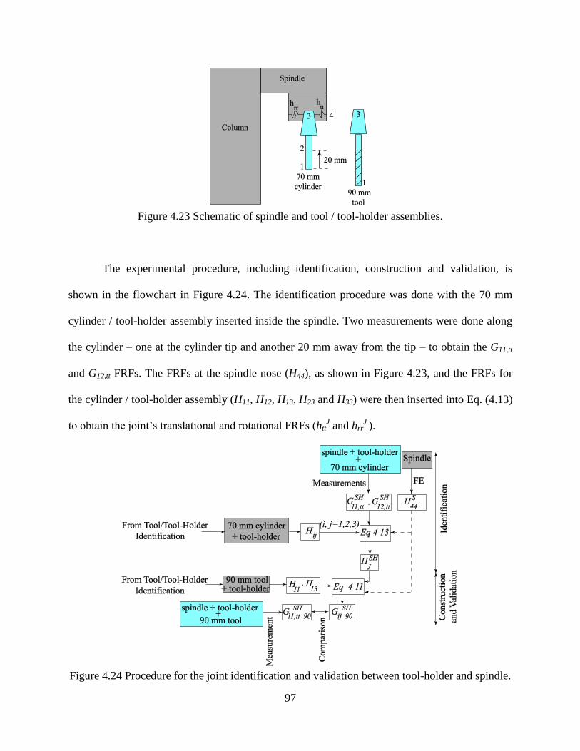
97

Figure 4.23 Schematic of spindle and tool / tool-holder assemblies.

The experimental procedure, including identification, construction and validation, is

shown in the flowchart in Figure 4.24. The identification procedure was done with the 70 mm

cylinder / tool-holder assembly inserted inside the spindle. Two measurements were done along

the cylinder – one at the cylinder tip and another 20 mm away from the tip – to obtain the G11,tt

and G12,tt FRFs. The FRFs at the spindle nose (H44), as shown in Figure 4.23, and the FRFs for

the cylinder / tool-holder assembly (H11, H12, H13, H23 and H33) were then inserted into Eq. (4.13)

to obtain the joint’s translational and rotational FRFs (httJ and hrr

J ).

Figure 4.24 Procedure for the joint identification and validation between tool-holder and spindle.

98

Figure 4.25 shows the joint’s translational FRF; and, as is evident in the figure, several

structural modes existed in the joint’s FRF. This shows that the joint between the tool-holder and

the spindle had more significant effects on the dynamics of the assembled structure than the joint

between the tool and tool-holder, which showed only one structural mode in Figure 4.20.

Figure 4.25 Joint’s translational FRF between the spindle and the tool-holder (httJ ).

The next step in the experimental procedure was the construction of the tool / tool-holder

/ spindle assembled structure’s FRFs by considering the joint dynamics between the tool and the

tool-holder and between the tool-holder and the spindle. The identified joint FRFs obtained using

the 70 mm cylinder / tool-holder assembly were used to build the tool tip FRFs for the 90 mm

end mill tool (Figure 4.24). For this purpose, the reconstructed FRFs for the 90 mm tool / tool-

holder assembly (H11, H13), the spindle nose FRF (H44) and the identified joint FRFs between the

tool-holder and the spindle (hJtt and h

Jrr) were inserted into the RC equation, Eq. (4.11).

In the validation of the accuracy of the identified joint properties, the reconstructed tool-

tip FRFs were compared with the measured tool-tip FRFs. To obtain the measured tool-tip FRFs,

the 70 mm cylinder was replaced with the 90 mm tool; and, the tool-tip FRFs were measured on

the machine. Figure 4.26 shows the comparison between the reconstructed FRF, measured FRF

99

at the tip of 90 mm tool and the assembled FRF obtained by considering a rigid joint between the

tool-holder and the spindle and between the tool and the tool-holder.

Figure 4.26 Direct FRFs at TCP with spindle / tool-holder / tool assembly (G11_90mm).

As evident from Figure 4.26, a close prediction of the tool-tip FRFs was obtained with

the model when compared to the measured FRFs. The considerable improvement obtained in

predicting the TCP FRFs compared to the rigid joint approximation shows the importance of the

joint dynamics properties between the tool-holder and the tool and between the tool-holder and

the spindle. If an accurate prediction at the TCP is sought, the joint dynamics effects should be

taken into account at both places.

4.6 Summary

A systematic procedure for the modeling and identification of joint characteristics was

presented in this chapter. The IRC method, which relates the joint’s FRFs to the assembled

structure’s translational FRFs and substructures FRFs, was developed and validated through FE

simulations. The IRC method obtained a joint’s exact parameters when the joint was comprised

of only stiffness and damping elements. For a continuous joint segment, the joint’s FRFs were

100

approximated through the IRC technique, in order to minimize the difference between the

predicted and measured assembled structure’s FRFs.

The IRC method suggests a symbolic solution for the joints’ FRFs, which eliminates the

necessity of a numerical solution. The proposed technique only requires two sets of

measurements on the translational FRFs of the assembled structure, which removes the need for

measuring rotational FRFs. This model is suitable for the structures where a limited number of

measurement locations are available.

In spite of these advantages, some limitations are associated with the IRC method. The

proposed joint FRF matrix, where the cross FRFs between the rotational and translational DOFs

are neglected, cannot be generalized for every type of joint and should be verified before

consideration with a structure.

Internal forces in the joint section are also considered to be equal in magnitude and

opposite in direction when a continuous joint was considered. This is an assumption that is

appropriate for structures where the joint acts as a connecting element with dominant stiffness

and damping properties. The joint can be modeled as a separate substructure to have a more

general joint model; however, this imposes more unknowns to the equations.

The proposed method was first applied on a lathe machine to obtain the joint dynamic

properties for a modular tool. The lathe machine and an inserted blank shaft inside the chuck

were considered as one substructure, and the modular tools were considered as the second

substructure. The identified joint dynamic properties were validated by using the identified

joint’s properties in predicting the behaviour of a different structure that used the same joint in its

setup.

101

The IRC method was then employed on a vertical CNC machine to find the joint

dynamics between the tool and the tool-holder and between the tool-holder and the spindle. A FE

model of the machine comprised of the column, table, head stock and spindle was first developed

and validated by idealizing the joints between the various structural components of the machine

as linear springs. The response obtained at the spindle nose with the validated virtual machine

tool model was subsequently used to approximate the full frequency response behaviour. This

was achieved by applying the IRC method and identifying joint dynamics between the tool and

the tool-holder and also between the tool-holder and the spindle. Although there still existed

some deviations between the predicted response and the measured behaviour, a considerable

improvement in response prediction for the assembled structure was observed by modeling and

identifying the joint dynamics compared to treating the joints as rigid.

The identified joint properties can be incorporated into the virtual model of an actual

machine to improve its accuracy and decrease the deviation between its prediction and the actual

behaviour of a structure. Having a validated virtual model of the machine tool center reduces the

need to perform several measurements at the tool tip, which were required in earlier studies, in

order to obtain TCP FRFs. Further studies are required to incorporate the effects of applied

prestress, tool diameter and drawbar clamp force on the identified properties.

All the studies in this chapter were conducted on 2D structures. However, the results

obtained in this study provided the essential knowledge to extend the introduced methodologies

to more general structures. In the next chapter, the proposed identification method is extended to

account for the effects of multiple joints in the structure.

102

Chapter 5. Multiple Joint Dynamics Identification

In reality, most structures do not behave as simple 2D structures and exhibit more

complex movement. For example, a multi-axial computer numerical control (CNC) machine is

comprised of different plates, bars and columns attached together at several locations. To obtain

joint dynamics properties in such structures, an identification technique that is capable of

identifying multiple joints dynamics is required. One of the major challenges in proposing such

identification technique is the measurement or estimation of the rotational frequency response

functions (FRFs). There are two types of rotational FRFs that are involved in the dynamics of

structures: (1) the angular displacement at location i to the applied force at location j (lij = θi/fj);

and, (2) the angular displacement at location i to the applied moment at location j (pij = θi/Mj).

Several methods have been proposed in order to address the difficulties associated with the

rotational FRFs. For instance, finite difference method [Schmitz and Duncan, 2005], has been

proposed to indirectly obtain the angular displacement at a particular location using two sets of

measurement. However, the measurement noise makes this method vulnerable to the errors.

Even if a reliable measurement technique is available, the application of pure moment to the

structure in a wide range of frequencies is very challenging, making direct measurement of pij

almost impossible. A new approach has been proposed by [Kumar and Schmitz, 2012] through

which the rotational FRFs of a milling tool are obtained by fitting a fixed-free Euler-Bernoulli

beam to each individual mode of the measured receptance. The rotational FRFs at the end of the

fitted fixed-free beam are then considered as the rotational FRFs of the tool.

The objective of this chapter is development of a joint identification method for

structures with multiple joints. Identification process is performed through the inverse receptance

103

coupling (IRC) method using translational receptances of the assembled structure obtained

through direct measurements and substructures’ FRFs obtained from the finite element (FE)

models. Provided that no excessive residual stress is induced in the structure after introducing the

joints, the IRC method obtains the joints’ FRFs by finding the difference between response of the

rigidly coupled substructures and response of the actual assembled structure with joints. To

overcome the difficulties associated with the rotational FRFs, a joint model comprised of only

translational elements is proposed. One of the assumptions of this model is that the moments

required in the joints originate from the couple between forces in the translational elements. The

assembled structure is also assumed to have dominant modes only in the directions that the joints

restrict.

This chapter is organized as follows. First, the general response-based receptance

coupling (RC) method that was introduced in Chapter 4 is extended to include effects of multiple

joints in a structure. Through the RC method, it is possible to obtain a structure’s FRFs based on

its constitutional elements’ dynamics. The IRC method is then proposed to relate the joint’s

FRFs to the FRFs of the assembled structure and substructures. The IRC method is employed in

a FE simulation to obtain the joints’ FRFs at four locations between two thin wall plates, which

were considered as substructures with 6 degrees of freedom (DOFs) at each node. The

simulations were treated as if the structures were actual cases and only the FRFs that could be

measured in practice were obtained from the FE models. Experimental tests on the thin shell

plates attached at four locations by bolted joints were also conducted to assess the applicability

of the proposed identification technique on the actual physical cases. To assure that the FE

models of the substructures in the experimental setup were accurate, the initial FE models were

modified through a model updating technique.

104

5.1 Extended Inverse Receptance Coupling Method

The RC method is a procedure that enables the determination of the dynamics of an

assembled structure by coupling the dynamics of its substructures, which are obtained

experimentally or mathematically, in the joint compatibility and equilibrium equations

[Mehrpouya et al., 2014; Park et al., 2003]. The proposed RC method in Chapter 4 is extended in

this chapter to account for the effects of multiple joints.

Figure 5.1 shows two Substructures, A and B, attached at n points through different joint

elements.

Figure 5.1 Generic substructures coupled through joint elements.

The relationship between the displacements and the applied forces on each substructure can be

written as:

AJAa

Aa

AaaAaa

AaaAaa

Aa

Aa

BJBb

Bb

BbbBbb

BbbBbb

Bb

Bb

FF

F

HH

HH

X

X

FF

F

HH

HH

X

X

(5.1)

where a’ and b’ represent the internal points on Substructures A and B, respectively; a =

{a1…an} and b = {b1…bn} represent the connecting points; {Xi}S and {Fi}S (i = a, b, a’, b’; S =

A, B) represent the displacement and external force vectors, respectively, at point i on

105

Substructure S; and, {FJ}S represents the internal force vectors at the joint. Considering that the

joints mainly impose stiffness and damping to the structure, the equilibrium condition becomes:

AJBJ

FF (5.2)

Therefore, the relationship between displacement vectors at the interface locations and the joint

forces is [Wang and Yang, 1999]:

BJJBbAa FHXX

(5.3)

where

JnJJJ

hhhDiagH ,,,21

(5.4)

is the joint’s FRF matrix and contains joints’ frequency dependant parameters. The assembled

structure’s FRFs can be obtained by substituting Eq. (5.3) back into Eq. (5.1):

a

a

b

b

aaaababa

aaaababa

ababbbbb

ababbbbb

a

a

b

b

F

F

F

F

GGGG

GGGG

GGGG

GGGG

X

X

X

X

][][][][

][][][][

][][][][

][][][][

(5.5)

where Gij (= Xi/Fj) are the FRFs of the assembled structure. Two of these FRFs can be expanded

as:

AaaBAaaAaaaa

BbbBBbbBbbbb

HHHHG

HHHHG

1

1

(5.6)

with

JBbbAaaB HHHH (5.7)

According to Eq. (5.5), the assembled structure’s FRFs are formulated based on the

substructures’ FRFs and the joints’ FRFs. Supposing that n locations on Substructure A are

connected to n locations on Substructure B through the joint and that each node has 6 DOFs, the

106

joint FRF matrix, HJ, and substructures FRF matrices, [Haa]A and [Hbb]B, become (n×6)×(n×6)

matrices. The assembled structure’s FRFs, including translational as well as rotational FRFs, can

be extracted through the RC method with known FRF values of the substructures and joints.

Although the consideration of a complete joint FRF matrix that includes all six DOFs at

each node generates exact values for the assembled structure FRFs, it requires high

computational effort, due to the dimensions of the large matrices. In particular, if the joint

parameters are sought and matrix inversion is required, large matrices impose major

computational restrictions on obtaining the required parameters. However, if the dominant

movements of a structure in a specific range of frequencies are known, the joint model can be

simplified to include only the elements in the directions that are excited at that particular

frequency range. This results in reducing the equations size with a simpler joint model while

obtaining an acceptable prediction over the assembled structures dynamics in the frequency

range of interest.

In the following section, a joint model that can represent the behaviour of the joint in the

structures that were examined in this chapter is presented. The joint model included only one

translational element at each connecting location between the two substructures, bringing the

joint FRF matrix size down to 4×4, while providing the required restrictions in the dominant

directions of the movement.

5.1.1 Modeling of the Joint

The structure considered in this chapter was comprised of two thin plates, i.e.

Substructures A and B, which were attached together at four locations. Each node on

Substructures A and B had 6 DOFs, including 3 translational DOFs along the x, y and z axes and

107

3 rotational degrees of freedom (RDOFs). The connections between the plates in the experiments

and simulations were provided through bolts and beam elements, respectively.

As shown in Figure 5.2(a), a complete joint model includes both translational (kt) and

rotational (kr) spring and damping elements in all directions. If such a model was considered for

the joint, the joint’s FRF matrix (Eq. (5.4)) would have 24 unknowns. In order to identify these

parameters, at least 24 measurements were needed on the assembled structure, with some of

these measurements on the RDOFs of the assembled structure. A simpler joint model was

proposed to overcome difficulties in measuring RDOFs and to avoid solving large equations.

(a) (b)

Figure 5.2 Substructures coupled through the joint element: (a) schematic model, (b) FE model.

In the simplified joint model, no translational elements were considered in the x and y

axes as the behaviour of the structure in these directions was not of interest. Also, the rotational

joint elements were eliminated, and their effects were assumed to originate from the moments of

the translational elements at different locations in the z direction [Movahhedy and Gerami,

2006]. The proposed joint model was valid while the dominant modes of the structure in Figure

5.2 were along the z axis and around the x and y axes in the studied frequency range. If other

modes significantly contributed to the response of the assembled structure, the proposed joint

model may not provide an acceptable prediction over the response of the assembled structure,

108

and a modified model that accounted for the effects of other contributing modes should be

provided.

By considering the simplified joint model, the assembled structure’s FRF (Ga’a’,zz)

becomes:

)41(,

0

0

14,

4

,3

,2

,1

1

444

3

2

1

44,

44,

34,

24,

14

,43

,33

,23

,13

,42

,32

,22

,12

,41,

31,

21,

11

44,

44,

34,

24,

14

,43

,33

,23

,13

,42

,32

,22

,12

,41

,31

,21

,11

41,

4,

3,

2,1

,

,

1

,,,,,

a

h

h

h

h

h

h

h

h

hhhh

hhhh

hhhh

hhhh

hhhh

hhhh

hhhh

hhhh

hhhhh

HHHHHhG

zzaa

zzaa

zzaa

zzaa

J

J

J

J

zzbbzzbbzzbbzzbb

zzbbzzbbzzbbzzbb

zzbbzzbbzzbbzzbb

zzbbzzbbzzbbzzbb

zzaazzaazzaazzaa

zzaazzaazzaazzaa

zzaazzaazzaazzaa

zzaazzaazzaazzaa

zzaazzaazzaazzaazzaa

zzaaJzzbbzzaazzaazzaazzaa

(5.8)

where G is the assembled structure’s FRF and hij,zz represents the FRFs of the substructures when

the measurement is on location i in the z direction and excitation is on location j in the z

direction.

Based on Eq. (5.8), the translational FRF of the assembled structure was related to the

substructures’ FRFs and a 4×4 joint FRF matrix. In order to find the joints’ FRFs, only four

measurements on the assembled structure were needed. This was a significant improvement over

the complete joint model, where 24 measurements were needed. If the joint is comprised of only

spring and damping elements, the off-diagonal terms of the joint FRF matrix in Eq. (5.8) were

zero. However, for a general joint, such as a bolted joint with inertial properties, the assumption

of considering the off-diagonal FRFs to be zero may result in some errors in the identified joints’

FRFs.

If the structure’s conditions for the validity of the joint model were satisfied, the joint’s

FRF matrix could be obtained using the measured receptances of the assembled structure and the

109

mathematically/experimentally obtained FRFs of the substructures. The identification technique

is described in the next section by introducing the IRC method.

5.1.2 Joint Identification

The proposed methodology for obtaining the FRFs of an assembled structure was

employed in an inverse way to extract the joints’ FRFs from the dynamics of the assembled

structure and substructures. Based on Eq. (5.8), points a’ (a’ = 1, 2, 3 and 4), which represent the

nodes on Substructure A in the assembled structure that were not involved in the connection

section, are expanded as:

)4:1,( ,1 jiHBHhG ajiaijij (5.9)

with

Jbbaa HHHB (5.10)

For simplicity, the zz subscript is not shown, since all the FRFs were obtained in the z direction;

therefore, hij was the FRF values between points i and j in the z direction on Substructure A in a

free-free boundary condition, and Hia and Hai were the FRF matrices between point i and the four

connecting points, i.e. a1, a2, a3 and a4 on Substructure A in a free-free boundary condition.

These values could be obtained from the FE model of Substructure A in free boundary

conditions. Gij was also the FRF between points i and j on the assembled structure, which could

be obtained experimentally by exciting the structure at location j and measuring at location i.

By considering four locations on Substructure A, Eq. (5.9) is expanded into a matrix form

as:

110

44144143142141

1

44414

413

412

411

44434241

34333231

24232221

14131211

44434241

34333231

24232221

14131211

aaaa

a

a

a

a

HHHHB

H

H

H

H

hhhh

hhhh

hhhh

hhhh

GGGG

GGGG

GGGG

GGGG

(5.11)

In order to obtain the joint FRF matrix, Eq. (5.11) needs to be solved for the B matrix, which can

be accomplished as:

1

1

4441

444441

1411

444441

1411

1

444

1

aa

a

a

Jbbaa

HH

GG

GG

hh

hh

H

H

HHHB

(5.12)

which yields to the joint FRF matrix as:

44342414

43332313

42322212

41312111

44342414

43332313

42322212

41312111

bbbbbbbb

bbbbbbbb

bbbbbbbb

bbbbbbbb

aaaaaaaa

aaaaaaaa

aaaaaaaa

aaaaaaaa

bbaaJ

hhhh

hhhh

hhhh

hhhh

hhhh

hhhh

hhhh

hhhh

B

HHBH

(5.13)

It should be noted that the G matrix can be constructed by measuring only one of the

rows or columns [Ewins, 1984]; therefore, four measurements on the assembled structure are

enough to reconstruct the complete matrix. From an experimental point of view, the only matrix

inversion that may be affected by measurement noise is the G matrix. The other matrices

involved in the inversion process were obtained from the FE model, which were noise free and

less prone to measurement errors. This was one of the benefits of the proposed methodology over

other methodologies that included the inversion of several measured matrices [Wang and Liou,

1990].

To investigate the accuracy of the proposed identification technique, two FE simulations

were conducted. The objective of these simulations was the determination of the joints’ FRFs or

111

joints’ parameters at different locations on an assembled structure using the proposed

identification technique. The simulations were treated as if they were real structures; and, only

the FRFs that could be measured on a physical structure (i.e. translational FRFs) were obtained

from the FE model. The identified joints’ FRFs were then used to obtain the FRFs of a new

assembled structure that had different substructures, but used the same joint configuration. The

details of each simulation are explained in the next section.

5.2 Finite Element Simulations

Two different simulations were conducted to investigate the effectiveness of the proposed

identification technique. The first simulation was performed to find the spring and damping

values of the joints, while the second simulation was aimed at finding the FRFs for the beam

segments that acted as the connecting joints. In these simulations, two substructures were

attached at four locations to each other, as shown in Figure 5.2(b). Substructure B was a 20 cm ×

7 cm × 6 mm plate with a modulus of elasticity (E) of 200 GPa, Poisson’s ratio () of 0.3 and

density of (ρ) of 7800 kg/m3. This substructure was clamped, and Substructure A was attached to

it through the joints.

Two plates were used in the simulations as Substructure A, namely Substructures A1 and

A2. Substructure A1 was used in the estimation of the joints’ parameters in the first simulation

and identification of joints’ FRFs in the second simulation. Substructure A2 was only used in the

second simulation to validate the identified joints’ FRFs obtained with Substructure A1. The first

plate (i.e. Substructure A1) was a 25 cm × 7 cm × 6 mm plate, and the second plate (i.e.

Substructure A2) was a 17 cm × 7 cm × 6 mm plate. Both of these substructures had the same

material properties as Substructure B.

112

The FE models of these plates were built in FE software and meshed with the shell

element (ANSYS shell181) [Ansys], which was a 4-node structural element with 6 DOFs at each

node. Two other elements, ANSYS combin14 and ANSYS beam188, were also used in the

simulations to provide the spring-damping model in the first simulation and the beam element in

the second simulation, respectively. After building the plate models, the damping properties were

introduced to the complete FE model. Since the only damping properties that were desirable to

be present in the joint section were damping values from the predefined combin14 element, the

damping properties were defined proportional to the mass matrix as C = 50 M, where C is the

damping matrix and M is the mass.

(a) (b)

Figure 5.3 FE simulation: (a) with the spring and damping elements, (b) with the beam elements.

The first simulation dealt with the identification of stiffness and damping constants that

were used in the assembled structure. This simulation included two substructures, Substructures

A1 and B that were connected at four points through the spring and damping elements, as shown

in Figure 5.3(a). The corresponding values for the connection elements are given in Table 5.1 at

each individual location. The objective of this simulation was the determination of the values of

each individual element using the proposed identification technique and four FRFs of the

assembled structure.

113

Table 5.1 Spring and damping constants used in the simulation of the joint.

Stiffness Constant (N/m) Damping Constant (N.s/m)

k1 = 4E6 c1 = 80

k2 = 9E6 c2 = 100

k3 = 10E6 c3 = 50

k4 = 7E6 c4 = 90

In order to use the proposed identification method, the FRFs of the assembled structure

and substructures were required. The FRFs of the assembled structure were chosen as the

translational FRFs at locations 1, 2, 3 and 4 in Figure 5.2(a). The required FRFs for each

substructure were derived from corresponding FE models. The free-free FE model of

Substructure A1 was used to obtain the direct and cross FRFs between points a1, a2, a3, a4, 1, 2, 3

and 4 in Figure 5.2(a). The clamped-free FE model of Substructure B was used to obtain the

FRFs at points b1, b2, b3 and b4. The obtained FRFs were then fed into Eq. (5.13) to calculate the

joint FRF values, which included the stiffness and damping constants as hJi = 1/(ki + j ω ci).

Figures 5.4 and 5.5 show the identified parameters for the stiffness and damping values.

The deviations that existed at low frequencies originated from the assumptions in the modeling

of the joint. Firstly, it was assumed that the joint could be modeled as a translational

spring/damping element in the z direction. The proposed identification technique yielded

accurate values for the joint if the structure underwent pure translation in the z direction and/or

rotation around the x/y axes. This is because the joints in the z direction accounted for the motion

of the structure in the z direction and the torque originated from every two springs accounted for

the rotation of the structure around the x/y direction. However, deviations were observed in the

identified parameters around the frequency ranges where the structure had a dominant mode in

other directions, i.e. translation in x/y or rotation around z, due to the negligible effects of the

joints in these directions. In this simulation, there were several modes in the x/y axes and around

114

the z axis around 0 Hz which contributed to the assembled structure’s FRFs at low frequencies.

Therefore, some deviations existed in the identified joint parameters below 50 Hz in Figures 5.4

and 5.5. The mode shapes for the first 3 structural modes of the structure are shown in Figure

5.6. There were three modes below 500 Hz; two translational modes in the z direction (Modes 1

and 2), and one rotational mode around the y axis (Mode 3). Both the contour plot and the

deformed shape are shown for each mode shape.

Figure 5.4 Identified stiffness values in Figure 5.3(a).

Figure 5.5 Identified damping constants in Figure 5.3(a).

Secondly, it has been observed through simulations that the response of the assembled

structure was insensitive to the joint parameters around the first natural frequency and below. In

other words, no significant changes occurred at low frequencies, i.e. below 150 Hz, in the

assembled structure’s FRF by changing the joint stiffness. Deviations observed in Figure 5.4 and

5.5 at low frequencies could also be attributed to the insensitivity of the assembled structure’s

response to the joint parameters. However, at higher frequencies, i.e. after 160 Hz, where the

115

assembled structure experienced local modes, the assembled structure’s FRF had higher

sensitivity to the joint parameters. For the proposed method to derive the joint’s parameters

accurately, the assembled structure’s FRFs needed to have high sensitivity to the joint

parameters. Also, the method needed to check the mode shapes of the structure for the locations

of the nodal points in each mode. In the frequency ranges where one or several joints fell around

the nodal points, the assembled structure’s response became highly insensitive to the joint

parameters and the identified parameters may deviate from the exact values.

(a) (b) (c)

Figure 5.6 Mode shapes of the assembled structure with B, A1 and spring/damping elements: (a)

32.00 Hz, (b) 160.47 Hz, (c) 308.49 Hz.

In the second simulation, the joints between the two substructures were provided through

beam elements, as shown in Figure 5.3(b). This simulation was done to investigate the

applicability of the proposed identification methodology in the cases where the joints contained

mass properties. The objectives of this simulation were the identification of the joints’ FRFs and

the use of the identified FRFs in a different assembled structure that had the same joint

configuration to predict its overall FRFs.

116

All four joint connections were built with beam elements with a diameter (D) of 5 mm,

modulus of elasticity (E) of 1 GPa, and density (ρ) of 2700 kg/m3. The assembled structure’s

FRFs, which were obtained at locations 1 to 4 in Figure 5.2, along with the substructures’ FRFs

were then inserted in Eq. (5.13), in order to obtain the joints’ FRFs at each individual location.

The identified joint FRFs are shown in Figure 5.7, where hJ1 and hJ3 refer to the identified joint’s

FRF at locations 1 and 3, respectively. The FRFs obtained at locations 2 and 4 were similar to

the FRFs at points 1 and 3, respectively. This was due to the fact that these points were under the

same deflection and stress in the studied frequency range.

Figure 5.7 Identified joint FRFs for the structure in Figure 5.3(b) with Substructures B and A1.

One of the assumptions in this study was approximation of the behaviour of the

continuous joint with a frequency-dependent translational spring/damping element in the z

direction. This assumption could result in deviations from the exact joint FRF because of

neglecting the effects of joint’s cross FRFs, ignoring the effects of the joint stiffness in the x and

y axes and ignoring the effects of joint rotational stiffness around the z axis. However, this

assumption was made in order to simplify the equations and rely only on the translational FRFs

of the assembled structure. If an accurate joint’s FRF was sought, the complete FRF matrix

which had more unknowns and required more measurements to solve should be considered for

117

the joint element. The validity of this assumptions and accuracy of identified FRF needed

assessment.

In order to assess the accuracy of the identified joints’ FRFs, the same joint configuration

was used in a different structure. To build the new assembly, Substructure A1 was replaced with

the shorter plate (i.e. Substructure A2). The identified joints’ FRFs along with the FRFs of

Substructures A2 and B were then used to predict the new assembled structure’s FRFs. The

reconstructed FRF was compared with the FE results to verify accuracy of the prediction.

The comparison between the predicted and simulated FRFs is shown in Figure 5.8. To

obtain the reconstructed FRF at point 1 in Figure 2(a), i.e. G11, the identified joints’ FRF from

the identification step and the FRFs of Substructures B and A2 were inserted into Eq. (5.8). The

reconstructed FRF is shown by the red line and the black line shows the reconstructed FRF when

the joints were considered to be rigid (i.e. Hj = 0 in Eq. (5.8)). The simulated (FE) FRF was

obtained by attaching Substructure A2 to Substructure B through the same beam elements that

were used in the identification structure and by performing a harmonic analysis on the assembled

structure’s FE model in Ansys FE software [Ansys].

Figure 5.8 Reconstructed G11 FRF for the assembled structure in Figure 5.3(b) with

Substructures B and A2.

118

From the results of Figure 5.8, it can be concluded that the identified joints’ FRFs were

able to provide an acceptable prediction over the FRFs of the new assembly, in terms of natural

frequencies, damping ratios and FRF magnitude. They also resulted in a considerable

improvement in the predicted FRFs compared to the rigid joint assumption. Figure 5.8 also

shows the range of validity of the assumptions in the modeling of the joint. Modeling of the

continuous joint as a frequency-dependent translational spring-damping element in the z

direction was valid in the range of frequencies where the structure had dominant modes in the z

direction and/or around x/y axes. At these frequencies, the effects of the joint in the x/y direction

and around the z axis were negligible as the structure was not moving in either of these

directions.

Mode shapes of the assembled structure are shown in Figure 5.9. As depicted in this

figure, there were 4 modes below 600 Hz. The first, third and fourth modes were the mode

shapes in the z direction and around the y axis, while the second mode shape was a translational

mode in the y direction. Having a close correlation between the reconstructed and simulated

assembled structure’s FRFs at high frequencies in Figure 5.8, i.e. after 100 Hz, showed the

effectiveness of the identification technique where the mode shapes were purely translational in

the z direction and/or rotational in the x/y directions. However, a poor correlation was obtained

between the predicted and simulated assembled structure’s FRF around the first two modes

where a translational mode in the y direction, Figure 5.9(b), occurred closely after the first mode.

This deviation was due to the limitations of our model which did not account for the effects of

translational modes in the y axis.

The two simulations that were discussed in this section showed the applicability of the

proposed technique in the identification of joint parameters and in the prediction of an assembled

119

structure’s dynamics. The simulations were treated as if the structures were actual physical

structures, and only the FRFs that could be measured in an actual structure were derived from the

FE model. In the next section, the proposed identification procedure was implemented on

physical structures to identify the joint FRFs and predict the assembled structure’s FRFs.

(a) (b)

(c) (d)

Figure 5.9 Mode shapes of the assembled structure with B, A2 and beam elements: (a) 41.48 Hz,

(b) 52.95 Hz, (c) 138.58 Hz, (d) 230.82 Hz.

5.3 Experimental Results

Several experiments were performed to further investigate the accuracy and applicability

of the proposed method in the identification of multiple joints on actual assembled structures.

120

The proposed IRC method was employed on an assembled structure to identify the joints’ FRFs

at four locations in the assembled structure. These FRFs were verified by replacing different

substructures. The effects of different conditions, such as adding an interface in the joint section,

were also investigated.

The experimental setup for the identification of multiple bolted joints included two thin

wall plates (i.e. Substructures A and B) attached together at four locations by bolted joints.

Substructure B, which remained unchanged in the identification and validation cases, was a

stainless steel plate clamped to a heavy solid plate, as shown in Figure 5.10(a). The clamped

length, width and thickness of this plate were 22 cm, 7.5 cm and 6.25 mm, respectively. This

substructure represented the part of a complex structure that had a complex geometry and the FE

model of which could not be easily made. Therefore, all the information for this substructure was

obtained through the experimental measurements.

In order to obtain the FRFs for Substructure B, four measurements were done at locations

b1 to b4, as shown in Figure 5.10(a). These measurements included both direct and cross FRFs.

The excitations were performed with an instrumented force hammer (PCB 2222), and the

measurements were conducted with a wide frequency bandwidth miniature accelerometer

(Kistler 8778A774) with a weight of 0.29 g.

Two identical plates with different lengths, 20 cm and 12 cm, were used as Substructure

A, as shown in Figure 5.10(b). The longer plate (Substructure A1) was used in the identification

step, and the shorter plate (Substructure A2) was used in the validation step. Substructures A1 and

A2 were assumed to have a simple geometry that could be modeled in FE. All the substructures’

plates had an identical thickness of 6.25 mm, with the corresponding material properties for

121

ST316 stainless steel: modulus of elasticity (E) of 193 GPa, Poisson’s ratio (ν) of 0.25 and

density (ρ) of 7990 kg/m3.

(a) (b) (c)

Figure 5.10 (a) Substructure B, (b) Substructure A, (c) assembled structure.

Although all the required FRFs for Substructures A1 and A2 could be obtained with direct

measurements, the FE model of this substructure was developed and used to decrease the number

of measurements. The FE models of these substructures were first developed with the estimated

parameters and then updated with the modal information, natural frequencies, obtained from

measurements on the free-free plates.

Table 5.2 Design variables boundary for the optimization scheme.

Design Variables

190 GPa < E < 210 GPa

7500 kg/m3 < ρ < 8100 kg/m

3

0.25 < υ < 0.35

5.8 mm < t < 7.0 mm

An optimization module of ANSYS software was used to perform the model updating

procedure. The estimated natural frequencies obtained from the FE model were compared to

122

those obtained from the measurements with the free-free condition. The design variables were E,

ρ, ν and the thickness of the plate (t). The lower and upper bounds for the design variables are

shown in Table 5.2.

The objective function was set as the square of the normalized difference between the

measured and predicted natural frequencies of the first two modes as:

2

1

2/

i

E

ni

E

ni

A

niobjfun (5.14)

whereniA and ni

E are the i

th natural frequency obtained from the FE model and the experiment,

respectively.

To perform measurements on Substructure A1 and A2, the 20-cm and 12-cm plates were

hung by a cord at location a4 to provide free-free boundary conditions, and the h11 (= x1/F1) FRF

was measured at point 1, as seen in Figure 5.10(b). The updating process was then initiated,

based on the measured and initially predicted natural frequencies. The updating process

converged after 4 iterations for Substructure A2. The natural frequencies of Substructure A2

before and after updating are presented in Table 5.3. Figure 5.11 shows the h11 FRF in

comparison with the measured FRF before and after updating. The updated design variables were

then used to improve the FE models of Substructure A2. A similar procedure was performed on

Substructure A1 to update the initial FE model.

Table 5.3 Comparison of natural frequencies before and after updating.

Measured

(Hz)

Before Updating

(Hz)

Error

(%)

After Updating

(Hz)

Error

(%)

n1 2031.0 2146.0 5.6 2042.0 0.5

n2 2116.0 2206.0 4.3 2102.0 0.7

123

Figure 5.11 h11 FRF for Substructure A2 before and after updating.

Using the curve fitting method on the measured FRF, the first damping ratio was

obtained as 1.4%. This value was introduced to the updated FE model of Substructures A1 and

A2 to obtain the required FRFs in the identification procedure.

To construct the assembled structure, Substructure A1 was attached to Substructure B at

four locations through identical steel bolts, and a torque of 8.5 N.m was applied to each bolt by a

torque wrench. The assembled structure’s FRFs were then measured at four locations 1 to 4

shown in Figure 5.10(c) to obtain G11, G12, G13 and G14. From these four FRFs, the other

components of the assembled structure’s FRF matrix (G) were constructed.

Once the required information for the substructures and assembled structure was

available, the proposed method was applied in the experimental setup. The process, including

identification and validation steps, is illustrated in the flow chart in Figure 5.12. In the

identification step, the properties of the joints, HJ, were identified using the FE model of

Substructure A1 and the measurements on the assembled structure and Substructure B. In the

validation step, Substructure A1 was replaced with Substructure A2, and the identified joints’

124

properties were used to predict the new structure’s FRF. This FRF was compared with the

experimentally obtained FRF of the new structure.

Figure 5.12 Experimental process for identification and validation.

In order to obtain the joint FRFs at each location between substructures, the measured

FRFs on the assembled structure and Substructure B, along with the analytical FRFs of

Substructure A1, were inserted into Eq. (5.13). This equation obtained the FRFs for each

individual connection between the two plates. The identified joint’s FRFs are shown in Figure

5.13. From this graph, it can be seen that hJ1 and hJ3 followed the same trend as those of hJ2 and

hJ4, respectively. This is because points 1 and 2 were located at the same longitudinal locations

(y direction in Figure 5.2) and experienced similar deformation in the studied frequency range.

This also applies to the joints at locations 3 and 4.

As shown in Figure 5.13, the joints’ FRFs were identified for each individual joint at

each frequency. These FRF values can be saved, with respect to the applied torque on the bolts,

125

joint materials and the contact area between substructures, and can then be used in the prediction

of the dynamics of another assembled structure provided that the joint conditions, such as

applied torque, manufacturing tolerances and the area of contact, stay similar.

Figure 5.13 Identified joint FRFs in the assembled structure in Figure 5.10(c).

After identification of the joints’ FRFs, the validation step was performed to examine the

accuracy of the identified joints’ FRFs. The validation was done by replacing the 20-cm long

plate of Substructure A1 with the 12-cm plate of Substructure A2 and providing similar joint

conditions to the new assembled structure. The identified joints’ FRFs that were acquired in the

identification step, shown in Figure 5.13, along with the FRFs of Substructures A2 and B were

then inserted in Eq. (5.8) to reconstruct the new assembled structure’s FRF at location 1, G11.

This FRF was also measured on the new assembly and compared with the predicted FRF. The

comparison is shown in Figure 5.14. To observe the improvement that was achieved in the

prediction of the assembled structure’s FRF compared to the rigid joint assumption, the joint’s

FRF was set to be zero in Eq. (5.8), i.e. Hj = 0; and, the assembled structure’s FRF was also

obtained for the rigid joint assumption.

126

Figure 5.14 Predicted vs. measured G11 FRFs for the assembled structure of Substructures B and

A2.

From Figure 5.14, it can be concluded that the predicted FRF obtained with the identified

joints’ FRFs had significant improvements in both the natural frequencies and the FRF amplitude

compared to the prediction obtained with the rigid joint assumption. The first peak at low

frequencies, around 50 Hz, was not considered as a structural mode, since the recorded

coherence in this region was poor. Although a good correlation was observed in the prediction of

the natural frequencies of the structure at the third and sixth modes, a significant discrepancy

existed between the predicted and measured damping ratio at these two frequencies. This

difference can be attributed to the inaccurate estimation of damping ratios for Substructure A1. A

poor recorded coherence at the 1400-1800 Hz interval also made the results obtained in this

region unreliable. Measurement errors and nonlinearities in the structure can also affect the

accuracy of the identification.

Table 5.4 compares the natural frequencies of the assembled structure obtained from the

measurements and from two predictions obtained with the identified joints and with the rigid

joint assumption.

127

Table 5.4 Comparison of the natural frequencies obtained from different FRFs.

ωn1 ωn2 ωn3 ωn4 ωn5 ωn6

Measured (Hz) 68.0 421.0 468.5 1183.0 1919.0 1999.0

Rigid Joint (Hz) 74.0 288.0 382.0 1052.0 1588.0 1768.0

Error (%) =

(Rigid Joint-Measured) ×100

Measured

8.8 31.6 18.5 11.1 17.2 11.6

Reconstructed (Hz) 54.0 434.0 454.0 1252.0 1902.0 1978.0

Error (%) =

(Reconstructed-Measured) ×100

Measured

20.6 3.1 3.0 5.8 0.9 1.1

The joints’ FRFs were obtained for the structure with no interface between the two plates,

as shown Figure 5.10(c). To investigate the effects of applying different conditions in the joint

section, different interfaces were inserted between plates. The identification procedure was then

applied to each new structure to find the joints’ FRFs and to compare them with the identified

joints’ FRFs from the structure with no interface. This investigation is discussed in the following

section.

5.3.1 Effects of Different Interfaces on the Joint Dynamics

The effects of adding different interfaces to the joints between the two plates were

studied through two experiments. In the first experiment, two nylon nuts were inserted between

the two plates at each joint location, as shown in Figure 5.15(a). The experimental substructure

included Substructures B and A1, as shown in Figures 5.10(a) and 5.10(b), attached together

through identical bolts and nuts. A torque of 8.5 N.m was applied to fasten the bolts when the

two nylon nuts were between the plates. Four FRFs were measured on the assembled structure at

locations 1 to 4 as shown in Figure 5.10(c). The measured FRFs along with the FRFs of

Substructures A1 and B were substituted into Eq. (5.13) to identify the joints’ FRF at the four

128

locations. The joint FRF at location 3 (J3 in Figure 5.15) is shown in Figure 5.16 in comparison

with the joint FRF obtained at the same location in the setup with no interface between the

plates, i.e. Figure 5.10(c).

Figure 5.15 Experimental setups: (a) nylon nut interface, and (b) elastic interface.

Figure 5.16 Identified joint’s FRF at location 3 (J3) on the structure with nylon nut interface and

on the structure without interface.

According to Figure 5.16, lower natural frequencies and static stiffness were obtained for

the structure with the nylon bolt interface than for the structure without any interface. This

observation can be attributed to the decreased stiffness of the contact area with the nylon bolts as

the contact area decreased after insertion of nylon bolts.

129

In the second experiment, the effect of inserting an elastic gasket between plates was

studied. The experimental structure included Substructures A1 and B with an ABS (acrylonitrile

butadiene styrene) rubber elastic gasket between two plates, as shown in Figure 5.15(b). Four

measurements were done at locations 1 to 4, as shown in Figure 5.10(c), on the assembled

structure to obtain the assembled structure’s FRF matrix. The measured assembled structure’s

FRFs along with the FRFs of the substructures were used in Eq. (5.13) to find joint’s FRFs at

four locations. The identified joint’s FRF at location 3 (J3 in Figure 5.15) was compared with the

identified joint’s FRF at the same location on the assembled structure without any interface.

Figure 5.17 shows the identified joint’s FRF when there was an elastic gasket in the joint

section and when there was no interface between the plates. Based on Figure 5.17, lower natural

frequencies were observed for the structure with an elastic interface between the plates. The

static stiffness was also lower than the structure with no interface between the plates. These

observations confirm the fact that the stiffness in the contact area decreased after introducing the

elastic interface to the joint.

Figure 5.17 Comparison of the identified joint’s FRF at location 3 (J3) on the structure with

elastic gasket and on the structure without any interface.

The two experiments conducted on the effects of different joint interfaces on the

identified joint’s FRFs proved the effectiveness of the identification procedure in distinguishing

130

the difference between different joint conditions. If the FRFs of the assembled structure and

substructures can be measured, the identification procedure can be applied to the structure, in

order to obtain the joint characteristics. Other joint conditions, such as effects of change in the

material of the joint, effects of temperature, effects of applied torque and effects of losing a bolt

can be subjects of further studies.

5.4 Summary

In this chapter, the IRC method was extended to include effects of multiple joints in the

structure. The proposed methodology related the joint’s FRFs to the FRFs of assembled structure

and substructures. By proposing a joint model that included only translational elements, the

identification method relied only on translational FRFs of the assembled structure. The FE

simulations proved accuracy of the proposed method. The experiments conducted on two plates

with four bolted joints were aimed at identifying the joint’s FRFs and using the identified joints

in the prediction of another assembled structure’s FRFs that used the same joint configuration

with similar conditions. A close correlation was observed between the measured FRF of the

assembled structure and the predicted FRF, confirming the effectiveness of the identified joints’

FRFs in predicting subsequent structure’s FRFs.

In addition to comparing the predicted FRFs with the measured FRFs, the joints’ FRFs

were also compared to each other for the different joint interfaces. The capability of the proposed

technique in capturing the changes in the joints and reflecting these changes in the identified

FRFs confirmed the reliability of the proposed technique in identifying different joint conditions.

In spite of applicability of the proposed technique in the real structures, there were

several assumptions and limitations associated with the proposed method. From the modeling

131

point of view, the joint model only included translational elements, and rotational properties

were assumed to originate from the couple between the translational elements. This assumption

may impose some errors in the identification of joint dynamics where two closely located

rotational and translational modes occur. In such a case, an overestimated parameter for the joint

parameter may be obtained. In such a case, the joints have to account for the rotational modes, as

well as the translational modes, at the same frequencies.

Based on the simulations and experimental tests, it was observed that the proposed

technique was reliable in the range of frequencies where the joint section was under sufficient

excitation and deformation. For the structure’s output to have a high sensitivity to the changes in

the joints’ parameters, the joint should have lower stiffness compared to the adjacent

substructures; otherwise, no deformation occurs at the first few structural modes in the joint

section, and the identification procedure will not accurately predict the joints’ FRFs. Also, the

proposed technique will not accurately predict the joints’ FRFs when there are dominant modes

in the lateral directions. These modes cannot be predicted by the proposed joint model, since no

joint element is considered in these directions. To have reliable joint’s FRFs, the lateral modes

should be far from the studied frequency range and make a low contribution to the assembled

structure’s response.

In the next Chapter, the IRC method is extended to 3D structures. A more generic joint

model which accounts for the inertial properties of the joint is proposed and the joint’s FRFs are

related to the translational FRFs of the assembled structure and substructure’s FRFs.

132

Chapter 6. Identification of Joint Dynamics in 3D Structures

Chapters 4 and 5 focused on the identification of joint dynamics in two-dimensional (2D)

structures. However, in actual physical structures, different degrees of freedoms (DOFs),

including rotational and translational DOFs, are coupled in the motion. In this chapter, the

identification of joint dynamics in three-dimensional (3D) structures is investigated. The

objective of this chapter is to provide a methodology through the inverse receptance coupling

(IRC) method to find joint’s rotational and translational frequency response functions (FRFs).

The proposed method requires only the translational FRFs of the assembled structure, thereby

avoiding the difficulties in the measurement of rotational FRFs. Unlike the majority of previous

studies, a complete joint FRF matrix, which accounts for the effects of cross FRFs, is proposed.

The proposed method also accounts for the effects of the joint’s inertial properties, which is

essential when the joint’s mass is comparable with that of the other substructures.

The existing IRC method is first extended in 3D structures to include the effects of

translational and rotational DOFs. Through the IRC method, it is possible to obtain a joint’s

FRFs using the FRFs of the assembled structure and substructures. A linear joint model with 6

DOFs at each node is utilized in the formulation of the proposed identification method. A

complete joint FRF matrix enables the determination of a joint’s accurate FRFs using only the

translational FRFs of the assembled structure.

A finite element (FE) simulation was performed to evaluate the accuracy of the proposed

methods. The effects of noise in the measurements were also investigated in the FE simulation,

and suggestions to mitigate noise effects were proposed. In the experimental setup, the

applicability of the proposed methodology was examined on a physical structure. FE models of

133

the substructures were built and updated using modal tests on the substructures. The translational

FRFs of the assembled structure that were measured on the physical structure were then fed into

the identification algorithm to obtain the joint FRFs.

The successful utilization of the proposed method in simulations and experiments

indicate that the proposed method can be applied on real structures, such as machine tools. It is

possible to obtain the joint properties between different components of a machine tool, such as

between the column and the base and between the column and spindle housing, through the

proposed methodology. These locations, which are usually ignored in virtual models, have

significant effects on the dynamics of the entire structure, especially at low frequencies.

6.1 Extended Inverse Receptance Coupling Method

Substructures A and B are connected through a generic joint element, as shown in Figure

6.1. The points on each substructure in the uncoupled state are divided into internal points (iA

and iB) and contact points (cA and cB).

Figure 6.1 Subcomponents in the uncoupled and coupled state.

The relations between the displacements and the forces in each substructure at the

uncoupled state are defined as:

134

(6.1)

where xiS and xc

S (S = A, B) represent the vectors of the translational and rotational displacements

in all 6 directions at locations i and c on Substructure S; fiS and fc

S represent the vectors of forces

and moments in all 6 directions at the internal and contact points, respectively; and, HS (S = A, B)

is the substructure’s FRF in the uncoupled state. For the joint section we have:

(6.2)

where fnJ (n = 1, 2) is the vector of forces and moments at location n on the joint; xn

J (n = 1, 2) is

the vector of the translational and rotational displacements in all 6 directions at location n on the

joint; and, HJ is the joint’s FRF.

In order to obtain the assembled structure’s FRFs based on the substructures’ FRFs, the

substructures’ FRFs need to be inserted into the equilibrium and compatibility equations. The

condition of equilibrium at the joint section is expressed as:

(6.3)

where FCS (S = A, B) represents the vector of forces and moments of the assembled structure at

the contact points of Substructure S. The condition of compatibility is:

(6.4)

where XCS (S = A, B) represents the vector of the translational and rotational displacements of the

assembled structure at the contact points on Substructure S. The internal forces and coordinates

do not change after coupling [Liu et al., 2002]. Therefore,

Sc

Si

Scc

Sci

Sic

Sii

Sc

Si

f

f

HH

HH

x

x

J

JJ

J

J

JJ

JJ

J

J

f

fH

f

f

HH

HH

x

x

2

1

2

1

2

1

2221

1211

J

J

Bc

Ac

BC

AC

f

f

f

f

F

F

2

1

J

J

Bc

Ac

BC

AC

x

x

x

x

X

X

2

1

135

and (6.5)

where FIS (S = A, B) represents the vector of forces and moments of the assembled structure at

the internal points on Substructure S; and, XIS (S = A, B) represents the vector of the translational

and rotational displacements of the assembled structure at the internal points on Substructure S.

Rearranging Eq. (6.3) and using Eq. (6.2) gives:

(6.6)

Replacing joint’s displacement vector with Eq. (6.4) gives:

Bc

Ac

Bcc

Acc

Bi

Ai

Bci

Aci

Bc

AcJ

BC

AC

Bc

Ac

f

f

H

H

f

f

H

H

x

xH

F

F

f

f

0

0

0

01 (6.7)

By replacing internal forces vector with Eq. (6.4), we have:

BI

AI

Bci

AciJ

BC

AC

Bc

Ac

Bcc

AccJ

F

F

H

HH

F

F

f

f

H

HHI

0

0

0

0 11 (6.8)

By expanding the first row of Eq. (6.1) for S = A and B, we have:

BI

AI

Bci

AciJ

BC

AC

Bcc

AccJ

Bic

Aic

BI

AI

Bii

Aii

BI

AI

F

F

H

HH

F

F

H

HHI

H

H

F

F

H

H

X

X

0

0

0

0

0

0

0

0

11

1

(6.9)

Simplifying Eq. (6.9) results in:

BC

ACJ

Bcc

AccJ

Bic

Aic

BI

AI

Bci

Aci

Bcc

AccJ

Bic

Aic

Bii

Aii

BI

AI

F

FH

H

HH

H

H

F

F

H

H

H

HH

H

H

H

H

X

X

1

1

0

0

0

0

0

0

0

0

0

0

0

0

(6.10)

Bi

Ai

BI

AI

f

f

F

F

Bi

Ai

BI

AI

x

x

X

X

J

JJ

BC

AC

J

J

BC

AC

Bc

Ac

x

xH

F

F

f

f

F

F

f

f

2

11

2

1

136

Therefore, the assembled structure’s FRFs at the internal coordinates become:

B

ci

A

ci

B

cc

A

cc

JJ

JJ

B

ic

A

ic

B

ii

A

ii

B

II

BA

II

AB

II

A

II

H

H

H

H

HH

HH

H

H

H

H

GG

GG

0

0

0

0

0

0

0

01

2221

1211 (6.11)

where GIIA and GII

B represent the assembled structure’s direct FRFs between the internal nodes

on Substructures B and A, respectively; and, GIIAB

represents assembled structure’s cross FRFs

between the internal nodes on Substructure B and the internal nodes on Substructure A.

Equation (6.11) is in the most general form for relating the assembled structure’s FRFs to

its subcomponents’ FRFs. This equation uses the complete joint FRF matrix, including cross

FRFs (i.e. H12J and H21

J ), to obtain the assembled structure’s FRFs. Ignoring the cross FRFs can

result in deviation from the exact assembled structure’s FRFs [Mehrpouya et al., 2013].

Figure 6.2 Assembled structure comprised of Substructures A and B and the joint.

Equation (6.11) was extended in this chapter to derive the FRFs of a 3D structure shown

in Figure 6.2. The assembled structure included two substructures, A and B, which were attached

at one location through a joint segment. Each substructure had 6 DOFs at each node, three

translational DOFs along the x, y and z axes, and three rotational DOFs around the translational

axes. The internal and contact points for Substructure A were selected as iA = {a1, a2, a3} and

137

cA = {1}, respectively. For Substructure B, the internal points were considered as iB = {b1, b2,

b3} and the one contact point was considered as cB = {2}.

Based on the selection of internal and contact nodes for Substructures A and B, HiiB and

HiiA became (3×6)×(3×6) matrices, while Hic

B and Hic

A were (3×6)×(1×6), Hcc

B and Hcc

A were

(1×6)×(1×6); and, HciB and Hci

A were (1×6)×(3×6). As an example, the Hci

B matrix was expanded

in Eq. (6.12) as:

(6.12)

where H2b1 is:

rzbrzrybrzrxbrzzbrzybrzxbrz

rzbryrybryrxbryzbryybryxbry

rzbrxrybrxrxbrxzbrxybrxxbrx

rzbzrybzrxbzzbzybzxbz

rzbyrybyrxbyzbyybyxby

rzbxrybxrxbxzbxybxxbx

b

hhhhhh

hhhhhh

hhhhhh

hhhhhh

hhhhhh

hhhhhh

H

1,21,21,21,21,21,2

1,21,21,21,21,21,2

1,21,21,21,21,21,2

1,21,21,21,21,21,2

1,21,21,21,21,21,2

1,21,21,21,21,21,2

12

(6.13)

In Eq. (6.13), h2x,b1x = x2 / fx,b1, h2y,b1ry = y2 / My,b1 and h2rz,b1rz = θz2 / Mz,b1 where x2 and y2

represent the translational DOF of point 2 in the x and y directions, respectively; fx,b1 represents

the force in the x direction at point b1; and, My,b1 and Mz,b1 represent the moment at point b1 in

the y and z directions, respectively.

The translational FRFs (i.e. hp,q with p,q = x, y, z) showed the displacements imposed by

the forces, and the rotational FRFs (i.e. hrp,rq) showed the rotations caused by the moments. The

fully populated joint FRF matrix enabled us to account for the displacements caused by moments

(i.e. hp,rq) and the rotations caused by the forces (i.e. hrp,q) through non-zero off-diagonal entities.

The joint element connected at two locations on the assembled structure made the joint’s

FRF a (2×6)×(2×6) matrix. H11J is expanded in Eq. (6.14):

322212 bbbBci HHHH

138

rzrzryrzrxrzzrzyrzxrz

rzryryryrxryzryyryxry

rzrxryrxrxrxzrxyrxxrx

rzzryzrxzzzyzxz

rzyryyrxyzyyyxy

rzxryxrxxzxyxxx

J

hhhhhh

hhhhhh

hhhhhh

hhhhhh

hhhhhh

hhhhhh

H

,11,11,11,11,11,1

,11,11,11,11,11,1

,11,11,11,11,11,1

,11,11,11,11,11,1

,11,11,11,11,11,1

1,11,11,11,11,11,1

11

(6.14)

As a result, the assembled structure’s FRF (GIIA) became a (3×6)×(3×6) matrix, which included

both translational and rotational FRFs.

Since there are many limitations associated with the measurement of rotational FRFs, our

interest in this chapter was the sole use of the translational FRFs of the assembled structure. The

use of only translational FRFs of the assembled structure in the joint identification has a

considerable benefit, as there is no need to measure or estimate the assembled structure’s

rotational FRFs. Although there are some methods that indirectly obtain rotational FRFs of a

structure [Ozsahin et al., 2009], these methods are highly sensitive to measurement noise.

Using Eq. (6.11), G1ax,1ax is expanded in Eq. (6.15) as:

Txarzxaryxarxxazxayxax

B

cc

A

cc

JJ

JJ

rzxaryxarxxazxayxaxxa

xaxaxaxa

hhhhhh

H

H

HH

HH

hhhhhh

hG

000000

0

0

000000

1,11,11,11,11,11,1

1

1,11,11,11,11,11,1

1,11,1

2221

1211

(6.15)

where subscript a denotes Substructure A.

Since the joint’s FRF matrix was a 12×12 matrix, we needed to form a 12×12 matrix of

the assembled structure’s translational FRFs on the left-hand-side of Eq. (6.15). This was

achieved by selecting 3 points on each substructure. Equation (6.16) presents the expanded

FRFs:

139

ciB

cc

A

cc

JJ

JJ

iciiII HH

H

HH

HHHHG

1

66

66

12120

0

2221

1211

(6.16)

ybybybybybybxbybxbybxbybyaybyaybyaybxaybxaybxayb

ybybybybybybxbybxbybxbybyaybyaybyaybxaybxaybxayb

ybybybybybybxbybxbybxbybyaybyaybyaybxaybxaybxayb

ybxbybxbybxbxbxbxbxbxbxbyaxbyaxbyaxbxaxbxaxbxaxb

ybxbybxbybxbxbxbxbxbxbxbyaxbyaxbyaxbxaxbxaxbxaxb

ybxbybxbybxbxbxbxbxbxbxbyaxbyaxbyaxbxaxbxaxbxaxb

ybyaybyaybyaxbyaxbyaxbyayayayayayayaxayaxayaxaya

ybyaybyaybyaxbyaxbyaxbyayayayayayayaxayaxayaxaya

ybyaybyaybyaxbyaxbyaxbyayayayayayayaxayaxayaxaya

ybxaybxaybxaxbxaxbxaxbxayaxayaxayaxaxaxaxaxaxaxa

ybxaybxaybxaxbxaxbxaxbxayaxayaxayaxaxaxaxaxaxaxa

ybxaybxaybxaxbxaxbxaxbxayaxayaxayaxaxaxaxaxaxaxa

II

GGGGGGGGGGGG

GGGGGGGGGGGG

GGGGGGGGGGGG

GGGGGGGGGGGG

GGGGGGGGGGGG

GGGGGGGGGGGG

GGGGGGGGGGGG

GGGGGGGGGGGG

GGGGGGGGGGGG

GGGGGGGGGGGG

GGGGGGGGGGGG

GGGGGGGGGGGG

G

3,32,31,33,32,31,33,32,31,33,32,31,3

3,22,21,23,22,21,23,22,21,23,22,21,2

3,12,11,13,12,11,13,12,11,13,12,11,1

3,32,31,33,32,31,33,32,31,33,32,31,3

3,22,21,23,22,21,23,22,21,23,22,21,2

3,12,11,13,12,11,13,12,11,13,12,11,1

3,32,31,33,32,31,33,32,31,33,32,31,3

3,22,21,23,22,21,23,22,21,23,22,21,2

3,12,11,13,12,11,13,12,11,13,12,11,1

3,32,31,33,32,31,33,32,31,33,32,31,3

3,22,21,23,22,21,23,22,21,23,22,21,2

3,12,11,13,12,11,13,12,11,13,12,11,1

ybybybybybybxbybxbybxbyb

ybybybybybybxbybxbybxbyb

ybybybybybybxbybxbybxbyb

ybxbybxbybxbxbxbxbxbxbxb

ybxbybxbybxbxbxbxbxbxbxb

ybxbybxbybxbxbxbxbxbxbxb

yayayayayayaxayaxayaxaya

yayayayayayaxayaxayaxaya

yayayayayayaxayaxayaxaya

yaxayaxayaxaxaxaxaxaxaxa

yaxayaxayaxaxaxaxaxaxaxa

yaxayaxayaxaxaxaxaxaxaxa

ii

hhhhhh

hhhhhh

hhhhhh

hhhhhhZEROS

hhhhhh

hhhhhh

hhhhhh

hhhhhh

ZEROShhhhhh

hhhhhh

hhhhhh

hhhhhh

H

3,32,31,33,32,31,3

3,22,21,23,22,21,2

3,12,11,13,12,11,1

3,32,31,33,32,31,3

3,22,21,23,22,21,2

3,12,11,13,12,11,1

3,32,31,33,32,31,3

3,22,21,23,22,21,2

3,12,11,13,12,11,1

3,32,31,33,32,31,3

3,22,21,23,22,21,2

3,12,11,13,12,11,1

)6(

)6(

140

Using Eq. (6.16), the joint’s FRF matrix can be obtained as:

(6.17)

Equation (6.17) gives the joint’s complete FRF matrix using the assembled structure’s

translational FRFs and its substructures’ FRFs. From an experimental point of view, only 12

measurements on the translational DOF of the assembled structure are required to obtain the full

joint’s FRF matrix. The substructures’ FRFs can also be found through updated FE models of

each individual substructure.

In the following section, a FE simulation is performed to investigate the accuracy of the

proposed method. This simulation was done to mimic the experimental conditions. All the

rzybryybrxybzybyybxyb

rzybryybrxybzybyybxyb

rzybryybrxybzybyybxyb

rzxbryxbrxxbzxbyxbxxb

rzxbryxbrxxbzxbyxbxxb

rzxbryxbrxxbzxbyxbxxb

rzyaryyarxyazyayyaxya

rzyaryyarxyazyayyaxya

rzyaryyarxyazyayyaxya

rzxaryxarxxazxayxaxxa

rzxaryxarxxazxayxaxxa

rzxaryxarxxazxayxaxxa

ic

hhhhhh

hhhhhh

hhhhhh

hhhhhhZEROS

hhhhhh

hhhhhh

hhhhhh

hhhhhh

ZEROShhhhhh

hhhhhh

hhhhhh

hhhhhh

H

2,32,32,32,32,32,3

2,22,22,22,22,22,2

2,12,12,12,12,12,1

2,32,32,32,32,32,3

2,22,22,22,22,22,2

2,12,12,12,12,12,1

1,31,31,31,31,31,3

1,21,21,21,21,21,2

1,11,11,11,11,11,1

1,31,31,31,31,31,3

1,21,21,21,21,21,2

1,11,11,11,11,11,1

)6(

)6(

ybrzybrzybrzxbrzxbrzxbrz

ybryybryybryxbryxbryxbry

ybrxybrxybrxxbrxxbrxxbrx

ybzybzybzxbzxbzxbz

ybyybyybyxbyxbyxby

ybxybxybxxbxxbxxbx

yarzyarzyarzxarzxarzxarz

yaryyaryyaryxaryxaryxary

yarxyarxyarxxarxxarxxarx

yazyazyazxazxazxaz

yayyayyayxayxayxay

yaxyaxyaxxaxxaxxax

ci

hhhhhh

hhhhhh

hhhhhh

hhhhhhZEROS

hhhhhh

hhhhhh

hhhhhh

hhhhhh

ZEROShhhhhh

hhhhhh

hhhhhh

hhhhhh

H

3,22,21,23,22,21,2

3,22,21,23,22,21,2

3,22,21,23,22,21,2

3,22,21,23,22,21,2

3,22,21,23,22,21,2

3,22,21,23,22,21,2

3,12,11,13,12,11,1

3,12,11,13,12,11,1

3,12,11,13,12,11,1

3,12,11,13,12,11,1

3,12,11,13,12,11,1

3,12,11,13,12,11,1

)6(

)6(

ccicIIiiciJ HHGHHH 1

141

required FRFs in the identification step were obtained from the FE models. The joint between

two subcomponents was provided by a beam element, which mimicked the experimental

conditions more realistically. The proposed method was then employed to obtain the joint’s

FRFs and validate the identified FRFs.

6.2 Finite Element Simulations

In order to assess the accuracy of the proposed identification method, a FE simulation

was conducted. The objective of this simulation was the utilization of the proposed methodology

to obtain the joint’s FRFs, using the FRFs of the substructures and the assembled structure. The

identified FRFs were then compared to the joint’s exact FRFs obtained from the corresponding

joint’s FE model.

Figure 6.2 shows the configuration that was studied in this simulation. Two substructures,

A and B, were attached at locations 1 and 2 by a continuous joint element. The dimensions of

each substructure are presented in Table 6.1. Both substructures were considered to have

material properties of aluminum with a modulus of elasticity (E) of 67.5 GPa, Poisson’s ratio ()

of 0.3 and a density of (ρ) of 2712 kg/m3. The joint was considered to have a diameter of 10 cm,

a length of 50 cm, a modulus of elasticity (E) of 200 GPa, Poisson’s ratio () of 0.3 and a density

of (ρ) 7850 kg/m3.

Table 6.1 Dimensions of the blocks used in the simulation.

h1 w1 l1 h2 w2 l2 h3 w3 l3

Length

(cm)

5 5 15 15 7.5 7.5 12.5 12.5 30

142

All substructures were modeled in ANSYS FE software [Ansys], and the required FRFs

were obtained from their corresponding FE models. Substructures A and B were modeled with

the 4-node tetrahedral SOLID72 element, which had 6 DOFs at each node. The joint was

modeled with a BEAM188 element, which was a 2-node element with 6 DOFs at each node. The

damping was arbitrarily introduced to each substructure proportional to its stiffness and mass

matrix as C = 20 M + 2×10-7

K, where C was the damping, M was the mass and K was the

stiffness matrix.

The procedure that was followed in this section is schematically shown in Figure 6.3.

Identification of the joint’s FRFs was done on the assembled structure with Substructures A and

B attached through a beam element. Three locations on Substructure A (a1, a2 and a3, Figure

6.2) and three locations on Substructure B (i.e. b1, b2 and b3, Figure 6.2) were selected to obtain

the assembled structure’s FRFs. These FRFs were obtained in the translational x and y directions.

Considering the symmetry of the GII matrix in Eq. (6.16), 12 FRFs were required to form the

entire FRF matrix. By obtaining only one column or row of an FRF matrix, all other entries can

be reconstructed [Ewins, 2000]. Substructure’s FRFs were obtained from the free-free FE model

of Substructure A and the free-free FE model of Substructure B at the same locations.

Figure 6.3 The procedures followed in the FE simulation to obtain joint’s FRFs.

143

Once the required FRFs were obtained, they were inserted into Eq. (6.17) to obtain the

joint’s FRFs. Figures 6.4(a) and 6.4(b) show the H1y1yJ

(= y1J

/ fy,1J) and H1rz1rz

J (= z,1

J / Mz,1

J)

FRFs, which were the joint’s translational FRF in the y direction and rotational FRF in the z

direction, respectively. The corresponding joint’s FRFs were also obtained from the FE model of

the joint and are shown in the same plots (solid blue line) for comparison.

The identified FRFs presented in Figures 6.4(a) and 6.4(b) showed an exact match with

the FRFs obtained from the FE model. This confirmed the accuracy of the proposed method in

the absence of any noise in the FRFs.

To obtain the joint’s FRFs, only translational FRFs of the assembled structure were used,

which makes this approach applicable for real structures. Although the effects of the purely

rotational modes may be lost by considering only the assembled structure’s translational FRFs in

the identification, significant reductions in the measurement noise and cost can be achieved. For

substructures, however, both the translational and rotational FRFs were used in the identification

procedure. It was assumed that each substructure had simple geometry that could be modeled in

the FE environment. In an actual structure, it is assumed that a reliable FE model for each

individual subcomponent can be obtained by fine-tuning the initial FE model through the FE

model updating technique.

(a) (b)

Figure 6.4 Comparison of the identified and FE FRFs for the joint: (a) H1y1yJ, (b) H1rz1rz

J.

144

6.2.1 Investigation of the Effects of Noise

In the previous simulation, no noise was introduced in the FRFs in order to assess the

accuracy of the proposed methodology. However, in the experiments, the measurements are

always convoluted with noise. In order to study the effects of noise on the identified FRFs and

propose a methodology to mitigate those effects, a similar FE simulation was conducted by

considering noise in the assembled structure’s FRFs.

The FE simulation was conducted by adding 1% Gaussian distributed random noise [Zill

and Cullen, 2000] to the matrix of the assembled structure. The substructures and assembled

structure’s FRFs were then inserted in the identification procedure to obtain the joint’s FRFs. For

the sake of verification, the identified FRFs were compared with the joint’s FRF obtained from

the corresponding FE model of the joint.

Figures 6.5 and 6.6 show the identified joint’s H1y1yJ (= y1

J / fy,1

J) and H1z1ry

J (= z1

J / My,1

J)

FRFs when the assembled structure’s FRFs at 3 locations on Substructure A and 3 locations on

Substructure B in the x and y directions were added with 1% noise and used in the identification

process (Eq. (6.16)). In order for the identification equations (i.e. Eq. (6.17)) to be exactly

determined, at least 12 entities on the assembled structures needed to be known. In Figures 6.5

and 6.6, the blue solid line shows the exact joint’s FRF obtained from the FE model, and the red

dashed line shows the identified FRF using 12 entities on the assembled structure.

As shown in Figures 6.5 and 6.6, there was a significant difference between the identified

joint’s FRFs using 12 measurements on the assembled structure and the exact FRF. In order to

improve this difference, more assembled structure’s FRFs were used in identification; and, the

problem of Eq. (6.16) was converted to the least square problem as follows.

145

Figure 6.5 Comparison of the identified and FE model translational H1z1zJ FRF for the joint (1%

noise added to the assembled structure’s FRFs).

Figure 6.6 Comparison of the identified and FE model rotational H1z1ryJ FRF for the joint (1%

noise added to the assembled structure’s FRFs).

Let us rearrange Eq. (6.16) as:

LLLnccincncncLic DHBH (6.18)

where [B] = (HJ + Hcc ) –1

and [D]= Hii – Gii. Equation (6.18) can be rewritten in the standard set

of linear equations as [Liu et al., 2002]:

(6.19)

where the elements of each matrix are defined as:

bAv

146

(6.20)

The relations between subscripts are:

(6.21)

Considering that the joint has 6 DOFs at each node and that the joint has two nodes then nc = 12.

If the assembled structure’s matrix is formed by measuring 3 locations on Substructure A

and 3 locations on Substructure B in each of the x and y directions (i.e. GII is a 12×12 matrix),

then L = 12. In order to investigate the effects of including more of the assembled structure’s

FRFs on the identified joint’s FRFs, the measured FRFs on Substructure A in the z direction

were also added to the assembled structure matrix (i.e. GII is a 15×15 matrix). In such a case, L =

15. The identified joint’s H1y1yJ

and H1y1rzJ

FRFs obtained by considering 15 measurements on

the assembled structure are shown in Figures 6.5 and 6.6 with the dashed green lines.

Figure 6.7 Condition number for matrix A in Eq. (6.19).

As seen in Figures 6.5 and 6.6, a better prediction over the joints’ FRF was obtained by

considering more measurement locations on the assembled structure. This can be attributed to the

klp

mnq

cinl

ickmpq

Db

Bv

HHa

Llncn

ncmLk

nncmqlLkp

,,2,1,,2,1

,,2,1,,2,1

)1()1(

147

condition number of the A matrix in Eq. (6.19). Figure 6.7 shows the condition of numbers of the

A matrix when 12 and 15 entities were used in the assembled structure. By increasing the number

of measurements on the assembled structure, a considerable reduction in the condition number of

the A matrix was achieved. Since the A matrix was inverted in order to find the joint’s FRF

matrix, a lower condition number resulted in more accurate results.

The FE simulation showed that there was a trade-off between the number of

measurements on the assembled structure and the accuracy of the identified parameters. If an

impeccable joint’s FRF are desired, more measurements on the assembled structure are required.

However, in real applications, there are limitations to the number of possible measurements. In

next section, the proposed methodology is employed on a real structure to investigate the

effectiveness of the proposed technique in the experimental tests.

6.3 Experimental Tests

Experimental tests were conducted to examine the applicability of the proposed

identification method on actual physical structures. The identification procedure was employed

on the experimental setup to obtain the joint’s dynamics. Once the joint properties were

extracted, the validity of the identified parameters was examined by using the same joint in a

different setup and predicting the response of the new structure through the identified

parameters.

The experimental setup included three aluminum blocks that were attached through a

joint element to mimic part of a machine tool that was comprised of a column, spindle casing and

spindle. All the pieces were made of aluminum (Al6061) with a modulus of elasticity (E) of 68.9

GPa, Poisson’s ratio () of 0.3 and a density (ρ) of 2712 kg/m3.

148

The first piece (substructure B) was a 12.5×12.5×30 cm aluminum block that represented

the column of a machine tool, as shown in Figure 6.8(a). Substructure A1 (Figure 6.8(b)), which

was used in the identification stage, was comprised of a 7.5×7.5×15 cm aluminum block welded

to a 5×5×15 cm aluminum block. This piece represented spindle and spindle casing. Substructure

A2 (Figure 6.8(c)), which was used in the validation step, was comprised of a 7.5×7.5×15 cm

aluminum block welded to a 5×5×7.5 cm aluminum block.

(a) (b) (c)

Figure 6.8 Experimental setups: (a) Substructure B (b) Substructure A1 and (c) Substructure A2.

Figure 6.9 shows the assembled structure on a soft foam to mimic the free-free boundary

condition. The joint was a 15 cm hexagonal aluminum rod connecting Substructures A and B.

There were two ¾″-16 threads on each side of the rod that were screwed into blocks A and B.

To perform the identification process, the FRFs of the substructures and translational

FRFs of the assembled structure were required. The translational FRFs of the assembled

structures were directly measured on the assembled structure with all the components attached

together. Since both the translational and rotational FRFs of the substructures were required in

the identification process, the FE model of each substructure was developed. In order to increase

149

the correlation between substructures’ FE models and the physical substructures, FE model

updating was performed on each substructure.

Figure 6.9 Assembled structure in the free-free condition.

6.3.1 Finite Element Model Updating

The initial FE models of the substructures were generated based on the material

properties that were provided by the vendor and the dimensions that were measured on the setup.

However, the primary modal analysis on the FE model showed some deviations in the natural

frequencies from the measured values. An optimization-based model updating technique was,

therefore, used in order to improve the accuracy of the FE models. The updated FE models were

then used to extract the translational and rotational FRFs for each substructure in the

identification process.

To perform the updating process, the optimization module of ANSYS software [Ansys]

was used. The natural frequencies of the initial FE model and the natural frequencies that were

measured on the structure were used to form the objective function. The objective function was:

(6.22)

2

1

2/

i

Expni

Expni

FEniobjfun

150

whereniFE

and niExp

were the ith

natural frequency obtained from the FE model and the

experiments, respectively. The design variables were considered as the modulus of elasticity (E),

density (ρ) and Poisson’s ratio (ν), where the lower and upper bounds are presented in Table 6.2.

Table 6.2 Design variables boundary for the optimization scheme.

Design Variables

60 GPa < E < 80 GPa

2500 kg/m3 < ρ < 2900 kg/m

3

0.20 < υ < 0.50

To perform the tests on Substructure B, the block was put on soft foam to provide free

support (Figure 6.8(a)). The H1z,1z (= z1 / fz,1) FRF was then determined when the block was hit at

location 1 in the z direction and the acceleration was measured at location 1 in the z direction.

The excitation was done by a force sensor equipped hammer (PCB 2222) with the sensitivity of

1.86 mV/N, and the measurements were conducted with a wide frequency bandwidth miniature

accelerometer (Kistler 8778A774) with a weight of 0.29 g and a sensitivity of 10.84 mV/g. The

captured FRF was then curve fitted to obtain the experimental natural frequencies. The updating

process finished after 5 iterations when the objective function decreased from 7.87e-3 to 1.69e-4.

Figure 6.10 shows the measured FRF against the FE FRFs obtained before and after the

updating.

Substructure A1 was tested in the free-free conditions to obtain its modal properties. To

provide the free-free boundary conditions, Substructure A1 was hung by a flexible cord (Figure

6.8(b)). H1x,3x (= x1 / fx,3) FRFs were measured on the substructure by hitting at location 3 and

151

measuring at location 1. The first two natural frequencies obtained for each substructure were

used in the optimization process of Eq. (6.22). The optimization process terminated after 4

iterations and the objective function decreased from 2.07e-2 to 1.24e-3. Figure 6.11(a) shows the

FRFs of Substructure A1 before and after updating. The result of updating the FE model of

Substructure A2 is shown in Figure 6.11(b).

Once the FE model of each substructure was updated using experimental tests on the

corresponding physical structure, the required FRFs for the joint identification were extracted

from the FE models. The assembled structure’s FRFs were also measured on the structure when

substructures were attached through the joint element. The measurement procedure and

identification step are discussed in the following section.

Figure 6.10 Measured and FE FRFs of Substructure B before and after updating.

(a) (b)

Figure 6.11 Measured and FE FRFs before and after updating for: (a) Substructure A1, (b)

Substructure A2.

152

6.3.2 Joint Identification

Identification of the joint dynamics was done on the assembled structure when

Substructure A1 was attached to Substructure B through a connecting rod with a 14 N.m torque

applied on the rod. The torque was measured with an interchangeable-head torque wrench.

Fifteen measurements were conducted on the assembled structure to form the assembled

structure’s FRF matrix in Eq. (6.18). The measurements were done on locations a1, a2 and a3 in

the x, y and z directions and on locations b1, b2 and b3 in the x and y directions, as shown in

Figure 6.9. The measured FRFs were Ga1x,a1x, Ga1x,a2x, Ga1x,a3x, Ga1x,a1y, Ga1x,a2y, Ga1x,a3y, Ga1x,a1z,

Ga1x,a2z, Ga1x,a3z, Ga1x,b1x, Ga1x,b2x, Ga1x,b3x, Ga1x,b1y, Ga1x,b2y and Ga1x,b3y. The rest of the assembled

structure’s matrix was developed using these 15 measurements.

These measurements and the FRFs obtained from the substructures were inserted into the

identification method (i.e. Eq. (6.19)). Throughout the identification method, the joint’s FRF

matrix was obtained. Two FRFs are shown in Figure 6.12 as an example. Figures 6.12(a) and

6.12(b) shows the joint’s H1y1rzJ

FRF, which represents the displacement of the joint in the y

direction in response to the applied moment in the z direction, and the H1z1zJ FRF, which

represents displacement of the joint in the z direction in response to the applied force in the z

direction, respectively.

As shown in Figure 6.12, there were few structural modes in the joint’s FRFs below 2500

Hz. This implies the importance of considering joint dynamics in the analysis of the structures

that use this type of joint as one of their constituent elements. In order to investigate accuracy of

the identified FRFs, a validation step using the identified joint’s FRFs in the analysis of

subsequent structures was conducted.

153

(a) (b)

Figure 6.12 Identified joint’s FRFs: (a) H1y1rzJ and (b) H1z1z

J.

6.3.3 Validation of Joint Dynamics

The primary objective of joint identification is the use of the identified parameters in the

analysis of subsequent structures, improving the prediction of their behaviour. In machine tools

in particular, it is essential to have accurate FRFs of the machine tool, in order to perform

optimization, stability analysis and tool deflection analysis.

In this section, the identified joint’s FRFs were used to predict the FRFs of a different

assembled structure that used the same joint as the identification structure, but had different

substructures. If an accurate prediction was obtained for the new assembled structure, the

identified joint’s FRFs could be saved for future analysis of structures with a similar joint. This

helps to build a database for the particular joint in this study, based on the amount of applied

torque and the joint’s material.

The new assembled structure was obtained by replacing Substructure A1 with

Substructure A2, shown in Figure 6.8. The previously obtained joint FRFs along with the FRFs

of Substructures A2 and B were then inserted into the RC method (i.e. Eq. (6.16)) to generate the

FRFs of the new assembled structure at point a1 in the z direction (i.e. Ga1za1z). For comparison,

154

the same FRF was measured on the new structure when Substructure A2 was attached to

Substructure B through the same joint with an applied torque of 14 N.m.

Figure 6.13 shows the comparison between the predicted and measured FRFs on the new

assembled structure. The solid blue line shows the measured FRF, the dashed red line shows the

assembled structure’s FRF obtained by considering the identified joint’s FRFs, and the dashed

black line shows the reconstructed FRF when the effects of joints were ignored.

From Figure 6.13, it can be observed that there was a significant deviation between the

FRF obtained by a rigid joint assumption and the actual measured FRF. None of the modes

below 2000 Hz were predicted, and a significant deviation existed in the FRF amplitude. This

deviation implies the dominant effects of joint dynamics on the response of the assembled

structure at low frequencies.

Figure 6.13 Comparison of the assembled structure’s FRFs obtained through the RC method

using the identified joint’s FRFs, through measurements and through consideration of a rigid

joint.

On the other hand, consideration of the joint dynamics resulted in a more accurate

prediction of the assembled structure FRFs. All three structural modes were observed in the

155

predicted FRF with some deviations in the natural frequencies. These deviations can be

attributed to the effects of noise in the measurements, the deviation of substructure FRFs from

their corresponding physical structures and nonlinearities that may exist in the physical structure.

Although the experimental setup was simplified in our tests to include only one joint in

the entire structure, it is possible to employ the proposed method on a real machine tool to obtain

joint dynamics at different locations. For instance, the proposed identification technique can be

first applied to the column / spindle housing setup to find the joint dynamics between these

components. The improved column / spindle housing model can then be used in conjunction with

the spindle to find the joint dynamics between spindle and spindle housing. Consequently, an

improved model for the entire structure comprised of a column, spindle housing and spindle can

be achieved.

6.4 Discussions on the Applicability of the IRC Method

In Chapter 4, the identification technique generated the exact joint values when the joint

was comprised of only spring and damping elements. The proposed technique was employed on

the structures with interfacial joints such as the joint between tool and tool-holder. In Chapter 6,

a new methodology which accounted for the inertial properties of the joint was introduced. This

methodology generated exact FRFs for a continuous joint element in the absence of noise in the

FRFs.

In this section, we first show that the proposed methodology in Chapter 6 will result in

similar equations as in Chapter 4, if the joint segment is comprised of only spring and damping

elements. Figure 6.14 shows two substructures attached through a joint element. Points 1 and 4

are the internal nodes on Substructures A and B, respectively.

156

Figure 6.14 Substructures in the uncoupled state.

Based on Eq. (6.11) we will have:

34

21

1

33

22

43

12

44

11

4441

1411

0

0

0

0

0

0

0

0

2221

1211

H

H

H

H

HH

HH

H

H

H

H

GG

GG

JJ

JJ

(6.23)

By factoring the joint’s FRF matrix, we can rearrange Eq. (6.23) to:

34

21

1

33

22

43

12

44

11

4441

1411

0

0

0

0

0

0

0

0

H

HZ

H

HZI

H

H

H

H

GG

GG (6.24)

where z is the joint’s dynamics stiffness and is defined as:

1

2221

1211

JJ

JJ

HH

HHz (6.25)

If the joint is comprised of only spring and damping elements, we will have:

cik

cikK

K

K

K

KZ

xx

0

0, (6.26)

Inserting Eq. (6.26) in Eq. (6.24) results in:

34

21

1

33

22

43

12

44

11

4441

1411

0

0

0

0

0

0

0

0

H

H

K

K

K

K

H

H

K

K

K

KI

H

H

H

H

GG

GG (6.27)

The first entity, G11, can be expanded as:

00

21

121111

HPHHG (6.28)

where,

K

K

K

K

IHKHK

HKIHKP

Q

1

3322

3322

(6.29)

157

To find the inverse of Q matrix, the Gauss-Jordan method [Zill and Cullen, 2000] is used as

follows.

)()()(0

)()()(01

2

211

)()()(0

1

2

2)(2

0

1

2

21)(2

0

1

2

211

0

01

2

22

1

332222

1

3322

22

1

332222

1

3322

22

1

332222

1

3322

1

3322

22223322

22

3322

3322

3322

HKIIHKHKHKIHKHKI

HKIIHKHKIHKIHKHKIIR

R

RRR

HKIIHKHKHKIHKHKI

IIIIR

R

RIHKHKR

HKIHKIHKHK

IIIIR

R

RRHKR

IIHKHK

IIIIR

R

RRR

IIHKHK

IHKIHKR

R

(6.30)

Therefore, the Q-1

matrix will be:

2222

3333

2222

33331

3322

1 )(HSKSHSK

HSKHSKS

HKIHK

HKHKIIHKHKQ

S

(6.31)

Inserting Q-1

into Eq. (6.29) gives:

SK

SK

SK

SK

K

K

K

K

HSKSHSK

HSKHSKS

K

K

K

KQP

2222

33331 (6.32)

Inserting P matrix into Eq. (6.28) gives:

212111

21

1211110

0 SKHHHH

SK

SK

SK

SKHHG

(6.33)

which can be simplified as:

158

21

11

3322121111 HKHHHHG (6.34)

which is similar to Eq. (4.7). This proves that if the joint is comprised of only stiffness and

damping elements, the two methodologies proposed in Chapters 4 and 6 will result in similar

parameters for the joint. Equation (6.34) can be used on a 2D structure with spring/damping

elements to obtain the joint properties. The explicit solution for the joint parameters is presented

in Eq. (4.12) which obtains joint’s FRFs using two assembled structure’s FRFs and the FRFs of

substructures.

Equation (6.23) can also be applied on a 2D structure with an inertial joint. In these

structures, at least 4 measurements on the assembled structure are required to obtain the joint’s

FRF matrix. The measurements need to be done on both Substructures A and B in the assembled

structure.

Since no assumption was considered for the substructures in Figure 6.14, Eq. (6.34) can

be applied on a 3D structure with stiffness/damping elements as the joint, as shown in Figure

6.15. By applying Eq. (6.34) on the structure of Figure 6.15, the joint FRF matrix can be related

to the FRFs of the assembled structure and substructures as:

T

ryyyyrxyxy

ryyyyrxyxy

ryxyxrxxxx

ryxyxrxxxx

J

ry

J

y

J

rx

J

x

ryryyryrxryxry

ryyyyrxyxy

ryrxyrxrxrxxrx

ryxyxrxxxx

ryryyryrxryxry

ryyyyrxyxy

ryrxyrxrxrxxrx

ryxyxrxxxx

ryyyyrxyxy

ryyyyrxyxy

ryxyxrxxxx

ryxyxrxxxx

yyxyyyxy

yyxyyyxy

yxxxyxxx

yxxxyxxx

yyxyyyxy

yyxyyyxy

yxxxyxxx

yxxxyxxx

hhhh

hhhh

hhhh

hhhh

hhhhdiag

hhhh

hhhh

hhhh

hhhh

hhhh

hhhh

hhhh

hhhh

hhhh

hhhh

hhhh

hhhh

hhhh

hhhh

hhhh

hhhh

GGGG

GGGG

GGGG

GGGG

3,23,23,23,2

3,13,13,13,1

3,23,23,23,2

3,13,13,13,1

1

4,44,44,44,4

4,44,44,44,4

4,44,44,44,4

4,44,44,44,4

3,33,33,33,3

3,33,33,33,3

3,33,33,33,3

3,33,33,33,3

3,23,23,23,2

3,13,13,13,1

3,23,23,23,2

3,13,13,13,1

2,22,21,21,2

2,12,11,11,1

2,22,21,21,2

2,12,11,11,1

2,22,21,21,2

2,12,11,11,1

2,22,21,21,2

2,12,11,11,1

])([

(6.35)

159

Based on Eq. (6.35), the assembled structure’s FRF matrix, G, can be formed by four

measurements on the translational DOFs of the assembled structure at locations 1 and 2 in the x

and y directions. Substructure’s FRFs are obtained from experiments or FE models at location 3

on Substructure A and at location 4 on Substructure B. Equation (6.35) can then be solved for the

joint’s FRF matrix which includes four joint’s FRFs.

Figure 6.15 A 3D structure with spring/damping elements as the joint.

Each method has advantages and disadvantages which need to be considered when

employed on a structure. Depending on the structures and type of the joints that are used in the

structures, different methodologies can be used. Including inertial properties of the joint required

more measurements on the assembled structure. Also, considering the 3D configuration of a

setup and including its motion in all directions necessitated more measurements on the

assembled structure.

Number of measurement on the 3D structure can be reduced by considering motion of the

structure in one direction and constraining its motion in other directions. For instance, if the

structure of Figure 6.2 is constrained in the x and z directions and its motion is considered only in

160

the y direction, as in Figure 6.16, four measurements on the assembled structure provide

sufficient equations to solve for the joint FRFs.

Figure 6.16 Plane view of the 3D setup in Figure 6.2.

Therefore, Eq. (6.23) can be rewritten as:

T

ybyyb

ybyyb

yayya

yayya

bbybb

bybybyb

aayaa

ayayaya

JJyJJJJyJJ

JyJyJyJJyJyJyJ

JJyJJJJyJJ

JyJyJyJJyJyJyJ

ybyyb

ybyyb

yayya

yayya

ybybybyb

ybybybyb

yayayaya

yayayaya

ybybybybyaybyayb

ybybybybyaybyayb

ybyaybyayayayaya

ybyaybyayayayaya

hh

hh

hh

hh

hh

hh

hh

hh

hhhh

hhhh

hhhh

hhhh

hh

hh

hh

hh

hh

hh

hh

hh

GGGG

GGGG

GGGG

GGGG

4,24,2

3,13,1

2,22,2

2,12,1

1

3,33,3

3,33,3

2,22,2

2,22,2

2,22,21,21,2

2,22,21,21,2

2,12,11,11,1

2,12,11,11,1

4,24,2

3,13,1

2,22,2

2,12,1

2,21,2

2,11,1

2,21,2

2,11,1

2,21,22,21,2

2,11,12,11,1

2,21,22,21,2

2,11,12,11,1

00

00

00

00

00

00

00

00

00

00

00

00

00

00

00

00

(6.36)

which implies that by 4 measurements on the assembled structure, G, the complete joint FRF

matrix for the joint that includes the translational and rotational FRFs in the y and θx directions

can be obtained.

6.5 Summary

This chapter presented a joint identification technique that is applicable to 3D structures.

The proposed technique used translational FRFs of the assembled structure and extracted the

161

joint’s FRFs. The joint model considered in this study was a linear model that considered the

translational, rotational and cross FRFs for the joint. Substructures were also considered to be in

a cubic form to highlight the effects of rotational DOFs.

One of the benefits of the proposed technique over existing methods is consideration of

the joint’s inertial properties. The joint’s complete FRF matrix enabled us to account for the

effects of joint’s inertial properties, which were ignored in previous studies. However, more

measurements on the assembled structures were required to obtain the joint’s properties.

The proposed identification technique was validated through FE simulations and

experiments. In the absence of any noise in the FRFs, an accurate prediction over the joint’s

FRFs was obtained. However, after adding noise to the assembled structure’s FRFs, some

deviations were observed in the prediction of joint FRFs. The condition number of the inverted

matrices in the proposed technique was improved by considering more measurements on the

assembled structure. For the proposed methodology to obtain more accurate prediction of the

joint dynamics, more measurements were required in the least square problem.

Substructures’ dynamics can also affect the accuracy of the identified parameters. FE

models of substructures were updated using direct measurements on each substructure. Some

deviations that existed in the identified joint parameters can be attributed to the deviation

between the updated FE model and the actual structure.

Although the experiments tried to mimic the structure of a machine tool center, some

simplifications were utilized in the setup so that only one joint was included in the structure.

Investigation of the applicability of the proposed method on a real machine tool center with

several joints at different locations can be the subject of future studies. The effects of the joint’s

nonlinearities and thermal effects also need to be addressed in future studies.

162

Chapter 7. Summary, Limitations and Future Works

Manufacturers have a great interest in virtual prototypes that can accurately represent the

behaviour of actual physical structures. Virtual prototypes can be treated like a real machine

structure, allowing all the optimization processes and design variations to be performed until the

required performance can be achieved. This eliminates the repetition between the design and

manufacturing steps and can lead to a considerable reduction in the cost and time of

manufacturing the final design. The development of an accurate virtual prototype requires

accurate information about all the elements of the machine, especially the joint dynamics. A

summary of this thesis and its novel contributions are presented in this chapter. Future works that

can be undertaken to improve the results of this thesis are also discussed at the end of this

chapter.

7.1 Summary

Joint dynamics have considerable effects on the overall dynamics of an assembled

structure and result in much of the structure’s flexibility and damping. Ignoring these effects can

result in deviations between the results of the model and the behaviour of the actual structure.

Therefore, many studies have focused on the identification of joint properties. This thesis

provides identification techniques that are applicable on a real CNC (computer numeric control)

machine, a lathe machine with modular tools, structures with multiple joints and 3D structures.

Chapter 2 was dedicated to reviewing the existing methodologies on joint identification,

and Chapter 3 described the experimental test setups. In Chapter 4, the inverse receptance

163

coupling (IRC) method, which allowed for the determination of joint dynamic properties based

on the substructures and assembled structure’s FRFs, was discussed.

A symbolic solution for the joints’ FRFs in two-dimensional (2D) structures was derived

based on two measurements of the assembled structure’s translational FRFs. The proposed IRC

method considered the effects of rotational FRFs in deriving the joint’s FRFs. The accuracy of

the proposed methodology was examined in different finite element (FE) simulations. The

applicability of the proposed technique to actual physical structures was assessed on two

structures: a lathe machine and a CNC machine. The first test setup included a lathe machine

with an inserted blank shaft as the first substructure and modular tools as the second

substructures. The joint dynamics between the modular tool and the blank shaft inside the chuck

was first identified using the proposed IRC method and two measured FRFs on the assemble

structure. Verification of the identified joint properties was performed by replacing the modular

tool with a new tool and predicting the assembled structure’s FRF on the new assembly.

In the second test setup, the proposed IRC method was applied on an actual CNC

machine to obtain the joint dynamic properties between the tool and the tool-holder and between

the tool-holder and the spindle. At first, the joint dynamics between the tool and the tool-holder

was identified by using the FE models of both substructures and the measurements on the free-

free tool / tool-holder setup. Next, the joint between the tool-holder and the spindle was

identified using the FE model of the machine, including the base, column, head stock and

spindle, and the improved FE model of the tool / tool-holder setup.

In Chapter 5, the IRC method was extended to include the effects of multiple joint

dynamics in a structure. The accuracy of the proposed method in this chapter was first examined

in FE simulations and then on an actual physical structure. Two rectangular plates were attached

164

at four locations through bolted joints, and the setup was clamped to the ground. Through the

identification method and four measurements on the assembled structure, the joint properties at

each individual location were identified. Validation of the identified parameters was performed

by replacing one of substructures with a new plate and predicting the response of the new

assembly. The predicted response was then compared to the measured FRFs on the new

assembly.

The effects of different interfaces on the joint dynamics properties were also investigated

through the proposed identification technique. A comparison between steel bolts and nylon bolts

was conducted by comparing the joint’s FRFs obtained in each case. A comparison between no

interface and an elastic interface in the joint segment was also performed.

Chapter 6 was dedicated to the joint dynamics identification in 3D structures. A joint

model which included FRFs in all translational and rotational directions and accounted for the

effects of joint’s inertial properties was proposed. The IRC method was modified to relate the

joint’s FRF matrix to the substructures’ FRFs and the assembled structure’s translational FRFs.

The proposed methodology was investigated in different FE simulations. First, a FE

simulation without any noise was conducted to examine the accuracy of the proposed method.

An exact FRF for the joint was obtained when there was no noise in the FRFs. The effects of

measurement noise were assessed in another FE simulation, where Gaussian noise was added to

the FRFs. It was shown that, in the presence of noise in the FRFs, more measurements can

improve the condition number of the inverted matrices and result in a closer prediction for the

joint’s FRFs.

The experimental test setup included two cubic blocks that were connected by a rod

element and set in the free-free boundary condition. The proposed identification technique was

165

conducted on the setup to obtain the joint dynamics properties. Fifteen measurements on the

assembled structure along with the FE models of the substructures were inserted in the

identification method. The obtained joint’s FRFs were then used to predict the response of a new

structure that had different substructures, but used the same joint condition.

Table 7.1 provides a summary of different methodologies that were proposed in this

research and discusses the pros and cons of each method. For 2D structures with interfacial joint,

as in Table 7.1a, there is an explicit solution as derived in Eq. (4.12). This equation derives the

equivalent stiffness and damping values of the joint at each individual frequency. The benefit of

this technique is that the required FRFs should be measured only on Substructure A in the

assembled structure. The assumptions of the proposed methodology, such as ignoring joint’s

inertial properties and ignoring the effects of cross FRF terms between translational and

rotational DOFs, are valid in the structures with interfacial joints. This methodology is, therefore,

recommended to be employed on the structures where the joint acts mainly as a connecting

element with dominant stiffness and damping properties.

Table 7.1 Different configurations and the required measurements.

Structure a) 2D Structure

(Interfacial Joint)

b) 2D Structure

(Inertial Joint)

c) 3D Structure

(Interfacial Joint)

d) 3D Structure

(Inertial Joint)

Required

Measurements G11,xx, G12,xx

G11,xx, G12,xx,

G13,xx, G14,xx

G11,xx, G12,xx,

G11,yy, G12,yy

G1x,1x, G1x,2x, G1x,3x, G1x,1y,G1x,2y

G1x,3y, G1x,1z, G1x,2z, G1x,3z,G1x,4x

G1x,5x, G1x,6x,G1x,4y, G1x,5y, G1x,6y

Equation 4.12 6.23 6.35 6.16

166

When the joint section in a 2D structure contains inertial properties, as in Table 7.1b, four

measurements on both substructures in the assembled structure will be required. No explicit

solution for the joint parameter was derived, and the joint’s FRF should be obtained by using Eq.

(6.23).

Joints in 3D structure can be modeled with stiffness/damping elements or, in the most

general form, as a continuous element. In the structures with spring/damping elements, Table

7.1c, assuming that these elements are only in the x and y directions, four measurements can be

used to obtain joint’s FRFs using Eq. (6.34). These measurements can be derived by

measurements only on Substructure A. No explicit solution was derived for this configuration,

but the number of required FRFs is considerably less than the number of required FRFs for a

case with inertial joint.

If the inertial properties of the joint are considered in a 3D structure, at least 12

measurements are required to solve for the joint’s FRF matrix through Eq. (6.16). The proposed

methodology considers inertial properties of the joint and generates exact FRFs for a continuous

joint. However, this methodology requires more FRFs of the assembled structure. These

measurements need to be done on both Substructures A and B in the assembled structure.

Therefore, it is recommended to use the proposed method on the structures where the joint’s

inertial properties in essential to be considered.

7.2 Novel Contributions

In this thesis, the existing IRC methodology in the identification of joint dynamics in 2D

structures was extended to account for the effects of multiple joints in structures. A new

methodology for identification of the complete joint FRF matrix by using only translational

167

FRFs of the assembled structure was also proposed. This methodology took into account the

effects of the joint’s inertial properties and cross FRFs. The proposed technique was then

extended to identification of joint dynamics in 3D structures.

Novel contributions of this thesis are outlined as follows:

1. Identification of Joint Dynamics at Multiple Locations

In the majority of existing studies, only one joint was considered between two

components; and, studies on the identification of joint dynamics at multiple locations were

limited to specific cases, such as two beams attached at two locations. In reality, structures often

have multiple joints connecting two general components. A new methodology that is capable of

identifying multiple joint dynamics in the structures has been proposed in this thesis.

The proposed methodology was employed on a structure that was comprised of two

rectangular plates attached at four locations through bolted joints. A joint model consisting of

translational frequency-dependent spring and damping elements was proposed. The moment

required in the joints to account for the effects of rotational degrees of freedom (RDOFs) was

assumed to originate from the couple between every two translational elements located at

different locations. The proposed model along with the extended IRC method enabled the

identification of the joint’s FRFs at each individual location. Obtaining FRFs at each location

provides the potential to design structures with different joints at different locations and to assess

the effects of each joint on the overall dynamics of the structure.

2. Investigation of the Applicability of Joint Identification Technique in Determining

Changes in the Joint Segment

168

Through the proposed methodology for identification of joint dynamics at multiple

locations, the effects of different interfaces at the joint segment were studied. Using the proposed

technique and monitoring the joint’s FRFs, it is possible to determine if any changes are

occurring in the material composition of the interfacial layer. It is also possible to build a joint

database based on the joint material and interfacial layer so that designers can incorporate this

data into the initial design.

3. Incorporation of the Effects of Joint Dynamics Between Tool and Tool-Holder and

Between Tool-Holder and Spindle in Tool Tip FRFs

Previous studies that investigated the effects of joint dynamics on the tool tip FRFs in

machine tools focused mainly on the joint dynamics between the tool and the tool-holder. In this

research, it was shown that, if the effects of joint dynamics between the tool-holder and the

spindle are ignored, there can be deviations from accurate tool tip FRFs. The proposed IRC

method was subsequently employed on a CNC machine tool to first identify the joint dynamics

between the tool and the tool-holder and then between the tool-holder and the spindle. By

considering the joint dynamics at two locations, it was possible to obtain an accurate prediction

over the tool tip FRFs in a wide range of frequencies.

4. Obtaining a Complete Joint FRF Matrix by Considering the Joint’s Inertial Properties

and Cross FRFs using only Translational FRFs of the Assembled Structure

The majority of existing methodologies for the identification of joint dynamics consider a

joint model with only spring and damping elements. Although this assumption reduces the

number of required measurements in the identification process, it limits the applicability of these

169

methods to the interfacial joint where the mass of the joint is negligible. However, in some

structures, the inertial properties of the joint cannot be ignored; and, representation of these joints

with spring and damping elements can result in deviation from the actual behaviour of the joint.

In this thesis, an identification technique that considered the joint’s inertial properties and

the cross FRFs terms between translational and rotational DOFs was proposed. A novel

identification procedure that obtained the joint’s FRFs using only translational FRFs of the

assembled structure was proposed. The proposed methodology can have potential application in

actual physical structures where there are difficulties in measuring rotational FRFs.

5. Identification of Joint Dynamics in 3D Structures

Most of the existing literature has been focused on the identification of joint dynamics in

two-dimensional (2D) structures, such as beams and bars; and, there is a lack of studies for the

identification techniques that are applicable to 3D structures. One novel contribution of this

thesis is the development of an identification technique that can be applied to 3D structures and

obtain the joint’s rotational and translational FRFs. The IRC method was extended to relate the

joint dynamic parameters in 6 directions to the translational FRFs of the assembled structure.

The identified joint parameters in translational and rotational directions can be incorporated into

initial models in order to increase accuracy of the model. The proposed methodology is

particularly advantageous when the joint mass and size is comparable to the rest of substructures.

7.3 Assumptions and Limitations

There were several assumptions and limitations associated with the proposed

methodologies in this thesis. Several factors, such as the size of the joint, joint material,

170

prestress, applied torque, excitation frequencies, pressure distribution on the joint segment, joint

lubrication, manufacturing tolerances and amplitude of vibration at the joint affect the joint

dynamics. One assumption in this research was that the conditions of the joint remained constant

after replacing substructures: i.e. for the identification technique to obtain an accurate prediction

for the assembled structure’s FRFs, a similar joint with the same material, length, diameter and

applied torque should be used after replacing the substructure.

The behaviour of the joints was considered to be time-invariant and stable in the studied

frequency range. In order to prevent any undesirable measurement noise effects, a Savitzky–

Golay filter [Orfanidis, 1996] was applied to the recorded signals. Using this filter, it was

possible to avoid noise amplification when the receptance matrices were inverted. To further

minimize the undesirable effects of noise on the identification techniques, experimental tests

were performed several times, and the results were averaged.

This research focused on the linear behaviour of the joint; and, nonlinear phenomena,

such as micro-slip, in the joint were ignored. Nonlinear phenomena can result in extra energy

dissipation in the structure [Ahmadian and Jalali, 2007]. The friction effects in this research were

considered to be a linear viscous damping mechanism. The conditions used to satisfy this

assumption were that the structure remained in the linear range, the joint size remained small,

and its contact area remained constant.

In order to assure that the nonlinear behaviour of the joint did not have a dominant effect

on the dynamics of the structure, the joint preload and excitation level were carefully monitored.

At high levels of excitations, the slipping mechanism becomes the dominant mechanism in the

joint [Ouyang et al., 2006]. Therefore, the structures were impacted at several low and moderate

levels, and the FRFs were recorded in the studied frequency range. Similar captured FRFs,

171

especially in the vicinity of natural frequencies, assured that the nonlinear effects were not

affecting the FRFs. Moreover, the torque applied to the joints was kept sufficiently high to avoid

micro-slip in the joint interface. In spite of all the efforts to avoid nonlinearities in the joint, other

sources of nonlinearities may have been reflected in the joint’s FRFs, due to inherent

measurement noise and the assumptions that were considered in the modeling.

The joint parameters were found to be frequency-dependent in the IRC method in 2D

structures. This was due to the type of the joint that was studied. In the interfacial joints, such as

the joint between tool and tool-holder, one single value cannot represent the behaviour of the

joint over a wide range of frequencies. Therefore, frequency-dependent stiffness and damping

elements were used to represent the behaviour of the joint.

In the identification of joint dynamics in 3D structures, it was assumed that the joint size

was comparable to the size of other substructures. Considering a complete joint FRF matrix

resulted in the necessity of several more measurements on the assembled structure. If the joint

mass was negligible and the joint mainly imposed stiffness and damping to the structure,

consideration of the frequency-dependent stiffness and damping elements will significantly

decrease the number of required measurements on the structure.

7.4 Future Works

Some of the assumptions and limitations of this study need further investigation.

Nonlinear behaviour of the joint can affect the accuracy of the identified joint’s properties.

Nonlinear effects, especially in the guideways in a machine tool, can affect the overall tool tip

FRFs. An identification technique that is capable of considering the nonlinear properties of the

172

joints and can relate the assembled structure’s FRFs to the FRFs of the substructures and joint

needs to be developed.

Other assumption of this study was that the joint conditions remain the same in the

identification and validation structures. A new study can be targeted at considering the effects of

changes in the joint conditions, such as changes in the surface area, joint material and applied

torque, and incorporate these effects in the prediction of subsequent structures.

Application of the 3D joint identification technique was only examined on a mock test

setup of a CNC machine. A new study can examine the application of the proposed methodology

on an actual physical CNC machine in order to obtain the joint dynamics properties between the

spindle and the column. In the proposed method for 3D structures, only one joint was considered

between substructures. A new methodology that can account for the effects of multiple joints in

3D structures needs to be developed. The proposed method should be adjusted to relate the

joints’ FRFs to only translational FRFs of the assembled structure.

In the study of 3D structures in Chapter 6, measurement locations were selected to

capture all the modes of the structure in the specified frequency range. If measurement locations

are close to a node of a mode shape, that mode may not be reflected in the measured FRFs.

Effective selection of measurement locations firstly requires study of the mode shapes to avoid

locations that are close to the nodes of mode shapes. Also, in order to optimize number of

measurements, a sensitivity analysis can be performed. Different locations on the assembled

structure can be selected as the candidates for measurements and a sensitivity analysis can

determine the locations with highest sensitivity to the changes in the joint parameters.

In Chapter 6, a methodology for obtaining the complete joint’s FRF matrix which

includes translational and rotational FRFs and considers inertial properties of the joint was

173

proposed. The proposed method required more measurements on the assembled structure, which

can yield to more cost in practical applications. If the joint’s inertial properties do not have

considerable effects on the overall assembly, simplification of joint behaviour with

spring/damping elements can considerably reduce number of measurements. Therefore, a future

study can define an acceptable range for the joint size and mass that can be simplified by

spring/damping elements without causing considerable deviation from the actual behaviour of

the joint.

174

References

Ahmadian H and Jalali H. (2007) Identification of bolted lap joints parameters in assembled

structures. Mechanical Systems and Signal Processing 21: 1041-1050.

Ahmadian H, Mottershead JE and Friswell MI. (1996) Joint modelling for finite element model

updating. Proceedings of the 14th International Modal Analysis Conference, Vols I & Ii

2768: 591-596.

Alhadid MA and Wright JR. (1990) Application of the force-state mapping approach to the

identification of nonlinear-systems. Mechanical Systems and Signal Processing 4: 463-

482.

Altintas Y. (2000) Manufacturing automation : metal cutting mechanics, machine tool

vibrations, and CNC design, New York: Cambridge University Press.

Altintas Y, Brecher C, Weck M, et al. (2005) Virtual machine tool. Cirp Annals-Manufacturing

Technology 54: 651-674.

Altintas Y and Weck M. (2004) Chatter stability of metal cutting and grinding. Cirp Annals-

Manufacturing Technology 53: 619-642.

ANSYS® (2012), Ansys Mechanical APDL Element Reference, Release 14.5, ANSYS, Inc.

Arruda JRF and Santos JMC. (1993) Mechanical joint parameter-estimation using frequency-

response functions and component mode synthesis. Mechanical Systems and Signal

Processing 7: 493-508.

Avitabile P. (2001) Experimental modal analysis - A simple non-mathematical presentation.

Sound and Vibration 35: 20-31.

Bampton MCC and Craig JRR. (1968) Coupling of substructures for dynamic analyses. Aiaa

Journal 6: 1313-1319.

Baruch M. (1978) Optimization procedure to correct stiffness and flexibility matrices using

vibration tests. Aiaa Journal 16: 1208-1210.

Beards CF. (1983) The Damping of structural vibration by controlled interfacial slip in joints.

Journal of Vibration Acoustics Stress and Reliability in Design-Transactions of the Asme

105: 369-373.

Beards CF and Imam IMA. (1978) Damping of plate vibration by interfacial slip between layers.

International Journal of Machine Tools & Manufacture 18: 131-137.

Berman A and Nagy EJ. (1983) Improvement of a large analytical model using test data. Aiaa

Journal 21: 1168-1173.

Bert CW. (1973) Material damping - Introductory review of mathematical-models, measures and

experimental techniques. Journal of Sound and Vibration 29: 129-153.

Bianchi G, Paolucci F, Van den Braembussche P, et al. (1996) Towards virtual engineering in

machine tool design. CIRP Annals - Manufacturing Technology 45: 381-384.

Cao YZ and Altintas Y. (2004) A general method for the modeling of spindle-bearing systems.

Journal of Mechanical Design 126: 1089-1104.

Catania G and Mancinelli N. (2011) Theoretical-experimental modeling of milling machines for

the prediction of chatter vibration. International Journal of Machine Tools &

Manufacture 51: 339-348.

Celic D and Boltezar M. (2009) The influence of the coordinate reduction on the identification of

the joint dynamic properties. Mechanical Systems and Signal Processing 23: 1260-1271.

175

Chapman JM, Shaw FH and Russell WC. (1986) Dynamics of trusses having nonlinear joints.

Workshop on Structure Control and Interaction Flexible Structures. Marshall Space

Flight Center, Huntsville.

Chen W and Deng X. (2005) Structural damping caused by micro-slip along frictional interfaces.

International Journal of Mechanical Sciences 47: 1191-1211.

Collins JD, Hart GC, Hasselma.Tk, et al. (1974) Statistical identification of structures. Aiaa

Journal 12: 185-190.

Crawley EF and Odonnell KJ. (1987) Force-state mapping identification of nonlinear joints. Aiaa

Journal 25: 1003-1010.

CUTPRO V9.3, Advanced Machining Simulation Software (www.malinc.com)

De Silva CW. (2005) Vibration and shock handbook, CRC Press: Taylor & Francis.

De Silva CW. (2007) Vibration damping, control, and design, Boca Raton: Taylor & Francis.

Dhupia JS, Powalka B, Ulsoy AG, et al. (2007) Effect of a nonlinear joint on the dynamic

performance of a machine tool. Journal of Manufacturing Science and Engineering-

Transactions of the Asme 129: 943-950.

Erturk A, Ozguven HN and Budak E. (2006) Analytical modeling of spindle-tool dynamics on

machine tools using Timoshenko beam model and receptance coupling for the prediction

of tool point FRF. International Journal of Machine Tools & Manufacture 46: 1901-

1912.

Ewins DJ. (1984) Modal testing : theory and practice, Letchworth, Hertfordshire, England New

York: Research Studies Press; Wiley.

Fengquan W and Shiyu C. (1996) A method to determine the boundary conditions of the finite

element model of a slender beam using measured modal parameters. Journal of Vibration

and Acoustics 118: 474-478.

Friswell MI, Inman DJ and Pilkey DF. (1998) Direct updating of damping and stiffness matrices.

Aiaa Journal 36: 491-493.

Friswell MI, Mottershead JE and Ahmadian H. (2001) Finite-element model updating using

experimental test data: parametrization and regularization. Philosophical Transactions of

the Royal Society of London Series a-Mathematical Physical and Engineering Sciences

359: 169-186.

Friswell MI and Penny JET. (1990) Updating model parameters from frequency-domain data via

reduced order models. Mechanical Systems and Signal Processing 4: 377-391.

Gaul L and Nitsche R. (2000) Friction control for vibration suppression. Mechanical Systems

and Signal Processing 14: 139-150.

Gaul L and Nitsche R. (2001) The role of friction in mechanical joints. Applied Mechanics

Reviews 54: 93-106.

Gaul L and Lenz J. (1997) Nonlinear dynamics of structures assembled by bolted joints. Acta

Mechanica 125: 169-181.

Geurtsen EAJ. (2007) Identification of Tool-Toolholder-Spindle Dynamics for High Speed

Milling. Eindhoven University of Technology.

Givoli D, Barbone PE and Patlashenko I. (2004) Which are the important modes of a subsystem?

International Journal for Numerical Methods in Engineering 59: 1657-1678.

Goldberg DE. (1989), Algorithm in Search, Optimization and Machine Learning, Boston, MA:

Addison-Wesley.

Grafe H. (1998) Model Updating Of Large Structural Dynamics Models Using Measured

Response Functions. University of London.

176

Graham E, Mehrpouya M, Nagamune R, et al. (2014) Robust prediction of chatter stability in

micro milling comparing edge theorem and LMI. CIRP Journal of Manufacturing

Science and Technology 7: 29-39.

Hansen SW and Spies RD. (1997) Structural damping in laminated beams due to interfacial slip.

Journal of Sound and Vibration 204: 183-202.

Hartwigsen CJ, Song Y, McFarland DM, et al. (2004) Experimental study of non-linear effects in

a typical shear lap joint configuration. Journal of Sound and Vibration 277: 327-351.

Heylen W, Lammens S and Sas P. (1998) Modal analysis theory and testing, Belgium:

Katholieke Universiteit Leuven, Faculty of Engineering, Dept. of Mechanical

Engineering, Division of Production Engineering, Machine Design and Automation.

Hong SW and Lee CW. (1991) Identification of linearized joint structural parameters by

combined use of measured and computed frequency responses. Mechanical Systems and

Signal Processing 5: 267-277.

Hung JP, Lai YL, Lin CY, et al. (2011) Modeling the machining stability of a vertical milling

machine under the influence of the preloaded linear guide. International Journal of

Machine Tools & Manufacture 51: 731-739.

Hwang DY and Stallings JM. (1994) Finite-element analysis of bolted flange connections.

Computers & Structures 51: 521-533.

Hwang HY. (1998) Identification techniques of structure connection parameters using frequency

response functions. Journal of Sound and Vibration 212: 469-479.

Ibrahim RA and Pettit CL. (2005) Uncertainties and dynamic problems of bolted joints and other

fasteners. Journal of Sound and Vibration 279: 857-936.

Ikegami R, Church SM, Keinholz DA, et al. (1986) Experimental characterization of deployable

trusses and joints. Workshop on Structure Control and Interaction Flexible Structures.

Marshall Space Flight Center, Huntsville.

Iranzad M and Ahmadian H. (2012) Identification of nonlinear bolted lap joint models.

Computers & Structures 96-97: 1-8.

Iwan WD. (1967) On a class of models for yielding behavior of continuous and composite

systems. Journal of Applied Mechanics 34: 612-617.

Jalali H, Ahmadian H and Mottershead JE. (2007) Identification of nonlinear bolted lap-joint

parameters by force-state mapping. International Journal of Solids and Structures 44:

8087-8105.

Kim J, Yoon JC and Kang BS. (2007) Finite element analysis and modeling of structure with

bolted joints. Applied Mathematical Modelling 31: 895-911.

Kim TR, Ehmann KF and Wu SM. (1991) Identification of joint structural parameters between

substructures. Journal of Engineering for Industry-Transactions of the Asme 113: 419-

424.

Kim TR, Eman KF and Wu SM. (1989) Identification of joint parameters for a taper joint.

Journal of Manufacturing Science and Engineering 111: 282-287.

Kolar P, Sulitka M and Janota M. (2011) Simulation of dynamic properties of a spindle and tool

system coupled with a machine tool frame. International Journal of Advanced

Manufacturing Technology 54: 11-20.

Kops L and Vo DT. (1990) Determination of the equivalent diameter of an end mill based on its

compliance. CIRP Annals - Manufacturing Technology 39: 93-96.

177

Kumar UV and Schmitz TL. (2012) Spindle dynamics identification for receptance coupling

substructure analysis. Precision Engineering-Journal of the International Societies for

Precision Engineering and Nanotechnology 36: 435-443.

Law M, Altintas Y and Srikantha Phani A. (2013a) Rapid evaluation and optimization of

machine tools with position-dependent stability. International Journal of Machine Tools

and Manufacture 68: 81-90.

Law M, Phani AS and Altintas Y. (2013b) Position-dependent multibody dynamic modeling of

machine tools based on improved reduced order models. Journal of Manufacturing

Science and Engineering-Transactions of the Asme 135.

Lee DH and Hwang WS. (2007) An identification method for joint structural parameters using

an FRF-based substructuring method and an optimization technique. Journal of

Mechanical Science and Technology 21: 2011-2022.

Lehnhoff TF and Wistehuff WE. (1996) Nonlinear effects on the stiffness of bolted joints.

Journal of Pressure Vessel Technology-Transactions of the Asme 118: 48-53.

Lei G, Hui Z, Peiqing Y, et al. (2010) On obtaining machine tool joints stiffness by integrated

modal analysis. Mechanic Automation and Control Engineering (MACE), 2010

International Conference on. 2661-2664.

Li WL. (2002) A new method for structural model updating and joint stiffness identification.

Mechanical Systems and Signal Processing 16: 155-167.

Lin CY, Hung JP and Lo TL. (2010) Effect of preload of linear guides on dynamic

characteristics of a vertical column-spindle system. International Journal of Machine

Tools & Manufacture 50: 741-746.

Lin RM. (1991) Identification Of The Dynamic Characteristic Of Nonlinear Structures.

University of London.

Liu W and Ewins DJ. (2002) Substructure synthesis via elastic media. Journal of Sound and

Vibration 257: 361-379.

Maglie P. (2012) Parallelization Of Design And Simulation: Virtual Machine Tools In Real

Product Development. ETH Zurich.

Maia NMM and Montalvão e Silva JM. (1997) Theoretical and experimental modal analysis,

Taunton, Somerset, England New York: Research Studies Press; Wiley.

Martz EO, Lakes RS and Park JB. (1996) Hysteresis behaviour and specific damping capacity of

negative Poisson's ratio foams. Cellular Polymers 15: 349-364.

Matlab Symbolic Toolbox, The Mathworks, 2001

Mehrpouya M, Graham E and Park SS. (2013) FRF based joint dynamics modeling and

identification. Mechanical Systems and Signal Processing 39: 265-279.

Mehrpouya M, Graham E and Park SS. (2014) Identification of multiple joint dynamics using the

inverse receptance coupling method. Journal of Vibration and Control (in press).

Mi L, Yin GF, Sun MN, et al. (2012) Effects of preloads on joints on dynamic stiffness of a

whole machine tool structure. Journal of Mechanical Science and Technology 26: 495-

508.

Mohanty RC. (2010) Damping Of Layered And Jointed Beams With Riveted Joints. Department

of Mechanical Engineering. National Institute Of Technology - Rourkela.

Mottershead JE and Friswell MI. (1993) Model updating in structural dynamics - a survey.

Journal of Sound and Vibration 167: 347-375.

178

Mottershead JE, Friswell MI, Ng GHT, et al. (1996) Geometric parameters for finite element

model updating of joints and constraints. Mechanical Systems and Signal Processing 10:

171-182.

Mottershead JE and Stanway R. (1986) Identification of structural vibration parameters by using

a frequency-domain filter. Journal of Sound and Vibration 109: 495-506.

Movahhedy MR and Gerami JM. (2006) Prediction of spindle dynamics in milling by sub-

structure coupling. International Journal of Machine Tools & Manufacture 46: 243-251.

MSC/Nastran. (2004) Reference Manual.

Nobari AS, Robb DA and Ewins DJ. (1995) A new approach to modal-based structural dynamic-

model updating and joint identification. Mechanical Systems and Signal Processing 9:

85-100.

Noor AK. (1994) Recent advances and applications of reduction methods. Applied Mechanics

Reviews 47: 125-146.

O’Donnell KL and Crawley EF. (1985) Identification Of Nonlinear Parameters In Space

Structure Joints Using The Force-State Mapping Technique. Cambridge: Space Systems

Laboratory, Massachusetts Institute of Technology.

Okwudire CE and Altintas Y. (2009) Hybrid modeling of ball screw drives with coupled axial,

torsional, and lateral dynamics. Journal of Mechanical Design 131.

Oldfield M, Ouyang H and Mottershead JE. (2005) Simplified models of bolted joints under

harmonic loading. Computers & Structures 84: 25-33.

Orfanidis SJ. (1996) Introduction to signal processing, Englewood Cliffs, N.J.: Prentice Hall.

Ouyang H, Oldfield MJ and Mottershead JE. (2006) Experimental and theoretical studies of a

bolted joint excited by a torsional dynamic load. International Journal of Mechanical

Sciences 48: 1447-1455.

Ozsahin O, Budak E and Ozguven HN. (2011) Investigating dynamics of machine tool spindles

under operational conditions. Modelling of Machining Operations 223: 610-621.

Ozsahin O, Erturk A, Ozguven HN, et al. (2009) A closed-form approach for identification of

dynamical contact parameters in spindle-holder-tool assemblies. International Journal of

Machine Tools & Manufacture 49: 25-35.

Pabst U and Hagedorn P. (1995) Identification of boundary-conditions as a part of model

correction. Journal of Sound and Vibration 182: 565-575.

Park JT and Choi NS. (2004) Flexural vibration analysis of a sandwich beam specimen with a

partially inserted viscoelastic layer. KSME International Journal 18: 347-356.

Park SS, Altintas Y and Movahhedy M. (2003) Receptance coupling for end mills. International

Journal of Machine Tools & Manufacture 43: 889-896.

Park SS and Chae J. (2008) Joint identification of modular tools using a novel receptance

coupling method. International Journal of Advanced Manufacturing Technology 35:

1251-1262.

Piezotronics P. Available at: http://www.pcb.com/products.aspx?m=086C03.

Rao SS. (2007) Vibration of continuous systems, Hoboken, N.J.: Wiley.

Ren Y and Beards CF. (1995) Identification of joint properties of a structure using FRF data.

Journal of Sound and Vibration 186: 567-587.

Ren Y and Beards CF. (1998) Identification of 'effective' linear joints using coupling and joint

identification techniques. Journal of Vibration and Acoustics-Transactions of the Asme

120: 331-338.

179

Richardson G, Crocombe AD and Smith PA. (1993) A Comparison of 2-dimensional and 3-

dimensional finite-element analyses of adhesive joints. International Journal of Adhesion

and Adhesives 13: 193-200.

Schmitz TL. (2000) Predicting high-speed machining dynamics by substructure analysis. Cirp

Annals 2000: Manufacturing Technology: 303-308.

Schmitz TL, Davies MA and Kennedy MD. (2001) Tool point frequency response prediction for

high-speed machining by RCSA. Journal of Manufacturing Science and Engineering-

Transactions of the Asme 123: 700-707.

Schmitz TL and Duncan GS. (2005) Three-component receptance coupling substructure analysis

for tool point dynamics prediction. Journal of Manufacturing Science and Engineering-

Transactions of the Asme 127: 781-790.

Segalman DJ. (2005) A four-parameter Iwan model for lap-type joints. Journal of Applied

Mechanics-Transactions of the Asme 72: 752-760.

Shabana A and Wehage RA. (1983) Variable degree-of-freedom component mode analysis of

inertia variant flexible mechanical systems. Journal of Mechanisms Transmissions and

Automation in Design-Transactions of the Asme 105: 371-378.

Shamine DM, Hong SW and Shin YC. (2000) An in situ modal-based method for structural

dynamic joint parameter identification. Proceedings of the Institution of Mechanical

Engineers Part C-Journal of Mechanical Engineering Science 214: 641-653.

Singh B and Nanda BK. (2012) Effect of interlayer slip on the damping of layered and welded

aluminium beams. Proceedings of the Institution of Mechanical Engineers Part G-

Journal of Aerospace Engineering 226: 898-911.

Song Y. (2004) Modeling, Identification And Simulation Of Dynamics Of Structures With Joints

And Interfaces. University o f Illinois at Urbana-Champaign.

THK Global. Available at www.thk.com.

Tsai JS and Chou YF. (1988) The identification of dynamic characteristics of a single bolt joint.

Journal of Sound and Vibration 125: 487-502.

Walker SJI, Aglietti GS and Cunningham P. (2009) A study of joint damping in metal plates.

Acta Astronautica 65: 184-191.

Wang JH and Liou CM. (1990) Identification of parameters of structural joints by use of noise-

contaminated FRFs. Journal of Sound and Vibration 142: 261-277.

Wang JH and Liou CM. (1991) Experimental identification of mechanical joint parameters.

Journal of Vibration and Acoustics-Transactions of the Asme 113: 28-36.

Wang JH and Yang MJ. (1999) Problems and solutions in identification of the parameters of

mechanical joints. 3rd International Conference on Inverse Problems in Engineering.

Port Ludlow, WA, USA.

Webster JG. (1999) The measurement, instrumentation, and sensors handbook, Boca Raton, Fla.:

CRC Press published in cooperation with IEEE Press.

Weule H. AA, Haberkem A., Neithardt W., Emmrich D. (2002) Computer aided optimisation of

the static and dynamic properties of parallel kinematics. 3rd Chemnitz Parallel Kinematic

Seminar. 527-546.

Wileman J, Choudhury M and Green I. (1991) Computation of member stiffness in bolted

connections. Journal of Mechanical Design 113: 432-437.

Y. I. (1974) A contribution to the effective range of the preload on a bolted joint. 14th

International Machine Tool Design and Research Conference. 503-507.

180

Yang KT and Park YS. (1993) Joint structural parameter-identification using a subset of

frequency-response function measurements. Mechanical Systems and Signal Processing

7: 509-530.

Yoshimura M, Takeuchi Y and Hitomi K. (1984) Design optimization of machine-tool structures

considering manufacturing cost, accuracy, and productivity. Journal of Mechanisms

Transmissions and Automation in Design-Transactions of the Asme 106: 531-537.

Yuan JX and Wu XM. (1985) Identification of the joint structural parameters of machine-tool by

DDS and FEM. Journal of Engineering for Industry-Transactions of the ASME 107: 64-

69.

Zaeh MF and Oertli T. (2004) Finite element modelling of ball screw feed drive systems. Cirp

Annals-Manufacturing Technology 53: 289-292.

Zatarain M, Lejardi E and Egana F. (1998) Modular synthesis of machine tools. Cirp Annals

1998 - Manufacturing Technology, Vol 47, No 1 47: 333-336.

Zhang GP, Huang YM, Shi WH, et al. (2003) Predicting dynamic behaviours of a whole

machine tool structure based on computer-aided engineering. International Journal of

Machine Tools & Manufacture 43: 699-706.

Zill DG, Cullen MR. (2000), Advanced Engineering Mathematics, London, UK: Jones and

Bartlett.

Zulaika JJ, Campa FJ and de Lacalle LNL. (2011) An integrated process-machine approach for

designing productive and lightweight milling machines. International Journal of Machine

Tools & Manufacture 51: 591-604.