MODEL

by

to

A PC-BASED TIDAL PRISM WATER QUALITY MODEL

FOR SMALL COASTAL BASINS AND TIDAL CREEKS

by

Albert Y. Kuo and Kyeong Park

A Report to the

Virginia Coastal Resources Management Program Virginia Department of Environmental Quality

Special Report No. 324 in Applied Marine Science and

Ocean Engineering

School of Marine Science/Virginia Institute of Marine Science The College of William and Mary in Virginia

Gloucester Point, VA 23062

September 1994

This study was funded, in part, by the Department of Environmental Quality's Coastal Resources Management Program through Grant #NA370Z0360-01 of the National Oceanic and Atmospheric Administration, Office of Ocean and Coastal Resource Management, under the Coastal Zone Management Act of 1972, as amended. The views expressed herein are those of the authors and do not necessarily reflect the views of NOAA or any of its subagencies.

Table of Contents

List of Tables . . . . . . . . . . . . . . . . . . . . . . . . . . . . . . . . . . . . . . . . . . . 111

List of Figures . . . . . . . . . . . . . . . . . . . . . . . . . . . . . . . . . . . . . . . . . . . iv Acknowledgements . . . . . . . . . . . . . . . , , , , , , , . . . , . . . . . . . . . . . . . . v

I. Introduction . . . . . . . . . . . . . . . . . . . . . . . . . . . . . . . . . . . . . . . . . . . 1

II. Formulation of Physical Transport Processes . . . . . . . . . . . . . . . . . . . . . . 4 Il-1. Segmentation of a Water Body . . . . . . . . . . . . . . . . . . . . . . . . . . . 5 Il-2. Determination of Segment Lengths . . . . . . . . . . . . . . . . . . . . . . . . . 6 II-3. Formulation for a Conservative Substance . . . . . . . . . . . . . . . . . . . . 7 II-4. Method of Solution for Nonconservative Water Quality State Variables . . . 16

III. Kinetic Formulation for Water Quality State Variables . . . . . . . . . . . . . . . . 24 III-1. Algae . . . . . . . . . . . . . . . . . . . . . . . . . . . . . . . . . . . . . . . . . . 24 III-2. Organic Carbon . . . . . . . . . . . . . . . . . . . . . . . . . . . . . . . . . . . . 30 III-3. Phosphorus . . . . . . . . . . . . . . . . . . . . . . . . . . . . . . . . . . . . . . . 35 III-4. Nitrogen .... ,. . . . . . . . . . . . . . . . . . . . . . . . . . . . . . . . . . . . 41 III-5. Silica . . . . . . . . . . . . . . . . . . . . . . . . . . . . . . . . . . . . . . . . . . 46 III-6. Chemical Oxygen Demand . . . . . . . . . . . . . . . . . . . . . . . . . . . . . 48 III-7. Dissolved Oxygen . . . . . . . . . . . . . . . . . . . . . . . . . . . . . . . . . . 49 III-8. Total Suspended Solid . . . . . . . . . . . . . . . . . . . . . . . . . . . . . . . . 51 III-9. Total Active Metal . . . . . . . . . . . . . . . . . . . . . . . . . . . . . . . . . . 52 III-10. Fecal Coliform Bacteria . . . . . . . . . . . . . . . . . . . . . . . . . . . . . . 54 ill-11. Temperature . . . . . . . . . . . . . . . . . . . . . . . . . . . . . . . . . . . . . 54 III-12. Method of Solution for Kinetic Equations . . . . . . . . . . . . . . . . . . . 55 III-13. Parameter Evaluation . . . . . . . . . . . . . . . . . . . . . . . . . . . . . . . . 66

IV. Sediment Process Model . . . . . . . . . . . . . . . . . . . . . . . . . . . . . . . . . . 74 IV-1. Depositional Flux . . . . . . . . . . . . . . . . . . . . . . . . . . . . . . . . . . . 75 N-2. Diagenesis Flux . . . . . . . . . . . . . . . . . . . . . . . . . . . . . . . . . . . . 77 IV-3. Sediment Flux . . . . . . . . . . . . . . . . . . . . . . . . . . . . . . . . . . . . . 78 IV-4. Silica . . . . . . . . . . . . . . . . . . . . . . . . . . . . . . . . . . . . . . . . . . 90 IV-5. Sediment temperature . . . . . . . . . . . . . . . . . . . . . . . . . . . . . . . . 92 IV-6. Method of Solution . . . . . . . . . . . . . . . . . . . . . . . . . . . . . . . . . . 92 IV-7. Parameter Evaluation . . . . . . . . . . . . . . . . . . . . . . . . . . . . . . . . 97

V. Model Operation (Execution) 113

References . . . . . . . . . . . . . . . . . . . . . . . . . . . . . . . . . . . . . . . . . . . . 115

Appendix A. Program Organization for Input and Output Files . . . . . . . . . . . . A-1 Appendix B. Graphic Interface . . . . . . . . . . . . . . . . . . . . . . . . . . . . . . . . B-1

11

List of Tables

3-1. Parameters related to algae in water column . . . . . . . . . . . . . . . . . . . . 67

3-2. Parameters related to organic carbon in water column . . . . . . . . . . . . . . 68

3-3. Parameters related to phosphorus in water column . . . . . . . . . . . . . . . . 69

3-4. Parameters related to nitrogen in water column . . . . . . . . . . . . . . . . . . 70

3-5. Parameters related to silica in water column . . . . . . . . . . . . . . . . . . . . 71

3-6. Parameters related to chemical oxygen demand and dissolved oxygen in water column .......................................... 71

3-7 Parameters related to total suspended solid, total active metal, fecal coliform bacteria and temperature in water column . . . . . . . . . . . . . . . . . . . . . 72

4-1. Assignment of water column particulate organic matter (POM) to sediment G classes used in Cereo & Cole (1994) . . . . . . . . . . . . . . . . . . . . . . . 109

4-2. Sediment burial rates (W) used in Cereo & Cole (1994) . . . . . . . . . . . 109

A-1. Data file organization for water column model . . . . . . . . . . . . . . . . A-32

A-2. Data file organization for sediment process model . . . . . . . . . . . . . . A-34

iii

List of Figures

Figure

2-1. Segmentation of a water body . . . . . . . . . . . . . . . . . . . . . . . . . . . . 18

2-2. Graphical method of segmentation of a water body . . . . . . . . . . . . . . . 19

2-3. Flows across transects at flood and ebb tides . . . . . . . . . . . . . . . . . . . 20

2-4. Mass transport across transects for the Type-2 segment i with branch k 21

2-5. Mass transport across transects for the Type-3 segment (k,n) with storage area . . . . . . . . . . . . . . . . . . . . . . . . . . . . . . . . . . . . . . . 22

2-6. Solution method for a nonconservative substance with "n" times of BGC update for a half tidal cycle· . . . . . . . . . . . . . . . . . . . . . . . . . . . . . . . . . . 23

3-1. A schematic diagram for water column water quality model . . . . . . . . . . 73

4-1. Sediment layers and processes included in sediment process model . . . . . 110

4-2. A schematic diagram for sediment process model . . . . . . . . . . . . . . . 111

4-3. Benthic stress (a) and its effect on particle mixing (b) as a function of overlying dissolved oxygen concentration . . . . . . . . . . . . . . . . . . . . . . . . . . . 112

lV

Acknowledgements

We would like to express our appreciation for helpful discussions to Carl F. Cereo

of US Army Corps of Engineers on water column kinetics, and James E. Bauer and

Robert J. Diaz of Virginia Institute of Marine Science and Dominic M. Di Toro of the

Manhattan College on sediment processes. We also thank Robert J. Byrne and Bruce J.

Neilson of Virginia Institute of Marine Science for their guidance and suggestions.

This study was funded, in part, by the Department of Environmental Quality's

Coastal Resources Management Program through Grant #NA370Z0360-01 of the

National Oceanic and Atmospheric Administration, Office of Ocean and Coastal Resource

Management, under the Coastal Zone Management Act of 1972, as amended.

The views expressed herein are those of the authors and do not necessarily reflect

the views of NOAA or any of its subagencies.

V

Chapter I. Introduction

To simulate the eutrophication process and its impact on the anoxic/hypoxic

conditions in Chesapeake Bay, the EPA Chesapeake Bay program has sponsored the

develooment of a three-dimensional model. The model consists of hvdrodvnamic model .L • J J

(Johnson et al. 1991), water quality model (Cereo & Cole 1994) and benthic process

model (DiToro & Fitzpatrick 1993). Results from the model application to the Bay

mainstem and major tributaries indicated that nutrient loads from Virginia tributaries do

not contribute significantly to the degraded water quality conditions of the Bay mainstem

(Thomann et al. 1994). The Bay conditions, however, can impact water quality

characteristics of the estuarine portion of the lower Bay tributaries (Kuo & Park 1992).

The upper Bay tributaries have a firm 40 % nutrient reduction allocation target.

The lower Bay Virginia tributaries have only interim 40% reduction targets, although

continued nutrient reductions in these tributaries and coastal basins will benefit the water

quality and resources within the tributaries themselves. Therefore, the strategies for

Virginia tributaries will emphasize continuing current nutrient reduction efforts while

final reduction targets are developed.

The 1992 Amendment of the Chesapeake Bay Agreement recognizes that model

refinement and enhancements are required in modeling the major tributaries. As well,

and of great significance, is the linkage of the modeling efforts to consequences for living

marine resources. To this end, the Bay Program just started to sponsor modeling

refinements in Virginia's three major tributaries: the James, York and Rappahannock

rivers. The Bay Program efforts, however, do not include the minor coastal basins and

tidal creeks fringing the Bay mainstem and major tributaries. The coastal basins,

connecting the land masses to the shallow waters of the Bay mainstem and major

tributaries, constitute the pathway of nutrients and sediments that either support or repress

the fringing marine resources. The application of a three-dimensional model to small

coastal basins is impractical due to their limited size and relatively shallow depths, and

the model furthermore is too complicated for local jurisdictions to use. Adoption of a

tidal prism model would be a cost-effective approach to fill the gap. This report

documents development of a tidal prism model including water column water quality

1

model and sediment process model for small coastal basins.

To provide a tool for water quality management of small coastal basins, the

Virginia Institute of Marine Science has developed a tidal prism model in the late 1970s

(Kuo & Neilson 1988). The tidal prism model simulates the physical transport processes

in terms of the concept of tidal flushing (Ketchum 1951). The implementation of the

concept in numerical computation is simple and straightforward, and thus ideal for small

coastal basins including those with a high degree of branching. The model was applied to

several small coastal basins in Virginia (Ho et al. 1977; Cereo & Kuo 1981), and has

been employed by Virginia Water Control Board for point source wasteload allocations

and by local planning district commissions to address impacts of nonpoint source

management. The Corps of Engineers also has used the model to assess the water quality

impact of canal construction in the Lynnhaven Bay system (Kuo & Hyer 1979).

The tidal prism model described in Kuo & Neilson (1988) simulates the conditions

in the main channel and its primary branches (those connected to the main channel) only.

The model is modified to include shallow embayments connected to the primary

branches, which allows the model to simulate the conditions in the secondary branches

(those connected to the primary branches). The modified model treats the secondary

branches as storage areas, which exchange the water masses with the primary branches as

tide rises and falls. A new solution scheme, in which decoupling of the kinetic processes

from the physical transport and external sources results in a simple and efficient

computational procedure, is developed and used for the present model. The formulation

of physical transport processes and the new solution scheme are described in Chapter II.

The kinetic portion of the tidal prism model in Kuo & Neilson (1988) is expanded to

more completely describe eutrophication processes and to be comparable with the

modeling efforts in the Bay mainstem and major tributaries. First, the kinetic

formulations used in the Chesapeake Bay three-dimensional water quality model (Cereo &

Cole 1994) are modified and used in the present model. The kinetic formulations for

water quality state variables, with the parameter values evaluated in Cereo & Cole

(1994), are described in Chapter III. Second, the sediment process model that was used

for modeling of the Chesapeake Bay mainstem and major tributaries (DiToro &

Fitzpatrick 1993) is slightly modified and incorporated into the present model to enhance

2

the predictive capability of the model. Chapter IV describes the sediment process model

along with the parameter values evaluated in DiToro & Fitzpatrick (1993). Chapter V

describes the general execution of the model. Input data file organization is described in

Appendix A. The graphic interface, which facilitates the model use, is described in

Appendix B.

3

Chapter II. Formulation of Physical Transport Processes

The tidal prism model predicts the longitudinal distribution of conservative and

nonconservative substances at slack-before-ebb (high slackwater), therefore it is more

applicable to an elongated coastal em~ayments or tidal creeks. The rise and fall of the

tide at the mouth of an embayment or tidal creek cause an exchange of water masses

through the entrance. This results in the temporary storage of large amounts of sea and

fresh water in the creek during flood tide and the drainage of these waters during ebb

tide. The volume of these waters is known as the tidal prism. Since water brought into

the creek on flood tide mixes with the creek water, .a portion of the pollutant mass in the

creek is flushed out on ebb tide. This flushing mechanism due to the rise and fall of the

tide is called tidal flushing. The model of transport by tidal flushing is based on the

division of the prototype water body into segments, each of which is considered to be

completely mixed at high tide. The length of each segment is defined by the tidal

excursion, the average distance travelled by a water particle on the flood tide, because

this is the maximum length over which complete mixing can be assumed.

Kuo & Neilson (1988) modified and expanded the tidal prism theory of Ketchum

(1951) to make the model applicable to cases where the creek is branched and/or

freshwater discharge is negligibly small. Their model retained some of the assumptions

used by Ketchum. One intrinsic assumption is that the tide rises and falls simultaneously

throughout the water body, which is most applicable to small coastal embayments. The

tidal creek also is assumed to be in hydrodynamic equilibrium. That is, the net seaward

transport of freshwater over a tidal cycle is equal to the volume of freshwater during the

same period.

The tidal prism model in Kuo & Neilson (1988) calculates the physical transport

processes in the main channel and its primary branches (those connected to the main

channel) only. The model is modified to include shallow embayments connected to the

primary branches, which allows the model to calculate the physical transport processes in

the secondary branches (those connected to the primary branches). The modified model

treats the secondary branches as storage areas, which exchange the water masses with the

primary branches as tide rises and falls. The formulation of physical transport processes

4

including this modification is described in this chapter.

II-1. Segmentation of a Water Body

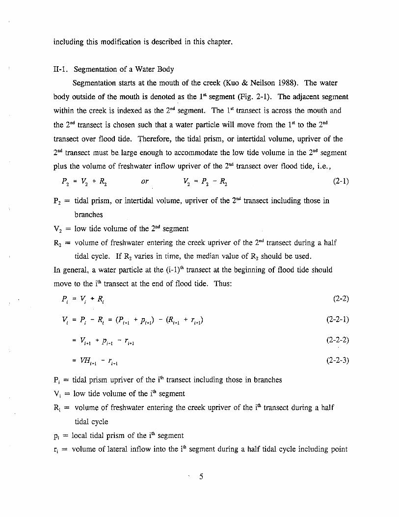
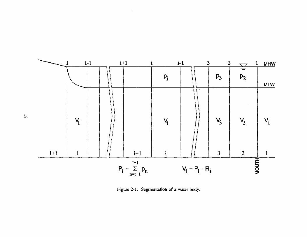
Segmentation starts at the mouth of the creek (Kuo & Neilson 1988). The water

body outside of the mouth is denoted as the pt segment (Fig. 2-1). The adjacent segment

within the creek is indexed as the 2nd segment. The 1st transect is across the mouth and

the 2nd transect is chosen such that a water particle will move from the 1st to the 2nd

transect over flood tide. Therefore, the tidal prism, or intertidal volume, upriver of the

2nd transect must be large enough to accommodate the low tide volume in the 2nd segment

plus the volume of freshwater inflow upriver of the 2nd transect over flood tide, i.e.,

or

P2 = tidal prism, or intertidal volume, upriver of the 2nd transect including those in

branches

V 2 = low tide volume of the 2nd segment

(2-1)

R2 = volume of freshwater entering the creek upriver of the 2nd transect during a half

tidal cycle. If R2 varies in time, the median value of R2 should be used.

In general, a water particle at the (i-l)th transect at the beginning of flood tide should

move to the ith transect at the end of flood tide. Thus:

Pi = tidal prism upriver of the ith transect including those in branches

Vi = low tide volume of the ith segment

(2-2)

(2-2-1)

(2-2-2)

(2-2-3)

Ri = volume of freshwater entering the creek upriver of the ith transect during a half

tidal cycle

Pi = local tidal prism of the ith segment

ri = volume of lateral inflow into the ith segment during a half tidal cycle including point

5

and nonpoint source discharges

VHi = high tide volume of the ith segment = Vi+I + Pi+I·

From the definitions:

l+I I+I

pi = I: pi and Ri = I: ri n=i+I n=i+I

(2-2-4)

Equation 2-2-3 states that the low tide volume of a segment is equal to the high tide

volume of its immediate upriver segment less the lateral freshwater inflow into that

segment.

It may be seen from Eq. 2-2-1 that Vi approaches zero as Pi decreases toward the

head of tide. Therefore, an infinite number of segments will result unless a cut-off

criterion is defined. One guideline is to continue segmentation until a segment length

becomes smaller than its width. As this condition is reached, the remainder of the tidal

creek is combined into one single segment, the fh segment (Fig. 2-1). The prism upriver

of the Ith transect is equal to the freshwater discharge upriver of the fh transect, i.e., P1 = R1• The length of the Ith segment will be larger than the local tidal excursion and

complete mixing cannot be achieved within this segment. The model simulated

concentration at this segment still represents the average value of the segment, however.

Landward of the fh transect, the creek behaves more like a fluvial stream than a tidal

creek and flushing is due solely to the freshwater discharge. Segmentation in the

freshwater section is arbitrary and governed only by the spatial resolution desired and the

segment length-to-width ratio.

For branches, segmentation also starts at the branch-main channel junction. As the

1st segment in the main channel is outside of the creek mouth, the 1st segment in the kth

branch entering the ith main channel segment, denoted as the (k, l)th segment, is located in

the main channel. That is, the (k,l)th segment shares the same segment as the ith

segment. Segmentation in branches proceeds upriver in the same manner as the main

channel.

II-2. Determination of Segment Lengths

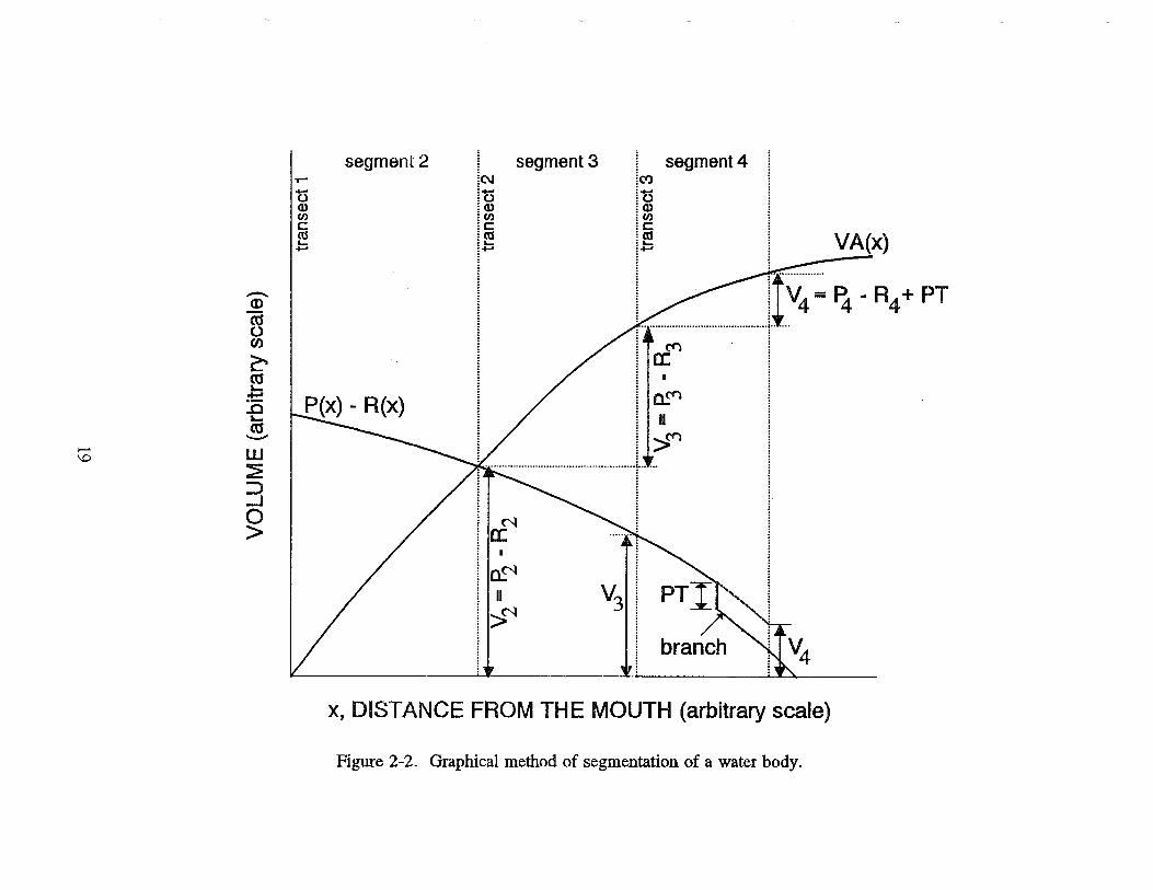
Figure 2-2 shows, for a hypothetical tidal creek, the accumulated low tide volume,

6

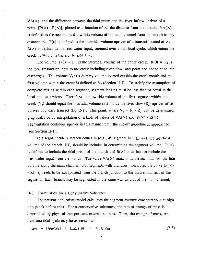
VA( x), and the difference between the tidal prism and the river inflow upriver of a

point, [P(X) - R(X)], plotted as a function of x, the distance from the mouth. VA(x)

is defined as the accumulated low tide volume of the main channel from the mouth to any

distance x. P(x) is defined as the intertidal volume upriver of a transect located at x .

R( X) is defined as the freshwater inout. summed over a half tidal cvcle. which enters the .... , .... ' , "' ,

creek upriver of a transect located at x.

The volume, P(O) = P 1, is the intertidal volume of the entire creek. R(O) = R1 is

the total freshwater input to the creek including river flow, and point and nonpoint source

discharges. The volume V 1 is a dummy volume located outside the creek mouth and the

first volume within the creek is defined as V 2 (Section II-1). To satisfy the assumption of

complete mixing within each segment, segment lengths must be less than or equal to the

local tidal excursions. Therefore, the low tide volume of the first segment within the

creek (V2) should equal the intertidal volume (P2) minus the river flow (R2) upriver of its

upriver boundary transect (Eq. 2-1). This point, where V2 = P2 - R2, can be determined

graphically or by interpolation of a table of values of VA(X) and [P(X) - R(X)].

Segmentation continues upriver in this manner until the cut-off guideline is approached

(see Section II-1).

In a segment where branch comes in (e.g., 4th segment in Fig. 2-2), the intertidal

volume of the branch, PT, should be included in determining the segment volume. P( x)

is defined to include the tidal prism of the branch and R( x) is defined to include the

freshwater input from the branch. The value VA(X) remains as the accumulated low tide

volume along the main channel. For segments with branches, therefore, the curve [P( x)

- R( x )] needs to be extrapolated from the branch junction to the upriver transect of the

segment. Each branch may be segmented in the same way as that of the main channel.

II-3. Formulation for a Conservative Substance

The present tidal prism model calculates the segment-average concentrations at high

tide (slack-before-ebb). For a conservative substance, the rate of change of mass is

determined by physical transport and external sources. Then, the change of mass, .1m,

over one tidal cycle may be expressed as:

t:.m = [sources] + [mass in] - [mass out]

7

(2-3)

where [sources] include point and nonpoint source input and exchange with storage area

over one tidal cycle.

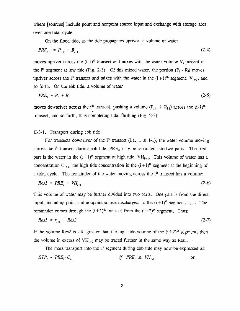
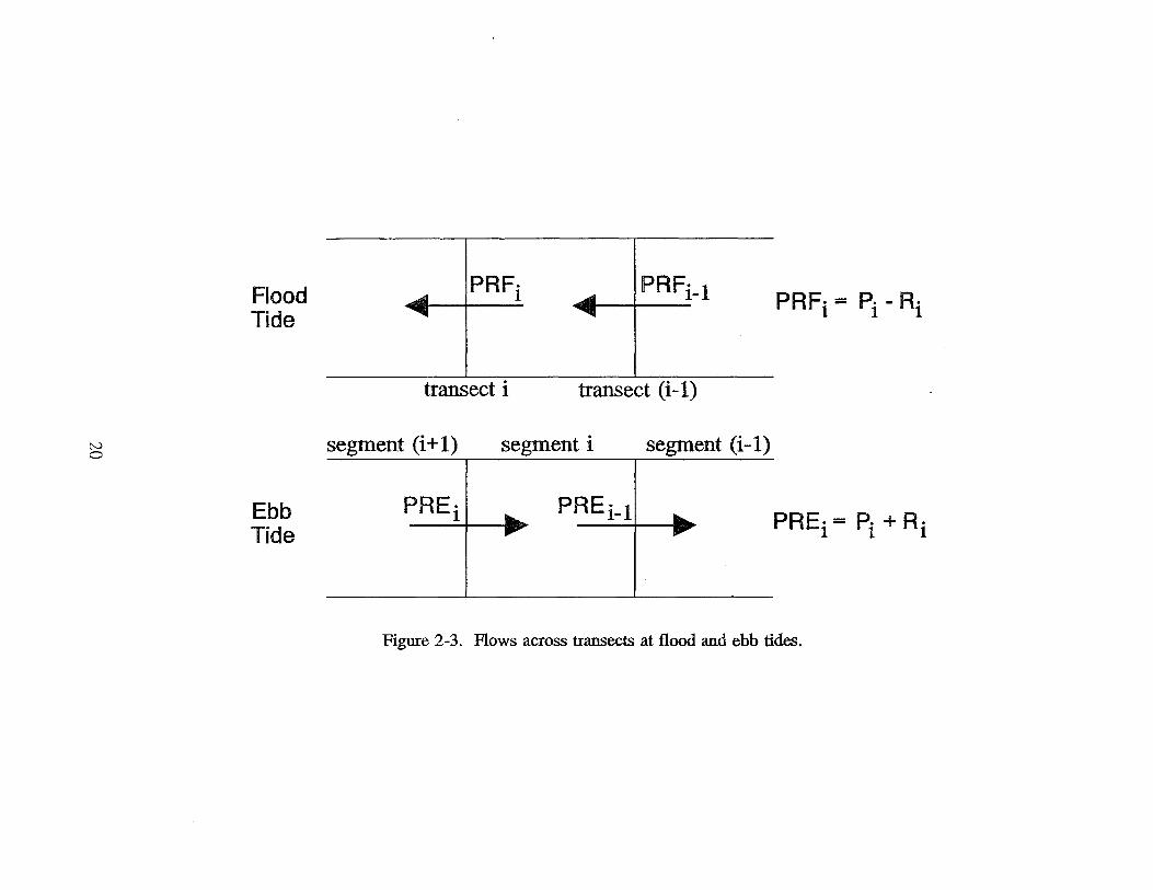
On the flood tide, as the tide propagates upriver, a volume of water

(2-4)

moves upriver across the (i-l)th transect and mixes with the water voiume Vi present in

the ith segment at low tide (Fig. 2-3). Of this mixed water, the portion (Pi - R;) moves

upriver across the ith transect and mixes with the water in the (i + l)th segment, Vi+i, and

so forth. On the ebb tide, a volume of water

(2-5)

moves downriver across the ith transect, pushing a volume (Pi-I + Ri_1) across the (i-l)lh

transect, and so forth, thus completing tidal flushing (Fig. 2-3).

II-3-1. Transport during ebb tide

For transects downriver of the Ith transect (i.e., i :::;; I-1), the water volume moving

across the ith transect during ebb tide, PREi, may be separated into two parts. The first

part is the water in the (i + l)th segment at high tide, VHi+I· This volume of water has a

concentration Ci+i, the high tide concentration in the (i + l)lh segment at the beginning of

a tidal cycle. The remainder of the water moving across the ith transect has a volume:

Resl = PREi - VHi+I (2-6)

This volume of water may be further divided into two parts. One part is from the direct

input, including point and nonpoint source discharges, to the (i + l)th segment, ri+I · The

remainder comes through the (i + l)th transect from the (i +2)th segment. Thus:

Resl = ri+I + Res2 (2-7)

If the volume Res2 is still greater than the high tide volume of the (i +2)1h segment, then

the volume in excess of VHi+2 may be traced further in the same way as Resl.

The mass transport into the ith segment during ebb tide may now be expressed as:

or

8

= VH . C + Resl WPi+t + WNPi•1 i+I i+l -- 2

ri•t or

WPi+I + WNP. l ETP,, = VH,.,·C,,. + ,+ + Res2·C,~~

l"T",l 'Tl 2 , l '~

if Res] > r;+i and Res2 ~ VHi.2

ETPi = ebb tide mass transport across the ith transect into the ith segment

WPi+t = point source mass input into the (i + l)th segment over a tidal cycle

WNPi+t = nonpoint source mass input into the (i + l)th segment over a tidal cycle

(2-8)

If Res2 > VHi+J, the calculation of ETPi should include additional terms relating to ri+2 ,

VHi+J and so forth, until the volume PREi is totally accounted for. Similarly, the ebb

tide transport out of the ith segment may be expressed as:

WP.+ WNP. ETPH :;;; VH/Ci + '

2 ' + Res2·Ci .. 1

(2-9)

ETPi-t = ebb tide mass transport across the (i-1 Y11 transect out of the P11 segment.

II-3-2. Transport during flood tide

On the flood tide, a volume PRFi moves upriver across the ith transect into the

(i + l)th segment (Fig. 2-3). It is possible that some fraction of this water is the water that

was transported into the ith segment during the previous ebb tide. This fraction of

returning old water, which has the concentration Ci+I is defined as a returning ratio, ai,

at the ith transect. The remaining fraction (1 - aJ is new water from the ith segment,

which has the concentration C2i where C2i is the high tide concentration at the end of a

tidal cycle. Therefore, the volume PRFi has the concentration [ai"Ci+I + (1 - a)·C2J

Then, the mass transport into and out of the ith segment during flood tide may be

expressed as:

(2-10)

(2-11)

9

FTPi-I = flood tide mass transport across the (i-l)th transect into the ith segment

FTPi = flood tide mass transport across the ith transect out of the ith segment.

II-3-3. Segments in main channel

The present model has four types of segments:

Type-1 = main channel segments without branch

Type-2 = main channel segments with branches

Type-3 = segments in the primary branches

Type-4 = segments in the secondary branches with each branch treated as a single

storage area connected to a Type-3 segment.

The governing equations for ~ain channel segments, both Type-1 and Type-2, are given

in this section, and those for Type-3 and Type-4 segments are presented in Section II-3-4.

A. Type-1 segment: From Eq. 2-3, the change of mass in the ilh segment over an entire

tidal cycle can be expressed as:

(C2i - C)'(V: + p) = [sources] + ETPi - ETPH - FTPi + FTPH (2-12)

The term [sources] includes point and nonpoint source input for main channel segments.

Therefore, for the ith main channel segment:

[sources] ::; WPi + WNPi (2-12-1)

Letting VHi = Vi + Pi and substituting Equations 2-10, 2-11 and 2-12-1, Eq. 2-12 can

then be solved for C2i:

[ l-1

PRF. C2. ::; TT.· 1 + --' (1 - a.) , , VH. ,

l

~::;Ci+ WPi~WNPi i

ETPi - ETPH PRF. + - --' a.·C.+1

VH VH. ' ' i I

(2-13)

(2-13-1)

For segments landward of the J1h transect (i.e., i > I+ 1), the creek becomes a

fluvial stream and no water is transported upriver during flood tide. The total volume of

10

water flowing through the ith transect during a tidal cycle is 2 · ~. Equations 2-13 and 2-

13-1 are applicable to the fluvial stream if letting

PREi = 2·Ri and PRFi = 0 (2-14)

Similar situations can occur at the inner portion of tidal creek during periods of high

freshwater inflow. For a transect in the tidal creek (i.e., i < I), the ebb tide transport is

always in the downriver direction regardless of freshwater inflow and is calculated using

Eq. 2-8. However, when the freshwater inflow exceeds volume increase during flood

tide (i.e., Pi - ~ < 0), the flood tide transport is in the downriver direction and may be

expressed as:

FTPi = (Pi - Ri) . Ci+t (2-15)

Note the difference between Equations 2-11 and 2-15. In Eq. 2-15, the negative flow (Pi

- Ri < 0) indicates that the flood tide transport is in the downriver direction. Under

these circumstances, Equations 2-13 and 2-13-1 are still applicable if the conditions in

Eq. 2-14 are forced.

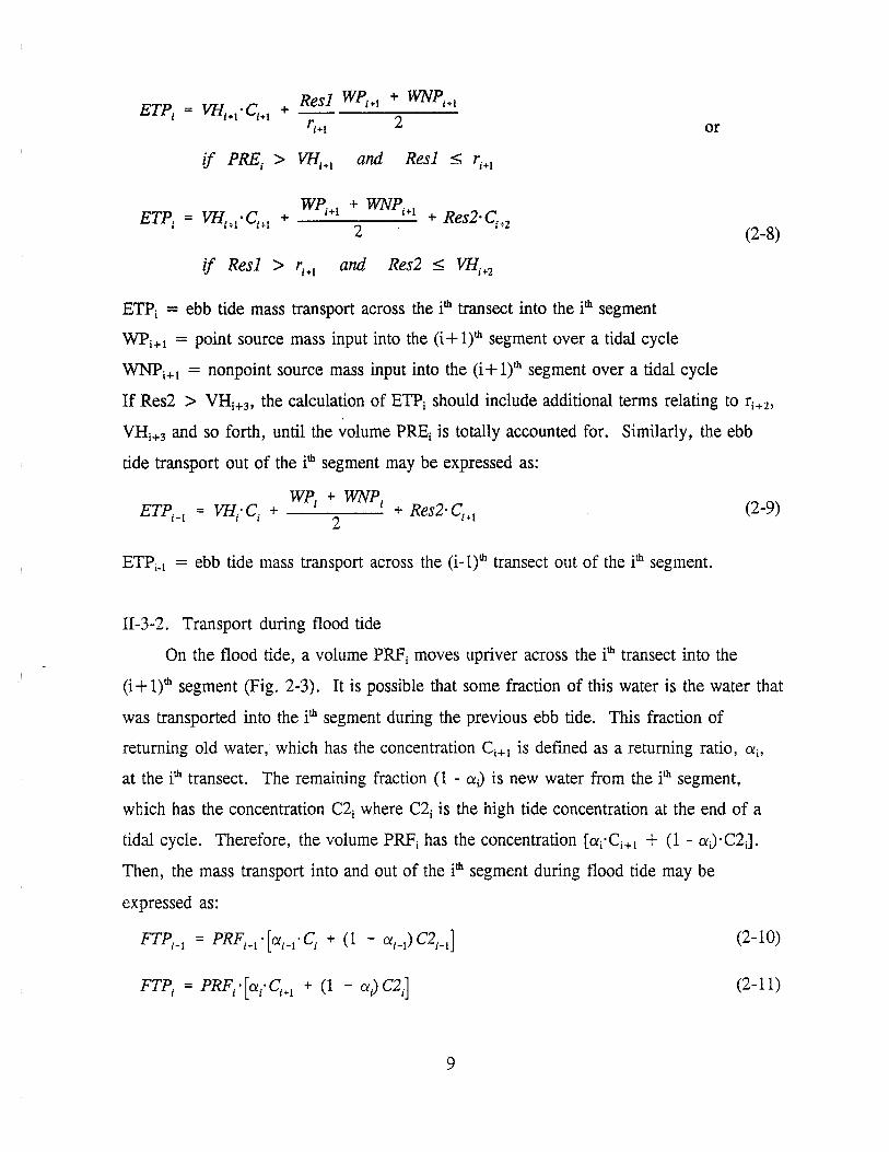
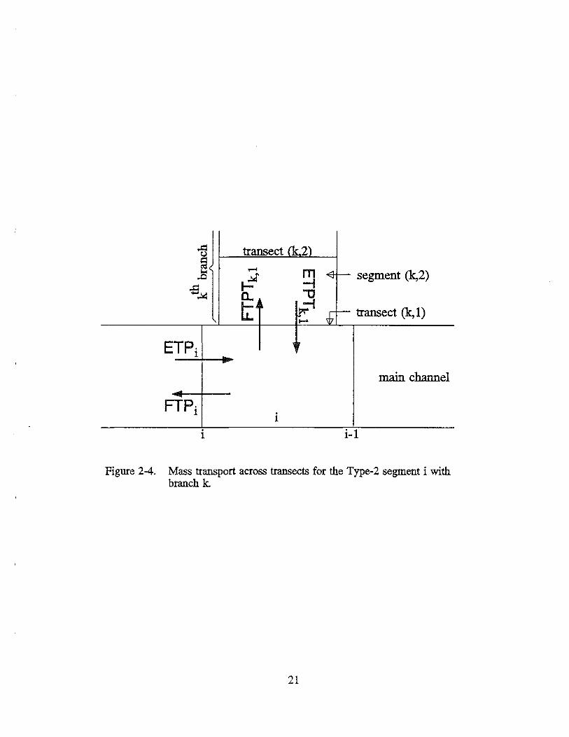
B. Type-2 segment: For main channel segments with branches, the mass transport

across the 1st branch transects should be considered. For the ith segment with K branches

coming in (Fig. 2-4), the extra terms that need to be added in the right-hand side of Eq.

2-12 are:

K

+ L (ETPTk,l - FTPTk) (2-16) k=I

The ebb tide mass transport across the (k, l)lh transect, ETPTk,t, is identical to Eq. 2-8.

The flood tide mass transport across the (k, l)lh transect, FTPTk,t, can be expressed from

Equations 2-4 and 2-11 as:

(2-16-1)

(2-16-2)

The variable names ending with 'T' designate those defined for the primary branches.

The equation to be solved for a Type-2 segment may be expressed as:

11

(2-17)

II-3-4. Segments in branch

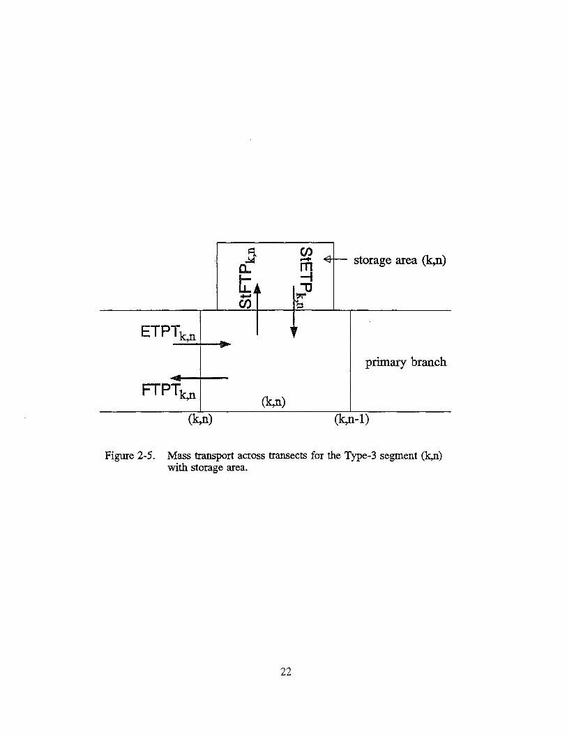
A. Type-3 segment: The present model treats Type-4 segments as storage areas, which

exchange the water and mass with Type-3 segments as tide rises and falls. For segments

in the primary branches (Type-3), the term [sources] in Eq. 2-12 includes point and

nonpoint source input, and exchange with storage area, if any. Therefore, for the (k,n)th

segment:

[sources] = (WPTk,n + WNPTk.n) + Stk,n (2-18)

where Stic,n represents the mass exchange over a tidal cycle with storage area at the (k,n)th

segment.

During ebb tide, the water surface goes down and storage area acts as a source for

Type-3 segment. The ebb tide transport into the (k,n)th segment due to volume change in

storage area and lateral inflow may be expressed as:

StETP = Stp + k,n k.n StC [

StPQ + StNPQ. l ~ ~ 2 ~

(2-19)

StETPk.n = ebb tide mass transport from the (k,n)th storage area into the (k,n)th segment

Stpk,n = local tidal prism (volume change over a half tidal cycle) in the (k,nt storage

area

StCk n = high tide concentration in the (k,n)th storage area at the beginning of a tidal

cycle

StPQk,n = point source volume discharge into the (k,n)th storage area over a tidal cycle

StNPQk,n = nonpoint source volume discharge into the ~k,n)th storage area over a tidal

12

cycle.

During flood, if volume change in storage area, StJ\:,n, is larger than lateral inflow,

(StP<2ic.n + StNP<2Jc,J/2, storage area acts as a sink for branch segment. The flood tide

transport may be expressed as:

StPQ + StNPQ1c,n if StQk,n = Stp - k,n > 0 k,n 2 (2-20-1)

StFTPk,n = flood tide mass transport into the (k,n)th storage area from the (k,n)th segment

Stak,n = returning ratio for the (k,n)th storage area

St~.n is the volume of water entering the (k,n)th storage area from the (k,n)th segment.

Returning ratio, Stak,n, represents the fraction of St<2Jc.n originated from the (k,nt storage

area, i.e., the fraction of St<2ic,n that leaves the (k,n)th storage area at falling tide and

returns from the (k,n)th segment at the following rising tide. However, if lateral inflow

exceeds volume increase during flood tide in storage area, the transport is in the opposite

direction from storage area into branch segment. Then, the flood tide transport may be

expressed as:

StFTPk,n = StQk,n . StCk,n StPQ + StNPQ1c n if StQk,n = Stp - k,n ' s; 0 (2-20-2) k,n 2

In Eq. 2-20-2, the negative transport (St<2ic,n s; 0) indicates that the transport is into the

(k,n)th segment.

Combining Equations 2-19 and 2-20-1 (or 2-20-2), Stk.n in Eq. 2-18, may be

expressed as:

Stk,n = StETPk,n - StFTPk,n (2-21)

Then, the mass-balance equation for a Type-3 segment may be expressed as (Fig. 2-5):

- FTPTk,n + FTPTk,n-1 + StETPk,n - StFTPk,n (2-22)

Substituting equivalent form of Eq. 2-11 or Eq. 2-16-2 for FTPTk,n and Eq. 2-20-1 or Eq.

2-20-2 for StFTPk.n, Eq. 2-22 can be solved for C2Tk,n for a Type-3 segment:

13

[ l-1

PRF'T StQ C2T = TIT. · 1 + k,n (1 - cxT ) + >.. • k,n (1 - Stcx ) k,n k,n VHT k,n VHT k,n

k,n k,n

TIT. = CT + WPTk,n + WNPTk,n k,n k,n

ETPTk,n - ETPTk,n-1 + ______ _

VHTk,n

PRF'T PRF'T - k,n ,VT ·CT + k,n-l ["'T ·CT + (1 "'T ) C2T ]

u. k k 1 u. k 1 k - u. k,n-1 k,n-1 VHT ,n ,n+ VHT ,n- ,n

+

StQk,n

>.. = 1

>.. = 0

k,n k,n

StETPk.n -VHTk,n

= Stp -k,n

and

and

StQ"n . {3kn·StCkn

VHT ' ' k,n

StPQk,n + StNPQk,n

2

f3k,n = Stcxk,n if StQk,n > 0

if StQk,n ::; 0

(2-23)

(2-23-1)

(2-23-2)

(2-23-3)

For Type-3 segments without storage area, Stpk,n, StP<1.n and StNPQk,n are set to zero. It

results in St<1,n = StETPk,n = 0, making Equations 2-23 and 2-23-1 identical to those for

Type-1 segments, main channel segments without branch (Equations 2-13 and 2-13-1).

B. Type-4 segment: Equation 2-23-1 requires evaluation of the concentrations in Type-

4 storage area segments, StCk,n· During ebb tide, the concentration of a conservative

substance in storage area is affected only by external sources including point and nonpoint

source loadings, but not by physical transport. Therefore, the mass in the (k,nl storage

area at low tide (slack-before-flood) is:

StWP + StWNP StC . St V. + k,n k,n k,n k,n 2 (2-24-1)

StVk,n = low tide volume in the (k,n)th storage area

StWPk,n = point source mass input into the (k,n)th storage area over a tidal cycle

StWNPk.n = nonpoint source mass input into the (k,n)th storage area over a tidal cycle.

During flood tide the mass coming into the storage area is:

14

StWPL + StWNPL StFTP + ,..,n ,..,n k,n 2

(2-24-2)

These result in the mass in the storage area at high tide:

(2-24-3)

StC2k,n = high tide concentration in the (k,n)lh storage area at the end of a tidal cycle

StVHk,n = high tide volume in the (k,n)th storage area = StV k,n + StI>ic.n·

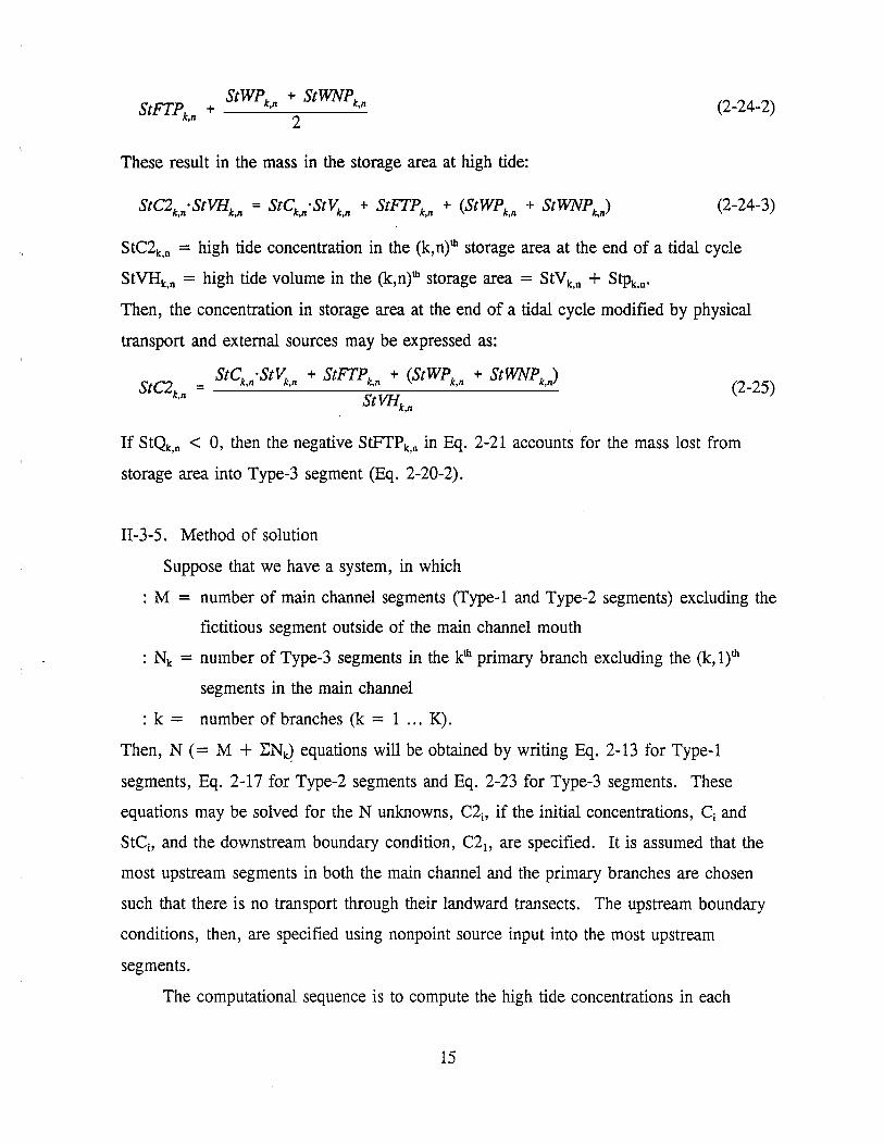
Then, the concentration in storage area at the end of a tidal cycle modified by physical

transport and external sources may be expressed as:

StC2 = StCk,n·StVk,n + StFTPk,n + (StWPk,n + StWNPk) k,n StVH

k,n

(2-25)

If St<1:,n < 0, then the negative StFTPk,n in Eq. 2-21 accounts for the mass lost from

storage area into Type-3 segment (Eq. 2-20-2).

II-3-5. Method of solution

Suppose that we have a system, in which

: M = number of main channel segments (Type-1 and Type-2 segments) excluding the

fictitious segment outside of the main channel mouth

: Nk = number of Type-3 segments in the kth primary branch excluding the (k, l)th

segments in the main channel

: k = number of branches (k = 1 ... K).

Then, N ( = M + l:Nk) equations will be obtained by writing Eq. 2-13 for Type-1

segments, Eq. 2-17 for Type-2 segments and Eq. 2-23 for Type-3 segments. These

equations may be solved for the N unknowns, C2i, if the initial concentrations, Ci and

StCi, and the downstream boundary condition, C21, are specified. It is assumed that the

most upstream segments in both the main channel and the primary branches are chosen

such that there is no transport through their landward transects. The upstream boundary

conditions, then, are specified using nonpoint source input into the most upstream

segments.

The computational sequence is to compute the high tide concentrations in each

15

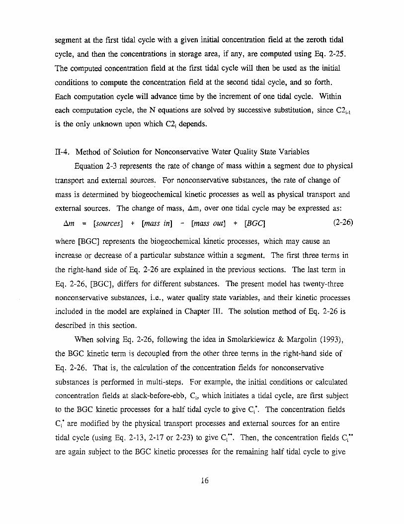
segment at the first tidal cycle with a given initial concentration field at the zeroth tidal

cycle, and then the concentrations in storage area, if any, are computed using Eq. 2-25.

The computed concentration field at the first tidal cycle will then be used as the initial

conditions to compute the concentration field at the second tidal cycle, and so forth.

Each computation cycle will advance time by the increment of one tidal cycle. Within

each computation cycle, the N equations are solved by successive substitution, since C2i-t

is the only unknown upon which C2i depends.

II-4. Method of Solution for Nonconservative Water Quality State Variables

Equation 2-3 represents the rate of change of mass within a segment due to physical

transport and external sources. For nonconservative substances, the rate of change of

mass is determined by biogeochemical kinetic processes as well as physical transport and

external sources. The change of mass, .!im, over one tidal cycle may be expressed as:

f).Jn = [sources] + [mass in] - [mass out] + [BGC] (2-26)

where [BGC] represents the biogeochemical kinetic processes, which may cause an

increase or decrease of a particular substance within a segment. The first three terms in

the right-hand side of Eq. 2-26 are explained in the previous sections. The last term in

Eq. 2-26, [BGC], differs for different substances. The present model has twenty-three

nonconservative substances, i.e., water quality state variables, and their kinetic processes

included in the model are explained in Chapter III. The solution method of Eq. 2-26 is

described in this section.

When solving Eq. 2-26, following the idea in Smolarkiewicz & Margolin (1993),

the BGC kinetic term is decoupled from the other three terms in the right-hand side of

Eq. 2-26. That is, the calculation of the concentration fields for nonconservative

substances is performed in multi-steps. For example, the initial conditions or calculated

concentration fields at slack-before-ebb, Ci, which initiates a tidal cycle, are first subject

to the BGC kinetic processes for a half tidal cycle to give C/. The concentration fields

Ct are modified by the physical transport processes and external sources for an entire

tidal cycle (using Eq. 2-13, 2-17 or 2-23) to give ct. Then, the concentration fields ct· are again subject to the BGC kinetic processes for the remaining half tidal cycle to give

16

the concentration fields at the next high tide, C2i.

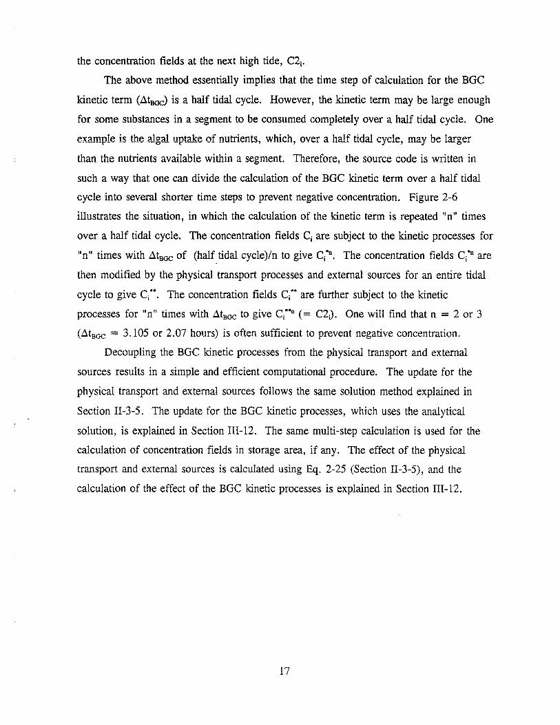
The above method essentially implies that the time step of calculation for the BGC

kinetic term (.6.tBoc) is a half tidal cycle. However, the kinetic term may be large enough

for some substances in a segment to be consumed completely over a half tidal cycle. One

ex~mple is the ~1g~1 uptake of nutrients, which, over a half tid~l cycle, may be larger

than the nutrients available within a segment. Therefore, the source code is written in

such a way that one can divide the calculation of the BGC kinetic term over a half tidal

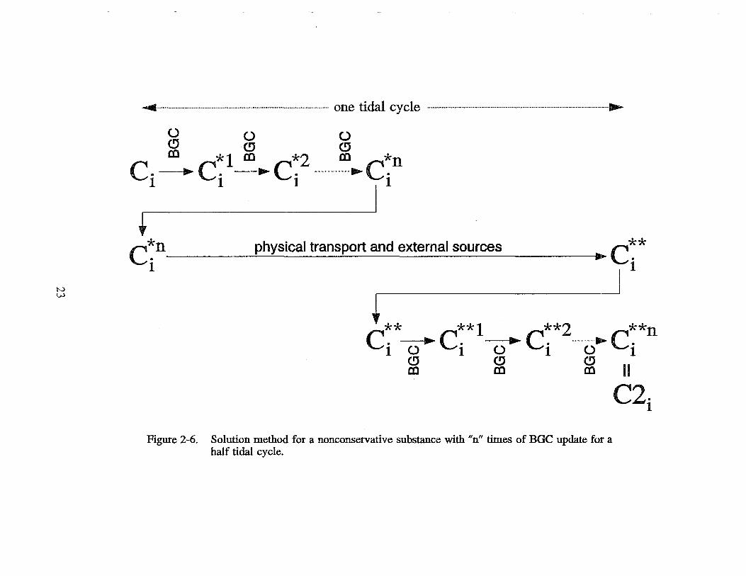
cycle into several shorter time steps to prevent negative concentration. Figure 2-6

illustrates the situation, in which the calculation of the kinetic term is repeated "n" times

over a half tidal cycle. The concentration fields Ci. are subject to the kinetic processes for

"n" times with AtBac of (half tidal cycle)/n to give C/'n. The concentration fields Ct11 are

then modified by the physical transport processes and external sources for an entire tidal

cycle to give ct·. The concentration fields ct are further subject to the kinetic

processes for "n" times with AtBoc to give C/*n ( = C2j. One will find that n = 2 or 3

(AtBoc = 3.105 or 2.07 hours) is often sufficient to prevent negative concentration.

Decoupling the BGC kinetic processes from the physical transport and external

sources results in a simple and efficient computational procedure. The update for the

physical transport and external sources follows the same solution method explained in

Section II-3-5. The update for the BGC kinetic processes, which uses the analytical

solution, is explained in Section III-12. The same multi-step calculation is used for the

calculation of concentration fields in storage area, if any. The effect of the physical

transport and external sources is calculated using Eq. 2-25 (Section II-3-5), and the

calculation of the effect of the BGC kinetic processes is explained in Section III-12.

17

..... 00

I I-1 i+l . 1 i-1 3 2 1 MHW

\ \ \ \ - I I \ \ J\ \ \, ..... -. --+-----1----,--+---

P3 P2 MLW

\ \ \ \ \ \ \\ l~ V. 11

// I //

Yr V3 Vz V1

I I I I I+ 1 I I I I / / i+ 1 i / / I 3 I 2 j 1

I+l

p. = E Pn 1 n""i+l

v. = p. - R· 1 1 1

Figure 2-1. Segmentation of a water body.

:I: I­::> 0 :E

,_.. \0

-Q)

ccs 0 u,

~ ccs ,._

.'!:

.0 ,._ ~ w ~ :::> _J

0 >

..-0 (I) (I) C

~ ~

segment 2 '

iC\I io ; (I) l (I) :C i~

segment 3

! 0:N i I

j a_N

I II

I >N V3

1 segment4 let:> : ...... :0 ; (I) l (I) :C 1i

1

__ VA(x)

I 1!v4 = ~ - R4 + PT . . . . . . ; •• •••••hn••••••un•••••••uuo••••••••oao~•• ••n

l (1') l i a: i . . . . I I I i a_(') l . . l II I i ..._er) i i ,,,,,, : : :

branch

x, DISTANCE FROM THE MOUTH (arbitrary scale)

Figure 2-2. Graphical method of segmentation of a water body.

N 0

Flood Tide

Ebb Tide

...11111 """'1111

PRF· 1

transect i

~ PRFi-1

transect (i-1)

segment (i + 1) segment i segment (i-1)

PRE· 1 ...... ,, PREi-1 ~

PRF· = p. - R· 1 1 1

PRE·= p. + R· 1 1 1

Figure 2-3. Flows across transects at flood and ebb tides.

-5 transect 2

~ ..... m segment (k,2) ,.0

~ -f ,£2~ a. -c

...... ~ transect (k, 1) u.. 1--"

ETP· 1

main channel

FTP· 1 i i i-1

Figure 2-4. Mass transport across transects for the Type-2 segment i with branch k.

21

.a: CJ) ~ - storage area (k,n) ......

a.. m J- -i U..a -0 .....

' Cl)

ETPT1c,n , r

-~

primary branch ..... -

FTPTk,n (k,n)

(k,n) (k,n-1)

Figure 2-5. Mass transport across transects for the Type-3 segment (k,n) with storage area.

22

N tJ.)

...,.. .............................................................................................. one tidal cycle ................................................................................................... ...,._

{) {) {) C, CJ CJ al *1 m *2 al *n c. ... c. ..... c ................ -...................... c.

1 1 1 11

t c~n physical transport and external sources c~* 1 J 1

+ ** **1 **2 **n c. ..... c. ..... c. .. .................... c. 1 0 1 0 1 0 1

c, CJ C!l II al al al

c2. 1

Figure 2-6. Solution method for a nonconservative substance with "n" times of BGC update for a half tidal cycle.

Chapter ill. Kinetic Fonnulation for Water Quality State Variables

The present model has twenty three water quality related model state variables (Fig.

3-1). The kinetic processes included in the model use mostly the fonnulations in

Chesapeake Bay three-dimensional water quality model, CE-QUAL-ICM (Cereo & Cole

1994).

1) cyanobacteria (blue-green algae)

3) green algae (others)

4) refractory particulate organic carbon

6) dissolved organic carbon

7) refractory particulate organic phosphorus

9) dissolved organic phosphorus

11) refractory particulate organic nitrogen

13) dissolved organic nitrogen

15) nitrate nitrogen

16) particulate biogenic silica

18) chemical oxygen demand

20) total suspended solid

22) fecal coliform bacteria

2) diatoms

5) labile particulate organic carbon

8) labile particulate organic phosphorus

10) total phosphate

12) labile particulate organic nitrogen

14) ammonium nitrogen

17) available silica

19) dissolved oxygen

21) total active metal

23) temperature

This chapter details the kinetic sources and sinks for each state variable. Figure 3-1

shows the interactions between state variables. The external sources including point and

nonpoint source inputs are taken care of in the formulations of physical transport

processes (Chapter II). The exchange fluxes at the sediment-water interface including

sediment oxygen demand are explained in the sediment process model (Chapter IV). An

asterisk mark (*) attached to equation number denotes the kinetic formulations that are

different from CE-QUAL-ICM. The solution method is described in Section III-12. The

parameters values used in Chesapeake Bay modeling (Cereo & Cole 1994) are presented

in Section III-13.

III-1. Algae

Algae, which occupies a central role in the model (Fig. 3-1), are grouped into three

24

model state variables: cyanobacteria (blue-green algae), diatoms and green algae. The

subscript, x, is used to denote three algal groups: c for cyanobacteria, d for diatoms and

g for green algae. Sources and sinks included in the model are

: growth (production)

: basal metabolism

: predation

: settling

Equations describing these processes are largely the same for three algal groups with

differences in the values of parameters in the equations. The governing equation

describing these processes is:

a~ w~ - = (P - BM - PR - -)B at .t X X h X

Bx = algal biomass of algal group x (g C m·3)

t = time (day)

Px = production rate of algal group x (day-1)

BMx = basal metabolism rate of algal group x (day·1)

PRx = predation rate of algal group x (day·1)

WSx = settling velocity of algal group x (m day·1)

h = total depth (m).

III-1-1. Growth (Production)

(3-1)

Algal growth depends on nutrient availability, ambient light and temperature. The

effects of these processes are considered to be multiplicative:

PMx = maximum growth rate under optimal conditions for algal group x ( day·1)

f1 (N) = effect of suboptimal nutrient concentration (0 ::; f1 < 1)

fz(I) = effect of suboptimal light intensity (0 ::; f2 ::; 1)

fiT) = effect of suboptimal temperature (0 ::; f3 ::; 1).

(3-la)

The freshwater cyanobacteria may undergo rapid mortality in salt water, e.g., freshwater

organisms in the Potomac River (Thomann et al. 1985). For the freshwater organisms,

25

the increased mortality may be included in the model by retaining salinity toxicity term in

the growth equation for cyanobacteria:

(3-lb)

f4(S) = effect of salinity on cyanobacteria growth (0 :::; f4 :::; 1).

Activation of the saiinity toxicity term, f4 (S), is an option in the source code.

ill-1-la. Effect of nutrients on growth

Using Liebig's "law of the minimum" (Odum 1971) that growth is determined by

the nutrient in least supply, the nutrient limitation for growth of cyanobacteria and green

algae is expressed as:

Ji = mzmmum f' (N) . . [ NH4 + N03 P04d l 1 KHN:r. + NH4 + N03 ' KHP.t + P04d

NH4 = ammonium nitrogen concentration (g N m-3)

N03 = nitrate nitrogen concentration (g N m-3)

KHNx = half-saturation constant for nitrogen uptake for algal group x (g N m-3)

P04d = dissolved phosphate phosphorus concentration (g P m-3)

(3-lc)

KHPx = half-saturation constant for phosphorus uptake for algal group x (g P m-3).

Some cyanobacteria, e.g., Anabaena, can fix nitrogen from atmosphere and thus is not

limited by nitrogen. Therefore, Eq. 3-lc is not applicable to the growth of nitrogen

fixers.

Since diatoms require silica as well as nitrogen and phosphorus for growth, the

nutrient limitation for diatoms is expressed as:

Ji 1,1 = mmzmum , , f' (-,..7\ . . [ NH4 + N03 P04d SAd l KHNd + NH4 + N03 KHPd + P04d KHS + SAd

(3-ld)

SAd = concentration of dissolved available silica (g Si m-3)

KHS = half-saturation constant for silica uptake for diatoms (g Si m-3).

III-1-lb. Effect of light on growth

The daily and vertically integrated form of Steele's equation is:

26

F(n = 2.718·FD (e-"• _ e-cx.;) J

2 "' Kess·h

I OI = __ o_ . e -Kess·h

B FD·(/)x

FD = fractional daylength (0 < FD < 1)

Kess = total light extinction coefficient (m-1)

I0 = daily light intensity (langleys day-1)

(IJx = optimal light intensity for algal group x (langleys day-1).

(3-le)

(3-lt)

(3-lg)

Light extinction in the water column consists of three fractions in the model: a

background value dependent on water color, extinction due to suspended particles and

extinction due to light absorption by ambient chlorophyll:

B Kess = Keb + Kers5·TSS + Ke011 • ,E (--·t-)

x=c,d,g CCh(t

Keb = background light extinction (m-1)

KeTss = light extinction coefficient for total suspended solid (m-1 per g m-3)

TSS = total suspended solid concentration (g m-3)

KeChl = light extinction coefficient for chlorophyll 'a' (m-1 per mg Chl m-3)

CChlx = carbon-to-chlorophyll ratio in algal group x (g C per mg Chl).

For a model that does not simulate TSS, Kerss may be set to zero and K~ may be

estimated to include light extinction due to suspended solid.

(3-lh)*

Optimal light intensity (Is) for photosynthesis depends on algal taxonomy, duration

of exposure, temperature, nutritional status and previous acclimation. Variations in Is are

largely due to adaptations by algae intended to maximize production in a variable

environment. Steel (1962) noted the result of adaptations is that optimal intensity is a

consistent fraction (approximately 50%) of daily intensity. Kremer & Nixon (1978)

reported J.n analogous finding that maximum algal growth occurs at a constant depth

(approximately 1 m) in the water column. Their approach is adopted so that optimal

27

intensity is expressed as:

(I)x = minimum {<(,)avg· e -Ke.rs·(D.,), , (/)min}

(DopJx = depth of maximum algal growth for algal group x (m)

(IJavg = adjusted surface light intensity (langleys day·1).

(3-li)

A minimum, (IJmm, in Eq. 3-li is specified so that algae do not thrive at extremely low

light levels. The time required for algae to adapt to changes in light intensity is

recognized by estimating (IJx based on a time-weighted average of daily light intensity:

(/ " = CI · I + CI · I + CI · I olavg a o b 1 c 2

I1 = daily light intensity one day preceding model day (langleys day·1)

I2 = daily light intensity two days preceding model day (langleys day-1)

(3-lj)

era, Cib & CIC = weighting factors for Io, I1 and I2, respectively: era + Cib + CIC = 1.

III-1-lc. Temperature

A Gaussian probability curve is used to represent temperature dependency of algal

growth:

h(T) = exp(-KTGlx[T - TMx]2)

= exp ( - KTG2 [TM - 7]2)

.t X

T = temperature (°C)

if T :5 ™x if T > TM_t

™x = optimal temperature for algal growth for algal group x (°C)

KTG lx = effect of temperature below ™x on growth for algal group x (0 c·2)

KTG2x = effect of temperature above ™x on growth for algal group x (°C·2).

III-1-ld. Effect of salinity on growth of freshwater cyanobacteria

The growth of freshwater cyanobacteria in salt water is limited by:

STOX2 f/S) = STOX2 + S2

STOX = salinity at which Microcystis growth is halved (ppt)

S = salinity in water column (ppt).

28

(3-lk)

(3-11)

ill-1-2. Basal Metabolism

Algal biomass in the present model decreases through basal metabolism (respiration

and excretion) and predation. Basal metabolism in the present model is the sum of all

internal processes that decrease algal biomass, and consists of two parts; respiration and

excretion. In basal metabolism, algal matter (carbon, nitrogen, phosphorus and silica) is

returned to organic and inorganic pools in the environment, mainly to dissolved organic

and inorganic matter. Respiration, which may be viewed as a reversal of production,

consumes dissolved oxygen. Basal metabolism is considered to be an exponentially

increasing function of temperature:

(3-lm)

BMRx = basal metabolism rate at TRx for algal group x (day-1)

KTBx = effect of temperature on metabolism for algal group x ( 0 C-1)

TRx = reference temperature for basal metabolism for algal group x (°C).

III-1-3. Predation

The present model does not include zooplankton. Instead, a constant rate is

specified for algal predation, which implicitly assumes zooplankton biomass is a constant

fraction of algal biomass. An equation similar to that for basal metabolism (Eq. 3-1 m) is

used for predation:

(3-ln)

PRRx = predation rate at TRx for algal group x (day-1).

The difference between predation and basal metabolism lies in the distribution of the end

products of two processes. In predation, algal matter (carbon, nitrogen, phosphorus and

silica) is returned to organic and inorganic pools in the environment, mainly to particulate

organic matter.

ill-1-4. Settling

Settling velocities for three algal groups, WS 0 , WSd and WSg, are specified as an

input. Seasonal variations in settling velocity of diatoms can be accounted for by

specifying time-varying WSd (Appendix A).

29

III-2. Organic Carbon

The present model has three state variables for organic carbon: dissolved, labile

particulate and refractory particulate.

A. Particulate organic carbon: Labile and refractory distinctions are based on the time

scale of decomposition. Labile parti~ulate organic carbon with a decomposition time

scale of days to weeks decomposes rapidly in the water column or in the sediments.

Refractory particulate organic carbon with longer-than-weeks decomposition time scale

decomposes slowly, primarily in the sediments, and may contribute to sediment oxygen

demand years after decomposition. For labile and refractory particulate organic carbon,

sources and sinks included in the model are (Fig. 3-1):

: algal predation

: dissolution to dissolved organic carbon

: settling

The governing equations for refractory and labile particulate organic carbons are:

aRPOC = " FCRP·PR ·B - K ·RPOC - WSRP RPOC at ~ x X RPOC h .t-c,d,g

aLPOC = " FCLP·PR ·B - K ·LPOC - WSLP LPOC at f-'. x x LPOC h X c,d, 0

RPOC = concentration of refractory particulate organic carbon (g C m·3)

LPOC = concentration of labile particulate organic carbon (g C m·3)

(3-2)

(3-3)

FCRP = fraction of predated carbon produced as refractory particulate organic carbon

FCLP = fraction of predated carbon produced as labile particulate organic carbon

KRPoc = dissolution rate of refractory particulate organic carbon (day·1)

KLPoc = dissolution rate of labile particulate organic carbon (day·1)

WSRP = settling velocity of refractory particulate organic matter (m day·1)

WSLP = settling velocity of labile particulate organic matter (m day·1).

B. Dissolved organic carbon: Sources and sinks included in the model are (Fig. 3-1):

: algal excretion (exudation) and predation

: dissolution from refractory and labile particulate organic carbon

: heterotrophic respiration of dissolved organic carbon (decomposition)

30

: denitrification

The governing equation describing these processes is:

anoc = ~ [ [FCD + (1 - FCD) KHRX ] BM + FCDP·PR] ·B at I-' x x KHR + no x x x x=c,d,g X

DOC = concentration of dissolved organic carbon (g C m·3)

FCDx = fraction of basal metabolism exuded as dissolved organic carbon at infinite

dissolved oxygen concentration for algal group x

(3-4)

KHRx = half-saturation constant of dissolved oxygen for algal dissolved organic carbon

excretion for group _x (g 0 2 m·3)

DO = dissolved oxygen concentration (g 0 2 m·3)

FCDP = fraction of predated carbon produced as dissolved organic carbon

KHR = heterotrophic respiration rate of dissolved organic carbon ( day·1)

Denit = denitrification rate (day·1) given in Eq. 3-41.

The remaining of this section explains each term in Equations 3-2 to 3-4.

III-2-1. Effect of algae on organic carbon

The terms within summation (E) in Equations 3-2 to 3-4 account for the effects of

algae on organic carbon through basal metabolism and predation.

A. Basal metabolism: Basal metabolism, consisting of respiration and excretion,

returns algal matter (carbon, nitrogen, phosphorus and silica) back to the environment.

Loss of algal biomass through basal metabolism is (Eq. 3-1):

aBX = -BM ·B at X X (3-4a)

which indicates that the total loss of algal biomass due to basal metabolism is independent

of ambient dissolved oxygen concentration. In this model, it is assumed that the

distribution of total loss between respiration and excretion is constant as long as there is

sufficient dissolved oxygen for algae to respire. Under that condition, the losses by

respiration and excretion may be written as:

31

(1 - FCD )·BM ·B X X X

FCD ·BM·B X X X

due to respiration

due to excretion

(3-4b)

(3-4c)

where FCDx is a constant of value between O and 1. Algae cannot respire in the absence

of oxygen, however. Although the t<?tal loss of algal biomass due to basal metabolism is

oxygen-independent (Eq. 3-4a), the distribution of total loss between respiration and

excretion is oxygen-dependent. When oxygen level is high, respiration is a large fraction

of the total. As dissolved oxygen becomes scarce, excretion becomes dominant. Thus,

Eq. 3-4b represents the loss by respiration only at high oxygen level. In general, Eq. 3-

4b can be decomposed into two fractions as a function of dissolved oxygen availability:

(1 - FCD) DO BM ·B. X KHR + DO X ~

X

due to respiration

due to excretion

(3-4d)

(3-4e)

Equation 3-4d represents the loss of algal biomass by respiration and Eq. 3-4e represents

additional excretion due to insufficient dissolved oxygen concentration. The parameter

KHRx, which is defined as half-saturation constant of dissolved oxygen for algal dissolved

organic carbon excretion in Eq. 3-4, can also be defined as half-saturation constant of

dissolved oxygen for algal respiration in Eq. 3-4d.

Combining Equations 3-4c and 3-4e, the total loss due to excretion is:

[FCD. + (1 - FCD.) KHRX l BM;B.

·• ~ KHR + DO ~ ·• X

(3-4f)

Equations 3-4d and 3-4f combine to give the total loss of algal biomass due to basal

metabolism, BMx·Bx (Eq. 3-4a). The definition of FCDx in Eq. 3-4 becomes apparent in

Eq. 3-4f; i.e., fraction of basal metabolism exuded as dissolved organic carbon at infinite

dissolved oxygen concentration. At zero oxygen level, 100 % of total loss due to basal

metabolism is by excretion regardless of FCDx-

The end carbon product of respiration is primarily carbon dioxide, an inorganic

form not considered in the present model, while the end carbon product of excretion is

32

primarily dissolved organic carbon. Therefore, Eq. 3-4f, that appears in Eq. 3-4,

represents the contribution of excretion to dissolved organic carbon, and there is no

source term for particulate organic carbon from algal basal metabolism in Equations 3-2

and 3-3.

B. Predation: Algae produce organic carbon through the effects of predation.

Zooplankton take up and redistribute algal carbon through grazing, assimilation,

respiration and excretion. Since zooplankton are not included in the model, routing of

algal carbon through zooplankton predation is simulated by empirical distribution

coefficients in Equations 3-2 to 3-4; FCRP, FCLP and FCDP. The sum of these three

predation fractions should be unity.

III-2-2. Heterotrophic respiration and dissolution

The second term on the RHS of Equations 3-2 and 3-3 represents dissolution of

particulate to dissolved organic carbon and the third term in the second line of Eq. 3-4

represents heterotrophic respiration of dissolved organic carbon. The oxic heterotrophic

respiration is a function of dissolved oxygen: the lower the dissolved oxygen, the smaller

the respiration term becomes. Heterotrophic respiration rate, therefore, is expressed

using a Monod function of dissolved oxygen:

K = DO K HR KHOR + DO DOC

DO

(3-4g)

KHOR00 = oxic respiration half-saturation constant for dissolved oxygen (g 0 2 m-3)

K00c = heterotrophic respiration rate of dissolved organic carbon at infinite dissolved

oxygen concentration (day-1).

Dissolution and heterotrophic respiration rates depend on the availability of

carbonaceous substrate and on heterotrophic activity. Algae produce labile carbon that

fuels heterotrophic activity: dissolution and heterotrophic respiration do not require the

presence of algae though, and may be fueled entirely by external carbon inputs. In the

model, algal biomass, as a surrogat•.; for heterotrophic activity, is incorporated into

formulations of dissolution and heterotrophic respiration rates. Formulations of these

rates require specification of algal-dependent and algal-independent rates:

33

KRPoc = (KRc + KRCaJg L B) · exp (KT HDR [T - TRHDR]) x•c,d,g

KLPoc = (Kie + Kica18 L B) · exp (KT HDR [T - TRHDR]) x=c,d,g

Kvoc = (Kvc + KDCaJg .E B)·exp,(KTMNL[T - TRM~) x=c,d,g

KRc = minimum dissolution rate of refractory particulate organic carbon (day·1)

KLc = minimum dissolution rate of labile particulate organic carbon (day·1)

Koc = minimum respiration rate of dissolved organic carbon (day·1)

KRca1g & KLca1g = constants that relate dissolution of refractory and labile particulate

organic carbon, respectively, to algal biomass (day·1 per g C m·3)

Koca1g = constant that relates respiration to algal biomass (day·1 per g C m·3)

KTHDR = effect of temperature on hydrolysis of particulate organic matter (0 C-1)

TRHDR = reference temperature for hydrolysis of particulate organic matter (°C)

KTMNL = effect of temperature on mineralization of dissolved organic matter (°C-1)

TRMNL = reference temperature for mineralization of dissolved organic matter (°C).

Equations 3-4h to 3-4j have exponential functions that relate rates to temperature.

(3-4h)

(3-4i)

(3-4j)

In the present model, the term "hydrolysis" is defined as the process by which

particulate organic matter is converted to dissolved organic form, and thus includes both

dissolution of particulate carbon and hydrolysis of particulate phosphorus and nitrogen.

Therefore, the parameters, KTHDR and TRHDR, are also used for the temperature effects on

hydrolysis of particulate phosphorus (Equations 3-8f and 3-8g) and nitrogen (Equations 3-

13b and 3-13c). The term "mineralization" is defined as the process by which dissolved

organic matter is converted to dissolved inorganic form, and thus includes both

heterotrophic respiration of dissolved organic carbon and mineralization of dissolved

organic phosphorus and nitrogen. Therefore, the parameters, KT MNL and TRMNL, are also

used for the temperature effects on mineralization of dissolved phosphorus (Eq. 3-8h) and

nitrogen (Eq. 3-13d).

III-2-3. Effect of denitrification on dissolved organic carbon

As oxygen is depleted from natural systems, organic matter is oxidized by the

34

reduction of alternate electron acceptors. Thermodynamically, the first alternate acceptor

reduced in the absence of oxygen is nitrate. The reduction of nitrate by a large number

of heterotrophic anaerobes is referred to as denitrification, and the stoichiometry of this

reaction is (Stumm & Morgan 1981):

(3-4k)

The last term in Eq. 3-4 accounts for the effect of denitrification on dissolved organic

carbon. The kinetics of denitrification in the model are first-order:

KHORDO N03 Denit = AANOX· K

KHORDO + DO KHDNN + N03 DOC (3-41)

KHDNN = denitrification half-saturation constant for nitrate (g N m-3)

AANOX = ratio of denitrification rate to oxic dissolved organic carbon respiration rate .

In Eq. 3-41, the dissolved organic carbon respiration rate, K00c, is modified so that

significant decomposition via denitrification occurs only when nitrate is freely available

and dissolved oxygen is depleted. The ratio, AANOX, makes the anoxic respiration

slower than oxic respiration. Note that K00c, defined in Eq. 3-4j, includes the

temperature effect on denitrification.

III-3. Phosphorus

The present model has four state variables for phosphorus: one inorganic form

(total phosphate) and three organic forms (dissolved, labile particulate and refractory

particulate).

A. Particulate organic phosphorus: For refractory and labile particulate organic

phosphorus, sources and sinks included in the model are (Fig. 3-1):

: algal basal metabolism and predation

: dissolution to dissolved organic phosphorus

: settling

The governing equations for refractory and labile particulate organic phosphorus are:

aRPOP = L (FPR/BMX + FPRP·PR)APC·Bx - KRPOP·RPOP - WSRP RPOP (3-5) at :t=c,d,g h

35

aLPOP = L (FPL/BMX + FPLP·PRX)APC·Bx - KLPo/LPOP - WSLP LPOP (3-6) at x=c,d,g h

RPOP = concentration of refractory particulate organic phosphorus (g P m-3)

LPOP = concentration of labile particulate organic phosphorus (g P m-3)

FPRx = fraction of metabolized phosphorus by algal group x produced as refractory

particulate organic phosphorus

FPLx = fraction of metabolized phosphorus by algal group x produced as labile

particulate organic phosphorus

FPRP = fraction of predated phosphorus produced as refractory particulate organic

phosphorus

FPLP = fraction of predated. phosphorus produced as labile particulate organic

phosphorus

APC = mean phosphorus-to-carbon ratio in all algal groups (g P per g C)

KRPoP = hydrolysis rate of refractory particulate organic phosphorus (day-1)

KLPoP = hydrolysis rate of labile particulate organic phosphorus (day-1).

B. Dissolved organic phosphorus: Sources and sinks included in the model are (Fig. 3-

1):

: algal basal metabolism and predation

: dissolution from refractory and labile particulate organic phosphorus

: mineralization to phosphate phosphorus

The governing equation describing these processes is:

aDOP = " (FPD ·BM + FPDP·PR )APC·B at ~ X .t .t X .t-c,d.g

DOP = concentration of dissolved organic phosphorus (g P m-3)

FPDx = fraction of metabolized phosphorus by algal group x produced as dissolved

organic phosphorus

FPDP = fraction of predated phosphorus produced as dissolved organic phosphorus

Knop = mineralization rate of dissolved organic phosphorus (day-1).

C. Total phosphate: For total phosphate that includes both dissolved and sorbed

36

(3-7)

phosphate (Section III-3-1), sources and sinks included in the model are (Fig. 3-1):

: algal basal metabolism, predation, and uptake

: mineralization from dissolved organic phosphorus

: settling of sorbed phosphate

• g<>rl1'm<>nt-tt1".lt<>1" P.Vf'h".lflae 0f d1' c:?c:?Qhled phnsphatP • """"' \-' \, Y'f' '41.""i '-'1'-V .&"41. f) .&. UU .a. Y - • -

The governing equation describing these processes is:

a~~4t = L (FPI_,:'BMX + FPIP·PRX ~ P)APC·Bx + KDOP·DOP

x=c,d,g

_ WSTSS P04p + BFP04 h h

P04t = total phosphate (g P m·3) = P04d + P04p

P04d = dissolved phosphate (g P m·3)

P04p = particulate (sorbed) phosphate (g P m·3)

FPix = fraction of metabolized phosphorus by algal group x produced as inorganic

phosphorus

FPIP = fraction of predated phosphorus produced as inorganic phosphorus

WSTss = settling velocity of suspended solid (m day-1)

BFP04 = exchange flux of phosphate at sediment-water interface (g P m·2 day·1).

(3-8)*

(3-8a)*

In Eq. 3-8, if total active metal is chosen as a measure of sorption site, the settling

velocity of total suspended solid, WSTss, is replaced by that of particulate metal, WSs

(Sections III-3-1 and III-9). The remaining of this section explains each term in

Equations 3-5 to 3-8 with the total phosphate system detailed in Section III-3-1.

III-3-1. Total phosphate system

Suspended and bottom sediment particles (clay, silt and metal hydroxides) adsorb

and desorb phosphate in river and estuarine waters. This adsorption-desorption process

has been suggested to buffer phosphate concentration in water column and to enhance the

transport of phosphate away from its external sources (Carritt & Goodgal 1954; Froelich

1988; Lebo 1991). To ease the computational complication due to the adsorption­

desorption of phosphate, dissolved and sorbed phosphate are treated and transported as a

37

single state variable. Therefore, the model phosphate state variable, total phosphate, is

defined as the sum of dissolved and sorbed phosphate (Eq. 3-8a), and the concentrations

for each fraction are determined by equilibrium partitioning of their sum.

In CE-QUAL-ICM, sorption of phosphate to particulate species of metals including

iron and manganese was considered based on phenomenon observed in the monitoring

data from mainstem of Chesapeake Bay: phosphate was rapidly depleted from anoxic

bottom waters during the autumn reaeration event (Cereo & Cole 1994). Their

hypothesis was that reaeration of bottom waters caused dissolved iron and manganese to

precipitate, and phosphate sorbed to newly-formed metal particles and rapidly settled to

the bottom. One state variable, total active metal, in CE-QUAL-ICM was defined as the

sum of all metals that act as sorption sites, and the total active metal was partitioned into

particulate and dissolved fractions via an equilibrium partitioning coefficient (Section III-

9). Then, phosphate was assumed to sorb to only the particulate fraction of the total

active metal.

In the treatment of phosphate sorption in CE-QUAL-ICM, the particulate fraction

of metal hydroxides was emphasized as a sorption site in bottom waters under anoxic

conditions. Phosphorus is a highly particle-reactive element, and phosphate in solution

reacts quickly with a wide variety of surfaces, being taken up by and released from

particles (Froelich 1988). The present model has two options, total suspended solid and

total active metal, as a measure of a sorption site for phosphate, and dissolved and sorbed

fractions are determined by equilibrium partitioning of their sum as a function of total

suspended solid or total active metal concentration:

K ·TSS P04p :;::: Po4

P P04t or 1 + KP04p°TSS

P04p:;::: KP04p·TAMp P04t (3-8b)*

1 + KP04p·TAMp

1 P04d:;::: ----P04t or P04d 1 P04t :;:::

1 + KP04p°TSS 1 + KP04/TAMp

:;::: P04t - P04p (3-8c)*

KP04p = empirical coefficient relating phosphate sorption to total suspended solid (per g

m-3) or particulate total active metal (per mol m-3) concentration

TAMp = particulate total active metal (mol m-3).

38

Dividing Eq. 3-8b by Eq. 3-8c gives:

K = P04p 1 Po4p P04d TSS or

K = P04p 1 P04p P04d TAMp

(3-8d)

where the meaning of KP04p becomes apparent, i.e., the ratio of sorbed to dissolved

phosphate per unit concentration of total suspended solid or pl'lrticulate total active metal

(i.e., per unit sorption site available).

III-3-2. Algal phosphorus-to-carbon ratio (APC)

Algal biomass is quantified in units of carbon per volume of water. In order to

express the effects of algal biomass on phosphorus and nitrogen, the ratios of phosphorus­

to-carbon and nitrogen-to-carbon in algal biomass must be specified. Although global

mean values of these ratios are well known (Redfield et al. 1963), algal composition

varies especially as a function of nutrient availability. As phosphorus and nitrogen

become scarce, algae adjust their composition so that smaller quantities of these vital

nutrients are required to produce carbonaceous biomass (DiToro 1980; Parsons et al.

1984). Examining the field data from the surface of upper Chesapeake Bay, Cereo &

Cole (1994) showed that the variation of nitrogen-to-carbon stoichiometry was small and

thus used a constant algal nitrogen-to-carbon ratio, ANCx. Large variations, however,

were observed for algal phosphorus-to-carbon ratio indicating the adaptation of algae to

ambient phosphorus concentration (Cereo & Cole 1994): algal phosphorus content is high

when ambient phosphorus is abundant and is low when ambient phosphorus is scarce.

Thus, a variable algal phosphorus-to-carbon ratio, APC, is used in model formulation. A

mean ratio for all algal group, APC, is described by an empirical approximation to the

trend observed in field data (Cereo & Cole 1994):

(3-8e)

CPpmiI = minimum carbon-to-phosphorus ratio (g C per g P)

CPpnn2 = difference between minimum and maximum carbon-to-phosphorus ratio (g C

per g P)

CPpnnJ = effect of dissolved phosphate concentration on carbon-to-phosphorus ratio (per g

P m·3).

39

III-3-3. Effect of algae on phosphorus

The terms within summation (E) in Equations 3-5 to 3-8 account for the effects of

algae on phosphorus. Both basal metabolism (respiration and excretion) and predation

are considered, and thus formulated, to contribute to organic and phosphate phosphorus.

That is, the total loss by basal metabqlism (BMx · Bx in Eq. 3-1) is distributed using

distribution coefficients; FPRx, FPLx, FPDx and FPix- The total loss by predation

(PRx·Bx in Eq. 3-1), is also distributed using distribution coefficients; FPRP, FPLP,

FPDP and FPIP. The sum of four distribution coefficients for basal metabolism should

be unity, and so is that for predation. Algae take up dissolved phosphate for growth, and

algae uptake of phosphate is represented by (- E P x" APC · BJ in Eq. 3-8.

III-3-4. Mineralization and hydrolysis

The third term on the RHS of Equations 3-5 and 3-6 represents hydrolysis of

particulate organic phosphorus and the last term in Eq. 3-7 represents mineralization of

dissolved organic phosphorus. Mineralization of organic phosphorus is mediated by the

release of nucleotidase and phosphatase enzymes by bacteria (Chr6st & Overbek 1987)

and algae (Boni et al. 1989). Since the algae themselves release the enzymes and

bacterial abundance is related to algal biomass, the rate of organic phosphorus

mineralization is related to algal biomass in model formulation. Another mechanism

included in model formulation is that algae stimulate production of an enzyme that

mineralizes organic phosphorus to phosphate when phosphate is scarce (Chr6st &

Overbek 1987; Boni et al. 1989). The formulations for hydrolysis and mineralization

rates including these processes are:

KHP '°' KRPOP = (KRP + KRPalg LJ B) . exp (KT HDR [T - TRHDR]) KHP + P04d x=c,d,g

(3-8±)

(3-8g)

KHP " KDOP = (KDP + KHP + P04dKDPalg !-' B). exp(Ki:~NL[T - TRMNL]) x-c,d,g

(3-8h)

KRP = minimum hydrolysis rate of refractory particulate organic phosphorus (day-1)

40

KLP = minimum hydrolysis rate of labile particulate organic phosphorus (day·1)

K0 p = minimum mineralization rate of dissolved organic phosphorus (day·1)

KRPa1g & KLPa1g = constants that relate hydrolysis of refractory and labile particulate

organic phosphorus, respectively, to algal biomass ( day·1 per g P m·3)

Kopa1g = constant L'1at relates mineralization to ::ilg::il biomass (day·1 per g P m·3)

KHP = mean half-saturation constant for algal phosphorus uptake (g P m·3)

= .!. L KHP 3 x=c,d,g x

(3-8i)

When phosphate is abundant relative to KHP, the rates become to be close to the

minimum values with little influence from algal biomass. When phosphate becomes

scarce relative to KHP, the rates increase with the magnitude of increase depending on

algal biomass. Equations 3-8f to 3-8h have exponential functions that relate rates to

temperature.

III-4. Nitrogen

The present model has five state variables for nitrogen: two inorganic forms (nitrate

and ammonium) and three organic forms (dissolved, labile particulate and refractory

particulate). The nitrate state variable in the model represents the sum of nitrate and

nitrite.

A. Particulate organic nitrogen: For refractory and labile particulate organic nitrogen,

sources and sinks included in the model are (Fig. 3-1):

: algal basal metabolism and predation

: dissolution to dissolved organic nitrogen

: settling

The governing equations for refractory and labile particulate organic nitrogen are:

aRPON = " (FNR ·BM +FNRP·PR)ANC ·B - K ·RPON - WSRPRPON (3-9) at !-' x x x x x RPON h .t-c,d,g

aLPON = " (FNL ·BM +FNLP·PR )ANC ·B - K ·LPON - WSLP LPON (3-10) at !-' X X .t X X I.PON h x-c,d,g

RPON = concentration of refractory particulate organic nitrogen (g N m·3)

41

LPON = concentration of labile particulate organic nitrogen (g N m·3)

FNRx = fraction of metabolized nitrogen by algal group x produced as refractory

particulate organic nitrogen

FNLx = fraction of metabolized nitrogen by algal group x produced as labile particulate

organic nitrogen

FNRP = fraction of predated nitrogen produced as refractory particulate organic nitrogen

FNLP = fraction of predated nitrogen produced as labile particulate organic nitrogen

ANCx = nitrogen-to-carbon ratio in algal group x (g N per g C)

KRPoN = hydrolysis rate of refractory particulate organic nitrogen (day·1)

KLPON = hydrolysis rate of labile particulate organic nitrogen (day·1).

B. Dissolved organic nitrogen: Sources and sinks included in the model are (Fig. 3-1):

: algal basal metabolism and predation

: dissolution from refractory and labile particulate organic nitrogen

: mineralization to ammonium

The governing equation describing these processes is:

a~~N = ~ (FND/BM_t + FNDP·PR)ANG_/Bx x-c,d,g

DON = concentration of dissolved organic nitrogen (g N m·3)

(3-11)

FNDx = fraction of metabolized nitrogen by algal group x produced as dissolved organic

nitrogen

FNDP = fraction of predated nitrogen produced as dissolved organic nitrogen

KooN = mineralization rate of dissolved organic nitrogen (day·1).

C. Ammonium nitrogen: Sources and sinks included in the model are (Fig. 3-1):

: algal basal metabolism, predation, and uptake

: mineralization from dissolved organic nitrogen

: nitrification to nitrate

: sediment-water exchange

The governing equation describing these processes is:

42

aNH4 == " (FNI ·BM + FNIP·PR - PN ·P)ANC ·B + K ·DON at L.J X X X X X X X DON

x=c,d,g

- Nit· NH4 + BFNH4 h

(3-12)

FNix = fraction of metabolized nitrogen by algal group x produced as inorganic nitrogen

FNIP = fraction of predated nitrogen produced as inorganic nitrogen

PNx = preference for ammonium uptake by algal group x (0 s; PNx s; 1)

Nit = nitrification rate (day-1) given in Eq. 3-13g

BFNH4 = exchange flux of ammonium at sediment-water interface (g N m-2 day-1).

D. Nitrate nitrogen: Sources and sinks included in the model are (Fig. 3-1):

: algal uptake

: nitrification from ammonium

: denitrification to nitrogen gas

: sediment-water exchange

The governing equation describing these processes is:

aNOJ == - " (1 - PN)P ·ANC ·B + Nit·NH4 - ANDC·Denit·DOC at L.J X X X X x=c,d,g

BFN03 + __ _ h

(3-13)

ANDC = mass of nitrate nitrogen reduced per mass of dissolved organic carbon oxidized

(0.933 g N per g C from Eq. 3-4k)

BFN03 = exchange flux of nitrate at sediment-water interface (g N m-2 day-1).

The remaining of this section explains each term in Equations 3-9 to 3-13.

III-4-1. Effect of algae on nitrogen

The terms within summation CE) in Equations 3-9 to 3-13 account for the effects of

algae on nitrogen. As in phosphorus, both basal metabolism (respiration and excretion)

and predation are considered, and thus formulated, to contribute to organic and

ammonium nitrogen. That is, algal nitrogen released by both basal metabolism and

predation are represented by distribution coefficients; FNRx, FNLx, FNDx, FNix, FNRP,

43

FNLP, FNDP and FNIP. The sum of four distribution coefficients for basal metabolism

should be unity, and so is that for predation.

Algae take up ammonium and nitrate for growth, and ammonium is preferred from

thermodynamic considerations. The preference of algae for ammonium is expressed as:

PN = NH4 N03 + NH4 KlJNX .t (KHNX + NH4) (KHNX + N03) (NH4 + N03) (KHNX + N03)

(3-13a)

This equation forces the preference for ammonium to be unity when nitrate absent, and to

be zero when ammonium is absent.

III-4-2. Mineralization and hydrolysis

The third term on the RHS of Equations 3-9 and 3-10 represents hydrolysis of

particulate organic nitrogen and the last term in Eq. 3-11 represents mineralization of

dissolved organic nitrogen. Including a mechanism for accelerated hydrolysis and

mineralization during nutrient-limited conditions (Section III-3-4), the formulations for

these processes are:

K <K KHN K " B) · ex (KT [T - TR ]) RPON = RN + KHN+ NH4 + NOJ RNalg ~ x P HDR HDR

x-c,d,g

KHN L K = K + K B · ex KT T - TR DON ( DN KHN+ NH4 + NOJ DNa/g _ ) P ( MNL [ MNL])

.t-c,d,g

KRN = minimum hydrolysis rate of refractory particulate organic nitrogen (day·1)

KLN = minimum hydrolysis rate of labile particulate organic nitrogen (day-1)

KDN = minimum mineralization rate of dissolved organic nitrogen (day·1)

(3-13b)

(3-13c)

(3-13d)

KRNa1g & KLNa1g = constants that relate hydrolysis of refractory and labile particulate

organic nitrogen, respectively, to algal biomass (day·1 per g N m·3)

KDNaJg = constant that relates mineralization to algal biomass (day·1 per g N m·3)

KHN = mean half-saturation constant for algal nitrogen uptake (g N m·3)

= ..!_ " KHN 3 ~ X .t-c,d,g

(3-13e)

44

Equations 3-13b to 3-13d have exponential functions that relate rates to temperature.

III-4-3. Nitrification

Nitrification is a process mediated by autotrophic nitrifying bacteria that obtain

energy through the oxidation of a...rnmqnium to niLrite and of nitrite to nitrate. The

stoichiometry of complete reaction is (Bowie et al. 1985):

NH/ + 202 - N03- + H20 + 2H+ (3-13t)

The first term in the second line of Eq. 3-12 and its corresponding term in Eq. 3-13

represent the effect of nitrification on ammonium and nitrate, respectively. The kinetics

of complete nitrification process are formulated as a function of available ammonium,

dissolved oxygen and temperature:

Nit = DO I Nit .F (1) KHNit + DO KHNit + NH4 m J Nit

DO N

!Nit<']) = exp ( - KNitl [T - TNit]2)

= exp ( - KNit2 [TNit - 1]2)

if T < TNit

if T > TNit

KHNitDo = nitrification half-saturation constant for dissolved oxygen (g 0 2 m-3)

KHNitN = nitrification half-saturation constant for ammonium (g N m-3)

Nitm = maximum nitrification rate at TNit (g N m-3 day-1)

TNit = optimum temperature for nitrification (°C)

KNitl = effect of temperature below TNit on nitrification rate (0 C-2)

KNit2 = effect of temperature above TNit on nitrification rate ( 0 C-2).

(3-13g)

(3-13g-l)

The Monod function of dissolved oxygen in Eq. 3-13g indicates the inhibition of

nitrification at low oxygen level. The Monod function of ammonium indicates that when

ammonium is abundant, the nitrification rate is limited by availability of nitrifying

bacteria. The effect of suboptimal temperature is represented using Gaussian form.

III-4-4. Denitrification

The effect of denitrification on dissolved organic carbon is described in Section III-

2-3. Denitrification removes nitrate from the system in stoichiometric proportion to

carbon removal as determined by Eq. 3-4k. The last term in the first line of Eq. 3-13

45

represent this removal of nitrate.

III-5. Silica

The present model has two state variables for silica: available silica and particulate

biogenic silica.

A. Particulate biogenic silica: Sources and sinks included in the model are (Fig. 3-1):

: diatom basal metabolism and predation

: dissolution to available silica

: settling

The governing equation describing these processes is:

(3-14)*

SU = concentration of particulate biogenic silica (g Si m-3).

FSP d = fraction of metabolized silica by diatoms produced as particulate biogenic silica

FSPP = fraction of predated diatom silica produced as particulate biogenic silica

ASCd = silica-to-carbon ratio of diatoms (g Si per g C)

KsuA = dissolution rate of particulate biogenic silica (day-1).

B. Available silica: Sources and sinks included in the model are (Fig. 3-1):

: diatom basal metabolism, predation, and uptake

: settling of sorbed (particulate) available silica

: dissolution from particulate biogenic silica

: sediment-water exchange of dissolved silica

The governing equation describing these processes is:

asA wsrss + BFSA (3 lS)* - = (FSliBMd+FSIP·PRd-P)ASCiBd + KsUA·SU - --SAp -at h h

SA = concentration of available silica (g Si m-3) = SAd + SAp

SAd = dissolved available silica (g Si m-3)

SAp = particulate (sorbed) available silica (g Si m-3)

FSid = fraction of metabolized silica by diatoms produced as available silica

FSIP = fraction of predated diatom silica produced as available silica

46

(3-15a)

BFSA = exchange flux of available silica at sediment-water interface (g Si m·2 day·1).

In Eq. 3-15, if total active metal is chosen as a measure of sorption site, the settling

velocity of total suspended solid, WSTss, is replaced by that of particulate metal, WSs

(Sections ill-5-1 and III-9). The remaining of this section explains each term in

Equations 3-14 ai,d 3-15.

III-5-1. Available silica system

Analysis of Chesapeake Bay monitoring data indicates that silica shows similar

behavior as phosphate in adsorption-desorption process (Cereo & Cole 1994). As in

phosphate, therefore, available silica is defined to include both dissolved and sorbed

fractions (Eq. 3-15a). Treatment of available silica is the same as total phosphate and the

same method to partition dissolved and sorbed phosphate is used to partition dissolved

and sorbed available silica:

K ·TSS SAp = SAp SA

1 + KSAp·TSS or SAp = KSAp·TAMp SA

1 + KsA/TAMp (3-15b)*

SAd = l SA 1 + KSAp·TSS

or SAd = l SA 1 + KsA/TAMp

= SA - SAp (3-15c)*

KsAp = empirical coefficient relating available silica sorption to total suspended solid (per

g m·3) or particulate total active metal (per mol m·3) concentration.

As in Kp04P in Section III-3-1, KsAp is the ratio of sorbed to dissolved available silica per

unit sorption site available.

III-5-2. Effect of diatoms on silica

In Equations 3-14 and 3-15, those terms expressed as a function of diatom biomass

(BJ account for the effects of diatoms on silica. As in phosphorus and nitrogen, both

basal metabolism (respiration and excretion) and predation are considered, and thus

formulated, to contribute to particulate biogenic and available silica. That is, diatom

silica released by both basal metabolism and predation are represented by distribution

coefficients; FSP ct, FSict, FSPP and FSIP. The sum of two distribution coefficients for

47

basal metabolism should be unity, and so is that for predation. Diatoms require silica as

well as phosphorus and nitrogen, and diatom uptake of available silica is represented by

(- Pd·ASCd·BJ in Eq. 3-15.

III-5-3. Dissolution

The term (- KsuA·SU) in Eq. 3-14 and its corresponding term in Eq. 3-15 represent

dissolution of particulate biogenic silica to available silica. The dissolution rate is

expressed as an exponential function of temperature:

Ksu = dissolution rate of particulate biogenic silica at TRsuA (day·1)

KTsuA = effect of temperature on dissolution of particulate biogenic silica (0 c·1)

TRsuA = reference temperature for dissolution of particulate biogenic silica (°C).

III-6. Chemical Oxygen Demand

(3-15d)

In the present model, chemical oxygen demand is the concentration of reduced

substances that are oxidizable through inorganic means. The source of chemical oxygen

demand in saline water is sulfide released from sediments. A cycle occurs in which

sulfate is reduced to sulfide in the sediments and reoxidized to sulfate in the water

column. In freshwater, methane is released to water column by the sediment process

model. Both sulfide and methane are quantified in units of oxygen demand and are

treated with the same kinetic formulation. The governing equation is:

aeon at = DO KCOD·COD + BFCOD

KHCOD + DO h

COD = concentration of chemical oxygen demand (g Oz-equivalents m·3)

(3-16)

KHcoo = half-saturation constant of dissolved oxygen required for oxidation of chemical

oxygen demand (g 0 2 m·3)

KCOD = oxidation rate of chemical oxygen demand (day-1)

BFCOD = sediment flux of chemical oxygen demand (g Oz-equivalents m·2 day·1).

An exponential function is used to describe the temperature effect on the oxidation

rate of chemical oxygen demand:

48

Ken = oxidation rate of chemical oxygen demand at TRcon (day-1)

KT con = effect of temperature on oxidation of chemical oxygen demand ( 0 c-1)

TRcon = reference temperature for oxidation of chemical oxygen demand (°C).

III-7. Dissolved Oxygen

(3-16a)

Sources and sinks of dissolved oxygen in the water column included in the model

are (Fig. 3-1):

: algal photosynthesis and respiration

: nitrification

: heterotrophic respiration of dissolved organic carbon

: oxidation of chemical oxygen demand

: surface reaeration

: sediment oxygen demand

The governing equation describing these processes is:

aDO = L [(1.3 - 0.3·PN)Px - (1 - FCD) DO BMx] AOCR·Bx at x=c,d,g KHRX + DO

- AONT-Nit·NH4 - AOCR·K ·DOC - DO KCOD·COD HR KHCOD + DO

+ K (DO - DO) + SOD r s h (3-17)

AONT = mass of dissolved oxygen consumed per unit mass of ammonium nitrogen

nitrified (4.33 g 0 2 per g N: Section III-7-2)

AOCR = dissolved oxygen-to-carbon ratio in respiration (2.67 g 0 2 per g C: Section III-

7-1)

Kr = reaeration coefficient ( day-1)

DOs = saturated concentration of dissolved oxygen (g 0 2 m-3)

SOD = sediment oxygen demand (g 0 2 m-2 day-1): positive is to the water column.

The two sink terms in Eq. 3-17, heterotrophic respiration and chemical oxygen demand,

are explained in Sections III-2-2 (Eq. 3-4g) and III-6 (Eq. 3-16), respectively. The

49

remaining of this section explains the effects of algae, nitrification and surface reaeration.

III-7-1. Effect of algae on dissolved oxygen

The first line on the RHS of Eq. 3-17 accounts for the effects of algae on dissolved

oxygen. Algae produce oxygen through photosynthesis and consume oxygen through

respiration. The quantity produced depends on the form of nitrogen utilized for growth.

Equations describing production of dissolved oxygen are (Morel 1983):

106C02 + 16NH/ + H2P04- + 106H20 ~ protoplasm + 10602

+ 15H+ (3-17a)

(3-l 7b)

When ammonium is the nitrogen source, one mole of oxygen is produced per mole of

carbon dioxide fixed. When nitrate is the nitrogen source, 1.3 moles of oxygen are

produced per mole of carbon dioxide fixed. The quantity, (1.3 - 0.3·PNJ, in the first

term of Eq. 3-17 is the photosynthesis ratio and represent the molar quantity of oxygen

produced per mole of carbon dioxide fixed. It approaches unity as the algal preference

for ammonium approaches unity.

The last term in the first line of Eq. 3-17 accounts for the oxygen consumption due

to algal respiration (Eq. 3-4d). A simple representation of respiration process is:

CH20 + 0 2 = CO2 + H20 (3-17c)

from which, AOCR = 2.67 g 0 2 per g C.

III-7-2. Effect of nitrification on dissolved oxygen

The stoichiometry of nitrification reaction (Eq. 3-13t) indicates that two moles of

oxygen are required to nitrify one mole of ammonium into nitrate. However, cell

synthesis by nitrifying bacteria is accomplished by the fixation of carbon dioxide so that

less than two moles of oxygen are consumed per mole ammonium utilized (Wezernak &

Gannon 1968): AONT = 4.33 g 0 2 per g N.

III-7-3. Effect of surface reaeration on dissolved oxygen

The reaeration rate of dissolved oxygen at the air-water interface is proportional to

50

the oxygen gradient across the interface, (DOs - DO), when assuming the air is saturated

with oxygen. The saturated concentration of dissolved oxygen, which decreases as

temperature and salinity increase, is specified using an empirical formula (Genet et al.

1974):

- CL· (1.665 X 1Q-4 - 5.866 X 10-6 • T + 9. 796 X 10-s · T2) (3-17d)

CL = chloride concentration = S/1.80655.

The reaeration coefficient includes the effect of turbulence generated by bottom

friction (O'Connor & Dobbins 1958) and that by surface wind stress (Banks & Herrera

1977):

K = r [ K ~eq + W l _!:_ . KT.T - 20

ro h rea h r eq

Kro = proportionality constant = 3.933 in MKS unit

ueq = weighted velocity over cross-section (m sec·1)

heq = weighted depth over cross-section (m)

W rea = wind-induced reaeration (m day-1)

= 0.728U/· - 0.317Uw + 0.0372U}

Uw = wind speed (m sec·1) at the height of 10 m above surface

KTr = constant for temperature adjustment of DO reaeration rate.

III-8. Total Suspended Solid

(3-17e)

(3-17f)

The total suspended solid state variable is the sum of fixed (non-volatile = inorganic) and volatile ( = organic) solids. The present model requires simulation of

suspended solid for two processes, light attenuation, and adsorption of phosphate and

silica (Fig. 3-1). One sink of suspended solid in water column is settling of solid

particles. As far as phosphate adsorption and particle settling are concerned, fixed and

volatile solids may behave differently. We, however, view the suspended solid to be

present in natural waters as a aggregate of fixed and volatile solids, and thus do not

differentiate fixed and volatile solids, which results in one model state variable, total

51

suspended solid.

Volatile ( = organic) solid includes algae, particulate carbon, particulate

phosphorus, particulate nitrogen and particulate biogenic silica, which makes the total

suspended solid nonconservative. Examination of particulate data from lower Chesapeake

Bay and York River collected in 1988. (Mo et al. 1993) indicates that five biogenic

particulates (algae, particulate carbon, particulate phosphorus, particulate nitrogen and

particulate biogenic silica) accounted for a mean of only 10% of total suspended solid. In

the present model, therefore, the total suspended solid is assumed to be conservative,

i.e., neglecting the changes caused by five biogenic particulates.

Possible sources and sinks for total suspended solid are:

: resuspension from the bottom

: deposition to the bottom

: settling

A tidal average model, such as tidal prism model, does not calculate intratidal velocity,

which makes the estimation of bottom shear stress unfeasible. Lack of bottom shear

stress makes it difficult to represent the resuspension and deposition terms in model

formulation. In the present model (one-dimensional, tidal average model), therefore, one

net term is used to represent the net effect of resuspension and deposition of suspended

solid. Then, the governing equation for total suspended solid may be written as:

a rss RDrss wsrss (3-18) __ = __ - --TSS ar h h

RDTss = net rate of resuspension and deposition (g m·2 day·1).

The rate term, RDTss, represents the net effect of resuspension and deposition of

suspended solid, and thus has to be calibrated.

III-9. Total Active Metal

The present model requires simulation of total active metal for adsorption of

phosphate and silica if that option is chosen (Fig. 3-1). The total active metal state

variable is the sum of iron and manganese concentrations, both particulate and dissolved.

In the model, the origin of total active metal is benthic sediments. Since sediment release

52

of metal is not explicit in the sediment model (Chapter IV), release is specified in the

kinetic portion of the water column model. The only other term included is settling of

the particulate fraction. Then, the governing equation for total active metal may be

written as:

oTAlvf = KHbmf BFI'AM eKJam<T- nam> _ WSs TAMp KHbmf + DO h h

TAM = total active metal concentration (mol m·3) = TAMd + TAMp

TAMd = dissolved total active metal (mol m·3)

TAMp= particulate total active metal (mol m·3)

(3-19)

(3-19a)

KHbmf = dissolved oxygen concentration at which total active metal release is half the

anoxic release rate. (g 0 2 m·3)

BFTAM = anoxic release rate of total active metal (mol m·2 day-1)

Ktam = effect of temperature on sediment release of total active metal (° c·1)

Ttam = reference temperature for sediment release of total active metal (°C).

WSs = settling velocity of particulate metal (m day·1).

In estuaries, iron and manganese exist in particular and dissolved forms depending

on dissolved oxygen concentration. In the oxygenated water, most of iron and

manganese exist as particulate while under anoxic conditions, large fractions are dissolved

although solid-phase sulfides and carbonates exist and may predominate. The partitioning

between particulate and dissolved phases is expressed using a concept that total active

metal concentration must achieve a minimum level, which is a function of dissolved

oxygen, before precipitation occurs:

TAMd = minimum{TAMdmx·exp(-Kdotam·DO) , TAM}

TAMp = TAM - TAMd

TAMdmx = solubility of total active metal under anoxic conditions (mol m·3)

Kdotam = constant that relates total active metal solubility to dissolved oxygen

concentration (per g 0 2 m·3).

The behavior of Eq. 3-19b is illustrated in Fig. 4-19 of Cereo & Cole (1994).

53

(3-19b-l)

(3-19b-2)

III-10. Fecal Coliform Bacteria

Fecal coliform bacteria are indicative of organisms from the intestinal tract of

humans and other animals and can be used as an indicator bacteria as a measure of public

health (Thomann & Mueller 1987). In the present model, fecal coliform bacteria have no

interaction with other state variables, and have only one sink term, die-off. The

governing equation may be written as:

a FCB = - KFCB· TFCB T - 20• FCB at

FCB = bacteria concentration (MPN per 100 ml)

KFCB = first order die-off rate at 20°C (day-1)

TFCB = effect of temperatur~ on decay of bacteria ( 0 C-1).

III-11. Temperature

(3-20)

Temperature affects most of rate coefficients. For practical purposes, in the present

model, the heat balance equation is written as a conservation of mass equation for

temperature. Two processes are included: exchange with atmosphere and with sediment.

The rate of change due to exchange with atmosphere is considered proportional to the

temperature difference between the water surface and a theoretical equilibrium

temperature (Edinger et al. 1974). The rate of change due to exchange exchange with

sediment is modeled based on the diffusion of heat between the water column and

sediment (Eq. 4-40). The governing equation may be written as:

aT at

= KT (T - 1) + D T (T - 1) p·C ·h e H2 s

p

KT = heat exchange coefficient (watt m-2 0 C-1)

p = density of water (1000 kg m-3)

Cp = Specific heat Of Water (4186 Watt sec kg-I °C-1)

Te = equilibrium temperature (°C)

DT = heat diffusion coefficient between the water column and sediment (m2 sec-1)

H = sediment depth (m)

Ts = sediment temperature given by Eq. 4-40.

54

(3-21)

The heat exchange coefficient is a function of water temperature and wind speed, and the

equilibrium temperature is defined as the hypothetical temperature at which the net rate of

surface heat exchange would be zero (Edinger et al. 197 4). Since KT and Te are coupled

via water temperature and meteorological conditions, these parameters are evaluated using

iterative te~hniques described in Edinger et al. (1974) and provide.cl as input. The last

term in Eq. 3-21, that represents the heat loss to the sediment, is applied only when the

sediment process model is activated.

Another option in the present model for water temperature is to use an annual

sinusoidal curve:

T + T. T - T. [ 2'1f' l T = OIAl( nun + max nun • COS - [t - t ] 2 2 T OIAl(

. p

(3-21-1)

TOIAJ( and Tmin = annual maximum and minimum water temperatures (°C), respectively

TP = a period = 365 days

l:.nax = number of days since January 1 to reach Tmax·

III-12. Method of Solution for Kinetic Equations

This section describes the solution method of the BGC kinetic equations. The

equation numbers with a$ mark are those used in the computer program source code.

As explained in Section II-4, the calculation of nonconservative water quality state

variables is performed in multi-steps. First, the concentration fields are updated for the

kinetic processes for a half tidal cycle. Then, the calculated concentration fields are

modified by the physical transport processes and external sources for an entire tidal cycle

using Eq. 2-13, 2-17 or 2-23. Finally, the calculated concentration fields are updated for

the kinetic processes for the remaining half tidal cycle to give the concentration fields at

the next high tide. The source code is written in such a way that one can divide the

calculation of the BGC kinetic term into as many steps as needed over a half tidal cycle

to prevent negative concentration. Therefore, the time step for the BGC kinetic term,

AtBoc, is less than, or equal to, a half tidal cycle (Section II-4).

Finite difference solution of differential equation has a truncation error, the

magnitude of which is proportional to the time step (At) used. For example, the second

55

order term that is often neglected in finite difference solution is proportional to (K· At)2/2

where K is a rate coefficient. In a tidal average model such as tidal prism model, the

time step (AtBoc ::;; 6.21 hours) may be large enough to make truncation error significant

depending on the magnitude of K. To avoid truncation error, analytical solutions, rather

than finite difference solutions, for the linearized differential equations of the kinetic

processes are used in the present tidal prism model. When solving differential equations,

it is assumed that all terms in the RHS of differential equations are known except for the

state variable for which each equation is being solved, as long as this treatment does not

violate mass conservation. Exceptions are explained below whenever encountered. To

facilitate the analytical solution, the differential equations are solved in the following

order in the source code.

A. First, temperature and total suspended solid are solved. Then, total active metal, if

chosen as sorption site, is solved. The governing equation for temperature (Eq. 3-21)

may be written as:

BT::Ro-Ko·T at T T

K o -T -

Ro =: KT T + DrT,o T p·C ·h e H2 S

p

The analytical solution of Eq. 3-22 is:

TN :: [ To _ Rf l e -K7,tJ + Rf Ko Ko

T T

At = AtBoc = time increment for the kinetic processes ::; 6.21 hours.

(3-22)

(3-22-1)

(3-22-2)

(3-22$)

The superscripts O and N designates the variables before and after, respectively, being

adjusted for the relevant kinetic processes. The temperature is calculated using Eq. 3-22$

after evaluating KT0 and RT0 using Equations 3-22-1 and 3-22-2. Then, the average

temperature between t 0 and t0 + flt is calculated using:

56

(3-22$-1)

The use of interval average, TA, will become clear below.

The governing equation for total suspended solid (Eq. 3-18) may be written as:

arss o o ~ = Rrss - Krss · TSS (3-23)

0 WSTSS Krss = --

h (3-23-1)

0 RDTSS Rrss = --

h (3-23-2)

Equation 3-23 can be solved in the same manner as Eq. 3-22. The solution is the same

as Eq. 3-22$ and the interval average is the same as Eq. 3-22$-1 after replacing KT0,

RT O , T° and TN with KTss O , RTss O, TSS0 and TSSN, respectively.

The governing equation for total active metal (Eq. 3-19) may be written as:

a TAM o o = RrAM - KrAM · TAM at

0 KTAM

ws = s

h

R.ZW = KHbmf BFTAM O

exp[Ktam (TA - Ttam)] + WSs TAMd 0

KHbmf + D0° h h

(3-24)

(3-24-1)

(3-24-2)

The interval average, TA, is used in Eq. 3-24. Equation 3-24 can be solved in the same

manner as Eq. 3-22. The solution is the same as Eq. 3-22$ and the interval average is

the same as Eq. 3-22$-1 after replacing K/, RT0, T0 and TN with KTAM0

, RTAM0, TAM0

and TAMN, respectively.

B. Then, algal biomass is solved. The governing equation (Eq. 3-1) may be written as:

aB _.t = Ko·B at B x

(3-25)

57

ws 0

KO = p O - BM O - PRO - X n X X X -h- (3-25-1)

The analytical solution of Eq. 3-25 is:

N O 0 Bx = Bx · exp (Kn · flt) (3-25$)

When calculating Px°, BM/, PRx0 and WS/ for KB0 (Eq. 3-25-1), the temperature and

light dependencies are evaluated using the interval averages, TA and TSSA. Then, the

algal biomass at a new time step is calculated for three algal groups using Eq. 3-25$, and

the average biomass between t0 and t0 +flt is calculated using:

l +l::.J O N . B - B BA = _!_ f B . dt = X X

X At X · 0 L.l • - flt· Kn

(3-25$-1)

C. Then, the carbon cycle is solved in the order of particulate organic and dissolved

carbon. The governing equation for refractory particulate organic carbon (Eq. 3-2) may

be written as:

aRPOC o o --- = Rc1 - Kc1·RPOC at

0 0 WSRP Kcz = KRPoc + --

h

R6 = :E FCRP· PR..° ·B/ .{=c,d.g

(3-26)

(3-26-1)

(3-26-2)

The interval averages, B/ and TA, should be used in Eq. 3-26 to ensure mass

conservation. Equation 3-26 can be solved in the same manner as Eq. 3-22. The

solution is the same as Eq. 3-22$ and the interval average is the same as Eq. 3-22$-1

after replacing KT0, RT0

, T0 and TN with Kci0, Rci0

, RPOC0 and RPOCN, respectively.

The governing equation for labile particulate organic carbon (Eq. 3-3) may be

written as:

aLPOC = Ro - Ko·LPOC C2 C2 at

58

(3-27)

0 0 WSLP Ke2 = KL.Poe + --

h (3-27-1)

Rg_ = :E FCLP· PR/· B/ (3-27-2) x=c,d,g

The interval averages, B/ and T\ should be used in Eq. 3-27 to ensure mass

conservation. Equation 3-27 can be solved in the same manner as Eq. 3-22. The

solution is the same as Eq. 3-22$ and the interval average is the same as Eq. 3-22$-1

after replacing KT0 , RT0 , T° and TN with Kci0, Rci0 , LPOC0 and LPOCN, respectively.

The governing equation for dissolved organic carbon (Eq. 3-4) may be written as:

a DOC = Ro - Ko ·DOC (3-28) at c.s c.s

Kg = K/k + Denit 0 (3-28-1)

= L [ [FCD.t + (1 - FCD) KHRx 0

] BM/ + FCDP·PR/] ·B/ x=c,d,g KHRx + DO

(3-28-2)

The interval averages, B/, T\ RPOCA and LPOC\ should be used in Eq. 3-28 to

ensure mass conservation. Equation 3-28 can be solved in the same manner as Eq. 3-22.

The solution is the same as Eq. 3-22$ and the interval average is the same as Eq. 3-22$-1

after replacing KT O, RT O, T° and TN with ~ 0 , Ro O, DOC0 and DOCN, respectively.

D. Then, the phosphorus cycle is solved in the order of particulate organic, dissolved

organic and total phosphate phosphorus. The governing equation for refractory

particulate organic phosphorus (Eq. 3-5) may be written as:

aRPOP = Ro _ Ko·RPOP at PI Pl (3-29)

(3-29-1)

59

Rh = L (FPRx·BM/ + FPRP·PR/)APC 0 ·B: (3-29-2) x=c,d,g

The interval averages, B/ and T\ should be used in Eq. 3-29 to ensure mass

conservation. Equation 3-29 can be solved in the same manner as Eq. 3-22. The

solution is the same as Eq, 3-22$ and the interval average is the same as Eq. 3-22$-1

after replacing K/, RT0, T° and TN with Kp1°, Rp1°, RPOP0 and RPOPN, respectively.

The governing equation for labile particulate organic phosphorus (Eq. 3-6) may be

written as:

aLPOP = Ro _ Ko·LPOP at n n (3-30)

0 0 WSLP Kn K = LPOP + --

h (3-30-1)

R:Z = L (FPLx·BMx0 + FPLP·PRx0 )APC 0 ·B: (3-30-2)

x=c,d,g

The interval averages, B/ and T\ should be used in Eq. 3-30 to ensure mass

conservation. Equation 3-30 can be solved in the same manner as Eq. 3-22. The

solution is the same as Eq. 3-22$ and the interval average is the same as Eq. 3-22$-1

after replacing KT0, RT0

, T° and TN with Kn 0, Rn 0, LPOP0 and LPOPN, respectively.

The governing equation for dissolved organic phosphorus (Eq. 3-7) may be written

as:

(3-31)

0 0 Kp3 = KvoP (3-31-1)

R~ = L (FPDx·BM/ + FPDP·PR/)APC 0 ·B: .t=c,d,g

(3-31-2)

The interval averages, B/, T\ RPOPA and LPOP\ should be used in Eq. 3-31 to ensure

mass conservation. Equation 3-31 can be solved in the same manner as Eq. 3-22. The

solution is the same as Eq. 3-22$ and the interval average is the same as Eq. 3-22$-1

60

after replacing KT0, RT0

, T° and TN with KP3°, RP3°, DOP0 and DOPN, respectively.

The governing equation for total phosphate (Eq. 3-8) is nonlinear because APC is a

function of P04t (Equations 3-8c and 3-8e). It is linearized by using known value

(P04t0) for APC. (The linearization of differential equation by using known values for

nonlinear terms is also used for other. state variables whenever needed.) Then, using the

expression for P04p (Eq. 3-8b, for example, for total suspended solid), Eq. 3-8 may be

written as:

a ~~4t = R~ - K~· P04t (3-32)

(3-32-1)

Rp04 = ~ (FPI ·BM 0 + FPIP·PR 0

- P 0 )APC 0 ·BA + K 0 ·DOPA L..J x X X X X DOP x=c,d,g

BFP04° + __ _ h

(3-32-2)

The interval averages, B/, TA and DOP\ should be used in Eq. 3-32 to ensure mass

conservation. Equation 3-32 can be solved in the same manner as Eq. 3-22. The

solution is the same as Eq. 3-22$ after replacing K/, RT0, T0 and TN with Kp/, Rp/,

P04t0 and P04tN, respectively. The present solution scheme does not require the

calculation for the interval average, P04r.

E. Then, the nitrogen cycle is solved in the order of particulate organic, dissolved

organic, ammonium and nitrate nitrogen. The governing equation for refractory

particulate organic nitrogen (Eq. 3-9) may be written as:

aR;~N = R~ - K~·RPON (3-33)

0 0 WSRP 3 33 1 KNI = KRPON + -- ( - - ) h

R:Z = L (FNRx·BM/ + FNRP·PRx0)ANC/B/ (3-33-2)

x=c,d,g

61

The interval averages, B/ and T\ should be used in Eq. 3-33 to ensure mass

conservation. Equation 3-33 can be solved in the same manner as Eq. 3-22. The

solution is the same as Eq. 3-22$ and the interval average is the same as Eq. 3-22$-1

after replacing KT0, RT0

, T° and TN with KNI0, RN1°, RPON° and RPONN, respectively.

The goveroJng equation for labile pa...rtJculate organic nitrogen (E.q. 3-10) may be

written as:

aLPON = Ro _ Ko·LPON at m m (3-34)

(3-34-1)

R/:i = L (FNL;c·BM:c° + FNLP·PR:c°)ANC/B;cA (3-34-2) :c=c,d,g

The interval averages, B/ and T\ should be used in Eq. 3-34 to ensure mass

conservation. Equation 3-34 can be solved in the same manner as Eq. 3-22. The

solution is the same as Eq. 3-22$ and the interval average is the same as Eq. 3-22$-1

after replacing KT0, R/, T° and TN with KN2°, RN2°, LPON° and LPONN, respectively.

The governing equation for dissolved organic nitrogen (Eq. 3-11) may be written

as:

aDON _ Ro _ Ko·DON at - N3 N3 (3-35)

(3-35-1)

R~ = L (FND:c·BM:c° + FNDP·PR:c°)ANC:c·B/ x=c,d,g

(3-35-2)

The interval averages, B/, TA, RPONA and LPON\ should be used in Eq. 3-35 to

ensure mass conservation. Equation 3-35 can be solved in the same manner as Eq. 3-22.

The solution is the same as Eq. 3-22$ and the interval average is the same as Eq. 3-22$-1

after replacing KT O, RT O, T0 and TN with KN3 °, RN3 °, DON° and DONN, respectively.

The governing equation for ammonium nitrogen (Eq. 3-12) is nonlinear because of

62

Monod function of ammonium in PNx (Eq. 3-13a) and Nit (Eq. 3-13g). Equation 3-12 is

linearized by using known value for ammonium (NH4°) in Eq. 3-13a and in denominator

of Monod function in Eq. 3-13g. Then, Eq. 3-12 may be written as:

D0° Nit K~ :: m exp(-KNit[TA - TNit]2) = Nit 0

KR.Nit DO + DO O KH.NitN + NH4 °

R! = L (FNJx·BMx0 + FNJP·PRx0

- PNx0 ·Px°)ANCx·BxA + KloN·DONA x=c,d,g

+ BFNH4° h

(3-36)

(3-36-1)

(3-36-2)

The interval averages, B/, TA and DON\ should be used in Eq. 3-36 to ensure mass

conservation. Equation 3-36 can be solved in the same manner as Eq. 3-22. The

solution is the same as Eq. 3-22$ and the interval average is the same as Eq. 3-22$-1

after replacing KT0, RT0

, T0 and TN with KN4°, RN/, NH4° and NH4N, respectively.

The governing equation for nitrate nitrogen (Eq. 3-13) is nonlinear because of

Monod function of nitrate in PNx (Eq. 3-13a) and Denit (Eq. 3-41). Equation 3-13 is

linearized by using known value for nitrate (N03°) in Eq. 3-13a and in denominator of

Monod function in Eq. 3-41: the latter conserves mass-balance compared to dissolved

organic carbon equation (Eq. 3-28). Then, Eq. 3-13 may be written as:

aN03 = Ro at N5

0 ~ 0 0 A O A O 4 RNs = - ~ (1 - PN.t )Px ·ANG_t·Bx + Nit ·NH4 - ANDC·Denit ·DOC· x=c,d,g

+ BFN03° h

(3-37)

(3-37-1)

When evaluating the nitrification term in Eq. 3-37-1, Nit0 (Eq. 3-36-1) should be used to

conserve mass-balance compared to ammonium nitrogen equation (Eq. 3-26). Also note

the interval averages, B/, T\ NH4A and DOC\ should be used in Eq. 3-37 to ensure

mass conservation. The solution of Eq. 3-37 may be expressed as:

63

NOJN = N03° + R!·flt (3-37$)

The present solution scheme does not require the calculation for the interval average,

N03A.

F. Then, the silica cycle is solved in the order of particulate biogenic silica and available

silica. The governing equation for particulate biogenic silica (Eq. 3-14) may be written

as:

asu = Ro _ Ko·SU a£ SI SI (3-38)

0 o o wsd

KsI = KsuA + --h

(3-38-1)

(3-38-2)

The interval averages, B/ and TA, should be used in Eq. 3-38 to ensure mass

conservation. Equation 3-38 can be solved in the same manner as Eq. 3-22. The

solution is the same as Eq. 3-22$ and the interval average is the same as Eq. 3-22$-1

after replacing KT O , RT O, T0 and TN with K51 °, R51 °, SU0 and SUN, respectively.

The governing equation for available silica (Eq. 3-15), using the expression for SAp

(Eq. 3-15b, for example, for total suspended solid), may be written as:

aSA _ Ro _ Ko·SA Tt - S2 S2 (3-39)

(3-39-1)

R O = (FSI ·BM 0 + FSIP·PR O - P°"ASC ·BA + K 0 ·SUA + BFSA

0

S2 d d d d ) d d SUA h (3-39-2)

The interval averages, B/, TA and SU\ should be used in Eq. 3-39 to ensure mass

conservation. Equation 3-39 can be solved in the same manner as Eq. 3-22. The

solution is the same as Eq. 3-22$ after replacing KT0, RT0

, T0 and TN with K52°, R52°, SAO and SAN, respectively. The present solution scheme does not require the calculation

64

for the interval average, SAA.

G. Then, chemical oxygen demand is solved. The governing equation (Eq. 3-16) may

be written as:

"',....,...""' Of-UV O O = Reon - Keon·COD at

0 D0° Keon = -----KCOD 0

KHeon + voo

0 BFCOD 0

Reon= ---h

(3-40)

(3-40-1)

(3-40-2)

As in all other sediment-water· exchange terms, the sediment flux of chemical oxygen

demand is evaluated before Eq. 3-40 is solved. Equation 3-40 can be solved in the same

manner as Eq. 3-22. The solution is the same as Eq. 3-22$ and the interval average is

the same as Eq. 3-22$-1 after replacing KT0, RT0

, T0 and TN with Kc00°, Rc00°, COD0

and CODN, respectively.

H. Then, dissolved oxygen is solved. In the governing equation (Eq. 3-17), almost all

terms are a function of dissolved oxygen. To linearize the equation and to conserve

mass-balance, the known value (D0°) is used for algal respiration (Eq. 3-4d),

nitrification (Eq. 3-13g), heterotrophic respiration (Eq. 3-4g), and chemical oxygen

demand (Eq. 3-16). Then, Eq. 3-17 may be written as:

aDo o o ~ = Rno - Kno·DO (3-41)

(3-41-1)

R%0 = L [(1.3 - 0.3·PN/)P/ - (1 - FCD) DO O

0BM/l AOCR·B/

x=c,d.g KHRx + DO

65

Dao KCODO·CODA + Ko·DOO + SODO O r s h

KHCOD + DO (3-41-2)

The interval averages, B/, TA, NH4\ DQCA and CODA should be used in Eq. 3-41 to

ensure mass conservation. Equation 3-41 can be solved in the same manner as Eq. 3-22.

R00 °, D0° and DQN, respectively. The present solution scheme does not require the

calculation for the interval average, DQA.

I. Finally, fecal coliform bacteria is solved. The governing equation (Eq. 3-20) may be

written as:

aFCB at

K:'c:8 = KFCB · TFCB r-• - 20

(3-42)

(3-42-1)

The interval average, T\ is used in Eq. 3-41. Equation 3-42 can be solved in the same

manner as Eq. 3-25. The solution is the same as Eq. 3-25$ after replacing KB0, Bx° and

B/ with - KFcB O, FCB0 and FCBN, respectively. The present solution scheme does not

require the calculation for the interval average, FCBA.

ill-12. Parameter Evaluation

The present water quality model involves many parameters that need to be

evaluated from field data or through model calibration. The parameter values found from

the model application to the Chesapeake Bay (Cereo & Cole 1994) are listed in Tables 3-

1 to 3-7. These values, that were established after analyzing extensive data sets and

model calibration, may serve as an excellent starting point for model application to

estuaries of the eastern United States.

66

Table 3-1. Parameters related to algae in water column.

Parameter Valuea Equation Number'

*PMc ( day-1) 2.5 (upper Potomac only) 3-la *PMd (day-1

) 2.25 3-la •p}vfg (day-I) ,, ' 3-la kl.-1.

KHNx (g N m-3) 0.01 (all groups) 3-lc

KHP x (g P m-3) 0.001 (all groups) 3-lc KHS (g Si m-3) 0.05 3-ld FD temporally-varying input 3-le I0 (langleys day-1) temporally-varying input 3-lf *Kc;, (m-1) spatially-varying input 3-lh Kerss (m-1 per g m-3

) NAC 3-lh KeChl (m·1 per mg Chl m·3) 0.017 3-lh CChlx (g C per mg Chl) 0.06 (all groups) 3-lh (DopJx (m) 1.0 (all groups) 3-li (Is)min (langleys day-1

) 40.0 3-li Cia, cib & CIC 0.7, 0.2 & 0.1 3-lj TMc, TMd & TMg (°C) 27.5, 20.0 & 25.0 3-lk KTGlc & KTG2c (0 C-2

) 0.005 & 0.004 3-lk KTG ld & KTG2d ( 0 C-2

) 0. 004 & 0. 006 3-lk KTGlg & KTG2g (0 C-2

) 0.008 & 0.01 3-lk STOX (ppt) 1.0 3-11 *BMRc (day·1) 0.04 3-lm *BMRd ( day·1) 0.01 3-lm

0.003 (Jan. - May in saltwater only) *BMRg (day·1) 0.01 3-lm TRX (°C) 20.0 (all groups) 3-lm KTBx (°C·1) 0.069 (all groups) 3-lm *FRR: (day·1) 0.01 3-ln *PRRd (day-1

) 0.215 3-ln 0.065 (Jan. - May in saltwater only)

•pRRg (day·1) 0.215 3-ln ·wsc (m day·1) 0.0 3-1 *WSd (m day-1

) 0.35 (January - May) 3-1 0.1 (June - December)

·wsg (m day·1) 0.1 3-1

a The evaluation of these values are detailed in Chapter IX of Cereo & Cole (1994). b The equation number where the corresponding parameter is first appeared and defined. c Not available in Cereo & Cole (1994) since their formulations do not include these

parameters. • The parameters declared as an array in the source code.

67

Table 3-2. Parameters related to organic carbon in water column.

Parameter

FCRP FCLP FCDP FCDx 'WSRP (m day-1)

·wsLP (m day-1) KHRx (g 0 2 m-3)

KHOR00 (g 0 2 m-3)

KRc (day-1) KLc (day-1) Koc (day-1) KRcaJg ( day-1 per g C m·3)

KLca1g ( day-1 per g C m-3)

Koca1g (day·1 per g C m·3)

TRHDR (°C) TRMNL (°C) KTHDR (0 C-1

)

KTr.lNL (oc-1) KHDNN (g N m·3)

AANOX

Valuea

0.35 0.55 0.10 0.0 (all groups) 1.0 1.0 0.5 (all groups) 0.5 0.005 0.075 0.01 0.0 0.0 0.0

20.0 20.0

0.069 0.069 0.1 0.5

Equation Numbet

3-2 3-3 3-4 3-4 3-2 3-3 3-4 3-4g 3-4h 3-4i 3-4j 3-4h 3-4i 3-4j 3-4h 3-4j 3-4h 3-4j 3-41 3-41

a The evaluation of these values are detailed in Chapter IX of Cereo & Cole (1994). b The equation number where the corresponding parameter is first appeared and defined. • The parameters declared as an array in the source code.

68

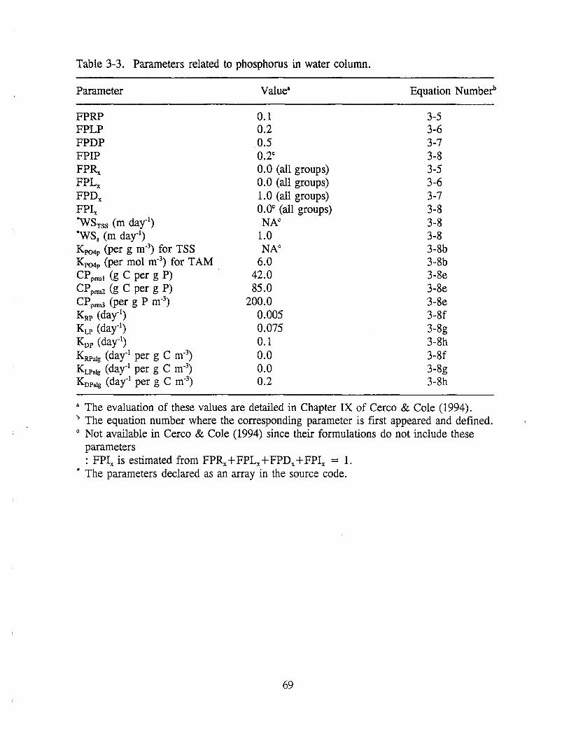
Table 3-3. Parameters related to phosphorus in water column.

Parameter Valuea Equation Number'

FPRP 0.1 3-5 FPLP 0.2 3-6 FPDP " ~ 3-7 v .. .1

FPIP 0.2c 3-8 FPRx 0.0 (all groups) 3-5 FPLx 0.0 (all groups) 3-6 FPDx 1.0 (all groups) 3-7 FPix O.oc (all groups) 3-8 "WSrss (m day·1

) NAC 3-8 'WSs (m day·1

) 1.0 3-8 KP04p (per g m·3) for TSS NAC 3-8b KP04p (per mol m·3

) for TAM . 6.0 3-8b CP pnnt (g C per g P) 42.0 3-8e CP pnn2 (g C per g P) 85.0 3-8e CPpnn3 (per g P m·3) 200.0 3-8e KRP (day·1

) 0.005 3-8f KLP (day·1

) 0.075 3-8g K0 p (day·1) 0.1 3-8h KRPa1g (day·1 per g C m·3) 0.0 3-8f KLPalg ( day·1 per g C m·3) 0.0 3-8g KnPatg ( day·1 per g C m·3) 0.2 3-Sh

a The evaluation of these values are detailed in Chapter IX of Cereo & Cole (1994). b The equation number where the corresponding parameter is first appeared and defined. c Not available in Cereo & Cole (1994) since their formulations do not include these

parameters : FPix is estimated from FPRx + FPLx + FPDx + FPix = 1.

• The parameters declared as an array in the source code.

69

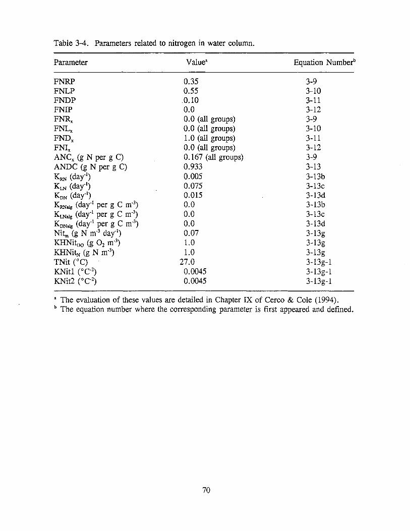
Table 3-4. Parameters related to nitrogen in water column.

Parameter

FNRP FNLP FNDP FNIP FNRx FNLX FNDx FNIX ANCx (g N per g C) ANDC (g N per g C) KRN (day·1)

KLN (day·1)

KnN (day·1)

KRNa1g ( day·1 per g C m·3)

KLNa1g ( day·1 per g C m·3)

KnNalg (day·1 per g C m·3)

Nit:.n (g N m·3 day·1)

KHNit00 (g 0 2 m·3)

KHNitN (g N m·3)

TNit (°C) KNitl (° c-2)

KNit2 (°C·2)

Valuea

0.35 0.55

.0.10 0.0 0.0 (all groups) 0.0 (all groups) 1.0 (all groups) 0.0 (all groups) 0.167 (all groups) 0.933 0.005 0.075 0.015 0.0 0.0 0.0 0.07 1.0 1.0

27.0 0.0045 0.0045

Equation Number'

3-9 3-10 3-11 3-12 3-9 3-10 3-11 3-12 3-9 3-13 3-13b 3-13c 3-13d 3-13b 3-13c 3-13d 3-13g 3-13g 3-13g 3-13g-1 3-13u-1

~

3-13g-1

a The evaluation of these values are detailed in Chapter IX of Cereo & Cole (1994). b The equation number where the corresponding parameter is first appeared and defined.

70

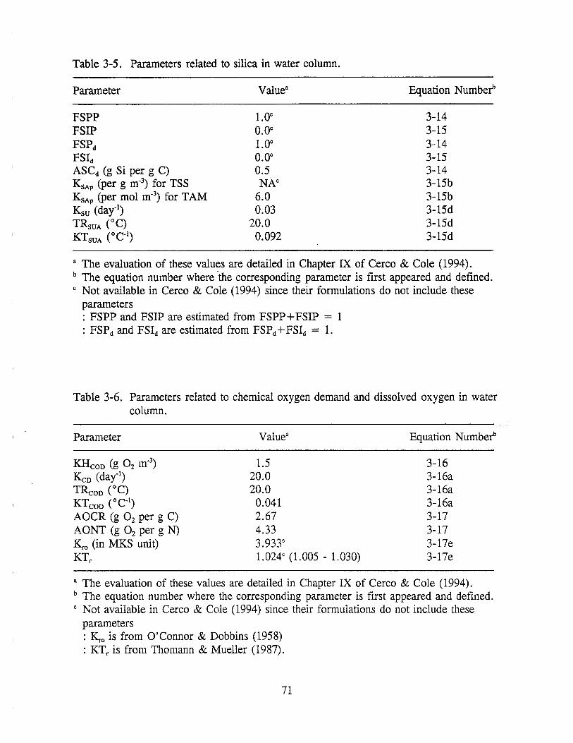
Table 3-5. Parameters related to silica in water column.

Parameter

FSPP FSIP FSPd FSid ASCd (g Si per g C) KsAp (per g m-3

) for TSS KsAp (per mol m-3

) for TAM Ksu (day-1

)

TRsuA (°C) KTsuA (°C-1)

1.oc o.oc 1 {)C

. .L.v

o.oc 0.5 NAC

6.0 0.03

20.0 0.092

Equation Number'>

3-14 3-15 3-14 3-15 3-14 3-15b 3-15b 3-15d 3-15d 3-15d

a The evaluation of these values are detailed in Chapter IX of Cereo & Cole (1994). b The equation number where ·the corresponding parameter is first appeared and defined. c Not available in Cereo & Cole (1994) since their formulations do not include these

parameters : FSPP and FSIP are estimated from FSPP+ FSIP = 1 : FSP d and FSid are estimated from FSP d + FSid = 1.

Table 3-6. Parameters related to chemical oxygen demand and dissolved oxygen in water column.

Parameter

KHcoo (g 02 m-3)

Keo (day-1) TRcoo (°C) KTcoo (°C-1

)

AOCR (g 0 2 per g C) AONT (g 0 2 per g N) Kro (in MKS unit) KTr

Value3

1.5 20.0 20.0

0.041 2.67 4.33 3.933c 1.024c (1.005 - 1.030)

Equation Numberb

3-16 3-16a 3-16a 3-16a 3-17 3-17 3-17e 3-17e

a The evaluation of these values are detailed in Chapter IX of Cereo & Cole (1994). b The equation number where the corresponding parameter is first appeared and defined. c Not available in Cereo & Cole (1994) since their formulations do not include these

parameters : Krois from O'Connor & Dobbins (1958) : KTr is from Thomann & Mueller (1987).

71

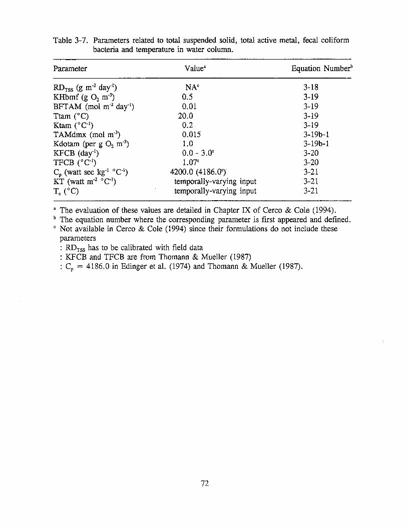
Table 3-7. Parameters related to total suspended solid, total active metal, fecal coliform bacteria and temperature in water column.

Parameter

RDTss (g m·2 day-1)

KHbmf (g 0 2 m·3)

BFTAM (mol m·2 day·i) Ttam (°C) Ktam (°C·1)

TAMdmx (mol m·3)

Kdotam (per g 0 2 m·3)

KFCB (day·1)

TFCB (°C·1)

cp (watt sec kg·1 0 c·1)

KT (watt m·2 0 c·1)

Te (°C)

NAC 0.5 0.01

20.0 0.2 0.015 1.0 0.0 - 3.oc 1.07c

4200.0 (4186.0c) temporally-varying input temporally-varying input

Equation Numberb

3-18 3-19 3-19 3-19 3-19 3-19b-1 3-19b-l 3-20 3-20 3-21 3-21 3-21

a The evaluation of these values are detailed in Chapter IX of Cereo & Cole (1994). b The equation number where the corresponding parameter is first appeared and defined. c Not available in Cereo & Cole (1994) since their formulations do not include these

parameters : RDTss has to be calibrated with field data : KFCB and TFCB are from Thomann & Mueller (1987) : CP = 4186.0 in Edinger et al. (1974) and Thomann & Mueller (1987).

72

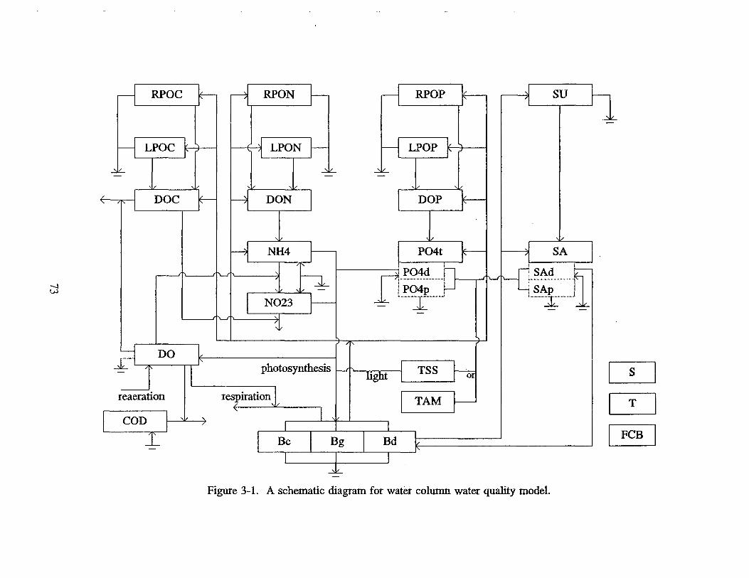
-..I VJ

RPOC

LPOC

DOC

DO

reaeration

COD

RPON RPOP SU

.1 LPON LPOP

DOP

P04t SA I l d r

~~i_l_ r--- I .

rl···!1..9.i~.-,.J -b 1~_J

photosynthesis TSS s

respiration TAM T

Be Bd FCB

Figure 3-1. A schematic diagram for water column water quality model.

Chapter IV. Sediment Process Model

The sediment process model developed by DiToro & Fitzpatrick (1993) was

coupled with CE-QUAL-ICM for Chesapeake Bay water quality modeling (Cereo & Cole

1994). This sediment model is slightly modified and included in the present model

package. An asterisk mark (*) attached to equation number denotes formulations that are

different from the model in DiToro & Fitzpatrick (1993): hereinafter this report is

referred to as D&F. The sediment process model has sixteen water quality related model

state variables and fluxes.

1) particulate organic carbon

3) particulate organic phosphorus

5) sulfide/ methane

7) nitrate nitrogen

9) available silica

10) ammonium nitrogen flux

12) phosphate phosphorus flux

14) sediment oxygen demand

16) sediment temperature

2) particulate organic nitrogen

4) particulate biogenic silica

6) ammonium nitrogen

8) phosphate phosphorus

11) nitrate nitrogen flux

13) silica flux

15) release of chemical oxygen demand

In the sediment model, benthic sediments are represented as two layers (Fig. 4-1).

The upper layer (Layer 1) is in contact with the water column and may be oxic or anoxic

depending on dissolved oxygen concentration in the overlying water. The lower layer

(Layer 2) is permanently anoxic. The upper layer depth, which is determined by the

penetration of oxygen into the sediments, is at its maximum only a small fraction of the

total. Because H1 ( - 0.1 cm) « H2,

(4-1)

where His the total depth (approximately 10 cm: see Section IV-7-2D), H1 is the upper

layer depth and H2 is the lower layer depth.

The model incorporates three basic processes (Fig. 4-2): 1) depositional flux of

particulate organic matter (POM), 2) their diagenesis and 3) resulting sediment flux. The

sediment model is driven by net settling of particulate organic carbon, nitrogen,

74

phosphorus and silica from the overlying water to the sediments ( depositional flux).

Because of the negligible thickness of the upper layer (Eq. 4-1), deposition is considered

to be proceeded from the water column directly to the lower layer. Within the lower

layer, the model simulates the diagenesis (mineralization or decay) of deposited POM,

which produces oxygen demand and inorganic nutrients (diagenesis flux). The third

basic process is the flux of substances produced by diagenesis (sediment flux). Oxygen

demand, as sulfide (in saltwater) or methane (in freshwater), takes three paths out of the

sediments: 1) oxidation at the sediment-water interface as sediment oxygen demand, 2)

export to the water column as chemical oxygen demand or 3) burial to deep, inactive

sediments. Inorganic nutrients produced by diagenesis takes two paths out of the

sediments: 1) release to the water column or 2) burial to deep, inactive sediments (Fig. 4-

2).

This chapter describes the three basic processes with reactions and sources/ sinks for

each state variable. The method of solution including finite difference equations, solution

scheme, boundary and initial conditions, and stand alone model are explained in Section

IV-6. Parameter evaluation and some limitations of the model formulations found in

D&F are described in Section IV-7. Complete model documentation can be found in

D&F.

IV-1. Depositional Flux

Deposition is one process that couples the water column model with the sediment

model. Consequently, deposition is represented in both the water column and sediment

models. In the water column model, the governing mass-balance equations for the

following state variables:

three algal groups, cyanobacteria, diatoms and green algae (Eq. 3-1)

refractory and labile particulate organic carbon (Equations 3-2 and 3-3)

refractory and labile particulate organic phosphorus (Equations 3-5 and 3-6) and

total phosphate (Eq. 3-8)

refractory and labile particulate organic nitrogen (Equations 3-9 and 3-10)

particulate biogenic silica (Eq. 3-14) and available silica (Eq. 3-15)

contain settling terms, which represent the depositional fluxes.

75

The sediment model receives these depositional fluxes of particulate organic carbon

(POC), particulate organic nitrogen (PON), particulate organic phosphorus (POP) and

particulate biogenic silica (PSi). Because of the negligible thickness of the upper layer

(Eq. 4-1), deposition is considered to proceed from the water column directly to the

lower layer. Since the sediment model has three G classes of POM, Gi (i = 1, 2 or 3),

depending on the time scales of reactivity (Section IV-2), the POM fluxes from the water

column should be mapped into three G classes based on their reactivity. Then, the

depositional fluxes for the ilh G class (i = 1, 2 or 3) may be expressed as:

JPOC,i = FCLP/WSLP·LPOCA + FCRP/WSRP·RPQCA + L FCBx/WSx·B/ (4-2) x=c,d,g

JPON,1' = FNLP:WS ·LPONA + FNRP:WS ·RPONA + "' FNB .·ANC ·WS ·BA (4-3) I LP . I RP L.J X,I X ., .,

x=c,d,g

J = FPLP:WS ·LPOPA + FPRP:WS ·RPOPA + "' FPB :APC·WS ·BA POP,i I LP I RP L.J x,1 x ·' x=c,d,g

+ \ · WSTSs· P04p A (4-4)

(4-5)

IroM,i = depositional flux of POM (M = C, Nor P) routed into the ilh G class (g m·2

day·1)

JPsi = depositional flux of PSi (g Si m·2 day·1)

FCLPi, FNLPi & FPLPi = fraction of water column labile POC, PON and POP,

respectively, routed into the ilh G class in sediment

FCRPi, FNRPi & FPRPi = fraction of water column refractory POC, PON and POP,

respectively, routed into the ilh G class in sediment

FCBx,i, FNBx,i & FPBx,i = fraction of POC, PON and POP, respectively, in the algal

group x routed into the ilh G class in sediment

Aj = 1 for i = 1

0 for i = 2 or 3.

The superscript A indicates the interval average as defined in Eq. 3-22$-1. The settling

of sorbed phosphate is considered to contribute to the labile G1 pool in Eq. 4-4, and

settling of sorbed silica contributes to Jpsi in Eq. 4-5 to avoid creation of additional

76

depsoitional fluxes for inorganic particulates. The sum of distribution coefficients should

be unity: Ei FCLPi = Ei FNLPi = Ei FPLPi = Ei FCRPi = Ei FNRPi = Ei FPRPi = Ei

FCBx,i = Ei FNBx,i = Ei FPBx,i = 1. The settling velocities, WSLP, WSRP, WSx and

WSTss, as defined in the water column model (Chapter III), are net settling velocities.

IV-2. Diagenesis Flux

Another coupling point of the sediment model to the water column model is the

sediment flux, which is described in Section IV-3. The computation of sediment flux

requires that the magnitude of the diagenesis flux be known. The diagenesis flux is

explicitly computed using mass-balance equations for deposited POC, PON and POP.

(Dissolved silica is produced in the sediments as the result of the dissolution of PSi.

Since the dissolution process is different from bacterial-mediated diagenesis process, it is

presented separately in Section IV-4.) In the mass-balance equations, the depositional

fluxes of POM are the source terms and the decay of POM in the sediments produces the

diagenesis fluxes. The integration of the mass-balance equations for POM provides the

diagenesis fluxes that are the inputs for the mass-balance equations for ammonium,

nitrate, phosphate and sulfide/methane in the sediments (Section IV-3).

The difference in decay rates of POM is accounted for by assigning a fraction of

POM to various decay classes (Westrisch & Berner 1984). POM in the sediments is

divided into three G classes, or fractions, representing three scales of reactivity. The G1

Oabile) fraction has a half life of 20 days, and the G2 (refractory) fraction has a half life

of one year. The G3 (inert) fraction is non-reactive, i.e., undergoes no significant decay

before burial into deep, inactive sediments. The varying reactivity of the G classes

controls the time scale over which changes in depositional flux will be reflected in

changes in diagenesis flux. If the G1 class would dominate the POM input into the

sediments, then there would be no significant time lag introduced by POM diagenesis and

any changes in depositional flux would be readily reflected in diagenesis flux.

Because the upper layer thickness is negligible (Eq. 4-1) and thus depositional flux

is considered to proceed directly to the lower layer (Equations 4-2 to 4-5), diagenesis is

considered to occur in the lower layer only. The mass-balance equations are similar for

POC, PON and POP, and for different G classes. The mass-balance equation in the

77

anoxic lower layer for the ith G class (i = 1, 2 or 3) may be expressed as:

H a GPOM,i 8r- 20 2 at = - KPOM,i • POM,i • a POM,i • H2 - w · a POM,i + 1 POM,i

(4-6)

GroM,i = concentration of POM (M = C, Nor P) in the ith G class in Layer 2 (g m·3)

KPOM,i = decay rate of the ith G class POM at 20°C in Layer 2 (day·1)

OroM,i = constant for temperature adjustment for KroM,i

T = sediment temperature (°C)

W = burial rate (m day·1).

Since the G3 class is inert, KPoM,3 = 0.

Once the mass-balance equations for GroM,t and GroM,2 are solved, the diagenesis

fluxes are computed from the .rate of mineralization of the two reactive G classes:

2

"' 8r - 20 G J M = L. KPOM,i' POM,i ' POM,i, H2 (4-7) i=I

JM = diagenesis flux (g m·2 day·1) of carbon (M = C), nitrogen (M = N) or phosphorus

(M = P).

IV-3. Sediment Flux

The mineralization of POM produces soluble intermediates, which are quantified as

diagenesis fluxes in the previous section. The intermediates react in the oxic and anoxic

layers, and portions are returned to the overlying water as sediment fluxes. Computation

of sediment fluxes requires mass-balance equations for ammonium, nitrate, phosphate,

sulfide/methane and available silica. This section describes the flux portion for

ammonium, nitrate, phosphate and sulfide/methane of the model. Available silica is

described in Section IV-4.

In the upper layer, the processes included in the flux portion are (Fig. 4-1)

: exchange of dissolved fraction between Layer 1 and the overlying water

: exchange of dissolved fraction between Layer 1 and 2 via diffusive transport

: exchange of particulate fraction between Layer 1 and 2 via particle mixing

: loss by burial to the lower layer (Layer 2)

: removal (sink) by reaction

78

: internal sources.

Since the upper layer is quite thin, H1 - 0.1 cm (Eq. 4-1) and the surface mass transfer

coefficient (s) is on the order of 0.1 m day·1, then the residence time in the upper layer

is: H/s - 10·2 days. Hence, a steady-state approximation is made in the upper layer.

Then, the mass-balance equation for ammonium, nit.1"3.te, phosphate or sulfide/methane in

the upper layer is:

ao1 H1 - = 0 = s(fd0·Ct0 - fd1·Ct1) + KL(fd2·Ct2 - fd1·Ct1) at

Ct1 & Ct2 = total concentrations in Layer 1 and 2, respectively (g m·3)

Ct0 = total concentration in the overlying water (g m·3)

s = surface mass transfer coefficient (m day·1)

KL = diffusion velocity for dissolved fraction between Layer 1 and 2 (m day·1)

~ = particle mixing velocity between Layer 1 and 2 (m day·1)

fd0 = dissolved fraction of total substance in the overlying water (0 :5 fd0 :5 1)

fd1 = dissolved fraction of total substance in Layer 1 (0 :5 fd1 :5 1)

fp1 = particulate fraction of total substance in Layer 1 ( = 1 - fd 1)

fd2 = dissolved fraction of total substance in Layer 2 (0 :5 fd2 :5 1)

fp2 = particulate fraction of total substance in Layer 2 ( = 1 - fd2)

K1 = reaction velocity in Layer 1 (m day·1)

J1 = sum of all internal sources in Layer 1 (g m·2 day-1).

(4-8)

The first term on the RHS of Eq. 4-8 represents the exchange across sediment­

water interface. Then, the sediment flux from Layer 1 to the overlying water, which

couples the sediment model to the water column model, may be expressed as:

J = s(fia ·Ct - fia ·Ct 'I aq 1 1 o ol (4-9)

Jaq = sediment flux of ammonium, nitrate, phosphate or sulfide/methane to the overlying

water (g m·2 day·1).

The convention used in Eq. 4-9 is that positive flux is from the sediment to the overlying

water.

79

In the lower layer, the processes included in the flux portion are (Fig. 4-1)

: exchange of dissolved fraction between Layer 1 and 2 via diffusive transport

: exchange of particulate fraction between Layer 1 and 2 via particle mixing

: deposition from Layer 1, and burial to the deep inactive sediments

: removal ( sink) by reaction

: internal sources including diagenetic source.

The mass-balance equation for ammonium, nitrate, phosphate or sulfide/methane in the

lower layer is:

act2 H2-- = at - KL (fia . Ct - fia . Ct ) - ~ (fp . Ct - fp . Ct ) 2 2 11 2 2 11

K2 = reaction velocity in Layer 2 (m day-1)

J2 = sum of all internal sources including diagenesis in Layer 2 (g m-2 day-1).

(4-10)

The substances produced by mineralization of POM in sediments may be present in

both dissolved and particulate phases. This distribution directly affects the magnitude of

the substance that is returned to the overlying water. In Equations 4-8 to 4-10, the

distribution of a substance between the dissolved and particulate phases in a sediment is

parameterized using a linear partitioning coefficient. The dissolved and particulate

fractions are computed from the partitioning equations:

fd1 = 1

1 + m1.,1r1 (4-11-1)

fd2 = 1

1 + m2 "Tr2 (4-11-2)

m1 & m2 = solid concentrations in Layer 1 and 2, respectively (kg L-1)

1r1 & 1r2 = partition coefficients in Layer 1 and 2, respectively (per kg L-1).

The partition coefficient is the ratio of particulate to dissolved fraction per unit solid

concentration (i.e., per unit sorption site available).

All terms, except the last two terms, in Equations 4-8 and 4-10 are common to all

state variables and are described in Section IV-3-1. The last two terms represent the

80

reaction and source/sink terms, respectively. These terms, which take different

mathematical formulations for different state variables, are described in Sections IV-3-2

to IV-3-5 for ammonium, nitrate, phosphate and sulfide/methane, respectively.

IV -3-1. Common pa...-ra.T.eters for sedi.ment flux

Parameters that are needed for the sediment fluxes are s, ~, KL, W, H2, m1, m2,

1r1, 1r2, K1, K2, 11 and 12 in Equations 4-8 to 4-11. Of these, Ki, K2, 11 and 12 are variable­

specific. Among the other common parameters, W (Section IV-7-2C), H2 (Section IV-7-

2D), and m1 and m2 (Section IV-7-3B), are specified as input. The modeling of the

remaining three parameters, s, ~' KL, are described in this section.

A. Surface mass transfer coefficient: Owing to the observation that the surface mass

transfer coefficient, s, can be related to the sediment oxygen demand, SOD (DiToro et al.

1990), s can be estimated from the ratio of SOD and overlying water oxygen

concentration:

s = D1 = SOD HI DOO

(4-12)

D1 = diffusion coefficient in Layer 1 (m2 day-1).

Knowings, it is possible to estimate the other model parameters.

B. Particulate phase mixing coefficient: The particle mixing velocity between Layer 1

and 2 is parameterized as:

fl- 20 G DO ~ = DP' Dp POC,l 0

H2 Gpoc,R KMDp + DOo

DP = apparent diffusion coefficient for particle mixing (m2 day-1)

00p = constant for temperature adjustment for DP

Gpoc,R = reference concentration for Gpoc,1 (g C m·3)

Kivlnp = particle mixing half-saturation constant for oxygen (g 0 2 m-3).

(4-13)

The enhanced mixing of sediment particles by macrobenthos (bioturbation) is quantified

by estimating DP. The particle mixing appears to be proportional to the benthic biomass

81

(Matisoff 1982), which is correlated to the carbon input to the sediment (Robbins et al.

1989). This is parameterized by assuming that benthic biomass is proportional to the

available labile carbon, Groc,1, and Groc,R is the reference concentration at which the

particle mixing velocity is at its nominal value. The Monod-type oxygen dependency

accounts for the oxygen dependency o_f benthic biomass.

It has been observed that a hysteresis exists in the relationship between the bottom

water oxygen and benthic biomass. Benthic biomass increases as the summer progresses.

However, the occurrence of anoxia/hypoxia reduces the biomass drastically and also

imposes stress on benthic activities. After full overturn, the bottom water oxygen

increases but the population does not recover immediately. Hence, the particle mixing

velocity, which is proportional to the benthic biomass, does not increase in response to

the increased bottom water oxygen. Recovery of benthic biomass following hypoxic

events depends on many factors including severity and longevity of hypoxia, constituent

species and salinity (Diaz & Rosenberg, submitted).

This phenomenon of reduced benthic activities and hysteresis is parameterized based

on the idea of stress that low oxygen imposes on the benthic population. It is analogous

to the modeling of the toxic effect of chemicals on organisms (Mancini 1983). A first

order differential equation is employed, in which the benthic stress 1) accumulates only

when overlying oxygen is below KM0 P and 2) is dissipated at a first order rate (Fig. 4-

3a):

asT = - K ·ST + [ 1 - DOO l at ST KAf Dp

(4-14)*

asT = - K ·ST at ST

ST = accumulated benthic stress (day)

KsT = first order decay rate for ST (day-1).

The behavior of this formulation can be understood by evaluating the steady-state stresses

at two extreme conditions of overlying water oxygen, D00:

as D00 = 0

as D00 ~ KMop

KsT·ST = 1

KsT·ST = 0

82

f(ST) = (1 - KsT·ST) = 0

f(ST) = (1 - KsT·ST) = 1

The unitless expression, f(ST) = 1 - KsT·ST, appears to be the proper variable to

quantify the effect of benthic stress on benthic biomass and thus particle mixing (Fig. 4-

3b).

The final formulation for the particle mixing velocity including the benthic stress is:

~ = DP. O~P- 20 GPoc,1 DOo . ft.ST) + Dpmm

H2 Gpoc,R KMDp + DOo H2 (4-15)

Dpmm = minimum diffusion coefficient for particle mixing (m2 day-1).

The reduction in particle mixing due to the benthic stress, f(ST), is estimated by

employing the following procedure. The stress, ST, is normally calculated with Eq. 4-

14. Once D00 drops below a critical concentration, DOsT,c, for NChypoxia consecutive days

or more, the calculated stress is not allowed to decrease until tMBS days of D00 > DOsT,c·

That is, only when hypoxic days are longer than critical hypoxia days (NChypoxiJ, the

maximum stress, or minimum (1 - KsT·ST), is retained for a specified period (tMBs days)

after D00 recovery (Fig. 4-3). No hysteresis occurs if D00 does not drop below DOsT,c

or if hypoxia lasts shorter than NChypoxia days. When applying maximum stress for tMBs

days, the subsequent hypopxic days are not included in tMBS. This parametrization of

hysteresis essentially assumes seasonal hypoxia, i.e., one or two major hypoxic events

during summer, and might be unsuitable for systems with multiple hypoxic events

throughout a year.

Three parameters relating to hysteresis, DOsT,c, NChypoxia and tMBs, are functions of

many factors including severity and longevity of hypoxia, constituent species and salinity,

and thus have site-specific variabilities (Diaz & Rosenberg, submitted). The critical

overlying oxygen concentration, DOsT,c, also depends on the distance from the bottom of

the location of D00 measurement, which is discussed in section for parameter evaluation

(Section IV-7-3B). The critical hypoxia days, NChypoxia, depends on tolerance of benthic

organisms to hypoxia and thus on benthic community structure (Diaz & Rosenberg,

submitted). The time lag for the recovery of benthic biomass following hypoxic events,

tMBS, tends to be longer for higher salinity. Since the present tidal prism model is

intended to be applied to relatively small systems, the above three parameters are

considered to be spatially constant input parameters.

83

C. Dissolved phase mixing coefficient: Dissolved phase mixing between Layer 1 and 2

is via passive molecular diffusion, which is enhanced by the mixing activities of the

benthic organisms (bio-irrigation). This is modeled by increasing the diffusion coefficient

relative to the molecular diffusion coefficient:

KL:::: D .. (}~ - 20 - a ·ud

H2

Dd = diffusion coefficient in pore water (m2 day·1)

Bod = constant for temperature adjustment for Dd

RBI.BT = ratio of bio-irrigation to bioturbation.

The last term in Eq. 4-16 accounts for the enhanced mixing by organism activities.

IV-3-2. Ammonium nitrogen

(4-16)

Diagenesis is assumed not to occur in the upper layer because of its shallow depth,

and ammonium is produced by diagenesis in the lower layer:

Jl,NH4 :::: Q 12,NH4 :::: J N (from Eq. 4-7) (4-17)

Ammonium is nitrified to nitrate in the presence of oxygen. A Monod-type expression is

used for the ammonium and oxygen dependency of the nitrification rate. Then, the oxic

layer reaction velocity in Eq. 4-8 for ammonium may be expressed as:

2 DOO KM.NH4 2 (JT - 20

Kt,NH4 :::: 2·.KM. DO KM. NH4 KNH4' NH4 NH4,02 + 0 NH4 + I

and then the nitrification flux becomes:

2

J . ;: Kt,NH4 • NH4 Nit S I

KMNH4•02 = nitrification half-saturation constant for dissolved oxygen (g 0 2 m·3)

NH41 = total ammonium nitrogen concentration in Layer 1 (g N m·3)

KMNH4 = nitrification half-saturation constant for ammonium (g N m·3)

KNH4 = optimal reaction velocity for nitrification at 20°C (m day-1)

ONH4 = constant for temperature adjustment for KNH4

JNit = nitrification flux (g N m·2 day-1).

84

(4-18)

(4-19)

Nitrification does not occur in the anoxic lower layer:

(4-20)

Once Equations 4-8 and 4-10 are solved for NH41 and NH42, the sediment flux of

ammonium to the overlying water, Jaq,NH4 , can be calculated using Eq. 4-9. Note that it is

not NH41 and NH42 that determine the magnitude of Iaq,NH4 (Section X-B-2 in D&F). The

magnitude is determined by 1) the diagenesis flux, 2) the fraction that is nitrified and 3)

surface mass transfer coefficient (s) that mixes the remaining portion.

IV-3-3. Nitrate nitrogen

Nitrification flux is the only source of nitrate in the upper layer, and there is no

diagenetic source for nitrate in both layers:

11,N03 = l,Vil (from Eq. 4-19) J2,N03 = 0 (4-21)

Nitrate is present in sediments as dissolved substance, i.e., 71"i,No3 = 71"2,N03 = 0, making

fd1,No3 = fd2,No3 = 1 (Eq. 4-11): it also makes fu meaningless, hence fu = 0. Nitrate is

removed by denitrification in both oxic and anoxic layers with the carbon required for

denitrification supplied by carbon diagenesis. The reaction velocities in Equations 4-8

and 4-10 for nitrate may be expressed as:

2 2 (}T - 20 K1,N03 = KN03,l' N03

OT - 20 K2,N03 = KN03,2 • N03

and the denitrification flux out of sediments as a nitrogen gas becomes:

2 K1,No3

lmv;> = -s-N031 + K2,No3·N032

KNo3,1 = reaction velocity for denitrification in Layer 1 at 20°C (m day·1)

KNo3,2 = reaction velocity for denitrification in Layer 2 at 20°C (m day·1)

(}N03 = constant for temperature adjustment for KNo3,1 and KNo3,2

JN2(g> = denitrification t1ux (g N m·2 day-1)

N03 1 = total nitrate nitrogen concentration in Layer 1 (g N m·3)

N032 = total nitrate nitrogen concentration in Layer 2 (g N m·3).

85

(4-22-1)

(4-22-2)

(4-23)

Once Equations 4-8 and 4-10 are solved for N031 and N032, the sediment flux of

nitrate to the overlying water, Iaq,No3 , can be calculated using Eq. 4-9. The steady-state

solution for nitrate showed that the nitrate flux is a linear function of N030 (Eq. III-15 in

D&F): the intercept quantifies the amount of ammonium in the sediment that is nitrified

but not denitrified (thus releases as Iaq,No3), and the slope quantifies the extent to which

overlying water nitrate is denitrified in the sediment. It also revealed that if the internal

production of nitrate is small relative to the flux of nitrate from the overlying water, the

normalized nitrate flux to the sediment, - Iaq,N03/N030, is linear in s for small s and

constant for larges (Section 111-C in D&F). For smalls (- 0.01 m day-1), H1 is large (Eq.

4-12) so that oxic layer denitrification predominates and Jaq,No3 is essentially zero

independent of N030 (Fig. III-4 in D&F).

IV -3-4. Phosphate phosphorus

Phosphate is produced by the diagenetic breakdown of POP in the lower layer:

11,p04 = 0 l 2,P04 = JP (from Eq. 4-7) (4-24)

A portion of the liberated phosphate remains in the dissolved form and a portion becomes

particulate phosphate, either via precipitation of phosphate-containing minerals (Troup

1974), e.g., vivianite, F~(P04)i(s), or by partitioning to phosphate sorption sites

(Lijklema 1980; Barrow 1983; Giordani & Astorri 1986). The extent of particulate

formation is determined by the magnitude of the partition coefficients, 7r1,p04 and 7r2,p04 , in

Eq. 4-11. Phosphate flux is strongly affected by D00, the overlying water oxygen

concentration. As D00 approaches zero, the phosphate flux from the sediments

increases. This mechanism is incorporated by making 7r1,p04 larger, under oxic

conditions, than 7r2,P04. In the model, when D00 exceeds a critical concentration,

(D00)crit,P04, sorption in the upper layer is enhanced by an amount A7rp04,1:

DOo > (DOJcrit,P04

When oxygen falls below (D00)crit,Po4, then:

_ • ( A )DO,J (DOJcn.P0< 71" 1,P04 - 71" 2,P04 l..l. 71" P04, 1 DOo :::;; (DOJcri1,P04

(4-25-1)

(4-25-2)

which smoothly reduces 7r1.p04 to 7r2,p04 as D00 goes to zero. There is no removal

86

reaction for phosphate in both layers:

K1,P04 = K2,P04 = Q (4-26)

Once Equations 4-8 and 4-10 are solved for P041 and P042, the sediment flux of

phosphate to the overlying water, Iaq,P04, can be calculated using Eq. 4-9.

IV-3-5. Sulfide/methane and oxygen demand

A. Sulfide: No diagenetic production of sulfide occurs in the upper layer. In the lower

layer, sulfide is produced by carbon diagenesis (Eq. 4-7) decremented by the organic

carbon consumed by denitrification (Eq. 4-23). Then:

f1,H2S = Q (4-27)

ao2.c = stoichiometric coefficient for carbon diagenesis consumed by sulfide oxidation

(2.6667 g 0 2-equivalents per g C)

ao2.N03 = stoichiometric coefficient for carbon diagenesis consumed by denitrification

(2.8571 g Orequivalents per g N).

A portion of the dissolved sulfide that is prodllced in the anoxic layer reacts with the iron

to form particulate iron monosulfide, FeS(s) (Morse et al. 1987). The particulate fraction

is mixed into the oxic layer where it can be oxidized to ferric oxyhydroxide, F~03(s).

The remaining dissolved fraction also diffuses into the oxic layer where it is oxidized to

sulfate. Partitioning between dissolved and particulate sulfide in the model represents the

formation of FeS(s), which is parameterized using partition coefficients, '71"1,828 and '71"2,82s,

in Eq. 4-11.

The present sediment model has three pathways for sulfide, the reduced end product

of carbon diagenesis: 1) sulfide oxidation, 2) aqueous sulfide flux and 3) burial. The

distribution of sulfide among the three pathways is controlled by the partitioning

coefficients and the oxidation reaction velocities (Section V-E in D&F). Both dissolved

and particulate sulfide are oxidized in the oxic layer, consuming oxygen in the process.

In the oxic upper layer, the oxidation rate that is linear in oxygen concentration is used

(Cline & Richards 1969; Millero 1986; Boudreau 1991). In the anoxic lower layer, no

oxidation can occur. Then, the reaction velocities in Equations 4-8 and 4-10 may be

expressed as:

87

2 2 2 r- 20 DOo Kt,H2S = (KH2S,dl 'fdt,H2S + KH2S,pl ·!P1,m) ()H2S 2·KM

HZS,02

K2H2S = Q .

(4-28-1)

(4-28-2)

KH2s,dt = reaction velocity for dissolved sulfide oxidation in Layer 1 at 20°C (m day-1)

KH2s,pi = reaction velocity for particulate sulfide oxidation in Layer 1 at 20°C (m day-1)

OH2s = constant for temperature adjustment for KH2s,dt and K82s,pt

KMH2s,o2 = constant to normalize the sulfide oxidation rate for oxygen (g 0 2 m-3).

The constant, KMH2s,o2, which is included for convenience only, is used to scale the

oxygen concentration in the overlying water. At D00 = KMH2s,o2, the reaction velocity

for sulfide oxidation rate is at its nominal value.

The oxidation reactions in the oxic upper layer cause oxygen flux to the sediment,

which exerts SOD. By convention, SOD is positive: SOD = -Jaq,02 • The SOD in the

model consists of two components, carbonaceous sediment oxygen demand (CSOD) due

to sulfide oxidation and nitrogenous sediment oxygen demand (NSOD) due to

nitrification:

2 Kt,H2S

SOD = CSOD + NSOD = --H2S1 + a02 NH4 • J tvu s .

H2S1 = total sulfide concentration in Layer 1 (g 0 2-equivalents m-3)

(4-29)

aa2,NH4 = stoichiometric coefficient for oxygen consumed by nitrification (4.33 g 0 2 per

g N: Section III-7-2).

Equation 4-29 is nonlinear for SOD because the RHS contains s ( = S0D/D00) so that

SOD appears on both sides of the equation: note that JNit (Eq. 4-19) is also a function of

s. A simple back substitution method is used, as explained in Section IV-6-1.

If the overlying water oxygen is low, then the sulfide that is not completely

oxidized in the upper layer can diffuse into the overlying water. This aqueous sulfide

flux out of the sediments, which contributes to the chemical oxygen demand in the water

column model, is modeled using

Jaq,H2S = S (fdl,H2S' H2S1 - COD) (4-30)*

The sulfide released from the sediment reacts very quickly in the water column when

88

oxygen is avilable, but can accumulate in the water column under anoxic conditions. The

COD, quantified as oxygen equivalents, is entirely supplied by benthic release in the

water column model (Eq. 3-16). Since sulfide also is quantified as oxygen equivalents,

COD is used as a measure of sulfide in the water column in Eq. 4-30.

B. Methane: When sulfate is used up, methane can be produced by carbon diagenesis

and methane oxidation consumes oxygen (DiToro et al. 1990). Owing to the abundant

sulfate in the saltwater, only the aforementioned sulfide production and oxidation are

considered to occur in the saltwater. Since the sulfate concentration in the freshwater is

generally insignificant, methane production is considered to replace sulfide production in

the freshwater. In the freshwater, methane is produced by carbon diagenesis in the lower

layer decremented by the organic carbon consumed by denitrification, and no diagenetic

production of methane occurs in the upper layer (Eq. 4-27):

12,CH4 = a02,C. JC - a02,N03. J N2(g) (4-31)

The dissolved methane produced takes two pathways: 1) oxidation in the oxic upper layer

causing CSOD or 2) escape from the sediment as aqueous flux or as gas flux:

J2,CH4 = CSOD + Jaq,CH4 + J CH4(g)

Jaq,cH4 = aqueous methane flux (g Oz-equivalents m·2 day·1)

JcH4(g> = gaseous methane flux (g Oz-equivalents m·2 day·1).

(4-32)

A portion of dissolved methane that is produced in the anoxic layer diffuses into the

oxic layer where it is oxidized. This methane oxidation causes CSOD in the freshwater

sediment (DiToro et al. 1990):

[ 0r - 20 l

CSOD = CSODmax. 1 - sech[ KCHis CH4

] (4-33)

(4-33-1)

CH4,., = 100 [ 1 + h ;/2 J 1.02420 - ' (4-33-2)

CSODmax = maximum CSOD occurring when all the dissolved methane transported to

89

the oxic layer is oxidized

KcH4 = reaction velocity for dissolved methane oxidation in Layer 1 at 20°C (m day·1)

OcH4 = constant for temperature adjustment for Kc84

CH4sat = saturation concentration of methane in the pore water (g Orequivalents m·3).

The term, (h + H2)/10 where hand H2 are in meters, in Eq. 4-33-2 is the depth from the

water surface that corrects for the in situ pressure. Equation 4-33-2 is accurate to within

3% of the reported methane solubility between 5 and 20°C (Yamamoto et al. 1976).

If the overlying water oxygen is low, the methane that is not completely oxidized

can escape the sediment into the overlying water either as aqueous flux or as gas flux.

The aqueous methane flux, which contributes to the chemical oxygen demand in the water

column model, is modeled using (DiToro et al. 1990):

T - 20 KcH/OcH4

Jaq CH4 ::; CSOD max' sech[ ] = CSOD max - CSOD . s (4-34)

Methane is only slightly soluble in water. If its solubility, CH4sat given by Eq. 4-33-2, is

exceeded in the pore water, it forms a gas phase that escapes as bubbles. The loss of

methane as bubbles, i.e., the gaseous methane flux, is modeled using Eq. 4-32 with J2.c84

from Eq. 4-31, CSOD from Eq. 4-33 and Jaq,cH4 from Eq. 4-34 (DiToro et al. 1990).

IV-4. Silica

The production of ammonium, nitrate and phosphate in sediments is the result of

the mineralization of POM by bacteria. The production of dissolved silica in sediments is

the result of the dissolution of particulate biogenic or opaline silica, which is thought to

be independent of bacterial processes.

The depositional flux of particulate biogenic silica from the overlying water to the

sediments is modeled using Eq. 4-5. With this source, the mass-balance equation for

particulate biogenic silica may be written as:

PSi = concentration of particulate biogenic silica in the sediment (g Si m·3)

Ssi = dissolution rate of PSi in Layer 2 (g Si m·3 day·1)

90

(4-35)

JPSi = depositional flux of PSi (g Si m-2 day-1) given by Eq. 4-5

Josi = detrital flux of PSi (g Si m-2 day-1) to account for PSi settling to the sediment that

is not associated with the algal flux of biogenic silica (??).

The processes included in Eq. 4-35 are dissolution (i.e., production of dissolved silica),

burial, ai,d depositional a....-1d detrital fluxes from the overlying water. Equation 4-35 can

be viewed as the analog of the diagenesis equations for POM (Eq. 4-6). The dissolution

rate is formulated using a reversible reaction that is first order in silica solubility deficit

and follows a Monod-type relationship in particulate silica:

Ssi = Ks/0~ - 20 PSi PSi (Sisat - fd2,s/Si2) + KMPSi

Ksi = first order dissolution rate for PSi at 20°C in Layer 2 (day-1)

Osi = constant for temperature adjustment for Ksi

K.Mpsi = silica dissolution half-saturation constant for PSi (g Si m-3)

Sisat = saturation concentration of silica in the pore water (g Si m-3).

(4-36)

The mass-balance equations for mineralized silica can be formulated using the

general forms, Equations 4-8 and 4-10. There is no source/sink term and no reaction in

the upper layer:

(4-37)

In the lower layer, silica is produced by the dissolution of particulate biogenic silica,

which is modeled using Eq. 4-36. The two terms in Eq. 4-36 correspond to the source

term and reaction term in Eq. 4-10:

1 =K·Or.-20 PSi s· H 2,Si Si s, PSz' KM l sat' 2

+ PSi (4-38-1)

= K ,(Jr. - 20 PSi +' ·H Si s, PSi + KMps/d2,Si 2

(4-38-2)

A portion of silica dissolved from particulate silica sorbs to solids and a portion

remains in the dissolved form. Partitioning using the partition coefficients, 7ri.si and 7r2,si,

in Eq. 4-11 controls the extent to which dissolved silica sorbs to solids. Since silica

shows similar behavior as phosphate in adsorption-desorption process, the same

91

partitioning method as applied to phosphate (Section IV-3-4) is used for silica. That is,

when D00 exceeds a critical concentration, (D00)cri1,sb sorption in the upper layer is

enhanced by an amount Li1rsi,1:

DOO > (DOJcrit,Si (4-39-1)

Wnen oxygen falls below (D00)crit,si, then:

(4-39-2)

which smoothly reduces 1r1,si to 1r2,si as D00 goes to zero.

Once Equations 4-8 and 4-10 are solved for Si1 and Si2 , the sediment flux of silica

to the overlying water, Iaq,si, can be calculated using Eq. 4-9.

IV-5. Sediment temperature

All rate coefficients in the aforementioned mass-balance equations are expressed as

a function of sediment temperature, T. The sediment temperature is modeled based on

the diffusion of heat between the water column and sediment:

aT = Dr (T _ 1) at H 2 w

DT = heat diffusion coefficient between the water column and sediment (m2 sec·1)

Tw = temperature in the overlying water column (°C) calculated by Eq. 3-21.

(4-40)

The model application in D&F and Cereo & Cole (1994) used DT = 1.8 x 10·7 m2 sec·1•

IV-6. Nlethod of Solution

IV -6-1. Finite difference equations and solution scheme

An implicit integration scheme is used to solve the governing mass-balance

equations. The finite difference form of Eq. 4-8 may be expressed as:

0 = s(fd0·Ct/i - fd1·Cti) + KL(fd2 ·Cti - fd,·Cti) + 'GlifA·Cti - fp 1·Cti) 2

I K1 I I - W· Ct1 - - Ct1 + 11 s

(4-41)

where the primed variables designate the values evaluated at t+ Lit and the unprimed

variables are those at t. The finite difference form of Eq. 4-10 may be expressed as:

92

(4-42)

The two terms, - (H/At)Cti' and (H/At)Ctz, are from the derivative term, H2(aCti/at) in

Eq. 4-10, each of which simply adds to the Layer 2 removal rate and the forcing

function, respectively. Setting these two terms equal to zero results in the steady-state

model. The two unknowns, Ct1' and Ct/, can be calculated at every time step using:

2 K1 I I

sjd1 + ai +- -a2

[ Ct[ l 11 + sjd0 • Ct0 s (4-43) = H2

~ + W.+ K2 H2 Cti Ii + -Ct2

-a1 +_ 11t 11t

ai = KLfd1 +?i:JfPi+W a2 = KLfd2 + ?i:JfA (4-43-1)

The solution of Eq. 4-43 requires an iterative method since the surface mass transfer

coefficient, s, is a function of the SOD (Eq. 4-12), which also is a function of s (Eq. 4-

29). A simple back substitution method is used:

(1) Start with an initial estimate of SOD: for example, SOD = ao2.c·Jc or the

previous time step SOD.

(2) Solve Eq. 4-43 for ammonium, nitrate and sulfide/methane.

(3) Compute the SOD using Eq. 4-29.

(4) Refine the estimate of SOD: a root finding method (Brent's method in Press et al.

1986) is used to make the new estimate.

(5) Go to (2) if no convergence.

(6) Solve Eq. 4-43 for phosphate and silica.

For the sake of symmetry, the equations for diagenesis, particulate biogenic silica

and sediment temperature are also solved in implicit form. The finite difference form of

the diagenesis equation (Eq. 4-6) may be expressed as:

(4-44)

The finite difference form of the PSi equation (Eq. 4-35) may be expressed as:

93

PSi' =[Psi+ M(J. +J .)] [1 + lit·K .9r_-20Sisat -fci2.s1·Si2 + Atw]-1 (4-45) H PSi DS1 SI S1 PSi + KM H

2 ~ 2

using Eq. 4-32 for the dissolution term, in which PSi in the Monod-type term has been

kept at time level t to simplify the solution. The finite difference form of the sediment

temperature equation (Eq. 4-40) may be expressed as:

T' = [ T + At D . r. J [ 1 + At D i -1 H2 T W H2 T (4-46)

IV-6-2. Boundary and initial conditions

The above finite difference equations constitute an initial boundary-value problem.

The boundary conditions are the depositional fluxes (JPOM,i and JpsJ and the overlying

water conditions (Cl:o and Tw) as a function of time, which are provided from the water

column water quality model. The initial conditions are the concentrations at t = 0,

GroM,i(O), PSi(O), Ct1(0), Ctz(O) and T(O), to start the computations. Strictly speaking,

these initial conditions should reflect the past history of the overlying water conditions

and depositional fluxes, which often is impractical because of lack of field data for these

earlier years. The procedure to evaluate the initial conditions using the stand-alone

model is described in Section IV -6-3.

IV-6-3. Stand-alone model

For the purposes of estimating initial conditions and "stand alone" application

(Section IV-7), a stand-alone version of sediment model is included in the present model

package. The stand-alone model application also requires initial and boundary conditions.

The steady-state solution for the average conditions on the first year, for which the field

data are available, is obtained and used as an arbitrary set of initial conditions. The

solution scheme in Section IV-6-1 becomes the steady-state one as At - oo.

The boundary conditions are the overlying water conditions including temperature

and the depositional fluxes. The overlying water conditions in the stand-alone model

have to be based on observations collected at the time sediment-water fluxes are

94

measured. These conditions as a function of time can be obtained using a four-term

Fourier series:

(4-47)

Since the field data are often sampled. at irregular intervals, the nine coefficients, ao ... c4

and b1 •• b4, may be estimated using a multiple linear regression. For multiple year data,

the data for each year may be fitted separately so that the period, Tp, is one year.

The stand-alone model may use the observed depositional fluxes, if available, as

boundary conditions. If the depositional flux of nitrogen, JroN ( = Ei JroN.J, is measured,

the depositional fluxes of carbon, phosphorus and silica can be established using suitable

stoichiometric ratios. However, the measurements of JroN for the entire model simulation

period are impractical and hardly exist. Two possibilities are avilable. One is to derive

JroM using the observed water column POM and estimate of settling velocity of POM.

The other is to assume that the depositional fluxes are constant within a year and that

seasonal variations in diagenesis fluxes are accounted for by the temperature dependency

of the diagenesis rate constants (Section VIII-E in D&F). Yearly average depositional

fluxes can be derived from the observed Jaq,NH4 , D00, SOD and NH40 by estimating the

ammonium diagenesis flux, JN. The procedure is described below.

From the observed Jaq,NH4, JN can be estimated using (Sections II-D and VIII-E in

D&F):

2

J J Kt,NH4NH4 N = aq,NH4 + -- l s

T - 20 2 nT - 20 D00 KMNH4·0KM,NH4 KNH4'uNH4

= J + NH4 aq,NH4 2·KM + DO KM ,(JT - 20 NH4 S l

NH4,02 0 NH4 KM,NH4 + l

(4-48)

where 0I<M,NH4, a constant for temperature adjustment for KMNH4, accounts for the effect

of temperature on KMNH4: OKM,NH4 = 1.125 is used in D&F. Equation 4-48, which can

be obtained by adding Equations 4-8 and 4-10 assuming steady-state and no burial, states

that JN is the sum of Jaq,NH4 and the quantity of ammonium that is nitrified to nitrate.

Rearrangement of Eq. 4-9 gives the oxic layer ammonium concentration:

95

NH4 = 1 [ Jaq,NH4 + NH4 l 1 fdt,NH4 S 0

(4-49)

Equations 4-48 and 4-49 can be applied pointwise to each measurement of Jaq,NH4, and the

resulting time series estimates of JN serve as the calibration data for estimating JroN·

With the initial conditions estimated from the steady-state solution for the average

conditions on the first year, the diagenesis portion of the model (Equations 4-6 and 4-7)

is solved to compute JN for an assumed JroN· Through the comparison of the model

calculated JN to the time series estimates, yearly average IroN can be evaluated. The

location-specific, yearly average IroN estimated using the Chesapeake Bay data set (1985-

1988) ranged 0.03 to 0.125 g N m-2 day-1 (Table 8-6 in D&F). The other depositional

fluxes, I roe, Jrop and Jpsi, can- be established using constant stoichiometric ratios:

1 ]POP = - •]POC

aC,P

ac.N = stoichiometric ratio of carbon to nitrogen in POM (g C per g N)

ac.P = stoichiometric ratio of carbon to phosphorus in POM (g C per g P)

ac,si = stoichiometric ratio of carbon to silica in POM (g C per g Si).

(4-50)

The above procedure may be viewed as being indexed by Jaq,NH4, since it starts from an

Observed Jaq,NH4•

Once the depositional fluxes are evaluated to reproduce the estimated JN, they are

distributed into the three G classes. Then, using the initial and boundary conditions

evaluated above for the first year average conditions, the stand-alone model is solved for

one year. The final concentrations at the end of the first year are then used as the initial

conditions and the stand-alone mode is solved again for the first year. This procedure is

repeated until the final concentrations at the end of the year are equal, within a tolerance,

the initial conditions at the beginning of the year. The final conditions represent the

situation that would be reached if the conditions for the first year repeatedly occurred and

the sediment had equilibrated to these conditions. When the kinetic coefficients need to

be changed to improve the calibration, the initial conditions are recalculated with the new

coefficients.

96

IV -7. Parameter Evaluation

The present sediment model involves many parameters that need to be evaluated

from field data or through model calibration. The parameter evaluation, which is at least

as important as model formulations, is described in this section. Some limitations of the

model formulations and the para.rneter values found from the model application to the

Chesapeake Bay are also presented.

As in Chesapeake Bay water quality modeling effort (Cereo & Cole 1994), it is

desirable that the sediment model is operated in a "stand alone" model during initial

application. Spatially-constant values are to be evaluated for model parameters in a

"stand alone" application. Then, the parameters not employed or only roughly evaluated

in the "stand alone" application are to be determined through the application of the

coupled sediment-water column model. The sediment model application in a coupled

model, which receives spatially-varying water column conditions, may require spatially­

varying sediment model parameters.

IV -7-1. Parameters for depositional flux

The "stand alone" sediment model application determines the depositional fluxes of

POM sufficient to reproduce the diagenesis rates that drive the stand-alone sediment

model (Section IV-6-3). Constant stoichiometric ratios used in Eq. 4-50 are required to

estimate Jroc, Jrop and JPsi from JroN· These ratios can be estimated using the pore water

profiles of ammonium, phosphate and sulfate (Section VIII-C in D&F). The values used

in D&F are:

ac,N = 5. 68 g C per g N ac,P = 41. 0 g C per g P

ac.si = 2.0 g C per g Si.

where ac.N and ac,P are Redfield ratios, and ac.si is based on a limited amount of overlying

water PSi data (Section VIII-E in D&F). The distribution coefficients of POM into three

G classes are described in Section IV-7-2A.

In the coupled model application, parameters that need to be estimated for the

depositional fluxes are the settling velocities in Equations 4-2 to 4-5: WSLP, WSRP, WSTSs

and WSx. These settling velocities, in principle, are determined from the water column

model application. The values determined for the Chesapeake Bay water quality

97

modeling (Cereo & Cole 1994) are listed in Tables 3-1 and 3-2. The depositional fluxes

determined from the "stand alone" application may help determining the settling velocities

in the water column model application.

IV-7-2. Parameters for diagenesis flux

Parameters that need to be estimated for the diagenesis fluxes are FMLPi, FMRPi

and FMBx,i in Equations 4-2 to 4-5, and KroM,i, OroM,i, Wand H2 in Eq. 4-6 for carbon

(M = C), nitrogen (M = N) and phosphorus (M = P). The data from the kinetic

experiments, measuring the rate at which reactants are consumed and end-products

accumulate in a closed reaction vessel (Section VIII-D in D&F), can be used to confirm

the determination of the reactive fractions (FMLPi, FMRPi and FMBx) and decay rates

(KroM,J·

A. Assignment to G classes: The sediment model has three classes: G1 (labile), G2

(refractory) and G3 (inert). In the "stand alone" application, the depositional fluxes are

estimated using the ammonium diagenesis flux and constant stoichiometric ratios. The

distribution of the depositional fluxes into the three G classes used for the "stand alone"

application (D&F) is listed in Table 4-1.

In the coupled model application, the deposited POM expressed in terms of the

water column model state variables, upon deposition in the sediments, needs to be

converted to the sediment model state variables. The water column model has two

classes of POM based on the time scale of decomposition, labile and refractory (Section

III-2A). Labile POM from the water column model is transferred directly into the G1

class in the sediment model owing to the similar time scales of their reactivity, e.g.,

FMLP1 = 1 and FMLP2 = FMLP3 = 0. Experiments by Westrisch & Berner (1984)

noted even split of refractory POC in the water column into G2 and G3 classes in the

sediment. The initial even distribution may be further modified from model calibration.

The results from the Chesapeake Bay water quality modeling (Cereo & Cole 1994)

are listed in Table 4-1. The observed carbon enrichment of sediment particles relative to

the water column was reflected by making nitrogen to be slightly more reactive than

carbon or phosphorus. Splits of refractory POM were spatially-varying. To reproduce

98

the observed water column nutrient concentrations, POM immediately below the fall lines

(Bay and Tributary Zones 1) was considered largely inert. Routing of algae settled to the

sediments into the sediment state variables also is listed in Table 4-1. The algal fraction

assigned to the 0 1 class was equivalent to the fraction of algal matter assigned to the

labile pa..rticles following mort.ality in .the water column (Tables 3-2 to 3-5). Split of

refractory algae into 0 2 and G3 classes was equivalent to the split employed for refractory

POM for most of the Bay away from the fall lines (i.e., except Bay Zones 1, 2 and 10,

and Tributary Zone 1).

B. Decay rate: Differences in reactivity of deposited POM are accounted for by

assigning them to three G cla~ses: e.g., FNRP2 > FCRP2 and FNBx,2 > FCBx,2 in Table

4-1. For any G class, the same values, that are representative of reported literature

values, may be used for the decay of POC, PON and POP. The values used in D&F are:

Kpoc.1 = KPoN,1 = KPoP,l = 0.035 day·1

Kpoc,2 = KPoN,2 = KPoP,2 = 0.0018 day-1

Kpoc,3 = KPoN,3 = KroP,3 = 0.0 day·1

Oroc,1 = OPoN,l = OPoP,l = 1.10

Opoc,2 = OPoN,2 = OPoP,2 = 1.15

Opoc,1 = OPoN,1 = OPoP,l = not available.

C. Burial (sedimentation) rate: Burial rates can be measured using a number of

method (21°I>b, 239Pu, 137Cs, Pollen, etc). The measurements tend to have considerable

variability since the rate at which solids are sedimented can depend on site specific

features. From the "stand alone" calibration, an average value of W = 0.25 cm yr·1 was

determined (D&F). For the coupled model application, spatially-varying values listed in

Table 4-2 were used (Cereo & Cole 1994). The values were calibrated, within the range

of observations, for the concentrations of sediment organic particles. In the Bay, burial

rates were highest near the Susquehanna, least in the central Bay and moderate near the

Bay mouth, in general agreement with Officer et al. (1984). In tributaries, burial rates

had the decreasing trend with distance away from the fall lines in general agreement with

Brush (1984).

D. Active layer depth: The active layer depth, H, controls the volume of the anoxic

layer reservoir. From Eq. 4-1, H ~ H2 • The mechanisms that influence the depth to

99

which solids are mixed determine H. These mixing mechanisms establish a homogeneous

layer within which the diagenesis and other reactions take place. The principal agents of

deep sediment mixing are the larger benthic organisms, and H is chosen to represent the

depth of organism mixing. Active layer depths of 5 to 15 cm have been reported for

estuaries (Aller 1982). A value of H2 = 10 cm was used in D&F.

E. Comparisons with field data

The most important validation of the diagenesis portion of the model is the

comparison to ammonium diagenesis. However, the composition of sediment POM is

also important. The gross sediment composition is almost entirely due to G3 class POM

since the reactive fractions, G~ and G2, have decayed to produce the diagenesis flux: the

median reactive fraction has been shown to be on the order of 10 % of the sediment POM

in Chesapeake Bay (Section VIII-Din D&F). Therefore, if measurements of the

sediment composition are available, they can be compared to model predictions of G3

class organic matter (Section VIII-F in D&F).

The G2 class POM dominates the reactive portion: the G2 class has been shown to

be on the order of 90% of the reactive portion of sediment POM, i.e., G1 + G2 (Section

VIII-D in D&F). Hence, the data from anoxic mineralization experiments can be used to

estimate the quantity of G2 fraction (Section VIII-Din D&F).

The primary source of POC in the sediments of Chesapeake Bay is algal POC. The

decay kinetics of algal chlorophyll in the sediments has been found to be relatively

independent of temperature with a first order decay constant of approximately 0.03 day·1•

Since this decay rate coincides with the mean mineralization rate of G1 class carbon

(Section IV-7-2B), the concentration of sediment chlorophyll should be a direct measure

of the concentration of G1 class carbon in the sediment (Section VIII-Gin D&F).

The above three comparisons using measurements of sediment composition and

algal POC may serve as additional measures of the reliability of the diagenesis portion of

the model.

IV-7-3. Common Parameters for sediment flux

Parameters that need to be estimated for the sediment fluxes ares, KL, ~' m1, m2,

100

11"1, 11"2, W, H2, K1, K2, J1 and J2 in Equations 4-8 to 4-11 for ammonium, nitrate,

phosphate and sulfide/methane. Among these, s, KL, ~. m1, m2, Wand H2 are the same

for different variables. The parameter sis estimated using Eq. 4-12. The estimation of

the parameters, Wand H2, has been described in Section N-7-2.

A. Particulate and dissolved phase mixing coefficients: Evaluation of 6> involves six

new parameters (Eq. 4-15). The values used in D&F are:

DP = 1.2 x 104 m2 day-1 (from calibration) Dpmin = 3.0 x lQ-6 m2 day-1

00 P = 1.117 (from data) KM0P = 4.0 g 0 2 m-3 (from data)

Groc,R = 100 g C m-3 KsT = 0.03 day·1•

Detailed vertical profiles of s~iment chlorophyll can be used to quantify the rate of

particle mixing by estimating the ratio of surface to depth averaged chlorophyll (Section

VIII-Gin D&F). Large ratio indicates little particle mixing, while the ratio approaching

unity indicates intense mixing.

Three more parameters, DOsT,c, NChypoxia and t1-ms, need to be evaluated to account

for the benthic stress and hysteresis explained in Section IV-3-lB. These parameters

depend on severity and longevity of hypoxia, constituent species and salinity (Diaz &

Rosenberg, submitted). Benthic infauna! mortality was suggested to be initiated when the

oxygen concentration drops below about 2.8 g 0 2 m·3 (Rosenberg 1980). However, Diaz

& Rosenberg (submitted) pointed out that the oxygen measurements in several of the field

studies referred to in Rosenberg (1980) were made at some distance above the bottom.

In areas with seasonal hypoxia (e.g., estuaries), the critical oxygen concentration for

benthic organisms is closer to about 1 g 0 2 m·3 (Llans6 1992). The present model

simulates segment mean dissolved oxygen concentration and thus oxygen concentration

immediately above bottom is not available. Hence, DOsT,c = 3 g 0 2 m·3 may be used as

an initial estimate when D00 is vertical mean. The critical hypoxia days, NChypoxia,

depends on tolerance of benthic organisms to hypoxia (Diaz & Rosenberg, submitted):

NChypoxia = 1 week will be used as an initial estimate. The time lag, t1'IBS, for the

recovery of benthic biomass following hypoxic events tends to be longer for higher

salinity and shorter for lower salinity: about 3 to 4 weeks for low salinity water, e.g., <

20 ppt, and about 3 to 4 months for high salinity water, e.g., > 20 ppt (Diaz, personal

101

communication).

Evaluation of KL involves three new parameters (Eq. 4-16). The values used in

D&F are:

Dd = 0.001 m2 day-1 (from calibration)

RBI.BT = 0.0.

{)Dd = 1.08

The value of Dd was estimated directly using observed Jaq,NH4, NH40, NH42 and estimated

JN ands (Eq. III-42 in D&F). The resulting diffusion coefficient, which is roughly ten

times the molecular diffusivity, indicates the importance of benthic enhancement. The

temperature coefficient was chosen to be typical of biological reactions.

B. Solids concentration: T~e dissolved and particulate fractions are computed from the

partitioning equations (Eq. 4-11), which require the concentration of sorbing solids.

After analyzing field data, D&F used a solids concentration of m1 = m2 = 0.5 kg L·1,

which are representative of the upper Bay conditions. This solids concentration is

equivalent to approximately 81 % porosity assuming dry sediment density of 2.65 kg L·1

(Mackin & Aller, 1984).

IV-7-4. Parameters for ammonium flux

The parameters that need to be estimated specifically for the ammonium flux are

I1,NH4, J2,NH4, K1.NH4, Kz,NH4, 7f't,NH4 and 7f'2,NH4 in Equations 4-8 to 4-11. As described in

Section IV-3-2:

Jl,NH4 = 0

K1,NH4 from Eq. 4-18

7f't,NH4 = 7f'2,NH4 = 1.0 L kg·1•

J2,NH4 = JN (Eq. 4-7)

K2,NH4 = 0

Partitioning is included although it has a negligible effect on the computation: from m1 = m2 = 0.5 kg L·1 (Section IV-7-3B) and Eq. 4-11, the partition coefficients, 7f' = 1,

indicate that approximately 67% of ammonium exists as dissolved form in sediments.

For the parameters in Eq. 4-18 for K1,NH4, the median values from a number of previous

studies were used for the "stand alone" application in D&F:

KNH4 = 0.131 m day·1 ONH4 = 1. 08

KMNH4 = 1.5 g N m·3

102

The parameters KNH4 and JN (Eq. 4-48) can be estimated from observed D00, SOD,

Iaq,NH4, NH41 (or NH40 and Eq. 4-49) and T, and estimated KMNH4, KMNH4,02 and ONH4

(Section II-Din D&F). If direct measurements of the nitrification rate in the sediments

are available, these can be compared to model predictions for JNit computed using Eq. 4-

19. This comparison may be used to confirm the estimated model parameters as well as

model formulation for nitrification (Section II-Fin D&F). The "stand alone" application

in D&F showed that approximately 76% of the depositional nitrogen flux was returned to

the water column as ammonium flux, and the reamining 24 % was lost either as PON

burial or became nitrate via nitrification (Section X-B-3 in D&F).

In the coupled model application, predicted ammonium flux from the sediment

during hypoxic/anoxic intervals often exceeded observations (Cereo & Cole 1994). The

excess anoxic release, which was due to blocking of the nitrification portion of the

nitrification-denitrification process that removes nitrogen from the sediments, was

reduced by lowering KMNH4,02 to a value consistent with that for the water column model,

KHNitno in Table 3-4. In saltwater, a significant portion of the nitrogen is released as

ammonium, while in freshwater, most of the mineralized nitrogen is often released from

the sediments as nitrogen gas (Gardner et al 1991). Sediments adjacent to fall lines

appeared to retain larger fractions of deposited phosphorus than sediments elsewhere.

These variations were parameterized in the coupled model by assigning larger values for

nitrification and denitrification rates, and phosphorus sorption coefficient in freshwater

relative to saltwater (Cereo & Cole 1994). The division between two regimes was set at

1 ppt salinity, the same salinity that separates sulfide or methane in the SOD kinetics

(Section IV-3-5). Small adjustment was made for KNH4 in the final calibration of the

coupled model. The coupled model had (Cereo & Cole 1994):

KNH4 = 0.14 m day·1 for saltwater (S > scrit,NH4)

= 0.20 m day·1 for freshwater (S < scrit,NH4)

IV -7-5. Parameters for nitrate flux

KMNH4,02 = 1. 0 g 0 2 m·3

Scrit,NH4 = 1 ppt.

The parameters that need to be estimated specifically for the nitrate flux are J1,N03 ,

I2,No3, K1,No3, Kz,No3, 71"1,No3 and 71"z,No3 in Equations 4-8 to 4-11. As described in Section

IV-3-3:

103

Jl,N03 = JNit from Eq. 4-19 J2,N03 = 0

KNo3,1 from Eq. 4-22-1 KNo3,2 from Eq. 4-22-2

~ = 0 71"1,NOJ = 71"2,NOJ = 0.

The parameters for Ki,NoJ (Eq. 4-22-1) and K2,NoJ (Eq. 4-22-2) can be estimated from

observed N031 (or N030 and Eq. 4-9), Jaq,NoJ and Jaq,NH4, and estimated s, JN (Eq. 4-48)

and ON03 (Section III-Hin D&F). If direct measurements of the denitrification rate in the

sediments are available, these may be compared to model predictions for JN2(g> (Eq. 4-23):

estimation of N031 and N032 is described in Section III-I in D&F. This comparison may

be used to confirm the estimated model parameters as well as model formulation for

denitrification (Section III-I in D&F). The "stand alone" model (D&F) had:

KNoJ,1 = 0.10 m day·1 KNo3,2 = 0.25 m day·1

ON03 = 1.08 (median value from previous studies).

The "stand alone" application showed that 76% of JN is returned as 1aq,NH4, and the

rest is either denitrified or returned as Jaq,No3 (Section III-K in D&F). Large fraction of

the nitrate produced by nitrification escapes as JNZ(gl while small fraction is returned as

1aq,No3: 22 % of JN escapes as JNZ(gl but this includes the denitrification of overlying water

nitrate as well (Sections III-J and III-Kin D&F). For large N030, Jaq,NoJ is negative (to

the sediment) and JNZ(gl is large owing to the denitrification of overlying water nitrate

transported to the sediment (Section III-J in D&F). One surprising result was that the

primary site of denitrification is in the oxic layer: mass transfer of nitrate to the anoxic

lower layer is insufficient for significant denitrification to occur in that layer (Section III­

H in D&F). This finding, which contradicts some measurements (e.g., S0rensen &

Revsbech 1990), may be resulted from an artifact of the two layer segmentation and

deserves further investigation.

As in nitrification rate in Section IV-7-4, spatially-varying values, larger in

freshwater, were used for KNo3,1 in the final calibration of the coupled model (Cereo &

Cole 1994):

KNo3,1 = 0.125 m day·1 for saltwater (S > scrit N03) Scrit,N03 = 1 ppt

= 0.300 m day-1 for freshwater (S < scrit,N03).

104

IV-7-6. Parameters for phosphate flux

The parameters that need to be estimated specifically for the phosphate flux are

J 1,P04, J2,P04, K1,P04, K2,P04, 7r1,P04 and 7r2,P04 in Equations 4-8 to 4-11. As described in

Section IV-3-4:

I 1,P04 = 0 J2,P04 = Jp from Eq. 4-7

K1,P04 = K2,P04 = 0.

Evaluation of the partition coefficients involves three parameters (Eq. 4-25). The "stand

alone" model (D&F) had:

71"2,P04 = 100.0 L kg-1

(D0o)crit,P04 = 2.0 g 02 m-3•

.d7rP04,l = 300.0

Any set of laboratory or_ field measurements that include simultaneous

measurements of ammonium and phosphate fluxes can be compared to model predictions

using the stand-alone model (Section IV-6-3, and Section VI-E in D&F). It has been

shown in D&F (Section VI-E), the steady-state model cannot produce the excess anoxic

Iaq,P04, which is due to the phosphate stored in the sediment during oxic periods. In time­

varying "stand alone" application, D&F noted that the formulation for phosphate

partitioning (Eq. 4-25) was not complete although the phosphate cycle still was

representative (Section X-F-2 in D&F). A number of cases occurred where the model

predicted a negative phosphate flux whereas the observation was positive. This

discrepancy occurred just after turnover when the overlying water oxygen increased. The

model recreated the oxic layer immediately with its high partition coefficient and the

resulting phosphate concentration in the oxic layer caused a flux to the sediment. They

suggested that a more realistic formulation would involve a model of the iron cycle, in

which the formation of iron oxyhydroxide would take place more slowly and the oxic

layer partition coefficient would increase more slowly.

Spatial variation in the ratio of dissolved to particulate sediment phosphate was

observed in the mainstem Chesapeake Bay: at the most upriver station, pore water

phosphate was lowest while particulate inorganic phosphate was highest (Fig. X-22 in

D&F). It suggests that the partition coefficient was largest at the upriver station and

decreased in the downriver direction (Fig. X-23 in D&F). Thus, as in nitrification rate

in Section IV-7-4, spatially-varying values, larger in freshwater, were used for .d7rp04,1 in

105

the final calibration of the coupled model (Cereo & Cole 1994):

A'71"P04,t = 300.0 for saltwater (S > Scrit.P04) Scrit.P04 = 1 ppt

= 3000.0 for freshwater (S < Scrit.P04).

IV-7-7. Parameters for sulfide/methane flux and SOD

The parameters that need to be estimated specifically for the sulfide flux and SOD

are li,H2s, J2,H2s, Ki,H2s, K2,H2s, '71"1,82s and '71"2,82s in Equations 4-8 to 4-11. As described in

Section IV -3-5:

Jl,H2S = 0

K2,H2s = 0.

J2,82s from Eq. 4-27

Evaluation of K1,82s involves s~x parameters (Eq. 4-28). The values used in D&F are:

11"1,H2s = 100.0 L kg-1 ?r2,82s = 100.0 L kg-1

KH2s,dt = 0.2 m day-1 K82s,p1 = 0.4 m day-1

8H2s = 1.08 KM82s,o2 = 4.0 g 0 2 m-3.

No adjustment was made for the parameters in the final calibration of the coupled model

application.

The methane flux in the freshwater (Equations 4-31 to 4-34) requires the following

parameters:

Jl,CH4 = 0 J2,CH4 from Eq. 4-31

KcH4 = 0.2 m day-1 8cH4 = 1.08.

The "stand alone" application in D&F showed that approximately 18% of the

depositional carbon flux was not returned as either CSOD or as a Jaq,H2s· Among 18%

loss, 15 % was due to the burial of the 0 3 class carbon (Table 4-1) and 3 % was lost by

burial of particulate sulfide. The "stand alone" application also noted that neither data

nor the model show any strong temperature dependency of SOD (Fig. X-19 in D&F). As

in phosphate flux, simultaneous measurements of ammonium and oxygen fluxes can be

used to compare to model predictions using the stand-alone model (Section IV-6-3, and

Section V-G in D&F).

It has been shown in D&F (Fig. V-4A), the steady-state model cannot produce the

excess SOD, which is due to the oxidation of particulate sulfide stored in the sediment

during periods where carbon diagenesis exceeds SOD. In time-varying "stand alone"

106

application, D&F noted that the sulfur cycle in the model was not complete although it

still was representative (Section X-D-2 in D&F). The model calculated particulate sulfide

concentrations higher than the observed FeS (acid volatile sulfide) but lower than the

observed FeS+FeS2 (chromate reducible sulfide) (Fig. X-13B in D&F). The model

forms FeS(s) only using a partitioning equilibria, which is considered to be reactive and

oxidized. However, FeS can also react with elemental sulfur to form iron pyrite, FeS2,

which is much less reactive and thus builds up in the sediment. They suggested that

inclusion of the reaction for FeS2 formation would lower the computed FeS

concentrations, thus improving the agreement with the observations, and would increase

the computed total sulfide owing to the build-up of FeS2• Another limitation of the model

found in D&F was that the m(?del predicted almost no seasonal variation whereas the pore

water sulfide data appeared to indicate a seasonal variation (Fig. X-16 in D&F). It was

both due to omission of FeS2 formation process and to use of constant linear partitioning.

IV-7-8. Parameters for silica

The parameters that need to be estimated for the particulate biogenic silica are Ssi,

H2, W, JPsi and Josi in Eq. 4-35. The parameters, H2 and W, are described in Section

IV-7-2, and JPSi is estimated from Eq. 4-5. D&F had:

Josi = 0.1 g Si m·2 day-1.

Evaluation of Ssi involves five parameters (Eq. 4-36). The values used in D&F are:

Ksi = 0.5 day·1 (}Si = 1.1

Sisat = 40.0 g Si m·3 1r2,si = 100.0 L kg·1

KMPSi = 5 x 104 g Si m·3.

The KMPsi value is equivalent to 0.1 g Si g·1 if solid concentration is 0.5 kg L·1 (Section

IV-7-3B).

The parameters that need to be estimated specifically for the silica flux are J1,si,

J2,si, K1,si, K2,si, 1r1,si and 1r2,si in Equations 4-8 to 4-11. As described in Section IV-4:

J1,si = 0 J2,si from Eq. 4-38-1

K1.si = 0 K2,si from Eq. 4-38-2.

Evaluation of the partition coefficients involves three parameters, 1r2,si, Ll1rsi,l and

(DOo)crit.si (Eq. 4-39). The values used in D&F are:

107

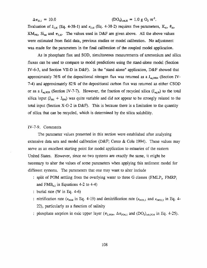
A1rsi,1 = 10.0

Evaluation of J2.si (Eq. 4-38-1) and K2,si (Eq. 4-38-2) requires five parameters, Ksi, Osi,

KMPSi, Sisat and 1r2,si· The values used in D&F are given above. All the above values

were estimated from field data, previous studies or model calibration. No adjustment

was made for the parameters in the final calibration of the coupled model application.

As in phosphate flux and SOD, simultaneous measurements of ammonium and silica

fluxes can be used to compare to model predictions using the stand-alone model (Section

IV-6-3, and Section VII-D in D&F). In the "stand alone" application, D&F showed that

approximately 76% of the depositional nitrogen flux was returned as a Jaq,NH4 (Section IV-

7-4) and approximately 82 % of the depositional carbon flux was returned as either CSOD

or as a J aq,ms (Section IV -7-7). However, the fraction of recycled silica (J aq,sJ to the total

silica input (JPSi + J0sJ was quite variable and did not appear to be strongly related to the

total input (Section X-G-2 in D&F). This is because there is a limitation to the quantity

of silica that can be recycled, which is determined by the silica solubility.

IV-7-9. Comments

The parameter values presented in this section were established after analyzing

extensive data sets and model calibration (D&F; Cereo & Cole 1994). These values may

serve as an excellent starting point for model application to estuaries of the eastern

United States. However, since no two systems are exactly the same, it might be

necessary to alter the values of some parameters when applying this sediment model for

different systems. The parameters that one may want to alter include

split of POM settling from the overlying water to three G classes (FMLPi, FMRPi

and FMBx,i in Equations 4-2 to 4-4)

burial rate (W in Eq. 4-6)

nitrification rate (KNH4 in Eq. 4-19) and denitrification rate (KNo3,1 and KNo3,2 in Eq. 4-

22), particularly as a function of salinity

phosphate sorption in oxic upper layer (7r2,p04 , A7rp04,1 and (D00\ni,Po4 in Eq. 4-25).

108

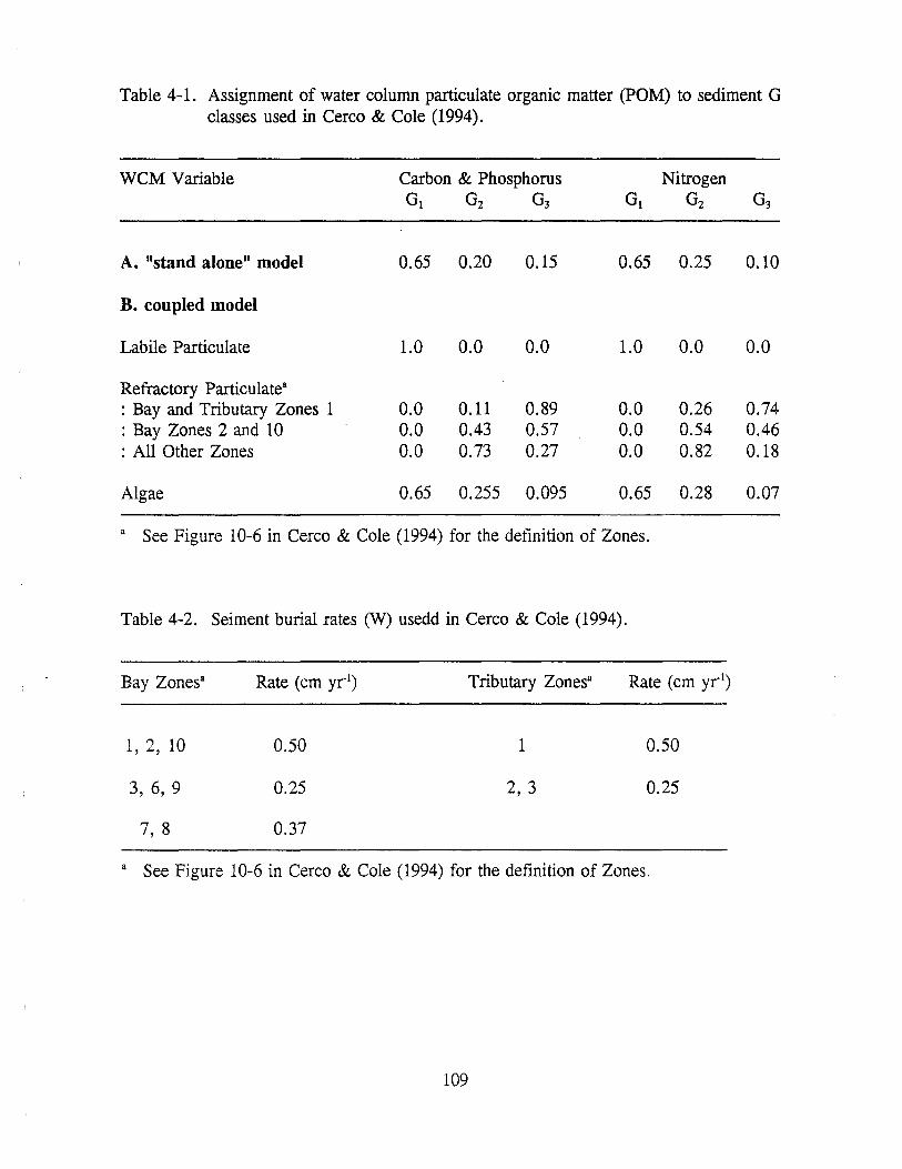
Table 4-1. Assignment of water column particulate organic matter (POM) to sediment G classes used in Cereo & Cole (1994).

WCM Variable Carbon & Phosphorus G1 G2 G3

A. "stand alone" model 0.65 0.20 0.15 0.65 0.25

B. coupled model

Labile Particulate 1.0 0.0 0.0 1.0 0.0

Refractory Particulatea : Bay and Tributary Zones 1 0.0 0.11 0.89 0.0 0.26 : Bay Zones 2 and 10 0.0 0.43 0.57 0.0 0.54 : All Other Zones 0.0 0.73 0.27 0.0 0.82

Algae 0.65 0.255 0.095 0.65 0.28

a See Figure 10-6 in Cereo & Cole (1994) for the definition of Zones.

Table 4-2. Seiment burial rates (W) usedd in Cereo & Cole (1994).

Bay Zonesa Rate (cm yr·1) Tributary Zonesa Rate (cm yr·1)

1, 2, 10

3, 6, 9

7, 8

0.50

0.25

0.37

1

2, 3

0.50

0.25

a See Figure 10-6 in Cereo & Cole (1994) for the definition of Zones.

109

0.10

0.0

0.74 0.46 0.18

0.07

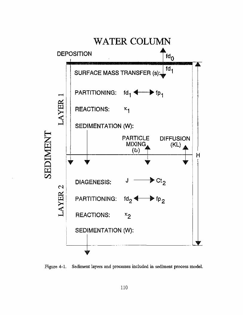
WATER COLUMN DEPOSITION

fd1 ~ ~

SURFACE MASS TRANSFER (s):, ,

,...-1 PARTITIONING: fd1 ~ ... fp1

~ j

REACTIONS: 1C1

SEDIMENTATION (YV): ~

~ ~

PARTICLE DIFFUSION MIXING (KL).,.~

{6l) .. ... H

~

Q , , , , ~ , , ,

~ C"/.l

N DIAGENESIS: J ... Ct2

fis ~

PARTITIONING: fd2 ~ .. fp2

j REACTIONS: 1C2

SEDIMENTATION (YV):

~ , ~ ,

Figure 4-1. Sediment layers and processes included in sediment process model.

110

,-.... ,-.... ,-....

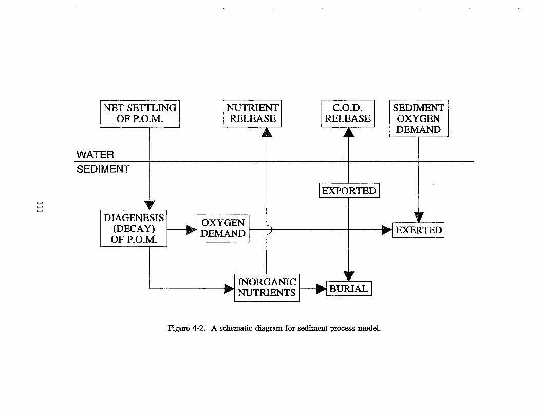
NET SEITLING OF P.O.M.

WATER SEDIMENT

•

NUTRIENT RELEASE

• C.O.D.

RELEASE

• IEXPO~TEDI

SEDIME~uT OXYGEN DEMAND

I • DIAGENESIS I I OXYGEN I > . ...I EXERTED] (DECAY) .... DEMAND OF P.O.M.

• I I INORGANIC .... NUTRIENTS I .... L~URIAL I

Figure 4-2. A schematic diagram for sediment process model.

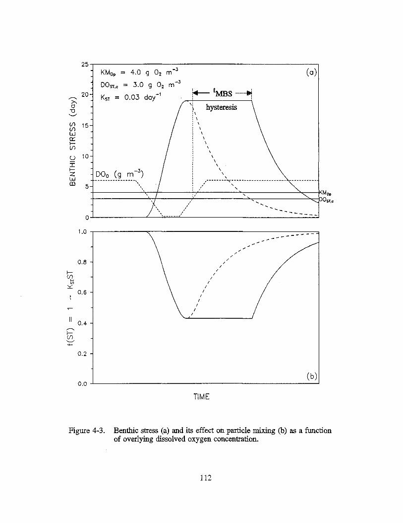
20

(f) 15 (f) w a::: 1-(f)

u 10 I 1-z w (I)

5

KMop = 4.0 g 02

DOsr,c = 3.0 g 02

Ksr = 0.03 day- 1

D00 (g m-3)

----------------,, '\,

I t ' ~ :rvms~ ' i

\ \ hysteresis !\ i \ j \

\ I I I

\ \

\ \

\

' ' ' ,---------x----------------------

', i'

,' ' / '

' .... .... ....

( a)

1.0 -.----------..::------------------------. ----

I-(f)

I-V1 ~

..-

II ,.--.,. I-(f) .___,, 4-

0.8

/ I

I

0.6 I I

I I

I I

0.4

0.2

/ /

/ /

/ /

/

.,. .,. -- ---

(b) 0.0 -'-------------------------------'

TIME

Figure 4-3. Bentbic stress (a) and its effect on particle mixing (b) as a function of overlying dissolved oxygen concentration.

112

Chapter V. Model Operation (Execution)

This chapter gives the general description of what the present model does when one

prepares the input data files and runs the model. When applying the model to any

system, data for geometry and calibra~ed constants are required. The geometric data

include identification of main channel and branches, segmentation and evaluation of high

tide volume, inter-tidal volume (tidal prism), depth, etc (see Chapter II and Appendix A-

1-1). The calibrated constants include return ratio (Section II-3-2) and a number of

biogeochemical coefficients described in Chapters III and IV, and Appendix A.

In addition, for each model simulation, initial and boundary conditions are required.

Initial conditions, the conditions at the beginning of a model simulation, need to be

specified for all state variables both in water column and in sediment. When the model

runs, it starts with initial conditions and calculates water column and sediment state

variables at each segment at each time step until the time that one specifies to stop the

model run. It takes some time for mass state variables to be stabilized, i.e., for the

model solution to be independent of initial conditions. Considerable effort, hence, is

required to specify the initial conditions, evaluation of initial conditions for the sediment

process model is described in Section IV-6.

To drive the model, the following external forcing variables are needed as boundary

conditions:

(a) concentrations for all water column state variables at downriver boundary, i.e., 1st

segment in main channel (see Section II-1),

(b) discharge rates from point and nonpoint source inputs,

(c) point and nonpoint source loadings for all water column state variables,

( d) solar radiation including heat exchange coefficient and equilibrium temperature

(see Eq. 3-21).

As the model calculation proceeds, it is constrained by the specified boundary conditions.

The boundary conditions, with accounting for the physical transport using tidal flushing,

drive the model to solve mass balance equations for state variables, and calculate spatial

and temporal distributions.

The present model implementation allows two types of output generation: snapshot

113

spatial distribution and time-series output. At each time that one specifies to generate the

snapshot output (Appendix A-1-2), the model writes instantaneous values of all state

variables at all segments. At each segment, up to ten segments, that one specifies to

generate the time-series output, the model writes the time-series information of all state

variables. Detailed description of input and output file organization is given in Appendix

A.

114

References

Aller, R.C. 1982. The effects of macrobenthos on chemical properties of marine sediment and overlying water, pp. 53-102. In: P.L. McCall & M.J.S. Tevesz (eds.), Animal-Sediment Relations: The Biogenic Alteration of Sediments, Plenum Press, NY.

Bank..s, R.B. & Herrera, F.F. 1977. Effect of wind and rain on surface reaeration. J. of the Environmental Engineering Division, ASCE, 103(EE3): 489-504.

Barrow, N.J. 1983. A mechanistic model for describing the sorption and desorption of phosphate by soil. J. of Soil Science, 34: 733-750.

Boni, L., Carpene, E., Wynne, D., & Reti, M. 1989. Alkaline phosphatase activity in Protogonyau/ax tamarensis. J. of Plankton Research, 11(5): 879-885.

Boudreau, B.P. 1991. Modelling the sulfide-oxygen reaction and associated pH gradients in porewaters. Geochimica et Cosmochimica Acta, 55: 145-159.

Bowie, G.L., Mills, W.B., Porcella, D.B., Campbell, C.L., Pagenkopf, J.R., Rupp, G.L., Johnson, K.M., Chan, P.W.H., Gherini, S.A. & Chamberlin, C.E. 1985. Rates, constants and kinetics formulations in surface water quality modeling (second edition). EPA/600/3-85/040, Environmental Research Lab., US EPA, 455 pp.

Brush, G.S. 1984. Patterns of recent sediment accumulation in Chesapeake Bay (Virginia-Maryland, U.S.A.) tributaries. Chemical Geology, 44: 227-242.

Carritt, D.E. & Goodgal, S. 1954. Sorption reactions and some ecological implications. Deep-Sea Research, 1: 224-243.

Cereo, C.F. & Kuo, A.Y. 1981. Water quality in a small tidal creek: Parker Creek, Virginia. Special Report in Applied Marine Science and Ocean Engineering (SRAMSOE) #145, Virginia Institute of Marine science (VIMS), The College of William and Mary, VA, 112 pp.

Cereo, C.F. & Cole, T.M. 1994. Three-dimensional eutrophication model of Chesapeake Bay: Volume 1, main report. Technical Report EL-94-4, US Army Engineer Waterways Experiment Station, Vicksburg, MS.

Chr6st, R.J. & Overbek, J. 1987. Kinetics of alkaline phosphatase activity and phosphorus availability for phytoplankton and bacterioplankton in Lake Pluflsee (North German eutrophic lake). Microbial Ecology, 13: 229-248.

Cline, J.D. & Richards, F.A. 1969. Oxygenation of hydrogen sulfide in seawater at constant salinity, temperature and pH. Environmental Science & Technology, 3(9): 838-843.

115

Diaz, R.J. & Rosenberg, R. submitted. Marine benthichypoxia - review of ecological effects and behavioral responses of benthic macrofauna. Oceanography Marine Biology Annual Review.

DiToro, D.M. 1980. Applicability of cellular equilibrium and Monod theory to phytoplankton growth kinetics. Ecological Modelling, 8: 201-218.

DiToro, D.M., Paquin, P.R., Subburamu, K. & Gruber, D.A. 1990. Sediment oxygen demand model: methane and ammonia oxidation. J. of Environmental Engineering, ASCE, 116(5): 945-986.

DiToro, D.M. & Fitzpatrick, J.J. 1993. Chesapeake bay sediment flux model. Contract Report EL-93-2, US Army Engineer Waterways Experiment Station, Vicksburg, MS, 316 pp.

Edinger, J.E., Brady, D.K. & Geyer, J.C. 1974. Heat exchange and transport in the environment. Report No. 14,· The Johns Hopkins Univeristy, Electric Pwoer Research Institute Publication No. 74-049-00-3, 125 pp.

Froelich, P.N. 1988. Kinetic control of dissolved phosphate in natural rivers and estuaries: a primer on the phosphate buffer mechanism. Limnology and Oceanography, 33(4, part 2): 649-668.

Gardner, W. S. , Seitzinger, S. P. & Malczyk, J.M. 1991. The effects of sea salts on the forms of nitrogen released from estuarine and freshwater sediments: does ion pairing affect ammonium flux? Estuaries, 14(2): 157-166.

Genet, L.A., Smith, D.J. & Sonnen, M.B. 1974. Computer program documentation for the dynamic estuary model. Prepared for US EPA, Systems Development Branch, Washington, D.C.

Giordani, P. & Astorri, M. 1986. Phosphate analysis of marine sediments. Chemistry in Ecology, 2: 103-112.

Ho, G.C., Kuo, A.Y. & Neilson, B.J. 1977. Mathematical models of Little Creek Harbor and the Lynnhaven Bay system. SRAMSOE #145, VIMS, The College of William and Mary, VA, 100 pp.

Johnson, B.H., Kim, K.W., Heath, R.H., Butler, H.L. & Hsieh, B.B. 1991. User's guide for a three-dimensional numerical hydrodynamic, salinity and temperature model of Chesapeake Bay. Technical Report HL-91-20, US Army Engineer Waterways Experiment Station, Vicksburg, MS, 41 pp.

Ketchum, B.H. 1951. The exchanges of fresh and salt waters in tidal estuaries. J. of Marine Research, 10(1): 18-38.

116

Kremer, J.N. & Nixon, S.W. 1978. A coastal marine ecosystem: simulation and analysis. Ecological Studies 24, Springer-Verlag, New York, 217 pp.

Kuo, A.Y. & Hyer, P.V. 1979. A water quality study of the Eastern Branch of the Lynnhaven Bay, Virginia. A Report to the Norfolk District, US Army Corps of Engineers, Prepared by VIMS, The College of William and Mary, VA, 29 pp.

Kuo, A. Y. & Neilson, B.J. 1988. A modified tidal prism model for water quality in small coastal embayments. Water Science Technology, 20(6/7): 133-142.

Kuo, A. Y. & Park, K. 1992. Transport of hypoxic waters: an estuary-subestuary exchange, pp. 599-615. In: D. Prandle (ed.), Dynamics and Exchanges in Estuaries and the Coastal Zone, Coastal and Estuarine Sciences 40, AGU, Washington D.C.

Lebo, M.E. 1991. Particle-bound phosphorus along an urbanized coastal plain estuary. Marine Chemistry, 34: 225-216,

Lijklema, L. 1980. Interaction of ortho-phosphate with iron (III) and aluminum hydroxides. Environmental Science & Technology, 14(5): 537-541.

Llans6, R.J. 1992. Effects of hypoxia on estuarine benthos: the lower Rappahannock River (Chesapeake Bay), a case study. Estuarine, Coastal and Shelf Science, 35: 491-515.

Mackin, J.E. & Aller, R.C. 1984. Ammonium adsorption in marine sediments. Limnology and oceanography, 29(2): 250-257.

Mancini, J.L. 1983. A method for calculating effects, on aquatic organisms, of time varying cocnentrations. Water Research, 17(10): 1355-1362.

Matisoff, G. 1982. Mathematical models of bioturbation, pp. 289-330. In: P.L. McCall & M.J.S. Tevesz (eds.), Animal-Sediment Relations: The Biogenic Alteration of Sediments, Plenum Press, NY.

Millero, F.J. 1986. The thermodynamics and kinetics of the hydrogen sulfide system in natural waters. Marine Chemistry, 18: 121-147.

Mo, C., Neilson, B.J. & Wetzel, R.L. 1993. Sediment processes monitoring data report for calendar year 1989. Data Report No. 48, VIMS, The College of William and Mary, VA, 39 pp.

Morel, F. 1983. Principles of Aquatic Chemistry. John Wiley & Sons, New York, NY, 446 pp.

Morse, J.W., Millero, F.J., Cornwell, J.C. & Rickard, D. 1987. The chemistry of the hydrogen sulfide and iron sulfide systems in natural waters. Earth-Science Reviews, 24:

117

1-42.

O'Connor, D.J. & Dobbins, W.E. 1958. Mechanism of reaeration in natural streams. Transactions of the Americal Society of Civil Engineers, 123(2934): 641-684.

Odum, E.P. 1971. Fundamentals of ecology (third edition). W.B. Saunders Co., Philadelphia, PA, 574pp.

Officer, C.B., Lynch, D.R., Setlock, G.H. & Helz, G.R. 1984. Recent sedimentation rates in Chesapeake Bay, pp. 131-157. In: V.S. Kennedy (ed.), The Estuary as a Filter, Academic Press.

Parsons, T.R., Takahashi, M. & Hargrave, B. 1984. Biological oceanographic processes (third edition). Pergamon Press, 330 pp.

Press, W.H., Flannery, B.P., Teukolsky, S.A. & Vetterling, W.T. 1986. Numerical recipes: the art of scientific computing. Cambridge University Press, 818 pp.

Redfield, A.C., Ketchum, B.H. & Richards, F.A. 1963. The influence of organisms on the composition of sea-water (Chapter 2) pp 26-77. In: M.N. Hill (ed.), The Sea - Ideas and Observations on Progress in the Study of the Seas: Vol. 2, Composition of Sea Water, Comparative and Descriptive Oceanography, Interscience Publishers.

Robbins, J.A., Keilty, T., White, D.S. & Edgington, D.N. 1989. Relationships among tubificid abundances, sediment composition and accumulation rates in Lake Erie. Canadian J. of Fisheries & Aquatic Sciences, 46(2): 223-231.

Rosenberg, R. 1980. Effect of oxygen deficiency on benthic macrofauna in fjords, pp. 499-514. In: H.J. Freeland, D.M. Farmer & C.D. Levings (eds.), Fjord Oceanography, Plenum Press, NY.

Smolarkiewicz, P.K. & Margolin, L.G. 1993. On forward-in-time differencing for fluids: extension to a curvilinear framework. Monthly Weather Review, 121: 1847-1859.

S0I'ensen, J. & Revsbech, N.P. 1990. Denitrification in stream biofilm and sediment: in situ variation and control factors, pp. 277-289. In: N.P. Revsbech & J. S0I'ensen (eds.), Denitrification in Soil and Sediment, FEMS Symposium No. 56, Plenum Press, NY.

Steele, J.H. 1962. Environmental control of photosynthesis in the sea. Limnology and Oceanography, 7(2): 137-150.

Stumm, W. & Morgan, J.J. 1981. Aquatic chemistry, an introduction emphasizing chemical equilibria in natural waters (second edition). John Wiley & Sons, Inc., 780 pp.

Thomann, R.V., Jaworski, N.J., Nixon, S.W., Paerl, H.W. & Taft, J. 1985. The 1983 algal bloom in the Potomac Estuary. The Algal Bloom Expert Panel, Pepared for the

118

Potomac Strategy State/EPA Management Committee, US EPA Region III, Philadelphia, PA.

Thomann, R.V. & Mueller, J.A. 1987. Principles of surface water quality modeling and control. Harper & Row, Publishers, Inc., 644 pp.

Thomann, R.V., Collier, J.R., Butt, A,R.; Casman, E. & Linker, L.C. 1994. Technical analysis of response of Chesapeake Bay water quality model to loading scenarios. CBP/TRS 101/94, Modeling Subcommittee of the Chesapeake Bay Program, US EPA.

Troup, R. 1974. The interaction of iron with phosphate, carbonate and sulfide in Chesapeake Bay interstitial waters: a thermodynamic interpretation. Ph.D. Dissertation, Johns Hopkins University, MD, 114 p.

Westrich, J.T. & Berner, R.A. 1984. The role of sedimentary organic matter in bacterial sulfate reduction: the G model tested. Limnology and Oceanography, 29(2): 236-249.

Wezernak, C.T. & Gannon, J.J. 1968. Evaluation of nitrification in streams. J. of the Sanitary Engineering Division, ASCE, 94(SA5): 883-895.

Yamamoto, S., Alcauskas, J.B. & Crozler, T.E. 1976. Solubility of methane in distilled water and seawater. J. of Chemical and Engineering Data, 21(1): 78-80.

119

Appendix A. Program Organization for Input and Output Files

Program input and output require several data files, each of which is specified in

the program by a logical unit number. Tables A-1 and A-2 list the logical unit numbers

for water column and sediment mode~s, respectively. You can run only the water column

model. The sediment process model, however, should be run with the water column

model since the water column model provides the depositional fluxes to the sediment

process model. Hence, all input and output units for sediment process model are

optional. This appendix describes input and output file organization for water column

and sediment process models.

A-1. Input Data Description for Water Column Model

This section explains line-by-line the input data files for water column model. Each

data group and each line are preceded by text titles for identification purpose. These text

titles, which do not affect the model run, are not described, and omitted using FORMAT

descriptor slash (/), in this section.

Once the model starts, it opens the unit numbers 7, 8 and 9 (Table A-1). Then,

control passes to the subroutine 'RCHyd' in 'SUB-READ.FOR', where input parameters

are read in from the unit number 7.

A-1-1. Logical unit 7 (GEO-HYD.IN)

The unit number 7 contains the geometric and hydrodynamic data.

VARIABLES (FORMAT)

Title(j), j=l,3 (A79)

: three-line text to identify a simulation.

NSEGm, Nbran, Tname(O) (/, 2I5, A30)

: NSEGm = number of segments in main channel.

: Nbran = number of primary branches.

: Tname ( o) = main channel name.

NSEGb(m), NMT(m), Tname(m), m=l,Nbran (2I5, A30)

: NSEGb (m) = number of segments in the mth primary branch.

A-1

: NMT (m) = main channel segment number to which the mlh branch is connected.

: Tname ( m) = name of the mlh primary branch.

NSt (IS, /)

: NSt = number of secondary branches (i.e., storage areas).

Title(j), j=l,3 (A79)

: three-line text to identify the following data group.

Index, DIST(i), VH(i), P(i), AL(i), HA(i), i=l,NSEGm (AS, SFB.3)

: Input file uses Index for channel and segment identification only.

: DIST(i) = distance (km) from the river mouth to the ilh main channel transect.

: VH ( i > = high tide volume (106 m3) of the ilh main channel segment.

: P ( i) = tidal prism ( or intertidal volume in 106 m3) upriver of the ilh main channel

transect including those in brap.ches.

: AL c i) = returning ratio at the ilh main channel transect.

: HA c i > = mean depth (m) of the ilh main channel segment.

(Index, DISTT(m,n), VHT(m,n), PT(m,n), ALT(m,n), HAT(m,n), n=l,NSEGb(m)) m=l,Nbran (AS, SFS.3)

: The last character "T" designates the variables at the primary branches. Note that

the first segment at each primary branch is in the main channel (see Section II-1).

Hence, DISTT(m,1) = 0 and for example, VHT(m,l) = VH(NMT(m) ).

(Index, StDIST(m,n), StVH(m,n), StP(m,n), StAL(m,n), StHA(m,n), n=l,NSEGb(m)) m=l,Nbran (AB, SFB,3)

: The first two characters "St" designates the variables at the secondary branches. For

those segments without storage area, stP(m,n) must be set to zero.

At this point, the unit number 7 is closed and control passes to the main program and

hence to the subroutine 'RWQCl'. Two subroutines 'RWQCl' and 'RWQC2' in 'SUB­

READ.FOR' read in input parameters from the unit number 8.

A-1-2. Logical unit 8 (TPM-CONT.IN)

The unit number 8 contains the program control parameters and constant parameters

for rate coefficients, initial conditions and boundary conditions, and files names for

spatially and/or temporally varying conditions.

A-2

Title(j), j=l,3 (A79)

: three-line text to identify a simulation.

Title(l) (/, A79)

: one blank line and one-line text to identify the following data group.

iPLT, iWQV, iTMP, iBEN, iSi, iTSS, iSRP, iFCB (/, BIB)

: iPLT = 1 opens the unit number .80 and writes the model results for the last 20 tidal

cycles, which will be used as input for Post-Processor. Otherwise no output to unit 80.

: iWQV = 1 simulates all water column state variables. Otherwise only salinity is

simulated.

: iTMP = 1 simulates water temperature. If iTMP = 0, spatially and temporally

constant temperature is read in from the unit number 8. If iTMP = 2, a sinusoidal curve

is used to generate spatially c9nstant temperature with coefficients read in from the unit

8. If iTMP = 3, spatially and/or temporally varying temperatures are read in from the

unit 17.

: iBEN = 1 activates the sediment process model. If iBEN = 0, spatially and

temporally constant benthic fluxes are read in from the unit number 8. If iBEN = 2,

spatially and/or temporally varying benthic fluxes are read in from the unit 16.

: isi = 1 simulates silica state variables, available silica (AS) and particulate biogenic

silica (SU). Otherwise no silica simulation.

: iTss = I simulates suspended solid (TSS). Otherwise no TSS simulation and thus

no effect of TSS on light attenuation and sorption of phosphate (P04) and AS.

: iSRP = 1 if total active metal (TAM) is simulated to account for the sorption of P04

and AS. If isRP = 2, TSS is simulated to account for the sorption of P04 and AS: an

error will be issued and the program be stopped if iSRP =2 and iTss ;c 1. Otherwise

no sorption of P04 and AS is simulated: TSS may be simulated but not TAM.

: iFCB = 1 simulates fecal coliform bacteria (FCB). Otherwise no FCB simulation.

Note that if any of iTMP, iBEN, iSi, iTSS, iSRP and iFCB is equal to 1, iWQV should be

1. Otherwise an error will be issued and the program be stopped.

iUKin, iBcS, iZK, iNR, iNC (/, SIB)

: iUKin = number of kinetic update over half tidal cycle (Section II-4).

: iBcs = 1 if salinity toxicity is applied to cyanobacteria (Eq. 3-lb), i.e., freshwater

A-3

species. Otherwise no salinity toxicity to cyanobacteria, i.e., saltwater species.

: iZK = 1 opens the unit number 22 and writes the diagnostic information for zero K0

(Section ill-12). Otherwise no output to unit 22.

: iNR = 1 opens the unit number 23 and writes the diagnostic information for negative

R0 (Section ill-12). Otherwise no output to unit 23.

: iNc = 1 opens the unit number 24 and writes the diagnostic information for zero

concentration. Otherwise no output to unit 24.

Lsal, LBc, LBd, Lpo4, Lnh4, Lno3, Lsa, Lo2, Ltmp (/, 9I8)

: Lsal = 1 opens the unit number 25 and writes the diagnostic information for

salinity. Otherwise no output to unit 25.

: LBc, LBd, Lpo4, Lnh4, Lno3, Lsa, Lo2 or Ltmp = 1 opens the unit number 26, 27,

28, 29, 30, 31, 32 or 33 and writes the diagnostic information for cyanobacteria,

diatoms, phosphate, ammonium, nitrate, available silica, dissolve oxygen or temperature.

iICI, iAGR, iSTL, iSUN, iPSL, iNPL (/, 6I8)

: iicr = 1 reads in spatially and/or temporally varying initial conditions for water

column state variables from the unit number 11. Otherwise constant conditions are read

in from the unit 8.

: iAGR = 1 reads in spatially and/or temporally varying algal growth, respiration and

predation rates, and base light extinction coefficient from the unit number 12. Otherwise

constant coefficients are read in from the unit 8.

: iSTL = 1 reads in spatially and/or temporally varying settling velocities for algae,

refractory particulates, labile particulates, particulate metal and TSS from the unit number

13. Otherwise constant coefficients are read in from the unit 8.

: iSUN = 1 reads in temporally varying parameters for light intensity (daily light

intensity and fractional daylength) and temperature (heat exchange coefficient and

equilibrium temperature) from the unit number 14. Otherwise constant coefficients are

read in from the unit 8.

: iPsL = 1 reads in temporally varying point source discharges and loadings from the

unit number 18. Otherwise constant inputs are read in from the unit 8.

A-4

: iNPL = 1 reads in spatially and/or temporally varying nonpoint source discharges

and loadings from the unit number 19. Otherwise constant inputs are read in from the

unit 8.

iBCSal, iBCB, iBCCO, iBCPO, iBCP!; iBCNO, iBCNI, iBCSU, iBCSA (/, 9I8) iBCCOD, iBC02, iBCTSS, iBCTAM, iBCFCB, iBCT (/, 6I8)

: control parameters for downriver boundary conditions of salinity (iacsal), algae

( iaca), organic carbon ( iacco), organic phosphorus ( iBcPo), inorganic phosphorus

(iBCPI), organic nitrogen (iBCNo), inorganic nitrogen (iBCNI), particulate biogenic silica

(iacsu), available silica (iacsA), COD (iaccoo), DO (iaco2), TSS (iBCTss), TAM

(iBCTAM), fecal coliform bacteria (iBCFCB) and temperature (iBCT). For example, if

iacco = 1, temporally varying downriver boundary conditions for three organic carbon

variables (refractory particulate, labile particulate and dissolved) are read in from the unit

number 15. If iacco ~ 1, the boundary conditions are genrated using:

(A-1)

where t = time (day); Tp = period (365 days). Three coefficients, c0, c1 and Ci, are

obtained from multiple linear regression, and read in from the unit 8. If c1 and ei are

zero, it is temporally constant boundary conditions, otherwise sinusoidally varying

boundary conbditions (Eq. A-1) are used.

If any of the above 15 parameters is equal to one, ioac is set to one, and if all of

the above 15 parameters are equal to one, ioac = 2. Otherwise, ioac = 0.

Tstrt (/, FS. 4)

: Tstrt = Julian day to start the model run.

iTmax, Nprn, iTimeS, iSTS, iETS (/, SIS, /)

: iTmax = time duration (in tidal cycles) for model run.

: Nprn = number of times to write the snapshot longitudinal distribution output.

: Write time-series output starting from isTs (tidal cycles) till iETs (tidal cycles) at

iTimes locations. Note that the present model implementation allows the maximum of 10

locations of time-series output and that iTimes ::,; 10. Setting iTimes ::,; 0 results in no

time-series output.

A-5

iTSCH(j), iTSSEG(j), j=l,iTimeS (2I8)

: To the unit numbers 34 to 43 (one unit for one location), the subroutine 'TSwrite' in

'SUB-READ.FOR' writes time-series output for salinity and 23 water quality variables

(Chapter III) at the channel number of iTscH < j > and segment number of iTSSEG ( j > • If

iTSCH ( j ) = 0, it is main channel. If iTSCH ( j ) = -m, it is secondary branch connecting

to the m!h primary branch.

iTout(j), j=l,Nprn (/, 15I5)

: To the unit number 21, the subroutine 'LDwrite' in 'SUB-READ.FOR' prints out the

snapshot information for salinity and 23 water quality variables (Chapter ID) at the time

of iTout ( j) tidal cycles from the model start. Note that the present model

implementation allows the maximum of 15 times of output printing and that O :::;;

iTout ( j ) < iTmax.

Title(!) (/, A79)

: one blank line and one-line text to identify the following data group (algae).

KRNc, KRNd, KRNg, KHPc, KHPd, KHPg, KHS, STOX (/, SFS.4) KeTSS, KeChl, CChlc, CChld, CChlg, DOPTc, DOPTd, DOPTg (/, SFS,4) rIO, risMIN, FD, Cia, Cib, Cic (/, 6FB,4) TMc, TMd, TMg, KTGlc, KTG2c, KTGld, KTG2d, KTGlg, KTG2g (/, 9F8,4) TRc, TRd, TRg, KTBc, KTBd, KTBg (/, 6F8.4)

: KHNx = half-saturation constant for nitrogen uptake (g N m-3) by algal group x (x = c for cyanobacteria, x = d for diatoms and x = g for green algae).

: KHPx = half-saturation constant for phosphorus uptake (g P m-3) by algal group x.

: KHs = half-saturation constant for silica uptake (g Si m-3) by diatoms.

: sTox = salinity (ppt) at which Microcystis growth is halved, which is applied to

cyanobacteria only when iBcs = 1.

: KeTss = light extinction coefficient for TSS (m-1 per g m-3).

: KeChl = light extinction coefficient for chlorophyll 'a' cm-1 per mg Chl m-3).

: CChlx = carbon-to-chlorophyll ratio (g C per mg Chl) in algal group x.

: DOPTx = depth of maximum algal growth (m) for algal group x.

: rIO = initial daily light intensity at water surface (langleys day-1).

: risMIN = minimum optimum light intensity (langleys day-1).

: FD = fractional daylength, which is used only when iSUN ~ 1.

: era, crb and ere = weighting factors for I0, I1 and I2, respectively (era + crb +

A-6

CIC = 1, see Eq. 3-lj).

: TMx = optimal temperature for algal growth (°C) for algal group x.

: KTGlx = temperature effect below TMx on algal growth (°C-2) for algal group x.

: KTG2x = temperature effect above TMx on algal growth (°C-2) for algal group x.

: TR.x = reference temperature for _basal metabolism (°C) for algal group x.

: KTBx = effect Of temperature On basal metabolism (°C-1) for algal group X.

Title(l) (/, A79)

: one blank line and one-line text to identify the following data group (carbon).

FCRP, FCLP, FCDP, FCDc, FCDd, FCDg, KHRc, KHRd, KHRg (/, 9F8.4) KRC, KLC, KDC, KRCalg, KLCalg, KDCalg (/, 6F8.4) TRllDR, TRMNL, KTHDR, KTMNL, KHORDO, KHDNN, AANOX (/ , 7 FS , 4)

: FCRP, FCLP and FCDP = fraction of predated carbon produced as refractory

particulate, labile particulate and dissolved organic carbon, respectively.

: FCDx = fraction of basal metabolism exuded as dissolved organic carbon at infinite

dissolved oxygen concentration for algal group x.

: KHRx = half-saturation constant of dissolve oxygen (g 0 2 m·3) for algal dissolved

organic carbon excretion by algal group x.

: KRC and KLC = minimum dissolution rate (day·1) of refractory and labile particulate

organic carbon, respectively.

: KDC = minimum respiration rate (day·1) of dissolved organic carbon.

: KRCalg and KLCalg = constants that relate dissolution of refractory and labile

particulate organic carbon, respectively, to algal biomass ( day·1 per g C m·3).

: KDCalg = constant that relates respiration to algal biomass ( day·1 per g C m·3).

: TRHDR = reference temperature for hydrolysis of particulate organic matter (°C).

: TRMNL = reference temperature for mineralization of dissolved organic matter (°C).

: KTHDR = temperature effect on hydrolysis of particulate organic matter (°C"1).

: KTMNL = temperature effect on mineralization of dissolved organic matter ( 0 c-1).

: KHORDo = oxic respiration half-saturation constant for dissolved oxygen (g 0 2 m·3).

: KHDNN = denitrification half-saturation constant for nitrate (g N m·3).

: AANox = rate ratio of denitrification to oxic dissolved organic carbon respiration.

A-7

Title(l) (/, A79)

: one blank line and one-line text to identify the following data group (phosphorus).

FPRP, FPLP, FPDP, FPIP, FPRc, FPRd, FPRg, FPLc, FPLd, FPLg (/, lOFB.4) FPDc, FPDd, FPDg, FPic, FPid, FPig, KP04p (/, 7F8.4) KRP, KLP, KDP, KRPalg, KLPalg, KDPalg, CPprml, CPprm2, CPprm3 (/, 9F8.4)

: FPRP, FPLP, FPDP and FPIP = fraction of predated phosphorus produced as

refractory particulate organic, labile particulate organic, dissolved organic and inorganic

phosphorus, respectively.

: FPRx, FPLx, FPDx and FPix = fraction of metabolized phosphorus by algal group x

produced as refractory particulate organic, labile particulate organic, dissolved organic

and inorganic phosphorus, respectively.

: KP04p = coefficient relating phosphate sorption to TSS (per g m·3) if isRP = 2 or

TAM (per mol m·3) if iSRP = 1. If iSRP ~ 1 and iSRP ~ 2, KP04p is forced to be 0.

: KRP and KLP = minimum hydrolysis rate (day·1) of refractory and labile particulate

organic phosphorus, respectively.

: KDP = minimum mineralization rate (day·1) of dissolved organic phosphorus.

: KRPalg and KLPalg = constants that relate hydrolysis of refractory and labile

particulate organic phosphorus, respectively, to algal biomass (day-1 per g P m·3).

: KDPalg = constant that relates mineralization to algal biomass (day·1 per g P m·3).

: CPprml (g C per g P), cPprm2 (g C per g C) and CPprm3 (per g P m·3) = constants

used to determine phosphorus-to-carbon ratio (Eq. 3-8e).

Title ( 1) (/, A79)

: one blank line and one-line text to identify the following data group (nitrogen).

FNRP, FNLP, FNDP, FNIP, FNRc, FNRd, FNRg, FNLc, FNLd, FNDc, FNDd, FNDg, FNic, FNid, FNig, ANCc, ANCd, ANCg ANDC, rNitM, KHNitDO, KHNitN, TNit, KNitl, KNit2 (/, KRN, KLN, KDN, KRNalg, KLNalg, KDNalg (/, 6FB,4)

FNLg (/, lOFB,4) (/, 9FB.4) 7FB,4)

: FNRP, FNLP, FNDP and FNIP = fraction of predated nitrogen produced as refractory

particulate organic, labile particulate organic, dissolved organic and inorganic nitrogen,

respectively.

: FNRx, FNLx, FNDx and FNix = fraction of metabolized nitrogen by algal group x

produced as refractory particulate organic, labile particulate organic, dissolved organic

and inorganic nitrogen, respectively.

A-8

: ANCx = nitrogen-to-carbon ratio (g N per g C) in algal group x.

: ANDc = mass of nitrate nitrogen reduced per mass of dissolved organic carbon

oxidized (0.933 g N per g C, see Eq. 3-13).

: rNitM = maximum nitrification rate (g N m·3 day-1) at temperature TNit.

: 1rnNitno = nitrification half-saturation constant for dissolve.cl oxygen (g 0 2 m·3).

: KHNitN = nitrification half-saturation constant for ammonium (g N m·3).

: TNit = optimum temperature (°C).

: KNitl and KNit2 = temperature effect on nitrification rate (°C-2) below and above

TNit, respectively.

: KRN and KLN = minimum hydrolysis rate ( day·1) of refractory and labile particulate

organic nitrogen, respectively.

: KDN = minimum mineralization rate (day-1) of dissolved organic nitrogen.

: KRNalg and KLNalg = constants that relate hydrolysis of refractory and labile

particulate organic nitrogen, respectively, to algal biomass (day·1 per g N m·3).

: KDNalg = constant that relates mineralization to algal biomass (day·1 per g N m·3).

Title(l) (/, A79)

: one blank line and one-line text to identify the following data group (silica).

FSPP, FSIP, FSPd, FSid, ASCd, KSAp, KSU, TRSUA, KTSUA (/, 9F8,4)

: FSPP and FSIP = fraction of predated diatom silica produced as particulate biogenic

and available silica, respectively.

: FSPd and FSid = fraction of metabolized silica by diatoms produced as particulate

biogenic and available silica, respectively.

: AS Cd = silica-to-carbon ratio of diatoms (g Si per g C).

: KSAp = coefficient relating available silica sorption to TSS (per g m·3) if iSRP = 2

or TAM (per mol m·3) if iSRP = 1. If iSRP ;z: 1 and iSRP ;z: 2, KSAp is forced to be 0.

: Ksu = dissolution rate of particulate biogenic silica (day-1) at temperature TRSUA.

: TRSUA = reference temperature for dissolution of particulate biogenic silica (°C).

: KTSUA = temperature effect on dissolution of particulate biogenic silica ( 0 C-1).

A-9

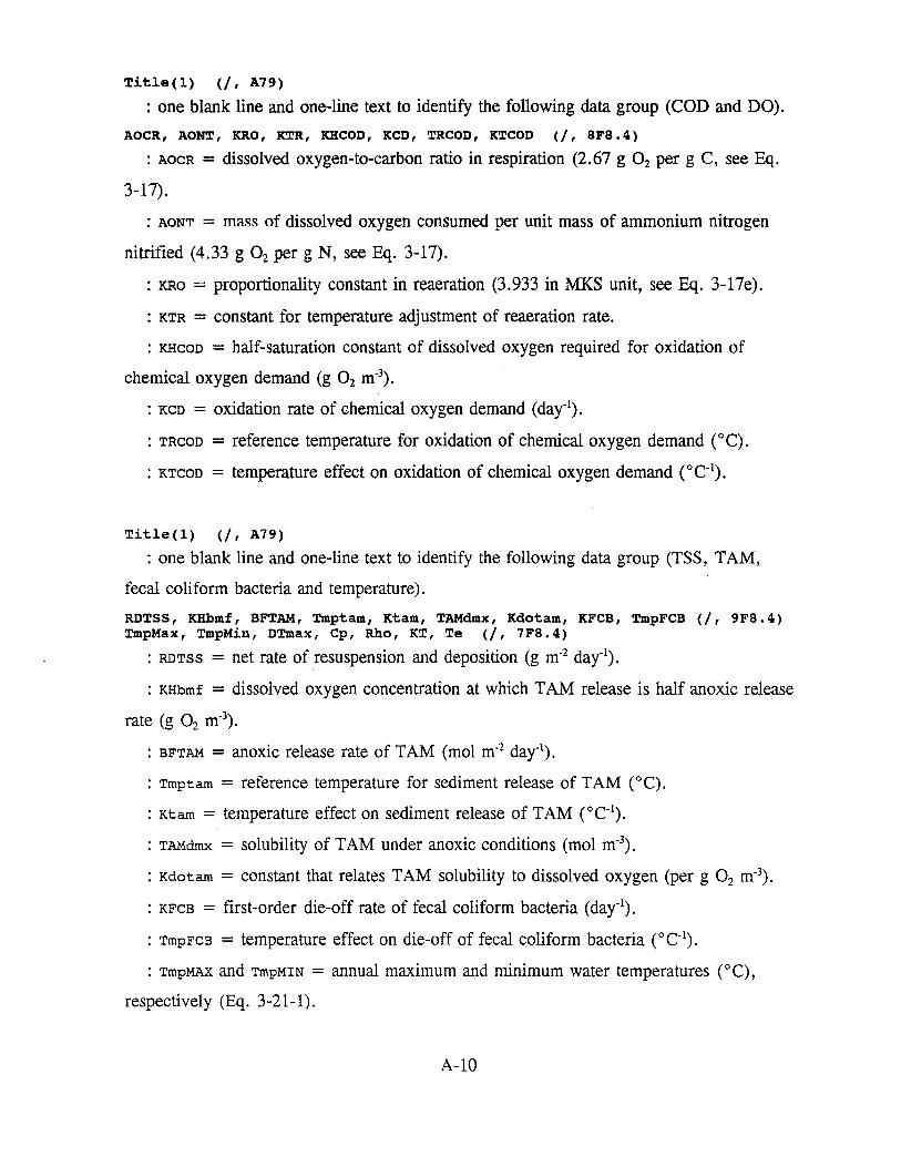
Title(l) (/, A79)

: one blank line and one-line text to identify the following data group (COD and DO).

AOCR, AONT, KRO, KTR, KHCOD, KCD, TRCOD, KTCOD (/, SFB,4)

: AOCR = dissolved oxygen-to-carbon ratio in respiration (2.67 g 0 2 per g C, see Eq.

3-17).

: AONT = mass of dissolved oxygen consumed per unit mass of ammonium nitrogen

nitrified (4.33 g 0 2 per g N, see Eq. 3-17).

: KRo = proportionality constant in reaeration (3.933 in MKS unit, see Eq. 3-17e).

: KTR = constant for temperature adjustment of reaeration rate.

: KHcoo = half-saturation constant of dissolved oxygen required for oxidation of

chemical oxygen demand (g 0 2 m-3).

: Keo = oxidation rate of chemical oxygen demand (day-1).

: TRcoo = reference temperature for oxidation of chemical oxygen demand ( ° C).

: KTcoo = temperature effect on oxidation of chemical oxygen demand (°C-1).

Title(l) (/, A79)

: one blank line and one-line text to identify the following data group (TSS, TAM,

fecal coliform bacteria and temperature).

RDTSS, KHbmf, BFTAM, Tmptam, Ktam, TAMdmx, Kdotam, KFCB, TmpFCB (/, 9F8.4) TmpMax, TmpMin, DTmax, Cp, Rho, KT, Te (/, 7F8.4)

: RDTss = net rate of resuspension and deposition (g m-2 day-1).

: KHbmf = dissolved oxygen concentration at which TAM release is half anoxic release

rate (g 0 2 m-3).

: BFTAM = anoxic release rate of TAM (mol m-2 day-1).

: Tmptam = reference temperature for sediment release of TAM (°C).

: Ktam = temperature effect on sediment release of TAM (°C-1).

: TAMdmx = solubility of TAM under anoxic conditions (mol m-3).

: Kdotam = constant that relates TAM solubility to dissolved oxygen (per g 0 2 m-3).

: KFCB = first-order die-off rate of fecal coliform bacteria (day-1).

: TmpFCB = temperature effect on die-off of fecal coliform bacteria (0 C-1).

: TmpMAX and TmpMIN = annual maximum and minimum water temperatures (°C),

respectively (Eq. 3-21-1).

A-10

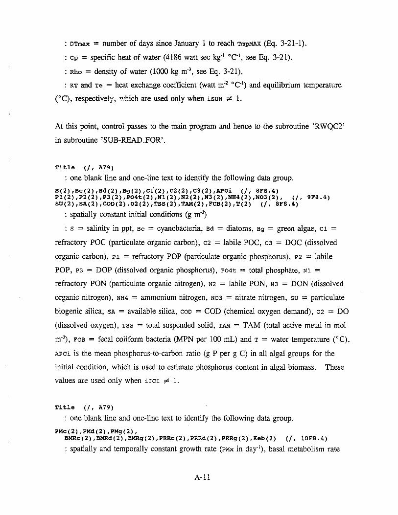
: DTmax = number of days since January 1 to reach TmpMAX (Eq. 3-21-1).

: cp = specific heat of water (4186 watt sec kg·1 0 c·1, see Eq. 3-21).

: Rho = density of water (1000 kg m·3, see Eq. 3-21).

: KT and Te = heat exchange coefficient (watt m·2 0 C-1) and equilibrium temperature

(°C), respectively, wJ:,Jch are used only when isuN ;c L

At this point, control passes to the main program and hence to the subroutine 'RWQC2'

in subroutine 'SUB-READ.FOR'.

Title (/, A79)

: one blank line and one-line text to identify the following data group.

S(2) ,Bc(2) ,Bd(2) ,Bg(2) ,Cl(2) ,C2(2) ,C3(2) ,APCi (/, SFS.4) Pl(2),P2(2),P3(2),P04t(2),Nl(2),N2(2),N3(2),NH4(2),N03(2), (/, 9FS.4) SU(2),SA(2),COD(2),02(2),TSS(2),TAM(2),FCB(2),T(2) (/, SFB,4)

: spatially constant initial conditions (g m·3)

: s = salinity in ppt, sc = cyanobacteria, Bd = diatoms, sg = green algae, c1 = refractory POC (particulate organic carbon), c2 = labile POC, c3 = DOC (dissolved

organic carbon), Pl = refractory POP (particulate organic phosphorus), P2 = labile

POP, P3 = DOP (dissolved organic phosphorus), P04t = total phosphate, Nl = refractory PON (particulate organic nitrogen), N2 = labile PON, N3 = DON (dissolved

organic nitrogen), NH4 = ammonium nitrogen, No3 = nitrate nitrogen, su = particulate

biogenic silica, SA = available silica, coo = COD ( chemical oxygen demand), 02 = DO

(dissolved oxygen), Tss = total suspended solid, TAM = TAM (total active metal in mol

m·3), Fca = fecal coliform bacteria (MPN per 100 mL) and T = water temperature (°C).

APci is the mean phosphorus-to-carbon ratio (g P per g C) in all algal groups for the

initial condition, which is used to estimate phosphorus content in algal biomass. These

values are used only when iICI ;c 1.

Title (/, A79)

: one blank line and one-line text to identify the following data group.

PMc(2),PMd(2),PMg(2), BMRc(2),BMRd(2),BMRg(2),PRRc(2),PRRd(2),PRRg(2),Keb(2) (/, lOFS,4)

: spatially and temporally constant growth rate (PMx in day-1), basal metabolism rate

A-11

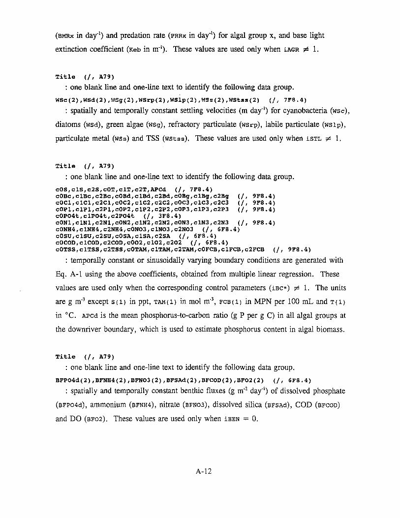
(BMRx in day-1) and predation rate (PRRx in day-1) for algal group x, and base light

extinction coefficient (Keh in m-1). These values are used only when iAGR ¢ 1.

Title (/, A79)

: one blank line and one-line text to identify the following data group.

WSc(2),WSd(2),WSg(2),WSrp(2),WSlp(2),WSs(2),WStss(2) (/; 7F8.4)

: spatially and temporally constant settling velocities (m day-1) for cyanobacteria (wsc),

diatoms (wsd), green algae (wsg), refractory particulate (wsrp), labile particulate (wslp),

particulate metal (wss) and TSS (wstss). These values are used only when iSTL ~ 1.

Title (/, A79)

: one blank line and one-li~e text to identify the following data group.

(/, 9F8,4) (/, 9F8,4) (/, 9F8,4)

cOS,clS,c2S,cOT,clT,c2T,APCd (/, 7F8,4) cOBc,clBc,c2Bc,c0Bd,clBd,c2Bd,c0Bg,clBg,c2Bg c0Cl,c1Cl,c2Cl,c0C2,clC2,c2C2,cOC3,clC3,c2C3 c0Pl,c1Pl,c2Pl,c0P2,clP2,c2P2,cOP3,clP3,c2P3 cOP04t,clP04t,c2P04t (/, 3F8,4) c0Nl,c1Nl,c2Nl,c0N2,clN2,c2N2,cON3,clN3,c2N3 (/, 9F8,4) cONH4,clNH4,c2NH4,cON03,clN03,c2N03 (/, 6F8.4) cOSU,clSU,c2SU,c0SA,clSA,c2SA (/, 6F8,4) cOCOD,clCOD,c2COD,c002,cl02,c202 (/, 6F8,4) cOTSS,clTSS,c2TSS,c0TAM,clTAM,c2TAM,c0FCB,clFCB,c2FCB (/, 9F8,4)

: temporally constant or sinusoidally varying boundary conditions are generated with

Eq. A-1 using the above coefficients, obtained from multiple linear regression. These

values are used only when the corresponding control parameters (iBC*) ~ 1. The units

are g m-3 except s ( 1) in ppt, TAM ( 1) in mol m-3, FCB ( 1) in MPN per 100 mL and T ( 1)

in °C. APCd is the mean phosphorus-to-carbon ratio (g P per g C) in all algal groups at

the downriver boundary, which is used to estimate phosphorus content in algal biomass.

Title (/, A79)

: one blank line and one-line text to identify the following data group.

BFP04d(2),BFNH4(2),BFN03(2),BFSAd(2),BFCOD(2),BF02(2) (/, 6F8,4)

: spatially and temporally constant benthic fluxes (g m·2 day-1) of dissolved phosphate

(BFP04d), ammonium (BFNH4), nitrate (BFN03), dissolved silica (BFSAd), COD (BFCOD)

and DO (BF02). These values are used only when iBEN = 0.

A-12

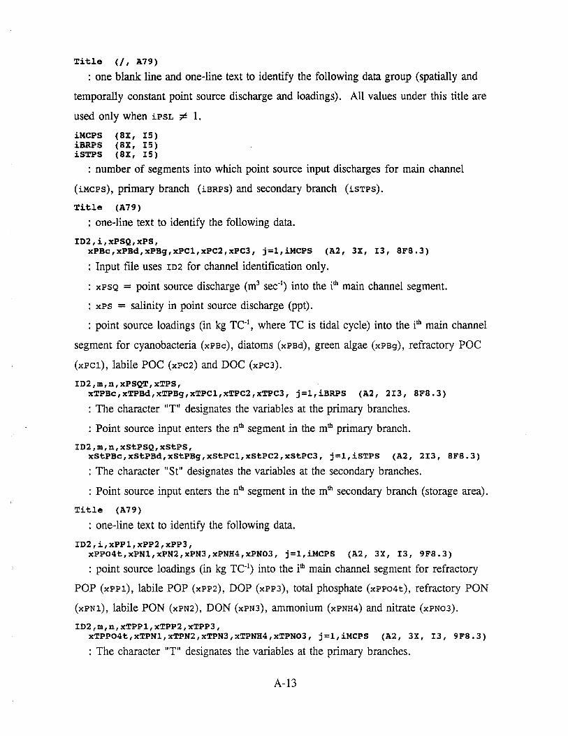
Title (/, A79)

: one blank line and one-line text to identify the following data group (spatially and

temporally constant point source discharge and loadings). All values under this title are

used only when iPSL ;c 1.

iMCPS (SX, IS) iBRPS (SX, IS) iSTPS (SX, IS)

: number of segments into which point source input discharges for main channel

(iMCPS), primary branch (iBRPS) and secondary branch (iSTPS).

Title (A79)

: one-line text to identify the following data.

ID2,i,xPSQ,xPS, xPBc,xPBd,xPBg,xPCl,xPC2,xPC3, j=l,iMCPS (A2, 3X, I3, SFS.3)

: Input file uses ID2 for channel identification only.

: xPSQ = point source discharge (m3 sec·1) into the ith main channel segment.

: xPs = salinity in point source discharge (ppt).

: point source loadings (in kg TC-1, where TC is tidal cycle) into the ith main channel

segment for cyanobacteria (xPBc), diatoms (xPBd), green algae (xPBg), refractory POC

(xPCl), labile POC (xPC2) and DOC (xPc3).

ID2,m,n,xPSQT,xTPS, xTPBc,xTPBd,xTPBg,xTPCl,xTPC2,xTPC3, j=l,iBRPS (A2, 2I3, 8F8.3)

: The character "T" designates the variables at the primary branches.

: Point source input enters the nth segment in the mth primary branch.

ID2,m,n,xStPSQ,xStPS, xStPBc,xStPBd,xStPBg,xStPCl,xStPC2,xStPC3, j=l,iSTPS (A2, 2I3, SFS,3)

: The character "St" designates the variables at the secondary branches.

: Point source input enters the nth segment in the mth secondary branch (storage area).

Title (A79)

: one-line text to identify the following data.

ID2,i,xPP1,xPP2,xPP3, xPP04t,xPNl,xPN2,xPN3,xPNH4,xPN03, j=l,iMCPS (A2, 3X, I3, 9F8,3)

: point source loadings (in kg TC·1) into the ith main channel segment for refractory

POP (xPPl), labile POP (xPP2), DOP (xPP3), total phosphate (xPP04t), refractory PON

(xPNl), labile PON (xPN2), DON (xPN3), ammonium (xPNH4) and nitrate (xPN03).

ID2,m,n,xTPPl,xTPP2,xTPP3, xTPP04t,xTPNl,xTPN2,xTPN3,xTPNH4,xTPN03, j=l,iMCPS (A2, 3X, I3, 9F8.3)

: The character "T" designates the variables at the primary branches.

A-13

: Point source input enters the nth segment in the mth primary branch.

ID2,m,n,xStPP1,xStPP2,xStPP3,xStPP04t, xStPNl,xStPN2,xStPN3,xStPNH4,xStPN03, j=l,iMCPS (A2, 3X, I3, 9F8.3)

: The character "St" designates the variables at the secondary branches.

: Point source input enters the nth segment in the mth secondary branch (storage area).

Title (A79)

: one-line text to identify the following data.

ID2,i,xPSU,xPSA,xPCOD, xP02,xPTSS,xPTAM,xPFCB,xPT, j=l,iMCPS (A2, 3X, I3, BFB.3)

: point source loadings (in kg Tc-1) into the ith main channel segment for particulate

biogenic silica (xPsu), available silica (xPsA), COD (xPcoo), TSS (xPTss) and TAM

(xPTAM in kmol TC"1).

: xP02 = DO in point sour~e discharge (g m·3).

: xPFCB = fecal coliform bacteria in point source discharge (MPN per 100 mL).

: xPT = temperature in point source discharge (° C).

ID2,m,n,xTPSU,xTPSA,xTPCOD, xTP02,xTPTSS,xTPTAM,xTPFCB,xTPT, j=l,iMCPS (A2, 3X, I3, SFB.3)

: The character "T" designates the variables at the primary branches.

: Point source input enters the nth segment in the mth primary branch.

ID2,m,n,xStPSU,xStPSA,xStPCOD, xStP02,xStPTSS,xStPTAM,xStPFCB,xStPT, j=l,iMCPS (A2, 3X, I3, SFS.3)

: The character "St" designates the variables at the secondary branches.

: Point source input enters the nth segment in the mth secondary branch (storage area).

Title (/, A79)

: one blank line and one-line text to identify the following data group.

xDSQ,xNS,xNBc,xNBd,xNBg,xNCl,xNC2,xNC3 (/, SFS.4) xNP1,xNP2,xNP3,xNP04t,xNNl,xNN2,xNN3,xNNH4,xNN03, (/, 9F8,4) xNSU,xNSA,xNCOD,xN02,xNTSS,xNTAM,xNFCB,xNT (/, SFS.4)

: spatially and temporally constant nonpoint source discharge and loadings into all

segments including branches.

: xDSQ = nonpoint source discharge (m sec·1).

: The first two characters "xN" designates nonpoint source input, and the definition and

unit of variables are the same as point source input except xNFCB in 109 MPN Tc·1•

: These values are used only when iNPL :;c 1.

A-14

Title (/, A79)

: one blank line and one-line text to identify the following data group.

ICIFN (44X, ASO)

: input file name for spatially and/or temporally varying initial conditions for water

column state variables. If ucr = 1, ICIFN is opened with the unit number 11. If ucr

;c 1, then rcrFN must be 'none', otherwise an error will be issued and the program be

stopped.

AGRFN (44X, ASO)

: input file name for spatially and/or temporally varying algal growth, respiration and

predation rates, and base light extinction coefficient. If iAGR = 1, AGRFN is opened with

the unit number 12. If iAGR ;;c 1, then AGRFN must be 'none', otherwise an error will be

issued and the program be stopped.

STLFN (44X, ASO)

: input file name for spatially and/or temporally varying settling velocities. If iSTL = 1, STLFN is opened with the unit number 13. If iSTL ;;c 1, then STLFN must be 'none',

otherwise an error will be issued and the program be stopped.

SUNFN (44X, ASO)

: input file name for temporally varying parameters for light intensity and temperature.

If iSUN = 1, suNFN is opened with the unit number 14. If iSUN ;c 1, then suNFN must

be 'none' , otherwise an error will be issued and the program be stopped.

DBCFN (44X, ASO)

: input file name for temporally varying downriver boundary conditions for water

column state variables. If iosc = 1, oscFN is opened with the unit number 15. If iosc

;;c 1, then DBCFN must be 'none', otherwise an error will be issued and the program be

stopped.

BENFN (44X, ASO)

: input file name for spatially and/or temporally varying benthic fluxes. If iBEN = 2,

BENFN is opened with the unit number 16. If iBEN ;;c 2, then BENFN must be 'none',

otherwise an error will be issued and the program be stopped.

TMPFN (44X, A50)

: input file name for spatially and/or temporally varying water temperatures. If iTMP

= 3, TMPFN is opened with the unit number 17. If iTMP ;;c 3, then TMPFN must be

'none', otherwise an error will be issued and the program be stopped.

A-15

PSLFN (44X, ASO)

: input file name for temporally varying point source discharges and loadings. If iPSL

= 1, PSLFN is opened with the unit number 18. If iPSL ,c 1, then PSLFN must be

'none', otherwise an error will be issued and the program be stopped.

NPLFN (44X, ASO)

: input file name for spatially and/or temporally varying nonpoint source discharges

and loadings. If iNPL = 1, NPLFN is opened with the unit number 19. If iNPL .c 1,

then NPLFN must be 'none', otherwise an error will be issued and the program be

stopped.

SMIFN (44X, ASO)

: input file name for sediment process model. If iBEN = 1, SMIFN is opened with the

unit number 20. If iBEN ,c 1, then sMIFN must be 'none', otherwise an error will be

issued and the program be stopped.

ZKOFN (44X, ASO)

: output file name for diagnostic information for zero K0 (Section III-12). If iZK = 1,

ZKOFN is opened with the unit number 22. If iZK ,c 1, then ZKOFN must be 'none',

otherwise an error will be issued and the program be stopped.

NROFN (44X, ASO)

: output file name for diagnostic information for negative R0 (Section III-12). If iNR

= 1, NROFN is opened with the unit number 23. If iNR ,c 1, then NROFN must be 'none',

otherwise an error will be issued and the program be stopped.

NCOFN (44X, ASO)

: output file name for diagnostic information for negative concentration. If iNc = 1,

NCOFN is opened with the unit number 24. If iNC ,c 1, then NCOFN must be 'none',

otherwise an error will be issued and the program be stopped.

DSOFN (44X, ASO)

: output file name for diagnostic information for salinity. If Lsal = 1, osoFN is

opened with the unit number 25. If Lsal .c 1, then osoFN must be 'none', otherwise an

error will be issued and the program be stopped.

DBcOFN (44X, ASO)

: output file name for diagnostic information for cyanobacteria. If LBc = 1, DBcOFN is

opened with the unit number 26. If LBc ,c 1, then oacoFN must be 'none', otherwise an

error will be issued and the program be stopped.

A-16

DBdOFN (44X, ASO)

: output file name for diagnostic information for diatoms. If LBd = 1, DBdOFN is

opened with the unit number 27. If LBd ;c 1, then DBdOFN must be 'none', otherwise an

error will be issued and the program be stopped.

DPOFN (44X, ASO)

: output file name for diagnostic information for phosphate. If Lpo4 = 1, DPOFN is

opened with the unit number 28. If Lpo4 ;c 1, then DPOFN must be 'none', otherwise an

error will be issued and the program be stopped.

DNOFNH4 (44X, ASO)

: output file name for diagnostic information for ammonium. If Lnh4 = 1, DNOFNH4 is

opened with the unit number 29. If Lnh4 ;c 1, then DNOFNH4 must be 'none', otherwise

an error will be issued and the program be stopped.

DNOFN (44X, ASO)

: output file name for diagnostic information for nitrate. If Lno3 = 1, DNOFN is

opened with the unit number 30. If Lno3 ;c 1, then DNOFN must be 'none', otherwise an

error will be issued and the program be stopped.

DSiOFN (44X, ASO)

: output file name for diagnostic information for available silica. If Lsa = 1, os iOFN

is opened with the unit number 31. If Lsa ;c 1, then osiOFN must be 'none', otherwise

an error will be issued and the program be stopped.

D020FN (44X, ASO)

: output file name for diagnostic information for dissolved oxygen. If Lo2 = 1,

0020FN is opened with the unit number 32. If Lo2 ;c 1, then 0020FN must be 'none',

otherwise an error will be issued and the program be stopped.

DTOFN (44X, ASO)

: output file name for diagnostic information for temperature. If Ltmp = 1, DTOFN is

opened with the unit number 33. If Ltmp ;c 1, then DTOFN must be 'none', otherwise an

error will be issued and the program be stopped.

LDOFN (44X, ASO)

: output file name for snapshot longitudinal distribution of water column state

variables. If Nprn ~ 1, LDOFN is opened with the unit number 21. If Nprn < 0, then

LDOFN must be 'none', otherwise an error will be issued and the program be stopped.

A-17

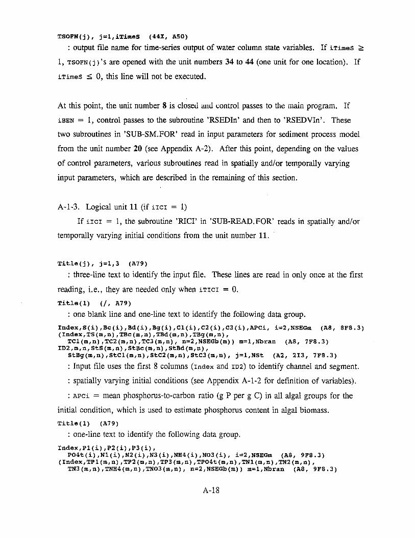
TSOFN(j), j=l,iTimeS (44X, ASO)

: output file name for time-series output of water column state variables. If iTimes >

1, TSOFN ( j) 's are opened with the unit numbers 34 to 44 (one unit for one location). If

iTimes < 0, this line will not be executed.

At this point, the unit number 8 is dosed and control passes to the main program. If

iBEN = 1, control passes to the subroutine 'RSEDin' and then to 'RSEDVIn'. These

two subroutines in 'SUB-SM.FOR' read in input parameters for sediment process model

from the unit number 20 (see Appendix A-2). After this point, depending on the values

of control parameters, various subroutines read in spatially and/or temporally varying

input parameters, which are described in the remaining of this section.

A-1-3. Logical unit 11 (if ucr = 1)

If ircr = 1, the subroutine 'RICI' in 'SUB-READ.FOR' reads in spatially and/or

temporally varying initial conditions from the unit number 11.

Title(j), j=l,3 (A79)

: three-line text to identify the input file. These lines are read in only once at the first

reading, i.e., they are needed only when iTICI = 0.

Title(l) (/, A79)

: one blank line and one-line text to identify the following data group.

Index,S(i),Bc(i),Bd(i),Bg(i),Cl(i),C2(i),C3(i),APCi, i=2,NSEGm (AS, SFS.3) (Index,TS(m,n),TBc(m,n),TBd(m,n),TBg(m,n),

TCl(m,n),TC2(m,n),TC3(m,n), n=2,NSEGb(m)) m=l,Nbran (AS, 7FS,3) ID2,m,n,StS(m,n),StBc(m,n),StBd(m,n),

StBg(m,n),StCl(m,n),StC2(m,n),StC3(m,n), j=l,NSt (A2, 2I3, 7FS.3)

: Input file uses the first 8 columns (Index and rn2) to identify channel and segment.

: spatially varying initial conditions (see Appendix A-1-2 for definition of variables).

: APCi = mean phosphorus-to-carbon ratio (g P per g C) in all algal groups for the

initial condition, which is used to estimate phosphorus content in algal biomass.

Title ( 1) (A79)

: one-line text to identify the following data group.

Index,Pl(i),P2(i),P3(i), P04t(i),Nl(i),N2(i),N3(i),NB4(i),N03(i), i=2,NSEGm (AS, 9F8.3)

(Index,TPl(m,n),TP2(m,n),TP3(m,n),TP04t(m,n),TNl(m,n),TN2(m,n), TN3(m,n),TNB4(m,n),TN03(m,n), n=2,NSEGb(m)) m=l,Nbran (AS, 9FS.3)

A-18

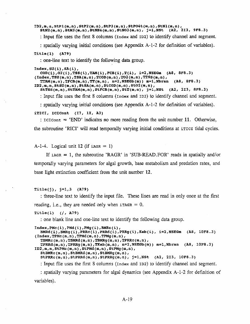
ID2,m,n,StPl(m,n),StP2(m,n),StP3(m,n),StP04t(m,n),StN1(m,n), StN2(m,n),StN3(m,n),StNH4(m,n),StN03(m,n), j=l,NSt (A2, 2I3, 9F8.3)

: Input file uses the first 8 columns (Index and ID2) to identify channel and segment.

: spatially varying initial conditions (see Appendix A-1-2 for definition of variables).

Title(l) (A79)

: one-line text to identify the following data group.

Index,SU(i),SA(i), COD(i),02(i),TSS(i),TAM(i),FCB(i),T(i), i=2,NSEGm (AS, SFS.3)

(Index,TSU(m,n),TSA(m,n),TCOD(m,n),T02(m,n),TTSS(m,n), TTAM(m,n),TFCB(m,n),TT(m,n), n=2,NSEGb(m)) m=l,Nbran (AS, SFS.3)

ID2,m,n,StSU(m,n),StSA(m,n),StCOD(m,n),St02(m,n), StTSS(m,n),StTAM(m,n),StFCB(m,n),StT(m,n), j=l,NSt (A2, 2I3, SFS.3)

: Input file uses the first 8 columns (Index and ID2) to identify channel and segment.

: spatially varying initial conditions (see Appendix A-1-2 for definition of variables).

iTICI, ICICont (I7, lX, A3)

: rcrcont = 'END' indicates no more reading from the unit number 11. Otherwise,

the subroutine 'RICI' will read temporally varying initial conditions at iTrcr tidal cycles.

A-1-4. Logical unit 12 (if iAGR = 1)

If iAGR = 1, the subroutine 'RAGR' in 'SUB-READ.FOR' reads in spatially and/or

temporally varying parameters for algal growth, base metabolism and predation rates, and

base light extinction coefficient from the unit number 12.

Title(j), j=l,3 (A79)

: three-line text to identify the input file. These lines are read in only once at the first

reading, i.e., they are needed only when iTAGR = 0.

Title(l) (/, A79)

: one blank line and one-line text to identify the following data group.

Index,PMc(i),PMd(i),PMg(i),BMRc(i), BMRd(i),BMRg(i),PRRc(i),PRRd(i),PRRg(i),Keb(i), i=2,NSEGm (AS, lOFS,3)

(Index,TPMc(m,n),TPMd(m,n),TPMg(m,n), TBMRc(m,n),TBMRd(m,n),TBMRg(m,n),TPRRc(m,n), TPRRd(m,n),TPRRg(m,n),TKeb(m,n), n=2,NSEGb(m)) m=l,Nbran (AS, lOFS,3)

ID2,m,n,StPMc(m,n),StPMd(m,n),StPMg(m,n), StBMRc(m,n),StBMRd(m,n),StBMRg(m,n), StPRRc(m,n),StPRRd(m,n),StPRRg(m,n), j=l,NSt (A2, 2I3, lOFS.3)

: Input file uses the first 8 columns (Index and ID2) to identify channel and segment.

: spatially varying parameters for algal dynamics (see Appendix A-1-2 for definition of

variables).

A-19

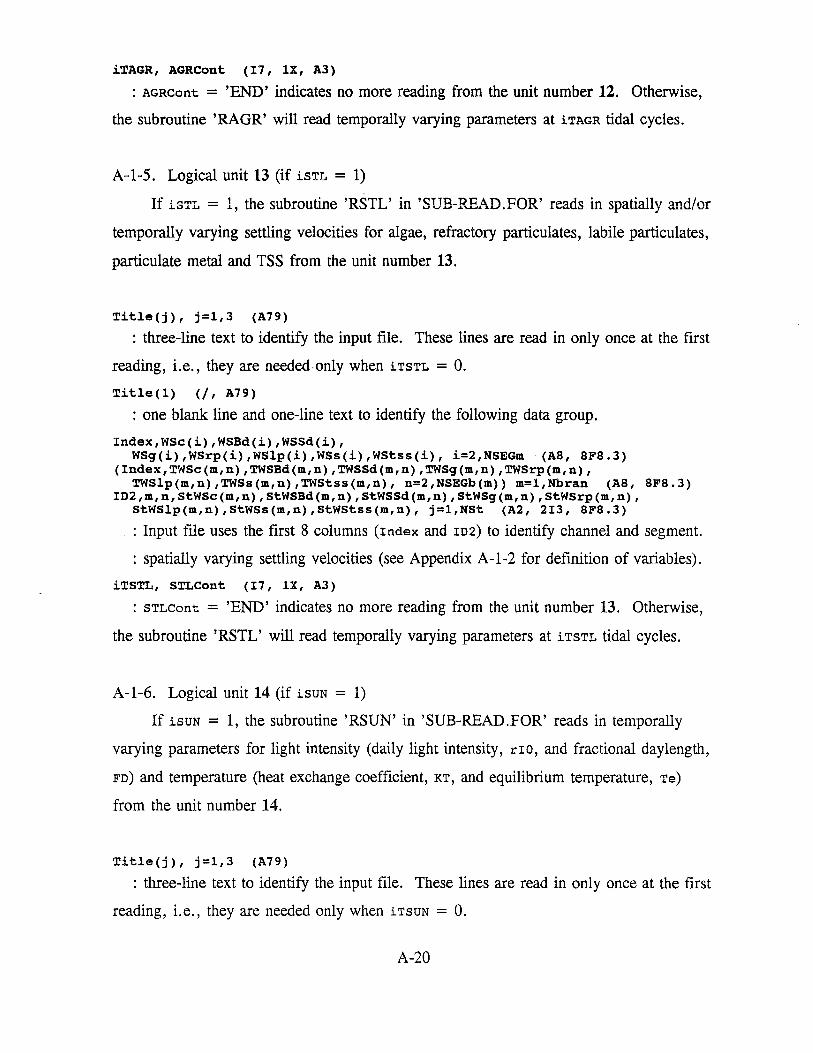
iTAGR, AGRCont (I7, lX, A3)

: AGRCont = 'END' indicates no more reading from the unit number 12. Otherwise,

the subroutine 'RAGR' will read temporally varying parameters at iTAGR tidal cycles.

A-1-5. Logical unit 13 (if iSTL = 1)

If iSTL = 1, the subroutine 'RSTL' in 'SUB-READ.FOR' reads in spatially a.rid/or

temporally varying settling velocities for algae, refractory particulates, labile particulates,

particulate metal and TSS from the unit number 13.

Title(j), j=l,3 (A79)

: three-line text to identify the input file. These lines are read in only once at the first

reading, i.e., they are needed.only when iTSTL = 0.

Title(l) (/, A79)

: one blank line and one-line text to identify the following data group.

Index,WSc(i),WSBd(i),WSSd(i), WSg(i),WSrp(i),WSlp(i),WSs(i),WStss(i), i=2,NSEGm (AS, SFS.3)

(Index,TWSc(m,n),TWSBd(m,n),TWSSd(m,n),TWSg(m,n),TWSrp(m,n), TWSlp(m,n),TWSs(m,n),TWStss(m,n), n=2,NSEGb(m)) m=l,Nbran (AS, SFS.3)

ID2,m,n,StWSc(m,n),StWSBd(m,n),StWSSd(m,n),StWSg(m,n),StWSrp(m,n), StWSlp(m,n),StWSs(m,n),StWStss(m,n), j=l,NSt (A2, 2I3, SFS.3)

: Input file uses the first 8 columns (Index and ro2) to identify channel and segment.

: spatially varying settling velocities (see Appendix A-1-2 for definition of variables).

iTSTL, STLCont (I7, lX, A3)

: STLcont = 'END' indicates no more reading from the unit number 13. Otherwise,

the subroutine 'RSTL' will read temporally varying parameters at iTSTL tidal cycles.

A-1-6. Logical unit 14 (if iSUN = 1)

If isUN = 1, the subroutine 'RSUN' in 'SUB-READ.FOR' reads in temporally

varying parameters for light intensity (daily light intensity, rIO, and fractional daylength,

FD) and temperature (heat exchange coefficient, KT, and equilibrium temperature, Te)

from the unit number 14.

Title(j), j=l,3 (A79)

: three-line text to identify the input file. These lines are read in only once at the first

reading, i.e., they are needed only when iTsuN = 0.

A-20

Title(!) (/, A79)

: one blank line and one-line text to identify the following data group.

rIO,FD,KT,Te (4F8,3)

: temporally varying parameters (see Appendix A-1-2 for definition of variables).

iTSUN, SUNCont (I7, lX, A3)

: suNcont = 'filID' indicates no more reading from the unit number 14. Otherwise,

the subroutine 'RSUN' will read temporally varying parameters at iTSUN tidal cycles.

A-1-7. Logical unit 15 (if iDBC = 1)

If ioac = 1, the subroutine 'RDBC' in 'SUB-READ.FOR' reads in temporally

varying downriver boundary conditions from the unit number 15.

Title(j), j=l,3 (A79)

: three-line text to identify the input file. These lines are read in only once at the first

reading, i.e., they are needed only when iToac = 0.

Title(l) (/, A79)

: one blank line and one-line text to identify the following data group.

S(l),Bc(l),Bd(l),Bg(l),Cl(l),C2(1),C3(1),APCd (8F8.3)

: temporally varying downriver boundary conditions (see Appendix A-1-2 for

definition of variables), and APCd is the mean phosphorus-to-carbon ratio (g P per g C) at

the downriver boundary.

Title(l) (A79)

: one-line text to identify the following data group.

Pl(l),P2(1),P3(1),P04t(l),Nl(l),N2(1),N3(1),NH4(1),N03(1) (9F8.3)

: temporally varying downriver boundary conditions (see Appendix A-1-2 for

definition of variables).

Title(l) (A79)

: one-line text to identify the following data group.

SU(l),SA(l),COD(l),02(1),TSS(l),TAM(l),FCB(l),T(l) (SFS.3)

: temporally varying downriver boundary conditions (see Appendix A-1-2 for

definition of variables).

iTDBC, DBCCont (I7, lX, A3)

: oaccont = 'END' indicates no more reading from the unit number 15. Otherwise,

the subroutine 'RDBC' will read temporally varying parameters at iToac tidal cycles.

A-21

Note that the 25 values are read in each time. However only those, for which the

corresponding control parameters (iBC*) = 1 (see Appendix A-1-2), are used. Those for

which iBC* ;c 1, the boundary conditions are generated using Eq. A-1 in the subroutine

'RDBCsin'.

A-1-8. Logical unit 16 (if iBEN = 2)

If iBEN = 2, the subroutine 'RBEN' in 'SUB-READ.FOR' reads in spatially and/or

temporally varying benthic fluxes from the unit number 16.

Title(j), j=l,3 (A79)

: three-line text to identify the input file. These lines are read in only once at the first

reading, i.e., they are needed.only when iTBEN = 0.

Title(l) (/, A79)

: one blank line and one-line text to identify the following data group.

Index,BFP04d(i), BFNH4(i),BFN03(i),BFSAd(i),BFCOD(i),BF02(i) i=2,NSEGm (AS, 6FS,3)

(Index,TBFP04d(m,n),TBFNH4(m,n),TBFN03(m,n), TBFSAd(m,n),TBFCOD(m,n),TBF02(m,n) n=2,NSEGb(m)) m=l,Nbran (AS, 6FS,3)

ID2,m,n,StBFP04d(m,n),StBFNH4(m,n),StBFN03(m,n), StBFSAd(m,n),StBFCOD(m,n),StBF02(m,n) j=l,NSt (A2, 2I3, 6FS,3)

: Input file uses the first 8 columns (Index and ID2) to identify channel and segment.

: spatially varying benthic fluxes (see Appendix A-1-2 for definition of variables).

iTBEN, BENCont (I7, lX, A3)

: BENCont = 'END' indicates no more reading from the unit number 16. Otherwise,

the subroutine 'RBEN' will read temporally varying parameters at iTBEN tidal cycles.

A-1-9. Logical unit 17 (if iTMP = 3)

If iTMP = 3, the subroutine 'RTMP' in 'SUB-READ.FOR' reads in spatially and/or

temporally varying temperatures from the unit number 17.

Title(j), j=l,3 (A79)

: three-line text to identify the input file. These lines are read in only once at the first

reading, i.e., they are needed only when iTTMP = 0.

Title(l) (/, A79)

: one blank line and one-line text to identify the following data group.

A-22

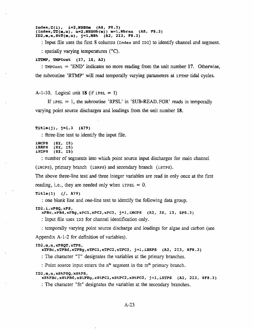
Index,T(i), i=2,NSEGm (AS, FS.3) (Index,TT(m,n), n=2,NSEGb(m)) m=l,Nbran (AS, FS.3) ID2,m,n,StT(m,n), j=l,NSt (A2, 2I3, FS.3)

: Input file uses the first 8 columns (Index and ID2) to identify channel and segment.

: spatially varying temperatures (°C).

iTTMP, TMPCont (I7, lX, AJ)

: TMPCont = 'END' indicates no more reading from the unit number 17. Otherwise,

the subroutine 'RTMP' will read temporally varying parameters at iTTMP tidal cycles.

A-1-10. Logical unit 18 (if iPSL = 1)

If iPsL = 1, the subroutine 'RPSL' in 'SUB-READ.FOR' reads in temporally

varying point source discharges and loadings from the unit number 18.

Title(j), j=l,3 (A79)

: three-line text to identify the input file.

iMCPS (BX, IS) iBRPS (BX, IS) iSTPS (BX, IS)

: number of segments into which point source input discharges for main channel

(iMCPs), primary branch (iBRPs) and secondary branch (iSTPs).

The above three-line text and three integer variables are read in only once at the first

reading, i.e., they are needed only when iTPSL = 0.

Title(l) (/, A79)

: one blank line and one-line text to identify the following data group.

ID2,i,xPSQ,xPS, xPBc,xPBd,xPBg,xPCl,xPC2,xPC3, j=l,iMCPS (A2, JX, IJ, SFS.3)

: Input file uses ID2 for channel identification only.

: temporally varying point source discharge and loadings for algae and carbon (see

Appendix A-1-2 for definition of variables).

ID2,m,n,xPSQT,xTPS, xTPBc,xTPBd,xTPBg,xTPCl,xTPC2,xTPC3, j=l,iBRPS (A2, 2!3, SFS.3)

: The character "T" designates the variables at the primary branches.

: Point source input enters the nth segment in the mth primary branch.

ID2,m,n,xStPSQ,xStPS, xStPBc,xStPBd,xStPBg,xStPCl,xStPC2,xStPC3, j=l,iSTPS (A2, 2I3, 8F8.3)

: The character "St" designates the variables at the secondary branches.

A-23

: Point source input enters the nth segment in the mlh secondary branch (storage area).

Title (A79)

: one-line text to identify the following data.

ID2,i,xPPl,xPP2,xPP3, xPP04t,xPNl,xPN2,xPN3,xPNH4,xPN03, j=l,iMCPS (A2, 3X, I3, 9F8.3)

ID2,m,n,xTPPl,xTPP2,xTPP3, xTPP04t,xTPNl,xTPN2,xTPN3,xTPNH4,xTPN03, j=l,iMCPS (A2, 3X, I3, 9F8.3)

!D2,m,n,xStPP1,xStPP2,xStPP3,xStPP04t, xStPNl,xStPN2,xStPN3,xStPNH4,xStPN03, j=l,iMCPS (A2, 3X, I3, 9F8.3)

: point source input for phosphorus and nitrogen (see Appendix A-1-2 for definition of

variables).

Title (A79)

: one-line text to identify the following data.

ID2,i,xPSU,xPSA,xPCOD, xP02,xPTSS,xPTAM,xPFCB,xPT, j=l,iMCPS (A2, 3X, I3, 8F8,3)

ID2,m,n,xTPSU,xTPSA,xTPCOD, xTP02,xTPTSS,xTPTAM,xTPFCB,xTPT, j=l,iMCPS (A2, 3X, I3, 8F8,3)

ID2,m,n,xStPSU,xStPSA,xStPCOD, xStP02,xStPTSS,xStPTAM,xStPFCB,xStPT, j=l,iMCPS (A2, 3X, I3, 8F8.3)

: point source input (see Appendix A-1-2 for definition of variables).

iTPSL, PSLCont (I7, lX, A3)

: PSLcont = 'END' indicates no more reading from the unit number 18. Otherwise,

the subroutine 'RPSL' will read temporally varying parameters at iTPSL tidal cycles.

A-1-11. Logical unit 19 (if iNPL = 1)

If iNPL = 1, the subroutine 'RNPL' in 'SUB-READ.FOR' reads in spatially and/or

temporally varying nonpoint source discharges and loadings from the unit number 19.

Title(j), j=l,3 (A79)

: three-line text to identify the input file. These lines are read in only once at the first

reading, i.e., they are needed only when iTNPL = 0.

Title (/, A79)

: one blank line and one-line text to identify the following data group.

Index,xDSQ,xNS,xNBc,xNBd,xNBg,xNCl,xNC2,xNC3, j=2,NSEGm (AS, 8F8,4) (Index,xDSQT,xTNS,xTNBc,

xTNBd,xTNBg,xTNCl,xTNC2,xTNC3, n=2,NSEGb(j)) j=l,Nbran (AS, 8F8,4) ID2,m,n,xStDSQ,xStNS,

xStNBc,xStNBd,xStNBg,xStNCl,xStNC2,xStNC3, j=l,NSt (A2, 2I3, 8F8,4)

: spatially varying nonpoint source discharge and loadings for algae and carbon (see

Appendix A-1-2 for definition of variables).

A-24

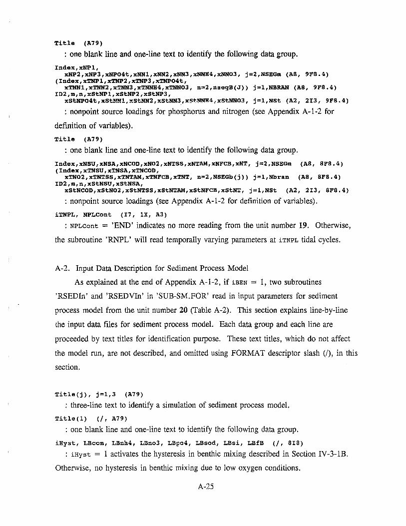
Title (A79)

: one blank line and one-line text to identify the following data group.

Index, xNP 1, xNP2,xNP3,xNP04t,x.NNl,x.NN2,xNN3,xNNB4,xNN03, j=2,NSEGm (AB, 9FB.4)

(Index,xTNP1,xTNP2,xTNP3,xTNP04t, xTNN1,xTNN2,xTNN3,xTNNH4,xTNN03, n=2,nsegB(J)) j=l,NBRAN (AB, 9FB,4)

ID2,m,n,xStNPl,xStNP2,xStNP3, xStHP04t,xSt..~1,xStNN2,xStNN3_;xStNNB:4,xStNN03, j=l,NSt (A2, 2I3, 9FB.4)

: nonpoint source loadings for phosphorus and nitrogen (see Appendix A-1-2 for

definition of variables).

Title (A79)

: one blank line and one-line text to identify the following data group.

Index,xNSU,xNSA,xNCOD,xN02,xNTSS,xNTAM,xNFCB,xNT, j=2,NSEGm (AB, BFB.4) (Index,xTNSU,xTNSA,xTNCOD,

xTN02,xTNTSS,xTNTAM,xTNFCB,xTNT, n=2,NSEGb(j)) j=l,Nbran (AB, BFB.4) ID2,m,n,xStNSU,xStNSA,

xStNCOD,xStN02,xStNTSS,xStNTAM,xStNFCB,xStNT, j=l,NSt (A2, 2I3, BFB.4)

: nonpoint source loadings (see Appendix A-1-2 for definition of variables).

iTNPL, NPLCont (I7, lX, A3)

: NPLcont = 'END' indicates no more reading from the unit number 19. Otherwise,

the subroutine 'RNPL' will read temporally varying parameters at iTNPL tidal cycles.

A-2. Input Data Description for Sediment Process Model

As explained at the end of Appendix A-1-2, if iBEN = 1, two subroutines

'RSEDin' and 'RSEDVIn' in 'SUB-SM.FOR' read in input parameters for sediment

process model from the unit number 20 (Table A-2). This section explains line-by-line

the input data files for sediment process model. Each data group and each line are

proceeded by text titles for identification purpose. These text titles, which do not affect

the model run, are not described, and omitted using FORMAT descriptor slash (/), in this

section.

Title(j), j=l,3 (A79)

: three-line text to identify a simulation of sediment process model.

Title(l) (/, A79)

: one blank line and one-line text to identify the following data group.

iHyst, LBcom, LBnh4, LBno3, LBpo4, LBsod, LBsi, LBfB (/, BIS)

: iHyst = 1 activates the hysteresis in benthic mixing described in Section IV-3-lB.

Otherwise, no hysteresis in benthic mixing due to low oxygen conditions.

A-25

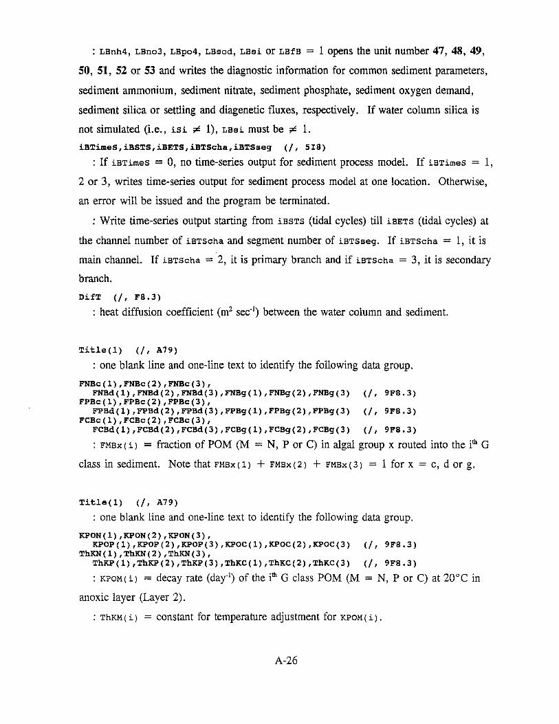
: LBnh4, LBno3, LBpo4, LBsod, LBsi or LBfB = 1 opens the unit number 47, 48, 49,

50, 51, 52 or 53 and writes the diagnostic information for common sediment parameters,

sediment ammonium, sediment nitrate, sediment phosphate, sediment oxygen demand,

sediment silica or settling and diagenetic fluxes, respectively. If water column silica is

not simulated (i.e., isi ;c 1), LBsi rp.ust be ;c 1.

iBTimeS,iBSTS,iBETS,iBTScha,iBTSseg (/, SIB)

: If iBTimes = 0, no time-series output for sediment process model. If iBTimes = 1,

2 or 3, writes time-series output for sediment process model at one location. Otherwise,

an error will be issued and the program be terminated.

: Write time-series output starting from iBsTs (tidal cycles) till iBETS (tidal cycles) at

the channel number of iBTScha and segment number of iBTSseg. If iBTScha = 1, it is

main channel. If iBTScha = 2, it is primary branch and if iBTScha = 3, it is secondary

branch.

DifT (/ , FB , 3)

: heat diffusion coefficient (m2 sec-1) between the water column and sediment.

Title(l) (/, A79)

: one blank line and one-line text to identify the following data group.

FNBc(l),FNBc(2),FNBc(3), FNBd(l) ,FNBd(2) ,FNBd(3) ,FNBg(l) ,FNBg(2) ,FNBg(3) (/, 9F8.3)

FPBc(l),FPBc(2),FPBc(3), FPBd(l),FPBd(2),FPBd(3),FPBg(l),FPBg(2),FPBg(3) (/, 9F8,3)

FCBc(l),FCBc(2),FCBc(3), FCBd(l),FCBd(2),FCBd(3),FCBg(l),FCBg(2),FCBg(3) (/, 9F8.3)

: FMBx ( i) = fraction of POM (M = N, P or C) in algal group x routed into the ith G

class in sediment. Note that FMBx(l) + FMBx(2) + FMBx(3) = 1 for x = c, d or g.

Title(l) (/, A79)

: one blank line and one-line text to identify the following data group.

KPON(l),KPON(2),KPON(3), KPOP(l),KPOP(2),KPOP(3),KPOC(l),KPOC(2),KPOC(3) (/, 9F8.3)

ThKN(l),ThKN(2),ThKN(3), ThKP(l),ThKP(2),ThKP(3),ThKC(l),ThKC(2),ThKC(3) (/, 9F8.3)

: KPOM(i) = decay rate (day·1) of the ith G class POM (M = N, P or C) at 20°C in

anoxic layer (Layer 2).

: ThKM( i) = constant for temperature adjustment for KPOM( i).

A-26

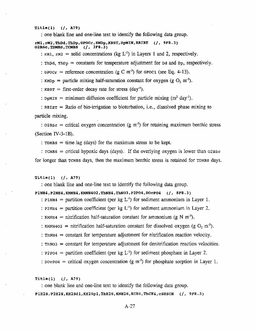
Title(!) (/, A79)

: one blank line and one-line text to identify the following data group.

rMl,rM2,ThDd,ThDp,GPOCr,KMDp,KBST,DpMIN,RBIBT (/, 9F8.3) 02BSc,TDMBS,TCMBS (/, 3F8.3)

: rMl, rM2 = solid concentrations (kg L-1) in Layers 1 and 2, respectively.

: ThDd, ThDp = constants for temperature adjustment for Dd and op; respectively.

: GPocr = reference concentration (g C m-3) for GPoc1 (see Eq. 4-13).

: KMDp = particle mixing half-saturation constant for oxygen (g 0 2 m-3).

: KBST = first-order decay rate for stress (day-1).

: DpMIN = minimum diffusion coefficient for particle mixing (m2 day-1).

: RBIBT = Ratio of bio-irrigation to bioturbation, i.e., dissolved phase mixing to

particle mixing.

: 02asc = critical oxygen concentration (g m-3) for retaining maximum benthic stress

(Section IV -3- lB).

: TOMBS = time lag (days) for the maximum stress to be kept.

: TCMBs = critical hypoxic days (days). If the overlying oxygen is lower than 02asc

for longer than TCMBS days, then the maximum benthic stress is retained for TOMBS days.

Title(!) (/, A79)

: one blank line and one-line text to identify the following data group.

PlNH4,P2NH4,KMNH4,KMNH402,ThNH4,ThN03,P2P04,DOcP04 (/, SFS.3)

: P1NH4 = partition coefficient (per kg L-1) for sediment ammonium in Layer 1.

: P2NH4 = partition coefficient (per kg L-1) for sediment ammonium in Layer 2.

: KMNH4 = nitrification half-saturation constant for ammonium (g N m-3).

: KMNH4o2 = nitrification half-saturation constant for dissolved oxygen (g 0 2 m-3).

: ThNH4 = constant for temperature adjustment for nitrification reaction velocity.

: ThNo3 = constant for temperature adjustment for denitrification reaction velocities.

: P2Po4 = partition coefficient (per kg L-1) for sediment phosphate in Layer 2.

: oocPo4 = critical oxygen concentration (g m-3) for phosphate sorption in Layer 1.

Title(l) (/, A79)

: one blank line and one-line text to identify the following data group.

PlH2S,P2H2S,KH2Sdl,KH2Spl,ThH2S,KMH2S,KCH4,ThCH4,cSHSCH (/, 9F8,3)

A-27

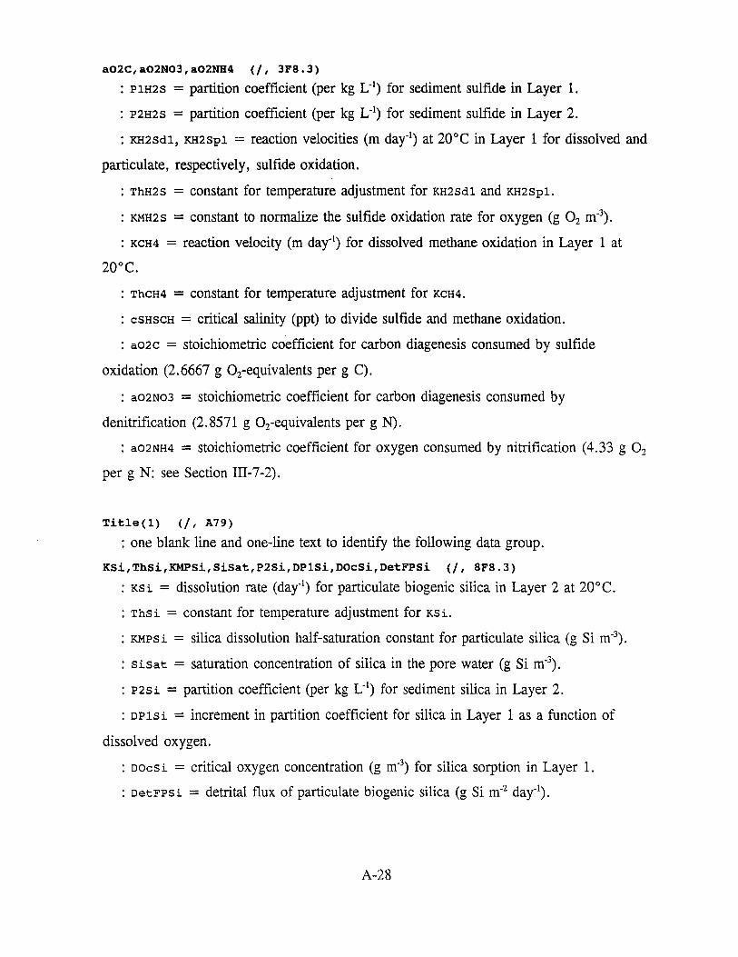
a02C,a02N03,a02NB4 (/, 3F8.3)

: P1H2S = partition coefficient (per kg L-1) for sediment sulfide in Layer 1.

: P2H2S = partition coefficient (per kg L-1) for sediment sulfide in Layer 2.

: KH2Sdl, KH2Spl = reaction velocities (m day-1) at 20°C in Layer 1 for dissolved and

particulate, respectively, sulfide oxidation.

: ThH2S = constant for temperature adjustment for KH2Sdl and KH2Spl.

: KMH2S = constant to normalize the sulfide oxidation rate for oxygen (g 0 2 m-3).

: KCH4 = reaction velocity (m day-1) for dissolved methane oxidation in Layer 1 at

20°c.

: ThCH4 = constant for temperature adjustment for KCH4.

: csascH = critical salinity (ppt) to divide sulfide and methane oxidation.

: ao2c = stoichiometric coefficient for carbon diagenesis consumed by sulfide

oxidation (2.6667 g Orequivalents per g C).

: ao2N03 = stoichiometric coefficient for carbon diagenesis consumed by

denitrification (2.8571 g 0 2-equivalents per g N).

: a02NH4 = stoichiometric coefficient for oxygen consumed by nitrification (4.33 g 0 2

per g N: see Section III-7-2).

Title(l) (/, A79)

: one blank line and one-line text to identify the following data group.

KSi,ThSi,KMPSi,SiSat,P2Si,DP1Si,DOcSi,DetFPSi (/, 8F8.3)

: KSi = dissolution rate (day-1) for particulate biogenic silica in Layer 2 at 20°C.

: Thsi = constant for temperature adjustment for KSL

: KMPSi = silica dissolution half-saturation constant for particulate silica (g Si m-3).

: sisat = saturation concentration of silica in the pore water (g Si m·3).

: P2Si = partition coefficient (per kg L·1) for sediment silica in Layer 2.

: DP1Si = increment in partition coefficient for silica in Layer 1 as a function of

dissolved oxygen.

: oocsi = critical oxygen concentration (g m·3) for silica sorption in Layer 1.

: oetFPSi = detrital flux of particulate biogenic silica (g Si m·2 day-1).

A-28

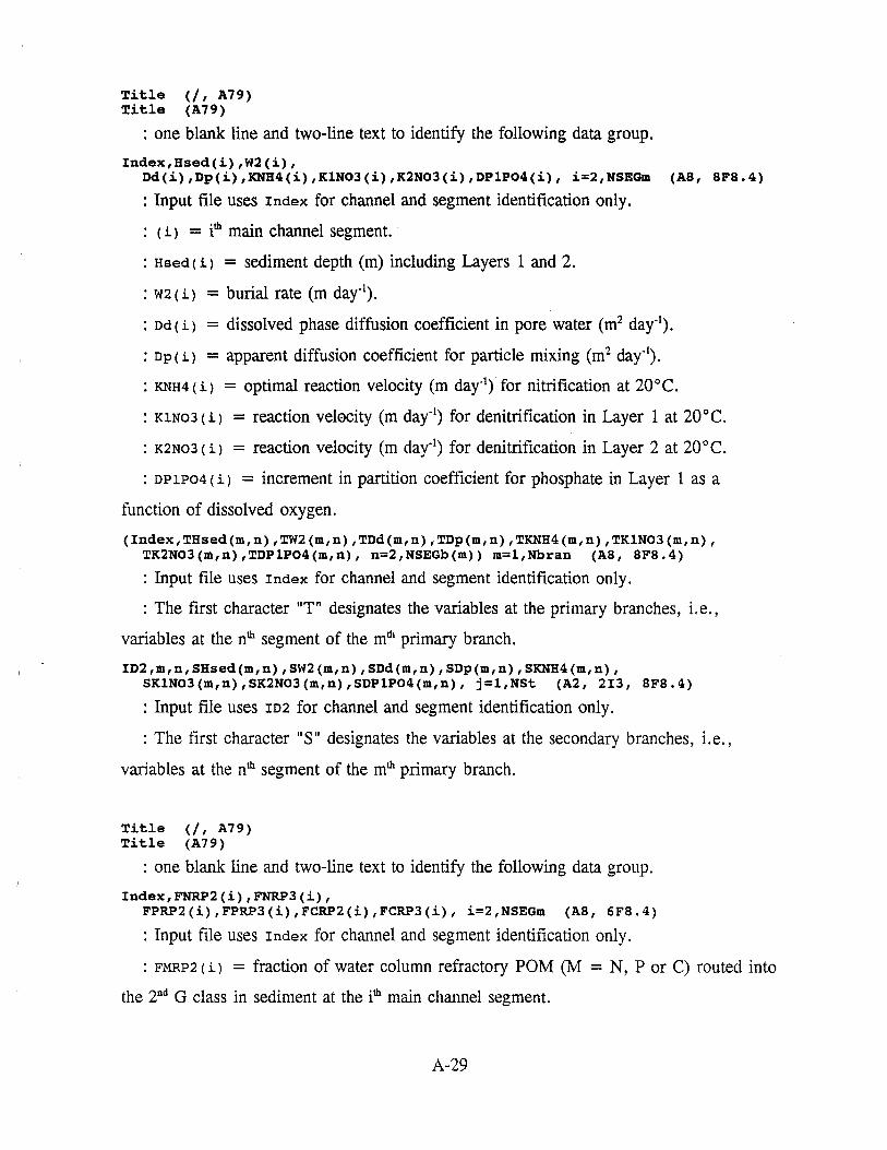
Title (/, A79) Title (A79)

: one blank line and two-line text to identify the following data group.

Index,Hsed(i),W2(i), Dd(i),Dp(i),KNH4(i),K1N03(i),K2N03(i),DP1P04(i), i=2,NSEGm (AS, BFS.4)

: Input file uses Index for channel and segment identification only.

: ( i > = ith main channel segment. ·

: Hsed ( i) = sediment depth (m) including Layers 1 and 2.

: w2 ( i) = burial rate (m day·1).

: od ( i) = dissolved phase diffusion coefficient in pore water (m2 day·1).

: op ( i) = apparent diffusion coefficient for particle mixing (m2 day·1).

: KNH4 ( i) = optimal reaction velocity (m day·1) for nitrification at 20°C.

: K1No3 ( i) = reaction velecity (m day·1) for denitrification in Layer 1 at 20°C.

: K2No3 ( i) = reaction velocity (m day-1) for denitrification in Layer 2 at 20°C.

: DP 1P04 ( i) = increment in partition coefficient for phosphate in Layer 1 as a

function of dissolved oxygen.

(Index,THsed(m,n),TW2(m,n),TDd(m,n),TDp(m,n),TKNH4(m,n),TK1N03(m,n), TK2N03(m,n),TDP1P04(m,n), n=2,NSEGb(m)) m=l,Nbran (AB, BFB.4)

: Input file uses Index for channel and segment identification only.

: The first character "T" designates the variables at the primary branches, i.e.,

variables at the nth segment of the mth primary branch.

ID2,m,n,SHsed(m,n),SW2(m,n),SDd(m,n),SDp(m,n),SKNH4(m,n), SK1N03(m,n),SK2N03(m,n),SDP1P04(m,n), j=l,NSt (A2, 2I3, BFS.4)

: Input file uses ID2 for channel and segment identification only.

: The first character II S II designates the variables at the secondary branches, i.e.,

variables at the nth segment of the mth primary branch.

Title (/, A79) Title (A79)

: one blank line and two-line text to identify the following data group.

Index,FNRP2(i),FNRP3(i), FPRP2(i),FPRP3(i),FCRP2(i),FCRP3(i), i=2,NSEGm (AB, 6F8.4)

: Input file uses Index for channel and segment identification only.

: FMRP2 ( i) = fraction of water column refractory POM (M = N, P or C) routed into

the 2nd G class in sediment at the ith main channel segment.

A-29

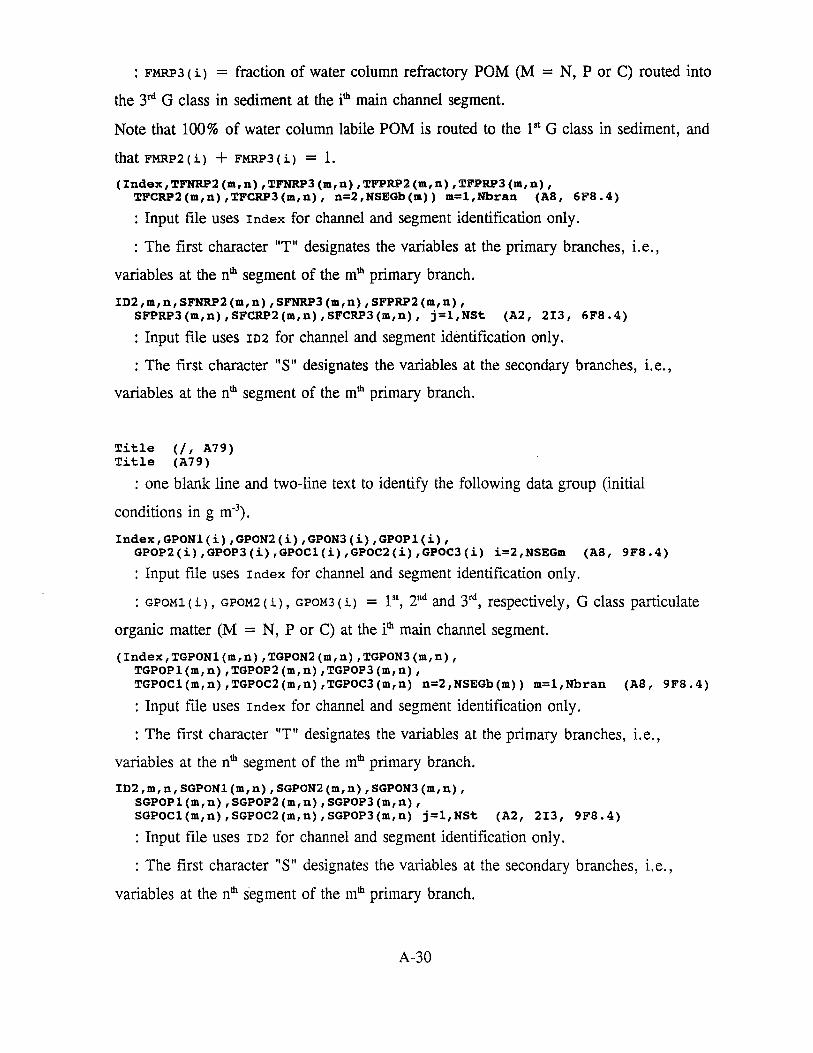
: FMRP 3 ( i) = fraction of water column refractory POM (M = N, P or C) routed into

the 3n1 G class in sediment at the ith main channel segment.

Note that 100% of water column labile POM is routed to the pt G class in sediment, and

that FMRP2(i) + FMRP3(i) = 1.

(Index,TFNRP2(m,n),TFNRP3(m,n),TFPRP2(m,n),TFPRP3(m,n), TFCRP2(m,n),TFCRP3(m,n), n=2,NSEGb(m)) m=l,Nbran (AS, 6FS.4)

: Input file uses Index for channel and segment identification only.

: The first character "T" designates the variables at the primary branches, i.e.,

variables at the nth segment of the mth primary branch.

ID2,m,n,SFNRP2(m,n),SFNRP3(m,n),SFPRP2(m,n), SFPRP3(m,n),SFCRP2(m,n),SFCRP3(m,n), j=l,NSt (A2, 2I3, 6FS.4)

: Input file uses ID2 for channel and segment identification only.

: The first character "S" designates the variables at the secondary branches, i.e.,

variables at the nth segment of the mth primary branch.

Title (/, A79) Title (A79)

: one blank line and two-line text to identify the following data group (initial

conditions in g m·3).

Index,GPONl(i),GPON2(i),GPON3(i),GPOPl(i), GPOP2(i),GPOP3(i),GPOCl(i),GPOC2(i),GPOC3(i) i=2,NSEGm (AS, 9FS.4)

: Input file uses Index for channel and segment identification only.

: GPOMl ( i) , GPOM2 ( i) , GPOM3 ( i) = l8\ 2nd and 3r\ respectively, G class particulate

organic matter (M = N, P or C) at the ith main channel segment.

(Index,TGPONl(m,n),TGPON2(m,n),TGPON3(m,n), TGPOPl(m,n),TGPOP2(m,n),TGPOP3(m,n), TGPOCl(m,n),TGPOC2(m,n),TGPOC3(m,n) n=2,NSEGb(m)) m=l,Nbran (AS, 9F8.4)

: Input file uses Index for channel and segment identification only.

: The first character "T" designates the variables at the primary branches, i.e.,

variables at the nth segment of the mth primary branch.

ID2,m,n,SGPONl(m,n),SGPON2(m,n),SGPON3(m,n), SGPOPl(m,n),SGPOP2(m,n),SGPOP3(m,n), SGPOCl(m,n),SGPOC2(m,n),SGPOP3(m,n) j=l,NSt (A2, 2I3, 9F8.4)

: Input file uses rn2 for channel and segment identification only.

: The first character "S" designates the variables at the secondary branches, i.e.,

variables at the nth segment of the mth primary branch.

A-30

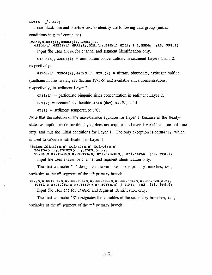
Title (/, A79)

: one blank line and one-line text to identify the following data group (initial

conditions in g m·3 continued).

Index,Gl.NB4(i),G2NH4(i),G2NOJ(i), G2P04(i),G2H2S(i),GPSi(i),G2Si(i),BST(i),GT(i) i=2,NSEGm (AS, 9FS.4)

: Input file uses Index for channel and segment identification only.

: G1NH4 ( i >, G2NH4 ( i) = ammonium concentrations in sediment Layers 1 and 2,

respective! y.

: G2N03 ( i), G2P04 ( i), G2H2S ( i), G2Si ( i) = nitrate, phosphate, hydrogen sulfide

(methane in freshwater, see Section IV-3-5) and available silica concentrations,

respectively, in sediment Layer 2.

: GPsi ( i) = particulate biogenic silica concentration in sediment Layer 2.

: BST(i) = accumulated benthic stress (day), see Eq. 4-14.

: GT ( i) = sediment temperature (° C).

Note that the solution of the mass-balance equation for Layer 1, because of the steady­

state assumption made for this layer, does not require the Layer 1 variables at an old time

step, and thus the initial conditions for Layer 1. The only exception is G1NH4 ( i >, which

is used to calculate nitrification in Layer 1.

(Index,TG1NH4(m,n),TG2NH4(m,n),TG2N03(m,n), TG2P04(m,n),TG2H2S(m,n),TGPSi(m,n), TG2Si(m,n),TBST(m,n),TGT(m,n) n=2,NSEGb(m)) m=l,Nbran (AS, 9F8.4)

: Input file uses Index for channel and segment identification only.

: The first character "T 11 designates the variables at the primary branches, i.e.,

variables at the nth segment of the mth primary branch.

ID2,m,n,SGlNH4(m,n),SG2NH4(m,n),SG2N03(m,n),SG2P04(m,n),SG2H2S(m,n), SGPSi(m,n),SG2Si(m,n),SBST(m,n),SGT(m,n) j=l,NSt (A2, 2I3, 9F8.4)

: Input file uses ID2 for channel and segment identification only.

: The first character II S II designates the variables at the secondary branches, i.e.,

variables at the nth segment of the mth primary branch.

A-31

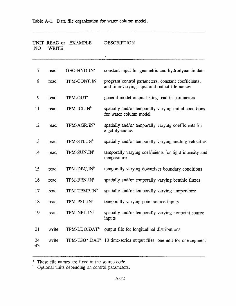
Table A-1. Data file organization for water column model.

UNIT READ or EXAMPLE DESCRIPTION NO WRITE

7 read GEO-HYD.INa constant input for geometric and hydrodynamic data

8 read TPM-CONT.IN program control parameters, constant coefficients, and time-varying input and output file names

9 read TPM.OUTa general model output listing read-in parameters

11 read TPM-ICI.INb spatially and/or temporally varying initial conditions for water column model

12 read TPM-AGR.INb spatially and/or temporally varying coefficients for algal dynamics

13 read TPM-STL.INb spatially and/or temporally varying settling velocities

14 read TPM-SUN.INb temporally varying coefficients for light intensity and temperature

15 read TPM-DBC.INb temporally varying downriver boundary conditions

16 read TPM-BENJNb spatially and/or temporally varying benthic fluxes

17 read TPM-TEMP .INb spatially and/or temporally varying temperature

18 read TPM-PSLJNb temporally varying point source inputs

19 read TPM-NPL.INb spatially and/or temporally varying nonpoint source inputs

21 write TPM-LDO.DATb output file for longitudinal distributions

34 write TPM-TSO*.DATb 10 time-series output files: one unit for one segment -43

a These file names are fixed in the source code. b Optional units depending on control parameters.

A-32

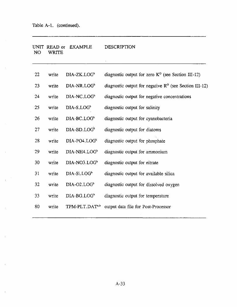
Table A-1. (continued).

UNIT READ or EXAMPLE DESCRIPTION NO WRITE

22 write DIA-ZK.LOGb diagnostic output for zero K0 (see Section III-12)

23 write DIA-NR.LOGb diagnostic output for negative R0 (see Section III-12)

24 write DIA-NC.LQGb diagnostic output for negative concentrations

25 write DIA-S.LOGb diagnostic output for salinity

26 write DIA-BC.LOGb diagnostic output for cyanobacteria

27 write DIA-BD.LOGb diagnostic output for diatoms

28 write DIA-P04.LQGb diagnostic output for phosphate

29 write DIA-NH4.LOGb diagnostic output for ammonium

30 write DIA-N03.LQGb diagnostic output for nitrate

31 write DIA-Si.LOGb diagnostic output for available silica

32 write DIA-02.LOGb diagnostic output for dissolved oxygen

33 write DIA-BG.LOGb diagnostic output for temperature

80 write TPM-PLT.DATa,b output data file for Post-Processor

A-33

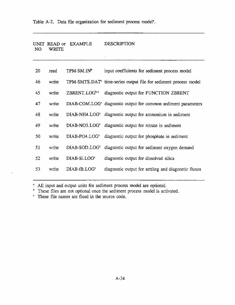
Table A-2. Data file organization for sediment process model1•

UNIT READ or EXAMPLE NO WRITE

20 read TPM-SM.INb

DESCRIPTION

input coefficients for sediment process model

46 write TPM-SMTS.DAr time-series output file for sediment process model

45 write ZBRENT .LOGb,c diagnostic output for FUNCTION ZBRENT

47 write DIAB-COM.LOGc diagnostic output for common sediment parameters

48 write DIAB-NH4.LOGC diagnostic output for ammonium in sediment

49 write DIAB-N03.LQGC diagnostic output for nitrate in sediment

50 write DIAB-P04.LOGC diagnostic output for phosphate in sediment

51 write DIAB-SOD.LQGC diagnostic output for sediment oxygen demand

52 write DIAB-Si.LOGC diagnostic output for dissolved silica

53 write DIAB-ffi.LQGC diagnostic output for settling and diagenetic fluxes

a All input and output units for sediment process model are optional. b These files are not optional once the sediment process model is activated. c These file names are fixed in the source code.

A-34

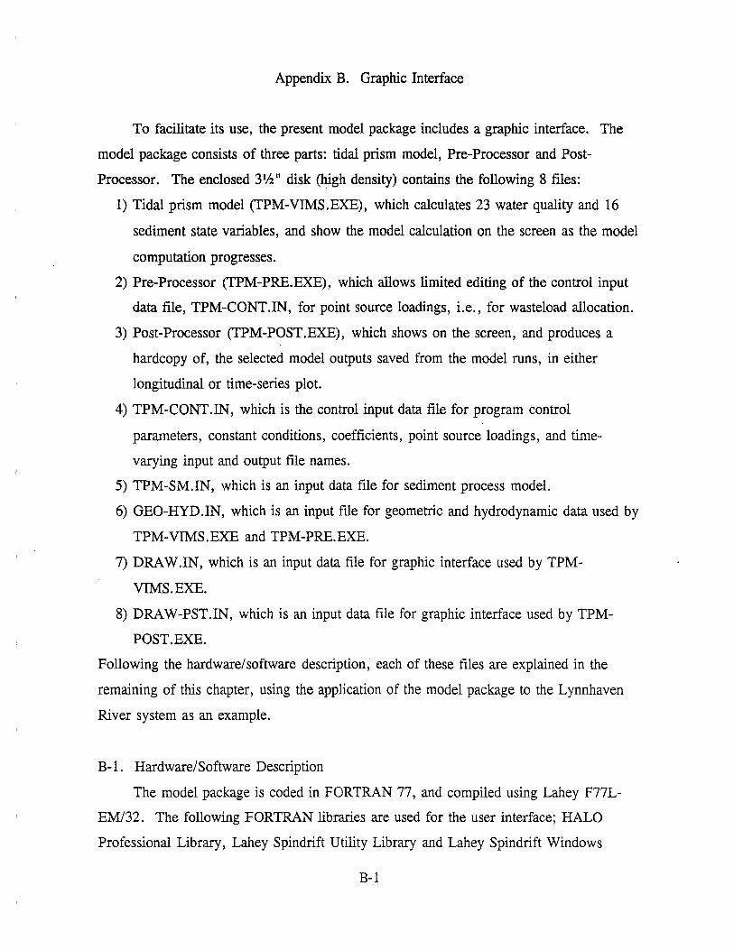
Appendix B. Graphic Interface

To facilitate its use, the present model package includes a graphic interface. The

model package consists of three parts: tidal prism model, Pre-Processor and Post­

Processor. The enclosed 31/2 11 disk (~igh density) contains the following 8 files:

1) Tidal prism model (TPM-VIMS.EXE), which calculates 23 water quality and 16

sediment state variables, and show the model calculation on the screen as the model

computation progresses.

2) Pre-Processor (TPM-PRE.EXE), which allows limited editing of the control input

data file, TPM-CONT.IN, for point source loadings, i.e., for wasteload allocation.

3) Post-Processor (TPM-POST.EXE), which shows on the screen, and produces a

hardcopy of, the selected model outputs saved from the model runs, in either

longitudinal or time-series plot.

4) TPM-CONT.IN, which is the control input data file for program control

parameters, constant conditions, coefficients, point source loadings, and time­

varying input and output file names.

5) TPM-SM.IN, which is an input data file for sediment process model.

6) GEO-BYD.IN, which is an input file for geometric and hydrodynamic data used by

TPM-VIMS.EXE and TPM-PRE.EXE.

7) DRAW.IN, which is an input data file for graphic interface used by TPM­

VIMS.EXE.

8) DRAW-PST.IN, which is an input data file for graphic interface used by TPM-

POST.EXE.

Following the hardware/software description, each of these files are explained in the

remaining of this chapter, using the application of the model package to the Lynnhaven

River system as an example.

B-1. Hardware/Software Description

The model package is coded in FORTRAN 77, and compiled using Lahey F77L­

EM/32. The following FORTRAN libraries are used for the user interface; HALO

Professional Library, Lahey Spindrift Utility Library and Lahey Spindrift Windows

B-1

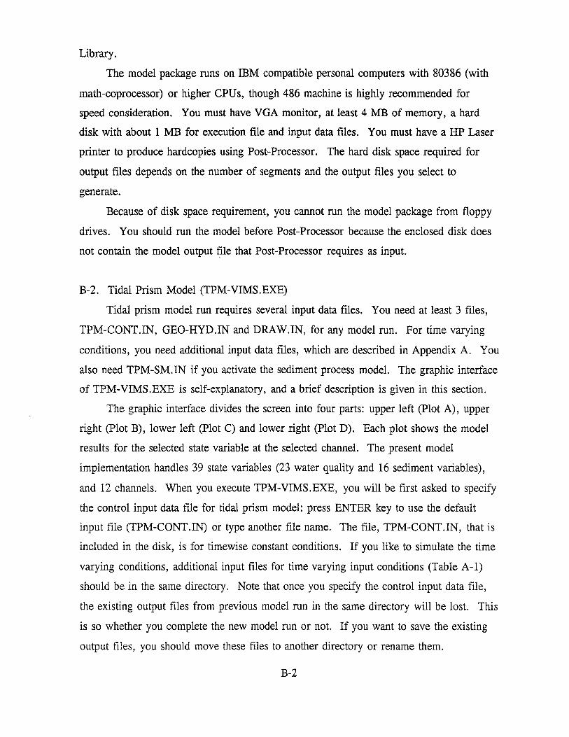
Library.

The model package runs on IBM compatible personal computers with 80386 (with

math-coprocessor) or higher CPUs, though 486 machine is highly recommended for

speed consideration. You must have VGA monitor, at least 4 MB of memory, a hard

disk with about 1 MB for execution file and input data files. You must have a HP Laser

printer to produce hardcopies using Post-Processor. The hard disk space required for

output files depends on the number of segments and the output files you select to

generate.

Because of disk space requirement, you cannot run the model package from floppy

drives. You should run the model before Post-Processor because the enclosed disk does

not contain the model output f_ile that Post-Processor requires as input.

B-2. Tidal Prism Model (TPM-VIMS.EXE)

Tidal prism model run requires several input data files. You need at least 3 files,

TPM-CONT.IN, GEO-HYD.IN and DRAW.IN, for any model run. For time varying

conditions, you need additional input data files, which are described in Appendix A. You

also need TPM-SM.IN if you activate the sediment process model. The graphic interface

of TPM-VIMS.EXE is self-explanatory, and a brief description is given in this section.

The graphic interface divides the screen into four parts: upper left (Plot A), upper

right (Plot B), lower left (Plot C) and lower right (Plot D). Each plot shows the model

results for the selected state variable at the selected channel. The present model

implementation handles 39 state variables (23 water quality and 16 sediment variables),

and 12 channels. When you execute TPM-VIMS.EXE, you will be first asked to specify

the control input data file for tidal prism model: press ENTER key to use the default

input file (TPM-CONT.IN) or type another file name. The file, TPM-CONT.IN, that is

included in the disk, is for timewise constant conditions. If you like to simulate the time

varying conditions, additional input files for time varying input conditions (Table A-1)

should be in the same directory. Note that once you specify the control input data file,

the existing output files from previous model run in the same directory will be lost. This

is so whether you complete the new model run or not. If you want to save the existing

output files, you should move these files to another directory or rename them.

B-2

After you specify the control input file, you will see the default selections of

variables and channels for four plots: salinity at main channel (Eastern Branch) for Plot

A, salinity at Western Branch for Plot B, chlorophyll 'a' at main channel for Plot C and

dissolved oxygen at main channel for Plot D. You may change variables and channels

for any plot by following the on-screen instructions. To distinguish sediment variables

from those in water column, sediment variable names are preceded by "s". Also note

that positive sediment oxygen demand (sSOD) indicates the oxygen flux into the

sediment, while other fluxes are positive to the overlying water column.

Upon pressing ENTER key, the next screen shows four plots that you choose. In

addition to these, the graphic screen has a clock showing the progress of model run. It

also has a line for time in Julian days and a line of menu at the bottom, which is

(P)ause (R)esume re(S)tart (O)ther-plots (Y)scale-change ESC-to-exit

Pressing P will pause the model run until you press R or any other key. Pressing S

restarts the model run from the beginning. Pressing O brings you to the previous menu

to let you change variable and channel selection for the plots. The model continues its

run after new selection. Pressing Y allows you to change the y-axis scale for four plots

at any time. You can abort the model run by pressing ESCAPE key. Note that the

current output files will be deleted if you abort the model run before its normal

termination. The marks, .... , at the top of each plot indicate the transect locations, and all

state variables are defined at the center of each segment. Since the 1st segments for both

main channel and branches are outside of the mouth (Section II-1), an arbitrary distance

of -0.5 km is assigned to designate the center of the pt segments.

B-3. Pre-Processor (TPM-PRE.EXE)

The Pre-Processor allows limited editing of the control input data file, TPM­

CONT.IN, for point source loadings, i.e., for wasteload allocation. When running TPM­

PRE.EXE, you need one more input file, GEO-HYD.IN, in the current directory. When

you execute TPM-PRE.EXE, you will be first asked to specify the control input data file

that you like to edit. You can press ENTER key to use the default data file (TPM­

CONT. IN) or type another file name.

Upon specifying the input data file, you will see the next screen displaying a menu.

B-3

You can choose each item either by moving cursor key followed by ENTER or by

pressing the first character. The one-line help for each item at the bottom of the screen

explains the meaning of above 16 items. For example, if you choose item o (Default), it

will read and display the values for each of the first 11 items from the default input data

file (TPM-CONT.IN), which should ~e in the current directory with TPM-PRE.EXE.

Choosing item P (Previous) will bring you back to the previous menu for input file

specification. Choosing item N (Next) will bring you to the next screen. Branch number

of zero indicate the point source loading entering the main channel, while positive branch

number indicates the point source loading into the primary branches. Negative branch

number indicates the point source loading into the secondary branch (storage area)

connected to the primary branch denoted by the branch number. For example, branch

number of -3 indicates the point source loading into the storage area connected to the 3rd

primary branch.

It should be noted that the Pre-Processor allows limited editing of the control input

data file: only the locations and loadings of no more than 4 point sources, which

discharge timewise constant waste water, are allowed. The model, however, can handle

time-varying point source discharges. You can edit the input parameters that the Pre­

Processor cannot modify using any ASCII editor: the input data file organization is

described in detail in Appendix A.

Upon choosing item N), you will see the next screen displaying another menu,

which allows you to edit the following parameters:

discharge rate (m3 sec-1),

loadings (kg per tidal cycle) for RPOC, LPOC, DOC, RPOP, LPOP, DOP, P04t,

RPON, LPON, DON, NH4, N03, SU, SA, TSS and TAM (kmol per tidal cycle),

concentration for DO (g m-3), PCB (MPN per 100 mL) and T (°C).

You can choose each item either by moving cursor key followed by ENTER or by

pressing the first character. The one-line help for each item at the bottom of the screen

explains the meaning of the item. Again, it should be noted that the above parameters

are timewise constant point source discharges, although the model can handle time­

varying ones.

B-4

B-4. Post-Processor (TPM-POST.EXE)

The tidal prism model generates, if iPLT = 1, a file (TPM-PLT.DAT) containing

the model results for all state variables over the last 20 tidal cycles. The Post-Processor

lets you examine, and produce hardcopy of, the model output in this file, in either

longitudinal or time-series plot. In addition to TPM-PLT.DA.T, you need another input

file, DRAW-PST.IN, in the current directory. When you execute TPM-POST.EXE, you

will be first asked to specify the input data file. You can press ENTER key to use the

default data file (TPM-PLT.DAT) or type another file name.

The Post-Processor divides the screen into four parts: three parts for plots, upper

left (Plot A), upper right (Plot B) and lower left (Plot C), and lower right part for model

values. The three plots show the model results in either longitudinal or time-series plot.

The longitudinal plot shows the snapshot information at the last tidal cycle for the

selected state variable at the selected channel. The time-series plot shows the time-series

information over the last 20 tidal cycles for the selected variable at all segments in

selected channel.

After you specify the input file, you will see the default selections of variables and

channels for three plots: longitudinal plot of salinity at main channel (Eastern Branch) for

Plot A, time-series plot of salinity at main channel for Plot B, and longitudinal plot of

dissolved oxygen at main channel for Plot C. You may change variables and channels

for any plot by following the on-screen instructions. As in TPM-VIMS.EXE, to

distinguish sediment variables from those in water column, sediment variable names are

preceded by "s". Also note that positive sediment oxygen demand (sSOD) indicates the

oxygen flux into the sediment, while other fluxes are positive to the overlying water

column.

Upon pressing ENTER key, the next screen shows three plots that you choose with

a line of menu at the bottom, which is

(O)ther-plots (Y)scale-change (P)rint (R)eset-view ESC-to-exit

Pressing O brings you to the previous menu to let you change variable and channel

selection. Pressing Y allows you to change the y-axis scale for three plots at any time.

Pressing P produces a hardcopy of current screen image. Pressing R redraws the current

screen. You can exit the Post-Processor by pressing ESCAPE key. The lower right part

B-5

of the screen shows the model values for the longitudinal plots only, i.e., the model

results for the selected variable at the last tidal cycle for all segments at the selected

channel.

B-6