Simulation Modelling Practice and Theory 27 (2012) 1–16

Contents lists available at SciVerse ScienceDirect

Simulation Modelling Practice and Theory

journal homepage: www.elsevier .com/ locate/s impat

Modeling and detecting the stator winding fault of permanentmagnet synchronous motors

Wenxin Liu a,⇑, Li Liu b,1, Il-Yop Chung c,2, David A. Cartes d,3, Wei Zhang a,4

a Klipsch School of Electrical and Computer Engineering, New Mexico State University, Thomas and Brown, Rm. 114, Las Cruces, NM 88003, USAb Controls-Common, Cummins Inc., 1460 N. National Rd., Columbus, IN 47201, USAc School of Electrical Engineering, Kookmin University, 861-1 Jeongneung-dong, Seongbuk-gu, Seoul 136-702, Republic of Koread Center for Advanced Power Systems, Florida State University, 2000 Levy Avenue, Tallahassee, FL 32310, USA

a r t i c l e i n f o

Article history:Received 30 August 2010Received in revised form 18 April 2012Accepted 19 April 2012Available online 2 June 2012

Keywords:Fault diagnosisPermanent magnet synchronous motorsStator winding faultParticle swarm optimizationParameter identificationReal-time implementation

1569-190X/$ - see front matter � 2012 Elsevier B.Vhttp://dx.doi.org/10.1016/j.simpat.2012.04.007

⇑ Corresponding author. Tel.: +1 575 646 2570; faE-mail addresses: wliu@nmsu.edu (W. Liu), lil

wzhang@nmsu.edu (W. Zhang).1 Tel.: +1 812 377 6409; fax: +1 812 377 2255.2 Tel.: +82 2 910 4702; fax: +82 2 910 4449.3 Tel.: +1 850 645 1184; fax: +1 850 645 9209.4 Tel.: +1 575 646 2570; fax: +1 575 646 1435.

a b s t r a c t

Because of its high efficiency, robustness, and high power density, a permanent magnetsynchronous machine (PMSM) is a desirable choice for high-performance applications,such as naval shipboard power systems. The stator winding fault is the most common elec-trical fault in PMSM; thus, detection of this type of fault is very important. The objective ofthis paper is to model and detect the location and severity of the stator winding fault ofPMSM. To achieve this objective, a mathematical model that can describe both healthyand fault conditions is developed. Simulation results match the observations of this typeof fault in the literature. According to the fault model, two parameters associated with faultlocation and fault severity must be identified in order to detect the fault. Because of thecomplex distribution of these two parameters in the fault model, the identification prob-lem is extremely difficult for nonlinear identification techniques. To overcome this diffi-culty, the detection/identification problem is first transformed into a correspondingoptimization problem and then solved using particle swarm optimization (PSO). By simu-lating a modified model instead of the original model, the PSO-based identification algo-rithm is able to identify the fault in real time. The real-time PSO-based identificationalgorithm also can be applied to many other identification problems.

� 2012 Elsevier B.V. All rights reserved.

1. Introduction

Electric machinery plays an important role in worldwide industries. Among the numerous types of machinery available,each offers its individual abilities that suit them well for different applications. The permanent magnet motor, which hasbeen around for many decades, is used primarily in small-scale applications, where its favorable power density offers adistinct advantage [1–3]. Its use in high-power applications, however, has not been very common because of the relativelyhigh cost of both materials and manufacturing. This is now changing due to the increasing need for new power solutions inspecial applications, where higher priorities are given to power density and efficiency. By removing brushes, permanent

. All rights reserved.

x: +1 575 646 1435.y.liu@cummins.com (L. Liu), chung@kookmin.ac.kr (I.-Y. Chung), dave@ieses.fsu.edu (D.A. Cartes),

2 W. Liu et al. / Simulation Modelling Practice and Theory 27 (2012) 1–16

magnet motors offer higher reliability and efficiency (no brush wear) in smaller and lighter packages compared to brushedand AC induction motors. According to the different voltage types fed into the motors, permanent magnet motors can bebroadly classified into two categories: the sinusoidally fed synchronous motor (PMSM) and the rectangular fed brushless dc(BLDC) motor. Though this paper restricts itself to PMSM applications, it is not difficult to extend the method to BLDCmotors.

Along with the increase in applications for which electric machines can be applied, there is a growing demand for morereliable operation of electrical motors. As the critical components of power sources, the fault or failure of the electric motorsusually leads to serious consequences, such as excessive downtimes, prohibitive maintenance costs, and even human casu-alties. Though PMSM are generally robust, their frequent exposure to severe circumstances inclines them to certain faultconditions after continuous operation. The possible fault modes in PMSM include electrical and mechanical sources [2]. Sta-tistics show that over 47% of the electric motor failures are due to electrical faults, among which the stator winding faultsconstitute the largest portion [4]. Stator winding faults usually are caused by insulation breakdown between coils in thesame phase or different phases. While the winding ‘‘short’’ usually emerges locally as an incipient fault, it can propagate rap-idly, culminating in the failure of the entire phase. This is due to the increased ohmic heating associated with the high cur-rent in the shorted portion of the winding, which eventually leads to a significant rapid temperature increase and causesfaster deterioration of the insulation system [5–8]. Therefore, an effective diagnostic system for these faults in motors is nec-essary to improve the reliability of such motors.

Most engineering designs rely on practical experiments during both the design and validation stages. Fault diagnosisis a very special engineering task in this regard. That is, the optimal experiments require these systems to operate undersignificant fault conditions, which are usually destructive, expensive, or dangerous; sometimes, however, these fault con-ditions are impossible to implement. Instead, mathematical analysis and computer simulation are more versatile andcost effective methods for gaining insight into the system dynamics under fault operating conditions. Recently, severalstudies on faulty electric machine dynamic modeling have been published. These studies use various methods for differ-ent purposes [6–11]. Fault modeling is becoming an important part of the fault diagnosis design process. In this paper, anew model for the stator winding fault of PMSM is proposed based upon the coupled magnetic circuit principle. Themodel is compatible with both healthy operation and operation under asymmetrical stator winding fault (turn-to-turnshort) conditions. Simulation results of the fault model match the observations of this kind of fault in the literature.In the developed fault model, two parameters are used, one to represent fault location and one for fault severity. If thesetwo parameters can be identified and are beyond a certain range, then the occurrence of a stator winding fault can beconcluded.

However, because of the complex distribution of these two parameters in the fault model, designing a nonlinear identi-fication algorithm is very difficult. To solve this problem, the identification problem is transformed into an optimizationproblem and then solved using PSO [1–3]. Because of its simplicity and computational efficiency, PSO has been used exten-sively to solve a broad range of optimization problems. Numerous applications have applied PSO for parameter tuning andidentification [4,12,13]. The applications of PSO-based algorithms are not limited by model structures, as are many tradi-tional identification algorithms. As long as the model performs differently with different parameters, which is almost alwaystrue, PSO will be able to identify the unknown parameters in the models.

However, most PSO-based model parameter identifications were only implemented offline. This is because PSO requires anumber of iterations to obtain a satisfactory solution. For each iteration, the system model has to be simulated once if themultiple particles can be simulated in parallel. Thus, the model must be simulated a number of times to identify parametersfrom each measurement. Because of the unavoidable simulation time, unless the simulations can be expedited, successfulidentification cannot be accomplished within the time allotted for measurement. The real-time detection objective of thispaper is to identify the unknown parameters within this timeframe.

To achieve the real-time objective, a simple method is proposed to realize faster than real-time simulation. By modifyingthe time constants of the original model, the modified model can run n-times faster. In addition, only a small part of the sys-tem model that comprises the parameters to be identified is simulated. As such, the simulation time required for parameterevaluation can be reduced tremendously. The saved time can be used to complete the predefined number of iterations. Byproperly adjusting the sample time, step size, and numbers of samples and iterations, the real-time objective can beachieved.

The real-time implementation of the PSO-based identification algorithm is much more difficult than the offlineimplementation. Many issues must be considered, such as initialization, flow control, and simulation synchronization,among others. This paper describes all the details of implementation using a hardware controller. The dSPACE� control-ler’s ability to run Simulink�/Real-time Workshop� generated C code seamlessly eases implementation. The implemen-tation is hardware independent and can accommodate other types of hardware controllers with minimum modification.In addition, the identification technique also can be applied to many other online identification and optimizationproblems.

The rest of this paper is organized as follows: Section 2 introduces the fault model and evaluation. Section 3 introducesPSO-based parameter identification and faster than real-time simulation. Section 4 describes the details regarding the real-time implementation of PSO-based stator wind fault detection, and Section 5 offers concluding remarks.

a

b

c

N

S

ias

ibs

ics

d-axis

q-axis

Ns

Rs

Ls

vas

vbsvcs

rθ

Short circuitwinding

if

Nf

fθ

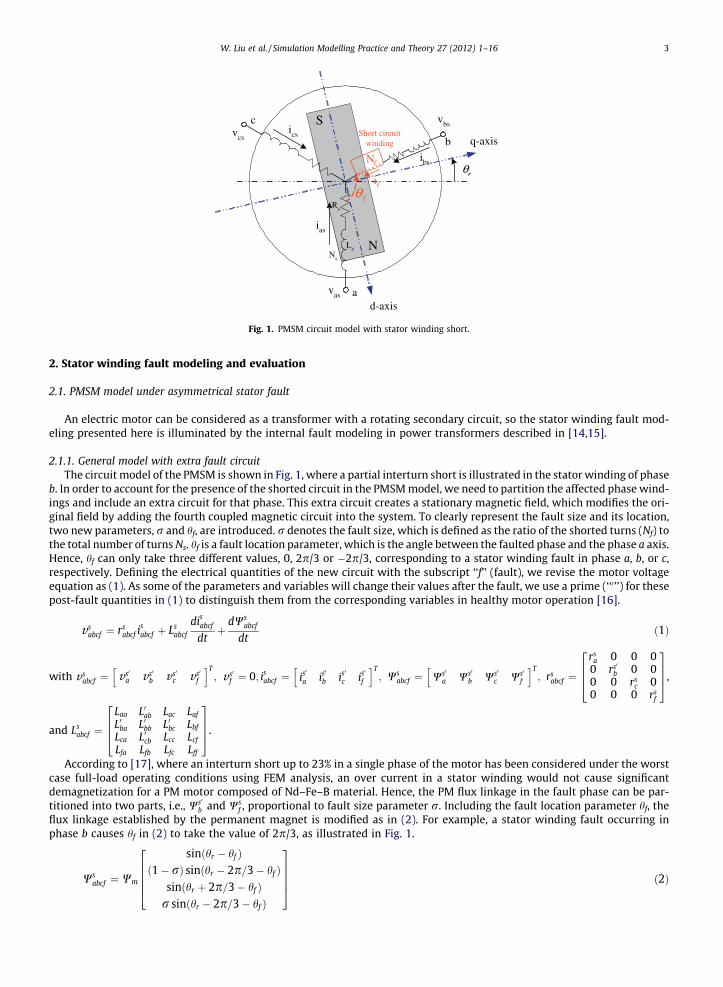
Fig. 1. PMSM circuit model with stator winding short.

W. Liu et al. / Simulation Modelling Practice and Theory 27 (2012) 1–16 3

2. Stator winding fault modeling and evaluation

2.1. PMSM model under asymmetrical stator fault

An electric motor can be considered as a transformer with a rotating secondary circuit, so the stator winding fault mod-eling presented here is illuminated by the internal fault modeling in power transformers described in [14,15].

2.1.1. General model with extra fault circuitThe circuit model of the PMSM is shown in Fig. 1, where a partial interturn short is illustrated in the stator winding of phase

b. In order to account for the presence of the shorted circuit in the PMSM model, we need to partition the affected phase wind-ings and include an extra circuit for that phase. This extra circuit creates a stationary magnetic field, which modifies the ori-ginal field by adding the fourth coupled magnetic circuit into the system. To clearly represent the fault size and its location,two new parameters, r and hf, are introduced. r denotes the fault size, which is defined as the ratio of the shorted turns (Nf) tothe total number of turns Ns. hf is a fault location parameter, which is the angle between the faulted phase and the phase a axis.Hence, hf can only take three different values, 0, 2p/3 or �2p/3, corresponding to a stator winding fault in phase a, b, or c,respectively. Defining the electrical quantities of the new circuit with the subscript ‘‘f’’ (fault), we revise the motor voltageequation as (1). As some of the parameters and variables will change their values after the fault, we use a prime (‘‘0’’) for thesepost-fault quantities in (1) to distinguish them from the corresponding variables in healthy motor operation [16].

vsabcf ¼ rs

abcf isabcf þ Ls

abcf

disabcf

dtþ

dWsabcf

dtð1Þ

with v sabcf ¼ v s0

a v s0b v s0

c vs0f

h iT; v s0

f ¼ 0; isabcf ¼ is0

a is0

b is0

c is0

f

h iT; Ws

abcf ¼ Ws0

a Ws0

b Ws0

c Ws0

f

h iT; rs

abcf ¼

rsa 0 0 0

0 rs0b 0 0

0 0 rsc 0

0 0 0 rsf

2664

3775,

and Lsabcf ¼

Laa L0ab Lac Laf

L0ba L0bb L0bc Lbf

Lca L0cb Lcc Lcf

Lfa Lfb Lfc Lff

2664

3775.

According to [17], where an interturn short up to 23% in a single phase of the motor has been considered under the worstcase full-load operating conditions using FEM analysis, an over current in a stator winding would not cause significantdemagnetization for a PM motor composed of Nd–Fe–B material. Hence, the PM flux linkage in the fault phase can be par-titioned into two parts, i.e., Ws0

b and Wsf , proportional to fault size parameter r. Including the fault location parameter hf, the

flux linkage established by the permanent magnet is modified as in (2). For example, a stator winding fault occurring inphase b causes hf in (2) to take the value of 2p/3, as illustrated in Fig. 1.

Wsabcf ¼ Wm

sinðhr � hf Þð1� rÞ sinðhr � 2p=3� hf Þ

sinðhr þ 2p=3� hf Þr sinðhr � 2p=3� hf Þ

26664

37775 ð2Þ

4 W. Liu et al. / Simulation Modelling Practice and Theory 27 (2012) 1–16

2.1.2. Calculation of new model parametersThe basic problem of fault modeling is how to calculate the new parameters of the PMSM, i.e., the new resistances and

inductances, which are now 4 � 4 matrices. For the resistances, a simple proportional property of the windings can be used.For instance, the shortening of Nf turns in phase b winding yields:

rs0b ¼ ð1� rÞrs; rs

f ¼ rrs with r ¼ Nf

Nsð3Þ

where rs is the phase resistance of the stator winding under healthy operating conditions.The key problem now is the calculation of the magnetic system inductance, Ls, composed of the self and mutual induc-

tances between the shorted portion of the fault winding and the other healthy portions. Several studies have discussed thisproblem, e.g., [14–16]. Bastard proposed a method for transformer fault studies in [15], which involves only a few assump-tions and provides good accuracy while maintaining the method’s mathematical simplicity. The principles of consistency,leakage and proportionality therein are applicable to the PMSM.

The consistency principle ensures that the new inductance matrix has no conflicts with the fault free case model. It guar-antees that when using the 4 � 4 inductance matrix for the fault free case simulation, we can obtain the same result as whenusing the 3 � 3 matrix. The leakage principle takes into account the physical winding properties and usually is representedby a small positive constant defined as the leakage factor. This factor is important because it is directly related to the currentdeveloped in the faulted circuit winding. It is treated as a parameter in this work. The principle of proportionality is em-ployed to describe the inductances’ fundamental relation to the number of turns in a coil. It is known that the self-induc-tances of windings are proportional to the square of the number of turns. In our stator winding fault study, theproportionality principle expresses an approximate relationship between the two parts of the partitioned winding. It isstrictly true only if the leakage is zero. However, it is a good approximation because the leakage is quite close to zero.

By applying the principles described above, we can derive the new inductance matrix during the stator winding interturnshort. First, we consider the elements related to the faulted phase windings, L0bb; Lff , and Lbf. According to [15], the three prin-ciples are as follows:

� Consistency:

L0bb þ 2Lbf þ Lff ¼ Lbb ð4Þ

� Leakage:

dbf ¼ 1�L2

bf

L0bbLffð5Þ

� Proportionality:

L0bb

Lbf¼ 1� r

r

� �2

ð6Þ

Therefore, the equations for inductances L0bb; Lff , and Lbf are obtained as:

L0bb ¼ ðLs þ LmÞ1

r1�r

� �2 þ 2 r1�r

ffiffiffiffiffiffiffiffiffiffiffiffiffiffiffi1� dbf

pþ 1

ð7Þ

Lff ¼ ðLs þ LmÞ1

1�rr

� �2 þ 2 1�rr

ffiffiffiffiffiffiffiffiffiffiffiffiffiffiffi1� dbf

pþ 1

ð8Þ

Lbf ¼ ðLs þ LmÞffiffiffiffiffiffiffiffiffiffiffiffiffiffiffi1� dbf

p1�rr þ r

1�rþ 2ffiffiffiffiffiffiffiffiffiffiffiffiffiffiffi1� dbf

p ð9Þ

where Ls is the self inductance, and Lm is the mutual inductance of stator windings under healthy conditions.For the mutual inductances between the faulted phase winding and the other phase windings, the consistency principle

states that:

L0bx þ Lfx ¼ Lbx; where x ¼ a; c ð10Þ

Together with the proportionality equation, we can obtain the elements L0ba; L0bc; Lfa, and Lfc:

L0ba ¼ L0bc ¼ �12ð1� rÞLm ð11Þ

Lfa ¼ Lfc ¼ �12rLm ð12Þ

The other elements in Lsabcf are either symmetrical to (9), (11) and (12), or maintain their original values. The entire 4 � 4

post-fault inductance matrix is now expressed as in (13).

PWM Inverter

PI

PI

PI

dq

abc

∑ ∑

∑

*rω

rω-

rdi

*rdi

rqi

*rqi

*rqv

*rdv

rθ

aibi

ci

-

-

Encoder

PMSM

Fig. 2. Simulation setup for PMSM fault model validation.

Table 1PMSM parameters.

PMSM parameters Nominal values (unit)

Pole pairs np 1Stator resistance rs 1.4 (X)q-axis inductance Lq 7.3 (mH)d-axis inductance Ld 7.3 (mH)PM flux linkage wm 0.1546 (Wb-turn)Frictional coefficient Bm 0.001 (N m/rad/s)Moment of inertia J 0.006 (kg m2)

Table 2Parameters of controllers.

Controllers Parameters

Kp Ki

Speed controller 2 0.001Current controller (d-axis) 20 5Current controller (q-axis) 20 5

0 0.03 0.05 0.07 0.1 0.13 0.15 0.17 0.2370

375

380

Time (s)

Pow

er o

utpu

t (M

W)

Proposed model

Conventional dq-model

Fig. 3. Simulation of healthy PMSM: rotor speed.

W. Liu et al. / Simulation Modelling Practice and Theory 27 (2012) 1–16 5

Lsabcf ¼

Ls þ Lm � 12 ð1� rÞLm . . . � 1

2 ð1� rÞLm � 12 rLm

� 12 ð1� rÞLm ðLs þ LmÞ 1

r1�rð Þ

2þ2 r

1�r

ffiffiffiffiffiffiffiffiffi1�dbf

pþ1

. . . � 12 ð1� rÞLm ðLs þ LmÞ

ffiffiffiffiffiffiffiffiffi1�dbf

p1�rr þ r

1�rþ2ffiffiffiffiffiffiffiffiffi1�dbf

p

� 12 ð1� rÞLm � 1

2 ð1� rÞLm . . . Ls þ Lm � 12 rLm

� 12 rLm ðLs þ LmÞ

ffiffiffiffiffiffiffiffiffi1�dbf

p1�rr þ r

1�rþ2ffiffiffiffiffiffiffiffiffi1�dbf

p . . . � 12 rLm ðLs þ LmÞ 1

1�rrð Þ2þ21�r

rffiffiffiffiffiffiffiffiffi1�dbf

pþ1

2666666664

3777777775

ð13Þ

Once the new motor parameters are calculated, we can obtain the PMSM dynamic response during the asymmetricalinterturn winding fault by solving (1) together with the mechanical model.

Under healthy conditions, r and hf are both zero. By substituting r = 0 and hf = 0 to the fault model, the fault model willbecome identical to the classical PMSM model, as seen in the following analysis.

0 0.02 0.05 0.08 0.1 0.12 0.14 0.16 0.18 0.20

0.2

0.4

0.6

0.8

1

Time (sec)

Tor

que

(N.m

)

Proposed modelConventional d-q model

Fig. 4. Simulation of healthy PMSM: electromagnetic torque.

0 0.02 0.04 0.06 0.08 0.1 0.12 0.14 0.16 0.18 0.2-5-4-3-2-1012345

Time (s)

Tor

que

(N.m

)

Ib If

Fig. 5. Simulation of healthy PMSM: currents in the partitioned phase b.

6 W. Liu et al. / Simulation Modelling Practice and Theory 27 (2012) 1–16

By substituting r = 0 and hf = 0 to (2), Ws0

b and Ws0

f become Wm sin(hr � 2p/3) and 0, respectively, which means

Wsabcf ¼ Ws

a Wsb Ws

c 0� �T . According to (3), rs0

b ¼ rsb and rs

f ¼ 0, which makes rsabcf ¼

rsa 0 0 0

0 rsb 0 0

0 0 rsc 0

0 0 0 0

2664

3775. Similarly, it is easy

to verify that Lsabcf ¼

Laa Lab Lac 0Lba Lbb Lbc 0Lca Lcb Lcc 00 0 0 0

2664

3775. According to the proposed model, the shorted-turns voltage component vs0

f is zero,

and solving (1) yields isf ¼ 0. Thus, the state variables v s

abcf and isabcf in the fault model in (1) will become

v sabcf ¼ vs

a v sb v s

c 0� �T and is

abcf ¼ isa is

b isc 0

� �T , respectively. By substituting the updated values of rsabcf , Ls

abcf , and

Wsabcf into the fault model and neglecting the fault components, the fault model will become:

vsabc ¼ rs

abcisabc þ Ls

abcdis

abc

dtþ dWs

abc

dtð14Þ

where v sabc ¼ v s

a v sb v s

c

� �T; is

abc ¼ isa is

b isc

� �T; Ws

abc ¼ Wsa Ws

b Wsc

� �T; rs

abc ¼rs

a 0 00 rs

a 00 0 rs

c

24

35 and Lsabc ¼

Laa Lab Lac

Lba Lbb Lbc

Lca Lcb Lcc

24

35:

Eq. (14) represents the classical PMSM model under healthy operating conditions, which can be found in many textbooksand related papers, such as [18]. The good agreement between the two modeling approaches indicates that the classicalPMSM model under healthy operating conditions is a special case of the proposed fault model when r = 0 and hf = 0. Thiscan also be observed from the following simulation studies under healthy conditions. Utilizing a universal PMSM modelfor both healthy and fault conditions allows us to simulate continuous transitions between healthy and faulty scenarios. Thisis very important for the design and testing of any fault diagnosis solution.

0 0.02 0.05 0.08 0.1 0.12 0.14 0.16 0.18 0.2-6

-4

-2

0

2

4

6

Time (s)

Cur

rent

(A

)

Ia Ib Ic

Fig. 6. Simulation of healthy PMSM: three-phase currents.

0 0.02 0.05 0.08 0.1 0.12 0.14 0.16 0.18 0.2370

375

380

Time (s)

Pow

er o

utpu

t (M

W) With fault

Healthy

Fig. 7. Rotor speed response to a 5% interturn short in phase b windings at t = 0.05 s.

W. Liu et al. / Simulation Modelling Practice and Theory 27 (2012) 1–16 7

2.2. Simulation studies

A three-phase PMSM with non-salient poles, as shown in Fig. 2, is simulated in MATLAB� to demonstrate the modelingapproach presented in the previous section. The nominal parameters of the simulated PMSM are summarized in Table 1. Thesimulation is performed for motor operations in both a normal healthy status and an asymmetrical internal turn-to-turnshort in one of its phase windings. The parameters of PI controllers utilized in the simulation are provided in Table 2.

2.2.1. Simulation result of healthy PMSMDuring the study, the proposed fault model is compared against the classical PMSM model used in the SimPowerSystems

toolbox in MATLAB. In this way, the validity and compatibility of the new four-equation model under normal operating con-ditions can be verified. Figs. 3 and 4 compare the PMSM rotor’s electrical speed xr and electromagnetic torque Te. The curvesin both of the figures almost overlap with each other. Fig. 5 displays the currents in the two subsections of the partitionedphase winding. The current flowing in the shorted turns is zero under normal conditions, just as expected. Finally, the per-fectly balanced three-phase currents are shown in Fig. 6.

2.2.2. Simulation results for PMSM with interturn faultsIn this subsection, the simulation results are provided for PMSM operating with the asymmetrical turn-to-turn winding

fault. An internal winding turn-to-turn short of 5% of the entire winding is introduced into phase b at t = 0.05 s. A fault of thissize can represent any typical incipient stator winding fault caused by initial insulation breakdown. Industrial experiencestell us that such a fault should not impact the motor’s operation substantially. In other words, the general motor perfor-mances characterized by the rotor’s angular speed and electromagnetic torque output are maintained under this fault con-dition, aside from the appearance of some higher-order harmonics due to the winding asymmetry. These expected motorbehaviors are observed from the simulation results shown in Figs. 7 and 8. The rotor speed responses with healthy and faultystator windings are contrasted in Fig. 7. The slight decrease in the magnitudes of the rotor speed seems insignificant untilcloser inspection. Similarly, the electromagnetic torque output displayed in Fig. 8 also shows a small decrease in the averagevalue after the fault is introduced at t = 0.05 s. Extra harmonics caused by the fault are clearly observed in both xr and Te.Oscillations also appear in the torque output in Fig. 8. These phenomena actually represent typical symptoms for the PMSMoperating under such asymmetrical stator faults.

Given that PMSM’s overall performances are not impacted significantly under a small stator winding fault, we can predictthat the three-phase currents of the motor will not change dramatically, either. However, three-phase waveforms under faultoperation will become unbalanced due to the winding asymmetry. This asymmetry in currents then gives rise to the har-monics in motor speed and torque, as illustrated previously. The three-phase currents in the fault condition are shown inFig. 9. The unbalance is apparent. Changes are noticeable in the faulty phase with significant harmonics, whereas the changesare relatively small in the other two phases. Rather than the overall motor performance, this study focuses on the fault cur-rent developed in the shorted portion of the fault phase. As mentioned in the introduction, a large magnitude of this faultcurrent can cause the local temperature to increase and can accelerate the propagation of an incipient fault, which can leadto the failure of the entire phase if not detected. To demonstrate this risk, the currents in the faulty phase b are displayed inFig. 10. The two waveforms are the current developed in the shorted portion, if, and the one in the good portion, i0b, respec-tively. The fault current in the short windings has a much larger magnitude and flows in the direction opposite to the oneflowing through the healthy portion of phase b. This fault current actually creates a braking torque that counteracts the over-all electromagnetic torque output. It is the root cause of the decrease in the average net torque during fault operations of thistype. Similar phenomena are observed in [19]. The result is also comparable to the one presented in [20] for a PM machineworking in generating mode. Further investigations show that as the fault grows larger, the general torque output decreases,accompanied by the emergence of higher-order harmonics. This agrees well with the results presented in [19]. The symptomcan be used for fault diagnosis in cases in which the motor’s torque can be measured accurately.

An observation of the stator winding fault model reveals that the fault parameters to identify (r and hf) are distributedover Eqs. (2) and (13). Due to the complexity of the nonlinear model, no classic diagnosis/identification method can be ap-plied. Thus, in the following section, the identification problem is transformed into an optimization problem and then solvedwith an intelligent optimization algorithm–particle swarm optimization (PSO).

0 0.02 0.05 0.08 0.1 0.12 0.14 0.16 0.18 0.20

0.2

0.4

0.6

0.8

1

Time (sec)

Tor

que

(N.m

)

with fault healthy

Fig. 8. Electromagnetic torque response to a 5% interturn short in phase b windings.

0 0.02 0.05 0.08 0.1 0.12 0.14 0.16 0.18 0.2

-6-4-20246

Time (s)

Pow

er o

utpu

t (M

W) Ia Ib Ic

Fig. 9. Three-phase current responses to a 5% interturn short in phase b windings.

0 0.02 0.05 0.08 0.1 0.12 0.14 0.16 0.18 0.2-50-40-30-20-10

01020304050

Time (s)

Cur

rent

(A

)

IfIb

Fig. 10. Faulted phase current responses to a 5% interturn short in phase b windings.

8 W. Liu et al. / Simulation Modelling Practice and Theory 27 (2012) 1–16

3. PSO-based parameter identification

3.1. Particle swarm optimization

Particle swarm optimization (PSO) is a population-based stochastic search algorithm first introduced by Kennedy andEberhart in 1995 [21]. Since then, it has been widely used to solve a broad range of optimization problems. The algorithmwas presented as simulating animals’ social activities, e.g., insects and birds. It attempts to mimic the natural process ofgroup communication to share individual knowledge when such swarms flock, migrate, or hunt. If one member sees a desir-able path to follow, the rest of this swarm will follow quickly [22,23]. In PSO, such animals behavior is imitated by particleswith certain positions and velocities in a searching space, wherein the population is called a swarm, and each member of theswarm is called a particle. Starting with a randomly initialized population, each particle in PSO flies through the searchingspace and remembers the best position it has seen. Members of a swarm communicate good positions to each other anddynamically adjust their own position and velocity based on these good positions. The velocity adjustment is based uponthe historical behaviors of the particles themselves as well as their neighbors. In this way, the particles tend to fly towardsbetter and better searching areas over the searching process [21]. The searching procedure based on this concept can be de-scribed by the following equation:

v i ¼ w � v i þ c1 � rand1 � ðxp � xiÞ þ c2 � rand2 � ðxg � xiÞxi ¼ xi þ v i

ð15Þ

where w, c1, and c2 are the inertia weight, cognitive acceleration and social acceleration constants, respectively; rand1 andrand2 are two random numbers; xi represents the location of the ith particle; xp represents the best solution (fitness) the par-ticle has achieved so far (pbest); xg represents the overall best location obtained so far by all particles in the population(gbest); and vi represents the velocity of the particle with vmin

i 6 v i 6 vmaxi .

Performance evaluator

System

PSO based identifier

System input u

System model

ˆ( )C p

Measured output y

yCalculated output

Identified parameter p

Fig. 11. Block diagram of the PSO-based identification approach.

W. Liu et al. / Simulation Modelling Practice and Theory 27 (2012) 1–16 9

vmaxi determines the resolution, or fitness, with which regions between the present position and target position are

searched. The constants c1 and c2 represent the weighting of the stochastic acceleration terms that pull each particle towardpbest and gbest positions. According to past experience, vmax

i often is set at 10–20% of the dynamic range of the variable oneach dimension, and w, c1, and c2 often are set to 0.8, 2, and 2.

The updating rules and flow charts that can be found in many PSO-related papers suggest that PSO is very simple in con-cept and easy in realization. Thus, PSO has gained popularity in recent years. Its development and applications in power sys-tems are presented in [24–26].

3.2. PSO-based parameter identification

The block diagram of the PSO-based parameter identification approach is illustrated in Fig. 11.First, the system response under input u is measured for identification. Then, the system model with tentative parameters

ðpÞ is simulated under the same initial condition and inputs as the system. The outputs of the simulated model ðyÞ and mea-surement (y) of the system are input to a performance evaluator for comparison. The performance evaluator calculates thefitness CðpÞ of the tentative solution according to a cost/fitness function. The commonly used cost function can be defined asa weighted quadratic function as in [5,6]. Once all of the candidate solutions (particles) have been evaluated, the PSO-basedidentifier can update candidate solutions according to the updating rules to provide a better set of candidate solutions. Thenew candidate solutions with updated p will be used to update the system model for the next iteration of optimization untila preset number of iterations has been accomplished or the preset maximum allowable cost/fitness CðpÞ has been met. Moredetails on the above identification process can be found in related literature, such as [27,28].

4. PSO-based real-time fault detection

4.1. Faster than real-time simulation

The requirements for or definition of ‘‘real-time’’ is different for different applications. In this paper, the objective is toachieve good identification within the time allotted for measuring system outputs. For example, if 1000 samples are mea-sured at a sample time of 10�4 s, meaning that it takes 0.1 s to measure the dataset of 1000 samples, then the PSO-basedalgorithm is required to identify system parameters within 0.1 s.

According to Section 2, PSO usually needs a number of iterations to identify parameters according to a measured dataset.For each iteration, the system model must be simulated once for each candidate solution. If there are n particles, which trans-lates to n candidate solutions, the system model must be simulated n times for each iteration. Even if all the particles can besimulated in parallel, the optimization must be conducted iteration after iteration. Thus, the major problem for real-timeimplementation is to complete the predefined number of simulations in a limited time. To realize the ‘‘real-time’’ objectivedescribed above, faster than real-time simulation is necessary. Instead of using hardware with powerful computing capabil-ities, the simulation time can be minimized by modifying the original system model. This idea can be illustrated using thefollowing equations:

_X1 ¼ FðX1Þ þ GðX1;U1Þ ð16Þ_X2 ¼ n � ½FðX2Þ þ GðX2;U2Þ� ð17Þ

Eq. (16) describes the dynamics of the original system, and (17) describes the modified system. In (17), n is a positivenumber that is larger than 1, and the definitions of F(�) and G(�) in (16) and (17) are the same. Because the time constantof (17) is 1/n that of (16), the system response of (17) is n times faster than (16). Given the same initial conditions and ntimes faster input, (17) can provide n times faster response than (16). If both systems are running in real-time and the sim-ulated system (17) is measured n times faster, only 1/n of the original measurement time is needed to obtain the same set ofsamples.

1 1

10 10

1 seconds

x x

x

t

2 2

20

10

10

0.1 seconds

x x

x

t

System 1:

System 2:

0 2 4 6 8 100

5

10

time in seconds

x1

0 0.2 0.4 0.6 0.8 10

5

10

time in seconds

x2

Fig. 12. Comparison of system response with different time constants.

10 W. Liu et al. / Simulation Modelling Practice and Theory 27 (2012) 1–16

The idea can be illustrated using a practical example, as shown in Fig. 12. The only difference between the two systems isthe time constants. The time constant of System 2 is 10 times smaller, so System 2 responds 10 times faster than System 1.To obtain the same number of samples for System 1, System 2 only needs to be simulated for 0.1 s.

Now, consider another practical example illustrated in Fig. 13. If 1000 samples are measured from the original system at asample time of 10�4 s, it will take 0.1 s to obtain the 1000 samples. If we modify the system model by making it run 10 timesfaster and then measure the modified system at a sample time of 10�5 s, it will only take 0.01 s to obtain the 1000 samplesfor the modified system. Even though their time stamps are different, the quantities of the two sets of 1000 samples will bethe same. According to the PSO-based identification algorithm, five particles in a swarm can be simulated in parallel. Thus,we can finish almost 10 iterations within 0.1 s. Because it takes time to update the parameters according to the PSO algo-rithm, we choose to run the optimization for 5 times/iterations in our implementation. Doing so allows us to realize fasteridentification, which means that the interval for updating identified parameters (just slightly longer than 0.05 s if consider-ing the updating process of PSO) is less than the measurement time (0.1 s).

The above-mentioned examples assume that the modified system can be simulated in real-time. During implementation,the actual simulation time is determined primarily by the capability of the controller’s hardware and the complexity of themodel. If the modified model can be simulated in real-time or even faster, the PSO-based identification can be implementedwith no problem. In the following discussion, we will consider the situation in which the modified model cannot be simu-lated in real-time. What can we do if we have to overcome the problem by tuning the algorithm rather than upgrading thecontroller hardware?

In such situations, the following two methods can be adopted, one after another. The first method is to decrease the sam-pling frequency, the number of samples, and the number of iterations. If this method works, there will be no impact on theperformance or the ‘‘real-time’’ objective. If the first method does not work, the second method can be employed. The secondmethod is to decrease n, which will always achieve success. However, the performance expectation must be lowered. De-tailed analyses are provided below.

MeasurementTime:

SimulationTime:

Time in second

5 particles

0 0.05 0.1 0.15 0.2

5 iterations 5 iterations 5 iterations

Identifiedparameterst [0, 0.1]∈

Identifiedparameters

t [0.05, 0.15]∈

Identifiedparameterst [0.1, 0.2]∈

Fig. 13. Running of the PSO-based identification algorithm.

PCdSPACEController

Code download

Data AcquisitionA/D D/A RTDS

Fig. 14. Block diagram of real-time hardware-in-the-loop simulation.

W. Liu et al. / Simulation Modelling Practice and Theory 27 (2012) 1–16 11

By decreasing the sampling frequency, the simulation can be focused on less fixed data points. In this way, the compu-tational burden on the controller hardware and I/O module can be alleviated. However, according to the Shannon samplingtheorem, if the sample time is too extended, the measurement will miss some important details in measurement. If decreas-ing the sampling frequency results in some identification errors, the minimum working sampling frequency should be main-tained, and other methods should be tried. The second method is to use fewer samples, which means simulating the systemfor a shorter period of time. As mentioned previously, the PSO-based identification algorithm has different requirements fordifferent parameters. If the samples are not enough to demonstrate sufficient difference, identification will prove very dif-ficult. Again, if using fewer samples does not work, the last method can be attempted, which is to reduce the number of iter-ations for each measured dataset without impacting the real-time performance. Less iteration means more simulation timefor each iteration, provided that the total time for identification is fixed. In this way, a more complicated simulation can berealized. However, PSO may require several iterations to find a good solution. Thus, the method of decreasing the number ofiterations may not work for complex problems. In the worst case scenario, if all three of the previously-mentioned methodsfail, we have to resort to the last method, which is to decrease n.

Decreasing n will result in slower simulation, so the predefined number of iterations may not be finished within the timeallotted for measurement. To provide accurate identification, the predefined number of iterations must be maintained. Thus,the interval for updating identified parameters has to be increased. This will limit the applications to problems whoseparameters do not change significantly. This situation may be unavoidable and is constrained by the capabilities of the con-troller hardware. However, by adjusting n and the above-mentioned related parameters, we can achieve the best possibleperformance with the existing hardware controller. Regardless, this problem does not hinder the application of the proposedtechniques to systems whose parameters do not change rapidly. With the development of computer techniques, improvedhardware will extend the real-time implementation techniques to a wider range of applications. In addition to the above-mentioned possible problems, there are many other issues to be considered during implementation. For example, thePSO-generated solutions may destabilize the running of the model; thus, the program should be able to terminate unstablesimulations and re-generate new stable ones.

4.2. Details of real-time implementation

For real-time controller hardware-in-the-loop simulation, we choose to use the dSPACE� controller and Real-Time DigitalSimulator� (RTDS). The experimental setup is shown in Fig. 14.

The dSPACE controller enables us to implement our real-time PSO-based identification algorithms using Simulink�. TheSimulink code can be converted to C code with the Real-time Workshop (RTW). Thus, the time-consuming C programmingcan be avoided. The RTDS allows us to test our hardware controller in real-time and under customizable simulation environ-ments. Through controller hardware-in-the-loop simulation, the proposed algorithm can be fully tested, just as with exper-imental studies.

The basic idea behind the implementation is to use the same step size and sampling time for both measurement and sim-ulations. In this way, the identification interval (the time used to identify parameters form a measured dataset) is fully con-trolled. Because the modified model is supposed to simulate n times faster than the original system, the measurement mustbe down-sampled n times to match the simulated data, as illustrated in Fig. 15.

The block diagram of the PSO-based identification algorithm running in the dSPACE controller is shown in Fig. 15. In thefigure, five particles are used to identify parameters from measurements. The simulations of the five particles are conductedin parallel and synchronized by the flow control module. The difficulties of this implementation include reproducing themeasured control signal, synchronizing the simulations of the modified models, and implementing the PSO algorithms stepby step. Definitions of the modules are provided in Table 3.

The ‘‘Init’’ module initializes the identification algorithm before the ‘‘FC’’ takes over the flow control. The ‘‘Init’’ block hasthree outputs. The first output is the ‘‘enable’’ signal, which will enable the ‘‘FC’’ block after a preset delay. The delay is usedto restrain the identification algorithm from running during the start-up transient. The second output, ‘Trigger 0’, initializesparticles (P1–P5) before using them to simulate the modified models. The third output, ‘Trigger 1’, is the triggering signal,which can trigger the ‘‘HD’’ block once the very first m samples have been measured after the start-up transient.

The ‘‘FC’’ module ensures the desired operating sequence of the PSO-based identification algorithm. The only input signalcomes from the ‘‘Init’’ module. The ‘‘FC’’ module will be enabled once the initialization process is complete. The first output is‘index’, which is input to both the ‘‘Vec2Str’’ and ‘‘Str2Vec’’ modules. In this way, the outputs in response to the correspond-ing inputs can be measured. Among the 6 triggering signals, Trigger 2 is used to initialize the modified system model inMM1–5. Trigger 3 is used to trigger the ‘CalCost’ module after all simulated data have been measured. Triggers 4–6 are usedto ensure the correct PSO updating sequence. The triggering process of corresponding modules is repeated for a preset num-ber of iterations. After one measured dataset has been identified, the ‘‘FC’’ module will trigger the ‘‘HD’’ module with ‘trigger

A/D DS HD

Vec2StrMM1

P1

Str2Vec

UpdGb

UpdXV

UpdPb

FC

Init

OR

MM2 Str2Vec

CalCost

CalCostUpdPb

P2

P3

P4

P5

P1

P2

P3

P4

P5

Trigger 6

Trigger 7

EnableTrigger 0Trigger 1

downsample hold

vector to stream

index

Trigger 2

inputinitial condition

stream to vector

stream to vector

calculate cost

calculate cost

updatepeer best

updatepeer best

Trigger 5Trigger 4Trigger 3

updateglobal best

updatePSO

MM3

MM4

MM5

Str2Vec

Str2Vec

Str2Vec

CalCost

CalCost

CalCost

UpdPb

UpdPb

UpdPb

output

flow control

PSO based identification algorithm running in Hardware controller

DISP

display

OR

Global best

Fig. 15. Block diagram of the real-time PSO algorithm running in the dSPACE controller.

Table 3Functions of the modules in Fig. 15.

Name Function

Init Initialize simulation model before ‘‘FC’’ takes over the flow controlFC Control the flowing of data by generating triggering signalsDS Down-sample the measured data n timesHD Hold the output of DS (measured dataset) for identificationVec2Str Convert vector (measured dataset) to streams of control inputsMM1–5 Simulate the modified modelStr2Vec Save the outputs of MM1–5 (samples) to the vector for comparisonCalCost Evaluate particles by comparing measured and simulated datasetsUpdPb Update the peer best particlesUpdGb Update the global best particleUpdXV Update the position and velocity vectorsP1–5 Store particles in memory for read/write

12 W. Liu et al. / Simulation Modelling Practice and Theory 27 (2012) 1–16

7’ to hold a new set of measurements for identification. The data measured from RTDS is input to the ‘‘DS’’ block fordown-sampling. The measurement is down-sampled n times continuously, and only the most recent m down-sampled dataare recorded for future use. Once the ‘‘HD’’ block is triggered, the output of the down-sampling model is held fixed for iden-tification by the PSO algorithm. Besides holding the input and output vectors, the ‘‘HD’’ block also initiates the simulation of‘‘MM1–5’’ modules and provides measured data to the ‘‘CalCost’’ module for comparison with simulated data.

The ‘‘Vec2Str’’ module is used to reproduce the sampled control signals one after another based on the index receivedfrom the ‘‘FC’’ module. The control signal is then applied to ‘‘MM1–5.’’ The same index is also input to the ‘‘Str2Vec’’ block,which will record simulation results for evaluation. Because the ‘‘index’’ inputs of ‘‘Vec2Str’’ and ‘‘Str2Vec’’ are the same, themeasured and simulated data can be synchronized. Once all of the m samples have been obtained from all of the ‘‘MM1–5,’’the ‘‘FC’’ module will generate a triggering signal for the ‘‘CalCost’’ module. Then, the ‘‘CalCost’’ module will evaluate the par-ticles according to the defined cost function.

The ‘‘MM1–5’’ modules take four inputs. The first input signal is the initial condition provided by the ‘‘HD’’ module. Thesecond input consists of the control signals generated from the ‘‘Vec2Str’’ module. These two inputs are necessary to simu-late the same operating condition as the system. The third input is the reset signal (trigger 5 generated by ‘‘FC’’), which willinitialize the modified simulation model before a new round of simulation. Once triggered, all the internal states of the MMmodules will be set to the same initial condition. The fourth signal consists of the particles (parameters) to be evaluated. Theoutput of the ‘‘MM1–5’’ modules will be measured and compared with system measurements. During simulation, an attempt

0.15 0.2 0.25 0.3 0.35 0.4 0.45 0.5 0.55 0.6 0.650.08

0.1

0.12

0.14

0.16

0.18

0.2

0.22

Time in seconds

Stat

or re

sist

ance

Rs

(ohm

s)Fig. 16. Identification of the stator resistance Rs.

W. Liu et al. / Simulation Modelling Practice and Theory 27 (2012) 1–16 13

should be made to avoid the whole control system model in order to minimize simulation time. This can be achieved by sim-ulating only the smallest independent module in which inputs and internal states can be measured.

After all samples have been measured for ‘‘MM1–5’’, the ‘‘FC’’ block will trigger the ‘‘CalCost’’ block, which will calculatethe cost/fitness of the corresponding particle. Based on the cost/fitness, the peer best solutions and the global best solutionwill be updated in the ‘‘UpdPb’’ and ‘‘UpdGb’’ modules, respectively. After that, the ‘‘UpdXV’’ module will update particleinformation, and the above evaluation process will be repeated until the terminating conditions have been met.

The ‘‘global best’’ is updated periodically, and two sets of values can be displayed; one consists of the identified param-eters, and the other is the corresponding cost. By observing the cost, we can track the running of the PSO algorithm and eval-uate how good the identification is.

4.3. Simulation studies

The real-time PSO-based identification algorithm is used to identify PMSM parameters under both healthy and statorwinding fault conditions described using the developed fault model. In these tests, the parameters of the PMSM control sys-tem are the same as before.

Based on the output of the PMSM model, the cost function for evaluating the identification performance of the PSO algo-rithm is shown in (18).

Cost ¼Xm

k¼1

ðiaðkÞ � iaðkÞÞ2 þ ðibðkÞ � ibðkÞÞ2 þ ðicðkÞ � icðkÞÞ2 þwðxrðkÞ � xrðkÞÞ2h i

ð18Þ

In (18), the phase currents iabc and the rotor speed xr are the measurable system outputs, iabc and xr are the estimatedvalues of iabc and xr, respectively, which are calculated from the system model, Rs and TL are the unknown parameters to beidentified, n is the number of samples, and the weighting factor w is defined as w = jiabcj/jxrj.

4.3.1. Identification under healthy conditionsUsually, PMSM operates under various operating conditions, in which various disturbances and parameter variations are

unavoidable and unmeasurable. Often, datasheet parameters only provide a rough starting point for simulation or practicaldesign purposes. They are not accurate enough for the entire PMSM operational range. For instance, the PMSM stator resis-tance, Rs, is directly related to the motor’s operating temperature. Its value tends to fluctuate up to twice its nominal value.Accurate knowledge of these parameters is important to control system performance. Therefore, it is valuable to investigatean efficient approach to achieve precise parameter identification. In this test, the PSO-based algorithm is used to identify thestator resistance Rs and load torque TL.

Figs. 16 and 17 show the identification of time-varying parameters, indicating that the proposed technique can identifytime-varying parameters successfully.

Fig. 18 shows the entire optimization process of the PSO algorithm. For each run of the PSO-based algorithm, the previ-ously optimized parameters are used as the initial value. Thus, the identification process for online applications tends to con-verge faster in that it has fewer iterations. This is especially true for systems with slowly time-varying parameters. Fig. 18indicates that the algorithm usually converges within five iterations because of a good initial guess. However, the figure alsoshows that the initial fitness for runs 5, 6, 7, and 8 are not as good as the others. This is because the sensitivity of the fitness toparameter changes is different at different operating points. Sometimes, even a small change in the parameters will result ina large change in the fitness.

4.3.2. Identification of fault parametersAs mentioned previously, the two parameters d and hf, which represent the ratio of shorted turns to total turns, and the

angle between the faulted phase and the phase a axis, respectively, are directly related to the fault severity and location.Thus, the objective of the stator winding fault diagnosis is to identify these two parameters.

0.15 0.2 0.25 0.3 0.35 0.4 0.45 0.5 0.55 0.6 0.652.8

2.85

2.9

2.95

3

3.05

3.1

3.15

Time in seconds

Torq

ue T

Ld (N

.m)

Fig. 17. Identification of the load torque TL.

0 10 20 30 40 50 60 70 80 90 1000

10

20

30

40

50

60

Number of iterations

Fitn

ess

Fig. 18. Optimization process of the PSO-based identification algorithm.

0.25 0.3 0.35 0.4 0.45-10

-5

0

5

10

Time (sec)

Phas

e cu

rrent

s (A

) ia ib icFault

Fig. 19. PMSM phase current under a 4.5% stator fault in phase b.

0 5 10 15 20 25 30

-2pi/3 (c)

0 (a)

2pi/3 (b)

Generation

Faul

t Loc

atio

n (ra

d)

Fig. 20. Fault location estimation during a 4.5% stator fault in phase b.

14 W. Liu et al. / Simulation Modelling Practice and Theory 27 (2012) 1–16

In our problem, hf can only take three different values, �2p/3, 0, or 2p/3. Therefore, a modification to the standard PSOalgorithm is necessary. First, during the initialization process, the values corresponding to hf are randomly set to one of thethree values. Second, during the calculation of its updated position, the new position particle is calculated based on the up-dated velocity particle, which is a continuous variable. This updated position particle is then rounded to its nearest feasiblevalue (�2p/3, 0, or 2p/3). Thus, the updating equations for this mixed variable optimization problem are consistent with (15)given some special treatment to the discrete variables, as just described.

During simulation, a 4.5% turn-to-turn fault is applied to stator phase b winding at 0.3 s. The fault of this magnituderepresents a typical incipient fault. If the proposed approach can successfully identify this small fault, then the approachcan certainly identify larger faults. The responses of the phase currents are displayed in Fig. 19. The original balanced

0 5 10 15 20 25 304.4

4.45

4.5

4.55

4.6

4.65

Generation

Faul

t siz

e (%

)

Fig. 21. Fault severity estimation during a 4.5% stator fault in phase b.

W. Liu et al. / Simulation Modelling Practice and Theory 27 (2012) 1–16 15

three-phase current becomes slightly unbalanced after the fault. Figs. 20 and 21 show a typical optimization process of thePSO-based fault diagnosis approach. Simulation studies show that the optimization process always converges within 25 iter-ations. Fig. 20 indicates that the estimation of hf converges to the ideal value even at the first iteration. This is because themodel with the ideal value provides much better fitness than models with the other two values. Thus, the best solution of hf

can always be found during the evaluation of the initial population.In this paper, the load is modeled as a constant torque of 0.6 N m. For a larger load, a larger excitation current is needed.

Accordingly, the fault current will become larger. However, due to the complexity of the model, it is difficult to develop anequation to analyze the impact of the loading condition on fault severity. This would be a worthwhile topic for future re-search. Because the proposed fault detection algorithm is independent of the loading condition, it can always identify thetwo fault parameters accurately.

5. Conclusion

To identify the stator winding fault for PMSM, this paper proposed a model that can describe both normal and fault con-ditions. The model has been verified by comparing the simulation results with observations in related literature. However,because there is no quantified comparison, it is difficult to evaluate the accuracy of the developed model. Further experimen-tal verification, if possible, is needed.

The fault detection problem can be approached by identifying the two parameters associated with fault location and faultseverity. Because of the complex distribution of these two parameters in the fault model, it is very difficult to design a non-linear identification algorithm. A real-time PSO-based identification algorithm is proposed to solve the detection/identifica-tion problem indirectly. Simulation studies on the developed model under both healthy and fault conditions demonstrate theperformance of the proposed algorithm. The implementation technique is hardware independent, and the real-time PSO-based identification algorithm also can be applied to many other types of identification problems.

References

[1] A.G. Jack, B.C. Mecrow, J.A. Haylock, A comparative study of permanent magnet and switched reluctance motors for high-performance fault-tolerantapplications, IEEE Trans. Ind. Appl. 32 (4) (1996) 889–895.

[2] O. Ojo, O. Osaloni, P. Kshirsagar, Models for the control and simulation of synchronous type machine drives under various fault conditions, in: 2002Conference Record Ind. Appl. Conference, 37th IAS Annual Meeting, vol. 3, pp. 1533–1540.

[3] P. Pillay, R. Krishnan, Modeling, simulation, and analysis of permanent-magnet motor drives. I. The permanent-magnet synchronous motor drive, IEEETrans. Ind. Appl. 25 (2) (1989) 265–273.

[4] P.F. Allbrecht, J.C. Appiarius, R.M. McCoy, et al, Assessment of the reliability of motors in utility applications – updated, IEEE Trans. Energy Convers. 1(1) (1986) 39–46.

[5] H.W. Penrose, Theory of Static Winding Circuit, BJM Corp, ALL-TEST Division, 2001.[6] J. Penman, H.G. Sedding, B.A. Lloyd, W.T. Fink, Detection and location of interturn short circuits in the stator windings of operating motors, IEEE Trans.

Energy Convers. 9 (4) (1994) 652–658.[7] M.A. Cash, T.G. Habetler, G.B. Kliman, Insulation failure prediction in AC machines using line-neutral voltages, IEEE Trans. Ind. Appl. 34 (6) (1998)

1234–1239.[8] J.A. Haylock, B.C. Mecrow, A. G Jack, D.J. Atkinson, Operation of fault tolerant machines with winding failures, IEEE Trans. Energy Convers. 14 (4) (1999)

1490–1495.[9] D. Muthumuni, P.G. McLaren, E. Dirks, V. Pathirana, A synchronous machine model to analyze internal faults, in: 2001 Conference Record Ind. Appl.

Conference, 36th IAS Annual Meeting, vol. 3, pp. 1595–1600.[10] S.M. Halpin, C.A. Gross, Time domain solutions for faulted power systems using detailed synchronous machine models, in: 22nd Southeastern

Symposium on System Theory, pp. 607–611, March 1990.[11] D.L. Brooks, S.M. Halpin, An improved fault analysis algorithm including detailed synchronous machine models and magnetic saturation, J. Electr.

Power Syst. Res. 42 (1) (1997) 3–9.[12] N. Bianchi, S. Bolognani, M. Zigliotto, High-performance PM synchronous motor drive for an electrical scooter, IEEE Trans. Ind. Appl. 37 (5) (2001)

1348–1355.[13] T.J. McCoy, Trends in Ship Electric Propulsion, IEEE Power Engineering Society Summer Meeting, July 2002.[14] M. Kezunovic, B. Kasztenny, A new ATP add-on for modeling internal faults in power transformers, in: 2000 Conference Record American Power

Conference, Chicago.[15] P. Bastard, P. Bertrand, M. Meunier, A transformer model for winding fault studies, IEEE Trans. Power Deliv. 9 (2) (1994) 690–699.[16] P.P. Reichmeider, C.A. Gross, D. Querrey, D. Novosel, S. Salon, Internal faults in synchronous machines. I. The machine model, IEEE Trans. Energy

Convers. 15 (4) (2000) 376–379.

16 W. Liu et al. / Simulation Modelling Practice and Theory 27 (2012) 1–16

[17] M. Dai, A. Keyhani, T. Sebastian, Fault analysis of a PM brushless DC motor using finite element method, IEEE Trans. Energy Convers. 20 (1) (2005) 1–6.[18] A.B. Dehkordi, A.M. Gole, T.L. Maguire, Permanent magnet synchronous machine model for real-time simulation, in: Proc. Interracial Conf. Power

Systems Transients, Montreal, QC, Canada, June 2005.[19] M.A. Awadallah, M.M. Morcos, S. Gopalakrishnan, T.W. A Nehl, Neuro-fuzzy approach to automatic diagnosis and location of stator interturn faults in

CSI-fed PM brushless DC motors, IEEE Trans. Energy Convers. 20 (2) (2005) 253–259.[20] A.A. Awdallah, V. Devanneaux, J. Faucher, B. Dagues, A. Randria, Modelling of surface-mounted permanent magnet synchronous machines with stator

faults, in: 2004 IEEE Proc. 30th Annual Conference Industrial Electronics Society, IECON, vol. 3, pp. 3031–3036.[21] J. Kennedy, R. Eberhart, Particle swarm optimization, in: Proceedings of IEEE International Conference on Neural Networks, vol. 4, Perth, Australia,

1995, pp. 1942–1948.[22] Y. Shi, Particle Swarm Optimization, Feature Article, Electronic Data Systems, Inc., IEEE Neural Networks Society, February 2004.[23] J. Kennedy, R.C. Eberhart, Y. Shi, Swarm Intelligence, Morgan Kaufman Publishers, San Francisco, 2001.[24] H. Yoshida, K. Kawata, Y. Fukuyama, S. Takayama, Y. Nakanishi, A particle swarm optimization for reactive power and voltage control considering

voltage security assessment, IEEE Trans. Power Syst. 15 (4) (2001) 1232–1239.[25] A.P. Alves da Silva, P.J. Abrao, Applications of evolutionary computation in electric power systems, in: Proceedings of the 2002 Congress on

Evolutionary Computation (CEC), vol. 2, 12–17 May 2002, pp. 1057–1062.[26] Y. del Valle, G.K. Venayagamoorthy, S. Mohagheghi, J. Hernandez, R.G. Harley, Particle swarm optimization: basic concepts, variants and applications in

power systems, IEEE Trans. Evol. Computat. 12 (2) (2008) 171–195.[27] W. Liu, J. Sarangapani, G.K. Venayagamoorthy, L. Liu, D.C. Wunsch, M.L. Crow, D.A. Cartes, Decentralized neural network based excitation control of

large scale power systems, Int. J. Control Autom. Syst. 5 (5) (2007) 526–538.[28] L. Liu, W. Liu, D.A. Cartes, Particle swarm optimization based parameter identification applied to permanent magnetic synchronous machine, Eng. Appl.

Artif. Intell. 21 (7) (2008) 1092–1100.