
Condition Monitoring of Stator Windings with a Networked ...
125
Doctoral Thesis in Electrical Engineering Condition Monitoring of Stator Windings with a Networked Electric Drive GIOVANNI ZANUSO Stockholm, Sweden 2022 kth royal institute of technology
-
Upload
khangminh22 -
Category
Documents
-
view
1 -
download
0
Transcript of Condition Monitoring of Stator Windings with a Networked ...

Doctoral Thesis in Electrical Engineering
Condition Monitoring of Stator Windings with a Networked Electric DriveGIOVANNI ZANUSO
Stockholm, Sweden 2022
kth royal institute of technology

Condition Monitoring of Stator Windings with a Networked Electric DriveGIOVANNI ZANUSO
Doctoral Thesis in Electrical EngineeringKTH Royal Institute of TechnologyStockholm, Sweden 2022
Academic Dissertation which, with due permission of the KTH Royal Institute of Technology, is submitted for public defence for the Degree of Doctor of Philosophy on Friday the 3rd of June 2022, at 10:00 a.m. in Kollegiesalen, Brinellvägen 6, Stockholm.

© Giovanni Zanuso© Viktoria Fodor, Luca Peretti, Oskar Wallmark, Konstantina Bitsi, Hareesh Babu, Sathiya Lingam Senthil Kumar ISBN 978-91-8040-221-7TRITA-EECS-AVL-2022:31 Printed by: Universitetsservice US-AB, Sweden 2022

iii
Abstract
Electric drives are widely used in industry, where they are also part ofthe plant communication architecture. This architecture is challenged by theIndustry 4.0 initiative that aims to make the devices in industrial plants moreinterconnected and with additional functionalities. These changes heavilyaffect electric drives, and thus their future role in industrial networks shouldbe investigated.
The first part of this work analyzes two examples of additional functional-ities for electric drives from a network system perspective: condition monitor-ing and multi-drive systems. The suitability of the industrial communicationprotocols is evaluated for both application cases. Condition monitoring andmulti-drive systems are further analyzed considering EtherCAT and CAN net-works. A performance model is proposed to control multi-drive systems withEtherCAT, where condition monitoring data is also considered. The transmis-sion of bulk data originated by condition monitoring methods is consideredin the traditional industrial fieldbus CAN, and an extended schedulabilityanalysis is proposed.
The second part of this work deals with the implementation of conditionmonitoring algorithms for the stator winding insulation in electric machines.Initially, interturn short-circuit faults in induction motors are investigated.An analytical and a finite-element model are developed and experimentallyvalidated by means of a motor prototype with tapped windings, which canemulate the interturn faults. Fault detection methods based on the negative-sequence current and the rotor slot harmonics are analyzed both theoreticallyand experimentally. The stator winding insulation condition, including thegroundwall insulation, is also considered for condition monitoring utilizing theMHz-range oscillations in the stator currents after switching transitions. Suchoscillations depend on the parasitic capacitances of the stator winding, whichin turn relate to the insulation condition. In order to quantify the variations inthe current oscillations, and thus the insulation change, two metrics are pro-posed and analyzed. The variations of the insulation condition are emulatedby adding additional capacitors to the stator winding taps, and then inducedthrough an accelerated aging procedure applied to the whole motor. All theexperiments are conducted with a custom converter that can simultaneouslyperform the drive control algorithm, the interturn fault detection methods,the communication with external devices, and the MHz-range sampling.
This work shows that condition monitoring and multi-drive system controlcan be implemented in electric drives using existing industrial communicationprotocols, such as EtherCAT and CAN. This work proves that industrialconverters can perform online both the detection of interturn short-circuitfaults and the monitoring of the stator insulation.Keywords: Industry 4.0, condition monitoring, multi-drive systems, Ether-CAT, CAN, stator interturn faults, stator insulation, accelerated aging.


v
Sammanfattning
Elektriska drivsystem används överallt inom industrin och utgör därmeden mycket framträdande komponent i de industriella anläggningarnas kom-munikationssystem. De traditionella kommunikationssystemen utmanas idagav nya initiativ såsom Industry 4.0 vilka har som mål att göra de ingåendeenheterna ännu mer sammankopplade och dessutom med ytterligare funktio-nalitet. Dessa trender påverkar i hög grad även de elektriska drivsystemen,och därför bör deras framtida roll i de industriella nätverken undersökas.
Den första delen av detta arbete studerar två användningsområden somkan ses som exempel på den nya funktionalitet som kommer att implemen-teras hos de elektriska drivsystemen: tillståndsövervakning och multidrivsy-stem. För bägge områdena utvärderas hur väl olika kommunikationsprotokolllämpar sig för en industriell användning. För de bägge områdena tillståndsö-vervakning och multidrivsystem görs en djupare analys när EtherCAT- ochCAN-nätverk används. Baserat på analysen föreslås en prestandamodell föratt styra multidrivsystem med EtherCAT, där också tillståndsövervakningingår. Användning av tillståndsövervakning resulterar i stora mängder datavilket studeras vid en analys av den traditionella CAN-bussen, och en utökadschemaläggningsanalys föreslås.
Den andra delen av detta arbete handlar om implementering av algoritmerför tillståndsövervakning av statorlindningens isolering hos elektriska maski-ner. Inledningsvis undersöks kortslutning mellan varven i asynkronmotorer.Såväl en analytisk som en finitelement modell utvecklas och valideras experi-mentellt med hjälp av en maskinprototyp som har en lindning med flera uttagvarvid man kan emulera kortslutning mellan varven. Feldetekteringsmetoderbaserade på den negativa strömkomponenten samt rotorspårsövertoner ana-lyseras både teoretiskt och experimentellt. Tillståndet hos statorlindningensisolering, även med hänsyn till spårisoleringen, analyseras med hjälp av deoscillationer i megahertzområdet som uppstår efter att krafthalvledare harslagits till eller från. Dessa oscillationer beror på statorlindningens parasitis-ka kapacitanser, som i sin tur beror på lindningens isoleringstillstånd. För attkvantifiera de aktuella oscillationerna och därmed förändringarna i isolering-en, föreslås och analyseras två utvärderingsmått. Förändringen av lindningensisolering emuleras genom att lägga till kondensatorer till statorlindningens ut-tag och därefter utsätts hela maskinen för en accelererad åldringsprocedur.Samtliga experiment utförs med en anpassad omvandlare som samtidigt kanutföra själva motorstyrningen, feldetekteringen av isolationsfel mellan varven,kommunikationen med externa enheter och samplingen i megahertzområdet.
Denna avhandling har visat att tillståndsövervakning och styrning av mul-tidrivsystem kan implementeras för elektriska drivsystem med hjälp av befint-liga industriella kommunikationsprotokoll, såsom EtherCAT och CAN. Arbe-tet har också visat att industriella omvandlare kan i realtid implementerabåde detektering av kortslutning mellan varven och övervakning av statornsisolering.Nyckelord: Industry 4.0, tillståndsövervakning, multidrivsystem, EtherCAT,CAN, statorlindningens isolering, accelererad åldringsprocedur.

Acknowledgements
This thesis concludes the research work I performed during my PhD project atthe Division of Electric Power and Energy Systems at KTH Royal Institute ofTechnology. This PhD project has been partially funded by Vinnova’s “Smartareelektroniksystem” strategic innovation program and the Swedish ElectromobilityCenter (SEC). I thank Vinnova and SEC for their financial support. I would alsolike to thank the E. C. Ericson and Malmes foundations for generously granting mescholarships, which allowed me to attend scientific conferences and courses.
During my PhD studies, I have been supervised by Professors Viktoria Fodor,Luca Peretti, and Oskar Wallmark. I would like to express my gratitude for thefreedom they offered me to drive my research and for their valuable guidance, inspi-ration, encouragement, and support. Notably, Viktoria helped me get acquaintedwith the networking field and was an excellent leader for the collaboration projects.I want to thank my mentor Luca Peretti for his guidance during the PhD periodand also for all these years we have been working together. In the first part of myPhD I received great help from the late Prof. Oskar Wallmark. I will never forgetOskar for the great person he was. I would also like to thank Mats Leksell forthe help in the former Electrical Machines and Drives team and to express specialgratitude to Prof. Nathaniel Taylor for his dedicated internal review.
In a PhD project lasting more than 5 years, I had the opportunity to collab-orate with numerous companies and people who contributed to the results of thiswork. I would like to thank Sam Al-Attiyah, Oscar Sverud, and Erik Tengedal ofImagimob, Christian Sahlin of LumenRadio, Ming Zeng of KTH, Sjoerd Bosga andDmitry Svechkarenko of ABB. Special thanks to Jörgen Engrström for his collab-oration and for allowing me to take measurements at the Scania Technical Centre,and to Åke Nyström and BEVI for providing me with the induction motor proto-types. I thank my former supervisor Prof. Mauro Zigliotto, and Dario Pasqualottoof the University of Padua for the collaboration and inspiring talks we had. Thanksalso to my brother Giacomo for the many insights about the diagnostics of electricmachines. The experiments detailed in this work were performed at the Sustain-able Power Laboratory at KTH. I thank Jesper Freiberg, Nicholas Honeth, PatrickJanus, Jelena Berg, and Janne Nilsson for their valuable help regarding the exper-imental setup. For making the lab work more fun, I would like to thank StefanBošnjak. I would also like to thank Elvan Helander, Peter Lönn, Eleni Nylén, and
vii

viii
Brigitt Högberg for their help throughout my time at KTH.An outstanding contribution to this work came from the M.Sc. students I su-
pervised at KTH. I will always be grateful to Sathiya, Hareesh, and Francesco, whodid their M.Sc thesis under my supervision, to Bhanu, Guilherme, Gokul, Akanshu,and Luigi, who completed their individual projects with me, and to Andrea, Diego,and Marco, whom I co-supervised.
By spending most of my PhD study time at KTH, I had the opportunity andprivilege to meet, collaborate, and share moments with many remarkable people.I thank my office mate Konstantina for all the talks and support. Thank youDanilo for the endless discussions and jokes. Thanks to the Kungshamra gang’smembers Stefan, Priyanka, Danilo, Konstantina, my Power Systems friends Fabi,Tin, Dimitris, and my Ottoman friends Baris and Evan for all the fun together andfor supporting each other, especially during the hard pandemic period. Thanksalso to Panos for all the moments and laughter we had during our commuting fromVästerås. I would like to thank Martin, Gustaf, Yixuan, An, and Omer for allthe nice times and for the work done together, and Angel, Mehrdad, and Mohsenfor all the talks and fikas. I would like to thank also all the former and presentcolleagues who made KTH a welcoming place: Jonas, Christian, Reed, Ilka, Rúdi,Hui, Yanmei, Matthijs, Keijo, Luca, Tim, Stefanie, Marina, Mojgan, Daniel, Erik,Juan, Lars, Dina, Alessandro, Anton, and many more!
My life in Sweden was made enjoyable by many friends. Thanks to the nowlong-time friends Peppe, Michele, Alessio, and the Stockholmare Nico, Paola, Irena,Adriano, Alessandro, Laura, Samer, Eirini, Luca, and Xueyan. Thanks also to allthe friends in Västerås Andrea, Elisabetta, Davide, Gaia, Fabio, Sara, Michele,Sofie, Marco, Elisa, Diana, Tomás, Araceli and to the many other friends in thatcity. I will never forget my amazing friends and former colleagues at ABB Minos,Meha, Damian, Paul, Pippo, Alessandro, Dani, Ana, Fernando, and Theo.
Whenever I go back to Italy, there is always someone who makes me feel at home.For this, I thank my long-time friends Michele, Gigi, Paolo, Moreno, Roberto,Luca, Matteo, Nicoló, Anita, Alessia, Elisabetta, Lisa, Alessia, Marta, and theirmany sons and daughters. A great thanks to Daria, Lisa, Staff, Cire, Giulia, Giangi,Michele, Federico, il Cimpe, ing. Matteo, young Giacomo, together with the “Acará”friends Valter, Elisa, Tiziano, Viola, and Marta, for all the amazing moments,inspiring discussions, and warmth, all over the years. I would also like to thank mycousins, uncles, and aunts for being an example.
Finally, I warmly thank the people close to my heart. Karila, I am lookingforward to continue the journey we just started. I have no words to express mygratitude to my parents, brothers, sister, and the whole big Family for their support,trust, and love. The last thought goes to Dimitri, Aliona, Eva, and to all the peoplein Ukraine. May better times will come for you all!
Stockholm, May 2022Giovanni Zanuso

ix
“If science teaches us anything,it teaches us to accept our failures,
as well as our successes,with quiet dignity and grace.” 1
1from the movie Young Frankenstein (1974)


Contents
Contents xi
Acronyms xv
1 Introduction 11.1 Background . . . . . . . . . . . . . . . . . . . . . . . . . . . . . . . . 11.2 Main objectives . . . . . . . . . . . . . . . . . . . . . . . . . . . . . . 21.3 Outline of the thesis . . . . . . . . . . . . . . . . . . . . . . . . . . . 31.4 Original contributions . . . . . . . . . . . . . . . . . . . . . . . . . . 41.5 List of appended papers . . . . . . . . . . . . . . . . . . . . . . . . . 51.6 List of related papers . . . . . . . . . . . . . . . . . . . . . . . . . . . 6
2 Networked electric drives in the Industry 4.0 72.1 Background . . . . . . . . . . . . . . . . . . . . . . . . . . . . . . . . 72.2 Electric drives in the industrial context . . . . . . . . . . . . . . . . 92.3 Industrial communication technologies . . . . . . . . . . . . . . . . . 122.4 Condition monitoring for electric drives . . . . . . . . . . . . . . . . 14
2.4.1 Condition monitoring with MCSA or similar methods . . . . 152.4.2 Condition monitoring based on current ringings . . . . . . . . 16
2.5 Multi-drive systems . . . . . . . . . . . . . . . . . . . . . . . . . . . . 172.5.1 Centralized control in a multi-drive system . . . . . . . . . . 182.5.2 Distributed control in a multi-drive system . . . . . . . . . . 19
2.6 Summary of chapter . . . . . . . . . . . . . . . . . . . . . . . . . . . 20
3 Application cases implemented in EtherCAT and CAN 213.1 Background . . . . . . . . . . . . . . . . . . . . . . . . . . . . . . . . 213.2 Multi-drive control and condition monitoring in EtherCAT . . . . . 22
3.2.1 Performance modeling of multi-drive control . . . . . . . . . . 233.2.2 Performance modeling of condition monitoring . . . . . . . . 25
3.3 Bulk data transfer in CAN for condition monitoring applications . . 263.3.1 Periodic control messages . . . . . . . . . . . . . . . . . . . . 273.3.2 Bulk data transmission . . . . . . . . . . . . . . . . . . . . . 293.3.3 Numerical example and results . . . . . . . . . . . . . . . . . 30
xi

xii CONTENTS
3.4 Summary of chapter . . . . . . . . . . . . . . . . . . . . . . . . . . . 32
4 Modeling of induction motors with inter-turn short circuit faults 334.1 Background . . . . . . . . . . . . . . . . . . . . . . . . . . . . . . . . 334.2 Analytical modeling . . . . . . . . . . . . . . . . . . . . . . . . . . . 36
4.2.1 Modeling assumptions for the faulted winding . . . . . . . . . 364.2.2 Generalized model in the natural reference frame . . . . . . . 374.2.3 Generalized model in the stationary reference frame αβ0 . . 394.2.4 Generalized model in the sequence components . . . . . . . . 424.2.5 Equivalent circuits and expressions for currents . . . . . . . . 42
4.3 Finite-element modeling . . . . . . . . . . . . . . . . . . . . . . . . . 444.4 Summary of chapter . . . . . . . . . . . . . . . . . . . . . . . . . . . 46
5 Fault detection methods for induction motors with inter-turnshort circuit faults 475.1 Background . . . . . . . . . . . . . . . . . . . . . . . . . . . . . . . . 475.2 Experimental setup for implementing inter-turn short circuit faults . 485.3 Models validation and fault detection . . . . . . . . . . . . . . . . . . 505.4 Fault detection based on high-frequency injection . . . . . . . . . . . 53
5.4.1 Fault signature behavior and analytical results at injectedhigh-frequency . . . . . . . . . . . . . . . . . . . . . . . . . . 55
5.4.2 Fault signatures at different operating points . . . . . . . . . 575.5 Fault detection based on rotor-slot harmonics . . . . . . . . . . . . . 585.6 Summary of chapter . . . . . . . . . . . . . . . . . . . . . . . . . . . 59
6 Insulation health monitoring with MHz-range current ringingmeasurements 636.1 Background . . . . . . . . . . . . . . . . . . . . . . . . . . . . . . . . 636.2 Description of current ringings . . . . . . . . . . . . . . . . . . . . . 666.3 Current ringings with added capacitors on taps . . . . . . . . . . . . 68
6.3.1 Influence of Cadd value on the current ringing . . . . . . . . . 696.3.2 Influence of Cadd position on the current ringing . . . . . . . 70
6.4 Current ringings with an aging stator insulation . . . . . . . . . . . . 726.5 Summary of chapter . . . . . . . . . . . . . . . . . . . . . . . . . . . 79
7 Experimental setup description 817.1 Background . . . . . . . . . . . . . . . . . . . . . . . . . . . . . . . . 817.2 Description of the custom converter . . . . . . . . . . . . . . . . . . 82
7.2.1 Software architecture . . . . . . . . . . . . . . . . . . . . . . . 847.3 Procedure for accelerated aging of motors . . . . . . . . . . . . . . . 857.4 Summary of chapter . . . . . . . . . . . . . . . . . . . . . . . . . . . 89
8 Concluding remarks 938.1 Conclusions . . . . . . . . . . . . . . . . . . . . . . . . . . . . . . . . 93

CONTENTS xiii
8.2 Suggestions for future work . . . . . . . . . . . . . . . . . . . . . . . 95
Bibliography 97
Appended Papers 109

Acronyms
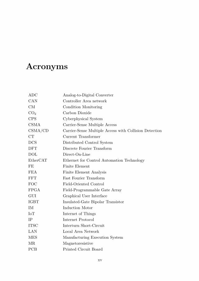
ADC Analog-to-Digital ConverterCAN Controller Area networkCM Condition MonitoringCO2 Carbon DioxideCPS Cyberphysical SystemCSMA Carrier-Sense Multiple AccessCSMA/CD Carrier-Sense Multiple Access with Collision DetectionCT Current TransformerDCS Distributed Control SystemDFT Discrete Fourier TransformDOL Direct-On-LineEtherCAT Ethernet for Control Automation TechnologyFE Finite ElementFEA Finite Element AnalysisFFT Fast Fourier TransformFOC Field-Oriented ControlFPGA Field-Programmable Gate ArrayGUI Graphical User InterfaceIGBT Insulated-Gate Bipolar TransistorIM Induction MotorIoT Internet of ThingsIP Internet ProtocolITSC Interturn Short-CircuitLAN Local Area NetworkMES Manufacturing Execution SystemMR MagnetoresistivePCB Printed Circuit Board
xv

xvi CONTENTS
PWM Pulse-Width ModulationSCADA Supervisory Control And Data AcquisitionSOC System-on-ChipTDMA Time-Division Multiple AccessVSD Variable-Speed Drive

Chapter 1
Introduction
1.1 Background
Despite being invented more than a century ago, electric motors are still essen-tial components in the modern industry. They are employed for the motion ofpumps, fans, conveyor belts, grinders and almost any moving mechanism in indus-trial plants. Electric motors use more than two-thirds of all the electrical energyconsumed in the industrial sector [1]. As a consequence, an important factor toachieve a more sustainable industry is the energy efficiency improvement of theindustrial applications where electric motors are applied. For this matter, energysavings can be obtained by supplying the electric motor with a frequency converter,and thus forming an electric drive [2]. Electric drives lead to efficiency improve-ments because they can guarantee accurate speed and torque profiles due to thefrequency converter presence.
Typically, an industrial plant is controlled and monitored through a hierarchi-cal communication architecture. Electric drives are located at the lowest level ofthe architecture and they have the limited roles of receiving commands from theupper-level controller and responding with alarms when a fault occurs. However,this established architecture is challenged by the Industry 4.0 initiative that aimsfor making the devices in industrial plants more interconnected and with additionalfunctionalities. This industrial shift poses two questions about the use of electricdrives. First, in the envisioned architecture, which functionalities of the electricdrives should be implemented or expanded? Secondly, which communication tech-nologies are suited for supporting these additional functionalities? The answers tothese questions should naturally take into account the practical applications whereelectric drives are used and the existing communication protocols that are employedin the industrial context.
Another key factor for the electric drives in industrial plants is their reliabil-ity. Failures negatively impact the total cost of ownership of electric drives [3] asthey hinder the operational activity of industrial plants. Failures in electric drives
1

2 CHAPTER 1. INTRODUCTION
can occur both in the frequency converter and the electric motor, each of whichconsists of many parts that are subjected to degradation and eventually to failure.Faults in electric drives can be early detected and possibly prevented by performingcondition monitoring techniques combined with predictive maintenance procedures.For this reason, during the last decades, an increasing research effort has investi-gated condition monitoring techniques. As electric motors are increasingly suppliedby frequency converters, an economical and practical strategy is to integrate suchcondition monitoring techniques in the frequency converter. In this manner, thesensors and computational unit already present in the converter could be exploitedfor the additional purpose of condition monitoring, without the need to install extraequipment in the industrial plant.
A considerable portion of the failures in electric machines is related to the sta-tor winding insulation, which accounts for a share between 9 % and 66 % of thetotal faults, depending on the machine size [4]. The insulation system of a statorwinding is made of several components that can lead to different kind of fault mech-anisms. Some of the stator winding fault types, such as the interturn short-circuitfaults, can be detected by analyzing specific signatures in electric quantities thatare commonly measured in electric drives. However, these fault signatures could bedependent not only on the stator fault itself but also on the operating conditions ofthe motor and other types of faults. Therefore, particular attention is given to thedevelopment of fault detection techniques that are independent of other conditions.Other stator winding fault types, such as the groundwall insulation faults, are lessprone to be detected with typical electric drive measurements at an early stage ofthe fault, which is before the fault has propagated too far to permanently damagethe motor. In this case, alternative solutions for the continuous monitoring of thestator insulation require non-conventional measurements in the electric drive.
1.2 Main objectives
The main objectives of this thesis are:
• Defining possible application cases of the additional functionalities enabled bythe Industry 4.0 initiative for electric drives in the industry. Moreover, thecommunication requirements of such application cases should be established.
• Implementing the above mentioned application cases with examples of in-dustrial communication protocols. Taking into account the requirements andlimitations of industrial communication protocols can give a better under-standing about the application cases practical feasibility.
• Developing and validating models for electric motors with interturn short-circuit faults. These models can be used to study the fault effects on themotor operation and to develop fault detection methods.

1.3. OUTLINE OF THE THESIS 3
• Developing and analyzing fault detection methods for electric motors with in-terturn short-circuit faults and studying monitoring methods for the ground-wall insulation.
• Developing an experimental setup to validate models, and to allow the emu-lation of interturn short-circuit faults and the degradation of the groundwallinsulation.
• Building a custom frequency converter capable of fault detection and moni-toring of the stator winding insulation.
1.3 Outline of the thesis
This thesis is a compilation of the key publications resulted from the work conductedduring the PhD studies. The purpose of the following chapters is to summarizethe papers appended in the thesis and to provide background and complementaryinformation. For the details and information not present in the thesis, the Readerwill be pointed to the papers.
The work conducted in the PhD studies is of multi-disciplinary nature, com-bining a smaller part related to communication networks with a bigger part aboutpower electrical engineering. In this thesis, Chapter 2 serves as an introduction forboth parts, whereas Chapter 3 is centered on the networking part. Chapters 4, 5, 6and 7 instead focus on the power engineering part. The thesis outline is summarizedas follows.
Chapter 2 gives an introduction to the Industry 4.0 initiative and to networkedelectric drives in an industrial context, and analyzes the application cases of con-dition monitoring and multi-drive systems.
Chapter 3 describes the implementation of the condition monitoring and multi-drive systems cases in industrial networks, where EtherCAT and CAN communi-cation protocols are employed.
Chapter 4 introduces the stator winding insulation system in electric machinesand its fault mechanisms. Both analytical and finite-element models of an inductionmotor with interturn short-circuit faults are provided.
Chapter 5 describes, analyzes and tests three detection methods for interturnshort-circuit faults in induction motors. The analytical and finite-element modelsare validated with experimental results.
Chapter 6 evaluates the behavior of MHz-range stator current oscillations withrespect to the stator winding insulation condition. The effects of insulation con-dition variations are tested experimentally both by adding additional capacitorsto the stator winding and also with an accelerated aging procedure applied to thewhole motor.

4 CHAPTER 1. INTRODUCTION
Chapter 7 gives an extended description of the experimental setup used in Chap-ters 5 and 6. A particular focus is put on the custom converter and on the acceler-ated aging procedure.
Chapter 8 summarizes the main conclusions of this thesis and proposes ideas forfuture work.
1.4 Original contributions
The original contributions of this thesis are listed as follows.
• A performance model for the multi-drive control and condition monitoringapplication cases implemented in the EtherCAT industrial communicationprotocol.
• A schedulability analysis for CAN-based networks where, together with smallperiodic control messages, also aperiodic bulk data is considered. The ape-riodic bulk data is an example of data generated by condition monitoringapplications.
• The development of a generalized model for induction motors with statorinterturn short-circuit faults. The model is general in two different aspects.First, it considers the interturn fault presence in any of the stator phases.Secondly, it allows to choose between two different modeling approaches forthe leakage inductances of the faulty winding.
• A theoretical analysis of a fault detection method for stator interturn short-circuit faults, which is based on a high-frequency injection. The analysis isbased on the developed generalized model and it is validated with experimen-tal results.
• The investigation of the behavior of MHz-range stator current oscillationswith respect to the variations of the stator winding insulation. Insulationstate metrics based on the current oscillations are developed and evaluated.
• The practical development of a frequency converter prototype capable ofperforming standard drive control, implementing a fault detection method,recording MHz-range stator current oscillations and communicating in a net-work.
• The investigation of an accelerated aging procedure for stator winding insu-lations of electric motors.

1.5. LIST OF APPENDED PAPERS 5
1.5 List of appended papers
This thesis is the summary of the papers listed below.
I G. Zanuso, V. Fodor, L. Peretti, and O. Wallmark, “Networked ElectricDrives in the Industry 4.0,” in 2018 21st International Conference on Elec-trical Machines and Systems (ICEMS), Oct. 2018, pp. 724–729.
II G. Zanuso, V. Fodor, L. Peretti, and O. Wallmark, “Multi-drive control andcondition monitoring in networked electric drives with EtherCAT,” in 2020International Conference on Electrical Machines (ICEM), Aug. 2020, vol. 1,pp. 1178–1184.
III G. Zanuso, and V. Fodor, “Bulk data transfer in Controller Area Networksfor Industry 4.0,” in 2020 IEEE Conference on Industrial Cyberphysical Sys-tems (ICPS), Jun. 2020, vol. 1, pp. 105–110.
IV G. Zanuso, S. Senthil Kumar, and L. Peretti, “Interturn Fault Detectionin Induction Machines based on High-Frequency Injection,” submitted forpublication in IEEE Transactions on Industrial Electronics, in review process.
V G. Zanuso, H. Babu, K. Bitsi and L. Peretti, “Induction Machine Analysiswith Extensive Stator Interturn Fault Conditions,” in 2022 11th InternationalConference on Power Electronics, Machines and Drives (PEMD 2022), ac-cepted for publication.
VI G. Zanuso, and L. Peretti, “Evaluation of High-Frequency Current RingingMeasurements for Insulation Health Monitoring in Electrical Machines,” sub-mitted for publication in IEEE Transactions on Energy Conversion, in reviewprocess.
VII G. Zanuso, and L. Peretti, “Accelerated aging procedure and online methodfor stator insulation monitoring,” submitted for publication in IEEE Trans-actions on Energy Conversion.
Giovanni Zanuso is the main author of Papers I-VII. The research work ofthese papers has been performed by Giovanni Zanuso in collaboration with the cor-responding co-authors and under the supervision of Viktoria Fodor, Luca Perettiand Oskar Wallmark. The performance evaluation of the EtherCAT protocol inPaper II were carried out by V. Fodor and G. Zanuso. The response time andschedulability analysis in III were developed with valuable inputs from V. Fodor.The Papers IV and V are partly based on the master thesis projects of S. SenthilKumar and H. Babu, respectively, who also contributed to the papers. L. Perettiprovided significant inputs and feedback in Paper I, and in Papers IV-VII.

6 CHAPTER 1. INTRODUCTION
1.6 List of related papers
Giovanni Zanuso authored or co-authored the following peer-reviewed papers thatare not included in the thesis.
i M. Pathmanathan, G. Zanuso, Z. Zhang, S. Valdemarsson, and E. Johans-son, “Self-Powered Supply and Control System for Hybrid Semiconductor DCSwitch,” in 2018 20th European Conference on Power Electronics and Appli-cations (EPE’18 ECCE Europe), Sep. 2018, pp. 1–10.
ii E. Velander, G. Bohlin, Å Sandberg, T. Wiik, F. Botling, M. Lindahl, G.Zanuso, and H. Nee, “An Ultralow Loss Inductorless dv/dt Filter Concept forMedium-Power Voltage Source Motor Drive Converters With SiC Devices,”IEEE Transactions on Power Electronics, vol. 33, no. 7, pp. 6072–6081, Jul.2018.
iii G. Zanuso, L. Peretti, and P. Sandulescu, “Model-based flux weakeningstrategy for synchronous machines without additional regulators,” IET Elec-tric Power Applications, vol. 12, no. 9, pp. 1283–1290, Nov. 2018.
iv L. Peretti and G. Zanuso, “Magneto-resistive sensors for condition moni-toring of insulation ageing in electrical machines: preliminary analysis andfuture prospects,” in Proceedings of the 15th International Symposium onMagnetoresistive Sensors and Magnetic Systems, Mar. 2019.
v F. Hohn, V. Fodor, G. Zanuso, and L. Nordström, “Scalable Integration ofHigh Sampling Rate Measurements in Deterministic Process-level Networks,”in 2021 IEEE International Conference on Communications, Control, andComputing Technologies for Smart Grids (SmartGridComm), Oct. 2021, pp.8–14.
vi R. Jain, A. Farjah, B. Ciftci, G. Zanuso, and S. Norrga, “Model-BasedDesign and System on Chip Implementation of DTC and PWM Techniques,”in 2022 IEEE Delhi Section Conference (DELCON), Feb. 2022, pp. 1-6.
vii A. Zhao and G. Zanuso, “Loss Calculation and Thermal Analysis of anInduction Motor under ITSC Fault Condition,” submitted for publication in2022 International Conference on Electrical Machines (ICEM), Sep. 2022.

Chapter 2
Networked electric drives in theIndustry 4.0
In this chapter, an extended introduction is given for Chapters 2 and 3. The re-maining content of this chapter is based on Paper I.
2.1 Background
Today’s industry is experiencing a profound change fed by the introduction ofmethods and devices from the information and communication technology world.Specifically, concepts as cyberphysical systems (CPSs) and internet of things (IoT)are applied to the industrial production systems. The term CPS refers to the in-tegration of computation with physical processes [5], whereas IoT stands for theinterconnection of physical objects through internet or other communication net-works. The application of these concepts to the industry aims to higher efficiency,availability and flexibility. These goals are achieved by means of an increasedconnectivity between the industrial plant devices and through the processing ofinformation in cloud-based applications.
This industrial shift is envisioned by the Industry 4.0 initiative that originatedin Germany in 2011, and for this reason it is also known as Industrie 4.0 [6]. Asimilar initiative has been brought up in North America with the name IndustrialInternet [7]. The term Industry 4.0 suggests that the present changes in the indus-try are part of a fourth industrial revolution. The first two industrial revolutions arewidely recognized by historians as periods of a great social and economical changes.Briefly described, the first industrial revolution started from the second half of the18th century in Great Britain. It involved the transition towards machine-basedmanufacturing supplied by steam and water power. The second industrial revolu-tion took place a hundred years later mainly in the United States and Europe. Itwas led by a growing mass production and standardization in the industry, whereelectrification and oil played an increasing role. The third industrial revolution con-
7

8 CHAPTER 2. NETWORKED ELECTRIC DRIVES IN THE INDUSTRY 4.0
sisted on the introduction of microelectronics and automation in the industry inthe early 1970s [8]. Differently from the first three, the fourth industrial revolutionannounced its arrival before taking place [6].
A more pragmatic manner to describe the Industry 4.0 is to relate to the commu-nication architecture of industrial plants. Fig. 2.1 shows the general architecture ofa distributed control system (DCS) that controls and monitors an industrial plant.SCADA (supervisory control and data acquisition) is a similar concept to DCSthat is often used as its alternative. The DCS is an interconnection of sensors,actuators, controllers and operators’ terminals. This architecture is based on ahierarchical structure where different communication networks can be used at thedifferent levels. For example, in the process electrification segment in Fig. 2.1, thevariable speed drive is connected to the AC800M controller with a fieldbus, which isrepresented by the purple line. In turn, the controller is connected with a local areanetwork (LAN) to various workstations and panels, representing the manufacturingexecution system (MES) at the upper level. Lastly, the MES is connected to theenterprise applications, shown in the business systems segment in the rightmostpart of Fig. 2.1. In this structure, the communication between two devices strictlyrespects the hierarchical levels.
Figure 2.1: General architecture of a DCS for industrial plants, based on ABB800xA (reproduced from [9]).
In the Industry 4.0, the architecture type shown in Fig. 2.1 is challenged with theintroduction of CPS and IoT concepts. Fig. 2.2 summarizes the structure of a cloud-based CPS. The CPS requires three levels: 1) the physical object; 2) the processdata, model and other information related to the physical object and process; and3) the services to apply on the available data [6]. The physical objects in Fig. 2.2represent the various devices at the lowest hierarchical level of Fig. 2.1, such as the

2.2. ELECTRIC DRIVES IN THE INDUSTRIAL CONTEXT 9
variable speed drive, or even the middle-layer devices as the controller. The presenceof the cloud in Fig. 2.2 enables the implementation of auxiliary services that caninteract with the physical objects and enhance their capabilities [10]. Moreover,part of the computation that occurred in the physical objects can be transferred tothe cloud.
Physical object
Services
Process dataModel
Other info
Algorithms
Figure 2.2: A cloud-based CPS.
The Industry 4.0 does not necessarily imply a complete substitution of the struc-ture in Fig. 2.1 with the one of Fig. 2.2. Instead, the cloud can integrate the existingarchitecture as shown in Fig. 2.3, which describes the possible transformation fromtoday’s industrial communication architecture to the future’s one [10]. The resultis a complex system that can facilitate the introduction of a new generation of ap-plications and services. In this context, the components can be dynamically addedor removed to the network, adding flexibility to the industrial plant.
2.2 Electric drives in the industrial context
The framework described by the Industry 4.0 vision offers more opportunities tothe devices in the industrial plant lower levels. Among these devices, this chapterfocuses specifically on the variable speed drive (VSD) and on its possible additionalfunctions that can be enabled by the new industrial architecture. VSDs are referredas electric drives in this work.
An electric drive is the combination of a frequency converter and an electricmotor. Electric drives play a major role in industrial automation because they canguarantee electromechanical conversion with accurate speed and torque profiles dueto the frequency converter’s presence. Electric drives are an upgrade of direct-on-line (DOL) motors, where the motor is directly connected to the fixed-frequencyand fixed-voltage AC grid supply and, as a consequence, the motor speed cannot

10 CHAPTER 2. NETWORKED ELECTRIC DRIVES IN THE INDUSTRY 4.0
Device DeviceDevice
DCS
MES
EnterpriseApplications
Device DeviceDevice
DCS
MES
EnterpriseApplications
(a) (b)
Figure 2.3: Transformation from (a) today to (b) future industrial communicationarchitectures.
be regulated to an optimal value. Instead, in electric drives the frequency converterregulates the motor speed in order to match the actual demand from the specificapplication. Hence, the electric motor energy consumption is decreased by typically30 % to 50 %, and in extreme case up to 70 % [11]. The case of pumps driven byan electric motor is a representative practical example of the efficiency benefitsbrought by electric drives. Pumps annually consume approximately 10 % of thetotal worldwide energy production [11]. Thus, even a slight improvement of theiraverage efficiency can bring large electricity savings and CO2 reductions. In pumpsdriven by a DOL motor, the motor rotates at full speed and the pump deliversthe maximum output. As the power consumed by the pump is proportional tothe cube of the speed, the required additional speed implies a large extra electricpower consumption. The extra power is wasted through friction by a valve thatreduces the output flow to the required value. Moreover, in this type of systemthe electric motors are often oversized as they need to provide more power thanactually required. Conversely, with electric drives the motor speed can be tuned tothe required value and the mentioned negative consequences are avoided.
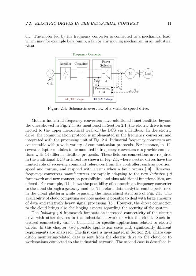
Fig. 2.4 shows the typical schematic of an electric drive, where a three-phasemotor M is supplied by the frequency converter. The frequency converter containsan AC/DC stage, which converts the AC grid voltage to a DC bus voltage, and aDC/AC stage that feeds the motor with pulse-width-modulated (PWM) voltages.In the whole system, the only intelligence available is the processing unit that hasthe main goal of commanding the power switches based on input signals as the DC-bus voltage UDC , the stator currents ia, ib, ic, and the rotor speed ωm or position
2.2. ELECTRIC DRIVES IN THE INDUSTRIAL CONTEXT 11
θm. The motor fed by the frequency converter is connected to a mechanical load,which may for example be a pump, a fan or any moving mechanism in an industrialplant.
M
ProcessingUnit
ACGrid
Load
Frequency Converter
PowerSwitches
Capacitor
iaib
ωm/θm
UDC
Rectifier
AC/DC stage DC/AC stage
Figure 2.4: Schematic overview of a variable speed drive.
Modern industrial frequency converters have additional functionalities beyondthe ones showed in Fig. 2.4. As mentioned in Section 2.1, the electric drive is con-nected to the upper hierarchical level of the DCS via a fieldbus. In the electricdrive, the communication protocol is implemented in the frequency converter, andintegrated with the processing unit of Fig. 2.4. Industrial frequency converters areconnectable with a wide variety of communication protocols. For instance, in [12]several adapter modules to be mounted in frequency converters can provide connec-tions with 14 different fieldbus protocols. These fieldbus connections are requiredin the traditional DCS architecture shown in Fig. 2.1, where electric drives have thelimited role of receiving command references from the controller, such as position,speed and torque, and respond with alarms when a fault occurs [13]. However,frequency converters manufacturers are rapidly adapting to the new Industry 4.0framework and new connection possibilities, and thus additional functionalities, areoffered. For example, [14] shows the possibility of connecting a frequency converterto the cloud through a gateway module. Therefore, data analytics can be performedin the cloud platform while bypassing the hierarchical structure of Fig. 2.1. Theavailability of cloud computing services makes it possible to deal with large amountsof data and relatively heavy signal processing [15]. However, the direct connectionto the cloud brings also challenging aspects regarding the security of the system.
The Industry 4.0 framework forecasts an increased connectivity of the electricdrive with other devices in the industrial network or with the cloud. Such in-creased connectivity can be beneficial for specific applications related to electricdrives. In this chapter, two possible application cases with significantly differentrequirements are analyzed. The first case is investigated in Section 2.4, where con-dition monitoring-related data is sent from the electric drive to the cloud or toworkstations connected to the industrial network. The second case is described in

12 CHAPTER 2. NETWORKED ELECTRIC DRIVES IN THE INDUSTRY 4.0
Section 2.5, where multi-drive systems require the communication between elec-tric drives within the same industrial network. Before describing these applicationcases, the next Section 2.3 gives an overview of the possible industrial communica-tion technologies that electric drives can exploit.
2.3 Industrial communication technologies
Modern electric drives can share information within an industrial network with alarge variety of communication protocols [16]. Before listing the several availablecommunication protocols and the different categories they belong to, it is worthintroducing the significant properties to evaluate their employment in an industrialnetwork. The generic industrial network considered for this purpose consists ofseveral nodes connected to a specific transmission medium with the same commu-nication protocol.
A first impacting characteristic is the ability of the communication protocol toperform in a hard real-time environment. Industrial control requires hard real-timeoperations, implying that missing a deadline causes a total system failure. Thehard real-time requirement demands that all network nodes should have the rightsto access the transmission medium periodically, i.e. a synchronous service should beimplemented. Conversely, an asynchronous service implies that a periodic access isnot guaranteed and therefore, generally, the hard real-time operation is not ensured.
Synchronous service can be implemented by several channel access methods aspolling, token passing and time-division multiple access (TDMA), where predefinedtime slots are assigned to the nodes. Moreover, in the remaining time availablethe transmission medium can be accessible asynchronously, often through randomchannel access with carrier sensing (CSMA). When polling is applied, a centralcontroller sends to or requests information from the controlled nodes in a round-robin manner. Similarly, in token passing the transmission rights are forwardedthrough a virtual ring without the need for a central controller.
Other than the type of access and the channel access method employed, themaximum obtainable transmission rate, i.e. the data rate, is another importantcharacteristic to take into account. The maximum data rate values given for thevarious communication protocols listed in this section are simple approximationsbecause the actual values depend on several network characteristics, like the net-work diameter and the node hardware. Furthermore, their values do not take intoaccount the presence of overhead bits in the transmission.
The industrial communication protocols are divided in three categories. Themost traditional one is represented by the fieldbus systems [?], already mentionedin Fig. 2.1. Fieldbuses are characterized by a robust communication suited for harshenvironments, with many small data packets transmitted at moderate data rates.Table 2.1 displays a few examples together with the service type, the channel accessmethod and the data rate. Some of these solutions, like Profibus and controller areanetwork (CAN), provide only asynchronous access, and thus do not directly ensure

2.3. INDUSTRIAL COMMUNICATION TECHNOLOGIES 13
the timely delivery of hard real-time messages. A more in-depth analysis of CANis done in Chapter 3 and in Paper III, where its hard real-time capabilities areensured by proper network dimensioning.
Table 2.1: Selected industrial fieldbus protocols.
Protocol Service Channel Access Data RateProfibus DP Async Polling 12 Mbps
CAN Async CSMA+priority 1 MbpsControlNet Sync + Async Token Passing 5 Mbps
The second category of industrial communication protocols is based on the Eth-ernet technology, but extended with real-time capabilities [16], [17]. Ethernet isa widely popular networking standard in the home and office world and it offershigh rates. Moreover, due to its popularity, Ethernet-related hardware has lowercosts compared to the fieldbus one. However, it employs a channel access methodbased on carrier-sense multiple access with collision detection (CSMA/CD), whichdoes not guarantee real-time operations, and thus it is not suited for industrial net-works. For this reason, the so-called industrial Ethernet protocols were developedfrom Ethernet and by adding real-time capabilities. Table 2.2 lists some examplesof the real-time Ethernet protocols. These solutions clearly guarantee higher trans-mission rates compared to the fieldbus systems, and the need for providing bothsynchronous and asynchronous access is widely recognized.
Table 2.2: Selected real-time Ethernet protocols.
Protocol Service Channel Access Data RatePROFINET Sync + Async Polling 100 Mbps
EtherCat Sync + Async Polling 100 MbpsEthernet Powerlink Sync + Async Polling 100 Mbps
The third and most recent category of industrial communication protocols isbased on wireless communications. Wireless communication, on one hand can en-sure the increased flexibility of the plants. On the other hand, the communicationitself may be unreliable in the harsh industrial environment due to disturbances,such as fading and shadowing. Table 2.3 displays a selection of industrial wirelessprotocols [18]. As a consequence of the different transmission medium, the datarates are considerably lower than the ones of fieldbus and real-time Ethernet pro-tocols. Higher data rates may be obtained with modern 5G-based networks forfactory automation, where latencies lower than 1 ms are targeted [19–21].

14 CHAPTER 2. NETWORKED ELECTRIC DRIVES IN THE INDUSTRY 4.0
Table 2.3: Selected industrial wireless protocols.
Protocol Service Channel Access Data RateWireless Hart Sync TDMA 250 kbpsISA100.11a Sync TDMA 250 kbps
Zigbee Sync + Async TDMA+CSMA 250 kbps6LoWPAN Sync + Async Polling+CSMA 250 kbps
2.4 Application case 1: Condition monitoring for electricdrives
Reliability is a key factor for the electric drives used in industrial plants. Failures inelectric drives may lead to the whole plant shutting down, with negative economicconsequences. The relation (2.1) shows that the total cost of ownership includesalso the cost of not running, which for an electric drive can account up to 30 % [3].
Cost of ownership = Purchase Cost + Cost of running + Cost of not running. (2.1)
Electric drives consist of many electrical and mechanical components that aresubject to failures. Failures can occur in the frequency converter components andin the electric motor, both in its electrical parts (stator windings, rotor bars) andits mechanical ones (bearings). Faults in electric drives can be detected early andpossibly prevented by performing condition monitoring (CM) techniques combinedwith predictive maintenance procedures. CM and diagnostic techniques for drivesystems are described in [22, 23], and in [24] the most recent CM techniques forindustrial electric machines are highlighted. A general classification of CM methodsfor electric drives is based on whether external apparatuses are required. Certainly,from a customer perspective, the preferable methods are those relying only on thesensors that are typically present in the electric drives for control purposes, such asthe current and speed/position sensors in Fig. 2.4. In this case, the additional costsof the CM techniques would depend only on the presence of additional software inthe processing unit in the frequency converter. A second general classification ofCM methods is between online and offline techniques, where the former ones arefavored because they perform during the electric drive normal operation, withoutthe need to wait for it to be halted.
Traditional online CM techniques are based on motor current signature analysis(MCSA), which relates the anomalies in the frequency spectrum of the measuredstator currents to specific faults [25]. Nevertheless, electric drives are affected bymany type of faults and distinguishing their effects in the current signature is achallenging task. CM methods alternative to MCSA, and thus without its limi-tations, have been developed over the years. In [26], turn-to-turn stator winding

2.4. CONDITION MONITORING FOR ELECTRIC DRIVES 15
faults are detected by analyzing the effects of a high-frequency voltage injection. Asimilar method based on high-frequency voltage injection is described and analyzedin Chapter 5 and Paper IV.
A completely different approach for the same fault type is used in [27], where theCM method is based on the MHz-range oscillations of the stator currents, occur-ring after a commutation of the power switches. Such current oscillations, namelycurrent ringings, depend on the several parasitic capacitances present between thewinding turns and between the winding and ground. The values of these parasiticcapacitances are therefore related to the winding insulation properties. Thus, theinsulation state can be monitored by analyzing the characteristics of the currentringings. The CM method based on such current ringings is further analyzed inChapter 6 and Papers VI and VII.
CM methods, both the traditional ones and those based on current ringings, areoften based on a comparison between present measurements and an initial referencemeasurement performed when the electric drive was supposedly healthy [22]. More-over, diagnostics methods that take into account the whole history of measurementsmay be developed. The emergence of faults in electric drives is however a relativelyslow process, which might take years if not decades. The measurement sessionsto acquire CM data are thus repeated periodically with a very low frequency, i.e.hours or even days, given the slowness of the degrading phenomena in electricdrives. Therefore, in order to apply diagnostics techniques that exploit the wholehistory of measurements, large amounts of data need to be acquired, stored andprocessed. These operations might exceed the computational limitation of the elec-tric frequency converter’s processing unit, which in the meanwhile needs to performcontinuously control-related tasks within stringent time constraints. Alternatively,these data could be stored in the cloud or in a local workstation connected to theindustrial network in order to perform CM algorithms and historical-data-based di-agnostics. The increasing spread of cloud computing services and industrial internetis therefore gradually shifting the CM of electric drives towards remote monitor-ing [15].
These solutions involving remote monitoring require to transmit the CM-relateddata from the electric drive to the cloud or industrial network. Thus, the industrialcommunication technologies listed in Section 2.3 are evaluated for the purpose ofcommunicating CM data. Specifically, Section 2.4.1 deals with the data generatedfrom traditional CM methods, such as the MCSA, whereas Section 2.4.2 deals withthe data from CM methods based on the current ringings.
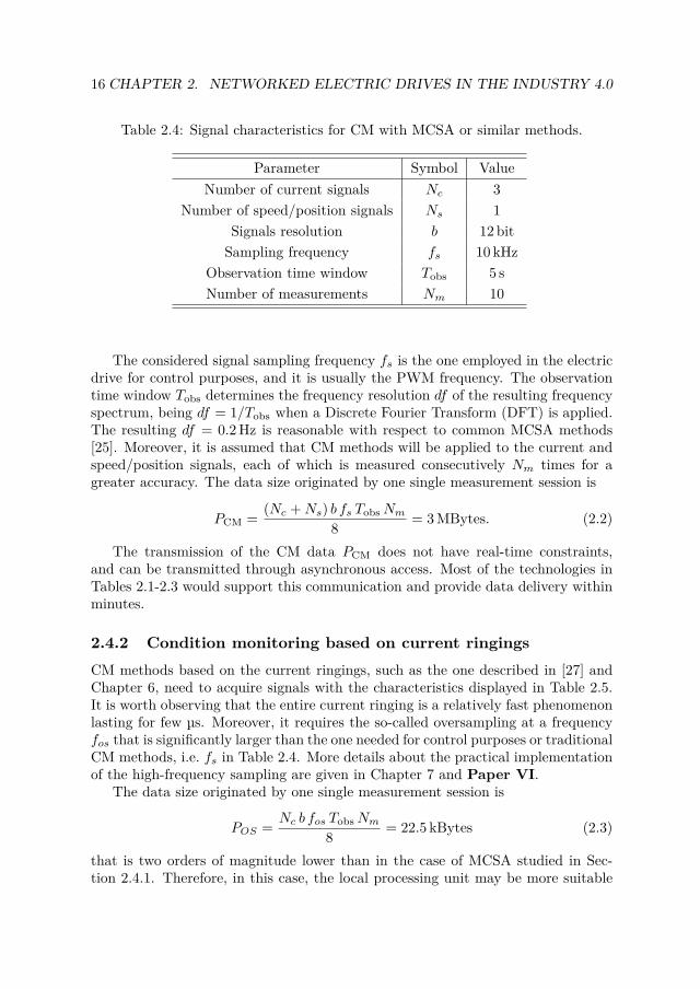
2.4.1 Condition monitoring with MCSA or similar methodsTraditional CM methods as the MCSA require the acquisition of signals having thecharacteristics displayed in Table 2.4. The listed values represent a possible casestudy where all three stator currents and the speed or position measurement areacquired, with typical analog-to-digital acquisition characteristics.
16 CHAPTER 2. NETWORKED ELECTRIC DRIVES IN THE INDUSTRY 4.0
Table 2.4: Signal characteristics for CM with MCSA or similar methods.
Parameter Symbol ValueNumber of current signals Nc 3
Number of speed/position signals Ns 1Signals resolution b 12 bit
Sampling frequency fs 10 kHzObservation time window Tobs 5 sNumber of measurements Nm 10
The considered signal sampling frequency fs is the one employed in the electricdrive for control purposes, and it is usually the PWM frequency. The observationtime window Tobs determines the frequency resolution df of the resulting frequencyspectrum, being df = 1/Tobs when a Discrete Fourier Transform (DFT) is applied.The resulting df = 0.2 Hz is reasonable with respect to common MCSA methods[25]. Moreover, it is assumed that CM methods will be applied to the current andspeed/position signals, each of which is measured consecutively Nm times for agreater accuracy. The data size originated by one single measurement session is
PCM = (Nc + Ns) b fs Tobs Nm
8 = 3 MBytes. (2.2)
The transmission of the CM data PCM does not have real-time constraints,and can be transmitted through asynchronous access. Most of the technologies inTables 2.1-2.3 would support this communication and provide data delivery withinminutes.
2.4.2 Condition monitoring based on current ringingsCM methods based on the current ringings, such as the one described in [27] andChapter 6, need to acquire signals with the characteristics displayed in Table 2.5.It is worth observing that the entire current ringing is a relatively fast phenomenonlasting for few µs. Moreover, it requires the so-called oversampling at a frequencyfos that is significantly larger than the one needed for control purposes or traditionalCM methods, i.e. fs in Table 2.4. More details about the practical implementationof the high-frequency sampling are given in Chapter 7 and Paper VI.
The data size originated by one single measurement session is
POS = Nc b fos Tobs Nm
8 = 22.5 kBytes (2.3)
that is two orders of magnitude lower than in the case of MCSA studied in Sec-tion 2.4.1. Therefore, in this case, the local processing unit may be more suitable

2.5. MULTI-DRIVE SYSTEMS 17
Table 2.5: Signal characteristics for CM based on current ringings.
Parameter Symbol ValueNumber of current signals Nc 3
Signals resolution b 12 bitHigh-frequency sampling fos 50 MHzObservation time window Tobs 10 µsNumber of measurements Nm 10
to perform CM techniques. Whether the data need to be sent to the cloud or in-dustrial network, all the communication technologies listed in Section 2.3 would besuitable.
2.5 Application case 2: Multi-drive systems
This section deals with the communication between electric drives within an indus-trial network. There are several industrial applications that can benefit from anincreased communication between electric drives. Industrial plants involving multi-drive systems (e.g. conveyor belts, tandem-connected motors, robots) are naturalexamples. Fig. 2.5 shows a general diagram of a multi-drive system, where a num-ber n of electric drives share the same DC bus. Each frequency converter FCi isequivalent to the one displayed in Fig. 2.4 without the presence of the AC/DCstage. The common DC bus gives the advantages of a reduced number of AC/DCstages (only one in Fig. 2.5) and the possibility to minimize the power flow from theAC grid, because the drives in motoring mode and those concurrently in generatingmode can share the power on the DC side [28]. The energy excess present in theDC bus can be redirected to the AC grid when a regenerative AC/DC converter isemployed, or be dissipated by balancing resistors.
Conventional conveyor belts are driven by multiple induction motors [29,30] as inFig. 2.5, where the involved power may reach the order of megawatts, making energyefficiency a critical factor. When the conveyor belt is not fully loaded, the systemefficiency decreases because the losses in induction motors are higher at partialloads [31]. For this reason, a cooperative dynamic load sharing strategy, based onan increased exchange of information within the multi-drive system may decreasethe total losses, compared to independent methods implemented in the drives. Loadsharing and total loss minimization techniques are beneficial for other industrialapplications where multi-drive systems are employed, for example when severalmotors are connected to the same load shaft, in the so-called tandem-connectedconfiguration [32], [33]. Similar cooperative control techniques are required in otherapplications, such as industrial robots [34] and port cranes [35], where multi-drive

18 CHAPTER 2. NETWORKED ELECTRIC DRIVES IN THE INDUSTRY 4.0
ACGrid
M
M
M
FC1
FC2
FCn
DC
bus
Figure 2.5: General diagram of a multi-drive system.
systems with independent loads are installed. In these systems, the common DCbus voltage needs to be limited within a specific threshold, regardless of the appliedloads.
As a consequence of the mentioned applications, multi-drives systems can ben-efit from a collaborative network of electric drives. The collaboration implies thatthe reference signals for each drive are generated by taking the state of all theother drives into account. This can be implemented by means of a centralized ordistributed control of multi-drive systems, as detailed in Section 2.5.1 and Sec-tion 2.5.2, respectively. For both cases, the suitability of the industrial communi-cation technologies listed in Section 2.3 is evaluated.
2.5.1 Centralized control in a multi-drive systemIn a centralized implementation of a multi-drive system collaborative control, acentralized processing unit completely takes care of the reference generation for eachdrive. Thus, the centralized processing unit should acquire all the state informationcoming from each of the electric drives, while all the local processing units stillperform low-level tasks, such as communication with drive sensors and PWM. Asa consequence, the centralized implementation may potentially induce a reductionof the computational power required for the local processing units and thereforeimpact the system cost.
The signals exchanged between the centralized control unit and each singleelectric drive in the network have the characteristics displayed in Table 2.6.
Differently from what reported in Section 2.4.1 and Section 2.4.2 for CM-relatedcases, the data communication must respect strict time constraints. At each PWMperiod, equal to the sampling period Ts = 1/fs, the measurements of currents,DC-bus voltage and speed (or position) are transmitted to the central processing

2.5. MULTI-DRIVE SYSTEMS 19
Table 2.6: Signals characteristics for a centralized control in a multi-drive system.
Parameter Symbol ValueNumber of current signals Nc 2
Number of DC-bus voltage signals Nv 1Number of speed/position signals Ns 1Number of PWM reference signals Nref 3
Signals resolution b 12 bitSampling frequency fs 10 kHz
unit, which calculates the references to be sent back to the local PWM modulatorof each electric drive. The data rate of the exchange between the central processingunit and one single local drive is
RMD,c = (Nc + Nv + Ns + Nref ) b fs = 840 kbps. (2.4)
The obtained result should be considered only for its order of magnitude, becauseoverhead bits required in the transmission are not taken into account. The totalnetwork transmission rate should consider the transmissions from all the electricdrives in the system. The transmission rate requirement of the multi-drive systemwith centralized implementation is high compared to the requirement of traditionaldrive control. The wired real-time Ethernet solutions in Table 2.2 can support thisapplication.
2.5.2 Distributed control in a multi-drive systemA distributed implementation of a multi-drive system collaborative control does notneed any central processing unit. Instead, the drives share their state informationwith each other, and each local processing unit performs the same optimizationtask to generate its own reference signals.
The data transmission rate of the distributed implementation depends on thebroadcast/multicast capability of the applied network technology. The minimumrequired rate can be obtained by assuming that each drive needs to transmit itsdata only once, and this is received by all the other drives. Since in this case theDC-bus voltage value does not need to be exchanged, and the reference signals donot need to be distributed, the resulting minimum transmission rate requirementbecomes
RMD,d = (Nc + Ns) b fs = 360 kbps. (2.5)
The numerical result in (2.5) is in the same order of magnitude as the one obtainedfor the centralized case in (2.4). As (2.5) is a minimum transmission rate that doesnot take into account the number of nodes in the network, also for the distributed

20 CHAPTER 2. NETWORKED ELECTRIC DRIVES IN THE INDUSTRY 4.0
case only the wired real-time Ethernet solutions in Table 2.2 are suitable for multi-drive system control.
In Chapter 3 more detailed results about both centralized and distributed con-trol in a multi-drive system are given for the EtherCAT communication protocol.
2.6 Summary of chapter
This chapter described how the Industry 4.0 vision offers more opportunities to thedevices in the industrial plant lower levels. The Industry 4.0 framework forecastsan increased connectivity of the electric drive with other devices in the industrialnetwork or with the cloud. Such increased connectivity can be beneficial for specificapplications related to electric drives. Two possible application cases were analyzed:the transfer of condition monitoring-related data in an industrial network or in thecloud, and the case of multi-drive systems connected within the same industrial net-work. For both cases, requirements in terms of minimum transmission data ratesand type of access to the network were established. A comparison was made be-tween such requirements and the capabilities of available industrial communicationtechnologies. As the transmission of condition monitoring data does not have real-time constraints, it is supported by most of the industrial communication protocols.However, only Ethernet-based real-time wired industrial network technologies cansupport the control of multi-drive systems.

Chapter 3
Application cases implemented inEtherCAT and CAN
The content of this chapter is based on Papers II and III.
3.1 Background
The previous chapter described two applications cases where electric drives benefitfrom an increased connectivity. Specifically, the case of CM-related data sent fromthe electric drive to the industrial network was analyzed in Section 2.4, whereas thecase of control of networked multi-drive systems was investigated in Section 2.5. Inthis chapter, these two cases are applied to two of the communication protocolsdescribed in Section 2.3: the Ethernet-based real-time protocol EtherCAT, and thetraditional industrial fieldbus CAN.
The messages generated in a network implementing the multi-drive control andCM applications have different requirements, which are summarized in Table 3.1.In multi-drive control, periodic messages with small data sizes are exchanged fre-quently with hard real-time constraints. Conversely, CM implies aperiodic messageswith larger sizes and with no hard real-time constraints.
Table 3.1: Summary of message requirements for multi-drive control application(MD) and condition monitoring (CM).
Case Data size Frequency Type Max. delayMD ∼ 10 bits 10 kHz Periodic 10 µsCM ∼ 1 MBytes 1 per hour Aperiodic -
21

22 CHAPTER 3. APPLICATION CASES IN ETHERCAT AND CAN
Both EtherCAT and CAN were designed for handling periodic control messages[36]. However, as described in Section 2.5, the transmission rate requirementsfor multi-drive control exceeds the characteristics of industrial fieldbuses, such asCAN. Therefore, multi-drive control will be implemented only with EtherCAT inSection 3.2. Previous uses of EtherCAT for multi-drive applications are reportedin [37] for large systems without strict delay requirements, and in [38,39] for delay-sensitive step motor control. Differently from the multi-drive control case, CMis implemented both with EtherCAT and CAN. In Section 3.2, the presence ofCM-related aperiodic messages is considered in EtherCAT in addition to the multi-drive control application. In section 3.3 the schedulability analysis of small periodiccontrol messages in CAN is extended for aperiodic bulk data.
3.2 Multi-drive control and condition monitoring inEtherCAT
EtherCAT is an Ethernet-based real-time communication protocol originally devel-oped by the automation company Beckhoff in the early 2000s [40]. Fig. 3.1 showsa typical EtherCAT network, with a daisy-chain bus topology and a master-slavearchitecture. The master station issues a frame that passes through all the slavestations sequentially. This frame is an Ethernet frame, as shown in Fig. 3.2, wherethe data field contains several EtherCAT telegrams addressed to the various slaves.Therefore, each slave reads its specific telegram and processes the data “on the fly”while the frame traverses the device. Then, the slave can write immediately to itstelegram before the frame leaves for the next node. This operation is repeated inall slaves and it relies on a fast processing time of the slave devices.
Ethernet frame
OUT IN
Data
Slave Slave SlaveEtherCAT Master
Figure 3.1: EtherCAT network and working principle.
Other than master-slave communications, EtherCAT also provides limited mul-ticast and slave-to-slave communications in the direction from the master towardsthe slaves on the bus. Moreover, although EtherCAT was conceived for periodicmessages, extensions have been proposed to allow the transmission of aperiodicmessages [36]. These capabilities of EtherCAT are well suited for implementing

3.2. MULTI-DRIVE AND CONDITION MONITORING IN ETHERCAT 23
headerEthernet Ethernet
tailer
Ethernet frame
EtherCATframe
EtherCATheader
Ethernet data
EtherCAT telegrams
telegram1st EtherCAT
telegram2nd EtherCAT
telegramS-th EtherCAT....
headerTelegram Data payload tailer
Telegram
Figure 3.2: EtherCAT frame format.
both control and monitoring of multi-drive systems, as summarized in this section.The performance modeling of multi-drive control with EtherCAT is described inSection 3.2.1. Section 3.2.2 adds to the developed model the presence of aperiodicmessages related to the condition monitoring data.
3.2.1 Performance modeling of multi-drive controlAs discussed in Section 2.5.1, multi-drive control can be implemented with central-ized decision making, where in an EtherCAT network the central processing unitis connected to the EtherCAT master node. In the distributed implementationof multi-drive control described in Section 2.5.2, each drive is an EtherCAT slavenode receiving updates from the other drives and computing control decisions lo-cally. Fig. 3.3 shows the communications and computing in the EtherCAT networkunder two sampling periods Ts, for both centralized and distributed cases.
In centralized multi-drive control, at the beginning of a sampling period, eachslave collects its state information, i.e. the measurements consisting of (Nc + Nv +Ns)b = 48 bits, and transmits it to the master. After the centralized computing,the master node sends Nref b = 36 bits related to the reference signal to each slave.In the distributed implementation, the state information of (Nc + Ns)b = 36 bitsfrom all the slaves is read by all other slaves. Direct slave to slave communication ispossible in only one direction on the bus, and therefore the master needs to collectand retransmit the state information of each drive. After the second transmission,each drive has all the information from the other drives and can compute locallyits reference signals. In both cases, two transmissions are needed in each samplingperiod. In the EtherCAT protocol, the start of the frame transmissions has tohappen periodically. Defining the cycle time Tc as the time from the start of thetransmission of an Ethernet frame at the master, until the time the last bit of the

24 CHAPTER 3. APPLICATION CASES IN ETHERCAT AND CAN
Figure 3.3: EtherCAT communication and processing times for the centralized andfor the distributed implementation of multi-drive control.
frame arrives back to the master, both cases should thus satisfy the condition
Tc + Tp <Ts
2 , (3.1)
where Tp is the processing time, which depends on the computing hardware.Models of the cycle time Tc in EtherCAT networks can be found in [21], [36]
and [41], whereas here a slightly simplified version is employed, where the exactcable lengths are not taken into account, giving
Tc = tp + S tf + ttr, (3.2)
where tp is the end-to-end propagation time on the bus, S is the number of slaves,ttr is the transmission time of the Ethernet frame at the master node and tf theforwarding time, which is the time a slave takes from the reception of the first bit ofthe frame until the transmission of the same bit. The values of tp and tf depend onthe EtherCAT hardware and are assumed constant in this model, whereas ttr = l/r,where l is the number of bits in the frame and r is the transmission rate. The valueof l includes both data and overhead bits in the frame displayed in Fig. 3.2. Theamount of data bits is obtained considering separately the specific centralized anddistributed cases, as detailed in Paper II.
The expressions (3.1) and (3.2) are combined in order to obtain the maximumnumber of drives, i.e. the number of slaves, that the EtherCAT network can serve formulti-drive control. Fig. 3.4 shows the limit on the number of slaves S as a function

3.2. MULTI-DRIVE AND CONDITION MONITORING IN ETHERCAT 25
Figure 3.4: Maximum number of drives that can be connected over an EtherCATbus for multi-drive control (Ts = 100 µs, tf = 0.5, 1, 1.5 µs.
of the processing time Tp and for different values of forwarding time tf , which hasa significant effect on the maximum number of drives. Moreover, the centralizedand distributed cases allow nearly the same number of slaves S, as a consequenceof the condition (3.1) that is valid for both cases. It is also worth noting that thenumber of connected devices is significantly lower than the one expected based onthe transmission rate of the bus, i.e. r = 100 Mbps, and the data rates per drivegiven in Section 2.5, i.e. 840 kbps and 360 kbps for the centralized and distributedcases, respectively. This demonstrates that the communication protocol overheadsand constraints have to be considered carefully at the system design.
3.2.2 Performance modeling of condition monitoringIn the time diagram of Fig. 3.3 there are idle times, when neither communication norcomputing happens, for both centralized and distributed multi-drive control. Theseperiods can be used to transmit aperiodic messages for CM data. The solutionpresented in [36] for the transmission of aperiodic information within EtherCATframes involves an EtherCAT telegram format where an aperiodic message of lo,a =12 Bytes is introduced. Thus, the time Ta available for the transmission of aperiodicdata within a sampling period is
Ta = max(
0,Ts
2 − Tc − lo,a
r
). (3.3)
As the aperiodic transmission occurs in Ta time within each sampling period Ts,the transmission rate becomes
Ra = Ta
Tsr. (3.4)

26 CHAPTER 3. APPLICATION CASES IN ETHERCAT AND CAN
Considering the same cycle time for the centralized and distributed implementa-tions, the resulting transmission rate of aperiodic traffic will be the same in bothcases. Fig. 3.5 shows that the achievable Ra is a linear function of the number ofslaves S. The forwarding time tf has significant effect as the network gets larger.Still, transmission rates of at least 10 Mbps are achievable for many cases. Theserates are suitable for the CM application, where data size was estimated to reach3 MBytes in Section 2.4. However, these transmission rates are significantly lowerthan the transmission rate of the bus, which shows again the limiting effects ofconstraints of the EtherCAT protocol.
Figure 3.5: Maximum achievable transmission rate of aperiodic traffic for drivemonitoring (Ts = 100 µs, tf = 0.5, 1, 1.5 µs.
3.3 Bulk data transfer in CAN for condition monitoringapplications
CAN is a serial communication bus introduced in the 1980s for in-vehicle networks[42]. In CAN, the medium access control is handled with priority-based arbitration[43]. Nodes are allowed to start transmitting only if the bus is idle. When twotransmissions begin at the same time, there will be an interference at the physicallayer and the message with higher priority remains in the bus. Thus, the node thattransmitted the message with lower priority notices the interference by sensing thebus, and stops its transmission.
Traditionally, CANs transmit periodic control messages with hard delivery dead-lines, and the main question of CAN dimensioning is the schedulability of the mes-sages. A priority-m message transmitted periodically with time period Tm needs tomeet the delivery deadline Dm. The worst-case response time Rm of the message mis defined as the longest possible time from the initiating event to the message be-

3.3. BULK DATA TRANSFER IN CAN FOR CONDITION MONITORING 27
ing received by the nodes that require it. The message m is considered schedulablewhen two conditions are met:
• The message is transmitted within the delivery deadline, i.e. Rm ≤ Dm.
• The message is transmitted before a new message is generated, i.e. Rm ≤ Tm.
The second condition comes from hardware constraints, as CAN nodes usually havesmall buffer capacity, but also from the fact that, in typical control applications, agiven type of information or control message becomes outdated when a new one isgenerated.
The schedulability of periodic control messages in CAN was analyzed in [42,44–46], where an analytical model for the worst-case message response time was pro-posed. This model is further exploited in order to consider the effects of faults [47],to provide algorithms for the dynamic extension of the address space [48], and topropose schedulability analysis in the presence of FIFO transceivers [49], or withpriority queues [50]. The model is extended in Paper III to the case where to-gether with small periodic control messages, also aperiodic bulk data is transmittedin CANs. Therefore, the proposed schedulability analysis considers also the aperi-odic bulk data, which represent the information generated by condition monitoringapplications. An example of the CAN examined in this section is shown on Fig. 3.6.The network contains the serial bus and the connected controllers (nodes), whereeach controller contains at least one buffer for periodic control messages and anotherone for possible bulk data transfer. Periodic control messages of N priority classesare transmitted in the network, which it may reflect a network with N nodes, or asmaller network with several buffers at each node. In addition, the nodes can oc-casionally transmit a bulk data of size Lb for condition monitoring purposes. As itexceeds the maximum payload of a single CAN packet, the bulk data is transmittedas a sequence of Nb packets, each with transmission time Cb.
This section continues as follows. Section 3.3.1 summarizes the traditionalschedulability analysis with a CAN with only periodic control messages. Sec-tion 3.3.2 describes the proposed schedulability analysis with the additional bulkdata transmission. A numerical example is given in Section 3.3.3.
3.3.1 Periodic control messagesThe worst-case response time Rm of a periodic control message with priority m isobtained with the following four steps, which are based the response time modelpresented in [42]. This model is built on the central concept of busy period. The busyperiod is a continuous time interval where the medium is occupied with messagesof priority m or higher.

28 CHAPTER 3. APPLICATION CASES IN ETHERCAT AND CAN
CAN transceiver
Message bufferControl Bulk data
CAN bus
Message bufferControl Bulk data
Message bufferControl Bulk data
CAN transceiver CAN transceiver
Figure 3.6: A CAN bus with nodes managing multiple transmission buffers fortransmitting control messages and a dedicated buffer for bulk data transfer.
Step 1 The maximum length tm of a busy period seen by a priority m queueis obtained as
tm = Bm +∑
∀k∈hep(m)
⌈tm + Jk + τbit
Tk
⌉Ck
Bm = maxCk, ∀k ∈ lp(m),(3.5)
where hep(m) is the set of messages with priority higher than or equal to m, andlp(m) with priority lower than m. The model parameters are Bm, which is themaximum time the channel can be blocked by a message of priority lower thanm, the jitter Jm between the generation of a packet and its placement in thetransmission buffer, and the transmission time of a bit τbit.
Step 2 The number Qm of instances of priority m messages transmitted withina busy period is calculated as
Qm =⌈
tm + Jm
Tm
⌉. (3.6)
Step 3 The maximum time wm(q) from the beginning of a busy period untilthe transmission of the q-th instance of the message m within the busy period, withq = 1 . . . Q,, is obtained as
wm(q) = Bm + (q − 1) Cm +∑
∀k∈hp(m)
⌈wm(q) + Jk + τbit
Tk
⌉Ck, (3.7)
where hp(m) is the set of messages with priority higher than m.
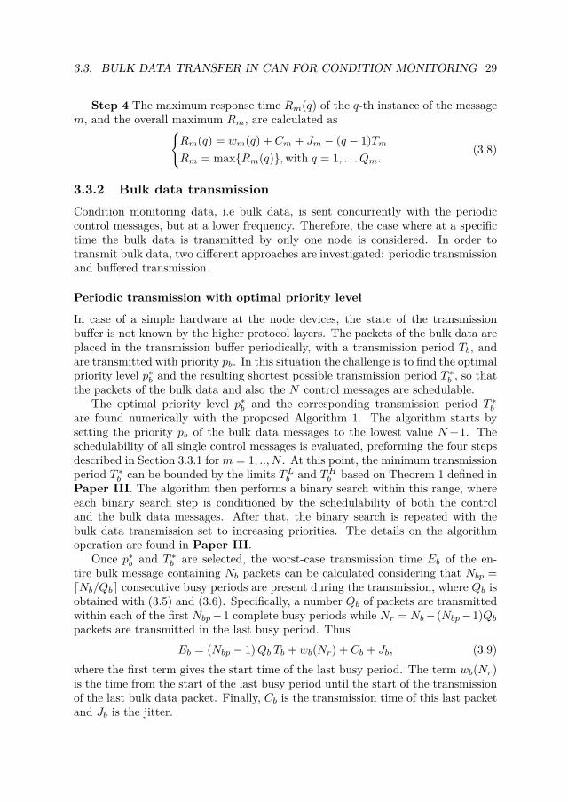
3.3. BULK DATA TRANSFER IN CAN FOR CONDITION MONITORING 29
Step 4 The maximum response time Rm(q) of the q-th instance of the messagem, and the overall maximum Rm, are calculated as
Rm(q) = wm(q) + Cm + Jm − (q − 1)Tm
Rm = maxRm(q), with q = 1, . . . Qm.(3.8)
3.3.2 Bulk data transmissionCondition monitoring data, i.e bulk data, is sent concurrently with the periodiccontrol messages, but at a lower frequency. Therefore, the case where at a specifictime the bulk data is transmitted by only one node is considered. In order totransmit bulk data, two different approaches are investigated: periodic transmissionand buffered transmission.
Periodic transmission with optimal priority level
In case of a simple hardware at the node devices, the state of the transmissionbuffer is not known by the higher protocol layers. The packets of the bulk data areplaced in the transmission buffer periodically, with a transmission period Tb, andare transmitted with priority pb. In this situation the challenge is to find the optimalpriority level p∗
b and the resulting shortest possible transmission period T ∗b , so that
the packets of the bulk data and also the N control messages are schedulable.The optimal priority level p∗
b and the corresponding transmission period T ∗b
are found numerically with the proposed Algorithm 1. The algorithm starts bysetting the priority pb of the bulk data messages to the lowest value N +1. Theschedulability of all single control messages is evaluated, preforming the four stepsdescribed in Section 3.3.1 for m = 1, .., N . At this point, the minimum transmissionperiod T ∗
b can be bounded by the limits T Lb and T H
b based on Theorem 1 defined inPaper III. The algorithm then performs a binary search within this range, whereeach binary search step is conditioned by the schedulability of both the controland the bulk data messages. After that, the binary search is repeated with thebulk data transmission set to increasing priorities. The details on the algorithmoperation are found in Paper III.
Once p∗b and T ∗
b are selected, the worst-case transmission time Eb of the en-tire bulk message containing Nb packets can be calculated considering that Nbp =⌈Nb/Qb⌉ consecutive busy periods are present during the transmission, where Qb isobtained with (3.5) and (3.6). Specifically, a number Qb of packets are transmittedwithin each of the first Nbp −1 complete busy periods while Nr = Nb − (Nbp −1)Qb
packets are transmitted in the last busy period. ThusEb = (Nbp − 1) Qb Tb + wb(Nr) + Cb + Jb, (3.9)
where the first term gives the start time of the last busy period. The term wb(Nr)is the time from the start of the last busy period until the start of the transmissionof the last bulk data packet. Finally, Cb is the transmission time of this last packetand Jb is the jitter.

30 CHAPTER 3. APPLICATION CASES IN ETHERCAT AND CAN
1: pb = N +1;2: Recalculate Bm for m = 1 . . . N +1;3: Evaluate schedulability for m = 1 . . . N ;4: If not schedulable, then goto End;5: Calculate T L
b , T Hb , based on Theorem 1;
6: Find schedulable Tb,N+1 via binary search in [T Lb , T H
b ];7: Set p∗
b = N +1, T ∗b = Tb,N+1;
8: For pb = N, pb > 0, pb−− do9: Change the priority of message m = pb to pb + 1;
10: Find schedulable Tb,bpvia binary search in
[wpb(1) + Cb + Jb, T ∗
b ];11: If Tb,bp found, then update p∗
b = pb, T ∗b = Tb,pb
;12: end For13: End
Algorithm 1: Periodic transmission of bulk data. Outputs: bulk datapriority p∗
b and transmission period T ∗b .
Buffered Transmission with low priority
In the previously-analyzed periodic transmission of bulk data, the state of thetransmission buffer was not known by the higher protocol layers at the device nodehardware. With a more intelligent node device, a new packet can be placed in thetransmission buffer as soon as this is not full. This case is named buffered datatransmission because on a higher level the entire data seems to be stored at thetransmitter.
The buffered transmission allows a continuous stream of bulk data packets whenthe bus is idle, and a shortest possible transmission delay of the bulk data. Thebulk data priority in this case has no effect and thus the lowest priority pb = N + 1is chosen. The entire bulk data transmission forms one busy period because all theidle time is filled in by the bulk data packets. The length of the busy period canbe calculated iteratively with
tb = Bb +∑
∀k∈hp(b)
⌈tb + Jk + τbit
Tk
⌉Ck + NbCb. (3.10)
The length of the busy period gives directly the worst-case delay Eb of the bulkdata transfer, which is
Eb = tb + Jb. (3.11)
3.3.3 Numerical example and resultsIn this section, the two approaches described in Section 3.3.2 for the transmissionof bulk data are evaluated with a numerical example. This example assumes a

3.3. BULK DATA TRANSFER IN CAN FOR CONDITION MONITORING 31
CAN bus with N nodes transmitting periodic control messages with priority m =1...N , where one of the nodes transmits Nb = 20 packets of bulk data. The sametransmission time for all control messages and bulk data is considered, i.e. Cm =Cb = 0.2 ms. Moreover, an equal transmission interval Tm for all periodic controlmessages is tuned such that a given load ρ is achieved on the CAN bus, obtainedas
ρ = NCm
Tm. (3.12)
For each message, a conservative delivery deadline is set as Dm = Tm − 2Cm.Fig. 3.7 shows Eb, the maximum time required to transmit the entire bulk data,
with an increasing load. Three transmission methods of the bulk data are com-pared: the periodic transmission with optimal priority level (OP) and the bufferedtransmission with low priority (BUF) described in Section 3.3.2, together with theperiodic transmission of bulk data packets, where the bulk data is transmitted withthe lowest priority (LP). The cases with N = 6 and N = 10 nodes are considered.Fig. 3.7 proves that the buffered transmission ensures the best results as it utilizesmost of the available capacity. Similar performances at low loads are obtained withthe periodic transmission with optimal priority, which instead leads to large Eb
values at high loads because low transmission intervals Tb of the bulk data cannotbe used as they would harm the schedulability of the control messages. For boththe buffered transmission and the periodic transmission with optimal priority, thenumber of nodes has little effect on the resulting Eb. Moreover, as expected, thetransmission based on lowest priority gives the worst performance, and it is alsodependent on the number of nodes.
0.1 0.2 0.3 0.4 0.5 0.6 0.7 0.80
10
20
30
40
50
Figure 3.7: Bulk data worst-case transmission time under increasing control trafficload, for the lowest priority (LP), optimal priority (OP) and buffered transmission(BUF) cases.
32 CHAPTER 3. APPLICATION CASES IN ETHERCAT AND CAN
3.4 Summary of chapter
The analyses performed in this chapter demonstrate that multi-drive control andfast delivery of monitoring data are possible over today’s wired industrial networks.Multi-drive control applications can be realized in EtherCAT both with centralizedcontrol, with the need of a powerful central controller, as well as with distributedcontrol, building on the computation capabilities of the drives themselves. Thenumerical results proved the significant influence of slaves number and forwardingtime over the feasibility of the applications in EtherCAT.
Moreover, this chapter investigated how traditional CAN can accommodate bulkdata transfer in addition to the usual transmission of periodic control messages. Ananalytic model of control message and bulk data transmission delays was providedand an algorithm for optimizing the priority level of bulk data transmission wasdesigned. The numerical results showed that the optimized selection of prioritylevel and transmission period allows low transmission times, whereas buffered bulkdata transmission has the largest gain when the control traffic load is high.

Chapter 4
Modeling of induction motors withinter-turn short circuit faults
In this chapter, an extended introduction is given for Chapters 4, 5, 6 and 7. Theremaining content of this chapter is based on Papers IV and V.
4.1 Background
As reported in Section 2.4, condition monitoring (CM) techniques allow the detec-tion and prevention of faults in electric drives, leading to an increased reliability andavailability of the whole industrial plant. Among the various fault types that canaffect an electric motor, the remaining part of this thesis focuses on the stator insu-lation faults and their related CM techniques. Specifically, the targeted insulationfaults are the ones of randomly-wound stator windings of induction motors (IMs).Fig. 4.1 shows an example of such winding type depicted during the manufacturingstage of an IM prototype.
The insulation system of a stator winding is made of several components that aresummarized in Fig. 4.2, where the schematic of a randomly-wound stator windinginsulation is shown. In such winding the stator coils are composed by a numberof turns, and each turn is made by one or more strands. A single strand consistsof a copper or aluminum conductor covered with a layer of enamel, which is thestrand insulation. In randomly-wound stators, the strand insulation is often theonly turn insulation, although an extra sleeve can be applied to strengthen theinsulation [51]. During the machine manufacturing, before placing the conductorsin the stator, a slot liner made of synthetic paper can be inserted in the stator slotsin order to protect the iron core and increase the insulation strength. Then, in thefinal manufacturing stage, the stator is usually impregnated with varnish or resin.Moreover, conductors of different phases, and thus with larger voltage differences,can be in proximity outside the stator slots in the so-called end windings or eveninside the stator slots whether each slot contains more than one layer of coils. In
33

34 CHAPTER 4. MODELING OF IMS WITH ITSC FAULTS
Figure 4.1: Stator winding during manufacturing stage (courtesy of Bevi AB). Theturns, iron core and several stator slots are clearly visible.
Conductor
Strand insulation
Pha
se in
sula
tion
Tur
n in
sula
tion
Gro
undw
all i
nsul
atio
n Slot liner
Extra-sleeve
Conductor
Strand insulation
Conductors in the same coil
Extra-sleeve
Impregnation
Slot liner
Impregnation
Conductor
Strand insulation
Slot liner
Extra-sleeve
Impregnation
Core
Figure 4.2: Schematic of an insulation system of a randomly-wound stator winding.
these situations, a phase insulation layer, of the same material type as the slot liner,can be placed between the different phase coils. In Fig. 4.1 phase insulation layersare visible as the large white foils that are not yet folded around the coils.
The main goal of the insulation system is to prevent any electric contact be-tween the metallic parts, i.e. the stator conductors and the stator iron core. Theseparts are separated by the two main portions of the stator insulation system: thegroundwall and the turn insulation, illustrated in Fig. 4.2. The groundwall in-sulation separates the conductors from the grounded stator core, and it is partly

4.1. BACKGROUND 35
constituted by the turn insulation. In contrast, the fundamental purpose of the turninsulation is to prevent low-resistance paths between the turns in a coil, namelyinterturn short-circuits (ITSCs). Turn and groundwall insulations are designed andmanufactured to withstand the various stresses affecting the insulation conditions,as displayed in Fig. 4.3. The stress due to repetitive voltage surges is present onlywhen motors are supplied by frequency converters, as the PWM-related switchingtransients cause fast rising voltages leading to the insulation aging. This problem iseven more relevant when modern wide bandgap devices are employed in frequencyconverters [52]. The combination of all the stresses causes a slow process of in-sulation degradation. Eventually, this can lead to a deterioration of the turn andgroundwall insulations, leading to ITSC and groundwall insulation faults, respec-tively. A groundwall fault can cause a machine breakdown, and thus the need fora substitution or rewinding of the stator. Another possible consequence is thatthe ground fault relay is triggered before the fault spreads further. In both cir-cumstances, the duty of the electric motor will be interrupted. When an ITSCfault occur, large currents may circulate in the shorted turns, inducing a local tem-perature increase and a further deterioration of the insulation, finally producing agroundwall insulation fault [51]. It is worth noting that the insulation degradationmechanism can also lead to phase-to-phase faults, which are not investigated in thiswork.
Insulation degradation
Machine breakdown Fault relay triggered
ITSC faultGroundwall insulation
fault
Insulation condition
Electrical stress
Mechanical stress
Thermal stress
Environmentalstress
Repetitivevoltage surges
Figure 4.3: Process leading to stator insulation failures [53].
The remainder of this chapter deals with the modeling of IMs with ITSC faults.Specifically, an analytical model is developed in Section 4.2 and a finite-elementmodel is described in Section 4.3. In the following Chapter 5, these models are em-

36 CHAPTER 4. MODELING OF IMS WITH ITSC FAULTS
ployed to analyze and test detection methods for ITSC faults. Instead, Chapter 6studies a method for monitoring the whole stator insulation, including the ground-wall insulation. Chapter 7 describes the experimental setup used to implementthese fault detection and monitoring methods.
4.2 Analytical modeling
4.2.1 Modeling assumptions for the faulted windingThe stator diagram of an IM with an ITSC fault is shown in Fig. 4.4, where as anexample the fault is present in phase a. The faulted phase winding a is divided
Figure 4.4: The three-phase stator winding of the faulted IM, where the in interturnfault is in the phase a. For the sake of clarity, mutual couplings are not shown here,but they are included in the equations.
into two parts, namely a1 and a2, where the pairs (Rs,a1, Ls,a1) and (Rs,a2, Ls,a2)are the resistance and inductance of the healthy and faulty parts, respectively. Thefault current if flows through Rf that represents the residual insulation resistancebetween the faulted turns. Other than Rf , the other parameter that characterizesthe ITSC fault is the ratio µ of faulted turns over the total number of turns in thephase winding. Both partial resistances Rs,a1, Rs,a2 and partial inductances Ls,a1,Ls,a2 can be expressed as a function of µ, with
Rs,a1 = (1 − µ) Rs
Rs,a2 = µ Rs
(4.1)
Ls,a1 =LsM,a1 + Lsl,a1
Ls,a2 =LsM,a2 + Lsl,a2,(4.2)
where Rs is the stator resistance, LsM,a1 and Lsl,a1 are the magnetizing and leakageinductances of the healthy part of the winding, respectively, whereas LsM,a2 and

4.2. ANALYTICAL MODELING 37
Lsl,a2 are their counterparts for the faulty part of the winding. The magnetizinginductances are proportional to the square of turns number, which leads to
LsM,a1 = (1 − µ)2 LsM
LsM,a2 = µ2 LsM
MsM,a1a2 = MsM,a2a1 = µ (1 − µ) LsM
(4.3)
where MsM,a1a2 and MsM,a2a1 are the mutual magnetizing inductances betweenthe faulty and healthy winding parts, and LsM is the total magnetizing inductance.
The modeling of the partial leakage inductances Lsl,a1 and Lsl,a2 is critical [54]and in literature different approaches are presented. In [55] the partial leakageinductances of the two stator sub-windings are directly proportional to their numberof turns. In [56] it is stated that a better approximation is reached when they areproportional to the square of the number of turns, giving
Lsl,a1 = (1 − µ)2 Lsl
Lsl,a2 = µ2 Lsl
(4.4)
where Lsl is the stator leakage inductance of the whole phase winding. The as-sumption (4.4) was taken as well in [57], [58] and [59], and it is the most commonin literature. A third approach for the partial leakage inductance modeling wasproposed in [54], where it is obtained
Lsl,a1 = (1 − µ)2
1 − 2µ + 2µ2 Lsl
Lsl,a2 = µ2
1 − 2µ + 2µ2 Lsl.
(4.5)
4.2.2 Generalized model in the natural reference frameStarting from the modeling assumptions given in Section 4.2.1, the stator and rotorequations of the IM with ITSC fault are written considering all the mutual couplingsbetween the stator healthy part, the stator faulty part and the rotor. Other thanthe stator and rotor equations, an equation for the fault circuit is needed for acomplete description of the system. The fault circuit is the loop created by thefaulty sub-winding and the residual resistance Rf in Fig. 4.4. In the resulting threeequations, the parameter θf and the vector µ displayed in Table 4.1 are employedto describe a generalized ITSC fault that can occur in any of the phases. The givenmodeling assumptions and extensive algebraic manipulations lead to the simplifiedexpressions (4.6), (4.7) and (4.8) for the stator, rotor and fault circuit voltageequations, respectively. Note that column vectors are represented by lower-case

38 CHAPTER 4. MODELING OF IMS WITH ITSC FAULTS
Table 4.1: Fault parameters for different faulted phases.
Fault in Phase a Fault in Phase b Fault in Phase c
θf 0 120 240
µ [µ 0 0]T [0 µ 0]T [0 0 µ]T
bold symbols and matrices by upper-case bold symbols.us,abc =Rs is,abc + d
dt(λs,abc) − Rs µ if
λs,abc =Lss,abc is,abc + Lsr,abc ir,abc
− (Lsl − Lsl,δ) µ if − µ xs if
(4.6)
0 = Rr ir,abc + d
dt(λr,abc)
λr,abc = Lrs,abc is,abc + Lrr,abc ir,abc − µ xr if
(4.7)
if (Rf + µRs) − Rs µT is,abc − d
dt(λf ) = 0
λf = (Lsl − Lsl,δ) µT is,abc + µ xTs is,abc
+ µ xTr ir,abc − µ2 (Lsl + LsM + Lsl,ε) if
(4.8)
In the stator voltage equation (4.6), the column vectors us,abc = [us,a us,b us,c]T ,is,abc = [is,a is,b is,c]T and λs,abc = [λs,a λs,b λs,c]T represent the three-phase statorvoltages, currents and flux linkages, respectively. In the rotor voltage equation (4.7),ir,abc = [ir,a ir,b ir,c]T and λr,abc = [λr,a λr,b λr,c]T represent the three-phase rotorcurrents and flux linkages, respectively, and Rr is the equivalent rotor resistance.In the fault circuit equation (4.8), λf represents the flux linkage of the faulty sub-winding, i.e. the corresponding flux linkage for the inductance Ls,a2 and the mutualcouplings, with Fig. 4.4 as a reference. The stator inductance matrix Lss,abc, therotor inductance matrix Lrr,abc, and the mutual inductance matrices Lsr,abc andLrs,abc between stator and rotor are described in (4.9), (4.10), (4.11) and (4.12),respectively, where Lrl is the rotor leakage inductance and θr is the rotor electricalangular position with respect to the stator. The fault-dependent vectors xs andxr, which are present in the flux linkage equations, are defined in (4.13).
Lss,abc =
Lsl + LsM − LsM
2 − LsM
2− LsM
2 Lsl + LsM − LsM
2− LsM
2 − LsM
2 Lsl + LsM
(4.9)
Lrr,abc =
Lrl + LsM − LsM
2 − LsM
2− LsM
2 Lrl + LsM − LsM
2− LsM
2 − LsM
2 Lrl + LsM
(4.10)

4.2. ANALYTICAL MODELING 39
Lsr,abc = LsM
cos (θr) cos(θr + 2π
3)
cos(θr − 2π
3)
cos(θr − 2π
3)
cos (θr) cos(θr + 2π
3)
cos(θr + 2π
3)
cos(θr − 2π
3)
cos (θr)
(4.11)
Lrs,abc = LTsr,abc (4.12)
xs = LsM
cos (θf )cos
(θf − 2π
3)
cos(θf + 2π
3) , xr = LsM
cos (θf − θr)cos
(θf − θr − 2π
3)
cos(θf − θr + 2π
3) (4.13)
It is worth noting that the stator (4.6) and rotor (4.7) voltage equations becomethe traditional equations of a healthy IM once the fraction of faulted turns µ is setto zero, whereas the fault circuit equation (4.8) becomes irrelevant. Moreover, theparameters Lsl,δ and Lsl,ε, present in the stator and fault circuit flux equations,allow the different modeling assumptions for the partial leakage inductances to beapplied. The assumption (4.4) is applied by setting to zero both Lsl,δ and Lsl,ε,and the assumption (4.5) is implemented using (4.14).
Lsl,δ =Lsl1 − 3 µ + 2 µ2
1 − 2 µ + 2 µ2
Lsl,ε =Lsl2 µ (1 − µ)
1 − 2 µ + 2 µ2
(4.14)
4.2.3 Generalized model in the stationary reference frame αβ0The model outlined in Section 4.2.2 in the natural coordinates abc is convertedinto the orthogonal coordinates αβ0. The transformation of the stator variables isobtained as
fs,αβ0 = Ks fs,abc , with Ks = 23
1 − 12 − 1
20
√3
2 −√
32
12
12
12
, (4.15)
where the vector fs can represent stator voltages, flux linkages or currents. As allthe rotor variables in Section 4.2.2 are referred to the rotor, they are transformedinto orthogonal coordinates referred to the stator with (4.16).
fr,αβ0 = Kr fr,abc , with Kr = 23
cos(θr) cos(θr + 2π
3)
cos(θr − 2π
3)
sin(θr) sin(θr + 2π
3)
sin(θr − 2π
3)
12
12
12
.
(4.16)The model described by the stator voltage equations (4.6), the rotor voltage
equation (4.7) and the fault circuit equations (4.8), is transformed using the matri-ces in (4.15) and in (4.16). The result of the transformations is the following model

40 CHAPTER 4. MODELING OF IMS WITH ITSC FAULTS
expressed in the orthogonal coordinates referred to the stator.us,αβ0 =Rs is,αβ0 + d
dt(λs,αβ0) − 2
3 µ Rs kf12 if
λs,αβ0 =Lss,αβ0 is,αβ0 + Lsr,αβ0 ir,αβ0 − µ LsM kf0 if
− 23 µ (Lsl − Lsl,δ) kf12 if
(4.17)
0 = Rr ir,αβ0 + d
dt(λr,αβ0) − ωr J3 λr,αβ0
λr,αβ0 = Lrs,αβ0is,αβ0 + Lrr,αβ0ir,αβ0 − µ LsM kf0 if
(4.18)
0 =if (Rf + µRs) − µ Rs kT
f1is,αβ0 − d
dt(λf )
λf =µ (Lsl − Lsl,δ) kTf1 is,αβ0 + 3
2 µ LsM kTf0 is,αβ0
+ 32µ LsM kT
f0ir,αβ0 − µ2 (Lsl + LsM + Lsl,ε) if
(4.19)
The transformed inductance matrices Lss,αβ0, Lsr,αβ0, Lrr,αβ0 and Lrs,αβ0 becomeall diagonal matrices as in (4.20), where the inductances Lm, Ls and Lr are definedin (4.21). In the rotor voltage equation (4.18), ωr is the electrical rotor speed andthe coupling matrix J3 is defined in (4.22).
Lss,αβ0 =Ks Lss,abc K−1s = diag [Ls Ls Lsl]
Lsr,αβ0 =Ks Lsr,abc K−1r = diag [Lm Lm 0]
Lrr,αβ0 =Kr Lrr,abc K−1r = diag [Lr Lr Lrl]
Lrs,αβ0 =Kr Lrs,abc K−1s = diag [Lm Lm 0]
(4.20)
Lm =32LsM
Ls =Lsl + 32LsM = Lsl + Lm
Lr =Lrl + 32LsM = Lrl + Lm
(4.21)
J3 =
0 −1 01 0 00 0 0
(4.22)
In (4.17), (4.18) and (4.19) there are the three newly-introduced fault-dependentvectors kf12, kf0 and kf1 defined in (4.23), which allow modeling of the interturnfault in any of the three phases.
kf12 = [cos (θf ) sin (θf ) 1/2]T
kf0 = [cos (θf ) sin (θf ) 0]T
kf1 = [cos (θf ) sin (θf ) 1]T(4.23)

4.2. ANALYTICAL MODELING 41
The generalized model of an IM with an ITSC fault is completed with theequation of the electromagnetic torque τe developed by the motor. It can be foundusing the described model equations in a power balance as in [60], or through thecoenergy partial derivative with respect to the mechanical rotor position. Theobtained expression is
τe =32 p Lm (iαriβs − iβriαs) − γ p Lm if [iαr sin(θf ) − iβr cos(θf )] (4.24)
where p is the number of pole pairs. In (4.24) the first term is the same as thehealthy machine torque formula whereas the second term is a consequence of thefault presence.
The model expressed with (4.17), (4.18) and (4.19) contains the zero-sequencecomponent, which can be exploited for implementing ITSC fault detection tech-niques, as in [61]. Nevertheless, in this work such techniques are not investigated.Moreover, only star-connected motors are considered and thus at this stage thezero sequence component can be removed, leading to simpler expressions. In theresulting equations in αβ coordinates, the inductance matrices in (4.20) and thecoupling matrix (4.22) are rewritten by removing their third rows and columns. Thefault-dependent vectors in (4.23) lose their third element and all of them becomeequal to
kf = [cos (θf ) sin (θf )]T . (4.25)
In order to do a further step that will be useful for the next section, the expres-sions in αβ coordinates and without the zero sequence components are rewrittenin their phasor form, assuming steady state conditions. The resulting steady-statemodel described with (4.26), (4.27) and (4.28) contains phasors, which in this workare represented with a capital symbol and, as complex quantities, are denoted witha “~” on the top.
U s,αβ =Rs Is,αβ + jω Λs,αβ − 23 µ Rs kf If
Λs,αβ =Lss,αβ Is,αβ + Lsr,αβ Ir,αβ
− 23 µ (Ls − Lsl,δ) kf If
(4.26)
0 = Rr Ir,αβ + jω Λr,αβ − ωr J2 Λr,αβ
Λr,αβ = Lrr,αβ Ir,αβ + Lrs,αβ Is,αβ − 23 µ Lm kf If
(4.27)
0 = If (Rf + µRs) − µ Rs kT
f Is,αβ − jω Λf
Λf = µ (Ls − Lsl,δ) kTf Is,αβ + µ Lm kT
f Ir,αβ
− µ2(
Lsl + 23Lm + Lsl,ε
)If .
(4.28)

42 CHAPTER 4. MODELING OF IMS WITH ITSC FAULTS
4.2.4 Generalized model in the sequence componentsUnbalanced systems, such as the IM with an ITSC fault, are commonly analyzedin steady state by means of symmetrical components. The relation between F αβ , avector of phasors expressed in the orthogonal reference frame αβ, and its equivalentF pn expressed in the sequence components pn is
F αβ = Spn7→αβ F pn , with Spn7→αβ =[
1 1−j j
]. (4.29)
The steady-state model described with (4.26), (4.27) and (4.28) is transformedinto sequence components using (4.29). The resulting model consists of the equa-tions shown in (4.30), (4.31) and (4.32), where as a consequence of the transforma-tion the complex vector cf and the matrix I−1 are introduced and defined in (4.33).Moreover, in the expressions in (4.32) the symbol “ ∗ ” on the complex vector cf isthe conjugate transpose operator.
U s,pn =Rs Is,pn + jω Λs,pn − 13 µ Rs cf If
Λs,pn =Ls Is,pn + Lm Ir,pn − 13 µ (Ls − Lsl,δ) cf If .
(4.30)
0 = Rr Ir,pn + jω Λr,pn − jωr I−1 Λ′r,pn
Λr,pn = Lr Ir,pn + Lm Is,pn − 13 µ Lm cf If
(4.31)
0 = If (Rf + µRs) − µ Rs c∗
f Is,pn − jω Λf
Λf = µ (Ls − Lsl,δ) c∗f Is,pn + µ Lm c∗
f Ir,pn
− µ2(
Lsl + 23Lm + Lsl,ε
)If
(4.32)
cf = 2 Sαβ 7→pn kf =[
cos(θf ) + j sin(θf )cos(θf ) − j sin(θf )
]; I−1 =
[1 00 −1
](4.33)
4.2.5 Equivalent circuits and expressions for currentsThe model outlined in Section 4.2.4 is conveniently represented by means of theequivalent circuits of the positive and negative sequences in Fig. 4.5, and the faultcircuit shown in Fig. 4.6. The rotor flux terms are expressed as function of the slips, obtained with the generic angular frequency ω and the electrical rotor speed ωr.The additional voltage sources Uadd,p and Uadd,n, present in Fig. 4.5, are definedin (4.34). In the equivalent circuits of Fig. 4.5 the only fault-dependent componentsare the current and voltage sources. The remaining electric network on the rightpart of both Fig. 4.5 (a) and (b) can be modeled as the positive-sequence impedance

4.2. ANALYTICAL MODELING 43
(a)
(b)
Figure 4.5: Equivalent circuits of the (a) positive and (b) negative sequence com-ponents of an IM with ITSC fault.
Figure 4.6: The fault circuit using the sequence components.
Zp and the negative-sequence impedance Zn in (4.35). Finally, the fault circuitimpedance Zf is defined in (4.36).
Uadd,p =13 jω Lsl,δ µ
(cos (θf ) + j sin (θf )
)If
Uadd,n =13 jω Lsl,δ µ
(cos (θf ) − j sin (θf )
)If
(4.34)

44 CHAPTER 4. MODELING OF IMS WITH ITSC FAULTS
Zp =(Rs + jω Lsl) +( Rr
s + jω Lrl) (jω Lm)Rr
s + jω (Lrl + Lm)
Zn =(Rs + jω Lsl) +( Rr
(2−s) + jω Lrl) (jω Lm)Rr
(2−s) + jω (Lrl + Lm)
(4.35)
Zf =Rf + µ Rs
(1 − 2
3µ
)+ jω µ2
(13Lsl
)+ jω µ2
(23Lsl,δ + Lsl,ε
)(4.36)
With the help of the equivalent circuits of Fig. 4.5 and Fig. 4.6, the IM modelwith ITSC fault is rewritten with the linear system in (4.37), where the non-diagonalimpedances are defined in (4.38). Us,p
Us,n
µ c∗f U s,pn
=
Zp 0 Z13
0 Zn Z23
Z31 Z32 Zf
Is,p
Is,n
If
(4.37)
Z13 =13 µ
(cos (θf ) + j sin (θf )
) (jω Lsl,δ − Zp
)Z23 =1
3 µ(
cos (θf ) − j sin (θf )) (
jω Lsl,δ − Zn
)Z31 =jω Lsl,δ µ
(cos (θf ) − j sin (θf )
)Z32 =jω Lsl,δ µ
(cos (θf ) + j sin (θf )
)(4.38)
The currents Is,p, Is,n and If can be obtained by solving (4.37) if the input voltagesUs,p and Us,n, the model parameters and the slip are known. The matrix in (4.37)results significantly simplified if Lsl,δ = Lsl,ε = 0, i.e. when the assumption (4.4)on the partial leakage inductances is applied. In that case, the terms Z31 and Z32become zero and the expressions for Zf , Z13 and Z23 in (4.36) and (4.38) containfewer terms.
4.3 Finite-element modeling
In this section a finite-element (FE) model of an IM with ITSC fault is brieflydescribed. Additional information can be found in Paper V. In literature severalFE models of IMs with ITSC fault were developed [62–71]. In this work, thesquirrel-cage IM with the geometry shown in Fig. 4.7 is modeled with the FEsoftware Comsol Multiphysics1. The IM parameters are displayed in Table 4.2.
The ITSC implementation in the FE model requires a different approach withrespect to the typical modeling of the stator winding. Fig. 4.8 shows the circuitof the healthy stator winding, where the numbers within square brackets indicatethe stator slots assigned to each coil. When an ITSC is implemented, the healthy
1Comsol Multiphysics is a registered trademark of COMSOL AB, Stockholm, Sweden

4.3. FINITE-ELEMENT MODELING 45
Table 4.2: IM parameters.
Parameter ValueNominal power 11 kW
Nominal current (RMS) 12.1 ANominal speed 1470 rpm
Nominal frequency 50 HzNumber of pole pairs 2
Number of stator slots 36Number of turns per coil 29
Number of rotor bars 28
Figure 4.7: IM geometry and conductors of the coil where the ITSC fault occurs(in red the shorted conductors).
stator circuit becomes the one shown in Fig. 4.9, where as an example the faultis introduced in the first coil of phase a, which is formed in the stator slots 3 and10. As shown in Fig. 4.7, in these two slots each of the 29 conductors is modeledindependently. As the ITSC involves the conductors colored in red, there are twosets of green-colored healthy conductors before and after the fault. Therefore, thefirst coil in phase a is divided in 3 parts as shown in Fig. 4.9, where the faultymiddle part represents the shorted turns, with the residual insulation resistanceRf connected in parallel. The stator circuit in Fig. 4.9 is completed with thethree-phase voltage supply formed by Uak, Ubk, Uck, the end-winding resistanceRs,ew and the leakage inductance Lsl,ew. The voltage supplies, resistances and
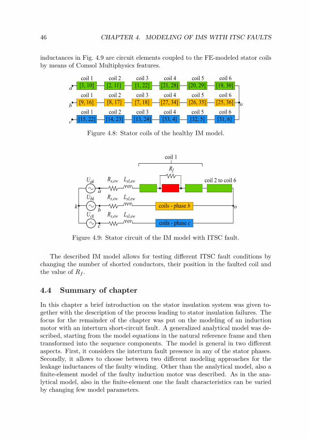
46 CHAPTER 4. MODELING OF IMS WITH ITSC FAULTS
inductances in Fig. 4.9 are circuit elements coupled to the FE-modeled stator coilsby means of Comsol Multiphysics features.
[15, 22] [14, 23]
[9, 16] [8, 17] [7, 18] [27, 34] [26, 35] [25, 36]
[13, 24]coil 1 coil 2 coil 3
[33, 4] [32, 5] [31, 6]coil 4 coil 5 coil 6
coil 4 coil 5 coil 6
coil 4 coil 5 coil 6
coil 1 coil 2 coil 3
[3, 10] [2, 11] [1, 22] [21, 28] [20, 29] [19, 30]coil 1 coil 2 coil 3
o
a
b
c
Figure 4.8: Stator coils of the healthy IM model.
coils - phase c
coils - phase b
coil 2 to coil 6
coil 1
o
a
b
c
k
Uak
Ubk
Uck Rs,ew Lsl,ew
Rs,ew Lsl,ew
Rs,ew
Rf
Lsl,ew
Figure 4.9: Stator circuit of the IM model with ITSC fault.
The described IM model allows for testing different ITSC fault conditions bychanging the number of shorted conductors, their position in the faulted coil andthe value of Rf .
4.4 Summary of chapter
In this chapter a brief introduction on the stator insulation system was given to-gether with the description of the process leading to stator insulation failures. Thefocus for the remainder of the chapter was put on the modeling of an inductionmotor with an interturn short-circuit fault. A generalized analytical model was de-scribed, starting from the model equations in the natural reference frame and thentransformed into the sequence components. The model is general in two differentaspects. First, it considers the interturn fault presence in any of the stator phases.Secondly, it allows to choose between two different modeling approaches for theleakage inductances of the faulty winding. Other than the analytical model, also afinite-element model of the faulty induction motor was described. As in the ana-lytical model, also in the finite-element one the fault characteristics can be variedby changing few model parameters.

Chapter 5
Fault detection methods forinduction motors with inter-turnshort circuit faults
The content of this chapter is based on Papers IV and V.
5.1 Background
In this chapter, detection methods for ITSC faults in IMs are proposed, analyzedand tested. Several fault detection methods have been developed in the last 30years because ITSC faults are a danger for the motor health. An ITSC fault intro-duces voltage and current unbalances, which are generally analyzed with sequencecomponents [72]. Among the methods based on sequence components, the mostcommonly employed fault signature is the negative-sequence current [58], [73]. Inthis chapter, the use of the negative-sequence current as fault signature is analyzedboth with the analytical and FE models described in Chapter 4, and experimentallytested.
The main drawback of the negative-sequence current as fault signature is itsdependency on the operating conditions. The research works in [26], [74], and [75]introduced a fault signature based on a high-frequency injection in order to over-come this disadvantage. Few other works have followed the approach of detectingstator faults by means of a high-frequency injection, such as [76] for detecting high-resistance connections in IMs, and [77] for ITSC faults in synchronous motors. AnITSC fault detection method based on a high-frequency injection is further analyzedin this chapter. It is proven theoretically and experimentally that for the injection-based method the fault signature angle gives directly the fault location and thatthe fault signature is not sensitive to the motor operating conditions. Moreover,experimental results are compared with the ones derived from the analytical model.
47

48 CHAPTER 5. FAULT DETECTION METHODS FOR ITSC FAULTS
Squirrel-cage IMs are characterized by the presence of rotor slot harmonics(RSHs) in the stator currents, which in the literature are also known as principal slotharmonics. As the stator current RSHs are dependent on the ITSC fault presence,they are exploited for diagnostic purposes in [78–80]. An analysis of stator currentRSHs as ITSC fault signature is given in this chapter, where experimental resultsare compared with the FE-model ones.
In the remainder of this chapter, Section 5.2 briefly describes the experimentalsetup allowing for the ITSC fault emulation that is used for obtaining the exper-imental results. In Section 5.3 the analytical and FE model are compared to theexperimental results, and the negative-sequence current is evaluated as fault signa-ture. Section 5.4 introduces the ITSC fault detection based on the high-frequencyinjection. Moreover, the analytical model is evaluated at the injected frequencyand compared to experimental results. The high-frequency based fault signature isthen tested at different operating conditions. Section 5.5 analyzes the stator currentRSHs as ITSC fault signature by means of FE model and experimental results.
5.2 Experimental setup for implementing inter-turn shortcircuit faults
The models described in Chapter 4 and the fault detection methods investigated inthis chapter are evaluated with the experimental setup shown in Fig. 5.1. An IMprototype with taps in the stator winding is employed to emulate the ITSC faultcondition. The prototype is based on a 11 kW BEVI 3SIE160-M4 IM for industrialuse, which has the parameters listed in Table 4.2 for the description of the FEmodel. The taps are located on three different coils, located in three differentphases of the stator winding. In the experimental results shown in this chapter,the taps on the fourth coil of phase-c winding are used, as shown in Fig. 5.2. Theresidual fault resistance Rf is implemented by an external resistor that is connectedbetween one terminal of the fourth coil to one of the 4 taps. The external resistoris a 3.3 kW TERCO variable resistor. The possible ITSC faults configurations arelisted in Table 5.1, where the involved turns and the related µ values are specified.
Table 5.1: ITSC fault configurations.
ITSC config. Turns µ
1 0 − 3 1.7 %2 0 − 7 4 %3 0 − 15 8.6 %4 0 − 29 16.7 %

5.2. EXPERIMENTAL SETUP FOR IMPLEMENTING FAULTS 49
Terminal box with taps
connection
IM prototype IM load
Fault current measurement
Custom converter
Current sensors
box
Xilinx ZC702
Variable resistor
Figure 5.1: Experimental setup for implementing ITSC faults.
Rf
Phase c
Star-point
Coil 1 Coil 2 Coil 3
Coil 4Coil 5Coil 6
Figure 5.2: Phase c winding schematic with taps and external resistor Rf .
The IM prototype is supplied by a 15 kW custom converter controlled by aXilinx ZC702 evaluation board, which in turn communicates via Ethernet with anexternal PC for data-logging purposes. The drive control, Ethernet communicationand the high-frequency injection scheme of Fig. 5.5 are implemented in the XilinxZynq System-on-Chip in the evaluation board. Detailed information regarding thecustom converter are given in Chapter 7. The mechanical load to the IM prototypeis provided by a similar IM but without taps, supplied by a 15 kW ABB ACS880converter. In the setup of Fig. 5.1, stator currents are measured with the customconverter, whereas the fault current flowing through the external resistor is mea-sured with a Tektronix TCP300 current probe connected to an Agilent MSO6104Aoscilloscope.

50 CHAPTER 5. FAULT DETECTION METHODS FOR ITSC FAULTS
5.3 Models validation and fault detection based on currentsequence-components
In order to validate experimentally the analytical and FE models described inChapter 4, the IM prototype is commanded with a V/Hz open-loop referencegenerator having a 150 V output and a ωs = 2π50 rad/s supply frequency. Thedrive speed is constant at 1450 rpm due to the load converter regulation. In thisoperating point the applied ITSC fault conditions are the tap configurations inTable 5.1, and for each of them the employed values of external resistance areRf = 1.3, 1.75, 2.5, 3.75, 5, 10, 20 Ω.
The mentioned operating point and fault conditions are also applied to the ana-lytical model represented by the linear system in (4.37). This model is solved withthe inputs Us,p, Us,n = 150, 0 V and ω = ωs. In such a model, the third ap-proach for leakage inductance modeling is chosen for calculating the partial leakageinductances, i.e. the assumption (4.5) and the setting (4.14). Fig. 5.3 shows a com-parison between the obtained experimental and analytical model results, where thedata points are marked with a star and a circle, respectively. The compared valuesare the magnitudes of the positive-sequence current Is,p, the negative-sequence cur-rent Is,n and the fault current If . The analytical model parameters were fine tunedto minimize the positive-sequence current magnitude and phase mismatches withthe experimental results. A similar comparison is performed between experimentaland FE model results, shown in Fig. 5.4. In the FE model described in Section 4.3,the imposed ITSC fault conditions are the same as the ones employed for the ex-perimental results, with the following exceptions. The first fault configuration inTable 5.1 was not simulated and the value of Rf = 1 Ω was employed instead ofRf = 1.3 Ω.
Both analytical and FE models in Fig. 5.3 (c) and Fig. 5.4 (c), respectively,show a good match between experimental and model results for the fault currentmagnitude. Regarding the negative-sequence current magnitude, the FE model inFig. 5.4 (b) is certainly more accurate than its analytical counterpart in Fig. 5.3 (b),especially for low Rf and high µ values. Referring to the computation of the experi-mental Is,n, it is worth noting that the IM prototype has inherent asymmetries thatcause default negative-sequence currents in healthy conditions. Thus, the measuredIs,n was corrected by subtracting these currents in all the experimental results. Fi-nally, about the positive-sequence current magnitude, Fig. 5.4 (a) shows an offseterror between the experimental and FE model results that is due to the inaccurateavailable data of the rotor bars.
All the magnitudes in Fig. 5.3 and Fig. 5.4 increase for higher fault severities, i.e.for Rf and high µ values. Specifically, the stator current negative-sequence and thefault current magnitudes manifest a larger relative variation dependent on the ITSCfault presence. Among these two, only the stator current negative-sequence Is,n canbe obtained from standard measurements in electric drives. For this reason, Is,n istypically used as a fault signature to detect the presence and severity of an ITSC

5.3. MODELS VALIDATION AND FAULT DETECTION 51
(a)
(b)
(c)
Figure 5.3: Comparison between analytical model and experimental results for themagnitudes of (a) positive-sequence current, (b) negative-sequence current and (c)fault current, evaluated at the fundamental frequency ωs, at different ITSC faultconditions.
fault [58], [59]. However, it should be taken into account that Is,n is also influencedby other possible unbalances present in the machine. Moreover, Is,n is affected bythe machine operating conditions as shown in (4.37) in Section 4.2.5, where Is,n
depends not only on the fault parameters set µ, θf , Rf , but also on the voltagesUs,p and Us,n, the frequency ω, and the slip s that is present in (4.35). Therefore,through Us,p, ω and s, the operating conditions impact the fault signature basedon Is,n. Regarding Us,n, it could be set to zero in case of an open-loop control, suchas the V/Hz regulator. In case of a closed-loop control, the current regulator may
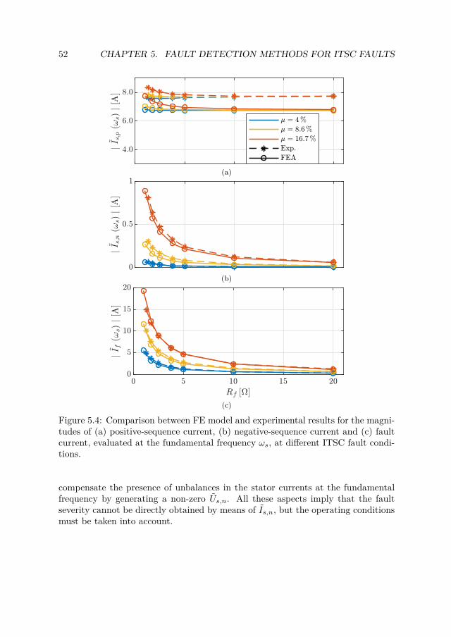
52 CHAPTER 5. FAULT DETECTION METHODS FOR ITSC FAULTS
(a)
(b)
(c)
Figure 5.4: Comparison between FE model and experimental results for the magni-tudes of (a) positive-sequence current, (b) negative-sequence current and (c) faultcurrent, evaluated at the fundamental frequency ωs, at different ITSC fault condi-tions.
compensate the presence of unbalances in the stator currents at the fundamentalfrequency by generating a non-zero Us,n. All these aspects imply that the faultseverity cannot be directly obtained by means of Is,n, but the operating conditionsmust be taken into account.

5.4. FAULT DETECTION BASED ON HIGH-FREQUENCY INJECTION 53
5.4 Fault detection based on high-frequency injection
In this section a fault signature based on a high-frequency injection is described.The resulting fault signature is not affected by the machine operating conditions,differently from the fault indicator Is,n(ωs) at the fundamental frequency examinedin Section 5.3. This method consists in superimposing a high-frequency voltage tothe voltage reference. The chosen injection frequency ωhf and the injected sequencecomponents Us,p(ωhf ) and Us,n(ωhf ) are set to constant values and thus they donot depend on operating conditions. Moreover, when ωhf is significantly larger thanωr, the slip becomes s ≈ 1 and therefore practically independent of the rotor speed.With these assumptions, the negative-sequence current evaluated at the injectionfrequency Is,n(ωhf ) does not depend on the motor operating conditions, whereas itstill depends on the ITSC fault conditions and thus it is a promising candidate asfault signature.
The high-frequency voltage is injected using the scheme of Fig. 5.5, where u∗αβ
is the voltage reference in the stationary reference frame αβ and u∗∗αβ is the final
voltage reference with the added injection. In this scheme, the positive-sequencevoltage vector uhf,dq+ is injected at high frequency, which is defined in (5.1) andhas a voltage magnitude Uhf . The vector uhf,dq+ is expressed in the reference framerotating at ωhf in the positive direction. The rotation matrix T dq+ 7→ αβ , in (5.2),transforms uhf,dq+ into the αβ fixed reference frame.
Figure 5.5: Block diagram of the high-frequency signal injection technique.
uhf,dq+ =[
Uhf
0
](5.1)
T αβ 7→ dq+ =[
cos (θhf ) sin (θhf )− sin (θhf ) cos (θhf )
]
T dq+ 7→ αβ =(T αβ 7→ dq+
)T
(5.2)
In case the voltage reference u∗αβ is the output of a current regulator, it may al-
ready contain positive- and negative-sequence components at ωhf that are added tothe injected voltage. This occurs when the regulator bandwidth is large enough withrespect to ωhf that the regulator reacts to the presence of positive- and negative-sequence currents at ωhf . In order to remove these undesired additional componentsfrom u∗
αβ , the filters shown in Fig. 5.5 are used. The filtering of the high-frequency

54 CHAPTER 5. FAULT DETECTION METHODS FOR ITSC FAULTS
positive-sequence is obtained with the scheme in Fig. 5.6, where the input signal istransformed into the positive high-frequency reference frame and then its DC com-ponents are removed with high-pass filters. A similar scheme is used for removingthe high-frequency negative-sequence, where instead of the transformations shownin (5.2), the ones in (5.3) are employed. The transformations in (5.3) are also usedto obtain magnitude and angle of the fault signature Is,n(ωhf ) as in Fig. 5.7. Thelow-pass filter extracts the DC values of the current components expressed in thereference frame rotating at ωhf in the negative direction. Additional informationon the injection values and filters parameters is given in Paper IV.
Figure 5.6: Block diagram of the high-frequency positive-sequence filtering.
T αβ 7→ dq− =[
cos (θhf ) − sin (θhf )− sin (θhf ) − cos (θhf )
]
T dq− 7→ αβ =(T αβ 7→ dq−
)T
(5.3)
Figure 5.7: Block diagram for obtaining the fault signature Is,n(ωhf ).
Similarly to the fault indicator based on the negative-sequence current evalu-ated at the fundamental frequency Is,n(ωs) investigated in Section 5.3, also themagnitude of the fault indicator Is,n(ωhf ) based on the high-frequency injectioncan be used to detect the fault severity, as it is shown in Section 5.4.1. However,differently from Is,n(ωs), the fault signature Is,n(ωhf ) contains in its angle usefulinformation regarding the ITSC fault. As detailed in Paper IV, writing the secondequation of the linear system (4.37) in Section 4.2.5 at the injected frequency ωhf
leads to∠Is,n(ωhf ) ≈ θf . (5.4)
Therefore, the angle of the fault signature Is,n(ωhf ) contains the information aboutwhich phase is affected by the ITSC fault.

5.4. FAULT DETECTION BASED ON HIGH-FREQUENCY INJECTION 55
5.4.1 Fault signature behavior and analytical results at injectedhigh-frequency
The experiments with emulated ITSC faults described in Section 5.3 are repeatedto evaluate the fault signature based on the high-frequency injection. Other thanemploying the same ITSC fault configurations, operating conditions and supply,a high-frequency voltage is superimposed to the fundamental voltage by means ofthe scheme in Fig. 5.5. This high-frequency injection scheme is implemented inthe custom converter introduced in Section 5.2 and more widely described in Chap-ter 7. The resulting high-frequency injection implies the sequence-components inputUs,p, Us,n = 40, 0 V at ωhf = 2π480 rad/s. These inputs and operating con-ditions are also applied to the analytical model in Section 4.2.5. Fig. 5.9 showsa comparison between the obtained experimental and analytical model results, forthe positive-sequence current Is,p, the negative-sequence current Is,n and the faultcurrent If , all evaluated at the injection frequency ωhf . Compared to the results inFig. 5.3 for the fundamental frequency case, Fig. 5.9 shows a higher mismatch be-tween model and experimental results. The reason lies in the modeling of the partialleakage inductances, which are more impacting at the injection frequency ωhf , asthe leakage reactances are proportional to the frequency. As done in Section 5.3, theemployed analytical model uses the third approach for leakage inductance modeling,i.e. the assumption (4.5). The mismatches in Fig. 5.9 caused by the adopted as-sumptions are considerably smaller compared to the ones obtained with the secondapproach for leakage inductance modeling, i.e. the assumption (4.4). A comparisonbetween the two modeling assumptions is done in Fig. 5.8, where the magnitudeof the fault signature Is,n(ωhf ) is shown for the experimental and modeling cases.Fig. 5.8 shows that the assumption (4.5) adopted in this paper brings considerableimprovements with respect to the assumption (4.4) that is commonly employed inliterature.
Figure 5.8: Magnitude of the negative-sequence current evaluated at the injectedfrequency ωhf . The modeling assumptions (4.4) and (4.5) are compared with theexperimental results for the case µ = 16.7 %.

56 CHAPTER 5. FAULT DETECTION METHODS FOR ITSC FAULTS
(a)
(b)
(c)
Figure 5.9: Comparison between analytical model and experimental results forthe magnitudes of (a) positive-sequence current, (b) negative-sequence current and(c) fault current, evaluated at the injected frequency ωhf , at different ITSC faultconditions.
Like the magnitude of Is,n(ωs), i.e. the fault signature at the fundamental fre-quency ωs, also the magnitude of Is,n(ωhf ) increases for higher levels of ITSC faultseverity, and thus it is a suitable fault signature for ITSC faults. The variationof both fault signatures can be used in fault detection methods to determine theemergence of ITSC faults. Nevertheless, the behaviors of these two fault signaturesdiffer when different operating points are considered, as discussed in Section 5.4.2.

5.4. FAULT DETECTION BASED ON HIGH-FREQUENCY INJECTION 57
5.4.2 Fault signatures at different operating pointsThe fault signatures Is,n(ωs) and Is,n(ωhf ) are experimentally evaluated at differentoperating points. Differently from what done in Section 5.3 and Section 5.4.1, theIM prototype is regulated with an indirect-field-orientation control scheme, withan external loop to regulate its speed. While the IM prototype is speed-controlled,the load machine is torque-controlled. The magnitude and angle of Is,n(ωs) andIs,n(ωhf ) are shown in Fig. 5.10, where the load torque τL is kept constant at 30 % ofthe nominal torque τN and the speed is varied. The ITSC fault condition employedfor all the experimental results is µ = 16.7 %, Rf = 2.5 Ω, which correspondsto a high fault severity. Fig. 5.10 shows that magnitude and angle of Is,n(ωs),represented by the blue curves, are largely dependent on the operating conditions,as explained in the end of Section 5.3. Moreover, the angle of Is,n(ωs) is not relatedto the phase with the ITSC fault, which is phase c. Conversely, for the magnitudeand angle of Is,n(ωhf ), represented by the red curves, the variation is small withrespect to the operating point changes. Additionally, as theoretically proved, theinformation given by the angle of Is,n(ωhf ) correctly points to where the ITSC faultis located, being θf = −120. As a result, the lower sensitivity to the operatingpoint and the accurate information about the faulty phase make the fault signatureIs,n based on the injection frequency ωhf superior to the traditional counterpartbased on the supply frequency ωs.
(a)
(b)
Figure 5.10: Current negative sequence (magnitude and angle) at different speedvalues and a load torque of 30 % τN , with µ = 16.7 %, Rf = 2.5 Ω.

58 CHAPTER 5. FAULT DETECTION METHODS FOR ITSC FAULTS
5.5 Fault detection based on rotor-slot harmonics
The fault signatures analyzed in Section 5.3 and Section 5.4 are based on com-ponents at the fundamental frequency and at an injected frequency, respectively.However, in IMs there are other spectral harmonics that are naturally presentwithout the need for an injection and that could be exploited for the ITSC faultdetection purpose. In this section, the rotor slot harmonics (RSHs) are analyzedby means of FE model and experimental results.
RSHs are a consequence of the rotor bar influence on the air-gap permeance.The general expression for the RSH frequencies fRSH can be obtained from themultiplication of the stator and rotor magnetomotive forces (MMFs) and the air-gap permeance [80], giving
fRSH = fs
[k Qr
p(1 − s) ± n
], with k, n = 1, 2, 3, ... , (5.5)
where fs is the supply frequency, p is the number of pole pairs, Qr the number ofrotor slots and s is the slip. The RSH frequencies described with (5.5) are visiblein Fig. 5.11, which shows the phase-b magnitude current spectrum of the healthyand faulty IM prototype. The spectra in Fig. 5.11 are obtained by processing thesteady state results of the FE model run with the operating conditions employedin Section 5.3. Fig. 5.11 displays how to relate the main RSHs to the coefficientsk and n in (5.5). Moreover, it highlights which of the RSHs is dependent solely onthe ITSC fault and the ones that are also present in the healthy IM, pointed bythe red and blue arrows, respectively. Applying k = 1, n = 1 to (5.5) producesthe two largest RSHs. The resulting left-side RSH is the dominant harmonic at627 Hz, which is present already in the healthy case with an amplitude of 0.44 A,and further increases in the faulty case, reaching 0.53 A. The right-side-RSH lies at727 Hz and it is absent in the healthy case. Due to their relatively large magnitudevalues and their relative difference between healthy and faulty cases, both theseRSHs are investigated as possible fault signatures.
Fig. 5.12 (a) shows a comparison between FE-model and experimental resultsfor the RSH at 627 Hz, obtained for the ITSC fault conditions of Section 5.3. Thisspecific RSH shows a similar behavior in all the stator currents of the three phases,as detailed in Paper V, with an offset presence between the FE model and exper-imental results due to the inaccurate available data of the rotor bars. Fig. 5.12 (b)shows the magnitude behavior of the right-hand side RSH at 727 Hz. Compared tothe RSHs of Fig. 5.12 (a), in this case the involved magnitudes have lower valuesthat are prone to numeric and measurement errors. Moreover, the RSHs behavedifferently in the three stator currents for both FE model and experimental results,as shown in Paper V. This asymmetry could be used to identify which phasecontains the ITSC fault. Regarding the determination of the fault severity, theleft-hand side RSH at 627 Hz seems to provide a clearer pattern compared to theright-hand side RSH at 727 Hz. Conversely, the left-hand side RSH drawback is

5.6. SUMMARY OF CHAPTER 59
RSH (k=1, n=3)527, 827 Hz
RSH (k=3, n=1)1980, 2080 Hz
(a)
RSH (k=1, n=1)627, 727 Hz
RSH (k=2, n=1)1303, 1403 Hz
(b)
Figure 5.11: FE model results of the phase-b magnitude current spectrum in twoconditions for the IM prototype: (a) healthy and (b) with an ITSC fault withµ = 16.7 %, Rf = 1 Ω. Note that the y-axis is limited, to highlight the RSHs. Ablue arrow indicates a RSH present in both healthy and faulty cases; a red arrowindicates a RSH present in only the faulty case.
its offset, which is present even in the healthy case, and it is dependent on theoperating point.
5.6 Summary of chapter
In this chapter, both the analytical and FE models described in Chapter 4 werevalidated with experimental results obtained from an IM prototype with tappedwindings, which can emulate ITSC faults. The FE model showed an overall greateraccuracy compared to the analytical model, although a considerable offset error

60 CHAPTER 5. FAULT DETECTION METHODS FOR ITSC FAULTS
(a)
(b)
Figure 5.12: Comparison between FE model and experimental results for the mag-nitude of phase-b current evaluated at the RSH frequencies (a) f = 627 Hz and (b)f = 727 Hz, at different ITSC fault conditions.
is present for the positive-sequence current magnitude due to the rotor bar datainaccuracy. Compared to the FE model, the analytical model showed a worsebehavior for the estimation of the negative-sequence current magnitude at highfault severities. The negative-sequence current magnitude was evaluated as faultsignature, and its influence by the machine operating conditions was discussed.
In order to circumvent the disadvantages of the fault signature based on thenegative-sequence current at the fundamental frequency, an ITSC fault detectionmethod based on a high-frequency injection was described and tested. In thismethod, the ITSC fault severity is related to the negative-sequence current at theinjection frequency. The proposed fault signature proved both theoretically andexperimentally to be independent from the operating conditions and to give correctinformation on the faulted phase location. Furthermore, it was analyzed how dif-ferent assumptions on the partial leakage inductances affect the analytical modelresults when evaluated at the injection frequency.
A further investigated ITSC fault detection method is related to the RSHs instator currents, which showed a dependency from the ITSC fault characteristicsbut also from the motor operating conditions. Another major drawback is that,differently from the fault signature of the high-frequency injection method, the

5.6. SUMMARY OF CHAPTER 61
RSHs amplitude cannot be adjusted to a suitable value that can be detected withthe measurement acquisition system. As a summary, the ITSC fault detectionmethod based on the high-frequency injection shows superior performances withrespect to the other two methods investigated in this chapter.
Regarding the analytical and FE models, the latter shows better accuracy whenthe accurate data on the geometry and materials are known. Moreover, the FEmodel allows for the simulation of space harmonics, such as the RSHs. The analyt-ical model instead gives insights into the ITSC fault consequences on the variousmotor signals, and it is useful for the development of fault signatures and the anal-ysis of their properties.


Chapter 6
Insulation health monitoring withMHz-range current ringingmeasurements
The content of this chapter is based on Papers VI and VII.
6.1 Background
The process leading to stator insulation failures, described in Section 4.1 and illus-trated with Fig. 4.3, implies that both ITSC and groundwall faults are consequencesof the insulation degradation. Thus, the monitoring of the stator insulation healthstate, together with the actuation of predictive maintenance procedures, could pre-vent the emergence of the stator faults. This chapter focuses on methods for mon-itoring of the stator insulation. Specifically, metrics that are related to the statorinsulation health state are developed and tested. These metrics can be employedby predictive maintenance procedures where, for instance, the remaining useful life(RUL) of an electric machine can be calculated. The development of algorithms forpredictive maintenance and the RUL calculation would require the testing of largenumber of motors, and therefore these aspects are not investigated in this work.
The CM methods studied in this work are of a different nature than the meth-ods analyzed in Chapter 5 for two reasons. First, the aim of the latter ones arefor fault detection and thus their application to predict stator faults is limited.Secondly, the methods in Chapter 5 considered only the ITSC fault type, whereasthe groundwall insulation was not taken into account. These methods for ITSCfault detection are hardly applicable to monitor the groundwall insulation state.This is because the deteriorating groundwall insulation has an insulation resistancethat is several orders of magnitude larger than the impedances of the machine low-frequency equivalent circuit. Therefore, the slow deterioration of the groundwall
63

64 CHAPTER 6. INSULATION HEALTH MONITORING
insulation has no effect on the stator currents sampled in the order of tens of kHzemployed for detecting ITSC faults.
CM of the groundwall insulation is traditionally performed with offline tests,such as the insulation resistance, polarization index and dissipation factor measure-ments. In [81] a method is proposed to perform these offline tests in a converter-fedmotor, by adding additional mechanical contacts and sensors to the converter. Nomatter how they are performed, offline tests require the interruption of the motoroperation, which may not be feasible in industrial applications. As mentioned inSection 2.4, in this work the focus is put on CM methods that exploit to a large ex-tent the measurement system and the hardware already present in existing convert-ers without the need for extra components. The only online groundwall insulationmonitoring that is extensively applied in the industry is the online partial dischargetest [24]. However, this method requires the installation of additional equipment.In [82] an online surge test is applied during machine operation, but additionalhardware to implement the surge is needed. In [83] the insulation impedance spec-trum is measured online using a signal generator, coupling capacitors and additionalcurrent sensors. Similarly, in [84] the stator winding resonances are detected with ahigh-frequency low-voltage generator coupled to the motor in order to superimposeits voltage to the motor supply, and a further current sensor. The groundwall andphase-to-phase insulation conditions are monitored online in [85] by measuring theleakage current for each phase. Three current transformers (CTs) and three voltageprobes are needed to estimate the insulation resistance, the equivalent insulationcapacitance and the dissipation factor. This method is modified in [86], where themeasurement for the common-mode leakage current is required. Similarly, in [87]and [88], a CT encircling all phases is needed for obtaining the common-mode capac-itance and for observing the leakage current transient, respectively. In [89] and [90],the insulation condition is monitored through the groundwall and phase-to-phasecapacitances, which are extracted using CTs and voltage probes. Instead, in [91]and [92], online CM is performed using the high-frequency common-mode current,obtained from measurements with Rogowski coils that are specifically developed forthis purpose. Rogowski coil sensors are also employed in [93] where changes in thecharacteristic impedance of the insulation are detected. Further works, in additionto online CM methods, also introduce the RUL estimation of the stator insulation.In [94] the groundwall equivalent resistance and capacitance are measured onlineusing additional sensors for the common-mode voltage and current. The RUL ispredicted from the equivalent capacitance value. In [95] instead the RUL is ob-tained from the leakage current peak-to-peak values, and a dedicated circuitry isemployed to measure the leakage current.
Differently from the works mentioned above, in [27] and [96] the insulation stateis monitored without the need for extra sensors or equipment. This method relies onthe MHz-range stator current ringings occurring after a switching transition of theconverter. Fig. 6.2 gives a visual explanation of the current ringing phenomenon.In Fig. 6.2, the PWM voltage and the current waveforms are the output of an idealconverter supplying a single-phase inductive load. The sinusoidal current contains a

6.1. BACKGROUND 65
triangular ripple due to the PWM voltage. In a real converter, the current ringingphenomenon would appear just after the rising and falling flanks of the PWMvoltage, as highlighted in Fig. 6.2 for a specific flank. The current ringings aredamped high-frequency oscillations that are superimposed to the expected ramp-like low-frequency behavior. It is worth noting that the measurement of theseoscillations requires a higher sampling frequency than the typical converter PWMfrequency.
Current ringing
Figure 6.1: Explanation of the current ringing phenomenon. The displayed wave-forms are the outputs of an ideal converter supplying a single-phase inductive load.
The approach of exploiting the current ringings for monitoring the insulationstate is further analyzed in this chapter. The relation between these current ringingsand the insulation state is explained as follows. Numerous parasitic capacitances arepresent between the turns and also between turns and the stator lamination, whichis connected to the machine ground. The parasitic capacitance values depend onthe configuration, geometry and materials of the insulation system [84], [97]. Suchparasitic capacitances influence the high-frequency behavior of the machine, whichis visible when steep voltage transients are applied to the stator winding duringconverter commutations, causing the ringings in the stator currents. Therefore, thecurrent ringings depend on the parasitic capacitances of the stator winding. Asthe parasitic capacitances values are influenced by the insulation materials, thereis a relation between the current ringings and the insulation state of the statorwinding [27], [96].
In this chapter, the behavior of the current ringing is analyzed by causing avariation of the insulation state in two different manners. First, the insulationchange is only emulated by adding extra capacitors in the stator winding. Withthis method, the relation between current ringings and parasitic capacitances can beanalyzed by means of several controlled tests, where the parasitic capacitance valuescan be established a priori. This method was previously employed in [27], [53] and[96]. The second method for imposing a variation of the stator insulation condition

66 CHAPTER 6. INSULATION HEALTH MONITORING
is the accelerated aging of the stator winding. The stator winding insulation changeswith accelerated aging are studied in [98], [99] and [100], where the focus was onthe wire insulation. In [94], [97] and [101], the whole stator winding was subjectedto accelerated aging tests. These two methods are exploited in this chapter to testand analyze the metrics, which are obtained from the current ringings, and whichare related to the parasitic capacitances and thus to the stator insulation condition.
In the remainder of this chapter, Section 6.2 describes the current ringings andhow they are influenced by the converter switching devices. Section 6.3 analysesthe current ringing variations and the related metrics when extra capacitors areadded to the stator winding. The same metrics are investigated in Section 6.4 withan aging stator insulation. Chapter 7 then gives details about the experimentalsetup capable of acquiring stator currents with MHz-range sampling and additionalinformation on the accelerated aging procedure.
6.2 Description of current ringings during switchcommutations
Fig. 6.2 shows two examples of ringings in positive and negative stator currents.The typical ramp-like behavior of stator currents due to the PWM voltages is barelyvisible due to the short time scale. Other than the parasitic capacitances in thestator winding, the converter can also affect the current ringings. For instance, theconverter’s presence causes the different ringing behavior for positive and negativecurrents, as shown in Fig. 6.2. The influence of the converter on the current ringingsis explained with Fig. 6.3 and the following analysis of almost-ideal commutations,where the parasitic elements of the switching devices are not taken into account.
The commutations in a typical two-level voltage source converter are of twodifferent types. The first type occurs when the lower-leg switch is turned off and,after a dead time, the upper-leg switch is turned on. In the second type, theopposite occurs. In this chapter only the current ringings occurring during thefirst type commutation are considered. This commutation type is explained inFig. 6.3 (a) and (b) for both the cases of positive and negative output currents,respectively.
In both cases, before turning on the upper- or lower-leg switch, a dead time iswaited from the moment the other switch in the same leg is turned off. For thepositive current case in Fig. 6.3 (a), the current flows through a diode both beforethe commutation (red-dotted line) and during the dead time (green-dashed line),whereas after the dead time it flows through an IGBT (blue-solid line). Therefore,the switching transition and thus the current ringing begins after the dead time haselapsed. Moreover, the IGBT is conducting during the current ringing. Conversely,as shown in Fig. 6.3 (b), the negative current flows through an IGBT before thecommutation (red-dotted line), whereas during the dead time (green-dashed line)and after the commutation (blue-solid line) it flows through a diode. In this case,the current ringing begins without the need to wait for the dead time and the diode

6.2. DESCRIPTION OF CURRENT RINGINGS 67
(a)
(b)
Figure 6.2: Current ringing for (a) positive and (b) negative currents, measuredwith two different current sensors.
Du
Dl
Su
Sl
DC+
DC−
i
(a)
Du
Dl
Su
Sl
DC+
DC−
i
(b)
Figure 6.3: Commutation with (a) positive and (b) negative currents. The currentpath in the commutation states is shown: dotted red before the commutation,dashed green during the dead time and solid blue after the commutation.

68 CHAPTER 6. INSULATION HEALTH MONITORING
conducts during the current ringing. It is important to consider the commutationdifferences between positive and negative currents when implementing the high-frequency sampling as done in Chapter 7, as the recording of the current ringingshould be delayed by a dead time in case of positive currents.
Fig. 6.2 (a) and (b) show the ringing phenomena for positive and negative cur-rents, respectively. In both cases, the recording of the oscillation started 1 µs beforethe switching transition, and the delay caused by the dead time for the positive cur-rent was taken into account. The influence of the conducting device during ringingcan be noted in the oscillation peaks, with a 25 % higher peak for the positive cur-rent compared to the negative one, whereas the main oscillation frequency does notvary significantly. Fig. 6.4 shows the frequency content of the current ringing forpositive currents, which is similar to the ones for negative currents. Other than themain oscillation frequency at 5 MHz, there are two other dominant resonances at1.2 MHz and 2.8 MHz.
Figure 6.4: Spectrum magnitude of the current ringing measured when i = +15 A.
6.3 Current ringing variations with added capacitors ontaps
The measured current ringings analyzed in this section are obtained with the sameIM prototype equipped with taps on the stator winding that is described in Sec-tion 5.2. In this case, the taps are exploited to insert extra capacitances in differentparts of the winding in order to modify the high-frequency behavior of the ma-chine and thus causing changes in the current ringings. Specifically, the taps onthe first coil of phase b winding are used, as shown in Fig. 6.5. The winding-to-ground parasitic capacitance of the IM prototype is Cw2g = 2.7 nF. This valuewas measured between the phase terminals and the motor ground point with anAgilent U1733C LCR meter. The employed values of additional capacitance areCadd = 22, 47, 100, 220, 470 pF, which with respect to Cw2g represent a varia-tion of 0.81, 1.7, 3.7, 8.1, 17.4 %, respectively. In Sections 6.3.1 and 6.3.2, threedifferent metrics are defined and tested to quantify the current ringing changes for

6.3. CURRENT RINGINGS WITH ADDED CAPACITORS ON TAPS 69
Phase b
Star-point
Coil 1 Coil 2 Coil 3
Coil 4Coil 5Coil 6
Cadd
Figure 6.5: Phase b winding schematic with taps and external capacitor Cadd.
different additional capacitance configurations. The current measurements are per-formed with Rogowski coils at a sampling frequency of 62.5 MHz. Paper VI showsadditional results where the currents are acquired with lower hardware specifica-tions that are closer to the industrial reality. It is proven that in such downgradedconditions the developed metrics do not significantly deteriorate.
6.3.1 Influence of Cadd value on the current ringingIn the first tested configuration the different capacitors Cadd are connected betweenthe phase b terminal, i.e. where the first coil in Fig. 6.5 begins, and ground. Asshown in Fig. 6.4, the current ringing spectrum contains three main resonant fre-quencies. The behavior of these resonances with different values of Cadd is shown inFig. 6.6, where the frequency and magnitude values are obtained with the parabolicinterpolation described in [102], resulting in improved resolutions. Fig. 6.6 showsthat the frequency of the third resonance, i.e. the frequency of the main ringing oscil-lation, decreases for growing Cadd values, as is expected in a LC circuit. Moreover,the two other resonant frequencies do not significantly vary and the magnitudesof the three resonant frequencies increase with a non-linear pattern. With respectto the insulation variation, the resonant frequencies do not show an overall linearbehavior and they are also of not immediate calculation. As a consequence, othercurrent ringing metrics are developed to represent the insulation variation.
The metrics analyzed in this chapter are based on the root mean square (RMS)value and the peak value of the current ringings. The peak and RMS values arecalculated considering the current ringing without its initial offset value, and theRMS is obtained over 2 µs of signal after the oscillation starts. Then, the metrics∆RMS and ∆peak are defined as the difference of peak and RMS values, respectively,obtained in two conditions: one with the varied insulation state (with Cadd) and theother with the healthy winding (without Cadd). Thus, the two metrics quantify theinsulation state variation. These two metrics are compared to the insulation stateindicator (ISI) defined in [96]. This indicator is obtained as the RMS deviationbetween the magnitudes of the current ringing spectra obtained with healthy andvaried insulation. More information on the ISI calculation are found in Paper VI

70 CHAPTER 6. INSULATION HEALTH MONITORING
Figure 6.6: Frequency and magnitude of the three main resonances observed inthe current ringing when ib = +15 A.
and in [96]. It is worth noting that the ISI calculation requires performing the FFTalgorithm, which is more time consuming than obtaining peak or RMS values.
Fig. 6.7 shows how the two proposed metrics and the ISI behave with differentCadd values. All three metrics exhibit a quasi-linear behavior with Cadd variationsfor positive currents (blue circles), whereas for negative currents (red stars) ∆RMS
shows an irregular behavior for small variations of Cadd. This implies that ∆RMS isbetter suited to be used for current ringings occurring when the current is positive.
6.3.2 Influence of Cadd position on the current ringingThe defined current ringing metrics are evaluated also when the additional capac-itor Cadd is connected between different parts of the winding and ground. Thisallows the observation of which part of the winding, and its local parasitic capac-itance, is more relevant for the current ringing variation. The following tests wereperformed using the single capacitor Cadd = 470 pF, representing a variation of17.4 % with respect to Cw2g, connected between the different turns of phase-b firstcoil and ground, as shown in Fig. 6.5. Specifically, Cadd was connected to the turns0, 1, 3, 15, 29, where the 0th turn represents the coil beginning. Fig. 6.8 shows

6.3. CURRENT RINGINGS WITH ADDED CAPACITORS ON TAPS 71
Figure 6.7: Current ringing metrics with parasitic capacitance values and Cadd
connected between the phase b terminal and ground.
the obtained metrics for each of the tested turn connections. It can be observedthat Cadd has a relevant influence on the current ringing only when it is placedon the first turns close to the terminal. Conversely, a change of the local parasiticcapacitances of the last turn of the first coil, i.e. the 29th turn, produces nearlythe same metrics as the healthy winding as all the metrics are close to zero. Al-though not shown, it was also checked that the parasitic capacitance changes onthe winding portion from the end of the first coil to the end of the winding havelittle relevance to the current ringing behavior.
Another set of experiments were executed by placing the additional capacitorCadd = 470 pF in parallel to different turns, instead of connecting it between turnsand ground. Specifically, Cadd was connected between the phase-b terminal andthe turns 3, 15, 29, 174 of phase b, where the 174th turn is the last turn of thewhole winding in Fig. 6.5. This set of experiments aims to emulate the changeof insulation between turns and to verify the consequent current ringing behavior.The current ringing metrics from these experiments are shown in Fig. 6.9. In thiscase a steep variation of the metrics ∆peak and ISI, implying a significant variation

72 CHAPTER 6. INSULATION HEALTH MONITORING
Figure 6.8: Current ringing metrics with Cadd = 17.4 % connected between thedifferent turns of phase-b first coil and ground.
of the current ringing, is present only when the parasitic capacitance between fewinitial turns is altered. The variation of these metrics gets saturated when a largernumber of turns is involved. These tests confirm again that the first turns are themost relevant part of the winding for the current ringing change.
6.4 Current ringing variations with an aging statorinsulation
In this section, the current ringing metrics defined in Section 6.3 are further testedby means of a motor with an aging insulation. An aging stator insulation givesa better understanding on the metrics behavior compared to the experiments per-formed in Section 6.3, where the insulation variation was only emulated. The agedmotor is the same IM type as the prototype described in Section 5.2, but without thetaps, which are unnecessary for this experiment. Instead, the aged IM is equippedwith 10 temperature sensors placed in different parts of the stator winding: 6 inthe stator slots and 4 in the end windings. The motor was aged in an accelerated

6.4. CURRENT RINGINGS WITH AN AGING STATOR INSULATION 73
Figure 6.9: Current ringing metrics with Cadd = 17.4 % connected between thephase b terminal and different turns of phase-b winding.
manner by bringing the motor temperature over the insulation class limit duringseveral thermal cycles. This motor has a class F insulation, corresponding to amaximum allowed temperature of 155 C. The accelerated aging was performed bykeeping the motor temperature up to 260 C for approximately 6 h during a singlethermal cycle, and 60 thermal cycles were conducted. The IM was heated by ap-plying stator currents, the amplitude of which was determined by a temperatureregulator. The feedback value employed for the temperature regulation was thelargest value between the 10 temperature sensors readings. Moreover, the rotor ofthe IM was locked so to speed up the heating process and avoid other possible faultsin the bearings. The employed accelerated aging procedure was partly inspired bythe IEEE Std 117 [103] and it is described with more details in Chapter 7.
During the accelerated aging procedure, the insulation resistance between wind-ings and ground, and also between the winding phases, was periodically monitoredwith a Fluke 1555 insulation tester, which always showed values over 1 GΩ. There-fore, the performed accelerated aging did not cause an insulation breakdown. Nev-ertheless, the variation of the stator insulation during the aging process is proved

74 CHAPTER 6. INSULATION HEALTH MONITORING
by Fig. 6.10, which shows the behavior of the parasitic capacitances during the per-formed tests. The parasitic capacitances were measured between the phases andthe motor ground point in Fig. 6.10 (a), and between the phases in Fig. 6.10 (b).These measurements were performed with the Agilent U1733C LCR meter every4 or 8 thermal cycles, once the IM was cooled down and the cabling was discon-nected. The cumulative testing time values in the x axis of Fig. 6.10 include boththe time intervals when the IM was heated and when the thermal steady state wasreached, but the cooling time was excluded. Fig. 6.10 shows that the three phasewindings aged in a similar manner because, at a given time, all the measurementsin different phases are similar. Moreover, the capacitance values dropped signif-icantly in the initial 60 h of aging, i.e. during the first 8 thermal cycles, followedby a quasi-linear decrease. Unfortunately, due to a lack of measurements, it isimpossible to exactly verify when the initial drop occurred. Overall, the parasiticcapacitances dropped by approximately 24 % from their initial values. The analysisof the parasitic capacitance drops in literature works, where similar accelerated ag-ing tests were performed, can give an idea of the extent of this IM aging. Table 6.1summarizes the values of parasitic capacitance drop for different types of agedspecimens. The aged specimens are entire randomly-wound stators, segments of arandomly-wound stator winding, namely motorettes, or segments of a form-woundcoil named formettes. Table 6.1 also specifies where the parasitic capacitance wasmeasured. In conclusion, the parasitic capacitance drops of approximately 24 %shown in Fig. 6.10 are consistent with the values found in literature, and indicatea stator insulation that has elapsed at least most of its lifetime.
Table 6.1: Parasitic capacitance drop in accelerated aging tests.
Aged specimen ∆C/C Cap. Meas. Ref.Randomly-wound stator 6 %-13 % Line-to-end coil [91]Randomly-wound stator 27 %-34 % Winding-to-ground [94]
Motorette 4 %-6 % Winding-to-winding [104]Motorette 11 %-14 % Winding-to-ground [104]Formette 18 %-25 % Winding-to-ground [96]Formette 5 %-6 % Winding-to-ground [105]
In the performed accelerated aging procedure, as the motor was heated by ap-plying stator currents supplied by a converter and not simply using an oven, it waspossible to measure the current ringings during the thermal cycles. Specifically, thecurrent ringings were recorded every 30 minutes at different current levels. Fromthese recordings, ∆RMS , ∆peak and ISI metrics are obtained. All three metrics arecalculated with respect to a baseline obtained during the first thermal cycle, whenthe motor was assumed to be in healthy conditions. These metrics are expected to

6.4. CURRENT RINGINGS WITH AN AGING STATOR INSULATION 75
(a)
(b)
Figure 6.10: Measured (a) winding-to-ground and (b) winding-to-winding parasiticcapacitances during accelerated aging as a function of cumulative testing time.
behave differently compared to the ones in Section 6.3, as for the following explana-tion. Although the insulation aging implies a decrease of the parasitic capacitances,as shown in Fig. 6.10 and documented in literature, in Section 6.3 the experimentswere conducted by adding extra capacitors and therefore increasing the total insula-tion capacitance. Thus, the testing conditions applied in Section 6.3 are unrealistic.However, adding capacitors to the stator winding was the only feasible practicalmethod to alter the insulation parasitic capacitance in a controlled manner, andtherefore to test the current ringing metrics. Differently from Section 6.3, as aconsequence of the parasitic capacitance decrease, in the accelerated aging test themetrics ∆RMS and ∆peak are negative, as they are based on a simple differencewith respect to their baseline values. Instead, the ISI metric is anyway positivebecause it is based on a quadratic difference with respect to its baseline value.
The current ringing metrics ∆RMS , ∆peak and ISI obtained during the motoraccelerated aging are displayed against the cumulative testing time in Fig. 6.11,Fig. 6.12 and Fig. 6.13, respectively. Each metric is plotted separately for thedifferent phases, for the sake of clarity. The displayed metrics are obtained fromthe current ringings measured with the current at the level i = +15 A. More-over, as detailed in Paper VII, the current ringings are dependent on the motortemperature and a consistent comparison between the metrics should be done con-sidering always similar operating temperatures. Thus, all the metrics in Fig. 6.11,Fig. 6.12 and Fig. 6.13 are obtained when the motor reached thermal steady state.

76 CHAPTER 6. INSULATION HEALTH MONITORING
Figure 6.11: Current ringing metric ∆RMS for the three stator currents, duringmotor accelerated aging. Only the measurements obtained at thermal steady stateare considered. The ringings are measured when the currents are at i = +15 A.
Paper VII shows that the metrics behavior for lower temperature follow similartrends. The most noticeable aspect of the data in Fig. 6.11, Fig. 6.12 and Fig. 6.13is the relatively large variance of the metrics, which was not observed in the resultsof Section 6.3. The variance is higher for the phase-a results, especially for ∆RMS
and ISI, whereas for ∆peak the variances for the results in the three phases are simi-lar. The large variance of the results suggests that several subsequent recordings ofthe current ringing should be taken in each measurement session in order to allowa statistical analysis of the results. Despite the presence of a large amount of scat-tered data points, it is possible to observe a trend in the results of all three metrics.∆RMS and ∆peak show a quasi-linear trend that starts nearly at the aging processbeginning. This behavior is consistent with the variation of the measured parasiticcapacitances displayed in Fig. 6.10. From a comparison between the variations ofthe ∆RMS and ∆peak metrics and the parasitic capacitances, it is reasonable todeduct that the drop in the values in Fig. 6.10 occurred in the first few hours of ag-

6.4. CURRENT RINGINGS WITH AN AGING STATOR INSULATION 77
Figure 6.12: Current ringing metric ∆peak for the three stator currents, duringmotor accelerated aging. Only measurements obtained at thermal steady state areconsidered. The ringings are measured when the currents are at i = +15 A.
ing. The ISI metrics behave differently and they seem to suggest a faster insulationdeterioration after 400 h of testing.
Regarding the magnitude of the metric variations, the values in Fig. 6.11,Fig. 6.12 and Fig. 6.13 can be compared to the ones in Fig. 6.7, where the ex-tra capacitors are added to emulate an insulation change. The largest parasiticcapacitance variation of 17.4 % in Fig. 6.7, for the experiment with emulated insu-lation change, is slightly smaller than the 24 % variation in Fig. 6.10 observed inthe aged motor. However, the metrics variations in the former experiment are 4 to8 times larger than their counterparts obtained with the aged motor. A possibleexplanation for this discrepancy is due to frequency dependence of the capacitance.In [94] the phase-to-ground parasitic capacitance of randomly-wound stator is mea-sured for different frequencies, showing a nearly flat behavior for frequencies lowerthan 100 kHz, followed by a highly-non linear behavior for higher-frequencies. Thecapacitance variation values in Fig. 6.7 and Fig. 6.10 are from measurements exe-

78 CHAPTER 6. INSULATION HEALTH MONITORING
Figure 6.13: Current ringing metric ISI for the three stator currents, during motoraccelerated aging. Only measurements obtained at thermal steady state are con-sidered. The ringings are measured when the currents are at i = +15 A.
cuted in the low-frequency flat area. However, the current ringings depend on allthe frequency spectrum up to 10 MHz, and therefore also on the non-linear high-frequency portion of the spectrum. Nevertheless, in the tests of Section 6.3 theinsulation change was emulated by adding ceramic capacitors to the winding. It issafe to assume that the high-frequency behavior of these ceramic capacitors, i.e. over100 kHz, is different from the high-frequency behavior of the parasitic capacitancesof the aged insulation winding. Hence, although having a similar low-frequencycapacitance variation, the high-frequency behavior in the two experimental casesis different, causing disproportionate variations in the current ringings and thus onthe metrics.

6.5. SUMMARY OF CHAPTER 79
6.5 Summary of chapter
In this chapter an online method for monitoring the insulation state of the statorwinding was analyzed. This method is based on the MHz-range current ringingsoccurring after a switching transition of the converter, and it does not requireadditional sensors or equipment in the drive system. The current ringings area consequence of the presence of parasitic capacitances in the stator windings.In turn, these capacitances depend on the stator insulation state. The converterswitching devices also have an influence on the current ringing. As a consequence,the current sign and the dead time presence should be taken into account wheninvestigating the current ringings.
The current ringings were analyzed by adding extra capacitors on the statorwindings of an induction motor prototype equipped with taps, and thus emulatinga changing insulation condition. In order to quantify the current ringing variations,the metrics ∆RMS and ∆peak based on the RMS and peak values of the ringing,respectively, were proposed and compared to the ISI metric that had been alreadydeveloped in previous literature works. The introduced metrics showed a quasi-linear behavior with respect to the change of the additional capacitance. Moreover,it was found that the parasitic capacitances mostly influencing the current ringingchange are localized on the first turns of the first coil. The proposed ∆RMS and∆peak metrics are substantially easier to calculate compared to the ISI, and couldalso be implemented with simple analog circuits in order to avoid the necessity ofa higher sampling frequency.
The current ringing metrics were further tested by means of a motor subjectedto an accelerated aging procedure. The stator insulation aging was confirmed by themeasured parasitic capacitances. After an initial drop, these capacitances showeda quasi-linear decrease with respect to the cumulative testing time. The metricswere computed from the current ringings that were periodically measured duringthe accelerated aging procedure. The analyzed metrics exhibited a large variance,suggesting that several recordings of the current ringing should be taken in eachmeasurement session in order to allow an improved statistical analysis of the re-sults. Despite the large variance, the proposed ∆RMS and ∆peak metrics behaviorshowed the expected decreasing trend that is consistent with the measured val-ues of the parasitic capacitances. Whereas the ∆RMS and ∆peak metrics have aquasi-linear behavior, the ISI metrics seems to suggest a highly non-linear aging.The different behavior of the metrics should be confirmed through additional agingspecimens. Moreover, in the accelerated aging procedure the metrics varied withdifferent magnitudes compared to the experiments conducted with the extra capac-itors. This discrepancy was explained and it implies that the method of insertingextra capacitors in the stator winding emulates only partially the insulation aging.


Chapter 7
Experimental setup description
This chapter gives an extended description of the experimental setup employed inPapers IV-VII, and in Chapters 5 and 6.
7.1 Background
The core part of the experimental setup employed in Chapters 5 and 6 is the customconverter. The functions that the custom converter is required to perform are:
1. Supply the tested electric motors with PWM voltages, with the possibility toperform field oriented control and speed regulation.
2. Implementation of the ITSC fault detection method based on high-frequencyinjection described in Chapter 5.
3. Capability of measuring the MHz-range current ringings that are analyzed inChapter 6.
4. Communication with other devices in order to receive commands and to trans-mit the measured data to be stored in a database, therefore enabling theapplication of CM algorithms based on historical data.
The challenge is to implement these functions in the same custom converterwithout any additional external measurement equipment, such as oscilloscopes,and without expensive rapid-prototyping tools typically employed in laboratories.In this manner, the target is to develop a demo case for the industry. Whereasthe functions of converter control, CM and communication can all together befound in industrial converters, the most demanding task to implement is the MHz-range sampling. This feature could be useful for other applications different fromthe case of stator insulation monitoring described in Chapter 6. For example, high-frequency sampling can be used for online CM of IGBT switches [106,107]. Anotherapplication is sensorless control, where additional samples can be used to estimate
81

82 CHAPTER 7. EXPERIMENTAL SETUP DESCRIPTION
the current ripple slopes and thus the motor inductances, in turn needed to extractthe rotor saliency information in synchronous machines [108–110].
The custom converter is employed in this work for ITSC fault detection methodsand stator insulation monitoring, but also to perform the accelerated aging proce-dure introduced in Section 6.4. In this Chapter, the custom converter is describedin Section 7.2, whereas the details of the accelerated aging procedure can be foundin Section 7.3.
7.2 Description of the custom converter
The aim of the custom converter is to perform the four tasks listed in Section 7.1. Allthese functions are implemented using a single Xilinx Zynq System-on-Chip (SoC),which is a component directly suited for products, differently from more expensiveand cumbersome rapid-prototyping tools that target laboratory use. The employedZynq SoC is mounted on a Xilinx ZC702 evaluation board, named Control Boardin Fig. 7.1, which is connected to a power stage, a sensors box and an externalPC. The power stage is taken from an ABB ACS880 industrial converter, and itcontains a passive rectifier to obtain the DC bus voltage and a three-phase IGBT-based converter. The power stage is commanded by the IGBT gate signals receivedfrom the Control Board. An illustration of the custom converter and the wholeexperimental setup is shown in Fig. 7.2, whereas the sensors box is shown in Fig. 7.3.
SensorsBox
Power Stage
M
RogowskiCoils
Core 0
Core 1 FPGA
Zynq SoC
Control Board
ADCBoard
PC
AC
AC CableMains
Custom Converter
Figure 7.1: Schematic of the custom converter and the experimental setup. Dashedand solid lines represent data and power signals, respectively.
The sensors box contains three Sensitec CMS3050 current sensors based on themagnetoresistive (MR) principle, which are PCB-mountable sensors for industrial

7.2. DESCRIPTION OF THE CUSTOM CONVERTER 83
IM prototype
Power Stage
Control Board
Sensors Box
RogowskiCoils
Figure 7.2: Custom converter and IM prototype.
Figure 7.3: Illustration of the sensors box content. The MR sensors are the yellowcomponents mounted on the red PCBs on the picture top part.
applications [111]. The original bandwidth of these sensors is 2 MHz if the RC fil-ter suggested by the manufacturer is applied to the sensor output. The aim of thisfilter is to remove the amplification introduced by these specific MR sensors at highfrequencies. Instead of using the RC filter, an analog second-order low-pass filter

84 CHAPTER 7. EXPERIMENTAL SETUP DESCRIPTION
was designed, which allows to extend the MR sensors bandwidth to 5.3 MHz. Suchextended bandwidth allows to keep most of the frequency content of the currentringing shown in Fig. 6.4. In order to validate these customized current measure-ments, three Rogowski coils for laboratory use were also utilized for a simultaneouscurrent measurement. The employed Rogowski coils are three CWT 6B with a30-MHz bandwidth and their outputs are processed by anti-aliasing second-orderlow-pass filters with a cut-off frequency of 10 MHz. While the MR sensors are placedinside the sensors box close to the converter power stage, the Rogowski coils are atthe motor terminals, as shown in Fig. 7.1. A comparison between the MR sensorsand Rogowski coils measurement is displayed in Fig. 6.2 in Chapter 6, which showsthe accuracy of the MR sensors when measuring the current ringing. Moreover, asin between the two sensor types there is the 2 m length of shielded cable, Fig. 6.2also confirms the negligible influence of this cable in the current ringing. The sig-nal conditioning circuits for sensors, including the mentioned low-pass filters forthe MR sensors and the Rogowski coils, are also included in the sensors box shownin Fig. 7.3. The outputs of the signal conditioning circuits are sent to the analog-to-digital converter (ADC) board that in turn is connected to the Control Board.The ADC board contains three 4-channels LTC2175 ADCs that are set to sampleat 62.5 MHz with a 14-bit resolution when the current ringings are acquired.
7.2.1 Software architectureThe brain of the custom converter shown in Fig. 7.1 is the Zynq SoC. The challengeis to implement in the Zynq SoC a standard drive control algorithm with communi-cation capabilities, with the possibility to perform the ITSC fault detection methodbased on high-frequency injection. Moreover, the recording of current ringings dur-ing the switching transitions should be handled. All these functions are performedin this single component for industrial use without the need for an external appara-tus with another measurement system. The Zynq SoC consists mainly of two ARMprocessor cores, namely Core 0 and Core 1, and a field-programmable gate array(FPGA). The tasks to perform in the Zynq SoC are divided between these threeparts.
The FPGA is responsible for the synchronization of all the system processesand of the generation of the IGBT gate signals. Other functions implemented inthe FPGA are the encoder driver and part of the drive protections. In the Core 0all the FOC, the fault detection method, and other basic drive functions are im-plemented. Additionally, the symmetrical space vector modulation is employed tocalculate the switching times sent to the FPGA. The FreeRTOS real-time operat-ing system is installed in Core 1, providing the internet protocol (IP) and thus thecommunication via Ethernet with the external PC, as shown in Fig. 7.1. A MatlabGUI was programmed in the external PC to command the drive, send referencesand parameters, display alarms, and for real-time data-logging. Core 1 receivesreferences, parameters and commands from the external PC and shares them withCore 0. In return, Core 0 shares the data logs, drive state and alarms with Core 1,
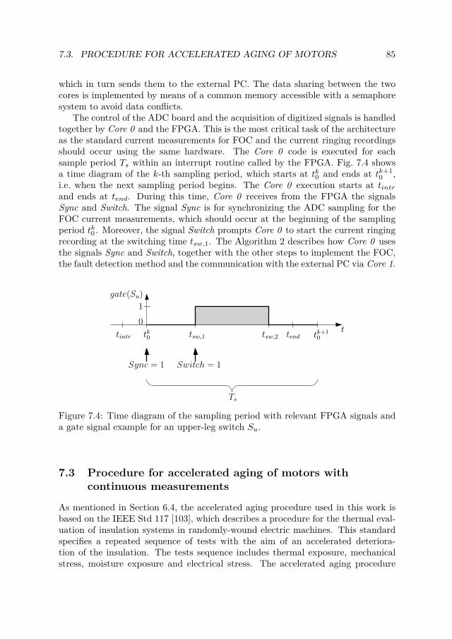
7.3. PROCEDURE FOR ACCELERATED AGING OF MOTORS 85
which in turn sends them to the external PC. The data sharing between the twocores is implemented by means of a common memory accessible with a semaphoresystem to avoid data conflicts.
The control of the ADC board and the acquisition of digitized signals is handledtogether by Core 0 and the FPGA. This is the most critical task of the architectureas the standard current measurements for FOC and the current ringing recordingsshould occur using the same hardware. The Core 0 code is executed for eachsample period Ts within an interrupt routine called by the FPGA. Fig. 7.4 showsa time diagram of the k-th sampling period, which starts at tk
0 and ends at tk+10 ,
i.e. when the next sampling period begins. The Core 0 execution starts at tintr
and ends at tend. During this time, Core 0 receives from the FPGA the signalsSync and Switch. The signal Sync is for synchronizing the ADC sampling for theFOC current measurements, which should occur at the beginning of the samplingperiod tk
0 . Moreover, the signal Switch prompts Core 0 to start the current ringingrecording at the switching time tsw,1. The Algorithm 2 describes how Core 0 usesthe signals Sync and Switch, together with the other steps to implement the FOC,the fault detection method and the communication with the external PC via Core 1.
gate(Su)
t
1
0
tk+10tk0 tsw,1 tsw,2 tendtintr
Sync = 1 Switch = 1
Ts
Figure 7.4: Time diagram of the sampling period with relevant FPGA signals anda gate signal example for an upper-leg switch Su.
7.3 Procedure for accelerated aging of motors withcontinuous measurements
As mentioned in Section 6.4, the accelerated aging procedure used in this work isbased on the IEEE Std 117 [103], which describes a procedure for the thermal eval-uation of insulation systems in randomly-wound electric machines. This standardspecifies a repeated sequence of tests with the aim of an accelerated deteriora-tion of the insulation. The tests sequence includes thermal exposure, mechanicalstress, moisture exposure and electrical stress. The accelerated aging procedure

86 CHAPTER 7. EXPERIMENTAL SETUP DESCRIPTION
1: tintr: Interrupt routine starts;2: While Sync = 0 do
Waiting for PWM period start;3: t0: ADC trigger and signal acquisition;4: Data post-processing and conversion;5: Checking limits, protections and drive state;6: Read data from Core 1 in the common memory
(commands, references and other data coming from the external PC);7: Reference frame conversions;8: Speed regulation;9: FOC and current regulation;
10: High-frequency injection and filtering for ITSC fault detection;11: Modulation and switching times calculations;12: Setting the ADC for MHz-range sampling:
fsampl = 62.5 MHz and Nsamples = 256;13: While Switch = 0 do
Waiting for switching transition;14: tsw,1: ADC trigger and signal acquisition;15: Setting the ADC for low-frequency sampling:
fsampl = 4 kHz and Nsamples = 1;16: Current ringing data post-processing and conversion;17: Write data to Core 1 in the common memory
(data logs, alarms and other data for the external PC);18: tend: Interrupt routine ends;
Algorithm 2: Steps executed in for combined drive control, ITSC fault de-tection method based on high-frequency injection, and MHz-range sampling.
conducted for this work took place in the Sustainable Power Lab at KTH, wherethe equipment for the mechanical stress and moisture exposure was not available.Therefore, only thermal and electrical stresses were applied in the performed agingprocedure. With reduced stresses applied, the risk was to have a too slow agingto give significant results in a reasonable time. Thus, a higher stress was appliedin the thermal cycles in order to compensate for the lack of mechanical stress andmoisture exposure. IEEE Std 117 makes suggestions for temperatures, and recom-mends adjusting these in order to obtain failure within 20 cycles. In this case ahigher temperature than the suggested value was used, yet even so there was noinsulation failure even after 60 cycles. The reference temperature values Tref setfor each of the thermal cycles are displayed in Table 7.1. During each thermal cycle,the motor was heated, then kept at the reference temperature for approximately6 h, and finally allowed to cool down during the night time, so as to be at roomtemperature the morning after, when another thermal cycle was started. As statedin IEEE Std 117, the considered cumulative testing time includes only the heating

7.3. PROCEDURE FOR ACCELERATED AGING OF MOTORS 87
and the thermal steady state times, but not the cooling time. The motor was as-sumed to be in thermal steady state when it reached a temperature 3 C lower thanthe reference. Fig. 7.5 shows the reached motor temperatures during acceleratingaging as a function of the cumulative testing time. In few thermal cycles the motortemperature temporarily dropped after reaching steady state because of practicalproblems that occurred during the procedure, which were promptly solved. Theperformed accelerated aging procedure amounts to a total cumulative testing timeof 550 h.
Table 7.1: Reference temperatures in the thermal cycles.
Thermal cycles Tref [C]1 - 28 24029 - 36 25037 - 44 25545 - 60 260
Figure 7.5: Temperature reached in the motor during accelerated aging as a functionof cumulative testing time. Temperature data points during the heating phase areexcluded for the sake of clarity.
The electrical stress was applied during all the thermal cycles as the motor wasfed with the PWM voltages of the custom converter in order to be heated. Theinsulation state was tested every 4 or 8 thermal cycles, with the motor at roomtemperature and all the cabling at the terminals disconnected. In these condi-tions, other than measuring the parasitic capacitances as described in Section 6.4,a Fluke 1555 insulation tester was employed to measure the insulation resistancebetween windings and ground, and also between the winding phases. A DC volt-age of 500 V was applied during this measurement, as suggested in the IEEE Std43 [112]. It is worth mentioning that, during the insulation resistance measure-ments, particular attention should be put on both the applied DC voltage value

88 CHAPTER 7. EXPERIMENTAL SETUP DESCRIPTION
and the actual motor temperature value. In a previous attempt of applying theaccelerated aging procedure to another IM specimen, a DC voltage of 1.8 kV wasapplied with the stator windings at over 150 C, causing the groundwall insulationbreakdown between phase a and ground. This insulation failure occurred when theprevious specimen had aged for only 12 thermal cycles, and with lower tempera-tures than the ones displayed in Table 7.1. Therefore, it was concluded that suchinsulation resistance measurement caused the premature failure of the motor andthus the interruption of the accelerated aging procedure without obtaining signifi-cant results. For this reason, during the attempt to age the second specimen thatis described in this section, a more conservative approach was taken during theinsulation resistance measurements.
The experimental setup employed for the accelerated aging procedure is shownin Fig. 7.6. The aged motor is the same 11 kW motor type as the prototypedescribed in Section 5.2, but without the taps. A mechanical lock was appliedto the rotor and thus, during the whole accelerated aging procedure, the motorwas at standstill. The locked rotor implied many practical simplifications to thetest procedure, in terms of noise and possible breaking of the bearings. Moreover,without any forced ventilation and with large rotor currents at standstill, the timeemployed for the heating phase could considerably decrease, reaching approximately3 h. The motor was supplied by the custom converter, where in the drive controlalgorithm the speed regulator was excluded and voltages at fixed 50 Hz frequencywere imposed. However, the current regulator was kept to tune the magnitude Is ofthe stator currents. The reference value for the current regulator was determined bya temperature regulator implemented in the Matlab GUI running on the externalPC, which communicates to the Zynq SoC via Ethernet. The temperature feedbackvalue for the temperature regulator was obtained as the maximum value Tmax
among the temperatures measured in the aging motor. In order to measure thetemperatures inside 6 stator slots and in 4 different points of the end windings,10 temperature sensors of type RTD PT100 were employed, which were connectedto a HP 34970A data acquisition unit that in turn was read by the Matlab GUIthrough serial communication. The temperature sampling and regulation wereactivated every 30 s. During the initial heating stage, regardless of the measuredtemperature values, the temperature regulator was set to give the maximum outputof 20 A to the current regulator in order to speed up the thermal cycle. Oncethe feedback temperature Tmax reached a value of 10 C below the reference valueTref , a PI regulator was activated for fine temperature regulation. Fig. 7.7 shows anexample of a single thermal cycle and the related regulation of the maximum motortemperature Tmax through the stator current magnitude Is, where the referencetemperature is 250 C.
In both attempts for the accelerated aging of IMs, fumes were produced when themotor temperature exceeded approximately 210 C, which is far above the class Finsulation limit of 155 C. These fumes were coming out through the plastic glandused to tighten the cable into the terminal box. The fumes consisted of evaporatedimpregnation varnish of the stator winding and they came out through the terminal

7.4. SUMMARY OF CHAPTER 89
Matlab GUI
Pump outlet
Pump intake
Custom converter
Aging motor
External PC
Pump
HP34970Ap
Figure 7.6: Complete illustration of the experimental setup for accelerated aging.
box that is the only unsealed part of the motor. In order to extract the fumes fromthe laboratory area, the pump and the blue pipe shown Fig. 7.6 were employed.The pipe intake was positioned on the top of the terminal box, and the outlet wasplaced outside the laboratory window. The accelerated aging consequences on theexternal appearance of the aged specimen are shown in Fig. 7.8, where the colorchange of the motor chassis is evident. Fig. 7.9 and Fig. 7.10 illustrate the impactson the stator winding and on the terminal box and its wiring, respectively. It canbe noted that after the accelerated aging process, most of the internal motor partswere covered by a layer of evaporated impregnation varnish.
7.4 Summary of chapter
This chapter provided a description of the experimental setup employed in thiswork. The custom converter is based on the Zynq SoC which could simultaneouslyperform the different required functionalities of drive control algorithm, ITSC faultdetection method, communication with external devices and MHz-range sampling.The details of the performed accelerated aging procedure were given, with particularfocus on the practicalities learned during the experiments.

90 CHAPTER 7. EXPERIMENTAL SETUP DESCRIPTION
(a)
(b)
Figure 7.7: Measurements taken during the 31st thermal cycle: (a) maximum motortemperature and (b) stator current magnitude.
(a) (b)
Figure 7.8: IM specimen (a) before and (b) after the accelerated aging process.Note the color change of the chassis, except for the motor feet.

7.4. SUMMARY OF CHAPTER 91
(a) (b)
Figure 7.9: Stator winding (a) before and (b) after the accelerated aging process.
(a) (b)
Figure 7.10: Terminal box and wiring (a) before and (b) after the accelerated agingprocess.


Chapter 8
Concluding remarks
8.1 Conclusions
This thesis is of multi-disciplinary nature and it collects topics from different fields.All the work done originated from the questions posed by the Industry 4.0 initiative,which forecasts the increased connectivity and additional functions of networkedelectric drives in industrial plants. Two application cases were analyzed as exam-ples of the additional functions of electric drives: condition monitoring and multi-drive systems. Generally, condition monitoring applications do not have real-timeconstraints as the degradation affecting electric drives is a slow phenomenon andthe data can be collected with very low frequencies, as hours or even days. For thisreason, condition monitoring data can be transmitted through asynchronous accessand it can be supported by all the described industrial communication protocols:traditional fieldbus, Ethernet-based and wireless-based. The situation is differentfor fault detection methods such as the ones described in Chapter 5, where a timelydetermination of a fast-spreading fault could guarantee the electric drive integrityby a forced stop of its operation. In this case, fault detection methods could di-rectly be implemented in the converter without the need for data transmission.Regarding the multi-drive systems application case, the resulting high transmis-sion rates, required in both cases of centralized and distributed control, demandthe real-time Ethernet communication protocols as the only possible solution for anetwork implementation.
Both condition monitoring and multi-drive control cases were applied to theEthernet-based real-time protocol EtherCAT. A performance model was proposedand analyzed for both centralized and distributed controls of multi-drive systemswith EtherCAT, where also aperiodic messages due to condition monitoring datawere considered. The feasibility of such EtherCAT implementations was proved tobe significantly influenced by the number of slaves and the forwarding times of theslaves. Moreover, the transmission of bulk data, originated by condition monitoringmethods, was considered in the traditional industrial fieldbus CAN. A model for
93

94 CHAPTER 8. CONCLUDING REMARKS
the schedulability analysis of small control periodic messages, developed in previousliterature, was extended to the case where also aperiodic bulk data is present in theCAN bus. An algorithm for optimizing the priority level of bulk data transmissionwas provided, showing a nearly optimal performance when the network load is low.
In the second and biggest part of the thesis, the focus was on the implementa-tion of condition monitoring algorithms for the stator winding insulation in elec-tric motors. The interturn short-circuit faults in induction motors were initiallyinvestigated. A generalized analytical model was described, which considers theinterturn fault presence in any of the stator phases and gives a choice between twodifferent modeling approaches for the leakage inductances of the faulty winding.Moreover, a finite-element model was developed, allowing inclusion of faults of dif-ferent severities and in different positions of the stator winding. Both analyticaland finite-element models were validated with experimental results obtained froman induction motor prototype with tapped windings, which can emulate the in-terturn short-circuit faults. On the one hand, the finite-element model shows anoverall greater accuracy compared to the analytical model and also the possibilityto simulate space harmonics, such as the rotor slot harmonics, which were furtherinvestigated as possible fault signatures. On the other hand, the analytical modelprovides a deeper understanding of the fault effects in the motor operation, andit can be used to evaluate fault detection methods. Two fault detection methodsbased on the negative-sequence current were analyzed both theoretically and exper-imentally. The first method is based on the negative-sequence current magnitudeat the fundamental frequency, and it was proven to be influenced by the machineoperating conditions. The second method, based on a high-frequency injection, isindependent of the operating conditions, and it gives correct information on thefaulted phase location.
The overall insulation condition of the stator winding insulation, including thegroundwall insulation, was monitored by means of MHz-range oscillations in thestator currents, namely current ringings, occurring after the switching transitionsof the converter. In order to quantify the current ringing variations and thus theinsulation change, metrics based on the RMS and peak values of the ringings wereproposed and analyzed. The variations of the insulation condition were emulatedby adding additional capacitors to the stator winding taps and then also inducedthrough an accelerated aging procedure applied to the whole machine. The in-troduced metrics show a quasi-linear behavior with respect to the change of theparasitic capacitances, which are dependent on the insulation state. All the ex-periments performed in this work were conducted using a setup in which a customconverter was the central part. This converter is based on the Zynq SoC which couldsimultaneously perform a drive control algorithm, the fault detection method basedon the high-frequency injection, an IP communication with external devices, andwhich was also able to record the stator current ringings after the switch commuta-tions. The custom converter was also employed for the accelerated aging procedureof the stator winding insulation, which is based on thermal and electrical stresses.This procedure allowed aging the motor while periodically measuring the required

8.2. SUGGESTIONS FOR FUTURE WORK 95
signals for monitoring purposes, such as the current ringings. Practical details weregiven for future applications of this procedure.
8.2 Suggestions for future work
The possible future work derived from this thesis is summarized as follows.
• The experimental realization of a network of electric drives, where the datagenerated by the condition monitoring and multi-drive system applicationcases could be exchanged and therefore analyzed. The specific EtherCAT andCAN protocols could be employed for this purpose, and thus the proposedperformance and scheduling models could be tested.
• The relations between the fault severity of an interturn short-circuit fault andthe various fault signatures were described in this work. The following stepto implement for a complete predictive maintenance method would imply todetermine at which level of fault severity it is necessary to stop the driveoperation.
• The online testing of the described fault detection methods with electric mo-tors where the interturn short-circuit fault is occurring in reality, instead ofbeing emulated with a motor equipped with taps. This could imply the needto age several motors in order to have a real example of the required fault.A more economic alternative could entail the use stator segments as the mo-torettes, instead of the whole motor.
• Test the proposed metrics based on the MHz-range current ringings withmore aging specimens. In this manner a proper statistical analysis can beconducted and algorithms calculating the remaining useful life of the statorwinding could be designed.
• Test the accelerated aging procedure with more specimens and for longertime, in order to establish how long it averagely take for a specimen to failcompared to the procedure suggested in the IEEE Std 117.
• A more compact design of the custom converter where all the processing unit,sensors, signal conditioning circuitry and signal acquisition board are placedin the same chassis together with the power unit.


Bibliography
[1] F. J. T. E. Ferreira and A. T. de Almeida, “Reducing Energy Costs in Electric-Motor-Driven Systems: Savings Through Output Power Reduction and En-ergy Regeneration,” IEEE Industry Applications Magazine, vol. 24, no. 1, pp.84–97, Jan. 2018.
[2] A. T. de Almeida, F. J. T. E. Ferreira, and G. Baoming, “Beyond InductionMotors—Technology Trends to Move Up Efficiency,” IEEE Transactions onIndustry Applications, vol. 50, no. 3, pp. 2103–2114, May 2014.
[3] ABB, “Cost of ownership.” [Online]. Available: https://new.abb.com/motors-generators/generators/generators-for-engines/cost-of-ownership/why-knowing-the-true-cost-of-ownership-of-your-process-can-help-avoid-catastrophic-failure
[4] K. N. Gyftakis and A. J. M. Cardoso, “Reliable Detection of Stator InterturnFaults of Very Low Severity Level in Induction Motors,” IEEE Transactionson Industrial Electronics, vol. 68, no. 4, pp. 3475–3484, Apr. 2021.
[5] E. A. Lee and S. A. Seshia, Introduction to Embedded Systems, A Cyber-Physical Systems Approach, 2nd ed. MIT Press, 2017.
[6] R. Drath and A. Horch, “Industrie 4.0: Hit or Hype?” IEEE IndustrialElectronics Magazine, vol. 8, no. 2, pp. 56–58, Jun. 2014.
[7] M. Wollschlaeger, T. Sauter, and J. Jasperneite, “The Future of IndustrialCommunication: Automation Networks in the Era of the Internet of Thingsand Industry 4.0,” IEEE Industrial Electronics Magazine, vol. 11, no. 1, pp.17–27, Mar. 2017.
[8] J. Taalbi, “Origins and pathways of innovation in the third industrial revo-lution,” Industrial and Corporate Change, vol. 28, no. 5, pp. 1125–1148, Oct.2019.
[9] ABB, “800xA architecture.” [Online]. Available: https://new.abb.com/control-systems/fi/system-800xa/hajautettu-800xa-ohjausjarjestelma/system/arkkitehtuuri
97

98 BIBLIOGRAPHY
[10] A. W. Colombo, S. Karnouskos, O. Kaynak, Y. Shi, and S. Yin, “IndustrialCyberphysical Systems: A Backbone of the Fourth Industrial Revolution,”IEEE Industrial Electronics Magazine, vol. 11, no. 1, pp. 6–16, Mar. 2017.
[11] ABB, “Boosting industrial profitability with energy ef-ficient drives and motors,” 2016. [Online]. Available:https://library.e.abb.com/public/2e734441d8744490867b941e74949d85/EN_Energy_efficiency_brochure_3AUA0000087517_REVC.pdf
[12] ——, “Fieldbus communications.” [Online]. Available: https://new.abb.com/drives/connectivity/fieldbus-connectivity
[13] F. Benzi, G. S. Buja, and M. Felser, “Communication architectures for elec-trical drives,” IEEE Transactions on Industrial Informatics, vol. 1, no. 1, pp.47–53, Feb. 2005.
[14] ABB, “ABB Ability™ digital services for drives,” 2020. [Online].Available: https://search.abb.com/library/Download.aspx?DocumentID=9AKK106930A8297&LanguageCode=en&DocumentPartId=&Action=Launch
[15] A. Belahcen, K. N. Gyftakis, J. Martinez, V. Climente-Alarcon, andT. Vaimann, “Condition monitoring of electrical machines and its relationto industrial internet,” in 2015 IEEE Workshop on Electrical Machines De-sign, Control and Diagnosis (WEMDCD), Mar. 2015, pp. 233–241.
[16] B. Galloway and G. P. Hancke, “Introduction to Industrial Control Net-works,” IEEE Communications Surveys Tutorials, vol. 15, no. 2, pp. 860–880,Jul. 2013.
[17] S. Vitturi, L. Peretti, L. Seno, M. Zigliotto, and C. Zunino, “Real-time Ether-net networks for motion control,” Computer Standards & Interfaces, vol. 33,no. 5, pp. 465–476, Sep. 2011.
[18] M. Raza, N. Aslam, H. Le-Minh, S. Hussain, Y. Cao, and N. M. Khan, “ACritical Analysis of Research Potential, Challenges, and Future Directives inIndustrial Wireless Sensor Networks,” IEEE Communications Surveys Tuto-rials, vol. 20, no. 1, pp. 39–95, 2018.
[19] M. Gidlund, T. Lennvall, and J. Åkerberg, “Will 5G Become Yet AnotherWireless Technology for Industrial Automation?” in 2017 IEEE InternationalConference on Industrial Technology (ICIT), Mar. 2017, pp. 1319–1324.
[20] B. Martinez, C. Cano, and X. Vilajosana, “A Square Peg in a Round Hole:The Complex Path for Wireless in the Manufacturing Industry,” IEEE Com-munications Magazine, vol. 57, no. 4, pp. 109–115, Apr. 2019.

BIBLIOGRAPHY 99
[21] M. Luvisotto, Z. Pang, and D. Dzung, “High-Performance Wireless Networksfor Industrial Control Applications: New Targets and Feasibility,” Proceed-ings of the IEEE, vol. 107, no. 6, pp. 1074–1093, Jun. 2019.
[22] M. Riera-Guasp, J. A. Antonino-Daviu, and G. A. Capolino, “Advances inElectrical Machine, Power Electronic, and Drive Condition Monitoring andFault Detection: State of the Art,” IEEE Transactions on Industrial Elec-tronics, vol. 62, no. 3, pp. 1746–1759, Mar. 2015.
[23] G. A. Capolino, J. A. Antonino-Daviu, and M. Riera-Guasp, “Modern Diag-nostics Techniques for Electrical Machines, Power Electronics, and Drives,”IEEE Transactions on Industrial Electronics, vol. 62, no. 3, pp. 1738–1745,Mar. 2015.
[24] S. B. Lee, G. C. Stone, J. Antonino-Daviu, K. N. Gyftakis, E. G. Strangas,P. Maussion, and C. A. Platero, “Condition Monitoring of Industrial Elec-tric Machines: State of the Art and Future Challenges,” IEEE IndustrialElectronics Magazine, vol. 14, no. 4, pp. 158–167, Dec. 2020.
[25] J. H. Jung, J. J. Lee, and B. H. Kwon, “Online Diagnosis of Induction MotorsUsing MCSA,” IEEE Transactions on Industrial Electronics, vol. 53, no. 6,pp. 1842–1852, Dec. 2006.
[26] F. Briz, M. W. Degner, A. Zamarron, and J. M. Guerrero, “Online statorwinding fault diagnosis in inverter-fed AC machines using high-frequency sig-nal injection,” IEEE Transactions on Industry Applications, vol. 39, no. 4,pp. 1109–1117, Jul. 2003.
[27] P. Nussbaumer, M. A. Vogelsberger, and T. M. Wolbank, “Induction MachineInsulation Health State Monitoring Based on Online Switching Transient Ex-ploitation,” IEEE Transactions on Industrial Electronics, vol. 62, no. 3, pp.1835–1845, Mar. 2015.
[28] T. M. Parreiras, J. C. G. Justino, A. V. Rocha, and B. d. J. C. Filho, “TrueUnit Power Factor Active Front End for High-Capacity Belt-Conveyor Sys-tems,” IEEE Transactions on Industry Applications, vol. 52, no. 3, pp. 2737–2746, May 2016.
[29] J. Iyer, M. Chapariha, F. Therrien, and J. Jatskevich, “Improved torque shar-ing in multi induction motor VFD systems using current feedback,” in 201225th IEEE Canadian Conference on Electrical and Computer Engineering(CCECE), Apr. 2012, pp. 1–5.
[30] D. Xiao, X. Li, and K. He, “Power Balance of Starting Process for Pipe BeltConveyor Based on Master-Slave Control,” IEEE Access, vol. 6, pp. 16 924–16 931, Mar. 2018.

100 BIBLIOGRAPHY
[31] M. P. Sruthi, C. Nagamani, and G. S. Ilango, “Dynamic Load Sharing inMulti-Machine Conveyor Belt Systems,” in 2017 IEEE PES Asia-PacificPower and Energy Engineering Conference (APPEEC), Nov. 2017, pp. 1–6.
[32] A. Kurt, A. K. Atalay, and D. A. Kocabas, “Load sharing analysis of identicalwound rotor induction motors driving the same load,” in 2016 InternationalAutomatic Control Conference (CACS), Nov. 2016, pp. 247–251.
[33] M. Bernia and P. Sicard, “A hierarchical algorithm for load sharing in Multi-machine Multi-converter Systems with flexible coupling,” in 2015 IEEE 28th
Canadian Conference on Electrical and Computer Engineering (CCECE),May 2015, pp. 1151–1155.
[34] D. Meike, M. Pellicciari, and G. Berselli, “Energy Efficient Use of MultirobotProduction Lines in the Automotive Industry: Detailed System Modeling andOptimization,” IEEE Transactions on Automation Science and Engineering,vol. 11, no. 3, pp. 798–809, Jul. 2014.
[35] G. Parise, L. Parise, A. Malerba, F. M. Pepe, A. Honorati, and P. B. Chavdar-ian, “Comprehensive Peak-Shaving Solutions for Port Cranes,” IEEE Trans-actions on Industry Applications, vol. 53, no. 3, pp. 1799–1806, May 2017.
[36] L. Lo Bello, E. Bini, and G. Patti, “Priority-Driven Swapping-Based Schedul-ing of Aperiodic Real-Time Messages Over EtherCAT Networks,” IEEETransactions on Industrial Informatics, vol. 11, no. 3, pp. 741–751, Jun. 2015.
[37] N. Bibinagar and W. Kim, “Switched Ethernet-Based Real-Time NetworkedControl System with Multiple-Client–Server Architecture,” IEEE/ASMETransactions on Mechatronics, vol. 18, no. 1, pp. 104–112, Feb. 2013.
[38] D. E. Lee, Q. V. Nguyen, T. Kim, J. Y. Moon, and J. W. Jeon, “Developmentof independent EtherCAT slave module and application to closed loop stepmotor drive with multi-axis,” in 2016 International Conference on Comput-ing, Communication and Automation (ICCCA), Apr. 2016, pp. 912–917.
[39] V. Q. Nguyen, N. Van Phan Tran, H. N. Tran, K. M. Le, and J. W. Jeon, “Aclosed-loop stepper motor drive based on EtherCAT,” in IECON 2017 - 43rd
Annual Conference of the IEEE Industrial Electronics Society, Oct. 2017, pp.3361–3365.
[40] EtherCAT Technology Group, “EtherCAT - The Ethernet Fieldbus.”[Online]. Available: https://www.ethercat.org/
[41] G. Prytz, “A performance analysis of EtherCAT and PROFINET IRT,” in2008 IEEE International Conference on Emerging Technologies and FactoryAutomation, Sep. 2008, pp. 408–415.

BIBLIOGRAPHY 101
[42] R. I. Davis, A. Burns, R. J. Bril, and J. J. Lukkien, “Controller Area Network(CAN) schedulability analysis: Refuted, revisited and revised,” Real-TimeSystems, vol. 35, no. 3, pp. 239–272, Apr. 2007.
[43] Road vehicles – Controller Area Network (CAN) – Part 1: Data link layerand physical signalling, ISO 11 898-1:2015, Dec. 2015. [Online]. Available:https://www.iso.org/standard/63648.html
[44] K. Tindell, H. Hansson, and A. J. Wellings, “Analysing real-time communica-tions: controller area network (CAN),” in 1994 Proceedings of the Real-TimeSystems Symposium, Dec. 1994, pp. 259–263.
[45] K. Tindell and A. Burns, “Guaranteeing Message Latencies on ControllerArea Network (CAN),” in Proceedings of the 1st International CAN Confer-ence, 1994.
[46] K. Tindell, A. Burns, and A. J. Wellings, “Calculating controller area network(CAN) message response times,” Control Engineering Practice, vol. 3, no. 8,pp. 1163–1169, Aug. 1995.
[47] I. Broster, A. Burns, and G. Rodriguez-Navas, “Probabilistic analysis of CANwith faults,” in 23rd IEEE Real-Time Systems Symposium, Dec. 2002.
[48] K. W. Schmidt, “Robust Priority Assignments for Extending Existing Con-troller Area Network Applications,” IEEE Transactions on Industrial Infor-matics, vol. 10, no. 1, pp. 578–585, Feb. 2014.
[49] R. I. Davis, S. Kollmann, V. Pollex, and F. Slomka, “Schedulability analysisfor Controller Area Network (CAN) with FIFO queues, priority queues andgateways,” Real-Time Systems, vol. 49, no. 1, pp. 73–116, Jan. 2013.
[50] S. Mubeen, J. Mäki-Turja, and M. Sjödin, “Extending worst case response-time analysis for Mixed Messages in Controller Area Network With Priorityand FIFO Queues,” IEEE Access, vol. 2, pp. 365–380, 2014.
[51] G. Stone, E. A. Boulter, I. Culbert, and H. Dhirani, Electrical Insulation forRotating Machines: Design, Evaluation, Aging, Testing, and Repair. IEEEPress Series on Power Engineering, 2004.
[52] A. Morya, M. C. Gardner, B. Anvari, L. Liu, A. G. Yepes, J. Doval-Gandoy,and H. Toliyat, “Wide Bandgap Devices in AC Electric Drives: Opportunitiesand Challenges,” IEEE Transactions on Transportation Electrification, vol. 5,pp. 3–20, Mar. 2019.
[53] C. Zoeller, M. A. Vogelsberger, T. M. Wolbank, and H. Ertl, “Impact of SiCsemiconductors switching transition speed on insulation health state moni-toring of traction machines,” IET Power Electronics, vol. 9, no. 15, pp. 2769–2775, 2016.

102 BIBLIOGRAPHY
[54] A. Berzoy, A. A. S. Mohamed, and O. Mohammed, “Complex-Vector Modelof Interturn Failure in Induction Machines for Fault Detection and Identi-fication,” IEEE Transactions on Industry Applications, vol. 53, no. 3, pp.2667–2678, May 2017.
[55] R. M. Tallam, T. G. Habetler, and R. G. Harley, “Transient model for in-duction machines with stator winding turn faults,” IEEE Transactions onIndustry Applications, vol. 38, no. 3, pp. 632–637, May 2002.
[56] S. M. A. Cruz and A. J. M. Cardoso, “Multiple reference frames theory: a newmethod for the diagnosis of stator faults in three-phase induction motors,”IEEE Transactions on Energy Conversion, vol. 20, no. 3, pp. 611–619, Sep.2005.
[57] S. Bachir, S. Tnani, J.-C. Trigeassou, and G. Champenois, “Diagnosis byparameter estimation of stator and rotor faults occurring in induction ma-chines,” IEEE Transactions on Industrial Electronics, vol. 53, no. 3, pp. 963–973, Jun. 2006.
[58] J. Yun, K. Lee, K. W. Lee, S. B. Lee, and J. Y. Yoo, “Detection and Classifi-cation of Stator Turn Faults and High-Resistance Electrical Connections forInduction Machines,” IEEE Transactions on Industry Applications, vol. 45,no. 2, pp. 666–675, Mar. 2009.
[59] D. C. Patel and M. C. Chandorkar, “Modeling and Analysis of Stator Inter-turn Fault Location Effects on Induction Machines,” IEEE Transactions onIndustrial Electronics, vol. 61, no. 9, pp. 4552–4564, Sep. 2014.
[60] S. Lingam Senthil Kumar, “Condition monitoring of induction machines usinga signal injection technique,” M.Sc. thesis, KTH Royal Institute of Technol-ogy, 2020.
[61] M. Otero, G. R. Bossio, P. M. de la Barrera, O. Tyshakin, and R. Leidhold,“Inter-turn faults detection in Induction Motor drives using zero-sequencesignal injection,” in 2018 International Symposium on Power Electronics,Electrical Drives, Automation and Motion (SPEEDAM), Jun. 2018, pp. 202–207.
[62] M. F. Far, A. Arkkio, and J. Roivainen, “Electrical fault diagnosis for aninduction motor using an electromechanical FE model,” in 2014 InternationalConference on Electrical Machines (ICEM), Sep. 2014, pp. 1881–1887.
[63] W. Zaabi, Y. Bensalem, and H. Trabelsi, “Fault analysis of induction machineusing finite element method (FEM),” in 2014 15th International Conferenceon Sciences and Techniques of Automatic Control and Computer Engineering(STA), Dec. 2014, pp. 388–393.

BIBLIOGRAPHY 103
[64] V. Fireteanu, V. Leconte, and A.-I. Constantin, “Finite element analysison early detection of the short-circuit faults in induction machines throughharmonics of the stator currents or of the neighboring magnetic field,” in2017 International Conference on Optimization of Electrical and ElectronicEquipment (OPTIM) 2017 Intl Aegean Conference on Electrical Machinesand Power Electronics (ACEMP), May 2017, pp. 420–427.
[65] M. Malekpour, B. T. Phung, and E. Ambikairajah, “Online technique for insu-lation assessment of induction motor stator windings under different load con-ditions,” IEEE Transactions on Dielectrics and Electrical Insulation, vol. 24,no. 1, pp. 349–358, Feb. 2017.
[66] W. Pietrowski and K. Górny, “Wavelet analysis of torque at startup of an in-duction machine under inter-turn short-circuit,” in 2017 International Sym-posium on Electrical Machines (SME), Jun. 2017, pp. 1–4.
[67] H. H. Eldeeb, A. Berzoy, and O. Mohammed, “Stator Fault Detection onDTC-Driven IM via Magnetic Signatures Aided by 2-D FEA Co-Simulation,”IEEE Transactions on Magnetics, vol. 55, no. 6, pp. 1–5, Jun. 2019.
[68] P. Kumar N. and T. B. Isha, “FEM based electromagnetic signature analysisof winding inter-turn short-circuit fault in inverter fed induction motor,” CESTransactions on Electrical Machines and Systems, vol. 3, no. 3, pp. 309–315,Sep. 2019.
[69] P. Chen, Y. Xie, and S. Hu, “The Effect of Stator Inter-Turn Short CircuitFaults on Electromagnetic Performances of Induction Motors,” in 2019 22nd
International Conference on Electrical Machines and Systems (ICEMS), Aug.2019, pp. 1–5, iSSN: 2642-5513.
[70] W. Pietrowski and K. Górny, “Analysis of Torque Ripples of an InductionMotor Taking into Account a Inter-Turn Short-Circuit in a Stator Winding,”Energies, vol. 13, no. 14, p. 3626, Jan. 2020.
[71] Y. Chen, A. U. Rehman, Y. Zhao, L. Wang, S. Wang, M. Zhang, Y. Zhao,Y. Cheng, and T. Tanaka, “Numerical Modeling, Electrical CharacteristicsAnalysis and Experimental Validation of Severe Inter-Turn Short CircuitFault Conditions on Stator Winding in DFIG of Wind Turbines,” IEEE Ac-cess, vol. 9, pp. 13 149–13 158, 2021.
[72] E. Elbouchikhi, Y. Amirat, G. Feld, and M. Benbouzid, “Generalized Like-lihood Ratio Test Based Approach for Stator-Fault Detection in a PWMInverter-Fed Induction Motor Drive,” IEEE Transactions on Industrial Elec-tronics, vol. 66, no. 8, pp. 6343–6353, Aug. 2019.
[73] S. Cheng, P. Zhang, and T. G. Habetler, “An Impedance Identification Ap-proach to Sensitive Detection and Location of Stator Turn-to-Turn Faults

104 BIBLIOGRAPHY
in a Closed-Loop Multiple-Motor Drive,” IEEE Transactions on IndustrialElectronics, vol. 58, no. 5, pp. 1545–1554, May 2011.
[74] F. Briz, M. W. Degner, P. Garcia, and A. B. Diez, “High-Frequency Carrier-Signal Voltage Selection for Stator Winding Fault Diagnosis in Inverter-FedAC Machines,” IEEE Transactions on Industrial Electronics, vol. 55, no. 12,pp. 4181–4190, Dec. 2008.
[75] F. Briz, M. W. Degner, A. B. Diez, and J. M. Guerrero, “Online diagnostics ininverter-fed induction machines using high-frequency signal injection,” IEEETransactions on Industry Applications, vol. 40, no. 4, pp. 1153–1161, Jul.2004.
[76] P. M. de la Barrera, G. R. Bossio, and J. A. Solsona, “High-Resistance Con-nection Detection in Induction Motor Drives Using Signal Injection,” IEEETransactions on Industrial Electronics, vol. 61, no. 7, pp. 3563–3573, Jul.2014.
[77] J. Zhang, Z. Xu, J. Wang, J. Zhao, Z. Din, and M. Cheng, “Detection andDiscrimination of Incipient Stator Faults for Inverter-Fed Permanent Mag-net Synchronous Machines,” IEEE Transactions on Industrial Electronics,vol. 68, no. 8, pp. 7505–7515, Aug. 2021.
[78] G. M. Joksimović and J. Penman, “The detection of inter-turn short circuitsin the stator windings of operating motors,” IEEE Transactions on IndustrialElectronics, vol. 47, no. 5, pp. 1078–1084, Oct. 2000.
[79] A. Stavrou, H. G. Sedding, and J. Penman, “Current monitoring for detectinginter-turn short circuits in induction motors,” IEEE Transactions on EnergyConversion, vol. 16, no. 1, pp. 32–37, Mar. 2001.
[80] V. Climente-Alarcon, J. A. Antonino-Daviu, A. Haavisto, and A. Arkkio,“Diagnosis of Induction Motors Under Varying Speed Operation by Princi-pal Slot Harmonic Tracking,” IEEE Transactions on Industry Applications,vol. 51, no. 5, pp. 3591–3599, Sep. 2015.
[81] J. Yang, S. B. Lee, J. Yoo, S. Lee, Y. Oh, and C. Choi, “A Stator WindingInsulation Condition Monitoring Technique for Inverter-Fed Machines,” IEEETransactions on Power Electronics, vol. 22, no. 5, pp. 2026–2033, Sep. 2007.
[82] S. Grubic, J. Restrepo, and T. G. Habetler, “Online Surge Testing Applied toan Induction Machine With Emulated Insulation Breakdown,” IEEE Trans-actions on Industry Applications, vol. 49, no. 3, pp. 1358–1366, May 2013.
[83] P. Neti and S. Grubic, “Online Broadband Insulation Spectroscopy of In-duction Machines Using Signal Injection,” IEEE Transactions on IndustryApplications, vol. 53, no. 2, pp. 1054–1062, Mar. 2017.
BIBLIOGRAPHY 105
[84] F. Perisse, P. Werynski, and D. Roger, “A New Method for AC MachineTurn Insulation Diagnostic Based on High Frequency Resonances,” IEEETransactions on Dielectrics and Electrical Insulation, vol. 14, no. 5, pp. 1308–1315, Oct. 2007.
[85] S. B. Lee, J. Yang, K. Younsi, and R. M. Bharadwaj, “An online groundwalland phase-to-phase insulation quality assessment technique for AC-machinestator windings,” IEEE Transactions on Industry Applications, vol. 42, no. 4,pp. 946–957, Jul. 2006.
[86] P. Zhang, K. Younsi, and P. Neti, “A Novel Online Stator Ground-Wall Insu-lation Monitoring Scheme for Inverter-Fed AC Motors,” IEEE Transactionson Industry Applications, vol. 51, no. 3, pp. 2201–2207, May 2015.
[87] D. Zheng, G. Lu, and P. Zhang, “An Improved Online Stator Insulation Mon-itoring Method Based on Common-mode Impedance Spectrum Consideringthe Effect of Ageing Position,” IEEE Transactions on Industry Applications,early access.
[88] F. Niu, Y. Wang, S. Huang, L. Wu, X. Huang, Y. Fang, and T. Yang, “AnOnline Groundwall Insulation Monitoring Method Based on Transient Char-acteristics of Leakage Current for Inverter-Fed Motors,” IEEE Transactionson Power Electronics, early access.
[89] D. Zheng and P. Zhang, “An Online Groundwall and Phase-to-Phase StatorInsulation Monitoring Method for Inverter-Fed Machine,” IEEE Transactionson Industrial Electronics, vol. 68, no. 6, pp. 5303–5313, Jun. 2021.
[90] P. Zhang, D. Zheng, and G. Lu, “The Effect and Compensation of Phase An-gle Deviation Along the Winding for the Online Stator Insulation ConditionMonitoring,” IEEE Transactions on Industrial Electronics, vol. 69, no. 8, pp.8440–8451, Aug. 2022.
[91] H. Li, Y. Gu, D. Xiang, P. Zhang, P. Yue, and Y. Cui, “Online ConditionMonitoring of Line-end Coils Insulation for Inverter-fed Machine by SwitchingOscillation Mode Decomposition,” IEEE Transactions on Industrial Electron-ics, early access.
[92] D. Xiang, H. Li, H. Yan, Y. Zheng, N. Zhao, and B. Liu, “Online Monitoringof Incipient Turn Insulation Degradation for Inverter-Fed Machine Using Sen-sitive Tail Component in PWM Switching Oscillations,” IEEE Transactionson Power Electronics, vol. 36, no. 8, pp. 8730–8742, Aug. 2021.
[93] R. Leuzzi, V. G. Monopoli, L. Rovere, F. Cupertino, and P. Zanchetta, “Anal-ysis and Detection of Electrical Aging Effects on High-Speed Motor Insula-tion,” IEEE Transactions on Industry Applications, vol. 55, no. 6, pp. 6018–6025, Nov. 2019.

106 BIBLIOGRAPHY
[94] I. Tsyokhla, A. Griffo, and J. Wang, “Online Condition Monitoring for Di-agnosis and Prognosis of Insulation Degradation of Inverter-Fed Machines,”IEEE Transactions on Industrial Electronics, vol. 66, no. 10, pp. 8126–8135,Oct. 2019.
[95] W. R. Jensen, E. G. Strangas, and S. N. Foster, “A Method for Online StatorInsulation Prognosis for Inverter-Driven Machines,” IEEE Transactions onIndustry Applications, vol. 54, no. 6, pp. 5897–5906, Nov. 2018.
[96] C. Zoeller, M. A. Vogelsberger, R. Fasching, W. Grubelnik, and T. M. Wol-bank, “Evaluation and Current-Response-Based Identification of InsulationDegradation for High Utilized Electrical Machines in Railway Application,”IEEE Transactions on Industry Applications, vol. 53, no. 3, pp. 2679–2689,May 2017.
[97] Z. Huang, A. Reinap, and M. Alaküla, “Dielectric properties modeling andmeasurement of single tooth coil insulation system under accelerated degra-dation test,” in 2016 XXII International Conference on Electrical Machines(ICEM), Sep. 2016, pp. 2698–2703.
[98] K. N. Gyftakis, M. Sumislawska, D. F. Kavanagh, D. A. Howey, and M. D.McCulloch, “Dielectric Characteristics of Electric Vehicle Traction MotorWinding Insulation Under Thermal Aging,” IEEE Transactions on IndustryApplications, vol. 52, no. 2, pp. 1398–1404, Mar. 2016.
[99] M. Sumislawska, K. N. Gyftakis, D. F. Kavanagh, M. D. McCulloch, K. J.Burnham, and D. A. Howey, “The Impact of Thermal Degradation on Proper-ties of Electrical Machine Winding Insulation Material,” IEEE Transactionson Industry Applications, vol. 52, no. 4, pp. 2951–2960, Jul. 2016.
[100] D. F. Kavanagh, K. N. Gyftakis, and M. D. McCulloch, “Thermal Degrada-tion Phenomena of Polymer Film on Magnet Wire for Electromagnetic Coils,”IEEE Transactions on Industry Applications, vol. 57, no. 1, pp. 458–467, Jan.2021.
[101] C. Zoeller, M. A. Vogelsberger, R. Fasching, W. Grubelnik, and T. M. Wol-bank, “Evaluation and current-response based identification of insulationdegradation for high utilized electrical machines in railway application,” in2015 IEEE 10th International Symposium on Diagnostics for Electrical Ma-chines, Power Electronics and Drives (SDEMPED). Institute of Electricaland Electronics Engineers (IEEE), Sep. 2015, pp. 266–272.
[102] M. Gasior and J. L. Gonzalez, “Improving FFT Frequency Measurement Res-olution by Parabolic and Gaussian Spectrum Interpolation,” AIP ConferenceProceedings, vol. 732, no. 1, pp. 276–285, Nov. 2004.

BIBLIOGRAPHY 107
[103] IEEE, “IEEE Standard Test Procedure for Thermal Evaluation of Systems ofInsulating Materials for Random-Wound AC Electric Machinery,” IEEE Std117-2015 (Revision of IEEE Std 117-1974), pp. 1–34, May 2016.
[104] Z. Huang, “Modeling and Testing of Insulation Degradation due to DynamicThermal Loading of Electrical Machines,” Ph.D. dissertation, Lund Univer-sity, Jan. 2017.
[105] M. Farahani, E. Gockenbach, H. Borsi, K. Schafer, and M. Kaufhold, “Be-havior of machine insulation systems subjected to accelerated thermal agingtest,” IEEE Transactions on Dielectrics and Electrical Insulation, vol. 17,no. 5, pp. 1364–1372, Oct. 2010.
[106] D. W. Brown, M. Abbas, A. Ginart, I. N. Ali, P. W. Kalgren, and G. J.Vachtsevanos, “Turn-Off Time as an Early Indicator of Insulated Gate BipolarTransistor Latch-up,” IEEE Transactions on Power Electronics, vol. 27, no. 2,pp. 479–489, Feb. 2012.
[107] J. Liu, G. Zhang, Q. Chen, L. Qi, Y. Geng, and J. Wang, “In situ Con-dition Monitoring of IGBTs Based on the Miller Plateau Duration,” IEEETransactions on Power Electronics, vol. 34, no. 1, pp. 769–782, Jan. 2019.
[108] P. Landsmann, “Sensorless Control of Synchronous Machines by Linear Ap-proximation of Oversampled Current,” Ph.D. dissertation, Technische Uni-versität München, Sep. 2014.
[109] D. M. Hind, “Current derivative estimation for sensorless motor drives,”Ph.D. dissertation, University of Nottingham, Jul. 2015.
[110] M. Giuliato, L. Peretti, F. Tinazzi, and M. Zigliotto, “Sensorless control for asynchronous reluctance motor based on current oversampling using standardPWM excitation,” in The 10th International Conference on Power Electron-ics, Machines and Drives (PEMD 2020), vol. 2020, Dec. 2020, pp. 13–18.
[111] Sensitec GmbH, “CMS3050 Highly Dynamic MagnetoRe-sistive Current Sensor,” Tech. Rep. [Online]. Avail-able: https://www.sensitec.com/fileadmin/sensitec/Service_and_Support/Downloads/Data_Sheets/CMS3000/SENSITEC_CMS3050_DSE_06.pdf
[112] IEEE, “IEEE Recommended Practice for Testing Insulation Resistance ofElectric Machinery,” IEEE Std 43-2013 (Revision of IEEE Std 43-2000), pp.1–37, Mar. 2014.