University of Central Florida University of Central Florida

STARS STARS

Electronic Theses and Dissertations, 2004-2019

2015

Modeling and Analysis of Automated Storage and Retrievals Modeling and Analysis of Automated Storage and Retrievals

System with Multiple in-the-aisle Pick Positions System with Multiple in-the-aisle Pick Positions

Faraz Ramtin University of Central Florida, faraz.ramtin84@gmail.com

Part of the Industrial Engineering Commons

Find similar works at: https://stars.library.ucf.edu/etd

University of Central Florida Libraries http://library.ucf.edu

This Doctoral Dissertation (Open Access) is brought to you for free and open access by STARS. It has been accepted

for inclusion in Electronic Theses and Dissertations, 2004-2019 by an authorized administrator of STARS. For more

information, please contact STARS@ucf.edu.

STARS Citation STARS Citation

Ramtin, Faraz, "Modeling and Analysis of Automated Storage and Retrievals System with Multiple in-the-

aisle Pick Positions" (2015). Electronic Theses and Dissertations, 2004-2019. 77.

https://stars.library.ucf.edu/etd/77

MODELING AND ANALYSIS OF AUTOMATED STORAGE AND

RETRIEVAL SYSTEM WITH MULTIPLE IN-THE-AISLE

PICK POSITIONS

by

FARAZ RAMTIN B.S. Shahid Beheshti University, 2007

M.S. Amirkabir University of Technology, 2010

A dissertation submitted in partial fulfillment of the requirements

for the degree of Doctor of Philosophy

in the Department of Industrial Engineering and Management Systems

in the College of Engineering and Computer Science

at the University of Central Florida

Orlando, Florida

Spring Term

2015

Major Professor: Jennifer Pazour

ii

© 2015 Faraz Ramtin

iii

ABSTRACT

This dissertation focuses on developing analytical models for automated storage and

retrieval system with multiple in-the-aisle pick positions (MIAPP-AS/RS). Specifically, our first

contribution develops an expected travel time model for different pick positions and different

physical configurations for a random storage policy. This contribution has been accepted for

publication in IIE Transactions (Ramtin & Pazour, 2014) and was the featured article in the IE

Magazine (Askin & Nussbaum, 2014). The second contribution addresses an important design

question associated with MIAPP-AS/RS, which is the assignment of items to pick positions in an

MIAPP-AS/RS. This contribution has been accepted for publication in IIE Transactions

(Ramtin & Pazour, 2015). Finally, the third contribution is to develop travel time models and to

determine the optimal SKUs to storage locations assignment under different storage assignment

polies such as dedicated and class-based storage policies for MIAPP-AS/RS.

An MIAPP-AS/RS is a case-level order-fulfillment technology that enables order picking

via multiple pick positions (outputs) located in the aisle. We develop expected travel time

models for different operating policies and different physical configurations. These models can

be used to analyze MIAPP-AS/RS throughput performance during peak and non-peak hours.

Moreover, closed-form approximations are derived for the case of an infinite number of pick

positions, which enable us to derive the optimal shape configuration that minimizes expected

travel times. We compare our expected travel time models with a simulation model of a discrete

rack, and the results validate that our models provide good estimates. Finally, we conduct a

numerical experiment to illustrate the trade-offs between performance of operating policies and

iv

design configurations. We find that MIAPP-AS/RS with a dual picking floor and input point is a

robust configuration because a single command operating policy has comparable throughput

performance to a dual command operating policy.

As a second contribution, we study the impact of selecting different pick position

assignments on system throughput, as well as system design trade-offs that occur when MIAPP-

AS/RS is running under different operating policies and different demand profiles. We study the

impact of product to pick position assignments on the expected throughput for different

operating policies, demand profiles, and shape factors. We develop efficient algorithms of

complexity ( ( )) that provide the assignment that minimizes the expected travel time.

Also, for different operating policies, shape configurations, and demand curves, we explore the

structure of the optimal assignment of products to pick positions and quantify the difference

between using a simple, practical assignment policy versus the optimal assignment. Finally, we

derive closed-form analytical travel time models by approximating the optimal assignment’s

expected travel time using continuous demand curves and assuming an infinite number of pick

positions in the aisle. We illustrate that these continuous models work well in estimating the

travel time of a discrete rack and use them to find optimal design configurations.

As the third and final contribution, we study the impact of dedicated and class-based

storage policy on the performance of MIAPP-AS/RS. We develop mathematical optimization

models to minimize the travel time of the crane by changing the assignment of the SKUs to pick

positions and storage locations simultaneously. We develop a more tractable solution approach

by applying a Benders decomposition approach, as well as an accelerated procedure for the

v

Benders algorithm. We observe high degeneracy for the optimal solution when we use

chebyshev metric to calculate the distances. As the result of this degeneracy, we realize that the

assignment of SKUs to pick positions does not impact the optimal solution. We also develop

closed-form travel time models for MIAPP-AS/RS under a class-based storage policy.

vi

This dissertation is dedicated to my compassionate mother, Farzaneh Heshmati, and my

supportive father, Tooraj Ramtin.

vii

ACKNOWLEDGMENTS

On Wednesday morning of August 31, 2011, I received this email, which changed the

path of my life, “Faraz, Would you have time today or tomorrow to stop by my office briefly to

discuss a possible funding opportunity?” This day became the first day I started the journey of

my Ph.D. at the University of Central Florida under supervision of Dr. Jennifer A. Pazour. I

would thank Dr. Pazour for her extreme dedication of her time and energy as well as four years

of financial support. I learned a lot during these four years more than any time in my life. I

learned to be meticulous researcher, to be hardworking person, and to be moral human. She was

not just my academic advisor, she was my teacher, my mentor, my supporter, and my motivator

through my research journey.

viii

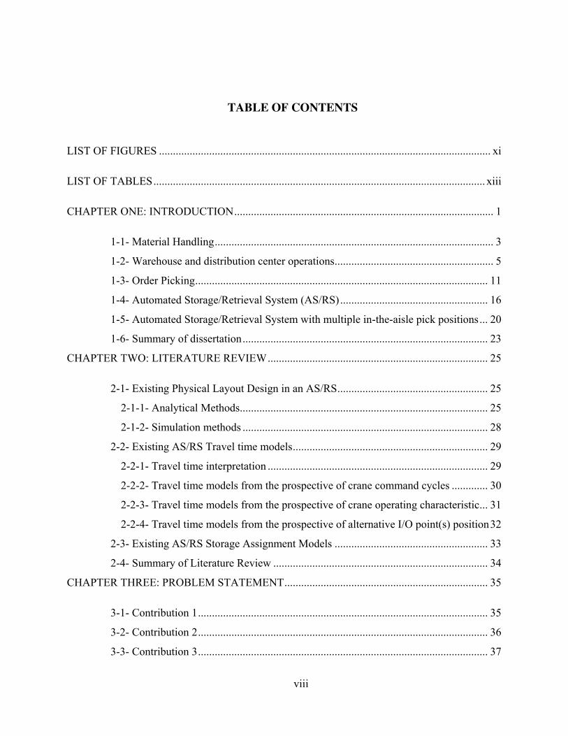
TABLE OF CONTENTS

LIST OF FIGURES ....................................................................................................................... xi

LIST OF TABLES ....................................................................................................................... xiii

CHAPTER ONE: INTRODUCTION ............................................................................................. 1

1-1- Material Handling .................................................................................................... 3

1-2- Warehouse and distribution center operations ......................................................... 5

1-3- Order Picking ......................................................................................................... 11

1-4- Automated Storage/Retrieval System (AS/RS) ..................................................... 16

1-5- Automated Storage/Retrieval System with multiple in-the-aisle pick positions ... 20

1-6- Summary of dissertation ........................................................................................ 23

CHAPTER TWO: LITERATURE REVIEW ............................................................................... 25

2-1- Existing Physical Layout Design in an AS/RS ...................................................... 25

2-1-1- Analytical Methods......................................................................................... 25

2-1-2- Simulation methods ........................................................................................ 28

2-2- Existing AS/RS Travel time models ...................................................................... 29

2-2-1- Travel time interpretation ............................................................................... 29

2-2-2- Travel time models from the prospective of crane command cycles ............. 30

2-2-3- Travel time models from the prospective of crane operating characteristic ... 31

2-2-4- Travel time models from the prospective of alternative I/O point(s) position 32

2-3- Existing AS/RS Storage Assignment Models ....................................................... 33

2-4- Summary of Literature Review ............................................................................. 34

CHAPTER THREE: PROBLEM STATEMENT ......................................................................... 35

3-1- Contribution 1 ........................................................................................................ 35

3-2- Contribution 2 ........................................................................................................ 36

3-3- Contribution 3 ........................................................................................................ 37

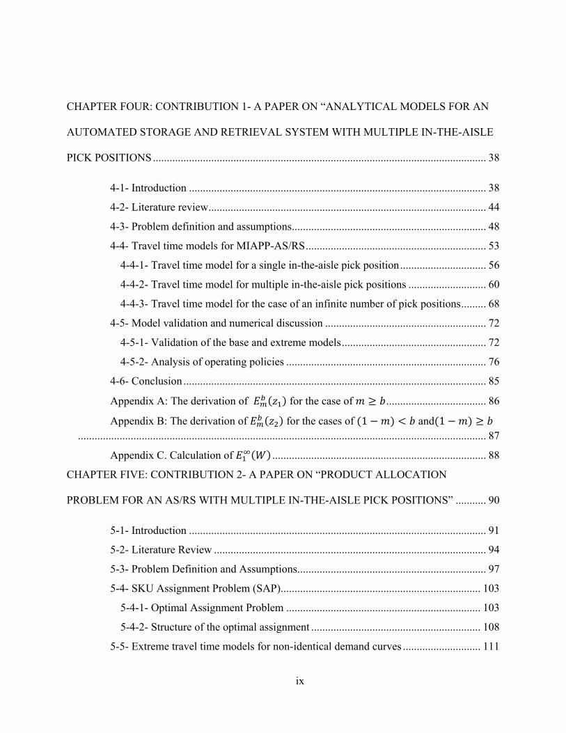
ix

CHAPTER FOUR: CONTRIBUTION 1- A PAPER ON “ANALYTICAL MODELS FOR AN

AUTOMATED STORAGE AND RETRIEVAL SYSTEM WITH MULTIPLE IN-THE-AISLE

PICK POSITIONS ........................................................................................................................ 38

4-1- Introduction ........................................................................................................... 38

4-2- Literature review .................................................................................................... 44

4-3- Problem definition and assumptions ...................................................................... 48

4-4- Travel time models for MIAPP-AS/RS ................................................................. 53

4-4-1- Travel time model for a single in-the-aisle pick position ............................... 56

4-4-2- Travel time model for multiple in-the-aisle pick positions ............................ 60

4-4-3- Travel time model for the case of an infinite number of pick positions ......... 68

4-5- Model validation and numerical discussion .......................................................... 72

4-5-1- Validation of the base and extreme models .................................................... 72

4-5-2- Analysis of operating policies ........................................................................ 76

4-6- Conclusion ............................................................................................................. 85

Appendix A: The derivation of ( ) for the case of .................................... 86

Appendix B: The derivation of ( ) for the cases of ( ) and( ) ................................................................................................................................................... 87

Appendix C. Calculation of ( ) ............................................................................. 88

CHAPTER FIVE: CONTRIBUTION 2- A PAPER ON “PRODUCT ALLOCATION

PROBLEM FOR AN AS/RS WITH MULTIPLE IN-THE-AISLE PICK POSITIONS” ........... 90

5-1- Introduction ........................................................................................................... 91

5-2- Literature Review .................................................................................................. 94

5-3- Problem Definition and Assumptions.................................................................... 97

5-4- SKU Assignment Problem (SAP)........................................................................ 103

5-4-1- Optimal Assignment Problem ...................................................................... 103

5-4-2- Structure of the optimal assignment ............................................................. 108

5-5- Extreme travel time models for non-identical demand curves ............................ 111

x

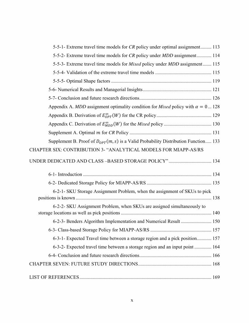
5-5-1- Extreme travel time models for CR policy under optimal assignment ......... 113

5-5-2- Extreme travel time models for CR policy under MDD assignment ............ 114

5-5-3- Extreme travel time models for Mixed policy under MDD assignment ....... 115

5-5-4- Validation of the extreme travel time models .............................................. 115

5-5-5- Optimal Shape factors .................................................................................. 119

5-6- Numerical Results and Managerial Insights ........................................................ 121

5-7- Conclusion and future research directions ........................................................... 126

Appendix A. MDD assignment optimality condition for Mixed policy with ... 128

Appendix B. Derivation of ( ) for the CR policy ............................................. 129

Appendix C. Derivation of ( ) for the Mixed policy ....................................... 130

Supplement A. Optimal for CR Policy ................................................................... 131

Supplement B. Proof of ( ) is a Valid Probability Distribution Function ..... 133

CHAPTER SIX: CONTRIBUTION 3- “ANALYTICAL MODELS FOR MIAPP-AS/RS

UNDER DEDICATED AND CLASS –BASED STORAGE POLICY” ................................... 134

6-1- Introduction ......................................................................................................... 134

6-2- Dedicated Storage Policy for MIAPP-AS/RS ..................................................... 135

6-2-1- SKU Storage Assignment Problem, when the assignment of SKUs to pick

positions is known ............................................................................................................... 138

6-2-2- SKU Assignment Problem, when SKUs are assigned simultaneously to

storage locations as well as pick positions .......................................................................... 140

6-2-3- Benders Algorithm Implementation and Numerical Result ......................... 150

6-3- Class-based Storage Policy for MIAPP-AS/RS .................................................. 157

6-3-1- Expected Travel time between a storage region and a pick position ............ 157

6-3-2- Expected travel time between a storage region and an input point .............. 164

6-4- Conclusion and future research directions ........................................................... 166

CHAPTER SEVEN: FUTURE STUDY DIRECTIONS ............................................................ 168

LIST OF REFERENCES ............................................................................................................ 169

xi

LIST OF FIGURES

Figure 1-1 : Material handling system equation (Tompkins et al., 2010) ...................................... 4

Figure 1-2 : Structure of the stock keeping units (NAVSUP Pub. 529) ......................................... 6

Figure 1-3 : Opportunities provided by distribution centers (Tompkins et al., 2010) .................... 9

Figure 1-4 : Typical warehouse functions and flows (modified after Tompkins et al. (2010)) ... 10

Figure 1-5 : Typical distribution of warehouse operating expenses (Tompkins et al., 2010) ...... 12

Figure 1-6 : Different AS/RS options (Roodbergen & Vis, 2009) ............................................... 18

Figure 1-7 : Schematic view of a typical MIAPP-AS/RS ............................................................. 21

Figure 4-1 : Schematic view of a typical MIAPP-AS/RS ............................................................. 40

Figure 4-2 : All possible cases of travels under a single picking floor configuration. ................. 51

Figure 4-3 : Visual illustrations of the trips .................................................................................. 54

Figure 4-4 : Typical normalized rack in terms of time ................................................................. 57

Figure 4-5 : Example of a Consecutive Retrieval operating policy for a single picking floor

configuration with three SC retrieval travels ................................................................................ 61

Figure 4-6 : Example of a Consecutive Retrieval operating policy for a dual picking floor

configuration ................................................................................................................................. 62

Figure 5-1 : Typical MIAPP-AS/RS ............................................................................................. 92

Figure 5-2 : Trips in MIAPP-AS/RS .......................................................................................... 100

Figure 5-3 : Pick positions’ expected travel time for different policies ..................................... 109

Figure 5-4 : Typical optimal SKU assignment for different policies (X-axis represents the

location of the pick positions and Y-axis represent the SKUs’ demand) ................................... 111

xii

Figure 5-5 : Continuous demand curves for different policies (based on 20/40 curve) ............. 113

Figure 5-6: Normalized travel time per operation for Mixed policy ( ) ............................. 126

Figure 6-1 : Typical 20/80 demand curve versus corresponding EOQ inventory curve ............ 138

Figure 6-2: Classic Benders algorithm convergence for and ............................. 153

Figure 6-3 : Classic and M-W accelerated Benders algorithm convergence for and ........................................................................................................................................ 154

Figure 6-4 : Optimal SKU assignment for and (for rectilinear distances) ....... 155

Figure 6-5 : Optimal SKU assignment for and (for rectilinear distances) ....... 156

Figure 6-6 : Expected travel time trip in a normalized rack for class-based storage policy ....... 158

Figure 6-7 : Expected travel time between an Input point and given region (Class) in a

normalized rack ........................................................................................................................... 165

xiii

LIST OF TABLES

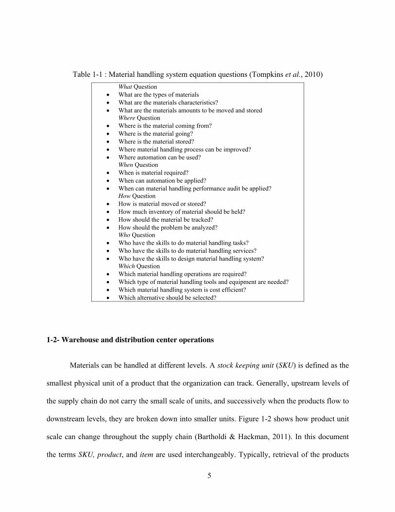
Table 1-1 : Material handling system equation questions (Tompkins et al., 2010) ........................ 5

Table 1-2 : Description of the warehouse operation problems (Gu et al., 2007) ......................... 11

Table 1-3 : Order picking work elements and means for elimination (Tompkins et al., 2010), .. 15

Table 1-4 : Classification of AS/RS design decision problems (Roodbergen & Vis, 2009) ........ 19

Table 4-1 : The denormalized results of the discrete rack simulation versus the base and extreme

travel time models for a single picking floor configuration ......................................................... 74

Table 4-2 : The denormalized results of the discrete rack simulation versus the base and extreme

travel time models for a dual picking floor configuration when and . ................ 75

Table 4-3 : Expected value of the best found numerically for different operating policies with a

given .......................................................................................................................................... 79

Table 4-4 : Denormalized expected ‘per retrieval’ travel time comparison of different operating

policies .......................................................................................................................................... 80

Table 4-5 : Denormalized expected ‘per operation’ travel time comparison of different operating

policies .......................................................................................................................................... 82

Table 5-1: Structure of shape configurations .............................................................................. 116

Table 5-2 : Simulation vs. extreme travel time results for a CR Policy under an optimal

assignment................................................................................................................................... 117

Table 5-3 : Simulation vs. extreme travel time results for a CR Policy under an optimal

assignment................................................................................................................................... 118

xiv

Table 5-4 : Simulation vs. extreme travel time for the Mixed Policy ( =0.4) under an MDD

assignment................................................................................................................................... 118

Table 5-5 : Optimal Shape factor for different policies .............................................................. 121

Table 5-6 : Expected travel time for CR Policy (optimal vs. MDD assignment) ....................... 124

Table 5-7 : Expected travel time for Mixed Policy (optimal vs. MDD assignment) .................. 125

Table 6-1 : Maximum inventory level ........................................................................................ 152

1

CHAPTER ONE: INTRODUCTION

A supply chain includes all of the parties that are involved directly or indirectly to fulfill

customer requests. A supply chain does not only include manufacturer and suppliers, but also

includes transporters, warehouses, distribution centers, retailers, and customers (Chopra &

Meindl, 2007). Distribution centers play a critical role in supporting a company’s supply chain

success. The mission of a distribution center is to effectively ship products in the requested

configuration to the downstream member in the supply chain. Logistics is the indispensable part

of any supply chain that manages the flow of materials between the point of origin and the point

of end-users. A part of logistics management focuses on activities within facilities and is known

as facility logistics. Facility logistics concentrates on facility design, material handling,

transportation (Noori et al., 2013, 2014; Kucukvar et al., 2014), and inventory management

within manufacturing, distribution, and service facilities. Material handling is the “art and

science of moving, storing, protecting, and controlling material". Material handling includes a

large variety of manual, semi-automated and automated equipment. The most labor-intensive

activity regarding material handling within a distribution center facility is order picking. Order

picking is the process of retrieving products from the storage locations to fulfill a specific

customer order. Order picking can occur at different levels, which include at the pallet, case, and

piece level. In this dissertation, we concentrate on a special type of case-level order fulfillment

technology that we call “automated storage and retrieval system with multiple in-the-aisle pick

positions” or “MIAPP-AS/RS”. MIAPP-AS/RS is a semi-automated order fulfillment technology

2

where the pallet-level put-away and retrieval activities are automated by cranes, but the case-

level order picking process is done by human order pickers walking and picking along the aisles.

The global demand for frozen food has grown during the past decade. According to the

“Global Frozen Food” report published by Datamonitor (2011) the demand rate for frozen food

continues to grow. The global frozen foods market was estimated to be BUSD 165.4 in 2009 and

is expected to grow by 21 percent to BUSD 199.5 by 2014. For decades, the majority of deep-

freeze distribution centers have been operated manually. Due to the increasing customer demand

for frozen products and a highly competitive market, the organizations in deep-freeze supply

chain are looking to improve the lead time, order accuracy, and product quality. One of the

solutions to decrease the manual operations is turning to “high-bay” deep-freeze distribution

centers that are equipped with automated material handling systems such as a MIAPP-AS/RS.

Due to the harsh working conditions and increased safety issues, personnel turnover in

deep freeze distribution centers is higher than ambient distribution centers. Also, the majority of

cold temperature loss occurs through the roof of a deep freeze distribution center; consequently,

effective utilization of vertical space is important (and MIAPP-AS/RSs have been designed as

high as 165 feet) (Swisslog Co., 2012). In addition, the MIAPP-AS/RS require less space, which

result in further space utilization gains. Therefore, MIAPP-AS/RSs are used to reduce the

number of operators who are required to work in the harsh environments, as well as to reduce the

amount of space that is required to be temperature controlled (which is both financially and

environmentally expensive). Additional benefits include the ability to monitor and control

temperature zones and automate the tracking of products.

3

1-1- Material Handling

The Material Handling Institute of America (MHIA) defines material handling as “the

movement, protection, storage and control of materials and products throughout manufacturing,

warehousing, distribution, consumption and disposal. As a process, material handling

incorporates a wide range of manual, semi-automated and automated equipment and systems that

support logistics and make the supply chain work”.

Material handling system design is one of the most critical components in any

distribution center design. These systems and processes can help extensively to increase the

customer service level, reduce inventory levels and order-fulfillment time, and decrease the

overall costs in manufacturing and distribution of the products. There is not a single way to

ensure that the material handling equipment and processes (including manual, semi-automated

and automated) in a distribution center work together as a unified whole. According to the

MHIA, in order to reach the material handling goals 10 principles should be considered to

properly design a system: 1) Planning, 2) Standardization, 3) Work, 4) Ergonomics, 5) Unit load,

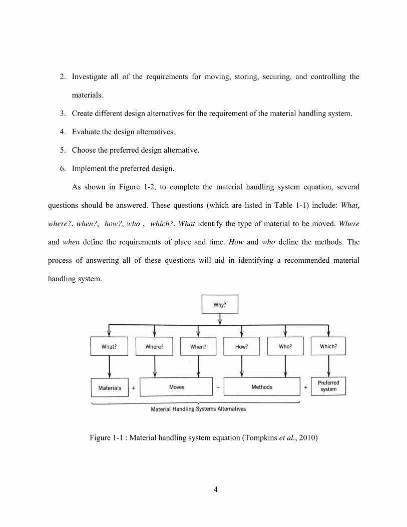
6) Space utilization, 7) System, 8) Environment, 9) Automation, 10) Life cycle cost. Based on

these general principles, Tompkins et al. (2010) provide the following six-step material handling

design process. This process results in the “material handling system equation” (see Figure 1-1),

which is the framework that generate solutions for material handling problems. The material

handling design process steps are:

1. Define the objectives, goals, and scope.

4

2. Investigate all of the requirements for moving, storing, securing, and controlling the

materials.

3. Create different design alternatives for the requirement of the material handling system.

4. Evaluate the design alternatives.

5. Choose the preferred design alternative.

6. Implement the preferred design.

As shown in Figure 1-2, to complete the material handling system equation, several

questions should be answered. These questions (which are listed in Table 1-1) include: What,

where?, when?, how?, who , which?. What identify the type of material to be moved. Where

and when define the requirements of place and time. How and who define the methods. The

process of answering all of these questions will aid in identifying a recommended material

handling system.

Figure 1-1 : Material handling system equation (Tompkins et al., 2010)

5

Table 1-1 : Material handling system equation questions (Tompkins et al., 2010)

What Question

What are the types of materials

What are the materials characteristics?

What are the materials amounts to be moved and stored

Where Question

Where is the material coming from?

Where is the material going?

Where is the material stored?

Where material handling process can be improved?

Where automation can be used?

When Question

When is material required?

When can automation be applied?

When can material handling performance audit be applied?

How Question

How is material moved or stored?

How much inventory of material should be held?

How should the material be tracked?

How should the problem be analyzed?

Who Question

Who have the skills to do material handling tasks?

Who have the skills to do material handling services?

Who have the skills to design material handling system?

Which Question

Which material handling operations are required?

Which type of material handling tools and equipment are needed?

Which material handling system is cost efficient?

Which alternative should be selected?

1-2- Warehouse and distribution center operations

Materials can be handled at different levels. A stock keeping unit (SKU) is defined as the

smallest physical unit of a product that the organization can track. Generally, upstream levels of

the supply chain do not carry the small scale of units, and successively when the products flow to

downstream levels, they are broken down into smaller units. Figure 1-2 shows how product unit

scale can change throughout the supply chain (Bartholdi & Hackman, 2011). In this document

the terms SKU, product, and item are used interchangeably. Typically, retrieval of the products

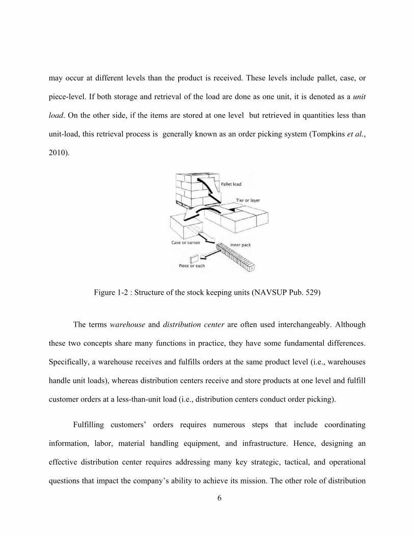
6

may occur at different levels than the product is received. These levels include pallet, case, or

piece-level. If both storage and retrieval of the load are done as one unit, it is denoted as a unit

load. On the other side, if the items are stored at one level but retrieved in quantities less than

unit-load, this retrieval process is generally known as an order picking system (Tompkins et al.,

2010).

Figure 1-2 : Structure of the stock keeping units (NAVSUP Pub. 529)

The terms warehouse and distribution center are often used interchangeably. Although

these two concepts share many functions in practice, they have some fundamental differences.

Specifically, a warehouse receives and fulfills orders at the same product level (i.e., warehouses

handle unit loads), whereas distribution centers receive and store products at one level and fulfill

customer orders at a less-than-unit load (i.e., distribution centers conduct order picking).

Fulfilling customers’ orders requires numerous steps that include coordinating

information, labor, material handling equipment, and infrastructure. Hence, designing an

effective distribution center requires addressing many key strategic, tactical, and operational

questions that impact the company’s ability to achieve its mission. The other role of distribution

7

center is to process orders. The orders should be process fast, effectively, and precisely;

otherwise, then a company’s supply chain planning will suffer. Information technology has a

significant role in making distribution center operate more effective, but the best information

system will be of little use if the physical systems necessary to get the products out the door are

constrained, misapplied, or outdated. There are several metrics to evaluate the performance of

distribution centers. These metrics measure the efficiency and effectiveness of labor, equipment,

space, financial performance, safety, and sustainability. The common metrics can be categorized

as order accuracy metrics, order fill rate, on-time delivery measures, throughput, etc. In practice,

an organization takes a collection of these metrics into account to obtain a better understanding

of the system.

The criteria to categorize distribution centers is primarily based on the customers who are

served. According to Bartholdi & Hackman (2011), important distinctions of distribution centers

are as follows.

1. A “retail distribution center” which typically provides products to a retail store. Wal-

Mart, Publix, and Target are some of the well-known examples. In this type of

distribution centers, the primary customer is retail stores. A distribution center generally

supplies several retail stores, and the orders include thousands of items. However,

planning ahead is possible as typically the orders are known in advance.

2. A “service parts distribution center” which generally hold the spare parts of tools or

equipment (e.g. airplanes and automobiles). Managing these distribution centers is very

challenging because they hold a large number of items with small demands. The variance

of the demand, as well as the lead times to replenish is generally large and so high level

8

of safety stock should be kept. These facts lead to requirement of relatively larger space

and consequently more costly order-fulfillment process. Another challenge for these

distribution centers is that the demand pattern for service parts are generally unusual as

they follow different life cycle patterns. The failure rates for early-, mid-, end-of- life

vary product to product. Therefore, it brings hard challenges for demand prediction as

well as distribution center design.

3. A “catalog fulfillment or e-commerce distribution center” which handles phone, fax, and

internet orders placed by the customers. Orders are comprised of a relatively small

number of items, but many of these orders are placed during a certain time. Generally, the

response time is the most important factor among distribution centers activities.

4. A “3PL distribution center” is used for other companies outsourcing warehouse

operations. A 3PL distribution center generally supplies more than one company and thus

can gain economies of scale that a single small company cannot gain by its own.

5. A “perishable products distribution center”, generally keeps very short shelf life

products such as food, flowers, and vaccines that need a temperature-controlled

environment. Space efficiency is one of the most challenging parts in these distribution

centers as the refrigeration is a very costly process. Other challenges within this type of

distribution center may include the handling and shipping of the products that should

generally follow the FIFO (First-In-First-Out) or FEFO (First-Expired-First-Out) basis.

Distribution centers can bring different opportunities including order picking,

productivity, and value-added services. Any of these opportunities or combination of them can

be found in distribution centers (Tompkins et al., 2010). Figure 1-3 shows the schematic view of

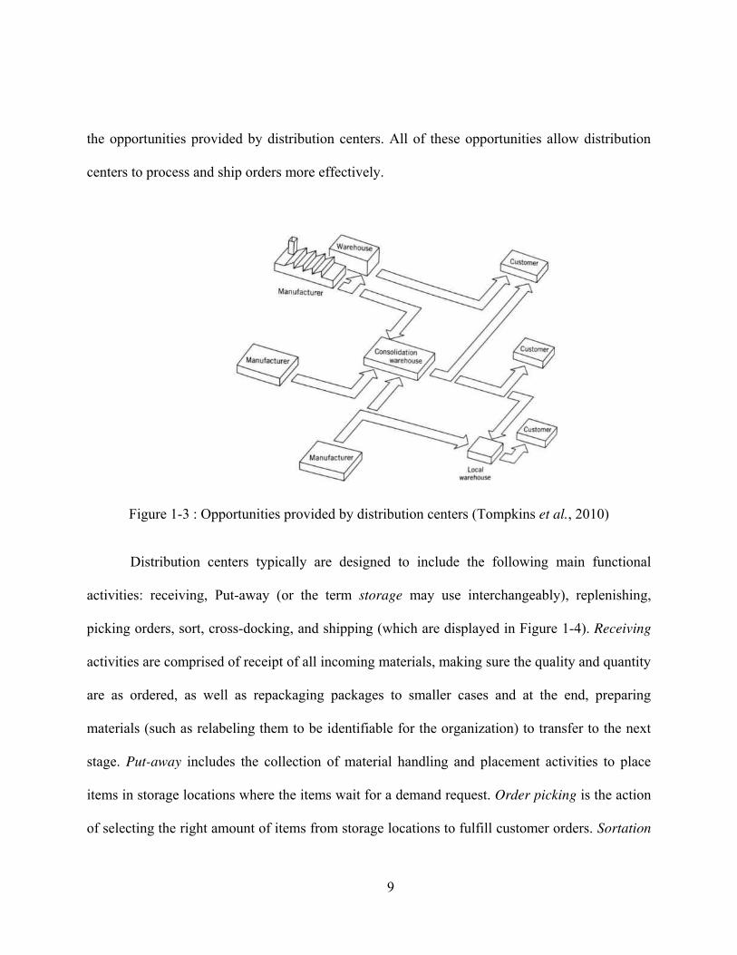
9

the opportunities provided by distribution centers. All of these opportunities allow distribution

centers to process and ship orders more effectively.

Figure 1-3 : Opportunities provided by distribution centers (Tompkins et al., 2010)

Distribution centers typically are designed to include the following main functional

activities: receiving, Put-away (or the term storage may use interchangeably), replenishing,

picking orders, sort, cross-docking, and shipping (which are displayed in Figure 1-4). Receiving

activities are comprised of receipt of all incoming materials, making sure the quality and quantity

are as ordered, as well as repackaging packages to smaller cases and at the end, preparing

materials (such as relabeling them to be identifiable for the organization) to transfer to the next

stage. Put-away includes the collection of material handling and placement activities to place

items in storage locations where the items wait for a demand request. Order picking is the action

of selecting the right amount of items from storage locations to fulfill customer orders. Sortation

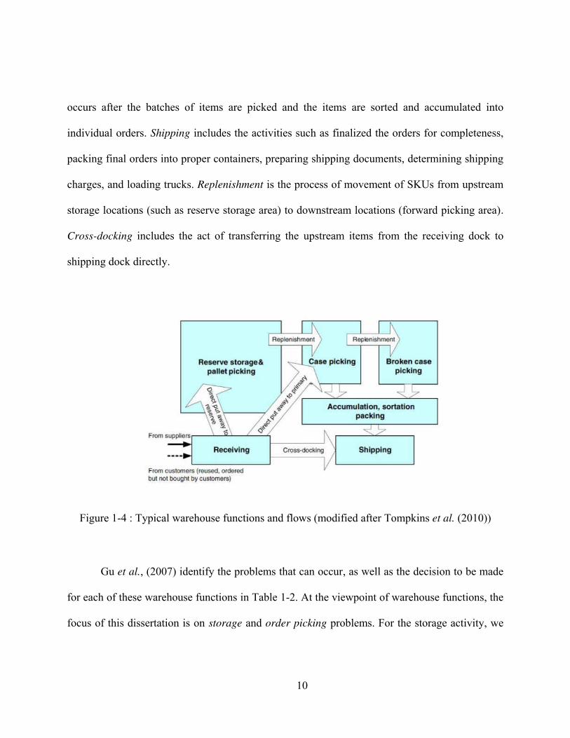
10

occurs after the batches of items are picked and the items are sorted and accumulated into

individual orders. Shipping includes the activities such as finalized the orders for completeness,

packing final orders into proper containers, preparing shipping documents, determining shipping

charges, and loading trucks. Replenishment is the process of movement of SKUs from upstream

storage locations (such as reserve storage area) to downstream locations (forward picking area).

Cross-docking includes the act of transferring the upstream items from the receiving dock to

shipping dock directly.

Figure 1-4 : Typical warehouse functions and flows (modified after Tompkins et al. (2010))

Gu et al., (2007) identify the problems that can occur, as well as the decision to be made

for each of these warehouse functions in Table 1-2. At the viewpoint of warehouse functions, the

focus of this dissertation is on storage and order picking problems. For the storage activity, we

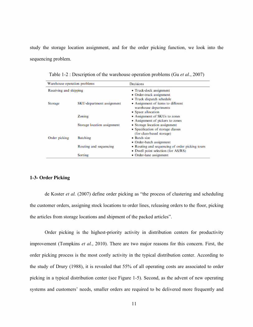
11

study the storage location assignment, and for the order picking function, we look into the

sequencing problem.

Table 1-2 : Description of the warehouse operation problems (Gu et al., 2007)

1-3- Order Picking

de Koster et al. (2007) define order picking as “the process of clustering and scheduling

the customer orders, assigning stock locations to order lines, releasing orders to the floor, picking

the articles from storage locations and shipment of the packed articles”.

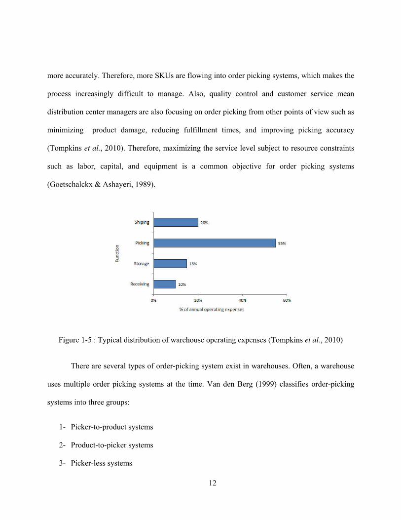
Order picking is the highest-priority activity in distribution centers for productivity

improvement (Tompkins et al., 2010). There are two major reasons for this concern. First, the

order picking process is the most costly activity in the typical distribution center. According to

the study of Drury (1988), it is revealed that 55% of all operating costs are associated to order

picking in a typical distribution center (see Figure 1-5). Second, as the advent of new operating

systems and customers’ needs, smaller orders are required to be delivered more frequently and

12

more accurately. Therefore, more SKUs are flowing into order picking systems, which makes the

process increasingly difficult to manage. Also, quality control and customer service mean

distribution center managers are also focusing on order picking from other points of view such as

minimizing product damage, reducing fulfillment times, and improving picking accuracy

(Tompkins et al., 2010). Therefore, maximizing the service level subject to resource constraints

such as labor, capital, and equipment is a common objective for order picking systems

(Goetschalckx & Ashayeri, 1989).

Figure 1-5 : Typical distribution of warehouse operating expenses (Tompkins et al., 2010)

There are several types of order-picking system exist in warehouses. Often, a warehouse

uses multiple order picking systems at the time. Van den Berg (1999) classifies order-picking

systems into three groups:

1- Picker-to-product systems

2- Product-to-picker systems

3- Picker-less systems

13

In a picker-to-product system, human order-pickers may walk or ride in vehicles to reach

the pick positions and pick the items. This picking process can be categorized into two types.

First, low-level picking occurs when the order pickers travel along the aisle and pick the items

from storage racks or bins. Second, high-level picking occurs when the order picker travels to the

picking spots by riding on board of lifting cranes. This type of the high-level picking is also

known as man-on-board order picking system. When the order is sufficiently large, each order

can be picked in its own single tour individually (Single or discrete order-picking). However,

when the number of the orders increases and the orders become relatively smaller, there is an

opportunity to reduce the travel time by grouping the multiple orders simultaneously in one tour,

which is denoted as batch picking. In batch picking, sortation is required. If the orders are sorted

during the order-picking process, it is known as sort-while-pick. Otherwise, if the sortation

process is done afterwards, it is called pick-and-sort (van den Berg, 1999).

In a product-to-picker system, the products are brought to the picker by employing

material handling technologies. Automated storage and retrieval systems (AS/RS) and the

carousel are two well-known examples of product-to-picker technologies. AS/RS consists of

high-rise storage racks and the fully automated cranes for handling the loads put-away and

retrieval. A carousel consists of storage racks that rotate horizontally or vertically around a

closed loop to bring the requested items to order pickers. Finally, picker-less systems use robot-

technology or automatic dispensers such as A-frame systems (van den Berg, 1999; Pazour and

Meller, 2011) to fulfill customer orders.

14

According to Tompkins et al. (2010), certain principles exist that are applicable to most

order picking processes regardless of material, customer, and warehouse specifications. We

mention some of these order picking principles based on relevance to the objectives of our study.

1. Use Pareto’s law. Pareto’s law is applicable for many cases in business and

manufacturing environments. In particular, in warehouses, it is typical to observe a large

portion of inventory to be attributed to a small number of SKUs. This idea can be

extended to other aspects in warehouses such as demand, throughput, space utilization,

and so on.

2. Provide an effective stock location system. Every warehouse should have a consistent

stock locating system. The effective system helps as an input to an efficient routing

system and prevents tedious non-value-added search for items.

3. Eliminate or combine order picking tasks. Order picking may include activities such that

traveling, extracting items, reaching to pick locations, documenting transactions, sorting,

searching for pick locations. These activities comprise the order pickers’ time. Several

opportunities exist to eliminate or combine these elements to reduce the overall picking

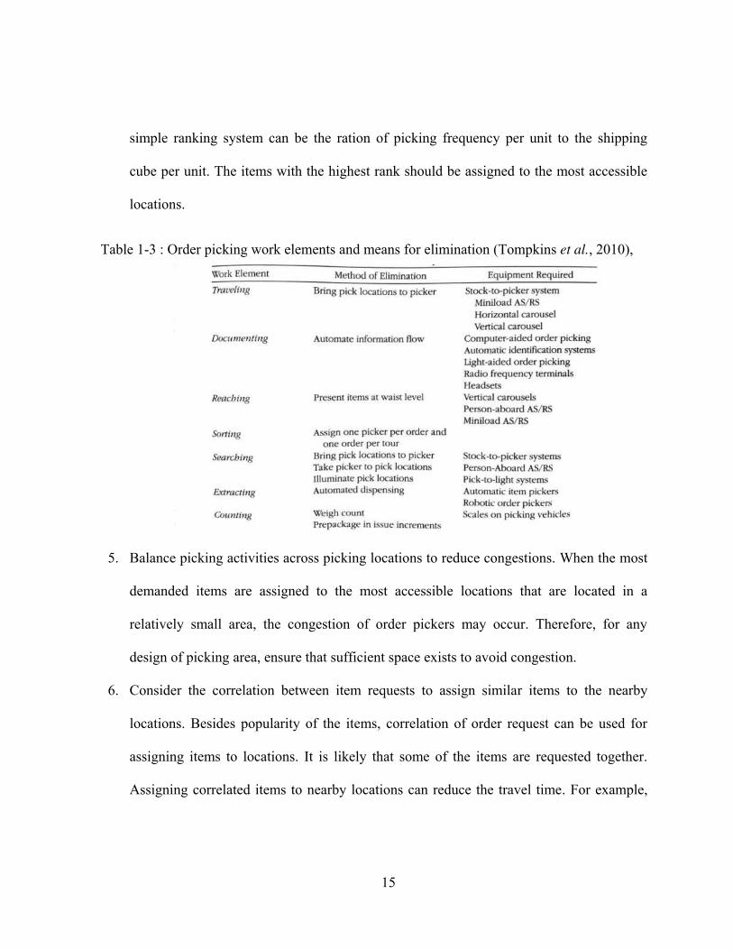
time. Some of these methods are provided in Table 1-3.

4. Allocate the most demanded items to the most accessible storage locations in the

warehouse. As another intuition from Pareto’s law, assigning fast-moving items to more

accessible locations can reduce the picking times. This rule can be applied for manual

and automated order picking. One of the common mistakes that is made in practice is

overlooking the size of the product. Therefore, the amount of space required by the items

should be considered in any ranking system that identifies the popularity of the items. A

15

simple ranking system can be the ration of picking frequency per unit to the shipping

cube per unit. The items with the highest rank should be assigned to the most accessible

locations.

Table 1-3 : Order picking work elements and means for elimination (Tompkins et al., 2010),

5. Balance picking activities across picking locations to reduce congestions. When the most

demanded items are assigned to the most accessible locations that are located in a

relatively small area, the congestion of order pickers may occur. Therefore, for any

design of picking area, ensure that sufficient space exists to avoid congestion.

6. Consider the correlation between item requests to assign similar items to the nearby

locations. Besides popularity of the items, correlation of order request can be used for

assigning items to locations. It is likely that some of the items are requested together.

Assigning correlated items to nearby locations can reduce the travel time. For example,

16

Frazelle (1989) presents a computerized procedure to consider the popularity and the

correlation of the demand of items at the same time.

1-4- Automated Storage/Retrieval System (AS/RS)

An automated storage and retrieval system (AS/RS) is defined by MHIA as “a

combination of equipment and controls that handle, store and retrieve materials as needed with

precision, accuracy and speed under a defined degree of automation. An AS/RS is used for raw

material, work-in-process, and finished goods. A significant increase in the number of AS/RS

used in the distribution environments have been seen in United States, and the installations of

such systems have become commonplace in all major industries”. AS/RSs have had a great

impact on manufacturing (especially pull-based systems), warehousing, and different service

facilities such as hospitals and libraries (Tompkins et al., 2010). Zollinger (1999) list the major

benefits of using AS/RS as follows.

improve efficiency of operators and storage capacity

reduce the WIP inventory

improve the quality and just-in-time performance

provide make-to-order capability as well as make-to-inventory production

control the inventory in real-time manner and prompt reporting functionality

higher inventory security

less product damage

17

The major disadvantages associated to AS/RS, which must be considered before

justifying acquisition of such a system, are:

low flexibility in layout

high initial capital cost

fixed storage capacity

lack of visibility

The system design process of implementing an AS/RS should include the following

considerations:

definition of current and future loads to be handled

number of the loads to be stored in the system

material flow description (including average and peak rates)

description of operations

architectural/engineering considerations

A typical AS/RS includes one or more aisles (each aisle has storage racks on either side),

a crane, and an input/output (I/O) queue. The crane can generally access the storage racks on

both sides of the aisle. A typical AS/RS storage operation includes the crane picking up a load at

the I/O point, moving the load to an empty storage location, depositing the load in the empty

storage location, and traveling empty to the I/O point. A similar process can occur for retrieving

a load from the AS/RS system. Because such operations are performed by conducting either one

storage or one retrieval, they are known as single command (SC) operations. A more efficient

18

operation that involves performing both a storage and a retrieval is called a dual command (DC)

operation. A DC operation consists of the crane picking up the load at the I/O point, travelling to

the empty storage location, depositing the load, moving empty to the location of desired

retrieval, picking up the load, moving back to the I/O point, and finally depositing the load.

If each aisle has its own crane, the system is known as aisle-captive. For some systems,

the activity level per aisle may vary during the year due to the seasonal demand. If the activity

level of one aisle is low enough that it does not justify dedicating a crane to that aisle, the

number of crane can be less than the number of aisles. In this case the system is designed such

that the crane(s) can move from one aisle to another.

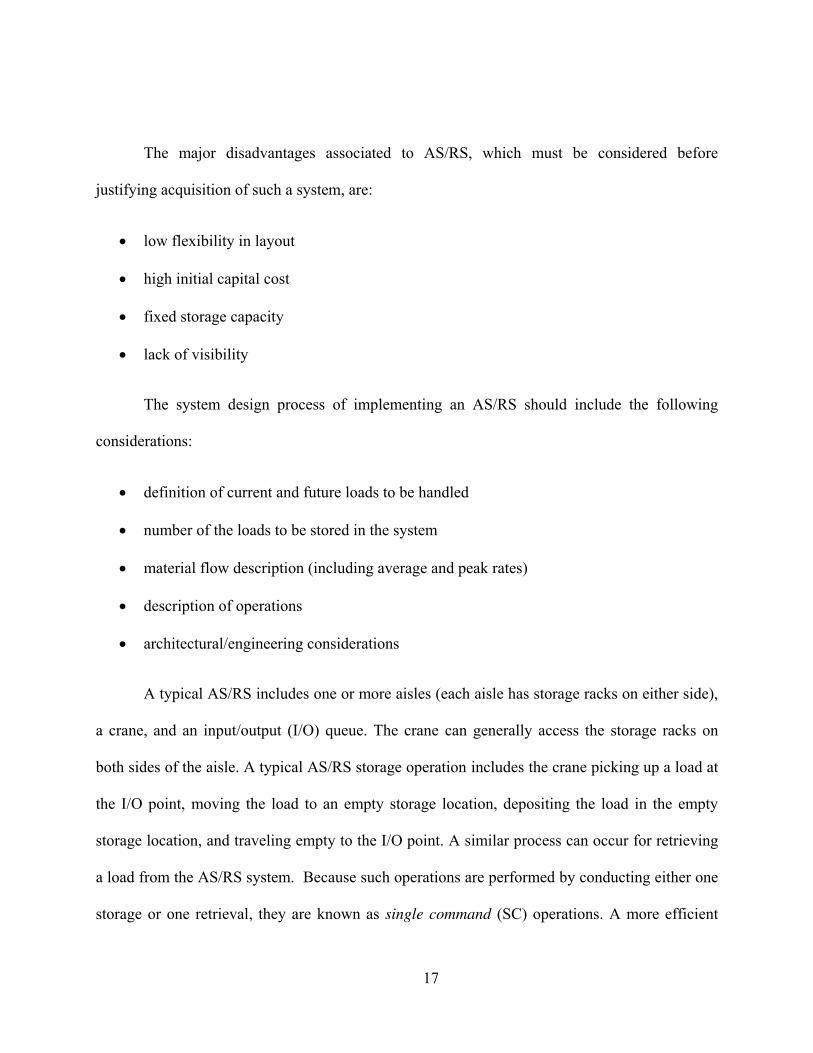
Figure 1-6 : Different AS/RS options (Roodbergen & Vis, 2009)

In AS/RS, horizontal and vertical crane travel occurs simultaneously. Therefore, the time

required for the crane to reach any point within the rack is equal to the maximum of the

horizontal and vertical travel time. This movement is known as a chebyshev distant metric. The

19

horizontal and vertical speeds of a typical crane are up to 600 and 150 feet per minute,

respectively (Tompkins et al., 2010).

When the loads have relatively low variety of loads in the system, throughput

requirement of each item become relatively high, thereby the number of loads to be stored is

high. In this case, storing items in a rack may occur double deep to increase the space utilization.

This rack configuration is often referred to double-deep racks (Tompkins et al., 2010).

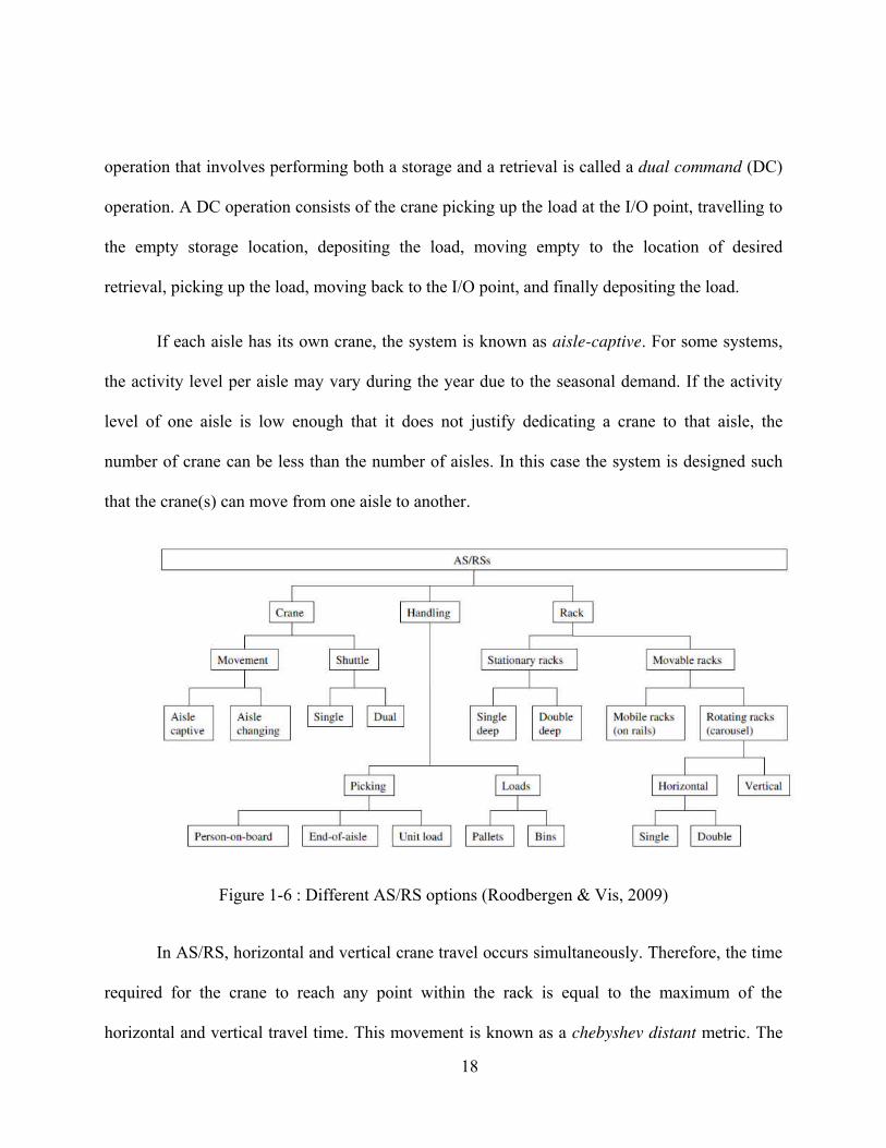
Roodbergen & Vis (2009) provide an extensive review of 30 years of literature on AS/RS

problems. As illustrated in Figure 1-6, they categorize the AS/RSs based on crane and rack

configurations as well as type of handling. Also, they categorize the AS/RS design decision

problems into: 1) system configuration, 2) storage assignment, 3) batching, 4) sequencing, and 5)

dwell-point problems (see Table 1-4). In this dissertation, we only study system configuration,

storage assignment, and sequencing aspects of AS/RS problems.

Table 1-4 : Classification of AS/RS design decision problems (Roodbergen & Vis, 2009)

20

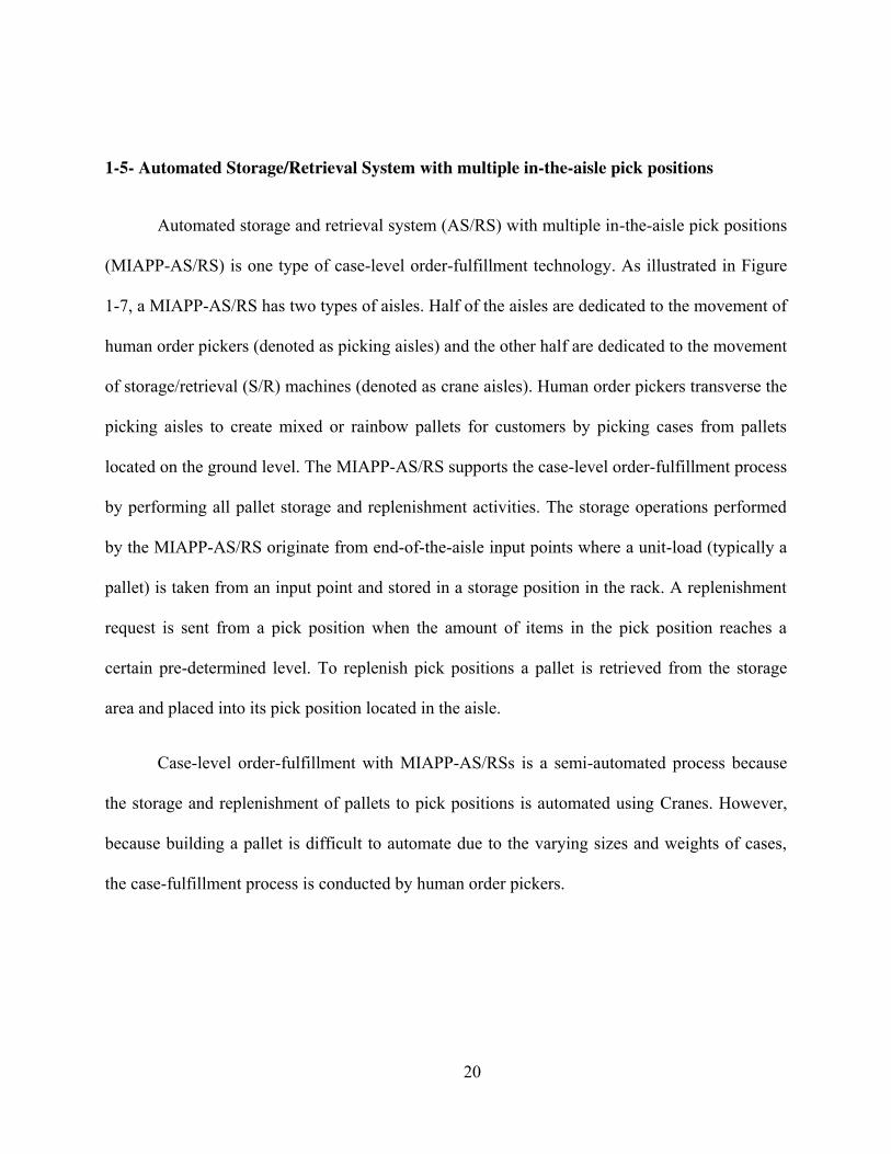
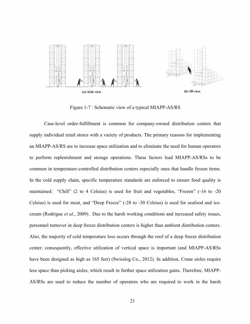
1-5- Automated Storage/Retrieval System with multiple in-the-aisle pick positions

Automated storage and retrieval system (AS/RS) with multiple in-the-aisle pick positions

(MIAPP-AS/RS) is one type of case-level order-fulfillment technology. As illustrated in Figure

1-7, a MIAPP-AS/RS has two types of aisles. Half of the aisles are dedicated to the movement of

human order pickers (denoted as picking aisles) and the other half are dedicated to the movement

of storage/retrieval (S/R) machines (denoted as crane aisles). Human order pickers transverse the

picking aisles to create mixed or rainbow pallets for customers by picking cases from pallets

located on the ground level. The MIAPP-AS/RS supports the case-level order-fulfillment process

by performing all pallet storage and replenishment activities. The storage operations performed

by the MIAPP-AS/RS originate from end-of-the-aisle input points where a unit-load (typically a

pallet) is taken from an input point and stored in a storage position in the rack. A replenishment

request is sent from a pick position when the amount of items in the pick position reaches a

certain pre-determined level. To replenish pick positions a pallet is retrieved from the storage

area and placed into its pick position located in the aisle.

Case-level order-fulfillment with MIAPP-AS/RSs is a semi-automated process because

the storage and replenishment of pallets to pick positions is automated using Cranes. However,

because building a pallet is difficult to automate due to the varying sizes and weights of cases,

the case-fulfillment process is conducted by human order pickers.

21

Figure 1-7 : Schematic view of a typical MIAPP-AS/RS

Case-level order-fulfillment is common for company-owned distribution centers that

supply individual retail stores with a variety of products. The primary reasons for implementing

an MIAPP-AS/RS are to increase space utilization and to eliminate the need for human operators

to perform replenishment and storage operations. These factors lead MIAPP-AS/RSs to be

common in temperature-controlled distribution centers especially ones that handle frozen items.

In the cold supply chain, specific temperature standards are enforced to ensure food quality is

maintained: “Chill” (2 to 4 Celsius) is used for fruit and vegetables, “Frozen” (-16 to -20

Celsius) is used for meat, and “Deep Freeze” (-28 to -30 Celsius) is used for seafood and ice-

cream (Rodrigue et al., 2009). Due to the harsh working conditions and increased safety issues,

personnel turnover in deep freeze distribution centers is higher than ambient distribution centers.

Also, the majority of cold temperature loss occurs through the roof of a deep freeze distribution

center; consequently, effective utilization of vertical space is important (and MIAPP-AS/RSs

have been designed as high as 165 feet) (Swisslog Co., 2012). In addition, Crane aisles require

less space than picking aisles, which result in further space utilization gains. Therefore, MIAPP-

AS/RSs are used to reduce the number of operators who are required to work in the harsh

22

environments, as well as to reduce the amount of space that is required to be temperature

controlled (which is both financially and environmentally expensive). Additional benefits

include the ability to monitor and control temperature zones and automate the tracking of

products.

The implementation of MIAPP-AS/RSs can be found in numerous grocery distribution

centers in the United States (E.g. Publix Super Markets and Wal-Mart), and Europe (E.g.

Walkers, Ferrero GmbH and Arla). In these distribution centers a large volume of heavy cases is

handled in Chill and Deep Freeze environments (Swisslog Co., 2013). The 2010 global frozen

food market is estimated to be worth 192.2 BUSD and the global demand for frozen food is

anticipated to grow at a rate of 4 percent annually (Datamonitor, 2011). Therefore, the number

of Deep Freeze distribution centers and the use of case-level order-fulfillment technology, in

general, and MIAPP-AS/RS in particular, are on the rise.

Because of high infrastructure investment costs and the critical importance of order

fulfillment on cost and customer satisfaction, designing and assessing an MIAPP-AS/RS is an

important strategic decision in warehouse design. Such systems are commonly constrained by

Crane throughput; therefore, estimating the average travel time for different design

configurations and operating policies is a fundamental step in designing MIAPP-AS/RSs. To

effectively handle a wide range of item requests in the order-fulfillment process, the number of

pick positions available is also an important design characteristic of MIAPP-AS/RSs. The

number of pick positions can be increased through the use of an additional elevated picking floor

on a mezzanine that enables case-level order-fulfillment to be performed at different elevations.

23

Distribution centers may have different operating policies during peak and non-peak

times. For example, many distribution centers have a peak-picking time where a large majority

of the distribution center’s orders are placed and must be picked before the last truck leaves the

dock for shipment. During peak times, the distribution center prioritizes fulfillment of orders

over storage requests that can be performed during non-peak times. Also, if a distribution center

experiences a balanced number of storage and retrieval requests throughout the day, the Crane

can perform a dual command travel that includes both a storage and a retrieval. Consequently,

estimating the throughput of an MIAPP-AS/RS is important for different operating strategies.

1-6- Summary of dissertation

This dissertation focuses on deriving analytical expressions to calculate the expected

travel time of an MIAPP-AS/RS that applies different operating policies and has different

physical configurations. These analytical models are used to find the expected throughput for

optimal assignment of SKUs to pick positions located in the aisle. Moreover, closed-form

approximations are derived for the case of an infinite number of pick positions that enable us to

derive the optimal shape configuration that minimizes travel times. Through comparison with a

simulation model, we illustrate that our models provide good estimates and can be used to aid in

design and evaluation of real-world systems.

The remainder of the dissertation is organized as follows. In the next chapter we review

the literature on travel time and throughput models developed for different aspects of AS/RS

design problems such as physical design and storage assignment problems. In Chapter 3, we state

the particular areas on which we concentrate as well as review our contributions in each area of

24

our study. In Chapter 4, we present the derivation of expected travel time models for MIAPP-

AS/RS under different operating policies and physical configurations. In Chapter 5, we provide

the models and procedures to find the optimal SKU assignment to pick positions, as well as

developing models to estimate the expected throughput for different SKU assignment cases. In

Chapter 6, we study the dedicated and class-based storage policy for MIAPP-AS/RS. Finally, in

Chapter 7, we identify the possible future research directions to continue the proposed topics in

this dissertation.

25

CHAPTER TWO: LITERATURE REVIEW

As the main focus of this dissertation is on the AS/RS problems, in this chapter, we focus

on reviewing the existing literature of AS/RS problems from different perspectives. First, we

review the physical design problems discussed in the literature, as one of the main focuses of our

study is to determine the appropriate design for the system. Second, we concentrate on the

various travel time models that exist in the literature from different points of view such as

command cycles, operating characteristic, and different I/O locations. Finally, we review the

storage assignment policy problems of AS/RS.

2-1- Existing Physical Layout Design in an AS/RS

According to Roodbergen & Vis (2009), as shown in Table 1-4, system configuration

decisions of the AS/RS involve determining the number of cranes, number of aisle, size of the

racks, and so on. However, only few papers consider AS/RS design in combination with other

material handling systems. According to Roodbergen & Vis (2009) and Vasili et al. (2012), there

are two general methods for AS/RS design problems: (1) analytical methods; and (2) simulation.

2-1-1- Analytical Methods

Among the several papers that consider designing and optimization of warehouse and

material handling systems problem, Zollinger (1975) is an early study that consider AS/RS

design based on cost analysis model.

26

Karasawa et al. (1980) build a deterministic mixed-integer programming (MIP) to

minimize the cost of AS/RS problem. They consider the number of the cranes and the size of the

rack as the decision variables of the model. The constraints of the model include number of the

cranes, storage volume, and throughput.

Ashayeri et al. (1985) develop a model to minimize the total investment and warehouse

operating costs. Their model identifies the optimal number of the cranes as well as the optimal

dimensions of the warehouse subject to system throughput, crane speeds, and size of the

building.

Bozer and White (1990) introduce the first analytical stochastic analysis for a mini-load

AS/RS that is modeled as a two-server closed queuing network. Bozer & White (1996) have

extended Bozer & White (1990) to determine the near-optimal pickers’ number and improve the

pickers’ utilization by considering the sequencing of container retrievals sequence for each order.

Lee (1997) categorizes the techniques of evaluating the performance of AS/RSs into

static (Egbelu, 1991; Egbelu and Wu, 1993), computer simulation (Egbelu and Wu, 1993; Linn

and Wysk, 1990; Randhawa et al., 1991; Randhawa and Shroff, 1995), and stochastic analysis.

He presents a stochastic analysis of unit-load AS/RS for the first time using a continuous time

Markov chain. His model is capable of using different formulas for SC and DC of various system

configurations such as the case when the I/O point is located other than on the lower left corner

of the rack.

Bozer and Cho (2005) extend Lee (1997) by developing analytical closed-form stochastic

models to determine if the system meets a desired throughput, as well as identifying the expected

27

S/R machine utilization. Their model can also apply to alternative I/O point locations or storage

methods if E(SC)>E(TB).

Malmborg (2001) generates the modified rule of thumb that does not require the

proportion of SC and DC as well as total storage capacity to compare randomized versus

dedicated storage. Also, crane utilization is considered in the cost estimation procedure. They

propose additional performance measures to evaluate different rack configurations.

Hwang et al. (2002) consider the combination of mini-load AS/RS with Automated

Guide Vehicle (AGV) to design the assembly line workstation. They propose nonlinear model as

well as heuristics to identify the optimal number of AGVs and optimal mini-load AS/RS design.

Le-Duc et al. (2006) and de Koster et al. (2008) develop the 3D AS/RS . Their focus is

on evaluating the performance and optimal dimension of the system. They derive a closed-form

expression for the expected travel time model when the system operates under SC basis. Also,

travel time approximation is developed for DC cycles.

28

2-1-2- Simulation and data mining methods

There exist several simulation and data mining techniques in the literature such as Principal

component analysis (PCA) (Wu et al., 2014; Yun et al., 2014), discrete-event simulation, agent-

based simulation (Beheshti & Sukthankar, 2012, 2013, 2014; Beheshti et al., 2015; Beheshti &

Mozayani, 2014), Monte Carlo simulation (Hadian et al., 2012, 2013), and simulation-

optimization.

Rosenblatt & Roll (1984) propose a simulation-optimization procedure to find the

optimal solution for a particular warehouse design problem that consider there different cost

functions (including initial investment cost, shortage cost, and storage cost).

Randhawa et al. (1991) analyze the impact of number of the I/O points on mean and

maximum waiting time by applying the simulation study. The simulation model investigates the

layouts with different number of I/O points per aisle as well as the relationship between the

source of storage and retrieval operations. They consider three performance measure (System

throughput, mean, and maximum waiting time) as well as three different unit-load AS/RS

performing under DC cycles. The results show that introducing two independent I/O points per

aisle where the input pallet loads are stored based on Closest Open Location (COL) policy, and

output pallet retrieval based on a Nearest Neighbor (NN) policy.

Randhawa & Shroff (1995) extende the work of Randhawa et al. (1991). They perform a

comprehensive study that evaluate the performance of six different layouts with single I/O point

(but the location varies) performing under three different scheduling policies. Their simulation

model considers three different performance measures including system throughput, waiting

29

times, and rejects due of I/O queues. The results show that locating the I/O point at the middle of

the rack can obtain higher throughput.

Rosenblatt et al. (1993) consider simulation and optimization model simultaneously to

determine the design parameters for the system. They capture the dynamic behavior of the

system as well as optimize the total cost of the system at the same time. In their model, they

assume that number of the crane can be less than the number of the aisles.

2-2- Existing AS/RS Travel time models

2-2-1- Travel time interpretation

As the throughput capacity is the inverse of the average travel time, estimating the

average travel time is one of the fundamental steps in AS/RS design. AS/RS systems are often

throughput constrained and one way to improve the system throughput is to reduce the travel

time. Also, because the total cost of the system is highly dependent to the number of the aisles; it

is critical to know the throughput of each aisle to determine the number of the aisles (Sarker &

Babu, 1995). To our knowledge, the only survey papers are Sarker & Babu (1995), Roodbergen

& Vis (2009) and Manzini (2012) are the only three papers discussing exclusively about AS/RS.

Except (Sarker & Babu, 1995) which is totally dedicated to travel time models of AS/RS, the

other two papers have the exclusive section about travel time models of AS/RS.

In most AS/RS, as the crane has independent and simultaneous movements in horizontal

and vertical directions, the maximum of the horizontal and vertical travel time Chebyshev distant

metric) is used to calculate the actual travel time. Horizontal and vertical travel speeds are up to

30

600 and 150 feet per minute, respectively (Tompkins et al., 2010). There are two approaches to

estimate the AS/RS travel time, discrete approach (see Egbelu (1991); Thonemann & Brandeau

(1998); Sari et al. (2005)) or continuous approximation approach (see Table 8 in Roodbergen &

Vis (2009)). Simulation studies have shown that there is not much significant difference between

the two approaches (see Bozer & White (1984); Hu et al. (2005); Sari et al. (2005)). Continuous

approximation has received much more considerations, as closed-form expressions can be

obtained in this case.

2-2-2- Travel time models from the prospective of crane command cycles

An AS/RS crane can have single or multi shuttle. A single shuttle AS/RS can perform

single SC or DC cycles. In a SC, either one storage operation or retrieval operation can be

performed in each cycle. However, in DC cycles, both storage and retrieval operation can be

performed in each cycle. A multi-shuttle AS/RS consists of more than one shuttle, where each

shuttle can handle one storage and retrieval of the items in each cycle (Sarker & Babu, 1995;

Meller & Mungwattana, 1997; Potrč et al., 2004).

Hausman et al. (1976) perform one of the first studies of the travel time model for SC

cycle. Graves et al. (1977), Bozer & White (1984) and Pan & Wang (1996) consider both SC and

DC cycle with some other system configurations. Bozer & White (1984) have presented several

closed-form expressions for different I/O point configurations by considering normalized

rectangular rack with length of 1.0 and height of shape factor in terms of time.

31

Sarker et al. (1991) analyze the double-shuttle AS/RS by considering FC cycle under NN

scheduling rule. They show that performing double shuttle system under NN scheduling rule

would outperform the throughput performance of single shuttle systems.

Foley & Frazelle (1991) consider end-of-the-aisle mini-load AS/RS with DC cycle. They

assume the rack is square-in-time and uniformly distributed, and the pick times are distributed

deterministically or exponentially. They derive the closed-form expression for maximum

throughput of system.

In order to handle above 20 tons heavy loads, Hu et al. (2005) develop a continuous

approximation travel time model under SC for a new kind of S/R mechanism which are referred

to split-platform AS/RS, or SP-AS/RS. In SP-AS/RS, the horizontal and vertical movements are

performed by separate devices.

2-2-3- Travel time models from the prospective of crane operating characteristic

Most of studies have ignored the acceleration and deceleration of the crane, and assumed

a constant speed for the crane. Guenov and Raeside (1989) realize by their study that an

optimum Chebyshev travel tour may be up to 3% higher than the optimal travel times when

model considers the acceleration/deceleration of the crane. Hwang & Lee (1990) derive the

continuous travel time model by considering both maximum velocity and the time required to

reach the peak velocity. They consider SC and DC cycle under randomized storage policy.

Chang et al. (1995) extend the work of Bozer & White (1984) by considering the speed

specifications that exist in real-world problems. Chang & Wen (1997) extend Chang et al., 1995)

to find out the impact of rack configurations on the crane speed profile. Wen et al. (2001) is

32

another extension of Chang et al. (1995) which consider different travel speeds ,where the

acceleration and deceleration rates are known. They concluded that their exponential travel time

model has satisfactory performance.

2-2-4- Travel time models from the prospective of alternative I/O point(s) position

Bozer and White (1984) develop and analyze the expected travel time of five alternative

I/O point configurations. They assume that the I/O point can be located at (1) the lower-left

corner of the aisle; (2) the opposite ends of the aisle; (3) the same end of the aisle, but at different

elevations; (4) the same elevation, but at a midpoint in the aisle; and (5) the end of the aisle, but

elevated. All five configurations consider only one input and one output point. The MIAPP-

AS/RS has multiple in-the-aisle points that are not necessarily located at the corner of the rack;

therefore, their models are not applicable.

Randhawa & Shroff (1995) extende the work of Randhawa et al. (1991). They perform a

comprehensive study that evaluate the performance of six different layouts with single I/O point

(but the location varies) performing under three different scheduling policies. Their simulation

model considers three different performance measures including system throughput, waiting

times, and rejects of I/O queues. The results show that locating the I/O point at the middle of the

rack can obtain higher throughput.

Ashayeri et al. (2002) develop geometrical algorithm to derive the travel time and

throughput of AS/RS under zone-based storage assignment. They consider one, double (located

at two opposite side of floor level), and multiple I/O points.

33

Vasili et al. (2008) develop a novel configuration in split-platform AS/RS (SP-AS/RS)

where the I/O point is located at the middle of the rack. They consider a continuous

approximation of the rack to model the expected travel time, reduce the mean handling travel

time in the system, and validate their model through Monte Carlo simulation. The results show

that their proposed configuration, for some particular ranges of shape factor, improve the

expected travel time comparing to Chen et al. (2003) and Hu et al. (2005).

2-3- Existing AS/RS Storage Assignment Models

A storage assignment policy determines the assignment of items to storage locations. The

primary goal of a storage policy is to minimize the average travel time subject to satisfying

various system constraints (Goetschalckx and Ratliff, 1990). The three most often used storage

policies in the literature are randomized storage, dedicated storage, and class-based storage (see

e.g., Hausman et al. (1976); Graves et al. (1977); Schwarz et al. (1978); Goetschalckx and

Ratliff (1990); Kouvelis and Papanicolaou (1995); Van den Berg (1999); Roodbergen and Vis

(2009)). Hausman et al. (1976) find that a significant reduction in travel time can be achieved

using class-based turnover assignment policies rather than randomized storage policies. Both

Rosenblatt and Eynan (1989) and Eynan and Rosenblatt (1994) consider the optimal boundaries

for n-class storage racks. They conclude that a storage rack with a limited number of classes (less

than 10) can improve the travel time compared to a full-turnover policy. Guenov and Raeside

(1992) compare three different zone shapes under DC scheduling. They conclude that

performance of the proposed shapes depends on the location of the I/O point. Goetschalckx and

Ratliff (1990) consider dedicated storage policies and shared storage policies. They develop a

34

duration-of-stay (DOS) shared policy for unit-load system with balanced input and output.

Kulturel et al. (1999) compare two shared storage assignment policies with respect to their

average travel time by using computer simulation.

2-4- Summary of Literature Review

A great portion of AS/RS literature looks at one I/O point, which is where the crane both

initiates an operation and terminates an operation. In MIAPP-AS/RS, a crane can initiate and

terminate at any of pick positions or in a storage location in the rack. Therefore, the travel time

models that exist in a literature are not applicable for MIAPP-AS/RS because they assume that

the travel time of the current operation is independent of the previous operation (which is not the

case in a MIAPP-AS/RS). Also, the literature on travel time models for AS/RS with more than

one I/O point examines the I/O points at the end-of-the aisle. However, we study the in-the-aisle

pick positions which have different travel distance to storage locations on the rack. Moreover,

the literature that examines the location of I/O points beyond the end-of-aisle only considers a

single I/O point in the middle of the rack. To the best of our knowledge, we are aware of no

literature that develops analytical models to analyze AS/RS design issues with multiple I/O

points in the aisle.

35

CHAPTER THREE: PROBLEM STATEMENT

This dissertation focuses on developing analytical models for MIAPP-AS/RS.

Specifically, our first contribution develops an expected travel time model for different pick

positions and different physical configurations for a random storage policy. This contribution

has been accepted for publication in IIE Transactions and was the featured article in the IE

Magazine. The second contribution addresses an important design question associated with

MIAPP-AS/RS, which is the assignment of items to pick positions in an MIAPP-AS/RS. This

contribution has been accepted for publication in IIE Transactions. Finally, the third contribution

is to develop travel time models and to determine the optimal SKUs to storage locations

assignment under different storage assignment polies such as dedicated and class-based storage

policies for MIAPP-AS/RS.

3-1- Contribution 1

An automated storage and retrieval system with multiple in-the-aisle pick positions

(MIAPP-AS/RS) is a case-level order-fulfillment technology that enables order picking via

multiple pick positions (outputs) located in the aisle. We develop expected travel time models for

different operating policies and different physical configurations. These models can be used to

analyze MIAPP-AS/RS throughput performance during peak and non-peak hours. Moreover,

closed-form approximations are derived for the case of an infinite number of pick positions,

which enable us to derive the optimal shape configuration that minimizes expected travel times.

We compare our expected travel time models with a simulation model of a discrete rack, and the

36

results validate that our models provide good estimates. Finally, we conduct a numerical

experiment to illustrate the trade-offs between performance of operating policies and design

configurations. We find that MIAPP-AS/RS with a dual picking floor and input point is a robust

configuration because a single command operating policy has comparable throughput

performance to a dual command operating policy.

3-2- Contribution 2

As a second contribution, we study the impact of selecting different pick position

assignments on system throughput, as well as system design trade-offs that occur when MIAPP-

AS/RS is running under different operating policies and different demand profiles. We study the

impact of product to pick position assignments on the expected throughput for different

operating policies, demand profiles, and shape factors. We develop efficient algorithms of

complexity ( ( )) that provide the assignment that minimizes the expected travel time.

Also, for different operating policies, shape configurations, and demand curves, we explore the

structure of the optimal assignment of products to pick positions and quantify the difference

between using a simple, practical assignment policy versus the optimal assignment. Finally, we

derive closed-form analytical travel time models by approximating the optimal assignment’s

expected travel time using continuous demand curves and assuming an infinite number of pick

positions in the aisle. We illustrate that these continuous models work well in estimating the

travel time of a discrete rack and use them to find optimal design configurations.

37

3-3- Contribution 3

As the third and final contribution, we study the impact of dedicated and class-based

storage policy on the performance of MIAPP-AS/RS. We develop mathematical optimization

models to minimize the travel time of the crane by changing the assignment of the SKUs to pick

positions and storage locations simultaneously. We develop a more tractable solution approach

by applying a Benders decomposition approach, as well as an accelerated procedure for the

Benders algorithm. We observe high degeneracy for the optimal solution when we use

chebyshev metric to calculate the distances. As the result of this degeneracy, we realize that the

assignment of SKUs to pick positions does not impact the optimal solution. We also develop

closed-form travel time models for MIAPP-AS/RS under a class-based storage policy.

38

CHAPTER FOUR: CONTRIBUTION 1- A PAPER ON “ANALYTICAL MODELS FOR AN AUTOMATED STORAGE AND RETRIEVAL SYSTEM

WITH MULTIPLE IN-THE-AISLE PICK POSITIONS

An automated storage and retrieval system with multiple in-the-aisle pick positions

(MIAPP-AS/RS) is a case-level order-fulfillment technology that enables order picking via

multiple pick positions (outputs) located in the aisle. We develop expected travel time models for

different operating policies and different physical configurations. These models can be used to

analyze MIAPP-AS/RS throughput performance during peak and non-peak hours. Moreover,

closed-form approximations are derived for the case of an infinite number of pick positions,

which enable us to derive the optimal shape configuration that minimizes expected travel times.

We compare our expected travel time models with a simulation model of a discrete rack, and the

results validate that our models provide good estimates. Finally, we conduct a numerical

experiment to illustrate the trade-offs between performance of operating policies and design

configurations. We find that MIAPP-AS/RS with a dual picking floor and input point is a robust

configuration because a single command operating policy has comparable throughput

performance to a dual command operating policy.

Keywords: AS/RS, Travel-time models, Multiple I/O points

4-1- Introduction

The most critical and costly task in a distribution center is order-fulfillment. Order-fulfillment is

the process of securing a customer order and applying resources to transfer the set of items in the

order to the customer (Pazour and Meller, 2011). Case-level order-fulfillment occurs in

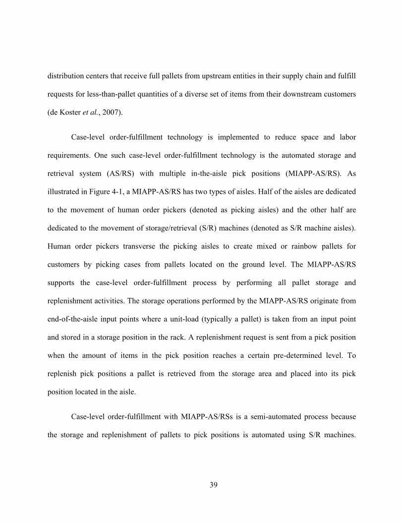
39

distribution centers that receive full pallets from upstream entities in their supply chain and fulfill

requests for less-than-pallet quantities of a diverse set of items from their downstream customers

(de Koster et al., 2007).

Case-level order-fulfillment technology is implemented to reduce space and labor

requirements. One such case-level order-fulfillment technology is the automated storage and

retrieval system (AS/RS) with multiple in-the-aisle pick positions (MIAPP-AS/RS). As

illustrated in Figure 4-1, a MIAPP-AS/RS has two types of aisles. Half of the aisles are dedicated

to the movement of human order pickers (denoted as picking aisles) and the other half are

dedicated to the movement of storage/retrieval (S/R) machines (denoted as S/R machine aisles).

Human order pickers transverse the picking aisles to create mixed or rainbow pallets for

customers by picking cases from pallets located on the ground level. The MIAPP-AS/RS

supports the case-level order-fulfillment process by performing all pallet storage and

replenishment activities. The storage operations performed by the MIAPP-AS/RS originate from

end-of-the-aisle input points where a unit-load (typically a pallet) is taken from an input point

and stored in a storage position in the rack. A replenishment request is sent from a pick position

when the amount of items in the pick position reaches a certain pre-determined level. To

replenish pick positions a pallet is retrieved from the storage area and placed into its pick

position located in the aisle.

Case-level order-fulfillment with MIAPP-AS/RSs is a semi-automated process because

the storage and replenishment of pallets to pick positions is automated using S/R machines.

40

However, because building a pallet is difficult to automate due to the varying sizes and weights

of cases, the case-fulfillment process is conducted by human order pickers.

Figure 4-1 : Schematic view of a typical MIAPP-AS/RS

Case-level order-fulfillment is common for company-owned distribution centers that

supply individual retail stores with a variety of products. The primary reasons for implementing

an MIAPP-AS/RS are to increase space utilization and to eliminate the need for human operators

to perform replenishment and storage operations. These factors lead MIAPP-AS/RSs to be

common in temperature-controlled distribution centers especially ones that handle frozen items.

In the cold supply chain, specific temperature standards are enforced to ensure food quality is

maintained: “Chill” (2 to 4 Celsius) is used for fruit and vegetables, “Frozen” (-16 to -20

Celsius) is used for meat, and “Deep Freeze” (-28 to -30 Celsius) is used for seafood and ice-

cream (Rodrigue et al., 2009). Due to the harsh working conditions and increased safety issues,

personnel turnover in deep freeze distribution centers is higher than ambient distribution centers.

Also, the majority of cold temperature loss occurs through the roof of a deep freeze distribution

center; consequently, effective utilization of vertical space is important (and MIAPP-AS/RSs

41

have been designed as high as 165 feet) (Swisslog Co., 2012). In addition, S/R machine aisles

require less space than picking aisles, which result in further space utilization gains. Therefore,

MIAPP-AS/RSs are used to reduce the number of operators who are required to work in the

harsh environments, as well as to reduce the amount of space that is required to be temperature

controlled (which is both financially and environmentally expensive). Additional benefits

include the ability to monitor and control temperature zones and automate the tracking of

products.

The implementation of MIAPP-AS/RSs can be found in numerous grocery distribution

centers in the United States (eg. Publix Super Markets and Wal-Mart), and Europe (eg. Walkers,

Ferrero GmbH and Arla). In these distribution centers a large volume of heavy cases is handled

in Chill and Deep Freeze environments (Swisslog Co., 2013). The 2010 global frozen food

market is estimated to be worth 192.2 Billion US Dollars and the global demand for frozen food

is anticipated to grow at a rate of 4 percent annually (Datamonitor, 2011). Therefore, the number

of Deep Freeze distribution centers and the use of case-level order-fulfillment technology, in

general, and MIAPP-AS/RS in particular, are on the rise.

Because of high infrastructure investment costs and the critical importance of order

fulfillment on cost and customer satisfaction, designing and assessing an MIAPP-AS/RS is an

important strategic decision in warehouse design. Such systems are commonly constrained by

S/R machine throughput; therefore, estimating the average travel time for different design

configurations and operating policies is a fundamental step in designing MIAPP-AS/RSs. To

effectively handle a wide range of item requests in the order-fulfillment process, the number of

42

pick positions available is also an important design characteristic of MIAPP-AS/RSs. The

number of pick positions can be increased through the use of an additional elevated picking floor

on a mezzanine that enables case-level order-fulfillment to be performed at different elevations.

Distribution centers may have different operating policies during peak and non-peak

times. For example, many distribution centers have a peak-picking time where a large majority

of the distribution center’s orders are placed and must be picked before the last truck leaves the

dock for shipment. During peak times, the distribution center prioritizes fulfillment of orders

over storage requests that can be performed during non-peak times. Also, if a distribution center

experiences a balanced number of storage and retrieval requests throughout the day, the S/R

machine can perform a dual command travel that includes both a storage and a retrieval.

Consequently, estimating the throughput of an MIAPP-AS/RS is important for different

operating strategies.

The objective of our research is to understand design decisions and trade-offs that occur

in selecting operating policies when implementing an MIAPP-AS/RS. While much research has

been conducted on the traditional end-of-aisle AS/RSs, these models are not applicable to in-the-

aisle AS/RSs. The difference lies in the location and number of output points, as well as the

retrieval operations. Traditional end-of-aisle AS/RSs have a single input/output (I/O) point for

each aisle where a S/R machine picks up items to be stored and brings items that are retrieved to

order pickers or conveyors. Consequently, travel time models derived for traditional AS/RSs

with a single I/O point result in all of the S/R machine trips starting and terminating at a single

point and each travel time is independent of the previous trip. Whereas, with MIAPP-AS/RSs,

43

retrievals occur to multiple pick positions (outputs) in the aisle. The S/R machine will start a

storage from an input point and terminate a retrieval at one of the in-the-aisle pick positions.

Therefore, the travel time depends on where the S/R machine terminated which requires

considering the previous trip.

Our contribution includes deriving analytical expressions to calculate the expected travel

time of an MIAPP-AS/RS that applies different operating policies and has different physical

configurations. Moreover, closed-form approximations are derived for the case of an infinite

number of pick positions that enable us to derive the optimal shape configuration that minimizes

travel times. Through comparison with a simulation model, we illustrate that our models provide

good estimates and can be used to aid in design and evaluation of real-world systems. Through a

numerical experiment, we assess throughput performance of MIAPP-AS/RSs during peak and

non-peak times for different design configurations. We find that operating policies have different

performance impacts depending on the design configuration.

The remainder of this article is organized as follows. In Section 4-2 we briefly review

relevant literature in the area of AS/RSs with an emphasis on AS/RSs with more than one I/O

point. Section 4-3 provides the description, structure and operations related to an MIAPP-AS/RS,

as well as the main assumptions of our models. In Section 4-4 the analytical travel time models

for the MIAPP-AS/RS are introduced under the presence of different operating policies and

design configurations. Section 4-5 is dedicated to the validation of our analytical models via

simulation analysis, as well as numerical experiments to analyze MIAPP-AS/RS system

performance that provide design insights into different operating policies and physical design

44

configurations. Finally, in Section 4-6, we review our contributions and provide future research

directions.

4-2- Literature review

During the past 30 years AS/RSs have received remarkable attention in the literature. A

wide range of issues relating to AS/RSs have been studied. This is illustrated in the following

review papers dedicated exclusively to AS/RSs: Roodbergen and Vis (2009), Sarker and Babu

(1995) and Vasili et al. (2012). AS/RSs have also been addressed in several warehouse design

and control review papers such as de Koster et al. (2007) and Gu et al. (2007).

Two approaches to estimate the AS/RS travel time exist: (1) a discrete approach (see

Egbelu (1991), Thonemann and Brandeau (1998) and Sari et al. (2005)) or (2) a continuous

approximation approach (see Roodbergen and Vis (2009, Table 8)). Simulation studies have

shown that the difference between the two approaches is not significant (see Bozer and White

(1984), Hu et al. (2005) and Sari et al. (2005)). Consequently, as closed-form expressions can be

obtained, continuous approximation models have received considerably higher attention. We also

use the continuous approximation approach in this paper.

AS/RS travel time models have been investigated from different operational perspectives.

Detailed information can be found in the survey papers of Sarker and Babu (1995) and Vasili et

al. (2012). Derivations for several expected travel time models of single command (SC), dual

command (DC), and travel between (TB) for different AS/RS configurations exist (Bozer and

45

White, 1984; Chang et al., 1995; Foley and Frazelle, 1991; Graves et al., 1977; Hu et al., 2005;

Kouvelis and Papanicolaou, 1995; Sarker and Babu, 1995).

Researchers have also studied the impact of different AS/RS storage assignment policies.

A storage assignment policy determines the assignment of items to storage locations. The

primary goal of a storage policy is to minimize the average travel time subject to satisfying

various system constraints (Goetschalckx and Ratliff 1990). The five most often used storage

policies in the literature are randomized storage; closest-open-location storage assignment; class-

based storage; full-turnover-based storage and dedicated storage (see e.g., Hausman et al. (1976);

Graves et al. (1977); Schwarz et al. (1978); Goetschalckx and Ratliff (1990); Kouvelis and

Papanicolaou (1995); Van den Berg (1999); Roodbergen and Vis (2009)). Hausman et al. (1976)

find that a significant reduction in travel time can be achieved using class-based turnover

assignment policies rather than closest-open-location policies. Both Rosenblatt and Eynan (1989)

and Eynan and Rosenblatt (1994) consider the optimal boundaries for n-class storage racks. They

conclude that a storage rack with a small number of classes (less than 10) can improve the travel

time compared to a full-turnover policy. Guenov and Raeside (1992) compare three different

zone shapes under DC scheduling. They conclude that performance of the proposed shapes

depends on the location of the I/O point. Goetschalckx and Ratliff (1990) consider dedicated

storage policies and shared storage policies. They develop a duration-of-stay (DOS) shared

policy for unit-load system with balanced input and output. Kulturel et al. (1999) compare two

shared storage assignment policies with respect to their average travel time by using computer

simulation.

46

Numerous studies have addressed other operational and control issues such as batching

(Elsayed, 1981; Hwang et al., 1988; Egbelu, 1991), dwell point strategies (Bozer and White,

1984; Egbelu, 1991; Peters et al., 1996; van den Berg, 2002), dual-shuttle or multi-shuttle

(Keserla and Peters, 1994; Sarker et al., 1994; Meller and Mungwattana, 1997), and sequencing

(Schwarz et al., 1978; Han et al., 1987; Eynan and Rosenblatt, 1993).

Lee (1997) categorizes the techniques of evaluating the performance of AS/RSs into

static (Egbelu, 1991; Egbelu and Wu, 1993), computer simulation (Egbelu and Wu, 1993; Linn

and Wysk, 1990; Randhawa et al., 1991; Randhawa and Shroff, 1995), and stochastic analysis.

Bozer and White (1990) introduce the first analytical stochastic analysis for a mini-load AS/RS

that is modeled as a two-server closed queuing network. Lee (1997) presents a stochastic

analysis of unit-load AS/RS for the first time using a continuous time Markov chain. His model

is capable of using different formulas for SC and DC of various system configurations such as

the case when the I/O point is located other than on the lower left corner of the rack. Bozer and

Cho (2005) extend Lee (1997) by developing analytical closed-form stochastic models to

determine if the system meets a desired throughput, as well as identifying the expected S/R

machine utilization. Their model can also apply to alternative I/O point locations or storage

methods if E(SC)>E(TB).

In addition to operational and control issues, many studies have focused on the physical

design and the system configuration of AS/RSs such as the shape of the storage rack, the number

of the cranes and aisles, as well as the number and location of the I/O points (see Vasili et al.

(2012) and references within). The mentioned studies helped extensively to design and operate

47

AS/RSs. However, there are only a few analytical and simulation studies addressing system

configuration with either more than one I/O point or with I/O points not located at the end-of-the

aisle.

Bozer and White (1984) develop and analyze the expected travel time of five alternative

I/O point configurations. They assume that the I/O point can be located at (1) the lower-left

corner of the aisle; (2) the opposite ends of the aisle; (3) the same end of the aisle, but at different

elevations; (4) the same elevation, but at a midpoint in the aisle; and (5) the end of the aisle, but

elevated. All five configurations consider only one input and one output point. The MIAPP-

AS/RS has multiple in-the-aisle points that are not necessarily located at the corner of the rack;

therefore, their models are not applicable. Randhawa et al. (1991) develop a simulation study to

identify the impact of the number of I/O points located at the end-of-the-aisle for three different

unit-load AS/RSs with DC cycles. The AS/RS layouts vary in the number of end-of-aisle I/O

points per aisle and the relationship between the storage and retrieval sources. System

throughput, mean waiting time and maximum waiting time are considered as criteria for system

evaluation. They find that the efficiency of the AS/RS can be improved by the introduction of

two end-of-aisle I/O points per aisle. Randhawa and Shroff (1995) extend the work of Randhawa

et al. (1991) by using simulation to analyze six different layouts with a single I/O point (with

varying location) using three different scheduling policies. The results are compared considering

the system throughput, storage and retrieval waiting times, and rejects due to the rack or I/O

queues being fully utilized. The authors conclude that higher throughput can be obtained by

locating the I/O point at middle of the aisle instead of at the end of the aisle. Both of the studies

use a simulation approach. Also, Randhawa et al. (1991) consider end-of-aisle I/O points only,

48

and Randhawa and Shroff (1995) evaluate a single I/O point in the middle of the aisle. Vasili et

al. (2008) propose a new configuration for the I/O point in a split-platform AS/RS to reduce

average handling time. They develop a continuous travel time model for this new configuration

of locating an I/O point at the center of the rack. The travel time model was validated by using

Monte Carlo simulation. They assume a single I/O point in the center of the rack and only

consider SC cycles.

In summary, the literature on travel time models for AS/RS with more than one I/O point

examines the I/O points at the end-of-the aisle. The literature that examines the location of I/O

points beyond the end-of-aisle only considers a single I/O point in the middle of the rack. To the

best of our knowledge, we are aware of no literature that develops analytical models to analyze

AS/RS design issues with multiple I/O points in the aisle.

4-3- Problem definition and assumptions

As illustrated in Figure 4-1 an MIAPP-AS/RS has two types of aisles that we previously

defined as picking aisles and S/R machine aisles. The picking aisles are wider than S/R machine

aisles to provide space for the pickers to move and conduct case picking. The picking aisle

consists of pick positions at both sides of the aisle. The S/R machine aisle consists of an input

point, a S/R machine, and storage racks on both sides of the aisle. If there is only one picking

floor on the ground, we denote this as a single picking floor configuration. We also study the

case where there is a mezzanine located vertically above the ground floor for each picking aisle

and the S/R machine services both the ground and mezzanine floors pick positions. We denote

this as a dual picking floor configuration. A dual picking floor configuration provides additional

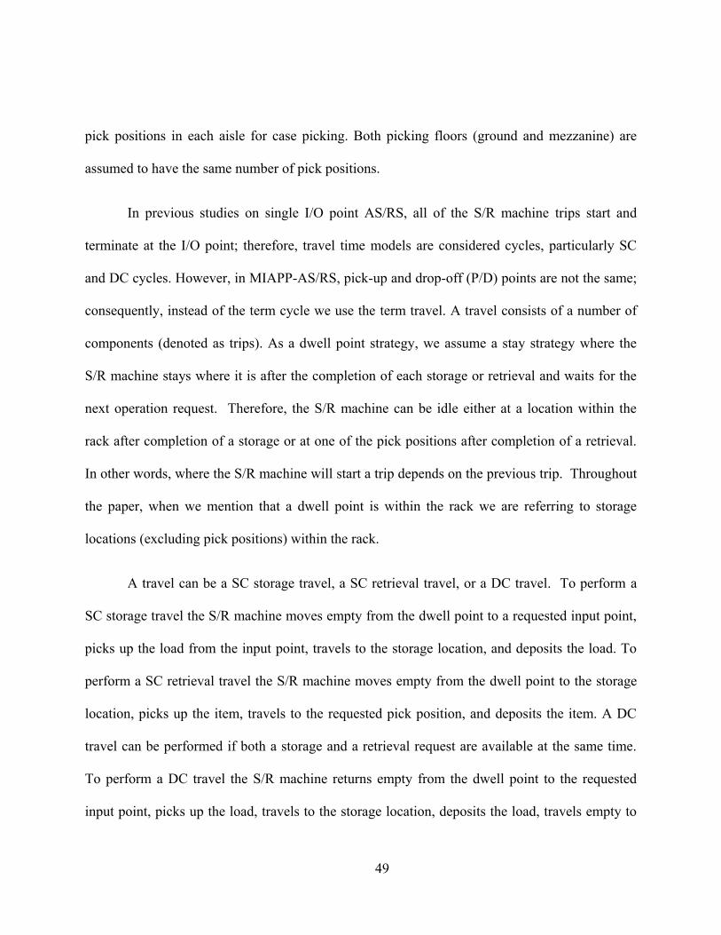
49

pick positions in each aisle for case picking. Both picking floors (ground and mezzanine) are

assumed to have the same number of pick positions.

In previous studies on single I/O point AS/RS, all of the S/R machine trips start and

terminate at the I/O point; therefore, travel time models are considered cycles, particularly SC

and DC cycles. However, in MIAPP-AS/RS, pick-up and drop-off (P/D) points are not the same;

consequently, instead of the term cycle we use the term travel. A travel consists of a number of

components (denoted as trips). As a dwell point strategy, we assume a stay strategy where the

S/R machine stays where it is after the completion of each storage or retrieval and waits for the

next operation request. Therefore, the S/R machine can be idle either at a location within the

rack after completion of a storage or at one of the pick positions after completion of a retrieval.

In other words, where the S/R machine will start a trip depends on the previous trip. Throughout

the paper, when we mention that a dwell point is within the rack we are referring to storage

locations (excluding pick positions) within the rack.

A travel can be a SC storage travel, a SC retrieval travel, or a DC travel. To perform a

SC storage travel the S/R machine moves empty from the dwell point to a requested input point,

picks up the load from the input point, travels to the storage location, and deposits the load. To

perform a SC retrieval travel the S/R machine moves empty from the dwell point to the storage

location, picks up the item, travels to the requested pick position, and deposits the item. A DC

travel can be performed if both a storage and a retrieval request are available at the same time.

To perform a DC travel the S/R machine returns empty from the dwell point to the requested

input point, picks up the load, travels to the storage location, deposits the load, travels empty to

50

the location of the load to be retrieved (called the travel between trip), picks up the load, travels

to the requested pick position, and deposits the load.

We study a system where the S/R machine can operate under either SC (storage or

retrieval) or DC travels. As the dwell point varies, one travel (SC storage, SC retrieval, and DC

travel) can consist of different trips. For example, if the dwell point is at one of the pick positions

a SC retrieval consists of two trips: one trip is from the pick position to the storage location of

item to be retrieved and the other trip is from the storage location to the requested pick position.

However, if the dwell point is at a point within the rack a SC retrieval travel will consist of one

travel between trip and one trip from the storage location to the requested pick position. Figure

4-2 illustrates all six possible cases for a SC storage, SC retrieval, and DC travel under a single

picking floor configuration ((a) SC storage travel when the dwell point is within the rack, (b) SC

retrieval travel when the dwell point is within the rack, and (c) DC travel when the dwell point is

within the rack. (d) SC storage travel when the dwell point is at a pick position, (e) SC retrieval

travel when the dwell point is at a pick position, and (f) DC travel when the dwell point is at a

pick position.). Similarly, for a dual picking configuration travels are also based on the dwell

point of the previous travel. For a dual picking configuration there are 24 possible travel cases as

there are 2 input points and 2 levels of pick positions ( 2 6 cases). In the next section we will

develop models that incorporate all of these cases as a way of calculating the expected travel

time for SC and DC travels.

51

Figure 4-2 : All possible cases of travels under a single picking floor configuration.

During the peak hours the priority is to fulfill customer orders and the AS/RS prefers to

perform only SC retrievals. We denote an AS/RS that performs only SC retrievals as a

Consecutive Retrievals operating policy. To balance the system the AS/RS will perform only SC

storages during non-peak hours (denoted as a Consecutive Storages operating policy). During

the periods that the system is more balanced (i.e. the number of storage and retrieval requests, as

well as their priority are fairly equal), we prefer to have the AS/RS perform DC travels to

decrease empty travels. However, there may not be storage and retrieval requests available at the

same time, which results in SC travels to be performed. Consequently, it is common for an

AS/RS to perform a mixture of SC and DC travels (denoted as a Mixed operating policy). We

consider both balanced and unbalanced periods in our analysis by developing travel time models

for a Consecutive Retrievals, Consecutive Storages and different Mixed operating policies in

Section 4-4. We also explore trade-offs associated with these policies for different design

configurations in more detail in Section 4-5.

We assume that storage locations are continuously and uniformly distributed over the

rack (Bozer and Cho, 2005; Bozer and White, 1984; Graves et al., 1977; Hu et al., 2005; Han et

52

al., 1987). We analyze MIAPP-AS/RSs where each aisle has a dedicated S/R machine (also

known as aisle-captive S/R machines). Therefore, we can analyze each aisle independently.

Furthermore, the S/R machine can move in the horizontal and vertical directions simultaneously.

Hence, the Chebyshev metric is used to calculate the travel time between two points within the

rack, i.e., the travel time between two points within the rack is equal to the maximum time

required for horizontal and vertical travel. Based on the approach used in Bozer and White

(1984) the rack can be normalized as follows.

Let: : length of rack, : height of the rack, : horizontal speed of the S/R machine, : vertical speed of the S/R machine, : time required to travel a distance of horizontally, and : time required to travel a distance of vertically.

By definition, ⁄ and ⁄ . Let { } an { ⁄ ⁄ }, which refer to the scaling factor and the shape factor, respectively. By definition, .

Assuming that h , the rack can be normalized as a rectangle with length of and height of . The rack is called square-in-time if ; otherwise, it is called rectangular-in-time.

The overall review of the assumptions of this paper is as follows.

1. The S/R machine carries unit-loads under either SC (storage/retrieval) or DC travels.

53

2. Demand and requested pick position locations for each item type are known and

independent.

3. A randomized storage assignment is used, i.e., any point within the rack is equal likely to

be selected for a storage.

4. Only the travel time model of the S/R machine is considered. Interactions with human

order pickers and the buffers capacity, as well as the P/D times to handle the loads are

ignored.

5. The S/R machine follows the Chebyshev metric and moves at a constant horizontal and

vertical speed, i.e., acceleration and deceleration are ignored.

6. A stay dwell point strategy is used. In a stay strategy the S/R machine stays where it is

after the completion of each storage or retrieval and waits for the next operation request.

7. For a single picking floor configuration the input point is located at the lower-left corner

and the pick positions are located on the bottom line of a normalized rack. For a dual

picking floor configuration the mezzanine is considered as a line located time units

above the bottom of the normalized rack. The mezzanine floor input point and pick

positions are located on the mezzanine line directly above the input point and pick

positions on the bottom line. The height of the pick positions and mezzanine structure are

ignored.

4-4- Travel time models for MIAPP-AS/RS

First, we present the trips and subsequent notation required to develop our models. Next,

travel time models are developed for a single pick position located in the aisle. These models are

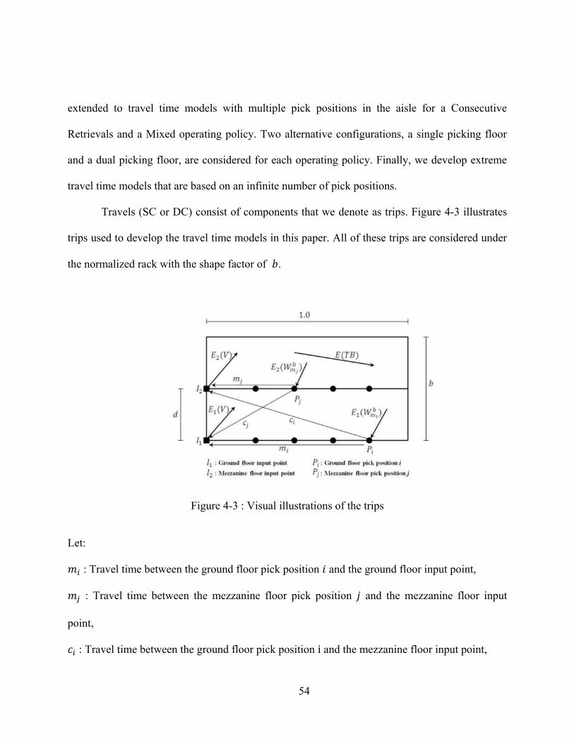
54

extended to travel time models with multiple pick positions in the aisle for a Consecutive

Retrievals and a Mixed operating policy. Two alternative configurations, a single picking floor

and a dual picking floor, are considered for each operating policy. Finally, we develop extreme

travel time models that are based on an infinite number of pick positions.

Travels (SC or DC) consist of components that we denote as trips. Figure 4-3 illustrates

trips used to develop the travel time models in this paper. All of these trips are considered under

the normalized rack with the shape factor of .

Figure 4-3 : Visual illustrations of the trips

Let: : Travel time between the ground floor pick position and the ground floor input point, : Travel time between the mezzanine floor pick position and the mezzanine floor input

point, : Travel time between the ground floor pick position and the mezzanine floor input point,

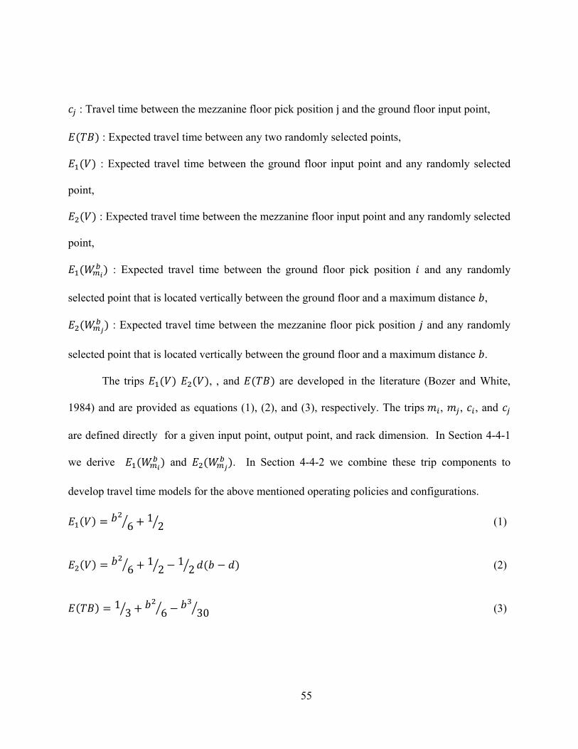
55

: Travel time between the mezzanine floor pick position and the ground floor input point, ( ) : Expected travel time between any two randomly selected points, ( ) : Expected travel time between the ground floor input point and any randomly selected

point, ( ) : Expected travel time between the mezzanine floor input point and any randomly selected

point, ( ) : Expected travel time between the ground floor pick position and any randomly

selected point that is located vertically between the ground floor and a maximum distance , ( ) : Expected travel time between the mezzanine floor pick position and any randomly

selected point that is located vertically between the ground floor and a maximum distance .

The trips ( ) ( ), , and ( ) are developed in the literature (Bozer and White,

1984) and are provided as equations (1), (2), and (3), respectively. The trips , , , and

are defined directly for a given input point, output point, and rack dimension. In Section 4-4-1

we derive ( ) and ( ). In Section 4-4-2 we combine these trip components to

develop travel time models for the above mentioned operating policies and configurations. ( ) ⁄ ⁄ (1)

( ) ⁄ ⁄ ⁄ ( ) (2)

( ) ⁄ ⁄ ⁄ (3)

56

4-4-1- Travel time model for a single in-the-aisle pick position

In this section, first, the travel time model for a single in-the-aisle pick position located

on the ground floor is developed. The result is then extended to determine the travel time model

for a single in-the-aisle pick position located on the mezzanine floor.

4-4-1-1- on the ground floor

To develop a travel time model for a single in-the-aisle pick position, select a point with

the distance of from the left corner of the normalized rack as a pick position and set the point

as the origin of the coordinate system, say ( ). As illustrated in Figure 4-4 the rack can be

divided into two rectangular regions from the point of origin, namely, region I and region II. Any

randomly selected point within the rack can be represented as the coordinate of ( ) in time if

the point belongs to region I, ( )or in time if the point belongs to region II, where (the positive value of is considered as represents time), , ,

and . We define and as the travel time of the S/R machine from the origin

to the point located within region I or region II, respectively. By definition of the Chebyshev

metric, { } and { }. The expected travel time is calculated for each of the two regions separately. Then, the

results obtained from the two regions are combined based on the probability of being in the two

regions. The expected travel time from region I is as follows.

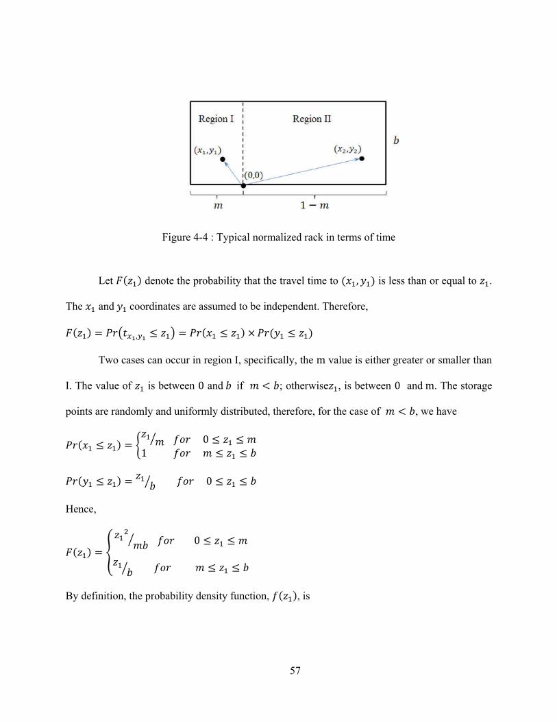
57

Figure 4-4 : Typical normalized rack in terms of time

Let ( ) denote the probability that the travel time to ( ) is less than or equal to .

The and coordinates are assumed to be independent. Therefore, ( ) ( ) ( ) ( ) Two cases can occur in region I, specifically, the value is either greater or smaller than . The value of is between and if ; otherwise , is between and . The storage

points are randomly and uniformly distributed, therefore, for the case of , we have

( ) { ⁄

( ) ⁄

Hence,

( ) { ⁄ ⁄

By definition, the probability density function, ( ), is

58

( ) ( ) { ⁄ ⁄

Le ( )t denote the expected travel time between the origin and any point located in

region I. By definition of the expected value ( ) for the case of is obtained as

follows.

( ) ∫ ( ) ∫ ⁄

∫ ⁄ ⁄ ⁄

The derivation of ( ) for the case of is similar (see Appendix A). Therefore,

the expected travel time between the origin and any point within region I can be calculated by

equation (4).

( ) { ⁄ ⁄ ⁄ ⁄ (4)

The derivation for region II is similar to region I (see Appendix B for the derivation). Let ( ) denote the expected travel time between the origin and any point located in region II. ( ) is presented in equation (5).

( ) { ( ) ⁄ ⁄ ( ) ( )⁄ ( ) ⁄ ( ) (5)

59

As any point within the rack is equal likely to be selected, any point can be situated in

region I or region II with the probability of and ( ), respectively. The expected travel

time between a single pick position on the ground floor and any point within the rack, ( ) is obtained as follows. ( ) ( ) ( ) ( ) (6)

The expected travel time for each region, ( ) and ( ), can be calculated for a

given value of and through equations (4) and (5), respectively. Finally, using equation

(6), ( ) can be calculated.

4-4-1-2- on the mezzanine floor

A mezzanine is located time units above the ground floor (where ). As illustrated

in Figure 4-3, the mezzanine divides the rack into two regions (the region above the mezzanine

and below the mezzanine). Equation (6) is valid for a single pick position located on the ground

floor. Expected travel time between a single pick position located on the mezzanine floor and

any point above the mezzanine and below the mezzanine can be calculated by substituting and ( ), respectively, for in equation (6). Due to a randomized storage policy the probabilities

that the point is above the mezzanine or below the mezzanine are and

( ) , respectively.

Therefore, the expected travel time between a single pick position on the mezzanine floor and

any point within the rack, ( ) can be calculated as the following.

( ) ⁄ ( ) ( ) ⁄ ( ) (7)

60

4-4-2- Travel time model for multiple in-the-aisle pick positions

In this section we extend the results of the previous section to include multiple in-the-

aisle pick positions. Let denote the number of the pick positions in each floor, denote the

corresponding index of each ground pick position, and denote the corresponding index of each

mezzanine pick position, where and .

4-4-2-1- Consecutive Retrievals operating policy

The Consecutive Retrievals operating policy is primarily used during peak hours to

maximize the number of retrievals. Thus, it is assumed that only SC retrieval travels are

performed consecutively. As a result all of the trips initiate or terminate at in-the-aisle pick

positions (see Figure 4-5 and Figure 4-6).

4-4-2-1-1- Travel time model for a single picking floor configuration

Let be the percentage of items requested at pick position (where ∑ ).

Therefore, the ratio of operations terminating to pick position is equal to . The travel time

between pick position to any point within the rack, ( ), can be calculated by equation (6).

As the demand of each pick position is independent the expected travel time of a one-way trip

(see solid lines in Figure 5-5) from any point within the rack to any pick position, ( ), is

equal to: ( ) ∑ ( ) (8)

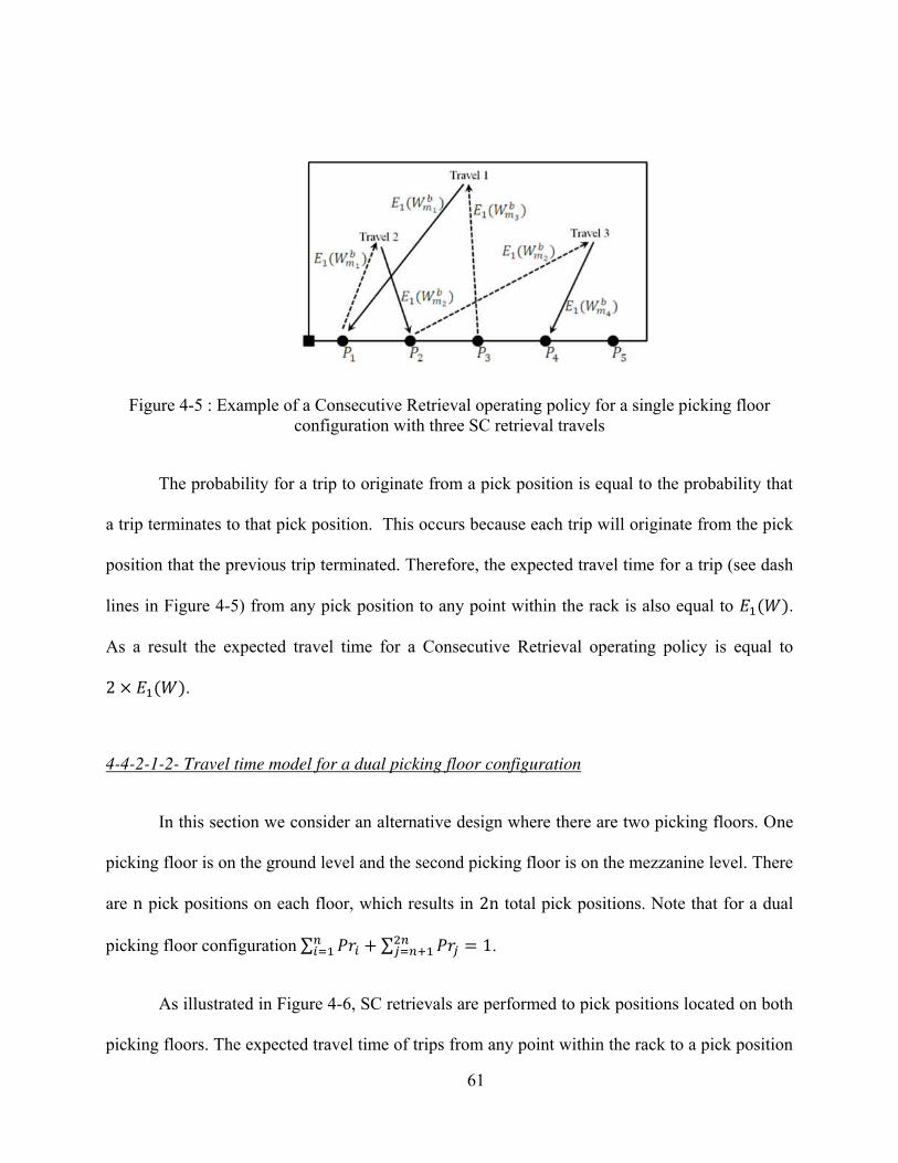
61

Figure 4-5 : Example of a Consecutive Retrieval operating policy for a single picking floor

configuration with three SC retrieval travels

The probability for a trip to originate from a pick position is equal to the probability that

a trip terminates to that pick position. This occurs because each trip will originate from the pick

position that the previous trip terminated. Therefore, the expected travel time for a trip (see dash

lines in Figure 4-5) from any pick position to any point within the rack is also equal to ( ). As a result the expected travel time for a Consecutive Retrieval operating policy is equal to ( ). 4-4-2-1-2- Travel time model for a dual picking floor configuration

In this section we consider an alternative design where there are two picking floors. One

picking floor is on the ground level and the second picking floor is on the mezzanine level. There

are pick positions on each floor, which results in total pick positions. Note that for a dual

picking floor configuration ∑ ∑ .

As illustrated in Figure 4-6, SC retrievals are performed to pick positions located on both

picking floors. The expected travel time of trips from any point within the rack to a pick position

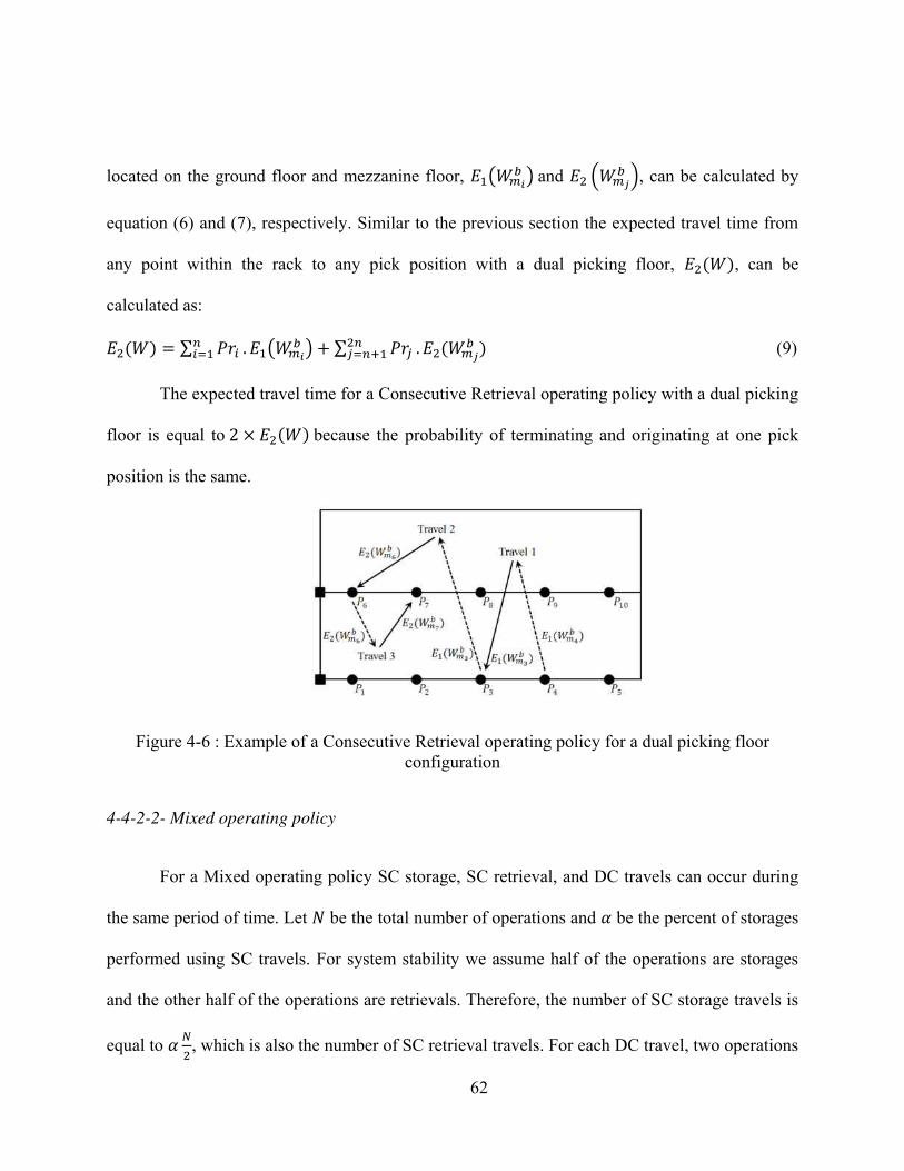
62

located on the ground floor and mezzanine floor, ( ) and ( ), can be calculated by

equation (6) and (7), respectively. Similar to the previous section the expected travel time from

any point within the rack to any pick position with a dual picking floor, ( ), can be

calculated as: ( ) ∑ ( ) ∑ ( ) (9)

The expected travel time for a Consecutive Retrieval operating policy with a dual picking

floor is equal to ( ) because the probability of terminating and originating at one pick

position is the same.

Figure 4-6 : Example of a Consecutive Retrieval operating policy for a dual picking floor

configuration

4-4-2-2- Mixed operating policy

For a Mixed operating policy SC storage, SC retrieval, and DC travels can occur during

the same period of time. Let be the total number of operations and be the percent of storages

performed using SC travels. For system stability we assume half of the operations are storages

and the other half of the operations are retrievals. Therefore, the number of SC storage travels is

equal to , which is also the number of SC retrieval travels. For each DC travel, two operations

63

(one storage and one retrieval) are performed, and ( ) is the number of DC travels. The

total number of travels performed is equal to ( ) .

Based on the provided number of travels, is the probability that a SC storage (or SC

retrieval) travel occurs, and is the probability that a DC travel occurs. In this section, first,

we develop the expected travel time ‘per travel’ for a Mixed operation policy. In many cases, the

expected travel time ‘per operation’ is required to be calculated and can be obtained by

multiplying the expected travel time ‘per travel’ by ( ).

To illustrate the difference between ‘per operation’ and ‘per travel,’ we present the

following example. Suppose there are 100 operations, 50 operations are storages and 50

operations are retrievals. If , 20 storages and 20 retrievals will be performed under SC

travels and 30 storages and 30 retrievals are performed together using DC travels (for a total of

30 DC travels). Consequently, a total of 70 travels (SC or DC) will be performed to accomplish

100 operations. Therefore, , which is the ratio of travels operated using SC

storage (or SC retrieval) and , which is equal to the ratio of travels operated

using DC. Additionally, the ratios of operations performed under SC storage (or SC retrieval)

and DC are and , respectively.

Using the trips we introduced at the beginning of Section 4-4, as well as the developed

models from Section 4-4-1 and 4-4-2-1, we develop the Mixed policy travel time models for both

single and dual picking floor configurations.

64

4-4-2-2-1- for a single picking floor configuration

For a single picking floor configuration a travel will originate from the point within the

rack if the previous travel was a SC storage. Otherwise, if the previous travel was either a SC

retrieval or DC the next travel will originate from one of the in-the-aisle pick positions.

Therefore, the probability that a travel starts at a point within the rack is and the probability

that a travel starts at the pick position is ( ). If a travel starts at some point within the rack the expected travel time to perform a SC

storage is equal to ( ), a SC retrieval is equal to ( ) ( ), and a DC is equal to ( ) ( ) ( ). If a travel starts at pick position the expected travel time to

perform a SC storage is equal to ( ), a SC retrieval is equal to ( ), and a DC is

equal to ( ) ( ) ( ). Let ( ) denote the expected travel time ‘per travel’

for a Mixed operating policy with a single picking floor configuration. According to the provided

probability of each travel during a Mixed policy, ( ) can be calculated as follows (the first

term represents the travel that starts from any point within the rack and the second term the travel

that starts from the pick position ).

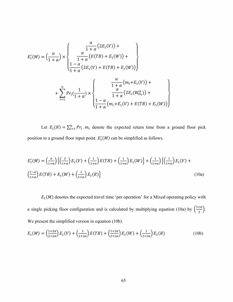
65

( ) ( ) { ( ( )) ( ( ) ( )) ( ( ) ( ) ( ))}

∑ ( ) { ( ( )) ( ( )) ( ( ) ( ) ( ))}

Let ( ) ∑ denote the expected return time from a ground floor pick

position to a ground floor input point. ( ) can be simplified as follows.

( ) ( ) {( ) ( ) ( ) ( ) ( ) ( )} ( ) {( ) ( ) ( ) ( ) ( ) ( ) ( )} (10a)

( ) denotes the expected travel time ‘per operation’ for a Mixed operating policy with

a single picking floor configuration and is calculated by multiplying equation (10a) by ( ).

We present the simplified version in equation (10b). ( ) ( ) ( ) ( ) ( ) ( ) ( ) ( ) ( ) (10b)

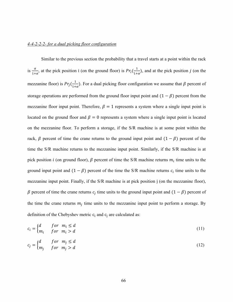
66

4-4-2-2-2- for a dual picking floor configuration

Similar to the previous section the probability that a travel starts at a point within the rack

is , at the pick position (on the ground floor) is ( ), and at the pick position (on the

mezzanine floor) is ( ). For a dual picking floor configuration we assume that percent of

storage operations are performed from the ground floor input point and ( ) percent from the

mezzanine floor input point. Therefore, represents a system where a single input point is

located on the ground floor and represents a system where a single input point is located

on the mezzanine floor. To perform a storage, if the S/R machine is at some point within the

rack, percent of time the crane returns to the ground input point and ( ) percent of the

time the S/R machine returns to the mezzanine input point. Similarly, if the S/R machine is at

pick position (on ground floor), percent of time the S/R machine returns time units to the

ground input point and ( ) percent of the time the S/R machine returns time units to the

mezzanine input point. Finally, if the S/R machine is at pick position (on the mezzanine floor), percent of time the crane returns time units to the ground input point and ( ) percent of

the time the crane returns time units to the mezzanine input point to perform a storage. By

definition of the Chebyshev metric and are calculated as:

{ (11)

{ (12)

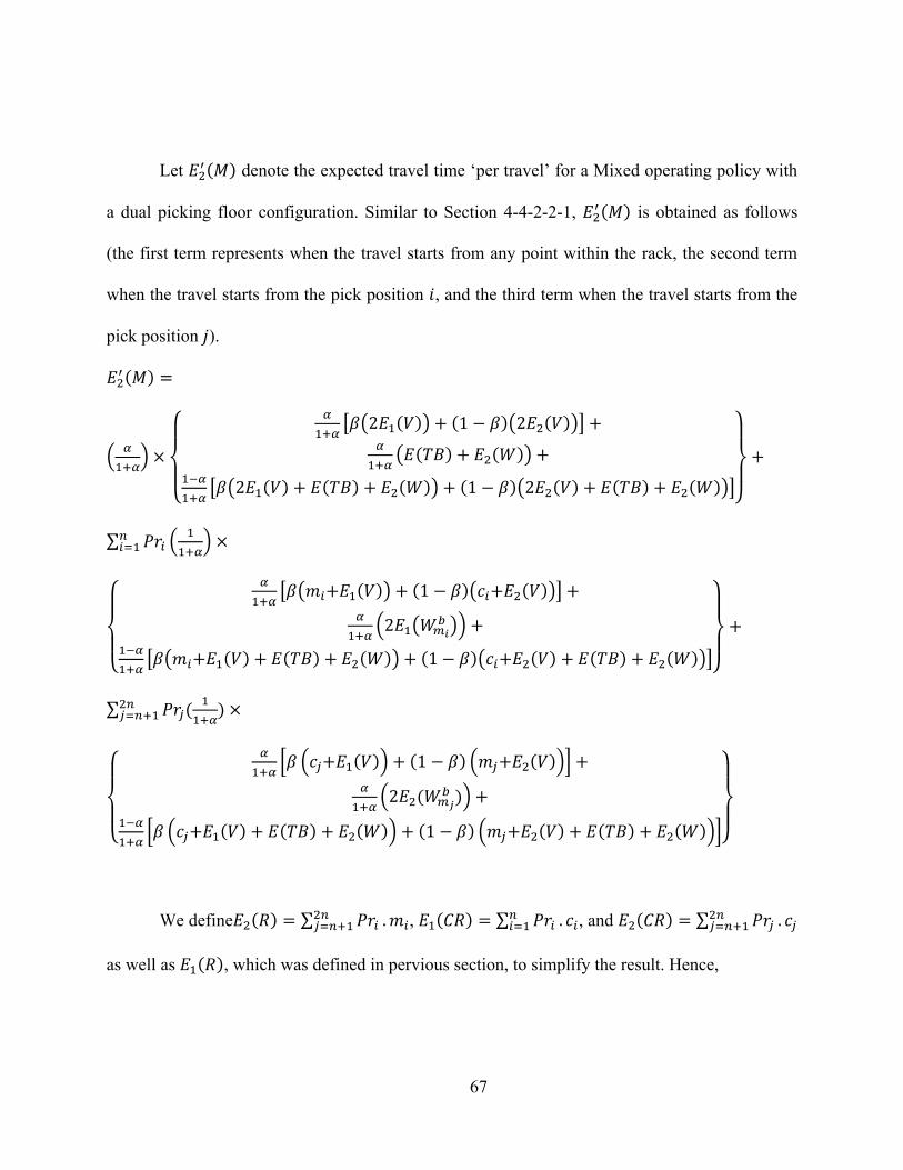
67

Let ( ) denote the expected travel time ‘per travel’ for a Mixed operating policy with

a dual picking floor configuration. Similar to Section 4-4-2-2-1, ( ) is obtained as follows

(the first term represents when the travel starts from any point within the rack, the second term

when the travel starts from the pick position , and the third term when the travel starts from the

pick position ). ( ) ( ) {

[ ( ( )) ( )( ( ))] ( ( ) ( )) [ ( ( ) ( ) ( )) ( )( ( ) ( ) ( ))]}

∑ ( )

{ [ ( ( )) ( )( ( ))] ( ( )) [ ( ( ) ( ) ( )) ( )( ( ) ( ) ( ))]}

∑ ( )

{ [ ( ( )) ( ) ( ( ))] ( ( )) [ ( ( ) ( ) ( )) ( ) ( ( ) ( ) ( ))]}

We define ( ) ∑ , ( ) ∑ , and ( ) ∑

as well as ( ), which was defined in pervious section, to simplify the result. Hence,

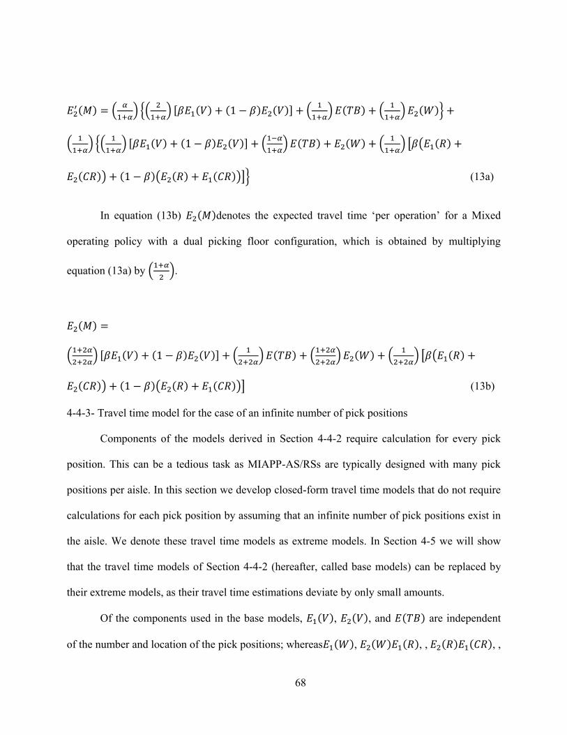
68

( ) ( ) {( ) [ ( ) ( ) ( )] ( ) ( ) ( ) ( )} ( ) {( ) [ ( ) ( ) ( )] ( ) ( ) ( ) ( ) [ ( ( ) ( )) ( )( ( ) ( ))]} (13a)

In equation (13b) ( )denotes the expected travel time ‘per operation’ for a Mixed

operating policy with a dual picking floor configuration, which is obtained by multiplying

equation (13a) by ( ).

( ) ( ) [ ( ) ( ) ( )] ( ) ( ) ( ) ( ) ( ) [ ( ( ) ( )) ( )( ( ) ( ))] (13b)

4-4-3- Travel time model for the case of an infinite number of pick positions

Components of the models derived in Section 4-4-2 require calculation for every pick

position. This can be a tedious task as MIAPP-AS/RSs are typically designed with many pick

positions per aisle. In this section we develop closed-form travel time models that do not require

calculations for each pick position by assuming that an infinite number of pick positions exist in

the aisle. We denote these travel time models as extreme models. In Section 4-5 we will show

that the travel time models of Section 4-4-2 (hereafter, called base models) can be replaced by

their extreme models, as their travel time estimations deviate by only small amounts.

Of the components used in the base models, ( ), ( ), and ( ) are independent

of the number and location of the pick positions; whereas ( ), ( ) ( ), , ( ) ( ), ,

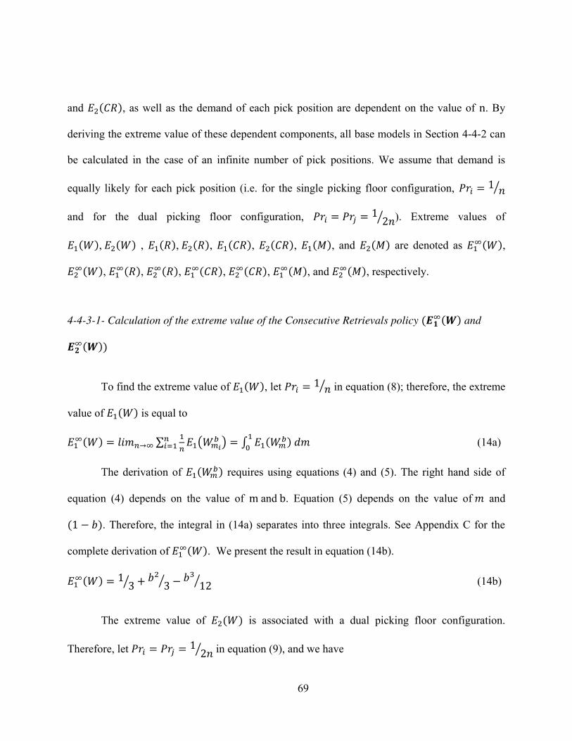
69

and ( ), as well as the demand of each pick position are dependent on the value of . By

deriving the extreme value of these dependent components, all base models in Section 4-4-2 can

be calculated in the case of an infinite number of pick positions. We assume that demand is

equally likely for each pick position (i.e. for the single picking floor configuration, ⁄

and for the dual picking floor configuration, ⁄ ). Extreme values of ( ), ( ) , ( ), ( ), ( ), ( ), ( ), and ( ) are denoted as ( ), ( ), ( ), ( ), ( ), ( ), ( ), and ( ), respectively.

4-4-3-1- Calculation of the extreme value of the Consecutive Retrievals policy ( ( ) and ( )) To find the extreme value of ( ), let ⁄ in equation (8); therefore, the extreme

value of ( ) is equal to ( ) ∑ ( ) ∫ ( ) (14a)

The derivation of ( ) requires using equations (4) and (5). The right hand side of

equation (4) depends on the value of and . Equation (5) depends on the value of and ( ). Therefore, the integral in (14a) separates into three integrals. See Appendix C for the

complete derivation of ( ). We present the result in equation (14b). ( ) ⁄ ⁄ ⁄ (14b)

The extreme value of ( ) is associated with a dual picking floor configuration.

Therefore, let ⁄ in equation (9), and we have

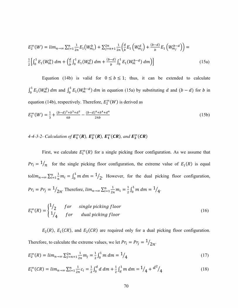
70

( ) ∑ ( ) ∑ ( ( ) ( ) ( )) [∫ ( ) ( ∫ ( ) ( ) ∫ ( ) )] (15a)

Equation (14b) is valid for ; thus, it can be extended to calculate ∫ ( ) and ∫ ( ) in equation (15a) by substituting and ( ) for in

equation (14b), respectively. Therefore, ( ) is derived as ( ) ( ) ( ) (15b)

4-4-3-2- Calculation of ( ), ( ), ( ), and ( )

First, we calculate ( ) for a single picking floor configuration. As we assume that ⁄ for the single picking floor configuration, the extreme value of ( ) is equal

to ∑ ∫ ⁄ . However, for the dual picking floor configuration,

⁄ . Therefore, ∑ ∫ ⁄ .

( ) { ⁄ ⁄ (16)

( ), ( ), and ( ) are required only for a dual picking floor configuration.

Therefore, to calculate the extreme values, we let ⁄ .

( ) ∑ ∫ ⁄ (17)

( ) ∑ ∫ ∫ ⁄ ⁄ (18)

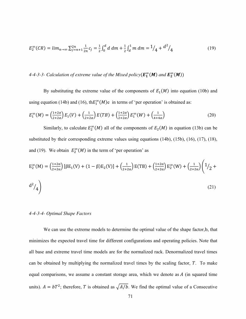
71

( ) ∑ ∫ ∫ ⁄ ⁄ (19)

4-4-3-3- Calculation of extreme value of the Mixed policy( ( ) and ( )) By substituting the extreme value of the components of ( ) into equation (10b) and

using equation (14b) and (16), th ( )e in terms of ‘per operation’ is obtained as: ( ) ( ) ( ) ( ) ( ) ( ) ( ) ( ) (20)

Similarly, to calculate ( ) all of the components of ( ) in equation (13b) can be

substituted by their corresponding extreme values using equations (14b), (15b), (16), (17), (18),

and (19). We obtain ( ) in the term of ‘per operation’ as

( ) ( ) [ ( ) ( ) ( )] ( ) ( ) ( ) ( ) ( ) ( ⁄ ⁄ ) (21)

4-4-3-4- Optimal Shape Factors

We can use the extreme models to determine the optimal value of the shape factor, , that

minimizes the expected travel time for different configurations and operating policies. Note that

all base and extreme travel time models are for the normalized rack. Denormalized travel times

can be obtained by multiplying the normalized travel times by the scaling factor, . To make

equal comparisons, we assume a constant storage area, which we denote as (in squared time

units). ; therefore, is obtained as √ ⁄ . We find the optimal value of a Consecutive

72

Retrievals policy with a single picking floor by first denormalizing the time units by multiplying

equation (14b) by √ ⁄ , then taking the derivative with respect to , setting the resulting equal

to zero, and solving for . The optimal value for ( ) is derived as 0.6825. Similarly, for

the Consecutive Retrievals policy with a dual picking floor, the optimal value is equal to

0.8965 for ( ) when ⁄ and . For either configuration using the Mixed policy

( ( ) and ( )), the optimal value is 1.0.

4-5- Model validation and numerical discussion

In this section, first, the travel time models developed in Section 4-4 are evaluated for

their accuracy. Next, insights and trade-offs between different operating policies under the single

and dual picking floor configurations are provided.

4-5-1- Validation of the base and extreme models

In this section the results of the base models presented in Section 4-4-2, as well as their

extreme models presented in Section 4-4-3 are compared to results obtained from a discrete-

event simulation that enforces a discrete rack. We present the results in this section as

denormalized expected travel times ‘per operation’. We coded and ran our models and

simulation in MATLAB 2010.

An opening in a rack can be either a pick position or a storage location. The number of

pick positions is assumed to be equal to the number of columns for a single picking floor

configuration and twice the number of columns for a dual picking floor configuration. Openings

are assumed to be 4 feet by 4 feet in width and height. We calculate the travel distance between

73

openings using a centroid method. The horizontal and vertical speeds of the S/R machine are

equal to 400 and 160 feet per minute, respectively. We consider six different ratios of the number

of columns to the number of levels. The ratios are selected such that the number of storage

locations remains approximately constant. We ran 5 replications of a sequence of 100,000

operations to simulate each ratio configuration. We test our models assuming that item demand

is equally likely for each pick position. To compare the results of our models and those obtained

from the simulation, the ‘% deviation’ is used and shown in equation (22). (22)

We compare the expected travel time from our base and extreme models from Section 4-

4 to the average travel time from the simulation. We report our results for a single and dual

picking floor configuration in Table 4-1 and Table 4-2, respectively. For the simulation results

we report the average and variance of the travel time per operation for each ratio configuration.

In Table 4-1, a rack with a single picking floor and approximately 950 storage openings is

considered. The results of our base models, as well as their extreme values are compared to the

simulation results for both a Consecutive Retrievals and a Mixed policy. For a Consecutive

Retrievals policy, the denormalized base and extreme model results are calculated as ( ) and ( ) using equations (8) and (14b), respectively. For a Mixed policy, the

denormalized base and extreme model results are equal to ( ) and ( ) using

equations (10b) and (20), respectively. Table 4-2 presents results for a dual picking floor with

approximately 900 storage openings. The denormalized base/extreme results for a Consecutive

Retrievals policy are calculated as ( ) and ( ) using equations (9) and (15b),

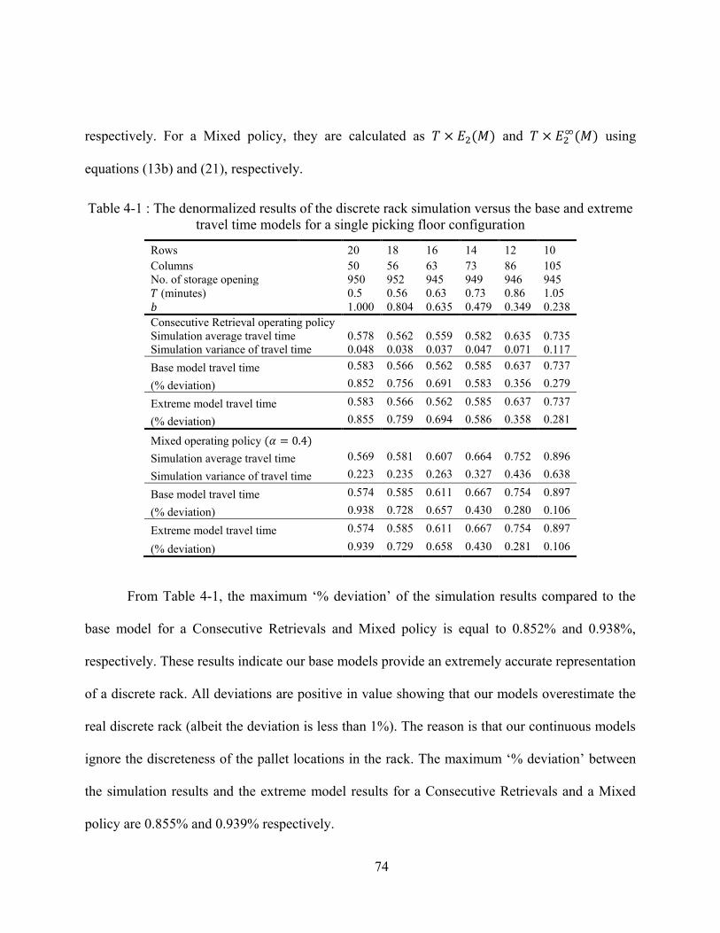
74

respectively. For a Mixed policy, they are calculated as ( ) and ( ) using

equations (13b) and (21), respectively.

Table 4-1 : The denormalized results of the discrete rack simulation versus the base and extreme

travel time models for a single picking floor configuration

Rows 20 18 16 14 12 10

Columns

50 56 63 73 86 105

No. of storage opening 950 952 945 949 946 945 (minutes) 0.5 0.56 0.63 0.73 0.86 1.05 1.000 0.804 0.635 0.479 0.349 0.238

Consecutive Retrieval operating policy

Simulation average travel time 0.578 0.562 0.559 0.582 0.635 0.735

Simulation variance of travel time 0.048 0.038 0.037 0.047 0.071 0.117

Base model travel time 0.583 0.566 0.562 0.585 0.637 0.737

(% deviation) 0.852 0.756 0.691 0.583 0.356 0.279

Extreme model travel time 0.583 0.566 0.562 0.585 0.637 0.737

(% deviation) 0.855 0.759 0.694 0.586 0.358 0.281

Mixed operating policy ( )

Simulation average travel time 0.569 0.581 0.607 0.664 0.752 0.896

Simulation variance of travel time 0.223 0.235 0.263 0.327 0.436 0.638

Base model travel time 0.574 0.585 0.611 0.667 0.754 0.897

(% deviation) 0.938 0.728 0.657 0.430 0.280 0.106

Extreme model travel time 0.574 0.585 0.611 0.667 0.754 0.897

(% deviation) 0.939 0.729 0.658 0.430 0.281 0.106

From Table 4-1, the maximum ‘% deviation’ of the simulation results compared to the

base model for a Consecutive Retrievals and Mixed policy is equal to 0.852% and 0.938%,

respectively. These results indicate our base models provide an extremely accurate representation

of a discrete rack. All deviations are positive in value showing that our models overestimate the

real discrete rack (albeit the deviation is less than 1%). The reason is that our continuous models

ignore the discreteness of the pallet locations in the rack. The maximum ‘% deviation’ between

the simulation results and the extreme model results for a Consecutive Retrievals and a Mixed

policy are 0.855% and 0.939% respectively.

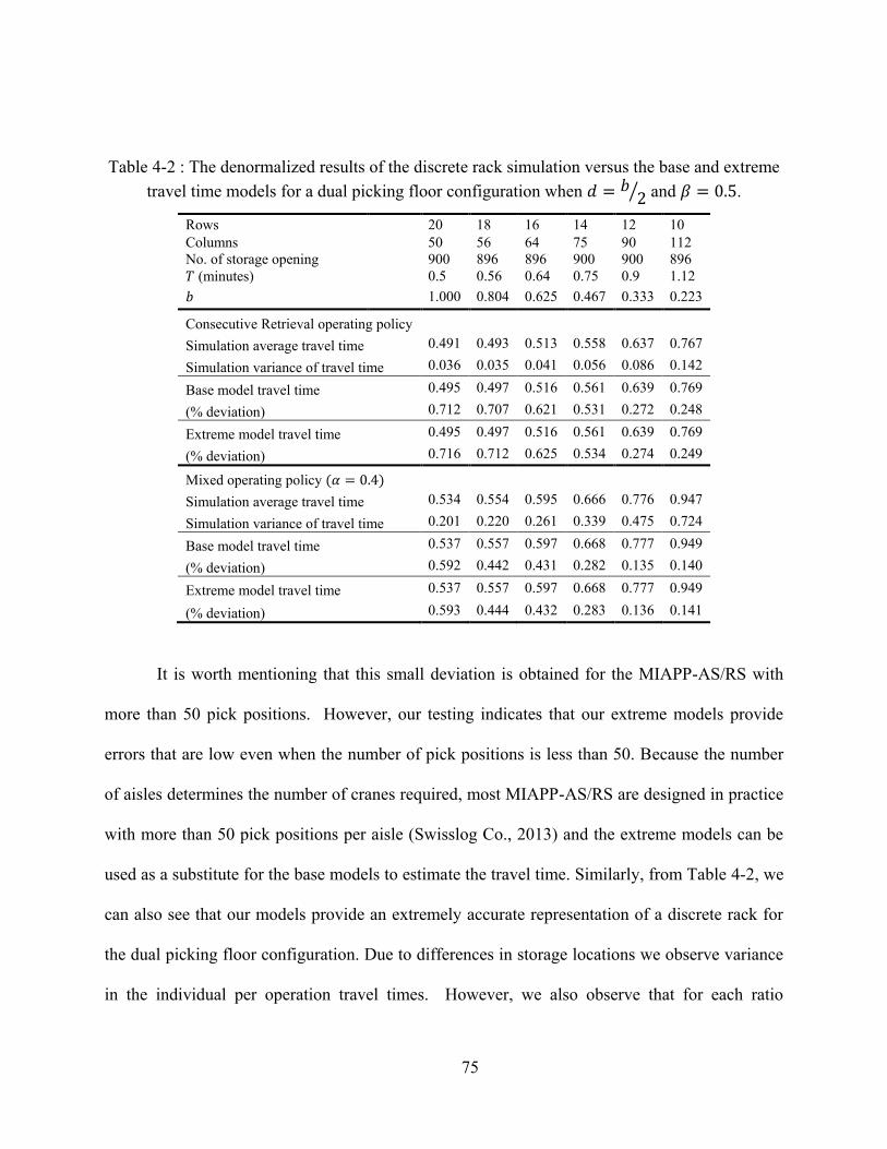
75

Table 4-2 : The denormalized results of the discrete rack simulation versus the base and extreme

travel time models for a dual picking floor configuration when ⁄ and .

Rows 20 18 16 14 12 10

Columns

50 56 64 75 90 112

No. of storage opening 900 896 896 900 900 896 (minutes) 0.5 0.56 0.64 0.75 0.9 1.12 1.000 0.804 0.625 0.467 0.333 0.223

Consecutive Retrieval operating policy

Simulation average travel time 0.491 0.493 0.513 0.558 0.637 0.767

Simulation variance of travel time 0.036 0.035 0.041 0.056 0.086 0.142

Base model travel time 0.495 0.497 0.516 0.561 0.639 0.769

(% deviation) 0.712 0.707 0.621 0.531 0.272 0.248

Extreme model travel time 0.495 0.497 0.516 0.561 0.639 0.769

(% deviation) 0.716 0.712 0.625 0.534 0.274 0.249

Mixed operating policy ( )

Simulation average travel time 0.534 0.554 0.595 0.666 0.776 0.947

Simulation variance of travel time 0.201 0.220 0.261 0.339 0.475 0.724

Base model travel time 0.537 0.557 0.597 0.668 0.777 0.949

(% deviation) 0.592 0.442 0.431 0.282 0.135 0.140

Extreme model travel time 0.537 0.557 0.597 0.668 0.777 0.949

(% deviation) 0.593 0.444 0.432 0.283 0.136 0.141

It is worth mentioning that this small deviation is obtained for the MIAPP-AS/RS with

more than 50 pick positions. However, our testing indicates that our extreme models provide

errors that are low even when the number of pick positions is less than 50. Because the number

of aisles determines the number of cranes required, most MIAPP-AS/RS are designed in practice

with more than 50 pick positions per aisle (Swisslog Co., 2013) and the extreme models can be

used as a substitute for the base models to estimate the travel time. Similarly, from Table 4-2, we

can also see that our models provide an extremely accurate representation of a discrete rack for

the dual picking floor configuration. Due to differences in storage locations we observe variance

in the individual per operation travel times. However, we also observe that for each ratio

76

configuration the variance of the 5 replications’ travel time is extremely small (i.e., the

maximum variance was 0.000003).

We use the extreme models to provide further design insights of MIAPP-AS/RS in the

following section.

4-5-2- Analysis of operating policies

In this section, we introduce three new policies that utilize the travel time models

developed in Section 4-4. The first two policies are extreme cases of the Mixed policy and the

last policy is a combination of the Consecutive Retrievals and the Consecutive Storages policies.

We note that the expected travel times for a mixed policy with other values of will fall

between the DC and Random Sequence of SC Storages and Retrievals policies.

1. DC Policy, which is a policy where all travels are DC. The expected travel time for this

policy is calculated using the model for the Mixed policy with .

2. Random Sequence of SC Storages and Retrievals Policy, which is a policy where all travels

are SC and the same number of SC storages and SC retrievals are sequenced randomly (e.g.

SRRSSRSRRS). The expected travel time for this policy is calculated using the Mixed policy

model with .

3. Consecutive Retrievals then Storages Policy, which is a policy where all travels are SC;

however, the SC retrievals are all completed consecutively followed by all of the SC storages

(e.g. RRRRRSSSSS). The expected travel time for this policy is calculated as the average of

the Consecutive Retrievals policy followed by the Consecutive Storages policy.

In this section we provide denormalized expected travel times for these different policies

under a single and dual picking floor configuration. We analyze performance using metrics based

77

on travel times ‘per retrieval’ and ‘per operation’. Denormalized expected travel times ‘per

operation’ for the Consecutive Retrievals then Storages policy under a single and dual picking

floor are calculated as [ ( ) ( )] and [ ( ) ( ( ) ( ) ( ))], respectively, using equations (1), (2), (14b) and (15b). Also, denormalized expected travel times

‘per operation’ for the Mixed policies under the single and dual picking floor configuration are

equal to ( ) and ( ), respectively, using equations (20) and (21).

Denormalized expected travel times ‘per retrieval’ for a Consecutive Retrievals policy under the

single and dual picking floor configuration are equal to ( ) and ( ) using

equations (14b) and (15b), respectively. As only half of the operations performed using a Mixed

policy are retrievals, denormalized expected travel times ‘per retrieval’ for these policies are

calculated as ( ) and ( ) under the single and dual picking floor using

equations (20) and (21), respectively. The numerical results in this section are created using the

same ratio configurations as Table 4-1 and 4-2 in Section 4-5-1. We use our models to provide

insights into the design of an MIAPP-AS/RS from four different perspectives.

First, we explore the impact of design criteria associated with the dual picking floor

configuration on the expected travel times. Specifically, we evaluate the percent of storage

operations being performed from the ground input floor versus the mezzanine input floor and the

location of the mezzanine floor. As retrievals are independent of the input point, the value does

not influence the Consecutive Retrievals policy. For the Consecutive Retrievals then Storages

policy and the mixed policies increasing will increase the expected travel time because ( ) ( ) for any . Therefore, to minimize the expected travel times for any policy

set , which represents a design where all storage operations originate from the mezzanine

78

floor input point. Such a design may require additional material handling equipment to transfer

the incoming unit loads to the elevated input point; therefore, in subsequent analysis we explore

the cases when is equal to 0.0, 0.5, or 1.0.

To analyze the location of the mezzanine floor, we find the optimal value that

minimizes the expected travel time for any given policy numerically. We coded the numerical

search using MATLAB 2010’s fminbnd function and our results are valid for the performance

metrics based on ‘per retrieval’ and ‘per operation’. In Table 4-3 we report the expected value of

the best for the different policies and values found over all values given in Table 4-2. The

maximum variance for a given policy and value is 0.0001; therefore, the values for the

mezzanine level given in Table 4-3 are good approximations regardless of the value of . From

Table 4-3, we observe that the mezzanine should be located such that . The

reasoning for this result is that three travels influence the value of : (1) the travel between the

mezzanine floor input point and a storage location in the rack, (2) the travel between a storage

location and a pick position on the mezzanine floor, and (3) the travel from a pick position on the

ground floor back to the mezzanine input point to begin a storage (or from a pick position on the

mezzanine level to the ground floor input point). The expected travel between the mezzanine

floor input point to a storage location in the rack or from a storage location to a pick position on

the mezzanine floor is minimized when (see equations (2) and (15b)). The expected

travel from a pick position on the mezzanine floor to the ground floor input point (or from a pick

position on the ground floor to the mezzanine input point) is minimized when (see

equations (11) and (12)).

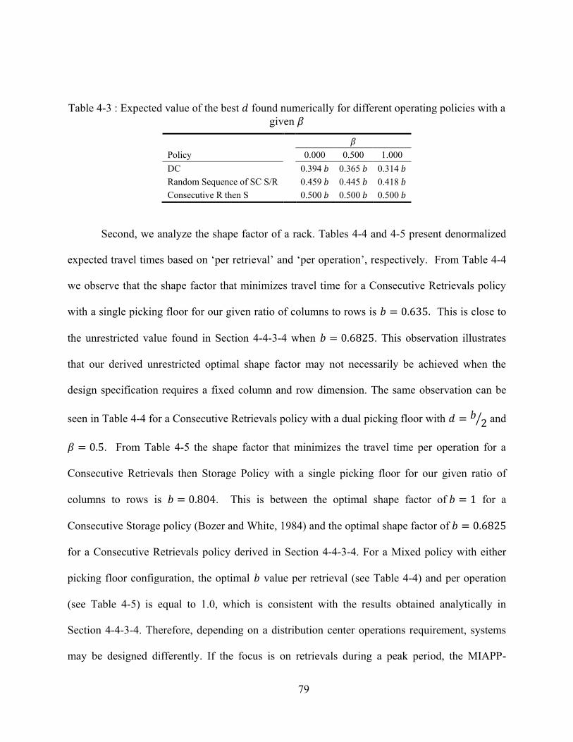
79

Table 4-3 : Expected value of the best found numerically for different operating policies with a

given

Policy

0.000 0.500 1.000

DC

0.394 0.365 0.314

Random Sequence of SC S/R

0.459 0.445 0.418

Consecutive R then S 0.500 0.500 0.500

Second, we analyze the shape factor of a rack. Tables 4-4 and 4-5 present denormalized

expected travel times based on ‘per retrieval’ and ‘per operation’, respectively. From Table 4-4

we observe that the shape factor that minimizes travel time for a Consecutive Retrievals policy

with a single picking floor for our given ratio of columns to rows is This is close to

the unrestricted value found in Section 4-4-3-4 when . This observation illustrates

that our derived unrestricted optimal shape factor may not necessarily be achieved when the

design specification requires a fixed column and row dimension. The same observation can be

seen in Table 4-4 for a Consecutive Retrievals policy with a dual picking floor with ⁄ and . From Table 4-5 the shape factor that minimizes the travel time per operation for a

Consecutive Retrievals then Storage Policy with a single picking floor for our given ratio of

columns to rows is . This is between the optimal shape factor of for a

Consecutive Storage policy (Bozer and White, 1984) and the optimal shape factor of

for a Consecutive Retrievals policy derived in Section 4-4-3-4. For a Mixed policy with either

picking floor configuration, the optimal value per retrieval (see Table 4-4) and per operation

(see Table 4-5) is equal to 1.0, which is consistent with the results obtained analytically in

Section 4-4-3-4. Therefore, depending on a distribution center operations requirement, systems

may be designed differently. If the focus is on retrievals during a peak period, the MIAPP-

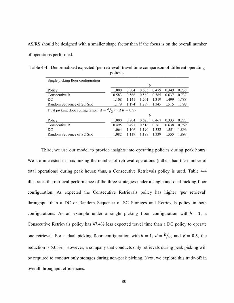
80

AS/RS should be designed with a smaller shape factor than if the focus is on the overall number

of operations performed.

Table 4-4 : Denormalized expected ‘per retrieval’ travel time comparison of different operating

policies

Single picking floor configuration

Policy

1.000 0.804 0.635 0.479 0.349 0.238

Consecutive R

0.583 0.566 0.562 0.585 0.637 0.737

DC

1.108 1.141 1.201 1.319 1.499 1.788

Random Sequence of SC S/R

1.179 1.194 1.239 1.345 1.515 1.798

Dual picking floor configuration ( ⁄ )

Policy

1.000 0.804 0.625 0.467 0.333 0.223

Consecutive R

0.495 0.497 0.516 0.561 0.638 0.769

DC

1.064 1.106 1.190 1.332 1.551 1.896

Random Sequence of SC S/R 1.082 1.119 1.199 1.339 1.555 1.898

Third, we use our model to provide insights into operating policies during peak hours.

We are interested in maximizing the number of retrieval operations (rather than the number of

total operations) during peak hours; thus, a Consecutive Retrievals policy is used. Table 4-4

illustrates the retrieval performance of the three strategies under a single and dual picking floor

configuration. As expected the Consecutive Retrievals policy has higher ‘per retrieval’

throughput than a DC or Random Sequence of SC Storages and Retrievals policy in both

configurations. As an example under a single picking floor configuration with , a

Consecutive Retrievals policy has 47.4% less expected travel time than a DC policy to operate

one retrieval. For a dual picking floor configuration with ⁄ , and , the

reduction is 53.5%. However, a company that conducts only retrievals during peak picking will

be required to conduct only storages during non-peak picking. Next, we explore this trade-off in

overall throughput efficiencies.

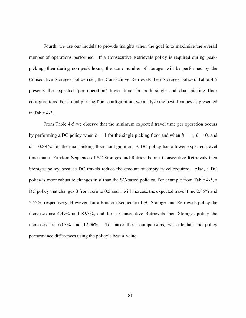
81

Fourth, we use our models to provide insights when the goal is to maximize the overall

number of operations performed. If a Consecutive Retrievals policy is required during peak-

picking; then during non-peak hours, the same number of storages will be performed by the

Consecutive Storages policy (i.e., the Consecutive Retrievals then Storages policy). Table 4-5

presents the expected ‘per operation’ travel time for both single and dual picking floor

configurations. For a dual picking floor configuration, we analyze the best values as presented

in Table 4-3.

From Table 4-5 we observe that the minimum expected travel time per operation occurs

by performing a DC policy when for the single picking floor and when , , and for the dual picking floor configuration. A DC policy has a lower expected travel

time than a Random Sequence of SC Storages and Retrievals or a Consecutive Retrievals then

Storages policy because DC travels reduce the amount of empty travel required. Also, a DC

policy is more robust to changes in than the SC-based policies. For example from Table 4-5, a

DC policy that changes from zero to 0.5 and 1 will increase the expected travel time 2.85% and

5.55%, respectively. However, for a Random Sequence of SC Storages and Retrievals policy the

increases are 4.49% and 8.93%, and for a Consecutive Retrievals then Storages policy the

increases are 6.03% and 12.06%. To make these comparisons, we calculate the policy

performance differences using the policy’s best value.

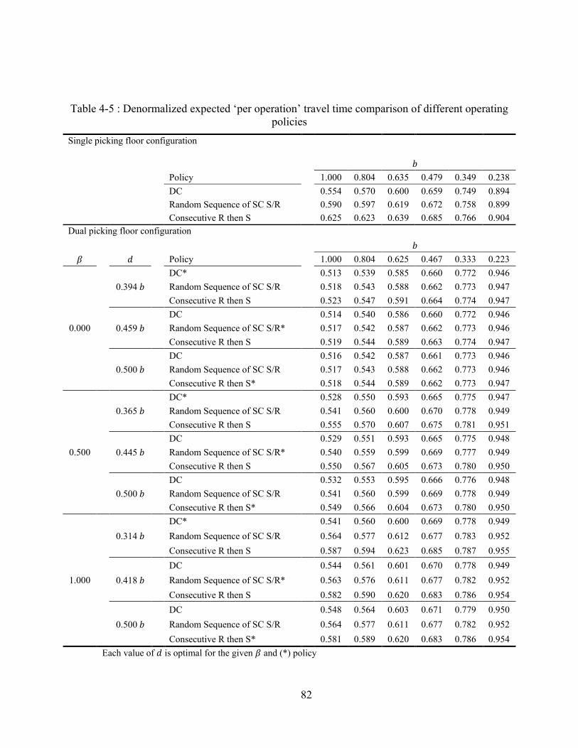
82

Table 4-5 : Denormalized expected ‘per operation’ travel time comparison of different operating policies

Single picking floor configuration

Policy

1.000 0.804 0.635 0.479 0.349 0.238

DC

0.554 0.570 0.600 0.659 0.749 0.894

Random Sequence of SC S/R

0.590 0.597 0.619 0.672 0.758 0.899

Consecutive R then S

0.625 0.623 0.639 0.685 0.766 0.904

Dual picking floor configuration

Policy

1.000 0.804 0.625 0.467 0.333 0.223

0.000

0.394

DC*

0.513 0.539 0.585 0.660 0.772 0.946

Random Sequence of SC S/R

0.518 0.543 0.588 0.662 0.773 0.947

Consecutive R then S 0.523 0.547 0.591 0.664 0.774 0.947

0.459

DC

0.514 0.540 0.586 0.660 0.772 0.946

Random Sequence of SC S/R*

0.517 0.542 0.587 0.662 0.773 0.946

Consecutive R then S 0.519 0.544 0.589 0.663 0.774 0.947

0.500

DC

0.516 0.542 0.587 0.661 0.773 0.946

Random Sequence of SC S/R

0.517 0.543 0.588 0.662 0.773 0.946

Consecutive R then S* 0.518 0.544 0.589 0.662 0.773 0.947

0.500

0.365

DC*

0.528 0.550 0.593 0.665 0.775 0.947

Random Sequence of SC S/R

0.541 0.560 0.600 0.670 0.778 0.949

Consecutive R then S 0.555 0.570 0.607 0.675 0.781 0.951

0.445

DC

0.529 0.551 0.593 0.665 0.775 0.948

Random Sequence of SC S/R*

0.540 0.559 0.599 0.669 0.777 0.949

Consecutive R then S 0.550 0.567 0.605 0.673 0.780 0.950

0.500

DC

0.532 0.553 0.595 0.666 0.776 0.948

Random Sequence of SC S/R

0.541 0.560 0.599 0.669 0.778 0.949

Consecutive R then S* 0.549 0.566 0.604 0.673 0.780 0.950

1.000

0.314

DC*

0.541 0.560 0.600 0.669 0.778 0.949

Random Sequence of SC S/R

0.564 0.577 0.612 0.677 0.783 0.952

Consecutive R then S 0.587 0.594 0.623 0.685 0.787 0.955

0.418

DC

0.544 0.561 0.601 0.670 0.778 0.949

Random Sequence of SC S/R*

0.563 0.576 0.611 0.677 0.782 0.952

Consecutive R then S 0.582 0.590 0.620 0.683 0.786 0.954

0.500

DC

0.548 0.564 0.603 0.671 0.779 0.950

Random Sequence of SC S/R

0.564 0.577 0.611 0.677 0.782 0.952

Consecutive R then S* 0.581 0.589 0.620 0.683 0.786 0.954

Each value of is optimal for the given and (*) policy

83

In addition, Table 4-5 illustrates that the Random Sequence of SC Storages and

Retrievals policy has lower expected travel times than the Consecutive Retrievals then Storages

policy (even though both are conducting only SC travels). This occurs because there is a lower

amount of empty travel required when storages and retrievals arrive in a random manner (versus

the Consecutive Retrievals then Storages policy). This observation is valid for both picking floor

configurations. However, using a Consecutive Retrieval then Storages policy with an MIAPP-

AS/RS with a dual picking floor configuration that utilizes the mezzanine input point has only a

small impact on throughput performance (even when compared to a DC policy). This result is

not common for traditional end-of-aisle AS/RSs and is also not the case for MIAPP-AS/RS with

a single picking floor or a dual picking floor when . For example under the single picking

floor when , a DC policy has 11.34% less travel time, and a Random Sequence of SC

Storages and Retrievals Policy has 5.60% less travel time than a Consecutive Retrievals then

Storages policy. For a dual picking floor configuration, when and , these

differences are less than 7.79% for a DC policy and less than 3.90% for a Random Sequence of

SC Storages and Retrievals Policy. Contrastingly, under the dual picking floor configuration

when and , these differences are less than 1.96% for a DC policy and 0.98% for a

Random Sequence of SC Storages and Retrievals Policy. When and , these

differences are 4.97% for a DC policy and 2.49% for a Random Sequence of SC Storages and

Retrievals Policy. To make these comparisons, we calculated the policy performance difference

over all values in Table 4-5 and took the maximum difference.

A reason for the difference in performance of SC-based policies versus DC-based

policies is due to the return trip to the input points to service a storage request. In a DC policy,

84

the trip back to the input point always occurs from a pick position. However, in the SC-based

policies, the trip back to an input point occurs half of the time from a pick position and the other

half of the time from a storage location in the rack. The expected travel time from any point in

the rack to an input point is less when the input point is at the mezzanine floor rather than the

ground floor. Consequently, the throughput performance of SC-based and DC-based operating

policies are closer to each other in a MIAPP-AS/RS with a dual picking floor configuration that

utilizes the mezzanine input point than in a single picking floor configuration or a dual picking

floor configuration that does not use the mezzanine input point. Consequently, a MIAPP-AS/RS

with a dual picking floor configuration that utilizes the mezzanine input point is a more robust

configuration than a single picking floor configuration.

In summary, when the concern is about number of retrievals (such as what occurs during

peak hours), a Consecutive Retrievals policy performs better than a Mixed policy. However,

such a policy sacrifices overall throughput performance by not being able to utilize the

efficiencies of DC travels. When the overall number of operations is important, a DC policy

performs best as it has the opportunity to reduce the amount of empty travel by doing DC travels.

An important insight from our analysis is the impact of operating policies for the different

configurations. For a dual picking floor MIAPP-AS/RS that utilizes the mezzanine input point, if

the distribution center operations are such that DC travels are not achievable (either due to peak-

hour picking requirements or the arrival patterns of inbound or outbound trucks); using a SC-

based operating policy does not considerably impact throughput performance. Consequently, by

performing only SC retrievals and then only SC storages does not lose much efficiency with a

dual picking floor configuration that utilizes the mezzanine input point.

85

4-6- Conclusion

In this paper, we modeled and analyzed the MIAPP-AS/RS, which is a material handling

technology that facilitates semi-automated case-level order picking by automating the storage

and replenishment of pallets to multiple in-the-aisle pick positions. We focused on evaluating the

expected throughput performance of such systems for a randomized storage policy by developing

analytical travel time models. We developed models for different operating policies that can

occur during peak and non-peak picking hours, as well as for two design configurations (i.e. the

MIAPP-AS/RS with a single picking level and the MIAPP-AS/RS with dual picking levels).We

derived base travel time models for pick positions on each floor, as well as extreme travel time

models, which produce closed-form solutions by assuming there are an infinite number of pick

positions and the requested demand for each pick position is equal likely. Optimal shape factor

for different operating policies were calculated using the extreme travel time models.

A simulation study was conducted for various shape factors showing that the base and

extreme models can approximate the discrete rack with less than 1% deviation. Through

numerical experiments we provided design insights for MIAPP-AS/RSs. We found that

operating policies have different impacts depending on the design configuration. To minimize

the expected travel times for any policy we found that the mezzanine should be located such that and all storage operations should originate from the mezzanine floor input point

(i.e., ). If the focus is on retrievals during a peak period, the MIAPP-AS/RS should be

designed with a smaller shape factor than if the focus is on the overall number of operations

performed. Finally, we found that a dual picking floor MIAPP-AS/RS that utilizes the mezzanine

input point can use a SC-based operating policy without much loss of efficiency when compared

86

to a DC policy. This is not the case with a single picking floor MIAPP-AS/RS or for traditional

end-of-aisle AS/RSs. Therefore, if a distribution center operates in an environment that has peak

picking times where only SC retrievals are performed, a dual picking floor configuration is a

more robust configuration.

This article is the first study that analyzes AS/RS with multiple in-the-aisle outputs.

Therefore, our study could help extensively to design and quantify the performance of systems

with in-the-aisle outputs or pick positions. Our study could be extended to consider the following

future research directions. The development of analytical models for MIAPP-AS/RS that

considers different storage policies, different dwell point strategies, and different sequencing

rules would be interesting to understand how policies impact throughput and storage space

performance. Also, the development of a systematic model that considers the interaction of

human order pickers and the MIAPP-AS/RS would be interesting from an inventory buffer

capacity, as well as a staff resource and scheduling perspective.

Appendix A: The derivation of ( )for the case of

( ) ⁄

( ) { ⁄

( ) ( ) ( ) { ⁄ ⁄

87

( ) ( ) { ⁄ ⁄

( ) ∫ ( ) ⁄ ⁄

Appendix B: The derivation of ( )for the cases of ( ) and( )

Let ( ) be the probability that the travel time between the origin and ( ) in region

II is less than or equal to . As the and coordinates are assumed to be independent, ( ) is equal to ( ) ( ) ( ) ( ) Based on randomized storage, when ( ) ,

( ) { ( )⁄ ( ) ( )

( ) ⁄

Hence,

( ) { ( ) ⁄ ( ) ⁄ ( )

( ) ( ) { ( ) ⁄ ( ) ⁄ ( )

88

( ) denotes the expected travel time between the origin and any point located in

region II. By definition, ( ) is obtained as follows.

( ) ∫ ( ) ( ) ⁄ ⁄ ( )

Similarly, when ( ) , ( ) ( )⁄ ( ) ( ) { ⁄ ( ) Hence,

( ) { ( ) ⁄ ( )⁄ ( )

( ) ( ) { ( ) ⁄ ( )⁄ ( ) ( ) ∫ ( )

( )⁄ ( ) ⁄ ( ) Appendix C. Calculation of ( )

According to equation (14a), ( ) ∫ ( ) . By substituting the right hand

side of equation (6) for ( ), we have

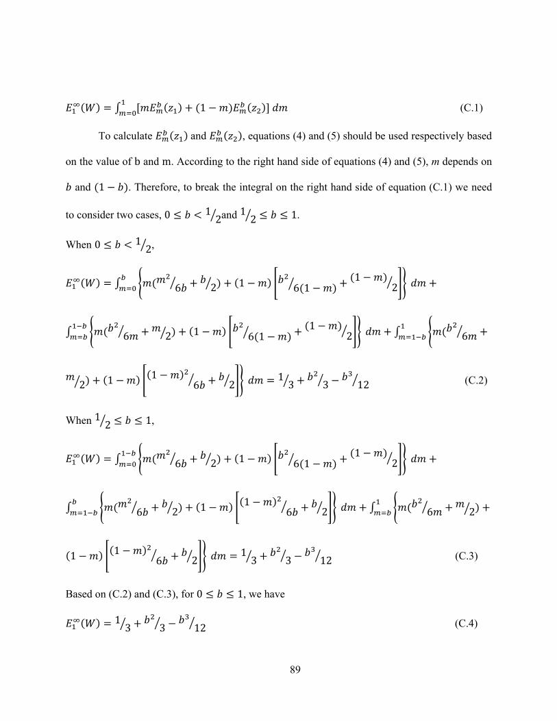
89

( ) ∫ [ ( ) ( ) ( )] (C.1)

To calculate ( ) and ( ), equations (4) and (5) should be used respectively based

on the value of and . According to the right hand side of equations (4) and (5), m depends on and ( ). Therefore, to break the integral on the right hand side of equation (C.1) we need

to consider two cases, ⁄ and ⁄ .

When ⁄ ,

( ) ∫ { ( ⁄ ⁄ ) ( ) [ ( )⁄ ( ) ⁄ ]} ∫ { ( ⁄ ⁄ ) ( ) [ ( )⁄ ( ) ⁄ ]} ∫ { ( ⁄ ⁄ ) ( ) [( ) ⁄ ⁄ ]} ⁄ ⁄ ⁄ (C.2)

When ⁄ ,

( ) ∫ { ( ⁄ ⁄ ) ( ) [ ( )⁄ ( ) ⁄ ]} ∫ { ( ⁄ ⁄ ) ( ) [( ) ⁄ ⁄ ]} ∫ { ( ⁄ ⁄ ) ( ) [( ) ⁄ ⁄ ]} ⁄ ⁄ ⁄ (C.3)

Based on (C.2) and (C.3), for , we have ( ) ⁄ ⁄ ⁄ (C.4)

90

CHAPTER FIVE: CONTRIBUTION 2- A PAPER ON “PRODUCT

ALLOCATION PROBLEM FOR AN AS/RS WITH MULTIPLE IN-THE-

AISLE PICK POSITIONS”

An automated storage/retrieval system (AS/RS) with multiple in-the-aisle pick positions

(MIAPP-AS/RS) is a semi-automated case-level order fulfillment technology that is widely used

in distribution centers. We study the impact of product to pick position assignments on the

expected throughput for different operating policies, demand profiles, and shape factors. We

develop efficient algorithms of complexity O(nlog(n)) that provide the assignment that

minimizes the expected travel time. Also, for different operating policies, shape configurations,

and demand curves, we explore the structure of the optimal assignment of products to pick

positions and quantify the difference between using a simple, practical assignment policy versus

the optimal assignment. Finally, we derive closed-form analytical travel time models by

approximating the optimal assignment’s expected travel time using continuous demand curves

and assuming an infinite number of pick positions in the aisle. We illustrate that these continuous

models work well in estimating the travel time of a discrete rack and use them to find optimal

design configurations.

Keywords: Automated Storage/Retrieval System, Case-level Order Picking, Closed-form

Travel-time, Multiple input/output (I/O) points

91

5-1- Introduction

According to the U.S. Roadmap for Material Handling & Logistics, currently 350,000

distribution centers operate in the Unites States. A distribution center’s most important, as well

as most costly and labor-intensive operation is to fulfill customer order requests. Thus, careful

design and control of order-fulfillment operations can result in considerable improvements in

distribution center performance. In this work, we are interested in case-level order-fulfillment

when non-identical demand is experienced for different products (i.e., item demand varies

among the set of items managed). A typical phenomenon exists where a small percentage of

stock-keeping-units (SKUs) will make up a large percentage of the total demand. This demand

skewness is captured in a well-known method called ABC analysis, which ranks the SKUs based

on their contribution to total demand. The “A” class represents the fast-moving SKUs, the “B”

class represents the medium-moving SKUs, and the “C” class represents the slow-moving SKUs.

An automated storage/retrieval system (AS/RS) with multiple in-the-aisle pick positions

(MIAPP-AS/RS) is an example of a case-level order-fulfillment technology that is frequently

used in distribution centers (See Fig. 5-1). These systems are common in temperature-controlled

distribution centers because of their ability to increase the space utilization and energy

efficiency, and to reduce the number of employees that have to work in the harsh environment.

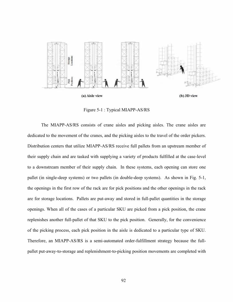
92

Figure 5-1 : Typical MIAPP-AS/RS

The MIAPP-AS/RS consists of crane aisles and picking aisles. The crane aisles are

dedicated to the movement of the cranes, and the picking aisles to the travel of the order pickers.

Distribution centers that utilize MIAPP-AS/RS receive full pallets from an upstream member of

their supply chain and are tasked with supplying a variety of products fulfilled at the case-level

to a downstream member of their supply chain. In these systems, each opening can store one

pallet (in single-deep systems) or two pallets (in double-deep systems). As shown in Fig. 5-1,

the openings in the first row of the rack are for pick positions and the other openings in the rack

are for storage locations. Pallets are put-away and stored in full-pallet quantities in the storage

openings. When all of the cases of a particular SKU are picked from a pick position, the crane

replenishes another full-pallet of that SKU to the pick position. Generally, for the convenience

of the picking process, each pick position in the aisle is dedicated to a particular type of SKU.

Therefore, an MIAPP-AS/RS is a semi-automated order-fulfillment strategy because the full-

pallet put-away-to-storage and replenishment-to-picking position movements are completed with

93

cranes. On the other hand, the picking of cases from pick positions in the aisle is done via

manual order pickers.

In this research, we are interested in the assignment of the SKUs to pick positions for

MIAPP-AS/RS. We call this problem as the SKU Assignment Problem (SAP). Two key research

questions regarding the SAP include:

1. How should SKUs be assigned to pick positions such that the maximum expected crane

throughput occurs?

2. What is the impact of different SKU to pick position assignments on throughput performance

under different operating policies, demand curves, and system configurations?

The goal of our study is to understand the impact of different SKU assignments on the

MIAPP-AS/RS throughput, as well as system design trade-offs that occur when MIAPP-AS/RS

are operating using different policies and demand profiles. To do so, we begin by reviewing the

relevant AS/RS and SKU assignment problem literature in Section 5-2. We describe the

MIAPP-AS/RS physical configuration, demand curve models, operating policies, and key

assumptions in Section 5-3. Next, in Section 5-4, we develop mathematical optimization models

to find the optimal assignment minimizing the expected travel time, and provide an optimal

assignment algorithm of complexity ( ( )). We also provide structural properties of the

optimal assignment of SKUs to pick positions in MIAPP-AS/RS’s for different operating

policies, demand profiles, and shape factors. We quantify the performance difference between

optimal assignments and a common assignment used in practice that assigns the most demanded

SKUs to the pick positions that are closest to the input point. In Section 5-5, we derive and

94

validate analytical closed-form models to approximate the expected travel time for different

assignments; also, we use these models to obtain the optimal shape factors for different policies.

These closed-form analytical travel time models are derived by using continuous demand curves

and assuming an infinite number of pick positions in the aisle to approximate the optimal

assignment’s expected travel time. In Section 5-6, we illustrate that these models work well in

estimating the travel time of a discrete rack and use them to derive optimal design configurations

and provide managerial insights. We also provide numerical results and managerial insights by

exploring the trade-offs that occur while implementing different assignments. Finally, in Section

5-7, we review our main contributions, provide insights from our study, and direction for future

research.

5-2- Literature Review

During the past three decades AS/RS have received notable attention from different

perspectives that can be categorized into: system configuration, travel time estimation, storage

assignment, dwell-point, and batching/sequencing (Roodbergen & Vis, 2009). In addition, some

AS/RS research has been addressed in warehouse design papers; interested readers may refer to

reviews papers such as de Koster et al. (2007) and Gu et al., (2007). In fact, AS/RS literature is

the exclusive focus in the following review papers: Sarker & Babu (1995), Roodbergen & Vis

(2009), Vasili et al. (2012), and Gagliardi et al. (2012). Among these review papers, Sarker and

Babu (1995) focus specifically on travel time models. According to the AS/RS review papers,

AS/RS with multiple I/O points is a subject that deserves further study.

95

Similar topics to the SAP include the storage location assignment problem (SLAP) and

the product allocation problem (PAP), which have been widely studied in traditional order-

picking and warehouse management literature. The SLAP represents a notable portion of the

AS/RS literature. A storage assignment policy identifies how items are assigned to storage

locations. Three main storage assignment policies have received the most attention in the

literature: randomized storage, turnover-based storage, and class-based storage. Generally,

randomized storage has the best space-utilization; turnover-based storage has the shortest

expected travel time; and class-based storage is a compromise between these two policies (Pohl

et al., 2011). The turnover-based and class-based storage policies incorporate that different

SKUs have different demand profiles when determining the assignment of SKUs to storage

locations. For the special cases of 2 or 3 classes in class-based storage, explicit travel time

analytical expressions have been developed by Hausman et al. (1976), Kouvelis & Papanicolaou

(1995) and Eynan & Rosenblatt (1994). Rosenblatt & Eynan (1989) and Eynan & Rosenblatt

(1994) provide a procedure to obtain optimal boundaries for n-classes under a specific layout.

Van den Berg (1996) develops a dynamic programming algorithm that optimally assigns

products and locations into a certain number of classes. He considers travel time minimization

under single command cycles. Goetschalckx & Ratliff (1990) consider a duration-of-stay shared

policy for unit-load AS/RS and show the optimality of this policy under an assumption of

perfectly balanced I/O flows. All of the above studies focus on the assignment of the SKUs to

storage locations in traditional AS/RS that have a single I/O point, and thus no SKU to pick

positions assignment problem exists. In contrast, we focus on the assignment of the non-identical

demanded SKUs to multiple in-the-aisle pick positions.

96

Also, the PAP has been widely studied in traditional order-picking systems literature

where a manual order picker traverses aisles to pick a set of items (Francis et al., 1992; de Koster

et al., 2007). The PAP determines which SKUs should be assigned to which picking locations to

minimize a given performance measure, such as travel time. For example, Francis et al. (1992)

analyze various assignment models in a traditional manual picking warehouse subject to different

space and throughput constraints. Jarvis & McDowell (1991) consider the PAP in different types

of order picking warehouses. They present a stochastic model to obtain the optimal results.

Petersen & Aase (2004) build a simulation model to evaluate the picking, storage, and routing

effect on order picking travel time. They show that order batching of products results in the

highest savings, particularly when the order sizes are smaller. Heragu et al. (2005) develop a

mathematical model and a heuristic procedure that simultaneously determines the allocation of

the products, as well as the size of the functional areas. Pazour & Meller (2011) analyze the SKU

assignment and allocation problem in an A-frame dispenser system, which is a fully automated

order picking technology. Guerriero et al. (2013) develop a nonlinear integer mathematical

model to minimize the handling cost considering compatibility constraints among classes. They

use an Iterated Local Search based algorithm to solve large scale instances. Our work is similar

to this area of research, in that we are also interested in assigning SKUs to pick position

locations. However, the focus of our study is on the assignment of SKUs to pick positions in a

MIAPP-AS/RS, which have different travel time dynamics than manual order picking

operations, including the need to consider simultaneous vertical and horizontal travel movements

and retrieving, as well as storage operations.

97

Only a few studies exist that study an AS/RS with either multiple I/O points or non-end-

of-aisle I/O points. Bozer & White (1984) derive and analyze the expected travel time for

different alternative I/O point locations; however, all of the alternatives considered a single input

and single output point. Randhawa et al. (1991) and their extended study by Randhawa & Shroff

(1995) focus on simulation analysis to identify the impact of changing the location and the

number of I/O points on travel time. They consider different layouts and performance measures

to evaluate their simulation studies. Vasili et al. (2008) develop a continuous travel time model

for the split-platform AS/RS, where an I/O point is located at the center of the rack. Ramtin &

Pazour (2014) are the first to study the AS/RS with multiple in-the-aisle pick position, and

develop expected travel time models for different operating policies and physical configurations.

For their closed-form travel time models and numerical analysis, they assume that the demand of

SKUs is identical and thus do not consider the assignment of SKUs to pick positions. To our

knowledge, no study exists that addresses the assignment of SKUs to multiple pick positions in

an AS/RS.

5-3- Problem Definition and Assumptions

In this section, we provide a description of the environment that we model. To do so, we

describe the MIAPP-AS/RS’s physical configuration, demand models, crane travels and

operational policies, as well as the key modeling assumptions.

98

Physical configuration

We assume the system has a single picking level and each crane aisle has its own crane

that is working independently from other cranes, as illustrated in Fig. 5-1 Each rack has one

input point located at the lower-left corner and the pick positions are located on the bottom line

of the rack. We develop our models considering a single rack.

Most of the existing AS/RS travel time model studies have used continuous

approximation of the rack to derive expected value models for different configurations (Graves

et al., 1977; Bozer & White, 1984; Foley & Frazelle, 1991; Chang et al., 1995; Kouvelis &

Papanicolaou, 1995; Sarker & Babu, 1995; Hu et al., 2005). We also use continuous

approximation of the rack for the travel time models in Section 5-4 and 5-5. The storage

locations are assumed to be continuously and uniformly distributed over the rack. We follow the

Bozer & White (1984) methodology used to ‘normalize’ the rack as follows. Let:

: time required to travel horizontally from the input point to the most distant point, : time required to travel vertically from the input point to the most distant point, : scaling factor, where { } : shape factor, where { ⁄ ⁄ }

By assuming , the rack can be normalized as a rectangle with length of and

height of , where .

Demand curve representation

99

We denote and as the sets of all pick positions and SKUs to be assigned to those pick

positions, respectively, such that { } and { }. Let and be the

index of pick positions and SKUs, respectively. Let denote the probability that pick position is visited such that ∑ Let denote the probability that a storage/retrieval request

is for SKU among a total of SKUs, where ∑ .

We use the continuous demand model in Hausman et al. (1976) to represent the ABC

analysis that ranks the items in monotonically decreasing order based on their contribution to

total demand. In this demand model, is the percentage of inventoried SKUs, [ ],

represents the skewness of the demand curve, and is the demand of the 100x percentage

SKU. We consider 20/20, 20/40, 20/60, 20/80, and 20/90 demand curves, which correspond to , , , , , respectively. For example, a 20/60

curve represents the case that 20% of inventoried SKUs contribute 80% of the total demand.

SKUs with identical demand can be represented by 20/20 curves. To calculate , the

continuous demand curve model can be discretized by the approach used in Pohl et al. (2011) as

shown in equation (1).

∫ ⁄ ∫ ( ) ⁄ (1)

Crane travels and operational policies structure

In a MIAPP-AS/RS, the crane can carry a single unit-load and travel between the input

point, storage locations, and pick positions. In a single command (SC) storage operation, full-

pallets of different SKUs originate from an input point and are transferred to a storage location in

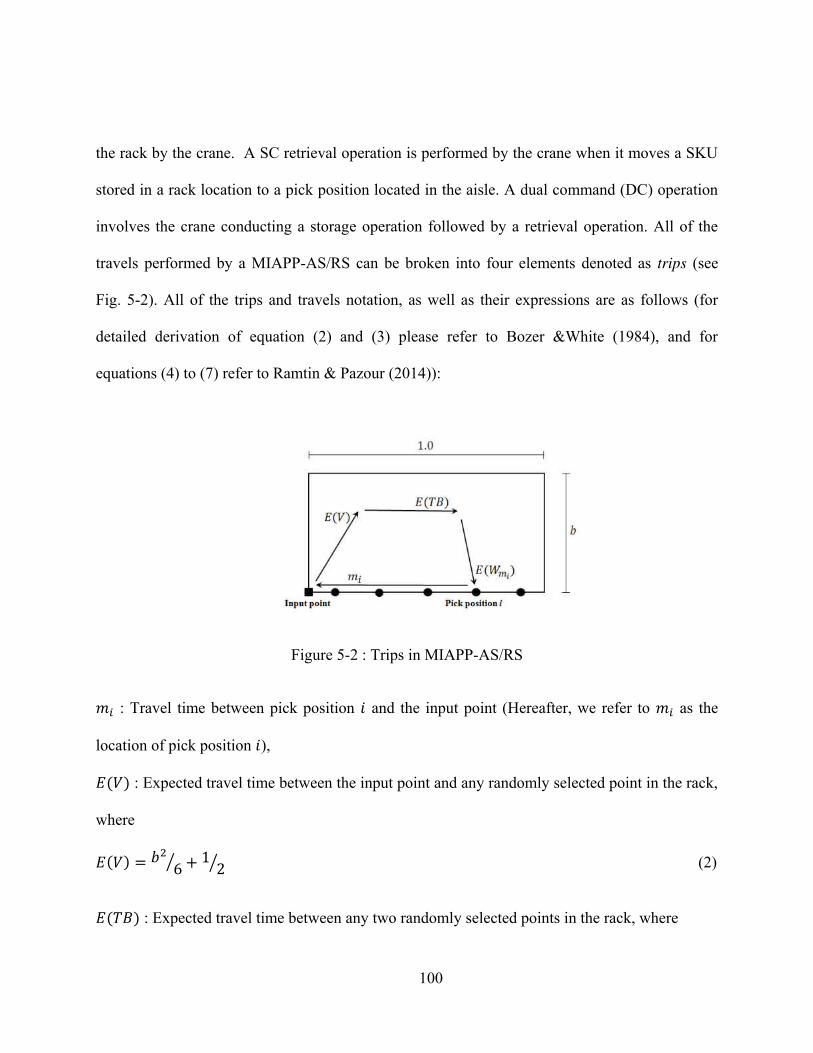
100

the rack by the crane. A SC retrieval operation is performed by the crane when it moves a SKU

stored in a rack location to a pick position located in the aisle. A dual command (DC) operation

involves the crane conducting a storage operation followed by a retrieval operation. All of the

travels performed by a MIAPP-AS/RS can be broken into four elements denoted as trips (see

Fig. 5-2). All of the trips and travels notation, as well as their expressions are as follows (for

detailed derivation of equation (2) and (3) please refer to Bozer &White (1984), and for

equations (4) to (7) refer to Ramtin & Pazour (2014)):

Figure 5-2 : Trips in MIAPP-AS/RS

: Travel time between pick position and the input point (Hereafter, we refer to as the

location of pick position ), ( ) : Expected travel time between the input point and any randomly selected point in the rack,

where ( ) ⁄ ⁄ (2)

( ) : Expected travel time between any two randomly selected points in the rack, where

101

( ) ⁄ ⁄ ⁄ (3)

( ) : Expected travel time between pick position and any randomly selected point in the

rack, where ( ) [ ( )] ( ) ( )[ ( )] ( ) (4)

We consider operating policies for the MIAPP-AS/RS that are common for peak and

non-peak hours. The first operating policy is a Consecutive Retrievals (CR) policy, where the

AS/RS performs only SC retrievals. This policy is used during the peak hours when the priority

is to fullfil the customer orders. In the case of a CR policy, the crane travels between storage

locations and pick positions only. Thus all trips are ( ) trips, and the overall expected travel

time can be calculated as ( ) using equation (5). If a CR policy is used during peak

hours, then the AS/RS will need to perform consecutive storages (CS) during the non-peak hours.

We call this policy as CR then CS policy, and the overall expected travel time for this policy can

be calculated as ( ( ) ( )), which is the average of the CR and CS policies. Another

policy we consider during non-peak hours is a Mixed policy. In a Mixed policy, the crane

performs both SC (storage/retrieval) and DC. In this policy the proportion of the number of SC

to DC operations is defined with the parameter . Let denote the percentage of storage (or

retrieval) operations that are performed under SC basis. For this policy the combination of all ( ), ( ), ( ), and trips may occur, and the overall expected travel time can be

obtained as ( ), where ( ) is defined in equation (7).

102

( ): Expected one-way travel time between any pick position and any randomly selected point

in the rack, where ( ) ∑ ( ) (5) ( ): Expected one-way travel time between any pick position and input point, where ( ) ∑ (6)

( ): Expected ‘per operation’ travel time for the Mixed policy, where

( ) ( ) ( ) ( ) ( ) ( ) ( ) ( ) ( ) (7)

Finally, a review of the assumptions of this work follows.

1. Each normalized rack has one input point located at the lower-left corner and the pick

positions are located on the bottom line of a normalized rack.

2. Demand for each item type (and thus each pick position location) is known and

independent.

3. For assigning SKUs to storage locations, a randomized storage assignment is used, i.e.,

any point within the rack is equally likely to be selected as a storage location. However,

assigning SKUs to pick positions is a decision discussed in Section 5-4.

4. Each pick position is dedicated to particular type of SKU.

5. We consider a single-deep rack, where each opening can contain a single pallet.

6. The storage and retrieval rate is assumed to be equal in steady state, and operation

requests are processed on a first-come-first-serve basis.

103

7. Only the travel time model of the crane is considered. Human order pickers travel time

and the pick/deposit times to handle the loads are ignored.

8. The crane carries unit-loads under either single command (SC) (storage/retrieval) or dual

command (DC) travels.

9. The crane travel time follows the Chebyshev metric and moves at a constant horizontal

and vertical speed, i.e., acceleration and deceleration are ignored.

10. A stay dwell point strategy is considered, i.e., after completing any storage or retrieval

operation, the crane stays where it is, and waits for the next operation request.

5-4- SKU Assignment Problem (SAP)

In this section, we analyze the SAP for the MIAPP-AS/RS, which determines the

assignment of SKUs to pick positions to minimize the expected travel time of the crane. When

SKUs’ demands are identical, changing the assignment of SKUs to pick positions does not

impact the expected travel time for any policy (see equations (5) and (7)). However, in the case

of non-identical demand, as the expected travel time to each pick position is different (see

equation (4)), assigning higher demanded SKUs to pick positions with less expected travel time

will result in less overall expected travel time.

5-4-1- Optimal Assignment Problem

Our objective is to minimize the expected travel time for different operating policies by

changing the assignment of SKUs to pick positions. Referring to equation (5) and (7), the

expected travel time models for CR and Mixed policy are linear functions of SKUs’ demands and

the locations of the pick positions. Therefore, we formulate our problems as a Linear

104

Assignment Problem (LAP) for each policy. Let be the binary variable where 1 denotes that

the pick position is assigned to SKU , and is 0 otherwise. We formulate the assignment

problem for the CR policy and denote it as Model 1. The objective function is to minimize the

expected travel time for a CR policy, which is expressed in equation (8). Equation (9) provides

the constraints that each SKU must be assigned to one pick position, and equation (10) provides

the constraints that each pick position must be assigned to one SKU.

Model 1 (for a CR Policy)

∑ ∑ ( ) (8)

∑ (9)

∑ (10)

{ } (11)

Model 2 is the SAP for the Mixed policy. In this case, the assignment problem depends

only on the elements of the Mixed policy expected travel time in equation (7) that are a function

of (the location of the pick positions). Consequently, ( ) and ( ) are not impacted.

Therefore, the objective function of the assignment problem for the Mixed policy is formulated

as equation (12) subject to constraints (9), (10), and (11).

Model 2 (for a Mixed Policy)

∑ ∑ ( ( ) ) (12)

105

Because of the structure of Model 1 and 2, we are able to provide an algorithm for the

optimal solution that is computationally tractable.

In order to simplify Model 1 and 2, we define ( ) and ( ) . Therefore, the objective functions of Model 1 and 2 become ∑ ∑ and ∑ ∑ , respectively.

Proposition 1a. The optimal solution to Model 1 is obtained by the assignment

permutation that has the pick positions sorted in ascending order based on their values and the

SKUs sorted in descending order based on their values.

Proof. is independent of a SKU’s demand. Hence, the cost of assigning SKU to pick

position is obtained by multiplying two independent parameters ( and ). Therefore, by

introducing permutation functions and , Model 1 can be represented as its combinatorial

formulation, ∑ ( ) ( ) . Let be the set of all permutations on and . According to the rearrangement inequality, the minimum value to this model is

obtained by the optimal permutations ( and ) such that ( ) ( ) ( ) and ( ) ( ) ( ) (For an extended proof, please refer to Hardy et al. (1988)).

Therefore, the optimal assignment for Model 1 can be obtained by bijective mapping of

permutation and , which is represented as equation (13).

{ ( ) ( ) (13)

106

Proposition 1b. The optimal solution to Model 2 is obtained by the assignment permutation that

has the pick positions sorted in ascending order based on their values and the SKUs sorted in

descending order based on their values.

Proof. Following directly from Proposition 1a’s proof. Let be the set of all permutations on and . The combinatorial formulation of Model 2 becomes as ∑ ( ) ( ) . The minimum value to this model is obtained by the

permutations ( and ) such that ( ) ( ) ( ) and ( ) ( ) ( ). Therefore, the optimal assignment for Model 2 can be obtained by bijective

mapping of permutation and , which is represented as equation (14).

{ ( ) ( ) (14)

Corollary 1. The minimum expected travel time ‘per operation’ with respect to the optimal

assignment of SKUs to pick positions is equal to equations (15) and (16) for a CR and a Mixed

policy, respectively.

( )=∑ ( ( )) ( ) (15)

( ) ( ) ( ) ∑ ( ) ( ( ( )) ( )) (16)

According to Proposition 1a and 1b, the optimal algorithm for the SKU assignment

problems is of complexity ( ( )), as it sorts two sets of cardinality n. The optimal

assignment can be obtained using the following procedure:

107

STEP 1: Calculate and for , as well as for .

STEP 2: Find permutations and by sorting and in monotonically increasing order,

respectively. Find permutation by sorting in monotonically decreasing order.

STEP 3: Provide the optimal assignment for Model 1 and 2 by equations (13) and (14),

respectively.

Example: Consider a square-in-time system ( ) where 40% of storages are

performed by SC in a Mixed policy ( ). Consider there are 5 pick positions ( ) whose

distance from the input point are 0.1, 0.3, 0.5, 0.7, 0.9; and 5 different SKUs which follows the

20-60 demand curve ( ). Therefore, based on the definitions, { }, { }, and by using equation (1), { }. We obtain { }, { }, and { } by sorting , , and as defined. According to Proposition 1a and 1b, the optimal

assignment of SKUs to pick positions for a CR and a Mixed policy is obtained by bijective

mapping and , respectively, on Based on equations (13) and (14), the optimal

assignment for CR policy has and for the Mixed policy has . Also, according to equations (15) and (16), ( ) and ( ) , respectively.

Proposition 2. When all of the storage and retrieval operations are performed by DC

( ), the assignment of SKUs ordered based on monotonically

108

decreasing demand to pick positions ordered from nearest to farthest from the input point is

optimal.

Proof. Appendix A.

For the sake of convenience, we call ‘the assignment of SKUs ordered based on

monotonically decreasing demand to pick positions ordered from nearest to farthest from the

input point’ as the monotonically decreasing demand (MDD) assignment and is shown in Fig. 5-

4(c). The insight behind Proposition 2, as well as the other assignment characteristics will be

discussed in Section 5-4-2.

According to the definition of the MDD assignment, the most demanded SKU is assigned

to the pick position closest to the input point, and the next demanded SKU to the next pick

position closest to input point, and so forth. The expected travel time for CR and Mixed policy

under MDD assignment can be calculated by substituting any monotonically decreasing demand

for into equation (5) and (7), respectively.

5-4-2- Structure of the optimal assignment

In this section, we explore the structure of the optimal assignment of SKUs to pick

positions introduced in Section 5-4-1. Recall that the set of is used to find the optimal

assignment for a CR policy and the set of for a Mixed policy. If we denote as the location of

a pick position from the input point ( ) these sets can be defined as functions of ,

such that ( ) and ( ) . To observe the behavior of the expected

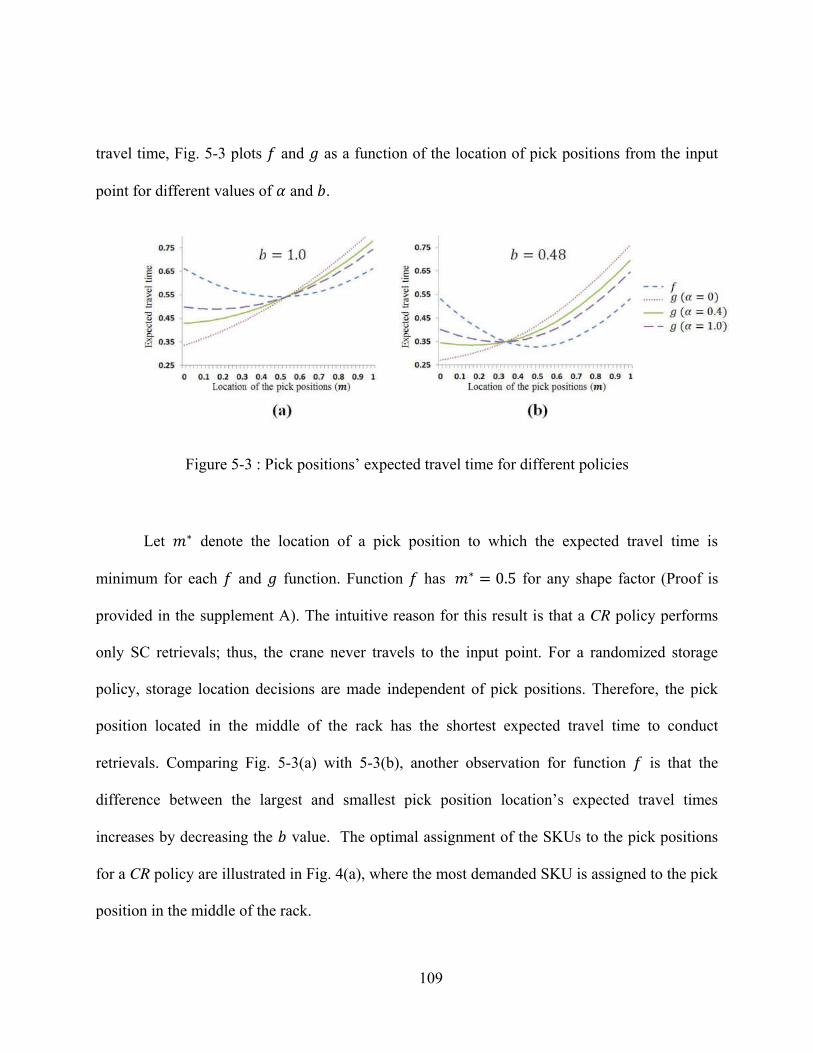
109

travel time, Fig. 5-3 plots and as a function of the location of pick positions from the input

point for different values of and .

Figure 5-3 : Pick positions’ expected travel time for different policies

Let denote the location of a pick position to which the expected travel time is

minimum for each and function. Function has for any shape factor (Proof is

provided in the supplement A). The intuitive reason for this result is that a CR policy performs

only SC retrievals; thus, the crane never travels to the input point. For a randomized storage

policy, storage location decisions are made independent of pick positions. Therefore, the pick

position located in the middle of the rack has the shortest expected travel time to conduct

retrievals. Comparing Fig. 5-3(a) with 5-3(b), another observation for function is that the

difference between the largest and smallest pick position location’s expected travel times

increases by decreasing the value. The optimal assignment of the SKUs to the pick positions

for a CR policy are illustrated in Fig. 4(a), where the most demanded SKU is assigned to the pick

position in the middle of the rack.

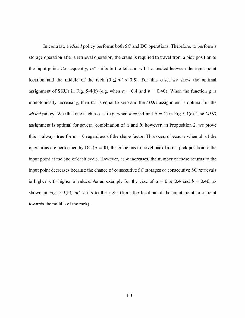
110

In contrast, a Mixed policy performs both SC and DC operations. Therefore, to perform a

storage operation after a retrieval operation, the crane is required to travel from a pick position to

the input point. Consequently, shifts to the left and will be located between the input point

location and the middle of the rack ( ). For this case, we show the optimal

assignment of SKUs in Fig. 5-4(b) (e.g. when and ). When the function is

monotonically increasing, then is equal to zero and the MDD assignment is optimal for the

Mixed policy. We illustrate such a case (e.g. when and ) in Fig 5-4(c). The MDD

assignment is optimal for several combination of and ; however, in Proposition 2, we prove

this is always true for regardless of the shape factor. This occurs because when all of the

operations are performed by DC ( ), the crane has to travel back from a pick position to the

input point at the end of each cycle. However, as increases, the number of these returns to the

input point decreases because the chance of consecutive SC storages or consecutive SC retrievals

is higher with higher values. As an example for the case of and , as

shown in Fig. 5-3(b), shifts to the right (from the location of the input point to a point

towards the middle of the rack).

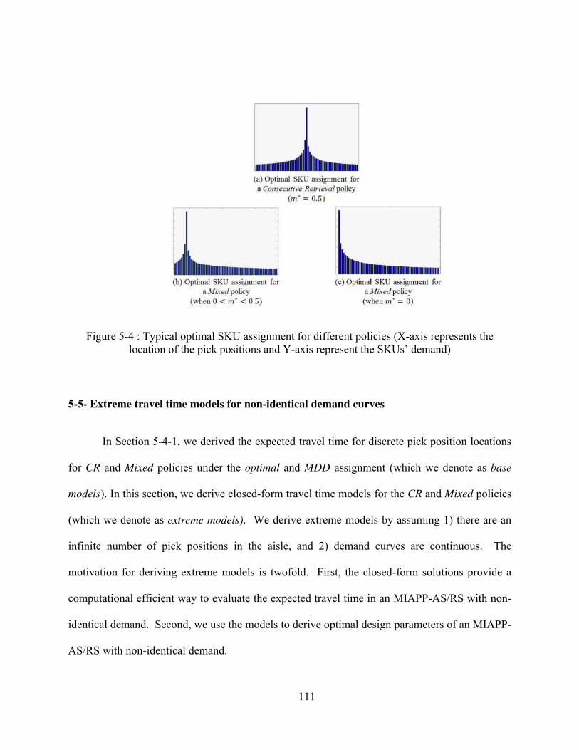
111

Figure 5-4 : Typical optimal SKU assignment for different policies (X-axis represents the

location of the pick positions and Y-axis represent the SKUs’ demand)

5-5- Extreme travel time models for non-identical demand curves

In Section 5-4-1, we derived the expected travel time for discrete pick position locations

for CR and Mixed policies under the optimal and MDD assignment (which we denote as base

models). In this section, we derive closed-form travel time models for the CR and Mixed policies

(which we denote as extreme models). We derive extreme models by assuming 1) there are an

infinite number of pick positions in the aisle, and 2) demand curves are continuous. The

motivation for deriving extreme models is twofold. First, the closed-form solutions provide a

computational efficient way to evaluate the expected travel time in an MIAPP-AS/RS with non-

identical demand. Second, we use the models to derive optimal design parameters of an MIAPP-

AS/RS with non-identical demand.

112

In the previous section, we showed that is optimal for the CR policy regardless

of the shape factor. Therefore, to approximate the optimal assignment for the CR policy shown in

Fig. 5-4(a), we introduce a new continuous demand curve defined in equation (17) and denoted

as ( ). Let and denote the location of the pick position and demand curve skewness

factor, respectively. As illustrated in Fig. 5-5(a), this curve assigns the highest demanded SKUs

to locations in the middle of the rack. We use this curve to represent the optimal assignment for

the CR policy.

( ) { ( ) ⁄ ( ) ⁄ (17)

This demand curve is obtained by truncating and shifting the demand curve expressed in

Hausman et al. (1976). Therefore, to represent the different demand curves (e.g. 20/20, 20/40,

20/60, 20/80, and 20/90), the same values provided in Section 5-3 can be used. ( ) is a

valid probability distribution function (PDF) for and (Proof is provided in

the supplement B).

We use the continuous monotonically decreasing demand curve defined in equation (18)

to represent the MDD assignment. As illustrated in Fig. 5-5(b), this curve is the continuous

representation of the MDD assignment shown in Fig. 5-4(c). This curve will be used for

representing the MDD assignment and we derive extreme models for both CR and Mixed policies

with an MDD assignment.

( ) (18)

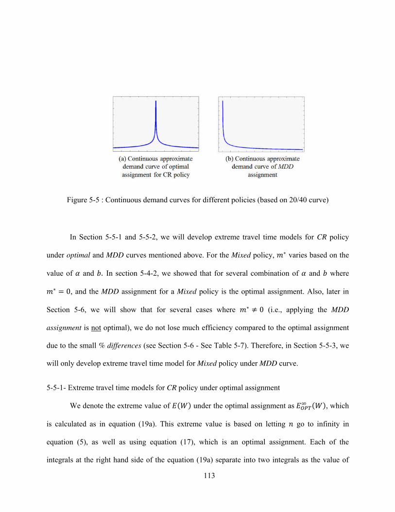
113

Figure 5-5 : Continuous demand curves for different policies (based on 20/40 curve)

In Section 5-5-1 and 5-5-2, we will develop extreme travel time models for CR policy

under optimal and MDD curves mentioned above. For the Mixed policy, varies based on the

value of and In section 5-4-2, we showed that for several combination of and where , and the MDD assignment for a Mixed policy is the optimal assignment. Also, later in

Section 5-6, we will show that for several cases where (i.e., applying the MDD

assignment is not optimal), we do not lose much efficiency compared to the optimal assignment

due to the small % differences (see Section 5-6 - See Table 5-7). Therefore, in Section 5-5-3, we

will only develop extreme travel time model for Mixed policy under MDD curve.

5-5-1- Extreme travel time models for CR policy under optimal assignment

We denote the extreme value of ( ) under the optimal assignment as ( ), which

is calculated as in equation (19a). This extreme value is based on letting go to infinity in

equation (5), as well as using equation (17), which is an optimal assignment. Each of the

integrals at the right hand side of the equation (19a) separate into two integrals as the value of

114

( ) changes for different and based on equation (4). The final closed-form result is

given in (19b). See Appendix B for the complete derivation of ( ) for the CR policy.

( ) ∑ ( ) ∫ ( ) ( ) (19a)

( ) { ( ) ( ) ( ) ( )( ( ) ( ) ( )( )) ( )( )( ) ⁄ ( ) ( ) ( ( ) ) ( )( ( ) ( ) ( )( )) ( )( )( ) ⁄ (19b)

5-5-2- Extreme travel time models for CR policy under MDD assignment

Let ( ) denote the extreme value of ( ) under the MDD assignment. Following

the same approach as in the previous section, by using the MDD assignment curve (given in

equation (18)), ( ) can be calculated as equation (20a), which results in the closed-form

expression given in equation (20b). Appendix C shows the complete derivation of ( ). ( ) ∑ ( ) ∫ ( ) ( ) (20a)

( ) ( ) [ ( ) ( )( ) ( ( ) ( )) ( ( ( ) ) ( ( )))] ( )( )( ) (20b)

Note that ( ) derived as equation (19b) varies from ( ) in equation (20b)

and are not replaceable because ( ) is derived based on the continuous demand curve used

for approximating optimal assignment for CR policy (equation (17)) and ( ) is derived

based on the MDD assignment continuous demand curve (equation (18)).

115

5-5-3- Extreme travel time models for Mixed policy under MDD assignment

To derive the extreme travel time model for the Mixed policy under an MDD assignment,

note that ( ) and ( ) are the only components of ( ) impacted by varying the location of

the pick positions and their assigned SKU’s demand (See equation (7)). Therefore, the extreme

value of ( ) under an MDD assignment can be obtained by replacing ( ) and ( ) with

their extreme values. Let ( ), ( ), and ( ) denote the extreme values of ( ), ( ), and ( ), respectively. The extreme values are derived using the continuous

demand curve for the MDD assignment given in equation (18). ( ) is derived in the

previous section as equation (20b), and ( ) is derived as equation (21). Finally, by

substituting ( ) and ( ) for ( ) and ( ), respectively, into equation (7), the

extreme value of ( ) under an MDD assignment is obtained as equation (22).

( ) ∑ ∫ ⁄ (21)

( ) ( ) ( ) ( ) ( ) ( ) ( ) ( ) ( ) (22)

5-5-4- Validation of the extreme travel time models

In this section the results of the extreme models developed in Section 5-5-1 to 5-5-3 are

compared to results from a discrete-event simulation. The purpose is to understand the impact of

the extreme models’ assumptions (i.e., a continuous rack, an infinite number of pick positions,

and continuous demand curves) on the expected travel time. We use MATLAB 2013a to code

and run the simulation.

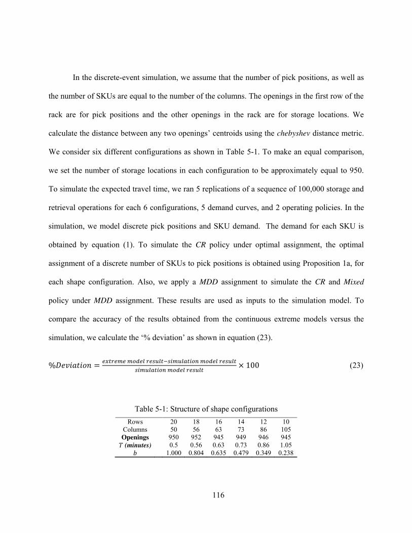
116

In the discrete-event simulation, we assume that the number of pick positions, as well as

the number of SKUs are equal to the number of the columns. The openings in the first row of the

rack are for pick positions and the other openings in the rack are for storage locations. We

calculate the distance between any two openings’ centroids using the chebyshev distance metric.

We consider six different configurations as shown in Table 5-1. To make an equal comparison,

we set the number of storage locations in each configuration to be approximately equal to 950.

To simulate the expected travel time, we ran 5 replications of a sequence of 100,000 storage and

retrieval operations for each 6 configurations, 5 demand curves, and 2 operating policies. In the

simulation, we model discrete pick positions and SKU demand. The demand for each SKU is

obtained by equation (1). To simulate the CR policy under optimal assignment, the optimal

assignment of a discrete number of SKUs to pick positions is obtained using Proposition 1a, for

each shape configuration. Also, we apply a MDD assignment to simulate the CR and Mixed

policy under MDD assignment. These results are used as inputs to the simulation model. To

compare the accuracy of the results obtained from the continuous extreme models versus the

simulation, we calculate the ‘% deviation’ as shown in equation (23).

(23)

Table 5-1: Structure of shape configurations

Rows

20 18 16 14 12 10

Columns

50 56 63 73 86 105

Openings

950 952 945 949 946 945 (minutes)

0.5 0.56 0.63 0.73 0.86 1.05

1.000 0.804 0.635 0.479 0.349 0.238

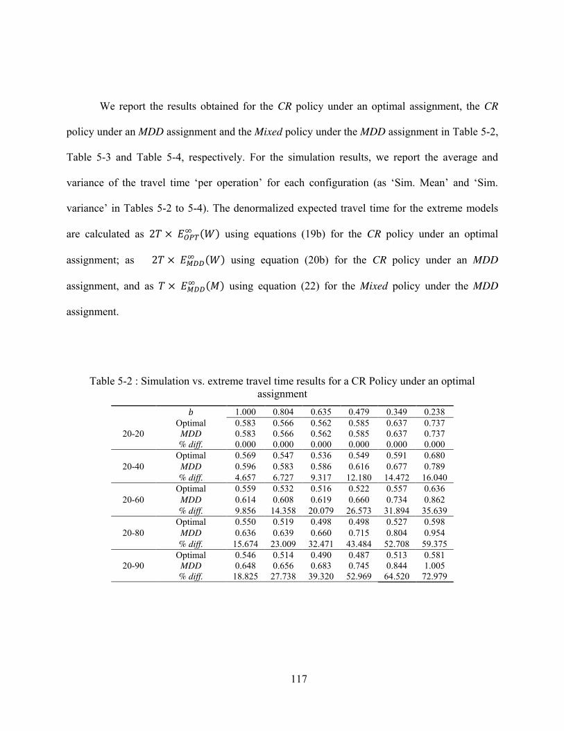
117

We report the results obtained for the CR policy under an optimal assignment, the CR

policy under an MDD assignment and the Mixed policy under the MDD assignment in Table 5-2,

Table 5-3 and Table 5-4, respectively. For the simulation results, we report the average and

variance of the travel time ‘per operation’ for each configuration (as ‘Sim. Mean’ and ‘Sim.

variance’ in Tables 5-2 to 5-4). The denormalized expected travel time for the extreme models

are calculated as ( ) using equations (19b) for the CR policy under an optimal

assignment; as ( ) using equation (20b) for the CR policy under an MDD

assignment, and as ( ) using equation (22) for the Mixed policy under the MDD

assignment.

Table 5-2 : Simulation vs. extreme travel time results for a CR Policy under an optimal

assignment

1.000 0.804 0.635 0.479 0.349 0.238

20-20

Optimal 0.583 0.566 0.562 0.585 0.637 0.737

MDD 0.583 0.566 0.562 0.585 0.637 0.737

% diff. 0.000 0.000 0.000 0.000 0.000 0.000

20-40

Optimal 0.569 0.547 0.536 0.549 0.591 0.680

MDD 0.596 0.583 0.586 0.616 0.677 0.789

% diff. 4.657 6.727 9.317 12.180 14.472 16.040

20-60

Optimal 0.559 0.532 0.516 0.522 0.557 0.636

MDD 0.614 0.608 0.619 0.660 0.734 0.862

% diff. 9.856 14.358 20.079 26.573 31.894 35.639

20-80

Optimal 0.550 0.519 0.498 0.498 0.527 0.598

MDD 0.636 0.639 0.660 0.715 0.804 0.954

% diff. 15.674 23.009 32.471 43.484 52.708 59.375

20-90

Optimal 0.546 0.514 0.490 0.487 0.513 0.581

MDD 0.648 0.656 0.683 0.745 0.844 1.005

% diff. 18.825 27.738 39.320 52.969 64.520 72.979

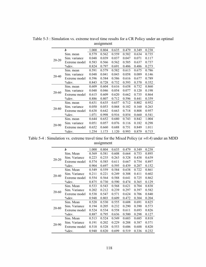
118

Table 5-3 : Simulation vs. extreme travel time results for a CR Policy under an optimal

assignment

b 1.000 0.804 0.635 0.479 0.349 0.238

20-20

Sim. mean 0.579 0.562 0.559 0.582 0.634 0.735

Sim. variance 0.048 0.039 0.037 0.047 0.071 0.117

Extreme model 0.583 0.566 0.562 0.585 0.637 0.737

%dev. 0.824 0.797 0.691 0.486 0.486 0.273

20-40

Sim. mean 0.591 0.579 0.582 0.613 0.675 0.786

Sim. variance 0.048 0.041 0.043 0.058 0.089 0.146

Extreme model 0.596 0.584 0.586 0.616 0.677 0.789

%dev. 0.843 0.728 0.732 0.593 0.370 0.352

20-60

Sim. mean 0.609 0.604 0.616 0.658 0.732 0.860

Sim. variance 0.048 0.046 0.054 0.077 0.120 0.198

Extreme model 0.615 0.609 0.620 0.662 0.735 0.864

%dev. 0.886 0.807 0.712 0.596 0.441 0.359

20-80

Sim. mean 0.631 0.635 0.657 0.712 0.802 0.952

Sim. variance 0.050 0.053 0.068 0.102 0.160 0.263

Extreme model 0.638 0.642 0.663 0.718 0.808 0.957

%dev. 1.071 0.998 0.916 0.854 0.660 0.541

20-90

Sim. mean 0.644 0.652 0.680 0.743 0.842 1.004

Sim. variance 0.051 0.057 0.076 0.116 0.182 0.298

Extreme model 0.652 0.660 0.688 0.751 0.849 1.011

%dev. 1.254 1.173 1.120 0.993 0.879 0.715

Table 5-4 : Simulation vs. extreme travel time for the Mixed Policy ( =0.4) under an MDD

assignment

b 1.000 0.804 0.635 0.479 0.349 0.238

20-20

Sim. Mean 0.569 0.581 0.608 0.664 0.753 0.895

Sim. Variance 0.223 0.235 0.263 0.328 0.438 0.639

Extreme model 0.574 0.585 0.611 0.667 0.754 0.897

%dev. 0.904 0.697 0.595 0.439 0.207 0.152

20-40

Sim. Mean 0.549 0.559 0.584 0.638 0.722 0.861

Sim. Variance 0.211 0.221 0.249 0.308 0.411 0.602

Extreme model 0.554 0.564 0.588 0.641 0.725 0.862

%dev. 0.875 0.730 0.590 0.474 0.365 0.129

20-60

Sim. Mean 0.533 0.543 0.568 0.621 0.704 0.838

Sim. Variance 0.202 0.212 0.239 0.297 0.397 0.582

Extreme model 0.538 0.547 0.571 0.624 0.706 0.840

%dev. 0.948 0.803 0.609 0.472 0.304 0.204

20-80

Sim. Mean 0.520 0.530 0.555 0.608 0.691 0.825

Sim. Variance 0.194 0.205 0.232 0.290 0.390 0.573

Extreme model 0.524 0.534 0.558 0.611 0.693 0.826

%dev. 0.887 0.795 0.636 0.500 0.298 0.127

20-90

Sim. Mean 0.513 0.524 0.549 0.603 0.685 0.818

Sim. Variance 0.191 0.202 0.229 0.288 0.387 0.571

Extreme model 0.518 0.528 0.553 0.606 0.688 0.820

%dev. 0.940 0.820 0.699 0.519 0.336 0.232

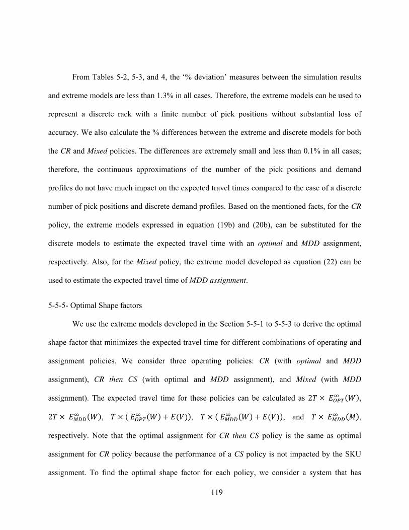
119

From Tables 5-2, 5-3, and 4, the ‘% deviation’ measures between the simulation results

and extreme models are less than 1.3% in all cases. Therefore, the extreme models can be used to

represent a discrete rack with a finite number of pick positions without substantial loss of

accuracy. We also calculate the % differences between the extreme and discrete models for both

the CR and Mixed policies. The differences are extremely small and less than 0.1% in all cases;

therefore, the continuous approximations of the number of the pick positions and demand

profiles do not have much impact on the expected travel times compared to the case of a discrete

number of pick positions and discrete demand profiles. Based on the mentioned facts, for the CR

policy, the extreme models expressed in equation (19b) and (20b), can be substituted for the

discrete models to estimate the expected travel time with an optimal and MDD assignment,

respectively. Also, for the Mixed policy, the extreme model developed as equation (22) can be

used to estimate the expected travel time of MDD assignment.

5-5-5- Optimal Shape factors

We use the extreme models developed in the Section 5-5-1 to 5-5-3 to derive the optimal

shape factor that minimizes the expected travel time for different combinations of operating and

assignment policies. We consider three operating policies: CR (with optimal and MDD

assignment), CR then CS (with optimal and MDD assignment), and Mixed (with MDD

assignment). The expected travel time for these policies can be calculated as ( ), ( ), ( ( ) ( )), ( ( ) ( )), and ( ),

respectively. Note that the optimal assignment for CR then CS policy is the same as optimal

assignment for CR policy because the performance of a CS policy is not impacted by the SKU

assignment. To find the optimal shape factor for each policy, we consider a system that has

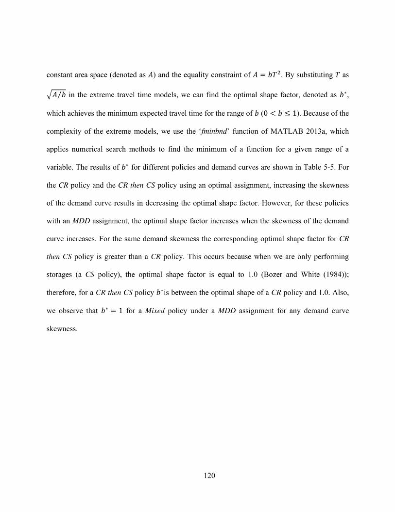
120

constant area space (denoted as ) and the equality constraint of . By substituting as √ ⁄ in the extreme travel time models, we can find the optimal shape factor, denoted as , which achieves the minimum expected travel time for the range of ( ). Because of the

complexity of the extreme models, we use the ‘fminbnd’ function of MATLAB 2013a, which

applies numerical search methods to find the minimum of a function for a given range of a

variable. The results of for different policies and demand curves are shown in Table 5-5. For

the CR policy and the CR then CS policy using an optimal assignment, increasing the skewness

of the demand curve results in decreasing the optimal shape factor. However, for these policies

with an MDD assignment, the optimal shape factor increases when the skewness of the demand

curve increases. For the same demand skewness the corresponding optimal shape factor for CR

then CS policy is greater than a CR policy. This occurs because when we are only performing

storages (a CS policy), the optimal shape factor is equal to 1.0 (Bozer and White (1984));

therefore, for a CR then CS policy is between the optimal shape of a CR policy and 1.0. Also,

we observe that for a Mixed policy under a MDD assignment for any demand curve

skewness.

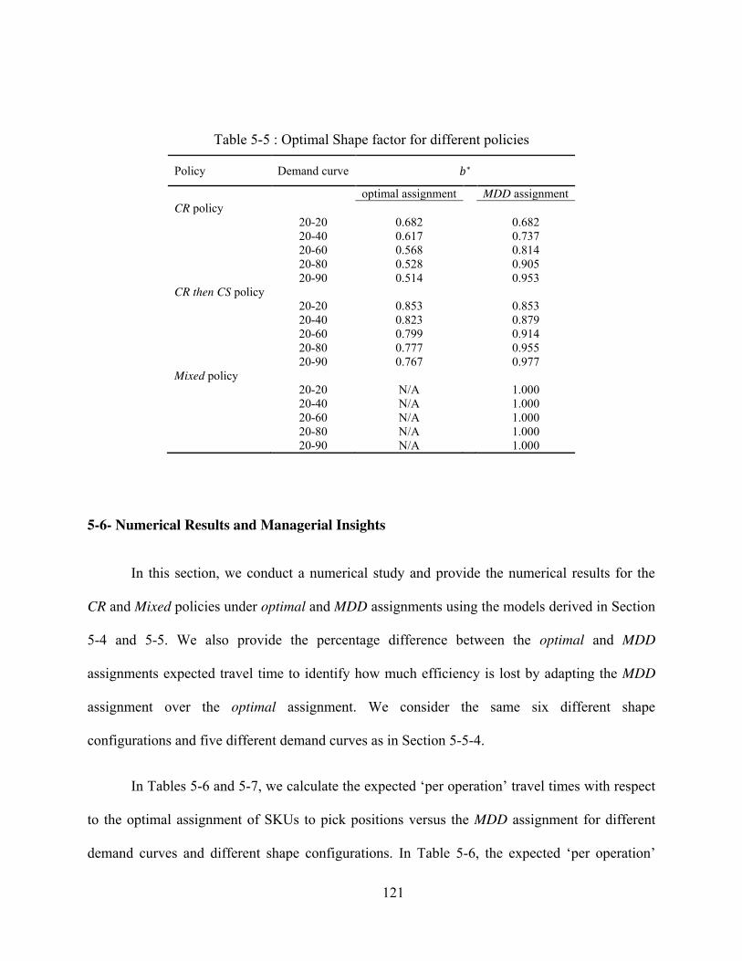
121

Table 5-5 : Optimal Shape factor for different policies

Policy Demand curve

optimal assignment

MDD assignment

CR policy

20-20 0.682

0.682

20-40 0.617

0.737

20-60 0.568

0.814

20-80 0.528

0.905

20-90 0.514

0.953

CR then CS policy

20-20 0.853

0.853

20-40 0.823

0.879

20-60 0.799

0.914

20-80 0.777

0.955

20-90 0.767

0.977

Mixed policy

20-20 N/A

1.000

20-40 N/A

1.000

20-60 N/A

1.000

20-80 N/A

1.000

20-90 N/A

1.000

5-6- Numerical Results and Managerial Insights

In this section, we conduct a numerical study and provide the numerical results for the

CR and Mixed policies under optimal and MDD assignments using the models derived in Section

5-4 and 5-5. We also provide the percentage difference between the optimal and MDD

assignments expected travel time to identify how much efficiency is lost by adapting the MDD

assignment over the optimal assignment. We consider the same six different shape

configurations and five different demand curves as in Section 5-5-4.

In Tables 5-6 and 5-7, we calculate the expected ‘per operation’ travel times with respect

to the optimal assignment of SKUs to pick positions versus the MDD assignment for different

demand curves and different shape configurations. In Table 5-6, the expected ‘per operation’

122

travel time for CR policy is calculated by the extreme models as ( ) and ( ) for the optimal and MDD assignments (as ‘OPT extreme’ and ‘MDD extreme’),

respectively. In Table 5-7, the expected ‘per operation’ travel time for the Mixed policy (for , , and ) with optimal assignment is calculated by the discrete base model as ( ) using equation (16) (as ‘OPT base’), and for the Mixed policy with the MDD

assignment is calculated by the extreme model as ( ) using equation (22) (as ‘MDD

extreme’). Note that all of the extreme models are based on continuous demand curves that

approximate the optimal and MDD assignments. In Table 5-7, we do not provide the results for , as we proved in Proposition 2 that results for the optimal and MDD assignment are equal

for the Mixed policy with . For demand profiles that have identical demand (i.e., 20/20

curves), the assignment problem does not impact the expected travel times and thus the

difference between the optimal and MDD assignment is zero for both CR and Mixed policies.

Table 5-6 and 5-7 show that when an optimal assignment is adopted, increasing the

skewness of the demand curve improves the expected travel time for any policy or configuration.

Intuitively, when demand curve skewness increases, the pick positions with shorter expected

travel time are visited more frequently, because the SKUs assigned to these pick positions have

higher levels of demand. However, when the MDD assignment is applied for the CR policy, the

expected travel degrades by increasing the demand curve skewness. The reason results from for the CR policy (as mentioned in section 5-4-2). That is, the pick position located in

the middle of the rack has the shortest expected travel time. Thus, the MDD assignment is far

from optimal because it allocates the highest demanded SKUs to pick positions nearest to the

input point (which as shown in Fig. 5-4(c)) have the highest expected travel time in a CR policy).

123

For all operating and assignment policies, the expected travel time increases as the shape

of the rack become more rectangular (i.e. decreases). This occurs because the difference

between the highest and shortest expected travel time increases by decreasing the value (see

Fig. 5-3(a) and Fig. 5-3(b)). For these reasons, when a distribution center adopts a MDD

assignment instead of the optimal assignment and uses a CR policy, it loses more efficiency by

increasing the skewness of the demand and decreasing the shape factor.

From Table 5-7, the same observation can be observed for a Mixed policy. However, the

% differences between the optimal and MDD assignment are much smaller compared to the CR

policy (i.e., all are less than 8%). For the Mixed policy, we have . As becomes

closer to zero, the % difference between the optimal assignment and the MDD assignment

becomes smaller as the pick positions with the shortest expected travel time are located closer to

the input point where the highest demanded SKUs are assigned in a MDD assignment (See Fig.

5-4(a) and (b)). We observe that the % difference increases by increasing , increasing the

skewness of the demand ( ), and decreasing the shape factor ( ). Therefore, the high %

differences occur in extreme cases of system parameters (e.g. for highly skewed demand curves

or relatively small shape factor configuration), and for most of the practical cases of , , and ,

the % differences are relatively small (less that 5%). In these cases, a system will not lose

considerable throughput by implementing a MDD assignment instead of an optimal assignment

for Mixed policies.

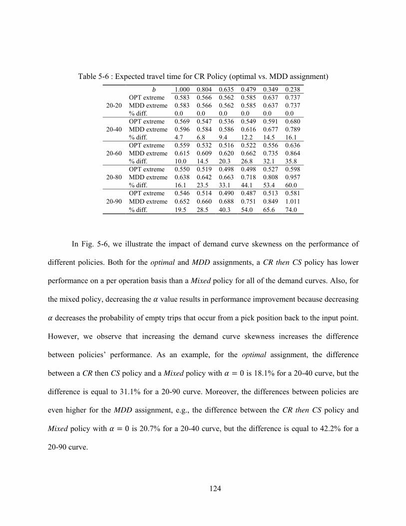
124

Table 5-6 : Expected travel time for CR Policy (optimal vs. MDD assignment)

1.000 0.804 0.635 0.479 0.349 0.238

20-20

OPT extreme 0.583 0.566 0.562 0.585 0.637 0.737

MDD extreme 0.583 0.566 0.562 0.585 0.637 0.737

% diff. 0.0 0.0 0.0 0.0 0.0 0.0

20-40

OPT extreme 0.569 0.547 0.536 0.549 0.591 0.680

MDD extreme 0.596 0.584 0.586 0.616 0.677 0.789

% diff. 4.7 6.8 9.4 12.2 14.5 16.1

20-60

OPT extreme 0.559 0.532 0.516 0.522 0.556 0.636

MDD extreme 0.615 0.609 0.620 0.662 0.735 0.864

% diff. 10.0 14.5 20.3 26.8 32.1 35.8

20-80

OPT extreme 0.550 0.519 0.498 0.498 0.527 0.598

MDD extreme 0.638 0.642 0.663 0.718 0.808 0.957

% diff. 16.1 23.5 33.1 44.1 53.4 60.0

20-90

OPT extreme 0.546 0.514 0.490 0.487 0.513 0.581

MDD extreme 0.652 0.660 0.688 0.751 0.849 1.011

% diff. 19.5 28.5 40.3 54.0 65.6 74.0

In Fig. 5-6, we illustrate the impact of demand curve skewness on the performance of

different policies. Both for the optimal and MDD assignments, a CR then CS policy has lower

performance on a per operation basis than a Mixed policy for all of the demand curves. Also, for

the mixed policy, decreasing the value results in performance improvement because decreasing decreases the probability of empty trips that occur from a pick position back to the input point.

However, we observe that increasing the demand curve skewness increases the difference

between policies’ performance. As an example, for the optimal assignment, the difference

between a CR then CS policy and a Mixed policy with is 18.1% for a 20-40 curve, but the

difference is equal to 31.1% for a 20-90 curve. Moreover, the differences between policies are

even higher for the MDD assignment, e.g., the difference between the CR then CS policy and

Mixed policy with is 20.7% for a 20-40 curve, but the difference is equal to 42.2% for a

20-90 curve.

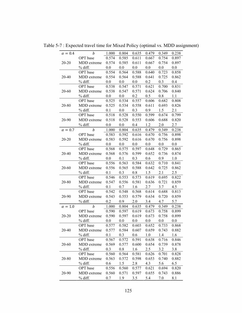
125

Table 5-7 : Expected travel time for Mixed Policy (optimal vs. MDD assignment) 1.000 0.804 0.635 0.479 0.349 0.238

20-20

OPT base 0.574 0.585 0.611 0.667 0.754 0.897

MDD extreme 0.574 0.585 0.611 0.667 0.754 0.897

% diff. 0.0 0.0 0.0 0.0 0.0 0.0

20-40

OPT base 0.554 0.564 0.588 0.640 0.723 0.858

MDD extreme 0.554 0.564 0.588 0.641 0.725 0.862

% diff. 0.0 0.0 0.0 0.2 0.3 0.4

20-60

OPT base 0.538 0.547 0.571 0.621 0.700 0.831

MDD extreme 0.538 0.547 0.571 0.624 0.706 0.840

% diff. 0.0 0.0 0.2 0.5 0.8 1.1

20-80

OPT base 0.525 0.534 0.557 0.606 0.682 0.808

MDD extreme 0.525 0.534 0.558 0.611 0.693 0.826

% diff. 0.1 0.0 0.3 0.9 1.5 2.1

20-90

OPT base 0.518 0.528 0.550 0.599 0.674 0.799

MDD extreme 0.518 0.528 0.553 0.606 0.688 0.820

% diff. 0.0 0.0 0.4 1.2 2.0 2.7 1.000 0.804 0.635 0.479 0.349 0.238

20-20

OPT base 0.583 0.592 0.616 0.670 0.756 0.898

MDD extreme 0.583 0.592 0.616 0.670 0.756 0.898

% diff. 0.0 0.0 0.0 0.0 0.0 0.0

20-40

OPT base 0.568 0.575 0.597 0.648 0.729 0.865

MDD extreme 0.568 0.576 0.599 0.652 0.736 0.874

% diff. 0.0 0.1 0.3 0.6 0.9 1.0

20-60

OPT base 0.556 0.563 0.584 0.632 0.710 0.841

MDD extreme 0.556 0.565 0.588 0.642 0.725 0.862

% diff. 0.1 0.3 0.8 1.5 2.1 2.5

20-80

OPT base 0.546 0.553 0.573 0.619 0.695 0.822

MDD extreme 0.547 0.556 0.581 0.636 0.721 0.859

% diff. 0.1 0.7 1.6 2.7 3.7 4.5

20-90

OPT base 0.542 0.548 0.568 0.614 0.688 0.813

MDD extreme 0.543 0.553 0.579 0.634 0.720 0.859

% diff. 0.2 0.9 2.0 3.4 4.7 5.7 1.000 0.804 0.635 0.479 0.349 0.238

20-20

OPT base 0.590 0.597 0.619 0.673 0.758 0.899

MDD extreme 0.590 0.597 0.619 0.673 0.758 0.899

% diff. 0.0 0.0 0.0 0.0 0.0 0.0

20-40

OPT base 0.577 0.582 0.603 0.652 0.733 0.868

MDD extreme 0.577 0.584 0.607 0.659 0.743 0.882

% diff. 0.1 0.3 0.6 1.0 1.4 1.6

20-60

OPT base 0.567 0.572 0.591 0.638 0.716 0.846

MDD extreme 0.569 0.577 0.600 0.654 0.739 0.878

% diff. 0.3 0.8 1.6 2.5 3.2 3.8

20-80

OPT base 0.560 0.564 0.581 0.626 0.701 0.828

MDD extreme 0.563 0.572 0.598 0.653 0.740 0.882

% diff. 0.6 1.5 2.8 4.3 5.6 6.5

20-90

OPT base 0.556 0.560 0.577 0.621 0.694 0.820

MDD extreme 0.560 0.571 0.597 0.655 0.743 0.886

% diff. 0.7 1.9 3.5 5.4 7.0 8.1

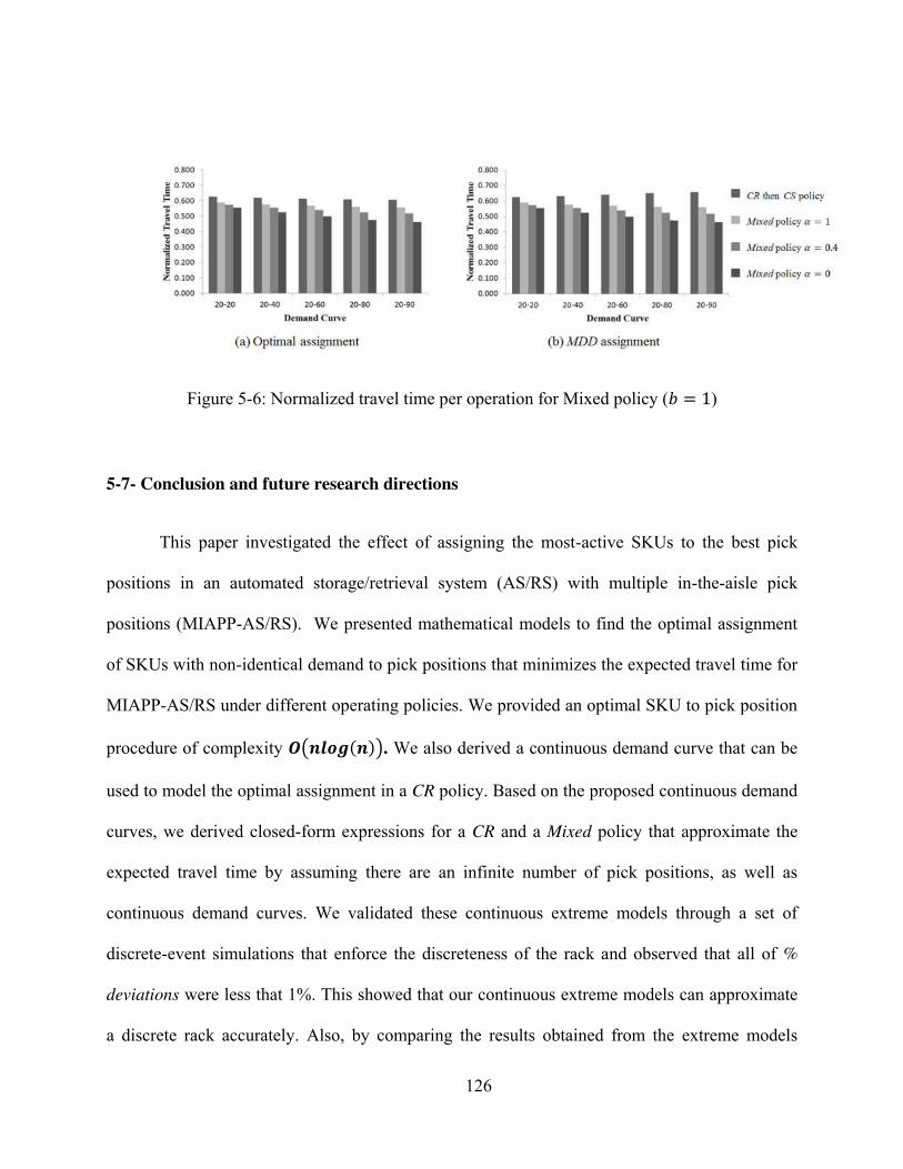
126

Figure 5-6: Normalized travel time per operation for Mixed policy ( )

5-7- Conclusion and future research directions

This paper investigated the effect of assigning the most-active SKUs to the best pick

positions in an automated storage/retrieval system (AS/RS) with multiple in-the-aisle pick

positions (MIAPP-AS/RS). We presented mathematical models to find the optimal assignment

of SKUs with non-identical demand to pick positions that minimizes the expected travel time for

MIAPP-AS/RS under different operating policies. We provided an optimal SKU to pick position

procedure of complexity ( ( )). We also derived a continuous demand curve that can be

used to model the optimal assignment in a CR policy. Based on the proposed continuous demand

curves, we derived closed-form expressions for a CR and a Mixed policy that approximate the

expected travel time by assuming there are an infinite number of pick positions, as well as

continuous demand curves. We validated these continuous extreme models through a set of

discrete-event simulations that enforce the discreteness of the rack and observed that all of %

deviations were less that 1%. This showed that our continuous extreme models can approximate

a discrete rack accurately. Also, by comparing the results obtained from the extreme models

127

versus the discrete models under the same assignment, we observed less than 0.1 % difference

for all cases. Using extreme models, we calculated the optimal shape configurations for each

demand curve and operating policy.

We analyzed structural results of the optimal assignment problem. For a CR policy with

an optimal assignment, we observed that regardless of the shape factor the most demanded SKU

is assigned to the pick position located in the middle of the rack, and the next most demanded

SKU is assigned to the next closest pick position to the middle of the rack and so on. For the

Mixed policy the smallest expected travel time occurs at a pick position located between the

input point and the middle of the rack.

We explored the impact of different SKU assignments on the expected throughput rates

that can be obtained under different system configurations, demand curves, and operating

policies for peak and non-peak hours. We compared the results obtained from the optimal

assignment with an easy-to-implement assignment that is often seen in practice -- the MDD

assignment, which assigns the highest demanded SKUs to the locations closest to the input point.

We observed that maximum % difference between the optimal and the MDD assignment for a

Mixed policy was less that 8%, and in most practical MIAPP-AS/RS configurations less than 5%.

As future research directions, this work can be extended by considering different storage

policies (such as turnover-based storage and class-based storage policy), different dwell point

strategies, and different sequencing rules. Applying these directions can help to increase

understanding of the impact of different storage policies and demand skewness on the throughput

and space utilization of MIAPP-AS/RS.

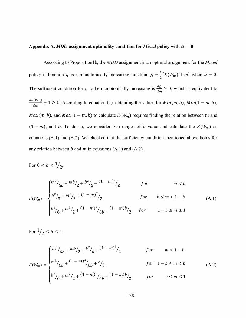
128

Appendix A. MDD assignment optimality condition for Mixed policy with

According to Proposition1b, the MDD assignment is an optimal assignment for the Mixed

policy if function is a monotonically increasing function. [ ( ) ] when .

The sufficient condition for to be monotonically increasing is , which is equivalent to

( ) . According to equation (4), obtaining the values for ( ), ( ), ( ), and ( ) to calculate ( ) requires finding the relation between and ( ), and . To do so, we consider two ranges of value and calculate the ( ) as

equations (A.1) and (A.2). We checked that the sufficiency condition mentioned above holds for

any relation between and in equations (A.1) and (A.2).

For ⁄ ,

( ) { ⁄ ⁄ ⁄ ( ) ⁄ ⁄ ⁄ ( ) ⁄ ⁄ ⁄ ( ) ⁄ ( ) ⁄ (A.1)

For ⁄ ,

( ) { ⁄ ⁄ ⁄ ( ) ⁄ ⁄ ( ) ⁄ ⁄ ⁄ ⁄ ( ) ⁄ ( ) ⁄ (A.2)

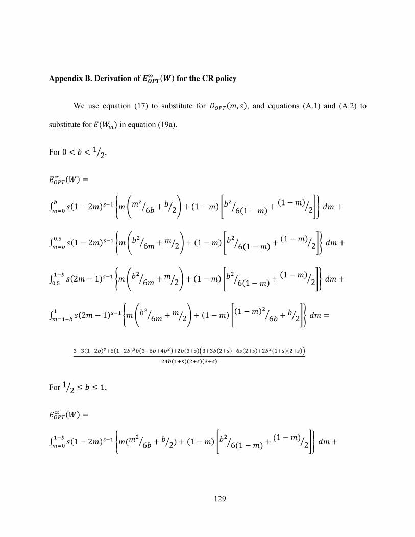
129

Appendix B. Derivation of ( ) for the CR policy

We use equation (17) to substitute for ( ), and equations (A.1) and (A.2) to

substitute for ( ) in equation (19a).

For ⁄ ,

( ) ∫ ( ) { ( ⁄ ⁄ ) ( ) [ ( )⁄ ( ) ⁄ ]} ∫ ( ) { ( ⁄ ⁄ ) ( ) [ ( )⁄ ( ) ⁄ ]} ∫ ( ) { ( ⁄ ⁄ ) ( ) [ ( )⁄ ( ) ⁄ ]} ∫ ( ) { ( ⁄ ⁄ ) ( ) [( ) ⁄ ⁄ ]}

( ) ( ) ( ) ( )( ( ) ( ) ( )( )) ( )( )( )

For ⁄ ,

( ) ∫ ( ) { ( ⁄ ⁄ ) ( ) [ ( )⁄ ( ) ⁄ ]}

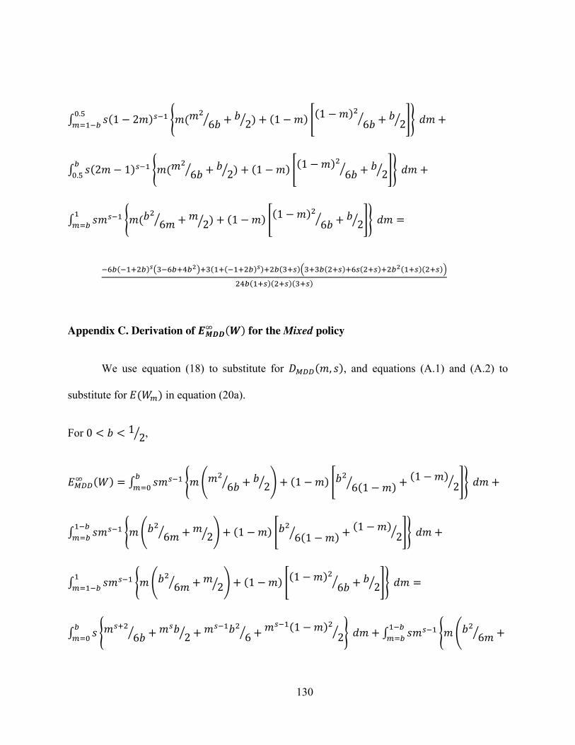
130

∫ ( ) { ( ⁄ ⁄ ) ( ) [( ) ⁄ ⁄ ]} ∫ ( ) { ( ⁄ ⁄ ) ( ) [( ) ⁄ ⁄ ]} ∫ { ( ⁄ ⁄ ) ( ) [( ) ⁄ ⁄ ]}

( ) ( ) ( ( ) ) ( )( ( ) ( ) ( )( )) ( )( )( )

Appendix C. Derivation of ( ) for the Mixed policy

We use equation (18) to substitute for ( ), and equations (A.1) and (A.2) to

substitute for ( ) in equation (20a).

For ⁄ ,

( ) ∫ { ( ⁄ ⁄ ) ( ) [ ( )⁄ ( ) ⁄ ]} ∫ { ( ⁄ ⁄ ) ( ) [ ( )⁄ ( ) ⁄ ]} ∫ { ( ⁄ ⁄ ) ( ) [( ) ⁄ ⁄ ]} ∫ { ⁄ ⁄ ⁄ ( ) ⁄ } ∫ { ( ⁄

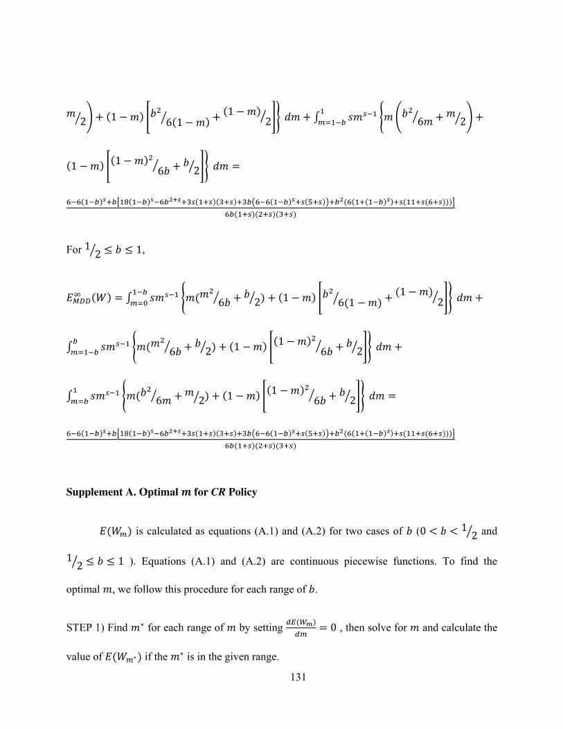
131

⁄ ) ( ) [ ( )⁄ ( ) ⁄ ]} ∫ { ( ⁄ ⁄ ) ( ) [( ) ⁄ ⁄ ]} ( ) [ ( ) ( )( ) ( ( ) ( )) ( ( ( ) ) ( ( )))] ( )( )( )

For ⁄ ,

( ) ∫ { ( ⁄ ⁄ ) ( ) [ ( )⁄ ( ) ⁄ ]} ∫ { ( ⁄ ⁄ ) ( ) [( ) ⁄ ⁄ ]} ∫ { ( ⁄ ⁄ ) ( ) [( ) ⁄ ⁄ ]} ( ) [ ( ) ( )( ) ( ( ) ( )) ( ( ( ) ) ( ( )))] ( )( )( )

Supplement A. Optimal for CR Policy

( ) is calculated as equations (A.1) and (A.2) for two cases of ( ⁄ and ⁄ ). Equations (A.1) and (A.2) are continuous piecewise functions. To find the

optimal , we follow this procedure for each range of .

STEP 1) Find for each range of by setting ( ) , then solve for and calculate the

value of ( ) if the is in the given range.

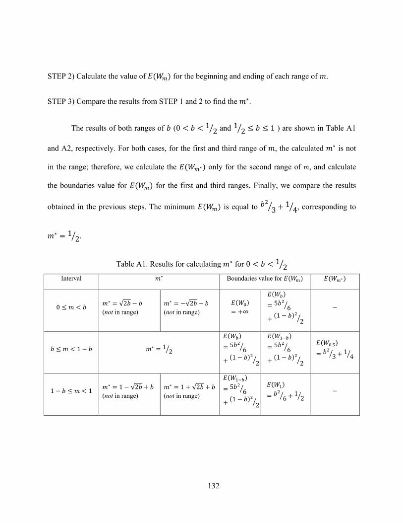
132

STEP 2) Calculate the value of ( ) for the beginning and ending of each range of .

STEP 3) Compare the results from STEP 1 and 2 to find the . The results of both ranges of ( ⁄ and ⁄ ) are shown in Table A1

and A2, respectively. For both cases, for the first and third range of , the calculated is not

in the range; therefore, we calculate the ( ) only for the second range of , and calculate

the boundaries value for ( ) for the first and third ranges. Finally, we compare the results

obtained in the previous steps. The minimum ( ) is equal to ⁄ ⁄ , corresponding to

⁄ .

Table A1. Results for calculating for ⁄

Interval Boundaries value for ( ) ( )

√

(not in range)

√

(not in range)

( )

( ) ⁄ ( ) ⁄

⁄

( ) ⁄ ( ) ⁄

( ) ⁄ ( ) ⁄

( ) ⁄ ⁄

√

(not in range)

√

(not in range)

( ) ⁄ ( ) ⁄

( ) ⁄ ⁄

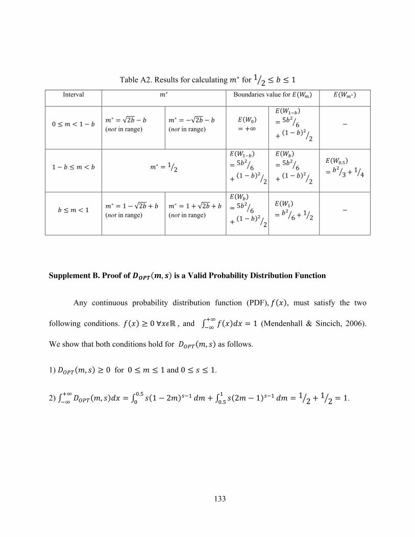
133

Table A2. Results for calculating for ⁄

Interval Boundaries value for ( ) ( )

√

(not in range)

√

(not in range)

( )

( ) ⁄ ( ) ⁄

⁄

( ) ⁄ ( ) ⁄

( ) ⁄ ( ) ⁄

( ) ⁄ ⁄

√

(not in range)

√

(not in range)

( ) ⁄ ( ) ⁄

( ) ⁄ ⁄

Supplement B. Proof of ( ) is a Valid Probability Distribution Function

Any continuous probability distribution function (PDF), ( ), must satisfy the two

following conditions. ( ) , and ∫ ( ) (Mendenhall & Sincich, 2006).

We show that both conditions hold for ( ) as follows.

1) ( ) for and .

2) ∫ ( ) ∫ ( ) ∫ ( ) ⁄ ⁄ .

134

CHAPTER SIX: CONTRIBUTION 3- “ANALYTICAL MODELS FOR MIAPP-AS/RS UNDER DEDICATED AND CLASS –BASED STORAGE

POLICY”

We study the impact of dedicated and class-based storage policies on the throughput

performance of MIAPP-AS/RS. We develop mathematical optimization models to minimize the

travel time of the crane by changing the assignment of the SKUs to pick positions and storage

locations simultaneously. We develop a more tractable solution approach by applying a Benders

decomposition approach, as well as an accelerated procedure for Benders algorithm. We observe

high degeneracy in the optimal solution when a chebyshev metric is used to calculate the

distances. As a result of this degeneracy, we realize that the assignment of SKUs to pick

positions does not impact the optimal solution in a dedicated storage policy. We also developed

closed-form travel time models for MIAPP-AS/RS under a class-based storage policy.

6-1- Introduction

Distribution centers and warehouses are generally operated under three storage policies:

randomized storage, dedicated storage, and class-based storage. In randomized storage, SKUs

are assigned to the storage locations on a random basis (e.g., SKUs are stored based on

availability of storage location at the time of storage request). The advantage of a randomized

storage policy is efficient space utilization. In Chapter 4 and Chapter 5, we developed several

travel time and optimization models when the system is operated under randomized storage. In a

dedicated storage policy, the specific storage locations are assigned to a specific SKU. If high

demanded SKUs are dedicated to the most convenient locations, a dedicated storage policy is

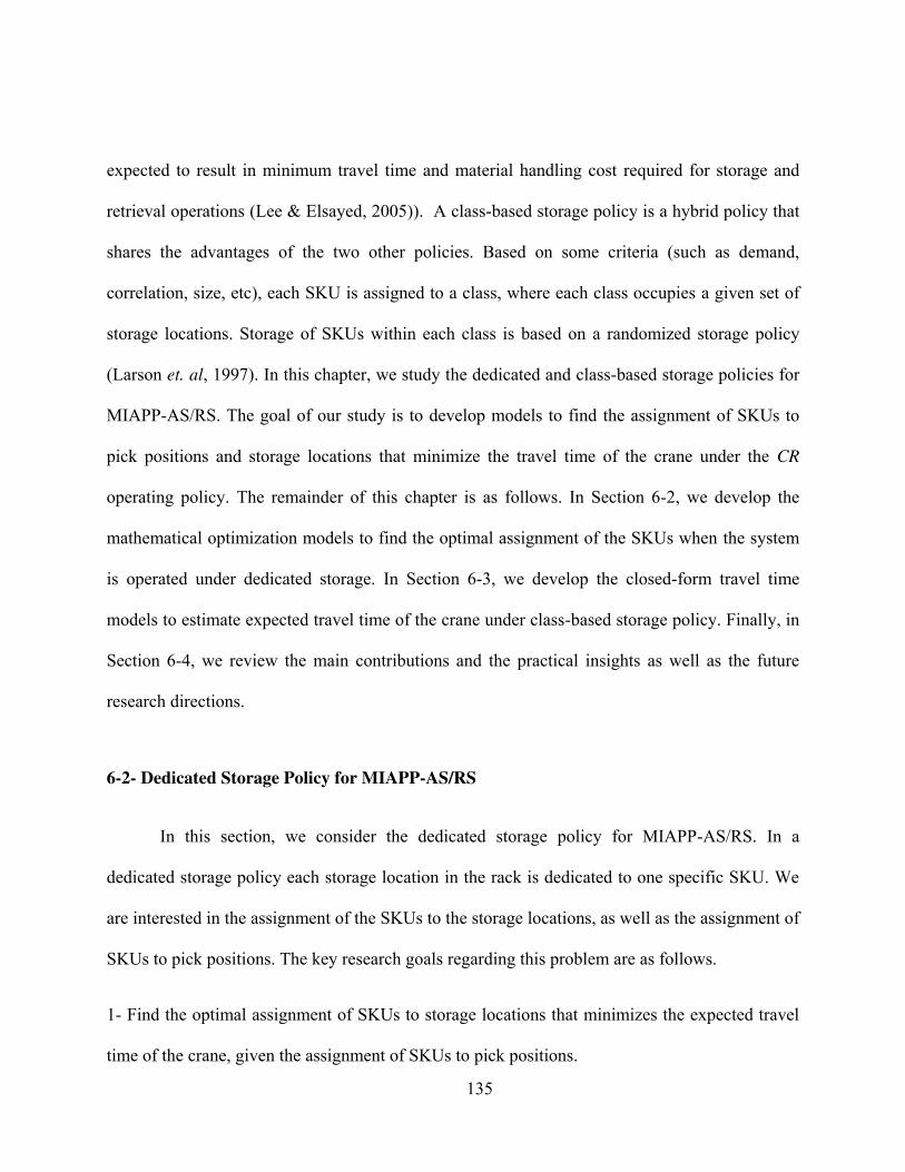
135

expected to result in minimum travel time and material handling cost required for storage and

retrieval operations (Lee & Elsayed, 2005)). A class-based storage policy is a hybrid policy that

shares the advantages of the two other policies. Based on some criteria (such as demand,

correlation, size, etc), each SKU is assigned to a class, where each class occupies a given set of

storage locations. Storage of SKUs within each class is based on a randomized storage policy

(Larson et. al, 1997). In this chapter, we study the dedicated and class-based storage policies for

MIAPP-AS/RS. The goal of our study is to develop models to find the assignment of SKUs to

pick positions and storage locations that minimize the travel time of the crane under the CR

operating policy. The remainder of this chapter is as follows. In Section 6-2, we develop the

mathematical optimization models to find the optimal assignment of the SKUs when the system

is operated under dedicated storage. In Section 6-3, we develop the closed-form travel time

models to estimate expected travel time of the crane under class-based storage policy. Finally, in

Section 6-4, we review the main contributions and the practical insights as well as the future

research directions.

6-2- Dedicated Storage Policy for MIAPP-AS/RS

In this section, we consider the dedicated storage policy for MIAPP-AS/RS. In a

dedicated storage policy each storage location in the rack is dedicated to one specific SKU. We

are interested in the assignment of the SKUs to the storage locations, as well as the assignment of

SKUs to pick positions. The key research goals regarding this problem are as follows.

1- Find the optimal assignment of SKUs to storage locations that minimizes the expected travel

time of the crane, given the assignment of SKUs to pick positions.

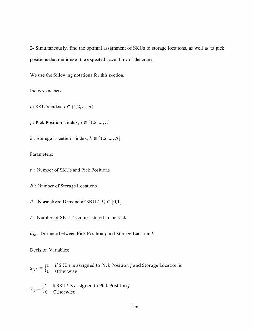
136

2- Simultaneously, find the optimal assignment of SKUs to storage locations, as well as to pick

positions that minimizes the expected travel time of the crane.

We use the following notations for this section.

Indices and sets:

: SKU’s index, { } : Pick Position’s index, { } : Storage Location’s index, { } Parameters:

: Number of SKUs and Pick Positions

: Number of Storage Locations

: Normalized Demand of SKU , [ ] : Number of SKU ’s copies stored in the rack

: Distance between Pick Position and Storage Location

Decision Variables:

{ {

137

{ We consider that there are SKUs and each of the SKUs have a single, dedicated pick

position; thus, there are also pick positions. The normalized demand of each SKU is denoted

as where , ∑ . The pick positions are replenished from storage locations. In a

dedicated storage policies, locations in the rack are dedicated to a specific SKU. The number of

storage locations dedicated to a specific SKU, say SKU , is equal to the number of SKU ’s

copies, which is denoted as . Note that for a dedicated storage policy, the total storage locations

that exist in the rack is equal to the sum of SKU’s copies (i.e. ∑ ). We assume that the

number of each SKU’s copies is equal to maximum inventory of that SKU. Defining the

inventory level of each SKU depends on the warehousing policies. In this work, we consider that

the inventory level of each SKU follows the EOQ inventory model; therefore, the inventory of

each SKU in the rack is proportional to the square root of each SKU’s demand (i.e. √ ). In

Fig. 6.1, we plot the normalized demand versus the normalized inventory level (inventory of

each SKU divided by total inventory) for the fixed number of SKUs for a 20/80 demand curve.

Fig. 6-1 shows that the skewness of the corresponding inventory curve is much less than the

skewness of the demand. As an example for the 20/80 curve, 80% of the total demand is

attributed to 20% of SKUs; however, for the inventory curve obtained by the described method,

only 50% of the total inventory is attributed to the top 20% of SKUs.

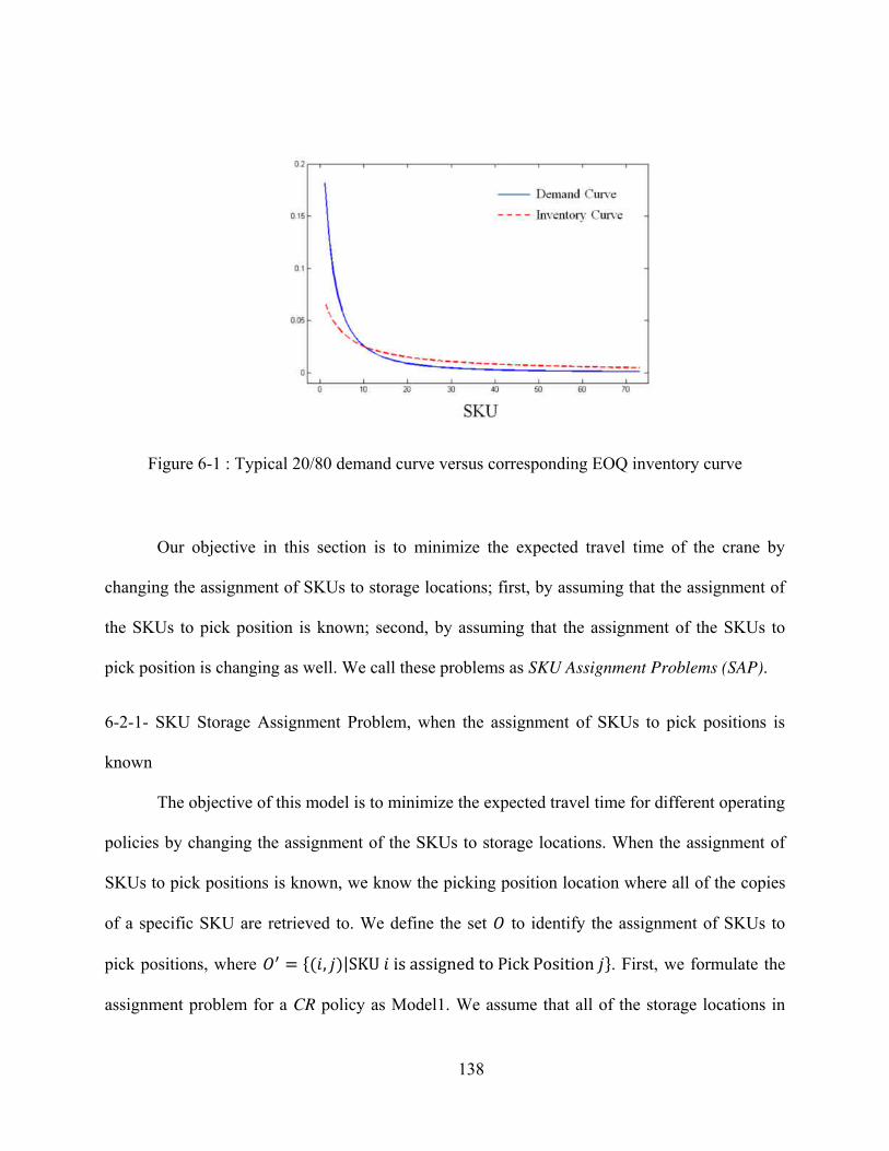
138

Figure 6-1 : Typical 20/80 demand curve versus corresponding EOQ inventory curve

Our objective in this section is to minimize the expected travel time of the crane by

changing the assignment of SKUs to storage locations; first, by assuming that the assignment of

the SKUs to pick position is known; second, by assuming that the assignment of the SKUs to

pick position is changing as well. We call these problems as SKU Assignment Problems (SAP).

6-2-1- SKU Storage Assignment Problem, when the assignment of SKUs to pick positions is

known

The objective of this model is to minimize the expected travel time for different operating

policies by changing the assignment of the SKUs to storage locations. When the assignment of

SKUs to pick positions is known, we know the picking position location where all of the copies

of a specific SKU are retrieved to. We define the set to identify the assignment of SKUs to

pick positions, where {( )| }. First, we formulate the

assignment problem for a CR policy as Model1. We assume that all of the storage locations in

139

the rack are occupied and the crane will perform only retrieval operations. A CR policy consists

of two types of trips. The first trip is from storage locations to the pick positions. For this trip

type, the crane is restricted to move to only the pick position that is dedicated to the certain SKU

stored in the storage location. The latter trip is from pick positions to storage locations. In this

case, the crane can move to any storage locations based on the next retrieval request; therefore,

we assume that each storage location in the rack is visited with the probability of ⁄ .

According to the mentioned properties of the crane movement in the CR policy, the model can be

formulated as follows. We call this model as SAP1.

SAP1:

∑ ∑ ∑ ∑ ∑ ⁄ ∑ ( ) (1)

∑ (2)

{ } (3)

Constraint (1) guarantees that the total number of storage locations assigned to each pick

position must be equal to the maximum inventory level of the SKU assigned to that pick

position. Equation (2) provides the constraint that each storage location must be assigned to just

one pick position. The structure of Model1 shares the same structure as the well-known

140

Transportation Problem. We can transform our problem into a Transportation Problem, by

imagining that there are pick positions that supplies SKUs and storage locations that each

have demand for 1 SKU. Consequently, according to the unimodular property of the

transportation problem, the linear programming relaxing of constraint (3) by considering as a

positive continuous variable will always result in being integer (given will always be

integer).

6-2-2- SKU Assignment Problem, when SKUs are assigned simultaneously to storage locations

as well as pick positions

The objective of this model is to minimize the expected travel time for different policies

by determining the assignment of the SKUs to storage locations, as well as determining the

assignment of SKUs to pick positions. This problem is similar to the problem described in

Section 6-2-1; however, the assignment of SKUs to pick positions is a decision, and it is not

known like in Section 6-2-1. Therefore, the number of storage locations that must be assigned to

each pick position is not known and depends on which SKU is assigned to each pick position. To

resolve this issue, we introduce the new binary variable, , that controls the assignment of

SKUs to pick positions, and controls the assignment of SKUs to storage locations. The

formulation of the assignment problem for this section is given as follows. We call this model as

SAP2.

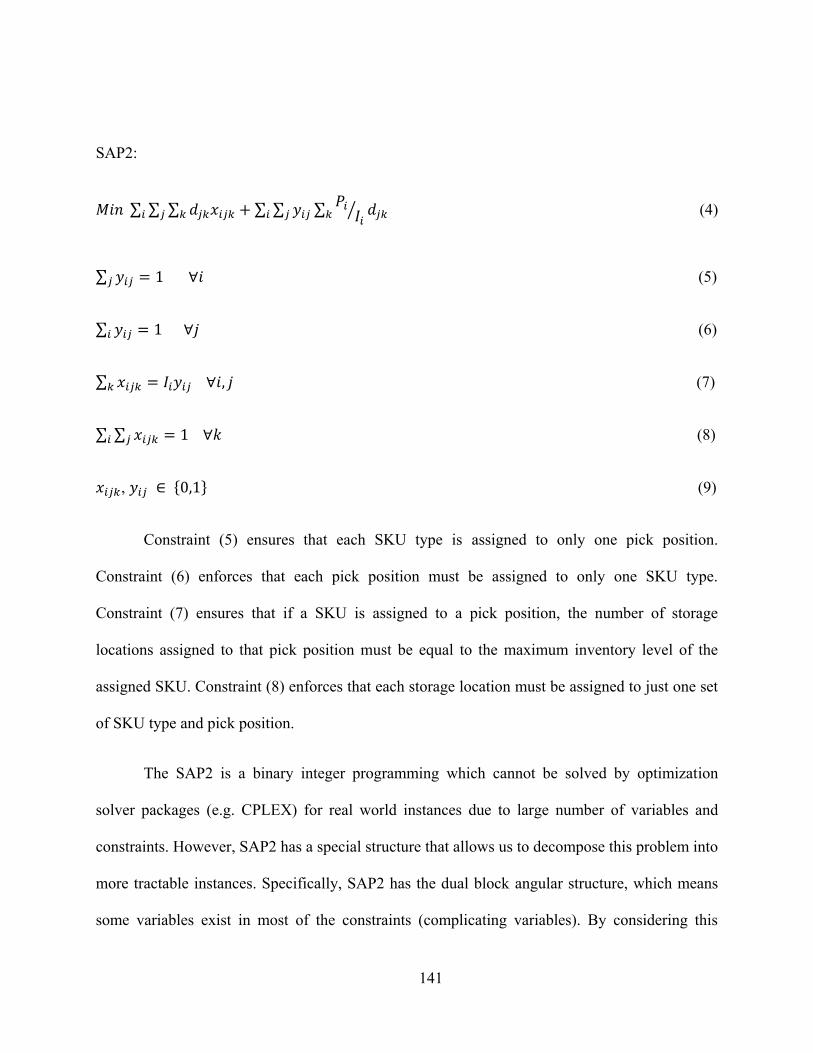
141

SAP2:

∑ ∑ ∑ ∑ ∑ ∑ ⁄ (4)

∑ (5)

∑ (6)

∑ (7)

∑ ∑ (8)

, { } (9)

Constraint (5) ensures that each SKU type is assigned to only one pick position.

Constraint (6) enforces that each pick position must be assigned to only one SKU type.

Constraint (7) ensures that if a SKU is assigned to a pick position, the number of storage

locations assigned to that pick position must be equal to the maximum inventory level of the

assigned SKU. Constraint (8) enforces that each storage location must be assigned to just one set

of SKU type and pick position.

The SAP2 is a binary integer programming which cannot be solved by optimization

solver packages (e.g. CPLEX) for real world instances due to large number of variables and

constraints. However, SAP2 has a special structure that allows us to decompose this problem into

more tractable instances. Specifically, SAP2 has the dual block angular structure, which means

some variables exist in most of the constraints (complicating variables). By considering this

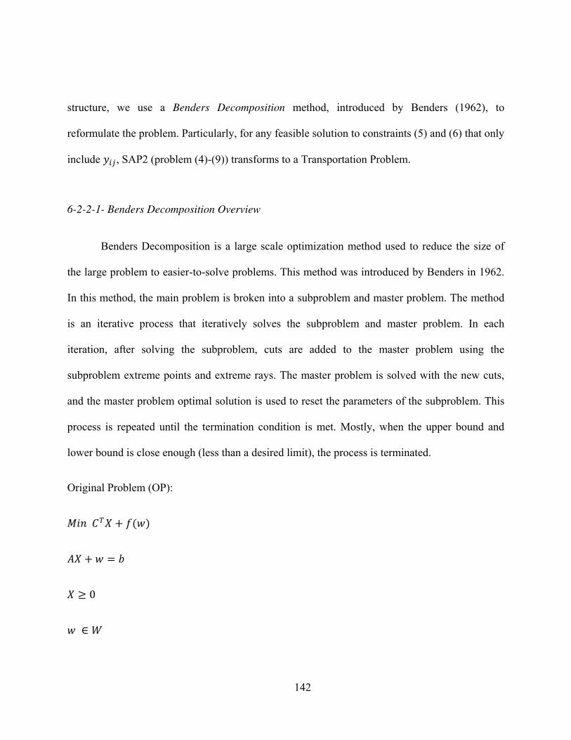
142

structure, we use a Benders Decomposition method, introduced by Benders (1962), to

reformulate the problem. Particularly, for any feasible solution to constraints (5) and (6) that only

include , SAP2 (problem (4)-(9)) transforms to a Transportation Problem.

6-2-2-1- Benders Decomposition Overview

Benders Decomposition is a large scale optimization method used to reduce the size of

the large problem to easier-to-solve problems. This method was introduced by Benders in 1962.

In this method, the main problem is broken into a subproblem and master problem. The method

is an iterative process that iteratively solves the subproblem and master problem. In each

iteration, after solving the subproblem, cuts are added to the master problem using the

subproblem extreme points and extreme rays. The master problem is solved with the new cuts,

and the master problem optimal solution is used to reset the parameters of the subproblem. This

process is repeated until the termination condition is met. Mostly, when the upper bound and

lower bound is close enough (less than a desired limit), the process is terminated.

Original Problem (OP):

( )

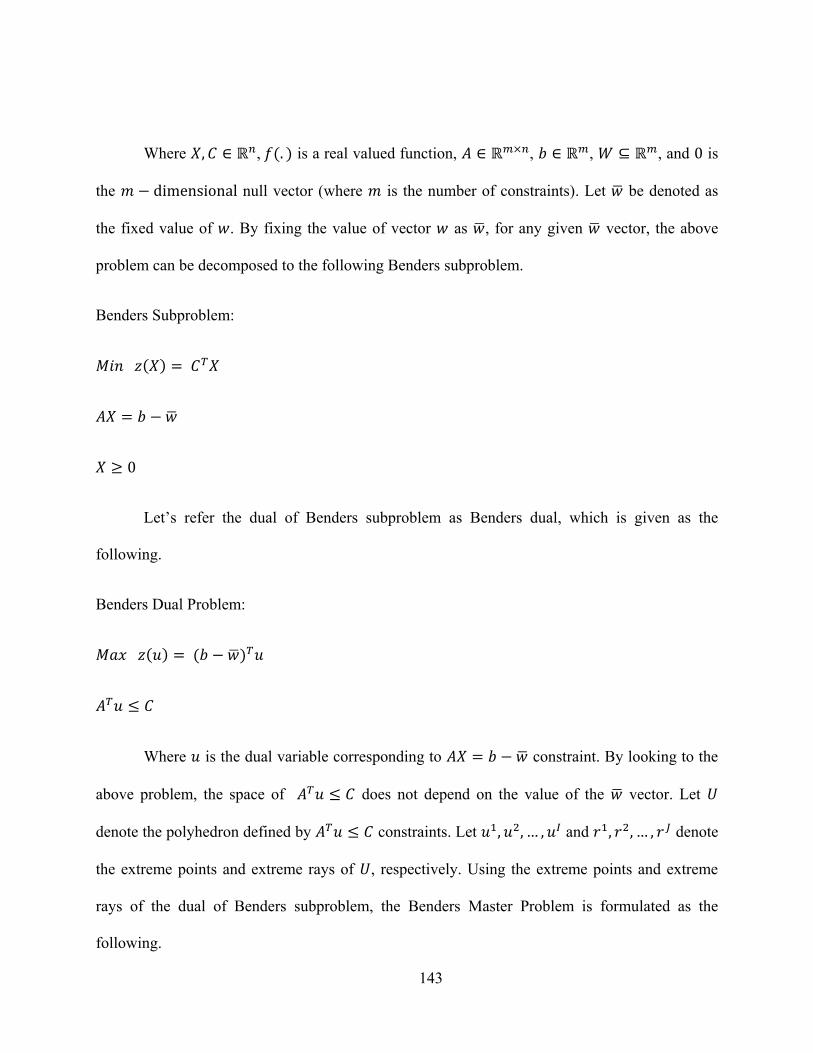
143

Where , ( ) is a real valued function, , , , and is

the null vector (where is the number of constraints). Let be denoted as

the fixed value of . By fixing the value of vector as , for any given vector, the above

problem can be decomposed to the following Benders subproblem.

Benders Subproblem:

( )

Let’s refer the dual of Benders subproblem as Benders dual, which is given as the

following.

Benders Dual Problem:

( ) ( )

Where is the dual variable corresponding to constraint. By looking to the

above problem, the space of does not depend on the value of the vector. Let

denote the polyhedron defined by constraints. Let and denote

the extreme points and extreme rays of , respectively. Using the extreme points and extreme

rays of the dual of Benders subproblem, the Benders Master Problem is formulated as the

following.

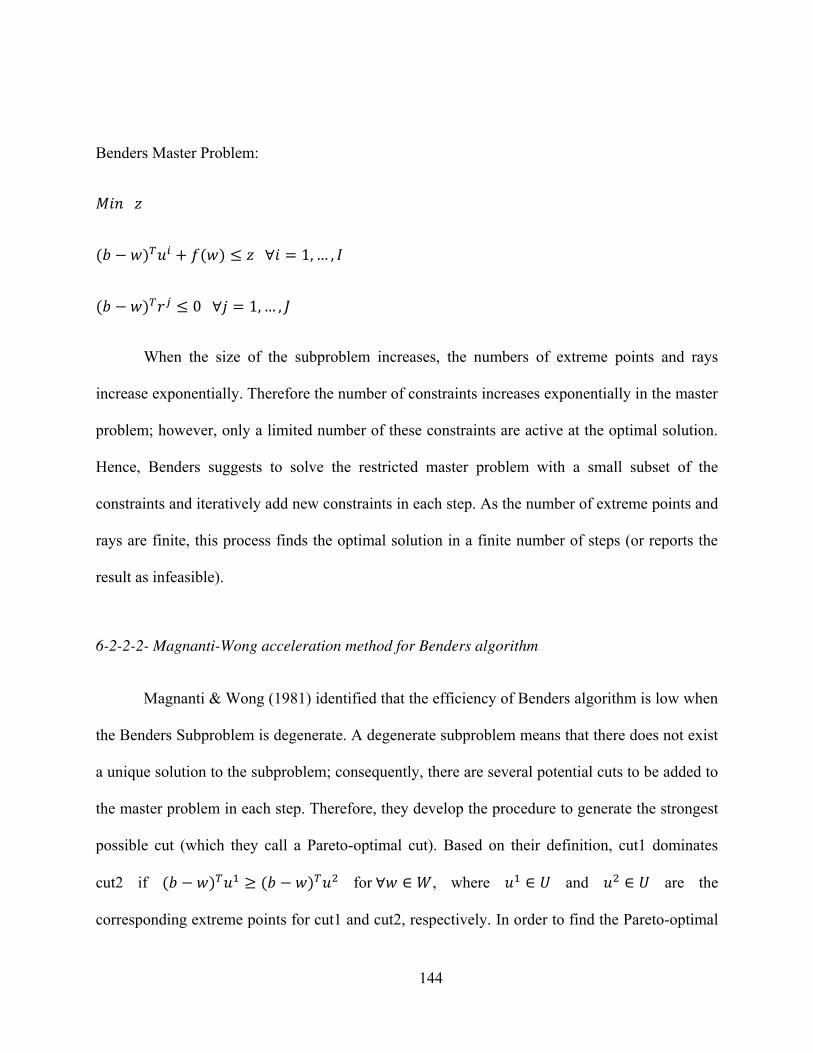
144

Benders Master Problem:

( ) ( ) ( )

When the size of the subproblem increases, the numbers of extreme points and rays

increase exponentially. Therefore the number of constraints increases exponentially in the master

problem; however, only a limited number of these constraints are active at the optimal solution.

Hence, Benders suggests to solve the restricted master problem with a small subset of the

constraints and iteratively add new constraints in each step. As the number of extreme points and

rays are finite, this process finds the optimal solution in a finite number of steps (or reports the

result as infeasible).

6-2-2-2- Magnanti-Wong acceleration method for Benders algorithm

Magnanti & Wong (1981) identified that the efficiency of Benders algorithm is low when

the Benders Subproblem is degenerate. A degenerate subproblem means that there does not exist

a unique solution to the subproblem; consequently, there are several potential cuts to be added to

the master problem in each step. Therefore, they develop the procedure to generate the strongest

possible cut (which they call a Pareto-optimal cut). Based on their definition, cut1 dominates

cut2 if ( ) ( ) for , where and are the

corresponding extreme points for cut1 and cut2, respectively. In order to find the Pareto-optimal

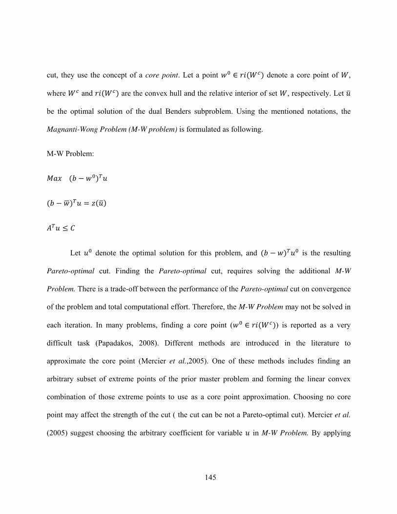
145

cut, they use the concept of a core point. Let a point ( ) denote a core point of ,

where and ( ) are the convex hull and the relative interior of set , respectively. Let

be the optimal solution of the dual Benders subproblem. Using the mentioned notations, the

Magnanti-Wong Problem (M-W problem) is formulated as following.

M-W Problem:

( )

( ) ( )

Let denote the optimal solution for this problem, and ( ) is the resulting

Pareto-optimal cut. Finding the Pareto-optimal cut, requires solving the additional M-W

Problem. There is a trade-off between the performance of the Pareto-optimal cut on convergence

of the problem and total computational effort. Therefore, the M-W Problem may not be solved in

each iteration. In many problems, finding a core point ( ( )) is reported as a very

difficult task (Papadakos, 2008). Different methods are introduced in the literature to

approximate the core point (Mercier et al.,2005). One of these methods includes finding an

arbitrary subset of extreme points of the prior master problem and forming the linear convex

combination of those extreme points to use as a core point approximation. Choosing no core

point may affect the strength of the cut ( the cut can be not a Pareto-optimal cut). Mercier et al.

(2005) suggest choosing the arbitrary coefficient for variable in M-W Problem. By applying

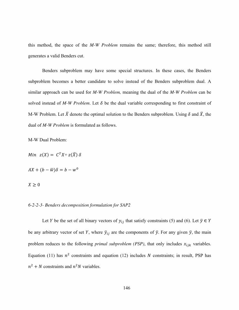
146

this method, the space of the M-W Problem remains the same; therefore, this method still

generates a valid Benders cut.

Benders subproblem may have some special structures. In these cases, the Benders

subproblem becomes a better candidate to solve instead of the Benders subproblem dual. A

similar approach can be used for M-W Problem, meaning the dual of the M-W Problem can be

solved instead of M-W Problem. Let be the dual variable corresponding to first constraint of

M-W Problem. Let denote the optimal solution to the Benders subproblem. Using and , the

dual of M-W Problem is formulated as follows.

M-W Dual Problem:

( ) + ( )

( )

6-2-2-3- Benders decomposition formulation for SAP2

Let be the set of all binary vectors of that satisfy constraints (5) and (6). Let

be any arbitrary vector of set , where are the components of For any given , the main

problem reduces to the following primal subproblem (PSP), that only includes variables.

Equation (11) has constraints and equation (12) includes constraints; in result, PSP has constraints and variables.

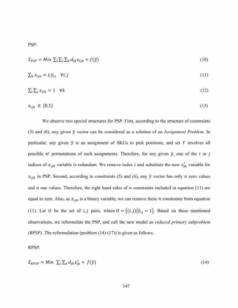
147

PSP:

∑ ∑ ∑ ( ) (10)

∑ (11)

∑ ∑ (12)

{ } (13)

We observe two special structures for PSP. First, according to the structure of constraints

(5) and (6), any given vector can be considered as a solution of an Assignment Problem. In

particular, any given is an assignment of SKUs to pick positions, and set involves all

possible permutations of such assignments. Therefore, for any given , one of the or indices of variable is redundant. We remove index and substitute the new variable for in PSP. Second, according to constraints (5) and (6), any vector has only zero values

and one values. Therefore, the right hand sides of constraints included in equation (11) are

equal to zero. Also, as is a binary variable, we can remove these constraints from equation

(11). Let be the set of pairs, where {( )| }. Based on these mentioned

observations, we reformulate the PSP, and call the new model as reduced primary subproblem

(RPSP). The reformulation (problem (14)-(17)) is given as follows.

RPSP:

∑ ∑ ( ) (14)

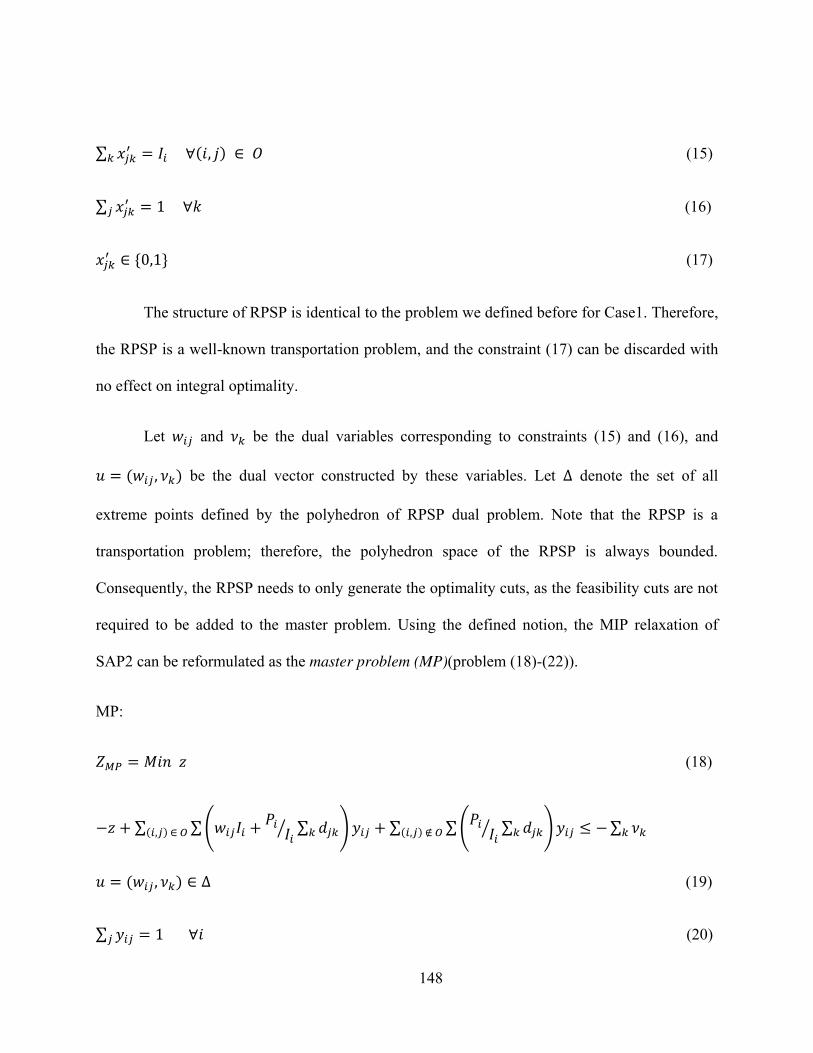
148

∑ ( ) (15)

∑ (16)

{ } (17)

The structure of RPSP is identical to the problem we defined before for Case1. Therefore,

the RPSP is a well-known transportation problem, and the constraint (17) can be discarded with

no effect on integral optimality.

Let and be the dual variables corresponding to constraints (15) and (16), and ( ) be the dual vector constructed by these variables. Let denote the set of all

extreme points defined by the polyhedron of RPSP dual problem. Note that the RPSP is a

transportation problem; therefore, the polyhedron space of the RPSP is always bounded.

Consequently, the RPSP needs to only generate the optimality cuts, as the feasibility cuts are not

required to be added to the master problem. Using the defined notion, the MIP relaxation of

SAP2 can be reformulated as the master problem (MP)(problem (18)-(22)).

MP:

(18)

∑ ∑( ⁄ ∑ ) ( ) ∑ ∑( ⁄ ∑ ) ( ) ∑

( ) (19)

∑ (20)

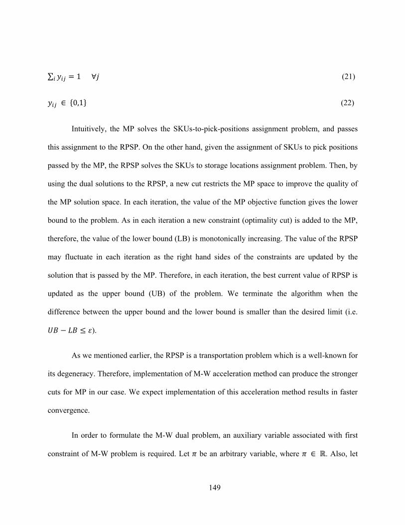
149

∑ (21)

{ } (22)

Intuitively, the MP solves the SKUs-to-pick-positions assignment problem, and passes

this assignment to the RPSP. On the other hand, given the assignment of SKUs to pick positions

passed by the MP, the RPSP solves the SKUs to storage locations assignment problem. Then, by

using the dual solutions to the RPSP, a new cut restricts the MP space to improve the quality of

the MP solution space. In each iteration, the value of the MP objective function gives the lower

bound to the problem. As in each iteration a new constraint (optimality cut) is added to the MP,

therefore, the value of the lower bound (LB) is monotonically increasing. The value of the RPSP

may fluctuate in each iteration as the right hand sides of the constraints are updated by the

solution that is passed by the MP. Therefore, in each iteration, the best current value of RPSP is

updated as the upper bound (UB) of the problem. We terminate the algorithm when the

difference between the upper bound and the lower bound is smaller than the desired limit (i.e. ).

As we mentioned earlier, the RPSP is a transportation problem which is a well-known for

its degeneracy. Therefore, implementation of M-W acceleration method can produce the stronger

cuts for MP in our case. We expect implementation of this acceleration method results in faster

convergence.

In order to formulate the M-W dual problem, an auxiliary variable associated with first

constraint of M-W problem is required. Let be an arbitrary variable, where . Also, let

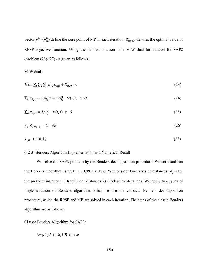
150

vector =( ) define the core point of MP in each iteration. denotes the optimal value of

RPSP objective function. Using the defined notations, the M-W dual formulation for SAP2

(problem (23)-(27)) is given as follows.

M-W dual:

∑ ∑ ∑ (23)

∑ ( ) (24)

∑ ( ) (25)

∑ ∑ (26)

{ } (27)

6-2-3- Benders Algorithm Implementation and Numerical Result

We solve the SAP2 problem by the Benders decomposition procedure. We code and run

the Benders algorithm using ILOG CPLEX 12.6. We consider two types of distances ( ) for

the problem instances 1) Rectilinear distances 2) Chebyshev distances. We apply two types of

implementation of Benders algorithm. First, we use the classical Benders decomposition

procedure, which the RPSP and MP are solved in each iteration. The steps of the classic Benders

algorithm are as follows.

Classic Benders Algorithm for SAP2:

Step 1) ,

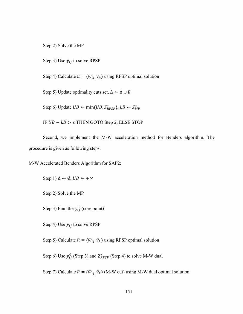
151

Step 2) Solve the MP

Step 3) Use to solve RPSP

Step 4) Calculate ( ) using RPSP optimal solution

Step 5) Update optimality cuts set,

Step 6) Update { },

IF THEN GOTO Step 2, ELSE STOP

Second, we implement the M-W acceleration method for Benders algorithm. The

procedure is given as following steps.

M-W Accelerated Benders Algorithm for SAP2:

Step 1) ,

Step 2) Solve the MP

Step 3) Find the (core point)

Step 4) Use to solve RPSP

Step 5) Calculate ( ) using RPSP optimal solution

Step 6) Use (Step 3) and (Step 4) to solve M-W dual

Step 7) Calculate ( ) (M-W cut) using M-W dual optimal solution

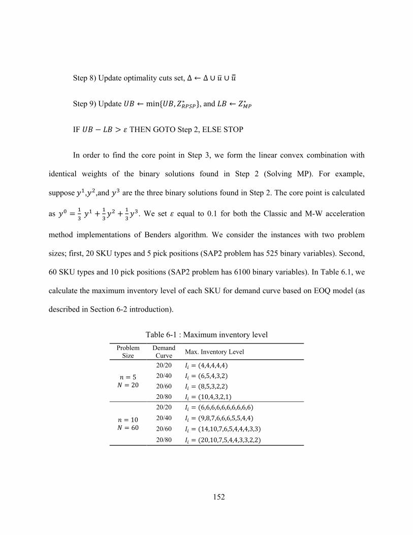
152

Step 8) Update optimality cuts set,

Step 9) Update { }, and

IF THEN GOTO Step 2, ELSE STOP

In order to find the core point in Step 3, we form the linear convex combination with

identical weights of the binary solutions found in Step 2 (Solving MP). For example,

suppose , ,and are the three binary solutions found in Step 2. The core point is calculated

as . We set equal to 0.1 for both the Classic and M-W acceleration

method implementations of Benders algorithm. We consider the instances with two problem

sizes; first, 20 SKU types and 5 pick positions (SAP2 problem has 525 binary variables). Second,

60 SKU types and 10 pick positions (SAP2 problem has 6100 binary variables). In Table 6.1, we

calculate the maximum inventory level of each SKU for demand curve based on EOQ model (as

described in Section 6-2 introduction).

Table 6-1 : Maximum inventory level

Problem

Size

Demand

Curve Max. Inventory Level

20/20 ( ) 20/40 ( ) 20/60 ( ) 20/80 ( )

20/20 ( ) 20/40 ( ) 20/60 ( ) 20/80 ( )

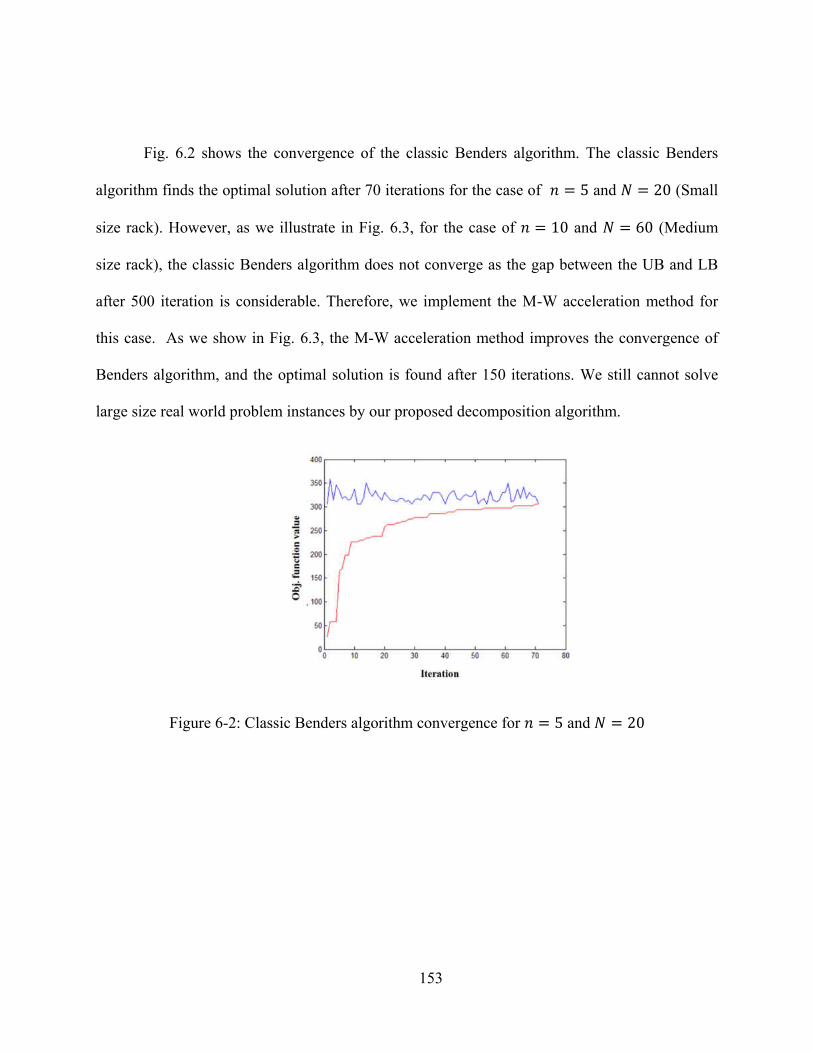
153

Fig. 6.2 shows the convergence of the classic Benders algorithm. The classic Benders

algorithm finds the optimal solution after 70 iterations for the case of and (Small

size rack). However, as we illustrate in Fig. 6.3, for the case of and (Medium

size rack), the classic Benders algorithm does not converge as the gap between the UB and LB

after 500 iteration is considerable. Therefore, we implement the M-W acceleration method for

this case. As we show in Fig. 6.3, the M-W acceleration method improves the convergence of

Benders algorithm, and the optimal solution is found after 150 iterations. We still cannot solve

large size real world problem instances by our proposed decomposition algorithm.

Figure 6-2: Classic Benders algorithm convergence for and

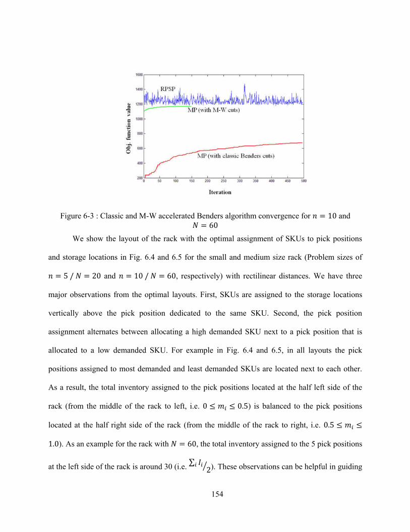
154

Figure 6-3 : Classic and M-W accelerated Benders algorithm convergence for and

We show the layout of the rack with the optimal assignment of SKUs to pick positions

and storage locations in Fig. 6.4 and 6.5 for the small and medium size rack (Problem sizes of and , respectively) with rectilinear distances. We have three

major observations from the optimal layouts. First, SKUs are assigned to the storage locations

vertically above the pick position dedicated to the same SKU. Second, the pick position

assignment alternates between allocating a high demanded SKU next to a pick position that is

allocated to a low demanded SKU. For example in Fig. 6.4 and 6.5, in all layouts the pick

positions assigned to most demanded and least demanded SKUs are located next to each other.

As a result, the total inventory assigned to the pick positions located at the half left side of the

rack (from the middle of the rack to left, i.e. ) is balanced to the pick positions

located at the half right side of the rack (from the middle of the rack to right, i.e. ). As an example for the rack with , the total inventory assigned to the 5 pick positions

at the left side of the rack is around 30 (i.e. ∑ ⁄ ). These observations can be helpful in guiding

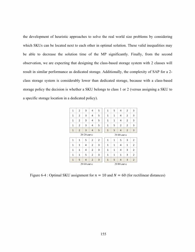
155

the development of heuristic approaches to solve the real world size problems by considering

which SKUs can be located next to each other in optimal solution. These valid inequalities may

be able to decrease the solution time of the MP significantly. Finally, from the second

observation, we are expecting that designing the class-based storage system with 2 classes will

result in similar performance as dedicated storage. Additionally, the complexity of SAP for a 2-

class storage system is considerably lower than dedicated storage, because with a class-based

storage policy the decision is whether a SKU belongs to class 1 or 2 (versus assigning a SKU to

a specific storage location in a dedicated policy).

Figure 6-4 : Optimal SKU assignment for and (for rectilinear distances)

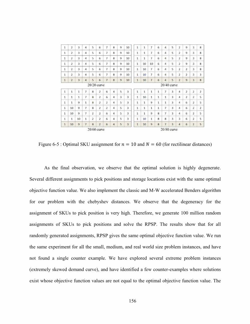
156

Figure 6-5 : Optimal SKU assignment for and (for rectilinear distances)

As the final observation, we observe that the optimal solution is highly degenerate.

Several different assignments to pick positions and storage locations exist with the same optimal

objective function value. We also implement the classic and M-W accelerated Benders algorithm

for our problem with the chebyshev distances. We observe that the degeneracy for the

assignment of SKUs to pick position is very high. Therefore, we generate 100 million random

assignments of SKUs to pick positions and solve the RPSP. The results show that for all

randomly generated assignments, RPSP gives the same optimal objective function value. We run

the same experiment for all the small, medium, and real world size problem instances, and have

not found a single counter example. We have explored several extreme problem instances

(extremely skewed demand curve), and have identified a few counter-examples where solutions

exist whose objective function values are not equal to the optimal objective function value. The

157

reasoning associated to the large number of multiple optimal solutions is that, several elements in

the chebyshev distance matrix, , are identical. Therefore, several different storage locations

have the same distance to particular pick positions. As a result, although RPSP finds the different

optimal assignment of SKUs to storage locations, the optimal objective function value remains

the same, which means changing the assignment of SKUs to pick positions do not impact the

optimal objective function value.

6-3- Class-based Storage Policy for MIAPP-AS/RS

In this section, we are interested to develop models to analyze class-based storage

policies for MIAPP-AS/RS. In the previous section, for dedicated storage policy, the distances

from storage locations to pick positions are fixed. However, in a class-based storage policy, the

SKUs assigned to a particular class are randomly stored in any location within that class.

Therefore, to have fixed distance between each class and each pick position, we consider the

expected travel time between each class and each pick position to use for an optimization model.

6-3-1- Expected Travel time between a storage region and a pick position

In this section, we are interested in deriving expected travel time models between a

storage region and an in-the-aisle pick position, and will use these travel times models as an

input to optimization models for systems with a class-based storage policy. In Section 4-4-1, we

developed models to derive the expected travel time between a pick position and any random

point within the rack. In this section, we intend to develop models that enable us to calculate the

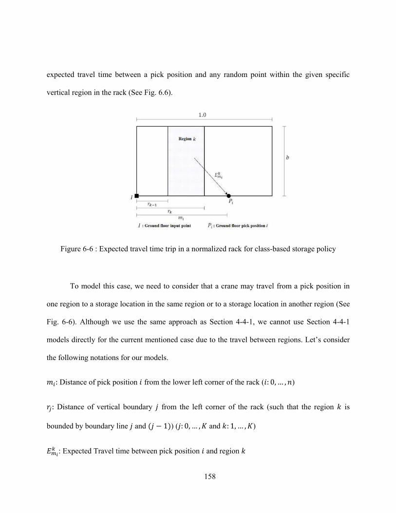
158

expected travel time between a pick position and any random point within the given specific

vertical region in the rack (See Fig. 6.6).

Figure 6-6 : Expected travel time trip in a normalized rack for class-based storage policy

To model this case, we need to consider that a crane may travel from a pick position in

one region to a storage location in the same region or to a storage location in another region (See

Fig. 6-6). Although we use the same approach as Section 4-4-1, we cannot use Section 4-4-1

models directly for the current mentioned case due to the travel between regions. Let’s consider

the following notations for our models.

Distance of pick position from the lower left corner of the rack ( )

Distance of vertical boundary from the left corner of the rack (such that the region is

bounded by boundary line and ( )) ( and )

: Expected Travel time between pick position and region

159

We assume that the storage locations are continuously and uniformly distributed in each

region (class). We consider the vertical regions in this case. Therefore, the boundaries of the

region can be defined with two points ( and ) on the bottom of the rack (See Fig. 6-6).

We consider three cases for the locations of a pick position; 1) the pick position is located within

the boundary of a given region ( ); 2) the pick position is located at the left side

of the region ( ), and 3) the pick position is located at the right side of the region

( ).

6-3-1-1- Pick Position is in Region ( )

In this case, we can use the models in Section 4-4-1 directly as the pick position is

located within the region. In Section 4-4-1, the normalized shape of the rack in terms of time is a

rectangle with a width of and height of . In this section, the given region has the same height

of , but a width of ( ). Therefore, similar to Cases 1 and 2 in Section 4-4-1, the

distance of the pick position to the left side of the region is equal to ( ), and to the

right side of the region is equal to ( ). Similar to Section 4-4-1, using equation (4) and

(5), we calculate the expected travel time between the pick position and any random point

within the left part of region and right part of region as equation (28) and (29), respectively.

The probability that a point is selected at the left side of region is equal to , and at the

right side of region is equal to . Hence, the overall expected travel time between pick

position and any random point within region , , is calculated as equation (30).

160

( ) { ( ) ⁄ ⁄ ( ) ( )⁄ ( ) ⁄ ( ) (28)

( ) { ( ) ⁄ ⁄ ( ) ( )⁄ ( ) ⁄ ( ) (29)

( ) ( ) (30)

6-3-1-2- Pick Position is Located at the Left Side of Region ( )

For this case, we follow the same methodology we used in Section 4-4-1 to derive the

travel times. The distance between the pick position and the boundaries are equal to ( ) and ( ). We follow the approach Bozer & White (1984) applied to normalized the rack

and derive the travel time (Similar to Section 4-4-1). All of the notations and assumptions are

similar to what we defined in Section 4-4-1. In this case, the horizontal travel time follows the

uniform distribution between ( ) and ( ). Also, the vertical travel time follows

the uniform distribution between and . Hence, we have

( ) ( )

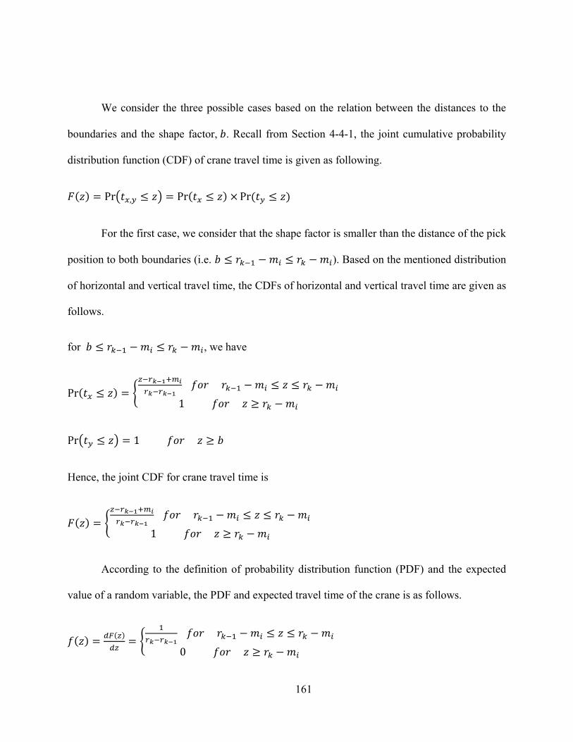
161

We consider the three possible cases based on the relation between the distances to the

boundaries and the shape factor, . Recall from Section 4-4-1, the joint cumulative probability

distribution function (CDF) of crane travel time is given as following.

( ) ( ) ( ) ( ) For the first case, we consider that the shape factor is smaller than the distance of the pick

position to both boundaries (i.e. ). Based on the mentioned distribution

of horizontal and vertical travel time, the CDFs of horizontal and vertical travel time are given as

follows.

for , we have

( ) {

( )

Hence, the joint CDF for crane travel time is

( ) {

According to the definition of probability distribution function (PDF) and the expected

value of a random variable, the PDF and expected travel time of the crane is as follows.

( ) ( ) {

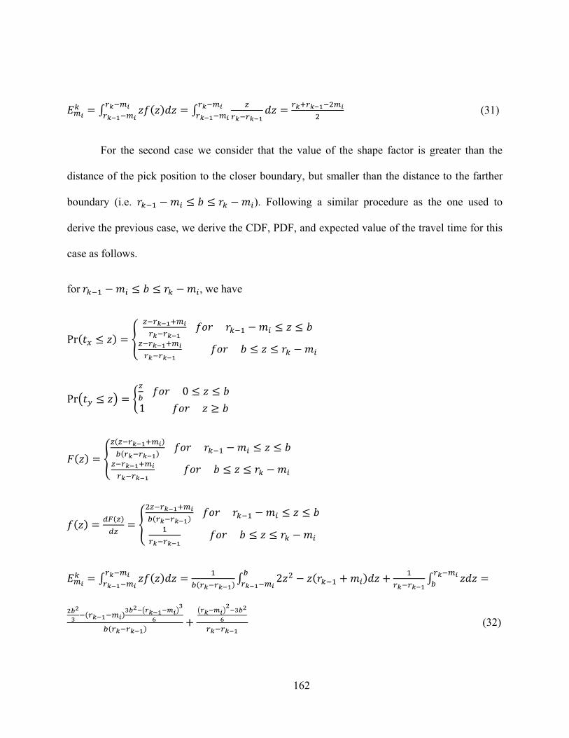
162

∫ ( ) ∫ (31)

For the second case we consider that the value of the shape factor is greater than the

distance of the pick position to the closer boundary, but smaller than the distance to the farther

boundary (i.e. ). Following a similar procedure as the one used to

derive the previous case, we derive the CDF, PDF, and expected value of the travel time for this

case as follows.

for , we have

( ) {

( ) {

( ) { ( ) ( )

( ) ( ) { ( )

∫ ( ) ( )∫ ( ) ∫ ( ) ( ) ( ) ( ) (32)

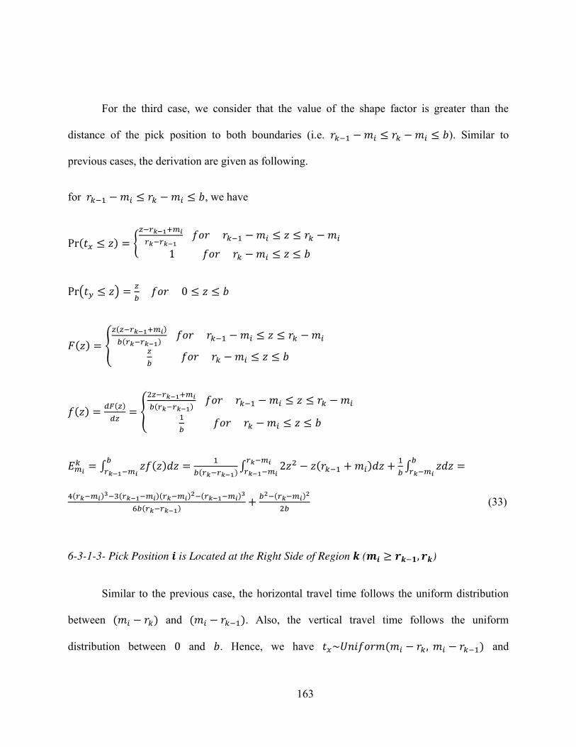
163

For the third case, we consider that the value of the shape factor is greater than the

distance of the pick position to both boundaries (i.e. ). Similar to

previous cases, the derivation are given as following.

for , we have

( ) {

( )

( ) { ( ) ( )

( ) ( ) { ( )

∫ ( ) ( )∫ ( ) ∫ ( ) ( )( ) ( ) ( ) ( ) (33)

6-3-1-3- Pick Position is Located at the Right Side of Region ( )

Similar to the previous case, the horizontal travel time follows the uniform distribution

between ( ) and ( ). Also, the vertical travel time follows the uniform

distribution between and . Hence, we have ( ) and

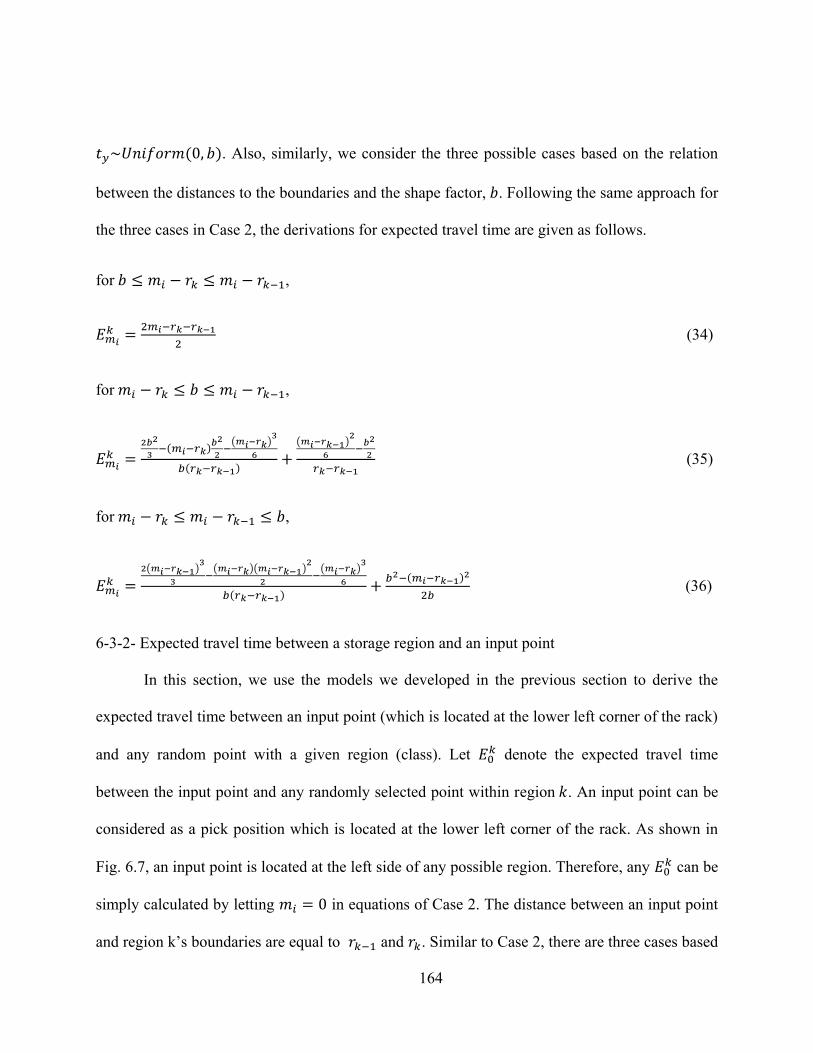
164

( ). Also, similarly, we consider the three possible cases based on the relation

between the distances to the boundaries and the shape factor, . Following the same approach for

the three cases in Case 2, the derivations for expected travel time are given as follows.

for ,

(34)

for ,

( ) ( ) ( ) ( ) (35)

for ,

( ) ( )( ) ( ) ( ) ( ) (36)

6-3-2- Expected travel time between a storage region and an input point

In this section, we use the models we developed in the previous section to derive the

expected travel time between an input point (which is located at the lower left corner of the rack)

and any random point with a given region (class). Let denote the expected travel time

between the input point and any randomly selected point within region . An input point can be

considered as a pick position which is located at the lower left corner of the rack. As shown in

Fig. 6.7, an input point is located at the left side of any possible region. Therefore, any can be

simply calculated by letting in equations of Case 2. The distance between an input point

and region k’s boundaries are equal to and . Similar to Case 2, there are three cases based

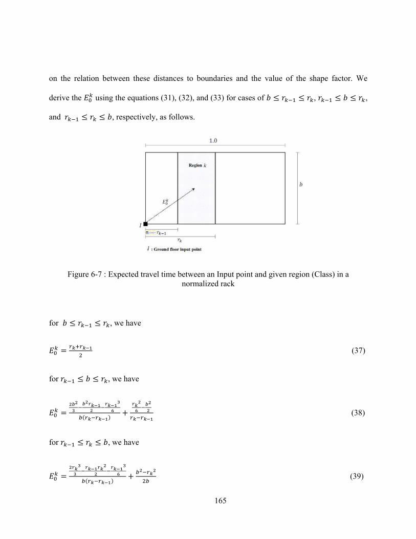
165

on the relation between these distances to boundaries and the value of the shape factor. We

derive the using the equations (31), (32), and (33) for cases of , ,

and , respectively, as follows.

Figure 6-7 : Expected travel time between an Input point and given region (Class) in a

normalized rack

for , we have

(37)

for , we have

( ) (38)

for , we have

( ) (39)

166

6-4- Conclusion and future research directions

In this chapter, we developed mathematical binary linear programming models to

minimize the travel time by changing the assignment of SKUs to pick positions and storage

locations under the dedicated storage policy. Because of the special structure of the problem, we

developed a solution approach based on the Benders decomposition algorithm to break the

original problem into the smaller tractable instances. Through this decomposition, the

subproblem is a well-known transportation problem that iteratively finds the assignment of the

SKUs to storage locations as well as the master problem that finds the assignment of the SKUs to

pick positions. Due to the degeneracy of the subproblem, we applied the Magnanti-Wong

acceleration method for Benders algorithm to speed up the convergence of the algorithm. We

implemented both algorithms for small and medium size problem instances. We observed some

intuitive results from the optimal solutions: 1) the layout of the optimal assignment includes

vertical SKUs stored above their dedicated pick positions 2) the pick positions dedicated to high

demanded SKUs are mostly assigned close to pick positions dedicated to low demanded SKUs 3)

The optimal assignment is highly degenerate for rectilinear and chebyshev distance metrics. Also

by applying the chebyshev metrics to realistic instances, changing the assignment of the SKUs to

pick positions does not impact the optimal objective function value for the original problem.

Finally, we developed the closed-form statements that can estimate the expected travel time of

the crane under the class-based storage policy.

167

As the future research directions, we propose to develop heuristic algorithms based on the

idea that the pick positions dedicated to high demanded SKUs are mostly assigned close to pick

positions dedicated to low demanded SKUs.

168

CHAPTER SEVEN: FUTURE STUDY DIRECTIONS

Contribution 1 is the first study that analyzes AS/RS with multiple in-the-aisle outputs.

Therefore, our study could help extensively to design and quantify the performance of systems

with in-the-aisle outputs or pick positions. In Contribution 2, we consider more realistic aspects

of the environment of MIAPP-AS/RS by incorporating the idea of non-identical SKUs’ demand,

which relaxed some of the assumptions in Contribution 1. This brings more practical design

decisions such as optimal SKU assignment problem, which is discussed in Contribution 2. In

Contribution 3, we relaxed the assumption of randomized storage and developed travel time and

optimization models based on dedicated and class-based storage policies. Our study could be

extended to consider the following future research directions. The development of analytical

models for MIAPP-AS/RS that considers different dwell point strategies and different

sequencing rules would be interesting to understand how policies impact throughput and storage

space performance. Also, the development of a systematic model that considers the interaction

of human order pickers and the MIAPP-AS/RS would be interesting from an inventory buffer

capacity, as well as a staff resource and scheduling perspective.

169

LIST OF REFERENCES

Ashayeri, J., Gelders, L., & Wassenhove, L. V. (1985). A microcomputer-based optimization

model for the design of automated warehouses. International Journal of Production

Research, 23(4), 825–839.

Ashayeri, J., Heuts, R. M., Valkenburg, M. W. T., Veraart, H. C., & Wilhelm, M. R. (2002). A

geometrical approach to computing expected cycle times for zone based storage layouts

in AS/RS. International Journal of Production Research, 40(17), 4467–4483.

Askin, R. and Nussbaum, M. A. (Aug., 2014) Executive summaries of IIE Transactions and IIE

Transactions on Occupational Ergonomics and Human Factors, Magazine of the Institute

of Industrial Engineers, 46(8), 0-0. Available at

http://www.iienet2.org/IndustrialEngineer/details.aspx?id=37467

Bartholdi, J. J., & Hackman, S. T. (2011). Warehouse & distribution science: release 0.95. The

Supply Chain and Logistics Institute, School of Industrial and Systems Engineering,

Georgia Institute of Technology, Atlanta, GA, 30332. Available at

http://www2.isye.gatech.edu/~jjb/wh/book/editions/wh-sci-0.95.pdf, accessed April

2014.

Beheshti, R., & Sukthankar, G. (2012). Extracting agent-based models of human transportation

patterns. In Social Informatics (SocialInformatics), 2012 International Conference on (pp.

157-164). IEEE.

170

Beheshti, R., & Sukthankar, G. (2013). Improving Markov Chain Monte Carlo estimation with

agent-based models. In Social Computing, Behavioral-Cultural Modeling and Prediction

(pp. 495-502). Springer Berlin Heidelberg.

Beheshti, R., & Mozayani, N. (2014). HOMAN, a learning based negotiation method for holonic

multi-agent systems. Journal of Intelligent and Fuzzy Systems, 26(2), 655-666.

Beheshti, R., & Sukthankar, G. (2014). A hybrid modeling approach for parking and traffic

prediction in urban simulations. AI & SOCIETY, 1-12.

Beheshti, R., Ali, A. M., & Sukthankar, G. (2015). Cognitive Social Learners: an Architecture

for Modeling Normative Behavior. Proceedings of the AAAI Conference on Artificial

Intelligence, Austin, TX (pp. 2017-2023).

Benders, J. F. (1962). Partitioning procedures for solving mixed-variables programming

problems. Numerische mathematik, 4(1), 238-252.

Bozer, Y. A., & Cho, M. (2005) Throughput performance of automated storage/retrieval systems

under stochastic demand. IIE Transactions, 37(4), 367–378.

Bozer, Y. A., & White, J. A. (1984) Travel-time models for automated storage/retrieval systems.

IIE Transactions, 16(4), 329–338.

Bozer, Y. A., & White, J. A. (1990) Design and performance models for end-of-aisle order

picking systems. Management Science, 36(7), 852-866.

Bozer, Y. A., & White, J. A. (1996). A generalized design and performance analysis model for

end-of-aisle order-picking systems. IIE Transactions, 28(4), 271–280.

Chang, D.-T., Wen, U.-P., & Lin, J. T. (1995) The impact of acceleration/deceleration on travel-

time models for automated storage/retrieval systems. IIE Transactions, 27(1), 108–111.

171

Chang, D.-T., & Wen, U.-P. (1997). The impact on rack configuration on the speed profile of the

storage and retrieval machine. IIE Transactions, 29(7), 525–531.

Chen, C., Huang, S.-Y., Hsu, W.-J., Toh, A. C., & Loh, C. K. (2003). Platform-based AS/RS for

container storage. In ICRA ’03 (pp. 181–187). Taipei.

Chopra, S., & Meindl, P. (2007). Supply chain management: strategy, planning, and operation

(3rd ed.). Upper Saddle River, NJ: Pearson.

Datamonitor. Frozen Food: Global Industry Guide 2011, available at

http://www.datamonitor.com/store/Product/frozen_food_global_industry_guide_2011?pr

oductid=BC26C3D2-321D-432F-B0C0-C2754F7FBD11, accessed December 2012.

de Koster, R., Le-Duc, T., & Roodbergen, K. J. (2007) Design and control of warehouse order

picking: A literature review. European Journal of Operational Research, 182(2), 481–501.

De Koster, R. (M. . B. M., Le-Duc, T., & Yugang, Y. (2008). Optimal storage rack design for a

3-dimensional compact AS/RS. International Journal of Production Research, 46(6),

1495–1514.

Drury, J. (1988). Towards more efficient order picking. Cranfield, UK: IMM Monograph

Number 1, The Institute of Materials Management.

Egbelu, P. J. (1991) Framework for dynamic positioning of storage/retrieval machines in an

automated storage/retrieval system. International Journal of Production Research, 29(1),

17–37.

Egbelu, P.I., & Wu, C.-T. (1993) A comparison of dwell point rules in an automated

storage/retrieval system. International Journal of Production Research, 31(11), 2515-

2530.

172

Elsayed, E. A. (1981) Algorithms for optimal material handling in automatic warehousing

systems. International Journal of Production Research, 19(5), 525–535.

Eynan, A., & Rosenblatt, M. J. (1993).An interleaving policy in automated storage/retrieval

systems. International Journal of Production Research, 31(1), 1–18.

Eynan, A., & Rosenblatt, M. J. (1994) Establishing zones in single-command class-based

rectangular AS/RS. IIE Transactions, 26(1), 38–46.

Francis, R. L., McGinnis, L. F., & White, J. A. (1992). Facility layout and location: an analytical

approach. Englewood Cliffs, N.J.: Prentice Hall.

Foley, R. D., & Frazelle, E. H. (1991) Analytical results for miniload throughput and the

distribution of dual command travel time. IIE Transactions, 23(3), 273–281.

Frazelle, E. H. (1989). Stock location assignment and order picking productivity, Ph.D.

Dissertation, Georigia Institute of Technology, December 1989.

Graves, S. C., Hausman, W. H., & Schwarz, L. B. (1977) Storage-retrieval interleaving in

automatic warehousing systems. Management Science, 23(9), 935–945.

Goetschalckx, M., & Ashayeri, J. (1989). CLASSIFICATION AND DESIGN OF ORDER

PICKING. Logistics Information Management, 2(2), 99–106. doi:10.1108/eb007469

Goetschalckx, M., & Ratliff, H.D. (1990) Shared storage policies based on the duration of stay of

unit loads. Management Science 36, 1120–1132.

Gu, J., Goetschalckx, M., & McGinnis, L. F. (2007) Research on warehouse operation: A

comprehensive review. European Journal of Operational Research, 177(1), 1–21.

173

Guenov, M., &Raeside, R. (1992) Zone shapes in class based storage and multicommand order

picking when storage/retrieval machines are used. European Journal of Operational

Research, 58(1), 37–47.

Hadian, S., Madani, K., Rowney, C., & Mokhtari, S. (2012). Toward More Efficient Global

Warming Policy Solutions: The Necessity for Multi-Criteria Selection of Energy Sources.

In World Environmental and Water Resources Congress 20-24 May 2012, Albuquerque,

New Mexico (pp. 2884–2892). Reston, VA: American Society of Civil Engineers.

Hadian, S., Madani, K., & Mokhtari, S. (2013). A Systems Approach to Energy Efficiency

Assessment. In World Environmental and Water Resources Congress, 19-23 May 2013,

Cincinnati, Ohio (pp. 2593–2600). Reston, VA: American Society of Civil Engineers.

Han, M.-H., McGinnis, L. F., Shieh, J. S., & White, J. A. (1987). On sequencing retrievals in an

automated storage/retrieval system. IIE Transactions, 19(1), 56–66.

Hausman, W. H., Schwarz, L. B., & Graves, S. C. (1976) Optimal storage assignment in

automatic warehousing systems. Management Science, 22(6), 629–638.

Hu, Y.-H., Huang, S. Y., Chen, C., Hsu, W.-J., Toh, A. C., Loh, C. K., & Song, T. (2005) Travel

time analysis of a new automated storage and retrieval system. Computers & Operations

Research, 32(6), 1515–1544.

Hwang, H., Baek, W. J., & Lee, M.-K. (1988) Clustering algorithms for order picking in an

automated storage and retrieval system. International Journal of Production Research,

26(2), 189–201.

174

Hwang, H., & Lee, S. B. (1990). Travel-time models considering the operating characteristics of

the storage and retrieval machine. International Journal of Production Research, 28(10),

1779.

Hwang, H., Moon, S., & Gen, M. (2002). An integrated model for the design of end-of-aisle

order picking system and the determination of unit load sizes of AGVs. Computers &

Industrial Engineering, 42(2–4), 249–258.

Karasawa, Y., Nakayama, H., & Dohi, S. (1980). Trade-off analysis for optimal design of

automated warehouses. International Journal of Systems Science, 11(5), 567–576.

Keserla, A., & Peters, B. A. (1994) Analysis of dual-shuttle automated storage/retrieval systems.

Journal of Manufacturing Systems, 13(6), 424–434.

Kouvelis, P., & Papanicolaou, V. (1995) Expected travel time and optimal boundary formulas for

a two-class-based automated storage/retrieval system. International Journal of Production

Research, 33(10), 2889–2905.

Kucukvar, M., Noori, M., Egilmez, G., & Tatari, O. (2014). Stochastic decision modeling for

sustainable pavement designs. The International Journal of Life Cycle Assessment, 19(6),

1185-1199.

Kulturel, S., Ozdemirel, N.E., Sepil, C., & Bozkurt, Z. (1999) Experimental investigation of

shared storage assignment policies in automated storage/ retrieval systems. IIE

Transactions 31, 739–749.

Larson, T. N., March, H., & Kusiak, A. (1997). A heuristic approach to warehouse layout with

class-based storage. IIE transactions, 29(4), 337-348.

175

Le-Duc, T., Koster, M. B. M. D., & Yu, Y. (2006). Optimal Storage Rack Design for a 3-

Dimensional Compact As/Rs (No. Reference No. ERS-2006-027-LIS). ERIM Report

Series. Retrieved from Available at SSRN: http://ssrn.com/abstract=911701

Lee, H.F. (1997) Performance analysis for automated storage and retrieval systems. IIE

Transactions 29, 15–28.

Lee, M. K., & Elsayed, E. A. (2005). Optimization of warehouse storage capacity under a

dedicated storage policy. International Journal of Production Research, 43(9), 1785-1805.

Linn, R.J., & Wysk, R.A. (1990) An expert system based controller for an automated

storage/retrieval system. International Journal of Production Research, 28(4), 735-756.

Magnanti, T. L., & Wong, R. T. (1981). Accelerating Benders decomposition: Algorithmic

enhancement and model selection criteria. Operations research,29(3), 464-484.

Malmborg, C. J. (2001). Rule of thumb heuristics for configuring storage racks in automated

storage and retrieval systems design. International Journal of Production Research, 39(3),

511–527. doi:10.1080/0020754001004368

Manzini, R., Gamberi, M., & Regattieri, A. (2006). Design and control of an AS/RS. The

International Journal of Advanced Manufacturing Technology, 28(7), 766–774.

Meller, R. D., & Mungwattana, A. (1997) Multi-shuttle automated storage/retrieval systems. IIE

Transactions, 29(10), 925–938.

Mercier, A., Cordeau, J. F., & Soumis, F. (2005). A computational study of Benders

decomposition for the integrated aircraft routing and crew scheduling

problem. Computers & Operations Research, 32(6), 1451-1476.

176

Noori, M., Kucukvar, M., & Tatari, O. (2013). A macro-level decision analysis of wind power as

a solution for sustainable energy in the USA. International Journal of Sustainable Energy,

1-16.

Noori, M., Tatari, O., Nam, B., Golestani, B., & Greene, J. (2014). A stochastic optimization

approach for the selection of reflective cracking mitigation techniques. Transportation

Research Part A: Policy and Practice, 69, 367-378.

Papadakos, N. (2008). Practical enhancements to the Magnanti–Wong method.Operations

Research Letters, 36(4), 444-449.

Pazour, J. A., & Meller, R. D. (2011) An analytical model for A-frame system design. IIE

Transactions, 43(10), 739–752.

Pan, C.-H., & Wang, C.-H. (1996). A framework for the dual command cycle travel time model

in automated warehousing systems. International Journal of Production Research, 34(8),

2099–2117.

Potrč, I., Lerher, T., Kramberger, J., & Šraml, M. (2004). Simulation model of multi-shuttle

automated storage and retrieval systems. Journal of Materials Processing Technology,

157–158, 236–244.

Peters, B. A., Smith, J. S., & Hale, T. S. (1996) Closed form models for determining the optimal

dwell point location in automated storage and retrieval systems. International Journal of

Production Research, 34(6), 1757–1771.

Randhawa, S. U., McDowell, E. D., & Wang, W.-T. (1991) Evaluation of scheduling rules for

single- and dual-dock automated storage/retrieval system. Computers & Industrial

Engineering, 20(4), 401–410.

177

Randhawa, S. U., & Shroff, R. (1995) Simulation-based design evaluation of unit load automated

storage/retrieval systems. Computers & Industrial Engineering, 28(1), 71–79.

Ramtin, F., & Pazour, J. A. (2014). Analytical models for an automated storage and retrieval

system with multiple in-the-aisle pick positions. IIE Transactions, 46(9), 968-986.

Ramtin, F. and Pazour J. A. (2015). Product Allocation Problem for an AS/RS with Multiple in-

the-Aisle Pick Positions. IIE Transaction, in press.

Rodrigue, J.-P., Comtois, C., & Slack, B. (2009) The Geography of Transport Systems,

Routledge, New York, NY, available at

http://people.hofstra.edu/geotrans/eng/ch5en/appl5en/cc_temperature_standards.html,

accessed December 2012.

Roodbergen, K. J., & Vis, I. F. A. (2009) A survey of literature on automated storage and

retrieval systems. European Journal of Operational Research, 194(2), 343–362.

Rosenblatt, M.J., & Eynan, A. (1989) Deriving the optimal boundaries for class-based automatic

storage/retrieval systems. Management Science 35(12), 1519–1524.

Rosenblatt, M. J., & Roll, Y. (1984). Warehouse design with storage policy considerations.

International Journal of Production Research, 22(5), 809.

Rosenblatt, M. J., Roll, Y., & Vered Zyser, D. (1993). A Combined Optimization and Simulation

Approach for Designing Automated Storage/Retrieval Systems. IIE Transactions, 25(1),

40–50.

Sari, Z., Saygin, C., & Ghouali, N. (2005) Travel-time models for flow-rack automated storage

and retrieval systems. The International Journal of Advanced Manufacturing Technology,

25(9), 979–987.

178

Sarker, B. R., & Babu, P. S. (1995) Travel time models in automated storage/retrieval systems: A

critical review. International Journal of Production Economics, 40(2–3), 173–184.

Sarker, B. R., Mann, L., & Leal Dos Santos, J. R. G. (1994) Evaluation of a class-based storage

scheduling technique applied to dual-shuttle automated storage and retrieval systems.

Production Planning & Control, 5(5), 442–449.

Swisslog Co. (2012) Deep-Freeze - Optimizing efficiency in Deep-Freeze Warehouses [White

paper], available at http://www.swisslog.com/whitepaper-deepfreeze_e-2.pdf , accessed

December 2012.

Swisslog Co. (2013) Warehouse & Distribution Solutions, References & Case Studies, available

at http://www.swisslog.com/index/wds-index/wds_downloads/wds_references.htm ,

accessed January 2013.

Schwarz, L. B., Graves, S. C., & Hausman, W. H. (1978) Scheduling policies for automatic

warehousing systems: Simulation results. AIIE Transactions, 10(3), 260–270.

Thonemann, U. W., & Brandeau, M. L. (1998) Optimal storage assignment policies for

automated storage and retrieval systems with stochastic demands. Management Science,

44(1), 142–148.

The Material Handling Institute of America (MHIA). Available at http://www.mhi.org, accessed

April 2014

Tompkins, J. A., White, J. A., Bozer, Y. A., & Tanchoco, J. M. A. (2010). Facilities Planning

(4th ed.). Wiley.

Van den Berg, J.P. (1999) A literature survey on planning and control of warehousing systems.

IIE Transactions 31, 751–762.

179

Van den Berg, J. P. (2002) Analytic expressions for the optimal dwell point in an automated

storage/retrieval system. International Journal of Production Economics, 76(1), 13–25.

Vasili, M., Hong, T. S., Homayouni, S. M., & Ismail, N. (2008) A statistical model for expected

cycle time of SP-AS/RS: An application of Monte Carlo simulation. Applied Artificial

Intelligence, 22(7-8), 824–840.

Vasili, M. R., Tang, S. H., & Vasili, M. (2012) Automated Storage and Retrieval Systems: A

Review on Travel Time Models and Control Policies. In Manzini, R. (Ed.), Warehousing

in the Global Supply Chain: Advanced Models, Tools and Applications for Storage

Systems, Springer, New York, NY, pp. 159–209.

Warehouse Modernization and Layout Planning Guide. (1978). NAVSUP Publication 529.

Naval Supply Systems Command, Department of the Navy, Washington, DC.

Wen, U. P., Chang, D. T., & Chen, S. P. (2001). The impact of acceleration/deceleration on

travel-time models in class-based automated S/R systems. IIE Transactions, 33(7), 599–

608.

Wu, L., Mokhtari, S., Nazef, A., Nam, B., & Yun, H.-B. (2014). Improvement of Crack-

Detection Accuracy Using a Novel Crack Defragmentation Technique in Image-Based

Road Assessment. Journal of Computing in Civil Engineering.

Yun, H.-B., Park, S.-H., Mehdawi, N., Mokhtari, S., Chopra, M., Reddi, L. N., & Park, K.-T.

(2014). Monitoring for close proximity tunneling effects on an existing tunnel using

principal component analysis technique with limited sensor data. Tunnelling and

Underground Space Technology, 43, 398–412.

180

Zollinger, H. "AS/RS application, benefits and justification in comparison to other storage

methods: A white paper. (2001). Automated Storage Retrieval Systems Production

Section of the Material Handling Industry of America. , available at

http://www.mhi.org/downloads/industrygroups/as-

rs/technicalpapers/asrswhitepaper2.pdf, accessed April 2014.