Model selection in magnetic resonance imaging measurements of vascular permeability: Gadomer in a 9L...

Model selection in magnetic resonance imagingmeasurements of vascular permeability: Gadomerin a 9L model of rat cerebral tumor

James R Ewing1,2, Stephen L Brown3, Mei Lu4, Swayamprava Panda1, Guangliang Ding1,Robert A Knight1, Yue Cao5, Quan Jiang1, Tavarekere N Nagaraja6, Jamie L Churchman1

and Joseph D Fenstermacher6

1Department of Neurology, Henry Ford Health Systems, University of Michigan, Detroit, Michigan, USA;2Department of Radiology, Henry Ford Health Systems, University of Michigan, Detroit, Michigan, USA;3Department of Radiation Oncology, Henry Ford Health Systems, University of Michigan, Detroit, Michigan,USA; 4Department of Biostatistics and Research Epidemiology, Henry Ford Health Systems, University ofMichigan, Detroit, Michigan, USA; 5Departments of Radiation Oncology and Radiology, Henry Ford HealthSystems, University of Michigan, Detroit, Michigan, USA; 6Department of Anesthesiology, Henry Ford HealthSystems, University of Michigan, Detroit, Michigan, USA

Vasculature in and around the cerebral tumor exhibits a wide range of permeabilities, from normalcapillaries with essentially no blood–brain barrier (BBB) leakage to a tumor vasculature that freelypasses even such large molecules as albumin. In measuring BBB permeability by magneticresonance imaging (MRI), various contrast agents, sampling intervals, and contrast distributionmodels can be selected, each with its effect on the measurement’s outcome. Using Gadomer, a largeparamagnetic contrast agent, and MRI measures of T1 over a 25-min period, BBB permeability wasestimated in 15 Fischer rats with day-16 9L cerebral gliomas. Three vascular models weredeveloped: (1) impermeable (normal BBB); (2) moderate influx (leakage without efflux); and (3) fastleakage with bidirectional exchange. For data analysis, these form nested models. Model 1 estimatesonly vascular plasma volume, vD, Model 2 (the Patlak graphical approach) vD and the influx transferconstant Ki. Model 3 estimates vD, Ki, and the reverse transfer constant, kb, through which theextravascular distribution space, ve, is calculated. For this contrast agent and experimental duration,Model 3 proved the best model, yielding the following central tumor means (7s.d.; n¼ 15): vD¼ 0.0770.03 for Ki¼ 0.010570.005 min�1 and ve¼ 0.1070.04. Model 2 Ki estimates were approximately 30%of Model 3, but highly correlated (r¼ 0.80, Po0.0003). Sizable inhomogeneity in vD, Ki, and kb

appeared within each tumor. We conclude that employing nested models enables accurateassessment of transfer constants among areas where BBB permeability, contrast agent distributionvolumes, and signal-to-noise vary.Journal of Cerebral Blood Flow & Metabolism (2006) 26, 310–320. doi:10.1038/sj.jcbfm.9600189; published online3 August 2005

Keywords: blood–brain barrier; 9L cerebral tumor; magnetic resonance contrast agents; MRI; transfer constants;vascular permeability

Introduction

Microvascular permeability within and around acerebral tumor can vary widely, and might be animportant measure of its aggressiveness (Daldrup

et al, 1998a; Roberts et al, 2002). Furthermore,changes in permeability from leaky toward normalmay signal the efficacy of therapeutic intervention(Bhujwalla et al, 2003; Turetschek et al, 2004).Because it is noninvasive, a magnetic resonanceimaging (MRI) measure of permeability can berepeated over time, allowing the continuous moni-toring of disease progression and its treatment. Insuch measurements, various contrast agents, sam-pling intervals, and contrast distribution models canbe selected, each decision affecting the measure-ment’s outcome. The purpose of this paper is todescribe the effects of these choices, that is, the

Received 15 February 2005; revised 18 April 2005; accepted 6June 2005; published online 3 August 2005

Correspondence: Dr JR Ewing, Neurology NMR Facility, E&RB126, Henry Ford Health Systems, 2799 W Grand Blvd, Detroit,MI 48202, USA. E-mail: [email protected] grant was funded in part by the following NIH grants: R01HL70023 MRI Measures of Blood Brain Barrier Permeability andNINCDS P01 NS 23393 Center for Stroke Research.

Journal of Cerebral Blood Flow & Metabolism (2006) 26, 310–320& 2006 ISCBFM All rights reserved 0271-678X/06 $30.00

www.jcbfm.com

‘operating characteristics’ of MRI estimates ofvascular permeability.

Compartmental theory with varying assumptionshas been used to arrive at MRI estimates of vascularpermeability. Tofts et al (1999) reviewed and unifiedthese efforts in a compartmental model (the ‘con-sensus model’) that was essentially identical to thatof earlier work that dealt with physiological markerssuch as radiotracers (Crone, 1963; Johnson andWilson, 1966; Lassen and Perl, 1979). A simplifiedmatrix model similar to that of Patlak (Patlak et al,1983), which presents the early-time data as a linearplot, is also extensively used in MRI (Daldrup et al,1998a, b; Daldrup-Link et al, 2004; Roberts et al,2002; Turetschek et al, 2004). The Patlak model hasbeen applied to MRI data obtained with the contrastagent gadolinium-diethylene-triaminepentaaceticacid (Gd-DTPA) and a rat model of transient cerebralischemia (Ewing et al, 2003a). In this work, the Gd-DTPA transfer constants obtained via Patlak plotswere shown to be well-correlated with those of 14C-sucrose assayed by quantitative autoradiography(QAR). To our knowledge, this was the first, andthus far the only, comparison of QAR and MRIestimates of blood–brain barrier (BBB) permeability.

The original Patlak model (Patlak et al, 1983)assumed that any compartments on the blood side ofthe BBB fills quickly with magnetic resonancecontrast agent (MRCA), then subsequently closelyfollows the changing plasma concentrationm, andthat the MRCA, once across the BBB, remains at ornear the site of leakage. Patlak and Blasberg (1985)later revised their model to allow for efflux from the‘irreversible’ compartment and linearization of theplotted data; the resultant analysis is essentiallyidentical to the consensus model. The theoreticaldevelopment of Patlak et al both presages and linkscurrent MRI approaches of estimating vasculartransfer constant, thus providing a useful frameworkfor model selection.

To apply the techniques previously developed intransient ischemia (Ewing et al, 2003a) to those of anaggressive cerebral tumor model with a broad rangeof BBB leakiness, it was necessary to use a largerMRCA than Gd-DTPA; to this end, Gadomer, anexperimental Gd-labeled MRCA (Schering AG), wasselected. Gadomer has a molecular weight ofapproximately 17 kDa and an effective size in vivonearly that of albumin.

Theory—Three Models

Consider the middle of our three nested models, theoriginal Patlak model (Model 2) (Table 1). It is amodel of the blood–brain exchange of an indicator(Patlak and Blasberg, 1985; Patlak et al, 1983) thathas one very critical, simplifying assumption. Thisassumption is that there exists an ‘irreversible’tissue region beyond the BBB, where the tracer isessentially trapped for the duration of the experi-

ment. The working equation for this system is:

CtðtÞ ¼ Ki

Zt

0

CpðtÞdtþ vdCpðtÞ þ vaCpðtÞ ð1Þ

where Cp and Ct are the plasma and tissueconcentrations of the indicator, Ki is the unidirec-tional transfer constant of the indicator from plasmaacross the barrier into the interstitial fluid, vd is thefractional volume of the rapidly reversible, plasma-tracking tissue space, and va is the fractional volumeof the plasma (Table 2 lists definitions and symbols).Since they cannot be estimated separately from thedata, vd and va will hereafter be combined into onevolume fraction, vD.

In this and all following expressions, units willfollow ‘MRI conventions,’ in which concentrationsare in mL indicator/mL tissue, flows and perme-ability-surface (PS) products are in min�1, etc. Thisis in distinction to the ‘radiological conventions,’ inwhich concentrations are in mL indicator/g tissue),and PS products are in mL/g min. Numerically,since the density of brain tissue is very close to 1,the two unit systems produce estimates of transferconstant and distribution volume that are nearlyidentical.

Patlak et al have introduced a method forlinearizing the problem of curve fitting. A graph ofthe ratio Ct(t)/Cp(t) versus

R0t Cp(t) dt/Cp(t) (generally

this abscissa is called ‘stretch time’) yields a linearrelationship, with a slope of Ki and an ordinateintercept of vD. Such a graph has become known asthe Patlak plot (Gjedde, 1997; Patlak et al, 1983). Forour purposes, this linearization is useful because itmakes model testing via F-test comparisons exact(see below).

In a later modification (Patlak and Blasberg, 1985),a correction for efflux from the ‘irreversible’ tissuecompartment back into blood was obtained:

CtðtÞ ¼ Ki

Zt

0

e�kbðt�tÞCpðtÞdtþ vDCpðtÞ ð2Þ

where the additional term, kb, is the transfer ratefrom the extravascular ‘irreversible’ compartment tothe plasma compartment and removal by thecirculation. This equation is exactly equivalent tothat of the ‘consensus’ model (Tofts et al, 1999). Theequivalence between the consensus model notationand the variables above are as follows: Ki¼Ktrans,kb¼ kep, vD¼Vb (this latter equivalence is approximate,

Table 1 Parametric estimates for Model 2 and Model 3, 15animals

Model 2 Model 3

vD 0.11970.054 0.066870.029K1 (min�1) 0.0027770.00133 0.010570.0046ve 0.097770.0374

Model selection in 9L tumors using Gadomer MRI contrastJR Ewing et al

311

Journal of Cerebral Blood Flow & Metabolism (2006) 26, 310–320

since vD as defined differs slightly from the bloodvolume itself). Hereafter, the notation of Patlak willbe followed because it: (1) takes precedence overthe later consensus model; (2) is unified amongthe three models examined; and (3) is closer tostandard scientific usage since, in the main, it usessingle-character subscripted variables to representphysical variables.

In terms of model testing, introducing kb extendsModel 2 by testing its central assumption of nobackflux across the BBB. As in the original Patlaktreatment, if the quantity Ct(t)/Cp(t) is plotted versusthe efflux-corrected arterial time integralR

t0e�kbðt�tÞCpðtÞdt divided by Cp(t), a linear plot

should result, with a slope of Ki and an intercept ofvD. The term kb corresponds to Ki/ve, where ve is theextravascular, extracellular space.

The Observation Equations

As detailed elsewhere (Cao et al, 2005), we assumethe fast exchange limit for the protons of water inboth tissue and blood. In this case, the observationequation equivalent to equation (1) is

ð1 � HctÞDR1tðtÞ ¼ Ki

Zt

0

DR1aðtÞdtþ vDDR1aðtÞ ð3Þ

where Hct is the hematocrit, R1a is the longitudinalrelaxation rate of all protons in the artery, R1t is thelongitudinal relaxation rate of all protons in the

tissue, and D refers to the subtraction of the pre-contrast rate from its postcontrast value. Plotting theratio (1�Hct)DR1t(t)/DR1a(t) versus (

R0tDR1a(t) dt)/(DR1a)

yields the Patlak plot (Model 2), with a slope of Ki

and an ordinate intercept of vD. If Ki is approxi-mately zero, the model (Model 1) will incorporateonly the distribution volume, vD.

The observation equation that corresponds toequation (2) (Model 3) and corrects for efflux fromthe ‘irreversible’ compartment is

ð1 � HctÞDR1tissðtÞ ¼Ki

Zt

0

e�kbðt�tÞDR1aðtÞdt

þ vDDR1aðtÞ

ð4Þ

We will show an example of both the original Patlakplot and the efflux-corrected version, show in asample of 15 animals the changes in the parametricestimates vD and Ki that result from this correction,and offer a criterion for choosing between thevarious models, that is, between no appreciableleakage of MRCA across the BBB, leakage of MRCAwith negligible tissue efflux, and leakage withappreciable tissue efflux.

The Effect of Missing Initial Arterial Data

Let us assume that, for some initial period trt0,neither tissue nor arterial data are determined, andthe measurement is taken up after t0. As detailed in

Table 2 Symbols, with units of measure

Symbol Use (units)

Cp(t) Plasma concentration as a function of time (mL tracer/mL plasma)CR Relaxivity of the contrast agent in units of (ms�1 per unit concentration)Ct(t) Tissue concentration as a function of time (mL tracer/mL tissue)Hct Hematocrit as a fraction of blood volume (mL erythrocytes/mL blood)kb Transvascular unidirectional (inward) transfer constant (min�1)Ki Transvascular unidirectional (outward) transfer constant (min�1)R1a, R1p Arterial, erythrocyte, and plasma (respectively) longitudinal relaxation rates (ms�1)DR1a, DR1t The change, due to the injection of contrast agent, in the arterial (subscript a) and tissue

(subscript t) longitudinal relaxation rates (ms�1)R1tiss, R1 Tissue, cellular, and extravascular extracellular (respectively) longitudinal relaxation rates (ms�1)Se, Sp, Sf Summed-squared residuals between the model and the data: extra, partial, and full, respectivelyt Time (min)t (Greek tau) Dummy variable of integration of time-varying quantitiesnd Fractional volume of rapidly equilibrating reversible space (mL/mL tissue)na Fractional volume of plasma (mL/mL tissue)nD¼ vd+va Combined fractional volume of plasma and rapidly equilibrating non-plasma spaces

(mL/mL tissue)ve Extravascular, extracellular volume fraction (mL EES/mL tissue)VD

0 The y-axis intercept of the linear portion of the Patlak plot in the event that an initial portion of thearterial input function is not measured

ne, np, nf (Greek nu) Degrees of freedom for extra, partial, and full summed-squares(1�Hct)DR1tiss(t)/DR1a(t) Patlak plot ordinateR

t0DR1aðtÞdtDR1aðtÞ

Patlak plot abscissa

Rt0

DR1ae�kbðt�tÞðtÞdt Efflux-corrected Patlak plot abscissa


312


the appendix, the apparent distribution volume, VD0 ,

should be related to the true distribution volume viathe following:

V 0D ¼

Ki

Rt00 CpðtÞdt

Cpðt0Þþ vD ð5Þ

and a plot of VD0 versus Ki with group data will

display a relationship with a slope equal toðR

t00 CpðtÞdtÞ=ðCpðt0ÞÞ and a y-intercept equal to the

actual distribution volume, vD.

Materials and methods

Animal Preparation—9L Tumors in Fischer 344 Rats

Fifteen male Fischer 344 rats (weight 220 to 300 g) werestudied in a protocol approved by the Henry Ford HealthSystems animal care committee.

The 9L tumor is a well-characterized rat brain tumormodel (Moulder and Rockwell, 1984; Wheeler and Wallen,1980). Obtained from Dr Kenneth Wheeler, Wake ForestUniversity, the tumor line was originally derived from ratbrain after induction by intravenous N-nitrosomethylurea.Cells were maintained by serial passage in vitro usingDulbecco’s medium and 10% fetal bovine serum. The rat’shead was immobilized using a small animal stereotacticdevice (Model 902, Kopf Instruments, Tujunga, CA, USA).After a midline incision, the skull was exposed and a burrhole drilled through the skull, taking care not to penetratethe dura. In all, 10,000 9L rat cells were injected at a rate of1 mL/min into a location 2.5 mm anterior to the bregma,2.0 mm to the right of the midline, and a depth of 3.0 mm,as described previously (Kim et al, 1995). After implanta-tion, the animals were returned to their cages for a periodof approximately 16 days. Untreated 9L brain tumors aretypically 2 to 3 mm in diameter on days 14, and 5 to 6 mmin diameter on day 18 (Brown et al, 1999).

Magnetic resonance imaging was performed 1672 daysafter cell implantation. Each rat was anesthetized with 3.0%halothane for induction, and then spontaneously respiredwith 1.0% to 2.0% halothane in a 2:1 N2O:O2 mixture usinga face mask. Body temperature was maintained constant(371C) with a recirculating water pad monitored via anintrarectal type T thermocouple. Femoral arterial and venousPE-50 catheters were inserted to obtain blood samples,record systemic arterial pressure, and inject the MRCA.

Magnetic Resonance Imaging

Magnetic resonance imaging procedures employed a 7 T,12 cm (clear bore) Magnex magnet with actively shieldedgradients of 250 mT/m and 100ms rise times. The magnetwas interfaced with a Bruker Avance console runningParavision V2.1.1. The RF coils were a Bruker volumeresonator for transmission and an actively decoupled 2 cmBruker surface coil for reception. The volume resonator,animal holder, and surface coil formed an imaging unit tobe inserted in the magnet. After animal location in theholder, the surface coil was centered over the brain, theholder was located in the volume coil, and the imaging

apparatus and animal were located in the magnet. Using athree-plane sequence, the central imaging slice was placedto view the largest lateral extent of the tumor.

Since the change in the longitudinal relaxation rate, R1

(R1¼ 1/T1) is generally thought to be linear in concentrationof MRCA, this measurement is critical in estimatingvascular permeability. AT-One by Multiple Read-Out Pulses(TOMROP) (Brix et al, 1990) sequence, developed on a 3 Thuman system (Gelman et al, 2000), was adapted to therequirements of the 7 T animal system (Ewing et al, 2003a).

T-One by Multiple Read-Out Pulses is a Look–Lockersequence (Look and Locker, 1970), and thus an efficientand unbiased estimate of T1 (Crawley and Henkelman,1988). At least one dummy cycle (N pulses followed byTrelax) was applied before the start of data acquisition.Inversion of the longitudinal magnetization was accom-plished using a nonselective hyperbolic secant adiabaticpulse of duration 12 ms. One phase-encode line of 24small-tip-angle (approximately 181 shaped pulses) gradient-echo images (echo time, TE 4 ms) was acquired after eachsuch adiabatic inversion, at 50-ms intervals, for a totalrecovery time of 1200 ms with a 2-sec relaxation intervalbetween each adiabatic inversion. Matrix size was128� 64, field-of-view (FOV) 32 mm, three 2-mm slices.

All images were obtained with 32 mm FOV. Before theadministration of MRCA, a single-slice arterial spinlabeling (ASL) perfusion study (Ewing et al, 2003b)(matrix 64� 64), a high-resolution T2-weighted image set(repetition time (TR)/TE¼ 2000/10 ms, 3 CPMG echoes,matrix 256� 192 seventeen 0.5-mm slices, 4 accumula-tions), a T1-weighted high-resolution image set (TR/TE¼ 1000/7.5, matrix 256/192, 27 0.5 mm slices, 4accumulations), and two baseline TOMROP studies wereobtained. Magnetic resonance contrast agent (250 mmol/kg)was administered in a 0.2 mL bolus over approximately4 secs. The dynamic contrast created by the bolus wasfollowed with an echo-planar spin-echo sequence (TR/TE¼ 1000/32, matrix 64� 64, three 2 mm slices) for a totalof 64 scans, with bolus administration beginning on thetenth scan. Immediately after the echo-planar sequence,10 TOMROP sequences were run, following the tissueconcentration of MRCA across a 25-min period. After thelast TOMROP study, a postcontrast T1-weighted image,identical to the precontrast study, was acquired. Data fromthe Echo-Planar study will be reported separately. Wenote, however, that approximately 1 min separated theadministration of the contrast agent and the beginning ofthe first postcontrast TOMROP acquisition.

Using the postcontrast T1-weighted image, each slicewas examined for the presence of tumor; if leakage wasseen, the area of leakage was outlined manually, filled,and the volume of tumor in the slice calculated bymultiplying the area of leakage by the slice thickness.All such volumes were summed, thus yielding an estimateof total tumor volume.

Data Analysis

Using TOMROP image sets taken at 145-sec intervals,pixel-by-pixel R1 maps were constructed using a maximum-


313


likelihood procedure constrained to yield nonnega-tive estimates of the model parameters (Gelman et al,2000).

Three 2-mm-thick slices of data on 2 mm centers wereavailable. The slice with the largest extent of tumor wasselected for further study. In most, but not all, cases, thiswas the center slice of the three-slice package. Sagittal DR1

was measured in the slice where that sinus was mosteasily visualized and used to estimate the DR1 of cerebralarterial blood, a practice previously validated (Ewing et al,2003a).

As we have noted, the tissue DR1 was used as a measureof tissue MRCA concentration. Equations (3) and (4) wereused to produce pixel-by-pixel estimates of Ki and vD,assuming arterial hematocrit to be 0.45. To visuallyevaluate the linearity of the data in tissue with abnormalBBB permeability, a region of interest (ROI) was selectedand demarcated in each animal by examination of thepostcontrast T1-weighted image. Using sagittal sinus dataand ROI DR1’s, Patlak plots (Models 1 and 2) and efflux-corrected Patlak plots (Model 3) were constructed for eachpixel within the ROI. In those cases where the single-sliceASL technique and the slice with the largest extent oftumor coincided, CBF was measured pixel-by-pixel acrossthe brain.

The general characteristics of the transfer constants bythe three models are: Model 1, Ki¼ 0, kb¼ 0; Model 2,Ki40, kb¼ 0; and Model 3, Ki40, kb40. The summed-squared residuals of the data plotted according to the threemodels was computed pixel by pixel, and the F-statisticcalculated (Bates and Watts, 1988). The results were thencompared 1 versus 2, and 2 versus 3; that is, first a modelwith no leakage was compared with one with irreversibleleakage and then a model with irreversible leakage wascompared with one with reversible leakage. The F-statisticwas computed and mapped on a pixel-by-pixel basis andalso computed for the entire ROI. The ROI uncorrectedand efflux-corrected Patlak plots were also examinedvisually. Because of the continuous decrease in bloodconcentration of MRCA, the later time data were lessreliable than those from earlier times. For this reason, wesystematically reduced the data set, point-by-point, untilthe 2 versus 3 F-test reached a maximum. For instance, wemight have started with 11 data points, but found that theModel 2 versus 3 F-test peaked at 9 points. In this case, theparametric estimates from both models for 9 fitted pointswere used in reporting the data. In all cases, at least sixpoints were used.

Statistical Tests—Model Comparisons

An ‘extra sum of squares analysis for nested variables’(Bates and Watts, 1988) was employed to examine whichmodel best resolved the data. In the following, the Patlakmodel will be referred to as the partial model, and theefflux-corrected model as the full model. The ratio (Se/ne)/(Sf/nf) was computed, where Se and Sf are sum-squaredresiduals (further described below), the subscript f refersto the full model, and the subscript e refers to the extravariance accounted for by the full model relative to the

partial model. The degrees of freedom ne and nf are, in thiscase, 1 (for the number of extra parameters in the fullmodel), and N�m, where N is the number of points on theclearance curve, and m is the number of parameters in thepartial model (m¼ 2 for Model 2, m¼ 3 for Model 3). It isfurther defined that Se¼Sp�Sf, where Sp is the sum of thesquared residuals of the partial model, and Sf is the sum ofthe squared residuals of the full model. For linear models,the ratio (Se/ne)/(Sf/nf) is distributed as the F-statistic, Fve;vF

,with ne and nf degrees of freedom.

In the F-test, the null hypothesis is that the two samplesof sum-squared residuals were drawn from the same pool,that is, the two models are equivalent. The failure of thishypothesis leads to acceptance of the larger model (themodel with the smaller sum-squared residuals). Theprobability associated with the F-test (the P-value) is thatof a Type I error, for example, the probability of acceptingModel 3 when the underlying truth was that of Model 2. Inthe problem at hand, we placed the threshold foracceptance of the larger model at P¼ 0.05, Bonferonni-corrected for (two) multiple comparisons. The F-testthreshold for each of the model comparisons was, thus,set at Po0.025.

As for reporting other data and comparisons, mean7standard deviation is given, and standard statistical testsare indicated where employed.

Results

Fifteen animals were studied. Mean tumor age was15.972.1 days (range 14 to 22 days). As measured bythe postcontrast T1-weighted images, mean tumorvolume, which varies exponentially with time afterimplantation, was 70.0764 mm3 (range 5 to229 mm3). For the nine animals in which the sliceof the CBF study coincided with the tumor slice,mean flow was estimated at 2.070.9 min�1.

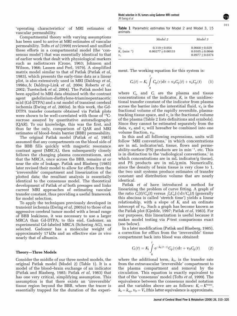
To introduce the findings, the data from a singleanimal studied 16 days postimplantation will bepresented. In this case, total tumor volume was121 mm3. Images of the (0.5-mm thick) center slice ofthe post-Gadomer T1-weighted image (taken ap-proximately 25 mins after injection) and a (2-mmthick) map of CBF are shown in Figure 1. Theseimages show the heterogeneity of microvascularleakage and CBF, respectively, typical of 9L tumors.This tumor had a mean flow rate (assuming thetissue density to be approximately 1.0) of1.41 min�1.

The time course of DR1 in the sagittal sinus blood(Figure 2, scaled by a factor of 4) and the tumor ROI(Figure 2) were typical of a bolus injection. Since theconstant of proportionality is the same for blood andtissue, DR1 indicates MRCA concentration in bothover the duration of the experiment. From thesedata, a Patlak plot according to equation (3) andefflux-corrected Patlak plot (equation (4)) were made(Figure 3). For the former (Model 2), vD and Ki wereestimated to be 0.170 and 0.00312 min�1, respec-tively, whereas, for the efflux-corrected plot (Model 3),


314


they were determined to be 0.0835 and 0.0116 min�1,respectively. Additionally, kb was estimated to be0.0798, which yields a vEES of 0.145. The discrepancyin the output between Model 2 and Model 3 is almostcertainly related to the curvature of the Model2-derived Patlak plot beyond the first three points(i.e., after 9 mins real time, the period of negligibleGadomer efflux in this instance). A visual examina-tion of these two plots across the entire duration of theexperiment indicates the superiority (better linearity)of the efflux-corrected plot.

The more formal and objective F-test analysisconfirms this impression. As indicated in Materialsand methods, two comparisons of F-test outcomeswere made among the models: Model 1 versusModel 2 and Model 2 versus Model 3. With 10

points to fit, the degrees of freedom for the first testwere 1 and 8, and for the second 1 and 7. The F-testsyielded 129 for the first comparison and 164 for thesecond (Po0.001 for both tests), thus rejectingModel 1 (no leakage of Gadomer) in favor of Model2 (irreversible leakage) and Model 2 in favor ofModel 3 (reversible leakage).

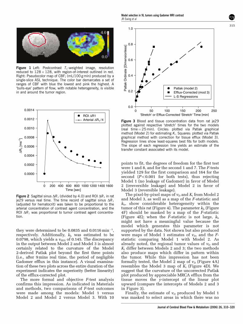
The pixel-by-pixel maps of vD and Ki from Model 2and Model 3, as well as a map of the F-statistic andkb, show considerable heterogeneity within thetumor of this rat (Figure 4). The parameter kb (Figure4F) should be masked by a map of the F-statistic(Figure 4E); when the F-statistic is not large, kb

might not have a meaningful value because themodel which generates this parameter is notsupported by the data. Not shown but also producedwere maps of Model 1 estimates of vD, and the F-statistic comparing Model 1 with Model 2. Asalready noted, the regional tumor values of vD andKi differ between Models 2 and 3; the two methodsalso produce maps which differ in pattern withinthe tumor. While this impression has not beenformally tested, the Model 2 map of vD (Figure 4A)resembles the Model 3 map of Ki (Figure 4D). Wesuggest that the curvature of the uncorrected Patlakplot produced by appreciable MRCA efflux from thetissue moves the y-intercept of the linear plotupward (compare the intercepts of Models 2 and 3in Figure 3).

Finally, the estimate of vD produced by Model 1was masked to select areas in which there was no

Figure 1 Left: Postcontrast T1-weighted image, resolutionreduced to 128�128, with region-of-interest outlined in red.Right: Pseudocolor map of CBF; (mL/100 g min) produced by asingle-slice ASL technique. The color bar demarcates a set ofranges of CBF with blue the lowest and pink the highest. A‘bulls-eye’ pattern of flow, with notable heterogeneity, is visiblein and around the tumor region.

Time [sec]0 200 400 600 800 1000 1200 1400 1600

0.0000

0.0002

0.0004

0.0006

0.0008

0.0010

0.0012

0.0014

ROI ∆R1Arterial ∆R1 / 4

∆R1

[ms-1

]

Figure 2 Sagittal sinus DR1 (divided by 4.0) and ROI DR1 in ratje29 versus real time. The time record of sagittal sinus DR1

(adjusted for hematocrit) was taken to be proportional to thearterial concentration of contrast agent concentration, and theROI DR1 was proportional to tumor contrast agent concentra-tion.

'Stretch' or Efflux-Corrected 'Stretch' Time [min]0 50 100 150 200 250

Pat

lak

Ord

inat

e [D

imen

sion

less

]

0.0

0.2

0.4

0.6

0.8

1.0

Patlak (model 2)Efflux-Corrected (mod 3)L-S Regressions

Figure 3 Blood and tissue concentration data from rat je29plotted against respective ‘stretch’ times for the two models(real time¼25 min). Circles: plotted via Patlak graphicalmethod (Model 2) for estimating Ki. Squares: plotted via Patlakgraphical method with correction for tissue efflux (Model 3).Regression lines show least-squares best fits for both models.The slope of each regression line yields an estimate of thetransfer constant associated with its model.


315


advantage of Model 2 over Model 1, which is to saythat these were areas within the ROI with little or noGadomer leakage and relatively normal microves-sels. The mean value of vD in these areas withnormal BBB function was 0.0312. Assuming hema-tocrit of 0.45, this yields a plasma volume of 0.014,which is approximately consistent with previouslyperformed estimates of cerebral plasma volumeusing radiotracers (Bereczki et al, 1992).

As for the group data, the F-test comparing Model2 to Model 1 exceeded 10 (Po0.025) in all animals,and Model 3 was always superior to Model 2 for thetumor ROI across the 15 animals. In accordance withthis, the mean vD of Gadomer in the group was foundto be approximately twofold larger with Model 2than Model 3, whereas the mean Ki of MRCA withModel 2 was approximately 30% of that with Model3 (Table 1). As expected, the application of theoriginal Patlak model to data from these experimentsyields an overestimation of vD and an underestima-tion of Ki. The Model 3 values for vD (approximately7%, Table 1), transfer constant, and extravascular,extracellular space (around 10%) characterize thistumor as vascular with a moderately leaky BBB(mean plasma flow approximately 11-fold greaterthan mean influx rate) and a fairly normal extra-cellular space. The latter space indicates that thetumor is mainly made up of viable, Gadomer-excluding cells and is not necrotic. As shown below,the microvascularity of the tumor might, however,be overestimated because vD was probably biasedhigh, the result of missing the initial part of thearterial input function.

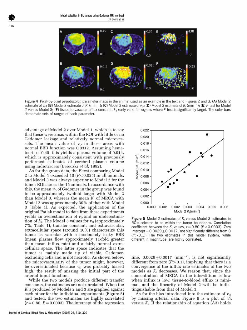
While the two models produce different transferconstants, the estimates are not unrelated. When theKi’s produced by Models 2 and 3 are graphed againsteach other for the individual experiments (Figure 5)and tested, the two estimates are highly correlated(r¼ 0.80, P¼ 0.0003). The intercept of the regression

line, 0.002970.0017 (min�1), is not significantlydifferent from zero (P40.1), implying that there is aconvergence of the influx rate estimates of the twomodels as Ki decreases. We reason that, since theconcentration of MRCA in the interstitium is lowwhen influx is low, tissue-to-blood efflux is mini-mal, and the linearity of Model 2 will be indis-tinguishable from that of Model 3.

As for the bias introduced into the estimate of vD

by missing arterial data, Figure 6 is a plot of VD0

versus Ki. If the relationship of equation (A3) holds

Figure 4 Pixel-by-pixel pseudocolor, parameter maps in the animal used as an example in the text and Figures 2 and 3. (A) Model 2estimate of vD; (B) Model 2 estimate of Ki (min�1); (C) Model 3 estimate of vD; (D) Model 3 estimate of Ki (min�1); (E) F-test for Model2 versus Model 3; (F) tissue-to-vascular efflux constant, kb (only valid for regions where F-test is significantly large). The color barsdemarcate sets of ranges of each parameter.

Model 2 Ki [min-1]0.000 0.001 0.002 0.003 0.004 0.005 0.006

Mod

el 3

Ki [

min

-1]

0.000

0.002

0.004

0.006

0.008

0.010

0.012

0.014

0.016

0.018

0.020

0.022

Figure 5 Model 2 estimates of Ki versus Model 3 estimates inROIs selected to be within the tumor boundaries. Correlationcoefficient between the Ki values, r¼0.80 (Po0.0003). Zerointercept¼0.002970.0017, not significantly different from 0(P40.1). The two estimates in this model system, whiledifferent in magnitude, are highly correlated.


316


(see appendix), then the slope of this line shouldestimate the quantity

Rt00 CpðtÞdt=Cpðt0Þ, and the

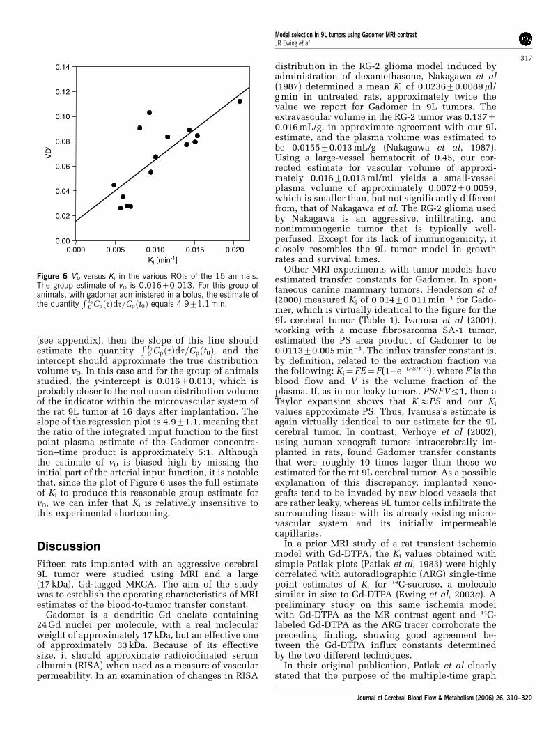
intercept should approximate the true distributionvolume vD. In this case and for the group of animalsstudied, the y-intercept is 0.01670.013, which isprobably closer to the real mean distribution volumeof the indicator within the microvascular system ofthe rat 9L tumor at 16 days after implantation. Theslope of the regression plot is 4.971.1, meaning thatthe ratio of the integrated input function to the firstpoint plasma estimate of the Gadomer concentra-tion–time product is approximately 5:1. Althoughthe estimate of vD is biased high by missing theinitial part of the arterial input function, it is notablethat, since the plot of Figure 6 uses the full estimateof Ki to produce this reasonable group estimate forvD, we can infer that Ki is relatively insensitive tothis experimental shortcoming.

Discussion

Fifteen rats implanted with an aggressive cerebral9L tumor were studied using MRI and a large(17 kDa), Gd-tagged MRCA. The aim of the studywas to establish the operating characteristics of MRIestimates of the blood-to-tumor transfer constant.

Gadomer is a dendritic Gd chelate containing24 Gd nuclei per molecule, with a real molecularweight of approximately 17 kDa, but an effective oneof approximately 33 kDa. Because of its effectivesize, it should approximate radioiodinated serumalbumin (RISA) when used as a measure of vascularpermeability. In an examination of changes in RISA

distribution in the RG-2 glioma model induced byadministration of dexamethasone, Nakagawa et al(1987) determined a mean Ki of 0.023670.0089 ml/g min in untreated rats, approximately twice thevalue we report for Gadomer in 9L tumors. Theextravascular volume in the RG-2 tumor was 0.13770.016 mL/g, in approximate agreement with our 9Lestimate, and the plasma volume was estimated tobe 0.015570.013 mL/g (Nakagawa et al, 1987).Using a large-vessel hematocrit of 0.45, our cor-rected estimate for vascular volume of approxi-mately 0.01670.013 ml/ml yields a small-vesselplasma volume of approximately 0.007270.0059,which is smaller than, but not significantly differentfrom, that of Nakagawa et al. The RG-2 glioma usedby Nakagawa is an aggressive, infiltrating, andnonimmunogenic tumor that is typically well-perfused. Except for its lack of immunogenicity, itclosely resembles the 9L tumor model in growthrates and survival times.

Other MRI experiments with tumor models haveestimated transfer constants for Gadomer. In spon-taneous canine mammary tumors, Henderson et al(2000) measured Ki of 0.01470.011 min�1 for Gado-mer, which is virtually identical to the figure for the9L cerebral tumor (Table 1). Ivanusa et al (2001),working with a mouse fibrosarcoma SA-1 tumor,estimated the PS area product of Gadomer to be0.011370.005 min�1. The influx transfer constant is,by definition, related to the extraction fraction viathe following: Ki¼FE¼F(1�e�(PS/FV)), where F is theblood flow and V is the volume fraction of theplasma. If, as in our leaky tumors, PS/FVr1, then aTaylor expansion shows that KiEPS and our Ki

values approximate PS. Thus, Ivanusa’s estimate isagain virtually identical to our estimate for the 9Lcerebral tumor. In contrast, Verhoye et al (2002),using human xenograft tumors intracerebrally im-planted in rats, found Gadomer transfer constantsthat were roughly 10 times larger than those weestimated for the rat 9L cerebral tumor. As a possibleexplanation of this discrepancy, implanted xeno-grafts tend to be invaded by new blood vessels thatare rather leaky, whereas 9L tumor cells infiltrate thesurrounding tissue with its already existing micro-vascular system and its initially impermeablecapillaries.

In a prior MRI study of a rat transient ischemiamodel with Gd-DTPA, the Ki values obtained withsimple Patlak plots (Patlak et al, 1983) were highlycorrelated with autoradiographic (ARG) single-timepoint estimates of Ki for 14C-sucrose, a moleculesimilar in size to Gd-DTPA (Ewing et al, 2003a). Apreliminary study on this same ischemia modelwith Gd-DTPA as the MR contrast agent and 14C-labeled Gd-DTPA as the ARG tracer corroborate thepreceding finding, showing good agreement be-tween the Gd-DTPA influx constants determinedby the two different techniques.

In their original publication, Patlak et al clearlystated that the purpose of the multiple-time graph

Ki [min-1]0.000 0.005 0.010 0.015 0.020

VD

'

0.00

0.02

0.04

0.06

0.08

0.10

0.12

0.14

Figure 6 VD0 versus Ki in the various ROIs of the 15 animals.

The group estimate of vD is 0.01670.013. For this group ofanimals, with gadomer administered in a bolus, the estimate ofthe quantity

Rt00 CpðtÞdt=Cpðt0Þ equals 4.971.1 min.


317


was to check the plotted data for linearity. Iflinearity was found for all or part of the curve, theninflux dominated the distribution process duringthat period, and the slope of the line was equal tothe influx constant. If not found, then this approachcannot be used. Such testing was performed (Ewinget al, 2003a), with no strong evidence of nonlinear-ity observed; Ki was subsequently evaluated fromthe line.

In the present tumor study, nonlinearity wasapparent across the typical time period of anexperiment, even when Gadomer—a much largerand presumably less permeable MRCA than Gd-DTPA—was employed. Accordingly, the generalizedPatlak graphical approach (Patlak and Blasberg,1985) was applied. If the variable kb in equations(2) and (4) is understood to equal Ki/ve, then thegeneralized Patlak approach and the consensusmodel are formally identical. This provides avaluable linkage between the Patlak graphicalapproach for MRI data and the consensus approach.In fact, the generalized Patlak, the original Patlak,and the hypothesis of no leakage at all form a set ofnested models, which we have labeled 3, 2, and 1,respectively, to indicate the number of parametersestimated in each. These series of models collec-tively form an extended methodology for MRIstudies of vascular permeability.

That the underlying models examine the linearityof the blood and tissue data is important, since itconsiderably simplifies the job of comparisonbetween them, both in statistical theory and in thevery necessary visual inspection of the plots. Anexamination of Figure 3, for instance, reveals thatthe data graphed under Model 2 are clearly non-linear after the first 3 points, whereas those plottedunder Model 3 form a straight line over the entireperiod of the experiment. To look at this in adifferent way, however, the first three points ofFigure 3 plotted via Model 2 form a decent straightline and define a short period of linearity, arevirtually identical to those of Model 3, and yieldsimilar values of Ki and vD.

Model 3 offers the best resolution of our data andthe best estimates of vD and Ki. In setting a thresholdfor the acceptance of an F-test, it was judged that aType I error (i.e., accepting evidence for nonlinearitywhen there was none) would not be a damagingerror. In the worst case, some additional error mightbe introduced to the estimates of vD and Ki. Thisoutcome was judged to be nonthreatening, and thelevel of acceptance of this type of error set to 5%,Bonferroni-corrected for multiple comparisons. Ourexperience with this criterion has generally beenpositive, with the outcomes matching visual exam-ination.

In our previous study of a transient ischemiamodel (Ewing et al, 2003a), the agreement of Model2 estimates of Ki with those of autoradiography didraise the question as to why MRI estimates of vD

were much higher than might be reasonably ex-

pected for the blood volume of a ischemia-injuredtissue, and in fact higher than an estimate producedby dynamic contrast studies conducted immediatelybefore the permeability studies. One possibility—that enhanced water exchange across a damagedBBB increased the effect of the MRCA—has beenruled out on theoretical grounds (Cao et al, 2005).Two other possibilities, which are not mutuallyexclusive, remain.

First, the artifact could be attributed to a sig-nificant nonlinearity in the Patlak plot introducedby tissue-to-vascular efflux. The efflux-correctedModel 3 estimates of vD were approximately halfthose found with uncorrected Model 2. The secondlikely source of artifact was our decision to use adifferent MRI sequence to follow the initial period ofindicator circulation and uptake, the missing dataproblem. Our subsequent analysis indicated that themissing blood data could be found in the y-interceptof the Patlak plot and that the estimate of vD from theplot should vary linearly with Ki. With the assump-tion that the arterial concentration–time coursevaried little from animal to animal, the amount ofmissing blood data and a better estimate of vD couldbe evaluated from the tissue-blood findings of theentire group of rats. In this case, this contributionreduced the estimate of vD from 6.7% to 1.6%.

Some consideration of our experimental design isin order. The sampling rate was approximately145 secs per point for the 25-min period. It wasslower than other recent experiments and is notpractical if these procedures are to be translated tohuman brain tumor studies. Moreover, we note frominspection that the first three points—approxi-mately 9 mins (Figure 3)—of most Patlak plots werecoincident for Models 2 and 3, thus defining aninterval in which it can be expected that MRCAefflux is negligible and Model 2 estimates of transferconstant can be used. In situations where influx iscomparable to that of the current work and MRI datacan be obtained at 1-min intervals, then the first 5 to10 min of data might be linear by Model 2 analysis,and the transfer numbers might be measurablewithout further modification. This is important torecognize when, for example, to compare multiple-time MRI estimates of microvascular permeability inbrain tumor models with those of single-time ARGmeasurements.

Sampling ‘as fast as possible’ might not be ideal,since this complicates the task of estimating thearterial input function, and raises the problem oftiming the arrival of indicator in the tissue. Wechose to sample slowly enough so that the change insagittal sinus indicator concentration could be takenas the arterial input function. The validity of thisapproach depends on several assumptions. First,most of the tissue draining into the saggital sinus isassumed to be normal and no MRCA is lost from theblood into brain en passage through such portions ofthe brain. Second, it is presupposed that thepresence of the tumor itself does not extract


318


sufficient MRCA from the blood to seriously affectthe shape of the venous concentration curve.Thirdly, the lag time between MRCA passagethrough the microvascular networks and sagittalsinus (3 to 6 secs) is assumed to not introduce asignificant uncertainty into the timing of theexperiment.

The second assumption is particularly important,since it interacts with the first-pass extraction of theMRCA. If there is a large first-pass extraction, it isnecessary to sample the tissue curve at highfrequency and determine the input function in anartery close to the tissue. This points to thedifficulties presented in the current clinical setting,where only small MRCAs (less than 1 kDa) areapproved for use in humans. In aggressive tumors,or any other lesion with highly permeable micro-vessels, quantifying vascular permeability viaMRCA uptake and clearance may become extremelydifficult because of the necessity for rapid andprecise estimates of MRCA concentration in botharterial blood and tissue. This suggests the need forclinically approved macromolecular MR contrastagents.

While the experimental design of permeabilitystudies in an aggressive cerebral tumor has beeninvestigated herein, the need for protocol flexibilityin other settings must be emphasized. Among thevarious neuropathological models, there is almostcertainly a broad range of microvascular permeabil-ities between and within lesions. This necessitatesthe selection and usage of an MRCA of appropriatesize, a duration of study, and analytical models thatfit the operating characteristics of the permeabilitymeasurement. To its advantage, the expanded orserial Patlak graphical approach offered in thepresent work linearizes an essentially nonlinearproblem, allows the visual examination of data forthe period of linearity, formally tests for alternativemodels, and even evaluates the systematic errorsdue to missing arterial data.

Acknowledgements

The authors wish to thank Schering AG for itsgift of Gadomer for use in the sample of animalsof this paper. We owe a great debt to CliffordPatlak for the many illuminating phone conversa-tions we had with him concerning the analysesherein.

References

Bates D, Watts D (1988 Nonlinear regression analysis andits application. New York: John Wiley and Sons

Bereczki D, Wei L, Acuff V, Gruber K, Tajima A, Patlak C,Fenstermacher J (1992) Technique-dependent varia-tions in cerebral microvessel blood volumes andhematocrits in the rat. J Appl Physiol 73:918–24

Bhujwalla ZM, Artemov D, Natarajan K, Solaiappan M,Kollars P, Kristjansen PEG (2003) Reduction of vascularand permeable regions in solid tumors detected bymacromolecular contrast magnetic resonance imagingafter treatment with antiangiogenic agent TNP-470.Clin Cancer Res 9:355–62

Brix G, Schad LR, Deimling M, Lorenz WJ (1990) Fast andprecise T1 imaging using a TOMROP sequence. MagnReson Imaging 8:351–6

Brown S, Ewing J, Kolozsvary A, Butt S, Cao Y, Kim J(1999) Magnetic resonance imaging of perfusion in ratcerebral 9L tumor after nicotinamide administration.Int J Radiat Oncol 43:627–33

Cao Y, Brown SL, Knight RA, Fenstermacher JD, Ewing JR(2005) Effect of intravascular-to-extravascular waterexchange on the determination of blood-to-tissuetransfer constant by magnetic resonance imaging. MagnResonance Med 53:282–93

Crawley AP, Henkelman MR (1988) A comparison of one-shot and recovery methods in T1 imaging. MagnResonance Med 7:23–4

Crone C (1963) The permeability of capillaries in variousorgans as determined by use of the ‘indicator diffusion’method. Acta Physiol Scand 58:292–305

Daldrup H, Shames DM, Wendland M, Okuhata Y, LinkTM, Rosenau W, Lu Y, Brasch RC (1998a) Correlation ofdynamic contrast-enhanced MR imaging with histolo-gic tumor grade: comparison of macromolecular andsmall-molecular contrast media. Am J Radiol 171:941–9

Daldrup HE, Shames DM, Husseini W, Wendland MF,Okuhata Y, Brasch RC (1998b) Quantification of theextraction fraction for gadopentate across breast cancercapillaries. Magn Resonance Med 40:537–43

Daldrup-Link H, Okuhata Y, Wolfe A, Srivastatav S, Ole S,Ferrara N, Cohen RL, Shames DM, Brasch RC (2004)Decrease in tumor apparent permeability-surface areaproduct to a MRI macromolecular contrast mediumfollowing angiogenesis inhibition with correlationsto cytotoxic drug accumulation. Microcirculation 11:387–96

Ewing JR, Knight RA, Nagaraja TN, Yee JS, Nagesh V,Whitton PA, Li L, Fenstermacher JD (2003a) Patlakplots of Gd-DTPA MRI data yield blood–brain transferconstants concordant with those of 14C-sucrose inareas of blood–brain barrier opening. Magn ResonanceMed 50:283–92

Ewing JR, Wei L, Knight RA, Pawa S, Nagaraja TN, BruscaT, Divine GW, Fenstermacher JD (2003b) A directcomparison of local cerebral blood flow rates measuredby MRI arterial spin-tagging and quantitative autora-diography in a rat model of experimental cerebralischemia (accepted for publication). J Cerebral BloodFlow Metab 23:198–209

Gelman N, Ewing J, Gorell J, Spickler E, Solomon E (2000)Interregional variation of longitudinal relaxation ratesin human brain at 3.0 T: relation to estimated iron andwater contents. Magn Resonance Med 45:71–9

Gjedde A (1997) Dark origins of the Patlak–Gjedde–Blasberg–Fenstermacher–Rutland–Rehling plot. NuclMed Commun 3:274–5

Henderson E, Sykes J, Drost D, Weinmann H-J, Rutt BK,Lee T-Y (2000) Simultaneous MRI measurement ofblood flow, blood volume, and capillary permeabilityin mammary tumors using two different contrastagents. J Magn Reson Imaging 12:991–1003

Ivanusa T, Beravs K, Cemazar M, Jevtic V, Demsar F, SersaG (2001) MRI macromolecular contrast agents as


319


indicators of changed tumor blood flow. Radiol Oncol35:139–47

Johnson JA, Wilson T (1966) A model for capillaryexchange. Am J Physiol 210:1299–303

Kim JH, Kim SH, Kolozsvary A, Brown SL, Kim OB,Freytag SO (1995) Selective enhancement of radiationresponse of herpes simplex virus thymidine kinasetransduced 9L gliosarcoma cells in vitro and in vivo byantiviral agents. Int J Radiat Oncol Biol Phys 33:861–8

Lassen NA, Perl W (1979) Tracer kinetic methods inmedical physiology. New York, NY: Raven Press

Look DC, Locker DR (1970) Time saving in measurementof NMR and EPR relaxation times. Rev Sci Instrum 41:250–1

Moulder JE, Rockwell S (1984) Hypoxic fractions of solidtumors: experimental techniques, methods of analysis,and a survey of existing data. Int J Radiat Oncol BiolPhys 10:695–712

Nakagawa H, Groothuis DR, Owens ES, Fenstermacher JD,Patlak CS, Blasberg RG (1987) Dexamethasone effectson [125-I]albumin distribution in experimental RG-2gliomas and adjacent brain. J Cerebral Blood FlowMetab 7:687–701

Patlak C, Blasberg R (1985) Graphical evaluation of bloodto brain transfer constants from multiple time up takedata. Generalizations. J Cerebral Blood Flow Metab 5:584–90

Patlak CS, Blasberg RG, Fenstermacher JD (1983) Graphi-cal evaluation of blood-to-brain transfer constants frommultiple-time uptake data. J Cerebral Blood Flow Metab3:1–7

Roberts H, Roberts T, Ley S, Dillon W, RC B (2002)Quantitative estimation of microvascular permeabilityin human brain tumors: correlation of dynamic Gd-DTPA-enhanced MR imaging with histopathologicgrading. Acad Radiol 9:51–5

Tofts PS, Brix G, Buckley DL, Evelhoch JL, Henderson E,Knopp MV, Larsson HB, Lee TY, Mayr NA, Parker GJ,Port RE, Taylor J, Weisskoff RM (1999) Estimatingkinetic parameters from dynamic contrast-enhancedT(1)-weighted MRI of a diffusable tracer: standardizedquantities and symbols. J Magn Reson Imaging 10:223–32

Turetschek K, Preda A, Novikov V, Brasch RC, WeinmannHJ, Wunderbaldinger P, Roberts TPL (2004) Tumormicrovascular changes in antiangiogenic treatment:assessment by magnetic resonance contrast media ofdifferent molecular weights. J Magn Reson Imaging 20:138–44

Verhoye M, van der Sanden BPJ, Rijken PFJW, PetersPWH, Van der Kogel AJ, Pee G, Vanhoutte G, HeerschapA, Van der Linden A (2002) Asssessment of the

neovascular permeability in glioma xenografts bydynamic T1 MRI with gadomer-17. Magn Reson Med 47:305–13

Wheeler KT, Wallen CA (1980) Is cell survival a determi-nant of the in situ response of 9L tumours? Br J Cancer41(Suppl IV):299–303

Appendix

The Effect of Missing Initial Arterial Data

Suppose that the data do follow the model ofequation (1):

CtðtÞ ¼ Ki

Zt

0

CpðtÞdtþ vDCpðtÞ

This is a reasonable assumption for early timepoints, well-supported by observation (see Figure3). Let us assume that, for some initial period trt0,neither tissue nor arterial data are measured, andthen the measurement is taken up after t0. Theobserved relationship between tissue concentrationand arterial concentration at t0 is

Ctðt0ÞCpðt0Þ

¼ Ki

R t00 CpðtÞdtCpðt0Þ

þ vD ðA1Þ

This, then, is the apparent zero intercept of thePatlak plot with missing initial data. After t0, webegin measuring, and the relationship between thetissue and arterial concentration becomes:

CtðtÞCpðtÞ

¼Ki

Rtt0

CpðtÞdtCpðtÞ

þ Ki

Rt00 CpðtÞdt

Cpðt0Þþ vD

( )ðA2Þ

Thus, the integral between 0 and t0 appears in the y-intercept, and vD is over estimated by the amountKi

R t00 CpðtÞdt=Cpðt0Þ. If this is true, the apparent

distribution volume VD0 should be related to the true

distribution volume via the following relationship:

V 0D ¼

Ki

Rt00 CpðtÞdtCpðt0Þ

þ vD ðA3Þ

and a plot of VD0 versus Ki in our sample of 15 studies

will display a relationship with a slope equal toRt00 CpðtÞdt=Cpðt0Þ, and a y-intercept of the true

distribution volume, vD.


320


Model selection in magnetic resonance imaging measurements of vascular permeability: Gadomer in a 9L...

Documents

Transcript of Model selection in magnetic resonance imaging measurements of vascular permeability: Gadomer in a 9L...