
Model documentation for the European Forest Information ...
119
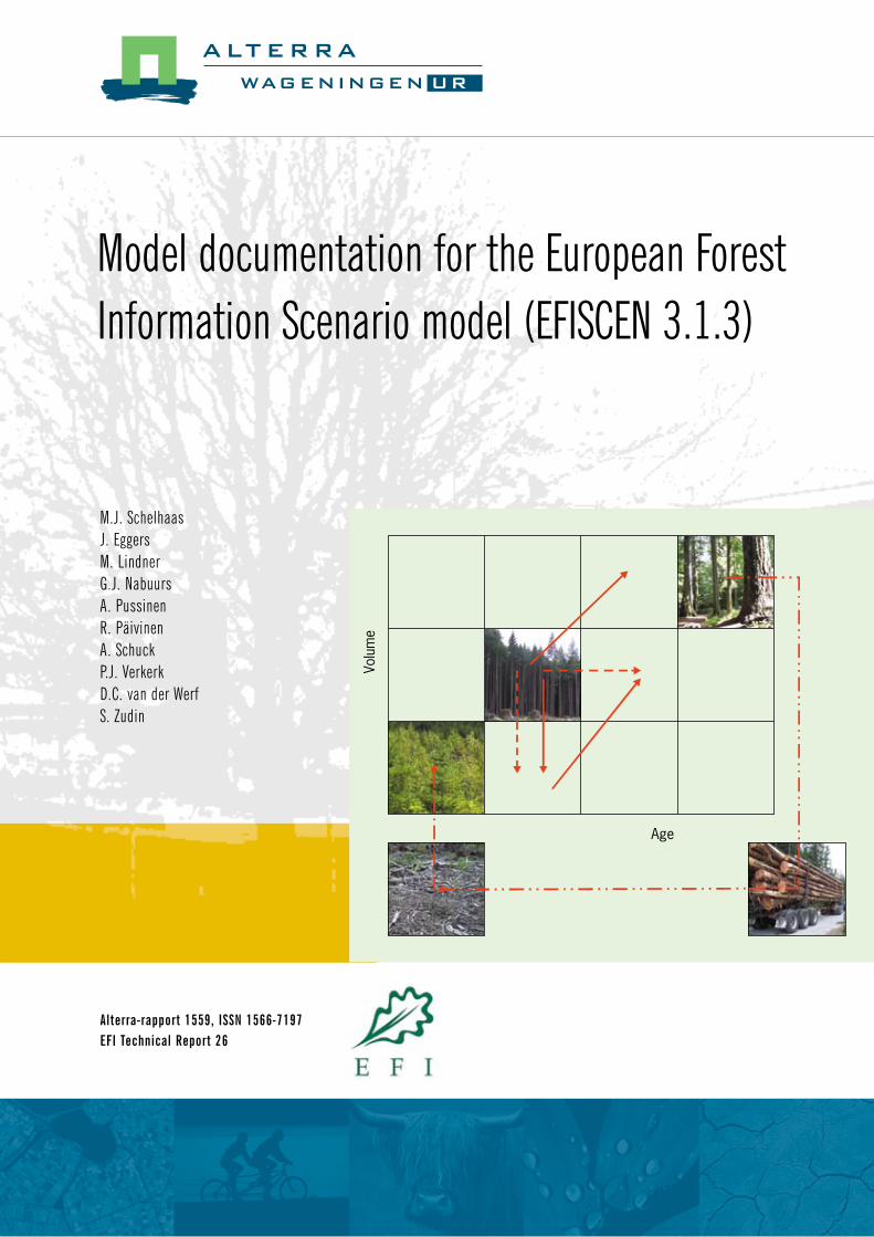
Age Volume M.J. Schelhaas J. Eggers M. Lindner G.J. Nabuurs A. Pussinen R. Päivinen A. Schuck P.J. Verkerk D.C. van der Werf S. Zudin Alterra-rapport 1559, ISSN 1566-7197 EFI Technical Report 26 Model documentation for the European Forest Information Scenario model (EFISCEN 3.1.3)
-
Upload
khangminh22 -
Category
Documents
-
view
1 -
download
0
Transcript of Model documentation for the European Forest Information ...
Age
Volume
M.J. SchelhaasJ. EggersM. LindnerG.J. NabuursA. PussinenR. PäivinenA. SchuckP.J. VerkerkD.C. van der WerfS. Zudin
Alterra-rapport 1559, ISSN 1566-7197EFI Technical Report 26
Model documentation for the European Forest Information Scenario model (EFISCEN 3.1.3)

Model documentation for the European Forest Information Scenario model (EFISCEN 3.1.3)

2 Alterra-rapport 1559

Model documentation for the European Forest Information Scenario model (EFISCEN 3.1.3) M.J. Schelhaas J. Eggers M. Lindner G.J. Nabuurs A. Pussinen R. Päivinen A. Schuck P.J. Verkerk D.C. van der Werf S. Zudin
Alterra-rapport 1559 EFI Technical Report 26 Alterra, Wageningen, 2007
4 Alterra-rapport 1559
ABSTRACT Schelhaas, M.J. J. Eggers, M. Lindner, G.J. Nabuurs, A. Pussinen, R. Päivinen, A. Schuck, P.J. Verkerk, D.C. van der Werf & S. Zudin, 2007. Model documentation for the European Forest Information Scenario model (EFISCEN 3.1.3). Wageningen, Alterra, Alterra-rapport 1559/EFI Technical Report 26, Joensuu, Finland. 118 blz.; 30 figs.; 8 tables.; 19 refs. EFISCEN is a forest resource projection model, used to gain insight into the future developmentof European forests. It has been used widely to study issues such as sustainable managementregimes, wood production possibilities, nature oriented management, climate change impacts,natural disturbances and carbon balance issues. This report describes the history of EFISCEN andthe current state of the model, version 3.1.3. It contains a user guide as well as a description of pastvalidations and an uncertainty analysis. Keywords: EFISCEN, forest scenario model, matrix model, European forests, wood production ISSN 1566-7197 This report is available in digital format at www.alterra.wur.nl. A printed version of the report, like all other Alterra publications, is available from Cereales Publishersin Wageningen (tel: +31 (0) 317 466666). For information about, conditions, prices and the quickest way of ordering see www.boomblad.nl/rapportenservice Also be published as EFI Technical Report 26
© 2007 Alterra P.O. Box 47; 6700 AA Wageningen; The Netherlands
Phone: + 31 317 474700; fax: +31 317 419000; e-mail: [email protected] No part of this publication may be reproduced or published in any form or by any means, or storedin a database or retrieval system without the written permission of Alterra. Alterra assumes no liability for any losses resulting from the use of the research results orrecommendations in this report. [Alterra-rapport 1559/September/2007]
Contents
Summary 7
1 Introduction 11 2 General description 13
2.1 Perspective 13 2.2 History of EFISCEN 14
3 Theoretical program description 25 3.1 Matrix initialization 25 3.2 Increment 28 3.3 Management activities 30
3.3.1 Thinning 30 3.3.2 Final felling 31
3.4 Regeneration 31 3.5 Natural mortality and standing dead wood 32 3.6 Afforestation and deforestation 32 3.7 Change of increment due to changed environment 32 3.8 Biomass and litter production 33 3.9 Soil 33
4 Technical program description 39 4.1 Introduction 39 4.2 Matrix initialisation (P-efsos) 39
4.2.1 Introduction 39 4.2.2 Files and directories 39 4.2.3 User guide 40
4.2.3.1 Getting started 40 4.2.3.2 Program inputs 41 4.2.3.3 Program execution 46
4.3 Main simulation Program (EFISCEN3.1.3) 48 4.3.1 Introduction 48 4.3.2 Files and directories 50 4.3.3 Technical implementation 51 4.3.4 User guide 52
4.3.4.1 Getting started 52 4.3.4.2 Program inputs 52 4.3.4.3 Program outputs 69 4.3.4.4 Program execution 74 4.3.4.5 Additional programs 76
5 Validation of EFISCEN 77 6 Sensitivity analysis 83
6.1 Introduction 83 6.2 Method 83

6 Alterra-rapport 1559
6.3 Design 85 6.4 Results 86 6.5 Discussion 93
7 Discussion 97
References 99 Annex A Utopia 101 Annex B Tests for EFISCEN 3.1.3 109 Annex C Recommended parameter values 118
Alterra-rapport 1559 7
Summary
Acronym and Name of the model EFISCEN (European Forest Information Scenario model) Organisation(s) involved in the development of the model EFISCEN has been jointly developed and applied at Alterra (part of Wageningen UR) and the European Forest Institute (EFI). It can be distributed to interested users on request. Contact persons - Gert-Jan Nabuurs, Alterra ([email protected]) - Marcus Lindner, European Forest Institute ([email protected]) - General email address: [email protected] General focus of the model EFISCEN is a forest resource projection model. It is used to gain insight into the future development of European forests for issues such as:
• sustainable management regimes; • wood production possibilities; • nature oriented management; • climate change impacts • natural disturbances; and • carbon balance issues.
Through its underlying detailed forest inventory database, the projections provide these insights at varying scales, thus serving forest managers and policy makers at the national and international levels. History and development stage of the model The core of the EFISCEN model was developed in the late 1980s for Sweden by Prof. Ola Sallnäs at the Swedish Agricultural University. The first European application of this model was carried out by the International Institute for Applied Systems Analysis (IIASA) in the early 1990s. With help from the original developers, the model was transferred to EFI in 1996, and given the name EFISCEN (version 1.0). At the same time, the underlying EFISCEN inventory database was updated and further expanded with the help of many country correspondents and inventory experts. Over the following years the model was developed further both by EFI and Alterra, including modules that allowed (i) growth changes due to climate change to be taken into account, (ii) calculation of carbon budgets of both biomass and soil and (iii) natural mortality. A separate version of EFISCEN features a module dealing with natural disturbances. In the early 2000s, work started at EFI to reprogram EFISCEN
8 Alterra-rapport 1559
in C++ (EFISCEN 3.x). The currently used version is 3.1.3. In August 2007 this version received the quality A status according to Alterra’s internal quality system. Concepts, modeling formalism EFISCEN is an area-based matrix model. For each forest type that is distinguished in the input data (according to species, region, site class and owner), a separate matrix is set up. One matrix consists of 60 age classes of 5-year width and 10 volume classes with widths that vary depending on the forest under study. Aging of the forest is simulated by moving area to a higher age class, while growth is simulated by moving the area to a higher volume class. Transition chances are derived from increment figures from the input data, or from growth and yield tables. These transitions can be changed over time to simulate changes in growing conditions, like climate change.
Thinning in the model is simulated by moving area one volume class down. The user can specify an age range where thinnings can be carried out. If a thinning will be carried out or not depends on the actual demand for thinnings. A user-defined fraction of the area that has been subjected to a thinning will be moved up one volume class extra to simulate the growth response after a thinning.
Final fellings are simulated by taking the area out of a certain cell of the matrix. Final felling chances can be set by the user as a function of age and volume class. The fraction that is actually harvested depends on the actual demand for wood from final fellings.
Area that is taken out of the matrix is put in a separate class, the non-stocked area. Regeneration is simulated as the movement from the non-stocked area into the lowest age and volume class of the matrix.
Natural mortality is simulated by moving a fraction of the area in a certain cell one volume class down. This fraction can be set by the user as a percentage of the growing stock, varying by age class. The actual fraction of the area that is moved down will then depend on the average volume before, and the difference between the volume classes. Only area that has not recently been thinned can be subjected to natural mortality. Architecture and modules of the model The EFISCEN model consists of two separate programs: The P-efsos program that initializes the matrices based on the input data and the main EFISCEN executable that performs the simulations. Within the EFISCEN model we can distinguish 1) the matrix simulator, 2) a carbon module to convert outputs to carbon stocks and 3) a soil module based on the YASSO soil model (Liski et al. 2005). Building the model
• Model input and parameters The forest area under study is usually separated into forest types, depending on the level of detail of inventory data, differences between types and resulting areas. In EFISCEN, forest types can be separated based on administrative unit, ownership,
Alterra-rapport 1559 9
tree species and site class. As input for the matrix set-up, EFISCEN needs the area and average volume per age class of each forest type. Further information on the current annual increment per age class is needed, either from inventory data or yield tables. If the user applies gross increment, data about natural mortality per age class is required. Furthermore, information needs to be available on the thinning and final felling regime. Input data on area, growing stock volumes and increment are usually derived from national forest inventories. All information and data included in the EFISCEN inventory database are freely available via the EFI website (www.efi.int). EFISCEN has been parameterized and applied to most European countries, and to some Russian regions. EFISCEN is also capable of converting wood volume into estimates of carbon in total tree biomass. For this conversion, the user needs to supply the model with biomass expansion factors. Additionally, the model can simulate carbon dynamics in the soil via the soil model YASSO. This requires data on turnover rates of different biomass components, data on quality of the litter, and some basic climate parameters for the region under study. • Testing and verification EFISCEN functionality has been tested carefully throughout its development. For these tests a simple sample country is available, called Utopia. This test country is also valuable for people who want to get accustomed to the model. • Validation and sensitivity analysis EFISCEN has been validated by comparing its growth functions against growth functions of other models, by comparing projections against projections of other models, and by running the model on historic data. A sensitivity analysis has been carried out. • Output Basic outputs of the model are developments of area, growing stock, increment, standing dead wood, harvest level and age class distribution over time. These are provided on different aggregation levels (per species, regions, total). Furthermore, the model can provide information on carbon stocks in biomass and soil if the corresponding modules were parameterized. Strengths and limitations of the model EFISCEN is designed for large forest areas, such as provinces or countries. Application to smaller areas is possible, but there have been no studies yet to determine the minimum size and effects of scale on uncertainty of the projections. Generally, several thousand hectares could be regarded as a safe minimum. EFISCEN has been developed for evenaged, managed forests. Deviations from this situation (e.g. unevenaged forests, unmanaged forests and shelterwood systems) make the application of EFISCEN less suitable. Furthermore, the model is currently not suited to simulate fast growing tree species with very short rotations, due to the

10 Alterra-rapport 1559
5-year time step. However, there have been some promising tests with a 1-year time step. The model can handle small decreases in forest area, but is not suited to deal with large-scale deforestation issues. As with all models, uncertainties in EFISCEN depend largely on the quality of the input data. Especially a correct estimation of the increment functions is important for the model outcomes. Initial uncertainties propagate through the model with every simulated time step, and thus the overall uncertainty increases. For 10–12 time steps (50–60 years) the model is believed to give reasonable projections. With increasing projection length, observed patterns become more important than absolute values.

Alterra-rapport 1559 11
1 Introduction
European forest resource projections have been an important task of the European Forest Institute (EFI). Since 1996 such projections have been carried out with the European Forest Information Scenario model, EFISCEN. Over the years the model has been expanded and improved, both at Alterra and at EFI. In 2001, a manual for EFISCEN 2.0 has been published (Pussinen et al., 2001), describing the state of the model as it was then. In the meanwhile, new versions have been developed and insights in the model have improved. The largest change has been the re-programming of the core model into C++ code and the addition of a user-interface. This new version of the model (EFISCEN 3.0 and higher) has been used in several projects already, but up to now a description of the model and a manual were lacking. The first aim of this report is to fill this gap. Simulation models are frequently used in science and as a tool for policy makers. However, in many cases it is not totally clear what the model assumptions are, and how uncertain the outcomes are. Without such information, model outcomes can easily be mis-interpreted or misused. One agency that frequently uses outcomes of simulation models is the Dutch Environment and Nature Planning Agency (Milieu- en Natuur Planbureau, MNP). To have a clear understanding of the models that are being used, and to guarantee the soundness of these models, a list of quality requirements have been set up. The second aim of this report is to fulfill these requirements. In August 2007 EFISCEN 3.1.3 received the quality A status according to these requirements. Chapter 2 gives a brief introduction into the model and describes the history of the model, its development over time and the different versions that exist and have existed. Further, it tries to list all historic applications of the model. Chapter 3 describes the outline and the theory of the model. The model implementation is described in Chapter 4. This chapter also explains how to use EFISCEN 3.1.3. Chapter 5 describes all validation exercises that have been done with different versions of EFISCEN, and synthesizes the results. Chapter 6 describes a sensitivity analysis for EFISCEN 3.1.2. This sensitivity analysis was part of the requirements for the MNP. In Chapter 7 we synthesize the results of all tests, validations and other exercises. We try to indicate in which situations or in which range EFISCEN is most reliable and where outcomes will become uncertain. Annex A contains a description of the country Utopia, which is used frequently for testing and teaching purposes. Annex B lists a series of tests to which EFISCEN has been subjected. Although this list is not meant to be exhaustive, it gives the user a somewhat deeper insight into the model. Furthermore, it can be used as a reference for future developers. Annex C gives an overview of recommended parameters.

Alterra-rapport 1559 13
2 General description
2.1 Perspective
EFISCEN is a model that simulates the development of forest resources at scales from provincial to European level. It is a timber assessment model, which means that the user specifies a certain harvest level and the model checks if it is possible to harvest that amount and simulates the forest development under that harvest level. EFISCEN is mostly used as a tool to evaluate and compare different scenarios. Scenarios can be defined in terms of changes in forest area, increment level, management regime and expected wood demand. Output consists of various characteristics or indicators of the forest resource. Examples are tree species distribution, felling/increment ratio, age class distribution, growing stock level and carbon sequestered in biomass and soil. The forest area under study is divided into forest types. Forest types are defined by region, owner class, site class and/or tree species. The number of forest types can differ per country. The detail level of the input data usually determines how many types can be distinguished. The input data are usually derived from national forest inventories. The following data are required for each forest type and age class:
• Area (ha)
• Average standing volume over bark (m3 per ha)
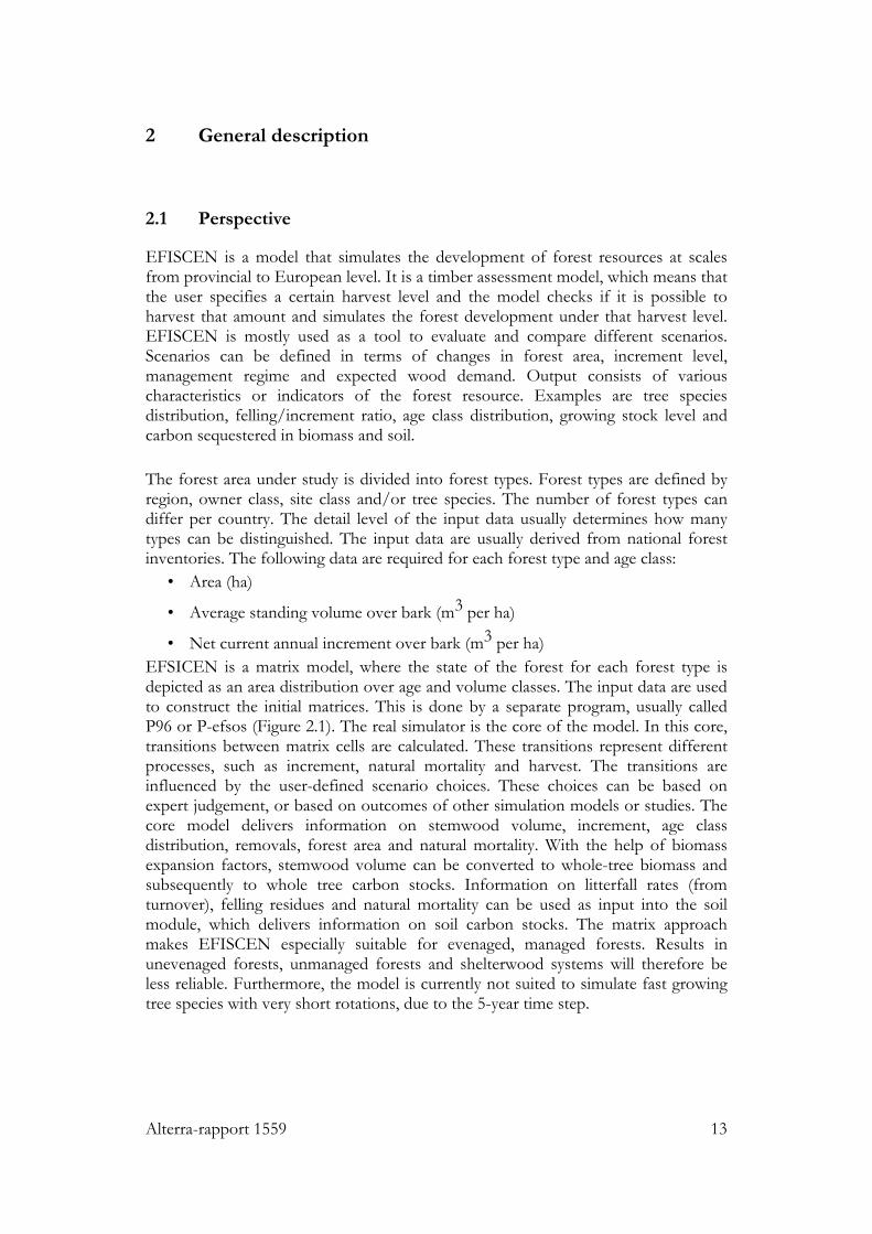
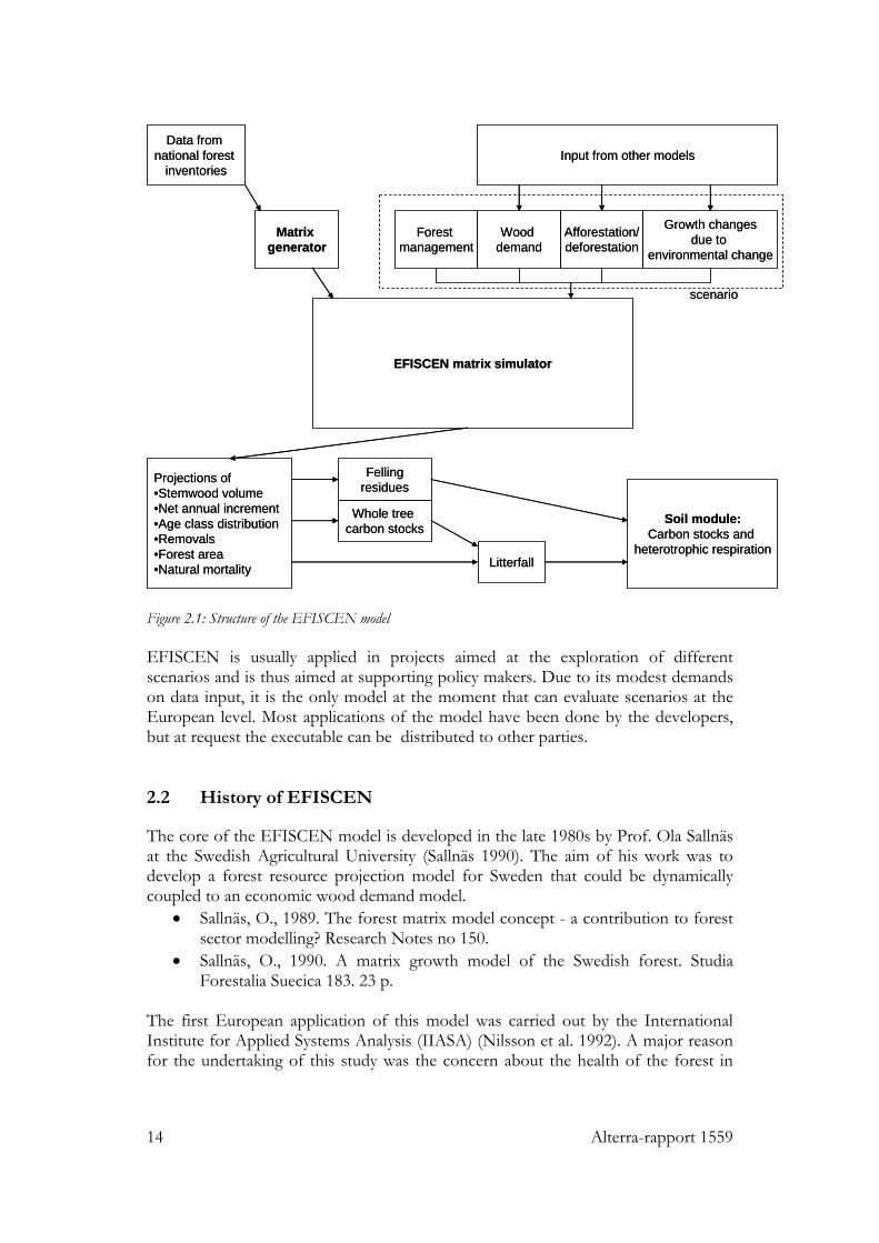
• Net current annual increment over bark (m3 per ha) EFSICEN is a matrix model, where the state of the forest for each forest type is depicted as an area distribution over age and volume classes. The input data are used to construct the initial matrices. This is done by a separate program, usually called P96 or P-efsos (Figure 2.1). The real simulator is the core of the model. In this core, transitions between matrix cells are calculated. These transitions represent different processes, such as increment, natural mortality and harvest. The transitions are influenced by the user-defined scenario choices. These choices can be based on expert judgement, or based on outcomes of other simulation models or studies. The core model delivers information on stemwood volume, increment, age class distribution, removals, forest area and natural mortality. With the help of biomass expansion factors, stemwood volume can be converted to whole-tree biomass and subsequently to whole tree carbon stocks. Information on litterfall rates (from turnover), felling residues and natural mortality can be used as input into the soil module, which delivers information on soil carbon stocks. The matrix approach makes EFISCEN especially suitable for evenaged, managed forests. Results in unevenaged forests, unmanaged forests and shelterwood systems will therefore be less reliable. Furthermore, the model is currently not suited to simulate fast growing tree species with very short rotations, due to the 5-year time step.
14 Alterra-rapport 1559
EFISCEN matrix simulator
Matrix generator
Data fromnational forest
inventories
Forestmanagement
Wooddemand
Afforestation/deforestation
Growth changesdue to
environmental change
Input from other models
Whole tree carbon stocks
Soil module:Carbon stocks and
heterotrophic respiration
Projections of•Stemwood volume•Net annual increment•Age class distribution•Removals•Forest area•Natural mortality
scenario
Fellingresidues
Litterfall
Figure 2.1: Structure of the EFISCEN model EFISCEN is usually applied in projects aimed at the exploration of different scenarios and is thus aimed at supporting policy makers. Due to its modest demands on data input, it is the only model at the moment that can evaluate scenarios at the European level. Most applications of the model have been done by the developers, but at request the executable can be distributed to other parties. 2.2 History of EFISCEN
The core of the EFISCEN model is developed in the late 1980s by Prof. Ola Sallnäs at the Swedish Agricultural University (Sallnäs 1990). The aim of his work was to develop a forest resource projection model for Sweden that could be dynamically coupled to an economic wood demand model.
• Sallnäs, O., 1989. The forest matrix model concept - a contribution to forest sector modelling? Research Notes no 150.
• Sallnäs, O., 1990. A matrix growth model of the Swedish forest. Studia Forestalia Suecica 183. 23 p.
The first European application of this model was carried out by the International Institute for Applied Systems Analysis (IIASA) (Nilsson et al. 1992). A major reason for the undertaking of this study was the concern about the health of the forest in
Alterra-rapport 1559 15
the light of acidification and expected large-scale dieback. The model was therefore extended by incorporating four health classes, with associated lower growth rates and management regimes. For this study, for the first time forest inventory data from all European countries were collected.
• Attebring, Nilsson and Sallnäs 1989. A model for long-term forecasting of timber yield - a description with special reference to the forest study at SUA-IIASA. Systems Analysis Modelling Simulation 6 (3): 171-180.
• Nilsson, S., Sallnäs, O. & Duinker, P. 1992. Future forest resources of Western and Eastern Europe. International Institute for Applied Systems Analysis. The Parthenon Publishing Group, UK. 496 p.
In the early years of the European Forest Institute, the need for a harmonised forest resource scenario tool at the European scale was acknowledged. After screening of available models, their data needs and availability of data, the Sallnäs/IIASA model was selected as the best candidate (Nabuurs and Päivinen, 1996). This choice was based on the modest data demands of the model, and the fact that there was already an underlying European wide database. With the permission and help from the original developers, the model was transferred to EFI in 1996. The original model was coded in Fortran77 and resided at a VAX terminal. The code was translated into a more modern Fortran version and the model became a PC based version. No changes were made to the functioning of the model. Furthermore the model was given the name EFISCEN. Although no naming convention had been adopted then, we can further refer to this version as EFISCEN 1.0. In 1996, all European countries were asked to submit more recent inventory data if available. This resulted in an update for many countries. The resulting database is available via the EFI website (Schelhaas et al. 1999).
• Nabuurs, G.J., R. Päivinen, 1996. Large Scale Forestry Scenario Models - a Compilation and Review. Working Paper 10. European Forest Institute, Joensuu, Finland. 174 p.
• Sallnäs, O., 1996. The IIASA-model for analysis of harvest potentials. EFI proceedings 5. Seminar and summerschool on 'Large scale forestry scenario models' held in Joensuu, Finland. 15-22 June 1995. European Forest Institute pp 19-30.
• Nabuurs, G.J., Päivinen, R., Sallnäs, O., Kupka, I., 1997. A large scale forestry scenario model as a planning tool for European forests. In: Moiseev, N.A., K. von Gadow and M. Krott. (eds.), Planning and decision making for forest management in the market economy. IUFRO conference, Pushkino, Moscow. 25-29 September 1996. Cuvillier Verlag, Goettingen. p. 89-102.
• Schelhaas, M.J., Varis, S., Schuck, A. and Nabuurs, G.J., 1999. EFISCEN's European Forest Resource Database, European Forest Institute, Joensuu, Finland. http://www.efi.fi/projects/eefr/.
Part of the received data concerned unevenaged forest, and did not match the data required by EFISCEN. Therefore, another model was selected for use in unevenaged forests (developed by B. Guo, Universite Laval, Quebec, Canada). This model is based on transitions between diameter classes. A case study with this model for Spain
16 Alterra-rapport 1559
can be found in Schelhaas (1997). Uncertainties in this model were very high, and the model has been applied only sporadically. The model is currently not in use anymore.
• Schelhaas, M.J., 1997. A forest resource projection for the Spanish forest inventory: report of a practical period at the IBN-DLO Institute. Wageningen Agricultural University, Department of Forestry. 77 p.
At the same time of the collection of the European inventory data, a project was initiated to apply the EFISCEN 1.0 model to the Leningrad region. This resulted in the following publications:
• Nabuurs, G.J., Lioubimov, A.V., 2000. Future development of the Leningrad region forests under nature-oriented forest management. Forest Ecology and Management 130, 235-251.
• Päivinen, R., Nabuurs, G.J. , Lioubimov, A.V. and Kuusela, K., 1999. The State, Utilisation and Possible Future Developments of Leningrad Region Forests. Working paper 18, European Forest Institute, Joensuu, Finland. 58 p.
• Lioubimow, A.V., Kudriashov, G.J. Nabuurs, R. Päivinen, S. Tetioukhine, and K. Kuusela. 1998. Leningrad region forests, past and future development. St. Petersburg Forest Technical Academy, St Petersburg in cooperation with Forest Committee of Leningrad Region and European Forest Institute. Joensuu, Finland. (In Russian)
In Autumn 1998, the EFISCEN 1.0 model was applied to the historic forest inventories of Finland to validate the model. Furthermore, the 1.0 version was applied to Norway, Finland and Sweden to evaluate different nature orientated scenarios (Verkaik and Nabuurs 2000).
• Nabuurs, G.J., Schelhaas, M.J., Pussinen, A., 2000. Validation of the European forest information scenario model (EFISCEN) and a projection of Finnish forests. Silva Fennica 34, 167-179.
• Verkaik, E., Nabuurs, G.J., 2000. Wood Production Potentials of Fenno-Scandinavian Forests Under Nature-Orientated Management. Scandinavian Journal for Forest research 15, 445-454.
During the LTEEF-II project (Long-term Regional Effects Climate Change on European Forests: Impact Assessment and Consequences for Carbon Budgets, January 1998 - July 2000), several changes were made to the EFISCEN model:
- The decline module as used in the IIASA study was taken out of the model code.
- The width of the age classes during simulations was set equal to the time step of the model (5 years). Before, the transition probabilities over the age classes were linked to width of the age classes in the inventory data. The transition probability in case of 20-year age classes was thus 25%. This led to a small portion of the area that changed age class every time step, thus leading to a very fast aging of some forest area, while some other area never grew older. In the new system, the input data is divided over 5-year age classes, assuming
Alterra-rapport 1559 17
an equal share in area and growing stock for each age class, and a probability of 1 to go to the next age class.
- The possibility to change the tree species after final harvest was introduced. Before, all harvested area was assumed to be afforested with the same species.
- The way thinnings are handled in the model was changed. In many simulations it was noted that a large part of the area in the matrix tended to stay in the low volume classes due to frequent thinnings. Since growth is relative to the growing stock, increment tended to decline after some decades of simulation. On the other hand, not thinning a forest resulted in rather high increments, because growing stocks increased. To change this counter-intuitive behaviour of the model, the growth boost after thinning was introduced. Moreover, the definition of the thinning regime was changed. Before, only a certain (user-defined) fraction of the increment in a certain age class could be thinned. This was changed in such a way that all area could be moved one volume class down, provided the that increment was possible in that cell. However, in all documentation concerning this version, it was stated that the thinning regime was defined by the age and volume classes where thinnings in principle could be carried out, but then only on all area that was moving to the next volume class.
- Complementary to the thinning boost in thinned stands, transition chances (and thus increment) in high volume classes were changed as well. Previously, absolute increments increased with increasing volume class, although the relative increment decreased (due to the Beta parameter). In the new version, increment increases only for the lower volume classes. The absolute increment for the higher volume classes (above the average volume as given in the input data) is constant.
- An option was built in to be able to change the transition chances over time, for example due to climate change.
- A biomass carbon module was added to estimate carbon stored in whole tree biomass with help of biomass expansion factors.
- A products module was developed to track carbon stored in wood products (Eggers 2002).
- A soil module (the YASSO soil model) was added to calculate carbon stocks in forest soils.
After these changes, we will further refer to this version as EFISCEN 2.0. A manual for this version of the model is available (Pussinen et al. 2001). Some of the changes are also described in Nabuurs et al. (2000). It is important to note that the biomass carbon module, the products module and the soil module are optional features that further process the output data as generated by the core of EFISCEN. Not including them does not change the functioning of the core model. It is also not obligatory to use the growth change module. Not all studies where EFISCEN 2.0 was applied did use (all of) these modules. For the LTEEF-II project, EFISCEN 2.0 was applied on a European scale. Input data were the same as those gathered in 1996. Projected growth changes due to
18 Alterra-rapport 1559
climate change and biomass expansion factors were derived from process-based models. The following EFISCEN-related publications are connected to the LTEEF-II project:
• Pussinen, A., Schelhaas, M.J., Verkaik, E., Heikkinen, E., Paivinen, R., Nabuurs, G.J., 2001. Manual for the European Forest Information Scenario Model (EFISCEN); version 2.0. EFI Internal report 5. European Forest Institute.
• Nabuurs, G.J., Pussinen, A., Liski, J., Karjalainen, T., 2001. Forest inventory-based approach. In: Kramer, K., Mohren, G.M.J. (Eds.), Long-term effects of climate change on carbon budgets of forests in Europe. Alterra report 194. Alterra, Wageningen.
• Nabuurs, G.J., A. Pussinen, J. Liski & T. Karjalainen, 2001. Upscaling based on forest inventory data and EFISCEN. In: G.M.J. Mohren, K.Kramer (Ed.), Long term effects of climate change on carbon budgets of forests in Europe. Alterra report. 194, Wageningen, pp. 220-234.
• Nabuurs, G.J., Pussinen, A., Karjalainen, T., Erhard, M., Kramer, K., 2002. Stemwood volume increment changes in European forests due to climate change-a simulation study with the EFISCEN model. Global Change Biology 8, 304-316.
• Eggers, T. 2002. The Impacts of Manufacturing and Utilisation of Wood Products on the European Carbon Budget. Internal Report 9, European Forest Institute, Joensuu, Finland. 90 p.
• Karjalainen, T., Pussinen, A., Liski, J., Nabuurs, G.-J., Eggers, T., Lapvetelainen, T., Kaipainen, T., 2003. Scenario analysis of the impacts of forest management and climate change on the European forest sector carbon budget. Forest Policy and Economics 5, 141-155.
• Karjalainen, T., Pussinen, A., Liski, J., Nabuurs, G.-J., Erhard, M., Eggers, T., Sonntag, M., Mohren, G.M.J., 2002. An approach towards an estimate of the impact of forest management and climate change on the European forest sector carbon budget: Germany as a case study. Forest Ecology and Management 162, 87-103.
• Nabuurs, G.-J. and A. Moiseyev 1999. Consequences of accelerated growth for the forests and forest sector in Germany. In: T. Karjalainen, H. Spiecker and O. Laroussinie (Eds.). Causes and Consequences of Accelerating Tree Growth in Europe. EFI Proceedings 27. European Forest Institute, pp. 197-206.
During 1999, EFISCEN 2.0 was expanded with a module to simulate natural disturbances and natural mortality (Schelhaas et al. 2002), hereafter termed EFISCEN 2.1. Because of the stochastic nature of natural disturbances, Monte Carlo simulation was used in this version. Moreover, a complete coupling with the soil module was not made, due to difficulties with the influence of fire on soil carbon. Later on, the natural disturbances were excluded from the code of version 2.1, essentially giving a version 2.0 with natural mortality. This version will hereafter be called version 2.2. Using version 2.2 with natural mortality set at zero will therefore yield identical results as version 2.0. Furthermore, it is important to note that using
Alterra-rapport 1559 19
natural mortality implies that the increment used in the input must be gross increment, whereas simulations without natural mortality implies net increment as input. Since natural mortality in managed European forests will generally be low, the difference between gross and net increment were assumed to be neglible. Therefore, the same increment functions were used in applications both with and without natural mortality. EFISCEN 2.1 has later on been applied to Germany (Dolstra, 2002) and France (Meyer, 2005).
• Schelhaas, M.J., Nabuurs, G.J., Sonntag, M., Pussinen, A., 2002. Adding natural disturbances to a large-scale forest scenario model and a case study for Switzerland. Forest Ecology and Management 167, 13-26.
• Dolstra, F., 2002. Simulating growth and development of the German forest: a large-scale scenario study incorporating the impact of natural disturbances and climate change. Afstudeerverslag Wageningen University, Environmental Sciences. 29 p.
• Meyer, J., 2005. Fire effects on forest resource development in the French Mediterranean region – projections with a large-scale forest scenario model. Technical Report 16. European Forest Institute. 86 p.
Parallel to the LTEEF-II project, several studies have been conducted at EFI/Alterra (formerly IBN-DLO) with different versions of the model, many of them in connection with the PhD thesis of Nabuurs (2001), and culminating in the EFI Research Report No 15 (Nabuurs et al. 2003). In the third paper of the thesis (Nabuurs et al. 2001), version 2.0 was used, while the fourth paper (Nabuurs et al. 2002) version 2.2 was used. In this fourth paper, for the first time all countries were simulated simultaneously, with wood demand per country dynamically depending on the forest resource and trade with and demand of other countries. This was done through a separate application that called the executable of EFISCEN 2.2. Although some technical adjustments were made to the source code to make this possible, the model itself did not essentially change. Preparatory work for this paper has been done by De Goede (2000). The runs in the EFI Research Report 15 are done with version 2.2.
• Nabuurs, G.J., 2001. European forests in the 21st century: impacts of nature-oriented forest management assessed with a large scale scenario model. PhD Thesis University of Joensuu. European Forest Institute and Alterra, Joensuu and Wageningen., pp. 130.
• Nabuurs, G.J., Paivinen, R., Schanz, H., 2001. Sustainable management regimes for Europe's forests – a projection with EFISCEN until 2050. Forest Policy and Economics 3, 155-173.
• Nabuurs, G.J., Paivinen, R., Schelhaas, M.J., Pussinen, A., Verkaik, E., Lioubimov, A., Mohren, G.M.J., 2001. Nature-Oriented Forest Management in Europe: Modeling the Long-Term Effects. Journal of Forestry 99, 28-33.
• De Goede, D. 2000. Between fear and hope. A scenario study into the long term international consequences of a changing forest management in western and central European countries. MSc thesis Wageningen University, AV2000-32.
20 Alterra-rapport 1559
• Nabuurs, G.J., de Goede, D., Michie, B., Schelhaas, M.J., Wesseling, J.G., 2002. Long term international impacts of nature oriented forest management on European forests - an assessment with the EFISCEN model. Journal of World Forest Resource Management 9, 101-129.
• Nabuurs, G.J., Paivinen, R., Pussinen, A., Schelhaas, M.J., 2003. Development of European Forests until 2050: European Forest Institute Research Report 15. Brill, Leiden - Boston.
An additional MSc thesis project focussed on the question of the advantages of having results at higher levels of spatial detail (Rooze, 2002). For this study EFISCEN 2.0 was used.
• Rooze, I., 2002. The spatial dimension in large scale forestry scenario models. Wageningen University MSc thesis. 68 p.
The project “Scenario analysis of sustainable wood production under different forest management regimes” (SCEFORMA project, 01.12.1998 - 30.11.2001) was aimed at the countries Poland, Czech Republic, Hungary and Ukraine. Within this project, national institutes provided new inventory data and applied themselves the EFISCEN 2.0 model for their countries under different scenarios. These new inventory data were exclusively used in this project and are not included in the EFISCEN database.
• Schelhaas, M.J., Cerny, M., Buksha, I.F., Cienciala, E., Csoka, P., Karjalainen, T., Kolozs, L., Nabuurs, G.J., Pasternak, V., Pussinen, A., Sodor, M., Wawrzoniak, J., 2004. Scenarios on forest management in Czech Republic, Hungary, Poland and Ukraine. European Forest Institute Research Report 17. Brill. Leiden, Boston, Kölln. 107 p.
EFISCEN 2.0 has also been applied in various regions in Russia:
• Trubin, D.V., Tretyakov, S., Koptev, S.V., Lioubimov, A.V., Päivinen, R. and Pussinen, A., 2000. The dynamics and Perspectives of Forest Use in Arkhangelsk Region. Arkhangelsk, Arkhangelsk State Technical University: 96. In Russian.
• Pussinen, A., Nabuurs, G.J., Lioubimov, A., Koptev, S., and Tretyakov S. 2000. Future scenarios for Leningrad and Arkhangelsk Region Forests. Forests & Nature in Northwest Russia. June 2000:7-10.
• Tikkanen I., Niskanen, A., Bouriaud L., Zyrina O., Michie B. and Pussinen, A., 2002. Forest-Based Sustainable Development: Forest Resource Potentials, Emerging Socio-Economic Issues and Policy Development Challenges in the CITs. In: Forests in Poverty Reduction Strategies: Capturing the Potential. EFI Proceedings 47, European Forest Institute. p. 23-44.
• Lyubimov A.V, Koudrjashova, A., Pussinen, A. and Jastrebova, B.D., 2003. Present State and Possible Future Development of the Vologda Region's Forests under Selected Management Scenarios. In: Economic Accessability of Forest Resources in North-West Russia, EFI Proceedings 48, European Forest Institute, p. 37-44.
Alterra-rapport 1559 21
In 2000, the UNECE started the work on the European Forest Sector Outlook Studies (EFSOS). EFISCEN 2.2 was selected as the model to project the forest resources part of that study. As part of the work, all European countries were asked for new inventory data if available, including the Newly Independent States. This resulted in an update for 13 countries, and data for 5 new countries. Some minor changes were done to the part of the code that builds the initial matrices to ease the work of preparation of the many new inventory data. This had no effects on the functioning of the model. Simultaneously, projections were made for the Confederation of European Pulp and Paper Industries (CEPI). These simulations were also done with EFISCEN 2.2 on the EFSOS data set, but with the scenarios focussed at possible competition between demand for pulp wood and extra demand for bioenergy.
• Schelhaas, M.J., J. van Brusselen, A. Pussinen, E. Pesonen, A. Schuck, G.J. Nabuurs, V. Sasse, 2006. Outlook for the development of European forest resources. A study prepared for the European Forest Sector Outlook Study (EFSOS). Geneva Timber and Forest Discussion Paper, ECE/TIM/DP/41. UN-ECE, Geneva. 118 p.
• Nabuurs G.J., Schelhaas M.J., Ouwehand A., Pussinen A., Van Brusselen J., Pesonen E., Schuck A., Jans M.F.F.W., Kuiper L. 2003. Future wood supply from European forests. Implications to the pulp and paper industry. Wageningen, Alterra, Green World Research. 147 p.
• Nabuurs, G.J., Pussinen, A., van Brusselen, J., Schelhaas, M.J., 2006. Future harvesting pressure on European forests. European Journal of Forest Research. 10.1007/s10342-006-0158-y
In the early 2000s, EFISCEN 2.2 was applied to a part of Switzerland for a new validation of the model (Thürig and Schelhaas, 2006).
• Thürig, E., Schelhaas, M.J. 2006. Evaluation of a large-scale forest scenario model in heterogeneous forests: A case study for Switzerland. Canadian Journal of Forest Research 36 (3) p. 671-683.
Also in the early 2000s, work started at EFI to translate EFISCEN from Fortran to C++. Limited by available resources, development was mostly driven by the needs of different projects and users. Therefore, many intermediate versions have existed over the years, without proper documentation of the stage of development. However, all these versions are grouped under the term EFISCEN 3.0, as all of them were expected to deliver results compatible to 2.0. EFISCEN 3.0 has been applied in several projects since. ATEAM dealt with the impact of changes in climate and landuse (Schröter et al., 2005), while SilviStrat aimed to develop new strategies to adapt forest management to climate change (Lindner et al., 2004; Pussinen et al., 2005). CarboInvent specifically aimed at improving biomass expansion factors (Schlamadinger, 2005). The aim of MEFYQUE was to explore possibilities to include wood quality parameters (Lindner et al., 2004). The EEA bio-energy project assessed the potential of the forest to provide biomass for bio-energy, both from residue extraction as well as from complementary fellings (EEA, 2007). Verkerk (2005) applied the model to the Kostroma region of Russia.
• Schröter, D., et al., 2005. ATEAM Final Report 2004: Detailed report, related
22 Alterra-rapport 1559
to overall project duration. Potsdam Institute for Climate Impact Research (PIK), Potsdam, Germany. http://www.pik-potsdam.de/ateam/ ateam_final_report_sections_5_to_6.pdf
• Lindner, M., J. Meyer, A. Pussinen, J. Liski, S. Zaehle, T. Lapveteläinen and E. Heikkinen, 2004. Forest resource development in Europe under changing climate. In H. Hasenauer and A. Mäkelä. (Eds) Modeling Forest Production - Scientific tools, data needs and sources, validation and application. Department of Forest- and Soil Sciences, BOKU University of Natural Resources and Applied Life Sciences, Vienna, pp. 244-251.
• Pussinen, A., Meyer, J., Zudin, S. and Lindner, M., 2005. European Mitigation Potential. In: Kellomäki, S. and Leinonen, S. (Eds). Management of European forests under changing climatic conditions. Final Report of the Project "Silvicultural Response Strategies to Climatic Change in Management of European Forests" funded by the European Union under the Contract EVK2-2000-00723 (SilviStrat) Eds. University of Joensuu, Faculty of Forestry, Joensuu, pp. 383-400.
• EEA (European Environment Agency), 2007. Environmentally compatible bio-energy potential from European forests. http://biodiversity-chm.eea.europa.eu/information/database/forests/EEA_Bio_Energy_10-01-2007_low.pdf
• Verkerk. P.J., 2005. Impact of wood demand and forest management on forest development and carbon stocks in Kostroma region, Russia : traineeship report. Wageningen Universiteit, Forest Ecology and Forest Management Group. 31 p.
• Lindner, M., T. Eggers, S. Zudin, J. Meyer, 2004. The MEFYQUE upscaling and integration approach using the large scale forest scenario model EFISCEN and a harvested wood products model. In: Randle, T. (Ed.) Forest and timber quality in Europe: modelling and forecasting yield and quality in Europe. www.efi.fi/projects/mefyque/docs/Mefyque_Finalreport_Mainv2.pdf
• Schlamadinger, B., 2005. Multi-source inventory methods for quantifying carbon stocks and stock changes in European forests (CarboInvent). Final Report to the EC. http://www.joanneum.ac.at/carboinvent/executive_summary.php
In 2005 work started to fulfill the quality requirements as set by the Dutch Environment and Nature Planning Agency (Milieu- en Natuur Planbureau, MNP). For this purpose, the model was extended with the feature to run in batch mode (i.e. from command line). Furthermore, an improvement to the simulation of natural mortality was implemented: the mortality rate did not longer refer to the area that had to be moved one volume class down, but referred to the share of standing volume that has to be killed. This version is further referred to as version 3.1.0. In the same year, disturbances were included in EFISCEN again, referred to as version 3.2. Exact developments for this EFISCEN branch are not listed in this report, since it is only applied in very specific cases by a very limited group of people. In May 2006, some differences were found in the way increment was handled in relation to thinning in the versions 3.0 and 3.1.0, as compared to version 2.2. The result was
Alterra-rapport 1559 23
extra increment for thinned forests, so effects were higher in intensively managed forests. The corrected version is further referred to as version 3.1.1. Additional features in version 3.1.1 were the inclusion of a standing dead wood pool and the possibility to remove part of the standing dead wood as well as topwood left after harvesting. The results for the Kostroma region have been re-calculated with this version (Verkerk, 2006).
• Verkerk, P.J., J. Eggers, M. Lindner, V.N. Korotkov, S. Zudin, 2006. Impact of wood demand and management regime on forest development and carbon stocks in Kostroma region. Proceedings of the international scientific conference on modern problems of sustainable forest management, inventory and monitoring of forests. St. Petersburg, 29-30 November 2006. pp 370-379.
In November 2006, a detailed comparison between the versions 2.2 and 3.1.1 was carried out. Several systematic differences were detected, as well as a bug in the calculation of increment in some cases. The resulting version 3.1.2 functions as close as possible to version 2.2. Differences between 3.1.2 and earlier versions of the version 3 series are:
- The difference in volume between two succesive volume classes should be calculated as the difference of their respective mean volumes. However, in the calculation of transition fractions for increment, the increase in volume was calculated as twice the difference of the mean volume to the upper class limit. Consequently, transition fractions (and thus increment) were overestimated if volume classes were of increasing size.
- The order of calculations in the bare forest land class changed. In earlier versions, final harvest was carried out before increment took place, but the respective area was added to the bare forest land class only after increment had been applied. Also other area changes in the bare land class, i.e. afforestation and deforestation, took place after the application of the increment routine. The consequence is that area subjected to a final felling missed increment for one time step, as compared to version 2.2 and 3.1.2.
- A memory was introduced for the area with the recently thinned status. In early version 3 versions, growth boost would be applied only to area that had been thinned in the previous time step. Now growth boost will be applied to all areas that still have the recently thinned status.
- The thinning mechanism has been changed. In all the previous documentation of EFISCEN 2.2 it was described that only area moving one volume class up could be thinned. However, after detailed checking of the functioning of version 2.2 it turned out that all area in a cell with non-zero transition fractions could be thinned (i.e. moved one voluem class down), regardless of the actual increment. In version 3.1.2, all area can be moved one volume class down, reagrdless of the transition fraction. Exceptions are the first volume class and recently thinned area. As a result, also the highest volume class can be thinned in version 3.1.2, which was not the case in version 2.2.
EFSICEN 3.1.2 has been used in the MEACAP project (Schelhaas et al., 2007) to quantify the effect of various measures to increase the carbon sink. Measures
24 Alterra-rapport 1559
included among others increase of rotation length and thinning intensity and removal of logging residues. The same version is used to re-calculate results of the ATEAM project (Meyer et al., in prep.). This is also the version used for the sensitivity analysis (see Chapter 6).
• Meyer, J., Lindner, M., Zudin, S., Zähle, S., Liski, J., In prep. Forest resource development in Europe under changing climate and land use.
• Schelhaas, M.J., E. Cienciala, M. Lindner, G.J. Nabuurs, G. Zianchi, 2007. Quantification of carbon gains of selected technical and management-based mitigation measures in forestry. MEACAP WP4 D11. 17 p.
In February 2007, versions 3.1.3 was released. This version corrected a mistake in the calculation of the initial soil carbon stock. Furthermore, this version allows to change the future growth conditions by age class, includes the possibility of species change after clearcut and allows to scale the total forest area. Additionally there is a number of publications where it was unclear which EFISCEN version was used, or where EFISCEN plays a role without referring to an explicit version:
• Berends, H., E. den Belder, N. Dankers, M.J. Schelhaas, 2000. Een multidisciplinaire benadering van de gebruikswaarde van natuur. Planbureau-werk in uitvoering. Werkdocument 2000/17. Alterra. 59 p.
• Lehikoinen, N., 2005. Forest management induced changes of the structure of regional forest resources derived from inventory data and modelling. Thesis North Karelia Polytechnic, Degree Programme in Forestry, MMNS01. 89 p.
• Mohren, GMJ. 2003. Large scale scenario analyses in forest ecology and management. Forest Policy and Economics 5, 103-110.
• Nabuurs, G.J., Päivinen, R., Schelhaas, M.J., Mohren, G.M.J., 1998. Hoe ziet het Europese bos eruit in 2050? Lange termijn effecten van natuurgericht bosbeheer. Nederlands Bosbouw Tijdschrift 70, 221-225.
• Nabuurs, G.J., Pajuoja. H., Kuusela, K., Päivinen, R., 1998. Forest Resource Scenario Methodologies for Europe. Discussion Paper 5, European Forest Institute, 30 p.
• Nuutinen, T., Kellomäki, S., 2001. A comparison of three modelling approaches for large-scale forest scenario analysis in Finland. Silva Fennica 35, 299–308.
• Pussinen, A., Nabuurs, G.J., Schelhaas, M.J., Paivinen, R., 2000. Endlose Forstressourcen in Europa! Oder vielleicht doch nicht? AFZ-DerWald 55, 568-570.
• Yrjölä, T., 2002. Forest Management Guidelines and Practices in Finland, Sweden and Norway. Internal report 11, European Forest Institute. 46 p.
Alterra-rapport 1559 25
3 Theoretical program description
3.1 Matrix initialization
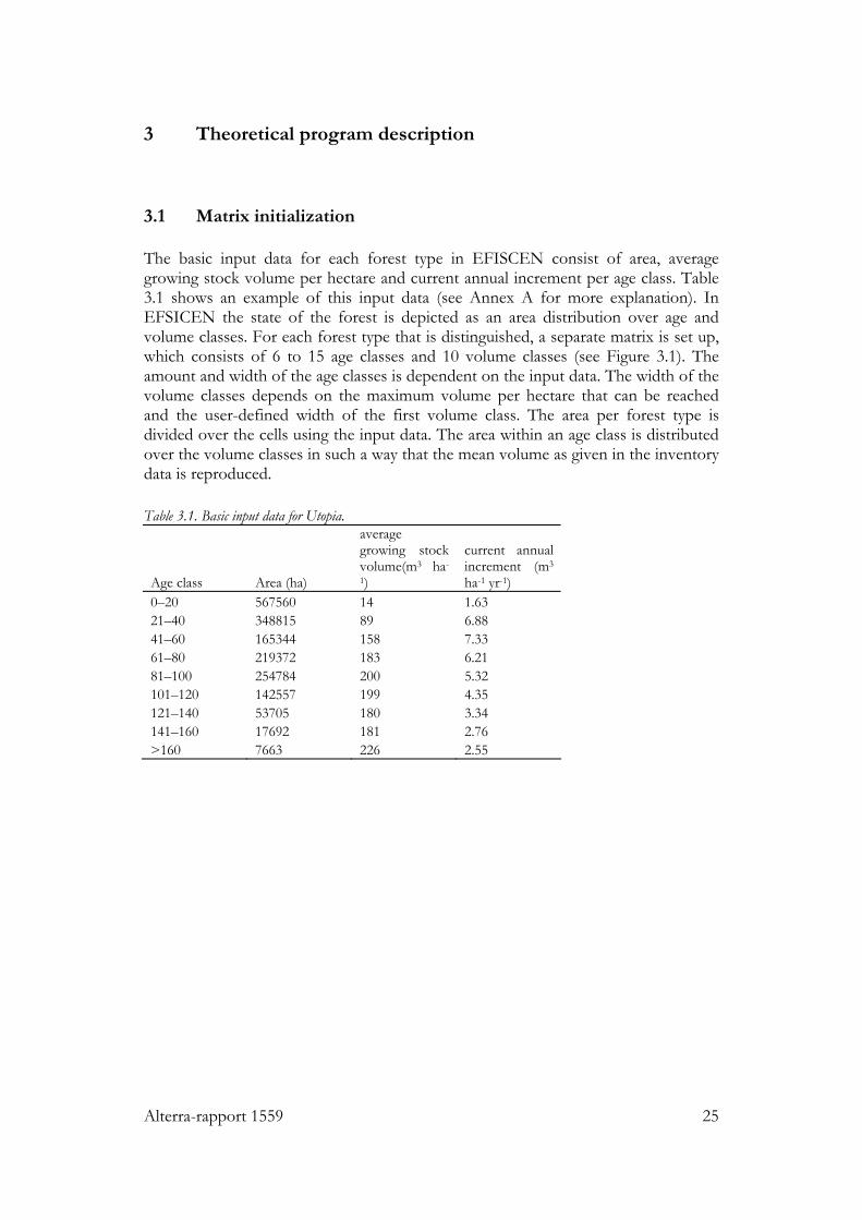
The basic input data for each forest type in EFISCEN consist of area, average growing stock volume per hectare and current annual increment per age class. Table 3.1 shows an example of this input data (see Annex A for more explanation). In EFSICEN the state of the forest is depicted as an area distribution over age and volume classes. For each forest type that is distinguished, a separate matrix is set up, which consists of 6 to 15 age classes and 10 volume classes (see Figure 3.1). The amount and width of the age classes is dependent on the input data. The width of the volume classes depends on the maximum volume per hectare that can be reached and the user-defined width of the first volume class. The area per forest type is divided over the cells using the input data. The area within an age class is distributed over the volume classes in such a way that the mean volume as given in the inventory data is reproduced. Table 3.1. Basic input data for Utopia.
Age class Area (ha)
average growing stock volume(m3 ha-
1)
current annual increment (m3 ha-1 yr-1)
0–20 567560 14 1.63 21–40 348815 89 6.88 41–60 165344 158 7.33 61–80 219372 183 6.21 81–100 254784 200 5.32 101–120 142557 199 4.35 121–140 53705 180 3.34 141–160 17692 181 2.76 >160 7663 226 2.55
26 Alterra-rapport 1559
Age
Vol
ume
GrowthAgingThinningNatural mortalityFinal harvestRegeneration
Forest types
Age
Vol
ume
GrowthAgingThinningNatural mortalityFinal harvestRegeneration
Forest types
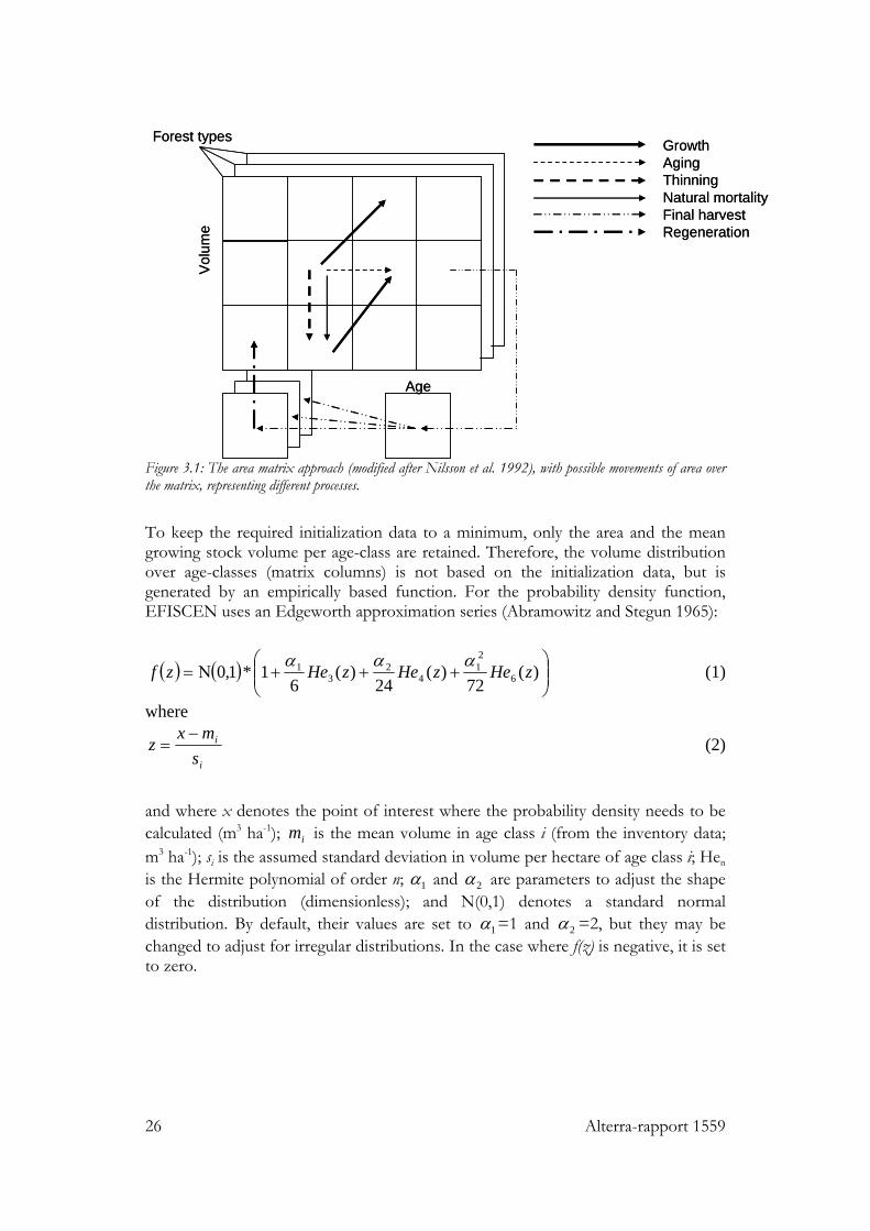
Figure 3.1: The area matrix approach (modified after Nilsson et al. 1992), with possible movements of area over the matrix, representing different processes. To keep the required initialization data to a minimum, only the area and the mean growing stock volume per age-class are retained. Therefore, the volume distribution over age-classes (matrix columns) is not based on the initialization data, but is generated by an empirically based function. For the probability density function, EFISCEN uses an Edgeworth approximation series (Abramowitz and Stegun 1965):
( ) ( ) ⎟⎟⎠
⎞⎜⎜⎝
⎛+++Ν= )(
72)(
24)(
61*1,0 6
21
42
31 zHezHezHezf
ααα (1)
where
i
i
smx
z−
= (2)
and where x denotes the point of interest where the probability density needs to be calculated (m3 ha-1); im is the mean volume in age class i (from the inventory data; m3 ha-1); si is the assumed standard deviation in volume per hectare of age class i; Hen is the Hermite polynomial of order n; 1α and 2α are parameters to adjust the shape of the distribution (dimensionless); and N(0,1) denotes a standard normal distribution. By default, their values are set to 1α =1 and 2α =2, but they may be changed to adjust for irregular distributions. In the case where f(z) is negative, it is set to zero.

Alterra-rapport 1559 27
The variance 2is of volume per hectare within an age class i is estimated as
ii Tks ln2 = (3)
where Ti is the mid point of age class i (year), and k is calculated according to
∑×−
=
iii fAreaT
cvVrk
*)ln())(1( 22
(4)
where V is the area-weighted average volume for the forest type (m3 ha-1); cv is the coefficient of variation of the volume per hectare for the forest type; r is the correlation between volume per hectare and ln(age) for the forest type; and fAreai is the fraction of the total area residing in age class i (dimensionless) Effectively, the denominator is the weighted average per forest type of ln(age). The parameter cv is 0.65 by default for all forest types, whereas r ranges from 0.45 to 0.7, depending on tree species, whether the data are separated into site classes, and whether the forests are well stocked (Table 3.2). The larger the correlation between volume and ln(age), the smaller is the variance of volume per hectare. Table 3.2. Recommended values for parameter r in different situations (Attebring et al. 1989).
All forests Separate site classes Forests well stocked Separate site classes and forests well stocked
Spruce, beech 0.55 0.6 0.65 0.7
Pine, oak 0.45 0.5 0.55 0.6
Others 0.5 0.55 0.6 0.65
The upper limit of the volume dimension in each matrix is determined by the highest volume per hectare that can be reached for that forest type. This is estimated from the largest volume per hectare from the initialization data plus three times the largest standard deviation:
)(*3)( 210 ii sMaxVMaxVCL += (5)
where VCL10 is the upper limit of the highest volume class (m3 ha-1); Max(Vi) is the maximum volume per hectare from the inventory for that forest type (m3 ha-1); and
)( 2isMax is the largest standard deviation as derived from equation 3. This definition
of the upper limit should ensure that the full range of variability in growing stocks is captured in the model. Assuming a normal distribution, this would imply that 99% of
28 Alterra-rapport 1559
the variability is captured. This volume range is then divided in 10 classes. The width of each volume class j (VCW; m3 ha-1) is calculated by: jj RVCWVCW *1= (6)
where R is determined such that the cumulative of these 10 volume classes equals VCL10:
101 )1/()1(* VCLRRVCW n =−− (7)
The left part of this equation is the cumulative of the 10 volume classes. VCW1 (also known in previous descriptions as X1) is set by the user. If the ratio between VCW1 and VCL10 is 10, the volume classes will be of equal width (R=1). In other cases, higher volume classes will be larger (ratio below 10, R>1) or smaller (ratio above 10, R<1). However, due to the way this is implemented in the code, R is restricted to the range between 1 and 2. Therefore, volume classes are either equidistant or of increasing width. Another consequence is that VCL10 is overruled in cases where R should have been lower than 1. This means that the maximum volume per hectare that can be reached is increased. By assigning the average volume of a certain volume class to all area in that class, it is implicitly assumed that the area is uniformly distributed within a class. This will cause a small deviation in the calculated average volume over all volume classes within one age class compared to the average volume in the input data. If the deviation is larger than 1 m3 ha-1, the distribution is adapted. If the calculated volume is too high, a certain fraction of the highest volume class is moved one class down. If all area of the highest volume class is moved and the difference is still larger than 1 m3 ha-1, a certain fraction of the area in the next highest volume class will be moved. This procedure is repeated until the difference is less than 1 m3 ha-1. In case the calculated volume is too low, areas are moved upward in a similar way, starting from the lowest volume class. 3.2 Increment
In EFISCEN, growth dynamics are simulated by shifting proportions of the area in the matrix from one cell to another. Each five-year time step, the area in each cell will move up one age class. Part of the area will also move up one volume class. When area reaches the highest volume class it will remain there until it is harvested, i.e. it cannot grow anymore. Growth dynamics are incorporated as five year net annual increment as a percentage of the growing stock. The growth functions of the model are of the following type:
221
0)(Ta
Ta
aTIvf ++= (8)
Alterra-rapport 1559 29
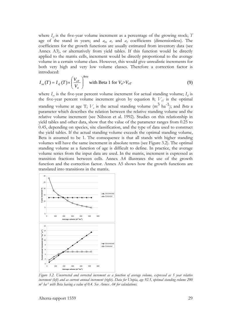
where Ivf is the five-year volume increment as a percentage of the growing stock; T age of the stand in years; and a0, a1 and a2 coefficients (dimensionless). The coefficients for the growth functions are usually estimated from inventory data (see Annex A3), or alternatively from yield tables. If this function would be directly applied to the matrix cells, increment would be directly proportional to the average volume in a certain volume class. However, this would give unrealistic increments for both very high and very low volume classes. Therefore a correction factor is introduced:
Beta
a
oTvfva V
VTITI ⎟⎟
⎠
⎞⎜⎜⎝
⎛×= )()( with Beta 1 for Va>VoT (9)
where Iva is the five-year percent volume increment for actual standing volume; Ivf is the five-year percent volume increment given by equation 8; VoT is the optimal standing volume at age T; Va is the actual standing volume (m3 ha-1); and Beta a parameter which describes the relation between the relative standing volume and the relative volume increment (see Nilsson et al. 1992). Studies on this relationship in yield tables and other data, show that the value of the parameter ranges from 0.25 to 0.45, depending on species, site classification, and the type of data used to construct the yield tables. If the actual standing volume exceeds the optimal standing volume, Beta is assumed to be 1. The consequence is that all stands with higher standing volumes will have the same increment in absolute terms (see Figure 3.2). The optimal standing volume as a function of age is difficult to define. In practice, the average volume series from the input data are used. In the matrix, increment is expressed as transition fractions between cells. Annex A4 illustrates the use of the growth function and the correction factor. Annex A5 shows how the growth functions are translated into transitions in the matrix.
0
5
10
15
20
25
30
0 100 200 300 400 500 600
Average volume (m3 ha-1)
5 ye
ar in
crem
ent %
UncorrectedCorrected
0
2
4
6
8
10
12
14
16
0 100 200 300 400 500 600
Average volume (m3 ha-1)
Curr
ent a
nnua
l inc
rem
ent (
m3 h
a-1 y
r-1)
UncorrectedCorrected
Figure 3.2. Uncorrected and corrected increment as a function of average volume, expressed as 5 year relative increment (left) and as current annual increment (right). Data for Utopia, age 92.5, optimal standing volume 200 m3 ha-1 with Beta having a value of 0.4. See Annex A4 for calculations.
30 Alterra-rapport 1559
3.3 Management activities
Management is controlled at two levels in the model. First, a basic management of thinning and final felling is incorporated for each forest type. This is the theoretical management regime, which is applied according to handbooks or expert knowledge for forest management in the region or country to be studied. This theoretical regime must be seen as constraint of what might be felled. Second, total required harvest volumes from thinning and final felling are specified for the region or country as a whole for each time period. Based on the theoretical management regimes, the model searches and might find, depending on the state of the forest, the required volumes. Further the success of a reforestation after clear felling can be incorporated per tree species, as well as a possible tree species change after a clear felling, and a forest area change. 3.3.1 Thinning
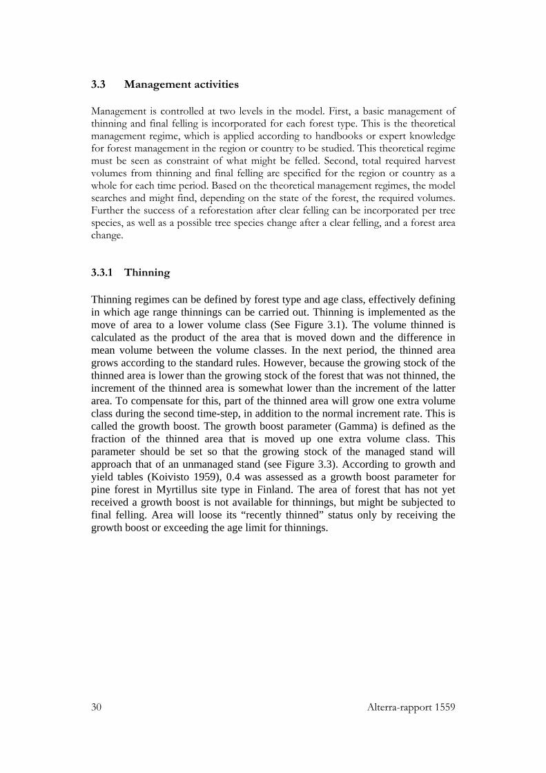
Thinning regimes can be defined by forest type and age class, effectively defining in which age range thinnings can be carried out. Thinning is implemented as the move of area to a lower volume class (See Figure 3.1). The volume thinned is calculated as the product of the area that is moved down and the difference in mean volume between the volume classes. In the next period, the thinned area grows according to the standard rules. However, because the growing stock of the thinned area is lower than the growing stock of the forest that was not thinned, the increment of the thinned area is somewhat lower than the increment of the latter area. To compensate for this, part of the thinned area will grow one extra volume class during the second time-step, in addition to the normal increment rate. This is called the growth boost. The growth boost parameter (Gamma) is defined as the fraction of the thinned area that is moved up one extra volume class. This parameter should be set so that the growing stock of the managed stand will approach that of an unmanaged stand (see Figure 3.3). According to growth and yield tables (Koivisto 1959), 0.4 was assessed as a growth boost parameter for pine forest in Myrtillus site type in Finland. The area of forest that has not yet received a growth boost is not available for thinnings, but might be subjected to final felling. Area will loose its “recently thinned” status only by receiving the growth boost or exceeding the age limit for thinnings.
Alterra-rapport 1559 31
050
100150200250300350400450500
0 10 20 30 40 50 60 70 80 90 100Time, years
Volu
me,
m3 h
a-1Standing volume, unmanaged
Standing volume, managed
Total exploitable cumulative woodproduction, managed
Figure 3.3. The development of standing volume of a stand in managed and unmanaged forests and the total cumulative exploitable wood production (thinned + standing volume) of a managed stand. 3.3.2 Final felling
As with thinnings, the final felling regime can be defined by forest type and age class. The final felling regime is expressed as the proportion of each cell that can be felled, depending on the stand age. How much of this maximum is actually used depends on the ratio between wood demand for final fellings and the maximum amount that could be felled if all potential final fellings were carried out. The felled area is moved outside the matrix to the bare-forest-land class, from where it can re-enter the matrix (see Figure 3.1). Usually this area will go to the bare land class of the original matrix. However, when a tree species change is defined, (part of) the area will be added to the bare land class of the respective matrix. The final felling regimes can be obtained by handbooks, yield tables or other sources, such as statistical yearbooks. 3.4 Regeneration
Regeneration is regarded as the movement of area from the bare-forest-land class to the first volume and age class (Figure 3.1). The amount of area that is regenerated is regulated by a parameter that expresses the intensity and success of regeneration, the young forest coefficient. This parameter is the percentage of area in the bare-forest-land class that will move to the first volume and age class in one time step. This area will then attain the average volume and age of that class. The amount of area in the bare forest land class depends on the intensity of clear felling, possible changes in tree species after final felling and the height of the young forest coefficient. Default values for the young forest coefficient can be found in annex C.
32 Alterra-rapport 1559
3.5 Natural mortality and standing dead wood
If the forest growth is given as gross annual increment, or if the demand scenario specifies a low roundwood demand and management is thus not very intensive, mortality should be included. When gross annual increment is applied, mortality should include all types of mortality, such as natural mortality, diseases, insect attacks, fire, windthrow or other physical damage. In EFISCEN, mortality is expressed as a fraction of the actual standing volume and is only applied in forests that are not thinned or felled the current time-step and that do not have a recently thinned status (i.e. recently thinned forests that did not receive a growth boost). Mortality can be defined by forest type and age class. EFISCEN performs mortality calculations by transferring area one volume class down to obtain the required reduction in standing volume. Note that this implies a maximum mortality rate of 10%. If all area in the highest volume class is moved down and volume classes are of equal width, the average volume will be decreased by 10%. The volume subject to mortality enters a standing dead wood pool, while branches, foliage and roots are lost in the same time-step and enter their respective litter pools in the soil module. Volume can leave the standing dead wood pool by falling down as complete tree or in smaller pieces, or by removal during management. A dead wood fall rate parameter defines the proportion of standing dead wood that reaches the ground each year. The fall rate can be defined by forest type. It describes a negative exponential curve and no lag period is assumed (Storaunet & Rolstad, 2004; but see e.g. Mäkinen et al., 2006). A proportion of dead wood can be removed from the forest during management operations. A dead wood removal parameter can be set for thinning and final felling separately and for each forest type and time-step. Dead wood is only removed in forests that are thinned or final felled. The standing dead wood pool is initialised by calculating the equilibrium between the input of dead wood, the fall down rate and the dead wood removal rate of the first time-step. Fallen dead wood enters the coarse woody litter pool of the soil module, in which fractionation and decomposition of lying dead wood is modelled as a reduction of mass; volume of lying dead wood is not projected by EFISCEN. 3.6 Afforestation and deforestation
EFISCEN can also take afforestation and deforestation into account. The user can add or remove area per tree species in each time step of the simulations. The area will then be added to the bare-forest-land class of each forest type of that tree species, or the area is removed from the bare-forest-land class. The maximum area for deforestation in one time steps equals the area in the bare-forest-land-class, but in that case also no regeneration will occur. 3.7 Change of increment due to changed environment
The model can simulate the development of the forest for decades. For various reasons, e.g. climate change, increment rates may change during long simulation
Alterra-rapport 1559 33
periods. The model can take into account such changes in increment rate by defining an expected relative change. The basis of the increment calculation is always the increment as calculated by the incorporated growth functions, which are based on the inventory data. The new increment rates are defined relative to the basic growth functions. The expected relative change can be defined per time step, by forest type and age class. 3.8 Biomass and litter production
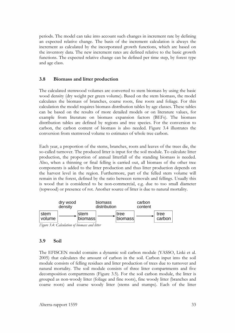
The calculated stemwood volumes are converted to stem biomass by using the basic wood density (dry weight per green volume). Based on the stem biomass, the model calculates the biomass of branches, coarse roots, fine roots and foliage. For this calculation the model requires biomass distribution tables by age classes. These tables can be based on the results of more detailed models or on literature values, for example from literature on biomass expansion factors (BEFs). The biomass distribution tables are defined by regions and tree species. For the conversion to carbon, the carbon content of biomass is also needed. Figure 3.4 illustrates the conversion from stemwood volume to estimates of whole tree carbon. Each year, a proportion of the stems, branches, roots and leaves of the trees die, the so-called turnover. The produced litter is input for the soil module. To calculate litter production, the proportion of annual litterfall of the standing biomass is needed. Also, when a thinning or final felling is carried out, all biomass of the other tree components is added to the litter production and thus litter production depends on the harvest level in the region. Furthermore, part of the felled stem volume will remain in the forest, defined by the ratio between removals and fellings. Usually this is wood that is considered to be non-commercial, e.g. due to too small diameter (topwood) or presence of rot. Another source of litter is due to natural mortality.
dry wooddensity
biomassdistribution
carboncontent
treecarbon
treebiomass
stembiomass
stemvolume
Figure 3.4: Calculation of biomass and litter 3.9 Soil
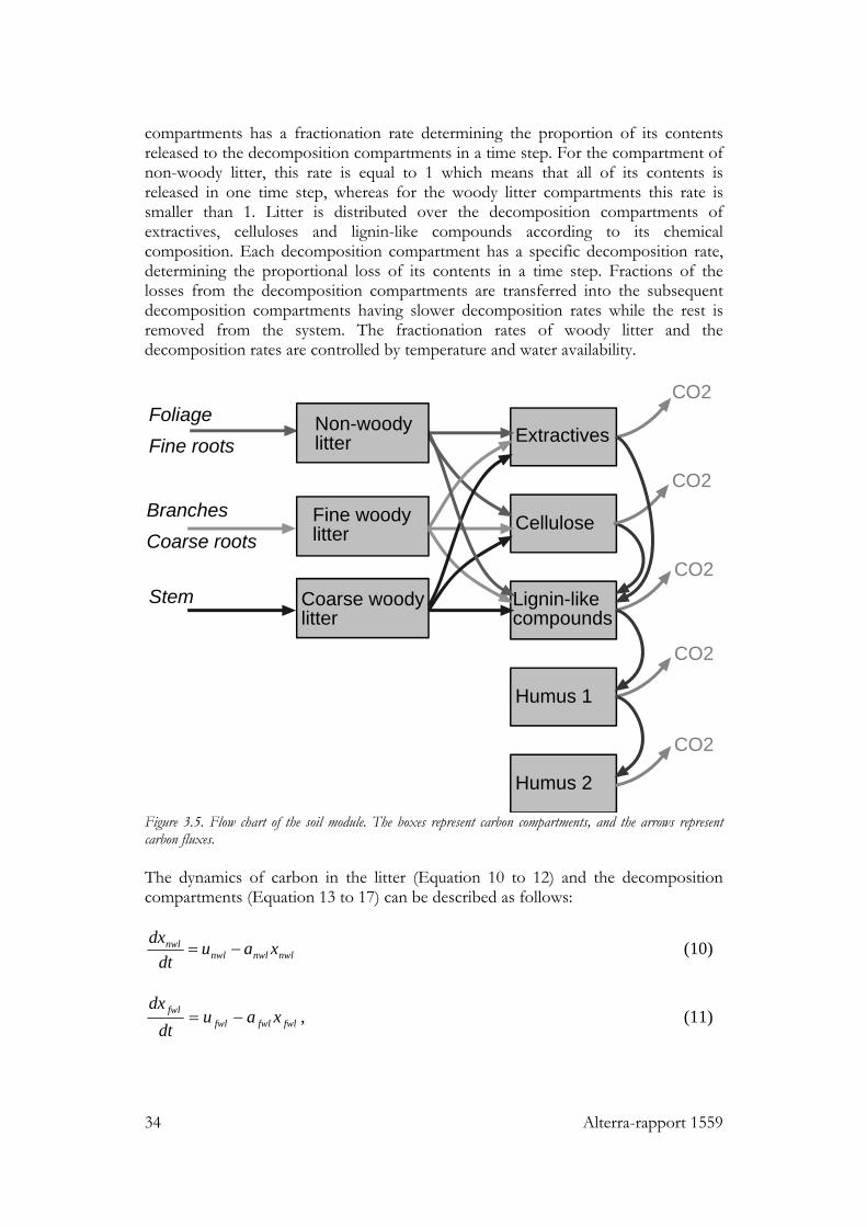
The EFISCEN model contains a dynamic soil carbon module (YASSO, Liski et al. 2005) that calculates the amount of carbon in the soil. Carbon input into the soil module consists of felling residues and litter production of trees due to turnover and natural mortality. The soil module consists of three litter compartments and five decomposition compartments (Figure 3.5). For the soil carbon module, the litter is grouped as non-woody litter (foliage and fine roots), fine woody litter (branches and coarse roots) and coarse woody litter (stems and stumps). Each of the litter
34 Alterra-rapport 1559
compartments has a fractionation rate determining the proportion of its contents released to the decomposition compartments in a time step. For the compartment of non-woody litter, this rate is equal to 1 which means that all of its contents is released in one time step, whereas for the woody litter compartments this rate is smaller than 1. Litter is distributed over the decomposition compartments of extractives, celluloses and lignin-like compounds according to its chemical composition. Each decomposition compartment has a specific decomposition rate, determining the proportional loss of its contents in a time step. Fractions of the losses from the decomposition compartments are transferred into the subsequent decomposition compartments having slower decomposition rates while the rest is removed from the system. The fractionation rates of woody litter and the decomposition rates are controlled by temperature and water availability.
Extractives
Cellulose
Lignin-likecompounds
Humus 1
Humus 2
Coarse woodylitter
Fine woodylitter
CO2
CO2
CO2
CO2
CO2
FoliageFine roots
BranchesCoarse roots
Stem
Non-woodylitter
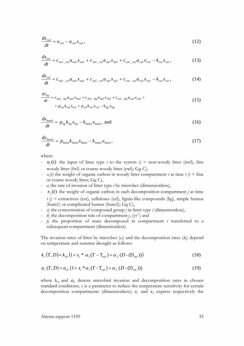
Figure 3.5. Flow chart of the soil module. The boxes represent carbon compartments, and the arrows represent carbon fluxes. The dynamics of carbon in the litter (Equation 10 to 12) and the decomposition compartments (Equation 13 to 17) can be described as follows:
nwlnwlnwlnwl xau
dtdx
−= (10)
fwlfwlfwlfwl xau
dtdx
−= , (11)
Alterra-rapport 1559 35
cwlcwlcwlcwl xau
dtdx
−= , (12)
extextcwlcwlextcwlfwlfwlextfwlnwlnwlextnwlext xkxacxacxac
dtdx
−++= ___ , (13)
celcelcwlcwlcelcwlfwlfwlcelfwlnwlnwlcelnwlcel xkxacxacxac
dtdx
−++= ___ , (14)
ligligcelcelcelextextext
cwlcwlligcwlfwlfwlligfwlnwlnwllignwllig
xkxkpxkp
xacxacxacdt
dx
−++
+++=
___ (15)
111
humhumligliglighum xkxkpdt
dx−= , and (16)
221112
humhumhumhumhumhum xkxkpdt
dx−= . (17)
where: - )(tui the input of litter type i to the system (i = non-woody litter (nwl), fine
woody litter (fwl) or coarse woody litter (cwl); Gg C), - xi(t) the weight of organic carbon in woody litter compartment i at time t (i = fine
or coarse woody litter; Gg C), - ai the rate of invasion of litter type i by microbes (dimensionless), - )(tx j the weight of organic carbon in each decomposition compartment j at time
t (j = extractives (ext), celluloses (cel), lignin-like compounds (lig), simple humus (hum1) or complicated humus (hum2); Gg C),
- cij the concentration of compound group j in litter type i (dimensionless), - kj the decomposition rate of compartment j, (yr-1) and - pi the proportion of mass decomposed in compartment i transferred to a
subsequent compartment (dimensionless). The invasion rates of litter by microbes (ai) and the decomposition rates (kj) depend on temperature and summer drought as follows:
( ) ( )))(D - ( )T ( * 1 , ref2ref10 DTskDTk iii αα +−+= (18)
)))(D - ( )T - ( * (1 ),( ref2ref10 DTsaDTa iii αα ++= (19) where ki0 and ai0 denote microbial invasion and decomposition rates in chosen standard conditions; si is a parameter to reduce the temperature sensitivity for certain decomposition compartments (dimensionless); α1 and α2 express respectively the
36 Alterra-rapport 1559
temperature and drought sensitivity (respectively °C-1 and mm-1); T is either the average annual temperature (old version of YASSO) or the effective temperature sum in the growing season (0 °C threshold); Tref is the reference temperature or temperature sum; D is the drought index during the growing season (precipitation minus potential evapotranspiration durign the growing season; mm); and Dref the reference drought index (mm). In earlier EFISCEN versions, an older version of YASSO was used. This version used the average annual temperature to express the temperature sensitivity. An improved version of YASSO uses the annual effective temperature sum instead (Liski et al., 2005). EFISCEN 3.X is able to use both methods, since both actual parameters and the reference values need to be supplied. Table 3.3 shows the parameter values for both approaches. Only the differences in the reference conditions and sensitivity parameters are due to the application of a different method. The differences in the other parameters reflect increased insights. Therefore, the second column reflects a typical parameterization as used in earlier applications (Pussinen et al. 2001), and the third column reflects the most up-to-date parameterization (Liski et al. 2005). For the humus compartments, parameter si may have a value lower than one to reduce the temperature sensitivity of humus decomposition (Liski et al. 1999; Giardina and Ryan 2000); for the other decomposition compartments, si is equal to one. At the start of the simulations the initial soil carbon content for each compartment should be known. This can be set by the user, or can be calculated by the model using the litter input of the first year, assuming a steady state. The soil module operates on an annual time step and assumes an equal distribution of litter input over the five-year time step of the forest model.
Alterra-rapport 1559 37
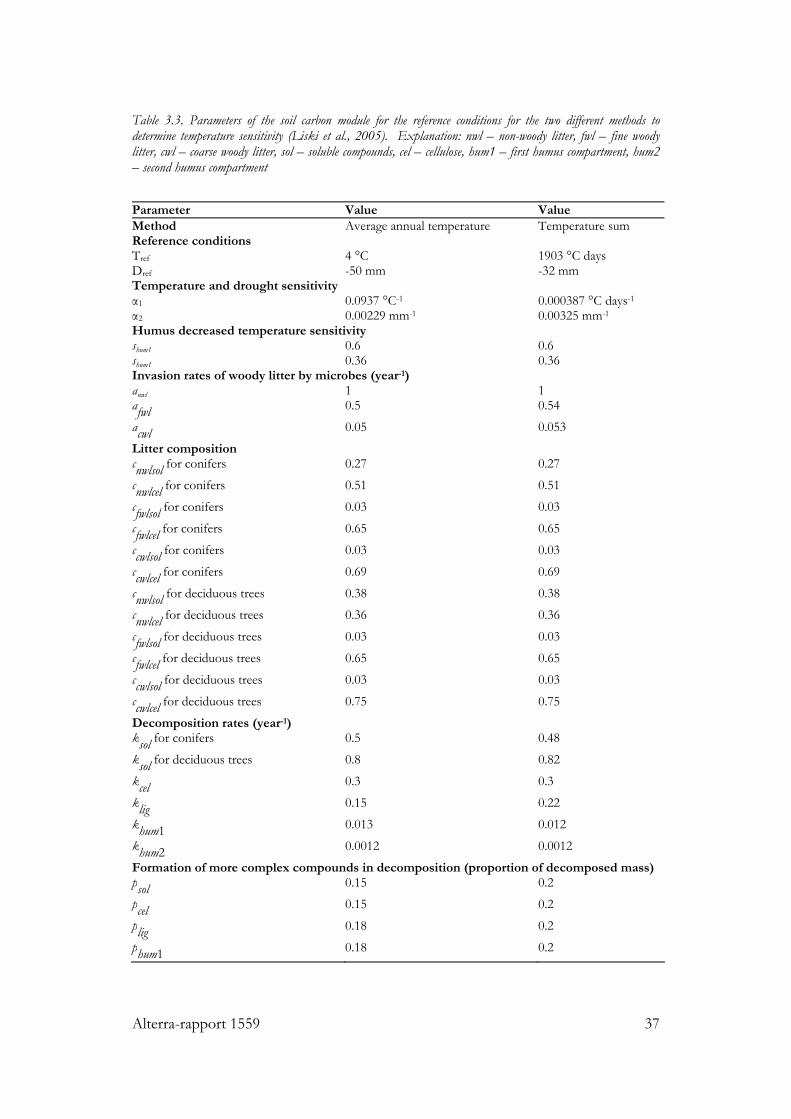
Table 3.3. Parameters of the soil carbon module for the reference conditions for the two different methods to determine temperature sensitivity (Liski et al., 2005). Explanation: nwl – non-woody litter, fwl – fine woody litter, cwl – coarse woody litter, sol – soluble compounds, cel – cellulose, hum1 – first humus compartment, hum2 – second humus compartment
Parameter Value Value Method Average annual temperature Temperature sum Reference conditions Tref 4 °C 1903 °C days Dref -50 mm -32 mm Temperature and drought sensitivity α1 0.0937 °C-1 0.000387 °C days-1 α2 0.00229 mm-1 0.00325 mm-1 Humus decreased temperature sensitivity shum1 0.6 0.6 shum1 0.36 0.36 Invasion rates of woody litter by microbes (year-1) anwl 1 1 afwl 0.5 0.54
acwl 0.05 0.053
Litter composition cnwlsol for conifers 0.27 0.27
cnwlcel for conifers 0.51 0.51
cfwlsol for conifers 0.03 0.03
cfwlcel for conifers 0.65 0.65
ccwlsol for conifers 0.03 0.03
ccwlcel for conifers 0.69 0.69
cnwlsol for deciduous trees 0.38 0.38
cnwlcel for deciduous trees 0.36 0.36
cfwlsol for deciduous trees 0.03 0.03
cfwlcel for deciduous trees 0.65 0.65
ccwlsol for deciduous trees 0.03 0.03
ccwlcel for deciduous trees 0.75 0.75
Decomposition rates (year-1) ksol for conifers 0.5 0.48
ksol for deciduous trees 0.8 0.82
kcel 0.3 0.3
klig 0.15 0.22
khum1 0.013 0.012
khum2 0.0012 0.0012
Formation of more complex compounds in decomposition (proportion of decomposed mass) psol 0.15 0.2
pcel 0.15 0.2
plig 0.18 0.2
phum1 0.18 0.2

Alterra-rapport 1559 39
4 Technical program description
4.1 Introduction
In this chapter we explain the model implementation and usage. EFISCEN 3.X consists of two separate programs: P-efsos to generate the initial matrices and EFISCEN to do the actual simulations (see also Figure 2.1). Both programs will be discussed separately in the next sections. In these descriptions, the symbol *** is used to denote the country name. 4.2 Matrix initialisation (P-efsos)
4.2.1 Introduction
The matrix initialisation program P-efsos is still largely the same program as it was delivered to EFI in 1996. The original program (P96) has been adapted during the EFSOS project to simplify the usage of the program, especially with regard to input handling. The programming language is Fortran (Digital Visual Fortran 6.0). 4.2.2 Files and directories
The program code is contained in only one file, P_efsos.for. The resulting executable is called P_efsos.exe. Since the name of the country and the specficiations of the forest types are coded explicitly, the name of the exectuable is often extended manually with the name or abbreviation of the country. Figure 4.1 shows which input files are needed and which output files are generated. It also indicates the type of information that the files contain. An exact description of the files is provided in the User Guide section later on. The input files utonewefsos.csv and Growth_func_EFSOS1.csv are both located in the same directory as the executable. The file uto-ecnt.dat is located in the directory \ecnt. Output files will be written to the directory \output. In earlier versions of EFISCEN, P-efsos provided both the initial matrices and the transition chances for the main program. In EFISCEN 3.X, transition chances are calculated in the main program, and thus some of the input and output files for P-efsos have become obsolete. The aim is to include the matrix generator into the main program in future, so no efforts have been made to solve these redundancies.
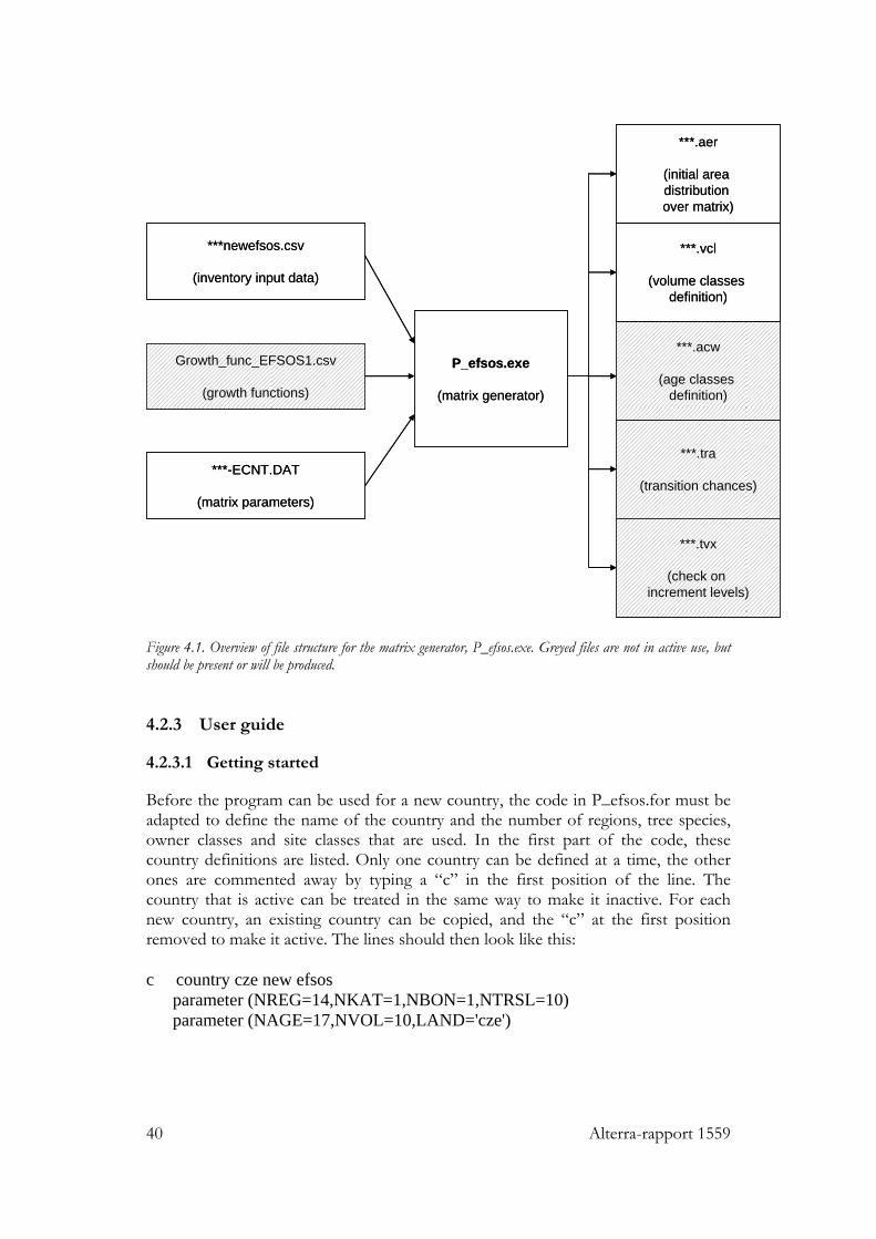
40 Alterra-rapport 1559
***.aer
(initial area distribution over matrix)
***.tra
(transition chances)
P_efsos.exe
(matrix generator)
***newefsos.csv
(inventory input data)
Growth_func_EFSOS1.csv
(growth functions)
***.acw
(age classes definition)
***.vcl
(volume classes definition)
***.tvx
(check on increment levels)
***-ECNT.DAT
(matrix parameters)
Figure 4.1. Overview of file structure for the matrix generator, P_efsos.exe. Greyed files are not in active use, but should be present or will be produced. 4.2.3 User guide
4.2.3.1 Getting started
Before the program can be used for a new country, the code in P_efsos.for must be adapted to define the name of the country and the number of regions, tree species, owner classes and site classes that are used. In the first part of the code, these country definitions are listed. Only one country can be defined at a time, the other ones are commented away by typing a “c” in the first position of the line. The country that is active can be treated in the same way to make it inactive. For each new country, an existing country can be copied, and the “c” at the first position removed to make it active. The lines should then look like this: c country cze new efsos parameter (NREG=14,NKAT=1,NBON=1,NTRSL=10) parameter (NAGE=17,NVOL=10,LAND='cze')
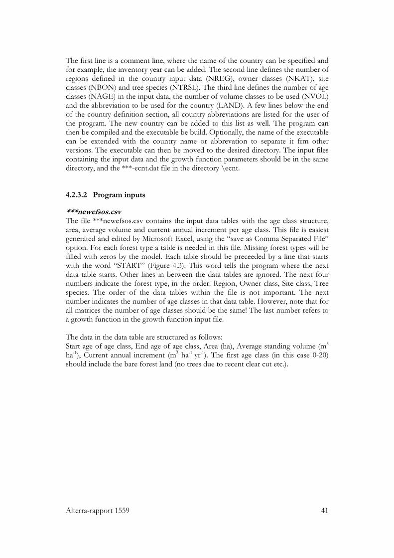
Alterra-rapport 1559 41
The first line is a comment line, where the name of the country can be specified and for example, the inventory year can be added. The second line defines the number of regions defined in the country input data (NREG), owner classes (NKAT), site classes (NBON) and tree species (NTRSL). The third line defines the number of age classes (NAGE) in the input data, the number of volume classes to be used (NVOL) and the abbreviation to be used for the country (LAND). A few lines below the end of the country definition section, all country abbreviations are listed for the user of the program. The new country can be added to this list as well. The program can then be compiled and the executable be build. Optionally, the name of the executable can be extended with the country name or abbrevation to separate it frm other versions. The executable can then be moved to the desired directory. The input files containing the input data and the growth function parameters should be in the same directory, and the ***-ecnt.dat file in the directory \ecnt. 4.2.3.2 Program inputs
***newefsos.csv The file ***newefsos.csv contains the input data tables with the age class structure, area, average volume and current annual increment per age class. This file is easiest generated and edited by Microsoft Excel, using the “save as Comma Separated File” option. For each forest type a table is needed in this file. Missing forest types will be filled with zeros by the model. Each table should be preceeded by a line that starts with the word “START” (Figure 4.3). This word tells the program where the next data table starts. Other lines in between the data tables are ignored. The next four numbers indicate the forest type, in the order: Region, Owner class, Site class, Tree species. The order of the data tables within the file is not important. The next number indicates the number of age classes in that data table. However, note that for all matrices the number of age classes should be the same! The last number refers to a growth function in the growth function input file. The data in the data table are structured as follows: Start age of age class, End age of age class, Area (ha), Average standing volume (m3 ha-1), Current annual increment (m3 ha-1 yr-1). The first age class (in this case 0-20) should include the bare forest land (no trees due to recent clear cut etc.).
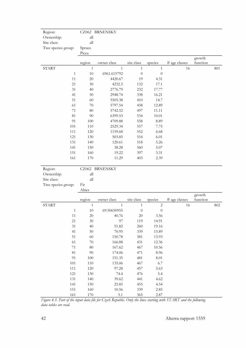
42 Alterra-rapport 1559
Region: CZ062 BRNENSKY Ownership: all Site class: all Tree species group: Spruce Picea
region owner class site class species # age classes growth function
START 1 1 1 1 16 8011 10 6961.615792 0 0
11 20 4420.67 19 4.31 21 30 4232.5 132 17.1 31 40 2776.79 232 17.77 41 50 2948.74 338 16.21 51 60 5505.38 410 14.7 61 70 5797.54 458 12.89 71 80 5742.52 497 11.11 81 90 6399.53 534 10.01 91 100 4709.88 558 8.89
101 110 2529.34 557 7.75 111 120 1159.68 552 6.68 121 130 503.85 554 6.01 131 140 120.61 518 5.26 141 150 38.28 560 5.07 151 160 19.22 397 3.31 161 170 11.29 403 2.39
Region: CZ062 BRNENSKY Ownership: all Site class: all Tree species group: Fir Abies
region owner class site class species # age classes growth function
START 1 1 1 2 16 8021 10 69.50650955 0 0
11 20 40.76 20 3.56 21 30 97 119 14.91 31 40 51.82 260 19.16 41 50 70.95 339 15.89 51 60 150.78 381 13.93 61 70 166.88 431 12.36 71 80 167.62 467 10.56 81 90 174.06 471 8.96 91 100 151.35 481 8.01
101 110 135.06 467 6.7 111 120 97.28 457 5.63 121 130 74.4 476 5.4 131 140 39.62 441 4.62 141 150 25.85 455 4.54 151 160 10.56 339 2.85 161 170 5.1 365 2.87
Figure 4.3. Part of the input data file for Czech Republic. Only the lines starting with START and the following data tables are read.
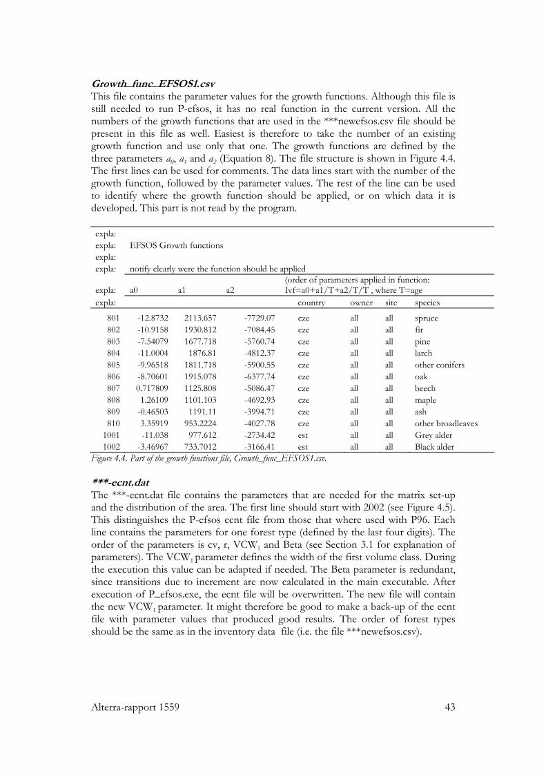
Alterra-rapport 1559 43
Growth_func_EFSOS1.csv This file contains the parameter values for the growth functions. Although this file is still needed to run P-efsos, it has no real function in the current version. All the numbers of the growth functions that are used in the ***newefsos.csv file should be present in this file as well. Easiest is therefore to take the number of an existing growth function and use only that one. The growth functions are defined by the three parameters a0, a1 and a2 (Equation 8). The file structure is shown in Figure 4.4. The first lines can be used for comments. The data lines start with the number of the growth function, followed by the parameter values. The rest of the line can be used to identify where the growth function should be applied, or on which data it is developed. This part is not read by the program. expla: expla: EFSOS Growth functions expla: expla: notify clearly were the function should be applied
expla: a0 a1 a2 (order of parameters applied in function: Ivf=a0+a1/T+a2/T/T , where T=age
expla: country owner site species
801 -12.8732 2113.657 -7729.07 cze all all spruce 802 -10.9158 1930.812 -7084.45 cze all all fir 803 -7.54079 1677.718 -5760.74 cze all all pine 804 -11.0004 1876.81 -4812.37 cze all all larch 805 -9.96518 1811.718 -5900.55 cze all all other conifers 806 -8.70601 1915.078 -6377.74 cze all all oak 807 0.717809 1125.808 -5086.47 cze all all beech 808 1.26109 1101.103 -4692.93 cze all all maple 809 -0.46503 1191.11 -3994.71 cze all all ash 810 3.35919 953.2224 -4027.78 cze all all other broadleaves
1001 -11.038 977.612 -2734.42 est all all Grey alder 1002 -3.46967 733.7012 -3166.41 est all all Black alder
Figure 4.4. Part of the growth functions file, Growth_func_EFSOS1.csv. ***-ecnt.dat The ***-ecnt.dat file contains the parameters that are needed for the matrix set-up and the distribution of the area. The first line should start with 2002 (see Figure 4.5). This distinguishes the P-efsos ecnt file from those that where used with P96. Each line contains the parameters for one forest type (defined by the last four digits). The order of the parameters is cv, r, VCW1 and Beta (see Section 3.1 for explanation of parameters). The VCW1 parameter defines the width of the first volume class. During the execution this value can be adapted if needed. The Beta parameter is redundant, since transitions due to increment are now calculated in the main executable. After execution of P_efsos.exe, the ecnt file will be overwritten. The new file will contain the new VCW1 parameter. It might therefore be good to make a back-up of the ecnt file with parameter values that produced good results. The order of forest types should be the same as in the inventory data file (i.e. the file ***newefsos.csv).
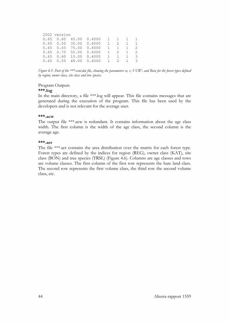
44 Alterra-rapport 1559
2002 version 0.65 0.60 45.00 0.4000 1 1 1 1 0.65 0.50 30.00 0.4000 1 2 1 1 0.65 0.45 75.00 0.4000 1 1 1 2 0.65 0.70 55.00 0.4000 1 2 1 2 0.65 0.60 10.00 0.4000 1 1 1 3 0.65 0.55 48.00 0.4000 1 2 1 3 Figure 4.5. Part of the ***-ecnt.dat file, showing the parameters cv, r, VCW1 and Beta for the forest types defined by region, owner class, site class and tree species. Program Outputs ***.log In the main directory, a file ***.log will appear. This file contains messages that are generated during the execution of the program. This file has been used by the developers and is not relevant for the average user. ***.acw The output file ***.acw is redundant. It contains information about the age class width. The first column is the width of the age class, the second column is the average age. ***.aer The file ***.aer contains the area distribution over the matrix for each forest type. Forest types are defined by the indices for region (REG), owner class (KAT), site class (BON) and tree species (TRSL) (Figure 4.6). Columns are age classes and rows are volume classes. The first column of the first row represents the bare land class. The second row represents the first volume class, the third row the second volume class, etc.
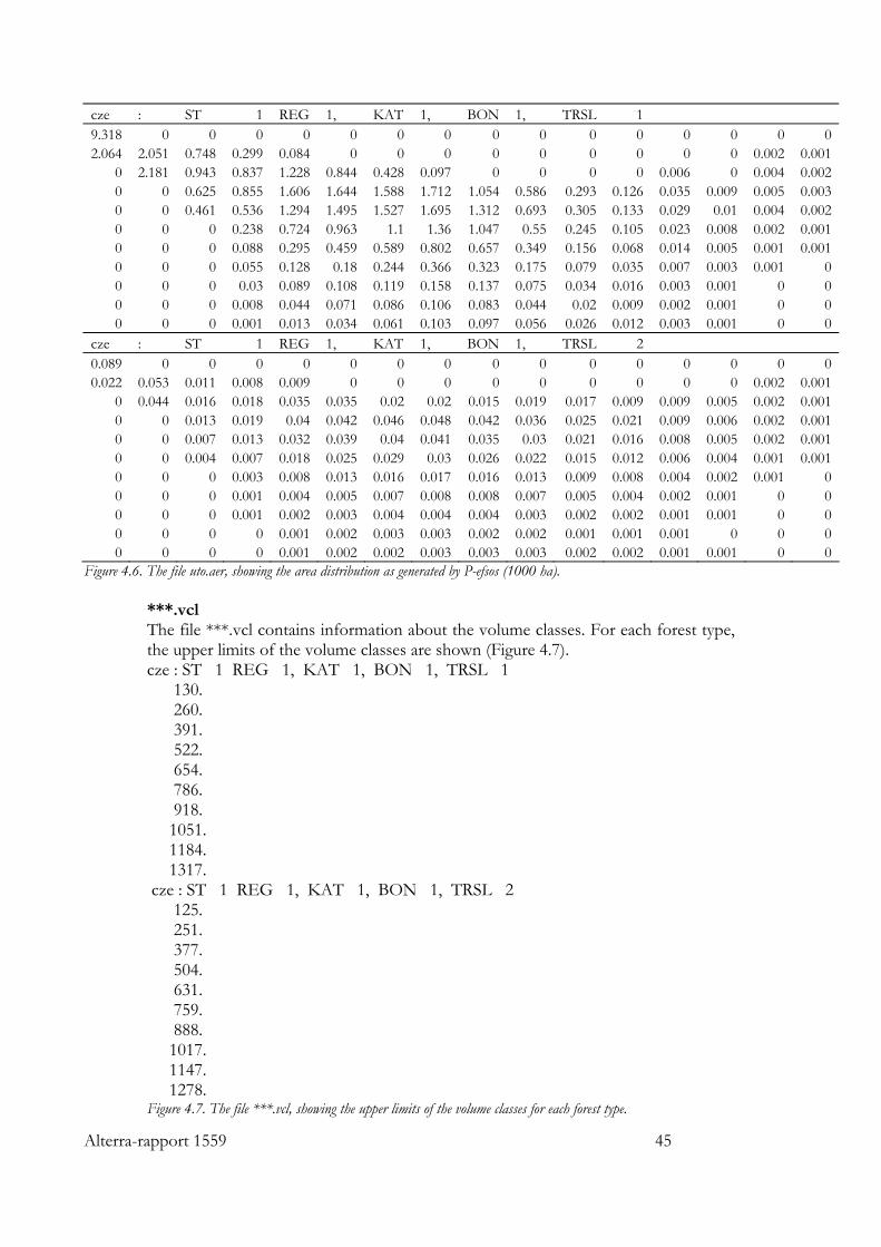
Alterra-rapport 1559 45
cze : ST 1 REG 1, KAT 1, BON 1, TRSL 1 9.318 0 0 0 0 0 0 0 0 0 0 0 0 0 0 02.064 2.051 0.748 0.299 0.084 0 0 0 0 0 0 0 0 0 0.002 0.001
0 2.181 0.943 0.837 1.228 0.844 0.428 0.097 0 0 0 0 0.006 0 0.004 0.0020 0 0.625 0.855 1.606 1.644 1.588 1.712 1.054 0.586 0.293 0.126 0.035 0.009 0.005 0.0030 0 0.461 0.536 1.294 1.495 1.527 1.695 1.312 0.693 0.305 0.133 0.029 0.01 0.004 0.0020 0 0 0.238 0.724 0.963 1.1 1.36 1.047 0.55 0.245 0.105 0.023 0.008 0.002 0.0010 0 0 0.088 0.295 0.459 0.589 0.802 0.657 0.349 0.156 0.068 0.014 0.005 0.001 0.0010 0 0 0.055 0.128 0.18 0.244 0.366 0.323 0.175 0.079 0.035 0.007 0.003 0.001 00 0 0 0.03 0.089 0.108 0.119 0.158 0.137 0.075 0.034 0.016 0.003 0.001 0 00 0 0 0.008 0.044 0.071 0.086 0.106 0.083 0.044 0.02 0.009 0.002 0.001 0 00 0 0 0.001 0.013 0.034 0.061 0.103 0.097 0.056 0.026 0.012 0.003 0.001 0 0
cze : ST 1 REG 1, KAT 1, BON 1, TRSL 2 0.089 0 0 0 0 0 0 0 0 0 0 0 0 0 0 00.022 0.053 0.011 0.008 0.009 0 0 0 0 0 0 0 0 0 0.002 0.001
0 0.044 0.016 0.018 0.035 0.035 0.02 0.02 0.015 0.019 0.017 0.009 0.009 0.005 0.002 0.0010 0 0.013 0.019 0.04 0.042 0.046 0.048 0.042 0.036 0.025 0.021 0.009 0.006 0.002 0.0010 0 0.007 0.013 0.032 0.039 0.04 0.041 0.035 0.03 0.021 0.016 0.008 0.005 0.002 0.0010 0 0.004 0.007 0.018 0.025 0.029 0.03 0.026 0.022 0.015 0.012 0.006 0.004 0.001 0.0010 0 0 0.003 0.008 0.013 0.016 0.017 0.016 0.013 0.009 0.008 0.004 0.002 0.001 00 0 0 0.001 0.004 0.005 0.007 0.008 0.008 0.007 0.005 0.004 0.002 0.001 0 00 0 0 0.001 0.002 0.003 0.004 0.004 0.004 0.003 0.002 0.002 0.001 0.001 0 00 0 0 0 0.001 0.002 0.003 0.003 0.002 0.002 0.001 0.001 0.001 0 0 00 0 0 0 0.001 0.002 0.002 0.003 0.003 0.003 0.002 0.002 0.001 0.001 0 0
Figure 4.6. The file uto.aer, showing the area distribution as generated by P-efsos (1000 ha). ***.vcl The file ***.vcl contains information about the volume classes. For each forest type, the upper limits of the volume classes are shown (Figure 4.7). cze : ST 1 REG 1, KAT 1, BON 1, TRSL 1 130. 260. 391. 522. 654. 786. 918. 1051. 1184. 1317. cze : ST 1 REG 1, KAT 1, BON 1, TRSL 2 125. 251. 377. 504. 631. 759. 888. 1017. 1147. 1278. Figure 4.7. The file ***.vcl, showing the upper limits of the volume classes for each forest type.
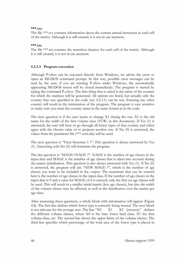
46 Alterra-rapport 1559
***.tvx The file ***.tvx contains information about the current annual increment in each cell of the matrix. Although it is still created, it is not in use anymore. ***.tra The file ***.tra contains the transition chances for each cell of the matrix. Although it is still created, it is not in use anymore. 4.2.3.3 Program execution
Although P-efsos can be executed directly from Windows, we advise the users to open an MS-DOS command prompt. In this way, possible error messages can be read by the user, if you are running P-efsos under Windows, the automatically apprearing MS-DOS screen will be closed immediately. The program is started by typing the command P_efsos. The first thing that is asked is the name of the country for which the matrices will be generated. All options are listed, but actually only the country that was specified in the code (see 4.2.3.1) can be run. Entering any other country will result in the termination of the program. The program is case sensitive so make sure you enter the country name in the same format as in the code. The next question is if the user wants to change X1 during the run. X1 is the old name for the width of the first volume class (VCW1 in this document). If Yes (1) is answered, the user will have to go through all forest types of that country and either agree with the chosen value or to propose another one. If No (0) is answered, the values from the parameter file (***-ecnt.dat) will be used. The next question is “Treat Structure 1 ?”. This question is always answered by Yes (1). Answering with No (0) will terminate the program. The last question is “MAGE=NAGE ?”. NAGE is the number of age classes in the input data and MAGE is the number of age classes that is taken into account during the matrix initialisation. This question is also always answered with Yes (1). If No (0) is answered, the program will ask “NEW MAGE ?”, which is the number of age classes you want to be included in the output. The maximum that can be entered here is the number of age classes in the input data. If the number of age classes in the input data is 9 and a value for MAGE of 6 is entered, only the first six age classes will be used. This will result in a smaller initial matrix (less age classes), but also the width of the volume classes may be affected, as well as the distribution over the matrix per age class. After answering these questions, a whole block with information will appear (Figure 4.8). The first line defines which forest type is currently being treated. The next block is not relevant for the average user. The line “X0 X1 X2 (etcetera)” defines the different volume classes, where X0 is the bare forest land class, X1 the first volume class, etc. The second line shows the upper limits of the volume classes. The third line specifies which percentage of the total area of the forest type is placed in
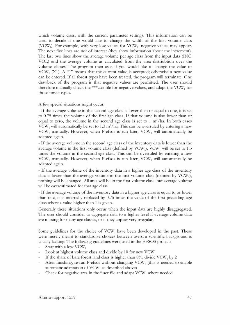
Alterra-rapport 1559 47
which volume class, with the current parameter settings. This information can be used to decide if one would like to change the width of the first volume class (VCW1). For example, with very low values for VCW1, negative values may appear. The next five lines are not of interest (they show information about the increment). The last two lines show the average volume per age class from the input data (ING VOL) and the average volume as calculated from the area distriubtion over the volume classes. The program then asks if you would like to change the value of VCW1 (X1). A “1” means that the current value is accepted; otherwise a new value can be entered. If all forest types have been treated, the program will terminate. One drawback of the program is that negative values are permitted. The user should therefore manually check the ***.aer file for negative values, and adapt the VCW1 for those forest types. A few special situations might occur: - If the average volume in the second age class is lower than or equal to one, it is set to 0.75 times the volume of the first age class. If that volume is also lower than or equal to zero, the volume in the second age class is set to 1 m3/ha. In both cases VCW1 will automatically be set to 1.3 m3/ha. This can be overruled by entering a new VCW1 manually. However, when P-efsos is run later, VCW1 will automatically be adapted again. - If the average volume in the second age class of the inventory data is lower than the average volume in the first volume class (defined by VCW1), VCW1 will be set to 1.3 times the volume in the second age class. This can be overruled by entering a new VCW1 manually. However, when P-efsos is run later, VCW1 will automatically be adapted again. - If the average volume of the inventory data in a higher age class of the inventory data is lower than the average volume in the first volume class (defined by VCW1), nothing will be changed. All area will be in the first volume class, but average volume will be overestimated for that age class. - If the average volume of the inventory data in a higher age class is equal to or lower than one, it is internally replaced by 0.75 times the value of the first preceding age class where a value higher than 1 is given. Generally these situations only occur when the input data are highly disaggregated. The user should consider to aggregate data to a higher level if average volume data are missing for many age classes, or if they appear very irregular. Some guidelines for the choice of VCW1 have been developed in the past. These were merely meant to standardize choices between users; a scientific background is usually lacking. The following guidelines were used in the EFSOS project: - Start with a low VCW1 - Look at highest volume class and divide by 10 for new VCW1 - If the share of bare forest land class is higher than 8%, divide VCW1 by 2 - After finishing, re-run P-efsos without changing VCW1 (this is needed to enable
automatic adaptation of VCW1 as described above) - Check for negative area in the *.aer file and adapt VCW1 where needed
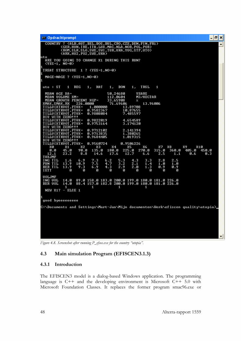
48 Alterra-rapport 1559
Figure 4.8. Screenshot after running P_efsos.exe for the country “utopia”. 4.3 Main simulation Program (EFISCEN3.1.3)
4.3.1 Introduction
The EFISCEN3 model is a dialog-based Windows application. The programming language is C++ and the developing environment is Microsoft C++ 5.0 with Microsoft Foundation Classes. It replaces the former program smac96.exe or
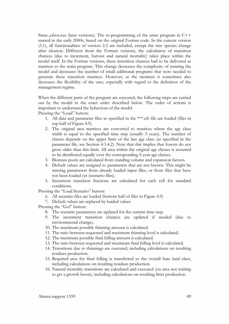
Alterra-rapport 1559 49
Smac_efsos.exe (later versions). The re-programming of the smac program in C++ started in the early 2000s, based on the original Fortran code. In the current version (3.1), all functionalities of version 2.2 are included, except the tree species change after clearcut. Different from the Fortran versions, the calculation of transition chances (due to increment, harvest and natural mortality) takes place within the model itself. In the Fortran versions, these transition chances had to be delivered as matrices to the main program. This change decreases the complexity of running the model and decreases the number of small additional programs that were needed to generate these transition matrices. However, at the moment it sometimes also decreases the flexibility of the user, especially with regard to the definition of the management regime. When the different parts of the program are executed, the following steps are carried out by the model in the exact order described below. The order of actions is important to understand the behaviour of the model. Pressing the “Load” button:
1. All data and parameter files as specified in the ***.efs file are loaded (files in top half of Figure 4.9).
2. The original area matrices are converted to matrices where the age class width is equal to the specified time step (usually 5 years). The number of classes depends on the upper limit of the last age class (as specified in the parameter file, see Section 4.3.4.2). Note that this implies that forests do not grow older than this limit. All area within the original age classes is assumed to be distributed equally over the corresponding 5-year age classes.
3. Biomass pools are calculated from standing volume and expansion factors. 4. Default values are assigned to parameters that are not known. This might be
missing parameters from already loaded input files, or from files that have not been loaded yet (scenario files).
5. Increment transition fractions are calculated for each cell for standard conditions.
Pressing the “Load Scenario” button: 6. All scenario files are loaded (bottom half of files in Figure 4.9) 7. Default values are replaced by loaded values
Pressing the “Go!” button: 8. The scenario parameters are updated for the current time step. 9. The increment transition chances are updated if needed (due to
environmental change). 10. The maximum possible thinning amount is calculated. 11. The ratio between requested and maximum thinning level is calculated. 12. The maximum possible final felling amount is calculated. 13. The ratio between requested and maximum final felling level is calculated. 14. Transitions due to thinnings are executed, including calculations on resulting
residues production. 15. Required area for final felling is transferred to the overall bare land class,
including calculations on resulting residues production. 16. Natural mortality transitions are calculated and executed (on area not waiting
to get a growth boost), including calculations on resulting litter production.
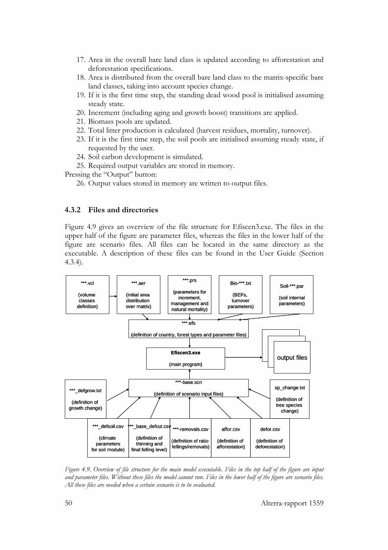
50 Alterra-rapport 1559
17. Area in the overall bare land class is updated according to afforestation and deforestation specifications.
18. Area is distributed from the overall bare land class to the matrix-specific bare land classes, taking into account species change.
19. If it is the first time step, the standing dead wood pool is initialised assuming steady state.
20. Increment (including aging and growth boost) transitions are applied. 21. Biomass pools are updated. 22. Total litter production is calculated (harvest residues, mortality, turnover). 23. If it is the first time step, the soil pools are initialised assuming steady state, if
requested by the user. 24. Soil carbon development is simulated. 25. Required output variables are stored in memory.
Pressing the “Output” button: 26. Output values stored in memory are written to output files.
4.3.2 Files and directories
Figure 4.9 gives an overview of the file structure for Efiscen3.exe. The files in the upper half of the figure are parameter files, whereas the files in the lower half of the figure are scenario files. All files can be located in the same directory as the executable. A description of these files can be found in the User Guide (Section 4.3.4).
***.aer
(initial area distribution over matrix)
***.vcl
(volume classes
definition)
Efiscen3.exe
(main program)
***.efs
(definition of country, forest types and parameter files)
***.prs
(parameters forincrement,
management andnatural mortality)
Bio-***.txt
(BEFs, turnover
parameters)
Soil-***.par
(soil internalparameters)
***-base.scn
(definition of scenario input files)
***_defsoil.csv
(climate parameters
for soil module)
***_defgrow.txt
(definition of growth change)
***_base_defcut.csv
(definition ofthinning and
final felling level)
***-removals.csv
(definition of ratio fellings/removals)
affor.csv
(definition of afforestation)
defor.csv
(definition of deforestation)
output files
sp_change.txt
(definition of tree species
change)
Figure 4.9. Overview of file structure for the main model executable. Files in the top half of the figure are input and parameter files. Without these files the model cannot run. Files in the lower half of the figure are scenario files. All these files are needed when a certain scenario is to be evaluated.
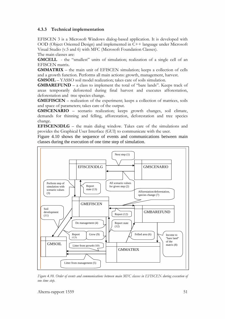
Alterra-rapport 1559 51
4.3.3 Technical implementation
EFISCEN 3 is a Microsoft Windows dialog-based application. It is developed with OOD (Object Oriented Design) and implemented in C++ language under Microsoft Visual Studio (v.5 and 6) with MFC (Microsoft Foundation Classes). The main classes are: GMCELL - the “smallest” units of simulation; realization of a single cell of an EFISCEN matrix. GMMATRIX – the main unit of EFISCEN simulation; keeps a collection of cells and a growth function. Performs all main actions: growth, management, harvest. GMSOIL – YASSO soil model realization; takes care of soils simulation. GMBAREFUND – a class to implement the total of “bare lands”. Keeps track of areas temporarily deforested during final harvest and executes afforestation, deforestation and tree species change. GMEFISCEN – realization of the experiment; keeps a collection of matrices, soils and space of parameters; takes care of the output. GMSCENARIO – scenario realization; keeps growth changes, soil climate, demands for thinning and felling, afforestation, deforestation and tree species change. EFISCEN3DLG – the main dialog window. Takes care of the simulations and provides the Graphical User Interface (GUI) to communicate with the user. Figure 4.10 shows the sequence of events and communications between main classes during the execution of one time step of simulation.
Figure 4.10. Order of events and communications between main MFC classes in EFISCEN during execution of one time step.
EFISCEN3DLG GMSCENARIO
GMEFISCEN
GMMATRIX GMSOIL
GMBAREFUND
Next step (1)
All scenario values for given step (2)
Perform step of simulation with scenario values (3)
Do management (4)
Litter from management (5)
Grow (9)
Litter from growth (10)
Felled area (6)
Afforestation/deforestation, species change (7)
Income to ”bare land” of the matrix (8)
Soil development (11)
Report (12)
Report state (12)
Report (12)
Report state (13)
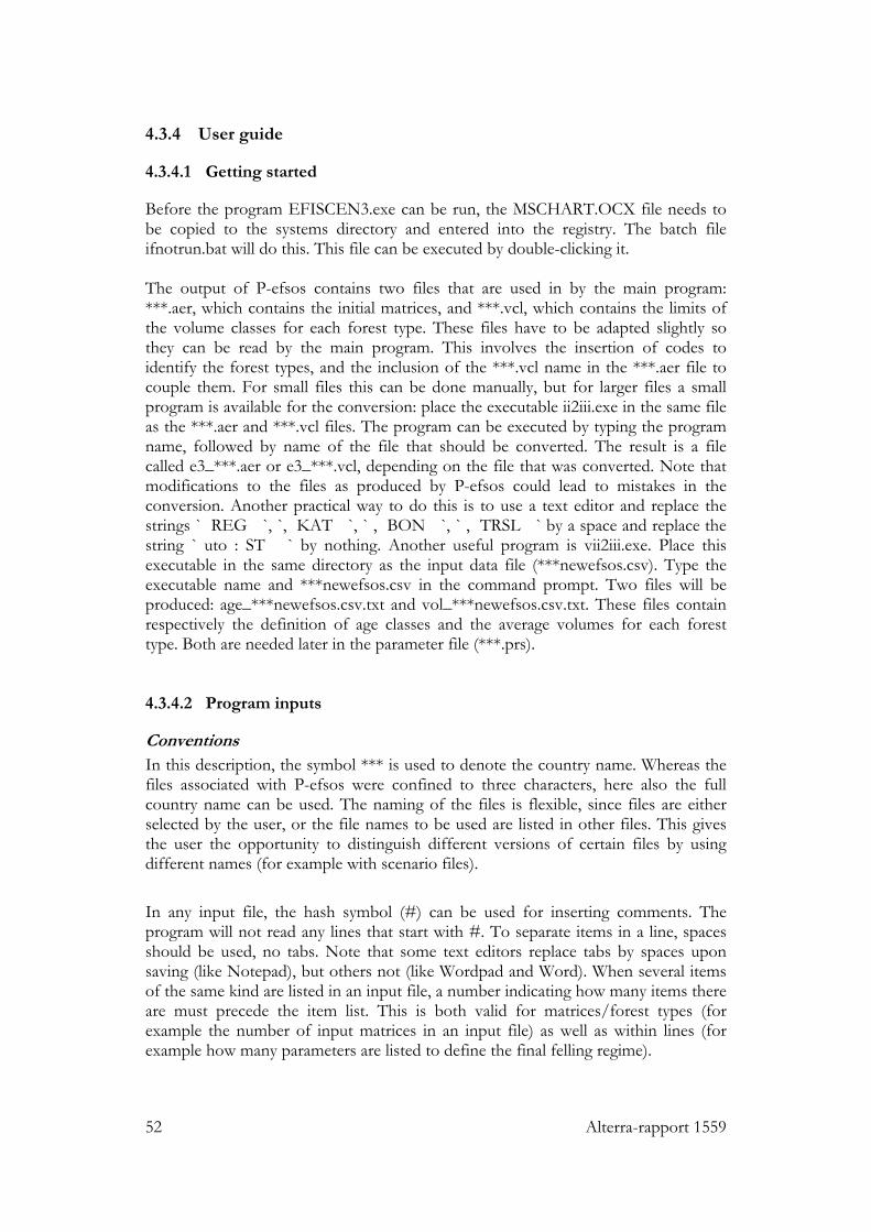
52 Alterra-rapport 1559
4.3.4 User guide
4.3.4.1 Getting started
Before the program EFISCEN3.exe can be run, the MSCHART.OCX file needs to be copied to the systems directory and entered into the registry. The batch file ifnotrun.bat will do this. This file can be executed by double-clicking it. The output of P-efsos contains two files that are used in by the main program: ***.aer, which contains the initial matrices, and ***.vcl, which contains the limits of the volume classes for each forest type. These files have to be adapted slightly so they can be read by the main program. This involves the insertion of codes to identify the forest types, and the inclusion of the ***.vcl name in the ***.aer file to couple them. For small files this can be done manually, but for larger files a small program is available for the conversion: place the executable ii2iii.exe in the same file as the ***.aer and ***.vcl files. The program can be executed by typing the program name, followed by name of the file that should be converted. The result is a file called e3_***.aer or e3_***.vcl, depending on the file that was converted. Note that modifications to the files as produced by P-efsos could lead to mistakes in the conversion. Another practical way to do this is to use a text editor and replace the strings ` REG `, `, KAT `, ` , BON `, ` , TRSL ` by a space and replace the string ` uto : ST ` by nothing. Another useful program is vii2iii.exe. Place this executable in the same directory as the input data file (***newefsos.csv). Type the executable name and ***newefsos.csv in the command prompt. Two files will be produced: age_***newefsos.csv.txt and vol_***newefsos.csv.txt. These files contain respectively the definition of age classes and the average volumes for each forest type. Both are needed later in the parameter file (***.prs). 4.3.4.2 Program inputs
Conventions In this description, the symbol *** is used to denote the country name. Whereas the files associated with P-efsos were confined to three characters, here also the full country name can be used. The naming of the files is flexible, since files are either selected by the user, or the file names to be used are listed in other files. This gives the user the opportunity to distinguish different versions of certain files by using different names (for example with scenario files). In any input file, the hash symbol (#) can be used for inserting comments. The program will not read any lines that start with #. To separate items in a line, spaces should be used, no tabs. Note that some text editors replace tabs by spaces upon saving (like Notepad), but others not (like Wordpad and Word). When several items of the same kind are listed in an input file, a number indicating how many items there are must precede the item list. This is both valid for matrices/forest types (for example the number of input matrices in an input file) as well as within lines (for example how many parameters are listed to define the final felling regime).
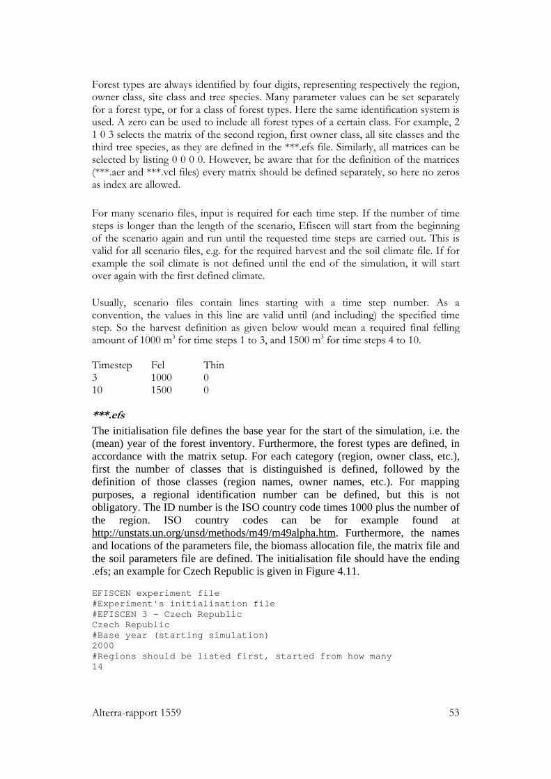
Alterra-rapport 1559 53
Forest types are always identified by four digits, representing respectively the region, owner class, site class and tree species. Many parameter values can be set separately for a forest type, or for a class of forest types. Here the same identification system is used. A zero can be used to include all forest types of a certain class. For example, 2 1 0 3 selects the matrix of the second region, first owner class, all site classes and the third tree species, as they are defined in the ***.efs file. Similarly, all matrices can be selected by listing 0 0 0 0. However, be aware that for the definition of the matrices (***.aer and ***.vcl files) every matrix should be defined separately, so here no zeros as index are allowed. For many scenario files, input is required for each time step. If the number of time steps is longer than the length of the scenario, Efiscen will start from the beginning of the scenario again and run until the requested time steps are carried out. This is valid for all scenario files, e.g. for the required harvest and the soil climate file. If for example the soil climate is not defined until the end of the simulation, it will start over again with the first defined climate. Usually, scenario files contain lines starting with a time step number. As a convention, the values in this line are valid until (and including) the specified time step. So the harvest definition as given below would mean a required final felling amount of 1000 m3 for time steps 1 to 3, and 1500 m3 for time steps 4 to 10. Timestep Fel Thin 3 1000 0 10 1500 0 ***.efs The initialisation file defines the base year for the start of the simulation, i.e. the (mean) year of the forest inventory. Furthermore, the forest types are defined, in accordance with the matrix setup. For each category (region, owner class, etc.), first the number of classes that is distinguished is defined, followed by the definition of those classes (region names, owner names, etc.). For mapping purposes, a regional identification number can be defined, but this is not obligatory. The ID number is the ISO country code times 1000 plus the number of the region. ISO country codes can be for example found at http://unstats.un.org/unsd/methods/m49/m49alpha.htm. Furthermore, the names and locations of the parameters file, the biomass allocation file, the matrix file and the soil parameters file are defined. The initialisation file should have the ending .efs; an example for Czech Republic is given in Figure 4.11. EFISCEN experiment file #Experiment's initialisation file #EFISCEN 3 - Czech Republic Czech Republic #Base year (starting simulation) 2000 #Regions should be listed first, started from how many 14
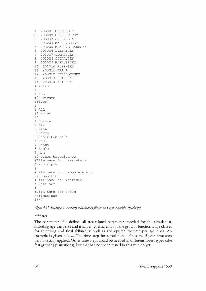
54 Alterra-rapport 1559
1 203001 BRENENSKY 2 203002 BUDEJOVICKY 3 203003 JIHLAVSKY 4 203004 KARLOVARSKY 5 203005 KRALOVEHRADECKY 6 203006 LIBERECKY 7 203007 OLOMOUCKY 8 203008 OSTRAVSKY 9 203009 PARDUBICKY 10 203010 PLZENSKY 11 203011 PRAHA 12 203012 STREDOCESKY 13 203013 USTECKY 14 203014 ZLINSKY #Owners 1 1 ALL #2 Private #Sites 1 1 ALL #Species 10 1 Spruce 2 Fir 3 Pine 4 Larch 5 Other_Conifers 6 Oak 7 Beech 8 Maple 9 Ash 10 Other_broadleaves #File name for parameters Czechia.prs # #File name for bioparameters biocomp.txt #File name for matrixes e3_cze.aer # #File name for soils soilcze.par #END Figure 4.11. Example of a country initialisation file for the Czech Republic (czechia.efs). ***.prs The parameters file defines all tree-related parameters needed for the simulation, including age class size and number, coefficients for the growth functions, age classes for thinnings and final fellings as well as the optimal volume per age class. An example is given below. The time step for simulation defines the 5-year time step that is usually applied. Other time steps could be needed in different forest types (like fast growing plantations), but that has not been tested in this version yet.
Alterra-rapport 1559 55
The number of age classes can be taken from the input data, and should correspond with the number of age classes in the ***.aer file. The lines that define the size of the age and volume classes are not in use. The growth function is defined by the three parameters a0, a1 and a2 (see Equation 8). Optionally, confidence intervals can be added, defining age limits for the application of the growth function. In that case, the minimum and maximum age must be given in addition to the growth function coefficients (see comment lines in example below). To define the final felling regime, the user can choose one out of two options: (1) giving the minimum age for final fellings; after reaching that age, all forest will be available for final felling or (2) to define the minimum age and the corresponding felling probability, the age at which the felling probability will reach 100%, and the felling probability for forest younger than the minimum age. In the example given below, the felling probability for the forest type is 10% for 81-year-old forests and 100% for 120-year-old forest. Between 81 and 120 years, linear interpolation is applied. Forests aged 65 to 81 can be cut with a felling probability of 1.5% (i.e. 1.5% of the forest in the corresponding matrix cells can be submitted to final fellings). For the thinning regime, the minimum and maximum age for thinnings is defined. So for the same forest type thinnings can be carried out when the forest is between 20 and 80 years old. When the age range of thinnings and final fellings overlap, part of the final fellings will not be found, even when there is enough volume available. The reason is that the model first calculates on which fraction of the available area thinnings and final fellings should be carried out, without taking into account the overlap. An area cannot be subjected to thinning and final felling in the same time step. Since thinnings are carried out first, less area is available for final fellings. However, the fraction to be subjected to final felling is not adapted to this change in available area. So it is good practice to have not too much overlap between the thinning and felling range. The volume series define the optimal volume per age class (see Section 3.2). This is difficult to determine, usually the values from the input data are copied (see also Section 4.3.4.5). Here, first the age class limits are defined for which the volume series are valid (AgeLims). These age class limits also define the age classes for the initial matrices, so they should also match the input data. Note that the maximum age defined here is used to define the upper limit of the age dimension in the matrix. Mortality can be defined by forest type and age class. In the example in Figure 4.12, 2% of the volume in forests up to 80 years will die due to natural mortality each time step. This 2% is converted into area transitions, depending on the average growing stock volume per volume class. The corresponding volume will move to a dead wood pool; it is assumed that the trees remain standing for a while. The dead wood
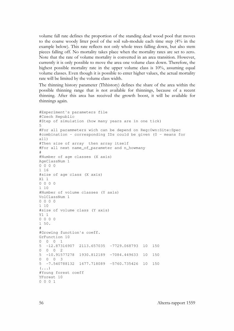
56 Alterra-rapport 1559
volume fall rate defines the proportion of the standing dead wood pool that moves to the coarse woody litter pool of the soil sub-module each time step (4% in the example below). This rate reflects not only whole trees falling down, but also stem pieces falling off. No mortality takes place when the mortality rates are set to zero. Note that the rate of volume mortality is converted in an area transition. However, currently it is only possible to move the area one volume class down. Therefore, the highest possible mortality rate in the upper volume class is 10%, assuming equal volume classes. Even though it is possible to enter higher values, the actual mortality rate will be limited by the volume class width. The thinning history parameter (Thhistory) defines the share of the area within the possible thinning range that is not available for thinnings, because of a recent thinning. After this area has received the growth boost, it will be available for thinnings again. #Experiment's parameters file #Czech Republic #Step of simulation (how many years are in one tick) 5 #For all parammeters wich can be depend on Reg:Own:Site:Spec #combination - corresponding IDs could be given (0 - means for all) #Then size of array then array itself #For all next name_of_parameter and n_howmany # #Number of age classes (X axis) AgeClassNum 1 0 0 0 0 1 16 #size of age class (X axis) X1 1 0 0 0 0 1 10 #Number of volume classes (Y axis) VolClassNum 1 0 0 0 0 1 10 #size of volume class (Y axis) Y1 1 0 0 0 0 1 50. # #Growing function's coeff. GrFunction 10 0 0 0 1 5 -12.87316907 2113.657035 -7729.068793 10 150 0 0 0 2 5 -10.91577278 1930.812189 -7084.449633 10 150 0 0 0 3 5 -7.540788132 1677.718089 -5760.735426 10 150 (...) #Young forest coeff YForest 10 0 0 0 1
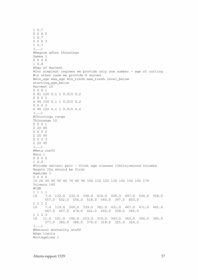
Alterra-rapport 1559 57
1 0.7 0 0 0 2 1 0.7 0 0 0 3 1 0.7 (...) #Regrow after thinnings Gamma 1 0 0 0 0 1 0.4 #Age of Harvest #for simplest regimes we provide only one number - age of cutting #in other case we provide 6 values #min_age max_age min_tresh max_tresh level_below starting_age_below Harvest 10 0 0 0 1 6 81 120 0.1 1 0.015 0.2 0 0 0 2 6 96 150 0.1 1 0.015 0.2 0 0 0 3 6 96 120 0.1 1 0.015 0.2 (...) #Thinnings range Thinrange 10 0 0 0 1 2 20 80 0 0 0 2 2 20 95 0 0 0 3 2 20 95 (...) #Beta coeff Beta 1 0 0 0 0 1 0.4 #Volume series: pair - first age classes limits;second volumes #again IDs should be first AgeLims 1 0 0 0 0 16 20 30 40 50 60 70 80 90 100 110 120 130 140 150 160 170 Volsers 140 #CZE 1 1 1 1 16 7.4 132.0 232.0 338.0 410.0 458.0 497.0 534.0 558.0
557.0 552.0 554.0 518.0 560.0 397.0 403.0 1 1 1 2 16 7.4 119.0 260.0 339.0 381.0 431.0 467.0 471.0 481.0
467.0 457.0 476.0 441.0 455.0 339.0 365.0 1 1 1 3 16 11.6 101.0 186.0 253.0 310.0 343.0 363.0 366.0 365.0
377.0 385.0 388.0 374.0 318.0 325.0 324.0 (...) #Natural mortality stuff #Age limits MortAgeLims 1

58 Alterra-rapport 1559
0 0 0 0 4 80 100 120 200 #now rates MortRates 1 0 0 0 0 4 0.02 0.04 0.1 0.25 #Dead wood volume fall rate Decay 1 0 0 0 0 1 0.04 #Thinnings history Thhistory 1 0 0 0 0 1 0.2 #to be continued... #END Figure 4.12. Example of parameter input file for Czech Republic (Czechia.prs). Note that only 3 forest types are shown for management regimes, young forest coefficient and optimal volume series. Data left out is indicated by (…). Biocomp-***.txt This file defines the parameters for carbon content, dry wood density, biomass allocation, and litter production. Each of these can be defined by region, species, owner and site class. Biomass allocation and litter production are age-specific and have to be defined for five tree compartments: stem, branches, coarse roots, fine roots and foliage. Biomass allocation values are shares of the total tree biomass and should add up to one. For example in Figure 4.13, in all spruce forest types (indicated by 0 0 0 1) the share of the stem in the total biomass is 38.52% in forests up to 30 years old. Branches account for 34.87%, coarse roots for 4.96%, fine roots for 5% and foliage for 16.65%. Litter production fractions define the proportion of the living biomass in a specific compartment that is added to the litter pool each year. In the example below, 0.43% of the stem biomass in spruce forests up to 30 years old is added to the soil as litter, 2.7% of the coarse root biomass, etc. Please note here that these amounts are not taken away from that compartment, since this is not a flow model. The stem litter fall rate, for example, does not influence the simulated standing volume. The user should be aware of the potential overlap with mortality as defined in the parameters file. The mortality as defined there actually decreases the volume in the simulation. When mortality is defined in the parameter file, already most of the stem litterfall rate will be covered. Additional stem turnover as defined in the biocomp-***.txt would therefore only cover parts of the stem that die, for example bark. However, a litterfall rate of zero seems appropriate in most cases. #Allocation of Biomass by compartments and litter production (Czech Republic)
#Almost same as in parameters file
#first Carbon content
Carbon 1
#All All All All
0 0 0 0
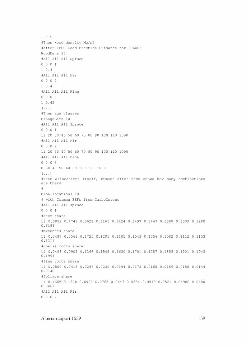
Alterra-rapport 1559 59
1 0.5
#Then wood density Mg/m3
#after IPCC Good Practice Guidance for LULUCF
WoodDens 10
#All All All Spruce
0 0 0 1
1 0.4
#All All All Fir
0 0 0 2
1 0.4
#All All All Pine
0 0 0 3
1 0.42
(...)
#Then age classes
BioAgeLims 10
#All All All Spruce
0 0 0 1
11 20 30 40 50 60 70 80 90 100 110 1000
#All All All Fir
0 0 0 2
11 20 30 40 50 60 70 80 90 100 110 1000
#All All All Pine
0 0 0 3
8 30 40 50 60 80 100 120 1000
(...)
#Then allocations itself, number after name shows how many combinations are there
#
BioAllocations 10
# with German BEFs from CarboInvent
#All All All spruce
0 0 0 1
#stem share
11 0.3852 0.4743 0.5622 0.6165 0.6424 0.6497 0.6443 0.6388 0.6339 0.6280 0.6188
#branches share
11 0.3487 0.2561 0.1725 0.1295 0.1105 0.1043 0.1056 0.1082 0.1112 0.1153 0.1211
#coarse roots share
11 0.0496 0.0905 0.1366 0.1545 0.1630 0.1701 0.1787 0.1853 0.1901 0.1943 0.1994
#fine roots share
11 0.0500 0.0413 0.0297 0.0230 0.0194 0.0175 0.0165 0.0156 0.0150 0.0144 0.0140
#foliage share
11 0.1665 0.1378 0.0990 0.0765 0.0647 0.0584 0.0549 0.0521 0.04980 0.0480 0.0467
#All All All Fir
0 0 0 2
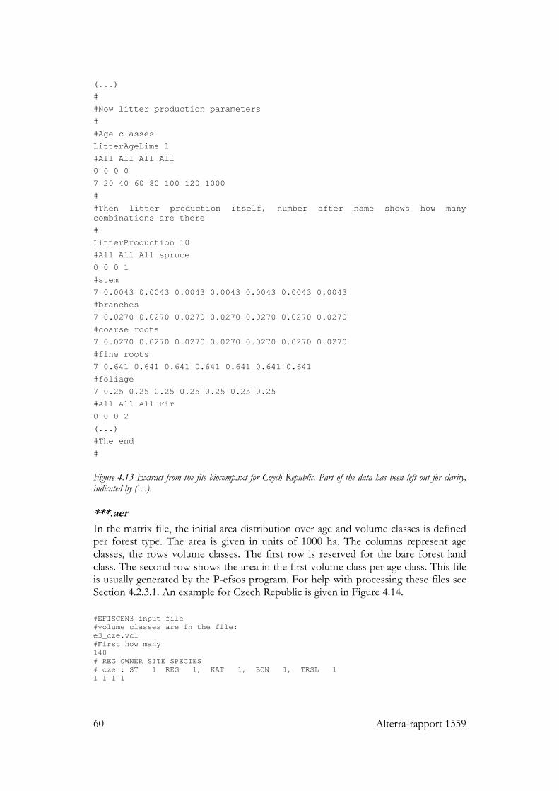
60 Alterra-rapport 1559
(...)
#
#Now litter production parameters
#
#Age classes
LitterAgeLims 1
#All All All All
0 0 0 0
7 20 40 60 80 100 120 1000
#
#Then litter production itself, number after name shows how many combinations are there
#
LitterProduction 10
#All All All spruce
0 0 0 1
#stem
7 0.0043 0.0043 0.0043 0.0043 0.0043 0.0043 0.0043
#branches
7 0.0270 0.0270 0.0270 0.0270 0.0270 0.0270 0.0270
#coarse roots
7 0.0270 0.0270 0.0270 0.0270 0.0270 0.0270 0.0270
#fine roots
7 0.641 0.641 0.641 0.641 0.641 0.641 0.641
#foliage
7 0.25 0.25 0.25 0.25 0.25 0.25 0.25
#All All All Fir
0 0 0 2
(...)
#The end
#
Figure 4.13 Extract from the file biocomp.txt for Czech Republic. Part of the data has been left out for clarity, indicated by (…). ***.aer In the matrix file, the initial area distribution over age and volume classes is defined per forest type. The area is given in units of 1000 ha. The columns represent age classes, the rows volume classes. The first row is reserved for the bare forest land class. The second row shows the area in the first volume class per age class. This file is usually generated by the P-efsos program. For help with processing these files see Section 4.2.3.1. An example for Czech Republic is given in Figure 4.14. #EFISCEN3 input file #volume classes are in the file: e3_cze.vcl #First how many 140 # REG OWNER SITE SPECIES # cze : ST 1 REG 1, KAT 1, BON 1, TRSL 1 1 1 1 1
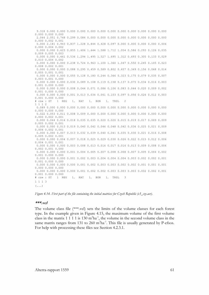
Alterra-rapport 1559 61
9.318 0.000 0.000 0.000 0.000 0.000 0.000 0.000 0.000 0.000 0.000 0.000 0.000 0.000 0.000 0.000 2.064 2.051 0.748 0.299 0.084 0.000 0.000 0.000 0.000 0.000 0.000 0.000 0.000 0.000 0.002 0.001 0.000 2.181 0.943 0.837 1.228 0.844 0.428 0.097 0.000 0.000 0.000 0.000 0.006 0.000 0.004 0.002 0.000 0.000 0.625 0.855 1.606 1.644 1.588 1.712 1.054 0.586 0.293 0.126 0.035 0.009 0.005 0.003 0.000 0.000 0.461 0.536 1.294 1.495 1.527 1.695 1.312 0.693 0.305 0.133 0.029 0.010 0.004 0.002 0.000 0.000 0.000 0.238 0.724 0.963 1.100 1.360 1.047 0.550 0.245 0.105 0.023 0.008 0.002 0.001 0.000 0.000 0.000 0.088 0.295 0.459 0.589 0.802 0.657 0.349 0.156 0.068 0.014 0.005 0.001 0.001 0.000 0.000 0.000 0.055 0.128 0.180 0.244 0.366 0.323 0.175 0.079 0.035 0.007 0.003 0.001 0.000 0.000 0.000 0.000 0.030 0.089 0.108 0.119 0.158 0.137 0.075 0.034 0.016 0.003 0.001 0.000 0.000 0.000 0.000 0.000 0.008 0.044 0.071 0.086 0.106 0.083 0.044 0.020 0.009 0.002 0.001 0.000 0.000 0.000 0.000 0.000 0.001 0.013 0.034 0.061 0.103 0.097 0.056 0.026 0.012 0.003 0.001 0.000 0.000 # cze : ST 1 REG 1, KAT 1, BON 1, TRSL 2 1 1 1 2 0.089 0.000 0.000 0.000 0.000 0.000 0.000 0.000 0.000 0.000 0.000 0.000 0.000 0.000 0.000 0.000 0.022 0.053 0.011 0.008 0.009 0.000 0.000 0.000 0.000 0.000 0.000 0.000 0.000 0.000 0.002 0.001 0.000 0.044 0.016 0.018 0.035 0.035 0.020 0.020 0.015 0.019 0.017 0.009 0.009 0.005 0.002 0.001 0.000 0.000 0.013 0.019 0.040 0.042 0.046 0.048 0.042 0.036 0.025 0.021 0.009 0.006 0.002 0.001 0.000 0.000 0.007 0.013 0.032 0.039 0.040 0.041 0.035 0.030 0.021 0.016 0.008 0.005 0.002 0.001 0.000 0.000 0.004 0.007 0.018 0.025 0.029 0.030 0.026 0.022 0.015 0.012 0.006 0.004 0.001 0.001 0.000 0.000 0.000 0.003 0.008 0.013 0.016 0.017 0.016 0.013 0.009 0.008 0.004 0.002 0.001 0.000 0.000 0.000 0.000 0.001 0.004 0.005 0.007 0.008 0.008 0.007 0.005 0.004 0.002 0.001 0.000 0.000 0.000 0.000 0.000 0.001 0.002 0.003 0.004 0.004 0.004 0.003 0.002 0.002 0.001 0.001 0.000 0.000 0.000 0.000 0.000 0.000 0.001 0.002 0.003 0.003 0.002 0.002 0.001 0.001 0.001 0.000 0.000 0.000 0.000 0.000 0.000 0.000 0.001 0.002 0.002 0.003 0.003 0.003 0.002 0.002 0.001 0.001 0.000 0.000 # cze : ST 1 REG 1, KAT 1, BON 1, TRSL 3
1 1 1 3
(...)
Figure 4.14. First part of the file containing the initial matrices for Czech Republic (e3_cze.aer). ***.vcl The volume class file (***.vcl) sets the limits of the volume classes for each forest type. In the example given in Figure 4.15, the maximum volume of the first volume class in the matrix 1 1 1 1 is 130 m3ha-1, the volume in the second volume class in the same matrix ranges from 131 to 260 m3ha-1. This file is usually generated by P-efsos. For help with processing these files see Section 4.2.3.1.
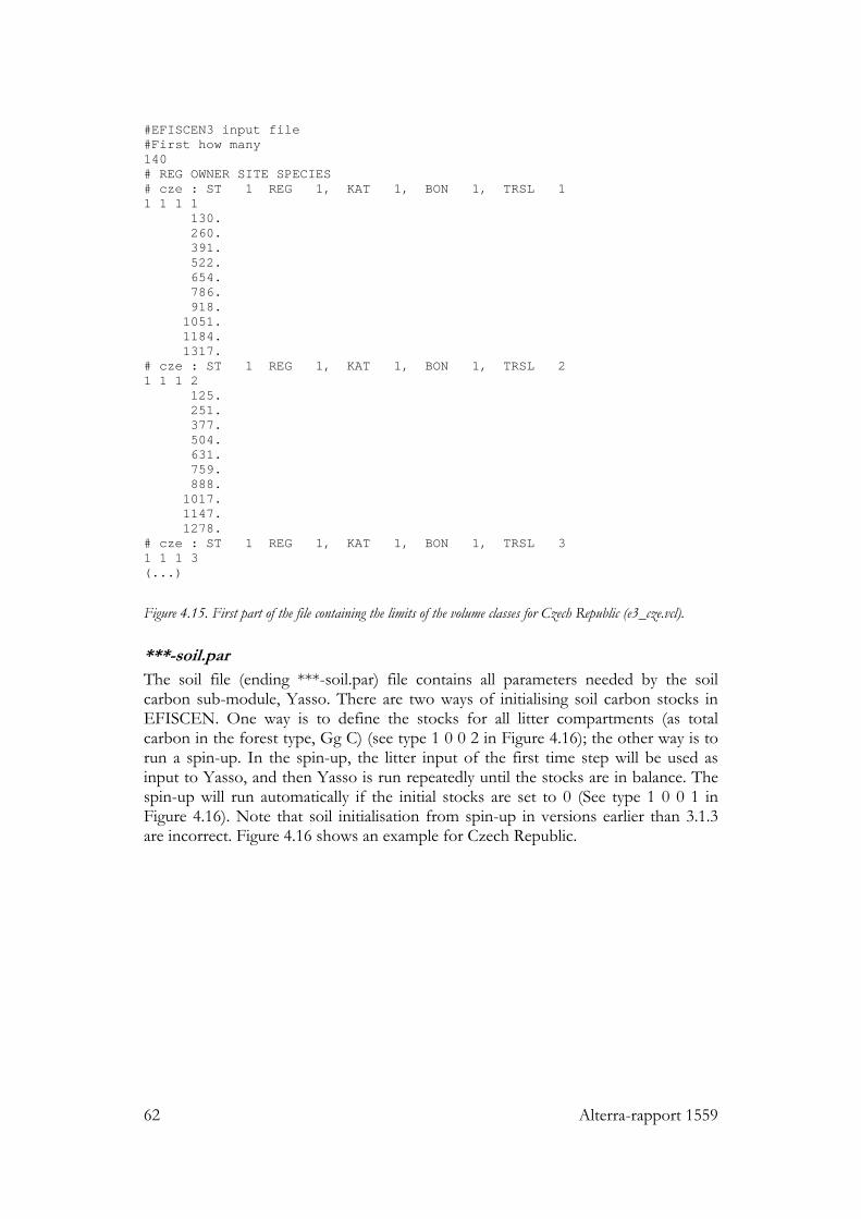
62 Alterra-rapport 1559
#EFISCEN3 input file #First how many 140 # REG OWNER SITE SPECIES # cze : ST 1 REG 1, KAT 1, BON 1, TRSL 1 1 1 1 1 130. 260. 391. 522. 654. 786. 918. 1051. 1184. 1317. # cze : ST 1 REG 1, KAT 1, BON 1, TRSL 2 1 1 1 2 125. 251. 377. 504. 631. 759. 888. 1017. 1147. 1278. # cze : ST 1 REG 1, KAT 1, BON 1, TRSL 3 1 1 1 3 (...)
Figure 4.15. First part of the file containing the limits of the volume classes for Czech Republic (e3_cze.vcl). ***-soil.par The soil file (ending ***-soil.par) file contains all parameters needed by the soil carbon sub-module, Yasso. There are two ways of initialising soil carbon stocks in EFISCEN. One way is to define the stocks for all litter compartments (as total carbon in the forest type, Gg C) (see type 1 0 0 2 in Figure 4.16); the other way is to run a spin-up. In the spin-up, the litter input of the first time step will be used as input to Yasso, and then Yasso is run repeatedly until the stocks are in balance. The spin-up will run automatically if the initial stocks are set to 0 (See type 1 0 0 1 in Figure 4.16). Note that soil initialisation from spin-up in versions earlier than 3.1.3 are incorrect. Figure 4.16 shows an example for Czech Republic.
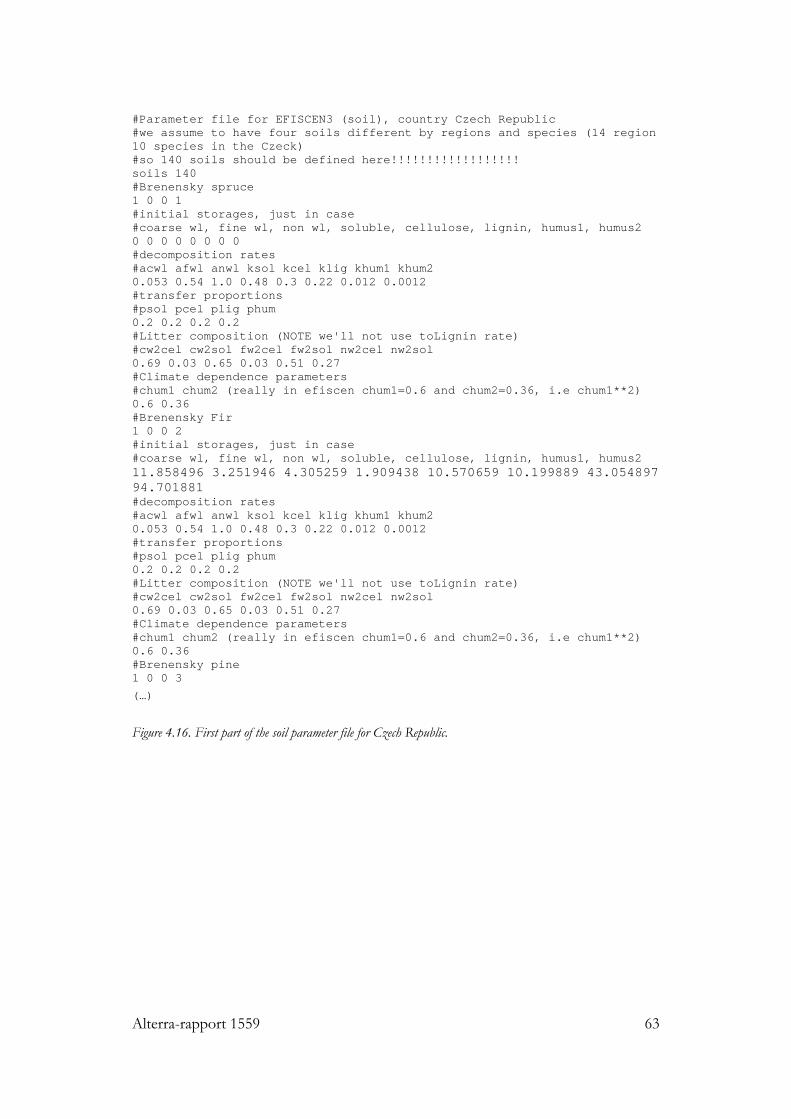
Alterra-rapport 1559 63
#Parameter file for EFISCEN3 (soil), country Czech Republic #we assume to have four soils different by regions and species (14 region 10 species in the Czeck) #so 140 soils should be defined here!!!!!!!!!!!!!!!!!! soils 140 #Brenensky spruce 1 0 0 1 #initial storages, just in case #coarse wl, fine wl, non wl, soluble, cellulose, lignin, humus1, humus2 0 0 0 0 0 0 0 0 #decomposition rates #acwl afwl anwl ksol kcel klig khum1 khum2 0.053 0.54 1.0 0.48 0.3 0.22 0.012 0.0012 #transfer proportions #psol pcel plig phum 0.2 0.2 0.2 0.2 #Litter composition (NOTE we'll not use toLignin rate) #cw2cel cw2sol fw2cel fw2sol nw2cel nw2sol 0.69 0.03 0.65 0.03 0.51 0.27 #Climate dependence parameters #chum1 chum2 (really in efiscen chum1=0.6 and chum2=0.36, i.e chum1**2) 0.6 0.36 #Brenensky Fir 1 0 0 2 #initial storages, just in case #coarse wl, fine wl, non wl, soluble, cellulose, lignin, humus1, humus2 11.858496 3.251946 4.305259 1.909438 10.570659 10.199889 43.054897 94.701881 #decomposition rates #acwl afwl anwl ksol kcel klig khum1 khum2 0.053 0.54 1.0 0.48 0.3 0.22 0.012 0.0012 #transfer proportions #psol pcel plig phum 0.2 0.2 0.2 0.2 #Litter composition (NOTE we'll not use toLignin rate) #cw2cel cw2sol fw2cel fw2sol nw2cel nw2sol 0.69 0.03 0.65 0.03 0.51 0.27 #Climate dependence parameters #chum1 chum2 (really in efiscen chum1=0.6 and chum2=0.36, i.e chum1**2) 0.6 0.36 #Brenensky pine 1 0 0 3
(…)
Figure 4.16. First part of the soil parameter file for Czech Republic.
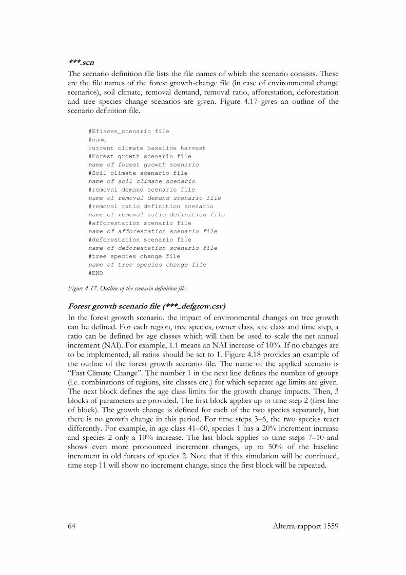
64 Alterra-rapport 1559
***.scn The scenario definition file lists the file names of which the scenario consists. These are the file names of the forest growth-change file (in case of environmental change scenarios), soil climate, removal demand, removal ratio, afforestation, deforestation and tree species change scenarios are given. Figure 4.17 gives an outline of the scenario definition file.
#Efiscen_scenario file #name current climate baseline harvest #Forest growth scenario file name of forest growth scenario #Soil climate scenario file name of soil climate scenario #removal demand scenario file name of removal demand scenario file #removal ratio definition scenario name of removal ratio definition file #afforestation scenario file name of afforestation scenario file #deforestation scenario file name of deforestation scenario file #tree species change file name of tree species change file #END
Figure 4.17. Outline of the scenario definition file. Forest growth scenario file (***_defgrow.csv) In the forest growth scenario, the impact of environmental changes on tree growth can be defined. For each region, tree species, owner class, site class and time step, a ratio can be defined by age classes which will then be used to scale the net annual increment (NAI). For example, 1.1 means an NAI increase of 10%. If no changes are to be implemented, all ratios should be set to 1. Figure 4.18 provides an example of the outline of the forest growth scenario file. The name of the applied scenario is “Fast Climate Change”. The number 1 in the next line defines the number of groups (i.e. combinations of regions, site classes etc.) for which separate age limits are given. The next block defines the age class limits for the growth change impacts. Then, 3 blocks of parameters are provided. The first block applies up to time step 2 (first line of block). The growth change is defined for each of the two species separately, but there is no growth change in this period. For time steps 3–6, the two species react differently. For example, in age class 41–60, species 1 has a 20% increment increase and species 2 only a 10% increase. The last block applies to time steps 7–10 and shows even more pronounced increment changes, up to 50% of the baseline increment in old forests of species 2. Note that if this simulation will be continued, time step 11 will show no increment change, since the first block will be repeated.
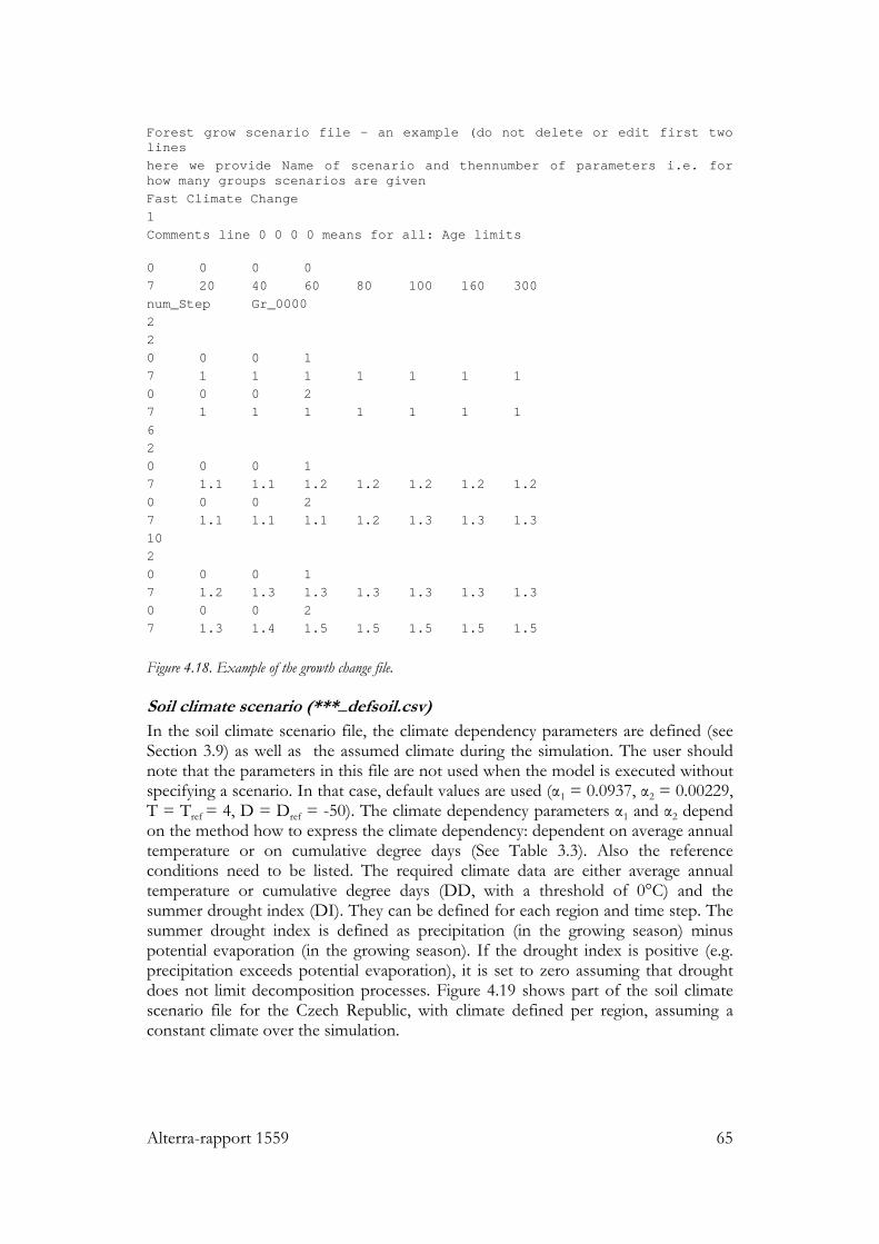
Alterra-rapport 1559 65
Forest grow scenario file - an example (do not delete or edit first two lines here we provide Name of scenario and thennumber of parameters i.e. for how many groups scenarios are given Fast Climate Change 1 Comments line 0 0 0 0 means for all: Age limits 0 0 0 0 7 20 40 60 80 100 160 300 num_Step Gr_0000 2 2 0 0 0 1 7 1 1 1 1 1 1 1 0 0 0 2 7 1 1 1 1 1 1 1 6 2 0 0 0 1 7 1.1 1.1 1.2 1.2 1.2 1.2 1.2 0 0 0 2 7 1.1 1.1 1.1 1.2 1.3 1.3 1.3 10 2 0 0 0 1 7 1.2 1.3 1.3 1.3 1.3 1.3 1.3 0 0 0 2 7 1.3 1.4 1.5 1.5 1.5 1.5 1.5
Figure 4.18. Example of the growth change file. Soil climate scenario (***_defsoil.csv) In the soil climate scenario file, the climate dependency parameters are defined (see Section 3.9) as well as the assumed climate during the simulation. The user should note that the parameters in this file are not used when the model is executed without specifying a scenario. In that case, default values are used (α1 = 0.0937, α2 = 0.00229, T = Tref = 4, D = Dref = -50). The climate dependency parameters α1 and α2 depend on the method how to express the climate dependency: dependent on average annual temperature or on cumulative degree days (See Table 3.3). Also the reference conditions need to be listed. The required climate data are either average annual temperature or cumulative degree days (DD, with a threshold of 0°C) and the summer drought index (DI). They can be defined for each region and time step. The summer drought index is defined as precipitation (in the growing season) minus potential evaporation (in the growing season). If the drought index is positive (e.g. precipitation exceeds potential evaporation), it is set to zero assuming that drought does not limit decomposition processes. Figure 4.19 shows part of the soil climate scenario file for the Czech Republic, with climate defined per region, assuming a constant climate over the simulation.
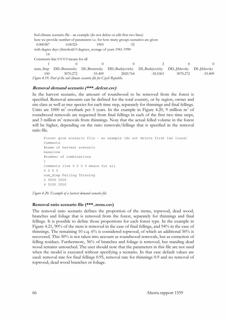
66 Alterra-rapport 1559
Soil climate scenario file - an example (do not delete or edit first two lines) here we provide number of parameters i.e. for how many groups scenarios are given
0.000387 0.00325 1903 -32 with degree days (threshold 0 degrees, average of years 1961-1990
14 Comments line 0 0 0 0 means for all
1 0 0 0 2 0 0num_Step DD_Brenensky DI_Brenensky DD_Budejovicky DI_Budejovicky DD_Jihlavsky DI_Jihlavsky
100 3070.272 -55.409 2820.764 -18.1063 3070.272 -55.409Figure 4.19. Part of the soil climate sceanrio file for Czech Republic. Removal demand scenario (***_defcut.csv) In the harvest scenario, the amount of roundwood to be removed from the forest is specified. Removal amounts can be defined for the total country, or by region, owner and site class as well as tree species for each time step, separately for thinnings and final fellings. Units are 1000 m3 overbark per 5 years. In the example in Figure 4.20, 9 million m3 of roundwood removals are requested from final fellings in each of the first two time steps, and 3 million m3 removals from thinnings. Note that the actual felled volume in the forest will be higher, depending on the ratio removals/fellings that is specified in the removal ratio file.
Forest grow scenario file - an example (do not delete first two lines) Comments #name of harvest scenario baseline #number of combinations 1 Comments line 0 0 0 0 means for all 0 0 0 0 num_Step Felling Thinning 2 9000 3000 4 9100 3050
Figure 4.20. Example of a harvest demand scenario file. Removal ratio scenario file (***_rems.csv)
The removal ratio scenario defines the proportion of the stems, topwood, dead wood, branches and foliage that is removed from the forest, separately for thinnings and final fellings. It is possible to define those proportions for each forest type. In the example in Figure 4.21, 90% of the stem is removed in the case of final fellings, and 94% in the case of thinnings. The remaining 10 c.q. 6% is considered topwood, of which an additional 50% is recovered. This 50% is not taken into account as roundwood removals, but as extraction of felling residues. Furthermore, 36% of branches and foliage is removed, but standing dead wood remains untouched. The user should note that the parameters in this file are not used when the model is executed without specifying a scenario. In that case default values are used: removal rate for final fellings 0.95, removal rate for thinnings 0.9 and no removal of topwood, dead wood branches or foliage.
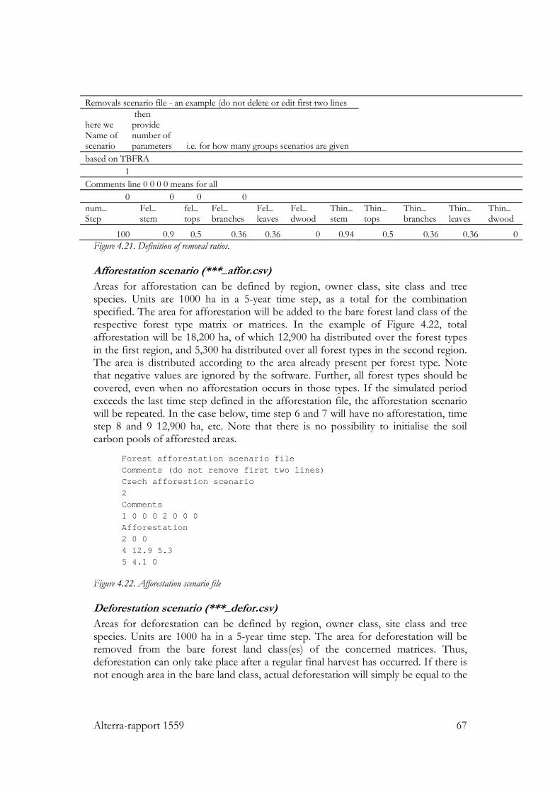
Alterra-rapport 1559 67
Removals scenario file - an example (do not delete or edit first two lines
here we Name of scenario
then provide number of parameters i.e. for how many groups scenarios are given
based on TBFRA 1
Comments line 0 0 0 0 means for all 0 0 0 0
num_ Step
Fel_ stem
fel_ tops
Fel_ branches
Fel_ leaves
Fel_ dwood
Thin_ stem
Thin_ tops
Thin_ branches
Thin_ leaves
Thin_ dwood
100 0.9 0.5 0.36 0.36 0 0.94 0.5 0.36 0.36 0Figure 4.21. Definition of removal ratios. Afforestation scenario (***_affor.csv) Areas for afforestation can be defined by region, owner class, site class and tree species. Units are 1000 ha in a 5-year time step, as a total for the combination specified. The area for afforestation will be added to the bare forest land class of the respective forest type matrix or matrices. In the example of Figure 4.22, total afforestation will be 18,200 ha, of which 12,900 ha distributed over the forest types in the first region, and 5,300 ha distributed over all forest types in the second region. The area is distributed according to the area already present per forest type. Note that negative values are ignored by the software. Further, all forest types should be covered, even when no afforestation occurs in those types. If the simulated period exceeds the last time step defined in the afforestation file, the afforestation scenario will be repeated. In the case below, time step 6 and 7 will have no afforestation, time step 8 and 9 12,900 ha, etc. Note that there is no possibility to initialise the soil carbon pools of afforested areas.
Forest afforestation scenario file Comments (do not remove first two lines) Czech afforestion scenario 2 Comments 1 0 0 0 2 0 0 0 Afforestation 2 0 0 4 12.9 5.3 5 4.1 0
Figure 4.22. Afforestation scenario file Deforestation scenario (***_defor.csv) Areas for deforestation can be defined by region, owner class, site class and tree species. Units are 1000 ha in a 5-year time step. The area for deforestation will be removed from the bare forest land class(es) of the concerned matrices. Thus, deforestation can only take place after a regular final harvest has occurred. If there is not enough area in the bare land class, actual deforestation will simply be equal to the
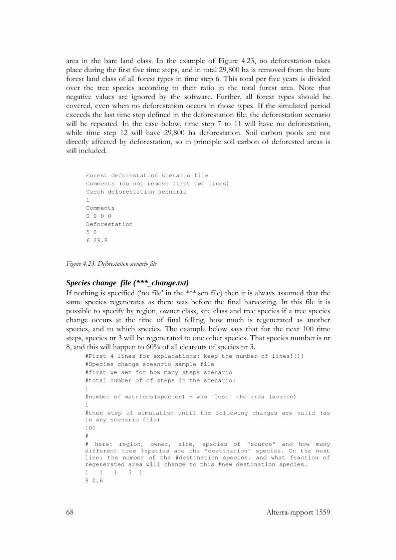
68 Alterra-rapport 1559
area in the bare land class. In the example of Figure 4.23, no deforestation takes place during the first five time steps, and in total 29,800 ha is removed from the bare forest land class of all forest types in time step 6. This total per five years is divided over the tree species according to their ratio in the total forest area. Note that negative values are ignored by the software. Further, all forest types should be covered, even when no deforestation occurs in those types. If the simulated period exceeds the last time step defined in the deforestation file, the deforestation scenario will be repeated. In the case below, time step 7 to 11 will have no deforestation, while time step 12 will have 29,800 ha deforestation. Soil carbon pools are not directly affected by deforestation, so in principle soil carbon of deforested areas is still included.
Forest deforestation scenario file Comments (do not remove first two lines) Czech deforestation scenario 1 Comments 0 0 0 0 Deforestation 5 0 6 29.8
Figure 4.23. Deforestation scenario file Species change file (***_change.txt) If nothing is specified (‘no file’ in the ***.scn file) then it is always assumed that the same species regenerates as there was before the final harvesting. In this file it is possible to specify by region, owner class, site class and tree species if a tree species change occurs at the time of final felling, how much is regenerated as another species, and to which species. The example below says that for the next 100 time steps, species nr 3 will be regenerated to one other species. That species number is nr 8, and this will happen to 60% of all clearcuts of species nr 3.
#First 4 lines for explanations: keep the number of lines!!!! #Species change sceanrio sample file #first we set for how many steps scenario #total number of of steps in the scenario: 1 #number of matrices(species) - who "lost" the area (source) 1 #then step of simulation until the following changes are valid (as in any scenario file) 100 # # here: region, owner, site, species of "source" and how many different tree #species are the "destination" species. On the next line: the number of the #destination species, and what fraction of regenerated area will change to this #new destination species. 1 1 1 3 1 8 0.6
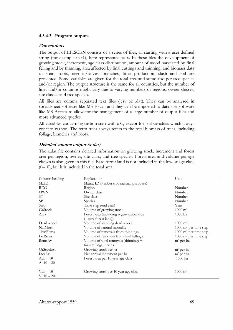
Alterra-rapport 1559 69
4.3.4.3 Program outputs
Conventions The output of EFISCEN consists of a series of files, all starting with a user defined string (for example test1), here represented as x. In these files the development of growing stock, increment, age class distribution, amount of wood harvested by final felling and by thinning, area affected by final cuttings and thinning, and biomass data of stem, roots, needles/leaves, branches, litter production, slash and soil are presented. Some variables are given for the total area and some also per tree species and/or region. The output structure is the same for all countries, but the number of lines and/or columns might vary due to varying numbers of regions, owner classes, site classes and tree species. All files are comma separated text files (.csv or .dat). They can be analysed in spreadsheet software like MS Excel, and they can be imported to database software like MS Access to allow for the management of a large number of output files and more advanced queries. All variables concerning carbon start with a C, except for soil variables which always concern carbon. The term trees always refers to the total biomass of trees, including foliage, branches and roots. Detailed volume output (x.dat) The x.dat file contains detailed information on growing stock, increment and forest area per region, owner, site class, and tree species. Forest area and volume per age classes is also given in this file. Bare forest land is not included in the lowest age class (0–10), but it is included in the total area. Column heading Explanation Unit M_ID Matrix ID number (for internal purposes) REG Region Number OWN Owner class Number ST Site class Number SP Species Number Step Time step (end year) Year GrStock Volume of growing stock 1000 m3 Area Forest area (including regeneration area
(=bare forest land)) 1000 ha
Dead wood Volume of standing dead wood 1000 m3 NatMort Volume of natural mortality 1000 m3 per time step ThinRems Volume of removals from thinnings 1000 m3 per time step FelRems Volume of removals from final fellings 1000 m3 per time step RemsAv Volume of total removals (thinnings +
final fellings) per ha m3 per ha
GrStockAv Growing stock per ha m3 per ha IncrAv Net annual increment per ha m3 per ha A_0 – 10 A_10 – 20 …
Forest area per 10 year age class 1000 ha
V_0 – 10 V_10 – 20…
Growing stock per 10 year age class 1000 m3
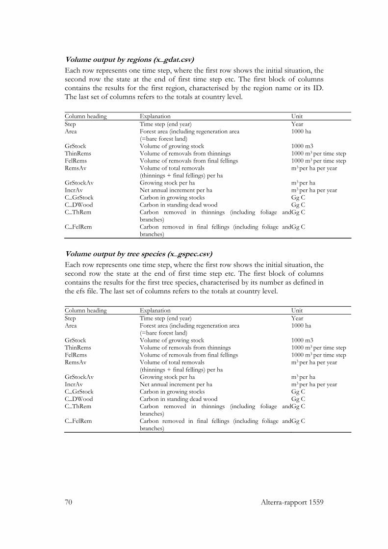
70 Alterra-rapport 1559
Volume output by regions (x_gdat.csv) Each row represents one time step, where the first row shows the initial situation, the second row the state at the end of first time step etc. The first block of columns contains the results for the first region, characterised by the region name or its ID. The last set of columns refers to the totals at country level. Column heading Explanation Unit Step Time step (end year) Year Area Forest area (including regeneration area
(=bare forest land) 1000 ha
GrStock Volume of growing stock 1000 m3 ThinRems Volume of removals from thinnings 1000 m3 per time step FelRems Volume of removals from final fellings 1000 m3 per time step RemsAv Volume of total removals
(thinnings + final fellings) per ha m3 per ha per year
GrStockAv Growing stock per ha m3 per ha IncrAv Net annual increment per ha m3 per ha per year C_GrStock Carbon in growing stocks Gg C C_DWood Carbon in standing dead wood Gg C C_ThRem Carbon removed in thinnings (including foliage and
branches) Gg C
C_FelRem Carbon removed in final fellings (including foliage andbranches)
Gg C
Volume output by tree species (x_gspec.csv) Each row represents one time step, where the first row shows the initial situation, the second row the state at the end of first time step etc. The first block of columns contains the results for the first tree species, characterised by its number as defined in the efs file. The last set of columns refers to the totals at country level. Column heading Explanation Unit Step Time step (end year) Year Area Forest area (including regeneration area
(=bare forest land) 1000 ha
GrStock Volume of growing stock 1000 m3 ThinRems Volume of removals from thinnings 1000 m3 per time step FelRems Volume of removals from final fellings 1000 m3 per time step RemsAv Volume of total removals
(thinnings + final fellings) per ha m3 per ha per year
GrStockAv Growing stock per ha m3 per ha IncrAv Net annual increment per ha m3 per ha per year C_GrStock Carbon in growing stocks Gg C C_DWood Carbon in standing dead wood Gg C C_ThRem Carbon removed in thinnings (including foliage and
branches) Gg C
C_FelRem Carbon removed in final fellings (including foliage andbranches)
Gg C
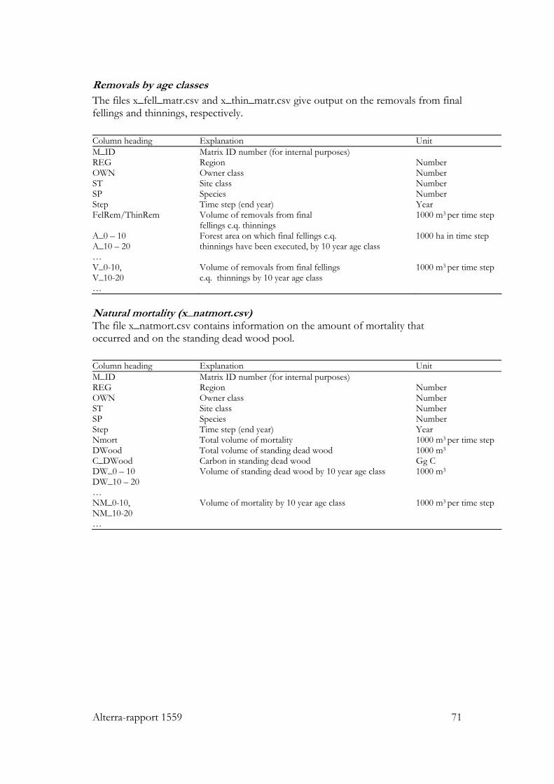
Alterra-rapport 1559 71
Removals by age classes The files x_fell_matr.csv and x_thin_matr.csv give output on the removals from final fellings and thinnings, respectively. Column heading Explanation Unit M_ID Matrix ID number (for internal purposes) REG Region Number OWN Owner class Number ST Site class Number SP Species Number Step Time step (end year) Year FelRem/ThinRem Volume of removals from final
fellings c.q. thinnings 1000 m3 per time step
A_0 – 10 A_10 – 20 …
Forest area on which final fellings c.q. thinnings have been executed, by 10 year age class
1000 ha in time step
V_0-10, V_10-20 …
Volume of removals from final fellings c.q. thinnings by 10 year age class
1000 m3 per time step
Natural mortality (x_natmort.csv) The file x_natmort.csv contains information on the amount of mortality that occurred and on the standing dead wood pool. Column heading Explanation Unit M_ID Matrix ID number (for internal purposes) REG Region Number OWN Owner class Number ST Site class Number SP Species Number Step Time step (end year) Year Nmort Total volume of mortality 1000 m3 per time step DWood Total volume of standing dead wood 1000 m3 C_DWood Carbon in standing dead wood Gg C DW_0 – 10 DW_10 – 20 …
Volume of standing dead wood by 10 year age class 1000 m3
NM_0-10, NM_10-20 …
Volume of mortality by 10 year age class 1000 m3 per time step
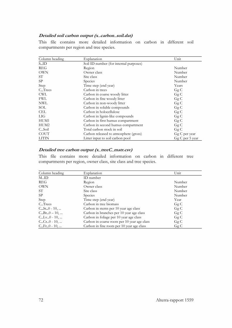
72 Alterra-rapport 1559
Detailed soil carbon output (x_carbon_soil.dat) This file contains more detailed information on carbon in different soil compartments per region and tree species. Column heading Explanation Unit S_ID Soil ID number (for internal purposes) REG Region Number OWN Owner class Number ST Site class Number SP Species Number Step Time step (end year) Years C_Trees Carbon in trees Gg C CWL Carbon in coarse woody litter Gg C FWL Carbon in fine woody litter Gg C NWL Carbon in non-woody litter Gg C SOL Carbon in soluble compounds Gg C CEL Carbon in holocellulose Gg C LIG Carbon in lignin-like compounds Gg C HUM1 Carbon in first humus compartment Gg C HUM2 Carbon in second humus compartment Gg C C_Soil Total carbon stock in soil Gg C COUT Carbon released to atmosphere (gross) Gg C per year LITIN Litter input to soil carbon pool Gg C per 5 year
Detailed tree carbon output (x_treeC_matr.csv) This file contains more detailed information on carbon in different tree compartments per region, owner class, site class and tree species. Column heading Explanation Unit M_ID ID number REG Region Number OWN Owner class Number ST Site class Number SP Species Number Step Time step (end year) Year C_Trees Carbon in tree biomass Gg C C_St_0 - 10, ... Carbon in stems per 10 year age class Gg C C_Br_0 – 10, ... Carbon in branches per 10 year age class Gg C C_Lv_0 - 10, ... Carbon in foliage per 10 year age class Gg C C_Cr_0 - 10, ... Carbon in coarse roots per 10 year age class Gg C C_Fr_0 - 10, ... Carbon in fine roots per 10 year age class Gg C
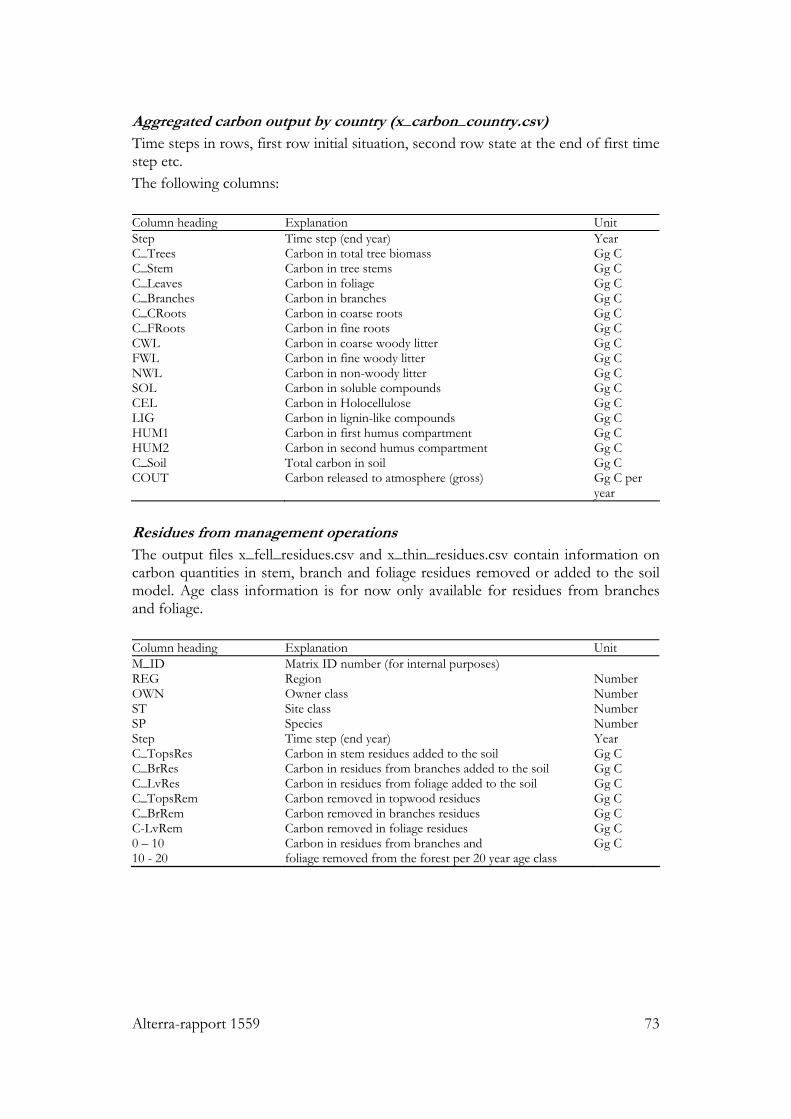
Alterra-rapport 1559 73
Aggregated carbon output by country (x_carbon_country.csv) Time steps in rows, first row initial situation, second row state at the end of first time step etc. The following columns: Column heading Explanation Unit Step Time step (end year) Year C_Trees Carbon in total tree biomass Gg C C_Stem Carbon in tree stems Gg C C_Leaves Carbon in foliage Gg C C_Branches Carbon in branches Gg C C_CRoots Carbon in coarse roots Gg C C_FRoots Carbon in fine roots Gg C CWL Carbon in coarse woody litter Gg C FWL Carbon in fine woody litter Gg C NWL Carbon in non-woody litter Gg C SOL Carbon in soluble compounds Gg C CEL Carbon in Holocellulose Gg C LIG Carbon in lignin-like compounds Gg C HUM1 Carbon in first humus compartment Gg C HUM2 Carbon in second humus compartment Gg C C_Soil Total carbon in soil Gg C COUT Carbon released to atmosphere (gross) Gg C per
year
Residues from management operations The output files x_fell_residues.csv and x_thin_residues.csv contain information on carbon quantities in stem, branch and foliage residues removed or added to the soil model. Age class information is for now only available for residues from branches and foliage. Column heading Explanation Unit M_ID Matrix ID number (for internal purposes) REG Region Number OWN Owner class Number ST Site class Number SP Species Number Step Time step (end year) Year C_TopsRes Carbon in stem residues added to the soil Gg C C_BrRes Carbon in residues from branches added to the soil Gg C C_LvRes Carbon in residues from foliage added to the soil Gg C C_TopsRem Carbon removed in topwood residues Gg C C_BrRem Carbon removed in branches residues Gg C C-LvRem Carbon removed in foliage residues Gg C 0 – 10 10 - 20
Carbon in residues from branches and foliage removed from the forest per 20 year age class
Gg C
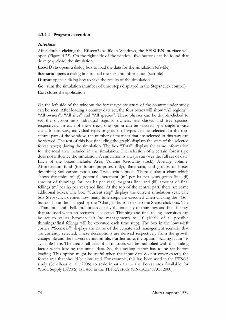
74 Alterra-rapport 1559
4.3.4.4 Program execution
Interface After double-clicking the Efiscen3.exe file in Windows, the EFISCEN interface will open (Figure 4.23). On the right side of the window, five buttons can be found that drive (c.q. close) the simulation: Load Data opens a dialog box to load the data for the simulation (efs-file) Scenario opens a dialog box to load the scenario information (scn-file) Output opens a dialog box to save the results of the simulation Go! runs the simulation (number of time steps displayed in the Steps/click control) Exit closes the application On the left side of the window the forest type structure of the country under study can be seen. After loading a country data set, the four boxes will show “All regions”, “All owners”, “All sites” and “All species”. These phrases can be double-clicked to see the division into individual regions, owners, site classes and tree species, respectively. In each of these trees, one option can be selected by a single mouse click. In this way, individual types or groups of types can be selected. In the top-central part of the window, the number of matrices that are selected in this way can be viewed. The rest of this box (including the graph) displays the state of the selected forest type(s) during the simulation. The box “Total” displays the same information for the total area included in the simulation. The selection of a certain forest type does not influence the simulation. A simulation is always run over the full set of data. Each of the boxes include: Area, Volume (Growing stock), Average volume, Afforestation fund (for future purposes only), Bare area, and groups of boxes describing Soil carbon pools and Tree carbon pools. There is also a chart which shows dynamics of: (i) potential increment (m3 per ha per year) green line; (ii) amount of thinnings (m3 per ha per year) magenta line; and (iii) amount of final fellings (m3 per ha per year) red line. At the top of the central part, there are some additional boxes. The box “Current step” displays the current simulation year. The box Steps/click defines how many time steps are executed when clicking the “Go” button. It can be changed by the “Change” button next to the Steps/click box. The “Thin. int.” and “Fell. int.” boxes display the intensity of thinnings and final fellings that are used when no scenario is selected. Thinning and final felling intensities can be set to values between 0.0 (no management) to 1.0 (100% of all possible thinnings/final fellings will be executed each time step). The box in the lower-left corner (“Scenario”) displays the name of the climate and management scenario that are currently selected. These descriptions are derived respectively from the growth change file and the harvest definition file. Furthermore, the option “Scaling factor” is available here. The area in all cells of all matrices will be multiplied with this scaling factor when loading the initial data. So, this scaling factor has to be set before loading. This option might be useful when the input data do not cover exactly the forest area that should be simulated. For example, this has been used in the EFSOS study (Schelhaas et al., 2006) to scale input data to the Forest area Available for Wood Supply (FAWS) as listed in the TBFRA study (UN-ECE/FAO, 2000).
Alterra-rapport 1559 75
Figure 4.23: The EFISCEN graphical user interface. Command line usage EFISCEN 3.1 can also run from command line, with or without specifying a scenario. In case no scenario is used, the syntax should be as following: Efiscen3.exe, number of steps, thinning rate, final felling rate, country description file(.efs), output file. By default, EFISCEN evaluates 5 time steps (“Steps/click” in Figure 4.23). The number of steps in the command line refers to how many times this should be evaluated, so how many times the “Go!” button would be clicked. The thinning rate and final felling rate have the same function as the “Thin. int.” and “Fell. int.” boxes in Figure 4.23. The command: Efiscen3.exe 5 1 0.5 uto\utopia.efs \uto\output\test.dat will run the efiscen model for utopia for 25 time steps, with all possible thinnings carried out and 50% of the final fellings. The output will be written to the directory “\output” as files starting with the string “test”. In case a scenario is used, the syntax should be as following:

76 Alterra-rapport 1559
Efiscen3.exe, number of steps, thinning rate, final felling rate, country description file(.efs), scenario name, output file, scaling factor. The parameters thinning rate and final felling rate are not used in this case, but should be present. The scaling factor is optional. 4.3.4.5 Additional programs
Several small additional programs have been developed to ease various tasks. They will not be described in detail here, but more information can be obtained from the development team ([email protected]). These programs can do the following: - Run the model for a specific scenario for the specified countries and use the
output of the first time step to create soil files with the initial data. - Run specified countries for specified scenarios - Run specified countries for all combinations of stepwise increasing rotation
lengths and stepwise increasing thinning shares - Read in specified output data for specified countries and group them into
broadleaves and conifers - Read in specified output data for specified countries, display the variables of
interest per country or accumulated over country groups - Sensitivity analysis: change one or more input parameters according to a
specified design, execute the model and store the data in a database. - Adapt harvest dynamically during a run, depending on the state and
development of the forest according to a specified formula

Alterra-rapport 1559 77
5 Validation of EFISCEN
Long-term forest projection models can be validated in various ways: 1) Validating the growth functions against growth functions of other models, 2) comparing the projections against other projections carried out for the same forests, 3) running the model on historic data and comparing the output to present day forest state. Comparison of growth functions Approach 1 has been applied by Sallnäs (1990) to the pre-EFISCEN version. He compared the growth as assessed in the area matrix approach with the growth function of the EKÖ model. The growth in the EKÖ model showed some differences with the growth in the (pre-) EFISCEN model, but these were explained by differences in input data. For the (pre-) EFISCEN model rather wide site classes were used. The site classes of the EKÖ model represented often extremes within these site classes. Moreover, the increment in the input data of (pre-) EFISCEN included some ‘poor’ years with increment values below average. The conclusion was that the overall growth level of the model is acceptable. Sterba (2003) compared the increment per volume class in EFISCEN 2.0 to increment in Bavarian yield tables for different stocking densities. He concluded that the relationships were quite similar, but only if the mean volume per age class as given in the input data really reflects the optimal density (optimum growing stock), as assumed in EFISCEN. If the mean volume in the input data is lower than the optimum density, deviations occur. Sterba concluded that EFISCEN seemed to depict Central European growth-densities quite well, provided that the mean volume per age class is close to the optimal density. Comparison to other projections Approach 2 has been tried by Nilsson et al. (1992) for European forests (Figure 5.1), by Päivinen et al (1998) for Leningrad Region forests and by Nabuurs et al. (1998) for a selected number of European countries. Nilsson et al. compared their results to the ETTS IV study and concluded that (pre-) EFISCEN did not consistently over- or underestimate growth in the countries. The differences with ETTS IV increment varied from almost 0% to +90% and -51%. Nilsson et al. explained these large differences found for Norway, Ireland, Italy and Luxembourg mainly being due to the difference in sources for input data. E.g. the small increment figure used for Ireland by Nilsson in the (pre-) EFISCEN model was probably caused by the fact that they had obtained only area data for Ireland. Volumes and thus increments had to be estimated from yield tables.
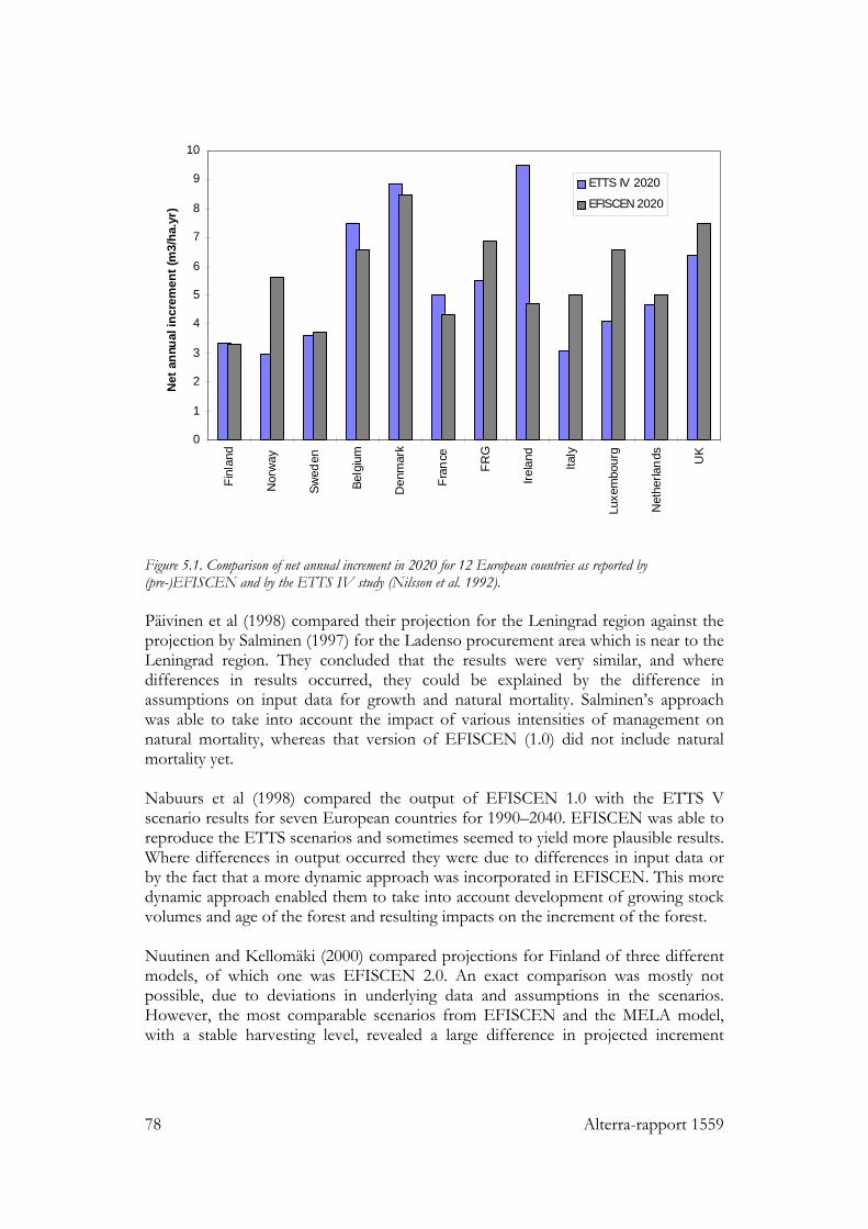
78 Alterra-rapport 1559
0
1
2
3
4
5
6
7
8
9
10
Finl
and
Nor
way
Swed
en
Belg
ium
Den
mar
k
Fran
ce
FRG
Irela
nd
Italy
Luxe
mbo
urg
Net
herla
nds
UK
Net
ann
ual i
ncre
men
t (m
3/ha
.yr)
ETTS IV 2020
EFISCEN 2020
Figure 5.1. Comparison of net annual increment in 2020 for 12 European countries as reported by (pre-)EFISCEN and by the ETTS IV study (Nilsson et al. 1992). Päivinen et al (1998) compared their projection for the Leningrad region against the projection by Salminen (1997) for the Ladenso procurement area which is near to the Leningrad region. They concluded that the results were very similar, and where differences in results occurred, they could be explained by the difference in assumptions on input data for growth and natural mortality. Salminen’s approach was able to take into account the impact of various intensities of management on natural mortality, whereas that version of EFISCEN (1.0) did not include natural mortality yet. Nabuurs et al (1998) compared the output of EFISCEN 1.0 with the ETTS V scenario results for seven European countries for 1990–2040. EFISCEN was able to reproduce the ETTS scenarios and sometimes seemed to yield more plausible results. Where differences in output occurred they were due to differences in input data or by the fact that a more dynamic approach was incorporated in EFISCEN. This more dynamic approach enabled them to take into account development of growing stock volumes and age of the forest and resulting impacts on the increment of the forest. Nuutinen and Kellomäki (2000) compared projections for Finland of three different models, of which one was EFISCEN 2.0. An exact comparison was mostly not possible, due to deviations in underlying data and assumptions in the scenarios. However, the most comparable scenarios from EFISCEN and the MELA model, with a stable harvesting level, revealed a large difference in projected increment
Alterra-rapport 1559 79
development and thus development of growing stock. EFISCEN projected a rather stable increment over time, whereas MELA projected an increasing increment with increasing growing stocks. The same was also noted by Nabuurs et al. (2000). Nuutinen and Kellomäki expected that the difference between the models would decrease with the introduction of a new self-thinning module in the MELA model. Application to historic data Approach 3 has been applied by Nabuurs et al. (2000) for Finland with EFISCEN 1.0, and by Thürig and Schelhaas (2006) for parts of Switzerland with EFISCEN 2.2. In the validation by Nabuurs et al. (2000), EFISCEN 1.0 was applied to Finland for the period 1921–1990. The initial situation was based on the results of the first national forest inventory, carried out in the years 1921–1924 (Ilvessalo 1927). Simulation results were then compared to corresponding later inventories. The most important conclusion, already noted in earlier studies, was that the increment gradually decreased over time. This decrease was a consequence of the interaction between thinnings and the way increment was calculated. Differences in increment level became apparent after 30–40 years, with visible consequences in growing stock levels after 50–60 years. In this case the simulated increments after 1963 deviated even more from the observed levels due to changes in management practices over time. Furthermore, deviations in age class structure occurred over time, most likely due to the fact that many stands in Finland were more or less unevenaged during the first half of the 20th century. Partial harvesting could thus influence the age of the stand, while the model could only leave the age as it was during a thinning, or regenerate the stand. A related problem is the use of advanced spruce regeneration under e.g. birch stands, which could not be simulated by the model. Another factor that influenced the deviations in age structure was the definition of the final felling regime. The chance that a stand would be harvested was only dependent on its age, and not its actual volume. This led in the simulation to rather low harvests per hectare, so much larger areas were needed to obtain the same felling level. Also the amount of forest that enters the matrix again from the bare forest land class (regulated by the so-called “young forest coefficient”) was questioned, and it also influences the age class distribution. It was concluded that due to the dynamic structure of the model, negative feedbacks can occur, which might cause deviations to enlarge over time. Another conclusion of the validation was that the results at a national level were fairly close to the observed levels, but that results at a lower level (per species and region) showed much more deviation. An important reason for this seemed to be the allocation of harvest over the regions and within the tree species groups. This allocation is largely depending on the definition of the final felling regime, but also influenced by the actual state (and development) of the resource in the range of cells that can be subjected to harvesting. Thürig and Schelhaas (2006) tested the performance of EFISCEN 2.2 in Switzerland. Firstly, they compared the matrix as initialised by EFISCEN with the original plot data from the second Swiss National Forest Inventory. The result of this comparison was in general satisfying. The largest deviations occurred in poor sites in the Alps region. This was attributed to the fact that forests on such sites usually have a
80 Alterra-rapport 1559
protective rather than a productive function. Such stands are generally managed in an unevenaged way, leading to a different distribution of growing stocks over age than in case of forests that are managed in a truly evenaged way. Secondly, they simulated the forest resource development for the canton Bern for different sets and time spans of inventory plots where repeated measurements were available. On the aggregated (national) level the model produced results comparable to the observed values. However, at a more detailed (forest type) level results deviated sometimes considerably, e.g. in terms of the thinning percentages, the distribution of the harvesting amount among the regions, the age class distribution, and the mortality. Thürig and Schelhaas concluded that detailed data, for example plot level data, could help to pinpoint sources of differences and improve simulation results at a more detailed level. Moreover, they concluded that the current structure of the model is not suitable to simulate the unevenaged, selective management as practised in the Alpine region. Discussion The results of approaches 1 and 2 show that the results of EFISCEN are more or less in line with other simulation models and projection studies. Where deviations occurred, likely explanations could be found. However, such comparisons are rather quantitative and only compare one model to the other. Approach 3 can be seen as the most reliable way of validation. From the Finnish validation, the most important conclusion was the observed decline in projected increment in EFISCEN 1.0. After this validation, increment and thinning processes have been adapted. In the Swiss validation, no decline in increment levels was observed, but the longest time series was only 30 years, which is most likely too short to observe such a trend. Although it is likely that the changes in the way thinnings and increment are handled will result in better increment levels in the long term, this has not really been proven by the validation. It is therefore very difficult to indicate a time horizon where the model will still give plausible results. Given the fact that no serious increment deviations occurred in 30 years in the Swiss case, the conclusions of the Finnish validation study will still be valid that up to about 50 years growing stock levels will be rather reliable. Both validations concluded that national simulation results were acceptable, but that results at lower levels (species, regions) showed considerable deviations. In the Finnish case, this was partly attributed to a lack of possibilities to include more detailed data in the model (for example harvest levels per region and tree species, instead of national per species group). In the Swiss case, such data was assumed not to be available, and additionally, harvest levels could still only be defined at the national level. The allocation of the harvest was thus totally depending on the definition of the assumed management regimes. Clearly the definition of these regimes did not reflect reality very well. In general, the Swiss validation study showed no major defects of the model in evenaged situations, but highlighted the importance of a proper parameterisation of the model. If regional outcomes are going to be used, much attention should be given to parameterisation at the regional level. Furthermore, both validations show that application of the model to situations other than evenaged forests should be done with great care. For shorter periods, simulation

Alterra-rapport 1559 81
of increment and growing stock will probably be rather good, but the age class distribution will be unreliable. Moreover, changes in the age class structure in the model will influences growth rates and growing stocks at the longer term, and thus thinning and harvesting possibilities.

Alterra-rapport 1559 83
6 Sensitivity analysis
6.1 Introduction
A sensitivity analysis is an important way to test a model and to gain insight in the relative importance of different parameters. Because the model has been in use for a long time already, a rather good picture exists about the sensitivity of the model to various parameters. However, this is based on user experience, incomplete tests and has rarely been documented. Therefore a systematic sensitivity analysis that was carried out in December 2006 on version 3.1.2, is reported in this chapter. This sensitivity analysis is carried out using the the imaginairy country “Utopia” (see Annex A). Utopia is a country that consists of only one forest type which eases the interpretation of the sensitivity analysis. To limit the number of parameters to be evaluated, we simplified the parameterisation as much as possible and foccussed only on the matrix part of EFISCEN. We therefore used a simple final harvest regime (one final felling age), one natural mortality rate for all ages and excluded the standing dead wood pool, carbon and soil calculations from the analysis. These modules can be seen as separate models, applied to the output of the matrix simulator. They have no feedback on the matrix simulations. The calculation of carbon contents of different tree compartments from simulated volume is a simple scaling exercise without interactions. The soil model YASSO is a separate model that has been evaluated separately (Liski et al., 2005). 6.2 Method
For each of the selected parameters a range is defined where the sensitivity is tested. This range can either be a theoretical maximum range (for example a fraction between 0 and 1) or a range of values that are more or less plausible or common. The model is then evaluated multiple times while each parameter is varied within its specified range. The parameter values are chosen according to a special design (Box and Draper, 1987), so that all combinations are tested with the least number of runs possible. For each of the output variables of interest, a lineair regression model is then fitted on the corresponding input parameter values. In this study we only considered pairwise combinations of model parameters, but higher order interactions are possible. The resulting regression model describes a multi-dimensional surface, which describes the reaction of the simulation model to changes in its input parameters. Next, a canonical analysis is performed on this surface (Box and Draper, 1987). This kind of analysis describes in which directions the response variable changes the fastest, and how well these directions correlate with any of the original input parameters. The results are presented as axes, as many as there are input parameters. For each of these axes is indicated how fast the response variable changes and how well it correlates with the input parameters. In this study we express the speed of change of each of these axes relative to the the most important axis. This is further referred to as relative sensitivity. No statistical test is available to
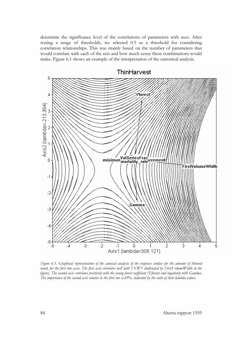
84 Alterra-rapport 1559
determine the significance level of the correlations of parameters with axes. After testing a range of thresholds, we selected 0.5 as a threshold for considering correlation relationships. This was mainly based on the number of parameters that would correlate with each of the axis and how much sense these combinations would make. Figure 6.1 shows an example of the interpretation of the canonical analysis.
Figure 6.1. Graphical representation of the canocial analysis of the response surface for the amount of thinned wood, for the first two axes. The first axis correlates well with VCW1 (indiciated by FirstVolumeWidth in the figure). The second axis correlates positively with the young forest coefficient (Yforest) and negatively with Gamma. The importance of the second axis relative to the first one is 69%, indicated by the ratio of their lambda values.
Alterra-rapport 1559 85
6.3 Design
The parameters are grouped into model parameters and scenario parameters. The model parameters are those that are modified to calibrate the model to a specific country. They usually concern increment and natural mortality. Scenario parameters are those that are usually changed in simple scenarios. They concern the management regime and the required felling level. In more complex scenarios, other parameters could be changed as well, like the natural mortality level or changing increment due to changing environmental conditions. The sensitivity analysis is done for these two parameter groups separately. All simulations were done for 50 years, since that is the time span applied in most EFISCEN analyses, and that is about the maximum range where EFISCEN is trusted to give reliable results (Nabuurs et al., 2000). The ouput variables that where evaluated in the analyses are: 1) total growing stock after 50 years (m3); 2) average increment level (m3 ha-1 yr-1) after 50 years; 3) volume from thinnings in time step 10 (m3); 4) volume from final fellings in time step 10 (m3) and 5) area of forest in the age classes 0–50 years, 50–100 years, and older than 100 years (ha) . Table 6.1 shows the parameters that have been selected for the sensitivity analysis, their default values and the range over which these parameters were varied. The initial state of the matrix is determined by the width of the first volume class (VCW1) and the parameters cv an r. From previous experiences it is known that the model is not very sensitive to cv and r, but VCW1 can be influential in some cases. Moreover, it also has an influence during the simulation, which is not the case with cv and r. To limit the number of parameters, we therefore did not include cv and r in the analysis. The range of VCW1 was chosen to represent the likely range this parameter would have for this forest type. The growth function parameters a0, a1 and a2 are the original ones fitted on inventory data for pine in South Finland. The range of these parameters was defined as the default value plus or minus 3 times the standard error of the estimation. This corresponds to the 99% confidence interval for these parameters, in the case of pine in South Finland. The range of these parameters in a European perspective is much wider, but depends very much on the local and initial conditions. It is therefore not possible to transfer these parameters from other species or locations without problems. The range for minimum and maximum age where the growth function is still valid reflects the usual range for growth functions within Europe. The parameters young forest coefficient, Beta and Gamma can theoretically range from 0 to 1. For Beta and Gamma we used this maximal range, but for the young forest coefficient we used 0.05 as a lower limit. A young forest coefficient of 0 would mean that no harvested area would be regenerated, which does not make sense. The optimal growing stock per age class is usually copied from the inventory data. We used a plausible range of plus or minus 20% of this value, although the theoretical range is between 0 and the maximum volume that can be reached within the matrix under consideration (i.e. the average volume of the highest volume class). The range for the mortality rate is specified to be between 0 and 10%. In case of equal volume

86 Alterra-rapport 1559
classes, the highest possible mortality rate is 10%, since area cannot move down more than one volume class. This also reflects a plausible range, including quite dense and unmanaged forests. One parameter that is not present is the thinning history. This parameter was added to EFSICEN 3.1.3 after the sensitivity analysis had been designed. Adding a new parameter to the desing was not feasible at that moment in time, due to the large additional work load needed. From experiences with earlier versions of EFISCEN, this parameter only influences the increment and avaialble thinnings in the first two to three time steps. The ranges defining start and end of possible thinnings and the start of final harvest reflect more or less the possible physical range. Thinning and final felling intensity are expressed as fractions and can range between 0 and 1. Table 6.1. Parameters included in the sensitivity analysis, with their default value and range. Parameter name explanation Default Min Max Model parameters 1 VCW1 Width of first volume class 42.5 10 75 2 a0 Growth function coefficient -2.0384 -3.31983 -0.75697 3 a1 Growth function coefficient 1604.33 1501.561 1707.099 4 a2 Growth function coefficient -10256 -11203.3 -9308.71
5 Max age inc Minimum age where growth function is valid 100 50 200
6 min age inc Maximum age where growth function is valid 5 2.5 15
7 YForest Young forest coefficient 0.6 0.05 1 8 Gamma Re-growth after thinnings 0.4 0 1 9 Beta Coefficient to avoid matrix diversion 0.4 0 1
10 VolSers Optimal growing stock per age class
from input data -20% +20%
11 MortRate Mortality rate 0.02 0 0.1 Scenario parameters 12 min_harvest_age start of final harvest 75 30 150 13 min_thinning_age start of thinnings 20 5 100 14 thinning_range age range of thinnings 50 5 100
15 felling_rate Fraction of available felling potential that is actually felled 0.5 0 1
16 thinning_rate Fraction of available thinning potential that is actually thinned 0.5 0 1
6.4 Results
The results of the canonical analysis for the model parameters are shown in Table 6.2a-c and for the scenario parameters in Table 6.3a-c. The first row shows the relative importance of each axis, compared to the first axis. Values in the table show the correlation of the parameters with each of the axes. For each of the output
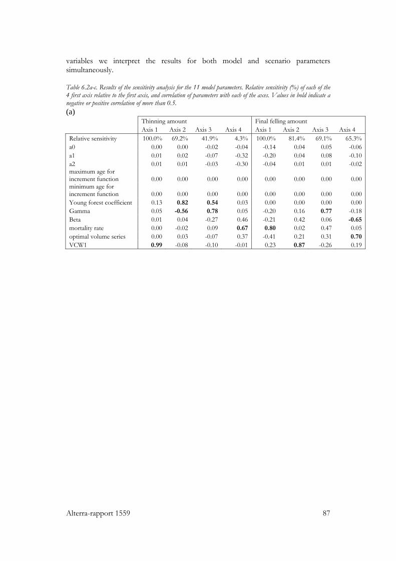
Alterra-rapport 1559 87
variables we interpret the results for both model and scenario parameters simultaneously. Table 6.2a-c. Results of the sensitivity analysis for the 11 model parameters. Relative sensitivity (%) of each of the 4 first axis relative to the first axis, and correlation of parameters with each of the axes. Values in bold indicate a negative or positive correlation of more than 0.5. (a) Thinning amount Final felling amount Axis 1 Axis 2 Axis 3 Axis 4 Axis 1 Axis 2 Axis 3 Axis 4 Relative sensitivity 100.0% 69.2% 41.9% 4.3% 100.0% 81.4% 69.1% 65.3%a0 0.00 0.00 -0.02 -0.04 -0.14 0.04 0.05 -0.06a1 0.01 0.02 -0.07 -0.32 -0.20 0.04 0.08 -0.10a2 0.01 0.01 -0.03 -0.30 -0.04 0.01 0.01 -0.02maximum age for increment function 0.00 0.00 0.00 0.00 0.00 0.00 0.00 0.00minimum age for increment function 0.00 0.00 0.00 0.00 0.00 0.00 0.00 0.00Young forest coefficient 0.13 0.82 0.54 0.03 0.00 0.00 0.00 0.00Gamma 0.05 -0.56 0.78 0.05 -0.20 0.16 0.77 -0.18Beta 0.01 0.04 -0.27 0.46 -0.21 0.42 0.06 -0.65mortality rate 0.00 -0.02 0.09 0.67 0.80 0.02 0.47 0.05optimal volume series 0.00 0.03 -0.07 0.37 -0.41 0.21 0.31 0.70VCW1 0.99 -0.08 -0.10 -0.01 0.23 0.87 -0.26 0.19
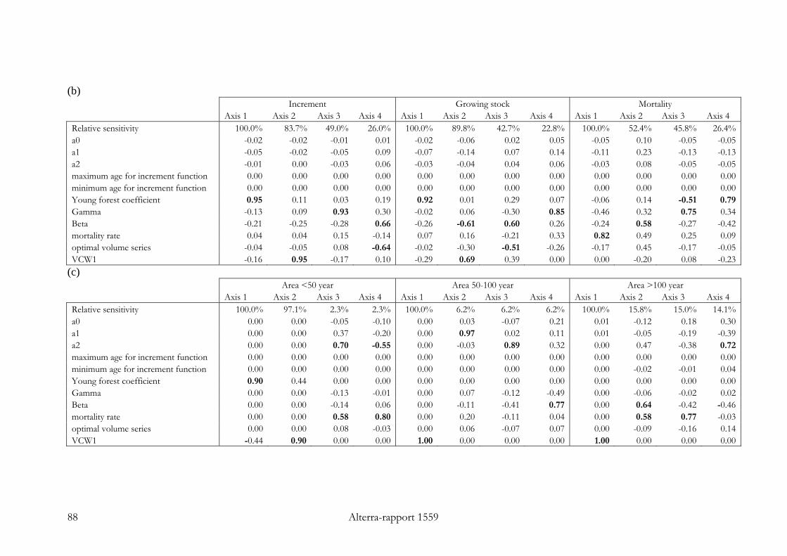
88 Alterra-rapport 1559
(b) Increment Growing stock Mortality Axis 1 Axis 2 Axis 3 Axis 4 Axis 1 Axis 2 Axis 3 Axis 4 Axis 1 Axis 2 Axis 3 Axis 4 Relative sensitivity 100.0% 83.7% 49.0% 26.0% 100.0% 89.8% 42.7% 22.8% 100.0% 52.4% 45.8% 26.4% a0 -0.02 -0.02 -0.01 0.01 -0.02 -0.06 0.02 0.05 -0.05 0.10 -0.05 -0.05 a1 -0.05 -0.02 -0.05 0.09 -0.07 -0.14 0.07 0.14 -0.11 0.23 -0.13 -0.13 a2 -0.01 0.00 -0.03 0.06 -0.03 -0.04 0.04 0.06 -0.03 0.08 -0.05 -0.05 maximum age for increment function 0.00 0.00 0.00 0.00 0.00 0.00 0.00 0.00 0.00 0.00 0.00 0.00 minimum age for increment function 0.00 0.00 0.00 0.00 0.00 0.00 0.00 0.00 0.00 0.00 0.00 0.00 Young forest coefficient 0.95 0.11 0.03 0.19 0.92 0.01 0.29 0.07 -0.06 0.14 -0.51 0.79 Gamma -0.13 0.09 0.93 0.30 -0.02 0.06 -0.30 0.85 -0.46 0.32 0.75 0.34 Beta -0.21 -0.25 -0.28 0.66 -0.26 -0.61 0.60 0.26 -0.24 0.58 -0.27 -0.42 mortality rate 0.04 0.04 0.15 -0.14 0.07 0.16 -0.21 0.33 0.82 0.49 0.25 0.09 optimal volume series -0.04 -0.05 0.08 -0.64 -0.02 -0.30 -0.51 -0.26 -0.17 0.45 -0.17 -0.05 VCW1 -0.16 0.95 -0.17 0.10 -0.29 0.69 0.39 0.00 0.00 -0.20 0.08 -0.23
(c) Area <50 year Area 50-100 year Area >100 year Axis 1 Axis 2 Axis 3 Axis 4 Axis 1 Axis 2 Axis 3 Axis 4 Axis 1 Axis 2 Axis 3 Axis 4 Relative sensitivity 100.0% 97.1% 2.3% 2.3% 100.0% 6.2% 6.2% 6.2% 100.0% 15.8% 15.0% 14.1% a0 0.00 0.00 -0.05 -0.10 0.00 0.03 -0.07 0.21 0.01 -0.12 0.18 0.30 a1 0.00 0.00 0.37 -0.20 0.00 0.97 0.02 0.11 0.01 -0.05 -0.19 -0.39 a2 0.00 0.00 0.70 -0.55 0.00 -0.03 0.89 0.32 0.00 0.47 -0.38 0.72 maximum age for increment function 0.00 0.00 0.00 0.00 0.00 0.00 0.00 0.00 0.00 0.00 0.00 0.00 minimum age for increment function 0.00 0.00 0.00 0.00 0.00 0.00 0.00 0.00 0.00 -0.02 -0.01 0.04 Young forest coefficient 0.90 0.44 0.00 0.00 0.00 0.00 0.00 0.00 0.00 0.00 0.00 0.00 Gamma 0.00 0.00 -0.13 -0.01 0.00 0.07 -0.12 -0.49 0.00 -0.06 -0.02 0.02 Beta 0.00 0.00 -0.14 0.06 0.00 -0.11 -0.41 0.77 0.00 0.64 -0.42 -0.46 mortality rate 0.00 0.00 0.58 0.80 0.00 0.20 -0.11 0.04 0.00 0.58 0.77 -0.03 optimal volume series 0.00 0.00 0.08 -0.03 0.00 0.06 -0.07 0.07 0.00 -0.09 -0.16 0.14 VCW1 -0.44 0.90 0.00 0.00 1.00 0.00 0.00 0.00 1.00 0.00 0.00 0.00
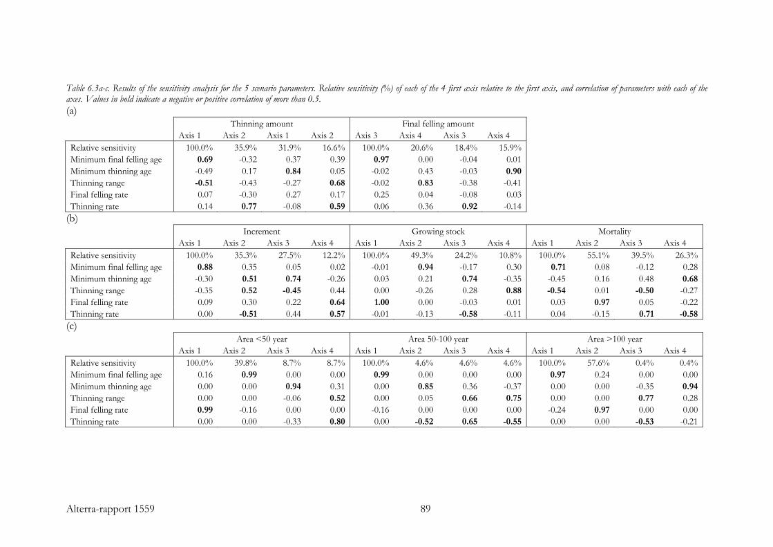
Alterra-rapport 1559 89
Table 6.3a-c. Results of the sensitivity analysis for the 5 scenario parameters. Relative sensitivity (%) of each of the 4 first axis relative to the first axis, and correlation of parameters with each of the axes. Values in bold indicate a negative or positive correlation of more than 0.5. (a) Thinning amount Final felling amount Axis 1 Axis 2 Axis 1 Axis 2 Axis 3 Axis 4 Axis 3 Axis 4 Relative sensitivity 100.0% 35.9% 31.9% 16.6% 100.0% 20.6% 18.4% 15.9%Minimum final felling age 0.69 -0.32 0.37 0.39 0.97 0.00 -0.04 0.01Minimum thinning age -0.49 0.17 0.84 0.05 -0.02 0.43 -0.03 0.90Thinning range -0.51 -0.43 -0.27 0.68 -0.02 0.83 -0.38 -0.41Final felling rate 0.07 -0.30 0.27 0.17 0.25 0.04 -0.08 0.03Thinning rate 0.14 0.77 -0.08 0.59 0.06 0.36 0.92 -0.14
(b) Increment Growing stock Mortality Axis 1 Axis 2 Axis 3 Axis 4 Axis 1 Axis 2 Axis 3 Axis 4 Axis 1 Axis 2 Axis 3 Axis 4 Relative sensitivity 100.0% 35.3% 27.5% 12.2% 100.0% 49.3% 24.2% 10.8% 100.0% 55.1% 39.5% 26.3% Minimum final felling age 0.88 0.35 0.05 0.02 -0.01 0.94 -0.17 0.30 0.71 0.08 -0.12 0.28 Minimum thinning age -0.30 0.51 0.74 -0.26 0.03 0.21 0.74 -0.35 -0.45 0.16 0.48 0.68 Thinning range -0.35 0.52 -0.45 0.44 0.00 -0.26 0.28 0.88 -0.54 0.01 -0.50 -0.27 Final felling rate 0.09 0.30 0.22 0.64 1.00 0.00 -0.03 0.01 0.03 0.97 0.05 -0.22 Thinning rate 0.00 -0.51 0.44 0.57 -0.01 -0.13 -0.58 -0.11 0.04 -0.15 0.71 -0.58
(c) Area <50 year Area 50-100 year Area >100 year Axis 1 Axis 2 Axis 3 Axis 4 Axis 1 Axis 2 Axis 3 Axis 4 Axis 1 Axis 2 Axis 3 Axis 4 Relative sensitivity 100.0% 39.8% 8.7% 8.7% 100.0% 4.6% 4.6% 4.6% 100.0% 57.6% 0.4% 0.4% Minimum final felling age 0.16 0.99 0.00 0.00 0.99 0.00 0.00 0.00 0.97 0.24 0.00 0.00 Minimum thinning age 0.00 0.00 0.94 0.31 0.00 0.85 0.36 -0.37 0.00 0.00 -0.35 0.94 Thinning range 0.00 0.00 -0.06 0.52 0.00 0.05 0.66 0.75 0.00 0.00 0.77 0.28 Final felling rate 0.99 -0.16 0.00 0.00 -0.16 0.00 0.00 0.00 -0.24 0.97 0.00 0.00 Thinning rate 0.00 0.00 -0.33 0.80 0.00 -0.52 0.65 -0.55 0.00 0.00 -0.53 -0.21
90 Alterra-rapport 1559
Age class distribution The development of the age class distribution is mainly influenced by the area that is felled and subsequently regenerated. For the area over 100 years, this is reflected by the model sensitivity to the scenario parameters minimum final felling age and final felling rate. Although the analysis showed sensitivity to VCW1 as well for area over 100 years old, the absolute differences are negligible. Logically the area younger than 50 years is sensitive to the same scenario parameters, minimum final felling age and final felling rate. The speed of regeneration is regulated by the young forest coefficient, which proves to be the most important model parameter for forest younger than 50 years. A low young forest coefficient will lead to an accumulation of land in the bare land class. For the same output variable, VCW1 proves to be very important as well. This parameter has an influence on the initial distribution between area in the matrix and in the bare land class, but only in the first age class. A high VCW1 will initially lead to more area in the bare land class, in order to keep the same average volume. This is a known problem, causing a clear depression in the simulated age class distributions, especially for countries with very low average volumes in the first age class. After 50 years of simulation, these initial differences can just influence the area between 50 and 100 years. This is confirmed by the analysis for this age class, where VCW1 dominates the first axis. No other model parameters have a great influence on the area in the classes 0–50 and 50–100 years. For the scenario parameters, only the minimum final felling age is important for the area between 50 and 100 years. This is logical, since it determines if area in this age class may be subjected to final felling or not. Thinning amount Thinnings can only take place in the age range defined by the thinning regime. This is for a large part reflected in the first axis of the scenario parameters by the length of the thinning age range and the start age of final fellings. Within this range, a certain fraction of the cells will move one volume class down, where the difference in average volume of these volume classes represents the thinned volume. The sensitivity to this fraction is reflected in the second axis of the scenario parameters through the thinning rate. Volume differences between volume classes are governed by VCW1, which dominates the first axis of the model parameters. A relatively low VCW1 leads to volume classes of increasing width. With a constant thinning rate, this will lead to larger amounts being thinned, but only if the area distribution is the same. However, the area distribution should be adapted, both through the initialisation procedure as well as via lower increment transitions. Further, as described above, VCW1 influences the area distribution over age classes up to 50 years, also influencing the area available for thinnings. Another parameter influencing the available area is the young forest coefficient, present in the second and third axis of the model parameters. Both axes also correlate with Gamma, negatively in the second axis and positively in the third axis. Gamma determines how quickly area becomes available for thinnings again. It is not clear how it interacts with the young forest coefficient.
Alterra-rapport 1559 91
Final felling The amount of final felling is basically the product of the area felled and the average volume on this area. The area actually felled depends only on the scenario parameters. The minimum age for final felling is the most important variable, but surprisingly the actual felling rate is not important at all. A low felling rate leads on the somewhat longer term to an accumulation of area in the higher age classes, with relatively high average volumes. A small fraction of this large reserve still reflects a considerable amount, comparable to a high fraction of a small reserve. However, the development of final felling amount over the time steps is very different with a different final felling rate. Thinning characteristics as reflected in the axes 2–4 of the scenario parameters will have some influence on the average standing stock in the older age classes. In the sensitivity analysis of the model parameters, final felling rate and age are fixed. Differences in final felling volume are thus caused by differences in the average growing stock of forest older than 75 years. The most influential parameter in this respect proves to be the mortality rate. A high mortality rate will lead to lower growing stock volumes. VCW1 is very influential as well. When the VCW1 is very high, the maximum attainable growing stock will increase, which might explain the positive sensitivity to this parameter. Part of the area that is recently thinned- will be moved to a higher volume class. The fraction of area that is moved to a higher volume class is determined by Gamma. Gamma is present in the third axis. The fourth axis correlates with Beta and the optimal volume series in opposite directions. The combination of these two parameters is found in Equation 9, which corrects the increment for differences between the actual and the optimal growing stock as expressed by the optimal volume series. By influencing the increment, these two parameters will thus influence the average growing stock Mortality Logically, the mortality level is most sensitive to the mortality rate. The second axis of the model parameters is determined by Beta. A higher Beta leads to more increment, especially in the lowest volume class. In the lowest volume class, no mortality can occur, and therefore a higher Beta would lead to more available area for mortality. Recently thinned forests are not subjected to mortality. A high Gamma will make thinned areas available for mortality quickly, and is thus positive for the mortality level. Indeed the third axis shows a positive correlation with Gamma, but the negative correlation with the young forest coefficient in this case is difficult to explain. The young forest coefficient shows a positive correlation with the fourth axis, which can be explained through its influence on the availability of area in the matrix. Mortality is determined for a large part through the management. The first axis of the scenario parameters correlates positively with the minimum age for final felling and negatively with the thinning range. Later fellings lead to higher growing stocks, and thus to more mortality. However, this is counteracted by an increasing thinning range, since thinned forests have no mortality. Independently (second axis) the felling rate has a high influence on the average growing stock, and thus on the mortality
92 Alterra-rapport 1559
level. The third axis shows a combination of thinning range and thinning rate. Thinning rate shows a positive correlation, indicating that more thinnings lead to more mortality. Probably thinnings lead to higher growing stocks, which eventually might lead to higher mortality. This is counteracted by a longer thinning interval, which causes the forest to be unavailable for thinnings for a longer time frame. The fourth axis shows that a later start of thinnings leads to higher mortality, which is counteracted by more intensive thinnings (higher thinning rate). Increment The most influential parameter of the model parameter for the increment proved to be the young forest coefficient. This parameter determines how much area of the bare forest land class will enter the matrix during a time step. In this way it influences the total area in the matrix and thus the area that can show increment. When area is transferred to the matrix, it will get the average volume of the first volume class, irrespective of its width. This is reflected in the second axis, which is dominated by VCW1. Gamma dominates the third axis, which can be explained by the extra increment obtained when receiving the growth boost. The fourth axis correlates most with Beta and the optimal volume series, in opposite directions. The combination of these two parameters is found in Equation 9, which corrects the increment for differences between the actual and the optimal growing stock The most influential parameter among the model parameters is the minimum final felling age. Apparently the forest is still growing well at the ages where final felling can be carried out, indicated by the positive correlation. However, this might vary with the simulation length considered. The second and third axis seem to represent two different thinning strategies. The second axis favours many light thinnings, indicated by a long thinning age range and a negative correlation of increment with thinning rate. The third axis favours a few heavy thinnings, indicated by a short age range, but positive correlation with thinning rate. Both strategies suggest a late start of thinnings as positive. However, the correlations with the third axis are partly below the 0.5 threshold. The fourth axis seems to represent the positive intensity of management in general, showing positive correlations with both thinning and final felling intensity. Growing stock Growing stock is the result of all processes described above. Increment is one of the most important processes, and thus at least partly the same parameters and combinations show up. Among the model parameters, the young forest coefficient is the most important. The second axis correlates with Beta and VCW1 in opposite directions. A large VCW1 will increase the maximum volume that can be reached. However, it is not clear why Beta could counteract this. The third axis shows the known combination of Beta and optimal volume series, which influences the increment. The fourth axis shows the positive effect of the growth boost parameter, Gamma. Compared to the increment, Gamma is less important, probably because the extra volume increment is compensated by the removal of volume by thinnings.
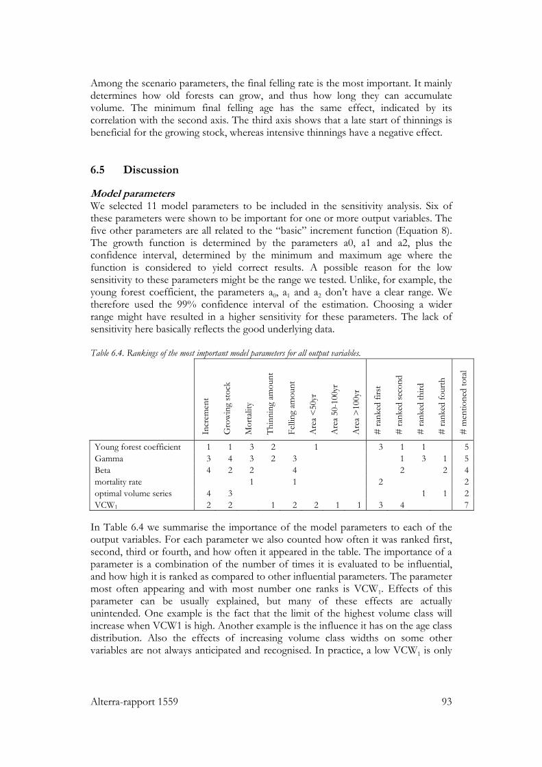
Alterra-rapport 1559 93
Among the scenario parameters, the final felling rate is the most important. It mainly determines how old forests can grow, and thus how long they can accumulate volume. The minimum final felling age has the same effect, indicated by its correlation with the second axis. The third axis shows that a late start of thinnings is beneficial for the growing stock, whereas intensive thinnings have a negative effect. 6.5 Discussion
Model parameters We selected 11 model parameters to be included in the sensitivity analysis. Six of these parameters were shown to be important for one or more output variables. The five other parameters are all related to the “basic” increment function (Equation 8). The growth function is determined by the parameters a0, a1 and a2, plus the confidence interval, determined by the minimum and maximum age where the function is considered to yield correct results. A possible reason for the low sensitivity to these parameters might be the range we tested. Unlike, for example, the young forest coefficient, the parameters a0, a1 and a2 don’t have a clear range. We therefore used the 99% confidence interval of the estimation. Choosing a wider range might have resulted in a higher sensitivity for these parameters. The lack of sensitivity here basically reflects the good underlying data. Table 6.4. Rankings of the most important model parameters for all output variables.
Incr
emen
t
Gro
win
g st
ock
Mor
talit
y
Thin
ning
am
ount
Felli
ng a
mou
nt
Are
a <
50yr
Are
a 50
-100
yr
Are
a >
100y
r
# ra
nked
firs
t
# ra
nked
seco
nd
# ra
nked
third
# ra
nked
four
th
# m
entio
ned
tota
l
Young forest coefficient 1 1 3 2 1 3 1 1 5Gamma 3 4 3 2 3 1 3 1 5Beta 4 2 2 4 2 2 4mortality rate 1 1 2 2optimal volume series 4 3 1 1 2VCW1 2 2 1 2 2 1 1 3 4 7
In Table 6.4 we summarise the importance of the model parameters to each of the output variables. For each parameter we also counted how often it was ranked first, second, third or fourth, and how often it appeared in the table. The importance of a parameter is a combination of the number of times it is evaluated to be influential, and how high it is ranked as compared to other influential parameters. The parameter most often appearing and with most number one ranks is VCW1. Effects of this parameter can be usually explained, but many of these effects are actually unintended. One example is the fact that the limit of the highest volume class will increase when VCW1 is high. Another example is the influence it has on the age class distribution. Also the effects of increasing volume class widths on some other variables are not always anticipated and recognised. In practice, a low VCW1 is only
94 Alterra-rapport 1559
needed to match low initial average volumes in the first age class in some countries. In all other cases an equal width of volume classes is usually strived for. However, the consequences it has on the whole model does not justify the approach chosen. A more targeted solution to the underlying problem is probably possible. The young forest coefficient is the second important parameter. It influences the age class distribution by controlling the area moving into the matrix from the bare land class. Because this area will get the average volume of the first volume class, it has an important effect on the increment and associated variables as well. The latter effect is basically unintended as well: the young forest coefficient was meant to express the regeneration success, and not to act as a way to boost the increment. However, its effect on the increment has been recognised in the past, and the use of default values has been encouraged (Pussinen et al., 2001 ; Annex C). Furthermore, we tested here the entire possible range, whereas in practice a smaller range of values is applied. Nonetheless, it might be worthwhile to look into possibilities for decoupling of regeneration success and increment effects. Mortality rate is mentioned only twice, but both times ranked as most influential parameter for the output variable under consideration. Forests simulated with EFISCEN are usually managed and thus mortality can be assumed to be low. However, mortality can be important for derived variables, such as standing dead wood volume and soil carbon modelling. Moreover, European forestry tends to lean towards the incorporation of more natural processes in forest management, which could make mortality more important. An increasing share of older forests will also lead to increased importance of mortality processes. Recent and ongoing efforts towards a better parameterisation of mortality are therefore well justified. Gamma appears often in Table 6.4, but is never ranked as the most important parameter. Although we tested the full possible range, in practice its value is restricted to those mentioned in Annex C. However, some documented validation or calibration of these values on local yield tables or plot data would increase the credibility. The model shows medium sensitivity to Beta. Again, we tested the full theoretical range, while in practice its value is always set to 0.4. However, the reasoning for the use of one value has never been documented. Nilsson et al. (1992) state that this value can range between 0.25 and 0.45. It might be worthwhile to check if this approach can and should be refined. Of the six parameters in Table 6.4, the optimal volume series showed the least influence. The real value of this parameter (or better parameter series) is unknown. It can perhaps be determined with the use of more detailed simulation models, but that is very time consuming and not possible for all forest types in EFISCEN. The current approach of using the average values from inventory data is unsure, but is probably not very influential for the simulation results.

Alterra-rapport 1559 95
Scenario parameters Table 6.5 summarises the sensitivity of EFISCEN to the scenario parameters. Generally the parameters concerning final felling are more influential than those concerning thinnings. This is logical, since final felling has more severe consequences, both in terms of age structure and increment. Especially the age where final felling starts is important. For thinnings, especially the width of the age range where thinnings can be carried out is influential in the results. Table 6.5. Rankings of the scenario parameters for all output variables.
Incr
emen
t
Gro
win
g st
ock
Mor
talit
y
Thin
ning
am
ount
Felli
ng a
mou
nt
Are
a <
50yr
Are
a 50
-100
yr
Are
a >
100y
r
# ra
nked
firs
t
# ra
nked
seco
nd
# ra
nked
third
# ra
nked
four
th
# m
entio
ned
tota
l
Minimum final felling age 1 2 1 1 1 2 1 1 6 2 8Minimum thinning age 2 3 4 3 4 3 1 3 2 6Thinning range 2 4 1 1 2 2 2 1 5Final felling rate 4 1 2 1 2 2 1 1 4Thinning rate 2 3 3 2 3 2 3 5
General We carried out a sensitivity analysis for Utopia, evaluating the state of the forest after 10 time steps. Such an analysis is invaluable for a proper evaluation of the model. However, generalisation of the results to real countries and other simulation lengths should be done with care. Especially the latter is dangerous, since some parameters have different effect on different time scales. The effect of parameters affecting the initial state of the forest will diminish over time, while the effect of others might increase over time. For example, the young forest coefficient will start to influence the amount of wood from final fellings only after a time period equal to the minimum final felling age.

Alterra-rapport 1559 97
7 Discussion
General EFISCEN or parts of it have been validated in different studies in different ways in different parts of Europe. All studies found good agreement, and where differences occurred they could be explained. However, it is clear that EFISCEN works best under even aged, managed conditions. Deviations from this situation will lead to less reliable results. Further, results on a regional level are less reliable than those on the country level. This is due to inaccuracies in the definition of the management regimes, leading to differences in the regional allocation of the harvest. If reliable results are required on the regional level, more attention should be given to an exact representation of harvest practices. Alternatively, required harvest levels should be specified at the regional level. Probably the same is valid for different owner categories, tree species and site classes. One outcome of the Finnish validation (Nabuurs et al., 2000) was a decrease in increment levels after 30–40 years in EFISCEN 1.0. In later versions a mechanism has been introduced to counteract this. Increment levels seem to be more realistic for longer timeframes now. However, a new validiation would be needed to determine appropriate time horizons for reliable projections. Despite this, the current practice of 50–60 years projection horizons seems to be well defendable. EFISCEN has been in use for many years, and considerable expertise has been built up. This has resulted in a stable model where most processes are well understood and default sets of parameters are available. However, it would be advisable to give some more attention to some parameters, like the optimal growing stock level per age class, the Beta parameter and the Gamma parameter. The current values of those parameters lack a solid basis, or have been derived for one country only. Furthermore, a proper parameterisation of mortality processes will need continued attention, since this will be important in Europe’s aging forests, especially for biodiversity indicators. Points of attention A few issues need special attention when using the EFISCEN model: o Deforestation takes area out of the bare land class. Using this option will work
well only when the area to deforest is small, and only if management is applied. Otherwise no area will be available in the bare land class.
o Soil carbon modelling does not take area changes into account. As a consequence, afforested area will have no initial soil stocks, and soil carbon in deforested areas will still be included in the totals reported.
o The use of equal volume class widths are recommended whenever possible. o When the ranges of thinning and final felling regimes overlap, the amount of
final fellings will not match the requested volume. This discrepancy increases with increasing overlap.
o When no scenario is specified, default values will be taken for soil climate parameters and for the removal/felling ratio.

98 Alterra-rapport 1559
o Be aware of the range for some of the parameters, like mortality (<10% recommended) and growth change (maximum depends on volume class width and current increment)
Plans for the future The EFISCEN tool is under constant development to suit project and user needs. Future developments will be steered by such needs and are therefore not easy to foresee. Current plans for further development include: o Creation of an input database to replace the current complicated input file
structure. This will make the program more user-friendly and less error-prone. o Making the volume class widths constant per matrix. An extra volume class will
be added with a very low average volume to prevent problems in forest types were the average volume is very low. This would make the parameter VCW1 obsolete, which solves some unexpected sensitivities to this parameter.
o Re-programming of the matrix initialisation program (P-efsos) and integration into the main simulator. The P-efsos program is not user friendly and the code is difficult to read. Hwoever, re-programming will probably doen only when new inventory data will become available.
o Inserting more warnings if parameters are missing or wrong, and when default values are assumed. Currently the program can crash on missing or wrong values without an error message. Further, missing input values are sometimes replaced by default values without notifying the user.
o Allowing insertion of initial soil carbon stock for afforested areas. o Allowing removal of soil carbon from deforested area from the simulation. o Integration with land use and economic models. Economics are important to
simulate supply behavior of forest owners under changing demand (for example due to increased demand for bioenergy) and to include trade between countries.
o Development of a tool that will be able to simulate at the plot level and able to handle mixed and uneven aged forests. The strength of the current model lies on large areas of even aged mono species forest, while forest management is shifting more and more towards uneven aged mixed forest. Also for many questions a finer spatial detail will be required.
Alterra-rapport 1559 99
References
Abramowitz, M., and Stegun, J.A. 1965. Handbook of mathematical functions: with formulas, graphs, and mathematical tables. Applied Mathematical Series 55. Dover Publications, New York
Attebring, Nilsson and Sallnaes 1989. A model for long-term forecasting of timber yield - a description with special reference to the forest study at SUA-IIASA. Systems Analysis Modelling Simulation 6 (3): 171-180.
Berg, B., M. P. Berg, P. Bottner, E. Box, A. Breymeyer, R. C. De Anta, M. Couteaux, E. Mälkönen, C. McClaugherty, V. Meentemeyer, F. Muñoz, P. Piussi, J. Remacle and A. V. De Santo (1993). "Litter mass loss in pine forests of Europe and Eastern United States: some relationships with climate and litter quality." Biogeochemistry 20: 127-159.
Berg, B., G. Ekholm and C. McClaugherty (1984). "Lignin and holocellulose relations during long-term decomposition of some forest litters. Long-term decomposition in a Scots pine forest. IV." Can. J. Bot. 62: 2540-2550.
Berg, B., K. Hannus, T. Popoff and O. Theander (1982). "Changes in organic chemical components of needle litter during decomposition. Long-term decomposition in a Scots pine forest. I." Canadian Journal of Botany 60: 1310-1319.
Box, G.E.P. and Draper, N.R., 1987. Empirical model-building and response surfaces. John Wiley&Son, New York. 669 p.
Giardina, C. P. and M. G. Ryan (2000). "Evidence that decomposition rates of organic carbon in mineral soil do not vary with temperature." Nature 404: 858-861.
Koivisto, P. (1959). Kasvu- ja tuottotaulukoita (Growth and yield tables). Communications Instituti Forestales Fenniae. Helsinki, Finland, Finnish Forest Research Institute. 51.
Liski, J., H. Ilvesniemi, A. Mäkelä and M. Starr (1998). "Model analysis of the effects of soil age, fires and harvesting on the carbon storage of boreal forest soils." European Journal of Soil Science 49(3): 407 - 416.
Liski, J., H. Ilvesniemi, A. Mäkelä and C. J. Westmann (1999). "CO2 emissions from soil in response to climatic warming are overestimated - The decomposition of old soil organic matter is tolerant of temperature." Ambio 28: 171-174.
Liski, J. and C. J. Westman (1995). "Density of organic carbon in soils at coniferous forest sites in southern Finland." Biogeochemistry 29: 183-197.
Nilsson, S., O. Sallnäs and P. Duinker (1992). A report on the IIASA forest study: Future forest resources of Western and Eastern Europe, The Parthenon Publishing Group, UK.
Liski, J., Palosuo, T., Peltoniemi, M. & Sievänen, R. 2005. Carbon and decomposition model Yasso for forest soils. Ecological Modelling 189(1-2): 168-182.
Nabuurs, G.J., Schelhaas, M.J., Pussinen, A., 2000. Validation of the European forest information scenario model (EFISCEN) and a projection of Finnish forests. Silva Fennica 34, 167-179.

100 Alterra-rapport 1559
Thürig, E., Schelhaas, M.J. 2006. Evaluation of a large-scale forest scenario model in heterogeneous forests: A case study for Switzerland. Canadian Journal of Forest Research 36 (3) p. 671-683.
FAOSTAT (2005) Forestry data. Roundwood, sawn wood, wood-based panels., http://faostat.fao.org/faostat/collections?subset=forestry.
Image-Team (2001). The IMAGE 2.2 implementation of the SRES scenarios: A comprehensive analysis of emissions, climate change and impacts in the 21st century. National Institute for Public Health and the Environment, Bilthoven.
Mäkinen, H., Hynynen, J., Siitonen, J., & Sievänen, R. (2006) Predicting the decomposition of Scots pine, Norway spruce and birch stems in Finland. Ecological Applications, 16, 1865-1879.
Storaunet, K.O. & Rolstad, J. (2004) How long do Norway spruce snags stand? Evaluating four estimation methods. Canadian Journal of Forest Research-Revue Canadienne De Recherche Forestiere, 34, 376-383.
UN-ECE/FAO, 2000. Forest Resources of Europe, CIS, North America, Australia, Japan and New Zealand, UN-ECE/FAO, Geneva.
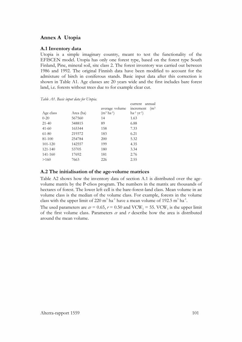
Alterra-rapport 1559 101
Annex A Utopia
A.1 Inventory data Utopia is a simple imaginary country, meant to test the functionality of the EFISCEN model. Utopia has only one forest type, based on the forest type South Finland, Pine, mineral soil, site class 2. The forest inventory was carried out between 1986 and 1992. The original Finnish data have been modified to account for the admixture of birch in coniferous stands. Basic input data after this correction is shown in Table A1. Age classes are 20 years wide and the first includes bare forest land, i.e. forests without trees due to for example clear cut. Table A1. Basic input data for Utopia.
Age class Area (ha) average volume (m3 ha-1)
current annual increment (m3 ha-1 yr-1)
0-20 567560 14 1.63 21-40 348815 89 6.88 41-60 165344 158 7.33 61-80 219372 183 6.21 81-100 254784 200 5.32 101-120 142557 199 4.35 121-140 53705 180 3.34 141-160 17692 181 2.76 >160 7663 226 2.55
A.2 The initialisation of the age-volume matrices Table A2 shows how the inventory data of section A.1 is distributed over the age-volume matrix by the P-efsos program. The numbers in the matrix are thousands of hectares of forest. The lower left cell is the bare-forest-land class. Mean volume in an volume class is the median of the volume class. For example, forests in the volume class with the upper limit of 220 m3 ha-1 have a mean volume of 192.5 m3 ha-1. The used parameters are cv = 0.65, r = 0.50 and VCW1 = 55. VCW1 is the upper limit of the first volume class. Parameters cv and r describe how the area is distributed around the mean volume.
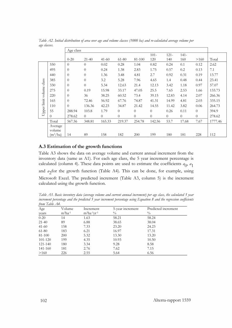
Alterra-rapport 1559 102
Table A2. Initial distribution of area over age and volume classes (1000 ha) and re-calculated average volume per age classes. Age class
0-20 21-40 41-60 61-80 81-100 101-120
121-140
141-160 >160 Total
550 0 0 0.02 0.28 1.04 0.82 0.24 0.1 0.12 2.62 495 0 0 0.24 1.38 2.83 1.75 0.57 0.2 0.13 7.1 440 0 0 1.36 3.48 4.81 2.7 0.92 0.31 0.19 13.77 385 0 0 3.2 5.28 7.96 4.65 1.4 0.48 0.44 23.41 330 0 0 5.34 12.63 21.4 12.13 3.42 1.18 0.97 57.07 275 0 0.19 15.98 33.17 47.05 25.5 7.65 2.53 1.66 133.73 220 0 36 38.25 60.52 73.4 39.15 12.83 4.14 2.07 266.36 165 0 72.46 56.92 67.76 74.87 41.31 14.99 4.81 2.03 335.15 110 0 136.36 42.23 34.87 21.42 14.55 11.42 3.82 0.06 264.73 55 288.94 103.8 1.79 0 0 0 0.26 0.11 0 394.9
Upp
er li
mit
volu
me
class
0 278.62 0 0 0 0 0 0 0 0 278.62 Total 567.56 348.81 165.33 219.37 254.78 142.56 53.7 17.68 7.67 1777.46
Average volume (m3/ha) 14 89 158 182 200 199 180 181 228 112
A.3 Estimation of the growth functions Table A3 shows the data on average volume and current annual increment from the inventory data (same as A1). For each age class, the 5 year increment percentage is calculated (column 4). These data points are used to estimate the coefficients a0, a1 and a2for the growth function (Table A4). This can be done, for example, using Microsoft Excel. The predicted increment (Table A3, column 5) is the increment calculated using the growth function. Table A3. Basic inventory data (average volume and current annual increment) per age class, the calculated 5 year increment percentage and the predicted 5 year increment percentage using Equation 8 and the regression coefficients from Table A4. Age Volume Increment 5-year increment Predicted increment years m3ha-1 m3ha-1yr-1 % % 0-20 14 1.63 58.21 58.24 21-40 89 6.88 38.65 38.04 41-60 158 7.33 23.20 24.23 61-80 183 6.21 16.97 17.31 81-100 200 5.32 13.30 13.20 101-120 199 4.35 10.93 10.50 121-140 180 3.34 9.28 8.58 141-160 181 2.76 7.62 7.15 >160 226 2.55 5.64 6.56
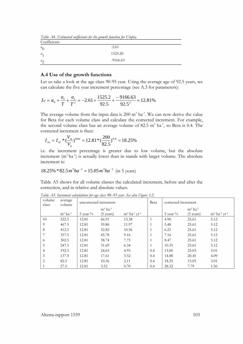
Alterra-rapport 1559 103
Table A4. Estimated coefficients for the growth function for Utopia. Coefficients a0 -2.61
a1 1525.20
a2 -9166.63
A.4 Use of the growth functions Let us take a look at the age class 90-95 year. Using the average age of 92.5 years, we can calculate the five year increment percentage (see A.3 for parameters):
%81.125.92
63.91665.922.152561.2 22
110 =
−++−=++=
Ta
TaaIvf
The average volume from the input data is 200 m3 ha-1. We can now derive the value for Beta for each volume class and calculate the corrected increment. For example, the second volume class has an average volume of 82.5 m3 ha-1, so Beta is 0.4. The corrected increment is then:
%25.18)5.82
200(*81.12)(* 4.0 === beta
a
mvfva V
VII
i.e. the increment percentage is greater due to low volume, but the absolute increment (m3 ha-1) is actually lower than in stands with larger volume. The absolute increment is:
1313 05.155.82*%25.18 −− = hamham (in 5 years)
Table A5 shows for all volume classes the calculated increment, before and after the correction, and in relative and absolute values. Table A5. Increment calculations for age class 90–95 year. See also Figure 3.2.
volume class
average volume uncorrected increment Beta corrected increment
m3 ha-1 5 year % m3 ha-1 (5 years) m3 ha-1 yr-1 5 year %
m3 ha-1 (5 years) m3 ha-1 yr-1
10 522.5 12.81 66.91 13.38 1 4.90 25.61 5.12 9 467.5 12.81 59.86 11.97 1 5.48 25.61 5.12 8 412.5 12.81 52.82 10.56 1 6.21 25.61 5.12 7 357.5 12.81 45.78 9.16 1 7.16 25.61 5.12 6 302.5 12.81 38.74 7.75 1 8.47 25.61 5.12 5 247.5 12.81 31.69 6.34 1 10.35 25.61 5.12 4 192.5 12.81 24.65 4.93 0.4 13.00 25.03 5.01 3 137.5 12.81 17.61 3.52 0.4 14.88 20.45 4.09 2 82.5 12.81 10.56 2.11 0.4 18.25 15.05 3.01 1 27.5 12.81 3.52 0.70 0.4 28.32 7.79 1.56
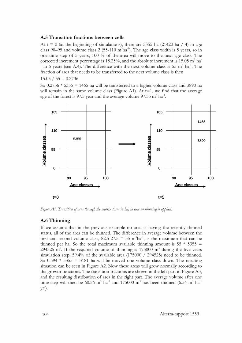
Alterra-rapport 1559 104
A.5 Transition fractions between cells At t = 0 (at the beginning of simulations), there are 5355 ha (21420 ha / 4) in age class 90–95 and volume class 2 (55-110 m3ha-1). The age class width is 5 years, so in one time step of 5 years, 100 % of the area will move to the next age class. The corrected increment percentage is 18.25%, and the absolute increment is 15.05 m3 ha-
1 in 5 years (see A.4). The difference with the next volume class is 55 m3 ha-1. The fraction of area that needs to be transferred to the next volume class is then 15.05 / 55 = 0.2736 So 0.2736 * 5355 = 1465 ha will be transferred to a higher volume class and 3890 ha will remain in the same volume class (Figure A1). At t=1, we find that the average age of the forest is 97.5 year and the average volume 97.55 m3 ha-1.
90 95 100
0
55
110
165
Age classes
Volu
me
clas
ses
90 95 100
0
55
110
165
Age classes
Volu
me
clas
ses5355 3890
1465
t=0 t=5
90 95 100
0
55
110
165
Age classes
Volu
me
clas
ses
90 95 100
0
55
110
165
Age classes
Volu
me
clas
ses
90 95 100
0
55
110
165
Age classes
Volu
me
clas
ses
90 95 100
0
55
110
165
Age classes
Volu
me
clas
ses5355 3890
1465
t=0 t=5 Figure A1. Transition of area through the matrix (area in ha) in case no thinning is applied. A.6 Thinning If we assume that in the previous example no area is having the recently thinned status, all of the area can be thinned. The difference in average volume between the first and second volume class, 82.5-27.5 = 55 m3ha-1, is the maximum that can be thinned per ha. So the total maximum available thinning amount is 55 * 5355 = 294525 m3. If the required volume of thinning is 175000 m3 during the five years simulation step, 59.4% of the available area (175000 / 294525) need to be thinned. So 0.594 * 5355 = 3181 ha will be moved one volume class down. The resulting situation can be seen in Figure A2. Now these areas will grow normally according to the growth functions. The transition fractions are shown in the left part in Figure A3, and the resulting distribution of area in the right part. The average volume after one time step will then be 60.56 m3 ha-1 and 175000 m3 has been thinned (6.54 m3 ha-1 yr1).
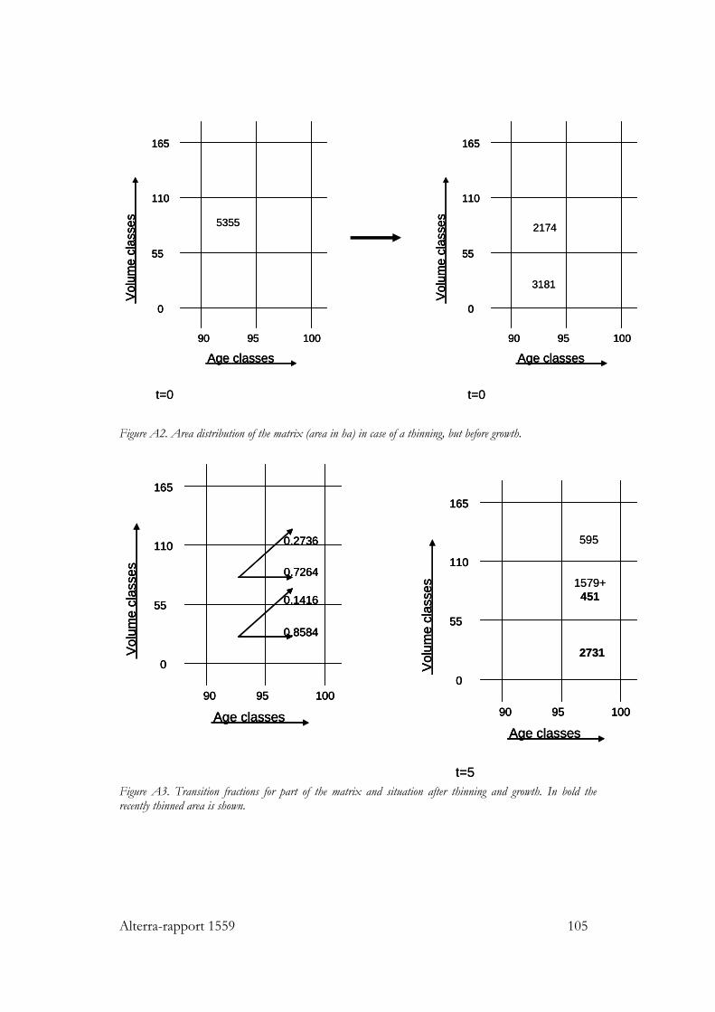
Alterra-rapport 1559 105
90 95 100
0
55
110
165
Age classes
Volu
me
clas
ses
90 95 100
0
55
110
165
Age classes
Volu
me
clas
ses5355 2174
t=0 t=0
3181
90 95 100
0
55
110
165
Age classes
Volu
me
clas
ses
90 95 100
0
55
110
165
Age classes
Volu
me
clas
ses
90 95 100
0
55
110
165
Age classes
Volu
me
clas
ses
90 95 100
0
55
110
165
Age classes
Volu
me
clas
ses5355 2174
t=0 t=0
3181
Figure A2. Area distribution of the matrix (area in ha) in case of a thinning, but before growth.
0.1416
0.2736
0.8584
0.7264
90 95 100
0
55
110
165
Age classes
Vol
ume
clas
ses
90 95 100
0
55
110
165
Age classes
Vol
ume
clas
ses 1579+
451
t=5
2731
595
0.1416
0.2736
0.8584
0.7264
90 95 100
0
55
110
165
Age classes
Vol
ume
clas
ses
0.1416
0.2736
0.8584
0.7264
90 95 100
0
55
110
165
Age classes
Vol
ume
clas
ses
90 95 100
0
55
110
165
Age classes
Vol
ume
clas
ses
90 95 100
0
55
110
165
Age classes
Vol
ume
clas
ses 1579+
451
t=5
2731
595
Figure A3. Transition fractions for part of the matrix and situation after thinning and growth. In bold the recently thinned area is shown.
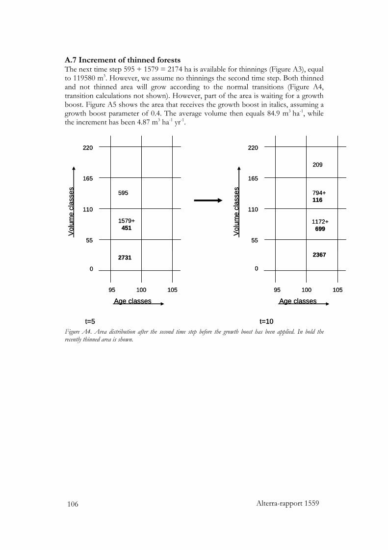
Alterra-rapport 1559 106
A.7 Increment of thinned forests The next time step 595 + 1579 = 2174 ha is available for thinnings (Figure A3), equal to 119580 m3. However, we assume no thinnings the second time step. Both thinned and not thinned area will grow according to the normal transitions (Figure A4, transition calculations not shown). However, part of the area is waiting for a growth boost. Figure A5 shows the area that receives the growth boost in italics, assuming a growth boost parameter of 0.4. The average volume then equals 84.9 m3 ha-1, while the increment has been 4.87 m3 ha-1 yr-1.
t=5 t=10
95 100 105
55
110
165
220
Age classes
Vol
ume
clas
ses
1579+451
595
95 100 105
55
110
165
220
Age classes
Vol
ume
clas
ses
1172+699
794+116
0 0
2731 2367
209
t=5 t=10
95 100 105
55
110
165
220
Age classes
Vol
ume
clas
ses
1579+451
595
95 100 105
55
110
165
220
Age classes
Vol
ume
clas
ses
1172+699
794+116
0 0
2731 2367
209
Figure A4. Area distribution after the second time step before the growth boost has been applied. In bold the recently thinned area is shown.
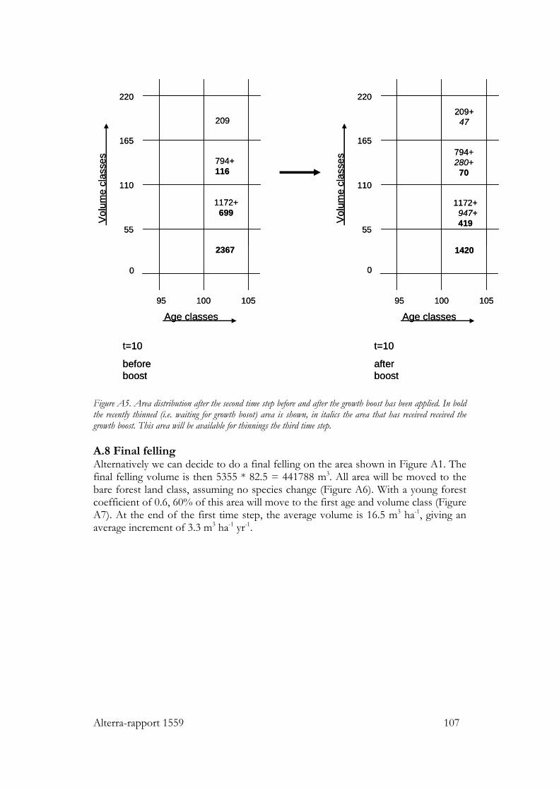
Alterra-rapport 1559 107
t=10
beforeboost
t=10
afterboost
95 100 105
55
110
165
220
Age classes
Vol
ume
clas
ses
95 100 105
55
110
165
220
Age classes
Vol
ume
clas
ses
1172+947+419
794+280+
70
0 0
1420
209+47
1172+699
794+116
2367
209
t=10
beforeboost
t=10
afterboost
95 100 105
55
110
165
220
Age classes
Vol
ume
clas
ses
95 100 105
55
110
165
220
Age classes
Vol
ume
clas
ses
1172+947+419
794+280+
70
0 0
1420
209+47
1172+699
794+116
2367
209
Figure A5. Area distribution after the second time step before and after the growth boost has been applied. In bold the recently thinned (i.e. waiting for growth bosot) area is shown, in italics the area that has received received the growth boost. This area will be available for thinnings the third time step. A.8 Final felling Alternatively we can decide to do a final felling on the area shown in Figure A1. The final felling volume is then 5355 * 82.5 = 441788 m3. All area will be moved to the bare forest land class, assuming no species change (Figure A6). With a young forest coefficient of 0.6, 60% of this area will move to the first age and volume class (Figure A7). At the end of the first time step, the average volume is 16.5 m3 ha-1, giving an average increment of 3.3 m3 ha-1 yr-1.
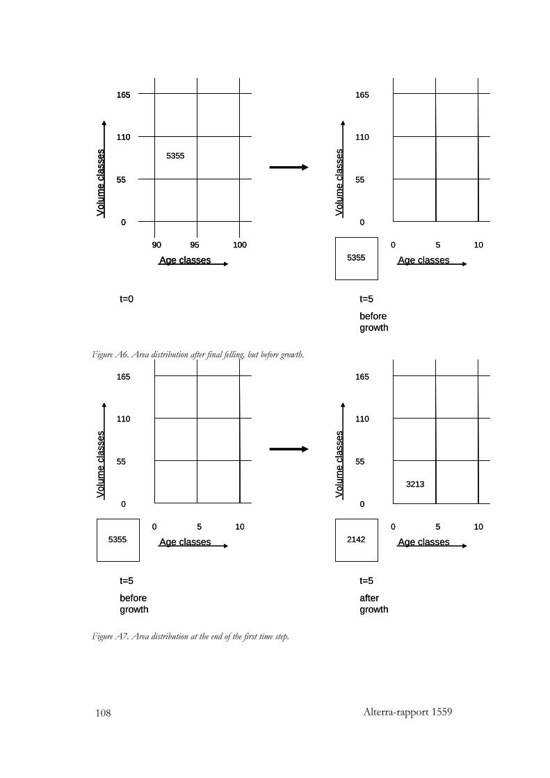
Alterra-rapport 1559 108
90 95 100
0
55
110
165
Age classes
Volu
me
clas
ses
0 5 10
0
55
110
165
Age classes
Volu
me
clas
ses5355
t=0 t=5
beforegrowth
535590 95 100
0
55
110
165
Age classes
Volu
me
clas
ses
90 95 100
0
55
110
165
Age classes
Volu
me
clas
ses
0 5 10
0
55
110
165
Age classes
Volu
me
clas
ses5355
t=0 t=5
beforegrowth
5355
Figure A6. Area distribution after final felling, but before growth.
0 5 10
0
55
110
165
Age classes
Volu
me
clas
ses
t=5
beforegrowth
t=5
aftergrowth
21420 5 10
0
55
110
165
Age classes
Volu
me
clas
ses
5355
3213
0 5 10
0
55
110
165
Age classes
Volu
me
clas
ses
t=5
beforegrowth
t=5
aftergrowth
21420 5 10
0
55
110
165
Age classes
Volu
me
clas
ses
5355
3213
Figure A7. Area distribution at the end of the first time step.
Alterra-rapport 1559 109
Annex B Tests for EFISCEN 3.1.3
In this annex, EFISCEN 3.1.3 is subjected to a series of tests. First, we evaluate how well the model is able to reproduce the input levels of average volume, increment and harvest for the test country Utopia. For these tests, we parameterised Utopia as close as possible to the corresponding Finnish forest type. From a simulation with current harvest levels for total Finland, we derived thinning and final felling volumes that were allocated to the forest type that serves as Utopia (Table B1). These levels were applied in this test series, together with the management regime and all other parameters being equal to the Finnish parameters. Secondly we tested the model outcomes against the theoretical calculations from Annex A. Thirdly we designed some logical tests to see if the model behaves as expected. These tests try to cover both the single modules as well as the behaviour of the whole model. For these tests, Utopia is used as a basis, but for specific purposes the original set-up may be changed, for example the area distribution.
Reproducing input levels Matrix initialisation In section A1 of Annex A the basic input data for Utopia is shown. In section A2, the distribution of the area over the matrix is shown. From this distribution we can recalculate the average volume per age class and for the whole area. Both per age class and for the whole area, tha average volumes match. When we aggregate the total area in the matrix, we get a total area of 1777.46 thousand ha, while the input data show 1777492 ha. This loss of 32 ha is 0.0018% of the original area and can most likely be attributed to rounding errors. In Figure B1, the distribution of the area per age class over the volume classes is shown. Due to the low number of volume classes the distriubtions are not very smooth, but the general picture is satisfying. All age classes show a kind of skewed Gaussian distribtion with a longer right tail. Also the patterns between the age classes are fully in line with what could be expected with regard to their respective average volumes.
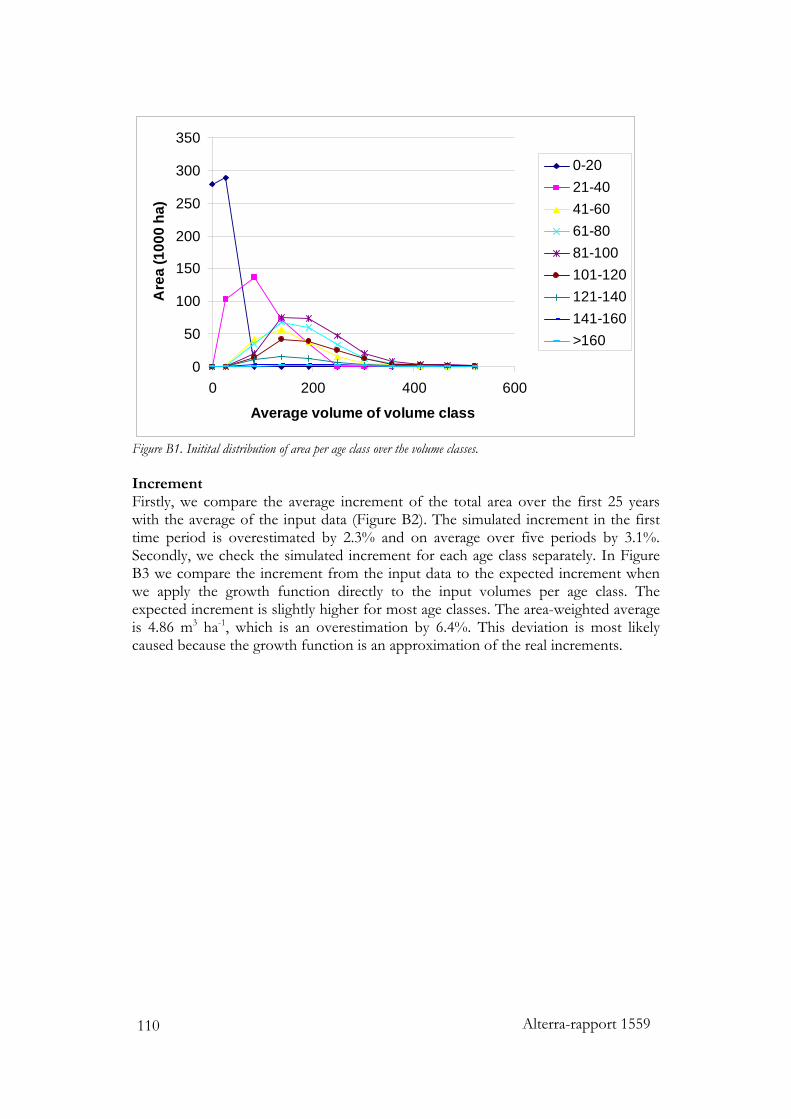
Alterra-rapport 1559 110
0
50
100
150
200
250
300
350
0 200 400 600
Average volume of volume class
Are
a (1
000
ha)
0-2021-4041-6061-8081-100101-120121-140141-160>160
Figure B1. Initital distribution of area per age class over the volume classes. Increment Firstly, we compare the average increment of the total area over the first 25 years with the average of the input data (Figure B2). The simulated increment in the first time period is overestimated by 2.3% and on average over five periods by 3.1%. Secondly, we check the simulated increment for each age class separately. In Figure B3 we compare the increment from the input data to the expected increment when we apply the growth function directly to the input volumes per age class. The expected increment is slightly higher for most age classes. The area-weighted average is 4.86 m3 ha-1, which is an overestimation by 6.4%. This deviation is most likely caused because the growth function is an approximation of the real increments.
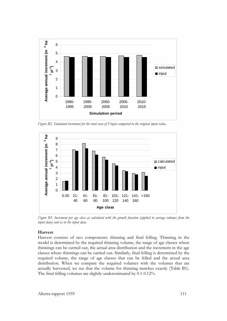
Alterra-rapport 1559 111
0
1
2
3
4
5
6
1990-1995
1995-2000
2000-2005
2005-2010
2010-2015
Simulation period
Ave
rage
ann
ual i
ncre
men
t (m
3 ha-
1 yr-1
) simulatedinput
Figure B2. Simulated increment for the total area of Utopia compared to the original input value.
0123456789
0-20 21-40
41-60
61-80
81-100
101-120
121-140
141-160
>160
Age class
Ave
rage
ann
ual i
ncre
men
t (m
3 ha-
1 yr-1
) calculatedinput
Figure B3. Increment per age class as calculated with the growth function (applied to average volumes from the input data) and as in the input data. Harvest Harvest consists of two components: thinning and final felling. Thinning in the model is determined by the required thinning volume, the range of age classes where thinnings can be carried out, the actual area distribution and the increment in the age classes where thinnings can be carried out. Similarly, final felling is determined by the required volume, the range of age classes that can be felled and the actual area distribution. When we compare the required volumes with the volumes that are actually harvested, we see that the volume for thinning matches exactly (Table B1). The final felling volumes are slightly underestimated by 0.1-0.12%.
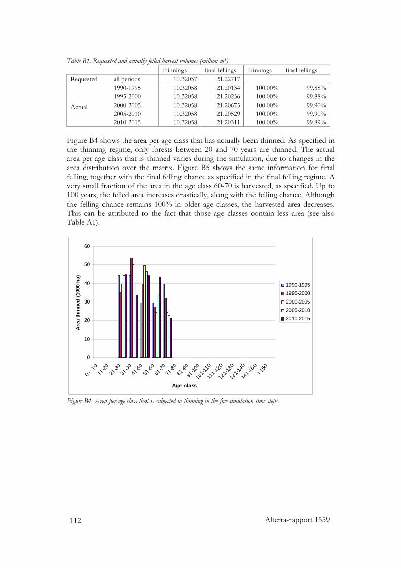
Alterra-rapport 1559 112
Table B1. Requested and actually felled harvest volumes (million m3) thinnings final fellings thinnings final fellings Requested all periods 10.32057 21.22717
1990-1995 10.32058 21.20134 100.00% 99.88% 1995-2000 10.32058 21.20236 100.00% 99.88% 2000-2005 10.32058 21.20675 100.00% 99.90% 2005-2010 10.32058 21.20529 100.00% 99.90%
Actual 2010-2015 10.32058 21.20311 100.00% 99.89%
Figure B4 shows the area per age class that has actually been thinned. As specified in the thinning regime, only forests between 20 and 70 years are thinned. The actual area per age class that is thinned varies during the simulation, due to changes in the area distribution over the matrix. Figure B5 shows the same information for final felling, together with the final felling chance as specified in the final felling regime. A very small fraction of the area in the age class 60-70 is harvested, as specified. Up to 100 years, the felled area increases drastically, along with the felling chance. Although the felling chance remains 100% in older age classes, the harvested area decreases. This can be attributed to the fact that those age classes contain less area (see also Table A1).
0
10
20
30
40
50
60
0 - 1
011
-2021
-3031
-4041
-5051
-6061
-7071
-8081
-90
91-10
0
101-1
10
111-1
20
121-1
30
131-1
40
141-1
50>15
0
Age class
Area
thin
ned
(100
0 ha
)
1990-19951995-20002000-20052005-20102010-2015
Figure B4. Area per age class that is subjected to thinning in the five simulation time steps.
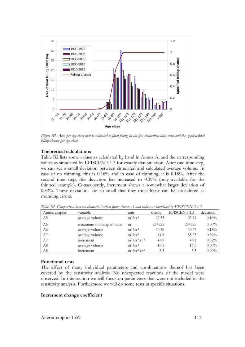
Alterra-rapport 1559 113
0
5
10
15
20
25
30
35
0 - 1
011
-2021
-3031
-4041
-5051
-6061
-7071
-8081
-90
91-10
0
101-1
10
111-1
20
121-1
30
131-1
40
141-1
50>15
0
Age class
Area
of f
inal
felli
ng (1
000
ha)
0
0.2
0.4
0.6
0.8
1
1.2
Spec
ified
felli
ng c
hanc
e
1990-19951995-20002000-20052005-20102010-2015Felling chance
Figure B5. Area per age class that is subjected to final felling in the five simulation time steps and the applied final felling chance per age class. Theoretical calculations Table B2 lists some values as calculated by hand in Annex A, and the corresponding values as simulated by EFISCEN 3.1.3 for exactly that situation. After one time step, we can see a small deviation between simulated and calculated average volume. In case of no thinning, this is 0.16% and in case of thinning, it is 0.18%. After the second time step, this deviation has increased to 0.39% (only available for the thinned example). Consequently, increment shows a somewhat larger deviation of 0.82%. These deviations are so small that they most likely can be considered as rounding errors. Table B2. Comparison between theoretical values from Annex A and values as simulated by EFISCEN 3.1.3.
Annex chapter variable unit theory EFISCEN 3.1.3 deviation A5 average volume m3 ha-1 97.55 97.71 0.16%A6 maximum thinning amount m3 294525 294525 0.00%A6 average volume m3 ha-1 60.56 60.67 0.18%A7 average volume m3 ha-1 84.9 85.23 0.39%A7 increment m3 ha-1 yr-1 4.87 4.91 0.82%A8 average volume m3 ha-1 16.5 16.5 0.00%A8 increment m3 ha-1 yr-1 3.3 3.3 0.00%
Functional tests The effect of many individual parameters and combinations thereof has been covered by the sensitivity analysis. No unexpected reactions of the model were observed. In this section we will focus on parameters that were not included in the sensitivity analysis. Furthermore we will do some tests in specific situations. Increment change coefficient
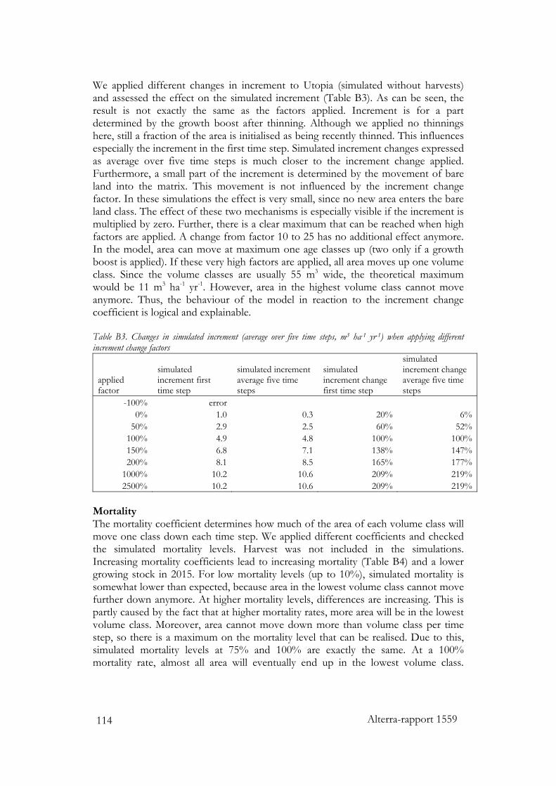
Alterra-rapport 1559 114
We applied different changes in increment to Utopia (simulated without harvests) and assessed the effect on the simulated increment (Table B3). As can be seen, the result is not exactly the same as the factors applied. Increment is for a part determined by the growth boost after thinning. Although we applied no thinnings here, still a fraction of the area is initialised as being recently thinned. This influences especially the increment in the first time step. Simulated increment changes expressed as average over five time steps is much closer to the increment change applied. Furthermore, a small part of the increment is determined by the movement of bare land into the matrix. This movement is not influenced by the increment change factor. In these simulations the effect is very small, since no new area enters the bare land class. The effect of these two mechanisms is especially visible if the increment is multiplied by zero. Further, there is a clear maximum that can be reached when high factors are applied. A change from factor 10 to 25 has no additional effect anymore. In the model, area can move at maximum one age classes up (two only if a growth boost is applied). If these very high factors are applied, all area moves up one volume class. Since the volume classes are usually 55 m3 wide, the theoretical maximum would be 11 m3 ha-1 yr-1. However, area in the highest volume class cannot move anymore. Thus, the behaviour of the model in reaction to the increment change coefficient is logical and explainable. Table B3. Changes in simulated increment (average over five time steps, m3 ha-1 yr-1) when applying different increment change factors
applied factor
simulated increment first time step
simulated increment average five time steps
simulated increment change first time step
simulated increment change average five time steps
-100% error 0% 1.0 0.3 20% 6%
50% 2.9 2.5 60% 52%100% 4.9 4.8 100% 100%150% 6.8 7.1 138% 147%200% 8.1 8.5 165% 177%
1000% 10.2 10.6 209% 219%2500% 10.2 10.6 209% 219%
Mortality The mortality coefficient determines how much of the area of each volume class will move one class down each time step. We applied different coefficients and checked the simulated mortality levels. Harvest was not included in the simulations. Increasing mortality coefficients lead to increasing mortality (Table B4) and a lower growing stock in 2015. For low mortality levels (up to 10%), simulated mortality is somewhat lower than expected, because area in the lowest volume class cannot move further down anymore. At higher mortality levels, differences are increasing. This is partly caused by the fact that at higher mortality rates, more area will be in the lowest volume class. Moreover, area cannot move down more than volume class per time step, so there is a maximum on the mortality level that can be realised. Due to this, simulated mortality levels at 75% and 100% are exactly the same. At a 100% mortality rate, almost all area will eventually end up in the lowest volume class.
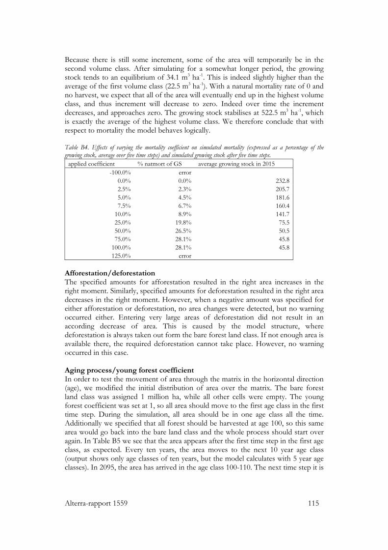
Alterra-rapport 1559 115
Because there is still some increment, some of the area will temporarily be in the second volume class. After simulating for a somewhat longer period, the growing stock tends to an equilibrium of 34.1 m3 ha-1. This is indeed slightly higher than the average of the first volume class (22.5 m3 ha-1). With a natural mortality rate of 0 and no harvest, we expect that all of the area will eventually end up in the highest volume class, and thus increment will decrease to zero. Indeed over time the increment decreases, and approaches zero. The growing stock stabilises at 522.5 m3 ha-1, which is exactly the average of the highest volume class. We therefore conclude that with respect to mortality the model behaves logically. Table B4. Effects of varying the mortality coefficient on simulated mortality (expressed as a percentage of the growing stock, average over five time steps) and simulated growing stock after five time steps.
applied coefficient % natmort of GS average growing stock in 2015 -100.0% error
0.0% 0.0% 232.8 2.5% 2.3% 205.7 5.0% 4.5% 181.6 7.5% 6.7% 160.4
10.0% 8.9% 141.7 25.0% 19.8% 75.5 50.0% 26.5% 50.5 75.0% 28.1% 45.8
100.0% 28.1% 45.8 125.0% error
Afforestation/deforestation The specified amounts for afforestation resulted in the right area increases in the right moment. Similarly, specified amounts for deforestation resulted in the right area decreases in the right moment. However, when a negative amount was specified for either afforestation or deforestation, no area changes were detected, but no warning occurred either. Entering very large areas of deforestation did not result in an according decrease of area. This is caused by the model structure, where deforestation is always taken out form the bare forest land class. If not enough area is available there, the required deforestation cannot take place. However, no warning occurred in this case. Aging process/young forest coefficient In order to test the movement of area through the matrix in the horizontal direction (age), we modified the initial distribution of area over the matrix. The bare forest land class was assigned 1 million ha, while all other cells were empty. The young forest coefficient was set at 1, so all area should move to the first age class in the first time step. During the simulation, all area should be in one age class all the time. Additionally we specified that all forest should be harvested at age 100, so this same area would go back into the bare land class and the whole process should start over again. In Table B5 we see that the area appears after the first time step in the first age class, as expected. Every ten years, the area moves to the next 10 year age class (output shows only age classes of ten years, but the model calculates with 5 year age classes). In 2095, the area has arrived in the age class 100-110. The next time step it is
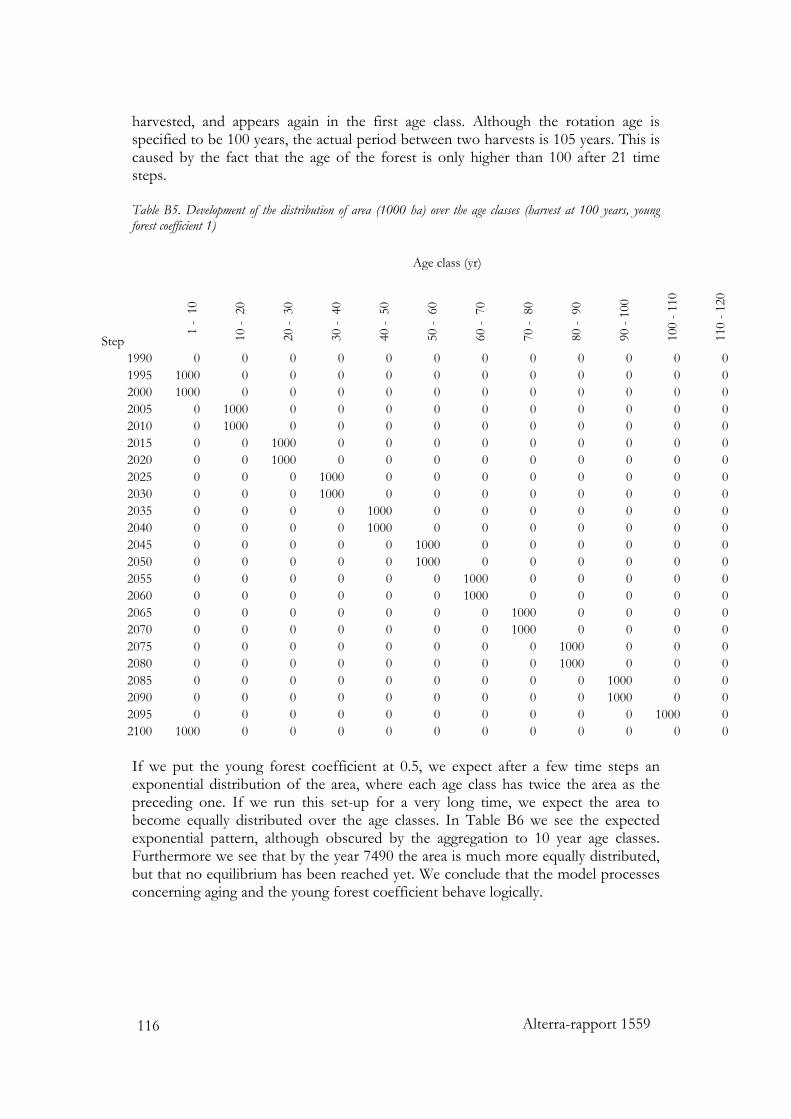
Alterra-rapport 1559 116
harvested, and appears again in the first age class. Although the rotation age is specified to be 100 years, the actual period between two harvests is 105 years. This is caused by the fact that the age of the forest is only higher than 100 after 21 time steps. Table B5. Development of the distribution of area (1000 ha) over the age classes (harvest at 100 years, young forest coefficient 1)
Age class (yr)
Step 1 -
10
10 -
20
20 -
30
30 -
40
40 -
50
50 -
60
60 -
70
70 -
80
80 -
90
90 -
100
100
- 110
110
- 120
1990 0 0 0 0 0 0 0 0 0 0 0 01995 1000 0 0 0 0 0 0 0 0 0 0 02000 1000 0 0 0 0 0 0 0 0 0 0 02005 0 1000 0 0 0 0 0 0 0 0 0 02010 0 1000 0 0 0 0 0 0 0 0 0 02015 0 0 1000 0 0 0 0 0 0 0 0 02020 0 0 1000 0 0 0 0 0 0 0 0 02025 0 0 0 1000 0 0 0 0 0 0 0 02030 0 0 0 1000 0 0 0 0 0 0 0 02035 0 0 0 0 1000 0 0 0 0 0 0 02040 0 0 0 0 1000 0 0 0 0 0 0 02045 0 0 0 0 0 1000 0 0 0 0 0 02050 0 0 0 0 0 1000 0 0 0 0 0 02055 0 0 0 0 0 0 1000 0 0 0 0 02060 0 0 0 0 0 0 1000 0 0 0 0 02065 0 0 0 0 0 0 0 1000 0 0 0 02070 0 0 0 0 0 0 0 1000 0 0 0 02075 0 0 0 0 0 0 0 0 1000 0 0 02080 0 0 0 0 0 0 0 0 1000 0 0 02085 0 0 0 0 0 0 0 0 0 1000 0 02090 0 0 0 0 0 0 0 0 0 1000 0 02095 0 0 0 0 0 0 0 0 0 0 1000 02100 1000 0 0 0 0 0 0 0 0 0 0 0 If we put the young forest coefficient at 0.5, we expect after a few time steps an exponential distribution of the area, where each age class has twice the area as the preceding one. If we run this set-up for a very long time, we expect the area to become equally distributed over the age classes. In Table B6 we see the expected exponential pattern, although obscured by the aggregation to 10 year age classes. Furthermore we see that by the year 7490 the area is much more equally distributed, but that no equilibrium has been reached yet. We conclude that the model processes concerning aging and the young forest coefficient behave logically.
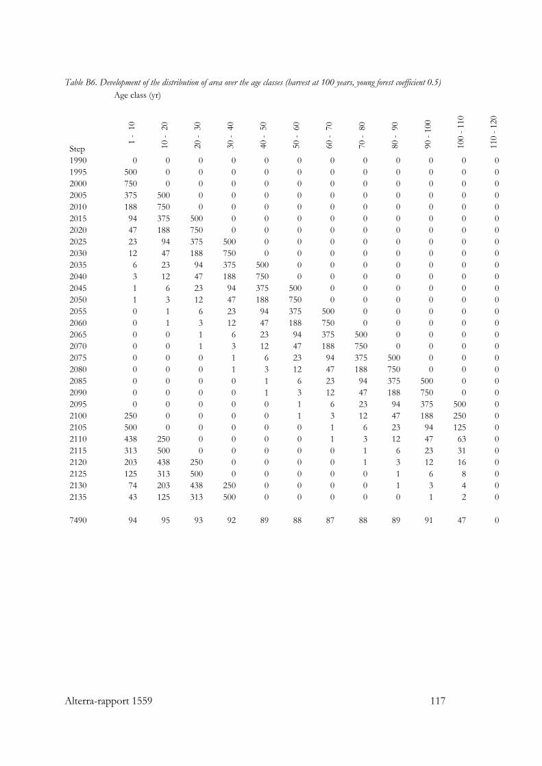
Alterra-rapport 1559 117
Table B6. Development of the distribution of area over the age classes (harvest at 100 years, young forest coefficient 0.5) Age class (yr)
Step 1 -
10
10 -
20
20 -
30
30 -
40
40 -
50
50 -
60
60 -
70
70 -
80
80 -
90
90 -
100
100
- 110
110
- 120
1990 0 0 0 0 0 0 0 0 0 0 0 01995 500 0 0 0 0 0 0 0 0 0 0 02000 750 0 0 0 0 0 0 0 0 0 0 02005 375 500 0 0 0 0 0 0 0 0 0 02010 188 750 0 0 0 0 0 0 0 0 0 02015 94 375 500 0 0 0 0 0 0 0 0 02020 47 188 750 0 0 0 0 0 0 0 0 02025 23 94 375 500 0 0 0 0 0 0 0 02030 12 47 188 750 0 0 0 0 0 0 0 02035 6 23 94 375 500 0 0 0 0 0 0 02040 3 12 47 188 750 0 0 0 0 0 0 02045 1 6 23 94 375 500 0 0 0 0 0 02050 1 3 12 47 188 750 0 0 0 0 0 02055 0 1 6 23 94 375 500 0 0 0 0 02060 0 1 3 12 47 188 750 0 0 0 0 02065 0 0 1 6 23 94 375 500 0 0 0 02070 0 0 1 3 12 47 188 750 0 0 0 02075 0 0 0 1 6 23 94 375 500 0 0 02080 0 0 0 1 3 12 47 188 750 0 0 02085 0 0 0 0 1 6 23 94 375 500 0 02090 0 0 0 0 1 3 12 47 188 750 0 02095 0 0 0 0 0 1 6 23 94 375 500 02100 250 0 0 0 0 1 3 12 47 188 250 02105 500 0 0 0 0 0 1 6 23 94 125 02110 438 250 0 0 0 0 1 3 12 47 63 02115 313 500 0 0 0 0 0 1 6 23 31 02120 203 438 250 0 0 0 0 1 3 12 16 02125 125 313 500 0 0 0 0 0 1 6 8 02130 74 203 438 250 0 0 0 0 1 3 4 02135 43 125 313 500 0 0 0 0 0 1 2 0 7490 94 95 93 92 89 88 87 88 89 91 47 0
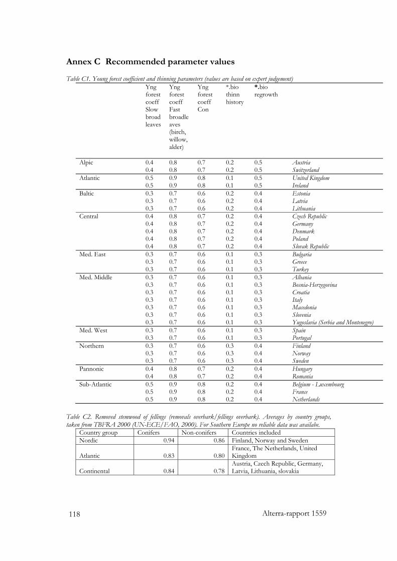
Alterra-rapport 1559 118
Annex C Recommended parameter values
Table C1. Young forest coefficient and thinning parameters (values are based on expert judgement) Yng
forest coeff Slow broadleaves
Yng forest coeff Fast broadleaves (birch, willow, alder)
Yng forest coeff Con
*.bio thinn history
*.bio regrowth
Alpic 0.4 0.8 0.7 0.2 0.5 Austria 0.4 0.8 0.7 0.2 0.5 Switzerland Atlantic 0.5 0.9 0.8 0.1 0.5 United Kingdom 0.5 0.9 0.8 0.1 0.5 Ireland Baltic 0.3 0.7 0.6 0.2 0.4 Estonia 0.3 0.7 0.6 0.2 0.4 Latvia 0.3 0.7 0.6 0.2 0.4 Lithuania Central 0.4 0.8 0.7 0.2 0.4 Czech Republic 0.4 0.8 0.7 0.2 0.4 Germany 0.4 0.8 0.7 0.2 0.4 Denmark 0.4 0.8 0.7 0.2 0.4 Poland 0.4 0.8 0.7 0.2 0.4 Slovak Republic Med. East 0.3 0.7 0.6 0.1 0.3 Bulgaria 0.3 0.7 0.6 0.1 0.3 Greece 0.3 0.7 0.6 0.1 0.3 Turkey Med. Middle 0.3 0.7 0.6 0.1 0.3 Albania 0.3 0.7 0.6 0.1 0.3 Bosnia-Herzegovina 0.3 0.7 0.6 0.1 0.3 Croatia 0.3 0.7 0.6 0.1 0.3 Italy 0.3 0.7 0.6 0.1 0.3 Macedonia 0.3 0.7 0.6 0.1 0.3 Slovenia 0.3 0.7 0.6 0.1 0.3 Yugoslavia (Serbia and Montenegro) Med. West 0.3 0.7 0.6 0.1 0.3 Spain 0.3 0.7 0.6 0.1 0.3 Portugal Northern 0.3 0.7 0.6 0.3 0.4 Finland 0.3 0.7 0.6 0.3 0.4 Norway 0.3 0.7 0.6 0.3 0.4 Sweden Pannonic 0.4 0.8 0.7 0.2 0.4 Hungary 0.4 0.8 0.7 0.2 0.4 Romania Sub-Atlantic 0.5 0.9 0.8 0.2 0.4 Belgium - Luxembourg 0.5 0.9 0.8 0.2 0.4 France 0.5 0.9 0.8 0.2 0.4 Netherlands
Table C2. Removed stemwood of fellings (removals overbark/fellings overbark). Averages by country groups, taken from TBFRA 2000 (UN-ECE/FAO, 2000). For Southern Europe no reliable data was availabe.
Country group Conifers Non-conifers Countries included Nordic 0.94 0.86 Finland, Norway and Sweden
Atlantic 0.83 0.80France, The Netherlands, United Kingdom
Continental 0.84 0.78Austria, Czech Republic, Germany, Latvia, Lithuania, slovakia