Mishkin's Economics of Money, Banking and Financial ...

Seventh Edition

Abel/BernankeMacroeconomics

Bade/ParkinFoundations of Microeconomics

Bade/ParkinFoundations of Macroeconomics

Bierman/FernandezGame Theory with Economic Applications

Binger/HoffmanMicroeconomics with Calculus

BoyerPrinciples of Transportation Economics

BransonMacroeconomic Theory and Policy

BrucePublic Finance and the American Economy

Byrns/StoneEconomics

Carlton/PerloffModern Industrial Organization

Caves/Frankel/JonesWorld Trade and Payments:An Introduction

ChapmanEnvironmental Economics:Theory, Application, and Policy

Cooter/UlenLaw and Economics

DownsAn Economic Theory of Democracy

Eaton/MishkinOnline Readings to AccompanyThe Economics of Money, Banking, andFinancial Markets

Ehrenberg/SmithModern Labor Economics

Ekelund/TollisonEconomics: Private Markets and Public Choice

FusfeldThe Age of the Economist

GerberInternational Economics

GhiaraLearning Economics:A Practical Workbook

GordonMacroeconomics

GregoryEssentials of Economics

Gregory/StuartRussian and Soviet Economic Performanceand Structure

Hartwick/OlewilerThe Economics of Natural Resource Use

HubbardMoney, the Financial System, and the Economy

Hughes/CainAmerican Economic History

Husted/MelvinInternational Economics

Jehle/RenyAdvanced Microeconomic Theory

KleinMathematical Methods for Economics

Krugman/ObstfeldInternational Economics:Theory and Policy

LaidlerThe Demand for Money: Theories, Evidence, and Problems

Leeds/von AllmenThe Economics of Sports

Lipsey/Courant/RaganEconomics

McCartyDollars and Sense: An Introduction to Economics

MelvinInternational Money and Finance

MillerEconomics Today

Miller/Benjamin/NorthThe Economics of Public Issues

Mills/HamiltonUrban Economics

MishkinThe Economics of Money, Banking, andFinancial Markets

ParkinEconomics

Parkin/BadeEconomics in Action Software

PerloffMicroeconomics

PhelpsHealth Economics

Riddell/Shackelford/Stamos/SchneiderEconomics: A Tool for CriticallyUnderstanding Society

Ritter/Silber/UdellPrinciples of Money, Banking, and Financial Markets

RohlfIntroduction to Economic Reasoning

Ruffin/GregoryPrinciples of Economics

Sargent Rational Expectations and Inflation

SchererIndustry Structure, Strategy, and Public Policy

SchotterMicroeconomics: A Modern Approach

Stock/WatsonIntroduction to Econometrics

StudenmundUsing Econometrics: A Practical Guide

TietenbergEnvironmental and Natural Resource Economics

TietenbergEnvironmental Economics and Policy

Todaro/SmithEconomic Development

Waldman/JensenIndustrial Organization:Theory and Practice

WilliamsonMacroeconomics

The Addison-Wesley Series in Economics

Frederic S. MishkinColumbia University

Editor in Chief: Denise Clinton

Acquisitions Editor: Victoria Warneck

Executive Development Manager: Sylvia Mallory

Development Editor: Jane Tufts

Production Supervisor: Meredith Gertz

Text Design: Studio Montage

Cover Design: Regina Hagen Kolenda and Studio Montage

Composition: Argosy Publishing

Senior Manufacturing Supervisor: Hugh Crawford

Senior Marketing Manager: Barbara LeBuhn

Cover images: © PhotoDisc

Media Producer: Melissa Honig

Supplements Editor: Diana Theriault

Credits to copyrighted material appear on p. C-1, which constitutes a continuation of the copyright page.

Library of Congress Cataloguing-in-Publication Data

Mishkin, Frederic S.The economics of money, banking, and financial markets / Frederic S. Mishkin.—7th ed.

p. cm. — (The Addison-Wesley series in economics)Supplemented by a subscription to a companion web site.Includes bibliographical references and index.ISBN 0-321-12235-61. Finance. 2. Money. 3. Banks and banking. I. Title. II. Series.

HG173.M632 2004332—dc21

2003041912

Copyright © 2004 by Frederic S. Mishkin. All rights reserved. No part of this publication may be repro-duced, stored in a retrieval system, or transmitted, in any form or by any means, electronic, mechanical,photocopying, recording, or otherwise, without the prior written permission of the publisher. Printed inthe United States of America.

1 2 3 4 5 6 7 8 9 10—DOW—06050403

To Sally

Introduction 11 Why Study Money, Banking, and Financial Markets? . . . . . . . . . . . . . . . . . . . .3

2 An Overview of the Financial System . . . . . . . . . . . . . . . . . . . . . . . . . . . . . . . .23

3 What Is Money? . . . . . . . . . . . . . . . . . . . . . . . . . . . . . . . . . . . . . . . . . . . . . . . .44

Financial Markets 594 Understanding Interest Rates . . . . . . . . . . . . . . . . . . . . . . . . . . . . . . . . . . . . . .61

5 The Behavior of Interest Rates . . . . . . . . . . . . . . . . . . . . . . . . . . . . . . . . . . . . .85

6 The Risk and Term Structure of Interest Rates . . . . . . . . . . . . . . . . . . . . . . . .120

7 The Stock Market, the Theory of Rational Expectations, and the Efficient Market Hypothesis . . . . . . . . . . . . . . . . . . . . . . . . . . . . . . .141

Financial Institutions 1678 An Economic Analysis of Financial Structure . . . . . . . . . . . . . . . . . . . . . . . .169

9 Banking and the Management of Financial Institutions . . . . . . . . . . . . . . . . .201

10 Banking Industry: Structure and Competition . . . . . . . . . . . . . . . . . . . . . . . .229

11 Economic Analysis of Banking Regulation . . . . . . . . . . . . . . . . . . . . . . . . . . .260

12 Nonbank Finance . . . . . . . . . . . . . . . . . . . . . . . . . . . . . . . . . . . . . . . . . . . . . .287

13 Financial Derivatives . . . . . . . . . . . . . . . . . . . . . . . . . . . . . . . . . . . . . . . . . . .309

Central Banking and the Conduct of Monetary Policy 33314 Structure of Central Banks and the Federal Reserve System . . . . . . . . . . . . .335

15 Multiple Deposit Creation and the Money Supply Process . . . . . . . . . . . . . .357

16 Determinants of the Money Supply . . . . . . . . . . . . . . . . . . . . . . . . . . . . . . . .374

17 Tools of Monetary Policy . . . . . . . . . . . . . . . . . . . . . . . . . . . . . . . . . . . . . . . .393

18 Conduct of Monetary Policy: Goals and Targets . . . . . . . . . . . . . . . . . . . . . .411

International Finance and Monetary Policy 43319 The Foreign Exchange Market . . . . . . . . . . . . . . . . . . . . . . . . . . . . . . . . . . . .435

20 The International Financial System . . . . . . . . . . . . . . . . . . . . . . . . . . . . . . . .462

21 Monetary Policy Strategy: The International Experience . . . . . . . . . . . . . . . .487

P A R T V

P A R T I V

P A R T I I I

P A R T I I

P A R T I

vii

CONTENTS IN BRIEF

Monetary Theory 51522 The Demand for Money . . . . . . . . . . . . . . . . . . . . . . . . . . . . . . . . . . . . . . . . .517

23 The Keynesian Framework and the ISLM Model . . . . . . . . . . . . . . . . . . . . . .536

24 Monetary and Fiscal Policy in the ISLM Model . . . . . . . . . . . . . . . . . . . . . . .561

25 Aggregate Demand and Supply Analysis . . . . . . . . . . . . . . . . . . . . . . . . . . . .582

26 Transmission Mechanisms of Monetary Policy: The Evidence . . . . . . . . . . . .603

27 Money and Inflation . . . . . . . . . . . . . . . . . . . . . . . . . . . . . . . . . . . . . . . . . . . .632

28 Rational Expectations: Implications for Policy . . . . . . . . . . . . . . . . . . . . . . . .658

P A R T V I

viii Contents in Brief

Introduction 1

CHAPTER 1WHY STUDY MONEY, BANKING, AND FINANCIAL MARKETS? . . . . . . . . . . . . . . . . .3Preview . . . . . . . . . . . . . . . . . . . . . . . . . . . . . . . . . . . . . . . . . . . . . . . . . . . . . . . . . . . .3

Why Study Financial Markets? . . . . . . . . . . . . . . . . . . . . . . . . . . . . . . . . . . . . . . . . . .3The Bond Market and Interest Rates . . . . . . . . . . . . . . . . . . . . . . . . . . . . . . . . . . . . . . . . . . .3The Stock Market . . . . . . . . . . . . . . . . . . . . . . . . . . . . . . . . . . . . . . . . . . . . . . . . . . . . . . . . .5The Foreign Exchange Market . . . . . . . . . . . . . . . . . . . . . . . . . . . . . . . . . . . . . . . . . . . . . . .5

Why Study Banking and Financial Institutions? . . . . . . . . . . . . . . . . . . . . . . . . . . . . .7Structure of the Financial System . . . . . . . . . . . . . . . . . . . . . . . . . . . . . . . . . . . . . . . . . . . . .7Banks and Other Financial Institutions . . . . . . . . . . . . . . . . . . . . . . . . . . . . . . . . . . . . . . . . .8Financial Innovation . . . . . . . . . . . . . . . . . . . . . . . . . . . . . . . . . . . . . . . . . . . . . . . . . . . . . . .8

Why Study Money and Monetary Policy? . . . . . . . . . . . . . . . . . . . . . . . . . . . . . . . . . .8Money and Business Cycles . . . . . . . . . . . . . . . . . . . . . . . . . . . . . . . . . . . . . . . . . . . . . . . . .9Money and Inflation . . . . . . . . . . . . . . . . . . . . . . . . . . . . . . . . . . . . . . . . . . . . . . . . . . . . . .10Money and Interest Rates . . . . . . . . . . . . . . . . . . . . . . . . . . . . . . . . . . . . . . . . . . . . . . . . . .12Conduct of Monetary Policy . . . . . . . . . . . . . . . . . . . . . . . . . . . . . . . . . . . . . . . . . . . . . . . .12Fiscal Policy and Monetary Policy . . . . . . . . . . . . . . . . . . . . . . . . . . . . . . . . . . . . . . . . . . . .12

How We Will Study Money, Banking, and Financial Markets . . . . . . . . . . . . . . . . . .13Exploring the Web . . . . . . . . . . . . . . . . . . . . . . . . . . . . . . . . . . . . . . . . . . . . . . . . . . . . . . .14

Concluding Remarks . . . . . . . . . . . . . . . . . . . . . . . . . . . . . . . . . . . . . . . . . . . . . . . .17

Summary, Key Terms, Questions and Problems, and Web Exercises . . . . . . . . . . . . .17

Appendix to Chapter 1Defining Aggregate Output, Income, the Price Level,and the Inflation Rate . . . . . . . . . . . . . . . . . . . . . . . . . . . . . . . . . . . . . . . . . . .20Aggregate Output and Income . . . . . . . . . . . . . . . . . . . . . . . . . . . . . . . . . . . . . . . . .20

Real Versus Nominal Magnitudes . . . . . . . . . . . . . . . . . . . . . . . . . . . . . . . . . . . . . . .20

Aggregate Price Level . . . . . . . . . . . . . . . . . . . . . . . . . . . . . . . . . . . . . . . . . . . . . . . .21

Growth Rates and the Inflation Rate . . . . . . . . . . . . . . . . . . . . . . . . . . . . . . . . . . . . .22

P A R T I

ix

CONTENTS

CHAPTER 2AN OVERVIEW OF THE FINANCIAL SYSTEM . . . . . . . . . . . . . . . . . . . . . . . . . . . . .23Preview . . . . . . . . . . . . . . . . . . . . . . . . . . . . . . . . . . . . . . . . . . . . . . . . . . . . . . . . . . .23

Function of Financial Markets . . . . . . . . . . . . . . . . . . . . . . . . . . . . . . . . . . . . . . . . .23

Structure of Financial Markets . . . . . . . . . . . . . . . . . . . . . . . . . . . . . . . . . . . . . . . . .25Debt and Equity Markets . . . . . . . . . . . . . . . . . . . . . . . . . . . . . . . . . . . . . . . . . . . . . . . . . .25Primary and Secondary Markets . . . . . . . . . . . . . . . . . . . . . . . . . . . . . . . . . . . . . . . . . . . . .26Exchanges and Over-the-Counter Markets . . . . . . . . . . . . . . . . . . . . . . . . . . . . . . . . . . . . .27Money and Capital Markets . . . . . . . . . . . . . . . . . . . . . . . . . . . . . . . . . . . . . . . . . . . . . . . .27

Internationalization of Financial Markets . . . . . . . . . . . . . . . . . . . . . . . . . . . . . . . . .28International Bond Market, Eurobonds, and Eurocurrencies . . . . . . . . . . . . . . . . . . . . . . . .28World Stock Markets . . . . . . . . . . . . . . . . . . . . . . . . . . . . . . . . . . . . . . . . . . . . . . . . . . . . .29

Function of Financial Intermediaries . . . . . . . . . . . . . . . . . . . . . . . . . . . . . . . . . . . .29Transaction Costs . . . . . . . . . . . . . . . . . . . . . . . . . . . . . . . . . . . . . . . . . . . . . . . . . . . . . . . .29

Following the Financial News Foreign Stock Market Indexes . . . . . . . . . . . . . . . .30

Box 1 Global: The Importance of Financial Intermediaries to Securities Markets: An International Comparison . . . . . . . . . . . . . . . . . . . . . . . . . . . . . . . . . .31

Risk Sharing . . . . . . . . . . . . . . . . . . . . . . . . . . . . . . . . . . . . . . . . . . . . . . . . . . . . . . . . . . . .31Asymmetric Information: Adverse Selection and Moral Hazard . . . . . . . . . . . . . . . . . . . . .32

Financial Intermediaries . . . . . . . . . . . . . . . . . . . . . . . . . . . . . . . . . . . . . . . . . . . . . .34Depository Institutions . . . . . . . . . . . . . . . . . . . . . . . . . . . . . . . . . . . . . . . . . . . . . . . . . . . .34Contractual Savings Institutions . . . . . . . . . . . . . . . . . . . . . . . . . . . . . . . . . . . . . . . . . . . . .35Investment Intermediaries . . . . . . . . . . . . . . . . . . . . . . . . . . . . . . . . . . . . . . . . . . . . . . . . .37

Regulation of the Financial System . . . . . . . . . . . . . . . . . . . . . . . . . . . . . . . . . . . . . .37Increasing Information Available to Investors . . . . . . . . . . . . . . . . . . . . . . . . . . . . . . . . . . .39Ensuring the Soundness of Financial Intermediaries . . . . . . . . . . . . . . . . . . . . . . . . . . . . . .39Financial Regulation Abroad . . . . . . . . . . . . . . . . . . . . . . . . . . . . . . . . . . . . . . . . . . . . . . . .40


CHAPTER 3WHAT IS MONEY? . . . . . . . . . . . . . . . . . . . . . . . . . . . . . . . . . . . . . . . . . . . . . . .44Preview . . . . . . . . . . . . . . . . . . . . . . . . . . . . . . . . . . . . . . . . . . . . . . . . . . . . . . . . . . .44

Meaning of Money . . . . . . . . . . . . . . . . . . . . . . . . . . . . . . . . . . . . . . . . . . . . . . . . . .44

Functions of Money . . . . . . . . . . . . . . . . . . . . . . . . . . . . . . . . . . . . . . . . . . . . . . . . .45Medium of Exchange . . . . . . . . . . . . . . . . . . . . . . . . . . . . . . . . . . . . . . . . . . . . . . . . . . . . .45Unit of Account . . . . . . . . . . . . . . . . . . . . . . . . . . . . . . . . . . . . . . . . . . . . . . . . . . . . . . . . .46Store of Value . . . . . . . . . . . . . . . . . . . . . . . . . . . . . . . . . . . . . . . . . . . . . . . . . . . . . . . . . . .47

Evolution of the Payments System . . . . . . . . . . . . . . . . . . . . . . . . . . . . . . . . . . . . . .48Commodity Money . . . . . . . . . . . . . . . . . . . . . . . . . . . . . . . . . . . . . . . . . . . . . . . . . . . . . . .48Fiat Money . . . . . . . . . . . . . . . . . . . . . . . . . . . . . . . . . . . . . . . . . . . . . . . . . . . . . . . . . . . . .48Checks . . . . . . . . . . . . . . . . . . . . . . . . . . . . . . . . . . . . . . . . . . . . . . . . . . . . . . . . . . . . . . . .48

Box 1 Global: Birth of the Euro: Will It Benefit Europe? . . . . . . . . . . . . . . . . . . . . .49

Electronic Payment . . . . . . . . . . . . . . . . . . . . . . . . . . . . . . . . . . . . . . . . . . . . . . . . . . . . . . .50

x Contents

Box 2 E-Finance: Why Are Scandinavians So Far Ahead of Americans in Using Electronic Payments? . . . . . . . . . . . . . . . . . . . . . . . . . . . . . . . . . . . . . . . . . .50

E-Money . . . . . . . . . . . . . . . . . . . . . . . . . . . . . . . . . . . . . . . . . . . . . . . . . . . . . . . . . . . . . . .51

Measuring Money . . . . . . . . . . . . . . . . . . . . . . . . . . . . . . . . . . . . . . . . . . . . . . . . . . .51The Federal Reserve’s Monetary Aggregates . . . . . . . . . . . . . . . . . . . . . . . . . . . . . . . . . . . . .51

Box 3 E-Finance: Are We Headed for a Cashless Society? . . . . . . . . . . . . . . . . . . . .52

Following the Financial News The Monetary Aggregates . . . . . . . . . . . . . . . . . . .54

How Reliable Are the Money Data? . . . . . . . . . . . . . . . . . . . . . . . . . . . . . . . . . . . . . .55


Financial Markets 59

CHAPTER 4UNDERSTANDING INTEREST RATES . . . . . . . . . . . . . . . . . . . . . . . . . . . . . . . . . .61Preview . . . . . . . . . . . . . . . . . . . . . . . . . . . . . . . . . . . . . . . . . . . . . . . . . . . . . . . . . . .61

Measuring Interest Rates . . . . . . . . . . . . . . . . . . . . . . . . . . . . . . . . . . . . . . . . . . . . . .61Present Value . . . . . . . . . . . . . . . . . . . . . . . . . . . . . . . . . . . . . . . . . . . . . . . . . . . . . . . . . . .61Four Types of Credit Market Instruments . . . . . . . . . . . . . . . . . . . . . . . . . . . . . . . . . . . . . .63Yield to Maturity . . . . . . . . . . . . . . . . . . . . . . . . . . . . . . . . . . . . . . . . . . . . . . . . . . . . . . . . .64

Box 1 Global: Negative T-Bill Rates? Japan Shows the Way . . . . . . . . . . . . . . . . . . .69

Other Measures of Interest Rates . . . . . . . . . . . . . . . . . . . . . . . . . . . . . . . . . . . . . . . .69Current Yield . . . . . . . . . . . . . . . . . . . . . . . . . . . . . . . . . . . . . . . . . . . . . . . . . . . . . . . . . . .70Yield on a Discount Basis . . . . . . . . . . . . . . . . . . . . . . . . . . . . . . . . . . . . . . . . . . . . . . . . . .71

Application Reading the Wall Street Journal: The Bond Page . . . . . . . . . . . . . . . . .72

Following the Financial News Bond Prices and Interest Rates . . . . . . . . . . . . . . .73

The Distinction Between Interest Rates and Returns . . . . . . . . . . . . . . . . . . . . . . . . .75Maturity and the Volatility of Bond Returns: Interest-Rate Risk . . . . . . . . . . . . . . . . . . . . . .78

Box 2 Helping Investors to Select Desired Interest-Rate Risk . . . . . . . . . . . . . . . . .79

Summary . . . . . . . . . . . . . . . . . . . . . . . . . . . . . . . . . . . . . . . . . . . . . . . . . . . . . . . . . . . . . .79

The Distinction Between Real and Nominal Interest Rates . . . . . . . . . . . . . . . . . . . .79

Box 3 With TIPS, Real Interest Rates Have Become Observable in the United States . . . . . . . . . . . . . . . . . . . . . . . . . . . . . . . . . . . . . . . . . . . . . . . . . . . . . .82


CHAPTER 5THE BEHAVIOR OF INTEREST RATES . . . . . . . . . . . . . . . . . . . . . . . . . . . . . . . . . .85Preview . . . . . . . . . . . . . . . . . . . . . . . . . . . . . . . . . . . . . . . . . . . . . . . . . . . . . . . . . . .85

Determinants of Asset Demand . . . . . . . . . . . . . . . . . . . . . . . . . . . . . . . . . . . . . . . . .85Wealth . . . . . . . . . . . . . . . . . . . . . . . . . . . . . . . . . . . . . . . . . . . . . . . . . . . . . . . . . . . . . . . .86

P A R T I I

Contents xi

Expected Returns . . . . . . . . . . . . . . . . . . . . . . . . . . . . . . . . . . . . . . . . . . . . . . . . . . . . . . . .86Risk . . . . . . . . . . . . . . . . . . . . . . . . . . . . . . . . . . . . . . . . . . . . . . . . . . . . . . . . . . . . . . . . . .87Liquidity . . . . . . . . . . . . . . . . . . . . . . . . . . . . . . . . . . . . . . . . . . . . . . . . . . . . . . . . . . . . . . .87Theory of Asset Demand . . . . . . . . . . . . . . . . . . . . . . . . . . . . . . . . . . . . . . . . . . . . . . . . . . .87

Supply and Demand in the Bond Market . . . . . . . . . . . . . . . . . . . . . . . . . . . . . . . . .87Demand Curve . . . . . . . . . . . . . . . . . . . . . . . . . . . . . . . . . . . . . . . . . . . . . . . . . . . . . . . . . .88Supply Curve . . . . . . . . . . . . . . . . . . . . . . . . . . . . . . . . . . . . . . . . . . . . . . . . . . . . . . . . . . .90Market Equilibrium . . . . . . . . . . . . . . . . . . . . . . . . . . . . . . . . . . . . . . . . . . . . . . . . . . . . . .90Supply and Demand Analysis . . . . . . . . . . . . . . . . . . . . . . . . . . . . . . . . . . . . . . . . . . . . . . .91Loanable Funds Framework . . . . . . . . . . . . . . . . . . . . . . . . . . . . . . . . . . . . . . . . . . . . . . . .91

Changes in Equilibrium Interest Rates . . . . . . . . . . . . . . . . . . . . . . . . . . . . . . . . . . .93Shifts in the Demand for Bonds . . . . . . . . . . . . . . . . . . . . . . . . . . . . . . . . . . . . . . . . . . . . .93Shifts in the Supply of Bonds . . . . . . . . . . . . . . . . . . . . . . . . . . . . . . . . . . . . . . . . . . . . . . .97

Application Changes in the Equilibrium Interest Rate Due to ExpectedInflation or Business Cycle Expansions . . . . . . . . . . . . . . . . . . . . . . . . . . . . . . . . . .99

Changes in Expected Inflation: The Fisher Effect . . . . . . . . . . . . . . . . . . . . . . . . . . . . . . . .99Business Cycle Expansion . . . . . . . . . . . . . . . . . . . . . . . . . . . . . . . . . . . . . . . . . . . . . . . . .100

Application Explaining Low Japanese Interest Rates . . . . . . . . . . . . . . . . . . . . . .103

Application Reading the Wall Street Journal “Credit Markets” Column . . . . . . . .103

Following the Financial News The “Credit Markets” Column . . . . . . . . . . . . . .104

Supply and Demand in the Market for Money: The Liquidity Preference Framework . . . . . . . . . . . . . . . . . . . . . . . . . . . . . . . . . . . . . . . . . . .105

Changes in Equilibrium Interest Rates in the Liquidity Reference Framework . . . . .107Shifts in the Demand for Money . . . . . . . . . . . . . . . . . . . . . . . . . . . . . . . . . . . . . . . . . . . .107Shifts in the Supply of Money . . . . . . . . . . . . . . . . . . . . . . . . . . . . . . . . . . . . . . . . . . . . . .108

Application Changes in the Equilibrium Interest Rate Due to Changes in Income, the Price Level, or the Money Supply . . . . . . . . . . . . . . . . . . . . . . . . .108

Changes in Income . . . . . . . . . . . . . . . . . . . . . . . . . . . . . . . . . . . . . . . . . . . . . . . . . . . . . .108Changes in the Price Level . . . . . . . . . . . . . . . . . . . . . . . . . . . . . . . . . . . . . . . . . . . . . . . .108Changes in the Money Supply . . . . . . . . . . . . . . . . . . . . . . . . . . . . . . . . . . . . . . . . . . . . .109

Following the Financial News Forecasting Interest Rates . . . . . . . . . . . . . . . . . .111

Application Money and Interest Rates . . . . . . . . . . . . . . . . . . . . . . . . . . . . . . . . .112

Does a Higher Rate of Growth of the Money Supply Lower Interest Rates? . . . . . . . . . . . .114

Summary, Key Terms, Questions and Problems, and Web Exercises . . . . . . . . . . . .117

CHAPTER 6THE RISK AND TERM STRUCTURE OF INTEREST RATES . . . . . . . . . . . . . . . . . . .120Preview . . . . . . . . . . . . . . . . . . . . . . . . . . . . . . . . . . . . . . . . . . . . . . . . . . . . . . . . . .120

Risk Structure of Interest Rates . . . . . . . . . . . . . . . . . . . . . . . . . . . . . . . . . . . . . . . .120Default Risk . . . . . . . . . . . . . . . . . . . . . . . . . . . . . . . . . . . . . . . . . . . . . . . . . . . . . . . . . . .120

Application The Enron Bankruptcy and the Baa-Aaa Spread . . . . . . . . . . . . . . . .124

xii Contents

Liquidity . . . . . . . . . . . . . . . . . . . . . . . . . . . . . . . . . . . . . . . . . . . . . . . . . . . . . . . . . . . . . .125Income Tax Considerations . . . . . . . . . . . . . . . . . . . . . . . . . . . . . . . . . . . . . . . . . . . . . . . .125Summary . . . . . . . . . . . . . . . . . . . . . . . . . . . . . . . . . . . . . . . . . . . . . . . . . . . . . . . . . . . . .127

Application Effects of the Bush Tax Cut on Bond Interest Rates . . . . . . . . . . . . .127

Term Structure of Interest Rates . . . . . . . . . . . . . . . . . . . . . . . . . . . . . . . . . . . . . . .127

Following the Financial News Yield Curves . . . . . . . . . . . . . . . . . . . . . . . . . . . .128

Expectations Theory . . . . . . . . . . . . . . . . . . . . . . . . . . . . . . . . . . . . . . . . . . . . . . . . . . . . .129Segmented Markets Theory . . . . . . . . . . . . . . . . . . . . . . . . . . . . . . . . . . . . . . . . . . . . . . .132Liquidity Premium and Preferred Habitat Theories . . . . . . . . . . . . . . . . . . . . . . . . . . . . . .133Evidence on the Term Structure . . . . . . . . . . . . . . . . . . . . . . . . . . . . . . . . . . . . . . . . . . . .136Summary . . . . . . . . . . . . . . . . . . . . . . . . . . . . . . . . . . . . . . . . . . . . . . . . . . . . . . . . . . . . .137

Application Interpreting Yield Curves, 1980–2003 . . . . . . . . . . . . . . . . . . . . . . .137


CHAPTER 7THE STOCK MARKET, THE THEORY OF RATIONAL EXPECTATIONS,AND THE EFFICIENT MARKET HYPOTHESIS . . . . . . . . . . . . . . . . . . . . . . . . . . . .141Preview . . . . . . . . . . . . . . . . . . . . . . . . . . . . . . . . . . . . . . . . . . . . . . . . . . . . . . . . . .141

Computing the Price of Common Stock . . . . . . . . . . . . . . . . . . . . . . . . . . . . . . . . .141The One-Period Valuation Model . . . . . . . . . . . . . . . . . . . . . . . . . . . . . . . . . . . . . . . . . . .142The Generalized Dividend Valuation Model . . . . . . . . . . . . . . . . . . . . . . . . . . . . . . . . . . .143The Gordon Growth Model . . . . . . . . . . . . . . . . . . . . . . . . . . . . . . . . . . . . . . . . . . . . . . .143

How the Market Sets Security Prices . . . . . . . . . . . . . . . . . . . . . . . . . . . . . . . . . . . .144

Application Monetary Policy and Stock Prices . . . . . . . . . . . . . . . . . . . . . . . . . .146

Application The September 11 Terrorist Attacks, the Enron Scandal, and the Stock Market . . . . . . . . . . . . . . . . . . . . . . . . . . . . . . . . . . . . . . . . . . . . . . .146

The Theory of Rational Expectations . . . . . . . . . . . . . . . . . . . . . . . . . . . . . . . . . . . .147Formal Statement of the Theory . . . . . . . . . . . . . . . . . . . . . . . . . . . . . . . . . . . . . . . . . . . .148Rationale Behind the Theory . . . . . . . . . . . . . . . . . . . . . . . . . . . . . . . . . . . . . . . . . . . . . . .149Implications of the Theory . . . . . . . . . . . . . . . . . . . . . . . . . . . . . . . . . . . . . . . . . . . . . . . .149

The Efficient Markets Hypothesis: Rational Expectations in Financial Markets . . . .150Rationale Behind the Hypothesis . . . . . . . . . . . . . . . . . . . . . . . . . . . . . . . . . . . . . . . . . . .151Stronger Version of the Efficient Market Hypothesis . . . . . . . . . . . . . . . . . . . . . . . . . . . . .152

Evidence on the Efficient Market Hypothesis . . . . . . . . . . . . . . . . . . . . . . . . . . . . .153Evidence in Favor of Market Efficiency . . . . . . . . . . . . . . . . . . . . . . . . . . . . . . . . . . . . . . .153

Application Should Foreign Exchange Rates Follow a Random Walk? . . . . . . . .155

Evidence Against Market Efficiency . . . . . . . . . . . . . . . . . . . . . . . . . . . . . . . . . . . . . . . . .156Overview of the Evidence on the Efficient Market Hypothesis . . . . . . . . . . . . . . . . . . . . .158

Application Practical Guide to Investing in the Stock Market . . . . . . . . . . . . . . .158

How Valuable Are Published Reports by Investment Advisers? . . . . . . . . . . . . . . . . . . . . .158

Contents xiii

Following the Financial News Stock Prices . . . . . . . . . . . . . . . . . . . . . . . . . . . . .159

Box 1 Should You Hire an Ape as Your Investment Adviser? . . . . . . . . . . . . . . . .160

Should You Be Skeptical of Hot Tips? . . . . . . . . . . . . . . . . . . . . . . . . . . . . . . . . . . . . . . . .160Do Stock Prices Always Rise When There Is Good News? . . . . . . . . . . . . . . . . . . . . . . . . .161Efficient Market Prescription for the Investor . . . . . . . . . . . . . . . . . . . . . . . . . . . . . . . . . .161

Evidence on Rational Expectations in Other Markets . . . . . . . . . . . . . . . . . . . . . . .162

Application What Do the Black Monday Crash of 1987 and the Tech Crash of 2000 Tell Us About Rational Expectations and Efficient Markets? . . . .163


Financial Institutions 167

CHAPTER 8AN ECONOMIC ANALYSIS OF FINANCIAL STRUCTURE . . . . . . . . . . . . . . . . . . . .169Preview . . . . . . . . . . . . . . . . . . . . . . . . . . . . . . . . . . . . . . . . . . . . . . . . . . . . . . . . . .169

Basic Puzzles About Financial Structure Throughout the World . . . . . . . . . . . . . . .169

Transaction Costs . . . . . . . . . . . . . . . . . . . . . . . . . . . . . . . . . . . . . . . . . . . . . . . . . .173How Transaction Costs Influence Financial Structure . . . . . . . . . . . . . . . . . . . . . . . . . . . .173How Financial Intermediaries Reduce Transaction Costs . . . . . . . . . . . . . . . . . . . . . . . . .173

Asymmetric Information: Adverse Selection and Moral Hazard . . . . . . . . . . . . . . . .174

The Lemons Problem: How Adverse Selection Influences Financial Structure . . . . .175Lemons in the Stock and Bond Markets . . . . . . . . . . . . . . . . . . . . . . . . . . . . . . . . . . . . . .175Tools to Help Solve Adverse Selection Problems . . . . . . . . . . . . . . . . . . . . . . . . . . . . . . . .176

Box 1 The Enron Implosion and the Arthur Andersen Conviction . . . . . . . . . . .178

How Moral Hazard Affects the Choice Between Debt and Equity Contracts . . . . . .180Moral Hazard in Equity Contracts: The Principal–Agent Problem . . . . . . . . . . . . . . . . . . .181Tools to Help Solve the Principal–Agent Problem . . . . . . . . . . . . . . . . . . . . . . . . . . . . . . .182

Box 2 E-Finance: Venture Capitalists and the High-Tech Sector . . . . . . . . . . . . . .183

How Moral Hazard Influences Financial Structure in Debt Markets . . . . . . . . . . . .184Tools to Help Solve Moral Hazard in Debt Contracts . . . . . . . . . . . . . . . . . . . . . . . . . . . .184Summary . . . . . . . . . . . . . . . . . . . . . . . . . . . . . . . . . . . . . . . . . . . . . . . . . . . . . . . . . . . . .186

Application Financial Development and Economic Growth . . . . . . . . . . . . . . . .187

Financial Crises and Aggregate Economic Activity . . . . . . . . . . . . . . . . . . . . . . . . .189Factors Causing Financial Crises . . . . . . . . . . . . . . . . . . . . . . . . . . . . . . . . . . . . . . . . . . .189

Application Financial Crises in the United States . . . . . . . . . . . . . . . . . . . . . . . .191

Box 3 Case Study of a Financial Crisis: The Great Depression . . . . . . . . . . . . . . .194

Application Financial Crises in Emerging-Market Countries: Mexico, 1994–1995; East Asia, 1997–1998; and Argentina, 2001–2002 . . . . . . .194


P A R T I I I

xiv Contents

CHAPTER 9BANKING AND THE MANAGEMENT OF FINANCIAL INSTITUTIONS . . . . . . . . . . . .201Preview . . . . . . . . . . . . . . . . . . . . . . . . . . . . . . . . . . . . . . . . . . . . . . . . . . . . . . . . . .201

The Bank Balance Sheet . . . . . . . . . . . . . . . . . . . . . . . . . . . . . . . . . . . . . . . . . . . . .201Liabilities . . . . . . . . . . . . . . . . . . . . . . . . . . . . . . . . . . . . . . . . . . . . . . . . . . . . . . . . . . . . .201Assets . . . . . . . . . . . . . . . . . . . . . . . . . . . . . . . . . . . . . . . . . . . . . . . . . . . . . . . . . . . . . . . .204

Basic Banking . . . . . . . . . . . . . . . . . . . . . . . . . . . . . . . . . . . . . . . . . . . . . . . . . . . . .205

General Principles of Bank Management . . . . . . . . . . . . . . . . . . . . . . . . . . . . . . . . .208Liquidity Management and the Role of Reserves . . . . . . . . . . . . . . . . . . . . . . . . . . . . . . . .208Asset Management . . . . . . . . . . . . . . . . . . . . . . . . . . . . . . . . . . . . . . . . . . . . . . . . . . . . . .211Liability Management . . . . . . . . . . . . . . . . . . . . . . . . . . . . . . . . . . . . . . . . . . . . . . . . . . . .212Capital Adequacy Management . . . . . . . . . . . . . . . . . . . . . . . . . . . . . . . . . . . . . . . . . . . . .213

Application Strategies for Managing Bank Capital . . . . . . . . . . . . . . . . . . . . . . . .215

Application Did the Capital Crunch Cause a Credit Crunch in the Early 1990s? . . . . . . . . . . . . . . . . . . . . . . . . . . . . . . . . . . . . . . . . . . . . . . . . . . . . .216

Managing Credit Risk . . . . . . . . . . . . . . . . . . . . . . . . . . . . . . . . . . . . . . . . . . . . . . .217Screening and Monitoring . . . . . . . . . . . . . . . . . . . . . . . . . . . . . . . . . . . . . . . . . . . . . . . .217Long-Term Customer Relationships . . . . . . . . . . . . . . . . . . . . . . . . . . . . . . . . . . . . . . . . .218Loan Commitments . . . . . . . . . . . . . . . . . . . . . . . . . . . . . . . . . . . . . . . . . . . . . . . . . . . . .219Collateral and Compensating Balances . . . . . . . . . . . . . . . . . . . . . . . . . . . . . . . . . . . . . . .219Credit Rationing . . . . . . . . . . . . . . . . . . . . . . . . . . . . . . . . . . . . . . . . . . . . . . . . . . . . . . . .220

Managing Interest-Rate Risk . . . . . . . . . . . . . . . . . . . . . . . . . . . . . . . . . . . . . . . . . .220Gap and Duration Analysis . . . . . . . . . . . . . . . . . . . . . . . . . . . . . . . . . . . . . . . . . . . . . . . .221

Application Strategies for Managing Interest-Rate Risk . . . . . . . . . . . . . . . . . . . .222

Off-Balance-Sheet Activities . . . . . . . . . . . . . . . . . . . . . . . . . . . . . . . . . . . . . . . . . .223Loan Sales . . . . . . . . . . . . . . . . . . . . . . . . . . . . . . . . . . . . . . . . . . . . . . . . . . . . . . . . . . . . .223Generation of Fee Income . . . . . . . . . . . . . . . . . . . . . . . . . . . . . . . . . . . . . . . . . . . . . . . . .223Trading Activities and Risk Management Techniques . . . . . . . . . . . . . . . . . . . . . . . . . . . .224

Box 1 Global: Barings, Daiwa, Sumitomo, and Allied Irish: Rogue Traders and the Principal–Agent Problem . . . . . . . . . . . . . . . . . . . . . . . . .225


CHAPTER 10BANKING INDUSTRY: STRUCTURE AND COMPETITION . . . . . . . . . . . . . . . . . . . .229Preview . . . . . . . . . . . . . . . . . . . . . . . . . . . . . . . . . . . . . . . . . . . . . . . . . . . . . . . . . .229

Historical Development of the Banking System . . . . . . . . . . . . . . . . . . . . . . . . . . . .229Multiple Regulatory Agencies . . . . . . . . . . . . . . . . . . . . . . . . . . . . . . . . . . . . . . . . . . . . . .231

Financial Innovation and the Evolution of the Banking Industry . . . . . . . . . . . . . .232Responses to Changes in Demand Conditions: Interest Rate Volatility . . . . . . . . . . . . . . .233Responses to Changes in Supply Conditions: Information Technology . . . . . . . . . . . . . . .234

Box 1 E-Finance: Will “Clicks” Dominate “Bricks” in the Banking Industry? . . . .236

Avoidance of Existing Regulations . . . . . . . . . . . . . . . . . . . . . . . . . . . . . . . . . . . . . . . . . .237Financial Innovation and the Decline of Traditional Banking . . . . . . . . . . . . . . . . . . . . . .239

Contents xv

Structure of the U.S. Commercial Banking Industry . . . . . . . . . . . . . . . . . . . . . . . .243Restrictions on Branching . . . . . . . . . . . . . . . . . . . . . . . . . . . . . . . . . . . . . . . . . . . . . . . . .244Response to Branching Restrictions . . . . . . . . . . . . . . . . . . . . . . . . . . . . . . . . . . . . . . . . .245

Bank Consolidation and Nationwide Banking . . . . . . . . . . . . . . . . . . . . . . . . . . . . .245

Box 2 E-Finance: Information Technology and Bank Consolidation . . . . . . . . . . .247

The Riegle-Neal Interstate Banking and Branching Efficiency Act of 1994 . . . . . . . . . . . .248What Will the Structure of the U.S. Banking Industry Look Like in the Future? . . . . . . . .248

Box 3 Global: Comparison of Banking Structure in the United States and Abroad . . . . . . . . . . . . . . . . . . . . . . . . . . . . . . . . . . . . . . . . . . . . . . . . . . . . . .249

Are Bank Consolidation and Nationwide Banking Good Things? . . . . . . . . . . . . . . . . . . .249

Separation of the Banking and Other Financial Service Industries . . . . . . . . . . . . . .250Erosion of Glass-Steagall . . . . . . . . . . . . . . . . . . . . . . . . . . . . . . . . . . . . . . . . . . . . . . . . . .250The Gramm-Leach-Bliley Financial Services Modernization Act of 1999:

Repeal of Glass-Steagall . . . . . . . . . . . . . . . . . . . . . . . . . . . . . . . . . . . . . . . . . . . . . . . .251Implications for Financial Consolidation . . . . . . . . . . . . . . . . . . . . . . . . . . . . . . . . . . . . .251Separation of Banking and Other Financial Services Industries Throughout the World . . .251

Thrift Industry: Regulation and Structure . . . . . . . . . . . . . . . . . . . . . . . . . . . . . . . .252Savings and Loan Associations . . . . . . . . . . . . . . . . . . . . . . . . . . . . . . . . . . . . . . . . . . . . .252Mutual Savings Banks . . . . . . . . . . . . . . . . . . . . . . . . . . . . . . . . . . . . . . . . . . . . . . . . . . . .253Credit Unions . . . . . . . . . . . . . . . . . . . . . . . . . . . . . . . . . . . . . . . . . . . . . . . . . . . . . . . . . .253

International Banking . . . . . . . . . . . . . . . . . . . . . . . . . . . . . . . . . . . . . . . . . . . . . . .253Eurodollar Market . . . . . . . . . . . . . . . . . . . . . . . . . . . . . . . . . . . . . . . . . . . . . . . . . . . . . .254

Box 4 Global: Ironic Birth of the Eurodollar Market . . . . . . . . . . . . . . . . . . . . . . .255

Structure of U.S. Banking Overseas . . . . . . . . . . . . . . . . . . . . . . . . . . . . . . . . . . . . . . . . . .255Foreign Banks in the United States . . . . . . . . . . . . . . . . . . . . . . . . . . . . . . . . . . . . . . . . . .256


CHAPTER 11ECONOMIC ANALYSIS OF BANKING REGULATION . . . . . . . . . . . . . . . . . . . . . . .260Preview . . . . . . . . . . . . . . . . . . . . . . . . . . . . . . . . . . . . . . . . . . . . . . . . . . . . . . . . . .260

Asymmetric Information and Banking Regulation . . . . . . . . . . . . . . . . . . . . . . . . . .260Government Safety Net: Deposit Insurance and the FDIC . . . . . . . . . . . . . . . . . . . . . . . .260

Box 1 Global: The Spread of Government Deposit Insurance Throughout the World: Is This a Good Thing? . . . . . . . . . . . . . . . . . . . . . . . . . . . . . . . . . . . . .262

Restrictions on Asset Holdings and Bank Capital Requirements . . . . . . . . . . . . . . . . . . . .264Bank Supervision: Chartering and Examination . . . . . . . . . . . . . . . . . . . . . . . . . . . . . . . .265

Box 2 Global: Basel 2: Is It Spinning Out of Control? . . . . . . . . . . . . . . . . . . . . . .265

Assessment of Risk Management . . . . . . . . . . . . . . . . . . . . . . . . . . . . . . . . . . . . . . . . . . . .267Disclosure Requirements . . . . . . . . . . . . . . . . . . . . . . . . . . . . . . . . . . . . . . . . . . . . . . . . .268Consumer Protection . . . . . . . . . . . . . . . . . . . . . . . . . . . . . . . . . . . . . . . . . . . . . . . . . . . .269Restrictions on Competition . . . . . . . . . . . . . . . . . . . . . . . . . . . . . . . . . . . . . . . . . . . . . . .269

Box 3 E-Finance: Electronic Banking: New Challenges for Bank Regulation . . . . .270

xvi Contents

International Banking Regulation . . . . . . . . . . . . . . . . . . . . . . . . . . . . . . . . . . . . . .272Problems in Regulating International Banking . . . . . . . . . . . . . . . . . . . . . . . . . . . . . . . . .272Summary . . . . . . . . . . . . . . . . . . . . . . . . . . . . . . . . . . . . . . . . . . . . . . . . . . . . . . . . . . . . .272

The 1980s U.S. Banking Crisis: Why? . . . . . . . . . . . . . . . . . . . . . . . . . . . . . . . . . . .273Early Stages of the Crisis . . . . . . . . . . . . . . . . . . . . . . . . . . . . . . . . . . . . . . . . . . . . . . . . . .274Later Stages of the Crisis: Regulatory Forbearance . . . . . . . . . . . . . . . . . . . . . . . . . . . . . .275Competitive Equality in Banking Act of 1987 . . . . . . . . . . . . . . . . . . . . . . . . . . . . . . . . . .276

Political Economy of the Savings and Loan Crisis . . . . . . . . . . . . . . . . . . . . . . . . . .276The Principal–Agent Problem for Regulators and Politicians . . . . . . . . . . . . . . . . . . . . . . .277

Savings and Loan Bailout: The Financial Institutions Reform, Recovery, andEnforcement Act of 1989 . . . . . . . . . . . . . . . . . . . . . . . . . . . . . . . . . . . . . . . . .278

Federal Deposit Insurance Corporation Improvement Act of 1991 . . . . . . . . . . . . .279

Banking Crises Throughout the World . . . . . . . . . . . . . . . . . . . . . . . . . . . . . . . . . .280Scandinavia . . . . . . . . . . . . . . . . . . . . . . . . . . . . . . . . . . . . . . . . . . . . . . . . . . . . . . . . . . .280Latin America . . . . . . . . . . . . . . . . . . . . . . . . . . . . . . . . . . . . . . . . . . . . . . . . . . . . . . . . . .281Russia and Eastern Europe . . . . . . . . . . . . . . . . . . . . . . . . . . . . . . . . . . . . . . . . . . . . . . . .282Japan . . . . . . . . . . . . . . . . . . . . . . . . . . . . . . . . . . . . . . . . . . . . . . . . . . . . . . . . . . . . . . . .282East Asia . . . . . . . . . . . . . . . . . . . . . . . . . . . . . . . . . . . . . . . . . . . . . . . . . . . . . . . . . . . . . .284“Déjà Vu All Over Again” . . . . . . . . . . . . . . . . . . . . . . . . . . . . . . . . . . . . . . . . . . . . . . . . .284


CHAPTER 12NONBANK FINANCE . . . . . . . . . . . . . . . . . . . . . . . . . . . . . . . . . . . . . . . . . . . .287Preview . . . . . . . . . . . . . . . . . . . . . . . . . . . . . . . . . . . . . . . . . . . . . . . . . . . . . . . . . .287

Insurance . . . . . . . . . . . . . . . . . . . . . . . . . . . . . . . . . . . . . . . . . . . . . . . . . . . . . . . .287Life Insurance . . . . . . . . . . . . . . . . . . . . . . . . . . . . . . . . . . . . . . . . . . . . . . . . . . . . . . . . . .287Property and Casualty Insurance . . . . . . . . . . . . . . . . . . . . . . . . . . . . . . . . . . . . . . . . . . .288The Competitive Threat from the Banking Industry . . . . . . . . . . . . . . . . . . . . . . . . . . . . .290

Application Insurance Management . . . . . . . . . . . . . . . . . . . . . . . . . . . . . . . . . . .290

Screening . . . . . . . . . . . . . . . . . . . . . . . . . . . . . . . . . . . . . . . . . . . . . . . . . . . . . . . . . . . . .291Risk-Based Premiums . . . . . . . . . . . . . . . . . . . . . . . . . . . . . . . . . . . . . . . . . . . . . . . . . . . .291Restrictive Provisions . . . . . . . . . . . . . . . . . . . . . . . . . . . . . . . . . . . . . . . . . . . . . . . . . . . .292Prevention of Fraud . . . . . . . . . . . . . . . . . . . . . . . . . . . . . . . . . . . . . . . . . . . . . . . . . . . . .292 Cancellation of Insurance . . . . . . . . . . . . . . . . . . . . . . . . . . . . . . . . . . . . . . . . . . . . . . . . .292Deductibles . . . . . . . . . . . . . . . . . . . . . . . . . . . . . . . . . . . . . . . . . . . . . . . . . . . . . . . . . . .292Coinsurance . . . . . . . . . . . . . . . . . . . . . . . . . . . . . . . . . . . . . . . . . . . . . . . . . . . . . . . . . . .293Limits on the Amount of Insurance . . . . . . . . . . . . . . . . . . . . . . . . . . . . . . . . . . . . . . . . .293Summary . . . . . . . . . . . . . . . . . . . . . . . . . . . . . . . . . . . . . . . . . . . . . . . . . . . . . . . . . . . . .293

Pension Funds . . . . . . . . . . . . . . . . . . . . . . . . . . . . . . . . . . . . . . . . . . . . . . . . . . . .294Private Pension Plans . . . . . . . . . . . . . . . . . . . . . . . . . . . . . . . . . . . . . . . . . . . . . . . . . . . .295Public Pension Plans . . . . . . . . . . . . . . . . . . . . . . . . . . . . . . . . . . . . . . . . . . . . . . . . . . . . .295

Box 1 Should Social Security Be Privatized? . . . . . . . . . . . . . . . . . . . . . . . . . . . . .296

Finance Companies . . . . . . . . . . . . . . . . . . . . . . . . . . . . . . . . . . . . . . . . . . . . . . . .296

Mutual Funds . . . . . . . . . . . . . . . . . . . . . . . . . . . . . . . . . . . . . . . . . . . . . . . . . . . . .297

Contents xvii

Box 2 E-Finance: Mutual Funds and the Internet . . . . . . . . . . . . . . . . . . . . . . . . .298

Money Market Mutual Funds . . . . . . . . . . . . . . . . . . . . . . . . . . . . . . . . . . . . . . . . . . . . . .299Hedge Funds . . . . . . . . . . . . . . . . . . . . . . . . . . . . . . . . . . . . . . . . . . . . . . . . . . . . . . . . . .299

Box 3 The Long-Term Capital Management Debacle . . . . . . . . . . . . . . . . . . . . . .300

Government Financial Intermediation . . . . . . . . . . . . . . . . . . . . . . . . . . . . . . . . . .301Federal Credit Agencies . . . . . . . . . . . . . . . . . . . . . . . . . . . . . . . . . . . . . . . . . . . . . . . . . .301

Box 4 Are Fannie Mae and Freddie Mac Getting Too Big for Their Britches? . . . .302

Securities Market Operations . . . . . . . . . . . . . . . . . . . . . . . . . . . . . . . . . . . . . . . . .302Investment Banking . . . . . . . . . . . . . . . . . . . . . . . . . . . . . . . . . . . . . . . . . . . . . . . . . . . . .303

Following the Financial News New Securities Issues . . . . . . . . . . . . . . . . . . . . .304

Securities Brokers and Dealers . . . . . . . . . . . . . . . . . . . . . . . . . . . . . . . . . . . . . . . . . . . . .304Organized Exchanges . . . . . . . . . . . . . . . . . . . . . . . . . . . . . . . . . . . . . . . . . . . . . . . . . . . .305

Box 5 The Return of the Financial Supermarket? . . . . . . . . . . . . . . . . . . . . . . . . .305

Box 6 E-Finance: The Internet Comes to Wall Street . . . . . . . . . . . . . . . . . . . . . . .306


CHAPTER 13FINANCIAL DERIVATIVES . . . . . . . . . . . . . . . . . . . . . . . . . . . . . . . . . . . . . . . . .309Preview . . . . . . . . . . . . . . . . . . . . . . . . . . . . . . . . . . . . . . . . . . . . . . . . . . . . . . . . . .309

Hedging . . . . . . . . . . . . . . . . . . . . . . . . . . . . . . . . . . . . . . . . . . . . . . . . . . . . . . . . .309

Interest-Rate Forward Contracts . . . . . . . . . . . . . . . . . . . . . . . . . . . . . . . . . . . . . . .310

Application Hedging with Interest-Rate Forward Contracts . . . . . . . . . . . . . . . .310

Pros and Cons of Forward Contracts . . . . . . . . . . . . . . . . . . . . . . . . . . . . . . . . . . . . . . . .311

Financial Futures Contracts and Markets . . . . . . . . . . . . . . . . . . . . . . . . . . . . . . . .311

Following the Financial News Financial Futures . . . . . . . . . . . . . . . . . . . . . . . .312

Application Hedging with Financial Futures . . . . . . . . . . . . . . . . . . . . . . . . . . . .314

Organization of Trading in Financial Futures Markets . . . . . . . . . . . . . . . . . . . . . . . . . . .315The Globalization of Financial Futures Markets . . . . . . . . . . . . . . . . . . . . . . . . . . . . . . . .317Explaining the Success of Futures Markets . . . . . . . . . . . . . . . . . . . . . . . . . . . . . . . . . . . .317

Application Hedging Foreign Exchange Risk . . . . . . . . . . . . . . . . . . . . . . . . . . . .319

Hedging Foreign Exchange Risk with Forward Contracts . . . . . . . . . . . . . . . . . . . . . . . . .319Hedging Foreign Exchange Risk with Futures Contracts . . . . . . . . . . . . . . . . . . . . . . . . . .320

Options . . . . . . . . . . . . . . . . . . . . . . . . . . . . . . . . . . . . . . . . . . . . . . . . . . . . . . . . .320

Following the Financial News Futures Options . . . . . . . . . . . . . . . . . . . . . . . . .321

Option Contracts . . . . . . . . . . . . . . . . . . . . . . . . . . . . . . . . . . . . . . . . . . . . . . . . . . . . . . .322Profits and Losses on Option and Futures Contracts . . . . . . . . . . . . . . . . . . . . . . . . . . . . .322

Application Hedging with Futures Options . . . . . . . . . . . . . . . . . . . . . . . . . . . . .325

xviii Contents

Factors Affecting the Prices of Option Premiums . . . . . . . . . . . . . . . . . . . . . . . . . . . . . . .326Summary . . . . . . . . . . . . . . . . . . . . . . . . . . . . . . . . . . . . . . . . . . . . . . . . . . . . . . . . . . . . .327

Interest-Rate Swaps . . . . . . . . . . . . . . . . . . . . . . . . . . . . . . . . . . . . . . . . . . . . . . . . .328Interest-Rate Swap Contracts . . . . . . . . . . . . . . . . . . . . . . . . . . . . . . . . . . . . . . . . . . . . . .328

Application Hedging with Interest-Rate Swaps . . . . . . . . . . . . . . . . . . . . . . . . . .329

Advantages of Interest-Rate Swaps . . . . . . . . . . . . . . . . . . . . . . . . . . . . . . . . . . . . . . . . . .329Disadvantages of Interest-Rate Swaps . . . . . . . . . . . . . . . . . . . . . . . . . . . . . . . . . . . . . . . .330Financial Intermediaries in Interest-Rate Swaps . . . . . . . . . . . . . . . . . . . . . . . . . . . . . . . .330


Central Banking and the Conduct of Monetary Policy 333

CHAPTER 14STRUCTURE OF CENTRAL BANKS AND THE FEDERAL RESERVE SYSTEM . . . . . . .335Preview . . . . . . . . . . . . . . . . . . . . . . . . . . . . . . . . . . . . . . . . . . . . . . . . . . . . . . . . . .335

Origins of the Federal Reserve System . . . . . . . . . . . . . . . . . . . . . . . . . . . . . . . . . .335

Box 1 Inside the Fed: The Political Genius of the Founders of the Federal Reserve System . . . . . . . . . . . . . . . . . . . . . . . . . . . . . . . . . . . . . . . . . . . . .336

Formal Structure of the Federal Reserve System . . . . . . . . . . . . . . . . . . . . . . . . . . .336Federal Reserve Banks . . . . . . . . . . . . . . . . . . . . . . . . . . . . . . . . . . . . . . . . . . . . . . . . . . .337

Box 2 Inside the Fed: The Special Role of the Federal Reserve Bank of New York . . . . . . . . . . . . . . . . . . . . . . . . . . . . . . . . . . . . . . . . . . . . . . . . . . . . . . . .339

Member Banks . . . . . . . . . . . . . . . . . . . . . . . . . . . . . . . . . . . . . . . . . . . . . . . . . . . . . . . . .340Board of Governors of the Federal Reserve System . . . . . . . . . . . . . . . . . . . . . . . . . . . . . .340Federal Open Market Committee (FOMC) . . . . . . . . . . . . . . . . . . . . . . . . . . . . . . . . . . . .341

Box 3 Inside the Fed: The Role of the Research Staff . . . . . . . . . . . . . . . . . . . . . . .342

The FOMC Meeting . . . . . . . . . . . . . . . . . . . . . . . . . . . . . . . . . . . . . . . . . . . . . . . . . . . . .343

Box 4 Inside the Fed: Green, Blue, and Beige: What Do These Colors Mean at the Fed? . . . . . . . . . . . . . . . . . . . . . . . . . . . . . . . . . . . . . . . . . . . . . . . . . . . . . . .344

Informal Structure of the Federal Reserve System . . . . . . . . . . . . . . . . . . . . . . . . . .344

Box 5 Inside the Fed: The Role of Member Banks in the FederalReserve System . . . . . . . . . . . . . . . . . . . . . . . . . . . . . . . . . . . . . . . . . . . . . . . . . . .346

How Independent Is the Fed? . . . . . . . . . . . . . . . . . . . . . . . . . . . . . . . . . . . . . . . . .346

Structure and Independence of Foreign Central Banks . . . . . . . . . . . . . . . . . . . . . .349Bank of Canada . . . . . . . . . . . . . . . . . . . . . . . . . . . . . . . . . . . . . . . . . . . . . . . . . . . . . . . .349Bank of England . . . . . . . . . . . . . . . . . . . . . . . . . . . . . . . . . . . . . . . . . . . . . . . . . . . . . . . .349Bank of Japan . . . . . . . . . . . . . . . . . . . . . . . . . . . . . . . . . . . . . . . . . . . . . . . . . . . . . . . . . .350European Central Bank . . . . . . . . . . . . . . . . . . . . . . . . . . . . . . . . . . . . . . . . . . . . . . . . . . .350The Trend Toward Greater Independence . . . . . . . . . . . . . . . . . . . . . . . . . . . . . . . . . . . . .351

Explaining Central Bank Behavior . . . . . . . . . . . . . . . . . . . . . . . . . . . . . . . . . . . . . .351

P A R T I V

Contents xix

Box 6 Inside the Fed: Federal Reserve Transparency . . . . . . . . . . . . . . . . . . . . . . .352

Should the Fed Be Independent? . . . . . . . . . . . . . . . . . . . . . . . . . . . . . . . . . . . . . .352The Case for Independence . . . . . . . . . . . . . . . . . . . . . . . . . . . . . . . . . . . . . . . . . . . . . . .352The Case Against Independence . . . . . . . . . . . . . . . . . . . . . . . . . . . . . . . . . . . . . . . . . . . .354Central Bank Independence and Macroeconomic Performance Throughout the World . . .354


CHAPTER 15MULTIPLE DEPOSIT CREATION AND THE MONEY SUPPLY PROCESS . . . . . . . . . .357Preview . . . . . . . . . . . . . . . . . . . . . . . . . . . . . . . . . . . . . . . . . . . . . . . . . . . . . . . . . .357

Four Players in the Money Supply Process . . . . . . . . . . . . . . . . . . . . . . . . . . . . . . .357

The Fed’s Balance Sheet . . . . . . . . . . . . . . . . . . . . . . . . . . . . . . . . . . . . . . . . . . . . .358Liabilities . . . . . . . . . . . . . . . . . . . . . . . . . . . . . . . . . . . . . . . . . . . . . . . . . . . . . . . . . . . . .358Assets . . . . . . . . . . . . . . . . . . . . . . . . . . . . . . . . . . . . . . . . . . . . . . . . . . . . . . . . . . . . . . . .359

Control of the Monetary Base . . . . . . . . . . . . . . . . . . . . . . . . . . . . . . . . . . . . . . . . .359Federal Reserve Open Market Operations . . . . . . . . . . . . . . . . . . . . . . . . . . . . . . . . . . . . .359Shifts from Deposits into Currency . . . . . . . . . . . . . . . . . . . . . . . . . . . . . . . . . . . . . . . . . .363

Box 1 Global: Foreign Exchange Rate Intervention and the Monetary Base . . . . .363

Discount Loans . . . . . . . . . . . . . . . . . . . . . . . . . . . . . . . . . . . . . . . . . . . . . . . . . . . . . . . . .364Other Factors That Affect the Monetary Base . . . . . . . . . . . . . . . . . . . . . . . . . . . . . . . . . .365Overview of the Fed’s Ability to Control the Monetary Base . . . . . . . . . . . . . . . . . . . . . . .365

Multiple Deposit Creation: A Simple Model . . . . . . . . . . . . . . . . . . . . . . . . . . . . . .365Deposit Creation: The Single Bank . . . . . . . . . . . . . . . . . . . . . . . . . . . . . . . . . . . . . . . . . .366Deposit Creation: The Banking System . . . . . . . . . . . . . . . . . . . . . . . . . . . . . . . . . . . . . . .367Deriving the Formula for Multiple Deposit Creation . . . . . . . . . . . . . . . . . . . . . . . . . . . . .370Critique of the Simple Model . . . . . . . . . . . . . . . . . . . . . . . . . . . . . . . . . . . . . . . . . . . . . .371


CHAPTER 16DETERMINANTS OF THE MONEY SUPPLY . . . . . . . . . . . . . . . . . . . . . . . . . . . . .374Preview . . . . . . . . . . . . . . . . . . . . . . . . . . . . . . . . . . . . . . . . . . . . . . . . . . . . . . . . . .374

The Money Supply Model and the Money Multiplier . . . . . . . . . . . . . . . . . . . . . . .375Deriving the Money Multiplier . . . . . . . . . . . . . . . . . . . . . . . . . . . . . . . . . . . . . . . . . . . . .375Intuition Behind the Money Multiplier . . . . . . . . . . . . . . . . . . . . . . . . . . . . . . . . . . . . . . .377

Factors that Determine the Money Multiplier . . . . . . . . . . . . . . . . . . . . . . . . . . . . .378Changes in the Required Reserve Ratio r . . . . . . . . . . . . . . . . . . . . . . . . . . . . . . . . . . . . . .378Changes in the Currency Ratio c . . . . . . . . . . . . . . . . . . . . . . . . . . . . . . . . . . . . . . . . . . . .379Changes in the Excess Reserves Ratio e . . . . . . . . . . . . . . . . . . . . . . . . . . . . . . . . . . . . . . .379

Additional Factors That Determine the Money Supply . . . . . . . . . . . . . . . . . . . . . .381Changes in the Nonborrowed Monetary Base MBn . . . . . . . . . . . . . . . . . . . . . . . . . . . . . .382Changes in the Discount Loans DL from the Fed . . . . . . . . . . . . . . . . . . . . . . . . . . . . . . .382

Overview of the Money Supply Process . . . . . . . . . . . . . . . . . . . . . . . . . . . . . . . . .383

Application Explaining Movements in the Money Supply, 1980–2002 . . . . . . . .384

xx Contents

Application The Great Depression Bank Panics, 1930–1933 . . . . . . . . . . . . . . . .387


CHAPTER 17TOOLS OF MONETARY POLICY . . . . . . . . . . . . . . . . . . . . . . . . . . . . . . . . . . . . .393Preview . . . . . . . . . . . . . . . . . . . . . . . . . . . . . . . . . . . . . . . . . . . . . . . . . . . . . . . . . .393

The Market for Reserves and the Federal Funds Rate . . . . . . . . . . . . . . . . . . . . . . .393Supply and Demand in the Market for Reserves . . . . . . . . . . . . . . . . . . . . . . . . . . . . . . . .394How Changes in the Tools of Monetary Policy Affect the Federal Funds Rate . . . . . . . . . .395

Open Market Operations . . . . . . . . . . . . . . . . . . . . . . . . . . . . . . . . . . . . . . . . . . . .398A Day at the Trading Desk . . . . . . . . . . . . . . . . . . . . . . . . . . . . . . . . . . . . . . . . . . . . . . . .398Advantages of Open Market Operations . . . . . . . . . . . . . . . . . . . . . . . . . . . . . . . . . . . . . .400

Discount Policy . . . . . . . . . . . . . . . . . . . . . . . . . . . . . . . . . . . . . . . . . . . . . . . . . . . .400Operation of the Discount Window . . . . . . . . . . . . . . . . . . . . . . . . . . . . . . . . . . . . . . . . .401Lender of Last Resort . . . . . . . . . . . . . . . . . . . . . . . . . . . . . . . . . . . . . . . . . . . . . . . . . . . .402Advantages and Disadvantages of Discount Policy . . . . . . . . . . . . . . . . . . . . . . . . . . . . . .403

Reserve Requirements . . . . . . . . . . . . . . . . . . . . . . . . . . . . . . . . . . . . . . . . . . . . . . .403

Box 1 Inside the Fed: Discounting to Prevent a Financial Panic: The Black Monday Stock Market Crash of 1987 and the Terrorist Destruction of the World Trade Center in September 2001 . . . . . . . . . . . . . . . . . . . . . . . . . . .404

Advantages and Disadvantages of Reserve Requirement Changes . . . . . . . . . . . . . . . . . . .405

Application Why Have Reserve Requirements Been Declining Worldwide? . . . .406

Application The Channel/Corridor System for Setting Interest Rates in Other Countries . . . . . . . . . . . . . . . . . . . . . . . . . . . . . . . . . . . . . . . . . . . . . . . . . . .406


CHAPTER 18CONDUCT OF MONETARY POLICY: GOALS AND TARGETS . . . . . . . . . . . . . . . . . .411Preview . . . . . . . . . . . . . . . . . . . . . . . . . . . . . . . . . . . . . . . . . . . . . . . . . . . . . . . . . .411

Goals of Monetary Policy . . . . . . . . . . . . . . . . . . . . . . . . . . . . . . . . . . . . . . . . . . . .411High Employment . . . . . . . . . . . . . . . . . . . . . . . . . . . . . . . . . . . . . . . . . . . . . . . . . . . . . .411Economic Growth . . . . . . . . . . . . . . . . . . . . . . . . . . . . . . . . . . . . . . . . . . . . . . . . . . . . . .412Price Stability . . . . . . . . . . . . . . . . . . . . . . . . . . . . . . . . . . . . . . . . . . . . . . . . . . . . . . . . . .412

Box 1 Global: The Growing European Commitment to Price Stability . . . . . . . . .413

Interest-Rate Stability . . . . . . . . . . . . . . . . . . . . . . . . . . . . . . . . . . . . . . . . . . . . . . . . . . . .413Stability of Financial Markets . . . . . . . . . . . . . . . . . . . . . . . . . . . . . . . . . . . . . . . . . . . . . .413Stability in Foreign Exchange Markets . . . . . . . . . . . . . . . . . . . . . . . . . . . . . . . . . . . . . . .414Conflict Among Goals . . . . . . . . . . . . . . . . . . . . . . . . . . . . . . . . . . . . . . . . . . . . . . . . . . .414

Central Bank Strategy: Use of Targets . . . . . . . . . . . . . . . . . . . . . . . . . . . . . . . . . . .414

Choosing the Targets . . . . . . . . . . . . . . . . . . . . . . . . . . . . . . . . . . . . . . . . . . . . . . . .416Criteria for Choosing Intermediate Targets . . . . . . . . . . . . . . . . . . . . . . . . . . . . . . . . . . . .418Criteria for Choosing Operating Targets . . . . . . . . . . . . . . . . . . . . . . . . . . . . . . . . . . . . . .419

Contents xxi

Fed Policy Procedures: Historical Perspective . . . . . . . . . . . . . . . . . . . . . . . . . . . . .419The Early Years: Discount Policy as the Primary Tool . . . . . . . . . . . . . . . . . . . . . . . . . . . .420Discovery of Open Market Operations . . . . . . . . . . . . . . . . . . . . . . . . . . . . . . . . . . . . . . .420The Great Depression . . . . . . . . . . . . . . . . . . . . . . . . . . . . . . . . . . . . . . . . . . . . . . . . . . . .421

Box 2 Inside the Fed: Bank Panics of 1930–1933: Why Did the Fed Let Them Happen? . . . . . . . . . . . . . . . . . . . . . . . . . . . . . . . . . . . . . . . . . . . . . . . . . . .421

Reserve Requirements as a Policy Tool . . . . . . . . . . . . . . . . . . . . . . . . . . . . . . . . . . . . . . .422War Finance and the Pegging of Interest Rates: 1942–1951 . . . . . . . . . . . . . . . . . . . . . . .422Targeting Money Market Conditions: The 1950s and 1960s . . . . . . . . . . . . . . . . . . . . . . .423Targeting Monetary Aggregates: The 1970s . . . . . . . . . . . . . . . . . . . . . . . . . . . . . . . . . . . .424New Fed Operating Procedures: October 1979–October 1982 . . . . . . . . . . . . . . . . . . . . .425De-emphasis of Monetary Aggregates: October 1982–Early 1990s . . . . . . . . . . . . . . . . . .426Federal Funds Targeting Again: Early 1990s and Beyond . . . . . . . . . . . . . . . . . . . . . . . . .427International Considerations . . . . . . . . . . . . . . . . . . . . . . . . . . . . . . . . . . . . . . . . . . . . . . .427

Box 3 Global: International Policy Coordination: The Plaza Agreement and the Louvre Accord . . . . . . . . . . . . . . . . . . . . . . . . . . . . . . . . . . . . . . . . . . . . . . . . .428

The Taylor Rule, NAIRU, and the Philips Curve . . . . . . . . . . . . . . . . . . . . . . . . . . .428

Box 4 Fed Watching . . . . . . . . . . . . . . . . . . . . . . . . . . . . . . . . . . . . . . . . . . . . . . .430


International Finance and Monetary Policy 433

CHAPTER 19THE FOREIGN EXCHANGE MARKET . . . . . . . . . . . . . . . . . . . . . . . . . . . . . . . . .435Preview . . . . . . . . . . . . . . . . . . . . . . . . . . . . . . . . . . . . . . . . . . . . . . . . . . . . . . . . . .435

Foreign Exchange Market . . . . . . . . . . . . . . . . . . . . . . . . . . . . . . . . . . . . . . . . . . . .435What Are Foreign Exchange Rates? . . . . . . . . . . . . . . . . . . . . . . . . . . . . . . . . . . . . . . . . . .436

Following the Financial News Foreign Exchange Rates . . . . . . . . . . . . . . . . . . .437

Why Are Exchange Rates Important? . . . . . . . . . . . . . . . . . . . . . . . . . . . . . . . . . . . . . . . .438How Is Foreign Exchange Traded? . . . . . . . . . . . . . . . . . . . . . . . . . . . . . . . . . . . . . . . . . .438

Exchange Rates in the Long Run . . . . . . . . . . . . . . . . . . . . . . . . . . . . . . . . . . . . . . .439Law of One Price . . . . . . . . . . . . . . . . . . . . . . . . . . . . . . . . . . . . . . . . . . . . . . . . . . . . . . .439Theory of Purchasing Power Parity . . . . . . . . . . . . . . . . . . . . . . . . . . . . . . . . . . . . . . . . . .439Why the Theory of Purchasing Power Parity Cannot Fully Explain Exchange Rates . . . . .440Factors That Affect Rates in the Long Run . . . . . . . . . . . . . . . . . . . . . . . . . . . . . . . . . . . .441

Exchange Rates in the Short Run . . . . . . . . . . . . . . . . . . . . . . . . . . . . . . . . . . . . . .443Comparing Expected Returns on Domestic and Foreign Deposits . . . . . . . . . . . . . . . . . . .443Interest Parity Condition . . . . . . . . . . . . . . . . . . . . . . . . . . . . . . . . . . . . . . . . . . . . . . . . .445Equilibrium in the Foreign Exchange Market . . . . . . . . . . . . . . . . . . . . . . . . . . . . . . . . . .446

Explaining Changes in Exchange Rates . . . . . . . . . . . . . . . . . . . . . . . . . . . . . . . . . .448Shifts in the Expected-Return Schedule for Foreign Deposits . . . . . . . . . . . . . . . . . . . . . .448Shifts in the Expected-Return Schedule for Domestic Deposits . . . . . . . . . . . . . . . . . . . . .450

P A R T V

xxii Contents

Application Changes in the Equilibrium Exchange Rate: Two Examples . . . . . .452

Changes in Interest Rates . . . . . . . . . . . . . . . . . . . . . . . . . . . . . . . . . . . . . . . . . . . . . . . . .452Changes in the Money Supply . . . . . . . . . . . . . . . . . . . . . . . . . . . . . . . . . . . . . . . . . . . . .453Exchange Rate Overshooting . . . . . . . . . . . . . . . . . . . . . . . . . . . . . . . . . . . . . . . . . . . . . .453

Application Why Are Exchange Rates So Volatile? . . . . . . . . . . . . . . . . . . . . . . .455

Application The Dollar and Interest Rates, 1973–2002 . . . . . . . . . . . . . . . . . . . .455

Application The Euro’s First Four Years . . . . . . . . . . . . . . . . . . . . . . . . . . . . . . . .457

Application Reading the Wall Street Journal: The “Currency Trading” Column .457

Following the Financial News The “Currency Trading” Column . . . . . . . . . . . .458


CHAPTER 20THE INTERNATIONAL FINANCIAL SYSTEM . . . . . . . . . . . . . . . . . . . . . . . . . . . . .462Preview . . . . . . . . . . . . . . . . . . . . . . . . . . . . . . . . . . . . . . . . . . . . . . . . . . . . . . . . . .462

Intervention in the Foreign Exchange Market . . . . . . . . . . . . . . . . . . . . . . . . . . . . .462Foreign Exchange Intervention and the Money Supply . . . . . . . . . . . . . . . . . . . . . . . . . . .462

Box 1 Inside the Fed: A Day at the Federal Reserve Bank of New York’s Foreign Exchange Desk . . . . . . . . . . . . . . . . . . . . . . . . . . . . . . . . . . . . . . . . . . . . .463

Unsterilized Intervention . . . . . . . . . . . . . . . . . . . . . . . . . . . . . . . . . . . . . . . . . . . . . . . . .465Sterilized Intervention . . . . . . . . . . . . . . . . . . . . . . . . . . . . . . . . . . . . . . . . . . . . . . . . . . .466

Balance of Payments . . . . . . . . . . . . . . . . . . . . . . . . . . . . . . . . . . . . . . . . . . . . . . . .467

Evolution of the International Financial System . . . . . . . . . . . . . . . . . . . . . . . . . . .468Gold Standard . . . . . . . . . . . . . . . . . . . . . . . . . . . . . . . . . . . . . . . . . . . . . . . . . . . . . . . . .469Bretton Woods System . . . . . . . . . . . . . . . . . . . . . . . . . . . . . . . . . . . . . . . . . . . . . . . . . . .469

Box 2 Global: The Euro’s Challenge to the Dollar . . . . . . . . . . . . . . . . . . . . . . . . .471

Managed Float . . . . . . . . . . . . . . . . . . . . . . . . . . . . . . . . . . . . . . . . . . . . . . . . . . . . . . . . .473European Monetary System (EMS) . . . . . . . . . . . . . . . . . . . . . . . . . . . . . . . . . . . . . . . . . .474

Application The Foreign Exchange Crisis of September 1992 . . . . . . . . . . . . . . .475

Application Recent Foreign Exchange Crises in Emerging Market Countries:Mexico 1994, East Asia 1997, Brazil 1999, and Argentina 2002 . . . . . . . . . . . . . .477

Capital Controls . . . . . . . . . . . . . . . . . . . . . . . . . . . . . . . . . . . . . . . . . . . . . . . . . . .478Controls on Capital Outflows . . . . . . . . . . . . . . . . . . . . . . . . . . . . . . . . . . . . . . . . . . . . . .478Controls on Capital Inflows . . . . . . . . . . . . . . . . . . . . . . . . . . . . . . . . . . . . . . . . . . . . . . .479

The Role of the IMF . . . . . . . . . . . . . . . . . . . . . . . . . . . . . . . . . . . . . . . . . . . . . . . .479Should the IMF Be an International Lender of Last Resort? . . . . . . . . . . . . . . . . . . . . . . . .480

International Considerations and Monetary Policy . . . . . . . . . . . . . . . . . . . . . . . . .482Direct Effects of the Foreign Exchange Market on the Money Supply . . . . . . . . . . . . . . . .482Balance-of-Payments Considerations . . . . . . . . . . . . . . . . . . . . . . . . . . . . . . . . . . . . . . . .483Exchange Rate Considerations . . . . . . . . . . . . . . . . . . . . . . . . . . . . . . . . . . . . . . . . . . . . .483


Contents xxiii

CHAPTER 21MONETARY POLICY STRATEGY: THE INTERNATIONAL EXPERIENCE . . . . . . . . . . .487Preview . . . . . . . . . . . . . . . . . . . . . . . . . . . . . . . . . . . . . . . . . . . . . . . . . . . . . . . . . .487

The Role of a Nominal Anchor . . . . . . . . . . . . . . . . . . . . . . . . . . . . . . . . . . . . . . . .487The Time-Consistency Problem . . . . . . . . . . . . . . . . . . . . . . . . . . . . . . . . . . . . . . . . . . . .488

Exchange-Rate Targeting . . . . . . . . . . . . . . . . . . . . . . . . . . . . . . . . . . . . . . . . . . . . .489Advantages of Exchange-Rate Targeting . . . . . . . . . . . . . . . . . . . . . . . . . . . . . . . . . . . . . .489Disadvantages of Exchange-Rate Targeting . . . . . . . . . . . . . . . . . . . . . . . . . . . . . . . . . . . .490When Is Exchange-Rate Targeting Desirable for Industrialized Countries? . . . . . . . . . . . .492When Is Exchange-Rate Targeting Desirable for Emerging Market Countries? . . . . . . . . .492Currency Boards . . . . . . . . . . . . . . . . . . . . . . . . . . . . . . . . . . . . . . . . . . . . . . . . . . . . . . . .492Dollarization . . . . . . . . . . . . . . . . . . . . . . . . . . . . . . . . . . . . . . . . . . . . . . . . . . . . . . . . . . .493

Box 1 Global: Argentina’s Currency Board . . . . . . . . . . . . . . . . . . . . . . . . . . . . . . .494

Monetary Targeting . . . . . . . . . . . . . . . . . . . . . . . . . . . . . . . . . . . . . . . . . . . . . . . . .496Monetary Targeting in Canada, the United Kingdom, Japan, Germany, and Switzerland . . .496

Box 2 Global: The European Central Bank’s Monetary Policy Strategy . . . . . . . . .498

Advantages of Monetary Targeting . . . . . . . . . . . . . . . . . . . . . . . . . . . . . . . . . . . . . . . . . .500Disadvantages of Monetary Targeting . . . . . . . . . . . . . . . . . . . . . . . . . . . . . . . . . . . . . . . .501

Inflation Targeting . . . . . . . . . . . . . . . . . . . . . . . . . . . . . . . . . . . . . . . . . . . . . . . . . .501Inflation Targeting in New Zealand, Canada, and the United Kingdom . . . . . . . . . . . . . . .501Advantages of Inflation Targeting . . . . . . . . . . . . . . . . . . . . . . . . . . . . . . . . . . . . . . . . . . .504Disadvantages of Inflation Targeting . . . . . . . . . . . . . . . . . . . . . . . . . . . . . . . . . . . . . . . . .506Nominal GDP Targeting . . . . . . . . . . . . . . . . . . . . . . . . . . . . . . . . . . . . . . . . . . . . . . . . . .508

Monetary Policy with an Implicit Nominal Anchor . . . . . . . . . . . . . . . . . . . . . . . . .509Advantages of the Fed’s Approach . . . . . . . . . . . . . . . . . . . . . . . . . . . . . . . . . . . . . . . . . . .510Disadvantages of the Fed’s Approach . . . . . . . . . . . . . . . . . . . . . . . . . . . . . . . . . . . . . . . .510


Monetary Theory 515

CHAPTER 22THE DEMAND FOR MONEY . . . . . . . . . . . . . . . . . . . . . . . . . . . . . . . . . . . . . . .517Preview . . . . . . . . . . . . . . . . . . . . . . . . . . . . . . . . . . . . . . . . . . . . . . . . . . . . . . . . . .517

Quantity Theory of Money . . . . . . . . . . . . . . . . . . . . . . . . . . . . . . . . . . . . . . . . . . .517Velocity of Money and Equation of Exchange . . . . . . . . . . . . . . . . . . . . . . . . . . . . . . . . . .518Quantity Theory . . . . . . . . . . . . . . . . . . . . . . . . . . . . . . . . . . . . . . . . . . . . . . . . . . . . . . . .519Quantity Theory of Money Demand . . . . . . . . . . . . . . . . . . . . . . . . . . . . . . . . . . . . . . . . .519

Is Velocity a Constant? . . . . . . . . . . . . . . . . . . . . . . . . . . . . . . . . . . . . . . . . . . . . . .520

Keynes’s Liquidity Preference Theory . . . . . . . . . . . . . . . . . . . . . . . . . . . . . . . . . . .521Transactions Motive . . . . . . . . . . . . . . . . . . . . . . . . . . . . . . . . . . . . . . . . . . . . . . . . . . . . .521Precautionary Motive . . . . . . . . . . . . . . . . . . . . . . . . . . . . . . . . . . . . . . . . . . . . . . . . . . . .522Speculative Motive . . . . . . . . . . . . . . . . . . . . . . . . . . . . . . . . . . . . . . . . . . . . . . . . . . . . . .522Putting the Three Motives Together . . . . . . . . . . . . . . . . . . . . . . . . . . . . . . . . . . . . . . . . .523

Further Developments in the Keynesian Approach . . . . . . . . . . . . . . . . . . . . . . . . .524Transactions Demand . . . . . . . . . . . . . . . . . . . . . . . . . . . . . . . . . . . . . . . . . . . . . . . . . . . .524

P A R T V I

xxiv Contents

Precautionary Demand . . . . . . . . . . . . . . . . . . . . . . . . . . . . . . . . . . . . . . . . . . . . . . . . . . .527Speculative Demand . . . . . . . . . . . . . . . . . . . . . . . . . . . . . . . . . . . . . . . . . . . . . . . . . . . . .527

Friedman’s Modern Quantity Theory of Money . . . . . . . . . . . . . . . . . . . . . . . . . . . .528

Distinguishing Between the Friedman and Keynesian Theories . . . . . . . . . . . . . . . .530

Empirical Evidence on the Demand for Money . . . . . . . . . . . . . . . . . . . . . . . . . . . .532Interest Rates and Money Demand . . . . . . . . . . . . . . . . . . . . . . . . . . . . . . . . . . . . . . . . . .533Stability of Money Demand . . . . . . . . . . . . . . . . . . . . . . . . . . . . . . . . . . . . . . . . . . . . . . .533


CHAPTER 23THE KEYNESIAN FRAMEWORK AND THE ISLM MODEL . . . . . . . . . . . . . . . . . . .536Preview . . . . . . . . . . . . . . . . . . . . . . . . . . . . . . . . . . . . . . . . . . . . . . . . . . . . . . . . . .536

Determination of Aggregate Output . . . . . . . . . . . . . . . . . . . . . . . . . . . . . . . . . . . .536Consumer Expenditure and the Consumption Function . . . . . . . . . . . . . . . . . . . . . . . . . .538Investment Spending . . . . . . . . . . . . . . . . . . . . . . . . . . . . . . . . . . . . . . . . . . . . . . . . . . . .539

Box 1 Meaning of the Word Investment . . . . . . . . . . . . . . . . . . . . . . . . . . . . . . . . .540

Equilibrium and the Keynesian Cross Diagram . . . . . . . . . . . . . . . . . . . . . . . . . . . . . . . . .540Expenditure Multiplier . . . . . . . . . . . . . . . . . . . . . . . . . . . . . . . . . . . . . . . . . . . . . . . . . . .542

Application The Collapse of Investment Spending and the Great Depression . .545

Government’s Role . . . . . . . . . . . . . . . . . . . . . . . . . . . . . . . . . . . . . . . . . . . . . . . . . . . . . .545Role of International Trade . . . . . . . . . . . . . . . . . . . . . . . . . . . . . . . . . . . . . . . . . . . . . . . .548Summary of the Determinants of Aggregate Output . . . . . . . . . . . . . . . . . . . . . . . . . . . . .548

The ISLM Model . . . . . . . . . . . . . . . . . . . . . . . . . . . . . . . . . . . . . . . . . . . . . . . . . . .551Equilibrium in the Goods Market: The IS Curve . . . . . . . . . . . . . . . . . . . . . . . . . . . . . . . .552Equilibrium in the Market for Money: The LM Curve . . . . . . . . . . . . . . . . . . . . . . . . . . . .555

ISLM Approach to Aggregate Output and Interest Rates . . . . . . . . . . . . . . . . . . . . .557


CHAPTER 24MONETARY AND FISCAL POLICY IN THE ISLM MODEL . . . . . . . . . . . . . . . . . . . .561Preview . . . . . . . . . . . . . . . . . . . . . . . . . . . . . . . . . . . . . . . . . . . . . . . . . . . . . . . . . .561

Factors That Cause the IS Curve to Shift . . . . . . . . . . . . . . . . . . . . . . . . . . . . . . . . .561

Factors That Cause the LM Curve to Shift . . . . . . . . . . . . . . . . . . . . . . . . . . . . . . . .564

Changes in Equilibrium Level of the Interest Rate and Aggregate Output . . . . . . . .566Response to a Change in Monetary Policy . . . . . . . . . . . . . . . . . . . . . . . . . . . . . . . . . . . . .566Response to a Change in Fiscal Policy . . . . . . . . . . . . . . . . . . . . . . . . . . . . . . . . . . . . . . . .567

Effectiveness of Monetary Versus Fiscal Policy . . . . . . . . . . . . . . . . . . . . . . . . . . . .568Monetary Policy Versus Fiscal Policy: The Case of Complete Crowding Out . . . . . . . . . . .568

Application Targeting Money Supply Versus Interest Rates . . . . . . . . . . . . . . . . .571

ISLM Model in the Long Run . . . . . . . . . . . . . . . . . . . . . . . . . . . . . . . . . . . . . . . . .575

ISLM Model and the Aggregate Demand Curve . . . . . . . . . . . . . . . . . . . . . . . . . . . .577Deriving the Aggregate Demand Curve . . . . . . . . . . . . . . . . . . . . . . . . . . . . . . . . . . . . . . .577Factors That Cause the Aggregate Demand Curve to Shift . . . . . . . . . . . . . . . . . . . . . . . .578


Contents xxv

CHAPTER 25AGGREGATE DEMAND AND SUPPLY ANALYSIS . . . . . . . . . . . . . . . . . . . . . . . . .582Preview . . . . . . . . . . . . . . . . . . . . . . . . . . . . . . . . . . . . . . . . . . . . . . . . . . . . . . . . . .582

Aggregate Demand . . . . . . . . . . . . . . . . . . . . . . . . . . . . . . . . . . . . . . . . . . . . . . . . .582Monetarist View of Aggregate Demand . . . . . . . . . . . . . . . . . . . . . . . . . . . . . . . . . . . . . . .582

Following the Financial News Aggregate Output, Unemployment, and the Price Level . . . . . . . . . . . . . . . . . . . . . . . . . . . . . . . . . . . . . . . . . . . . . . . . . . . . . . .583

Keynesian View of Aggregate Demand . . . . . . . . . . . . . . . . . . . . . . . . . . . . . . . . . . . . . . .585The Crowding-Out Debate . . . . . . . . . . . . . . . . . . . . . . . . . . . . . . . . . . . . . . . . . . . . . . . .586

Aggregate Supply . . . . . . . . . . . . . . . . . . . . . . . . . . . . . . . . . . . . . . . . . . . . . . . . . .587Shifts in the Aggregate Supply Curve . . . . . . . . . . . . . . . . . . . . . . . . . . . . . . . . . . . . . . . .588

Equilibrium in Aggregate Supply and Demand Analysis . . . . . . . . . . . . . . . . . . . . .588Equilibrium in the Short Run . . . . . . . . . . . . . . . . . . . . . . . . . . . . . . . . . . . . . . . . . . . . . .589Equilibrium in the Long Run . . . . . . . . . . . . . . . . . . . . . . . . . . . . . . . . . . . . . . . . . . . . . .589Shifts in Aggregate Demand . . . . . . . . . . . . . . . . . . . . . . . . . . . . . . . . . . . . . . . . . . . . . . .592Shifts in Aggregate Supply . . . . . . . . . . . . . . . . . . . . . . . . . . . . . . . . . . . . . . . . . . . . . . . .594Shifts in the Long-Run Aggregate Supply Curve: Real Business Cycle Theory

and Hysteresis . . . . . . . . . . . . . . . . . . . . . . . . . . . . . . . . . . . . . . . . . . . . . . . . . . . . . . .596Conclusions . . . . . . . . . . . . . . . . . . . . . . . . . . . . . . . . . . . . . . . . . . . . . . . . . . . . . . . . . . .597

Application Explaining Past Business Cycle Episodes . . . . . . . . . . . . . . . . . . . . .598

Vietnam War Buildup, 1964–1970 . . . . . . . . . . . . . . . . . . . . . . . . . . . . . . . . . . . . . . . . . .598Negative Supply Shocks, 1973–1975 and 1978–1980 . . . . . . . . . . . . . . . . . . . . . . . . . . .598Favorable Supply Shocks, 1995–1999 . . . . . . . . . . . . . . . . . . . . . . . . . . . . . . . . . . . . . . .599


CHAPTER 26TRANSMISSION MECHANISMS OF MONETARY POLICY: THE EVIDENCE . . . . . . .603Preview . . . . . . . . . . . . . . . . . . . . . . . . . . . . . . . . . . . . . . . . . . . . . . . . . . . . . . . . . .603

Framework for Evaluating Empirical Evidence . . . . . . . . . . . . . . . . . . . . . . . . . . . .603Structural Model Evidence . . . . . . . . . . . . . . . . . . . . . . . . . . . . . . . . . . . . . . . . . . . . . . . .604Reduced-Form Evidence . . . . . . . . . . . . . . . . . . . . . . . . . . . . . . . . . . . . . . . . . . . . . . . . . .604Advantages and Disadvantages of Structural Model Evidence . . . . . . . . . . . . . . . . . . . . . .605Advantages and Disadvantages of Reduced-Form Evidence . . . . . . . . . . . . . . . . . . . . . . .606

Box 1 Perils of Reverse Causation: A Russian Folk Tale . . . . . . . . . . . . . . . . . . . .606

Box 2 Perils of Ignoring an Outside Driving Factor: How to Lose a Presidential Election . . . . . . . . . . . . . . . . . . . . . . . . . . . . . . . . . . . . . . . . . . . . . . .607

Conclusions . . . . . . . . . . . . . . . . . . . . . . . . . . . . . . . . . . . . . . . . . . . . . . . . . . . . . . . . . . .607

Early Keynesian Evidence on the Importance of Money . . . . . . . . . . . . . . . . . . . . .607Objections to Early Keynesian Evidence . . . . . . . . . . . . . . . . . . . . . . . . . . . . . . . . . . . . . .608

Early Monetarist Evidence on the Importance of Money . . . . . . . . . . . . . . . . . . . . .611Timing Evidence . . . . . . . . . . . . . . . . . . . . . . . . . . . . . . . . . . . . . . . . . . . . . . . . . . . . . . . .611Statistical Evidence . . . . . . . . . . . . . . . . . . . . . . . . . . . . . . . . . . . . . . . . . . . . . . . . . . . . . .613

xxvi Contents

Historical Evidence . . . . . . . . . . . . . . . . . . . . . . . . . . . . . . . . . . . . . . . . . . . . . . . . . . . . . .615

Overview of the Monetarist Evidence . . . . . . . . . . . . . . . . . . . . . . . . . . . . . . . . . . .615

Box 3 Real Business Cycle Theory and the Debate on Money and Economic Activity . . . . . . . . . . . . . . . . . . . . . . . . . . . . . . . . . . . . . . . . . . . . . . . . .616

Transmission Mechanisms of Monetary Policy . . . . . . . . . . . . . . . . . . . . . . . . . . . .616Traditional Interest-Rate Channels . . . . . . . . . . . . . . . . . . . . . . . . . . . . . . . . . . . . . . . . . .617Other Asset Price Channels . . . . . . . . . . . . . . . . . . . . . . . . . . . . . . . . . . . . . . . . . . . . . . . .618Credit View . . . . . . . . . . . . . . . . . . . . . . . . . . . . . . . . . . . . . . . . . . . . . . . . . . . . . . . . . . .621

Box 4 Consumers’ Balance Sheets and the Great Depression . . . . . . . . . . . . . . . .624

Why Are Credit Channels Likely to Be Important? . . . . . . . . . . . . . . . . . . . . . . . . . . . . . .625

Application Corporate Scandals and the Slow Recovery from the March 2001 Recession . . . . . . . . . . . . . . . . . . . . . . . . . . . . . . . . . . . . . . . . . . . . . .625

Lessons for Monetary Policy . . . . . . . . . . . . . . . . . . . . . . . . . . . . . . . . . . . . . . . . . .626

Application Applying the Monetary Policy Lessons to Japan . . . . . . . . . . . . . . .628


CHAPTER 27MONEY AND INFLATION . . . . . . . . . . . . . . . . . . . . . . . . . . . . . . . . . . . . . . . . . .632Preview . . . . . . . . . . . . . . . . . . . . . . . . . . . . . . . . . . . . . . . . . . . . . . . . . . . . . . . . . .632

Money and Inflation: Evidence . . . . . . . . . . . . . . . . . . . . . . . . . . . . . . . . . . . . . . . .632German Hyperinflation, 1921–1923 . . . . . . . . . . . . . . . . . . . . . . . . . . . . . . . . . . . . . . . . .633Recent Episodes of Rapid Inflation . . . . . . . . . . . . . . . . . . . . . . . . . . . . . . . . . . . . . . . . . .633

Meaning of Inflation . . . . . . . . . . . . . . . . . . . . . . . . . . . . . . . . . . . . . . . . . . . . . . . .634

Views of Inflation . . . . . . . . . . . . . . . . . . . . . . . . . . . . . . . . . . . . . . . . . . . . . . . . . .635Monetarist View . . . . . . . . . . . . . . . . . . . . . . . . . . . . . . . . . . . . . . . . . . . . . . . . . . . . . . . .635Keynesian View . . . . . . . . . . . . . . . . . . . . . . . . . . . . . . . . . . . . . . . . . . . . . . . . . . . . . . . .636Summary . . . . . . . . . . . . . . . . . . . . . . . . . . . . . . . . . . . . . . . . . . . . . . . . . . . . . . . . . . . . .638

Origins of Inflationary Monetary Policy . . . . . . . . . . . . . . . . . . . . . . . . . . . . . . . . .638High Employment Targets and Inflation . . . . . . . . . . . . . . . . . . . . . . . . . . . . . . . . . . . . . .639Budget Deficits and Inflation . . . . . . . . . . . . . . . . . . . . . . . . . . . . . . . . . . . . . . . . . . . . . .643

Application Explaining the Rise in U.S. Inflation, 1960–1980 . . . . . . . . . . . . . .646

Activist/Nonactivist Policy Debate . . . . . . . . . . . . . . . . . . . . . . . . . . . . . . . . . . . . . .650Responses to High Unemployment . . . . . . . . . . . . . . . . . . . . . . . . . . . . . . . . . . . . . . . . . .650Activist and Nonactivist Positions . . . . . . . . . . . . . . . . . . . . . . . . . . . . . . . . . . . . . . . . . . .651Expectations and the Activist/Nonactivist Debate . . . . . . . . . . . . . . . . . . . . . . . . . . . . . . .652

Box 1 Perils of Accommodating Policy: The Terrorism Dilemma . . . . . . . . . . . . .654

Rules Versus Discretion: Conclusions . . . . . . . . . . . . . . . . . . . . . . . . . . . . . . . . . . . . . . . .654

Application Importance of Credibility to Volcker’s Victory over Inflation . . . . . .655


Contents xxvii

CHAPTER 28RATIONAL EXPECTATIONS: IMPLICATIONS FOR POLICY . . . . . . . . . . . . . . . . . . .658Preview . . . . . . . . . . . . . . . . . . . . . . . . . . . . . . . . . . . . . . . . . . . . . . . . . . . . . . . . . .658

The Lucas Critique of Policy Evaluation . . . . . . . . . . . . . . . . . . . . . . . . . . . . . . . . .659Econometric Policy Evaluation . . . . . . . . . . . . . . . . . . . . . . . . . . . . . . . . . . . . . . . . . . . . .659Example: The Term Structure of Interest Rates . . . . . . . . . . . . . . . . . . . . . . . . . . . . . . . . .659

New Classical Macroeconomic Model . . . . . . . . . . . . . . . . . . . . . . . . . . . . . . . . . . .660Effects of Unanticipated and Anticipated Policy . . . . . . . . . . . . . . . . . . . . . . . . . . . . . . . .661

Box 1 Proof of the Policy Ineffectiveness Proposition . . . . . . . . . . . . . . . . . . . . . .663

Can an Expansionary Policy Lead to a Decline in Aggregate Output? . . . . . . . . . . . . . . . .663Implications for Policymakers . . . . . . . . . . . . . . . . . . . . . . . . . . . . . . . . . . . . . . . . . . . . . .664

New Keynesian Model . . . . . . . . . . . . . . . . . . . . . . . . . . . . . . . . . . . . . . . . . . . . . .665Effects of Unanticipated and Anticipated Policy . . . . . . . . . . . . . . . . . . . . . . . . . . . . . . . .666Implications for Policymakers . . . . . . . . . . . . . . . . . . . . . . . . . . . . . . . . . . . . . . . . . . . . . .666

Comparison of the Two New Models with the Traditional Model . . . . . . . . . . . . . .666Short-Run Output and Price Responses . . . . . . . . . . . . . . . . . . . . . . . . . . . . . . . . . . . . . .668Stabilization Policy . . . . . . . . . . . . . . . . . . . . . . . . . . . . . . . . . . . . . . . . . . . . . . . . . . . . . .670Anti-inflation Policies . . . . . . . . . . . . . . . . . . . . . . . . . . . . . . . . . . . . . . . . . . . . . . . . . . . .671Credibility in Fighting Inflation . . . . . . . . . . . . . . . . . . . . . . . . . . . . . . . . . . . . . . . . . . . .673

Box 2 Global: Ending the Bolivian Hyperinflation: Case Study of a Successful Anti-inflation Program . . . . . . . . . . . . . . . . . . . . . . . . . . . . . . . . . . . . .674

Application Credibility and the Reagan Budget Deficits . . . . . . . . . . . . . . . . . . .675

Impact of the Rational Expectations Revolution . . . . . . . . . . . . . . . . . . . . . . . . . . .676


GLOSSARY . . . . . . . . . . . . . . . . . . . . . . . . . . . . . . . . . . . . . . . . . . . . . . . . . . . G-1

ANSWERS TO SELECTED QUESTIONS AND PROBLEMS . . . . . . . . . . . . . . . . . . . A-1

CREDITS . . . . . . . . . . . . . . . . . . . . . . . . . . . . . . . . . . . . . . . . . . . . . . . . . . . . C-1

INDEX . . . . . . . . . . . . . . . . . . . . . . . . . . . . . . . . . . . . . . . . . . . . . . . . . . . . . . . I-1

xxviii Contents

I have continually strived to improve this textbook with each new edition, and theSeventh Edition of The Economics of Money, Banking, and Financial Markets is noexception. The text has undergone a major revision, but it retains the basic hall-marks that have made it the best-selling textbook on money and banking in the pastsix editions:

• A unifying, analytic framework that uses a few basic economic principles toorganize students’ thinking about the structure of financial markets, the foreignexchange markets, financial institution management, and the role of monetarypolicy in the economy

• A careful, step-by-step development of models (an approach found in the bestprinciples of economics textbooks), which makes it easier for students to learn

• The complete integration of an international perspective throughout the text• A thoroughly up-to-date treatment of the latest developments in monetary theory• Special features called “Following the Financial News” and “Reading the Wall

Street Journal” to encourage reading of a financial newspaper• An applications-oriented perspective with numerous applications and special-

topic boxes that increase students’ interest by showing them how to apply the-ory to real-world examples

What’s New in the Seventh Edition

In addition to the expected updating of all data through the end of 2002 wheneverpossible, there is major new material in every part of the text. Indeed, this revisionis one of the most substantial that I have ever done.

With the wide swings in the stock prices in recent years, students of money andbanking have become increasingly interested in what drives the stock market. As aresult, I have expanded the discussion of this market by describing simple valua-tion methods for stocks and examining recent developments in the stock marketand the link between monetary policy and stock prices. I have combined this mate-rial with the discussion of the theory of rational expectations and efficient capitalmarkets to create a new Chapter 7, “The Stock Market, the Theory of RationalExpectations, and the Efficient Market Hypothesis.”

ExpandedCoverage of theStock Market

xxix

PREFACE

In light of continuing changes in financial markets and institutions, I have addedthe following new material to keep the text current:

• Extensive discussion of recent corporate scandals and the collapse of Enron,including their impact on the economy (Chapters 6, 7, 11, and 26)

• Discussion of the role of venture capitalists in the high-tech sector (Chapter 8)• Examination of how information technology is influencing bank consolidation,

and analysis of whether clicks will dominate bricks in the banking industry(Chapter 10)

• New material on the Basel Committee on Bank Supervision and where the BaselAccord is heading (Chapter 11)

• Discussion of the spread of deposit insurance throughout the world (Chapter 11)• Perspective on the growing concerns about Fannie Mae and Freddie Mac

(Chapter 12)• A new type of special-interest box, the E-Finance box, which relates how

changes in technology have affected the conduct of business in banking andfinancial markets. The placement of these boxes throughout the text helps todemonstrate the impact of technology across a broad range of areas in finance.

The growing importance of the global economy has encouraged me to add morenew material with an international perspective:

• Extensive discussion of recent developments in Argentina (Chapters 1, 8, 11,20, and 21)

• Analysis of how central banks set overnight interest rates in other countries(Chapter 17)

• Discussion of how the euro has fared in its first four years (Chapter 19)• Additional treatment of recent events in the Japanese economy (Chapters 11

and 26)

Drawing on my continuing involvement with central banks around the world, Ihave added new material to keep the discussion of monetary theory and policycurrent:

• New boxes on Fed watching and Federal Reserve transparency (Chapters 14and 18)

• Discussion of the changes (implemented in 2003) in the way the Fed adminis-ters the discount window (Chapter 17)

• An updated discussion of the market for reserves and how the channel/corri-dor system for setting interest rates works (Chapter 17)

• Discussion of how the recent corporate scandals have hindered the recovery ofthe economy from the 2001–2002 recession (Chapter 25)

The incredible advances in electronic (computer and telecommunications) tech-nology in recent years have had a major impact on the financial system. This SeventhEdition reflects these developments by adding many new features with an electronicfocus.

Web Enhancement. The Seventh Edition embraces the exploding world of informa-tion now available over the World Wide Web. There are few areas where the Internet

E-Focus

New Material onMonetary Theoryand Policy

IncreasedInternationalPerspective

New Material onFinancialInstitutions

xxx Preface

has been as valuable as in the realm of money, banking, and financial markets. Datathat were once difficult and tedious to collect are now readily available. To help stu-dents appreciate what they can access online, I have added a number of new features:

1. Web Exercises. This edition adds all-new end-of-chapter Web Exercises.These require that students collect information from online sources or useonline resources to enhance their learning experience. The Web Exercises arerelatively quick and easy to complete, while still accomplishing the goal offamiliarizing students with online sources of data.

2. Web Sources. Much of the data used to create the many tables and charts werecollected from online sources. Wherever a Web URL is available, it is exactlyreported as the source. The interested student or instructor can use this URL tosee what has happened since the chart or table was created.

3. Marginal Web References. In addition to listing the sources of data used tocreate the charts and graphs, I have also included in the margin URLs to Websites that provide information or data that supplement the text. These refer-ences include a brief description of what students will find at the site.Interested students can use these sites to extend their study, and instructors candraw from them to supplement their lecture notes. Because the URLs for Websources and references do sometimes change, the Mishkin Companion WebSite at www.aw.com/mishkin will provide the new URLs when they are needed.

E-Finance Boxes. To illustrate how electronic technology has increasingly perme-ated financial markets and institutions, I have included the all-new E-Financeboxes, described earlier, to show the ongoing real-world impact of this remarkabledevelopment.

As textbooks go into later editions, they often grow in length. Over the years, I haveresisted this tendency, and in this edition have made even greater efforts to stream-line the book. Despite the addition of a lot of new material, the book is substantiallyshorter. Moreover, at the suggestion of reviewers, I have moved the discussion ofrational expectations and efficient markets earlier in the book, to Chapter 7. I havealso shifted the material on the foreign exchange market and the determination ofexchange rates to Chapter 19 so that it comes immediately before the chapter onthe international financial system, allowing this material to be taught together.

The Web site for this book, www.aw.com/mishkin, has allowed me to produce alarge amount of new material for the book without lengthening the text, because wehave placed this material in appendices on the Web site. The appendices include:

Chapter 2: Financial Market InstrumentsChapter 4: Measuring Interest-Rate Risk: DurationChapter 5: Models of Asset PricingChapter 5: Applying the Asset Market Approach to a Commodity Market:

The Case of GoldChapter 9: Duration Gap AnalysisChapter 9: Measuring Bank PerformanceChapter 11: Evaluating FDICIA and Other Proposed Reforms of the Bank

Regulatory System

Appendices on the Web

StreamlinedCoverage andOrganization

Preface xxxi

Chapter 15: The Fed’s Balance Sheet and the Monetary BaseChapter 16: The M2 Money MultiplierChapter 16: Explaining the Behavior of the Currency RatioChapter 22: A Mathematical Treatment of the Baumol-Tobin and Tobin Mean

Variance ModelChapter 22: Empirical Evidence on the Demand for MoneyChapter 24: Algebra of the ISLM ModelChapter 25: Aggregate Supply and the Phillips Curve

Instructors can either use these appendices in class to supplement the material inthe textbook, or recommend them to students who want to expand their knowledgeof the money and banking field.

Flexibility

In using previous editions, adopters, reviewers, and survey respondents have con-tinually praised this text’s flexibility. There are as many ways to teach money, bank-ing, and financial markets as there are instructors. To satisfy the diverse needs ofinstructors, the text achieves flexibility as follows:

• Core chapters provide the basic analysis used throughout the book, and otherchapters or sections of chapters can be used or omitted according to instructorpreferences. For example, Chapter 2 introduces the financial system and basicconcepts such as transaction costs, adverse selection, and moral hazard. Aftercovering Chapter 2, the instructor may decide to give more detailed coverageof financial structure by assigning Chapter 8, or may choose to skip Chapter 8and take any of a number of different paths through the book.

• The text also allows instructors to cover the most important issues in monetarytheory and policy without having to use the ISLM model in Chapters 23 and24, while more complete treatments of monetary theory make use of the ISLMchapters.

• The internationalization of the text through marked international sections withinchapters, as well as through complete separate chapters on the foreign exchangemarket and the international monetary system, is comprehensive yet flexible.Although many instructors will teach all the international material, others willnot. Instructors who want less emphasis on international topics can easily skipChapter 19 on the foreign exchange market and Chapter 20 on the internationalfinancial system and monetary policy. The international sections within chaptersare self-contained and can be omitted with little loss of continuity.

To illustrate how this book can be used for courses with varying emphases, sev-eral course outlines are suggested for a semester teaching schedule. More detailedinformation about how the text can be used flexibly in your course is available inthe Instructor’s Manual.

• General Money and Banking Course: Chapters 1–5, 9–11, 14, 17, 18, 25, 27,with a choice of 6 of the remaining 15 chapters.

• General Money and Banking Course with an International Emphasis: Chapters 1–5,9–11, 14, 17–20, 25, 27 with a choice of 4 of the remaining 13 chapters.

xxxii Preface

• Financial Markets and Institutions Course: Chapters 1–13, with a choice of 6 ofthe remaining 15 chapters.

• Monetary Theory and Policy Course: Chapters 1–5, 14, 15, 17, 18, 21, 25–28,with a choice of 5 of the remaining 14 chapters.

Pedagogical Aids

In teaching theory or its applications, a textbook must be a solid motivational tool.To this end, I have incorporated a wide variety of pedagogical features to make thematerial easy to learn:

1. Previews at the beginning of each chapter tell students where the chapter isheading, why specific topics are important, and how they relate to other topicsin the book.

2. Applications, numbering more than 50, demonstrate how the analysis in thebook can be used to explain many important real-world situations. A special setof applications, called “Reading the Wall Street Journal,” shows students how toread daily columns in this leading financial newspaper.

3. “Following the Financial News” boxes introduce students to relevant newsarticles and data that are reported daily in the press, and explain how to readthem.

4. “Inside the Fed” boxes give students a feel for what is important in the oper-ation and structure of the Federal Reserve System.

5. Global boxes include interesting material with an international focus.6. E-Finance boxes relate how changes in technology have affected financial mar-

kets or institutions. 7. Special-interest boxes highlight dramatic historical episodes, interesting

ideas, and intriguing facts related to the subject matter.8. Study Guides are highlighted statements scattered throughout the text that

provide hints to the student on how to think about or approach a topic.9. Summary tables provide a useful study aid in reviewing material.

10. Key statements are important points set in boldface italic type so that studentscan easily find them for later reference.

11. Graphs with captions, numbering more than 150, help students clearlyunderstand the interrelationship of the variables plotted and the principles ofanalysis.

12. Summary at the end of each chapter lists the main points covered.13. Key terms are important words or phrases, boldfaced when they are defined

for the first time and listed by page number at the end of the chapter.14. End-of-chapter questions and problems, numbering more than 400, help

students learn the subject matter by applying economic concepts, including aspecial class of problems that students find particularly relevant, under theheading “Using Economic Analysis to Predict the Future.”

15. Web Exercises encourage students to collect information from online sourcesor use online resources to enhance their learning experience.

16. Web sources report the Web URL source of the data used to create the manytables and charts.

Preface xxxiii

17. Marginal Web references point the student to Web sites that provide infor-mation or data that supplement the text material.

18. Glossary at the back of the book provides definitions of all the key terms.19. Answers section at the back of the book provides solutions to half of the ques-

tions and problems (marked by *).

An Easier Way to Teach Money, Banking, and Financial Markets

The demands for good teaching have increased dramatically in recent years. Tomeet these demands, I have provided the instructor with supplementary materials,unlike those available with any competing text, that should make teaching thiscourse substantially easier.

This book comes with not only full-color Microsoft PowerPoint electronictransparencies of all the figures and tables but also full-color overhead transparen-cies. Furthermore, the Instructor’s Manual contains transparency masters of the lec-ture notes, perforated so that they can be easily detached for use in class.

The lecture notes are comprehensive and outline all the major points coveredin the text. They have been class-tested successfully—they are in fact the notes thatI use in class—and they should help other instructors prepare their lectures as theyhave helped me. Some instructors might use these lecture notes as their own classnotes and prefer to teach with a blackboard. But for those who prefer to teach withvisual aids, the PowerPoint presentation and the full-color transparencies of the fig-ures and tables afford the flexibility to take this approach.

I am also aware that many instructors want to make variations in their lecturesthat depart somewhat from material covered in the text. For their convenience, theentire set of lecture notes has been put on the Instructor’s Resource CD-ROM usingMicrosoft Word. Instructors can modify the lecture notes as they see fit for their ownuse, for class handouts, or for transparencies to be used with an overhead projector.

The Instructor’s Resource CD-ROM also offers the entire contents of theInstructor’s Manual, which includes chapter outlines, overviews, and teaching tips;answers to the end-of-chapter problems that are not included in the text. Using thishandy feature, instructors can prepare student handouts such as solutions to prob-lem sets made up of end-of-chapter problems, the outline of the lecture that day, oressay discussion questions for homework. I have used handouts of this type in myteaching and have found them to be very effective. Instructors have my permissionand are encouraged to photocopy all of the materials on the CD-ROM and use themas they see fit in class.

Supplements Program to Accompany the Seventh Edition

The Economics of Money, Banking, and Financial Markets, Seventh Edition, includesthe most comprehensive program of supplements of any money, banking, andfinancial markets textbook. These items are available to qualified domestic adopters,but in some cases may not be available to international adopters.

1. Instructor’s Resource Manual, a print supplement prepared by me and offer-ing conventional elements such as sample course outlines, chapter outlines, and

For the Professor

xxxiv Preface

answers to questions and problems in the text. In addition, the manual containsmy Lecture Notes, numbering more than 300, in transparency master format;these notes comprehensively outline the major points covered in the textbook.

2. Instructor’s Resource CD-ROM, which conveniently holds the MS Word filesto the Instructor’s Manual, the Computerized Test Bank, and the MS PowerPointLecture Presentation.

3. Full-Color Transparencies, numbering more than 150, for all of the figures,tables, and summary tables.

4. PowerPoint Electronic Lecture Presentation, numbering more than 300images, which include all the book’s figures and tables in full color, plus the lec-ture notes. Available on the Instructor’s Resource CD-ROM.

5. Printed Test Bank by James Butkiewicz of the University of Delaware, compris-ing more than 4,500 multiple-choice and essay test items, many with graphs.

6. Computerized Test Bank, allowing the instructor to produce exams efficiently.This product consists of the multiple-choice and essay questions in the printedTest Bank and offers editing capabilities. It is available in Macintosh and Windowsversions on the Instructor’s Resource CD-ROM.

1. Study Guide and Workbook, prepared by Erick Eschker of Humboldt StateUniversity, John McArthur of Wofford College, and me, which includes chap-ter synopses and completions, exercises, self-tests, and answers to the exercisesand self-tests.

2. Readings in Money, Banking, and Financial Markets, edited by James W.Eaton of Bridgewater College and me, updated annually, with over half the arti-cles new each year to enable instructors to keep the content of their course cur-rent throughout the life of an edition of the text. The readings are availablewithin MyEconLab (see next section).

Course Management with MyEconLab

Every student who buys a new textbook receives a prepaid subscription toMyEconLab. New to the Seventh Edition of The Economics of Money, Banking, andFinancial Markets, MyEconLab delivers rich online content and innovative learningtools to your classroom. Instructors who use MyEconLab gain access to powerfulcommunication and assessment tools, and their students receive access to the addi-tional learning resources described next.

MyEconLab delivers the content and tools your students need to succeed withinAddison-Wesley’s innovative CourseCompass system. Students whose instructorsuse MyEconLab gain access to a variety of resources:

• The complete textbook online, in PDF format, with animated graphs that helpstudents master the key concepts

• MathXL for Economics—a powerful tutorial to refresh students on the basicsof creating and interpreting graphs; solving applied problems using graphs; cal-culating ratios and percentages; performing calculations; calculating average,median, and mode; and finding areas

• Research Navigator™—a one-stop research tool, with extensive help on the entireresearch process, including evaluating sources, drafting, and documentation, as

Students andMyEconLab

For the Student

Preface xxxv

well as access to a variety of scholarly journals and publications, a completeyear of search for full-text articles from the New York Times, and a “Best of theWeb” Link Library of peer-reviewed Web sites

• eThemes of the Times—thematically related articles from the New York Times,accompanied by critical-thinking questions

• Readings on Money, Banking, and Financial Markets—edited by James W. Eatonof Bridgewater College and me and updated annually, with a focus on articlesfrom Federal Reserve publications and economics and finance journals

• Additional study resources such as self-testing quizzes for each chapter, aweekly current events feature, online glossary term flashcards, and additionalarticles and supplemental materials

The Student Access Kit that arrives bundled with all new books walks studentsstep-by-step through the registration process.

With MyEconLab, instructors can customize existing content and add their own.They can manage, create, and assign tests to students, choosing from our Test Bank,or upload tests they’ve written themselves. MyEconLab also includes advancedtracking features that record students’ usage and performance and a Gradebook fea-ture to see students’ test results. Please refer to the Instructor Quick Start Guide orcontact your Addison-Wesley sales representative to set up MyEconLab for yourcourse.

Acknowledgments

As always in so large a project, there are many people to thank. My gratitude goesto Victoria Warneck, economics editor at Addison Wesley; Sylvia Mallory, ExecutiveDevelopment Manager; and Jane Tufts, the best development editor in the business.I also have been assisted by comments from my colleagues at Columbia and frommy students.

In addition, I have been guided by the thoughtful commentary of outsidereviewers and correspondents, especially Jim Eaton. Their feedback has made thisa better book. In particular, I thank the following:

Burton Abrams, University of DelawareFrancis W. Ahking, University of ConnecticutMohammed Akacem, Metropolitan State College of DenverHarjit K. Arora, Le Moyne CollegeStacie Beck, University of DelawareGerry Bialka, University of North FloridaDaniel K. Biederman, University of North DakotaJohn Bishop, East Carolina UniversityDaniel Blake, California State University, NorthridgeRobert Boatler, Texas Christian UniversityHenning Bohn, University of California, Santa BarbaraMichael W. Brandl, University of Texas at AustinOscar T. Brookins, Northeastern UniversityWilliam Walter Brown, California State University, Northridge

Instructors andMyEconLab

xxxvi Preface

James L. Butkiewicz, University of DelawareColleen M. Callahan, Lehigh UniversityRay Canterbery, Florida State UniversitySergio Castello, University of MobileJen-Chi Cheng, Wichita State UniversityPatrick Crowley, Middlebury CollegeSarah E. Culver, University of Alabama, BirminghamMaria Davis, San Antonio CollegeRanjit S. Dighe, State University of New York, OswegoRichard Douglas, Bowling Green UniversityDonald H. Dutkowsky, Syracuse UniversityRichard Eichhorn, Colorado State UniversityPaul Emberton, Southwest Texas State UniversityErick Eschker, Humboldt State UniversityRobert Eyler, Sonoma State UniversityL. S. Fan, Colorado State UniversitySasan Fayazmanesh, California State University, FresnoDennis Fixler, George Washington UniversityGary Fleming, Roanoke CollegeGrant D. Forsyth, Eastern Washington UniversityJames Gale, Michigan Technological UniversityStuart M. Glosser, University of Wisconsin, WhitewaterFred C. Graham, American UniversityJo Anna Gray, University of OregonDavid Gulley, Bentley CollegeDaniel Haak, Stanford UniversityLarbi Hammami, McGill UniversityBassan Harik, Western Michigan UniversityJ. C. Hartline, Rutgers UniversityScott E. Hein, Texas Tech UniversityRobert Stanley Herren, North Dakota State UniversityJane Himarios, University of Texas, ArlingtonDar-Yeh Hwang, National Taiwan UniversityJayvanth Ishwaran, Stephen F. Austin State UniversityJonatan Jelen, Queens College and City College of CUNYU Jin Jhun, State University of New York, OswegoFrederick L. Joutz, George Washington UniversityBryce Kanago, University of Northern IowaMagda Kandil, International Monetary FundGeorge G. Kaufman, Loyola University ChicagoRichard H. Keehn, University of Wisconsin, ParksideElizabeth Sawyer Kelly, University of Wisconsin, MadisonJim Lee, Fort Hays State UniversityRobert Leeson, University of Western OntarioTony Lima, California State University, HaywardBernard Malamud, University of Nevada, Las VegasMarvin Margolis, Millersville UniversityStephen McCafferty, Ohio State UniversityJames McCown, Ohio State University

Preface xxxvii

Cheryl McGaughey, Angelo State UniversityW. Douglas McMillin, Louisiana State UniversityWilliam Merrill, Iowa State UniversityCarrie Meyer, George Mason UniversityStephen M. Miller, University of ConnecticutMasoud Moghaddam, Saint Cloud State UniversityThomas S. Mondschean, DePaul UniversityClair Morris, U.S. Naval AcademyJon Nadenichek, California State University, NorthridgeJohn Nader, Grand Valley State UniversityLeonce Ndikumana, University of Massachusetts, AmherstRay Nelson, Brigham Young UniversityInder P. Nijhawan, Fayetteville State UniversityNick Noble, Miami University of OhioDennis O’Toole, Virginia Commonwealth UniversityMark J. Perry, University of Michigan, FlintChung Pham, University of New MexicoMarvin M. Phaup, George Washington UniversityGanga P. Ramdas, Lincoln UniversityRonald A. Ratti, University of Missouri, ColumbiaHans Rau, Ball State UniversityProsper Raynold, Miami UniversityJavier Reyes, Texas A&M UniversityJack Russ, San Diego State UniversityRobert S. Rycroft, Mary Washington CollegeLynn Schneider, Auburn University, MontgomeryWalter Schwarm, Colorado State UniversityHarinder Singh, Grand Valley State UniversityLarry Taylor, Lehigh UniversityLeigh Tesfatsion, Iowa State UniversityFrederick D. Thum, University of Texas, AustinRobert Tokle, Idaho State UniversityC. Van Marrewijk, Erasmus UniversityChristopher J. Waller, Indiana UniversityMaurice Weinrobe, Clark UniversityJames R. Wible, University of New HampshirePhilip R. Wiest, George Mason UniversityWilliam Wilkes, Athens State UniversityThomas Williams, William Paterson UniversityLaura Wolff, Southern Illinois University, EdwardsvilleRobert Wright, University of VirginiaBen T. Yu, California State University, NorthridgeKy H. Yuhn, Florida Atlantic UniversityJeffrey Zimmerman, Methodist College

Finally, I want to thank my wife, Sally; my son, Matthew; and my daughter,Laura, who provide me with a warm and happy environment that enables me to domy work, and my father, Sydney, now deceased, who a long time ago put me on thepath that led to this book.

Frederic S. Mishkin

xxxviii Preface

P a r t I

Introduction

PREVIEW On the evening news you have just heard that the Federal Reserve is raising the fed-eral funds rate by of a percentage point. What effect might this have on the interestrate of an automobile loan when you finance your purchase of a sleek new sports car?Does it mean that a house will be more or less affordable in the future? Will it makeit easier or harder for you to get a job next year?

This book provides answers to these and other questions by examining howfinancial markets (such as those for bonds, stocks, and foreign exchange) and finan-cial institutions (banks, insurance companies, mutual funds, and other institutions)work and by exploring the role of money in the economy. Financial markets and insti-tutions not only affect your everyday life but also involve huge flows of funds (tril-lions of dollars) throughout our economy, which in turn affect business profits, theproduction of goods and services, and even the economic well-being of countriesother than the United States. What happens to financial markets, financial institu-tions, and money is of great concern to our politicians and can even have a majorimpact on our elections. The study of money, banking, and financial markets willreward you with an understanding of many exciting issues. In this chapter we providea road map of the book by outlining these issues and exploring why they are worthstudying.

Why Study Financial Markets?

Part II of this book focuses on financial markets, markets in which funds are trans-ferred from people who have an excess of available funds to people who have a short-age. Financial markets such as bond and stock markets are crucial to promotinggreater economic efficiency by channeling funds from people who do not have a pro-ductive use for them to those who do. Indeed, well-functioning financial markets area key factor in producing high economic growth, and poorly performing financialmarkets are one reason that many countries in the world remain desperately poor.Activities in financial markets also have direct effects on personal wealth, the behav-ior of businesses and consumers, and the cyclical performance of the economy.

A security (also called a financial instrument) is a claim on the issuer’s future incomeor assets (any financial claim or piece of property that is subject to ownership). Abond is a debt security that promises to make payments periodically for a specified

The Bond Marketand InterestRates

12

3

Ch a p te r

Why Study Money, Banking, and Financial Markets?

1

period of time.1 The bond market is especially important to economic activity becauseit enables corporations or governments to borrow to finance their activities andbecause it is where interest rates are determined. An interest rate is the cost of bor-rowing or the price paid for the rental of funds (usually expressed as a percentage ofthe rental of $100 per year). There are many interest rates in the economy—mortgageinterest rates, car loan rates, and interest rates on many different types of bonds.

Interest rates are important on a number of levels. On a personal level, high inter-est rates could deter you from buying a house or a car because the cost of financingit would be high. Conversely, high interest rates could encourage you to save becauseyou can earn more interest income by putting aside some of your earnings as savings.On a more general level, interest rates have an impact on the overall health of theeconomy because they affect not only consumers’ willingness to spend or save butalso businesses’ investment decisions. High interest rates, for example, might cause acorporation to postpone building a new plant that would ensure more jobs.

Because changes in interest rates have important effects on individuals, financialinstitutions, businesses, and the overall economy, it is important to explain fluctua-tions in interest rates that have been substantial over the past twenty years. For exam-ple, the interest rate on three-month Treasury bills peaked at over 16% in 1981. Thisinterest rate then fell to 3% in late 1992 and 1993, rose to above 5% in the mid tolate 1990s, and then fell to a low of below 2% in the early 2000s.

Because different interest rates have a tendency to move in unison, economistsfrequently lump interest rates together and refer to “the” interest rate. As Figure 1

4 P A R T I Introduction

1The definition of bond used throughout this book is the broad one in common use by academics, which coversshort- as well as long-term debt instruments. However, some practitioners in financial markets use the word bondto describe only specific long-term debt instruments such as corporate bonds or U.S. Treasury bonds.

F I G U R E 1 Interest Rates on Selected Bonds, 1950–2002

Sources: Federal Reserve Bulletin; www.federalreserve.gov/releases/H15/data.htm.

0

5

10

15

20

1950 1955 1960 1965 1970 1975 1980 1985 1990 1995 2000 2005

Interest Rate (%)

U.S. GovernmentLong-Term Bonds

Corporate Baa Bonds

Three-MonthTreasury Bills

www.federalreserve.gov/releases/

Daily, weekly, monthly,quarterly, and annual releasesand historical data for selectedinterest rates, foreign exchange

rates, and so on.

shows, however, interest rates on several types of bonds can differ substantially. Theinterest rate on three-month Treasury bills, for example, fluctuates more than the otherinterest rates and is lower, on average. The interest rate on Baa (medium-quality) cor-porate bonds is higher, on average, than the other interest rates, and the spreadbetween it and the other rates became larger in the 1970s.

In Chapter 2 we study the role of bond markets in the economy, and in Chapters4 through 6 we examine what an interest rate is, how the common movements ininterest rates come about, and why the interest rates on different bonds vary.

A common stock (typically just called a stock) represents a share of ownership in acorporation. It is a security that is a claim on the earnings and assets of the corpora-tion. Issuing stock and selling it to the public is a way for corporations to raise fundsto finance their activities. The stock market, in which claims on the earnings of cor-porations (shares of stock) are traded, is the most widely followed financial market inAmerica (that’s why it is often called simply “the market”). A big swing in the pricesof shares in the stock market is always a big story on the evening news. People oftenspeculate on where the market is heading and get very excited when they can bragabout their latest “big killing,” but they become depressed when they suffer a big loss.The attention the market receives can probably be best explained by one simple fact:It is a place where people can get rich—or poor—quickly.

As Figure 2 indicates, stock prices have been extremely volatile. After the marketrose in the 1980s, on “Black Monday,” October 19, 1987, it experienced the worstone-day drop in its entire history, with the Dow Jones Industrial Average (DJIA) fallingby 22%. From then until 2000, the stock market experienced one of the great bullmarkets in its history, with the Dow climbing to a peak of over 11,000. With the col-lapse of the high-tech bubble in 2000, the stock market fell sharply, dropping by over30% by 2002. These considerable fluctuations in stock prices affect the size of peo-ple’s wealth and as a result may affect their willingness to spend.

The stock market is also an important factor in business investment decisions,because the price of shares affects the amount of funds that can be raised by sellingnewly issued stock to finance investment spending. A higher price for a firm’s sharesmeans that it can raise a larger amount of funds, which can be used to buy produc-tion facilities and equipment.

In Chapter 2 we examine the role that the stock market plays in the financial sys-tem, and we return to the issue of how stock prices behave and respond to informa-tion in the marketplace in Chapter 7.

For funds to be transferred from one country to another, they have to be convertedfrom the currency in the country of origin (say, dollars) into the currency of the coun-try they are going to (say, euros). The foreign exchange market is where this con-version takes place, and so it is instrumental in moving funds between countries. It isalso important because it is where the foreign exchange rate, the price of one coun-try’s currency in terms of another’s, is determined.

Figure 3 shows the exchange rate for the U.S. dollar from 1970 to 2002 (meas-ured as the value of the American dollar in terms of a basket of major foreign cur-rencies). The fluctuations in prices in this market have also been substantial: Thedollar weakened considerably from 1971 to 1973, rose slightly in value until 1976,and then reached a low point in the 1978–1980 period. From 1980 to early 1985, thedollar appreciated dramatically in value, but since then it has fallen substantially.

The ForeignExchange Market

The Stock Market

C H A P T E R 1 Why Study Money, Banking, and Financial Markets? 5

http://stockcharts.com/charts/historical/

Historical charts of variousstock indexes over differing

time periods.

What have these fluctuations in the exchange rate meant to the American publicand businesses? A change in the exchange rate has a direct effect on American con-sumers because it affects the cost of imports. In 2001 when the euro was wortharound 85 cents, 100 euros of European goods (say, French wine) cost $85. When thedollar subsequently weakened, raising the cost of a euro near $1, the same 100 eurosof wine now cost $100. Thus a weaker dollar leads to more expensive foreign goods,makes vacationing abroad more expensive, and raises the cost of indulging yourdesire for imported delicacies. When the value of the dollar drops, Americans willdecrease their purchases of foreign goods and increase their consumption of domes-tic goods (such as travel in the United States or American-made wine).

Conversely, a strong dollar means that U.S. goods exported abroad will cost morein foreign countries, and hence foreigners will buy fewer of them. Exports of steel, forexample, declined sharply when the dollar strengthened in the 1980–1985 and


F I G U R E 2 Stock Prices as Measured by the Dow Jones Industrial Average, 1950–2002

Source: Dow Jones Indexes: http://finance.yahoo.com/?u.

01950 1955 1960 1965 1970 1975 1980 1985 1990 2000 20051995

2,000

4,000

6,000

8,000

10,000

12,000

Dow JonesIndustrial Average

1995–2001 periods. A strong dollar benefited American consumers by making for-eign goods cheaper but hurt American businesses and eliminated some jobs by cut-ting both domestic and foreign sales of their products. The decline in the value of thedollar from 1985 to 1995 and 2001 to 2002 had the opposite effect: It made foreigngoods more expensive, but made American businesses more competitive. Fluctuationsin the foreign exchange markets have major consequences for the American economy.

In Chapter 19 we study how exchange rates are determined in the foreignexchange market in which dollars are bought and sold for foreign currencies.

Why Study Banking and Financial Institutions?

Part III of this book focuses on financial institutions and the business of banking.Banks and other financial institutions are what make financial markets work. Withoutthem, financial markets would not be able to move funds from people who save topeople who have productive investment opportunities. They thus also have importanteffects on the performance of the economy as a whole.

The financial system is complex, comprising many different types of private sectorfinancial institutions, including banks, insurance companies, mutual funds, financecompanies, and investment banks, all of which are heavily regulated by the govern-ment. If an individual wanted to make a loan to IBM or General Motors, for example,he or she would not go directly to the president of the company and offer a loan.Instead, he or she would lend to such companies indirectly through financial inter-mediaries, institutions that borrow funds from people who have saved and in turnmake loans to others.

Why are financial intermediaries so crucial to well-functioning financial markets?Why do they extend credit to one party but not to another? Why do they usually write

Structure ofthe FinancialSystem


F I G U R E 3 Exchange Rate of the U.S. Dollar, 1970–2002

Source: Federal Reserve: www.federalreserve.gov/releases/H10/summary.

1970 1975 1980 1985 1990 1995 2000 2005

75

90

105

120

135

150

Index(March 1973 = 100)

complicated legal documents when they extend loans? Why are they the most heav-ily regulated businesses in the economy?

We answer these questions in Chapter 8 by developing a coherent framework foranalyzing financial structure in the United States and in the rest of the world.

Banks are financial institutions that accept deposits and make loans. Included underthe term banks are firms such as commercial banks, savings and loan associations,mutual savings banks, and credit unions. Banks are the financial intermediaries thatthe average person interacts with most frequently. A person who needs a loan to buya house or a car usually obtains it from a local bank. Most Americans keep a large pro-portion of their financial wealth in banks in the form of checking accounts, savingsaccounts, or other types of bank deposits. Because banks are the largest financialintermediaries in our economy, they deserve the most careful study. However, banksare not the only important financial institutions. Indeed, in recent years, other finan-cial institutions such as insurance companies, finance companies, pension funds,mutual funds, and investment banks have been growing at the expense of banks, andso we need to study them as well.

In Chapter 9, we examine how banks and other financial institutions managetheir assets and liabilities to make profits. In Chapter 10, we extend the economicanalysis in Chapter 8 to understand why bank regulation takes the form it does andwhat can go wrong in the regulatory process. In Chapters 11 and 12, we look at thebanking industry and at nonbank financial institutions; we examine how the com-petitive environment has changed in these industries and learn why some financialinstitutions have been growing at the expense of others. Because the economic envi-ronment for banks and other financial institutions has become increasingly risky,these institutions must find ways to manage risk. How they manage risk with finan-cial derivatives is the topic of Chapter 13.

In the good old days, when you took cash out of the bank or wanted to check youraccount balance, you got to say hello to the friendly human teller. Nowadays you aremore likely to interact with an automatic teller machine when withdrawing cash, andyou can get your account balance from your home computer. To see why theseoptions have been developed, in Chapter 10 we study why and how financial inno-vation takes place, with particular emphasis on how the dramatic improvements ininformation technology have led to new means of delivering financial services elec-tronically, in what has become known as e-finance. We also study financial innova-tion, because it shows us how creative thinking on the part of financial institutionscan lead to higher profits. By seeing how and why financial institutions have been cre-ative in the past, we obtain a better grasp of how they may be creative in the future.This knowledge provides us with useful clues about how the financial system maychange over time and will help keep our knowledge about banks and other financialinstitutions from becoming obsolete.

Why Study Money and Monetary Policy?

Money, also referred to as the money supply, is defined as anything that is generallyaccepted in payment for goods or services or in the repayment of debts. Money is linked

FinancialInnovation

Banks and OtherFinancialInstitutions


to changes in economic variables that affect all of us and are important to the health ofthe economy. The final two parts of the book examine the role of money in the economy.

In 1981–1982, total production of goods and services (called aggregate output) inthe U.S. economy fell and the unemployment rate (the percentage of the availablelabor force unemployed) rose to over 10%. After 1982, the economy began to expandrapidly, and by 1989 the unemployment rate had declined to 5%. In 1990, the eight-year expansion came to an end, with the unemployment rate rising above 7%. Theeconomy bottomed out in 1991, and the subsequent recovery was the longest in U.S.history, with the unemployment rate falling to around 4%. A mild economic down-turn then began in March 2001, with unemployment rising to 6%.

Why did the economy expand from 1982 to 1990, contract in 1990 to 1991,boom again from 1991 to 2001, and then contract again in 2001? Evidence suggeststhat money plays an important role in generating business cycles, the upward anddownward movement of aggregate output produced in the economy. Business cyclesaffect all of us in immediate and important ways. When output is rising, for example,it is easier to find a good job; when output is falling, finding a good job might be dif-ficult. Figure 4 shows the movements of the rate of money growth over the1950–2002 period, with the shaded areas representing recessions, periods of declin-ing aggregate output. What we see is that the rate of money growth has declinedbefore every recession. Indeed, every recession since the beginning of the twentiethcentury has been preceded by a decline in the rate of money growth, indicating that

Money andBusiness Cycles


F I G U R E 4 Money Growth (M2 Annual Rate) and the Business Cycle in the United States, 1950–2002

Note: Shaded areas represent recessions. Source: Federal Reserve Bulletin, p. A4, Table 1.10; www.federalreserve.gov/releases/h6/hist/h6hist1.txt.

1950 1955 1960 1965 1970 1975 1980 1985 1990 20001995

15

10

5

0

MoneyGrowth Rate

(%)

Money GrowthRate (M2)

2005

www.federalreserve.gov

General information, monetarypolicy, banking system,

research, and economic data ofthe Federal Reserve.

changes in money might also be a driving force behind business cycle fluctuations.However, not every decline in the rate of money growth is followed by a recession.

We explore how money might affect aggregate output in Chapters 22 through 28,where we study monetary theory, the theory that relates changes in the quantity ofmoney to changes in aggregate economic activity and the price level.

Thirty years ago, the movie you might have paid $9 to see last week would have setyou back only a dollar or two. In fact, for $9 you could probably have had dinner,seen the movie, and bought yourself a big bucket of hot buttered popcorn. As shownin Figure 5, which illustrates the movement of average prices in the U.S. economyfrom 1950 to 2002, the prices of most items are quite a bit higher now than they werethen. The average price of goods and services in an economy is called the aggregateprice level, or, more simply, the price level (a more precise definition is found in theappendix to this chapter). From 1950 to 2002, the price level has increased more thansixfold. Inflation, a continual increase in the price level, affects individuals, busi-nesses, and the government. Inflation is generally regarded as an important problemto be solved and has often been a primary concern of politicians and policymakers.To solve the inflation problem, we need to know something about its causes.

Money andInflation


F I G U R E 5 Aggregate Price Level and the Money Supply in the United States, 1950–2002

Sources: www.stls.frb.org/fred/data/gdp/gdpdef; www.federalreserve.gov/releases/h6/hist/h6hist10.txt.

0

25

50

75

100

125

150

1950 1955 1960 1965 1970 1975 1980 1985 1990 20001995

Aggregate Price Level(GDP Deflator)

Money Supply(M2)

175

200

225

Index (1987= 100)

www.newsengin.com/neFreeTools.nsf/CPIcalc

?OpenView

Calculator lets you computehow buying power has changed

since 1913.

What explains inflation? One clue to answering this question is found in Figure 5,which plots the money supply and the price level. As we can see, the price level andthe money supply generally move closely together. These data seem to indicate that acontinuing increase in the money supply might be an important factor in causing thecontinuing increase in the price level that we call inflation.

Further evidence that inflation may be tied to continuing increases in the moneysupply is found in Figure 6. For a number of countries, it plots the average inflationrate (the rate of change of the price level, usually measured as a percentage change peryear) over the ten-year period 1992–2002 against the average rate of money growthover the same period. As you can see, there is a positive association between inflationand the growth rate of the money supply: The countries with the highest inflation ratesare also the ones with the highest money growth rates. Belarus, Brazil, Romania, andRussia, for example, experienced very high inflation during this period, and their ratesof money growth were high. By contrast, the United Kingdom and the United Stateshad very low inflation rates over the same period, and their rates of money growth havebeen low. Such evidence led Milton Friedman, a Nobel laureate in economics, to makethe famous statement, “Inflation is always and everywhere a monetary phenomenon.”2

We look at money’s role in creating inflation by studying in detail the relationshipbetween changes in the quantity of money and changes in the price level in Chapter 27.


F I G U R E 6 Average Inflation Rate Versus Average Rate of Money Growth for Selected Countries, 1992–2002

Source: International Financial Statistics.

20 40 60 80 100 120 140 160 180 200 220

20

40

60

80

100

120

140

160

180

200

220

AverageInflation Rate (%)

Average Money Growth Rate (%)0

United States

UruguayPeru

Argentina

Brazil

Belarus

RomaniaUnited Kingdom

Venezuela

Mexico

EcuadorColombia

Chile

Russia

2Milton Friedman, Dollars and Deficits (Upper Saddle River, N.J.: Prentice Hall, 1968), p. 39.

In addition to other factors, money plays an important role in interest-rate fluctua-tions, which are of great concern to businesses and consumers. Figure 7 shows thechanges in the interest rate on long-term Treasury bonds and the rate of moneygrowth. As the money growth rate rose in the 1960s and 1970s, the long-term bondrate rose with it. However, the relationship between money growth and interest rateshas been less clear-cut since 1980. We analyze the relationship between money andinterest rates when we examine the behavior of interest rates in Chapter 5.

Because money can affect many economic variables that are important to the well-being of our economy, politicians and policymakers throughout the world care aboutthe conduct of monetary policy, the management of money and interest rates. Theorganization responsible for the conduct of a nation’s monetary policy is the centralbank. The United States’ central bank is the Federal Reserve System (also calledsimply the Fed). In Chapters 14–18 and 21, we study how central banks like theFederal Reserve System can affect the quantity of money in the economy and thenlook at how monetary policy is actually conducted in the United States and elsewhere.

Fiscal policy involves decisions about government spending and taxation. A budgetdeficit is the excess of government expenditures over tax revenues for a particulartime period, typically a year, while a budget surplus arises when tax revenues exceedgovernment expenditures. The government must finance any deficit by borrowing,while a budget surplus leads to a lower government debt burden. As Figure 8 shows,the budget deficit, relative to the size of our economy, peaked in 1983 at 6% ofnational output (as calculated by the gross domestic product, or GDP, a measure of

Fiscal Policy andMonetary Policy

Conduct ofMonetary Policy

Money andInterest Rates


F I G U R E 7 Money Growth (M2 Annual Rate) and Interest Rates (Long-Term U.S. Treasury Bonds), 1950–2002

Sources: Federal Reserve Bulletin, p. A4, Table 1.10; www.federalreserve.gov/releases/h6/hist/h6hist1.txt.

0

2

4

6

8

10

12

14

16

1950 1955 1960 1965 1970 1975 1980 1985 19900

2

4

6

8

10

12

14

16

MoneyGrowth Rate(% annual rate)

InterestRate (%)

Money Growth Rate (M2)

Interest Rate

1985 1995 2000 2005

aggregate output described in the appendix to this chapter). Since then, the budgetdeficit at first declined to less than 3% of GDP, rose again to over 5% by 1989, andfell subsequently, leading to budget surpluses from 1999 to 2001. In the aftermath ofthe terrorist attacks of September 11, 2001, the budget has swung back again intodeficit. What to do about budget deficits and surpluses has been the subject of legis-lation and bitter battles between the president and Congress in recent years.

You may have heard statements in newspapers or on TV that budget surpluses area good thing while deficits are undesirable. We explore the accuracy of such claims inChapters 8 and 21 by seeing how budget deficits might lead to a financial crisis asthey did in Argentina in 2001. In Chapter 27, we examine why deficits might resultin a higher rate of money growth, a higher rate of inflation, and higher interest rates.

How We Will Study Money, Banking, and Financial Markets

This textbook stresses the economic way of thinking by developing a unifying frame-work to study money, banking, and financial markets. This analytic framework usesa few basic economic concepts to organize your thinking about the determination ofasset prices, the structure of financial markets, bank management, and the role ofmoney in the economy. It encompasses the following basic concepts:

• A simplified approach to the demand for assets • The concept of equilibrium • Basic supply and demand to explain behavior in financial markets • The search for profits


F I G U R E 8 Government Budget Surplus or Deficit as a Percentage of Gross Domestic Product, 1950–2002

Source: http://w3.access.gpo.gov/usbudget/fy2003/spreadsheets.html.

6

5

4

3

2

1

0

1

2

3

1950 1955 1960 1965 1970 1975 1980 1985 1990 20001995

Percent of GDP

Deficit

Surplus

www.kowaldesign.com/budget/

This site reports the currentFederal budget deficit or

surplus and how it has changedsince the 1950s. It also reports

how the federal budget is spent.

www.brillig.com/debt_clock/

National Debt clock. This sitereports the exact national debt

at each point in time.

• An approach to financial structure based on transaction costs and asymmetricinformation

• Aggregate supply and demand analysis

The unifying framework used in this book will keep your knowledge frombecoming obsolete and make the material more interesting. It will enable you to learnwhat really matters without having to memorize a mass of dull facts that you will for-get soon after the final exam. This framework will also provide you with the tools tounderstand trends in the financial marketplace and in variables such as interest rates,exchange rates, inflation, and aggregate output.

To help you understand and apply the unifying analytic framework, simple mod-els are constructed in which the variables held constant are carefully delineated, eachstep in the derivation of the model is clearly and carefully laid out, and the modelsare then used to explain various phenomena by focusing on changes in one variableat a time, holding all other variables constant.

To reinforce the models’ usefulness, this text uses case studies, applications, andspecial-interest boxes to present evidence that supports or casts doubts on the theo-ries being discussed. This exposure to real-life events and data should dissuade youfrom thinking that all economists make abstract assumptions and develop theoriesthat have little to do with actual behavior.

To function better in the real world outside the classroom, you must have thetools to follow the financial news that appears in leading financial publications suchas the Wall Street Journal. To help and encourage you to read the financial section ofthe newspaper, this book contains two special features. The first is a set of specialboxed inserts titled “Following the Financial News” that contain actual columns anddata from the Wall Street Journal that typically appear daily or periodically. Theseboxes give you the detailed information and definitions you need to evaluate the databeing presented. The second feature is a set of special applications titled “Reading theWall Street Journal” that expand on the “Following the Financial News” boxes. Theseapplications show you how the analytic framework in the book can be used directlyto make sense of the daily columns in the United States’ leading financial newspaper.In addition to these applications, this book also contains nearly 400 end-of-chapterproblems that ask you to apply the analytic concepts you have learned to other real-world issues. Particularly relevant is a special class of problems headed “Predicting theFuture.” So that you can work on many of these problems on your own, answers tohalf of them are found at the end of the book. These give you an opportunity toreview and apply many of the important financial concepts and tools presentedthroughout the book.

The World Wide Web has become an extremely valuable and convenient resource forfinancial research. We emphasize the importance of this tool in several ways. First,wherever we utilize the Web to find information to build the charts and tables thatappear throughout the text, we include the source site’s URL. These sites often con-tain additional information and are updated frequently. Second, in the margin of thetext, we have included the URLs of sites related to the material being discussed. Visitthese sites to further explore a topic you find of particular interest. Finally, we haveadded Web exercises to the end of each chapter. These exercises prompt you to visitsites related to the chapter and to work with real-time data and information.

Web site URLs are subject to frequent change. We have tried to select stable sites, butwe realize that even government URLs change. The publisher’s web site (www.aw.com/mishkin) will maintain an updated list of current URLs for your reference.

Exploring the Web


A sample Web exercise has been included in this chapter. This is an especiallyimportant example, since it demonstrates how to export data from a web site intoMicrosoft® Excel for further analysis. We suggest you work through this problem onyour own so that you will be able to perform this activity when prompted in subse-quent Web exercises.

You have been hired by Risky Ventures, Inc., as a consultant to help them analyze interest ratetrends. They are initially interested in determining the historical relationship between long-and short-term interest rates. The biggest task you must immediately undertake is collectingmarket interest-rate data. You know the best source of this information is the Web.

1. You decide that your best indicator of long-term interest rates is the 30-year U.S. Treasurynote. Your first task is to gather historical data. Go to www.federalreserve.gov/releases/ andclick “H.15 Selected Interest Rates, Historical data.” The site should look like Figure 9.a. Click on “Historical data.” Scroll down to “U.S. Government securities/Treasury

constant maturities/30 year.” Scroll over to the right and click on “annual.”


Web Exercises

F I G U R E 9 Federal Reserve Board Web Site

b. While you have located an accurate source of historical interest rate data, getting itonto a spreadsheet will be very tedious. You recall that Excel will let you convert textdata into columns. Begin by highlighting the two columns of data (the year and rate).Right-click on the mouse and choose COPY. Now open Excel and put the cursor in acell. Click PASTE. Now choose DATA from the tool bar and click on TEXT TO COLUMNS.Follow the wizard (Figure 10), checking the fixed-width option. The list of interestrates should now have the year in one column and the interest rate in the next column.Label your columns.

Repeat the above steps to collect the 1-year interest rate series. Put it in the columnnext to the 30-year series. Be sure to line up the years correctly and delete any yearsthat are not included in both series.

c. You now want to analyze the interest rates by graphing them. Again highlight the twocolumns of data you just created in Excel. Click on the charts icon on the tool bar (orINSERT/CHART). Select scatter diagram and choose any type of scatter diagram thatconnects the dots. Let the Excel wizard take you through the steps of completing thegraph. (See Figure 11.)


F I G U R E 1 0 Excel Spreadsheet with Interest Rate Data

Concluding Remarks

The topic of money, banking, and financial markets is an exciting field that directlyaffects your life—interest rates influence earnings on your savings and the paymentson loans you may seek on a car or a house, and monetary policy may affect your jobprospects and the prices of goods in the future. Your study of money, banking, andfinancial markets will introduce you to many of the controversies about the conductof economic policy that are currently the subject of hot debate in the political arenaand will help you gain a clearer understanding of economic phenomena you fre-quently hear about in the news media. The knowledge you gain will stay with youand benefit you long after the course is done.


Summary

1. Activities in financial markets have direct effects onindividuals’ wealth, the behavior of businesses, and theefficiency of our economy. Three financial marketsdeserve particular attention: the bond market (whereinterest rates are determined), the stock market (which

has a major effect on people’s wealth and on firms’investment decisions), and the foreign exchange market(because fluctuations in the foreign exchange rate havemajor consequences for the American economy).

F I G U R E 1 1 Excel Graph of Interest Rate Data


Key Terms

aggregate income (appendix), p. 20

aggregate output, p. 9

aggregate price level, p. 10

asset, p. 3

banks, p. 8

bond, p. 3

budget deficit, p. 12

budget surplus, p. 12

business cycles, p. 9

central bank, p. 12

common stock, p. 5

e-finance, p. 8

Federal Reserve System (the Fed), p. 12

financial intermediaries, p. 7

financial markets, p. 3

fiscal policy, p. 12

foreign exchange market, p. 5

foreign exchange rate, p. 5

gross domestic product (appendix),p. 12, 20

inflation, p. 10

inflation rate, p. 11

interest rate, p. 4

monetary policy, p. 12

monetary theory, p. 10

money (money supply), p. 8

recession, p. 9

security, p. 3

stock, p. 5

unemployment rate, p. 9

Questions and Problems

Questions marked with an asterisk are answered at the endof the book in an appendix, “Answers to Selected Questionsand Problems.”

1. Has the inflation rate in the United States increased ordecreased in the past few years? What about interestrates?

* 2. If history repeats itself and we see a decline in the rateof money growth, what might you expect to happen to:a. real outputb. the inflation rate, andc. interest rates?

3. When was the most recent recession?

* 4. When interest rates fall, how might you change youreconomic behavior?

5. Can you think of any financial innovation in the pastten years that has affected you personally? Has it madeyou better off or worse off? Why?

* 6. Is everybody worse off when interest rates rise?

7. What is the basic activity of banks?

*8. Why are financial markets important to the health ofthe economy?

9. What is the typical relationship between interest rateson three-month Treasury bills, long-term Treasurybonds, and Baa corporate bonds?

*10. What effect might a fall in stock prices have on busi-ness investment?

11. What effect might a rise in stock prices have on con-sumers’ decisions to spend?

2. Banks and other financial institutions channel fundsfrom people who might not put them to productive useto people who can do so and thus play a crucial role inimproving the efficiency of the economy.

3. Money appears to be a major influence on inflation,business cycles, and interest rates. Because theseeconomic variables are so important to the health of theeconomy, we need to understand how monetary policyis and should be conducted. We also need to study

government fiscal policy because it can be an influentialfactor in the conduct of monetary policy.

4. This textbook stresses the economic way of thinking bydeveloping a unifying analytic framework for the studyof money, banking, and financial markets using a few basic economic principles. This textbook alsoemphasizes the interaction of theoretical analysis andempirical data.

QUIZ

gloss18.html

quiz18.html


*12. How does a fall in the value of the pound sterlingaffect British consumers?

13. How does an increase in the value of the pound ster-ling affect American businesses?

*14. Looking at Figure 3, in what years would you havechosen to visit the Grand Canyon in Arizona ratherthan the Tower of London?

15. When the dollar is worth more in relation to curren-cies of other countries, are you more likely to buyAmerican-made or foreign-made jeans? Are U.S. com-panies that manufacture jeans happier when the dollaris strong or when it is weak? What about an Americancompany that is in the business of importing jeansinto the United States?

Web Exercises

1. In this exercise we are going to practice collecting datafrom the Web and graphing it using Excel. Use theexample in the text as a guide. Go to www.forecasts.org/data/index.htm, click on “stock indices” at the top ofthe page then choose the U.S. Stock indices –monthly option. Finally, choose the Dow JonesIndustrial Average option. a. Using the method presented in this chapter, move

the data into an Excel spreadsheet.b. Using the data from a, prepare a graph. Use the

graphing wizard to properly label your axes.

2. In Web Exercise 1 you collected and graphed the DowJones Industrial Average. This same site reports fore-cast values of the DJIA. Go to www.forecasts.org/data/index.htm and click on “FFC Home” at the topof the page. Click on the Dow Jones Industrial linkunder Forecasts in the far left column. a. What is the Dow forecast to be in 3 months?b. What percentage increase is forecast for the next

three months?

links19.html

20

Because these terms are used so frequently throughout the text, we need to have aclear understanding of the definitions of aggregate output, income, the price level, andthe inflation rate.

Aggregate Output and Income

The most commonly reported measure of aggregate output, the gross domesticproduct (GDP), is the market value of all final goods and services produced in acountry during the course of the year. This measure excludes two sets of items that atfirst glance you might think would be included. Purchases of goods that have beenproduced in the past, whether a Rembrandt painting or a house built 20 years ago,are not counted as part of GDP, nor are purchases of stocks or bonds. None of theseenter into GDP because they are not goods and services produced during the courseof the year. Intermediate goods, which are used up in producing final goods and serv-ices, such as the sugar in a candy bar or the energy used to produce steel, are also notcounted separately as part of GDP. Because the value of the final goods alreadyincludes the value of the intermediate goods, to count them separately would be tocount them twice.

Aggregate income, the total income of factors of production (land, labor, and cap-ital) from producing goods and services in the economy during the course of the year,is best thought of as being equal to aggregate output. Because the payments for finalgoods and services must eventually flow back to the owners of the factors of produc-tion as income, income payments must equal payments for final goods and services.For example, if the economy has an aggregate output of $10 trillion, total income pay-ments in the economy (aggregate income) are also $10 trillion.

Real Versus Nominal Magnitudes

When the total value of final goods and services is calculated using current prices, theresulting GDP measure is referred to as nominal GDP. The word nominal indicates thatvalues are measured using current prices. If all prices doubled but actual productionof goods and services remained the same, nominal GDP would double even though

appendixto chap ter

Defining Aggregate Output, Income,the Price Level, and the Inflation Rate

1

people would not enjoy the benefits of twice as many goods and services. As a result,nominal variables can be misleading measures of economic well-being.

A more reliable measure of economic well-being expresses values in terms ofprices for an arbitrary base year, currently 1996. GDP measured with constant pricesis referred to as real GDP, the word real indicating that values are measured in termsof fixed prices. Real variables thus measure the quantities of goods and services anddo not change because prices have changed, but rather only if actual quantities havechanged.

A brief example will make the distinction clearer. Suppose that you have a nom-inal income of $30,000 in 2004 and that your nominal income was $15,000 in 1996.If all prices doubled between 1996 and 2004, are you better off? The answer is no:Although your income has doubled, your $30,000 buys you only the same amountof goods because prices have also doubled. A real income measure indicates that yourincome in terms of the goods it can buy is the same. Measured in 1996 prices, the$30,000 of nominal income in 2004 turns out to be only $15,000 of real income.Because your real income is actually the same in the two years, you are no better orworse off in 2004 than you were in 1996.

Because real variables measure quantities in terms of real goods and services, theyare typically of more interest than nominal variables. In this text, discussion of aggre-gate output or aggregate income always refers to real measures (such as real GDP).

Aggregate Price Level

In this chapter, we defined the aggregate price level as a measure of average prices inthe economy. Three measures of the aggregate price level are commonly encounteredin economic data. The first is the GDP deflator, which is defined as nominal GDPdivided by real GDP. Thus if 2004 nominal GDP is $10 trillion but 2004 real GDP in1996 prices is $9 trillion,

The GDP deflator equation indicates that, on average, prices have risen 11 per-cent since 1996. Typically, measures of the price level are presented in the form of aprice index, which expresses the price level for the base year (in our example, 1996)as 100. Thus the GDP deflator for 2004 would be 111.

Another popular measure of the aggregate price level (which officials in the Fedfrequently focus on) is the PCE deflator, which is similar to the GDP deflator and isdefined as nominal personal consumption expenditures (PCE) divided by real PCE.The measure of the aggregate price level that is most frequently reported in the pressis the consumer price index (CPI). The CPI is measured by pricing a “basket” list of goodsand services bought by a typical urban household. If over the course of the year, thecost of this basket of goods and services rises from $500 to $600, the CPI has risen by20 percent. The CPI is also expressed as a price index with the base year equal to 100.

The CPI, the PCE deflator, and the GDP deflator measures of the price level canbe used to convert or deflate a nominal magnitude into a real magnitude. This isaccomplished by dividing the nominal magnitude by the price index. In our example,

GDP deflator �$10 trillion

$9 trillion� 1.11


in which the GDP deflator for 2004 is 1.11 (expressed as an index value of 111), realGDP for 2004 equals

which corresponds to the real GDP figure for 2004 mentioned earlier.

Growth Rates and the Inflation Rate

The media often talk about the economy’s growth rate, and particularly the growthrate of real GDP. A growth rate is defined as the percentage change in a variable,1 i.e.,

where t indicates today and t � 1 a year earlier. For example, if real GDP grew from $9 trillion in 2004 to $9.5 trillion in 2005,

then the GDP growth rate for 2005 would be 5.6%:

The inflation rate is defined as the growth rate of the aggregate price level. Thusif the GDP deflator rose from 111 in 2004 to 113 in 2005, the inflation rate using theGDP deflator would be 1.8%:

inflation rate �113 � 111

111� 100 � 1.8%

GDP growth rate �$9.5 trillion � $9 trillion

$9 trillion� 100 � 5.6%

growth rate �xt � xt�1

xt�1

� 100

$10 trillion

1.11� $9 trillion in 1996 prices


1If the growth rate is for a period less than one year, it is usually reported on an annualized basis; that is, it is con-verted to the growth rate over a year’s time, assuming that the growth rate remains constant. For GDP, which isreported quarterly, the annualized growth rate would be approximately four times the percentage change in GDPfrom the previous quarter. For example, if GDP rose % from the first quarter of 2004 to the second quarter of2004, then the annualized GDP growth rate for the second quarter of 2004 would be reported as 2% (� 4 � %).(A more accurate calculation would be 2.02%, because a precise quarterly growth rate should be compoundedon a quarterly basis.)

12

12

PREVIEW Inez the Inventor has designed a low-cost robot that cleans house (even does win-dows), washes the car, and mows the lawn, but she has no funds to put her wonder-ful invention into production. Walter the Widower has plenty of savings, which heand his wife accumulated over the years. If we could get Inez and Walter together sothat Walter could provide funds to Inez, Inez’s robot would see the light of day, andthe economy would be better off: We would have cleaner houses, shinier cars, andmore beautiful lawns.

Financial markets (bond and stock markets) and financial intermediaries (banks,insurance companies, pension funds) have the basic function of getting people likeInez and Walter together by moving funds from those who have a surplus of funds(Walter) to those who have a shortage of funds (Inez). More realistically, when IBMinvents a better computer, it may need funds to bring it to market. Similarly, when alocal government needs to build a road or a school, it may need more funds than localproperty taxes provide. Well-functioning financial markets and financial intermedi-aries are crucial to economic health.

To study the effects of financial markets and financial intermediaries on the econ-omy, we need to acquire an understanding of their general structure and operation.In this chapter, we learn about the major financial intermediaries and the instrumentsthat are traded in financial markets as well as how these markets are regulated.

This chapter presents an overview of the fascinating study of financial marketsand institutions. We return to a more detailed treatment of the regulation, structure,and evolution of the financial system in Chapters 8 through 13.

Function of Financial Markets

Financial markets perform the essential economic function of channeling funds fromhouseholds, firms, and governments that have saved surplus funds by spending lessthan their income to those that have a shortage of funds because they wish to spendmore than their income. This function is shown schematically in Figure 1. Those whohave saved and are lending funds, the lender-savers, are at the left, and those whomust borrow funds to finance their spending, the borrower-spenders, are at the right.The principal lender-savers are households, but business enterprises and the govern-ment (particularly state and local government), as well as foreigners and their gov-ernments, sometimes also find themselves with excess funds and so lend them out.

23

Ch a p te r

An Overview of theFinancial System

2

The most important borrower-spenders are businesses and the government (particu-larly the federal government), but households and foreigners also borrow to financetheir purchases of cars, furniture, and houses. The arrows show that funds flow fromlender-savers to borrower-spenders via two routes.

In direct finance (the route at the bottom of Figure 1), borrowers borrow fundsdirectly from lenders in financial markets by selling them securities (also called finan-cial instruments), which are claims on the borrower’s future income or assets.Securities are assets for the person who buys them but liabilities (IOUs or debts) forthe individual or firm that sells (issues) them. For example, if General Motors needsto borrow funds to pay for a new factory to manufacture electric cars, it might bor-row the funds from savers by selling them bonds, debt securities that promise to makepayments periodically for a specified period of time.

Why is this channeling of funds from savers to spenders so important to the econ-omy? The answer is that the people who save are frequently not the same people whohave profitable investment opportunities available to them, the entrepreneurs. Let’sfirst think about this on a personal level. Suppose that you have saved $1,000 thisyear, but no borrowing or lending is possible because there are no financial markets.If you do not have an investment opportunity that will permit you to earn incomewith your savings, you will just hold on to the $1,000 and will earn no interest.However, Carl the Carpenter has a productive use for your $1,000: He can use it to


F I G U R E 1 Interest Rates on Selected Bonds, 1950–2002

Sources: Federal Reserve Bulletin; www.frb.fed.us/releases/.

F I G U R E 1 Flows of Funds Through the Financial System

INDIRECT FINANCE

FinancialIntermediaries

FU

ND

SFUNDS FUNDS

FinancialMarkets

Borrower-Spenders 1. Business firms2. Government3. Households4. Foreigners

Lender-Savers1. Households2. Business firms3. Government4. Foreigners

DIRECT FINANCE

FUNDS FUNDS

purchase a new tool that will shorten the time it takes him to build a house, therebyearning an extra $200 per year. If you could get in touch with Carl, you could lendhim the $1,000 at a rental fee (interest) of $100 per year, and both of you would bebetter off. You would earn $100 per year on your $1,000, instead of the zero amountthat you would earn otherwise, while Carl would earn $100 more income per year(the $200 extra earnings per year minus the $100 rental fee for the use of the funds).

In the absence of financial markets, you and Carl the Carpenter might never gettogether. Without financial markets, it is hard to transfer funds from a person who hasno investment opportunities to one who has them; you would both be stuck with thestatus quo, and both of you would be worse off. Financial markets are thus essentialto promoting economic efficiency.

The existence of financial markets is also beneficial even if someone borrows fora purpose other than increasing production in a business. Say that you are recentlymarried, have a good job, and want to buy a house. You earn a good salary, butbecause you have just started to work, you have not yet saved much. Over time, youwould have no problem saving enough to buy the house of your dreams, but by thenyou would be too old to get full enjoyment from it. Without financial markets, youare stuck; you cannot buy the house and must continue to live in your tiny apartment.

If a financial market were set up so that people who had built up savings couldlend you the funds to buy the house, you would be more than happy to pay them someinterest in order to own a home while you are still young enough to enjoy it. Then,over time, you would pay back your loan. The overall outcome would be such that youwould be better off, as would the persons who made you the loan. They would nowearn some interest, whereas they would not if the financial market did not exist.

Now we can see why financial markets have such an important function in theeconomy. They allow funds to move from people who lack productive investmentopportunities to people who have such opportunities. Thus financial markets are crit-ical for producing an efficient allocation of capital, which contributes to higher pro-duction and efficiency for the overall economy. Indeed, as we will explore in Chapter8, when financial markets break down during financial crises, as they have in Mexico,East Asia, and Argentina in recent years, severe economic hardship results, which caneven lead to dangerous political instability.

Well-functioning financial markets also directly improve the well-being of con-sumers by allowing them to time their purchases better. They provide funds to youngpeople to buy what they need and can eventually afford without forcing them to waituntil they have saved up the entire purchase price. Financial markets that are operat-ing efficiently improve the economic welfare of everyone in the society.

Structure of Financial Markets

Now that we understand the basic function of financial markets, let’s look at theirstructure. The following descriptions of several categorizations of financial marketsillustrate essential features of these markets.

A firm or an individual can obtain funds in a financial market in two ways. The mostcommon method is to issue a debt instrument, such as a bond or a mortgage, whichis a contractual agreement by the borrower to pay the holder of the instrument fixed

Debt and EquityMarkets

C H A P T E R 2 An Overview of the Financial System 25

dollar amounts at regular intervals (interest and principal payments) until a specifieddate (the maturity date), when a final payment is made. The maturity of a debtinstrument is the number of years (term) until that instrument’s expiration date. Adebt instrument is short-term if its maturity is less than a year and long-term if itsmaturity is ten years or longer. Debt instruments with a maturity between one and tenyears are said to be intermediate-term.

The second method of raising funds is by issuing equities, such as commonstock, which are claims to share in the net income (income after expenses and taxes)and the assets of a business. If you own one share of common stock in a company thathas issued one million shares, you are entitled to 1 one-millionth of the firm’s netincome and 1 one-millionth of the firm’s assets. Equities often make periodic pay-ments (dividends) to their holders and are considered long-term securities becausethey have no maturity date. In addition, owning stock means that you own a portionof the firm and thus have the right to vote on issues important to the firm and to electits directors.

The main disadvantage of owning a corporation’s equities rather than its debt isthat an equity holder is a residual claimant; that is, the corporation must pay all itsdebt holders before it pays its equity holders. The advantage of holding equities is thatequity holders benefit directly from any increases in the corporation’s profitability orasset value because equities confer ownership rights on the equity holders. Debt hold-ers do not share in this benefit, because their dollar payments are fixed. We examinethe pros and cons of debt versus equity instruments in more detail in Chapter 8,which provides an economic analysis of financial structure.

The total value of equities in the United States has typically fluctuated between$1 and $20 trillion since the early 1970s, depending on the prices of shares. Althoughthe average person is more aware of the stock market than any other financial mar-ket, the size of the debt market is often larger than the size of the equities market: Thevalue of debt instruments was $20 trillion at the end of 2002 while the value of equi-ties was $11 trillion at the end of 2002.

A primary market is a financial market in which new issues of a security, such as abond or a stock, are sold to initial buyers by the corporation or government agencyborrowing the funds. A secondary market is a financial market in which securitiesthat have been previously issued (and are thus secondhand) can be resold.

The primary markets for securities are not well known to the public because theselling of securities to initial buyers often takes place behind closed doors. An impor-tant financial institution that assists in the initial sale of securities in the primary mar-ket is the investment bank. It does this by underwriting securities: It guarantees aprice for a corporation’s securities and then sells them to the public.

The New York and American stock exchanges and NASDAQ, in which previouslyissued stocks are traded, are the best-known examples of secondary markets, althoughthe bond markets, in which previously issued bonds of major corporations and theU.S. government are bought and sold, actually have a larger trading volume. Otherexamples of secondary markets are foreign exchange markets, futures markets, andoptions markets. Securities brokers and dealers are crucial to a well-functioning sec-ondary market. Brokers are agents of investors who match buyers with sellers of secu-rities; dealers link buyers and sellers by buying and selling securities at stated prices.

When an individual buys a security in the secondary market, the person who hassold the security receives money in exchange for the security, but the corporation that

Primary andSecondaryMarkets


www.nyse.com

New York Stock Exchange. Find listed companies, quotes,company historical data, real-

time market indices, and more.

http://stockcharts.com/def/servlet/Favorites.CServlet

?obj=msummary&cmd=show&disp=SXA

This site contains historical stock market index

charts for many countriesaround the world.

issued the security acquires no new funds. A corporation acquires new funds onlywhen its securities are first sold in the primary market. Nonetheless, secondary mar-kets serve two important functions. First, they make it easier and quicker to sell thesefinancial instruments to raise cash; that is, they make the financial instruments moreliquid. The increased liquidity of these instruments then makes them more desirableand thus easier for the issuing firm to sell in the primary market. Second, they deter-mine the price of the security that the issuing firm sells in the primary market. Theinvestors that buy securities in the primary market will pay the issuing corporationno more than the price they think the secondary market will set for this security. Thehigher the security’s price in the secondary market, the higher will be the price thatthe issuing firm will receive for a new security in the primary market, and hence thegreater the amount of financial capital it can raise. Conditions in the secondary mar-ket are therefore the most relevant to corporations issuing securities. It is for this rea-son that books like this one, that deal with financial markets, focus on the behaviorof secondary markets rather than primary markets.

Secondary markets can be organized in two ways. One is to organize exchanges,where buyers and sellers of securities (or their agents or brokers) meet in one centrallocation to conduct trades. The New York and American stock exchanges for stocksand the Chicago Board of Trade for commodities (wheat, corn, silver, and other rawmaterials) are examples of organized exchanges.

The other method of organizing a secondary market is to have an over-the-counter (OTC) market, in which dealers at different locations who have an inven-tory of securities stand ready to buy and sell securities “over the counter” to anyonewho comes to them and is willing to accept their prices. Because over-the-counterdealers are in computer contact and know the prices set by one another, the OTCmarket is very competitive and not very different from a market with an organizedexchange.

Many common stocks are traded over-the-counter, although a majority of thelargest corporations have their shares traded at organized stock exchanges such as theNew York Stock Exchange. The U.S. government bond market, with a larger tradingvolume than the New York Stock Exchange, is set up as an over-the-counter market.Forty or so dealers establish a “market” in these securities by standing ready to buyand sell U.S. government bonds. Other over-the-counter markets include those thattrade other types of financial instruments such as negotiable certificates of deposit,federal funds, banker’s acceptances, and foreign exchange.

Another way of distinguishing between markets is on the basis of the maturity of thesecurities traded in each market. The money market is a financial market in whichonly short-term debt instruments (generally those with original maturity of less thanone year) are traded; the capital market is the market in which longer-term debt(generally those with original maturity of one year or greater) and equity instrumentsare traded. Money market securities are usually more widely traded than longer-termsecurities and so tend to be more liquid. In addition, as we will see in Chapter 4,short-term securities have smaller fluctuations in prices than long-term securities,making them safer investments. As a result, corporations and banks actively use themoney market to earn interest on surplus funds that they expect to have only tem-porarily. Capital market securities, such as stocks and long-term bonds, are often

Money andCapital Markets

Exchanges andOver-the-CounterMarkets


www.nasdaq.com

Detailed market and securityinformation for the NASDAQ

OTC stock exchange.

held by financial intermediaries such as insurance companies and pension funds,which have little uncertainty about the amount of funds they will have available inthe future.1

Internationalization of Financial Markets

The growing internationalization of financial markets has become an important trend.Before the 1980s, U.S. financial markets were much larger than financial markets out-side the United States, but in recent years the dominance of U.S. markets has beendisappearing. The extraordinary growth of foreign financial markets has been theresult of both large increases in the pool of savings in foreign countries such as Japanand the deregulation of foreign financial markets, which has enabled them to expandtheir activities. American corporations and banks are now more likely to tap interna-tional capital markets to raise needed funds, and American investors often seekinvestment opportunities abroad. Similarly, foreign corporations and banks raisefunds from Americans, and foreigners have become important investors in the UnitedStates. A look at international bond markets and world stock markets will give us apicture of how this globalization of financial markets is taking place.

The traditional instruments in the international bond market are known as foreignbonds. Foreign bonds are sold in a foreign country and are denominated in thatcountry’s currency. For example, if the German automaker Porsche sells a bond in theUnited States denominated in U.S. dollars, it is classified as a foreign bond. Foreignbonds have been an important instrument in the international capital market for cen-turies. In fact, a large percentage of U.S. railroads built in the nineteenth century werefinanced by sales of foreign bonds in Britain.

A more recent innovation in the international bond market is the Eurobond, abond denominated in a currency other than that of the country in which it is sold—for example, a bond denominated in U.S. dollars sold in London. Currently, over 80percent of the new issues in the international bond market are Eurobonds, and themarket for these securities has grown very rapidly. As a result, the Eurobond marketis now larger than the U.S. corporate bond market.

A variant of the Eurobond is Eurocurrencies, which are foreign currenciesdeposited in banks outside the home country. The most important of the Euro-currencies are Eurodollars, which are U.S. dollars deposited in foreign banks outsidethe United States or in foreign branches of U.S. banks. Because these short-termdeposits earn interest, they are similar to short-term Eurobonds. American banks bor-row Eurodollar deposits from other banks or from their own foreign branches, andEurodollars are now an important source of funds for American banks (over $190 bil-lion outstanding).

Note that the new currency, the euro, can create some confusion about the termsEurobond, Eurocurrencies, and Eurodollars. A bond denominated in euros is called a

InternationalBond Market,Eurobonds, andEurocurrencies


1If you would like more detail about the different types of money and capital market instruments, you can findthis information in an appendix to this chapter, which can be found on this book’s web site at www.aw.com/mishkin.

Eurobond only if it is sold outside the countries that have adopted the euro. In fact, mostEurobonds are not denominated in euros but are instead denominated in U.S. dollars.Similarly, Eurodollars have nothing to do with euros, but are instead U.S. dollarsdeposited in banks outside the United States.

Until recently, the U.S. stock market was by far the largest in the world, but foreignstock markets have been growing in importance. Now the United States is not alwaysnumber one: In the mid-1980s, the value of stocks traded in Japan at times exceededthe value of stocks traded in the United States. The increased interest in foreign stockshas prompted the development in the United States of mutual funds specializing intrading in foreign stock markets. American investors now pay attention not only tothe Dow Jones Industrial Average but also to stock price indexes for foreign stockmarkets such as the Nikkei 225 Average (Tokyo) and the Financial Times–StockExchange 100-Share Index (London).

The internationalization of financial markets is having profound effects on theUnited States. Foreigners, particularly the Japanese, are not only providing funds tocorporations in the United States, but are also helping finance the federal government.Without these foreign funds, the U.S. economy would have grown far less rapidly inthe last twenty years. The internationalization of financial markets is also leading theway to a more integrated world economy in which flows of goods and technologybetween countries are more commonplace. In later chapters, we will encounter manyexamples of the important roles that international factors play in our economy.

Function of Financial Intermediaries

As shown in Figure 1 (p. 24), funds can move from lenders to borrowers by a secondroute, called indirect finance because it involves a financial intermediary that standsbetween the lender-savers and the borrower-spenders and helps transfer funds from oneto the other. A financial intermediary does this by borrowing funds from the lender-savers and then using these funds to make loans to borrower-spenders. For example, abank might acquire funds by issuing a liability to the public (an asset for the public) inthe form of savings deposits. It might then use the funds to acquire an asset by makinga loan to General Motors or by buying a GM bond in the financial market. The ultimateresult is that funds have been transferred from the public (the lender-savers) to GM (theborrower-spender) with the help of the financial intermediary (the bank).

The process of indirect finance using financial intermediaries, called financialintermediation, is the primary route for moving funds from lenders to borrowers.Indeed, although the media focus much of their attention on securities markets, par-ticularly the stock market, financial intermediaries are a far more important source offinancing for corporations than securities markets are. This is true not only for theUnited States but for other industrialized countries as well (see Box 1). Why are finan-cial intermediaries and indirect finance so important in financial markets? To answerthis question, we need to understand the role of transaction costs, risk sharing, andinformation costs in financial markets.

Transaction costs, the time and money spent in carrying out financial transactions,are a major problem for people who have excess funds to lend. As we have seen, Carlthe Carpenter needs $1,000 for his new tool, and you know that it is an excellent

Transaction Costs

World StockMarkets


http://quote.yahoo.com/m2?u

Major world stock indices, withcharts, news, and components.

investment opportunity. You have the cash and would like to lend him the money, butto protect your investment, you have to hire a lawyer to write up the loan contractthat specifies how much interest Carl will pay you, when he will make these interestpayments, and when he will repay you the $1,000. Obtaining the contract will costyou $500. When you figure in this transaction cost for making the loan, you realizethat you can’t earn enough from the deal (you spend $500 to make perhaps $100)and reluctantly tell Carl that he will have to look elsewhere.

This example illustrates that small savers like you or potential borrowers like Carlmight be frozen out of financial markets and thus be unable to benefit from them. Cananyone come to the rescue? Financial intermediaries can.

Financial intermediaries can substantially reduce transaction costs because theyhave developed expertise in lowering them; because their large size allows them totake advantage of economies of scale, the reduction in transaction costs per dollar oftransactions as the size (scale) of transactions increases. For example, a bank knows


Source: Wall Street Journal, Tuesday, January 21, 2003, p. C6.

Following the Financial News

Foreign stock market indexes are pub-lished daily in the Wall Street Journal nextto the “World Markets” column, whichreports developments in foreign stockmarkets.

The first column identifies the coun-try of the foreign stock exchange fol-lowed by the market index; for example,the circled entry is for the Nikkei 225Average in Japan. The second column,“CLOSE,” gives the closing value of theindex, which was 8558.82 for the Nikkei225 Average on January 20, 2003. The“NET CHG” column indicates thechange in the index from the previoustrading day, �131.43, and the “% CHG”column indicates the percentage changein the index, �1.51%. The “YTD NETCHG” column indicates the change inthe index from the beginning of the year(year to date), �20.13, and the “YTD %CHG” column indicates the percentagechange in the index from the beginningof the year, �0.23%.

Foreign Stock Market IndexesInternational Stock Market Indexes

1/20/03 NET % YTD YTDCOUNTRY INDEX CLOSE CHG CHG NET CHG % CHG

Argentina Merval 575.74 � 1.46 � 0.25 � 50.79 � 9.68Australia All Ordinaries 3028.20 � 3.50 � 0.12 � 52.70 � 1.77Belgium Bel–20 1944.77 � 14.75 � 0.75 � 80.27 � 3.96Brazil Sao Paulo Bovespa 11648.38 � 27.32 � 0.23 � 379.91 � 3.37Canada Toronto 300 Composite 6740.37 � 15.55 � 0.23 � 125.83 � 1.90Chile Santiago IPSA 1017.96 � 5.05 � 0.50 � 17.96 � 1.80China Dow Jones China 88 127.54 � 0.09 � 0.07 � 9.33 � 7.89China Dow Jones Shanghai 181.24 � 0.26 � 0.14 � 13.30 � 7.92China Dow Jones Shenzhen 170.61 � 0.68 � 0.40 � 13.16 � 8.36Europe DJ STOXX (Euro) 198.30 � 2.63 � 1.31 � 3.42 � 1.70Europe DJ STOXX 50 2337.76 � 44.76 � 1.88 � 69.75 � 2.90Euro Zone DJ Euro STOXX 205.29 � 2.39 � 1.15 � 0.65 � 0.32Euro Zone DJ Euro STOXX 50 2352.81 � 37.55 � 1.57 � 33.60 � 1.41France Paris CAC 40 3020.07 � 36.86 � 1.21 � 43.84 � 1.43Germany Frankfurt Xetra DAX 2893.55 � 25.27 � 0.87 � 0.92 � 0.03Hong Kong Hang Seng 9552.02 � 62.57 � 0.65 � 230.73 � 2.48India Bombay Sensex 3341.89 � 28.50 � 0.85 � 35.39 � 1.05Israel Tel Aviv 25 311.62 � 1.87 � 0.60 � 22.29 � 6.68Italy Milan MIBtel 17339.00 � 199.00 � 1.13 � 146.00 � 0.84Japan Tokyo Nikkei 225 8558.82 � 131.43 � 1.51 � 20.13 � 0.23Japan Tokyo Nikkei 300 166.81 � 1.58 � 0.94 � 1.36 � 0.82Japan Tokyo Topix Index 853.90 � 5.35 � 0.62 � 10.61 � 1.26Mexico I.P.C. All-Share 6161.12 � 43.34 � 0.70 � 34.03 � 0.56Netherlands Amsterdam AEX 313.04 � 5.55 � 1.74 � 9.69 � 3.00Singapore Straits Times 1363.19 � 3.64 � 0.27 � 22.16 � 1.65South Africa Johannesburg All Share 9485.48 � 2.94 � 0.03 � 208.26 � 2.24South Korea KOSPI 634.50 � 1.96 � 0.31 � 6.95 � 1.11Spain IBEX 35 6390.80 � 67.40 � 1.04 � 353.90 � 5.86Sweden SX All Share 155.40 � 1.56 � 1.01 � 5.83 � 3.90Switzerland Zurich Swiss Market 4679.70 � 73.90 � 1.55 � 48.90 � 1.06Taiwan Weighted 4951.03 � 43.25 � 0.88 � 498.58 � 11.20U.K. London FTSE 100-share 3778.60 � 42.00 � 1.10 � 161.80 � 4.11U.K. London FTSE 250-share 4312.50 � 9.20 � 0.21 � 6.80 � 0.16

how to find a good lawyer to produce an airtight loan contract, and this contract canbe used over and over again in its loan transactions, thus lowering the legal cost pertransaction. Instead of a loan contract (which may not be all that well written) cost-ing $500, a bank can hire a topflight lawyer for $5,000 to draw up an airtight loancontract that can be used for 2,000 loans at a cost of $2.50 per loan. At a cost of $2.50per loan, it now becomes profitable for the financial intermediary to lend Carl the$1,000.

Because financial intermediaries are able to reduce transaction costs substantially,they make it possible for you to provide funds indirectly to people like Carl with pro-ductive investment opportunities. In addition, a financial intermediary’s low transac-tion costs mean that it can provide its customers with liquidity services, services thatmake it easier for customers to conduct transactions. For example, banks providedepositors with checking accounts that enable them to pay their bills easily. In addi-tion, depositors can earn interest on checking and savings accounts and yet still con-vert them into goods and services whenever necessary.

Another benefit made possible by the low transaction costs of financial institutions isthat they can help reduce the exposure of investors to risk; that is, uncertainty aboutthe returns investors will earn on assets. Financial intermediaries do this through theprocess known as risk sharing: they create and sell assets with risk characteristicsthat people are comfortable with, and the intermediaries then use the funds theyacquire by selling these assets to purchase other assets that may have far more risk.

Risk Sharing


Box 1: Global

The Importance of Financial Intermediaries to Securities Markets: An International ComparisonPatterns of financing corporations differ across coun-tries, but one key fact emerges. Studies of the majordeveloped countries, including the United States,Canada, Great Britain, Japan, Italy, Germany, andFrance, show that when businesses go looking forfunds to finance their activities, they usually obtainthem indirectly through financial intermediaries andnot directly from securities markets.* Even in theUnited States and Canada, which have the mostdeveloped securities markets in the world, loans fromfinancial intermediaries are far more important forcorporate finance than securities markets are. Thecountries that have made the least use of securitiesmarkets are Germany and Japan; in these two coun-tries, financing from financial intermediaries has been

almost ten times greater than that from securitiesmarkets. However, with the deregulation of Japanesesecurities markets in recent years, the share of corpo-rate financing by financial intermediaries has beendeclining relative to the use of securities markets.

Although the dominance of financial intermedi-aries over securities markets is clear in all countries,the relative importance of bond versus stock marketsdiffers widely across countries. In the United States, thebond market is far more important as a source of cor-porate finance: On average, the amount of new financ-ing raised using bonds is ten times the amount usingstocks. By contrast, countries such as France andItaly make use of equities markets more than thebond market to raise capital.

*See, for example, Colin Mayer, “Financial Systems, Corporate Finance, and Economic Development,” in Asymmetric Information, Corporate Finance, andInvestment, ed. R. Glenn Hubbard (Chicago: University of Chicago Press, 1990), pp. 307–332.

Low transaction costs allow financial intermediaries to do risk sharing at low cost,enabling them to earn a profit on the spread between the returns they earn on riskyassets and the payments they make on the assets they have sold. This process of risksharing is also sometimes referred to as asset transformation, because in a sense,risky assets are turned into safer assets for investors.

Financial intermediaries also promote risk sharing by helping individuals to diver-sify and thereby lower the amount of risk to which they are exposed. Diversificationentails investing in a collection (portfolio) of assets whose returns do not always movetogether, with the result that overall risk is lower than for individual assets.(Diversification is just another name for the old adage that “you shouldn’t put all youreggs in one basket.”) Low transaction costs allow financial intermediaries to do this bypooling a collection of assets into a new asset and then selling it to individuals.

The presence of transaction costs in financial markets explains, in part, why financialintermediaries and indirect finance play such an important role in financial markets.An additional reason is that in financial markets, one party often does not knowenough about the other party to make accurate decisions. This inequality is calledasymmetric information. For example, a borrower who takes out a loan usually hasbetter information about the potential returns and risk associated with the investmentprojects for which the funds are earmarked than the lender does. Lack of informationcreates problems in the financial system on two fronts: before the transaction isentered into and after.2

Adverse selection is the problem created by asymmetric information before thetransaction occurs. Adverse selection in financial markets occurs when the potentialborrowers who are the most likely to produce an undesirable (adverse) outcome—thebad credit risks—are the ones who most actively seek out a loan and are thus mostlikely to be selected. Because adverse selection makes it more likely that loans mightbe made to bad credit risks, lenders may decide not to make any loans even thoughthere are good credit risks in the marketplace.

To understand why adverse selection occurs, suppose that you have two aunts towhom you might make a loan—Aunt Louise and Aunt Sheila. Aunt Louise is a con-servative type who borrows only when she has an investment she is quite sure willpay off. Aunt Sheila, by contrast, is an inveterate gambler who has just come across aget-rich-quick scheme that will make her a millionaire if she can just borrow $1,000to invest in it. Unfortunately, as with most get-rich-quick schemes, there is a highprobability that the investment won’t pay off and that Aunt Sheila will lose the$1,000.

Which of your aunts is more likely to call you to ask for a loan? Aunt Sheila, ofcourse, because she has so much to gain if the investment pays off. You, however,would not want to make a loan to her because there is a high probability that herinvestment will turn sour and she will be unable to pay you back.

If you knew both your aunts very well—that is, if your information were notasymmetric—you wouldn’t have a problem, because you would know that AuntSheila is a bad risk and so you would not lend to her. Suppose, though, that you don’t

AsymmetricInformation:Adverse Selectionand Moral Hazard


2Asymmetric information and the adverse selection and moral hazard concepts are also crucial problems for theinsurance industry (see Chapter 12).

know your aunts well. You are more likely to lend to Aunt Sheila than to Aunt Louisebecause Aunt Sheila would be hounding you for the loan. Because of the possibilityof adverse selection, you might decide not to lend to either of your aunts, even thoughthere are times when Aunt Louise, who is an excellent credit risk, might need a loanfor a worthwhile investment.

Moral hazard is the problem created by asymmetric information after the trans-action occurs. Moral hazard in financial markets is the risk (hazard) that the borrowermight engage in activities that are undesirable (immoral) from the lender’s point ofview, because they make it less likely that the loan will be paid back. Because moralhazard lowers the probability that the loan will be repaid, lenders may decide thatthey would rather not make a loan.

As an example of moral hazard, suppose that you made a $1,000 loan to anotherrelative, Uncle Melvin, who needs the money to purchase a word processor so he canset up a business typing students’ term papers. Once you have made the loan, how-ever, Uncle Melvin is more likely to slip off to the track and play the horses. If he betson a 20-to-1 long shot and wins with your money, he is able to pay you back your$1,000 and live high off the hog with the remaining $19,000. But if he loses, as islikely, you don’t get paid back, and all he has lost is his reputation as a reliable,upstanding uncle. Uncle Melvin therefore has an incentive to go to the track becausehis gains ($19,000) if he bets correctly are much greater than the cost to him (his rep-utation) if he bets incorrectly. If you knew what Uncle Melvin was up to, you wouldprevent him from going to the track, and he would not be able to increase the moralhazard. However, because it is hard for you to keep informed about his where-abouts—that is, because information is asymmetric—there is a good chance thatUncle Melvin will go to the track and you will not get paid back. The risk of moralhazard might therefore discourage you from making the $1,000 loan to Uncle Melvin,even if you were sure that you would be paid back if he used it to set up his business.

Study Guide Because the concepts of adverse selection and moral hazard are extremely useful inunderstanding the behavior we examine in this and many of the later chapters (andin life in general), you must understand them fully. One way to distinguish betweenthem is to remember that adverse selection is a problem of asymmetric informationbefore entering into a transaction, whereas moral hazard is a problem of asymmetricinformation after the transaction has occurred. A helpful way to nail down these con-cepts is to think of other examples, for financial or other types of transactions, inwhich adverse selection or moral hazard plays a role. Several problems at the end ofthe chapter provide additional examples of situations involving adverse selection andmoral hazard.

The problems created by adverse selection and moral hazard are an importantimpediment to well-functioning financial markets. Again, financial intermediaries canalleviate these problems.

With financial intermediaries in the economy, small savers can provide their fundsto the financial markets by lending these funds to a trustworthy intermediary—say, theHonest John Bank—which in turn lends the funds out either by making loans or bybuying securities such as stocks or bonds. Successful financial intermediaries havehigher earnings on their investments than small savers, because they are better


equipped than individuals to screen out bad credit risks from good ones, therebyreducing losses due to adverse selection. In addition, financial intermediaries have highearnings because they develop expertise in monitoring the parties they lend to, thusreducing losses due to moral hazard. The result is that financial intermediaries canafford to pay lender-savers interest or provide substantial services and still earn a profit.

As we have seen, financial intermediaries play an important role in the economybecause they provide liquidity services, promote risk sharing, and solve informationproblems. The success of financial intermediaries in performing this role is evidencedby the fact that most Americans invest their savings with them and obtain loans fromthem. Financial intermediaries play a key role in improving economic efficiencybecause they help financial markets channel funds from lender-savers to people withproductive investment opportunities. Without a well-functioning set of financialintermediaries, it is very hard for an economy to reach its full potential. We willexplore further the role of financial intermediaries in the economy in Part III.

Financial Intermediaries

We have seen why financial intermediaries play such an important role in the econ-omy. Now we look at the principal financial intermediaries themselves and how theyperform the intermediation function. They fall into three categories: depository insti-tutions (banks), contractual savings institutions, and investment intermediaries. Table1 provides a guide to the discussion of the financial intermediaries that fit into thesethree categories by describing their primary liabilities (sources of funds) and assets(uses of funds). The relative size of these intermediaries in the United States is indi-cated in Table 2, which lists the amount of their assets at the end of 1970, 1980, 1990,and 2002.

Depository institutions (for simplicity, we refer to these as banks throughout this text)are financial intermediaries that accept deposits from individuals and institutions andmake loans. The study of money and banking focuses special attention on this groupof financial institutions, because they are involved in the creation of deposits, animportant component of the money supply. These institutions include commercialbanks and the so-called thrift institutions (thrifts): savings and loan associations,mutual savings banks, and credit unions.

Commercial Banks. These financial intermediaries raise funds primarily by issuingcheckable deposits (deposits on which checks can be written), savings deposits(deposits that are payable on demand but do not allow their owner to write checks),and time deposits (deposits with fixed terms to maturity). They then use these fundsto make commercial, consumer, and mortgage loans and to buy U.S. governmentsecurities and municipal bonds. There are slightly fewer than 8,000 commercialbanks in the United States, and as a group, they are the largest financial intermediaryand have the most diversified portfolios (collections) of assets.

Savings and Loan Associations (S&Ls) and Mutual Savings Banks. These depository insti-tutions, of which there are approximately 1,500, obtain funds primarily through savingsdeposits (often called shares) and time and checkable deposits. In the past, these insti-

DepositoryInstitutions


tutions were constrained in their activities and mostly made mortgage loans for resi-dential housing. Over time, these restrictions have been loosened so that the distinctionbetween these depository institutions and commercial banks has blurred. These inter-mediaries have become more alike and are now more competitive with each other.

Credit Unions. These financial institutions, numbering about 9,500, are very smallcooperative lending institutions organized around a particular group: union mem-bers, employees of a particular firm, and so forth. They acquire funds from depositscalled shares and primarily make consumer loans.

Contractual savings institutions, such as insurance companies and pension funds, arefinancial intermediaries that acquire funds at periodic intervals on a contractual basis.Because they can predict with reasonable accuracy how much they will have to pay

ContractualSavingsInstitutions


Primary Liabilities Primary AssetsType of Intermediary (Sources of Funds) (Uses of Funds)

Depository institutions (banks)Commercial banks Deposits Business and consumer

loans, mortgages, U.S.government securitiesand municipal bonds

Savings and loan associations Deposits MortgagesMutual savings banks Deposits MortgagesCredit unions Deposits Consumer loans

Contractual savings institutionsLife insurance companies Premiums from policies Corporate bonds and

mortgagesFire and casualty insurance Premiums from policies Municipal bonds,

companies corporate bonds and stock, U.S. government securities

Pension funds, government Employer and employee Corporate bonds and stockretirement funds contributions

Investment intermediariesFinance companies Commercial paper, Consumer and business

stocks, bonds loansMutual funds Shares Stocks, bondsMoney market mutual funds Shares Money market instruments

Table 1 Primary Assets and Liabilities of Financial Intermediaries

out in benefits in the coming years, they do not have to worry as much as depositoryinstitutions about losing funds. As a result, the liquidity of assets is not as importanta consideration for them as it is for depository institutions, and they tend to investtheir funds primarily in long-term securities such as corporate bonds, stocks, andmortgages.

Life Insurance Companies. Life insurance companies insure people against financialhazards following a death and sell annuities (annual income payments upon retire-ment). They acquire funds from the premiums that people pay to keep their policiesin force and use them mainly to buy corporate bonds and mortgages. They also pur-chase stocks, but are restricted in the amount that they can hold. Currently, with $3.3trillion in assets, they are among the largest of the contractual savings institutions.

Fire and Casualty Insurance Companies. These companies insure their policyholdersagainst loss from theft, fire, and accidents. They are very much like life insurancecompanies, receiving funds through premiums for their policies, but they have agreater possibility of loss of funds if major disasters occur. For this reason, they usetheir funds to buy more liquid assets than life insurance companies do. Their largestholding of assets is municipal bonds; they also hold corporate bonds and stocks andU.S. government securities.


Value of Assets($ billions, end of year)

Type of Intermediary 1970 1980 1990 2002

Depository institutions (banks)Commercial banks 517 1,481 3,334 7,161Savings and loan associations

and mutual savings banks 250 792 1,365 1,338Credit unions 18 67 215 553

Contractual savings institutionsLife insurance companies 201 464 1,367 3,269Fire and casualty insurance companies 50 182 533 894Pension funds (private) 112 504 1,629 3,531State and local government retirement funds 60 197 737 1,895

Investment intermediariesFinance companies 64 205 610 1,165Mutual funds 47 70 654 3,419Money market mutual funds 0 76 498 2,106

Source: Federal Reserve Flow of Funds Accounts: www.federalreserve.gov/releases/Z1/LevelTables.

Table 2 Principal Financial Intermediaries and Value of Their Assets

Pension Funds and Government Retirement Funds. Private pension funds and state andlocal retirement funds provide retirement income in the form of annuities to employ-ees who are covered by a pension plan. Funds are acquired by contributions fromemployers or from employees, who either have a contribution automatically deductedfrom their paychecks or contribute voluntarily. The largest asset holdings of pensionfunds are corporate bonds and stocks. The establishment of pension funds has beenactively encouraged by the federal government, both through legislation requiringpension plans and through tax incentives to encourage contributions.

This category of financial intermediaries includes finance companies, mutual funds,and money market mutual funds.

Finance Companies. Finance companies raise funds by selling commercial paper (ashort-term debt instrument) and by issuing stocks and bonds. They lend these fundsto consumers, who make purchases of such items as furniture, automobiles, andhome improvements, and to small businesses. Some finance companies are organizedby a parent corporation to help sell its product. For example, Ford Motor CreditCompany makes loans to consumers who purchase Ford automobiles.

Mutual Funds. These financial intermediaries acquire funds by selling shares to manyindividuals and use the proceeds to purchase diversified portfolios of stocks andbonds. Mutual funds allow shareholders to pool their resources so that they can takeadvantage of lower transaction costs when buying large blocks of stocks or bonds. Inaddition, mutual funds allow shareholders to hold more diversified portfolios thanthey otherwise would. Shareholders can sell (redeem) shares at any time, but thevalue of these shares will be determined by the value of the mutual fund’s holdings ofsecurities. Because these fluctuate greatly, the value of mutual fund shares will too;therefore, investments in mutual funds can be risky.

Money Market Mutual Funds. These relatively new financial institutions have the char-acteristics of a mutual fund but also function to some extent as a depository institutionbecause they offer deposit-type accounts. Like most mutual funds, they sell shares toacquire funds that are then used to buy money market instruments that are both safeand very liquid. The interest on these assets is then paid out to the shareholders.

A key feature of these funds is that shareholders can write checks against thevalue of their shareholdings. In effect, shares in a money market mutual fund func-tion like checking account deposits that pay interest. Money market mutual fundshave experienced extraordinary growth since 1971, when they first appeared. By2002, their assets had climbed to nearly $2.1 trillion.

Regulation of the Financial System

The financial system is among the most heavily regulated sectors of the Americaneconomy. The government regulates financial markets for two main reasons: toincrease the information available to investors and to ensure the soundness of thefinancial system. We will examine how these two reasons have led to the present reg-ulatory environment. As a study aid, the principal regulatory agencies of the U.S.financial system are listed in Table 3.

InvestmentIntermediaries


ESOMASCHINI

Evidenziato

fino qui 27/12/05

ESOMASCHINI

Re: Evidenziato

fino qui 27/12/05

ESOMASCHINI

Nota

Marked impostata da ESOMASCHINI

ESOMASCHINI

Sottolineato


Table 3 Principal Regulatory Agencies of the U.S. Financial System

Regulatory Agency

Securities and ExchangeCommission (SEC)

Commodities FuturesTrading Commission(CFTC)

Office of the Comptrollerof the Currency

National Credit UnionAdministration (NCUA)

State banking andinsurance commissions

Federal Deposit InsuranceCorporation (FDIC)

Federal Reserve System

Office of Thrift Supervision

Subject of Regulation

Organized exchangesand financial markets

Futures marketexchanges

Federally charteredcommercial banks

Federally charteredcredit unions

State-chartereddepository institutions

Commercial banks,mutual savings banks,savings and loanassociations

All depository institutions

Savings and loan associations

Nature of Regulations

Requires disclosure ofinformation, restricts insidertrading

Regulates procedures for tradingin futures markets

Charters and examines thebooks of federally charteredcommercial banks andimposes restrictions on assetsthey can hold

Charters and examines thebooks of federally charteredcredit unions and imposesrestrictions on assets they canhold

Charters and examines thebooks of state-charteredbanks and insurancecompanies, imposesrestrictions on assets they canhold, and imposes restrictionson branching

Provides insurance of up to$100,000 for each depositorat a bank, examines the booksof insured banks, andimposes restrictions on assetsthey can hold

Examines the books ofcommercial banks that aremembers of the system, setsreserve requirements for allbanks

Examines the books of savingsand loan associations,imposes restrictions on assetsthey can hold

ESOMASCHINI

Sottolineato

ESOMASCHINI

Sottolineato

Asymmetric information in financial markets means that investors may be subject toadverse selection and moral hazard problems that may hinder the efficient operationof financial markets. Risky firms or outright crooks may be the most eager to sell secu-rities to unwary investors, and the resulting adverse selection problem may keepinvestors out of financial markets. Furthermore, once an investor has bought a secu-rity, thereby lending money to a firm, the borrower may have incentives to engage inrisky activities or to commit outright fraud. The presence of this moral hazard prob-lem may also keep investors away from financial markets. Government regulation canreduce adverse selection and moral hazard problems in financial markets and increasetheir efficiency by increasing the amount of information available to investors.

As a result of the stock market crash in 1929 and revelations of widespread fraudin the aftermath, political demands for regulation culminated in the Securities Act of1933 and the establishment of the Securities and Exchange Commission (SEC). TheSEC requires corporations issuing securities to disclose certain information about theirsales, assets, and earnings to the public and restricts trading by the largest stockholders(known as insiders) in the corporation. By requiring disclosure of this information andby discouraging insider trading, which could be used to manipulate security prices, theSEC hopes that investors will be better informed and be protected from some of theabuses in financial markets that occurred before 1933. Indeed, in recent years, the SEChas been particularly active in prosecuting people involved in insider trading.

Asymmetric information can also lead to widespread collapse of financial intermedi-aries, referred to as a financial panic. Because providers of funds to financial inter-mediaries may not be able to assess whether the institutions holding their funds aresound, if they have doubts about the overall health of financial intermediaries, theymay want to pull their funds out of both sound and unsound institutions. The possi-ble outcome is a financial panic that produces large losses for the public and causesserious damage to the economy. To protect the public and the economy from finan-cial panics, the government has implemented six types of regulations.

Restrictions on Entry. State banking and insurance commissions, as well as the Officeof the Comptroller of the Currency (an agency of the federal government), have cre-ated very tight regulations governing who is allowed to set up a financial intermedi-ary. Individuals or groups that want to establish a financial intermediary, such as abank or an insurance company, must obtain a charter from the state or the federalgovernment. Only if they are upstanding citizens with impeccable credentials and alarge amount of initial funds will they be given a charter.

Disclosure. There are stringent reporting requirements for financial intermediaries.Their bookkeeping must follow certain strict principles, their books are subject toperiodic inspection, and they must make certain information available to the public.

Restrictions on Assets and Activities. There are restrictions on what financial interme-diaries are allowed to do and what assets they can hold. Before you put your fundsinto a bank or some other such institution, you would want to know that your fundsare safe and that the bank or other financial intermediary will be able to meet its obli-gations to you. One way of doing this is to restrict the financial intermediary fromengaging in certain risky activities. Legislation passed in 1933 (repealed in 1999) sep-arated commercial banking from the securities industry so that banks could notengage in risky ventures associated with this industry. Another way is to restrict financial

Ensuring theSoundness ofFinancialIntermediaries

IncreasingInformationAvailable toInvestors


www.sec.gov

The United States Securities andExchange Commission home

page. It contains vast SECresources, laws and regulations,

investor information, andlitigation.

ESOMASCHINI

Sottolineato

ESOMASCHINI

Sottolineato

ESOMASCHINI

Sottolineato

ESOMASCHINI

Sottolineato

ESOMASCHINI

Commento su testo

diffusione?

ESOMASCHINI

Sottolineato

ESOMASCHINI

Sottolineato

ESOMASCHINI

Commento su testo

garanzia?

ESOMASCHINI

Commento su testo

informazione

ESOMASCHINI

Sottolineato

intermediaries from holding certain risky assets, or at least from holding a greaterquantity of these risky assets than is prudent. For example, commercial banks andother depository institutions are not allowed to hold common stock because stockprices experience substantial fluctuations. Insurance companies are allowed to holdcommon stock, but their holdings cannot exceed a certain fraction of their total assets.

Deposit Insurance. The government can insure people’s deposits so that they do notsuffer any financial loss if the financial intermediary that holds these deposits shouldfail. The most important government agency that provides this type of insurance isthe Federal Deposit Insurance Corporation (FDIC), which insures each depositor at acommercial bank or mutual savings bank up to a loss of $100,000 per account. Allcommercial and mutual savings banks, with a few minor exceptions, are contributersto the FDIC’s Bank Insurance Fund, which is used to pay off depositors in the case ofa bank’s failure. The FDIC was created in 1934 after the massive bank failures of1930–1933, in which the savings of many depositors at commercial banks werewiped out. Similar government agencies exist for other depository institutions: TheSavings Association Insurance Fund (part of the FDIC) provides deposit insurance forsavings and loan associations, and the National Credit Union Share Insurance Fund(NCUSIF) does the same for credit unions.

Limits on Competition. Politicians have often declared that unbridled competitionamong financial intermediaries promotes failures that will harm the public. Althoughthe evidence that competition does this is extremely weak, it has not stopped the stateand federal governments from imposing many restrictive regulations. First are therestrictions on the opening of additional locations (branches). In the past, banks werenot allowed to open up branches in other states, and in some states, banks wererestricted from opening additional locations.

Restrictions on Interest Rates. Competition has also been inhibited by regulationsthat impose restrictions on interest rates that can be paid on deposits. For decadesafter 1933, banks were prohibited from paying interest on checking accounts. Inaddition, until 1986, the Federal Reserve System had the power under Regulation Qto set maximum interest rates that banks could pay on savings deposits. These regu-lations were instituted because of the widespread belief that unrestricted interest-ratecompetition helped encourage bank failures during the Great Depression. Later evi-dence does not seem to support this view, and restrictions like Regulation Q havebeen abolished.

In later chapters, we will look more closely at government regulation of financialmarkets and will see whether it has improved the functioning of financial markets.

Not surprisingly, given the similarity of the economic system here and in Japan,Canada, and the nations of Western Europe, financial regulation in these countries issimilar to financial regulation in the United States. The provision of information isimproved by requiring corporations issuing securities to report details about assets andliabilities, earnings, and sales of stock, and by prohibiting insider trading. The sound-ness of intermediaries is ensured by licensing, periodic inspection of financial inter-mediaries’ books, and the provision of deposit insurance (although its coverage issmaller than in the United States and its existence is often intentionally not advertised).

The major differences between financial regulation in the United States andabroad relate to bank regulation. In the past, the United States was the only industri-alized country to subject banks to restrictions on branching, which limited banks’ size

FinancialRegulation Abroad


ESOMASCHINI

Sottolineato

ESOMASCHINI

Sottolineato

ESOMASCHINI

Sottolineato

ESOMASCHINI

Sottolineato

and restricted them to certain geographic regions. (These restrictions were abolishedby legislation in 1994.) U.S. banks are also the most restricted in the range of assetsthey may hold. Banks abroad frequently hold shares in commercial firms; in Japanand Germany, those stakes can be sizable.


Summary

1. The basic function of financial markets is to channelfunds from savers who have an excess of funds tospenders who have a shortage of funds. Financialmarkets can do this either through direct finance, inwhich borrowers borrow funds directly from lenders byselling them securities, or through indirect finance,which involves a financial intermediary that standsbetween the lender-savers and the borrower-spendersand helps transfer funds from one to the other. Thischanneling of funds improves the economic welfare ofeveryone in the society, because it allows funds to movefrom people who have no productive investmentopportunities to those who have such opportunities,thereby contributing to increased efficiency in theeconomy. In addition, channeling of funds directlybenefits consumers by allowing them to makepurchases when they need them most.

2. Financial markets can be classified as debt and equitymarkets, primary and secondary markets, exchangesand over-the-counter markets, and money and capitalmarkets.

3. An important trend in recent years is the growinginternationalization of financial markets. Eurobonds,which are denominated in a currency other than that ofthe country in which they are sold, are now thedominant security in the international bond market andhave surpassed U.S. corporate bonds as a source of newfunds. Eurodollars, which are U.S. dollars deposited inforeign banks, are an important source of funds forAmerican banks.

4. Financial intermediaries are financial institutions thatacquire funds by issuing liabilities and in turn use thosefunds to acquire assets by purchasing securities ormaking loans. Financial intermediaries play animportant role in the financial system, because theyreduce transaction costs, allow risk sharing, and solveproblems created by adverse selection and moralhazard. As a result, financial intermediaries allow smallsavers and borrowers to benefit from the existence offinancial markets, thereby increasing the efficiency ofthe economy.

5. The principal financial intermediaries fall into threecategories: (a) banks—commercial banks, savings andloan associations, mutual savings banks, and creditunions; (b) contractual savings institutions—lifeinsurance companies, fire and casualty insurancecompanies, and pension funds; and (c) investmentintermediaries—finance companies, mutual funds, andmoney market mutual funds.

6. The government regulates financial markets andfinancial intermediaries for two main reasons: toincrease the information available to investors and toensure the soundness of the financial system.Regulations include requiring disclosure of informationto the public, restrictions on who can set up a financialintermediary, restrictions on what assets financialintermediaries can hold, the provision of depositinsurance, reserve requirements, and the setting ofmaximum interest rates that can be paid on checkingaccounts and savings deposits.

Key Terms

asset transformation, p. 32

adverse selection, p. 32

asymmetric information, p. 32

brokers, p. 26

capital market, p. 27

dealers, p. 26

diversification, p. 32

dividends, p. 26

economies of scale, p. 30

gloss41.html


equities, p. 26

Eurobond, p. 28

Eurocurrencies, p. 28

Eurodollars, p. 28

exchanges, p. 27

financial intermediation, p. 29

financial panic, p. 39

foreign bonds, p. 28

intermediate-term, p. 26

investment bank, p. 26

liabilities, p. 24

liquid, p. 27

liquidity services, p. 31

long-term, p. 26

maturity, p. 26

money market, p. 27

moral hazard, p. 33

over-the-counter (OTC) market, p. 27

portfolio, p. 32

primary market, p. 26

risk, p. 31

risk sharing, p. 31

secondary market, p. 26

short-term, p. 26

thrift institutions (thrifts), p. 34

transaction costs, p. 29

underwriting, p. 26



*1. Why is a share of IBM common stock an asset for itsowner and a liability for IBM?

2. If I can buy a car today for $5,000 and it is worth$10,000 in extra income next year to me because itenables me to get a job as a traveling anvil seller,should I take out a loan from Larry the Loan Shark ata 90% interest rate if no one else will give me a loan?Will I be better or worse off as a result of taking outthis loan? Can you make a case for legalizing loan-sharking?

*3. Some economists suspect that one of the reasons thateconomies in developing countries grow so slowly isthat they do not have well-developed financial mar-kets. Does this argument make sense?

4. The U.S. economy borrowed heavily from the Britishin the nineteenth century to build a railroad system.What was the principal debt instrument used? Whydid this make both countries better off?

*5. “Because corporations do not actually raise any fundsin secondary markets, they are less important to theeconomy than primary markets.” Comment.

6. If you suspect that a company will go bankrupt nextyear, which would you rather hold, bonds issued bythe company or equities issued by the company?Why?

*7. How can the adverse selection problem explain whyyou are more likely to make a loan to a family mem-ber than to a stranger?

8. Think of one example in which you have had to dealwith the adverse selection problem.

*9. Why do loan sharks worry less about moral hazard inconnection with their borrowers than some otherlenders do?

10. If you are an employer, what kinds of moral hazardproblems might you worry about with your employees?

*11. If there were no asymmetry in the information that aborrower and a lender had, could there still be amoral hazard problem?

12. “In a world without information and transaction costs,financial intermediaries would not exist.” Is this state-ment true, false, or uncertain? Explain your answer.

*13. Why might you be willing to make a loan to yourneighbor by putting funds in a savings account earn-ing a 5% interest rate at the bank and having the banklend her the funds at a 10% interest rate rather thanlend her the funds yourself?

14. How does risk sharing benefit both financial interme-diaries and private investors?

*15. Discuss some of the manifestations of the globalizationof world capital markets.

QUIZ

quiz42.html

1. One of the single best sources of information aboutfinancial institutions is the U.S. Flow of Funds reportproduced by the Federal Reserve. This document con-tains data on most financial intermediaries. Go towww.federalreserve.gov/releases/Z1/. Go to the mostcurrent release. You may have to load Acrobat Readerif your computer does not already have it. The site hasa link for a free patch. Go to the Level Tables andanswer the following.a. What percent of assets do commercial banks hold

in loans? What percent of assets are held in mort-gage loans?

b. What percent of assets do Savings and Loans holdin mortgage loans?

c. What percent of assets do credit unions hold inmortgage loans and in consumer loans?

2. The most famous financial market in the world is theNew York Stock Exchange. Go to www.nyse.com.a. What is the mission of the NYSE?b. Firms must pay a fee to list their shares for sale on

the NYSE. What would be the fee for a firm with 5million shares common outstanding?


Web Exercises

links43.html

ESOMASCHINI

Sottolineato

Here we examine the securities (instruments) traded in financial markets. We firstfocus on the instruments traded in the money market and then turn to those tradedin the capital market.

Because of their short terms to maturity, the debt instruments traded in the moneymarket undergo the least price fluctuations and so are the least risky investments. Themoney market has undergone great changes in the past three decades, with theamount of some financial instruments growing at a far more rapid rate than others.

The principal money market instruments are listed in Table 1 along with theamount outstanding at the end of 1970, 1980, 1990, and 2002.

United States Treasury Bills. These short-term debt instruments of the U.S. govern-ment are issued in 3-, 6-, and 12-month maturities to finance the federal government.They pay a set amount at maturity and have no interest payments, but they effectivelypay interest by initially selling at a discount, that is, at a price lower than the setamount paid at maturity. For instance, you might pay $9,000 in May 2004 for a one-year Treasury Bill that can be redeemed in May 2005 for $10,000.

U.S. Treasury bills are the most liquid of all the money market instruments,because they are the most actively traded. They are also the safest of all money mar-ket instruments, because there is almost no possibility of default, a situation in whichthe party issuing the debt instrument (the federal government, in this case) is unableto make interest payments or pay off the amount owed when the instrument matures.The federal government is always able to meet its debt obligations, because it can raisetaxes or issue currency (paper money or coins) to pay off its debts. Treasury bills areheld mainly by banks, although small amounts are held by households, corporations,and other financial intermediaries.

Negotiable Bank Certificates of Deposit. A certificate of deposit (CD) is a debt instru-ment, sold by a bank to depositors, that pays annual interest of a given amount and atmaturity, pays back the original purchase price. Before 1961, CDs were nonnegotiable;that is, they could not be sold to someone else and could not be redeemed from thebank before maturity without paying a substantial penalty. In 1961, to make CDs moreliquid and more attractive to investors, Citibank introduced the first negotiable CD inlarge denominations (over $100,000) that could be resold in a secondary market. Thisinstrument is now issued by almost all the major commercial banks and has beenextremely successful, with the amount outstanding currently around $1.2 trillion. CDs

Money MarketInstruments

1

Financial Market Instruments

appendixto chap ter

2

ESOMASCHINI

Sottolineato

ESOMASCHINI

Sottolineato

are an extremely important source of funds for commercial banks, from corporations,money market mutual funds, charitable institutions, and government agencies.

Commercial Paper. Commercial paper is a short-term debt instrument issued by largebanks and well-known corporations, such as General Motors and AT&T. Before the1960s, corporations usually borrowed their short-term funds from banks, but sincethen they have come to rely more heavily on selling commercial paper to other finan-cial intermediaries and corporations for their immediate borrowing needs; in otherwords, they engage in direct finance. Growth of the commercial paper market hasbeen substantial: The amount of commercial paper outstanding has increased by over3,900% (from $33 billion to $1.3 trillion) in the period 1970–2002. We discuss whythe commercial paper market has had such tremendous growth in Chapter 10.

Banker’s Acceptances. These money market instruments are created in the course ofcarrying out international trade and have been in use for hundreds of years. A banker’sacceptance is a bank draft (a promise of payment similar to a check) issued by a firm,payable at some future date, and guaranteed for a fee by the bank that stamps it“accepted.” The firm issuing the instrument is required to deposit the required fundsinto its account to cover the draft. If the firm fails to do so, the bank’s guarantee meansthat it is obligated to make good on the draft. The advantage to the firm is that thedraft is more likely to be accepted when purchasing goods abroad, because the for-eign exporter knows that even if the company purchasing the goods goes bankrupt,the bank draft will still be paid off. These “accepted” drafts are often resold in a sec-ondary market at a discount and are therefore similar in function to Treasury bills.Typically, they are held by many of the same parties that hold Treasury bills, and theamount outstanding has experienced limited growth, rising by 28% ($7 billion to $9billion) from 1970 to 2002.

2 Appendix to Chapter 2

Amount Outstanding($ billions, end of year)

Type of Instrument 1970 1980 1990 2002

U.S. Treasury bills 81 216 527 888Negotiable bank certificates of

deposit (large denominations) 55 317 543 1,177Commercial paper 33 122 557 1,321Banker’s acceptances 7 42 52 9Repurchase agreements 3 57 144 470Federal funds* 16 18 61 29Eurodollars 2 55 92 213

*Figures after 1970 are for large banks only.

Sources: Federal Reserve Flow of Funds Accounts; Federal Reserve Bulletin; Banking and Monetary Statistics, 1945–1970; Annual StatisticalDigest, 1971–1975; Economic Report of the President. www.federalreserve.gov/releases/z1

Table 1 Principal Money Market Instruments

ESOMASCHINI

Sottolineato

ESOMASCHINI

Sottolineato

Repurchase Agreements. Repurchase agreements, or repos, are effectively short-termloans (usually with a maturity of less than two weeks) in which Treasury bills serve ascollateral, an asset that the lender receives if the borrower does not pay back the loan.Repos are made as follows: A large corporation, such as General Motors, may havesome idle funds in its bank account, say $1 million, which it would like to lend for aweek. GM uses this excess $1 million to buy Treasury bills from a bank, which agrees

Financial Market Instruments 3

Source: Wall Street Journal, Wednesday, June 4, 2003, p. C14.


The Wall Street Journal publishes daily a listing of inter-est rates on many different financial instruments in its“Money Rates” column. (See “Today’s Contents” onpage 1 of the Journal for the location.)

The four interest rates in the “Money Rates” col-umn that are discussed most frequently in the mediaare these:• Prime rate: The base interest rate on corporate

bank loans, an indicator of the cost of businessborrowing from banks

• Federal funds rate: The interest rate charged onovernight loans in the federal funds market, a sen-

sitive indicator of the cost to banks of borrowingfunds from other banks and the stance of mone-tary policy

• Treasury bill rate: The interest rate on U.S. Treasurybills, an indicator of general interest-rate move-ments

• Federal Home Loan Mortgage Corporation rates:Interest rates on “Freddie Mac”–guaranteed mort-gages, an indicator of the cost of financing resi-dential housing purchases

Money Market Rates

Wednesday, June 3, 2003The key U.S., and foreign annual interest rates below are a guide to generallevels but don’t always represent actual transactions.PRIME RATE: 4.25% (effective 11/07/02).DISCOUNT RATE: 2.25% (effective 01/09/03).FEDERAL FUNDS: 1.250% high, 1.000% low, 1.125% near closing bid,1.188% offered. Effective rate: 1.22%. Source: Prebon Yamane (USA) Inc.Federal-funds target rate: 1.250% (effective 11/06/02).CALL MONEY: 3.00% (effective 11/07/02).COMMERCIAL PAPER: Placed directly by General Electric Capital Corp.:1.05% 30 to 35 days; 1.24% 36 to 43 days; 1.23% 44 to 70 days; 1.21%71 to 99 days; 1.19% 100 to 113 days; 1.05% 114 to 122 days; 1.19%123 to 143 days; 1.17% 144 to 270 days.EURO COMMERCIAL PAPER: Placed directly by General Electric CapitalCorp.: 2.25% 30 days; 2.20% two months; 2.19% three months; 2.15% fourmonths; 2.14% five months; 2.13% six months.DEALER COMMERCIAL PAPER: High-grade unsecured notes sold throughdealers by major corporations: 1.21% 30 days; 1.20% 60 days; 1.19% 90days.CERTIFICATES OF DEPOSIT: 1.26% one month; 1.21% three months;1.18% six months.BANKERS ACCEPTANCE: 1.25% 30 days; 1.22% 60 days; 1.19% 90 days;1.17% 120 days; 1.16% 150 days; 1.14% 180 days; Source: PrebonYamane (USA) Inc.

LONDON INTERBANK OFFERED RATES (LIBOR): 1.31875% one month;1.2800% three months; 1.2300% six months; 1.2300% one year. Effectiverate for contracts entered into two days from date appearing at top of thiscolumn.EURO INTERBANK OFFERED RATES (EURIBOR): 2.319% one month; 2.235%three months; 2.179% six months; 2.122% one year. Source: Reuters.FOREIGN PRIME RATES: Canada 5.00%; European Central Bank 2.50%;Japan 1.375%; Switzerland 2.25%; Britain 3.75%TREASURY BILLS: Results of the Monday, June 2, 2003, auction of short-term U.S. government bills, sold at a discount from face value in units of$1,000 to $1 million: 1.110% 13 weeks; 1.095% 26 weeks. Tuesday, June3, 2003 auction: 1.140% 4 weeks.OVERNIGHT REPURCHASE RATE: 1.22%. Source: Garban IntercapitalFREDDIE MAC: Posted yields on 30-year mortgage commitments. Deliverywithin 30 days 4.68%, 60 days 4.80%, standard conventional fixed-ratemortgages: 2.875%, 2% rate capped one-year adjustable rate mortgages.FANNIE MAE: Posted yields on 30 year mortgage commitments (priced atpar) for delivery within 30 days 4.78%, 60 days 4.87% standard conven-tional fixed-rate mortgages; 3.00% 6/2 rate capped one-year adjustable ratemortgages. Constant Maturity Debt Index: 1.193% three months; 1.119% sixmonths; 1.187% one yearMERRILL LYNCH READY ASSETS TRUST: 0.78%.CONSUMER PRICE INDEX: April 183.8, up 2.2% from a year ago. Bureau ofLabor Statistics.

M O N E Y R A T E S

to repurchase them the next week at a price slightly above GM’s purchase price. Theeffect of this agreement is that GM makes a loan of $1 million to the bank and holds$1 million of the bank’s Treasury bills until the bank repurchases the bills to pay offthe loan. Repurchase agreements are a fairly recent innovation in financial markets,having been introduced in 1969. They are now an important source of bank funds(over $400 billion). The most important lenders in this market are large corporations.

Federal (Fed) Funds. These are typically overnight loans between banks of theirdeposits at the Federal Reserve. The federal funds designation is somewhat confusing,because these loans are not made by the federal government or by the FederalReserve, but rather by banks to other banks. One reason why a bank might borrowin the federal funds market is that it might find it does not have enough deposits atthe Fed to meet the amount required by regulators. It can then borrow these depositsfrom another bank, which transfers them to the borrowing bank using the Fed’s wiretransfer system. This market is very sensitive to the credit needs of the banks, so theinterest rate on these loans, called the federal funds rate, is a closely watched barom-eter of the tightness of credit market conditions in the banking system and the stanceof monetary policy; when it is high, it indicates that the banks are strapped for funds,whereas when it is low, banks’ credit needs are low.

Capital market instruments are debt and equity instruments with maturities of greaterthan one year. They have far wider price fluctuations than money market instrumentsand are considered to be fairly risky investments. The principal capital market instru-ments are listed in Table 2, which shows the amount outstanding at the end of 1970,1980, 1990, and 2002.

Capital MarketInstruments


Amount Outstanding($ billions, end of year)

Type of Instrument 1970 1980 1990 2002

Corporate stocks (market value) 906 1,601 4,146 11,734Residential mortgages 355 1,106 2,886 6,930Corporate bonds 167 366 1,008 2,699U.S. government securities 160 407 1,653 2,169

(marketable long-term)U.S. government agency securities 51 193 435 2,305State and local government bonds 146 310 870 1,442Bank commercial loans 152 459 818 1,345Consumer loans 134 355 813 1,757Commercial and farm mortgages 116 352 829 1,461

Sources: Federal Reserve Flow of Funds Accounts; Federal Reserve Bulletin; Banking and Monetary Statistics, 1941–1970. http://www.federalreserve.gov/releases/z1

Table 2 Principal Capital Market Instruments

ESOMASCHINI

Sottolineato

ESOMASCHINI

Sottolineato

ESOMASCHINI

Sottolineato

Stocks. Stocks are equity claims on the net income and assets of a corporation. Theirvalue of $11 trillion at the end of 2002 exceeds that of any other type of security inthe capital market. The amount of new stock issues in any given year is typically quitesmall—less than 1% of the total value of shares outstanding. Individuals hold aroundhalf of the value of stocks; the rest are held by pension funds, mutual funds, andinsurance companies.

Mortgages. Mortgages are loans to households or firms to purchase housing, land, orother real structures, where the structure or land itself serves as collateral for theloans. The mortgage market is the largest debt market in the United States, with theamount of residential mortgages (used to purchase residential housing) outstandingmore than quadruple the amount of commercial and farm mortgages. Savings andloan associations and mutual savings banks have been the primary lenders in the res-idential mortgage market, although commercial banks have started to enter this mar-ket more aggressively. The majority of commercial and farm mortgages are made bycommercial banks and life insurance companies. The federal government plays anactive role in the mortgage market via the three government agencies—the FederalNational Mortgage Association (FNMA, “Fannie Mae”), the Government NationalMortgage Association (GNMA, “Ginnie Mae”), and the Federal Home Loan MortgageCorporation (FHLMC, “Freddie Mac”)—that provide funds to the mortgage marketby selling bonds and using the proceeds to buy mortgages. An important develop-ment in the residential mortgage market in recent years is the mortgage-backed secu-rity (see Box 1).

Financial Market Instruments 5

Box 1

Mortgage-Backed SecuritiesA major change in the residential mortgage market inrecent years has been the creation of an active sec-ondary market for mortgages. Because mortgageshave different terms and interest rates, they were notsufficiently liquid to trade as securities on secondarymarkets. To stimulate mortgage lending, in 1970 theGovernment National Mortgage Association (GNMA,called “Ginnie Mae”) developed the concept of a pass-through mortgage-backed security when it began a pro-gram in which it guaranteed interest and principalpayments on bundles of standardized mortgages.Under this program, private financial institutionssuch as savings and loans and commercial banks werenow able to gather a group of GNMA-guaranteedmortgages into a bundle of, say, $1 million and thensell this bundle as a security to a third party (usuallya large institutional investor such as a pension fund).When individuals make their mortgage payments on

the GNMA-guaranteed mortgage to the financialinstitution, the financial institution passes the pay-ments through to the owner of the security by send-ing a check for the total of all the payments. BecauseGNMA guarantees the payments, these pass-throughsecurities have a very low default risk and are verypopular, with amounts outstanding exceeding $500billion.

Mortgage-backed securities are issued not only bythe government agencies, but also by private financialinstitutions. Indeed, mortgage-backed securities havebeen so successful that they have completely trans-formed the residential mortgage market. Throughoutthe 1970s, over 80% of residential mortgages wereowned outright by savings and loans, mutual savingsbanks, and commercial banks. Now only one-thirdare owned outright by these institutions, with two-thirds held as mortgage-backed securities.

ESOMASCHINI

Sottolineato

ESOMASCHINI

Sottolineato

Corporate Bonds. These are long-term bonds issued by corporations with very strongcredit ratings. The typical corporate bond sends the holder an interest payment twicea year and pays off the face value when the bond matures. Some corporate bonds,called convertible bonds, have the additional feature of allowing the holder to convertthem into a specified number of shares of stock at any time up to the maturity date.This feature makes these convertible bonds more desirable to prospective purchasersthan bonds without it, and allows the corporation to reduce its interest payments,because these bonds can increase in value if the price of the stock appreciates suffi-ciently. Because the outstanding amount of both convertible and nonconvertiblebonds for any given corporation is small, they are not nearly as liquid as other secu-rities such as U.S. government bonds.

Although the size of the corporate bond market is substantially smaller than thatof the stock market, with the amount of corporate bonds outstanding less than one-fourth that of stocks, the volume of new corporate bonds issued each year is sub-stantially greater than the volume of new stock issues. Thus the behavior of thecorporate bond market is probably far more important to a firm’s financing decisionsthan the behavior of the stock market. The principal buyers of corporate bonds arelife insurance companies; pension funds and households are other large holders.

U.S. Government Securities. These long-term debt instruments are issued by the U.S.Treasury to finance the deficits of the federal government. Because they are the mostwidely traded bonds in the United States (the volume of transactions on averageexceeds $100 billion daily), they are the most liquid security traded in the capitalmarket. They are held by the Federal Reserve, banks, households, and foreigners.

U.S. Government Agency Securities. These are long-term bonds issued by various gov-ernment agencies such as Ginnie Mae, the Federal Farm Credit Bank, and theTennessee Valley Authority to finance such items as mortgages, farm loans, or power-generating equipment. Many of these securities are guaranteed by the federal govern-ment. They function much like U.S. government bonds and are held by similarparties.

State and Local Government Bonds. State and local bonds, also called municipal bonds,are long-term debt instruments issued by state and local governments to financeexpenditures on schools, roads, and other large programs. An important feature ofthese bonds is that their interest payments are exempt from federal income tax andgenerally from state taxes in the issuing state. Commercial banks, with their highincome tax rate, are the biggest buyers of these securities, owning over half the totalamount outstanding. The next biggest group of holders consists of wealthy individu-als in high income brackets, followed by insurance companies.

Consumer and Bank Commercial Loans. These are loans to consumers and businessesmade principally by banks, but—in the case of consumer loans—also by finance com-panies. There are often no secondary markets in these loans, which makes them theleast liquid of the capital market instruments listed in Table 2. However, secondarymarkets have been rapidly developing.


ESOMASCHINI

Sottolineato

ESOMASCHINI

Sottolineato

44

PREVIEW If you had lived in America before the Revolutionary War, your money might haveconsisted primarily of Spanish doubloons (silver coins that were also called pieces ofeight). Before the Civil War, the principal forms of money in the United States werenot only gold and silver coins but also paper notes, called banknotes, issued by privatebanks. Today, you use not only coins and dollar bills issued by the government asmoney, but also checks written on accounts held at banks. Money has been differentthings at different times; however, it has always been important to people and to theeconomy.

To understand the effects of money on the economy, we must understand exactlywhat money is. In this chapter, we develop precise definitions by exploring the func-tions of money, looking at why and how it promotes economic efficiency, tracing howits forms have evolved over time, and examining how money is currently measured.

Meaning of Money

As the word money is used in everyday conversation, it can mean many things, but toeconomists, it has a very specific meaning. To avoid confusion, we must clarify howeconomists’ use of the word money differs from conventional usage.

Economists define money (also referred to as the money supply) as anything that isgenerally accepted in payment for goods or services or in the repayment of debts.Currency, consisting of dollar bills and coins, clearly fits this definition and is one typeof money. When most people talk about money, they’re talking about currency (papermoney and coins). If, for example, someone comes up to you and says, “Your moneyor your life,” you should quickly hand over all your currency rather than ask, “Whatexactly do you mean by ‘money’?”

To define money merely as currency is much too narrow for economists. Becausechecks are also accepted as payment for purchases, checking account deposits areconsidered money as well. An even broader definition of money is often needed,because other items such as savings deposits can in effect function as money if theycan be quickly and easily converted into currency or checking account deposits. Asyou can see, there is no single, precise definition of money or the money supply, evenfor economists.

Ch a p te r

What Is Money?3

ESOMASCHINI

Commento su testo

fino qui

To complicate matters further, the word money is frequently used synonymouslywith wealth. When people say, “Joe is rich—he has an awful lot of money,” they prob-ably mean that Joe has not only a lot of currency and a high balance in his checkingaccount but has also stocks, bonds, four cars, three houses, and a yacht. Thus while“currency” is too narrow a definition of money, this other popular usage is much toobroad. Economists make a distinction between money in the form of currency,demand deposits, and other items that are used to make purchases and wealth, thetotal collection of pieces of property that serve to store value. Wealth includes notonly money but also other assets such as bonds, common stock, art, land, furniture,cars, and houses.

People also use the word money to describe what economists call income, as in thesentence “Sheila would be a wonderful catch; she has a good job and earns a lot ofmoney.” Income is a flow of earnings per unit of time. Money, by contrast, is a stock:It is a certain amount at a given point in time. If someone tells you that he has anincome of $1,000, you cannot tell whether he earned a lot or a little without know-ing whether this $1,000 is earned per year, per month, or even per day. But if some-one tells you that she has $1,000 in her pocket, you know exactly how much this is.

Keep in mind that the money discussed in this book refers to anything that is gen-erally accepted in payment for goods and services or in the repayment of debts and isdistinct from income and wealth.

Functions of Money

Whether money is shells or rocks or gold or paper, it has three primary functions inany economy: as a medium of exchange, as a unit of account, and as a store of value.Of the three functions, its function as a medium of exchange is what distinguishesmoney from other assets such as stocks, bonds, and houses.

In almost all market transactions in our economy, money in the form of currency orchecks is a medium of exchange; it is used to pay for goods and services. The use ofmoney as a medium of exchange promotes economic efficiency by minimizing thetime spent in exchanging goods and services. To see why, let’s look at a barter econ-omy, one without money, in which goods and services are exchanged directly for othergoods and services.

Take the case of Ellen the Economics Professor, who can do just one thing well:give brilliant economics lectures. In a barter economy, if Ellen wants to eat, she mustfind a farmer who not only produces the food she likes but also wants to learn eco-nomics. As you might expect, this search will be difficult and time-consuming, andEllen might spend more time looking for such an economics-hungry farmer than shewill teaching. It is even possible that she will have to quit lecturing and go into farm-ing herself. Even so, she may still starve to death.

The time spent trying to exchange goods or services is called a transaction cost. Ina barter economy, transaction costs are high because people have to satisfy a “doublecoincidence of wants”—they have to find someone who has a good or service theywant and who also wants the good or service they have to offer.

Medium ofExchange

C H A P T E R 3 What Is Money? 45

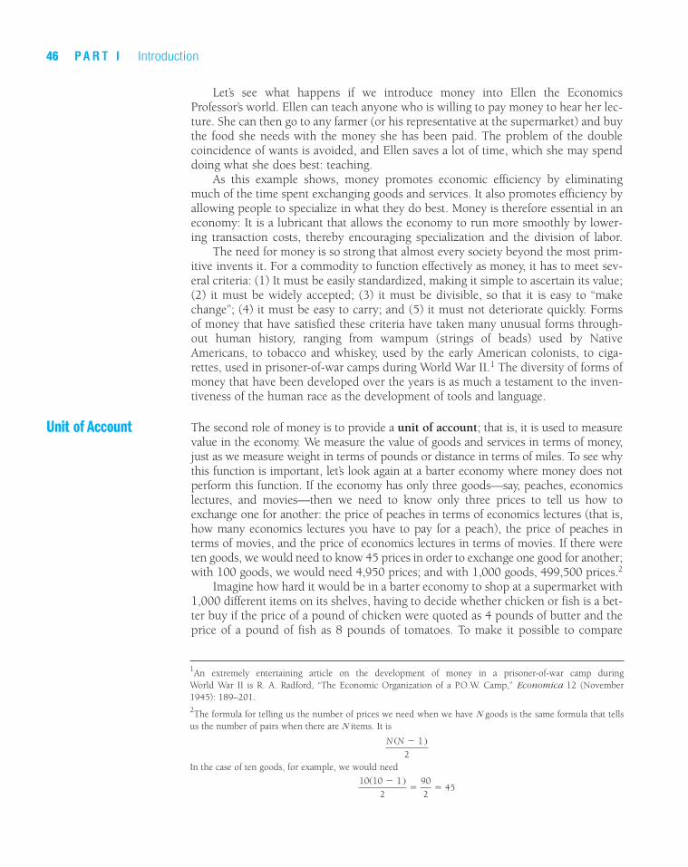
Let’s see what happens if we introduce money into Ellen the EconomicsProfessor’s world. Ellen can teach anyone who is willing to pay money to hear her lec-ture. She can then go to any farmer (or his representative at the supermarket) and buythe food she needs with the money she has been paid. The problem of the doublecoincidence of wants is avoided, and Ellen saves a lot of time, which she may spenddoing what she does best: teaching.

As this example shows, money promotes economic efficiency by eliminatingmuch of the time spent exchanging goods and services. It also promotes efficiency byallowing people to specialize in what they do best. Money is therefore essential in aneconomy: It is a lubricant that allows the economy to run more smoothly by lower-ing transaction costs, thereby encouraging specialization and the division of labor.

The need for money is so strong that almost every society beyond the most prim-itive invents it. For a commodity to function effectively as money, it has to meet sev-eral criteria: (1) It must be easily standardized, making it simple to ascertain its value;(2) it must be widely accepted; (3) it must be divisible, so that it is easy to “makechange”; (4) it must be easy to carry; and (5) it must not deteriorate quickly. Formsof money that have satisfied these criteria have taken many unusual forms through-out human history, ranging from wampum (strings of beads) used by NativeAmericans, to tobacco and whiskey, used by the early American colonists, to ciga-rettes, used in prisoner-of-war camps during World War II.1 The diversity of forms ofmoney that have been developed over the years is as much a testament to the inven-tiveness of the human race as the development of tools and language.

The second role of money is to provide a unit of account; that is, it is used to measurevalue in the economy. We measure the value of goods and services in terms of money,just as we measure weight in terms of pounds or distance in terms of miles. To see whythis function is important, let’s look again at a barter economy where money does notperform this function. If the economy has only three goods—say, peaches, economicslectures, and movies—then we need to know only three prices to tell us how toexchange one for another: the price of peaches in terms of economics lectures (that is,how many economics lectures you have to pay for a peach), the price of peaches interms of movies, and the price of economics lectures in terms of movies. If there wereten goods, we would need to know 45 prices in order to exchange one good for another;with 100 goods, we would need 4,950 prices; and with 1,000 goods, 499,500 prices.2

Imagine how hard it would be in a barter economy to shop at a supermarket with1,000 different items on its shelves, having to decide whether chicken or fish is a bet-ter buy if the price of a pound of chicken were quoted as 4 pounds of butter and theprice of a pound of fish as 8 pounds of tomatoes. To make it possible to compare

Unit of Account


1An extremely entertaining article on the development of money in a prisoner-of-war camp duringWorld War II is R. A. Radford, “The Economic Organization of a P.O.W. Camp,” Economica 12 (November1945): 189–201.2The formula for telling us the number of prices we need when we have N goods is the same formula that tellsus the number of pairs when there are N items. It is

In the case of ten goods, for example, we would need

10(10 � 1 )2

�90

2� 45

N (N � 1 )2

prices, the tag on each item would have to list up to 999 different prices, and the timespent reading them would result in very high transaction costs.

The solution to the problem is to introduce money into the economy and have allprices quoted in terms of units of that money, enabling us to quote the price of eco-nomics lectures, peaches, and movies in terms of, say, dollars. If there were only threegoods in the economy, this would not be a great advantage over the barter system,because we would still need three prices to conduct transactions. But for ten goodswe now need only ten prices; for 100 goods, 100 prices; and so on. At the 1,000-goodsupermarket, there are now only 1,000 prices to look at, not 499,500!

We can see that using money as a unit of account reduces transaction costs in aneconomy by reducing the number of prices that need to be considered. The benefitsof this function of money grow as the economy becomes more complex.

Money also functions as a store of value; it is a repository of purchasing power overtime. A store of value is used to save purchasing power from the time income isreceived until the time it is spent. This function of money is useful, because most ofus do not want to spend our income immediately upon receiving it, but rather preferto wait until we have the time or the desire to shop.

Money is not unique as a store of value; any asset—whether money, stocks,bonds, land, houses, art, or jewelry—can be used to store wealth. Many such assetshave advantages over money as a store of value: They often pay the owner a higherinterest rate than money, experience price appreciation, and deliver services such asproviding a roof over one’s head. If these assets are a more desirable store of value thanmoney, why do people hold money at all?

The answer to this question relates to the important economic concept ofliquidity, the relative ease and speed with which an asset can be converted into amedium of exchange. Liquidity is highly desirable. Money is the most liquid asset ofall because it is the medium of exchange; it does not have to be converted into any-thing else in order to make purchases. Other assets involve transaction costs whenthey are converted into money. When you sell your house, for example, you have topay a brokerage commission (usually 5% to 7% of the sales price), and if you needcash immediately to pay some pressing bills, you might have to settle for a lower pricein order to sell the house quickly. Because money is the most liquid asset, people arewilling to hold it even if it is not the most attractive store of value.

How good a store of value money is depends on the price level, because its valueis fixed in terms of the price level. A doubling of all prices, for example, means thatthe value of money has dropped by half; conversely, a halving of all prices means thatthe value of money has doubled. During inflation, when the price level is increasingrapidly, money loses value rapidly, and people will be more reluctant to hold theirwealth in this form. This is especially true during periods of extreme inflation, knownas hyperinflation, in which the inflation rate exceeds 50% per month.

Hyperinflation occurred in Germany after World War I, with inflation rates some-times exceeding 1,000% per month. By the end of the hyperinflation in 1923, theprice level had risen to more than 30 billion times what it had been just two yearsbefore. The quantity of money needed to purchase even the most basic items becameexcessive. There are stories, for example, that near the end of the hyperinflation, awheelbarrow of cash would be required to pay for a loaf of bread. Money was losingits value so rapidly that workers were paid and given time off several times during theday to spend their wages before the money became worthless. No one wanted to hold

Store of Value


on to money, and so the use of money to carry out transactions declined and barterbecame more and more dominant. Transaction costs skyrocketed, and as we wouldexpect, output in the economy fell sharply.

Evolution of the Payments System

We can obtain a better picture of the functions of money and the forms it has takenover time by looking at the evolution of the payments system, the method of con-ducting transactions in the economy. The payments system has been evolving overcenturies, and with it the form of money. At one point, precious metals such as goldwere used as the principal means of payment and were the main form of money. Later,paper assets such as checks and currency began to be used in the payments systemand viewed as money. Where the payments system is heading has an important bear-ing on how money will be defined in the future.

To obtain perspective on where the payments system is heading, it is worth exploringhow it has evolved. For any object to function as money, it must be universally accept-able; everyone must be willing to take it in payment for goods and services. An objectthat clearly has value to everyone is a likely candidate to serve as money, and a natu-ral choice is a precious metal such as gold or silver. Money made up of precious met-als or another valuable commodity is called commodity money, and from ancienttimes until several hundred years ago, commodity money functioned as the mediumof exchange in all but the most primitive societies. The problem with a payments sys-tem based exclusively on precious metals is that such a form of money is very heavyand is hard to transport from one place to another. Imagine the holes you’d wear inyour pockets if you had to buy things only with coins! Indeed, for large purchasessuch as a house, you’d have to rent a truck to transport the money payment.

The next development in the payments system was paper currency (pieces of paperthat function as a medium of exchange). Initially, paper currency carried a guaranteethat it was convertible into coins or into a quantity of precious metal. However, cur-rency has evolved into fiat money, paper currency decreed by governments as legaltender (meaning that legally it must be accepted as payment for debts) but not con-vertible into coins or precious metal. Paper currency has the advantage of being muchlighter than coins or precious metal, but it can be accepted as a medium of exchangeonly if there is some trust in the authorities who issue it and if printing has reached asufficiently advanced stage that counterfeiting is extremely difficult. Because papercurrency has evolved into a legal arrangement, countries can change the currency thatthey use at will. Indeed, this is currently a hot topic of debate in Europe, which hasadopted a unified currency (see Box 1).

Major drawbacks of paper currency and coins are that they are easily stolen andcan be expensive to transport in large amounts because of their bulk. To combat thisproblem, another step in the evolution of the payments system occurred with thedevelopment of modern banking: the invention of checks.

A check is an instruction from you to your bank to transfer money from your accountto someone else’s account when she deposits the check. Checks allow transactions to

Checks

Fiat Money

CommodityMoney


www.federalreserve.gov/paymentsys.htm

This site reports on the FederalReserve’s policies regarding

payments systems.

take place without the need to carry around large amounts of currency. The introduc-tion of checks was a major innovation that improved the efficiency of the paymentssystem. Frequently, payments made back and forth cancel each other; without checks,this would involve the movement of a lot of currency. With checks, payments that can-cel each other can be settled by canceling the checks, and no currency need be moved.The use of checks thus reduces the transportation costs associated with the paymentssystem and improves economic efficiency. Another advantage of checks is that they canbe written for any amount up to the balance in the account, making transactions forlarge amounts much easier. Checks are also advantageous in that loss from theft isgreatly reduced, and because they provide convenient receipts for purchases.

There are, however, two problems with a payments system based on checks. First,it takes time to get checks from one place to another, a particularly serious problemif you are paying someone in a different location who needs to be paid quickly. Inaddition, if you have a checking account, you know that it usually takes several busi-ness days before a bank will allow you to make use of the funds from a check youhave deposited. If your need for cash is urgent, this feature of paying by check can be


Box 1: Global

Birth of the Euro: Will It Benefit Europe?As part of the December 1991 Maastricht Treaty onEuropean Union, the European Economic Commissionoutlined a plan to achieve the creation of a singleEuropean currency starting in 1999. Despite con-cerns, the new common currency—the euro—cameinto existence right on schedule in January 1999,with 11 of the 15 European Union countries partici-pating in the monetary union: Austria, Belgium,Finland, France, Germany, Italy, Ireland, Luxembourg,the Netherlands, Portugal, and Spain. Denmark,Sweden, and the United Kingdom chose not to par-ticipate initially, and Greece failed to meet the eco-nomic criteria specified by the Maastricht Treaty(such as having a budget deficit less than 3% of GDPand total government debt less than 60% of GDP) butwas able to join later.

Starting January 1, 1999, the exchange rates ofcountries entering the monetary union were fixed per-manently to the euro (which became a unit of account),the European Central Bank took over monetary policyfrom the individual national central banks, and thegovernments of the member countries began to issuedebt in euros. In early 2002, euro notes and coinsbegan to circulate and by June 2002, the old national

currencies were phased out completely, so that onlyeuros could be used in the member countries.

Advocates of monetary union point out the advan-tages that the single currency has in eliminating thetransaction costs incurred in exchanging one currencyfor another. In addition, the use of a single currencymay promote further integration of the Europeaneconomies and enhance competition. Skeptics whothink that monetary union may be bad for Europesuggest that because labor will not be very mobileacross national boundaries and because fiscal transfers(i.e., tax income from one region being spent onanother) from better-performing regions to worse-performing regions will not take place as occurs in theUnited States, a single currency may lead to someregions of Europe being depressed for substantialperiods of time while other regions are booming.

Whether the euro will be good for the economiesof Europe and increase their GDP is an open question.However, the motive behind monetary union wasprobably more political than economic. Europeanmonetary union may encourage political union, pro-ducing a unified Europe that can play a stronger eco-nomic and political role on the world stage.

frustrating. Second, all the paper shuffling required to process checks is costly; it isestimated that it currently costs over $10 billion per year to process all the checkswritten in the United States.

The development of inexpensive computers and the spread of the Internet now makeit cheap to pay bills electronically. In the past, you had to pay your bills by mailing acheck, but now banks provide a web site in which you just log on, make a few clicks,and thereby transmit your payment electronically. Not only do you save the cost ofthe stamp, but paying bills becomes (almost) a pleasure, requiring little effort.Electronic payment systems provided by banks now even spare you the step of log-ging on to pay the bill. Instead, recurring bills can be automatically deducted fromyour bank account. Estimated cost savings when a bill is paid electronically ratherthan by a check exceed one dollar. Electronic payment is thus becoming far morecommon in the United States, but Americans lag considerably behind Europeans, par-ticularly Scandinavians, in their use of electronic payments (see Box 2).

ElectronicPayment


Why Are Scandinavians So Far Ahead of Americans in Using Electronic Payments? Americans are the biggest users of checks in theworld. Close to 100 billion checks are written everyyear in the United States, and over three-quarters ofnoncash transactions are conducted with paper. Incontrast, in most countries of Europe, more thantwo-thirds of noncash transactions are electronic,with Finland and Sweden having the greatest propor-tion of online banking customers of any countries inthe world. Indeed, if you were Finnish or Swedish,instead of writing a check, you would be far morelikely to pay your bills online, using a personal com-puter or even a mobile phone. Why do Europeansand especially Scandinavians so far outpace Americansin the use of electronic payments?

First, Europeans got used to making paymentswithout checks even before the advent of the personalcomputer. Europeans have long made use of so-calledgiro payments, in which banks and post offices trans-fer funds for customers to pay bills. Second,Europeans—and particularly Scandinavians—aremuch greater users of mobile phones and the Internetthan are Americans. Finland has the highest per capitause of mobile phones in the world, and Finland andSweden lead the world in the percentage of the popu-lation that accesses the Internet. Maybe these usage

patterns stem from the low population densities ofthese countries and the cold and dark winters thatkeep Scandinavians inside at their PCs. For their part,Scandinavians would rather take the view that theirhigh-tech culture is the product of their good educa-tion systems and the resulting high degree of com-puter literacy, the presence of top technologycompanies such as Finland’s Nokia and Sweden’sEricsson, and government policies promoting theincreased use of personal computers, such as Sweden’stax incentives for companies to provide their employ-ees with home computers. The wired populations ofFinland and Sweden are (percentage-wise) the biggestusers of online banking in the world.

Americans are clearly behind the curve in their useof electronic payments, which has imposed a highcost on the U.S. economy. Switching from checks toelectronic payments might save the U.S. economytens of billions of dollars per year, according to someestimates. Indeed, the U.S. federal government is try-ing to switch all its payments to electronic ones bydirectly depositing them into bank accounts, in orderto reduce its expenses. Can Americans be weanedfrom paper checks and fully embrace the world ofhigh-tech electronic payments?

Box 2: E-Finance

Electronic payments technology can not only substitute for checks, but can substitutefor cash, as well, in the form of electronic money (or e-money), money that existsonly in electronic form. The first form of e-money was the debit card. Debit cards,which look like credit cards, enable consumers to purchase goods and services byelectronically transferring funds directly from their bank accounts to a merchant’saccount. Debit cards are used in many of the same places that accept credit cards andare now often becoming faster to use than cash. At most supermarkets, for example,you can swipe your debit card through the card reader at the checkout station, pressa button, and the amount of your purchases is deducted from your bank account.Most banks and companies such as Visa and MasterCard issue debit cards, and yourATM card typically can function as a debit card.

A more advanced form of e-money is the stored-value card. The simplest form ofstored-value card is purchased for a preset dollar amount that the consumer pays upfront, like a prepaid phone card. The more sophisticated stored-value card is knownas a smart card. It contains a computer chip that allows it to be loaded with digitalcash from the owner’s bank account whenever needed. Smart cards can be loadedfrom ATM machines, personal computers with a smart card reader, or speciallyequipped telephones.

A third form of electronic money is often referred to as e-cash, which is used onthe Internet to purchase goods or services. A consumer gets e-cash by setting up anaccount with a bank that has links to the Internet and then has the e-cash transferredto her PC. When she wants to buy something with e-cash, she surfs to a store on theWeb and clicks the “buy” option for a particular item, whereupon the e-cash is auto-matically transferred from her computer to the merchant’s computer. The merchantcan then have the funds transferred from the consumer’s bank account to his beforethe goods are shipped.

Given the convenience of e-money, you might think that we would move quicklyto the cashless society in which all payments were made electronically. However, thishasn’t happened, as discussed in Box 3.

Measuring Money

The definition of money as anything that is generally accepted in payment for goodsand services tells us that money is defined by people’s behavior. What makes an assetmoney is that people believe it will be accepted by others when making payment. Aswe have seen, many different assets have performed this role over the centuries, rang-ing from gold to paper currency to checking accounts. For that reason, this behavioraldefinition does not tell us exactly what assets in our economy should be consideredmoney. To measure money, we need a precise definition that tells us exactly whatassets should be included.

The Federal Reserve System (the Fed), the central banking authority responsible formonetary policy in the United States, has conducted many studies on how to meas-ure money. The problem of measuring money has recently become especially crucialbecause extensive financial innovation has produced new types of assets that mightproperly belong in a measure of money. Since 1980, the Fed has modified its meas-ures of money several times and has settled on the following measures of the money

The FederalReserve’sMonetaryAggregates

E-Money


supply, which are also referred to as monetary aggregates (see Table 1 and theFollowing the Financial News box).

The narrowest measure of money that the Fed reports is M1, which includes cur-rency, checking account deposits, and traveler’s checks. These assets are clearlymoney, because they can be used directly as a medium of exchange. Until the mid-1970s, only commercial banks were permitted to establish checking accounts, andthey were not allowed to pay interest on them. With the financial innovation that hasoccurred (discussed more extensively in Chapter 9), regulations have changed so thatother types of banks, such as savings and loan associations, mutual savings banks,and credit unions, can also offer checking accounts. In addition, banking institutionscan offer other checkable deposits, such as NOW (negotiated order of withdrawal)accounts and ATS (automatic transfer from savings) accounts, that do pay interest ontheir balances. Table 1 lists the assets included in the measures of the monetary aggre-gates; both demand deposits (checking accounts that pay no interest) and these othercheckable deposits are included in the M1 measure.

The M2 monetary aggregate adds to M1 other assets that have check-writing fea-tures (money market deposit accounts and money market mutual fund shares) andother assets (savings deposits, small-denomination time deposits and repurchaseagreements) that are extremely liquid, because they can be turned into cash quicklyat very little cost.


Are We Headed for a Cashless Society?Predictions of a cashless society have been around fordecades, but they have not come to fruition. Forexample, Business Week predicted in 1975 that elec-tronic means of payment “would soon revolutionizethe very concept of money itself,” only to reverseitself several years later. Pilot projects in recent yearswith smart cards to convert consumers to the use ofe-money have not been a success. Mondex, one of thewidely touted, early stored-value cards that waslaunched in Britain in 1995, is only used on a fewBritish university campuses. In Germany andBelgium, millions of people carry bank cards withcomputer chips embedded in them that enable themto make use of e-money, but very few use them. Whyhas the movement to a cashless society been so slowin coming?

Although e-money might be more convenient andmay be more efficient than a payments system basedon paper, several factors work against the disappear-ance of the paper system. First, it is very expensive toset up the computer, card reader, and telecommuni-cations networks necessary to make electronic money

the dominant form of payment. Second, electronicmeans of payment raise security and privacy con-cerns. We often hear media reports that an unautho-rized hacker has been able to access a computerdatabase and to alter information stored there.Because this is not an uncommon occurrence,unscrupulous persons might be able to access bankaccounts in electronic payments systems and stealfunds by moving them from someone else’s accountsinto their own. The prevention of this type of fraud isno easy task, and a whole new field of computer sci-ence has developed to cope with security issues. Afurther concern is that the use of electronic means ofpayment leaves an electronic trail that contains a largeamount of personal data on buying habits. There areworries that government, employers, and marketersmight be able to access these data, thereby encroach-ing on our privacy.

The conclusion from this discussion is thatalthough the use of e-money will surely increase inthe future, to paraphrase Mark Twain, “the reports ofcash’s death are greatly exaggerated.”

Box 3: E-Finance

www.federalreserve.gov/releases/h6/Current/

The Federal Reserve reports thecurrent levels of M1, M2, and

M3 on its web site.

The M3 monetary aggregate adds to M2 somewhat less liquid assets such as large-denomination time deposits and repurchase agreements, Eurodollars, and institu-tional money market mutual fund shares.

Because we cannot be sure which of the monetary aggregates is the true measure ofmoney, it is logical to wonder if their movements closely parallel one another. If they do,then using one monetary aggregate to predict future economic performance and to con-duct policy will be the same as using another, and it does not matter much that we arenot sure of the appropriate definition of money for a given policy decision. However, ifthe monetary aggregates do not move together, then what one monetary aggregate tellsus is happening to the money supply might be quite different from what another mon-etary aggregate would tell us. The conflicting stories might present a confusing picturethat would make it hard for policymakers to decide on the right course of action.

Figure 1 plots the growth rates M1, M2, and M3 from 1960 to 2002. The growthrates of these three monetary aggregates do tend to move together; the timing of theirrise and fall is roughly similar until the 1990s, and they all show a higher growth rateon average in the 1970s than in the 1960s.

Yet some glaring discrepancies exist in the movements of these aggregates.According to M1, the growth rate of money did not accelerate between 1968, when it


Value as of December 2002($billions)

M1 � Currency 626.5� Traveler’s checks 7.7� Demand deposits 290.7� Other checkable deposits 281.2

Total M1 1,206.1

M2 � M1� Small-denomination time deposits and repurchase agreements 1,332.3� Savings deposits and money market deposit accounts 2,340.4� Money market mutual fund shares (noninstitutional) 923.7

Total M2 5,802.5

M3 � M2� Large-denomination time deposits and repurchase agreements 1,105.2� Money market mutual fund shares (institutional) 767.7� Repurchase agreements 511.7� Eurodollars 341.1

Total M3 8,528.2

Source: www.federalreserve.gov/releases/h6/hist.

Note: The Travelers checks item includes only traveler’s checks issued by non-banks, while traveler’s checks issued by banks are includedin the Demand deposits item, which also includes checkable deposits to businesses and which also do not pay interest.

Table 1 Measures of the Monetary Aggregates


Source: Wall Street Journal, Friday, January 3, 2003, p. C10.

F E D E R A L R E S E R V E D ATAMONETARY AGGREGATES (daily average in billions)

1 Week Ended:Dec. 23 Dec. 16

Money supply (M1) sa . . . 1227.1 1210.1Money supply (M1) nsa . . . 1256.0 1214.9Money supply (M2) sa . . . 5822.7 5811.3Money supply (M2) nsa . . . 5834.5 5853.9Money supply (M3) sa . . . 8542.8 8549.2Money supply (M3) nsa . . . 8572.6 8623.0

4 Weeks Ended:Dec. 23 Nov. 25

Money supply (M1) sa . . . 1218.3 1197.5Money supply (M1) nsa . . . 1230.9 1195.9Money supply (M2) sa . . . 5815.5 5795.8Money supply (M2) nsa . . . 5835.7 5780.7Money supply (M3) sa . . . 8543.4 8465.4Money supply (M3) nsa . . . 8578.1 8440.5

MonthNov. Oct.

Money supply (M1) sa . . . 1200.7 1199.6Money supply (M2) sa . . . 5800.7 5753.8Money supply (M3) sa . . . 8485.2 8348.4nsa-Not seasonally adjustedsa-Seasonally adjusted.


Data for the Federal Reserve’s monetary aggregates (M1,M2, and M3) are published every Friday. In the WallStreet Journal, the data are found in the “Federal ReserveData” column, an example of which is presented here.

The third entry indicates that the money supply(M2) averaged $5,822.7 billion for the week ending

December 23, 2002. The notation “sa” for this entryindicates that the data are seasonally adjusted; that is,seasonal movements, such as those associated withChristmas shopping, have been removed from thedata. The notation “nsa” indicates that the data havenot been seasonally adjusted.

The Monetary Aggregates

F I G U R E 1 Growth Rates of the Three Money Aggregates, 1960–2002

Sources: Federal Reserve Bulletin, p. A4, Table 1.10, various issues; Citibase databank; www.federalreserve.gov/releases/h6/hist/h6hist1.txt.

-5

0

-10

AnnualGrowth Rate (%)

5

10

15

20

1960 1965 1970 1975 1980 1985 1990 20001995 2005

M3 M2 M1

was in the 6–7% range, and 1971, when it was at a similar level. In the same period,the M2 and M3 measures tell a different story; they show a marked acceleration fromthe 8–10% range to the 12–15% range. Similarly, while the growth rate of M1 actu-ally increased from 1989 to 1992, the growth rates of M2 and M3 in this same periodinstead showed a downward trend. Furthermore, from 1992 to 1998, the growth rateof M1 fell sharply while the growth rates of M2 and M3 rose substantially; from 1998to 2002, M1 growth generally remained well below M2 and M3 growth. Thus, the dif-ferent measures of money tell a very different story about the course of monetary pol-icy in recent years.

From the data in Figure 1, you can see that obtaining a single precise, correct meas-ure of money does seem to matter and that it does make a difference which monetaryaggregate policymakers and economists choose as the true measure of money.

How Reliable Are the Money Data?

The difficulties of measuring money arise not only because it is hard to decide whatis the best definition of money, but also because the Fed frequently later revises ear-lier estimates of the monetary aggregates by large amounts. There are two reasons whythe Fed revises its figures. First, because small depository institutions need to reportthe amounts of their deposits only infrequently, the Fed has to estimate these amountsuntil these institutions provide the actual figures at some future date. Second, theadjustment of the data for seasonal variation is revised substantially as more databecome available. To see why this happens, let’s look at an example of the seasonalvariation of the money data around Christmas-time. The monetary aggregates alwaysrise around Christmas because of increased spending during the holiday season; therise is greater in some years than in others. This means that the factor that adjusts thedata for the seasonal variation due to Christmas must be estimated from several yearsof data, and the estimates of this seasonal factor become more precise only as moredata become available. When the data on the monetary aggregates are revised, the sea-sonal adjustments often change dramatically from the initial calculation.

Table 2 shows how severe a problem these data revisions can be. It provides therates of money growth from one-month periods calculated from initial estimates ofthe M2 monetary aggregate, along with the rates of money growth calculated from amajor revision of the M2 numbers published in February 2003. As the table shows,for one-month periods the initial versus the revised data can give a different pictureof what is happening to monetary policy. For January 2003, for example, the initialdata indicated that the growth rate of M2 at an annual rate was 2.2%, whereas therevised data indicate a much higher growth rate of 5.4%.

A distinctive characteristic shown in Table 2 is that the differences between theinitial and revised M2 series tend to cancel out. You can see this by looking at the lastrow of the table, which shows the average rate of M2 growth for the two series andthe average difference between them. The average M2 growth for the initial calcula-tion of M2 is 6.5%, and the revised number is 6.5%, a difference of 0.0%. The con-clusion we can draw is that the initial data on the monetary aggregates reported bythe Fed are not a reliable guide to what is happening to short-run movements in themoney supply, such as the one-month growth rates. However, the initial money dataare reasonably reliable for longer periods, such as a year. The moral is that we prob-ably should not pay much attention to short-run movements in the money supplynumbers, but should be concerned only with longer-run movements.



Initial Revised DifferencePeriod Rate Rate (Revised Rate – Initial Rate)January 2.2 5.4 3.2February 6.8 8.7 1.9March –1.4 0.2 1.6April –4.0 –2.6 1.4May 14.8 15.4 0.6June 7.6 7.1 –0.5July 13.6 11.0 –2.6August 9.9 8.6 –1.3September 5.1 5.7 0.6October 10.9 8.3 –2.6November 10.2 8.0 –2.2December 2.8 2.8 0.0

Average 6.5 6.5 0.0

Source: Federal Reserve Statistical Release H.6: www.federalreserve.gov/releases/h6.

Table 2 Growth Rate of M2: Initial and Revised Series, 2002 (percent, compounded annual rate)

Summary

1. To economists, the word money has a different meaningfrom income or wealth. Money is anything that isgenerally accepted as payment for goods or services orin the repayment of debts.

2. Money serves three primary functions: as a medium ofexchange, as a unit of account, and as a store of value.Money as a medium of exchange avoids the problem ofdouble coincidence of wants that arises in a bartereconomy by lowering transaction costs andencouraging specialization and the division of labor.Money as a unit of account reduces the number ofprices needed in the economy, which also reducestransaction costs. Money also functions as a store ofvalue, but performs this role poorly if it is rapidly losingvalue due to inflation.

3. The payments system has evolved over time. Until severalhundred years ago, the payments system in all but themost primitive societies was based primarily on precious

metals. The introduction of paper currency lowered thecost of transporting money. The next major advance wasthe introduction of checks, which lowered transactioncosts still further. We are currently moving toward anelectronic payments system in which paper is eliminatedand all transactions are handled by computers. Despitethe potential efficiency of such a system, obstacles areslowing the movement to the checkless society and thedevelopment of new forms of electronic money.

4. The Federal Reserve System has defined three differentmeasures of the money supply—M1, M2, and M3.These measures are not equivalent and do not alwaysmove together, so they cannot be used interchangeablyby policymakers. Obtaining the precise, correctmeasure of money does seem to matter and hasimplications for the conduct of monetary policy.

5. Another problem in the measurement of money is thatthe data are not always as accurate as we would like.


Substantial revisions in the data do occur; they indicatethat initially released money data are not a reliableguide to short-run (say, month-to-month) movements

in the money supply, although they are more reliableover longer periods of time, such as a year.

Key Terms

commodity money, p. 48

currency, p. 44

e-cash, p. 51

electronic money (e-money), p. 51

fiat money, p. 48

hyperinflation, p. 47

income, p. 45

liquidity, p. 47

M1, p. 52

M2, p. 52

M3, p. 53

medium of exchange, p. 45

monetary aggregates, p. 52

payments system, p. 48

smart card, p. 51

store of value, p. 47

unit of account, p. 46

wealth, p. 45



1. Which of the following three expressions uses theeconomists’ definition of money?a. “How much money did you earn last week?”b. “When I go to the store, I always make sure that I

have enough money.”c. “The love of money is the root of all evil.”

*2. There are three goods produced in an economy bythree individuals:

Good Producer

Apples Orchard owner

Bananas Banana grower

Chocolate Chocolatier

If the orchard owner likes only bananas, the bananagrower likes only chocolate, and the chocolatier likesonly apples, will any trade between these three per-sons take place in a barter economy? How will intro-ducing money into the economy benefit these threeproducers?

3. Why did cavemen not need money?

*4. Why were people in the United States in the nine-teenth century sometimes willing to be paid by check

rather than with gold, even though they knew thatthere was a possibility that the check might bounce?

5. In ancient Greece, why was gold a more likely candi-date for use as money than wine was?

*6. Was money a better store of value in the United Statesin the 1950s than it was in the 1970s? Why or whynot? In which period would you have been more will-ing to hold money?

7. Would you be willing to give up your checkbook andinstead use an electronic means of payment if it weremade available? Why or why not?

8. Rank the following assets from most liquid to least liquid:a. Checking account depositsb. Housesc. Currencyd. Washing machinese. Savings depositsf. Common stock

*9. Why have some economists described money during ahyperinflation as a “hot potato” that is quickly passedfrom one person to another?

10. In Brazil, a country that was undergoing a rapid infla-tion before 1994, many transactions were conductedin dollars rather than in reals, the domestic currency.Why?

QUIZ

gloss57.html

quiz57.html

*11. Suppose that a researcher discovers that a measure ofthe total amount of debt in the U.S. economy over thepast 20 years was a better predictor of inflation andthe business cycle than M1, M2, or M3. Does this dis-covery mean that we should define money as equal tothe total amount of debt in the economy?

12. Look up the M1, M2, and M3 numbers in the FederalReserve Bulletin for the most recent one-year period.Have their growth rates been similar? What implica-tions do their growth rates have for the conduct ofmonetary policy?

*13. Which of the Federal Reserve’s measures of the mone-tary aggregates, M1, M2, or M3, is composed of themost liquid assets? Which is the largest measure?

14. For each of the following assets, indicate which of themonetary aggregates (M1, M2, M3) includes them:a. Currencyb. Money market mutual fundsc. Eurodollarsd. Small-denomination time depositse. Large-denomination repurchase agreementsf. Checkable deposits

*15. Why are revisions of monetary aggregates less of aproblem for measuring long-run movements of themoney supply than they are for measuring short-runmovements?


Web Exercises

1. Go to www.federalreserve.gov/releases/h6/Current/. a. What has been the growth rate in M1, M2, and M3

over the last 12 months? b. From what you know about the state of the econ-

omy, does this seem expansionary or restrictive?

2. Go to www.federalreserve.gov/paymentsys.htm andselect one topic on which the Federal Reserve has awritten policy. Write a one-paragraph summary of thispolicy.

links58.html

P a r t I I

FinancialMarkets

PREVIEW Interest rates are among the most closely watched variables in the economy. Theirmovements are reported almost daily by the news media, because they directly affectour everyday lives and have important consequences for the health of the economy.They affect personal decisions such as whether to consume or save, whether to buy ahouse, and whether to purchase bonds or put funds into a savings account. Interestrates also affect the economic decisions of businesses and households, such aswhether to use their funds to invest in new equipment for factories or to save theirmoney in a bank.

Before we can go on with the study of money, banking, and financial markets, wemust understand exactly what the phrase interest rates means. In this chapter, we seethat a concept known as the yield to maturity is the most accurate measure of interestrates; the yield to maturity is what economists mean when they use the term interestrate. We discuss how the yield to maturity is measured and examine alternative (butless accurate) ways in which interest rates are quoted. We’ll also see that a bond’sinterest rate does not necessarily indicate how good an investment the bond isbecause what it earns (its rate of return) does not necessarily equal its interest rate.Finally, we explore the distinction between real interest rates, which are adjusted forinflation, and nominal interest rates, which are not.

Although learning definitions is not always the most exciting of pursuits, it isimportant to read carefully and understand the concepts presented in this chapter.Not only are they continually used throughout the remainder of this text, but a firmgrasp of these terms will give you a clearer understanding of the role that interest ratesplay in your life as well as in the general economy.

Measuring Interest Rates

Different debt instruments have very different streams of payment with very differenttiming. Thus we first need to understand how we can compare the value of one kindof debt instrument with another before we see how interest rates are measured. To dothis, we make use of the concept of present value.

The concept of present value (or present discounted value) is based on the common-sense notion that a dollar paid to you one year from now is less valuable to you thana dollar paid to you today: This notion is true because you can deposit a dollar in a

Present Value

61

Ch a p te r

Understanding Interest Rates4

www.bloomberg.com/markets/

Under “Rates & Bonds,” youcan access information on keyinterest rates, U.S. Treasuries,

Government bonds, andmunicipal bonds.

ESOMASCHINI

Evidenziato

arrivato fino qui

savings account that earns interest and have more than a dollar in one year.Economists use a more formal definition, as explained in this section.

Let’s look at the simplest kind of debt instrument, which we will call a simpleloan. In this loan, the lender provides the borrower with an amount of funds (calledthe principal) that must be repaid to the lender at the maturity date, along with anadditional payment for the interest. For example, if you made your friend, Jane, a sim-ple loan of $100 for one year, you would require her to repay the principal of $100in one year’s time along with an additional payment for interest; say, $10. In the caseof a simple loan like this one, the interest payment divided by the amount of the loanis a natural and sensible way to measure the interest rate. This measure of the so-called simple interest rate, i, is:

If you make this $100 loan, at the end of the year you would have $110, whichcan be rewritten as:

$100 � (1 � 0.10) � $110

If you then lent out the $110, at the end of the second year you would have:

$110 � (1 � 0.10) � $121

or, equivalently,

$100 � (1 � 0.10) � (1 � 0.10) � $100 � (1 � 0.10)2 � $121

Continuing with the loan again, you would have at the end of the third year:

$121 � (1 � 0.10) � $100 � (1 � 0.10)3 � $133

Generalizing, we can see that at the end of n years, your $100 would turn into:

$100 � (1 � i)n

The amounts you would have at the end of each year by making the $100 loan todaycan be seen in the following timeline:

This timeline immediately tells you that you are just as happy having $100 todayas having $110 a year from now (of course, as long as you are sure that Jane will payyou back). Or that you are just as happy having $100 today as having $121 two yearsfrom now, or $133 three years from now or $100 � (1 � 0.10)n, n years from now.The timeline tells us that we can also work backward from future amounts to the pres-ent: for example, $133 � $100 � (1 � 0.10)3 three years from now is worth $100today, so that:

The process of calculating today’s value of dollars received in the future, as we havedone above, is called discounting the future. We can generalize this process by writing

$100 �$133

(1 � 0.10 )3

$100 � (1 � 0.10)n

Yearn

Today0

$100 $110

Year1

$121

Year2

$133

Year3

i �$10

$100� 0.10 � 10%

62 P A R T I I Financial Markets

today’s (present) value of $100 as PV, the future value of $133 as FV, and replacing0.10 (the 10% interest rate) by i. This leads to the following formula:

(1)

Intuitively, what Equation 1 tells us is that if you are promised $1 for certain tenyears from now, this dollar would not be as valuable to you as $1 is today because ifyou had the $1 today, you could invest it and end up with more than $1 in ten years.

The concept of present value is extremely useful, because it allows us to figureout today’s value (price) of a credit market instrument at a given simple interest ratei by just adding up the individual present values of all the future payments received.This information allows us to compare the value of two instruments with very differ-ent timing of their payments.

As an example of how the present value concept can be used, let’s assume thatyou just hit the $20 million jackpot in the New York State Lottery, which promisesyou a payment of $1 million for the next twenty years. You are clearly excited, buthave you really won $20 million? No, not in the present value sense. In today’s dol-lars, that $20 million is worth a lot less. If we assume an interest rate of 10% as in theearlier examples, the first payment of $1 million is clearly worth $1 million today, butthe next payment next year is only worth $1 million/(1 � 0.10) � $909,090, a lot lessthan $1 million. The following year the payment is worth $1 million/(1 � 0.10)2 �$826,446 in today’s dollars, and so on. When you add all these up, they come to $9.4million. You are still pretty excited (who wouldn’t be?), but because you understandthe concept of present value, you recognize that you are the victim of false advertis-ing. You didn’t really win $20 million, but instead won less than half as much.

In terms of the timing of their payments, there are four basic types of credit marketinstruments.

1. A simple loan, which we have already discussed, in which the lender providesthe borrower with an amount of funds, which must be repaid to the lender at thematurity date along with an additional payment for the interest. Many money marketinstruments are of this type: for example, commercial loans to businesses.

2. A fixed-payment loan (which is also called a fully amortized loan) in which thelender provides the borrower with an amount of funds, which must be repaid by mak-ing the same payment every period (such as a month), consisting of part of the princi-pal and interest for a set number of years. For example, if you borrowed $1,000, afixed-payment loan might require you to pay $126 every year for 25 years. Installmentloans (such as auto loans) and mortgages are frequently of the fixed-payment type.

3. A coupon bond pays the owner of the bond a fixed interest payment (couponpayment) every year until the maturity date, when a specified final amount (facevalue or par value) is repaid. The coupon payment is so named because the bond-holder used to obtain payment by clipping a coupon off the bond and sending it tothe bond issuer, who then sent the payment to the holder. Nowadays, it is no longernecessary to send in coupons to receive these payments. A coupon bond with $1,000face value, for example, might pay you a coupon payment of $100 per year for tenyears, and at the maturity date repay you the face value amount of $1,000. (The facevalue of a bond is usually in $1,000 increments.)

A coupon bond is identified by three pieces of information. First is the corpora-tion or government agency that issues the bond. Second is the maturity date of the

Four Types ofCredit MarketInstruments

PV �FV

(1 � i )n

C H A P T E R 4 Understanding Interest Rates 63

ESOMASCHINI

Sottolineato

ESOMASCHINI

Sottolineato

ESOMASCHINI

Sottolineato

bond. Third is the bond’s coupon rate, the dollar amount of the yearly coupon pay-ment expressed as a percentage of the face value of the bond. In our example, thecoupon bond has a yearly coupon payment of $100 and a face value of $1,000. Thecoupon rate is then $100/$1,000 � 0.10, or 10%. Capital market instruments suchas U.S. Treasury bonds and notes and corporate bonds are examples of coupon bonds.

4. A discount bond (also called a zero-coupon bond) is bought at a price belowits face value (at a discount), and the face value is repaid at the maturity date. Unlikea coupon bond, a discount bond does not make any interest payments; it just pays offthe face value. For example, a discount bond with a face value of $1,000 might bebought for $900; in a year’s time the owner would be repaid the face value of $1,000.U.S. Treasury bills, U.S. savings bonds, and long-term zero-coupon bonds are exam-ples of discount bonds.

These four types of instruments require payments at different times: Simple loansand discount bonds make payment only at their maturity dates, whereas fixed-paymentloans and coupon bonds have payments periodically until maturity. How would youdecide which of these instruments provides you with more income? They all seem sodifferent because they make payments at different times. To solve this problem, we usethe concept of present value, explained earlier, to provide us with a procedure formeasuring interest rates on these different types of instruments.

Of the several common ways of calculating interest rates, the most important is theyield to maturity, the interest rate that equates the present value of paymentsreceived from a debt instrument with its value today.1 Because the concept behind thecalculation of the yield to maturity makes good economic sense, economists considerit the most accurate measure of interest rates.

To understand the yield to maturity better, we now look at how it is calculatedfor the four types of credit market instruments.

Simple Loan. Using the concept of present value, the yield to maturity on a simpleloan is easy to calculate. For the one-year loan we discussed, today’s value is $100,and the payments in one year’s time would be $110 (the repayment of $100 plus theinterest payment of $10). We can use this information to solve for the yield to matu-rity i by recognizing that the present value of the future payments must equal today’svalue of a loan. Making today’s value of the loan ($100) equal to the present value ofthe $110 payment in a year (using Equation 1) gives us:

Solving for i,

This calculation of the yield to maturity should look familiar, because it equalsthe interest payment of $10 divided by the loan amount of $100; that is, it equals thesimple interest rate on the loan. An important point to recognize is that for simpleloans, the simple interest rate equals the yield to maturity. Hence the same term i is usedto denote both the yield to maturity and the simple interest rate.

i �$110 � $100

$100�

$10

$100� 0.10 � 10%

$100 �$110

1 � i

Yield to Maturity


1In other contexts, it is also called the internal rate of return.

ESOMASCHINI

Sottolineato

Study Guide The key to understanding the calculation of the yield to maturity is equating today’svalue of the debt instrument with the present value of all of its future payments. Thebest way to learn this principle is to apply it to other specific examples of the four typesof credit market instruments in addition to those we discuss here. See if you can developthe equations that would allow you to solve for the yield to maturity in each case.

Fixed-Payment Loan. Recall that this type of loan has the same payment every periodthroughout the life of the loan. On a fixed-rate mortgage, for example, the borrowermakes the same payment to the bank every month until the maturity date, when theloan will be completely paid off. To calculate the yield to maturity for a fixed-paymentloan, we follow the same strategy we used for the simple loan—we equate today’svalue of the loan with its present value. Because the fixed-payment loan involves morethan one payment, the present value of the fixed-payment loan is calculated as thesum of the present values of all payments (using Equation 1).

In the case of our earlier example, the loan is $1,000 and the yearly payment is$126 for the next 25 years. The present value is calculated as follows: At the end ofone year, there is a $126 payment with a PV of $126/(1 � i); at the end of two years,there is another $126 payment with a PV of $126/(1 � i)2; and so on until at the endof the twenty-fifth year, the last payment of $126 with a PV of $126/(1 � i)25 is made.Making today’s value of the loan ($1,000) equal to the sum of the present values of allthe yearly payments gives us:

More generally, for any fixed-payment loan,

(2)

where LV � loan valueFP � fixed yearly payment

n � number of years until maturity

For a fixed-payment loan amount, the fixed yearly payment and the number ofyears until maturity are known quantities, and only the yield to maturity is not. So wecan solve this equation for the yield to maturity i. Because this calculation is not easy,many pocket calculators have programs that allow you to find i given the loan’s num-bers for LV, FP, and n. For example, in the case of the 25-year loan with yearly paymentsof $126, the yield to maturity that solves Equation 2 is 12%. Real estate brokers alwayshave a pocket calculator that can solve such equations so that they can immediately tellthe prospective house buyer exactly what the yearly (or monthly) payments will be ifthe house purchase is financed by taking out a mortgage.2

Coupon Bond. To calculate the yield to maturity for a coupon bond, follow the samestrategy used for the fixed-payment loan: Equate today’s value of the bond with itspresent value. Because coupon bonds also have more than one payment, the present

LV �FP

1 � i�

FP

(1 � i )2 �FP

(1 � i )3 � . . . �FP

(1 � i )n

$1,000 �$126

1 � i�

$126

(1 � i )2 �$126

(1 � i )3 � . . . �$126

(1 � i )25


2The calculation with a pocket calculator programmed for this purpose requires simply that you enterthe value of the loan LV, the number of years to maturity n, and the interest rate i and then run the program.

value of the bond is calculated as the sum of the present values of all the coupon pay-ments plus the present value of the final payment of the face value of the bond.

The present value of a $1,000-face-value bond with ten years to maturity andyearly coupon payments of $100 (a 10% coupon rate) can be calculated as follows:At the end of one year, there is a $100 coupon payment with a PV of $100/(1 � i );at the end of the second year, there is another $100 coupon payment with a PV of$100/(1 � i )2; and so on until at maturity, there is a $100 coupon payment with aPV of $100/(1 � i )10 plus the repayment of the $1,000 face value with a PV of$1,000/(1 � i )10. Setting today’s value of the bond (its current price, denoted by P)equal to the sum of the present values of all the payments for this bond gives:

More generally, for any coupon bond,3

(3)

where P � price of coupon bondC � yearly coupon paymentF � face value of the bondn � years to maturity date

In Equation 3, the coupon payment, the face value, the years to maturity, and theprice of the bond are known quantities, and only the yield to maturity is not. Hencewe can solve this equation for the yield to maturity i. Just as in the case of the fixed-payment loan, this calculation is not easy, so business-oriented pocket calculatorshave built-in programs that solve this equation for you.4

Let’s look at some examples of the solution for the yield to maturity on our 10%-coupon-rate bond that matures in ten years. If the purchase price of the bond is$1,000, then either using a pocket calculator with the built-in program or looking ata bond table, we will find that the yield to maturity is 10 percent. If the price is $900,we find that the yield to maturity is 11.75%. Table 1 shows the yields to maturity cal-culated for several bond prices.

P �C

1 � i�

C

(1 � i )2 �C

(1 � i )3 � . . . �C

(1 � i )n �F

(1 � i )n

P �$100

1 � i�

$100

(1 � i )2 �$100

(1 � i )3 � . . . �$100

(1 � i )10 �$1,000

(1 � i )10


3Most coupon bonds actually make coupon payments on a semiannual basis rather than once a year as assumedhere. The effect on the calculations is only very slight and will be ignored here.4The calculation of a bond’s yield to maturity with the programmed pocket calculator requires simply that youenter the amount of the yearly coupon payment C, the face value F, the number of years to maturity n, and theprice of the bond P and then run the program.

Price of Bond ($) Yield to Maturity (%)1,200 7.131,100 8.481,000 10.00

900 11.75800 13.81

Table 1 Yields to Maturity on a 10%-Coupon-Rate Bond Maturing in TenYears (Face Value = $1,000)

Three interesting facts are illustrated by Table 1:

1. When the coupon bond is priced at its face value, the yield to maturity equals thecoupon rate.

2. The price of a coupon bond and the yield to maturity are negatively related; thatis, as the yield to maturity rises, the price of the bond falls. As the yield to matu-rity falls, the price of the bond rises.

3. The yield to maturity is greater than the coupon rate when the bond price isbelow its face value.

These three facts are true for any coupon bond and are really not surprising if youthink about the reasoning behind the calculation of the yield to maturity. When youput $1,000 in a bank account with an interest rate of 10%, you can take out $100 everyyear and you will be left with the $1,000 at the end of ten years. This is similar to buy-ing the $1,000 bond with a 10% coupon rate analyzed in Table 1, which pays a $100coupon payment every year and then repays $1,000 at the end of ten years. If the bondis purchased at the par value of $1,000, its yield to maturity must equal 10%, whichis also equal to the coupon rate of 10%. The same reasoning applied to any couponbond demonstrates that if the coupon bond is purchased at its par value, the yield tomaturity and the coupon rate must be equal.

It is straightforward to show that the bond price and the yield to maturity are neg-atively related. As i, the yield to maturity, rises, all denominators in the bond price for-mula must necessarily rise. Hence a rise in the interest rate as measured by the yieldto maturity means that the price of the bond must fall. Another way to explain whythe bond price falls when the interest rises is that a higher interest rate implies thatthe future coupon payments and final payment are worth less when discounted backto the present; hence the price of the bond must be lower.

There is one special case of a coupon bond that is worth discussing because itsyield to maturity is particularly easy to calculate. This bond is called a consol or a per-petuity; it is a perpetual bond with no maturity date and no repayment of principalthat makes fixed coupon payments of $C forever. Consols were first sold by theBritish Treasury during the Napoleonic Wars and are still traded today; they are quiterare, however, in American capital markets. The formula in Equation 3 for the priceof the consol P simplifies to the following:5

(4)P �C

i


5The bond price formula for a consol is:

which can be written as:

in which x � 1/(1 � i). The formula for an infinite sum is:

and so:

which by suitable algebraic manipulation becomes:

P � C �1 � i

i�

i

i � �C

i

P � C � 1

1 � x� 1� � C c 1

1 � 1�(1 � i )� 1 d

1 � x � x 2 � x 3 � . . . �1

1 � x for x � 1

P � C (x � x 2 � x 3 � . . . )

P �C

1 � i�

C

(1 � i )2 �C

(1 � i )3 � . . .

where P = price of the consolC = yearly payment

One nice feature of consols is that you can immediately see that as i goes up, theprice of the bond falls. For example, if a consol pays $100 per year forever and theinterest rate is 10%, its price will be $1,000 � $100/0.10. If the interest rate rises to20%, its price will fall to $500 � $100/0.20. We can also rewrite this formula as

(5)

We see then that it is also easy to calculate the yield to maturity for the consol(despite the fact that it never matures). For example, with a consol that pays $100yearly and has a price of $2,000, the yield to maturity is easily calculated to be 5%(� $100/$2,000).

Discount Bond. The yield-to-maturity calculation for a discount bond is similar tothat for the simple loan. Let us consider a discount bond such as a one-year U.S.Treasury bill, which pays off a face value of $1,000 in one year’s time. If the currentpurchase price of this bill is $900, then equating this price to the present value of the$1,000 received in one year, using Equation 1, gives:

and solving for i,

More generally, for any one-year discount bond, the yield to maturity can be writ-ten as:

(6)

where F � face value of the discount bondP � current price of the discount bond

In other words, the yield to maturity equals the increase in price over the yearF – P divided by the initial price P. In normal circumstances, investors earn positivereturns from holding these securities and so they sell at a discount, meaning that thecurrent price of the bond is below the face value. Therefore, F – P should be positive,and the yield to maturity should be positive as well. However, this is not always thecase, as recent extraordinary events in Japan indicate (see Box 1).

An important feature of this equation is that it indicates that for a discount bond,the yield to maturity is negatively related to the current bond price. This is the sameconclusion that we reached for a coupon bond. For example, Equation 6 shows thata rise in the bond price from $900 to $950 means that the bond will have a smaller

i �F � P

P

i �$1,000 � $900

$900� 0.111 � 11.1%

$900i � $1,000 � $900

$900 � $900i � $1,000

(1 � i ) � $900 � $1,000

$900 �$1,000

1 � i

i �C

P


increase in its price at maturity, and the yield to maturity falls from 11.1 to 5.3%.Similarly, a fall in the yield to maturity means that the price of the discount bond hasrisen.

Summary. The concept of present value tells you that a dollar in the future is not asvaluable to you as a dollar today because you can earn interest on this dollar.Specifically, a dollar received n years from now is worth only $1/(1 � i)n today. Thepresent value of a set of future payments on a debt instrument equals the sum of thepresent values of each of the future payments. The yield to maturity for an instrumentis the interest rate that equates the present value of the future payments on that instru-ment to its value today. Because the procedure for calculating the yield to maturity isbased on sound economic principles, this is the measure that economists think mostaccurately describes the interest rate.

Our calculations of the yield to maturity for a variety of bonds reveal the importantfact that current bond prices and interest rates are negatively related: When theinterest rate rises, the price of the bond falls, and vice versa.

Other Measures of Interest Rates

The yield to maturity is the most accurate measure of interest rates; this is what econ-omists mean when they use the term interest rate. Unless otherwise specified, theterms interest rate and yield to maturity are used synonymously in this book. However,because the yield to maturity is sometimes difficult to calculate, other, less accurate


Box 1: Global

Negative T-Bill Rates? Japan Shows the WayWe normally assume that interest rates must alwaysbe positive. Negative interest rates would imply thatyou are willing to pay more for a bond today thanyou will receive for it in the future (as our formula foryield to maturity on a discount bond demonstrates).Negative interest rates therefore seem like an impos-sibility because you would do better by holding cashthat has the same value in the future as it does today.

The Japanese have demonstrated that this reasoningis not quite correct. In November 1998, interest rateson Japanese six-month Treasury bills became negative,yielding an interest rate of –0.004%, with investorspaying more for the bills than their face value. This isan extremely unusual event—no other country in theworld has seen negative interest rates during the lastfifty years. How could this happen?

As we will see in Chapter 5, the weakness of theJapanese economy and a negative inflation rate droveJapanese interest rates to low levels, but these twofactors can’t explain the negative rates. The answer isthat large investors found it more convenient to holdthese six-month bills as a store of value rather thanholding cash because the bills are denominated inlarger amounts and can be stored electronically. Forthat reason, some investors were willing to holdthem, despite their negative rates, even though inmonetary terms the investors would be better offholding cash. Clearly, the convenience of T-bills goesonly so far, and thus their interest rates can go only alittle bit below zero.

www.teachmefinance.com

A review of the key financial concepts: time value

of money, annuities,perpetuities, and so on.

measures of interest rates have come into common use in bond markets. You will fre-quently encounter two of these measures—the current yield and the yield on a discountbasis—when reading the newspaper, and it is important for you to understand whatthey mean and how they differ from the more accurate measure of interest rates, theyield to maturity.

The current yield is an approximation of the yield to maturity on coupon bonds that isoften reported, because in contrast to the yield to maturity, it is easily calculated. It isdefined as the yearly coupon payment divided by the price of the security,

(7)

where ic � current yieldP � price of the coupon bondC � yearly coupon payment

This formula is identical to the formula in Equation 5, which describes the cal-culation of the yield to maturity for a consol. Hence, for a consol, the current yield isan exact measure of the yield to maturity. When a coupon bond has a long term tomaturity (say, 20 years or more), it is very much like a consol, which pays coupon pay-ments forever. Thus you would expect the current yield to be a rather close approxi-mation of the yield to maturity for a long-term coupon bond, and you can safely usethe current-yield calculation instead of calculating the yield to maturity with a finan-cial calculator. However, as the time to maturity of the coupon bond shortens (say, itbecomes less than five years), it behaves less and less like a consol and so the approx-imation afforded by the current yield becomes worse and worse.

We have also seen that when the bond price equals the par value of the bond, theyield to maturity is equal to the coupon rate (the coupon payment divided by the parvalue of the bond). Because the current yield equals the coupon payment divided by thebond price, the current yield is also equal to the coupon rate when the bond price is atpar. This logic leads us to the conclusion that when the bond price is at par, the currentyield equals the yield to maturity. This means that the closer the bond price is to thebond’s par value, the better the current yield will approximate the yield to maturity.

The current yield is negatively related to the price of the bond. In the caseof our 10%-coupon-rate bond, when the price rises from $1,000 to $1,100, the cur-rent yield falls from 10% (� $100/$1,000) to 9.09% (� $100/$1,100). As Table 1indicates, the yield to maturity is also negatively related to the price of the bond; whenthe price rises from $1,000 to $1,100, the yield to maturity falls from 10 to 8.48%.In this we see an important fact: The current yield and the yield to maturity alwaysmove together; a rise in the current yield always signals that the yield to maturity hasalso risen.

The general characteristics of the current yield (the yearly coupon paymentdivided by the bond price) can be summarized as follows: The current yield betterapproximates the yield to maturity when the bond’s price is nearer to the bond’s parvalue and the maturity of the bond is longer. It becomes a worse approximation whenthe bond’s price is further from the bond’s par value and the bond’s maturity is shorter.Regardless of whether the current yield is a good approximation of the yield to matu-rity, a change in the current yield always signals a change in the same direction of theyield to maturity.

ic �C

P

Current Yield


Before the advent of calculators and computers, dealers in U.S. Treasury bills found itdifficult to calculate interest rates as a yield to maturity. Instead, they quoted the inter-est rate on bills as a yield on a discount basis (or discount yield), and they still doso today. Formally, the yield on a discount basis is defined by the following formula:

(8)

where idb � yield on a discount basisF � face value of the discount bondP � purchase price of the discount bond

This method for calculating interest rates has two peculiarities. First, it uses thepercentage gain on the face value of the bill (F � P)/F rather than the percentage gainon the purchase price of the bill (F � P)/P used in calculating the yield to maturity.Second, it puts the yield on an annual basis by considering the year to be 360 dayslong rather than 365 days.

Because of these peculiarities, the discount yield understates the interest rate onbills as measured by the yield to maturity. On our one-year bill, which is selling for$900 and has a face value of $1,000, the yield on a discount basis would be as follows:

whereas the yield to maturity for this bill, which we calculated before, is 11.1%. Thediscount yield understates the yield to maturity by a factor of over 10%. A little morethan 1% ([365 � 360]/360 � 0.014 � 1.4%) can be attributed to the understatementof the length of the year: When the bill has one year to maturity, the second term onthe right-hand side of the formula is 360/365 � 0.986 rather than 1.0, as it should be.

The more serious source of the understatement, however, is the use of the per-centage gain on the face value rather than on the purchase price. Because, by defini-tion, the purchase price of a discount bond is always less than the face value, thepercentage gain on the face value is necessarily smaller than the percentage gain onthe purchase price. The greater the difference between the purchase price and the facevalue of the discount bond, the more the discount yield understates the yield to matu-rity. Because the difference between the purchase price and the face value gets largeras maturity gets longer, we can draw the following conclusion about the relationshipof the yield on a discount basis to the yield to maturity: The yield on a discount basisalways understates the yield to maturity, and this understatement becomes moresevere the longer the maturity of the discount bond.

Another important feature of the discount yield is that, like the yield to matu-rity, it is negatively related to the price of the bond. For example, when the price ofthe bond rises from $900 to $950, the formula indicates that the yield on a discountbasis declines from 9.9 to 4.9%. At the same time, the yield to maturity declines from11.1 to 5.3%. Here we see another important factor about the relationship of yieldon a discount basis to yield to maturity: They always move together. That is, a rise inthe discount yield always means that the yield to maturity has risen, and a decline in thediscount yield means that the yield to maturity has declined as well.

The characteristics of the yield on a discount basis can be summarized as follows:Yield on a discount basis understates the more accurate measure of the interest rate,the yield to maturity; and the longer the maturity of the discount bond, the greater

idb �$1,000 � $900

$1,000 �

360

365� 0.099 � 9.9%

idb �F � P

F �

360

days to maturity

Yield on aDiscount Basis


this understatement becomes. Even though the discount yield is a somewhat mis-leading measure of the interest rates, a change in the discount yield always indicatesa change in the same direction for the yield to maturity.


Reading the Wall Street Journal: The Bond PageApplication

Now that we understand the different interest-rate definitions, let’s apply ourknowledge and take a look at what kind of information appears on the bondpage of a typical newspaper, in this case the Wall Street Journal. The“Following the Financial News” box contains the Journal ’s listing for threedifferent types of bonds on Wednesday, January 23, 2003. Panel (a) containsthe information on U.S. Treasury bonds and notes. Both are coupon bonds,the only difference being their time to maturity from when they were origi-nally issued: Notes have a time to maturity of less than ten years; bonds havea time to maturity of more than ten years.

The information found in the “Rate” and “Maturity” columns identifiesthe bond by coupon rate and maturity date. For example, T-bond 1 has acoupon rate of 4.75%, indicating that it pays out $47.50 per year on a$1,000-face-value bond and matures in January 2003. In bond market parl-ance, it is referred to as the Treasury’s 4 s of 2003. The next three columnstell us about the bond’s price. By convention, all prices in the bond marketare quoted per $100 of face value. Furthermore, the numbers after the colonrepresent thirty-seconds (x/32, or 32nds). In the case of T-bond 1, the firstprice of 100:02 represents 100 � 100.0625, or an actual price of $1000.62for a $1,000-face-value bond. The bid price tells you what price you willreceive if you sell the bond, and the asked price tells you what you must payfor the bond. (You might want to think of the bid price as the “wholesale”price and the asked price as the “retail” price.) The “Chg.” column indicateshow much the bid price has changed in 32nds (in this case, no change) fromthe previous trading day.

Notice that for all the bonds and notes, the asked price is more than the bidprice. Can you guess why this is so? The difference between the two (the spread )provides the bond dealer who trades these securities with a profit. For T-bond 1,the dealer who buys it at 100 , and sells it for 100 , makes a profit of . Thisprofit is what enables the dealer to make a living and provide the service ofallowing you to buy and sell bonds at will.

The “Ask Yld.” column provides the yield to maturity, which is 0.43% forT-bond 1. It is calculated with the method described earlier in this chapterusing the asked price as the price of the bond. The asked price is used in thecalculation because the yield to maturity is most relevant to a person who isgoing to buy and hold the security and thus earn the yield. The person sell-ing the security is not going to be holding it and hence is less concerned withthe yield.

The figure for the current yield is not usually included in the newspaper’squotations for Treasury securities, but it has been added in panel (a) to giveyou some real-world examples of how well the current yield approximates

132

332

232

232

34



Bond prices and interest rates are published daily. Inthe Wall Street Journal, they can be found in the“NYSE/AMEX Bonds” and “Treasury/Agency Issues”

section of the paper. Three basic formats for quotingbond prices and yields are illustrated here.

Bond Prices and Interest Rates

TREASURY BILLS

GOVT. BONDS & NOTESMaturity Ask

Rate Mo/Yr Bid Asked Chg. Yld.4.750 Jan 03n 100:02 100:03 . . . 0.435.500 Jan 03n 100:02 100:03 —1 0.465.750 Aug 03n 102:17 102:18 . . . 0.1611.125 Aug 03 105:16 105:17 —1 1.22

5.250 Feb 29 103:17 103:18 23 5.003.875 Apr 29i 122:03 122:04 2 2.696.125 Aug 29 116:10 116:11 24 5.005.375 Feb 31 107:27 107:28 24 4.86

T-bond 1

T-bond 2

T-bond 3

T-bond 4

Current Yield � 4.75%




(a) Treasury bondsand notes

(b) Treasury bills

Source: Wall Street Journal, Thursday, January 23, 2003, p. C11.

Daysto Ask

Maturity Mat. Bid Asked Chg. Yld.May 01 03 98 1.14 1.13 –0.02 1.15May 08 03 105 1.14 1.13 –0.03 1.15May 15 03 112 1.15 1.14 –0.02 1.16May 22 03 119 1.15 1.14 –0.02 1.16May 29 03 126 1.15 1.14 –0.01 1.16Jun 05 03 133 1.15 1.14 –0.02 1.16Jun 12 03 140 1.16 1.15 –0.01 1.17Jun 19 03 147 1.15 1.14 –0.02 1.16Jun 26 03 154 1.15 1.14 –0.01 1.16Jul 03 03 161 1.15 1.14 –0.02 1.16Jul 10 03 168 1.16 1.15 –0.02 1.17Jul 17 03 175 1.16 1.15 –0.03 1.17Jul 24 03 182 1.17 1.16 . . . 1.18

Representative Over-the-Counter quotation based on transactions of $1million or more.

Treasury bond, note and bill quotes are as of mid-afternoon. Colonsin bid-and-asked quotes represent 32nds; 101:01 means 101 1/32. Netchanges in 32nds. n-Treasury note. i-Inflation-Indexed issue. Treasury billquotes in hundredths, quoted on terms of a rate of discount. Days tomaturity calculated from settlement date. All yields are to maturity andbased on the asked quote. Latest 13-week and 26-week bills are bold-faced. For bonds callable prior to maturity, yields are computed to theearliest call date for issues quoted above par and to the maturity datefor issues below par. *When issued.

Source: eSpeed/Cantor Fitzgerald

U.S. Treasury strips as of 3 p.m. Eastern time, also based ontransactions of $1 million or more. Colons in bid and asked quotes rep-resent 32nds; 99:01 means 99 1/32. Net changes in 32nds. Yieldscalculated on the asked quotation. ci-stripped coupon interest. bp-Treasury bond, stripped principal. np-Treasury note, stripped principal.For bonds callable prior to maturity, yields are computed to the earliestcall date for issues quoted above par and to the maturity date forissues below par.

Source: Bear, Stearns & Co. via Street Software Technology, Inc.

Daysto Ask

Maturity Mat. Bid Asked Chg. Yld.Jan 30 03 7 1.15 1.14 –0.01 1.16Feb 06 03 14 1.14 1.13 –0.01 1.15Feb 13 03 21 1.14 1.13 –0.01 1.15Feb 20 03 28 1.14 1.13 . . . 1.15Feb 27 03 35 1.13 1.12 –0.01 1.14Mar 06 03 42 1.13 1.12 . . . 1.14Mar 13 03 49 1.13 1.12 –0.01 1.14Mar 20 03 56 1.12 1.11 –0.01 1.13Mar 27 03 63 1.13 1.12 –0.01 1.14Apr 03 03 70 1.13 1.12 –0.01 1.14Apr 10 03 77 1.12 1.11 –0.03 1.13Apr 17 03 84 1.14 1.13 –0.01 1.15Apr 24 03 91 1.15 1.14 . . . 1.16

(c) New York StockExchange bonds

NEW YORK BONDSCORPORATION BONDS

Cur NetBonds Yld Vol Close Chg.AT&T 55/804 5.5 238 101.63 . . .AT&T 63/804 6.2 60 102.63 –0.13AT&T 71/204 7.2 101 103.63 –0.13AT&T 81/824 8.0 109 101 0.38ATT 8.35s25 8.3 60 101 0.50AT&T 61/229 7.5 190 87.25 0.13AT&T 85/831 8.4 138 102.75 0.88

Bond 1

Bond 2

Yield to Maturity � 3.68%

Yield to Maturity � 8.40%

TREASURY BONDS, NOTES AND BILLSJanuary 22, 2003


the yield to maturity. Our previous discussion provided us with some rulesfor deciding when the current yield is likely to be a good approximation andwhen it is not.

T-bonds 3 and 4 mature in around 30 years, meaning that their char-acteristics are like those of a consol. The current yields should then be a goodapproximation of the yields to maturity, and they are: The current yields arewithin two-tenths of a percentage point of the values for the yields to matu-rity. This approximation is reasonable even for T-bond 4, which has a priceabout 7% above its face value.

Now let’s take a look at T-bonds 1 and 2, which have a much shortertime to maturity. The price of T-bond 1 differs by less than 1% from the parvalue, and look how poor an approximation the current yield is for theyield to maturity; it overstates the yield to maturity by more than 4 per-centage points. The approximation for T-bond 2 is even worse, with theoverstatement over 9 percentage points. This bears out what we learnedearlier about the current yield: It can be a very misleading guide to thevalue of the yield to maturity for a short-term bond if the bond price is notextremely close to par.

Two other categories of bonds are reported much like the Treasurybonds and notes in the newspaper. Government agency and miscellaneoussecurities include securities issued by U.S. government agencies such as theGovernment National Mortgage Association, which makes loans to savingsand loan institutions, and international agencies such as the World Bank.Tax-exempt bonds are the other category reported in a manner similar topanel (a), except that yield-to-maturity calculations are not usually provided.Tax-exempt bonds include bonds issued by local government and publicauthorities whose interest payments are exempt from federal income taxes.

Panel (b) quotes yields on U.S. Treasury bills, which, as we have seen,are discount bonds. Since there is no coupon, these securities are identifiedsolely by their maturity dates, which you can see in the first column. Thenext column, “Days to Mat.,” provides the number of days to maturity of thebill. Dealers in these markets always refer to prices by quoting the yield on adiscount basis. The “Bid” column gives the discount yield for people sellingthe bills to dealers, and the “Asked” column gives the discount yield for peo-ple buying the bills from dealers. As with bonds and notes, the dealers’ prof-its are made by the asked price being higher than the bid price, leading to theasked discount yield being lower than the bid discount yield.

The “Chg.” column indicates how much the asked discount yieldchanged from the previous day. When financial analysts talk about changesin the yield, they frequently describe the changes in terms of basis points,which are hundredths of a percentage point. For example, a financial analystwould describe the �0.01 change in the asked discount yield for theFebruary 13, 2003, T-bill by saying that it had fallen by 1 basis point.

As we learned earlier, the yield on a discount basis understates theyield to maturity, which is reported in the column of panel (b) headed “AskYld.” This is evident from a comparison of the “Ask Yld.” and “Asked”columns. As we would also expect from our discussion of the calculation ofyields on a discount basis, the understatement grows as the maturity of thebill lengthens.

The Distinction BetweenInterest Rates and Returns

Many people think that the interest rate on a bond tells them all they need to knowabout how well off they are as a result of owning it. If Irving the Investor thinks he isbetter off when he owns a long-term bond yielding a 10% interest rate and the inter-est rate rises to 20%, he will have a rude awakening: As we will shortly see, if he hasto sell the bond, Irving has lost his shirt! How well a person does by holding a bondor any other security over a particular time period is accurately measured by thereturn, or, in more precise terminology, the rate of return. For any security, the rateof return is defined as the payments to the owner plus the change in its value,expressed as a fraction of its purchase price. To make this definition clearer, let us seewhat the return would look like for a $1,000-face-value coupon bond with a couponrate of 10% that is bought for $1,000, held for one year, and then sold for $1,200. Thepayments to the owner are the yearly coupon payments of $100, and the change in itsvalue is $1,200 � $1,000 � $200. Adding these together and expressing them as afraction of the purchase price of $1,000 gives us the one-year holding-period returnfor this bond:

You may have noticed something quite surprising about the return that we havejust calculated: It equals 30%, yet as Table 1 indicates, initially the yield to maturitywas only 10 percent. This demonstrates that the return on a bond will not necessar-ily equal the interest rate on that bond. We now see that the distinction betweeninterest rate and return can be important, although for many securities the two maybe closely related.

$100 � $200

$1,000�

$300

$1,000� 0.30 � 30%


Panel (c) has quotations for corporate bonds traded on the New YorkStock Exchange. Corporate bonds traded on the American Stock Exchangeare reported in like manner. The first column identifies the bond by indicat-ing the corporation that issued it. The bonds we are looking at have all beenissued by American Telephone and Telegraph (AT&T). The next column tellsthe coupon rate and the maturity date (5 and 2004 for Bond 1). The “Cur.Yld.” column reports the current yield (5.5), and “Vol.” gives the volume oftrading in that bond (238 bonds of $1,000 face value traded that day). The“Close” price is the last traded price that day per $100 of face value. The priceof 101.63 represents $1016.30 for a $1,000-face-value bond. The “Net Chg.”is the change in the closing price from the previous trading day.

The yield to maturity is also given for two bonds. This information isnot usually provided in the newspaper, but it is included here because itshows how misleading the current yield can be for a bond with a short matu-rity such as the 5 s, of 2004. The current yield of 5.5% is a misleading meas-ure of the interest rate because the yield to maturity is actually 3.68 percent.By contrast, for the 8 s, of 2031, with nearly 30 years to maturity, the cur-rent yield and the yield to maturity are exactly equal.

58

58

58

Study Guide The concept of return discussed here is extremely important because it is used con-tinually throughout the book. Make sure that you understand how a return is calcu-lated and why it can differ from the interest rate. This understanding will make thematerial presented later in the book easier to follow.

More generally, the return on a bond held from time t to time t � 1 can be writ-ten as:

(9)

where RET � return from holding the bond from time t to time t � 1Pt � price of the bond at time t

Pt �1 � price of the bond at time t � 1C � coupon payment

A convenient way to rewrite the return formula in Equation 9 is to recognize thatit can be split into two separate terms:

The first term is the current yield ic (the coupon payment over the purchase price):

The second term is the rate of capital gain, or the change in the bond’s price rela-tive to the initial purchase price:

where g � rate of capital gain. Equation 9 can then be rewritten as:

(10)

which shows that the return on a bond is the current yield ic plus the rate of capitalgain g. This rewritten formula illustrates the point we just discovered. Even for a bondfor which the current yield ic is an accurate measure of the yield to maturity, the returncan differ substantially from the interest rate. Returns will differ from the interest rate,especially if there are sizable fluctuations in the price of the bond that produce sub-stantial capital gains or losses.

To explore this point even further, let’s look at what happens to the returns onbonds of different maturities when interest rates rise. Table 2 calculates the one-yearreturn on several 10%-coupon-rate bonds all purchased at par when interest rates on

RET � ic � g

Pt�1 � Pt

Pt

� g

C

Pt

� ic

RET � C

Pt

�Pt�1 � Pt

Pt

RET �C � Pt�1 � Pt

Pt


all these bonds rise from 10 to 20%. Several key findings in this table are generallytrue of all bonds:

• The only bond whose return equals the initial yield to maturity is one whose timeto maturity is the same as the holding period (see the last bond in Table 2).

• A rise in interest rates is associated with a fall in bond prices, resulting in capitallosses on bonds whose terms to maturity are longer than the holding period.

• The more distant a bond’s maturity, the greater the size of the percentage pricechange associated with an interest-rate change.

• The more distant a bond’s maturity, the lower the rate of return that occurs as aresult of the increase in the interest rate.

• Even though a bond has a substantial initial interest rate, its return can turn outto be negative if interest rates rise.

At first it frequently puzzles students (as it puzzles poor Irving the Investor) thata rise in interest rates can mean that a bond has been a poor investment. The trick tounderstanding this is to recognize that a rise in the interest rate means that the priceof a bond has fallen. A rise in interest rates therefore means that a capital loss hasoccurred, and if this loss is large enough, the bond can be a poor investment indeed.For example, we see in Table 2 that the bond that has 30 years to maturity when pur-chased has a capital loss of 49.7% when the interest rate rises from 10 to 20%. Thisloss is so large that it exceeds the current yield of 10%, resulting in a negative return(loss) of �39.7%. If Irving does not sell the bond, his capital loss is often referred toas a “paper loss.” This is a loss nonetheless because if he had not bought this bondand had instead put his money in the bank, he would now be able to buy more bondsat their lower price than he presently owns.


(1)Years to (2) (4) (5) (6)Maturity Initial (3) Price Rate of Rate of

When Current Initial Next Capital ReturnBond Is Yield Price Year* Gain (2 + 5)

Purchased (%) ($) ($) (%) (%)

30 10 1,000 503 �49.7 �39.720 10 1,000 516 �48.4 �38.410 10 1,000 597 �40.3 �30.3

5 10 1,000 741 �25.9 �15.92 10 1,000 917 �8.3 �1.71 10 1,000 1,000 0.0 �10.0

*Calculated using Equation 3.

Table 2 One-Year Returns on Different-Maturity 10%-Coupon-Rate Bonds When Interest Rates Rise from 10% to 20%

The finding that the prices of longer-maturity bonds respond more dramatically tochanges in interest rates helps explain an important fact about the behavior of bond mar-kets: Prices and returns for long-term bonds are more volatile than those for shorter-term bonds. Price changes of �20% and �20% within a year, with correspondingvariations in returns, are common for bonds more than 20 years away from maturity.

We now see that changes in interest rates make investments in long-term bondsquite risky. Indeed, the riskiness of an asset’s return that results from interest-ratechanges is so important that it has been given a special name, interest-rate risk.6

Dealing with interest-rate risk is a major concern of managers of financial institutionsand investors, as we will see in later chapters (see also Box 2).

Although long-term debt instruments have substantial interest-rate risk, short-term debt instruments do not. Indeed, bonds with a maturity that is as short as theholding period have no interest-rate risk.7 We see this for the coupon bond at the bot-tom of Table 2, which has no uncertainty about the rate of return because it equalsthe yield to maturity, which is known at the time the bond is purchased. The key tounderstanding why there is no interest-rate risk for any bond whose time to maturitymatches the holding period is to recognize that (in this case) the price at the end ofthe holding period is already fixed at the face value. The change in interest rates canthen have no effect on the price at the end of the holding period for these bonds, andthe return will therefore be equal to the yield to maturity known at the time the bondis purchased.8

Maturity and theVolatility of BondReturns: Interest-Rate Risk


6Interest-rate risk can be quantitatively measured using the concept of duration. This concept and how it iscalculated is discussed in an appendix to this chapter, which can be found on this book’s web site atwww.aw.com/mishkin. 7The statement that there is no interest-rate risk for any bond whose time to maturity matches the holding periodis literally true only for discount bonds and zero-coupon bonds that make no intermediate cash payments beforethe holding period is over. A coupon bond that makes an intermediate cash payment before the holding periodis over requires that this payment be reinvested. Because the interest rate at which this payment can be reinvestedis uncertain, there is some uncertainty about the return on this coupon bond even when the time to maturityequals the holding period. However, the riskiness of the return on a coupon bond from reinvesting the couponpayments is typically quite small, and so the basic point that a coupon bond with a time to maturity equaling theholding period has very little risk still holds true.8In the text, we are assuming that all holding periods are short and equal to the maturity on short-term bonds andare thus not subject to interest-rate risk. However, if an investor’s holding period is longer than the term to maturityof the bond, the investor is exposed to a type of interest-rate risk called reinvestment risk. Reinvestment risk occursbecause the proceeds from the short-term bond need to be reinvested at a future interest rate that is uncertain.

To understand reinvestment risk, suppose that Irving the Investor has a holding period of two years anddecides to purchase a $1,000 one-year bond at face value and will then purchase another one at the end of thefirst year. If the initial interest rate is 10%, Irving will have $1,100 at the end of the year. If the interest rate risesto 20%, as in Table 2, Irving will find that buying $1,100 worth of another one-year bond will leave him at theend of the second year with $1,100 � (1 � 0.20) � $1,320. Thus Irving’s two-year return will be($1,320 � $1,000)/1,000 � 0.32 � 32%, which equals 14.9% at an annual rate. In this case, Irving has earnedmore by buying the one-year bonds than if he had initially purchased the two-year bond with an interest rate of10%. Thus when Irving has a holding period that is longer than the term to maturity of the bonds he purchases,he benefits from a rise in interest rates. Conversely, if interest rates fall to 5%, Irving will have only $1,155 at theend of two years: $1,100 � (1 � 0.05). Thus his two-year return will be ($1,155 � $1,000)/1,000 � 0.155 �15.5%, which is 7.2 percent at an annual rate. With a holding period greater than the term to maturity of thebond, Irving now loses from a fall in interest rates.

We have thus seen that when the holding period is longer than the term to maturity of a bond, the return isuncertain because the future interest rate when reinvestment occurs is also uncertain—in short, there is rein-vestment risk. We also see that if the holding period is longer than the term to maturity of the bond, the investorbenefits from a rise in interest rates and is hurt by a fall in interest rates.

The return on a bond, which tells you how good an investment it has been over theholding period, is equal to the yield to maturity in only one special case: when theholding period and the maturity of the bond are identical. Bonds whose term tomaturity is longer than the holding period are subject to interest-rate risk: Changesin interest rates lead to capital gains and losses that produce substantial differencesbetween the return and the yield to maturity known at the time the bond is pur-chased. Interest-rate risk is especially important for long-term bonds, where the cap-ital gains and losses can be substantial. This is why long-term bonds are notconsidered to be safe assets with a sure return over short holding periods.

The Distinction Between Real andNominal Interest Rates

So far in our discussion of interest rates, we have ignored the effects of inflation on thecost of borrowing. What we have up to now been calling the interest rate makes noallowance for inflation, and it is more precisely referred to as the nominal interest rate,which is distinguished from the real interest rate, the interest rate that is adjusted bysubtracting expected changes in the price level (inflation) so that it more accuratelyreflects the true cost of borrowing.9 The real interest rate is more accurately defined bythe Fisher equation, named for Irving Fisher, one of the great monetary economists of the

Summary


Box 2

Helping Investors to Select Desired Interest-Rate RiskBecause many investors want to know how muchinterest-rate risk they are exposed to, some mutualfund companies try to educate investors about the per-ils of interest-rate risk, as well as to offer investmentalternatives that match their investors’ preferences.

Vanguard Group, for example, offers eight separatehigh-grade bond mutual funds. In its prospectus,Vanguard separates the funds by the average maturityof the bonds they hold and demonstrates the effect ofinterest-rate changes by computing the percentagechange in bond value resulting from a 1% increaseand decrease in interest rates. Three of the bond funds

invest in bonds with average maturities of one to threeyears, which Vanguard rates as having the lowestinterest-rate risk. Three other funds hold bonds withaverage maturities of five to ten years, which Vanguardrates as having medium interest-rate risk. Two fundshold long-term bonds with maturities of 15 to 30years, which Vanguard rates as having high interest-rate risk.

By providing this information, Vanguard hopes toincrease its market share in the sales of bond funds.Not surprisingly, Vanguard is one of the most suc-cessful mutual fund companies in the business.

9The real interest rate defined in the text is more precisely referred to as the ex ante real interest rate because it isadjusted for expected changes in the price level. This is the real interest rate that is most important to economicdecisions, and typically it is what economists mean when they make reference to the “real” interest rate. The inter-est rate that is adjusted for actual changes in the price level is called the ex post real interest rate. It describes howwell a lender has done in real terms after the fact.

www.martincapital.com/charts.htm

Go to charts of real versusnominal rates to view 30 years ofnominal interest rates compared

to real rates for the 30-year T-bond and 90-day T-bill.

twentieth century. The Fisher equation states that the nominal interest rate i equalsthe real interest rate ir plus the expected rate of inflation �e:10

(11)

Rearranging terms, we find that the real interest rate equals the nominal interest rateminus the expected inflation rate:

(12)

To see why this definition makes sense, let us first consider a situation in whichyou have made a one-year simple loan with a 5% interest rate (i � 5%) and youexpect the price level to rise by 3% over the course of the year (�e � 3%). As a resultof making the loan, at the end of the year you will have 2% more in real terms, thatis, in terms of real goods and services you can buy. In this case, the interest rate youhave earned in terms of real goods and services is 2%; that is,

as indicated by the Fisher definition.Now what if the interest rate rises to 8%, but you expect the inflation rate to be

10% over the course of the year? Although you will have 8% more dollars at the endof the year, you will be paying 10% more for goods; the result is that you will be ableto buy 2% fewer goods at the end of the year and you are 2% worse off in real terms.This is also exactly what the Fisher definition tells us, because:

ir � 8% � 10% � �2%

As a lender, you are clearly less eager to make a loan in this case, because interms of real goods and services you have actually earned a negative interest rate of2%. By contrast, as the borrower, you fare quite well because at the end of the year,the amounts you will have to pay back will be worth 2% less in terms of goods andservices—you as the borrower will be ahead by 2% in real terms. When the real inter-est rate is low, there are greater incentives to borrow and fewer incentives to lend.

A similar distinction can be made between nominal returns and real returns.Nominal returns, which do not allow for inflation, are what we have been referring toas simply “returns.” When inflation is subtracted from a nominal return, we have thereal return, which indicates the amount of extra goods and services that can be pur-chased as a result of holding the security.

The distinction between real and nominal interest rates is important because thereal interest rate, which reflects the real cost of borrowing, is likely to be a better indi-cator of the incentives to borrow and lend. It appears to be a better guide to how peo-

ir � 5% � 3% � 2%

ir � i � �e

i � ir � �e


10A more precise formulation of the Fisher equation is:

because:

and subtracting 1 from both sides gives us the first equation. For small values of ir and �e, the termir � �e is so small that we ignore it, as in the text.

1 � i � (1 � ir )(1 � �e ) � 1 � ir � �e � (ir � �e )

i � ir � �e � (ir � �e )

ple will be affected by what is happening in credit markets. Figure 1, which presentsestimates from 1953 to 2002 of the real and nominal interest rates on three-monthU.S. Treasury bills, shows us that nominal and real rates often do not move together.(This is also true for nominal and real interest rates in the rest of the world.) In par-ticular, when nominal rates in the United States were high in the 1970s, real rateswere actually extremely low—often negative. By the standard of nominal interestrates, you would have thought that credit market conditions were tight in this period,because it was expensive to borrow. However, the estimates of the real rates indicatethat you would have been mistaken. In real terms, the cost of borrowing was actuallyquite low.11


F I G U R E 1 Real and Nominal Interest Rates (Three-Month Treasury Bill), 1953–2002

Sources: Nominal rates from www.federalreserve.gov/releases/H15. The real rate is constructed using the procedure outlined in Frederic S. Mishkin, “The RealInterest Rate: An Empirical Investigation,” Carnegie-Rochester Conference Series on Public Policy 15 (1981): 151–200. This procedure involves estimating expectedinflation as a function of past interest rates, inflation, and time trends and then subtracting the expected inflation measure from the nominal interest rate.

16

12

8

4

0

–41955 1960 1970 1990 2000

Interest Rate (%)

19801965 1975 19951985

Estimated Real Rate

Nominal Rate

11Because most interest income in the United States is subject to federal income taxes, the true earnings in realterms from holding a debt instrument are not reflected by the real interest rate defined by the Fisher equation butrather by the after-tax real interest rate, which equals the nominal interest rate after income tax payments have beensubtracted, minus the expected inflation rate. For a person facing a 30% tax rate, the after-tax interest rate earnedon a bond yielding 10% is only 7% because 30% of the interest income must be paid to the Internal RevenueService. Thus the after-tax real interest rate on this bond when expected inflation is 5% equals 2% (� 7% � 5%).More generally, the after-tax real interest rate can be expressed as:

where � � the income tax rate.This formula for the after-tax real interest rate also provides a better measure of the effective cost of borrowing

for many corporations and homeowners in the United States because in calculating income taxes, they can deduct

i (1 � � ) � �e

Until recently, real interest rates in the United States were not observable; onlynominal rates were reported. This all changed when, in January 1997, the U.S.Treasury began to issue indexed bonds, whose interest and principal payments areadjusted for changes in the price level (see Box 3).


Box 3

With TIPS, Real Interest Rates Have Become Observable in the United StatesWhen the U.S. Treasury decided to issue TIPS(Treasury Inflation Protection Securities), in January1997, a version of indexed Treasury coupon bonds,it was somewhat late in the game. Other countriessuch as the United Kingdom, Canada, Australia, andSweden had already beaten the United States to thepunch. (In September 1998, the U.S. Treasury alsobegan issuing the Series I savings bond, which pro-vides inflation protection for small investors.)

These indexed securities have successfullyacquired a niche in the bond market, enabling gov-ernments to raise more funds. In addition, becausetheir interest and principal payments are adjusted forchanges in the price level, the interest rate on thesebonds provides a direct measure of a real interest rate.

These indexed bonds are very useful to policymakers,especially monetary policymakers, because by sub-tracting their interest rate from a nominal interest rateon a nonindexed bond, they generate more insightinto expected inflation, a valuable piece of informa-tion. For example, on January 22, 2003, the interestrate on the ten-year Treasury bond was 3.84%, whilethat on the ten-year TIPS was 2.19%. Thus, theimplied expected inflation rate for the next ten years,derived from the difference between these two rates,was 1.65%. The private sector finds the informationprovided by TIPS very useful: Many commercial andinvestment banks routinely publish the expected U.S.inflation rates derived from these bonds.

Summary

1. The yield to maturity, which is the measure that mostaccurately reflects the interest rate, is the interest ratethat equates the present value of future payments of adebt instrument with its value today. Application of thisprinciple reveals that bond prices and interest rates arenegatively related: When the interest rate rises, theprice of the bond must fall, and vice versa.

2. Two less accurate measures of interest rates arecommonly used to quote interest rates on coupon and

discount bonds. The current yield, which equals thecoupon payment divided by the price of a couponbond, is a less accurate measure of the yield to maturitythe shorter the maturity of the bond and the greater thegap between the price and the par value. The yield on adiscount basis (also called the discount yield) understatesthe yield to maturity on a discount bond, and theunderstatement worsens with the distance frommaturity of the discount security. Even though these

interest payments on loans from their income. Thus if you face a 30% tax rate and take out a mortgage loan witha 10% interest rate, you are able to deduct the 10% interest payment and thus lower your taxes by 30% of thisamount. Your after-tax nominal cost of borrowing is then 7% (10% minus 30% of the 10% interest payment), andwhen the expected inflation rate is 5%, the effective cost of borrowing in real terms is again 2% (� 7% � 5%).

As the example (and the formula) indicates, after-tax real interest rates are always below the real interest ratedefined by the Fisher equation. For a further discussion of measures of after-tax real interest rates, see FredericS. Mishkin, “The Real Interest Rate: An Empirical Investigation,” Carnegie-Rochester Conference Series on PublicPolicy 15 (1981): 151–200.


measures are misleading guides to the size of theinterest rate, a change in them always signals a changein the same direction for the yield to maturity.

3. The return on a security, which tells you how well youhave done by holding this security over a stated periodof time, can differ substantially from the interest rate asmeasured by the yield to maturity. Long-term bondprices have substantial fluctuations when interest rateschange and thus bear interest-rate risk. The resulting

capital gains and losses can be large, which is why long-term bonds are not considered to be safe assets with asure return.

4. The real interest rate is defined as the nominal interestrate minus the expected rate of inflation. It is a bettermeasure of the incentives to borrow and lend than thenominal interest rate, and it is a more accurate indicatorof the tightness of credit market conditions than thenominal interest rate.

Key Terms

basis point, p. 74

consol or perpetuity, p. 67

coupon bond, p. 63

coupon rate, p. 64

current yield, p. 70

discount bond (zero-coupon bond),p. 64

face value (par value), p. 63

fixed-payment loan (fully amortizedloan), p. 63

indexed bond, p. 82

interest-rate risk, p. 78

nominal interest rate, p. 79

present discounted value, p. 61

present value, p. 61

rate of capital gain, p. 76

real interest rate, p. 79

real terms, p. 80

return (rate of return), p. 75

simple loan, p. 62

yield on a discount basis (discountyield), p. 71

yield to maturity, p. 64



*1. Would a dollar tomorrow be worth more to you todaywhen the interest rate is 20% or when it is 10%?

2. You have just won $20 million in the state lottery,which promises to pay you $1 million (tax free) everyyear for the next 20 years. Have you really won $20million?

*3. If the interest rate is 10%, what is the present value ofa security that pays you $1,100 next year, $1,210 theyear after, and $1,331 the year after that?

4. If the security in Problem 3 sold for $3,500, is theyield to maturity greater or less than 10%? Why?

*5. Write down the formula that is used to calculate theyield to maturity on a 20-year 10% coupon bond with$1,000 face value that sells for $2,000.

6. What is the yield to maturity on a $1,000-face-valuediscount bond maturing in one year that sells for$800?

*7. What is the yield to maturity on a simple loan for $1million that requires a repayment of $2 million in fiveyears’ time?

8. To pay for college, you have just taken out a $1,000government loan that makes you pay $126 per yearfor 25 years. However, you don’t have to start makingthese payments until you graduate from college twoyears from now. Why is the yield to maturity necessar-ily less than 12%, the yield to maturity on a normal$1,000 fixed-payment loan in which you pay $126per year for 25 years?

*9. Which $1,000 bond has the higher yield to maturity, a20-year bond selling for $800 with a current yield of15% or a one-year bond selling for $800 with a cur-rent yield of 5%?

QUIZ

gloss83.html

quiz83.html


10. Pick five U.S. Treasury bonds from the bond page ofthe newspaper, and calculate the current yield. Notewhen the current yield is a good approximation of theyield to maturity.

*11. You are offered two bonds, a one-year U.S. Treasurybond with a yield to maturity of 9% and a one-yearU.S. Treasury bill with a yield on a discount basis of8.9%. Which would you rather own?

12. If there is a decline in interest rates, which would yourather be holding, long-term bonds or short-termbonds? Why? Which type of bond has the greaterinterest-rate risk?

*13. Francine the Financial Adviser has just given you thefollowing advice: “Long-term bonds are a great invest-ment because their interest rate is over 20%.” IsFrancine necessarily right?

14. If mortgage rates rise from 5% to 10% but theexpected rate of increase in housing prices rises from2% to 9%, are people more or less likely to buyhouses?

*15. Interest rates were lower in the mid-1980s than theywere in the late 1970s, yet many economists havecommented that real interest rates were actually muchhigher in the mid-1980s than in the late 1970s. Doesthis make sense? Do you think that these economistsare right?

Web Exercises

1. Investigate the data available from the Federal Reserveat www.federalreserve.gov/releases/. Answer the fol-lowing questions:a. What is the difference in the interest rates on com-

mercial paper for financial firms when compared tononfinancial firms?

b. What was the interest rate on the one-monthEurodollar at the end of 2002?

c. What is the most recent interest rate report for the30-year Treasury note?

2. Figure 1 in the text shows the estimated real andnominal rates for three-month treasury bills. Go towww.martincapital.com/charts.htm and click on“interest rates and yields,” then on “real interest rates.” a. Compare the three-month real rate to the long-

term real rate. Which is greater?b. Compare the short-term nominal rate to the long-

term nominal rate. Which appears most volatile?

3. In this chapter we have discussed long-term bonds asif there were only one type, coupon bonds. In factthere are also long-term discount bonds. A discountbond is sold at a low price and the whole returncomes in the form of a price appreciation. You can eas-ily compute the current price of a discount bond usingthe financial calculator at http://app.ny.frb.org/sbr/.

To compute the redemption values for savingsbonds, fill in the information at the site and click onthe Compute Values button. A maximum of five yearsof data will be displayed for each computation.

links84.html

In our discussion of interest-rate risk, we saw that when interest rates change, a bondwith a longer term to maturity has a larger change in its price and hence more interest-rate risk than a bond with a shorter term to maturity. Although this is a useful gen-eral fact, in order to measure interest-rate risk, the manager of a financial institutionneeds more precise information on the actual capital gain or loss that occurs when theinterest rate changes by a certain amount. To do this, the manager needs to make useof the concept of duration, the average lifetime of a debt security’s stream of payments.

The fact that two bonds have the same term to maturity does not mean that theyhave the same interest-rate risk. A long-term discount bond with ten years to matu-rity, a so-called zero-coupon bond, makes all of its payments at the end of the ten years,whereas a 10% coupon bond with ten years to maturity makes substantial cash pay-ments before the maturity date. Since the coupon bond makes payments earlier thanthe zero-coupon bond, we might intuitively guess that the coupon bond’s effectivematurity, the term to maturity that accurately measures interest-rate risk, is shorterthan it is for the zero-coupon discount bond.

Indeed, this is exactly what we find in example 1.

EXAMPLE 1: Rate of Capital Gain

Calculate the rate of capital gain or loss on a ten-year zero-coupon bond for which theinterest rate has increased from 10% to 20%. The bond has a face value of $1,000.

SolutionThe rate of capital gain or loss is �49.7%.

g �

where

Pt � 1 � price of the bond one year from now � � $193.81

Pt � price of the bond today � � $385.54$1,000

(1 � 0.10 )10

$1,000

(1 � 0.20 )9

Pt�1 � Pt

Pt

Measuring Interest-Rate Risk: Duration

appendixto chap ter

4

1

Thus:

g �

g � �0.497 � �49.7%

But as we have already calculated in Table 2 in Chapter 4, the capital gain on the10% ten-year coupon bond is �40.3%. We see that interest-rate risk for the ten-yearcoupon bond is less than for the ten-year zero-coupon bond, so the effective maturityon the coupon bond (which measures interest-rate risk) is, as expected, shorter thanthe effective maturity on the zero-coupon bond.

To calculate the duration or effective maturity on any debt security, FrederickMacaulay, a researcher at the National Bureau of Economic Research, invented theconcept of duration more than half a century ago. Because a zero-coupon bond makesno cash payments before the bond matures, it makes sense to define its effective matu-rity as equal to its actual term to maturity. Macaulay then realized that he could meas-ure the effective maturity of a coupon bond by recognizing that a coupon bond isequivalent to a set of zero-coupon discount bonds. A ten-year 10% coupon bond witha face value of $1,000 has cash payments identical to the following set of zero-couponbonds: a $100 one-year zero-coupon bond (which pays the equivalent of the $100coupon payment made by the $1,000 ten-year 10% coupon bond at the end of oneyear), a $100 two-year zero-coupon bond (which pays the equivalent of the $100coupon payment at the end of two years), … , a $100 ten-year zero-coupon bond(which pays the equivalent of the $100 coupon payment at the end of ten years), anda $1,000 ten-year zero-coupon bond (which pays back the equivalent of the couponbond’s $1,000 face value). This set of coupon bonds is shown in the following timeline:

This same set of coupon bonds is listed in column (2) of Table 1, which calculates theduration on the ten-year coupon bond when its interest rate is 10%.

To get the effective maturity of this set of zero-coupon bonds, we would want tosum up the effective maturity of each zero-coupon bond, weighting it by the per-centage of the total value of all the bonds that it represents. In other words, the dura-tion of this set of zero-coupon bonds is the weighted average of the effectivematurities of the individual zero-coupon bonds, with the weights equaling the pro-portion of the total value represented by each zero-coupon bond. We do this in sev-eral steps in Table 1. First we calculate the present value of each of the zero-couponbonds when the interest rate is 10% in column (3). Then in column (4) we divideeach of these present values by $1,000, the total present value of the set of zero-coupon bonds, to get the percentage of the total value of all the bonds that each bondrepresents. Note that the sum of the weights in column (4) must total 100%, as shownat the bottom of the column.

0 1 2 3 4 5 6 7 8 9 10Year When Paid

Amount$100 $100 $100 $100 $100 $100 $100 $100 $100 $100

$1,000

CalculatingDuration

$193.81 � $385.54

$385.54

Appendix to Chapter 42

To get the effective maturity of the set of zero-coupon bonds, we add up theweighted maturities in column (5) and obtain the figure of 6.76 years. This figure forthe effective maturity of the set of zero-coupon bonds is the duration of the 10% ten-year coupon bond because the bond is equivalent to this set of zero-coupon bonds.In short, we see that duration is a weighted average of the maturities of the cashpayments.

The duration calculation done in Table 1 can be written as follows:

(1)

where DUR � durationt � years until cash payment is made

CPt � cash payment (interest plus principal) at time ti � interest raten � years to maturity of the security

This formula is not as intuitive as the calculation done in Table 1, but it does have theadvantage that it can easily be programmed into a calculator or computer, makingduration calculations very easy.

If we calculate the duration for an 11-year 10% coupon bond when the interestrate is again 10%, we find that it equals 7.14 years, which is greater than the 6.76years for the ten-year bond. Thus we have reached the expected conclusion: All elsebeing equal, the longer the term to maturity of a bond, the longer its duration.

DUR � �n

t�1

tCPt

(1 � i )t �n

t�1

CPt

(1 � i )t

Measuring Interest-Rate Risk: Duration

(1) (2) (3) (4) (5)Present

Cash Payments Value (PV) Weights Weighted(Zero-Coupon of Cash Payments (% of total Maturity

Bonds) (i � 10%) PV � PV/$1,000) (1 � 4)/100Year ($) ($) (%) (years)

1 100 90.91 9.091 0.090912 100 82.64 8.264 0.165283 100 75.13 7.513 0.225394 100 68.30 6.830 0.273205 100 62.09 6.209 0.310456 100 56.44 5.644 0.338647 100 51.32 5.132 0.359248 100 46.65 4.665 0.373209 100 42.41 4.241 0.38169

10 100 38.55 3.855 0.3855010 1,000 385.54 38.554 3.85500Total 1,000.00 100.000 6.75850

Table 1 Calculating Duration on a $1,000 Ten-Year 10% Coupon Bond When Its Interest Rate Is 10%

3

You might think that knowing the maturity of a coupon bond is enough to tellyou what its duration is. However, that is not the case. To see this and to give youmore practice in calculating duration, in Table 2 we again calculate the duration forthe ten-year 10% coupon bond, but when the current interest rate is 20%, rather than10% as in Table 1. The calculation in Table 2 reveals that the duration of the couponbond at this higher interest rate has fallen from 6.76 years to 5.72 years. The expla-nation is fairly straightforward. When the interest rate is higher, the cash payments inthe future are discounted more heavily and become less important in present-valueterms relative to the total present value of all the payments. The relative weight forthese cash payments drops as we see in Table 2, and so the effective maturity of thebond falls. We have come to an important conclusion: All else being equal, wheninterest rates rise, the duration of a coupon bond falls.

The duration of a coupon bond is also affected by its coupon rate. For example,consider a ten-year 20% coupon bond when the interest rate is 10%. Using the sameprocedure, we find that its duration at the higher 20% coupon rate is 5.98 years ver-sus 6.76 years when the coupon rate is 10%. The explanation is that a higher couponrate means that a relatively greater amount of the cash payments are made earlier inthe life of the bond, and so the effective maturity of the bond must fall. We have thusestablished a third fact about duration: All else being equal, the higher the couponrate on the bond, the shorter the bond’s duration.


(1) (2) (3) (4) (5)Present

Cash Payments Value (PV) Weights Weighted(Zero-Coupon of Cash Payments (% of total Maturity

Bonds) (i � 20%) PV � PV/$580.76) (1 � 4)/100Year ($) ($) (%) (years)

1 100 83.33 14.348 0.143482 100 69.44 11.957 0.239143 100 57.87 9.965 0.298954 100 48.23 8.305 0.332205 100 40.19 6.920 0.346006 100 33.49 5.767 0.346027 100 27.91 4.806 0.336428 100 23.26 4.005 0.320409 100 19.38 3.337 0.30033

10 100 16.15 2.781 0.2781010 $1,000 161.51 27.808 2.78100Total 580.76 100.000 5.72204

Table 2 Calculating Duration on a $1,000 Ten-Year 10% Coupon Bond When Its Interest Rate Is 20%

4

Study Guide To make certain that you understand how to calculate duration, practice doing thecalculations in Tables 1 and 2. Try to produce the tables for calculating duration inthe case of an 11-year 10% coupon bond and also for the 10-year 20% coupon bondmentioned in the text when the current interest rate is 10%. Make sure your calcula-tions produce the same results found in this appendix.

One additional fact about duration makes this concept useful when applied to aportfolio of securities. Our examples have shown that duration is equal to theweighted average of the durations of the cash payments (the effective maturities of thecorresponding zero-coupon bonds). So if we calculate the duration for two differentsecurities, it should be easy to see that the duration of a portfolio of the two securi-ties is just the weighted average of the durations of the two securities, with theweights reflecting the proportion of the portfolio invested in each.

EXAMPLE 2: Duration

A manager of a financial institution is holding 25% of a portfolio in a bond with a five-year duration and 75% in a bond with a ten-year duration. What is the duration of theportfolio?

SolutionThe duration of the portfolio is 8.75 years.

(0.25 � 5) � (0.75 � 10) � 1.25 � 7.5 � 8.75 years

We now see that the duration of a portfolio of securities is the weighted averageof the durations of the individual securities, with the weights reflecting the propor-tion of the portfolio invested in each. This fact about duration is often referred to asthe additive property of duration, and it is extremely useful, because it means that theduration of a portfolio of securities is easy to calculate from the durations of the indi-vidual securities.

To summarize, our calculations of duration for coupon bonds have revealedfour facts:

1. The longer the term to maturity of a bond, everything else being equal, thegreater its duration.

2. When interest rates rise, everything else being equal, the duration of a couponbond falls.

3. The higher the coupon rate on the bond, everything else being equal, the shorterthe bond’s duration.

4. Duration is additive: The duration of a portfolio of securities is the weighted aver-age of the durations of the individual securities, with the weights reflecting theproportion of the portfolio invested in each.

Measuring Interest-Rate Risk: Duration 5

Now that we understand how duration is calculated, we want to see how it can beused by the practicing financial institution manager to measure interest-rate risk.Duration is a particularly useful concept, because it provides a good approximation,particularly when interest-rate changes are small, for how much the security pricechanges for a given change in interest rates, as the following formula indicates:

(2)

where %�P � (Pt�1 � Pt)/Pt � percent change in the price of the securityfrom t to t � 1 � rate of capital gain

DUR � durationi � interest rate

EXAMPLE 3: Duration and Interest-Rate Risk

A pension fund manager is holding a ten-year 10% coupon bond in the fund’s portfolioand the interest rate is currently 10%. What loss would the fund be exposed to if theinterest rate rises to 11% tomorrow?

SolutionThe approximate percentage change in the price of the bond is �6.15%.

As the calculation in Table 1 shows, the duration of a ten-year 10% coupon bondis 6.76 years.

whereDUR � duration � 6.76

�i � change in interest rate � 0.11 � 0.10 � 0.01i � current interest rate � 0.10

Thus:

%�P � �6.76 �

%�P � �0.0615 � �6.15%

EXAMPLE 4: Duration and Interest-Rate Risk

Now the pension manager has the option to hold a ten-year coupon bond with a couponrate of 20% instead of 10%. As mentioned earlier, the duration for this 20% couponbond is 5.98 years when the interest rate is 10%. Find the approximate change in thebond price when the interest rate increases from 10% to 11%.

SolutionThis time the approximate change in bond price is �5.4%. This change in bond priceis much smaller than for the higher-duration coupon bond:

%�P � �DUR � �i

1 � i

0.01

1 � 0.10

%�P � �DUR � �i

1 � i

%�P � �DUR � �i

1 � i

Duration andInterest-Rate Risk


whereDUR � duration � 5.98

�i � change in interest rate � 0.11 � 0.10 � 0.01i � current interest rate � 0.10

Thus:

%�P � �5.98 �

%�P � �0.054 � �5.4%

The pension fund manager realizes that the interest-rate risk on the 20% couponbond is less than on the 10% coupon, so he switches the fund out of the 10%coupon bond and into the 20% coupon bond.

Examples 3 and 4 have led the pension fund manager to an important conclusionabout the relationship of duration and interest-rate risk: The greater the duration ofa security, the greater the percentage change in the market value of the security fora given change in interest rates. Therefore, the greater the duration of a security,the greater its interest-rate risk.

This reasoning applies equally to a portfolio of securities. So by calculating theduration of the fund’s portfolio of securities using the methods outlined here, a pen-sion fund manager can easily ascertain the amount of interest-rate risk the entire fundis exposed to. As we will see in Chapter 9, duration is a highly useful concept for themanagement of interest-rate risk that is widely used by managers of banks and otherfinancial institutions.

0.01

1 � 0.10

Measuring Interest-Rate Risk: Duration 7

PREVIEW In the early 1950s, nominal interest rates on three-month Treasury bills were about1% at an annual rate; by 1981, they had reached over 15%, then fell to 3% in 1993,rose to above 5% by the mid-1990s, and fell below 2% in the early 2000s. Whatexplains these substantial fluctuations in interest rates? One reason why we studymoney, banking, and financial markets is to provide some answers to this question.

In this chapter, we examine how the overall level of nominal interest rates (whichwe refer to as simply “interest rates”) is determined and which factors influence theirbehavior. We learned in Chapter 4 that interest rates are negatively related to the priceof bonds, so if we can explain why bond prices change, we can also explain why inter-est rates fluctuate. To do this, we make use of supply and demand analysis for bondmarkets and money markets to examine how interest rates change.

In order to derive a demand curve for assets like money or bonds, the first stepin our analysis, we must first understand what determines the demand for theseassets. We do this by examining an economic theory known as the theory of assetdemand, which outlines criteria that are important when deciding how much of anasset to buy. Armed with this theory, we can then go on to derive the demand curvefor bonds or money. After deriving supply curves for these assets, we develop theconcept of market equilibrium, the point at which the quantity supplied equals thequantity demanded. Then we use this model to explain changes in equilibrium inter-est rates.

Because interest rates on different securities tend to move together, in this chap-ter we will proceed as if there were only one type of security and a single interest ratein the entire economy. In the following chapter, we expand our analysis to look at whyinterest rates on different types of securities differ.

Determinants of Asset Demand

Before going on to our supply and demand analysis of the bond market and the mar-ket for money, we must first understand what determines the quantity demanded ofan asset. Recall that an asset is a piece of property that is a store of value. Items suchas money, bonds, stocks, art, land, houses, farm equipment, and manufacturingmachinery are all assets. Facing the question of whether to buy and hold an asset or

85

Ch a p te r

The Behavior of Interest Rates5

whether to buy one asset rather than another, an individual must consider the fol-lowing factors:

1. Wealth, the total resources owned by the individual, including all assets2. Expected return (the return expected over the next period) on one asset relative

to alternative assets3. Risk (the degree of uncertainty associated with the return) on one asset relative

to alternative assets4. Liquidity (the ease and speed with which an asset can be turned into cash) rela-

tive to alternative assets

Study Guide As we discuss each factor that influences asset demand, remember that we are alwaysholding all the other factors constant. Also, think of additional examples of howchanges in each factor would influence your decision to purchase a particular asset:say, a house or a share of common stock. This intuitive approach will help you under-stand how the theory works in practice.

When we find that our wealth has increased, we have more resources available withwhich to purchase assets, and so, not surprisingly, the quantity of assets we demandincreases. Therefore, the effect of changes in wealth on the quantity demanded of anasset can be summarized as follows: Holding everything else constant, an increase inwealth raises the quantity demanded of an asset.

In Chapter 4, we saw that the return on an asset (such as a bond) measures how muchwe gain from holding that asset. When we make a decision to buy an asset, we areinfluenced by what we expect the return on that asset to be. If a Mobil OilCorporation bond, for example, has a return of 15% half the time and 5% the otherhalf of the time, its expected return (which you can think of as the average return) is10% (� 0.5 � 15% � 0.5 � 5%).1 If the expected return on the Mobil Oil bond risesrelative to expected returns on alternative assets, holding everything else constant,then it becomes more desirable to purchase it, and the quantity demanded increases.This can occur in either of two ways: (1) when the expected return on the Mobil Oilbond rises while the return on an alternative asset—say, stock in IBM—remainsunchanged or (2) when the return on the alternative asset, the IBM stock, falls whilethe return on the Mobil Oil bond remains unchanged. To summarize, an increase inan asset’s expected return relative to that of an alternative asset, holding everythingelse unchanged, raises the quantity demanded of the asset.

Expected Returns

Wealth


1If you are interested in finding out more information on how to calculate expected returns, as well as standarddeviations of returns that measure risk, you can look at an appendix to this chapter describing models of assetpricing that is on this book’s web site at www.aw.com/mishkin. This appendix also describes how diversificationlowers the overall risk of a portfolio and has a discussion of systematic risk and basic asset pricing models suchas the capital asset pricing model and arbitrage pricing theory.

The degree of risk or uncertainty of an asset’s returns also affects the demand for theasset. Consider two assets, stock in Fly-by-Night Airlines and stock in Feet-on-the-Ground Bus Company. Suppose that Fly-by-Night stock has a return of 15% half thetime and 5% the other half of the time, making its expected return 10%, while stockin Feet-on-the-Ground has a fixed return of 10%. Fly-by-Night stock has uncertaintyassociated with its returns and so has greater risk than stock in Feet-on-the-Ground,whose return is a sure thing.

A risk-averse person prefers stock in Feet-on-the-Ground (the sure thing) to Fly-by-Night stock (the riskier asset), even though the stocks have the same expectedreturn, 10%. By contrast, a person who prefers risk is a risk preferrer or risk lover. Mostpeople are risk-averse, especially in their financial decisions: Everything else beingequal, they prefer to hold the less risky asset. Hence, holding everything else con-stant, if an asset’s risk rises relative to that of alternative assets, its quantitydemanded will fall.

Another factor that affects the demand for an asset is how quickly it can be convertedinto cash at low costs—its liquidity. An asset is liquid if the market in which it is tradedhas depth and breadth; that is, if the market has many buyers and sellers. A house isnot a very liquid asset, because it may be hard to find a buyer quickly; if a house mustbe sold to pay off bills, it might have to be sold for a much lower price. And the trans-action costs in selling a house (broker’s commissions, lawyer’s fees, and so on) are sub-stantial. A U.S. Treasury bill, by contrast, is a highly liquid asset. It can be sold in awell-organized market where there are many buyers, so it can be sold quickly at lowcost. The more liquid an asset is relative to alternative assets, holding everythingelse unchanged, the more desirable it is, and the greater will be the quantitydemanded.

All the determining factors we have just discussed can be assembled into the theoryof asset demand, which states that, holding all of the other factors constant:

1. The quantity demanded of an asset is positively related to wealth.2. The quantity demanded of an asset is positively related to its expected return rel-

ative to alternative assets.3. The quantity demanded of an asset is negatively related to the risk of its returns

relative to alternative assets.4. The quantity demanded of an asset is positively related to its liquidity relative to

alternative assets.

These results are summarized in Table 1.

Supply and Demand in the Bond Market

Our first approach to the analysis of interest-rate determination looks at supply anddemand in the bond market. The first step in the analysis is to obtain a bond demandcurve, which shows the relationship between the quantity demanded and the pricewhen all other economic variables are held constant (that is, values of other variablesare taken as given). You may recall from previous economics courses that the

Theory of Asset Demand

Liquidity

Risk

C H A P T E R 5 The Behavior of Interest Rates 87

assumption that all other economic variables are held constant is called ceteris paribus,which means “other things being equal” in Latin.

To clarify our analysis, let us consider the demand for one-year discount bonds,which make no coupon payments but pay the owner the $1,000 face value in a year.If the holding period is one year, then as we have seen in Chapter 4, the return on thebonds is known absolutely and is equal to the interest rate as measured by the yieldto maturity. This means that the expected return on this bond is equal to the interestrate i, which, using Equation 6 in Chapter 4, is:

where i � interest rate � yield to maturity� expected return

F � face value of the discount bondP � initial purchase price of the discount bond

This formula shows that a particular value of the interest rate corresponds to eachbond price. If the bond sells for $950, the interest rate and expected return is:

At this 5.3% interest rate and expected return corresponding to a bond price of$950, let us assume that the quantity of bonds demanded is $100 billion, which isplotted as point A in Figure 1. To display both the bond price and the correspondinginterest rate, Figure 1 has two vertical axes. The left vertical axis shows the bond price,with the price of bonds increasing from $750 near the bottom of the axis toward $1,000at the top. The right vertical axis shows the interest rate, which increases in the oppo-site direction from 0% at the top of the axis to 33% near the bottom. The right and leftvertical axes run in opposite directions because, as we learned in Chapter 4, bond

$1,000 � $950

$950� 0.053 � 5.3%

RET e

i � RETe �F � P

P

Demand Curve


Table 1 Response of the Quantity of an Asset Demanded to Changes in Wealth,Expected Returns, Risk, and Liquidity

S U M M A R Y

Change inVariable Change in Variable Quantity Demanded

Wealth ↑ ↑Expected return relative to other assets ↑ ↑Risk relative to other assets ↑ ↓Liquidity relative to other assets ↑ ↑

Note: Only increases in the variables are shown. The effect of decreases in the variables on the change in demand would be the oppositeof those indicated in the rightmost column.

price and interest rate are always negatively related: As the price of the bond rises, theinterest rate on the bond necessarily falls.

At a price of $900, the interest rate and expected return equals:

Because the expected return on these bonds is higher, with all other economic vari-ables (such as income, expected returns on other assets, risk, and liquidity) held con-stant, the quantity demanded of bonds will be higher as predicted by the theory of assetdemand. Point B in Figure 1 shows that the quantity of bonds demanded at the price of$900 has risen to $200 billion. Continuing with this reasoning, if the bond price is $850(interest rate and expected return � 17.6%), the quantity of bonds demanded (point C)will be greater than at point B. Similarly, at the lower prices of $800 (interest rate �25%) and $750 (interest rate � 33.3%), the quantity of bonds demanded will be evenhigher (points D and E). The curve Bd, which connects these points, is the demand curvefor bonds. It has the usual downward slope, indicating that at lower prices of the bond(everything else being equal), the quantity demanded is higher.2

$1,000 � $900

$900� 0.111 � 11.1%


2Note that although our analysis indicates that the demand curve is downward-sloping, it does not imply that the curveis a straight line. For ease of exposition, however, we will draw demand curves and supply curves as straight lines.

100 200 300 400 500

750

800

P * = 850

900

950

1,000

33.0

25.0

17.6 = i *

11.1

5.3

0.0

Quantity of Bonds, B($ billions)

A

B

C

D

EF

G

H

I

Bs

Bd

Interest Rate, i (%)(i increases )

↑Price of Bonds, P ($)(P increases )↑

F I G U R E 1 Supply andDemand for Bonds

Equilibrium in the bond marketoccurs at point C, the intersec-tion of the demand curve Bd andthe bond supply curve Bs. Theequilibrium price is P* � $850,and the equilibrium interest rateis i* � 17.6%. (Note: P and iincrease in opposite directions. Pon the left vertical axis increasesas we go up the axis from $750near the bottom to $1,000 at thetop, while i on the right verticalaxis increases as we go down theaxis from 0% at the top to 33%near the bottom.)

anim89.html

An important assumption behind the demand curve for bonds in Figure 1 is that allother economic variables besides the bond’s price and interest rate are held constant.We use the same assumption in deriving a supply curve, which shows the relation-ship between the quantity supplied and the price when all other economic variablesare held constant.

When the price of the bonds is $750 (interest rate � 33.3%), point F shows thatthe quantity of bonds supplied is $100 billion for the example we are considering. Ifthe price is $800, the interest rate is the lower rate of 25%. Because at this interestrate it is now less costly to borrow by issuing bonds, firms will be willing to borrowmore through bond issues, and the quantity of bonds supplied is at the higher levelof $200 billion (point G). An even higher price of $850, corresponding to a lowerinterest rate of 17.6%, results in a larger quantity of bonds supplied of $300 billion(point C). Higher prices of $900 and $950 result in even greater quantities of bondssupplied (points H and I). The Bs curve, which connects these points, is the supplycurve for bonds. It has the usual upward slope found in supply curves, indicating thatas the price increases (everything else being equal), the quantity supplied increases.

In economics, market equilibrium occurs when the amount that people are willingto buy (demand) equals the amount that people are willing to sell (supply) at a givenprice. In the bond market, this is achieved when the quantity of bonds demandedequals the quantity of bonds supplied:

Bd � Bs (1)

In Figure 1, equilibrium occurs at point C, where the demand and supply curvesintersect at a bond price of $850 (interest rate of 17.6%) and a quantity of bonds of$300 billion. The price of P* � 850, where the quantity demanded equals the quan-tity supplied, is called the equilibrium or market-clearing price. Similarly, the interestrate of i* � 17.6% that corresponds to this price is called the equilibrium or market-clearing interest rate.

The concepts of market equilibrium and equilibrium price or interest rate areuseful, because there is a tendency for the market to head toward them. We can seethat it does in Figure 1 by first looking at what happens when we have a bond pricethat is above the equilibrium price. When the price of bonds is set too high, at, say,$950, the quantity of bonds supplied at point I is greater than the quantity of bondsdemanded at point A. A situation like this, in which the quantity of bonds suppliedexceeds the quantity of bonds demanded, is called a condition of excess supply.Because people want to sell more bonds than others want to buy, the price of thebonds will fall, and this is why the downward arrow is drawn in the figure at the bondprice of $950. As long as the bond price remains above the equilibrium price, therewill continue to be an excess supply of bonds, and the price will continue to fall. Thiswill stop only when the price has reached the equilibrium price of $850, where theexcess supply of bonds has been eliminated.

Now let’s look at what happens when the price of bonds is below the equilibriumprice. If the price of the bonds is set too low, at, say, $750, the quantity demanded atpoint E is greater than the quantity supplied at point F. This is called a condition ofexcess demand. People now want to buy more bonds than others are willing to sell,and so the price of bonds will be driven up. This is illustrated by the upward arrowdrawn in the figure at the bond price of $750. Only when the excess demand for

MarketEquilibrium

Supply Curve


bonds is eliminated by the price rising to the equilibrium level of $850 is there no fur-ther tendency for the price to rise.

We can see that the concept of equilibrium price is a useful one because it indicateswhere the market will settle. Because each price on the left vertical axis of Figure 1 cor-responds to a value of the interest rate on the right vertical axis, the same diagram alsoshows that the interest rate will head toward the equilibrium interest rate of 17.6%.When the interest rate is below the equilibrium interest rate, as it is when it is at 5.3%,the price of the bond is above the equilibrium price, and there will be an excess supplyof bonds. The price of the bond then falls, leading to a rise in the interest rate towardthe equilibrium level. Similarly, when the interest rate is above the equilibrium level, asit is when it is at 33.3%, there is excess demand for bonds, and the bond price will rise,driving the interest rate back down to the equilibrium level of 17.6%.

Our Figure 1 is a conventional supply and demand diagram with price on the left ver-tical axis and quantity on the horizontal axis. Because the interest rate that corre-sponds to each bond price is also marked on the right vertical axis, this diagramallows us to read the equilibrium interest rate, giving us a model that describes thedetermination of interest rates. It is important to recognize that a supply and demanddiagram like Figure 1 can be drawn for any type of bond because the interest rate andprice of a bond are always negatively related for any type of bond, whether a discountbond or a coupon bond.

Throughout this book we will use diagrams like Figure 1 and analyze interest ratebehavior in terms of the supply and demand for bonds. However, the analysis of thebond market that we have developed here has another interpretation with a differentterminology. Here we discuss this other terminology, which is couched in terms of thesupply and demand for loanable funds used by some economists. We include this dis-cussion in case you come across this other terminology, but you will not need to makeuse of it to understand how interest rates are determined.

One disadvantage of the diagram in Figure 1 is that interest rates run in anunusual direction on the right vertical axis: As we go up the right axis, interest ratesfall. Because economists are typically more concerned with the value of interest ratesthan with the price of bonds, we could plot the supply of and demand for bonds ona diagram that has only a left vertical axis that provides the values of the interest ratesrunning in the usual direction, rising as we go up the axis. Figure 2 is such a diagram,in which points A through I match the corresponding points in Figure 1.

However, making interest rates run in the “usual” direction on the vertical axispresents us with a problem. Our demand curve for bonds, points A through E, nowlooks peculiar because it has an upward slope. This upward slope is, however, com-pletely consistent with our usual demand analysis, which produces a negative rela-tionship between price and quantity. The inverse relationship between bond pricesand interest rates means that in moving from point A to point B to point C, bondprices are falling and, consistent with usual demand analysis, the quantity demandedis rising. Similarly, our supply curve for bonds, points F through I, has an unusual-looking downward slope but is completely consistent with the usual view that priceand the quantity supplied are positively related.

One way to give the demand curve the usual downward slope and the supplycurve the usual upward slope is to rename the horizontal axis and the demand and

Loanable FundsFramework

Supply andDemand Analysis


supply curves. Because a firm supplying bonds is in fact taking out a loan from a per-son buying a bond, “supplying a bond” is equivalent to “demanding a loan.” Thus thesupply curve for bonds can be reinterpreted as indicating the quantity of loansdemanded for each value of the interest rate. If we rename the horizontal axis loanablefunds, defined as the quantity of loans, the supply of bonds can be reinterpreted asthe demand for loanable funds. Similarly, the demand curve for bonds can be reidenti-fied as the supply of loanable funds because buying (demanding) a bond is equivalentto supplying a loan. Figure 2 relabels the curves and the horizontal axis using theloanable funds terminology in parentheses, and now the renamed loanable fundsdemand curve has the usual downward slope and the renamed loanable funds supplycurve the usual upward slope.

Because supply and demand diagrams that explain how interest rates are deter-mined in the bond market often use the loanable funds terminology, this analysis isfrequently referred to as the loanable funds framework. However, because in laterchapters describing the conduct of monetary policy we focus on how the demand forand supply of bonds is affected, we will continue to conduct supply and demandanalysis in terms of bonds, as in Figure 1, rather than loanable funds. Whether theanalysis is done in terms of loanable funds or in terms of the demand for and supply


33.0

100 200 300 400 600500

25.0

i * = 17.6

11.1

5.3

0.0

Quantity of Bonds, B(Loanable Funds, L)

($ billions)

C

Supply of Bonds, Bs

(Demand for Loanable Funds, Ld )

Demand for Bonds, Bd

(Supply of Loanable Funds, Ls )Interest Rate, i (%)

(i increases )↑

F

G

H

IA

B

D

E

F I G U R E 2 A Comparison of Terminology: Loanable Funds and Supply and Demand for BondsThe demand for bonds is equivalent to the supply of loanable funds, and the supply of bonds is equivalent to the demand for loanablefunds. (Note: i increases as we go up the vertical axis, in contrast to Figure 1, in which the opposite occurs.)

of bonds, the results are the same: The two ways of analyzing the determination ofinterest rates are equivalent.

An important feature of the analysis here is that supply and demand are alwaysin terms of stocks (amounts at a given point in time) of assets, not in terms of flows.This approach is somewhat different from certain loanable funds analyses, which areconducted in terms of flows (loans per year). The asset market approach for under-standing behavior in financial markets—which emphasizes stocks of assets ratherthan flows in determining asset prices—is now the dominant methodology used byeconomists, because correctly conducting analyses in terms of flows is very tricky,especially when we encounter inflation.3

Changes in Equilibrium Interest Rates

We will now use the supply and demand framework for bonds to analyze why inter-est rates change. To avoid confusion, it is important to make the distinction betweenmovements along a demand (or supply) curve and shifts in a demand (or supply) curve.When quantity demanded (or supplied) changes as a result of a change in the priceof the bond (or, equivalently, a change in the interest rate), we have a movement alongthe demand (or supply) curve. The change in the quantity demanded when we movefrom point A to B to C in Figure 1, for example, is a movement along a demand curve.A shift in the demand (or supply) curve, by contrast, occurs when the quantitydemanded (or supplied) changes at each given price (or interest rate) of the bond inresponse to a change in some other factor besides the bond’s price or interest rate.When one of these factors changes, causing a shift in the demand or supply curve,there will be a new equilibrium value for the interest rate.

In the following pages, we will look at how the supply and demand curves shiftin response to changes in variables, such as expected inflation and wealth, and whateffects these changes have on the equilibrium value of interest rates.

The theory of asset demand demonstrated at the beginning of the chapter provides aframework for deciding what factors cause the demand curve for bonds to shift. Thesefactors include changes in four parameters:

1. Wealth2. Expected returns on bonds relative to alternative assets3. Risk of bonds relative to alternative assets4. Liquidity of bonds relative to alternative assets

To see how a change in each of these factors (holding all other factors constant) canshift the demand curve, let us look at some examples. (As a study aid, Table 2 sum-marizes the effects of changes in these factors on the bond demand curve.)

Shifts in theDemand forBonds


3The asset market approach developed in the text is useful in understanding not only how interest rates behavebut also how any asset price is determined. A second appendix to this chapter, which is on this book’s web siteat www.aw.com/mishkin, shows how the asset market approach can be applied to understanding the behavior ofcommodity markets; in particular, the gold market.


Table 2 Factors That Shift the Demand Curve for BondsS U M M A R Y

Change inChange in Quantity Shift in

Variable Variable Demanded Demand Curve

Wealth ↑ ↑

Expected interest rate ↑ ↓

Expected inflation ↑ ↓

Riskiness of bonds ↑ ↓relative to other assets

Liquidity of bonds ↑ ↑relative to other assets

Note: P and i increase in opposite directions: P on the left vertical axis increases as we go up the axis, while i on the right vertical axis increasesas we go down the axis. Only increases in the variables are shown. The effect of decreases in the variables on the change in demand wouldbe the opposite of those indicated in the remaining columns.

Bd1Bd

2

←(increases )

↑i

(increases )

↑i

(increases )

↑i

(increases )

↑i

(increases )↑P

(increases )↑P

(increases )↑P

(increases )↑P

B

B

B

B

Bd1Bd

2

←

Bd1Bd

2

←

Bd1 Bd

2

←

(increases )

↑i (increases )↑

P

B

Bd1 Bd

2

←

Wealth. When the economy is growing rapidly in a business cycle expansion andwealth is increasing, the quantity of bonds demanded at each bond price (or interestrate) increases as shown in Figure 3. To see how this works, consider point B on theinitial demand curve for bonds Bd

1. It tells us that at a bond price of $900 and an inter-est rate of 11.1%, the quantity of bonds demanded is $200 billion. With higherwealth, the quantity of bonds demanded at the same interest rate must rise, say, to$400 billion (point B�). Similarly, the higher wealth causes the quantity demanded ata bond price of $800 and an interest rate of 25% to rise from $400 billion to $600billion (point D to D�). Continuing with this reasoning for every point on the initialdemand curve Bd

1, we can see that the demand curve shifts to the right from Bd1 to Bd

2as is indicated by the arrows.

The conclusion we have reached is that in a business cycle expansion with grow-ing wealth, the demand for bonds rises and the demand curve for bonds shifts to theright. Using the same reasoning, in a recession, when income and wealth are falling,the demand for bonds falls, and the demand curve shifts to the left.

Another factor that affects wealth is the public’s propensity to save. If householdssave more, wealth increases and, as we have seen, the demand for bonds rises and thedemand curve for bonds shifts to the right. Conversely, if people save less, wealth andthe demand for bonds will fall and the demand curve shifts to the left.

Expected Returns. For a one-year discount bond and a one-year holding period, theexpected return and the interest rate are identical, so nothing besides today’s interestrate affects the expected return.


F I G U R E 3 Shift in theDemand Curve for Bonds

When the demand for bondsincreases, the demand curveshifts to the right as shown.(Note: P and i increase in oppo-site directions. P on the leftvertical axis increases as we goup the axis, while i on the rightvertical axis increases as we godown the axis.)

A

B

C

D

E

A�

B�

C�

D�

E�750

800

850

900

950

1,000

100 200 300 400 500 600 700


0.0

5.3

11.1

17.6

25.0

33.0

Bd1

Bd2

Price of Bonds, P(P increases )


↑

↑

anim95.html

For bonds with maturities of greater than one year, the expected return may dif-fer from the interest rate. For example, we saw in Chapter 4, Table 2, that a rise in theinterest rate on a long-term bond from 10 to 20% would lead to a sharp decline inprice and a very negative return. Hence if people begin to think that interest rates willbe higher next year than they had originally anticipated, the expected return today onlong-term bonds would fall, and the quantity demanded would fall at each interestrate. Higher expected interest rates in the future lower the expected return for long-term bonds, decrease the demand, and shift the demand curve to the left.

By contrast, a revision downward of expectations of future interest rates wouldmean that long-term bond prices would be expected to rise more than originallyanticipated, and the resulting higher expected return today would raise the quantitydemanded at each bond price and interest rate. Lower expected interest rates in thefuture increase the demand for long-term bonds and shift the demand curve to theright (as in Figure 3).

Changes in expected returns on other assets can also shift the demand curve forbonds. If people suddenly became more optimistic about the stock market and beganto expect higher stock prices in the future, both expected capital gains and expectedreturns on stocks would rise. With the expected return on bonds held constant, theexpected return on bonds today relative to stocks would fall, lowering the demand forbonds and shifting the demand curve to the left.

A change in expected inflation is likely to alter expected returns on physical assets(also called real assets) such as automobiles and houses, which affect the demand forbonds. An increase in expected inflation, say, from 5 to 10%, will lead to higher priceson cars and houses in the future and hence higher nominal capital gains. The result-ing rise in the expected returns today on these real assets will lead to a fall in theexpected return on bonds relative to the expected return on real assets today and thuscause the demand for bonds to fall. Alternatively, we can think of the rise in expectedinflation as lowering the real interest rate on bonds, and the resulting decline in therelative expected return on bonds causes the demand for bonds to fall. An increasein the expected rate of inflation lowers the expected return for bonds, causing theirdemand to decline and the demand curve to shift to the left.

Risk. If prices in the bond market become more volatile, the risk associated withbonds increases, and bonds become a less attractive asset. An increase in the riski-ness of bonds causes the demand for bonds to fall and the demand curve to shift tothe left.

Conversely, an increase in the volatility of prices in another asset market, such asthe stock market, would make bonds more attractive. An increase in the riskiness ofalternative assets causes the demand for bonds to rise and the demand curve to shiftto the right (as in Figure 3).

Liquidity. If more people started trading in the bond market, and as a result it becameeasier to sell bonds quickly, the increase in their liquidity would cause the quantity ofbonds demanded at each interest rate to rise. Increased liquidity of bonds results inan increased demand for bonds, and the demand curve shifts to the right (see Figure3). Similarly, increased liquidity of alternative assets lowers the demand for bondsand shifts the demand curve to the left. The reduction of brokerage commissions fortrading common stocks that occurred when the fixed-rate commission structure was


abolished in 1975, for example, increased the liquidity of stocks relative to bonds,and the resulting lower demand for bonds shifted the demand curve to the left.

Certain factors can cause the supply curve for bonds to shift, among them these:

1. Expected profitability of investment opportunities2. Expected inflation3. Government activities

We will look at how the supply curve shifts when each of these factors changes (allothers remaining constant). (As a study aid, Table 3 summarizes the effects of changesin these factors on the bond supply curve.)

Shifts in theSupply of Bonds


Table 3 Factors That Shift the Supply of BondsS U M M A R Y

Change inChange in Quantity Shift in

Variable Variable Supplied Supply Curve

Profitability of ↑ ↑investments

Expected inflation ↑ ↑

Government deficit ↑ ↑

Note: P and i increase in opposite directions: P on the left vertical axis increases as we go up the axis, while i on the right vertical axis increasesas we go down the axis. Only increases in the variables are shown. The effect of decreases in the variables on the change in supply wouldbe the opposite of those indicated in the remaining columns.

Bs2

Bs1

B

←

(increases )↑P

(increases )

↑i

Bs2

Bs1

B

←

(increases )↑P

(increases )

↑i

Bs2

Bs1

B

←

(increases )↑P

(increases )

↑i

Expected Profitability of Investment Opportunities. The more profitable plant andequipment investments that a firm expects it can make, the more willing it will be toborrow in order to finance these investments. When the economy is growing rapidly,as in a business cycle expansion, investment opportunities that are expected to beprofitable abound, and the quantity of bonds supplied at any given bond price andinterest rate will increase (see Figure 4). Therefore, in a business cycle expansion, thesupply of bonds increases, and the supply curve shifts to the right. Likewise, in arecession, when there are far fewer expected profitable investment opportunities,the supply of bonds falls, and the supply curve shifts to the left.

Expected Inflation. As we saw in Chapter 4, the real cost of borrowing is more accu-rately measured by the real interest rate, which equals the (nominal) interest rateminus the expected inflation rate. For a given interest rate, when expected inflationincreases, the real cost of borrowing falls; hence the quantity of bonds suppliedincreases at any given bond price and interest rate. An increase in expected inflationcauses the supply of bonds to increase and the supply curve to shift to the right (seeFigure 4).

Government Activities. The activities of the government can influence the supply ofbonds in several ways. The U.S. Treasury issues bonds to finance government deficits,the gap between the government’s expenditures and its revenues. When these deficitsare large, the Treasury sells more bonds, and the quantity of bonds supplied at eachbond price and interest rate increases. Higher government deficits increase the sup-ply of bonds and shift the supply curve to the right (see Figure 4). On the other hand,


F I G U R E 4 Shift in theSupply Curve for Bonds

When the supply of bondsincreases, the supply curve shiftsto the right. (Note: P and iincrease in opposite directions. Pon the left vertical axis increasesas we go up the axis, while i onthe right vertical axis increasesas we go down the axis.)

F�750

800

850

900

950

1,000

100 200 300 400 500 600 700


0.0

5.3

11.1

17.6

25.0

33.0

Price of Bonds, P ($)(P increases )


↑

↑

I

H

C

G

F

I�

H�

C�

G�

Bs1 Bs

2

ftp://ftp.bls.gov/pub/special.requests/cpi/cpiai.txt

Contains historical informationabout inflation.

anim98.html

government surpluses, as occurred in the late 1990s, decrease the supply of bondsand shift the supply curve to the left.

State and local governments and other government agencies also issue bonds tofinance their expenditures, and this can also affect the supply of bonds. We will seein later chapters that the conduct of monetary policy involves the purchase and saleof bonds, which in turn influences the supply of bonds.


Changes in the Equilibrium Interest Rate Due to Expected Inflationor Business Cycle Expansions

Application

We now can use our knowledge of how supply and demand curves shift toanalyze how the equilibrium interest rate can change. The best way to do thisis to pursue several applications that are particularly relevant to our under-standing of how monetary policy affects interest rates.

Study Guide Supply and demand analysis for the bond market is best learned by practic-ing applications. When there is an application in the text and we look at howthe interest rate changes because some economic variable increases, see if youcan draw the appropriate shifts in the supply and demand curves when thissame economic variable decreases. While you are practicing applications,keep two things in mind:

1. When you examine the effect of a variable change, remember that we areassuming that all other variables are unchanged; that is, we are makinguse of the ceteris paribus assumption.

2. Remember that the interest rate is negatively related to the bond price,so when the equilibrium bond price rises, the equilibrium interest ratefalls. Conversely, if the equilibrium bond price moves downward, theequilibrium interest rate rises.

We have already done most of the work to evaluate how a change in expectedinflation affects the nominal interest rate, in that we have already analyzedhow a change in expected inflation shifts the supply and demand curves.Figure 5 shows the effect on the equilibrium interest rate of an increase inexpected inflation.

Suppose that expected inflation is initially 5% and the initial supply anddemand curves Bs

1 and Bd1 intersect at point 1, where the equilibrium bond

price is P1 and the equilibrium interest rate is i1. If expected inflation rises to10%, the expected return on bonds relative to real assets falls for any givenbond price and interest rate. As a result, the demand for bonds falls, and thedemand curve shifts to the left from Bd

1 to Bd2. The rise in expected inflation

also shifts the supply curve. At any given bond price and interest rate, thereal cost of borrowing has declined, causing the quantity of bonds suppliedto increase, and the supply curve shifts to the right, from Bs

1 to B s2.

When the demand and supply curves shift in response to the change inexpected inflation, the equilibrium moves from point 1 to point 2, the intersection

Changes inExpected Inflation:The Fisher Effect


F I G U R E 5 Response to aChange in Expected Inflation

When expected inflation rises,the supply curve shifts from Bs

1to Bs

2 , and the demand curveshifts from Bd

1 to Bd2 . The equi-

librium moves from point 1 topoint 2, with the result that theequilibrium bond price (leftaxis) falls from P1 to P2 and theequilibrium interest rate (rightaxis) rises from i1 to i2. (Note: Pand i increase in oppositedirections. P on the left verticalaxis increases as we go up theaxis, while i on the right verti-cal axis increases as we godown the axis.)

1

2

Bd1

Bd2

i1

i2

P1

P2

Price of Bonds, P (P increases )

Interest Rate, i (i increases )

Quantity of Bonds, B

↑

↑Bs

1

Bs2

of Bd2 and Bs

2. The equilibrium bond price has fallen from P1 to P2, andbecause the bond price is negatively related to the interest rate (as is indicatedby the interest rate rising as we go down the right vertical axis), this meansthat the interest rate has risen from i1 to i2. Note that Figure 5 has been drawnso that the equilibrium quantity of bonds remains the same for both point 1and point 2. However, depending on the size of the shifts in the supply anddemand curves, the equilibrium quantity of bonds could either rise or fallwhen expected inflation rises.

Our supply and demand analysis has led us to an important observation:When expected inflation rises, interest rates will rise. This result has beennamed the Fisher effect, after Irving Fisher, the economist who first pointedout the relationship of expected inflation to interest rates. The accuracy ofthis prediction is shown in Figure 6. The interest rate on three-monthTreasury bills has usually moved along with the expected inflation rate.Consequently, it is understandable that many economists recommend thatinflation must be kept low if we want to keep interest rates low.

Figure 7 analyzes the effects of a business cycle expansion on interest rates.In a business cycle expansion, the amounts of goods and services being pro-duced in the economy rise, so national income increases. When this occurs,businesses will be more willing to borrow, because they are likely to havemany profitable investment opportunities for which they need financing.Hence at a given bond price and interest rate, the quantity of bonds that firmswant to sell (that is, the supply of bonds) will increase. This means that in abusiness cycle expansion, the supply curve for bonds shifts to the right (seeFigure 7) from Bs

1 to Bs2.

Business CycleExpansion

anim100.html


F I G U R E 6 Expected Inflation and Interest Rates (Three-Month Treasury Bills), 1953–2002

Source: Expected inflation calculated using procedures outlined in Frederic S. Mishkin, “The Real Interest Rate: An Empirical Investigation,” Carnegie-Rochester ConferenceSeries on Public Policy 15 (1981): 151–200. These procedures involve estimating expected inflation as a function of past interest rates, inflation, and time trends.

1955

20

16

12

8

4

0

1960 1970 1980 1990 2000

Annual Rate (%)

1965 1975 1985 1995

Interest Rate

Expected Inflation

F I G U R E 7 Response to aBusiness Cycle Expansion

In a business cycle expansion,when income and wealth arerising, the demand curve shiftsrightward from Bd

1 to Bd2, and

the supply curve shifts right-ward from Bs

1 to Bs2. If the sup-

ply curve shifts to the rightmore than the demand curve, asin this figure, the equilibriumbond price (left axis) moves downfrom P1 to P2, and the equilib-rium interest rate (right axis) risesfrom i1 to i2. (Note: P and iincrease in opposite directions.P on the left vertical axisincreases as we go up the axis,while i on the right vertical axisincreases as we go down theaxis.)

Price of Bonds, P (P increases )

Interest Rate, i (i increases )


↑

↑

1

2

Bd1

Bd2

i 1

i 2

P1

P2

Bs1

Bs2

anim101.html


Expansion in the economy will also affect the demand for bonds. As thebusiness cycle expands, wealth is likely to increase, and then the theory ofasset demand tells us that the demand for bonds will rise as well. We see thisin Figure 7, where the demand curve has shifted to the right, from Bd

1 to Bd2.

Given that both the supply and demand curves have shifted to the right,we know that the new equilibrium reached at the intersection of Bd

2 and Bs2

must also move to the right. However, depending on whether the supplycurve shifts more than the demand curve or vice versa, the new equilibriuminterest rate can either rise or fall.

The supply and demand analysis used here gives us an ambiguousanswer to the question of what will happen to interest rates in a businesscycle expansion. The figure has been drawn so that the shift in the supplycurve is greater than the shift in the demand curve, causing the equilibriumbond price to fall to P2, leading to a rise in the equilibrium interest rate to i2.The reason the figure has been drawn so that a business cycle expansion anda rise in income lead to a higher interest rate is that this is the outcome weactually see in the data. Figure 8 plots the movement of the interest rate onthree-month U.S. Treasury bills from 1951 to 2002 and indicates when thebusiness cycle is undergoing recessions (shaded areas). As you can see, theinterest rate rises during business cycle expansions and falls during reces-sions, which is what the supply and demand diagram indicates.

F I G U R E 8 Business Cycle and Interest Rates (Three-Month Treasury Bills), 1951–2002

Shaded areas indicate periods of recession. The figure shows that interest rates rise during business cycle expansions and fall during contrac-tions, which is what Figure 7 suggests would happen.

Source: Federal Reserve: www.federalreserve.gov/releases/H15/data.htm.

16

14

18

12

10

8

6

4

2

01950 1960 1970 1980 1990

Interest Rate (%)

20001955 1965 1975 1985 1995

Interest Rate


Explaining Low Japanese Interest RatesApplicationIn the 1990s and early 2000s, Japanese interest rates became the lowest inthe world. Indeed, in November 1998, an extraordinary event occurred:Interest rates on Japanese six-month Treasury bills turned slightly negative(see Chapter 4). Why did Japanese rates drop to such low levels?

In the late 1990s and early 2000s, Japan experienced a prolonged reces-sion, which was accompanied by deflation, a negative inflation rate. Usingthese facts, analysis similar to that used in the preceding application explainsthe low Japanese interest rates.

Negative inflation caused the demand for bonds to rise because theexpected return on real assets fell, thereby raising the relative expected returnon bonds and in turn causing the demand curve to shift to the right. The neg-ative inflation also raised the real interest rate and therefore the real cost ofborrowing for any given nominal rate, thereby causing the supply of bondsto contract and the supply curve to shift to the left. The outcome was thenexactly the opposite of that graphed in Figure 5: The rightward shift of thedemand curve and leftward shift of the supply curve led to a rise in the bondprice and a fall in interest rates.

The business cycle contraction and the resulting lack of investmentopportunities in Japan also led to lower interest rates, by decreasing the sup-ply of bonds and shifting the supply curve to the left. Although the demandcurve also would shift to the left because wealth decreased during the busi-ness cycle contraction, we have seen in the preceding application that thedemand curve would shift less than the supply curve. Thus, the bond pricerose and interest rates fell (the opposite outcome to that in Figure 7).

Usually, we think that low interest rates are a good thing, because theymake it cheap to borrow. But the Japanese example shows that just as thereis a fallacy in the adage, “You can never be too rich or too thin”: (maybe youcan’t be too rich, but you can certainly be too thin and do damage to yourhealth), there is a fallacy in always thinking that lower interest rates are bet-ter. In Japan, the low and even negative interest rates were a sign that theJapanese economy was in real trouble, with falling prices and a contractingeconomy. Only when the Japanese economy returns to health will interestrates rise back to more normal levels.

Reading the Wall Street Journal “Credit Markets” ColumnApplication

Now that we have an understanding of how supply and demand determineprices and interest rates in the bond market, we can use our analysis tounderstand discussions about bond prices and interest rates appearing in thefinancial press. Every day, the Wall Street Journal reports on developments inthe bond market on the previous business day in its “Credit Markets” col-umn, an example of which is found in the “Following the Financial News”box. Let’s see how statements in the “Credit Markets” column can beexplained using our supply and demand framework.


The column describes how the coming announcement of the Bush stimu-lus package, which was larger than expected, has led to a decline in the pricesof Treasury bonds. This is exactly what our supply and demand analysis pre-dicts would happen.

The larger than expected stimulus package has raised concerns about ris-ing future issuance of government bonds, as is mentioned in the second para-graph. The increased supply of bonds in the future will thus shift the supplycurve to the right, thereby lowering the price of these bonds in the future bymore than expected. The resulting decline in the expected return on thesebonds because of their higher future price will lead to an immediate rightwardshift in the demand for these bonds today. The outcome is thus a fall in theirequilibrium price and a rise in their interest rates.

Our analysis thus demonstrates why, even though the Bush plan has notincreased the supply of bonds today, the price of these bonds falls immediately.

BY MICHAEL MACKENZIE

Dow Jones Newswires

NEW YORK—Already buckling amid signsof improvement in the economy and a depar-ture of investors seeking better returns in cor-porate bonds and equities, Treasurys faceanother bearish element when President Bushoutlines his fiscal-stimulus package today.

Reports that the package could totalabout $600 billion over 10 years, muchlarger than expected by bond investors, con-tributed to a further selloff yesterday amidconcerns about rising future issuance of gov-ernment bonds.

After closing 2002 around 2.73% and3.81%, respectively, five-year and 10-yearTreasury yields have risen sharply in the newyear. Yesterday, five-year and 10-year yieldsended at 3.04% and 4.06%, respectively, upfrom 2.98% and 4.03% Friday.

The benchmark 10-year note’s price,which moves inversely to its yield, at 4 p.m.was down 11/32 point, or $3.44 per $1,000face value, at 99 15/32.

The 30-year bond’s price was down 14/32point at 105 27/32 to yield 4.984%, up from4.949% Friday.

The selloff was concentrated in shorter-maturity Treasurys, as investors sold thoseissues while buying long-dated Treasurys inso-called curve-flattening trades. Later, hedg-ing related to nongovernment bond issueshelped lift prices from lows but failed tospark any real rally.

Although uncertainty about geopoliticalissues continued to lend some support toTreasurys, the proposed Bush stimulus pack-age “is front and center for the Treasurysmarket at the moment,” said MichaelKastner, head of taxable fixed income forDeutsche Private Banking, New York.“Details are leaking out, and Treasurys areselling off.”

The prospect of rising government spend-ing means more Treasury issuance, concen-trated in the five-and 10-year areas, analystssaid. Lehman Brothers forecast “net supply”of Treasurys would increase about $300 bil-lion this year.

“The Treasury market already reflects theassumption that a large stimulus packagewill be unveiled,” said Joseph Shatz, govern-ment-securities strategist at Merrill Lynch.However, he noted that key questions for themarket are “what elements of stimulus will

be passed, and the time frame of stimulusobjectives.”

Indeed, there are some factors that miti-gate the package’s short-term impact on theeconomy and the market, some added.Analysts at Wrightson ICAP in Jersey City,N.J., said roughly half of a $500 billion to$600 billion stimulus package “will belonger-term supply-side tax reform measuresspread evenly over the period, while theother half would be more quick-focused fixesfor the business cycle.”

The proposal to eliminate taxes individu-als pay on dividends would boost stocks,likely at the expense of bonds, analysts said.

They also noted that the Bush proposalshave to muster congressional support, whichcould take some time.

Yet, most added, there is no escaping thesense that the stars are aligned against theTreasury market this year, with a hefty stim-ulus package another bleak factor cloudingthe outlook for government bonds.

“Treasury yields are currently too low,” saidDeutsche’s Mr. Kastner. “Uncertainty over Iraqis maintaining some support for Treasurys,but we are starting to sense that the mood ofthe market is one of selling the rallies.”

Treasurys Drop Ahead of Bush Stimulus PackageSelloff Is Fueled by Reports Of More Extensive Plan Than Investors Expected

C R E D I T M A R K E T S

Source: Wall Street Journal, Tuesday, January 7, 2003, p. C14.


The “Credit Markets” column appears daily inthe Wall Street Journal ; an example is presented here.

It is found in the third section, “Money and Investing.”

The “Credit Markets” Column

Supply and Demand in the Market for Money:The Liquidity Preference Framework

Whereas the loanable funds framework determines the equilibrium interest rate usingthe supply of and demand for bonds, an alternative model developed by JohnMaynard Keynes, known as the liquidity preference framework, determines theequilibrium interest rate in terms of the supply of and demand for money. Althoughthe two frameworks look different, the liquidity preference analysis of the market formoney is closely related to the loanable funds framework of the bond market.4

The starting point of Keynes’s analysis is his assumption that there are two maincategories of assets that people use to store their wealth: money and bonds. Therefore,total wealth in the economy must equal the total quantity of bonds plus money in theeconomy, which equals the quantity of bonds supplied (Bs) plus the quantity ofmoney supplied (Ms). The quantity of bonds (Bd) and money (Md) that people wantto hold and thus demand must also equal the total amount of wealth, because peoplecannot purchase more assets than their available resources allow. The conclusion isthat the quantity of bonds and money supplied must equal the quantity of bonds andmoney demanded:

Bs � Ms � Bd � Md (2)

Collecting the bond terms on one side of the equation and the money terms onthe other, this equation can be rewritten as:

Bs � Bd � Md � Ms (3)

The rewritten equation tells us that if the market for money is in equilibrium (Ms �Md ), the right-hand side of Equation 3 equals zero, implying that Bs � Bd, meaningthat the bond market is also in equilibrium.

Thus it is the same to think about determining the equilibrium interest rate byequating the supply and demand for bonds or by equating the supply and demandfor money. In this sense, the liquidity preference framework, which analyzes the mar-ket for money, is equivalent to the loanable funds framework, which analyzes thebond market. In practice, the approaches differ, because by assuming that there areonly two kinds of assets, money and bonds, the liquidity preference approach implic-itly ignores any effects on interest rates that arise from changes in the expected returnson real assets such as automobiles and houses. In most instances, however, bothframeworks yield the same predictions.

The reason that we approach the determination of interest rates with both frame-works is that the loanable funds framework is easier to use when analyzing the effectsfrom changes in expected inflation, whereas the liquidity preference framework pro-vides a simpler analysis of the effects from changes in income, the price level, and thesupply of money.

Because the definition of money that Keynes used includes currency (which earnsno interest) and checking account deposits (which in his time typically earned little


4Note that the term market for money refers to the market for the medium of exchange, money. This market dif-fers from the money market referred to by finance practitioners, which is the financial market in which short-termdebt instruments are traded.

or no interest), he assumed that money has a zero rate of return. Bonds, the only alter-native asset to money in Keynes’s framework, have an expected return equal to theinterest rate i.5 As this interest rate rises (holding everything else unchanged), theexpected return on money falls relative to the expected return on bonds, and as thetheory of asset demand tells us, this causes the demand for money to fall.

We can also see that the demand for money and the interest rate should be nega-tively related by using the concept of opportunity cost, the amount of interest(expected return) sacrificed by not holding the alternative asset—in this case, a bond.As the interest rate on bonds, i, rises, the opportunity cost of holding money rises,and so money is less desirable and the quantity of money demanded must fall.

Figure 9 shows the quantity of money demanded at a number of interest rates,with all other economic variables, such as income and the price level, held constant.At an interest rate of 25%, point A shows that the quantity of money demanded is $100billion. If the interest rate is at the lower rate of 20%, the opportunity cost of money islower, and the quantity of money demanded rises to $200 billion, as indicated by themove from point A to point B. If the interest rate is even lower, the quantity of moneydemanded is even higher, as is indicated by points C, D, and E. The curve Md con-necting these points is the demand curve for money, and it slopes downward.

At this point in our analysis, we will assume that a central bank controls theamount of money supplied at a fixed quantity of $300 billion, so the supply curve for


F I G U R E 9 Equilibrium in theMarket for Money

5

10

20

25

30

0 200 300 400 600500

i * = 15

Quantity of Money, M($ billions)

M s

M d

100

Interest Rate, i( % )

A

B

C

D

E

5Keynes did not actually assume that the expected returns on bonds equaled the interest rate but rather arguedthat they were closely related (see Chapter 24). This distinction makes no appreciable difference in our analysis.

anim106.html

money Ms in the figure is a vertical line at $300 billion. The equilibrium where thequantity of money demanded equals the quantity of money supplied occurs at theintersection of the supply and demand curves at point C, where

Md � Ms (4)

The resulting equilibrium interest rate is at i* � 15%.We can again see that there is a tendency to approach this equilibrium by first

looking at the relationship of money demand and supply when the interest rate isabove the equilibrium interest rate. When the interest rate is 25%, the quantity ofmoney demanded at point A is $100 billion, yet the quantity of money supplied is$300 billion. The excess supply of money means that people are holding more moneythan they desire, so they will try to get rid of their excess money balances by tryingto buy bonds. Accordingly, they will bid up the price of bonds, and as the bond pricerises, the interest rate will fall toward the equilibrium interest rate of 15%. This ten-dency is shown by the downward arrow drawn at the interest rate of 25%.

Likewise, if the interest rate is 5%, the quantity of money demanded at point E is$500 billion, but the quantity of money supplied is only $300 billion. There is nowan excess demand for money because people want to hold more money than they cur-rently have. To try to obtain more money, they will sell their only other asset—bonds—and the price will fall. As the price of bonds falls, the interest rate will risetoward the equilibrium rate of 15%. Only when the interest rate is at its equilibriumvalue will there be no tendency for it to move further, and the interest rate will settleto its equilibrium value.

Changes in Equilibrium Interest Rates in the Liquidity Preference Framework

Analyzing how the equilibrium interest rate changes using the liquidity preferenceframework requires that we understand what causes the demand and supply curvesfor money to shift.

Study Guide Learning the liquidity preference framework also requires practicing applications.When there is an application in the text to examine how the interest rate changesbecause some economic variable increases, see if you can draw the appropriate shiftsin the supply and demand curves when this same economic variable decreases. Andremember to use the ceteris paribus assumption: When examining the effect of achange in one variable, hold all other variables constant.

In Keynes’s liquidity preference analysis, two factors cause the demand curve formoney to shift: income and the price level.

Income Effect. In Keynes’s view, there were two reasons why income would affect thedemand for money. First, as an economy expands and income rises, wealth increasesand people will want to hold more money as a store of value. Second, as the economy

Shifts in theDemand forMoney


expands and income rises, people will want to carry out more transactions usingmoney, with the result that they will also want to hold more money. The conclusionis that a higher level of income causes the demand for money to increase and thedemand curve to shift to the right.

Price-Level Effect. Keynes took the view that people care about the amount of moneythey hold in real terms; that is, in terms of the goods and services that it can buy.When the price level rises, the same nominal quantity of money is no longer as valu-able; it cannot be used to purchase as many real goods or services. To restore theirholdings of money in real terms to its former level, people will want to hold a greaternominal quantity of money, so a rise in the price level causes the demand for moneyto increase and the demand curve to shift to the right.

We will assume that the supply of money is completely controlled by the central bank,which in the United States is the Federal Reserve. (Actually, the process that deter-mines the money supply is substantially more complicated, involving banks, deposi-tors, and borrowers from banks. We will study it in more detail later in the book.) Fornow, all we need to know is that an increase in the money supply engineered by theFederal Reserve will shift the supply curve for money to the right.

Shifts in theSupply of Money


Changes in the Equilibrium Interest Rate Due to Changes inIncome, the Price Level, or the Money Supply

Application

To see how the liquidity preference framework can be used to analyze the move-ment of interest rates, we will again look at several applications that will be use-ful in evaluating the effect of monetary policy on interest rates. (As a study aid,Table 4 summarizes the shifts in the demand and supply curves for money.)

When income is rising during a business cycle expansion, we have seen thatthe demand for money will rise, shown in Figure 10 by the shift rightward inthe demand curve from Md

1 to Md2. The new equilibrium is reached at point

2 at the intersection of the Md2 curve with the money supply curve Ms. As you

can see, the equilibrium interest rate rises from i1 to i2. The liquidity prefer-ence framework thus generates the conclusion that when income is risingduring a business cycle expansion (holding other economic variables con-stant), interest rates will rise. This conclusion is unambiguous when con-trasted to the conclusion reached about the effects of a change in income oninterest rates using the loanable funds framework.

When the price level rises, the value of money in terms of what it can pur-chase is lower. To restore their purchasing power in real terms to its formerlevel, people will want to hold a greater nominal quantity of money. A higherprice level shifts the demand curve for money to the right from Md

1 to Md2

(see Figure 10). The equilibrium moves from point 1 to point 2, where theequilibrium interest rate has risen from i1 to i2, illustrating that when theprice level increases, with the supply of money and other economic vari-ables held constant, interest rates will rise.

Changes in thePrice Level

Changes in Income


An increase in the money supply due to expansionary monetary policy by theFederal Reserve implies that the supply curve for money shifts to the right.As is shown in Figure 11 by the movement of the supply curve from Ms

1 toMs

2, the equilibrium moves from point 1 down to point 2, where the Ms2 sup-

ply curve intersects with the demand curve Md and the equilibrium interestrate has fallen from i1 to i2. When the money supply increases (everythingelse remaining equal), interest rates will decline.6

Changes in theMoney Supply

Table 4 Factors That Shift the Demand for and Supply of MoneyS U M M A R Y

Change in MoneyChange in Demand (Md) Change in

Variable Variable or Supply (Ms) Interest Rate

Income ↑ Md ↑ ↑

Price level ↑ Md ↑ ↑

Money supply ↑ Ms ↑ ↓

Note: Only increases in the variables are shown. The effect of decreases in the variables on the change in demand would be the oppositeof those indicated in the remaining columns.

i

M

Ms

i2

i1

Md1

Md2

←

M

i1

i

i2

Ms1 Ms

2

←

Md

i

M

i2

i1

Md1

Md2

←

Ms

6This same result can be generated using the loanable funds framework. As we will see in Chapters 15 and 16,the primary way that a central bank produces an increase in the money supply is by buying bonds and therebydecreasing the supply of bonds to the public. The resulting shift to the left of the supply curve for bonds will leadto a decline in the equilibrium interest rate.

www.federalreserve.gov/releases/H6/Current

The Federal Reserve reportsmoney supply data at

4:30 p.m. every Thursday.


F I G U R E 1 0 Response to aChange in Income or the Price Level

In a business cycle expansion,when income is rising, or whenthe price level rises, the demandcurve shifts from Md

1 to Md2. The

supply curve is fixed at Ms � .The equilibrium interest rate risesfrom i1 to i2.

M

F I G U R E 1 1 Response to aChange in the Money Supply

When the money supply increases,the supply curve shifts from M s

1 toMs

2 , and the equilibrium interestrate falls from i1 to i2.

Md1

Md2

2

1

i2

i1

M

Interest Rate, i

Quantity of Money, M

Ms


Ms Ms

2

1

i2

i1

Interest Rate, i

M d

1 2

anim110a.html

anim110b.html



Forecasting interest rates is a time-honored profes-sion. Economists are hired (sometimes at very highsalaries) to forecast interest rates, because businessesneed to know what the rates will be in order to plantheir future spending, and banks and investorsrequire interest-rate forecasts in order to decidewhich assets to buy. Interest-rate forecasters predictwhat will happen to the factors that affect the supplyand demand for bonds and for money—factors suchas the strength of the economy, the profitability ofinvestment opportunities, the expected inflation rate,

and the size of government budget deficits and bor-rowing. They then use the supply and demand analy-sis we have outlined in this chapter to come up withtheir interest-rate forecasts.

The Wall Street Journal reports interest-rate forecastsby leading prognosticators twice a year (early Januaryand July) in its “Economy” column or in its “CreditMarkets” column, which surveys developments in thebond market daily. Forecasting interest rates is a per-ilous business. To their embarrassment, even the topexperts are frequently far off in their forecasts.

Forecasting Interest Rates

The Wall Street Journal Forecasting Survey for 2003In percent except for dollar vs. yen and dollar vs. euro

JULY 2002 SURVEY NEW FORECASTS FOR 20033-MO. 10-YR. GDP-b CPI-c $U.S. UNEMPL. 3-MO. 10-YR. GDP-b CPI-c $U.S. $U.S. UNEMPL.

TREASURY vs. TREASURY vs. vs.BILL-a NOTE Q1–Q3 YEN BILLS-a NOTE Q1 Q2 Q3 Q4 YEN EURODec. Dec. 2002 Nov. Dec. Nov. June June 2003 2003 2003 2003 May June June May

Susan M. Sterne, Economic Analysis 2.50 5.30 2.9 2.1 125 5.8 2.25 5.50 4.6 4.0 4.2 4.3 2.5 115 1.10 5.6Gail Fosler, The Conference Board 2.30 5.35 2.2 2.7 132 6.1 1.50 5.10 4.2 3.1 4.1 5.2 2.5 131 0.87 5.9Stephen Gallagher, Societe Generale 2.15 5.60 2.4 2.7 120 5.9 1.25 4.50 4.0 3.0 3.5 3.5 2.3 125 1.00 5.7Ian Shepherdson, High Frequency Economics 2.00 5.25 3.3 N.A. 135 6.5 1.25 4.75 4.0 4.0 5.0 5.0 2.2 N.A. N.A. 6.5James F. Smith, University of North Carolina 2.45 4.30 4.8 1.8 143 5.2 1.48 4.00 3.8 4.3 3.2 2.8 1.5 137 0.89 5.6Lawrence Kudlow, Kudlow & Co. LLC 1.90 5.30 3.7 2.2 130 5.8 1.50 5.00 3.6 4.5 4.5 5.0 2.1 130 1.00 5.8D. Malpass/J. Ryding, Bear Stearns 2.00 5.10 1.6 1.9 132 6.1 1.60 4.80 3.6 3.9 4.1 4.1 1.8 130 0.95 5.9Michael K. Evans, Evans Carroll & Assoc. 1.75 5.00 1.0 2.1 130 6.1 1.30 4.30 3.5 2.0 3.5 2.5 3.0 135 1.00 6.2Tracy Herrick, Jefferies & Company Inc. 2.60 5.40 2.3 1.8 118 5.4 1.20 4.00 3.5 3.0 3.5 4.0 2.7 125 1.05 5.7David L. Littman, Comerica Bank 2.42 5.50 3.4 1.2 117 6.0 1.60 4.80 3.5 4.0 4.0 4.0 2.2 130 0.97 5.7Paul McCulley, PIMCO 1.70 5.20 2.3 1.5 130 6.0 1.20 4.15 3.5 2.5 3.0 2.5 2.3 125 1.03 5.8Henry Willmore, Barclays Capital 2.40 5.60 4.2 2.3 135 6.2 1.40 4.40 3.5 4.5 4.5 2.0 2.3 135 0.92 5.9J. Meil/A. Raha, Eaton Corp. 2.80 5.40 N.A. 2.8 130 5.6 1.50 4.30 3.3 3.5 3.4 3.4 2.2 123 1.00 6.0A. Hodge/W. Mak, Global Insight 2.30 5.60 1.2 2.0 125 6.0 1.30 5.60 3.2 3.3 3.9 4.5 2.2 123 0.98 6.1Kurt Karl, Swiss Re 2.70 5.40 0.4 2.5 120 6.0 1.60 5.00 3.2 3.6 4.2 3.9 1.9 128 1.00 5.8Richard D. Rippe, Prudential Securities 2.25 5.20 3.3 2.4 115 6.0 1.30 4.50 3.2 3.5 3.9 4.3 2.3 120 1.05 6.1Daniel Laufenberg, American Express 2.30 5.15 3.1 2.5 125 5.6 1.50 4.50 3.1 3.0 4.1 3.8 2.0 120 1.04 5.7John D. Mueller, LBMC LLC 2.50 5.60 4.7 1.6 115 5.5 1.50 4.90 3.1 5.5 6.7 6.0 0.9 118 0.96 5.6Diane C. Swonk, Bank One, NA 3.00 5.10 2.5 2.0 123 5.7 1.44 4.00 3.1 2.9 3.3 3.3 2.9 123 0.98 6.1David Wyss, Standard and Poor’s 1.80 4.90 2.1 2.4 115 5.7 1.20 4.30 3.1 3.1 4.5 3.8 2.2 130 1.02 6.4James W. Coons, Huntington National Bank 1.85 5.00 1.5 2.5 120 5.7 1.50 4.35 3.0 3.5 3.5 3.5 2.4 130 1.00 5.8Richard DeKaser, National City Corporation 2.69 5.05 2.5 2.3 135 5.7 1.27 4.53 3.0 3.2 4.3 4.4 2.4 118 1.04 5.8Neal Soss, CSFB 1.70 4.25 2.0 2.6 122 5.5 1.25 3.40 3.0 2.7 2.9 2.7 2.4 112 1.07 6.1Brian S. Wesbury, Griffin Kubik Steph. & Thomp. 2.32 5.80 1.8 2.1 126 5.4 1.25 4.50 3.0 3.0 4.8 5.2 2.6 125 1.05 5.8Stuart Hoffman, PNC Financial Services Group 2.00 5.30 1.3 2.3 125 5.7 1.25 4.05 2.8 3.0 3.5 3.5 2.4 125 1.02 5.8John Lonski, Moody’s Investors Service 2.30 5.40 2.4 1.8 125 5.5 1.53 4.40 2.8 2.9 3.5 3.7 2.3 122 1.04 5.7R. T. McGee/T.W. Synnott, US Trust Co. 2.00 5.40 1.8 2.2 125 5.7 1.20 4.30 2.8 2.9 3.5 3.8 2.2 125 1.05 5.8David Lereah, National Association of Realtors N.A. N.A. N.A. N.A. N.A. N.A. 1.80 4.40 2.7 3.0 3.6 3.2 2.4 125 0.98 5.7Maria Fiorini Ramirez, MFR Inc. 2.00 5.00 1.7 1.7 123 5.9 1.25 4.00 2.6 2.0 2.5 2.7 2.1 128 1.05 6.2J. Prakken/C. Varvares, Macroeconomic Adv. N.A. N.A. N.A. N.A. N.A. N.A. 1.20 4.32 2.6 3.4 3.7 3.7 2.0 121 1.01 5.7David W. Berson, Fannie Mae 2.00 5.20 2.2 2.6 121 5.5 1.30 4.40 2.5 3.5 3.7 3.6 2.0 135 1.05 5.8

(continued)

N.A. Not Available; a Treasury bill rates are on a bond-equivalent basis; b Real gross domestic product, average annualized rate for first three quarters, based on January and July surveys; c Year-to-year change in the consumer price index; d David Rosenberg replaces Bruce Steinberg at Merrill Lynch; e Averages are for analysts polled at time of survey

Source: Wall Street Journal, Thursday, January 2, 2003, p. A2.


Money and Interest RatesApplication

The liquidity preference analysis in Figure 11 seems to lead to the conclusionthat an increase in the money supply will lower interest rates. This conclu-sion has important policy implications because it has frequently causedpoliticians to call for a more rapid growth of the money supply in order todrive down interest rates.

But is this conclusion that money and interest rates should be negativelyrelated correct? Might there be other important factors left out of the liquid-ity preference analysis in Figure 11 that would reverse this conclusion? Wewill provide answers to these questions by applying the supply and demandanalysis we have used in this chapter to obtain a deeper understanding of therelationship between money and interest rates.

An important criticism of the conclusion that a rise in the money supplylowers interest rates has been raised by Milton Friedman, a Nobel laureate ineconomics. He acknowledges that the liquidity preference analysis is correctand calls the result—that an increase in the money supply (everything else


The Wall Street Journal Forecasting Survey for 2003 (continued )In percent except for dollar vs. yen and dollar vs. euro

JULY 2002 SURVEY NEW FORECASTS FOR 20033-MO. 10-YR. GDP-b CPI-c $U.S. UNEMPL. 3-MO. 10-YR. GDP-b CPI-c $U.S. $U.S. UNEMPL.

TREASURY vs. TREASURY vs. vs.BILL-a NOTE Q1–Q3 YEN BILLS-a NOTE Q1 Q2 Q3 Q4 YEN EURODec. Dec. 2002 Nov. Dec. Nov. June June 2003 2003 2003 2003 May June June May

Maury Harris, UBS Warburg 2.00 5.00 1.7 2.0 120 5.9 1.60 4.60 2.5 4.5 3.5 3.5 2.3 115 1.05 5.7William B. Hummer, Wayne Hummer Invest. 2.21 5.05 2.2 2.4 119 5.5 1.31 4.14 2.5 3.1 3.6 3.8 2.1 125 1.05 5.8R. Shrouds/R. Fry, DuPont Co. 1.80 5.00 2.9 2.1 110 5.8 1.30 4.50 2.5 3.0 3.5 3.5 1.9 128 1.05 6.0Allen Sinai, Decision Economics Inc. 1.82 4.94 0.8 1.9 123 6.0 1.27 4.17 2.5 2.2 2.9 3.2 2.2 135 1.06 6.5Sung Won Sohn, Wells Fargo & Co. 2.05 5.20 1.8 3.0 115 5.7 1.30 4.40 2.5 3.7 3.8 3.8 1.5 125 0.99 5.8Gary Thayer, A.G. Edwards 2.20 5.60 2.0 1.8 120 5.5 1.40 4.50 2.5 3.5 3.0 4.5 2.1 119 1.06 5.7Mark Zandi, Economy.com 2.20 5.25 1.1 2.2 125 6.0 1.70 4.50 2.4 2.7 3.2 3.8 2.2 125 1.00 6.3R. Berner/D. Greenlaw, Morgan Stanley 2.00 5.30 1.9 2.6 124 5.8 1.50 4.50 2.3 3.8 3.9 3.5 1.9 120 1.05 5.9David Resler, Nomura Securities International 1.90 5.10 3.2 2.4 120 5.9 1.25 4.25 2.3 3.0 3.5 3.8 1.8 125 1.04 6.0Edward Leamer, UCLA Anderson Forecast N.A. N.A. N.A. N.A. N.A. N.A. 2.03 4.00 2.2 2.3 2.7 3.2 2.4 N.A. 1.10 6.1David Rosenberg, Merrill Lynch[d] 2.25 5.25 2.3 2.0 125 5.8 1.20 4.00 2.2 3.3 3.0 3.5 2.4 125 1.07 6.5Saul Hymans, RSQE, University of Michigan 2.30 5.30 1.9 2.7 122 5.6 1.72 4.03 2.1 4.3 4.2 4.2 2.4 N.A. N.A. 6.1Nicholas S. Perna, Perna Associates 2.62 5.53 1.3 2.1 122 5.7 1.47 4.53 2.1 3.0 2.9 3.1 2.3 114 1.03 5.5Richard Yamarone, Argus Research 3.00 5.65 3.1 2.8 128 4.7 1.70 4.60 2.1 2.5 3.0 2.5 3.3 128 1.00 5.6Ram Bhagavatula, The Royal Bank of Scotland 2.45 5.35 3.8 2.4 121 5.4 1.10 3.75 2.0 2.8 4.1 4.3 21 127 1.06 6.1J. Dewey Daane, Vanderbilt University 2.00 5.00 0.8 2.0 121 6.0 1.60 4.50 2.0 2.2 2.4 2.6 2.0 118 1.00 5.9Peter Hooper, Deutsche Bank Securities 2.25 5.40 2.7 2.3 130 5.7 1.75 4.50 2.0 4.0 4.0 3.9 1.4 130 1.05 6.1William T. Wilson, Ernst & Young 2.50 6.25 2.0 2.5 115 5.5 1.60 5.40 2.0 5.0 4.0 4.1 1.4 120 1.00 5.6Robert DiClemente, Citibank SSB 1.90 5.30 2.6 1.9 125 5.8 1.30 4.60 1.8 2.7 3.3 4.1 1.9 132 0.93 5.9Mike Cosgrove, Econoclast 2.00 5.30 2.1 2.3 130 6.0 1.30 4.30 1.6 2.9 3.5 4.0 2.4 125 1.00 6.0William C. Dudley, Goldman Sachs 2.00 5.00 1.5 2.4 132 6.0 1.00 4.20 1.5 2.5 3.0 3.5 2.1 120 1.08 6.4Ethan S. Harris, Lehman Brothers N.A. 4.85 N.A. 2.2 116 6.1 1.20 4.20 1.5 3.0 3.5 4.0 2.3 124 1.07 6.2Donald H. Straszheim, Straszheim Global Adv. 2.25 5.15 N.A. 1.9 114 5.9 1.40 4.40 1.0 2.0 4.0 4.0 2.0 127 1.04 6.1A. Gary Shilling, A. Gary Shilling & Co. 1.50 4.00 –1.1 0.5 130 6.4 0.75 3.50 –2.0 –2.0 2.0 3.0 1.2 130 0.94 7.3AVERAGE [e] 2.20 5.20 2.3 2.2 122 5.8 1.41 4.42 2.7 3.2 3.7 3.7 2.2 125 1.02 6.0ACTUAL NUMBERS as of Dec. 31, 2002 1.21 3.82 3.4 2.2 119 6.0

N.A. Not Available; a Treasury bill rates are on a bond-equivalent basis; b Real gross domestic product, average annualized rate for first three quarters, based on January and July surveys; c Year-to-year change in the consumer price index; d David Rosenberg replaces Bruce Steinberg at Merrill Lynch; e Averages are for analysts polled at time of survey

Source: Wall Street Journal, Thursday, January 2, 2003, p. A2.


remaining equal) lowers interest rates—the liquidity effect. However, he viewsthe liquidity effect as merely part of the story: An increase in the money sup-ply might not leave “everything else equal” and will have other effects on theeconomy that may make interest rates rise. If these effects are substantial, it isentirely possible that when the money supply rises, interest rates too may rise.

We have already laid the groundwork to discuss these other effectsbecause we have shown how changes in income, the price level, andexpected inflation affect the equilibrium interest rate.

Study Guide To get further practice with the loanable funds and liquidity preferenceframeworks, show how the effects discussed here work by drawing the sup-ply and demand diagrams that explain each effect. This exercise will alsoimprove your understanding of the effect of money on interest rates.

1. Income Effect. Because an increasing money supply is an expansion-ary influence on the economy, it should raise national income and wealth.Both the liquidity preference and loanable funds frameworks indicate thatinterest rates will then rise (see Figures 7 and 10). Thus the income effect ofan increase in the money supply is a rise in interest rates in response to thehigher level of income.

2. Price-Level Effect. An increase in the money supply can also cause theoverall price level in the economy to rise. The liquidity preference frameworkpredicts that this will lead to a rise in interest rates. So the price-level effectfrom an increase in the money supply is a rise in interest rates in responseto the rise in the price level.

3. Expected-Inflation Effect. The higher inflation rate that results from anincrease in the money supply also affects interest rates by affecting theexpected inflation rate. Specifically, an increase in the money supply may leadpeople to expect a higher price level in the future—hence the expected infla-tion rate will be higher. The loanable funds framework has shown us that thisincrease in expected inflation will lead to a higher level of interest rates.Therefore, the expected-inflation effect of an increase in the money supply isa rise in interest rates in response to the rise in the expected inflation rate.

At first glance it might appear that the price-level effect and theexpected-inflation effect are the same thing. They both indicate that increasesin the price level induced by an increase in the money supply will raise inter-est rates. However, there is a subtle difference between the two, and this iswhy they are discussed as two separate effects.

Suppose that there is a onetime increase in the money supply today thatleads to a rise in prices to a permanently higher level by next year. As theprice level rises over the course of this year, the interest rate will rise via theprice-level effect. Only at the end of the year, when the price level has risento its peak, will the price-level effect be at a maximum.

The rising price level will also raise interest rates via the expected-inflation effect, because people will expect that inflation will be higher overthe course of the year. However, when the price level stops rising next year,inflation and the expected inflation rate will return to zero. Any rise in inter-est rates as a result of the earlier rise in expected inflation will then be


reversed. We thus see that in contrast to the price-level effect, which reachesits greatest impact next year, the expected-inflation effect will have its small-est impact (zero impact) next year. The basic difference between the twoeffects, then, is that the price-level effect remains even after prices havestopped rising, whereas the expected-inflation effect disappears.

An important point is that the expected-inflation effect will persist onlyas long as the price level continues to rise. As we will see in our discussionof monetary theory in subsequent chapters, a onetime increase in the moneysupply will not produce a continually rising price level; only a higher rate ofmoney supply growth will. Thus a higher rate of money supply growth isneeded if the expected-inflation effect is to persist.

We can now put together all the effects we have discussed to help us decidewhether our analysis supports the politicians who advocate a greater rate ofgrowth of the money supply when they feel that interest rates are too high.Of all the effects, only the liquidity effect indicates that a higher rate of moneygrowth will cause a decline in interest rates. In contrast, the income, price-level, and expected-inflation effects indicate that interest rates will rise whenmoney growth is higher. Which of these effects are largest, and how quicklydo they take effect? The answers are critical in determining whether interestrates will rise or fall when money supply growth is increased.

Generally, the liquidity effect from the greater money growth takes effectimmediately, because the rising money supply leads to an immediate decline inthe equilibrium interest rate. The income and price-level effects take time towork, because it takes time for the increasing money supply to raise the pricelevel and income, which in turn raise interest rates. The expected-inflationeffect, which also raises interest rates, can be slow or fast, depending onwhether people adjust their expectations of inflation slowly or quickly whenthe money growth rate is increased.

Three possibilities are outlined in Figure 12; each shows how interestrates respond over time to an increased rate of money supply growth startingat time T. Panel (a) shows a case in which the liquidity effect dominates theother effects so that the interest rate falls from i1 at time T to a final level ofi2. The liquidity effect operates quickly to lower the interest rate, but as timegoes by, the other effects start to reverse some of the decline. Because the liq-uidity effect is larger than the others, however, the interest rate never risesback to its initial level.

Panel (b) has a smaller liquidity effect than the other effects, with theexpected-inflation effect operating slowly because expectations of inflation areslow to adjust upward. Initially, the liquidity effect drives down the interestrate. Then the income, price-level, and expected-inflation effects begin to raiseit. Because these effects are dominant, the interest rate eventually rises aboveits initial level to i2. In the short run, lower interest rates result from increasedmoney growth, but eventually they end up climbing above the initial level.

Panel (c) has the expected-inflation effect dominating as well as operatingrapidly because people quickly raise their expectations of inflation when therate of money growth increases. The expected-inflation effect begins immedi-ately to overpower the liquidity effect, and the interest rate immediately starts

Does a Higher Rateof Growth of theMoney Supply LowerInterest Rates?


F I G U R E 1 2 Response Over Time to an Increase in Money Supply Growth

LiquidityEffect

Income, Price-Level,and Expected-Inflation Effects

( a ) Liquidity effect larger than other effects

Time

i1i2

T

LiquidityEffect

Income, Price-Level,and Expected-Inflation Effects

( b ) Liquidity effect smaller than other effects and slow adjustment of expected inflation

Time

i1

i2

T

Liquidity andExpected-Inflation Effects

Income and Price- Level Effects

( c ) Liquidity effect smaller than expected-inflation effect and fast adjustment of expected inflation

Time

i1

i2

T

Interest Rate, i

Interest Rate, i

Interest Rate, i


F I G U R E 1 3 Money Growth (M2, Annual Rate) and Interest Rates (Three-Month Treasury Bills), 1950–2002

Sources: Federal Reserve: www.federalreserve.gov/releases/h6/hist/h6hist1.txt.

0

2

4

6

8

10

12

14

16

18

22

20

Money Growth Rate (M2)

Interest Rate

InterestRate (%)

MoneyGrowth Rate(% annual rate)

1955 1960 1965 1970 1975 1980 1985 1990 1995 20001950

2

4

6

8

10

12

14

0

to climb. Over time, as the income and price-level effects start to take hold,the interest rate rises even higher, and the eventual outcome is an interest ratethat is substantially above the initial interest rate. The result shows clearly thatincreasing money supply growth is not the answer to reducing interest rates;rather, money growth should be reduced in order to lower interest rates!

An important issue for economic policymakers is which of these threescenarios is closest to reality. If a decline in interest rates is desired, then anincrease in money supply growth is called for when the liquidity effect dom-inates the other effects, as in panel (a). A decrease in money growth is appro-priate if the other effects dominate the liquidity effect and expectations ofinflation adjust rapidly, as in panel (c). If the other effects dominate the liq-uidity effect but expectations of inflation adjust only slowly, as in panel (b),then whether you want to increase or decrease money growth depends onwhether you care more about what happens in the short run or the long run.

Which scenario is supported by the evidence? The relationship of interestrates and money growth from 1950 to 2002 is plotted in Figure 13. When therate of money supply growth began to climb in the mid-1960s, interest ratesrose, indicating that the liquidity effect was dominated by the price-level,income, and expected-inflation effects. By the 1970s, interest rates reached


Summary

1. The theory of asset demand tells us that the quantitydemanded of an asset is (a) positively related to wealth,(b ) positively related to the expected return on theasset relative to alternative assets, (c) negatively relatedto the riskiness of the asset relative to alternative assets,and (d) positively related to the liquidity of the assetrelative to alternative assets.

2. The supply and demand analysis for bonds, frequentlyreferred to as the loanable funds framework, providesone theory of how interest rates are determined. Itpredicts that interest rates will change when there is achange in demand because of changes in income (orwealth), expected returns, risk, or liquidity or whenthere is a change in supply because of changes in theattractiveness of investment opportunities, the real costof borrowing, or government activities.

3. An alternative theory of how interest rates aredetermined is provided by the liquidity preferenceframework, which analyzes the supply of and demandfor money. It shows that interest rates will change whenthere is a change in the demand for money because ofchanges in income or the price level or when there is achange in the supply of money.

4. There are four possible effects of an increase in themoney supply on interest rates: the liquidity effect, theincome effect, the price-level effect, and the expected-inflation effect. The liquidity effect indicates that a risein money supply growth will lead to a decline in interestrates; the other effects work in the opposite direction.The evidence seems to indicate that the income, price-level, and expected-inflation effects dominate theliquidity effect such that an increase in money supplygrowth leads to higher rather than lower interest rates.

levels unprecedented in the post-World War II period, as did the rate ofmoney supply growth.

The scenario depicted in panel (a) of Figure 12 seems doubtful, and thecase for lowering interest rates by raising the rate of money growth is muchweakened. Looking back at Figure 6, which shows the relationship betweeninterest rates and expected inflation, you should not find this too surprising.The rise in the rate of money supply growth in the 1960s and 1970s ismatched by a large rise in expected inflation, which would lead us to predictthat the expected-inflation effect would be dominant. It is the most plausibleexplanation for why interest rates rose in the face of higher money growth.However, Figure 13 does not really tell us which one of the two scenarios,panel (b) or panel (c) of Figure 12, is more accurate. It depends critically onhow fast people’s expectations about inflation adjust. However, recentresearch using more sophisticated methods than just looking at a graph likeFigure 13 do indicate that increased money growth temporarily lowers short-term interest rates.7

7See Lawrence J. Christiano and Martin Eichenbaum, “Identification and the Liquidity Effect of aMonetary Policy Shock,” in Business Cycles, Growth, and Political Economy, ed. Alex Cukierman, ZviHercowitz, and Leonardo Leiderman (Cambridge, Mass.: MIT Press, 1992), pp. 335–370; Eric M.Leeper and David B. Gordon, “In Search of the Liquidity Effect,” Journal of Monetary Economics 29(1992): 341–370; Steven Strongin, “The Identification of Monetary Policy Disturbances: Explaining theLiquidity Puzzle,” Journal of Monetary Economics 35 (1995): 463–497; Adrian Pagan and John C.Robertson, “Resolving the Liquidity Effect,” Federal Reserve Bank of St. Louis Review 77 (May-June1995): 33–54; and Ben S. Bernanke and Ilian Mihov, “Measuring Monetary Policy,” Quarterly Journal ofEconomics 113, 3 (August 1998), pp. 869–902.


Key Terms

asset market approach, p. 93

demand curve, p. 87

expected return, p. 86

excess demand, p. 90

excess supply, p. 90

Fisher effect, p. 100

liquidity, p. 86

liquidity preference framework, p. 105

loanable funds, p. 92

loanable funds framework, p. 92

market equilibrium, p. 90

opportunity cost, p. 106

risk, p. 86

supply curve, p. 90

theory of asset demand, p. 87

wealth, p. 86



1. Explain why you would be more or less willing to buya share of Microsoft stock in the following situations:a. Your wealth falls.b. You expect the stock to appreciate in value.c. The bond market becomes more liquid.d. You expect gold to appreciate in value.e. Prices in the bond market become more volatile.

*2. Explain why you would be more or less willing to buya house under the following circumstances:a. You just inherited $100,000.b. Real estate commissions fall from 6% of the sales

price to 5% of the sales price.c. You expect Microsoft stock to double in value next

year.d. Prices in the stock market become more volatile.e. You expect housing prices to fall.

3. Explain why you would be more or less willing to buygold under the following circumstances:a. Gold again becomes acceptable as a medium of

exchange.b. Prices in the gold market become more volatile.c. You expect inflation to rise, and gold prices tend to

move with the aggregate price level.d. You expect interest rates to rise.

*4. Explain why you would be more or less willing to buylong-term AT&T bonds under the following circum-stances:a. Trading in these bonds increases, making them eas-

ier to sell.

b. You expect a bear market in stocks (stock pricesare expected to decline).

c. Brokerage commissions on stocks fall.d. You expect interest rates to rise.e. Brokerage commissions on bonds fall.

5. What would happen to the demand for Rembrandts ifthe stock market undergoes a boom? Why?

Answer each question by drawing the appropriate supplyand demand diagrams.

*6. An important way in which the Federal Reservedecreases the money supply is by selling bonds to thepublic. Using a supply and demand analysis forbonds, show what effect this action has on interestrates. Is your answer consistent with what you wouldexpect to find with the liquidity preference frame-work?

7. Using both the liquidity preference framework andsupply and demand for bonds framework, show whyinterest rates are procyclical (rising when the economyis expanding and falling during recessions).

*8. Why should a rise in the price level (but not inexpected inflation) cause interest rates to rise whenthe nominal money supply is fixed?

9. Find the “Credit Markets” column in the Wall StreetJournal. Underline the statements in the column thatexplain bond price movements, and draw the appro-priate supply and demand diagrams that support thesestatements.

10. What effect will a sudden increase in the volatility ofgold prices have on interest rates?

QUIZ

quiz118.html


*11. How might a sudden increase in people’s expectationsof future real estate prices affect interest rates?

12. Explain what effect a large federal deficit might haveon interest rates.

*13. Using both the supply and demand for bonds and liq-uidity preference frameworks, show what the effect ison interest rates when the riskiness of bonds rises. Arethe results the same in the two frameworks?

14. If the price level falls next year, remaining fixed there-after, and the money supply is fixed, what is likely tohappen to interest rates over the next two years? (Hint:Take account of both the price-level effect and theexpected-inflation effect.)

*15. Will there be an effect on interest rates if brokeragecommissions on stocks fall? Explain your answer.

Using Economic Analysis to Predict the Future16. The president of the United States announces in a

press conference that he will fight the higher inflationrate with a new anti-inflation program. Predict whatwill happen to interest rates if the public believes him.

*17. The chairman of the Fed announces that interest rateswill rise sharply next year, and the market believeshim. What will happen to today’s interest rate onAT&T bonds, such as the 8 s of 2022?

18. Predict what will happen to interest rates if the publicsuddenly expects a large increase in stock prices.

*19. Predict what will happen to interest rates if prices inthe bond market become more volatile.

20. If the next chair of the Federal Reserve Board has areputation for advocating an even slower rate ofmoney growth than the current chair, what will hap-pen to interest rates? Discuss the possible resultingsituations.

18

Web Exercises

1. One of the largest single influences on the level ofinterest rates is inflation. There are a number of sitesthat report inflation over time. Go to ftp://ftp.bls.gov/pub/special.requests/cpi/cpiai.txt and review the dataavailable. Note that the last columns report variousaverages. Move this data into a spreadsheet using themethod discussed in the Web exploration at the endof Chapter 1. What has the average rate of inflationbeen since 1950, 1960, 1970, 1980, and 1990? Whatyear had the lowest level of inflation? What year hadthe highest level of inflation?

2. Increasing prices erodes the purchasing power of thedollar. It is interesting to compute what goods wouldhave cost at some point in the past after adjusting forinflation. Go to www.interest.com/hugh/calc/cpi.cgi.What would a car that cost $22,000 today have costthe year that you were born?

3. One of the points made in this chapter is that inflationerodes investment returns. Go to www.src-net.com/InvestmentMultiplier/iminflation.htm and review howchanges in inflation alter your real return. What hap-pens to the difference between the adjusted value of aninvestment compared to its inflation-adjusted value as:a. Inflation increases?b. The investment horizon lengthens?c. Expected returns increase?

links119.html

In Chapter 4, we saw that the return on an asset (such as a bond) measures howmuch we gain from holding that asset. When we make a decision to buy an asset, weare influenced by what we expect the return on that asset to be and its risk. Here weshow how to calculate expected return and risk, which is measured by the standarddeviation.

Expected Return

If a Mobil Oil Corporation bond, for example, has a return of 15% half of the timeand 5% the other half of the time, its expected return (which you can think of as theaverage return) is 10%. More formally, the expected return on an asset is the weightedaverage of all possible returns, where the weights are the probabilities of occurrenceof that return:

Re � p1R1 � p2R2 � . . . � pnRn (1)

where Re � expected returnn � number of possible outcomes (states of nature)

Ri � return in the ith state of naturepi � probability of occurrence of the return Ri

EXAMPLE 1: Expected Return

What is the expected return on the Mobil Oil bond if the return is 12% two-thirds of thetime and 8% one-third of the time?

SolutionThe expected return is 10.68%:

Re � p1R1 � p2R2

where

p1 � probability of occurrence of return 1 � � 0.67

R1 � return in state 1 �12% � 0.12

23

Models of Asset Pricing

appendix 1to chapter

5

1

p2 � probability of occurrence return 2 � � .33

R2 � return in state 2 � 8% � 0.08

Thus:

Re � (0.67)(0.12) � (0.33)(0.08) � 0.1068 � 10.68%

The degree of risk or uncertainty of an asset’s returns also affects the demand for theasset. Consider two assets, stock in Fly-by-Night Airlines and stock in Feet-on-the-Ground Bus Company. Suppose that Fly-by-Night stock has a return of 15% half ofthe time and 5% the other half of the time, making its expected return 10%, whilestock in Feet-on-the-Ground has a fixed return of 10%. Fly-by-Night stock has uncer-tainty associated with its returns and so has greater risk than stock in Feet-on-the-Ground, whose return is a sure thing.

To see this more formally, we can use a measure of risk called the standard devi-ation. The standard deviation of returns on an asset is calculated as follows. First cal-culate the expected return, Re; then subtract the expected return from each return toget a deviation; then square each deviation and multiply it by the probability of occur-rence of that outcome; finally, add up all these weighted squared deviations and takethe square root. The formula for the standard deviation, �, is thus:

� � (2)

The higher the standard deviation, �, the greater the risk of an asset.

EXAMPLE 2: Standard Deviation

What is the standard deviation of the returns on the Fly-by-Night Airlines stock and Feet-on-the-Ground Bus Company, with the same return outcomes and probabilitiesdescribed above? Of these two stocks, which is riskier?

SolutionFly-by-Night Airlines has a standard deviation of returns of 5%.

� �

Re � p1R1 � p2R2

where





Re � expected return � (0.50)(0.15) � (0.50)(0.05) � 0.10

12

12

�p1(R1 � R e )2 � p2(R2 � R e )2

�p1(R1 � R e )2 � p2(R2 � R e )2 � . . . � pn(Rn � R e )2

CalculatingStandard Deviationof Returns

13

Models of Asset Pricing 2

Thus:

� �

� � � 0.05 � 5%

Feet-on-the-Ground Bus Company has a standard deviation of returns of 0%.

� �

Re � p1R1

where

p1 � probability of occurrence of return 1 � 1.0


Re � expected return � (1.0)(0.10) � 0.10

Thus:

�

Clearly, Fly-by-Night Airlines is a riskier stock, because its standard deviation ofreturns of 5% is higher than the zero standard deviation of returns for Feet-on-the-Ground Bus Company, which has a certain return.

Benefits of Diversification

Our discussion of the theory of asset demand indicates that most people like to avoidrisk; that is, they are risk-averse. Why, then, do many investors hold many risky assetsrather than just one? Doesn’t holding many risky assets expose the investor to morerisk?

The old warning about not putting all your eggs in one basket holds the key tothe answer: Because holding many risky assets (called diversification) reduces the over-all risk an investor faces, diversification is beneficial. To see why this is so, let’s lookat some specific examples of how an investor fares on his investments when he isholding two risky securities.

Consider two assets: common stock of Frivolous Luxuries, Inc., and commonstock of Bad Times Products, Unlimited. When the economy is strong, which we’llassume is one-half of the time, Frivolous Luxuries has high sales and the return onthe stock is 15%; when the economy is weak, the other half of the time, sales are lowand the return on the stock is 5%. On the other hand, suppose that Bad TimesProducts thrives when the economy is weak, so that its stock has a return of 15%, butit earns less when the economy is strong and has a return on the stock of 5%. Sinceboth these stocks have an expected return of 15% half the time and 5% the other halfof the time, both have an expected return of 10%. However, both stocks carry a fairamount of risk, because there is uncertainty about their actual returns.

Suppose, however, that instead of buying one stock or the other, Irving theInvestor puts half his savings in Frivolous Luxuries stock and the other half in Bad

�0 � 0 � 0%

� � �(1.0 )(0.10 � 0.10 )2

�p1(R1 � R e )2

�(0.50 )(0.0025 ) � (0.50 )(0.0025 ) � �0.0025

�(0.50 )(0.15 � 0.10 )2 � (0.50 )(0.05 � 0.10 )2

Appendix 1 to Chapter 53

Times Products stock. When the economy is strong, Frivolous Luxuries stock has areturn of 15%, while Bad Times Products has a return of 5%. The result is that Irvingearns a return of 10% (the average of 5% and 15%) on his holdings of the two stocks.When the economy is weak, Frivolous Luxuries has a return of only 5% and Bad TimesProducts has a return of 15%, so Irving still earns a return of 10% regardless of whetherthe economy is strong or weak. Irving is better off from this strategy of diversificationbecause his expected return is 10%, the same as from holding either FrivolousLuxuries or Bad Times Products alone, and yet he is not exposed to any risk.

Although the case we have described demonstrates the benefits of diversification,it is somewhat unrealistic. It is quite hard to find two securities with the characteristicthat when the return of one is high, the return of the other is always low.1 In the realworld, we are more likely to find at best returns on securities that are independent ofeach other; that is, when one is high, the other is just as likely to be high as to be low.

Suppose that both securities have an expected return of 10%, with a return of 5%half the time and 15% the other half of the time. Sometimes both securities will earnthe higher return and sometimes both will earn the lower return. In this case if Irvingholds equal amounts of each security, he will on average earn the same return as if hehad just put all his savings into one of these securities. However, because the returnson these two securities are independent, it is just as likely that when one earns thehigh 15% return, the other earns the low 5% return and vice versa, giving Irving areturn of 10% (equal to the expected return). Because Irving is more likely to earnwhat he expected to earn when he holds both securities instead of just one, we cansee that Irving has again reduced his risk through diversification.2

The one case in which Irving will not benefit from diversification occurs when thereturns on the two securities move perfectly together. In this case, when the first secu-rity has a return of 15%, the other also has a return of 15% and holding both securi-ties results in a return of 15%. When the first security has a return of 5%, the otherhas a return of 5% and holding both results in a return of 5%. The result of diversi-fying by holding both securities is a return of 15% half of the time and 5% the otherhalf of the time, which is exactly the same set of returns that are earned by holdingonly one of the securities. Consequently, diversification in this case does not lead toany reduction of risk.

The examples we have just examined illustrate the following important pointsabout diversification:

1. Diversification is almost always beneficial to the risk-averse investor since itreduces risk unless returns on securities move perfectly together (which is anextremely rare occurrence).

2. The less the returns on two securities move together, the more benefit (risk reduc-tion) there is from diversification.


1Such a case is described by saying that the returns on the two securities are perfectly negatively correlated.2 We can also see that diversification in the example above leads to lower risk by examining the standard devi-ation of returns when Irving diversifies and when he doesn’t. The standard deviation of returns if Irving holdsonly one of the two securities is . When Irving holdsequal amounts of each security, there is a probability of 1/4 that he will earn 5% on both (for a total return of5%), a probability of 1/4 that he will earn 15% on both (for a total return of 15%), and a probability of 1/2 thathe will earn 15% on one and 5% on the other (for a total return of 10%). The standard deviation of returns whenIrving diversifies is thus .Since the standard deviation of returns when Irving diversifies is lower than when he holds only one security,we can see that diversification has reduced risk.

�0.25 � (15% � 10% )2 � 0.25 � (5% � 10% )2 � 0.5 � (10% � 10% )2 � 3.5%

�0.5 � (15% � 10% )2 � 0.5 � (5% � 10% )2 � 5%

4

Diversification and Beta

In the previous section, we demonstrated the benefits of diversification. Here, weexamine diversification and the relationship between risk and returns in more detail.As a result, we obtain an understanding of two basic theories of asset pricing: the cap-ital asset pricing model (CAPM) and arbitrage pricing theory (APT).

We start our analysis by considering a portfolio of n assets whose return is:

Rp � x1R1 � x2R2 � … � xnRn (3)

where Rp � the return on the portfolio of n assetsRi � the return on asset ixi � the proportion of the portfolio held in asset i

The expected return on this portfolio, E(Rp), equals

E(Rp) � E(x1R1) � E(x2R2) � … � E(xnRn)

� x1E(R1) � x2E(R2) � … � xnE(Rn) (4)

An appropriate measure of the risk for this portfolio is the standard deviation of theportfolio’s return (�p) or its squared value, the variance of the portfolio’s return (� p

2),which can be written as:

� p2 � E[Rp � E(Rp)]

2 � E[{x1R1 � … � xnRn} � {x1E(R1) � … � xnE(Rn)}]2

� E[x1{R1 � E(R1)} � … � xn{Rn � E(Rn)}]2

This expression can be rewritten as:

�p2 � E[{x1[R1 � E(R1)] � … � xn[Rn � E(Rn)]} � {Rp � E(Rp)}]

� x1E[{R1 � E(R1)} � {Rp � E(Rp)}] � … � xnE[{Rn � E(Rn)} � {Rp � E(Rp)}]

This gives us the following expression for the variance for the portfolio’s return:

�p2 � x1�1p � x2�2p � xn�np (5)

where

�ip � the covariance of the return on asset i

with the portfolio’s return � E[{Ri � E(Ri)} � {Rp � E(Rp)}]

Equation 5 tells us that the contribution to risk of asset i to the portfolio is xi�ip.By dividing this contribution to risk by the total portfolio risk (�p

2), we have the pro-portionate contribution of asset i to the portfolio risk:

xi�ip/�p2

The ratio �ip/�p2 tells us about the sensitivity of asset i’s return to the portfolio’s return.

The higher the ratio is, the more the value of the asset moves with changes in the


value of the portfolio, and the more asset i contributes to portfolio risk. Our algebraicmanipulations have thus led to the following important conclusion: The marginalcontribution of an asset to the risk of a portfolio depends not on the risk of the assetin isolation, but rather on the sensitivity of that asset’s return to changes in thevalue of the portfolio.

If the total of all risky assets in the market is included in the portfolio, then it iscalled the market portfolio. If we suppose that the portfolio, p, is the market portfolio,m, then the ratio �im/�m

2 is called the asset i’s beta, that is:

�i � �im /�m2 (6)

where

�i � the beta of asset i

An asset’s beta then is a measure of the asset’s marginal contribution to the risk of themarket portfolio. A higher beta means that an asset’s return is more sensitive tochanges in the value of the market portfolio and that the asset contributes more to therisk of the portfolio.

Another way to understand beta is to recognize that the return on asset i can beconsidered as being made up of two components—one that moves with the market’sreturn (Rm) and the other a random factor with an expected value of zero that isunique to the asset (�i) and so is uncorrelated with the market return:

Ri � i � �iRm � �i (7)

The expected return of asset i can then be written as:

E(Ri) � i � �iE(Rm)

It is easy to show that �i in the above expression is the beta of asset i we defined beforeby calculating the covariance of asset i’s return with the market return using the twoequations above:

�im � E[{Ri � E(Ri)} � {Rm � E(Rm)}] � E[{�i[Rm � E(Rm)] � �i}

� {Rm � E(Rm)}]

However, since �i is uncorrelated with Rm, E[{�i} � {Rm � E(Rm)}] � 0. Therefore,

�im � �i�m2

Dividing through by �m2 gives us the following expression for �i:

�i � �im /�m2

which is the same definition for beta we found in Equation 6.The reason for demonstrating that the �i in Equation 7 is the same as the one we

defined before is that Equation 7 provides better intuition about how an asset’s betameasures its sensitivity to changes in the market return. Equation 7 tells us that when


the beta of an asset is 1.0, it’s return on average increases by 1 percentage point whenthe market return increases by 1 percentage point; when the beta is 2.0, the asset’sreturn increases by 2 percentage points when the market return increases by 1 per-centage point; and when the beta is 0.5, the asset’s return only increases by 0.5 per-centage point on average when the market return increases by 1 percentage point.

Equation 7 also tells us that we can get estimates of beta by comparing the aver-age return on an asset with the average market return. For those of you who know alittle econometrics, this estimate of beta is just an ordinary least squares regression ofthe asset’s return on the market return. Indeed, the formula for the ordinary leastsquares estimate of �i � �im/�m

2 is exactly the same as the definition of �i earlier.

Systematic and Nonsystematic Risk

We can derive another important idea about the riskiness of an asset using Equation7. The variance of asset i’s return can be calculated from Equation 7 as:

� i2 � E[Ri � E(Ri)]

2 � E{�i[Rm � E(Rm)} � �i]2

and since �i is uncorrelated with market return:

� i2 � � i

2� m2 � ��

2

The total variance of the asset’s return can thus be broken up into a component thatis related to market risk, � i

2� m2 , and a component that is unique to the asset, ��

2. The� i

2� m2 component related to market risk is referred to as systematic risk and the ��

2

component unique to the asset is called nonsystematic risk. We can thus write the totalrisk of an asset as being made up of systematic risk and nonsystematic risk:

Total Asset Risk � Systematic Risk � Nonsystematic Risk (8)

Systematic and nonsystematic risk each have another feature that makes the dis-tinction between these two types of risk important. Systematic risk is the part of anasset’s risk that cannot be eliminated by holding the asset as part of a diversified port-folio, whereas nonsystematic risk is the part of an asset’s risk that can be eliminatedin a diversified portfolio. Understanding these features of systematic and nonsystem-atic risk leads to the following important conclusion: The risk of a well-diversifiedportfolio depends only on the systematic risk of the assets in the portfolio.

We can see that this conclusion is true by considering a portfolio of n assets, eachof which has the same weight on the portfolio of (1/n). Using Equation 7, the returnon this portfolio is:

which can be rewritten as:

Rp � � �Rm � 1�n )�n

i�1

�i

Rp � (1�n )�n

i�1

i � (1�n )�n

i�1

�iRm � (1�n )�n

i�1

�i


where

� the average of the i’s �

� the average of the �i’s �

If the portfolio is well diversified so that the �i’s are uncorrelated with each other, thenusing this fact and the fact that all the �i’s are uncorrelated with the market return, thevariance of the portfolio’s return is calculated as:

(average varience of �i)

As n gets large the second term, (1/n)(average variance of �i), becomes very small, sothat a well-diversified portfolio has a risk of , which is only related to system-atic risk. As the previous conclusion indicated, nonsystematic risk can be eliminatedin a well-diversified portfolio. This reasoning also tells us that the risk of a well-diversifiedportfolio is greater than the risk of the market portfolio if the average beta of the assetsin the portfolio is greater than one; however, the portfolio’s risk is less than the mar-ket portfolio if the average beta of the assets is less than one.

The Capital Asset Pricing Model (CAPM)

We can now use the ideas we developed about systematic and nonsystematic risk andbetas to derive one of the most widely used models of asset pricing—the capital assetpricing model (CAPM) developed by William Sharpe, John Litner, and Jack Treynor.

Each cross in Figure 1 shows the standard deviation and expected return for eachrisky asset. By putting different proportions of these assets into portfolios, we can gen-erate a standard deviation and expected return for each of the portfolios usingEquations 4 and 5. The shaded area in the figure shows these combinations of stan-dard deviation and expected return for these portfolios. Since risk-averse investorsalways prefer to have higher expected return and lower standard deviation of thereturn, the most attractive standard deviation-expected return combinations are theones that lie along the heavy line, which is called the efficient portfolio frontier. Theseare the standard deviation-expected return combinations risk-averse investors wouldalways prefer.

The capital asset pricing model assumes that investors can borrow and lend asmuch as they want at a risk-free rate of interest, Rf. By lending at the risk-free rate, theinvestor earns an expected return of Rf and his investment has a zero standard devia-tion because it is risk-free. The standard deviation-expected return combination forthis risk-free investment is marked as point A in Figure 1. Suppose an investor decidesto put half of his total wealth in the risk-free loan and the other half in the portfolio onthe efficient portfolio frontier with a standard deviation-expected return combinationmarked as point M in the figure. Using Equation 4, you should be able to verify thatthe expected return on this new portfolio is halfway between Rf and E(Rm); that is,[Rf � E(Rm)]/2. Similarly, because the covariance between the risk-free return and thereturn on portfolio M must necessarily be zero, since there is no uncertainty about the

�2�2m

�2p � �2�2

m � (1�n )

(1�n )�n

i�1

i�

(1�n )�n

i�1

i


return on the risk-free loan, you should also be able to verify, using Equation 5, thatthe standard deviation of the return on the new portfolio is halfway between zero and�m, that is, (1/2)�m. The standard deviation-expected return combination for this newportfolio is marked as point B in the figure, and as you can see it lies on the linebetween point A and point M. Similarly, if an investor borrows the total amount of herwealth at the risk-free rate Rf and invests the proceeds plus her wealth (that is, twiceher wealth) in portfolio M, then the standard deviation of this new portfolio will betwice the standard deviation of return on portfolio M, 2�m. On the other hand, usingEquation 4, the expected return on this new portfolio is E(Rm) plus E(Rm) � Rf, whichequals 2E(Rm) � Rf. This standard deviation-expected return combination is plottedas point C in the figure.

You should now be able to see that both point B and point C are on the line con-necting point A and point M. Indeed, by choosing different amounts of borrowingand lending, an investor can form a portfolio with a standard deviation-expectedreturn combination that lies anywhere on the line connecting points A and M. Youmay have noticed that point M has been chosen so that the line connecting points Aand M is tangent to the efficient portfolio frontier. The reason for choosing point Min this way is that it leads to standard deviation-expected return combinations alongthe line that are the most desirable for a risk-averse investor. This line can be thoughtof as the opportunity locus, which shows the best combinations of standard deviationsand expected returns available to the investor.

The capital asset pricing model makes another assumption: All investors have thesame assessment of the expected returns and standard deviations of all assets. In thiscase, portfolio M is the same for all investors. Thus when all investors’ holdings ofportfolio M are added together, they must equal all of the risky assets in the market,


F I G U R E 1 Risk ExpectedReturn Trade-offThe crosses show the combinationof standard deviation and expectedreturn for each risky asset. Theefficient portfolio frontier indicatesthe most preferable standard deviation-expected return combi-nations that can be achieved byputting risky assets into portfolios.By borrowing and lending at therisk-free rate and investing in port-folio M, the investor can obtainstandard deviation-expected returncombinations that lie along theline connecting A, B, M, and C.This line, the opportunity locus,contains the best combinations ofstandard deviations and expectedreturns available to the investor;hence the opportunity locus showsthe trade-off between expectedreturns and risk for the investor.

ExpectedReturn

E(R)

2E(Rm) — Rf

E(Rm)

Rf + E(Rm)2

Rf

EfficientPortfolioFrontier

OpportunityLocus

1/2�m �m 2�m

A

B

M

C

Standard Deviation of Retuns �

+++ +

+ +

+++

++ +

++ +

9

which is just the market portfolio. The assumption that all investors have the sameassessment of risk and return for all assets thus means that portfolio M is the marketportfolio.Therefore, the Rm and �m in Figure 1 are identical to the market return, Rm,and the standard deviation of this return, �m, referred to earlier in this appendix.

The conclusion that the market portfolio and portfolio M are one and the samemeans that the opportunity locus in Figure 1 can be thought of as showing the trade-off between expected returns and increased risk for the investor. This trade-off isgiven by the slope of the opportunity locus, E(Rm) � Rf, and it tells us that when aninvestor is willing to increase the risk of his portfolio by �m, then he can earn an addi-tional expected return of E(Rm) � Rf. The market price of a unit of market risk, �m,is E(Rm) � Rf. E(Rm) � Rf is therefore referred to as the market price of risk.

We now know that market price of risk is E(Rm) � Rf and we also have learnedthat an asset’s beta tells us about systematic risk, because it is the marginal contribu-tion of that asset to a portfolio’s risk. Therefore the amount an asset’s expected returnexceeds the risk-free rate, E(Ri) � Rf, should equal the market price of risk times themarginal contribution of that asset to portfolio risk, [E(Rm) � Rf]�i. This reasoningyields the CAPM asset pricing relationship:

E(Ri) � Rf � �i[E(Rm) � Rf] (9)

This CAPM asset pricing equation is represented by the upward sloping line in Figure 2,which is called the security market line. It tells us the expected return that the marketsets for a security given its beta. For example, it tells us that if a security has a beta of1.0 so that its marginal contribution to a portfolio’s risk is the same as the marketportfolio, then it should be priced to have the same expected return as the marketportfolio, E(Rm).


F I G U R E 2 Security Market LineThe security market line derivedfrom the capital asset pricingmodel describes the relationshipbetween an asset’s beta and itsexpected return.

S

T

ExpectedReturn

E(R)

SecurityMarket

LineE(Rm)

Rf

0.5 1.0 Beta �

10

To see that securities should be priced so that their expected return-beta combi-nation should lie on the security market line, consider a security like S in Figure 2,which is below the security market line. If an investor makes an investment in whichhalf is put into the market portfolio and half into a risk-free loan, then the beta of thisinvestment will be 0.5, the same as security S. However, this investment will have anexpected return on the security market line, which is greater than that for security S.Hence investors will not want to hold security S and its current price will fall, thusraising its expected return until it equals the amount indicated on the security mar-ket line. On the other hand, suppose there is a security like T which has a beta of 0.5but whose expected return is above the security market line. By including this secu-rity in a well-diversified portfolio with other assets with a beta of 0.5, none of whichcan have an expected return less than that indicated by the security line (as we haveshown), investors can obtain a portfolio with a higher expected return than thatobtained by putting half into a risk-free loan and half into the market portfolio. Thiswould mean that all investors would want to hold more of security T, and so its pricewould rise, thus lowering its expected return until it equaled the amount indicated onthe security market line.

The capital asset pricing model formalizes the following important idea: An assetshould be priced so that is has a higher expected return not when it has a greaterrisk in isolation, but rather when its systematic risk is greater.

Arbitrage Pricing Theory

Although the capital asset pricing model has proved to be very useful in practice,deriving it does require the adoption of some unrealistic assumptions; for example,the assumption that investors can borrow and lend freely at the risk-free rate, or theassumption that all investors have the same assessment of expected returns and stan-dard deviations of returns for all assets. An important alternative to the capital assetpricing model is the arbitrage pricing theory (APT) developed by Stephen Ross ofM.I.T.

In contrast to CAPM, which has only one source of systematic risk, the marketreturn, APT takes the view that there can be several sources of systematic risk in theeconomy that cannot be eliminated through diversification. These sources of risk canbe thought of as factors that may be related to such items as inflation, aggregate out-put, default risk premiums, and/or the term structure of interest rates. The return onan asset i can thus be written as being made up of components that move with thesefactors and a random component that is unique to the asset (�i):

Ri � � i1 (factor 1) � � i

2 (factor 2) � … � � ik (factor k) � �i (10)

Since there are k factors, this model is called a k-factor model. The � i1 ,…, � i

k describethe sensitivity of the asset i’s return to each of these factors.

Just as in the capital asset pricing model, these systematic sources of risk shouldbe priced. The market price for each factor j can be thought of as E(Rfactor j ) � Rf, andhence the expected return on a security can be written as:

E(Ri) � Rf � � i1 [E(Rfactor 1) � Rf] � … �� i

k [E(Rfactor k) � Rf] (11)


This asset pricing equation indicates that all the securities should have the same mar-ket price for the risk contributed by each factor. If the expected return for a securitywere above the amount indicated by the APT pricing equation, then it would providea higher expected return than a portfolio of other securities with the same averagesensitivity to each factor. Hence investors would want to hold more of this securityand its price would rise until the expected return fell to the value indicated by theAPT pricing equation. On the other hand, if the security’s expected return were lessthan the amount indicated by the APT pricing equation, then no one would want tohold this security, because a higher expected return could be obtained with a portfo-lio of securities with the same average sensitivity to each factor. As a result, the priceof the security would fall until its expected return rose to the value indicated by theAPT equation.

As this brief outline of arbitrage pricing theory indicates, the theory supports abasic conclusion from the capital asset pricing model: An asset should be priced sothat it has a higher expected return not when it has a greater risk in isolation, butrather when its systematic risk is greater. There is still substantial controversy aboutwhether a variant of the capital asset pricing model or the arbitrage pricing theory isa better description of reality. At the present time, both frameworks are consideredvaluable tools for understanding how risk affects the prices of assets.


Both models of interest-rate determination in Chapter 4 make use of an asset marketapproach in which supply and demand are always considered in terms of stocks of assets(amounts at a given point in time). The asset market approach is useful in understand-ing not only why interest rates fluctuate but also how any asset’s price is determined.

One asset that has fascinated people for thousands of years is gold. It has been adriving force in history: The conquest of the Americas by Europeans was to a greatextent the result of the quest for gold, to cite just one example. The fascination withgold continues to the present day, and developments in the gold market are followedclosely by financial analysts and the media. This appendix shows how the asset mar-ket approach can be applied to understanding the behavior of commodity markets, inparticular the gold market. (The analysis in this appendix can also be used to under-stand behavior in many other asset markets.)

Supply and Demand in the Gold Market

The analysis of a commodity market, such as the gold market, proceeds in a similarfashion to the analysis of the bond market by examining the supply of and demandfor the commodity. We again use our analysis of the determinants of asset demand toobtain a demand curve for gold, which shows the relationship between the quantityof gold demanded and the price when all other economic variables are held constant.

To derive the relationship between the quantity of gold demanded and its price, weagain recognize that an important determinant of the quantity demanded is itsexpected return:

where Re � expected returnPt � price of gold today

Pet � 1 � expected price of gold next year

ge � expected capital gain

In deriving the demand curve, we hold all other variables constant, particularlythe expected price of gold next year P e

t�1. With a given value of the expected price ofgold next year P e

t�1, a lower price of gold today Pt means that there will be a greater

R e �Pe

t�1 � Pt

Pt

� ge

Demand Curve

Applying the Asset MarketApproach to a Commodity Market: The Case of Gold


5

1

appreciation in the price of gold over the coming year. The result is that a lower priceof gold today implies a higher expected capital gain over the coming year and hencea higher expected return: Re � (P e

t�1� Pt)/Pt. Thus because the price of gold today(which for simplicity we will denote as P) is lower, the expected return on gold ishigher, and the quantity demanded is higher. Consequently, the demand curve Gd

1slopes downward in Figure 1.

To derive the supply curve, expressing the relationship between the quantity suppliedand the price, we again assume that all other economic variables are held constant. Ahigher price of gold will induce producers to mine for extra gold and also possiblyinduce governments to sell some of their gold stocks to the public, thus increasing thequantity supplied. Hence the supply curve Gs

1 in Figure 1 slopes upward. Notice thatthe supply curve in the figure is drawn to be very steep. The reason for this is that theactual amount of gold produced in any year is only a tiny fraction of the outstandingstock of gold that has been accumulated over hundreds of years. Thus the increase inthe quantity of the gold supplied in response to a higher price is only a small fractionof the stock of gold, resulting in a very steep supply curve.

Market equilibrium in the gold market occurs when the quantity of gold demandedequals the quantity of gold supplied:

Gd � Gs

With the initial demand and supply curves of G d1 and G s

1, equilibrium occursat point 1, where these curves intersect at a gold price of P1. At a price above this

MarketEquilibrium

Supply Curve

Applying the Asset Market Approach to a Commodity Market: The Case of Gold

F I G U R E 1 A Change in theEquilibrium Price of GoldWhen the demand curve shifts right-ward from G1

d to G2d—say, because

expected inflation rises—equilibriummoves from point 1 to point 2, andthe equilibrium price of gold risesfrom P1 to P2.

1

P2

P1

Price of Gold P

Gd1

Gd2

Gs1

Quantity of Gold G

2

2

equilibrium, the amount of gold supplied exceeds the amount demanded, and thiscondition of excess supply leads to a decline in the gold price until it reaches P1, theequilibrium price. Similarly, if the price is below P1, there is excess demand for gold,which drives the price upward until it settles at the equilibrium price P1.

Changes in the Equilibrium Price of Gold

Changes in the equilibrium price of gold occur when there is a shift in either the sup-ply curve or the demand curve; that is, when the quantity demanded or suppliedchanges at each given price of gold in response to a change in some factor other thantoday’s gold price.

Our analysis of the determinants of asset demand in the chapter provides the factorsthat shift the demand curve for gold: wealth, expected return on gold relative to alter-native assets, riskiness of gold relative to alternative assets, and liquidity of gold rela-tive to alternative assets. The analysis of how changes in each of these factors shift thedemand curve for gold is the same as that found in the chapter.

When wealth rises, at a given price of gold, the quantity demanded increases, andthe demand curve shifts to the right, as in Figure 1. When the expected return on goldrelative to other assets rises—either because speculators think that the future price ofgold will be higher or because the expected return on other assets declines—goldbecomes more desirable; the quantity demanded therefore increases at any given priceof gold, and the demand curve shifts to the right, as in Figure 1. When the relativeriskiness of gold declines, either because gold prices become less volatile or becausereturns on other assets become more volatile, gold becomes more desirable, the quan-tity demanded at every given price rises, and the demand curve again shifts to theright. When the gold market becomes relatively more liquid and gold thereforebecomes more desirable, the quantity demanded at any given price rises, and thedemand curve also shifts to the right, as in Figure 1.

The supply curve for gold shifts when there are changes in technology that make goldmining more efficient or when governments at any given price of gold decide toincrease sales of their holdings of gold. In these cases, the quantity of gold suppliedat any given price increases, and the supply curve shifts to the right.

Study Guide To give yourself practice with supply and demand analysis in the gold market, see ifyou can analyze what happens to the price of gold for the following situations,remembering that all other things are held constant: 1) Interest rates rise, 2) the goldmarket becomes more liquid, 3) the volatility of gold prices increases, 4) the stockmarket is expected to turn bullish in the near future, 5) investors suddenly becomefearful that there will be a collapse in real estate prices, and 6) Russia sells a lot of goldin the open market to raise hard currency to finance expenditures.

Shifts in theSupply Curve forGold

Shift in theDemand Curve for Gold


Applying the Asset Market Approach to a Commodity Market: The Case of Gold

Changes in the Equilibrium Price of Gold Due to a Rise inExpected Inflation

Application

To illustrate how changes in the equilibrium price of gold occur when sup-ply and demand curves shift, let’s look at what happens when there is achange in expected inflation.

Suppose that expected inflation is 5% and the initial supply and demandcurves are at G s

1 and Gd1 so that the equilibrium price of gold is at P1 in Figure

1. If expected inflation now rises to 10%, prices of goods and commoditiesnext year will be expected to be higher than they otherwise would have been,and the price of gold next year P e

t�1 will also be expected to be higher thanotherwise. Now at any given price of gold today, gold is expected to have agreater rate of appreciation over the coming year and hence a higher expectedcapital gain and return. The greater expected return means that the quantityof gold demanded increases at any given price, thus shifting the demandcurve from Gd

1 to Gd2. Equilibrium therefore moves from point 1 to point 2,

and the price of gold rises from P1 to P2.By using a supply and demand diagram like that in Figure 1, you should

be able to see that if the expected rate of inflation falls, the price of gold todaywill also fall. We thus reach the following conclusion: The price of goldshould be positively related to the expected inflation rate.

Because the gold market responds immediately to any changes inexpected inflation, it is considered a good barometer of the trend of inflationin the future. Indeed, Alan Greenspan, the chairman of the Board ofGovernors of the Federal Reserve System, at one point advocated using theprice of gold as an indicator of inflationary pressures in the economy. Notsurprisingly, then, the gold market is followed closely by financial analystsand monetary policymakers.

4

120

PREVIEW In our supply and demand analysis of interest-rate behavior in Chapter 5, we exam-ined the determination of just one interest rate. Yet we saw earlier that there are enor-mous numbers of bonds on which the interest rates can and do differ. In this chapter,we complete the interest-rate picture by examining the relationship of the variousinterest rates to one another. Understanding why they differ from bond to bond canhelp businesses, banks, insurance companies, and private investors decide whichbonds to purchase as investments and which ones to sell.

We first look at why bonds with the same term to maturity have different inter-est rates. The relationship among these interest rates is called the risk structure ofinterest rates, although risk, liquidity, and income tax rules all play a role in deter-mining the risk structure. A bond’s term to maturity also affects its interest rate, andthe relationship among interest rates on bonds with different terms to maturity iscalled the term structure of interest rates. In this chapter, we examine the sourcesand causes of fluctuations in interest rates relative to one another and look at a num-ber of theories that explain these fluctuations.

Risk Structure of Interest Rates

Figure 1 shows the yields to maturity for several categories of long-term bonds from1919 to 2002. It shows us two important features of interest-rate behavior for bondsof the same maturity: Interest rates on different categories of bonds differ from oneanother in any given year, and the spread (or difference) between the interest ratesvaries over time. The interest rates on municipal bonds, for example, are above thoseon U.S. government (Treasury) bonds in the late 1930s but lower thereafter. In addi-tion, the spread between the interest rates on Baa corporate bonds (riskier than Aaacorporate bonds) and U.S. government bonds is very large during the GreatDepression years 1930–1933, is smaller during the 1940s–1960s, and then widensagain afterwards. What factors are responsible for these phenomena?

One attribute of a bond that influences its interest rate is its risk of default, whichoccurs when the issuer of the bond is unable or unwilling to make interest paymentswhen promised or pay off the face value when the bond matures. A corporation suf-fering big losses, such as Chrysler Corporation did in the 1970s, might be more likely

Default Risk

Ch a p te r

The Risk and Term Structure of Interest Rates

6

to suspend interest payments on its bonds.1 The default risk on its bonds wouldtherefore be quite high. By contrast, U.S. Treasury bonds have usually been consid-ered to have no default risk because the federal government can always increase taxesto pay off its obligations. Bonds like these with no default risk are called default-freebonds. (However, during the budget negotiations in Congress in 1995 and 1996, theRepublicans threatened to let Treasury bonds default, and this had an impact on thebond market, as one application following this section indicates.) The spread betweenthe interest rates on bonds with default risk and default-free bonds, called the riskpremium, indicates how much additional interest people must earn in order to bewilling to hold that risky bond. Our supply and demand analysis of the bond marketin Chapter 5 can be used to explain why a bond with default risk always has a posi-tive risk premium and why the higher the default risk is, the larger the risk premiumwill be.

To examine the effect of default risk on interest rates, let us look at the supply anddemand diagrams for the default-free (U.S. Treasury) and corporate long-term bondmarkets in Figure 2. To make the diagrams somewhat easier to read, let’s assume thatinitially corporate bonds have the same default risk as U.S. Treasury bonds. In thiscase, these two bonds have the same attributes (identical risk and maturity); theirequilibrium prices and interest rates will initially be equal (P c

1 � P T1 and i c

1 � i T1 ),

and the risk premium on corporate bonds (i c1 � i T

1 ) will be zero.

C H A P T E R 6 The Risk and Term Structure of Interest Rates 121

F I G U R E 1 Long-Term Bond Yields, 1919–2002

Sources: Board of Governors of the Federal Reserve System, Banking and Monetary Statistics, 1941–1970; Federal Reserve: www.federalreserve.gov/releases/h15/data/.

16

14

12

10

8

6

4

2

01950 1960 1970 1980 1990 2000

State and Local Government(Municipal)

U.S. GovernmentLong-Term Bonds

Corporate Baa Bonds

Annual Yield (%)

Corporate Aaa Bonds

194019301920

1Chrysler did not default on its loans in this period, but it would have were it not for a government bailout planintended to preserve jobs, which in effect provided Chrysler with funds that were used to pay off creditors.

www.federalreserve.gov/Releases/h15/update/

The Federal Reserve reports thereturns on different quality

bonds. Look at the bottom ofthe listing of interest rates forAAA and BBB rated bonds.

Study Guide Two exercises will help you gain a better understanding of the risk structure:

1. Put yourself in the shoes of an investor—see how your purchase decision wouldbe affected by changes in risk and liquidity.

2. Practice drawing the appropriate shifts in the supply and demand curves whenrisk and liquidity change. For example, see if you can draw the appropriate shiftsin the supply and demand curves when, in contrast to the examples in the text,a corporate bond has a decline in default risk or an improvement in its liquidity.

If the possibility of a default increases because a corporation begins to suffer largelosses, the default risk on corporate bonds will increase, and the expected return onthese bonds will decrease. In addition, the corporate bond’s return will be moreuncertain as well. The theory of asset demand predicts that because the expectedreturn on the corporate bond falls relative to the expected return on the default-freeTreasury bond while its relative riskiness rises, the corporate bond is less desirable(holding everything else equal), and demand for it will fall. The demand curve forcorporate bonds in panel (a) of Figure 2 then shifts to the left, from D c

1 to D c2.

At the same time, the expected return on default-free Treasury bonds increasesrelative to the expected return on corporate bonds, while their relative riskiness


F I G U R E 2 Response to an Increase in Default Risk on Corporate BondsAn increase in default risk on corporate bonds shifts the demand curve from D c

1 to D c2. Simultaneously, it shifts the demand curve for

Treasury bonds from D T1 to D T

2. The equilibrium price for corporate bonds (left axis) falls from P c1 to P c

2, and the equilibrium interest rateon corporate bonds (right axis) rises from i c

1 to i c2. In the Treasury market, the equilibrium bond price rises from P T

1 to P T2, and the equilib-

rium interest rate falls from i T1 to i T

2. The brace indicates the difference between i c2 and i T

2, the risk premium on corporate bonds. (Note: Pand i increase in opposite directions. P on the left vertical axis increases as we go up the axis, while i on the right vertical axis increases aswe go down the axis.)

Quantity of Corporate Bonds Quantity of Treasury Bonds

Price of Bonds, P(P increases ↑)

Interest Rate, i(i increases )↑



(a) Corporate bond market (b) Default-free (U.S. Treasury) bond market

RiskPremium

P c2

P c1

S c

D c1D c

2

i c1

P T2

P T1

i c2

S T

D T1

DT2

i T1

i T2

i T2

anim89.html

declines. The Treasury bonds thus become more desirable, and demand rises, asshown in panel (b) by the rightward shift in the demand curve for these bonds fromD T

1 to D T2.

As we can see in Figure 2, the equilibrium price for corporate bonds (left axis)falls from P c

1 to P c2, and since the bond price is negatively related to the interest rate,

the equilibrium interest rate on corporate bonds (right axis) rises from i c1 to i c

2. At thesame time, however, the equilibrium price for the Treasury bonds rises from P T

1 to P T2,

and the equilibrium interest rate falls from i T1 to i T

2. The spread between the interestrates on corporate and default-free bonds—that is, the risk premium on corporatebonds—has risen from zero to i c

2 � i T2. We can now conclude that a bond with

default risk will always have a positive risk premium, and an increase in its defaultrisk will raise the risk premium.

Because default risk is so important to the size of the risk premium, purchasersof bonds need to know whether a corporation is likely to default on its bonds. Twomajor investment advisory firms, Moody’s Investors Service and Standard and Poor’sCorporation, provide default risk information by rating the quality of corporate andmunicipal bonds in terms of the probability of default. The ratings and their descrip-tion are contained in Table 1. Bonds with relatively low risk of default are calledinvestment-grade securities and have a rating of Baa (or BBB) and above. Bonds with


Rating

Standard Examples of Corporations withMoody’s and Poor’s Descriptions Bonds Outstanding in 2003

Aaa AAA Highest quality General Electric, Pfizer Inc.,(lowest default risk) North Carolina State,

Mobil OilAa AA High quality Wal-Mart, McDonald’s,

Credit Suisse First BostonA A Upper medium grade Hewlett-Packard,

Anheuser-Busch,Ford, Household Finance

Baa BBB Medium grade Motorola, Albertson’s, Pennzoil,Weyerhaeuser Co.,Tommy Hilfiger

Ba BB Lower medium grade Royal Caribbean, Levi StraussB B Speculative Rite Aid, Northwest Airlines Inc.,

Six FlagsCaa CCC, CC Poor (high default risk) Revlon, United AirlinesCa C Highly speculative US Airways, PolaroidC D Lowest grade Enron, Oakwood Homes

Table 1 Bond Ratings by Moody’s and Standard and Poor’s

ratings below Baa (or BBB) have higher default risk and have been aptly dubbedspeculative-grade or junk bonds. Because these bonds always have higher interestrates than investment-grade securities, they are also referred to as high-yield bonds.

Next let’s look back at Figure 1 and see if we can explain the relationship betweeninterest rates on corporate and U.S. Treasury bonds. Corporate bonds always havehigher interest rates than U.S. Treasury bonds because they always have some risk ofdefault, whereas U.S. Treasury bonds do not. Because Baa-rated corporate bonds havea greater default risk than the higher-rated Aaa bonds, their risk premium is greater,and the Baa rate therefore always exceeds the Aaa rate. We can use the same analysisto explain the huge jump in the risk premium on Baa corporate bond rates during theGreat Depression years 1930–1933 and the rise in the risk premium after 1970 (seeFigure 1). The depression period saw a very high rate of business failures and defaults.As we would expect, these factors led to a substantial increase in default risk for bondsissued by vulnerable corporations, and the risk premium for Baa bonds reachedunprecedentedly high levels. Since 1970, we have again seen higher levels of businessfailures and defaults, although they were still well below Great Depression levels.Again, as expected, default risks and risk premiums for corporate bonds rose, widen-ing the spread between interest rates on corporate bonds and Treasury bonds.


The Enron Bankruptcy and the Baa-Aaa SpreadApplication

In December 2001, the Enron Corporation, a firm specializing in trading in theenergy market, and once the seventh-largest corporation in the United States,was forced to declare bankruptcy after it became clear that it had used shadyaccounting to hide its financial problems. (The Enron bankruptcy, the largestever in the United States, will be discussed further in Chapter 8.) Because of thescale of the bankruptcy and the questions it raised about the quality of the infor-mation in accounting statements, the Enron collapse had a major impact on thecorporate bond market. Let’s see how our supply and demand analysis explainsthe behavior of the spread between interest rates on lower quality (Baa-rated) andhighest quality (Aaa-rated) corporate bonds in the aftermath of the Enron failure.

As a consequence of the Enron bankruptcy, many investors began todoubt the financial health of corporations with lower credit ratings such asBaa. The increase in default risk for Baa bonds made them less desirable atany given interest rate, decreased the quantity demanded, and shifted thedemand curve for Baa bonds to the left. As shown in panel (a) of Figure 2,the interest rate on Baa bonds should have risen, which is indeed what hap-pened. Interest rates on Baa bonds rose by 24 basis points (0.24 percentagepoints) from 7.81% in November 2001 to 8.05% in December 2001. But theincrease in the perceived default risk for Baa bonds after the Enron bank-ruptcy made the highest quality (Aaa) bonds relatively more attractive andshifted the demand curve for these securities to the right—an outcomedescribed by some analysts as a “flight to quality.” Just as our analysis predictsin Figure 2, interest rates on Aaa bonds fell by 20 basis points, from 6.97%in November to 6.77% in December. The overall outcome was that thespread between interest rates on Baa and Aaa bonds rose by 44 basis pointsfrom 0.84% before the bankruptcy to 1.28% afterward.

Another attribute of a bond that influences its interest rate is its liquidity. As welearned in Chapter 4, a liquid asset is one that can be quickly and cheaply convertedinto cash if the need arises. The more liquid an asset is, the more desirable it is (hold-ing everything else constant). U.S. Treasury bonds are the most liquid of all long-termbonds, because they are so widely traded that they are the easiest to sell quickly andthe cost of selling them is low. Corporate bonds are not as liquid, because fewer bondsfor any one corporation are traded; thus it can be costly to sell these bonds in anemergency, because it might be hard to find buyers quickly.

How does the reduced liquidity of the corporate bonds affect their interest ratesrelative to the interest rate on Treasury bonds? We can use supply and demand analy-sis with the same figure that was used to analyze the effect of default risk, Figure 2,to show that the lower liquidity of corporate bonds relative to Treasury bondsincreases the spread between the interest rates on these two bonds. Let us start theanalysis by assuming that initially corporate and Treasury bonds are equally liquidand all their other attributes are the same. As shown in Figure 2, their equilibriumprices and interest rates will initially be equal: P c

1 � P T1 and i c

1 � i T1. If the corporate

bond becomes less liquid than the Treasury bond because it is less widely traded, then(as the theory of asset demand indicates) its demand will fall, shifting its demandcurve from D c

1 to D c2 as in panel (a). The Treasury bond now becomes relatively more

liquid in comparison with the corporate bond, so its demand curve shifts rightwardfrom D T

1 to D T2 as in panel (b). The shifts in the curves in Figure 2 show that the price

of the less liquid corporate bond falls and its interest rate rises, while the price of themore liquid Treasury bond rises and its interest rate falls.

The result is that the spread between the interest rates on the two bond types hasrisen. Therefore, the differences between interest rates on corporate bonds andTreasury bonds (that is, the risk premiums) reflect not only the corporate bond’sdefault risk but its liquidity, too. This is why a risk premium is more accurately a “riskand liquidity premium,” but convention dictates that it is called a risk premium.

Returning to Figure 1, we are still left with one puzzle—the behavior of municipalbond rates. Municipal bonds are certainly not default-free: State and local govern-ments have defaulted on the municipal bonds they have issued in the past, particu-larly during the Great Depression and even more recently in the case of OrangeCounty, California, in 1994 (more on this in Chapter 13). Also, municipal bonds arenot as liquid as U.S. Treasury bonds.

Why is it, then, that these bonds have had lower interest rates than U.S. Treasurybonds for at least 40 years, as indicated in Figure 1? The explanation lies in the factthat interest payments on municipal bonds are exempt from federal income taxes, afactor that has the same effect on the demand for municipal bonds as an increase intheir expected return.

Let us imagine that you have a high enough income to put you in the 35% incometax bracket, where for every extra dollar of income you have to pay 35 cents to the gov-ernment. If you own a $1,000-face-value U.S. Treasury bond that sells for $1,000 andhas a coupon payment of $100, you get to keep only $65 of the payment after taxes.Although the bond has a 10% interest rate, you actually earn only 6.5% after taxes.

Suppose, however, that you put your savings into a $1,000-face-value municipalbond that sells for $1,000 and pays only $80 in coupon payments. Its interest rate isonly 8%, but because it is a tax-exempt security, you pay no taxes on the $80 couponpayment, so you earn 8% after taxes. Clearly, you earn more on the municipal bond

Income TaxConsiderations

Liquidity


after taxes, so you are willing to hold the riskier and less liquid municipal bond eventhough it has a lower interest rate than the U.S. Treasury bond. (This was not truebefore World War II, when the tax-exempt status of municipal bonds did not conveymuch of an advantage because income tax rates were extremely low.)

Another way of understanding why municipal bonds have lower interest rates thanTreasury bonds is to use the supply and demand analysis displayed in Figure 3. Weassume that municipal and Treasury bonds have identical attributes and so have thesame bond prices and interest rates as drawn in the figure: P m

1 � P T1 and i m

1 � i T1. Once

the municipal bonds are given a tax advantage that raises their after-tax expected returnrelative to Treasury bonds and makes them more desirable, demand for them rises, andtheir demand curve shifts to the right, from D m

1 to D m2. The result is that their equilib-

rium bond price rises from Pm1 to P m

2, and their equilibrium interest rate falls from i m1 to

i m2. By contrast, Treasury bonds have now become less desirable relative to municipal

bonds; demand for Treasury bonds decreases, and D T1 shifts to D T

2. The Treasury bondprice falls from P T

1 to P T2, and the interest rate rises from i T

1 to i T2. The resulting lower

interest rates for municipal bonds and higher interest rates for Treasury bonds explainswhy municipal bonds can have interest rates below those of Treasury bonds.2


F I G U R E 3 Interest Rates on Municipal and Treasury Bonds

When the municipal bond is given tax-free status, demand for the municipal bond shifts rightward from Dm1 to Dm

2 and demandfor the Treasury bond shifts leftward from DT

1 to DT2. The equilibrium price of the municipal bond (left axis) rises from Pm

1 toP m

2, so its interest rate (right axis) falls from im1 to im

2, while the equilibrium price of the Treasury bond falls from PT1 to PT

2 andits interest rate rises from iT1 to iT2. The result is that municipal bonds end up with lower interest rates than those on Treasurybonds. (Note: P and i increase in opposite directions. P on the left vertical axis increases as we go up the axis, while i on theright vertical axis increases as we go down the axis.)

Quantity of Treasury BondsQuantity of Municipal Bonds




(a) Market for municipal bonds (b) Market for Treasury bonds


P m1

P m2

S m

D m1

i m1

i m2

D m2

P T2

P T1

S T

DT1DT

2

i T1

i T2

2In contrast to corporate bonds, Treasury bonds are exempt from state and local income taxes. Using the analy-sis in the text, you should be able to show that this feature of Treasury bonds provides an additional reason whyinterest rates on corporate bonds are higher than those on Treasury bonds.

anim89.html

The risk structure of interest rates (the relationship among interest rates on bondswith the same maturity) is explained by three factors: default risk, liquidity, and theincome tax treatment of the bond’s interest payments. As a bond’s default riskincreases, the risk premium on that bond (the spread between its interest rate and theinterest rate on a default-free Treasury bond) rises. The greater liquidity of Treasurybonds also explains why their interest rates are lower than interest rates on less liquidbonds. If a bond has a favorable tax treatment, as do municipal bonds, whose inter-est payments are exempt from federal income taxes, its interest rate will be lower.

Summary

Term Structure of Interest Rates

We have seen how risk, liquidity, and tax considerations (collectively embedded in therisk structure) can influence interest rates. Another factor that influences the interestrate on a bond is its term to maturity: Bonds with identical risk, liquidity, and taxcharacteristics may have different interest rates because the time remaining to matu-rity is different. A plot of the yields on bonds with differing terms to maturity but thesame risk, liquidity, and tax considerations is called a yield curve, and it describes theterm structure of interest rates for particular types of bonds, such as governmentbonds. The “Following the Financial News” box shows several yield curves forTreasury securities that were published in the Wall Street Journal. Yield curves can beclassified as upward-sloping, flat, and downward-sloping (the last sort is oftenreferred to as an inverted yield curve). When yield curves slope upward, as in the“Following the Financial News” box, the long-term interest rates are above the short-term interest rates; when yield curves are flat, short- and long-term interest rates arethe same; and when yield curves are inverted, long-term interest rates are belowshort-term interest rates. Yield curves can also have more complicated shapes inwhich they first slope up and then down, or vice versa. Why do we usually see


Effects of the Bush Tax Cut on Bond Interest RatesApplication

The Bush tax cut passed in 2001 scheduled a reduction of the top income taxbracket from 39% to 35% over a ten-year period. What is the effect of thisincome tax decrease on interest rates in the municipal bond market relativeto those in the Treasury bond market?

Our supply and demand analysis provides the answer. A decreased incometax rate for rich people means that the after-tax expected return on tax-freemunicipal bonds relative to that on Treasury bonds is lower, because theinterest on Treasury bonds is now taxed at a lower rate. Because municipalbonds now become less desirable, their demand decreases, shifting thedemand curve to the left, which lowers their price and raises their interestrate. Conversely, the lower income tax rate makes Treasury bonds more desir-able; this change shifts their demand curve to the right, raises their price, andlowers their interest rates.

Our analysis thus shows that the Bush tax cut raises the interest rates onmunicipal bonds relative to interest rates on Treasury bonds.

upward slopes of the yield curve as in the “Following the Financial News” box butsometimes other shapes?

Besides explaining why yield curves take on different shapes at different times, agood theory of the term structure of interest rates must explain the following threeimportant empirical facts:

1. As we see in Figure 4, interest rates on bonds of different maturities movetogether over time.

2. When short-term interest rates are low, yield curves are more likely to have anupward slope; when short-term interest rates are high, yield curves are morelikely to slope downward and be inverted.

3. Yield curves almost always slope upward, as in the “Following the FinancialNews” box.

Three theories have been put forward to explain the term structure of interestrates; that is, the relationship among interest rates on bonds of different maturitiesreflected in yield curve patterns: (1) the expectations theory, (2) the segmented mar-kets theory, and (3) the liquidity premium theory, each of which is described in thefollowing sections. The expectations theory does a good job of explaining the first twofacts on our list, but not the third. The segmented markets theory can explain fact 3but not the other two facts, which are well explained by the expectations theory.Because each theory explains facts that the other cannot, a natural way to seek a bet-ter understanding of the term structure is to combine features of both theories, whichleads us to the liquidity premium theory, which can explain all three facts.

If the liquidity premium theory does a better job of explaining the facts and ishence the most widely accepted theory, why do we spend time discussing the othertwo theories? There are two reasons. First, the ideas in these two theories provide the



The Wall Street Journal publishes a daily plot of the yieldcurves for Treasury securities, an example of which ispresented here. It is typically found on page 2 of the“Money and Investing” section.

The numbers on the vertical axis indicate the interestrate for the Treasury security, with the maturity given bythe numbers on the horizontal axis. For example, theyield curve marked “Yesterday” indicates that the interestrate on the three-month Treasury bill yesterday was1.25%, while the one-year bill had an interest rate of1.35% and the ten-year bond had an interest rate of4.0%. As you can see, the yield curves in the plot have thetypical upward slope.

Source: Wall Street Journal, Wednesday, January 22, 2003, p. C2.

Yield Curves

www.ratecurve.com/yc2.html

Check out today’s yield curve.

Treasury Yield CurveYield to maturity of current bills,notes and bonds.

Source: Reuters

11.0

2.0

3.0

4.0

5.0%

3 6 2 5 10 30mos. yrs. maturity

Yesterday1 month ago1 year ago

groundwork for the liquidity premium theory. Second, it is important to see howeconomists modify theories to improve them when they find that the predicted resultsare inconsistent with the empirical evidence.

The expectations theory of the term structure states the following commonsenseproposition: The interest rate on a long-term bond will equal an average of short-terminterest rates that people expect to occur over the life of the long-term bond. Forexample, if people expect that short-term interest rates will be 10% on average overthe coming five years, the expectations theory predicts that the interest rate on bondswith five years to maturity will be 10% too. If short-term interest rates were expectedto rise even higher after this five-year period so that the average short-term interestrate over the coming 20 years is 11%, then the interest rate on 20-year bonds wouldequal 11% and would be higher than the interest rate on five-year bonds. We can seethat the explanation provided by the expectations theory for why interest rates onbonds of different maturities differ is that short-term interest rates are expected tohave different values at future dates.

The key assumption behind this theory is that buyers of bonds do not preferbonds of one maturity over another, so they will not hold any quantity of a bond ifits expected return is less than that of another bond with a different maturity. Bondsthat have this characteristic are said to be perfect substitutes. What this means in prac-tice is that if bonds with different maturities are perfect substitutes, the expectedreturn on these bonds must be equal.

ExpectationsTheory


F I G U R E 4 Movements over Time of Interest Rates on U.S. Government Bonds with Different Maturities

Sources: Board of Governors of the Federal Reserve System, Banking and Monetary Statistics, 1941–1970; Federal Reserve: www.federalreserve.gov/releases/h15/data.htm#top.

16

14

12

10

8

6

4

2

01950 1955 1960 1965 1970 1975 1980 1985 1990 1995 2000

20-Year BondAverages

Three-Month Bills(Short-Term)

Three-toFive-YearAverages

InterestRate (%)

To see how the assumption that bonds with different maturities are perfect sub-stitutes leads to the expectations theory, let us consider the following two investmentstrategies:

1. Purchase a one-year bond, and when it matures in one year, purchase anotherone-year bond.

2. Purchase a two-year bond and hold it until maturity.

Because both strategies must have the same expected return if people are holdingboth one- and two-year bonds, the interest rate on the two-year bond must equal theaverage of the two one-year interest rates. For example, let’s say that the current interestrate on the one-year bond is 9% and you expect the interest rate on the one-year bondnext year to be 11%. If you pursue the first strategy of buying the two one-year bonds,the expected return over the two years will average out to be (9% � 11%)/2 � 10% peryear. You will be willing to hold both the one- and two-year bonds only if the expectedreturn per year of the two-year bond equals this. Therefore, the interest rate on the two-year bond must equal 10%, the average interest rate on the two one-year bonds.

We can make this argument more general. For an investment of $1, consider thechoice of holding, for two periods, a two-period bond or two one-period bonds.Using the definitions

it � today’s (time t) interest rate on a one-period bondi e

t�1 � interest rate on a one-period bond expected for next period (time t � 1)i2t � today’s (time t) interest rate on the two-period bond

the expected return over the two periods from investing $1 in the two-period bondand holding it for the two periods can be calculated as:

(1 � i2t )(1 � i2t ) � 1 � 1 � 2i2t � (i2t )2 � 1 = 2i2t � (i2t )

2

After the second period, the $1 investment is worth (1 � i2 t )(1 � i2 t ). Subtractingthe $1 initial investment from this amount and dividing by the initial $1 investmentgives the rate of return calculated in the previous equation. Because (i2 t )

2 is extremelysmall—if i2 t � 10% � 0.10, then (i2 t )

2 � 0.01—we can simplify the expected returnfor holding the two-period bond for the two periods to

2i2t

With the other strategy, in which one-period bonds are bought, the expectedreturn on the $1 investment over the two periods is:

(1 � it)(1 � i et�1) � 1 � 1 � it � i e

t�1 � it(iet�1) � 1 � it � i e

t � it(iet�1)

This calculation is derived by recognizing that after the first period, the $1 investmentbecomes 1 � it , and this is reinvested in the one-period bond for the next period,yielding an amount (1 � it )(1 � i e

t�1). Then subtracting the $1 initial investmentfrom this amount and dividing by the initial investment of $1 gives the expectedreturn for the strategy of holding one-period bonds for the two periods. Becauseit(i

et�1) is also extremely small—if it � i e

t�1 � 0.10, then it(iet�1) � 0.01—we can sim-

plify this to:

it � i et�1

Both bonds will be held only if these expected returns are equal; that is, when:

2i2t � it � i et�1


Solving for i2t in terms of the one-period rates, we have:

(1)

which tells us that the two-period rate must equal the average of the two one-periodrates. Graphically, this can be shown as:

We can conduct the same steps for bonds with a longer maturity so that we can exam-ine the whole term structure of interest rates. Doing so, we will find that the interestrate of int on an n-period bond must equal:

(2)

Equation 2 states that the n-period interest rate equals the average of the one-period interest rates expected to occur over the n-period life of the bond. This is arestatement of the expectations theory in more precise terms.3

A simple numerical example might clarify what the expectations theory inEquation 2 is saying. If the one-year interest rate over the next five years is expectedto be 5, 6, 7, 8, and 9%, Equation 2 indicates that the interest rate on the two-yearbond would be:

while for the five-year bond it would be:

Doing a similar calculation for the one-, three-, and four-year interest rates, youshould be able to verify that the one- to five-year interest rates are 5.0, 5.5, 6.0, 6.5,and 7.0%, respectively. Thus we see that the rising trend in expected short-term inter-est rates produces an upward-sloping yield curve along which interest rates rise asmaturity lengthens.

The expectations theory is an elegant theory that provides an explanation of whythe term structure of interest rates (as represented by yield curves) changes at differ-ent times. When the yield curve is upward-sloping, the expectations theory suggeststhat short-term interest rates are expected to rise in the future, as we have seen in ournumerical example. In this situation, in which the long-term rate is currently abovethe short-term rate, the average of future short-term rates is expected to be higherthan the current short-term rate, which can occur only if short-term interest rates areexpected to rise. This is what we see in our numerical example. When the yield curveis inverted (slopes downward), the average of future short-term interest rates is

5% � 6% � 7% � 8% � 9%

5� 7%

5% � 6%

2� 5.5%

in t �it � i e

t�1 � i et�2� . . . � i e

t�(n�1)

n

Today0

Year1

Year2

it i et�1

i 2t �it � i e

t�1

2

i2t �it � i e

t�1

2


3The analysis here has been conducted for discount bonds. Formulas for interest rates on coupon bonds woulddiffer slightly from those used here, but would convey the same principle.

expected to be below the current short-term rate, implying that short-term interestrates are expected to fall, on average, in the future. Only when the yield curve is flatdoes the expectations theory suggest that short-term interest rates are not expected tochange, on average, in the future.

The expectations theory also explains fact 1 that interest rates on bonds with dif-ferent maturities move together over time. Historically, short-term interest rates havehad the characteristic that if they increase today, they will tend to be higher in thefuture. Hence a rise in short-term rates will raise people’s expectations of future short-term rates. Because long-term rates are the average of expected future short-termrates, a rise in short-term rates will also raise long-term rates, causing short- and long-term rates to move together.

The expectations theory also explains fact 2 that yield curves tend to have anupward slope when short-term interest rates are low and are inverted when short-term rates are high. When short-term rates are low, people generally expect them torise to some normal level in the future, and the average of future expected short-termrates is high relative to the current short-term rate. Therefore, long-term interest rateswill be substantially above current short-term rates, and the yield curve would thenhave an upward slope. Conversely, if short-term rates are high, people usually expectthem to come back down. Long-term rates would then drop below short-term ratesbecause the average of expected future short-term rates would be below current short-term rates and the yield curve would slope downward and become inverted.4

The expectations theory is an attractive theory because it provides a simple expla-nation of the behavior of the term structure, but unfortunately it has a major short-coming: It cannot explain fact 3, which says that yield curves usually slope upward.The typical upward slope of yield curves implies that short-term interest rates are usu-ally expected to rise in the future. In practice, short-term interest rates are just aslikely to fall as they are to rise, and so the expectations theory suggests that the typi-cal yield curve should be flat rather than upward-sloping.

As the name suggests, the segmented markets theory of the term structure sees mar-kets for different-maturity bonds as completely separate and segmented. The interestrate for each bond with a different maturity is then determined by the supply of anddemand for that bond with no effects from expected returns on other bonds withother maturities.

The key assumption in the segmented markets theory is that bonds of differentmaturities are not substitutes at all, so the expected return from holding a bond of onematurity has no effect on the demand for a bond of another maturity. This theory ofthe term structure is at the opposite extreme to the expectations theory, whichassumes that bonds of different maturities are perfect substitutes.

The argument for why bonds of different maturities are not substitutes is thatinvestors have strong preferences for bonds of one maturity but not for another, sothey will be concerned with the expected returns only for bonds of the maturity theyprefer. This might occur because they have a particular holding period in mind, and

SegmentedMarkets Theory


4The expectations theory explains another important fact about the relationship between short-term and long-terminterest rates. As you can see in Figure 4, short-term interest rates are more volatile than long-term rates. If inter-est rates are mean-reverting—that is, if they tend to head back down after they are at unusually high levels or goback up when they are at unusually low levels—then an average of these short-term rates must necessarily havelower volatility than the short-term rates themselves. Because the expectations theory suggests that the long-termrate will be an average of future short-term rates, it implies that the long-term rate will have lower volatility thanshort-term rates.

if they match the maturity of the bond to the desired holding period, they can obtaina certain return with no risk at all.5 (We have seen in Chapter 4 that if the term tomaturity equals the holding period, the return is known for certain because it equalsthe yield exactly, and there is no interest-rate risk.) For example, people who have ashort holding period would prefer to hold short-term bonds. Conversely, if you wereputting funds away for your young child to go to college, your desired holding periodmight be much longer, and you would want to hold longer-term bonds.

In the segmented markets theory, differing yield curve patterns are accounted forby supply and demand differences associated with bonds of different maturities. If, asseems sensible, investors have short desired holding periods and generally preferbonds with shorter maturities that have less interest-rate risk, the segmented marketstheory can explain fact 3 that yield curves typically slope upward. Because in the typ-ical situation the demand for long-term bonds is relatively lower than that for short-term bonds, long-term bonds will have lower prices and higher interest rates, andhence the yield curve will typically slope upward.

Although the segmented markets theory can explain why yield curves usuallytend to slope upward, it has a major flaw in that it cannot explain facts 1 and 2.Because it views the market for bonds of different maturities as completely segmented,there is no reason for a rise in interest rates on a bond of one maturity to affect theinterest rate on a bond of another maturity. Therefore, it cannot explain why interestrates on bonds of different maturities tend to move together (fact 1). Second, becauseit is not clear how demand and supply for short- versus long-term bonds change withthe level of short-term interest rates, the theory cannot explain why yield curves tendto slope upward when short-term interest rates are low and to be inverted whenshort-term interest rates are high (fact 2).

Because each of our two theories explains empirical facts that the other cannot, alogical step is to combine the theories, which leads us to the liquidity premium theory.

The liquidity premium theory of the term structure states that the interest rate on along-term bond will equal an average of short-term interest rates expected to occurover the life of the long-term bond plus a liquidity premium (also referred to as a termpremium) that responds to supply and demand conditions for that bond.

The liquidity premium theory’s key assumption is that bonds of different maturi-ties are substitutes, which means that the expected return on one bond does influencethe expected return on a bond of a different maturity, but it allows investors to preferone bond maturity over another. In other words, bonds of different maturities areassumed to be substitutes but not perfect substitutes. Investors tend to prefer shorter-term bonds because these bonds bear less interest-rate risk. For these reasons,investors must be offered a positive liquidity premium to induce them to hold longer-term bonds. Such an outcome would modify the expectations theory by adding a pos-itive liquidity premium to the equation that describes the relationship between long-and short-term interest rates. The liquidity premium theory is thus written as:

(3)int �it � i e

t�1� i et�2 � . . . � i e

t�(n�1)

n� lnt

Liquidity Premium andPreferred HabitatTheories


5The statement that there is no uncertainty about the return if the term to maturity equals the holding period isliterally true only for a discount bond. For a coupon bond with a long holding period, there is some risk becausecoupon payments must be reinvested before the bond matures. Our analysis here is thus being conducted fordiscount bonds. However, the gist of the analysis remains the same for coupon bonds because the amount of thisrisk from reinvestment is small when coupon bonds have the same term to maturity as the holding period.

where lnt � the liquidity (term) premium for the n-period bond at time t, which isalways positive and rises with the term to maturity of the bond, n.

Closely related to the liquidity premium theory is the preferred habitat theory,which takes a somewhat less direct approach to modifying the expectations hypothe-sis but comes up with a similar conclusion. It assumes that investors have a prefer-ence for bonds of one maturity over another, a particular bond maturity (preferredhabitat) in which they prefer to invest. Because they prefer bonds of one maturity overanother they will be willing to buy bonds that do not have the preferred maturity onlyif they earn a somewhat higher expected return. Because investors are likely to preferthe habitat of short-term bonds over that of longer-term bonds, they are willing tohold long-term bonds only if they have higher expected returns. This reasoning leadsto the same Equation 3 implied by the liquidity premium theory with a term premiumthat typically rises with maturity.

The relationship between the expectations theory and the liquidity premiums andpreferred habitat theories is shown in Figure 5. There we see that because the liquid-ity premium is always positive and typically grows as the term to maturity increases,the yield curve implied by the liquidity premium theory is always above the yieldcurve implied by the expectations theory and generally has a steeper slope.

A simple numerical example similar to the one we used for the expectationshypothesis further clarifies what the liquidity premium and preferred habitat theoriesin Equation 3 are saying. Again suppose that the one-year interest rate over the nextfive years is expected to be 5, 6, 7, 8, and 9%, while investors’ preferences for hold-ing short-term bonds means that the liquidity premiums for one- to five-year bondsare 0, 0.25, 0.5, 0.75, and 1.0%, respectively. Equation 3 then indicates that the inter-est rate on the two-year bond would be:

5% � 6%

2� 0.25% � 5.75%


http://stockcharts.com/charts/YieldCurve.html

This site lets you look at thedynamic yield curve at anypoint in time since 1995.

F I G U R E 5 The RelationshipBetween the Liquidity Premium(Preferred Habitat) and ExpectationsTheory

Because the liquidity premium isalways positive and grows as theterm to maturity increases, theyield curve implied by the liquid-ity premium and preferred habitattheories is always above the yieldcurve implied by the expectationstheory and has a steeper slope.Note that the yield curve impliedby the expectations theory isdrawn under the scenario ofunchanging future one-year inter-est rates.

302520151050

Years to Maturity, n

InterestRate, int

Expectations TheoryYield Curve

Liquidity Premium, lnt

Liquidity Premium (Preferred Habitat) TheoryYield Curve

while for the five-year bond it would be:

Doing a similar calculation for the one-, three-, and four-year interest rates, youshould be able to verify that the one- to five-year interest rates are 5.0, 5.75, 6.5, 7.25,and 8.0%, respectively. Comparing these findings with those for the expectations the-ory, we see that the liquidity premium and preferred habitat theories produce yieldcurves that slope more steeply upward because of investors’ preferences for short-term bonds.

Let’s see if the liquidity premium and preferred habitat theories are consistentwith all three empirical facts we have discussed. They explain fact 1 that interest rateson different-maturity bonds move together over time: A rise in short-term interestrates indicates that short-term interest rates will, on average, be higher in the future,and the first term in Equation 3 then implies that long-term interest rates will risealong with them.

They also explain why yield curves tend to have an especially steep upwardslope when short-term interest rates are low and to be inverted when short-termrates are high (fact 2). Because investors generally expect short-term interest ratesto rise to some normal level when they are low, the average of future expected short-term rates will be high relative to the current short-term rate. With the additionalboost of a positive liquidity premium, long-term interest rates will be substantiallyabove current short-term rates, and the yield curve would then have a steep upwardslope. Conversely, if short-term rates are high, people usually expect them to comeback down. Long-term rates would then drop below short-term rates because theaverage of expected future short-term rates would be so far below current short-term rates that despite positive liquidity premiums, the yield curve would slopedownward.

The liquidity premium and preferred habitat theories explain fact 3 that yieldcurves typically slope upward by recognizing that the liquidity premium rises with abond’s maturity because of investors’ preferences for short-term bonds. Even if short-term interest rates are expected to stay the same on average in the future, long-terminterest rates will be above short-term interest rates, and yield curves will typicallyslope upward.

How can the liquidity premium and preferred habitat theories explain the occa-sional appearance of inverted yield curves if the liquidity premium is positive? It mustbe that at times short-term interest rates are expected to fall so much in the future thatthe average of the expected short-term rates is well below the current short-term rate.Even when the positive liquidity premium is added to this average, the resulting long-term rate will still be below the current short-term interest rate.

As our discussion indicates, a particularly attractive feature of the liquidity pre-mium and preferred habitat theories is that they tell you what the market is predict-ing about future short-term interest rates just from the slope of the yield curve. Asteeply rising yield curve, as in panel (a) of Figure 6, indicates that short-term inter-est rates are expected to rise in the future. A moderately steep yield curve, as in panel(b), indicates that short-term interest rates are not expected to rise or fall much in thefuture. A flat yield curve, as in panel (c), indicates that short-term rates are expectedto fall moderately in the future. Finally, an inverted yield curve, as in panel (d), indi-cates that short-term interest rates are expected to fall sharply in the future.

5% � 6% � 7% � 8% � 9%

5� 1% � 8%


In the 1980s, researchers examining the term structure of interest rates questionedwhether the slope of the yield curve provides information about movements of futureshort-term interest rates.6 They found that the spread between long- and short-terminterest rates does not always help predict future short-term interest rates, a findingthat may stem from substantial fluctuations in the liquidity (term) premium for long-term bonds. More recent research using more discriminating tests now favors a dif-ferent view. It shows that the term structure contains quite a bit of information for thevery short run (over the next several months) and the long run (over several years)

Evidence on theTerm Structure


6Robert J. Shiller, John Y. Campbell, and Kermit L. Schoenholtz, “Forward Rates and Future Policy: Interpretingthe Term Structure of Interest Rates,” Brookings Papers on Economic Activity 1 (1983): 173–217; N. GregoryMankiw and Lawrence H. Summers, “Do Long-Term Interest Rates Overreact to Short-Term Interest Rates?”Brookings Papers on Economic Activity 1 (1984): 223–242.

F I G U R E 6 Yield Curves and the Market’s Expectations of Future Short-Term Interest Rates According to the Liquidity Premium Theory

Term to Maturity

Term to Maturity

Term to Maturity

Term to Maturity

(a) Future short-term interest ratesexpected to rise

(b) Future short-term interest ratesexpected to stay the same

(c) Future short-term interest ratesexpected to fall moderately

(d) Future short-term interest ratesexpected to fall sharply

Yield toMaturity

Yield toMaturity

Yield toMaturity

Yield toMaturity

but is unreliable at predicting movements in interest rates over the intermediate term(the time in between).7

The liquidity premium and preferred habitat theories are the most widely acceptedtheories of the term structure of interest rates because they explain the major empir-ical facts about the term structure so well. They combine the features of both theexpectations theory and the segmented markets theory by asserting that a long-terminterest rate will be the sum of a liquidity (term) premium and the average of theshort-term interest rates that are expected to occur over the life of the bond.

The liquidity premium and preferred habitat theories explain the following facts:(1) Interest rates on bonds of different maturities tend to move together over time, (2)yield curves usually slope upward, and (3) when short-term interest rates are low,yield curves are more likely to have a steep upward slope, whereas when short-terminterest rates are high, yield curves are more likely to be inverted.

The theories also help us predict the movement of short-term interest rates in thefuture. A steep upward slope of the yield curve means that short-term rates are expectedto rise, a mild upward slope means that short-term rates are expected to remain thesame, a flat slope means that short-term rates are expected to fall moderately, and aninverted yield curve means that short-term rates are expected to fall sharply.

Summary


7Eugene Fama, “The Information in the Term Structure,” Journal of Financial Economics 13 (1984): 509–528;Eugene Fama and Robert Bliss, “The Information in Long-Maturity Forward Rates,” American Economic Review 77(1987): 680–692; John Y. Campbell and Robert J. Shiller, “Cointegration and Tests of the Present Value Models,”Journal of Political Economy 95 (1987): 1062–1088; John Y. Campbell and Robert J. Shiller, “Yield Spreads andInterest Rate Movements: A Bird’s Eye View,” Review of Economic Studies 58 (1991): 495–514.

Interpreting Yield Curves, 1980–2003Application

Figure 7 illustrates several yield curves that have appeared for U.S. govern-ment bonds in recent years. What do these yield curves tell us about the pub-lic’s expectations of future movements of short-term interest rates?

Study Guide Try to answer the preceding question before reading further in the text. If youhave trouble answering it with the liquidity premium and preferred habitattheories, first try answering it with the expectations theory (which is simplerbecause you don’t have to worry about the liquidity premium). When youunderstand what the expectations of future interest rates are in this case,modify your analysis by taking the liquidity premium into account.

The steep inverted yield curve that occurred on January 15, 1981, indi-cated that short-term interest rates were expected to decline sharply in thefuture. In order for longer-term interest rates with their positive liquiditypremium to be well below the short-term interest rate, short-term interestrates must be expected to decline so sharply that their average is far belowthe current short-term rate. Indeed, the public’s expectations of sharply lowershort-term interest rates evident in the yield curve were realized soon afterJanuary 15; by March, three-month Treasury bill rates had declined from the16% level to 13%.


The steep upward-sloping yield curves on March 28, 1985, and January23, 2003, indicated that short-term interest rates would climb in the future.The long-term interest rate is above the short-term interest rate when short-term interest rates are expected to rise because their average plus the liquid-ity premium will be above the current short-term rate. The moderatelyupward-sloping yield curves on May 16, 1980, and March 3, 1997, indicatedthat short-term interest rates were expected neither to rise nor to fall in thenear future. In this case, their average remains the same as the current short-term rate, and the positive liquidity premium for longer-term bonds explainsthe moderate upward slope of the yield curve.

F I G U R E 7 Yield Curves for U.S. Government Bonds

Sources: Federal Reserve Bank of St. Louis; U.S. Financial Data, various issues; Wall Street Journal, various dates.

1 2 3 4 5 5 10 15 20

6

8

10

12

14

16

Terms to Maturity (Years)

Interest Rate (%)

May 16, 1980

March 28, 1985

January 15, 1981

March 3, 1997

0

4

2

January 23, 2003

Summary

1. Bonds with the same maturity will have differentinterest rates because of three factors: default risk,liquidity, and tax considerations. The greater a bond’sdefault risk, the higher its interest rate relative to otherbonds; the greater a bond’s liquidity, the lower its

interest rate; and bonds with tax-exempt status willhave lower interest rates than they otherwise would.The relationship among interest rates on bonds with thesame maturity that arise because of these three factors isknown as the risk structure of interest rates.


2. Four theories of the term structure provideexplanations of how interest rates on bonds withdifferent terms to maturity are related. The expectationstheory views long-term interest rates as equaling theaverage of future short-term interest rates expected tooccur over the life of the bond; by contrast, thesegmented markets theory treats the determination ofinterest rates for each bond’s maturity as the outcome ofsupply and demand in that market only. Neither ofthese theories by itself can explain the fact that interestrates on bonds of different maturities move togetherover time and that yield curves usually slope upward.

3. The liquidity premium and preferred habitat theoriescombine the features of the other two theories, and by

so doing are able to explain the facts just mentioned.They view long-term interest rates as equaling theaverage of future short-term interest rates expected tooccur over the life of the bond plus a liquiditypremium. These theories allow us to infer the market’sexpectations about the movement of future short-terminterest rates from the yield curve. A steeply upward-sloping curve indicates that future short-term rates areexpected to rise, a mildly upward-sloping curveindicates that short-term rates are expected to stay thesame, a flat curve indicates that short-term rates areexpected to decline slightly, and an inverted yield curveindicates that a substantial decline in short-term rates isexpected in the future.

Key Terms

default, p. 120

default-free bonds, p. 121

expectations theory, p. 129

inverted yield curve, p. 127

junk bonds, p. 124

liquidity premium theory, p. 133

preferred habitat theory, p. 134

risk premium, p. 121

risk structure of interest rates, p. 120

segmented markets theory, p. 132

term structure of interest rates, p. 120

yield curve, p. 127



1. Which should have the higher risk premium on itsinterest rates, a corporate bond with a Moody’s Baarating or a corporate bond with a C rating? Why?

*2. Why do U.S. Treasury bills have lower interest ratesthan large-denomination negotiable bank CDs?

3. Risk premiums on corporate bonds are usually anticycli-cal; that is, they decrease during business cycle expan-sions and increase during recessions. Why is this so?

*4. “If bonds of different maturities are close substitutes, theirinterest rates are more likely to move together.” Is thisstatement true, false, or uncertain? Explain your answer.

5. If yield curves, on average, were flat, what would thissay about the liquidity (term) premiums in the termstructure? Would you be more or less willing to acceptthe expectations theory?

*6. Assuming that the expectations theory is the correcttheory of the term structure, calculate the interestrates in the term structure for maturities of one to fiveyears, and plot the resulting yield curves for the fol-lowing series of one-year interest rates over the nextfive years:

(a) 5%, 7%, 7%, 7%, 7%(b) 5%, 4%, 4%, 4%, 4%

How would your yield curves change if people pre-ferred shorter-term bonds over longer-term bonds?

7. Assuming that the expectations theory is the correcttheory of the term structure, calculate the interest ratesin the term structure for maturities of one to five years,and plot the resulting yield curves for the followingpath of one-year interest rates over the next five years:

(a) 5%, 6%, 7%, 6%, 5%(b) 5%, 4%, 3%, 4%, 5%

How would your yield curves change if people pre-ferred shorter-term bonds over longer-term bonds?

QUIZ

gloss139.html

quiz139.html

*8. If a yield curve looks like the one shown in figure (a)in this section, what is the market predicting aboutthe movement of future short-term interest rates?What might the yield curve indicate about the mar-ket’s predictions about the inflation rate in the future?

9. If a yield curve looks like the one shown in (b), whatis the market predicting about the movement of futureshort-term interest rates? What might the yield curveindicate about the market’s predictions about the infla-tion rate in the future?

*10. What effect would reducing income tax rates have onthe interest rates of municipal bonds? Would interestrates of Treasury securities be affected, and if so, how?

Using Economic Analysis to Predict the Future11. Predict what will happen to interest rates on a

corporation’s bonds if the federal government guaran-tees today that it will pay creditors if the corporationgoes bankrupt in the future. What will happen to theinterest rates on Treasury securities?

*12. Predict what would happen to the risk premiums oncorporate bonds if brokerage commissions were low-ered in the corporate bond market.

13. If the income tax exemption on municipal bonds wereabolished, what would happen to the interest rates onthese bonds? What effect would the change have oninterest rates on U.S. Treasury securities?

*14. If the yield curve suddenly becomes steeper, howwould you revise your predictions of interest rates inthe future?

15. If expectations of future short-term interest rates sud-denly fall, what would happen to the slope of theyield curve?


Web Exercises

1. The amount of additional interest investors receivedue to the various premiums changes over time.Sometimes the risk premiums are much larger than atother times. For example, the default risk premiumwas very small in the late 1990s when the economywas so healthy business failures were rare. This riskpremium increases during recessions.

Go to www.federalreserve.gov/releases/releases/h15(historical data) and find the interest rate listings forAAA and Baa rated bonds at three points in time, themost recent, June 1, 1995, and June 1, 1992. Preparea graph that shows these three time periods (seeFigure 1 for an example). Are the risk premiums sta-ble or do they change over time?

2. Figure 7 shows a number of yield curves at variouspoints in time. Go to www.bloomberg.com, and clickon “Markets” at the top of the page. Find the Treasuryyield curve. Does the current yield curve fall above orbelow the most recent one listed in Figure 7? Is thecurrent yield curve flatter or steeper than the mostrecent one reported in Figure 7?

3. Investment companies attempt to explain to investorsthe nature of the risk the investor incurs when buyingshares in their mutual funds. For example, Vanguardcarefully explains interest rate risk and offers alterna-tive funds with different interest rate risks. Go tohttp://flagship5.vanguard.com/VGApp/hnw/FundsStocksOverview. a. Select the bond fund you would recommend to an

investor who has very low tolerance for risk and ashort investment horizon. Justify your answer.

b. Select the bond fund you would recommend to aninvestor who has very high tolerance for risk and along investment horizon. Justify your answer.

Yield toMaturity

Term to Maturity(a)

Yield toMaturity

Term to Maturity(b)

links140.html

PREVIEW Rarely does a day go by that the stock market isn’t a major news item. We have wit-nessed huge swings in the stock market in recent years. The 1990s were an extraor-dinary decade for stocks: the Dow Jones and S&P 500 indexes increased more than400%, while the tech-laden NASDAQ index rose more than 1,000%. By early 2000,both indexes had reached record highs. Unfortunately, the good times did not last,and many investors lost their shirts. Starting in early 2000, the stock market began todecline: the NASDAQ crashed, falling by over 50%, while the Dow Jones and S&P500 indexes fell by 30% through January 2003.

Because so many people invest in the stock market and the price of stocks affectsthe ability of people to retire comfortably, the market for stocks is undoubtedly thefinancial market that receives the most attention and scrutiny. In this chapter, we lookat how this important market works.

We begin by discussing the fundamental theories that underlie the valuation ofstocks. These theories are critical to understanding the forces that cause the value ofstocks to rise and fall minute by minute and day by day. Once we have learned themethods for stock valuation, we need to explore how expectations about the marketaffect its behavior. We do so by examining the theory of rational expectations. Whenthis theory is applied to financial markets, the outcome is the efficient market hypoth-esis. The theory of rational expectations is also central to debates about the conductof monetary policy, to be discussed in Chapter 28.

Theoretically, the theory of rational expectations should be a powerful tool foranalyzing behavior. But to establish that it is in reality a useful tool, we must comparethe outcomes predicted by the theory with empirical evidence. Although the evidenceis mixed and controversial, it indicates that for many purposes, the theory of rationalexpectations is a good starting point for analyzing expectations.

Computing the Price of Common Stock

Common stock is the principal way that corporations raise equity capital. Holders ofcommon stock own an interest in the corporation consistent with the percentage ofoutstanding shares owned. This ownership interest gives stockholders—those whohold stock in a corporation—a bundle of rights. The most important are the right tovote and to be the residual claimant of all funds flowing into the firm (known ascash flows), meaning that the stockholder receives whatever remains after all other

141

Ch a p te r The Stock Market, the Theory ofRational Expectations, and theEfficient Market Hypothesis

7

claims against the firm’s assets have been satisfied. Stockholders are paid dividendsfrom the net earnings of the corporation. Dividends are payments made periodically,usually every quarter, to stockholders. The board of directors of the firm sets the levelof the dividend, usually upon the recommendation of management. In addition, thestockholder has the right to sell the stock.

One basic principle of finance is that the value of any investment is found bycomputing the value today of all cash flows the investment will generate over its life.For example, a commercial building will sell for a price that reflects the net cash flows(rents – expenses) it is projected to have over its useful life. Similarly, we value com-mon stock as the value in today’s dollars of all future cash flows. The cash flows astockholder might earn from stock are dividends, the sales price, or both.

To develop the theory of stock valuation, we begin with the simplest possible sce-nario: You buy the stock, hold it for one period to get a dividend, then sell the stock.We call this the one-period valuation model.

Suppose that you have some extra money to invest for one year. After a year, you willneed to sell your investment to pay tuition. After watching CNBC or Wall Street Weekon TV, you decide that you want to buy Intel Corp. stock. You call your broker andfind that Intel is currently selling for $50 per share and pays $0.16 per year in divi-dends. The analyst on Wall Street Week predicts that the stock will be selling for $60in one year. Should you buy this stock?

To answer this question, you need to determine whether the current price accu-rately reflects the analyst’s forecast. To value the stock today, you need to find the pres-ent discounted value of the expected cash flows (future payments) using the formulain Equation 1 of Chapter 4. Note that in this equation, the discount factor used to dis-count the cash flows is the required return on investments in equity rather than theinterest rate. The cash flows consist of one dividend payment plus a final sales price.When these cash flows are discounted back to the present, the following equationcomputes the current price of the stock:

(1)

where P0 =the current price of the stock. The zero subscript refers totime period zero, or the present.

Div1 =the dividend paid at the end of year 1.ke =the required return on investments in equity.P1 =the price at the end of the first period; the assumed sales

price of the stock.

To see how Equation 1 works, let’s compute the price of the Intel stock if, aftercareful consideration, you decide that you would be satisfied to earn a 12% return onthe investment. If you have decided that ke = 0.12, are told that Intel pays $0.16 peryear in dividends (Div1 = 0.16), and forecast the share price of $60 for next year (P1= $60), you get the following from Equation 1:

P0 �0.16

1 � 0.12�

$60

1 � 0.12� $0.14 � $53.57 � $53.71

P0 �Div1

(1 � ke )�

P1

(1 � ke )

The One-PeriodValuation Model


http://stocks.tradingcharts.com

Access detailed stock quotes,charts, and historical stock data.

Based on your analysis, you find that the present value of all cash flows from thestock is $53.71. Because the stock is currently priced at $50 per share, you wouldchoose to buy it. However, you should be aware that the stock may be selling for lessthan $53.71, because other investors place a different risk on the cash flows or esti-mate the cash flows to be less than you do.

Using the same concept, the one-period dividend valuation model can be extended toany number of periods: The value of stock is the present value of all future cash flows.The only cash flows that an investor will receive are dividends and a final sales pricewhen the stock is ultimately sold in period n. The generalized multi-period formulafor stock valuation can be written as:

(2)

If you tried to use Equation 2 to find the value of a share of stock, you wouldsoon realize that you must first estimate the value the stock will have at some pointin the future before you can estimate its value today. In other words, you must findPn in order to find P0. However, if Pn is far in the future, it will not affect P0. For exam-ple, the present value of a share of stock that sells for $50 seventy-five years from nowusing a 12% discount rate is just one cent [$50/(1.1275)=$0.01]. This reasoningimplies that the current value of a share of stock can be calculated as simply the pres-ent value of the future dividend stream. The generalized dividend model is rewrit-ten in Equation 3 without the final sales price:

(3)

Consider the implications of Equation 3 for a moment. The generalized dividendmodel says that the price of stock is determined only by the present value of the div-idends and that nothing else matters. Many stocks do not pay dividends, so how is itthat these stocks have value? Buyers of the stock expect that the firm will pay dividendssomeday. Most of the time a firm institutes dividends as soon as it has completed therapid growth phase of its life cycle.

The generalized dividend valuation model requires that we compute the presentvalue of an infinite stream of dividends, a process that could be difficult, to say theleast. Therefore, simplified models have been developed to make the calculations eas-ier. One such model is the Gordon growth model, which assumes constant dividendgrowth.

Many firms strive to increase their dividends at a constant rate each year. Equation 4rewrites Equation 3 to reflect this constant growth in dividends:

(4)

where D0 =the most recent dividend paidg =the expected constant growth rate in dividends

ke =the required return on an investment in equity

P0 �D0 � (1 � g )1

(1 � ke )1 �

D0 � (1 � g )2

(1 � ke )2 � … �

D0 � (1 � g )�

(1 � ke )�

The GordonGrowth Model

P0 � �∞

t�1

Dt

(1 � ke )t

P0 �D1

(1 � ke )1 �

D2

(1 � ke )2 � ... �

Dn

(1 � ke )n �

Pn

(1 � ke )n

The GeneralizedDividendValuation Model

C H A P T E R 7 The Stock Market, the Theory of Rational Expectations, and the Efficient Market Hypothesis 143

Equation 4 has been simplified using algebra to obtain Equation 5.1

(5)

This model is useful for finding the value of stock, given a few assumptions:

1. Dividends are assumed to continue growing at a constant rate forever. Actually, as longas they are expected to grow at a constant rate for an extended period of time, themodel should yield reasonable results. This is because errors about distant cashflows become small when discounted to the present.

2. The growth rate is assumed to be less than the required return on equity, ke. MyronGordon, in his development of the model, demonstrated that this is a reasonableassumption. In theory, if the growth rate were faster than the rate demanded byholders of the firm’s equity, in the long run the firm would grow impossibly large.

How the Market Sets Security Prices

Suppose you went to an auto auction. The cars are available for inspection before theauction begins, and you find a little Mazda Miata that you like. You test-drive it in theparking lot and notice that it makes a few strange noises, but you decide that youwould still like the car. You decide $5,000 would be a fair price that would allow youto pay some repair bills should the noises turn out to be serious. You see that the auc-tion is ready to begin, so you go in and wait for the Miata to enter.

Suppose there is another buyer who also spots the Miata. He test-drives the carand recognizes that the noises are simply the result of worn brake pads that he canfix himself at a nominal cost. He decides that the car is worth $7,000. He also goes inand waits for the Miata to enter.

Who will buy the car and for how much? Suppose only the two of you are inter-ested in the Miata. You begin the bidding at $4,000. He ups your bid to $4,500. You

P0 �D0 � (1 � g )

(ke � g )�

D1

(ke � g )


1To generate Equation 5 from Equation 4, first multiply both sides of Equation 4 by (1 � ke)/(1 � g) and sub-tract Equation 4 from the result. This yields:

Assuming that ke is greater than g, the term on the far right will approach zero and can be dropped. Thus, afterfactoring P0 out of the left-hand side:

Next, simplify by combining terms to:

P0 �D0 � (1 � g )

ke � g�

D1

ke � g

P0 �(1 � ke ) � (1 � g )

1 � g� D0

P0 � c1 � ke

1 � g� 1 d � D0

P0 � (1 � ke )(1 � g )

� P0 � D0 �D0 � (1 � g )∞

(1 � ke )∞

bid your top price of $5,000. He counters with $5,100. The price is now higher thanyou are willing to pay, so you stop bidding. The car is sold to the more informed buyerfor $5,100.

This simple example raises a number of points. First, the price is set by the buyerwilling to pay the highest price. The price is not necessarily the highest price the assetcould fetch, but it is incrementally greater than what any other buyer is willing to pay.

Second, the market price will be set by the buyer who can take best advantage ofthe asset. The buyer who purchased the car knew that he could fix the noise easilyand cheaply. Because of this he was willing to pay more for the car than you were. Thesame concept holds for other assets. For example, a piece of property or a buildingwill sell to the buyer who can put the asset to the most productive use.

Finally, the example shows the role played by information in asset pricing.Superior information about an asset can increase its value by reducing its risk. Whenyou consider buying a stock, there are many unknowns about the future cash flows.The buyer who has the best information about these cash flows will discount them ata lower interest rate than will a buyer who is very uncertain.

Now let us apply these ideas to stock valuation. Suppose that you are consider-ing the purchase of stock expected to pay a $2 dividend next year. Market analystsexpect the firm to grow at 3% indefinitely. You are uncertain about both the constancyof the dividend stream and the accuracy of the estimated growth rate. To compensateyourself for this uncertainty (risk), you require a return of 15%.

Now suppose Jennifer, another investor, has spoken with industry insiders andfeels more confident about the projected cash flows. Jennifer requires only a 12%return because her perceived risk is lower than yours. Bud, on the other hand, is dat-ing the CEO of the company. He knows with more certainty what the future of thefirm actually is, and thus requires only a 10% return.

What are the values each investor will give to the stock? Applying the Gordongrowth model yields the following stock prices:

You are willing to pay $16.67 for the stock. Jennifer would pay up to $22.22, andBud would pay $28.57. The investor with the lowest perceived risk is willing to paythe most for the stock. If there were no other traders but these three, the market pricewould be between $22.22 and $28.57. If you already held the stock, you would sellit to Bud.

We thus see that the players in the market, bidding against each other, establishthe market price. When new information is released about a firm, expectationschange and with them, prices change. New information can cause changes in expec-tations about the level of future dividends or the risk of those dividends. Since mar-ket participants are constantly receiving new information and revising their expectations,it is reasonable that stock prices are constantly changing as well.

Investor Discount Rate Stock Price

You 15% $16.67

Jennifer 12% $22.22

Bud 10% $28.57



Monetary Policy and Stock PricesApplication

Stock market analysts tend to hang on every word that the Chairman of theFederal Reserve utters because they know that an important determinant ofstock prices is monetary policy. But how does monetary policy affect stockprices?

The Gordon growth model in Equation 5 tells us how. Monetary policycan affect stock prices in two ways. First, when the Fed lowers interest rates,the return on bonds (an alternative asset to stocks) declines, and investors arelikely to accept a lower required rate of return on an investment in equity(ke). The resulting decline in ke would lower the denominator in the Gordongrowth model (Equation 5), lead to a higher value of P0, and raise stockprices. Furthermore, a lowering of interest rates is likely to stimulate theeconomy, so that the growth rate in dividends, g, is likely to be somewhathigher. This rise in g also causes the denominator in Equation 5 to fall, whichalso leads to a higher P0 and a rise in stock prices.

As we will see in Chapter 26, the impact of monetary policy on stockprices is one of the key ways in which monetary policy affects the economy.

The September 11 Terrorist Attacks,the Enron Scandal, and the Stock Market

Application

In 2001, two big shocks hit the stock market: the September 11 terroristattacks and the Enron scandal. Our analysis of stock price evaluation, againusing the Gordon growth model, can help us understand how these eventsaffected stock prices.

The September 11 terrorist attacks raised the possibility that terrorismagainst the United States would paralyze the country. These fears led to adownward revision of the growth prospects for U.S. companies, thus lower-ing the dividend growth rate (g) in the Gordon model. The resulting rise inthe denominator in Equation 5 would lead to a decline in P0 and hence adecline in stock prices.

Increased uncertainty for the U.S. economy would also raise the requiredreturn on investment in equity. A higher ke also leads to a rise in the denomi-nator in Equation 5, a decline in P0, and a general fall in stock prices. As theGordon model predicts, the stock market fell by over 10% immediately afterSeptember 11.

Subsequently, the U.S. successes against the Taliban in Afghanistan andthe absence of further terrorist attacks reduced market fears and uncertainty,causing g to recover and ke to fall. The denominator in Equation 5 then fell,leading to a recovery in P0 and a rebound in the stock market in October andNovember. However, by the beginning of 2002, the Enron scandal and dis-closures that many companies had overstated their earnings caused manyinvestors to doubt the formerly rosy forecast of earnings and dividend growth

The Theory of Rational Expectations

The analysis of stock price evaluation we have outlined in the previous sectiondepends on people’s expectations—especially of cash flows. Indeed, it is difficult tothink of any sector in the economy in which expectations are not crucial; this is whyit is important to examine how expectations are formed. We do so by outlining thetheory of rational expectations, currently the most widely used theory to describe theformation of business and consumer expectations.

In the 1950s and 1960s, economists regularly viewed expectations as formedfrom past experience only. Expectations of inflation, for example, were typicallyviewed as being an average of past inflation rates. This view of expectation formation,called adaptive expectations, suggests that changes in expectations will occur slowlyover time as past data change.2 So if inflation had formerly been steady at a 5% rate,expectations of future inflation would be 5% too. If inflation rose to a steady rate of10%, expectations of future inflation would rise toward 10%, but slowly: In the firstyear, expected inflation might rise only to 6%; in the second year, to 7%; and so on.

Adaptive expectations have been faulted on the grounds that people use moreinformation than just past data on a single variable to form their expectations of thatvariable. Their expectations of inflation will almost surely be affected by their predic-tions of future monetary policy as well as by current and past monetary policy. Inaddition, people often change their expectations quickly in the light of new informa-tion. To meet these objections to adaptive expectations, John Muth developed analternative theory of expectations, called rational expectations, which can be statedas follows: Expectations will be identical to optimal forecasts (the best guess of thefuture) using all available information.3

What exactly does this mean? To explain it more clearly, let’s use the theory ofrational expectations to examine how expectations are formed in a situation that mostof us encounter at some point in our lifetime: our drive to work. Suppose that whenJoe Commuter travels when it is not rush hour, it takes an average of 30 minutes for


for corporations. The resulting revision of g downward, and the rise in kebecause of increased uncertainty about the quality of accounting information,would lead to a rise in the denominator in the Gordon Equation 5, therebylowering P0 for many companies and hence the overall stock market. As pre-dicted by our analysis, this is exactly what happened. The stock marketrecovery was aborted, and the market began a downward slide.

2More specifically, adaptive expectations—say, of inflation—are written as a weighted average of past inflationrates:

where � et � adaptive expectation of inflation at time t

�t�j � inflation at time t � j� � a constant between the values of 0 and 1

3John Muth, “Rational Expectations and the Theory of Price Movements,” Econometrica 29 (1961): 315–335.

�et � (1 � �)�

�

j�0

�j � t�j

his trip. Sometimes it takes him 35 minutes, other times 25 minutes, but the averagenon-rush-hour driving time is 30 minutes. If, however, Joe leaves for work during therush hour, it takes him, on average, an additional 10 minutes to get to work. Giventhat he leaves for work during the rush hour, the best guess of the driving time—theoptimal forecast—is 40 minutes.

If the only information available to Joe before he leaves for work that would havea potential effect on his driving time is that he is leaving during the rush hour, whatdoes rational expectations theory allow you to predict about Joe’s expectations of hisdriving time? Since the best guess of his driving time using all available informationis 40 minutes, Joe’s expectation should also be the same. Clearly, an expectation of 35minutes would not be rational, because it is not equal to the optimal forecast, the bestguess of the driving time.

Suppose that the next day, given the same conditions and the same expectations,it takes Joe 45 minutes to drive because he hits an abnormally large number of redlights, and the day after that he hits all the lights right and it takes him only 35 min-utes. Do these variations mean that Joe’s 40-minute expectation is irrational? No, anexpectation of 40 minutes’ driving time is still a rational expectation. In both cases,the forecast is off by 5 minutes, so the expectation has not been perfectly accurate.However, the forecast does not have to be perfectly accurate to be rational—it needonly be the best possible given the available information; that is, it has to be correct onaverage, and the 40-minute expectation meets this requirement. Since there is boundto be some randomness in Joe’s driving time regardless of driving conditions, an opti-mal forecast will never be completely accurate.

The example makes the following important point about rational expectations:Even though a rational expectation equals the optimal forecast using all availableinformation, a prediction based on it may not always be perfectly accurate.

What if an item of information relevant to predicting driving time is unavailableor ignored? Suppose that on Joe’s usual route to work there is an accident that causesa two-hour traffic jam. If Joe has no way of ascertaining this information, his rush-hour expectation of 40 minutes’ driving time is still rational, because the accidentinformation is not available to him for incorporation into his optimal forecast.However, if there was a radio or TV traffic report about the accident that Joe did notbother to listen to or heard but ignored, his 40-minute expectation is no longerrational. In light of the availability of this information, Joe’s optimal forecast shouldhave been two hours and 40 minutes.

Accordingly, there are two reasons why an expectation may fail to be rational:

1. People might be aware of all available information but find it takes too mucheffort to make their expectation the best guess possible.

2. People might be unaware of some available relevant information, so their bestguess of the future will not be accurate.

Nonetheless, it is important to recognize that if an additional factor is important butinformation about it is not available, an expectation that does not take account of itcan still be rational.

We can state the theory of rational expectations somewhat more formally. If X standsfor the variable that is being forecast (in our example, Joe Commuter’s driving time),X e for the expectation of this variable ( Joe’s expectation of his driving time), and Xof

Formal Statementof the Theory


for the optimal forecast of X using all available information (the best guess possible ofhis driving time), the theory of rational expectations then simply says:

X e � Xof (6)

That is, the expectation of X equals the optimal forecast using all available information.

Why do people try to make their expectations match their best possible guess of thefuture using all available information? The simplest explanation is that it is costlyfor people not to do so. Joe Commuter has a strong incentive to make his expecta-tion of the time it takes him to drive to work as accurate as possible. If he under-predicts his driving time, he will often be late to work and risk being fired. If heoverpredicts, he will, on average, get to work too early and will have given up sleepor leisure time unnecessarily. Accurate expectations are desirable, and there arestrong incentives for people to try to make them equal to optimal forecasts by usingall available information.

The same principle applies to businesses. Suppose that an appliance manufac-turer—say, General Electric—knows that interest-rate movements are important tothe sales of appliances. If GE makes poor forecasts of interest rates, it will earn lessprofit, because it might produce either too many appliances or too few. There arestrong incentives for GE to acquire all available information to help it forecast inter-est rates and use the information to make the best possible guess of future interest-rate movements.

The incentives for equating expectations with optimal forecasts are especiallystrong in financial markets. In these markets, people with better forecasts of the futureget rich. The application of the theory of rational expectations to financial markets(where it is called the efficient market hypothesis or the theory of efficient capitalmarkets) is thus particularly useful.

Rational expectations theory leads to two commonsense implications for the formingof expectations that are important in the analysis of the aggregate economy:

1. If there is a change in the way a variable moves, the way in which expecta-tions of this variable are formed will change as well. This tenet of rational expecta-tions theory can be most easily understood through a concrete example. Suppose thatinterest rates move in such a way that they tend to return to a “normal” level in thefuture. If today’s interest rate is high relative to the normal level, an optimal forecastof the interest rate in the future is that it will decline to the normal level. Rationalexpectations theory would imply that when today’s interest rate is high, the expecta-tion is that it will fall in the future.

Suppose now that the way in which the interest rate moves changes so that whenthe interest rate is high, it stays high. In this case, when today’s interest rate is high,the optimal forecast of the future interest rate, and hence the rational expectation, isthat it will stay high. Expectations of the future interest rate will no longer indicatethat the interest rate will fall. The change in the way the interest-rate variable moveshas therefore led to a change in the way that expectations of future interest rates areformed. The rational expectations analysis here is generalizable to expectations of anyvariable. Hence when there is a change in the way any variable moves, the way inwhich expectations of this variable are formed will change too.

Implications ofthe Theory

Rationale Behindthe Theory


2. The forecast errors of expectations will on average be zero and cannot bepredicted ahead of time. The forecast error of an expectation is X � X e, the differencebetween the realization of a variable X and the expectation of the variable; that is, ifJoe Commuter’s driving time on a particular day is 45 minutes and his expectation ofthe driving time is 40 minutes, the forecast error is 5 minutes.

Suppose that in violation of the rational expectations tenet, Joe’s forecast error isnot, on average, equal to zero; instead, it equals 5 minutes. The forecast error is nowpredictable ahead of time because Joe will soon notice that he is, on average, 5 min-utes late for work and can improve his forecast by increasing it by 5 minutes. Rationalexpectations theory implies that this is exactly what Joe will do because he will wanthis forecast to be the best guess possible. When Joe has revised his forecast upwardby 5 minutes, on average, the forecast error will equal zero so that it cannot be pre-dicted ahead of time. Rational expectations theory implies that forecast errors ofexpectations cannot be predicted.

The Efficient Market Hypothesis: Rational Expectations in Financial Markets

While the theory of rational expectations was being developed by monetary econo-mists, financial economists were developing a parallel theory of expectation formationin financial markets. It led them to the same conclusion as that of the rational expec-tations theorists: Expectations in financial markets are equal to optimal forecasts usingall available information.4 Although financial economists gave their theory anothername, calling it the efficient market hypothesis, in fact their theory is just an applicationof rational expectations to the pricing of securities.

The efficient market hypothesis is based on the assumption that prices of securi-ties in financial markets fully reflect all available information. You may recall fromChapter 4 that the rate of return from holding a security equals the sum of the capi-tal gain on the security (the change in the price), plus any cash payments, divided bythe initial purchase price of the security:

(7)

where R � rate of return on the security held from time t to t � 1 (say, the end of 2000 to the end of 2001)

Pt�1 � price of the security at time t � 1, the end of the holding periodPt � price of the security at time t, the beginning of the holding

periodC � cash payment (coupon or dividend payments) made in the

period t to t � 1

Let’s look at the expectation of this return at time t, the beginning of the holdingperiod. Because the current price Pt and the cash payment C are known at the begin-ning, the only variable in the definition of the return that is uncertain is the price next

R �Pt�1 � Pt � C

Pt


4The development of the efficient market hypothesis was not wholly independent of the development of rationalexpectations theory, in that financial economists were aware of Muth’s work.

www.investorhome.com/emh.htm

Learn more about the efficientmarket hypothesis.

period, Pt�1.5 Denoting the expectation of the security’s price at the end of the hold-

ing period as P et�1, the expected return Re is:

The efficient market hypothesis also views expectations of future prices as equalto optimal forecasts using all currently available information. In other words, the mar-ket’s expectations of future securities prices are rational, so that:

which in turn implies that the expected return on the security will equal the optimalforecast of the return:

Re � Rof (8)

Unfortunately, we cannot observe either Re or P et�1, so the rational expectations equa-

tions by themselves do not tell us much about how the financial market behaves.However, if we can devise some way to measure the value of Re, these equations willhave important implications for how prices of securities change in financial markets.

The supply and demand analysis of the bond market developed in Chapter 5shows us that the expected return on a security (the interest rate, in the case of thebond examined) will have a tendency to head toward the equilibrium return thatequates the quantity demanded to the quantity supplied. Supply and demand analysisenables us to determine the expected return on a security with the following equilib-rium condition: The expected return on a security Re equals the equilibrium return R*,which equates the quantity of the security demanded to the quantity supplied; that is,

Re � R* (9)

The academic field of finance explores the factors (risk and liquidity, for example) thatinfluence the equilibrium returns on securities. For our purposes, it is sufficient toknow that we can determine the equilibrium return and thus determine the expectedreturn with the equilibrium condition.

We can derive an equation to describe pricing behavior in an efficient market byusing the equilibrium condition to replace Re with R* in the rational expectationsequation (Equation 8). In this way, we obtain:

Rof � R* (10)

This equation tells us that current prices in a financial market will be set so that theoptimal forecast of a security’s return using all available information equals thesecurity’s equilibrium return. Financial economists state it more simply: In an effi-cient market, a security’s price fully reflects all available information.

Let’s see what the efficient markets condition means in practice and why it is a sensi-ble characterization of pricing behavior. Suppose that the equilibrium return on asecurity—say, Exxon common stock—is 10% at an annual rate, and its current price

Rationale Behindthe Hypothesis

P et�1 � P of

t�1

R e �P e

t�1 � Pt � C

Pt


5There are cases where C might not be known at the beginning of the period, but that does not make a substan-tial difference to the analysis. We would in that case assume that not only price expectations but also the expec-tations of C are optimal forecasts using all available information.

Pt is lower than the optimal forecast of tomorrow’s price P tof�1 so that the optimal fore-

cast of the return at an annual rate is 50%, which is greater than the equilibriumreturn of 10%. We are now able to predict that, on average, Exxon’s return would beabnormally high. This situation is called an unexploited profit opportunity because,on average, people would be earning more than they should, given the characteristicsof that security. Knowing that, on average, you can earn such an abnormally high rateof return on Exxon because Rof R*, you would buy more, which would in turndrive up its current price Pt relative to the expected future price P t

of�1, thereby lower-

ing Rof. When the current price had risen sufficiently so that Rof equals R* and the effi-cient markets condition (Equation 10) is satisfied, the buying of Exxon will stop, andthe unexploited profit opportunity will have disappeared.

Similarly, a security for which the optimal forecast of the return is �5% and theequilibrium return is 10% (Rof R*) would be a poor investment, because, on aver-age, it earns less than the equilibrium return. In such a case, you would sell the secu-rity and drive down its current price relative to the expected future price until Rof roseto the level of R* and the efficient markets condition is again satisfied. What we haveshown can be summarized as follows:

Rof R* → Pt↑ → Rof↓Rof R* → Pt↓ → Rof↑

untilRof � R*

Another way to state the efficient markets condition is this: In an efficient market, allunexploited profit opportunities will be eliminated.

An extremely important factor in this reasoning is that not everyone in a finan-cial market must be well informed about a security or have rational expectations forits price to be driven to the point at which the efficient markets condition holds.Financial markets are structured so that many participants can play. As long as a fewkeep their eyes open for unexploited profit opportunities, they will eliminate theprofit opportunities that appear, because in so doing, they make a profit. The efficientmarket hypothesis makes sense, because it does not require everyone in a market tobe cognizant of what is happening to every security.

Many financial economists take the efficient market hypothesis one step further in theiranalysis of financial markets. Not only do they define efficient markets as those inwhich expectations are rational—that is, equal to optimal forecasts using all availableinformation—but they also add the condition that an efficient market is one in whichprices reflect the true fundamental (intrinsic) value of the securities. Thus in an effi-cient market, all prices are always correct and reflect market fundamentals (items thathave a direct impact on future income streams of the securities). This stronger view ofmarket efficiency has several important implications in the academic field of finance.First, it implies that in an efficient capital market, one investment is as good as anyother because the securities’ prices are correct. Second, it implies that a security’s pricereflects all available information about the intrinsic value of the security. Third, itimplies that security prices can be used by managers of both financial and nonfinan-cial firms to assess their cost of capital (cost of financing their investments) accuratelyand hence that security prices can be used to help them make the correct decisionsabout whether a specific investment is worth making or not. The stronger version ofmarket efficiency is a basic tenet of much analysis in the finance field.

Stronger Versionof the EfficientMarketHypothesis


Evidence on the Efficient Market Hypothesis

Early evidence on the efficient market hypothesis was quite favorable to it, but inrecent years, deeper analysis of the evidence suggests that the hypothesis may notalways be entirely correct. Let’s first look at the earlier evidence in favor of the hypoth-esis and then examine some of the more recent evidence that casts some doubt on it.

Evidence in favor of market efficiency has examined the performance of investmentanalysts and mutual funds, whether stock prices reflect publicly available informa-tion, the random-walk behavior of stock prices, and the success of so-called techni-cal analysis.

Performance of Investment Analysts and Mutual Funds. We have seen that one implica-tion of the efficient market hypothesis is that when purchasing a security, you cannotexpect to earn an abnormally high return, a return greater than the equilibriumreturn. This implies that it is impossible to beat the market. Many studies shed lighton whether investment advisers and mutual funds (some of which charge steep salescommissions to people who purchase them) beat the market. One common test thathas been performed is to take buy and sell recommendations from a group of advis-ers or mutual funds and compare the performance of the resulting selection of stockswith the market as a whole. Sometimes the advisers’ choices have even been com-pared to a group of stocks chosen by throwing darts at a copy of the financial page ofthe newspaper tacked to a dartboard. The Wall Street Journal, for example, has a reg-ular feature called “Investment Dartboard” that compares how well stocks picked byinvestment advisers do relative to stocks picked by throwing darts. Do the adviserswin? To their embarrassment, the dartboard beats them as often as they beat the dart-board. Furthermore, even when the comparison includes only advisers who havebeen successful in the past in predicting the stock market, the advisers still don’t reg-ularly beat the dartboard.

Consistent with the efficient market hypothesis, mutual funds also do not beatthe market. Not only do mutual funds not outperform the market on average, butwhen they are separated into groups according to whether they had the highest orlowest profits in a chosen period, the mutual funds that did well in the first period donot beat the market in the second period.6

The conclusion from the study of investment advisers and mutual fund perform-ance is this: Having performed well in the past does not indicate that an investmentadviser or a mutual fund will perform well in the future. This is not pleasing newsto investment advisers, but it is exactly what the efficient market hypothesis predicts.It says that some advisers will be lucky and some will be unlucky. Being lucky doesnot mean that a forecaster actually has the ability to beat the market.

Evidence in Favorof MarketEfficiency


6An early study that found that mutual funds do not outperform the market is Michael C. Jensen, “ThePerformance of Mutual Funds in the Period 1945–64,” Journal of Finance 23 (1968): 389–416. Further studieson mutual fund performance are Mark Grimblatt and Sheridan Titman, “Mutual Fund Performance: An Analysisof Quarterly Portfolio Holdings,” Journal of Business 62 (1989): 393–416; R. A. Ippolito, “Efficiency with CostlyInformation: A Study of Mutual Fund Performance, 1965–84,” Quarterly Journal of Economics 104 (1989): 1–23;J. Lakonishok, A. Shleifer, and R. Vishny, “The Structure and Performance of the Money Management Industry,”Brookings Papers on Economic Activity, Microeconomics (1992); and B. Malkiel, “Returns from Investing in EquityMutual Funds, 1971–1991,” Journal of Finance 50 (1995): 549–72.

Do Stock Prices Reflect Publicly Available Information? The efficient market hypothesispredicts that stock prices will reflect all publicly available information. Thus if infor-mation is already publicly available, a positive announcement about a company willnot, on average, raise the price of its stock because this information is already reflectedin the stock price. Early empirical evidence also confirmed this conjecture from theefficient market hypothesis: Favorable earnings announcements or announcements ofstock splits (a division of a share of stock into multiple shares, which is usually fol-lowed by higher earnings) do not, on average, cause stock prices to rise.7

Random-Walk Behavior of Stock Prices. The term random walk describes the move-ments of a variable whose future changes cannot be predicted (are random) because,given today’s value, the variable is just as likely to fall as to rise. An important impli-cation of the efficient market hypothesis is that stock prices should approximately fol-low a random walk; that is, future changes in stock prices should, for all practicalpurposes, be unpredictable. The random-walk implication of the efficient markethypothesis is the one most commonly mentioned in the press, because it is the mostreadily comprehensible to the public. In fact, when people mention the “random-walk theory of stock prices,” they are in reality referring to the efficient markethypothesis.

The case for random-walk stock prices can be demonstrated. Suppose that peo-ple could predict that the price of Happy Feet Corporation (HFC) stock would rise1% in the coming week. The predicted rate of capital gains and rate of return on HFCstock would then be over 50% at an annual rate. Since this is very likely to be farhigher than the equilibrium rate of return on HFC stock (Rof R*), the efficient mar-kets hypothesis indicates that people would immediately buy this stock and bid upits current price. The action would stop only when the predictable change in the pricedropped to near zero so that Rof � R*.

Similarly, if people could predict that the price of HFC stock would fall by 1%,the predicted rate of return would be negative (Rof R*), and people would imme-diately sell. The current price would fall until the predictable change in the price roseback to near zero, where the efficient market condition again holds. The efficient mar-ket hypothesis suggests that the predictable change in stock prices will be near zero,leading to the conclusion that stock prices will generally follow a random walk.8

Financial economists have used two types of tests to explore the hypothesis thatstock prices follow a random walk. In the first, they examine stock market records tosee if changes in stock prices are systematically related to past changes and hencecould have been predicted on that basis. The second type of test examines the data tosee if publicly available information other than past stock prices could have been usedto predict changes. These tests are somewhat more stringent because additional infor-mation (money supply growth, government spending, interest rates, corporate prof-its) might be used to help forecast stock returns. Early results from both types of tests


7Ray Ball and Philip Brown, “An Empirical Evaluation of Accounting Income Numbers,” Journal of AccountingResearch 6 (1968):159–178, and Eugene F. Fama, Lawrence Fisher, Michael C. Jensen, and Richard Roll, “TheAdjustment of Stock Prices to New Information,” International Economic Review 10 (1969): 1–21.8Note that the random-walk behavior of stock prices is only an approximation derived from the efficient markethypothesis. It would hold exactly only for a stock for which an unchanged price leads to its having the equi-librium return. Then, when the predictable change in the stock price is exactly zero, Rof � R*.

generally confirmed the efficient market view that stock prices are not predictable andfollow a random walk.9

Technical Analysis. A popular technique used to predict stock prices, called technicalanalysis, is to study past stock price data and search for patterns such as trends andregular cycles. Rules for when to buy and sell stocks are then established on the basisof the patterns that emerge. The efficient market hypothesis suggests that technicalanalysis is a waste of time. The simplest way to understand why is to use the random-walk result derived from the efficient market hypothesis that holds that past stockprice data cannot help predict changes. Therefore, technical analysis, which relies onsuch data to produce its forecasts, cannot successfully predict changes in stock prices.

Two types of tests bear directly on the value of technical analysis. The first per-forms the empirical analysis described earlier to evaluate the performance of any finan-cial analyst, technical or otherwise. The results are exactly what the efficient markethypothesis predicts: Technical analysts fare no better than other financial analysts; onaverage, they do not outperform the market, and successful past forecasting does notimply that their forecasts will outperform the market in the future. The second type oftest (first performed by Sidney Alexander) takes the rules developed in technical analy-sis for when to buy and sell stocks and applies them to new data.10 The performanceof these rules is then evaluated by the profits that would have been made using them.These tests also discredit technical analysis: It does not outperform the overall market.


9The first type of test, using only stock market data, is referred to as a test of weak-form efficiency, because theinformation that can be used to predict stock prices is restricted to past price data. The second type of test isreferred to as a test of semistrong-form efficiency, because the information set is expanded to include all publiclyavailable information, not just past stock prices. A third type of test is called a test of strong-form efficiency, becausethe information set includes insider information, known only to the managers (directors) of the corporation, aswhen they plan to declare a high dividend. Strong-form tests do sometimes indicate that insider information canbe used to predict changes in stock prices. This finding does not contradict the efficient market hypothesis,because the information is not available to the market and hence cannot be reflected in market prices. In fact,there are strict laws against using insider information to trade in financial markets. For an early survey on thethree forms of tests, see Eugene F. Fama, “Efficient Capital Markets: A Review of Theory and Empirical Work,”Journal of Finance 25 (1970): 383– 416.10Sidney Alexander, “Price Movements in Speculative Markets: Trends or Random Walks?” Industrial ManagementReview, May 1961, pp. 7–26, and Sidney Alexander, “Price Movements in Speculative Markets: Trends or RandomWalks? No. 2,” in The Random Character of Stock Prices, ed. Paul Cootner (Cambridge, Mass.: MIT Press, 1964),pp. 338–372. More recent evidence also seems to discredit technichal analysis; for example, F. Allen and R.Karjalainen, “Using Genetic Algorithms to Find Technical Trading Rules,” Journal of Financial Economics 51(1999): 245–271. However, some other research is more favorable to technical analysis: e.g., R. Sullivan, A.Timmerman, and H. White, “Data-Snooping, Technical Trading Rule Performance and the Bootstrap,” Centre forEconomic Policy Research Discussion Paper No. 1976, 1998.

Should Foreign Exchange Rates Follow a Random Walk?ApplicationAlthough the efficient market hypothesis is usually applied to the stock mar-ket, it can also be used to show that foreign exchange rates, like stock prices,should generally follow a random walk. To see why this is the case, considerwhat would happen if people could predict that a currency would appreciate

All the early evidence supporting the efficient market hypothesis appeared to be over-whelming, causing Eugene Fama, a prominent financial economist, to state in hisfamous 1970 survey of the empirical evidence on the efficient market hypothesis, “Theevidence in support of the efficient markets model is extensive, and (somewhat uniquelyin economics) contradictory evidence is sparse.”12 However, in recent years, the hypoth-esis has begun to show a few cracks, referred to as anomalies, and empirical evidenceindicates that the efficient market hypothesis may not always be generally applicable.

Small-Firm Effect. One of the earliest reported anomalies in which the stock market didnot appear to be efficient is called the small-firm effect. Many empirical studies haveshown that small firms have earned abnormally high returns over long periods of time,even when the greater risk for these firms has been taken into account.13 The small-firmeffect seems to have diminished in recent years, but is still a challenge to the efficientmarket hypothesis. Various theories have been developed to explain the small-firmeffect, suggesting that it may be due to rebalancing of portfolios by institutionalinvestors, tax issues, low liquidity of small-firm stocks, large information costs in eval-uating small firms, or an inappropriate measurement of risk for small-firm stocks.

January Effect. Over long periods of time, stock prices have tended to experience anabnormal price rise from December to January that is predictable and hence incon-sistent with random-walk behavior. This so-called January effect seems to havediminished in recent years for shares of large companies but still occurs for shares ofsmall companies.14 Some financial economists argue that the January effect is due to

Evidence AgainstMarket Efficiency


by 1% in the coming week. By buying this currency, they could earn a greaterthan 50% return at an annual rate, which is likely to be far above the equi-librium return for holding a currency. As a result, people would immediatelybuy the currency and bid up its current price, thereby reducing the expectedreturn. The process would stop only when the predictable change in theexchange rate dropped to near zero so that the optimal forecast of the returnno longer differed from the equilibrium return. Likewise, if people could pre-dict that the currency would depreciate by 1% in the coming week, theywould sell it until the predictable change in the exchange rate was again nearzero. The efficient market hypothesis therefore implies that future changes inexchange rates should, for all practical purposes, be unpredictable; in otherwords, exchange rates should follow random walks. This is exactly whatempirical evidence finds.11

11See Richard A. Meese and Kenneth Rogoff, “Empirical Exchange Rate Models of the Seventies: Do They Fit Outof Sample?” Journal of International Economics 14 (1983): 3–24.12Eugene F. Fama, “Efficient Capital Markets: A Review of Theory and Empirical Work,” Journal of Finance 25(1970): 383– 416.13For example, see Marc R. Reinganum, “The Anomalous Stock Market Behavior of Small Firms in January:Empirical Tests of Tax Loss Selling Effects,” Journal of Financial Economics 12 (1983): 89–104; Jay R. Ritter, “TheBuying and Selling Behavior of Individual Investors at the Turn of the Year,” Journal of Finance 43 (1988):701–717; and Richard Roll, “Vas Ist Das? The Turn-of-the-Year Effect: Anomaly or Risk Mismeasurement?”Journal of Portfolio Management 9 (1988): 18–28.14For example, see Donald B. Keim, “The CAPM and Equity Return Regularities,” Financial Analysts Journal 42(May–June 1986): 19–34.

tax issues. Investors have an incentive to sell stocks before the end of the year inDecember, because they can then take capital losses on their tax return and reducetheir tax liability. Then when the new year starts in January, they can repurchase thestocks, driving up their prices and producing abnormally high returns. Although thisexplanation seems sensible, it does not explain why institutional investors such as pri-vate pension funds, which are not subject to income taxes, do not take advantage ofthe abnormal returns in January and buy stocks in December, thus bidding up theirprice and eliminating the abnormal returns.15

Market Overreaction. Recent research suggests that stock prices may overreact tonews announcements and that the pricing errors are corrected only slowly.16 Whencorporations announce a major change in earnings—say, a large decline—the stockprice may overshoot, and after an initial large decline, it may rise back to more nor-mal levels over a period of several weeks. This violates the efficient market hypothe-sis, because an investor could earn abnormally high returns, on average, by buying astock immediately after a poor earnings announcement and then selling it after a cou-ple of weeks when it has risen back to normal levels.

Excessive Volatility. A phenomenon closely related to market overreaction is that thestock market appears to display excessive volatility; that is, fluctuations in stock pricesmay be much greater than is warranted by fluctuations in their fundamental value. Inan important paper, Robert Shiller of Yale University found that fluctuations in theS&P 500 stock index could not be justified by the subsequent fluctuations in the div-idends of the stocks making up this index. There has been much subsequent techni-cal work criticizing these results, but Shiller’s work, along with research finding thatthere are smaller fluctuations in stock prices when stock markets are closed, has pro-duced a consensus that stock market prices appear to be driven by factors other thanfundamentals.17

Mean Reversion. Some researchers have also found that stock returns display meanreversion: Stocks with low returns today tend to have high returns in the future, andvice versa. Hence stocks that have done poorly in the past are more likely to do well inthe future, because mean reversion indicates that there will be a predictable positivechange in the future price, suggesting that stock prices are not a random walk. Otherresearchers have found that mean reversion is not nearly as strong in data after World


15Another anomaly that makes the stock market seem less than efficient is that the Value Line Survey, one of themost prominent investment advice newsletters, has produced stock recommendations that have yielded abnor-mally high returns on average. See Fischer Black, “Yes, Virginia, There Is Hope: Tests of the Value Line RankingSystem,” Financial Analysts Journal 29 (September–October 1973): 10–14, and Gur Huberman and ShmuelKandel, “Market Efficiency and Value Line’s Record,” Journal of Business 63 (1990): 187–216. Whether the excel-lent performance of the Value Line Survey will continue in the future is, of course, a question mark.16Werner De Bondt and Richard Thaler, “Further Evidence on Investor Overreaction and Stock MarketSeasonality,” Journal of Finance 62 (1987): 557–580.17Robert Shiller, “Do Stock Prices Move Too Much to Be Justified by Subsequent Changes in Dividends?” AmericanEconomic Review 71 (1981): 421– 436, and Kenneth R. French and Richard Roll, “Stock Return Variances: TheArrival of Information and the Reaction of Traders,” Journal of Financial Economics 17 (1986): 5–26.

War II and so have raised doubts about whether it is currently an important phenom-enon. The evidence on mean reversion remains controversial.18

New Information Is Not Always Immediately Incorporated into Stock Prices. Although itis generally found that stock prices adjust rapidly to new information, as is suggestedby the efficient market hypothesis, recent evidence suggests that, inconsistent withthe efficient market hypothesis, stock prices do not instantaneously adjust to profitannouncements. Instead, on average stock prices continue to rise for some time afterthe announcement of unexpectedly high profits, and they continue to fall after sur-prisingly low profit announcments.19

As you can see, the debate on the efficient market hypothesis is far from over. The evi-dence seems to suggest that the efficient market hypothesis may be a reasonable start-ing point for evaluating behavior in financial markets. However, there do seem to beimportant violations of market efficiency that suggest that the efficient market hypoth-esis may not be the whole story and so may not be generalizable to all behavior infinancial markets.

Overview of theEvidence on theEfficient MarketHypothesis


18Evidence for mean reversion has been reported by James M. Poterba and Lawrence H. Summers, “MeanReversion in Stock Prices: Evidence and Implications,” Journal of Financial Economics 22 (1988): 27–59;Eugene F. Fama and Kenneth R. French, “Permanent and Temporary Components of Stock Prices,” Journal ofPolitical Economy 96 (1988): 246–273; and Andrew W. Lo and A. Craig MacKinlay, “Stock Market Prices DoNot Follow Random Walks: Evidence from a Simple Specification Test,” Review of Financial Studies 1 (1988):41–66. However, Myung Jig Kim, Charles R. Nelson, and Richard Startz, in “Mean Reversion in Stock Prices?A Reappraisal of the Evidence,” Review of Economic Studies 58 (1991): 515–528, question whether some ofthese findings are valid. For an excellent summary of this evidence, see Charles Engel and Charles S. Morris,“Challenges to Stock Market Efficiency: Evidence from Mean Reversion Studies,” Federal Reserve Bank of KansasCity Economic Review, September–October 1991, pp. 21–35. See also N. Jegadeesh and Sheridan Titman,“Returns to Buying Winners and Selling Losers: Implications for Stock Market Efficiency,” Journal of Finance48 (1993): 65–92, which shows that mean reversion also occurs for individual stocks.19For example, see R. Ball and P. Brown, “An Empirical Evaluation of Accounting Income Numbers,” Journal ofAccounting Research 6 (1968): 159–178, L. Chan, N. Jegadeesh, and J. Lakonishok, “Momentum Strategies,” Journalof Finance 51 (1996): 1681–1713, and Eugene Fama, “Market Efficiency, Long-Term Returns and BehavioralFinance,” Journal of Financial Economics 49 (1998): 283–306.

Practical Guide to Investing in the Stock Market Application

The efficient market hypothesis has numerous applications to the real world.It is especially valuable because it can be applied directly to an issue that con-cerns many of us: how to get rich (or at least not get poor) in the stock mar-ket. (The “Following the Financial News” box shows how stock prices arereported daily.) A practical guide to investing in the stock market, which wedevelop here, provides a better understanding of the use and implications ofthe efficient market hypothesis.

Suppose you have just read in the “Heard on the Street” column of the WallStreet Journal that investment advisers are predicting a boom in oil stocksbecause an oil shortage is developing. Should you proceed to withdraw allyour hard-earned savings from the bank and invest it in oil stocks?

How Valuable ArePublished Reportsby InvestmentAdvisers?


The efficient market hypothesis tells us that when purchasing a security,we cannot expect to earn an abnormally high return, a return greater than theequilibrium return. Information in newspapers and in the published reportsof investment advisers is readily available to many market participants and isalready reflected in market prices. So acting on this information will not yieldabnormally high returns, on average. As we have seen, the empirical evidencefor the most part confirms that recommendations from investment adviserscannot help us outperform the general market. Indeed, as Box 1 suggests,human investment advisers in San Francisco do not on average even outper-form an orangutan!

Probably no other conclusion is met with more skepticism by studentsthan this one when they first hear it. We all know or have heard of somebodywho has been successful in the stock market for a period of many years. Wewonder, “How could someone be so consistently successful if he or she didnot really know how to predict when returns would be abnormally high?”

YTD 52-Week Yld. Vol. Net% Chg. Hi Lo Stock (Sym.) Div. % PE 100s Close Chg.

0.6 23.85 15.50♣ IntAlum IAL 1.20 6.9 88 21 17.39 0.104.0 126.39 54.01 IBM IBM .60 .7 29 76523 80.57 3.071.9 37.45 26.05 IntFlavor IFF .60 1.7 21 5952 35.78 0.682.9 80.10 47.75♣ IntGameTch IGT ... 24 9427 78.15 2.23

Source: Wall Street Journal, January 3, 2003, p. C4.


Stock prices are published daily, and in the Wall StreetJournal, they are reported in the sections “NYSE—Composite Transactions,” “Amex—Composite Trans-

actions,” and “NASDAQ National Market Issues.”Stock prices are quoted in the following format:

The following information is included in each col-umn. International Business Machines (IBM) com-mon stock is used as an example.

YTD % Chg: The stock price percentage change for thecalendar year to date, adjusted for stock splits anddividends over 10%

52 Weeks Hi: Highest price of a share in the past 52weeks: 126.39 for IBM stock

52 Weeks Lo: Lowest price of a share in the past 52weeks: 54.01 for IBM stock

Stock: Company name: IBM for International BusinessMachines

Sym: Symbol that identifies company: IBMDiv: Annual dividends: $0.60 for IBMYld %: Yield for stock expressed as annual dividends

divided by today’s closing price: 0.7% (� 0.6 �80.57) for IBM stock

PE: Price-earnings ratio; the stock price divided bythe annual earnings per share: 29

Vol 100s: Number of shares (in hundreds) traded thatday: 7,652,300 shares for IBM

Close: Closing price (last price) that day: 80.57Net Chg: Change in the closing price from the previ-

ous day: 3.07

Prices quoted for shares traded over-the-counter(through dealers rather than on an organizedexchange) are sometimes quoted with the same infor-mation, but in many cases only the bid price (the pricethe dealer is willing to pay for the stock) and theasked price (the price the dealer is willing to sell thestock for) are quoted.

Stock Prices

The following story, reported in the press, illustrates why such anecdotal evi-dence is not reliable.

A get-rich-quick artist invented a clever scam. Every week, he wrote twoletters. In letter A, he would pick team A to win a particular football game,and in letter B, he would pick the opponent, team B. A mailing list wouldthen be separated into two groups, and he would send letter A to the peoplein one group and letter B to the people in the other. The following week hewould do the same thing but would send these letters only to the group whohad received the first letter with the correct prediction. After doing this forten games, he had a small cluster of people who had received letters predict-ing the correct winning team for every game. He then mailed a final letter tothem, declaring that since he was obviously an expert predictor of the out-come of football games (he had picked winners ten weeks in a row) and sincehis predictions were profitable for the recipients who bet on the games, hewould continue to send his predictions only if he were paid a substantialamount of money. When one of his clients figured out what he was up to, thecon man was prosecuted and thrown in jail!

What is the lesson of the story? Even if no forecaster is an accurate pre-dictor of the market, there will always be a group of consistent winners. Aperson who has done well regularly in the past cannot guarantee that he orshe will do well in the future. Note that there will also be a group of persist-ent losers, but you rarely hear about them because no one brags about a poorforecasting record.

Suppose your broker phones you with a hot tip to buy stock in the HappyFeet Corporation (HFC) because it has just developed a product that is com-pletely effective in curing athlete’s foot. The stock price is sure to go up.Should you follow this advice and buy HFC stock?

The efficient market hypothesis indicates that you should be skeptical ofsuch news. If the stock market is efficient, it has already priced HFC stock sothat its expected return will equal the equilibrium return. The hot tip is notparticularly valuable and will not enable you to earn an abnormally highreturn.

You might wonder, though, if the hot tip is based on new information andwould give you an edge on the rest of the market. If other market participants

Should You BeSkeptical ofHot Tips?


Box 1

Should You Hire an Ape as Your Investment Adviser?The San Francisco Chronicle came up with an amus-ing way of evaluating how successful investmentadvisers are at picking stocks. They asked eight ana-lysts to pick five stocks at the beginning of the yearand then compared the performance of their stockpicks to those chosen by Jolyn, an orangutan living atMarine World/Africa USA in Vallejo, California.

Consistent with the results found in the“Investment Dartboard” feature of the Wall StreetJournal, Jolyn beat the investment advisers as oftenas they beat her. Given this result, you might bejust as well off hiring an orangutan as your invest-ment adviser as you would hiring a human being!

have gotten this information before you, the answer is no. As soon as theinformation hits the street, the unexploited profit opportunity it creates will bequickly eliminated. The stock’s price will already reflect the information, andyou should expect to realize only the equilibrium return. But if you are one ofthe first to gain the new information, it can do you some good. Only then canyou be one of the lucky ones who, on average, will earn an abnormally highreturn by helping eliminate the profit opportunity by buying HFC stock.

If you follow the stock market, you might have noticed a puzzling phenom-enon: When good news about a stock, such as a particularly favorable earn-ings report, is announced, the price of the stock frequently does not rise. Theefficient market hypothesis and the random-walk behavior of stock pricesexplain this phenomenon.

Because changes in stock prices are unpredictable, when information isannounced that has already been expected by the market, the stock price willremain unchanged. The announcement does not contain any new informa-tion that should lead to a change in stock prices. If this were not the case andthe announcement led to a change in stock prices, it would mean that thechange was predictable. Because that is ruled out in an efficient market, stockprices will respond to announcements only when the information beingannounced is new and unexpected. If the news is expected, there will be nostock price response. This is exactly what the evidence we described earlier,which shows that stock prices reflect publicly available information, suggestswill occur.

Sometimes an individual stock price declines when good news isannounced. Although this seems somewhat peculiar, it is completely consis-tent with the workings of an efficient market. Suppose that although theannounced news is good, it is not as good as expected. HFC’s earnings mayhave risen 15%, but if the market expected earnings to rise by 20%, the newinformation is actually unfavorable, and the stock price declines.

What does the efficient market hypothesis recommend for investing in thestock market? It tells us that hot tips, investment advisers’ published recom-mendations, and technical analysis—all of which make use of publicly avail-able information—cannot help an investor outperform the market. Indeed, itindicates that anyone without better information than other market partici-pants cannot expect to beat the market. So what is an investor to do?

The efficient market hypothesis leads to the conclusion that such aninvestor (and almost all of us fit into this category) should not try to out-guess the market by constantly buying and selling securities. This processdoes nothing but boost the income of brokers, who earn commissions oneach trade.20 Instead, the investor should pursue a “buy and hold” strategy—purchase stocks and hold them for long periods of time. This will lead to thesame returns, on average, but the investor’s net profits will be higher,because fewer brokerage commissions will have to be paid.

Efficient MarketPrescription for theInvestor

Do Stock PricesAlways Rise WhenThere Is Good News?


20The investor may also have to pay Uncle Sam capital gains taxes on any profits that are realized when a secu-rity is sold—an additional reason why continual buying and selling does not make sense.

Evidence on Rational Expectations in Other Markets

Evidence in other financial markets also supports the efficient market hypothesis andhence the rationality of expectations. For example, there is little evidence that finan-cial analysts are able to outperform the bond market.21 The returns on bonds appearto conform to the efficient markets condition of Equation 10.

Rationality of expectations is, however, much harder to test in markets other thanfinancial markets, because price data that reflect expectations are not as readily avail-able. The most common tests of rational expectations in these markets make use ofsurvey data on the forecasts of market participants. For example, one well-knownstudy by James Pesando used a survey of inflation expectations collected from promi-nent economists and inflation forecasters.22 In that survey, these people were askedwhat they predicted the inflation rate would be over the next six months and over thenext year. Because rational expectations theory implies that forecast errors should onaverage be zero and cannot be predicted, tests of the theory involve asking whetherthe forecast errors in a survey could be predicted ahead of time using publicly avail-able information. The evidence from Pesando’s and subsequent studies is mixed.Sometimes the forecast errors cannot be predicted, and at other times they can. Theevidence is not as supportive of rational expectations theory as the evidence fromfinancial markets.

Does the fact that forecast errors from surveys are often predictable suggest thatwe should reject rational expectations theory in these other markets? The answer is:not necessarily. One problem with this evidence is that the expectations data areobtained from surveys rather than from actual economic decisions of market partici-pants. That is a serious criticism of this evidence. Survey responses are not alwaysreliable, because there is little incentive for participants to tell the truth. For example,when people are asked in surveys how much television they watch, responses greatlyunderestimate the actual time spent. Neither are people very truthful about the shows

It is frequently a sensible strategy for a small investor, whose costs ofmanaging a portfolio may be high relative to its size, to buy into a mutualfund rather than individual stocks. Because the efficient market hypothesisindicates that no mutual fund can consistently outperform the market, aninvestor should not buy into one that has high management fees or thatpays sales commissions to brokers, but rather should purchase a no-load(commission-free) mutual fund that has low management fees.

As we have seen, the evidence indicates that it will not be easy to beatthe prescription suggested here, although some of the anomalies to the effi-cient market hypothesis suggest that an extremely clever investor (whichrules out most of us) may be able to outperform a buy-and-hold strategy.


21See the discussion in Frederic S. Mishkin, “Efficient Markets Theory: Implications for Monetary Policy,”Brookings Papers on Economic Activity 3 (1978): 707–768, of the results in Michael J. Prell, “How Well Do theExperts Forecast Interest Rates?” Federal Reserve Bank of Kansas City Monthly Review, September–October 1973,pp. 3–15.22James Pesando, “A Note on the Rationality of the Livingston Price Expectations,” Journal of Political Economy 83(1975): 845–858.

they watch. They may say they watch ballet on public television, but we know theyare actually watching Vanna White light up the letters on Wheel of Fortune instead,because it, not ballet, gets high Nielsen ratings. How many people will admit to beingregular watchers of Wheel of Fortune?

A second problem with survey evidence is that a market’s behavior may not beequally influenced by the expectations of all the survey participants, making surveyevidence a poor guide to market behavior. For example, we have already seen thatprices in financial markets often behave as if expectations are rational even thoughmany of the market participants do not have rational expectations.23

Proof is not yet conclusive on the validity of rational expectations theory in mar-kets other than financial markets. One important conclusion, however, that is sup-ported by the survey evidence is that if there is a change in the way a variable moves,there will be a change in the way expectations of this variable are formed as well.


23There is some fairly strong evidence for this proposition. For example, Frederic S. Mishkin, “Are MarketForecasts Rational?” American Economic Review 71 (1981): 295–306, finds that although survey forecasts of short-term interest rates are not rational, the bond market behaves as if the expectations of these interest rates arerational.

What Do the Black Monday Crash of 1987 and the Tech Crash of2000 Tell Us About Rational Expectations and Efficient Markets?

Application

On October 19, 1987, dubbed “Black Monday,” the Dow Jones Industrial Averagedeclined more than 20%, the largest one-day decline in U.S. history. The collapseof the high-tech companies’ share prices from their peaks in March 2000 causedthe heavily tech-laden NASDAQ index to fall from around 5,000 in March 2000to around 1,500 in 2001 and 2002, for a decline of well over 60%. These twocrashes have caused many economists to question the validity of efficient mar-kets and rational expectations. They do not believe that a rational marketplacecould have produced such a massive swing in share prices. To what degreeshould these stock market crashes make us doubt the validity of rational expec-tations and the efficient market hypothesis?

Nothing in rational expectations theory rules out large changes in stockprices. A large change in stock prices can result from new information that pro-duces a dramatic decline in optimal forecasts of the future valuation of firms.However, economists are hard pressed to come up with fundamental changes inthe economy that can explain the Black Monday and tech crashes. One lessonfrom these crashes is that factors other than market fundamentals probably havean effect on stock prices. Hence these crashes have convinced many economiststhat the stronger version of the efficient market hypothesis, which states that assetprices reflect the true fundamental (intrinsic) value of securities, is incorrect. Theyattribute a large role in determination of stock prices to market psychology andto the institutional structure of the marketplace. However, nothing in this viewcontradicts the basic reasoning behind rational expectations or the efficientmarket hypothesis—that market participants eliminate unexploited profitopportunities. Even though stock market prices may not always solely reflect


market fundamentals, this does not mean that rational expectations do nothold. As long as stock market crashes are unpredictable, the basic lessons ofthe theory of rational expectations hold.

Some economists have come up with theories of what they call rationalbubbles to explain stock market crashes. A bubble is a situation in which theprice of an asset differs from its fundamental market value. In a rational bub-ble, investors can have rational expectations that a bubble is occurringbecause the asset price is above its fundamental value but continue to holdthe asset anyway. They might do this because they believe that someone elsewill buy the asset for a higher price in the future. In a rational bubble, assetprices can therefore deviate from their fundamental value for a long timebecause the bursting of the bubble cannot be predicted and so there are nounexploited profit opportunities.

However, other economists believe that the Black Monday crash of 1987and the tech crash of 2000 suggest that there may be unexploited profitopportunities and that the theory of rational expectations and the efficientmarket hypothesis might be fundamentally flawed. The controversy overwhether capital markets are efficient or expectations are rational continues.

Summary

1. Stocks are valued as the present value of future dividends.Unfortunately, we do not know very precisely whatthese dividends will be. This introduces a great deal oferror to the valuation process. The Gordon growthmodel is a simplified method of computing stock valuethat depends on the assumption that the dividends aregrowing at a constant rate forever. Given our uncertaintyregarding future dividends, this assumption is often thebest we can do.

2. The interaction among traders in the market is whatactually sets prices on a day-to-day basis. The traderthat values the security the most (either because of lessuncertainty about the cash flows or because of greaterestimated cash flows) will be willing to pay the most. Asnew information is released, investors will revise theirestimates of the true value of the security and will eitherbuy or sell it depending upon how the market pricecompares to their estimated valuation. Because smallchanges in estimated growth rates or required returnresult in large changes in price, it is not surprising thatthe markets are often volatile.

3. The efficient market hypothesis states that currentsecurity prices will fully reflect all available information,because in an efficient market, all unexploited profit

opportunities are eliminated. The elimination ofunexploited profit opportunities necessary for afinancial market to be efficient does not require that allmarket participants be well informed.

4. The evidence on the efficient market hypothesis is quitemixed. Early evidence on the performance ofinvestment analysts and mutual funds, whether stockprices reflect publicly available information, therandom-walk behavior of stock prices, and the successof so-called technical analysis was quite favorable to theefficient market hypothesis. However, in recent years,evidence on the small-firm effect, the January effect,market overreaction, excessive volatility, meanreversion, and new information is not alwaysincorporated into stock prices, suggesting that thehypothesis may not always be entirely correct. Theevidence seems to suggest that the efficient markethypothesis may be a reasonable starting point forevaluating behavior in financial markets but may not begeneralizable to all behavior in financial markets.

5. The efficient market hypothesis indicates that hot tips,investment advisers’ published recommendations, andtechnical analysis cannot help an investor out-performthe market. The prescription for investors is to pursue a


buy-and-hold strategy—purchase stocks and hold themfor long periods of time. Empirical evidence generallysupports these implications of the efficient markethypothesis in the stock market.

6. The stock market crash of 1987 and the tech crash of2000 have convinced many financial economists thatthe stronger version of the efficient market hypothesis,which states that asset prices reflect the true

fundamental (intrinsic) value of securities, is notcorrect. It is less clear that these crashes shows that theweaker version of the efficient market hypothesis iswrong. Even if the stock market was driven by factorsother than fundamentals, these crashes do not clearlydemonstrate that many of the basic lessons of theefficient market hypothesis are no longer valid, as longas these crashes could not have been predicted.

Key Terms

adaptive expectations, p. 147

bubble, p. 164

cash flows, p. 141

dividends, p. 142

efficient market hypothesis, p. 149

generalized dividend model, p. 143

Gordon growth model, p. 143

January effect, p. 156

market fundamentals, p. 152

mean reversion, p. 157

optimal forecast, p. 148

random walk, p. 154

rational expectations, p. 147

residual claimant, p. 141

stockholders, p. 141

theory of efficient capital markets, p. 149

unexploited profit opportunity, p. 152



1. What basic principle of finance can be applied to thevaluation of any investment asset?

*2. Identify the cash flows available to an investor instock. How reliably can these cash flows be estimated?Compare the problem of estimating stock cash flowsto estimating bond cash flows. Which security wouldyou predict to be more volatile?

3. Compute the price of a share of stock that pays a $1per year dividend and that you expect to be able tosell in one year for $20, assuming you require a 15%return.

*4. After careful analysis, you have determined that afirm’s dividends should grow at 7% on average in theforeseeable future. Its last dividend was $3. Computethe current price of this stock, assuming the requiredreturn is 18%.

5. Some economists think that the central banks shouldtry to prick bubbles in the stock market before they

get out of hand and cause later damage when theyburst. How can monetary policy be used to prick abubble? Explain how it can do this using the Gordongrowth model.

*6. “Forecasters’ predictions of inflation are notoriouslyinaccurate, so their expectations of inflation cannot berational.” Is this statement true, false, or uncertain?Explain your answer.

7. “Whenever it is snowing when Joe Commuter gets upin the morning, he misjudges how long it will takehim to drive to work. Otherwise, his expectations ofthe driving time are perfectly accurate. Consideringthat it snows only once every ten years where Joelives, Joe’s expectations are almost always perfectlyaccurate.” Are Joe’s expectations rational? Why orwhy not?

*8. If a forecaster spends hours every day studying data toforecast interest rates but his expectations are not asaccurate as predicting that tomorrow’s interest rateswill be identical to today’s interest rate, are his expec-tations rational?

QUIZ

gloss165.html

quiz165.html


9. “If stock prices did not follow a random walk, therewould be unexploited profit opportunities in the mar-ket.” Is this statement true, false, or uncertain? Explainyour answer.

*10. Suppose that increases in the money supply lead to arise in stock prices. Does this mean that when you seethat the money supply has had a sharp rise in the pastweek, you should go out and buy stocks? Why or whynot?

11. If the public expects a corporation to lose $5 a sharethis quarter and it actually loses $4, which is still thelargest loss in the history of the company, what doesthe efficient market hypothesis say will happen to theprice of the stock when the $4 loss is announced?

*12. If I read in the Wall Street Journal that the “smartmoney” on Wall Street expects stock prices to fall,should I follow that lead and sell all my stocks?

13. If my broker has been right in her five previous buyand sell recommendations, should I continue listeningto her advice?

*14. Can a person with rational expectations expect theprice of IBM to rise by 10% in the next month?

15. “If most participants in the stock market do not followwhat is happening to the monetary aggregates, pricesof common stocks will not fully reflect informationabout them.” Is this statement true, false, or uncertain?Explain your answer.

*16. “An efficient market is one in which no one ever prof-its from having better information than the rest.” Isthis statement true, false, or uncertain? Explain youranswer.

17. If higher money growth is associated with higherfuture inflation and if announced money growth turnsout to be extremely high but is still less than the mar-ket expected, what do you think would happen tolong-term bond prices?

*18. “Foreign exchange rates, like stock prices, should fol-low a random walk.” Is this statement true, false, oruncertain? Explain your answer.

19. Can we expect the value of the dollar to rise by 2%next week if our expectations are rational?

*20. “Human fear is the source of stock market crashes, sothese crashes indicate that expectations in the stockmarket cannot be rational.” Is this statement true,false, or uncertain? Explain your answer.

Web Exercises

1. Visit www.forecasts.org/data/index.htm. Click on“Stock Index” at the very top of the page. Now choose“U.S. Stock Indices-monthly.” Review the indices forthe DJIA, the S&P 500, and the NASDAQ composite.Which index appears most volatile? In which indexwould you have rather invested in 1985 if theinvestment had been allowed to compound until now?

2. The Internet is a great source of information on stockprices and stock price movements. There are manysites that provide up-to-the minute data on stockmarket indices. One of the best is found athttp://finance.lycos.com/home/livecharts. This siteprovides free real-time streaming of stock market data.Click on the $indu to have the chart display the DowJones Industrial Average. Look at the stock trend overvarious intervals by adjusting the update frequency(click on “INT” at the top of the chart). Have stockprices been going up or down over the last day, week,month, and year?

links166.html

P a r t I I I

FinancialInstitutions

PREVIEW A healthy and vibrant economy requires a financial system that moves funds frompeople who save to people who have productive investment opportunities. But howdoes the financial system make sure that your hard-earned savings get channeled toPaula the Productive Investor rather than to Benny the Bum?

This chapter answers that question by providing an economic analysis of how ourfinancial structure is designed to promote economic efficiency. The analysis focuseson a few simple but powerful economic concepts that enable us to explain features ofour financial system, such as why financial contracts are written as they are and whyfinancial intermediaries are more important than securities markets for getting fundsto borrowers. The analysis also demonstrates the important link between the financialsystem and the performance of the aggregate economy, which is the subject of Part Vof the book. The economic analysis of financial structure explains how the perform-ance of the financial sector affects economic growth and why financial crises occurand have such severe consequences for aggregate economic activity.

Basic Puzzles About Financial Structure Throughout the World

The financial system is complex in structure and function throughout the world. Itincludes many different types of institutions: banks, insurance companies, mutualfunds, stock and bond markets, and so on—all of which are regulated by govern-ment. The financial system channels billions of dollars per year from savers to peoplewith productive investment opportunities. If we take a close look at financial struc-ture all over the world, we find eight basic puzzles that we need to solve in order tounderstand how the financial system works.

The pie chart in Figure 1 indicates how American businesses financed their activ-ities using external funds (those obtained from outside the business itself) in theperiod 1970–1996. The Bank Loans category is made up primarily of bank loans;Nonbank Loans is composed primarily of loans by other financial intermediaries; theBonds category includes marketable debt securities such as corporate bonds and com-mercial paper; and Stock consists of new issues of new equity (stock market shares).Figure 2 uses the same classifications as Figure 1 and compares the U.S. data to thoseof Germany and Japan.

169

Ch a p te r

An Economic Analysis of Financial Structure

8

Now let us explore the eight puzzles.

1. Stocks are not the most important source of external financing for busi-nesses. Because so much attention in the media is focused on the stock market, manypeople have the impression that stocks are the most important sources of financing forAmerican corporations. However, as we can see from the pie chart in Figure 1, thestock market accounted for only a small fraction of the external financing of Americanbusinesses in the 1970–1996 period: 9.2%.1 (In fact, in the mid- to late 1980s,American corporations generally stopped issuing shares to finance their activities;instead they purchased large numbers of shares, meaning that the stock market wasactually a negative source of corporate finance in those years.) Similarly small figuresapply in the other countries presented in Figure 2 as well. Why is the stock market lessimportant than other sources of financing in the United States and other countries?

2. Issuing marketable debt and equity securities is not the primary way inwhich businesses finance their operations. Figure 1 shows that bonds are a far moreimportant source of financing than stocks in the United States (35.5% versus 9.2%).However, stocks and bonds combined (44.7%), which make up the total share ofmarketable securities, still supply less than one-half of the external funds corporationsneed to finance their activities. The fact that issuing marketable securities is not themost important source of financing is true elsewhere in the world as well. Indeed, as

170 P A R T I I I Financial Institutions

F I G U R E 1 Sources of ExternalFunds for Nonfinancial Businesses inthe United States

Source: Reinhard H. Schmidt,“Differences Between Financial Systemsin European Countries: Consequencesfor EMU,” in Deutsche Bundesbank,ed., The Monetary Transmission Process:Recent Developments and Lessons forEurope (Hampshire: Palgrave Publishers,2001), p. 222.

Bonds35.5%

Bank Loans40.2%

NonbankLoans15.1%

Stock9.2%

1The 9.2% figure for the percentage of external financing provided by stocks is based on the flows of externalfunds to corporations. However, this flow figure is somewhat misleading, because when a share of stock is issued,it raises funds permanently; whereas when a bond is issued, it raises funds only temporarily until they are paidback at maturity. To see this, suppose that a firm raises $1,000 by selling a share of stock and another $1,000 byselling a $1,000 one-year bond. In the case of the stock issue, the firm can hold on to the $1,000 it raised thisway, but to hold on to the $1,000 it raised through debt, it has to issue a new $1,000 bond every year. If we lookat the flow of funds to corporations over a 26-year period, as in Figure 1, the firm will have raised $1,000 witha stock issue only once in the 26-year period, while it will have raised $1,000 with debt 26 times, once in eachof the 26 years. Thus it will look as though debt is 26 times more important than stocks in raising funds, eventhough our example indicates that they are actually equally important for the firm.

we see in Figure 2, other countries have a much smaller share of external financingsupplied by marketable securities than the United States. Why don’t businesses usemarketable securities more extensively to finance their activities?

3. Indirect finance, which involves the activities of financial intermediaries, ismany times more important than direct finance, in which businesses raise fundsdirectly from lenders in financial markets. Direct finance involves the sale to house-holds of marketable securities such as stocks and bonds. The 44.7% share of stocks andbonds as a source of external financing for American businesses actually greatly over-states the importance of direct finance in our financial system. Since 1970, less than 5%of newly issued corporate bonds and commercial paper and around 50% of stocks havebeen sold directly to American households. The rest of these securities have beenbought primarily by financial intermediaries such as insurance companies, pensionfunds, and mutual funds. These figures indicate that direct finance is used in less than10% of the external funding of American business. Because in most countries marketablesecurities are an even less important source of finance than in the United States, directfinance is also far less important than indirect finance in the rest of the world. Why arefinancial intermediaries and indirect finance so important in financial markets? In recentyears, indirect finance has been declining in importance. Why is this happening?

4. Banks are the most important source of external funds used to finance busi-nesses. As we can see in Figures 1 and 2, the primary sources of external funds for

C H A P T E R 8 An Economic Analysis of Financial Structure 171

F I G U R E 2 Sources of External Funds for Nonfinancial Businesses: A Comparison of the United States with Germany and JapanThe categories of external funds are the same as in Figure 1 and the data are for the period 1970–1996.

Source: Reinhard H. Schmidt, “Differences Between Financial Systems in European Countries: Consequences for EMU,” in Deutsche Bundesbank, ed., TheMonetary Transmission Process: Recent Developments and Lessons for Europe (Hampshire: Palgrave Publishers, 2001), p. 222.

United States

Germany

Japan

%

0

10

20

30

40

50

60

70

80

90

100

StockBondsNonbank LoansBank Loans

businesses throughout the world are loans (55.3% in the United States). Most of theseloans are bank loans, so the data suggest that banks have the most important role infinancing business activities. An extraordinary fact that surprises most people is thatin an average year in the United States, more than four times more funds are raisedwith bank loans than with stocks. Banks are even more important in countries suchas Germany and Japan than they are in the United States, and in developing countriesbanks play an even more important role in the financial system than they do in theindustrialized countries. What makes banks so important to the workings of thefinancial system? Although banks remain important, their share of external funds forbusinesses has been declining in recent years. What is driving their decline?

5. The financial system is among the most heavily regulated sectors of the econ-omy. You learned in Chapter 2 that the financial system is heavily regulated, not onlyin the United States but in all other developed countries as well. Governments regu-late financial markets primarily to promote the provision of information, in part, toprotect consumers, and to ensure the soundness (stability) of the financial system.Why are financial markets so extensively regulated throughout the world?

6. Only large, well-established corporations have easy access to securities mar-kets to finance their activities. Individuals and smaller businesses that are not wellestablished are less likely to raise funds by issuing marketable securities. Instead, theymost often obtain their financing from banks. Why do only large, well-known corpo-rations find it easier to raise funds in securities markets?

7. Collateral is a prevalent feature of debt contracts for both households andbusinesses. Collateral is property that is pledged to the lender to guarantee paymentin the event that the borrower is unable to make debt payments. Collateralized debt(also known as secured debt to contrast it with unsecured debt, such as credit carddebt, which is not collateralized) is the predominant form of household debt and iswidely used in business borrowing as well. The majority of household debt in theUnited States consists of collateralized loans: Your automobile is collateral for yourauto loan, and your house is collateral for your mortgage. Commercial and farm mort-gages, for which property is pledged as collateral, make up one-quarter of borrowingby nonfinancial businesses; corporate bonds and other bank loans also often involvepledges of collateral. Why is collateral such an important feature of debt contracts?

8. Debt contracts typically are extremely complicated legal documents thatplace substantial restrictions on the behavior of the borrower. Many students thinkof a debt contract as a simple IOU that can be written on a single piece of paper. Thereality of debt contracts is far different, however. In all countries, bond or loan con-tracts typically are long legal documents with provisions (called restrictive covenants)that restrict and specify certain activities that the borrower can engage in. Restrictivecovenants are not just a feature of debt contracts for businesses; for example, personalautomobile loan and home mortgage contracts have covenants that require the bor-rower to maintain sufficient insurance on the automobile or house purchased with theloan. Why are debt contracts so complex and restrictive?

As you may recall from Chapter 2, an important feature of financial markets isthat they have substantial transaction and information costs. An economic analysis ofhow these costs affect financial markets provides us with solutions to the eight puz-zles, which in turn provide us with a much deeper understanding of how our finan-cial system works. In the next section, we examine the impact of transaction costs onthe structure of our financial system. Then we turn to the effect of information costson financial structure.


Transaction Costs

Transaction costs are a major problem in financial markets. An example will makethis clear.

Say you have $5,000 you would like to invest, and you think about investing in thestock market. Because you have only $5,000, you can buy only a small number ofshares. The stockbroker tells you that your purchase is so small that the brokeragecommission for buying the stock you picked will be a large percentage of the purchaseprice of the shares. If instead you decide to buy a bond, the problem is even worse,because the smallest denomination for some bonds you might want to buy is as muchas $10,000, and you do not have that much to invest. Indeed, the broker may not beinterested in your business at all, because the small size of your account doesn’t makespending time on it worthwhile. You are disappointed and realize that you will not beable to use financial markets to earn a return on your hard-earned savings. You cantake some consolation, however, in the fact that you are not alone in being stymied byhigh transaction costs. This is a fact of life for many of us: Only around one-half ofAmerican households own any securities.

You also face another problem because of transaction costs. Because you haveonly a small amount of funds available, you can make only a restricted number ofinvestments. That is, you have to put all your eggs in one basket, and your inabilityto diversify will subject you to a lot of risk.

This example of the problems posed by transaction costs and the example outlined inChapter 2 when legal costs kept you from making a loan to Carl the Carpenter illus-trate that small savers like you are frozen out of financial markets and are unable tobenefit from them. Fortunately, financial intermediaries, an important part of thefinancial structure, have evolved to reduce transaction costs and allow small saversand borrowers to benefit from the existence of financial markets.

Economies of Scale. One solution to the problem of high transaction costs is to bun-dle the funds of many investors together so that they can take advantage of economiesof scale, the reduction in transaction costs per dollar of investment as the size (scale) oftransactions increases. By bundling investors’ funds together, transaction costs for eachindividual investor are far smaller. Economies of scale exist because the total cost ofcarrying out a transaction in financial markets increases only a little as the size of thetransaction grows. For example, the cost of arranging a purchase of 10,000 shares ofstock is not much greater than the cost of arranging a purchase of 50 shares of stock.

The presence of economies of scale in financial markets helps explain why finan-cial intermediaries developed and have become such an important part of our finan-cial structure. The clearest example of a financial intermediary that arose because ofeconomies of scale is a mutual fund. A mutual fund is a financial intermediary that sellsshares to individuals and then invests the proceeds in bonds or stocks. Because it buyslarge blocks of stocks or bonds, a mutual fund can take advantage of lower transac-tion costs. These cost savings are then passed on to individual investors after themutual fund has taken its cut in the form of management fees for administering theiraccounts. An additional benefit for individual investors is that a mutual fund is largeenough to purchase a widely diversified portfolio of securities. The increased diversi-fication for individual investors reduces their risk, making them better off.

How FinancialIntermediariesReduceTransaction Costs

How TransactionCosts InfluenceFinancialStructure


Economies of scale are also important in lowering the costs of things such ascomputer technology that financial institutions need to accomplish their tasks. Oncea large mutual fund has invested a lot of money in setting up a telecommunicationssystem, for example, the system can be used for a huge number of transactions at alow cost per transaction.

Expertise. Financial intermediaries are also better able to develop expertise to lowertransaction costs. Their expertise in computer technology enables them to offer cus-tomers convenient services like being able to call a toll-free number for informationon how well their investments are doing and to write checks on their accounts.

An important outcome of a financial intermediary’s low transaction costs is theability to provide its customers with liquidity services, services that make it easier forcustomers to conduct transactions. Money market mutual funds, for example, notonly pay shareholders high interest rates, but also allow them to write checks for con-venient bill-paying.

Asymmetric Information: Adverse Selection and Moral Hazard

The presence of transaction costs in financial markets explains in part why financialintermediaries and indirect finance play such an important role in financial markets(puzzle 3). To understand financial structure more fully, however, we turn to the roleof information in financial markets.2

Asymmetric information—one party’s insufficient knowledge about the other partyinvolved in a transaction to make accurate decisions—is an important aspect of finan-cial markets. For example, managers of a corporation know whether they are honestor have better information about how well their business is doing than the stock-holders do. The presence of asymmetric information leads to adverse selection andmoral hazard problems, which were introduced in Chapter 2.

Adverse selection is an asymmetric information problem that occurs before thetransaction occurs: Potential bad credit risks are the ones who most actively seek outloans. Thus the parties who are the most likely to produce an undesirable outcomeare the ones most likely to want to engage in the transaction. For example, big risktakers or outright crooks might be the most eager to take out a loan because theyknow that they are unlikely to pay it back. Because adverse selection increases thechances that a loan might be made to a bad credit risk, lenders might decide not tomake any loans, even though there are good credit risks in the marketplace.

Moral hazard arises after the transaction occurs: The lender runs the risk that theborrower will engage in activities that are undesirable from the lender’s point of viewbecause they make it less likely that the loan will be paid back. For example, onceborrowers have obtained a loan, they may take on big risks (which have possible highreturns but also run a greater risk of default) because they are playing with someoneelse’s money. Because moral hazard lowers the probability that the loan will be repaid,lenders may decide that they would rather not make a loan.


2An excellent survey of the literature on information and financial structure that expands on the topics discussedin the rest of this chapter is contained in Mark Gertler, “Financial Structure and Aggregate Economic Activity: AnOverview,” Journal of Money, Credit and Banking 20 (1988): 559–588.

The analysis of how asymmetric information problems affect economic behavioris called agency theory. We will apply this theory here to explain why financial struc-ture takes the form it does, thereby solving the puzzles described at the beginning ofthe chapter.

The Lemons Problem: How Adverse Selection Influences Financial Structure

A particular characterization of the adverse selection problem and how it interfereswith the efficient functioning of a market was outlined in a famous article by Nobelprize winner George Akerlof. It is referred to as the “lemons problem,” because itresembles the problem created by lemons in the used-car market.3 Potential buyers ofused cars are frequently unable to assess the quality of the car; that is, they can’t tellwhether a particular used car is a good car that will run well or a lemon that will con-tinually give them grief. The price that a buyer pays must therefore reflect the averagequality of the cars in the market, somewhere between the low value of a lemon andthe high value of a good car.

The owner of a used car, by contrast, is more likely to know whether the car is apeach or a lemon. If the car is a lemon, the owner is more than happy to sell it at theprice the buyer is willing to pay, which, being somewhere between the value of alemon and a good car, is greater than the lemon’s value. However, if the car is a peach,the owner knows that the car is undervalued by the price the buyer is willing to pay,and so the owner may not want to sell it. As a result of this adverse selection, very fewgood used cars will come to the market. Because the average quality of a used caravailable in the market will be low and because very few people want to buy a lemon,there will be few sales. The used-car market will then function poorly, if at all.

A similar lemons problem arises in securities markets, that is, the debt (bond) andequity (stock) markets. Suppose that our friend Irving the Investor, a potential buyerof securities such as common stock, can’t distinguish between good firms with highexpected profits and low risk and bad firms with low expected profits and high risk.In this situation, Irving will be willing to pay only a price that reflects the averagequality of firms issuing securities—a price that lies between the value of securitiesfrom bad firms and the value of those from good firms. If the owners or managers ofa good firm have better information than Irving and know that they are a good firm,they know that their securities are undervalued and will not want to sell them toIrving at the price he is willing to pay. The only firms willing to sell Irving securitieswill be bad firms (because the price is higher than the securities are worth). Ourfriend Irving is not stupid; he does not want to hold securities in bad firms, and hencehe will decide not to purchase securities in the market. In an outcome similar to that

Lemons in theStock and BondMarkets


3George Akerlof, “The Market for ‘Lemons’: Quality, Uncertainty and the Market Mechanism,” Quarterly Journalof Economics 84 (1970): 488–500. Two important papers that have applied the lemons problem analysis to finan-cial markets are Stewart Myers and N. S. Majluf, “Corporate Financing and Investment Decisions When FirmsHave Information That Investors Do Not Have,” Journal of Financial Economics 13 (1984): 187–221, and BruceGreenwald, Joseph E. Stiglitz, and Andrew Weiss, “Information Imperfections in the Capital Market andMacroeconomic Fluctuations,” American Economic Review 74 (1984): 194–199.

www.nobel.se/economics/laureates/2001/public.html

A complete discussion of thelemons problem on a sitededicated to Nobel prize

winners.

in the used-car market, this securities market will not work very well because fewfirms will sell securities in it to raise capital.

The analysis is similar if Irving considers purchasing a corporate debt instrumentin the bond market rather than an equity share. Irving will buy a bond only if its inter-est rate is high enough to compensate him for the average default risk of the good andbad firms trying to sell the debt. The knowledgeable owners of a good firm realize thatthey will be paying a higher interest rate than they should, and so they are unlikelyto want to borrow in this market. Only the bad firms will be willing to borrow, andbecause investors like Irving are not eager to buy bonds issued by bad firms, they willprobably not buy any bonds at all. Few bonds are likely to sell in this market, and soit will not be a good source of financing.

The analysis we have just conducted explains puzzle 2—why marketable securi-ties are not the primary source of financing for businesses in any country in the world.It also partly explains puzzle 1—why stocks are not the most important source offinancing for American businesses. The presence of the lemons problem keeps secu-rities markets such as the stock and bond markets from being effective in channelingfunds from savers to borrowers.

In the absence of asymmetric information, the lemons problem goes away. If buyersknow as much about the quality of used cars as sellers, so that all involved can tell agood car from a bad one, buyers will be willing to pay full value for good used cars.Because the owners of good used cars can now get a fair price, they will be willing tosell them in the market. The market will have many transactions and will do itsintended job of channeling good cars to people who want them.

Similarly, if purchasers of securities can distinguish good firms from bad, they willpay the full value of securities issued by good firms, and good firms will sell theirsecurities in the market. The securities market will then be able to move funds to thegood firms that have the most productive investment opportunities.

Private Production and Sale of Information. The solution to the adverse selection prob-lem in financial markets is to eliminate asymmetric information by furnishing peoplesupplying funds with full details about the individuals or firms seeking to financetheir investment activities. One way to get this material to saver-lenders is to have pri-vate companies collect and produce information that distinguishes good from badfirms and then sell it. In the United States, companies such as Standard and Poor’s,Moody’s, and Value Line gather information on firms’ balance sheet positions andinvestment activities, publish these data, and sell them to subscribers (individuals,libraries, and financial intermediaries involved in purchasing securities).

The system of private production and sale of information does not completelysolve the adverse selection problem in securities markets, however, because of the so-called free-rider problem. The free-rider problem occurs when people who do notpay for information take advantage of the information that other people have paid for.The free-rider problem suggests that the private sale of information will be only a par-tial solution to the lemons problem. To see why, suppose that you have just purchasedinformation that tells you which firms are good and which are bad. You believe thatthis purchase is worthwhile because you can make up the cost of acquiring this infor-mation, and then some, by purchasing the securities of good firms that are underval-ued. However, when our savvy (free-riding) investor Irving sees you buying certainsecurities, he buys right along with you, even though he has not paid for any infor-

Tools to HelpSolve AdverseSelectionProblems


mation. If many other investors act as Irving does, the increased demand for theundervalued good securities will cause their low price to be bid up immediately toreflect the securities’ true value. Because of all these free riders, you can no longer buythe securities for less than their true value. Now because you will not gain any prof-its from purchasing the information, you realize that you never should have paid forthis information in the first place. If other investors come to the same realization, pri-vate firms and individuals may not be able to sell enough of this information to makeit worth their while to gather and produce it. The weakened ability of private firms toprofit from selling information will mean that less information is produced in the mar-ketplace, and so adverse selection (the lemons problem) will still interfere with theefficient functioning of securities markets.

Government Regulation to Increase Information. The free-rider problem prevents theprivate market from producing enough information to eliminate all the asymmetricinformation that leads to adverse selection. Could financial markets benefit from gov-ernment intervention? The government could, for instance, produce information tohelp investors distinguish good from bad firms and provide it to the public free ofcharge. This solution, however, would involve the government in releasing negativeinformation about firms, a practice that might be politically difficult. A second possi-bility (and one followed by the United States and most governments throughout theworld) is for the government to regulate securities markets in a way that encouragesfirms to reveal honest information about themselves so that investors can determinehow good or bad the firms are. In the United States, the Securities and ExchangeCommission (SEC) is the government agency that requires firms selling their securi-ties in public markets to adhere to standard accounting principles and to discloseinformation about their sales, assets, and earnings. Similar regulations are found inother countries. However, disclosure requirements do not always work well, as therecent collapse of Enron and accounting scandals at other corporations (WorldCom,etc.) suggest (Box 1).

The asymmetric information problem of adverse selection in financial marketshelps explain why financial markets are among the most heavily regulated sectors inthe economy (puzzle 5). Government regulation to increase information for investorsis needed to reduce the adverse selection problem, which interferes with the efficientfunctioning of securities (stock and bond) markets.

Although government regulation lessens the adverse selection problem, it doesnot eliminate it. Even when firms provide information to the public about their sales,assets, or earnings, they still have more information than investors: There is a lot moreto knowing the quality of a firm than statistics can provide. Furthermore, bad firmshave an incentive to make themselves look like good firms, because this would enablethem to fetch a higher price for their securities. Bad firms will slant the informationthey are required to transmit to the public, thus making it harder for investors to sortout the good firms from the bad.

Financial Intermediation. So far we have seen that private production of informationand government regulation to encourage provision of information lessen, but do noteliminate, the adverse selection problem in financial markets. How, then, can thefinancial structure help promote the flow of funds to people with productive invest-ment opportunities when there is asymmetric information? A clue is provided by thestructure of the used-car market.


An important feature of the used-car market is that most used cars are not solddirectly by one individual to another. An individual considering buying a used car mightpay for privately produced information by subscribing to a magazine like ConsumerReports to find out if a particular make of car has a good repair record. Nevertheless,reading Consumer Reports does not solve the adverse selection problem, because even ifa particular make of car has a good reputation, the specific car someone is trying to sellcould be a lemon. The prospective buyer might also bring the used car to a mechanicfor a once-over. But what if the prospective buyer doesn’t know a mechanic who can betrusted or if the mechanic would charge a high fee to evaluate the car?

Because these roadblocks make it hard for individuals to acquire enough infor-mation about used cars, most used cars are not sold directly by one individual toanother. Instead, they are sold by an intermediary, a used-car dealer who purchasesused cars from individuals and resells them to other individuals. Used-car dealersproduce information in the market by becoming experts in determining whether a caris a peach or a lemon. Once they know that a car is good, they can sell it with some


Box 1

The Enron Implosion and the Arthur Andersen ConvictionUntil 2001, Enron Corporation, a firm that specializedin trading in the energy market, appeared to be spec-tacularly successful. It had a quarter of the energy-trading market and was valued as high as $77 billionin August 2000 (just a little over a year before its col-lapse), making it the seventh-largest corporation inthe United States at that time. However, toward theend of 2001, Enron came crashing down. In October2001, Enron announced a third-quarter loss of $618million and disclosed accounting “mistakes.” The SECthen engaged in a formal investigation of Enron’sfinancial dealings with partnerships led by its formerfinance chief. It became clear that Enron was engagedin a complex set of transactions by which it was keep-ing substantial amounts of debt and financial con-tracts off of its balance sheet. These transactionsenabled Enron to hide its financial difficulties. Despitesecuring as much as $1.5 billion of new financingfrom J. P. Morgan Chase and Citigroup, the companywas forced to declare bankruptcy in December 2001,the largest bankruptcy in U.S. history up to then.

Arthur Andersen, Enron’s accounting firm, and oneof the so-called Big Five accounting firms, was thenindicted and finally convicted in June 2002 forobstruction of justice for impeding the SEC’s investi-gation of the Enron collapse. This conviction—thefirst ever against a major accounting firm—meant that

Andersen could no longer conduct audits of publiclytraded firms, a development leading to its demise.

Enron’s incredibly rapid collapse, combined withrevelations of faulty accounting information fromother publicly traded firms (e.g., WorldCom, whichoverstated its earnings by nearly $4 billion in 2001and 2002), has raised concerns that disclosure andaccounting regulations may be inadequate for firmsthat are involved in complicated financial transac-tions, and that accounting firms may not have theproper incentives to make sure that the accountingnumbers are accurate. The scandals at Enron, ArthurAndersen, and other corporations resulted in the pas-sage of legislation that is intended to make futureEnrons less likely. The law established an independ-ent oversight board for the accounting profession,prohibited auditors from offering certain consultingservices to their clients, increased criminal penaltiesfor corporate fraud, and required corporate chiefexecutive officers and chief financial officers to certifyfinancial reports.

The Enron collapse illustrates that governmentregulation can lessen asymmetric information prob-lems, but cannot eliminate them. Managers havetremendous incentives to hide their companies’ prob-lems, making it hard for investors to know the truevalue of the firm.

form of a guarantee: either a guarantee that is explicit, such as a warranty, or animplicit guarantee in which they stand by their reputation for honesty. People aremore likely to purchase a used car because of a dealer’s guarantee, and the dealer isable to make a profit on the production of information about automobile quality bybeing able to sell the used car at a higher price than the dealer paid for it. If dealerspurchase and then resell cars on which they have produced information, they avoidthe problem of other people free-riding on the information they produced.

Just as used-car dealers help solve adverse selection problems in the automobilemarket, financial intermediaries play a similar role in financial markets. A financialintermediary, such as a bank, becomes an expert in the production of information aboutfirms, so that it can sort out good credit risks from bad ones. Then it can acquirefunds from depositors and lend them to the good firms. Because the bank is able tolend mostly to good firms, it is able to earn a higher return on its loans than the inter-est it has to pay to its depositors. The resulting profit that the bank earns allows it toengage in this information production activity.

An important element in the ability of the bank to profit from the information itproduces is that it avoids the free-rider problem by primarily making private loansrather than by purchasing securities that are traded in the open market. Because a pri-vate loan is not traded, other investors cannot watch what the bank is doing and bid upthe loan’s price to the point that the bank receives no compensation for the informationit has produced. The bank’s role as an intermediary that holds mostly nontraded loansis the key to its success in reducing asymmetric information in financial markets.

Our analysis of adverse selection indicates that financial intermediaries in general—and banks in particular, because they hold a large fraction of nontraded loans—shouldplay a greater role in moving funds to corporations than securities markets do. Ouranalysis thus explains puzzles 3 and 4: why indirect finance is so much more impor-tant than direct finance and why banks are the most important source of externalfunds for financing businesses.

Another important fact that is explained by the analysis here is the greater impor-tance of banks in the financial systems of developing countries. As we have seen,when the quality of information about firms is better, asymmetric information prob-lems will be less severe, and it will be easier for firms to issue securities. Informationabout private firms is harder to collect in developing countries than in industrializedcountries; therefore, the smaller role played by securities markets leaves a greater rolefor financial intermediaries such as banks. A corollary of this analysis is that as infor-mation about firms becomes easier to acquire, the role of banks should decline. Amajor development in the past 20 years in the United States has been huge improve-ments in information technology. Thus the analysis here suggests that the lending roleof financial institutions such as banks in the United States should have declined, andthis is exactly what has occurred (see Chapter 10).

Our analysis of adverse selection also explains puzzle 6, which questions whylarge firms are more likely to obtain funds from securities markets, a direct route,rather than from banks and financial intermediaries, an indirect route. The betterknown a corporation is, the more information about its activities is available in themarketplace. Thus it is easier for investors to evaluate the quality of the corporationand determine whether it is a good firm or a bad one. Because investors have fewerworries about adverse selection with well-known corporations, they will be willing toinvest directly in their securities. Our adverse selection analysis thus suggests thatthere should be a pecking order for firms that can issue securities. The larger andmore established a corporation is, the more likely it will be to issue securities to raise


funds, a view that is known as the pecking order hypothesis. This hypothesis is sup-ported in the data, and is described in puzzle 6.

Collateral and Net Worth. Adverse selection interferes with the functioning of finan-cial markets only if a lender suffers a loss when a borrower is unable to make loanpayments and thereby defaults. Collateral, property promised to the lender if the bor-rower defaults, reduces the consequences of adverse selection because it reduces thelender’s losses in the event of a default. If a borrower defaults on a loan, the lendercan sell the collateral and use the proceeds to make up for the losses on the loan. Forexample, if you fail to make your mortgage payments, the lender can take title to yourhouse, auction it off, and use the receipts to pay off the loan. Lenders are thus morewilling to make loans secured by collateral, and borrowers are willing to supply col-lateral because the reduced risk for the lender makes it more likely they will get theloan in the first place and perhaps at a better loan rate. The presence of adverse selec-tion in credit markets thus provides an explanation for why collateral is an importantfeature of debt contracts (puzzle 7).

Net worth (also called equity capital), the difference between a firm’s assets(what it owns or is owed) and its liabilities (what it owes), can perform a similar roleto collateral. If a firm has a high net worth, then even if it engages in investments thatcause it to have negative profits and so defaults on its debt payments, the lender cantake title to the firm’s net worth, sell it off, and use the proceeds to recoup some ofthe losses from the loan. In addition, the more net worth a firm has in the first place,the less likely it is to default, because the firm has a cushion of assets that it can useto pay off its loans. Hence when firms seeking credit have high net worth, the conse-quences of adverse selection are less important and lenders are more willing to makeloans. This analysis lies behind the often-heard lament, “Only the people who don’tneed money can borrow it!”

Summary. So far we have used the concept of adverse selection to explain seven of theeight puzzles about financial structure introduced earlier: The first four emphasize theimportance of financial intermediaries and the relative unimportance of securities mar-kets for the financing of corporations; the fifth, that financial markets are among themost heavily regulated sectors of the economy; the sixth, that only large, well-estab-lished corporations have access to securities markets; and the seventh, that collateral isan important feature of debt contracts. In the next section, we will see that the otherasymmetric information concept of moral hazard provides additional reasons for theimportance of financial intermediaries and the relative unimportance of securities mar-kets for the financing of corporations, the prevalence of government regulation, and theimportance of collateral in debt contracts. In addition, the concept of moral hazard canbe used to explain our final puzzle (puzzle 8) of why debt contracts are complicatedlegal documents that place substantial restrictions on the behavior of the borrower.

How Moral Hazard Affects the Choice Between Debt and Equity Contracts

Moral hazard is the asymmetric information problem that occurs after the financialtransaction takes place, when the seller of a security may have incentives to hideinformation and engage in activities that are undesirable for the purchaser of the secu-


rity. Moral hazard has important consequences for whether a firm finds it easier toraise funds with debt than with equity contracts.

Equity contracts, such as common stock, are claims to a share in the profits and assetsof a business. Equity contracts are subject to a particular type of moral hazard calledthe principal–agent problem. When managers own only a small fraction of the firmthey work for, the stockholders who own most of the firm’s equity (called the princi-pals) are not the same people as the managers of the firm, who are the agents of theowners. This separation of ownership and control involves moral hazard, in that themanagers in control (the agents) may act in their own interest rather than in the inter-est of the stockholder-owners (the principals) because the managers have less incen-tive to maximize profits than the stockholder-owners do.

To understand the principal–agent problem more fully, suppose that your friendSteve asks you to become a silent partner in his ice-cream store. The store requires aninvestment of $10,000 to set up and Steve has only $1,000. So you purchase an equitystake (stock shares) for $9,000, which entitles you to 90% of the ownership of the firm,while Steve owns only 10%. If Steve works hard to make tasty ice cream, keeps thestore clean, smiles at all the customers, and hustles to wait on tables quickly, after allexpenses (including Steve’s salary), the store will have $50,000 in profits per year, ofwhich Steve receives 10% ($5,000) and you receive 90% ($45,000).

But if Steve doesn’t provide quick and friendly service to his customers, uses the$50,000 in income to buy artwork for his office, and even sneaks off to the beachwhile he should be at the store, the store will not earn any profit. Steve can earn theadditional $5,000 (his 10% share of the profits) over his salary only if he works hardand forgoes unproductive investments (such as art for his office). Steve might decidethat the extra $5,000 just isn’t enough to make him expend the effort to be a goodmanager; he might decide that it would be worth his while only if he earned an extra$10,000. If Steve feels this way, he does not have enough incentive to be a good man-ager and will end up with a beautiful office, a good tan, and a store that doesn’t showany profits. Because the store won’t show any profits, Steve’s decision not to act inyour interest will cost you $45,000 (your 90% of the profits if he had chosen to be agood manager instead).

The moral hazard arising from the principal–agent problem might be even worseif Steve were not totally honest. Because his ice-cream store is a cash business, Stevehas the incentive to pocket $50,000 in cash and tell you that the profits were zero. Henow gets a return of $50,000, but you get nothing.

Further indications that the principal–agent problem created by equity contractscan be severe are provided by recent corporate scandals in corporations such as Enronand Tyco International, in which managers have been accused of diverting funds fortheir own personal use. Besides pursuing personal benefits, managers might also pur-sue corporate strategies (such as the acquisition of other firms) that enhance their per-sonal power but do not increase the corporation’s profitability

The principal–agent problem would not arise if the owners of a firm had com-plete information about what the managers were up to and could prevent wastefulexpenditures or fraud. The principal–agent problem, which is an example of moralhazard, arises only because a manager, like Steve, has more information about hisactivities than the stockholder does—that is, there is asymmetric information. Theprincipal–agent problem would also not arise if Steve alone owned the store and therewere no separation of ownership and control. If this were the case, Steve’s hard work

Moral Hazard inEquity Contracts:The Principal–Agent Problem


and avoidance of unproductive investments would yield him a profit (and extra income)of $50,000, an amount that would make it worth his while to be a good manager.

Production of Information: Monitoring. You have seen that the principal–agent problemarises because managers have more information about their activities and actual profitsthan stockholders do. One way for stockholders to reduce this moral hazard problem isfor them to engage in a particular type of information production, the monitoring of thefirm’s activities: auditing the firm frequently and checking on what the management isdoing. The problem is that the monitoring process can be expensive in terms of timeand money, as reflected in the name economists give it, costly state verification. Costlystate verification makes the equity contract less desirable, and it explains, in part, whyequity is not a more important element in our financial structure.

As with adverse selection, the free-rider problem decreases the amount of infor-mation production that would reduce the moral hazard (principal–agent) problem. Inthis example, the free-rider problem decreases monitoring. If you know that otherstockholders are paying to monitor the activities of the company you hold shares in,you can take a free ride on their activities. Then you can use the money you save bynot engaging in monitoring to vacation on a Caribbean island. If you can do this,though, so can other stockholders. Perhaps all the stockholders will go to the islands,and no one will spend any resources on monitoring the firm. The moral hazard prob-lem for shares of common stock will then be severe, making it hard for firms to issuethem to raise capital (providing an additional explanation for puzzle 1).

Government Regulation to Increase Information. As with adverse selection, the govern-ment has an incentive to try to reduce the moral hazard problem created by asym-metric information, which provides another reason why the financial system is soheavily regulated (puzzle 5). Governments everywhere have laws to force firms toadhere to standard accounting principles that make profit verification easier. Theyalso pass laws to impose stiff criminal penalties on people who commit the fraud ofhiding and stealing profits. However, these measures can be only partly effective.Catching this kind of fraud is not easy; fraudulent managers have the incentive tomake it very hard for government agencies to find or prove fraud.

Financial Intermediation. Financial intermediaries have the ability to avoid the free-rider problem in the face of moral hazard, and this is another reason why indirectfinance is so important (puzzle 3). One financial intermediary that helps reduce themoral hazard arising from the principal–agent problem is the venture capital firm.Venture capital firms pool the resources of their partners and use the funds to helpbudding entrepreneurs start new businesses. In exchange for the use of the venturecapital, the firm receives an equity share in the new business. Because verification ofearnings and profits is so important in eliminating moral hazard, venture capital firmsusually insist on having several of their own people participate as members of themanaging body of the firm, the board of directors, so that they can keep a close watchon the firm’s activities. When a venture capital firm supplies start-up funds, the equityin the firm is not marketable to anyone but the venture capital firm. Thus otherinvestors are unable to take a free ride on the venture capital firm’s verification activ-ities. As a result of this arrangement, the venture capital firm is able to garner the fullbenefits of its verification activities and is given the appropriate incentives to reduce

Tools to HelpSolve thePrincipal–AgentProblem


the moral hazard problem. Venture capital firms have been important in the develop-ment of the high-tech sector in the United States, which has resulted in job creation,economic growth, and increased international competitiveness. However, these firmshave made mistakes, as Box 2 indicates.

Debt Contracts. Moral hazard arises with an equity contract, which is a claim onprofits in all situations, whether the firm is making or losing money. If a contractcould be structured so that moral hazard would exist only in certain situations, therewould be a reduced need to monitor managers, and the contract would be moreattractive than the equity contract. The debt contract has exactly these attributesbecause it is a contractual agreement by the borrower to pay the lender fixed dollaramounts at periodic intervals. When the firm has high profits, the lender receives thecontractual payments and does not need to know the exact profits of the firm. If themanagers are hiding profits or are pursuing activities that are personally beneficial butdon’t increase profitability, the lender doesn’t care as long as these activities do notinterfere with the ability of the firm to make its debt payments on time. Only whenthe firm cannot meet its debt payments, thereby being in a state of default, is there aneed for the lender to verify the state of the firm’s profits. Only in this situation dolenders involved in debt contracts need to act more like equity holders; now theyneed to know how much income the firm has in order to get their fair share.


Venture Capitalists and the High-Tech SectorOver the last half century, venture capital firms havenurtured the growth of America’s high technologysector. Venture capitalists backed many of the mostsuccessful high-technology companies during the1980s and 1990s, including Apple Computer, CiscoSystems, Genetech, Microsoft, Netscape, and SunMicrosystems.

Venture capital firms experienced explosivegrowth during the last half of the 1990s, with invest-ments growing from $5.6 billion in 1995 to morethan $103 billion by 2000, increasingly focused oninvesting in Internet “dot-com” companies. Thesetwo developments led to large losses for venture cap-italists, for the following reasons.

First, it is likely that there are relatively few proj-ects worthy of financing at any one time. When toomuch money chases too few deals, firms that wouldbe rejected at other times will obtain financing.Second, the surge of money into venture capitalfunds reduced the ability of partners of venture capi-tal firms to provide quality monitoring. Third, the

infatuation with dot-com firms, many of which didnot have adequately developed business plans, meantthat too much investment was directed to this sector.Consequently, in the late 1990s, venture capital firmsmade many poor investments, which led to largelosses by the early 2000s.

Consider the case of Webvan, an Internet grocerthat received more than $1 billion in venture capitalfinancing. Even though it was backed by a group ofexperienced financiers, including Goldman Sachsand Sequoia Capital, its business plan was funda-mentally flawed. In its short life, Webvan spent morethan $1 billion building automated warehouses andpricey tech gear. The resulting high overhead made itimpossible to compete in the grocery business. Hadthe venture capitalists been actively monitoring theactivities of Webvan, they might have balked atWebvan’s plan to develop an infrastructure thatrequried 4,000 orders per day per warehouse just tobreak even. Not surprisingly, Webvan declared bank-ruptcy in July 2001.

Box 2: E-Finance

The advantage of a less frequent need to monitor the firm, and thus a lower costof state verification, helps explain why debt contracts are used more frequently thanequity contracts to raise capital. The concept of moral hazard thus helps explain puz-zle 1, why stocks are not the most important source of financing for businesses.4

How Moral Hazard Influences Financial Structure in Debt Markets

Even with the advantages just described, debt contracts are still subject to moral haz-ard. Because a debt contract requires the borrowers to pay out a fixed amount and letsthem keep any profits above this amount, the borrowers have an incentive to take oninvestment projects that are riskier than the lenders would like.

For example, suppose that because you are concerned about the problem of ver-ifying the profits of Steve’s ice-cream store, you decide not to become an equity part-ner. Instead, you lend Steve the $9,000 he needs to set up his business and have adebt contract that pays you an interest rate of 10%. As far as you are concerned, thisis a surefire investment because there is a strong and steady demand for ice cream inyour neighborhood. However, once you give Steve the funds, he might use them forpurposes other than you intended. Instead of opening up the ice-cream store, Stevemight use your $9,000 loan to invest in chemical research equipment because hethinks he has a 1-in-10 chance of inventing a diet ice cream that tastes every bit asgood as the premium brands but has no fat or calories.

Obviously, this is a very risky investment, but if Steve is successful, he willbecome a multimillionaire. He has a strong incentive to undertake the riskier invest-ment with your money, because the gains to him would be so large if he succeeded.You would clearly be very unhappy if Steve used your loan for the riskier investment,because if he were unsuccessful, which is highly likely, you would lose most, if notall, of the money you gave him. And if he were successful, you wouldn’t share in hissuccess—you would still get only a 10% return on the loan because the principal andinterest payments are fixed. Because of the potential moral hazard (that Steve mightuse your money to finance a very risky venture), you would probably not make theloan to Steve, even though an ice-cream store in the neighborhood is a good invest-ment that would provide benefits for everyone.

Net Worth. When borrowers have more at stake because their net worth (the differ-ence between their assets and their liabilities) is high, the risk of moral hazard—thetemptation to act in a manner that lenders find objectionable—will be greatly reducedbecause the borrowers themselves have a lot to lose. Let’s return to Steve and his ice-cream business. Suppose that the cost of setting up either the ice-cream store or theresearch equipment is $100,000 instead of $10,000. So Steve needs to put $91,000of his own money into the business (instead of $1,000) in addition to the $9,000 sup-plied by your loan. Now if Steve is unsuccessful in inventing the no-calorie nonfat icecream, he has a lot to lose—the $91,000 of net worth ($100,000 in assets minus the$9,000 loan from you). He will think twice about undertaking the riskier investment

Tools to HelpSolve MoralHazard in DebtContracts


4Another factor that encourages the use of debt contracts rather than equity contracts in the United States is ourtax code. Debt interest payments are a deductible expense for American firms, whereas dividend payments toequity shareholders are not.

and is more likely to invest in the ice-cream store, which is more of a sure thing.Hence when Steve has more of his own money (net worth) in the business, you aremore likely to make him the loan.

One way of describing the solution that high net worth provides to the moral haz-ard problem is to say that it makes the debt contract incentive-compatible; that is, italigns the incentives of the borrower with those of the lender. The greater the bor-rower’s net worth, the greater the borrower’s incentive to behave in the way that thelender expects and desires, the smaller the moral hazard problem in the debt contractis, and the easier it is for the firm to borrow. Conversely, when the borrower’s net worthis lower, the moral hazard problem is greater, and it is harder for the firm to borrow.

Monitoring and Enforcement of Restrictive Covenants. As the example of Steve and hisice-cream store shows, if you could make sure that Steve doesn’t invest in anythingriskier than the ice-cream store, it would be worth your while to make him the loan.You can ensure that Steve uses your money for the purpose you want it to be used forby writing provisions (restrictive covenants) into the debt contract that restrict hisfirm’s activities. By monitoring Steve’s activities to see whether he is complying with therestrictive covenants and enforcing the covenants if he is not, you can make sure thathe will not take on risks at your expense. Restrictive covenants are directed at reduc-ing moral hazard either by ruling out undesirable behavior or by encouraging desirablebehavior. There are four types of restrictive covenants that achieve this objective:

1. Covenants to discourage undesirable behavior. Covenants can be designed tolower moral hazard by keeping the borrower from engaging in the undesirable behav-ior of undertaking risky investment projects. Some such covenants mandate that aloan can be used only to finance specific activities, such as the purchase of particularequipment or inventories. Others restrict the borrowing firm from engaging in certainrisky business activities, such as purchasing other businesses.

2. Covenants to encourage desirable behavior. Restrictive covenants can encour-age the borrower to engage in desirable activities that make it more likely that the loanwill be paid off. One restrictive covenant of this type requires the breadwinner in ahousehold to carry life insurance that pays off the mortgage upon that person’s death.Restrictive covenants of this type for businesses focus on encouraging the borrowingfirm to keep its net worth high because higher borrower net worth reduces moral haz-ard and makes it less likely that the lender will suffer losses. These restrictivecovenants typically specify that the firm must maintain minimum holdings of certainassets relative to the firm’s size.

3. Covenants to keep collateral valuable. Because collateral is an important pro-tection for the lender, restrictive covenants can encourage the borrower to keep thecollateral in good condition and make sure that it stays in the possession of the bor-rower. This is the type of covenant ordinary people encounter most often. Automobileloan contracts, for example, require the car owner to maintain a minimum amount ofcollision and theft insurance and prevent the sale of the car unless the loan is paid off.Similarly, the recipient of a home mortgage must have adequate insurance on thehome and must pay off the mortgage when the property is sold.

4. Covenants to provide information. Restrictive covenants also require a bor-rowing firm to provide information about its activities periodically in the form ofquarterly accounting and income reports, thereby making it easier for the lender tomonitor the firm and reduce moral hazard. This type of covenant may also stipulatethat the lender has the right to audit and inspect the firm’s books at any time.


We now see why debt contracts are often complicated legal documents withnumerous restrictions on the borrower’s behavior (puzzle 8): Debt contracts requirecomplicated restrictive covenants to lower moral hazard.

Financial Intermediation. Although restrictive covenants help reduce the moral haz-ard problem, they do not eliminate it completely. It is almost impossible to writecovenants that rule out every risky activity. Furthermore, borrowers may be cleverenough to find loopholes in restrictive covenants that make them ineffective.

Another problem with restrictive covenants is that they must be monitored andenforced. A restrictive covenant is meaningless if the borrower can violate it knowingthat the lender won’t check up or is unwilling to pay for legal recourse. Because mon-itoring and enforcement of restrictive covenants are costly, the free-rider problemarises in the debt securities (bond) market just as it does in the stock market. If youknow that other bondholders are monitoring and enforcing the restrictive covenants,you can free-ride on their monitoring and enforcement. But other bondholders cando the same thing, so the likely outcome is that not enough resources are devoted tomonitoring and enforcing the restrictive covenants. Moral hazard therefore continuesto be a severe problem for marketable debt.

As we have seen before, financial intermediaries—particularly banks—have theability to avoid the free-rider problem as long as they make primarily private loans.Private loans are not traded, so no one else can free-ride on the intermediary’s moni-toring and enforcement of the restrictive covenants. The intermediary making privateloans thus receives the benefits of monitoring and enforcement and will work toshrink the moral hazard problem inherent in debt contracts. The concept of moralhazard has provided us with additional reasons why financial intermediaries play amore important role in channeling funds from savers to borrowers than marketablesecurities do, as described in puzzles 3 and 4.

The presence of asymmetric information in financial markets leads to adverse selec-tion and moral hazard problems that interfere with the efficient functioning of thosemarkets. Tools to help solve these problems involve the private production and saleof information, government regulation to increase information in financial markets,the importance of collateral and net worth to debt contracts, and the use of monitor-ing and restrictive covenants. A key finding from our analysis is that the existence ofthe free-rider problem for traded securities such as stocks and bonds indicates thatfinancial intermediaries—particularly banks—should play a greater role than securi-ties markets in financing the activities of businesses. Economic analysis of the conse-quences of adverse selection and moral hazard has helped explain the basic featuresof our financial system and has provided solutions to the eight puzzles about ourfinancial structure outlined at the beginning of this chapter.

Study Guide To help you keep track of all the tools that help solve asymmetric information prob-lems, summary Table 1 provides a listing of the asymmetric information problems andwhat tools can help solve them. In addition, it lists how these tools and asymmetricinformation problems explain the eight puzzles of financial structure described at thebeginning of the chapter.

Summary



Table 1 Asymmetric Information Problems and Tools to Solve ThemS U M M A R Y

ExplainsAsymmetric Information Problem Tools to Solve It Puzzle No.

Adverse Selection Private Production and Sale of Information 1, 2Government Regulation to Increase Information 5Financial Intermediation 3, 4, 6Collateral and Net Worth 7

Moral Hazard in Equity Contracts Production of Information: Monitoring 1(Principal–Agent Problem) Government Regulation to Increase Information 5

Financial Intermediation 3Debt Contracts 1

Moral Hazard in Debt Contracts Net Worth Monitoring and Enforcement of Restrictive Covenants 8Financial Intermediation 3, 4

Note: List of puzzles:

1. Stocks are not the most important source of external financing.2. Marketable securities are not the primary source of finance.3. Indirect finance is more important than direct finance.4. Banks are the most important source of external funds.5. The financial system is heavily regulated.6. Only large, well-established firms have access to securities markets.7. Collateral is prevalent in debt contracts.8. Debt contracts have numerous restrictive covenants.

5See World Bank, Finance for Growth: Policy Choices in a Volatile World (World Bank and Oxford University Press,2001) for a survey of this literature and a list of additional references.

Financial Development and Economic GrowthApplicationRecent research has found that an important reason why many developing coun-tries or ex-communist countries like Russia (which are referred to as transitioncountries) experience very low rates of growth is that their financial systems areunderdeveloped (a situation referred to as financial repression).5 The economicanalysis of financial structure helps explain how an underdeveloped financial sys-tem leads to a low state of economic development and economic growth.

The financial systems in developing and transition countries face severaldifficulties that keep them from operating efficiently. As we have seen, twoimportant tools used to help solve adverse selection and moral hazard prob-lems in credit markets are collateral and restrictive covenants. In many devel-oping countries, the legal system functions poorly, making it hard to make


effective use of these two tools. In these countries, bankruptcy procedures areoften extremely slow and cumbersome. For example, in many countries, cred-itors (holders of debt) must first sue the defaulting debtor for payment, whichcan take several years, and then, once a favorable judgment has beenobtained, the creditor has to sue again to obtain title to the collateral. Theprocess can take in excess of five years, and by the time the lender acquiresthe collateral, it well may have been neglected and thus have little value. Inaddition, governments often block lenders from foreclosing on borrowers inpolitically powerful sectors such as agriculture. Where the market is unable touse collateral effectively, the adverse selection problem will be worse, becausethe lender will need even more information about the quality of the borrowerin order to screen out a good loan from a bad one. The result is that it will beharder for lenders to channel funds to borrowers with the most productiveinvestment opportunities, thereby leading to less productive investment, andhence a slower-growing economy. Similarly, a poorly developed legal systemmay make it extremely difficult for borrowers to enforce restrictive covenants.Thus they may have a much more limited ability to reduce moral hazard onthe part of borrowers and so will be less willing to lend. Again the outcomewill be less productive investment and a lower growth rate for the economy.

Governments in developing and transition countries have also oftendecided to use their financial systems to direct credit to themselves or tofavored sectors of the economy by setting interest rates at artificially low lev-els for certain types of loans, by creating so-called development finance insti-tutions to make specific types of loans, or by directing existing institutions tolend to certain entities. As we have seen, private institutions have an incen-tive to solve adverse selection and moral hazard problems and lend to bor-rowers with the most productive investment opportunities. Governmentshave less incentive to do so because they are not driven by the profit motiveand so their directed credit programs may not channel funds to sectors thatwill produce high growth for the economy. The outcome is again likely toresult in less efficient investment and slower growth.

In addition, banks in many developing and transition countries havebeen nationalized by their governments. Again, because of the absence of theprofit motive, these nationalized banks have little incentive to allocate theircapital to the most productive uses. Indeed, the primary loan customer ofthese nationalized banks is often the government, which does not always usethe funds wisely.

We have seen that government regulation can increase the amount ofinformation in financial markets to make them work more efficiently. Manydeveloping and transition countries have an underdeveloped regulatory appa-ratus that retards the provision of adequate information to the marketplace.For example, these countries often have weak accounting standards, makingit very hard to ascertain the quality of a borrower’s balance sheet. As a result,asymmetric information problems are more severe, and the financial system isseverely hampered in channeling funds to the most productive uses.

The institutional environment of a poor legal system, weak accountingstandards, inadequate government regulation, and government interventionthrough directed credit programs and nationalization of banks all helpexplain why many countries stay poor while others grow richer.

Financial Crises and Aggregate Economic Activity

Agency theory, our economic analysis of the effects of adverse selection and moralhazard, can help us understand financial crises, major disruptions in financial mar-kets that are characterized by sharp declines in asset prices and the failures of manyfinancial and nonfinancial firms. Financial crises have been common in most coun-tries throughout modern history. The United States experienced major financial crisesin 1819, 1837, 1857, 1873, 1884, 1893, 1907, and 1930–1933 but has not had afull-scale financial crisis since then.6 Studying financial crises is worthwhile becausethey have led to severe economic downturns in the past and have the potential fordoing so in the future.

Financial crises occur when there is a disruption in the financial system thatcauses such a sharp increase in adverse selection and moral hazard problems in finan-cial markets that the markets are unable to channel funds efficiently from savers topeople with productive investment opportunities. As a result of this inability of finan-cial markets to function efficiently, economic activity contracts sharply.

To understand why banking and financial crises occur and, more specifically, howthey lead to contractions in economic activity, we need to examine the factors thatcause them. Five categories of factors can trigger financial crises: increases in interestrates, increases in uncertainty, asset market effects on balance sheets, problems in thebanking sector, and government fiscal imbalances.

Increases in Interest Rates. As we saw earlier, individuals and firms with the riskiestinvestment projects are exactly those who are willing to pay the highest interest rates.If market interest rates are driven up sufficiently because of increased demand forcredit or because of a decline in the money supply, good credit risks are less likely towant to borrow while bad credit risks are still willing to borrow. Because of the result-ing increase in adverse selection, lenders will no longer want to make loans. The sub-stantial decline in lending will lead to a substantial decline in investment andaggregate economic activity.

Increases in Uncertainty. A dramatic increase in uncertainty in financial markets, dueperhaps to the failure of a prominent financial or nonfinancial institution, a recession,or a stock market crash, makes it harder for lenders to screen good from bad creditrisks. The resulting inability of lenders to solve the adverse selection problem makesthem less willing to lend, which leads to a decline in lending, investment, and aggre-gate economic activity.

Asset Market Effects on Balance Sheets. The state of firms’ balance sheets has impor-tant implications for the severity of asymmetric information problems in the financialsystem. A sharp decline in the stock market is one factor that can cause a serious dete-rioration in firms’ balance sheets that can increase adverse selection and moral hazard

Factors CausingFinancial Crises


6Although we in the United States have not experienced any financial crises since the Great Depression, we havehad several close calls—the October 1987 stock market crash, for example. An important reason why we haveescaped financial crises is the timely action of the Federal Reserve to prevent them during episodes like that ofOctober 1987. We look at the issue of the Fed’s role in preventing financial crises in Chapter 17.

problems in financial markets and provoke a financial crisis. A decline in the stockmarket means that the net worth of corporations has fallen, because share prices arethe valuation of a corporation’s net worth. The decline in net worth as a result of astock market decline makes lenders less willing to lend because, as we have seen, thenet worth of a firm plays a role similar to that of collateral. When the value of collat-eral declines, it provides less protection to lenders, meaning that losses on loans arelikely to be more severe. Because lenders are now less protected against the conse-quences of adverse selection, they decrease their lending, which in turn causes invest-ment and aggregate output to decline. In addition, the decline in corporate net worthas a result of a stock market decline increases moral hazard by providing incentives forborrowing firms to make risky investments, as they now have less to lose if their invest-ments go sour. The resulting increase in moral hazard makes lending less attractive—another reason why a stock market decline and resultant decline in net worth leadsto decreased lending and economic activity.

In economies in which inflation has been moderate, which characterizes mostindustrialized countries, many debt contracts are typically of fairly long maturity withfixed interest rates. In this institutional environment, unanticipated declines in theaggregate price level also decrease the net worth of firms. Because debt payments arecontractually fixed in nominal terms, an unanticipated decline in the price level raisesthe value of firms’ liabilities in real terms (increases the burden of the debt) but doesnot raise the real value of firms’ assets. The result is that net worth in real terms (thedifference between assets and liabilities in real terms) declines. A sharp drop in theprice level therefore causes a substantial decline in real net worth and an increase inadverse selection and moral hazard problems facing lenders. An unanticipated declinein the aggregate price level thus leads to a drop in lending and economic activity.

Because of uncertainty about the future value of the domestic currency in devel-oping countries (and in some industrialized countries), many nonfinancial firms,banks, and governments in these countries find it easier to issue debt denominated inforeign currencies. This can lead to a financial crisis in a similar fashion to an unan-ticipated decline in the price level. With debt contracts denominated in foreign cur-rency, when there is an unanticipated decline in the value of the domestic currency,the debt burden of domestic firms increases. Since assets are typically denominated indomestic currency, there is a resulting deterioration in firms’ balance sheets and adecline in net worth, which then increases adverse selection and moral hazard prob-lems along the lines just described. The increase in asymmetric information problemsleads to a decline in investment and economic activity.

Although we have seen that increases in interest rates have a direct effect onincreasing adverse selection problems, increases in interest rates also play a role inpromoting a financial crisis through their effect on both firms’ and households’ bal-ance sheets. A rise in interest rates and therefore in households’ and firms’ interestpayments decreases firms’ cash flow, the difference between cash receipts and cashexpenditures. The decline in cash flow causes a deterioration in the balance sheetbecause it decreases the liquidity of the household or firm and thus makes it harderfor lenders to know whether the firm or household will be able to pay its bills. As aresult, adverse selection and moral hazard problems become more severe for poten-tial lenders to these firms and households, leading to a decline in lending and eco-nomic activity. There is thus an additional reason why sharp increases in interest ratescan be an important factor leading to financial crises.


Problems in the Banking Sector. Banks play a major role in financial markets becausethey are well positioned to engage in information-producing activities that facilitateproductive investment for the economy. The state of banks’ balance sheets has animportant effect on bank lending. If banks suffer a deterioration in their balancesheets and so have a substantial contraction in their capital, they will have fewerresources to lend, and bank lending will decline. The contraction in lending thenleads to a decline in investment spending, which slows economic activity.

If the deterioration in bank balance sheets is severe enough, banks will start tofail, and fear can spread from one bank to another, causing even healthy banks to gounder. The multiple bank failures that result are known as a bank panic. The sourceof the contagion is again asymmetric information. In a panic, depositors, fearing forthe safety of their deposits (in the absence of deposit insurance) and not knowing thequality of banks’ loan portfolios, withdraw their deposits to the point that the banksfail. The failure of a large number of banks in a short period of time means that thereis a loss of information production in financial markets and hence a direct loss offinancial intermediation by the banking sector. The decrease in bank lending duringa financial crisis also decreases the supply of funds to borrowers, which leads tohigher interest rates. The outcome of a bank panic is an increase in adverse selectionand moral hazard problems in credit markets: These problems produce an evensharper decline in lending to facilitate productive investments that leads to an evenmore severe contraction in economic activity.

Government Fiscal Imbalances. In emerging market countries (Argentina, Brazil, andTurkey are recent examples), government fiscal imbalances may create fears of defaulton the government debt. As a result, the government may have trouble getting peo-ple to buy its bonds and so it might force banks to purchase them. If the debt thendeclines in price—which, as we have seen in Chapter 6, will occur if a governmentdefault is likely—this can substantially weaken bank balance sheets and lead to a con-traction in lending for the reasons described earlier. Fears of default on the govern-ment debt can also spark a foreign exchange crisis in which the value of the domesticcurrency falls sharply because investors pull their money out of the country. Thedecline in the domestic currency’s value will then lead to the destruction of the bal-ance sheets of firms with large amounts of debt denominated in foreign currency.These balance sheet problems lead to an increase in adverse selection and moral haz-ard problems, a decline in lending, and a contraction of economic activity.


Financial Crises in the United StatesApplication

As mentioned, the United States has a long history of banking and financialcrises, such crises having occurred every 20 years or so in the nineteenth andearly twentieth centuries—in 1819, 1837, 1857, 1873, 1884, 1893, 1907,and 1930–1933. Our analysis of the factors that lead to a financial crisis canexplain why these crises took place and why they were so damaging to theU.S. economy.


Study Guide To understand fully what took place in a U.S. financial crisis, make sure thatyou can state the reasons why each of the factors—increases in interest rates,increases in uncertainty, asset market effects on balance sheets, and problemsin the banking sector—increases adverse selection and moral hazard prob-lems, which in turn lead to a decline in economic activity. To help you under-stand these crises, you might want to refer to Figure 3, a diagram that tracesthe sequence of events in a U.S. financial crisis.

As shown in Figure 3, most financial crises in the United States havebegun with a deterioration in banks’ balance sheets, a sharp rise in interestrates (frequently stemming from increases in interest rates abroad), a steepstock market decline, and an increase in uncertainty resulting from a failureof major financial or nonfinancial firms (the Ohio Life Insurance & TrustCompany in 1857, the Northern Pacific Railroad and Jay Cooke & Companyin 1873, Grant & Ward in 1884, the National Cordage Company in 1893,the Knickerbocker Trust Company in 1907, and the Bank of United States in1930). During these crises, deterioration in banks’ balance sheets, theincrease in uncertainty, the rise in interest rates, and the stock market declineincreased the severity of adverse selection problems in credit markets; thestock market decline, the deterioration in banks’ balance sheets, and the risein interest rates, which decreased firms’ cash flow, also increased moral haz-ard problems. The rise in adverse selection and moral hazard problems thenmade it less attractive for lenders to lend and led to a decline in investment andaggregate economic activity.

Because of the worsening business conditions and uncertainty abouttheir bank’s health (perhaps banks would go broke), depositors began towithdraw their funds from banks, which led to bank panics. The resultingdecline in the number of banks raised interest rates even further anddecreased the amount of financial intermediation by banks. Worsening of theproblems created by adverse selection and moral hazard led to further eco-nomic contraction.

Finally, there was a sorting out of firms that were insolvent (had a neg-ative net worth and hence were bankrupt) from healthy firms by bankruptcyproceedings. The same process occurred for banks, often with the help ofpublic and private authorities. Once this sorting out was complete, uncer-tainty in financial markets declined, the stock market underwent a recovery,and interest rates fell. The overall result was that adverse selection and moralhazard problems diminished and the financial crisis subsided. With thefinancial markets able to operate well again, the stage was set for the recov-ery of the economy.

If, however, the economic downturn led to a sharp decline in prices, therecovery process was short-circuited. In this situation, shown in Figure 3, aprocess called debt deflation occurred, in which a substantial decline in theprice level set in, leading to a further deterioration in firms’ net worthbecause of the increased burden of indebtedness. When debt deflation set in,

www.amatecon.com/gd/gdtimeline.html

A time line of the Great Depression.


the adverse selection and moral hazard problems continued to increase sothat lending, investment spending, and aggregate economic activity remaineddepressed for a long time. The most significant financial crisis that includeddebt deflation was the Great Depression, the worst economic contraction inU.S. history (see Box 3).

F I G U R E 3 Sequence of Events in U.S. Financial CrisesThe solid arrows trace the sequence of events in a typical financial crisis; the dotted arrows show the additional set of events that occur if thecrisis develops into a debt deflation.

Consequences of Changes in Factors

Factors Causing Financial Crises

TypicalFinancialCrisis

DebtDeflation

Increase in Interest Rates

Increase inUncertainty

Stock MarketDecline

Unanticipated Declinein Price Level

BankPanic

Economic ActivityDeclines



Adverse Selection and MoralHazard Problems Worsen



Deterioration inBanks’ Balance Sheets


Box 3

Case Study of a Financial CrisisThe Great Depression. Federal Reserve officialsviewed the stock market boom of 1928 and 1929, dur-ing which stock prices doubled, as excessive specula-tion. To curb it, they pursued a tight monetary policy toraise interest rates. The Fed got more than it bargainedfor when the stock market crashed in October 1929.

Although the 1929 crash had a great impact on theminds of a whole generation, most people forget thatby the middle of 1930, more than half of the stockmarket decline had been reversed. What might havebeen a normal recession turned into something fardifferent, however, with adverse shocks to the agri-cultural sector, a continuing decline in the stock mar-ket after the middle of 1930, and a sequence of bankcollapses from October 1930 until March 1933 inwhich over one-third of the banks in the UnitedStates went out of business (events described in moredetail in Chapter 18).

The continuing decline in stock prices after mid-1930 (by mid-1932 stocks had declined to 10% oftheir value at the 1929 peak) and the increase inuncertainty from the unsettled business conditionscreated by the economic contraction made adverseselection and moral hazard problems worse in the

credit markets. The loss of one-third of the banksreduced the amount of financial intermediation. Thisintensified adverse selection and moral hazard prob-lems, thereby decreasing the ability of financial mar-kets to channel funds to firms with productiveinvestment opportunities. As our analysis predicts,the amount of outstanding commercial loans fell byhalf from 1929 to 1933, and investment spendingcollapsed, declining by 90% from its 1929 level.

The short-circuiting of the process that kept theeconomy from recovering quickly, which it does inmost recessions, occurred because of a fall in theprice level by 25% in the 1930–1933 period. Thishuge decline in prices triggered a debt deflation inwhich net worth fell because of the increased burdenof indebtedness borne by firms. The decline in networth and the resulting increase in adverse selectionand moral hazard problems in the credit markets ledto a prolonged economic contraction in which unem-ployment rose to 25% of the labor force. The finan-cial crisis in the Great Depression was the worst everexperienced in the United States, and it explains whythis economic contraction was also the most severeone ever experienced by the nation.*

*See Ben Bernanke, “Nonmonetary Effects of the Financial Crisis in the Propagation of the Great Depression,” American Economic Review 73 (1983): 257–276, for adiscussion of the role of asymmetric information problems in the Great Depression period.

Financial Crises in Emerging-Market Countries: Mexico,1994–1995; East Asia, 1997–1998; and Argentina, 2001–2002

Application

In recent years, many emerging-market countries have experienced financialcrises, the most dramatic of which were the Mexican crisis, which started inDecember 1994; the East Asian crisis, which started in July 1997; and theArgentine crisis, which started in 2001. An important puzzle is how a devel-oping country can shift dramatically from a path of high growth before afinancial crisis—as was true for Mexico and particularly the East Asian coun-tries of Thailand, Malaysia, Indonesia, the Philippines, and South Korea—to asharp decline in economic activity. We can apply our asymmetric information


analysis of financial crises to explain this puzzle and to understand theMexican, East Asian, and Argentine financial situations.7

Because of the different institutional features of emerging-market coun-tries’ debt markets, the sequence of events in the Mexican, East Asian, andArgentine crises is different from that occurring in the United States in thenineteenth and twentieth centuries. Figure 4 diagrams the sequence of eventsthat occurred in Mexico, East Asia, and Argentina.

An important factor leading up to the financial crises in Mexico and EastAsia was the deterioration in banks’ balance sheets because of increasing loanlosses. When financial markets in these countries were deregulated in theearly 1990s, a lending boom ensued in which bank credit to the private non-financial business sector accelerated sharply. Because of weak supervision bybank regulators and a lack of expertise in screening and monitoring borrow-ers at banking institutions, losses on the loans began to mount, causing anerosion of banks’ net worth (capital). As a result of this erosion, banks hadfewer resources to lend, and this lack of lending eventually led to a contrac-tion in economic activity.

Argentina also experienced a deterioration in bank balance sheets lead-ing up to its crisis, but the source of this deterioration was quite different. Incontrast to Mexico and the East Asian crisis countries, Argentina had a well-supervised banking system, and a lending boom did not occur before the cri-sis. On the other hand, in 1998 Argentina entered a recession (you can findout more on why this occurred in Chapter 20) that led to some loan losses.However, it was the fiscal problems of the Argentine government that led tosevere weakening of bank balance sheets. Again in contrast to Mexico and theEast Asian countries before their crises, Argentina was running substantialbudget deficits that could not be financed by foreign borrowing. To solve itsfiscal problems, the Argentine government coerced banks into absorbinglarge amounts of government debt. When investors lost confidence in theability of the Argentine government to repay this debt, the price of this debtplummeted, leaving big holes in commercial banks’ balance sheets. Thisweakening in bank balance sheets, as in Mexico and East Asia, helped lead toa contraction of economic activity.

Consistent with the U.S. experience in the nineteenth and early twenti-eth centuries, another precipitating factor in the Mexican and Argentine (butnot East Asian) financial crises was a rise in interest rates abroad. Before theMexican crisis, in February 1994, and before the Argentine crisis, in mid-1999, the Federal Reserve began a cycle of raising the federal funds rate tohead off inflationary pressures. Although the monetary policy moves by theFed were quite successful in keeping inflation in check in the United States,they put upward pressure on interest rates in both Mexico and Argentina.

7This chapter does not examine two other recent crises, those in Brazil and Russia. Russia’s financial crisis inAugust 1998 can also be explained with the asymmetric information story here, but it is more appropriate to viewit as a symptom of a wider breakdown in the economy—and this is why we do not focus on it here. The Braziliancrisis in January 1999 has features of a more traditional balance-of-payments crisis (see Chapter 20), rather thana financial crisis.


Increase in Interest Rates

Increase inUncertainty

Deterioration inBanks’ Balance Sheets

FiscalImbalances

Stock MarketDecline

BankingCrisis

Foreign ExchangeCrisis






Consequences of Changes in Factors

Factors Causing Financial Crises

F I G U R E 4 Sequence of Events in the Mexican, East Asian, and Argentine Financial CrisesThe arrows trace the sequence of events during the financial crisis.

The rise in interest rates in Mexico and Argentina directly added to increasedadverse selection in their financial markets because, as discussed earlier, itwas more likely that the parties willing to take on the most risk would seekloans.

Also consistent with the U.S. experience in the nineteenth and earlytwentieth centuries, stock market declines and increases in uncertaintyoccurred prior to and contributed to full-blown crises in Mexico, Thailand,


South Korea, and Argentina. (The stock market declines in Malaysia,Indonesia, and the Philippines, on the other hand, occurred simultaneouslywith the onset of the crisis.) The Mexican economy was hit by politicalshocks in 1994 (specifically, the assassination of the ruling party’s presiden-tial candidate and an uprising in the southern state of Chiapas) that createduncertainty, while the ongoing recession increased uncertainty in Argentina.Right before their crises, Thailand and Korea experienced major failures offinancial and nonfinancial firms that increased general uncertainty in finan-cial markets

As we have seen, an increase in uncertainty and a decrease in net worthas a result of a stock market decline increase asymmetric information prob-lems. It becomes harder to screen out good from bad borrowers, and thedecline in net worth decreases the value of firms’ collateral and increases theirincentives to make risky investments because there is less equity to lose if theinvestments are unsuccessful. The increase in uncertainty and stock marketdeclines that occurred before the crisis, along with the deterioration in banks’balance sheets, worsened adverse selection and moral hazard problems(shown at the top of the diagram in Figure 4) and made the economies ripefor a serious financial crisis.

At this point, full-blown speculative attacks developed in the foreignexchange market, plunging these countries into a full-scale crisis. With theColosio assassination, the Chiapas uprising, and the growing weakness in thebanking sector, the Mexican peso came under attack. Even though the Mexicancentral bank intervened in the foreign exchange market and raised interestrates sharply, it was unable to stem the attack and was forced to devalue thepeso on December 20, 1994. In the case of Thailand, concerns about thelarge current account deficit and weakness in the Thai financial system, cul-minating with the failure of a major finance company, Finance One, led to asuccessful speculative attack that forced the Thai central bank to allow thebaht to float downward in July 1997. Soon thereafter, speculative attacksdeveloped against the other countries in the region, leading to the collapse ofthe Philippine peso, the Indonesian rupiah, the Malaysian ringgit, and theSouth Korean won. In Argentina, a full-scale banking panic began inOctober–November 2001. This, along with realization that the governmentwas going to default on its debt, also led to a speculative attack on theArgentine peso, resulting in its collapse on January 6, 2002.

The institutional structure of debt markets in Mexico and East Asia nowinteracted with the currency devaluations to propel the economies into full-fledged financial crises. Because so many firms in these countries had debtdenominated in foreign currencies like the dollar and the yen, depreciationof their currencies resulted in increases in their indebtedness in domesticcurrency terms, even though the value of their assets remained unchanged.When the peso lost half its value by March 1995 and the Thai, Philippine,Malaysian, and South Korean currencies lost between a third and half of theirvalue by the beginning of 1998, firms’ balance sheets took a big negative hit,causing a dramatic increase in adverse selection and moral hazard problems.This negative shock was especially severe for Indonesia and Argentina, whichsaw the value of their currencies fall by over 70%, resulting in insolvency forfirms with substantial amounts of debt denominated in foreign currencies.


The collapse of currencies also led to a rise in actual and expectedinflation in these countries, and market interest rates rose sky-high (toaround 100% in Mexico and Argentina). The resulting increase in interestpayments caused reductions in households’ and firms’ cash flow, which ledto further deterioration in their balance sheets. A feature of debt markets inemerging-market countries, like those in Mexico, East Asia, and Argentinais that debt contracts have very short durations, typically less than onemonth. Thus the rise in short-term interest rates in these countries meantthat the effect on cash flow and hence on balance sheets was substantial. Asour asymmetric information analysis suggests, this deterioration in house-holds’ and firms’ balance sheets increased adverse selection and moral haz-ard problems in the credit markets, making domestic and foreign lenderseven less willing to lend.

Consistent with the theory of financial crises outlined in this chapter, thesharp decline in lending helped lead to a collapse of economic activity, withreal GDP growth falling sharply.

As shown in Figure 4, further deterioration in the economy occurredbecause the collapse in economic activity and the deterioration in the cashflow and balance sheets of both firms and households led to worsening bank-ing crises. The problems of firms and households meant that many of themwere no longer able to pay off their debts, resulting in substantial losses forthe banks. Even more problematic for the banks was that they had manyshort-term liabilities denominated in foreign currencies, and the sharpincrease in the value of these liabilities after the devaluation lead to a furtherdeterioration in the banks’ balance sheets. Under these circumstances, thebanking system would have collapsed in the absence of a government safetynet—as it did in the United States during the Great Depression—but with theassistance of the International Monetary Fund, these countries were in somecases able to protect depositors and avoid a bank panic. However, given theloss of bank capital and the need for the government to intervene to prop upthe banks, the banks’ ability to lend was nevertheless sharply curtailed. As wehave seen, a banking crisis of this type hinders the ability of the banks to lendand also makes adverse selection and moral hazard problems worse in finan-cial markets, because banks are less capable of playing their traditional finan-cial intermediation role. The banking crisis, along with other factors thatincreased adverse selection and moral hazard problems in the credit marketsof Mexico, East Asia, and Argentina, explains the collapse of lending andhence economic activity in the aftermath of the crisis.

In the aftermath of their crises, Mexico began to recover in 1996, whilethe crisis countries in East Asia saw the glimmer of recovery in 1999.Argentina was still in a severe depression in 2003. In all these countries, theeconomic hardship caused by the financial crises was tremendous.Unemployment rose sharply, poverty increased substantially, and even thesocial fabric of the society was stretched thin. For example, Mexico City andBuenos Aires have become crime-ridden, while Indonesia has experiencedwaves of ethnic violence.


Summary

1. There are eight basic puzzles about our financialstructure. The first four emphasize the importance offinancial intermediaries and the relative unimportanceof securities markets for the financing of corporations;the fifth recognizes that financial markets are among themost heavily regulated sectors of the economy; the sixthstates that only large, well-established corporationshave access to securities markets; the seventh indicatesthat collateral is an important feature of debt contracts;and the eighth presents debt contracts as complicatedlegal documents that place substantial restrictions onthe behavior of the borrower.

2. Transaction costs freeze many small savers andborrowers out of direct involvement with financialmarkets. Financial intermediaries can take advantage ofeconomies of scale and are better able to developexpertise to lower transaction costs, thus enabling theirsavers and borrowers to benefit from the existence offinancial markets.

3. Asymmetric information results in two problems:adverse selection, which occurs before the transaction,and moral hazard, which occurs after the transaction.Adverse selection refers to the fact that bad credit risksare the ones most likely to seek loans, and moral hazardrefers to the risk of the borrower’s engaging in activitiesthat are undesirable from the lender’s point of view.

4. Adverse selection interferes with the efficientfunctioning of financial markets. Tools to help reducethe adverse selection problem include privateproduction and sale of information, government

regulation to increase information, financialintermediation, and collateral and net worth. The free-rider problem occurs when people who do not pay forinformation take advantage of information that otherpeople have paid for. This problem explains whyfinancial intermediaries, particularly banks, play a moreimportant role in financing the activities of businessesthan securities markets do.

5. Moral hazard in equity contracts is known as theprincipal–agent problem, because managers (theagents) have less incentive to maximize profits thanstockholders (the principals). The principal–agentproblem explains why debt contracts are so much moreprevalent in financial markets than equity contracts.Tools to help reduce the principal–agent probleminclude monitoring, government regulation to increaseinformation, and financial intermediation.

6. Tools to reduce the moral hazard problem in debtcontracts include net worth, monitoring and enforcementof restrictive covenants, and financial intermediaries.

7. Financial crises are major disruptions in financialmarkets. They are caused by increases in adverseselection and moral hazard problems that preventfinancial markets from channeling funds to people withproductive investment opportunities, leading to a sharpcontraction in economic activity. The five types of factorsthat lead to financial crises are increases in interest rates,increases in uncertainty, asset market effects on balancesheets, problems in the banking sector, and governmentfiscal imbalances.

Key Terms

agency theory, p. 175, 189

bank panic, p. 191

cash flow, p. 190

collateral, p. 172

costly state verification, p. 182

creditor, p. 188

debt deflation, p. 192

financial crisis, p. 189

free-rider problem, p. 176

incentive-compatible, p. 185

insolvent, p. 192

net worth (equity capital), p. 180

pecking order hypothesis, p. 180

principal–agent problem, p. 181

restrictive covenants, p. 172

secured debt, p. 172

unsecured debt, p. 172

venture capital firm, p. 182

gloss199.html




1. How can economies of scale help explain the existenceof financial intermediaries?

*2. Describe two ways in which financial intermediarieshelp lower transaction costs in the economy.

3. Would moral hazard and adverse selection still arise infinancial markets if information were not asymmetric?Explain.

*4. How do standard accounting principles required bythe government help financial markets work more effi-ciently?

5. Do you think the lemons problem would be moresevere for stocks traded on the New York StockExchange or those traded over-the-counter? Explain.

*6. Which firms are most likely to use bank financingrather than to issue bonds or stocks to finance theiractivities? Why?

7. How can the existence of asymmetric information pro-vide a rationale for government regulation of financialmarkets?

*8. Would you be more willing to lend to a friend if sheput all of her life savings into her business than youwould if she had not done so? Why?

9. Rich people often worry that others will seek to marrythem only for their money. Is this a problem ofadverse selection?

*10. The more collateral there is backing a loan, the lessthe lender has to worry about adverse selection. Is thisstatement true, false, or uncertain? Explain youranswer.

11. How does the free-rider problem aggravate adverseselection and moral hazard problems in financialmarkets?

*12. Explain how the separation of ownership and control inAmerican corporations might lead to poor management.

13. Is a financial crisis more likely to occur when theeconomy is experiencing deflation or inflation?Explain.

*14. How can a stock market crash provoke a financial crisis?

15. How can a sharp rise in interest rates provoke a finan-cial crisis?

Web Exercises

1. In this chapter we discuss the lemons problem and itseffect on the efficient functioning of a market. Thistheory was initially developed by George Akerlof. Go towww.nobel.se/economics/laureates/2001/public.html.This site reports that Akerlof, Spence, and Stiglitzwere awarded the Nobel prize in economics in 2001for their work. Read this report down through the sec-tion on George Akerlof. Summarize his research ideasin one page.

2. This chapter discusses how an understanding ofadverse selection and moral hazard can help us betterunderstand financial crises. The greatest financial crisisfaced by the U.S. has been the Great Depression from1929–1933. Go to www.amatecon.com/greatdepression.html. This site contains a brief discussion of the fac-tors that led to the Depression. Write a one-page sum-mary explaining how adverse selection and moralhazard contributed to the Depression.

QUIZ

links200.html

quiz200.html

PREVIEW Because banking plays such a major role in channeling funds to borrowers with pro-ductive investment opportunities, this financial activity is important in ensuring thatthe financial system and the economy run smoothly and efficiently. In the UnitedStates, banks (depository institutions) supply more than $5 trillion in credit annually.They provide loans to businesses, help us finance our college educations or the pur-chase of a new car or home, and provide us with services such as checking and sav-ings accounts.

In this chapter, we examine how banking is conducted to earn the highest profitspossible: how and why banks make loans, how they acquire funds and manage theirassets and liabilities (debts), and how they earn income. Although we focus on com-mercial banking, because this is the most important financial intermediary activity,many of the same principles are applicable to other types of financial intermediation.

The Bank Balance Sheet

To understand how banking works, first we need to examine the bank balance sheet,a list of the bank’s assets and liabilities. As the name implies, this list balances; that is,it has the characteristic that:

total assets � total liabilities � capital

Furthermore, a bank’s balance sheet lists sources of bank funds (liabilities) anduses to which they are put (assets). Banks obtain funds by borrowing and by issuingother liabilities such as deposits. They then use these funds to acquire assets such assecurities and loans. Banks make profits by charging an interest rate on their holdingsof securities and loans that is higher than the expenses on their liabilities. The balancesheet of all commercial banks as of January 2003 appears in Table 1.

A bank acquires funds by issuing (selling) liabilities, which are consequently alsoreferred to as sources of funds. The funds obtained from issuing liabilities are used topurchase income-earning assets.

Checkable Deposits. Checkable deposits are bank accounts that allow the owner ofthe account to write checks to third parties. Checkable deposits include all accounts

Liabilities

201

Ch a p te r

Banking and the Management ofFinancial Institutions

9

www.bankofamerica.com/investor/index.cfm?section=700

This web site shows a samplebank balance sheet.

on which checks can be drawn: non-interest-bearing checking accounts (demanddeposits), interest-bearing NOW (negotiable order of withdrawal) accounts, andmoney market deposit accounts (MMDAs). Introduced with the DepositoryInstitutions Act in 1982, MMDAs have features similar to those of money marketmutual funds and are included in the checkable deposits category. However, MMDAsdiffer from checkable deposits in that they are not subject to reserve requirements(discussed later in the chapter) as checkable deposits are and are not included in theM1 definition of money. Table 1 shows that the category of checkable deposits is animportant source of bank funds, making up 9% of bank liabilities. Once checkabledeposits were the most important source of bank funds (over 60% of bank liabilitiesin 1960), but with the appearance of new, more attractive financial instruments, suchas money market mutual funds, the share of checkable deposits in total bank liabili-ties has shrunk over time.

Checkable deposits and money market deposit accounts are payable on demand;that is, if a depositor shows up at the bank and requests payment by making a with-drawal, the bank must pay the depositor immediately. Similarly, if a person whoreceives a check written on an account from a bank, presents that check at the bank,it must pay the funds out immediately (or credit them to that person’s account).

A checkable deposit is an asset for the depositor because it is part of his or herwealth. Conversely, because the depositor can withdraw from an account funds that


Assets (Uses of Funds)* Liabilities (Sources of Funds)

Reserves and cash items 5 Checkable deposits 9Securities Nontransaction deposits

U.S. government and agency 15 Small-denomination time depositsState and local government and (< $100,000) + savings deposits 42

other securities 10 Large-denomination time deposits 14Loans Borrowings 28

Commercial and industrial 14 Bank capital 7Real estate 29Consumer 9Interbank 4Other 8

Other assets (for example,physical capital) 6

Total 100 Total 100

*In order of decreasing liquidity.

Source: www.federalreserve.gov/releases/h8/current/.

Table 1 Balance Sheet of All Commercial Banks (items as a percentage of the total, January 2003)

the bank is obligated to pay, checkable deposits are a liability for the bank. They areusually the lowest-cost source of bank funds because depositors are willing to forgosome interest in order to have access to a liquid asset that can be used to make pur-chases. The bank’s costs of maintaining checkable deposits include interest paymentsand the costs incurred in servicing these accounts—processing and storing canceledchecks, preparing and sending out monthly statements, providing efficient tellers(human or otherwise), maintaining an impressive building and conveniently locatedbranches, and advertising and marketing to entice customers to deposit their fundswith a given bank. In recent years, interest paid on deposits (checkable and time) hasaccounted for around 25% of total bank operating expenses, while the costs involvedin servicing accounts (employee salaries, building rent, and so on) have been approx-imately 50% of operating expenses.

Nontransaction Deposits. Nontransaction deposits are the primary source of bankfunds (56% of bank liabilities in Table 1). Owners cannot write checks on nontrans-action deposits, but the interest rates are usually higher than those on checkabledeposits. There are two basic types of nontransaction deposits: savings accounts andtime deposits (also called certificates of deposit, or CDs).

Savings accounts were once the most common type of nontransaction deposit. Inthese accounts, to which funds can be added or from which funds can be withdrawnat any time, transactions and interest payments are recorded in a monthly statementor in a small book (the passbook) held by the owner of the account.

Time deposits have a fixed maturity length, ranging from several months to overfive years, and have substantial penalties for early withdrawal (the forfeiture of severalmonths’ interest). Small-denomination time deposits (deposits of less than $100,000)are less liquid for the depositor than passbook savings, earn higher interest rates, andare a more costly source of funds for the banks.

Large-denomination time deposits (CDs) are available in denominations of$100,000 or over and are typically bought by corporations or other banks. Large-denomination CDs are negotiable; like bonds, they can be resold in a secondary mar-ket before they mature. For this reason, negotiable CDs are held by corporations,money market mutual funds, and other financial institutions as alternative assets toTreasury bills and other short-term bonds. Since 1961, when they first appeared,negotiable CDs have become an important source of bank funds (14%).

Borrowings. Banks obtain funds by borrowing from the Federal Reserve System, theFederal Home Loan banks, other banks, and corporations. Borrowings from the Fedare called discount loans (also known as advances). Banks also borrow reservesovernight in the federal (fed) funds market from other U.S. banks and financial insti-tutions. Banks borrow funds overnight in order to have enough deposits at theFederal Reserve to meet the amount required by the Fed. (The federal funds designa-tion is somewhat confusing, because these loans are not made by the federal govern-ment or by the Federal Reserve, but rather by banks to other banks.) Other sourcesof borrowed funds are loans made to banks by their parent companies (bank holdingcompanies), loan arrangements with corporations (such as repurchase agreements),and borrowings of Eurodollars (deposits denominated in U.S. dollars residing in for-eign banks or foreign branches of U.S. banks). Borrowings have become a moreimportant source of bank funds over time: In 1960, they made up only 2% of bankliabilities; currently, they are 28% of bank liabilities.

C H A P T E R 9 Banking and the Management of Financial Institutions 203

Bank Capital. The final category on the liabilities side of the balance sheet is bankcapital, the bank’s net worth, which equals the difference between total assets and lia-bilities (7% of total bank assets in Table 1). The funds are raised by selling new equity(stock) or from retained earnings. Bank capital is a cushion against a drop in the valueof its assets, which could force the bank into insolvency (having liabilities in excessof assets, meaning that the bank can be forced into liquidation).

A bank uses the funds that it has acquired by issuing liabilities to purchase income-earning assets. Bank assets are thus naturally referred to as uses of funds, and the inter-est payments earned on them are what enable banks to make profits.

Reserves. All banks hold some of the funds they acquire as deposits in an accountat the Fed. Reserves are these deposits plus currency that is physically held by banks(called vault cash because it is stored in bank vaults overnight). Although reservescurrently do not pay any interest, banks hold them for two reasons. First, somereserves, called required reserves, are held because of reserve requirements, theregulation that for every dollar of checkable deposits at a bank, a certain fraction (10cents, for example) must be kept as reserves. This fraction (10 percent in the exam-ple) is called the required reserve ratio. Banks hold additional reserves, calledexcess reserves, because they are the most liquid of all bank assets and can be usedby a bank to meet its obligations when funds are withdrawn, either directly by adepositor or indirectly when a check is written on an account.

Cash Items in Process of Collection. Suppose that a check written on an account atanother bank is deposited in your bank and the funds for this check have not yet beenreceived (collected) from the other bank. The check is classified as a cash item inprocess of collection, and it is an asset for your bank because it is a claim on anotherbank for funds that will be paid within a few days.

Deposits at Other Banks. Many small banks hold deposits in larger banks in exchangefor a variety of services, including check collection, foreign exchange transactions,and help with securities purchases. This is an aspect of a system called correspondentbanking.

Collectively, reserves, cash items in process of collection, and deposits at otherbanks are often referred to as cash items. In Table 1, they constitute only 5% of totalassets, and their importance has been shrinking over time: In 1960, for example, theyaccounted for 20% of total assets.

Securities. A bank’s holdings of securities are an important income-earning asset:Securities (made up entirely of debt instruments for commercial banks, because banksare not allowed to hold stock) account for 25% of bank assets in Table 1, and theyprovide commercial banks with about 10% of their revenue. These securities can beclassified into three categories: U.S. government and agency securities, state and localgovernment securities, and other securities. The United States government andagency securities are the most liquid because they can be easily traded and convertedinto cash with low transaction costs. Because of their high liquidity, short-term U.S.government securities are called secondary reserves.

State and local government securities are desirable for banks to hold, primarilybecause state and local governments are more likely to do business with banks that

Assets


hold their securities. State and local government and other securities are less mar-ketable (hence less liquid) and are also riskier than U.S. government securities, pri-marily because of default risk: There is some possibility that the issuer of the securitiesmay not be able to make its interest payments or pay back the face value of the secu-rities when they mature.

Loans. Banks make their profits primarily by issuing loans. In Table 1, some 64% ofbank assets are in the form of loans, and in recent years they have generally producedmore than half of bank revenues. A loan is a liability for the individual or corporationreceiving it, but an asset for a bank, because it provides income to the bank. Loansare typically less liquid than other assets, because they cannot be turned into cashuntil the loan matures. If the bank makes a one-year loan, for example, it cannot getits funds back until the loan comes due in one year. Loans also have a higher proba-bility of default than other assets. Because of the lack of liquidity and higher defaultrisk, the bank earns its highest return on loans.

As you saw in Table 1, the largest categories of loans for commercial banks arecommercial and industrial loans made to businesses and real estate loans. Commercialbanks also make consumer loans and lend to each other. The bulk of these interbankloans are overnight loans lent in the federal funds market. The major difference in thebalance sheets of the various depository institutions is primarily in the type of loan inwhich they specialize. Savings and loans and mutual savings banks, for example, spe-cialize in residential mortgages, while credit unions tend to make consumer loans.

Other Assets. The physical capital (bank buildings, computers, and other equip-ment) owned by the banks is included in this category.

Basic Banking

Before proceeding to a more detailed study of how a bank manages its assets and lia-bilities in order to make the highest profit, you should understand the basic opera-tion of a bank.

In general terms, banks make profits by selling liabilities with one set of charac-teristics (a particular combination of liquidity, risk, size, and return) and using theproceeds to buy assets with a different set of characteristics. This process is oftenreferred to as asset transformation. For example, a savings deposit held by one personcan provide the funds that enable the bank to make a mortgage loan to another per-son. The bank has, in effect, transformed the savings deposit (an asset held by thedepositor) into a mortgage loan (an asset held by the bank). Another way this processof asset transformation is described is to say that the bank “borrows short and lendslong” because it makes long-term loans and funds them by issuing short-dateddeposits.

The process of transforming assets and providing a set of services (check clearing,record keeping, credit analysis, and so forth) is like any other production process ina firm. If the bank produces desirable services at low cost and earns substantialincome on its assets, it earns profits; if not, the bank suffers losses.

To make our analysis of the operation of a bank more concrete, we use a toolcalled a T-account. A T-account is a simplified balance sheet, with lines in the formof a T, that lists only the changes that occur in balance sheet items starting from some


initial balance sheet position. Let’s say that Jane Brown has heard that the FirstNational Bank provides excellent service, so she opens a checking account with a$100 bill. She now has a $100 checkable deposit at the bank, which shows up as a$100 liability on the bank’s balance sheet. The bank now puts her $100 bill into itsvault so that the bank’s assets rise by the $100 increase in vault cash. The T-accountfor the bank looks like this:

Since vault cash is also part of the bank’s reserves, we can rewrite the T-account as follows:

Note that Jane Brown’s opening of a checking account leads to an increase in the bank’sreserves equal to the increase in checkable deposits.

If Jane had opened her account with a $100 check written on an account atanother bank, say, the Second National Bank, we would get the same result. The ini-tial effect on the T-account of the First National Bank is as follows:

Checkable deposits increase by $100 as before, but now the First National Bank isowed $100 by the Second National Bank. This asset for the First National Bank isentered in the T-account as $100 of cash items in process of collection because theFirst National Bank will now try to collect the funds that it is owed. It could godirectly to the Second National Bank and ask for payment of the funds, but if the twobanks are in separate states, that would be a time-consuming and costly process.Instead, the First National Bank deposits the check in its account at the Fed, and theFed collects the funds from the Second National Bank. The result is that the Fed trans-fers $100 of reserves from the Second National Bank to the First National Bank, andthe final balance sheet positions of the two banks are as follows:


FIRST NATIONAL BANK

Assets Liabilities

Vault cash �$100 Checkable deposits �$100

Assets Liabilities

Reserves �$100 Checkable deposits �$100

Assets Liabilities

Cash items in process �$100 Checkable deposits �$100of collection

FIRST NATIONAL BANK SECOND NATIONAL BANK

Assets Liabilities Assets Liabilities

Reserves �$100 Checkable �$100 Reserves �$100 Checkable �$100deposits deposits

The process initiated by Jane Brown can be summarized as follows: When a checkwritten on an account at one bank is deposited in another, the bank receiving thedeposit gains reserves equal to the amount of the check, while the bank on which thecheck is written sees its reserves fall by the same amount. Therefore, when a bankreceives additional deposits, it gains an equal amount of reserves; when it losesdeposits, it loses an equal amount of reserves.

Study Guide T-accounts are used to study various topics throughout this text. Whenever you see aT-account, try to analyze what would happen if the opposite action were taken; forexample, what would happen if Jane Brown decided to close her $100 account at theFirst National Bank by writing a $100 check and depositing it in a new checkingaccount at the Second National Bank?

Now that you understand how banks gain and lose reserves, we can examine howa bank rearranges its balance sheet to make a profit when it experiences a change inits deposits. Let’s return to the situation when the First National Bank has justreceived the extra $100 of checkable deposits. As you know, the bank is obliged tokeep a certain fraction of its checkable deposits as required reserves. If the fraction(the required reserve ratio) is 10%, the First National Bank’s required reserves haveincreased by $10, and we can rewrite its T-account as follows:

Let’s see how well the bank is doing as a result of the additional checkable deposits.Because reserves pay no interest, it has no income from the additional $100 of assets.But servicing the extra $100 of checkable deposits is costly, because the bank mustkeep records, pay tellers, return canceled checks, pay for check clearing, and so forth.The bank is taking a loss! The situation is even worse if the bank makes interest pay-ments on the deposits, as with NOW accounts. If it is to make a profit, the bank mustput to productive use all or part of the $90 of excess reserves it has available.

Let us assume that the bank chooses not to hold any excess reserves but to makeloans instead. The T-account then looks like this:

The bank is now making a profit because it holds short-term liabilities such ascheckable deposits and uses the proceeds to buy longer-term assets such as loans


FIRST NATIONAL BANK

Assets Liabilities

Required reserves �$10 Checkable deposits �$100Excess reserves �$90

Assets Liabilities

Required reserves �$10 Checkable deposits �$100Loans �$90

with higher interest rates. As mentioned earlier, this process of asset transformationis frequently described by saying that banks are in the business of “borrowing shortand lending long.” For example, if the loans have an interest rate of 10% per year, thebank earns $9 in income from its loans over the year. If the $100 of checkabledeposits is in a NOW account with a 5% interest rate and it costs another $3 per yearto service the account, the cost per year of these deposits is $8. The bank’s profit onthe new deposits is then $1 per year (a 1% return on assets).

General Principles of Bank Management

Now that you have some idea of how a bank operates, let’s look at how a bank man-ages its assets and liabilities in order to earn the highest possible profit. The bankmanager has four primary concerns. The first is to make sure that the bank hasenough ready cash to pay its depositors when there are deposit outflows, that is,when deposits are lost because depositors make withdrawals and demand payment.To keep enough cash on hand, the bank must engage in liquidity management, theacquisition of sufficiently liquid assets to meet the bank’s obligations to depositors.Second, the bank manager must pursue an acceptably low level of risk by acquiringassets that have a low rate of default and by diversifying asset holdings (asset man-agement). The third concern is to acquire funds at low cost (liability management).Finally, the manager must decide the amount of capital the bank should maintain andthen acquire the needed capital (capital adequacy management).

To understand bank and other financial institution management fully, we must gobeyond the general principles of bank asset and liability management described nextand look in more detail at how a financial institution manages its assets. The two sec-tions following this one provide an in-depth discussion of how a financial institutionmanages credit risk, the risk arising because borrowers may default, and how it man-ages interest-rate risk, the riskiness of earnings and returns on bank assets thatresults from interest-rate changes.

Let us see how a typical bank, the First National Bank, can deal with deposit outflowsthat occur when its depositors withdraw cash from checking or savings accounts orwrite checks that are deposited in other banks. In the example that follows, weassume that the bank has ample excess reserves and that all deposits have the samerequired reserve ratio of 10% (the bank is required to keep 10% of its time and check-able deposits as reserves). Suppose that the First National Bank’s initial balance sheetis as follows:

The bank’s required reserves are 10% of $100 million, or $10 million. Since it holds$20 million of reserves, the First National Bank has excess reserves of $10 million. If adeposit outflow of $10 million occurs, the bank’s balance sheet becomes:

LiquidityManagementand the Role ofReserves


Assets Liabilities

Reserves $20 million Deposits $100 millionLoans $80 million Bank capital $ 10 millionSecurities $10 million

The bank loses $10 million of deposits and $10 million of reserves, but since itsrequired reserves are now 10% of only $90 million ($9 million), its reserves stillexceed this amount by $1 million. In short, if a bank has ample reserves, a depositoutflow does not necessitate changes in other parts of its balance sheet.

The situation is quite different when a bank holds insufficient excess reserves.Let’s assume that instead of initially holding $10 million in excess reserves, the FirstNational Bank makes loans of $10 million, so that it holds no excess reserves. Its ini-tial balance sheet would be:

When it suffers the $10 million deposit outflow, its balance sheet becomes:

After $10 million has been withdrawn from deposits and hence reserves, the bank hasa problem: It has a reserve requirement of 10% of $90 million, or $9 million, but ithas no reserves! To eliminate this shortfall, the bank has four basic options. One is toacquire reserves to meet a deposit outflow by borrowing them from other banks inthe federal funds market or by borrowing from corporations.1 If the First NationalBank acquires the $9 million shortfall in reserves by borrowing it from other banks orcorporations, its balance sheet becomes:


Assets Liabilities

Reserves $10 million Deposits $90 millionLoans $80 million Bank capital $10 millionSecurities $10 million

Assets Liabilities

Reserves $10 million Deposits $100 millionLoans $90 million Bank capital $ 10 millionSecurities $10 million

Assets Liabilities

Reserves $ 0 Deposits $90 millionLoans $90 million Bank capital $10 millionSecurities $10 million

Assets Liabilities

Reserves $ 9 million Deposits $90 millionLoans $90 million Borrowings from otherSecurities $10 million banks or corporations $ 9 million

Bank capital $10 million

1One way that the First National Bank can borrow from other banks and corporations is by selling negotiablecertificates of deposit. This method for obtaining funds is discussed in the section on liability management.

The cost of this activity is the interest rate on these borrowings, such as the federal funds rate.A second alternative is for the bank to sell some of its securities to help cover the

deposit outflow. For example, it might sell $9 million of its securities and deposit theproceeds with the Fed, resulting in the following balance sheet:

The bank incurs some brokerage and other transaction costs when it sells these secu-rities. The U.S. government securities that are classified as secondary reserves are veryliquid, so the transaction costs of selling them are quite modest. However, the othersecurities the bank holds are less liquid, and the transaction cost can be appreciablyhigher.

A third way that the bank can meet a deposit outflow is to acquire reserves byborrowing from the Fed. In our example, the First National Bank could leave its secu-rity and loan holdings the same and borrow $9 million in discount loans from theFed. Its balance sheet would be:

The cost associated with discount loans is the interest rate that must be paid to the Fed(called the discount rate).

Finally, a bank can acquire the $9 million of reserves to meet the deposit outflowby reducing its loans by this amount and depositing the $9 million it then receiveswith the Fed, thereby increasing its reserves by $9 million. This transaction changesthe balance sheet as follows:

The First National Bank is once again in good shape because its $9 million of reservessatisfies the reserve requirement.

However, this process of reducing its loans is the bank’s costliest way of acquir-ing reserves when there is a deposit outflow. If the First National Bank has numerousshort-term loans renewed at fairly short intervals, it can reduce its total amount of


Assets Liabilities

Reserves $ 9 million Deposits $90 millionLoans $90 million Bank capital $10 millionSecurities $ 1 million

Assets Liabilities

Reserves $ 9 million Deposits $90 millionLoans $90 million Discount loansSecurities $10 million from the Fed $ 9 million

Bank capital $10 million

Assets Liabilities

Reserves $ 9 million Deposits $90 millionLoans $81 million Bank capital $10 millionSecurities $10 million

loans outstanding fairly quickly by calling in loans—that is, by not renewing someloans when they come due. Unfortunately for the bank, this is likely to antagonize thecustomers whose loans are not being renewed because they have not done anythingto deserve such treatment. Indeed, they are likely to take their business elsewhere inthe future, a very costly consequence for the bank.

A second method for reducing its loans is for the bank to sell them off to otherbanks. Again, this is very costly because other banks do not personally know the cus-tomers who have taken out the loans and so may not be willing to buy the loans at theirfull value (This is just the lemons adverse selection problem described in Chapter 8.)

The foregoing discussion explains why banks hold excess reserves even thoughloans or securities earn a higher return. When a deposit outflow occurs, holdingexcess reserves allows the bank to escape the costs of (1) borrowing from other banksor corporations, (2) selling securities, (3) borrowing from the Fed, or (4) calling in orselling off loans. Excess reserves are insurance against the costs associated withdeposit outflows. The higher the costs associated with deposit outflows, the moreexcess reserves banks will want to hold.

Just as you and I would be willing to pay an insurance company to insure usagainst a casualty loss such as the theft of a car, a bank is willing to pay the cost ofholding excess reserves (the opportunity cost, which is the earnings forgone by notholding income-earning assets such as loans or securities) in order to insure againstlosses due to deposit outflows. Because excess reserves, like insurance, have a cost,banks also take other steps to protect themselves; for example, they might shift theirholdings of assets to more liquid securities (secondary reserves).

Study Guide Bank management is easier to grasp if you put yourself in the banker’s shoes andimagine what you would do in the situations described. To understand a bank’s pos-sible responses to deposit outflows, imagine how you as a banker might respond totwo successive deposit outflows of $10 million.

Now that you understand why a bank has a need for liquidity, we can examine thebasic strategy a bank pursues in managing its assets. To maximize its profits, a bankmust simultaneously seek the highest returns possible on loans and securities, reducerisk, and make adequate provisions for liquidity by holding liquid assets. Banks try toaccomplish these three goals in four basic ways.

First, banks try to find borrowers who will pay high interest rates and are unlikelyto default on their loans. They seek out loan business by advertising their borrowingrates and by approaching corporations directly to solicit loans. It is up to the bank’sloan officer to decide if potential borrowers are good credit risks who will make inter-est and principal payments on time (i.e., engage in screening to reduce the adverseselection problem). Typically, banks are conservative in their loan policies; the defaultrate is usually less than 1%. It is important, however, that banks not be so conserva-tive that they miss out on attractive lending opportunities that earn high interest rates.

Second, banks try to purchase securities with high returns and low risk. Third, inmanaging their assets, banks must attempt to lower risk by diversifying. They accom-plish this by purchasing many different types of assets (short- and long-term, U.S.Treasury, and municipal bonds) and approving many types of loans to a number of

AssetManagement


customers. Banks that have not sufficiently sought the benefits of diversification oftencome to regret it later. For example, banks that had overspecialized in making loansto energy companies, real estate developers, or farmers suffered huge losses in the1980s with the slump in energy, property, and farm prices. Indeed, many of thesebanks went broke because they had “put too many eggs in one basket.”

Finally, the bank must manage the liquidity of its assets so that it can satisfy itsreserve requirements without bearing huge costs. This means that it will hold liquidsecurities even if they earn a somewhat lower return than other assets. The bank mustdecide, for example, how much in excess reserves must be held to avoid costs from adeposit outflow. In addition, it will want to hold U.S. government securities as sec-ondary reserves so that even if a deposit outflow forces some costs on the bank, thesewill not be terribly high. Again, it is not wise for a bank to be too conservative. If itavoids all costs associated with deposit outflows by holding only excess reserves,losses are suffered because reserves earn no interest, while the bank’s liabilities arecostly to maintain. The bank must balance its desire for liquidity against the increasedearnings that can be obtained from less liquid assets such as loans.

Before the 1960s, liability management was a staid affair: For the most part, bankstook their liabilities as fixed and spent their time trying to achieve an optimal mix ofassets. There were two main reasons for the emphasis on asset management. First,over 60% of the sources of bank funds were obtained through checkable (demand)deposits that by law could not pay any interest. Thus banks could not actively com-pete with one another for these deposits by paying interest on them, and so theiramount was effectively a given for an individual bank. Second, because the marketsfor making overnight loans between banks were not well developed, banks rarely bor-rowed from other banks to meet their reserve needs.

Starting in the 1960s, however, large banks (called money center banks) in keyfinancial centers, such as New York, Chicago, and San Francisco, began to exploreways in which the liabilities on their balance sheets could provide them with reservesand liquidity. This led to an expansion of overnight loan markets, such as the federalfunds market, and the development of new financial instruments such as negotiableCDs (first developed in 1961), which enabled money center banks to acquire fundsquickly.2

This new flexibility in liability management meant that banks could take a differ-ent approach to bank management. They no longer needed to depend on checkabledeposits as the primary source of bank funds and as a result no longer treated theirsources of funds (liabilities) as given. Instead, they aggressively set target goals fortheir asset growth and tried to acquire funds (by issuing liabilities) as they wereneeded.

For example, today, when a money center bank finds an attractive loan opportu-nity, it can acquire funds by selling a negotiable CD. Or, if it has a reserve shortfall,funds can be borrowed from another bank in the federal funds market without incur-ring high transaction costs. The federal funds market can also be used to financeloans. Because of the increased importance of liability management, most banks now

LiabilityManagement


2Because small banks are not as well known as money center banks and so might be a higher credit risk, theyfind it harder to raise funds in the negotiable CD market. Hence they do not engage nearly as actively in liabilitymanagement.

manage both sides of the balance sheet together in a so-called asset–liability manage-ment (ALM) committee.

The emphasis on liability management explains some of the important changesover the past three decades in the composition of banks’ balance sheets. While nego-tiable CDs and bank borrowings have greatly increased in importance as a source ofbank funds in recent years (rising from 2% of bank liabilities in 1960 to 42% by theend of 2002), checkable deposits have decreased in importance (from 61% of bankliabilities in 1960 to 9% in 2002). Newfound flexibility in liability management andthe search for higher profits have also stimulated banks to increase the proportion oftheir assets held in loans, which earn higher income (from 46% of bank assets in 1960to 64% in 2002).

Banks have to make decisions about the amount of capital they need to hold for threereasons. First, bank capital helps prevents bank failure, a situation in which the bankcannot satisfy its obligations to pay its depositors and other creditors and so goes outof business. Second, the amount of capital affects returns for the owners (equity hold-ers) of the bank. And third, a minimum amount of bank capital (bank capitalrequirements) is required by regulatory authorities.

How Bank Capital Helps Prevent Bank Failure. Let’s consider two banks with identicalbalance sheets, except that the High Capital Bank has a ratio of capital to assets of10% while the Low Capital Bank has a ratio of 4%.

Suppose that both banks get caught up in the euphoria of the telecom market,only to find that $5 million of their telecom loans became worthless later. Whenthese bad loans are written off (valued at zero), the total value of assets declines by$5 million, and so bank capital, which equals total assets minus liabilities, alsodeclines by $5 million. The balance sheets of the two banks now look like this:

Capital AdequacyManagement


HIGH CAPITAL BANK LOW CAPITAL BANK


Reserves $10 million Deposits $90 million Reserves $10 million Deposits $96 millionLoans $90 million Bank $10 million Loans $90 million Bank $ 4 million

capital capital

HIGH CAPITAL BANK LOW CAPITAL BANK


Reserves $10 million Deposits $90 million Reserves $10 million Deposits $96 millionLoans $85 million Bank $ 5 million Loans $85 million Bank �$ 1 million

capital capital

The High Capital Bank takes the $5 million loss in stride because its initial cush-ion of $10 million in capital means that it still has a positive net worth (bank capital)of $5 million after the loss. The Low Capital Bank, however, is in big trouble. Nowthe value of its assets has fallen below its liabilities, and its net worth is now �$1 mil-lion. Because the bank has a negative net worth, it is insolvent: It does not have suf-ficient assets to pay off all holders of its liabilities (creditors). When a bank becomesinsolvent, government regulators close the bank, its assets are sold off, and its man-agers are fired. Since the owners of the Low Capital Bank will find their investmentwiped out, they would clearly have preferred the bank to have had a large enoughcushion of bank capital to absorb the losses, as was the case for the High Capital Bank.We therefore see an important rationale for a bank to maintain a high level of capital:A bank maintains bank capital to lessen the chance that it will become insolvent.

How the Amount of Bank Capital Affects Returns to Equity Holders. Because owners of abank must know whether their bank is being managed well, they need good meas-ures of bank profitability. A basic measure of bank profitability is the return on assets(ROA), the net profit after taxes per dollar of assets:

The return on assets provides information on how efficiently a bank is being run,because it indicates how much profits are generated on average by each dollar ofassets.

However, what the bank’s owners (equity holders) care about most is how muchthe bank is earning on their equity investment. This information is provided by theother basic measure of bank profitability, the return on equity (ROE), the net profitafter taxes per dollar of equity (bank) capital:

There is a direct relationship between the return on assets (which measures howefficiently the bank is run) and the return on equity (which measures how well theowners are doing on their investment). This relationship is determined by the so-calledequity multiplier (EM), which is the amount of assets per dollar of equity capital:

To see this, we note that:

which, using our definitions, yields:

ROE � ROA � EM (1)

The formula in Equation 1 tells us what happens to the return on equity when abank holds a smaller amount of capital (equity) for a given amount of assets. As wehave seen, the High Capital Bank initially has $100 million of assets and $10 millionof equity, which gives it an equity multiplier of 10 (� $100 million/$10 million). The

net profit after taxes

equity capital�

net profit after taxes

assets �

assets

equity capital

EM �assets

equity capital

ROE �net profit after taxes

equity capital

ROA �net profit after taxes

assets


Low Capital Bank, by contrast, has only $4 million of equity, so its equity multiplieris higher, equaling 25 (� $100 million/$4 million). Suppose that these banks havebeen equally well run so that they both have the same return on assets, 1%. Thereturn on equity for the High Capital Bank equals 1% � 10 � 10%, while the returnon equity for the Low Capital Bank equals 1% � 25 � 25%. The equity holders inthe Low Capital Bank are clearly a lot happier than the equity holders in the HighCapital Bank because they are earning more than twice as high a return. We now seewhy owners of a bank may not want it to hold too much capital. Given the return onassets, the lower the bank capital, the higher the return for the owners of the bank.

Trade-off Between Safety and Returns to Equity Holders. We now see that bank capitalhas benefits and costs. Bank capital benefits the owners of a bank in that it makes theirinvestment safer by reducing the likelihood of bankruptcy. But bank capital is costlybecause the higher it is, the lower will be the return on equity for a given return onassets. In determining the amount of bank capital, managers must decide how muchof the increased safety that comes with higher capital (the benefit) they are willing totrade off against the lower return on equity that comes with higher capital (the cost).

In more uncertain times, when the possibility of large losses on loans increases,bank managers might want to hold more capital to protect the equity holders.Conversely, if they have confidence that loan losses won’t occur, they might want toreduce the amount of bank capital, have a high equity multiplier, and thereby increasethe return on equity.

Bank Capital Requirements. Banks also hold capital because they are required to do soby regulatory authorities. Because of the high costs of holding capital for the reasonsjust described, bank managers often want to hold less bank capital relative to assetsthan is required by the regulatory authorities. In this case, the amount of bank capital isdetermined by the bank capital requirements. We discuss the details of bank capitalrequirements and why they are such an important part of bank regulation in Chapter 11.


Strategies for Managing Bank CapitalApplication

Suppose that as the manager of the First National Bank, you have to makedecisions about the appropriate amount of bank capital. Looking at the bal-ance sheet of the bank, which like the High Capital Bank has a ratio of bankcapital to assets of 10% ($10 million of capital and $100 million of assets),you are concerned that the large amount of bank capital is causing the returnon equity to be too low. You conclude that the bank has a capital surplus andshould increase the equity multiplier to increase the return on equity. Whatshould you do?

To lower the amount of capital relative to assets and raise the equity mul-tiplier, you can do any of three things: (1) You can reduce the amount of bankcapital by buying back some of the bank’s stock. (2) You can reduce thebank’s capital by paying out higher dividends to its stockholders, therebyreducing the bank’s retained earnings. (3) You can keep bank capital constantbut increase the bank’s assets by acquiring new funds—say, by issuing CDs—and then seeking out loan business or purchasing more securities with thesenew funds. Because you think that it would enhance your position with the


stockholders, you decide to pursue the second alternative and raise the div-idend on the First National Bank stock.

Now suppose that the First National Bank is in a similar situation to theLow Capital Bank and has a ratio of bank capital to assets of 4%. You nowworry that the bank is short on capital relative to assets because it does nothave a sufficient cushion to prevent bank failure. To raise the amount of cap-ital relative to assets, you now have the following three choices: (1) You canraise capital for the bank by having it issue equity (common stock). (2) Youcan raise capital by reducing the bank’s dividends to shareholders, therebyincreasing retained earnings that it can put into its capital account. (3) Youcan keep capital at the same level but reduce the bank’s assets by makingfewer loans or by selling off securities and then using the proceeds to reduceits liabilities. Suppose that raising bank capital is not easy to do at the cur-rent time because capital markets are tight or because shareholders willprotest if their dividends are cut. Then you might have to choose the thirdalternative and decide to shrink the size of the bank.

In past years, many banks experienced capital shortfalls and had torestrict asset growth, as you might have to do if the First National Bank wereshort of capital. The important consequences of this for the credit marketsare discussed in the application that follows.

Did the Capital Crunch Cause a Credit Crunch in the Early 1990s?Application

During the 1990–1991 recession and the year following, there occurred aslowdown in the growth of credit that was unprecedented in the post–WorldWar II era. Many economists and politicians have claimed that there was a“credit crunch” during this period in which credit was hard to get, and as aresult the performance of the economy in 1990–1992 was very weak. Wasthe slowdown in credit growth a manifestation of a credit crunch, and if so,what caused it?

Our analysis of how a bank manages bank capital suggests that a creditcrunch was likely to have occurred in 1990–1992 and that it was caused atleast in part by the so-called capital crunch in which shortfalls of bank capi-tal led to slower credit growth.

The period of the late 1980s saw a boom and then a major bust in thereal estate market that led to huge losses for banks on their real estate loans.As our example of how bank capital helps prevent bank failures demon-strates, the loan losses caused a substantial fall in the amount of bank capi-tal. At the same time, regulators were raising capital requirements (a subjectdiscussed in Chapter 11). The resulting capital shortfalls meant that bankshad to either raise new capital or restrict their asset growth by cutting backon lending. Because of the weak economy at the time, raising new capital wasextremely difficult for banks, so they chose the latter course. Banks didrestrict their lending, and borrowers found it harder to obtain loans, leadingto complaints from banks’ customers. Only with the stronger recovery of theeconomy in 1993, helped by a low-interest-rate policy at the Federal Reserve,did these complaints subside.

Managing Credit Risk

As seen in the earlier discussion of general principles of asset management, banks andalso other financial institutions must make successful loans that are paid back in full(and so subject the institution to little credit risk) in order to earn high profits. Theeconomic concepts of adverse selection and moral hazard (introduced in Chapters 2and 8) provide a framework for understanding the principles that financial institu-tions have to follow to reduce credit risk and make successful loans.3

Adverse selection in loan markets occurs because bad credit risks (those mostlikely to default on their loans) are the ones who usually line up for loans; in otherwords, those who are most likely to produce an adverse outcome are the most likelyto be selected. Borrowers with very risky investment projects have much to gain if theirprojects are successful, and so they are the most eager to obtain loans. Clearly, how-ever, they are the least desirable borrowers because of the greater possibility that theywill be unable to pay back their loans.

Moral hazard exists in loan markets because borrowers may have incentives toengage in activities that are undesirable from the lender’s point of view. In such situ-ations, it is more likely that the lender will be subjected to the hazard of default. Onceborrowers have obtained a loan, they are more likely to invest in high-risk investmentprojects—projects that pay high returns to the borrowers if successful. The high risk,however, makes it less likely that they will be able to pay the loan back.

To be profitable, financial institutions must overcome the adverse selection andmoral hazard problems that make loan defaults more likely. The attempts of financialinstitutions to solve these problems help explain a number of principles for manag-ing credit risk: screening and monitoring, establishment of long-term customer rela-tionships, loan commitments, collateral and compensating balance requirements, andcredit rationing.

Asymmetric information is present in loan markets because lenders have less infor-mation about the investment opportunities and activities of borrowers than borrow-ers do. This situation leads to two information-producing activities by banks andother financial institutions—screening and monitoring. Indeed, Walter Wriston, a for-mer head of Citicorp, the largest bank corporation in the United States, was oftenquoted as stating that the business of banking is the production of information.

Screening. Adverse selection in loan markets requires that lenders screen out the badcredit risks from the good ones so that loans are profitable to them. To accomplisheffective screening, lenders must collect reliable information from prospective bor-rowers. Effective screening and information collection together form an importantprinciple of credit risk management.

When you apply for a consumer loan (such as a car loan or a mortgage to pur-chase a house), the first thing you are asked to do is fill out forms that elicit a greatdeal of information about your personal finances. You are asked about your salary,your bank accounts and other assets (such as cars, insurance policies, and furnish-ings), and your outstanding loans; your record of loan, credit card, and charge

Screening andMonitoring


3Other financial intermediaries, such as insurance companies, pension funds, and finance companies, also makeprivate loans, and the credit risk management principles we outline here apply to them as well.

account repayments; the number of years you’ve worked and who your employershave been. You also are asked personal questions such as your age, marital status, andnumber of children. The lender uses this information to evaluate how good a creditrisk you are by calculating your “credit score,” a statistical measure derived from youranswers that predicts whether you are likely to have trouble making your loan pay-ments. Deciding on how good a risk you are cannot be entirely scientific, so thelender must also use judgment. The loan officer, whose job is to decide whether youshould be given the loan, might call your employer or talk to some of the personalreferences you supplied. The officer might even make a judgment based on yourdemeanor or your appearance. (This is why most people dress neatly and conserva-tively when they go to a bank to apply for a loan.)

The process of screening and collecting information is similar when a financialinstitution makes a business loan. It collects information about the company’s profitsand losses (income) and about its assets and liabilities. The lender also has to evalu-ate the likely future success of the business. So in addition to obtaining informationon such items as sales figures, a loan officer might ask questions about the company’sfuture plans, how the loan will be used, and the competition in the industry. The offi-cer may even visit the company to obtain a firsthand look at its operations. The bot-tom line is that, whether for personal or business loans, bankers and other financialinstitutions need to be nosy.

Specialization in Lending. One puzzling feature of bank lending is that a bank oftenspecializes in lending to local firms or to firms in particular industries, such as energy.In one sense, this behavior seems surprising, because it means that the bank is notdiversifying its portfolio of loans and thus is exposing itself to more risk. But fromanother perspective, such specialization makes perfect sense. The adverse selectionproblem requires that the bank screen out bad credit risks. It is easier for the bank tocollect information about local firms and determine their creditworthiness than tocollect comparable information on firms that are far away. Similarly, by concentratingits lending on firms in specific industries, the bank becomes more knowledgeableabout these industries and is therefore better able to predict which firms will be ableto make timely payments on their debt.

Monitoring and Enforcement of Restrictive Covenants. Once a loan has been made, theborrower has an incentive to engage in risky activities that make it less likely that theloan will be paid off. To reduce this moral hazard, financial institutions must adhereto the principle for managing credit risk that a lender should write provisions (restric-tive covenants) into loan contracts that restrict borrowers from engaging in riskyactivities. By monitoring borrowers’ activities to see whether they are complying withthe restrictive covenants and by enforcing the covenants if they are not, lenders canmake sure that borrowers are not taking on risks at their expense. The need for banksand other financial institutions to engage in screening and monitoring explains whythey spend so much money on auditing and information-collecting activities.

An additional way for banks and other financial institutions to obtain informationabout their borrowers is through long-term customer relationships, another impor-tant principle of credit risk management.

If a prospective borrower has had a checking or savings account or other loanswith a bank over a long period of time, a loan officer can look at past activity on theaccounts and learn quite a bit about the borrower. The balances in the checking and

Long-TermCustomerRelationships


savings accounts tell the banker how liquid the potential borrower is and at what timeof year the borrower has a strong need for cash. A review of the checks the borrowerhas written reveals the borrower’s suppliers. If the borrower has borrowed previouslyfrom the bank, the bank has a record of the loan payments. Thus long-term customerrelationships reduce the costs of information collection and make it easier to screenout bad credit risks.

The need for monitoring by lenders adds to the importance of long-term cus-tomer relationships. If the borrower has borrowed from the bank before, the bank hasalready established procedures for monitoring that customer. Therefore, the costs ofmonitoring long-term customers are lower than those for new customers.

Long-term relationships benefit the customers as well as the bank. A firm with aprevious relationship will find it easier to obtain a loan at a low interest rate becausethe bank has an easier time determining if the prospective borrower is a good creditrisk and incurs fewer costs in monitoring the borrower.

A long-term customer relationship has another advantage for the bank. No bankcan think of every contingency when it writes a restrictive covenant into a loan con-tract; there will always be risky borrower activities that are not ruled out. However,what if a borrower wants to preserve a long-term relationship with a bank because itwill be easier to get future loans at low interest rates? The borrower then has the incen-tive to avoid risky activities that would upset the bank, even if restrictions on theserisky activities are not specified in the loan contract. Indeed, if a bank doesn’t like whata borrower is doing even when the borrower isn’t violating any restrictive covenants, ithas some power to discourage the borrower from such activity: The bank can threatennot to let the borrower have new loans in the future. Long-term customer relationshipstherefore enable banks to deal with even unanticipated moral hazard contingencies.

Banks also create long-term relationships and gather information by issuing loancommitments to commercial customers. A loan commitment is a bank’s commitment(for a specified future period of time) to provide a firm with loans up to a givenamount at an interest rate that is tied to some market interest rate. The majority ofcommercial and industrial loans are made under the loan commitment arrangement.The advantage for the firm is that it has a source of credit when it needs it. The advan-tage for the bank is that the loan commitment promotes a long-term relationship,which in turn facilitates information collection. In addition, provisions in the loancommitment agreement require that the firm continually supply the bank with infor-mation about the firm’s income, asset and liability position, business activities, and soon. A loan commitment arrangement is a powerful method for reducing the bank’scosts for screening and information collection.

Collateral requirements for loans are important credit risk management tools.Collateral, which is property promised to the lender as compensation if the borrowerdefaults, lessens the consequences of adverse selection because it reduces the lender’slosses in the case of a loan default. If a borrower defaults on a loan, the lender can sellthe collateral and use the proceeds to make up for its losses on the loan. One partic-ular form of collateral required when a bank makes commercial loans is called com-pensating balances: A firm receiving a loan must keep a required minimum amountof funds in a checking account at the bank. For example, a business getting a $10 mil-lion loan may be required to keep compensating balances of at least $1 million in itschecking account at the bank. This $1 million in compensating balances can then betaken by the bank to make up some of the losses on the loan if the borrower defaults.

Collateral andCompensatingBalances

LoanCommitments


Besides serving as collateral, compensating balances help increase the likelihoodthat a loan will be paid off. They do this by helping the bank monitor the borrowerand consequently reduce moral hazard. Specifically, by requiring the borrower to usea checking account at the bank, the bank can observe the firm’s check payment prac-tices, which may yield a great deal of information about the borrower’s financial con-dition. For example, a sustained drop in the borrower’s checking account balance maysignal that the borrower is having financial trouble, or account activity may suggestthat the borrower is engaging in risky activities; perhaps a change in suppliers meansthat the borrower is pursuing new lines of business. Any significant change in the bor-rower’s payment procedures is a signal to the bank that it should make inquiries.Compensating balances therefore make it easier for banks to monitor borrowers moreeffectively and are another important credit risk management tool.

Another way in which financial institutions deal with adverse selection and moralhazard is through credit rationing: refusing to make loans even though borrowers arewilling to pay the stated interest rate or even a higher rate. Credit rationing takes twoforms. The first occurs when a lender refuses to make a loan of any amount to a bor-rower, even if the borrower is willing to pay a higher interest rate. The second occurswhen a lender is willing to make a loan but restricts the size of the loan to less thanthe borrower would like.

At first you might be puzzled by the first type of credit rationing. After all, even ifthe potential borrower is a credit risk, why doesn’t the lender just extend the loan butat a higher interest rate? The answer is that adverse selection prevents this solution.Individuals and firms with the riskiest investment projects are exactly those that arewilling to pay the highest interest rates. If a borrower took on a high-risk investmentand succeeded, the borrower would become extremely rich. But a lender wouldn’twant to make such a loan precisely because the investment risk is high; the likely out-come is that the borrower will not succeed and the lender will not be paid back.Charging a higher interest rate just makes adverse selection worse for the lender; thatis, it increases the likelihood that the lender is lending to a bad credit risk. The lenderwould therefore rather not make any loans at a higher interest rate; instead, it wouldengage in the first type of credit rationing and would turn down loans.

Financial institutions engage in the second type of credit rationing to guardagainst moral hazard: They grant loans to borrowers, but not loans as large as the bor-rowers want. Such credit rationing is necessary because the larger the loan, the greaterthe benefits from moral hazard. If a bank gives you a $1,000 loan, for example, youare likely to take actions that enable you to pay it back because you don’t want to hurtyour credit rating for the future. However, if the bank lends you $10 million, you aremore likely to fly down to Rio to celebrate. The larger your loan, the greater yourincentives to engage in activities that make it less likely that you will repay the loan.Since more borrowers repay their loans if the loan amounts are small, financial insti-tutions ration credit by providing borrowers with smaller loans than they seek.

Managing Interest-Rate Risk

With the increased volatility of interest rates that occurred in the 1980s, banks andother financial institutions became more concerned about their exposure to interest-rate risk, the riskiness of earnings and returns that is associated with changes in

Credit Rationing


interest rates. To see what interest-rate risk is all about, let’s again take a look at theFirst National Bank, which has the following balance sheet:

A total of $20 million of its assets are rate-sensitive, with interest rates that changefrequently (at least once a year), and $80 million of its assets are fixed-rate, with inter-est rates that remain unchanged for a long period (over a year). On the liabilities side,the First National Bank has $50 million of rate-sensitive liabilities and $50 million offixed-rate liabilities. Suppose that interest rates rise by 5 percentage points on aver-age, from 10% to 15%. The income on the assets rises by $1 million (� 5% � $20million of rate-sensitive assets), while the payments on the liabilities rise by $2.5 mil-lion (� 5% � $50 million of rate-sensitive liabilities). The First National Bank’s prof-its now decline by $1.5 million (� $1 million � $2.5 million). Conversely, if interestrates fall by 5 percentage points, similar reasoning tells us that the First NationalBank’s profits rise by $1.5 million. This example illustrates the following point: If abank has more rate-sensitive liabilities than assets, a rise in interest rates willreduce bank profits and a decline in interest rates will raise bank profits.

The sensitivity of bank profits to changes in interest rates can be measured moredirectly using gap analysis, in which the amount of rate-sensitive liabilities is sub-tracted from the amount of rate-sensitive assets. In our example, this calculation(called the “gap”) is �$30 million (� $20 million � $50 million). By multiplying thegap times the change in the interest rate, we can immediately obtain the effect onbank profits. For example, when interest rates rise by 5 percentage points, the changein profits is 5% � �$30 million, which equals �$1.5 million, as we saw.

The analysis we just conducted is known as basic gap analysis, and it can berefined in two ways. Clearly, not all assets and liabilities in the fixed-rate category havethe same maturity. One refinement, the maturity bucket approach, is to measure the gapfor several maturity subintervals, called maturity buckets, so that effects of interest-ratechanges over a multiyear period can be calculated. The second refinement, calledstandardized gap analysis, accounts for the differing degrees of rate sensitivity for dif-ferent rate-sensitive assets and liabilities.

An alternative method for measuring interest-rate risk, called duration analysis,examines the sensitivity of the market value of the bank’s total assets and liabilities tochanges in interest rates. Duration analysis is based on what is known as Macaulay’s

Gap and DurationAnalysis


FIRST NATIONAL BANK

Assets Liabilities

Rate-sensitive assets $20 million Rate-sensitive liabilities $50 millionVariable-rate and Variable-rate CDs

short-term loans Money market depositShort-term securities accounts

Fixed-rate assets $80 million Fixed-rate liabilities $50 millionReserves Checkable depositsLong-term loans Savings depositsLong-term securities Long-term CDs

Equity capital

concept of duration, which measures the average lifetime of a security’s stream of pay-ments.4 Duration is a useful concept because it provides a good approximation of thesensitivity of a security’s market value to a change in its interest rate:

percent change in market value of security � � percentage-point change in interest rate � duration in years

where � denotes “approximately equals.”Duration analysis involves using the average (weighted) duration of a financial

institution’s assets and of its liabilities to see how its net worth responds to a changein interest rates. Going back to our example of the First National Bank, suppose thatthe average duration of its assets is three years (that is, the average lifetime of thestream of payments is three years), while the average duration of its liabilities is twoyears. In addition, the First National Bank has $100 million of assets and $90 millionof liabilities, so its bank capital is 10% of assets. With a 5-percentage-point increasein interest rates, the market value of the bank’s assets falls by 15% (� �5% � 3years), a decline of $15 million on the $100 million of assets. However, the marketvalue of the liabilities falls by 10% (� �5% � 2 years), a decline of $9 million on the$90 million of liabilities. The net result is that the net worth (the market value of theassets minus the liabilities) has declined by $6 million, or 6% of the total original assetvalue. Similarly, a 5-percentage-point decline in interest rates increases the net worthof the First National Bank by 6% of the total asset value.

As our example makes clear, both duration analysis and gap analysis indicate thatthe First National Bank will suffer if interest rates rise but will gain if they fall.Duration analysis and gap analysis are thus useful tools for telling a manager of afinancial institution its degree of exposure to interest-rate risk.


4Algebraically, Macaulay’s duration, D, is defined as:

where � � time until cash payment is madeCP� � cash payment (interest plus principal) at time �

i � interest rateN � time to maturity of the security

For a more detailed discussion of duration gap analysis using the concept of Macaulay’s duration, you can lookat an appendix to this chapter that is on this book’s web site at www.aw.com/mishkin.

D � �N

��1

� CP�

(1 � i )� �N

��1

CP�

(1 � i )�

Strategies for Managing Interest-Rate RiskApplication

Suppose that as the manager of the First National Bank, you have done aduration and gap analysis for the bank as discussed in the text. Now youneed to decide what alternative strategies you should pursue to manage theinterest-rate risk.

If you firmly believe that interest rates will fall in the future, you maybe willing to take no action because you know that the bank has more rate-sensitive liabilities than rate-sensitive assets and so will benefit from the

Off-Balance-Sheet Activities

Although asset and liability management has traditionally been the major concern ofbanks, in the more competitive environment of recent years banks have been aggres-sively seeking out profits by engaging in off-balance-sheet activities.5 Off-balance-sheet activities involve trading financial instruments and generating income fromfees and loan sales, activities that affect bank profits but do not appear on bank bal-ance sheets. Indeed, off-balance-sheet activities have been growing in importance forbanks: The income from these activities as a percentage of assets has nearly doubledsince 1980.

One type of off-balance-sheet activity that has grown in importance in recent yearsinvolves income generated by loan sales. A loan sale, also called a secondary loan par-ticipation, involves a contract that sells all or part of the cash stream from a specificloan and thereby removes the loan from the bank’s balance sheet. Banks earn profitsby selling loans for an amount slightly greater than the amount of the original loan.Because the high interest rate on these loans makes them attractive, institutions arewilling to buy them, even though the higher price means that they earn a slightlylower interest rate than the original interest rate on the loan, usually on the order of0.15 percentage point.

Another type of off-balance-sheet activity involves the generation of income from feesthat banks receive for providing specialized services to their customers, such as mak-ing foreign exchange trades on a customer’s behalf, servicing a mortgage-backed secu-rity by collecting interest and principal payments and then paying them out,guaranteeing debt securities such as banker’s acceptances (by which the bank promises

Generation ofFee Income

Loan Sales


5Managers of financial institutions also need to know how well their banks are doing at any point in time. A sec-ond appendix to this chapter discusses how bank performance is measured; it can be found on the book’s website at www.aw.com/mishkin.

expected interest-rate decline. However, you also realize that the FirstNational Bank is subject to substantial interest-rate risk because there isalways a possibility that interest rates will rise rather than fall. What shouldyou do to eliminate this interest-rate risk? One thing you could do is toshorten the duration of the bank’s assets to increase their rate sensitivity.Alternatively, you could lengthen the duration of the liabilities. By this adjust-ment of the bank’s assets and liabilities, the bank’s income will be less affectedby interest-rate swings.

One problem with eliminating the First National Bank’s interest-raterisk by altering the balance sheet is that doing so might be very costly in theshort run. The bank may be locked in to assets and liabilities of particulardurations because of where its expertise lies. Fortunately, recently developedfinancial instruments known as financial derivatives—financial forwards andfutures, options, and swaps—can help the bank reduce its interest-rate riskexposure but do not require that the bank rearrange its balance sheet. We dis-cuss these instruments and how banks and other financial institutions canuse them to manage interest-rate risk in Chapter 13.

to make interest and principal payments if the party issuing the security cannot), andproviding backup lines of credit. There are several types of backup lines of credit. Wehave already mentioned the most important, the loan commitment, under which fora fee the bank agrees to provide a loan at the customer’s request, up to a given dollaramount, over a specified period of time. Credit lines are also now available to bankdepositors with “overdraft privileges”—these bank customers can write checks inexcess of their deposit balances and, in effect, write themselves a loan. Other lines ofcredit for which banks get fees include standby letters of credit to back up issues ofcommercial paper and other securities and credit lines (called note issuance facilities,NIFs, and revolving underwriting facilities, RUFs) for underwriting Euronotes, whichare medium-term Eurobonds.

Off-balance-sheet activities involving guarantees of securities and backup creditlines increase the risk a bank faces. Even though a guaranteed security does notappear on a bank balance sheet, it still exposes the bank to default risk: If the issuerof the security defaults, the bank is left holding the bag and must pay off the security’sowner. Backup credit lines also expose the bank to risk because the bank may beforced to provide loans when it does not have sufficient liquidity or when the bor-rower is a very poor credit risk.

We have already mentioned that banks’ attempts to manage interest-rate risk led themto trading in financial futures, options for debt instruments, and interest-rate swaps.Banks engaged in international banking also conduct transactions in the foreignexchange market. All transactions in these markets are off-balance-sheet activitiesbecause they do not have a direct effect on the bank’s balance sheet. Although banktrading in these markets is often directed toward reducing risk or facilitating otherbank business, banks also try to outguess the markets and engage in speculation. Thisspeculation can be a very risky business and indeed has led to bank insolvencies, themost dramatic being the failure of Barings, a British bank, in 1995.

Trading activities, although often highly profitable, are dangerous because theymake it easy for financial institutions and their employees to make huge bets quickly.A particular problem for management of trading activities is that the principal-agentproblem, discussed in Chapter 8, is especially severe. Given the ability to place largebets, a trader (the agent), whether she trades in bond markets, in foreign exchangemarkets or in financial derivatives, has an incentive to take on excessive risks: If hertrading strategy leads to large profits, she is likely to receive a high salary and bonuses,but if she takes large losses, the financial institution (the principal) will have to coverthem. As the Barings Bank failure in 1995 so forcefully demonstrated, a trader sub-ject to the principal–agent problem can take an institution that is quite healthy anddrive it into insolvency very fast (see Box 1).

To reduce the principal–agent problem, managers of financial institutions mustset up internal controls to prevent debacles like the one at Barings. Such controlsinclude the complete separation of the people in charge of trading activities fromthose in charge of the bookkeeping for trades. In addition, managers must set limitson the total amount of traders’ transactions and on the institution’s risk exposure.Managers must also scrutinize risk assessment procedures using the latest computertechnology. One such method involves the so-called value-at-risk approach. In thisapproach, the institution develops a statistical model with which it can calculate the

Trading Activitiesand RiskManagementTechniques


www.federalreserve.gov/boarddocs/SupManual/default.htm#trading

The Federal Reserve BankTrading and Capital MarketActivities Manual offers an

in-depth discussion of a widerange of risk management

issues encountered in tradingoperations.


Box 1: Global

Barings, Daiwa, Sumitomo, and Allied IrishRogue Traders and the Principal–Agent Problem.The demise of Barings, a venerable British bank over acentury old, is a sad morality tale of how the principal–agent problem operating through a rogue trader cantake a financial institution that has a healthy balancesheet one month and turn it into an insolvent tragedythe next.

In July 1992, Nick Leeson, Barings’s new headclerk at its Singapore branch, began to speculate onthe Nikkei, the Japanese version of the Dow Jonesstock index. By late 1992, Leeson had suffered lossesof $3 million, which he hid from his superiors bystashing the losses in a secret account. He even fooledhis superiors into thinking he was generating largeprofits, thanks to a failure of internal controls at hisfirm, which allowed him to execute trades on theSingapore exchange and oversee the bookkeeping ofthose trades. (As anyone who runs a cash business,such as a bar, knows, there is always a lower likeli-hood of fraud if more than one person handles thecash. Similarly for trading operations, you never mixmanagement of the back room with management ofthe front room; this principle was grossly violated byBarings management.)

Things didn’t get better for Leeson, who by late1994 had losses exceeding $250 million. In Januaryand February 1995, he bet the bank. On January 17,1995, the day of the Kobe earthquake, he lost $75million, and by the end of the week had lost morethan $150 million. When the stock market declinedon February 23, leaving him with a further loss of$250 million, he called it quits and fled Singapore.Three days later, he turned himself in at the Frankfurtairport. By the end of his wild ride, Leeson’s losses,$1.3 billion in all, ate up Barings’s capital and causedthe bank to fail. Leeson was subsequently convictedand sent to jail in Singapore for his activities. He wasreleased in 1999 and apologized for his actions.

Our asymmetric information analysis of the princi-pal–agent problem explains Leeson’s behavior and thedanger of Barings’s management lapse. By letting

Leeson control both his own trades and the backroom, it increased asymmetric information, because itreduced the principal’s (Barings’s) knowledge aboutLeeson’s trading activities. This lapse increased themoral hazard incentive for him to take risks at thebank’s expense, as he was now less likely to be caught.Furthermore, once he had experienced large losses, hehad even greater incentives to take on even higher riskbecause if his bets worked out, he could reverse hislosses and keep in good standing with the company,whereas if his bets soured, he had little to lose sincehe was out of a job anyway. Indeed, the bigger hislosses, the more he had to gain by bigger bets, whichexplains the escalation of the amount of his trades ashis losses mounted. If Barings’s managers had under-stood the principal–agent problem, they would havebeen more vigilant at finding out what Leeson was upto, and the bank might still be here today.

Unfortunately, Nick Leeson is no longer a rarity inthe rogue traders’ billionaire club, those who havelost more than $1 billion. Over 11 years, ToshihideIguchi, an officer in the New York branch of DaiwaBank, also had control of both the bond trading oper-ation and the back room, and he racked up $1.1 bil-lion in losses over the period. In July 1995, Iguchidisclosed his losses to his superiors, but the manage-ment of the bank did not disclose them to its regula-tors. The result was that Daiwa was slapped with a$340 million fine and the bank was thrown out of thecountry by U.S. bank regulators. Yasuo Hamanaka isanother member of the billionaire club. In July 1996,he topped Leeson’s and Iguchi’s record, losing $2.6billion for his employer, the Sumitomo Corporation,one of Japan’s top trading companies. John Rusnaklost only $691 million for his bank, Allied IrishBanks, over the period from 1997 until he was caughtin February 2002. The moral of these stories is thatmanagement of firms engaged in trading activitiesmust reduce the principal–agent problem by closelymonitoring their traders’ activities, or the rogues’gallery will continue to grow.

maximum loss that its portfolio is likely to sustain over a given time interval, dubbedthe value at risk, or VAR. For example, a bank might estimate that the maximum lossit would be likely to sustain over one day with a probability of 1 in 100 is $1 million;the $1 million figure is the bank’s calculated value at risk. Another approach is called“stress testing.” In this approach, a manager asks models what would happen if adoomsday scenario occurs; that is, she looks at the losses the institution would sus-tain if an unusual combination of bad events occurred. With the value-at-riskapproach and stress testing, a financial institution can assess its risk exposure and takesteps to reduce it.

Because of the increased risk that banks are facing from their off-balance-sheetactivities, U.S. bank regulators have become concerned about increased risk frombanks’ off-balance-sheet activities and, as we will see in Chapter 11, are encouragingbanks to pay increased attention to risk management. In addition, the Bank forInternational Settlements is developing additional bank capital requirements based onvalue-at-risk calculations for a bank’s trading activities.


Summary

1. The balance sheet of commercial banks can be thoughtof as a list of the sources and uses of bank funds. Thebank’s liabilities are its sources of funds, which includecheckable deposits, time deposits, discount loans fromthe Fed, borrowings from other banks and corporations,and bank capital. The bank’s assets are its uses of funds,which include reserves, cash items in process ofcollection, deposits at other banks, securities, loans,and other assets (mostly physical capital).

2. Banks make profits through the process of assettransformation: They borrow short (accept deposits)and lend long (make loans). When a bank takes inadditional deposits, it gains an equal amount ofreserves; when it pays out deposits, it loses an equalamount of reserves.

3. Although more-liquid assets tend to earn lower returns,banks still desire to hold them. Specifically, banks holdexcess and secondary reserves because they provideinsurance against the costs of a deposit outflow. Banksmanage their assets to maximize profits by seeking thehighest returns possible on loans and securities while atthe same time trying to lower risk and making adequateprovisions for liquidity. Although liability managementwas once a staid affair, large (money center) banks nowactively seek out sources of funds by issuing liabilitiessuch as negotiable CDs or by actively borrowing fromother banks and corporations. Banks manage theamount of capital they hold to prevent bank failure andto meet bank capital requirements set by the regulatory

authorities. However, they do not want to hold toomuch capital because by so doing they will lower thereturns to equity holders.

4. The concepts of adverse selection and moral hazardexplain many credit risk management principlesinvolving loan activities: screening and monitoring,establishment of long-term customer relationships andloan commitments, collateral and compensatingbalances, and credit rationing.

5. With the increased volatility of interest rates thatoccurred in the 1980s, financial institutions becamemore concerned about their exposure to interest-raterisk. Gap and duration analyses tell a financialinstitution if it has more rate-sensitive liabilities thanassets (in which case a rise in interest rates will reduceprofits and a fall in interest rates will raise profits).Financial institutions manage their interest-rate risk bymodifying their balance sheets but can also usestrategies (outlined in Chapter 13) involving financialderivatives.

6. Off-balance-sheet activities consist of trading financialinstruments and generating income from fees and loansales, all of which affect bank profits but are not visibleon bank balance sheets. Because these off-balance-sheetactivities expose banks to increased risk, bankmanagement must pay particular attention to riskassessment procedures and internal controls to restrictemployees from taking on too much risk.


Key Terms

asset management, p. 208

balance sheet, p. 201

capital adequacy management, p. 208

compensating balance, p. 219

credit rationing, p. 220

credit risk, p. 208

deposit outflows, p. 208

discount loans, p. 203

discount rate, p. 210

duration analysis, p. 221

equity multiplier (EM), p. 214

excess reserves, p. 204

gap analysis, p. 221

interest-rate risk, p. 208

liability management, p. 208

liquidity management, p. 208

loan commitment, p. 219

loan sale, p. 223

money center banks, p. 212

off-balance-sheet activities, p. 223

required reserve ratio, p. 204

required reserves, p. 204

reserve requirements, p. 204

reserves, p. 204

return on assets (ROA), p. 214

return on equity (ROE), p. 214

secondary reserves, p. 204

T-account, p. 205

vault cash, p. 204



1. Why might a bank be willing to borrow funds fromother banks at a higher rate than it can borrow fromthe Fed?

*2. Rank the following bank assets from most to least liquid:a. Commercial loansb. Securitiesc. Reservesd. Physical capital

3. Using the T-accounts of the First National Bank andthe Second National Bank, describe what happenswhen Jane Brown writes a $50 check on her accountat the First National Bank to pay her friend Joe Green,who in turn deposits the check in his account at theSecond National Bank.

*4. What happens to reserves at the First National Bank ifone person withdraws $1,000 of cash and anotherperson deposits $500 of cash? Use T-accounts toexplain your answer.

5. The bank you own has the following balance sheet:

If the bank suffers a deposit outflow of $50 millionwith a required reserve ratio on deposits of 10%, whatactions must you take to keep your bank from failing?

*6. If a deposit outflow of $50 million occurs, which bal-ance sheet would a bank rather have initially, the bal-ance sheet in Problem 5 or the following balancesheet? Why?

7. Why has the development of overnight loan marketsmade it more likely that banks will hold fewer excessreserves?

*8. If the bank you own has no excess reserves and asound customer comes in asking for a loan, shouldyou automatically turn the customer down, explainingthat you don’t have any excess reserves to lend out?Why or why not? What options are available for youto provide the funds your customer needs?

9. If a bank finds that its ROE is too low because it hastoo much bank capital, what can it do to raise its ROE?

*10. If a bank is falling short of meeting its capital require-ments by $1 million, what three things can it do torectify the situation?

Assets Liabilities

Reserves $ 75 million Deposits $500 millionLoans $525 million Bank capital $100 million

Assets Liabilities

Reserves $100 million Deposits $500 millionLoans $500 million Bank capital $100 million

QUIZ

gloss227.html

quiz227.html


11. Why is being nosy a desirable trait for a banker?

*12. A bank almost always insists that the firms it lends tokeep compensating balances at the bank. Why?

13. “Because diversification is a desirable strategy foravoiding risk, it never makes sense for a bank to spe-cialize in making specific types of loans.” Is this state-ment true, false, or uncertain? Explain your answer.

*14. Suppose that you are the manager of a bank whose$100 billion of assets have an average duration of fouryears and whose $90 billion of liabilities have an aver-age duration of six years. Conduct a duration analysisfor the bank, and show what will happen to the networth of the bank if interest rates rise by 2 percentagepoints. What actions could you take to reduce thebank’s interest-rate risk?

15. Suppose that you are the manager of a bank that has$15 million of fixed-rate assets, $30 million of rate-sensitive assets, $25 million of fixed-rate liabilities,and $20 million of rate-sensitive liabilities. Conduct agap analysis for the bank, and show what will happento bank profits if interest rates rise by 5 percentagepoints. What actions could you take to reduce thebank’s interest-rate risk?

Web Exercises

1. Table 1 reports the balance sheet of all commercialbanks based on aggregate data found in the FederalReserve Bulletin. Compare this table to the balancesheet reported by Wachovia found at www.wachovia.com/investor/annualfinancials.asp. Does Wachovia havemore or less of its portfolio in loans than the averagebank? What type of loan is most common?

2. It is relatively easy to find up-to-date information onbanks because of their extensive reporting require-ments. Go to www2.fdic.gov/qbp/. This site is spon-sored by the Federal Deposit Insurance Corporation.You will find summary data on financial institutions.Go to the most recent Quarterly Banking Profile.Scroll to the bottom and open Table 1-A. a. Have banks’ return on assets been increasing or

decreasing over the last few years?b. Has the core capital been increasing and how does

it compare to the capital ratio reported in Table 1in the text?

c. How many institutions are currently reporting tothe FDIC?

links228.html

An alternative method for measuring interest-rate risk, called duration gap analysis,examines the sensitivity of the market value of the financial institution’s net worth tochanges in interest rates. Duration analysis is based on Macaulay’s concept of duration,which measures the average lifetime of a security’s stream of payments (described inthe appendix to Chapter 4). Recall that duration is a useful concept, because it pro-vides a good approximation, particularly when interest-rate changes are small, of thesensitivity of a security’s market value to a change in its interest rate using the fol-lowing formula:

(1)

where%�P � (Pt � 1 � Pt)/Pt � percent change in market value of the securityDUR � duration

i � interest rate

After having determined the duration of all assets and liabilities on the bank’s bal-ance sheet, the bank manager could use this formula to calculate how the marketvalue of each asset and liability changes when there is a change in interest rates andthen calculate the effect on net worth. There is, however, an easier way to go aboutdoing this, derived from the basic fact about duration we learned in the appendix toChapter 4: Duration is additive; that is, the duration of a portfolio of securities is theweighted average of the durations of the individual securities, with the weights reflect-ing the proportion of the portfolio invested in each. What this means is that the bankmanager can figure out the effect that interest-rate changes will have on the marketvalue of net worth by calculating the average duration for assets and for liabilities andthen using those figures to estimate the effects of interest-rate changes.

To see how a bank manager would do this, let’s return to the balance sheet of theFirst National Bank. The bank manager has already used the procedures outlined inthe appendix to Chapter 4 to calculate the duration of each asset and liability, as listedin Table 1. For each asset, the manager then calculates the weighted duration by mul-tiplying the duration times the amount of the asset divided by total assets, which inthis case is $100 million. For example, in the case of securities with maturities lessthan one year, the manager multiplies the 0.4 year of duration times $5 milliondivided by $100 million to get a weighted duration of 0.02. (Note that physical assetshave no cash payments, so they have a duration of zero years.) Doing this for all the

%�P � �DUR � �i

1 � i

Duration Gap Analysis

appendix 1to chap ter

9

1

assets and adding them up, the bank manager gets a figure for the average durationof the assets of 2.70 years.

The manager follows a similar procedure for the liabilities, noting that total lia-bilities excluding capital are $95 million. For example, the weighted duration forcheckable deposits is determined by multiplying the 2.0-year duration by $15 milliondivided by $95 million to get 0.32. Adding up these weighted durations, the managerobtains an average duration of liabilities of 1.03 years.


WeightedAmount Duration Duration

($ millions) (years) (years)

AssetsReserves and cash items 5 0.0 0.00Securities

Less than 1 year 5 0.4 0.021 to 2 years 5 1.6 0.08Greater than 2 years 10 7.0 0.70

Residential mortgagesVariable-rate 10 0.5 0.05Fixed-rate (30-year) 10 6.0 0.60

Commercial loansLess than 1 year 15 0.7 0.111 to 2 years 10 1.4 0.14Greater than 2 years 25 4.0 1.00

Physical capital 5 0.0 0.00Average duration 2.70

LiabilitiesCheckable deposits 15 2.0 0.32Money market deposit accounts 5 0.1 0.01Savings deposits 15 1.0 0.16CDs

Variable-rate 10 0.5 0.05Less than 1 year 15 0.2 0.031 to 2 years 5 1.2 0.06Greater than 2 years 5 2.7 0.14

Fed funds 5 0.0 0.00Borrowings


Average duration 1.03

Table 1 Duration of the First National Bank’s Assets and Liabilities

2

EXAMPLE 1: Duration Gap Analysis

The bank manager wants to know what happens when interest rates rise from 10% to11%. The total asset value is $100 million, and the total liability value is $95 million.Use Equation 1 to calculate the change in the market value of the assets and liabilities.

SolutionWith a total asset value of $100 million, the market value of assets falls by $2.5 mil-lion ($100 million � 0.025 � $2.5 million):

%�P � �DUR �

where

DUR � duration � 2.70�i � change in interest rate � 0.11 � 0.10 � 0.01

i � interest rate � 0.10

Thus:

%�P � �2.70 � � �0.025 � �2.5%

With total liabilities of $95 million, the market value of liabilities falls by $0.9 million($95 million � 0.009 � �$0.9 million):

%�P � �DUR �

where

DUR � duration � 1.03�i � change in interest rate � 0.11 � 0.10 � 0.01


Thus:

%�P � �1.03 � � �0.009 � �0.9%

The result is that the net worth of the bank would decline by $1.6 million (�$2.5million � (�$0.9 million) � �$2.5 million � $0.9 million � �$1.6 million).

The bank manager could have gotten to the answer even more quickly by calcu-lating what is called a duration gap, which is defined as follows:

DURgap � DURa � (2)

where DURa � average duration of assetsDURl � average duration of liabilities

L � market value of liabilitiesA � market value of assets

�L

A� DURl�

0.01

1 � 0.10

�i

1 � i

0.01

1 � 0.10

�i

1 � i



Based on the information provided in Example 1, use Equation 2 to determine the dura-tion gap for First National Bank.

SolutionThe duration gap for First National Bank is 1.72 years:

DURgap � DURa �

where

DURa � average duration of assets � 2.70L � market value of liabilities � 95A � market value of assets � 100

DURl � average duration of liabilities � 1.03

Thus:

DURgap � 2.70 � � 1.72 years

To estimate what will happen if interest rates change, the bank manager uses theDURgap calculation in Equation 1 to obtain the change in the market value of networth as a percentage of total assets. In other words, the change in the market valueof net worth as a percentage of assets is calculated as:

� �DURgap � (3)


What is the change in the market value of net worth as a percentage of assets if inter-est rates rise from 10% to 11%? (Use Equation 3.)

SolutionA rise in interest rates from 10% to 11% would lead to a change in the market valueof net worth as a percentage of assets of �1.6%:

� �DURgap �

where

DURgap � duration gap � 1.72�i � change in interest rate � 0.11 � 0.10 � 0.01


Thus:

� �1.72 � � �0.016 � �1.6%0.01

1 � 0.10

�NW

A

�i

1 � i

�NW

A

�i

1 � i

�NW

A

� 95

100� 1.03�

�L

A� DURl�

Duration Gap Analysis 4

With assets totaling $100 million, Example 3 indicates a fall in the market valueof net worth of $1.6 million, which is the same figure that we found in Example 1.

As our examples make clear, both income gap analysis and duration gap analysisindicate that the First National Bank will suffer from a rise in interest rates. Indeed, inthis example, we have seen that a rise in interest rates from 10% to 11% will causethe market value of net worth to fall by $1.6 million, which is one-third the initialamount of bank capital. Thus the bank manager realizes that the bank faces substan-tial interest-rate risk because a rise in interest rates could cause it to lose a lot of itscapital. Clearly, income gap analysis and duration gap analysis are useful tools fortelling a financial institution manager the institution’s degree of exposure to interest-rate risk.

Study Guide To make sure that you understand income gap and duration gap analysis, you shouldbe able to verify that if interest rates fall from 10% to 5%, the First National Bank willfind its income increasing and the market value of its net worth rising.

So far we have focused on an example involving a banking institution that has bor-rowed short and lent long so that when interest rates rise, both income and the networth of the institution fall. It is important to recognize that income and duration gapanalysis applies equally to other financial institutions. Furthermore, it is important foryou to see that some financial institutions have income and duration gaps that areopposite in sign to those of banks, so that when interest rates rise, both income andnet worth rise rather than fall. To get a more complete picture of income and dura-tion gap analysis, let us look at a nonbank financial institution, the Friendly FinanceCompany, which specializes in making consumer loans.

The Friendly Finance Company has the following balance sheet:

The manager of the Friendly Finance Company calculates the rate-sensitive assetsto be equal to the $5 million of securities with maturities less than one year plus the

Example of aNonbankingFinancialInstitution


Friendly Finance Company

Assets Liabilities

Cash and deposits $3 million Commercial paper $40 millionSecurities Bank loans

Less than 1 year $5 million Less than 1 year $3 million1 to 2 years $1 million 1 to 2 years $2 millionGreater than 2 years $1 million Greater than 2 years $5 million

Consumer loans Long-term bonds andLess than 1 year $50 million other long-term debt $40 million1 to 2 years $20 million Capital $10 millionGreater than 2 years $15 million

Physical capital $5 millionTotal $100 million Total $100 million

5

$50 million of consumer loans with maturities of less than one year, for a total of $55million of rate-sensitive assets. The manager then calculates the rate-sensitive liabili-ties to be equal to the $40 million of commercial paper, all of which has a maturity ofless than one year, plus the $3 million of bank loans maturing in less than a year, fora total of $43 million. The calculation of the income gap is then:

GAP � RSA � RSL � $55 million � $43 million � $12 million

To calculate the effect on income if interest rates rise by 1%, the manager multipliesthe GAP of $12 million times the change in the interest rate to get the following:

�I � GAP � �i � $12 million � 1% � $120,000

Thus the manager finds that the finance company’s income will rise by $120,000when interest rates rise by 1%. The reason that the company has benefited from theinterest-rate rise, in contrast to the First National Bank, whose profits suffer from therise in interest rates, is that the Friendly Finance Company has a positive income gapbecause it has more rate-sensitive assets than liabilities.

Like the bank manager, the manager of the Friendly Finance Company is also inter-ested in what happens to the market value of the net worth of the company when inter-est rates rise by 1%. So the manager calculates the weighted duration of each item in thebalance sheet, adds them up as in Table 2, and obtains a duration for the assets of 1.16years and for the liabilities, 2.77 years. The duration gap is then calculated to be:

Since the Friendly Finance Company has a negative duration gap, the manager real-izes that a rise in interest rates by 1 percentage point from 10% to 11% will increasethe market value of net worth of the firm. The manager checks this by calculating thechange in the market value of net worth as a percentage of assets:

With assets of $100 million, this calculation indicates that net worth will rise in mar-ket value by $1.2 million.

Even though the income and duration gap analysis indicates that the FriendlyFinance Company gains from a rise in interest rates, the manager realizes that if inter-est rates go in the other direction, the company will suffer a fall in income and mar-ket value of net worth. Thus the finance company manager, like the bank manager,realizes that the institution is subject to substantial interest-rate risk.

Although you might think that income and duration gap analysis is complicatedenough, further complications make a financial institution manager’s job even harder.

One assumption that we have been using in our discussion of income and dura-tion gap analysis is that when the level of interest rates changes, interest rates on allmaturities change by exactly the same amount. That is the same as saying that we con-ducted our analysis under the assumption that the slope of the yield curve remainsunchanged. Indeed, the situation is even worse for duration gap analysis, because the

Some Problemswith Income andDuration GapAnalysis

�NW � �DURgap ��i

1 � i� �(�1.33 ) �

0.01

1 � 0.10� 0.012 � 1.2%

DURgap � DURa � �L

A� DURl� � 1.16 � � 90

100� 2.77� � �1.33 years

Duration Gap Analysis 6

duration gap is calculated assuming that interest rates for all maturities are the same—in other words, the yield curve is assumed to be flat. As our discussion of the termstructure of interest rates in Chapter 6 indicated, however, the yield curve is not flat,and the slope of the yield curve fluctuates and has a tendency to change when thelevel of the interest rate changes. Thus to get a truly accurate assessment of interest-rate risk, a financial institution manager has to assess what might happen to the slopeof the yield curve when the level of the interest rate changes and then take this infor-mation into account when assessing interest-rate risk. In addition, duration gap analy-sis is based on the approximation in Equation 1 and thus only works well for smallchanges in interest rates.

A problem with income gap analysis is that, as we have seen, the financial insti-tution manager must make estimates of the proportion of supposedly fixed-rate assetsand liabilities that may be rate-sensitive. This involves estimates of the likelihood ofprepayment of loans or customer shifts out of deposits when interest rates change.Such guesses are not easy to make, and as a result, the financial institution manager’sestimates of income gaps may not be very accurate. A similar problem occurs in cal-


WeightedAmount Duration Duration

($ millions) (years) (years)

AssetsCash and deposits 3 0.0 0.00Securities


Consumer loansLess than 1 year 50 0.5 0.251 to 2 years 20 1.5 0.30Greater than 2 years 15 3.0 0.45

Physical capital 5 0.0 0.00Average duration 1.16

LiabilitiesCommercial paper 40 0.2 0.09Bank loans


Long-term bonds and otherlong-term debt 40 5.5 2.44

Average duration 2.77

Table 2 Duration of the Friendly Finance Company’s Assets and Liabilities

7

culating durations of assets and liabilities, because many of the cash payments areuncertain. Thus the estimate of the duration gap might not be accurate either.

Do these problems mean that managers of banks and other financial institutionsshould give up on gap analysis as a tool for measuring interest-rate risk? Financialinstitutions do use more sophisticated approaches to measuring interest-rate risk,such as scenario analysis and value-at-risk analysis, which make greater use of com-puters to more accurately measure changes in prices of assets when interest rateschange. Income and duration gap analyses, however, still provide simple frameworksto help financial institution managers to get a first assessment of interest-rate risk, andthey are thus useful tools in the financial institution manager’s toolkit.


Strategies for Managing Interest-Rate RiskApplication

Once financial institution managers have done the duration and income gapanalysis for their institutions, they must decide which alternative strategies topursue. If the manager of the First National Bank firmly believes that inter-est rates will fall in the future, he or she may be willing to take no actionknowing that the bank has more rate-sensitive liabilities than rate-sensitiveassets, and so will benefit from the expected interest-rate decline. However,the bank manager also realizes that the First National Bank is subject to sub-stantial interest-rate risk, because there is always a possibility that interestrates will rise rather than fall, and as we have seen, this outcome could bank-rupt the bank. The manager might try to shorten the duration of the bank’sassets to increase their rate sensitivity either by purchasing assets of shortermaturity or by converting fixed-rate loans into adjustable-rate loans.Alternatively, the bank manager could lengthen the duration of the liabilities.With these adjustments to the bank’s assets and liabilities, the bank would beless affected by interest-rate swings.

For example, the bank manager might decide to eliminate the incomegap by increasing the amount of rate-sensitive assets to $49.5 million toequal the $49.5 million of rate-sensitive liabilities. Or the manager couldreduce rate-sensitive liabilities to $32 million so that they equal rate-sensitiveassets. In either case, the income gap would now be zero, so a change ininterest rates would have no effect on bank profits in the coming year.

Alternatively, the bank manager might decide to immunize the marketvalue of the bank’s net worth completely from interest-rate risk by adjustingassets and liabilities so that the duration gap is equal to zero. To do this, themanager can set DURgap equal to zero in Equation 2 and solve for DURa:

DURa � � DURl � � 1.03 � 0.98

These calculations reveal that the manager should reduce the average dura-tion of the bank’s assets to 0.98 year. To check that the duration gap is setequal to zero, the calculation is:

DURgap � 0.98 � � 0� 95

100 � 1.03�

95

100

L

A

8


In this case, as in Equation 3, the market value of net worth would remainunchanged when interest rates change. Alternatively, the bank manager couldcalculate the value of the duration of the liabilities that would produce aduration gap of zero. To do this would involve setting DURgap equal to zeroin Equation 2 and solving for DURl:

DURl � DURa � � 2.70 � � 2.84

This calculation reveals that the interest-rate risk could also be eliminatedby increasing the average duration of the bank’s liabilities to 2.84 years.The manager again checks that the duration gap is set equal to zero by cal-culating:

DURgap � 2.70 � � 0

Study Guide To see if you understand how a financial institution manager can protectincome and net worth from interest-rate risk, first calculate how the FriendlyFinance Company might change the amount of its rate-sensitive assets or itsrate-sensitive liabilities to eliminate the income gap. You should find that theincome gap can be eliminated either by reducing the amount of rate-sensitiveassets to $43 million or by raising the amount of rate-sensitive liabilities to$55 million. Also do the calculations to determine what modifications to theduration of the assets or liabilities would immunize the market value ofFriendly Finance’s net worth from interest-rate risk. You should find thatinterest-rate risk would be eliminated if the duration of the assets were set to2.49 years or if the duration of the liabilities were set to 1.29 years.

One problem with eliminating a financial institution’s interest-rate riskby altering the balance sheet is that doing so might be very costly in theshort run. The financial institution may be locked into assets and liabilitiesof particular durations because of its field of expertise. Fortunately, recentlydeveloped financial instruments, such as financial futures, options, andinterest-rate swaps, help financial institutions manage their interest-rate riskwithout requiring them to rearrange their balance sheets. We discuss theseinstruments and how they can be used to manage interest-rate risk inChapter 13.

� 95

100 � 2.84�

100

95

A

L

9

To understand how well a bank is doing, we need to start by looking at a bank’sincome statement, the description of the sources of income and expenses that affectthe bank’s profitability.

The end-of-year 2002 income statement for all federally insured commercial banksappears in Table 1.

Operating Income. Operating income is the income that comes from a bank’s ongoingoperations. Most of a bank’s operating income is generated by interest on its assets,particularly loans. As we see in Table 1, in 2002 interest income represented 67.6%of commercial banks’ operating income. Interest income fluctuates with the level ofinterest rates, and so its percentage of operating income is highest when interest ratesare at peak levels. That is exactly what happened in 1981, when interest rates roseabove 15% and interest income rose to 93% of total bank operating income.

Noninterest income is generated partly by service charges on deposit accounts, butthe bulk of it comes from the off-balance-sheet activities, which generate fees or trad-ing profits for the bank. The importance of these off-balance-sheet activities to bankprofits has been growing in recent years. Whereas in 1980 other noninterest incomefrom off-balance-sheet activities represented only 5% of operating income, it reached26.8% in 2002.

Operating Expenses. Operating expenses are the expenses incurred in conducting thebank’s ongoing operations. An important component of a bank’s operating expensesis the interest payments that it must make on its liabilities, particularly on its deposits.Just as interest income varies with the level of interest rates, so do interest expenses.Interest expenses as a percentage of total operating expenses reached a peak of 74%in 1981, when interest rates were at their highest, and fell to 30.1% in 2002 as inter-est rates moved lower. Noninterest expenses include the costs of running a bankingbusiness: salaries for tellers and officers, rent on bank buildings, purchases of equip-ment such as desks and vaults, and servicing costs of equipment such as computers.

The final item listed under operating expenses is provisions for loan losses. Whena bank has a bad debt or anticipates that a loan might become a bad debt in the future,it can write up the loss as a current expense in its income statement under the “pro-vision for loan losses” heading. Provisions for loan losses are directly related to loanloss reserves. When a bank wants to increase its loan loss reserves account by, say, $1million, it does this by adding $1 million to its provisions for loan losses. Loan loss

Bank’s IncomeStatement

Measuring Bank Performance

appendix 2to chap ter

9

1

reserves rise when this is done because by increasing expenses when losses have notyet occurred, earnings are being set aside to deal with the losses in the future.

Provisions for loan losses have been a major element in fluctuating bank profitsin recent years. The 1980s brought the third-world debt crisis; a sharp decline inenergy prices in 1986, which caused substantial losses on loans to energy producers;and a collapse in the real estate market. As a result, provisions for loan losses wereparticularly high in the late 1980s, reaching a peak of 13% of operating expenses in


Share ofOperating

Amount Income or($ billions) Expenses (%)

Operating IncomeInterest income 357.7 67.6

Interest on loans 266.3 50.3Interest on securities 60.1 11.4Other interest 31.3 5.9

Noninterest income 171.4 32.4Service charges on deposit accounts 29.7 5.6Other noninterest income 141.7 26.8

Total operating income 529.1 100.0

Operating ExpensesInterest expenses 120.8 30.1

Interest on deposits 82.3 20.5Interest on fed funds and repos 10.4 2.6Other 28.1 7.0

Noninterest expenses 232.6 57.9Salaries and employee benefits 100.4 25.0Premises and equipment 29.4 7.3Other 102.8 25.6

Provisions for loan losses 48.0 12.0Total operating expense 401.4 100.0

Net Operating Income 127.7Gains (losses) on securities 6.5Extraordinary items, net 0.0Income taxes –44.1

Net Income 90.1

Source: www.fdic.gov/banks/statistical/statistics/0106/cbr

Table 1 Income Statement for All Federally Insured Commercial Banks, 2002

2

1987. Since then, losses on loans have begun to subside, and in 2002, provisions forloan losses dropped to 12% of operating expenses.

Income. Subtracting the $401.4 billion in operating expenses from the $529.1 bil-lion of operating income in 2002 yields net operating income of $127.7 billion. Netoperating income is closely watched by bank managers, bank shareholders, and bankregulators because it indicates how well the bank is doing on an ongoing basis.

Two items, gains (or losses) on securities sold by banks (�$6.5 billion) and netextraordinary items, which are events or transactions that are both unusual and infre-quent (insignificant), are added to the $127.7 billion net operating income figure toget the $134.2 billion figure for net income before taxes. Net income before taxes ismore commonly referred to as profits before taxes. Subtracting the $44.1 billion ofincome taxes then results in $90.1 billion of net income. Net income, more com-monly referred to as profits after taxes, is the figure that tells us most directly how wellthe bank is doing because it is the amount that the bank has available to keep asretained earnings or to pay out to stockholders as dividends.

Although net income gives us an idea of how well a bank is doing, it suffers from onemajor drawback: It does not adjust for the bank’s size, thus making it hard to com-pare how well one bank is doing relative to another. A basic measure of bank prof-itability that corrects for the size of the bank is the return on assets (ROA), mentionedearlier in the chapter, which divides the net income of the bank by the amount of itsassets. ROA is a useful measure of how well a bank manager is doing on the jobbecause it indicates how well a bank’s assets are being used to generate profits. At thebeginning of 2003, the assets of all federally insured commercial banks amounted to$7,075 billion, so using the $90.1 billion net income figure from Table 1 gives us areturn on assets of:

ROA � � 0.0127 � 1.27%

Although ROA provides useful information about bank profitability, we havealready seen that it is not what the bank’s owners (equity holders) care about most.They are more concerned about how much the bank is earning on their equity invest-ment, an amount that is measured by the return on equity (ROE), the net income perdollar of equity capital. At the beginning of 2003, equity capital for all federallyinsured commercial banks was $647.9 billion, so the ROE was therefore:

� 0.1391 � 13.91%

Another commonly watched measure of bank performance is called the net inter-est margin (NIM), the difference between interest income and interest expenses as apercentage of total assets:

As we have seen earlier in the chapter, one of a bank’s primary intermediationfunctions is to issue liabilities and use the proceeds to purchase income-earningassets. If a bank manager has done a good job of asset and liability management suchthat the bank earns substantial income on its assets and has low costs on its liabilities,

NIM �interest income � interest expenses

assets

ROE �net income

capital�

90.1

647.9

net income

assets�

90.1

7,075

Measures of BankPerformance

Measuring Bank Performance 3

profits will be high. How well a bank manages its assets and liabilities is affected bythe spread between the interest earned on the bank’s assets and the interest costs onits liabilities. This spread is exactly what the net interest margin measures. If the bankis able to raise funds with liabilities that have low interest costs and is able to acquireassets with high interest income, the net interest margin will be high, and the bank islikely to be highly profitable. If the interest cost of its liabilities rises relative to theinterest earned on its assets, the net interest margin will fall, and bank profitabilitywill suffer.

Table 2 provides measures of return on assets (ROA), return on equity (ROE), and thenet interest margin (NIM) for all federally insured commercial banks from 1980 to2002. Because the relationship between bank equity capital and total assets for allcommercial banks remained fairly stable in the 1980s, both the ROA and ROE meas-

Recent Trends inBank PerformanceMeasures


Return on Return on Net InterestYear Assets (ROA) (%) Equity (ROE) (%) Margin (NIM)(%)

1980 0.77 13.38 3.331981 0.79 13.68 3.311982 0.73 12.55 3.391983 0.68 11.60 3.341984 0.66 11.04 3.471985 0.72 11.67 3.621986 0.64 10.30 3.481987 0.09 1.54 3.401988 0.82 13.74 3.571989 0.50 7.92 3.581990 0.49 7.81 3.501991 0.53 8.25 3.601992 0.94 13.86 3.891993 1.23 16.30 3.971994 1.20 15.00 3.951995 1.17 14.66 4.291996 1.19 14.45 4.271997 1.23 14.69 4.211998 1.18 13.30 3.471999 1.31 15.31 4.072000 1.19 14.02 3.952001 1.13 12.45 3.282002 1.27 13.91 3.34

Source: www2.fdic.gov/qbp

Table 2 Measures of Bank Performance, 1980–2002

4

ures of bank performance move closely together and indicate that from the early tothe late 1980s, there was a sharp decline in bank profitability. The rightmost column,net interest margin, indicates that the spread between interest income and interestexpenses remained fairly stable throughout the 1980s and even improved in the late1980s and early 1990s, which should have helped bank profits. The NIM measurethus tells us that the poor bank performance in the late 1980s was not the result ofinterest-rate movements.

The explanation of the weak performance of commercial banks in the late 1980sis that they had made many risky loans in the early 1980s that turned sour. Theresulting huge increase in loan loss provisions in that period directly decreased netincome and hence caused the fall in ROA and ROE. (Why bank profitability deterio-rated and the consequences for the economy are discussed in Chapters 9 and 11.)

Beginning in 1992, bank performance improved substantially. The return onequity rose to nearly 14% in 1992 and remained above 12% in the 1993–2003period. Similarly, the return on assets rose from the 0.5% level in the 1990–1991period to around the 1.2% level in 1993–2003. The performance measures in Table2 suggest that the banking industry has returned to health.

Measuring Bank Performance 5

PREVIEW The operations of individual banks (how they acquire, use, and manage funds tomake a profit) are roughly similar throughout the world. In all countries, banks arefinancial intermediaries in the business of earning profits. When you consider thestructure and operation of the banking industry as a whole, however, the UnitedStates is in a class by itself. In most countries, four or five large banks typically dom-inate the banking industry, but in the United States there are on the order of 8,000commercial banks, 1,500 savings and loan associations, 400 mutual savings banks,and 10,000 credit unions.

Is more better? Does this diversity mean that the American banking system ismore competitive and therefore more economically efficient and sound than bankingsystems in other countries? What in the American economic and political systemexplains this large number of banking institutions? In this chapter, we try to answerthese questions by examining the historical trends in the banking industry and itsoverall structure.

We start by examining the historical development of the banking system and howfinancial innovation has increased the competitive environment for the bankingindustry and is causing fundamental changes in it. We then go on to look at the com-mercial banking industry in detail and then discuss the thrift industry, which includessavings and loan associations, mutual savings banks, and credit unions. We spendmore time on commercial banks because they are by far the largest depository insti-tutions, accounting for over two-thirds of the deposits in the banking system. In addi-tion to looking at our domestic banking system, we also examine the forces behindthe growth in international banking to see how it has affected us in the United States.

Historical Development of the Banking System

The modern commercial banking industry in the Unted States began when the Bankof North America was chartered in Philadelphia in 1782. With the success of thisbank, other banks opened for business, and the American banking industry was offand running. (As a study aid, Figure 1 provides a time line of the most importantdates in the history of American banking before World War II.)

A major controversy involving the industry in its early years was whether the fed-eral government or the states should charter banks. The Federalists, particularlyAlexander Hamilton, advocated greater centralized control of banking and federal

229

Ch a p te r

Banking Industry: Structure and Competition

10

chartering of banks. Their efforts led to the creation in 1791 of the Bank of the UnitedStates, which had elements of both a private and a central bank, a government insti-tution that has responsibility for the amount of money and credit supplied in theeconomy as a whole. Agricultural and other interests, however, were quite suspiciousof centralized power and hence advocated chartering by the states. Furthermore, theirdistrust of moneyed interests in the big cities led to political pressures to eliminate theBank of the United States, and in 1811 their efforts met with success, when its char-ter was not renewed. Because of abuses by state banks and the clear need for a cen-tral bank to help the federal government raise funds during the War of 1812,Congress was stimulated to create the Second Bank of the United States in 1816.Tensions between advocates and opponents of centralized banking power were arecurrent theme during the operation of this second attempt at central banking in theUnited States, and with the election of Andrew Jackson, a strong advocate of states’rights, the fate of the Second Bank was sealed. After the election in 1832, Jacksonvetoed the rechartering of the Second Bank of the United States as a national bank,and its charter lapsed in 1836.

Until 1863, all commercial banks in the United States were chartered by thebanking commission of the state in which each operated. No national currencyexisted, and banks obtained funds primarily by issuing banknotes (currency circulatedby the banks that could be redeemed for gold). Because banking regulations were


F I G U R E 1 Time Line of the Early History of Commercial Banking in the United States

Bank of North America is chartered.

Bank of the United States is chartered.

Bank of the United States’charter is allowed to lapse.

Second Bank of theUnited States is chartered.

Andrew Jackson vetoes rechartering of Second Bank of the United States;charter lapses in 1836.

National Bank Act of 1863establishes national banksand Office of the Comptrollerof the Currency.

Federal Reserve Act of 1913creates Federal Reserve System.

Banking Act of 1933(Glass-Steagall) creates

Federal Deposit InsuranceCorporation (FDIC) and separatesbanking and securities industries.

19331913186318321816181117911782

extremely lax in many states, banks regularly failed due to fraud or lack of sufficientbank capital; their banknotes became worthless.

To eliminate the abuses of the state-chartered banks (called state banks), theNational Bank Act of 1863 (and subsequent amendments to it) created a new bank-ing system of federally chartered banks (called national banks), supervised by theOffice of the Comptroller of the Currency, a department of the U.S. Treasury. This leg-islation was originally intended to dry up sources of funds to state banks by impos-ing a prohibitive tax on their banknotes while leaving the banknotes of the federallychartered banks untaxed. The state banks cleverly escaped extinction by acquiringfunds through deposits. As a result, today the United States has a dual banking sys-tem in which banks supervised by the federal government and banks supervised bythe states operate side by side.

Central banking did not reappear in this country until the Federal Reserve System(the Fed) was created in 1913 to promote an even safer banking system. All nationalbanks were required to become members of the Federal Reserve System and becamesubject to a new set of regulations issued by the Fed. State banks could choose (butwere not required) to become members of the system, and most did not because ofthe high costs of membership stemming from the Fed’s regulations.

During the Great Depression years 1930–1933, some 9,000 bank failures wipedout the savings of many depositors at commercial banks. To prevent future depositorlosses from such failures, banking legislation in 1933 established the Federal DepositInsurance Corporation (FDIC), which provided federal insurance on bank deposits.Member banks of the Federal Reserve System were required to purchase FDIC insur-ance for their depositors, and non–Federal Reserve commercial banks could chooseto buy this insurance (almost all of them did). The purchase of FDIC insurance madebanks subject to another set of regulations imposed by the FDIC.

Because investment banking activities of the commercial banks were blamed formany bank failures, provisions in the banking legislation in 1933 (also known as theGlass-Steagall Act) prohibited commercial banks from underwriting or dealing in cor-porate securities (though allowing them to sell new issues of government securities)and limited banks to the purchase of debt securities approved by the bank regulatoryagencies. Likewise, it prohibited investment banks from engaging in commercialbanking activities. In effect, the Glass-Steagall Act separated the activities of commer-cial banks from those of the securities industry.

Under the conditions of the Glass-Steagall Act, which was repealed in 1999, com-mercial banks had to sell off their investment banking operations. The First National Bankof Boston, for example, spun off its investment banking operations into the First BostonCorporation, now part of one of the most important investment banking firms in America,Credit Suisse First Boston. Investment banking firms typically discontinued their depositbusiness, although J. P. Morgan discontinued its investment banking business and reor-ganized as a commercial bank; however, some senior officers of J. P. Morgan went on toorganize Morgan Stanley, another one of the largest investment banking firms today.

Commercial bank regulation in the United States has developed into a crazy quilt ofmultiple regulatory agencies with overlapping jurisdictions. The Office of the Comptrollerof the Currency has the primary supervisory responsibility for the 2,100 nationalbanks that own more than half of the assets in the commercial banking system. TheFederal Reserve and the state banking authorities have joint primary responsibility forthe 1,200 state banks that are members of the Federal Reserve System. The Fed also

MultipleRegulatoryAgencies

C H A P T E R 1 0 Banking Industry: Structure and Competition 231

www.fdic.gov/bank/index.htm

The FDIC gathers data aboutindividual financial institutions

and the banking industry.

has regulatory responsibility over companies that own one or more banks (calledbank holding companies) and secondary responsibility for the national banks. TheFDIC and the state banking authorities jointly supervise the 5,800 state banks thathave FDIC insurance but are not members of the Federal Reserve System. The statebanking authorities have sole jurisdiction over the fewer than 500 state banks with-out FDIC insurance. (Such banks hold less than 0.2% of the deposits in the com-mercial banking system.)

If you find the U.S. bank regulatory system confusing, imagine how confusing itis for the banks, which have to deal with multiple regulatory agencies. Several pro-posals have been raised by the U.S. Treasury to rectify this situation by centralizingthe regulation of all depository institutions under one independent agency. However,none of these proposals has been successful in Congress, and whether there will beregulatory consolidation in the future is highly uncertain.

Financial Innovation and the Evolution of the Banking Industry

To understand how the banking industry has evolved over time, we must first under-stand the process of financial innovation, which has transformed the entire financialsystem. Like other industries, the financial industry is in business to earn profits byselling its products. If a soap company perceives that there is a need in the market-place for a laundry detergent with fabric softener, it develops a product to fit the need.Similarly, to maximize their profits, financial institutions develop new products to sat-isfy their own needs as well as those of their customers; in other words, innovation—which can be extremely beneficial to the economy—is driven by the desire to get (orstay) rich. This view of the innovation process leads to the following simple analysis:A change in the financial environment will stimulate a search by financial institu-tions for innovations that are likely to be profitable.

Starting in the 1960s, individuals and financial institutions operating in financialmarkets were confronted with drastic changes in the economic environment: Inflationand interest rates climbed sharply and became harder to predict, a situation thatchanged demand conditions in financial markets. The rapid advance in computertechnology changed supply conditions. In addition, financial regulations becamemore burdensome. Financial institutions found that many of the old ways of doingbusiness were no longer profitable; the financial services and products they had beenoffering to the public were not selling. Many financial intermediaries found that theywere no longer able to acquire funds with their traditional financial instruments, andwithout these funds they would soon be out of business. To survive in the new eco-nomic environment, financial institutions had to research and develop new productsand services that would meet customer needs and prove profitable, a process referredto as financial engineering. In their case, necessity was the mother of innovation.

Our discussion of why financial innovation occurs suggests that there are threebasic types of financial innovation: responses to changes in demand conditions,responses to changes in supply conditions, and avoidance of regulations. Now that wehave a framework for understanding why financial institutions produce innovations,let’s look at examples of how financial institutions in their search for profits have pro-duced financial innovations of the three basic types.


The most significant change in the economic environment that altered the demandfor financial products in recent years has been the dramatic increase in the volatil-ity of interest rates. In the 1950s, the interest rate on three-month Treasury billsfluctuated between 1.0% and 3.5%; in the 1970s, it fluctuated between 4.0% and11.5%; in the 1980s, it ranged from 5% to over 15%. Large fluctuations in inter-est rates lead to substantial capital gains or losses and greater uncertainty aboutreturns on investments. Recall that the risk that is related to the uncertainty aboutinterest-rate movements and returns is called interest-rate risk, and high volatilityof interest rates, such as we saw in the 1970s and 1980s, leads to a higher level ofinterest-rate risk.

We would expect the increase in interest-rate risk to increase the demand forfinancial products and services that could reduce that risk. This change in theeconomic environment would thus stimulate a search for profitable innovations byfinancial institutions that meet this new demand and would spur the creation of newfinancial instruments that help lower interest-rate risk. Two examples of financialinnovations that appeared in the 1970s confirm this prediction: the development ofadjustable-rate mortgages and financial derivations.

Adjustable-Rate Mortgages. Like other investors, financial institutions find that lend-ing is more attractive if interest-rate risk is lower. They would not want to make amortgage loan at a 10% interest rate and two months later find that they could obtain12% in interest on the same mortgage. To reduce interest-rate risk, in 1975 savingsand loans in California began to issue adjustable-rate mortgages; that is, mortgageloans on which the interest rate changes when a market interest rate (usually theTreasury bill rate) changes. Initially, an adjustable-rate mortgage might have a 5%interest rate. In six months, this interest rate might increase or decrease by the amountof the increase or decrease in, say, the six-month Treasury bill rate, and the mortgagepayment would change. Because adjustable-rate mortgages allow mortgage-issuinginstitutions to earn higher interest rates on mortgages when rates rise, profits are kepthigher during these periods.

This attractive feature of adjustable-rate mortgages has encouraged mortgage-issuing institutions to issue adjustable-rate mortgages with lower initial interest ratesthan on conventional fixed-rate mortgages, making them popular with many house-holds. However, because the mortgage payment on a variable-rate mortgage canincrease, many households continue to prefer fixed-rate mortgages. Hence both typesof mortgages are widespread.

Financial Derivatives. Given the greater demand for the reduction of interest-raterisk, commodity exchanges such as the Chicago Board of Trade recognized that if theycould develop a product that would help investors and financial institutions to pro-tect themselves from, or hedge, interest-rate risk, then they could make profits byselling this new instrument. Futures contracts, in which the seller agrees to providea certain standardized commodity to the buyer on a specific future date at an agreed-on price, had been around for a long time. Officials at the Chicago Board of Trade real-ized that if they created futures contracts in financial instruments, which are calledfinancial derivatives because their payoffs are linked to previously issued securities,they could be used to hedge risk. Thus in 1975, financial derivatives were born. Wewill study financial derivatives later in the book, in Chapter 13.

Responses toChanges inDemandConditions:Interest RateVolatility


The most important source of the changes in supply conditions that stimulate finan-cial innovation has been the improvement in computer and telecommunications tech-nology. This technology, called information technology, has had two effects. First, it haslowered the cost of processing financial transactions, making it profitable for financialinstitutions to create new financial products and services for the public. Second, it hasmade it easier for investors to acquire information, thereby making it easier for firmsto issue securities. The rapid developments in information technology have resultedin many new financial products and services that we examine here.

Bank Credit and Debit Cards. Credit cards have been around since well before WorldWar II. Many individual stores (Sears, Macy’s, Goldwater’s) institutionalized chargeaccounts by providing customers with credit cards that allowed them to make pur-chases at these stores without cash. Nationwide credit cards were not established untilafter World War II, when Diners Club developed one to be used in restaurants all overthe country (and abroad). Similar credit card programs were started by AmericanExpress and Carte Blanche, but because of the high cost of operating these programs,cards were issued only to selected persons and businesses that could afford expensivepurchases.

A firm issuing credit cards earns income from loans it makes to credit card hold-ers and from payments made by stores on credit card purchases (a percentage of thepurchase price, say 5%). A credit card program’s costs arise from loan defaults, stolencards, and the expense involved in processing credit card transactions.

Seeing the success of Diners Club, American Express, and Carte Blanche, bankerswanted to share in the profitable credit card business. Several commercial banksattempted to expand the credit card business to a wider market in the 1950s, but thecost per transaction of running these programs was so high that their early attemptsfailed.

In the late 1960s, improved computer technology, which lowered the transactioncosts for providing credit card services, made it more likely that bank credit card pro-grams would be profitable. The banks tried to enter this business again, and this timetheir efforts led to the creation of two successful bank credit card programs:BankAmericard (originally started by the Bank of America but now an independentorganization called Visa) and MasterCharge (now MasterCard, run by the InterbankCard Association). These programs have become phenomenally successful; more than200 million of their cards are in use. Indeed, bank credit cards have been so profitablethat nonfinancial institutions such as Sears (which launched the Discover card), GeneralMotors, and AT&T have also entered the credit card business. Consumers have bene-fited because credit cards are more widely accepted than checks to pay for purchases(particularly abroad), and they allow consumers to take out loans more easily.

The success of bank credit cards has led these institutions to come up with a newfinancial innovation, debit cards. Debit cards often look just like credit cards and canbe used to make purchases in an identical fashion. However, in contrast to creditcards, which extend the purchaser a loan that does not have to be paid off immedi-ately, a debit card purchase is immediately deducted from the card holder’s bankaccount. Debit cards depend even more on low costs of processing transactions, sincetheir profits are generated entirely from the fees paid by merchants on debit card pur-chases at their stores. Debit cards have grown increasingly popular in recent years.

Electronic Banking. The wonders of modern computer technology have also enabledbanks to lower the cost of bank transactions by having the customer interact with an

Responses toChanges inSupplyConditions:InformationTechnology


electronic banking (e-banking) facility rather than with a human being. One impor-tant form of an e-banking facility is the automated teller machine (ATM), an elec-tronic machine that allows customers to get cash, make deposits, transfer funds fromone account to another, and check balances. The ATM has the advantage that it doesnot have to be paid overtime and never sleeps, thus being available for use 24 hoursa day. Not only does this result in cheaper transactions for the bank, but it also pro-vides more convenience for the customer. Furthermore, because of their low cost,ATMs can be put at locations other than a bank or its branches, further increasing cus-tomer convenience. The low cost of ATMs has meant that they have sprung up every-where and now number over 250,000 in the United States alone. Furthermore, it isnow as easy to get foreign currency from an ATM when you are traveling in Europeas it is to get cash from your local bank. In addition, transactions with ATMs are somuch cheaper for the bank than ones conducted with human tellers that some bankscharge customers less if they use the ATM than if they use a human teller.

With the drop in the cost of telecommunications, banks have developed anotherfinancial innovation, home banking. It is now cost-effective for banks to set up an elec-tronic banking facility in which the bank’s customer is linked up with the bank’s com-puter to carry out transactions by using either a telephone or a personal computer.Now a bank’s customers can conduct many of their bank transactions without everleaving the comfort of home. The advantage for the customer is the convenience ofhome banking, while banks find that the cost of transactions is substantially less thanhaving the customer come to the bank. The success of ATMs and home banking hasled to another innovation, the automated banking machine (ABM), which combinesin one location an ATM, an Internet connection to the bank’s web site, and a tele-phone link to customer service.

With the decline in the price of personal computers and their increasing presencein the home, we have seen a further innovation in the home banking area, the appear-ance of a new type of banking institution, the virtual bank, a bank that has no phys-ical location but rather exists only in cyberspace. In 1995, Security First NetworkBank, based in Atlanta but now owned by Royal Bank of Canada, became the first vir-tual bank, planning to offer an array of banking services on the Internet—acceptingchecking account and savings deposits, selling certificates of deposits, issuing ATMcards, providing bill-paying facilities, and so on. The virtual bank thus takes homebanking one step further, enabling the customer to have a full set of banking servicesat home 24 hours a day. In 1996, Bank of America and Wells Fargo entered the vir-tual banking market, to be followed by many others, with Bank of America now beingthe largest Internet bank in the United States. Will virtual banking be the predomi-nant form of banking in the future (see Box 1)?

Junk Bonds. Before the advent of computers and advanced telecommunications, itwas difficult to acquire information about the financial situation of firms that mightwant to sell securities. Because of the difficulty in screening out bad from good creditrisks, the only firms that were able to sell bonds were very well established corpora-tions that had high credit ratings.1 Before the 1980s, then, only corporations that couldissue bonds with ratings of Baa or above could raise funds by selling newly issuedbonds. Some firms that had fallen on bad times, so-called fallen angels, had previously


1The discussion of adverse selection problems in Chapter 8 provides a more detailed analysis of why only well-established firms with high credit ratings were able to sell securities.

issued long-term corporate bonds that now had ratings that had fallen below Baa,bonds that were pejoratively dubbed “junk bonds.”

With the improvement in information technology in the 1970s, it became easierfor investors to screen out bad from good credit risks, thus making it more likely thatthey would buy long-term debt securities from less well known corporations withlower credit ratings. With this change in supply conditions, we would expect thatsome smart individual would pioneer the concept of selling new public issues of junkbonds, not for fallen angels but for companies that had not yet achieved investment-grade status. This is exactly what Michael Milken of Drexel Burnham, an investmentbanking firm, started to do in 1977. Junk bonds became an important factor in thecorporate bond market, with the amount outstanding exceeding $200 billion by thelate 1980s. Although there was a sharp slowdown in activity in the junk bond mar-ket after Milken was indicted for securities law violations in 1989, it heated up againin the 1990s.

Commercial Paper Market. Commercial paper is a short-term debt security issued bylarge banks and corporations. The commercial paper market has undergone tremen-dous growth since 1970, when there was $33 billion outstanding, to over $1.3 tril-lion outstanding at the end of 2002. Indeed, commercial paper has been one of thefastest-growing money market instruments.


Will “Clicks” Dominate “Bricks” in the Banking Industry?With the advent of virtual banks (“clicks”) and theconvenience they provide, a key question is whetherthey will become the primary form in which banksdo their business, eliminating the need for physicalbank branches (“bricks”) as the main delivery mech-anism for banking services. Indeed, will stand-aloneInternet banks be the wave of the future?

The answer seems to be no. Internet-only bankssuch as Wingspan (owned by Bank One), First-e(Dublin-based), and Egg (a British Internet-only bankowned by Prudential) have had disappointing rev-enue growth and profits. The result is that pureonline banking has not been the success that propo-nents had hoped for. Why has Internet banking beena disappointment?

There have been several strikes against Internetbanking. First, bank depositors want to know thattheir savings are secure, and so are reluctant to puttheir money into new institutions without a long trackrecord. Second, customers worry about the security of

their online transactions and whether their transac-tions will truly be kept private. Traditional banks areviewed as being more secure and trustworthy in termsof releasing private information. Third, customers mayprefer services provided by physical branches. Forexample, banking customers seem to prefer to pur-chase long-term savings products face-to-face. Fourth,Internet banking has run into technical problems—server crashes, slow connections over phone lines,mistakes in conducting transactions—that will proba-bly diminish over time as technology improves.

The wave of the future thus does not appear to bepure Internet banks. Instead it looks like “clicks andbricks” will be the predominant form of banking, inwhich online banking is used to complement theservices provided by traditional banks. Nonetheless,the delivery of banking services is undergoing mas-sive changes, with more and more banking servicesdelivered over the Internet and the number of phys-ical bank branches likely to decline in the future.

Box 1: E-Finance

Improvements in information technology also help provide an explanation for therapid rise of the commercial paper market. We have seen that the improvement ininformation technology made it easier for investors to screen out bad from good creditrisks, thus making it easier for corporations to issue debt securities. Not only did thismake it easier for corporations to issue long-term debt securities as in the junk bondmarket, but it also meant that they could raise funds by issuing short-term debt secu-rities like commercial paper more easily. Many corporations that used to do theirshort-term borrowing from banks now frequently raise short-term funds in the com-mercial paper market instead.

The development of money market mutual funds has been another factor in therapid growth in the commercial paper market. Because money market mutual fundsneed to hold liquid, high-quality, short-term assets such as commercial paper, thegrowth of assets in these funds to around $2.1 trillion has created a ready market incommercial paper. The growth of pension and other large funds that invest in com-mercial paper has also stimulated the growth of this market.

Securitization. An important example of a financial innovation arising from improve-ments in both transaction and information technology is securitization, one of the mostimportant financial innovations in the past two decades. Securitization is the processof transforming otherwise illiquid financial assets (such as residential mortgages, autoloans, and credit card receivables), which have typically been the bread and butter ofbanking institutions, into marketable capital market securities. As we have seen,improvements in the ability to acquire information have made it easier to sell mar-ketable capital market securities. In addition, with low transaction costs because ofimprovements in computer technology, financial institutions find that they can cheaplybundle together a portfolio of loans (such as mortgages) with varying small denomi-nations (often less than $100,000), collect the interest and principal payments on themortgages in the bundle, and then “pass them through” (pay them out) to third par-ties. By dividing the portfolio of loans into standardized amounts, the financial insti-tution can then sell the claims to these interest and principal payments to third partiesas securities. The standardized amounts of these securitized loans make them liquidsecurities, and the fact that they are made up of a bundle of loans helps diversify risk,making them desirable. The financial institution selling the securitized loans makes aprofit by servicing the loans (collecting the interest and principal payments and pay-ing them out) and charging a fee to the third party for this service.

The process of financial innovation we have discussed so far is much like innovationin other areas of the economy: It occurs in response to changes in demand and sup-ply conditions. However, because the financial industry is more heavily regulatedthan other industries, government regulation is a much greater spur to innovation inthis industry. Government regulation leads to financial innovation by creating incen-tives for firms to skirt regulations that restrict their ability to earn profits. EdwardKane, an economist at Boston College, describes this process of avoiding regulationsas “loophole mining.” The economic analysis of innovation suggests that when theeconomic environment changes such that regulatory constraints are so burdensomethat large profits can be made by avoiding them, loophole mining and innovation aremore likely to occur.

Because banking is one of the most heavily regulated industries in America, loop-hole mining is especially likely to occur. The rise in inflation and interest rates from

Avoidance ofExistingRegulations


the late 1960s to 1980 made the regulatory constraints imposed on this industry evenmore burdensome, leading to financial innovation.

Two sets of regulations have seriously restricted the ability of banks to make prof-its: reserve requirements that force banks to keep a certain fraction of their depositsas reserves (vault cash and deposits in the Federal Reserve System) and restrictions onthe interest rates that can be paid on deposits. For the following reasons, these regu-lations have been major forces behind financial innovation.

1. Reserve requirements. The key to understanding why reserve requirements ledto financial innovation is to recognize that they act, in effect, as a tax on deposits.Because the Fed does not pay interest on reserves, the opportunity cost of holdingthem is the interest that a bank could otherwise earn by lending the reserves out. Foreach dollar of deposits, reserve requirements therefore impose a cost on the bankequal to the interest rate, i, that could be earned if the reserves could be lent out timesthe fraction of deposits required as reserves, r. The cost of i � r imposed on the bankis just like a tax on bank deposits of i � r.

It is a great tradition to avoid taxes if possible, and banks also play this game. Justas taxpayers look for loopholes to lower their tax bills, banks seek to increase theirprofits by mining loopholes and by producing financial innovations that allow themto escape the tax on deposits imposed by reserve requirements.

2. Restrictions on interest paid on deposits. Until 1980, legislation prohibited banksin most states from paying interest on checking account deposits, and throughRegulation Q, the Fed set maximum limits on the interest rate that could be paid ontime deposits. To this day, banks are not allowed to pay interest on corporate check-ing accounts. The desire to avoid these deposit rate ceilings also led to financialinnovations.

If market interest rates rose above the maximum rates that banks paid on timedeposits under Regulation Q, depositors withdrew funds from banks to put them intohigher-yielding securities. This loss of deposits from the banking system restricted theamount of funds that banks could lend (called disintermediation) and thus limitedbank profits. Banks had an incentive to get around deposit rate ceilings, because byso doing, they could acquire more funds to make loans and earn higher profits.

We can now look at how the desire to avoid restrictions on interest payments andthe tax effect of reserve requirements led to two important financial innovations.

Money Market Mutual Funds. Money market mutual funds issue shares that areredeemable at a fixed price (usually $1) by writing checks. For example, if you buy5,000 shares for $5,000, the money market fund uses these funds to invest in short-term money market securities (Treasury bills, certificates of deposit, commercialpaper) that provide you with interest payments. In addition, you are able to writechecks up to the $5,000 held as shares in the money market fund. Although moneymarket fund shares effectively function as checking account deposits that earn inter-est, they are not legally deposits and so are not subject to reserve requirements or pro-hibitions on interest payments. For this reason, they can pay higher interest rates thandeposits at banks.

The first money market mutual fund was created by two Wall Street mavericks,Bruce Bent and Henry Brown, in 1971. However, the low market interest rates from1971 to 1977 (which were just slightly above Regulation Q ceilings of 5.25 to 5.5%)kept them from being particularly advantageous relative to bank deposits. In early1978, the situation changed rapidly as market interest rates began to climb over 10%,


well above the 5.5% maximum interest rates payable on savings accounts and timedeposits under Regulation Q. In 1977, money market mutual funds had assets under$4 billion; in 1978, their assets climbed to close to $10 billion; in 1979, to over $40billion; and in 1982, to $230 billion. Currently, their assets are around $2 trillion. Tosay the least, money market mutual funds have been a successful financial innovation,which is exactly what we would have predicted to occur in the late 1970s and early1980s when interest rates soared beyond Regulation Q ceilings.

Sweep Accounts. Another innovation that enables banks to avoid the “tax” from reserverequirements is the sweep account. In this arrangement, any balances above a certainamount in a corporation’s checking account at the end of a business day are “swept out”of the account and invested in overnight securities that pay the corporation interest.Because the “swept out” funds are no longer classified as checkable deposits, they arenot subject to reserve requirements and thus are not “taxed.” They also have the advan-tage that they allow banks in effect to pay interest on these corporate checking accounts,which otherwise is not allowed under existing regulations. Because sweep accounts havebecome so popular, they have lowered the amount of required reserves to the degreethat most banking institutions do not find reserve requirements binding: In otherwords, they voluntarily hold more reserves than they are required to.

The financial innovation of sweep accounts is particularly interesting because itwas stimulated not only by the desire to avoid a costly regulation, but also by a changein supply conditions: in this case, information technology. Without low-cost comput-ers to process inexpensively the additional transactions required by these accounts,this innovation would not have been profitable and therefore would not have beendeveloped. Technological factors often combine with other incentives, such as thedesire to get around a regulation, to produce innovation.

The traditional financial intermediation role of banking has been to make long-termloans and to fund them by issuing short-term deposits, a process of asset transforma-tion commonly referred to as “borrowing short and lending long.” Here we examinehow financial innovations have created a more competitive environment for the bank-ing industry, causing the industry to change dramatically, with its traditional bankingbusiness going into decline.

In the United States, the importance of commercial banks as a source of funds tononfinancial borrowers has shrunk dramatically. As we can see in Figure 2, in 1974,commercial banks provided close to 40% of these funds; by 2002, their market sharewas down to below 30%. The decline in market share for thrift institutions has beeneven more precipitous: from more than 20% in the late 1970s to 6% today. Anotherway of viewing the declining role of banking in traditional financial intermediation isto look at the size of banks’ balance sheet assets relative to those of other financialintermediaries (see Table 1 in Chapter 12, page 289). Commercial banks’ share oftotal financial intermediary assets has fallen from about 40% in the 1960–1980 periodto 30% by the end of 2002. Similarly, the share of total financial intermediary assetsheld by thrift institutions has declined even more from the 20% level of the1960–1980 period to about 5% by 2002.

Clearly, the traditional financial intermediation role of banking, whereby banksmake loans that are funded with deposits, is no longer as important in our financialsystem. However, the decline in the market share of banks in total lending and totalfinancial intermediary assets does not necessarily indicate that the banking industry is

FinancialInnovation andthe Decline ofTraditionalBanking


www.financialservicefacts.org/international/INT-1.htm

Learn about the number ofemployees and the currentprofitability of commercial

banks and saving institutions.

in decline. There is no evidence of a declining trend in bank profitability. However,overall bank profitability is not a good indicator of the profitability of traditional bank-ing, because it includes an increasing amount of income from nontraditional off-balance-sheet activities, discussed in Chapter 9. Noninterest income derived fromoff-balance-sheet activities, as a share of total banking income, increased from around7% in 1980 to more than 45% of total bank income today. Given that the overall prof-itability of banks has not risen, the increase in income from off-balance-sheet activitiesimplies that the profitability of traditional banking business has declined. This declinein profitability then explains why banks have been reducing their traditional business.

To understand why traditional banking business has declined in both size and prof-itability, we need to look at how the financial innovations described earlier have causedbanks to suffer declines in their cost advantages in acquiring funds, that is, on the lia-bilities side of their balance sheet, while at the same time they have lost income advan-tages on the assets side of their balance sheet. The simultaneous decline of cost andincome advantages has resulted in reduced profitability of traditional banking and aneffort by banks to leave this business and engage in new and more profitable activities.

Decline in Cost Advantages in Acquiring Funds (Liabilities). Until 1980, banks were sub-ject to deposit rate ceilings that restricted them from paying any interest on checkabledeposits and (under Regulation Q) limited them to paying a maximum interest rateof a little over 5% on time deposits. Until the 1960s, these restrictions worked to the


F I G U R E 2 Bank Share of Total Nonfinancial Borrowing, 1960–2002

Source: Federal Reserve Flow of Funds Accounts; Federal Reserve Bulletin.

% ofTotal Credit

Advanced

Commercial Banks

Thrifts

0

10

20

30

40

20001995 20051990198519801975197019651960

banks’ advantage because their major source of funds (over 60%) was checkabledeposits, and the zero interest cost on these deposits meant that the banks had a verylow cost of funds. Unfortunately, this cost advantage for banks did not last. The risein inflation from the late 1960s on led to higher interest rates, which made investorsmore sensitive to yield differentials on different assets. The result was the so-calleddisintermediation process, in which people began to take their money out of banks,with their low interest rates on both checkable and time deposits, and began to seekout higher-yielding investments. Also, as we have seen, at the same time, attempts toget around deposit rate ceilings and reserve requirements led to the financial innova-tion of money market mutual funds, which put the banks at an even further disad-vantage because depositors could now obtain checking account–like services whileearning high interest on their money market mutual fund accounts. One manifesta-tion of these changes in the financial system was that the low-cost source of funds,checkable deposits, declined dramatically in importance for banks, falling from over60% of bank liabilities to below 10% today.

The growing difficulty for banks in raising funds led to their supporting legisla-tion in the 1980s that eliminated Regulation Q ceilings on time deposit interest ratesand allowed checkable deposit accounts that paid interest. Although these changes inregulation helped make banks more competitive in their quest for funds, it also meantthat their cost of acquiring funds had risen substantially, thereby reducing their ear-lier cost advantage over other financial institutions.

Decline in Income Advantages on Uses of Funds (Assets). The loss of cost advantages onthe liabilities side of the balance sheet for American banks is one reason that they havebecome less competitive, but they have also been hit by a decline in income advan-tages on the assets side from the financial innovations we discussed earlier—junkbonds, securitization, and the rise of the commercial paper market.

We have seen that improvements in information technology have made it easierfor firms to issue securities directly to the public. This has meant that instead of goingto banks to finance short-term credit needs, many of the banks’ best business cus-tomers now find it cheaper to go instead to the commercial paper market for funds.The loss of this competitive advantage for banks is evident in the fact that before1970, nonfinancial commercial paper equaled less than 5% of commercial and indus-trial bank loans, whereas the figure has risen to 16% today. In addition, this growthin the commercial paper market has allowed finance companies, which depend pri-marily on commercial paper to acquire funds, to expand their operations at theexpense of banks. Finance companies, which lend to many of the same businessesthat borrow from banks, have increased their market share relative to banks: Before1980, finance company loans to business equaled about 30% of commercial andindustrial bank loans; currently, they are over 45%.

The rise of the junk bond market has also eaten into banks’ loan business.Improvements in information technology have made it easier for corporations to selltheir bonds to the public directly, thereby bypassing banks. Although Fortune 500companies started taking this route in the 1970s, now lower-quality corporate bor-rowers are using banks less often because they have access to the junk bond market.

We have also seen that improvements in computer technology have led to secu-ritization, whereby illiquid financial assets such as bank loans and mortgages aretransformed into marketable securities. Computers enable other financial institutionsto originate loans because they can now accurately evaluate credit risk with statistical


methods, while computers have lowered transaction costs, making it possible to bun-dle these loans and sell them as securities. When default risk can be easily evaluatedwith computers, banks no longer have an advantage in making loans. Without theirformer advantages, banks have lost loan business to other financial institutions eventhough the banks themselves are involved in the process of securitization. Securitizationhas been a particular problem for mortgage-issuing institutions such as S&Ls, becausemost residential mortgages are now securitized.

Banks’ Responses. In any industry, a decline in profitability usually results in exitfrom the industry (often due to widespread bankruptcies) and a shrinkage of marketshare. This occurred in the banking industry in the United States during the 1980svia consolidations and bank failures (discussed in the next chapter).

In an attempt to survive and maintain adequate profit levels, many U.S. banksface two alternatives. First, they can attempt to maintain their traditional lendingactivity by expanding into new and riskier areas of lending. For example, U.S. banksincreased their risk taking by placing a greater percentage of their total funds in com-mercial real estate loans, traditionally a riskier type of loan. In addition, they increasedlending for corporate takeovers and leveraged buyouts, which are highly leveragedtransaction loans. The decline in the profitability of banks’ traditional business maythus have helped lead to the crisis in banking in the 1980s and early 1990s that wediscuss in the next chapter.

The second way banks have sought to maintain former profit levels is to pursuenew off-balance-sheet activities that are more profitable. U.S. commercial banks didthis during the early 1980s, more than doubling the share of their income comingfrom off-balance-sheet, noninterest-income activities. This strategy, however, has gen-erated concerns about what activities are proper for banks and whether nontraditionalactivities might be riskier, and thus result in excessive risk-taking by banks.

The decline of banks’ traditional business has thus meant that the banking indus-try has been driven to seek out new lines of business. This could be beneficial becauseby so doing, banks can keep vibrant and healthy. Indeed, bank profitability has beenhigh in recent years, and nontraditional, off-balance-sheet activities have been play-ing an important role in the resurgence of bank profits. However, there is a dangerthat the new directions in banking could lead to increased risk taking, and thus thedecline in traditional banking requires regulators to be more vigilant. It also posesnew challenges for bank regulators, who, as we will see in Chapter 11, must now befar more concerned about banks’ off-balance-sheet activities.

Decline of Traditional Banking in Other Industrialized Countries. Forces similar to thosein the United States have been leading to the decline of traditional banking in otherindustrialized countries. The loss of banks’ monopoly power over depositors hasoccurred outside the United States as well. Financial innovation and deregulation areoccurring worldwide and have created attractive alternatives for both depositors andborrowers. In Japan, for example, deregulation has opened a wide array of new finan-cial instruments to the public, causing a disintermediation process similar to that inthe United States. In European countries, innovations have steadily eroded the barri-ers that have traditionally protected banks from competition.

In other countries, banks have also faced increased competition from the expan-sion of securities markets. Both financial deregulation and fundamental economic


forces in other countries have improved the availability of information in securitiesmarkets, making it easier and less costly for firms to finance their activities by issuingsecurities rather than going to banks. Further, even in countries where securities mar-kets have not grown, banks have still lost loan business because their best corporatecustomers have had increasing access to foreign and offshore capital markets, such asthe Eurobond market. In smaller economies, like Australia, which still do not havewell-developed corporate bond or commercial paper markets, banks have lost loanbusiness to international securities markets. In addition, the same forces that drove thesecuritization process in the United States are at work in other countries and willundercut the profitability of traditional banking in these countries as well. The UnitedStates is not unique in seeing its banks face a more difficult competitive environment.Thus, although the decline of traditional banking has occurred earlier in the UnitedStates than in other countries, the same forces are causing a decline in traditionalbanking abroad.

Structure of the U.S. Commercial Banking Industry

There are approximately 8,000 commercial banks in the United States, far more thanin any other country in the world. As Table 1 indicates, we have an extraordinarynumber of small banks. Ten percent of the banks have less than $25 million in assets.Far more typical is the size distribution in Canada or the United Kingdom, where fiveor fewer banks dominate the industry. In contrast, the ten largest commercial banksin the United States (listed in Table 2) together hold just 58% of the assets in theirindustry.

Most industries in the United States have far fewer firms than the commercialbanking industry; typically, large firms tend to dominate these industries to a greaterextent than in the commercial banking industry. (Consider the computer software


Number Share of Share ofAssets of Banks Banks (%) Assets Held (%)

Less than $25 million 796 10.0 0.2$25–$50 million 1,421 17.9 0.8$50–$100 million 2,068 26.1 2.2$100–$500 million 2,868 36.2 8.6$500 million–$1 billion 381 4.8 3.7$1–$10 billion 319 4.0 13.2More than $10 billion 80 1.0 71.3

Total 7,933 100.0 100.0

Source: www.fdic.gov/bank/statistical/statistics/0209/allstru.html.

Table 1 Size Distribution of Insured Commercial Banks, September 30, 2002

www.fdic.gov/bank/statistical/statistics/index.html

Visit this web site to gatherstatistics on the banking

industry.

industry, which is dominated by Microsoft, or the automobile industry, which is dom-inated by General Motors, Ford, Daimler-Chrysler, Toyota, and Honda.) Does the largenumber of banks in the commercial banking industry and the absence of a few domi-nant firms suggest that commercial banking is more competitive than other industries?

The presence of so many commercial banks in the United States actually reflects pastregulations that restricted the ability of these financial institutions to open branches(additional offices for the conduct of banking operations). Each state had its own regu-lations on the type and number of branches that a bank could open. Regulations onboth coasts, for example, tended to allow banks to open branches throughout a state; inthe middle part of the country, regulations on branching were more restrictive. TheMcFadden Act of 1927, which was designed to put national banks and state banks onan equal footing (and the Douglas Amendment of 1956, which closed a loophole in theMcFadden Act) effectively prohibited banks from branching across state lines and forcedall national banks to conform to the branching regulations in the state of their location.

The McFadden Act and state branching regulations constituted strong anticom-petitive forces in the commercial banking industry, allowing many small banks to stayin existence, because larger banks were prevented from opening a branch nearby. Ifcompetition is beneficial to society, why have regulations restricting branching arisenin America? The simplest explanation is that the American public has historically beenhostile to large banks. States with the most restrictive branching regulations were typ-ically ones in which populist antibank sentiment was strongest in the nineteenth cen-

Restrictions onBranching


Assets Share of All CommercialBank ($ millions) Bank Assets (%)

1. Citibank, National Association, New York 1,057,657 15.192. JP Morgan Chase, New York 712,508 10.233. Bank of America, National Association,

Charlotte, N.C. 619,921 8.904. Wachovia National Bank, Charlotte, N.C. 319,853 4.595. Wells Fargo, National Association,

San Francisco 311,509 4.476. Bank One, National Association, Chicago 262,947 3.777. Taunus Corporation, New York 235,867 3.398. Fleet National Bank, Providence, R.I. 192,032 2.769. ABN Amro, North America, Chicago 174,451 2.50

10. US Bancorp, Minneapolis, Minnesota 164,745 2.36Total 4,051,490 58.16

Source: www.infoplease.com/pia/A0763206.html.

Table 2 Ten Largest U.S. Banks, February 2003

tury. (These states usually had large farming populations whose relations with banksperiodically became tempestuous when banks would foreclose on farmers who couldn’tpay their debts.) The legacy of nineteenth-century politics was a banking system withrestrictive branching regulations and hence an inordinate number of small banks.However, as we will see later in this chapter, branching restrictions have been elimi-nated, and we are heading toward nationwide banking.

An important feature of the U.S. banking industry is that competition can be repressedby regulation but not completely quashed. As we saw earlier in this chapter, the exis-tence of restrictive regulation stimulates financial innovations that get around theseregulations in the banks’ search for profits. Regulations restricting branching have stim-ulated similar economic forces and have promoted the development of two financialinnovations: bank holding companies and automated teller machines.

Bank Holding Companies. A holding company is a corporation that owns several dif-ferent companies. This form of corporate ownership has important advantages forbanks. It has allowed them to circumvent restrictive branching regulations, because theholding company can own a controlling interest in several banks even if branching isnot permitted. Furthermore, a bank holding company can engage in other activitiesrelated to banking, such as the provision of investment advice, data processing andtransmission services, leasing, credit card services, and servicing of loans in other states.

The growth of the bank holding companies has been dramatic over the past threedecades. Today bank holding companies own almost all large banks, and over 90% ofall commercial bank deposits are held in banks owned by holding companies.

Automated Teller Machines. Another financial innovation that avoided the restrictionson branching is the automated teller machine (ATM). Banks realized that if they didnot own or rent the ATM, but instead let it be owned by someone else and paid foreach transaction with a fee, the ATM would probably not be considered a branch ofthe bank and thus would not be subject to branching regulations. This is exactly whatthe regulatory agencies and courts in most states concluded. Because they enablebanks to widen their markets, a number of these shared facilities (such as Cirrus andNYCE) have been established nationwide. Furthermore, even when an ATM is ownedby a bank, states typically have special provisions that allow wider establishment ofATMs than is permissible for traditional “brick and mortar” branches.

As we saw earlier in this chapter, avoiding regulation was not the only reason forthe development of the ATM. The advent of cheaper computer and telecommunica-tions technology enabled banks to provide ATMs at low cost, making them aprofitable innovation. This example further illustrates that technological factors oftencombine with incentives such as the desire to avoid restrictive regulations like branch-ing restrictions to produce financial innovation.

Bank Consolidation and Nationwide Banking

As we can see in Figure 3, after a remarkable period of stability from 1934 to the mid-1980s, the number of commercial banks began to fall dramatically. Why has this sud-den decline taken place?

Response toBranchingRestrictions


The banking industry hit some hard times in the 1980s and early 1990s, withbank failures running at a rate of over 100 per year from 1985 to 1992 (more on thislater in the chapter and in Chapter 11). But bank failures are only part of the story. Inthe years 1985–1992, the number of banks declined by 3,000—more than double thenumber of failures. And in the period 1992–2002, when the banking industryreturned to health, the number of commercial banks declined by a little over 4,100,less than 5% of which were bank failures, and most of these were of small banks. Thuswe see that bank failures played an important, though not predominant, role in thedecline in the number of banks in the 1985–1992 period and an almost negligiblerole in the decline in the number of banks since then.

So what explains the rest of the story? The answer is bank consolidation. Bankshave been merging to create larger entities or have been buying up other banks.This gives rise to a new question: Why has bank consolidation been taking place inrecent years?

As we have seen, loophole mining by banks has reduced the effectiveness ofbranching restrictions, with the result that many states have recognized that it wouldbe in their best interest if they allowed ownership of banks across state lines. The resulthas been the formation of reciprocal regional compacts in which banks in one state areallowed to own banks in other states in the region. In 1975, Maine enacted the firstinterstate banking legislation that allowed out-of-state bank holding companies to pur-chase banks in that state. In 1982, Massachusetts enacted a regional compact withother New England states to allow interstate banking, and many other regional com-


F I G U R E 3 Number of Insured Commercial Banks in the United States, 1934–2002

Source: www2.fdic.gov/qbp/qbpSelect.asp?menuitem=STAT.

1935 1945 1955 1965 1975 1985 1995 2000 20050

2,000

6,000

8,000

10,000

12,000

14,000

16,000

Numberof Banks

4,000

pacts were adopted thereafter until by the early 1990s, almost all states allowed someform of interstate banking.

With the barriers to interstate banking breaking down in the early 1980s, banksrecognized that they could gain the benefits of diversification because they wouldnow be able to make loans in many states rather than just one. This gave them theadvantage that if one state’s economy was weak, another in which they operated mightbe strong, thus decreasing the likelihood that loans in different states would defaultat the same time. In addition, allowing banks to own banks in other states meant thatthey could take advantage of economies of scale by increasing their size through out-of-state acquisition of banks or by merging with banks in other states. Mergers andacquisitions explain the first phase of banking consolidation, which has played suchan important role in the decline in the number of banks since 1985. Another resultof the loosening of restrictions on interstate branching is the development of a newclass of bank, the so-called superregional banks, bank holding companies that havebegun to rival the money center banks in size but whose headquarters are not in oneof the money center cities (New York, Chicago, and San Francisco). Examples of thesesuperregional banks are Bank of America of Charlotte, North Carolina, and Banc Oneof Columbus, Ohio.

Not surprisingly, the advent of the Web and improved computer technology isanother factor driving bank consolidation. Economies of scale have increased, becauselarge upfront investments are required to set up many information technology plat-forms for financial institutions (see Box 2). To take advantage of these economies ofscale, banks have needed to get bigger, and this development has led to additional


Information Technology and Bank ConsolidationAchieving low costs in banking requires huge invest-ments in information technology. In turn, such enor-mous investments require a business line of very largescale. This has been particularly true in the creditcard business in recent years, in which huge technol-ogy investments have been made to provide cus-tomers with convenient web sites and to developbetter systems to handle processing and risk analysisfor both credit and fraud risk. The result has beensubstantial consolidation: As recently as 1995, thetop five banking institutions issuing credit cards heldless than 40% of total credit card debt, while todaythis number is above 60%.

Information technology has also spurred increasingconsolidation of the bank custody business. Bankshold the actual certificate for investors when they pur-chase a stock or bond and provide data on the value of

these securities and how much risk an investor is fac-ing. Because this business is also computer-intensive, italso requires very large-scale investments in computertechnology in order for the bank to offer these servicesat competitive rates. The percentage of assets at the topten custody banks has therefore risen from 40% in1990 to more than 90% today.

The increasing importance of e-finance, in whichthe computer is playing a more central role in deliv-ering financial services, is bringing tremendouschanges to the structure of the banking industry.Although banks are more than willing to offer a fullrange of products to their customers, they no longerfind it profitable to produce all of them. Instead, theyare contracting out the business, a practice that willlead to further consolidation of technology-intensivebanking businesses in the future.

Box 2: E-Finance

consolidation. Information technology has also been increasing economies of scope,the ability to use one resource to provide many different products and services. Forexample, details about the quality and creditworthiness of firms not only inform deci-sions about whether to make loans to them, but also can be useful in determining atwhat price their shares should trade. Similarly, once you have marketed one financialproduct to an investor, you probably know how to market another. Business peopledescribe economies of scope by saying that there are “synergies” between differentlines of business, and information technology is making these synergies more likely.The result is that consolidation is taking place not only to make financial institutionsbigger, but also to increase the combination of products and services they can pro-vide. This consolidation has had two consequences. First, different types of financialintermediaries are encroaching on each other’s territory, making them more alike.Second, consolidation has led to the development of what the Federal Reserve hasnamed large, complex, banking organizations (LCBOs). This development hasbeen facilitated by the repeal of the Glass-Steagall restrictions on combinations ofbanking and other financial service industries discussed in the next section.

Banking consolidation has been given further stimulus by the passage in 1994 of theRiegle-Neal Interstate Banking and Branching Efficiency Act. This legislation expandsthe regional compacts to the entire nation and overturns the McFadden Act andDouglas Amendment’s prohibition of interstate banking. Not only does this act allowbank holding companies to acquire banks in any other state, notwithstanding anystate laws to the contrary, but bank holding companies can merge the banks they owninto one bank with branches in different states. States also have the option of optingout of interstate branching, a choice only Texas has made.

The Riegle-Neal Act finally establishes the basis for a true nationwide bankingsystem. Although interstate banking was accomplished previously by out-of-statepurchase of banks by bank holding companies, up until 1994 interstate branchingwas virtually nonexistent, because very few states had enacted interstate branchinglegislation. Allowing banks to conduct interstate banking through branching is espe-cially important, because many bankers feel that economies of scale cannot be fullyexploited through the bank holding company structure, but only through branchingnetworks in which all of the bank’s operations are fully coordinated.

Nationwide banks are now emerging. With the merger in 1998 of Bank ofAmerica and NationsBank, which created the first bank with branches on both coasts,consolidation in the banking industry is leading to banking organizations with oper-ations in almost all of the fifty states.

With true nationwide banking in the U.S. becoming a reality, the benefits of bank con-solidation for the banking industry have increased substantially, thus driving the nextphase of mergers and acquisitions and accelerating the decline in the number of com-mercial banks. With great changes occurring in the structure of this industry, thequestion naturally arises: What will the industry look like in ten years?

One view is that the industry will become more like that in many other coun-tries (see Box 3) and we will end up with only a couple of hundred banks. A moreextreme view is that the industry will look like that of Canada or the UnitedKingdom, with a few large banks dominating the industry. Research on this question,however, comes up with a different answer. The structure of the U.S. banking indus-try will still be unique, but not to the degree it once was. Most experts predict that

What Will theStructure of theU.S. BankingIndustry Look Likein the Future?

The Riegle-NealInterstateBanking andBranchingEfficiencyAct of 1994


the consolidation surge will settle down as the U.S. banking industry approaches sev-eral thousand, rather than several hundred, banks.2

Banking consolidation will result not only in a smaller number of banks, but asthe mergers between Chase Manhattan Bank and Chemical Bank and between Bankof America and NationsBank suggest, a shift in assets from smaller banks to largerbanks as well. Within ten years, the share of bank assets in banks with less than $100million in assets is expected to halve, while the amount at the so-called megabanks,those with over $100 billion in assets, is expected to more than double. Indeed, someanalysts have predicted that we won’t have long to wait before the first trillion-dollarbank emerges in the United States.

Advocates of nationwide banking believe that it will produce more efficient banksand a healthier banking system less prone to bank failures. However, critics of bankconsolidation fear that it will eliminate small banks, referred to as community banks,and that this will result in less lending to small businesses. In addition, they worrythat a few banks will come to dominate the industry, making the banking businessless competitive.

Most economists are skeptical of these criticisms of bank consolidation. As wehave seen, research indicates that even after bank consolidation is completed, theUnited States will still have plenty of banks. The banking industry will thus remainhighly competitive, probably even more so than now considering that banks that havebeen protected from competition from out-of-state banks will now have to competewith them vigorously to stay in business.

Are BankConsolidationand NationwideBanking GoodThings?


Box 3: Global

Comparison of Banking Structure in the United States and AbroadThe structure of the commercial banking industry inthe United States is radically different from that inother industrialized nations. The United States is theonly country that is just now developing a truenational banking system in which banks havebranches throughout the country. One result is thatthere are many more banks in the United States thanin other industrialized countries. In contrast to theUnited States, which has on the order of 8,000 com-

mercial banks, every other industrialized country haswell under 1,000. Japan, for example, has fewer than100 commercial banks—a mere fraction of the num-ber in the United States, even though its economyand population are half the size of the United States.Another result of the past restrictions on branching inthe United States is that our banks tend to be muchsmaller than those in other countries.

2For example, see Allen N. Berger, Anil K. Kashyap, and Joseph Scalise, “The Transformation of the U.S. BankingIndustry: What a Long, Strange Trip It’s Been,” Brookings Papers on Economic Activity 2 (1995): 55–201, andTimothy Hannan and Stephen Rhoades, “Future U.S. Banking Structure, 1990–2010,” Antitrust Bulletin 37 (1992)737–798. For a more detailed treatment of the bank consolidation process taking place in the United States, seeFrederic S. Mishkin, “Bank Consolidation: A Central Banker’s Perspective,” in Mergers of Financial Institutions, ed.Yakov Amihud and Geoffrey Wood (Boston: Kluwer Academic Publishers, 1998), pp. 3–19.

It also does not look as though community banks will disappear. When New YorkState liberalized branching laws in 1962, there were fears that community banksupstate would be driven from the market by the big New York City banks. Not onlydid this not happen, but some of the big boys found that the small banks were ableto run rings around them in the local markets. Similarly, California, which has hadunrestricted statewide branching for a long time, continues to have a thriving num-ber of community banks.

Economists see some important benefits of bank consolidation and nationwidebanking. The elimination of geographic restrictions on banking will increase compe-tition and drive inefficient banks out of business, thus raising the efficiency of thebanking sector. The move to larger banking organizations also means that there willbe some increase in efficiency because they can take advantage of economies of scaleand scope. The increased diversification of banks’ loan portfolios may lower the prob-ability of a banking crisis in the future. In the 1980s and early 1990s, bank failureswere often concentrated in states with weak economies. For example, after the declinein oil prices in 1986, all the major commercial banks in Texas, which had been veryprofitable, now found themselves in trouble. At that time, banks in New England weredoing fine. However, when the 1990–1991 recession hit New England hard, NewEngland banks started failing. With nationwide banking, a bank could make loans inboth New England and Texas and would thus be less likely to fail, because when loansgo sour in one location, they would likely be doing well in the other. Thus nation-wide banking is seen as a major step toward creating a banking system that is lessprone to banking crises.

Two concerns remain about the effects of bank consolidation—that it may lead toa reduction in lending to small businesses and that banks rushing to expand into newgeographic markets may take increased risks leading to bank failures. The jury is stillout on these concerns, but most economists see the benefits of bank consolidationand nationwide banking as outweighing the costs.

Separation of the Banking and Other Financial Service Industries

Another important feature of the structure of the banking industry in the UnitedStates until recently was the separation of the banking and other financial servicesindustries—such as securities, insurance, and real estate—mandated by the Glass-Steagall Act of 1933. As pointed out earlier in the chapter, Glass-Steagall allowedcommercial banks to sell new offerings of government securities but prohibited themfrom underwriting corporate securities or from engaging in brokerage activities. Italso prevented banks from engaging in insurance and real estate activities. In turn, itprevented investment banks and insurance companies from engaging in commercialbanking activities and thus protected banks from competition.

Despite the Glass-Steagall prohibitions, the pursuit of profits and financial innovationstimulated both banks and other financial institutions to bypass the intent of theGlass-Steagall Act and encroach on each other’s traditional territory. Brokerage firmsengaged in the traditional banking business of issuing deposit instruments with thedevelopment of money market mutual funds and cash management accounts. Afterthe Federal Reserve used a loophole in Section 20 of the Glass-Steagall Act in 1987 to

Erosion of Glass-Steagall


allow bank holding companies to underwrite previously prohibited classes of securi-ties, banks began to enter this business. The loophole allowed affiliates of approvedcommercial banks to engage in underwriting activities as long as the revenue didn’texceed a specified amount, which started at 10% but was raised to 25% of the affili-ates’ total revenue. After the U.S. Supreme Court validated the Fed’s action in July1988, the Federal Reserve allowed J.P. Morgan, a commercial bank holding company,to underwrite corporate debt securities (in January 1989) and to underwrite stocks(in September 1990), with the privilege extended to other bank holding companies.The regulatory agencies later allowed banks to engage in some real estate and someinsurance activities.

Because restrictions on commercial banks’ securities and insurance activities putAmerican banks at a competitive disadvantage relative to foreign banks, bills to over-turn Glass-Steagall appeared in almost every session of Congress in the 1990s. Withthe merger in 1998 of Citicorp, the second-largest bank in the United States, andTravelers Group, an insurance company that also owned the third-largest securitiesfirm in the country (Salomon Smith Barney), the pressure to abolish Glass-Steagallbecame overwhelming. Legislation to eliminate Glass-Steagall finally came to fruitionin 1999. This legislation, the Gramm-Leach-Bliley Financial Services ModernizationAct of 1999, allows securities firms and insurance companies to purchase banks, andallows banks to underwrite insurance and securities and engage in real estate activi-ties. Under this legislation, states retain regulatory authority over insurance activities,while the Securities and Exchange Commission continues to have oversight of secu-rities activities. The Office of the Comptroller of the Currency has the authority to reg-ulate bank subsidiaries engaged in securities underwriting, but the Federal Reservecontinues to have the authority to oversee bank holding companies under which allreal estate and insurance activities and large securities operations will be housed.

As we have seen, the Riegle-Neal Interstate Banking and Branching Efficiency Act of1994 has stimulated consolidation of the banking industry. The financial consolida-tion process will be further hastened by the Gramm-Leach-Bliley Act of 1999, becausethe way is now open to consolidation in terms not only of the number of bankinginstitutions, but also across financial service activities. Given that information tech-nology is increasing economies of scope, mergers of banks with other financial serv-ice firms like that of Citicorp and Travelers should become increasingly common, andmore mega-mergers are likely to be on the way. Banking institutions are becoming notonly larger, but also increasingly complex, organizations, engaging in the full gamutof financial service activities.

Not many other countries in the aftermath of the Great Depression followed the leadof the United States in separating the banking and other financial services industries.In fact, in the past this separation was the most prominent difference between bank-ing regulation in the United States and in other countries. Around the world, thereare three basic frameworks for the banking and securities industries.

The first framework is universal banking, which exists in Germany, the Nether-lands, and Switzerland. It provides no separation at all between the banking and secu-rities industries. In a universal banking system, commercial banks provide a full rangeof banking, securities, real estate, and insurance services, all within a single legal

Separation ofBankingand OtherFinancial ServicesIndustriesThroughout theWorld

Implicationsfor FinancialConsolidation

The Gramm-Leach-BlileyFinancial ServicesModernization Actof 1999: Repealof Glass-Steagall


entity. Banks are allowed to own sizable equity shares in commercial firms, and oftenthey do.

The British-style universal banking system, the second framework, is found in theUnited Kingdom and countries with close ties to it, such as Canada and Australia, andnow the United States. The British-style universal bank engages in securities under-writing, but it differs from the German-style universal bank in three ways: Separatelegal subsidiaries are more common, bank equity holdings of commercial firms areless common, and combinations of banking and insurance firms are less common.

The third framework features some legal separation of the banking and otherfinancial services industries, as in Japan. A major difference between the U.S. andJapanese banking systems is that Japanese banks are allowed to hold substantialequity stakes in commercial firms, whereas American banks cannot. In addition, mostAmerican banks use a bank-holding-company structure, but bank holding companiesare illegal in Japan. Although the banking and securities industries are legally sepa-rated in Japan under Section 65 of the Japanese Securities Act, commercial banks areincreasingly being allowed to engage in securities activities and like U.S. banks arethus becoming more like British-style universal banks.

Thrift Industry: Regulation and Structure

Not surprisingly, the regulation and structure of the thrift industry (savings and loanassociations, mutual savings banks, and credit unions) closely parallels the regulationand structure of the commercial banking industry.

Just as there is a dual banking system for commercial banks, savings and loan associ-ations (S&Ls) can be chartered either by the federal government or by the states. MostS&Ls, whether state or federally chartered, are members of the Federal Home LoanBank System (FHLBS). Established in 1932, the FHLBS was styled after the FederalReserve System. It has 12 district Federal Home Loan banks, which are supervised bythe Office of Thrift Supervision.

Federal deposit insurance (up to $100,000 per account) for S&Ls is provided bythe Savings Association Insurance Fund, a subsidiary of the FDIC. The Office of ThriftSupervision regulates federally insured S&Ls by setting minimum capital require-ments, requiring periodic reports, and examining the S&Ls. It is also the charteringagency for federally chartered S&Ls, and for these S&Ls it approves mergers and setsthe rules for branching.

The branching regulations for S&Ls were more liberal than for commercialbanks: In the past, almost all states permitted branching of S&Ls, and since 1980,federally chartered S&Ls were allowed to branch statewide in all states. Since 1981,mergers of financially troubled S&Ls were allowed across state lines, and nationwidebranching of S&Ls is now a reality.

The FHLBS, like the Fed, makes loans to the members of the system (obtainingfunds for this purpose by issuing bonds). However, in contrast to the Fed’s discountloans, which are expected to be repaid quickly, the loans from the FHLBS often neednot be repaid for long periods of time. In addition, the rates charged to S&Ls for theseloans are often below the rates that the S&Ls must pay when they borrow in the openmarket. In this way, the FHLBS loan program provides a subsidy to the savings and

Savings and LoanAssociations


loan industry (and implicitly to the housing industry, since most of the S&L loans arefor residential mortgages).

As we will see in the next chapter, the savings and loans experienced serious dif-ficulties in the 1980s. Because savings and loans now engage in many of the sameactivities as commercial banks, many experts view having a separate charter and reg-ulatory apparatus for S&Ls an anachronism that no longer makes sense.

Of the 400 or so mutual savings banks, approximately half are chartered by states.Although the mutual savings banks are primarily regulated by the states in which theyare located, the majority have their deposits insured by the FDIC up to the limit of$100,000 per account; these banks are also subject to many of the FDIC’s regulationsfor state-chartered banks. As a rule, the mutual savings banks whose deposits are notinsured by the FDIC have their deposits insured by state insurance funds.

The branching regulations for mutual savings banks are determined by the statesin which they operate. Because these regulations are not too restrictive, there are fewmutual savings banks with assets of less than $25 million.

Credit unions are small cooperative lending institutions organized around a particu-lar group of individuals with a common bond (union members or employees of a par-ticular firm). They are the only financial institutions that are tax-exempt and can bechartered either by the states or by the federal government; over half are federallychartered. The National Credit Union Administration (NCUA) issues federal chartersand regulates federally chartered credit unions by setting minimum capital require-ments, requiring periodic reports, and examining the credit unions. Federal depositinsurance (up to the $100,000-per-account limit) is provided to both federally-chartered and state-chartered credit unions by a subsidiary of the NCUA, the NationalCredit Union Share Insurance Fund (NCUSIF). Since the majority of credit unionlending is for consumer loans with fairly short terms to maturity, they did not sufferthe financial difficulties of the S&Ls and mutual savings banks.

Because their members share a common bond, credit unions are typically quitesmall; most hold less than $10 million of assets. In addition, their ties to a particularindustry or company make them more likely to fail when large numbers of workersin that industry or company are laid off and have trouble making loan payments.Recent regulatory changes allow individual credit unions to cater to a more diversegroup of people by interpreting the common bond requirement less strictly, and thishas encouraged an expansion in the size of credit unions that may help reduce creditunion failures in the future.

Often a credit union’s shareholders are dispersed over many states, and some-times even worldwide, so branching across state lines and into other countries is per-mitted for federally chartered credit unions. The Navy Federal Credit Union, forexample, whose shareholders are members of the U.S. Navy and Marine Corps, hasbranches throughout the world.

International Banking

In 1960, only eight U.S. banks operated branches in foreign countries, and their totalassets were less than $4 billion. Currently, around 100 American banks have branches

Credit Unions

Mutual SavingsBanks


abroad, with assets totaling over $500 billion. The spectacular growth in internationalbanking can be explained by three factors.

First is the rapid growth in international trade and multinational (worldwide)corporations that has occurred since 1960. When American firms operate abroad,they need banking services in foreign countries to help finance international trade.For example, they might need a loan in a foreign currency to operate a factory abroad.And when they sell goods abroad, they need to have a bank exchange the foreign cur-rency they have received for their goods into dollars. Although these firms could useforeign banks to provide them with these international banking services, many ofthem prefer to do business with the U.S. banks with which they have establishedlong-term relationships and which understand American business customs and prac-tices. As international trade has grown, international banking has grown with it.

Second, American banks have been able to earn substantial profits by being veryactive in global investment banking, in which they underwrite foreign securities. Theyalso sell insurance abroad, and they derive substantial profits from these investmentbanking and insurance activities.

Third, American banks have wanted to tap into the large pool of dollar-denominateddeposits in foreign countries known as Eurodollars. To understand the structure ofU.S. banking overseas, let us first look at the Eurodollar market, an important sourceof growth for international banking.

Eurodollars are created when deposits in accounts in the United States are transferredto a bank outside the country and are kept in the form of dollars. (For a discussion ofthe birth of the Eurodollar, see Box 4.) For example, if Rolls-Royce PLC deposits a $1million check, written on an account at an American bank, in its bank in London—specifying that the deposit is payable in dollars—$1 million in Eurodollars is created.3

Over 90% of Eurodollar deposits are time deposits, more than half of them certificatesof deposit with maturities of 30 days or more. The total amount of Eurodollars out-standing is on the order of $4.4 trillion, making the Eurodollar market one of themost important financial markets in the world economy.

Why would companies like Rolls-Royce want to hold dollar deposits outside theUnited States? First, the dollar is the most widely used currency in international trade,so Rolls-Royce might want to hold deposits in dollars to conduct its internationaltransactions. Second, Eurodollars are “offshore” deposits—they are held in countriesthat will not subject them to regulations such as reserve requirements or restrictions(called capital controls) on taking the deposits outside the country.4

The main center of the Eurodollar market is London, a major international finan-cial center for hundreds of years. Eurodollars are also held outside Europe in locationsthat provide offshore status to these deposits—for example, Singapore, the Bahamas,and the Cayman Islands.

Eurodollar Market


3Note that the London bank keeps the $1 million on deposit at the American bank, so the creation of Eurodollarshas not caused a reduction in the amount of bank deposits in the United States.4Although most offshore deposits are denominated in dollars, some are also denominated in other currencies.Collectively, these offshore deposits are referred to as Eurocurrencies. A Japanese yen-denominated deposit heldin London, for example, is called a Euroyen.

The minimum transaction in the Eurodollar market is typically $1 million, andapproximately 75% of Eurodollar deposits are held by banks. Plainly, you and I areunlikely to come into direct contact with Eurodollars. The Eurodollar market is, how-ever, an important source of funds to U.S. banks, whose borrowing of these depositsis over $100 billion. Rather than using an intermediary and borrowing all the depositsfrom foreign banks, American banks decided that they could earn higher profits byopening their own branches abroad to attract these deposits. Consequently, theEurodollar market has been an important stimulus to U.S. banking overseas.

U.S. banks have most of their foreign branches in Latin America, the Far East, theCaribbean, and London. The largest volume of assets is held by branches in London,because it is a major international financial center and the central location for theEurodollar market. Latin America and the Far East have many branches because ofthe importance of U.S. trade with these regions. Parts of the Caribbean (especially theBahamas and the Cayman Islands) have become important as tax havens, with mini-mal taxation and few restrictive regulations. In actuality, the bank branches in theBahamas and the Cayman Islands are “shell operations” because they function prima-rily as bookkeeping centers and do not provide normal banking services.

An alternative corporate structure for U.S. banks that operate overseas is the EdgeAct corporation, a special subsidiary engaged primarily in international banking.U.S. banks (through their holding companies) can also own a controlling interest inforeign banks and in foreign companies that provide financial services, such asfinance companies. The international activities of U.S. banking organizations are gov-erned primarily by the Federal Reserve’s Regulation K.

In late 1981, the Federal Reserve approved the creation of international bank-ing facilities (IBFs) within the United States that can accept time deposits from for-eigners but are not subject to either reserve requirements or restrictions on interestpayments. IBFs are also allowed to make loans to foreigners, but they are not allowedto make loans to domestic residents. States have encouraged the establishment of IBFsby exempting them from state and local taxes. In essence, IBFs are treated like foreign

Structure of U.S.Banking Overseas


Box 4: Global

Ironic Birth of the Eurodollar MarketOne of capitalism’s great ironies is that the Eurodollarmarket, one of the most important financial marketsused by capitalists, was fathered by the Soviet Union.In the early 1950s, during the height of the Cold War,the Soviets had accumulated a substantial amount ofdollar balances held by banks in the United States.Because the Russians feared that the U.S. governmentmight freeze these assets in the United States, theywanted to move the deposits to Europe, where they

would be safe from expropriation. (This fear was notunjustified—consider the U.S. freeze on Iranianassets in 1979 and Iraqi assets in 1990.) However,they also wanted to keep the deposits in dollars sothat they could be used in their international transac-tions. The solution to the problem was to transfer thedeposits to European banks but to keep the depositsdenominated in dollars. When the Soviets did this,the Eurodollar was born.

branches of U.S. banks and are not subject to domestic regulations and taxes. Thepurpose of establishing IBFs is to encourage American and foreign banks to do morebanking business in the United States rather than abroad. From this point of view,IBFs were a success: Their assets climbed to nearly $200 billion in the first two years,but have currently fallen to below $100 billion.

The growth in international trade has not only encouraged U.S. banks to open officesoverseas, but has also encouraged foreign banks to establish offices in the UnitedStates. Foreign banks have been extremely successful in the United States. Currently,they hold more than 10% of total U.S. bank assets and do a large portion of all U.S.bank lending, with nearly a 19% market share for lending to U.S. corporations.

Foreign banks engage in banking activities in the United States by operating anagency office of the foreign bank, a subsidiary U.S. bank, or a branch of the foreignbank. An agency office can lend and transfer funds in the United States, but it cannotaccept deposits from domestic residents. Agency offices have the advantage of notbeing subject to regulations that apply to full-service banking offices (such as require-ments for FDIC insurance). A subsidiary U.S. bank is just like any other U.S. bank (itmay even have an American-sounding name) and is subject to the same regulations,but it is owned by the foreign bank. A branch of a foreign bank bears the foreignbank’s name and is usually a full-service office. Foreign banks may also form Edge Actcorporations and IBFs.

Before 1978, foreign banks were not subject to many regulations that applied todomestic banks: They could open branches across state lines and were not expectedto meet reserve requirements, for example. The passage of the International BankingAct of 1978, however, put foreign and domestic banks on a more equal footing. Nowforeign banks may open new full-service branches only in the state they designate astheir home state or in states that allow the entry of out-of-state banks. Limited-servicebranches and agency offices in any other state are permitted, however, and foreignbanks are allowed to retain any full-service branches opened before ratification of theInternational Banking Act of 1978.

The internationalization of banking, both by U.S. banks going abroad and by for-eign banks entering the United States, has meant that financial markets throughoutthe world have become more integrated. As a result, there is a growing trend towardinternational coordination of bank regulation, one example of which is the 1988 Baselagreement to standardize minimum capital requirements in industrialized countries,discussed in Chapter 11. Financial market integration has also encouraged bank con-solidation abroad, culminating in the creation of the first trillion-dollar bank with theproposed merger of the Industrial Bank of Japan, Dai-Ichi Kangyo Bank, and FujiBank, announced in August 1999, but which took place in 2002. Another develop-ment has been the importance of foreign banks in international banking. As is shownin Table 3, in 2002, eight of the ten largest banks in the world were foreign. Theimplications of this financial market integration for the operation of our economy isexamined further in Chapter 20 when we discuss the international financial system inmore detail.

Foreign Banks inthe United States



Bank Assets (U.S. $ millions)

1. Mizuho Holdings, Japan 1,281,3892. Citigroup, U.S. 1,057,6573. Mitsubishi Tokyo Financial Group, Japan 854,7494. Deutsche Bank, Germany 815,1265. Allianz, Germany 805,4336. UBS, Switzerland 753,8337. BNP, France 734,8338. HSBC Holdings, U.K. 694,5909. J.P. Morgan & Chase Company, U.S. 712,508

10. Bayerische Hypo-Und Vereinsbanken, Germany 638,544

Source: American Banker, 167 (132): 17, July 12, 2002.

Table 3 Ten Largest Banks in the World, 2002

Summary

1. The history of banking in the United States has left uswith a dual banking system, with commercial bankschartered by the states and the federal government.Multiple agencies regulate commercial banks: the Officeof the Comptroller, the Federal Reserve, the FDIC, andthe state banking authorities.

2. A change in the economic environment will stimulatefinancial institutions to search for financial innovations.Changes in demand conditions, especially the rise ininterest-rate risk; changes in supply conditions,especially improvements in information technology;and the desire to avoid costly regulations have beenmajor driving forces behind financial innovation.Financial innovation has caused banks to suffer declinesin cost advantages in acquiring funds and in incomeadvantages on their assets. The resulting squeeze hashurt profitability in banks’ traditional lines of businessand has led to a decline in traditional banking.

3. Restrictive state branching regulations and theMcFadden Act, which prohibited branching across statelines, led to a large number of small commercial banks.

The large number of commercial banks in the UnitedStates reflected the past lack of competition, not thepresence of vigorous competition. Bank holdingcompanies and ATMs were important responses tobranching restrictions that weakened the restrictions’anticompetitive effect.

4. Since the mid-1980s, bank consolidation has beenoccurring at a rapid pace. The first phase of bankconsolidation was the result of bank failures and thereduced effectiveness of branching restrictions. Thesecond phase has been stimulated by informationtechnology and the Riegle-Neal Interstate Banking andBranching Efficiency Act of 1994, which establishes thebasis for a nationwide banking system. Once bankingconsolidation has settled down, we are likely to be leftwith a banking system with several thousand banks.Most economists believe that the benefits of bankconsolidation and nationwide banking will outweighthe costs.

5. The Glass-Steagall Act separated commercial bankingfrom the securities industry. Legislation in 1999,


Key Terms

automated banking machine (ABM),p. 235

automated teller machine (ATM), p. 235

bank holding companies, p. 232

branches, p. 244

central bank, p. 230

deposit rate ceilings, p. 238

disintermediation, p. 238

dual banking system, p. 231

economies of scope, p. 248

Edge Act corporation, p. 255

financial derivatives, p. 233

financial engineering, p. 232

futures contracts, p. 233

hedge, p. 233

international banking facilities (IBFs),p. 255

large, complex, banking organizations(LCBOs), p. 248

national banks, p. 231

securitization, p. 237

state banks, p. 231

superregional banks, p. 247

sweep account, p. 239

virtual bank, p. 235



1. Why was the United States one of the last of the majorindustrialized countries to have a central bank?

*2. Which regulatory agency has the primary responsibil-ity for supervising the following categories of commer-cial banks?a. National banksb. Bank holding companiesc. Non–Federal Reserve state banksd. Federal Reserve member state banks

3. “The commercial banking industry in Canada is lesscompetitive than the commercial banking industry in

the United States because in Canada only a few largebanks dominate the industry, while in the UnitedStates there are around 8,000 commercial banks.” Isthis statement true, false, or uncertain? Explain youranswer.

*4. Why did new technology make it harder to enforcelimitations on bank branching?

5. Why has there been such a dramatic increase in bankholding companies?

*6. Why is there a higher percentage of banks with under$25 million of assets among commercial banks thanamong savings and loans and mutual savings banks?

however, repealed the Glass-Steagall Act, removing theseparation of these industries.

6. The regulation and structure of the thrift industry(savings and loan associations, mutual savings banks,and credit unions) parallel closely the regulation andstructure of the commercial banking industry. Savingsand loans are primarily regulated by the Office ofThrift Supervision, and deposit insurance isadministered by the FDIC. Mutual savings banks areregulated by the states, and federal deposit insurance isprovided by the FDIC. Credit unions are regulated bythe National Credit Union Administration, and deposit

insurance is provided by the National Credit UnionShare Insurance Fund.

7. With the rapid growth of world trade since 1960,international banking has grown dramatically. UnitedStates banks engage in international banking activitiesby opening branches abroad, owning controllinginterests in foreign banks, forming Edge Actcorporations, and operating international bankingfacilities (IBFs) located in the United States. Foreignbanks operate in the United States by owning asubsidiary American bank or by operating branches oragency offices in the United States.

QUIZ

quiz258.html

gloss258.html

7. Unlike commercial banks, savings and loans, andmutual savings banks, credit unions did not haverestrictions on locating branches in other states. Why,then, are credit unions typically smaller than the otherdepository institutions?

*8. What incentives have regulatory agencies created toencourage international banking? Why have they donethis?

9. How could the approval of international banking facil-ities (IBFs) by the Fed in 1981 have reduced employ-ment in the banking industry in Europe?

*10. If the bank at which you keep your checking accountis owned by Saudi Arabians, should you worry thatyour deposits are less safe than if the bank wereowned by Americans?

11. If reserve requirements were eliminated in the future,as some economists advocate, what effects would thishave on the size of money market mutual funds?

*12. Why have banks been losing cost advantages inacquiring funds in recent years?

13. “If inflation had not risen in the 1960s and 1970s, thebanking industry might be healthier today.” Is thisstatement true, false, or uncertain? Explain youranswer.

*14. Why have banks been losing income advantages ontheir assets in recent years?

15. “The invention of the computer is the major factorbehind the decline of the banking industry.” Is thisstatement true, false, or uncertain? Explain youranswer.


Web Exercises

1. Go to www.fdic.gov/bank/statistical/statistics/index.html. Select “Highlights and Trends.” Choose“Number of FDIC-Insured Commercial Banks andTrust Companies.” Looking at the trend in bankbranches, does the public appear to have more or lessaccess to banking facilities? How many banks werethere in 1934 and how many are there now? Does thegraph indicate that the trend toward consolidation iscontinuing?

2. Despite the regulations that protect banks from fail-ure, some do fail. Go to www2.fdic.gov/hsob/. Selectthe tab labeled “Bank and Thrift Failures.” How manybank failures occurred in the U.S. during the mostrecent complete calendar year? What were the totalassets held by the banks that failed? How many banksfailed in 1937?

links259.html

260

PREVIEW As we have seen in the previous chapters, the financial system is among the mostheavily regulated sectors of the economy, and banks are among the most heavily reg-ulated of financial institutions. In this chapter, we develop an economic analysis ofwhy regulation of banking takes the form it does.

Unfortunately, the regulatory process may not always work very well, as evi-denced by recent crises in the banking systems, not only in the United States but inmany countries throughout the world. Here we also use our economic analysis ofbanking regulation to explain the worldwide crises in banking and how the regula-tory system can be reformed to prevent future disasters.

Asymmetric Information and Banking Regulation

In earlier chapters, we have seen how asymmetric information, the fact that differentparties in a financial contract do not have the same information, leads to adverse selec-tion and moral hazard problems that have an important impact on our financial system.The concepts of asymmetric information, adverse selection, and moral hazard are espe-cially useful in understanding why government has chosen the form of banking regula-tion we see in the United States and in other countries. There are eight basic categoriesof banking regulation: the government safety net, restrictions on bank asset holdings,capital requirements, chartering and bank examination, assessment of risk management,disclosure requirements, consumer protection, and restrictions on competition.

As we saw in Chapter 8, banks are particularly well suited to solving adverse selec-tion and moral hazard problems because they make private loans that help avoid thefree-rider problem. However, this solution to the free-rider problem creates anotherasymmetric information problem, because depositors lack information about thequality of these private loans. This asymmetric information problem leads to two rea-sons why the banking system might not function well.

First, before the FDIC started operations in 1934, a bank failure (in which abank is unable to meet its obligations to pay its depositors and other creditors and somust go out of business) meant that depositors would have to wait to get their depositfunds until the bank was liquidated (until its assets had been turned into cash); at thattime, they would be paid only a fraction of the value of their deposits. Unable to learn

GovernmentSafety Net:Deposit Insuranceand the FDIC

Ch a p te r

Economic Analysis of Banking Regulation11

www.ny.frb.org/Pihome/regs.html

View bank regulationinformation.

if bank managers were taking on too much risk or were outright crooks, depositorswould be reluctant to put money in the bank, thus making banking institutions lessviable. Second is that depositors’ lack of information about the quality of bank assetscan lead to bank panics, which, as we saw in Chapter 8, can have serious harmfulconsequences for the economy. To see this, consider the following situation. There isno deposit insurance, and an adverse shock hits the economy. As a result of the shock,5% of the banks have such large losses on loans that they become insolvent (have anegative net worth and so are bankrupt). Because of asymmetric information, depos-itors are unable to tell whether their bank is a good bank or one of the 5% that areinsolvent. Depositors at bad and good banks recognize that they may not get back 100cents on the dollar for their deposits and will want to withdraw them. Indeed, becausebanks operate on a “sequential service constraint” (a first-come, first-served basis),depositors have a very strong incentive to show up at the bank first, because if theyare last in line, the bank may run out of funds and they will get nothing. Uncertaintyabout the health of the banking system in general can lead to runs on banks bothgood and bad, and the failure of one bank can hasten the failure of others (referred toas the contagion effect). If nothing is done to restore the public’s confidence, a bankpanic can ensue.

Indeed, bank panics were a fact of American life in the nineteenth and early twen-tieth centuries, with major ones occurring every 20 years or so in 1819, 1837, 1857,1873, 1884, 1893, 1907, and 1930–1933. Bank failures were a serious problem evenduring the boom years of the 1920s, when the number of bank failures averagedaround 600 per year.

A government safety net for depositors can short-circuit runs on banks and bankpanics, and by providing protection for the depositor, it can overcome reluctance toput funds in the banking system. One form of the safety net is deposit insurance, aguarantee such as that provided by the Federal Deposit Insurance Corporation (FDIC)in the United States in which depositors are paid off in full on the first $100,000 theyhave deposited in the bank no matter what happens to the bank. With fully insureddeposits, depositors don’t need to run to the bank to make withdrawals—even if theyare worried about the bank’s health—because their deposits will be worth 100 centson the dollar no matter what. From 1930 to 1933, the years immediately precedingthe creation of the FDIC, the number of bank failures averaged over 2,000 per year.After the establishment of the FDIC in 1934, bank failures averaged fewer than 15 peryear until 1981.

The FDIC uses two primary methods to handle a failed bank. In the first, calledthe payoff method, the FDIC allows the bank to fail and pays off deposits up to the$100,000 insurance limit (with funds acquired from the insurance premiums paid bythe banks who have bought FDIC insurance). After the bank has been liquidated, theFDIC lines up with other creditors of the bank and is paid its share of the proceedsfrom the liquidated assets. Typically, when the payoff method is used, account hold-ers with deposits in excess of the $100,000 limit get back more than 90 cents on thedollar, although the process can take several years to complete.

In the second method, called the purchase and assumption method, the FDIC reor-ganizes the bank, typically by finding a willing merger partner who assumes (takesover) all of the failed bank’s deposits so that no depositor loses a penny. The FDICmay help the merger partner by providing it with subsidized loans or by buying someof the failed bank’s weaker loans. The net effect of the purchase and assumptionmethod is that the FDIC has guaranteed all deposits, not just those under the

C H A P T E R 1 1 Economic Analysis of Banking Regulation 261

$100,000 limit. The purchase and assumption method was the FDIC’s most commonprocedure for dealing with a failed bank before new banking legislation in 1991.

Deposit insurance is not the only way in which governments provide a safety netfor depositors. In other countries, governments have often stood ready to providesupport to domestic banks when they face runs even in the absence of explicit depositinsurance. This support is sometimes provided by lending from the central bank totroubled institutions and is often referred to as the “lender of last resort” role of thecentral bank. In other cases, funds are provided directly by the government to trou-bled institutions, or these institutions are taken over by the government and the gov-ernment then guarantees that depositors will receive their money in full. However, inrecent years, government deposit insurance has been growing in popularity and hasspread to many countries throughtout the world. Whether this trend is desirable isdiscussed in Box 1.

Moral Hazard and the Government Safety Net. Although a government safety net hasbeen successful at protecting depositors and preventing bank panics, it is a mixedblessing. The most serious drawback of the government safety net stems from moralhazard, the incentives of one party to a transaction to engage in activities detrimentalto the other party. Moral hazard is an important concern in insurance arrangementsin general because the existence of insurance provides increased incentives for taking


Box 1: Global

The Spread of Government Deposit Insurance Throughout the World: Is This a Good Thing?For the first 30 years after federal deposit insurancewas established in the United States, only 6 countriesemulated the United States and adopted depositinsurance. However, this began to change in the late1960s, with the trend accelerating in the 1990s, whenthe number of countries adopting deposit insurancedoubled to over 70. Government deposit insurancehas taken off throughout the world because of grow-ing concern about the health of banking systems, par-ticularly after the increasing number of banking crisesin recent years (documented at the end of this chap-ter). Has this spread of deposit insurance been a goodthing? Has it helped improve the performance of thefinancial system and prevent banking crises?

The answer seems to be no under many circum-stances. Research at the World Bank has found thaton average, the adoption of explicit governmentdeposit insurance is associated with less banking sec-

tor stability and a higher incidence of bankingcrises.* Furthermore, on average it seems to retardfinancial development. However, the negative effectsof deposit insurance appear only in countries withweak institutional environments: an absence of ruleof law, ineffective regulation and supervision of thefinancial sector, and high corruption. This is exactlywhat might be expected because, as we will see laterin this chapter, a strong institutional environment isneeded to limit the incentives for banks to engage inthe excessively risky behavior encouraged by depositinsurance. The problem is that developing a stronginstitutional environment may be very difficult toachieve in many emerging market countries. Thisleaves us with the following conclusion: Adoption ofdeposit insurance may be exactly the wrong medicinefor promoting stability and efficiency of banking sys-tems in emerging market countries.

*See World Bank, Finance for Growth: Policy Choices in a Volatile World (Oxford: World Bank and Oxford University Press, 2001).

risks that might result in an insurance payoff. For example, some drivers with auto-mobile collision insurance that has a low deductible might be more likely to driverecklessly, because if they get into an accident, the insurance company pays most ofthe costs for damage and repairs.

Moral hazard is a prominent concern in government arrangements to provide asafety net. Because with a safety net depositors know that they will not suffer losses ifa bank fails, they do not impose the discipline of the marketplace on banks by with-drawing deposits when they suspect that the bank is taking on too much risk.Consequently, banks with a government safety net have an incentive to take on greaterrisks than they otherwise would.

Adverse Selection and the Government Safety Net. A further problem with a govern-ment safety net like deposit insurance arises because of adverse selection, the fact thatthe people who are most likely to produce the adverse outcome insured against (bankfailure) are those who most want to take advantage of the insurance. For example, baddrivers are more likely than good drivers to take out automobile collision insurancewith a low deductible. Because depositors protected by a government safety net havelittle reason to impose discipline on the bank, risk-loving entrepreneurs might findthe banking industry a particularly attractive one to enter—they know that they willbe able to engage in highly risky activities. Even worse, because protected depositorshave so little reason to monitor the bank’s activities, without government interventionoutright crooks might also find banking an attractive industry for their activitiesbecause it is easy for them to get away with fraud and embezzlement.

“Too Big to Fail.” The moral hazard created by a government safety net and the desireto prevent bank failures have presented bank regulators with a particular quandary.Because the failure of a very large bank makes it more likely that a major financial dis-ruption will occur, bank regulators are naturally reluctant to allow a big bank to failand cause losses to its depositors. Indeed, consider Continental Illinois, one of the tenlargest banks in the United States when it became insolvent in May 1984. Not onlydid the FDIC guarantee depositors up to the $100,000 insurance limit, but it alsoguaranteed accounts exceeding $100,000 and even prevented losses for ContinentalIllinois bondholders. Shortly thereafter, the Comptroller of the Currency (the regula-tor of national banks) testified to Congress that the FDIC’s policy was to regard the 11largest banks as “too big to fail”—in other words, the FDIC would bail them out sothat no depositor or creditor would suffer a loss. The FDIC would do this by usingthe purchase and assumption method, giving the insolvent bank a large infusion ofcapital and then finding a willing merger partner to take over the bank and itsdeposits. The too-big-to-fail policy was extended to big banks that were not evenamong the 11 largest. (Note that “too big to fail” is somewhat misleading becausewhen a bank is closed or merged into another bank, the managers are usually firedand the stockholders in the bank lose their investment.)

One problem with the too-big-to-fail policy is that it increases the moral hazardincentives for big banks. If the FDIC were willing to close a bank using the alternativepayoff method, paying depositors only up to the $100,000 limit, large depositors withmore than $100,000 would suffer losses if the bank failed. Thus they would have anincentive to monitor the bank by examining the bank’s activities closely and pullingtheir money out if the bank was taking on too much risk. To prevent such a loss ofdeposits, the bank would be more likely to engage in less risky activities. However,once large depositors know that a bank is too big to fail, they have no incentive to


monitor the bank and pull out their deposits when it takes on too much risk: No mat-ter what the bank does, large depositors will not suffer any losses. The result of thetoo-big-to-fail policy is that big banks might take on even greater risks, thereby mak-ing bank failures more likely.1

Financial Consolidation and the Government Safety Net. With financial innovation andthe passage of the Riegle-Neal Interstate Banking and Branching and Efficiency Act of1994 and the Gramm-Leach-Bliley Financial Services Modernization Act in 1999,financial consolidation has been proceeding at a rapid pace, leading to both larger andmore complex banking organizations. Financial consolidation poses two challenges tobanking regulation because of the existence of the government safety net. First, theincreased size of banks as a result of financial consolidation increases the too-big-to-fail problem, because there will now be more large institutions whose failure exposesthe financial system to systemic (system-wide) risk. Thus more banking institutionsare likely to be treated as too big to fail, and the increased moral hazard incentives forthese large institutions to take on greater risk can then increase the fragility of thefinancial system. Second, financial consolidation of banks with other financial serv-ices firms means that the government safety net may be extended to new activitiessuch as securities underwriting, insurance, or real estate activities, thereby increasingincentives for greater risk taking in these activities that can also weaken the fabric ofthe financial system. Limiting the moral hazard incentives for the larger, more com-plex financial organizations that are resulting from recent changes in legislation willbe one of the key issues facing banking regulators in the future.

As we have seen, the moral hazard associated with a government safety net encour-ages too much risk taking on the part of banks. Bank regulations that restrict assetholdings and bank capital requirements are directed at minimizing this moral hazard,which can cost the taxpayers dearly.

Even in the absence of a government safety net, banks still have the incentive totake on too much risk. Risky assets may provide the bank with higher earnings whenthey pay off; but if they do not pay off and the bank fails, depositors are left holdingthe bag. If depositors were able to monitor the bank easily by acquiring informationon its risk-taking activities, they would immediately withdraw their deposits if thebank was taking on too much risk. To prevent such a loss of deposits, the bank wouldbe more likely to reduce its risk-taking activities. Unfortunately, acquiring informa-tion on a bank’s activities to learn how much risk the bank is taking can be a difficulttask. Hence most depositors are incapable of imposing discipline that might preventbanks from engaging in risky activities. A strong rationale for government regulationto reduce risk taking on the part of banks therefore existed even before the establish-ment of federal deposit insurance.

Bank regulations that restrict banks from holding risky assets such as commonstock are a direct means of making banks avoid too much risk. Bank regulations alsopromote diversification, which reduces risk by limiting the amount of loans in par-ticular categories or to individual borrowers. Requirements that banks have sufficient

Restrictions onAsset Holdingsand Bank CapitalRequirements


1Evidence reveals, as our analysis predicts, that large banks took on riskier loans than smaller banks and that thisled to higher loan losses for big banks; see John Boyd and Mark Gertler, “U.S. Commercial Banking: Trends,Cycles and Policy,” NBER Macroeconomics Annual, 1993, pp. 319–368.

bank capital are another way to change the bank’s incentives to take on less risk.When a bank is forced to hold a large amount of equity capital, the bank has more tolose if it fails and is thus more likely to pursue less risky activities.

Bank capital requirements take two forms. The first type is based on the so-calledleverage ratio, the amount of capital divided by the bank’s total assets. To be classi-fied as well capitalized, a bank’s leverage ratio must exceed 5%; a lower leverage ratio,especially one below 3%, triggers increased regulatory restrictions on the bank.Through most of the 1980s, minimum bank capital in the United States was set solelyby specifying a minimum leverage ratio.

In the wake of the Continental Illinois and savings and loans bailouts, regulatorsin the United States and the rest of the world have become increasingly worried aboutbanks’ holdings of risky assets and about the increase in banks’ off-balance-sheetactivities, activities that involve trading financial instruments and generating incomefrom fees, which do not appear on bank balance sheets but nevertheless expose banksto risk. An agreement among banking officials from industrialized nations set up theBasel Committee on Banking Supervision (because it meets under the auspices ofthe Bank for International Settlements in Basel, Switzerland), which has implementedthe so-called Basel Accord on a second type of capital requirements, risk-based cap-ital requirements. The Basel Accord, which required that banks hold as capital at least8% of their risk-weighted assets, has been adopted by more than 100 countries,including the United States. Assets and off-balance-sheet activities were allocated intofour categories, each with a different weight to reflect the degree of credit risk. Thefirst category carries a zero weight and includes items that have little default risk, suchas reserves and government securities in the OECD, Organization for EconomicCooperation and Development, (industrialized) countries. The second category has a20% weight and includes claims on banks in OECD countries. The third category hasa weight of 50% and includes municipal bonds and residential mortgages. The fourthcategory has the maximum weight of 100% and includes loans to consumers and cor-porations. Off-balance-sheet activities are treated in a similar manner by assigning acredit-equivalent percentage that converts them to on-balance-sheet items to whichthe appropriate risk weight applies. The 1996 Market Risk Amendment to the Accordset minimum capital requirements for risks in banks’ trading accounts.

Over time, limitations of the Accord have become apparent, because the regula-tory measure of bank risk as stipulated by the risk weights can differ substantiallyfrom the actual risk the bank faces. This has resulted in what is known as regulatoryarbitrage, in which banks keep on their books assets that have the same risk-basedcapital requirement but are relatively risky, such as a loan to a company with a verylow credit rating, while taking off their books low-risk assets, such as a loan to a com-pany with a very high credit rating. The Basel Accord could thus lead to increased risktaking, the opposite of its intent. To address these limitations, the Basel Committee onBank Supervision has released proposals for a new capital accord, often referred to asBasel 2, but it is not clear if it is workable or if it will be implemented (see Box 2).

The Basel Committee’s work on bank capital requirements is never-ending. As thebanking industry changes, the regulation of bank capital must change with it toensure the safety and soundness of the banking institutions.

Overseeing who operates banks and how they are operated, referred to as banksupervision or more generally as prudential supervision, is an important methodfor reducing adverse selection and moral hazard in the banking business. Because

Bank Supervision:Chartering andExamination


banks can be used by crooks or overambitious entrepreneurs to engage in highly spec-ulative activities, such undesirable people would be eager to run a bank. Charteringbanks is one method for preventing this adverse selection problem; through charter-ing, proposals for new banks are screened to prevent undesirable people from con-trolling them.

Regular on-site bank examinations, which allow regulators to monitor whetherthe bank is complying with capital requirements and restrictions on asset holdings,also function to limit moral hazard. Bank examiners give banks a so-called CAMELSrating (the acronym is based on the six areas assessed: capital adequacy, asset quality,management, earnings, liquidity, and sensitivity to market risk). With this informa-tion about a bank’s activities, regulators can enforce regulations by taking such formalactions as cease and desist orders to alter the bank’s behavior or even close a bank if itsCAMELS rating is sufficiently low. Actions taken to reduce moral hazard by restrict-ing banks from taking on too much risk help reduce the adverse selection problemfurther, because with less opportunity for risk taking, risk-loving entrepreneurs willbe less likely to be attracted to the banking industry. Note that the methods regula-tors use to cope with adverse selection and moral hazard have their counterparts inprivate financial markets (see Chapters 8 and 9). Chartering is similar to the screen-ing of potential borrowers, regulations restricting risky asset holdings are similar torestrictive covenants that prevent borrowing firms from engaging in risky investmentactivities, bank capital requirements act like restrictive covenants that require


Box 2: Global

Basel 2: Is It Spinning Out of Control?Starting in June 1999, the Basel Committee onBanking Supervision released several proposals toreform the original 1988 Basel Accord. These effortshave culminated in what bank supervisors refer to asBasel 2, which is based on three pillars. Pillar 1 intendsto link capital requirements more closely to actual risk.It does so by specifying many more categories of riskwith different weights in its so-called standardizedapproach. Alternatively, it allows sophisticated banksto pursue instead an internal ratings–based approachthat permits banks to use their own models of creditrisk. Pillar 2 focuses on strengthening the supervisoryprocess, particularly in assessing the quality of riskmanagement in banking institutions and in evaluatingwhether these institutions have adequate proceduresto determine how much capital they need. Pillar 3focuses on improving market discipline throughincreased disclosure of details about the bank’s creditexposures, its amount of reserves and capital, the offi-

cials who control the bank, and the effectiveness of itsinternal ratings system.

Although Basel 2 makes great strides toward limit-ing excessive risk taking by banking institutions, it hascome at a cost of greatly increasing the complexity ofthe Accord. The document describing the originalBasel Accord was twenty-six pages, while the seconddraft of Basel 2 issued in January 2001 exceeds 500pages. The original timetable called for the comple-tion of the final round of consultation by the end ofMay 2001, with the new rules taking effect by 2004.However, criticism from banks, trade associations,and national regulators has led to several postpone-ments, with the final draft now scheduled to be pub-lished in the last quarter of 2003 and the Accord to beimplemented in 2006. Will the increasing complexityof the Basel Accord lead to further postponements?Will Basel 2 eventually be put into operation? As ofthis writing, these questions remain unanswered.

www.federalreserve.gov/Regulations/default.htm

Access regulatory publicationsof the Federal Reserve Board.

minimum amounts of net worth for borrowing firms, and regular bank examinationsare similar to the monitoring of borrowers by lending institutions.

A commercial bank obtains a charter either from the Comptroller of the Currency(in the case of a national bank) or from a state banking authority (in the case of a statebank). To obtain a charter, the people planning to organize the bank must submit anapplication that shows how they plan to operate the bank. In evaluating the applica-tion, the regulatory authority looks at whether the bank is likely to be sound by exam-ining the quality of the bank’s intended management, the likely earnings of the bank,and the amount of the bank’s initial capital. Before 1980, the chartering agency typi-cally explored the issue of whether the community needed a new bank. Often a newbank charter would not be granted if existing banks in a community would be hurtby its presence. Today this anticompetitive stance (justified by the desire to preventbank failures of existing banks) is no longer as strong in the chartering agencies.

Once a bank has been chartered, it is required to file periodic (usually quarterly)call reports that reveal the bank’s assets and liabilities, income and dividends, owner-ship, foreign exchange operations, and other details. The bank is also subject to exam-ination by the bank regulatory agencies to ascertain its financial condition at leastonce a year. To avoid duplication of effort, the three federal agencies work togetherand usually accept each other’s examinations. This means that, typically, nationalbanks are examined by the Office of the Comptroller of the Currency, the state banksthat are members of the Federal Reserve System are examined by the Fed, and insurednonmember state banks are examined by the FDIC.

Bank examinations are conducted by bank examiners, who sometimes makeunannounced visits to the bank (so that nothing can be “swept under the rug” inanticipation of their examination). The examiners study a bank’s books to see whetherit is complying with the rules and regulations that apply to its holdings of assets. If abank is holding securities or loans that are too risky, the bank examiner can force thebank to get rid of them. If a bank examiner decides that a loan is unlikely to be repaid,the examiner can force the bank to declare the loan worthless (to write off the loan).If, after examining the bank, the examiner feels that it does not have sufficient capi-tal or has engaged in dishonest practices, the bank can be declared a “problem bank”and will be subject to more frequent examinations.

Traditionally, on-site bank examinations have focused primarily on assessment of thequality of the bank’s balance sheet at a point in time and whether it complies withcapital requirements and restrictions on asset holdings. Although the traditional focusis important for reducing excessive risk taking by banks, it is no longer felt to be ade-quate in today’s world, in which financial innovation has produced new markets andinstruments that make it easy for banks and their employees to make huge bets eas-ily and quickly. In this new financial environment, a bank that is quite healthy at aparticular point in time can be driven into insolvency extremely rapidly from tradinglosses, as forcefully demonstrated by the failure of Barings in 1995 (discussed inChapter 9). Thus an examination that focuses only on a bank’s position at a point intime may not be effective in indicating whether a bank will in fact be taking on exces-sive risk in the near future.

This change in the financial environment for banking institutions has resulted ina major shift in thinking about the bank supervisory process throughout the world.Bank examiners are now placing far greater emphasis on evaluating the soundness ofa bank’s management processes with regard to controlling risk. This shift in thinking

Assessment ofRisk Management


was reflected in a new focus on risk management in the Federal Reserve System’s 1993guidelines to examiners on trading and derivatives activities. The focus was expandedand formalized in the Trading Activities Manual issued early in 1994, which providedbank examiners with tools to evaluate risk management systems. In late 1995, theFederal Reserve and the Comptroller of the Currency announced that they would beassessing risk management processes at the banks they supervise. Now bank examin-ers give a separate risk management rating from 1 to 5 that feeds into the overall man-agement rating as part of the CAMELS system. Four elements of sound riskmanagement are assessed to come up with the risk management rating: (1) The qual-ity of oversight provided by the board of directors and senior management, (2) theadequacy of policies and limits for all activities that present significant risks, (3) thequality of the risk measurement and monitoring systems, and (4) the adequacy ofinternal controls to prevent fraud or unauthorized activities on the part of employees.

This shift toward focusing on management processes is also reflected in recentguidelines adopted by the U.S. bank regulatory authorities to deal with interest-raterisk. At one point, U.S. regulators were contemplating requiring banks to use a stan-dard model to calculate the amount of capital a bank would need to have to allow forthe interest-rate risk it bears. Because coming up with a one-size-fits-all model thatwould work for all banks has proved difficult, the regulatory agencies have insteaddecided to adopt guidelines for the management of interest-rate risk, although bankexaminers will continue to consider interest-rate risk in deciding on the bank’s capi-tal requirements. These guidelines require the bank’s board of directors to establishinterest-rate risk limits, appoint officials of the bank to manage this risk, and monitorthe bank’s risk exposure. The guidelines also require that senior management of abank develop formal risk management policies and procedures to ensure that theboard of director’s risk limits are not violated and to implement internal controls tomonitor interest-rate risk and compliance with the board’s directives.

The free-rider problem described in Chapter 8 indicates that individual depositorsand other bank creditors will not have enough incentive to produce private informa-tion about the quality of a bank’s assets. To ensure that there is better information fordepositors and the marketplace, regulators can require that banks adhere to certainstandard accounting principles and disclose a wide range of information that helpsthe market assess the quality of a bank’s portfolio and the amount of the bank’s expo-sure to risk. More public information about the risks incurred by banks and the qual-ity of their portfolio can better enable stockholders, creditors, and depositors toevaluate and monitor banks and so act as a deterrent to excessive risk taking. Thisview is consistent with a position paper issued by the Eurocurrency StandingCommittee of the G-10 Central Banks, which recommends that estimates of financialrisk generated by firms’ own internal risk management systems be adapted for publicdisclosure purposes.2 Such information would supplement disclosures based on tra-

DisclosureRequirements


2See Eurocurrency Standing Committee of Central Banks of Group of Ten Countries (Fisher Group), “DiscussionPaper on Public Disclosure of Markets and Credit Risks by Financial Intermediaries,” September 1994, and acompanion piece to this report, Federal Reserve Bank of New York, “A Discussion Paper on Public Disclosure ofRisks Related to Market Activity,” September 1994.

ditional accounting conventions by providing information about risk exposure andrisk management that is not normally included in conventional balance sheet andincome statement reports.

The existence of asymmetric information also suggests that consumers may not haveenough information to protect themselves fully. Consumer protection regulation hastaken several forms. First is “truth in lending,” mandated under the ConsumerProtection Act of 1969, which requires all lenders, not just banks, to provide infor-mation to consumers about the cost of borrowing including a standardized interestrate (called the annual percentage rate, or APR) and the total finance charges on theloan. The Fair Credit Billing Act of 1974 requires creditors, especially credit cardissuers, to provide information on the method of assessing finance charges andrequires that billing complaints be handled quickly. Both of these acts are adminis-tered by the Federal Reserve System under Regulation Z.

Congress has also passed legislation to reduce discrimination in credit markets.The Equal Credit Opportunity Act of 1974 and its extension in 1976 forbid discrim-ination by lenders based on race, gender, marital status, age, or national origin. It isadministered by the Federal Reserve under Regulation B. The Community ReinvestmentAct (CRA) of 1977 was enacted to prevent “redlining,” a lender’s refusal to lend in aparticular area (marked off by a hypothetical red line on a map). The CommunityReinvestment Act requires that banks show that they lend in all areas in which theytake deposits, and if banks are found to be in noncompliance with the act, regulatorscan reject their applications for mergers, branching, or other new activities.

Increased competition can also increase moral hazard incentives for banks to take onmore risk. Declining profitability as a result of increased competition could tip theincentives of bankers toward assuming greater risk in an effort to maintain formerprofit levels. Thus governments in many countries have instituted regulations to pro-tect banks from competition. These regulations have taken two forms in the UnitedStates in the past. First were restrictions on branching, such as those described inChapter 10, which reduced competition between banks. The second form involvedpreventing nonbank institutions from competing with banks by engaging in bankingbusiness, as embodied in the Glass-Steagall Act, which was repealed in 1999.

Although restricting competition propped up the health of banks, restrictions oncompetition also had serious disadvantages: They led to higher charges to consumersand decreased the efficiency of banking institutions, which did not have to competeas hard. Thus, although the existence of asymmetric information provided a rationalefor anticompetitive regulations, it did not mean that they would be beneficial. Indeed,in recent years, the impulse of governments in industrialized countries to restrictcompetition has been waning. Electronic banking has raised a new set of concerns forregulators to deal with. See Box 3 for a discussion of this challenge.

Study Guide Because so many laws regulating banking have been passed in the United States, it ishard to keep track of them all. As a study aid, Table 1 lists the major banking legisla-tion in the twentieth century and its key provisions.

Restrictions onCompetition

ConsumerProtection


www.fdic.gov/regulations/laws/important/index.html

Describes the most importantlaws that have affected banking

industry in the U.S.


Electronic Banking: New Challenges for Bank RegulationThe advent of electronic banking has raised new con-cerns for banking regulation, specifically about secu-rity and privacy.

Worries about the security of electronic bankingand e-money are an important barrier to theirincreased use. With electronic banking, you mightworry that criminals might access your bank accountand steal your money by moving your balances tosomeone else’s account. Indeed, a notorious case ofthis happened in 1995, when a Russian computerprogrammer got access to Citibank’s computers andmoved funds electronically into his and his conspira-tors’ accounts. Private solutions to deal with this prob-lem have arisen with the development of more secureencryption technologies to prevent this kind of fraud.However, because bank customers are not knowl-edgeable about computer security issues, there is arole for the government to regulate electronic bankingto make sure that encryption procedures are adequate.Similar encryption issues apply to e-money, sorequirements that banks make it difficult for criminalsto engage in digital counterfeiting make sense. Tomeet these challenges, bank examiners in the UnitedStates assess how a bank deals with the special secu-rity issues raised by electronic banking and also over-see third-party providers of electronic banking

platforms. Also, because consumers want to knowthat electronic banking transactions are executed cor-rectly, bank examiners also assess the technical skillsof banks in setting up electronic banking services andthe bank’s capabilities for dealing with problems.Another security issue of concern to bank customersis the validity of digital signatures. The ElectronicSignatures in Global and National Commerce Act of2000 makes electronic signatures as legally binding aswritten signatures in most circumstances.

Electronic banking also raises serious privacyconcerns. Because electronic transactions can bestored on databases, banks are able to collect a hugeamount of information about their customers—theirassets, creditworthiness, what they purchase, and soon—that can be sold to other financial institutionsand businesses. This potential invasion of our pri-vacy rightfully makes us very nervous. To protectcustomers’ privacy, the Gramm-Leach-Bliley Act of1999 has limited the distribution of these data, butit does not go as far as the European Data ProtectionDirective, which prohibits the transfer of informationabout online transactions. How to protect consumers’privacy in our electronic age is one of the great chal-lenges our society faces, so privacy regulations forelectronic banking are likely to evolve over time.

Box 3: E-Finance

Federal Reserve Act (1913)Created the Federal Reserve System

McFadden Act of 1927Effectively prohibited banks from branching across state linesPut national and state banks on equal footing regarding branching

Banking Act of 1933 (Glass-Steagall) and 1935Created the FDICSeparated commercial banking from the securities industryProhibited interest on checkable deposits and restricted such deposits to commercial banksPut interest-rate ceilings on other deposits

Table 1 Major Banking Legislation in the United States in the Twentieth Century

(continues)


Bank Holding Company Act and Douglas Amendment (1956)Clarified the status of bank holding companies (BHCs)Gave the Federal Reserve regulatory responsibility for BHCs

Depository Institutions Deregulation and Monetary Control Act (DIDMCA) of 1980Gave thrift institutions wider latitude in activitiesApproved NOW and sweep accounts nationwidePhased out interest rate ceilings on depositsImposed uniform reserve requirements on depository institutionsEliminated usury ceilings on loansIncreased deposit insurance to $100,000 per account

Depository Institutions Act of 1982 (Garn–St. Germain)Gave the FDIC and the FSLIC emergency powers to merge banks and thrifts across state linesAllowed depository institutions to offer money market deposit accounts (MMDAs)Granted thrifts wider latitude in commercial and consumer lending

Competitive Equality in Banking Act (CEBA) of 1987Provided $10.8 billion to the FSLICMade provisions for regulatory forbearance in depressed areas

Financial Institutions Reform, Recovery, and Enforcement Act (FIRREA) of 1989Provided funds to resolve S&L failuresEliminated the FSLIC and the Federal Home Loan Bank BoardCreated the Office of Thrift Supervision to regulate thriftsCreated the Resolution Trust Corporation to resolve insolvent thriftsRaised deposit insurance premiumsReimposed restrictions on S&L activities

Federal Deposit Insurance Corporation Improvement Act (FDICIA) of 1991Recapitalized the FDICLimited brokered deposits and the too-big-to-fail policySet provisions for prompt corrective actionInstructed the FDIC to establish risk-based premiumsIncreased examinations, capital requirements, and reporting requirementsIncluded the Foreign Bank Supervision Enhancement Act (FBSEA), which strengthened the Fed’s

Authority to supervise foreign banks

Riegle-Neal Interstate Banking and Branching Efficiency Act of 1994Overturned prohibition of interstate bankingAllowed branching across state lines

Gramm-Leach-Bliley Financial Services Modernization Act of 1999Repealed Glass-Steagall and removed the separation of banking and securities industries

Table 1 Major Banking Legislation in the United States in the Twentieth Century (continued)

International Banking Regulation

Because asymmetric information problems in the banking industry are a fact of lifethroughout the world, bank regulation in other countries is similar to that in theUnited States. Banks are chartered and supervised by government regulators, just asthey are in the United States. Deposit insurance is also a feature of the regulatory sys-tems in most other developed countries, although its coverage is often smaller than inthe United States and is intentionally not advertised. We have also seen that bank cap-ital requirements are in the process of being standardized across countries with agree-ments like the Basel Accord.

Particular problems in bank regulation occur when banks are engaged in internationalbanking and thus can readily shift their business from one country to another. Bankregulators closely examine the domestic operations of banks in their country, but theyoften do not have the knowledge or ability to keep a close watch on bank operationsin other countries, either by domestic banks’ foreign affiliates or by foreign banks withdomestic branches. In addition, when a bank operates in many countries, it is notalways clear which national regulatory authority should have primary responsibilityfor keeping the bank from engaging in overly risky activities. The difficulties inherentin regulating international banking were highlighted by the collapse of the Bank ofCredit and Commerce International (BCCI). BCCI, which was operating in more than70 countries, including the United States and the United Kingdom, was supervisedby Luxembourg, a tiny country unlikely to be up to the task. When massive fraud wasdiscovered, the Bank of England closed BCCI down, but not before depositors andstockholders were exposed to huge losses. Cooperation among regulators in differentcountries and standardization of regulatory requirements provide potential solutionsto the problems of regulating international banking. The world has been moving inthis direction through agreements like the Basel Accords and oversight proceduresannounced by the Basel Committee in July 1992, which require a bank’s worldwideoperations to be under the scrutiny of a single home-country regulator with enhancedpowers to acquire information on the bank’s activities. Also, the Basel Committeeruled that regulators in other countries can restrict the operations of a foreign bank ifthey feel that it lacks effective oversight. Whether agreements of this type will solvethe problem of regulating international banking in the future is an open question.

Asymmetric information analysis explains what types of banking regulations areneeded to reduce moral hazard and adverse selection problems in the banking sys-tem. However, understanding the theory behind regulation does not mean that regu-lation and supervision of the banking system are easy in practice. Getting bankregulators and supervisors to do their job properly is difficult for several reasons.First, as we learned in the discussion of financial innovation in Chapter 10, in theirsearch for profits, financial institutions have strong incentives to avoid existing regu-lations by loophole mining. Thus regulation applies to a moving target: Regulators arecontinually playing cat-and-mouse with financial institutions—financial institutionsthink up clever ways to avoid regulations, which then causes regulators to modifytheir regulation activities. Regulators continually face new challenges in a dynamicallychanging financial system, and unless they can respond rapidly to change, they maynot be able to keep financial institutions from taking on excessive risk. This problemcan be exacerbated if regulators and supervisors do not have the resources or expert-

Summary

Problems inRegulatingInternationalBanking


ise to keep up with clever people in financial institutions who think up ways to hidewhat they are doing or to get around the existing regulations.

Bank regulation and supervision are difficult for two other reasons. In the regu-lation and supervision game, the devil is in the details. Subtle differences in the detailsmay have unintended consequences; unless regulators get the regulation and super-vision just right, they may be unable to prevent excessive risk taking. In addition, reg-ulators and supervisors may be subject to political pressure to not do their jobsproperly. For all these reasons, there is no guarantee that bank regulators and super-visors will be successful in promoting a healthy financial system. Indeed, as we willsee, bank regulation and supervision have not always worked well, leading to bank-ing crises in the United States and throughout the world.

The 1980s U.S. Banking Crisis: Why?

Before the 1980s, federal deposit insurance seemed to work exceedingly well. In con-trast to the pre-1934 period, when bank failures were common and depositors fre-quently suffered losses, the period from 1934 to 1980 was one in which bank failureswere a rarity, averaging 15 a year for commercial banks and fewer than 5 a year forsavings and loans. After 1981, this rosy picture changed dramatically. Failures in bothcommercial banks and savings and loans climbed to levels more than ten times greaterthan in earlier years, as can be seen in Figure 1. Why did this happen? How did a


F I G U R E 1 Bank Failures in the United States, 1934–2002

Source: www2.fdic.gov/qbp/2002sep/cbl.html.

1935 1940 1945 1950 1955 1960 1965 1970 1975 1980 1985 1990 1995 2000 2005

0

50

25

75

100

150

200

Number of BankFailures

125

175

225

deposit insurance system that seemed to be working well for half a century find itselfin so much trouble?

The story starts with the burst of financial innovation in the 1960s, 1970s, and early1980s. As we saw in the previous chapter, financial innovation decreased the prof-itability of certain traditional business for commercial banks. Banks now facedincreased competition for their sources of funds from new financial institutions suchas money market mutual funds while they were losing commercial lending businessto the commercial paper market and securitization.

With the decreasing profitability of their traditional business, by the mid-1980s,commercial banks were forced to seek out new and potentially risky business to keeptheir profits up, by placing a greater percentage of their total loans in real estate andin credit extended to assist corporate takeovers and leveraged buyouts (called highlyleveraged transaction loans).

The existence of deposit insurance increased moral hazard for banks becauseinsured depositors had little incentive to keep the banks from taking on too muchrisk. Regardless of how much risk banks were taking, deposit insurance guaranteedthat depositors would not suffer any losses.

Adding fuel to the fire, financial innovation produced new financial instrumentsthat widened the scope for risk taking. New markets in financial futures, junk bonds,swaps, and other instruments made it easier for banks to take on extra risk—makingthe moral hazard problem more severe. New legislation that deregulated the bankingindustry in the early 1980s, the Depository Institutions Deregulation and MonetaryControl Act (DIDMCA) of 1980 and the Depository Institutions (Garn–St. Germain)Act of 1982, gave expanded powers to the S&Ls and mutual savings banks to engagein new risky activities. These thrift institutions, which had been restricted almostentirely to making loans for home mortgages, now were allowed to have up to 40%of their assets in commercial real estate loans, up to 30% in consumer lending, andup to 10% in commercial loans and leases. In the wake of this legislation, S&L regu-lators allowed up to 10% of assets to be in junk bonds or in direct investments (com-mon stocks, real estate, service corporations, and operating subsidiaries).

In addition, DIDMCA increased the mandated amount of federal deposit insur-ance from $40,000 per account to $100,000 and phased out Regulation Q deposit-rate ceilings. Banks and S&Ls that wanted to pursue rapid growth and take on riskyprojects could now attract the necessary funds by issuing larger-denominationinsured certificates of deposit with interest rates much higher than those being offeredby their competitors. Without deposit insurance, high interest rates would not haveinduced depositors to provide the high-rolling banks with funds because of the real-istic expectation that they might not get the funds back. But with deposit insurance,the government was guaranteeing that the deposits were safe, so depositors were morethan happy to make deposits in banks with the highest interest rates.

Financial innovation and deregulation in the permissive atmosphere of theReagan years led to expanded powers for the S&L industry that in turn led to sev-eral problems. First, many S&L managers did not have the required expertise tomanage risk appropriately in these new lines of business. Second, the newexpanded powers meant that there was a rapid growth in new lending, particularlyto the real estate sector. Even if the required expertise was available initially, rapidcredit growth may outstrip the available information resources of the banking insti-tution, resulting in excessive risk taking. Third, these new powers of the S&Ls and

Early Stages ofthe Crisis


www2.fdic.gov/hsob/SelectRpt.asp?EntryTyp=30

Search for data on bank failures in any year.

the lending boom meant that their activities were expanding in scope and werebecoming more complicated, requiring an expansion of regulatory resources tomonitor these activities appropriately. Unfortunately, regulators of the S&Ls at theFederal Savings and Loan Insurance Corporation (FSLIC) had neither the expertisenor the resources that would have enabled them to monitor these new activities suf-ficiently. Given the lack of expertise in both the S&L industry and the FSLIC, theweakening of the regulatory apparatus, and the moral hazard incentives providedby deposit insurance, it is no surprise that S&Ls took on excessive risks, which ledto huge losses on bad loans.

In addition, the incentives of moral hazard were increased dramatically by a his-torical accident: the combination of sharp increases in interest rates from late 1979until 1981 and a severe recession in 1981–1982, both of which were engineered bythe Federal Reserve to bring down inflation. The sharp rises in interest rates producedrapidly rising costs of funds for the savings and loans that were not matched by higherearnings on the S&Ls’ principal asset, long-term residential mortgages (whose rateshad been fixed at a time when interest rates were far lower). The 1981–1982 reces-sion and a collapse in the prices of energy and farm products hit the economies of cer-tain parts of the country, such as Texas, very hard. As a result, there were defaults onmany S&L loans. Losses for savings and loan institutions mounted to $10 billion in1981–1982, and by some estimates over half of the S&Ls in the United States had anegative net worth and were thus insolvent by the end of 1982.

At this point, a logical step might have been for the S&L regulators—the FederalHome Loan Bank Board and its deposit insurance subsidiary, the Federal Savings andLoan Insurance Fund (FSLIC), both now abolished—to close the insolvent S&Ls.Instead, these regulators adopted a stance of regulatory forbearance: They refrainedfrom exercising their regulatory right to put the insolvent S&Ls out of business. Tosidestep their responsibility to close ailing S&Ls, they adopted irregular regulatoryaccounting principles that in effect substantially lowered capital requirements. Forexample, they allowed S&Ls to include in their capital calculations a high value forintangible capital, called goodwill (an accounting entry to reflect value to the firm ofits having special expertise or a particularly profitable business line).

There were three main reasons why the Federal Home Loan Bank Board andFSLIC opted for regulatory forbearance. First, the FSLIC did not have sufficientfunds in its insurance fund to close the insolvent S&Ls and pay off their deposits.Second, the Federal Home Loan Bank Board was established to encourage thegrowth of the savings and loan industry, so the regulators were probably too close tothe people they were supposed to be regulating. Third, because bureaucrats do notlike to admit that their own agency is in trouble, the Federal Home Loan Bank Boardand the FSLIC preferred to sweep their problems under the rug in the hope that theywould go away.

Regulatory forbearance increases moral hazard dramatically because an operatingbut insolvent S&L (nicknamed a “zombie S&L” by economist Edward Kane becauseit is the “living dead”) has almost nothing to lose by taking on great risk and “bettingthe bank”: If it gets lucky and its risky investments pay off, it gets out of insolvency.Unfortunately, if, as is likely, the risky investments don’t pay off, the zombie S&L’slosses will mount, and the deposit insurance agency will be left holding the bag.

This strategy is similar to the “long bomb” strategy in football. When a footballteam is almost hopelessly behind and time is running out, it often resorts to a high-risk

Later Stages ofthe Crisis:RegulatoryForbearance


play: the throwing of a long pass to try to score a touchdown. Of course, the longbomb is unlikely to be successful, but there is always a small chance that it will work.If it doesn’t, the team has lost nothing, since it would have lost the game anyway.

Given the sequence of events we have discussed here, it should be no surprisethat savings and loans began to take huge risks: They built shopping centers in thedesert, bought manufacturing plants to convert manure to methane, and purchasedbillions of dollars of high-risk, high-yield junk bonds. The S&L industry was nolonger the staid industry that once operated on the so-called 3-6-3 rule: You took inmoney at 3%, lent it at 6%, and played golf at 3 P.M. Although many savings and loanswere making money, losses at other S&Ls were colossal.

Another outcome of regulatory forbearance was that with little to lose, zombieS&Ls attracted deposits away from healthy S&Ls by offering higher interest rates.Because there were so many zombie S&Ls in Texas pursuing this strategy, above-market interest rates on deposits at Texas S&Ls were said to have a “Texas premium.”Potentially healthy S&Ls now found that to compete for deposits, they had to payhigher interest rates, which made their operations less profitable and frequentlypushed them into the zombie category. Similarly, zombie S&Ls in pursuit of assetgrowth made loans at below-market interest rates, thereby lowering loan interest ratesfor healthy S&Ls, and again made them less profitable. The zombie S&Ls had actu-ally taken on attributes of vampires—their willingness to pay above-market rates fordeposits and take below-market interest rates on loans was sucking the lifeblood(profits) out of healthy S&Ls.

Toward the end of 1986, the growing losses in the savings and loan industry werebankrupting the insurance fund of the FSLIC. The Reagan administration sought $15billion in funds for the FSLIC, a completely inadequate sum considering that manytimes this amount was needed to close down insolvent S&Ls. The legislation passedby Congress, the Competitive Equality in Banking Act (CEBA) of 1987, did not evenmeet the administration’s requests. It allowed the FSLIC to borrow only $10.8 billionthrough a subsidiary corporation called Financing Corporation (FICO) and, what wasworse, included provisions that directed the Federal Home Loan Bank Board to con-tinue to pursue regulatory forbearance (allow insolvent institutions to keep operat-ing), particularly in economically depressed areas such as Texas.

The failure of Congress to deal with the savings and loan crisis was not going tomake the problem go away. Consistent with our analysis, the situation deterioratedrapidly. Losses in the savings and loan industry surpassed $10 billion in 1988 andapproached $20 billion in 1989. The crisis was reaching epidemic proportions. Thecollapse of the real estate market in the late 1980s led to additional huge loan lossesthat greatly exacerbated the problem.

Political Economy of the Savings and Loan Crisis

Although we now have a grasp of the regulatory and economic forces that created theS&L crisis, we still need to understand the political forces that produced the regula-tory structure and activities that led to it. The key to understanding the political econ-omy of the S&L crisis is to recognize that the relationship between voter-taxpayersand the regulators and politicians creates a particular type of moral hazard problem,

CompetitiveEquality inBanking Act of1987


discussed in Chapter 8: the principal–agent problem, which occurs when representa-tives (agents) such as managers have incentives that differ from those of theiremployer (the principal) and so act in their own interest rather than in the interest ofthe employer.

Regulators and politicians are ultimately agents for voter-taxpayers (principals),because in the final analysis, taxpayers bear the cost of any losses by the deposit insur-ance agency. The principal–agent problem occurs because the agent (a politician orregulator) does not have the same incentives to minimize costs to the economy as theprincipal (the taxpayer).

To act in the taxpayers’ interest and lower costs to the deposit insurance agency,regulators have several tasks, as we have seen. They must set tight restrictions onholding assets that are too risky, must impose high capital requirements, and mustnot adopt a stance of regulatory forbearance, which allows insolvent institutions tocontinue to operate. However, because of the principal–agent problem, regulatorshave incentives to do the opposite. Indeed, as our sad saga of the S&L debacle indi-cates, they have at times loosened capital requirements and restrictions on risky assetholdings and pursued regulatory forbearance. One important incentive for regulatorsthat explains this phenomenon is their desire to escape blame for poor performanceby their agency. By loosening capital requirements and pursuing regulatory forbear-ance, regulators can hide the problem of an insolvent bank and hope that the situa-tion will improve. Edward Kane characterizes such behavior on the part of regulatorsas “bureaucratic gambling.”

Another important incentive for regulators is that they want to protect theircareers by acceding to pressures from the people who most influence their careers.These people are not the taxpayers but the politicians who try to keep regulatorsfrom imposing tough regulations on institutions that are major campaign contrib-utors. Members of Congress have often lobbied regulators to ease up on a partic-ular S&L that contributed large sums to their campaigns. Regulatory agencies thathave little independence from the political process are more vulnerable to thesepressures.

In addition, both Congress and the presidential administration promoted bank-ing legislation in 1980 and 1982 that made it easier for savings and loans to engagein risk-taking activities. After the legislation passed, the need for monitoring the S&Lindustry increased because of the expansion of permissible activities. The S&L regu-latory agencies needed more resources to carry out their monitoring activities prop-erly, but Congress (successfully lobbied by the S&L industry) was unwilling toallocate the necessary funds. As a result, the S&L regulatory agencies became soshort-staffed that they actually had to cut back on their on-site examinations justwhen these were needed most. In the period from January 1984 to July 1986, forexample, several hundred S&Ls were not examined even once. Even worse, spurredon by the intense lobbying efforts of the S&L industry, Congress passed theCompetitive Equality in Banking Act of 1987, which, as we have seen, provided inad-equate funding to close down the insolvent S&Ls and also hampered the S&L regu-lators from doing their job properly by including provisions encouraging regulatoryforbearance.

As these examples indicate, the structure of our political system has created a seri-ous principal–agent problem; politicians have strong incentives to act in their owninterests rather than in the interests of taxpayers. Because of the high cost of running

The Principal–Agent Problem forRegulators andPoliticians


campaigns, American politicians must raise substantial contributions. This situationmay provide lobbyists and other campaign contributors with the opportunity to influ-ence politicians to act against the public interest.

Savings and Loan Bailout: The Financial Institutions Reform,Recovery, and Enforcement Act of 1989

Immediately after taking office, the first Bush administration proposed new legislationto provide adequate funding to close down the insolvent S&Ls. The resulting legisla-tion, the Financial Institutions Reform, Recovery, and Enforcement Act (FIRREA), wassigned into law on August 9, 1989. It was the most significant legislation to affect thethrift industry since the 1930s. FIRREA’s major provisions were as follows: The regu-latory apparatus was significantly restructured, eliminating the Federal Home LoanBank Board and the FSLIC, both of which had failed in their regulatory tasks. The reg-ulatory role of the Federal Home Loan Bank Board was relegated to the Office of ThriftSupervision (OTS), a bureau within the U.S. Treasury Department whose responsi-bilities are similar to those that the Office of the Comptroller of the Currency has overthe national banks. The regulatory responsibilities of the FSLIC were given to theFDIC, and the FDIC became the sole administrator of the federal deposit insurancesystem with two separate insurance funds: the Bank Insurance Fund (BIF) and theSavings Association Insurance Fund (SAIF). Another new agency, the Resolution TrustCorporation (RTC), was established to manage and resolve insolvent thrifts placed inconservatorship or receivership. It was made responsible for selling more than $450billion of real estate owned by failed institutions. After seizing the assets of about 750insolvent S&Ls, over 25% of the industry, the RTC sold over 95% of them, with arecovery rate of over 85%. After this success, the RTC went out of business onDecember 31, 1995.

The cost of the bailout ended up on the order of $150 billion. The funding forthe bailout came partly from capital in the Federal Home Loan Banks (owned by theS&L industry) but mostly from the sale of government debt by both the Treasury andthe Resolution Funding Corporation (RefCorp).

FIRREA also imposed new restrictions on thrift activities that in essence reregu-lated the S&L industry to the asset choices it had before 1982. It increased the core-capital leverage requirement from 3% to 8% and imposed the same risk-based capitalstandards imposed on commercial banks. FIRREA also enhanced the enforcementpowers of thrift regulators by making it easier for them to remove managers, issuecease and desist orders, and impose civil money penalties.

FIRREA was a serious attempt to deal with some of the problems created by theS&L crisis in that it provided substantial funds to close insolvent thrifts. However, thelosses that continued to mount for the FDIC in 1990 and 1991 would have depletedits Bank Insurance Fund by 1992, requiring that this fund be recapitalized. In addi-tion, FIRREA did not focus on the underlying adverse selection and moral hazardproblems created by deposit insurance. FIRREA did, however, mandate that the U.S.Treasury produce a comprehensive study and plan for reform of the federal depositinsurance system. After this study appeared in 1991, Congress passed the FederalDeposit Insurance Corporation Improvement Act (FDICIA), which engendered majorreforms in the bank regulatory system.


Federal Deposit Insurance Corporation Improvement Act of 1991

FDICIA’s provisions were designed to serve two purposes: to recapitalize the BankInsurance Fund of the FDIC and to reform the deposit insurance and regulatory sys-tem so that taxpayer losses would be minimized.

FDICIA recapitalized the Bank Insurance Fund by increasing the FDIC’s ability toborrow from the Treasury and also mandated that the FDIC assess higher depositinsurance premiums until it could pay back its loans and achieve a level of reservesin its insurance funds that would equal 1.25 percent of insured deposits.

The bill reduced the scope of deposit insurance in several ways, but the mostimportant one is that the too-big-to-fail doctrine has been substantially limited. TheFDIC must now close failed banks using the least-costly method, thus making it farmore likely that uninsured depositors will suffer losses. An exception to this provi-sion, whereby a bank would be declared too big to fail so that all depositors, bothinsured and uninsured, would be fully protected, would be allowed only if not doingso would “have serious adverse effects on economic conditions or financial stability.”Furthermore, to invoke the too-big-to-fail policy, a two-thirds majority of both theBoard of Governors of the Federal Reserve System and the directors of the FDIC, aswell as the approval of the Secretary of the Treasury, are required. Furthermore, FDICIArequires that the Fed share the FDIC’s losses if long-term Fed lending to a bank thatfails increases the FDIC’s losses.

Probably the most important feature of FDICIA is its prompt corrective action pro-visions, which require the FDIC to intervene earlier and more vigorously when a bankgets into trouble. Banks are now classified into five groups based on bank capital.Group 1, classified as “well capitalized,” are banks that significantly exceed minimumcapital requirements and are allowed privileges such as the ability to do some securi-ties underwriting. Banks in group 2, classified as “adequately capitalized,” meet mini-mum capital requirements and are not subject to corrective actions but are not allowedthe privileges of the well-capitalized banks. Banks in group 3, “undercapitalized,” failto meet capital requirements. Banks in groups 4 and 5 are “significantly undercapital-ized” and “critically undercapitalized,” respectively, and are not allowed to pay intereston their deposits at rates that are higher than average. In addition, for group 3 banks,the FDIC is required to take prompt corrective actions such as requiring them to sub-mit a capital restoration plan, restrict their asset growth, and seek regulatory approvalto open new branches or develop new lines of business. Banks that are so undercapi-talized as to have equity capital less than 2% of assets fall into group 5, and the FDICmust take steps to close them down.

FDICIA also instructed the FDIC to come up with risk-based insurance premi-ums. The system that the FDIC has put in place, however, has not worked very well,because it resulted in more than 90% of the banks with over 95% of the deposits pay-ing the same premium. Other provisions of FDICIA are listed in Table 1 on page 271.

FDICIA is an important step in the right direction, because it increases the incen-tives for banks to hold capital and decreases their incentives to take on excessive risk.However, concerns that it has not adequately addressed risk-based premiums or thetoo-big-to-fail problem have led economists to continue to search for further reformsthat might help promote the safety and soundness of the banking system.3


3A further discussion of how well FDICIA has worked and other proposed reforms of the banking regulatorysystem appears in an appendix to this chapter that can be found on this book’s web site at www.aw.com/mishkin.

Banking Crises Throughout the World

Because misery loves company, it may make you feel better to know that the UnitedStates has by no means been alone in suffering a banking crisis. Indeed, as Table 2 andFigure 2 illustrate, banking crises have struck a large number of countries throughoutthe world, and many of them have been substantially worse than ours. We will exam-ine what took place in several of these other countries and see that the same forces thatproduced a banking crisis in the United States have been at work elsewhere too.

As in the United States, an important factor in the banking crises in Norway, Sweden,and Finland was the financial liberalization that occurred in the 1980s. Before the1980s, banks in these Scandinavian countries were highly regulated and subject torestrictions on the interest rates they could pay to depositors and on the interest ratesthey could earn on loans. In this noncompetitive environment, and with artificiallylow rates on both deposits and loans, these banks lent only to the best credit risks,and both banks and their regulators had little need to develop expertise in screeningand monitoring borrowers. With the deregulated environment, a lending boomensued, particularly in the real estate sector. Given the lack of expertise in both thebanking industry and its regulatory authorities in keeping risk taking in check, banks

Scandinavia


Date Country Cost as a % of GDP

1980–1982 Argentina 551997–ongoing Indonesia 501981–1983 Chile 411997–ongoing Thailand 331997–ongoing South Korea 271997–ongoing Malaysia 161994–1997 Venezuela 221995 Mexico 191990–ongoing Japan 201989–1991 Czech Republic 121991–1994 Finland 111991–1995 Hungary 101994–1996 Brazil 131987–1993 Norway 81998 Russia 5–71991–1994 Sweden 41984–1991 United States 3

Source: Daniela Klingebiel and Luc Laewen, eds., Managing the Real and Fiscal Effects of Banking Crises,World Bank Discussion Paper No. 428 (Washington: World Bank, 2002).

Table 2 The Cost of Rescuing Banks in Several Countries

engaged in risky lending. When real estate prices collapsed in the late 1980s, massiveloan losses resulted. The outcome of this process was similar to what happened in thesavings and loan industry in the United States. The government was forced to bail outalmost the entire banking industry in these countries in the late 1980s and early 1990son a scale that was even larger relative to GDP than in the United States (see Table 2).

The Latin American banking crises typically show a pattern similar to those in theUnited States and in Scandinavia. Before the 1980s, banks in many Latin Americancountries were owned by the government and were subject to interest-rate restrictionsas in Scandinavia. Their lending was restricted to the government and other low-riskborrowers. With the deregulation trend that was occurring world-wide, many of thesecountries liberalized their credit markets and privatized their banks. We then see thesame pattern we saw in the United States and Scandinavia, a lending boom in the faceof inadequate expertise on the part of both bankers and regulators. The result wasagain massive loan losses and the inevitable government bailout. The Argentine bank-ing crisis of 2001, which is ongoing, differed from those typically seen in LatinAmerica. Argentina’s banks were well supervised and in relatively good shape before

Latin America


F I G U R E 2 Banking Crises Throughout the World Since 1970

Source: Gerard Caprio and Daniela Klingebiel, “Episodes of Systemic and Borderline Financial Crises” mimeo., World Bank, October 1999.

Systemicbanking crises

Episodes ofnonsystemicbanking crises

No crises

Insufficientinformation

the government coerced them into purchasing large amounts of Argentine govern-ment debt in order to help solve the government’s fiscal problem. However, whenmarket confidence in the government plummeted, spreads between Argentine gov-ernment debt and U.S. Treasuries soared to more than 2,500 basis points (25 per-centage points), leading to a sharp fall in the price of these securities. The losses ontheir holdings of government debt and rising bad loans because of the ongoing severerecession increased doubts about the solvency of the banking system.

A banking panic erupted in October and November 2001, with the Argentinepublic rushing to withdraw their deposits. On December 1, after losing more than $8billion of deposits, the government imposed a $1,000 monthly limit on deposit with-drawals. Then with the collapse of the peso and the requirement that the banks mustpay back their dollar deposits at a higher exchange value than they would be paidback on their dollar loans, banks’ balance sheets went even further in the hole. Thecost of the recent Argentine banking crisis is not yet clear, but it could very well be aslarge as the previous banking crisis in Argentina in the 1980–1982 period listed inTable 2 and could exceed 50% of GDP.

What is particularly striking about the Latin American experience is that the costof the bailouts relative to GDP dwarfs that in the United States. The cost to the tax-payer of the government bailouts in Latin America has been anywhere from around20% to more than 50% of GDP, in contrast to the 3% figure for the United States.

Before the end of the Cold War, in the communist countries of Eastern Europe andthe Soviet Union, banks were owned by the state. When the downfall of communismoccurred, banks in these countries had little expertise in screening and monitoringloans. Furthermore, bank regulatory and supervisory apparatus that could rein in thebanks and keep them from taking on excessive risk barely existed. Given the lack ofexpertise on the part of regulators and banks, not surprisingly, substantial loan lossesensued, resulting in the failure or government bailout of many banks. For example,in the second half of 1993, eight banks in Hungary with 25% of the financial system’sassets were insolvent, and in Bulgaria, an estimated 75% of all loans in the bankingsystem were estimated to be substandard in 1995.

On August 24, 1995, a bank panic requiring government intervention occurredin Russia when the interbank loan market seized up and stopped functioning becauseof concern about the solvency of many new banks. This was not the end of troublesin the Russian banking system. On August 17, 1998, the Russian governmentannounced that Russia would impose a moratorium on the repayment of foreign debtbecause of insolvencies in the banking system. In November, the Russian central bankannounced that nearly half of the country’s 1,500 commercial banks might go underand the cost of the bailout is expected to be on the order of $15 billion.

Japan was a latecomer to the banking crisis game. Before 1990, the vaunted Japaneseeconomy looked unstoppable. Unfortunately, it has recently experienced many of thesame pathologies that we have seen in other countries. Before the 1980s, Japan’sfinancial markets were among the most heavily regulated in the world, with very strictrestrictions on the issuing of securities and interest rates. Financial deregulation andinnovation produced a more competitive environment that set off a lending boom,with banks lending aggressively in the real estate sector. As in the other countries wehave examined here, financial disclosure and monitoring by regulators did not keep

Japan

Russia andEastern Europe


pace with the new financial environment. The result was that banks could and didtake on excessive risks. When property values collapsed in the early 1990s, the bankswere left holding massive amounts of bad loans. For example, Japanese banks decidedto get into the mortgage lending market by setting up the so-called jusen, home mort-gage lending companies that raised funds by borrowing from banks and then lentthese funds out to households. Seven of these jusen became insolvent, leaving bankswith $60 billion or so of bad loans.

As a result the Japanese have experienced their first bank failures since WorldWar II. In July 1995, Tokyo-based Cosmo Credit Corporation, Japan’s fifth-largestcredit union, failed and on August 30, the Osaka authorities announced the imminentclosing of Kizu Credit Cooperative, Japan’s second-largest credit union. (Kizu’s storyis remarkably similar to that of many U.S. savings and loans. Kizu, like manyAmerican S&Ls, began offering high rates on large time deposits and grew at a blis-tering pace, with deposits rising from $2.2 billion in 1988 to $12 billion by 1995 andreal estate loans growing by a similar amount. When the property market collapsed,so did Kizu.) On the same day, the Ministry of Finance announced that it was liqui-dating Hyogo Bank, a midsize Kobe bank that was the first commercial bank to fail.Larger banks now began to follow the same path. In late 1996, the Hanwa Bank, alarge regional bank, was liquidated, followed in 1997 by a government-assistedrestructuring of the Nippon Credit Bank, Japan’s seventeenth-largest bank. InNovember 1997, Hokkaido Takushoku Bank was forced to go out of business, mak-ing it the first city bank (a large commercial bank) to be closed during the crisis.

The Japanese have been going through a cycle of forbearance similar to the onethat occurred in the United States in the 1980s. The Japanese regulators in the Ministryof Finance enabled banks to meet capital standards and to keep operating by allowingthem to artificially inflate the value of their assets. For example, they were allowed tovalue their large holdings of equities at historical value, rather than market value,which was much lower. Inadequate amounts were allocated for recapitalization of thebanking system, and the extent of the problem was grossly underestimated by govern-ment officials. Furthermore, until the closing of the Hokkaido Takushoku Bank, thebank regulators in the Ministry of Finance were unwilling to close down city banks andimpose any losses on stockholders or any uninsured creditors.

By the middle of 1998, the Japanese government began to take some steps toattack these problems. In June, supervisory authority over financial institutions wastaken away from the Ministry of Finance and transferred to the Financial SupervisoryAgency (FSA), which reports directly to the prime minister. This was the first instancein half a century in which the all-powerful Ministry of Finance was stripped of someof its authority. In October, the parliament passed a bailout package of $500 billion(60 trillion yen). However, disbursement of the funds depended on the voluntarycooperation of the banks: the law did not require insolvent banks to close or to acceptthe funds. Indeed, acceptance of the funds required the bailed-out bank to open itsbooks and reveal its true losses, and thus many banks remain very undercapitalized.The banking sector in Japan thus remains in very poor shape: It is burdened with badloans and poor profitability. Indeed, many private sector analysts estimate that badloans have reached a level of more than $1 trillion.

There has been some progress in cleaning up the banking mess: immediately afterthe 1998 banking law was passed, one of the ailing city banks, Long-Term CreditBank of Japan, was taken over by the government and declared insolvent, and inDecember 1998, the Nippon Credit Bank was finally put out of its misery and closed


down by the government. Since then, the clean-up process has stalled and the econ-omy has remained weak, with a growth rate from 1991–2002 averaging an anemic1%. A new, reform-oriented prime minister, Junichiro Koizumi, who pledged to cleanup the banking system, came into office in 2001; yet he has been unable to come togrips with the Japanese banking problem. This situation does not bode well for theJapanese economy.

We discussed the banking and financial crisis in the East Asian countries (Thailand,Malaysia, Indonesia, the Philippines, and South Korea) in Chapter 8. Due to inade-quate supervision of the banking system, the lending booms that arose in the after-math of financial liberalization led to substantial loan losses, which became huge afterthe currency collapses that occurred in the summer of 1997. An estimated 15% to35% of all bank loans have turned sour in Thailand, Indonesia, Malaysia, and SouthKorea, and the cost of the bailout for the banking system is estimated at more than20% of GDP in these countries and over 50% of GDP in Indonesia. The Philippinesis expected to fare somewhat better, with the cost below 10% of GDP.

What we see in banking crises in these different countries is that history has kept onrepeating itself. The parallels between the banking crisis episodes in all these coun-tries are remarkably similar, leaving us with a feeling of déjà vu. Although financialliberalization is generally a good thing because it promotes competition and can makea financial system more efficient, as we have seen in the countries examined here, itcan lead to an increase in moral hazard, with more risk taking on the part of banks ifthere is lax regulation and supervision; the result can then be banking crises.However, these episodes do differ in that deposit insurance has not played an impor-tant role in many of the countries experiencing banking crises. For example, the sizeof the Japanese equivalent of the FDIC, the Deposit Insurance Corporation, was sotiny relative to the FDIC that it did not play a prominent role in the banking systemand exhausted its resources almost immediately with the first bank failures. Thismeans that deposit insurance is not to blame for some of these banking crises.However, what is common to all the countries discussed here is the existence of a gov-ernment safety net, in which the government stands ready to bail out banks whetherdeposit insurance is an important feature of the regulatory environment or not. It isthe existence of a government safety net, and not deposit insurance per se, thatincreases moral hazard incentives for excessive risk taking on the part of banks.

“Déjà Vu All Over Again”

East Asia


Summary

1. The concepts of asymmetric information, adverse selection,and moral hazard help explain the eight types of bankingregulation that we see in the United States and othercountries: the government safety net, restrictions on bankasset holdings, capital requirements, bank supervision,assessment of risk mangement, disclosure requirements,consumer protection, and restrictions on competition.

2. Because asymmetric information problems in thebanking industry are a fact of life throughout the world,bank regulation in other countries is similar to that inthe United States. It is particularly problematic toregulate banks engaged in international banking,because they can readily shift their business from onecountry to another.

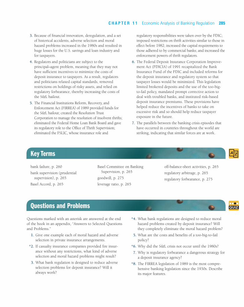
3. Because of financial innovation, deregulation, and a setof historical accidents, adverse selection and moralhazard problems increased in the 1980s and resulted inhuge losses for the U.S. savings and loan industry andfor taxpayers.

4. Regulators and politicians are subject to theprincipal–agent problem, meaning that they may nothave sufficient incentives to minimize the costs ofdeposit insurance to taxpayers. As a result, regulatorsand politicians relaxed capital standards, removedrestrictions on holdings of risky assets, and relied onregulatory forbearance, thereby increasing the costs ofthe S&L bailout.

5. The Financial Institutions Reform, Recovery, andEnforcement Act (FIRREA) of 1989 provided funds forthe S&L bailout; created the Resolution TrustCorporation to manage the resolution of insolvent thrifts;eliminated the Federal Home Loan Bank Board and gaveits regulatory role to the Office of Thrift Supervision;eliminated the FSLIC, whose insurance role and

regulatory responsibilities were taken over by the FDIC;imposed restrictions on thrift activities similar to those ineffect before 1982; increased the capital requirements tothose adhered to by commercial banks; and increased theenforcement powers of thrift regulators.

6. The Federal Deposit Insurance Corporation Improve-ment Act (FDICIA) of 1991 recapitalized the BankInsurance Fund of the FDIC and included reforms forthe deposit insurance and regulatory system so thattaxpayer losses would be minimized. This legislationlimited brokered deposits and the use of the too-big-to-fail policy, mandated prompt corrective action todeal with troubled banks, and instituted risk-baseddeposit insurance premiums. These provisions havehelped reduce the incentives of banks to take onexcessive risk and so should help reduce taxpayerexposure in the future.

7. The parallels between the banking crisis episodes thathave occurred in countries throughout the world arestriking, indicating that similar forces are at work.


Key Terms

bank failure, p. 260

bank supervision (prudential supervision), p. 265

Basel Accord, p. 265

Basel Committee on BankingSupervision, p. 265

goodwill, p. 275

leverage ratio, p. 265

off-balance-sheet activities, p. 265

regulatory arbitrage, p. 265

regulatory forbearance, p. 275



1. Give one example each of moral hazard and adverseselection in private insurance arrangements.

*2. If casualty insurance companies provided fire insur-ance without any restrictions, what kind of adverseselection and moral hazard problems might result?

3. What bank regulation is designed to reduce adverseselection problems for deposit insurance? Will italways work?

*4. What bank regulations are designed to reduce moralhazard problems created by deposit insurance? Willthey completely eliminate the moral hazard problem?

5. What are the costs and benefits of a too-big-to-failpolicy?

*6. Why did the S&L crisis not occur until the 1980s?

7. Why is regulatory forbearance a dangerous strategy fora deposit insurance agency?

*8. The FIRREA legislation of 1989 is the most compre-hensive banking legislation since the 1930s. Describeits major features.

QUIZ

gloss285.html

quiz285.html

9. What steps were taken in the FDICIA legislation of1991 to improve the functioning of federal depositinsurance?

*10. Some advocates of campaign reform believe that gov-ernment funding of political campaigns and restric-tions on campaign spending might reduce theprincipal–agent problem in our political system. Doyou agree? Explain your answer.

11. How can the S&L crisis be blamed on theprincipal–agent problem?

*12. Do you think that eliminating or limiting the amountof deposit insurance would be a good idea? Explainyour answer.

13. Do you think that removing the impediments to anationwide banking system will be beneficial to theeconomy? Explain your answer.

*14. How could higher deposit insurance premiums forbanks with riskier assets benefit the economy?

15. How has too-big-too-fail been limited in the FDICIAlegislation? How might limiting too-big-too-fail helpreduce the risk of a future banking crisis?


Web Exercises

1. Go to www.fdic.gov/regulations/laws/important/index.html. This site reports on the most significantpieces of legislation affecting banks since the 1800s.Summarize the most recently enacted bank regulationlisted on this site.

2. The Office of the Comptroller of the Currency isresponsible for many of the regulations affecting bankoperations. Go to www.occ.treas.gov/. Click on“Regulatory Information.” Now click on the 12 CFRParts 1 to 199. What does Part 1 cover? How manyparts are there in 12 CRF? Open Part 18. What topicdoes it cover? Summarize its purpose.

links286.html

FDICIA is a major step in reforming the banking regulatory system. How well will itwork to solve the adverse selection and moral hazard problems of the bank regulatorysystem? Let’s use the analysis in the chapter to evaluate the most important provisionsof this legislation to answer this question.

Study Guide Before looking at the evaluation for each set of provisions and proposals in this appli-cation, try to reason out how well they will solve the current problems with bankingregulation. This exercise will help you develop a deeper understanding of the mate-rial in this chapter.

FDICIA’s reduction of the scope of deposit insurance by limiting insurance on bro-kered deposits and restricting the use of the too-big-to-fail policy might haveincreased the incentives for uninsured depositors to monitor banks and to withdrawfunds if the bank is taking on too much risk. Because banks might now fear the lossof deposits when they engage in risky activities, they might have less incentive to takeon too much risk. Limitations on the use of the too-big-to-fail policy starting in 1992have resulted in increased losses to uninsured depositors at failed banks as planned.

Although the cited elements of FDICIA strengthen the incentive of depositors tomonitor banks, some critics of FDICIA would take these limitations on the scope ofdeposit insurance even further. Some suggest that deposit insurance should be elim-inated entirely or should be reduced in amount from the current $100,000 limit to,say, $50,000 or $20,000. Another proposed reform would institute a system of coin-surance in which only a percentage of a deposit—say, 90%—would be covered byinsurance. In this system, the insured depositor would suffer a percentage of thelosses along with the deposit insurance agency. Because depositors facing a lower limiton deposit insurance or coinsurance would suffer losses if the bank goes broke, theywill have an incentive to monitor the bank’s activities. Other critics believe that FDICIAprovides too much support for the too-big-to-fail policy. Because under FDICIA theFed, the Treasury, and the FDIC can still agree to implement too-big-to-fail and thusbail out uninsured as well as insured depositors, big banks will not be subjected toenough discipline by uninsured depositors. These critics advocate eliminating thetoo-big-to-fail policy entirely, thereby decreasing the incentives of big banks to takeon too much risk.

Limits on theScope of DepositInsurance

Evaluating FDICIA and OtherProposed Reforms of the Banking Regulatory System

appendixto chap ter

11

1

However, other experts do not believe that depositors are capable of monitoringbanks and imposing discipline on them. The basic problem with reducing the scopeof deposit insurance even further as proposed is that banks would be subject to runs,sudden withdrawals by nervous depositors. Such runs could by themselves lead tobank failures. In addition to protecting individual depositors, the purpose of depositinsurance is to prevent a large number of bank failures, which would lead to an unsta-ble banking system and an unstable economy as occurred periodically before theestablishment of federal deposit insurance in 1934. From this perspective, federaldeposit insurance has been a resounding success. Bank panics, in which there aresimultaneous failures of many banks and consequent disruption of the financial sys-tem, have not occurred since federal deposit insurance was established.

On the one hand, evidence that the largest banks benefiting from the de facto too-big-to-fail policy before 1991 were also the ones that took on the most risk suggeststhat limiting its application, as FDICIA does, may substantially reduce risk taking. Onthe other hand, eliminating the too-big-to-fail policy altogether would also cause someof the same problems that would occur if deposit insurance were eliminated orreduced: The probability of bank panics would increase. If a big bank were allowed tofail, the repercussions in the financial system might be immense. Other banks with acorrespondent relationship with the failed bank (those that have deposits at the bankin exchange for a variety of services) would suffer large losses and might fail in turn,leading to a full-scale panic. In addition, the problem of liquidating the big bank’s loanportfolio might create a major disruption in the financial market.

The prompt corrective action provisions of FDICIA should also substantially reduceincentives for bank risk taking and reduce taxpayer losses. FDICIA uses a carrot-and-stick approach to get banks to hold more capital. If they are well capitalized, theyreceive valuable privileges; if their capital ratio falls, they are subject to more andmore onerous regulation. Increased bank capital reduces moral hazard incentives forthe bank, because the bank now has more to lose if it fails and so is less likely to takeon too much risk.

In addition, encouraging banks to hold more capital reduces potential losses forthe FDIC, because increased bank capital is a cushion that makes bank failure lesslikely. Furthermore, forcing the FDIC to close banks once their net worth is less than2% (group 5) rather than waiting until net worth has fallen to zero makes it morelikely that when a bank is closed, it will still have a positive net worth, thus limitingFDIC losses.

Prompt corrective action, which requires regulators to intervene early when bankcapital begins to fall, is a serious attempt to reduce the principal–agent problem forpoliticians and regulators. With prompt corrective action provisions, regulators nolonger have the option of regulatory forbearance, which, as we have seen, can greatlyincrease moral hazard incentives for banks.

Some critics of FDICIA feel that there are too many loopholes in the billthat still allow regulators too much discretion, thus leaving open the possibility ofregulatory forbearance. However, an often overlooked part of the bill increases theaccountability of regulators. FDICIA requires a mandatory review of any bank failurethat imposes costs on the FDIC. The resulting report must be made available to anymember of Congress and to the general public upon request, and the GeneralAccounting Office must do an annual review of these reports. Opening up the actionsof the regulators to public scrutiny will make regulatory forbearance less attractive to

Prompt Corrective Action

Evaluating FDICIA and Other Proposed Reforms of the Banking Regulatory System 2

them, thereby reducing the principal–agent problem. It will also reduce the incentivesof politicians to lean on regulators to relax their regulatory supervision of banks.

Under FDICIA, banks deemed to be taking on greater risk, in the form of lower cap-ital or riskier assets, will be subjected to higher insurance premiums. Risk-basedinsurance premiums will consequently reduce the moral hazard incentives for banksto take on higher risk. In addition, the fact that risk-based premiums drop as thebank’s capital increases encourages the bank to hold more capital, which has the ben-efits already mentioned.

One problem with risk-based premiums is that the scheme for determining theamount of risk the bank is taking may not be very accurate. For example, it mightbe hard for regulators to determine when a bank’s loans are risky. Some critics havealso pointed out that the classification of banks by such measures as the Basel risk-based capital standard solely reflects credit risk and does not take sufficient accountof interest-rate risk. The regulatory authorities, however, are encouraged by FDICIAto modify existing risk-based standards to include interest-rate risk and, as we haveseen earlier in the chapter, have proposed guidelines to encourage banks to manageinterest-rate risk.

FDICIA’s requirements that regulators perform bank examinations at least once a yearare necessary for monitoring banks’ compliance with bank capital requirements andasset restrictions. As the S&L debacle illustrates, frequent supervisory examinationsof banks are necessary to keep them from taking on too much risk or committingfraud. Similarly, beefing up the ability of the Federal Reserve to monitor foreign banksmight help dissuade international banks from engaging in these undesirable activities.

The stricter and more burdensome reporting requirements for banks have theadvantage of providing more information to regulators to help them monitor bankactivities. However, these reporting requirements have been criticized by banks,which claim that the requirements make it harder to lend to small businesses.

Regulatory Consolidation. The current bank regulatory system in the United Stateshas banking institutions supervised by four federal agencies: the FDIC, the Office ofthe Comptroller of the Currency, the Office of Thrift Supervision, and the FederalReserve. Critics of this system of multiple regulatory agencies with overlapping juris-dictions believe it creates a system that is too complex and too costly because it is rifewith duplication. The Clinton administration proposed a consolidation in which theduties of the four regulatory agencies would be given to a new Federal BankingCommission governed by a five-member board with one member from the Treasury,one from the Federal Reserve, and three independent members appointed by thepresident and confirmed by the Senate. The Federal Reserve strongly opposed thisproposal because it believed that it needed to have hands-on supervision of the largestbanks through their bank holding companies (as is the case currently) in order tohave the information that would enable the Fed to respond sufficiently quickly in acrisis. The Fed also pointed out that a monolithic regulator might be less effectivethan two or more regulators in providing checks and balances for regulatory supervi-sion. The Clinton administration’s proposal was not passed by Congress, but the issueof regulatory consolidation is sure to come up again.

Other ProposedChanges inBankingRegulations

Other FDICIAProvisions

Risk-BasedInsurancePremiums


Market-Value Accounting for Capital Requirements. We have seen that the requirementthat a bank have substantial equity capital makes the bank less likely to fail. Therequirement is also advantageous, because a bank with high equity capital has moreto lose if it takes on risky investments and so will have less incentive to hold riskyassets. Unfortunately, capital requirements, including new risk-based measures, arecalculated on a historical-cost (book value) basis in which the value of an asset is setat its initial purchase price. The problem with historical-cost accounting is thatchanges in the value of assets and liabilities because of changes in interest rates ordefault risk are not reflected in the calculation of the firm’s equity capital. Yet changesin the market value of assets and liabilities and hence changes in the market value ofequity capital are what indicate if a firm is truly insolvent. Furthermore, it is the mar-ket value of capital that determines the incentives for a bank to hold risky assets.

Market-value accounting when calculating capital requirements is another reformthat receives substantial support. All assets and liabilities could be updated to marketvalue periodically—say, every three months—to determine if a bank’s capital is suffi-cient to meet the minimum requirements. This market-value accounting informationwould let the deposit insurance agency know quickly when a bank was falling belowits capital requirement. The bank could then be closed down before its net worth fellbelow zero, thus preventing a loss to the deposit insurance agency. The market-value-based capital requirement would also ensure that banks would not be operating withnegative capital, thereby preventing the bet-the-bank strategy of taking on excessiverisk.

Objections to market-value-based capital requirements center on the difficulty ofmaking accurate and straightforward market-value estimates of capital. Historical-costaccounting has an important advantage in that accounting rules are easier to defineand standardize when the value of an asset is simply set at its purchase price. Market-value accounting, by contrast, requires estimates and approximations that are harderto standardize. For example, it might be hard to assess the market value of your friendJoe’s car loan, whereas it would be quite easy to value a government bond. In addi-tion, conducting market-value accounting would prove costly to banks because esti-mation of market values requires the collection of more information about thecharacteristics of assets and liabilities. Nevertheless, proponents of market-valueaccounting for capital requirements point out that although market-value accountinginvolves some estimates and approximations, it would still provide regulators withmore accurate assessment of bank equity capital than historical-cost accounting does.

FDICIA appears to be an important step in the right direction, because it increases theincentives for banks to hold capital and decreases their incentives to take on exces-sive risk. However, more could be done to improve the incentives for banks to limittheir risk taking. Yet eliminating deposit insurance and the too-big-to-fail policy alto-gether may be going too far, because these proposals might make the banking systemtoo prone to a banking panic.

Overall Evaluation

Evaluating FDICIA and Other Proposed Reforms of the Banking Regulatory System 4

PREVIEW Banking is not the only type of financial intermediation you are likely to experience.You might decide to purchase insurance, take out an installment loan from a financecompany, or buy a share of stock. In each of these transactions you will be engagedin nonbank finance and will deal with nonbank financial institutions. In our economy,nonbank finance also plays an important role in channeling funds from lender-saversto borrower-spenders. Furthermore, the process of financial innovation we discussedin Chapter 10 has increased the importance of nonbank finance and is blurring thedistinction between different financial institutons. This chapter examines in moredetail how institutions engaged in nonbank finance operate, how they are regulated,and recent trends in nonbank finance.

Insurance

Every day we face the possibility of the occurrence of certain catastrophic events thatcould lead to large financial losses. A spouse’s earnings might disappear due to deathor illness; a car accident might result in costly repair bills or payments to an injuredparty. Because financial losses from crises could be large relative to our financialresources, we protect ourselves against them by purchasing insurance coverage thatwill pay a sum of money if catastrophic events occur. Life insurance companies sellpolicies that provide income if a person dies, is incapacitated by illness, or retires.Property and casualty companies specialize in policies that pay for losses incurred asa result of accidents, fire, or theft.

The first life insurance company in the United States (Presbyterian Ministers’ Fund inPhiladelphia) was established in 1759 and is still in existence. There are currentlyabout 1,400 life insurance companies, which are organized in two forms: as stockcompanies or as mutuals. Stock companies are owned by stockholders; mutuals aretechnically owned by the policyholders. Although over 90% of life insurance compa-nies are organized as stock companies, some of the largest ones are organized asmutuals.

Unlike commercial banks and other depository institutions, life insurance com-panies have never experienced widespread failures, so the federal government has notseen the need to regulate the industry. Instead, regulation is left to the states in whicha company operates. State regulation is directed at sales practices, the provision of

Life Insurance

287

Ch a p te r

Nonbank Finance12

www.iii.org

The Insurance InformationInstitute publishes facts and

statistics about the insurance industry.

adequate liquid assets to cover losses, and restrictions on the amount of risky assets(such as common stock) that the companies can hold. The regulatory authority is typ-ically a state insurance commissioner.

Because death rates for the population as a whole are predictable with a highdegree of certainty, life insurance companies can accurately predict what their payoutsto policyholders will be in the future. Consequently, they hold long-term assets thatare not particularly liquid—corporate bonds and commercial mortgages as well assome corporate stock.

There are two principal forms of life insurance policies: permanent life insurance(such as whole, universal, and variable life) and temporary insurance (such as term).Permanent life insurance policies have a constant premium throughout the life of thepolicy. In the early years of the policy, the size of this premium exceeds the amountneeded to insure against death because the probability of death is low. Thus the pol-icy builds up a cash value in its early years, but in later years the cash value declinesbecause the constant premium falls below the amount needed to insure against death,the probability of which is now higher. The policyholder can borrow against the cashvalue of the permanent life policy or can claim it by canceling the policy.

Term insurance, by contrast, has a premium that is matched every year to theamount needed to insure against death during the period of the term (such as oneyear or five years). As a result, term policies have premiums that rise over time as theprobability of death rises (or level premiums with a decline in the amount of deathbenefits). Term policies have no cash value and thus, in contrast to permanent lifepolicies, provide insurance only, with no savings aspect.

Weak investment returns on permanent life insurance in the 1960s and 1970s ledto slow growth of demand for life insurance products. The result was a shrinkage inthe size of the life insurance industry relative to other financial intermediaries, withtheir share of total financial intermediary assets falling from 19.6% at the end of 1960to 11.5% at the end of 1980. (See Table 1, which shows the relative shares of financialintermediary assets for each of the financial intermediaries discussed in this chapter.)

Beginning in the mid-1970s, life insurance companies began to restructure theirbusiness to become managers of assets for pension funds. An important factor behindthis restructuring was 1974 legislation that encouraged pension funds to turn fundmanagement over to life insurance companies. Now more than half of the assets man-aged by life insurance companies are for pension funds and not for life insurance.Insurance companies have also begun to sell investment vehicles for retirement suchas annuities, arrangements whereby the customer pays an annual premium inexchange for a future stream of annual payments beginning at a set age, say 65, andcontinuing until death. The result of this new business has been that the market shareof life insurance companies as a percentage of total financial intermediary assets hasheld steady since 1980.

There are on the order of 3,000 property and casualty insurance companies in theUnited States, the two largest of which are State Farm and Allstate. Property and casu-alty companies are organized as both stock and mutual companies and are regulatedby the states in which they operate.

Although property and casualty insurance companies had a slight increase intheir share of total financial intermediary assets from 1960 to 1990 (see Table 1), inrecent years they have not fared well, and insurance premiums have skyrocketed.With the high interest rates in the 1970s and 1980s, insurance companies had high

Property andCasualtyInsurance


www.federalreserve.gov/releases/Z1/

The Flow of Funds Accounts ofthe United States reports details

about the current state of theinsurance industry. Scroll downthrough the table of contents to

find the location of data oninsurance companies.

investment income that enabled them to keep insurance rates low. Since then, how-ever, investment income has fallen with the decline in interest rates, while the growthin lawsuits involving property and casualty insurance and the explosion in amountsawarded in such cases have produced substantial losses for companies.

To return to profitability, insurance companies have raised their rates dramati-cally—sometimes doubling or even tripling premiums—and have refused to providecoverage for some people. They have also campaigned actively for limits on insurancepayouts, particularly for medical malpractice. In the search for profits, insurance com-panies are also branching out into uncharted territory by insuring the payment ofinterest on municipal and corporate bonds and on mortgage-backed securities. Oneworry is that the insurance companies may be taking on excessive risk in order toboost their profits. One result of the concern about the health of the property andcasualty insurance industry is that insurance regulators have proposed new rules thatwould impose risk-based capital requirements on these companies based on the risk-iness of their assets and operations.

The investment policies of these companies are affected by two basic facts. First,because they are subject to federal income taxes, the largest share of their assets is heldin tax-exempt municipal bonds. Second, because property losses are more uncertainthan the death rate in a population, these insurers are less able to predict how muchthey will have to pay policyholders than life insurance companies are. Natural or

C H A P T E R 1 2 Nonbank Finance 289

1960 1970 1980 1990 2002

Insurance CompaniesLife insurance 19.6 15.3 11.5 12.5 13.6Property and casualty 4.4 3.8 4.5 4.9 3.7

Pension FundsPrivate 6.4 8.4 12.5 14.9 14.7Public (state and local government) 3.3 4.6 4.9 6.7 7.9

Finance Companies 4.7 4.9 5.1 5.6 3.2

Mutual FundsStock and bond 2.9 3.6 1.7 5.9 10.6Money market 0.0 0.0 1.9 4.6 8.8

Depository Institutions (Banks)Commercial banks 38.6 38.5 36.7 30.4 29.8S&L and mutual savings banks 19.0 19.4 19.6 12.5 5.6Credit unions 1.1 1.4 1.6 2.0 2.3

Total 100.0 100.0 100.0 100.0 100.0

Source: Federal Reserve Flow of Funds Accounts.

Table 1 Relative Shares of Total Financial Intermediary Assets, 1960–2002 (percent)

unnatural disasters such as the Los Angeles earthquake in 1994 and Hurricane Floydin 1999, which devastated parts of the East Coast, and the September 11, 2001destruction of the World Trade Center, exposed the property and casualty insurancecompanies to billions of dollars of losses. Therefore, property and casualty insurancecompanies hold more liquid assets than life insurance companies; municipal bondsand U.S. government securities amount to over half their assets, and most of theremainder is held in corporate bonds and corporate stock.

Property and casualty insurance companies will insure against losses from almostany type of event, including fire, theft, negligence, malpractice, earthquakes, andautomobile accidents. If a possible loss being insured is too large for any one firm,several firms may join together to write a policy in order to share the risk. Insurancecompanies may also reduce their risk exposure by obtaining reinsurance. Reinsuranceallocates a portion of the risk to another company in exchange for a portion of thepremium and is particularly important for small insurance companies. You can thinkof reinsurance as insurance for the insurance company. The most famous risk-sharingoperation is Lloyd’s of London, an association in which different insurance companiescan underwrite a fraction of an insurance policy. Lloyd’s of London has claimed thatit will insure against any contingency—for a price.

Until recently, banks have been restricted in their ability to sell life insurance prod-ucts. This has been changing rapidly, however. Over two-thirds of the states allowbanks to sell life insurance in one form or another. In recent years, the bank regula-tory authorities, particularly the Office of the Comptroller of the Currency (OCC),have also encouraged banks to enter the insurance field because getting into insur-ance would help diversify banks’ business, thereby improving their economic healthand making bank failures less likely. For example, in 1990, the OCC ruled that sell-ing annuities was a form of investment that was incidental to the banking businessand so was a permissible banking activity. As a result, the banks’ share of the annu-ities market has surpassed 20%. Currently, more than 40% of banks sell insuranceproducts, and the number is expected to grow in the future.

Insurance companies and their agents reacted to this competitive threat with bothlawsuits and lobbying actions to block banks from entering the insurance business.Their efforts were set back by several Supreme Court rulings that favored the banks.Particularly important was a ruling in favor of Barnett Bank in March 1996, which heldthat state laws to prevent banks from selling insurance can be superseded by federalrulings from banking regulators that allow banks to sell insurance. The decision gavebanks a green light to further their insurance activities, and with the passage of theGramm-Leach-Bliley Act of 1999, banking institutions will further engage in the insur-ance business, thus blurring the distinction between insurance companies and banks.

The CompetitiveThreat from theBanking Industry


Insurance ManagementApplication

Insurance, like banking, is in the financial intermediation business of trans-forming one type of asset into another for the public. Insurance providersuse the premiums paid on policies to invest in assets such as bonds, stocks,mortgages, and other loans; the earnings from these assets are then used topay out claims on the policies. In effect, insurers transform assets such as


bonds, stocks, and loans into insurance policies that provide a set of serv-ices (for example, claim adjustments, savings plans, friendly insuranceagents). If the insurer’s production process of asset transformation efficientlyprovides its customers with adequate insurance services at low cost and if itcan earn high returns on its investments, it will make profits; if not, it willsuffer losses.

In Chapter 9 the economic concepts of adverse selection and moral haz-ard allowed us to understand principles of bank management related to man-aging credit risk; many of these same principles also apply to the lendingactivities of insurers. Here again we apply the adverse selection and moral haz-ard concepts to explain many management practices specific to insurance.

In the case of an insurance policy, moral hazard arises when the existenceof insurance encourages the insured party to take risks that increase the like-lihood of an insurance payoff. For example, a person covered by burglaryinsurance might not take as many precautions to prevent a burglary becausethe insurance company will reimburse most of the losses if a theft occurs.Adverse selection holds that the people most likely to receive large insurancepayoffs are the ones who will want to purchase insurance the most. Forexample, a person suffering from a terminal disease would want to take outthe biggest life and medical insurance policies possible, thereby exposing theinsurance company to potentially large losses. Both adverse selection andmoral hazard can result in large losses to insurance companies, because theylead to higher payouts on insurance claims. Lowering adverse selection andmoral hazard to reduce these payouts is therefore an extremely importantgoal for insurance companies, and this goal explains the insurance practiceswe will discuss here.

To reduce adverse selection, insurance providers try to screen out good insur-ance risks from poor ones. Effective information collection procedures aretherefore an important principle of insurance management.

When you apply for auto insurance, the first thing your insurance agentdoes is ask you questions about your driving record (number of speedingtickets and accidents), the type of car you are insuring, and certain personalmatters (age, marital status). If you are applying for life insurance, you gothrough a similar grilling, but you are asked even more personal questionsabout such things as your health, smoking habits, and drug and alcohol use.The life insurer even orders a medical evaluation (usually done by an inde-pendent company) that involves taking blood and urine samples. Just as abank calculates a credit score to evaluate a potential borrower, the insurersuse the information you provide to allocate you to a risk class—a statisticalestimate of how likely you are to have an insurance claim. Based on thisinformation, the insurer can decide whether to accept you for the insuranceor to turn you down because you pose too high a risk and thus would be anunprofitable customer.

Charging insurance premiums on the basis of how much risk a policyholderposes for the insurance provider is a time-honored principle of insurancemanagement. Adverse selection explains why this principle is so importantto insurance company profitability.

Risk-BasedPremiums

Screening


To understand why an insurance provider finds it necessary to have risk-based premiums, let’s examine an example of risk-based insurance premiumsthat at first glance seems unfair. Harry and Sally, both college students with noaccidents or speeding tickets, apply for auto insurance. Normally, Harry willbe charged a much higher premium than Sally. Insurance providers do thisbecause young males have a much higher accident rate than young females.Suppose, though, that one insurer did not base its premiums on a risk classi-fication but rather just charged a premium based on the average combinedrisk for males and females. Then Sally would be charged too much and Harrytoo little. Sally could go to another insurer and get a lower rate, while Harrywould sign up for the insurance. Because Harry’s premium isn’t high enoughto cover the accidents he is likely to have, on average the insurer would losemoney on Harry. Only with a premium based on a risk classification, so thatHarry is charged more, can the insurance provider make a profit.1

Restrictive provisions in policies are an insurance management tool forreducing moral hazard. Such provisions discourage policyholders fromengaging in risky activities that make an insurance claim more likely. Forexample, life insurers have provisions in their policies that eliminate deathbenefits if the insured person commits suicide within the first two years thatthe policy is in effect. Restrictive provisions may also require certain behav-ior on the part of the insured. A company renting motor scooters may berequired to provide helmets for renters in order to be covered for any liabil-ity associated with the rental. The role of restrictive provisions is not unlikethat of restrictive covenants on debt contracts described in Chapter 8: Bothserve to reduce moral hazard by ruling out undesirable behavior.

Insurance providers also face moral hazard because an insured person has anincentive to lie to the insurer and seek a claim even if the claim is not valid.For example, a person who has not complied with the restrictive provisionsof an insurance contract may still submit a claim. Even worse, a person mayfile claims for events that did not actually occur. Thus an important manage-ment principle for insurance providers is conducting investigations to pre-vent fraud so that only policyholders with valid claims receive compensation.

Being prepared to cancel policies is another insurance management tool.Insurers can discourage moral hazard by threatening to cancel a policy whenthe insured person engages in activities that make a claim more likely. If yourauto insurance company makes it clear that coverage will be canceled if adriver gets too many speeding tickets, you will be less likely to speed.

The deductible is the fixed amount by which the insured’s loss is reducedwhen a claim is paid off. A $250 deductible on an auto policy, for example,

Deductibles

Cancellation ofInsurance

Prevention of Fraud

RestrictiveProvisions

1Note that the example here is in fact the lemons problem described in Chapter 8.


means that if you suffer a loss of $1,000 because of an accident, the insurerwill pay you only $750. Deductibles are an additional management tool thathelps insurance providers reduce moral hazard. With a deductible, you expe-rience a loss along with the insurer when you make a claim. Because you alsostand to lose when you have an accident, you have an incentive to drive morecarefully. A deductible thus makes a policyholder act more in line with whatis profitable for the insurer; moral hazard has been reduced. And becausemoral hazard has been reduced, the insurance provider can lower the pre-mium by more than enough to compensate the policyholder for the existenceof the deductible. Another function of the deductible is to eliminate theadministrative costs of handling small claims by forcing the insured to bearthese losses.

When a policyholder shares a percentage of the losses along with the insurer,their arrangement is called coinsurance. For example, some medical insur-ance plans provide coverage for 80% of medical bills, and the insured personpays 20% after a certain deductible has been met. Coinsurance works toreduce moral hazard in exactly the same way that a deductible does. A policy-holder who suffers a loss along with the insurer has less incentive to takeactions, such as going to the doctor unnecessarily, that involve higher claims.Coinsurance is thus another useful management tool for insurance providers.

Another important principle of insurance management is that there shouldbe limits on the amount of insurance provided, even though a customer iswilling to pay for more coverage. The higher the insurance coverage, themore the insured person can gain from risky activities that make an insur-ance payoff more likely and hence the greater the moral hazard. For exam-ple, if Zelda’s car were insured for more than its true value, she might nottake proper precautions to prevent its theft, such as making sure that thekey is always removed or putting in an alarm system. If it were stolen, shecomes out ahead because the excessive insurance payment would allow herto buy an even better car. By contrast, when the insurance payments arelower than the value of her car, she will suffer a loss if it is stolen and willthus take precautions to prevent this from happening. Insurance providersmust always make sure that their coverage is not so high that moral hazardleads to large losses.

Effective insurance management requires several practices: information col-lection and screening of potential policyholders, risk-based premiums, restric-tive provisions, prevention of fraud, cancellation of insurance, deductibles,coinsurance, and limits on the amount of insurance. All of these practicesreduce moral hazard and adverse selection by making it harder for policy-holders to benefit from engaging in activities that increase the amount andlikelihood of claims. With smaller benefits available, the poor insurance risks(those who are more likely to engage in the activities in the first place) seeless benefit from the insurance and are thus less likely to seek it out.

Summary

Limits on theAmount ofInsurance

Coinsurance

Pension Funds

In performing the financial intermediation function of asset transformation, pensionfunds provide the public with another kind of protection: income payments onretirement. Employers, unions, or private individuals can set up pension plans,which acquire funds through contributions paid in by the plan’s participants. As wecan see in Table 1, pension plans both public and private have grown in importance,with their share of total financial intermediary assets rising from 10% at the end of1960 to 22.6% at the end of 2002. Federal tax policy has been a major factor behindthe rapid growth of pension funds because employer contributions to employee pen-sion plans are tax-deductible. Furthermore, tax policy has also encouraged employeecontributions to pension funds by making them tax-deductible as well and enablingself-employed individuals to open up their own tax-sheltered pension plans, Keoghplans, and individual retirement accounts (IRAs).

Because the benefits paid out of the pension fund each year are highly pre-dictable, pension funds invest in long-term securities, with the bulk of their assetholdings in bonds, stocks, and long-term mortgages. The key management issues forpension funds revolve around asset management: Pension fund managers try to holdassets with high expected returns and lower risk through diversification. They alsouse techniques we discussed in Chapter 9 to manage credit and interest-rate risk.The investment strategies of pension plans have changed radically over time. In theaftermath of World War II, most pension fund assets were held in governmentbonds, with less than 1% held in stock. However, the strong performance of stocksin the 1950s and 1960s afforded pension plans higher returns, causing them to shifttheir portfolios into stocks, currently on the order of two-thirds of their assets. As aresult, pension plans now have a much stronger presence in the stock market: In theearly 1950s, they held on the order of 1% of corporate stock outstanding; currentlythey hold on the order of 25%. Pension funds are now the dominant players in thestock market.

Although the purpose of all pension plans is the same, they can differ in a num-ber of attributes. First is the method by which payments are made: If the benefits aredetermined by the contributions into the plan and their earnings, the pension is adefined-contribution plan; if future income payments (benefits) are set in advance,the pension is a defined-benefit plan. In the case of a defined-benefit plan, a furtherattribute is related to how the plan is funded. A defined-benefit plan is fully fundedif the contributions into the plan and their earnings over the years are sufficient to payout the defined benefits when they come due. If the contributions and earnings arenot sufficient, the plan is underfunded. For example, if Jane Brown contributes $100per year into her pension plan and the interest rate is 10%, after ten years the con-tributions and their earnings would be worth $1,753.2 If the defined benefit on her


2The $100 contributed in year 1 would become worth $100 � (1 � 0.10)10� $259.37 at the end of ten years;

the $100 contributed in year 2 would become worth $100 � (1 � 0.10)9� $235.79; and so on until the $100

contributed in year 10 would become worth $100 � (1 � 0.10) � $110. Adding these together, we get the totalvalue of these contributions and their earnings at the end of ten years:

$259.37 � $235.79 � $214.36 � $194.87 � $177.16 � $161.05 � $146.41 � $133.10 � $121.00 � $110.00 � $1,753.11

pension plan pays her $1,753 or less after ten years, the plan is fully funded becauseher contributions and earnings will fully pay for this payment. But if the definedbenefit is $2,000, the plan is underfunded, because her contributions and earningsdo not cover this amount.

A second characteristic of pension plans is their vesting, the length of time that aperson must be enrolled in the pension plan (by being a member of a union or anemployee of a company) before being entitled to receive benefits. Typically, firms requirethat an employee work five years for the company before being vested and qualifying toreceive pension benefits; if the employee leaves the firm before the five years are up,either by quitting or being fired, all rights to benefits are lost.

Private pension plans are administered by a bank, a life insurance company, or a pen-sion fund manager. In employer-sponsored pension plans, contributions are usuallyshared between employer and employee. Many companies’ pension plans are under-funded because they plan to meet their pension obligations out of current earningswhen the benefits come due. As long as companies have sufficient earnings, under-funding creates no problems, but if not, they may not be able to meet their pensionobligations. Because of potential problems caused by corporate underfunding, mis-management, fraudulent practices, and other abuses of private pension funds(Teamsters pension funds are notorious in this regard), Congress enacted the EmployeeRetirement Income Security Act (ERISA) in 1974. This act established minimum stan-dards for the reporting and disclosure of information, set rules for vesting and thedegree of underfunding, placed restrictions on investment practices, and assigned theresponsibility of regulatory oversight to the Department of Labor.

ERISA also created the Pension Benefit Guarantee Corporation (called “PennyBenny”), which performs a role similar to that of the FDIC. It insures pension bene-fits up to a limit (currently over $40,000 per year per person) if a company with anunderfunded pension plan goes bankrupt or is unable to meet its pension obligationsfor other reasons. Penny Benny charges pension plans premiums to pay for this insur-ance, and it can also borrow funds up to $100 million from the U.S. Treasury.Unfortunately, the problem of pension plan underfunding has been growing worse inrecent years. In 1993, the secretary of labor indicated that underfunding had reachedlevels in excess of $45 billion, with one company’s pension plan alone, that of GeneralMotors, underfunded to the tune of $11.8 billion. As a result, Penny Benny, whichinsures the pensions of one of every three workers, may have to foot the bill if com-panies with large underfunded pensions go broke.

The most important public pension plan is Social Security (Old Age and Survivors’Insurance Fund), which covers virtually all individuals employed in the private sector.Funds are obtained from workers through Federal Insurance Contribution Act (FICA)deductions from their paychecks and from employers through payroll taxes. SocialSecurity benefits include retirement income, Medicare payments, and aid to the disabled.

When Social Security was established in 1935, the federal government intended tooperate it like a private pension fund. However, unlike a private pension plan, bene-fits are typically paid out from current contributions, not tied closely to a participant’spast contributions. This “pay as you go” system at one point led to a massive under-funding, estimated at over $1 trillion.

The problems of the Social Security system could become worse in the futurebecause of the growth in the number of retired people relative to the working

Public PensionPlans

Private PensionPlans


www.ssa.gov/

The web site for the SocialSecurity Administration

contains information on yourbenefits available from social

security.

www.pbgc.gov/

The web site for the PensionBenefit Guarantee Corporation

contains information aboutpensions and the insurance that

it provides.

population. Congress has been grappling with the problems of the Social Security sys-tem for years, but the prospect of a huge bulge in new retirees when the 77 billionbaby boomers born between 1946 and 1964 start to retire in 2011 has resulted incalls for radical surgery on Social Security (see Box 1).

State and local governments and the federal government, like private employers,have also set up pension plans for their employees. These plans are almost identical inoperation to private pension plans and hold similar assets. Underfunding of the plans isalso prevalent, and some investors in municipal bonds worry that it may lead to futuredifficulties in the ability of state and local governments to meet their debt obligations.

Finance Companies

Finance companies acquire funds by issuing commercial paper or stocks and bondsor borrowing from banks, and they use the proceeds to make loans (often for smallamounts) that are particularly well suited to consumer and business needs. The finan-


Box 1

Should Social Security Be Privatized?In recent years, public confidence in the SocialSecurity system has reached a new low. Some surveyssuggest that young people have more confidence inthe existence of flying saucers than they do in the gov-ernment’s promise to pay them their Social Securitybenefits. Without some overhaul of the system, SocialSecurity will not be able to meet its future obligations.The government has set up advisory commissions andhas been holding hearings to address this problem.

Currently, the assets of the Social Security system,which reside in a trust fund, are all invested in U.S.Treasury securities. Because stocks and corporatebonds have higher returns than Treasury securities,many proposals to save the Social Security systemsuggest investing part of the trust fund in corporatesecurities and thus partially privatizing the system.

Suggestions for privatization take three basic forms:

1. Government investment of trust fund assets in cor-porate securities. This plan has the advantage of pos-sibly improving the trust fund’s overall return, whileminimizing transactions costs because it exploits theeconomies of scale of the trust fund. Critics warnthat government ownership of private assets couldlead to increased government intervention in the pri-vate sector.

2. Shift of trust fund assets to individual accounts thatcan be invested in private assets. This option has theadvantage of possibly increasing the return on invest-ments and does not involve the government in theownership of private assets. However, critics warnthat it might expose individuals to greater risk and totransaction costs on individual accounts that mightbe very high because of the small size of many ofthese accounts.

3. Individual accounts in addition to those in the trustfund. This option has advantages and disadvantagessimilar to those of option 2 and may provide morefunds to individuals at retirement. However, someincrease in taxes would be required to fund theseaccounts.

Whether some privatization of the Social Securitysystem occurs is an open question. In the shortterm, Social Security reform is likely to involve anincrease in taxes, a reduction in benefits, or both.For example, the age at which benefits begin isalready scheduled to increase from 65 to 67, andmight be increased further to 70. It is also likely thatthe cap on wages subject to the Social Security taxwill be raised further, thereby increasing taxes paidinto the system.

cial intermediation process of finance companies can be described by saying that theyborrow in large amounts but often lend in small amounts—a process quite differentfrom that of banking institutions, which collect deposits in small amounts and thenoften make large loans.

A key feature of finance companies is that although they lend to many of the samecustomers that borrow from banks, they are virtually unregulated compared to com-mercial banks and thrift institutions. States regulate the maximum amount they canloan to individual consumers and the terms of the debt contract, but there are norestrictions on branching, the assets they hold, or how they raise their funds. The lackof restrictions enables finance companies to tailor their loans to customer needs bet-ter than banking institutions can.

There are three types of finance companies: sales, consumer, and business.

1. Sales finance companies are owned by a particular retailing or manufacturingcompany and make loans to consumers to purchase items from that company. Sears,Roebuck Acceptance Corporation, for example, finances consumer purchases of allgoods and services at Sears stores, and General Motors Acceptance Corporationfinances purchases of GM cars. Sales finance companies compete directly with banksfor consumer loans and are used by consumers because loans can frequently beobtained faster and more conveniently at the location where an item is purchased.

2. Consumer finance companies make loans to consumers to buy particular itemssuch as furniture or home appliances, to make home improvements, or to help refi-nance small debts. Consumer finance companies are separate corporations (likeHousehold Finance Corporation) or are owned by banks (Citigroup owns Person-to-Person Finance Company, which operates offices nationwide). Typically, these com-panies make loans to consumers who cannot obtain credit from other sources andcharge higher interest rates.

3. Business finance companies provide specialized forms of credit to businesses bymaking loans and purchasing accounts receivable (bills owed to the firm) at a dis-count; this provision of credit is called factoring. For example, a dressmaking firmmight have outstanding bills (accounts receivable) of $100,000 owed by the retailstores that have bought its dresses. If this firm needs cash to buy 100 new sewingmachines, it can sell its accounts receivable for, say, $90,000 to a finance company,which is now entitled to collect the $100,000 owed to the firm. Besides factoring,business finance companies also specialize in leasing equipment (such as railroadcars, jet planes, and computers), which they purchase and then lease to businesses fora set number of years.

Mutual Funds

Mutual funds are financial intermediaries that pool the resources of many smallinvestors by selling them shares and using the proceeds to buy securities. Through theasset transformation process of issuing shares in small denominations and buying largeblocks of securities, mutual funds can take advantage of volume discounts on broker-age commissions and purchase diversified holdings (portfolios) of securities. Mutualfunds allow the small investor to obtain the benefits of lower transaction costs in pur-chasing securities and to take advantage of the reduction of risk by diversifying theportfolio of securities held. Many mutual funds are run by brokerage firms, but othersare run by banks or independent investment advisers such as Fidelity or Vanguard.


www.federalreserve.gov/Releases/G20/current

/default.htm

Federal reserve informationabout financial companies.

www.ici.org/facts_figures/factbook_toc.html

The Mutual Fund Fact Bookpublished by Investment

Company Institute includesinformation about the mutual

funds industry’s history,regulation, taxation, and

shareholders.

Mutual funds have seen a large increase in their market share since 1980 (seeTable 1), due primarily to the then-booming stock market. Another source of growthhas been mutual funds that specialize in debt instruments, which first appeared in the1970s. Before 1970, mutual funds invested almost solely in common stocks. Fundsthat purchase common stocks may specialize even further and invest solely in foreignsecurities or in specialized industries, such as energy or high technology. Funds thatpurchase debt instruments may specialize further in corporate, U.S. government, ortax-exempt municipal bonds or in long-term or short-term securities.

Mutual funds are primarily held by households (around 80%) with the rest heldby other financial institutions and nonfinancial businesses. Mutual funds havebecome increasingly important in household savings. In 1980, only 6% of householdsheld mutual fund shares; this number has risen to around 50% in recent years. Theage group with the greatest participation in mutual fund ownership includes individ-uals between 50 and 70, which makes sense because they are the most interested insaving for retirement. Interestingly, Generation X (18–30) is the second most activeage group in mutual fund ownership, suggesting that they have a greater tolerance forinvestment risk than those who are somewhat older. Generation X is also leading theway in Internet access to mutual funds (see Box 2).

The growing importance of investors in mutual funds and pension funds, so-called institutional investors, has resulted in their controlling over 50% of the out-standing stock in the United States. Thus, institutional investors are the predominantplayers in the stock markets, with over 70% of the total daily volume in the stockmarket due to their trading. Increased ownership of stocks has also meant that insti-tutional investors have more clout with corporate boards, often forcing changes inleadership or in corporate policies.

Mutual funds are structured in two ways. The more common structure is anopen-end fund, from which shares can be redeemed at any time at a price that is tied


Mutual Funds and the InternetThe Investment Company Institute estimates that asof 2000, 68% of households owning mutual fundsuse the Internet, and nearly half of those onlineshareholders visit fund-related web sites. TheInternet increases the attractiveness of mutual fundsbecause it enables shareholders to review perform-ance information and share prices and personalaccount information.

Of all U.S. households that conducted mutualfunds transactions between April 1999 and March2000, 18% bought or sold fund shares online. Themedian number of funds transactions conducted overthe Internet during the 12-month period was four,while the average number was eight, indicating that a

high volume of online transactions were conductedby a small number of shareholders.

Online shareholders were typically younger, hadgreater household income, and were better educatedthan those not using the Internet. The median onlineshareholder was 42 years old, had a householdincome of $100,900, and was college-educated. Themedian shareholder not using the Internet was 51years old, had a household income of $41,000, anddid not have a college degree.

The use of the Internet to track and trade mutualfunds is rapidly increasing. The number of share-holders who visited web sites offering fund sharesnearly doubled between April 1999 and March 2000.

Box 2: E-Finance

to the asset value of the fund. Mutual funds also can be structured as a closed-endfund, in which a fixed number of nonredeemable shares are sold at an initial offeringand are then traded like a common stock. The market price of these shares fluctuateswith the value of the assets held by the fund. In contrast to the open-end fund, how-ever, the price of the shares may be above or below the value of the assets held by thefund, depending on factors such as the liquidity of the shares or the quality of themanagement. The greater popularity of the open-end funds is explained by the greaterliquidity of their redeemable shares relative to the nonredeemable shares of closed-end funds.

Originally, shares of most open-end mutual funds were sold by salespeople (usu-ally brokers) who were paid a commission. Since this commission is paid at the timeof purchase and is immediately subtracted from the redemption value of the shares,these funds are called load funds. Most mutual funds are currently no-load funds;they are sold directly to the public with no sales commissions. In both types of funds,the managers earn their living from management fees paid by the shareholders. Thesefees amount to approximately 0.5% of the asset value of the fund per year.

Mutual funds are regulated by the Securities and Exchange Commission, whichwas given the ability to exercise almost complete control over investment companiesin the Investment Company Act of 1940. Regulations require periodic disclosure ofinformation on these funds to the public and restrictions on the methods of solicitingbusiness.

An important addition to the family of mutual funds resulting from the financial inno-vation process described in earlier chapters is the money market mutual fund. Recallthat this type of mutual fund invests in short-term debt (money market) instrumentsof very high quality, such as Treasury bills, commercial paper, and bank certificates ofdeposit. There is some fluctuation in the market value of these securities, but becausetheir maturity is typically less than six months, the change in the market value is smallenough that these funds allow their shares to be redeemed at a fixed value. (Changesin the market value of the securities are figured into the interest paid out by the fund.)Because these shares can be redeemed at a fixed value, the funds allow shareholdersto redeem shares by writing checks on the fund’s account at a commercial bank. Inthis way, shares in money market mutual funds effectively function as checkabledeposits that earn market interest rates on short-term debt securities.

In 1977, the assets in money market mutual funds were less than $4 billion; by1980, they had climbed to over $50 billion and now stand at $2.1 trillion, with ashare of financial intermediary assets that has grown to nearly 9% (see Table 1).Currently, money market mutual funds account for around one-quarter of the assetvalue of all mutual funds.

Hedge funds are a special type of mutual fund, with estimated assets of more than$500 billion. Hedge funds have received considerable attention recently due to theshock to the financial system resulting from the near collapse of Long-Term CapitalManagement, once one of the most important hedge funds (Box 3). Well-knownhedge funds include Moore Capital Management and the Quantum group of fundsassociated with George Soros. Like mutual funds, hedge funds accumulate moneyfrom many people and invest on their behalf, but several features distinguish themfrom traditional mutual funds. Hedge funds have a minimum investment requirement

Hedge Funds

Money MarketMutual Funds


between $100,000 and $20 million, with the typical minimum investment being $1million. Long-Term Capital Management required a $10 million minimum invest-ment. Federal law limits hedge funds to have no more than 99 investors (limited part-ners) who must have steady annual incomes of $200,000 or more or a net worth of$1 million, excluding their homes. These restrictions are aimed at allowing hedgefunds to be largely unregulated, on the theory that the rich can look out for them-selves. Many of the 4,000 hedge funds are located offshore to escape regulatoryrestrictions.

Hedge funds also differ from traditional mutual funds in that they usually requirethat investors commit their money for long periods of time, often several years. Thepurpose of this requirement is to give managers breathing room to pursue long-run


Box 3

The Long-Term Capital Management DebacleLong-Term Capital Management was a hedge fundwith a star cast of managers, including 25 PhDs, twoNobel Prize winners in economics (Myron Scholesand Robert Merton), a former vice-chairman of theFederal Reserve System (David Mullins), and one ofWall Street’s most successful bond traders (JohnMeriwether). It made headlines in September 1998because its near collapse roiled markets and requireda private rescue plan organized by the FederalReserve Bank of New York.

The experience of Long-Term Capital demon-strates that hedge funds are far from risk-free,despite their use of market-neutral strategies. Long-Term Capital got into difficulties when it thoughtthat the spread between prices on long-termTreasury bonds and long-term corporate bonds wastoo high, and bet that this “anomaly” would disap-pear and the spread would narrow. In the wake ofthe collapse of the Russian financial system inAugust 1998, investors increased their assessment ofthe riskiness of corporate securities and as we saw inChapter 6, the spread between corporates andTreasuries rose rather than narrowed as Long-TermCapital had predicted. The result was that Long-Term Capital took big losses on its positions, eatingup much of its equity position.

By mid-September, Long-Term Capital was unableto raise sufficient funds to meet the demands of itscreditors. With Long-Term Capital facing the poten-

tial need to liquidate its portfolio of $80 billion insecurities and more than $1 trillion of notional valuein derivatives (discussed in Chapter 13), the FederalReserve Bank of New York stepped in on September23 and organized a rescue plan with its creditors. TheFed’s rationale for stepping in was that a sudden liq-uidation of Long-Term Capital’s portfolio would cre-ate unacceptable systemic risk. Tens of billions ofdollars of illiquid securities would be dumped on analready jittery market, causing potentially huge lossesto numerous lenders and other institutions. The res-cue plan required creditors, banks and investmentbanks, to supply an additional $3.6 billion of fundsto Long-Term Capital in exchange for much tightermanagement control of funds and a 90% reduction inthe managers’ equity stake. In the middle of 1999,John Meriwether began to wind down the fundsoperations.

Even though no public funds were expended, theFed’s involvement in organizing the rescue of Long-Term Capital was highly controversial. Some criticsargue that the Fed intervention increased moral haz-ard by weakening discipline imposed by the marketon fund managers because future Fed interventions ofthis type would be expected. Others think that theFed’s action was necessary to prevent a major shock tothe financial system that could have provoked a finan-cial crisis. The debate on whether the Fed should haveintervened is likely to go on for some time.

strategies. Hedge funds also typically charge large fees to investors. The typical fundcharges a 1% annual fee on the assets it manages plus 20% of profits, and some chargesignificantly more. Long-Term Capital, for example, charged investors a 2% assetmanagement fee and took 25% of the profits.

The term hedge fund is highly misleading, because the word “hedge” typicallyindicates strategies to avoid risk. As the near failure of Long-Term Capital illustrates,despite their name, these funds can and do take big risks. Many hedge funds engagein what are called “market-neutral” strategies where they buy a security, such as abond, that seems cheap and sell an equivalent amount of a similar security thatappears to be overvalued. If interest rates as a whole go up or down, the fund ishedged, because the decline in value of one security is matched by the rise in valueof the other. However, the fund is speculating on whether the spread between theprice on the two securities moves in the direction predicted by the fund managers. Ifthe fund bets wrong, it can lose a lot of money, particularly if it has leveraged up itspositions; that is, has borrowed heavily against these positions so that its equity stakeis small relative to the size of its portfolio. When Long-Term Capital was rescued, ithad a leverage ratio of 50 to 1; that is, its assets were fifty times larger than its equity,and even before it got into trouble, it was leveraged 20 to 1.

In the wake of the near collapse of Long-Term Capital, many U.S. politicians havecalled for regulation of these funds. However, because many of these funds operateoffshore in places like the Cayman Islands and are outside of U.S. jurisdiction, theywould be extremely hard to regulate. What U.S. regulators can do is ensure that U.S.banks and investment banks have clear guidelines on the amount of lending they canprovide to hedge funds and require that these institutions get the appropriate amountof disclosure from hedge funds as to the riskiness of their positions.

Government Financial Intermediation

The government has become involved in financial intermediation in two basic ways:first, by setting up federal credit agencies that directly engage in financial intermedi-ation and, second, by supplying government guarantees for private loans.

To promote residential housing, the government has created three government agen-cies that provide funds to the mortgage market by selling bonds and using the pro-ceeds to buy mortgages: the Government National Mortgage Association (GNMA, or“Ginnie Mae”), the Federal National Mortgage Association (FNMA, or “Fannie Mae”),and the Federal Home Loan Mortgage Corporation (FHLMC, or “Freddie Mac”).Except for Ginnie Mae, which is a federal agency and is thus an entity of the U.S. gov-ernment, the other agencies are federally sponsored agencies (FSEs) that function asprivate corporations with close ties to the government. As a result, the debt of spon-sored agencies is not explicitly backed by the U.S. government, as is the case forTreasury bonds. As a practical matter, however, it is unlikely that the federal govern-ment would allow a default on the debt of these sponsored agencies.

Agriculture is another area in which financial intermediation by governmentagencies plays an important role. The Farm Credit System (composed of Banks forCooperatives, Farm Credit banks, and various farm credit associations) issues securi-ties and then uses the proceeds to make loans to farmers.

Federal CreditAgencies


In recent years, government financial intermediaries experienced financial diffi-culties. The Farm Credit System is one example. The rising tide of farm bankrupt-cies meant losses in the billions of dollars for the Farm Credit System, and as a resultit required a bailout from the federal government in 1987. The agency was author-ized to borrow up to $4 billion to be repaid over a 15-year period and received over$1 billion in assistance. There is growing concern in Washington about the health ofthe federal credit agencies. To head off government bailouts like that for the FarmCredit System, the Federal Credit Reform Act of 1990 set new rules that require suchagencies to increase their capital to provide a greater cushion to offset any potentiallosses. However, there have been growing concerns about Fannie Mae and FreddieMac (Box 4).

Securities Market Operations

The smooth functioning of securities markets, in which bonds and stocks are traded,involves several financial institutions, including securities brokers and dealers, invest-ment banks, and organized exchanges. None of these institutions were included in ourlist of financial intermediaries in Chapter 2, because they do not perform the interme-diation function of acquiring funds by issuing liabilities and then using the funds toacquire financial assets. Nonetheless, they are important in the process of channelingfunds from savers to spenders and can be thought of as “financial facilitators.”

First, however, we must recall the distinction between primary and secondarysecurities markets discussed in Chapter 2. In a primary market, new issues of a secu-rity are sold to buyers by the corporation or government agency borrowing the funds.A secondary market then trades the securities that have been sold in the primary mar-


Box 4

Are Fannie Mae and Freddie Mac Getting Too Big for Their Britches?With the growth of Fannie Mae and Freddie Mac toimmense proportions, there are rising concerns thatthese federally sponsored agencies could threaten thehealth of the financial system. Fannie Mae andFreddie Mac either own or insure the risk on close tohalf of U.S. residential mortgages (amounting to $2trillion). In fact, their publicly issued debt is well overhalf that issued by the federal government. A failureof either of these institutions would therefore pose agrave shock to the financial system. Although the fed-eral government would be unlikely to stand by andlet them fail, in such a case, the taxpayer would facesubstantial costs, as in the S&L crisis.

Concerns about the safety and soundness of theseinstitutions arise because they have much smaller

capital-to-asset ratios than banks. Critics also chargethat Fannie Mae and Freddie Mac have become solarge that they wield too much political influence. Inaddition, these federally sponsored agencies haveconflicts of interest, because they have to serve twomasters: as publicly traded corporations, they aresupposed to maximize profits for the shareholders,but as government agencies, they are supposed towork in the interests of the public. These concernshave led to calls for reform of these agencies, withmany advocating full privatization as was done vol-untarily by the Student Loan Market Association(“Sallie Mae”) in the mid-1990s.

ket (and so are secondhand). Investment banks assist in the initial sale of securities inthe primary market; securities brokers and dealers assist in the trading of securities inthe secondary markets, some of which are organized into exchanges.

When a corporation wishes to borrow (raise) funds, it normally hires the services of aninvestment banker to help sell its securities. (Despite its name, an investment bankeris not a banker in the ordinary sense; that is, it is not engaged in financial intermedia-tion that takes in deposits and then lends them out.) Some of the well-known U.S.investment banking firms are Merrill Lynch, Salomon Smith Barney, Morgan StanleyDean Witter, Goldman Sachs, Lehman Brothers, and Credit Suisse First Boston, whichhave been very successful not only in the United States but outside it as well.

Investment bankers assist in the sale of securities as follows. First, they advise thecorporation on whether it should issue bonds or stock. If they suggest that the cor-poration issue bonds, investment bankers give advice on what the maturity and inter-est payments on the bonds should be. If they suggest that the corporation should sellstock, they give advice on what the price should be. This is fairly easy to do if the firmhas prior issues currently selling in the market, called seasoned issues. However,when a firm issues stock for the first time in what is called an initial public offering(IPO), it is more difficult to determine what the correct price should be. All the skillsand expertise of the investment banking firm then need to be brought to bear to deter-mine the most appropriate price. IPOs have become very important in the U.S. econ-omy, because they are a major source of financing for Internet companies, whichbecame all the rage on Wall Street in the late 1990s. Not only have IPOs helped thesecompanies to acquire capital to substantially expand their operations, but they havealso made the original owners of these firms very rich. Many a nerdy 20- to 30-year-old became an instant millionaire when his stake in his Internet company was givena high valuation after the initial public offering of shares in the company. However,with the bursting of the tech bubble in 2000, many of them lost much of their wealthwhen the value of their shares came down to earth.

When the corporation decides which kind of financial instrument it will issue, itoffers them to underwriters—investment bankers that guarantee the corporation aprice on the securities and then sell them to the public. If the issue is small, only oneinvestment banking firm underwrites it (usually the original investment banking firmhired to provide advice on the issue). If the issue is large, several investment bankingfirms form a syndicate to underwrite the issue jointly, thus limiting the risk that anyone investment bank must take. The underwriters sell the securities to the generalpublic by contacting potential buyers, such as banks and insurance companies,directly and by placing advertisements in newspapers like the Wall Street Journal (seethe “Following the Financial News” box).

The activities of investment bankers and the operation of primary markets areheavily regulated by the Securities and Exchange Commission (SEC), which was cre-ated by the Securities and Exchange Acts of 1933 and 1934 to ensure that adequateinformation reaches prospective investors. Issuers of new securities to the generalpublic (for amounts greater than $1.5 million in a year with a maturity longer than270 days) must file a registration statement with the SEC and must provide to poten-tial investors a prospectus containing all relevant information on the securities. Theissuer must then wait 20 days after the registration statement is filed with the SECbefore it can sell any of the securities. If the SEC does not object during the 20-daywaiting period, the securities can be sold.

InvestmentBanking


www.ipo.com

The site reports initial public offering news andinformation and includes

advanced search tools for IPOofferings, venture capital

research reports, and so on.

Securities brokers and dealers conduct trading in secondary markets. Brokers act asagents for investors in the purchase or sale of securities. Their function is to matchbuyers with sellers, a function for which they are paid brokerage commissions. Incontrast to brokers, dealers link buyers and sellers by standing ready to buy and sellsecurities at given prices. Therefore, dealers hold inventories of securities and maketheir living by selling these securities for a slightly higher price than they paid forthem—that is, on the “spread” between the asked price and the bid price. This can bea high-risk business because dealers hold securities that can rise or fall in price; inrecent years, several firms specializing in bonds have collapsed. Brokers, by contrast,are not as exposed to risk because they do not own the securities involved in theirbusiness dealings.

Brokerage firms engage in all three securities market activities, acting as brokers,dealers, and investment bankers. The largest in the United States is Merrill Lynch;other well-known ones are PaineWebber, Morgan Stanley Dean Witter, and SalomonSmith Barney. The SEC not only regulates the investment banking operation of thefirms but also restricts brokers and dealers from misrepresenting securities and from

SecuritiesBrokers andDealers



Information about new securities being issued is pre-sented in distinctive advertisements published in theWall Street Journal and other newspapers. Theseadvertisements, called “tombstones” because of theirappearance, are typically found in the “Money andInvesting” section of the Wall Street Journal.

The tombstone indicates the number of shares ofstock being issued (5.7 million shares for Cinergy)and the investment bank involved in selling them.

Source: Wall Street Journal, Wednesday, February 12, 2003, p. C5.

New Securities Issues

www.sec.gov

The Securities and ExchangeCommission web site contains

regulatory actions, conceptreleases, interpretive releases,

and more.

This announcement is under no circumstances to be construed as an offer to sell or as a solicitation of an offer to buy any of these securities.

The offering is made only by the Prospectus Supplement and the Prospectus to which it relates.

New Issue January 31, 2003

5,700,000 Shares

Common Stock

Price $31.10 Per Share

Copies of the Prospectus Supplement and the Prospectus to which it relates may beobtained in any State or jurisdiction in which this announcement is circulated from theundersigned or other dealers or brokers as may lawfully offer these securities in suchState or jurisdiction.

Merrill Lynch & Co.

trading on insider information, nonpublic information known only to the managementof a corporation.

The forces of competition led to an important development: Brokerage firmsstarted to engage in activities traditionally conducted by commercial banks. In 1977,Merrill Lynch developed the cash management account (CMA), which provides apackage of financial services that includes credit cards, immediate loans, check-writing privileges, automatic investment of proceeds from the sale of securities into amoney market mutual fund, and unified record keeping. CMAs were adopted byother brokerage firms and spread rapidly. The result is that the distinction betweenbanking activities and the activities of nonbank financial institutions has becomeblurred (see Box 5). Another development is the growing importance of the Internetin securities markets (Box 6).

As discussed in Chapter 2, secondary markets can be organized either as over-the-counter markets, in which trades are conducted using dealers, or as organizedexchanges, in which trades are conducted in one central location. The New YorkStock Exchange (NYSE), trading thousands of securities, is the largest organizedexchange in the world, and the American Stock Exchange (AMEX) is a distant second.A number of smaller regional exchanges, which trade only a small number of securi-ties (under 100), exist in places such as Boston and Los Angeles.

Organized stock exchanges actually function as a hybrid of an auction market(in which buyers and sellers trade with each other in a central location) and a dealer

OrganizedExchanges


Box 5

The Return of the Financial Supermarket?In the 1980s, companies dreamed of creating “finan-cial supermarkets” in which there would be one-stopshopping for financial services. Consumers would beable to make deposits into their checking accounts,buy mutual funds, get a mortgage or a student loan,get a car or life insurance policy, obtain a credit card,or buy real estate. In the early 1980s, Sears, whichalready owned Allstate Insurance and a consumerfinance subsidiary, bought Coldwell Banker RealEstate and Dean Witter, a brokerage firm. It alsoacquired a $6 billion California-based savings bankand introduced its Discover Card. Unfortunately, theconcept of the financial supermarket never worked atSears. (Indeed, the concept was derided as “stocks ’n’socks.”) Sears’s financial service firms lost money andSears began to sell off these businesses in the late1980s and early 1990s.

Sears is not the only firm to find it difficult tomake a go of the financial supermarket concept. In

the 1980s, American Express bought Shearson, LoebRhodes, a brokerage and securities firm, only to findit unprofitable. Similarly, Bank of America’s purchaseof Charles Schwab, the discount broker, also provedto be unprofitable.

Citicorp and Travelers Group, which merged inOctober 1998 with the view that Congress wouldremove all barriers to combining banking and non-banking businesses in a financial service firm (whichthe Congress subsequently did in 1999), bet that thefinancial supermarket is an idea whose time has come.Citigroup hopes that the time is right to take advan-tage of economies of scope. With Citicorp’s success atretail banking and the credit card business—it is thelargest credit card issuer, with over 60 million out-standing—and Travelers’ success in the insurance andsecurities business, the merged company, Citigroup,hopes to generate huge profits by providing conven-ient financial shopping for the consumer.

www.nyse.com

At the New York StockExchange home page, you will find listed companies,

member information, real-timemarket indices, and current

stock quotes.

market (in which dealers make the market by buying and selling securities at givenprices). Securities are traded on the floor of the exchange with the help of a specialkind of dealer-broker called a specialist. A specialist matches buy and sell orderssubmitted at the same price and so performs a brokerage function. However, if buyand sell orders do not match up, the specialist buys stocks or sells from a personalinventory of securities, in this manner performing a dealer function. By assumingboth functions, the specialist maintains orderly trading of the securities for which heor she is responsible.

Organized exchanges in which securities are traded are also regulated by the SEC.Not only does the SEC have the authority to impose regulations that govern the behav-ior of brokers and dealers involved with exchanges, but it also has the authority to alterthe rules set by exchanges. In 1975, for example, the SEC disallowed rules that set min-imum brokerage commission rates. The result was a sharp drop in brokerage commis-sion rates, especially for institutional investors (mutual funds and pension funds), whichpurchase large blocks of stock. The Securities Amendments Act of 1975 confirmed theSEC’s action by outlawing the setting of minimum brokerage commissions.

Furthermore, the Securities Amendments Act directed the SEC to facilitate anational market system that consolidates trading of all securities listed on the nationaland regional exchanges as well as those traded in the over-the-counter market usingthe National Association of Securities Dealers’ automated quotation system (NASDAQ).Computers and advanced telecommunications, which reduce the costs of linkingthese markets, have encouraged the expansion of a national market system. We thussee that legislation and modern computer technology are leading the way to a morecompetitive securities industry.

The growing internationalization of capital markets has encouraged another trendin securities trading. Increasingly, foreign companies are being listed on U.S. stockexchanges, and the markets are moving toward trading stocks internationally, 24hours a day.


The Internet Comes to Wall StreetAn important development in recent years is thegrowing importance of the Internet in securities mar-kets. Initial public offerings of stock are now beingsold on the Internet, and many brokerage firms allowclients to conduct securities trades online or to trans-mit buy and sell orders via e-mail. In June of 1999,

Wall Street was rocked by the announcement that itslargest full-service brokerage firm, Merrill Lynch,would begin offering online trading for as little as$29.95 a trade to its five million customers. Nowonline trading is ubiquitous. The brokerage businesswill never be the same.

Box 6: E-Finance

Summary

1. Insurance providers, which are regulated by the states,acquire funds by selling policies that pay out benefits ifcatastrophic events occur. Property and casualtyinsurance companies hold more liquid assets than life

insurance companies because of greater uncertaintyregarding the benefits they will have to pay out. Allinsurers face moral hazard and adverse selectionproblems that explain the use of insurance management


tools, such as information collection and screening ofpotential policyholders, risk-based premiums,restrictive provisions, prevention of fraud, cancellationof insurance, deductibles, coinsurance, and limits onthe amount of insurance.

2. Pension plans provide income payments to peoplewhen they retire after contributing to the plans formany years. Pension funds have experienced very rapidgrowth as a result of encouragement by federal taxpolicy and now play an important role in the stockmarket. Many pension plans are underfunded, whichmeans that in future years they will have to pay outhigher benefits than the value of their contributions andearnings. The problem of underfunding is especiallyacute for public pension plans such as Social Security.To prevent abuses, Congress enacted the EmployeeRetirement Income Security Act (ERISA), whichestablished minimum standards for reporting, vesting,and degree of underfunding of private pension plans.This act also created the Pension Benefit GuaranteeCorporation, which insures pension benefits.

3. Finance companies raise funds by issuing commercialpaper and stocks and bonds and use the proceeds tomake loans that are particularly suited to consumer and

business needs. Virtually unregulated in comparison tocommercial banks and thrift institutions, financecompanies have been able to tailor their loans tocustomer needs very quickly and have grown rapidly.

4. Mutual funds sell shares and use the proceeds to buysecurities. Open-end funds issue shares that can beredeemed at any time at a price tied to the asset valueof the firm. Closed-end funds issue nonredeemableshares, which are traded like common stock. They areless popular than open-end funds because their sharesare not as liquid. Money market mutual funds holdonly short-term, high-quality securities, allowingshares to be redeemed at a fixed value using checks.Shares in these funds effectively function as checkabledeposits that earn market interest rates. All mutualfunds are regulated by the Securities and ExchangeCommission (SEC).

5. Investment bankers assist in the initial sale of securitiesin primary markets, whereas securities brokers anddealers assist in the trading of securities in thesecondary markets, some of which are organized intoexchanges. The SEC regulates the financial institutionsin the securities markets and ensures that adequateinformation reaches prospective investors.

Key Terms

annuities, p. 288

brokerage firms, p. 304

closed-end fund, p. 299

coinsurance, p. 293

deductible, p. 292

defined-benefit plan, p. 294

defined-contribution plan, p. 294

fully funded, p. 294

hedge fund, p. 299

initial public offering (IPO), p. 303

load funds, p. 299

no-load funds, p. 299

open-end fund, p. 298

reinsurance, p. 290

seasoned issue, p. 303

specialist, p. 306

underfunded, p. 294

underwriters, p. 303



*1. If death rates were to become less predictable thanthey are, how would life insurance companies changethe types of assets they hold?

2. Why do property and casualty insurance companieshave large holdings of municipal bonds but life insur-ance companies do not?

*3. Why are all defined contribution pension plans fullyfunded?

4. How can favorable tax treatment of pension plansencourage saving?

QUIZ

quiz307.html

gloss307.html

*5. “In contrast to private pension plans, governmentpension plans are rarely underfunded.” Is this state-ment true, false, or uncertain? Explain your answer.

6. What explains the widespread use of deductibles ininsurance policies?

*7. Why might insurance companies restrict the amountof insurance a policyholder can buy?

8. Why are restrictive provisions a necessary part ofinsurance policies?

*9. If you needed to take out a loan, why might you firstgo to your local bank rather than to a finance com-pany?

10. Explain why shares in closed-end mutual funds typi-cally sell for less than the market value of the stocksthey hold.

*11. Why might you buy a no-load mutual fund instead ofa load fund?

12. Why can a money market mutual fund allow itsshareholders to redeem shares at a fixed price butother mutual funds cannot?

*13. Why might government loan guarantees be a high-cost way for the government to subsidize certainactivities?

14. If you like to take risks, would you rather be a dealer,a broker, or a specialist? Why?

*15. Is investment banking a good career for someone whois afraid of taking risks? Why or why not?


Web Exercises

1. Initial public offerings (IPOs) are where securities aresold to the public for the very first time. Go tohttp://ipo.com. This site lists various statistics regard-ing the IPO market.a. What is the largest IPO year to date ranked by

amount raised?b. What is the next IPO to be offered to the public?c. How many IPOs were priced this year?

2. The Federal Reserve maintains extensive data on financecompanies. Go to www.federalreserve.gov/releases andscroll down until you find G.20 Finance Companies.Click on “Releases” and find the current release.a. Review the terms of credit for new car loans. What

is the most recent average interest rate and what isthe term to maturity? How much is the averagenew car loan offered by finance companies?

b. Do finance companies make more consumer loans,real estate loans, or business loans?

c. Which type of loan has grown most rapidly overthe last 5 years?

links308.html

PREVIEW Starting in the 1970s and increasingly in the 1980s and 1990s, the world became ariskier place for the financial institutions described in this part of the book. Swings ininterest rates widened, and the bond and stock markets went through some episodesof increased volatility. As a result of these developments, managers of financial insti-tutions became more concerned with reducing the risk their institutions faced. Giventhe greater demand for risk reduction, the process of financial innovation describedin Chapter 9 came to the rescue by producing new financial instruments that helpfinancial institution managers manage risk better. These instruments, called financialderivatives, have payoffs that are linked to previously issued securities and areextremely useful risk reduction tools.

In this chapter, we look at the most important financial derivatives that managersof financial institutions use to reduce risk: forward contracts, financial futures,options, and swaps. We examine not only how markets for each of these financialderivatives work but also how they can be used by financial institutions to managerisk. We also study financial derivatives because they have become an importantsource of profits for financial institutions, particularly larger banks, which, as we sawin Chapter 10, have found their traditional business declining.

Hedging

Financial derivatives are so effective in reducing risk because they enable financialinstitutions to hedge; that is, engage in a financial transaction that reduces or elimi-nates risk. When a financial institution has bought an asset, it is said to have taken along position, and this exposes the institution to risk if the returns on the asset areuncertain. On the other hand, if it has sold an asset that it has agreed to deliver toanother party at a future date, it is said to have taken a short position, and this canalso expose the institution to risk. Financial derivatives can be used to reduce risk byinvoking the following basic principle of hedging: Hedging risk involves engaging ina financial transaction that offsets a long position by taking an additional shortposition, or offsets a short position by taking an additional long position. In otherwords, if a financial institution has bought a security and has therefore taken a longposition, it conducts a hedge by contracting to sell that security (take a short position)at some future date. Alternatively, if it has taken a short position by selling a securitythat it needs to deliver at a future date, then it conducts a hedge by contracting to buy

309

Ch a p te r

Financial Derivatives13

that security (take a long position) at a future date. We look at how this principle canbe applied using forward and futures contracts.

Interest-Rate Forward Contracts

Forward contracts are agreements by two parties to engage in a financial transactionat a future (forward) point in time. Here we focus on forward contracts that are linkedto debt instruments, called interest-rate forward contracts; later in the chapter, wediscuss forward contracts for foreign currencies.

Interest-rate forward contracts involve the future sale of a debt instrument andhave several dimensions: (1) specification of the actual debt instrument that will bedelivered at a future date, (2) amount of the debt instrument to be delivered, (3) price(interest rate) on the debt instrument when it is delivered, and (4) date on whichdelivery will take place. An example of an interest-rate forward contract might be anagreement for the First National Bank to sell to the Rock Solid Insurance Company,one year from today, $5 million face value of the 8s of 2023 Treasury bonds (that is,coupon bonds with an 8% coupon rate that mature in 2023) at a price that yields thesame interest rate on these bonds as today’s, say 8%. Because Rock Solid will buy thesecurities at a future date, it is said to have taken a long position, while the FirstNational Bank, which will sell the securities, has taken a short position.


Hedging with Interest-Rate Forward Contracts Application

Why would the First National Bank want to enter into this forward contractwith Rock Solid Insurance Company in the first place?

To understand, suppose that you are the manager of the First NationalBank and have bought $5 million of the 8s of 2023 Treasury bonds. Thebonds are currently selling at par value, so their yield to maturity is 8%.Because these are long-term bonds, you recognize that you are exposed tosubstantial interest-rate risk: If interest rates rise in the future, the price ofthese bonds will fall and result in a substantial capital loss that may cost youyour job. How do you hedge this risk?

Knowing the basic principle of hedging, you see that your long positionin these bonds can be offset by a short position with a forward contract. Thatis, you need to contract to sell these bonds at a future date at the current parvalue price. As a result, you agree with another party—in this case, RockSolid Insurance Company—to sell them the $5 million of the 8s of 2023Treasury bonds at par one year from today. By entering into this forward con-tract, you have successfully hedged against interest-rate risk. By locking inthe future price of the bonds, you have eliminated the price risk you facefrom interest-rate changes.

Why would Rock Solid Insurance Company want to enter into the futurescontract with the First National Bank? Rock Solid expects to receive premiumsof $5 million in one year’s time that it will want to invest in the 8s of 2023,but worries that interest rates on these bonds will decline between now andnext year. By using the forward contract, it is able to lock in the 8% interestrate on the Treasury bonds that will be sold to it by the First National Bank.

The advantage of forward contracts is that they can be as flexible as the partiesinvolved want them to be. This means that an institution like the First National Bankmay be able to hedge completely the interest-rate risk for the exact security it is hold-ing in its portfolio, just as it has in our example.

However, forward contracts suffer from two problems that severely limit theirusefulness. The first is that it may be very hard for an institution like the First NationalBank to find another party (called a counterparty) to make the contract with. Thereare brokers to facilitate the matching up of parties like the First National Bank withthe Rock Solid Insurance Company, but there may be few institutions that want toengage in a forward contract specifically for the 8s of 2023. This means that it mayprove impossible to find a counterparty when a financial institution like the FirstNational Bank wants to make a specific type of forward contract. Furthermore, evenif the First National Bank finds a counterparty, it may not get as high a price as itwants because there may not be anyone else to make the deal with. A serious prob-lem for the market in interest-rate forward contracts, then, is that it may be difficultto make the financial transaction or that it will have to be made at a disadvantageousprice; in the parlance of financial economists, this market suffers from a lack of liquid-ity. (Note that this use of the term liquidity when it is applied to a market is somewhatbroader than its use when it is applied to an asset. For an asset, liquidity refers to theease with which the asset can be turned into cash; whereas for a market, liquidityrefers to the ease of carrying out financial transactions.)

The second problem with forward contracts is that they are subject to default risk.Suppose that in one year’s time, interest rates rise so that the price of the 8s of 2023falls. The Rock Solid Insurance Company might then decide that it would like todefault on the forward contract with the First National Bank, because it can now buythe bonds at a price lower than the agreed price in the forward contract. Or perhapsRock Solid may not have been rock solid after all, and may have gone bust duringthe year, and no longer be available to complete the terms of the forward contract.Because there is no outside organization guaranteeing the contract, the only recourseis for the First National Bank to go to the courts to sue Rock Solid, but this processwill be costly. Furthermore, if Rock Solid is already bankrupt, the First National Bankwill suffer a loss; the bank can no longer sell the 8s of 2023 at the price it had agreedon with Rock Solid, but instead will have to sell at a price well below that, becausethe price of these bonds has fallen.

The presence of default risk in forward contracts means that parties to these con-tracts must check each other out to be sure that the counterparty is both financiallysound and likely to be honest and live up to its contractual obligations. Because thistype of investigation is costly and because all the adverse selection and moral hazardproblems discussed in earlier chapters apply, default risk is a major barrier to the useof interest-rate forward contracts. When the default risk problem is combined with alack of liquidity, we see that these contracts may be of limited usefulness to financialinstitutions. Although there is a market for interest-rate forward contracts, particu-larly in Treasury and mortgage-backed securities, it is not nearly as large as the finan-cial futures market, to which we turn next.

Financial Futures Contracts and Markets

Given the default risk and liquidity problems in the interest-rate forward market, anothersolution to hedging interest-rate risk was needed. This solution was provided by the devel-opment of financial futures contracts by the Chicago Board of Trade starting in 1975.

Pros and Consof ForwardContracts

C H A P T E R 1 3 Financial Derivatives 311

A financial futures contract is similar to an interest-rate forward contract, in thatit specifies that a financial instrument must be delivered by one party to another on astated future date. However, it differs from an interest-rate forward contract in severalways that overcome some of the liquidity and default problems of forward markets.

To understand what financial futures contracts are all about, let’s look at one ofthe most widely traded futures contracts—that for Treasury bonds, which are tradedon the Chicago Board of Trade. (An illustration of how prices on these contracts arequoted can be found in the “Following the Financial News” box.) The contract valueis for $100,000 face value of bonds. Prices are quoted in points, with each point equalto $1,000, and the smallest change in price is one thirty-second of a point ($31.25).This contract specifies that the bonds to be delivered must have at least 15 years tomaturity at the delivery date (and must also not be callable—that is, redeemable bythe Treasury at its option—in less than 15 years). If the Treasury bonds delivered tosettle the futures contract have a coupon rate different from the 8% specified in thefutures contract, the amount of bonds to be delivered is adjusted to reflect the differ-ence in value between the delivered bonds and the 8% coupon bond. In line with theterminology used for forward contracts, parties who have bought a futures contract



The prices for financial futures contracts for debtinstruments are published daily. In the Wall StreetJournal, these prices are found in the “Commodities”

section under the “Interest Rate” heading of the“Future Prices” columns. An excerpt is reproducedhere.

Information for each contract is presented incolumns, as follows. (The Chicago Board of Trade’scontract for delivery of long-term Treasury bonds inMarch 2000 is used as an example.)

Open: Opening price; each point corresponds to$1,000 of face value—111 8/32 is $111,250 forthe March contract

High: Highest traded price that day—111 30/32 is$111,938 for the March contract

Low: Lowest traded price that day—110 24/32 is$110,750 for the March contract

Settle: Settlement price, the closing price that day—111 23/32 is $111,719 for the March contract

Chg: Change in the settlement price from the previoustrading day—21/32 is $656.25 for the March contract

Lifetime High: Highest price ever—113 28/32 is$113,875 for the March contract

Lifetime Low: Lowest price ever—100 5/32 is$100,156 for the March contract

Open Interest: Number of contracts outstanding—393,546 for the March contract, with a face valueof $39 billion (393,546 � $100,000)

Financial Futures

Source: Wall Street Journal, January 31, 2003, p. B6.

INTEREST RATETREASURY BONDS (CBT)-$100,000; pts. 32nds of 100%

Lifetime OpenOpen High Low Settle Chg. High Low Int.

Mar 111-08 111-30 110-24 111-23 21 113-28 100-05 393,546June 109-26 110-13 109-15 110-12 21 112-15 105-00 37,713

Est vol 179,387; vol Wed 159,069; open int 431,381, +368.

http://home.teleport.com/~rpotts/fincontr.html

Find information aboutfinancial futures contract

specifications.

and thereby agreed to buy (take delivery of ) the bonds are said to have taken a longposition, and parties who have sold a futures contract and thereby agreed to sell(deliver) the bonds have taken a short position.

To make our understanding of this contract more concrete, let’s consider whathappens when you buy or sell a Treasury bond futures contract. Let’s say that onFebruary 1, you sell one $100,000 June contract at a price of 115 (that is, $115,000).By selling this contract, you agree to deliver $100,000 face value of the long-termTreasury bonds to the contract’s counterparty at the end of June for $115,000. By buy-ing the contract at a price of 115, the buyer has agreed to pay $115,000 for the$100,000 face value of bonds when you deliver them at the end of June. If interestrates on long-term bonds rise, so that when the contract matures at the end of June,the price of these bonds has fallen to 110 ($110,000 per $100,000 of face value), thebuyer of the contract will have lost $5,000, because he or she paid $115,000 for thebonds but can sell them only for the market price of $110,000. But you, the seller ofthe contract, will have gained $5,000, because you can now sell the bonds to thebuyer for $115,000 but have to pay only $110,000 for them in the market.

It is even easier to describe what happens to the parties who have purchasedfutures contracts and those who have sold futures contracts if we recognize the fol-lowing fact: At the expiration date of a futures contract, the price of the contract isthe same as the price of the underlying asset to be delivered. To see why this is thecase, consider what happens on the expiration date of the June contract at the end ofJune when the price of the underlying $100,000 face value Treasury bond is 110($110,000). If the futures contract is selling below 110—say at 109—a trader can buythe contract for $109,000, take delivery of the bond, and immediately sell it for$110,000, thereby earning a quick profit of $1,000. Because earning this profitinvolves no risk, it is a great deal that everyone would like to get in on. That meansthat everyone will try to buy the contract, and as a result, its price will rise. Only whenthe price rises to 110 will the profit opportunity cease to exist and the buying pres-sure disappear. Conversely, if the price of the futures contract is above 110—say at111—everyone will want to sell the contract. Now the sellers get $111,000 from sell-ing the futures contract but have to pay only $110,000 for the Treasury bonds thatthey must deliver to the buyer of the contract, and the $1,000 difference is theirprofit. Because this profit involves no risk, traders will continue to sell the futurescontract until its price falls back down to 110, at which price there are no longer anyprofits to be made. The elimination of riskless profit opportunities in the futures mar-ket is referred to as arbitrage, and it guarantees that the price of a futures contract atexpiration equals the price of the underlying asset to be delivered.1

Armed with the fact that a futures contract at expiration equals the price of theunderlying asset makes it even easier to see who profits and who loses from such acontract when interest rates change. When interest rates have risen so that the priceof the Treasury bond is 110 on the expiration day at the end of June, the June Treasurybond futures contract will also have a price of 110. Thus if you bought the contractfor 115 in February, you have a loss of 5 points, or $5,000 (5% of $100,000). But ifyou sold the futures contract at 115 in February, the decline in price to 110 meansthat you have a profit of 5 points, or $5,000.


1In actuality, futures contracts sometimes set conditions for delivery of the underlying assets that cause the priceof the contract at expiration to differ slightly from the price of the underlying assets. Because the difference inprice is extremely small, we ignore it in this chapter.


Hedging with Financial FuturesApplication

First National Bank can also use financial futures contracts to hedge the inter-est rate risk on its holdings of $5 million of the 8s of 2023. To see how, sup-pose that in March 2004, the 8s of 2023 are the long-term bonds that wouldbe delivered in the Chicago Board of Trade’s T-bond futures contract expiringone year in the future, in March 2005. Also suppose that the interest rate onthese bonds is expected to remain at 8% over the next year, so that both the8s of 2023 and the futures contract are selling at par (i.e., the $5 million ofbonds is selling for $5 million and the $100,000 futures contract is sellingfor $100,000). The basic principle of hedging indicates that you need to off-set the long position in these bonds with a short position, and so you haveto sell the futures contract. But how many contracts should you sell? Thenumber of contracts required to hedge the interest-rate risk is found bydividing the amount of the asset to be hedged by the dollar value of each con-tract, as is shown in Equation (1):

NC � VA/VC (1)

where NC � number of contracts for the hedgeVA � value of the assetVC � value of each contract

Given that the 8s of 2023 are the long-term bonds that would be deliveredin the CBT T-bond futures contract expiring one year in the future and thatthe interest rate on these bonds is expected to remain at 8% over the nextyear, so that both the 8s of 2023 and the futures contract are selling at par,how many contracts must First National sell to remove its interest-rate expo-sure from its $5 million holdings of the 8s of 2023?2 Since VA � $5 millionand VC � $100,000:

NC � $5 million/$100,000 � 50

You therefore hedge the interest-rate risk by selling 50 of the Treasury Bondfutures contracts.

Now suppose that over the next year, interest rates increase to 10% dueto an increased threat of inflation. The value of the 8s of 2023 that the FirstNational Bank is holding will then fall to $4,163,508 in March 2005.3 Thusthe loss from the long position in these bonds is $836,492:

Value on March 2005 @ 10% interest rate $ 4,163,508Value on March 2004 @ 8% interest rate � $ 5,000,000Loss � $ 836,492

2In the real world, designing a hedge is somewhat more complicated than the example here, because the bondthat is most likely to be delivered might not be an 8s of 2023.3The value of the bonds can be calculated using a financial calculator as follows: FV � $5,000,000, PMT � $500,000, I � 10%, N � 19, PV � $4,163,508.

Financial futures contracts are traded in the United States on organized exchangessuch as the Chicago Board of Trade, the Chicago Mercantile Exchange, the New YorkFutures Exchange, the MidAmerica Commodity Exchange, and the Kansas City Boardof Trade. These exchanges are highly competitive with one another, and each organi-zation tries to design contracts and set rules that will increase the amount of futurestrading on its exchange.

The futures exchanges and all trades in financial futures in the United States areregulated by the Commodity Futures Trading Commission (CFTC), which was cre-ated in 1974 to take over the regulatory responsibilities for futures markets from theDepartment of Agriculture. The CFTC oversees futures trading and the futuresexchanges to ensure that prices in the market are not being manipulated, and it alsoregisters and audits the brokers, traders, and exchanges to prevent fraud and toensure the financial soundness of the exchanges. In addition, the CFTC approves pro-posed futures contracts to make sure that they serve the public interest. The mostwidely traded financial futures contracts listed in the Wall Street Journal and theexchanges where they are traded (along with the number of contracts outstanding,called open interest, on January 30, 2003) are listed in Table 1.

Given the globalization of other financial markets in recent years, it is not sur-prising that increased competition from abroad has been occurring in financial futuresmarkets as well.

Organizationof Trading inFinancial FuturesMarkets


However, the short position in the 50 futures contracts that obligate you todeliver $5 million of the 8s of 2023 on March 2004 have a value equal to$4,163,568, the value of the $5 million of bonds after the interest rate hasrisen to 10%, as we have seen before. Yet when you sold the futures contract,the buyer was obligated to pay you $5 million on the maturity date. Thus thegain from the short position on these contracts is also $836,492:

Amount paid to you on March 2005, agreed upon in March 2004 $5,000,000

Value of bonds delivered on March 2005 @ 10% interest rate – $4,163,508

Gain $ 836,492

Therefore the net gain for the First National Bank is zero, indicating that thehedge has been conducted successfully.

The hedge just described is called a micro hedge because the financialinstitution is hedging the interest-rate risk for a specific asset it is holding. Asecond type of hedge that financial institutions engage in is called a macrohedge, in which the hedge is for the institution’s entire portfolio. For exam-ple, if a bank has more rate-sensitive liabilities than assets, we have seen inChapter 9 that a rise in interest rates will cause the value of the bank todecline. By selling interest-rate future contracts that will yield a profit wheninterest rates rise, the bank can offset the losses on its overall portfolio froman interest-rate rise and thereby hedge its interest-rate risk.

www.rmahq.org

The web site of the RiskManagement Association

reports useful information suchas annual statement studies, on-

line publications, and so on.

www.usafutures.com/stockindexfutures.htm

Detailed information aboutstock index futures.


Open InterestJanuary 30, 2003

Type of Contract Contract Size Exchange* Reflects March 2003 Futures

Treasury Rate ContractsTreasury bonds $100,000 CBT 393,546Treasury notes $100,000 CBT 746,015Five-year Treasury notes $100,000 CBT 683,499Two-year Treasury notes $200,000 CBT 106,184Thirty-day Fed levels $5 million CBT 49,069Treasury bills $1 million CME 292One-month LIBOR $3 million CME 6,389Municipal Bond Index $1,000 CBT 2,683Eurodollar $4 million CME 747,691Euroyen $100 million CME 10,765Sterling £500,000 LIFFE 159,800Long Gilt £100,000 LIFFE 90,093Three-month Euribor € 1 million LIFFE 497,688Euroswiss franc SF 1 million LIFFE 85,366Ten-year Euronational bonds € 100,000 EUREX 812,029Canadian banker’s acceptance C$1 million ME 64,333

Stock Index ContractsStandard & Poor’s 500 Index $250 � index CME 577,661Standard & Poor’s MIDCAP 400 $500 � index CME 13,652NASDAQ 100 $100 � index CME 71,233Nikkei 225 Stock Average $5 � index CME 16,193Financial Times–Stock Exchange

100-Share Index £10 per index point LIFFE 460,997

Currency ContractsYen 12,500,000 yen CME 90,508Euro 125,000 euros CME 102,536Canadian dollar 100,000 Canadian $ CME 89,651British pound 100,000 pounds CME 102,536Swiss franc 125,000 francs CME 55,402Mexican peso 500,000 new pesos CME 29,774

*Exchange abbreviations: CBT, Chicago Board of Trade; CME, Chicago Mercantile Exchange; LIFFE, London International FinancialFutures Exchange; EUREX, European Exchange; ME, Montreal Exchange.

Source: Wall Street Journal, January 31, 2003, p. C21.

Table 1 Widely Traded Financial Futures Contracts

Because American futures exchanges were the first to develop financial futures, theydominated the trading of financial futures in the early 1980s. For example, in 1985,all of the top ten futures contracts were traded on exchanges in the United States.With the rapid growth of financial futures markets and the resulting high profits madeby the American exchanges, foreign exchanges saw a profit opportunity and began toenter this business. By the 1990s, Eurodollar contracts traded on the LondonInternational Financial Futures Exchange, Japanese government bond contracts andEuroyen contracts traded on the Tokyo Stock Exchange, French government bondcontracts traded on the Marché à Terme International de France, and Nikkei 225 con-tracts traded on the Osaka Securities Exchange all became among the most widelytraded futures contracts in the world.

Foreign competition has also spurred knockoffs of the most popular financialfutures contracts initially developed in the United States. These contracts traded onforeign exchanges are virtually identical to those traded in the United States andhave the advantage that they can be traded when the American exchanges areclosed. The movement to 24-hour-a-day trading in financial futures has been fur-ther stimulated by the development of the Globex electronic trading system, whichallows traders throughout the world to trade futures even when the exchanges arenot officially open. Financial futures trading has thus become completely interna-tionalized, and competition between U.S. and foreign exchanges will be intense inthe future.

The tremendous success of the financial futures market in Treasury bonds is evidentfrom the fact that the total open interest of Treasury bond contracts was over 393,000on January 30, 2003, for a total value of over $39 billion (393,000 � $100,000).There are several differences between financial futures and forward contracts and inthe organization of their markets that help explain why financial futures markets likethose for Treasury bonds have been so successful.

Several features of futures contracts were designed to overcome the liquidityproblem inherent in forward contracts. The first feature is that, in contrast to forwardcontracts, the quantities delivered and the delivery dates of futures contracts arestandardized, making it more likely that different parties can be matched up in thefutures market, thereby increasing the liquidity of the market. In the case of theTreasury bond contract, the quantity delivered is $100,000 face value of bonds, andthe delivery dates are set to be the last business day of March, June, September, andDecember. The second feature is that after the futures contract has been bought orsold, it can be traded (bought or sold) again at any time until the delivery date. Incontrast, once a forward contract is agreed on, it typically cannot be traded. Thethird feature is that in a futures contract, not just one specific type of Treasury bondis deliverable on the delivery date, as in a forward contract. Instead, any Treasurybond that matures in more than 15 years and is not callable for 15 years is eligiblefor delivery. Allowing continuous trading also increases the liquidity of the futuresmarket, as does the ability to deliver a range of Treasury bonds rather than one spe-cific bond.

Another reason why futures contracts specify that more than one bond is eligiblefor delivery is to limit the possibility that someone might corner the market and“squeeze” traders who have sold contracts. To corner the market, someone buys upall the deliverable securities so that investors with a short position cannot obtain fromanyone else the securities that they contractually must deliver on the delivery date. As

Explaining theSuccess ofFutures Markets

The Globalizationof FinancialFutures Markets


a result, the person who has cornered the market can set exorbitant prices for thesecurities that investors with a short position must buy to fulfill their obligationsunder the futures contract. The person who has cornered the market makes a fortune,but investors with a short position take a terrific loss. Clearly, the possibility that cor-ners might occur in the market will discourage people from taking a short positionand might therefore decrease the size of the market. By allowing many different secu-rities to be delivered, the futures contract makes it harder for anyone to corner themarket, because a much larger amount of securities would have to be purchased toestablish the corner. Corners are a concern to both regulators and the organizedexchanges that design futures contracts.

Trading in the futures market has been organized differently from trading inforward markets to overcome the default risk problems arising in forward contracts.In both types, for every contract, there must be a buyer who is taking a long posi-tion and a seller who is taking a short position. However, the buyer and seller of afutures contract make their contract not with each other but with the clearinghouseassociated with the futures exchange. This setup means that the buyer of the futurescontract does not need to worry about the financial health or trustworthiness of theseller, or vice versa, as in the forward market. As long as the clearinghouse is finan-cially solid, buyers and sellers of futures contracts do not have to worry aboutdefault risk.

To make sure that the clearinghouse is financially sound and does not run intofinancial difficulties that might jeopardize its contracts, buyers or sellers of futurescontracts must put an initial deposit, called a margin requirement, of perhaps$2,000 per Treasury bond contract into a margin account kept at their brokerage firm.Futures contracts are then marked to market every day. What this means is that atthe end of every trading day, the change in the value of the futures contract is addedto or subtracted from the margin account. Suppose that after you buy the Treasurybond contract at a price of 115 on Wednesday morning, its closing price at the endof the day, the settlement price, falls to 114. You now have a loss of 1 point, or $1,000,on the contract, and the seller who sold you the contract has a gain of 1 point, or$1,000. The $1,000 gain is added to the seller’s margin account, making a total of$3,000 in that account, and the $1,000 loss is subtracted from your account, so younow only have $1,000 in your account. If the amount in this margin account fallsbelow the maintenance margin requirement (which can be the same as the initialrequirement but is usually a little less), the trader is required to add money to theaccount. For example, if the maintenance margin requirement is also $2,000, youwould have to add $1,000 to your account to bring it up to $2,000. Margin require-ments and marking to market make it far less likely that a trader will default on a con-tract, thus protecting the futures exchange from losses.

A final advantage that futures markets have over forward markets is that mostfutures contracts do not result in delivery of the underlying asset on the expirationdate, whereas forward contracts do. A trader who sold a futures contract is allowed toavoid delivery on the expiration date by making an offsetting purchase of a futurescontract. Because the simultaneous holding of the long and short positions means thatthe trader would in effect be delivering the bonds to itself, under the exchange rulesthe trader is allowed to cancel both contracts. Allowing traders to cancel their con-tracts in this way lowers the cost of conducting trades in the futures market relativeto the forward market in that a futures trader can avoid the costs of physical delivery,which is not so easy with forward contracts.



Hedging Foreign Exchange RiskApplicationAs we discussed in Chapter 1, foreign exchange rates have been highlyvolatile in recent years. The large fluctuations in exchange rates subjectfinancial institutions and other businesses to significant foreign exchangerisk because they generate substantial gains and losses. Luckily for financialinstitution managers, the financial derivatives discussed in this chapter—forward and financial futures contracts—can be used to hedge foreignexchange risk.

To understand how financial institution managers manage foreignexchange risk, let’s suppose that in January, the First National Bank’s cus-tomer Frivolous Luxuries, Inc. is due a payment of 10 million euros in twomonths for $10 million worth of goods it has just sold in Germany. FrivolousLuxuries is concerned that if the value of the euro falls substantially from itscurrent value of $1, the company might suffer a large loss because the 10 mil-lion euro payment will no longer be worth $10 million. So Sam, the CEO ofFrivolous Luxuries, calls up his friend Mona, the manager of the FirstNational Bank, and asks her to hedge this foreign exchange risk for his com-pany. Let’s see how the bank manager does this using forward and financialfutures contracts.

Forward markets in foreign exchange have been highly developed by com-mercial banks and investment banking operations that engage in extensiveforeign exchange trading and so are widely used to hedge foreign exchangerisk. Mona knows that she can use this market to hedge the foreign exchangerisk for Frivolous Luxuries. Such a hedge is quite straightforward for her toexecute. Because the payment of euros in two months means that at that timeSam would hold a long position in euros, Mona knows that the basic princi-ple of hedging indicates that she should offset this long position by a shortposition. Thus, she just enters a forward contract that obligates her to sell 10million euros two months from now in exchange for dollars at the currentforward rate of $1 per euro.4

In two months, when her customer receives the 10 million euros, the for-ward contract ensures that it is exchanged for dollars at an exchange rate of$1 per euro, thus yielding $10 million. No matter what happens to futureexchange rates, Frivolous Luxuries will be guaranteed $10 million for thegoods it sold in Germany. Mona calls up her friend Sam to let him know thathis company is now protected from any foreign exchange movements, and hethanks her for her help.

Hedging ForeignExchange Risk withForward Contracts

4The forward exchange rate will probably differ slightly from the current spot rate of $1 per euro because theinterest rates in Germany and the United States may not be equal. In that case, as we will see in Equation 2 inChapter 19, the future expected exchange rate will not equal the current spot rate and neither will the forwardrate. However, since interest differentials have typically been less than 6% at an annual rate (1% bimonthly), theexpected appreciation or depreciation of the euro over a two-month period has always been less than 1%. Thusthe forward rate is always close to the current spot rate, and so our assumption in the example that the forwardrate and the spot rate are the same is a reasonable one.

Options

Another vehicle for hedging interest-rate and stock market risk involves the use ofoptions on financial instruments. Options are contracts that give the purchaser theoption, or right, to buy or sell the underlying financial instrument at a specified price,called the exercise price or strike price, within a specific period of time (the term toexpiration) . The seller (sometimes called the writer) of the option is obligated to buyor sell the financial instrument to the purchaser if the owner of the option exercisesthe right to sell or buy. These option contract features are important enough to beemphasized: The owner or buyer of an option does not have to exercise the option; heor she can let the option expire without using it. Hence the owner of an option is notobligated to take any action, but rather has the right to exercise the contract if he orshe so chooses. The seller of an option, by contrast, has no choice in the matter; heor she must buy or sell the financial instrument if the owner exercises the option.

Because the right to buy or sell a financial instrument at a specified price hasvalue, the owner of an option is willing to pay an amount for it called a premium.There are two types of option contracts: American options can be exercised at anytime up to the expiration date of the contract, and European options can be exercisedonly on the expiration date.

Option contracts are written on a number of financial instruments (an exampleof which is shown in the “Following the Financial News” box). Options on individ-


As an alternative, Mona could have used the currency futures market to hedgethe foreign exchange risk. In this case, she would see that the ChicagoMercantile Exchange has a euro contract with a contract amount of 125,000euros and a price of $1 per euro. To do the hedge, Mona must sell euros aswith the forward contract, to the tune of 10 million euros of the Marchfutures. How many of the Chicago Mercantile Exchange March euro contractsmust Mona sell in order to hedge the 10 million euro payment due in March?

Using Equation 1 with VA � 10 million euros and VC � 125,000 euros:

NC � 10 million/125,000 � 40

Thus Mona does the hedge by selling 40 of the CME euro contracts. Giventhe $1-per-euro price, the sale of the contract yields 40 � 125, 000 euros �$10 million. The futures hedge thus again enables her to lock in the exchangerate for Frivolous Luxuries so that it gets its payment of $10 million.

One advantage of using the futures market is that the contract size of125,000 euros, worth $125,000, is quite a bit smaller than the minimum sizeof a forward contract, which is usually $1 million or more. However, in thiscase, the bank manager is making a large enough transaction that she can useeither the forward or the futures market. Her choice depends on whether thetransaction costs are lower in one market than in the other. If the FirstNational Bank is active in the forward market, that market would probablyhave the lower transaction costs, but if First National rarely deals in foreignexchange forward contracts, the bank manager may do better by stickingwith the futures market.

Hedging ForeignExchange Risk withFutures Contracts

ual stocks are called stock options, and such options have existed for a long time.Option contracts on financial futures called financial futures options or, more com-monly, futures options, were developed in 1982 and have become the most widelytraded option contracts.

You might wonder why option contracts are more likely to be written on finan-cial futures than on underlying debt instruments such as bonds or certificates ofdeposit. As you saw earlier in the chapter, at the expiration date, the price of thefutures contract and of the deliverable debt instrument will be the same because ofarbitrage. So it would seem that investors should be indifferent about having theoption written on the debt instrument or on the futures contract. However, financialfutures contracts have been so well designed that their markets are often more liquidthan the markets in the underlying debt instruments. So investors would rather havethe option contract written on the more liquid instrument, in this case the futurescontract. That explains why the most popular futures options are written on many ofthe same futures contracts listed in Table 1.

The regulation of option markets is split between the Securities and ExchangeCommission (SEC), which regulates stock options, and the Commodity FuturesTrading Commission (CFTC), which regulates futures options. Regulation focuses onensuring that writers of options have enough capital to make good on their contrac-tual obligations and on overseeing traders and exchanges to prevent fraud and ensurethat the market is not being manipulated.



The prices for financial futures options are publisheddaily. In the Wall Street Journal, they are found in thesection “Futures Options Prices” under the “InterestRate” heading. An excerpt from this listing is repro-duced here.

Information for each contract is reported incolumns, as follows. (The Chicago Board of Trade’soption on its Treasury bonds futures contract is usedas an example.)

Strike Price: Strike (exercise) price of each contract,which runs from 111 to 116

Calls-Settle: Premium (price) at settlement for calloptions on the Treasury bond futures expiring inthe month listed, with each full point representing$1,000 and 64ths of a point listed to the right ofthe hyphen; at a strike price of 112, the March calloption’s premium is 1 45/64, or $1,703.10 percontract

Puts-Settle: Premium (price) at settlement for putoptions on the Treasury bond futures expiring inthe month listed, with each full point representing$1,000 and 64ths of a point listed to the right ofthe hyphen; at a strike price of 112, the March putoption’s premium is 19/64, or $296.90 per contract

Futures Options

Source: Wall Street Journal, February 14, 2003, p. C10.

INTEREST RATET-BONDS (CBT)

$100,000; points and 64ths of 100%Strike Calls-Settle Puts-SettlePrice Mar Apr May Mar Apr May111 2-34 2-21 2-62 0-08 1-15 1-57112 1-45 1-50 2-28 0-19 1-43 2-22113 1-01 1-20 1-61 0-39 2-14 ...114 0-34 0-59 1-36 1-08 2-52 ...115 0-16 0-41 1-14 1-54 ... ...116 0-07 0-28 0-60 2-45 ... ...Est vol 78,455;Wd vol 51,578 calls 17,896 putsOp int Wed 252,705 calls 282,711 puts

A call option is a contract that gives the owner the right to buy a financial instrumentat the exercise price within a specific period of time. A put option is a contract thatgives the owner the right to sell a financial instrument at the exercise price within aspecific period of time.

Study Guide Remembering which is a call option and which is a put option is not always easy. Tokeep them straight, just remember that having a call option to buy a financial instru-ment is the same as having the option to call in the instrument for delivery at a spec-ified price. Having a put option to sell a financial instrument is the same as having theoption to put up an instrument for the other party to buy.

To understand option contracts more fully, let’s first examine the option on the sameJune Treasury bond futures contract that we looked at earlier in the chapter. Recallthat if you buy this futures contract at a price of 115 (that is, $115,000), you haveagreed to pay $115,000 for $100,000 face value of long-term Treasury bonds whenthey are delivered to you at the end of June. If you sold this futures contract at a priceof 115, you agreed, in exchange for $115,000, to deliver $100,000 face value of thelong-term Treasury bonds at the end of June. An option contract on the Treasury bondfutures contract has several key features: (1) It has the same expiration date as theunderlying futures contract, (2) it is an American option and so can be exercised atany time before the expiration date, and (3) the premium (price) of the option isquoted in points that are the same as in the futures contract, so each point corre-sponds to $1,000. If, for a premium of $2,000, you buy one call option contract onthe June Treasury bond contract with an exercise price of 115, you have purchasedthe right to buy (call in) the June Treasury bond futures contract for a price of 115($115,000 per contract) at any time through the expiration date of this contract at theend of June. Similarly, when for $2,000 you buy a put option on the June Treasurybond contract with an exercise price of 115, you have the right to sell (put up) theJune Treasury bond futures contract for a price of 115 ($115,000 per contract) at anytime until the end of June.

Futures option contracts are somewhat complicated, so to explore how they workand how they can be used to hedge risk, let’s first examine how profits and losses onthe call option on the June Treasury bond futures contract occur. In February, our oldfriend Irving the Investor buys, for a $2,000 premium, a call option on the $100,000June Treasury bond futures contract with a strike price of 115. (We assume that ifIrving exercises the option, it is on the expiration date at the end of June and notbefore.) On the expiration date at the end of June, suppose that the underlyingTreasury bond for the futures contract has a price of 110. Recall that on the expira-tion date, arbitrage forces the price of the futures contract to be the same as the priceof the underlying bond, so it too has a price of 110 on the expiration date at the endof June. If Irving exercises the call option and buys the futures contract at an exerciseprice of 115, he will lose money by buying at 115 and selling at the lower marketprice of 110. Because Irving is smart, he will not exercise the option, but he will beout the $2,000 premium he paid. In such a situation, in which the price of the under-lying financial instrument is below the exercise price, a call option is said to be “outof the money.” At the price of 110 (less than the exercise price), Irving thus suffers a

Profits andLosses on Optionand FuturesContracts

Option Contracts


loss on the option contract of the $2,000 premium he paid. This loss is plotted aspoint A in panel (a) of Figure 1.

On the expiration date, if the price of the futures contract is 115, the call optionis “at the money,” and Irving is indifferent whether he exercises his option to buy thefutures contract or not, since exercising the option at 115 when the market price isalso at 115 produces no gain or loss. Because he has paid the $2,000 premium, at theprice of 115 his contract again has a net loss of $2,000, plotted as point B.

If the futures contract instead has a price of 120 on the expiration day, the optionis “in the money,” and Irving benefits from exercising the option: He would buy thefutures contract at the exercise price of 115 and then sell it for 120, thereby earninga 5-point gain ($5,000 profit) on the $100,000 Treasury bond contract. BecauseIrving paid a $2,000 premium for the option contract, however, his net profit is


F I G U R E 1 Profits and Losses on Options Versus Futures ContractsThe futures contract is the $100,000 June Treasury bond contract, and the option contracts are written on this futures contract with an exer-cise price of 115. Panel (a) shows the profits and losses for the buyer of the call option and the buyer of the futures contract, and panel (b)shows the profits and losses for the buyer of the put option and the seller of the futures contract.

Buyer ofFutures

Buyer of Call Option

Price ofFuturesContractat Expiration($)

Profit ($)

Loss ($) Loss ($)

(a) Profit or loss for buyer of call option and buyer of futures

A�

AB

B�

C

C�

D�

D

110 120 1250

2,000

4,000

6,000

8,000

12,000

Profit ($)

12,000

10,000

– 2,000

– 4,000

– 6,000

– 8,000

–12,000 –12,000

– 10,000Seller ofFutures

Buyer of Put Option

Price of FuturesContract at Expiration ($)

(b) Profit or loss for buyer of put option and seller of futures

A�

A

B

B�

C

C�

D�

D

110 120 1250

2,000

4,000

6,000

8,000

10,000

– 2,000

– 4,000

– 6,000

– 8,000

– 10,000

115 115

$3,000 ($5,000 � $2,000). The $3,000 profit at a price of 120 is plotted as point C.Similarly, if the price of the futures contract rose to 125, the option contract wouldyield a net profit of $8,000 ($10,000 from exercising the option minus the $2,000premium), plotted as point D. Plotting these points, we get the kinked profit curvefor the call option that we see in panel (a).

Suppose that instead of purchasing the futures option contract in February, Irvingdecides instead to buy the $100,000 June Treasury bond futures contract at the priceof 115. If the price of the bond on the expiration day at the end of June declines to110, meaning that the price of the futures contract also falls to 110, Irving suffers aloss of 5 points, or $5,000. The loss of $5,000 on the futures contract at a price of110 is plotted as point A� in panel (a). At a price of 115 on the expiration date, Irvingwould have a zero profit on the futures contract, plotted as point B�. At a price of 120,Irving would have a profit on the contract of 5 points, or $5,000 (point C�), and at aprice of 125, the profit would be 10 percentage points, or $10,000 (point D�).Plotting these points, we get the linear (straight-line) profit curve for the futures con-tract that appears in panel (a).

Now we can see the major difference between a futures contract and an optioncontract. As the profit curve for the futures contract in panel (a) indicates, the futurescontract has a linear profit function: Profits grow by an equal dollar amount for everypoint increase in the price of the underlying financial instrument. By contrast, thekinked profit curve for the option contract is nonlinear, meaning that profits do notalways grow by the same amount for a given change in the price of the underlyingfinancial instrument. The reason for this nonlinearity is that the call option protectsIrving from having losses that are greater than the amount of the $2,000 premium. Incontrast, Irving’s loss on the futures contract is $5,000 if the price on the expirationday falls to 110, and if the price falls even further, Irving’s loss will be even greater. Thisinsurance-like feature of option contracts explains why their purchase price is referredto as a premium. Once the underlying financial instrument’s price rises above the exer-cise price, however, Irving’s profits grow linearly. Irving has given up something bybuying an option rather than a futures contract. As we see in panel (a), when the priceof the underlying financial instrument rises above the exercise price, Irving’s profits arealways less than that on the futures contract by exactly the $2,000 premium he paid.

Panel (b) plots the results of the same profit calculations if Irving buys not a callbut a put option (an option to sell) with an exercise price of 115 for a premium of$2,000 and if he sells the futures contract rather than buying one. In this case, if onthe expiration date the Treasury bond futures have a price above the 115 exercise price,the put option is “out of the money.” Irving would not want to exercise the put optionand then have to sell the futures contract he owns as a result at a price below the mar-ket price and lose money. He would not exercise his option, and he would be out onlythe $2,000 premium he paid. Once the price of the futures contract falls below the 115exercise price, Irving benefits from exercising the put option because he can sell thefutures contract at a price of 115 but can buy it at a price below this. In such a situa-tion, in which the price of the underlying instrument is below the exercise price, theput option is “in the money,” and profits rise linearly as the price of the futures con-tract falls. The profit function for the put option illustrated in panel (b) of Figure 1 iskinked, indicating that Irving is protected from losses greater than the amount of thepremium he paid. The profit curve for the sale of the futures contract is just the nega-tive of the profit for the futures contract in panel (a) and is therefore linear.

Panel (b) of Figure 1 confirms the conclusion from panel (a) that profits onoption contracts are nonlinear but profits on futures contracts are linear.


Study Guide To make sure you understand how profits and losses on option and futures contractsare generated, calculate the net profits on the put option and the short position in thefutures contract at prices on the expiration day of 110, 115, 120, and 125. Then ver-ify that your calculations correspond to the points plotted in panel (b) of Figure 1.

Two other differences between futures and option contracts must be mentioned.The first is that the initial investment on the contracts differs. As we saw earlier in thechapter, when a futures contract is purchased, the investor must put up a fixedamount, the margin requirement, in a margin account. But when an option contract ispurchased, the initial investment is the premium that must be paid for the contract.The second important difference between the contracts is that the futures contractrequires money to change hands daily when the contract is marked to market, whereasthe option contract requires money to change hands only when it is exercised.


Hedging with Futures OptionsApplication

Earlier in the chapter, we saw how the First National Bank could hedge theinterest-rate risk on its $5 million holdings of 8s of 2023 by selling $5 mil-lion of T-bond futures. A rise in interest rates and the resulting fall in bondprices and bond futures contracts would lead to profits on the bank’s sale ofthe futures contracts that would exactly offset the losses on the 8s of 2023the bank is holding.

As panel (b) of Figure 1 suggests, an alternative way for the manager toprotect against a rise in interest rates and hence a decline in bond prices is tobuy $5 million of put options written on the same Treasury bond futures. Aslong as the exercise price is not too far from the current price as in panel (b),the rise in interest rates and decline in bond prices will lead to profits on thefutures and the futures put options, profits that will offset any losses on the$5 million of Treasury bonds.

The one problem with using options rather than futures is that the FirstNational Bank will have to pay premiums on the options contracts, therebylowering the bank’s profits in order to hedge the interest-rate risk. Why mightthe bank manager be willing to use options rather than futures to conduct thehedge? The answer is that the option contract, unlike the futures contract,allows the First National Bank to gain if interest rates decline and bond pricesrise. With the hedge using futures contracts, the First National Bank does notgain from increases in bond prices because the profits on the bonds it is hold-ing are offset by the losses from the futures contracts it has sold. However, aspanel (b) of Figure 1 indicates, the situation when the hedge is conductedwith put options is quite different: Once bond prices rise above the exerciseprice, the bank does not suffer additional losses on the option contracts. Atthe same time, the value of the Treasury bonds the bank is holding willincrease, thereby leading to a profit for the bank. Thus using options ratherthan futures to conduct the micro hedge allows the bank to protect itself fromrises in interest rates but still allows the bank to benefit from interest-ratedeclines (although the profit is reduced by the amount of the premium).


Similar reasoning indicates that the bank manager might prefer to useoptions to conduct the macro hedge to immunize the entire bank portfoliofrom interest-rate risk. Again, the strategy of using options rather than futureshas the disadvantage that the First National Bank has to pay the premiums onthese contracts up front. By contrast, using options allows the bank to keep thegains from a decline in interest rates (which will raise the value of the bank’sassets relative to its liabilities), because these gains will not be offset by largelosses on the option contracts.

In the case of a macro hedge, there is another reason why the bank mightprefer option contracts to futures contracts. Profits and losses on futures con-tracts can cause accounting problems for banks because such profits andlosses are not allowed to be offset by unrealized changes in the value of therest of the bank’s portfolio. Consider what happens when interest rates fall.If First National sells futures contracts to conduct the macro hedge, thenwhen interest rates fall and the prices of the Treasury bond futures contractsrise, it will have large losses on these contracts. Of course, these losses are off-set by unrealized profits in the rest of the bank’s portfolio, but the bank is notallowed to offset these losses in its accounting statements. So even though themacro hedge is serving its intended purpose of immunizing the bank’s port-folio from interest-rate risk, the bank would experience large accountinglosses when interest rates fall. Indeed, bank managers have lost their jobswhen perfectly sound hedges with interest-rate futures have led to largeaccounting losses. Not surprisingly, bank managers might shrink from usingfinancial futures to conduct macro hedges for this reason.

Futures options, however, can come to the rescue of the managers ofbanks and other financial institutions. Suppose that First National conductedthe macro hedge by buying put options instead of selling Treasury bondfutures. Now if interest rates fall and bond prices rise well above the exerciseprice, the bank will not have large losses on the option contracts, because itwill just decide not to exercise its options. The bank will not suffer theaccounting problems produced by hedging with financial futures. Because ofthe accounting advantages of using futures options to conduct macro hedges,option contracts have become important to financial institution managers astools for hedging interest-rate risk.

If we again look closely at the Wall Street Journal entry for Treasury bond futuresoptions in the “Following the Financial News” box on page 321, we learn severalinteresting facts about how the premiums on option contracts are priced. The firstthing you may have noticed is that when the strike (exercise) price for a contract isset at a higher level, the premium for the call option is lower and the premium for theput option is higher. For example, in going from a contract with a strike price of 112to one with 115, the premium for the March call option falls from 1 45/64 to 16/64,and the premium for the March put option rises from 19/64 to 1 54/64.

Our understanding of the profit function for option contracts illustrated in Figure1 helps explain this fact. As we saw in panel (a), a higher price for the underlyingfinancial instrument (in this case a Treasury bond futures contract) relative to theoption’s exercise price results in higher profits on the call (buy) option. Thus the lowerthe strike price, the higher the profits on the call option contract and the greater the

Factors Affectingthe Prices ofOption Premiums

premium that investors like Irving are willing to pay. Similarly, we saw in panel (b)that a higher price for the underlying financial instrument relative to the exercise pricelowers profits on the put (sell) option, so that a higher strike price increases profitsand thus causes the premium to increase.

The second thing you may have noticed in the Wall Street Journal entry is that asthe period of time over which the option can be exercised (the term to expiration) getslonger, the premiums for both call and put options rise. For example, at a strike priceof 112, the premium on the call option increases from 1 45/64 in March to 1 50/64in April and to 2 28/64 in May. Similarly, the premium on the put option increasesfrom 19/64 in March to 1 43/64 in April and to 2 22/64 in May. The fact that premi-ums increase with the term to expiration is also explained by the nonlinear profitfunction for option contracts. As the term to expiration lengthens, there is a greaterchance that the price of the underlying financial instrument will be very high or verylow by the expiration date. If the price becomes very high and goes well above theexercise price, the call (buy) option will yield a high profit, but if the price becomesvery low and goes well below the exercise price, the losses will be small because theowner of the call option will simply decide not to exercise the option. The possibilityof greater variability of the underlying financial instrument as the term to expirationlengthens raises profits on average for the call option.

Similar reasoning tells us that the put (sell) option will become more valuable asthe term to expiration increases, because the possibility of greater price variability ofthe underlying financial instrument increases as the term to expiration increases. Thegreater chance of a low price increases the chance that profits on the put option willbe very high. But the greater chance of a high price does not produce substantial lossesfor the put option, because the owner will again just decide not to exercise the option.

Another way of thinking about this reasoning is to recognize that option contractshave an element of “heads, I win; tails, I don’t lose too badly.” The greater variabilityof where the prices might be by the expiration date increases the value of both kindsof options. Since a longer term to the expiration date leads to greater variability ofwhere the prices might be by the expiration date, a longer term to expiration raisesthe value of the option contract.

The reasoning that we have just developed also explains another important factabout option premiums. When the volatility of the price of the underlying instrumentis great, the premiums for both call and put options will be higher. Higher volatilityof prices means that for a given expiration date, there will again be greater variabilityof where the prices might be by the expiration date. The “heads, I win; tails, I don’tlose too badly” property of options then means that the greater variability of possibleprices by the expiration date increases average profits for the option and thusincreases the premium that investors are willing to pay.

Our analysis of how profits on options are affected by price movements for the under-lying financial instrument leads to the following conclusions about the factors thatdetermine the premium on an option contract:

1. The higher the strike price, everything else being equal, the lower the premiumon call (buy) options and the higher the premium on put (sell) options.

2. The greater the term to expiration, everything else being equal, the higher thepremiums for both call and put options.

3. The greater the volatility of prices of the underlying financial instrument, every-thing else being equal, the higher the premiums for both call and put options.

Summary


The results we have derived here appear in more formal models, such as theBlack-Scholes model, which analyze how the premiums on options are priced. Youmight study such models in finance courses.

Interest-Rate Swaps

In addition to forwards, futures, and options, financial institutions use one otherimportant financial derivative to manage risk. Swaps are financial contracts that obli-gate each party to the contract to exchange (swap) a set of payments (not assets) itowns for another set of payments owned by another party. There are two basic kindsof swaps: Currency swaps involve the exchange of a set of payments in one currencyfor a set of payments in another currency. Interest-rate swaps involve the exchangeof one set of interest payments for another set of interest payments, all denominatedin the same currency.

Interest-rate swaps are an important tool for managing interest-rate risk, and they firstappeared in the United States in 1982, when, as we have seen, there was an increasein the demand for financial instruments that could be used to reduce interest-rate risk.The most common type of interest-rate swap (called the plain vanilla swap) specifies(1) the interest rate on the payments that are being exchanged; (2) the type of interestpayments (variable or fixed-rate); (3) the amount of notional principal, which is theamount on which the interest is being paid; and (4) the time period over which theexchanges continue to be made. There are many other more complicated versions ofswaps, including forward swaps and swap options (called swaptions), but here we willlook only at the plain vanilla swap. Figure 2 illustrates an interest-rate swap betweenthe Midwest Savings Bank and the Friendly Finance Company. Midwest Savings agreesto pay Friendly Finance a fixed rate of 7% on $1 million of notional principal for thenext ten years, and Friendly Finance agrees to pay Midwest Savings the one-yearTreasury bill rate plus 1% on $1 million of notional principal for the same period.Thus, as shown in Figure 2, every year the Midwest Savings Bank would be paying theFriendly Finance Company 7% on $1 million, while Friendly Finance would be pay-ing Midwest Savings the one-year T-bill rate plus 1% on $1 million.

Interest-RateSwap Contracts


F I G U R E 2 Interest-Rate SwapPaymentsIn this swap arrangement with anotional principal of $1 million anda term of ten years, the MidwestSavings Bank pays a fixed rate of7% � $1 million to the FriendlyFinance Company, which in turnagrees to pay the one-year Treasurybill rate plus 1% � $1 million tothe Midwest Savings Bank.

MidwestSavingsBank

Fixed rateover

ten-year period7% � $1 million

Variable rateover

ten-year period(T-bill + 1%) � $1 million

Pays

Receives

FriendlyFinanceCompany

Receives

Pays

To eliminate interest-rate risk, both the Midwest Savings Bank and the FriendlyFinance Company could have rearranged their balance sheets by converting fixed-rateassets into rate-sensitive assets, and vice versa, instead of engaging in an interest-rateswap. However, this strategy would have been costly for both financial institutions forseveral reasons. The first is that financial institutions incur substantial transactioncosts when they rearrange their balance sheets. Second, different financial institutionshave informational advantages in making loans to certain customers who may prefercertain maturities. Thus, adjusting the balance sheet to eliminate interest-rate riskmight result in a loss of these informational advantages, which the financial institu-tion is unwilling to give up. Interest-rate swaps solve these problems for financialinstitutions, because in effect, they allow the institutions to convert fixed-rate assets

Advantages ofInterest-RateSwaps


Hedging with Interest-Rate SwapsApplication

You might wonder why these two parties find it advantageous to enter intothis swap agreement. The answer is that it may help both of them hedgeinterest-rate risk.

Suppose that the Midwest Savings Bank, which tends to borrow short-term and then lend long-term in the mortgage market, has $1 million less ofrate-sensitive assets than it has of rate-sensitive liabilities. As we learned inChapter 9, this situation means that as interest rates rise, the rise in the costof funds (liabilities) is greater than the rise in interest payments it receives onits assets, many of which are fixed-rate. The result of rising interest rates isthus a shrinking of Midwest Savings’ net interest margin and a decline in itsprofitability. As we saw in Chapter 9, to avoid this interest-rate risk, MidwestSavings would like to convert $1 million of its fixed-rate assets into $1 mil-lion of rate-sensitive assets, in effect making rate-sensitive assets equal rate-sensitive liabilities, thereby eliminating the gap. This is exactly what happenswhen it engages in the interest-rate swap. By taking $1 million of its fixed-rate income and exchanging it for $1 million of rate-sensitive Treasury billincome, it has converted income on $1 million of fixed-rate assets intoincome on $1 million of rate-sensitive assets. Now when interest ratesincrease, the rise in rate-sensitive income on its assets exactly matches therise in the rate-sensitive cost of funds on its liabilities, leaving the net inter-est margin and bank profitability unchanged.

The Friendly Finance Company, which issues long-term bonds to raisefunds and uses them to make short-term loans, finds that it is in exactly theopposite situation to Midwest Savings: It has $1 million more of rate-sensitiveassets than of rate-sensitive liabilities. It is therefore concerned that a fall ininterest rates, which will result in a larger drop in income from its assets thanthe decline in the cost of funds on its liabilities, will cause a decline in prof-its. By doing the interest-rate swap, it eliminates this interest-rate riskbecause it has converted $1 million of rate-sensitive income into $1 millionof fixed-rate income. Now the Friendly Finance Company finds that wheninterest rates fall, the decline in rate-sensitive income is smaller and so ismatched by the decline in the rate-sensitive cost of funds on its liabilities,leaving its profitability unchanged.

into rate-sensitive assets without affecting the balance sheet. Large transaction costsare avoided, and the financial institutions can continue to make loans where theyhave an informational advantage.

We have seen that financial institutions can also hedge interest-rate risk withother financial derivatives such as futures contracts and futures options. Interest-rateswaps have one big advantage over hedging with these other derivatives: They can bewritten for very long horizons, sometimes as long as 20 years, whereas financialfutures and futures options typically have much shorter horizons, not much morethan a year. If a financial institution needs to hedge interest-rate risk for a long hori-zon, financial futures and option markets may not do it much good. Instead it canturn to the swap market.

Although interest-rate swaps have important advantages that make them very popu-lar with financial institutions, they also have disadvantages that limit their usefulness.Swap markets, like forward markets, can suffer from a lack of liquidity. Let’s return tolooking at the swap between the Midwest Savings Bank and the Friendly FinanceCompany. As with a forward contract, it might be difficult for the Midwest SavingsBank to link up with the Friendly Finance Company to arrange the swap. In addition,even if the Midwest Savings Bank could find a counterparty like the Friendly FinanceCompany, it might not be able to negotiate a good deal because it couldn’t find anyother institution with which to negotiate.

Swap contracts also are subject to the same default risk that we encountered forforward contracts. If interest rates rise, the Friendly Finance Company would love toget out of the swap contract, because the fixed-rate interest payments it receives areless than it could get in the open market. It might then default on the contract, expos-ing Midwest Savings to a loss. Alternatively, the Friendly Finance Company could gobust, meaning that the terms of the swap contract would not be fulfilled.

As we have just seen, financial institutions do have to be aware of the possibility of lossesfrom a default on swaps. As with a forward contract, each party to a swap must have alot of information about the other party to make sure that the contract is likely to be ful-filled. The need for information about counterparties and the liquidity problems in swapmarkets could limit the usefulness of these markets. However, as we saw in Chapter 8,when informational and liquidity problems crop up in a market, financial intermediariescome to the rescue. That is exactly what happens in swap markets. Intermediaries suchas investment banks and especially large commercial banks have the ability to acquireinformation cheaply about the creditworthiness and reliability of parties to swap con-tracts and are also able to match up parties to a swap. Hence large commercial banksand investment banks have set up swap markets in which they act as intermediaries.

FinancialIntermediaries inInterest-RateSwaps

Disadvantages ofInterest-RateSwaps


Summary

1. Interest-rate forward contracts, which are agreements tosell a debt instrument at a future (forward) point intime, can be used to hedge interest-rate risk. Theadvantage of forward contracts is that they are flexible,but the disadvantages are that they are subject todefault risk and their market is illiquid.

2. A financial futures contract is similar to an interest-rateforward contract, in that it specifies that a debtinstrument must be delivered by one party to anotheron a stated future date. However, it has advantages overa forward contract in that it is not subject to default riskand is more liquid. Forward and futures contracts can


be used by financial institutions to hedge (protect)against interest-rate risk.

3. An option contract gives the purchaser the right to buy(call option) or sell (put option) a security at theexercise (strike) price within a specific period of time.The profit function for options is nonlinear—profits donot always grow by the same amount for a given changein the price of the underlying financial instrument. Thenonlinear profit function for options explains why theirvalue (as reflected by the premium paid for them) isnegatively related to the exercise price for call options,positively related to the exercise price for put options,positively related to the term to expiration for both calland put options, and positively related to the volatilityof the prices of the underlying financial instrument forboth call and put options. Financial institutions use

futures options to hedge interest-rate risk in a similarfashion to the way they use financial futures andforward contracts. Futures options may be preferred formacro hedges because they suffer from feweraccounting problems than financial futures.

4. Interest-rate swaps involve the exchange of one set ofinterest payments for another set of interest paymentsand have default risk and liquidity problems similar tothose of forward contracts. As a result, interest-rateswaps often involve intermediaries such as largecommercial banks and investment banks that make amarket in swaps. Financial institutions find thatinterest-rate swaps are useful ways to hedge interest-rate risk. Interest-rate swaps have one big advantageover financial futures and options: They can be writtenfor very long horizons.

Key Terms

American option, p. 320

arbitrage, p. 313

call option, p. 322

currency swap, p. 328

European option, p. 320

exercise price (strike price), p. 320

financial derivatives, p. 309

financial futures contract, p. 312

financial futures option (futuresoption), p. 321

forward contract, p. 310

hedge, p. 309

interest-rate forward contract, p. 310

interest-rate swap, p. 328

long position, p. 309

macro hedge, p. 315

margin requirement, p. 318

marked to market, p. 318

micro hedge, p. 315

notional principal, p. 328

open interest, p. 315

option, p. 320

premium, p. 320

put option, p. 322

short position, p. 309

stock option, p. 321

swap, p. 328



1. If the pension fund you manage expects to have aninflow of $120 million six months from now, whatforward contract would you seek to enter into to lockin current interest rates?

*2. If the portfolio you manage is holding $25 million of8s of 2023 Treasury bonds with a price of 110, whatforward contract would you enter into to hedge theinterest-rate risk on these bonds over the coming year?

3. If at the expiration date, the deliverable Treasury bondis selling for 101 but the Treasury bond futures con-tract is selling for 102, what will happen to the futuresprice? Explain your answer.

*4. If you buy a $100,000 June Treasury bond contractfor 108 and the price of the deliverable Treasury bondat the expiration date is 102, what is your profit orloss on the contract?

5. Suppose that the pension you are managing is expect-ing an inflow of funds of $100 million next year andyou want to make sure that you will earn the current

QUIZ

gloss331.html

quiz331.html

interest rate of 8% when you invest the incomingfunds in long-term bonds. How would you use thefutures market to do this?

*6. How would you use the options market to accomplishthe same thing as in Problem 5? What are the advan-tages and disadvantages of using an options contractrather than a futures contract?

7. If you buy a put option on a $100,000 Treasury bondfutures contract with an exercise price of 95 and theprice of the Treasury bond is 120 at expiration, is thecontract in the money, out of the money, or at themoney? What is your profit or loss on the contract ifthe premium was $4,000?

*8. Suppose that you buy a call option on a $100,000Treasury bond futures contract with an exercise priceof 110 for a premium of $1,500. If on expiration thefutures contract has a price of 111, what is your profitor loss on the contract?

9. Explain why greater volatility or a longer term tomaturity leads to a higher premium on both call andput options.

*10. Why does a lower strike price imply that a call optionwill have a higher premium and a put option a lowerpremium?

11. If the finance company you manage has a gap of �$5million (rate-sensitive assets greater than rate-sensitiveliabilities by $5 million), describe an interest-rate swapthat would eliminate the company’s income gap.

*12. If the savings and loan you manage has a gap of �$42million, describe an interest-rate swap that would elimi-nate the S&L’s income risk from changes in interest rates.

13. If your company has a payment of 200 million eurosdue one year from now, how would you hedge the for-eign exchange risk in this payment with 125,000 eurofutures contracts?

*14. If your company has to make a 10 million euro pay-ment to a German company in June, three months fromnow, how would you hedge the foreign exchange risk inthis payment with a 125,000 euro futures contract?

15. Suppose that your company will be receiving 30 mil-lion euros six months from now and the euro is cur-rently selling for 1 euro per dollar. If you want tohedge the foreign exchange risk in this payment, whatkind of forward contract would you want to enterinto?


Web Exercises

1. We have discussed the various stock markets in detailthroughout this text. Another market that is less wellknown is the New York Mercantile Exchange. Herecontracts on a wide variety of commodities are tradedon a daily basis. Go to www.nymex.com/welcome/info_01.htm and read the discussion explaining theorigin and purpose of the mercantile exchange. Writea one-page summary discussing this material.

2. The following site can be used to demonstrate howthe features of an option affect the option’s prices. Goto www.intrepid.com/~robertl/option-pricer4.html.What happens to the price of an option under each ofthe following situations?a. The strike price increasesb. Interest rates increasec. Volatility increasesd. The time until the option matures increases

links332.html

P a r t I V

Central Bankingand the Conductof MonetaryPolicy

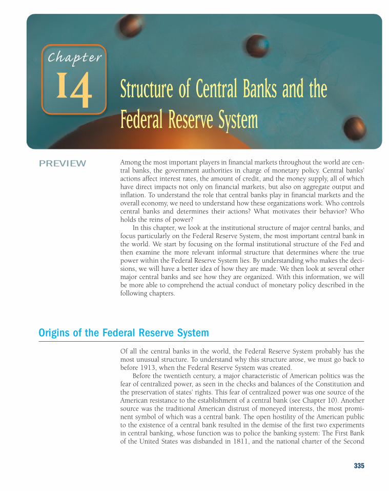
PREVIEW Among the most important players in financial markets throughout the world are cen-tral banks, the government authorities in charge of monetary policy. Central banks’actions affect interest rates, the amount of credit, and the money supply, all of whichhave direct impacts not only on financial markets, but also on aggregate output andinflation. To understand the role that central banks play in financial markets and theoverall economy, we need to understand how these organizations work. Who controlscentral banks and determines their actions? What motivates their behavior? Whoholds the reins of power?

In this chapter, we look at the institutional structure of major central banks, andfocus particularly on the Federal Reserve System, the most important central bank inthe world. We start by focusing on the formal institutional structure of the Fed andthen examine the more relevant informal structure that determines where the truepower within the Federal Reserve System lies. By understanding who makes the deci-sions, we will have a better idea of how they are made. We then look at several othermajor central banks and see how they are organized. With this information, we willbe more able to comprehend the actual conduct of monetary policy described in thefollowing chapters.

Origins of the Federal Reserve System

Of all the central banks in the world, the Federal Reserve System probably has themost unusual structure. To understand why this structure arose, we must go back tobefore 1913, when the Federal Reserve System was created.

Before the twentieth century, a major characteristic of American politics was thefear of centralized power, as seen in the checks and balances of the Constitution andthe preservation of states’ rights. This fear of centralized power was one source of theAmerican resistance to the establishment of a central bank (see Chapter 10). Anothersource was the traditional American distrust of moneyed interests, the most promi-nent symbol of which was a central bank. The open hostility of the American publicto the existence of a central bank resulted in the demise of the first two experimentsin central banking, whose function was to police the banking system: The First Bankof the United States was disbanded in 1811, and the national charter of the Second

335

Ch a p te r

Structure of Central Banks and theFederal Reserve System

14

Bank of the United States expired in 1836 after its renewal was vetoed in 1832 byPresident Andrew Jackson.

The termination of the Second Bank’s national charter in 1836 created a severe prob-lem for American financial markets, because there was no lender of last resort who couldprovide reserves to the banking system to avert a bank panic. Hence in the nineteenthand early twentieth centuries, nationwide bank panics became a regular event, occurringevery twenty years or so, culminating in the panic of 1907. The 1907 panic resulted insuch widespread bank failures and such substantial losses to depositors that the publicwas finally convinced that a central bank was needed to prevent future panics.

The hostility of the American public to banks and centralized authority createdgreat opposition to the establishment of a single central bank like the Bank ofEngland. Fear was rampant that the moneyed interests on Wall Street (including thelargest corporations and banks) would be able to manipulate such an institution togain control over the economy and that federal operation of the central bank mightresult in too much government intervention in the affairs of private banks. Seriousdisagreements existed over whether the central bank should be a private bank or agovernment institution. Because of the heated debates on these issues, a compromisewas struck. In the great American tradition, Congress wrote an elaborate system ofchecks and balances into the Federal Reserve Act of 1913, which created the FederalReserve System with its 12 regional Federal Reserve banks (see Box 1).

Formal Structure of the Federal Reserve System

The formal structure of the Federal Reserve System was intended by writers of theFederal Reserve Act to diffuse power along regional lines, between the private sectorand the government, and among bankers, businesspeople, and the public. This initialdiffusion of power has resulted in the evolution of the Federal Reserve System to

336 P A R T I V Central Banking and the Conduct of Monetary Policy

The history of the United States has been one of pub-lic hostility to banks and especially to a central bank.How were the politicians who founded the FederalReserve able to design a system that has become oneof the most prestigious institutions in the UnitedStates?

The answer is that the founders recognized that ifpower was too concentrated in either Washington orNew York, cities that Americans often love to hate, anAmerican central bank might not have enough pub-lic support to operate effectively. They thus decidedto set up a decentralized system with 12 FederalReserve banks spread throughout the country to

make sure that all regions of the country were rep-resented in monetary policy deliberations. In addition,they made the Federal Reserve banks quasi-privateinstitutions overseen by directors from the privatesector living in that district who represent views fromthat region and are in close contact with the presi-dent of the Federal Reserve bank. The unusualstructure of the Federal Reserve System has promoteda concern in the Fed with regional issues as is evidentin Federal Reserve bank publications. Without thisunusual structure, the Federal Reserve Systemmight have been far less popular with the public,making the institution far less effective.

The Political Genius of the Founders of the Federal Reserve System

Box 1: Inside the Fed

include the following entities: the Federal Reserve banks, the Board of Governorsof the Federal Reserve System, the Federal Open Market Committee (FOMC),the Federal Advisory Council, and around 4,800 member commercial banks. Figure 1outlines the relationships of these entities to one another and to the three policy toolsof the Fed (open market operations, the discount rate, and reserve requirements) dis-cussed in Chapters 15 to 17.

Each of the 12 Federal Reserve districts has one main Federal Reserve bank, whichmay have branches in other cities in the district. The locations of these districts, theFederal Reserve banks, and their branches are shown in Figure 2. The three largest

Federal ReserveBanks

C H A P T E R 1 4 Structure of Central Banks and the Federal Reserve System 337

F I G U R E 1 Formal Structure and Allocation of Policy Tools in the Federal Reserve

Twelve Federal ReserveBanks (FRBs)

Each with nine directors who appoint president and other officers ofthe FRB

Open marketoperations

Board of Governors

Seven members appointedby the president of the United States and confirmed by the Senate

Pol

icy

Too

lsF

eder

alR

eser

ve S

yste

m

Reviews anddetermines

Appoints threedirectors to each FRB

Elect sixdirectors toeach FRB

Federal Advisory Council

Twelve members (bankers)

Discountrate

Reserverequirements

Select

Sets (withinlimits)

Directs

Establish

Federal Open MarketCommittee (FOMC)

Seven members of Boardof Governors pluspresidents of FRB of NewYork and four other FRBs

Around 4,800member commercialbanks

www.federalreserve.gov/pubs/frseries/frseri.htm

Information on the structure ofthe Federal Reserve System.

Federal Reserve banks in terms of assets are those of New York, Chicago, and SanFrancisco—combined they hold over 50% of the assets (discount loans, securities, andother holdings) of the Federal Reserve System. The New York bank, with around one-quarter of the assets, is the most important of the Federal Reserve banks (see Box 2).

Each of the Federal Reserve banks is a quasi-public (part private, part govern-ment) institution owned by the private commercial banks in the district that aremembers of the Federal Reserve System. These member banks have purchased stockin their district Federal Reserve bank (a requirement of membership), and the divi-dends paid by that stock are limited by law to 6% annually. The member banks electsix directors for each district bank; three more are appointed by the Board ofGovernors. Together, these nine directors appoint the president of the bank (subjectto the approval of the Board of Governors).

The directors of a district bank are classified into three categories, A, B, and C:The three A directors (elected by the member banks) are professional bankers, andthe three B directors (also elected by the member banks) are prominent leaders fromindustry, labor, agriculture, or the consumer sector. The three C directors, who areappointed by the Board of Governors to represent the public interest, are not allowedto be officers, employees, or stockholders of banks. This design for choosing directorswas intended by the framers of the Federal Reserve Act to ensure that the directors ofeach Federal Reserve bank would reflect all constituencies of the American public.


F I G U R E 2 Federal Reserve System

Source: Federal Reserve Bulletin.

Miami

124

10

9

11

6

5

3

1

2

7

8

Board of Governors of the FederalReserve SystemFederal Reserve bank cities

Boundaries of Federal Reserve districts(Alaska and Hawaii are in District 12)

Federal Reserve branch cities

Federal Reserve districts1

Seattle

Portland Helena

Dallas

Omaha

Kansas City

Jacksonville

Atlanta

New York

BostonBuffalo

Detroit

Salt LakeCity

Los Angeles

El Paso

Oklahoma City

Minneapolis

Chicago

St. Louis

Memphis

Little Rock

Houston

New Orleans

Birmingham

Nashville

Louisville

Richmond

WASHINGTONBaltimore

Philadelphia

Denver

San Francisco

San Antonio

Charlotte

CulpeperCulpeperCulpeperCulpeperCulpeperCulpeperCulpeperCulpeper

PittsburghPittsburghPittsburghPittsburgh

ClevelandClevelandClevelandClevelandCleveland

CincinnatiCincinnatiCincinnatiCincinnati

BirmingBirmingBirmingBirmingham

www.federalreserve.gov/otherfrb.htm

Addresses and phone numbersof Federal Reserve banks,

branches, and RCPCs and linksto the main pages of the 12reserve banks and Board of

Governors.

The 12 Federal Reserve banks perform the following functions:

• Clear checks• Issue new currency• Withdraw damaged currency from circulation• Administer and make discount loans to banks in their districts• Evaluate proposed mergers and applications for banks to expand their activities• Act as liaisons between the business community and the Federal Reserve System• Examine bank holding companies and state-chartered member banks• Collect data on local business conditions• Use their staffs of professional economists to research topics related to the con-

duct of monetary policy


The Federal Reserve Bank of New York plays a spe-cial role in the Federal Reserve System for several rea-sons. First, its district contains many of the largestcommercial banks in the United States, the safety andsoundness of which are paramount to the health ofthe U.S. financial system. The Federal Reserve Bankof New York conducts examinations of bank holdingcompanies and state-chartered banks in its district,making it the supervisor of some of the most impor-tant financial institutions in our financial system. Notsurprisingly, given this responsibility, the bank super-vision group is one of the largest units of the NewYork Fed and is by far the largest bank supervisiongroup in the Federal Reserve System.

The second reason for the New York Fed’s specialrole is its active involvement in the bond and for-eign exchange markets. The New York Fed housesthe open market desk, which conducts open marketoperations—the purchase and sale of bonds—thatdetermine the amount of reserves in the bankingsystem. Because of this involvement in the Treasurysecurities market, as well as its walking-distancelocation near the New York and American StockExchanges, the officials at the Federal Reserve Bankof New York are in constant contact with the majordomestic financial markets in the United States. Inaddition, the Federal Reserve Bank of New York alsohouses the foreign exchange desk, which conductsforeign exchange interventions on behalf of theFederal Reserve System and the U.S. Treasury. Its

involvement in these financial markets means thatthe New York Fed is an important source of infor-mation on what is happening in domestic and for-eign financial markets, particularly during crisisperiods, as well as a liaison between officials in theFederal Reserve System and private participants inthe markets.

The third reason for the Federal Reserve Bank ofNew York’s prominence is that it is the only FederalReserve bank to be a member of the Bank forInternational Settlements (BIS). Thus the president ofthe New York Fed, along with the chairman of theBoard of Governors, represents the Federal ReserveSystem in its regular monthly meetings with othermajor central bankers at the BIS. This close contactwith foreign central bankers and interaction with for-eign exchange markets means that the New York Fedhas a special role in international relations, both withother central bankers and with private market partic-ipants. Adding to its prominence in international cir-cles is that the New York Fed is the repository for over$100 billion of the world’s gold, an amount greaterthan the gold at Fort Knox.

Finally, the president of the Federal Reserve Bankof New York is the only permanent member of theFOMC among the Federal Reserve bank presidents,serving as the vice-chairman of the committee. Thushe and the chairman and vice-chairman of the Boardof Governors are the three most important officials inthe Federal Reserve System.

The Special Role of the Federal Reserve Bank of New York


The 12 Federal Reserve banks are involved in monetary policy in several ways:

1. Their directors “establish” the discount rate (although the discount rate in eachdistrict is reviewed and determined by the Board of Governors).

2. They decide which banks, member and nonmember alike, can obtain discountloans from the Federal Reserve bank.

3. Their directors select one commercial banker from each bank’s district to serve onthe Federal Advisory Council, which consults with the Board of Governors andprovides information that helps in the conduct of monetary policy.

4. Five of the 12 bank presidents each have a vote in the Federal Open MarketCommittee, which directs open market operations (the purchase and sale ofgovernment securities that affect both interest rates and the amount of reserves inthe banking system). As explained in Box 2, the president of the New York Fedalways has a vote in the FOMC, making it the most important of the banks; theother four votes allocated to the district banks rotate annually among the remain-ing 11 presidents.

All national banks (commercial banks chartered by the Office of the Comptroller of theCurrency) are required to be members of the Federal Reserve System. Commercialbanks chartered by the states are not required to be members, but they can choose tojoin. Currently, around one-third of the commercial banks in the United States aremembers of the Federal Reserve System, having declined from a peak figure of 49%in 1947.

Before 1980, only member banks were required to keep reserves as deposits atthe Federal Reserve banks. Nonmember banks were subject to reserve requirementsdetermined by their states, which typically allowed them to hold much of theirreserves in interest-bearing securities. Because no interest is paid on reservesdeposited at the Federal Reserve banks, it was costly to be a member of the system,and as interest rates rose, the relative cost of membership rose, and more and morebanks left the system.

This decline in Fed membership was a major concern of the Board of Governors(one reason was that it lessened the Fed’s control over the money supply, making itmore difficult for the Fed to conduct monetary policy). The chairman of the Board ofGovernors repeatedly called for new legislation requiring all commercial banks to bemembers of the Federal Reserve System. One result of the Fed’s pressure on Congresswas a provision in the Depository Institutions Deregulation and Monetary Control Actof 1980: All depository institutions became subject (by 1987) to the same require-ments to keep deposits at the Fed, so member and nonmember banks would be onan equal footing in terms of reserve requirements. In addition, all depository institu-tions were given access to the Federal Reserve facilities, such as the discount window(discussed in Chapter 17) and Fed check clearing, on an equal basis. These provisionsended the decline in Fed membership and reduced the distinction between memberand nonmember banks.

At the head of the Federal Reserve System is the seven-member Board of Governors,headquartered in Washington, D.C. Each governor is appointed by the president ofthe United States and confirmed by the Senate. To limit the president’s control overthe Fed and insulate the Fed from other political pressures, the governors serve one

Board ofGovernors of theFederal ReserveSystem

Member Banks


nonrenewable 14-year term, with one governor’s term expiring every other January.1

The governors (many are professional economists) are required to come from differ-ent Federal Reserve districts to prevent the interests of one region of the country frombeing overrepresented. The chairman of the Board of Governors is chosen fromamong the seven governors and serves a four-year term. It is expected that once a newchairman is chosen, the old chairman resigns from the Board of Governors, even ifthere are many years left to his or her term as a governor.

The Board of Governors is actively involved in decisions concerning the conductof monetary policy. All seven governors are members of the FOMC and vote on theconduct of open market operations. Because there are only 12 voting members on thiscommittee (seven governors and five presidents of the district banks), the Board hasthe majority of the votes. The Board also sets reserve requirements (within limitsimposed by legislation) and effectively controls the discount rate by the “review anddetermination” process, whereby it approves or disapproves the discount rate “estab-lished” by the Federal Reserve banks. The chairman of the Board advises the presidentof the United States on economic policy, testifies in Congress, and speaks for theFederal Reserve System to the media. The chairman and other governors may alsorepresent the United States in negotiations with foreign governments on economicmatters. The Board has a staff of professional economists (larger than those of indi-vidual Federal Reserve banks), which provides economic analysis that the board usesin making its decisions. (Box 3 discusses the role of the research staff.)

Through legislation, the Board of Governors has often been given duties notdirectly related to the conduct of monetary policy. In the past, for example, the Boardset the maximum interest rates payable on certain types of deposits under RegulationQ. (After 1986, ceilings on time deposits were eliminated, but there is still a restric-tion on paying any interest on business demand deposits.) Under the Credit ControlAct of 1969 (which expired in 1982), the Board had the ability to regulate and con-trol credit once the president of the United States approved. The Board of Governorsalso sets margin requirements, the fraction of the purchase price of securities that hasto be paid for with cash rather than borrowed funds. It also sets the salary of the pres-ident and all officers of each Federal Reserve bank and reviews each bank’s budget.Finally, the Board has substantial bank regulatory functions: It approves bank merg-ers and applications for new activities, specifies the permissible activities of bankholding companies, and supervises the activities of foreign banks in the United States.

The FOMC usually meets eight times a year (about every six weeks) and makes deci-sions regarding the conduct of open market operations, which influence the mone-tary base. Indeed, the FOMC is often referred to as the “Fed” in the press: for example,when the media say that the Fed is meeting, they actually mean that the FOMC ismeeting. The committee consists of the seven members of the Board of Governors, thepresident of the Federal Reserve Bank of New York, and the presidents of four otherFederal Reserve banks. The chairman of the Board of Governors also presides as thechairman of the FOMC. Even though only the presidents of five of the Federal Reserve

Federal OpenMarketCommittee(FOMC)


1Although technically the governor’s term is nonrenewable, a governor can resign just before the term expiresand then be reappointed by the president. This explains how one governor, William McChesney Martin Jr.,served for 28 years. Since Martin, the chairman from 1951 to 1970, retired from the board in 1970, the practiceof extending a governor’s term beyond 14 years has become a rarity.

www.federalreserve.gov/bios/1199member.pdf

Lists all the members of theBoard of Governors of theFederal Reserve since its

inception.

banks are voting members of the FOMC, the other seven presidents of the districtbanks attend FOMC meetings and participate in discussions. Hence they have someinput into the committee’s decisions.

Because open market operations are the most important policy tool that the Fedhas for controlling the money supply, the FOMC is necessarily the focal point for pol-icymaking in the Federal Reserve System. Although reserve requirements and the dis-count rate are not actually set by the FOMC, decisions in regard to these policy tools


The Federal Reserve System is the largest employer ofeconomists not just in the United States, but in theworld. The system’s research staff has around 1,000people, about half of whom are economists. Of these500 economists, 250 are at the Board of Governors,100 are at the Federal Reserve Bank of New York, andthe remainder are at the other Federal Reserve banks.What do all these economists do?

The most important task of the Fed’s economists isto follow the incoming data from government agen-cies and private sector organizations on the economyand provide guidance to the policymakers on wherethe economy may be heading and what the impact ofmonetary policy actions on the economy might be.Before each FOMC meeting, the research staff at eachFederal Reserve bank briefs its president and the sen-ior management of the bank on its forecast for theU.S. economy and the issues that are likely to be dis-cussed at the meeting. The research staff also providesbriefing materials or a formal briefing on the eco-nomic outlook for the bank’s region, something thateach president discusses at the FOMC meeting.Meanwhile, at the Board of Governors, economistsmaintain a large econometric model (a model whoseequations are estimated with statistical procedures)that helps them produce their forecasts of thenational economy, and they too brief the governorson the national economic outlook.

The research staffers at the banks and the boardalso provide support for the bank supervisory staff,tracking developments in the banking sector andother financial markets and institutions and provid-ing bank examiners with technical advice that theymight need in the course of their examinations.Because the Board of Governors has to decide on

whether to approve bank mergers, the research staffat both the board and the bank in whose district themerger is to take place prepare information on whateffect the proposed merger might have on the com-petitive environment. To assure compliance with theCommunity Reinvestment Act, economists also ana-lyze a bank’s performance in its lending activities indifferent communities.

Because of the increased influence of develop-ments in foreign countries on the U.S. economy, themembers of the research staff, particularly at the NewYork Fed and the Board, produce reports on themajor foreign economies. They also conduct researchon developments in the foreign exchange marketbecause of its growing importance in the monetarypolicy process and to support the activities of the for-eign exchange desk. Economists also help supportthe operation of the open market desk by projectingreserve growth and the growth of the monetaryaggregates.

Staff economists also engage in basic research onthe effects of monetary policy on output and infla-tion, developments in the labor markets, interna-tional trade, international capital markets, bankingand other financial institutions, financial markets,and the regional economy, among other topics. Thisresearch is published widely in academic journalsand in Reserve bank publications. (Federal Reservebank reviews are a good source of supplementalmaterial for money and banking students.)

Another important activity of the research staff pri-marily at the Reserve banks is in the public educationarea. Staff economists are called on frequently to makepresentations to the board of directors at their banksor to make speeches to the public in their district.

The Role of the Research Staff


www.federalreserve.gov/fomc

Find general information on theFOMC, its schedule of meetings,

statements, minutes, andtranscripts; information on its

members, and the “beige book.”

are effectively made there. The FOMC does not actually carry out securities purchasesor sales. Rather it issues directives to the trading desk at the Federal Reserve Bank ofNew York, where the manager for domestic open market operations supervises aroomful of people who execute the purchases and sales of the government or agencysecurities. The manager communicates daily with the FOMC members and their staffsconcerning the activities of the trading desk.

The FOMC meeting takes place in the boardroom on the second floor of the mainbuilding of the Board of Governors in Washington. The seven governors and the 12Reserve Bank presidents, along with the secretary of the FOMC, the Board’s directorof the Research and Statistics Division and his deputy, and the directors of theMonetary Affairs and International Finance Divisions, sit around a massive conferencetable. Although only five of the Reserve Bank presidents have voting rights on theFOMC at any given time, all actively participate in the deliberations. Seated aroundthe sides of the room are the directors of research at each of the Reserve banks andother senior board and Reserve Bank officials, who, by tradition, do not speak at themeeting.

Except for the meetings prior to the February and July testimony by the chairmanof the Board of Governors before Congress, the meeting starts on Tuesday at 9:00 A.M.sharp with a quick approval of the minutes of the previous meeting of the FOMC. Thefirst substantive agenda item is the report by the manager of system open marketoperations on foreign currency and domestic open market operations and other issuesrelated to these topics. After the governors and Reserve Bank presidents finish askingquestions and discussing these reports, a vote is taken to ratify them.

The next stage in the meeting is a presentation of the Board staff’s national eco-nomic forecast, referred to as the “green book” forecast (see Box 4), by the director ofthe Research and Statistics Division at the board. After the governors and ReserveBank presidents have queried the division director about the forecast, the so-called go-round occurs: Each bank president presents an overview of economic conditions in hisor her district and the bank’s assessment of the national outlook, and each governor,except for the chairman, gives a view of the national outlook. By tradition, remarksavoid the topic of monetary policy at this time.

After a coffee break, everyone returns to the boardroom and the agenda turns tocurrent monetary policy and the domestic policy directive. The Board’s director of theMonetary Affairs Division then leads off the discussion by outlining the different sce-narios for monetary policy actions outlined in the blue book (see Box 4) and maydescribe an issue relating to how monetary policy should be conducted. After a question-and-answer period, the chairman (currently Alan Greenspan) sets the stage for the fol-lowing discussion by presenting his views on the state of the economy and thentypically makes a recommendation for what monetary policy action should be taken.Then each of the FOMC members as well as the nonvoting bank presidents expresseshis or her views on monetary policy, and the chairman summarizes the discussion andproposes specific wording for the directive on the federal funds rate target transmit-ted to the open market desk. The secretary of the FOMC formally reads the proposedstatement, and the members of the FOMC vote.2

The FOMCMeeting


2The decisions expressed in the directive may not be unanimous, and the dissenting views are made public.However, except in rare cases, the chairman’s vote is always on the winning side.

Then there is an informal buffet lunch, and while eating, the participants hear apresentation on the latest developments in Congress on banking legislation and otherlegislation relevant to the Federal Reserve. Around 2:15 P.M., the meeting breaks upand a public announcement is made about the outcome of the meeting: whether thetarget federal funds rate and discount rate have been raised, lowered, or leftunchanged, and an assessment of the “balance of risks” in the future, whether towardhigher inflation or toward a weaker economy.3 The postmeeting announcement is aninnovation initiated in 1994. Before then, no such announcement was made, and themarkets had to guess what policy action was taken. The decision to announce thisinformation was a step in the direction of greater openness by the Fed.

Informal Structure of the Federal Reserve System

The Federal Reserve Act and other legislation give us some idea of the formal struc-ture of the Federal Reserve System and who makes decisions at the Fed. What is writ-ten in black and white, however, does not necessarily reflect the reality of the powerand decision-making structure.

As envisioned in 1913, the Federal Reserve System was to be a highly decentral-ized system designed to function as 12 separate, cooperating central banks. In theoriginal plan, the Fed was not responsible for the health of the economy through itscontrol of the money supply and its ability to affect interest rates. Over time, it has


3The meetings before the February and July chairman’s testimony before Congress, in which the Monetary Reportto Congress is presented, have a somewhat different format. Rather than start Tuesday morning at 9:00 A.M. likethe other meetings, they start in the afternoon on Tuesday and go over to Wednesday, with the usual announce-ment around 2:15 P.M. These longer meetings consider the longer-term economic outlook as well as the currentconduct of open market operations.

What Do These Colors Mean at the Fed? Threeresearch documents play an important role in themonetary policy process and at Federal Open MarketCommittee meetings. The national forecast for thenext two years, generated by the Federal ReserveBoard of Governors’ Research and Statistics Division,is placed between green covers and is thus known asthe “green book.” It is provided to all who attend theFOMC meeting. The “blue book,” in blue covers, alsoprovided to all participants at the FOMC meeting,contains the projections for the monetary aggregates

prepared by the Monetary Affairs Division at theBoard of Governors and typically also presents threealternative scenarios for the stance of monetary pol-icy (labeled A, B, and C). The “beige book,” withbeige covers, is produced by the Reserve banks anddetails evidence gleaned either from surveys orfrom talks with key businesses and financial institu-tions on the state of the economy in each of theFederal Reserve districts. This is the only one of thethree books that is distributed publicly, and it oftenreceives a lot of attention in the press.

Green, Blue, and Beige


acquired the responsibility for promoting a stable economy, and this responsibility hascaused the Federal Reserve System to evolve slowly into a more unified central bank.

The framers of the Federal Reserve Act of 1913 intended the Fed to have only onebasic tool of monetary policy: the control of discount loans to member banks. The useof open market operations as a tool for monetary control was not yet well understood,and reserve requirements were fixed by the Federal Reserve Act. The discount toolwas to be controlled by the joint decision of the Federal Reserve banks and theFederal Reserve Board (which later became the Board of Governors), so that bothwould share equally in the determination of monetary policy. However, the Board’sability to “review and determine” the discount rate effectively allowed it to dominatethe district banks in setting this policy.

Banking legislation during the Great Depression years centralized power withinthe newly created Board of Governors by giving it effective control over the remain-ing two tools of monetary policy, open market operations and changes in reserverequirements. The Banking Act of 1933 granted the FOMC authority to determineopen market operations, and the Banking Act of 1935 gave the Board the majority ofvotes in the FOMC. The Banking Act of 1935 also gave the Board authority to changereserve requirements.

Since the 1930s, then, the Board of Governors has acquired the reins of controlover the tools for conducting monetary policy. In recent years, the power of the Boardhas become even greater. Although the directors of a Federal Reserve bank choose itspresident with the approval of the Board, the Board sometimes suggests a choice(often a professional economist) for president of a Federal Reserve bank to the direc-tors of the bank, who then often follow the Board’s suggestions. Since the Board setsthe salary of the bank’s president and reviews the budget of each Federal Reservebank, it has further influence over the district banks’ activities.

If the Board of Governors has so much power, what power do the FederalAdvisory Council and the “owners” of the Federal Reserve banks—the memberbanks—actually have within the Federal Reserve System? The answer is almost none.Although member banks own stock in the Federal Reserve banks, they have none ofthe usual benefits of ownership. First, they have no claim on the earnings of the Fedand get paid only a 6% annual dividend, regardless of how much the Fed earns.Second, they have no say over how their property is used by the Federal ReserveSystem, in contrast to stockholders of private corporations. Third, usually only a sin-gle candidate for each of the six A and B directorships is “elected” by the memberbanks, and this candidate is frequently suggested by the president of the FederalReserve bank (who, in turn, is approved by the Board of Governors). The net resultis that member banks are essentially frozen out of the political process at the Fed andhave little effective power. Fourth, as its name implies, the Federal Advisory Councilhas only an advisory capacity and has no authority over Federal Reserve policymak-ing. Although the member bank “owners” do not have the usual power associatedwith being a stockholder, they do play an important, but subtle, role in the FederalReserve System (see Box 5).

A fair characterization of the Federal Reserve System as it has evolved is that itfunctions as a central bank, headquartered in Washington, D.C., with branches in 12cities. Because all aspects of the Federal Reserve System are essentially controlled bythe Board of Governors, who controls the Board? Although the chairman of the Boardof Governors does not have legal authority to exercise control over this body, he effec-tively does so through his ability to act as spokesperson for the Fed and negotiate with


Congress and the president of the United States. He also exercises control by settingthe agenda of Board and FOMC meetings. For example, the fact that the agenda at theFOMC has the chairman speak first about monetary policy enables him to havegreater influence over what the policy action will be. The chairman also influences theBoard through the force of stature and personality. Chairmen of the Board ofGovernors (including Marriner S. Eccles, William McChesney Martin Jr., ArthurBurns, Paul A. Volcker, and Alan Greenspan) have typically had strong personalitiesand have wielded great power.

The chairman also exercises power by supervising the Board’s staff of professionaleconomists and advisers. Because the staff gathers information for the Board and con-ducts the analyses that the Board uses in its decisions, it also has some influence overmonetary policy. In addition, in the past, several appointments to the Board itself havecome from within the ranks of its professional staff, making the chairman’s influenceeven farther-reaching and longer-lasting than a four-year term.

The informal power structure of the Fed, in which power is centralized in thechairman of the Board of Governors, is summarized in Figure 3.

How Independent Is the Fed?

When we look, in the next four chapters, at how the Federal Reserve conducts mon-etary policy, we will want to know why it decides to take certain policy actions butnot others. To understand its actions, we must understand the incentives that moti-vate the Fed’s behavior. How free is the Fed from presidential and congressional pres-sures? Do economic, bureaucratic, or political considerations guide it? Is the Fed trulyindependent of outside pressures?


Although the member bank stockholders in eachFederal Reserve bank have little direct power in theFederal Reserve System, they do play an importantrole. Their six representatives on the board of direc-tors of each bank have a major oversight function.Along with the three public interest directors, theyoversee the audit process for the Federal Reservebank, making sure it is being run properly, and alsoshare their management expertise with the seniormanagement of the bank. Because they vote on rec-ommendations by each bank to raise, lower, or main-tain the discount rate at its current level, they engagein discussions about monetary policy and transmittheir private sector views to the president and seniormanagement of the bank. They also get to understand

the inner workings of the Federal Reserve banks andthe system so that they can help explain the positionof the Federal Reserve to their contacts in the privateand political sectors. Advisory councils like theFederal Advisory Council and others that are often setup by the district banks—for example, the SmallBusiness and Agriculture Advisory Council and theThrift Advisory Council at the New York Fed—are aconduit for the private sector to express views on boththe economy and the state of the banking system.

So even though the owners of the Reserve banksdo not have the usual voting rights, they are impor-tant to the Federal Reserve System, because theymake sure it does not get out of touch with the needsand opinions of the private sector.

The Role of Member Banks in the Federal Reserve System


Stanley Fischer, who was a professor at MIT and then the Deputy ManagingDirector of the International Monetary Fund, has defined two different types of inde-pendence of central banks: instrument independence, the ability of the central bankto set monetary policy instruments, and goal independence, the ability of the centralbank to set the goals of monetary policy. The Federal Reserve has both types of inde-pendence and is remarkably free of the political pressures that influence other gov-ernment agencies. Not only are the members of the Board of Governors appointed fora 14-year term (and so cannot be ousted from office), but also the term is technicallynot renewable, eliminating some of the incentive for the governors to curry favor withthe president and Congress.

Probably even more important to its independence from the whims of Congress isthe Fed’s independent and substantial source of revenue from its holdings of securities


F I G U R E 3 Informal Power Structure of the Federal Reserve System

Six othermembers ofthe Boardof Governors

Discountrate

Reserverequirements

Boardstaff

Federal OpenMarketCommittee( FOMC )

Advises

Advises

CHAIRMAN OF THE BOARD OF GOVERNORS

Advises Five FederalReserve bankpresidents

Vote

Vote

Sets agenda Supervises Votes andsets agenda

Set ( within limits ) Set

Directs

Open marketoperations

and, to a lesser extent, from its loans to banks. In recent years, for example, the Fedhas had net earnings after expenses of around $28 billion per year—not a bad livingif you can find it! Because it returns the bulk of these earnings to the Treasury, it doesnot get rich from its activities, but this income gives the Fed an important advantageover other government agencies: It is not subject to the appropriations process usu-ally controlled by Congress. Indeed, the General Accounting Office, the auditingagency of the federal government, cannot audit the monetary policy or foreignexchange market functions of the Federal Reserve. Because the power to control thepurse strings is usually synonymous with the power of overall control, this feature of theFederal Reserve System contributes to its independence more than any other factor.

Yet the Federal Reserve is still subject to the influence of Congress, because the leg-islation that structures it is written by Congress and is subject to change at any time.When legislators are upset with the Fed’s conduct of monetary policy, they frequentlythreaten to take control of the Fed’s finances and force it to submit a budget requestlike other government agencies. A recent example was the call by Senators Dorgan andReid in 1996 for Congress to have budgetary authority over the nonmonetary activi-ties of the Federal Reserve. This is a powerful club to wield, and it certainly has someeffect in keeping the Fed from straying too far from congressional wishes.

Congress has also passed legislation to make the Federal Reserve more account-able for its actions. In 1975, Congress passed House Concurrent Resolution 133,which requires the Fed to announce its objectives for the growth rates of the mone-tary aggregates. In the Full Employment and Balanced Growth Act of 1978 (theHumphrey-Hawkins Act), the Fed is required to explain how these objectives are con-sistent with the economic plans of the president of the United States.

The president can also influence the Federal Reserve. Because congressional leg-islation can affect the Fed directly or affect its ability to conduct monetary policy, thepresident can be a powerful ally through his influence on Congress. Second, althoughostensibly a president might be able to appoint only one or two members to the Boardof Governors during each presidential term, in actual practice the president appointsmembers far more often. One reason is that most governors do not serve out a full14-year term. (Governors’ salaries are substantially below what they can earn in theprivate sector, thus providing an incentive for them to take private sector jobs beforetheir term expires.) In addition, the president is able to appoint a new chairman ofthe Board of Governors every four years, and a chairman who is not reappointed isexpected to resign from the board so that a new member can be appointed.

The power that the president enjoys through his appointments to the Board ofGovernors is limited, however. Because the term of the chairman is not necessarilyconcurrent with that of the president, a president may have to deal with a chairmanof the Board of Governors appointed by a previous administration. Alan Greenspan,for example, was appointed chairman in 1987 by President Ronald Reagan and wasreappointed to another term by another Republican president, George Bush. WhenBill Clinton, a Democrat, became president in 1993, Greenspan had several years leftto his term. Clinton was put under tremendous pressure to reappoint Greenspanwhen his term expired and did so in 1996 and again in 2000, even though Greenspanis a Republican.4


4Similarly, William McChesney Martin, Jr., the chairman from 1951 to 1970, was appointed by President Truman(Dem.) but was reappointed by Presidents Eisenhower (Rep.), Kennedy (Dem.), Johnson (Dem.), and Nixon(Rep.). Also Paul Volcker, the chairman from 1979 to 1987, was appointed by President Carter (Dem.) but wasreappointed by President Reagan (Rep.).

You can see that the Federal Reserve has extraordinary independence for a gov-ernment agency and is one of the most independent central banks in the world.Nonetheless, the Fed is not free from political pressures. Indeed, to understand theFed’s behavior, we must recognize that public support for the actions of the FederalReserve plays a very important role.5

Structure and Independence of Foreign Central Banks

In contrast to the Federal Reserve System, which is decentralized into 12 privatelyowned district banks, central banks in other industrialized countries consist of onecentralized unit that is owned by the government. Here we examine the structure anddegree of independence of four of the most important foreign central banks: the Bankof Canada, the Bank of England, the Bank of Japan, and the European Central Bank.

Canada was late in establishing a central bank: The Bank of Canada was founded in1934. Its directors are appointed by the government to three-year terms, and theyappoint the governor, who has a seven-year term. A governing council, consisting ofthe four deputy governors and the governor, is the policymaking body comparable tothe FOMC that makes decisions about monetary policy.

The Bank Act was amended in 1967 to give the ultimate responsibility for mon-etary policy to the government. So on paper, the Bank of Canada is not as instrument-independent as the Federal Reserve. In practice, however, the Bank of Canada doesessentially control monetary policy. In the event of a disagreement between the bankand the government, the minister of finance can issue a directive that the bank mustfollow. However, because the directive must be in writing and specific and applicablefor a specified period, it is unlikely that such a directive would be issued, and nonehas been to date. The goal for monetary policy, a target for inflation, is set jointly bythe Bank of Canada and the government, so the Bank of Canada has less goal inde-pendence than the Fed.

Founded in 1694, the Bank of England is one of the oldest central banks. The BankAct of 1946 gave the government statutory authority over the Bank of England. TheCourt (equivalent to a board of directors) of the Bank of England is made up of thegovernor and two deputy governors, who are appointed for five-year terms, and 16non-executive directors, who are appointed for three-year terms.

Until 1997, the Bank of England was the least independent of the central banksexamined in this chapter because the decision to raise or lower interest rates residednot within the Bank of England but with the chancellor of the Exchequer (the equiv-alent of the U.S. secretary of the Treasury). All of this changed when the new Labourgovernment came to power in May 1997. At this time, the new chancellor of theExchequer, Gordon Brown, made a surprise announcement that the Bank of Englandwould henceforth have the power to set interest rates. However, the Bank was notgranted total instrument independence: The government can overrule the Bank and

Bank of England

Bank of Canada


5An inside view of how the Fed interacts with the public and the politicians can be found in Bob Woodward,Maestro: Greenspan’s Fed and the American Boom (New York: Simon and Schuster, 2000).

www.bank-banque-canada.ca/

The website for the Bank ofCanada.

www.bankofengland.co.ukLinks/setframe.html

The website for the Bank ofEngland.

set rates “in extreme economic circumstances” and “for a limited period.” Nonethe-less, as in Canada, because overruling the Bank would be so public and is supposedto occur only in highly unusual circumstances and for a limited time, it likely to be arare occurrence.

The decision to set interest rates resides in the Monetary Policy Committee, madeup of the governor, two deputy governors, two members appointed by the governorafter consultation with the chancellor (normally central bank officials), plus four out-side economic experts appointed by the chancellor. (Surprisingly, two of the four out-side experts initially appointed to this committee were not British citizens—one wasDutch and the other American, although both were residents of the United Kingdom.)The inflation target for the Bank of England is set by the Chancellor of the Exchequer,so the Bank of England is also less goal-independent than the Fed.

The Bank of Japan (Nippon Ginko) was founded in 1882 during the Meiji Restora-tion. Monetary policy is determined by the Policy Board, which is composed of thegovernor; two vice governors; and six outside members appointed by the cabinet andapproved by the parliament, all of whom serve for five-year terms.

Until recently, the Bank of Japan was not formally independent of the govern-ment, with the ultimate power residing with the Ministry of Finance. However, thenew Bank of Japan Law, which took effect in April 1998 and was the first majorchange in the powers of the Bank of Japan in 55 years, has changed this. In additionto stipulating that the objective of monetary policy is to attain price stability, the lawgranted greater instrument and goal independence to the Bank of Japan. Before this,the government had two voting members on the Policy Board, one from the Ministryof Finance and the other from the Economic Planning Agency. Now the governmentmay send two representatives from these agencies to board meetings, but they nolonger have voting rights, although they do have the ability to request delays in mon-etary policy decisions. In addition, the Ministry of Finance lost its authority to over-see many of the operations of the Bank of Japan, particularly the right to dismisssenior officials. However, the Ministry of Finance continues to have control over thepart of the Bank’s budget that is unrelated to monetary policy, which might limit itsindependence to some extent.

The Maastricht Treaty established the European Central Bank (ECB) and the EuropeanSystem of Central Banks (ESCB), which began operation in January 1999. The struc-ture of the central bank is patterned after the U.S. Federal Reserve System in that cen-tral banks for each country have a role similar to that of the Federal Reserve banks.The executive board of the ECB is made up of the president, a vice president, and fourother members, who are appointed for eight-year terms. The monetary policymakingbody of the bank includes the six members of the executive board and the central-bank governors from each of the euro countries, all of whom must have five-yearterms at a minimum.

The European Central Bank will be the most independent in the world—evenmore independent than the German central bank, the Bundesbank, which, beforethe establishment of the ECB, was considered the world’s most independent centralbank, along with the Swiss National Bank. The ECB is both instrument- and goal-independent of both the European Union and the national governments and has com-plete control over monetary policy. In addition, the ECB’s mandated mission is the

European CentralBank

Bank of Japan


www.boj.or.jp/en/index.htm

The website for the Bank ofJapan.

www.ecb.int

The website for the EuropeanCentral Bank

pursuit of price stability. The ECB is far more independent than any other centralbank in the world because its charter cannot be changed by legislation: It can bechanged only by revision of the Maastricht Treaty, a difficult process, because all sig-natories to the treaty would have to agree.

As our survey of the structure and independence of the major central banks indicates,in recent years we have been seeing a remarkable trend toward increasing independ-ence. It used to be that the Federal Reserve was substantially more independent thanalmost all other central banks, with the exception of those in Germany andSwitzerland. Now the newly established European Central Bank is far more inde-pendent than the Fed, and greater independence has been granted to central bankslike the Bank of England and the Bank of Japan, putting them more on a par with theFed, as well as to central banks in such diverse countries as New Zealand, Sweden,and the euro nations. Both theory and experience suggest that more independent cen-tral banks produce better monetary policy, thus providing an impetus for this trend.

Explaining Central Bank Behavior

One view of government bureaucratic behavior is that bureaucracies serve the publicinterest (this is the public interest view) . Yet some economists have developed a theoryof bureaucratic behavior that suggests other factors that influence how bureaucraciesoperate. The theory of bureaucratic behavior suggests that the objective of a bureaucracyis to maximize its own welfare, just as a consumer’s behavior is motivated by the max-imization of personal welfare and a firm’s behavior is motivated by the maximizationof profits. The welfare of a bureaucracy is related to its power and prestige. Thus thistheory suggests that an important factor affecting a central bank’s behavior is itsattempt to increase its power and prestige.

What predictions does this view of a central bank like the Fed suggest? One isthat the Federal Reserve will fight vigorously to preserve its autonomy, a predictionverified time and time again as the Fed has continually counterattacked congressionalattempts to control its budget. In fact, it is extraordinary how effectively the Fed hasbeen able to mobilize a lobby of bankers and businesspeople to preserve its inde-pendence when threatened.

Another prediction is that the Federal Reserve will try to avoid conflict with pow-erful groups that might threaten to curtail its power and reduce its autonomy. TheFed’s behavior may take several forms. One possible factor explaining why the Fed issometimes slow to increase interest rates and so smooths out their fluctuations is thatit wishes to avoid a conflict with the president and Congress over increases in inter-est rates. The desire to avoid conflict with Congress and the president may alsoexplain why in the past the Fed was not at all transparent about its actions and is stillnot fully transparent (see Box 6).

The desire of the Fed to hold as much power as possible also explains why it vig-orously pursued a campaign to gain control over more banks. The campaign culmi-nated in legislation that expanded jurisdiction of the Fed’s reserve requirements to allbanks (not just the member commercial banks) by 1987.

The theory of bureaucratic behavior seems applicable to the Federal Reserve’sactions, but we must recognize that this view of the Fed as being solely concerned

The Trend TowardGreaterIndependence


with its own self-interest is too extreme. Maximizing one’s welfare does not rule outaltruism. (You might give generously to a charity because it makes you feel goodabout yourself, but in the process you are helping a worthy cause.) The Fed is surelyconcerned that it conduct monetary policy in the public interest. However, muchuncertainty and disagreement exist over what monetary policy should be.6 When it isunclear what is in the public interest, other motives may influence the Fed’s behavior.In these situations, the theory of bureaucratic behavior may be a useful guide to pre-dicting what motivates the Fed.

Should the Fed Be Independent?

As we have seen, the Federal Reserve is probably the most independent governmentagency in the United States. Every few years, the question arises in Congress whetherthe independence of the Fed should be curtailed. Politicians who strongly oppose aFed policy often want to bring it under their supervision in order to impose a policymore to their liking. Should the Fed be independent, or would we be better off witha central bank under the control of the president or Congress?

The strongest argument for an independent Federal Reserve rests on the view thatsubjecting the Fed to more political pressures would impart an inflationary bias tomonetary policy. In the view of many observers, politicians in a democratic society are

The Case forIndependence


As the theory of bureaucratic behavior predicts, theFed has incentives to hide its actions from the pub-lic and from politicians to avoid conflicts with them.In the past, this motivation led to a penchant forsecrecy in the Fed, about which one former Fed offi-cial remarked that “a lot of staffers would concedethat [secrecy] is designed to shield the Fed frompolitical oversight.”* For example, the Fed pursuedan active defense of delaying its release of FOMCdirectives to Congress and the public. However, aswe have seen, in 1994, it began to reveal the FOMCdirective immediately after each FOMC meeting. In

1999, it also began to immediately announce the“bias” toward which direction monetary policy waslikely to go, later expressed as the balance of risks inthe economy. In 2002, the Fed started to report theroll call vote on the federal funds rate target taken atthe FOMC meeting. Thus the Fed has increased itstransparency in recent years. Yet even today, the Fedis not fully transparent: it still does not release theminutes of the FOMC meetings until six weeks aftera meeting has taken place, and it does not publish itsforecasts of the economy as some other centralbanks do.

Federal Reserve Transparency


*Quoted in “Monetary Zeal: How the Federal Reserve Under Volcker Finally Slowed Down Inflation,” Wall Street Journal, December 7, 1984, p. 23.

6One example of the uncertainty over how best to conduct monetary policy was discussed in Chapter 3:Economists are not sure how to measure money. So even if economists agreed that controlling the quantity ofmoney is the appropriate way to conduct monetary policy (a controversial position, as we will see in later chap-ters), the Fed cannot be sure which monetary aggregate it should control.

shortsighted because they are driven by the need to win their next election. With thisas the primary goal, they are unlikely to focus on long-run objectives, such as pro-moting a stable price level. Instead, they will seek short-run solutions to problems,like high unemployment and high interest rates, even if the short-run solutions haveundesirable long-run consequences. For example, we saw in Chapter 5 that highmoney growth might lead initially to a drop in interest rates but might cause anincrease later as inflation heats up. Would a Federal Reserve under the control ofCongress or the president be more likely to pursue a policy of excessive moneygrowth when interest rates are high, even though it would eventually lead to inflationand even higher interest rates in the future? The advocates of an independent FederalReserve say yes. They believe that a politically insulated Fed is more likely to be con-cerned with long-run objectives and thus be a defender of a sound dollar and a sta-ble price level.

A variation on the preceding argument is that the political process in Americaleads to the so-called political business cycle, in which just before an election,expansionary policies are pursued to lower unemployment and interest rates. Afterthe election, the bad effects of these policies—high inflation and high interest rates—come home to roost, requiring contractionary policies that politicians hope the pub-lic will forget before the next election. There is some evidence that such a politicalbusiness cycle exists in the United States, and a Federal Reserve under the control ofCongress or the president might make the cycle even more pronounced.

Putting the Fed under the control of the president (making it more subject toinfluence by the Treasury) is also considered dangerous because the Fed can be usedto facilitate Treasury financing of large budget deficits by its purchases of Treasurybonds.7 Treasury pressure on the Fed to “help out” might lead to a more inflationarybias in the economy. An independent Fed is better able to resist this pressure from theTreasury.

Another argument for Fed independence is that control of monetary policy is tooimportant to leave to politicians, a group that has repeatedly demonstrated a lack ofexpertise at making hard decisions on issues of great economic importance, such asreducing the budget deficit or reforming the banking system. Another way to state thisargument is in terms of the principal–agent problem discussed in Chapters 8 and 11.Both the Federal Reserve and politicians are agents of the public (the principals), andas we have seen, both politicians and the Fed have incentives to act in their own inter-est rather than in the interest of the public. The argument supporting Federal Reserveindependence is that the principal–agent problem is worse for politicians than for theFed because politicians have fewer incentives to act in the public interest.

Indeed, some politicians may prefer to have an independent Fed, which can beused as a public “whipping boy” to take some of the heat off their backs. It is possiblethat a politician who in private opposes an inflationary monetary policy will be forcedto support such a policy in public for fear of not being reelected. An independent Fedcan pursue policies that are politically unpopular yet in the public interest.


7The Federal Reserve Act prohibited the Fed from buying Treasury bonds directly from the Treasury (except toroll over maturing securities); instead the Fed buys Treasury bonds on the open market. One possible reason forthis prohibition is consistent with the foregoing argument: The Fed would find it harder to facilitate Treasuryfinancing of large budget deficits.

Proponents of a Fed under the control of the president or Congress argue that it isundemocratic to have monetary policy (which affects almost everyone in the econ-omy) controlled by an elite group responsible to no one. The current lack of account-ability of the Federal Reserve has serious consequences: If the Fed performs badly,there is no provision for replacing members (as there is with politicians). True, theFed needs to pursue long-run objectives, but elected officials of Congress vote onlong-run issues also (foreign policy, for example). If we push the argument furtherthat policy is always performed better by elite groups like the Fed, we end up withsuch conclusions as the Joint Chiefs of Staff should determine military budgets or theIRS should set tax policies with no oversight from the president or Congress. Wouldyou advocate this degree of independence for the Joint Chiefs or the IRS?

The public holds the president and Congress responsible for the economic well-being of the country, yet they lack control over the government agency that may wellbe the most important factor in determining the health of the economy. In addition, toachieve a cohesive program that will promote economic stability, monetary policy mustbe coordinated with fiscal policy (management of government spending and taxation).Only by placing monetary policy under the control of the politicians who also controlfiscal policy can these two policies be prevented from working at cross-purposes.

Another argument against Federal Reserve independence is that an independentFed has not always used its freedom successfully. The Fed failed miserably in its statedrole as lender of last resort during the Great Depression, and its independence cer-tainly didn’t prevent it from pursuing an overly expansionary monetary policy in the1960s and 1970s that contributed to rapid inflation in this period.

Our earlier discussion also suggests that the Federal Reserve is not immune frompolitical pressures.8 Its independence may encourage it to pursue a course of narrowself-interest rather than the public interest.

There is yet no consensus on whether Federal Reserve independence is a goodthing, although public support for independence of the central bank seems to havebeen growing in both the United States and abroad. As you might expect, people wholike the Fed’s policies are more likely to support its independence, while those whodislike its policies advocate a less independent Fed.

We have seen that advocates of an independent central bank believe that macroeco-nomic performance will be improved by making the central bank more independent.Recent research seems to support this conjecture: When central banks are rankedfrom least independent to most independent, inflation performance is found to be thebest for countries with the most independent central banks.9 Although a more inde-pendent central bank appears to lead to a lower inflation rate, this is not achieved atthe expense of poorer real economic performance. Countries with independent cen-tral banks are no more likely to have high unemployment or greater output fluctua-tions than countries with less independent central banks.

Central BankIndependence andMacroeconomicPerformanceThroughout TheWorld

The Case AgainstIndependence


8For evidence on this issue, see Robert E. Weintraub, “Congressional Supervision of Monetary Policy,” Journal ofMonetary Economics 4 (1978): 341–362. Some economists suggest that lessening the independence of the Fedmight even reduce the incentive for politically motivated monetary policy; see Milton Friedman, “MonetaryPolicy: Theory and Practice,” Journal of Money, Credit and Banking 14 (1982): 98–118.9Alberto Alesina and Lawrence H. Summers, “Central Bank Independence and Macroeconomic Performance:Some Comparative Evidence,” Journal of Money, Credit and Banking 25 (1993): 151–162. However, Adam Posen,“Central Bank Independence and Disinflationary Credibility: A Missing Link,” Federal Reserve Bank of New YorkStaff Report No. 1, May 1995, has cast some doubt on whether the causality runs from central bank independ-ence to improved inflation performance.


Summary

1. The Federal Reserve System was created in 1913 tolessen the frequency of bank panics. Because of publichostility to central banks and the centralization ofpower, the Federal Reserve System was created withmany checks and balances to diffuse power.

2. The formal structure of the Federal Reserve Systemconsists of 12 regional Federal Reserve banks, around4,800 member commercial banks, the Board ofGovernors of the Federal Reserve System, the FederalOpen Market Committee, and the Federal AdvisoryCouncil.

3. Although on paper the Federal Reserve System appearsto be decentralized, in practice it has come to functionas a unified central bank controlled by the Board ofGovernors, especially the board’s chairman.

4. The Federal Reserve is more independent than mostagencies of the U.S. government, but it is still subject topolitical pressures because the legislation that structures

the Fed is written by Congress and can be changed atany time. The theory of bureaucratic behavior suggeststhat one factor driving the Fed’s behavior might be itsattempt to increase its power and prestige. This viewexplains many of the Fed’s actions, although the agencymay also try to act in the public interest.

5. The case for an independent Federal Reserve rests onthe view that curtailing the Fed’s independence andsubjecting it to more political pressures would impartan inflationary bias to monetary policy. An independentFed can afford to take the long view and not respond toshort-run problems that will result in expansionarymonetary policy and a political business cycle. The caseagainst an independent Fed holds that it is undemocraticto have monetary policy (so important to the public)controlled by an elite that is not accountable to thepublic. An independent Fed also makes thecoordination of monetary and fiscal policy difficult.

Key Terms

Board of Governors of the FederalReserve System, p. 337

Federal Open Market Committee(FOMC), p. 337

Federal Reserve banks, p. 337

goal independence, p. 347

instrument independence, p. 347

open market operations, p. 340

political business cycle, p. 353



*1. Why was the Federal Reserve System set up with 12regional Federal Reserve banks rather than one centralbank, as in other countries?

2. What political realities might explain why the FederalReserve Act of 1913 placed two Federal Reserve banksin Missouri?

*3. “The Federal Reserve System resembles the U.S.Constitution in that it was designed with many checksand balances.” Discuss.

4. In what ways can the regional Federal Reserve banksinfluence the conduct of monetary policy?

*5. Which entities in the Federal Reserve System controlthe discount rate? Reserve requirements? Open marketoperations?

6. Do you think that the 14-year nonrenewable terms forgovernors effectively insulate the Board of Governorsfrom political pressure?

*7. Over time, which entities have gained power in theFederal Reserve System and which have lost power?Why do you think this has happened?

QUIZ

quiz355.html

gloss355.html


Web Exercises

1. Go to www.federalreserve.gov/general.htm and clickon the link to general information. Choose “Structureof the Federal Reserve.” According to the FederalReserve, what is the most important responsibility ofthe Board of Governors?

2. Go to the above site and click on “Monetary Policy” tofind the beige book. According to the summary of themost recently published book, is the economy weak-ening or recovering?

8. The Fed is the most independent of all U.S. govern-ment agencies. What is the main difference between itand other government agencies that explains itsgreater independence?

*9. What is the primary tool that Congress uses to exer-cise some control over the Fed?

10. In the 1960s and 1970s, the Federal Reserve Systemlost member banks at a rapid rate. How can the the-ory of bureaucratic behavior explain the Fed’s cam-paign for legislation to require all commercial banksto become members? Was the Fed successful in thiscampaign?

*11. “The theory of bureaucratic behavior indicates that theFed never operates in the public interest.” Is this state-ment true, false, or uncertain? Explain your answer.

12. Why might eliminating the Fed’s independence leadto a more pronounced political business cycle?

*13. “The independence of the Fed leaves it completelyunaccountable for its actions.” Is this statement true,false, or uncertain? Explain your answer.

14. “The independence of the Fed has meant that it takesthe long view and not the short view.” Is this state-ment true, false, or uncertain? Explain your answer.

*15. The Fed promotes secrecy by not releasing the min-utes of the FOMC meetings to Congress or the publicimmediately. Discuss the pros and cons of this policy.

links356.html

PREVIEW As we saw in Chapter 5 and will see in later chapters on monetary theory, movementsin the money supply affect interest rates and the overall health of the economy andthus affect us all. Because of its far-reaching effects on economic activity, it is impor-tant to understand how the money supply is determined. Who controls it? Whatcauses it to change? How might control of it be improved? In this and subsequentchapters, we answer these questions by providing a detailed description of the moneysupply process, the mechanism that determines the level of the money supply.

Because deposits at banks are by far the largest component of the money supply,understanding how these deposits are created is the first step in understanding themoney supply process. This chapter provides an overview of how the banking systemcreates deposits, and describes the basic principles of the money supply, needed tounderstand later chapters.

Four Players in the Money Supply Process

The “cast of characters” in the money supply story is as follows:

1. The central bank—the government agency that oversees the banking system andis responsible for the conduct of monetary policy; in the United States, it is calledthe Federal Reserve System

2. Banks (depository institutions)—the financial intermediaries that accept depositsfrom individuals and institutions and make loans: commercial banks, savings andloan associations, mutual savings banks, and credit unions

3. Depositors—individuals and institutions that hold deposits in banks4. Borrowers from banks—individuals and institutions that borrow from the depos-

itory institutions and institutions that issue bonds that are purchased by thedepository institutions

Of the four players, the central bank—the Federal Reserve System—is the mostimportant. The Fed’s conduct of monetary policy involves actions that affect its bal-ance sheet (holdings of assets and liabilities), to which we turn now.

357

Ch a p te r

Multiple Deposit Creation and theMoney Supply Process

15

The Fed’s Balance Sheet

The operation of the Fed and its monetary policy involve actions that affect its bal-ance sheet, its holdings of assets and liabilities. Here we discuss a simplified balancesheet that includes just four items that are essential to our understanding of themoney supply process.1

The two liabilities on the balance sheet, currency in circulation and reserves, are oftenreferred to as the monetary liabilities of the Fed. They are an important part of themoney supply story, because increases in either or both will lead to an increase in themoney supply (everything else being constant). The sum of the Fed’s monetary liabil-ities (currency in circulation and reserves) and the U.S. Treasury’s monetary liabilities(Treasury currency in circulation, primarily coins) is called the monetary base. Whendiscussing the monetary base, we will focus only on the monetary liabilities of the Fedbecause the monetary liabilities of the Treasury account for less then 10% of the base.2

1. Currency in circulation. The Fed issues currency (those green-and-gray piecesof paper in your wallet that say “Federal Reserve Note” at the top). Currency in circu-lation is the amount of currency in the hands of the public. (Currency held by depos-itory institutions is also a liability of the Fed, but is counted as part of the reserves.)

Federal Reserve notes are IOUs from the Fed to the bearer and are also liabilities,but unlike most, they promise to pay back the bearer solely with Federal Reservenotes; that is, they pay off IOUs with other IOUs. Accordingly, if you bring a $100 billto the Federal Reserve and demand payment, you will receive two $50s, five $20s, ten$10s, or one hundred $1 bills.

People are more willing to accept IOUs from the Fed than from you or mebecause Federal Reserve notes are a recognized medium of exchange; that is, they areaccepted as a means of payment and so function as money. Unfortunately, neither younor I can convince people that our IOUs are worth anything more than the paper theyare written on.3

Liabilities


FEDERAL RESERVE SYSTEM

Assets Liabilities

Government securities Currency in circulationDiscount loans Reserves

1A detailed discussion of the Fed’s balance sheet and the factors that affect the monetary base can be found in theappendix to this chapter, which you can find on this book’s web site at www.aw.com/mishkin.2It is also safe to ignore the Treasury’s monetary liabilities when discussing the monetary base because theTreasury cannot actively supply its monetary liabilities to the economy due to legal restrictions.3The currency item on our balance sheet refers only to currency in circulation; that is, the amount in the hands ofthe public. Currency that has been printed by the U.S. Bureau of Engraving and Printing is not automatically a lia-bility of the Fed. For example, consider the importance of having $1 million of your own IOUs printed up. Yougive out $100 worth to other people and keep the other $999,900 in your pocket. The $999,900 of IOUs doesnot make you richer or poorer and does not affect your indebtedness. You care only about the $100 of liabilitiesfrom the $100 of circulated IOUs. The same reasoning applies for the Fed in regard to its Federal Reserve notes.

For similar reasons, the currency component of the money supply, no matter how it is defined, includes onlycurrency in circulation. It does not include any additional currency that is not yet in the hands of the public. Thefact that currency has been printed but is not circulating means that it is not anyone’s asset or liability and thuscannot affect anyone’s behavior. Therefore, it makes sense not to include it in the money supply.

www.rich.frb.org/research/econed/museum/

A virtual tour of the FederalReserve’s money museum.

www.federalreserve.gov/boarddocs/rptcongress/annual01/default.htm

See the most recent FederalReserve financial statement.

2. Reserves. All banks have an account at the Fed in which they hold deposits.Reserves consist of deposits at the Fed plus currency that is physically held by banks(called vault cash because it is stored in bank vaults). Reserves are assets for the banksbut liabilities for the Fed, because the banks can demand payment on them at anytime and the Fed is required to satisfy its obligation by paying Federal Reserve notes.As you will see, an increase in reserves leads to an increase in the level of deposits andhence in the money supply.

Total reserves can be divided into two categories: reserves that the Fed requiresbanks to hold (required reserves) and any additional reserves the banks choose tohold (excess reserves). For example, the Fed might require that for every dollar ofdeposits at a depository institution, a certain fraction (say, 10 cents) must be held asreserves. This fraction (10%) is called the required reserve ratio. Currently, the Fedpays no interest on reserves.

The two assets on the Fed’s balance sheet are important for two reasons. First, changesin the asset items lead to changes in reserves and consequently to changes in themoney supply. Second, because these assets (government securities and discountloans) earn interest while the liabilities (currency in circulation and reserves) do not,the Fed makes billions of dollars every year—its assets earn income, and its liabilitiescost nothing. Although it returns most of its earnings to the federal government, theFed does spend some of it on “worthy causes,” such as supporting economic research.

1. Government securities. This category of assets covers the Fed’s holdings ofsecurities issued by the U.S. Treasury. As you will see, the Fed provides reserves to thebanking system by purchasing securities, thereby increasing its holdings of theseassets. An increase in government securities held by the Fed leads to an increase inthe money supply.

2. Discount loans. The Fed can provide reserves to the banking system by mak-ing discount loans to banks. An increase in discount loans can also be the source ofan increase in the money supply. The interest rate charged banks for these loans iscalled the discount rate.

Control of the Monetary Base

The monetary base (also called high-powered money) equals currency in circulationC plus the total reserves in banking system R.4 The monetary base MB can beexpressed as

MB � C � R

The Federal Reserve exercises control over the monetary base through its purchasesor sale of government securities in the open market, called open market operations,and through its extension of discount loans to banks.

The primary way in which the Fed causes changes in the monetary base is through itsopen market operations. A purchase of bonds by the Fed is called an open marketpurchase, and a sale of bonds by the Fed is called an open market sale.

Federal ReserveOpen MarketOperations

Assets

C H A P T E R 1 5 Multiple Deposit Creation and the Money Supply Process 359

4Here currency in circulation includes both Federal Reserve currency (Federal Reserve notes) and Treasury cur-rency (primarily coins).

Open Market Purchase from a Bank. Suppose that the Fed purchases $100 of bondsfrom a bank and pays for them with a $100 check. The bank will either deposit thecheck in its account with the Fed or cash it in for currency, which will be counted asvault cash. To understand what occurs as a result of this transaction, we look atT-accounts, which list only the changes that occur in balance sheet items starting fromthe initial balance sheet position. Either action means that the bank will find itselfwith $100 more reserves and a reduction in its holdings of securities of $100. TheT-account for the banking system, then, is:

The Fed meanwhile finds that its liabilities have increased by the additional $100 ofreserves, while its assets have increased by the $100 of additional securities that itnow holds. Its T-account is:

The net result of this open market purchase is that reserves have increased by $100,the amount of the open market purchase. Because there has been no change of cur-rency in circulation, the monetary base has also risen by $100.

Open Market Purchase from the Nonbank Public. To understand what happens whenthere is an open market purchase from the nonbank public, we must look at twocases. First, let’s assume that the person or corporation that sells the $100 of bonds tothe Fed deposits the Fed’s check in the local bank. The nonbank public’s T-accountafter this transaction is:

When the bank receives the check, it credits the depositor’s account with the $100and then deposits the check in its account with the Fed, thereby adding to its reserves.The banking system’s T-account becomes:


BANKING SYSTEM

Assets Liabilities

Securities �$100Reserves �$100


Assets Liabilities

Securities �$100 Reserves �$100

NONBANK PUBLIC

Assets Liabilities

Securities �$100Checkable deposits �$100

The effect on the Fed’s balance sheet is that it has gained $100 of securities in itsassets column, while it has an increase of $100 of reserves in its liabilities column:

As you can see in the above T-account, when the Fed’s check is deposited in abank, the net result of the Fed’s open market purchase from the nonbank public isidentical to the effect of its open market purchase from a bank: Reserves increase bythe amount of the open market purchase, and the monetary base increases by thesame amount.

If, however, the person or corporation selling the bonds to the Fed cashes theFed’s check either at a local bank or at a Federal Reserve bank for currency, the effecton reserves is different.5 This seller will receive currency of $100 while reducing hold-ings of securities by $100. The bond seller’s T-account will be:

The Fed now finds that it has exchanged $100 of currency for $100 of securities, soits T-account is:


BANKING SYSTEM

Assets Liabilities



Assets Liabilities

Securities �$100 Reserves �$100

NONBANK PUBLIC

Assets Liabilities

Securities �$100Currency �$100

5If the bond seller cashes the check at the local bank, its balance sheet will be unaffected, because the $100 ofvault cash that it pays out will be exactly matched by the deposit of the $100 check at the Fed. Thus its reserveswill remain the same, and there will be no effect on its T-account. That is why a T-account for the banking sys-tem does not appear here.


Assets Liabilities

Securities �$100 Currency in circulation �$100

The net effect of the open market purchase in this case is that reserves are unchanged,while currency in circulation increases by the $100 of the open market purchase.Thus the monetary base increases by the $100 amount of the open market purchase,while reserves do not. This contrasts with the case in which the seller of the bondsdeposits the Fed’s check in a bank; in that case, reserves increase by $100, and so doesthe monetary base.

The analysis reveals that the effect of an open market purchase on reservesdepends on whether the seller of the bonds keeps the proceeds from the sale in cur-rency or in deposits. If the proceeds are kept in currency, the open market purchasehas no effect on reserves; if the proceeds are kept as deposits, reserves increase by theamount of the open market purchase.

The effect of an open market purchase on the monetary base, however, is alwaysthe same (the monetary base increases by the amount of the purchase) whether theseller of the bonds keeps the proceeds in deposits or in currency. The impact of anopen market purchase on reserves is much more uncertain than its impact on themonetary base.

Open Market Sale. If the Fed sells $100 of bonds to a bank or the nonbank public,the monetary base will decline by $100. For example, if the Fed sells the bonds to anindividual who pays for them with currency, the buyer exchanges $100 of currencyfor $100 of bonds, and the resulting T-account is:

The Fed, for its part, has reduced its holdings of securities by $100 and has also low-ered its monetary liability by accepting the currency as payment for its bonds, therebyreducing the amount of currency in circulation by $100:

The effect of the open market sale of $100 of bonds is to reduce the monetary baseby an equal amount, although reserves remain unchanged. Manipulations of T-accounts in cases in which the buyer of the bonds is a bank or the buyer pays for thebonds with a check written on a checkable deposit account at a local bank lead to thesame $100 reduction in the monetary base, although the reduction occurs becausethe level of reserves has fallen by $100.


NONBANK PUBLIC

Assets Liabilities

Securities �$100Currency �$100


Assets Liabilities

Securities �$100 Currency in circulation �$100

Study Guide The best way to learn how open market operations affect the monetary base is to useT-accounts. Using T-accounts, try to verify that an open market sale of $100 of bondsto a bank or to a person who pays with a check written on a bank account leads to a$100 reduction in the monetary base.

The following conclusion can now be drawn from our analysis of open market pur-chases and sales: The effect of open market operations on the monetary base is muchmore certain than the effect on reserves. Therefore, the Fed can control the monetarybase with open market operations more effectively than it can control reserves.

Open market operations can also be done in other assets besides governmentbonds and have the same effects on the monetary base we have described here. Oneexample of this is a foreign exchange intervention by the Fed (see Box 1).

Even if the Fed does not conduct open market operations, a shift from deposits to cur-rency will affect the reserves in the banking system. However, such a shift will haveno effect on the monetary base, another reason why the Fed has more control overthe monetary base than over reserves.

Let’s suppose that Jane Brown (who opened a $100 checking account at the FirstNational Bank in Chapter 9) decides that tellers are so abusive in all banks that shecloses her account by withdrawing the $100 balance in cash and vows never to depositit in a bank again. The effect on the T-account of the nonbank public is:

Shifts fromDeposits intoCurrency


NONBANK PUBLIC

Assets Liabilities

Checkable deposits �$100Currency �$100

Box 1: Global

Foreign Exchange Rate Intervention and the Monetary BaseIt is common to read in the newspaper about a FederalReserve intervention to buy or sell dollars in the foreignexchange market. (Note that this intervention occurs atthe request of the U.S. Treasury.) Can this interventionalso be a factor that affects the monetary base? Theanswer is yes, because a Federal Reserve intervention inthe foreign exchange market involves a purchase or saleof assets denominated in a foreign currency.

Suppose that the Fed purchases $100 of depositsdenominated in euros in exchange for $100 of deposits

at the Fed (a sale of dollars for euros). A FederalReserve purchase of any asset, whether it is a U.S. gov-ernment bond or a deposit denominated in a foreigncurrency, is still just an open market purchase and soleads to an equal rise in the monetary base. Similarly, asale of foreign currency deposits is just an open marketsale and leads to a decline in the monetary base.Federal Reserve interventions in the foreign exchangemarket are thus an important influence on the mone-tary base, a topic that we discuss further in Chapter 20.

The banking system loses $100 of deposits and hence $100 of reserves:

For the Fed, Jane Brown’s action means that there is $100 of additional currencycirculating in the hands of the public, while reserves in the banking system have fallenby $100. The Fed’s T-account is:

The net effect on the monetary liabilities of the Fed is a wash; the monetary base isunaffected by Jane Brown’s disgust at the banking system. But reserves are affected.Random fluctuations of reserves can occur as a result of random shifts into currencyand out of deposits, and vice versa. The same is not true for the monetary base, mak-ing it a more stable variable.

In this chapter so far we have seen changes in the monetary base solely as a result ofopen market operations. However, the monetary base is also affected when the Fedmakes a discount loan to a bank. When the Fed makes a $100 discount loan to theFirst National Bank, the bank is credited with $100 of reserves from the proceeds ofthe loan. The effects on the balance sheets of the banking system and the Fed are illus-trated by the following T-accounts:

The monetary liabilities of the Fed have now increased by $100, and the mone-tary base, too, has increased by this amount. However, if a bank pays off a loan fromthe Fed, thereby reducing its borrowings from the Fed by $100, the T-accounts of thebanking system and the Fed are as follows:

Discount Loans


BANKING SYSTEM FEDERAL RESERVE SYSTEM


Reserves �$100 Discount �$100 Discount �$100 Reserves �$100loans loans

BANKING SYSTEM

Assets Liabilities



Assets Liabilities

Currency in circulation �$100Reserves �$100

The net effect on the monetary liabilities of the Fed, and hence on the monetarybase, is then a reduction of $100. We see that the monetary base changes one-for-onewith the change in the borrowings from the Fed.

So far in this chapter, it seems as though the Fed has complete control of the mone-tary base through its open market operations and discount loans. However, the worldis a little bit more complicated for the Fed. Two important items that are not con-trolled by the Fed but affect the monetary base are float and Treasury deposits at theFed. When the Fed clears checks for banks, it often credits the amount of the checkto a bank that has deposited it (increases the bank’s reserves) but only later debits(decreases the reserves of) the bank on which the check is drawn. The resulting tem-porary net increase in the total amount of reserves in the banking system (and hencein the monetary base) occurring from the Fed’s check-clearing process is called float.When the U.S. Treasury moves deposits from commercial banks to its account at theFed, leading to a rise in Treasury deposits at the Fed, it causes a deposit outflow at thesebanks like that shown in Chapter 9 and thus causes reserves in the banking systemand the monetary base to fall. Thus float (affected by random events such as theweather, which affects how quickly checks are presented for payment) and Treasurydeposits at the Fed (determined by the U.S. Treasury’s actions) both affect the monetarybase but are not fully controlled by the Fed. Decisions by the U.S. Treasury to havethe Fed intervene in the foreign exchange market also affect the monetary base, as canbe seen in Box 1.

The factor that most affects the monetary base is the Fed’s holdings of securities,which are completely controlled by the Fed through its open market operations.Factors not controlled by the Fed (for example, float and Treasury deposits with theFed) undergo substantial short-run variations and can be important sources of fluc-tuations in the monetary base over time periods as short as a week. However, thesefluctuations are usually quite predictable and so can be offset through open marketoperations. Although float and Treasury deposits with the Fed undergo substantialshort-run fluctuations, which complicate control of the monetary base, they do notprevent the Fed from accurately controlling it.

Multiple Deposit Creation: A Simple Model

With our understanding of how the Federal Reserve controls the monetary base andhow banks operate (Chapter 9), we now have the tools necessary to explain howdeposits are created. When the Fed supplies the banking system with $1 of additional

Overview of theFed’s Ability toControl theMonetary Base

Other FactorsThat Affect theMonetary Base


BANKING SYSTEM FEDERAL RESERVE SYSTEM


Reserves �$100 Discount �$100 Discount �$100 Reserves �$100loans loans

reserves, deposits increase by a multiple of this amount—a process called multipledeposit creation.

Suppose that the $100 open market purchase described earlier was conducted withthe First National Bank. After the Fed has bought the $100 bond from the FirstNational Bank, the bank finds that it has an increase in reserves of $100. To analyzewhat the bank will do with these additional reserves, assume that the bank does notwant to hold excess reserves because it earns no interest on them. We begin the analy-sis with the following T-account:

Because the bank has no increase in its checkable deposits, required reservesremain the same, and the bank finds that its additional $100 of reserves means thatits excess reserves have increased by $100. Let’s say that the bank decides to make aloan equal in amount to the $100 increase in excess reserves. When the bank makesthe loan, it sets up a checking account for the borrower and puts the proceeds of theloan into this account. In this way, the bank alters its balance sheet by increasing itsliabilities with $100 of checkable deposits and at the same time increasing its assetswith the $100 loan. The resulting T-account looks like this:

The bank has created checkable deposits by its act of lending. Because checkabledeposits are part of the money supply, the bank’s act of lending has in fact created money.

In its current balance sheet position, the First National Bank still has excessreserves and so might want to make additional loans. However, these reserves will notstay at the bank for very long. The borrower took out a loan not to leave $100 idle atthe First National Bank but to purchase goods and services from other individuals andcorporations. When the borrower makes these purchases by writing checks, they willbe deposited at other banks, and the $100 of reserves will leave the First NationalBank. A bank cannot safely make loans for an amount greater than the excessreserves it has before it makes the loan.

Deposit Creation:The Single Bank


FIRST NATIONAL BANK

Assets Liabilities

Securities �$100Reserves �$100

FIRST NATIONAL BANK

Assets Liabilities

Securities �$100 Checkable deposits �$100Reserves �$100Loans �$100

The final T-account of the First National Bank is:

The increase in reserves of $100 has been converted into additional loans of $100 atthe First National Bank, plus an additional $100 of deposits that have made their wayto other banks. (All the checks written on accounts at the First National Bank aredeposited in banks rather than converted into cash, because we are assuming that thepublic does not want to hold any additional currency.) Now let’s see what happens tothese deposits at the other banks.

To simplify the analysis, let us assume that the $100 of deposits created by FirstNational Bank’s loan is deposited at Bank A and that this bank and all other bankshold no excess reserves. Bank A’s T-account becomes:

If the required reserve ratio is 10%, this bank will now find itself with a $10 increasein required reserves, leaving it $90 of excess reserves. Because Bank A (like the FirstNational Bank) does not want to hold on to excess reserves, it will make loans for theentire amount. Its loans and checkable deposits will then increase by $90, but whenthe borrower spends the $90 of checkable deposits, they and the reserves at Bank Awill fall back down by this same amount. The net result is that Bank A’s T-account willlook like this:

Deposit Creation:The BankingSystem


FIRST NATIONAL BANK

Assets Liabilities

Securities �$100Loans �$100

BANK A

Assets Liabilities


BANK A

Assets Liabilities

Reserves �$10 Checkable deposits �$100Loans �$90

If the money spent by the borrower to whom Bank A lent the $90 is deposited inanother bank, such as Bank B, the T-account for Bank B will be:

The checkable deposits in the banking system have increased by another $90, fora total increase of $190 ($100 at Bank A plus $90 at Bank B). In fact, the distinctionbetween Bank A and Bank B is not necessary to obtain the same result on the overallexpansion of deposits. If the borrower from Bank A writes checks to someone whodeposits them at Bank A, the same change in deposits would occur. The T-accountsfor Bank B would just apply to Bank A, and its checkable deposits would increase bythe total amount of $190.

Bank B will want to modify its balance sheet further. It must keep 10% of $90($9) as required reserves and has 90% of $90 ($81) in excess reserves and so canmake loans of this amount. Bank B will make an $81 loan to a borrower, who spendsthe proceeds from the loan. Bank B’s T-account will be:

The $81 spent by the borrower from Bank B will be deposited in another bank (BankC). Consequently, from the initial $100 increase of reserves in the banking system, thetotal increase of checkable deposits in the system so far is $271 (� $100 � $90 �$81).

Following the same reasoning, if all banks make loans for the full amount of theirexcess reserves, further increments in checkable deposits will continue (at Banks C,D, E, and so on), as depicted in Table 1. Therefore, the total increase in deposits fromthe initial $100 increase in reserves will be $1,000: The increase is tenfold, the recip-rocal of the 0.10 reserve requirement.

If the banks choose to invest their excess reserves in securities, the result is thesame. If Bank A had taken its excess reserves and purchased securities instead of mak-ing loans, its T-account would have looked like this:


BANK B

Assets Liabilities


BANK B

Assets Liabilities

Reserves �$ 9 Checkable deposits �$90Loans �$81

BANK A

Assets Liabilities

Reserves �$10 Checkable deposits �$100Securities �$90

When the bank buys $90 of securities, it writes a $90 check to the seller of thesecurities, who in turn deposits the $90 at a bank such as Bank B. Bank B’s checkabledeposits rise by $90, and the deposit expansion process is the same as before.Whether a bank chooses to use its excess reserves to make loans or to purchasesecurities, the effect on deposit expansion is the same.

You can now see the difference in deposit creation for the single bank versus thebanking system as a whole. Because a single bank can create deposits equal only to theamount of its excess reserves, it cannot by itself generate multiple deposit expansion. Asingle bank cannot make loans greater in amount than its excess reserves, because thebank will lose these reserves as the deposits created by the loan find their way to otherbanks. However, the banking system as a whole can generate a multiple expansion ofdeposits, because when a bank loses its excess reserves, these reserves do not leave thebanking system even though they are lost to the individual bank. So as each bank makesa loan and creates deposits, the reserves find their way to another bank, which uses themto make additional loans and create additional deposits. As you have seen, this processcontinues until the initial increase in reserves results in a multiple increase in deposits.

The multiple increase in deposits generated from an increase in the banking sys-tem’s reserves is called the simple deposit multiplier.6 In our example with a 10%required reserve ratio, the simple deposit multiplier is 10. More generally, the simpledeposit multiplier equals the reciprocal of the required reserve ratio, expressed as afraction (10 � 1/0.10), so the formula for the multiple expansion of deposits can bewritten as:

(1)�D �1

r � �R


Increase in Increase in Increase inBank Deposits ($) Loans ($) Reserves ($)

First National 0.00 100.00 0.00A 100.00 90.00 10.00B 90.00 81.00 9.00C 81.00 72.90 8.10D 72.90 65.61 7.29E 65.61 59.05 6.56F 59.05 53.14 5.91. . . .. . . .. . . .

Total for all banks 1,000.00 1,000.00 100.00

Table 1 Creation of Deposits (assuming 10% reserve requirement and a$100 increase in reserves)

6This multiplier should not be confused with the Keynesian multiplier, which is derived through a similar step-by-step analysis. That multiplier relates an increase in income to an increase in investment, whereas the simpledeposit multiplier relates an increase in deposits to an increase in reserves.

where �D � change in total checkable deposits in the banking systemr � required reserve ratio (0.10 in the example)

�R � change in reserves for the banking system ($100 in the example)7

The formula for the multiple creation of deposits can also be derived directly usingalgebra. We obtain the same answer for the relationship between a change in depositsand a change in reserves, but more quickly.

Our assumption that banks do not hold on to any excess reserves means that thetotal amount of required reserves for the banking system RR will equal the totalreserves in the banking system R:

RR � R

The total amount of required reserves equals the required reserve ratio r times thetotal amount of checkable deposits D:

RR � r � D

Substituting r � D for RR in the first equation:

r � D � R

and dividing both sides of the preceding equation by r gives us:

Taking the change in both sides of this equation and using delta to indicate a change:

which is the same formula for deposit creation found in Equation 1.This derivation provides us with another way of looking at the multiple creation

of deposits, because it forces us to look directly at the banking system as a whole ratherthan one bank at a time. For the banking system as a whole, deposit creation (or con-traction) will stop only when all excess reserves in the banking system are gone; thatis, the banking system will be in equilibrium when the total amount of requiredreserves equals the total amount of reserves, as seen in the equation RR � R. Whenr � D is substituted for RR, the resulting equation R � r � D tells us how high check-able deposits will have to be in order for required reserves to equal total reserves.Accordingly, a given level of reserves in the banking system determines the level ofcheckable deposits when the banking system is in equilibrium (when ER � 0); putanother way, the given level of reserves supports a given level of checkable deposits.

�D �1

r � �R

D �1

r � R

Deriving theFormula forMultiple DepositCreation


7A formal derivation of this formula follows. Using the reasoning in the text, the change in checkable depositsis $100 (� �R � 1) plus $90 [� �R � (1 � r)] plus $81 [� �R � (1 � r)2 and so on, which can be rewrit-ten as:

�D � �R � [1 � (1 � r) � (1 � r)2� (1 � r)3

� . . .]

Using the formula for the sum of an infinite series found in footnote 5 in Chapter 4, this can be rewritten as:

�D � �R � 1

1 � (1 � r )�

1

r � �R

In our example, the required reserve ratio is 10%. If reserves increase by $100,checkable deposits must rise to $1,000 in order for total required reserves also toincrease by $100. If the increase in checkable deposits is less than this, say $900, thenthe increase in required reserves of $90 remains below the $100 increase in reserves,so there are still excess reserves somewhere in the banking system. The banks withthe excess reserves will now make additional loans, creating new deposits, and thisprocess will continue until all reserves in the system are used up. This occurs whencheckable deposits have risen to $1,000.

We can also see this by looking at the T-account of the banking system as a whole(including the First National Bank) that results from this process:

The procedure of eliminating excess reserves by loaning them out means that thebanking system (First National Bank and Banks A, B, C, D, and so on) continues tomake loans up to the $1,000 amount until deposits have reached the $1,000 level. Inthis way, $100 of reserves supports $1,000 (ten times the quantity) of deposits.

Our model of multiple deposit creation seems to indicate that the Federal Reserve isable to exercise complete control over the level of checkable deposits by setting therequired reserve ratio and the level of reserves. The actual creation of deposits is muchless mechanical than the simple model indicates. If proceeds from Bank A’s $90 loanare not deposited but are kept in cash, nothing is deposited in Bank B, and the depositcreation process stops dead in its tracks. The total increase in checkable deposits isonly $100—considerably less than the $1,000 we calculated. So if some proceedsfrom loans are used to raise the holdings of currency, checkable deposits will notincrease by as much as our streamlined model of multiple deposit creation tells us.

Another situation ignored in our model is one in which banks do not make loansor buy securities in the full amount of their excess reserves. If Bank A decides to holdon to all $90 of its excess reserves, no deposits would be made in Bank B, and thiswould also stop the deposit creation process. The total increase in deposits wouldagain be only $100 and not the $1,000 increase in our example. Hence if bankschoose to hold all or some of their excess reserves, the full expansion of deposits pre-dicted by the simple model of multiple deposit creation does not occur.

Our examples rightly indicate that the Fed is not the only player whose behaviorinfluences the level of deposits and therefore the money supply. Banks’ decisionsregarding the amount of excess reserves they wish to hold, depositors’ decisionsregarding how much currency to hold, and borrowers’ decisions on how much to bor-row from banks can cause the money supply to change. In the next chapter, we stressthe behavior and interactions of the four players in constructing a more realisticmodel of the money supply process.

Critique of theSimple Model


BANKING SYSTEM

Assets Liabilities

Securities �$ 100 Checkable deposits �$1,000Reserves �$ 100Loans �$1,000


Summary

1. There are four players in the money supply process: thecentral bank, banks (depository institutions), depositors,and borrowers from banks.

2. Four items in the Fed’s balance sheet are essential to ourunderstanding of the money supply process: the twoliability items, currency in circulation and reserves,which together make up the monetary base, and the twoasset items, government securities and discount loans.

3. The Federal Reserve controls the monetary basethrough open market operations and extension ofdiscount loans to banks and has better control over themonetary base than over reserves. Although float andTreasury deposits with the Fed undergo substantialshort-run fluctuations, which complicate control of themonetary base, they do not prevent the Fed fromaccurately controlling it.

4. A single bank can make loans up to the amount of itsexcess reserves, thereby creating an equal amount of

deposits. The banking system can create a multipleexpansion of deposits, because as each bank makes aloan and creates deposits, the reserves find their way toanother bank, which uses them to make loans andcreate additional deposits. In the simple model ofmultiple deposit creation in which banks do not holdon to excess reserves and the public holds no currency,the multiple increase in checkable deposits (simpledeposit multiplier) equals the reciprocal of the requiredreserve ratio.

5. The simple model of multiple deposit creation hasserious deficiencies. Decisions by depositors to increasetheir holdings of currency or of banks to hold excessreserves will result in a smaller expansion of depositsthan the simple model predicts. All four players—theFed, banks, depositors, and borrowers from banks—areimportant in the determination of the money supply.

Key Terms

discount rate, p. 359

excess reserves, p. 359

float, p. 365

high-powered money, p. 359

monetary base, p. 358

multiple deposit creation, p. 366

open market operations, p. 359

open market purchase, p. 359

open market sale, p. 359

required reserve ratio, p. 359

required reserves, p. 359

reserves, p. 359

simple deposit multiplier, p. 369



1. If the Fed sells $2 million of bonds to the FirstNational Bank, what happens to reserves and the mon-etary base? Use T-accounts to explain your answer.

*2. If the Fed sells $2 million of bonds to Irving theInvestor, who pays for the bonds with a briefcase filled

with currency, what happens to reserves and the mon-etary base? Use T-accounts to explain your answer.

*3. If the Fed lends five banks an additional total of $100million but depositors withdraw $50 million and holdit as currency, what happens to reserves and the mon-etary base? Use T-accounts to explain your answer.

4. The First National Bank receives an extra $100 ofreserves but decides not to lend any of these reserves

QUIZ

gloss372.html

quiz372.html


out. How much deposit creation takes place for theentire banking system?

Unless otherwise noted, the following assumptions are made in allthe remaining problems: The required reserve ratio on checkabledeposits is 10%, banks do not hold any excess reserves, and thepublic’s holdings of currency do not change.

*5. Using T-accounts, show what happens to checkabledeposits in the banking system when the Fed lends anadditional $1 million to the First National Bank.

6. Using T-accounts, show what happens to checkabledeposits in the banking system when the Fed sells $2million of bonds to the First National Bank.

*7. Suppose that the Fed buys $1 million of bonds fromthe First National Bank. If the First National Bank andall other banks use the resulting increase in reserves topurchase securities only and not to make loans, whatwill happen to checkable deposits?

8. If the Fed buys $1 million of bonds from the FirstNational Bank, but an additional 10% of any deposit isheld as excess reserves, what is the total increase incheckable deposits? (Hint: Use T-accounts to show whathappens at each step of the multiple expansion process.)

*9. If a bank depositor withdraws $1,000 of currencyfrom an account, what happens to reserves and check-able deposits?

10. If reserves in the banking system increase by $1 bil-lion as a result of discount loans of $1 billion and

checkable deposits increase by $9 billion, why isn’tthe banking system in equilibrium? What will con-tinue to happen in the banking system until equilib-rium is reached? Show the T-account for the bankingsystem in equilibrium.

*11. If the Fed reduces reserves by selling $5 million worthof bonds to the banks, what will the T-account of thebanking system look like when the banking system isin equilibrium? What will have happened to the levelof checkable deposits?

12. If the required reserve ratio on checkable depositsincreases to 20%, how much multiple deposit creationwill take place when reserves are increased by $100?

*13. If a bank decides that it wants to hold $1 million ofexcess reserves, what effect will this have on checkabledeposits in the banking system?

14. If a bank sells $10 million of bonds back to the Fed inorder to pay back $10 million on the discount loan itowes, what will be the effect on the level of checkabledeposits?

*15. If you decide to hold $100 less cash than usual andtherefore deposit $100 in cash in the bank, what effectwill this have on checkable deposits in the bankingsystem if the rest of the public keeps its holdings ofcurrency constant?

Web Exercises

1. Go to www.federalreserve.gov/boarddocs/rptcongress/and find the most recent annual report of the FederalReserve. Read the first section of the annual reportthat summarizes Monetary Policy and the EconomicOutlook. Write a one-page summary of this section ofthe report.

2. Go to www.federalreserve.gov/releases/h6/hist/ andfind the historical report of M1, M2, and M3.Compute the growth rate in each aggregate over eachof the last 3 years (it will be easier to do if you movethe data into Excel as demonstrated in Chapter 1).Does it appear that the Fed has been increasing ordecreasing the rate of growth of the money supply? Isthis consistent with what you understand the econ-omy needs? Why?

links373.html

Just as any other bank has a balance sheet that lists its assets and liabilities, so doesthe Fed. We examine each of its categories of assets and liabilities because changes inthem are an important way the Fed manipulates the money supply.

1. Securities. These are the Fed’s holdings of securities, which consist primarilyof Treasury securities but in the past have also included banker’s acceptances. Thetotal amount of securities is controlled by open market operations (the Fed’s purchaseand sale of these securities). As shown in Table 1, “Securities” is by far the largest cat-egory of assets in the Fed’s balance sheet.

2. Discount loans. These are loans the Fed makes to banks. The amount isaffected by the Fed’s setting the discount rate, the interest rate that the Fed chargesbanks for these loans.

These first two Fed assets are important because they earn interest. Because theliabilities of the Fed do not pay interest, the Fed makes billions of dollars every year—its assets earn income, and its liabilities cost nothing. Although it returns most of itsearnings to the federal government, the Fed does spend some of it on “worthycauses,” such as supporting economic research.

Assets

The Fed’s Balance Sheet and the Monetary Base

appendixto chap ter

15

Assets Liabilities

Securities: U.S. government 668.9 Federal Reserve notes 654.3and agency securities and outstandingbanker’s acceptances Bank deposits (Reserves) 22.5

Discount loans 10.3 U.S. Treasury deposits 4.4Gold and SDR certificate accounts 13.2 Foreign and other deposits 0.1Coin 0.9 Deferred-availability cash items 9.4Cash items in process of collection 10.2 Other Federal Reserve liabilitiesOther Federal Reserve assets 28.5 and capital accounts 41.3

Total 732.0 Total 732.0


Table 1 Consolidated Balance Sheet of the Federal Reserve System ($ billions, end of 2002)

1

3. Gold and SDR certificate accounts. Special drawing rights (SDRs) are issued togovernments by the International Monetary Fund (IMF) to settle international debtsand have replaced gold in international financial transactions. When the Treasuryacquires gold or SDRs, it issues certificates to the Fed that are claims on the gold orSDRs and is in turn credited with deposit balances at the Fed. The gold and SDRaccounts are made up of these certificates issued by the Treasury.

4. Coin. This is the smallest item in the balance sheet, consisting of Treasury cur-rency (mostly coins) held by the Fed.

5. Cash items in process of collection. These arise from the Fed’s check-clearingprocess. When a check is given to the Fed for clearing, the Fed will present it to thebank on which it is written and will collect funds by deducting the amount of thecheck from the bank’s deposits (reserves) with the Fed. Before these funds are col-lected, the check is a cash item in process of collection and is a Fed asset.

6. Other Federal Reserve assets. These include deposits and bonds denominatedin foreign currencies as well as physical goods such as computers, office equipment,and buildings owned by the Federal Reserve.

1. Federal Reserve notes (currency) outstanding. The Fed issues currency (thosegreen-and-gray pieces of paper in your wallet that say “Federal Reserve note” at thetop). The Federal Reserve notes outstanding are the amount of this currency that is inthe hands of the public. (Currency held by depository institutions is also a liability ofthe Fed but is counted as part of the reserves liability.)

Federal Reserve notes are IOUs from the Fed to the bearer and are also liabilities,but unlike most liabilities, they promise to pay back the bearer solely with FederalReserve notes; that is, they pay off IOUs with other IOUs. Accordingly, if you bring a$100 bill to the Federal Reserve and demand payment, you will receive two $50s, five$20s, ten $10s, or one hundred $1 bills.

People are more willing to accept IOUs from the Fed than from you or me becauseFederal Reserve notes are a recognized medium of exchange; that is, they are accepted asa means of payment and so function as money. Unfortunately, neither you nor I can con-vince people that our IOUs are worth anything more than the paper they are written on.1

2. Reserves. All banks have an account at the Fed in which they hold deposits.Reserves consist of deposits at the Fed plus currency that is physically held by banks(called vault cash because it is stored in bank vaults). Reserves are assets for the banksbut liabilities for the Fed, because the banks can demand payment on them at anytime and the Fed is required to satisfy its obligation by paying Federal Reserve notes.As shown in the chapter, an increase in reserves leads to an increase in the level ofdeposits and hence in the money supply.

Liabilities

The Fed’s Balance Sheet and the Monetary Base

1The “Federal Reserve notes outstanding” item on the Fed’s balance sheet refers only to currency in circulation,the amount in the hands of the public. Currency that has been printed by the U.S. Bureau of Engraving andPrinting is not automatically a liability of the Fed. For example, consider the importance of having $1 million ofyour own IOUs printed up. You give out $100 worth to other people and keep the other $999,900 in yourpocket. The $999,900 of IOUs does not make you richer or poorer and does not affect your indebtedness. Youcare only about the $100 of liabilities from the $100 of circulated IOUs. The same reasoning applies for the Fedin regard to its Federal Reserve notes.

For similar reasons, the currency component of the money supply, no matter how it is defined, includes onlycurrency in circulation. It does not include any additional currency that is not yet in the hands of the public.The fact that currency has been printed but is not circulating means that it is not anyone’s asset or liability andthus cannot affect anyone’s behavior. Therefore, it makes sense not to include it in the money supply.

2

Total reserves can be divided into two categories: reserves that the Fed requiresbanks to hold (required reserves) and any additional reserves the banks choose to hold(excess reserves). For example, the Fed might require that for every dollar of depositsat a depository institution, a certain fraction (say, 10 cents) must be held as reserves.This fraction (10%) is called the required reserve ratio. Currently, the Fed pays no inter-est on reserves.

3. U.S. Treasury deposits. The Treasury keeps deposits at the Fed, against whichit writes all its checks.

4. Foreign and other deposits. These include the deposits with the Fed owned byforeign governments, foreign central banks, international agencies (such as the WorldBank and the United Nations), and U.S. government agencies (such as the FDIC andFederal Home Loan banks).

5. Deferred-availability cash items. Like cash items in process of collection, thesealso arise from the Fed’s check-clearing process. When a check is submitted for clear-ing, the Fed does not immediately credit the bank that submitted the check. Instead,it promises to credit the bank within a certain prearranged time limit, which neverexceeds two days. These promises are the deferred-availability items and are a liabil-ity of the Fed.

6. Other Federal Reserve liabilities and capital accounts. This item includes all theremaining Federal Reserve liabilities not included elsewhere on the balance sheet. Forexample, stock in the Federal Reserve System purchased by member banks isincluded here.

The first two liabilities on the balance sheet, Federal Reserve notes (currency) out-standing and reserves, are often referred to as the monetary liabilities of the Fed. Whenwe add to these liabilities the U.S. Treasury’s monetary liabilities (Treasury currencyin circulation, primarily coins), we get a construct called the monetary base. The mon-etary base is an important part of the money supply, because increases in it will leadto a multiple increase in the money supply (everything else being constant). This iswhy the monetary base is also called high-powered money. Recognizing that Treasurycurrency and Federal Reserve currency can be lumped together into the category cur-rency in circulation, denoted by C, the monetary base equals the sum of currency incirculation plus reserves R. The monetary base MB is expressed as2:

MB � (Federal Reserve notes � Treasury currency � coin) � reserves

� C � R

The items on the right-hand side of this equation indicate how the base is usedand are called the uses of the base. Unfortunately, this equation does not tell us the fac-tors that determine the base (the sources of the base), but the Federal Reserve balancesheet in Table 1 comes to the rescue, because like all balance sheets, it has the prop-erty that the total assets on the left-hand side must equal the total liabilities on theright-hand side. Because the “Federal Reserve notes” and “reserves” items in the usesof the base are Federal Reserve liabilities, the “assets equals liabilities” property of theFed balance sheet enables us to solve for these items in terms of the Fed balance sheet

Monetary Base


2In the member bank reserves data that the Fed publishes every week, Treasury currency outstanding is definedto include Treasury currency that is held at the Treasury (called “Treasury cash holdings”). What we have definedas “Treasury currency” is actually equal to “Treasury currency outstanding” minus “Treasury cash holdings.”

3

items that are included in the sources of the base: Specifically, Federal Reserve notesand reserves equal the sum of all the Fed assets minus all the other Fed liabilities:

Federal Reserve notes � reserves � Securities � discount loans � gold and SDRs� coin � cash items in process of collection � other Federal Reserve assets

� Treasury deposits � foreign and other deposits � deferred-availability cash items� other Federal Reserve liabilities and capital

The two balance sheet items related to check clearing can be collected into oneterm called float, defined as “Cash items in process of collection” minus “Deferred-availability cash items.” Substituting all the right-hand-side items in the equation for“Federal Reserve notes � reserves” in the uses-of-the-base equation, we obtain the fol-lowing expression describing the sources of the monetary base:

MB � Securities � discount loans � gold and SDRs � float � other Federal Reserve assets � Treasury currency � Treasury deposits � (1)

foreign and other deposits � other Federal Reserve liabilities and capital

Accounting logic has led us to a useful equation that clearly identifies the ninefactors affecting the monetary base listed in Table 2. As Equation 1 and Table 2 depict,increases in the first six factors increase the monetary base, and increases in the lastthree reduce the monetary base.

The Fed’s Balance Sheet and The Monetary Base

Table 2 Factors Affecting the Monetary BaseS U M M A R Y

Value($ billions, Change Change in

Factor end of 2002) in Factor Monetary Base

Factors That Increase the Monetary Base1. Securities: U.S. government and agency 668.9 ↑ ↑

securities and banker’s acceptances2. Discount loans 10.3 ↑ ↑3. Gold and SDR certificate accounts 13.2 ↑ ↑4. Float 10.2 ↑ ↑5. Other Federal Reserve assets 28.5 ↑ ↑6. Treasury currency 25.5 ↑ ↑

Subtotal 1 756.6

Factors That Decrease the Monetary Base7. Treasury deposits with the Fed 4.4 ↑ ↓8. Foreign and other deposits with the Fed 22.6 ↑ ↓9. Other Federal Reserve liabilities and 41.3 ↑ ↓

capital accountsSubtotal 2 68.3

Monetary BaseSubtotal 1 � Subtotal 2 688.3


4

374

PREVIEW In Chapter 15, we developed a simple model of multiple deposit creation that showedhow the Fed can control the level of checkable deposits by setting the required reserveratio and the level of reserves. Unfortunately for the Fed, life isn’t that simple; controlof the money supply is far more complicated. Our critique of this model indicatedthat decisions by depositors about their holdings of currency and by banks abouttheir holdings of excess reserves also affect the money supply. To deal with this cri-tique, in this chapter we develop a money supply model in which depositors andbanks assume their important roles. The resulting framework provides an in-depthdescription of the money supply process to help you understand the complexity ofthe Fed’s role.

To simplify the analysis, we separate the development of our model into severalsteps. First, because the Fed can exert more precise control over the monetary base(currency in circulation plus total reserves in the banking system) than it can overtotal reserves alone, our model links changes in the money supply to changes in themonetary base. This link is achieved by deriving a money multiplier (a ratio thatrelates the change in the money supply to a given change in the monetary base).Finally, we examine the determinants of the money multiplier.

Study Guide One reason for breaking the money supply model into its component parts is to helpyou answer questions using intuitive step-by-step logic rather than memorizing howchanges in the behavior of the Fed, depositors, or banks will affect the money supply.

In deriving a model of the money supply process, we focus here on a simple def-inition of money (currency plus checkable deposits), which corresponds to M1.Although broader definitions of money—particularly, M2—are frequently used inpolicymaking, we conduct the analysis with an M1 definition because it is less com-plicated and yet provides a basic understanding of the money supply process.Furthermore, all analyses and results using the M1 definition apply equally well to theM2 definition. A somewhat more complicated money supply model for the M2 defi-nition is developed in an appendix to this chapter, which can be viewed online atwww.aw.com/mishkin.

Ch a p te r

Determinants of the Money Supply16

The Money Supply Model and the Money Multiplier

Because, as we saw in Chapter 15, the Fed can control the monetary base better thanit can control reserves, it makes sense to link the money supply M to the monetarybase MB through a relationship such as the following:

M � m � MB (1)

The variable m is the money multiplier, which tells us how much the money supplychanges for a given change in the monetary base MB. This multiplier tells us whatmultiple of the monetary base is transformed into the money supply. Because themoney multiplier is larger than 1, the alternative name for the monetary base, high-powered money, is logical; a $1 change in the monetary base leads to more than a $1change in the money supply.

The money multiplier reflects the effect on the money supply of other factorsbesides the monetary base, and the following model will explain the factors that deter-mine the size of the money multiplier. Depositors’ decisions about their holdings ofcurrency and checkable deposits are one set of factors affecting the money multiplier.Another involves the reserve requirements imposed by the Fed on the banking sys-tem. Banks’ decisions about excess reserves also affect the money multiplier.

In our model of multiple deposit creation in Chapter 15, we ignored the effects ondeposit creation of changes in the public’s holdings of currency and banks’ holdingsof excess reserves. Now we incorporate these changes into our model of the moneysupply process by assuming that the desired level of currency C and excess reservesER grows proportionally with checkable deposits D ; in other words, we assume thatthe ratios of these items to checkable deposits are constants in equilibrium, as thebraces in the following expressions indicate:

c � {C/D} � currency ratioe � {ER/D} � excess reserves ratio

We will now derive a formula that describes how the currency ratio desired bydepositors, the excess reserves ratio desired by banks, and the required reserve ratioset by the Fed affect the multiplier m. We begin the derivation of the model of themoney supply with the equation:

R � RR � ER

which states that the total amount of reserves in the banking system R equals the sumof required reserves RR and excess reserves ER. (Note that this equation correspondsto the equilibrium condition RR � R in Chapter 15, where excess reserves wereassumed to be zero.)

The total amount of required reserves equals the required reserve ratio r times theamount of checkable deposits D:

RR � r � D

Deriving theMoney Multiplier

C H A P T E R 1 6 Determinants of the Money Supply 375

Substituting r � D for RR in the first equation yields an equation that links reservesin the banking system to the amount of checkable deposits and excess reserves theycan support:

R � (r � D) � ER

A key point here is that the Fed sets the required reserve ratio r to less than 1. Thus$1 of reserves can support more than $1 of deposits, and the multiple expansion ofdeposits can occur.

Let’s see how this works in practice. If excess reserves are held at zero (ER � 0),the required reserve ratio is set at r � 0.10, and the level of checkable deposits in thebanking system is $800 billion, the amount of reserves needed to support thesedeposits is $80 billion (� 0.10 � $800 billion). The $80 billion of reserves can sup-port ten times this amount in checkable deposits, just as in Chapter 15, because mul-tiple deposit creation will occur.

Because the monetary base MB equals currency C plus reserves R, we can gener-ate an equation that links the amount of monetary base to the levels of checkabledeposits and currency by adding currency to both sides of the equation:

MB � R � C � (r � D) � ER � C

Another way of thinking about this equation is to recognize that it reveals the amountof the monetary base needed to support the existing amounts of checkable deposits,currency, and excess reserves.

An important feature of this equation is that an additional dollar of MB that arisesfrom an additional dollar of currency does not support any additional deposits. Thisoccurs because such an increase leads to an identical increase in the right-hand sideof the equation with no change occurring in D. The currency component of MB doesnot lead to multiple deposit creation as the reserves component does. Put anotherway, an increase in the monetary base that goes into currency is not multiplied,whereas an increase that goes into supporting deposits is multiplied.

Another important feature of this equation is that an additional dollar of MB thatgoes into excess reserves ER does not support any additional deposits or currency. Thereason for this is that when a bank decides to hold excess reserves, it does not makeadditional loans, so these excess reserves do not lead to the creation of deposits.Therefore, if the Fed injects reserves into the banking system and they are held asexcess reserves, there will be no effect on deposits or currency and hence no effect onthe money supply. In other words, you can think of excess reserves as an idle com-ponent of reserves that are not being used to support any deposits (although they areimportant for bank liquidity management, as we saw in Chapter 9). This means thatfor a given level of reserves, a higher amount of excess reserves implies that the bank-ing system in effect has fewer reserves to support deposits.

To derive the money multiplier formula in terms of the currency ratio c � {C/D}and the excess reserves ratio e � {ER/D}, we rewrite the last equation, specifying C asc � D and ER as e � D:

MB � (r � D) � (e � D) � (c � D) � (r � e � c) � D

We next divide both sides of the equation by the term inside the parentheses to getan expression linking checkable deposits D to the monetary base MB:

(2)D �1

r � e � c � MB


Using the definition of the money supply as currency plus checkable deposits (M �D � C ) and again specifying C as c � D,

M � D � (c � D) � (1 � c) � D

Substituting in this equation the expression for D from Equation 2, we have:

(3)

Finally, we have achieved our objective of deriving an expression in the form of our ear-lier Equation 1. As you can see, the ratio that multiplies MB is the money multiplierthat tells how much the money supply changes in response to a given change in themonetary base (high-powered money). The money multiplier m is thus:

(4)

and it is a function of the currency ratio set by depositors c, the excess reserves ratioset by banks e, and the required reserve ratio set by the Fed r.

Although the algebraic derivation we have just completed shows you how themoney multiplier is constructed, you need to understand the basic intuition behind itto understand and apply the money multiplier concept without having to memorize it.

In order to get a feel for what the money multiplier means, let us again construct anumerical example with realistic numbers for the following variables:

r � required reserve ratio � 0.10C � currency in circulation � $400 billionD � checkable deposits � $800 billion

ER � excess reserves � $0.8 billionM � money supply (M1) � C � D � $1,200 billion

From these numbers we can calculate the values for the currency ratio c and theexcess reserves ratio e:

The resulting value of the money multiplier is:

The money multiplier of 2.5 tells us that, given the required reserve ratio of 10% oncheckable deposits and the behavior of depositors as represented by c � 0.5 andbanks as represented by e � 0.001, a $1 increase in the monetary base leads to a$2.50 increase in the money supply (M1).

An important characteristic of the money multiplier is that it is less than the sim-ple deposit multiplier of 10 found in Chapter 15. The key to understanding this result

m �1 � 0.5

0.1 � 0.001 � 0.5�

1.5

0.601� 2.5

e �$0.8 billion

$800 billion� 0.001

c �$400 billion

$800 billion� 0.5

Intuition Behindthe MoneyMultiplier

m �1 � c

r � e � c

M �1 � c

r � e � c � MB


of our money supply model is to realize that although there is multiple expansion ofdeposits, there is no such expansion for currency. Thus if some portion of theincrease in high-powered money finds its way into currency, this portion does notundergo multiple deposit expansion. In our analysis in Chapter 15, we did not allowfor this possibility, and so the increase in reserves led to the maximum amount of mul-tiple deposit creation. However, in our current model of the money multiplier, thelevel of currency does increase when the monetary base MB and checkable depositsD increase because c is greater than zero. As previously stated, any increase in MB thatgoes into an increase in currency is not multiplied, so only part of the increase in MBis available to support checkable deposits that undergo multiple expansion. The over-all level of multiple deposit expansion must be lower, meaning that the increase in M,given an increase in MB, is smaller than the simple model in Chapter 15 indicated.1

Factors That Determine the Money Multiplier

To develop our intuition of the money multiplier even further, let us look at how thismultiplier changes in response to changes in the variables in our model: c, e, and r.The “game” we are playing is a familiar one in economics: We ask what happens whenone of these variables changes, leaving all other variables the same (ceteris paribus).

If the required reserve ratio on checkable deposits increases while all the other vari-ables stay the same, the same level of reserves cannot support as large an amount ofcheckable deposits; more reserves are needed because required reserves for thesecheckable deposits have risen. The resulting deficiency in reserves then means thatbanks must contract their loans, causing a decline in deposits and hence in themoney supply. The reduced money supply relative to the level of MB, which hasremained unchanged, indicates that the money multiplier has declined as well.Another way to see this is to realize that when r is higher, less multiple expansion ofcheckable deposits occurs. With less multiple deposit expansion, the money multi-plier must fall.2

We can verify that the foregoing analysis is correct by seeing what happens to thevalue of the money multiplier in our numerical example when r increases from 10%to 15% (leaving all the other variables unchanged). The money multiplier becomes:

which, as we would expect, is less than 2.5.

m �1 � 0.5

0.15 � 0.001 � 0.5�

1.5

0.651� 2.3

Changes in theRequired ReserveRatio r


1Another reason the money multiplier is smaller is that e is a constant fraction greater than zero, indicating thatan increase in MB and D leads to higher excess reserves. The resulting higher amount of excess reserves meansthat the amount of reserves used to support checkable deposits will not increase as much as it otherwise would.Hence the increase in checkable deposits and the money supply will be lower, and the money multiplier will besmaller. However, because e is currently so tiny—around 0.001—the impact of this ratio on the money multi-plier is now quite small. But there have been periods when e has been much larger and so has had a more impor-tant role in lowering the money multiplier.2This result can be demonstrated from the Equation 4 formula as follows: When r rises, the denominator of themoney multiplier rises, and therefore the money multiplier must fall.

The analysis just conducted can also be applied to the case in which the requiredreserve ratio falls. In this case, there will be more multiple expansion for checkabledeposits because the same level of reserves can now support more checkable deposits,and the money multiplier will rise. For example, if r falls from 10% to 5%, pluggingthis value into our money multiplier formula (leaving all the other variablesunchanged) yields a money multiplier of:

which is above the initial value of 2.5.We can now state the following result: The money multiplier and the money sup-

ply are negatively related to the required reserve ratio r.

Next, what happens to the money multiplier when depositor behavior causes c toincrease with all other variables unchanged? An increase in c means that depositorsare converting some of their checkable deposits into currency. As shown before,checkable deposits undergo multiple expansion while currency does not. Hence whencheckable deposits are being converted into currency, there is a switch from a com-ponent of the money supply that undergoes multiple expansion to one that does not.The overall level of multiple expansion declines, and so must the multiplier.3

This reasoning is confirmed by our numerical example, where c rises from 0.50to 0.75. The money multiplier then falls from 2.5 to:

We have now demonstrated another result: The money multiplier and the moneysupply are negatively related to the currency ratio c.

When banks increase their holdings of excess reserves relative to checkable deposits,the banking system in effect has fewer reserves to support checkable deposits. Thismeans that given the same level of MB, banks will contract their loans, causing adecline in the level of checkable deposits and a decline in the money supply, and themoney multiplier will fall.4

This reasoning is supported in our numerical example when e rises from 0.001to 0.005. The money multiplier declines from 2.5 to:

Note that although the excess reserves ratio has risen fivefold, there has been only asmall decline in the money multiplier. This decline is small, because in recent years e

m �1 � 0.5

0.1 � 0.005 � 0.5�

1.5

0.605� 2.48

Changes in theExcess ReservesRatio e

m �1 � 0.75

0.1 � 0.001 � 0.75�

1.75

0.851� 2.06

Changes in theCurrency Ratio c

m �1 � 0.5

0.05 � 0.001 � 0.5�

1.5

0.551� 2.72


3As long as r � e is less than 1 (as is the case using the realistic numbers we have used), an increase in c raisesthe denominator of the money multiplier proportionally by more than it raises the numerator. The increase in ccauses the multiplier to fall. If you would like to know more about what explains movements in the currencyratio c, take a look at an appendix to this chapter on this topic, which can be found on this book’s web site atwww.aw.com/mishkin. Another appendix to this chapter, also found on the web site, discusses how the moneymultiplier for M2 is determined.4This result can be demonstrated from the Equation 4 formula as follows: When e rises, the denominator of themoney multiplier rises, and so the money multiplier must fall.

has been extremely small, so changes in it have only a small impact on the moneymultiplier. However, there have been times, particularly during the Great Depression,when this ratio was far higher, and its movements had a substantial effect on themoney supply and the money multiplier. Thus our final result is still an importantone: The money multiplier and the money supply are negatively related to the excessreserves ratio e.

To understand the factors that determine the level of e in the banking system, wemust look at the costs and benefits to banks of holding excess reserves. When thecosts of holding excess reserves rise, we would expect the level of excess reserves andhence e to fall; when the benefits of holding excess reserves rise, we would expect thelevel of excess reserves and e to rise. Two primary factors affect these costs and bene-fits and hence affect the excess reserves ratio: market interest rates and expecteddeposit outflows.

Market Interest Rates. As you may recall from our analysis of bank management inChapter 9, the cost to a bank of holding excess reserves is its opportunity cost, theinterest that could have been earned on loans or securities if they had been heldinstead of excess reserves. For the sake of simplicity, we assume that loans and secu-rities earn the same interest rate i, which we call the market interest rate. If i increases,the opportunity cost of holding excess reserves rises, and the desired ratio of excessreserves to deposits falls. A decrease in i, conversely, will reduce the opportunity costof excess reserves, and e will rise. The banking system’s excess reserves ratio e is neg-atively related to the market interest rate i.

Another way of understanding the negative effect of market interest rates on e isto return to the theory of asset demand, which states that if the expected returns onalternative assets rise relative to the expected returns on a given asset, the demand forthat asset will decrease. As the market interest rate increases, the expected return onloans and securities rises relative to the zero return on excess reserves, and the excessreserves ratio falls.

Figure 1 shows us (as the theory of asset demand predicts) that there is a nega-tive relationship between the excess reserves ratio and a representative market inter-est rate, the federal funds rate. The period 1960–1981 saw an upward trend in thefederal funds rate and a declining trend in e, whereas in the period 1981–2002, adecline in the federal funds rate is associated with a rise in e. The empirical evidencethus supports our analysis that the excess reserves ratio is negatively related to mar-ket interest rates.

Expected Deposit Outflows. Our analysis of bank management in Chapter 9 also indi-cated that the primary benefit to a bank of holding excess reserves is that they pro-vide insurance against losses due to deposit outflows; that is, they enable the bankexperiencing deposit outflows to escape the costs of calling in loans, selling securities,borrowing from the Fed or other corporations, or bank failure. If banks fear thatdeposit outflows are likely to increase (that is, if expected deposit outflows increase),they will want more insurance against this possibility and will increase the excessreserves ratio. Another way to put it is this: If expected deposit outflows rise, theexpected benefits, and hence the expected returns for holding excess reserves,increase. As the theory of asset demand predicts, excess reserves will then rise.Conversely, a decline in expected deposit outflows will reduce the insurance benefit


of excess reserves, and their level should fall. We have the following result: The excessreserves ratio e is positively related to expected deposit outflows.

Additional Factors That Determine the Money Supply

So far we have been assuming that the Fed has accurate control over the monetarybase. However, whereas the amount of open market purchases or sales is completelycontrolled by the Fed’s placing orders with dealers in bond markets, the central bankcannot unilaterally determine, and therefore cannot perfectly predict, the amount ofborrowing by banks from the Fed. The Federal Reserve sets the discount rate (inter-est rate on discount loans), and then banks make decisions about whether to borrow.The amount of discount loans, though influenced by the Fed’s setting of the discountrate, is not completely controlled by the Fed; banks’ decisions play a role, too.

Therefore, we might want to split the monetary base into two components: onethat the Fed can control completely and another that is less tightly controlled. The lesstightly controlled component is the amount of the base that is created by discountloans from the Fed. The remainder of the base (called the nonborrowed monetary


F I G U R E 1 The Excess Reserves Ratio e and the Interest Rate (Federal Funds Rate)

Source: Federal Reserve: www.federalreserve.gov/releases/h3/hist/h3hist2.txt.

0.0

0.001

0.002

0.003

0.004

0.005

0.006

0.007

5

10

15

20Interest Rate

Excess Reserves Ratio

1960 1965 1970 1975 1980 1985 1990 1995 2000 20050

ExcessReserves Ratio,

e InterestRate (%)

0.008

0.009

0.010

base) is under the Fed’s control, because it results primarily from open market oper-ations.5 The nonborrowed monetary base is formally defined as the monetary baseminus discount loans from the Fed:

MBn � MB � DL

where MBn � nonborrowed monetary baseMB � monetary baseDL � discount loans from the Fed

The reason for distinguishing the nonborrowed monetary base MBn from themonetary base MB is that the nonborrowed monetary base, which is tied to open mar-ket operations, is directly under the control of the Fed, whereas the monetary base,which is also influenced by discount loans from the Fed, is not.

To complete the money supply model, we use MB � MBn � DL and rewrite themoney supply model as:

M � m � (MBn � DL) (5)

where the money multiplier m is defined as in Equation 4. Thus in addition to theeffects on the money supply of the required reserve ratio, currency ratio, and excessreserves ratio, the expanded model stipulates that the money supply is also affectedby changes in MBn and DL. Because the money multiplier is positive, Equation 5immediately tells us that the money supply is positively related to both the nonbor-rowed monetary base and discount loans. However, it is still worth developing theintuition for these results.

As shown in Chapter 15, the Fed’s open market purchases increase the nonborrowedmonetary base, and its open market sales decrease it. Holding all other variables con-stant, an increase in MBn arising from an open market purchase increases the amountof the monetary base that is available to support currency and deposits, so the moneysupply will increase. Similarly, an open market sale that decreases MBn shrinks theamount of the monetary base available to support currency and deposits, therebycausing the money supply to decrease.

We have the following result: The money supply is positively related to the non-borrowed monetary base MBn.

With the nonborrowed monetary base MBn unchanged, more discount loans from theFed provide additional reserves (and hence higher MB) to the banking system, andthese are used to support more currency and deposits. As a result, the increase in DLwill lead to a rise in the money supply. If banks reduce the level of their discountloans, with all other variables held constant, the amount of MB available to supportcurrency and deposits will decline, causing the money supply to decline.

Changes inDiscountLoans DLfrom the Fed

Changes in theNonborrowedMonetary BaseMBn


5Actually, there are other items on the Fed’s balance sheet (discussed in the appendix on the web site) that affectthe magnitude of the nonborrowed monetary base. Since their effects on the nonborrowed base relative to openmarket operations are both small and predictable, these other items do not present the Fed with difficulties incontrolling the nonborrowed base.

The result is this: The money supply is positively related to the level of discountloans DL from the Fed. However, because the Federal Reserve now (since January2003) keeps the interest rate on discount loans (the discount rate) above market inter-est rates at which banks can borrow from each other, banks usually have little incen-tive to take out discount loans. Discount lending, DL, is thus very small except underexceptional circumstances that will be discussed in the next chapter.

Overview of the Money Supply Process

We now have a model of the money supply process in which all four of the players—the Federal Reserve System, depositors, banks, and borrowers from banks—directlyinfluence the money supply. As a study aid, Table 1 charts the money supply (M1)response to the six variables discussed and gives a brief synopsis of the reasoningbehind each result.

Study Guide To improve your understanding of the money supply process, slowly work throughthe logic behind the results in Table 1 rather than just memorizing the results. Thensee if you can construct your own table in which all the variables decrease rather thanincrease.


Table 1 Money Supply (M1) ResponseS U M M A R Y

Change in Money SupplyPlayer Variable Variable Response Reason

Federal Reserve r ↑ ↓ Less multiple deposit System expansion

MBn ↑ ↑ More MB to support D and C

DL ↑ ↑ More MB to support D and C

Depositors c ↑ ↓ Less multiple deposit expansion

Depositors Expected ↑ ↓ e ↑ so fewer reserves and banks deposit outflows to support D

Borrowers from i ↑ ↑ e ↓ so more reserves banks and the to support Dother three players

Note: Only increases ( ↑ ) in the variables are shown. The effects of decreases on the money supply would be the opposite of thoseindicated in the “Money Supply Response” column.

The variables are grouped by the player or players who either influence the vari-able or are most influenced by it. The Federal Reserve, for example, influences themoney supply by controlling the first three variables—r, MBn, and DL, also known asthe tools of the Fed. (How these tools are used is discussed in subsequent chapters.)Depositors influence the money supply through their decisions about the currencyratio c, while banks influence the money supply by their decisions about e, which areaffected by their expectations about deposit outflows. Because depositors’ behavioralso influences bankers’ expectations about deposit outflows, this variable also reflectsthe role of both depositors and bankers in the money supply process. Market interestrates, as represented by i, affect the money supply through the excess reserves ratio e.As shown in Chapter 5, the demand for loans by borrowers influences market interestrates, as does the supply of money. Therefore, all four players are important in thedetermination of i.


Explaining Movements in the Money Supply, 1980–2002Application

To make the theoretical analysis of this chapter more concrete, we need to seewhether the model of the money supply process developed here helps usunderstand recent movements of the money supply. We look at money sup-ply movements from 1980 to 2002—a particularly interesting period, becausethe growth rate of the money supply displayed unusually high variability.

Figure 2 shows the movements of the money supply (M1) from 1980 to2002, with the percentage next to each bracket representing the annual growthrate for the bracketed period: From January 1980 to October 1984, for exam-ple, the money supply grew at a 7.2% annual rate. The variability of moneygrowth in the 1980–2002 period is quite apparent, swinging from 7.2% to13.1%, down to 3.3%, then up to 11.1% and finally back down to 2.3%.What explains these sharp swings in the growth rate of the money supply?

Our money supply model, as represented by Equation 5, suggests that themovements in the money supply that we see in Figure 2 are explained by eitherchanges in MBn � DL (the nonborrowed monetary base plus discount loans)or by changes in m (the money multiplier). Figure 3 plots these variables andshows their growth rates for the same bracketed periods as in Figure 2.

Over the whole period, the average growth rate of the money supply(5.3%) is reasonably well explained by the average growth rate of the non-borrowed monetary base MBn (7.4%). In addition, we see that DL is rarely animportant source of fluctuations in the money supply since MBn � DL isclosely tied to MBn except for the unusual period in 1984 and September 2001when discount loans increased dramatically. (Both of these episodes involvedemergency lending by the Fed and are discussed in the following chapter.)

The conclusion drawn from our analysis is this: Over long periods, theprimary determinant of movements in the money supply is the nonborrowedmonetary base MBn , which is controlled by Federal Reserve open marketoperations.

For shorter time periods, the link between the growth rates of the non-borrowed monetary base and the money supply is not always close, prima-rily because the money multiplier m experiences substantial short-run swings

www.federalreserve.gov/Releases/h3/

The Federal Reserve web sitereports data about aggregatereserves and the monetary

base. This site also reports onthe volume of discount

window lending.

www.federalreserve.gov/Releases/h6/

This site reports current andhistorical levels of M1, M2, and

M3, and other data on themoney supply.


that have a major impact on the growth rate of the money supply. The cur-rency ratio c, which is also plotted in Figure 3, explains most of these move-ments in the money multiplier.

From January 1980 until October 1984, c is relatively constant.Unsurprisingly, there is almost no trend in the money multiplier m, so thegrowth rates of the money supply and the nonborrowed monetary base havesimilar magnitudes. The upward movement in the money multiplier fromOctober 1984 to January 1987 is explained by the downward trend in thecurrency ratio. The decline in c meant that there was a shift from one com-ponent of the money supply with less multiple expansion (currency) to onewith more (checkable deposits), so the money multiplier rose. In the periodfrom January 1987 to April 1991, c underwent a substantial rise. As ourmoney supply model predicts, the rise in c led to a fall in the money multi-plier, because there was a shift from checkable deposits, with more multipleexpansion, to currency, which had less. From April 1991 to December 1993,c fell somewhat. The decline in c led to a rise in the money multiplier,because there was again a shift from the currency component of the moneysupply with less multiple expansion to the checkable deposits component

F I G U R E 2 Money Supply (M1), 1980–2002Percentage for each bracket indicates the annual growth rate of the money supply over the bracketed period.

Source: Federal Reserve: www.federalreserve.gov/releases.

1200

1000

400

500

600

800

700

900

1100

300

0

M1 MoneySupply

($ billions)

M1

1980 1981 1982 1983 1984 1985 1986 1987 1988 1989 1990 1991 1992 1994 1995 1996 1997 1998 1999 2000 20051993

11.1%

3.3%

2.3%

13.1%

7.2%


F I G U R E 3 Determinants of the Money Supply, 1980–2002Percentage for each bracket indicates the annual growth rate of the series over the bracketed period.

Source: Federal Reserve: www.federalreserve.gov/releases.

m

500

600700

400

300

200

100

3.0

2.6

0.30

1980 1981 1982 1983 1984 1985 1986 1987 1988 1989 1990

2.0%

–4.9%

– 3.6%4.4%0.1%

9.1%

7.0%

10.0%

6.6%

7.1%

8.7%

6.9%

9.1%

6.6%

6.3%

MBn + DL

MBn

c

1991 1992 1993 1994 1995 1996 1997 1998 1999 2000 2005

2.4

2.2

2.0

1.8

2.8

3.2

0.40

0.50

0.60

0.70

0.80

0.90

1.00

1.10


with more. Finally, the sharp rise in c from December 1993 to December2002 should have led to a decline in the money multiplier, because the shiftinto currency produces less multiple deposit expansion. As our money sup-ply model predicts, the money multiplier did indeed fall sharply in thisperiod, and there was a dramatic deceleration of money growth.

Although our examination of the 1980–2002 period indicates that fac-tors such as changes in c can have a major impact on the money supply overshort periods, we must not forget that over the entire period, the growth rateof the money supply is closely linked to the growth rate of the nonborrowedmonetary base MBn. Indeed, empirical evidence suggests that more thanthree-fourths of the fluctuations in the money supply can be attributed toFederal Reserve open market operations, which determine MBn.

The Great Depression Bank Panics, 1930–1933Application

We can also use our money supply model to help us understand major move-ments in the money supply that have occurred in the past. In this application,we use the model to explain the monetary contraction that occurred duringthe Great Depression, the worst economic downturn in U.S. history. InChapter 8, we discussed bank panics and saw that they could harm the econ-omy by making asymmetric information problems more severe in credit mar-kets, as they did during the Great Depression. Here we can see that anotherconsequence of bank panics is that they can cause a substantial reduction inthe money supply. As we will see in the chapters on monetary theory later inthe book, such reductions can also cause severe damage to the economy.

Figure 4 traces the bank crisis during the Great Depression by showingthe volume of deposits at failed commercial banks from 1929 to 1933. Intheir classic book A Monetary History of the United States, 1867–1960, MiltonFriedman and Anna Schwartz describe the onset of the first banking crisis inlate 1930 as follows:

Before October 1930, deposits of suspended [failed] commercial banks hadbeen somewhat higher than during most of 1929 but not out of line withexperience during the preceding decade. In November 1930, they were morethan double the highest value recorded since the start of monthly data in1921. A crop of bank failures, particularly in Missouri, Indiana, Illinois, Iowa,Arkansas, and North Carolina, led to widespread attempts to convert check-able and time deposits into currency, and also, to a much lesser extent, intopostal savings deposits. A contagion of fear spread among depositors, startingfrom the agricultural areas, which had experienced the heaviest impact of bankfailures in the twenties. But failure of 256 banks with $180 million of depositsin November 1930 was followed by the failure of 532 with over $370 millionof deposits in December (all figures seasonally unadjusted), the most dramaticbeing the failure on December 11 of the Bank of United States with over


$200 million of deposits. That failure was especially important. The Bank ofUnited States was the largest commercial bank, as measured by volume ofdeposits, ever to have failed up to that time in U.S. history. Moreover, thoughit was just an ordinary commercial bank, the Bank of United States’s name hadled many at home and abroad to regard it somehow as an official bank, henceits failure constituted more of a blow to confidence than would have beenadministered by the fall of a bank with a less distinctive name.6

The first bank panic, from October 1930 to January 1931, is clearly vis-ible in Figure 4 at the end of 1930, when there is a rise in the amount ofdeposits at failed banks. Because there was no deposit insurance at the time(the FDIC wasn’t established until 1934), when a bank failed, depositorswould receive only partial repayment of their deposits. Therefore, whenbanks were failing during a bank panic, depositors knew that they would belikely to suffer substantial losses on deposits and thus the expected return ondeposits would be negative. The theory of asset demand predicts that withthe onset of the first bank crisis, depositors would shift their holdings fromcheckable deposits to currency by withdrawing currency from their bank

F I G U R E 4 Deposits of FailedCommercial Banks, 1929–1933

Source: Milton Friedman and AnnaJacobson Schwartz, A Monetary Historyof the United States, 1867–1960(Princeton, N.J.: Princeton UniversityPress, 1963), p. 309.

100

20

30

40

50

100

200

400 500

300

1929 1930 19321931 1933

Start of First Banking

CrisisEnd of Final

BankingCrisis

Deposits($ millions)

6Milton Friedman and Anna Jacobson Schwartz, A Monetary History of the United States, 1867–1960 (Princeton,N.J.: Princeton University Press, 1963), pp. 308–311.


accounts, and c would rise. Our earlier analysis of the excess reserves ratiosuggests that the resulting surge in deposit outflows would cause the banksto protect themselves by substantially increasing their excess reserves ratio e.Both of these predictions are borne out by the data in Figure 5. During thefirst bank panic (October 1930–January 1931) c began to climb. Even morestriking is the behavior of e, which more than doubled from November 1930to January 1931.

The money supply model predicts that when e and c increase, themoney supply will fall. The rise in c results in a decline in the overall level ofmultiple deposit expansion, leading to a smaller money multiplier and adecline in the money supply, while the rise in e reduces the amount ofreserves available to support deposits and also causes the money supply tofall. Thus our model predicts that the rise in e and c after the onset of the firstbank crisis would result in a decline in the money supply—a predictionborne out by the evidence in Figure 6. The money supply declined sharplyin December 1930 and January 1931 during the first bank panic.

Banking crises continued to occur from 1931 to 1933, and the patternpredicted by our model persisted: c continued to rise, and so did e. By the

F I G U R E 5 Excess Reserves Ratio and Currency Ratio, 1929–1933

Sources: Federal Reserve Bulletin; Milton Friedman and Anna Jacobson Schwartz, A Monetary History of the United States, 1867–1960 (Princeton, N.J.: PrincetonUniversity Press, 1963), p. 333.

1929 1933193219311930

0.40

0.01

0.02

0.03

0.04

0.05

0.06

0.07

0.08

0.05

0.10

0.15

0.20

0.25

0.30

0.35

Start ofFirst Banking

Crisis

End ofFinal Banking

Crisis

Excess ReservesRatio, e

Currency Ratio,c

0.0

c

e

0.0

end of the crises in March 1933, the money supply (M1) had declined byover 25%—by far the largest decline in all of American history—and it coin-cided with the nation’s worst economic contraction (see Chapter 8). Evenmore remarkable is that this decline occurred despite a 20% rise in the levelof the monetary base—which illustrates how important the changes in c ande during bank panics can be in the determination of the money supply. It alsoillustrates that the Fed’s job of conducting monetary policy can be compli-cated by depositor and bank behavior.


F I G U R E 6 M1 and the Monetary Base, 1929–1933

Source: Milton Friedman and Anna Jacobson Schwartz, A Monetary History of the United States, 1867–1960 (Princeton, N.J.: Princeton University Press, 1963), p. 333.

1933193219311930192906

7

8

9

19

20

21

22

23

24

25

26

27

28

29

Money Supply($ billions)

End ofFinal Banking

Crisis

M1

Monetary Base

Start of First Banking

Crisis

Summary

1. We developed a model to describe how the moneysupply is determined. First, we linked the monetary baseto the money supply using the concept of the moneymultiplier, which tells us how much the money supplychanges when there is a change in the monetary base.

2. The money supply is negatively related to the requiredreserve ratio r, the currency ratio c, and the excessreserves ratio e. It is positively related to the level ofdiscount loans DL from the Fed and the nonborrowedbase MBn, which is determined by Fed open market


operations. The money supply model therefore allowsfor the behavior of all four players in the money supplyprocess: the Fed through its setting of the requiredreserve ratio, the discount rate, and open marketoperations; depositors through their decisions about thecurrency ratio; the banks through their decisions about

the excess reserves ratio and discount loans from theFed; and borrowers from banks indirectly through theireffect on market interest rates, which affect bankdecisions regarding the excess reserves ratio andborrowings from the Fed.

Key Terms

money multiplier, p. 374 nonborrowed monetary base, p. 381



*1. “The money multiplier is necessarily greater than 1.” Isthis statement true, false, or uncertain? Explain youranswer.

2. “If reserve requirements on checkable deposits wereset at zero, the amount of multiple deposit expansionwould go on indefinitely.” Is this statement true, false,or uncertain? Explain.

*3. During the Great Depression years 1930–1933, thecurrency ratio c rose dramatically. What do you thinkhappened to the money supply? Why?

4. During the Great Depression, the excess reserves ratioe rose dramatically. What do you think happened tothe money supply? Why?

*5. Traveler’s checks have no reserve requirements and areincluded in the M1 measure of the money supply.When people travel during the summer and convertsome of their checking account deposits into traveler’schecks, what happens to the money supply? Why?

6. If Jane Brown closes her account at the First NationalBank and uses the money instead to open a moneymarket mutual fund account, what happens to M1?Why?

*7. Some experts have suggested that reserve require-ments on checkable deposits and time deposits shouldbe set equal because this would improve control ofM2. Does this argument make sense? (Hint: Look at

the second appendix to this chapter and think aboutwhat happens when checkable deposits are convertedinto time deposits or vice versa.)

8. Why might the procyclical behavior of interest rates(rising during business cycle expansions and fallingduring recessions) lead to procyclical movements inthe money supply?

Using Economic Analysis to Predict the Future*9. The Fed buys $100 million of bonds from the public

and also lowers r. What will happen to the moneysupply?

10. The Fed has been discussing the possibility of payinginterest on excess reserves. If this occurred, whatwould happen to the level of e?

*11. If the Fed sells $1 million of bonds and banks reducetheir discount loans by $1 million, predict what willhappen to the money supply.

12. Predict what will happen to the money supply if thereis a sharp rise in the currency ratio.

*13. What do you predict would happen to the moneysupply if expected inflation suddenly increased?

14. If the economy starts to boom and loan demand picksup, what do you predict will happen to the moneysupply?

*15. Milton Friedman once suggested that Federal Reservediscount lending should be abolished. Predict whatwould happen to the money supply if Friedman’s sug-gestion were put into practice.

QUIZ

quiz391.html

gloss391.html


Web Exercises

1. An important aspect of the supply of money is reservebalances. Go to www.federalreserve.gov/Releases/h41/and locate the most recent release. This site reportschanges in factors that affect depository reserve balances.a. What is the current reserve balance?b. What is the change in reserve balances since a

year ago?c. Based on Questions a and b, does it appear that the

money supply should be increasing or decreasing?

2. Refer to Figure 3: Determinants of the Money Supply,1980–2002. Go to www.federalreserve.gov/Releases/h3/Current/ where the monetary base (MB) and bor-rowings (DL) are reported. Compute the growth ratein MB � DL since the end of 2002. How does thiscompare to previous periods reported on the graph?

links392.html

The derivation of a money multiplier for the M2 definition of money requires onlyslight modifications to the analysis in the chapter. The definition of M2 is:

M2 � C � D � T � MMF

where C � currency in circulationD � checkable depositsT � time and savings deposits

MMF � primarily money market mutual fund shares and money marketdeposit accounts, plus overnight repurchase agreements andovernight Eurodollars

We again assume that all desired quantities of these variables rise proportionallywith checkable deposits so that the equilibrium ratios c, t � {T/D}, and mm �{MMF/D} set by depositors are treated as constants. Replacing C by c � D, T by t �D, and MMF by mm � D in the definition of M2 just given, we get:

M2 � D � (c � D) � (t � D) � (mm � D)

� (1 � c � t � mm) � D

Substituting in the expression for D from Equation 2 in the chapter,1 we have

(1)

To see what this formula implies about the M2 money multiplier, we continue withthe same numerical example in the chapter, with the additional information that T �$2,400 billion and MMF � $400 billion so that t � 3 and mm � 0.5. The resultingvalue of the multiplier for M2 is:

m2 �1 � 0.5 � 3 � 0.5

0.10 � 0.001 � 0.5�

5.0

0.601� 8.32

M2 �1 � c � t � mm

r � e � c � MB

The M2 Money Multiplier


16

1From the derivation here it is clear that the quantity of checkable deposits D is unaffected by the depositor ratiost and mm even though time deposits and money market mutual fund shares are included in M2. This is just aconsequence of the absence of reserve requirements on time deposits and money market mutual fund shares, soT and MMF do not appear in any of the equations in the derivation of D in the chapter.

1

An important feature of the M2 multiplier is that it is substantially above the M1multiplier of 2.5 that we found in the chapter. The crucial concept in understandingthis difference is that a lower required reserve ratio for time deposits or money mar-ket mutual fund shares means that they undergo more multiple expansion becausefewer reserves are needed to support the same amount of them. Time deposits andMMFs have a lower required reserve ratio than checkable deposits—zero—and theywill therefore have more multiple expansion than checkable deposits will. Thus theoverall multiple expansion for the sum of these deposits will be greater than forcheckable deposits alone, and so the M2 money multiplier will be greater than the M1money multiplier.

Factors That Determine the M2 Money Multiplier

The economic reasoning analyzing the effect of changes in the required reserve ratioand the currency ratio on the M2 money multiplier is identical to that used for the M1multiplier in the chapter. An increase in the required reserve ratio r will decrease theamount of multiple deposit expansion, thus lowering the M2 money multiplier. Anincrease in c means that depositors have shifted out of checkable deposits into cur-rency, and since currency has no multiple deposit expansion, the overall level of mul-tiple deposit expansion for M2 must also fall, lowering the M2 multiplier. An increasein the excess reserves ratio e means that banks use fewer reserves to support deposits,so deposits and the M2 money multiplier fall.

We thus have the same results we found for the M1 multiplier: The M2 moneymultiplier and M2 money supply are negatively related to the required reserve ratior, the currency ratio c, and the excess reserves ratio e.

An increase in either t or mm leads to an increase in the M2 multiplier, because therequired reserve ratios on time deposits and money market mutual fund shares arezero and hence are lower than the required reserve ratio on checkable deposits.

Both time deposits and money market mutual fund shares undergo more multi-ple expansion than checkable deposits. Thus a shift out of checkable deposits intotime deposits or money market mutual funds, increasing t or mm, implies that theoverall level of multiple expansion will increase, raising the M2 money multiplier.

A decline in t or mm will result in less overall multiple expansion, and the M2money multiplier will decrease, leading to the following conclusion: The M2 moneymultiplier and M2 money supply are positively related to both the time deposit ratiot and the money market fund ratio mm.

The response of the M2 money supply to all the depositor and required reserveratios is summarized in Table 1.

Response toChanges in t and mm

Changes in r,c, and e

The M2 Money Multiplier 2


Table 1 Response of the M2 Money Supply to Changes in MBn, DL, r, e, c, t, and mmS U M M A R Y

Change in M2 MoneyVariable Variable Supply Response Reason

MBn ↑ ↑ More MB to support C and DDL ↑ ↑ More MB to support C and Dr ↑ ↓ Less multiple deposit expansione ↑ ↓ Fewer reserves to support C and Dc ↑ ↓ Less overall deposit expansiont ↑ ↑ More multiple deposit expansionmm ↑ ↑ More multiple deposit expansion

Note: Only increases ( ↑ ) in the variables are shown; the effects of decreases in the variables on the money multiplier would be theopposite of those indicated in the “Response” column.

3

The general outline of the movements of the currency ratio c since 1892 is shown inFigure 1. As you can see, several episodes stand out:

1. The declining trend in the ratio from 1892 until 1917, when the United Statesentered World War I

2. The sharp increase in the ratio during World War I and the decline thereafter3. The steepest increase in the ratio that we see in the figure, which occurs during

the Great Depression years from 1930 to 19334. The increase in the ratio during World War II5. The reversal in the early 1960s of the downward trend in the ratio and the rise

thereafter6. The halt in the upward trend from 1980 to 19937. The upward trend from 1994 to 2002

Expanding Behavior of the Currency Ratio


16

F I G U R E 1 Currency-Checkable Deposits Ratio: 1892–2002

Sources: Federal Reserve Bulletin and Banking and Monetary Statistics. www.federalreserve.gov/releases/h6/hist/h6hist1.txt

0.25

1892 1900 1910 1920 1930 1940 1950 1960 1970 1980 1990 2000 2010

0.50

WWI WWIIGreatDepression

CurrencyRatio c

1

To be worthwhile, our analysis of c must be able to explain these movements.These movements, however, will help us develop the analysis because they provideclues to the factors that influence c.

A natural way to approach the analysis of the relative amount of assets (currencyand checkable deposits) people want to hold, hence the currency-checkable depositsratio, is to use the theory of asset demand developed in Chapter 5. Recall the theorystates that four categories of factors influence the demand for an asset such as cur-rency or checkable deposits: (1) the total resources available to individuals, that is,wealth; (2) the expected return on one asset relative to the expected return on alter-native assets; (3) the degree of uncertainty or risk associated with the return from thisasset relative to the alternative assets; and (4) the liquidity of one asset relative to alter-native assets. Because risk and liquidity factors have not changed independently ofwealth and expected returns and lead to similar conclusions on the historical move-ments of c, we will focus only on how factors affecting wealth and expected returnsinfluence c.

What is the relative response of currency to checkable deposits when an individual’sresources change? Currency is a necessity because it is used extensively by peoplewith low incomes and little wealth, which means that the demand for currency growsproportionately less with accumulation of wealth. In contrast, checkable deposits areheld by people with greater wealth, so checkable deposits are less of a necessity. Putanother way, as wealth grows, the holdings of checkable deposits relative to the hold-ings of currency increase, and the amount of currency relative to checkable depositsfalls, causing the currency ratio c to decline. A decrease in income will lead to anincrease in the amount of currency relative to checkable deposits, causing c toincrease. The currency ratio is negatively related to income or wealth.

The second factor that influences the decision to hold currency versus checkabledeposits involves the expected returns on the checkable deposits relative to currencyand other assets. Four primary factors influence expected returns (and hence the cur-rency ratio): interest rates on checkable deposits, the cost of acquiring currency, bankpanics, and illegal activity.1

Interest Rates on Checkable Deposits. By its very nature, currency cannot pay inter-est. Yet banks can and do pay interest on checkable deposits. One measure of theexpected return on checkable deposits relative to currency is the interest rate oncheckable deposits. As this interest rate increases, the theory of asset demand tells usthat people will want to hold less currency relative to checkable deposits, and c willfall. Conversely, a decline in this interest rate will cause c to rise. The currency ratiois negatively related to the interest rate paid on checkable deposits.

Between 1933 and 1980, regulations prevented banks from paying interest onmost checkable deposits,2 and before 1933, these interest rates were low and did not

Effect of Changesin ExpectedReturns

Effect of Changesin Wealth


1Changes in interest rates on other alternative assets (such as U.S. Treasury bills) could have a differential effecton the demand for currency versus the checkable deposits, resulting in some effect on c. However, the evidencefor this effect is weak.2Although banks could not pay interest on checkable deposits, they provided services to their checking account cus-tomers that can be thought of as implicit interest payments. Because these services changed only slowly over time,these implicit interest payments were not a major factor causing the demand for checkable deposits to fluctuate.

2

undergo substantial fluctuations. However, since 1980, banks have been allowed topay any interest rate they choose on checkable deposits, suggesting that fluctuationsin these rates can now be an important factor influencing c movements.

Cost of Acquiring Currency. If currency is made easier to acquire, thereby lowering thecost of using it, then in effect its expected return rises relative to deposits and the cur-rency ratio c should rise. Lowering the cost of acquiring currency leads to a rise inthe currency ratio. The explosion of ATMs in recent years has indeed made it easierfor depositors at banks to get their hands on currency and should thus have increasedits use, raising c.

Bank Panics. Our discussion of interest-rate effects suggests that they did not havea substantial impact on c before 1980. You might conclude that expected returnshave had little importance in determining this ratio for most of its history. Figure 1provides us with a clue that we are overlooking an important factor when measur-ing expected returns solely by the interest rates on assets. The steepest rise in coccurred during the Great Depression years 1930–1933, when the banking systemnearly collapsed. Legend has it that during this period, people stuffed their mat-tresses with cash rather than keep it in banks, because they had lost confidence inthem as a safe haven for their hard-earned savings. Can the theory of asset demandexplain this phenomenon?

A bank failure occurs when the bank is no longer able to pay back its depositors.Before creation of the FDIC in 1933, if you had an account at a bank that failed, youwould suffer a substantial loss—you could not withdraw your savings and mightreceive only a small fraction of the value of your deposits sometime in the future. Thesimultaneous failure of many banks is called a bank panic, and the Great Depressionyears 1930–1933 witnessed the worst set of bank panics in U.S. history. From the endof 1930 to the bank holiday in March 1933, more than one-third of the banks in theUnited States failed.

Bank panics can have a devastating effect on the expected returns from holdingdeposits. When a bank is likely to fail during a bank panic, depositors know that ifthey have deposits in this bank, they are likely to suffer substantial losses, and theexpected return on deposits can be negative. The theory of asset demand predicts thatdepositors will shift their holdings from checkable deposits to currency by withdraw-ing currency from their bank accounts, and c will rise. This is exactly what we see inFigure 1 during the bank panics of the Great Depression period 1930–1933 and to alesser extent 1893 and 1907, when smaller-scale bank panics occurred. The conclusionis that bank panics lead to a sharp increase in the currency ratio. Bank panics havebeen an important source of fluctuations in this ratio in the past and could be impor-tant in the future.

Illegal Activity. Expected returns on checkable deposits relative to currency can alsobe affected by the amount of illegal activity conducted in an economy. U.S. law allowsgovernment prosecutors access to bank records when conducting a criminal investi-gation. So if you were engaged in some illegal activity, you would not conduct yourtransactions with checks, because they are traceable and therefore a potentially pow-erful piece of evidence against you. Currency, however, is much harder to trace. Theexpected return on currency relative to checkable deposits is higher when you areengaged in illegal transactions. Hence when illegal activity in a society increases, there

Expanding Behavior of the Currency Ratio 3

is an increase in the use of currency relative to checkable deposits, and c rises. Thereis a positive association between illegal activity and the currency ratio.3

Looking at Figure 1, what types of increases in illegal activity would lead to anincrease in c? Beginning in the 1960s, c began to climb—just when the illegal drug tradebegan to experience phenomenal growth. Because illegal drug transactions are alwayscarried out with currency, it is likely that the rise in drug trade is related to the rise in c.Supporting evidence is the current huge flow of currency into southern Florida, themajor center for illegal drug importing in the United States.4 Other illegal activities—prostitution, black markets, gambling, loan sharking, fencing of stolen goods, theemployment of illegal aliens—could also be sources of a higher currency ratio.

Another interesting set of movements in c are the two increases during both worldwars, which are associated with large increases in income taxes. Income taxes wereraised substantially in 1917 to help finance America’s entry into World War I. Althoughincome tax rates were reduced after the war, they were again raised substantially dur-ing World War II to finance that conflict—never to return to prewar levels.

Increases in c when income tax rates rise can be explained in the following man-ner: Higher tax rates promote the evasion of taxes. When income tax rates rise, theincentive is high to evade taxes by conducting transactions in cash. If you receive anunreported cash payment for some service (for example, as a cab driver, waiter, ordoctor), it is less likely that the Internal Revenue Service can prove that you areunderstating your income. If you are paid with a check or credit card, you would bewise to declare the income. The conclusion is clear: Higher tax rates will lead to arise in c.

Not only does income tax evasion explain the rise in c during the two world wars,but it also helps explain the rise in the 1960s and 1970s. This may seem surprisingbecause the income tax rate schedule was not raised during this period. However, theburden of income taxes was increasing because the American income tax system isprogressive (as income increases, the tax rate rises). A rising price level in the 1960sand 1970s raised the nominal income and pushed more individuals into higher taxbrackets (a phenomenon called bracket creep). This meant that the effective tax rateincreased even though the tax schedule was unchanged. As a result, incentivesincreased to evade paying taxes by not declaring income, and people would avoid theuse of checkable deposits. In other words, the expected return on checkable depositsfell, so c rose.

Increased tax evasion and other illegal activities not only reflect an increase in thecurrency ratio but also imply that more income will go unreported to the government.The result is an understatement of statistics on economic activity such as gross domes-tic product (GDP), which measures the total production of goods and services in theeconomy.


3 One exception to this is an increase in street crime. Checkable deposits have the advantage over currency thatif you are mugged, the loss from carrying checks is likely to be far less than the loss from carrying currency. Soif muggings are on the rise, the expected return on currency will fall relative to the expected return on check-able deposits, and you would hold less currency relative to checkable deposits. The resulting negative associa-tion of the illegal activity of street crime and c is ignored in the text because it is not an important source offluctuations in c.4 The Drug Enforcement Agency has estimated that the retail value of the illegal drug trade exceeds $100 bil-lion, making it one of the largest businesses in the United States. Evidence that the drug trade has affected c isfound in Ralph C. Kimball, “Trends in the Use of Currency,” New England Economic Review, September–October1981, pp. 43–53.

4

This unreported economic activity has been labeled the underground economy.Evidence of its scope is the fact that the amount of currency for every man, woman,and child in the United States (as measured by currency in circulation in 2002divided by the population) is around $1,000. Very few people hold this amount ofcurrency; the likelihood is that much is used to conduct transactions in the under-ground economy. Calculations of the size of the underground economy indicate thatit may exceed 10% of total economic activity. If this is true, and unreported incomecould be taxed, America would solve its budget deficit problems overnight!

Expanding Behavior of The Currency Ratio

Explaining the Historical Record of cApplication

The interaction of historical data with the theory of asset demand has helpedus identify the factors that influence the currency ratio. We have seen that thetheory of asset demand developed in Chapter 5 can help us understand howthese different factors influence c.

To put our analysis in perspective, let us proceed to explain the majormovements of c in Figure 1 by time periods.

Study Guide An excellent way to test your understanding of the factors influencing c is toexplain the movements in Figure 1 before reading this section of the text.This exercise will give you practice in using the ideas developed in the pre-ceding discussion and should help make the abstract analysis clearer.

1892–1917. The general decline in c reflected in this period is explained bythe increase in wealth. Because checkable deposits have a higher wealth elas-ticity than currency, the general trend of rising wealth over this span impliesthat the holdings of currency will grow more slowly than the holdings ofcheckable deposits, thus lowering c.

The upward blips in the ratio seen in 1893 and 1907 were due to bankpanics, which temporarily reduced the expected return on checkable depositsand increased the risk—these factors led to a temporary increase in the hold-ings of currency relative to checkable deposits, temporarily increasing c.

1917–1919. The upward surge in c when America entered World War I isexplained by the use of the income tax to help finance the war. The resultingattempts at tax evasion encouraged people to avoid the use of checks, whichwould make their income visible to the IRS; put another way, the increaseddesire to avoid taxes lowered the expected return on checkable deposits,resulting in a lower demand for them. The resulting increase in the use ofcurrency relative to checkable deposits raised c.

1919–1921. When income taxes were reduced after the war, the demand forcurrency relative to checkable deposits began to fall back toward its old level,and the rise in c that occurred during the war was reversed. However, a severerecession in 1920–1921 led to a decline in wealth along with an increasednumber of bank failures, both of which might have caused a rise in c at thattime. The decline in wealth led to a decline in the demand for both currencyand checkable deposits, but the higher wealth elasticity of checkable deposits

5


meant that they declined more than currency, raising the currency ratio. Theincreased number of bank failures also made checkable deposits less desirablebecause it lowered their expected return, also leading to a rise in c.

1921–1929. During the prosperous period of the Roaring Twenties, wewould expect to see the downward trend in c reasserting itself. The rise inwealth would lead to a fall in c because the holdings of currency would growmore slowly than the holdings of checkable deposits.

1929–1933. The decline in income during the Great Depression was onefactor in the rise in c, but far more important were the bank panics that beganin late 1930 and ended in March 1933. The consequent sharp rise in c from1930 to 1933 was a major factor in the financial and economic collapse.These panics (the most severe in all of U.S. history) lowered the expectedreturn on deposits, thereby raising the demand for currency relative tocheckable deposits.

1933–1941. With the end of the bank panics and some restoration of theconfidence in banks (helped by establishment of the FDIC), c fell. This declinewas strengthened by a rise in wealth. However, c did not return to pre-Depression levels, primarily because a loss of confidence in the U.S. bankingsystem lingered in the public mind. As a result, expected returns on depositsdid not return to their pre-Depression levels, leaving a high level of c.

1941–1945. When income tax rates were raised to unprecedented levels tofinance combat in World War II, c underwent a substantial rise. The incen-tive to evade taxes was especially strong; hence the expected return on check-able deposits fell. Price controls imposed during the war may also havecontributed to the rise in c because they stimulated black market activity,whose transactions could be hidden using currency.

1945–Early 1960s. After the war, income tax rates were reduced slightly, butnot to anywhere near their prewar levels. Income taxes remained at perma-nently higher levels because of the revenue needed to support an expandedrole for the U.S. military as the “world’s police force” and enlarged social pro-grams such as welfare, unemployment insurance, housing and urban devel-opment, and Social Security. Although some decline in c occurred after thewar due to a reduction in tax rates, permanently higher income tax rates leftstrong incentives for tax evasion, and c remained high. The steady rise inwealth after the war promoted the return to a declining trend in c, but itseffect was not sufficiently strong to reduce the ratio below prewar levels.

Early 1960s–1980. The declining trend beginning at the end of World WarII began to reverse in the early 1960s for a number of reasons. Most impor-tant was the growth of the underground economy, both because of the spec-tacular rise in illegal drug trade and because of the increased desirability ofevading taxes due to bracket creep, which raised the effective tax rates. Theincrease in illegal activity lowered the expected return on checkable deposits,leading to an increased use of currency in relation to checkable deposits,thereby raising c.

1980–1993. A halt in the upward trend in c can be attributed to the dereg-ulation of the banking system that allowed banks to pay interest on check-

6

Expanding Behavior of The Currency Ratio

able deposits. This raised the expected return on checkable deposits relativeto currency, and the resulting reduced demand for currency helped lower c.

1994–2002. The upward trend in c can be explained by the explosion in thenumber of ATMs starting in the 1990s, which has been discussed in Chapter10. The increase in the number of ATMs has dramatically lowered the cost ofacquiring currency and this has, in effect, raised the expected return on cur-rency relative to deposits, thereby raising c.

Predicting the Future of cApplication

A good economic model not only explains the past but also helps predict theresponse of economic variables to new events. The analysis of factors thatinfluence the currency ratio outlined here has this capability. Let us considertwo possible changes in the economic environment of the future and askwhat our analysis would predict will happen to the currency ratio as a result.These predictions could be of interest to policymakers, who would want toknow how the money supply might be affected in each of these cases.

Study Guide Try to provide the reasoning for the predictions here without having to referto the text. This will give you excellent practice with the economic analysisof c that we have developed in this chapter. You can get additional practiceby answering problems at the end of the chapter, which also ask you to pre-dict future movements in c.

Much talk is circulating about balancing the budget by increasing taxes.What would happen to the currency ratio if income taxes were raised?

Higher tax rates would increase the incentives to evade taxes. Theexpected return on checkable deposits would then effectively decline. Theuse of currency would increase relative to checkable deposits (if other factorsare held constant), and we would predict a rise in c.

There have always been swings back and forth from deregulation to increasedregulation. What if the present tide of deregulation is reversed and regula-tions were imposed that returned us to the situation when banks were notallowed to pay interest on checkable deposits? What would happen to thecurrency ratio in this case?

This policy would mean that the expected return on checkable depositswould fall below its current level, and the expected return on checkabledeposits relative to currency would also fall. The resulting decreased attrac-tiveness of checkable deposits relative to currency would mean that holdingsof currency relative to checkable deposits would increase, raising c.

The usefulness of the foregoing analysis is not restricted to the predic-tions of the response of c to the events discussed here. With this framework,many other possible changes in our economic environment that would havean impact on c can be analyzed (a few are discussed in the problems at theend of the chapter).

Abolishment ofInterest Paymentson CheckingAccounts

Rise in Income TaxRates to Balancethe Budget

7

PREVIEW In the chapters describing the structure of the Federal Reserve System and the moneysupply process, we mentioned three policy tools that the Fed can use to manipulatethe money supply and interest rates: open market operations, which affect the quan-tity of reserves and the monetary base; changes in discount lending, which affect themonetary base; and changes in reserve requirements, which affect the money multi-plier. Because the Fed’s use of these policy tools has such an important impact oninterest rates and economic activity, it is important to understand how the Fed wieldsthem in practice and how relatively useful each tool is.

In recent years, the Federal Reserve has increased its focus on the federal fundsrate (the interest rate on overnight loans of reserves from one bank to another) as theprimary indicator of the stance of monetary policy. Since February 1994, the Fedannounces a federal funds rate target at each FOMC meeting, an announcement thatis watched closely by market participants because it affects interest rates throughoutthe economy. Thus, to fully understand how the Fed’s tools are used in the conductof monetary policy, we must understand not only their effect on the money supply,but their direct effects on the federal funds rate as well. The chapter thus begins witha supply-and-demand analysis of the market for reserves to explain how the Fed’s set-tings for the three tools of monetary policy determine the federal funds rate. We thengo on to look in more detail at each of the three tools—open market operations, dis-count rate policy, and reserve requirements—to see how they are used in practice andto ask whether the use of these tools could be modified to improve the conduct ofmonetary policy.

The Market for Reserves and the Federal Funds Rate

In Chapter 15, we saw how open market operations and discount lending affect thebalance sheet of the Fed and the amount of reserves. The market for reserves is wherethe federal funds rate is determined, and this is why we turn to a supply-and-demandanalysis of this market to analyze how all three tools of monetary policy affect the fed-eral funds rate.

393

Ch a p te r

Tools of Monetary Policy17

The analysis of the market for reserves proceeds in a similar fashion to the analysis ofthe bond market we conducted in Chapter 5. We derive a demand and supply curvefor reserves. Then the market equilibrium in which the quantity of reservesdemanded equals the quantity of reserves supplied determines the federal funds rate,the interest rate charged on the loans of these reserves.

Demand Curve. To derive the demand curve for reserves, we need to ask what hap-pens to the quantity of reserves demanded, holding everything else constant, as thefederal funds rate changes. Recall from Chapter 16 that the amount of reserves can besplit up into two components: (1) required reserves, which equal the required reserveratio times the amount of deposits on which reserves are required, and (2) excessreserves, the additional reserves banks choose to hold. Therefore, the quantity ofreserves demanded equals required reserves plus the quantity of excess reservesdemanded. Excess reserves are insurance against deposit outflows, and the cost ofholding these excess reserves is their opportunity cost, the interest rate that couldhave been earned on lending these reserves out, which is equivalent to the federalfunds rate. Thus as the federal funds rate decreases, the opportunity cost of holdingexcess reserves falls and, holding everything else constant, including the quantity ofrequired reserves, the quantity of reserves demanded rises. Consequently, the demandcurve for reserves, Rd, slopes downward in Figure 1.

Supply Curve. The supply of reserves, Rs, can be broken up into two components: theamount of reserves that are supplied by the Fed’s open market operations, called non-borrowed reserves (Rn), and the amount of reserves borrowed from the Fed, calleddiscount loans (DL). The primary cost of borrowing discount loans from the Fed is

Supply andDemand in theMarket forReserves


F I G U R E 1 Equilibrium in theMarket for ReservesEquilibrium occurs at the inter-section of the supply curve Rs andthe demand curve Rd at point 1and an interest rate of i*ff .

Quantity of Reserves, R

Rn

id

1i ff

i ff

i ff

FederalFunds Rate

Rd

Rs

2

*

1

anim394.html

the interest rate the Fed charges on these loans, the discount rate (id). Because bor-rowing federal funds is a substitute for taking out discount loans from the Fed, if thefederal funds rate iff is below the discount rate id, then banks will not borrow from theFed and discount loans will be zero because borrowing in the federal funds market ischeaper. Thus, as long as iff remains below id, the supply of reserves will just equal theamount of nonborrowed reserves supplied by the Fed, Rn, and so the supply curve willbe vertical as shown in Figure 1. However, as the federal funds rate begins to rise abovethe discount rate, banks would want to keep borrowing more and more at id and thenlending out the proceeds in the federal funds market at the higher rate, iff. The resultis that the supply curve becomes flat (infinitely elastic) at id, as shown in Figure 1.

Market Equilibrium. Market equilibrium occurs where the quantity of reservesdemanded equals the quantity supplied, Rs � Rd. Equilibrium therefore occurs at theintersection of the demand curve Rd and the supply curve Rs at point 1, with an equi-librium federal funds rate of i*ff . When the federal funds rate is above the equilibriumrate at i2

f f , there are more reserves supplied than demanded (excess supply) and so thefederal funds rate falls to i*ff as shown by the downward arrow. On the other hand,when the federal funds rate is below the equilibrium rate at i1

f f , there are more reservesdemanded than supplied (excess demand) and so the federal funds rate rises as shownby the upward arrow. (Note that Figure 1 is drawn so that id is above i*ff because theFederal Reserve now keeps the discount rate substantially above the target for the fed-eral funds rate.)

Now that we understand how the federal funds rate is determined, we can examinehow changes in the three tools of monetary policy—open market operations, dis-count lending, and reserve requirements—affect the market for reserves and the equi-librium federal funds rate.

Open Market Operations. We have already seen that an open market purchase leadsto a greater quantity of reserves supplied; this is true at any given federal funds ratebecause of the higher amount of nonborrowed reserves, which rises from R1

n to R2n. An

open market purchase therefore shifts the supply curve to the right from Rs1 to Rs

2 andmoves the equilibrium from point 1 to point 2, lowering the federal funds rate fromi1ff to i2

ff (see Figure 2).1 The same reasoning implies that an open market sale decreasesthe quantity of reserves supplied, shifts the supply curve to the left and causes the fed-eral funds rate to rise.

The result is that an open market purchase causes the federal funds rate to fall,whereas an open market sale causes the federal funds rate to rise.

Discount Lending. The effect of a discount rate change depends on whether thedemand curve intersects the supply curve in its vertical section versus its flat section.Panel a of Figure 3 shows what happens if the intersection occurs at the vertical sectionof the supply curve so there is no discount lending. In this case, when the discount rate

How Changesin the Tools ofMonetary PolicyAffect the FederalFunds Rate

C H A P T E R 1 7 Tools of Monetary Policy 395

1We come to the same conclusion using the money supply framework in Chapter 16, along with the liquiditypreference framework in Chapter 5. An open market purchase raises reserves and the money supply, and thenthe liquidity preference framework shows that interest rates fall.

www.federalreserve.gov/fomc/fundsrate.htm

This site lists historical federalfunds rates and also discusses

Federal Reserve targets.


F I G U R E 2 Response to anOpen Market OperationAn open market purchase increasesnonborrowed reserves and hencethe reserves supplied, and shiftsthe supply curve from Rs

1 to R s2.

The equilibrium moves frompoint 1 to point 2, lowering thefederal funds rate from i1

ff to i 2ff .

Quantity of Reserves, R

Rn Rn

id

1

2

i ff

i ff

FederalFunds Rate

R1

R2R1

1

2

s s

1 2

d

F I G U R E 3 Response to a Change in the Discount RateIn panel a when the discount rate is lowered by the Fed from i1

d to i2d, the vertical section of the supply curve just shortens, as in Rs

2, so that theequilibrium federal funds rate remains unchanged at i 1

f f. In panel b when the discount rate is lowered by the Fed from i1d to i2

d, the horizontalsection of the supply curve Rs

2 falls, and the equilibrium federal funds rate falls from i 1f f to i 2

f f .

Quantity ofReserves, R

Rn

FederalFunds Rate

R2

(a) No discount lending


Rn

i ff = i d1

2i ff = i d

FederalFunds Rate

(b) Some discount lending

id1

i ff1

id2

R1d

1

R1s

s

R1s

R2s

R1d

1 1

2 2

anim396a.html

anim396b.html

is lowered by the Fed from i1d to i2

d, the vertical section of the supply curve wherethere is no discount lending just shortens, as in Rs

2, while the intersection of the sup-ply and demand curve remains at the same point. Thus, in this case there is nochange in the equilibrium federal funds rate, which remains at i1ff. Because this is thetypical situation—since the Fed now usually keeps the discount rate above its targetfor the federal funds rate—the conclusion is that most changes in the discount ratehave no effect on the federal funds rate.

However, if the demand curve intersects the supply curve on its flat section, sothere is some discount lending, as in panel b of Figure 3, changes in the discount ratedo affect the federal funds rate. In this case, initially discount lending is positive andthe equilibrium federal funds rate equals the discount rate, i1ff � i1d. When the discountrate is lowered by the Fed from i1

d to i2d, the horizontal section of the supply curve Rs

2falls, moving the equilibrium from point 1 to point 2, and the equilibrium federalfunds rate falls from i1ff to i2

ff (� i2d) in panel b.

Reserve Requirements. When the required reserve ratio increases, required reservesincrease and hence the quantity of reserves demanded increases for any given inter-est rate. Thus a rise in the required reserve ratio shifts the demand curve to the rightfrom Rd

1 to Rd2 in Figure 4, moves the equilibrium from point 1 to point 2, and in turn

raises the federal funds rate from i1ff to i 2

ff . The result is that when the Fed raises reserve requirements, the federal funds

rate rises.2


F I G U R E 4 Response to aChange in Required ReservesWhen the Fed raises reserverequirements, required reservesincrease, which increases thedemand for reserves. The demandcurve shifts from Rd

1 to Rd2, the

equilibrium moves from point 1to point 2, and the federal fundrate rises from i 1

f f to i 2f f .


Rn

id

1

2i ff

FederalFunds Rate

R1s

R2d

R1d

i ff1

2

2Because an increase in the required reserve ratio means that the same amount of reserves is able to support asmaller amount of deposits, a rise in the required reserve ratio leads to a decline in the money supply. Using theliquidity preference framework, the fall in the money supply results in a rise in interest rates, yielding the sameconclusion in the text that raising reserve requirements leads to higher interest rates.

www.frbdiscountwindow.org/

Information on the operation ofthe discount window and data

on current and historicalinterest rates.

www.federalreserve.gov/monetarypolicy/reservereq.htm

Historical data and discussionabout reserve requirements.

anim397.html

Similarly, a decline in the required reserve ratio lowers the quantity of reservesdemanded, shifts the demand curve to the left, and causes the federal funds rate tofall. When the Fed decreases reserve requirements, it leads to a fall in the federalfunds rate.

Now that we understand how the three tools of monetary policy—open marketoperations, discount lending, and reserve requirements—can be used by the Fed tomanipulate the money supply and interest rates, we will look at each of them in turnto see how the Fed wields them in practice and how relatively useful each tool is.

Open Market Operations

Open market operations are the most important monetary policy tool, because theyare the primary determinants of changes in interest rates and the monetary base, themain source of fluctuations in the money supply. Open market purchases expandreserves and the monetary base, thereby raising the money supply and loweringshort-term interest rates. Open market sales shrink reserves and the monetary base,lowering the money supply and raising short-term interest rates. Now that we under-stand from Chapter 15 the factors that influence the reserves and monetary base, wecan examine how the Federal Reserve conducts open market operations with theobject of controlling short-term interest rates and the money supply.

There are two types of open market operations: Dynamic open market opera-tions are intended to change the level of reserves and the monetary base, and defen-sive open market operations are intended to offset movements in other factors thataffect reserves and the monetary base, such as changes in Treasury deposits with theFed or float. The Fed conducts open market operations in U.S. Treasury and govern-ment agency securities, especially U.S. Treasury bills.3 The Fed conducts most of itsopen market operations in Treasury securities because the market for these securitiesis the most liquid and has the largest trading volume. It has the capacity to absorb theFed’s substantial volume of transactions without experiencing excessive price fluctu-ations that would disrupt the market.

As we saw in Chapter 14, the decision-making authority for open market opera-tions is the Federal Open Market Committee (FOMC), which sets a target for the fed-eral funds rate. The actual execution of these operations, however, is conducted by thetrading desk at the Federal Reserve Bank of New York. The best way to see how thesetransactions are executed is to look at a typical day at the trading desk, located in anewly built trading room on the ninth floor of the Federal Reserve Bank of New York.

The manager of domestic open market operations supervises the analysts and traderswho execute the purchases and sales of securities in order to hit the federal funds ratetarget. To get a grip on what might happen in the federal funds market that day, herworkday and that of her staff begins with a review of developments in the federalfunds market the previous day and with an update on the actual amount of reserves

A Day at theTrading Desk


3To avoid conflicts of interest, the Fed does not conduct open market operations in privately issued securities.(For example, think of the conflict if the Federal Reserve purchased bonds issued by a company owned by thechairman’s brother-in-law.)

www.federalreserve.gov/fomc

A discussion about the federalopen market committee, list of

current members, meetingdates, and other current

information.

in the banking system the day before. Later in the morning, her staff issues updatedreports that contain detailed forecasts of what will be happening to some of the short-term factors affecting the supply and demand of reserves (discussed in Chapter 15).For example, if float is predicted to decrease because good weather throughout thecountry is speeding up check delivery, the manager of domestic open market opera-tions knows that she will have to conduct a defensive open market operation (in thiscase, a purchase of securities) to offset the expected decline in reserves and the mon-etary base from the decreased float. However, if Treasury deposits with the Fed arepredicted to fall, a defensive open market sale would be needed to offset the expectedincrease in reserves. The report also predicts the change in the public’s holding of cur-rency. If currency holdings are expected to rise, then, as we have seen in Chapters 15and 16, reserves fall, and an open market purchase is needed to raise reserves backup again.

This information will help the manager of domestic open market operations andher staff decide how large a change in reserves is needed to obtain the federal fundsrate target. If the amount of reserves in the banking system is too large, many bankswill have excess reserves to lend that other banks may have little desire to hold, andthe federal funds rate will fall. If the level of reserves is too low, banks seeking to bor-row reserves from the few banks that have excess reserves to lend may push the fundsrate higher than the desired level. Also during the morning, the staff will monitor thebehavior of the federal funds rate and contact some of the major participants in thefunds market, which may provide independent information about whether a changein reserves is needed to achieve the desired level of the federal funds rate. Early in themorning, members of the manager’s staff contact several representatives of the so-called primary dealers, government securities dealers (who operate out of privatefirms or commercial banks) that the open market desk trades with. Her staff finds outhow the dealers view market conditions to get a feel for what may happen to theprices of the securities they trade in over the course of the day. They also call theTreasury to get updated information on the expected level of Treasury balances at theFed in order to refine their estimates of the supply of reserves.

Afterward, members of the Monetary Affairs Division at the Board of Governorsare contacted, and the New York Fed’s forecasts of reserve supply and demand arecompared with the Board’s. On the basis of these projections and the observed behav-ior of the federal funds market, the desk will formulate and propose a course of actionto be taken that day, which may involve plans to add reserves to or drain reserves fromthe banking system through open market operations. If an operation is contemplated,the type, size, and maturity will be discussed.

The whole process is currently completed by midmorning, at which time a dailyconference call is arranged linking the desk with the Office of the Director ofMonetary Affairs at the Board and with one of the four voting Reserve Bank presidentsoutside of New York. During the call, a member of the open market operations unitwill outline the desk’s proposed reserve management strategy for the day. After theplan is approved, the desk is instructed to execute immediately any temporary openmarket operations that were planned for that day. (Outright operations, to bedescribed shortly, may be conducted at other times of the day.)

The desk is linked electronically with its domestic open market trading counter-parties by a computer system called TRAPS (Trading Room Automated ProcessingSystem), and all open market operations are now performed over this system. A mes-sage will be electronically transmitted simultaneously to all the primary dealers overTRAPS indicating the type and maturity of the operation being arranged. The dealers


are given several minutes to respond via TRAPS with their propositions to buy or sellgovernment securities. The propositions are then assembled and displayed on a com-puter screen for evaluation. The desk will select all propositions, beginning with themost attractively priced, up to the point where the desired amount is purchased orsold, and it will then notify each dealer via TRAPS which of its propositions have beenchosen. The entire selection process is typically completed in a matter of minutes.

These temporary transactions are of two basic types. In a repurchase agreement(often called a repo), the Fed purchases securities with an agreement that the sellerwill repurchase them in a short period of time, anywhere from 1 to 15 days from theoriginal date of purchase. Because the effects on reserves of a repo are reversed on theday the agreement matures, a repo is actually a temporary open market purchase andis an especially desirable way of conducting a defensive open market purchase thatwill be reversed shortly. When the Fed wants to conduct a temporary open marketsale, it engages in a matched sale–purchase transaction (sometimes called a reverserepo) in which the Fed sells securities and the buyer agrees to sell them back to theFed in the near future.

At times, the desk may see the need to address a persistent reserve shortage or sur-plus and wish to arrange an operation that will have a permanent impact on the sup-ply of reserves. Outright transactions, which involve a purchase or sale of securitiesthat is not self-reversing, are also conducted over TRAPS. These operations are tradi-tionally executed at times of day when temporary operations are not being conducted.

Open market operations have several advantages over the other tools of monetary policy.

1. Open market operations occur at the initiative of the Fed, which has completecontrol over their volume. This control is not found, for example, in discount opera-tions, in which the Fed can encourage or discourage banks to take out discount loansby altering the discount rate but cannot directly control the volume of discount loans.

2. Open market operations are flexible and precise; they can be used to anyextent. No matter how small a change in reserves or the monetary base is desired,open market operations can achieve it with a small purchase or sale of securities.Conversely, if the desired change in reserves or the base is very large, the open mar-ket operations tool is strong enough to do the job through a very large purchase orsale of securities.

3. Open market operations are easily reversed. If a mistake is made in conduct-ing an open market operation, the Fed can immediately reverse it. If the Fed decidesthat the federal funds rate is too low because it has made too many open market pur-chases, it can immediately make a correction by conducting open market sales.

4. Open market operations can be implemented quickly; they involve no admin-istrative delays. When the Fed decides that it wants to change the monetary base orreserves, it just places orders with securities dealers, and the trades are executedimmediately.

Discount Policy

The Federal Reserve facility at which discount loans are made to banks is called thediscount window. The easiest way to understand how the Fed affects the volume ofdiscount loans is by looking at how the discount window operates.

Advantages ofOpen MarketOperations


The Fed’s discount loans to banks are of three types: primary credit, secondary credit,and seasonal credit.4 Primary credit is the discount lending that plays the most impor-tant role in monetary policy. Healthy banks are allowed to borrow all they want fromthe primary credit facility, and it is therefore referred to as a standing lending facility.The interest rate on these loans is the discount rate, and as we mentioned before, it isset higher than the federal funds rate target, usually by 100 basis points (one per-centage point), and thus in most circumstances the amount of discount lending underthe primary credit facility is very small. Then why does the Fed have this facility?

The answer is that the facility is intended to be a backup source of liquidity forsound banks so that the federal funds rate never rises too far above the federal fundstarget. To see how the primary credit facility works, let’s see what happens if there isa large increase in the demand for reserves, say because deposits have surged unex-pectedly and have led to an increase in required reserves. This situation is analyzedin Figure 5. Suppose that initially, the demand and supply curve for reserves intersectat point 1 so that the federal funds rate is at its target level, iTff. Now the increase inrequired reserves shifts the demand curve to Rd

2 and the equilibrium moves to point2. The result is that discount lending increases from zero to DL2 and the federal fundsrate rises to id and can rise no further. The primary credit facility has thus put a ceil-ing on the federal funds rate of id.

Operation of theDiscount Window


4The procedures for administering the discount window were changed in January 2003. The primary credit facil-ity replaced an adjustment credit facility whose discount rate was typically set below market interest rates, sobanks were restricted in their access to this credit. In contrast, now healthy banks can borrow all they want fromthe primary credit facility. The secondary credit facility replaced the extended credit facility which focused some-what more on longer-term credit extensions. The seasonal credit facility remains basically unchanged.

F I G U R E 5 How the PrimaryCredit Facility Puts a Ceiling on theFederal Funds RateThe rightward shift of the demandcurve to reserves from Rd

1 to Rd2

moves the equilibrium from point1 to point 2 where i 2

f f � id anddiscount lending rises from zeroto DL2.


Rn DL2

1

2i ff = id

i ff

FederalFunds Rate

Rs2

T

R1d

R2d

anim401.html

Secondary credit is given to banks that are in financial trouble and are experienc-ing severe liquidity problems. The interest rate on secondary credit is set at 50 basispoints (0.5 percentage points) above the discount rate. This interest rate on theseloans is set at a higher, penalty rate to reflect the less-sound condition of these bor-rowers. Seasonal credit is given to meet the needs of a limited number of small banksin vacation and agricultural areas that have a seasonal pattern of deposits. The inter-est rate charged on seasonal credit is tied to the average of the federal funds rate andcertificate of deposit rates. The Federal Reserve has questioned the need for the sea-sonal credit facility because of improvements in credit markets and is thus contem-plating eliminating it in the future.

In addition to its use as a tool to influence reserves, the monetary base, and the moneysupply, discounting is important in preventing financial panics. When the FederalReserve System was created, its most important role was intended to be as the lenderof last resort; to prevent bank failures from spinning out of control, it was to providereserves to banks when no one else would, thereby preventing bank and financialpanics. Discounting is a particularly effective way to provide reserves to the bankingsystem during a banking crisis because reserves are immediately channeled to thebanks that need them most.

Using the discount tool to avoid financial panics by performing the role of lenderof last resort is an extremely important requirement of successful monetary policy-making. As we demonstrated with our money supply analysis in Chapter 16, the bankpanics in the 1930–1933 period were the cause of the sharpest decline in the moneysupply in U.S. history, which many economists see as the driving force behind the col-lapse of the economy during the Great Depression. Financial panics can also severelydamage the economy because they interfere with the ability of financial intermediariesand markets to move funds to people with productive investment opportunities (seeChapter 8).

Unfortunately, the discount tool has not always been used by the Fed to preventfinancial panics, as the massive failures during the Great Depression attest. The Fedlearned from its mistakes of that period and has performed admirably in its role oflender of last resort in the post–World War II period. The Fed has used its discountlending weapon several times to avoid bank panics by extending loans to troubledbanking institutions, thereby preventing further bank failures. The largest of theseoccurred in 1984, when the Fed lent Continental Illinois, at that time one of the tenlargest banks in the United States, more than $5 billion.

At first glance, it might seem that the presence of the FDIC, which insures depos-itors up to a limit of $100,000 per account from losses due to a bank’s failure, wouldmake the lender-of-last-resort function of the Fed superfluous. (The FDIC is describedin detail in Chapter 11.) There are two reasons why this is not the case. First, it isimportant to recognize that the FDIC’s insurance fund amounts to around 1% of theamount of these deposits outstanding. If a large number of bank failures occurred, theFDIC would not be able to cover all the depositors’ losses. Indeed, the large numberof bank failures in the 1980s and early 1990s, described in Chapter 11, led to largelosses and a shrinkage in the FDIC’s insurance fund, which reduced the FDIC’s abil-ity to cover depositors’ losses. This fact has not weakened the confidence of smalldepositors in the banking system because the Fed has been ready to stand behind thebanks to provide whatever reserves are needed to prevent bank panics. Second, thenearly $1 trillion of large-denomination deposits in the banking system are not

Lender of LastResort


guaranteed by the FDIC, because they exceed the $100,000 limit. A loss of confidencein the banking system could still lead to runs on banks from the large-denominationdepositors, and bank panics could still occur despite the existence of the FDIC. Theimportance of the Federal Reserve’s role as lender of last resort is, if anything, moreimportant today because of the high number of bank failures experienced in the1980s and early 1990s.

Not only can the Fed be a lender of last resort to banks, but it can also play thesame role for the financial system as a whole. The existence of the Fed’s discount win-dow can help prevent financial panics that are not triggered by bank failures, as wasthe case during the Black Monday stock market crash of 1987 and the terroristdestruction of the World Trade Center in September 2001 (see Box 1).

Although the Fed’s role as the lender of last resort has the benefit of preventingbank and financial panics, it does have a cost. If a bank expects that the Fed will pro-vide it with discount loans when it gets into trouble, as occurred with ContinentalIllinois, it will be willing to take on more risk knowing that the Fed will come to therescue. The Fed’s lender-of-last-resort role has thus created a moral hazard problemsimilar to the one created by deposit insurance (discussed in Chapter 11): Banks takeon more risk, thus exposing the deposit insurance agency, and hence taxpayers, togreater losses. The moral hazard problem is most severe for large banks, which maybelieve that the Fed and the FDIC view them as “too big to fail”; that is, they willalways receive Fed loans when they are in trouble because their failure would be likelyto precipitate a bank panic.

Similarly, Federal Reserve actions to prevent financial panic, as occurred after theOctober 1987 stock market crash and the September 11, 2001 terrorist attacks, mayencourage financial institutions other than banks to take on greater risk. They, too,expect the Fed to ensure that they could get loans if a financial panic seemed immi-nent. When the Fed considers using the discount weapon to prevent panics, it there-fore needs to consider the trade-off between the moral hazard cost of its role as lenderof last resort and the benefit of preventing financial panics. This trade-off explains whythe Fed must be careful not to perform its role as lender of last resort too frequently.

The most important advantage of discount policy is that the Fed can use it to performits role of lender of last resort. Experiences with Continental Illinois, the Black Mondaycrash, and September 11, 2001 indicate that this role has become more important inthe past couple of decades. In the past, discount policy was used as a tool of monetarypolicy, with the discount rate changed in order to affect interest rates and the monetarymarket. However, because the decisions to take out discount loans are made by banksand are therefore not completely controlled by the Fed, while open market operationsare completely controlled by the Fed, the use of discount policy to conduct monetarypolicy has little to recommend it. This is why the Fed moved in January 2003 to thecurrent system in which the discount facility is not used to set the federal funds rate,but is only a backup facility to prevent the federal funds rate from rising too far aboveits target.

Reserve Requirements

As we saw in Chapter 16, changes in reserve requirements affect the money supply bycausing the money supply multiplier to change. A rise in reserve requirements reduces

Advantages andDisadvantages ofDiscount Policy



The Black Monday Stock Market Crash of 1987and the Terrorist Destruction of the World TradeCenter in September 2001. Although October 19,1987, dubbed “Black Monday,” will go down in thehistory books as the largest one-day percentagedecline in stock prices to date (the Dow JonesIndustrial Average declined by more than 20%), itwas on Tuesday, October 20, 1987, that financialmarkets almost stopped functioning. Felix Rohatyn,one of the most prominent men on Wall Street, statedflatly: “Tuesday was the most dangerous day we hadin 50 years.”* Much of the credit for prevention of amarket meltdown after Black Monday must be givento the Federal Reserve System and the chairman ofthe Board of Governors, Alan Greenspan.

The stress of keeping markets functioning duringthe sharp decline in stock prices on Monday, October19, meant that many brokerage houses and specialists(dealer-brokers who maintain orderly trading on thestock exchanges) were severely in need of additionalfunds to finance their activities. However, under-standably enough, New York banks, as well as foreignand regional U.S. banks, growing very nervous aboutthe financial health of securities firms, began to cutback credit to the securities industry at the very timewhen it was most needed. Panic was in the air. Onechairman of a large specialist firm commented that onMonday, “from 2 P.M. on, there was total despair. Theentire investment community fled the market. Wewere left alone on the field.” It was time for the Fed,like the cavalry, to come to the rescue.

Upon learning of the plight of the securities indus-try, Alan Greenspan and E. Gerald Corrigan, thenpresident of the Federal Reserve Bank of New Yorkand the Fed official most closely in touch with WallStreet, became fearful of a spreading collapse of secu-rities firms. To prevent this from occurring, Greenspanannounced before the market opened on Tuesday,October 20, the Federal Reserve System’s “readiness

to serve as a source of liquidity to support the eco-nomic and financial system.” In addition to thisextraordinary announcement, the Fed made it clearthat it would provide discount loans to any bank thatwould make loans to the securities industry, althoughthis did not prove to be necessary. As one New Yorkbanker said, the Fed’s message was, “We’re here.Whatever you need, we’ll give you.”

The outcome of the Fed’s timely action was that afinancial panic was averted. The markets kept func-tioning on Tuesday, and a market rally ensued thatday, with the Dow Jones Industrial Average climbingover 100 points.

A similar lender-of-last-resort operation was carriedout in the aftermath of the destruction of the WorldTrade Center in New York City on Tuesday, September11, 2001—the worst terrorist incident in U.S. history.Because of the disruption to the most important finan-cial center in the world, the liquidity needs of thefinancial system skyrocketed. To satisfy these needsand to keep the financial system from seizing up,within a few hours of the incident, the Fed made anannouncement similar to that made after the crash of1987: “The Federal Reserve System is open and oper-ating. The discount window is available to meet liq-uidity needs.”** The Fed thenproceeded to provide$45 billion to banks through the discount window, a200-fold increase over the previous week. As a resultof this action, along with the injection of as much as$80 billion of reserves into the banking systemthrough open market operations, the financial systemkept functioning. When the stock market reopened onMonday, September 17, trading was orderly, althoughthe Dow Jones average did decline 7%.

The terrorists were able to bring down the twintowers of the World Trade Center, with nearly 3,000dead. However, they were unable to bring down theU.S. financial system because of the timely actions ofthe Federal Reserve.

*“Terrible Tuesday: How the Stock Market Almost Disintegrated a Day After the Crash,” Wall Street Journal, November 20, 1987, p. 1. This article provides a fasci-nating and more detailed view of the events described here and is the source of all the quotations cited.

**“Economic Front: How Policy Makers Regrouped to Defend the Financial System,” Wall Street Journal, Tuesday, September 18, 2001, p. A1, provides more detailon this episode.

Discounting to Prevent a Financial Panic


the amount of deposits that can be supported by a given level of the monetary baseand will lead to a contraction of the money supply. A rise in reserve requirementsalso increases the demand for reserves and raises the federal funds rate. Conversely,a decline in reserve requirements leads to an expansion of the money supply and afall in the federal funds rate. The Fed has had the authority to vary reserve require-ments since the 1930s; this is a powerful way of affecting the money supply andinterest rates. Indeed, changes in reserve requirements have such large effects on themoney supply and interest rates that the Fed rarely resorts to using this tool to con-trol them.

The Depository Institutions Deregulation and Monetary Control Act of 1980 pro-vided a simpler scheme for setting reserve requirements. All depository institutions,including commercial banks, savings and loan associations, mutual savings banks,and credit unions, are subject to the same reserve requirements, as follows: Requiredreserves on all checkable deposits—including non-interest-bearing checkingaccounts, NOW accounts, super-NOW accounts, and ATS (automatic transfer sav-ings) accounts—are equal to 3% of the bank’s first $42.1 million of checkabledeposits5 and 10% of the checkable deposits over $42.1 million, and the percentageset initially at 10% can be varied between 8 and 14%, at the Fed’s discretion. Inextraordinary circumstances, the percentage can be raised as high as 18%.

The main advantage of using reserve requirements to control the money supply andinterest rates is that they affect all banks equally and have a powerful effect on themoney supply. The fact that changing reserve requirements is a powerful tool, how-ever, is probably more of a curse than a blessing, because small changes in the moneysupply and interest rates are hard to engineer by varying reserve requirements. Withcheckable deposits currently around the $600 billion level, a -percentage-pointincrease in the reserve requirement on these deposits would reduce excess reserves by$30 billion. Because this decline in excess reserves would result in multiple depositcontraction, the decline in the money supply would be even greater. It is true thatsmall changes in the money supply could be obtained by extremely small changes inreserve requirements (say, by 0.001 percentage point), but because it is so expensiveto administer changes in reserve requirements, such a strategy is not practical. Usingreserve requirements to fine-tune the money supply is like trying to use a jackham-mer to cut a diamond.

Another disadvantage of using reserve requirements to control the money supplyand interest rates is that raising the requirements can cause immediate liquidity prob-lems for banks with low excess reserves. When the Fed has raised these requirementsin the past, it has usually softened the blow by conducting open market purchases orby making the discount window more available, thus providing reserves to banks thatneeded them. Continually fluctuating reserve requirements would also create moreuncertainty for banks and make their liquidity management more difficult.

The policy tool of changing reserve requirements does not have much torecommend it, and it is rarely used.

12

Advantages andDisadvantagesof ReserveRequirementChanges


5The $42.1 million figure is as of the end of 2002. Each year, the figure is adjusted upward by 80% of the percent-age increase in checkable deposits in the United States.


Why Have Reserve Requirements Been Declining Worldwide?ApplicationIn recent years, central banks in many countries in the world have been reduc-ing or eliminating their reserve requirements. In the United States, the FederalReserve eliminated reserve requirements on time deposits in December 1990and lowered reserve requirements on checkable deposits from 12% to 10% inApril 1992. As a result, the majority of U.S. depository institutions—but notthe largest ones with the bulk of deposits—find that reserve requirements arenot binding: In order to service their depositors, many depository institutionsneed to keep sufficient vault cash on hand (which counts toward meetingreserve requirements) that they more than meet reserve requirements volun-tarily. Canada has gone a step further: Financial market legislation taking effectin June 1992 eliminated all reserve requirements over a two-year period. Thecentral banks of Switzerland, New Zealand, and Australia have also eliminatedreserve requirements entirely. What explains the downward trend for reserverequirements in most countries?

You may recall from Chapter 9 that reserve requirements act as a tax onbanks. Because central banks typically do not pay interest on reserves, thebank earns nothing on them and loses the interest that could have beenearned if the bank held loans instead. The cost imposed on banks fromreserve requirements means that banks, in effect, have a higher cost of fundsthan intermediaries not subject to reserve requirements, making them lesscompetitive. We have already seen in Chapter 10 that additional marketforces have been making banks less competitive, weakening the health ofbanking systems throughout the world. Central banks have thus been reduc-ing reserve requirements to make banks more competitive and stronger.6 TheFederal Reserve was explicit about this rationale for its April 1992 reductionwhen it announced it on February 18, 1992, stating in its press release thatthe reduction “will reduce funding costs for depositories and strengthen theirbalance sheets. Over time, it is expected that most of these cost savings willbe passed on to depositors and borrowers.”

6Many economists believe that the Fed should pay market interest rates on reserves, another suggestion for deal-ing with this problem.7See Benjamin Friedman, “The Future of Monetary Policy: The Central Bank as an Army with Only a SignalCorps?” International Finance 2 (1999), pp. 321–338, and the rest of the symposium on this topic in the samejournal.

The Channel/Corridor System for Setting Interest Rates in Other CountriesApplicationThe fall in reserve requirements has elicited the concern that if the demandfor reserves falls to zero, then a central bank may not be able to exercise con-trol over interest rates.7 However, the so-called channel or corridor systemfor conducting monetary policy—which has been adopted by Canada,


Australia, and New Zealand, all of which have eliminated reserve require-ments—shows that central banks can continue to effectively set overnight,interbank interest rates like the federal funds rate. How the channel/corridorsystem works is illustrated by Figure 6, which describes the market forreserves along the lines discussed at the beginning of this chapter.

In the channel/corridor system, the central bank sets up a standing lend-ing facility, like the one currently in place in the United States and in mostindustrialized countries, in which the central bank stands ready to lendovernight any amount banks ask for at a fixed interest rate, il. This standinglending facility is commonly called a lombard facility and the interest ratecharged on these loans is often called a lombard rate. (This name comes fromLombardy, a region in northern Italy that was an important center of bank-ing in the middle ages.) As we saw at the beginning of the chapter, with astanding lending facility, the central bank does not limit the amount of bor-rowing by banks, but always stands ready to supply any amount the bankswant at the lending rate il. Thus the quantity of reserves supplied is flat (infi-nitely elastic) at il as shown in Figure 6, because if the overnight interest rate,denoted by iff, begins to rise above il, banks would just keep borrowing dis-count loans indefinitely.

In the channel/corridor system the central bank sets up another standingfacility that pays banks a fixed interest rate ir on any reserves (deposits) theywould like to keep at the central bank. The quantity of reserves supplied isalso flat at ir, because if the overnight rate begins to fall below this rate, bankswould not lend in the overnight market. Instead they would keep increasingthe amount of their deposits in the central bank (effectively lending to thecentral bank), and would thereby keep lowering the quantity of reserves thecentral bank is supplying. In between ir and il, the quantity of reserves sup-plied equals nonborrowed reserves Rn, which are determined by open mar-ket operations. Nonborrowed reserves are set to zero if the demand forreserves is also expected to be zero. The supply curve for reserves Rs is thusthe step function depicted in Figure 6.

The demand curve for reserves Rd has the usual downward slope. As wecan see in Figure 6, when the demand curve shifts to the left to Rd

1 theovernight interest rate never falls below ir, while if the demand curve shiftsto the right to Rd

2, the overnight rate never rises above il. Thus the channel/corridor system enables the central bank to keep the overnight interest ratein between the narrow channel/corridor with an upper limit of il and lowerlimit of ir. In Canada, Australia, and New Zealand the lending rate il is set 25basis points (0.25 percentage points) above the announced target rate, whilethe interest rate paid on reserves kept at the central bank is set at 25 basispoints below the target. More in-depth analysis shows that banks will set thedemand for reserves so that the demand curve is expected to intersect thesupply curve at the announced target overnight rate of i*ff, with the result thatdeviations from the announced target are fairly small.8

8See Michael Woodford, “Monetary Policy in the Information Economy,” in Symposium on Economic Policy for theInformation Economy (Federal Reserve Bank of Kansas City: 2001), pp. 297–370.


F I G U R E 6 The Channel/Corridor System for Setting InterestRatesIn the channel/corridor systemstanding facilities result in a stepfunction supply curve, Rs. Then ifthe demand curve shifts betweenRd

1 and Rd2, the overnight interest

rate iff always remains between ir

and il.


Rn

i l

i r

Overnight Interest Rate, i ff

Rd

Rs

i ff*

R1d

R2d

Summary

1. A supply and demand analysis of the market forreserves yields the following results. When the Fedmakes an open market purchase or lowers reserverequirements, the federal funds rate declines. When theFed makes an open market sale or raises reserverequirements, the federal funds rate rises. Changes inthe discount rate may also affect the federal funds rate.

2. The amount of an open market operation conducted onany given day by the trading desk of the FederalReserve Bank of New York is determined by the amountof the dynamic open market operation intended tochange reserves and the monetary base and by theamount of the defensive open market operation used tooffset other factors that affect reserves and the monetarybase. Open market operations are the primary tool used

by the Fed to control the money supply because theyoccur at the initiative of the Fed, are flexible, are easilyreversed, and can be implemented quickly.

3. The volume of discount loans is affected by thediscount rate. Besides its effect on the monetary baseand the money supply, discounting allows the Fed toperform its role as the lender of last resort. However,because the decisions by banks to take out discountloans are not controlled by the Fed, the use of discountpolicy to conduct monetary policy has little torecommend it.

4. Changing reserve requirements is too blunt a tool to usefor controlling the money supply, and hence it is rarelyused.

The important point of this analysis is that the channel/corridor approachenables the central bank to set the overnight policy rate, whatever the demandfor reserves, including zero demand. Thus in the future, continuing declinesin the demand for reserves may eventually lead central banks to follow in thefootsteps of the central banks of Canada, Australia, and New Zealand, and toadopt the channel/corridor system for conducting monetary policy.

anim408.html


Key Terms

defensive open market operations, p. 398

discount window, p. 400

dynamic open market operations, p. 398

federal funds rate, p. 393

lender of last resort, p. 402

matched sale–purchase transaction(reverse repo), p. 400

primary dealers, p. 399

repurchase agreement (repo), p. 400



*1. If the manager of the open market desk hears that asnowstorm is about to strike New York City, making itdifficult to present checks for payment there and soraising the float, what defensive open market opera-tions will the manager undertake?

2. During Christmastime, when the public’s holdings ofcurrency increase, what defensive open market opera-tions typically occur? Why?

*3. If the Treasury has just paid for a supercomputer andas a result its deposits with the Fed fall, what defen-sive open market operations will the manager of theopen market desk undertake?

4. If float decreases below its normal level, why mightthe manager of domestic operations consider it moredesirable to use repurchase agreements to affect themonetary base rather than an outright purchase ofbonds?

*5. Most open market operations are currently repurchaseagreements. What does this tell us about the likelyvolume of defensive open market operations relativeto dynamic open market operations?

6. “The only way that the Fed can affect the level of dis-count loans is by adjusting the discount rate.” Is thisstatement true, false, or uncertain? Explain your answer.

*7. Using the supply and demand analysis of the marketfor reserves, show what happens to the federal fundsrate, holding everything else constant, if the economyis surprisingly strong, leading to a rise in the amountof checkable deposits.

8. If there is a switch from deposits into currency, whathappens to the federal funds rate? Use the supply anddemand analysis of the market for reserves to explainyour answer.

*9. “Discounting is no longer needed because the pres-ence of the FDIC eliminates the possibility of bankpanics.” Discuss.

10. The benefits of using Fed discount operations to pre-vent bank panics are straightforward. What are thecosts?

*11. You often read in the newspaper that the Fed has justlowered the discount rate. Does this signal that theFed is moving to a more expansionary monetary pol-icy? Why or why not?

12. How can the procyclical movement of interest rates(rising during business cycle expansions and fallingduring business cycle contractions) lead to a procycli-cal movement in the money supply as a result of Feddiscounting? Why might this movement of the moneysupply be undesirable?

*13. “If reserve requirements were eliminated, it wouldbe harder to control interest rates.” True, false, oruncertain?

14. “Considering that raising reserve requirements to100% makes complete control of the money supplypossible, Congress should authorize the Fed to raisereserve requirements to this level.” Discuss.

*15. Compare the use of open market operations, dis-counting, and changes in reserve requirements tocontrol the money supply on the following criteria:flexibility, reversibility, effectiveness, and speed ofimplementation.

QUIZ

gloss409.html

quiz409.html


Web Exercises

1. Go to www.federalreserve.gov/fomc/. This site reportsactivity by the open market committee. Scroll down toCalendar and click on the statement released after thelast meeting. Summarize this statement in one para-graph. Be sure to note whether the committee hasdecided to increase or decrease the rate of growth ofreserves. Now review the statements of the last twomeetings. Has the stance of the committee changed?

2. Go to www.federalreserve.gov/releases/h15/update/.What is the current Federal Funds Rate (define thisrate as well)? What is the current Federal ReserveDiscount rate (define this rate as well)? Is the differ-ence between these rates similar to what is usuallyobserved, based on Figure 4? Have short-term ratesincreased or declined since the end of 2002?

links410.html

PREVIEW Now that we understand the tools that central banks like the Federal Reserve use toconduct monetary policy, we can proceed to how monetary policy is actually con-ducted. Understanding the conduct of monetary policy is important, because it notonly affects the money supply and interest rates but also has a major influence on thelevel of economic activity and hence on our well-being.

To explore this subject, we look at the goals that the Fed establishes for monetarypolicy and its strategies for attaining them. After examining the goals and strategies,we can evaluate the Fed’s conduct of monetary policy in the past, with the hope thatit will give us some clues to where monetary policy may head in the future.

Goals of Monetary Policy

Six basic goals are continually mentioned by personnel at the Federal Reserve andother central banks when they discuss the objectives of monetary policy: (1) highemployment, (2) economic growth, (3) price stability, (4) interest-rate stability, (5)stability of financial markets, and (6) stability in foreign exchange markets.

The Employment Act of 1946 and the Full Employment and Balanced Growth Act of1978 (more commonly called the Humphrey-Hawkins Act) commit the U.S. govern-ment to promoting high employment consistent with a stable price level. Highemployment is a worthy goal for two main reasons: (1) the alternative situation—highunemployment—causes much human misery, with families suffering financial dis-tress, loss of personal self-respect, and increase in crime (though this last conclusionis highly controversial), and (2) when unemployment is high, the economy has notonly idle workers but also idle resources (closed factories and unused equipment),resulting in a loss of output (lower GDP).

Although it is clear that high employment is desirable, how high should it be? Atwhat point can we say that the economy is at full employment? At first, it might seemthat full employment is the point at which no worker is out of a job; that is, whenunemployment is zero. But this definition ignores the fact that some unemployment,called frictional unemployment, which involves searches by workers and firms to findsuitable matchups, is beneficial to the economy. For example, a worker who decides

High Employment

411

Ch a p te r

Conduct of Monetary Policy: Goals and Targets

18

www.federalreserve.gov/pf/pf.htm

Review what the FederalReserve reports as its primary

purposes and functions.

to look for a better job might be unemployed for a while during the job search.Workers often decide to leave work temporarily to pursue other activities (raising afamily, travel, returning to school), and when they decide to reenter the job market,it may take some time for them to find the right job. The benefit of having someunemployment is similar to the benefit of having a nonzero vacancy rate in the mar-ket for rental apartments. As many of you who have looked for an apartment have dis-covered, when the vacancy rate in the rental market is too low, you will have a difficulttime finding the right apartment.

Another reason that unemployment is not zero when the economy is at fullemployment is due to what is called structural unemployment, a mismatch between jobrequirements and the skills or availability of local workers. Clearly, this kind of unem-ployment is undesirable. Nonetheless, it is something that monetary policy can do lit-tle about.

The goal for high employment should therefore not seek an unemployment levelof zero but rather a level above zero consistent with full employment at which thedemand for labor equals the supply of labor. This level is called the natural rate ofunemployment.

Although this definition sounds neat and authoritative, it leaves a troublesomequestion unanswered: What unemployment rate is consistent with full employment?On the one hand, in some cases, it is obvious that the unemployment rate is too high:The unemployment rate in excess of 20% during the Great Depression, for example,was clearly far too high. In the early 1960s, on the other hand, policymakers thoughtthat a reasonable goal was 4%, a level that was probably too low, because it led toaccelerating inflation. Current estimates of the natural rate of unemployment place itbetween 4 and 6%, but even this estimate is subject to a great deal of uncertainty anddisagreement. In addition, it is possible that appropriate government policy, such asthe provision of better information about job vacancies or job training programs,might decrease the natural rate of unemployment.

The goal of steady economic growth is closely related to the high-employment goalbecause businesses are more likely to invest in capital equipment to increase produc-tivity and economic growth when unemployment is low. Conversely, if unemploy-ment is high and factories are idle, it does not pay for a firm to invest in additionalplants and equipment. Although the two goals are closely related, policies can bespecifically aimed at promoting economic growth by directly encouraging firms toinvest or by encouraging people to save, which provides more funds for firms toinvest. In fact, this is the stated purpose of so-called supply-side economics policies,which are intended to spur economic growth by providing tax incentives for busi-nesses to invest in facilities and equipment and for taxpayers to save more. There isalso an active debate over what role monetary policy can play in boosting growth.

Over the past few decades, policymakers in the United States have become increas-ingly aware of the social and economic costs of inflation and more concerned with astable price level as a goal of economic policy. Indeed, price stability is increasinglyviewed as the most important goal for monetary policy. (This view is also evident inEurope—see Box 1.) Price stability is desirable because a rising price level (inflation)creates uncertainty in the economy, and that uncertainty might hamper economicgrowth. For example, when the overall level of prices is changing, the informationconveyed by the prices of goods and services is harder to interpret, which complicates

Price Stability

Economic Growth

12


www.economagic.com/

A comprehensive listing of sites that offer a wide variety of economic summary data

and graphs.

www.bls.gov/cpi/

View current data on theconsumer price index.

decision making for consumers, businesses, and government. Not only do publicopinion surveys indicate that the public is very hostile to inflation, but a growingbody of evidence suggests that inflation leads to lower economic growth.1 The mostextreme example of unstable prices is hyperinflation, such as Argentina, Brazil, andRussia have experienced in the recent past. Many economists attribute the slowergrowth that these countries have experienced to their problems with hyperinflation.

Inflation also makes it hard to plan for the future. For example, it is more diffi-cult to decide how much funds should be put aside to provide for a child’s collegeeducation in an inflationary environment. Further, inflation can strain a country’ssocial fabric: Conflict might result, because each group in the society may competewith other groups to make sure that its income keeps up with the rising level ofprices.

Interest-rate stability is desirable because fluctuations in interest rates can createuncertainty in the economy and make it harder to plan for the future. Fluctuations ininterest rates that affect consumers’ willingness to buy houses, for example, make itmore difficult for consumers to decide when to purchase a house and for construc-tion firms to plan how many houses to build. A central bank may also want to reduceupward movements in interest rates for the reasons we discussed in Chapter 14:Upward movements in interest rates generate hostility toward central banks like theFed and lead to demands that their power be curtailed.

As our analysis in Chapter 8 showed, financial crises can interfere with the ability offinancial markets to channel funds to people with productive investment opportuni-ties, thereby leading to a sharp contraction in economic activity. The promotion of amore stable financial system in which financial crises are avoided is thus an importantgoal for a central bank. Indeed, as discussed in Chapter 14, the Federal Reserve Systemwas created in response to the bank panic of 1907 to promote financial stability.

Stability ofFinancial Markets

Interest-RateStability

C H A P T E R 1 8 Conduct of Monetary Policy: Goals and Targets 413

1For example, see Stanley Fischer, “The Role of Macroeconomic Factors in Growth,” Journal of MonetaryEconomics 32 (1993): 485–512.

Box 1: Global

The Growing European Commitment to Price StabilityNot surprisingly, given Germany’s experience withhyperinflation in the 1920s, Germans have had thestrongest commitment to price stability as the pri-mary goal for monetary policy. Other Europeans havebeen coming around to the view that the primaryobjective for a central bank should be price stability.The increased importance of this goal was reflected inthe December 1991 Treaty of European Union,

known as the Maastricht Treaty. This treaty createdthe European System of Central Banks, which func-tions very much like the Federal Reserve System. Thestatute of the European System of Central Banks setsprice stability as the primary objective of this systemand indicates that the general economic policiesof the European Union are to be supported only ifthey are not in conflict with price stability.

The stability of financial markets is also fostered by interest-rate stability, becausefluctuations in interest rates create great uncertainty for financial institutions. Anincrease in interest rates produces large capital losses on long-term bonds and mort-gages, losses that can cause the failure of the financial institutions holding them. Inrecent years, more pronounced interest-rate fluctuations have been a particularlysevere problem for savings and loan associations and mutual savings banks, many ofwhich got into serious financial trouble in the 1980s and early 1990s (as we have seenin Chapter 11).

With the increasing importance of international trade to the U.S. economy, the valueof the dollar relative to other currencies has become a major consideration for theFed. A rise in the value of the dollar makes American industries less competitive withthose abroad, and declines in the value of the dollar stimulate inflation in the UnitedStates. In addition, preventing large changes in the value of the dollar makes it easierfor firms and individuals purchasing or selling goods abroad to plan ahead. Stabilizingextreme movements in the value of the dollar in foreign exchange markets is thusviewed as a worthy goal of monetary policy. In other countries, which are even moredependent on foreign trade, stability in foreign exchange markets takes on evengreater importance.

Although many of the goals mentioned are consistent with each other—high employ-ment with economic growth, interest-rate stability with financial market stability—this is not always the case. The goal of price stability often conflicts with the goals ofinterest-rate stability and high employment in the short run (but probably not in thelong run). For example, when the economy is expanding and unemployment isfalling, both inflation and interest rates may start to rise. If the central bank tries toprevent a rise in interest rates, this might cause the economy to overheat and stimu-late inflation. But if a central bank raises interest rates to prevent inflation, in the shortrun unemployment could rise. The conflict among goals may thus present centralbanks like the Federal Reserve with some hard choices. We return to the issue of howcentral banks should choose conflicting goals in later chapters when we examine howmonetary policy affects the economy.

Central Bank Strategy: Use of Targets

The central bank’s problem is that it wishes to achieve certain goals, such as price sta-bility with high employment, but it does not directly influence the goals. It has a setof tools to employ (open market operations, changes in the discount rate, and changesin reserve requirements) that can affect the goals indirectly after a period of time (typ-ically more than a year). If the central bank waits to see what the price level andemployment will be one year later, it will be too late to make any corrections to itspolicy—mistakes will be irreversible.

All central banks consequently pursue a different strategy for conducting mone-tary policy by aiming at variables that lie between its tools and the achievement of itsgoals. The strategy is as follows: After deciding on its goals for employment and theprice level, the central bank chooses a set of variables to aim for, called intermediatetargets, such as the monetary aggregates (M1, M2, or M3) or interest rates (short- or

Conflict AmongGoals

Stability inForeign ExchangeMarkets


long-term), which have a direct effect on employment and the price level. However,even these intermediate targets are not directly affected by the central bank’s policytools. Therefore, it chooses another set of variables to aim for, called operating tar-gets, or alternatively instrument targets, such as reserve aggregates (reserves, non-borrowed reserves, monetary base, or nonborrowed base) or interest rates (federalfunds rate or Treasury bill rate), which are more responsive to its policy tools. (Recallthat nonborrowed reserves are total reserves minus borrowed reserves, which are theamount of discount loans; the nonborrowed base is the monetary base minus bor-rowed reserves; and the federal funds rate is the interest rate on funds loanedovernight between banks.)2

The central bank pursues this strategy because it is easier to hit a goal by aimingat targets than by aiming at the goal directly. Specifically, by using intermediate andoperating targets, it can more quickly judge whether its policies are on the right track,rather than waiting until it sees the final outcome of its policies on employment andthe price level.3 By analogy, NASA employs the strategy of using targets when it is try-ing to send a spaceship to the moon. It will check to see whether the spaceship ispositioned correctly as it leaves the atmosphere (we can think of this as NASA’s “oper-ating target”). If the spaceship is off course at this stage, NASA engineers will adjustits thrust (a policy tool) to get it back on target. NASA may check the position of thespaceship again when it is halfway to the moon (NASA’s “intermediate target”) and canmake further midcourse corrections if necessary.

The central bank’s strategy works in a similar way. Suppose that the central bank’semployment and price-level goals are consistent with a nominal GDP growth rate of5%. If the central bank feels that the 5% nominal GDP growth rate will be achievedby a 4% growth rate for M2 (its intermediate target), which will in turn be achieved bya growth rate of 31

�2% for the monetary base (its operating target), it will carry out openmarket operations (its tool) to achieve the 31

�2% growth in the monetary base. Afterimplementing this policy, the central bank may find that the monetary base is growingtoo slowly, say at a 2% rate; then it can correct this too slow growth by increasing theamount of its open market purchases. Somewhat later, the central bank will begin tosee how its policy is affecting the growth rate of the money supply. If M2 is growingtoo fast, say at a 7% rate, the central bank may decide to reduce its open market pur-chases or make open market sales to reduce the M2 growth rate.

One way of thinking about this strategy (illustrated in Figure 1) is that the centralbank is using its operating and intermediate targets to direct monetary policy (thespace shuttle) toward the achievement of its goals. After the initial setting of the policytools (the liftoff), an operating target such as the monetary base, which the central bankcan control fairly directly, is used to reset the tools so that monetary policy is channeledtoward achieving the intermediate target of a certain rate of money supply growth.Midcourse corrections in the policy tools can be made again when the central bank


2There is some ambiguity as to whether to call a particular variable an operating target or an intermediate target.The monetary base and the Treasury bill rate are often viewed as possible intermediate targets, even though theymay function as operating targets as well. In addition, if the Fed wants to pursue a goal of interest-rate stability,an interest rate can be both a goal and a target.3This reasoning for the use of monetary targets has come under attack, because information on employment andthe price level can be useful in evaluating policy. See Benjamin M. Friedman, “The Inefficiency of Short-RunMonetary Targets for Monetary Policy,” Brookings Papers on Economic Activity 2 (1977): 292–346.

sees what is happening to its intermediate target, thus directing monetary policy sothat it will achieve its goals of high employment and price stability (the space shuttlelaunches the satellite in the appropriate orbit).

Choosing the Targets

As we see in Figure 1, there are two different types of target variables: interest ratesand aggregates (monetary aggregates and reserve aggregates). In our example, the cen-tral bank chose a 4% growth rate for M2 to achieve a 5% rate of growth for nominalGDP. It could have chosen to lower the interest rate on the three-month Treasury billsto, say, 3% to achieve the same goal. Can the central bank choose to pursue both ofthese targets at the same time? The answer is no. The application of the supply anddemand analysis of the money market that we covered in Chapter 5 explains why acentral bank must choose one or the other.

Let’s first see why a monetary aggregate target involves losing control of the inter-est rate. Figure 2 contains a supply and demand diagram for the money market.Although the central bank expects the demand curve for money to be at Md*, it fluc-tuates between Md� and Md� because of unexpected increases or decreases in outputor changes in the price level. The money demand curve might also shift unexpectedlybecause the public’s preferences about holding bonds versus money could change. Ifthe central bank’s monetary aggregate target of a 4% growth rate in M2 results in amoney supply of M*, it expects that the interest rate will be i*. However, as the fig-ure indicates, the fluctuations in the money demand curve between Md� and Md� willresult in an interest rate fluctuating between i� and i�. Pursuing a monetary aggregatetarget implies that interest rates will fluctuate.

The supply and demand diagram in Figure 3 shows the consequences of an interest-rate target set at i*. Again, the central bank expects the money demand curve to be atMd*, but it fluctuates between Md� and Md � due to unexpected changes in output, the


F I G U R E 1 Central Bank Strategy

Tools of the Central Bank

Open market operationsDiscount policyReserve requirements

Operating (Instrument) Targets

Reserve aggregates(reserves, nonborrowedreserves, monetary base,nonborrowed base)Interest rates (short-termsuch as federal funds rate)

Intermediate Targets

Monetary aggregates(M1, M2, M3)Interest rates (short-and long-term)

Goals

High employment,price stability,financial marketstability, and so on.

price level, or the public’s preferences toward holding money. If the demand curvefalls to Md�, the interest rate will begin to fall below i*, and the price of bonds willrise. With an interest-rate target, the central bank will prevent the interest rate fromfalling by selling bonds to drive their price back down and the interest rate back up


F I G U R E 2 Result of Targetingon the Money SupplyTargeting on the money supply atM* will lead to fluctuations in theinterest rate between i� and i�because of fluctuations in themoney demand curve between Md�

and Md�.

i*

i ��

i �

Interest Rate, i

M d �

M d*

M d ��


M *

M s*

F I G U R E 3 Result of Targetingon the Interest RateTargeting the interest rate at M*will lead to fluctuations of themoney supply between M� and M�because of fluctuations in themoney demand curve between Md�

and Md �.

i*

i ��

i �

Interest Rate, i M s*

M d �

M d*

M d ��


M s ��M s �

M * M ��M �

Interest RateTarget, i *

anim417a.html

anim417b.html

to its former level. The central bank will make open market sales until the money sup-ply declines to Ms�, at which point the equilibrium interest rate is again i*. Conversely,if the demand curve rises to Md� and drives up the interest rate, the central bankwould keep interest rates from rising by buying bonds to keep their prices fromfalling. The central bank will make open market purchases until the money supplyrises to Ms� and the equilibrium interest rate is i*. The central bank’s adherence to theinterest-rate target thus leads to a fluctuating money supply as well as fluctuations inreserve aggregates such as the monetary base.

The conclusion from the supply and demand analysis is that interest-rate andmonetary aggregate targets are incompatible: A central bank can hit one or the otherbut not both. Because a choice between them has to be made, we need to examinewhat criteria should be used to decide on the target variable.

The rationale behind a central bank’s strategy of using targets suggests three criteriafor choosing an intermediate target: It must be measurable, it must be controllable bythe central bank, and it must have a predictable effect on the goal.

Measurability. Quick and accurate measurement of an intermediate-target variable isnecessary, because the intermediate target will be useful only if it signals rapidly whenpolicy is off track. What good does it do for the central bank to plan to hit a 4%growth rate for M2 if it has no way of quickly and accurately measuring M2? Data onthe monetary aggregates are obtained after a two-week delay, and interest-rate data areavailable almost immediately. Data on a variable like GDP that serves as a goal, bycontrast, are compiled quarterly and are made available with a month’s delay. In addi-tion, the GDP data are less accurate than data on the monetary aggregates or interestrates. On these grounds alone, focusing on interest rates and monetary aggregates asintermediate targets rather than on a goal like GDP can provide clearer signals aboutthe status of the central bank’s policy.

At first glance, interest rates seem to be more measurable than monetary aggre-gates and hence more useful as intermediate targets. Not only are the data on interestrates available more quickly than on monetary aggregates, but they are also measuredmore precisely and are rarely revised, in contrast to the monetary aggregates, whichare subject to a fair amount of revision (as we saw in Chapter 3). However, as welearned in Chapter 4, the interest rate that is quickly and accurately measured, thenominal interest rate, is typically a poor measure of the real cost of borrowing, whichindicates with more certainty what will happen to GDP. This real cost of borrowing ismore accurately measured by the real interest rate—the interest rate adjusted forexpected inflation (ir � i � � e). Unfortunately, the real interest rate is extremely hardto measure, because we have no direct way to measure expected inflation. Since bothinterest rate and monetary aggregates have measurability problems, it is not clearwhether one should be preferred to the other as an intermediate target.

Controllability. A central bank must be able to exercise effective control over a vari-able if it is to function as a useful target. If the central bank cannot control an inter-mediate target, knowing that it is off track does little good, because the central bankhas no way of getting the target back on track. Some economists have suggested thatnominal GDP should be used as an intermediate target, but since the central bank haslittle direct control over nominal GDP, it will not provide much guidance on how theFed should set its policy tools. A central bank does, however, have a good deal of con-trol over the monetary aggregates and interest rates.

Criteria forChoosingIntermediateTargets


Our discussion of the money supply process and the central bank’s policy toolsindicates that a central bank does have the ability to exercise a powerful effect on themoney supply, although its control is not perfect. We have also seen that open mar-ket operations can be used to set interest rates by directly affecting the price of bonds.Because a central bank can set interest rates directly, whereas it cannot completelycontrol the money supply, it might appear that interest rates dominate the monetaryaggregates on the controllability criterion. However, a central bank cannot set realinterest rates, because it does not have control over expectations of inflation. So again,a clear-cut case cannot be made that interest rates are preferable to monetary aggre-gates as an intermediate target or vice versa.

Predictable Effect on Goals. The most important characteristic a variable must have tobe useful as an intermediate target is that it must have a predictable impact on a goal.If a central bank can accurately and quickly measure the price of tea in China and cancompletely control its price, what good will it do? The central bank cannot use theprice of tea in China to affect unemployment or the price level in its country. Becausethe ability to affect goals is so critical to the usefulness of an intermediate-target vari-able, the linkage of the money supply and interest rates with the goals—output,employment, and the price level—is a matter of much debate. The evidence onwhether these goals have a closer (more predictable) link with the money supply thanwith interest rates is discussed in Chapter 26.

The choice of an operating target can be based on the same criteria used to evaluateintermediate targets. Both the federal funds rate and reserve aggregates are measuredaccurately and are available daily with almost no delay; both are easily controllableusing the policy tools that we discussed in Chapter 17. When we look at the third cri-terion, however, we can think of the intermediate target as the goal for the operatingtarget. An operating target that has a more predictable impact on the most desirableintermediate target is preferred. If the desired intermediate target is an interest rate,the preferred operating target will be an interest-rate variable like the federal fundsrate because interest rates are closely tied to each other (as we saw in Chapter 6).However, if the desired intermediate target is a monetary aggregate, our money sup-ply model in Chapters 15 and 16 shows that a reserve aggregate operating target suchas the monetary base will be preferred. Because there does not seem to be much rea-son to choose an interest rate over a reserve aggregate on the basis of measurability orcontrollability, the choice of which operating target is better rests on the choice of theintermediate target (the goal of the operating target).

Fed Policy Procedures: Historical Perspective

The well-known adage “The road to hell is paved with good intentions” applies asmuch to the Federal Reserve as it does to human beings. Understanding a centralbank’s goals and the strategies it can use to pursue them cannot tell us how monetarypolicy is actually conducted. To understand the practical results of the theoreticalunderpinnings, we have to look at how central banks have actually conducted policyin the past. First we will look at the Federal Reserve’s past policy procedures: itschoice of goals, policy tools, operating targets, and intermediate targets. This histori-cal perspective will not only show us how our central bank carries out its duties but

Criteria forChoosingOperating Targets


will also help us interpret the Fed’s activities and see where U.S. monetary policy maybe heading in the future. Once we are done studying the Fed, we will then examinecentral banks’ experiences in other countries.

Study Guide The following discussion of the Fed’s policy procedures and their effect on the moneysupply provides a review of the money supply process and how the Fed’s policy toolswork. If you have trouble understanding how the particular policies described affectthe money supply, it might be helpful to review the material in Chapters 15 and 16.

When the Fed was created, changing the discount rate was the primary tool of mon-etary policy—the Fed had not yet discovered that open market operations were amore powerful tool for influencing the money supply, and the Federal Reserve Actmade no provisions for changes in reserve requirements. The guiding principle for theconduct of monetary policy was that as long as loans were being made for “produc-tive” purposes—that is, to support the production of goods and services—providingreserves to the banking system to make these loans would not be inflationary.4 Thistheory, now thoroughly discredited, became known as the real bills doctrine. Inpractice, it meant that the Fed would make loans to member commercial banks whenthey showed up at the discount window with eligible paper, loans to facilitate the pro-duction and sale of goods and services. (Note that since the 1920s, the Fed has notconducted discount operations in this way.) The Fed’s act of making loans to memberbanks was initially called rediscounting, because the original bank loans to businesseswere made by discounting (loaning less than) the face value of the loan, and the Fedwould be discounting them again. (Over time, when the Fed’s emphasis on eligiblepaper diminished, the Fed’s loans to banks became known as discounts, and the inter-est rate on these loans the discount rate, which is the terminology we use today.)

By the end of World War I, the Fed’s policy of rediscounting eligible paper andkeeping interest rates low to help the Treasury finance the war had led to a raginginflation; in 1919 and 1920, the inflation rate averaged 14%. The Fed decided that itcould no longer follow the passive policy prescribed by the real bills doctrine becauseit was inconsistent with the goal of price stability, and for the first time the Fedaccepted the responsibility of playing an active role in influencing the economy. InJanuary 1920, the Fed raised the discount rate from 4 % to 6%, the largest jump inits history, and eventually raised it further, to 7% in June 1920, where it remained fornearly a year. The result of this policy was a sharp decline in the money supply andan especially sharp recession in 1920–1921. Although the blame for this severe reces-sion can clearly be laid at the Fed’s doorstep, in one sense the Fed’s policy was verysuccessful: After an initial decline in the price level, the inflation rate went to zero,paving the way for the prosperous Roaring Twenties.

In the early 1920s, a particularly important event occurred: The Fed accidentally dis-covered open market operations. When the Fed was created, its revenue came exclu-sively from the interest it received on the discount loans it made to member banks.After the 1920–1921 recession, the volume of discount loans shrank dramatically, and

Discovery of OpenMarketOperations

34

The EarlyYears: DiscountPolicy as thePrimary Tool


4Another guiding principle was the maintenance of the gold standard, which we will discuss in Chapter 20.

the Fed was pressed for income. It solved this problem by purchasing income-earningsecurities. In doing so, the Fed noticed that reserves in the banking system grew andthere was a multiple expansion of bank loans and deposits. This result is obvious tous now (we studied the multiple deposit creation process in Chapter 15), but to theFed at that time it was a revelation. A new monetary policy tool was born, and by theend of the 1920s, it was the most important weapon in the Fed’s arsenal.

The stock market boom in 1928 and 1929 created a dilemma for the Fed. It wantedto temper the boom by raising the discount rate, but it was reluctant to do so, becausethat would mean raising interest rates to businesses and individuals who had legiti-mate needs for credit. Finally, in August 1929, the Fed raised the discount rate, butby then it was too late; the speculative excesses of the market boom had alreadyoccurred, and the Fed’s action only hastened the stock market crash and pushed theeconomy into recession.

The weakness of the economy, particularly in the agricultural sector, led to whatMilton Friedman and Anna Schwartz labeled a “contagion of fear” that triggered sub-stantial withdrawals from banks, building to a full-fledged panic in November andDecember 1930. For the next two years, the Fed sat idly by while one bank panic afteranother occurred, culminating in the final panic in March 1933, at which point thenew president, Franklin Delano Roosevelt, declared a bank holiday. (Why the Fedfailed to engage in its lender-of-last-resort role during this period is discussed in Box 2.)

The GreatDepression


The Federal Reserve System was totally passive dur-ing the bank panics of the Great Depression periodand did not perform its intended role of lender of lastresort to prevent them. In retrospect, the Fed’s behav-ior seems quite extraordinary, but hindsight is alwaysclearer than foresight.

The primary reason for the Fed’s inaction was thatFederal Reserve officials did not understand the neg-ative impact that bank failures could have on themoney supply and economic activity. Friedman andSchwartz report that the Federal Reserve officials“tended to regard bank failures as regrettable conse-quences of bank management or bad banking prac-tices, or as inevitable reactions to prior speculativeexcesses, or as a consequence but hardly a cause ofthe financial and economic collapse in process.” Inaddition, bank failures in the early stages of the bankpanics “were concentrated among smaller banks and,

since the most influential figures in the system werebig-city bankers who deplored the existence ofsmaller banks, their disappearance may have beenviewed with complacency.”*

Friedman and Schwartz also point out that politi-cal infighting may have played an important role inthe passivity of the Fed during this period. TheFederal Reserve Bank of New York, which until 1928was the dominant force in the Federal ReserveSystem, strongly advocated an active program ofopen market purchases to provide reserves to thebanking system during the bank panics. However,other powerful figures in the Federal Reserve Systemopposed the New York bank’s position, and the bankwas outvoted. (Friedman and Schwartz’s discussionof the politics of the Federal Reserve System duringthis period makes for fascinating reading, and youmight enjoy their highly readable book.)

Bank Panics of 1930–1933: Why Did the Fed Let Them Happen?


*Milton Friedman and Anna Jacobson Schwartz, A Monetary History of the United States, 1867–1960 (Princeton, N.J.: Princeton University Press, 1963), p. 358.

The spate of bank panics from 1930 to 1933 were the most severe in U.S. history, andRoosevelt aptly summed up the problem in his statement “The only thing we have tofear is fear itself.” By the time the panics were over in March 1933, more than one-third of the commercial banks in the United States had failed.

In Chapter 16, we examined how the bank panics of this period led to a declinein the money supply by over 25%. The resulting unprecedented decline in the moneysupply during this period is thought by many economists, particularly monetarists, tohave been the major contributing factor to the severity of the depression, neverequaled before or since.

The Thomas Amendment to the Agricultural Adjustment Act of 1933 provided theFederal Reserve’s Board of Governors with emergency power to alter reserve require-ments with the approval of the president of the United States. In the Banking Act of1935, this emergency power was expanded to allow the Fed to alter reserve require-ments without the president’s approval.

The first use of reserve requirements as a tool of monetary control proved that theFederal Reserve was capable of adding to the blunders that it had made during thebank panics of the early 1930s. By the end of 1935, banks had increased their hold-ings of excess reserves to unprecedented levels, a sensible strategy, considering theirdiscovery during the 1930–1933 period that the Fed would not always perform itsintended role as lender of last resort. Bankers now understood that they would haveto protect themselves against a bank run by holding substantial amounts of excessreserves. The Fed viewed these excess reserves as a nuisance that made it harder toexercise monetary control. Specifically, the Fed worried that these excess reservesmight be lent out and would produce “an uncontrollable expansion of credit in thefuture.”5

To improve monetary control, the Fed raised reserve requirements in three steps:August 1936, January 1937, and May 1937. The result of this action was, as we wouldexpect from our money supply model, a slowdown of money growth toward the endof 1936 and an actual decline in 1937. The recession of 1937–1938, which com-menced in May 1937, was a severe one and was especially upsetting to the Americanpublic because even at its outset unemployment was intolerably high. So not onlydoes it appear that the Fed was at fault for the severity of the Great Depression con-traction in 1929–1933, but to add insult to injury, it appears that it was also respon-sible for aborting the subsequent recovery. The Fed’s disastrous experience withvarying its reserve requirements made it far more cautious in the use of this policytool in the future.

With the entrance of the United States into World War II in late 1941, governmentspending skyrocketed, and to finance it, the Treasury issued huge amounts of bonds.The Fed agreed to help the Treasury finance the war cheaply by pegging interest ratesat the low levels that had prevailed before the war: % on Treasury bills and 2 % onlong-term Treasury bonds. Whenever interest rates rose above these levels and theprice of bonds began to fall, the Fed would make open market purchases, therebybidding up bond prices and driving interest rates down again. The result was a rapid

12

38

War Finance andthe Pegging ofInterest Rates:1942–1951

ReserveRequirementsas a Policy Tool


5Milton Friedman and Anna Jacobson Schwartz, A Monetary History of the United States, 1867–1960 (Princeton,N.J.: Princeton University Press, 1963), p. 524.

growth in the monetary base and the money supply. The Fed had thus in effect relin-quished its control of monetary policy to meet the financing needs of the government.

When the war ended, the Fed continued to peg interest rates, and because therewas little pressure on them to rise, this policy did not result in an explosive growthin the money supply. When the Korean War broke out in 1950, however, interest ratesbegan to climb, and the Fed found that it was again forced to expand the monetarybase at a rapid rate. Because inflation began to heat up (the consumer price index rose8% between 1950 and 1951), the Fed decided that it was time to reassert its controlover monetary policy by abandoning the interest-rate peg. An often bitter debateensued between the Fed and the Treasury, which wanted to keep its interest costsdown and so favored a continued pegging of interest rates at low levels. In March1951, the Fed and the Treasury came to an agreement known as the Accord, in whichpegging was abandoned but the Fed promised that it would not allow interest ratesto rise precipitously. After Eisenhower’s election as president in 1952, the Fed wasgiven complete freedom to pursue its monetary policy objectives.

With its freedom restored, the Federal Reserve, then under the chairmanship ofWilliam McChesney Martin Jr., took the view that monetary policy should begrounded in intuitive judgment based on a feel for the money market. The policy pro-cedure that resulted can be described as one in which the Fed targeted on money mar-ket conditions, and particularly on interest rates.

An important characteristic of this policy procedure was that it led to more rapidgrowth in the money supply when the economy was expanding and a slowing ofmoney growth when the economy was in recession. The so-called procyclical monetarypolicy (a positive association of money supply growth with the business cycle) isexplained by the following step-by-step reasoning. As we learned in Chapter 5, a risein national income (Y↑ ) leads to a rise in market interest rates (i↑ ). With the rise ininterest rates, the Fed would purchase bonds to bid their price up and lower interestrates to their target level. The resulting increase in the monetary base caused themoney supply to rise and the business cycle expansion to be accompanied by a fasterrate of money growth. In summary:

Y↑ ⇒ i↑ ⇒ MB↑ ⇒ M↑

In a recession, the opposite sequence of events would occur, and the decline inincome would be accompanied by a slower rate of growth in the money supply(Y↓ ⇒ M↓ ).

A further problem with using interest rates as the primary operating target is thatthey may encourage an inflationary spiral to get out of control. As we saw in Chapter5, when inflation and hence expected inflation rises, nominal interest rates rise via theFisher effect. If the Fed attempted to prevent this increase by purchasing bonds, thiswould also lead to a rise in the monetary base and the money supply:

�↑ ⇒ �e↑ ⇒ i↑ ⇒ MB↑ ⇒ M↑

Higher inflation could thus lead to an increase in the money supply, which wouldincrease inflationary pressures further.

By the late 1960s, the rising chorus of criticism of procyclical monetary policy bysuch prominent monetarist economists such as Milton Friedman, Karl Brunner, and

Targeting MoneyMarket Conditions:The 1950s and1960s


Allan Meltzer and concerns about inflation finally led the Fed to abandon its focus onmoney market conditions.

In 1970, Arthur Burns was appointed chairman of the Board of Governors, and soonthereafter the Fed stated that it was committing itself to the use of monetary aggre-gates as intermediate targets. Did monetary policy cease to be procyclical? A glance atFigure 4 in Chapter 1 indicates that monetary policy was as procyclical in the 1970sas in the 1950s and 1960s. What went wrong? Why did the conduct of monetary pol-icy not improve? The answers to these questions lie in the Fed’s operating proceduresduring the period, which suggest that its commitment to targeting monetary aggre-gates was not very strong.

Every six weeks, the Federal Open Market Committee would set target ranges forthe growth rates of various monetary aggregates and would determine what federalfunds rate (the interest rate on funds loaned overnight between banks) it thought con-sistent with these aims. The target ranges for the growth in monetary aggregates werefairly broad—a typical range for M1 growth might be 3% to 6%; for M2, 4% to 7%—while the range for the federal funds rate was a narrow band, say from 7 % to 8 %.The trading desk at the Federal Reserve Bank of New York was then instructed tomeet both sets of targets, but as we saw earlier, interest-rate targets and monetaryaggregate targets might not be compatible. If the two targets were incompatible—say,the federal funds rate began to climb higher than the top of its target band when M1was growing too rapidly—the trading desk was instructed to give precedence to thefederal funds rate target. In the situation just described, this would mean thatalthough M1 growth was too high, the trading desk would make open market pur-chases to keep the federal funds rate within its target range.

The Fed was actually using the federal funds rate as its operating target. Duringthe six-week period between FOMC meetings, an unexpected rise in output (whichwould cause the federal funds rate to hit the top of its target band) would then induceopen market purchases and a too rapid growth of the money supply. When the FOMCmet again, it would try to bring money supply growth back on track by raising thetarget range on the federal funds rate. However, if income continued to rise unex-pectedly, money growth would overshoot again. This is exactly what occurred fromJune 1972 to June 1973, when the economy boomed unexpectedly: M1 growthgreatly exceeded its target, increasing at approximately an 8% rate, while the federalfunds rate climbed from 4 % to 8 %. The economy soon became overheated, andinflationary pressures began to mount.

The opposite chain of events occurred at the end of 1974, when the economiccontraction was far more severe than anyone had predicted. The federal funds rate felldramatically, from over 12% to 5%, and persistently bumped against the bottom of itstarget range. The trading desk conducted open market sales to keep the federal fundsrate from falling, and money growth dropped precipitously, actually turning negativeby the beginning of 1975. Clearly, this sharp drop in money growth when the UnitedStates was experiencing one of the worst economic contractions of the postwar erawas a serious mistake.

Using the federal funds rate as an operating target promoted a procyclical mone-tary policy despite the Fed’s lip service to monetary aggregate targets. If the FederalReserve really intended to pursue monetary aggregate targets, it seems peculiar that itwould have chosen an interest rate for an operating target rather than a reserve aggre-gate. The explanation for the Fed’s choice of an interest rate as an operating target is

12

12

14

12

TargetingMonetaryAggregates:The 1970s


that it was still very concerned with achieving interest-rate stability and was reluctantto relinquish control over interest-rate movements. The incompatibility of the Fed’spolicy procedure with its stated intent of targeting on the monetary aggregates hadbecome very clear by October 1979, when the Fed’s policy procedures underwentdrastic revision.

In October 1979, two months after Paul Volcker became chairman of the Board ofGovernors, the Fed finally deemphasized the federal funds rate as an operating targetby widening its target range more than fivefold: A typical range might be from 10%to 15%. The primary operating target became nonborrowed reserves, which the Fedwould set after estimating the volume of discount loans the banks would borrow. Notsurprisingly, the federal funds rate underwent much greater fluctuations after it wasdeemphasized as an operating target. What is surprising, however, is that the deem-phasis of the federal funds target did not result in improved monetary control: AfterOctober 1979, the fluctuations in the rate of money supply growth increased ratherthan decreased as would have been expected. In addition, the Fed missed its M1growth target ranges in all three years of the 1979–1982 period.6 What went wrong?

There are several possible answers to this question. The first is that the economywas exposed to several shocks during this period that made monetary control moredifficult: the acceleration of financial innovation and deregulation, which added newcategories of deposits such as NOW accounts to the measures of monetary aggregates;the imposition by the Fed of credit controls from March to July 1980, which restrictedthe growth of consumer and business loans; and the back-to-back recessions of 1980and 1981–1982.7

A more persuasive explanation for poor monetary control, however, is that con-trolling the money supply was never really the intent of Volcker’s policy shift. DespiteVolcker’s statements about the need to target monetary aggregates, he was not com-mitted to these targets. Rather, he was far more concerned with using interest-ratemovements to wring inflation out of the economy. Volcker’s primary reason for chang-ing the Fed’s operating procedure was to free his hand to manipulate interest rates inorder to fight inflation. It was necessary to abandon interest-rate targets if Volckerwere to be able to raise interest rates sharply when a slowdown in the economy wasrequired to dampen inflation. This view of Volcker’s strategy suggests that the Fed’sannounced attachment to monetary aggregate targets may have been a smokescreento keep the Fed from being blamed for the high interest rates that would result fromthe new policy.

New FedOperatingProcedures:October 1979–October 1982


6The M1 target ranges and actual growth rates for 1980–1982 were as follows:Year Target Range (%) Actual (%)1980 4.5–7.0 7.51981 6.0–8.5 5.11982 2.5–5.5 8.8

Source: Board of Governors of the Federal Reserve System, Monetary Policy Objectives, 1981–1983.7Another explanation focuses on the technical difficulties of monetary control when using a nonborrowedreserves operating target under a system of lagged reserve requirements, in which required reserves for a givenweek are calculated on the basis of the level of deposits two weeks earlier. See David Lindsey, “NonborrowedReserve Targeting and Monetary Control,” in Improving Money Stock Control, ed. Laurence Meyer (Boston: Kluwer-Nijhoff, 1983), pp. 3–41.

Interest-rate movements during this period support this interpretation of Fedstrategy. After the October 1979 announcement, short-term interest rates were drivenup by nearly 5%, until in March 1980 they exceeded 15%. With the imposition ofcredit controls in March 1980 and the rapid decline in real GDP in the second quar-ter of 1980, the Fed eased up on its policy and allowed interest rates to declinesharply. When recovery began in July 1980, inflation remained persistent, stillexceeding 10%. Because the inflation fight was not yet won, the Fed tightened thescrews again, sending short-term rates above the 15% level for a second time. The1981–1982 recession and its large decline in output and high unemployment beganto bring inflation down. With inflationary psychology apparently broken, interestrates were allowed to fall.

The Fed’s anti-inflation strategy during the October 1979–October 1982 periodwas neither intended nor likely to produce smooth growth in the monetary aggre-gates. Indeed, the large fluctuations in interest rates and the business cycle, along withfinancial innovation, helped generate volatile money growth.

In October 1982, with inflation in check, the Fed returned, in effect, to a policy ofsmoothing interest rates. It did this by placing less emphasis on monetary aggregatetargets and shifting to borrowed reserves (discount loan borrowings) as an operatingtarget. To see how a borrowed reserves target produces interest-rate smoothing, let’sconsider what happens when the economy expands (Y↑ ) so that interest rates aredriven up. The rise in interest rates (i↑ ) increases the incentives for banks to borrowmore from the Fed, so borrowed reserves rise (DL↑ ). To prevent the resulting rise inborrowed reserves from exceeding the target level, the Fed must lower interest ratesby bidding up the price of bonds through open market purchases. The outcome oftargeting on borrowed reserves, then, is that the Fed prevents a rise in interest rates.In doing so, however, the Fed’s open market purchases increase the monetary base(MB↑ ) and lead to a rise in the money supply (M↑ ), which produces a positive asso-ciation of money and national income (Y↑ ⇒ M↑ ). Schematically,

Y↑ ⇒ i↑ ⇒ DL↑ ⇒ MB↑ ⇒ M↑

A recession causes the opposite chain of events: The borrowed reserves target pre-vents interest rates from falling and results in a drop in the monetary base, leading toa fall in the money supply (Y↓ ⇒ M↓ ).

The de-emphasis of monetary aggregates and the change to a borrowed reserves tar-get led to much smaller fluctuations in the federal funds rate after October 1982 butcontinued to have large fluctuations in money supply growth. Finally, in February 1987,the Fed announced that it would no longer even set M1 targets. The abandonment ofM1 targets was defended on two grounds. The first was that the rapid pace of financialinnovation and deregulation had made the definition and measurement of money verydifficult. The second is that there had been a breakdown in the stable relationshipbetween M1 and economic activity (discussed in Chapter 22). These two argumentssuggested that a monetary aggregate such as M1 might no longer be a reliable guide formonetary policy. As a result, the Fed switched its focus to the broader monetary aggre-gate M2, which it felt had a more stable relationship with economic activity. However,in the early 1990s, this relationship also broke down, and in July 1993, Board ofGovernors Chairman Alan Greenspan testified in Congress that the Fed would no longeruse any monetary targets, including M2, as a guide for conducting monetary policy.

De-emphasis ofMonetaryAggregates:October 1982–Early 1990s


www.federalreserve.gov/releases/H3

Historic and current data on the aggregate reserves of

depository institutions and themonetary base.

Finally, legislation in 2000 amending the Federal Reserve Act dropped the requirementthat the Fed report target ranges for monetary aggregates to Congress.

Having abandoned monetary aggregates as a guide for monetary policy, the FederalReserve returned to using a federal funds target in the early 1990s. Indeed, from late1992 until February 1994, a period of a year and a half, the Fed kept the federal fundsrate targeted at the constant rate of 3%, a low level last seen in the 1960s. The expla-nation for this unusual period of keeping the federal funds rate pegged so low forsuch a long period of time was fear on the part of the Federal Reserve that the creditcrunch mentioned in Chapter 9 was putting a drag on the economy (the “headwinds”referred to by Greenspan) that was producing a sluggish recovery from the1990–1991 recession. Starting in February 1994, after the economy returned to rapidgrowth, the Fed began a preemptive strike to head off any future inflationary pres-sures by raising the federal funds rate in steps to 6% by early 1995. The Fed not onlyhas engaged in preemptive strikes against a rise in inflation, but it has acted preemp-tively against negative shocks to demand. It lowered the federal funds rate in early1996 to deal with a possible slowing in the economy and took the dramatic step ofreducing the federal funds rate by of a percentage point when the collapse of LongTerm Capital Management in the fall of 1998 (discussed in Chapter 12) led to con-cerns about the health of the financial system. With the strong growth of the econ-omy in 1999 and heightened concerns about inflation, the Fed reversed course andbegan to raise the federal funds rate again. The Fed’s timely actions kept the economyon track, helping to produce the longest business cycle expansion in U.S. history.With a weakening economy, in January 2001 (just before the start of the recession inMarch 2001) the Fed reversed course again and began to reduce sharply the federalfunds rate from its height of 6.5% to near 1% eventually.

In February 1994, with the first change in the federal funds rate in a year and ahalf, the Fed adopted a new policy procedure. Instead of keeping the federal fundstarget secret, as it had done previously, the Fed now announced any federal funds ratetarget change. As mentioned in Chapter 14, around 2:15 P.M., after every FOMC meet-ing, the Fed now announces whether the federal funds rate target has been raised,lowered, or kept the same. This move to greater transparency of Fed policy was fol-lowed by another such move, when in February 1999 the Fed indicated that in thefuture it would announce the direction of bias to where the federal funds rate willhead in the future. However, dissatisfaction with the confusion that the biasannouncement created for market participants led the Fed to revise its policy, andstarting in February 2000, the Fed switched to an announcement of a statement out-lining the “balance of risks” in the future, whether toward higher inflation or towarda weaker economy. As a result of these announcements, the outcome of the FOMCmeeting is now big news, and the media devote much more attention to FOMC meet-ing, because announced changes in the federal funds rate feeds into changes in otherinterest rates that affect consumers and businesses.

The increasing importance of international trade to the American economy has broughtinternational considerations to the forefront of Federal Reserve policymaking in recentyears. By 1985, the strength of the dollar had contributed to a deterioration in Americancompetitiveness with foreign businesses. In public pronouncements, Chairman Volckerand other Fed officials made it clear that the dollar was at too high a value and neededto come down. Because, as we will see in Chapter 19, expansionary monetary policy is

InternationalConsiderations

34

Federal FundsTargeting Again:Early 1990s andBeyond


one way to lower the value of the dollar, it is no surprise that the Fed engineered anacceleration in the growth rates of the monetary aggregates in 1985 and 1986 and thatthe value of the dollar declined. By 1987, policymakers at the Fed agreed that the dol-lar had fallen sufficiently, and sure enough, monetary growth in the United Statesslowed. These monetary policy actions by the Fed were encouraged by the process ofinternational policy coordination (agreements among countries to enact policiescooperatively) that led to the Plaza Agreement in 1985 and the Louvre Accord in 1987(see Box 3).

International considerations also played a role in the Fed’s decision to lower thefederal funds rate by of a percentage point in the fall of 1998. Concerns about thepotential for a worldwide financial crisis in the wake of the collapse of the Russianfinancial system at that time and weakness in economies abroad, particularly in Asia,stimulated the Fed to take a dramatic step to calm down markets. International con-siderations, although not the primary focus of the Federal Reserve, are likely to be amajor factor in the conduct of American monetary policy in the future.

The Taylor Rule, NAIRU, and the Phillips Curve

As we have seen, the Federal Reserve currently conducts monetary policy by settinga target for the federal funds rate. But how should this target be chosen?

John Taylor of Stanford University has come up with an answer, his so-calledTaylor rule. The Taylor rule indicates that the federal (fed) funds rate should be setequal to the inflation rate plus an “equilibrium” real fed funds rate (the real fed funds

34


Box 3: Global

International Policy CoordinationThe Plaza Agreement and the Louvre Accord. By1985, the decrease in the competitiveness of Americancorporations as a result of the strong dollar was rais-ing strong sentiment in Congress for restrictingimports. This protectionist threat to the internationaltrading system stimulated finance ministers and theheads of central banks from the Group of Five (G-5)industrial countries—the United States, the UnitedKingdom, France, West Germany, and Japan—toreach an agreement at New York’s Plaza Hotel inSeptember 1985 to bring down the value of the dol-lar. From September 1985 until the beginning of1987, the value of the dollar did indeed undergo asubstantial decline, falling by 35 percent on averagerelative to foreign currencies. At this point, there wasgrowing controversy over the decline in the dollar,and another meeting of policymakers from the G-5countries plus Canada took place in February 1987 atthe Louvre Museum in Paris. There the policymakers

agreed that exchange rates should be stabilizedaround the levels currently prevailing. Although thevalue of the dollar did continue to fluctuate relative toforeign currencies after the Louvre Accord, its down-ward trend had been checked as intended.

Because subsequent exchange rate movementswere pretty much in line with the Plaza Agreementand the Louvre Accord, these attempts at interna-tional policy coordination have been considered suc-cessful. However, other aspects of the agreementswere not adhered to by all signatories. For example,West German and Japanese policymakers agreed thattheir countries should pursue more expansionary poli-cies by increasing government spending and cuttingtaxes, and the United States agreed to try to bringdown its budget deficit. At that time, the United Stateswas not particularly successful in lowering its deficit,and the Germans were reluctant to pursue expansion-ary policies because of their concerns about inflation.

www.federalreserve.gov/centralbanks.htm

The Federal Reserve provideslinks to other central bank

web pages.

rate that is consistent with full employment in the long run) plus a weighted averageof two gaps: (1) an inflation gap, current inflation minus a target rate, and (2) an out-put gap, the percentage deviation of real GDP from an estimate of its potential fullemployment level.8 This rule can be written as follows:

Federal funds rate target � inflation rate � equilibrium real fed funds rate � 1/2 (inflation gap) � 1/2 (output gap)

Taylor has assumed that the equilibrium real fed funds rate is 2% and that an appro-priate target for inflation would also be 2%, with equal weights of 1/2 on the inflationand output gaps. For an example of the Taylor rule in practice suppose that the infla-tion rate were at 3%, leading to a positive inflation gap of 1% (� 3% � 2%), and realGDP was 1% above its potential, resulting in a positive output gap of 1%. Then theTaylor rule suggests that the federal funds rate should be set at 6% [� 3% inflation �2% equilibrium real fed funds rate � 1/2 (1% inflation gap) � 1/2 (1% output gap)].

The presence of both an inflation gap and an output gap in the Taylor rule mightindicate that the Fed should care not only about keeping inflation under control, butalso about minimizing business cycle fluctuations of output around its potential.Caring about both inflation and output fluctuations is consistent with many state-ments by Federal Reserve officials that controlling inflation and stabilizing real outputare important concerns of the Fed.

An alternative interpretation of the presence of the output gap in the Taylor rule isthat the output gap is an indicator of future inflation as stipulated in Phillips curvetheory. Phillips curve theory indicates that changes in inflation are influenced by thestate of the economy relative to its productive capacity, as well as to other factors. Thisproductive capacity can be measured by potential GDP, which is a function of the nat-ural rate of unemployment, the rate of unemployment consistent with full employ-ment. A related concept is the NAIRU, the nonaccelerating inflation rate ofunemployment, the rate of unemployment at which there is no tendency for inflationto change.9 Simply put, the theory states that when the unemployment rate is aboveNAIRU with output below potential, inflation will come down, but if it is belowNAIRU with output above potential, inflation will rise. Prior to 1995, the NAIRU wasthought to reside around 6%. However, with the decline in unemployment to aroundthe 4% level in the late 1990s, with no increase in inflation and even a slight decrease,some critics have questioned the value of Phillips curve theory. Either they claim thatit just doesn’t work any more or alternatively believe that there is great uncertaintyabout the value of NAIRU, which may have fallen to below 5% for reasons that are notabsolutely clear. Phillips curve theory is now highly controversial, and many econo-mists believe that it should not be used as a guide for the conduct of monetary policy.

As Figure 4 shows, the Taylor rule does a pretty good job of describing the Fed’ssetting of the federal funds rate under Chairman Greenspan. It also provides a per-spective on the Fed’s conduct of monetary policy under Chairmen Burns and Volcker.During the Burns period, from 1970 to 1979, the federal funds rate was consistently


8John B. Taylor, “Discretion Versus Policy Rules in Practice,” Carnegie-Rochester Conference Series on Public Policy39 (1993): 195–214. A more intuitive discussion with a historical perspective can be found in John B. Taylor, “AHistorical Analysis of Monetary Policy Rules,” in Monetary Policy Rules, ed. John B. Taylor (Chicago: Universityof Chicago Press, 1999), pp. 319–341.9There are however subtle differences between the two concepts as is discussed in Arturo Estrella and FredericS. Mishkin, “The Role of NAIRU in Monetary Policy: Implications of Uncertainty and Model Selection,” inMonetary Policy Rules, ed. John Taylor (Chicago: University of Chicago Press, 1999): 405–430.

lower than that indicated by the Taylor rule. This fact helps explain why inflation roseduring this period. During the Volcker period, when the Fed was trying to bring infla-tion down quickly, the funds rate was generally higher than that recommended by theTaylor rule. The closer correspondence between the actual funds rate and the Taylorrule recommendation during the Greenspan era may help explain why the Fed’s per-formance has been so successful in recent years.


F I G U R E 4 The Taylor Rule for the Federal Funds Rate, 1970–2002

Source: Federal Reserve: www.federalreserve.gov/releases and author’s calculations.

Federal FundsRate (%)

Taylor Rule

Federal Funds Rate

0

5

10

15

20

2005200019951990198519801975197019651960

Box 4

Fed WatchingAs we have seen, the most important player in thedetermination of the U.S. money supply and interestrates is the Federal Reserve. When the Fed wants toinject reserves into the system, it conducts open mar-ket purchases of bonds, which cause bond prices toincrease and their interest rates to fall, at least in theshort term. If the Fed withdraws reserves from thesystem, it sells bonds, thereby depressing their priceand raising their interest rates. From a longer-runperspective, if the Fed pursues an expansionary mon-etary policy with high money growth, inflation willrise and, as we saw in Chapter 5, interest rates willrise as well. Contractionary monetary policy is likelyto lower inflation in the long run and lead to lowerinterest rates.

Knowing what actions the Fed might be taking canthus help investors and financial institutions to pre-dict the future course of interest rates with greateraccuracy. Because, as we have seen, changes in inter-est rates have a major impact on investors and finan-cial institutions’ profits, they are particularly interestedin scrutinizing the Fed’s behavior. To assist in this task,financial institutions hire so-called Fed watchers, expertson Federal Reserve behavior who may have worked inthe Federal Reserve System and so have an insider’sview of Federal Reserve operations. A Fed watcherwho can accurately predict the course of monetary pol-icy is a very valuable commodity, and successful Fedwatchers therefore often earn very high salaries, wellinto the six-figure range and sometimes even higher.


Summary

1. The six basic goals of monetary policy are highemployment, economic growth, price stability, interest-rate stability, stability of financial markets, and stabilityin foreign exchange markets.

2. By using intermediate and operating targets, a centralbank like the Fed can more quickly judge whether itspolicies are on the right track and make midcoursecorrections, rather than waiting to see the final outcomeof its policies on such goals as employment and theprice level. The Fed’s policy tools directly affect itsoperating targets, which in turn affect the intermediatetargets, which in turn affect the goals.

3. Because interest-rate and monetary aggregate targets areincompatible, a central bank must choose between themon the basis of three criteria: measurability, controllability,and the ability to affect goal variables predictably.Unfortunately, these criteria do not establish anoverwhelming case for one set of targets over another.

4. The historical record of the Fed’s conduct of monetarypolicy reveals that the Fed has switched its operatingtargets many times, returning to a federal funds ratetarget in recent years.

5. The Taylor rule indicates that the federal funds rateshould be set equal to the inflation rate plus an“equilibrium” real funds rate plus a weighted average oftwo gaps: (1) an inflation gap, current inflation minus atarget rate, and (2) an output gap, the percentagedeviation of real GDP from an estimate of its potentialfull employment level. The output gap in the Taylorrule could represent an indicator of future inflation asstipulated in Phillips curve theory. However, this theoryis controversial, because high output relative topotential as measured by low unemployment has notseemed to produce higher inflation in recent years.

Key Terms

instrument target, p. 415

intermediate targets, p. 414

international policy coordination, p. 428

natural rate of unemployment, p. 412

nonaccelerating inflation rate ofunemployment (NAIRU), p. 429

operating target, p. 415

Phillips curve theory, p. 429

real bills doctrine, p. 420

Taylor rule, p. 428



*1. “Unemployment is a bad thing, and the governmentshould make every effort to eliminate it.” Do you agreeor disagree? Explain your answer.

2. Classify each of the following as either an operatingtarget or an intermediate target, and explain why.a. The three-month Treasury bill rateb. The monetary basec. M2

*3. “If the demand for money did not fluctuate, the Fedcould pursue both a money supply target and aninterest-rate target at the same time.” Is this statementtrue, false, or uncertain? Explain your answer.

4. If the Fed has an interest-rate target, why will anincrease in money demand lead to a rise in the moneysupply?

*5. What procedures can the Fed use to control the three-month Treasury bill rate? Why does control of thisinterest rate imply that the Fed will lose control of themoney supply?

QUIZ

quiz431.html

gloss431.html

6. Compare the monetary base to M2 on the grounds ofcontrollability and measurability. Which do you preferas an intermediate target? Why?

*7. “Interest rates can be measured more accurately andmore quickly than the money supply. Hence an inter-est rate is preferred over the money supply as an inter-mediate target.” Do you agree or disagree? Explainyour answer.

8. Explain why the rise in the discount rate in 1920 ledto a sharp decline in the money supply.

*9. How did the Fed’s failure to perform its role as thelender of last resort contribute to the decline of themoney supply in the 1930–1933 period?

10. Excess reserves are frequently called idle reserves, sug-gesting that they are not useful. Does the episode ofthe rise in reserve requirements in 1936–1937 bearout this view?

*11. “When the economy enters a recession, an interest-rate target will lead to a slower rate of growth for themoney supply.” Explain why this statement is true.What does it say about the use of interest rates astargets?

12. “The failure of the Fed to control the money supply inthe 1970s and 1980s suggests that the Fed is not ableto control the money supply.” Do you agree or dis-agree? Explain your answer.

*13. Which is more likely to produce smaller fluctuationsin the federal funds rate, a nonborrowed reserves tar-get or a borrowed reserves target? Why?

14. How can bank behavior and the Fed’s behavior causemoney supply growth to be procyclical (rising inbooms and falling in recessions)?

*15. Why might the Fed say that it wants to control themoney supply but in reality not be serious aboutdoing so?


Web Exercises

1. The Federal Open Market Committee (FOMC) meetsabout every six weeks to assess the state of the econ-omy and to decide what actions the central bankshould take. The minutes of this meeting arereleased after the next scheduled meeting; however,a brief press release is made available immediately.Find the schedule of minutes and press releases atwww.federalreserve.gov/fomc/.a. When was the last scheduled meeting of the

FOMC? When is the next meeting?b. Review the press release from the last meeting.

What did the committee decide to do about short-term interest rates?

c. Review the most recently published meeting min-utes. What areas of the economy seemed to be ofmost concern to the committee members?

2. It is possible to access other central bank web sites tolearn about their structure. One example is theEuropean Central bank. Go to www.ecb.int/index.html.On the ECB home page, locate the link to the currentexchange rate between the euro and the dollar. It wasinitially set at 1 to 1. What is it now?

links432.html

P a r t V

InternationalFinance andMonetaryPolicy

PREVIEW In the mid-1980s, American businesses became less competitive with their foreigncounterparts; subsequently, in the 1990s and 2000s, their competitiveness increased.Did this swing in competitiveness occur primarily because American management felldown on the job in the 1980s and then got its act together afterwards? Not really.American business became less competitive in the 1980s because American dollarsbecome worth more in terms of foreign currencies, making American goods moreexpensive relative to foreign goods. By the 1990s and 2000s, the value of the U.S. dol-lar had fallen appreciably from its highs in the mid-1980s, making American goodscheaper and American businesses more competitive.

The price of one currency in terms of another is called the exchange rate. It affectsthe economy and our daily lives, because when the U.S. dollar becomes more valuablerelative to foreign currencies, foreign goods become cheaper for Americans andAmerican goods become more expensive for foreigners. When the U.S. dollar falls invalue, foreign goods become more expensive for Americans and American goodsbecome cheaper for foreigners. We begin our study of international finance by exam-ining the foreign exchange market, the financial market where exchange rates aredetermined.

As you can see in Figure 1, exchange rates are highly volatile. What factorsexplain the rise and fall of exchange rates? Why are exchange rates so volatile fromday to day?

To answer these questions, we develop a modern view of exchange rate determi-nation that explains recent behavior in the foreign exchange market.

Foreign Exchange Market

Most countries of the world have their own currencies: The United States has its dol-lar; the European Monetary Union, the euro; Brazil, its real; and India, its rupee. Tradebetween countries involves the mutual exchange of different currencies (or, more usu-ally, bank deposits denominated in different currencies). When an American firmbuys foreign goods, services, or financial assets, for example, U.S. dollars (typically,bank deposits denominated in U.S. dollars) must be exchanged for foreign currency(bank deposits denominated in the foreign currency).

The trading of currency and bank deposits denominated in particular currenciestakes place in the foreign exchange market. Transactions conducted in the foreign

435

Ch a p te r

The Foreign Exchange Market19

www.ny.frb.org/Pihome/addpub/usfxm

Get detailed information aboutthe foreign exchange market in

the United States.

exchange market determine the rates at which currencies are exchanged, which inturn determine the cost of purchasing foreign goods and financial assets.

There are two kinds of exchange rate transactions. The predominant ones, called spottransactions, involve the immediate (two-day) exchange of bank deposits. Forwardtransactions involve the exchange of bank deposits at some specified future date. Thespot exchange rate is the exchange rate for the spot transaction, and the forwardexchange rate is the exchange rate for the forward transaction.

When a currency increases in value, it experiences appreciation; when it falls invalue and is worth fewer U.S. dollars, it undergoes depreciation. At the beginning of1999, for example, the euro was valued at 1.18 dollars, and as indicated in the“Following the Financial News” box, on February 5, 2003, it was valued at 1.08 dol-lars. The euro depreciated by 8%: (1.08 � 1.18)/1.18 � �0.08 � �8%. Equivalently, wecould say that the U.S. dollar, which went from a value of 0.85 euros per dollar at the

What Are ForeignExchange Rates?

436 P A R T V International Finance and Monetary Policy

F I G U R E 1 Exchange Rates, 1990–2002Dollar prices of selected currencies. Note that a rise in these plots indicates a strengthening of the currency (weakening of the dollar).

Source: Federal Reserve: www.federalreserve.gov/releases/h10/hist.

Canadian dollar

British pound

Japanese yen Euro

1990

0.50

0.60

0.70

0.80

0.90

1.00

0.006

0.007

0.008

0.009

0.010

0.011

0.012

1.00

1.20

1.40

1.60

1.80

2.00

0.60

0.70

0.80

0.90

1.00

1.10

1.20

1990 2000

200019901990

$ $

$ $

2000

2000

http://quotes.ino.com/chart/

Go to this web site and click on“Foreign Exchange” to get

market rates and time charts forthe exchange rate of the U.S.

dollar to major worldcurrencies.

C H A P T E R 1 9 The Foreign Exchange Market 437


Foreign exchange rates are published daily andappear in the “Currency Trading” column of the WallStreet Journal. The entries from one such column,shown here, are explained in the text.

The first entry for the euro lists the exchange ratefor the spot transaction (the spot exchange rate) onFebruary 5, 2003, and is quoted in two ways: $1.0795per euro and 0.9264 euros per dollar. Americans gen-

erally regard the exchange rate with the euro as$1.0795 per euro, while Europeans think of it as0.9264 euros per dollar. The three entries immedi-ately below the spot exchange rates for some curren-cies give the rates for forward transactions (theforward exchange rates) that will take place onemonth, three months, and six months in the future.

Foreign Exchange Rates

Wednesday, February 5, 2003

EXCHANGE RATESThe foreign exchange mid-range rates below apply to trading among banks inamounts of $1 million and more, as quoted at 4 p.m. Eastern time by Reutersand other sources. Retail transactions provide fewer units of foreign currencyper dollar.

CurrencyU.S. $ Equivalent per U.S. $

Country Wed Tue Wed Tue

Argentina (Peso)-y . . . . . .3160 .3160 3.1646 3.1646Australia (Dollar) . . . . . . .5901 .5915 1.6946 1.6906Bahrain (Dinar) . . . . . . . . 2.6522 2.6523 .3770 .3770Brazil (Real) . . . . . . . . . . .2784 .2798 3.5920 3.5740Canada (Dollar) . . . . . . . .6574 .6602 1.5211 1.5147

1-month forward . . . . . .6566 .6595 1.5230 1.51633-months forward . . . . .6548 .6576 1.5272 1.52076-months forward . . . . .6517 .6544 1.5344 1.5281

Chile (Peso) . . . . . . . . . . .001348 .001346 741.84 742.94China (Renminbi) . . . . . . .1208 .1208 8.2781 8.2781Colombia (Peso) . . . . . . . .0003372 .0003378 2965.60 2960.33Czech. Rep. (Koruna)

Commercial rate . . . . . .03398 .03438 29.429 29.087Denmark (Krone) . . . . . . .1453 .1463 6.8823 6.8353Ecuador (US Dollar) . . . . 1.0000 1.0000 1.0000 1.0000Hong Kong (Dollar) . . . . . .1282 .1282 7.8003 7.8003Hungary (Forint) . . . . . . . .004406 .004454 226.96 224.52India (Rupee) . . . . . . . . . .02099 .02094 47.642 47.756Indonesia (Rupiah) . . . . . .0001128 .0001127 8865 8873Israel (Shekel) . . . . . . . . .2050 .2049 4.8780 4.8804Japan (Yen) . . . . . . . . . . .008336 .008353 119.96 119.72


Jordan (Dinar) . . . . . . . . . 1.4094 1.4085 .7095 .7100Kuwait (Dinar) . . . . . . . . 3.3479 3.3523 .2987 .2983Lebanon (Pound) . . . . . . . .0006634 .0006634 1507.39 1507.39Malaysia (Ringgit)-b . . . . .2632 .2632 3.7994 3.7994Malta (Lira) . . . . . . . . . . 2.5690 2.5861 .3893 .3867Mexico (Peso)

Floating rate . . . . . . . . .0920 .0913 10.8648 10.9481New Zealand (Dollar) . . . .5494 .5496 1.8202 1.8195Norway (Krone) . . . . . . . . .1434 .1448 6.9735 6.9061

CurrencyU.S. $ Equivalent per U.S. $

Country Wed Tue Wed Tue

Pakistan (Rupee) . . . . . . .01719 .01723 58.173 58.038Peru (new Sol) . . . . . . . . .2866 .2863 3.4892 3.4928Philippines (Peso) . . . . . . .01852 .01853 53.996 53.967Poland (Zloty) . . . . . . . . . .2606 .2622 3.8373 3.8139Russia (Ruble)-a . . . . . . . 0.3142 0.3142 31.827 31.827Saudi Arabia . . . . . . . . . . .2667 .2667 3.7495 3.7495Singapore (Dollar) . . . . . . .5742 .5755 1.7416 1.7376Slovak Rep. (Koruna) . . . .02579 .02607 38.775 38.358South Africa (Rand) . . . . .1192 .1202 8.3893 8.3195South Korea (Won) . . . . . .0008516 .0008529 1174.26 1172.47Sweden (Krona) . . . . . . . .1169 .1177 8.5543 8.4962Switzerland (Franc) . . . . . .7358 .7424 1.3591 1.3470


Taiwan (Dollar) . . . . . . . . .02881 .02881 34.710 34.710Thailand (Baht) . . . . . . . . .02338 .02342 42.772 42.699Turkey (Lira) . . . . . . . . . . .00000061 .00000061 1639344 1639344U.K. (Pound) . . . . . . . . . . 1.6423 1.6485 .6089 .6066

1-month forward . . . . . 1.6391 1.6452 .6101 .60783-months forward . . . . 1.6322 1.6382 .6127 .61046-months forward . . . . 1.6221 1.6283 .6165 .6141

United Arab (Dirham) . . . .2723 .2723 3.6724 3.6724Uruguay (Peso)

Financial . . . . . . . . . . . .03500 .03550 28.571 28.169Venezuela (Bolivar) . . . . . .000520 .000520 1923.08 1923.08

SDR . . . . . . . . . . . . . . . . 1.3741 1.3697 .7277 .7301Euro . . . . . . . . . . . . . . . 1.0795 1.0883 .9264 .9189

Special Drawing Rights (SDR) are based on exchange rates for the U.S.,British, and Japanese currencies. Source: International Monetary Fund.

a-Russian Central Bank rate. b-Government rate. y-Floating rate.

Source: Wall Street Journal, Thursday, February 6, 2003, p. C12.

C U R R E N C Y T R A D I N G

beginning of 1999 to a value of 0.93 euros per dollar on February 5, 2003, appreci-ated by 9%: (0.93 � 0.85)/0.85 � 0.09 � 9%.

Exchange rates are important because they affect the relative price of domestic andforeign goods. The dollar price of French goods to an American is determined by theinteraction of two factors: the price of French goods in euros and the euro/dollarexchange rate.

Suppose that Wanda the Winetaster, an American, decides to buy a bottle of 1961(a very good year) Château Lafite Rothschild to complete her wine cellar. If the priceof the wine in France is 1,000 euros and the exchange rate is $1.08 to the euro, thewine will cost Wanda $1,080 (� 1,000 euros � $1.08/euro). Now suppose thatWanda delays her purchase by two months, at which time the euro has appreciatedto $1.20 per euro. If the domestic price of the bottle of Lafite Rothschild remains1,000 euros, its dollar cost will have risen from $1,080 to $1,200.

The same currency appreciation, however, makes the price of foreign goods inthat country less expensive. At an exchange rate of $1.08 per euro, a Compaq com-puter priced at $2,000 costs Pierre the Programmer 1,852 euros; if the exchange rateincreases to $1.20 per euro, the computer will cost only 1,667 euros.

A depreciation of the euro lowers the cost of French goods in America but raisesthe cost of American goods in France. If the euro drops in value to $0.90, Wanda’sbottle of Lafite Rothschild will cost her only $900 instead of $1,080, and the Compaqcomputer will cost Pierre 2,222 euros rather than 1,852.

Such reasoning leads to the following conclusion: When a country’s currencyappreciates (rises in value relative to other currencies), the country’s goods abroadbecome more expensive and foreign goods in that country become cheaper (holdingdomestic prices constant in the two countries). Conversely, when a country’s cur-rency depreciates, its goods abroad become cheaper and foreign goods in that coun-try become more expensive.

Appreciation of a currency can make it harder for domestic manufacturers to selltheir goods abroad and can increase competition at home from foreign goods, becausethey cost less. From 1980 to early 1985, the appreciating dollar hurt U.S. industries.For instance, the U.S. steel industry was hurt not just because sales abroad of themore expensive American steel declined, but also because sales of relatively cheap for-eign steel in the United States increased. Although appreciation of the U.S. dollar hurtsome domestic businesses, American consumers benefited because foreign goodswere less expensive. Japanese videocassette recorders and cameras and the cost ofvacationing in Europe fell in price as a result of the strong dollar.

You cannot go to a centralized location to watch exchange rates being determined;currencies are not traded on exchanges such as the New York Stock Exchange.Instead, the foreign exchange market is organized as an over-the-counter market inwhich several hundred dealers (mostly banks) stand ready to buy and sell depositsdenominated in foreign currencies. Because these dealers are in constant telephoneand computer contact, the market is very competitive; in effect, it functions no dif-ferently from a centralized market.

An important point to note is that while banks, companies, and governments talkabout buying and selling currencies in foreign exchange markets, they do not take afistful of dollar bills and sell them for British pound notes. Rather, most trades involvethe buying and selling of bank deposits denominated in different currencies. So when

How Is ForeignExchange Traded?

Why Are ExchangeRates Important?


we say that a bank is buying dollars in the foreign exchange market, what we actuallymean is that the bank is buying deposits denominated in dollars. The volume in thismarket is colossal, exceeding $1 trillion per day.

Trades in the foreign exchange market consist of transactions in excess of$1 million. The market that determines the exchange rates in the “Following theFinancial News” box is not where one would buy foreign currency for a trip abroad.Instead, we buy foreign currency in the retail market from dealers such as AmericanExpress or from banks. Because retail prices are higher than wholesale, when we buyforeign exchange, we obtain fewer units of foreign currency per dollar than exchangerates in the box indicate.

Exchange Rates in the Long Run

Like the price of any good or asset in a free market, exchange rates are determined bythe interaction of supply and demand. To simplify our analysis of exchange rates in afree market, we divide it into two parts. First, we examine how exchange rates aredetermined in the long run; then we use our knowledge of the long-run determinantsof the exchange rate to help us understand how they are determined in the short run.

The starting point for understanding how exchange rates are determined is a simpleidea called the law of one price: If two countries produce an identical good, andtransportation costs and trade barriers are very low, the price of the good should bethe same throughout the world no matter which country produces it. Suppose thatAmerican steel costs $100 per ton and identical Japanese steel costs 10,000 yen perton. For the law of one price to hold, the exchange rate between the yen and the dol-lar must be 100 yen per dollar ($0.01 per yen) so that one ton of American steel sellsfor 10,000 yen in Japan (the price of Japanese steel) and one ton of Japanese steel sellsfor $100 in the United States (the price of U.S. steel). If the exchange rate were 200yen to the dollar, Japanese steel would sell for $50 per ton in the United States or halfthe price of American steel, and American steel would sell for 20,000 yen per ton inJapan, twice the price of Japanese steel. Because American steel would be more expen-sive than Japanese steel in both countries and is identical to Japanese steel, thedemand for American steel would go to zero. Given a fixed dollar price for Americansteel, the resulting excess supply of American steel will be eliminated only if theexchange rate falls to 100 yen per dollar, making the price of American steel andJapanese steel the same in both countries.

One of the most prominent theories of how exchange rates are determined is the the-ory of purchasing power parity (PPP). It states that exchange rates between any twocurrencies will adjust to reflect changes in the price levels of the two countries. Thetheory of PPP is simply an application of the law of one price to national price levelsrather than to individual prices. Suppose that the yen price of Japanese steel rises 10%(to 11,000 yen) relative to the dollar price of American steel (unchanged at $100). Forthe law of one price to hold, the exchange rate must rise to 110 yen to the dollar, a10% appreciation of the dollar. Applying the law of one price to the price levels in thetwo countries produces the theory of purchasing power parity, which maintains thatif the Japanese price level rises 10% relative to the U.S. price level, the dollar willappreciate by 10%.

Theory ofPurchasing Power Parity

Law ofOne Price


www.oecd.org/EN/home/0,,EN-home-513-15-no-no-no

-0,00.html

The purchasing power paritieshome page includes the PPPprogram overview, statistics,research, publications, and

OECD meetings on PPP.

As our U.S./Japanese example demonstrates, the theory of PPP suggests that ifone country’s price level rises relative to another’s, its currency should depreciate (theother country’s currency should appreciate). As you can see in Figure 2, this predic-tion is borne out in the long run. From 1973 to the end of 2002, the British price levelrose 99% relative to the U.S. price level, and as the theory of PPP predicts, the dollarappreciated against the pound; though by 73%, an amount smaller than the 99%increase predicted by PPP.

Yet, as the same figure indicates, PPP theory often has little predictive power inthe short run. From early 1985 to the end of 1987, for example, the British price levelrose relative to that of the United States. Instead of appreciating, as PPP theory pre-dicts, the U.S. dollar actually depreciated by 40% against the pound. So even thoughPPP theory provides some guidance to the long-run movement of exchange rates, itis not perfect and in the short run is a particularly poor predictor. What explains PPPtheory’s failure to predict well?

The PPP conclusion that exchange rates are determined solely by changes in relativeprice levels rests on the assumption that all goods are identical in both countries andthat transportation costs and trade barriers are very low. When this assumption istrue, the law of one price states that the relative prices of all these goods (that is, therelative price level between the two countries) will determine the exchange rate. Theassumption that goods are identical may not be too unreasonable for American andJapanese steel, but is it a reasonable assumption for American and Japanese cars? Is aToyota the equivalent of a Chevrolet?

Because Toyotas and Chevys are obviously not identical, their prices do not haveto be equal. Toyotas can be more expensive relative to Chevys and both Americansand Japanese will still purchase Toyotas. Because the law of one price does not holdfor all goods, a rise in the price of Toyotas relative to Chevys will not necessarily mean

Why the Theory ofPurchasing PowerParity CannotFully ExplainExchange Rates


F I G U R E 2 Purchasing PowerParity, United States/UnitedKingdom, 1973–2002(Index: March 1973 = 100.)

Source: www.statistics.gov.uk/statbase/tsdataset2.asp.

1973

200

100

150

1983 1993 2003

Levels (CPIUK/CPIUS)

Exchange Rate (£/$)

250

Index

Relative Price

that the yen must depreciate by the amount of the relative price increase of Toyotasover Chevys.

PPP theory furthermore does not take into account that many goods and services(whose prices are included in a measure of a country’s price level) are not tradedacross borders. Housing, land, and services such as restaurant meals, haircuts, andgolf lessons are not traded goods. So even though the prices of these items might riseand lead to a higher price level relative to another country’s, there would be littledirect effect on the exchange rate.

Our analysis indicates that in the long run, four major factors affect the exchange rate:relative price levels, tariffs and quotas, preferences for domestic versus foreign goods,and productivity. We examine how each of these factors affects the exchange ratewhile holding the others constant.

The basic reasoning proceeds along the following lines: Anything that increases thedemand for domestic goods relative to foreign goods tends to appreciate the domesticcurrency because domestic goods will continue to sell well even when the value of thedomestic currency is higher. Similarly, anything that increases the demand for foreigngoods relative to domestic goods tends to depreciate the domestic currency becausedomestic goods will continue to sell well only if the value of the domestic currency islower.

Relative Price Levels. In line with PPP theory, when prices of American goods rise(holding prices of foreign goods constant), the demand for American goods falls andthe dollar tends to depreciate so that American goods can still sell well. By contrast,if prices of Japanese goods rise so that the relative prices of American goods fall, thedemand for American goods increases, and the dollar tends to appreciate, becauseAmerican goods will continue to sell well even with a higher value of the domesticcurrency. In the long run, a rise in a country’s price level (relative to the foreign pricelevel) causes its currency to depreciate, and a fall in the country’s relative price levelcauses its currency to appreciate.

Trade Barriers. Barriers to free trade such as tariffs (taxes on imported goods) andquotas (restrictions on the quantity of foreign goods that can be imported) can affectthe exchange rate. Suppose that the United States increases its tariff or puts a lowerquota on Japanese steel. These increases in trade barriers increase the demand forAmerican steel, and the dollar tends to appreciate because American steel will still sellwell even with a higher value of the dollar. Increasing trade barriers cause a coun-try’s currency to appreciate in the long run.

Preferences for Domestic Versus Foreign Goods. If the Japanese develop an appetite forAmerican goods—say, for Florida oranges and American movies—the increaseddemand for American goods (exports) tends to appreciate the dollar, because theAmerican goods will continue to sell well even at a higher value for the dollar.Likewise, if Americans decide that they prefer Japanese cars to American cars, theincreased demand for Japanese goods (imports) tends to depreciate the dollar.Increased demand for a country’s exports causes its currency to appreciate in thelong run; conversely, increased demand for imports causes the domestic currency todepreciate.

Factors ThatAffect ExchangeRates in theLong Run


Productivity. If one country becomes more productive than other countries, busi-nesses in that country can lower the prices of domestic goods relative to foreign goodsand still earn a profit. As a result, the demand for domestic goods rises, and thedomestic currency tends to appreciate. If, however, its productivity lags behind thatof other countries, its goods become relatively more expensive, and the currencytends to depreciate. In the long run, as a country becomes more productive relativeto other countries, its currency appreciates.1

Study Guide The trick to figuring out what long-run effect a factor has on the exchange rate is toremember the following: If a factor increases the demand for domestic goods rela-tive to foreign goods, the domestic currency will appreciate, and if a factor decreasesthe relative demand for domestic goods, the domestic currency will depreciate. Seehow this works by explaining what happens to the exchange rate when any of the fac-tors in Table 1 decreases rather than increases.

Our long-run theory of exchange rate behavior is summarized in Table 1. We usethe convention that the exchange rate E is quoted so that an appreciation of the cur-rency corresponds to a rise in the exchange rate. In the case of the United States, thismeans that we are quoting the exchange rate as units of foreign currency per dollar(say, yen per dollar).2


1A country might be so small that a change in productivity or the preferences for domestic or foreign goodswould have no effect on prices of these goods relative to foreign goods. In this case, changes in productivity orchanges in preferences for domestic or foreign goods affect the country’s income but will not necessarily affectthe value of the currency. In our analysis, we are assuming that these factors can affect relative prices and con-sequently the exchange rate.2Exchange rates can be quoted either as units of foreign currency per domestic currency or alternatively as unitsof domestic currency per foreign currency. In professional writing, many economists quote exchange rates asunits of domestic currency per foreign currency so that an appreciation of the domestic currency is portrayed asa fall in the exchange rate. The opposite convention is used in the text here, because it is more intuitive to thinkof an appreciation of the domestic currency as a rise in the exchange rate.

Table 1 Factors That Affect Exchange Rates in the Long RunS U M M A R Y

Change in Response of theFactor Factor Exchange Rate, E*

Domestic price level† ↑ ↓Trade barriers† ↑ ↑Import demand ↑ ↓Export demand ↑ ↑Productivity† ↑ ↑

*Units of foreign currency per dollar: ↑ indicates domestic currency appreciation; ↓ , depreciation.

†Relative to other countries.

Note: Only increases ( ↑ ) in the factors are shown; the effects of decreases in the variables on theexchange rate are the opposite of those indicated in the “Response” column.

Exchange Rates in the Short Run

We have developed a theory of the long-run behavior of exchange rates. However, ifwe are to understand why exchange rates exhibit such large changes (sometimes sev-eral percent) from day to day, we must develop a theory of how current exchange rates(spot exchange rates) are determined in the short run.

The key to understanding the short-run behavior of exchange rates is to recognizethat an exchange rate is the price of domestic bank deposits (those denominated in thedomestic currency) in terms of foreign bank deposits (those denominated in the foreigncurrency). Because the exchange rate is the price of one asset in terms of another, thenatural way to investigate the short-run determination of exchange rates is through anasset market approach that relies heavily on the theory of asset demand developed inChapter 5. As you will see, however, the long-run determinants of the exchange rate wehave just outlined also play an important role in the short-run asset market approach.3

Earlier approaches to exchange rate determination emphasized the role of importand export demand. The more modern asset market approach used here does notemphasize the flows of purchases of exports and imports over short periods, becausethese transactions are quite small relative to the amount of domestic and foreign bankdeposits at any given time. For example, foreign exchange transactions in the UnitedStates each year are well over 25 times greater than the amount of U.S. exports andimports. Thus over short periods such as a year, decisions to hold domestic or foreignassets play a much greater role in exchange rate determination than the demand forexports and imports does.

In this analysis, we treat the United States as the home country, so as an example,domestic bank deposits are denominated in dollars. For simplicity, we use euros tostand for any foreign country’s currency, so foreign bank deposits are denominated ineuros. The theory of asset demand suggests that the most important factor affectingthe demand for domestic (dollar) deposits and foreign (euro) deposits is the expectedreturn on these assets relative to each other. When Americans or foreigners expect thereturn on dollar deposits to be high relative to the return on foreign deposits, there isa higher demand for dollar deposits and a correspondingly lower demand for eurodeposits. To understand how the demands for dollar and foreign deposits change, weneed to compare the expected returns on dollar deposits and foreign deposits.

To illustrate further, suppose that dollar deposits have an interest rate (expectedreturn payable in dollars) of iD, and foreign bank deposits have an interest rate(expected return payable in the foreign currency, euros) of i F. To compare theexpected returns on dollar deposits and foreign deposits, investors must convert thereturns into the currency unit they use.

First let us examine how François the Foreigner compares the returns on dollardeposits and foreign deposits denominated in his currency, the euro. When he con-siders the expected return on dollar deposits in terms of euros, he recognizes that itdoes not equal iD; instead, the expected return must be adjusted for any expectedappreciation or depreciation of the dollar. If the dollar were expected to appreciate by7%, for example, the expected return on dollar deposits in terms of euros would be

ComparingExpected Returnson Domestic andForeign Deposits


3For a further description of the modern asset market approach to exchange rate determination that we use here,see Paul Krugman and Maurice Obstfeld, International Economics, 6th ed. (Reading, Mass.: Addison WesleyLongman, 2003).

www.federalreserve.gov/releases/

The Federal Reserve reportscurrent and historical exchange

rates for many countries.

7% higher because the dollar has become worth 7% more in terms of euros. Thus ifthe interest rate on dollar deposits is 10%, with an expected appreciation of the dol-lar of 7%, the expected return on dollar deposits in terms of euros is 17%: the 10%interest rate plus the 7% expected appreciation of the dollar. Conversely, if the dollarwere expected to depreciate by 7% over the year, the expected return on dollardeposits in terms of euros would be only 3%: the 10% interest rate minus the 7%expected depreciation of the dollar.

Writing the currency exchange rate (the spot exchange rate) as Et and theexpected exchange rate for the next period as E e

t�1, we can write the expected rate ofappreciation of the dollar as (E e

t�1 � Et )/Et. Our reasoning indicates that the expectedreturn on dollar deposits RD in terms of foreign currency can be written as the sum ofthe interest rate on dollar deposits plus the expected appreciation of the dollar:4

However, François’s expected return on foreign deposits RF in terms of euros isjust i F. Thus in terms of euros, the relative expected return on dollar deposits (that is, thedifference between the expected return on dollar deposits and euro deposits) is cal-culated by subtracting i F from the expression just given to yield

(1)

As the relative expected return on dollar deposits increases, foreigners will want tohold more dollar deposits and fewer foreign deposits.

Next let us look at the decision to hold dollar deposits versus euro deposits fromAl the American’s point of view. Following the same reasoning we used to evaluate thedecision for François, we know that the expected return on foreign deposits RF interms of dollars is the interest rate on foreign deposits i F plus the expected apprecia-tion of the foreign currency, equal to minus the expected appreciation of the dollar,�(E e

t�1 � Et )/Et, that is:

R F in terms of dollars � i F �E e

t�1� Et

Et

Relative R D � i D � i F �E e

t�1� Et

Et

R D in terms of euros � i D �E e

t�1� Et

Et


4This expression is actually an approximation of the expected return in terms of euros, which can be more pre-cisely calculated by thinking how a foreigner invests in the dollar deposit. Suppose that François decides to putone euro into dollar deposits. First he buys 1/E t of U.S. dollar deposits (recall that E t, the exchange rate betweendollar and euro deposits, is quoted in euros per dollar), and at the end of the period he is paid (1 � iD)(1/Et )in dollars. To convert this amount into the number of euros he expects to receive at the end of the period, hemultiplies this quantity by E e

t�1. François’s expected return on his initial investment of one euro can thus bewritten as (1 � iD)(E e

t�1/Et ) minus his initial investment of one euro:

which can be rewritten as

which is approximately equal to the expression in the text because E et�1/Et is typically close to 1.

i D�E et�1

E t� �

E et�1 � E t

E t

(1 � i D )�E et�1

Et� � 1

If the interest rate on euro deposits is 5%, for example, and the dollar is expectedto appreciate by 4%, then the expected return on euro deposits in terms of dollars is1%. Al earns the 5% interest rate, but he expects to lose 4% because he expects theeuro to be worth 4% less in terms of dollars as a result of the dollar’s appreciation.

Al’s expected return on the dollar deposits RD in terms of dollars is just iD. Hencein terms of dollars, the relative expected return on dollar deposits is calculated bysubtracting the expression just given from iD to obtain:

This equation is the same as the one describing François’s relative expected returnon dollar deposits (calculated in terms of euros). The key point here is that the rela-tive expected return on dollar deposits is the same whether it is calculated by Françoisin terms of euros or by Al in terms of dollars. Thus as the relative expected return ondollar deposits increases, both foreigners and domestic residents respond in exactlythe same way—both will want to hold more dollar deposits and fewer foreigndeposits.

We currently live in a world in which there is capital mobility: Foreigners can easilypurchase American assets such as dollar deposits, and Americans can easily purchaseforeign assets such as euro deposits. Because foreign bank deposits and Americanbank deposits have similar risk and liquidity and because there are few impedimentsto capital mobility, it is reasonable to assume that the deposits are perfect substitutes(that is, equally desirable). When capital is mobile and when bank deposits are per-fect substitutes, if the expected return on dollar deposits is above that on foreigndeposits, both foreigners and Americans will want to hold only dollar deposits andwill be unwilling to hold foreign deposits. Conversely, if the expected return on for-eign deposits is higher than on dollar deposits, both foreigners and Americans will notwant to hold any dollar deposits and will want to hold only foreign deposits. Forexisting supplies of both dollar deposits and foreign deposits to be held, it must there-fore be true that there is no difference in their expected returns; that is, the relativeexpected return in Equation 1 must equal zero. This condition can be rewritten as:

(2)

This equation is called the interest parity condition, and it states that thedomestic interest rate equals the foreign interest rate minus the expected appreciationof the domestic currency. Equivalently, this condition can be stated in a more intuitiveway: The domestic interest rate equals the foreign interest rate plus the expectedappreciation of the foreign currency. If the domestic interest rate is above the foreigninterest rate, this means that there is a positive expected appreciation of the foreigncurrency, which compensates for the lower foreign interest rate. A domestic interestrate of 15% versus a foreign interest rate of 10% means that the expected apprecia-tion of the foreign currency must be 5% (or, equivalently, that the expected depreci-ation of the dollar must be 5%).

There are several ways to look at the interest parity condition. First, we shouldrecognize that interest parity means simply that the expected returns are the same onboth dollar deposits and foreign deposits. To see this, note that the left side of theinterest parity condition (Equation 2) is the expected return on dollar deposits, while

i D � i F �E e

t�1� Et

Et

Interest ParityCondition

Relative R D � i D � �i F �E e

t�1� Et

Et� � i D � i F �

E et�1� Et

Et


the right side is the expected return on foreign deposits, both calculated in terms ofa single currency, the U.S. dollar. Given our assumption that domestic and foreignbank deposits are perfect substitutes (equally desirable), the interest parity conditionis an equilibrium condition for the foreign exchange market. Only when the exchangerate is such that expected returns on domestic and foreign deposits are equal—thatis, when interest parity holds—will the outstanding domestic and foreign deposits bewillingly held.

To see how the interest parity equilibrium condition works in determining theexchange rate, our first step is to examine how the expected returns on euro and dol-lar deposits change as the current exchange rate changes.

Expected Return on Euro Deposits. As we demonstrated earlier, the expected return interms of dollars on foreign deposits RF is the foreign interest rate minus the expectedappreciation of the domestic currency: i F � (E e

t�1 � Et )/Et. Suppose that the foreigninterest rate i F is 10% and that the expected exchange rate next period E e

t�1 is 1 europer dollar. When the current exchange rate Et is 0.95 euros per dollar, the expectedappreciation of the dollar is (1.00 � 0.95)/0.95 � 0.052 � 5.2%, so the expectedreturn on euro deposits RF in terms of dollars is 4.8% (equal to the 10% foreign inter-est rate minus the 5.2% dollar appreciation). This expected return when Et � 0.95euros per dollar is plotted as point A in Figure 3. At a higher current exchange rate ofEt � 1 euro per dollar, the expected appreciation of the dollar is zero because E e

t�1also equals 1 euro per dollar. Hence RF, the expected dollar return on euro deposits,is now just i F � 10%. This expected return on euro deposits when Et � 1 euro perdollar is plotted as point B. At an even higher exchange rate of Et � 1.05 euros per

Equilibrium inthe ForeignExchange Market


F I G U R E 3 Equilibrium in theForeign Exchange MarketEquilibrium in the foreignexchange market occurs at theintersection of the schedules forthe expected return on eurodeposits RF and the expectedreturn on dollar deposits RD atpoint B. The equilibriumexchange rate is E* � 1 euro perdollar.

RDExchange Rate, Et(euros/$)

1.05

Expected Return (in $ terms)

E * = 1.00

5% 10% 15%

RF

0.95

E

C

D

B

A

anim446.html

dollar, the expected change in the value of the dollar is now �4.8% [� (1.00 –1.05)/1.05 � �0.048], so the expected dollar return on foreign deposits RF has nowrisen to 14.8% [� 10% �(�4.8%)]. This combination of exchange rate and expectedreturn on euro deposits is plotted as point C.

The curve connecting these points is the schedule for the expected return on eurodeposits in Figure 3, labeled RF, and as you can see, it slopes upward; that is, as theexchange rate Et rises, the expected return on euro deposits rises. The intuition forthis upward slope is that because the expected next-period exchange rate is held con-stant as the current exchange rate rises, there is less expected appreciation of the dol-lar. Hence a higher current exchange rate means a greater expected appreciation of theforeign currency in the future, which increases the expected return on foreigndeposits in terms of dollars.

Expected Return on Dollar Deposits. The expected return on dollar deposits in terms ofdollars RD is always the interest rate on dollar deposits i D no matter what the exchangerate is. Suppose that the interest rate on dollar deposits is 10%. The expected returnon dollar deposits, whether at an exchange rate of 0.95, 1.00, or 1.05 euros per dollar,is always 10% (points D, B, and E) since no foreign-exchange transaction is needed toconvert the interest payments into dollars. The line connecting these points is theschedule for the expected return on dollar deposits, labeled RD in Figure 3.

Equilibrium. The intersection of the schedules for the expected return on dollardeposits RD and the expected return on euro deposits RF is where equilibrium occursin the foreign exchange market; in other words,

RD � RF

At the equilibrium point B where the exchange rate E* is 1 euro per dollar, theinterest parity condition is satisfied because the expected returns on dollar depositsand on euro deposits are equal.

To see that the exchange rate actually heads toward the equilibrium exchange rateE*, let’s see what happens if the exchange rate is 1.05 euros per dollar, a value abovethe equilibrium exchange rate. As we can see in Figure 3, the expected return on eurodeposits at point C is greater than the expected return on dollar deposits at point E.Since dollar and euro deposits are perfect substitutes, people will not want to holdany dollar deposits, and holders of dollar deposits will try to sell them for eurodeposits in the foreign exchange market (which is referred to as “selling dollars” and“buying euros”). However, because the expected return on these dollar deposits isbelow that on euro deposits, no one holding euros will be willing to exchange themfor dollar deposits. The resulting excess supply of dollar deposits means that the priceof the dollar deposits relative to euro deposits must fall; that is, the exchange rate(amount of euros per dollar) falls as is illustrated by the downward arrow drawn inthe figure at the exchange rate of 1.05 euros per dollar. The decline in the exchangerate will continue until point B is reached at the equilibrium exchange rate of 1 europer dollar, where the expected return on dollar and euro deposits is now equalized.

Now let us look at what happens when the exchange rate is 0.95 euros per dol-lar, a value below the equilibrium level. Here the expected return on dollar depositsis greater than that on euro deposits. No one will want to hold euro deposits, andeveryone will try to sell them to buy dollar deposits (“sell euros” and “buy dollars”),thus driving up the exchange rate as illustrated by the upward arrow. As the exchange


rate rises, there is a higher expected depreciation of the dollar and so a higherexpected appreciation of the euro, thereby increasing the expected return on eurodeposits. Finally, when the exchange rate has risen to E* � 1 euro per dollar, theexpected return on euro deposits has risen enough so that it again equals the expectedreturn on dollar deposits.

Explaining Changes in Exchange Rates

To explain how an exchange rate changes over time, we have to understand the fac-tors that shift the expected-return schedules for domestic (dollar) deposits and for-eign (euro) deposits.

As we have seen, the expected return on foreign (euro) deposits depends on the for-eign interest rate i F minus the expected appreciation of the dollar (E e

t�1 � Et )/Et.Because a change in the current exchange rate Et results in a movement along theexpected-return schedule for euro deposits, factors that shift this schedule must workthrough the foreign interest rate i F and the expected future exchange rate E e

t�1. Weexamine the effect of changes in these factors on the expected-return schedule foreuro deposits RF, holding everything else constant.

Study Guide To grasp how the expected-return schedule for euro deposits shifts, just think of your-self as an investor who is considering putting funds into foreign deposits. When avariable changes (i F, for example), decide whether at a given level of the currentexchange rate, holding all other variables constant, you would earn a higher or lowerexpected return on euro deposits.

Changes in the Foreign Interest Rate. If the interest rate on foreign deposits i F

increases, holding everything else constant, the expected return on these depositsmust also increase. Hence at a given exchange rate, the increase in i F leads to a right-ward shift in the expected-return schedule for euro deposits from RF

1 to RF2 in Figure 4.

As you can see in the figure, the outcome is a depreciation of the dollar from E1 to E2.An alternative way to see this is to recognize that the increase in the expected returnon euro deposits at the original equilibrium exchange rate resulting from the rise ini F means that people will want to buy euros and sell dollars, so the value of the dol-lar must fall. Our analysis thus generates the following conclusion: An increase in theforeign interest rate i F shifts the RF schedule to the right and causes the domesticcurrency to depreciate (E↓).

Conversely, if i F falls, the expected return on euro deposits falls, the RF scheduleshifts to the left, and the exchange rate rises. This yields the following conclusion: Adecrease in i F shifts the RF schedule to the left and causes the domestic currency toappreciate (E↑).

Changes in the Expected Future Exchange Rate. Any factor that causes the expectedfuture exchange rate Ee

t�1 to fall decreases the expected appreciation of the dollar andhence raises the expected appreciation of the euro. The result is a higher expected return

Shifts in theExpected-ReturnSchedulefor ForeignDeposits


on euro deposits, which shifts the schedule for the expected return on euro depositsto the right and leads to a decline in the exchange rate as in Figure 4. Conversely, arise in E e

t�1 raises the expected appreciation of the dollar, lowers the expected returnon foreign deposits, shifts the RF schedule to the left, and raises the exchange rate. Tosummarize, a rise in the expected future exchange rate shifts the RF schedule to theleft and causes an appreciation of the domestic currency; a fall in the expectedfuture exchange rate shifts the RF schedule to the right and causes a depreciation ofthe domestic currency.

Summary. Our analysis of the long-run determinants of the exchange rate indicatesthe factors that influence the expected future exchange rate: the relative price level,relative tariffs and quotas, import demand, export demand, and relative productivity(refer to Table 1). The theory of purchasing power parity suggests that if a higherAmerican price level relative to the foreign price level is expected to persist, the dol-lar will depreciate in the long run. A higher expected relative American price levelshould thus have a tendency to lower E e

t�1, raise the expected return on eurodeposits, shift the RF schedule to the right, and lower the current exchange rate.

Similarly, the other long-run determinants of the exchange rate we discussed ear-lier can also influence the expected return on euro deposits and the current exchangerate. Briefly, the following changes will lower E e

t�1, increase the expected return oneuro deposits, shift the RF schedule to the right, and cause a depreciation of the domes-tic currency, the dollar: (1) expectations of a rise in the American price level relativeto the foreign price level, (2) expectations of lower American trade barriers relative toforeign trade barriers, (3) expectations of higher American import demand, (4) expec-tations of lower foreign demand for American exports, and (5) expectations of lowerAmerican productivity relative to foreign productivity.


F I G U R E 4 Shifts in theSchedule for the Expected Return onForeign Deposits RF

An increase in the expectedreturn on foreign deposits, whichoccurs when either the foreigninterest rate rises or the expectedfuture exchange rate falls, shiftsthe schedule for the expectedreturn on foreign deposits fromRF

1 to RF2, and the exchange rate

falls from E1 to E2.

Exchange Rate, Et(euros/$)


R F1

E1 1

2E2

R F2

i D

RD

anim449.html

Since the expected return on domestic (dollar) deposits is just the interest rate onthese deposits i D, this interest rate is the only factor that shifts the schedule for theexpected return on dollar deposits.

Changes in the Domestic Interest Rate. A rise in i D raises the expected return on dol-lar deposits, shifts the RD schedule to the right, and leads to a rise in the exchangerate, as is shown in Figure 5. Another way of seeing this is to recognize that a rise ini D, which raises the expected return on dollar deposits, creates an excess demand fordollar deposits at the original equilibrium exchange rate, and the resulting purchasesof dollar deposits cause an appreciation of the dollar. A rise in the domestic interestrate i D shifts the RD schedule to the right and causes an appreciation of the domes-tic currency; a fall in i D shifts the RD schedule to the left and causes a depreciationof the domestic currency.

Study Guide As a study aid, the factors that shift the RF and RD schedules and lead to changes inthe current exchange rate Et are listed in Table 2. The table shows what happens tothe exchange rate when there is an increase in each of these variables, holding every-thing else constant. To give yourself practice, see if you can work out what happensto the RF and RD schedules and to the exchange rate if each of these factors falls ratherthan rises. Check your answers by seeing if you get the opposite change in theexchange rate to those indicated in Table 2.

Shifts in theExpected-ReturnSchedule forDomesticDeposits


F I G U R E 5 Shifts in theSchedule for the Expected Return onDomestic Deposits RD

An increase in the expected returnon dollar deposits i D shifts theexpected return on domestic (dol-lar) deposits from RD

1 to RD2 and

the exchange rate from E1 to E2.



R F1

E2

1E1

iD2iD1

RD1 RD

2

2

anim450.html


Table 2 Factors That Shift the RF and RD Schedules and Affect the Exchange RateS U M M A R Y

Change Response ofFactor in Factor Exchange Rate Et

Domestic interest rate i D ↑ ↑

Foreign interest rate i F ↑ ↓

Expected domestic price level* ↑ ↓

Expected trade barriers* ↑ ↑

Expected import demand ↑ ↓

Expected export demand ↑ ↑

Expected productivity* ↑ ↑

*Relative to other countries.

Note: Only increases ( ↑ ) in the factors are shown; the effects of decreases in the variables on the exchange rate are the opposite of thoseindicated in the “Response” column.

RD

RD

RD

RD

RD

E1

E2

RF

←

E2

E1 RF2

RF1

←

E1

E2 RF1

RF2

←

E2

E1 RF2

RF1

←

E2

E1 RF2

RF1

←

E1

E2 RF1

RF2

←

E1

E2 RF1

RF2

←

RD

RD1 RD

2E t

E t

E t

E t

E t

E t

R in $

R in $

R in $

R in $

R in $

R in $

E t

R in $


Changes in the Equilibrium Exchange Rate: Two ExamplesApplication

Our analysis has revealed the factors that affect the value of the equilibriumexchange rate. Now we use this analysis to take a close look at the responseof the exchange rate to changes in interest rates and money growth.

Changes in domestic interest rates i D are often cited as a major factor affect-ing exchange rates. For example, we see headlines in the financial press likethis one: “Dollar Recovers As Interest Rates Edge Upward.” But is the viewpresented in this headline always correct?

Not necessarily, because to analyze the effects of interest rate changes, wemust carefully distinguish the sources of the changes. The Fisher equation(Chapter 4) states that a (nominal) interest rate equals the real interest rateplus expected inflation: i � i r � � e. The Fisher equation indicates that aninterest rate i can change for two reasons: Either the real interest rate i rchanges or the expected inflation rate � e changes. The effect on the exchangerate is quite different, depending on which of these two factors is the sourceof the change in the nominal interest rate.

Suppose that the domestic real interest rate increases so that the nomi-nal interest rate i D rises while expected inflation remains unchanged. In thiscase, it is reasonable to assume that the expected appreciation of the dollarwill be unchanged because expected inflation is unchanged, and so theexpected return on foreign deposits will remain unchanged for any givenexchange rate. The result is that the RF schedule stays put and the RD sched-ule shifts to the right, and we end up with the situation depicted in Figure 5,which analyzes an increase in i D, holding everything else constant. Ourmodel of the foreign exchange market produces the following result: Whendomestic real interest rates rise, the domestic currency appreciates.

When the nominal interest rate rises because of an increase in expectedinflation, we get a different result from the one shown in Figure 5. The rise inexpected domestic inflation leads to a decline in the expected appreciation ofthe dollar (a higher appreciation of the euro), which is typically thought to belarger than the increase in the domestic interest rate i D.5 As a result, at anygiven exchange rate, the expected return on foreign deposits rises more thanthe expected return on dollar deposits. Thus, as we see in Figure 6, the RF

schedule shifts to the right more than the RD schedule, and the exchange ratefalls. Our analysis leads to this conclusion: When domestic interest rates risedue to an expected increase in inflation, the domestic currency depreciates.

Because this conclusion is completely different from the one reachedwhen the rise in the domestic interest rate is associated with a higher real

Changes in Interest Rates

5This conclusion is standard in asset market models of exchange rate determination; see Rudiger Dornbusch,“Expectations and Exchange Rate Dynamics,” Journal of Political Economy 84 (1976): 1061–1076. It is also con-sistent with empirical evidence that suggests that nominal interest rates do not rise one-for-one with increases inexpected inflation. See Frederic S. Mishkin, “The Real Interest Rate: An Empirical Investigation,” Carnegie-Rochester Conference Series on Public Policy 15 (1981): 151–200; and Lawrence Summers, “The Nonadjustmentof Nominal Interest Rates: A Study of the Fisher Effect,” in Macroeconomics, Prices and Quantities, ed. James Tobin(Washington, D.C.: Brookings Institution, 1983), pp. 201–240.


interest rate, we must always distinguish between real and nominal measureswhen analyzing the effects of interest rates on exchange rates.

Suppose that the Federal Reserve decides to increase the level of the moneysupply in order to reduce unemployment, which it believes to be excessive.The higher money supply will lead to a higher American price level in thelong run (as we will see in Chapter 25) and hence to a lower expected futureexchange rate. The resulting decline in the expected appreciation of the dol-lar increases the expected return on foreign deposits at any given currentexchange rate and so shifts the RF schedule rightward from RF

1 to RF2 in Figure

7. In addition, the higher money supply will lead to a higher real money sup-ply M/P because the price level does not immediately increase in the shortrun. As suggested in Chapter 5, the resulting rise in the real money supplycauses the domestic interest rate to fall from iD

1 to iD2 , which lowers the

expected return on domestic (dollar) deposits, shifting the RD schedule left-ward from RD

1 to RD2. As we can see in Figure 7, the result is a decline in the

exchange rate from E1 to E2. The conclusion is this: A higher domestic moneysupply causes the domestic currency to depreciate.

Our analysis of the effect of an increase in the money supply on the exchangerate is not yet over—we still need to look at what happens to the exchangerate in the long run. A basic proposition in monetary theory, called monetaryneutrality, states that in the long run, a one-time percentage rise in themoney supply is matched by the same one-time percentage rise in the pricelevel, leaving unchanged the real money supply and all other economic vari-ables such as interest rates. An intuitive way to understand this proposition

Exchange RateOvershooting

Changes in theMoney Supply

F I G U R E 6 Effect of a Rise inthe Domestic Nominal Interest Rateas a Result of an Increase inExpected Inflation

Because a rise in domesticexpected inflation leads to adecline in expected dollar appre-ciation that is larger than theresulting increase in the domesticinterest rate, the expected returnon foreign deposits rises by morethan the expected return ondomestic (dollar) deposits. RF

shifts to the right more than RD,and the equilibrium exchange ratefalls from E1 to E2.

i D1 i D

2

RD2RD

1Exchange Rate, Et

(euros/$)


RF1

E1 1

2E2

RF2

anim453.html


F I G U R E 7 Effect of a Rise inthe Money SupplyA rise in the money supply leadsto a higher domestic price level inthe long run, which in turn leadsto a lower expected futureexchange rate. The resultingdecline in the expected apprecia-tion of the dollar raises theexpected return on foreigndeposits, shifting the RF schedulerightward from RF

1 to RF2. In the

short run, the domestic interestrate iD falls, shifting RD from RD

1to RD

2. The short-run outcome isthat the exchange rate falls fromE1 to E2. In the long run, how-ever, the interest rate returns to iD

1and RD returns to RD

1. Theexchange rate thus rises from E2to E3 in the long run.



RD1

RF1

E1 1

2

E3

RD2

RF2

E2

3

i D1i D

2

is to think of what would happen if our government announced overnightthat an old dollar would now be worth 100 new dollars. The money supplyin new dollars would be 100 times its old value and the price level wouldalso be 100 times higher, but nothing in the economy would really havechanged; real and nominal interest rates and the real money supply wouldremain the same. Monetary neutrality tells us that in the long run, the rise inthe money supply would not lead to a change in the domestic interest rateand so it would return to i D

1 in the long run, and the schedule for theexpected return on domestic deposits would return to RD

1. As we can see inFigure 7, this means that the exchange rate would rise from E2 to E3 in thelong run.

The phenomenon we have described here in which the exchange ratefalls by more in the short run than it does in the long run when the moneysupply increases is called exchange rate overshooting. It is importantbecause, as we will see in the following application, it can help explain whyexchange rates exhibit so much volatility.

Another way of thinking about why exchange rate overshooting occursis to recognize that when the domestic interest rate falls in the short run,equilibrium in the foreign exchange market means that the expected returnon foreign deposits must be lower. With the foreign interest rate given, thislower expected return on foreign deposits means that there must be anexpected appreciation of the dollar (depreciation of the euro) in order for theexpected return on foreign deposits to decline when the domestic interestrate falls. This can occur only if the current exchange rate falls below its long-run value.

anim454.html


Why Are Exchange Rates So Volatile?Application

The high volatility of foreign exchange rates surprises many people. Thirty orso years ago, economists generally believed that allowing exchange rates to bedetermined in the free market would not lead to large fluctuations in their val-ues. Recent experience has proved them wrong. If we return to Figure 1, wesee that exchange rates over the 1980–2002 period have been very volatile.

The asset market approach to exchange rate determination that we haveoutlined in this chapter gives a straightforward explanation of volatileexchange rates. Because expected appreciation of the domestic currencyaffects the expected return on foreign deposits, expectations about the pricelevel, inflation, trade barriers, productivity, import demand, export demand,and the money supply play important roles in determining the exchange rate.When expectations about any of these variables change, our model indicatesthat there will be an immediate effect on the expected return on foreigndeposits and therefore on the exchange rate. Since expectations on all thesevariables change with just about every bit of news that appears, it is not sur-prising that the exchange rate is volatile. In addition, we have seen that ourexchange rate analysis produces exchange rate overshooting when the moneysupply increases. Exchange rate overshooting is an additional reason for thehigh volatility of exchange rates.

Because earlier models of exchange rate behavior focused on goods mar-kets rather than asset markets, they did not emphasize changing expectationsas a source of exchange rate movements, and so these earlier models couldnot predict substantial fluctuations in exchange rates. The failure of earliermodels to explain volatility is one reason why they are no longer so popular.The more modern approach developed here emphasizes that the foreignexchange market is like any other asset market in which expectations of thefuture matter. The foreign exchange market, like other asset markets such asthe stock market, displays substantial price volatility, and foreign exchangerates are notoriously hard to forecast.

The Dollar and Interest Rates, 1973–2002Application

In the chapter preview, we mentioned that the dollar was weak in the late1970s, rose substantially from 1980 to 1985, and declined thereafter. We canuse our analysis of the foreign exchange market to understand exchange ratemovements and help explain the dollar’s rise and fall in the 1980s.

Some important information for tracing the dollar’s changing value ispresented in Figure 8, which plots measures of real and nominal interest ratesand the value of the dollar in terms of a basket of foreign currencies (calledan effective exchange rate index ). We can see that the value of the dollarand the measure of real interest rates tend to rise and fall together. In the late1970s, real interest rates were at low levels, and so was the value of the dol-lar. Beginning in 1980, however, real interest rates in the United States began


to climb sharply, and at the same time so did the dollar. After 1984, the realinterest rate declined substantially, as did the dollar.

Our model of exchange rate determination helps explain the rise and fallin the dollar in the 1980s. As Figure 5 indicates, a rise in the U.S. real inter-est rate raises the expected return on dollar deposits while leaving theexpected return on foreign deposits unchanged. The resulting increaseddemand for dollar deposits then leads to purchases of dollar deposits (andsales of foreign deposits), which raise the exchange rate. This is exactly whatoccurred in the 1980–1984 period. The subsequent fall in U.S. real interestrates then lowered the expected return on dollar deposits relative to foreigndeposits, and the resulting sales of dollar deposits (and purchases of foreigndeposits) lowered the exchange rate.

The plot of nominal interest rates in Figure 8 also demonstrates that thecorrespondence between nominal interest rates and exchange rate move-ments is not nearly as close as that between real interest rates and exchangerate movements. This is also exactly what our analysis predicts. The rise innominal interest rates in the late 1970s was not reflected in a correspondingrise in the value of the dollar; indeed, the dollar actually fell in the late 1970s.

F I G U R E 8 Value of the Dollar and Interest Rates, 1973–2002Sources: Federal Reserve: www.federalreserve.gov/releases/h10/summary/indexn_m.txt; real interest rate from Figure 1 in Chapter 4.

Effective Exchange Rate

15

20

10

5

0

–51974 1978 1982 1986 1994 1998 20021990

Interest Rate (%)

175

150

125

100

EffectiveExchange Rate (Index: March1973 = 100)

RealInterestRate

NominalInterest Rate


Figure 8 explains why the rise in nominal rates in the late 1970s did not pro-duce a rise in the dollar. As a comparison of the real and nominal interestrates in the late 1970s indicates, the rise in nominal interest rates reflected anincrease in expected inflation and not an increase in real interest rates. As ouranalysis in Figure 6 demonstrates, the rise in nominal interest rates stemmingfrom a rise in expected inflation should lead to a decline in the dollar, andthat is exactly what happened.

If there is a moral to the story, it is that a failure to distinguish betweenreal and nominal interest rates can lead to poor predictions of exchange ratemovements: The weakness of the dollar in the late 1970s and the strength ofthe dollar in the early 1980s can be explained by movements in real interestrates but not by movements in nominal interest rates.

The Euro’s First Four YearsApplication

With much fanfare, the euro debuted on January 1, 1999, at an exchange rateof 1.18 dollars per euro. Despite initial hopes that the euro would be a strongcurrency, it has proved to be weak, declining 30% to a low of 83 cents pereuro in October 2000, only to recover to 1.05 dollars per euro by the begin-ning of 2003. What explains the weakness of the euro in its first two years,and its recovery in its third and fourth year?

The previous application has shown that changes in real interest rates arean important factor determining the exchange rate. When the domestic realinterest rate falls relative to the foreign real interest rate, the domestic cur-rency declines in value. Indeed, this is exactly what has happened to theeuro. While the euro was coming into existence, European economies wereexperiencing only slow recoveries from recession, thus causing both real andnominal interest rates to fall. In contrast, in 1999 and 2000, the United Statesexperienced very rapid growth, substantially above their European counter-parts. As in the analysis of the previous application, low real interest rates inEurope relative to those in the United States drove down the value of theeuro.

With the slowing of the U.S. economy, which entered into recession inthe spring of 2001, the process reversed. The U.S. growth rate fell slightlybehind Europe’s, so that U.S. relative real and nominal interest rates fell, set-ting the stage for a recovery in the euro.

Reading the Wall Street Journal: The “Currency Trading” ColumnApplication

Now that we have an understanding of how exchange rates are determined,we can use our analysis to understand discussions about developments in theforeign exchange market reported in the financial press.

Every day, the Wall Street Journal reports on developments in the for-eign exchange market on the previous business day in its “Currency


Trading” column, an example of which is presented in the “Following theFinancial News” box.

The column indicates that concerns about a possible war against Iraqand weak economic data have put downward pressure on the U.S. dollar.Our analysis of the foreign exchange market explains why these develop-ments have led to a weak dollar.


Concerns About War Put Pressure on the Dollar

Source: Wall Street Journal, Monday, January 13, 2003, p. C16.

C U R R E N C Y T R A D I N G

BY GRAINNE MCCARTHY

Dow Jones Newswires

NEW YORK—Having fallen swiftly on theback of some surprisingly weak U.S.employment data, the dollar is set toremain under pressure this week, increas-ingly vulnerable to the drumbeat of warsurrounding Iraq and nuclear saber-rattlingin North Korea.

“People are positioned for Armageddonon the dollar. In that scenario, you can getwacky moves,” says Paul Podolsky, chiefstrategist at Fleet Global Markets in Boston.

Investors unsure of the dollar’s vulnerabil-ity to the U.S. economic data got a resound-ing wake-up call Friday, with the currencytumbling swiftly after the governmentreported a dismal December payrolls reportthat fueled concerns about the lingering softspot dogging the world’s largest economy.The dollar hit a fresh three-year troughagainst the euro, while sliding to its weakestpoint against the Swiss franc in four years.

In late New York trading Friday, the eurowas at $1.0579, up steeply from $1.0488late Thursday. Against the Swiss franc, thedollar was at 1.3799 francs, down sharplyfrom 1.3912 francs, while sterling was at$1.6084, modestly up from $1.6064. Thedollar was at 119.16 yen, modestly lowerthan 119.30 yen Thursday.

Even as Canada reported anotherremarkably strong month of employmentgrowth, job losses in the U.S. soared to

101,000, far from consensus forecasts for amodest increase of 20,000.

There were clearly some seasonal expla-nations for the leap, but the report stillunderscored a view that the sluggish U.S.economic recovery isn’t creating jobs. Thatpotentially bodes ill for the dollar at a timewhen it is already being undermined bywar concerns.

“Until Iraq goes away and the outlookfor consumer confidence and businessspending improves, the dollar is going toremain under pressure,” said Jay Bryson,global economist at Wachovia Securities inCharlotte, N.C.

There will certainly be plenty of eco-nomic data this week for dollar investors tosink their teeth into, with the focus mostlikely on somewhat stronger economicactivity and benign inflation. Retail salesfor December, to be reported tomorrow, areexpected to come in very firm, mostlybecause of the 18% jump in auto salesalready reported. But excluding autos,economists anticipate just a 0.3% increase.

The U.S. will also get December’s pro-ducer-price and consumer-price indexeson Wednesday and Thursday, respectively.The focus for Friday will be squarely on theinitial University of Michigan consumer-sentiment report for January, which shouldprovide a glimpse of how confidence isholding up amid growing war jitters.

But aside from the clear significance ofmuch of these data, many analysts expect

the dollar to look more to the Pentagon,State Department and, ultimately, theWhite House for signposts for near-termdirection.

As the central emblem in financial mar-kets of the world’s only superpower, thedollar is beset by multiple threats to globalstability that are breaking out on severalfronts. As well as the situations in NorthKorea and Iraq, the continuing battleagainst terrorist network al Qaeda is highon the list of issues facing the Bush admin-istration. The U.S., given its position ofglobal hegemony, has almost by defaultbecome the first line of defense in tacklingthese challenges.

“Connect the dots, and what emerges ishardly encouraging for the dollar in partic-ular and the financial markets in general,”said Joseph Quinlan, global economist atJohns Hopkins University.

He argues that investors in U.S. assets,while certainly cognizant of a war risk, mayhave priced in an overly rosy scenariounder which the war on terrorism hasalready been won, the war against Iraq hasalready been priced in, and a war on theKorean peninsula is too remote a possibil-ity to take seriously.

An upset to this more optimistic picturecould weigh more heavily on global capitalflows, ultimately depressing the dollar,given the U.S.’s status as a creditor nationdependent on capital inflows to finance thecurrent account.

The “Currency Trading” column appears daily inthe Wall Street Journal; an example is presented

here. It is usually found in the third section, “Moneyand Investing.”

The “Currency Trading” Column

The column starts by pointing out that surprisingly weak U.S. employ-ment data has led to a falling dollar. The weakness in the U.S. economy sug-gests that real interest rates in the United States are likely to fall in the future.As a result, in the future we have the opposite scenario to Figure 5 occurring,the RD curve shifts to the left, lowering the value of the dollar. The futuredecline in the dollar then means that the foreign currency is expected toappreciate, thus raising the expected return on foreign deposits today andshifting the RF curve to the right. Thus as we see in Figure 4 the dollardeclines today.

Concerns about a war with Iraq also have a similar impact. The possibilitythat the war in Iraq might not go well and could lead to increased terrorist inci-dents suggests that the U.S. economy might suffer negative consequences. Thisprovides an additional reason for a possible weakening of the economy and wethen get the identical analysis to that in the paragraph above, which shows thatthe U.S. dollar would fall in response to these war fears.


Summary

1. Foreign exchange rates (the price of one country’s cur-rency in terms of another’s) are important because theyaffect the price of domestically produced goods soldabroad and the cost of foreign goods bought domestically.

2. The theory of purchasing power parity suggests thatlong-run changes in the exchange rate between twocountries are determined by changes in the relativeprice levels in the two countries. Other factors thataffect exchange rates in the long run are tariffs and quo-tas, import demand, export demand, and productivity.

3. Exchange rates are determined in the short run by theinterest parity condition, which states that theexpected return on domestic deposits is equal to theexpected return on foreign deposits.

4. Any factor that changes the expected returns ondomestic or foreign deposits will lead to changes inthe exchange rate. Such factors include changes inthe interest rates on domestic and foreign deposits aswell as changes in any of the factors that affect thelong-run exchange rate and hence the expectedfuture exchange rate. Changes in the money supplylead to exchange rate overshooting, causing theexchange rate to change by more in the short runthan in the long run.

5. The asset market approach to exchange rate determi-nation can explain both the volatility of exchange ratesand the rise of the dollar in the 1980–1984 periodand its subsequent fall.

Key Terms

appreciation, p. 436

capital mobility, p. 445

depreciation, p. 436

effective exchange rate index, p. 455

exchange rate, p. 435

exchange rate overshooting, p. 454

foreign exchange market, p. 435

forward exchange rate, p. 436

forward transaction, p. 436

interest parity condition, p. 445

law of one price, p. 439

monetary neutrality, p. 453

gloss459.html




1. When the euro appreciates, are you more likely todrink California or French wine?

*2. “A country is always worse off when its currency isweak (falls in value).” Is this statement true, false, oruncertain? Explain your answer.

3. In a newspaper, check the exchange rates for the for-eign currencies listed in the “Following the FinancialNews” box on page 437. Which of these currencieshave appreciated and which have depreciated sinceFebruary 5, 2003?

*4. If the Japanese price level rises by 5% relative to theprice level in the United States, what does the theoryof purchasing power parity predict will happen to thevalue of the Japanese yen in terms of dollars?

5. If the demand for a country’s exports falls at the sametime that tariffs on imports are raised, will the coun-try’s currency tend to appreciate or depreciate in thelong run?

*6. In the mid- to late 1970s, the yen appreciated relativeto the dollar even though Japan’s inflation rate washigher than America’s. How can this be explained byan improvement in the productivity of Japanese indus-try relative to American industry?

Using Economic Analysis to Predict the FutureAnswer the remaining questions by drawing the appropriateexchange market diagrams.

7. The president of the United States announces that hewill reduce inflation with a new anti-inflation pro-gram. If the public believes him, predict what willhappen to the U.S. exchange rate.

*8. If the British central bank prints money to reduceunemployment, what will happen to the value of thepound in the short run and the long run?

9. If the Canadian government unexpectedly announcesthat it will be imposing higher tariffs on foreign goodsone year from now, what will happen to the value ofthe Canadian dollar today?

*10. If nominal interest rates in America rise but real inter-est rates fall, predict what will happen to the U.S.exchange rate.

11. If American auto companies make a breakthrough inautomobile technology and are able to produce a carthat gets 60 miles to the gallon, what will happen tothe U.S. exchange rate?

*12. If Americans go on a spending spree and buy twice asmuch French perfume, Japanese TVs, Englishsweaters, Swiss watches, and Italian wine, what willhappen to the value of the U.S. dollar?

13. If expected inflation drops in Europe so that interestrates fall there, predict what will happen to the U.S.exchange rate.

*14. If the European central bank decides to contract themoney supply in order to fight inflation, what willhappen to the value of the U.S. dollar?

15. If there is a strike in France, making it harder to buyFrench goods, what will happen to the value of theeuro?

quotas, p. 441

spot exchange rate, p. 436

spot transaction, p. 436

tariffs, p. 441

theory of purchasing power parity(PPP), p. 439

QUIZ

quiz460.html


Web Exercises

1. The Federal Reserve maintains a web site that lists theexchange rate between the U.S. dollar and many othercurrencies. Go to www.federalreserve.gov/releases/H10/hist/. Go to the historical data from 1999 andlater and find the Euro. a. What has the percentage change in the Euro-dollar

exchange rate been between introduction and now? b. What has been the annual percentage change in the

Euro-dollar exchange rate for each year since theEuro’s introduction?

2. International travelers and business people frequentlyneed to accurately convert from one currency toanother. It is often easy to find the rate needed toconvert the U.S. dollar into another currency. It canbe more difficult to find cross-conversion rates. Go towww.oanda.com/convert/classic. This site lets youconvert from any currency into any other currency.How many Lithuanian Litas can you currently buywith one Chilean Peso?

links461.html

462

PREVIEW Thanks to the growing interdependence between the U.S. economy and the econo-mies of the rest of the world, a country’s monetary policy can no longer be conductedwithout taking international considerations into account. In this chapter, we examinehow international financial transactions and the structure of the international finan-cial system affect monetary policy. We also examine the evolution of the internationalfinancial system during the past half century and consider where it may be headingin the future.

Intervention in the Foreign Exchange Market

In Chapter 19, we analyzed the foreign exchange market as if it were a completely freemarket that responds to all market pressures. Like many other markets, however, theforeign exchange market is not free of government intervention; central banks regu-larly engage in international financial transactions called foreign exchange interven-tions in order to influence exchange rates. In our current international financialarrangement, called a managed float regime (or a dirty float), exchange rates fluc-tuate from day to day, but central banks attempt to influence their countries’ exchangerates by buying and selling currencies. The exchange rate analysis we developed inChapter 19 is used here to explain the impact that central bank intervention has onthe foreign exchange market.

The first step in understanding how central bank intervention in the foreign exchangemarket affects exchange rates is to see the impact on the monetary base from a cen-tral bank sale in the foreign exchange market of some of its holdings of assets denom-inated in a foreign currency (called international reserves). Suppose that the Feddecides to sell $1 billion of its foreign assets in exchange for $1 billion of U.S. cur-rency. (This transaction is conducted at the foreign exchange desk at the FederalReserve Bank of New York—see Box 1.) The Fed’s purchase of dollars has two effects.First, it reduces the Fed’s holding of international reserves by $1 billion. Second,because its purchase of currency removes it from the hands of the public, currency in

Foreign ExchangeIntervention andthe Money Supply

Ch a p te r

The International Financial System20

circulation falls by $1 billion. We can see this in the following T-account for theFederal Reserve:

Because the monetary base is made up of currency in circulation plus reserves, thisdecline in currency implies that the monetary base has fallen by $1 billion.

If instead of paying for the foreign assets sold by the Fed with currency, the personsbuying the foreign assets pay for them by checks written on accounts at domestic banks,

C H A P T E R 2 0 The International Financial System 463

Although the U.S. Treasury is primarily responsiblefor foreign exchange policy, decisions to intervene inthe foreign exchange market are made jointly by theU.S. Treasury and the Federal Reserve as representedby the FOMC (Federal Open Market Committee).The actual conduct of foreign exchange interventionis the responsibility of the foreign exchange desk atthe Federal Reserve Bank of New York, which is rightnext to the open market desk.

The manager of foreign exchange operations at theNew York Fed supervises the traders and analystswho follow developments in the foreign exchangemarket. Every morning at 7:30, a trader on his staffwho has arrived at the New York Fed in the predawnhours speaks on the telephone with counterparts atthe U.S. Treasury and provides an update onovernight activity in overseas financial and foreignexchange markets. Later in the morning, at 9:30, themanager and his staff hold a conference call with sen-ior staff at the Board of Governors of the FederalReserve in Washington. In the afternoon, at 2:30,they have a second conference call, which is a jointbriefing of officials at the board and the Treasury.

Although by statute the Treasury has the lead role insetting foreign exchange policy, it strives to reach aconsensus among all three parties—the Treasury, theBoard of Governors, and the Federal Reserve Bank ofNew York. If they decide that a foreign exchangeintervention is necessary that day—an unusualoccurrence, as a year may go by without a U.S. for-eign exchange intervention—the manager instructshis traders to carry out the agreed-on purchase orsale of foreign currencies. Because funds for exchangerate intervention are held separately by the Treasury(in its Exchange Stabilization Fund) and the FederalReserve, the manager and his staff are not trading thefunds of the Federal Reserve Bank of New York;rather they act as an agent for the Treasury and theFOMC in conducting these transactions.

As part of their duties, before every FOMC meet-ing, the staff help prepare a lengthy document full ofdata for the FOMC members, other Reserve bankpresidents, and Treasury officials. It describes devel-opments in the domestic and foreign markets overthe previous five or six weeks, a task that keeps themespecially busy right before the FOMC meeting.

A Day at the Federal Reserve Bank of New York’s Foreign Exchange Desk



Assets Liabilities

Foreign assets (inter- Currency innational reserves) �$1 billion circulation �$1 billion

then the Fed deducts the $1 billion from the deposit accounts these banks have withthe Fed. The result is that deposits with the Fed (reserves) decline by $1 billion, asshown in the following T-account:

In this case, the outcome of the Fed sale of foreign assets and the purchase of dollardeposits is a $1 billion decline in reserves and a $1 billion decline in the monetarybase because reserves are also a component of the monetary base.

We now see that the outcome for the monetary base is exactly the same when acentral bank sells foreign assets to purchase domestic bank deposits or domestic cur-rency. This is why when we say that a central bank has purchased its domestic cur-rency, we do not have to distinguish whether it actually purchased currency or bankdeposits denominated in the domestic currency. We have thus reached an importantconclusion: A central bank’s purchase of domestic currency and corresponding saleof foreign assets in the foreign exchange market leads to an equal decline in itsinternational reserves and the monetary base.

We could have reached the same conclusion by a more direct route. A centralbank sale of a foreign asset is no different from an open market sale of a governmentbond. We learned in our exploration of the money supply process that an open mar-ket sale leads to an equal decline in the monetary base; therefore, a sale of foreignassets also leads to an equal decline in the monetary base. By similar reasoning, a cen-tral bank purchase of foreign assets paid for by selling domestic currency, like an openmarket purchase, leads to an equal rise in the monetary base. Thus we reach the fol-lowing conclusion: A central bank’s sale of domestic currency to purchase foreignassets in the foreign exchange market results in an equal rise in its internationalreserves and the monetary base.

The intervention we have just described, in which a central bank allows the pur-chase or sale of domestic currency to have an effect on the monetary base, is called anunsterilized foreign exchange intervention. But what if the central bank does notwant the purchase or sale of domestic currency to affect the monetary base? All it hasto do is to counter the effect of the foreign exchange intervention by conducting anoffsetting open market operation in the government bond market. For example, in thecase of a $1 billion purchase of dollars by the Fed and a corresponding $1 billion saleof foreign assets, which, as we have seen, would decrease the monetary base by $1billion, the Fed can conduct an open market purchase of $1 billion of governmentbonds, which would increase the monetary base by $1 billion. The resulting T-accountfor the foreign exchange intervention and the offsetting open market operation leavesthe monetary base unchanged:



Assets Liabilities

Foreign assets (inter- Deposits withnational reserves) �$1 billion the Fed (reserves) �$1 billion

A foreign exchange intervention with an offsetting open market operation that leavesthe monetary base unchanged is called a sterilized foreign exchange intervention.

Now that we understand that there are two types of foreign exchange interventions—unsterilized and sterilized—let’s look at how each affects the exchange rate.

Your intuition might lead you to suspect that if a central bank wants to lower the valueof the domestic currency, it should sell its currency in the foreign exchange marketand purchase foreign assets. Indeed, this intuition is correct for the case of an unster-ilized intervention.

Recall that in an unsterilized intervention, if the Federal Reserve decides to selldollars in order to buy foreign assets in the foreign exchange market, this works justlike an open market purchase of bonds to increase the monetary base. Hence the saleof dollars leads to an increase in the money supply, and we find ourselves analyzingexactly the situation already described in Figure 7 of Chapter 19, which is reproducedhere as Figure 1. The higher money supply leads to a higher U.S. price level in thelong run and so to a lower expected future exchange rate. The resulting decline in theexpected appreciation of the dollar increases the expected return on foreign depositsand shifts the RF schedule to the right. In addition, the increase in the money supplywill lead to a higher real money supply in the short run, which causes the interest rateon dollar deposits to fall. The resulting lower expected return on dollar deposits trans-lates as a leftward shift in the RD schedule. The fall in the expected return on dollardeposits and the increase in the expected return on foreign deposits means that for-eign assets have a higher expected return than dollar deposits at the old equilibriumexchange rate. Hence people will try to sell their dollar deposits, and the exchangerate will fall. Indeed, as we saw in the previous chapter, the increase in the moneysupply will lead to exchange rate overshooting, whereby the exchange rate falls bymore in the short run than it does in the long run.

Our analysis leads us to the following conclusion about unsterilized interventionsin the foreign exchange market: An unsterilized intervention in which domestic cur-rency is sold to purchase foreign assets leads to a gain in international reserves, anincrease in the money supply, and a depreciation of the domestic currency.

The reverse result is found for an unsterilized intervention in which domesticcurrency is purchased by selling foreign assets. The purchase of domestic currency byselling foreign assets (reducing international reserves) works like an open market saleto reduce the monetary base and the money supply. The decrease in the money sup-ply raises the interest rate on dollar deposits and shifts RD rightward, while causing

UnsterilizedIntervention



Assets Liabilities

Foreign assets (inter- Monetary basenational reserves) �$1 billion (reserves) 0Government bonds �$1 billion

RF to shift leftward, because it leads to a lower U.S. price level in the long run andthus to a higher expected appreciation of the dollar, and hence a lower expectedreturn on foreign deposits. The increase in the expected return on dollar deposits rel-ative to foreign deposits will mean that people will want to buy more dollar deposits,and the exchange rate will rise. An unsterilized intervention in which domestic cur-rency is purchased by selling foreign assets leads to a drop in international reserves,a decrease in the money supply, and an appreciation of the domestic currency.

The key point to remember about a sterilized intervention is that the central bankengages in offsetting open market operations, so that there is no impact on the mone-tary base and the money supply. In the context of the model of exchange rate determi-nation we have developed here, it is straightforward to show that a sterilizedintervention has no effect on the exchange rate. Remember that in our model, foreignand domestic deposits are perfect substitutes, so equilibrium in the foreign exchangemarket occurs when the expected returns on foreign and domestic deposits are equal.A sterilized intervention leaves the money supply unchanged and so has no way ofdirectly affecting interest rates or the expected future exchange rate.1 Because the

SterilizedIntervention


F I G U R E 1 Effect of a Sale ofDollars and a Purchase of ForeignAssetsA sale of dollars and the conse-quent open market purchase of for-eign assets increase the monetarybase. The resulting rise in themoney supply leads to a higherdomestic price level in the longrun, which leads to a lowerexpected future exchange rate. Theresulting decline in the expectedappreciation of the dollar raisesthe expected return on foreigndeposits, shifting the RF schedulerightward from RF

1 to RF2. In the

short run, the domestic interestrate iD falls, shifting RD from RD

1 toRD

2. The short-run outcome is thatthe exchange rate falls from E1 toE2. In the long run, however, theinterest rate returns to i D

1, and RD

returns to RD1. The exchange rate

therefore rises from E2 to E3 inthe long run.


Expected Return(in $ terms)

RD1

i D1

RF1

E1 1

2

E3

RD2

i D2

RF2

E2

3

1Note that a sterilized intervention could indicate what central banks want to happen to the future exchange rateand so might provide a signal about the course of future monetary policy. In this way, a sterilized interventioncould lead to shifts in the RF schedule, but in reality it is the future change in monetary policy, not the sterilizedintervention, that is the ultimate source of exchange rate effects. For a discussion of the signaling effect, seeMaurice Obstfeld, “The Effectiveness of Foreign Exchange Intervention: Recent Experience, 1985–1988,” inInternational Policy Coordination and Exchange Rate Fluctuations, ed. William H. Branson, Jacob A. Frenkel, andMorris Goldstein (Chicago: University of Chicago Press, 1990), pp. 197–237.

anim466.html

expected returns on dollar and foreign deposits are unaffected, the expected returnschedules remain at RD

1 and RF1 in Figure 1, and the exchange rate remains unchanged

at E1.At first it might seem puzzling that a central bank purchase or sale of domestic

currency that is sterilized does not lead to a change in the exchange rate. A centralbank purchase of domestic currency cannot raise the exchange rate, because with noeffect on the domestic money supply or interest rates, any resulting rise in theexchange rate would mean that the expected return on foreign deposits would begreater than the expected return on domestic deposits. Given our assumption that for-eign and domestic deposits are perfect substitutes (equally desirable), this wouldmean that no one would want to hold domestic deposits.2 So the exchange rate wouldhave to fall back to its previous level, where the expected returns on domestic and for-eign deposits were equal.

Balance of Payments

Because international financial transactions such as foreign exchange interventionshave considerable effects on monetary policy, it is worth knowing how these transac-tions are measured. The balance of payments is a bookkeeping system for recordingall receipts and payments that have a direct bearing on the movement of fundsbetween a nation (private sector and government) and foreign countries.

Here we examine the key items in the balance of payments that you often hearabout in the media.

The current account shows international transactions that involve currently pro-duced goods and services. The difference between merchandise exports and imports,the net receipts from trade, is called the trade balance. When merchandise importsare greater than exports (by $427 billion), we have a trade deficit; if exports aregreater than imports, we have a trade surplus.

Three additional items included in the current account are the net receipts thatarise from investment income, the purchase and sale of services, and unilateral trans-fers (gifts, pensions, and foreign aid). In 2001, for example, net investment incomewas negative $19 billion for the United States because Americans received less invest-ment income from abroad than they paid out. Americans bought less in services fromforeigners than foreigners bought from Americans, so net services generated $79 bil-lion in receipts. Since Americans made more unilateral transfers to foreign countries(especially foreign aid) than foreigners made to the United States, net unilateral trans-fers were negative $50 billion. The sum of the previous three items plus the trade bal-ance is the current account balance, which in 2001 showed a deficit of $417 billion(� $427 � $19 � $79 � $50 � � $417 billion).

Another important item in the balance of payments is the capital account, the netreceipts from capital transactions. In 2001 the capital account was � $416 billion,


2If domestic and foreign deposits are not perfect substitutes, a sterilized intervention can affect the exchange rate.However, most studies find little evidence to support the position that sterilized intervention has a significantimpact on foreign exchange rates. For a further discussion of the effects of sterilized versus unsterilized inter-vention, see Paul Krugman and Maurice Obstfeld, International Economics, 5th ed. (Reading, Mass.: AddisonWesley Longman, 2000).

http://research.stlouisfed.org/fred/data/exchange.html

This web site contains exchangerates, balance of payments, and

trade data.

indicating that $416 billion more capital came into the United States than went out.Another way of saying this is that the United States had a net capital inflow of $416 bil-lion.3 The sum of the current account and the capital account equals the official reservetransactions balance, which was negative $1 billion in 2001 (�$417 � $416 � �$1billion). When economists refer to a surplus or deficit in the balance of payments, theyactually mean a surplus or deficit in the official reserve transactions balance.

Because the balance of payments must balance, the official reserve transactionsbalance, which equals the current account plus the capital account, tells us the netamount of international reserves that must move between governments (as repre-sented by their central banks) to finance international transactions: i.e.,

Current account � capital account � net change in government international reserves

This equation shows us why the current account receives so much attention fromeconomists and the media. The current account balance tells us whether the UnitedStates (private sector and government combined) is increasing or decreasing its claimson foreign wealth. A surplus indicates that America is increasing its claims on foreignwealth, and a deficit, as in 2001, indicates that the country is reducing its claims onforeign wealth.4

Financial analysts follow the current account balance closely because they believethat it can provide information on the future movement of exchange rates. The cur-rent account balance provides some indication of what is happening to the demandfor imports and exports, which, as we saw in the previous chapter, can affect theexchange rate. In addition, the current account balance provides information aboutwhat will be happening to U.S. claims on foreign wealth in the long run. Because amovement of foreign wealth to American residents can affect the demand for dollarassets, changes in U.S. claims on foreign wealth, reflected in the current account bal-ance, can affect the exchange rate over time.5

Evolution of the International Financial System

Before examining the impact of international financial transactions on monetary pol-icy, we need to understand the past and current structure of the international finan-cial system.


3Note that the capital account balance number reported above includes a statistical discrepancy item that repre-sents errors due to unrecorded transactions involving smuggling and other capital flows (�$39 billion in 2001).Many experts believe that the statistical discrepancy item, which keeps the balance of payments in balance, is pri-marily the result of large hidden capital flows, and this is why it is included in the capital account balancereported above.4The current account balance can also be viewed as showing the amount by which total saving exceeds privatesector and government investment in the United States. We can see this by noting that total U.S. saving equalsthe increase in total wealth held by the U.S. private sector and government. Total investment equals the increasein the U.S. capital stock (wealth physically in the United States). The difference between them is the increase inU.S. claims on foreign wealth.5If American residents have a greater preference for dollar assets than foreigners do, a movement of foreign wealthto American residents when there is a balance-of-payments surplus will increase the demand for dollar assets overtime and will cause the dollar to appreciate.

Before World War I, the world economy operated under the gold standard, meaningthat the currency of most countries was convertible directly into gold. American dol-lar bills, for example, could be turned in to the U.S. Treasury and exchanged forapproximately ounce of gold. Likewise, the British Treasury would exchange ounce of gold for £1 sterling. Because an American could convert $20 into 1 ounceof gold, which could be used to buy £4, the exchange rate between the pound andthe dollar was effectively fixed at $5 to the pound. Tying currencies to gold resultedin an international financial system with fixed exchange rates between currencies. Thefixed exchange rates under the gold standard had the important advantage of encour-aging world trade by eliminating the uncertainty that occurs when exchange ratesfluctuate.

To see how the gold standard operated in practice, let us see what occurs if, underthe gold standard, the British pound begins to appreciate above the $5 par value. Ifan American importer of £100 of English tweed tries to pay for the tweed with dol-lars, it costs more than the $500 it cost before. Nevertheless, the importer has anotheroption involving the purchase of gold that can reduce the cost of the tweed. Insteadof using dollars to pay for the tweed, the American importer can exchange the $500for gold, ship the gold to Britain, and convert it into £100. The shipment of gold toBritain is cheaper as long as the British pound is above the $5 par value (plus a smallamount to pay for the cost of shipping the gold).

Under the gold standard, the appreciation of the pound leads to a British gain ofinternational reserves (gold) and an equal U.S. loss. Because a change in a country’sholdings of international reserves (gold) leads to an equal change in its monetarybase, the movement of gold from the United States to Britain causes the British mon-etary base to rise and the American monetary base to fall. The resulting rise in theBritish money supply raises the British price level, while the fall in the U.S. moneysupply lowers the U.S. price level. The resulting increase in the British price level rel-ative to the United States then causes the pound to depreciate. This process will con-tinue until the value of the pound falls back down to its $5 par value.

A depreciation of the pound below the $5 par value, on the contrary, stimulatesgold shipments from Britain to the United States. These shipments raise the Americanmoney supply and lower the British money supply, causing the pound to appreciateback toward the $5 par value. We thus see that under the gold standard, a rise or fallin the exchange rate sets in motion forces that return it to the par value.

As long as countries abided by the rules under the gold standard and kept theircurrencies backed by and convertible into gold, exchange rates remained fixed.However, adherence to the gold standard meant that a country had no control overits monetary policy, because its money supply was determined by gold flows betweencountries. Furthermore, monetary policy throughout the world was greatly influencedby the production of gold and gold discoveries. When gold production was low in the1870s and 1880s, the money supply throughout the world grew slowly and did notkeep pace with the growth of the world economy. The result was deflation (fallingprice levels). Gold discoveries in Alaska and South Africa in the 1890s then greatlyexpanded gold production, causing money supplies to increase rapidly and price lev-els to rise (inflation) until World War I.

World War I caused massive trade disruptions. Countries could no longer convert theircurrencies into gold, and the gold standard collapsed. Despite attempts to revive it inthe interwar period, the worldwide depression, beginning in 1929, led to its permanent

Bretton WoodsSystem

14

120

Gold Standard


demise. As the Allied victory in World War II was becoming certain in 1944, the Alliesmet in Bretton Woods, New Hampshire, to develop a new international monetary sys-tem to promote world trade and prosperity after the war. In the agreement worked outamong the Allies, central banks bought and sold their own currencies to keep theirexchange rates fixed at a certain level (called a fixed exchange rate regime). Theagreement lasted from 1945 to 1971 and was known as the Bretton Woods system.

The Bretton Woods agreement created the International Monetary Fund (IMF),headquartered in Washington, D.C., which had 30 original member countries in 1945and currently has over 180. The IMF was given the task of promoting the growth ofworld trade by setting rules for the maintenance of fixed exchange rates and by mak-ing loans to countries that were experiencing balance-of-payments difficulties. As partof its role of monitoring the compliance of member countries with its rules, the IMFalso took on the job of collecting and standardizing international economic data.

The Bretton Woods agreement also set up the International Bank for Reconstructionand Development, commonly referred to as the World Bank, also headquartered inWashington, D.C., which provides long-term loans to help developing countries builddams, roads, and other physical capital that would contribute to their economicdevelopment. The funds for these loans are obtained primarily by issuing World Bankbonds, which are sold in the capital markets of the developed countries.6

Because the United States emerged from World War II as the world’s largest eco-nomic power, with over half of the world’s manufacturing capacity and the greaterpart of the world’s gold, the Bretton Woods system of fixed exchange rates was basedon the convertibility of U.S. dollars into gold (for foreign governments and centralbanks only) at $35 per ounce. The fixed exchange rates were to be maintained byintervention in the foreign exchange market by central banks in countries besides theUnited States who bought and sold dollar assets, which they held as internationalreserves. The U.S. dollar, which was used by other countries to denominate the assetsthat they held as international reserves, was called the reserve currency. Thus animportant feature of the Bretton Woods system was the establishment of the UnitedStates as the reserve currency country. Even after the breakup of the Bretton Woodssystem, the U.S. dollar has kept its position as the reserve currency in which mostinternational financial transactions are conducted. However, with the creation of theeuro in 1999, the supremacy of the U.S. dollar may be subject to a serious challenge(see Box 2).

How a Fixed Exchange Rate Regime Works. The most important feature of the BrettonWoods system was that it set up a fixed exchange rate regime. Figure 2 shows how afixed exchange rate regime works in practice using the model of exchange rate deter-mination we learned in the previous chapter. Panel (a) describes a situation in whichthe domestic currency is initially overvalued: The schedule for the expected return onforeign deposits RF

1 intersects the schedule for the expected return on domesticdeposits RD

1 at exchange rate E1, which is lower than the par (fixed) value of theexchange rate Epar. To keep the exchange rate at Epar, the central bank must intervenein the foreign exchange market to purchase domestic currency by selling foreignassets, and this action, like an open market sale, means that the monetary base and


6In 1960, the World Bank established an affiliate, the International Development Association (IDA), which pro-vides particularly attractive loans to third-world countries (with 50-year maturities and zero interest rates, forexample). Funds for these loans are obtained by direct contributions of member countries.

the money supply decline. Because the exchange rate will continue to be fixed at Epar,the expected future exchange rate remains unchanged, and so the schedule for theexpected return on foreign deposits remains at RF

1. However, the purchase of domestic


F I G U R E 2 Intervention in the Foreign Exchange Market Under a Fixed Exchange Rate RegimeIn panel (a), the exchange rate at Epar is overvalued. To keep the exchange rate at Epar (point 2), the central bank must purchase domestic cur-rency to shift the schedule for the expected return on domestic deposits to RD

2 . In panel (b), the exchange rate at Epar is undervalued, so a cen-tral bank sale of domestic currency is needed to shift RD to RD

2 to keep the exchange rate at Epar (point 2).

2

1

RD1

RF1

R2Exchange rate, Et(foreign currency/

domestic currency)

i D1 i D

2

Expected Return( in domestic currency terms )

Epar

E1

2

RF1

RD2

Exchange rate, Et( foreign currency/

domestic currency )

i D2

Expected Return( in domestic currency terms )

Epar

E1 1

RD1

i D1

(a) Intervention in the case of an overvalued exchange rate

( b ) Intervention in the case of an undervalued exchange rate

Box 2: Global

The Euro’s Challenge to the DollarWith the creation of the European Monetary Systemand the euro in 1999, the U.S. dollar may face a chal-lenge to its position as the key reserve currency ininternational financial transactions. Adoption of theeuro increases integration of Europe’s financial mar-kets, which could help them rival those in the UnitedStates. The resulting increase in the use of euros infinancial markets will make it more likely that inter-national transactions are carried out in the euro. Theeconomic clout of the European Union rivals that ofthe United States: Both have a similar share of world

GDP (around 20%) and world exports (around 15%).If the European Central Bank can make sure thatinflation remains low so that the euro becomes asound currency, this should bode well for the euro.

However, for the euro to eat into the dollar’s posi-tion as a reserve currency, the European Union mustfunction as a cohesive political entity that is able toexert its influence on the world stage. There are seri-ous doubts on this score, and most analysts think itwill be a long time before the euro beats out the dol-lar in international financial transactions.

anim471.html

currency, which leads to a fall in the money supply, also causes the interest rate ondomestic deposits i D to rise. This increase in turn shifts the expected return ondomestic deposits RD to the right. The central bank will continue purchasing domes-tic currency and selling foreign assets until the RD curve reaches RD

2 and the equilib-rium exchange rate is at Epar at point 2 in panel (a).

We have thus come to the conclusion that when the domestic currency is over-valued, the central bank must purchase domestic currency to keep the exchange ratefixed, but as a result it loses international reserves.

Panel (b) in Figure 2 shows how a central bank intervention keeps the exchangerate fixed at Epar when the exchange rate is initially undervalued; that is, when RF

1 andthe initial RD

1 intersect at exchange rate E 1, which is above Epar. Here the central bankmust sell domestic currency and purchase foreign assets, and this works like an openmarket purchase to raise the money supply and lower the interest rate on domesticdeposits i D. The central bank keeps selling domestic currency and lowers i D until RD

shifts all the way to RD2, where the equilibrium exchange rate is at Epar—point 2 in

panel (b). Our analysis thus leads us to the following result: When the domestic cur-rency is undervalued, the central bank must sell domestic currency to keep theexchange rate fixed, but as a result, it gains international reserves.

As we have seen, if a country’s currency has an overvalued exchange rate, its cen-tral bank’s attempts to keep the currency from depreciating will result in a loss ofinternational reserves. If the country’s central bank eventually runs out of interna-tional reserves, it cannot keep its currency from depreciating, and then a devaluationmust occur, meaning that the par exchange rate is reset at a lower level.

If, by contrast, a country’s currency has an undervalued exchange rate, its centralbank’s intervention to keep the currency from appreciating leads to a gain of interna-tional reserves. Because, as we will see shortly, the central bank might not want toacquire these international reserves, it might want to reset the par value of itsexchange rate at a higher level (a revaluation) .

Note that if domestic and foreign deposits are perfect substitutes, as is assumedin the model of exchange rate determination used here, a sterilized exchange rateintervention would not be able to keep the exchange rate at Epar because, as we haveseen earlier in the chapter, neither RF nor RD will shift. For example, if the exchangerate is overvalued, a sterilized purchase of domestic currency will still leave theexpected return on domestic deposits below the expected return on foreign depositsat the par exchange rate—so pressure for a depreciation of the domestic currency isnot removed. If the central bank keeps on purchasing its domestic currency but con-tinues to sterilize, it will just keep on losing international reserves until it finally runsout of them and is forced to let the value of the currency seek a lower level.

One implication of the foregoing analysis is that a country that ties its exchangerate to a larger country’s currency loses control of its monetary policy. If the largercountry pursues a more contractionary monetary policy and decreases its money sup-ply, this would lead to lower expected inflation in the larger country, thus causing anappreciation of the larger country’s currency and a depreciation of the smaller coun-try’s currency. The smaller country, having locked in its exchange rate, will now findits currency overvalued and will therefore have to sell the larger country’s currencyand buy its own to keep its currency from depreciating. The result of this foreignexchange intervention will then be a decline in the smaller country’s internationalreserves, a contraction of the monetary base, and thus a decline in its money supply.Sterilization of this foreign exchange intervention is not an option because this would


just lead to a continuing loss of international reserves until the smaller country wasforced to devalue. The smaller country no longer controls its monetary policy, becausemovements in its money supply are completely determined by movements in thelarger country’s money supply.

Another way to see that when a country fixes its exchange rate to a larger coun-try’s currency it loses control of its monetary policy is through the interest parity con-dition discussed in the previous chapter. There we saw that when there is capitalmobility, the domestic interest rate equals the foreign interest rate minus the expectedappreciation of the domestic currency. With a fixed exchange rate, expected appreci-ation of the domestic currency is zero, so that the domestic interest rate equals theforeign interest rate. Therefore changes in the monetary policy in the large countrythat affect its interest rate are directly transmitted to interest rates in the small coun-try. Furthermore, because the monetary authorities in the small country cannot maketheir interest rate deviate from that of the larger country, they have no way to usemonetary policy to affect their economy.

Bretton Woods System of Fixed Exchange Rates. Under the Bretton Woods system,exchange rates were supposed to change only when a country was experiencing a“fundamental disequilibrium”; that is, large persistent deficits or surpluses in its bal-ance of payments. To maintain fixed exchange rates when countries had balance-of-payments deficits and were losing international reserves, the IMF would loan deficitcountries international reserves contributed by other members. As a result of itspower to dictate loan terms to borrowing countries, the IMF could encourage deficitcountries to pursue contractionary monetary policies that would strengthen their cur-rency or eliminate their balance-of-payments deficits. If the IMF loans were not suffi-cient to prevent depreciation of a currency, the country was allowed to devalue itscurrency by setting a new, lower exchange rate.

A notable weakness of the Bretton Woods system was that although deficit coun-tries losing international reserves could be pressured into devaluing their currency orpursuing contractionary policies, the IMF had no way to force surplus countries torevise their exchange rates upward or pursue more expansionary policies. Particularlytroublesome in this regard was the fact that the reserve currency country, the UnitedStates, could not devalue its currency under the Bretton Woods system even if the dol-lar was overvalued. When the United States attempted to reduce domestic unem-ployment in the 1960s by pursuing an inflationary monetary policy, a fundamentaldisequilibrium of an overvalued dollar developed. Because surplus countries were notwilling to revise their exchange rates upward, adjustment in the Bretton Woods sys-tem did not take place, and the system collapsed in 1971. Attempts to patch up theBretton Woods system with the Smithsonian Agreement in December 1971 provedunsuccessful, and by 1973, America and its trading partners had agreed to allowexchange rates to float.

Although exchange rates are currently allowed to change daily in response to marketforces, central banks have not been willing to give up their option of intervening inthe foreign exchange market. Preventing large changes in exchange rates makes it eas-ier for firms and individuals purchasing or selling goods abroad to plan into thefuture. Furthermore, countries with surpluses in their balance of payments frequentlydo not want to see their currencies appreciate, because it makes their goods moreexpensive abroad and foreign goods cheaper in their country. Because an appreciation

Managed Float


might hurt sales for domestic businesses and increase unemployment, surplus coun-tries have often sold their currency in the foreign exchange market and acquired inter-national reserves.

Countries with balance-of-payments deficits do not want to see their currencylose value, because it makes foreign goods more expensive for domestic consumersand can stimulate inflation. To keep the value of the domestic currency high, deficitcountries have often bought their own currency in the foreign exchange market andgiven up international reserves.

The current international financial system is a hybrid of a fixed and a flexibleexchange rate system. Rates fluctuate in response to market forces but are not deter-mined solely by them. Furthermore, many countries continue to keep the value oftheir currency fixed against other currencies, as was the case in the European MonetarySystem (to be described shortly).

Another important feature of the current system is the continuing de-emphasis ofgold in international financial transactions. Not only has the United States suspendedconvertibility of dollars into gold for foreign central banks, but since 1970 the IMFhas been issuing a paper substitute for gold, called special drawing rights (SDRs).Like gold in the Bretton Woods system, SDRs function as international reserves.Unlike gold, whose quantity is determined by gold discoveries and the rate of pro-duction, SDRs can be created by the IMF whenever it decides that there is a need foradditional international reserves to promote world trade and economic growth.

The use of gold in international transactions was further de-emphasized by theIMF’s elimination of the official gold price in 1975 and by the sale of gold by the U.S.Treasury and the IMF to private interests in order to demonetize it. Currently, theprice of gold is determined in a free market. Investors who want to speculate in it areable to purchase and sell at will, as are jewelers and dentists who use gold in theirbusinesses.

In March 1979, eight members of the European Economic Community (Germany,France, Italy, the Netherlands, Belgium, Luxembourg, Denmark, and Ireland) set upthe European Monetary System (EMS), in which they agreed to fix their exchangerates vis-à-vis one another and to float jointly against the U.S. dollar. Spain joined theEMS in June 1989, the United Kingdom in October 1990, and Portugal in April 1992.The EMS created a new monetary unit, the European currency unit (ECU), whose valuewas tied to a basket of specified amounts of European currencies. Each member of theEMS was required to contribute 20% of its holdings of gold and dollars to theEuropean Monetary Cooperation Fund and in return received an equivalent amountof ECUs.

The exchange rate mechanism (ERM) of the European Monetary System workedas follows. The exchange rate between every pair of currencies of the participatingcountries was not allowed to fluctuate outside narrow limits around a fixed exchangerate. (The limits were typically �2.25% but were raised to �15% in August 1993.)When the exchange rate between two countries’ currencies moved outside these lim-its, the central banks of both countries were supposed to intervene in the foreignexchange market. If, for example, the French franc depreciated below its lower limitagainst the German mark, the Bank of France was required to buy francs and sellmarks, thereby giving up international reserves. Similarly, the German central bankwas also required to intervene to sell marks and buy francs and consequently increaseits international reserves. The EMS thus required that intervention be symmetric

EuropeanMonetary System(EMS)


www.imf.org/external/np/exr/facts/sdr.htm

Find information about specialdrawing rights, allocation,valuation, and SDR users’

guide.

when a currency fell outside the limits, with the central bank with the weak currencygiving up international reserves and the one with the strong currency gaining them.Central bank intervention was also very common even when the exchange rate waswithin the limits, but in this case, if one central bank intervened, no others wererequired to intervene as well.

A serious shortcoming of fixed exchange rate systems such as the Bretton Woodssystem or the European Monetary System is that they can lead to foreign exchangecrises involving a “speculative attack” on a currency—massive sales of a weak cur-rency or purchases of a strong currency to cause a sharp change in the exchange rate.In the following application, we use our model of exchange rate determination tounderstand how the September 1992 exchange rate crisis that rocked the EuropeanMonetary System came about.


The Foreign Exchange Crisis of September 1992Application

In the aftermath of German reunification in October 1990, the German cen-tral bank, the Bundesbank, faced rising inflationary pressures, with inflationhaving accelerated from below 3% in 1990 to near 5% by 1992. To get mon-etary growth under control and to dampen inflation, the Bundesbank raisedGerman interest rates to near double-digit levels. Figure 3 shows the conse-quences of these actions by the Bundesbank in the foreign exchange marketfor sterling. Note that in the diagram, the pound sterling is the domestic cur-rency and RD is the expected return on sterling deposits, whereas the foreigncurrency is the German mark (deutsche mark, DM), so RF is the expectedreturn on mark deposits.

The increase in German interest rates i F shifted the RF schedule right-ward to RF

2 in Figure 3, so that the intersection of the RD1 and the RF

2 sched-ules at point 1� was below the lower exchange rate limit (2.778 marks perpound, denoted Epar ) under the exchange rate mechanism. To lower thevalue of the mark relative to the pound and restore the pound/markexchange rate to within the ERM limits, either the Bank of England had topursue a contractionary monetary policy, thereby raising British interest ratesto i D

2 and shifting the RD1 schedule to the right to point 2, or the Bundesbank

could pursue an expansionary monetary policy, thereby lowering Germaninterest rates, which would shift the RF schedule to the left to move back topoint 1. (The shift in RD to point 2 is not shown in the figure.)

The catch was that the Bundesbank, whose primary goal was fightinginflation, was unwilling to pursue an expansionary monetary policy, and theBritish, who were facing their worst recession in the postwar period, wereunwilling to pursue a contractionary monetary policy to prop up the pound.This impasse became clear when in response to great pressure from othermembers of the EMS, the Bundesbank was willing to lower its lending ratesby only a token amount on September 14 after a speculative attack wasmounted on the currencies of the Scandinavian countries. So at some pointin the near future, the value of the pound would have to decline to point 1�.Speculators now knew that the appreciation of the mark was imminent and


hence that the value of foreign (mark) deposits would rise in value relativeto the pound. As a result, the expected return on mark deposits increasedsharply, shifting the RF schedule to RF

3 in Figure 3.The huge potential losses on pound deposits and potential gains on mark

deposits caused a massive sell-off of pounds (and purchases of marks) byspeculators. The need for the British central bank to intervene to raise thevalue of the pound now became much greater and required a huge rise inBritish interest rates, all the way to i D

3. After a major intervention effort on thepart of the Bank of England, which included a rise in its lending rate from10% to 15%, which still wasn’t enough, the British were finally forced to giveup on September 16: They pulled out of the ERM indefinitely, allowing thepound to depreciate by 10% against the mark.

Speculative attacks on other currencies forced devaluation of the Spanishpeseta by 5% and the Italian lira by 15%. To defend its currency, the Swedishcentral bank was forced to raise its daily lending rate to the astronomical levelof 500%! By the time the crisis was over, the British, French, Italian, Spanish,and Swedish central banks had intervened to the tune of $100 billion; theBundesbank alone had laid out $50 billion for foreign exchange intervention.Because foreign exchange crises lead to large changes in central banks’ hold-ings of international reserves and thus affect the official reserve asset itemsin the balance of payments, these crises are also referred to as balance-of-payments crises.

The attempt to prop up the European Monetary System was not cheap forthese central banks. It is estimated that they lost $4 to $6 billion as a result of

F I G U R E 3 Foreign ExchangeMarket for British Pounds in 1992The realization by speculators thatthe United Kingdom would soondevalue the pound increased theexpected return on foreign(German mark, DM) deposits andshifted RF

2 rightward to RF3. The

result was the need for a muchgreater purchase of pounds by theBritish central bank to raise theinterest rate to i D

3 to keep theexchange rate at 2.778 Germanmarks per pound.

Expected Return ( in £ terms )

RF2

RD1

Epar = 2.778

Exchange Rate, Et

1 2

1�

3

RF1

i D1 i D

2 i D3

( DM/£ )RF

3

anim476.html


exchange rate intervention during the crisis. What the central banks lost, thespeculators gained. A speculative fund run by George Soros ran up $1 billion ofprofits during the crisis, and Citibank traders are reported to have made $200million. When an exchange rate crisis comes, life can certainly be sweet forexchange rate speculators.

Recent Foreign Exchange Crises in Emerging Market Countries:Mexico 1994, East Asia 1997, Brazil 1999, and Argentina 2002

Application

Major currency crises in emerging market countries have been a commonoccurrence in recent years. We can use Figure 3 to understand the sequenceof events during the currency crises in Mexico in 1994, East Asia in 1997,Brazil in 1999, and Argentina in 2002. To do so, we just need to recognizethat dollars are the foreign currency, so that RF is the expected return on dol-lar deposits, while RD is the expected return on deposits denominated in thedomestic currency, whether it was pesos, baht, or reals. (Note that theexchange rate label on the vertical axis would be in terms of dollars/domes-tic currency and that the label on the horizontal axis would be expectedreturn in the domestic currency—say, pesos.)

In Mexico in March 1994, political instability (the assassination of theruling party’s presidential candidate) sparked investors’ concerns that thepeso might be devalued. The result was that the expected return on dollardeposits rose, thus moving the RF schedule from RF

1 to RF2 in Figure 3. In the

case of Thailand in May 1997, the large current account deficit and the weak-ness of the Thai financial system raised similar concerns about the devalua-tion of the domestic currency, with the same effect on the RF schedule. InBrazil in late 1998 and Argentina in 2001, concerns about fiscal situationsthat could lead to the printing of money to finance the deficit, and therebyraise inflation, also meant that a devaluation was more likely to occur. Theconcerns thus raised the expected return on dollar deposits and shifted theRF schedule from RF

1 to RF2. In all of these cases, the result was that the inter-

section of the RD1 and RF

2 curves was below the pegged value of the domesticcurrency at Epar.

To keep their domestic currencies from falling below Epar, these countries’central banks needed to buy the domestic currency and sell dollars to raiseinterest rates to iD

2 and shift the RD curve to the right, in the process losinginternational reserves. At first, the central banks were successful in contain-ing this speculative attack. However, when more bad news broke, specula-tors became even more confident that these countries could not defend theircurrencies. (The bad news was everywhere: in Mexico, with an uprising inChiappas and revelations about problems in the banking system; in Thailand,there was a major failure of a financial institution; in Brazil, a worsening fis-cal situation was reported, along with a threat by a governor to default on hisstate’s debt; and in Argentina, a full-scale bank panic and an actual default onthe government debt occurred.) As a result, the expected returns on dollardeposits shot up further, and RF moved much farther to the right, to RF

3; and

Capital Controls

Because capital flows have been an important element in the currency crises in Mexicoand East Asia, politicians and some economists have advocated that capital mobilityin emerging market countries should be restricted with capital controls in order toavoid financial instability. Are capital controls a good idea?

Capital outflows can promote financial instability in emerging market countries,because when domestic residents and foreigners pull their capital out of a country, theresulting capital outflow forces a country to devalue its currency. This is why somepoliticians in emerging market countries have recently found capital controls partic-ularly attractive. For example, Prime Minister Mahathir of Malaysia instituted capitalcontrols in 1998 to restrict outflows in the aftermath of the East Asian crisis.

Although these controls sound like a good idea, they suffer from several disad-vantages. First, empirical evidence indicates that controls on capital outflows are sel-dom effective during a crisis because the private sector finds ingenious ways to evadethem and has little difficulty moving funds out of the country.7 Second, the evidence

Controls onCapital Outflows


the central banks lost even more international reserves. Given the stress on theeconomy from rising interest rates and the loss of reserves, eventually themonetary authorities could no longer continue to defend the currency andwere forced to give up and let their currencies depreciate. This scenario hap-pened in Mexico in December 1994, in Thailand in July 1997, in Brazil inJanuary 1999, and in Argentina in January 2002.

Concerns about similar problems in other countries then triggered spec-ulative attacks against them as well. This contagion occurred in the aftermathof the Mexican crisis (jauntily referred to as the “Tequila effect”) with specu-lative attacks on other Latin American currencies, but there were no furthercurrency collapses. In the East Asian crisis, however, fears of devaluationspread throughout the region, leading to a scenario akin to that depicted inFigure 3. Consequently, one by one, Indonesia, Malaysia, South Korea, andthe Philippines were forced to devalue sharply. Even Hong Kong, Singapore,and Taiwan were subjected to speculative attacks, but because these coun-tries had healthy financial systems, the attacks were successfully averted.

As we saw in Chapter 8, the sharp depreciations in Mexico, East Asia,and Argentina led to full-scale financial crises that severely damaged thesecountries’ economies. The foreign exchange crisis that shocked the EuropeanMonetary System in September 1992 cost central banks a lot of money, butthe public in European countries were not seriously affected. By contrast, thepublic in Mexico, Argentina, and the crisis countries of East Asia were not solucky: The collapse of these currencies triggered by speculative attacks led tothe financial crises described in Chapter 8, producing severe depressions thatcaused hardship and political unrest.

7See Sebastian Edwards, “How Effective are Capital Controls?” Journal of Economic Perspectives, Winter 2000; vol.13, no. 4, pp. 65–84.

suggests that capital flight may even increase after controls are put into place, becauseconfidence in the government is weakened. Third, controls on capital outflows oftenlead to corruption, as government officials get paid off to look the other way whendomestic residents are trying to move funds abroad. Fourth, controls on capital out-flows may lull governments into thinking they do not have to take the steps to reformtheir financial systems to deal with the crisis, with the result that opportunities arelost to improve the functioning of the economy.

Although most economists find the arguments against controls on capital outflowspersuasive, controls on capital inflows receive more support. Supporters reason thatif speculative capital cannot come in, then it cannot go out suddenly and create a cri-sis. Our analysis of the financial crises in East Asia in Chapter 8 provides support forthis view by suggesting that capital inflows can lead to a lending boom and excessiverisk taking on the part of banks, which then helps trigger a financial crisis.

However, controls on capital inflows have the undesirable feature that they mayblock from entering a country funds that would be used for productive investmentopportunities. Although such controls may limit the fuel supplied to lending boomsthrough capital flows, over time they produce substantial distortions and misalloca-tion of resources as households and businesses try to get around them. Indeed, justas with controls on capital outflows, controls on capital inflows can lead to corrup-tion. There are serious doubts whether capital controls can be effective in today’s envi-ronment, in which trade is open and where there are many financial instruments thatmake it easier to get around these controls.

On the other hand, there is a strong case for improving bank regulation andsupervision so that capital inflows are less likely to produce a lending boom andencourage excessive risk taking by banking institutions. For example, restrictingbanks in how fast their borrowing could grow might have the impact of substantiallylimiting capital inflows. Supervisory controls of this type, focusing on the sources offinancial fragility rather than the symptoms, can enhance the efficiency of the finan-cial system rather than hampering it.

The Role of the IMF

The International Monetary Fund was originally set up under the Bretton Woods sys-tem to help countries deal with balance-of-payments problems and stay with the fixedexchange rate by lending to deficit countries. With the collapse of the Bretton Woodssystem of fixed exchange rates in 1971, the IMF has taken on new roles.

The IMF continues to function as a data collector and provide technical assistanceto its member countries. Although the IMF no longer attempts to encourage fixedexchange rates, its role as an international lender has become more importantrecently. This role first came to the fore in the 1980s during the third-world debt cri-sis, in which the IMF assisted developing countries in repaying their loans. The finan-cial crises in Mexico in 1994–1995 and in East Asia in 1997–1998 led to huge loansby the IMF to these and other affected countries to help them recover from theirfinancial crises and to prevent the spread of these crises to other countries. This role,in which the IMF acts like an international lender of last resort to cope with financialinstability, is indeed highly controversial.

Controls onCapital Inflows


As we saw in Chapter 17, in industrialized countries when a financial crisis occurs andthe financial system threatens to seize up, domestic central banks can address matterswith a lender-of-last-resort operation to limit the degree of instability in the bankingsystem. In emerging market countries, however, where the credibility of the centralbank as an inflation-fighter may be in doubt and debt contracts are typically short-termand denominated in foreign currencies, a lender-of-last-resort operation becomes atwo-edged sword—as likely to exacerbate the financial crisis as to alleviate it. Forexample, when the U.S. Federal Reserve engaged in a lender-of-last-resort operationduring the 1987 stock market crash (Chapter 17), there was almost no sentiment inthe markets that there would be substantially higher inflation. However, for a centralbank having less inflation-fighting credibility than the Fed, central bank lending to thefinancial system in the wake of a financial crisis—even under the lender-of-last-resortrhetoric—may well arouse fears of inflation spiraling out of control, causing an evengreater currency depreciation and still greater deterioration of balance sheets. Theresulting increase in moral hazard and adverse selection problems in financial markets,along the lines discussed in Chapter 8, would only worsen the financial crisis.

Central banks in emerging market countries therefore have only a very limitedability to successfully engage in a lender-of-last-resort operation. However, liquidityprovided by an international lender of last resort does not have these undesirable con-sequences, and in helping to stabilize the value of the domestic currency, it strength-ens domestic balance sheets. Moreover, an international lender of last resort may beable to prevent contagion, the situation in which a successful speculative attack onone emerging market currency leads to attacks on other emerging market currencies,spreading financial and economic disruption as it goes. Since a lender of last resortfor emerging market countries is needed at times, and since it cannot be provideddomestically, there is a strong rationale for an international institution to fill this role.Indeed, since Mexico’s financial crisis in 1994, the International Monetary Fund andother international agencies have stepped into the lender-of-last-resort role and pro-vided emergency lending to countries threatened by financial instability.

However, support from an international lender of last resort brings risks of itsown, especially the risk that the perception it is standing ready to bail out irresponsi-ble financial institutions may lead to excessive risk taking of the sort that makes finan-cial crises more likely. In the Mexican and East Asian crises, governments in the crisiscountries used IMF support to protect depositors and other creditors of banking insti-tutions from losses. This safety net creates a well-known moral hazard problembecause the depositors and other creditors have less incentive to monitor these bank-ing institutions and withdraw their deposits if the institutions are taking on too muchrisk. The result is that these institutions are encouraged to take on excessive risks.Indeed, critics of the IMF—most prominently, the Congressional Commission headedby Professor Alan Meltzer of Carnegie-Mellon University—contend that IMF lendingin the Mexican crisis, which was used to bail out foreign lenders, set the stage for theEast Asian crisis, because these lenders expected to be bailed out if things wentwrong, and thus provided funds that were used to fuel excessive risk taking.8

An international lender of last resort must find ways to limit this moral hazardproblem, or it can actually make the situation worse. The international lender of lastresort can make it clear that it will extend liquidity only to governments that put the

Should the IMF Bean InternationalLender of LastResort?


8See International Financial Institution Advisory Commission, Report (IFIAC: Washington, D.C., 2000).

proper measures in place to prevent excessive risk taking. In addition, it can reducethe incentives for risk taking by restricting the ability of governments to bail outstockholders and large uninsured creditors of domestic financial institutions. Somecritics of the IMF believe that the IMF has not put enough pressure on the govern-ments to which it lends to contain the moral hazard problem.

One problem that arises for international organizations like the IMF engaged inlender-of-last-resort operations is that they know that if they don’t come to the res-cue, the emerging market country will suffer extreme hardship and possible politicalinstability. Politicians in the crisis country may exploit these concerns and engage ina game of chicken with the international lender of last resort: They resist necessaryreforms, hoping that the IMF will cave in. Elements of this game were present in theMexican crisis of 1995 and were also a particularly important feature of the negotia-tions between the IMF and Indonesia during the Asian crisis.

The IMF would produce better outcomes if it made clear that it will not play thisgame. Just as giving in to ill-behaved children may be the easy way out in the shortrun, but supports a pattern of poor behavior in the long run, some critics worry thatthe IMF may not be tough enough when confronted by short-run humanitarian con-cerns. For example, these critics have been particularly critical of the IMF’s lending tothe Russian government, which resisted adopting appropriate reforms to stabilize itsfinancial system.

The IMF has also been criticized for imposing on the East Asian countries so-called austerity programs that focus on tight macroeconomic policies rather than onmicroeconomic policies to fix the crisis-causing problems in the financial sector. Suchprograms are likely to increase resistance to IMF recommendations, particularly inemerging market countries. Austerity programs allow these politicians to label insti-tutions such as the IMF as being anti-growth, rhetoric that helps the politicians mobi-lize the public against the IMF and avoid doing what they really need to do to reformthe financial system in their country. IMF programs focused instead on microeco-nomic policies related to the financial sector would increase the likelihood that theIMF will be seen as a helping hand in the creation of a more efficient financial system.

An important historical feature of successful lender-of-last-resort operations isthat the faster the lending is done, the lower is the amount that actually has to be lent.An excellent example occurred in the aftermath of the stock market crash on October19, 1987 (Chapter 17). At the end of that day, in order to service their customers’accounts, securities firms needed to borrow several billion dollars to maintain orderlytrading. However, given the unprecedented developments, banks were very nervousabout extending further loans to these firms. Upon learning this, the Federal Reserveengaged in an immediate lender-of-last-resort operation, with the Fed making it clearthat it would provide liquidity to banks making loans to the securities industry.Indeed, what is striking about this episode is that the extremely quick intervention ofthe Fed not only resulted in a negligible impact of the stock market crash on the econ-omy, but also meant that the amount of liquidity that the Fed needed to supply to theeconomy was not very large.

The ability of the Fed to engage in a lender-of-last-resort operation within a dayof a substantial shock to the financial system is in sharp contrast to the amount of timeit has taken the IMF to supply liquidity during the recent crises in emerging marketcountries. Because IMF lending facilities were originally designed to provide fundsafter a country was experiencing a balance-of-payments crisis and because the condi-tions for the loan had to be negotiated, it took several months before the IMF made


funds available. By this time, the crises had gotten much worse—and much largersums of funds were needed to cope with the crisis, often stretching the resources ofthe IMF. One reason central banks can lend so much more quickly than the IMF isthat they have set up procedures in advance to provide loans, with the terms and con-ditions for this lending agreed upon beforehand. The need for quick provision of liq-uidity, to keep the loan amount manageable, argues for similar credit facilities at theinternational lender of last resort, so that funds can be provided quickly, as long asthe borrower meets conditions such as properly supervising its banks or keepingbudget deficits low. A step in this direction was made in 1999 when the IMF set up anew lending facility, the Contingent Credit Line, so that it can provide liquidity fasterduring a crisis.

The debate on whether the world will be better off with the IMF operating as aninternational lender of last resort is currently a hot one. Much attention is beingfocused on making the IMF more effective in performing this role, and redesign of theIMF is at the center of proposals for a new international financial architecture to helpreduce international financial instability.

International Considerations and Monetary Policy

Our analysis in this chapter so far has suggested several ways in which monetary pol-icy can be affected by international matters. Awareness of these effects can have sig-nificant implications for the way monetary policy is conducted.

When central banks intervene in the foreign exchange market, they acquire or sell offinternational reserves, and their monetary base is affected. When a central bank inter-venes in the foreign exchange market, it gives up some control of its money supply.For example, in the early 1970s, the German central bank faced a dilemma. Inattempting to keep the German mark from appreciating too much against the U.S.dollar, the Germans acquired huge quantities of international reserves, leading to arate of money growth that the German central bank considered inflationary.

The Bundesbank could have tried to halt the growth of the money supply bystopping its intervention in the foreign exchange market and reasserting control overits own money supply. Such a strategy has a major drawback when the central bankis under pressure not to allow its currency to appreciate: The lower price of importsand higher price of exports as a result of an appreciation in its currency will hurtdomestic producers and increase unemployment.

Because the U.S. dollar has been a reserve currency, the U.S. monetary base andmoney supply have been less affected by developments in the foreign exchange mar-ket. As long as foreign central banks, rather than the Fed, intervene to keep the valueof the dollar from changing, American holdings of international reserves are unaf-fected. The ability to conduct monetary policy is typically easier when a country’s cur-rency is a reserve currency.9

Direct Effectsof the ForeignExchange Marketon the MoneySupply


9However, the central bank of a reserve currency country must worry about a shift away from the use of its cur-rency for international reserves.

Under the Bretton Woods system, balance-of-payments considerations were moreimportant than they are under the current managed float regime. When a non-reserve currency country is running balance-of-payments deficits, it necessarilygives up international reserves. To keep from running out of these reserves, underthe Bretton Woods system it had to implement contractionary monetary policy tostrengthen its currency—exactly what occurred in the United Kingdom before itsdevaluation of the pound in 1967. When policy became expansionary, the balanceof payments deteriorated, and the British were forced to “slam on the brakes” byimplementing a contractionary policy. Once the balance of payments improved,policy became more expansionary until the deteriorating balance of payments againforced the British to pursue a contractionary policy. Such on-again, off-again actionsbecame known as a “stop-go” policy, and the domestic instability it created was crit-icized severely.

Because the United States is a major reserve currency country, it can run large balance-of-payments deficits without losing huge amounts of international reserves. This doesnot mean, however, that the Federal Reserve is never influenced by developments inthe U.S. balance of payments. Current account deficits in the United States suggestthat American businesses may be losing some of their ability to compete because thevalue of the dollar is too high. In addition, large U.S. balance-of-payments deficitslead to balance-of-payments surpluses in other countries, which can in turn lead tolarge increases in their holdings of international reserves (this was especially trueunder the Bretton Woods system). Because such increases put a strain on the inter-national financial system and may stimulate world inflation, the Fed worries aboutU.S. balance-of-payments and current account deficits. To help shrink these deficits,the Fed might pursue a more contractionary monetary policy.

Unlike balance-of-payments considerations, which have become less importantunder the current managed float system, exchange rate considerations now play agreater role in the conduct of monetary policy. If a central bank does not want to seeits currency fall in value, it may pursue a more contractionary monetary policy ofreducing the money supply to raise the domestic interest rate, thereby strengtheningits currency. Similarly, if a country experiences an appreciation in its currency,domestic industry may suffer from increased foreign competition and may pressurethe central bank to pursue a higher rate of money growth in order to lower theexchange rate.

The pressure to manipulate exchange rates seems to be greater for central banksin countries other than the United States, but even the Federal Reserve is not com-pletely immune. The growing tide of protectionism stemming from the inability ofAmerican firms to compete with foreign firms because of the strengthening dollarfrom 1980 to early 1985 stimulated congressional critics of the Fed to call for a moreexpansionary monetary policy to lower the value of the dollar. As we saw in Chapter18, the Fed then did let money growth surge to very high levels. A policy to bring thedollar down was confirmed in the Plaza Agreement of September 1985, in which thefinance ministers from the five most important industrial nations in the free world(the United States, Japan, West Germany, the United Kingdom, and France) agreed tointervene in foreign exchange markets to achieve a decline in the dollar. The dollarcontinued to fall rapidly after the Plaza Agreement, and the Fed played an importantrole in this decline by continuing to expand the money supply at a rapid rate.

Exchange RateConsiderations

Balance-of-PaymentsConsiderations



Summary

1. An unsterilized central bank intervention in which thedomestic currency is sold to purchase foreign assetsleads to a gain in international reserves, an increase inthe money supply, and a depreciation of the domesticcurrency. Available evidence suggests, however, thatsterilized central bank interventions have little long-term effect on the exchange rate.

2. The balance of payments is a bookkeeping system forrecording all payments between a country and foreigncountries that have a direct bearing on the movement offunds between them. The official reserve transactionsbalance is the sum of the current account balance plusthe items in the capital account. It indicates the amountof international reserves that must be moved betweencountries to finance international transactions.

3. Before World War I, the gold standard waspredominant. Currencies were convertible into gold,thus fixing exchange rates between countries. AfterWorld War II, the Bretton Woods system and the IMFwere established to promote a fixed exchange ratesystem in which the U.S. dollar was convertible intogold. The Bretton Woods system collapsed in 1971. Wenow have an international financial system that haselements of a managed float and a fixed exchange ratesystem. Some exchange rates fluctuate from day to day,although central banks intervene in the foreignexchange market, while other exchange rates are fixed.

4. Controls on capital outflows receive support becausethey may prevent domestic residents and foreignersfrom pulling capital out of a country during a crisis andmake devaluation less likely. Controls on capital inflowsmake sense under the theory that if speculative capital

cannot flow in, then it cannot go out suddenly andcreate a crisis. However, capital controls suffer fromseveral disadvantages: they are seldom effective, theylead to corruption, and they may allow governments toavoid taking the steps needed to reform their financialsystems to deal with the crisis.

5. The IMF has recently taken on the role of aninternational lender of last resort. Because central banksin emerging market countries are unlikely to be able toperform a lender-of-last-resort operation successfully,an international lender of last resort like the IMF isneeded to prevent financial instability. However, theIMF’s role as an international lender of last resortcreates a serious moral hazard problem that canencourage excessive risk taking and make a financialcrisis more likely, but avoiding the problem may bepolitically hard to do. In addition, it needs to be able toprovide liquidity quickly during a crisis in order tokeep manageable the amount of funds lent.

6. Three international considerations affect the conduct ofmonetary policy: direct effects of the foreign exchangemarket on the money supply, balance-of-paymentsconsiderations, and exchange rate considerations.Inasmuch as the United States has been a reservecurrency country in the post–World War II period, U.S.monetary policy has been less affected by developmentsin the foreign exchange market and its balance ofpayments than is true for other countries. However, inrecent years, exchange rate considerations have beenplaying a more prominent role in influencing U.S.monetary policy.

Key Terms

balance of payments, p. 467

balance-of-payments crisis, p. 476

Bretton Woods system, p. 470

capital account, p. 467

current account, p. 467

devaluation, p. 472

fixed exchange rate regime, p. 470

foreign exchange intervention, p. 462

gold standard, p. 469

International Monetary Fund (IMF),p. 470

international reserves, p. 462

managed float regime (dirty float), p. 462

official reserve transactions balance,p. 468

reserve currency, p. 470

revaluation, p. 472

gloss484.html


special drawing rights (SDRs), p. 474

sterilized foreign exchangeintervention, p. 465

trade balance, p. 467

unsterilized foreign exchange inter-vention, p. 464

World Bank, p. 470



1. If the Federal Reserve buys dollars in the foreignexchange market but conducts an offsetting open mar-ket operation to sterilize the intervention, what will bethe impact on international reserves, the money sup-ply, and the exchange rate?

*2. If the Federal Reserve buys dollars in the foreignexchange market but does not sterilize the interven-tion, what will be the impact on international reserves,the money supply, and the exchange rate?

3. For each of the following, identify in which part of thebalance-of-payments account it appears (currentaccount, capital account, or method of financing) andwhether it is a receipt or a payment.a. A British subject’s purchase of a share of Johnson &

Johnson stockb. An American’s purchase of an airline ticket from

Air Francec. The Swiss government’s purchase of U.S. Treasury

billsd. A Japanese’s purchase of California orangese. $50 million of foreign aid to Hondurasf. A loan by an American bank to Mexicog. An American bank’s borrowing of Eurodollars

*4. Why does a balance-of-payments deficit for the UnitedStates have a different effect on its internationalreserves than a balance-of-payments deficit for theNetherlands?

5. Under the gold standard, if Britain became more pro-ductive relative to the United States, what would hap-pen to the money supply in the two countries? Whywould the changes in the money supply help preservea fixed exchange rate between the United States andBritain?

*6. What is the exchange rate between dollars and Swissfrancs if one dollar is convertible into ounce of

gold and one franc is convertible into ounce ofgold?

7. If a country’s par exchange rate was undervaluedduring the Bretton Woods fixed exchange rateregime, what kind of intervention would that coun-try’s central bank be forced to undertake, and whateffect would it have on its international reserves andthe money supply?

*8. How can a large balance-of-payments surplus con-tribute to the country’s inflation rate?

9. “If a country wants to keep its exchange rate fromchanging, it must give up some control over its moneysupply.” Is this statement true, false, or uncertain?Explain your answer.

*10. Why can balance-of-payments deficits force somecountries to implement a contractionary monetarypolicy?

11. “Balance-of-payments deficits always cause a countryto lose international reserves.” Is this statement true,false, or uncertain? Explain your answer.

*12. How can persistent U.S. balance-of-payments deficitsstimulate world inflation?

13. “Inflation is not possible under the gold standard.” Isthis statement true, false, or uncertain? Explain youranswer.

*14. Why is it that in a pure flexible exchange rate system,the foreign exchange market has no direct effects onthe money supply? Does this mean that the foreignexchange market has no effect on monetary policy?

15. “The abandonment of fixed exchange rates after 1973has meant that countries have pursued more inde-pendent monetary policies.” Is this statement true,false, or uncertain? Explain your answer.

140

120

QUIZ

quiz485.html


Web Exercises

1. The Federal Reserve publishes information online thatexplains the workings of the foreign exchange market.One such publication can be found at www.ny.frb.org/pihome/addpub/usfxm/. Review the table of con-tents and open Chapter 10, the evolution of the inter-national monetary system. Read this chapter and writea one-page summary that discusses why each monetarystandard was dropped in favor of the succeeding one.

2. The International Monetary Fund stands ready to helpnations facing monetary crises. Go to www.imf.org.Click on the tab labeled “About IMF.” What is thestated purpose of the IMF? How many nations partici-pate and when was it established?

links486.html

PREVIEW Getting monetary policy right is crucial to the health of the economy. Overly expan-sionary monetary policy leads to high inflation, which decreases the efficiency of theeconomy and hampers economic growth. The United States has not been exemptfrom inflationary episodes, but more extreme cases of inflation, in which the inflationrate climbs to over 100% per year, have been prevalent in some regions of the worldsuch as Latin America, and have been very harmful to the economy. Monetary policythat is too tight can produce serious recessions in which output falls and unemploy-ment rises. It can also lead to deflation, a fall in the price level, as occurred in theUnited States during the Great Depression and in Japan more recently. As we haveseen in Chapter 8, deflation can be especially damaging to the economy, because itpromotes financial instability and can even help trigger financial crises.

In Chapter 18 our discussion of the conduct of monetary policy focused prima-rily on the United States. However, the United States is not the source of all wisdomabout how to do monetary policy well. In thinking about what strategies for the con-duct of monetary policy might be best, we need to examine monetary policy experi-ences in other countries.

A central feature of monetary policy strategies in all countries is the use of a nom-inal anchor (a nominal variable that monetary policymakers use to tie down the pricelevel such as the inflation rate, an exchange rate, or the money supply) as an inter-mediate target to achieve an ultimate goal such as price stability. We begin the chap-ter by examining the role a nominal anchor plays in promoting price stability. Thenwe examine three basic types of monetary policy strategy—exchange-rate targeting,monetary targeting, and inflation targeting—and compare them to the FederalReserve’s current monetary policy strategy, which features an implicit (not an explicit)nominal anchor. We will see that despite the recent excellent performance of mone-tary policy in the United States, there is much to learn from the foreign experience.

The Role of a Nominal Anchor

Adherence to a nominal anchor forces a nation’s monetary authority to conduct mon-etary policy so that the nominal anchor variable such as the inflation rate or themoney supply stays within a narrow range. A nominal anchor thus keeps the pricelevel from growing or falling too fast and thereby preserves the value of a country’s

487

Ch a p te r

Monetary Policy Strategy: The International Experience

21

www.federalreserve.gov/centralbanks.htm

Features links to home pagesfor central banks around the

world.

money. Thus, a nominal anchor of some sort is a necessary element in successful mon-etary policy strategies.

One reason a nominal anchor is necessary for monetary policy is that it can helppromote price stability, which most countries now view as the most important goalfor monetary policy. A nominal anchor promotes price stability by tying inflationexpectations to low levels directly through its constraint on the value of domesticmoney. A more subtle reason for a nominal anchor’s importance is that it can limit thetime-consistency problem, in which monetary policy conducted on a discretionary,day-by-day basis leads to poor long-run outcomes.1

The time-consistency problem of discretionary policy arises because economic behav-ior is influenced by what firms and people expect the monetary authorities to do inthe future. With firms’ and people’s expectations assumed to remain unchanged, pol-icymakers think they can boost economic output (or lower unemployment) by pur-suing discretionary monetary policy that is more expansionary than expected, and sothey have incentives to pursue this policy. This situation is described by saying thatdiscretionary monetary policy is time-consistent; that is, the policy is what policymak-ers are likely to want to pursue at any given point in time. The problem with time-consistent, discretionary policy is that it leads to bad outcomes. Because decisionsabout wages and prices reflect expectations about policy, workers and firms will raisetheir expectations not only of inflation but also of wages and prices. On average, out-put will not be higher under such an expansionary strategy, but inflation will be. (Weexamine this more formally in Chapter 28.)

Clearly, a central bank will do better if it does not try to boost output by surpris-ing people with an unexpectedly expansionary policy, but instead keeps inflationunder control. However, even if a central bank recognizes that discretionary policywill lead to a poor outcome—high inflation with no gains on the output front—it maystill fall into the time-consistency trap, because politicians are likely to apply pressureon the central bank to try to boost output with overly expansionary monetary policy.

Although the analysis sounds somewhat complicated, the time-consistency prob-lem is actually something we encounter in everyday life. For example, at any givenpoint in time, it seems to make sense for a parent to give in to a child to keep the childfrom acting up. The more the parent gives in, however, the more the demanding thechild is likely to become. Thus, the discretionary time-consistent actions by the par-ent lead to a bad outcome—a very spoiled child—because the child’s expectations areaffected by what the parent does. How-to books on parenting suggest a solution tothe time-consistency problem (although they don’t call it that) by telling parents thatthey should set rules for their children and stick to them.

A nominal anchor is like a behavior rule. Just as rules help to prevent the time-consistency problem in parenting, a nominal anchor can help to prevent the time-

The Time-ConsistencyProblem


1The time-consistency problem is also called the time-inconsistency problem because monetary policy that leadsto a good outcome by controlling inflation is not sustainable (and is thus time-inconsistent). When the centralbank pursues such a policy, it has incentives to deviate from it to try to boost output by engaging in discretionary,time-consistent policy. The time-consistency problem was first outlined in Finn Kydland and Edward Prescott,“Rules Rather Than Discretion: The Inconsistency of Optimal Plans,” Journal of Political Economy 85 (1977):473–491; Guillermo Calvo, “On the Time Consistency of Optimal Policy in the Monetary Economy,” Econometrica46 (November 1978): 1411–1428; and Robert J. Barro and David Gordon, “A Positive Theory of Monetary Policyin a Natural Rate Model,” Journal of Political Economy 91 (August 1983).

consistency problem in monetary policy by providing an expected constraint on discre-tionary policy. In the following sections, we examine three monetary policy strategies—exchange-rate targeting, monetary targeting, and inflation targeting—that use anominal anchor.

Exchange-Rate Targeting

Targeting the exchange rate is a monetary policy strategy with a long history. It cantake the form of fixing the value of the domestic currency to a commodity such asgold, the key feature of the gold standard described in Chapter 20. More recently,fixed exchange-rate regimes have involved fixing the value of the domestic currencyto that of a large, low-inflation country like the United States or Germany (called theanchor country). Another alternative is to adopt a crawling target or peg, in which acurrency is allowed to depreciate at a steady rate so that the inflation rate in the peg-ging country can be higher than that of the anchor country.

Exchange-rate targeting has several advantages. First, the nominal anchor of anexchange-rate target directly contributes to keeping inflation under control by tyingthe inflation rate for internationally traded goods to that found in the anchor country.It does this because the foreign price of internationally traded goods is set by theworld market, while the domestic price of these goods is fixed by the exchange-ratetarget. For example, until 2002 in Argentina the exchange rate for the Argentine pesowas exactly one to the dollar, so that a bushel of wheat traded internationally at fivedollars had its price set at five pesos. If the exchange-rate target is credible (i.e.,expected to be adhered to), the exchange-rate target has the added benefit of anchor-ing inflation expectations to the inflation rate in the anchor country.

Second, an exchange-rate target provides an automatic rule for the conduct ofmonetary policy that helps mitigate the time-consistency problem. As we saw inChapter 20, an exchange-rate target forces a tightening of monetary policy when thereis a tendency for the domestic currency to depreciate or a loosening of policy whenthere is a tendency for the domestic currency to appreciate, so that discretionary,time-consistent monetary policy is less of an option.

Third, an exchange-rate target has the advantage of simplicity and clarity,which makes it easily understood by the public. A “sound currency” is an easy-to-understand rallying cry for monetary policy. In the past, this aspect was important inFrance, where an appeal to the “franc fort” (strong franc) was often used to justifytight monetary policy.

Given its advantages, it is not surprising that exchange-rate targeting has beenused successfully to control inflation in industrialized countries. Both France and theUnited Kingdom, for example, successfully used exchange-rate targeting to lower infla-tion by tying the value of their currencies to the German mark. In 1987, when Francefirst pegged its exchange rate to the mark, its inflation rate was 3%, two percentagepoints above the German inflation rate. By 1992, its inflation rate had fallen to 2%, alevel that can be argued is consistent with price stability, and was even below that inGermany. By 1996, the French and German inflation rates had converged, to a num-ber slightly below 2%. Similarly, after pegging to the German mark in 1990, the UnitedKingdom was able to lower its inflation rate from 10% to 3% by 1992, when it wasforced to abandon the exchange rate mechanism (ERM, discussed in Chapter 20).

Advantages ofExchange-RateTargeting

C H A P T E R 2 1 Monetary Policy Strategy: The International Experience 489

Exchange-rate targeting has also been an effective means of reducing inflationquickly in emerging market countries. For example, before the devaluation in Mexicoin 1994, its exchange-rate target enabled it to bring inflation down from levels above100% in 1988 to below 10% in 1994.

Despite the inherent advantages of exchange-rate targeting, there are several seriouscriticisms of this strategy. The problem (as we saw in Chapter 20) is that with capitalmobility the targeting country no longer can pursue its own independent monetarypolicy and so loses its ability to use monetary policy to respond to domestic shocksthat are independent of those hitting the anchor country. Furthermore, an exchange-rate target means that shocks to the anchor country are directly transmitted to the tar-geting country, because changes in interest rates in the anchor country lead to acorresponding change in interest rates in the targeting country.

A striking example of these problems occurred when Germany reunified in 1990.In response to concerns about inflationary pressures arising from reunification andthe massive fiscal expansion required to rebuild East Germany, long-term Germaninterest rates rose until February 1991 and short-term rates rose until December1991. This shock to the anchor country in the exchange rate mechanism (ERM) wastransmitted directly to the other countries in the ERM whose currencies were peggedto the mark, and their interest rates rose in tandem with those in Germany.Continuing adherence to the exchange-rate target slowed economic growth andincreased unemployment in countries such as France that remained in the ERM andadhered to the exchange-rate peg.

A second problem with exchange-rate targets is that they leave countries open tospeculative attacks on their currencies. Indeed, one aftermath of German reunificationwas the foreign exchange crisis of September 1992. As we saw in Chapter 20, the tightmonetary policy in Germany following reunification meant that the countries in theERM were subjected to a negative demand shock that led to a decline in economicgrowth and a rise in unemployment. It was certainly feasible for the governments ofthese countries to keep their exchange rates fixed relative to the mark in these cir-cumstances, but speculators began to question whether these countries’ commitmentto the exchange-rate peg would weaken. Speculators reasoned that these countrieswould not tolerate the rise in unemployment resulting from keeping interest rateshigh enough to fend off attacks on their currencies.

At this stage, speculators were, in effect, presented with a one-way bet, becausethe currencies of countries like France, Spain, Sweden, Italy, and the United Kingdomcould go only in one direction and depreciate against the mark. Selling these curren-cies before the likely depreciation occurred gave speculators an attractive profitopportunity with potentially high expected returns. The result was the speculativeattack in September 1992 discussed in Chapter 20. Only in France was the commit-ment to the fixed exchange rate strong enough so that France did not devalue. Thegovernments in the other countries were unwilling to defend their currencies at allcosts and eventually allowed their currencies to fall in value.

The different response of France and the United Kingdom after the September1992 exchange-rate crisis illustrates the potential cost of an exchange-rate target.France, which continued to peg to the mark and was thus unable to use monetarypolicy to respond to domestic conditions, found that economic growth remained slowafter 1992 and unemployment increased. The United Kingdom, on the other hand,

Disadvantages ofExchange-RateTargeting


which dropped out of the ERM exchange-rate peg and adopted inflation targeting(discussed later in this chapter), had much better economic performance: economicgrowth was higher, the unemployment rate fell, and yet its inflation was not muchworse than France’s.

In contrast to industrialized countries, emerging market countries (including theso-called transition countries of Eastern Europe) may not lose much by giving up anindependent monetary policy when they target exchange rates. Because many emerg-ing market countries have not developed the political or monetary institutions thatallow the successful use of discretionary monetary policy, they may have little to gainfrom an independent monetary policy, but a lot to lose. Thus, they would be betteroff by, in effect, adopting the monetary policy of a country like the United Statesthrough targeting exchange rates than by pursuing their own independent policy. Thisis one of the reasons that so many emerging market countries have adopted exchange-rate targeting.

Nonetheless, exchange-rate targeting is highly dangerous for these countries,because it leaves them open to speculative attacks that can have far more serious con-sequences for their economies than for the economies of industrialized countries.Indeed, as we saw in Chapters 8 and 20, the successful speculative attacks in Mexicoin 1994, East Asia in 1997, and Argentina in 2002 plunged their economies into full-scale financial crises that devastated their economies.

An additional disadvantage of an exchange-rate target is that it can weaken theaccountability of policymakers, particularly in emerging market countries. Becauseexchange-rate targeting fixes the exchange rate, it eliminates an important signal thatcan help constrain monetary policy from becoming too expansionary. In industrial-ized countries, particularly in the United States, the bond market provides an impor-tant signal about the stance of monetary policy. Overly expansionary monetary policyor strong political pressure to engage in overly expansionary monetary policy pro-duces an inflation scare in which inflation expectations surge, interest rates risebecause of the Fisher effect (described in Chapter 5), and there is a sharp decline inlong-term bond prices. Because both central banks and the politicians want to avoidthis kind of scenario, overly expansionary, time-consistent monetary policy will beless likely.

In many countries, particularly emerging market countries, the long-term bondmarket is essentially nonexistent. Under a flexible exchange-rate regime, however, ifmonetary policy is too expansionary, the exchange rate will depreciate. In these coun-tries the daily fluctuations of the exchange rate can, like the bond market in UnitedStates, provide an early warning signal that monetary policy is too expansionary. Just asthe fear of a visible inflation scare in the bond market constrains central bankers frompursuing overly expansionary monetary policy and also constrains politicians from put-ting pressure on the central bank to engage in overly expansionary monetary policy, fearof exchange-rate depreciations can make overly expansionary, time-consistent monetarypolicy less likely.

The need for signals from the foreign exchange market may be even more acutefor emerging market countries, because the balance sheets and actions of the centralbanks are not as transparent as they are in industrialized countries. Targeting theexchange rate can make it even harder to ascertain the central bank’s policy actions,as was true in Thailand before the July 1997 currency crisis. The public is less able tokeep a watch on the central banks and the politicians pressuring it, which makes iteasier for monetary policy to become too expansionary.


Given the above disadvantages with exchange-rate targeting, when might it makesense?

In industrialized countries, the biggest cost to exchange-rate targeting is the lossof an independent monetary policy to deal with domestic considerations. If an inde-pendent, domestic monetary policy can be conducted responsibly, this can be a seri-ous cost indeed, as the comparison between the post-1992 experience of France andthe United Kingdom indicates. However, not all industrialized countries have foundthat they are capable of conducting their own monetary policy successfully, eitherbecause of the lack of independence of the central bank or because political pressureson the central bank lead to an inflation bias in monetary policy. In these cases, givingup independent control of domestic monetary policy may not be a great loss, whilethe gain of having monetary policy determined by a better-performing central bankin the anchor country can be substantial.

Italy provides an example: It was not a coincidence that the Italian public was themost favorable of all those in Europe to the European Monetary Union. The pastrecord of Italian monetary policy was not good, and the Italian public recognized thathaving monetary policy controlled by more responsible outsiders had benefits that faroutweighed the costs of losing the ability to focus monetary policy on domestic con-siderations.

A second reason why industrialized countries might find targeting exchange ratesuseful is that it encourages integration of the domestic economy with its neighbors.Clearly this was the rationale for long-standing pegging of the exchange rate to thedeutsche mark by countries such as Austria and the Netherlands, and the more recentexchange-rate pegs that preceded the European Monetary Union.

To sum up, exchange-rate targeting for industrialized countries is probably notthe best monetary policy strategy to control the overall economy unless (1) domesticmonetary and political institutions are not conducive to good monetary policymak-ing or (2) there are other important benefits of an exchange-rate target that have noth-ing to do with monetary policy.

In countries whose political and monetary institutions are particularly weak and whotherefore have been experiencing continued bouts of hyperinflation, a characteriza-tion that applies to many emerging market (including transition) countries, exchange-rate targeting may be the only way to break inflationary psychology and stabilize theeconomy. In this situation, exchange-rate targeting is the stabilization policy of lastresort. However, if the exchange-rate targeting regimes in emerging market countriesare not always transparent, they are more likely to break down, often resulting in dis-astrous financial crises.

Are there exchange-rate strategies that make it less likely that the exchange-rateregime will break down in emerging market countries? Two such strategies that havereceived increasing attention in recent years are currency boards and dollarization.

One solution to the problem of lack of transparency and commitment to the exchange-rate target is the adoption of a currency board, in which the domestic currency isbacked 100% by a foreign currency (say, dollars) and in which the note-issuing author-ity, whether the central bank or the government, establishes a fixed exchange rate tothis foreign currency and stands ready to exchange domestic currency for the foreigncurrency at this rate whenever the public requests it. A currency board is just a vari-ant of a fixed exchange-rate target in which the commitment to the fixed exchange

Currency Boards

When IsExchange-RateTargetingDesirable forEmerging MarketCountries?

When IsExchange-RateTargetingDesirable forIndustrializedCountries?


http://users.erols.com/kurrency/intro.htm

A detailed discussion of thehistory, purpose, and function

of currency boards.

rate is especially strong because the conduct of monetary policy is in effect put onautopilot, taken completely out of the hands of the central bank and the government.In contrast, the typical fixed or pegged exchange-rate regime does allow the monetaryauthorities some discretion in their conduct of monetary policy because they can stilladjust interest rates or print money.

A currency board arrangement thus has important advantages over a monetarypolicy strategy that just uses an exchange-rate target. First, the money supply canexpand only when foreign currency is exchanged for domestic currency at the centralbank. Thus the increased amount of domestic currency is matched by an equalincrease in foreign exchange reserves. The central bank no longer has the ability toprint money and thereby cause inflation. Second, the currency board involves astronger commitment by the central bank to the fixed exchange rate and may there-fore be effective in bringing down inflation quickly and in decreasing the likelihoodof a successful speculative attack against the currency.

Although they solve the transparency and commitment problems inherent in anexchange-rate target regime, currency boards suffer from some of the same shortcom-ings: the loss of an independent monetary policy and increased exposure of the econ-omy to shocks from the anchor country, and the loss of the central bank’s ability tocreate money and act as a lender of last resort. Other means must therefore be used tocope with potential banking crises. Also, if there is a speculative attack on a currencyboard, the exchange of the domestic currency for foreign currency leads to a sharp con-traction of the money supply, which can be highly damaging to the economy.

Currency boards have been established recently in countries such as Hong Kong(1983), Argentina (1991), Estonia (1992), Lithuania (1994), Bulgaria (1997), andBosnia (1998). Argentina’s currency board, which operated from 1991 to 2002 andrequired the central bank to exchange U.S. dollars for new pesos at a fixed exchangerate of 1 to 1, is one of the most interesting. Box 1 describes Argentina’s experiencewith its currency board.

Another solution to the problems created by a lack of transparency and commitmentto the exchange-rate target is dollarization, the adoption of a sound currency, like theU.S. dollar, as a country’s money. Indeed, dollarization is just another variant of afixed exchange-rate target with an even stronger commitment mechanism than a cur-rency board provides. A currency board can be abandoned, allowing a change in thevalue of the currency, but a change of value is impossible with dollarization: a dollarbill is always worth one dollar whether it is held in the United States or outside of it.

Dollarization has been advocated as a monetary policy strategy for emerging mar-ket countries: It has been discussed actively by Argentine officials in the aftermath ofthe devaluation of the Brazilian real in January 1999 and was adopted by Ecuador inMarch 2000. Dollarization’s key advantage is that it completely avoids the possibilityof a speculative attack on the domestic currency (because there is none). (Such anattack is still a danger even under a currency board arrangement.)

Dollarization is subject to the usual disadvantages of an exchange-rate target (theloss of an independent monetary policy, increased exposure of the economy to shocksfrom the anchor country, and the inability of the central bank to create money and actas a lender of last resort). Dollarization has one additional disadvantage not charac-teristic of currency boards or other exchange-rate target regimes. Because a countryadopting dollarization no longer has its own currency it loses the revenue that a gov-ernment receives by issuing money, which is called seignorage. Because governments

Dollarization


(or their central banks) do not have to pay interest on their currency, they earn rev-enue (seignorage) by using this currency to purchase income-earning assets such asbonds. In the case of the Federal Reserve in the United States, this revenue is on theorder of $30 billion per year. If an emerging market country dollarizes and gives upits currency, it needs to make up this loss of revenue somewhere, which is not alwayseasy for a poor country.

Study Guide As a study aid, the advantages and disadvantages of exchange-rate targeting and theother monetary policy strategies are listed in Table 1.


Box 1: Global

Argentina’s Currency BoardArgentina has had a long history of monetary insta-bility, with inflation rates fluctuating dramatically andsometimes surging to beyond 1,000% a year. To endthis cycle of inflationary surges, Argentina decided toadopt a currency board in April 1991. The Argentinecurrency board worked as follows. Under Argentina’sconvertibility law, the peso/dollar exchange rate wasfixed at one to one, and a member of the public cango to the Argentine central bank and exchange a pesofor a dollar, or vice versa, at any time.

The early years of Argentina’s currency boardlooked stunningly successful. Inflation, which hadbeen running at an 800% annual rate in 1990, fell toless than 5% by the end of 1994, and economicgrowth was rapid, averaging almost 8% at an annualrate from 1991 to 1994. In the aftermath of theMexican peso crisis, however, concern about thehealth of the Argentine economy resulted in the pub-lic pulling money out of the banks (deposits fell by18%) and exchanging pesos for dollars, thus causinga contraction of the Argentine money supply. Theresult was a sharp drop in Argentine economic activ-ity, with real GDP shrinking by more than 5% in 1995and the unemployment rate jumping above 15%.Only in 1996 did the economy begin to recover.

Because the central bank of Argentina had no con-trol over monetary policy under the currency boardsystem, it was relatively helpless to counteract the con-tractionary monetary policy stemming from the pub-

lic’s behavior. Furthermore, because the currencyboard did not allow the central bank to create pesosand lend them to the banks, it had very little capabilityto act as a lender of last resort. With help from interna-tional agencies, such as the IMF, the World Bank, andthe Interamerican Development Bank, whichlent Argentina over $5 billion in 1995 to help shore upits banking system, the currency board survived.

However, in 1998 Argentina entered another reces-sion, which was both severe and very long lasting. Bythe end of 2001, unemployment reached nearly 20%,a level comparable to that experienced in the UnitedStates during the Great Depression of the 1930s. Theresult has been civil unrest and the fall of the electedgovernment, as well as a major banking crisis and adefault on nearly $150 billion of government debt.Because the Central Bank of Argentina had no controlover monetary policy under the currency board sys-tem, it was unable to use monetary policy to expandthe economy and get out of its recession. Furthermore,because the currency board did not allow the centralbank to create pesos and lend them to banks, it hadvery little capability to act as a lender of last resort. InJanuary 2002, the currency board finally collapsedand the peso depreciated by more than 70%. Theresult was the full-scale financial crisis described inChapter 8, with inflation shooting up and an extremelysevere depression. Clearly, the Argentine public is notas enamored of its currency board as it once was.


Table 1 Advantages and Disadvantages of Different Monetary Policy StrategiesS U M M A R Y

Exchange-Rate Monetary Inflation Implicit NominalTargeting Targeting Targeting Anchor

AdvantagesDirectly ties down inflation of internationally traded goods

Automatic rule for conduct of monetary policy

Simplicity and clarity Simplicity and clarityof target of target

Independent monetary Independent monetary Independent monetary policy can focus on policy can focus on policy can focus on domestic considerations domestic considerations domestic considerations

Immediate signal onachievement of target

Does not rely on stable Does not rely on stablemoney–inflation relationship money–inflation relationship

Increased accountability ofcentral bank

Reduced effects of inflationary shocks

Demonstrated success in U.S.

DisadvantagesLoss of independentmonetary policy

Open to speculative attacks(less for currency board and not a problem for dollarization)

Loss of exchange-rate signal

Relies on stable money–inflation relationship

Delayed signal aboutachievement of target

Could impose rigid rule(though not in practice)

Larger output fluctuationsif sole focus on inflation(though not in practice)

Lack of transparency

Success depends on individuals

Low accountability

Monetary Targeting

In many countries, exchange-rate targeting is not an option, because either the coun-try (or bloc of countries) is too large or because there is no country whose currencyis an obvious choice to serve as the nominal anchor. Exchange-rate targeting is there-fore clearly not an option for the United States, Japan, or the European MonetaryUnion. These countries must look to other strategies for the conduct of monetary pol-icy, one of which is monetary targeting.

In the 1970s, monetary targeting was adopted by several countries, notably Germany,Switzerland, Canada, the United Kingdom, and Japan, as well as in the United States(already discussed in Chapter 18). This strategy involves using monetary aggregatesas an intermediate target of the type described in Chapter 18 to achieve an ultimategoal such as price stability. Monetary targeting as practiced was quite different fromMilton Friedman’s suggestion that the chosen monetary aggregate be targeted to growat a constant rate. Indeed, in all these countries the central banks never adhered tostrict, ironclad rules for monetary growth and in some of these countries monetarytargeting was not pursued very seriously.

Canada and the United Kingdom. In a move similar to that made by the United States,the Bank of Canada responded to a rise in inflation in the early 1970s by introducinga program of monetary targeting referred to as “monetary gradualism.” Under this pol-icy, which began in 1975, M1 growth would be controlled within a gradually fallingtarget range. The British introduced monetary targeting in late 1973, also in responseto mounting concerns about inflation. The Bank of England targeted M3, a broadermonetary target than the Bank of Canada or the Fed used.

By 1978, only three years after monetary targeting had begun, the Bank ofCanada began to distance itself from this strategy out of concern for the exchange rate.Because of the conflict with exchange-rate goals, as well as the uncertainty about M1as a reliable guide to monetary policy, the M1 targets were abandoned in November1982. Gerald Bouey, then governor of the Bank of Canada, described the situation bysaying, “We didn’t abandon monetary aggregates, they abandoned us.”

In the United Kingdom, after monetary aggregates overshot their targets andinflation accelerated in the late 1970s, Prime Minister Margaret Thatcher in 1980introduced the Medium-Term Financial Strategy, which proposed a gradual decelera-tion of M3 growth. Unfortunately, the M3 targets ran into problems similar to thoseof the M1 targets in the United States: They were not reliable indicators of the tight-ness of monetary policy. After 1983, arguing that financial innovation was wreakinghavoc with the relationship between M3 and national income, the Bank of Englandbegan to de-emphasize M3 in favor of a narrower monetary aggregate, M0 (the mon-etary base). The target for M3 was temporarily suspended in October 1985 and wascompletely dropped in 1987.

A feature of monetary targeting in Canada and especially in the United Kingdomwas that there was substantial game playing: Their central banks targeted multipleaggregates, allowed base drift (by applying target growth rates to a new base at whichthe target ended up every period), did not announce targets on a regular schedule,used artificial means to bring down the growth of a targeted aggregate, often overshottheir targets without reversing the overshoot later, and often obscured why deviationsfrom the monetary targets occurred.

MonetaryTargeting inCanada, theUnited Kingdom,Japan, Germany,and Switzerland


Japan. The increase in oil prices in late 1973 was a major shock for Japan, whichexperienced a huge jump in the inflation rate, to greater than 20% in 1974—a surgefacilitated by money growth in 1973 in excess of 20%. The Bank of Japan, like theother central banks discussed here, began to pay more attention to money growthrates. In 1978, the Bank of Japan began to announce “forecasts” at the beginning ofeach quarter for M2 � CDs. Although the Bank of Japan was not officially committedto monetary targeting, monetary policy appeared to be more money-focused after1978. For example, after the second oil price shock in 1979, the Bank of Japanquickly reduced M2 � CDs growth, rather than allowing it to shoot up as occurredafter the first oil shock. The Bank of Japan conducted monetary policy with operatingprocedures that were similar in many ways to those that the Federal Reserve has usedin the United States. The Bank of Japan uses the interest rate in the Japanese inter-bank market (which has a function similar to that of the federal funds market in theUnited States) as its daily operating target, just as the Fed has done.

The Bank of Japan’s monetary policy performance during the 1978–1987 periodwas much better than the Fed’s. Money growth in Japan slowed gradually, beginningin the mid-1970s, and was much less variable than in the United States. The outcomewas a more rapid braking of inflation and a lower average inflation rate. In addition,these excellent results on inflation were achieved with lower variability in real outputin Japan than in the United States.

In parallel with the United States, financial innovation and deregulation in Japanbegan to reduce the usefulness of the M2 � CDs monetary aggregate as an indicatorof monetary policy. Because of concerns about the appreciation of the yen, the Bankof Japan significantly increased the rate of money growth from 1987 to 1989. Manyobservers blame speculation in Japanese land and stock prices (the so-called bubbleeconomy) on the increase in money growth. To reduce this speculation, in 1989 theBank of Japan switched to a tighter monetary policy aimed at slower money growth.The aftermath was a substantial decline in land and stock prices and the collapse ofthe bubble economy.

The 1990s and afterwards has not been a happy period for the Japanese economy.The collapse of land and stock prices helped provoke a severe banking crisis, dis-cussed in Chapter 11, that has continued to be a severe drag on the economy. Theresulting weakness of the economy has even led to bouts of deflation, promoting fur-ther financial instability. The outcome has been an economy that has been stagnatingfor over a decade. Many critics believe that the Bank of Japan has pursued overly tightmonetary policy and needs to substantially increase money growth in order to lift theeconomy out of its stagnation.

Germany and Switzerland. The two countries that officially engaged in monetary tar-geting for over 20 years starting at the end of 1974 were Germany and Switzerland,and this is why we will devote more attention to them. The success of monetary pol-icy in these two countries in controlling inflation is the reason that monetary target-ing still has strong advocates and is an element of the official policy regime for theEuropean Central Bank (see Box 2).

The monetary aggregate chosen by the Germans was a narrow one they calledcentral bank money, the sum of currency in circulation and bank deposits weighted bythe 1974 required reserve ratios. In 1988, the Bundesbank switched targets from cen-tral bank money to M3. The Swiss began targeting the M1 monetary aggregate, but in1980 switched to the narrower monetary aggregate, M0, the monetary base.


The key fact about monetary targeting regimes in Germany and Switzerland isthat the targeting regimes were very far from a Friedman-type monetary targeting rulein which a monetary aggregate is kept on a constant-growth-rate path and is the pri-mary focus of monetary policy. As Otmar Issing, at the time the chief economist of theBundesbank has noted, “One of the secrets of success of the German policy of money-growth targeting was that ... it often did not feel bound by monetarist orthodoxy asfar as its more technical details were concerned.”2 The Bundesbank allowed growthoutside of its target ranges for periods of two to three years, and overshoots of its tar-gets were subsequently reversed. Monetary targeting in Germany and Switzerland wasinstead primarily a method of communicating the strategy of monetary policy focusedon long-run considerations and the control of inflation.

The calculation of monetary target ranges put great stress on making policy trans-parent (clear, simple, and understandable) and on regular communication with thepublic. First and foremost, a numerical inflation goal was prominently featured in thesetting of target ranges. Second, monetary targeting, far from being a rigid policy rule,was quite flexible in practice. The target ranges for money growth were missed on theorder of 50% of the time in Germany, often because of the Bundesbank’s concernabout other objectives, including output and exchange rates. Furthermore, theBundesbank demonstrated its flexibility by allowing its inflation goal to vary overtime and to converge gradually to the long-run inflation goal.


2Otmar Issing, “Is Monetary Targeting in Germany Still Adequate?” In Monetary Policy in an Integrated WorldEconomy: Symposium 1995, ed. Horst Siebert (Tübingen: Mohr, 1996), p. 120.

Box 2: Global

The European Central Bank’s Monetary Policy StrategyThe European Central Bank (ECB) has adopted ahybrid monetary policy strategy that has much incommon with the monetary targeting strategy previ-ously used by the Bundesbank but also has some ele-ments of inflation targeting. The ECB’s strategy hastwo key “pillars.” First is a prominent role for mone-tary aggregates with a “reference value” for the growthrate of a monetary aggregate (M3). Second is abroadly based assessment of the outlook for futureprice developments with a goal of price stabilitydefined as a year-on-year increase in the consumerprice index below 2%. After critics pointed out that adeflationary situation with negative inflation wouldsatisfy the stated price stability criteria, the ECB pro-vided a clarification that inflation meant positiveinflation only, so that the price stability goal shouldbe interpreted as a range for inflation of 0–2%.

The ECB’s strategy is somewhat unclear and hasbeen subjected to criticism for this reason. Althoughthe 0–2% range for the goal of price stability soundslike an inflation target, the ECB has not been willingto live with this interpretation—it has repeatedlystated that it does not have an inflation target. On theother hand, the ECB has downgraded the importanceof monetary aggregates in its strategy by using theterm “reference value” rather than “target” in describ-ing its strategy and has indicated that it will alsomonitor broadly based developments on the pricelevel. The ECB seems to have decided to try to haveits cake and eat it too by not committing too stronglyto either a monetary or an inflation-targeting strategy.The resulting difficulty of assessing what the ECB’sstrategy is likely to be has the potential to reduce theaccountability of this new institution.

When the Bundesbank first set its monetary targets at the end of 1974, itannounced a medium-term inflation goal of 4%, well above what it considered to bean appropriate long-run goal. It clarified that this medium-term inflation goal differedfrom the long-run goal by labeling it the “unavoidable rate of price increase.” Its grad-ualist approach to reducing inflation led to a period of nine years before the medium-term inflation goal was considered to be consistent with price stability. When thisoccurred at the end of 1984, the medium-term inflation goal was renamed the “nor-mative rate of price increase” and was set at 2%. It continued at this level until 1997,when it was changed to 1.5 to 2%. The Bundesbank also responded to negative sup-ply shocks, restrictions in the supply of energy or raw materials that raise the pricelevel, by raising its medium-term inflation goal: specifically, it raised the unavoidablerate of price increase from 3.5% to 4% in the aftermath of the second oil price shockin 1980.

The monetary targeting regimes in Germany and Switzerland demonstrated astrong commitment to clear communication of the strategy to the general public. Themoney growth targets were continually used as a framework to explain the monetarypolicy strategy, and both the Bundesbank and the Swiss National Bank expendedtremendous effort in their publications and in frequent speeches by central bank offi-cials to communicate to the public what the central bank was trying to achieve. Giventhat both central banks frequently missed their money growth targets by significantamounts, their monetary targeting frameworks are best viewed as a mechanism fortransparently communicating how monetary policy is being directed to achieve infla-tion goals and as a means for increasing the accountability of the central bank.

The success of Germany’s monetary targeting regime in producing low inflationhas been envied by many other countries, explaining why it was chosen as the anchorcountry for the exchange rate mechanism. One clear indication of Germany’s successoccurred in the aftermath of German reunification in 1990. Despite a temporary surgein inflation stemming from the terms of reunification, high wage demands, and thefiscal expansion, the Bundesbank was able to keep these temporary effects frombecoming embedded in the inflation process, and by 1995, inflation fell back downbelow the Bundesbank’s normative inflation goal of 2%.

Monetary targeting in Switzerland has been more problematic than in Germany,suggesting the difficulties of targeting monetary aggregates in a small open economythat also underwent substantial changes in the institutional structure of its moneymarkets. In the face of a 40% trade-weighted appreciation of the Swiss franc from thefall of 1977 to the fall of 1978, the Swiss National Bank decided that the countrycould not tolerate this high a level of the exchange rate. Thus, in the fall of 1978, themonetary targeting regime was abandoned temporarily, with a shift from a monetarytarget to an exchange-rate target until the spring of 1979, when monetary targetingwas reintroduced (although not announced).

The period from 1989 to 1992 was also not a happy one for Swiss monetary tar-geting, because the Swiss National Bank failed to maintain price stability after it suc-cessfully reduced inflation. The substantial overshoot of inflation from 1989 to 1992,reaching levels above 5%, was due to two factors. The first was that the strength ofthe Swiss franc from 1985 to 1987 caused the Swiss National Bank to allow the mon-etary base to grow at a rate greater than the 2% target in 1987 and then caused it toraise the money growth target to 3% for 1988. The second arose from the introduc-tion of a new interbank payment system, Swiss Interbank Clearing (SIC), and a wide-ranging revision of the commercial banks’ liquidity requirements in 1988. The result


of the shocks to the exchange rate and the shift in the demand for monetary base aris-ing from the above institutional changes created a serious problem for its targetedaggregate. As the 1988 year unfolded, it became clear that the Swiss National Bankhad guessed wrong in predicting the effects of these shocks, so that monetary policywas too easy, even though the monetary target was undershot. The result was a sub-sequent rise in inflation to above the 5% level.

As a result of these problems with monetary targeting Switzerland substantiallyloosened its monetary targeting regime (and ultimately, adopted inflation targeting in2000). The Swiss National Bank recognized that its money growth targets were ofdiminished utility as a means of signaling the direction of monetary policy. Thus, itsannouncement at the end of 1990 of the medium-term growth path did not specify ahorizon for the target or the starting point of the growth path. At the end of 1992, thebank specified the starting point for the expansion path, and at the end of 1994, itannounced a new medium-term path for money base growth for the period 1995 to1999. By setting this path, the bank revealed retroactively that the horizon of the firstpath was also five years (1990–1995). Clearly, the Swiss National Bank moved to amuch more flexible framework in which hitting one-year targets for money basegrowth has been abandoned. Nevertheless, Swiss monetary policy continued to besuccessful in controlling inflation, with inflation rates falling back down below the 1%level after the temporary bulge in inflation from 1989 to 1992.

There are two key lessons to be learned from our discussion of German and Swissmonetary targeting. First, a monetary targeting regime can restrain inflation in thelonger run, even when the regime permits substantial target misses. Thus adherenceto a rigid policy rule has not been found to be necessary to obtain good inflation out-comes. Second, the key reason why monetary targeting has been reasonably success-ful in these two countries, despite frequent target misses, is that the objectives ofmonetary policy are clearly stated and both the central banks actively engaged incommunicating the strategy of monetary policy to the public, thereby enhancing thetransparency of monetary policy and the accountability of the central bank.

As we will see in the next section, these key elements of a successful targetingregime—flexibility, transparency, and accountability—are also important elements ininflation-targeting regimes. German and Swiss monetary policy was actually closer inpractice to inflation targeting than it was to Friedman-like monetary targeting, andthus might best be thought of as “hybrid” inflation targeting.

A major advantage of monetary targeting over exchange-rate targeting is that itenables a central bank to adjust its monetary policy to cope with domestic consid-erations. It enables the central bank to choose goals for inflation that may differfrom those of other countries and allows some response to output fluctuations. Also,as with an exchange-rate target, information on whether the central bank is achiev-ing its target is known almost immediately—figures for monetary aggregates aretypically reported within a couple of weeks. Thus, monetary targets can send almostimmediate signals to the public and markets about the stance of monetary policy andthe intentions of the policymakers to keep inflation in check. In turn, these signalshelp fix inflation expectations and produce less inflation. Monetary targets alsoallow almost immediate accountability for monetary policy to keep inflation low,thus helping to constrain the monetary policymaker from falling into the time-consistency trap.

Advantagesof MonetaryTargeting


All of the above advantages of monetary aggregate targeting depend on a big if: Theremust be a strong and reliable relationship between the goal variable (inflation or nom-inal income) and the targeted aggregate. If the relationship between the monetaryaggregate and the goal variable is weak, monetary aggregate targeting will not work;this seems to have been a serious problem in Canada, the United Kingdom, andSwitzerland, as well as in the United States. The weak relationship implies that hit-ting the target will not produce the desired outcome on the goal variable and thus themonetary aggregate will no longer provide an adequate signal about the stance ofmonetary policy. As a result, monetary targeting will not help fix inflation expecta-tions and be a good guide for assessing the accountability of the central bank. In addi-tion, an unreliable relationship between monetary aggregates and goal variablesmakes it difficult for monetary targeting to serve as a communications device thatincreases the transparency of monetary policy and makes the central bank account-able to the public.

Inflation Targeting

Given the breakdown of the relationship between monetary aggregates and goal vari-ables such as inflation, many countries that want to maintain an independent mone-tary policy have recently adopted inflation targeting as their monetary policy regime.New Zealand was the first country to formally adopt inflation targeting in 1990, fol-lowed by Canada in 1991, the United Kingdom in 1992, Sweden and Finland in1993, and Australia and Spain in 1994. Israel, Chile, and Brazil, among others, havealso adopted a form of inflation targeting.

Inflation targeting involves several elements: (1) public announcement ofmedium-term numerical targets for inflation; (2) an institutional commitment to pricestability as the primary, long-run goal of monetary policy and a commitment toachieve the inflation goal; (3) an information-inclusive strategy in which many vari-ables and not just monetary aggregates are used in making decisions about monetarypolicy; (4) increased transparency of the monetary policy strategy through communi-cation with the public and the markets about the plans and objectives of monetarypolicymakers; and (5) increased accountability of the central bank for attaining itsinflation objectives.

We begin our look at inflation targeting with New Zealand, because it was the firstcountry to adopt it. We then go on to look at the experiences in Canada and theUnited Kingdom, which were next to adopt this strategy.3

New Zealand. As part of a general reform of the government’s role in the economy,the New Zealand parliament passed a new Reserve Bank of New Zealand Act in 1989,

Inflation Targetingin New Zealand,Canada, and theUnited Kingdom

Disadvantagesof MonetaryTargeting


3For further discussion of experiences with inflation targeting, particularly in other countries, see LeonardoLeiderman and Lars E. O. Svensson, Inflation Targeting (London: Centre for Economic Policy Research, 1995);Frederic S. Mishkin and Adam Posen, “Inflation Targeting: Lessons from Four Countries,” Federal Reserve Bankof New York, Economic Policy Review 3 (August 1997), pp. 9–110; and Ben S. Bernanke, Thomas Laubach,Frederic S. Mishkin, and Adam S. Posen, Inflation Targeting: Lessons from the International Experience (Princeton:Princeton University Press, 1999).

www.ny.frb.org/rmaghome/econ_pol/897fmis.htm

Research on inflation targetingpublished by the Federal

Reserve and coauthored by theauthor of this text.

which became effective on February 1, 1990. Besides increasing the independence ofthe central bank, moving it from being one of the least independent to one of the mostindependent among the developed countries, the act also committed the ReserveBank to a sole objective of price stability. The act stipulated that the minister offinance and the governor of the Reserve Bank should negotiate and make public aPolicy Targets Agreement, a statement that sets out the targets by which monetary pol-icy performance will be evaluated, specifying numerical target ranges for inflation andthe dates by which they are to be reached. An unusual feature of the New Zealand leg-islation is that the governor of the Reserve Bank is held highly accountable for the suc-cess of monetary policy. If the goals set forth in the Policy Targets Agreement are notsatisfied, the governor is subject to dismissal.

The first Policy Targets Agreement, signed by the minister of finance and the gov-ernor of the Reserve Bank on March 2, 1990, directed the Reserve Bank to achieve anannual inflation rate within a 3–5% range. Subsequent agreements lowered the rangeto 0–2% until the end of 1996, when the range was changed to 0–3%. As a result oftight monetary policy, the inflation rate was brought down from above 5% to below2% by the end of 1992 (see Figure 1, panel a), but at the cost of a deep recession anda sharp rise in unemployment. Since then, inflation has typically remained within thetargeted range, with the exception of a brief period in 1995 when it exceeded therange by a few tenths of a percentage point. (Under the Reserve Bank Act, the gover-nor, Donald Brash, could have been dismissed, but after parliamentary debate he wasretained in his job.) Since 1992, New Zealand’s growth rate has generally been high,with some years exceeding 5%, and unemployment has come down significantly.

Canada. On February 26, 1991, a joint announcement by the minister of finance andthe governor of the Bank of Canada established formal inflation targets. The targetranges were 2–4% by the end of 1992, 1.5–3.5% by June 1994, and 1–3% byDecember 1996. After the new government took office in late 1993, the target rangewas set at 1–3% from December 1995 until December 1998 and has been kept at thislevel. Canadian inflation has also fallen dramatically since the adoption of inflationtargets, from above 5% in 1991, to a 0% rate in 1995, and to between 1 and 2% inthe late 1990s (see Figure 1, panel b). As was the case in New Zealand, however, thisdecline was not without cost: unemployment soared to above 10% from 1991 until1994, but then declined substantially.

United Kingdom. Once the U.K. left the European Monetary System after the specu-lative attack on the pound in September 1992 (discussed in Chapter 20), the Britishdecided to turn to inflation targets instead of the exchange rate as their nominalanchor. As you may recall from Chapter 14, the central bank in the U.K., the Bank ofEngland, did not have statutory authority over monetary policy until 1997; it couldonly make recommendations about monetary policy. Thus it was the chancellor of theExchequer (the equivalent of the U.S. Treasury secretary) who announced an inflationtarget for the U.K. on October 8, 1992. Three weeks later he “invited” the governorof the Bank of England to begin producing an Inflation Report, a quarterly report onthe progress being made in achieving the target—an invitation the governor accepted.The inflation target range was set at 1–4% until the next election, spring 1997 at thelatest, with the intent that the inflation rate should settle down to the lower half of therange (below 2.5%). In May 1997, after the new Labour government came intopower, it adopted a point target of 2.5% for inflation and gave the Bank of Englandthe power to set interest rates henceforth, granting it a more independent role in mon-etary policy.



F I G U R E 1 Inflation Rates and Inflation Targets for New Zealand, Canada, and the United Kingdom, 1980–2002(a) New Zealand; (b) Canada; (c) United Kingdom

Source: Ben S. Bernanke, Thomas Laubach, Frederic S. Mishkin, and Adam S. Poson, Inflation Targeting: Lessons from the International Experience (Princeton:Princeton University Press, 1999), updates from the same sources, and www.rbnz.govt.nz/statistics/econind/a3/ha3.xls.

(c) United KingdomInflation

(%)

1981 1982 1983 1984 1985 1986 1987 1988 1989 1990 1991 1992 1993 1994 1995 1996 1997 1998 1999 20000

5

10

15

20

25

(a) New Zealand

01981 1982 1983 1984 1985 1986 1987 1988 1989 1990 1991 1992 1993 1994 1995 1996 1997 1998 1999 2000 2001 2002 2003

2001 2002 2003

2001 2002 2003

5

10

15

20

Inflation(%)

Inflationtargetingbegins



(b) Canada

Inflation(%)

-2

0

5

10

15

1981 1982 1983 1984 1985 1986 1987 1988 1989 1990 1991 1992 1993 1994 1995 1996 1997 1998 1999 2000

Target range

Target midpoint

Target range

Target midpoint

Target range

Target midpoint

Before the adoption of inflation targets, inflation had already been falling in theU.K. from a peak of 9% at the beginning of 1991 to 4% at the time of adoption (seeFigure 1, panel c). After a small upward movement in early 1993, inflation continuedto fall until by the third quarter of 1994, it was at 2.2%, within the intended rangearticulated by the chancellor. Subsequently inflation rose, climbing slightly above the2.5% level by 1996, but has remained around the 2.5% target since then. Meanwhile,growth of the U.K. economy has been strong, causing a substantial reduction in theunemployment rate.

Inflation targeting has several advantages over exchange-rate and monetary targetingas a strategy for the conduct of monetary policy. In contrast to exchange-rate target-ing, but like monetary targeting, inflation targeting enables monetary policy to focuson domestic considerations and to respond to shocks to the domestic economy.Inflation targeting also has the advantage that stability in the relationship betweenmoney and inflation is not critical to its success, because it does not rely on this rela-tionship. An inflation target allows the monetary authorities to use all available infor-mation, not just one variable, to determine the best settings for monetary policy.

Inflation targeting, like exchange-rate targeting, also has the key advantage that itis readily understood by the public and is thus highly transparent. Monetary targets,in contrast, are less likely to be easily understood by the public than inflation targets,and if the relationship between monetary aggregates and the inflation goal variable issubject to unpredictable shifts, as has occurred in many countries, monetary targetslose their transparency because they are no longer able to accurately signal the stanceof monetary policy.

Because an explicit numerical inflation target increases the accountability of thecentral bank, inflation targeting also has the potential to reduce the likelihood that thecentral bank will fall into the time-consistency trap, trying to expand output andemployment by pursuing overly expansionary monetary policy. A key advantage ofinflation targeting is that it can help focus the political debate on what a central bankcan do in the long run—that is, control inflation, rather than what it cannot do, whichis permanently increase economic growth and the number of jobs through expan-sionary monetary policy. Thus, inflation targeting has the potential to reduce politicalpressures on the central bank to pursue inflationary monetary policy and thereby toreduce the likelihood of time-consistent policymaking.

Inflation-targeting regimes also put great stress on making policy transparent andon regular communication with the public. Inflation-targeting central banks have fre-quent communications with the government, some mandated by law and some inresponse to informal inquiries, and their officials take every opportunity to make pub-lic speeches on their monetary policy strategy. While these techniques are also com-monly used in countries that have not adopted inflation targeting (such as Germanybefore EMU and the United States), inflation-targeting central banks have taken pub-lic outreach a step further: not only do they engage in extended public informationcampaigns, including the distribution of glossy brochures, but they publish docu-ments like the Bank of England’s Inflation Report. The publication of these documentsis particularly noteworthy, because they depart from the usual dull-looking, formalreports of central banks and use fancy graphics, boxes, and other eye-catching designelements to engage the public’s interest.

The above channels of communication are used by central banks in inflation-targeting countries to explain the following concepts to the general public, financial

Advantagesof InflationTargeting


market participants, and the politicians: (1) the goals and limitations of monetary pol-icy, including the rationale for inflation targets; (2) the numerical values of the infla-tion targets and how they were determined, (3) how the inflation targets are to beachieved, given current economic conditions; and (4) reasons for any deviations fromtargets. These communications have improved private sector planning by reducinguncertainty about monetary policy, interest rates, and inflation; they have promotedpublic debate of monetary policy, in part by educating the public about what a cen-tral bank can and cannot achieve; and they have helped clarify the responsibilities ofthe central bank and of politicians in the conduct of monetary policy.

Another key feature of inflation-targeting regimes is the tendency towardincreased accountability of the central bank. Indeed, transparency and communica-tion go hand in hand with increased accountability. The strongest case of accounta-bility of a central bank in an inflation-targeting regime is in New Zealand, where thegovernment has the right to dismiss the Reserve Bank’s governor if the inflation tar-gets are breached, even for one quarter. In other inflation-targeting countries, the cen-tral bank’s accountability is less formalized. Nevertheless, the transparency of policyassociated with inflation targeting has tended to make the central bank highlyaccountable to the public and the government. Sustained success in the conduct ofmonetary policy as measured against a pre-announced and well-defined inflation tar-get can be instrumental in building public support for a central bank’s independenceand for its policies. This building of public support and accountability occurs even inthe absence of a rigidly defined and legalistic standard of performance evaluation andpunishment.

Two remarkable examples illustrate the benefits of transparency and accountabil-ity in the inflation-targeting framework. The first occurred in Canada in 1996, whenthe president of the Canadian Economic Association made a speech criticizing theBank of Canada for pursuing monetary policy that he claimed was too contractionary.His speech sparked a widespread public debate. In countries not pursuing inflationtargeting, such debates often degenerate into calls for the immediate expansion ofmonetary policy with little reference to the long-run consequences of such a policychange. In this case, however, the very existence of inflation targeting channeled thedebate into a discussion over what should be the appropriate target for inflation, withboth the bank and its critics obliged to make explicit their assumptions and estimatesof the costs and benefits of different levels of inflation. Indeed, the debate and theBank of Canada’s record and responsiveness increased support for the Bank ofCanada, with the result that criticism of the bank and its conduct of monetary policywas not a major issue in the 1997 elections as it had been before the 1993 elections.

The second example occurred upon the granting of operational independence tothe Bank of England on May 6, 1997. Prior to that date, the government, as repre-sented by the chancellor of the Exchequer, controlled the decision to set monetary pol-icy instruments, while the Bank of England was relegated to acting as the government’scounterinflationary conscience. On May 6, the new chancellor of the Exchequer,Gordon Brown, announced that the Bank of England would henceforth have theresponsibility for setting interest rates and for engaging in short-term exchange-rateinterventions. Two factors were cited by Chancellor Brown that justified the govern-ment’s decision: first was the bank’s successful performance over time as measuredagainst an announced clear target; second was the increased accountability that anindependent central bank is exposed to under an inflation-targeting framework, makingthe bank more responsive to political oversight. The granting of operational independence


to the Bank of England occurred because it would operate under a monetary policyregime to ensure that monetary policy goals cannot diverge from the interests of soci-ety for extended periods of time. Nonetheless, monetary policy was to be insulatedfrom short-run political considerations. An inflation-targeting regime makes it morepalatable to have an independent central bank that focuses on long-run objectives butis consistent with a democratic society because it is accountable.

The performance of inflation-targeting regimes has been quite good. Inflation-targeting countries seem to have significantly reduced both the rate of inflation andinflation expectations beyond what would likely have occurred in the absence of infla-tion targets. Furthermore, once down, inflation in these countries has stayed down;following disinflations, the inflation rate in targeting countries has not bounced backup during subsequent cyclical expansions of the economy.

Inflation targeting also seems to ameliorate the effects of inflationary shocks. Forexample, shortly after adopting inflation targets in February 1991, the Bank ofCanada was faced with a new goods and services tax (GST), an indirect tax similar toa value-added tax—an adverse supply shock that in earlier periods might have led toa ratcheting up in inflation. Instead the tax increase led to only a one-time increase inthe price level; it did not generate second- and third-round increases in wages andprices that would have led to a persistent rise in the inflation rate. Another exampleis the experience of the United Kingdom and Sweden following their departures fromthe ERM exchange-rate pegs in 1992. In both cases, devaluation would normally havestimulated inflation because of the direct effects on higher export and import pricesfrom devaluation and the subsequent effects on wage demands and price-settingbehavior. Again, it seems reasonable to attribute the lack of inflationary response inthese episodes to adoption of inflation targeting, which short-circuited the second-and later-round effects and helped to focus public attention on the temporary natureof the inflation shocks. Indeed, one reason why inflation targets were adopted in bothcountries was to achieve exactly this result.

Critics of inflation targeting cite four disadvantages/criticisms of this monetary policystrategy: delayed signaling, too much rigidity, the potential for increased output fluc-tuations, and low economic growth. We look at each in turn and examine the valid-ity of these criticisms.

Delayed Signaling. In contrast to exchange rates and monetary aggregates, inflation isnot easily controlled by the monetary authorities. Furthermore, because of the longlags in the effects of monetary policy, inflation outcomes are revealed only after a sub-stantial lag. Thus, an inflation target is unable to send immediate signals to both thepublic and markets about the stance of monetary policy. However, we have seen thatthe signals provided by monetary aggregates may not be very strong and that anexchange-rate peg may obscure the ability of the foreign exchange market to signaloverly expansionary policies. Hence, it is not at all clear that these other strategies aresuperior to inflation targeting on these grounds.

Too Much Rigidity. Some economists have criticized inflation targeting because theybelieve it imposes a rigid rule on monetary policymakers, limiting their discretion torespond to unforeseen circumstances. For example, policymakers in countries thatadopted monetary targeting did not foresee the breakdown of the relationshipbetween monetary aggregates and goal variables such as nominal spending or infla-

Disadvantagesof InflationTargeting


tion. With rigid adherence to a monetary rule, the breakdown in their relationshipcould have been disastrous. However, the traditional distinction between rules anddiscretion can be highly misleading. Useful policy strategies exist that are “rule-like,”in that they involve forward-looking behavior that limits policymakers from system-atically engaging in policies with undesirable long-run consequences. Such policiesavoid the time-consistency problem and would best be described as “constraineddiscretion.”

Indeed, inflation targeting can be described exactly in this way. Inflation target-ing, as actually practiced, is far from rigid. First, inflation targeting does not prescribesimple and mechanical instructions on how the central bank should conduct mone-tary policy. Rather, it requires the central bank to use all available information todetermine what policy actions are appropriate to achieve the inflation target. Unlikesimple policy rules, inflation targeting never requires the central bank to focus solelyon one key variable. Second, inflation targeting as practiced contains a substantialdegree of policy discretion. Inflation targets have been modified depending on eco-nomic circumstances, as we have seen. Moreover, central banks under inflation-targetingregimes have left themselves considerable scope to respond to output growth andfluctuations through several devices.

Potential for Increased Output Fluctuations. An important criticism of inflation target-ing is that a sole focus on inflation may lead to monetary policy that is too tight wheninflation is above target and thus may lead to larger output fluctuations. Inflation tar-geting does not, however, require a sole focus on inflation—in fact, experience hasshown that inflation targeters do display substantial concern about output fluctua-tions. All the inflation targeters have set their inflation targets above zero.4 For exam-ple, currently New Zealand has the lowest midpoint for an inflation target, 1.5%,while Canada and Sweden set the midpoint of their inflation target at 2%; and theUnited Kingdom and Australia currently have their midpoints at 2.5%.

The decision by inflation targeters to choose inflation targets above zero reflectsthe concern of monetary policymakers that particularly low inflation can have sub-stantial negative effects on real economic activity. Deflation (negative inflation inwhich the price level actually falls) is especially to be feared because of the possibil-ity that it may promote financial instability and precipitate a severe economic con-traction (Chapter 8). The deflation in Japan in recent years has been an importantfactor in the weakening of the Japanese financial system and economy. Targeting infla-tion rates of above zero makes periods of deflation less likely. This is one reason whysome economists both within and outside of Japan have been calling on the Bank ofJapan to adopt an inflation target at levels of 2% or higher.

Inflation targeting also does not ignore traditional stabilization goals. Centralbankers in inflation-targeting countries continue to express their concern about fluc-tuations in output and employment, and the ability to accommodate short-run stabi-lization goals to some degree is built into all inflation-targeting regimes. Allinflation-targeting countries have been willing to minimize output declines by gradu-ally lowering medium-term inflation targets toward the long-run goal.


4CPI indices have been found to have an upward bias in the measurement of true inflation, and so it is not sur-prising that inflation targets would be chosen to exceed zero. However, the actual targets have been set to exceedthe estimates of this measurement bias, indicating that inflation targeters have decided to have targets for infla-tion that exceed zero even after measurement bias is accounted for.

In addition, many inflation targeters, particularly the Bank of Canada, haveemphasized that the floor of the target range should be emphasized every bit as muchas the ceiling, thus helping to stabilize the real economy when there are negativeshocks to demand. Inflation targets can increase the central bank’s flexibility inresponding to declines in aggregate spending. Declines in aggregate demand thatcause the inflation rate to fall below the floor of the target range will automaticallystimulate the central bank to loosen monetary policy without fearing that its actionwill trigger a rise in inflation expectations.

Another element of flexibility in inflation-targeting regimes is that deviations frominflation targets are routinely allowed in response to supply shocks, such as restric-tions in the supply of energy or raw materials that could have substantial negativeeffects on output. First, the price index on which the official inflation targets are basedis often defined to exclude or moderate the effects of “supply shocks”; for example,the officially targeted price index may exclude some combination of food and energyprices. Second, following (or in anticipation of) a supply shock, such as a rise in avalue-added tax (similar to a sales tax), the central bank would first deviate from itsplanned policies as needed and then explain to the public the reasons for its action.

Low Economic Growth. Another common concern about inflation targeting is that itwill lead to low growth in output and employment. Although inflation reduction hasbeen associated with below-normal output during disinflationary phases in inflation-targeting regimes, once low inflation levels were achieved, output and employmentreturned to levels at least as high as they were before. A conservative conclusion isthat once low inflation is achieved, inflation targeting is not harmful to the real econ-omy. Given the strong economic growth after disinflation in many countries (such asNew Zealand) that have adopted inflation targets, a case can be made that inflationtargeting promotes real economic growth, in addition to controlling inflation.

The concern that a sole focus on inflation may lead to larger output fluctuations hasled some economists to propose a variation on inflation targeting in which centralbanks would target the growth rate of nominal GDP (real GDP times the price level)rather than inflation. Relative to inflation, nominal GDP growth has the advantage thatit does put some weight on output as well as prices in the policymaking process. Witha nominal GDP target, a decline in projected real output growth would automaticallyimply an increase in the central bank’s inflation target. This increase would tend to bestabilizing, because it would automatically lead to an easier monetary policy.

Nominal GDP targeting is close in spirit to inflation targeting, and although it hasthe advantages mentioned in the previous paragraph, it has disadvantages as well.First, a nominal GDP target forces the central bank or the government to announce anumber for potential (long-term) GDP growth. Such an announcement is highlyproblematic, because estimates of potential GDP growth are far from precise andchange over time. Announcing a specific number for potential GDP growth may thusimply a certainty that policymakers do not have and may also cause the public to mis-takenly believe that this estimate is actually a fixed target for potential GDP growth.Announcing a potential GDP growth number is likely to be political dynamite,because it opens policymakers to the criticism that they are willing to settle for long-term growth rates that the public may consider too low. Indeed, a nominal GDP tar-get may lead to an accusation that the central bank or the targeting regime isanti-growth, when the opposite is true, because a low inflation rate is a means to pro-

Nominal GDPTargeting


mote a healthy economy with high growth. In addition, if the estimate for potentialGDP growth is higher than the true potential for long-term growth and becomesembedded in the public mind as a target, it can lead to a positive inflation bias.

Second, information on prices is more timely and more frequently reported thandata on nominal GDP (and could be made even more so)—a practical considerationthat offsets some of the theoretical appeal of nominal GDP as a target. Although col-lecting data on nominal GDP could be improved, measuring nominal GDP requiresdata on current quantities and current prices, and the need to collect two pieces ofinformation is perhaps intrinsically more difficult to accomplish in a timely manner.

Third, the concept of inflation in consumer prices is much better understood bythe public than the concept of nominal GDP, which can easily be confused with realGDP. Consequently, it seems likely that communication with the public and account-ability would be better served by using an inflation rather than a nominal GDP growthtarget. While a significant number of central banks have adopted inflation targeting,none has adopted a nominal GDP target.

Finally, as argued earlier, inflation targeting, as it is actually practiced, allows con-siderable flexibility for policy in the short run, and elements of monetary policy tac-tics based on nominal GDP targeting could easily be built into an inflation-targetingregime. Thus it is doubtful that, in practice, nominal GDP targeting would be moreeffective than inflation targeting in achieving short-run stabilization.

When all is said and done, inflation targeting has almost all the benefits of nom-inal GDP targeting, but without the problems that arise from potential confusionabout what nominal GDP is or the political complications that arise because nominalGDP requires announcement of a potential GDP growth path.

Monetary Policy with an Implicit Nominal Anchor

In recent years, the United States has achieved excellent macroeconomic performance(including low and stable inflation) without using an explicit nominal anchor such asan exchange rate, a monetary aggregate, or an inflation target. Although the FederalReserve has not articulated an explicit strategy, a coherent strategy for the conduct ofmonetary policy exists nonetheless. This strategy involves an implicit but not anexplicit nominal anchor in the form of an overriding concern by the Federal Reserveto control inflation in the long run. In addition, it involves forward-looking behaviorin which there is careful monitoring for signs of future inflation using a wide range ofinformation, coupled with periodic “pre-emptive strikes” by monetary policy againstthe threat of inflation.

As emphasized by Milton Friedman, monetary policy effects have long lags. Inindustrialized countries with a history of low inflation, the inflation process seems to havetremendous inertia: Estimates from large macroeconometric models of the U.S. economy,for example, suggest that monetary policy takes over a year to affect output and over twoyears to have a significant impact on inflation. For countries whose economies respondmore quickly to exchange-rate changes or that have experienced highly variable inflation,and therefore have more flexible prices, the lags may be shorter.

The presence of long lags means that monetary policy cannot wait to responduntil inflation has already reared its ugly head. If the central bank waited until overtsigns of inflation appeared, it would already be too late to maintain stable prices, atleast not without a severe tightening of policy: inflation expectations would already


be embedded in the wage- and price-setting process, creating an inflation momentumthat would be hard to halt. Inflation becomes much harder to control once it has beenallowed to gather momentum, because higher inflation expectations become ingrainedin various types of long-term contracts and pricing agreements.

To prevent inflation from getting started, therefore, monetary policy needs to beforward-looking and pre-emptive: that is, depending on the lags from monetary pol-icy to inflation, monetary policy needs to act long before inflationary pressures appearin the economy. For example, suppose it takes roughly two years for monetary policyto have a significant impact on inflation. In this case, even if inflation is currently lowbut policymakers believe inflation will rise over the next two years with an unchangedstance of monetary policy, they must now tighten monetary policy to prevent the infla-tionary surge.

Under Alan Greenspan, the Federal Reserve has been successful in pursuing a pre-emptive monetary policy. For example, the Fed raised interest rates from 1994 to 1995before a rise in inflation got a toehold. As a result, inflation not only did not rise, butfell slightly. This pre-emptive monetary policy strategy is clearly also a feature of inflation-targeting regimes, because monetary policy instruments are adjusted to take accountof the long lags in their effects in order to hit future inflation targets. However, the Fed’spolicy regime, which has no nominal anchor and so might best be described as a “justdo it” policy, differs from inflation targeting in that it does not officially have a nomi-nal anchor and is much less transparent in its monetary policy strategy.

The Fed’s “just do it” approach, which has some of the key elements of inflation tar-geting, has many of the same advantages. It also enables monetary policy to focus ondomestic considerations and does not rely on a stable money–inflation relationship.As with inflation targeting, the central bank uses many sources of information todetermine the best settings for monetary policy. The Fed’s forward-looking behaviorand stress on price stability also help to discourage overly expansionary monetarypolicy, thereby ameliorating the time-consistency problem.

Another key argument for the “just do it” strategy is its demonstrated success. TheFederal Reserve has been able to bring down inflation in the United States from double-digit levels in 1980 to around the 3% level by the end of 1991. Since then, inflationhas dropped to around the 2% level, which is arguably consistent with the price sta-bility goal. The Fed conducted a successful pre-emptive strike against inflation fromFebruary 1994 until early 1995, when in several steps it raised the federal funds ratefrom 3% to 6% even though inflation was not increasing during this period. The sub-sequent lengthy business-cycle expansion, the longest in U.S. history, brought unem-ployment down to around 4%, a level not seen since the 1960s, while CPI inflationfell to a level near 2%. In addition, the overall U.S. growth rate was very strongthroughout the 1990s. Indeed, the performance of the U.S. economy became the envyof the industrialized world in the 1990s.

Given the success of the “just do it” strategy in the United States, why should theUnited States consider other monetary policy strategies? (If it ain’t broke, why fix it?)The answer is that the “just do it” strategy has some disadvantages that may cause itto work less well in the future.

One disadvantage of the strategy is a lack of transparency. The Fed’s close-mouthed approach about its intentions gives rise to a constant guessing game aboutwhat it is going to do. This high level of uncertainty leads to unnecessary volatility in

Disadvantagesof the Fed’sApproach

Advantages of theFed’s Approach


financial markets and creates doubt among producers and the general public aboutthe future course of inflation and output. Furthermore, the opacity of its policymak-ing makes it hard to hold the Federal Reserve accountable to Congress and the gen-eral public: The Fed can’t be held accountable if there are no predetermined criteriafor judging its performance. Low accountability may make the central bank more sus-ceptible to the time-consistency problem, whereby it may pursue short-term objec-tives at the expense of long-term ones.

Probably the most serious problem with the “just do it” approach is strongdependence on the preferences, skills, and trustworthiness of the individuals incharge of the central bank. In recent years in the United States, Federal ReserveChairman Alan Greenspan and other Federal Reserve officials have emphasized forward-looking policies and inflation control, with great success. The Fed’s prestige andcredibility with the public have risen accordingly. But the Fed’s leadership will even-tually change, and there is no guarantee that the new team will be committed to thesame approach. Nor is there any guarantee that the relatively good working rela-tionship that has existed between the Fed and the executive branch will continue. Ina different economic or political environment, the Fed might face strong pressure toengage in over-expansionary policies, raising the possibility that time consistencymay become a more serious problem. In the past, after a successful period of lowinflation, the Federal Reserve has reverted to inflationary monetary policy—the1970s are one example—and without an explicit nominal anchor, this could certainlyhappen again.

Another disadvantage of the “just do it” approach is that it has some inconsisten-cies with democratic principles. As described in Chapter 14, there are good reasons—notably, insulation from short-term political pressures—for the central bank to havesome degree of independence, as the Federal Reserve currently does, and the evidencedoes generally support central bank independence. Yet the practical economic argu-ments for central bank independence coexist uneasily with the presumption that gov-ernment policies should be made democratically, rather than by an elite group.

In contrast, inflation targeting can make the institutional framework for the con-duct of monetary policy more consistent with democratic principles and avoid someof the above problems. The inflation-targeting framework promotes the accountabil-ity of the central bank to elected officials, who are given some responsibility for set-ting the goals for monetary policy and then monitoring the economic outcomes.However, under inflation targeting as it has generally been practiced, the central bankhas complete control over operational decisions, so that it can be held accountable forachieving its assigned objectives.

Inflation targeting thus can help to promote operational independence of the cen-tral bank. The example of the granting of independence to the Bank of England in1997 indicates how inflation targeting can reduce the tensions between central bankindependence and democratic principles and promote central bank independence.When operational independence was granted to the Bank of England in May 1997,the chancellor of the Exchequer made it clear that this action had been made possi-ble by the adoption of an inflation-targeting regime, which had increased the trans-parency of policy and the accountability of the bank for achieving policy objectivesset by the government.

The Fed’s monetary policy strategy may move more toward inflation targeting in thefuture. Inflation targeting is not too far from the Fed’s current policymaking philosophy,which has stressed the importance of price stability as the overriding, long-run goal of


monetary policy. Also, a move to inflation targeting is consistent with recent steps by theFed to increase the transparency of monetary policy, such as shortening the time beforethe minutes of the FOMC meeting are released, the practice of announcing the FOMC’sdecision about whether to change the target for the federal funds rates immediately afterthe conclusion of the FOMC meeting, and the announcement of the “balance of risks”in the future, whether toward higher inflation or toward a weaker economy.


Summary

1. A nominal anchor is a key element in monetary policystrategies. It helps promote price stability by tyingdown inflation expectations and limiting the time-consistency problem, in which monetary policymakersconduct monetary policy in a discretionary way thatproduces poor long-run outcomes.

2. Exchange-rate targeting has the following advantages:(1) it directly keeps inflation under control by tying theinflation rate for internationally traded goods to thatfound in the anchor country to whom its currency ispegged; (2) it provides an automatic rule for theconduct of monetary policy that helps mitigate thetime-consistency problem; and (3) it has the advantageof simplicity and clarity. Exchange-rate targeting alsohas serious disadvantages: (1) it results in a loss ofindependent monetary policy and increases theexposure of the economy to shocks from the anchorcountry; (2) it leaves the currency open to speculativeattacks; and (3) it can weaken the accountability ofpolicymakers because the exchange-rate signal is lost.Two strategies that make it less likely that the exchange-rate regime will break down are currency boards, inwhich the central bank stands ready to automaticallyexchange domestic for foreign currency at a fixed rate,and dollarization, in which a sound currency like theU.S. dollar is adopted as the country’s money.

3. Monetary targeting has two main advantages: It enablesa central bank to adjust its monetary policy to copewith domestic considerations, and information onwhether the central bank is achieving its target isknown almost immediately. On the other hand,monetary targeting suffers from the disadvantage that itworks well only if there is a reliable relationshipbetween the monetary aggregate and the goal variable,inflation, a relationship that has often not held indifferent countries.

4. Inflation targeting has several advantages: (1) it enablesmonetary policy to focus on domestic considerations;(2) stability in the relationship between money andinflation is not critical to its success; (3) it is readilyunderstood by the public and is highly transparent; (4) it increases accountability of the central bank; and(5) it appears to ameliorate the effects of inflationaryshocks. It does have some disadvantages, however: (1) inflation is not easily controlled by the monetaryauthorities, so that an inflation target is unable to sendimmediate signals to both the public and markets; (2) itmight impose a rigid rule on policymakers, althoughthis has not been the case in practice; and (3) a solefocus on inflation may lead to larger outputfluctuations, although this has also not been the case inpractice. The concern that a sole focus on inflation maylead to larger output fluctuations has led someeconomists to propose a variant of inflation targeting,nominal GDP targeting, in which central banks targetthe growth in nominal GDP rather than inflation.

5. The Federal Reserve has a strategy of having animplicit, not an explicit, nominal anchor. This strategyhas the following advantages: (1) it enables monetarypolicy to focus on domestic considerations; (2) it doesnot rely on a stable money–inflation relationship; and(3) it has had a demonstrated success, producing lowinflation with the longest business cycle expansion inU.S. history. However, it does have some disadvantages:(1) it has a lack of transparency; (2) it is stronglydependent on the preferences, skills, andtrustworthiness of individuals in the central bank andthe government; and (3) it has some inconsistencieswith democratic principles, because the central bank isnot highly accountable.


Key Terms

currency board, p. 492

dollarization, p. 493

nominal anchor, p. 487

seignorage, p. 493

time-consistency problem, p. 488



1. What are the benefits of using a nominal anchor forthe conduct of monetary policy?

2. Give an example of the time-consistency problem thatyou experience in your everyday life.

3. What incentives arise for a central bank to engage intime-consistent behavior?

*4. What are the key advantages of exchange-rate target-ing as a monetary policy strategy?

5. Why did the exchange-rate peg lead to difficulties forthe countries in the ERM when German reunificationoccurred?

*6. How can exchange-rate targets lead to a speculativeattack on a currency?

7. Why may the disadvantage of exchange-rate targetingof not having an independent monetary policy be lessof an issue for emerging market countries than forindustrialized countries?

*8. How can the long-term bond market help reduce thetime-consistency problem for monetary policy? Canthe foreign exchange market also perform this role?

9. When is exchange-rate targeting likely to be a sensiblestrategy for industrialized countries? When isexchange-rate targeting likely to be a sensible strategyfor emerging market countries?

*10. What are the advantages and disadvantages of a cur-rency board over a monetary policy that just uses anexchange-rate target?

11. What are the key advantages and disadvantages of dol-larization over other forms of exchange-rate targeting?

*12. What are the advantages of monetary targeting as astrategy for the conduct of monetary policy?

13. What is the big if necessary for the success of mone-tary targeting? Does the experience with monetary tar-geting suggest that the big if is a problem?

*14. What methods have inflation-targeting central banksused to increase communication with the public andincrease the transparency of monetary policymaking?

15. Why might inflation targeting increase support for theindependence of the central bank to conduct mone-tary policy?

*16. “Because the public can see whether a central bankhits its monetary targets almost immediately, whereasit takes time before the public can see whether aninflation target is achieved, monetary targeting makescentral banks more accountable than inflation target-ing does.” True, false, or uncertain? Explain.

17. “Because inflation targeting focuses on achieving theinflation target, it will lead to excessive output fluctua-tions.” True, false, or uncertain? Explain.

*18. What are the most important advantages and disad-vantages of nominal GDP targeting over inflation tar-geting?

19. What are the key advantages and disadvantages of themonetary strategy used in the United States underAlan Greenspan in which the nominal anchor is onlyimplicit?

*20. What is the advantage that monetary targeting, infla-tion targeting, and a monetary strategy with animplicit, but not an explicit, nominal anchor have incommon?

QUIZ

gloss513.html

quiz513.html


Web Exercises

1. Many countries have central banks that are responsible for their nation’s monetary policy. Go towww.federalreserve.gov/centralbanks.htm and selectone of the central banks (for example, Norway).Review that bank’s web site to determine its policiesregarding application of monetary policy. How doesthis bank’s policies compare to those of the U.S. cen-tral bank?

2. The web provides a rich source of information aboutinternational issues. The topic of dollarization hasmany references. Go to www.imf.org/external/pubs/ft/fandd/2000/03/berg.htm. Summarize this reportsponsored by the International Monetary Fund aboutthe value of dollarization.

links514.html

P a r t V I

MonetaryTheory

PREVIEW In earlier chapters, we spent a lot of time and effort learning what the money supplyis, how it is determined, and what role the Federal Reserve System plays in it. Nowwe are ready to explore the role of the money supply in determining the price leveland total production of goods and services (aggregate output) in the economy. Thestudy of the effect of money on the economy is called monetary theory, and weexamine this branch of economics in the chapters of Part VI.

When economists mention supply, the word demand is sure to follow, and the dis-cussion of money is no exception. The supply of money is an essential building blockin understanding how monetary policy affects the economy, because it suggests thefactors that influence the quantity of money in the economy. Not surprisingly, anotheressential part of monetary theory is the demand for money.

This chapter describes how the theories of the demand for money have evolved.We begin with the classical theories refined at the start of the twentieth century byeconomists such as Irving Fisher, Alfred Marshall, and A. C. Pigou; then we move onto the Keynesian theories of the demand for money. We end with Milton Friedman’smodern quantity theory.

A central question in monetary theory is whether or to what extent the quantityof money demanded is affected by changes in interest rates. Because this issue is cru-cial to how we view money’s effects on aggregate economic activity, we focus on therole of interest rates in the demand for money.1

Quantity Theory of Money

Developed by the classical economists in the nineteenth and early twentieth centuries,the quantity theory of money is a theory of how the nominal value of aggregateincome is determined. Because it also tells us how much money is held for a givenamount of aggregate income, it is also a theory of the demand for money. The mostimportant feature of this theory is that it suggests that interest rates have no effect onthe demand for money.

517

Ch a p te r

The Demand for Money22

1In Chapter 24, we will see that the responsiveness of the quantity of money demanded to changes in interestrates has important implications for the relative effectiveness of monetary policy and fiscal policy in influencingaggregate economic activity.

The clearest exposition of the classical quantity theory approach is found in the work ofthe American economist Irving Fisher, in his influential book The Purchasing Power ofMoney, published in 1911. Fisher wanted to examine the link between the total quantityof money M (the money supply) and the total amount of spending on final goods andservices produced in the economy P � Y, where P is the price level and Y is aggregateoutput (income). (Total spending P � Y is also thought of as aggregate nominal incomefor the economy or as nominal GDP.) The concept that provides the link between M andP � Y is called the velocity of money (often reduced to velocity), the rate of turnover ofmoney; that is, the average number of times per year that a dollar is spent in buying thetotal amount of goods and services produced in the economy. Velocity V is defined moreprecisely as total spending P � Y divided by the quantity of money M:

(1)

If, for example, nominal GDP (P � Y ) in a year is $5 trillion and the quantity ofmoney is $1 trillion, velocity is 5, meaning that the average dollar bill is spent fivetimes in purchasing final goods and services in the economy.

By multiplying both sides of this definition by M, we obtain the equation ofexchange, which relates nominal income to the quantity of money and velocity:

M � V � P � Y (2)

The equation of exchange thus states that the quantity of money multiplied by thenumber of times that this money is spent in a given year must be equal to nominalincome (the total nominal amount spent on goods and services in that year).2

As it stands, Equation 2 is nothing more than an identity—a relationship that is trueby definition. It does not tell us, for instance, that when the money supply M changes,nominal income (P � Y ) changes in the same direction; a rise in M, for example, couldbe offset by a fall in V that leaves M � V (and therefore P � Y ) unchanged. To convertthe equation of exchange (an identity) into a theory of how nominal income is deter-mined requires an understanding of the factors that determine velocity.

Irving Fisher reasoned that velocity is determined by the institutions in an econ-omy that affect the way individuals conduct transactions. If people use charge accountsand credit cards to conduct their transactions and consequently use money less oftenwhen making purchases, less money is required to conduct the transactions generatedby nominal income (M↓ relative to P � Y ) , and velocity (P � Y )/M will increase.Conversely, if it is more convenient for purchases to be paid for with cash or checks(both of which are money), more money is used to conduct the transactions generatedby the same level of nominal income, and velocity will fall. Fisher took the view that

V �P � Y

M

Velocity of Moneyand Equation ofExchange

518 P A R T V I Monetary Theory

2Fisher actually first formulated the equation of exchange in terms of the nominal value of transactions in theeconomy PT:

MVT � PT

where P � average price per transactionT � number of transactions conducted in a year

VT � PT/M � transactions velocity of money

Because the nominal value of transactions T is difficult to measure, the quantity theory has been formulatedin terms of aggregate output Y as follows: T is assumed to be proportional to Y so that T � vY, where v is aconstant of proportionality. Substituting vY for T in Fisher’s equation of exchange yields MVT � vPY, which canbe written as Equation 2 in the text, in which V � VT /v.

http://cepa.newschool.edu/het/profiles/fisher.htm

A brief biography and summaryof the writings of Irving Fisher.

the institutional and technological features of the economy would affect velocity onlyslowly over time, so velocity would normally be reasonably constant in the short run.

Fisher’s view that velocity is fairly constant in the short run transforms the equationof exchange into the quantity theory of money, which states that nominal income isdetermined solely by movements in the quantity of money: When the quantity ofmoney M doubles, M � V doubles and so must P � Y, the value of nominal income.To see how this works, let’s assume that velocity is 5, nominal income (GDP) is ini-tially $5 trillion, and the money supply is $1 trillion. If the money supply doubles to$2 trillion, the quantity theory of money tells us that nominal income will double to$10 trillion (� 5 � $2 trillion).

Because the classical economists (including Fisher) thought that wages and priceswere completely flexible, they believed that the level of aggregate output Y producedin the economy during normal times would remain at the full-employment level, soY in the equation of exchange could also be treated as reasonably constant in the shortrun. The quantity theory of money then implies that if M doubles, P must also dou-ble in the short run, because V and Y are constant. In our example, if aggregate out-put is $5 trillion, the velocity of 5 and a money supply of $1 trillion indicate that theprice level equals 1 because 1 times $5 trillion equals the nominal income of $5 tril-lion. When the money supply doubles to $2 trillion, the price level must also doubleto 2 because 2 times $5 trillion equals the nominal income of $10 trillion.

For the classical economists, the quantity theory of money provided an explana-tion of movements in the price level: Movements in the price level result solely fromchanges in the quantity of money.

Because the quantity theory of money tells us how much money is held for a givenamount of aggregate income, it is in fact a theory of the demand for money. We cansee this by dividing both sides of the equation of exchange by V, thus rewriting it as:

where nominal income P � Y is written as PY. When the money market is in equi-librium, the quantity of money M that people hold equals the quantity of moneydemanded Md, so we can replace M in the equation by Md. Using k to represent thequantity 1/V (a constant, because V is a constant), we can rewrite the equation as:

Md � k � PY (3)

Equation 3 tells us that because k is a constant, the level of transactions generated by afixed level of nominal income PY determines the quantity of money Md that peopledemand. Therefore, Fisher’s quantity theory of money suggests that the demand for moneyis purely a function of income, and interest rates have no effect on the demand for money.3

Fisher came to this conclusion because he believed that people hold money only toconduct transactions and have no freedom of action in terms of the amount they wantto hold. The demand for money is determined (1) by the level of transactions generated

M �1

V � PY

Quantity Theory ofMoney Demand

Quantity Theory

C H A P T E R 2 2 The Demand for Money 519

3While Fisher was developing his quantity theory approach to the demand for money, a group of classical econ-omists in Cambridge, England, came to similar conclusions, although with slightly different reasoning. Theyderived Equation 3 by recognizing that two properties of money motivate people to hold it: its utility as a mediumof exchange and as a store of wealth.

by the level of nominal income PY and (2) by the institutions in the economy that affectthe way people conduct transactions and thus determine velocity and hence k.

Is Velocity a Constant?

The classical economists’ conclusion that nominal income is determined by movementsin the money supply rested on their belief that velocity PY/M could be treated as reason-ably constant.4 Is it reasonable to assume that velocity is constant? To answer this, let’slook at Figure 1, which shows the year-to-year changes in velocity from 1915 to 2002(nominal income is represented by nominal GDP and the money supply by M1 and M2).

What we see in Figure 1 is that even in the short run, velocity fluctuates too muchto be viewed as a constant. Prior to 1950, velocity exhibited large swings up anddown. This may reflect the substantial instability of the economy in this period, whichincluded two world wars and the Great Depression. (Velocity actually falls, or at leastits rate of growth declines, in years when recessions are taking place.) After 1950,velocity appears to have more moderate fluctuations, yet there are large differences in


4Actually, the classical conclusion still holds if velocity grows at some uniform rate over time that reflects changesin transaction technology. Hence the concept of a constant velocity should more accurately be thought of here asa lack of upward and downward fluctuations in velocity.

F I G U R E 1 Change in the Velocity of M1 and M2 from Year to Year, 1915–2002Shaded areas indicate recessions. Velocities are calculated using nominal GNP before 1959 and nominal GDP thereafter.

Sources: Economic Report of the President; Banking and Monetary Statistics; www.federalreserve.gov/releases/h6/.

-20

-15

-10

-5

0

5

10

15

20

Change inVelocity

(%)

1950 1960 1970 1980 19900

1940193019201915

M1

M2

2000 2005

www.usagold.com/gildedopinion/puplava

/20020614.html

A summary of how variousfactors affect the velocity of

money.

the growth rate of velocity from year to year. The percentage change in M1 velocity(GDP/M1) from 1981 to 1982, for example, was �2.5%, whereas from 1980 to 1981velocity grew at a rate of 4.2%. This difference of 6.7% means that nominal GDP was6.7% lower than it would have been if velocity had kept growing at the same rate asin 1980–1981.5 The drop is enough to account for the severe recession that tookplace in 1981–1982. After 1982, M1 velocity appears to have become even morevolatile, a fact that has puzzled researchers when they examine the empirical evidenceon the demand for money (discussed later in this chapter). M2 velocity remainedmore stable than M1 velocity after 1982, with the result that the Federal Reservedropped its M1 targets in 1987 and began to focus more on M2 targets. However,instability of M2 velocity in the early 1990s resulted in the Fed’s announcement inJuly 1993 that it no longer felt that any of the monetary aggregates, including M2, wasa reliable guide for monetary policy.

Until the Great Depression, economists did not recognize that velocity declinessharply during severe economic contractions. Why did the classical economists notrecognize this fact when it is easy to see in the pre-Depression period in Figure 1?Unfortunately, accurate data on GDP and the money supply did not exist beforeWorld War II. (Only after the war did the government start to collect these data.)Economists had no way of knowing that their view of velocity as a constant wasdemonstrably false. The decline in velocity during the Great Depression years was sogreat, however, that even the crude data available to economists at that time suggestedthat velocity was not constant. This explains why, after the Great Depression, econo-mists began to search for other factors influencing the demand for money that mighthelp explain the large fluctuations in velocity.

Let us now examine the theories of money demand that arose from this search fora better explanation of the behavior of velocity.

Keynes’s Liquidity Preference Theory

In his famous 1936 book The General Theory of Employment, Interest, and Money, JohnMaynard Keynes abandoned the classical view that velocity was a constant and developeda theory of money demand that emphasized the importance of interest rates. His theoryof the demand for money, which he called the liquidity preference theory, asked thequestion: Why do individuals hold money? He postulated that there are three motivesbehind the demand for money: the transactions motive, the precautionary motive, andthe speculative motive.

In the classical approach, individuals are assumed to hold money because it is a mediumof exchange that can be used to carry out everyday transactions. Following the classicaltradition, Keynes emphasized that this component of the demand for money is deter-mined primarily by the level of people’s transactions. Because he believed that thesetransactions were proportional to income, like the classical economists, he took thetransactions component of the demand for money to be proportional to income.

TransactionsMotive


5We reach a similar conclusion if we use M2 velocity. The percentage change in M2 velocity (GDP/M2) from 1981to 1982 was �5.0%, whereas from 1980 to 1981 it was �2.3%. This difference of 7.3% means that nominalGDP was 7.3% lower than it would have been if M2 velocity had kept growing at the same rate as in 1980–1981.

http://www-gap.dcs.st-and.ac.uk/~history

/Mathematicians/Keynes.html

A brief history of John Maynard Keynes.

Keynes went beyond the classical analysis by recognizing that in addition to holdingmoney to carry out current transactions, people hold money as a cushion against anunexpected need. Suppose that you’ve been thinking about buying a fancy stereo; youwalk by a store that is having a 50%-off sale on the one you want. If you are holdingmoney as a precaution for just such an occurrence, you can purchase the stereo rightaway; if you are not holding precautionary money balances, you cannot take advan-tage of the sale. Precautionary money balances also come in handy if you are hit withan unexpected bill, say for car repair or hospitalization.

Keynes believed that the amount of precautionary money balances people wantto hold is determined primarily by the level of transactions that they expect to makein the future and that these transactions are proportional to income. Therefore, hepostulated, the demand for precautionary money balances is proportional to income.

If Keynes had ended his theory with the transactions and precautionary motives,income would be the only important determinant of the demand for money, and hewould not have added much to the classical approach. However, Keynes took theview that money is a store of wealth and called this reason for holding money the spec-ulative motive. Since he believed that wealth is tied closely to income, the speculativecomponent of money demand would be related to income. However, Keynes lookedmore carefully at the factors that influence the decisions regarding how much moneyto hold as a store of wealth, especially interest rates.

Keynes divided the assets that can be used to store wealth into two categories:money and bonds. He then asked the following question: Why would individualsdecide to hold their wealth in the form of money rather than bonds?

Thinking back to the discussion of the theory of asset demand (Chapter 5), youwould want to hold money if its expected return was greater than the expected returnfrom holding bonds. Keynes assumed that the expected return on money was zerobecause in his time, unlike today, most checkable deposits did not earn interest. Forbonds, there are two components of the expected return: the interest payment and theexpected rate of capital gains.

You learned in Chapter 4 that when interest rates rise, the price of a bond falls. Ifyou expect interest rates to rise, you expect the price of the bond to fall and thereforesuffer a negative capital gain—that is, a capital loss. If you expect the rise in interestrates to be substantial enough, the capital loss might outweigh the interest payment,and your expected return on the bond would be negative. In this case, you would wantto store your wealth as money because its expected return is higher; its zero returnexceeds the negative return on the bond.

Keynes assumed that individuals believe that interest rates gravitate to some nor-mal value (an assumption less plausible in today’s world). If interest rates are below thisnormal value, individuals expect the interest rate on bonds to rise in the future and soexpect to suffer capital losses on them. As a result, individuals will be more likely tohold their wealth as money rather than bonds, and the demand for money will be high.

What would you expect to happen to the demand for money when interest ratesare above the normal value? In general, people will expect interest rates to fall, bondprices to rise, and capital gains to be realized. At higher interest rates, they are morelikely to expect the return from holding a bond to be positive, thus exceeding theexpected return from holding money. They will be more likely to hold bonds thanmoney, and the demand for money will be quite low. From Keynes’s reasoning, we canconclude that as interest rates rise, the demand for money falls, and therefore moneydemand is negatively related to the level of interest rates.

SpeculativeMotive

PrecautionaryMotive


In putting the three motives for holding money balances together into a demand formoney equation, Keynes was careful to distinguish between nominal quantities andreal quantities. Money is valued in terms of what it can buy. If, for example, all pricesin the economy double (the price level doubles), the same nominal quantity of moneywill be able to buy only half as many goods. Keynes thus reasoned that people wantto hold a certain amount of real money balances (the quantity of money in realterms)—an amount that his three motives indicated would be related to real incomeY and to interest rates i. Keynes wrote down the following demand for money equa-tion, known as the liquidity preference function, which says that the demand for realmoney balances Md/P is a function of (related to) i and Y :6

(4)

The minus sign below i in the liquidity preference function means that the demandfor real money balances is negatively related to the interest rate i, and the plus signbelow Y means that the demand for real money balances and real income Y are posi-tively related. This money demand function is the same one that was used in ouranalysis of money demand discussed in Chapter 5. Keynes’s conclusion that thedemand for money is related not only to income but also to interest rates is a majordeparture from Fisher’s view of money demand, in which interest rates can have noeffect on the demand for money.

By deriving the liquidity preference function for velocity PY/M, we can see thatKeynes’s theory of the demand for money implies that velocity is not constant, butinstead fluctuates with movements in interest rates. The liquidity preference equationcan be rewritten as:

Multiplying both sides of this equation by Y and recognizing that Md can be replacedby M because they must be equal in money market equilibrium, we solve for velocity:

(5)

We know that the demand for money is negatively related to interest rates; when igoes up, f (i, Y ) declines, and therefore velocity rises. In other words, a rise in inter-est rates encourages people to hold lower real money balances for a given level ofincome; therefore, the rate of turnover of money (velocity) must be higher. This rea-soning implies that because interest rates have substantial fluctuations, the liquiditypreference theory of the demand for money indicates that velocity has substantialfluctuations as well.

An interesting feature of Equation 5 is that it explains some of the velocity move-ments in Figure 1, in which we noted that when recessions occur, velocity falls or itsrate of growth declines. What fact regarding the cyclical behavior of interest rates (dis-cussed in Chapter 5) might help us explain this phenomenon? You might recall that

V �PY

M�

Y

f (i, Y )

P

M d �1

f (i, Y )

M d

P� f ( i, Y )

��

Putting the ThreeMotives Together


6The classical economists’ money demand equation can also be written in terms of real money balances by divid-ing both sides of Equation 3 by the price level P to obtain:

M d

P� k � Y

interest rates are procyclical, rising in expansions and falling in recessions. The liq-uidity preference theory indicates that a rise in interest rates will cause velocity to risealso. The procyclical movements of interest rates should induce procyclical move-ments in velocity, and that is exactly what we see in Figure 1.

Keynes’s model of the speculative demand for money provides another reason whyvelocity might show substantial fluctuations. What would happen to the demand formoney if the view of the normal level of interest rates changes? For example, what ifpeople expect the future normal interest rate to be higher than the current normal inter-est rate? Because interest rates are then expected to be higher in the future, more peo-ple will expect the prices of bonds to fall and will anticipate capital losses. The expectedreturns from holding bonds will decline, and money will become more attractive rela-tive to bonds. As a result, the demand for money will increase. This means that f (i, Y )will increase and so velocity will fall. Velocity will change as expectations about futurenormal levels of interest rates change, and unstable expectations about future move-ments in normal interest rates can lead to instability of velocity. This is one more reasonwhy Keynes rejected the view that velocity could be treated as a constant.

Study Guide Keynes’s explanation of how interest rates affect the demand for money will be easierto understand if you think of yourself as an investor who is trying to decide whetherto invest in bonds or to hold money. Ask yourself what you would do if you expectedthe normal interest rate to be lower in the future than it is currently. Would you ratherbe holding bonds or money?

To sum up, Keynes’s liquidity preference theory postulated three motives forholding money: the transactions motive, the precautionary motive, and the specula-tive motive. Although Keynes took the transactions and precautionary components ofthe demand for money to be proportional to income, he reasoned that the speculativemotive would be negatively related to the level of interest rates.

Keynes’s model of the demand for money has the important implication thatvelocity is not constant, but instead is positively related to interest rates, which fluc-tuate substantially. His theory also rejected the constancy of velocity, because changesin people’s expectations about the normal level of interest rates would cause shifts inthe demand for money that would cause velocity to shift as well. Thus Keynes’s liq-uidity preference theory casts doubt on the classical quantity theory that nominalincome is determined primarily by movements in the quantity of money.

Further Developments in the Keynesian Approach

After World War II, economists began to take the Keynesian approach to the demandfor money even further by developing more precise theories to explain the threeKeynesian motives for holding money. Because interest rates were viewed as a crucialelement in monetary theory, a key focus of this research was to understand better therole of interest rates in the demand for money.

William Baumol and James Tobin independently developed similar demand formoney models, which demonstrated that even money balances held for transactions

TransactionsDemand


purposes are sensitive to the level of interest rates.7 In developing their models, theyconsidered a hypothetical individual who receives a payment once a period andspends it over the course of this period. In their model, money, which earns zerointerest, is held only because it can be used to carry out transactions.

To refine this analysis, let’s say that Grant Smith receives $1,000 at the beginningof the month and spends it on transactions that occur at a constant rate during thecourse of the month. If Grant keeps the $1,000 in cash in order to carry out his trans-actions, his money balances follow the sawtooth pattern displayed in panel (a) ofFigure 2. At the beginning of the month he has $1,000, and by the end of the monthhe has no cash left because he has spent it all. Over the course of the month, his hold-ings of money will on average be $500 (his holdings at the beginning of the month,$1,000, plus his holdings at the end of the month, $0, divided by 2).

At the beginning of the next month, Grant receives another $1,000 payment,which he holds as cash, and the same decline in money balances begins again. Thisprocess repeats monthly, and his average money balance during the course of the yearis $500. Since his yearly nominal income is $12,000 and his holdings of money aver-age $500, the velocity of money (V � PY/M ) is $12,000/$500 � 24.

Suppose that as a result of taking a money and banking course, Grant realizes thathe can improve his situation by not always holding cash. In January, then, he decidesto hold part of his $1,000 in cash and puts part of it into an income-earning securitysuch as bonds. At the beginning of each month, Grant keeps $500 in cash and usesthe other $500 to buy a Treasury bond. As you can see in panel (b), he starts out each


7William J. Baumol, “The Transactions Demand for Cash: An Inventory Theoretic Approach,” Quarterly Journalof Economics 66 (1952): 545–556; James Tobin, “The Interest Elasticity of the Transactions Demand for Cash,”Review of Economics and Statistics 38 (1956): 241–247.

F I G U R E 2 Cash Balances in the Baumol-Tobin ModelIn panel (a), the $1,000 payment at the beginning of the month is held entirely in cash and is spent at a constant rate until it is exhausted bythe end of the month. In panel (b), half of the monthly payment is put into cash and the other half into bonds. At the middle of the month,cash balances reach zero and bonds must be sold to bring balances up to $500. By the end of the month, cash balances again dwindle to zero.

Cashbalances($)

1,000

500

0 1 2

Months(a)

Cashbalances($)

1,000

500

0 1 1 2

Months(b)

12

12

month with $500 of cash, and by the middle of the month, his cash balance has rundown to zero. Because bonds cannot be used directly to carry out transactions, Grantmust sell them and turn them into cash so that he can carry out the rest of the month’stransactions. At the middle of the month, then, Grant’s cash balance rises back up to$500. By the end of the month, the cash is gone. When he again receives his next$1,000 monthly payment, he again divides it into $500 of cash and $500 of bonds,and the process continues. The net result of this process is that the average cash bal-ance held during the month is $500/2 � $250—just half of what it was before.Velocity has doubled to $12,000/$250 � 48.

What has Grant Smith gained from his new strategy? He has earned interest on$500 of bonds that he held for half the month. If the interest rate is 1% per month,he has earned an additional $2.50 (� 1/2 � $500 � 1%) per month.

Sounds like a pretty good deal, doesn’t it? In fact, if he had kept $333.33 in cashat the beginning of the month, he would have been able to hold $666.67 in bonds forthe first third of the month. Then he could have sold $333.33 of bonds and held onto $333.34 of bonds for the next third of the month. Finally, two-thirds of the waythrough the month, he would have had to sell the remaining bonds to raise cash. Thenet result of this is that Grant would have earned $3.33 per month [� (1/3 � $666.67� 1%) � (1/3 � $333.34 � 1%)]. This is an even better deal. His average cash hold-ings in this case would be $333.33/2 � $166.67. Clearly, the lower his average cashbalance, the more interest he will earn.

As you might expect, there is a catch to all this. In buying bonds, Grant incurs trans-action costs of two types. First, he must pay a straight brokerage fee for the buying andselling of the bonds. These fees increase when average cash balances are lower becauseGrant will be buying and selling bonds more often. Second, by holding less cash, he willhave to make more trips to the bank to get the cash, once he has sold some of his bonds.Because time is money, this must also be counted as part of the transaction costs.

Grant faces a trade-off. If he holds very little cash, he can earn a lot of interest onbonds, but he will incur greater transaction costs. If the interest rate is high, the ben-efits of holding bonds will be high relative to the transaction costs, and he will holdmore bonds and less cash. Conversely, if interest rates are low, the transaction costsinvolved in holding a lot of bonds may outweigh the interest payments, and Grantwould then be better off holding more cash and fewer bonds.

The conclusion of the Baumol-Tobin analysis may be stated as follows: As inter-est rates increase, the amount of cash held for transactions purposes will decline,which in turn means that velocity will increase as interest rates increase.8 Put anotherway, the transactions component of the demand for money is negatively related tothe level of interest rates.

The basic idea in the Baumol-Tobin analysis is that there is an opportunity costof holding money—the interest that can be earned on other assets. There is also a ben-efit to holding money—the avoidance of transaction costs. When interest ratesincrease, people will try to economize on their holdings of money for transactionspurposes, because the opportunity cost of holding money has increased. By using


8Similar reasoning leads to the conclusion that as brokerage fees increase, the demand for transactions moneybalances increases as well. When these fees rise, the benefits from holding transactions money balances increasebecause by holding these balances, an individual will not have to sell bonds as often, thereby avoiding thesehigher brokerage costs. The greater benefits to holding money balances relative to the opportunity cost of inter-est forgone, then, lead to a higher demand for transactions balances.

simple models, Baumol and Tobin revealed something that we might not otherwisehave seen: that the transactions demand for money, and not just the speculativedemand, will be sensitive to interest rates. The Baumol-Tobin analysis presents a nicedemonstration of the value of economic modeling.9

Study Guide The idea that as interest rates increase, the opportunity cost of holding moneyincreases so that the demand for money falls, can be stated equivalently with the ter-minology of expected returns used earlier. As interest rates increase, the expectedreturn on the other asset, bonds, increases, causing the relative expected return onmoney to fall, thereby lowering the demand for money. These two explanations are infact identical, because as we saw in Chapter 5, changes in the opportunity cost of anasset are just a description of what is happening to the relative expected return. Theopportunity cost terminology was used by Baumol and Tobin in their work on thetransactions demand for money, and that is why we used this terminology in the text.To make sure you understand the equivalence of the two terminologies, try to trans-late the reasoning in the precautionary demand discussion from opportunity cost ter-minology to expected returns terminology.

Models that explore the precautionary motive of the demand for money have beendeveloped along lines similar to the Baumol-Tobin framework, so we will not go intogreat detail about them here. We have already discussed the benefits of holding pre-cautionary money balances, but weighed against these benefits must be the opportu-nity cost of the interest forgone by holding money. We therefore have a trade-offsimilar to the one for transactions balances. As interest rates rise, the opportunity costof holding precautionary balances rises, and so the holdings of these money balancesfall. We then have a result similar to the one found for the Baumol-Tobin analysis.10

The precautionary demand for money is negatively related to interest rates.

Keynes’s analysis of the speculative demand for money was open to several seriouscriticisms. It indicated that an individual holds only money as a store of wealth whenthe expected return on bonds is less than the expected return on money and holdsonly bonds when the expected return on bonds is greater than the expected return onmoney. Only when people have expected returns on bonds and money that areexactly equal (a rare instance) would they hold both. Keynes’s analysis thereforeimplies that practically no one holds a diversified portfolio of bonds and moneysimultaneously as a store of wealth. Since diversification is apparently a sensible strat-egy for choosing which assets to hold, the fact that it rarely occurs in Keynes’s analy-sis is a serious shortcoming of his theory of the speculative demand for money.

Tobin developed a model of the speculative demand for money that attempted toavoid this criticism of Keynes’s analysis.11 His basic idea was that not only do people

SpeculativeDemand

PrecautionaryDemand


9The mathematics behind the Baumol-Tobin model can be found in an appendix to this chapter on this book’sweb site at www.aw.com/mishkin.10These models of the precautionary demand for money also reveal that as uncertainty about the level of future trans-actions grows, the precautionary demand for money increases. This is so because greater uncertainty means that indi-viduals are more likely to incur transaction costs if they are not holding precautionary balances. The benefit of holdingsuch balances then increases relative to the opportunity cost of forgone interest, and so the demand for them rises.11James Tobin, “Liquidity Preference as Behavior Towards Risk,” Review of Economic Studies 25 (1958): 65–86.

care about the expected return on one asset versus another when they decide what tohold in their portfolio, but they also care about the riskiness of the returns from eachasset. Specifically, Tobin assumed that most people are risk-averse—that they wouldbe willing to hold an asset with a lower expected return if it is less risky. An impor-tant characteristic of money is that its return is certain; Tobin assumed it to be zero.Bonds, by contrast, can have substantial fluctuations in price, and their returns canbe quite risky and sometimes negative. So even if the expected returns on bondsexceed the expected return on money, people might still want to hold money as astore of wealth because it has less risk associated with its return than bonds do.

The Tobin analysis also shows that people can reduce the total amount of risk in aportfolio by diversifying; that is, by holding both bonds and money. The model suggeststhat individuals will hold bonds and money simultaneously as stores of wealth. Sincethis is probably a more realistic description of people’s behavior than Keynes’s, Tobin’srationale for the speculative demand for money seems to rest on more solid ground.

Tobin’s attempt to improve on Keynes’s rationale for the speculative demand formoney was only partly successful, however. It is still not clear that the speculativedemand even exists. What if there are assets that have no risk—like money—but earna higher return? Will there be any speculative demand for money? No, because anindividual will always be better off holding such an asset rather than money. Theresulting portfolio will enjoy a higher expected return yet has no higher risk. Do suchassets exist in the American economy? The answer is yes. U.S. Treasury bills and otherassets that have no default risk provide certain returns that are greater than thoseavailable on money. Therefore, why would anyone want to hold money balances as astore of wealth (ignoring for the moment transactions and precautionary reasons)?

Although Tobin’s analysis did not explain why money is held as a store of wealth,it was an important development in our understanding of how people should chooseamong assets. Indeed, his analysis was an important step in the development of theacademic field of finance, which examines asset pricing and portfolio choice (the deci-sion to buy one asset over another).

To sum up, further developments of the Keynesian approach have attempted togive a more precise explanation for the transactions, precautionary, and speculativedemand for money. The attempt to improve Keynes’s rationale for the speculativedemand for money has been only partly successful; it is still not clear that this demandeven exists. However, the models of the transactions and precautionary demand formoney indicate that these components of money demand are negatively related tointerest rates. Hence Keynes’s proposition that the demand for money is sensitive tointerest rates—suggesting that velocity is not constant and that nominal income mightbe affected by factors other than the quantity of money—is still supported.

Friedman’s Modern Quantity Theory of Money

In 1956, Milton Friedman developed a theory of the demand for money in a famousarticle, “The Quantity Theory of Money: A Restatement.”12 Although Friedman fre-quently refers to Irving Fisher and the quantity theory, his analysis of the demand formoney is actually closer to that of Keynes than it is to Fisher’s.


12Milton Friedman, “The Quantity Theory of Money: A Restatement,” in Studies in the Quantity Theory of Money,ed. Milton Friedman (Chicago: University of Chicago Press, 1956), pp. 3–21.

Like his predecessors, Friedman pursued the question of why people choose tohold money. Instead of analyzing the specific motives for holding money, as Keynesdid, Friedman simply stated that the demand for money must be influenced by thesame factors that influence the demand for any asset. Friedman then applied the the-ory of asset demand to money.

The theory of asset demand (Chapter 5) indicates that the demand for moneyshould be a function of the resources available to individuals (their wealth) and theexpected returns on other assets relative to the expected return on money. LikeKeynes, Friedman recognized that people want to hold a certain amount of realmoney balances (the quantity of money in real terms). From this reasoning, Friedmanexpressed his formulation of the demand for money as follows:

(6)

where Md/P � demand for real money balancesYp � Friedman’s measure of wealth, known as permanent income (techni-

cally, the present discounted value of all expected future income, butmore easily described as expected average long-run income)

rm � expected return on moneyrb � expected return on bondsre � expected return on equity (common stocks)

�e � expected inflation rate

and the signs underneath the equation indicate whether the demand for money ispositively (�) related or negatively (�) related to the terms that are immediatelyabove them.13

Let us look in more detail at the variables in Friedman’s money demand functionand what they imply for the demand for money.

Because the demand for an asset is positively related to wealth, money demand ispositively related to Friedman’s wealth concept, permanent income (indicated by theplus sign beneath it). Unlike our usual concept of income, permanent income (whichcan be thought of as expected average long-run income) has much smaller short-runfluctuations, because many movements of income are transitory (short-lived). Forexample, in a business cycle expansion, income increases rapidly, but because someof this increase is temporary, average long-run income does not change very much.Hence in a boom, permanent income rises much less than income. During a reces-sion, much of the income decline is transitory, and average long-run income (hencepermanent income) falls less than income. One implication of Friedman’s use of theconcept of permanent income as a determinant of the demand for money is that thedemand for money will not fluctuate much with business cycle movements.

M d

P� f (Yp , rb � rm , re � rm , � e � rm )

� � � �


13Friedman also added to his formulation a term h that represented the ratio of human to nonhuman wealth. Hereasoned that if people had more permanent income coming from labor income and thus from their human cap-ital, they would be less liquid than if they were receiving income from financial assets. In this case, they mightwant to hold more money because it is a more liquid asset than the alternatives. The term h plays no essentialrole in Friedman’s theory and has no important implications for monetary theory. That is why we ignore it in themoney demand function.

An individual can hold wealth in several forms besides money; Friedman catego-rized them into three types of assets: bonds, equity (common stocks), and goods. Theincentives for holding these assets rather than money are represented by the expectedreturn on each of these assets relative to the expected return on money, the last threeterms in the money demand function. The minus sign beneath each indicates that aseach term rises, the demand for money will fall.

The expected return on money rm, which appears in all three terms, is influencedby two factors:

1. The services provided by banks on deposits included in the money supply, such asprovision of receipts in the form of canceled checks or the automatic paying of bills.When these services are increased, the expected return from holding money rises.

2. The interest payments on money balances. NOW accounts and other depositsthat are included in the money supply currently pay interest. As these interestpayments rise, the expected return on money rises.

The terms rb � rm and re � rm represent the expected return on bonds and equityrelative to money; as they rise, the relative expected return on money falls, and thedemand for money falls. The final term, � e � rm, represents the expected return ongoods relative to money. The expected return from holding goods is the expected rate ofcapital gains that occurs when their prices rise and hence is equal to the expected infla-tion rate � e. If the expected inflation rate is 10%, for example, then goods’ prices areexpected to rise at a 10% rate, and their expected return is 10%. When � e � rm rises,the expected return on goods relative to money rises, and the demand for money falls.

Distinguishing Between the Friedman and Keynesian Theories

There are several differences between Friedman’s theory of the demand for money andthe Keynesian theories. One is that by including many assets as alternatives to money,Friedman recognized that more than one interest rate is important to the operation ofthe aggregate economy. Keynes, for his part, lumped financial assets other than moneyinto one big category—bonds—because he felt that their returns generally movetogether. If this is so, the expected return on bonds will be a good indicator of theexpected return on other financial assets, and there will be no need to include themseparately in the money demand function.

Also in contrast to Keynes, Friedman viewed money and goods as substitutes; thatis, people choose between them when deciding how much money to hold. That is whyFriedman included the expected return on goods relative to money as a term in hismoney demand function. The assumption that money and goods are substitutes indicatesthat changes in the quantity of money may have a direct effect on aggregate spending.

In addition, Friedman stressed two issues in discussing his demand for moneyfunction that distinguish it from Keynes’s liquidity preference theory. First, Friedmandid not take the expected return on money to be a constant, as Keynes did. Wheninterest rates rise in the economy, banks make more profits on their loans, and theywant to attract more deposits to increase the volume of their now more profitableloans. If there are no restrictions on interest payments on deposits, banks attractdeposits by paying higher interest rates on them. Because the industry is competitive,the expected return on money held as bank deposits then rises with the higher inter-est rates on bonds and loans. The banks compete to get deposits until there are no


excess profits, and in doing so they close the gap between interest earned on loansand interest paid on deposits. The net result of this competition in the banking indus-try is that rb � rm stays relatively constant when the interest rate i rises.14

What if there are restrictions on the amount of interest that banks can pay on theirdeposits? Will the expected return on money be a constant? As interest rates rise, willrb � rm rise as well? Friedman thought not. He argued that although banks might berestricted from making pecuniary payments on their deposits, they can still competeon the quality dimension. For example, they can provide more services to depositorsby hiring more tellers, paying bills automatically, or making more cash machines avail-able at more accessible locations. The result of these improvements in money servicesis that the expected return from holding deposits will rise. So despite the restrictionson pecuniary interest payments, we might still find that a rise in market interest rateswill raise the expected return on money sufficiently so that rb � rm will remain rela-tively constant.15 Unlike Keynes’s theory, which indicates that interest rates are animportant determinant of the demand for money, Friedman’s theory suggests thatchanges in interest rates should have little effect on the demand for money.

Therefore, Friedman’s money demand function is essentially one in which per-manent income is the primary determinant of money demand, and his moneydemand equation can be approximated by:

� f(Yp) (7)

In Friedman’s view, the demand for money is insensitive to interest rates—not becausehe viewed the demand for money as insensitive to changes in the incentives for hold-ing other assets relative to money, but rather because changes in interest rates shouldhave little effect on these incentive terms in the money demand function. The incen-tive terms remain relatively constant, because any rise in the expected returns onother assets as a result of the rise in interest rates would be matched by a rise in theexpected return on money.

The second issue Friedman stressed is the stability of the demand for moneyfunction. In contrast to Keynes, Friedman suggested that random fluctuations in thedemand for money are small and that the demand for money can be predicted accu-rately by the money demand function. When combined with his view that thedemand for money is insensitive to changes in interest rates, this means that velocityis highly predictable. We can see this by writing down the velocity that is implied bythe money demand equation (Equation 7):

(8)

Because the relationship between Y and Yp is usually quite predictable, a stable moneydemand function (one that does not undergo pronounced shifts, so that it predicts the

V �Y

f (Yp )

M d

P


14Friedman does suggest that there is some increase in rb � rm when i rises because part of the money supply (espe-cially currency) is held in forms that cannot pay interest in a pecuniary or nonpecuniary form. See, for example,Milton Friedman, “Why a Surge of Inflation Is Likely Next Year,” Wall Street Journal, September 1, 1983, p. 24.15Competing on the quality of services is characteristic of many industries that are restricted from competing onprice. For example, in the 1960s and early 1970s, when airfares were set high by the Civil Aeronautics Board,airlines were not allowed to lower their fares to attract customers. Instead, they improved the quality of their serviceby providing free wine, fancier food, piano bars, movies, and wider seats.

demand for money accurately) implies that velocity is predictable as well. If we canpredict what velocity will be in the next period, a change in the quantity of moneywill produce a predictable change in aggregate spending. Even though velocity is nolonger assumed to be constant, the money supply continues to be the primary deter-minant of nominal income as in the quantity theory of money. Therefore, Friedman’stheory of money demand is indeed a restatement of the quantity theory, because itleads to the same conclusion about the importance of money to aggregate spending.

You may recall that we said that the Keynesian liquidity preference function (inwhich interest rates are an important determinant of the demand for money) is able toexplain the procyclical movements of velocity that we find in the data. Can Friedman’smoney demand formulation explain this procyclical velocity phenomenon as well?

The key clue to answering this question is the presence of permanent incomerather than measured income in the money demand function. What happens to per-manent income in a business cycle expansion? Because much of the increase inincome will be transitory, permanent income rises much less than income. Friedman’smoney demand function then indicates that the demand for money rises only a smallamount relative to the rise in measured income, and as Equation 8 indicates, velocityrises. Similarly, in a recession, the demand for money falls less than income, becausethe decline in permanent income is small relative to income, and velocity falls. In thisway, we have the procyclical movement in velocity.

To summarize, Friedman’s theory of the demand for money used a similar approachto that of Keynes but did not go into detail about the motives for holding money.Instead, Friedman made use of the theory of asset demand to indicate that the demandfor money will be a function of permanent income and the expected returns on alter-native assets relative to the expected return on money. There are two major differencesbetween Friedman’s theory and Keynes’s. Friedman believed that changes in interestrates have little effect on the expected returns on other assets relative to money. Thus,in contrast to Keynes, he viewed the demand for money as insensitive to interest rates.In addition, he differed from Keynes in stressing that the money demand function doesnot undergo substantial shifts and is therefore stable. These two differences also indicatethat velocity is predictable, yielding a quantity theory conclusion that money is the pri-mary determinant of aggregate spending.

Empirical Evidence on the Demand for Money

As we have seen, the alternative theories of the demand for money can have very differ-ent implications for our view of the role of money in the economy. Which of these theo-ries is an accurate description of the real world is an important question, and it is thereason why evidence on the demand for money has been at the center of many debateson the effects of monetary policy on aggregate economic activity. Here we examine theempirical evidence on the two primary issues that distinguish the different theories ofmoney demand and affect their conclusions about whether the quantity of money is theprimary determinant of aggregate spending: Is the demand for money sensitive tochanges in interest rates, and is the demand for money function stable over time?16


16If you are interested in a more detailed discussion of the empirical research on the demand for money, you canfind it in an appendix to this chapter on this book’s web site at www.aw.com/mishkin.

Earlier in the chapter, we saw that if interest rates do not affect the demand for money,velocity is more likely to be a constant—or at least predictable—so that the quantitytheory view that aggregate spending is determined by the quantity of money is morelikely to be true. However, the more sensitive the demand for money is to interestrates, the more unpredictable velocity will be, and the less clear the link between themoney supply and aggregate spending will be. Indeed, there is an extreme case ofultrasensitivity of the demand for money to interest rates, called the liquidity trap, inwhich monetary policy has no effect on aggregate spending, because a change in themoney supply has no effect on interest rates. (If the demand for money is ultrasensi-tive to interest rates, a tiny change in interest rates produces a very large change in thequantity of money demanded. Hence in this case, the demand for money is com-pletely flat in the supply and demand diagrams of Chapter 5. Therefore, a change inthe money supply that shifts the money supply curve to the right or left results in itintersecting the flat money demand curve at the same unchanged interest rate.)

The evidence on the interest sensitivity of the demand for money found by dif-ferent researchers is remarkably consistent. Neither extreme case is supported by thedata: The demand for money is sensitive to interest rates, but there is little evidencethat a liquidity trap has ever existed.

If the money demand function, like Equation 4 or 6, is unstable and undergoes sub-stantial unpredictable shifts, as Keynes thought, then velocity is unpredictable, andthe quantity of money may not be tightly linked to aggregate spending, as it is in themodern quantity theory. The stability of the money demand function is also crucial towhether the Federal Reserve should target interest rates or the money supply (seeChapter 18 and 24). Thus it is important to look at the question of whether themoney demand function is stable, because it has important implications for howmonetary policy should be conducted.

By the early 1970s, evidence strongly supported the stability of the moneydemand function. However, after 1973, the rapid pace of financial innovation, whichchanged what items could be counted as money, led to substantial instability in esti-mated money demand functions. The recent instability of the money demand func-tion calls into question whether our theories and empirical analyses are adequate. Italso has important implications for the way monetary policy should be conducted,because it casts doubt on the usefulness of the money demand function as a tool toprovide guidance to policymakers. In particular, because the money demand functionhas become unstable, velocity is now harder to predict, and as discussed in Chapter21, setting rigid money supply targets in order to control aggregate spending in theeconomy may not be an effective way to conduct monetary policy.

Stability of MoneyDemand

Interest Ratesand MoneyDemand


Summary

1. Irving Fisher developed a transactions-based theory ofthe demand for money in which the demand for realbalances is proportional to real income and isinsensitive to interest-rate movements. An implicationof his theory is that velocity, the rate of turnover ofmoney, is constant. This generates the quantity theory

of money, which implies that aggregate spending isdetermined solely by movements in the quantity ofmoney.

2. The classical view that velocity can be effectively treatedas a constant is not supported by the data. Thenonconstancy of velocity became especially clear to the


economics profession after the sharp drop in velocityduring the years of the Great Depression.

3. John Maynard Keynes suggested three motives forholding money: the transactions motive, theprecautionary motive, and the speculative motive. Hisresulting liquidity preference theory views thetransactions and precautionary components of moneydemand as proportional to income. However, thespeculative component of money demand is viewed assensitive to interest rates as well as to expectationsabout the future movements of interest rates. Thistheory, then, implies that velocity is unstable andcannot be treated as a constant.

4. Further developments in the Keynesian approachprovided a better rationale for the three Keynesianmotives for holding money. Interest rates were found tobe important to the transactions and precautionarycomponents of money demand as well as to thespeculative component.

5. Milton Friedman’s theory of money demand used asimilar approach to that of Keynes. Treating money likeany other asset, Friedman used the theory of assetdemand to derive a demand for money that is afunction of the expected returns on other assets relativeto the expected return on money and permanentincome. In contrast to Keynes, Friedman believed thatthe demand for money is stable and insensitive tointerest-rate movements. His belief that velocity ispredictable (though not constant) in turn leads to thequantity theory conclusion that money is the primarydeterminant of aggregate spending.

6. There are two main conclusions from the research onthe demand for money: The demand for money issensitive to interest rates, but there is little evidence thatthe liquidity trap has ever existed; and since 1973,money demand has been found to be unstable, with themost likely source of the instability being the rapid paceof financial innovation.

Key Terms

equation of exchange, p. 518

liquidity preference theory, p. 521

monetary theory, p. 517

quantity theory of money, p. 519

real money balances, p. 523

velocity of money, p. 518



*1. The money supply M has been growing at 10% peryear, and nominal GDP PY has been growing at 20%per year. The data are as follows (in billions of dollars):

2001 2002 2003

M 100 110 121

PY 1,000 1,200 1,440

Calculate the velocity in each year. At what rate isvelocity growing?

2. Calculate what happens to nominal GDP if velocityremains constant at 5 and the money supply increasesfrom $200 billion to $300 billion.

*3. What happens to nominal GDP if the money supplygrows by 20% but velocity declines by 30%?

4. If credit cards were made illegal by congressional leg-islation, what would happen to velocity? Explain youranswer.

*5. If velocity and aggregate output are reasonably con-stant (as the classical economists believed), what hap-pens to the price level when the money supplyincreases from $1 trillion to $4 trillion?

6. If velocity and aggregate output remain constant at 5and 1,000, respectively, what happens to the pricelevel if the money supply declines from $400 billionto $300 billion?

*7. Looking at Figure 1 in the chapter, when were the twolargest falls in velocity? What do declines like this sug-

QUIZ

quiz534.html

gloss534.html


gest about how velocity moves with the businesscycle? Given the data in Figure 1, is it reasonable toassume, as the classical economists did, that declinesin aggregate spending are caused by declines in thequantity of money?

8. Using data from the Economic Report of the President,calculate velocity for the M2 definition of the moneysupply in the past five years. Does velocity appear tobe constant?

*9. In Keynes’s analysis of the speculative demand formoney, what will happen to money demand if peoplesuddenly decide that the normal level of the interestrate has declined? Why?

10. Why is Keynes’s analysis of the speculative demand formoney important to his view that velocity willundergo substantial fluctuations and thus cannot betreated as constant?

*11. If interest rates on bonds go to zero, what does theBaumol-Tobin analysis suggest Grant Smith’s averageholdings of money balances should be?

12. If brokerage fees go to zero, what does the Baumol-Tobin analysis suggest Grant Smith’s average holdingsof money should be?

*13. “In Tobin’s analysis of the speculative demand formoney, people will hold both money and bonds, evenif bonds are expected to earn a positive return.” Is thisstatement true, false, or uncertain? Explain youranswer.

14. Both Keynes’s and Friedman’s theories of the demandfor money suggest that as the relative expected returnon money falls, demand for it will fall. Why doesFriedman think that money demand is unaffected bychanges in interest rates, but Keynes thought that it isaffected?

*15. Why does Friedman’s view of the demand for moneysuggest that velocity is predictable, whereas Keynes’sview suggests the opposite?

Web Exercises

1. Refer to Figure 1. The formula for computing thevelocity of money is GDP/M1. Go to www.research.stlouisfed.org/fred/data/gdp.html and look up the GDP.Next go to www.federalreserve.gov/Releases/h6/Current/and find M1. Compute the most recent year’s velocity ofmoney and compare it to its level in 2002. Has it risenor fallen? Suggest reasons for its change since that time.

2. John Maynard Keynes is among the most well knowneconomic theorists. Go to www-gap.dcsn.st-and.ac.uk/~history/Mathematicians/Keynes.html and writea one-page summary of his life and contributions.

links535.html

Baumol-Tobin Model of Transactions Demand for Money

The basic idea behind the Baumol-Tobin model was laid out in the chapter. Here weexplore the mathematics that underlie the model. The assumptions of the model areas follows:

1. An individual receives income of T0 at the beginning of every period. 2. An individual spends this income at a constant rate, so at the end of the period,

all income T0 has been spent. 3. There are only two assets—cash and bonds. Cash earns a nominal return of zero,

and bonds earn an interest rate i. 4. Every time an individual buys or sells bonds to raise cash, a fixed brokerage fee

of b is incurred.

Let us denote the amount of cash that the individual raises for each purchase orsale of bonds as C, and n � the number of times the individual conducts a transac-tion in bonds. As we saw in Figure 3 in the chapter, where T0 � 1,000, C � 500, andn � 2:

Because the brokerage cost of each bond transaction is b, the total brokerage costs fora period are:

Not only are there brokerage costs, but there is also an opportunity cost to holdingcash rather than bonds. This opportunity cost is the bond interest rate i times aver-age cash balances held during the period, which, from the discussion in the chapter,we know is equal to C/2. The opportunity cost is then:

Combining these two costs, we have the total costs for an individual equal to:

COSTS �bT0

C�

iC

2

iC

2

nb �bT0

C

n �T0

C

A Mathematical Treatment of the Baumol-Tobin and Tobin Mean-Variance Models


22

1

The individual wants to minimize costs by choosing the appropriate level of C.This is accomplished by taking the derivative of costs with respect to C and setting itto zero.1 That is:

Solving for C yields the optimal level of C:

Because money demand Md is the average desired holding of cash balances C/2,

(1)

This is the famous square root rule.2 It has these implications for the demand formoney:

1. The transactions demand for money is negatively related to the interest rate i. 2. The transactions demand for money is positively related to income, but there are

economies of scale in money holdings—that is, the demand for money rises lessthan proportionally with income. For example, if T0 quadruples in Equation 1,the demand for money only doubles.

3. A lowering of the brokerage costs due to technological improvements woulddecrease the demand for money.

4. There is no money illusion in the demand for money. If the price level doubles,T0 and b will double. Equation 1 then indicates that M will double as well. Thusthe demand for real money balances remains unchanged, which makes sensebecause neither the interest rate nor real income has changed.

Md �1

2�2bT0

i� �bT0

2i

C � �2bT0

i

d COSTS

dC�

� bT0

C2 �i

2� 0

A Mathematical Treatment of the Baumol-Tobin and Tobin Mean-Variance Models

1To minimize costs, the second derivative must be greater than zero. We find that it is, because:

2An alternative way to get Equation 1 is to have the individual maximize profits, which equal the interest onbonds minus the brokerage costs. The average holding of bonds over a period is just:

Thus profits are:

Then:

This equation yields the same square root rule as Equation 1.

d PROFITS

dC�

� i

2�

bT0

C2 � 0

PROFITS � �i

2(T0 � C ) �

bT0

C

T0

2�

C

2

d2COSTS

dC2 ��2

C3 (�bT0 ) �2bT0

C3 0

2

Tobin Mean-Variance Model

Tobin’s mean-variance analysis of money demand is just an application of the basicideas in the theory of portfolio choice. Tobin assumes that the utility that peoplederive from their assets is positively related to the expected return on their portfolioof assets and is negatively related to the riskiness of this portfolio as represented bythe variance (or standard deviation) of its returns. This framework implies that anindividual has indifference curves that can be drawn as in Figure 1. Notice that theseindifference curves slope upward because an individual is willing to accept more riskif offered a higher expected return. In addition, as we go to higher indifference curves,utility is higher, because for the same level of risk, the expected return is higher.

Tobin looks at the choice of holding money, which earns a certain zero return, orbonds, whose return can be stated as:

RB � i � g

where i � interest rate on the bondg � capital gain

Tobin also assumes that the expected capital gain is zero3 and its variance is �g2. That is,

E(g) � 0 and so E(RB) � i � 0 � i

Var(g) � E[g � E(g)]2 � E(g2) � �g2


F I G U R E 1 Indifference Curvesin a Mean-Variace ModelThe indifference curves areupward-sloping, and higher indif-ference curves indicate that utilityis higher. In other words, U3 U2 U1.

Expected Return �

HigherUtility

Standard Deviation of Returns �

U3U2

U1

3 This assumption is not critical to the results. If E(g) ≠ 0, it can be added to the interest term i, and the analy-sis proceeds as indicated.

3

where E � expectation of the variable inside the parenthesesVar � variance of the variable inside the parentheses

If A is the fraction of the portfolio put into bonds (0 ≤ A ≤ 1) and 1 � A is thefraction of the portfolio held as money, the return R on the portfolio can be writ-ten as:

R � ARB � (1 � A)(0) � ARB � A(i � g)

Then the mean and variance of the return on the portfolio, denoted respectively as �and �2, can be calculated as follows:

� � E(R) � E(ARB) � AE(RB) � Ai

�2 � E(R � �)2 � E[A(i � g) � Ai]2 � E(Ag)2 � A2E(g2) � A2�g2

Taking the square root of both sides of the equation directly above and solving for Ayields:

(2)

Substituting for A in the equation � � Ai using the preceding equation gives us:

(3)

Equation 3 is known as the opportunity locus because it tells us the combinationsof � and � that are feasible for the individual. This equation is written in a form inwhich the � variable corresponds to the Y axis and the � variable to the X axis. Theopportunity locus is a straight line going through the origin with a slope of i/�g. It isdrawn in the top half of Figure 2 along with the indifference curves from Figure 1.

The highest indifference curve is reached at point B, the tangency of the indiffer-ence curve and the opportunity locus. This point determines the optimal level of risk�* in the figure. As Equation 2 indicates, the optimal level of A, A*, is:

This equation is solved in the bottom half of Figure 2. Equation 2 for A is a straightline through the origin with a slope of 1/�g. Given �*, the value of A read off this lineis the optimal value A*. Notice that the bottom part of the figure is drawn so that aswe move down, A is increasing.

Now let’s ask ourselves what happens when the interest rate increases from i1 toi2. This situation is shown in Figure 3. Because �g is unchanged, the Equation 2 linein the bottom half of the figure does not change. However, the slope of the opportu-nity locus does increase as i increases. Thus the opportunity locus rotates up and wemove to point C at the tangency of the new opportunity locus and the indifferencecurve. As you can see, the optimal level of risk increases from �*

1 and �*2 the optimal

fraction of the portfolio in bonds rises from A*1 to A*

2. The result is that as the interest

A ��

�g

� �i

�g

�

A �1

�g

�

A Mathematical Treatment of The Baumol-Tobin and Tobin Mean-Variance Models

* *

4

rate on bonds rises, the demand for money falls; that is, 1 � A, the fraction of theportfolio held as money, declines.4

Tobin’s model then yields the same result as Keynes’s analysis of the speculativedemand for money: It is negatively related to the level of interest rates. This model,however, makes two important points that Keynes’s model does not:

1. Individuals diversify their portfolios and hold money and bonds at the same time. 2. Even if the expected return on bonds is greater than the expected return on

money, individuals will still hold money as a store of wealth because its return ismore certain.


F I G U R E 2 Optimal Choice ofthe Fraction of the Portfolio in BondsThe highest indifference curve isreached at a point B, the tangencyof the indifference curve with theopportunity locus. This pointdetermines the optimal risk �*,and using Equation 2 in the bot-tom half of the figure, we solve forthe optimal fraction of the portfo-lio in bonds A*.

�

�

�*

A*

A

B

Slope = i/�g

Slope = 1/�g

Eq. 3OpportunityLocus

Eq. 2

4The indifference curves have been drawn so that the usual result is obtained that as i goes up, A* goes up aswell. However, there is a subtle issue of income versus substitution effects. If, as people get wealthier, they arewilling to bear less risk, and if this income effect is larger than the substitution effect, then it is possible to getthe opposite result that as i increases, A* declines. This set of conditions is unlikely, which is why the figure isdrawn so that the usual result is obtained. For a discussion of income versus substitution effects, see DavidLaidler, The Demand for Money: Theories and Evidence, 4th ed. (New York: HarperCollins, 1993).

5

A Mathematical Treatment of The Baumol-Tobin and Tobin Mean-Variance Models

F I G U R E 3 Optimal Choice ofthe Fraction of the Portfolio in Bondsas the Interest Rate RisesThe interest rate on bonds risesfrom i1 to i2, rotating the opportu-nity locus upward. The highestindifference curve is now at pointC, where it is tangent to the newopportunity locus. The optimallevel of risk rises from �1

* to �2*,

and then Equation 2, in the bot-tom haf of the figure, shows thatthe optimal fraction of the portfo-lio in bonds rises from A1

* to A2*.

�

�

�*

A*

A

B

C

Slope = i2/�g

Slope = 1/�g

Slope = i1/�g

1 �*2

1

A*2

6

Here we examine the empirical evidence on the two primary issues that distinguishthe different theories of money demand and affect their conclusions about whetherthe quantity of money is the primary determinant of aggregate spending: Is thedemand for money sensitive to changes in interest rates, and is the demand for moneyfunction stable over time?

James Tobin conducted one of the earliest studies on the link between interest ratesand money demand using U.S. data.1 Tobin separated out transactions balances fromother money balances, which he called “idle balances,” assuming that transactionsbalances were proportional to income only, and idle balances were related to interestrates only. He then looked at whether his measure of idle balances was inverselyrelated to interest rates in the period 1922–1941 by plotting the average level of idlebalances each year against the average interest rate on commercial paper that year.When he found a clear-cut inverse relationship between interest rates and idle bal-ances, Tobin concluded that the demand for money is sensitive to interest rates.2

Additional empirical evidence on the demand for money strongly confirmsTobin’s finding.3 Does this sensitivity ever become so high that we approach the caseof the liquidity trap in which monetary policy is ineffective? The answer is almost cer-tainly no. Keynes suggested in The General Theory that a liquidity trap might occurwhen interest rates are extremely low. (However, he did state that he had never yetseen an occurrence of a liquidity trap.)

Typical of the evidence demonstrating that the liquidity trap has never occurredis that of David Laidler, Karl Brunner, and Allan Meltzer, who looked at whether theinterest sensitivity of money demand increased in periods when interest rates were

Interest Ratesand MoneyDemand



22

1James Tobin, “Liquidity Preference and Monetary Policy,” Review of Economics and Statistics 29 (1947): 124–131.2A problem with Tobin’s procedure is that idle balances are not really distinguishable from transactions balances.As the Baumol-Tobin model of transactions demand for money makes clear, transactions balances will be relatedto both income and interest rates, just like idle balances.3See David E. W. Laidler, The Demand for Money: Theories and Evidence, 4th ed. (New York: HarperCollins, 1993).Only one major study has found that the demand for money is insensitive to interest rates: Milton Friedman,“The Demand for Money: Some Theoretical and Empirical Results,” Journal of Political Economy 67 (1959):327–351. He concluded that the demand for money is not sensitive to interest-rate movements, but as later workby David Laidler (using the same data as Friedman) demonstrated, Friedman used a faulty statistical procedurethat biased his results: David E. W. Laidler, “The Rate of Interest and the Demand for Money: Some EmpiricalEvidence,” Journal of Political Economy 74 (1966): 545–555. When Laidler employed the correct statistical pro-cedure, he found the usual result that the demand for money is sensitive to interest rates. In later work, Friedmanhas also concluded that the demand for money is sensitive to interest rates.

1

very low.4 Laidler and Meltzer looked at this question by seeing whether the interestsensitivity of money demand differed across periods, especially in periods such as the1930s when interest rates were particularly low.5 They found that there was no ten-dency for interest sensitivity to increase as interest rates fell—in fact, interest sensi-tivity did not change from period to period. Brunner and Meltzer explored thisquestion by recognizing that higher interest sensitivity in the 1930s as a result of a liq-uidity trap implies that a money demand function estimated for this period shouldnot predict well in more normal periods. What Brunner and Meltzer found was thata money demand function, estimated mostly with data from the 1930s, accuratelypredicted the demand for money in the 1950s. This result provided little evidence infavor of the existence of a liquidity trap during the Great Depression period.

The evidence on the interest sensitivity of the demand for money found by dif-ferent researchers is remarkably consistent. Neither extreme case is supported by thedata: The demand for money is sensitive to interest rates, but there is little evidencethat a liquidity trap has ever existed.

If the money demand function, like Equation 4 or 6 in Chapter 22, is unstable andundergoes substantial unpredictable shifts, as Keynes thought, then velocity is unpre-dictable, and the quantity of money may not be tightly linked to aggregate spending,as it is in the modern quantity theory. The stability of the money demand function isalso crucial to whether the Federal Reserve should target interest rates or the moneysupply (see Chapter 24). Thus it is important to look at the question of whether themoney demand function is stable, because it has important implications for howmonetary policy should be conducted.

As our discussion of the Brunner and Meltzer article indicates, evidence on thestability of the demand for money function is related to the evidence on the existenceof a liquidity trap. Brunner and Meltzer’s finding that a money demand function esti-mated using data mostly from the 1930s predicted the demand for money well in thepostwar period not only suggests that a liquidity trap did not exist in the 1930s, butalso indicates that the money demand function has been stable over long periods oftime. The evidence that the interest sensitivity of the demand for money did notchange from period to period also suggests that the money demand function is stable,since a changing interest sensitivity would mean that the demand for money functionestimated in one period would not be able to predict well in another period.

By the early 1970s, the evidence using quarterly data from the postwar periodstrongly supported the stability of the money demand function when M1 was used asthe definition of the money supply. For example, a well-known study by StephenGoldfeld published in 1973 found not only that the interest sensitivity of M1 moneydemand did not undergo changes in the postwar period, but also that the M1 moneydemand function predicted extremely well throughout the postwar period.6 As a

Stability of MoneyDemand


4David E. W. Laidler, “Some Evidence on the Demand for Money,” Journal of Political Economy 74 (1966): 55–68;Allan H. Meltzer, “The Demand for Money: The Evidence from the Time Series,” Journal of Political Economy 71(1963): 219–246; Karl Brunner and Allan H. Meltzer, “Predicting Velocity: Implications for Theory and Policy,”Journal of Finance 18 (1963): 319–354.5Interest sensitivity is measured by the interest elasticity of money demand, which is defined as the percentagechange in the demand for money divided by the percentage change in the interest rate.6Stephen M. Goldfeld, “The Demand for Money Revisited,” Brookings Papers on Economic Activity 3 (1973):577–638.

2

result of this evidence, the M1 money demand function became the conventionalmoney demand function used by economists.

The Case of the Missing Money. The stability of the demand for money, then, was awell-established fact when, starting in 1974, the conventional M1 money demandfunction began to severely overpredict the demand for money. Stephen Goldfeldlabeled this phenomenon of instability in the demand for money function “the case ofthe missing money.”7 It presented a serious challenge to the usefulness of the moneydemand function as a tool for understanding how monetary policy affects aggregateeconomic activity. In addition, it had important implications for how monetary pol-icy should be conducted. As a result, the instability of the M1 money demand func-tion stimulated an intense search for a solution to the mystery of the missing moneyso that a stable money demand function could be resurrected.

The search for a stable money demand function took two directions. The firstdirection focused on whether an incorrect definition of money could be the reasonwhy the demand for money function had become so unstable. Inflation, high nomi-nal interest rates, and advances in computer technology caused the payments mech-anism and cash management techniques to undergo rapid changes after 1974. Inaddition, many new financial instruments emerged and have grown in importance.This has led some researchers to suspect that the rapid pace of financial innovationsince 1974 has meant that the conventional definitions of the money supply no longerapply. They searched for a stable money demand function by actually looking directlyfor the missing money; that is, they looked for financial instruments that have beenincorrectly left out of the definition of money used in the money demand function.

Overnight repurchase agreements (RPs) are one example. These are one-day loanswith little default risk because they are structured to provide Treasury bills as collat-eral. (The appendix to Chapter 2 gives a more detailed discussion of the structure ofthis type of loan.) Corporations with demand deposit accounts at commercial banksfrequently lend out substantial amounts of their account balances overnight withthese RPs, lowering the measures of the money supply. However, the amounts lent outare very close substitutes for money, since the corporation can quickly make a deci-sion to decrease these loans if it needs more money in its demand deposit account topay its bills. Gillian Garcia and Simon Pak, for example, found that includingovernight RPs in measures of the money supply substantially reduced the degree towhich money demand functions overpredicted the money supply.8 More recent evi-dence using later data has cast some doubt on whether including overnight RPs andother highly liquid assets in measures of the money supply produces money demandfunctions that are stable.9

The second direction of search for a stable money demand function was to lookfor new variables to include in the money demand function that will make it stable.


7Stephen M. Goldfeld, “The Case of the Missing Money,” Brookings Papers on Economic Activity 3 (1976):683–730.8Gillian Garcia and Simon Pak, “Some Clues in the Case of the Missing Money,” American Economic Review 69(1979): 330–334.9See the survey in John P. Judd and John L. Scadding, “The Search for a Stable Money Demand Function,” Journalof Economic Literature 20 (1982): 993–1023.

3

Michael Hamburger, for example, found that including the average dividend–priceratio on common stocks (average dividends divided by average price) as a measure oftheir interest rate resulted in a money demand function that is stable.10 Otherresearchers, such as Heller and Khan, added the entire term structure of interest ratesto their money demand function and found that this produces a stable moneydemand function.11

These attempts to produce a stable money demand function have been criticizedon the grounds that these additional variables do not accurately measure the oppor-tunity cost of holding money, and so the theoretical justification for including themin the money demand function is weak.12 Also, later research questions whether thesealterations to the money demand function will lead to continuing stability in thefuture.13

Velocity Slowdown in the 1980s. The woes of conventional money demand functionsincreased in the 1980s. We have seen that they overpredicted money demand in themiddle and late 1970s; that is, they underpredicted velocity (PY/M ), which rose fasterthan expected. The tables turned beginning in 1982; as can be seen in Figure 1 inChapter 22, economists now faced a surprising slowdown in M1 velocity, which con-ventional money demand functions also could not predict. Although researchers havetried to explain this velocity slowdown, they have not been entirely successful.14

M2 to the Rescue? As we saw in Figure 1, M2 velocity remained far more stable thanM1 velocity in the 1980s. The relative stability of M2 velocity suggests that moneydemand functions in which the money supply is defined as M2 might perform sub-stantially better than those in which the money supply is defined as M1. Researchersat the Federal Reserve found that M2 money demand functions performed well in the1980s, with M2 velocity moving quite closely with the opportunity cost of holdingM2 (market interest rates minus an average of the interest paid on deposits and finan-cial instruments that make up M2).15 However, in the early 1990s, M2 growth under-went a dramatic slowdown, which some researchers believe cannot be explained by


10Michael Hamburger, “Behavior of the Money Stock: Is There a Puzzle?” Journal of Monetary Economics 3 (1977):265–288. The stability of his money demand function also depends on his assumption that the income elastic-ity of the demand for money is unity. This assumption has been strongly criticized by many critics, including R.W. Hafer and Scott E. Hein, “Evidence on the Temporal Stability of the Demand for Money Relationship in theUnited States,” Federal Reserve Bank of St. Louis Review (1979): 3–14, who find that this assumption is stronglyrejected by the data.11H. Heller and Moshin S. Khan, “The Demand for Money and the Term Structure of Interest Rates,” Journal ofPolitical Economy 87 (1979): 109–129.12Frederic S. Mishkin, “Discussion of Asset Substitutability and the Impact of Federal Deficits,” in The EconomicConsequences of Government Deficits, ed. Laurence H. Meyer (Boston: Kluwer-Nijhoff, 1983), pp. 117–120;Frederic S. Mishkin, “Discussion of Recent Velocity Behavior: The Demand for Money and Monetary Policy,” inMonetary Targeting and Velocity (San Francisco: Federal Reserve Bank of San Francisco, 1983), pp. 129–132.13This research is discussed in Judd and Scadding (note 9).14See, for example, Robert H. Rasche, “M1 Velocity and Money-Demand Functions: Do Stable RelationshipsExist?” Empirical Studies of Velocity, Real Exchange Rates, Unemployment, and Productivity, Carnegie-RochesterConference Series on Public Policy 17 (Autumn 1987), pp. 9–88.15See David H. Small and Richard D. Porter, “Understanding the Behavior of M2 and V2,” Federal Reserve Bulletin75 (1989): 244–254.

4

traditional money demand functions.16 In the late 1990s, M2 velocity seemed to set-tle down, suggesting a more normal relationship between M2 demand and macro-economic variables. However, doubts continue to arise about the stability of moneydemand.17

Conclusion. The main conclusion from the research on the money demand functionseems to be that the most likely cause of its instability is the rapid pace of financialinnovation occurring after 1973, which has changed what items can be counted asmoney. The evidence is still somewhat tentative, however, and a truly stable and sat-isfactory money demand function has not yet been found. And so the search for a sta-ble money demand function goes on.

The recent instability of the money demand function calls into question whetherour theories and empirical analyses are adequate.18 It also has important implicationsfor the way monetary policy should be conducted because it casts doubt on the use-fulness of the money demand function as a tool to provide guidance to policymakers.In particular, because the money demand function has become unstable, velocity isnow harder to predict, and as discussed in Chapter 21, setting rigid money supplytargets in order to control aggregate spending in the economy may not be an effectiveway to conduct monetary policy.


16See, for example, Bryon Higgins, “Policy Implications of Recent M2 Behavior,” Federal Reserve Bank of KansasCity Economic Review (Third Quarter 1992): 21–36. For a contrary view, see Robert L. Hetzel, “How Useful IsM2 Today,” Federal Reserve Bank of Richmond Economic Review (September–October 1992): 12–26.17For example, see Kelly Ragan and Bharat Trehan, “Is It Time to Look at M2 Again?” Federal Reserve Bank ofSan Francisco Economic Letter #98-07 (March 6, 1998).18Thomas F. Cooley and Stephen F. Le Roy, “Identification and Estimation of Money Demand,” AmericanEconomic Review 71 (1981): 825–844, is especially critical of the empirical research on the demand for money.

5

536

PREVIEW In the media, you often see forecasts of GDP and interest rates by economists and gov-ernment agencies. At times, these forecasts seem to come from a crystal ball, but econ-omists actually make their predictions using a variety of economic models. Onemodel widely used by economic forecasters is the ISLM model, which was developedby Sir John Hicks in 1937 and is based on the analysis in John Maynard Keynes’sinfluential book The General Theory of Employment, Interest, and Money, published in1936.1 The ISLM model explains how interest rates and total output produced in theeconomy (aggregate output or, equivalently, aggregate income) are determined, givena fixed price level.

The ISL M model is valuable not only because it can be used in economic fore-casting, but also because it provides a deeper understanding of how government pol-icy can affect aggregate economic activity. In Chapter 24 we use it to evaluate theeffects of monetary and fiscal policy on the economy and to learn some lessons abouthow monetary policy might best be conducted.

In this chapter, we begin by developing the simplest framework for determiningaggregate output, in which all economic actors (consumers, firms, and others) exceptthe government play a role. Government fiscal policy (spending and taxes) is thenadded to the framework to see how it can affect the determination of aggregate out-put. Finally, we achieve a complete picture of the ISL M model by adding monetarypolicy variables: the money supply and the interest rate.

Determination of Aggregate Output

Keynes was especially interested in understanding movements of aggregate outputbecause he wanted to explain why the Great Depression had occurred and how gov-ernment policy could be used to increase employment in a similar economic situa-tion. Keynes’s analysis started with the recognition that the total quantity demandedof an economy’s output was the sum of four types of spending: (1) consumer expen-diture (C ) , the total demand for consumer goods and services (hamburgers, stereos,rock concerts, visits to the doctor, and so on); (2) planned investment spending ( I ) ,

Ch a p te r

The Keynesian Framework and the ISLM Model

23

1John Hicks, “Mr. Keynes and the Classics: A Suggested Interpretation,” Econometrica (1937): 147–159.

http://research.stlouisfed.org/fred/index.html

Information about themacroeconomic variablesdiscussed in this chapter.

the total planned spending by businesses on new physical capital (machines, com-puters, factories, raw materials, and the like) plus planned spending on new homes;(3) government spending (G ) , the spending by all levels of government on goodsand services (aircraft carriers, government workers, red tape, and so forth); and (4)net exports (NX ) , the net foreign spending on domestic goods and services, equalto exports minus imports.2 The total quantity demanded of an economy’s output,called aggregate demand (Y ad ) , can be written as:

Y ad � C � I � G � NX (1)

Using the common-sense concept from supply and demand analysis, Keynes rec-ognized that equilibrium would occur in the economy when total quantity of outputsupplied (aggregate output produced) Y equals quantity of output demanded Y ad, thatis, when:

Y � Y ad (2)

When this equilibrium condition is satisfied, producers are able to sell all of their out-put and have no reason to change their production. Keynes’s analysis explains twothings: (1) why aggregate output is at a certain level (which involves understandingwhat factors affect each component of aggregate demand) and (2) how the sum ofthese components can add up to an output smaller than the economy is capable ofproducing, resulting in less than full employment of resources.

Keynes was especially concerned with explaining the low level of output andemployment during the Great Depression. Because inflation was not a serious prob-lem during this period, he assumed that output could change without causing achange in prices. Keynes’s analysis assumes that the price level is fixed; that is, dol-lar amounts for variables such as consumer expenditure, investment, and aggregateoutput do not have to be adjusted for changes in the price level to tell us how muchthe real quantities of these variables change. Because the price level is assumed to befixed, when we talk in this chapter about changes in nominal quantities, we are talk-ing about changes in real quantities as well.

Our discussion of Keynes’s analysis begins with a simple framework of aggregateoutput determination in which the role of government, net exports, and the possibleeffects of money and interest rates are ignored. Because we are assuming that govern-ment spending and net exports are zero (G � 0 and NX � 0), we need only examineconsumer expenditure and investment spending to explain how aggregate output isdetermined. This simple framework is unrealistic, because both government andmonetary policy are left out of the picture, and because it makes other simplifyingassumptions, such as a fixed price level. Still, the model is worth studying, becauseits simplified view helps us understand the key factors that explain how the economyworks. It also clearly illustrates the Keynesian idea that the economy can come to restat a level of aggregate output below the full employment level. Once you understandthis simple framework, we can proceed to more complex and more realistic models.

C H A P T E R 2 3 The Keynesian Framework and the ISLM Model 537

2Imports are subtracted from exports in arriving at the net exports component of the total quantity demandedof an economy’s output because imports are already counted in C, I, and G but do not add to the demand for theeconomy’s output.

Ask yourself what determines how much you spend on consumer goods and services.Your likely response is that your income is the most important factor, because if yourincome rises, you will be willing to spend more. Keynes reasoned similarly that con-sumer expenditure is related to disposable income, the total income available forspending, equal to aggregate income (which is equivalent to aggregate output) minustaxes (Y � T ) . He called this relationship between disposable income YD and con-sumer expenditure C the consumption function and expressed it as:

C � a � (mpc � YD ) (3)

The term mpc, the marginal propensity to consume, is the slope of the consump-tion function line (�C/�YD ) and reflects the change in consumer expenditure thatresults from an additional dollar of disposable income. Keynes assumed that mpc was aconstant between the values of 0 and 1. If, for example, a $1.00 increase in disposableincome leads to an increase in consumer expenditure of $0.50, then mpc � 0.5.

The term a stands for autonomous consumer expenditure, the amount of con-sumer expenditure that is independent of disposable income. It tells us how muchconsumers will spend when disposable income is 0 (they still must have food, cloth-ing, and shelter). If a is $200 billion when disposable income is 0, consumer expen-diture will equal $200 billion.3

A numerical example of a consumption function using the values of mpc � 0.5and a � 200 will clarify the preceding concept. The $200 billion of consumer expen-diture at a disposable income of 0 is listed in the first row of Table 1 and is plotted aspoint E in Figure 1. (Remember that throughout this chapter, dollar amounts for allvariables in the figures correspond to real quantities, because Keynes assumed that theprice level is fixed.) Because mpc � 0.5, when disposable income increases by $400billion, the change in consumer expenditure—�C in column 3 of Table 1—is $200billion (0.5 � $400 billion). Thus when disposable income is $400 billion, consumerexpenditure is $400 billion (initial value of $200 billion when income is 0 plus the$200 billion change in consumer expenditure). This combination of consumer expen-diture and disposable income is listed in the second row of Table 1 and is plotted aspoint F in Figure 1. Similarly, at point G, where disposable income has increased byanother $400 billion to $800 billion, consumer expenditure will rise by another $200billion to $600 billion. By the same reasoning, at point H, at which disposable incomeis $1,200 billion, consumer expenditure will be $800 billion. The line connectingthese points in Figure 1 graphs the consumption function.

Study Guide The consumption function is an intuitive concept that you can readily understand ifyou think about how your own spending behavior changes as you receive more dis-posable income. One way to make yourself more comfortable with this concept is toestimate your marginal propensity to consume (for example, it might be 0.8) and yourlevel of consumer expenditure when your disposable income is 0 (it might be $2,000)and then construct a consumption function similar to that in Table 1.

ConsumerExpenditure andthe ConsumptionFunction


3Consumer expenditure can exceed income if people have accumulated savings to tide them over bad times. Analternative is to have parents who will give you money for food (or to pay for school) when you have no income.The situation in which consumer expenditure is greater than disposable income is called dissaving.

It is important to understand that there are two types of investment. The first type,fixed investment, is the spending by firms on equipment (machines, computers, air-planes) and structures (factories, office buildings, shopping centers) and plannedspending on residential housing. The second type, inventory investment, is spend-ing by firms on additional holdings of raw materials, parts, and finished goods, cal-culated as the change in holdings of these items in a given time period—say a year.(Box 1 explains how economists’ use of the word investment differs from everyday useof the term.)

Suppose that Compaq, a company that produces personal computers, has 100,000computers sitting in its warehouses on December 31, 2003, ready to be shipped to

InvestmentSpending


Change inChange in Consumer

Point in Disposable Disposable Expenditure �C ConsumerFigure 1 income YD Income �YD (0.5 � �YD) Expenditure C

(1) (2) (3) (4)

E 0 — — 200 (� a)F 400 400 200 400G 800 400 200 600H 1,200 400 200 800

Table 1 Consumption Function: Schedule of Consumer Expenditure C When mpc = 0.5 and a = 200 ($ billions)

F I G U R E 1 ConsumptionFunctionThe consumption function plottedhere is from Table 1; mpc � 0.5and a � 200.

ConsumerExpenditure, C

($ billions)

Disposable Income, YD ($ billions)

200 400 600 800 1,000 1,200 1,400 1,600

200

400

600

800

1000

1,200

a = 200

0

C = 200 + 0.5YD

E

F

G

H

http://nova.umuc.edu/~black/consf1000.html

A dynamic interactivedemonstration of how changingthe inputs to the consumption

function alters the results.

dealers. If each computer has a wholesale price of $1,000, Compaq has an inventoryworth $100 million. If by December 31, 2004, its inventory of personal computershas risen to $150 million, its inventory investment in 2004 is $50 million, the changein the level of its inventory over the course of the year ($150 million minus $100 mil-lion). Now suppose that there is a drop in the level of inventories; inventory invest-ment will then be negative.

Compaq may also have additional inventory investment if the level of raw mate-rials and parts that it is holding to produce these computers increases over the courseof the year. If on December 31, 2003, it holds $20 million of computer chips used toproduce its computers and on December 31, 2004, it holds $30 million, it has anadditional $10 million of inventory investment in 2001.

An important feature of inventory investment is that—in contrast to fixed invest-ment, which is always planned—some inventory investment can be unplanned.Suppose that the reason Compaq finds itself with an additional $50 million of com-puters on December 31, 2004 is that $50 million less of its computers were sold in2004 than expected. This $50 million of inventory investment in 2004 wasunplanned. In this situation, Compaq is producing more computers than it can selland will cut production.

Planned investment spending, a component of aggregate demand Y ad, is equal toplanned fixed investment plus the amount of inventory investment planned by firms.Keynes mentioned two factors that influence planned investment spending: interestrates and businesses’ expectations about the future. How these factors affect invest-ment spending is discussed later in this chapter. For now, planned investment spend-ing will be treated as a known value. At this stage, we want to explain how aggregateoutput is determined for a given level of planned investment spending; we can thenexamine how interest rates and business expectations influence aggregate output byaffecting planned investment spending.

We have now assembled the building blocks (consumer expenditure and plannedinvestment spending) that will enable us to see how aggregate output is determinedwhen we ignore the government. Although unrealistic, this stripped-down analysisclarifies the basic principles of output determination. In the next section, governmententers the picture and makes our model more realistic.

The diagram in Figure 2, known as the Keynesian cross diagram, shows how aggre-gate output is determined. The vertical axis measures aggregate demand, and the hor-izontal axis measures the level of aggregate output. The 45° line shows all the points

Equilibrium andthe KeynesianCross Diagram


Box 1

Meaning of the Word InvestmentEconomists use the word investment somewhat differ-ently than other people do. When people say that theyare making an investment, they are normally refer-ring to the purchase of common stocks or bonds,purchases that do not necessarily involve newly pro-

duced goods and services. But when economistsspeak of investment spending, they are referring tothe purchase of new physical assets such as newmachines or new houses—purchases that add toaggregate demand.

at which aggregate output Y equals aggregate demand Y ad; that is, it shows all thepoints at which the equilibrium condition Y � Y ad is satisfied. Since governmentspending and net exports are zero (G � 0 and NX � 0), aggregate demand is:

Y ad � C � I

Because there is no government sector to collect taxes, there are none in our simpli-fied economy; disposable income YD then equals aggregate output Y (remember thataggregate income and aggregate output are equivalent; see the appendix to Chapter 1).Thus the consumption function with a � 200 and mpc � 0.5 plotted in Figure 1 canbe written as C � 200 � 0.5Y and is plotted in Figure 2. Given that planned invest-ment spending is $300 billion, aggregate demand can then be expressed as:

Y ad � C � I � 200 � 0.5Y � 300 � 500 � 0.5Y

This equation, plotted in Figure 2, represents the quantity of aggregate demand at anygiven level of aggregate output and is called the aggregate demand function.

The aggregate demand function Y ad � C � I is the vertical sum of the consump-tion function line (C � 200 � 0.5Y ) and planned investment spending (I � 300).The point at which the aggregate demand function crosses the 45° line Y � Y ad indi-cates the equilibrium level of aggregate demand and aggregate output. In Figure 2,equilibrium occurs at point J, with both aggregate output Y * and aggregate demandY ad* at $1,000 billion.

As you learned in Chapter 5, the concept of equilibrium is useful only if there isa tendency for the economy to settle there. To see whether the economy heads towardthe equilibrium output level of $1,000 billion, let’s first look at what happens if the


F I G U R E 2 Keynesian CrossDiagramWhen I � 300 and C � 200 �0.5Y, equilibrium output occurs at Y * � 1,000, where the aggre-gate demand function Y ad � C � Iintersects with the 45° line Y � Y ad.

AggregateDemand, Y ad

($ billions)

Aggregate Output, Y ($ billions)

200 400 600 800 1,000 1,200

200

500

800

Y ad * = 1,000

1,200

a = 200

0

C = 200 + 0.5Y900

1,100

I = 300

Y = Y ad

Yad = C + I = 500 + 0.5Y

Iu= + 100

I u = – 100

45°

JI

K

H

L

Y *

amount of output produced in the economy is $1,200 billion and is therefore abovethe equilibrium level. At this level of output, aggregate demand is $1,100 billion(point K), $100 billion less than the $1,200 billion of output (point L on the 45° line).Since output exceeds aggregate demand by $100 billion, firms are saddled with $100billion of unsold inventory. To keep from accumulating unsold goods, firms will cutproduction. As long as it is above the equilibrium level, output will exceed aggregatedemand and firms will cut production, sending aggregate output toward the equilib-rium level.

Another way to observe a tendency of the economy to head toward equilibriumat point J is from the viewpoint of inventory investment. When firms do not sell alloutput produced, they add unsold output to their holdings of inventory, and inven-tory investment increases. At an output level of $1,200 billion, for instance, the $100billion of unsold goods leads to $100 billion of unplanned inventory investment,which firms do not want. Companies will decrease production to reduce inventory tothe desired level, and aggregate output will fall (indicated by the arrow near the hor-izontal axis). This viewpoint means that unplanned inventory investment for theentire economy I u equals the excess of output over aggregate demand. In our exam-ple, at an output level of $1,200 billion, I u � $100 billion. If I u is positive, firms willcut production and output will fall. Output will stop falling only when it has returnedto its equilibrium level at point J, where I u � 0.

What happens if aggregate output is below the equilibrium level of output? Let’ssay output is $800 billion. At this level of output, aggregate demand at point I is $900billion, $100 billion higher than output (point H on the 45° line). At this level, firmsare selling $100 billion more goods than they are producing, so inventory falls belowthe desired level. The negative unplanned inventory investment (I u � �$100 billion)will induce firms to increase their production in order to raise inventory to desiredlevels. As a result, output rises toward the equilibrium level, shown by the arrow inFigure 2. As long as output is below the equilibrium level, unplanned inventoryinvestment will remain negative, firms will continue to raise production, and outputwill continue to rise. We again see the tendency for the economy to settle at point J,where aggregate demand Y equals output Yad and unplanned inventory investment iszero ( I u � 0).

Now that we understand that equilibrium aggregate output is determined by the posi-tion of the aggregate demand function, we can examine how different factors shift thefunction and consequently change aggregate output. We will find that either a rise inplanned investment spending or a rise in autonomous consumer expenditure shiftsthe aggregate demand function upward and leads to an increase in aggregate output.

Output Response to a Change in Planned Investment Spending. Suppose that a new elec-tric motor is invented that makes all factory machines three times more efficient.Because firms are suddenly more optimistic about the profitability of investing in newmachines that use this new motor, planned investment spending increases by $100billion from an initial level of I1 � $300 billion to I2 � $400 billion. What effect doesthis have on output?

The effects of this increase in planned investment spending are analyzed in Figure 3using a Keynesian cross diagram. Initially, when planned investment spending I1 is$300 billion, the aggregate demand function is Y 1

ad, and equilibrium occurs at point1, where output is $1,000 billion. The $100 billion increase in planned investment

ExpenditureMultiplier


spending adds directly to aggregate demand and shifts the aggregate demand functionupward to Y 2

ad. Aggregate demand now equals output at the intersection of Y 2ad with

the 45° line Y � Y ad (point 2). As a result of the $100 billion increase in plannedinvestment spending, equilibrium output rises by $200 billion to $1,200 billion (Y2 ) .For every dollar increase in planned investment spending, aggregate output hasincreased twofold.

The ratio of the change in aggregate output to a change in planned investmentspending, �Y/� I, is called the expenditure multiplier. (This multiplier should notbe confused with the money supply multiplier developed in Chapter 16, which meas-ures the ratio of the change in the money supply to a change in the monetary base.)In Figure 3, the expenditure multiplier is 2.

Why does a change in planned investment spending lead to an even larger changein aggregate output so that the expenditure multiplier is greater than 1? The expen-diture multiplier is greater than 1 because an increase in planned investment spend-ing, which raises output, also leads to an additional increase in consumer expenditure(mpc � �Y ) . The increase in consumer expenditure in turn raises aggregate demandand output further, resulting in a multiple change of output from a given change inplanned investment spending. This conclusion can be derived algebraically by solv-ing for the unknown value of Y in terms of a, mpc, and I, resulting in the followingequation:4

(4)Y � (a � I ) �1

1 � mpc


F I G U R E 3 Response ofAggregate Output to a Change inPlanned InvestmentA $100 billion increase in plannedinvestment spending from I1 �300 to I2 � 400 shifts the aggre-gate demand function upwardfrom Y 1

ad to Y 2ad. The equilibrium

moves from point 1 to point 2,and equilibrium output rises fromY1 � 1,000 to Y2 � 1,200.

200 400 600 800 1,000 1,200

200

500

800

1,000

1,200

0

600

400

Y1 Y2



($ billions)

Y = Y ad

Y 2ad = C + I2 = 600 + 0.5Y

Y 1ad = C + I1 = 500 + 0.5Y

1

2

45°

4Substituting the consumption function C � a � (mpc � Y) into the aggregate demand function Yad � C � Iyields:

Yad � a � (mpc � Y) � I

Because I is multiplied by the term 1/(1 � mpc) , this equation tells us that a $1change in I leads to a $1/(1 � mpc) change in aggregate output; thus 1/(1 � mpc) isthe expenditure multiplier. When mpc � 0.5, the change in output for a $1 change inI is $2 [ � 1/(1 � 0.5)]; if mpc � 0.8, the change in output for a $1 change in I is $5.The larger the marginal propensity to consume, the higher the expenditure multiplier.

Response to Changes in Autonomous Spending. Because a is also multiplied by the term1/(1 � mpc) in Equation 4, a $1 change in autonomous consumer expenditure a alsochanges aggregate output by 1/(1 � mpc), the amount of the expenditure multiplier.Therefore, we see that the expenditure multiplier applies equally well to changes inautonomous consumer expenditure. In fact, Equation 4 can be rewritten as:

(5)

in which A � autonomous spending � a � I.This rewritten equation tells us that any change in autonomous spending,

whether from a change in a, in I, or in both, will lead to a multiplied change in Y. If botha and I decrease by $100 billion each, so that A decreases by $200 billion, and mpc� 0.5, the expenditure multiplier is 2 [� 1/(1 � 0.5)], and aggregate output Y willfall by 2 � $200 billion � $400 billion. Conversely, a rise in I by $100 billion that isoffset by a $100 billion decline in a will leave autonomous spending A, and hence Y,unchanged. The expenditure multiplier 1/(1 � mpc) can therefore be defined moregenerally as the ratio of the change in aggregate output to a change in autonomousspending (�Y/�A) .

Another way to reach this conclusion—that any change in autonomous spendingwill lead to a multiplied change in aggregate output—is to recognize that the shift inthe aggregate demand function in Figure 3 did not have to come from an increase inI; it could also have come from an increase in a, which directly raises consumerexpenditure and therefore aggregate demand. Alternatively, it could have come froman increase in both a and I. Changes in the attitudes of consumers and firms aboutthe future, which cause changes in their spending, will result in multiple changes inaggregate output.

Keynes believed that changes in autonomous spending are dominated by unsta-ble fluctuations in planned investment spending, which is influenced by emotionalwaves of optimism and pessimism—factors he labeled “animal spirits.” His view wascolored by the collapse in investment spending during the Great Depression, whichhe saw as the primary reason for the economic contraction. We will examine the con-sequences of this fall in investment spending in the following application.

Y � A �1

1 � mpc


4 continued

In equilibrium, where aggregate output equals aggregate demand,

Y � Yad � a � (mpc � Y) � I

Subtracting the term mpc � Y from both sides of this equation in order to collect the terms involving Y on theleft side, we have:

Y � (mpc � Y) � Y(1 � mpc) � a � I

Dividing both sides by 1 � mpc to solve for Y leads to Equation 4 in the text.

After witnessing the events in the Great Depression, Keynes took the view that aneconomy would continually suffer major output fluctuations because of the volatilityof autonomous spending, particularly planned investment spending. He was espe-cially worried about sharp declines in autonomous spending, which would inevitably

Government’sRole


The Collapse of Investment Spending and the Great DepressionApplication

From 1929 to 1933, the U.S. economy experienced the largest percentagedecline in investment spending ever recorded. One explanation for theinvestment collapse was the ongoing set of financial crises during this period,described in Chapter 8. In 1996 dollars, investment spending fell from $218billion to $36 billion—a decline of over 80%. What does the Keynesiananalysis developed so far suggest should have happened to aggregate outputin this period?

Figure 4 demonstrates how the $182 billion drop in planned investmentspending would shift the aggregate demand function downward from Y 1

ad toY 2

ad, moving the economy from point 1 to point 2. Aggregate output wouldthen fall sharply; real GDP actually fell by $330 billion (a multiple of the $182billion drop in investment spending), from $1,111 billion to $781 billion (in1996 dollars). Because the economy was at full employment in 1929, the fallin output resulted in massive unemployment, with over 25% of the labor forceunemployed in 1933.

F I G U R E 4 Response ofAggregate Output to the Collapse ofInvestment Spending, 1929–1933The decline of $182 billion (in1996 dollars) in planned invest-ment spending from 1929 to 1933shifted the aggregate demand func-tion down from Y 1

ad to Y 2ad and

caused the economy to move frompoint 1 to point 2, where outputfell by $330 billion.

Source: Economic Report of the President.

1

2

781 1,111 Aggregate Output, Y($ billions, 1996)


($ billions, 1996)

�I = –182

45°

Y2 Y1

�Y= –330

Y = Y ad

Y 2ad

0

Y 1ad

lead to large declines in output and an equilibrium with high unemployment. Ifautonomous spending fell sharply, as it did during the Great Depression, how couldan economy be restored to higher levels of output and more reasonable levels ofunemployment? Not by an increase in autonomous investment and consumer spend-ing, since the business outlook was so grim. Keynes’s answer to this question involvedlooking at the role of government in determining aggregate output.

Keynes realized that government spending and taxation could also affect the posi-tion of the aggregate demand function and hence be manipulated to restore the econ-omy to full employment. As shown in the aggregate demand equation Y ad � C � I �G � NX, government spending G adds directly to aggregate demand. Taxes, however,do not affect aggregate demand directly, as government spending does. Instead, taxeslower the amount of income that consumers have available for spending and affectaggregate demand by influencing consumer expenditure; that is, when there are taxes,disposable income YD does not equal aggregate output; it equals aggregate output Yminus taxes T: YD � Y � T. The consumption function C � a � (mpc � YD ) can berewritten as follows:

C � a � [mpc � (Y � T ) ] � a � (mpc � Y ) � (mpc � T ) (6)

This consumption function looks similar to the one used in the absence of taxes, butit has the additional term �(mpc � T ) on the right side. This term indicates that iftaxes increase by $100, consumer expenditure declines by mpc multiplied by thisamount; if mpc � 0.5, consumer expenditure declines by $50. This occurs becauseconsumers view $100 of taxes as equivalent to a $100 reduction in income andreduce their expenditure by the marginal propensity to consume times this amount.

To see how the inclusion of government spending and taxes modifies our analy-sis, first we will observe the effect of a positive level of government spending on aggre-gate output in the Keynesian cross diagram of Figure 5. Let’s say that in the absenceof government spending or taxes, the economy is at point 1, where the aggregatedemand function Y 1

ad � C � I � 500 � 0.5Y crosses the 45° line Y � Y ad. Here equi-librium output is at $1,000 billion. Suppose, however, that the economy reaches fullemployment at an aggregate output level of $1,800 billion. How can governmentspending be used to restore the economy to full employment at $1,800 billion ofaggregate output?

If government spending is set at $400 billion, the aggregate demand functionshifts upward to Y 2

ad � C � I � G � 900 � 0.5Y. The economy moves to point 2,and aggregate output rises by $800 billion to $1,800 billion. Figure 5 indicates thataggregate output is positively related to government spending and that a change ingovernment spending leads to a multiplied change in aggregate output, equal to theexpenditure multiplier, 1/(1 � mpc) � 1/(1 � 0.5) � 2. Therefore, declines inplanned investment spending that produce high unemployment (as occurred duringthe Great Depression) can be offset by raising government spending.

What happens if the government decides that it must collect taxes of $400 bil-lion to balance the budget? Before taxes are raised, the economy is in equilibrium atthe same point 2 found in Figure 5. Our discussion of the consumption function(which allows for taxes) indicates that taxes T reduce consumer expenditure bympc � T because there is T less income now available for spending. In our example,mpc � 0.5, so consumer expenditure and the aggregate demand function shift down-ward by $200 billion (� 0.5 � 400); at the new equilibrium, point 3, the level of out-put has declined by twice this amount (the expenditure multiplier) to $1,400 billion.


Although you can see that aggregate output is negatively related to the level oftaxes, it is important to recognize that the change in aggregate output from the $400billion increase in taxes (�Y � �$400 billion) is smaller than the change in aggregateoutput from the $400 billion increase in government spending (�Y � $800 billion).If both taxes and government spending are raised equally—by $400 billion, as occursin going from point 1 to point 3 in Figure 5, aggregate output will rise.

The Keynesian framework indicates that the government can play an importantrole in determining aggregate output by changing the level of government spendingor taxes. If the economy enters a deep recession, in which output drops severely andunemployment climbs, the analysis we have just developed provides a prescriptionfor restoring the economy to health. The government might raise aggregate output byincreasing government spending, or it could lower taxes and reverse the processdescribed in Figure 5 (that is, a tax cut makes more income available for spending atany level of output, shifting the aggregate demand function upward and causing theequilibrium level of output to rise).


F I G U R E 5 Response of Aggregate Output to Government Spending and TaxesWith no government spending or taxes, the aggregate demand function is Y 1

ad, and equilibrium output is Y1 � 1,000. With government spend-ing of $400 billion, the aggregate demand function shifts upward to Y 2

ad, and aggregate output rises by $800 billion to Y2 � $1,800 billion. Taxesof $400 billion lower consumer expenditure and the aggregate demand function by $200 billion from Y 2

ad to Y 3ad, and aggregate output falls by $400

billion to Y3 � $1,400 billion.

200 600 1,000

200

500

800

1,000

1,200

0

600

400

Y1 Y3



($ billions)Y = Y ad

Y 3ad = C + I + G = 700 + 0.5Y

1

3

1,400 1,800

700

900

1,400

1,600

1,800

Y2

G = 400

2

– mpc � T = – 200 Y 1ad = C + I = 500 + 0.5Y

Y 2ad = C + I + G = 900 + 0.5Y

International trade also plays a role in determining aggregate output because netexports (exports minus imports) are a component of aggregate demand. To analyzethe effect of net exports in the Keynesian cross diagram of Figure 6, suppose that ini-tially net exports are equal to zero (NX1 � 0) so that the economy is at point 1, wherethe aggregate demand function Y 1

ad � C � I � G � NX 1 � 500 � 0.5Y crosses the45° line Y � Y 1

ad. Equilibrium output is again at $1,000 billion. Now foreigners sud-denly get an urge to buy more American products so that net exports rise to $100 bil-lion (NX2 � 100). The $100 billion increase in net exports adds directly to aggregatedemand and shifts the aggregate demand function upward to Y 2

ad � C � I � G �NX2 � 600 � 0.5Y. The economy moves to point 2, and aggregate output rises by$200 billion to $1,200 billion (Y2 ) . Figure 6 indicates that, just as we found forplanned investment spending and government spending, a rise in net exports leads toa multiplied rise in aggregate output, equal to the expenditure multiplier, 1/(1 �mpc) � 1/(1 � 0.5) � 2. Therefore, changes in net exports can be another importantfactor affecting fluctuations in aggregate output.

Our analysis of the Keynesian framework so far has identified five autonomous fac-tors (factors independent of income) that shift the aggregate demand function andhence the level of aggregate output:

1. Changes in autonomous consumer expenditure (a)2. Changes in planned investment spending (I )3. Changes in government spending (G )4. Changes in taxes (T )5. Changes in net exports (NX )

Summary of theDeterminants ofAggregate Output

Role ofInternationalTrade


F I G U R E 6 Response of Aggregate Output to a Change in Net ExportsA $100 billion increase in net exports from NX1 � 0 to NX2 � 100 shifts the aggregate demand function upward from Y 1

ad to Y 2ad. The equi-

librium moves from point 1 to point 2, and equilibrium output rises from Y1 � $1,000 billion to Y2 � $1,200 billion.

200 400 600 800 1,0001,200

200

500

800

1,000

1,200

0

600

400

Y1 Y2



($ billions)

Y = Y ad

1

2Y 2

ad = C + I + G + NX 2 = 600 + 0.5YY 1

ad = C + I + G + NX 1 = 500 + 0.5Y

The effects of changes in each of these variables on aggregate output are summa-rized in Table 2 and discussed next in the text.

Changes in Autonomous Consumer Spending (a). A rise in autonomous consumerexpenditure a (say, because consumers become more optimistic about the economywhen the stock market booms) directly raises consumer expenditure and shifts theaggregate demand function upward, resulting in an increase in aggregate output. Adecrease in a causes consumer expenditure to fall, leading ultimately to a decline in


Table 2 Response of Aggregate Output Y to Autonomous Changes in a, I, G, T, and NXS U M M A R Y

Change in Response ofVariable Variable Aggregate Output, Y

Autonomous ↑ ↑consumerexpenditure, a

Investment, I ↑ ↑

Government ↑ ↑spending, G

Taxes, T ↑ ↓

Net exports, NX ↑ ↑

Note: Only increases ( ↑ ) in the variables are shown; the effects of decreases in the variables on aggregate output would be the oppositeof those indicated in the “Response” column.

Y 2ad

45

Yad

Yad

Yad

Yad

Yad

Y 2ad

Y 1ad

Y 2ad

Y 1ad

Y 1ad

Y 2ad

Y 1ad

Y 2ad

Y 1ad

↑

↑

↑

↑

↑

Y1 Y2

Y1 Y2

Y1 Y2

Y1Y2

Y1 Y2

Y

Y

Y

Y

Y

45

45

45

45

aggregate output. Therefore, aggregate output is positively related to autonomousconsumer expenditure a.

Changes in Planned Investment Spending (l ). A rise in planned investment spendingadds directly to aggregate demand, thus raising the aggregate demand function andaggregate output. A fall in planned investment spending lowers aggregate demandand causes aggregate output to fall. Therefore, aggregate output is positively relatedto planned investment spending I.

Changes in Government Spending (G). A rise in government spending also adds directlyto aggregate demand and raises the aggregate demand function, increasing aggregateoutput. A fall directly reduces aggregate demand, lowers the aggregate demand func-tion, and causes aggregate output to fall. Therefore, aggregate output is positivelyrelated to government spending G.

Changes in Taxes (T ). A rise in taxes does not affect aggregate demand directly, butdoes lower the amount of income available for spending, reducing consumer expen-diture. The decline in consumer expenditure then leads to a fall in the aggregatedemand function, resulting in a decline in aggregate output. A lowering of taxesmakes more income available for spending, raises consumer expenditure, and leadsto higher aggregate output. Therefore, aggregate output is negatively related to thelevel of taxes T.

Changes in Net Exports (NX). A rise in net exports adds directly to aggregate demandand raises the aggregate demand function, increasing aggregate output. A fall directlyreduces aggregate demand, lowers the aggregate demand function, and causes aggre-gate output to fall. Therefore, aggregate output is positively related to net exports NX.

Size of the Effects from the Five Factors. The aggregate demand function in theKeynesian cross diagrams shifts vertically by the full amount of the change in a, I, G,or NX, resulting in a multiple effect on aggregate output through the effects of theexpenditure multiplier, 1/(1 � mpc). A change in taxes has a smaller effect on aggre-gate output, because consumer expenditure changes only by mpc times the change intaxes (�mpc � �T ), which in the case of mpc � 0.5 means that aggregate demandshifts vertically by only half of the change in taxes.

If there is a change in one of these autonomous factors that is offset by a changein another (say, I rises by $100 billion, but a, G, or NX falls by $100 billion or T risesby $200 billion when mpc � 0.5), the aggregate demand function will remain in thesame position, and aggregate output will remain unchanged.5


5These results can be derived algebraically as follows. Substituting the consumption function allowing for taxes(Equation 6) into the aggregate demand function (Equation 1), we have:

Y ad � a � (mpc � T ) � (mpc � Y ) � I � G � NX

If we assume that taxes T are unrelated to income, we can define autonomous spending in the aggregatedemand function to be:

A � a � (mpc � T ) � I � G � NX

The expenditure equation can be rewritten as:

Y ad � A � (mpc � Y )

In equilibrium, aggregate demand equals aggregate output:

Y � A � (mpc � Y)

Study Guide To test your understanding of the Keynesian analysis of how aggregate output changesin response to changes in the factors described, see if you can use Keynesian cross dia-grams to illustrate what happens to aggregate output when each variable decreasesrather than increases. Also, be sure to do the problems at the end of the chapter thatask you to predict what will happen to aggregate output when certain economic vari-ables change.

The ISLM Model

So far, our analysis has excluded monetary policy. We now include money and inter-est rates in the Keynesian framework in order to develop the more intricate ISLMmodel of how aggregate output is determined, in which monetary policy plays animportant role. Why another complex model? The ISLM model is more versatile andallows us to understand economic phenomena that cannot be analyzed with the sim-pler Keynesian cross framework used earlier. The ISLM model will help you under-stand how monetary policy affects economic activity and interacts with fiscal policy(changes in government spending and taxes) to produce a certain level of aggregateoutput; how the level of interest rates is affected by changes in investment spendingas well as by changes in monetary and fiscal policy; how best to conduct monetarypolicy; and how the ISLM model generates the aggregate demand curve, an essentialbuilding block for the aggregate supply and demand analysis used in Chapter 25 andthereafter.

Like our simplified Keynesian model, the full Keynesian ISLM model examinesan equilibrium in which aggregate output produced equals aggregate demand, andsince it assumes a fixed price level, real and nominal quantities are the same. The firststep in constructing the ISLM model is to examine the effect of interest rates onplanned investment spending and hence on aggregate demand. Next we use aKeynesian cross diagram to see how the interest rate affects the equilibrium level ofaggregate output. The resulting relationship between equilibrium aggregate outputand the interest rate is known as the IS curve.

Just as a demand curve alone cannot tell us the quantity of goods sold in a mar-ket, the IS curve by itself cannot tell us what the level of aggregate output will bebecause the interest rate is still unknown. We need another relationship, called theLM curve, which describes the combinations of interest rates and aggregate output forwhich the quantity of money demanded equals the quantity of money supplied.


which can be solved for Y. The resulting equation:

is the same equation that links autonomous spending and aggregate output in the text (Equation 5), but it nowallows for additional components of autonomous spending in A. We see that any increase in autonomousexpenditure leads to a multiple increase in output. Thus any component of autonomous spending that entersA with a positive sign (a, I, G, and NX ) will have a positive relationship with output, and any component witha negative sign (�mpc � T ) will have a negative relationship with output. This algebraic analysis also shows usthat any rise in a component of A that is offset by a movement in another component of A, leaving A unchanged,will also leave output unchanged.

Y � A �1

1 � mpc

When the IS and LM curves are combined in the same diagram, the intersection ofthe two determines the equilibrium level of aggregate output as well as the interestrate. Finally, we will have obtained a more complete analysis of the determination ofaggregate output in which monetary policy plays an important role.

In Keynesian analysis, the primary way that interest rates affect the level of aggregateoutput is through their effects on planned investment spending and net exports. Afterexplaining why interest rates affect planned investment spending and net exports, wewill use Keynesian cross diagrams to learn how interest rates affect equilibrium aggre-gate output.6

Interest Rates and Planned Investment Spending. Businesses make investments inphysical capital (machines, factories, and raw materials) as long as they expect to earnmore from the physical capital than the interest cost of a loan to finance the invest-ment. When the interest rate is high, few investments in physical capital will earnmore than the cost of borrowed funds, so planned investment spending is low. Whenthe interest rate is low, many investments in physical capital will earn more than theinterest cost of borrowed funds. Therefore, when interest rates are lower, businessfirms are more likely to undertake an investment in physical capital, and plannedinvestment spending will be higher.

Even if a company has surplus funds and does not need to borrow to undertakean investment in physical capital, its planned investment spending will be affected bythe interest rate. Instead of investing in physical capital, it could purchase a security,such as a bond. If the interest rate on this security is high, the opportunity cost (for-gone interest earnings) of an investment is high, and planned investment spendingwill be low, because the firm would probably prefer to purchase the security than toinvest in physical capital. As the interest rate and the opportunity cost of investingfall, planned investment spending will increase because investments in physical cap-ital are more likely than the security to earn greater income for the firm.

The relationship between the amount of planned investment spending and anygiven level of the interest rate is illustrated by the investment schedule in panel (a) ofFigure 7. The downward slope of the schedule reflects the negative relationshipbetween planned investment spending and the interest rate. At a low interest rate i1,the level of planned investment spending I1 is high; for a high interest rate i3, plannedinvestment spending I3 is low.

Interest Rates and Net Exports. As discussed in more detail in Chapter 19, wheninterest rates rise in the United States (with the price level fixed), U.S. dollar bankdeposits become more attractive relative to deposits denominated in foreign curren-cies, thereby causing a rise in the value of dollar deposits relative to other currencydeposits; that is, a rise in the exchange rate. The higher value of the dollar resultingfrom the rise in interest rates makes domestic goods more expensive than foreigngoods, thereby causing a fall in net exports. The resulting negative relationshipbetween interest rates and net exports is shown in panel (b) of Figure 7. At a low

Equilibrium in theGoods Market:The IS Curve


6More modern Keynesian approaches suggest that consumer expenditure, particularly for consumerdurables (cars, furniture, appliances), is influenced by the interest rate. This interest sensitivity of con-sumer expenditure can be allowed for in the model here by defining planned investment spending moregenerally to include the interest-sensitive component of consumer expenditure.


F I G U R E 7 Deriving the IS CurveThe investment schedule in panel(a) shows that as the interest raterises from i1 to i2 to i3, plannedinvestment spending falls from I1to I2 to I3, and panel (b) showsthat net exports also fall from NX1to NX2 to NX3 as the interest raterises. Panel (c) then indicates thelevels of equilibrium output Y1, Y2,and Y3 that correspond to thosethree levels of planned investmentand net exports. Finally, panel (d)plots the level of equilibrium out-put corresponding to each of thethree interest rates; the line thatconnects these points is the IScurve.

Y 1ad = C + I1 + G + NX1

2

1

3

InterestRate, i

InvestmentSchedule

I2I3 I1

i1

i2

i3

Planned Investment Spending, I

(a) Interest rates and planned investment spending

2

1

3

InterestRate, i

Net ExportsSchedule

NX2 NX1NX3

i1

i2

i3

Net Exports, NX

Aggregate Output, Y

2

1

3

Y1Y2Y3


45°

(b) Interest rates and net exports

(c) Keynesian cross diagram

Y = Y ad

Y 2ad = C + I2 + G + NX2

Y 3ad = C + I3 + G + NX3

2

1

3

InterestRate, i

IScurve

i1

i2

i3

Y1Y2Y3

A

B

ExcessSupplyof Goods

(d) IS curve

Aggregate Output, Y

ExcessDemandfor Goods

interest rate i1, the exchange rate is low and net exports NX1 are high; at a high inter-est rate i3, the exchange rate is high and net exports NX3 are low.

Deriving the IS Curve. We can now use what we have learned about the relationshipof interest rates to planned investment spending and net exports in panels (a) and (b)to examine the relationship between interest rates and the equilibrium level of aggre-gate output (holding government spending and autonomous consumer expenditureconstant). The three levels of planned investment spending and net exports in panels(a) and (b) are represented in the three aggregate demand functions in the Keynesiancross diagram of panel (c). The lowest interest rate i1 has the highest level of bothplanned investment spending I1 and net exports NX1, and hence the highest aggre-gate demand function Y 1

ad. Point 1 in panel (d) shows the resulting equilibrium levelof output Y1, which corresponds to interest rate i1. As the interest rate rises to i2, bothplanned investment spending and net exports fall, to I2 and NX2, so equilibrium out-put falls to Y2. Point 2 in panel (d) shows the lower level of output Y2, which corre-sponds to interest rate i2. Finally, the highest interest rate i3 leads to the lowest levelof planned investment spending and net exports, and hence the lowest level of equi-librium output, which is plotted as point 3.

The line connecting the three points in panel (d), the IS curve, shows the combi-nations of interest rates and equilibrium aggregate output for which aggregate outputproduced equals aggregate demand.7 The negative slope indicates that higher interestrates result in lower planned investment spending and net exports, and hence lowerequilibrium output.

What the IS Curve Tells Us. The IS curve traces out the points at which the total quan-tity of goods produced equals the total quantity of goods demanded. It describespoints at which the goods market is in equilibrium. For each given level of the inter-est rate, the IS curve tells us what aggregate output must be for the goods market to bein equilibrium. As the interest rate rises, planned investment spending and net exportsfall, which in turn lowers aggregate demand; aggregate output must be lower in orderfor it to equal aggregate demand and satisfy goods market equilibrium.

The IS curve is a useful concept because output tends to move toward points onthe curve that satisfy goods market equilibrium. If the economy is located in the areato the right of the IS curve, it has an excess supply of goods. At point B, for example,aggregate output Y1 is greater than the equilibrium level of output Y3 on the IS curve.This excess supply of goods results in unplanned inventory accumulation, whichcauses output to fall toward the IS curve. The decline stops only when output is againat its equilibrium level on the IS curve.

If the economy is located in the area to the left of the IS curve, it has an excessdemand for goods. At point A, aggregate output Y3 is below the equilibrium level ofoutput Y1 on the IS curve. The excess demand for goods results in an unplanneddecrease in inventory, which causes output to rise toward the IS curve, stopping onlywhen aggregate output is again at its equilibrium level on the IS curve.

Significantly, equilibrium in the goods market does not produce a unique equi-librium level of aggregate output. Although we now know where aggregate outputwill head for a given level of the interest rate, we cannot determine aggregate output


7The IS was so named by Sir John Hicks because in the simplest Keynesian framework with no government sector,equilibrium in the Keynesian cross diagram occurs when investment spending I equals savings S.

because we do not know what the interest rate is. To complete our analysis of aggre-gate output determination, we need to introduce another market that produces anadditional relationship that links aggregate output and interest rates. The market formoney fulfills this function with the LM curve. When the LM curve is combined withthe IS curve, a unique equilibrium that determines both aggregate output and theinterest rate is obtained.

Just as the IS curve is derived from the equilibrium condition in the goods market(aggregate output equals aggregate demand), the LM curve is derived from the equi-librium condition in the market for money, which requires that the quantity of moneydemanded equal the quantity of money supplied. The main building block in Keynes’sanalysis of the market for money is the demand for money he called liquidity prefer-ence. Let us briefly review his theory of the demand for money (discussed at length inChapters 5 and 22).

Keynes’s liquidity preference theory states that the demand for money in realterms Md/P depends on income Y (aggregate output) and interest rates i. The demandfor money is positively related to income for two reasons. First, a rise in income raisesthe level of transactions in the economy, which in turn raises the demand for moneybecause it is used to carry out these transactions. Second, a rise in income increasesthe demand for money because it increases the wealth of individuals who want tohold more assets, one of which is money. The opportunity cost of holding money isthe interest sacrificed by not holding other assets (such as bonds) instead. As interestrates rise, the opportunity cost of holding money rises, and the demand for moneyfalls. According to the liquidity preference theory, the demand for money is positivelyrelated to aggregate output and negatively related to interest rates.

Deriving the LM Curve. In Keynes’s analysis, the level of interest rates is determinedby equilibrium in the market for money, at which point the quantity of moneydemanded equals the quantity of money supplied. Figure 8 depicts what happens toequilibrium in the market for money as the level of output changes. Because the LMcurve is derived holding the money supply at a fixed level, it is fixed at the level of in panel (a).8 Each level of aggregate output has its own money demand curve becauseas aggregate output changes, the level of transactions in the economy changes, whichin turn changes the demand for money.

When aggregate output is Y1, the money demand curve is Md(Y1 ) : It slopesdownward because a lower interest rate means that the opportunity cost of holdingmoney is lower, so the quantity of money demanded is higher. Equilibrium in themarket for money occurs at point 1, at which the interest rate is i1. When aggregateoutput is at the higher level Y2 , the money demand curve shifts rightward to Md(Y2 )because the higher level of output means that at any given interest rate, the quantityof money demanded is higher. Equilibrium in the market for money now occurs atpoint 2, at which the interest rate is at the higher level of i2 . Similarly, a still higherlevel of aggregate output Y3 results in an even higher level of the equilibrium interestrate i3 .

M

Equilibrium inthe Marketfor Money: TheLM Curve


8As pointed out in earlier chapters on the money supply process, the money supply is positively related to inter-est rates, and so the M s curve in panel (a) should actually have a positive slope. The M s curve is assumed to bevertical in panel (a) in order to simplify the graph, but allowing for a positive slope leads to identical results.

Panel (b) plots the equilibrium interest rates that correspond to the different out-put levels, with points 1, 2, and 3 corresponding to the equilibrium points 1, 2, and3 in panel (a). The line connecting these points is the LM curve, which shows thecombinations of interest rates and output for which the market for money is in equi-librium.9 The positive slope arises because higher output raises the demand formoney and thus raises the equilibrium interest rate.

What the LM Curve Tells Us. The LM curve traces out the points that satisfy the equi-librium condition that the quantity of money demanded equals the quantity of moneysupplied. For each given level of aggregate output, the LM curve tells us what the inter-est rate must be for there to be equilibrium in the market for money. As aggregate out-put rises, the demand for money increases and the interest rate rises, so that moneydemanded equals money supplied and the market for money is in equilibrium.

Just as the economy tends to move toward the equilibrium points represented bythe IS curve, it also moves toward the equilibrium points on the LM curve. If theeconomy is located in the area to the left of the LM curve, there is an excess supplyof money. At point A, for example, the interest rate is i3 and aggregate output is Y1 .The interest rate is above the equilibrium level, and people are holding more moneythan they want to. To eliminate their excess money balances, they will purchasebonds, which causes the price of the bonds to rise and their interest rate to fall. (Theinverse relationship between the price of a bond and its interest rate is discussed in


F I G U R E 8 Deriving the LM CurvePanel (a) shows the equilibrium levels of the interest rate in the market for money that arise when aggregate output is at Y1, Y2, and Y3. Panel(b) plots the three levels of the equilibrium interest rate i1, i2, and i3 corresponding to these three levels of output; the line that connects thesepoints is the LM curve.

InterestRate, i

M_

/P

i1

i2

i3

Quantity of Real Money Balances, M/P

(a) Market for money

2

1

3

M s

M d(Y3)M d(Y2)

M d(Y1)

InterestRate, i

i1

i2

i3

Aggregate Output Y

(b) LM curve

2

1

3

Y3Y2Y1

ExcessDemandfor Money

B

LM Curve

A

Excess Supply of Money

9Hicks named this the LM curve to indicate that it represents the combinations of interest rates and output forwhich money demand, which Keynes denoted as L to represent liquidity preference, equals money supply M.

Chapter 4.) As long as an excess supply of money exists, the interest rate will fall untilit comes to rest on the LM curve.

If the economy is located in the area to the right of the LM curve, there is anexcess demand for money. At point B, for example, the interest rate i1 is below theequilibrium level, and people want to hold more money than they currently do. Toacquire this money, they will sell bonds and drive down bond prices, and the interestrate will rise. This process will stop only when the interest rate rises to an equilibriumpoint on the LM curve.

ISLM Approach to Aggregate Output and Interest Rates

Now that we have derived the IS and LM curves, we can put them into the same dia-gram (Figure 9) to produce a model that enables us to determine both aggregate out-put and the interest rate. The only point at which the goods market and the marketfor money are in simultaneous equilibrium is at the intersection of the IS and LMcurves, point E. At this point, aggregate output equals aggregate demand (IS ) and thequantity of money demanded equals the quantity of money supplied (LM ) . At anyother point in the diagram, at least one of these equilibrium conditions is not satis-fied, and market forces move the economy toward the general equilibrium, point E.

To learn how this works, let’s consider what happens if the economy is at pointA, which is on the IS curve but not the LM curve. Even though at point A the goodsmarket is in equilibrium, so that aggregate output equals aggregate demand, the inter-est rate is above its equilibrium level, so the demand for money is less than the sup-ply. Because people have more money than they want to hold, they will try to get ridof it by buying bonds. The resulting rise in bond prices causes a fall in interest rates,


F I G U R E 9 ISLM Diagram:Simultaneous Determination of Outputand the Interest RateOnly at point E, when the interestrate is i* and output is Y *, is thereequilibrium simultaneously inboth the goods market (as meas-ured by the IS curve) and the mar-ket for money (as measured by theLM curve). At other points, such asA, B, C, or D, one of the two mar-kets is not in equilibrium, andthere will be a tendency to headtoward the equilibrium, point E.

InterestRate, i

Y *

i *

Aggregate Output, Y

E

A

LM

B

CD

IS

which in turn causes both planned investment spending and net exports to rise, andthus aggregate output rises. The economy then moves down along the IS curve, andthe process continues until the interest rate falls to i* and aggregate output rises toY *—that is, until the economy is at equilibrium point E.

If the economy is on the LM curve but off the IS curve at point B, it will also headtoward the equilibrium at point E. At point B, even though money demand equalsmoney supply, output is higher than the equilibrium level and exceeds aggregatedemand. Firms are unable to sell all their output, and unplanned inventory accumu-lates, prompting them to cut production and lower output. The decline in outputmeans that the demand for money will fall, lowering interest rates. The economy thenmoves down along the LM curve until it reaches equilibrium point E.

Study Guide To test your understanding of why the economy heads toward equilibrium point E atthe intersection of the IS and LM curves, see if you can provide the reasoning behindthe movement to point E from points such as C and D in the figure.

We have finally developed a model, the ISLM model, that tells us how both inter-est rates and aggregate output are determined when the price level is fixed. Althoughwe have demonstrated that the economy will head toward an aggregate output levelof Y *, there is no reason to assume that at this level of aggregate output the economyis at full employment. If the unemployment rate is too high, government policymak-ers might want to increase aggregate output to reduce it. The ISLM apparatus indi-cates that they can do this by manipulating monetary and fiscal policy. We willconduct an ISLM analysis of how monetary and fiscal policy can affect economicactivity in the next chapter.


Summary

1. In the simple Keynesian framework in which the pricelevel is fixed, output is determined by the equilibriumcondition in the goods market that aggregate outputequals aggregate demand. Aggregate demand equals the sum of consumer expenditure, planned investmentspending, government spending, and net exports.Consumer expenditure is described by the consumptionfunction, which indicates that consumer expenditurewill rise as disposable income increases. Keynes’sanalysis shows that aggregate output is positivelyrelated to autonomous consumer expenditure, plannedinvestment spending, government spending, and netexports and negatively related to the level of taxes. Achange in any of these factors leads, through theexpenditure multiplier, to a multiple change inaggregate output.

2. The ISLM model determines aggregate output and theinterest rate for a fixed price level using the IS and LM

curves. The IS curve traces out the combinations of theinterest rate and aggregate output for which the goodsmarket is in equilibrium, and the LM curve traces outthe combinations for which the market for money is inequilibrium. The IS curve slopes downward, becausehigher interest rates lower planned investment spendingand net exports and so lower equilibrium output. TheLM curve slopes upward, because higher aggregateoutput raises the demand for money and so raises theequilibrium interest rate.

3. The simultaneous determination of output and interestrates occurs at the intersection of the IS and LM curves,where both the goods market and the market formoney are in equilibrium. At any other level of interestrates and output, at least one of the markets will be outof equilibrium, and forces will move the economytoward the general equilibrium point at the intersectionof the IS and LM curves.


Key Terms

aggregate demand, p. 537

aggregate demand function, p. 541

“animal spirits,” p. 544

autonomous consumer expenditure,p. 538

consumer expenditure, p. 536

consumption function, p. 538

disposable income, p. 538

expenditure multiplier, p. 543

fixed investment, p. 539

government spending, p. 537

inventory investment, p. 539

IS curve, p. 551

LM curve, p. 551

marginal propensity to consume, p. 538

net exports, p. 537

planned investment spending, p. 536



1. Calculate the value of the consumption function ateach level of disposable income in Table 1 if a � 100and mpc � 0.9.

*2. Why do companies cut production when they findthat their unplanned inventory investment is greaterthan zero? If they didn’t cut production, what effectwould this have on their profits? Why?

3. Plot the consumption function C � 100 � 0.75Y ongraph paper.a. Assuming no government sector, if planned invest-

ment spending is 200, what is the equilibrium levelof aggregate output? Show this equilibrium level onthe graph you have drawn.

b. If businesses become more pessimistic about theprofitability of investment and planned investmentspending falls by 100, what happens to the equilib-rium level of output?

*4. If the consumption function is C � 100 � 0.8Y andplanned investment spending is 200, what is theequilibrium level of output? If planned investmentfalls by 100, how much does the equilibrium level ofoutput fall?

5. Why are the multipliers in Problems 3 and 4 different?Explain intuitively why one is higher than the other.

*6. If firms suddenly become more optimistic about theprofitability of investment and planned investmentspending rises by $100 billion, while consumersbecome more pessimistic and autonomous consumer

spending falls by $100 billion, what happens to aggre-gate output?

7. “A rise in planned investment spending by $100 bil-lion at the same time that autonomous consumerexpenditure falls by $50 billion has the same effect onaggregate output as a rise in autonomous consumerexpenditure alone by $50 billion.” Is this statementtrue, false, or uncertain? Explain your answer.

*8. If the consumption function is C � 100 � 0.75Y, I �

200, and government spending is 200, what will be theequilibrium level of output? Demonstrate your answerwith a Keynesian cross diagram. What happens toaggregate output if government spending rises by 100?

9. If the marginal propensity to consume is 0.5, howmuch would government spending have to rise inorder to raise output by $1,000 billion?

*10. Suppose that government policymakers decide thatthey will change taxes to raise aggregate output by$400 billion, and mpc � 0.5. By how much will taxeshave to be changed?

11. What happens to aggregate output if both taxes andgovernment spending are lowered by $300 billion andmpc � 0.5? Explain your answer.

*12. Will aggregate output rise or fall if an increase inautonomous consumer expenditure is matched by anequal increase in taxes?

13. If a change in the interest rate has no effect onplanned investment spending, trace out what happensto the equilibrium level of aggregate output as interestrates fall. What does this imply about the slope of theIS curve?

QUIZ

gloss559.html

quiz559.html

*14. Using a supply and demand diagram for the marketfor money, show what happens to the equilibriumlevel of the interest rate as aggregate output falls.What does this imply about the slope of the LMcurve?

15. “If the point describing the combination of the interestrate and aggregate output is not on either the IS or theLM curve, the economy will have no tendency to headtoward the intersection of the two curves.” Is thisstatement true, false, or uncertain? Explain youranswer.


Web Exercises

1. The study tip on page 538 suggests that you constructa consumption function based on your own propensityto consume. This process can be automated by usingthe tools available at http://nova.umuc.edu/~black/consf1000.html. Assume your level of consumerexpenditure as $2,000 (input as 20) and that yourmarginal propensity to spend is 0.8. Review theresulting graphs. At an income level of $5,000 (50 onthe graph), what is your expenditure?

2. Refer to question 1. Again go to http://nova.umuc.edu/~black/consf1000.html. Input any level ofconsumer expenditure and marginal propensity toconsume. According to the resulting graph, where dothe 45° line and the consumption function cross? Whatis the significance of this point? Will you be a saver ordissaver at income levels below this point?

links560.html

PREVIEW Since World War II, government policymakers have tried to promote high employmentwithout causing inflation. If the economy experiences a recession such as the one thatbegan in March 2001, policymakers have two principal sets of tools that they can useto affect aggregate economic activity: monetary policy, the control of interest rates or themoney supply, and fiscal policy, the control of government spending and taxes.

The ISLM model can help policymakers predict what will happen to aggregateoutput and interest rates if they decide to increase the money supply or increase gov-ernment spending. In this way, ISLM analysis enables us to answer some importantquestions about the usefulness and effectiveness of monetary and fiscal policy in influ-encing economic activity.

But which is better? When is monetary policy more effective than fiscal policy atcontrolling the level of aggregate output, and when is it less effective? Will fiscal pol-icy be more effective if it is conducted by changing government spending rather thanchanging taxes? Should the monetary authorities conduct monetary policy by manip-ulating the money supply or interest rates?

In this chapter, we use the ISLM model to help answer these questions and tolearn how the model generates the aggregate demand curve featured prominently inthe aggregate demand and supply framework (examined in Chapter 25), which isused to understand changes not only in aggregate output but in the price level as well.Our analysis will show why economists focus so much attention on topics such as thestability of the demand for money function and whether the demand for money isstrongly influenced by interest rates.

First, however, let’s examine the ISLM model in more detail to see how the IS andLM curves developed in Chapter 23 shift and the implications of these shifts. (Wecontinue to assume that the price level is fixed so that real and nominal quantities arethe same.)

Factors That Cause the IS Curve to Shift

You have already learned that the IS curve describes equilibrium points in the goodsmarket—the combinations of aggregate output and interest rate for which aggregateoutput produced equals aggregate demand. The IS curve shifts whenever a change inautonomous factors (independent of aggregate output) occurs that is unrelated to theinterest rate. (A change in the interest rate that affects equilibrium aggregate output

561

Ch a p te r

Monetary and Fiscal Policy in the ISLM Model

24

causes a movement only along the IS curve.) We have already identified five candi-dates as autonomous factors that can shift aggregate demand and hence affect the levelof equilibrium output. We can now ask how changes in each of these factors affect theIS curve.

1. Changes in Autonomous Consumer Expenditure. A rise in autonomous consumerexpenditure shifts aggregate demand upward and shifts the IS curve to the right (seeFigure 1). To see how this shift occurs, suppose that the IS curve is initially at IS1 inpanel (a) and a huge oil field is discovered in Wyoming, perhaps containing more oilthan in Saudi Arabia. Consumers now become more optimistic about the future healthof the economy, and autonomous consumer expenditure rises. What happens to the


F I G U R E 1 Shift in the IS CurveThe IS curve will shift from IS1 toIS2 as a result of (1) an increase inautonomous consumer spending,(2) an increase in planned invest-ment spending due to businessoptimism, (3) an increase in gov-ernment spending, (4) a decreasein taxes, or (5) an increase in netexports that is unrelated to interestrates. Panel (b) shows how changesin these factors lead to the right-ward shift in the IS curve using aKeynesian cross diagram. For anygiven interest rate (here iA) , thesechanges shift the aggregatedemand function upward and raiseequilibrium output from YA to YA�.

(b) Effect on goodsmarket equilibriumwhen the interestrate is iA

iAA A�

YA YA�

Aggregate output, Y

InterestRate, i

(a ) Shift of theIS curve

IS1

IS2

A

A�

YA YA�

Aggregate Output, Y


Y=Y ad

Y 2ad

Y 1ad

45°

http://cepa.newschool.edu/het/essays/keynes/hickshansen.htm

A detailed discussion of ISLManalysis.

equilibrium level of aggregate output as a result of this rise in autonomous consumerexpenditure when the interest rate is held constant at iA?

The IS1 curve tells us that equilibrium aggregate output is at YA when the interestrate is at iA (point A). Panel (b) shows that this point is an equilibrium in the goodsmarket because the aggregate demand function Y 1

ad at an interest rate iA crosses the45° line Y � Y ad at an aggregate output level of YA. When autonomous consumerexpenditure rises because of the oil discovery, the aggregate demand function shiftsupward to Y 2

ad and equilibrium output rises to YA�. This rise in equilibrium outputfrom YA to YA� when the interest rate is iA is plotted in panel (a) as a movement frompoint A to point A�. The same analysis can be applied to every point on the initial IS1curve; therefore, the rise in autonomous consumer expenditure shifts the IS curve tothe right from IS1 to IS2 in panel (a).

A decline in autonomous consumer expenditure reverses the direction of theanalysis. For any given interest rate, the aggregate demand function shifts downward,the equilibrium level of aggregate output falls, and the IS curve shifts to the left.

2. Changes in Investment Spending Unrelated to the Interest Rate. In Chapter 23, welearned that changes in the interest rate affect planned investment spending and hencethe equilibrium level of output, but this change in investment spending merely causesa movement along the IS curve and not a shift. A rise in planned investment spendingunrelated to the interest rate (say, because companies become more confident aboutinvestment profitability after the Wyoming oil discovery) shifts the aggregate demandfunction upward, as in panel (b) of Figure 1. For any given interest rate, the equilibriumlevel of aggregate output rises, and the IS curve will shift to the right, as in panel (a).

A decrease in investment spending because companies become more pessimisticabout investment profitability shifts the aggregate demand function downward forany given interest rate; the equilibrium level of aggregate output falls, shifting the IScurve to the left.

3. Changes in Government Spending. An increase in government spending willalso cause the aggregate demand function at any given interest rate to shift upward,as in panel (b). The equilibrium level of aggregate output rises at any given interestrate, and the IS curve shifts to the right. Conversely, a decline in government spend-ing shifts the aggregate demand function downward, and the equilibrium level of out-put falls, shifting the IS curve to the left.

4. Changes in Taxes. Unlike changes in other factors that directly affect the aggre-gate demand function, a decline in taxes shifts the aggregate demand function by rais-ing consumer expenditure and shifting the aggregate demand function upward at anygiven interest rate. A decline in taxes raises the equilibrium level of aggregate outputat any given interest rate and shifts the IS curve to the right (as in Figure 1). Recall,however, that a change in taxes has a smaller effect on aggregate demand than anequivalent change in government spending. So for a given change in taxes, the IScurve will shift less than for an equal change in government spending.

A rise in taxes lowers the aggregate demand function and reduces the equilibriumlevel of aggregate output at each interest rate. Therefore, a rise in taxes shifts the IScurve to the left.

5. Changes in Net Exports Unrelated to the Interest Rate. As with planned invest-ment spending, changes in net exports arising from a change in interest rates merelycause a movement along the IS curve and not a shift. An autonomous rise in netexports unrelated to the interest rate—say, because American-made jeans becomemore chic than French-made jeans—shifts the aggregate demand function upwardand causes the IS curve to shift to the right, as in Figure 1. Conversely, an autonomous

C H A P T E R 2 4 Monetary and Fiscal Policy in the ISLM Model 563

fall in net exports shifts the aggregate demand function downward, and the equilib-rium level of output falls, shifting the IS curve to the left.

Factors That Cause the LM Curve to Shift

The LM curve describes the equilibrium points in the market for money—the com-binations of aggregate output and interest rate for which the quantity of moneydemanded equals the quantity of money supplied. Whereas five factors can cause theIS curve to shift (changes in autonomous consumer expenditure, planned investmentspending unrelated to the interest rate, government spending, taxes, and net exportsunrelated to the interest rate), only two factors can cause the LM curve to shift:autonomous changes in money demand and changes in the money supply. How dochanges in these two factors affect the LM curve?

1. Changes in the Money Supply. A rise in the money supply shifts the LM curveto the right, as shown in Figure 2. To see how this shift occurs, suppose that the LMcurve is initially at LM1 in panel (a) and the Federal Reserve conducts open marketpurchases that increase the money supply. If we consider point A, which is on the ini-tial LM1 curve, we can examine what happens to the equilibrium level of the interestrate, holding output constant at YA.

Panel (b), which contains a supply and demand diagram for the market for money,depicts the equilibrium interest rate initially as iA at the intersection of the supply curvefor money M s

1 and the demand curve for money Md. The rise in the quantity of moneysupplied shifts the supply curve to M s

2, and, holding output constant at YA, the equi-librium interest rate falls to iA�. In panel (a), this decline in the equilibrium interest ratefrom iA to iA� is shown as a movement from point A to point A�. The same analysis canbe applied to every point on the initial LM1curve, leading to the conclusion that at anygiven level of aggregate output, the equilibrium interest rate falls when the money sup-ply increases. Thus LM2is below and to the right of LM1.

Reversing this reasoning, a decline in the money supply shifts the LM curve to theleft. A decline in the money supply results in a shortage of money at points on the ini-tial LM curve. This condition of excess demand for money can be eliminated by a risein the interest rate, which reduces the quantity of money demanded until it againequals the quantity of money supplied.

2. Autonomous Changes in Money Demand. The theory of asset demand outlinedin Chapter 5 indicates that there can be an autonomous rise in money demand (notcaused by a change in the price level, aggregate output, or the interest rate). For exam-ple, an increase in the volatility of bond returns would make bonds riskier relative tomoney and would increase the quantity of money demanded at any given interestrate, price level, or amount of aggregate output. The resulting autonomous increasein the demand for money shifts the LM curve to the left, as shown in Figure 3.Consider point A on the initial LM1 curve. Suppose that a massive financial panicoccurs, sending many companies into bankruptcy. Because bonds have become ariskier asset, people want to shift from holding bonds to holding money; they willhold more money at all interest rates and output levels. The resulting increase inmoney demand at an output level of YA is shown by the shift of the money demandcurve from M d

1 to M d2 in panel (b). The new equilibrium in the market for money now

indicates that if aggregate output is constant at YA, the equilibrium interest rate willrise to iA�, and the point of equilibrium moves from A to A�.


http://web.mit.edu/rigobon/www/Pdfs/islm.pdf

Visit this web site for anadditional discussion of

factors that cause shifts in the LM curve.


F I G U R E 2 Shift in the LM Curve from an Increase in the Money SupplyThe LM curve shifts to the right from L M1 to L M2 when the money supply increases because, as indicated in panel (b), at any given level ofaggregate output (say, YA) , the equilibrium interest rate falls (point A to A�).

A�

InterestRate, i

A

A�

YA

Aggregate Output, Y

iA

iA�

LM1

LM2

A

InterestRate, i

iA

iA�

M d ( YA )

Ms1 Ms

2

M1/P M2/PQuantity of Real Money

Balances, M/P

(b) Effect on the market for money when aggregate output is constant at YA

(a) Shift of the LM curve

F I G U R E 3 Shift in the LM Curve When Money Demand IncreasesThe LM curve shifts to the left from LM1 to LM2 when money demand increases because, as indicated in panel (b), at any given level of aggre-gate output (say, YA) , the equilibrium interest rate rises (point A to A�).

InterestRate, i

A

A�

YAAggregate Output, Y

iA

iA�

LM1LM2

(a) Shift in the LM curve

A

A�

InterestRate, i

iA

iA�

M d2( YA )

M s

M1/PQuantity of Real Money

Balances, M/P

(b) Effect on the market for money when aggregate output is constant at YA

M d1( YA )

Conversely, an autonomous decline in money demand would lead to a rightwardshift in the LM curve. The fall in money demand would create an excess supply ofmoney, which is eliminated by a rise in the quantity of money demanded from adecline in the interest rate.

Changes in Equilibrium Level of the Interest Rate and Aggregate Output

You can now use your knowledge of factors that cause the IS and LM curves to shiftfor the purpose of analyzing how the equilibrium levels of the interest rate and aggre-gate output change in response to changes in monetary and fiscal policies.

Figure 4 illustrates the response of output and interest rate to an increase in themoney supply. Initially, the economy is in equilibrium for both the goods market andthe market for money at point 1, the intersection of IS1 and LM1. Suppose that at theresulting level of aggregate output Y1, the economy is suffering from an unemploy-ment rate of 10%, and the Federal Reserve decides it should try to raise output andreduce unemployment by raising the money supply. Will the Fed’s change in mone-tary policy have the intended effect?

The rise in the money supply causes the LM curve to shift rightward to LM2, andthe equilibrium point for both the goods market and the market for money moves topoint 2 (intersection of IS1 and LM2) . As a result of an increase in the money supply,the interest rate declines to i2, as we found in Figure 2, and aggregate output rises toY2; the Fed’s policy has been successful in improving the health of the economy.

For a clear understanding of why aggregate output rises and the interest ratedeclines, think about exactly what has happened in moving from point 1 to point 2.

Response to aChange inMonetary Policy


F I G U R E 4 Response ofAggregate Output and the InterestRate to an Increase in theMoney SupplyThe increase in the money supplyshifts the LM curve to the rightfrom LM1 to LM2; the economymoves to point 2, where outputhas increased to Y2 and the interestrate has declined to i2.

Interest Rate, i

i1

i2

Y1 Y2

1

2

LM1

LM2

IS1

Aggregate Output, Y

anim566.html

When the economy is at point 1, the increase in the money supply (rightward shift ofthe LM curve) creates an excess supply of money, resulting in a decline in the inter-est rate. The decline causes investment spending and net exports to rise, which inturn raises aggregate demand and causes aggregate output to rise. The excess supplyof money is eliminated when the economy reaches point 2 because both the rise inoutput and the fall in the interest rate have raised the quantity of money demandeduntil it equals the new higher level of the money supply.

A decline in the money supply reverses the process; it shifts the LM curve to theleft, causing the interest rate to rise and output to fall. Accordingly, aggregate outputis positively related to the money supply; aggregate output expands when the moneysupply increases and falls when it decreases.

Suppose that the Federal Reserve is not willing to increase the money supply whenthe economy is suffering from a 10% unemployment rate at point 1. Can the federalgovernment come to the rescue and manipulate government spending and taxes toraise aggregate output and reduce the massive unemployment?

The ISLM model demonstrates that it can. Figure 5 depicts the response of out-put and the interest rate to an expansionary fiscal policy (increase in governmentspending or decrease in taxes). An increase in government spending or a decrease intaxes causes the IS curve to shift to IS2, and the equilibrium point for both the goodsmarket and the market for money moves to point 2 (intersection of IS2 with LM1 ) .The result of the change in fiscal policy is a rise in aggregate output to Y2 and a risein the interest rate to i2. Note the difference in the effect on the interest rate betweenan expansionary fiscal policy and an expansionary monetary policy. In the case of anexpansionary fiscal policy, the interest rate rises, whereas in the case of an expansion-ary monetary policy, the interest rate falls.

Response to aChange in FiscalPolicy


F I G U R E 5 Response ofAggregate Output and the InterestRate to an Expansionary Fiscal PolicyExpansionary fiscal policy (a risein government spending or adecrease in taxes) shifts the IScurve to the right from IS1 to IS2;the economy moves to point 2,aggregate output increases to Y2,and the interest rate rises to i2.

Interest Rate, i

i2

i1

Y1 Y2

L M1

IS1

IS2

Aggregate Output, Y

1

2

anim567.html

Why does an increase in government spending or a decrease in taxes move theeconomy from point 1 to point 2, causing a rise in both aggregate output and theinterest rate? An increase in government spending raises aggregate demand directly; adecrease in taxes makes more income available for spending and raises aggregatedemand by raising consumer expenditure. The resulting increase in aggregatedemand causes aggregate output to rise. The higher level of aggregate output raisesthe quantity of money demanded, creating an excess demand for money, which inturn causes the interest rate to rise. At point 2, the excess demand for money createdby a rise in aggregate output has been eliminated by a rise in the interest rate, whichlowers the quantity of money demanded.

A contractionary fiscal policy (decrease in government spending or increase intaxes) reverses the process described in Figure 5; it causes aggregate demand to fall,which shifts the IS curve to the left and causes both aggregate output and the interestrate to fall. Aggregate output and the interest rate are positively related to govern-ment spending and negatively related to taxes.

Study Guide As a study aid, Table 1 indicates the effect on aggregate output and interest rates of achange in the seven factors that shift the IS and LM curves. In addition, the table pro-vides schematics describing the reason for the output and interest-rate response. ISLManalysis is best learned by practicing applications. To get this practice, you might tryto develop the reasoning for your own Table 1 in which all the factors decrease ratherthan increase or answer Problems 5–7 and 13–15 at the end of this chapter.

Effectiveness of Monetary Versus Fiscal Policy

Our discussion of the effects of fiscal and monetary policy suggests that a governmentcan easily lift an economy out of a recession by implementing any of a number of poli-cies (changing the money supply, government spending, or taxes). But how can pol-icymakers decide which of these policies to use if faced with too much unemployment?Should they decrease taxes, increase government spending, raise the money supply,or do all three? And if they decide to increase the money supply, by how much?Economists do not pretend to have all the answers, and although the ISLM model willnot clear the path to aggregate economic bliss, it can help policymakers decide whichpolicies may be most effective under certain circumstances.

The ISLM model developed so far in this chapter shows that both monetary and fis-cal policy affect the level of aggregate output. To understand when monetary policy ismore effective than fiscal policy, we will examine a special case of the ISLM model inwhich money demand is unaffected by the interest rate (money demand is said to beinterest-inelastic) so that monetary policy affects output but fiscal policy does not.

Consider the slope of the LM curve if the demand for money is unaffected bychanges in the interest rate. If point 1 in panel (a) of Figure 6 is such that the quan-tity of money demanded equals the quantity of money supplied, then it is on the LMcurve. If the interest rate rises to, say, i2, the quantity of money demanded is unaf-fected, and it will continue to equal the unchanged quantity of money supplied only if

Monetary PolicyVersus FiscalPolicy: The Caseof CompleteCrowding Out


http://ingrimayne.saintjoe.edu/econ/optional/ISLM

/Limitations.html

A paper discussing limitationsof ISLM analysis, posted by the

Federal Reserve.


Table 1 Effects from Factors That Shift the IS and LM CurvesS U M M A R Y

AutonomousChange

Factor in Factor Response Reason

Consumer ↑ Y ↑ , i ↑ C ↑ ⇒ Y ad↑ ⇒expenditure C IS shifts right

Investment I ↑ Y ↑ , i ↑ I ↑ ⇒ Y ad↑ ⇒IS shifts right

Government ↑ Y ↑ , i ↑ G ↑ ⇒ Y ad↑ ⇒spending G IS shifts right

Taxes T ↑ Y ↓ , i ↓ T ↑ ⇒ C↓ ⇒ Y ad↓ ⇒IS shifts left

Net exports N X ↑ Y ↑ , i ↑ NX ↑ ⇒ Y ad↑ ⇒IS shifts right

Money supply Ms ↑ Y ↑ , i ↓ Ms↑ ⇒ i ↓ ⇒L M shifts right

Money demand Md ↑ Y ↓ , i ↑ Md↑ ⇒ i ↑ ⇒LM shifts left

Note: Only increases (↑ ) in the factors are shown. The effect of decreases in the factors would be theopposite of those indicated in the “Response” column.

i1i2

L M1

Y1 Y2

IS1

L M2

i2i1

Y1Y2

IS1

L M1i2i1

Y1 Y2

IS1

IS2

L M1

L M1

i2

i1

Y1Y2

IS1

L M2

L M1i2i1

Y1 Y2

IS1

IS2

L M1i2i1

Y1 Y2

IS1

IS2

L M1i2i1

Y1 Y2

IS1

IS2

IS2

Y

Y

Y

Y

Y

Y

Y

i

i

i

i

i

i

i

←

←

←

←

←

←

aggregate output remains unchanged at Y1 (point 2). Equilibrium in the market formoney will occur at the same level of aggregate output regardless of the interest rate,and the LM curve will be vertical, as shown in both panels of Figure 6.

Suppose that the economy is suffering from a high rate of unemployment, whichpolicymakers try to eliminate with either expansionary fiscal or monetary policy. Panel(a) depicts what happens when an expansionary fiscal policy (increase in governmentspending or cut in taxes) is implemented, shifting the IS curve to the right from IS1 toIS2. As you can see in panel (a), the fiscal expansion has no effect on output; aggregateoutput remains at Y1 when the economy moves from point 1 to point 2.

In our earlier analysis, expansionary fiscal policy always increased aggregatedemand and raised the level of output. Why doesn’t that happen in panel (a)? The


F I G U R E 6 Effectiveness ofMonetary and Fiscal Policy WhenMoney Demand Is Unaffected by theInterest RateWhen the demand for money isunaffected by the interest rate, theLM curve is vertical. In panel (a),an expansionary fiscal policy(increase in government spendingor a cut in taxes) shifts the IScurve from IS1 to IS2 and leavesaggregate output unchanged at Y1.In panel (b), an increase in themoney supply shifts the LM curvefrom LM1 to LM2 and raises aggre-gate output from Y1 to Y2.Therefore, monetary policy iseffective, but fiscal policy is not.

i2

i1

Y1

IS1

IS2

InterestRate, i

InterestRate, i

i2

i1

Y1

LM1

IS1

Aggregate Output, Y

(b) Response to expansionary monetary policy

(a) Response to expansionary fiscal policy

LM2

Y2

2

2

1

LM1

Aggregate Output, Y

1

www.bothell.washington.edu/faculty/danby/islm

/animation.html

An animated explanation of ISLM.

anim570.html


answer is that because the LM curve is vertical, the rightward shift of the IS curveraises the interest rate to i2, which causes investment spending and net exports to fallenough to offset completely the increased spending of the expansionary fiscal policy.Put another way, increased spending that results from expansionary fiscal policy hascrowded out investment spending and net exports, which decrease because of the risein the interest rate. This situation in which expansionary fiscal policy does not lead toa rise in output is frequently referred to as a case of complete crowding out.1

Panel (b) shows what happens when the Federal Reserve tries to eliminate highunemployment through an expansionary monetary policy (increase in the moneysupply). Here the LM curve shifts to the right from LM1 to LM2, because at each inter-est rate, output must rise so that the quantity of money demanded rises to match theincrease in the money supply. Aggregate output rises from Y1 to Y2 (the economymoves from point 1 to point 2), and expansionary monetary policy does affect aggre-gate output in this case.

We conclude from the analysis in Figure 6 that if the demand for money is unaf-fected by changes in the interest rate (money demand is interest-inelastic), monetarypolicy is effective but fiscal policy is not. An even more general conclusion can bereached: The less interest-sensitive money demand is, the more effective monetarypolicy is relative to fiscal policy.2

Because the interest sensitivity of money demand is important to policymakers’decisions regarding the use of monetary or fiscal policy to influence economic activ-ity, the subject has been studied extensively by economists and has been the focus ofmany debates. Findings on the interest sensitivity of money demand are discussed inChapter 22.

Targeting Money Supply Versus Interest RatesApplication

In the 1970s and early 1980s, central banks in many countries pursued astrategy of monetary targeting—that is, they used their policy tools to hit amoney supply target (tried to make the money supply equal to a targetvalue). However, as we saw in Chapter 18, many of these central banks aban-doned monetary targeting in the 1980s to pursue interest-rate targetinginstead, because of the breakdown of the stable relationship between themoney supply and economic activity. The ISLM model has important impli-cations for which variable a central bank should target and we can apply it

1When the demand for money is affected by the interest rate, the usual case in which the LM curve slopesupward but is not vertical, some crowding out occurs. The rightward shift of the IS curve also raises the inter-est rate, which causes investment spending and net exports to fall somewhat. However, as Figure 5 indicates,the rise in the interest rate is not sufficient to reduce investment spending and net exports to the point whereaggregate output does not increase. Thus expansionary fiscal policy increases aggregate output, and only par-tial crowding out occurs.2This result and many others in this and the previous chapter can be obtained more directly by using algebra.An algebraic treatment of the ISLM model can be found in an appendix to this chapter, which is on this book’sweb site at www.aw.com/mishkin.


to explain why central banks have abandoned monetary targeting for interest-rate targeting.3

As we saw in Chapter 18, when the Federal Reserve attempts to hit amoney supply target, it cannot at the same time pursue an interest-rate tar-get; it can hit one target or the other but not both. Consequently, it needs toknow which of these two targets will produce more accurate control of aggre-gate output.

In contrast to the textbook world you have been inhabiting, in which theIS and LM curves are assumed to be fixed, the real world is one of greatuncertainty in which IS and LM curves shift because of unanticipatedchanges in autonomous spending and money demand. To understandwhether the Fed should use a money supply target or an interest-rate target,we need to look at two cases: first, one in which uncertainty about the IScurve is far greater than uncertainty about the LM curve and another inwhich uncertainty about the LM curve is far greater than uncertainty aboutthe IS curve.

The ISLM diagram in Figure 7 illustrates the outcome of the two target-ing strategies for the case in which the IS curve is unstable and uncertain, andso it fluctuates around its expected value of IS* from IS� to IS �, while the LMcurve is stable and certain, so it stays at LM*. Since the central bank knowsthat the expected position of the IS curve is at IS* and desires aggregate out-put of Y *, it will set its interest-rate target at i* so that the expected level ofoutput is Y *. This policy of targeting the interest rate at i* is labeled“Interest-Rate Target.”

How would the central bank keep the interest rate at its target level ofi*? Recall from Chapter 18 that the Fed can hit its interest-rate target by buy-ing and selling bonds when the interest rate differs from i*. When the IScurve shifts out to IS�, the interest rate would rise above i* with the moneysupply unchanged. To counter this rise in interest rates, however, the centralbank would need to buy bonds just until their price is driven back up so thatthe interest rate comes back down to i*. (The result of these open marketpurchases, as we have seen in Chapters 15 and 16, is that the monetary baseand the money supply rise until the LM curve shifts to the right to intersectthe IS� curve at i*—not shown in the diagram for simplicity.) When theinterest rate is below i*, the central bank needs to sell bonds to lower theirprice and raise the interest rate back up to i*. (These open market salesreduce the monetary base and the money supply until the LM curve shifts tothe left to intersect the IS curve at IS�—again not shown in the diagram.) Theresult of pursuing the interest-rate target is that aggregate output fluctuatesbetween Y �I and Y �I in Figure 7.

If, instead, the Fed pursues a money supply target, it will set the moneysupply so that the resulting LM curve LM* intersects the IS* curve at thedesired output level of Y *. This policy of targeting the money supply is

3 The classic paper on this topic is William Poole, “The Optimal Choice of Monetary Policy Instruments in aSimple Macro Model,” Quarterly Journal of Economics 84 (1970): 192–216. A less mathematical version of hisanalysis, far more accessible to students, is contained in William Poole, “Rules of Thumb for Guiding MonetaryPolicy,” in Open Market Policies and Operating Procedures: Staff Studies (Washington, D.C.: Board of Governors ofthe Federal Reserve System, 1971).


labeled “Money Supply Target.” Because it is not changing the money supplyand so keeps the LM curve at LM *, aggregate output will fluctuate betweenY �M and Y �M for the money supply target policy.

As you can see in the figure, the money supply target leads to smaller out-put fluctuations around the desired level than the interest-rate target. A right-ward shift of the IS curve to IS �, for example, causes the interest rate to rise,given a money supply target, and this rise in the interest rate leads to a lowerlevel of investment spending and net exports and hence to a smaller increasein aggregate output than occurs under an interest-rate target. Because smalleroutput fluctuations are desirable, the conclusion is that if the IS curve is moreunstable than the LM curve, a money supply target is preferred.

The outcome of the two targeting strategies for the case of a stable IScurve and an unstable LM curve caused by unanticipated changes in moneydemand is illustrated in Figure 8. Again, the interest-rate and money supplytargets are set so that the expected level of aggregate output equals thedesired level Y*. Because the L M curve is now unstable, it fluctuates betweenLM� and LM� even when the money supply is fixed, causing aggregate out-put to fluctuate between Y �M and Y �M.

The interest-rate target, by contrast, is not affected by uncertainty aboutthe LM curve, because it is set by the Fed’s adjusting the money supplywhenever the interest rate tries to depart from i*. When the interest ratebegins to rise above i* because of an increase in money demand, the centralbank again just buys bonds, driving up their price and bringing the interestrate back down to i*. The result of these open market purchases is a rise inthe monetary base and the money supply. Similarly, if the interest rate fallsbelow i*, the central bank sells bonds to lower their price and raise the inter-est rate back to i*, thereby causing a decline in the monetary base and the

F I G U R E 7 Money Supply andInterest-Rate Targets When the ISCurve Is Unstable and the LM Curve IsStableThe unstable IS curve fluctuatesbetween IS� and IS �. The moneysupply target produces smallerfluctuations in output (Y �M to Y �M )than the interest rate targets (Y �I toY �I ) . Therefore, the money supplytarget is preferred.

IS�

InterestRate, i

i *

YI�

Money Supply Target, LM *

IS*

Aggregate Output, Y

IS �

YM�Y *YI� YM�

Interest-Rate Target


money supply. The only effect of the fluctuating LM curve, then, is that themoney supply fluctuates more as a result of the interest-rate target policy. Theoutcome of the interest-rate target is that output will be exactly at the desiredlevel with no fluctuations.

Since smaller output fluctuations are desirable, the conclusion fromFigure 8 is that if the LM curve is more unstable than the IS curve, an interest-rate target is preferred.

We can now see why many central banks decided to abandon monetarytargeting for interest-rate targeting in the 1980s. With the rapid proliferationof new financial instruments whose presence can affect the demand formoney (see Chapter 22), money demand (which is embodied in the LMcurve) became highly unstable in many countries. Thus central banks inthese countries recognized that they were more likely to be in the situationin Figure 8 and decided that they would be better off with an interest-ratetarget than a money supply target.4

F I G U R E 8 Money Supply andInterest-Rate Targets When the LMCurve Is Unstable and the IS Curve IsStableThe unstable LM curve fluctuatesbetween LM� and LM �. Themoney supply target then pro-duces bigger fluctuations in output(Y �M to Y �M ) than the interest-ratetarget (which leaves output fixed atY *). Therefore, the interest-ratetarget is preferred.

IS

InterestRate, i

i *

Money Supply Target

Aggregate Output, Y

YM�Y *YM�

Interest-Rate Target

LM �

LM*

LM �

4It is important to recognize, however, that the crucial factor in deciding which target is preferred is the relativeinstability of the IS and LM curves. Although the LM curve has been unstable recently, the evidence supportinga stable IS curve is also weak. Instability in the money demand function does not automatically mean that moneysupply targets should be abandoned for an interest-rate target. Furthermore, the analysis so far has been con-ducted assuming that the price level is fixed. More realistically, when the price level can change, so that there isuncertainty about expected inflation, the case for an interest-rate target is less strong. As we learned in Chapters4 and 5, the interest rate that is more relevant to investment decisions is not the nominal interest rate but the realinterest rate (the nominal interest rate minus expected inflation). Hence when expected inflation rises, at eachgiven nominal interest rate, the real interest rate falls and investment and net exports rise, shifting the IS curveto the right. Similarly, a fall in expected inflation raises the real interest rate at each given nominal interest rate,lowers investment and net exports, and shifts the IS curve to the left. Since in the real world, expected inflationundergoes large fluctuations, the IS curve in Figure 8 will also have substantial fluctuations, making it less likelythat the interest-rate target is preferable to the money supply target.

ISLM Model in the Long Run

So far in our ISLM analysis, we have been assuming that the price level is fixed so thatnominal values and real values are the same. This is a reasonable assumption for theshort run, but in the long run the price level does change. To see what happens in theISLM model in the long run, we make use of the concept of the natural rate level ofoutput (denoted by Yn ) , which is the rate of output at which the price level has notendency to rise or fall. When output is above the natural rate level, the boomingeconomy will cause prices to rise; when output is below the natural rate level, theslack in the economy will cause prices to fall.

Because we now want to examine what happens when the price level changes, wecan no longer assume that real and nominal values are the same. The spending vari-ables that affect the IS curve (consumer expenditure, investment spending, govern-ment spending, and net exports) describe the demand for goods and services and arein real terms; they describe the physical quantities of goods that people want to buy.Because these quantities do not change when the price level changes, a change in theprice level has no effect on the IS curve, which describes the combinations of theinterest rate and aggregate output in real terms that satisfy goods market equilibrium.

Figure 9 shows what happens in the ISLM model when output rises above thenatural rate level, which is marked by a vertical line at Yn. Suppose that initially theIS and LM curves intersect at point 1, where output Y � Yn. Panel (a) examines what


F I G U R E 9 The ISLM Model in the Long RunIn panel (a), a rise in the money supply causes the LM curve to shift rightward to LM2, and the equilibrium moves to point 2, where the inter-est rate falls to i2 and output rises to Y2. Because output at Y2 is above the natural rate level Yn, the price level rises, the real money supply falls,and the LM curve shifts back to LM1; the economy has returned to the original equilibrium at point 1. In panel (b), an increase in governmentspending shifts the IS curve to the right to IS2, and the economy moves to point 2, at which the interest rate has risen to i2 and output hasrisen to Y2. Because output at Y2 is above the natural rate level Yn, the price level begins to rise, real money balances M /P begin to fall, and theLM curve shifts to the left to LM2. The long-run equilibrium at point 2� has an even higher interest rate at i2�, and output has returned to Yn.

InterestRate, i

i1

i2

Yn Y2

1

2

LM1

LM2

Aggregate Output, Y

(a) Response to a rise in the money supply M

InterestRate, i

i2�

i2

Y2

2�

2

LM1

LM2

IS1

Aggregate Output, Y

(b) Response to a rise in government spending G

Yn

1i1IS2

IS1

anim575.html

happens to output and interest rates when there is a rise in the money supply. As wesaw in Figure 2, the rise in the money supply causes the LM curve to shift to LM2,and the equilibrium moves to point 2 (the intersection of IS1 and LM2 ) , where theinterest rate falls to i2 and output rises to Y2. However, as we can see in panel (a), thelevel of output at Y2 is greater than the natural rate level Yn, and so the price levelbegins to rise.

In contrast to the IS curve, which is unaffected by a rise in the price level, the LMcurve is affected by the price level rise because the liquidity preference theory statesthat the demand for money in real terms depends on real income and interest rates.This makes sense because money is valued in terms of what it can buy. However, themoney supply that you read about in newspapers is not the money supply in realterms; it is a nominal quantity. As the price level rises, the quantity of money in realterms falls, and the effect on the LM curve is identical to a fall in the nominal moneysupply with the price level fixed. The lower value of the real money supply creates anexcess demand for money, causing the interest rate to rise at any given level of aggre-gate output, and the LM curve shifts back to the left. As long as the level of outputexceeds the natural rate level, the price level will continue to rise, shifting the LMcurve to the left, until finally output is back at the natural rate level Yn. This occurswhen the LM curve has returned to LM1, where real money balances M/P havereturned to the original level and the economy has returned to the original equilib-rium at point 1. The result of the expansion in the money supply in the long run isthat the economy has the same level of output and interest rates.

The fact that the increase in the money supply has left output and interest ratesunchanged in the long run is referred to as long-run monetary neutrality. The onlyresult of the increase in the money supply is a higher price level, which has increasedproportionally to the increase in the money supply so that real money balances M/Pare unchanged.

Panel (b) looks at what happens to output and interest rates when there is expan-sionary fiscal policy such as an increase in government spending. As we saw earlier,the increase in government spending shifts the IS curve to the right to IS2, and in theshort run the economy moves to point 2 (the intersection of IS2 and LM1) , where theinterest rate has risen to i2 and output has risen to Y2. Because output at Y2 is abovethe natural rate level Yn, the price level begins to rise, real money balances M/P beginto fall, and the LM curve shifts to the left. Only when the LM curve has shifted to LM2and the equilibrium is at point 2�, where output is again at the natural rate level Yn,does the price level stop rising and the LM curve come to rest. The resulting long-runequilibrium at point 2� has an even higher interest rate at i2� and output has not risenfrom Yn. Indeed, what has occurred in the long run is complete crowding out: Therise in the price level, which has shifted the LM curve to LM2, has caused the inter-est rate to rise to i2�, causing investment and net exports to fall enough to offset theincreased government spending completely. What we have discovered is that eventhough complete crowding out does not occur in the short run in the ISLM model(when the LM curve is not vertical), it does occur in the long run.

Our conclusion from examining what happens in the ISLM model from an expan-sionary monetary or fiscal policy is that although monetary and fiscal policy canaffect output in the short run, neither affects output in the long run. Clearly, animportant issue in deciding on the effectiveness of monetary and fiscal policy to raiseoutput is how soon the long run occurs. This is a topic that we explore in the nextchapter.


ISLM Model and the Aggregate Demand Curve

We now examine further what happens in the ISLM model when the price levelchanges. When we conduct the ISLM analysis with a changing price level, we findthat as the price level falls, the level of aggregate output rises. Thus we obtain a rela-tionship between the price level and quantity of aggregate output for which the goodsmarket and the market for money are in equilibrium, called the aggregate demandcurve. This aggregate demand curve is a central element in the aggregate supply anddemand analysis of Chapter 25, which allows us to explain changes not only in aggre-gate output but also in the price level.

Now that you understand how a change in the price level affects the LM curve, wecan analyze what happens in the ISLM diagram when the price level changes. Thisexercise is carried out in Figure 10. Panel (a) contains an ISLM diagram for a givenvalue of the nominal money supply. Let us first consider a price level of P1. The LMcurve at this price level is LM (P1) , and its intersection with the IS curve is at point1, where output is Y1. The equilibrium output level Y1 that occurs when the pricelevel is P1 is also plotted in panel (b) as point 1. If the price level rises to P2, then inreal terms the money supply has fallen. The effect on the LM curve is identical to adecline in the nominal money supply when the price level is fixed: The LM curve willshift leftward to LM (P2 ) . The new equilibrium level of output has fallen to Y2,because planned investment and net exports fall when the interest rate rises. Point 2

Deriving theAggregateDemand Curve


F I G U R E 1 0 Deriving the Aggregate Demand CurveThe ISLM diagram in panel (a) shows that with a given nominal money supply as the price level rises from P1 to P2 to P3, the LM curve shiftsto the left, and equilibrium output falls. The combinations of the price level and equilibrium output from panel (a) are then plotted in panel(b), and the line connecting them is the aggregate demand curve AD.

InterestRate, i

i1

i2

Y1

1

2

IS

Aggregate Output, Y

(a) ISLM diagram

3i3

Y2Y3

LM (P3)

LM (P2)

LM (P1)

PriceLevel, P

P1

P2

Y1

1

2

AD

Aggregate Output, Y

(b) Aggregate demand curve

3P3

Y2Y3

in panel (b) plots this level of output for price level P2. A further increase in the pricelevel to P3 causes a further decline in the real money supply, leading to a further increasein the interest rate and a further decline in planned investment and net exports, and out-put declines to Y3. Point 3 in panel (b) plots this level of output for price level P3.

The line that connects the three points in panel (b) is the aggregate demand curveAD, and it indicates the level of aggregate output consistent with equilibrium in thegoods market and the market for money at any given price level. This aggregatedemand curve has the usual downward slope, because a higher price level reduces themoney supply in real terms, raises interest rates, and lowers the equilibrium level ofaggregate output.

ISLM analysis demonstrates how the equilibrium level of aggregate output changes fora given price level. A change in any factor (except a change in the price level) thatcauses the IS or LM curve to shift causes the aggregate demand curve to shift. To seehow this works, let’s first look at what happens to the aggregate demand curve whenthe IS curve shifts.

Shifts in the IS Curve. Five factors cause the IS curve to shift: changes in autonomousconsumer spending, changes in investment spending related to business confidence,changes in government spending, changes in taxes, and autonomous changes in netexports. How changes in these factors lead to a shift in the aggregate demand curveis examined in Figure 11.

Factors ThatCause theAggregateDemand Curveto Shift


F I G U R E 1 1 Shift in the Aggregate Demand Curve Caused by a Shift in the IS CurveExpansionary fiscal policy, a rise in net exports, or more optimistic consumers and firms shift the IS curve to the right in panel (b), and at aprice level of PA , equilibrium output rises from YA to YA�. This change in equilibrium output is shown as a movement from point A to point A�in panel (a); hence the aggregate demand curve shifts to the right, from AD1 to AD2.

PriceLevel, P

PA

YA

A

A�

AD1

Aggregate Output, Y

(a) Shift in AD

InterestRate, i

iA�

YA�

A�

LM1(PA)

IS1

Aggregate Output, Y

(b) Shift in IS

YA

AiAIS2

AD2

YA�

www.worldbank.org.ru/wbimo/islmcl/islmcl.html

The World Bank has designedan animated ISLM model thatlets you set various parameters

and observe the results.

Suppose that initially the aggregate demand curve is at AD1 and there is a rise in,for example, government spending. The ISLM diagram in panel (b) shows what thenhappens to equilibrium output, holding the price level constant at PA. Initially, equi-librium output is at YA at the intersection of IS1 and LM1. The rise in governmentspending (holding the price level constant at PA) shifts the IS curve to the right andraises equilibrium output to YA�. In panel (a), this rise in equilibrium output is shownas a movement from point A to point A�, and the aggregate demand curve shifts tothe right (to AD2).

The conclusion from Figure 11 is that any factor that shifts the IS curve shiftsthe aggregate demand curve in the same direction . Therefore, “animal spirits” thatencourage a rise in autonomous consumer spending or planned investment spending,a rise in government spending, a fall in taxes, or an autonomous rise in net exports—all of which shift the IS curve to the right—will also shift the aggregate demand curveto the right. Conversely, a fall in autonomous consumer spending, a fall in plannedinvestment spending, a fall in government spending, a rise in taxes, or a fall in netexports will cause the aggregate demand curve to shift to the left.

Shifts in the LM Curve. Shifts in the LM curve are caused by either an autonomouschange in money demand (not caused by a change in P, Y, or i) or a change in themoney supply. Figure 12 shows how either of these changes leads to a shift in the aggre-gate demand curve. Again, we are initially at the AD1 aggregate demand curve, and welook at what happens to the level of equilibrium output when the price level is held


F I G U R E 1 2 Shift in the Aggregate Demand Curve Caused by a Shift in the LM CurveA rise in the money supply or a fall in money demand shifts the L M curve to the right in panel (b), and at a price level of PA, equilibrium out-put rises from YA to YA�. This change in equilibrium output is shown as a movement from point A to point A� in panel (a); hence the aggre-gate demand curve shifts to the right, from AD1 to AD2.

PriceLevel, P

PA

YA

A A�

AD1

Aggregate Output, Y

(a) Shift in AD

InterestRate, i

iA�

YA�

A�

LM1(PA)

IS1

Aggregate Output, Y

(b) Shift in LM

YA

AiA

AD2

YA�

LM2(PA )

constant at PA. A rise in the money supply shifts the LM curve to the right and raisesequilibrium output to YA�. This rise in equilibrium output is shown as a movement frompoint A to point A� in panel (a), and the aggregate demand curve shifts to the right.

Our conclusion from Figure 12 is similar to that of Figure 11: Holding the pricelevel constant, any factor that shifts the LM curve shifts the aggregate demandcurve in the same direction. Therefore, a decline in money demand as well as anincrease in the money supply, both of which shift the LM curve to the right, also shiftthe aggregate demand curve to the right. The aggregate demand curve will shift to theleft, however, if the money supply declines or money demand rises.

You have now derived and analyzed the aggregate demand curve—an essentialelement in the aggregate demand and supply framework that we examine in Chapter25. The aggregate demand and supply framework is particularly useful, because itdemonstrates how the price level is determined and enables us to examine factors thataffect aggregate output when the price level varies.


Summary

1. The IS curve is shifted to the right by a rise inautonomous consumer spending, a rise in plannedinvestment spending related to business confidence, arise in government spending, a fall in taxes, or anautonomous rise in net exports. A movement in theopposite direction of these five factors will shift the IScurve to the left.

2. The LM curve is shifted to the right by a rise in themoney supply or an autonomous fall in moneydemand; it is shifted to the left by a fall in the moneysupply or an autonomous rise in money demand.

3. A rise in the money supply raises equilibrium output, butlowers the equilibrium interest rate. Expansionary fiscalpolicy (a rise in government spending or a fall in taxes)raises equilibrium output, but, in contrast to expansionarymonetary policy, also raises the interest rate.

4. The less interest-sensitive money demand is, the moreeffective monetary policy is relative to fiscal policy.

5. The ISLM model provides the following conclusionabout the conduct of monetary policy: When the IScurve is more unstable than the LM curve, pursuing amoney supply target provides smaller output fluctuations

than pursuing an interest-rate target and is preferred;when the LM curve is more unstable than the IS curve,pursuing an interest-rate target leads to smaller outputfluctuations and is preferred.

6. The conclusion from examining what happens in theISLM model from an expansionary monetary or fiscalpolicy is that although monetary and fiscal policy canaffect output in the short run, neither affects output inthe long run.

7. The aggregate demand curve tells us the level ofaggregate output consistent with equilibrium in thegoods market and the market for money for any givenprice level. It slopes downward because a lower pricelevel creates a higher level of the real money supply,lowers the interest rate, and raises equilibrium output.The aggregate demand curve shifts in the samedirection as a shift in the IS or L M curve; hence it shiftsto the right when government spending increases, taxesdecrease, “animal spirits” encourage consumer andbusiness spending, autonomous net exports increase,the money supply increases, or money demanddecreases.

Key Terms

aggregate demand curve, p. 577

complete crowding out, p. 571

long-run monetary neutrality, p. 576 natural rate level of output, p. 575

gloss580.html


Web Exercises

1. We can continue our study of the ISLM framework byreviewing a dynamic interactive site. Go to http://nova.umuc.edu/~black/econ0.html. Assume that thechange in government spending is $25, the tax rate is30%, the velocity of money is 12, and the money sup-ply is increased by $2. What is the resulting change ininterest rates? (Be sure to check the button aboveISLM.)

2. An excellent way to learn about how changes in vari-ous factors affect the IS and LM curves is to visit

www.worldbank.org.ru/wbimo/islmcl/islmcl.html. Thissite, sponsored by the World Bank, allows you tomake changes and to observe immediately theirimpact on the ISLM model. a. Increase G from 1,200 to 1,400. What happens to

the interest rate?b. Reduce T0 to .08. What happens to aggregate out-

put Y ?c. Increase the M to 1,100. What happens to the

interest rate and aggregate output?



1. If taxes and government spending rise by equalamounts, what will happen to the position of the IScurve? Explain this with a Keynesian cross diagram.

*2. What happened to the IS curve during the GreatDepression when investment spending collapsed? Why?

3. What happens to the position of the L M curve if theFed decides that it will decrease the money supply tofight inflation and if, at the same time, the demand formoney falls?

*4. “An excess demand for money resulting from a rise inthe demand for money can be eliminated only by arise in the interest rate.” Is this statement true, false, oruncertain? Explain your answer.

In Problems 5–15, demonstrate your answers with an ISLMdiagram.

5. In late 1969, the Federal Reserve reduced the moneysupply while the government raised taxes. What doyou think should have happened to interest rates andaggregate output?

*6. “The high level of interest rates and the rapidly grow-ing economy during Ronald Reagan’s third and fourthyears as president can be explained by a tight mone-tary policy combined with an expansionary fiscal pol-icy.” Do you agree? Why or why not?

7. Suppose that the Federal Reserve wants to keepinterest rates from rising when the government

sharply increases military spending. How can theFed do this?

*8. Evidence indicates that lately the demand for moneyhas become quite unstable. Why is this finding impor-tant to Federal Reserve policymakers?

9. “As the price level rises, the equilibrium level of outputdetermined in the ISLM model also rises.” Is this state-ment true, false, or uncertain? Explain your answer.

*10. What will happen to the position of the aggregatedemand curve if the money supply is reduced whengovernment spending increases?

11. An equal rise in government spending and taxes willhave what effect on the position of the aggregatedemand curve?

*12. If money demand is unaffected by changes in theinterest rate, what effect will a rise in governmentspending have on the position of the aggregatedemand curve?

Using Economic Analysis to Predict the Future13. Predict what will happen to interest rates and output

if a stock market crash causes autonomous consumerexpenditure to fall.

*14. Predict what will happen to interest rates and aggre-gate output when there is an autonomous export boom.

15. If a series of defaults in the bond market make bondsriskier and as a result the demand for money rises,predict what will happen to interest rates and aggre-gate output.

QUIZ

links581.html

quiz581.html

The use of algebra to analyze the ISLM model allows us to extend the multiplier analy-sis in Chapter 23 and to obtain many of the results of Chapters 23 and 24 veryquickly.

Basic Closed-Economy ISLM Model

The goods market can be described by the following equations:

Consumption function: C � � mpc (Y � T) (1)Investment function: I � � di (2)Taxes: T � (3)Government spending: G � (4)Goods market equilibrium condition: Y � Yad � C � I � G (5)

The money market is described by these equations:

Money demand function: Md � d � eY � fi (6)Money supply: Ms � (7)Money market equilibrium condition: Md � Ms (8)

The uppercase terms are the variables of the model; , , and , are the values of thepolicy variables that are set exogenously (outside the model); and , , and d areautonomous components of consumer expenditure, investment spending, and moneydemand that are also determined exogenously (outside the model). Except for theinterest rate i, the lowercase terms are the parameters, the givens of the model, andall are assumed to be positive. The definitions of these variables and parameters areas follows:

C � consumer spendingI � investment spending

G � � government spendingY � outputT � � taxes

Md � money demandMs � � money supply

i � interest rate� autonomous consumer spendingC

M

T

G

MICMTG

MM

GTIC

Algebra of the ISLM Model

appendixto chap ter

24

1

d � interest sensitivity of investment spending� autonomous investment spending related to business confidence

d � autonomous money demande � income sensitivity of money demandf � interest sensitivity of money demand

mpc � marginal propensity to consume

Substituting for C, I, and G in the goods market equilibrium condition and then solv-ing for Y, we obtain the IS curve:

(9)

Solving for i from Equations 6, 7, and 8, we obtain the LM curve:

(10)

The solution to the model occurs at the intersection of the IS and LM curves, whichinvolves solving for Y and i simultaneously, using Equations 9 and 10, as follows:

(11)

(12)

The conclusions reached with these algebraic solutions are the same as those reachedin Chapters 23 and 24; for example:

1. Because all the coefficients are positive, Equation 11 indicates that a rise in , ,, and leads to a rise in Y and that a rise in or d leads to a fall in Y.

2. Equation 12 indicates that a rise in , , , and d leads to a rise in i and that arise in or leads to a fall in i.

3. As f, the interest sensitivity of money demand, increases, the multiplier term:

increases, and so fiscal policy ( , ) has more effect on output; conversely, theterm multiplying ,

declines, so monetary policy has less effect on output. 4. By similar reasoning, as d, the interest sensitivity of investment spending,

increases, monetary policy has more effect on output and fiscal policy has lesseffect on output.

d

f �1

1 � mpc � de�f� �d

f(1 � mpc ) � de

MTG

1

1 � mpc � de�f

TMMGIC

MTMGIC

Implications

i �1

f(1 � mpc ) � d3e(C � I � mpc T � G ) � Md(1 � mpc ) � M(1 � mpc ) 4

Y �1

1 � mpc � de�f�C � I � mpc T � G �dMd

f�

dM

f �

Solution of theModel

i �Md � M � eY

f

Y �1

1 � mpc(C � I � mpc T � G � di )

IS and LM Curves

MI


Open-Economy ISLM Model

To make the basic ISLM model into an open-economy model, we need to include netexports in the goods market equilibrium condition so that Equation 5 becomesEquation 5':

Y � Yad � C � I � G � NX (5')

As the discussion in Chapter 24 suggests, the net exports and exchange rate relationscan be written:

(13)

(14)

where NX � net exports� autonomous net exports

h � exchange rate sensitivity of net exportsE � exchange rate (value of domestic currency)

� autonomous exchange ratej � interest sensitivity of exchange rate

Substituting for net exports in the goods market equilibrium condition (Equation 5')using the net exports and exchange rate relations and then solving for Y as in the basicmodel, we obtain the open-economy IS curve:

(15)

The LM curve is the same as in the basic model, and so the solutions for Y and i areas follows:

(16)

(17)

1. As the IS curve in Equation 15 indicates, including net exports in aggregatedemand provides an additional reason for the negative relationship between Yand i (the downward slope of the IS curve). This additional reason for the nega-tive relationship of Y and i is represented by hj in the term �(d � hj)i.

Implications

� 3e(C � I � mpc T � G � NX � hE ) � Md(1 � mpc ) � M(1 � mpc ) 4

i �1

f(1 � mpc ) � (d � hj )e

� �C � I � mpc T � G �d � hj

f Md �

d � hj

f M � NX � hE�

Y �1

1 � mpc � (d � hj )e�f

Y �1

1 � mpc3C � I � mpc T � G � NX � hE � (d � hj )i 4

E

NX

E � E � ji

NX � NX � hE

Algebra of the ISLM Model 3

2. Equations 16 and 17 indicate that all the results we found for the basic model stillhold.

3. Equation 16 indicates that a rise in leads to a rise in Y, and an autonomousrise in the value of the domestic currency leads to a decline in Y.

4. Equation 17 indicates that a rise in leads to a rise in i, and a rise in leads toa decline in i.

ENXE

NX


582

PREVIEW In earlier chapters, we focused considerable attention on monetary policy, because ittouches our everyday lives by affecting the prices of the goods we buy and the quan-tity of available jobs. In this chapter, we develop a basic tool, aggregate demand andsupply analysis, that will enable us to study the effects of money on output and prices.Aggregate demand is the total quantity of an economy’s final goods and servicesdemanded at different price levels. Aggregate supply is the total quantity of finalgoods and services that firms in the economy want to sell at different price levels. Aswith other supply and demand analyses, the actual quantity of output and the pricelevel are determined by equating aggregate demand and aggregate supply.

Aggregate demand and supply analysis will enable us to explore how aggregateoutput and the price level are determined. (The “Following the Financial News” boxindicates when data on aggregate output and the price level are published.) Not onlywill the analysis help us interpret recent episodes in the business cycle, but it will alsoenable us to understand the debates on how economic policy should be conducted.

Aggregate Demand

The first building block of aggregate supply and demand analysis is the aggregatedemand curve, which describes the relationship between the quantity of aggregateoutput demanded and the price level when all other variables are held constant.Monetarists (led by Milton Friedman) view the aggregate demand curve as downward-sloping with one primary factor that causes it to shift—changes in the quantity ofmoney. Keynesians (followers of Keynes) also view the aggregate demand curve asdownward-sloping, but they believe that changes in government spending and taxesor in consumer and business willingness to spend can also cause it to shift.

The monetarist view of aggregate demand links the quantity of money M with totalnominal spending on goods and services P � Y (P � price level and Y � aggregatereal output or, equivalently, aggregate real income). To do this it uses the concept ofthe velocity of money: the average number of times per year that a dollar is spent on

Monetarist Viewof AggregateDemand

Ch a p te r

Aggregate Demand and Supply Analysis

25

final goods and services. More formally, velocity V is calculated by dividing nominalspending P � Y by the money supply M:

Suppose that the total nominal spending in a year was $2 trillion and the money sup-ply was $1 trillion; velocity would then be $2 trillion/$1 trillion � 2. On average, themoney supply supports a level of transactions associated with 2 times its value in finalgoods and services in the course of a year. By multiplying both sides by M, we obtainthe equation of exchange, which relates the money supply to aggregate spending:

M � V � P � Y (1)

At this point, the equation of exchange is nothing more than an identity; that is,it is true by definition. It does not tell us that when M rises, aggregate spending willrise as well. For example, the rise in M could be offset by a fall in V, with the resultthat M � V does not rise. However, Friedman’s analysis of the demand for money (dis-cussed in detail in Chapter 22) suggests that velocity varies over time in a predictablemanner unrelated to changes in the money supply. With this analysis, the equation of

V �P � Y

M

C H A P T E R 2 5 Aggregate Demand and Supply Analysis 583


Newspapers and Internet sites periodically reportdata that provide information on the level of aggre-gate output, unemployment, and the price level. Hereis a list of the relevant data series, their frequency, andwhen they are published.

Aggregate Output and UnemploymentReal GDP: Quarterly (January–March, April–June,

July–September, October–December); publishedthree to four weeks after the end of a quarter.

Industrial production: Monthly. Industrial productionis not as comprehensive a measure of aggregateoutput as real GDP, because it measures onlymanufacturing output; the estimate for the previ-ous month is reported in the middle of the fol-lowing month.

Unemployment rate: Monthly; previous month’s fig-ure is usually published on the Friday of the firstweek of the following month.

Price LevelGDP deflator: Quarterly. This comprehensive meas-

ure of the price level (described in the appendixto Chapter 1) is published at the same time asthe real GDP data.

Consumer price index (CPI): Monthly. The CPI is ameasure of the price level for consumers (alsodescribed in the appendix to Chapter 1); thevalue for the previous month is published in thethird or fourth week of the following month.

Producer price index (PPI): Monthly. The PPI is ameasure of the average level of wholesale pricescharged by producers and is published at thesame time as industrial production data.

Aggregate Output, Unemployment, and the Price Level

www.bls.gov/data/home.htm

The home page of the Bureau of Labor Statistics lists

information on unemploymentand price levels.

exchange is transformed into a theory of how aggregate spending is determined andis called the modern quantity theory of money.

To see how the theory works, let’s look at an example. If velocity is predicted tobe 2 and the money supply is $1 trillion, the equation of exchange tells us that aggre-gate spending will be $2 trillion (2 � $1 trillion). If the money supply doubles to$2 trillion, Friedman’s analysis suggests that velocity will continue to be 2 and aggre-gate spending will double to $4 trillion (2 � $2 trillion). Thus Friedman’s modernquantity theory of money concludes that changes in aggregate spending are deter-mined primarily by changes in the money supply.

Deriving the Aggregate Demand Curve. To learn how the modern quantity theory ofmoney generates the aggregate demand curve, let’s look at an example in which wemeasure aggregate output in trillions of 1996 dollars, with the price level in 1996 hav-ing a value of 1.0. As just shown, with a predicted velocity of 2 and a money supplyof $1 trillion, aggregate spending will be $2 trillion. If the price level is given at 2.0,the quantity of aggregate output demanded is $1 trillion because aggregate spendingP �Y then continues to equal 2.0 � $1 trillion � $2 trillion, the value of M � V. Thiscombination of a price level of 2.0 and aggregate output of 1 is marked as point Ain Figure 1. If the price level is given as 1.0 instead, aggregate output demanded is$2 trillion (point B), so aggregate spending continues to equal $2 trillion (� 1.0 �2 trillion). Similarly, at an even lower price level of 0.5, the quantity of outputdemanded rises to $4 trillion, shown by point C. The curve connecting these points,marked AD1, is the aggregate demand curve, given a money supply of $1 trillion. Asyou can see, it has the usual downward slope of a demand curve, indicating that as theprice level falls (everything else held constant), the quantity of output demanded rises.

Shifts in the Aggregate Demand Curve. In Friedman’s modern quantity theory, changesin the money supply are the primary source of the changes in aggregate spending andshifts in the aggregate demand curve. To see how a change in the money supply shiftsthe aggregate demand curve in Figure 1, let’s look at what happens when the money sup-ply increases to $2 trillion. Now aggregate spending rises to 2 � $2 trillion � $4 trillion,


F I G U R E 1 Aggregate DemandCurveAn aggregate demand curve isdrawn for a fixed level of themoney supply. A rise in the moneysupply from $1 trillion to $2 tril-lion leads to a shift in the aggre-gate demand curve from AD1 toAD2.

82 4 6

0.5

1.0

2.0

Aggregate PriceLevel, P (1996 = 1.0 )

A A�

B B�

C C�

AD1

AD2

0.0

Aggregate Output, Y ($ trillions, 1996)

anim584.html

and at a price level of 2.0, the quantity of aggregate output demanded will rise to $2trillion so that 2.0 � 2 trillion � $4 trillion. Therefore, at a price level of 2.0, theaggregate demand curve moves from point A to A�. At a price level of 1.0, the quan-tity of output demanded rises from $2 to $4 trillion (from point B to B�), and at a pricelevel of 0.5, output demanded rises from $4 to $8 trillion (from point C to C�). Theresult is that the rise in the money supply to $2 trillion shifts the aggregate demandcurve outward to AD2.

Similar reasoning indicates that a decline in the money supply lowers aggregatespending proportionally and reduces the quantity of aggregate output demanded ateach price level. Thus a decline in the money supply shifts the aggregate demandcurve to the left.

Rather than determining aggregate demand from the equation of exchange, Keynesiansanalyze aggregate demand in terms of its four component parts: consumer expendi-ture, the total demand for consumer goods and services; planned investment spend-ing,1 the total planned spending by business firms on new machines, factories, andother inputs to production, plus planned spending on new homes; governmentspending, spending by all levels of government (federal, state, and local) on goodsand services (paper clips, computers, computer programming, missiles, governmentworkers, and so on); and net exports, the net foreign spending on domestic goodsand services, equal to exports minus imports. Using the symbols C for consumerexpenditure, I for planned investment spending, G for government spending, and NXfor net exports, we can write the following expression for aggregate demand Y ad:

Y ad � C � I � G � NX (2)

Deriving the Aggregate Demand Curve. Keynesian analysis, like monetarist analysis,suggests that the aggregate demand curve is downward-sloping because a lower pricelevel (P↓ ), holding the nominal quantity of money (M) constant, leads to a largerquantity of money in real terms (in terms of the goods and services that it can buy,M/P ↑ ). The larger quantity of money in real terms (M/P ↑ ) that results from the lowerprice level causes interest rates to fall (i↓ ), as suggested in Chapter 5 and 24. Theresulting lower cost of financing purchases of new physical capital makes investmentmore profitable and stimulates planned investment spending (I↑ ). Because, as shownin Equation 2, the increase in planned investment spending adds directly to aggregatedemand (Yad↑ ), the lower price level leads to a higher level of aggregate demand (P↓⇒ Y ad↑ ). Schematically, we can write the mechanism just described as follows:

P↓ ⇒ M/P↑ ⇒ i↓ ⇒ I↑ ⇒ Y ad↑

Another mechanism that generates a downward-sloping aggregate demand curveoperates through international trade. Because a lower price level (P↓ ) leads to a largerquantity of money in real terms (M/P↑ ) and lower interest rates (i↓ ), U.S. dollar bankdeposits become less attractive relative to deposits denominated in foreign currencies,thereby causing a fall in the value of dollar deposits relative to other currency deposits

Keynesian View ofAggregateDemand


1Recall that economists restrict use of the word investment to the purchase of new physical capital, such as a newmachine or a new house, that adds to expenditure.

(a decline in the exchange rate, denoted by E↓ ). The lower value of the dollar, whichmakes domestic goods cheaper relative to foreign goods, then causes net exports torise, which in turn increases aggregate demand:

P↓ ⇒ M/P ↑ ⇒ i↓ ⇒ E↓ ⇒ NX↑ ⇒ Y ad↑

Shifts in the Aggregate Demand Curve. The mechanisms described also indicate whyKeynesian analysis suggests that changes in the money supply shift the aggregatedemand curve. For a given price level, a rise in the money supply causes the realmoney supply to increase (M/P ↑ ), which leads to an increase in aggregate demand,as shown. Thus an increase in the money supply shifts the aggregate demand curveto the right (as in Figure 1), because it lowers interest rates and stimulates plannedinvestment spending and net exports. Similarly, a decline in the money supply shiftsthe aggregate demand curve to the left.2

In contrast to monetarists, Keynesians believe that other factors (manipulation ofgovernment spending and taxes, changes in net exports, and changes in consumer andbusiness spending) are also important causes of shifts in the aggregate demand curve.For instance, if the government spends more (G ↑) or net exports increase (NX↑),aggregate demand rises, and the aggregate demand curve shifts to the right. A decreasein government taxes (T↓) leaves consumers with more income to spend, so consumerexpenditure rises (C ↑). Aggregate demand also rises, and the aggregate demand curveshifts to the right. Finally, if consumer and business optimism increases, consumerexpenditure and planned investment spending rise (C ↑ , I↑), again shifting the aggre-gate demand curve to the right. Keynes described these waves of optimism and pes-simism as “animal spirits” and considered them a major factor affecting the aggregatedemand curve and an important source of business cycle fluctuations.

You have seen that both monetarists and Keynesians agree that the aggregate demandcurve is downward-sloping and shifts in response to changes in the money supply.However, monetarists see only one important source of movements in the aggregatedemand curve—changes in the money supply—while Keynesians suggest that otherfactors—fiscal policy, net exports, and “animal spirits”—are equally important sourcesof shifts in the aggregate demand curve.

Because aggregate demand can be written as the sum of C � I � G � NX, it mightappear that any factor affecting one of its components must cause aggregate demandto change. Then it would seem that a fiscal policy change such as a rise in govern-ment spending (holding the money supply constant) would necessarily shift theaggregate demand curve. Because monetarists view changes in the money supply asthe only important source of shifts in the aggregate demand curve, they must be ableto explain why the foregoing reasoning is invalid.

Monetarists agree that an increase in government spending will raise aggregatedemand if the other components of aggregate demand—C, I, and NX—remainedunchanged after the government spending rise. They contend, however, that theincrease in government spending will crowd out private spending (C, I, and NX ),which will fall by exactly the amount of the government spending increase. For exam-ple, an increase of $50 billion in government spending might be offset by a decline of$30 billion in consumer expenditure, $10 billion in investment spending, and $10

The Crowding-OutDebate


2A complete demonstration of the Keynesian analysis of the aggregate demand curve is given in Chapters 23 and 24.

billion in net exports. This phenomenon of an exactly offsetting movement of privatespending to an expansionary fiscal policy, such as a rise in government spending, iscalled complete crowding out.

How might complete crowding out occur? When government spending increases(G ↑), the government has to finance this spending by competing with private borrow-ers for funds in the credit market. Interest rates will rise (i↑), increasing the cost offinancing purchases of both physical capital and consumer goods and lowering netexports. The result is that private spending will fall (C↓ , I↓ , NX↓), and so aggregatedemand may remain unchanged. This chain of reasoning can be summarized as follows:

G↑ ⇒ i↑ ⇒ C↓ , I↓ , NX↓

Therefore, C � I � G � NX � Y ad is unchanged.Keynesians do not deny the validity of the first set of steps. They agree that an

increase in government spending raises interest rates, which in turn lowers privatespending; indeed, this is a feature of the Keynesian analysis of aggregate demand (seeChapters 23 and 24). However, they contend that in the short run only partialcrowding out occurs—some decline in private spending that does not completely off-set the rise in government spending.

The Keynesian crowding-out picture suggests that when government spendingrises, aggregate demand does increase, and the aggregate demand curve shifts to theright. The extent to which crowding out occurs is the issue that separates monetaristand Keynesian views of the aggregate demand curve. We will discuss the evidence onthis issue in Chapter 26.

Aggregate Supply

The key feature of aggregate supply is that as the price level increases, the quantity ofoutput supplied increases in the short run. Figure 2 illustrates the positive relationshipbetween quantity of output supplied and price level. Suppose that initially the quantity


F I G U R E 2 Aggregate SupplyCurve in the Short RunA rise in the costs of productionshifts the supply curve leftwardfrom AS1 to AS2.

82 4 6

1.0

2.0

Aggregate PriceLevel, P (1996 = 1.0 )

AA�

BB�

AS1AS2

Aggregate Output, Y ($ trillions, 1996)

0.0

anim587.html

of output supplied at a price level of 1.0 is $4 trillion, represented by point A. A risein the price level to 2.0 leads, in the short run, to an increase to $6 trillion in thequantity of output supplied (point B). The line AS1 connecting points A and Bdescribes the relationship between the quantity of output supplied in the short runand the price level and is called the aggregate supply curve; as you can see, it isupward-sloping.

To understand why the aggregate supply curve slopes upward, we have to look atthe factors that cause the quantity of output supplied to change. Because the goal ofbusiness is to maximize profits, the quantity of output supplied is determined by theprofit made on each unit of output. If profit rises, more output will be produced, andthe quantity of output supplied will increase; if it falls, less output will be produced,and the quantity of output supplied will fall.

Profit on a unit of output equals the price for the unit minus the costs of pro-ducing it. In the short run, costs of many factors that go into producing goods andservices are fixed; wages, for example, are often fixed for periods of time by labor con-tracts (sometimes as long as three years), and raw materials are often bought by firmsunder long-term contracts that fix the price. Because these costs of production arefixed in the short run, when the overall price level rises, the price for a unit of outputwill be rising relative to the costs of producing it, and the profit per unit will rise.Because the higher price level results in higher profits in the short run, firms increaseproduction, and the quantity of aggregate output supplied rises, resulting in anupward-sloping aggregate supply curve.

Frequent mention of the short run in the preceding paragraph hints that theaggregate supply curve (AS1 in Figure 2) may not remain fixed as time passes. To seewhat happens over time, we need to understand what makes the aggregate supplycurve shift.3

We have seen that the profit on a unit of output determines the quantity of outputsupplied. If the cost of producing a unit of output rises, profit on a unit of output falls,and the quantity of output supplied falls. To learn what this implies for the positionof the aggregate supply curve, let’s consider what happens at a price level of 1.0 whenthe costs of production increase. Now that firms are earning a lower profit per unit ofoutput, they reduce production, and the quantity of aggregate output supplied fallsfrom $4 (point A) to $2 trillion (point A�). Applying the same reasoning at point Bindicates that aggregate output supplied falls to point B�. What we see is that theaggregate supply curve shifts to the left when costs of production increase and to theright when costs decrease.

Equilibrium in Aggregate Supply and Demand Analysis

The equilibrium level of aggregate output and the price level will occur at the pointwhere the quantity of aggregate output demanded equals the quantity of aggregateoutput supplied. However, in the context of aggregate supply and demand analysis,there are two types of equilibrium: short-run and long-run.

Shifts in theAggregate SupplyCurve


3The aggregate supply curve is closely linked to the Phillips curve discussed in Chapter 18. More information onthe Phillips and aggregate supply curve can be found in an appendix to this chapter, which is on this book’s website at www.aw.com/mishkin.

http://hadm.sph.sc.edu/Courses/Econ/SD/SD.html

An interactive lecture onaggregate supply and demand.

Figure 3 illustrates an equilibrium in the short run in which the quantity of aggregateoutput demanded equals the quantity of output supplied; that is, where the aggregatedemand curve AD and the aggregate supply curve AS intersect at point E. The equi-librium level of aggregate output equals Y *, and the equilibrium price level equals P *.

As in our earlier supply and demand analyses, equilibrium is a useful conceptonly if there is a tendency for the economy to head toward it. We can see that theeconomy heads toward the equilibrium at point E by first looking at what happenswhen we are at a price level above the equilibrium price level P *. If the price level isat P�, the quantity of aggregate output supplied at point D is greater than the quan-tity of aggregate output demanded at point A. Because people want to sell more goodsand services than others want to buy (a condition of excess supply) , the prices of goodsand services will fall, and the aggregate price level will drop, as shown by the down-ward arrow. This decline in the price level will continue until it has reached its equi-librium level of P * at point E.

When the price level is below the equilibrium price level, say at P�, the quantityof output demanded is greater than the quantity of output supplied. Now the pricelevel will rise, as shown by the upward arrow, because people want to buy more goodsthan others want to sell (a condition of excess demand) . This rise in the price level willcontinue until it has again reached its equilibrium level of P * at point E.

Usually in supply and demand analysis, once we find the equilibrium at which thequantity demanded equals the quantity supplied, there is no need for additional dis-cussion. In aggregate supply and demand analysis, however, that is not the case. Evenwhen the quantity of aggregate output demanded equals the quantity supplied, forcesoperate that can cause the equilibrium to move over time. To understand why, we mustremember that if costs of production change, the aggregate supply curve will shift.

The most important component of production costs is wages (approximately 70%of production costs), which are determined in the labor market. If the economy isbooming, employers will find that they have difficulty hiring qualified workers andmay even have a hard time keeping their present employees. In this case, the labor

Equilibrium inthe Long Run

Equilibrium inthe Short Run


F I G U R E 3 Equilibrium in theShort RunEquilibrium occurs at point E atthe intersection of the aggregatedemand curve AD and the aggre-gate supply curve AS.

P E

A D

C B

P �

P �

Y

AD

AS

Aggregate Output, Y

Aggregate Price Level, P

anim589.html

market is tight, because the demand for labor exceeds the supply; employers will raisewages to attract needed workers, and this raises the costs of production. The highercosts of production lower the profits per unit of output at each price level, and theaggregate supply curve shifts to the left (see Figure 2).

By contrast, if the economy enters a recession and the labor market is slack,because demand for labor is less than supply, workers who cannot find jobs will bewilling to work for lower wages. In addition, employed workers may be willing tomake wage concessions to keep from losing their jobs. Therefore, in a slack labor mar-ket in which the quantity of labor demanded is less than the quantity supplied, wagesand hence costs of production will fall, profits per unit of output will rise, and theaggregate supply curve will shift to the right.

Our analysis suggests that the aggregate supply curve will shift depending onwhether the labor market is tight or slack. How do we decide which it is? One help-ful concept is the natural rate of unemployment, the rate of unemployment towhich the economy gravitates in the long run at which demand for labor equals sup-ply. (A related concept is the NAIRU, the nonaccelerating inflation rate of unem-ployment, the rate of unemployment at which there is no tendency for inflation tochange.) Many economists believe that the rate is currently around 5%. When unem-ployment is at, say, 4%, below the natural rate of unemployment of 5%, the labormarket is tight; wages will rise, and the aggregate supply curve will shift leftward.When unemployment is at, say, 8%, above the natural rate of unemployment, thelabor market is slack; wages will fall, and the aggregate supply curve will shift right-ward. Only when unemployment is at the natural rate will no pressure exist from thelabor market for wages to rise or fall, so the aggregate supply need not shift.

The level of aggregate output produced at the natural rate of unemployment iscalled the natural rate level of output. Because, as we have seen, the aggregate sup-ply curve will not remain stationary when unemployment and aggregate output differfrom their natural rate levels, we need to look at how the short-run equilibriumchanges over time in response to two situations: when equilibrium is initially belowthe natural rate level and when it is initially above the natural rate level.

In panel (a) of Figure 4, the initial equilibrium occurs at point 1, the intersectionof the aggregate demand curve AD and the initial aggregate supply curve AS1. Becausethe level of equilibrium output Y1 is greater than the natural rate level Yn, unemploy-ment is less than the natural rate, and excessive tightness exists in the labor market.This tightness drives wages up, raises production costs, and shifts the aggregate sup-ply curve to AS2. The equilibrium is now at point 2, and output falls to Y2. Becauseaggregate output Y2 is still above the natural rate level, Yn, wages continue to be drivenup, eventually shifting the aggregate supply curve to AS3. The equilibrium reached atpoint 3 is on the vertical line at Yn and is a long-run equilibrium. Because output isat the natural rate level, there is no further pressure on wages to rise and thus no fur-ther tendency for the aggregate supply curve to shift.

The movements in panel (a) indicate that the economy will not remain at a levelof output higher than the natural rate level because the aggregate supply curve willshift to the left, raise the price level, and cause the economy to slide upward along theaggregate demand curve until it comes to rest at a point on the vertical line throughthe natural rate level of output Yn. Because the vertical line through Yn is the onlyplace at which the aggregate supply curve comes to rest, this vertical line indicates thequantity of output supplied in the long run for any given price level. We can charac-terize this as the long-run aggregate supply curve.


In panel (b), the initial equilibrium at point 1 is one at which output Y1 is belowthe natural rate level. Because unemployment is higher than the natural rate, wagesbegin to fall, shifting the aggregate supply curve rightward until it comes to rest atAS3. The economy slides downward along the aggregate demand curve until itreaches the long-run equilibrium point 3, the intersection of the aggregate demandcurve AD and the long-run aggregate supply curve at Yn. Here, as in panel (a), theeconomy comes to rest when output has again returned to the natural rate level.

A striking feature of both panels of Figure 4 is that regardless of where output isinitially, it returns eventually to the natural rate level. This feature is described by say-ing that the economy has a self-correcting mechanism.

An important issue for policymakers is how rapidly this self-correcting mecha-nism works. Many economists, particularly Keynesians, believe that the self-correctingmechanism takes a long time, so the approach to long-run equilibrium is slow. This


F I G U R E 4 Adjustment to Long-Run Equilibrium in Aggregate Supplyand Demand AnalysisIn both panels, the initial equilib-rium is at point 1 at the intersec-tion of AD and AS1. In panel (a),Y1 � Yn , so the aggregate supplycurve keeps shifting to the leftuntil it reaches AS3, where outputhas returned to Yn . In panel (b), Y1 � Yn , so the aggregate supplycurve keeps shifting to the rightuntil output is again returned toYn . Hence in both cases, the econ-omy displays a self-correctingmechanism that returns it to thenatural rate level of output.

P3

P2

P1

Y1Y2YnAggregate Output, Y

AggregatePrice Level, P

↑

↑

AS3

AS2

AS1

1

2

3

(a) Initial equilibrium in which Y > Yn

P3

P2

P1

YnY2Y1Aggregate Output, Y


↑

↑

AS1

AS2

AS3

1

2

3

(b) Initial equilibrium in which Y < Yn

AD

AD

anim591.html

view is reflected in Keynes’s often quoted remark, “In the long run, we are all dead.”These economists view the self-correcting mechanism as slow, because wages areinflexible, particularly in the downward direction when unemployment is high. Theresulting slow wage and price adjustments mean that the aggregate supply curvedoes not move quickly to restore the economy to the natural rate of unemployment.Hence when unemployment is high, these economists (called activists) are morelikely to see the need for active government policy to restore the economy to fullemployment.

Other economists, particularly monetarists, believe that wages are sufficientlyflexible that the wage and price adjustment process is reasonably rapid. As a result ofthis flexibility, adjustment of the aggregate supply curve to its long-run position andthe economy’s return to the natural rate levels of output and unemployment willoccur quickly. Thus these economists (called nonactivists) see much less need foractive government policy to restore the economy to the natural rate levels of outputand unemployment when unemployment is high. Indeed, monetarists advocate theuse of a rule whereby the money supply or the monetary base grows at a constant rateso as to minimize fluctuations in aggregate demand that might lead to output fluctu-ations. We will return in Chapter 27 to the debate about whether active governmentpolicy to keep the economy near full employment is beneficial.

You are now ready to analyze what happens when the aggregate demand curve shifts.Our discussion of the Keynesian and monetarist views of aggregate demand indicatesthat six factors can affect the aggregate demand curve: the money supply, governmentspending, net exports, taxes, consumer optimism, and business optimism—the lasttwo (“animal spirits”) affecting willingness to spend. The possible effect on the aggre-gate demand curve of these six factors is summarized in Table 1.

Figure 5 depicts the effect of a rightward shift in the aggregate demand curvecaused by an increase in the money supply (M↑ ), an increase in government spend-ing (G↑ ), an increase in net exports (NX↑ ), a decrease in taxes (T↓ ), or an increasein the willingness of consumers and businesses to spend because they become more

Shifts inAggregateDemand


F I G U R E 5 Response of Outputand the Price Level to a Shift in theAggregate Demand CurveA shift in the aggregate demandcurve from AD1 to AD2 moves theeconomy from point 1 to point 1�.Because Y1� � Yn , the aggregatesupply curve begins to shift left-ward, eventually reaching AS2,where output returns to Yn and theprice level has risen to P2.

Yn Y1'

1

1�

2

P1

P1�

P2

AS2

AS1

AD2

AD1

Aggregate Output, Y


↑

↑

http://ecedweb.unomaha.edu/Dem_Sup/demand.htm

An interactive tutorial ondemand and how various

factors cause changes in thedemand curve.

anim592.html


Table 1 Factors That Shift the Aggregate Demand CurveS U M M A R Y

Shift in the AggregateFactor Change Demand Curve

Money supply M ↑

Government spending G ↑

Taxes T ↑

Net exports NX ↑

Consumer optimism C ↑

Business optimism I ↑

Note: Only increases (↑ ) in the factors are shown. The effect of decreases in the factors would be theopposite of those indicated in the “Shift” column. Note that monetarists view only the money supplyas an important cause of shifts in the aggregate demand curve.

←

AD2 AD1

P

Y

←

AD2AD1

P

Y

←

AD2AD1

P

Y

P

Y

←

AD2AD1

P

Y

←

AD2AD1

P

Y

←

AD2AD1

optimistic (C↑ , I↑ ). The figure has been drawn so that initially the economy is inlong-run equilibrium at point 1, where the initial aggregate demand curve AD1 inter-sects the aggregate supply AS1 curve at Yn. When the aggregate demand curve shiftsrightward to AD2, the economy moves to point 1�, and both output and the price levelrise. However, the economy will not remain at point 1�, because output at Y1� is abovethe natural rate level. Wages will rise, eventually shifting the aggregate supply curveleftward to AS2, where it finally comes to rest. The economy thus slides up the aggre-gate demand curve from point 1� to point 2, which is the point of long-run equilib-rium at the intersection of AD2 and Yn. Although the initial short-run effect of therightward shift in the aggregate demand curve is a rise in both the price level andoutput, the ultimate long-run effect is only a rise in the price level.

Not only can shifts in aggregate demand be a source of fluctuations in aggregate out-put (the business cycle), but so can shifts in aggregate supply. Factors that cause theaggregate supply curve to shift are the ones that affect the costs of production: (1)tightness of the labor market, (2) expectations of inflation, (3) workers’ attempts topush up their real wages, and (4) changes in the production costs that are unrelatedto wages (such as energy costs). The first three factors shift the aggregate supply curveby affecting wage costs; the fourth affects other costs of production.

Tightness of the Labor Market. Our analysis of the approach to long-run equilibriumhas shown us that when the labor market is tight (Y � Yn ) , wages and hence pro-duction costs rise, and when the labor market is slack (Y � Yn ) , wages and produc-tion costs fall. The effects on the aggregate supply curve are as follows: Whenaggregate output is above the natural rate level, the aggregate supply curve shiftsto the left; when aggregate output is below the natural rate level, the aggregate sup-ply curve shifts to the right.

Expected Price Level. Workers and firms care about wages in real terms; that is, interms of the goods and services that wages can buy. When the price level increases, aworker earning the same nominal wage will be able to buy fewer goods and services.A worker who expects the price level to rise will thus demand a higher nominal wagein order to keep the real wage from falling. For example, if Chuck the ConstructionWorker expects prices to increase by 5%, he will want a wage increase of at least 5%(more if he thinks he deserves an increase in real wages). Similarly, if Chuck’semployer knows that the houses he is building will rise in value at the same rate asinflation (5%), his employer will be willing to pay Chuck 5% more. An increase in theexpected price level leads to higher wages, which in turn raise the costs of produc-tion, lower the profit per unit of output at each price level, and shift the aggregatesupply curve to the left (see Figure 2). Therefore, a rise in the expected price levelcauses the aggregate supply curve to shift to the left; the greater the expectedincrease in price level (that is, the higher the expected inflation), the larger the shift.

Wage Push. Suppose that Chuck and his fellow construction workers decide to strikeand succeed in obtaining higher real wages. This wage push will then raise the costsof production, and the aggregate supply curve will shift leftward. A successful wagepush by workers will cause the aggregate supply curve to shift to the left.

Changes in Production Costs Unrelated to Wages. Changes in technology and in the sup-ply of raw materials (called supply shocks) can also shift the aggregate supply curve.A negative supply shock, such as a reduction in the availability of raw materials (like

Shifts inAggregate Supply


www.census.gov/statab/www/

Statistics on the U.S. economy in an easy-to-

understand format.

oil), which raises their price, increases production costs and shifts the aggregate supplycurve leftward. A positive supply shock, such as unusually good weather that leads to abountiful harvest and lowers the cost of food, will reduce production costs and shift theaggregate supply curve rightward. Similarly, the development of a new technology thatlowers production costs, perhaps by raising worker productivity, can also be considereda positive supply shock that shifts the aggregate supply curve to the right.

The effect on the aggregate supply curve of changes in production costs unrelatedto wages can be summarized as follows: A negative supply shock that raises produc-tion costs shifts the aggregate supply curve to the left; a positive supply shock thatlowers production costs shifts the aggregate supply curve to the right.4

Study Guide As a study aid, factors that shift the aggregate supply curve are listed in Table 2.


Table 2 Factors That Shift the Aggregate Supply CurveS U M M A R Y

Shifts in Shifts inthe Aggregate the Aggregate

Factor Supply Curve Factor Supply Curve

Y � Yn Wage push

Y �Yn Positive supply shock

Rise in expected Negative supply shockprice level

P

Y

←

AS2AS1

P

Y

←

AS2

AS1

P

Y

←

AS2AS1

P

Y

←

AS2AS1

P

Y

←

AS2

AS1

P

Y

←

AS2AS1

4Developments in the foreign exchange market can also shift the aggregate supply curve by changing domesticproduction costs. As discussed in more detail in Chapter 19, an increase in the value of the dollar makes foreigngoods cheaper in the United States. The decline in prices of foreign goods and hence foreign factors of produc-tion lowers U.S. production costs and thus raises the profit per unit of output at each price level in the UnitedStates. An increase in the value of the dollar therefore shifts the aggregate supply curve to the right. Conversely,a decline in the value of the dollar, which makes foreign factors of production more expensive, shifts the aggre-gate supply curve to the left.

Now that we know what factors can affect the aggregate supply curve, we canexamine what occurs when they cause the aggregate supply curve to shift leftward, asin Figure 6. Suppose that the economy is initially at the natural rate level of output atpoint 1 when the aggregate supply curve shifts from AS1 to AS2 because of a negativesupply shock (a sharp rise in energy prices, for example). The economy will movefrom point 1 to point 2, where the price level rises but aggregate output falls. A situ-ation of a rising price level but a falling level of aggregate output, as pictured in Figure6, has been labeled stagflation (a combination of words stagnation and inflation). Atpoint 2, output is below the natural rate level, so wages fall and shift the aggregatesupply curve back to where it was initially at AS1. The result is that the economyslides down the aggregate demand curve AD1 (assuming that the aggregate demandcurve remains in the same position), and the economy returns to the long-run equi-librium at point 1. Although a leftward shift in the aggregate supply curve initiallyraises the price level and lowers output, the ultimate effect is that output and pricelevel are unchanged (holding the aggregate demand curve constant).

To this point, we have assumed that the natural rate level of output Yn and hence thelong-run aggregate supply curve (the vertical line through Yn ) are given. However,over time, the natural rate level of output increases as a result of economic growth.If the productive capacity of the economy is growing at a steady rate of 3% per year,for example, this means that every year, Yn will grow by 3% and the long-run aggre-gate supply curve at Yn will shift to the right by 3%. To simplify the analysis whenYn grows at a steady rate, Yn and the long-run aggregate supply curve are drawn asfixed in the aggregate demand and supply diagrams. Keep in mind, however, that thelevel of aggregate output pictured in these diagrams is actually best thought of as the levelof aggregate output relative to its normal rate of growth (trend).

The usual assumption when conducting aggregate demand and supply analysis isthat shifts in either the aggregate demand or aggregate supply curve have no effect onthe natural rate level of output (which grows at a steady rate). Movements of aggre-gate output around the Yn level in the diagram then describe short-run (businesscycle) fluctuations in aggregate output. However, some economists take issue with theassumption that Yn is unaffected by aggregate demand and supply shocks.

Shifts in theLong-RunAggregate SupplyCurve: RealBusiness CycleTheory andHysteresis


F I G U R E 6 Response of Outputand the Price Level to a Shift inAggregate SupplyA shift in the aggregate supplycurve from AS1 to AS2 moves theeconomy from point 1 to point 2.Because Y2 � Yn , the aggregatesupply curve begins to shift backto the right, eventually returningto AS1, where the economy isagain at point 1.

1

2P2

P1

AS2

AS1

AD1

Y2 Yn

←


Aggregate Output, Y

www.fgn.unisg.ch/eumacro/IntrTutor/SGEadas.html

Work with an animatedinteractive AD/AS graph.

anim596.html

One group, led by Edward Prescott of the University of Minnesota, has developeda theory of aggregate economic fluctuations called real business cycle theory, inwhich aggregate supply (real) shocks do affect the natural rate level of output Yn. Thistheory views shocks to tastes (workers’ willingness to work, for example) and tech-nology (productivity) as the major driving forces behind short-run fluctuations in thebusiness cycle, because these shocks lead to substantial short-run fluctuations in Yn.Shifts in the aggregate demand curve, perhaps as a result of changes in monetary pol-icy, by contrast are not viewed as being particularly important to aggregate outputfluctuations. Because real business cycle theory views most business cycle fluctuationsas resulting from fluctuations in the natural rate level of output, it does not see muchneed for activist policy to eliminate high unemployment. Real business cycle theoryis highly controversial and is the subject of intensive research.5

Another group of economists disagrees with the assumption that the natural ratelevel of output Yn is unaffected by aggregate demand shocks. These economists con-tend that the natural rate level of unemployment and output are subject to hystere-sis, a departure from full employment levels as a result of past high unemployment.6

When unemployment rises because of a reduction of aggregate demand that shifts theAD curve inward, the natural rate of unemployment is viewed as rising above the fullemployment level. This could occur because the unemployed become discouragedand fail to look hard for work or because employers may be reluctant to hire workerswho have been unemployed for a long time, seeing it as a signal that the worker isundesirable. The outcome is that the natural rate of unemployment shifts upwardafter unemployment has become high, and Yn falls below the full employment level.In this situation, the self-correcting mechanism will be able to return the economyonly to the natural rate levels of output and unemployment, not to the full employ-ment level. Only with expansionary policy to shift the aggregate demand curve to theright and raise aggregate output can the natural rate of unemployment be lowered (Ynraised) to the full employment level. Proponents of hysteresis are thus more likely topromote activist, expansionary policies to restore the economy to full employment.

Study Guide Aggregate supply and demand analysis are best learned by practicing applications. Inthis section, we have traced out what happens to aggregate output when there is anincrease in the money supply or a negative supply shock. Make sure you can alsodraw the appropriate shifts in the aggregate demand and supply curves and analyzewhat happens when other variables such as taxes or the expected price level change.

Aggregate demand and supply analysis yields the following conclusions (under theusual assumption that the natural rate level of output is unaffected by aggregatedemand and supply shocks):

1. A shift in the aggregate demand curve—which can be caused by changes inmonetary policy (the money supply), fiscal policy (government spending or taxes),

Conclusions


5See Charles Plosser, “Understanding Real Business Cycles,” Journal of Economic Perspectives (1989): 51–77, for anontechnical discussion of real business cycle theory.6For a further discussion of hysteresis, see Olivier Blanchard and Lawrence Summers, “Hysteresis in the EuropeanUnemployment Problem,” NBER Macroeconomics Annual, 1986, 1, ed. Stanley Fischer (Cambridge, Mass.: M.I.T.Press, 1986), pp. 15–78.

www.whitehouse.gov/fsbr/esbr.html

The White House sponsors aneconomic statistics briefing

room that reports a wide varietyof interesting data dealing with

the state of the economy.

international trade (net exports), or “animal spirits” (business and consumer optimism)—affects output only in the short run and has no effect in the long run. Furthermore,the initial change in the price level is less than is achieved in the long run, when theaggregate supply curve has fully adjusted.

2. A shift in the aggregate supply curve—which can be caused by changes inexpected inflation, workers’ attempts to push up real wages, or a supply shock—affects output and prices only in the short run and has no effect in the long run (hold-ing the aggregate demand curve constant).

3. The economy has a self-correcting mechanism, which will return it to the nat-ural rate levels of unemployment and aggregate output over time.


Explaining Past Business Cycle EpisodesApplication

Aggregate supply and demand analysis is an extremely useful tool for ana-lyzing aggregate economic activity; we will apply it to several business cycleepisodes. To simplify our analysis, we always assume in all three examplesthat aggregate output is initially at the natural rate level.

America’s involvement in Vietnam began to escalate in the early 1960s, andafter 1964, the United States was fighting a full-scale war. Beginning in 1965,the resulting increases in military expenditure raised government spending,while at the same time the Federal Reserve increased the rate of moneygrowth in an attempt to keep interest rates from rising. What does aggregatesupply and demand analysis suggest should have happened to aggregate out-put and the price level as a result of the Vietnam War buildup?

The rise in government spending and the higher rate of money growthwould shift the aggregate demand curve to the right (shown in Figure 5). Asa result, aggregate output would rise, unemployment would fall, and theprice level would rise. Table 3 demonstrates that this is exactly what hap-pened: The unemployment rate fell steadily from 1964 to 1969, remainingwell below what economists now think was the natural rate of unemploy-ment during that period (around 5%), and inflation began to rise. As Figure5 predicts, unemployment would eventually begin to return to the naturalrate level because of the economy’s self-correcting mechanism. This is exactlywhat we saw occurring in 1970, when the inflation rate rose even higher andunemployment increased.

In 1973, the U.S. economy was hit by a series of negative supply shocks. As aresult of the oil embargo stemming from the Arab-Israeli war of 1973, theOrganization of Petroleum Exporting Countries (OPEC) was able to engineera quadrupling of oil prices by restricting oil production. In addition, a seriesof crop failures throughout the world led to a sharp increase in food prices.Another factor was the termination of wage and price controls in 1973 and1974, which led to a push by workers to obtain wage increases that had beenprevented by the controls. The triple thrust of these events caused the aggre-gate supply curve to shift sharply leftward, and as the aggregate demand and

Negative SupplyShocks, 1973–1975and 1978–1980

Vietnam WarBuildup,1964–1970


supply diagram in Figure 6 predicts, both the price level and unemploymentbegan to rise dramatically (see Table 4).

The 1978–1980 period was almost an exact replay of the 1973–1975period. By 1978, the economy had just about fully recovered from the1973–1974 supply shocks, when poor harvests and a doubling of oil prices(as a result of the overthrow of the Shah of Iran) again led to another sharpleftward shift of the aggregate supply curve. The pattern predicted by Figure6 played itself out again—inflation and unemployment both shot upward(see Table 4).

In February 1994, the Federal Reserve began to raise interest rates, becauseit believed the economy would be reaching the natural rate of output andunemployment in 1995 and might become overheated thereafter. As we cansee in Table 5, however, the economy continued to grow rapidly, with unem-

FavorableSupply Shocks,1995–1999

Year Unemployment Rate (%) Inflation (Year to Year) (%)

1964 5.0 1.31965 4.4 1.61966 3.7 2.91967 3.7 3.11968 3.5 4.21969 3.4 5.51970 4.8 5.7


Table 3 Unemployment and Inflation During the Vietnam War Buildup,1964–1970

Unemployment Inflation Unemployment InflationYear Rate (%) (Year to Year) (%) Year Rate (%) (Year to Year) (%)

1973 4.8 6.2 1978 6.0 7.61974 5.5 11.0 1979 5.8 11.31975 8.3 9.1 1980 7.0 13.5


Table 4 Unemployment and Inflation During the Negative Supply Shock Periods, 1973–1975 and1978–1980


Year Unemployment Rate (%) Inflation (Year to Year) (%)

1995 5.6 2.81996 5.4 3.01997 4.9 2.31998 4.5 1.61999 4.2 2.2

Source: Economic Report of the President; ftp://ftp.bls.gov/pub/special.requests/cpi/cpiai.txt.

Table 5 Unemployment and Inflation During the Favorable Supply ShockPeriod, 1995–2000

ployment falling to below 5%, well below what many economists believed tobe the natural rate level, and yet inflation continued to fall, declining toaround 2%. Can aggregate demand and supply analysis explain what hap-pened?

The answer is yes. Two favorable supply shocks hit the economy in thelate 1990s. First, changes in the health care industry, such as the movementsto health maintenance organizations (HMOs), reduced medical care costssubstantially relative to other goods and services. Second, the computer rev-olution finally began to have a favorable impact on productivity, raising thepotential growth rate of the economy (which journalists have dubbed the“new economy”). The outcome was a rightward shift in the aggregate supplycurve, producing the opposite result depicted in Figure 6: Aggregate outputrose, and unemployment fell, while inflation also declined.

Summary

1. The aggregate demand curve indicates the quantity ofaggregate output demanded at each price level, and it isdownward-sloping. Monetarists view changes in themoney supply as the primary source of shifts in theaggregate demand curve. Keynesians believe that notonly are changes in the money supply important toshifts in the aggregate demand curve, but so arechanges in fiscal policy (government spending andtaxes), net exports, and the willingness of consumersand businesses to spend (“animal spirits”).

2. In the short run, the aggregate supply curve slopesupward, because a rise in the price level raises the profitearned on each unit of production, and the quantity ofoutput supplied rises. Four factors can cause the

aggregate supply curve to shift: tightness of the labormarket as represented by unemployment relative to thenatural rate, expectations of inflation, workers’ attemptsto push up their real wages, and supply shocks unrelatedto wages that affect production costs.

3. Equilibrium in the short run occurs at the point wherethe aggregate demand curve intersects the aggregatesupply curve. Although this is where the economyheads temporarily, it has a self-correcting mechanism,which leads it to settle permanently at the long-runequilibrium where aggregate output is at its natural ratelevel. Shifts in either the aggregate demand or theaggregate supply curve can produce changes inaggregate output and the price level.


Key Terms

activists, p. 592

aggregate demand, p. 582

aggregate demand curve, p. 582

aggregate supply, p. 582

aggregate supply curve, p. 588

“animal spirits,” p. 586

complete crowding out, p. 587

consumer expenditure, p. 585

equation of exchange, p. 583

government spending, p. 585

hysteresis, p. 597

Keynesians, p. 582

long-run aggregate supply curve, p. 590

modern quantity theory of money, p. 584

monetarists, p. 582

natural rate level of output, p. 590

natural rate of unemployment, p. 590

net exports, p. 585

nonaccelerating inflation rate ofunemployment (NAIRU), p. 590

nonactivists, p. 592

partial crowding out, p. 587

planned investment spending, p. 585

real business cycle theory, p. 597

self-correcting mechanism, p. 591

supply shocks, p. 594

velocity of money, p. 582



1. Given that a monetarist predicts velocity to be 5,graph the aggregate demand curve that results if themoney supply is $400 billion. If the money supplyfalls to $50 billion, what happens to the position ofthe aggregate demand curve?

*2. Milton Friedman states, “Money is all that matters tonominal income.” How is this statement built into theaggregate demand curve in the monetarist framework?

3. Suppose that government spending is raised at thesame time that the money supply is lowered. Whatwill happen to the position of the Keynesian aggregatedemand curve? The monetarist aggregate demandcurve?

*4. Why does the Keynesian aggregate demand curve shiftwhen “animal spirits” change, but the monetaristaggregate demand curve does not?

5. If the dollar increases in value relative to foreign cur-rencies so that foreign goods become cheaper in theUnited States, what will happen to the position of theaggregate supply curve? The aggregate demand curve?

*6. “Profit-maximizing behavior on the part of firmsexplains why the aggregate supply curve is upward-sloping.” Is this statement true, false, or uncertain?Explain your answer.

7. If huge budget deficits cause the public to think thatthere will be higher inflation in the future, what islikely to happen to the aggregate supply curve whenbudget deficits rise?

*8. If a pill were invented that made workers twice as pro-ductive but their wages did not change, what wouldhappen to the position of the aggregate supply curve?

9. When aggregate output is below the natural rate level,what will happen to the price level over time if theaggregate demand curve remains unchanged? Why?

*10. Show how aggregate supply and demand analysis canexplain why both aggregate output and the price levelfell sharply when investment spending collapsed dur-ing the Great Depression.

11. “An important difference between monetarists andKeynesians rests on how long they think the long runactually is.” Is this statement true, false, or uncertain?Explain your answer.

Using Economic Analysis to Predict the Future*12. Predict what will happen to aggregate output and the

price level if the Federal Reserve increases the moneysupply at the same time that Congress implements anincome tax cut.

13. Suppose that the public believes that a newlyannounced anti-inflation program will work and solowers its expectations of future inflation. What will

QUIZ

gloss601.html

quiz601.html


happen to aggregate output and the price level in theshort run?

*14. Proposals have come before Congress that advocatethe implementation of a national sales tax. Predict theeffect of such a tax on both the aggregate supply anddemand curves and on aggregate output and the pricelevel.

15. When there is a decline in the value of the dollar,some experts expect this to lead to a dramaticimprovement in the ability of American firms to com-pete abroad. Predict what would happen to outputand the price level in the United States as a result.

Web Exercises

1. As this book goes to press, the U.S. economy is stillsuffering from slow growth and relatively high unem-ployment. Go to www.whitehouse.gov/fsbr/esbr.htmland follow the link to unemployment statistics. Whathas happened to unemployment since the lastreported figure in Table 5?

2. As the economy stalled toward the end of 2002, Fedpolicymakers were beginning to be concerned aboutdeflation. Go to www.whitehouse.gov/fsbr/esbr.htmland follow the link to prices. What has happened toprices since the last reported figure in Table 5? Doesdeflation still appear to be a threat?

links602.html

In this appendix, we examine how economists’ view of aggregate supply has evolvedover time and how the concept called the Phillips curve, which described the relation-ship between unemployment and inflation, fits into the analysis of aggregate supply.

The classical economists, who predated Keynes, believed that wages and priceswere extremely flexible, so the economy would always adjust quickly to the naturalrate level of output Yn. This view is equivalent to assuming that the aggregate supplycurve is vertical at an output level of Yn even in the short run.

With the advent of the Great Depression in 1929 and the subsequent long periodof high unemployment, the classical view of an economy that adjusts quickly to thenatural rate level of output became less tenable. The teachings of John Maynard Keynesemerged as the dominant way of thinking about the determination of aggregate out-put, and the view that aggregate supply is vertical was abandoned. Instead, Keynesiansin the 1930s, 1940s, and 1950s assumed that for all practical purposes, the price levelcould be treated as fixed. They viewed aggregate supply as a horizontal curve alongwhich aggregate output could increase without an increase in the price level.

In 1958, A. W. Phillips published a famous paper that outlined a relationshipbetween unemployment and inflation.1 This relationship was popularized by PaulSamuelson and Robert Solow of the Massachusetts Institute of Technology in the early1960s, and naturally enough, it became known as the Phillips curve, after its discov-erer. The Phillips curve indicates that the rate of change of wages �w/w, called wageinflation, is negatively related to the difference between the actual unemployment rateU and the natural rate of unemployment Un:

�w/w � �h(U � Un)

where h is a constant that indicates how much wage inflation changes for a givenchange in U � Un. If h were 2, for example, a 1 percent increase in the unemploymentrate relative to the natural rate would result in a 2 percent decline in wage inflation.

The Phillips curve provides a view of aggregate supply because it indicates that arise in aggregate output that lowers the unemployment rate will raise wage inflationand thus lead to a higher level of wages and the price level. In other words, thePhillips curve implies that the aggregate supply curve will be upward-sloping. Inaddition, it indicates that when U > Un (the labor market is slack), �w/w is negative

Aggregate Supply and the Phillips Curve

appendixto chap ter

25

1A. W. Phillips, “The Relationship Between Unemployment and the Rate of Change of Money Wages in theUnited Kingdom, 1861–1957,” Economica 25 (1958): 283–299.

1

and wages decline over time. Hence the Phillips curve supports the view of aggregatesupply in Chapter 24 that when the labor market is slack, production costs will falland the aggregate supply curve will shift to the right.2

Figure 1 shows what the Phillips curve relationship looks like for the UnitedStates. As we can see from panel (a), the relationship works well until 1969 and seemsto indicate an apparent trade-off between unemployment and wage inflation: If thepublic wants to have a lower unemployment rate, it can “buy” this by accepting ahigher rate of wage inflation.

In 1967, however, Milton Friedman pointed out a severe flaw in the Phillipscurve analysis: It left out an important factor that affects wage changes: workers’expectations of inflation.3 Friedman noted that firms and workers are concerned with


2 Because workers normally become more productive over time as a result of new technology and increases inphysical capital, their real wages grow over time even when the economy is at the natural rate of unemployment.To reflect this, the Phillips curve should include a term that reflects the growth in real wages due to higherworker productivity. We have left this term out of the equation in the text, because higher productivity thatresults in higher real wages will not cause the aggregate supply curve to shift. If, for example, workers become3 percent more productive every year and their real wages grow at 3 percent per year, the effective cost of work-ers to the firm (called unit labor costs) remains unchanged, and the aggregate supply curve does not shift. Thusthe �w/w term in the Phillips curve is more accurately thought of as the change in the unit labor costs.3 This criticism of the Phillips curve was outlined in Milton Friedman’s famous presidential address to theAmerican economic Association: Milton Friedman, “The Role of Monetary Policy,” American Economic Review 58(1968): 1–17.

F I G U R E 1 Phillips Curve in the United StatesAlthough the Phillips curve relationship worked fairly well from 1948 to 1969, after this period it appeared to shift upward, as is clear frompanel (b). Looking at the whole period after World War II, there is no apparent trade-off between unemployment and inflation.

Source: Economic Report of the President. http://w3.access.gpo.gov/usbudget/

8

6

4

2

0 1 2 3 4 5 6 7 8 9 10

AnnualRate of

WageChange

(%)

Phillips Curve,1948–1969

Annual Unemloyment Rate (%)

8

6

4

2

0 1 2 3 4 5 6 7 8 9 10

AnnualRate of

WageChange

(%)

Phillips CurveEarly 1970's

Phillips CurveEarly 1980's

Phillips Curve1948–19691985–1991

Phillips CurveMid-to-late 1970's

Phillips Curve,1992–2002

Annual Unemloyment Rate (%)

51

4869

68

53

52

55

56 655764

63

60 49

54

6158

6667

50

59

62

5148

7972

787473

9050

7169

6891

53

52

55

5665

578970

6463

5387

60 49

54

6158

8586

669296

959493

979998

67

50

59

62 84

8078

7583

82

77

81

(a) Phillips Curve, 1948–1969 (b) Phillips Curve, 1948–2002

2

real wages, not nominal wages; they are concerned with the wage adjusted for anyexpected increase in the price level—that is, they look at the rate of change of wagesminus expected inflation. When unemployment is high relative to the natural rate,real (not nominal) wages should fall (�w/w � �e 0); when unemployment is lowrelative to the natural state, real wages should rise (�w/w � �e 0). The Phillipscurve relationship thus needs to be modified by replacing �w/w by �w/w � �e. Thisresults in an expectations-augmented Phillips curve, expressed as:

�w/w � �e � �h(U � Un) or �w/w � �h(U � Un) � �e

The expectations-augmented Phillips curve implies that as expected inflation rises,nominal wages will be increased to prevent real wages from falling, and the Phillipscurve will shift upward. The resulting rise in production costs will then shift theaggregate supply curve leftward. The conclusion from Friedman’s modification ofthe Phillips curve is therefore that the higher inflation is expected to be, the larger theleftward shift in the aggregate supply curve; this conclusion is built into the analysisof the aggregate supply curve in the chapter.

Friedman’s modifications of the Phillips curve analysis was remarkably clairvoy-ant: As inflation increased in the late 1960s, the Phillips curve did indeed begin toshift upward, as we can see from panel (b). An important feature of panel (b) is thata trade-off between unemployment and wage inflation is no longer apparent; there isno clear-cut relationship between unemployment and wage inflation—a high rate ofwage inflation does not mean that unemployment is low, nor does a low rate of wageinflation mean that unemployment is high. This is exactly what the expectations-aug-mented Phillips curve predicts: A rate of unemployment permanently below the nat-ural rate of unemployment cannot be “bought” by accepting a higher rate of inflationbecause no long-run trade-off between unemployment and wage inflation exists.4

A further refinement of the concept of aggregate supply came from research byMilton Friedman, Edmund Phelps, and Robert Lucas, who explored the implicationsof the expectations-augmented Phillips curve for the behavior of unemployment.Solving the expectations-augmented Phillips curve for U leads to the followingexpression:

U � Un � (�w/w � �e)/h

Because wage inflation and price inflation are closely tied to each other, � can be sub-stituted for �w/w in this expression to obtain:

U � Un � (� � �e)/h

Aggregate Supply and The Phillips Curve

4 This prediction can be derived from the expectations-augmented Phillips curve as follows. When wage infla-tion is held at a constant level, inflation and expected inflation will eventually equal wage inflation. Thus in thelong run, �e � �w/w. Substituting the long-run value of �e into the expectations-augmented Phillips curve gives:

�w/w � �h(U � Un) � �w/w

Subtracting �w/w from both sides of the equation gives 0 � �h(U � Un), which implies that U � Un. This tellsus that in the long run, for any level of wage inflation, unemployment will settle to its natural rate level; hence thelong-run Phillips curve is vertical, and there is no long-run trade-off between unemployment and wage inflation.

3

This expression, often referred to as Lucas supply function, indicates that deviations ofunemployment and aggregate output from the natural rate levels respond to unantic-ipated inflation (actual inflation minus expected inflation, � � �e). When inflation isgreater than anticipated, unemployment will be below the natural rate (and aggregateoutput above the natural rate). When inflation is below its anticipated value, unem-ployment will rise above the natural rate level. The conclusion from this view ofaggregate supply is that only unanticipated policy can cause deviations from the nat-ural rate of unemployment and output. The implications of this view are explored indetail in Chapter 28.


PREVIEW Since 1980, the U.S. economy has been on a roller coaster, with output, unemploy-ment, and inflation undergoing drastic fluctuations. At the start of the 1980s, infla-tion was running at double-digit levels, and the recession of 1980 was followed byone of the shortest economic expansions on record. After a year, the economyplunged into the 1981–1982 recession, the most severe economic contraction in thepostwar era—the unemployment rate climbed to over 10%, and only then did theinflation rate begin to come down to below the 5% level. The 1981–1982 recessionwas then followed by a long economic expansion that reduced the unemploymentrate to below 6% in the 1987–1990 period. With Iraq’s invasion of Kuwait and a risein oil prices in the second half of 1990, the economy again plunged into recession.Subsequent growth in the economy was sluggish at first but eventually sped up, low-ering the unemployment rate to below 5% in the late 1990s. In March 2001, the econ-omy slipped into recession, with the unemployment rate climbing to around 6%. Inlight of large fluctuations in aggregate output (reflected in the unemployment rate)and inflation, and the economic instability that accompanies them, policymakers facethe following dilemma: What policy or policies, if any, should be implemented toreduce output and inflation fluctuations in the future?

To answer this question, monetary policymakers must have an accurate assess-ment of the timing and effect of their policies on the economy. To make this assess-ment, they need to understand the mechanisms through which monetary policyaffects the economy. In this chapter, we examine empirical evidence on the effect ofmonetary policy on economic activity. We first look at a framework for evaluatingempirical evidence and then use this framework to understand why there are stilldeep disagreements on the importance of monetary policy to the economy. We thengo on to examine the transmission mechanisms of monetary policy and evaluate theempirical evidence on them to better understand the role that monetary policy playsin the economy. We will see that these monetary transmission mechanisms emphasizethe link between the financial system (which we studied in the first three parts of thisbook) and monetary theory, the subject of this part.

Framework for Evaluating Empirical Evidence

To develop a framework for understanding how to evaluate empirical evidence, weneed to recognize that there are two basic types of empirical evidence in economicsand other scientific disciplines: Structural model evidence examines whether one

603

Ch a p te r

Transmission Mechanisms ofMonetary Policy: The Evidence

26

variable affects another by using data to build a model that explains the channelsthrough which this variable affects the other; reduced-form evidence examineswhether one variable has an effect on another simply by looking directly at the rela-tionship between the two variables.

Suppose that you were interested in whether drinking coffee leads to heart dis-ease. Structural model evidence would involve developing a model that analyzed dataon how coffee is metabolized by the human body, how it affects the operation of theheart, and how its effects on the heart lead to heart attacks. Reduced-form evidencewould involve looking directly at whether coffee drinkers tend to experience heartattacks more frequently than non–coffee drinkers.

How you look at the evidence—whether you focus on structural model evidenceor reduced-form evidence—can lead to different conclusions. This is particularly truefor the debate between monetarists and Keynesians. Monetarists tend to focus onreduced-form evidence and feel that changes in the money supply are more impor-tant to economic activity than Keynesians do; Keynesians, for their part, focus onstructural model evidence. To understand the differences in their views about theimportance of monetary policy, we need to look at the nature of the two types of evi-dence and the advantages and disadvantages of each.

The Keynesian analysis discussed in Chapter 25 is specific about the channelsthrough which the money supply affects economic activity (called the transmissionmechanisms of monetary policy). Keynesians typically examine the effect of moneyon economic activity by building a structural model, a description of how the econ-omy operates using a collection of equations that describe the behavior of firms andconsumers in many sectors of the economy. These equations then show the channelsthrough which monetary and fiscal policy affect aggregate output and spending. AKeynesian structural model might have behavioral equations that describe the work-ings of monetary policy with the following schematic diagram:

The model describes the transmission mechanism of monetary policy as follows: Themoney supply M affects interest rates i, which in turn affect investment spending I,which in turn affects aggregate output or aggregate spending Y. The Keynesians exam-ine the relationship between M and Y by looking at empirical evidence (structuralmodel evidence) on the specific channels of monetary influence, such as the linkbetween interest rates and investment spending.

Monetarists do not describe specific ways in which the money supply affects aggre-gate spending. Instead, they examine the effect of money on economic activity bylooking at whether movements in Y are tightly linked to (have a high correlation with)movements in M. Using reduced-form evidence, monetarists analyze the effect of Mon Y as if the economy were a black box whose workings cannot be seen. The mon-etarist way of looking at the evidence can be represented by the following schematicdiagram, in which the economy is drawn as a black box with a question mark:

M ? Y

Reduced-FormEvidence

M Y i I

Structural ModelEvidence


Now that we have seen how monetarists and Keynesians look at the empiricalevidence on the link between money and economic activity, we can consider theadvantages and disadvantages of their approaches.

The structural model approach, used primarily by Keynesians, has the advantage ofgiving us an understanding of how the economy works. If the structure is correct—ifit contains all the transmission mechanisms and channels through which monetaryand fiscal policy can affect economic activity, the structural model approach has threemajor advantages over the reduced-form approach.

1. Because we can evaluate each transmission mechanism separately to seewhether it is plausible, we will obtain more pieces of evidence on whether money hasan important effect on economic activity. If we find important effects of monetary pol-icy on economic activity, for example, we will have more confidence that changes inmonetary policy actually cause the changes in economic activity; that is, we will havemore confidence on the direction of causation between M and Y.

2. Knowing how changes in monetary policy affect economic activity may helpus predict the effect of M on Y more accurately. For example, expansions in the moneysupply might be found to be less effective when interest rates are low. Then, wheninterest rates are higher, we would be able to predict that an expansion in the moneysupply would have a larger impact on Y than would otherwise be the case.

3. By knowing how the economy operates, we may be able to predict how insti-tutional changes in the economy might affect the link between M and Y. For instance,before 1980, when Regulation Q was still in effect, restrictions on interest paymentson savings deposits meant that the average consumer would not earn more on sav-ings when interest rates rose. Since the termination of Regulation Q, the average con-sumer now earns more on savings when interest rates rise. If we understand howearnings on savings affect consumer spending, we might be able to say that a changein monetary policy, which affects interest rates, will have a different effect today thanit would have had before 1980. Because of the rapid pace of financial innovation, theadvantage of being able to predict how institutional changes affect the link betweenM and Y may be even more important now than in the past.

These three advantages of the structural model approach suggest that thisapproach is better than the reduced-form approach if we know the correct structure ofthe model. Put another way, structural model evidence is only as good as the structuralmodel it is based on; it is best only if all the transmission mechanisms are fully under-stood. This is a big if, as failing to include one or two relevant transmission mecha-nisms for monetary policy in the structural model might result in a seriousunderestimate of the impact of M on Y.

Monetarists worry that many Keynesian structural models may ignore the trans-mission mechanisms for monetary policy that are most important. For example, if themost important monetary transmission mechanisms involve consumer spending ratherthan investment spending, the Keynesian structural model (such as the M ↑ ⇒ i↓ ⇒I↑ ⇒ Y↑ model we used earlier), which focuses on investment spending for its mon-etary transmission mechanism, may underestimate the importance of money to eco-nomic activity. In other words, monetarists reject the interpretation of evidence frommany Keynesian structural models because they believe that the channels of monetaryinfluence are too narrowly defined. In a sense, they accuse Keynesians of wearingblinders that prevent them from recognizing the full importance of monetary policy.

Advantages andDisadvantages ofStructural ModelEvidence

C H A P T E R 2 6 Transmission Mechanisms of Monetary Policy: The Evidence 605

The main advantage of reduced-form evidence over structural model evidence is thatno restrictions are imposed on the way monetary policy affects the economy. If we arenot sure that we know what all the monetary transmission mechanisms are, we maybe more likely to spot the full effect of M on Y by looking at whether movements inY correlate highly with movements in M. Monetarists favor reduced-form evidence,because they believe that the particular channels through which changes in the moneysupply affect Y are diverse and continually changing. They contend that it may be toodifficult to identify all the transmission mechanisms of monetary policy.

The most notable objection to reduced-form evidence is that it may misleadinglysuggest that changes in M cause changes in Y when that is not the case. A basic prin-ciple applicable to all scientific disciplines, including economics, states that correla-tion does not necessarily imply causation. That movement of one variable is linkedto another doesn’t necessarily mean that one variable causes the other.

Suppose, for example, you notice that wherever criminal activity abounds, morepolice patrol the street. Should you conclude from this evidence that police patrolscause criminal activity and recommend pulling police off the street to lower the crimerate? The answer is clearly no, because police patrols do not cause criminal activity;criminal activity causes police patrols. This situation is called reverse causation andcan produce misleading conclusions when interpreting correlations (see Box 1).

The reverse causation problem may be present when examining the link betweenmoney and aggregate output or spending. Our discussion of the conduct of monetarypolicy in Chapter 18 suggested that when the Federal Reserve has an interest-rate ora free reserves target, higher output may lead to a higher money supply. If most of thecorrelation between M and Y occurs because of the Fed’s interest-rate target, control-ling the money supply will not help control aggregate output, because it is actually Ythat is causing M rather than the other way around.

Another facet of the correlation–causation question is that an outside factor, yetunknown, could be the driving force behind two variables that move together. Coffeedrinking might be associated with heart disease not because coffee drinking causesheart attacks but because coffee drinkers tend to be people who are under a lot ofstress and the stress causes heart attacks. Getting people to stop drinking coffee, then,would not lower the incidence of heart disease. Similarly, if there is an unknown out-side factor that causes M and Y to move together, controlling M will not improve con-trol of Y. (The perils of ignoring an outside driving factor are illustrated in Box 2.)

Advantages andDisadvantages ofReduced-FormEvidence


Box 1

Perils of Reverse CausationA Russian Folk Tale. A Russian folk tale illustratesthe problems that can arise from reverse causation.As the story goes, there once was a severe epidemicin the Russian countryside and many doctors weresent to the towns where the epidemic was at its

worst. The peasants in the towns noticed that wher-ever doctors went, many people were dying. So toreduce the death rate, they killed all the doctors.

Were the peasants better off? Clearly not.

No clear-cut case can be made that reduced-form evidence is preferable to structuralmodel evidence or vice versa. The structural model approach, used primarily byKeynesians, offers an understanding of how the economy works. If the structure iscorrect, it predicts the effect of monetary policy more accurately, allows predictions ofthe effect of monetary policy when institutions change, and provides more confidencein the direction of causation between M and Y. If the structure of the model is not cor-rectly specified because it leaves out important transmission mechanisms of monetarypolicy, it could be very misleading.

The reduced-form approach, used primarily by monetarists, does not restrict theway monetary policy affects the economy and may be more likely to spot the fulleffect of M on Y. However, reduced-form evidence cannot rule out reverse causation,whereby changes in output cause changes in money, or the possibility that an outsidefactor drives changes in both output and money. A high correlation of money and out-put might then be misleading, because controlling the money supply would not helpcontrol the level of output.

Armed with the framework to evaluate empirical evidence we have outlined here,we can now use it to evaluate the empirical debate between monetarists andKeynesians on the importance of money to the economy.

Early Keynesian Evidence on the Importance of Money

Although Keynes proposed his theory for analyzing aggregate economic activity in1936, his views reached their peak of popularity among economists in the 1950s andearly 1960s, when the majority of economists had accepted his framework. AlthoughKeynesians currently believe that monetary policy has important effects on economicactivity, the early Keynesians of the 1950s and early 1960s characteristically held the

Conclusions


Box 2

Perils of Ignoring an Outside Driving FactorHow to Lose a Presidential Election. Ever sinceMuncie, Indiana, was dubbed “Middletown” by twosociology studies over half a century ago, it has pro-duced a vote for president that closely mirrors thenational vote; that is, in every election, there hasbeen a very high correlation between Muncie’s voteand the national vote. Noticing this, a politicaladviser to a presidential candidate recommends thatthe candidate’s election will be assured if all the can-didate’s campaign funds are spent in Muncie. Shouldthe presidential candidate promote or fire thisadviser? Why?

It is very unlikely that the vote in a small town likeMuncie drives the vote in a national election. Rather,it is more likely that national preferences are a thirddriving factor that determines the vote in Muncie andalso determines the vote in the national election.Changing the vote in Muncie will thus only break therelationship between that town’s vote and nationalpreferences and will have almost no impact on theelection. Spending all the campaign money on thistown will therefore be a waste of money.

The presidential candidate should definitely firethe adviser.

view that monetary policy does not matter at all to movements in aggregate output andhence to the business cycle.

Their belief in the ineffectiveness of monetary policy stemmed from three piecesof structural model evidence:

1. During the Great Depression, interest rates on U.S. Treasury securities fell toextremely low levels; the three-month Treasury bill rate, for example, declined tobelow 1%. Early Keynesians viewed monetary policy as affecting aggregate demandsolely through its effect on nominal interest rates, which in turn affect investmentspending; they believed that low interest rates during the depression indicated thatmonetary policy was easy (expansionary) because it encouraged investment spendingand so could not have played a contractionary role during this period. Seeing thatmonetary policy was not capable of explaining why the worst economic contractionin U.S. history had taken place, they concluded that changes in the money supplyhave no effect on aggregate output—in other words, that money doesn’t matter.

2. Early empirical studies found no linkage between movements in nominalinterest rates and investment spending. Because early Keynesians saw this link as thechannel through which changes in the money supply affect aggregate demand, find-ing that the link was weak also led them to the conclusion that changes in the moneysupply have no effect on aggregate output.

3. Surveys of businesspeople revealed that their decisions on how much to investin new physical capital were not influenced by market interest rates. This evidencefurther confirmed that the link between interest rates and investment spending wasweak, strengthening the conclusion that money doesn’t matter. The result of thisinterpretation of the evidence was that most economists paid only scant attention tomonetary policy until the mid-1960s.

Study Guide Before reading about the objections that were raised against early Keynesian interpre-tations of the evidence, use the ideas on the disadvantages of structural model evi-dence to see if you can come up with some objections yourself. This will help youlearn to apply the principles of evaluating evidence discussed earlier.

While Keynesian economics was reaching its ascendancy in the 1950s and 1960s, asmall group of economists at the University of Chicago, led by Milton Friedman,adopted what was then the unfashionable view that money does matter to aggregatedemand. Friedman and his disciples, who later became known as monetarists,objected to the early Keynesian interpretation of the evidence on the grounds that thestructural model used by the early Keynesians was severely flawed. Because structuralmodel evidence is only as good as the model it is based on, the monetarist critique ofthis evidence needs to be taken seriously.

In 1963, Friedman and Anna Schwartz published their classic monetary historyof the United States, which showed that contrary to the early Keynesian beliefs, mon-etary policy during the Great Depression was not easy; indeed, it had never been morecontractionary.1 Friedman and Schwartz documented the massive bank failures of this

Objections toEarly KeynesianEvidence


1Milton Friedman and Anna Jacobson Schwartz, A Monetary History of the United States, 1867–1960 (Princeton,N.J.: Princeton University Press, 1963).

period and the resulting decline in the money supply—the largest ever experiencedin the United States (see Chapter 16). Hence monetary policy could explain the worsteconomic contraction in U.S. history, and the Great Depression could not be singledout as a period that demonstrates the ineffectiveness of monetary policy.

A Keynesian could still counter Friedman and Schwartz’s argument that moneywas contractionary during the Great Depression by citing the low level of interestrates. But were these interest rates really so low? Referring to Figure 1 in Chapter 6,you will note that although interest rates on U.S. Treasury securities and high-gradecorporate bonds were low during the Great Depression, interest rates on lower-gradebonds, such as Baa corporate bonds, rose to unprecedented high levels during thesharpest part of the contraction phase (1930–1933). By the standard of these lower-grade bonds, then, interest rates were high and monetary policy was tight.

There is a moral to this story. Although much aggregate economic analysis pro-ceeds as though there is only one interest rate, we must always be aware that there aremany interest rates, which may tell different stories. During normal times, most inter-est rates move in tandem, so lumping them all together and looking at one represen-tative interest rate may not be too misleading. But that is not always so. Unusualperiods (like the Great Depression), when interest rates on different securities beginto diverge, do occur. This is exactly the kind of situation in which a structural model(like the early Keynesians’) that looks at only the interest rates on a low-risk securitysuch as a U.S. Treasury bill or bond can be very misleading.

There is a second, potentially more important reason why the early Keynesianstructural model’s focus on nominal interest rates provides a misleading picture of thetightness of monetary policy during the Great Depression. In a period of deflation,when there is a declining price level, low nominal interest rates do not necessarilyindicate that the cost of borrowing is low and that monetary policy is easy—in fact,the cost of borrowing could be quite high. If, for example, the public expects the pricelevel to decline at a 10% rate, then even though nominal interest rates are at zero, thereal cost of borrowing would be as high as 10%. (Recall from Chapter 4 that the realinterest rate equals the nominal interest rate, 0, minus the expected rate of inflation,�10%, so the real interest rate equals 0 � (�10%) � 10%.)

You can see in Figure 1 that this is exactly what happened during the GreatDepression: Real interest rates on U.S. Treasury bills were far higher during the1931–1933 contraction phase of the depression than was the case throughout thenext 40 years.2 As a result, movements of real interest rates indicate that, contrary tothe early Keynesians’ beliefs, monetary policy was extremely tight during the GreatDepression. Because an important role for monetary policy during this depressedperiod could no longer be ruled out, most economists were forced to rethink theirposition regarding whether money matters.

Monetarists also objected to the early Keynesian structural model’s view that aweak link between nominal interest rates and investment spending indicates thatinvestment spending is unaffected by monetary policy. A weak link between nominal


2In the 1980s, real interest rates rose to exceedingly high levels, approaching those of the Great Depressionperiod. Research has tried to explain this phenomenon, some of which points to monetary policy as the sourceof high real rates in the 1980s. For example, see Oliver J. Blanchard and Lawrence H. Summers, “Perspectives onHigh World Interest Rates,” Brookings Papers on Economic Activity 2 (1984): 273–324; and John Huizinga andFrederic S. Mishkin, “Monetary Policy Regime Shifts and the Unusual Behavior of Real Interest Rates,” Carnegie-Rochester Conference Series on Public Policy 24 (1986): 231–274.

interest rates and investment spending does not rule out a strong link between realinterest rates and investment spending. As depicted in Figure 1, nominal interest ratesare often a very misleading indicator of real interest rates—not only during the GreatDepression, but in later periods as well. Because real interest rates more accuratelyreflect the true cost of borrowing, they should be more relevant to investment deci-sions than nominal interest rates. Accordingly, the two pieces of early Keynesian evi-dence indicating that nominal interest rates have little effect on investment spendingdo not rule out a strong effect of changes in the money supply on investment spend-ing and hence on aggregate demand.

Monetarists also assert that interest-rate effects on investment spending might beonly one of many channels through which monetary policy affects aggregate demand.Monetary policy could then have a major impact on aggregate demand even if interest-rate effects on investment spending are small, as was suggested by the early Keynesians.

Study Guide As you read the monetarist evidence presented in the next section, again try to thinkof objections to the evidence. This time use the ideas on the disadvantages of reduced-form evidence.


F I G U R E 1 Real and Nominal Interest Rates on Three-Month Treasury Bills, 1931–2002

Sources: Nominal rates from www.federalreserve.gov/releases/h15/update/. The real rate is constructed using the procedure outlined in Frederic S. Mishkin, “TheReal Interest Rate: An Empirical Investigation,” Carnegie-Rochester Conference Series on Public Policy 15 (1981): 151–200. This involves estimating expected infla-tion as a function of past interest rates, inflation, and time trends and then subtracting the expected inflation measure from the nominal interest rate.

Estimated Real Interest Rate

Nominal Interest Rate

– 8

– 4

0

4

8

12

16

Annual Interest Rate (%)

1950 1960 1970 1980 2000 20051990

Great Depression

194019331932 1934

www.martincapital.com/

Click on “charts and data,” then on “nominal versus real

market rates” to find up-to-the-minute data showing the spread

between real rates and nominal rates.

Early Monetarist Evidence on the Importance of Money

In the early 1960s, Milton Friedman and his followers published a series of studiesbased on reduced-form evidence that promoted the case for a strong effect of moneyon economic activity. In general, reduced-form evidence can be broken down intothree categories: timing evidence, which looks at whether the movements in one vari-able typically occur before another; statistical evidence, which performs formal statis-tical tests on the correlation of the movements of one variable with another; andhistorical evidence, which examines specific past episodes to see whether movementsin one variable appear to cause another. Let’s look at the monetarist evidence on theimportance of money that falls into each of these three categories.

Monetarist timing evidence reveals how the rate of money supply growth moves rel-ative to the business cycle. The evidence on this relationship was first presented byFriedman and Schwartz in a famous paper published in 1963.3 Friedman andSchwartz found that in every business cycle over nearly a century that they studied,the money growth rate always turned down before output did. On average, the peakin the rate of money growth occurred 16 months before the peak in the level of out-put. However, this lead time could vary, ranging from a few months to more than twoyears. The conclusion that these authors reached on the basis of this evidence is thatmoney growth causes business cycle fluctuations, but its effect on the business cycleoperates with “long and variable lags.”

Timing evidence is based on the philosophical principle first stated in Latin aspost hoc, ergo propter hoc, which means that if one event occurs after another, the sec-ond event must have been caused by the first. This principle is valid only if we knowthat the first event is an exogenous event, an event occurring as a result of an inde-pendent action that could not possibly be caused by the event following it or by someoutside factor that might affect both events. If the first event is exogenous, when thesecond event follows the first we can be more confident that the first event is causingthe second.

An example of an exogenous event is a controlled experiment. A chemist mixestwo chemicals; suddenly his lab blows up and he with it. We can be absolutely surethat the cause of his demise was the act of mixing the two chemicals together. Theprinciple of post hoc, ergo propter hoc is extremely useful in scientific experimentation.

Unfortunately, economics does not enjoy the precision of hard sciences likephysics or chemistry. Often we cannot be sure that an economic event, such as adecline in the rate of money growth, is an exogenous event—it could have beencaused, itself, by an outside factor or by the event it is supposedly causing. Whenanother event (such as a decline in output) typically follows the first event (a declinein money growth), we cannot conclude with certainty that one caused the other.Timing evidence is clearly of a reduced-form nature because it looks directly at therelationship of the movements of two variables. Money growth could lead output, orboth could be driven by an outside factor.

Because timing evidence is of a reduced-form nature, there is also the possibilityof reverse causation, in which output growth causes money growth. How can this

Timing Evidence


3Milton Friedman and Anna Jacobson Schwartz, “Money and Business Cycles,” Review of Economics and Statistics45, Suppl. (1963): 32–64.

reverse causation occur while money growth still leads output? There are several waysin which this can happen, but we will deal with just one example.4

Suppose that you are in a hypothetical economy with a very regular businesscycle movement, plotted in panel (a) of Figure 2, that is four years long (four yearsfrom peak to peak). Let’s assume that in our hypothetical economy, there is reversecausation from output to the money supply, so movements in the money supply andoutput are perfectly correlated; that is, the money supply M and output Y moveupward and downward at the same time. The result is that the peaks and troughs ofthe M and Y series in panels (a) and (b) occur at exactly the same time; therefore, nolead or lag relationship exists between them.

Now let’s construct the rate of money supply growth from the money supplyseries in panel (b). This is done in panel (c). What is the rate of growth of the moneysupply at its peaks in years 1 and 5? At these points, it is not growing at all; the rateof growth is zero. Similarly, at the trough in year 3, the growth rate is zero. When themoney supply is declining from its peak in year 1 to its trough in year 3, it has a neg-ative growth rate, and its decline is fastest sometime between years 1 and 3 (year 2).Translating to panel (c), the rate of money growth is below zero from years 1 to 3,with its most negative value reached at year 2. By similar reasoning, you can see thatthe growth rate of money is positive in years 0 to 1 and 3 to 5, with the highest val-ues reached in years 0 and 4. When we connect all these points together, we get themoney growth series in panel (c), in which the peaks are at years 0 and 4, with atrough in year 2.

Now let’s look at the relationship of the money growth series of panel (c) with thelevel of output in panel (a). As you can see, the money growth series consistently hasits peaks and troughs exactly one year before the peaks and troughs of the outputseries. We conclude that in our hypothetical economy, the rate of money growthalways decreases one year before output does. This evidence does not, however, implythat money growth drives output. In fact, by assumption, we know that this economyis one in which causation actually runs from output to the level of money supply, andthere is no lead or lag relationship between the two. Only by our judicious choice ofusing the growth rate of the money supply rather than its level have we found a lead-ing relationship.

This example shows how easy it is to misinterpret timing relationships. Further-more, by searching for what we hope to find, we might focus on a variable, such as agrowth rate, rather than a level, which suggests a misleading relationship. Timing evi-dence can be a dangerous tool for deciding on causation.

Stated even more forcefully, “one person’s lead is another person’s lag.” For exam-ple, you could just as easily interpret the relationship of money growth and output inFigure 2 to say that the money growth rate lags output by three years—after all, thepeaks in the money growth series occur three years after the peaks in the outputseries. In short, you could say that output leads money growth.

We have seen that timing evidence is extremely hard to interpret. Unless we can besure that changes in the leading variable are exogenous events, we cannot be sure thatthe leading variable is actually causing the following variable. And it is all too easy to


4A famous article by James Tobin, “Money and Income: Post Hoc, Ergo Propter Hoc,” Quarterly Journal of Economics84 (1970): 301–317, describes an economic system in which changes in aggregate output cause changes in thegrowth rate of money but changes in the growth rate of money have no effect on output. Tobin shows that sucha system with reverse causation could yield timing evidence similar to that found by Friedman and Schwartz.

www.economagic.com/bci_97.htm

A site with extensive data on the factors that define

business cycles.

find what we seek when looking for timing evidence. Perhaps the best way of describ-ing this danger is to say that “timing evidence may be in the eyes of the beholder.”

Monetarist statistical evidence examines the correlations between money and aggre-gate output or aggregate spending by performing formal statistical tests. Again in

StatisticalEvidence


F I G U R E 2 Hypothetical Example in Which Money Growth Leads OutputAlthough neither M nor Y leads the other (that is, their peaks and troughs coincide), �M/M has its peaks and troughs one year ahead of M andY, thus leading both series. (Note that M and Y in the panels are drawn as movements around a positive average value; a plus sign indicates avalue above the average, and a minus sign indicates a value below the average, not a negative value.)

1 2 3 4 5

Peak

Trough

Peak

Years

(a) Aggregate output

Output, Y

+

–

1 2 3 4 5

Peak

Trough

Peak

Years

(b) Money supply

MoneySupply, M

+

–

1 2 3 4 5

Trough

PeakPeak

Years

(c) Rate of money supply growth

Rate of Money Supply Growth,

M /M +

–

1963 (obviously a vintage year for the monetarists), Milton Friedman and DavidMeiselman published a paper that proposed the following test of a monetarist modelagainst a Keynesian model.5 In the Keynesian framework, investment and govern-ment spending are sources of fluctuations in aggregate demand, so Friedman andMeiselman constructed a “Keynesian” autonomous expenditure variable A equal toinvestment spending plus government spending. They characterized the Keynesianmodel as saying that A should be highly correlated with aggregate spending Y, whilethe money supply M should not. In the monetarist model, the money supply is thesource of fluctuations in aggregate spending, and M should be highly correlated withY, while A should not.

A logical way to find out which model is better would be to see which is morehighly correlated with Y: M or A. When Friedman and Meiselman conducted this testfor many different periods of U.S. data, they discovered that the monetarist modelwins! 6 They concluded that monetarist analysis gives a better description thanKeynesian analysis of how aggregate spending is determined.

Several objections were raised against the Friedman-Meiselman evidence:

1. The standard criticisms of this reduced-form evidence are the ones we havealready discussed: Reverse causation could occur, or an outside factor might driveboth series.

2. The test may not be fair because the Keynesian model is characterized too sim-plistically. Keynesian structural models commonly include hundreds of equations.The one-equation Keynesian model that Friedman-Meiselman tested may not ade-quately capture the effects of autonomous expenditure. Furthermore, Keynesian mod-els usually include the effects of other variables. By ignoring them, the effect ofmonetary policy might be overestimated and the effect of autonomous expenditureunderestimated.

3. The Friedman-Meiselman measure of autonomous expenditure A might beconstructed poorly, preventing the Keynesian model from performing well. For exam-ple, orders for military hardware affect aggregate demand before they appear asspending in the autonomous expenditure variable that Friedman and Meiselmanused. A more careful construction of the autonomous expenditure variable shouldtake account of the placing of orders for military hardware. When the autonomousexpenditure variable was constructed more carefully by critics of the Friedman-Meiselman study, they found that the results were reversed: The Keynesian modelwon.7 A more recent postmortem on the appropriateness of various ways of deter-mining autonomous expenditure does not give a clear-cut victory to either theKeynesian or the monetarist model.8


5Milton Friedman and David Meiselman, “The Relative Stability of Monetary Velocity and the InvestmentMultiplier,” in Stabilization Policies, ed. Commission on Money and Credit (Upper Saddle River, N.J.: Prentice-Hall, 1963), pp. 165–268.6Friedman and Meiselman did not actually run their tests using the Y variable because they felt that this gave anunfair advantage to the Keynesian model in that A is included in Y. Instead, they subtracted A from Y and testedfor the correlation of Y � A with M or A.7See, for example, Albert Ando and Franco Modigliani, “The Relative Stability of Monetary Velocity and theInvestment Multiplier,” American Economic Review 55 (1965): 693–728.8See William Poole and Edith Kornblith, “The Friedman-Meiselman CMC Paper: New Evidence on an OldControversy,” American Economic Review 63 (1973): 908–917.

The monetarist historical evidence found in Friedman and Schwartz’s A MonetaryHistory, has been very influential in gaining support for the monetarist position. Wehave already seen that the book was extremely important as a criticism of earlyKeynesian thinking, showing as it did that the Great Depression was not a period ofeasy monetary policy and that the depression could be attributed to the sharp declinein the money supply from 1930 to 1933 resulting from bank panics. In addition, thebook documents in great detail that the growth rate of money leads business cycles,because it declines before every recession. This timing evidence is, of course, subjectto all the criticisms raised earlier.

The historical evidence contains one feature, however, that makes it differentfrom other monetarist evidence we have discussed so far. Several episodes occur inwhich changes in the money supply appear to be exogenous events. These episodes arealmost like controlled experiments, so the post hoc, ergo propter hoc principle is far morelikely to be valid: If the decline in the growth rate of the money supply is soon fol-lowed by a decline in output in these episodes, much stronger evidence is presentedthat money growth is the driving force behind the business cycle.

One of the best examples of such an episode is the increase in reserve require-ments in 1936–1937 (discussed in Chapter 18), which led to a sharp decline in themoney supply and in its rate of growth. The increase in reserve requirements wasimplemented because the Federal Reserve wanted to improve its control of monetarypolicy; it was not implemented in response to economic conditions. We can thus ruleout reverse causation from output to the money supply. Also, it is hard to think of anoutside factor that could have driven the Fed to increase reserve requirements and thatcould also have directly affected output. Therefore, the decline in the money supplyin this episode can probably be classified as an exogenous event with the characteris-tics of a controlled experiment. Soon after this experiment, the very severe recessionof 1937–1938 occurred. We can conclude with confidence that in this episode, thechange in the money supply due to the Fed’s increase in reserve requirements wasindeed the source of the business cycle contraction that followed.

A Monetary History also documents other historical episodes, such as the bankpanic of 1907 and other years in which the decline in money growth again appearsto have been an exogenous event. The fact that recessions have frequently followedapparently exogenous declines in money growth is very strong evidence that changesin the growth rate of the money supply do have an impact on aggregate output.Recent work by Christina and David Romer, both of the University of California,Berkeley, applies the historical approach to more recent data using more sophisticatedstatistical techniques and also finds that monetary policy shifts have had an importantimpact on the aggregate economy.9

Overview of the Monetarist Evidence

Where does this discussion of the monetarist evidence leave us? We have seen thatbecause of reverse causation and outside-factor possibilities, there are some seriousdoubts about the conclusions that can be drawn from timing and statistical evidencealone. However, some of the historical evidence in which exogenous declines in

HistoricalEvidence


9Christina Romer and David Romer, “Does Monetary Policy Matter? A New Test in the Spirit of Friedman and Schwartz,”NBER Macroeconomics Annual, 1989, 4, ed. Stanley Fischer (Cambridge, Mass.: M.I.T. Press, 1989), 121–170.

money growth are followed by business cycle contractions does provide stronger sup-port for the monetarist position. When historical evidence is combined with timingand statistical evidence, the conclusion that money does matter seems warranted.

As you can imagine, the economics profession was quite shaken by the appearanceof the monetarist evidence, as up to that time most economists believed that moneydoes not matter at all. Monetarists had demonstrated that this early Keynesian positionwas probably wrong, and it won them a lot of converts. Recognizing the fallacy of theposition that money does not matter does not necessarily mean that we must acceptthe position that money is all that matters. Many Keynesian economists shifted theirviews toward the monetarist position, but not all the way. Instead, they adopted anintermediate position compatible with the Keynesian aggregate supply and demandanalysis described in Chapter 25: They allowed that money, fiscal policy, net exports,and “animal spirits” all contributed to fluctuations in aggregate demand. The result hasbeen a convergence of the Keynesian and monetarist views on the importance ofmoney to economic activity. However, proponents of a new theory of aggregate fluctu-ations called real business cycle theory are more critical of the monetarist reduced-formevidence that money is important to business cycle fluctuations because they believethere is reverse causation from the business cycle to money (see Box 3).

Transmission Mechanisms of Monetary Policy

After the successful monetarist attack on the early Keynesian position, economicresearch went in two directions. One direction was to use more sophisticated mone-tarist reduced-form models to test for the importance of money to economic activity.10


Box 3

Real Business Cycle Theory and the Debate on Money and Economic ActivityNew entrants to the debate on money and economicactivity are advocates of real business cycle theory,which states that real shocks to tastes and technology(rather than monetary shocks) are the driving forcesbehind business cycles. Proponents of this theory arecritical of the monetarist view that money matters tobusiness cycles because they believe that the correla-tion of output with money reflects reverse causation;that is, the business cycle drives money, rather thanthe other way around. An important piece of evi-

dence they offer to support the reverse causationargument is that almost none of the correlationbetween money and output comes from the monetarybase, which is controlled by the monetary authori-ties.* Instead, the money–output correlation stemsfrom other sources of money supply movements that,as we saw in Chapters 15 and 16, are affected by theactions of banks, depositors, and borrowers frombanks and are more likely to be influenced by thebusiness cycle.

*Robert King and Charles Plosser, “Money, Credit and Prices in a Real Business Cycle,” American Economic Review 74 (1984): 363–380; Charles Plosser,“Understanding Real Business Cycles,” Journal of Economic Perspectives 3 (Summer 1989): 51–78.

10The most prominent example of more sophisticated reduced-form research is the so-called St. Louis model,which was developed at the Federal Reserve Bank of St. Louis in the late 1960s and early 1970s. It provided sup-port for the monetarist position, but is subject to the same criticisms of reduced-form evidence outlined in thetext. The St. Louis model was first outlined in Leonall Andersen and Jerry Jordan, “Monetary and Fiscal Actions:A Test of Their Relative Importance in Economic Stabilization,” Federal Reserve Bank of St. Louis Review 50(November 1968): 11–23.

The second direction was to pursue a structural model approach and to develop a bet-ter understanding of channels (other than interest-rate effects on investment) throughwhich monetary policy affects aggregate demand. In this section we examine some ofthese channels, or transmission mechanisms, beginning with interest-rate channels,because they are the key monetary transmission mechanism in the Keynesian ISLMand AD/AS models you have seen in Chapters 23, 24, and 25.

The traditional Keynesian view of the monetary transmission mechanism can be char-acterized by the following schematic showing the effect of a monetary expansion:

M↑ ⇒ ir↓ ⇒ I↑ ⇒ Y↑ (1)

where M↑ indicates an expansionary monetary policy leading to a fall in real interestrates (ir↓), which in turn lowers the cost of capital, causing a rise in investment spend-ing (I↑), thereby leading to an increase in aggregate demand and a rise in output (Y↑).

Although Keynes originally emphasized this channel as operating through busi-nesses’ decisions about investment spending, the search for new monetary transmis-sion mechanisms recognized that consumers’ decisions about housing and consumerdurable expenditure (spending by consumers on durable items such as automobilesand refrigerators) also are investment decisions. Thus the interest-rate channel ofmonetary transmission outlined in Equation 1 applies equally to consumer spending,in which I represents residential housing and consumer durable expenditure.

An important feature of the interest-rate transmission mechanism is its emphasison the real rather than the nominal interest rate as the rate that affects consumer andbusiness decisions. In addition, it is often the real long-term interest rate and not theshort-term interest rate that is viewed as having the major impact on spending. Howis it that changes in the short-term nominal interest rate induced by a central bankresult in a corresponding change in the real interest rate on both short- and long-termbonds? The key is the phenomenon known as sticky prices, the fact that the aggregateprice level adjusts slowly over time, meaning that expansionary monetary policy,which lowers the short-term nominal interest rate, also lowers the short-term realinterest rate. The expectations hypothesis of the term structure described in Chapter6, which states that the long-term interest rate is an average of expected future short-term interest rates, suggests that the lower real short-term interest rate leads to a fallin the real long-term interest rate. These lower real interest rates then lead to rises inbusiness fixed investment, residential housing investment, inventory investment, andconsumer durable expenditure, all of which produce the rise in aggregate output.

The fact that it is the real interest rate rather than the nominal rate that affectsspending provides an important mechanism for how monetary policy can stimulatethe economy, even if nominal interest rates hit a floor of zero during a deflationaryepisode. With nominal interest rates at a floor of zero, an expansion in the money sup-ply (M↑ ) can raise the expected price level (P e↑ ) and hence expected inflation (� e↑ ),thereby lowering the real interest rate (ir � [i � � e]↓ ) even when the nominal inter-est rate is fixed at zero and stimulating spending through the interest-rate channel:

M↑ ⇒ P e↑ ⇒ � e↑ ⇒ ir↓ ⇒ I↑ ⇒ Y ↑ (2)

This mechanism thus indicates that monetary policy can still be effective even whennominal interest rates have already been driven down to zero by the monetary authori-ties. Indeed, this mechanism is a key element in monetarist discussions of why the U.S.economy was not stuck in a liquidity trap (in which increases in the money supply

TraditionalInterest-RateChannels


might be unable to lower interest rates, discussed in Chapter 22) during the GreatDepression and why expansionary monetary policy could have prevented the sharpdecline in output during that period.

Some economists, such as John Taylor of Stanford University, take the positionthat there is strong empirical evidence for substantial interest-rate effects on consumerand investment spending through the cost of capital, making the interest-rate mone-tary transmission mechanism a strong one. His position is highly controversial, andmany researchers, including Ben Bernanke of Princeton University and Mark Gertlerof New York University, believe that the empirical evidence does not support stronginterest-rate effects operating through the cost of capital.11 Indeed, these researcherssee the empirical failure of traditional interest-rate monetary transmission mecha-nisms as having provided the stimulus for the search for other transmission mecha-nisms of monetary policy.

These other transmission mechanisms fall into two basic categories: those operat-ing through asset prices other than interest rates and those operating through asym-metric information effects on credit markets (the so-called credit view). (All thesemechanisms are summarized in the schematic diagram in Figure 3.)

As we have seen earlier in the chapter, a key monetarist objection to the Keynesiananalysis of monetary policy effects on the economy is that it focuses on only one assetprice, the interest rate, rather than on many asset prices. Monetarists envision a trans-mission mechanism in which other relative asset prices and real wealth transmit mon-etary effects onto the economy. In addition to bond prices, two other asset pricesreceive substantial attention as channels for monetary policy effects: foreign exchangeand equities (stocks).

Exchange Rate Effects on Net Exports. With the growing internationalization ofeconomies throughout the world and the advent of flexible exchange rates, moreattention has been paid to how monetary policy affects exchange rates, which in turnaffect net exports and aggregate output.

This channel also involves interest-rate effects, because, as we have seen inChapter 19, when domestic real interest rates fall, domestic dollar deposits becomeless attractive relative to deposits denominated in foreign currencies. As a result, thevalue of dollar deposits relative to other currency deposits falls, and the dollar depre-ciates (denoted by E↓ ). The lower value of the domestic currency makes domesticgoods cheaper than foreign goods, thereby causing a rise in net exports (NX↑ ) andhence in aggregate output (Y↑ ). The schematic for the monetary transmission mech-anism that operates through the exchange rate is:

M↑ ⇒ ir↓ ⇒ E↓ ⇒ NX↑ ⇒ Y↑ (3)

Recent research has found that this exchange rate channel plays an important role inhow monetary policy affects the domestic economy.12

Other AssetPrice Channels


11See John Taylor, “The Monetary Transmission Mechanism: An Empirical Framework,” Journal of EconomicPerspectives 9 (Fall 1995): 11–26, and Ben Bernanke and Mark Gertler, “Inside the Black Box: The Credit Channelof Monetary Policy Transmission,” Journal of Economic Perspectives 9 (Fall 1995): 27–48.12For example, see Ralph Bryant, Peter Hooper, and Catherine Mann, Evaluating Policy Regimes: New EmpiricalResearch in Empirical Macroeconomics (Washington, D.C.: Brookings Institution, 1993), and John B. Taylor,Macroeconomic Policy in a World Economy: From Econometric Design to Practical Operation (New York: Norton, 1993).

619

MO

NE

TA

RY

PO

LIC

Y

GR

OS

S D

OM

ES

TIC

PR

OD

UC

T

Mon

etar

ypo

licy

Rea

lin

tere

st r

ates

Mon

etar

ypo

licy

Rea

lin

tere

st r

ates

Exc

hang

era

te

Mon

etar

ypo

licy

Sto

ck p

rices

Tob

in’s

q

Mon

etar

ypo

licy

Sto

ck p

rices

Fin

anci

alw

ealth

Mon

etar

ypo

licy

Ban

k de

posi

ts

Ban

k lo

ans

Mon

etar

ypo

licy

Sto

ck p

rices

Mor

al h

azar

d,ad

vers

ese

lect

ion

Lend

ing

activ

ity

Mon

etar

ypo

licy

Una

ntic

ipat

edpr

ice

leve

l

Mor

al h

azar

d,ad

vers

ese

lect

ion

Lend

ing

activ

ity

Mon

etar

ypo

licy

Sto

ck p

rices

Fin

anci

alw

ealth

Pro

babi

lity

of fi

nanc

ial

dist

ress

Mon

etar

ypo

licy

Nom

inal

inte

rest

rat

es

Cas

h flo

w

Mor

al h

azar

d,ad

vers

ese

lect

ion

Lend

ing

activ

ity

TOB

IN'S

qTH

EO

RY

TR

AD

ITIO

NA

LIN

TER

ES

T-R

ATE

EFF

EC

TS

EX

CH

AN

GE

RA

TEE

FFE

CTS

ON

NE

T E

XP

OR

TS

OTH

ER

AS

SE

T P

RIC

E E

FFE

CTS

CR

ED

IT V

IEW

WE

ALT

HE

FFE

CTS

B

AN

KLE

ND

ING

CH

AN

NE

L

BA

LAN

CE

SH

EE

TC

HA

NN

EL

CA

SH

FLO

WC

HA

NN

EL

UN

AN

TIC

IPA

TED

PR

ICE

LE

VE

LC

HA

NN

EL

HO

US

EH

OLD

LIQ

UID

ITY

EFF

EC

TS

INV

ES

TME

NT

INV

ES

TME

NT

RE

SID

EN

TIA

LH

OU

SIN

G

CO

NS

UM

ER

DU

RA

BLE

EX

PE

ND

ITU

RE

NE

T E

XP

OR

TS

CO

NS

UM

PTI

ON

INV

ES

TME

NT

RE

SID

EN

TIA

LH

OU

SIN

G

INV

ES

TME

NT

INV

ES

TME

NT

INV

ES

TME

NT

RE

SID

EN

TIA

LH

OU

SIN

G

CO

NS

UM

ER

DU

RA

BLE

EX

PE

ND

ITU

RE

TRANSMISSIONMECHANISMS

COMPONENTS OFSPENDING (GDP)

FIG

UR

E 3

The

Link

Bet

ween

Mon

etar

y Po

licy

and

GDP:

Mon

etar

y Tra

nsm

issi

on M

echa

nism

s

Tobin’s q Theory. James Tobin developed a theory, referred to as Tobin’s q Theory, thatexplains how monetary policy can affect the economy through its effects on the valu-ation of equities (stock). Tobin defines q as the market value of firms divided by thereplacement cost of capital. If q is high, the market price of firms is high relative tothe replacement cost of capital, and new plant and equipment capital is cheap rela-tive to the market value of firms. Companies can then issue stock and get a high pricefor it relative to the cost of the facilities and equipment they are buying. Investmentspending will rise, because firms can buy a lot of new investment goods with only asmall issue of stock.

Conversely, when q is low, firms will not purchase new investment goods becausethe market value of firms is low relative to the cost of capital. If companies want toacquire capital when q is low, they can buy another firm cheaply and acquire old cap-ital instead. Investment spending, the purchase of new investment goods, will then bevery low. Tobin’s q theory gives a good explanation for the extremely low rate ofinvestment spending during the Great Depression. In that period, stock prices col-lapsed, and by 1933, stocks were worth only one-tenth of their value in late 1929; qfell to unprecedented low levels.

The crux of this discussion is that a link exists between Tobin’s q and investmentspending. But how might monetary policy affect stock prices? Quite simply, whenmonetary policy is expansionary, the public finds that it has more money than it wantsand so gets rid of it through spending. One place the public spends is in the stockmarket, increasing the demand for stocks and consequently raising their prices.13

Combining this with the fact that higher stock prices (Ps) will lead to a higher q andthus higher investment spending I leads to the following transmission mechanism ofmonetary policy:14

M↑ ⇒ Ps↑ ⇒ q↑ ⇒ I↑ ⇒ Y↑ (4)

Wealth Effects. In their search for new monetary transmission mechanisms,researchers also looked at how consumers’ balance sheets might affect their spendingdecisions. Franco Modigliani was the first to take this tack, using his famous life cyclehypothesis of consumption. Consumption is spending by consumers on nondurablegoods and services.15 It differs from consumer expenditure in that it does not includespending on consumer durables. The basic premise of Modigliani’s theory is that con-sumers smooth out their consumption over time. Therefore, what determines con-sumption spending is the lifetime resources of consumers, not just today’s income.


13See James Tobin, “A General Equilibrium Approach to Monetary Theory,” Journal of Money, Credit, and Banking1 (1969): 15–29. A somewhat more Keynesian story with the same outcome is that the increase in the moneysupply lowers interest rates on bonds so that the yields on alternatives to stocks fall. This makes stocks moreattractive relative to bonds, so demand for them increases, raises their price, and thereby lowers their yield.14An alternative way of looking at the link between stock prices and investment spending is that higher stockprices lower the yield on stocks and reduce the cost of financing investment spending through issuing equity.This way of looking at the link between stock prices and investment spending is formally equivalent to Tobin’s qapproach; see Barry Bosworth, “The Stock Market and the Economy,” Brookings Papers on Economic Activity 2(1975): 257–290.15Consumption also includes another small component, the services that a consumer receives from the owner-ship of housing and consumer durables.

An important component of consumers’ lifetime resources is their financialwealth, a major component of which is common stocks. When stock prices rise, thevalue of financial wealth increases, thereby increasing the lifetime resources of con-sumers, and consumption should rise. Considering that, as we have seen, expansion-ary monetary policy can lead to a rise in stock prices, we now have another monetarytransmission mechanism:

M↑ ⇒ Ps↑ ⇒ wealth ↑ ⇒ consumption ↑ ⇒ Y↑ (5)

Modigliani’s research found this relationship to be an extremely powerful mechanismthat adds substantially to the potency of monetary policy.16

The wealth and Tobin’s q channels allow for a general definition of equity, so theTobin q framework can also be applied to the housing market, where housing isequity. An increase in house prices, which raises their prices relative to replacementcost, leads to a rise in Tobin’s q for housing, thereby stimulating its production.Similarly, housing and land prices are extremely important components of wealth,and so rises in these prices increase wealth, thereby raising consumption. Monetaryexpansion, which raises land and housing prices through the Tobin’s q and wealthmechanisms described here, thus leads to a rise in aggregate demand.

Dissatisfaction with the conventional stories that interest-rate effects explain theimpact of monetary policy on expenditures on durable assets has led to a new expla-nation based on the problem of asymmetric information in financial markets (seeChapter 8). This explanation, referred to as the credit view, proposes that two types ofmonetary transmission channels arise as a result of information problems in creditmarkets: those that operate through effects on bank lending and those that operatethrough effects on firms’ and households’ balance sheets.17

Bank Lending Channel. The bank lending channel is based on the analysis in Chapter8, which demonstrated that banks play a special role in the financial system becausethey are especially well suited to solve asymmetric information problems in creditmarkets. Because of banks’ special role, certain borrowers will not have access to thecredit markets unless they borrow from banks. As long as there is no perfect substi-tutability of retail bank deposits with other sources of funds, the bank lending chan-nel of monetary transmission operates as follows. Expansionary monetary policy,which increases bank reserves and bank deposits, increases the quantity of bank loansavailable. Because many borrowers are dependent on bank loans to finance theiractivities, this increase in loans will cause investment (and possibly consumer) spend-ing to rise. Schematically, the monetary policy effect is:

M↑ ⇒ bank deposits ↑ ⇒ bank loans ↑ ⇒ I↑ ⇒ Y↑ (6)

Credit View


16See Franco Modigliani, “Monetary Policy and Consumption,” in Consumer Spending and Money Policy: TheLinkages (Boston: Federal Reserve Bank, 1971), pp. 9–84.17Surveys of the credit view can be found in Ben Bernanke, “Credit in the Macroeconomy,” Federal Reserve Bankof New York Quarterly Review, Spring 1993, pp. 50–70; Ben Bernanke and Mark Gertler, “Inside the Black Box:The Credit Channel of Monetary Policy Transmission,” Journal of Economic Perspectives 9 (Fall 1995): 27–48;Stephen G. Cecchetti, “Distinguishing Theories of the Monetary Transmission Mechanism,” Federal Reserve Bankof St. Louis Review 77 (May–June 1995): 83–97; and R. Glenn Hubbard, “Is There a ‘Credit Channel’ forMonetary Policy?” Federal Reserve Bank of St. Louis Review 77 (May–June 1995): 63–74.

An important implication of the credit view is that monetary policy will have a greatereffect on expenditure by smaller firms, which are more dependent on bank loans,than it will on large firms, which can access the credit markets directly through stockand bond markets (and not only through banks).

Though this result has been confirmed by researchers, doubts about the banklending channel have been raised in the literature, and there are reasons to suspectthat the bank lending channel in the United States may not be as powerful as it oncewas.18 The first reason this channel is not as powerful is that the current U.S. regula-tory framework no longer imposes restrictions on banks that hinder their ability toraise funds (see Chapter 9). Prior to the mid-1980s, certificates of deposit (CDs) weresubjected to reserve requirements and Regulation Q deposit rate ceilings, which madeit hard for banks to replace deposits that flowed out of the banking system during amonetary contraction. With these regulatory restrictions abolished, banks can moreeasily respond to a decline in bank reserves and a loss of retail deposits by issuing CDsat market interest rates that do not have to be backed up by required reserves. Second,the worldwide decline of the traditional bank lending business (see Chapter 10) hasrendered the bank lending channel less potent. Nonetheless, many economists believethat the bank lending channel played an important role in the slow recovery in theU.S. from the 1990–91 recession.

Balance Sheet Channel. Even though the bank lending channel may be declining inimportance, it is by no means clear that this is the case for the other credit channel, thebalance sheet channel. Like the bank lending channel, the balance sheet channel alsoarises from the presence of asymmetric information problems in credit markets. InChapter 8, we saw that the lower the net worth of business firms, the more severe theadverse selection and moral hazard problems in lending to these firms. Lower networth means that lenders in effect have less collateral for their loans, and so potentiallosses from adverse selection are higher. A decline in net worth, which raises theadverse selection problem, thus leads to decreased lending to finance investmentspending. The lower net worth of businesses also increases the moral hazard problembecause it means that owners have a lower equity stake in their firms, giving themmore incentive to engage in risky investment projects. Since taking on riskier invest-ment projects makes it more likely that lenders will not be paid back, a decrease inbusinesses’ net worth leads to a decrease in lending and hence in investment spending.

Monetary policy can affect firms’ balance sheets in several ways. Expansionarymonetary policy (M↑ ), which causes a rise in stock prices (Ps↑ ) along lines describedearlier, raises the net worth of firms and so leads to higher investment spending (I↑ )and aggregate demand (Y↑ ) because of the decrease in adverse selection and moralhazard problems. This leads to the following schematic for one balance sheet channelof monetary transmission:

M↑ ⇒ Ps↑ ⇒ adverse selection ↓, moral hazard ↓ ⇒ lending ↑ ⇒ I↑ ⇒ Y↑ (7)

Cash Flow Channel. Another balance sheet channel operates through its effects oncash flow, the difference between cash receipts and cash expenditures. Expansionary


18For example, see Valerie Ramey, “How Important Is the Credit Channel in the Transmission of MonetaryPolicy?” Carnegie-Rochester Conference Series on Public Policy 39 (1993): 1–45, and Allan H. Meltzer, “Monetary,Credit (and Other) Transmission Processes: A Monetarist Perspective,” Journal of Economic Perspectives 9 (Fall1995): 49–72.

monetary policy, which lowers nominal interest rates, also causes an improvement infirms’ balance sheets because it raises cash flow. The rise in cash flow causes animprovement in the balance sheet because it increases the liquidity of the firm (orhousehold) and thus makes it easier for lenders to know whether the firm (or house-hold) will be able to pay its bills. The result is that adverse selection and moral haz-ard problems become less severe, leading to an increase in lending and economicactivity. The following schematic describes this additional balance sheet channel:

M↑ ⇒ i↓ ⇒ cash flow ↑ ⇒ adverse selection ↓ ,moral hazard ↓ ⇒ lending ↑ ⇒ I↑ ⇒ Y↑ (8)

An important feature of this transmission mechanism is that it is nominal interest ratesthat affect firms’ cash flow. Thus this interest-rate mechanism differs from the tradi-tional interest-rate mechanism discussed earlier, in which it is the real rather than thenominal interest rate that affects investment. Furthermore, the short-term interest rateplays a special role in this transmission mechanism, because it is interest payments onshort-term rather than long-term debt that typically have the greatest impact onhouseholds’ and firms’ cash flow.

A related mechanism involving adverse selection through which expansionarymonetary policy that lowers interest rates can stimulate aggregate output involves thecredit-rationing phenomenon. As we discussed in Chapter 9, credit rationing occursin cases where borrowers are denied loans even when they are willing to pay a higherinterest rate. This is because individuals and firms with the riskiest investment proj-ects are exactly the ones who are willing to pay the highest interest rates, for if thehigh-risk investment succeeds, they will be the primary beneficiaries. Thus higherinterest rates increase the adverse selection problem, and lower interest rates reduceit. When expansionary monetary policy lowers interest rates, less risk-prone borrow-ers make up a higher fraction of those demanding loans, and so lenders are more will-ing to lend, raising both investment and output, along the lines of parts of theschematic in Equation 8.

Unanticipated Price Level Channel. A third balance sheet channel operates throughmonetary policy effects on the general price level. Because in industrialized countriesdebt payments are contractually fixed in nominal terms, an unanticipated rise in theprice level lowers the value of firms’ liabilities in real terms (decreases the burden ofthe debt) but should not lower the real value of the firms’ assets. Monetary expansionthat leads to an unanticipated rise in the price level (P↑ ) therefore raises real networth, which lowers adverse selection and moral hazard problems, thereby leading toa rise in investment spending and aggregate output as in the following schematic:

M↑ ⇒ unanticipated P↑ ⇒ adverse selection ↓ ,moral hazard ↓ ⇒ lending ↑ ⇒ I↑ ⇒ Y↑ (9)

The view that unanticipated movements in the price level have important effectson aggregate demand has a long tradition in economics: It is the key feature in thedebt-deflation view of the Great Depression we outlined in Chapter 8.

Household Liquidity Effects. Although most of the literature on the credit channelfocuses on spending by businesses, the credit view should apply equally well to con-sumer spending, particularly on consumer durables and housing. Declines in bank


lending induced by a monetary contraction should cause a decline in durables andhousing purchases by consumers who do not have access to other sources of credit.Similarly, increases in interest rates cause a deterioration in household balance sheets,because consumers’ cash flow is adversely affected.

Another way of looking at how the balance sheet channel may operate throughconsumers is to consider liquidity effects on consumer durable and housingexpenditures—found to have been important factors during the Great Depression (seeBox 4). In the liquidity effects view, balance sheet effects work through their impact onconsumers’ desire to spend rather than on lenders’ desire to lend. Because of asymmet-ric information about their quality, consumer durables and housing are very illiquidassets. If, as a result of a bad income shock, consumers needed to sell their consumerdurables or housing to raise money, they would expect a big loss because they could notget the full value of these assets in a distress sale. (This is just a manifestation of thelemons problem described in Chapter 8.) In contrast, if consumers held financial assets(such as money in the bank, stocks, or bonds), they could easily sell them quickly fortheir full market value and raise the cash. Hence if consumers expect a higher likelihoodof finding themselves in financial distress, they would rather be holding fewer illiquidconsumer durable or housing assets and more liquid financial assets.

A consumer’s balance sheet should be an important influence on his or her esti-mate of the likelihood of suffering financial distress. Specifically, when consumershave a large amount of financial assets relative to their debts, their estimate of theprobability of financial distress is low, and they will be more willing to purchase con-sumer durables or housing. When stock prices rise, the value of financial assets risesas well; consumer durable expenditure will also rise because consumers have a moresecure financial position and a lower estimate of the likelihood of suffering financialdistress. This leads to another transmission mechanism for monetary policy, operat-ing through the link between money and stock prices:19

M↑ ⇒ Ps↑ ⇒ financial assets ↑ ⇒ likelihood of financial distress ↓⇒ consumer durable and housing expenditure ↑ ⇒ Y↑ (10)


Box 4

Consumers’ Balance Sheets and the Great DepressionThe years between 1929 and 1933 witnessed theworst deterioration in consumers’ balance sheets everseen in the United States. The stock market crash in1929, which caused a slump that lasted until 1933,reduced the value of consumers’ wealth by $692 bil-lion (in 1996 dollars), and as expected, consumptiondropped sharply (by over $100 billion). Because ofthe decline in the price level in that period, the level

of real debt consumers owed also increased sharply(by over 20%). Consequently, the value of financialassets relative to the amount of debt declined sharply,increasing the likelihood of financial distress. Notsurprisingly, spending on consumer durables andhousing fell precipitously: From 1929 to 1933, con-sumer durable expenditure declined by over 50%,while expenditure on housing declined by 80%.*

*For further discussion of the effect of consumers’ balance sheets on spending during the Great Depression, see Frederic S. Mishkin, “The Household Balance Sheetand the Great Depression,” Journal of Economic History 38 (1978): 918–937.

19See Frederic S. Mishkin, “What Depressed the Consumer? The Household Balance Sheet and the 1973–1975Recession,” Brookings Papers on Economic Activity 1 (1977): 123–164.

The illiquidity of consumer durable and housing assets provides another reasonwhy a monetary expansion, which lowers interest rates and thereby raises cash flowto consumers, leads to a rise in spending on consumer durables and housing. A risein consumer cash flow decreases the likelihood of financial distress, which increasesthe desire of consumers to hold durable goods or housing, thus increasing spendingon them and hence aggregate output. The only difference between this view of cashflow effects and that outlined in Equation 8 is that it is not the willingness of lendersto lend to consumers that causes expenditure to rise but the willingness of consumersto spend.

There are three reasons to believe that credit channels are important monetary trans-mission mechanisms. First, a large body of evidence on the behavior of individual firmssupports the view that credit market imperfections of the type crucial to the operationof credit channels do affect firms’ employment and spending decisions.20 Second, thereis evidence that small firms (which are more likely to be credit-constrained) are hurtmore by tight monetary policy than large firms, which are unlikely to be credit-con-strained.21 Third, and maybe most compelling, the asymmetric information view ofcredit market imperfections at the core of the credit channel analysis is a theoreticalconstruct that has proved useful in explaining many other important phenomena,such as why many of our financial institutions exist, why our financial system has thestructure that it has, and why financial crises are so damaging to the economy (all top-ics discussed in Chapter 8). The best support for a theory is its demonstrated useful-ness in a wide range of applications. By this standard, the asymmetric informationtheory supporting the existence of credit channels as an important monetary trans-mission mechanism has much to recommend it.

Why Are CreditChannels Likely toBe Important?


Corporate Scandals and the Slow Recovery from the March 2001 RecessionApplicationThe collapse of the tech boom and the stock market slump led to a declinein investment spending that triggered a recession starting in March 2001. Justas the recession got under way, the Fed rapidly lowered the federal fundsrate. At first it appeared that the Fed’s actions would keep the recession mildand stimulate a recovery. However, the economy did not bounce back asquickly as the Fed had hoped. Why was the recovery from the recession sosluggish?

One explanation is that the corporate scandals at Enron, ArthurAndersen, and several other large firms caused investors to doubt the qualityof the information about corporations. Doubts about the quality of corporateinformation meant that asymmetric information problems worsened, so thatit became harder for an investor to screen out good firms from bad firmswhen making investment decisions. Because of the potential for increasedadverse selection, as described in the credit view, individuals and financial

20For a survey of this evidence, see Hubbard, “Is There a ‘Credit Channel’ for Monetary Policy?” (note 17).21See Mark Gertler and Simon Gilchrist, “Monetary Policy, Business Cycles, and the Behavior of SmallManufacturing Firms,” Quarterly Journal of Economics 109 (May 1994): 309– 340.

Lessons for Monetary Policy

What useful implications for central banks’ conduct of monetary policy can we drawfrom the analysis in this chapter? There are four basic lessons to be learned.

1. It is dangerous always to associate the easing or tightening of monetary pol-icy with a fall or a rise in short-term nominal interest rates. Because most centralbanks use short-term nominal interest rates—typically, the interbank rate—as the keyoperating instrument for monetary policy, there is a danger that central banks and thepublic will focus too much on short-term nominal interest rates as an indicator of thestance of monetary policy. Indeed, it is quite common to see statements that alwaysassociate monetary tightenings with a rise in the interbank rate and monetary easingswith a decline in the rate. This view is highly problematic, because—as we have seenin our discussion of the Great Depression period—movements in nominal interestrates do not always correspond to movements in real interest rates, and yet it is typi-cally the real and not the nominal interest rate that is an element in the channel ofmonetary policy transmission. For example, we have seen that during the contractionphase of the Great Depression in the United States, short-term interest rates fell tonear zero and yet real interest rates were extremely high. Short-term interest rates thatare near zero therefore do not indicate that monetary policy is easy if the economy isundergoing deflation, as was true during the contraction phase of the GreatDepression. As Milton Friedman and Anna Schwartz have emphasized, the period ofnear-zero short-term interest rates during the contraction phase of the GreatDepression was one of highly contractionary monetary policy rather than the reverse.

2. Other asset prices besides those on short-term debt instruments containimportant information about the stance of monetary policy because they are impor-tant elements in various monetary policy transmission mechanisms. As we haveseen in this chapter, economists have come a long way in understanding that otherasset prices besides interest rates have major effects on aggregate demand. The viewin Figure 3 that other asset prices, such as stock prices, foreign exchange rates, andhousing and land prices, play an important role in monetary transmission mecha-nisms is held by both monetarists and Keynesians. Furthermore, the discussion ofsuch additional channels as those operating through the exchange rate, Tobin’s q, and


institutions were less willing to lend. This reluctance to lend in turn led to adecline in investment and aggregate output.

In addition, as we saw in Chapter 7, the corporate scandals causedinvestors to be less optimistic about earnings growth and to think that stockswere riskier, an effect leading to a further drop in the stock market. Thedecline in the stock market also weakened the economy, because it loweredhousehold wealth. In turn, the decrease in household wealth led not only torestrained consumer spending, but also to weaker investment, because of theresulting drop in Tobin’s q. In addition, the stock market decline weakenedcorporate balance sheets. This weakening increased asymmetric informationproblems and decreased lending and investment spending.

Corporate scandals have not only decreased our confidence in businessleaders, but have also created a drag on the economy that has hindered therecovery from recession.

wealth effects provides additional reasons why other asset prices play such an impor-tant role in the monetary transmission mechanisms. Although there are strong dis-agreements among economists about which channels of monetary transmission arethe most important—not surprising, given that economists, particularly those in aca-demia, always like to disagree—they do agree that other asset prices play an impor-tant role in the way monetary policy affects the economy.

The view that other asset prices besides short-term interest rates matter hasimportant implications for monetary policy. When we try to assess the stance of pol-icy, it is critical that we look at other asset prices besides short-term interest rates. Forexample, if short-term interest rates are low or even zero and yet stock prices are low,land prices are low, and the value of the domestic currency is high, monetary policyis clearly tight, not easy.

3. Monetary policy can be highly effective in reviving a weak economy even ifshort-term interest rates are already near zero. We have recently entered a worldwhere inflation is not always the norm. Japan, for example, recently experienced aperiod of deflation, when the price level was actually falling. One common view isthat when a central bank has driven down short-term nominal interest rates to nearzero, there is nothing more that monetary policy can do to stimulate the economy.The transmission mechanisms of monetary policy described here indicate that thisview is false. As our discussion of the factors that affect the monetary base in Chapter15 indicated, expansionary monetary policy to increase liquidity in the economy canbe conducted with open market purchases, which do not have to be solely in short-term government securities. For example, purchases of foreign currencies, like pur-chases of government bonds, lead to an increase in the monetary base and in themoney supply. This increased liquidity helps revive the economy by raising generalprice-level expectations and by reflating other asset prices, which then stimulateaggregate demand through the channels outlined here. Therefore, monetary policycan be a potent force for reviving economies that are undergoing deflation and haveshort-term interest rates near zero. Indeed, because of the lags inherent in fiscal pol-icy and the political constraints on its use, expansionary monetary policy is the keypolicy action required to revive an economy experiencing deflation.

4. Avoiding unanticipated fluctuations in the price level is an important objec-tive of monetary policy, thus providing a rationale for price stability as the primarylong-run goal for monetary policy. As we saw in Chapter 18, central banks in recentyears have been putting greater emphasis on price stability as the primary long-rungoal for monetary policy. Several rationales have been proposed for this goal, includ-ing the undesirable effects of uncertainty about the future price level on business deci-sions and hence on productivity, distortions associated with the interaction ofnominal contracts and the tax system with inflation, and increased social conflictstemming from inflation. The discussion here of monetary transmission mechanismsprovides an additional reason why price stability is so important. As we have seen,unanticipated movements in the price level can cause unanticipated fluctuations inoutput, an undesirable outcome. Particularly important in this regard is the know-ledge that, as we saw in Chapter 8, price deflation can be an important factor leadingto a prolonged financial crisis, as occurred during the Great Depression. An under-standing of the monetary transmission mechanisms thus makes it clear that the goalof price stability is desirable, because it reduces uncertainty about the future pricelevel. Thus the price stability goal implies that a negative inflation rate is at least asundesirable as too high an inflation rate. Indeed, because of the threat of financialcrises, central banks must work very hard to prevent price deflation.



Applying the Monetary Policy Lessons to JapanApplication

Until 1990, it looked as if Japan might overtake the United States in percapita income. Since then, the Japanese economy has been stagnating, withdeflation and low growth. As a result, Japanese living standards have beenfalling farther and farther behind those in the United States. Many econo-mists take the view that Japanese monetary policy is in part to blame for thepoor performance of the Japanese economy. Could applying the four lessonsoutlined in the previous section have helped Japanese monetary policy per-form better?

The first lesson suggests that it is dangerous to think that declines ininterest rates always mean that monetary policy has been easing. In the mid-1990s, when short-term interest rates began to decline, falling to near zero inthe late 1990s and early 2000s, the monetary authorities in Japan took theview that monetary policy was sufficiently expansionary. Now it is widely rec-ognized that this view was incorrect, because the falling and eventually neg-ative inflation rates in Japan meant that real interest rates were actually quitehigh and that monetary policy was tight, not easy. If the monetary authoritiesin Japan had followed the advice of the first lesson, they might have pursueda more expansionary monetary policy, which would have helped boost theeconomy.

The second lesson suggests that monetary policymakers should payattention to other asset prices in assessing the stance of monetary policy. Atthe same time interest rates were falling in Japan, stock and real estate priceswere collapsing, thus providing another indication that Japanese monetarypolicy was not easy. Recognizing the second lesson might have led Japanesemonetary policymakers to recognize sooner that they needed a more expan-sionary monetary policy.

The third lesson indicates that monetary policy can still be effective evenif short-term interest rates are near zero. Officials at the Bank of Japan havefrequently claimed that they have been helpless in stimulating the economy,because short-term interest rates had fallen to near zero. Recognizing thatmonetary policy can still be effective even when interest rates are near zero,as the third lesson suggests, would have helped them to take monetary pol-icy actions that would have stimulated aggregate demand by raising otherasset prices and inflationary expectations.

The fourth lesson indicates that unanticipated fluctuations in the pricelevel should be avoided. If the Japanese monetary authorities had adhered tothis lesson, they might have recognized that allowing deflation to occur couldbe very damaging to the economy and would be inconsistent with the goalof price stability. Indeed, critics of the Bank of Japan have suggested that thebank should announce an inflation target in order to promote the price sta-bility objective, but the bank has resisted this suggestion.

Heeding the advice from the four lessons in the previous section mighthave led to a far more successful conduct of monetary policy in Japan inrecent years.


Summary

1. There are two basic types of empirical evidence: reduced-form evidence and structural model evidence. Both haveadvantages and disadvantages. The main advantage ofstructural model evidence is that it provides us with anunderstanding of how the economy works and gives usmore confidence in the direction of causation betweenmoney and output. However, if the structure is notcorrectly specified, because it ignores importantmonetary transmission mechanisms, it could seriouslyunderestimate the effectiveness of monetary policy.Reduced-form evidence has the advantage of notrestricting the way monetary policy affects economicactivity and so may be more likely to capture the fulleffects of monetary policy. However, reduced-formevidence cannot rule out the possibility of reversecausation or an outside driving factor, which could lead tomisleading conclusions about the importance of money.

2. The early Keynesians believed that money does notmatter, because they found weak links between interestrates and investment and because low interest rates onTreasury securities convinced them that monetary policywas easy during the worst economic contraction in U.S.history, the Great Depression. Monetarists objected tothis interpretation of the evidence on the grounds that(a) the focus on nominal rather than real interest ratesmay have obscured any link between interest rates andinvestment, (b) interest-rate effects on investment mightbe only one of many channels through which monetarypolicy affects aggregate demand, and (c) by thestandards of real interest rates and interest rates onlower-grade bonds, monetary policy was extremelycontractionary during the Great Depression.

3. Early monetarist evidence falls into three categories:timing, statistical, and historical. Because of reverse

causation and outside-factor possibilities, some seriousdoubts exist regarding conclusions that can be drawnfrom timing and statistical evidence alone. However, someof the historical evidence in which exogenous declines inmoney growth are followed by recessions providesstronger support for the monetarist position that moneymatters. As a result of empirical research, Keynesian andmonetarist opinion has converged to the view that moneydoes matter to aggregate economic activity and the pricelevel. However, Keynesians do not agree with themonetarist position that money is all that matters.

4. The transmission mechanisms of monetary policyinclude traditional interest-rate channels that operatethrough the cost of capital and affect investment; otherasset price channels such as exchange rate effects,Tobin’s q theory, and wealth effects; and the credit viewchannels—the bank lending channel, the balance sheetchannel, the cash flow channel, the unanticipated pricelevel channel, and household liquidity effects.

5. Four lessons for monetary policy can be drawn from thischapter: (a) It is dangerous always to associate monetarypolicy easing or tightening with a fall or a rise in short-term nominal interest rates; (b) other asset pricesbesides those on short-term debt instruments containimportant information about the stance of monetarypolicy because they are important elements in themonetary policy transmission mechanisms; (c) monetarypolicy can be highly effective in reviving a weakeconomy even if short-term interest rates are alreadynear zero; and (d) avoiding unanticipated fluctuations inthe price level is an important objective of monetarypolicy, thus providing a rationale for price stability as theprimary long-run goal for monetary policy.

Key Terms

consumer durable expenditure, p. 617

consumption, p. 620

credit view, p. 618

reduced-form evidence, p. 604

reverse causation, p. 606

structural model, p. 604

structural model evidence, p. 603

transmission mechanisms ofmonetary policy, p. 604

gloss629.html




1. Suppose that a researcher is trying to determinewhether jogging is good for a person’s health. Sheexamines this question in two ways. In method A, shelooks to see whether joggers live longer than nonjog-gers. In method B, she looks to see whether joggingreduces cholesterol in the bloodstream and lowersblood pressure; then she asks whether lower choles-terol and blood pressure prolong life. Which of thesetwo methods will produce reduced-form evidence andwhich will produce structural model evidence?

2. If research indicates that joggers do not have lowercholesterol and blood pressure than nonjoggers, is itstill possible that jogging is good for your health? Givea concrete example.

3. If research indicates that joggers live longer than non-joggers, is it possible that jogging is not good for yourhealth? Give a concrete example.

*4. Suppose that you plan to buy a car and want to knowwhether a General Motors car is more reliable than aFord. One way to find out is to ask owners of bothcars how often their cars go into the shop for repairs.Another way is to visit the factory producing the carsand see which one is built better. Which procedurewill provide reduced-form evidence and which struc-tural model evidence?

*5. If the GM car you plan to buy has a better repairrecord than a Ford, does this mean that the GM car isnecessarily more reliable? (GM car owners might, forexample, change their oil more frequently than Fordowners.)

*6. Suppose that when you visit the Ford and GM car fac-tories to examine how the cars are built, you havetime only to see how well the engine is put together. IfFord engines are better built than GM engines, doesthat mean that the Ford will be more reliable than theGM car?

7. How might bank behavior (described in Chapter 16)lead to causation running from output to the moneysupply? What does this say about evidence that finds astrong correlation between money and output?

*8. What operating procedures of the Fed (described inChapter 18) might explain how movements in outputmight cause movements in the money supply?

9. “In every business cycle in the past 100 years, the rateat which the money supply is growing always decreasesbefore output does. Therefore, the money supplycauses business cycle movements.” Do you agree?What objections can you raise against this argument?

*10. How did the research strategies of Keynesian andmonetarist economists differ after they were exposedto the earliest monetarist evidence?

11. In the 1973–1975 recession, the value of commonstocks in real terms fell by nearly 50%. How mightthis decline in the stock market have affected aggre-gate demand and thus contributed to the severity ofthis recession? Be specific about the mechanismsthrough which the stock market decline affected theeconomy.

*12. “The cost of financing investment is related only tointerest rates; therefore, the only way that monetarypolicy can affect investment spending is through itseffects on interest rates.” Is this statement true, false,or uncertain? Explain your answer.

13. Predict what will happen to stock prices if the moneysupply rises. Explain why you are making this pre-diction.

*14. Franco Modigliani found that the most importanttransmission mechanisms of monetary policy involveconsumer expenditure. Describe how at least two ofthese mechanisms work.

15. “The monetarists have demonstrated that the earlyKeynesians were wrong in saying that money doesn’tmatter at all to economic activity. Therefore, weshould accept the monetarist position that money isall that matters.” Do you agree? Why or why not?

QUIZ

quiz630.html


Web Exercises

1. Figure 1 shows the relationship between estimated realinterest rates and nominal interest rates. Go towww.martincapital.com/ and click on “charts anddata” then on “nominal versus real market rates” tofind data showing the spread between real interest andnominal interest rates. Discuss how the current spreaddiffers from that shown most recently in Figure 1.What are the implications of this change?

2. Figure 2 discusses business cycles. While peaks andtroughs of economic activity are a normal part of thebusiness cycle, recessions are not. They represent a

failure of economic policy. Go to www.econlib.org/library/Enc/Recessions.html and review the materialreported on recessions. a. What is the formal definition of a recession?b. What are the problems with the definition?c. What are the three Ds used by the National

Bureau of Economic Research (NBER) to define a recession?

d. Review Chart 1. What trend is apparent about thelength of recessions?

links631.html

632

PREVIEW Since the early 1960s, when the inflation rate hovered between 1 and 2%, the econ-omy has suffered from higher and more variable rates of inflation. By the late 1960s,the inflation rate had climbed beyond 5%, and by 1974, it reached the double-digitlevel. After moderating somewhat during the 1975–1978 period, it shot above 10%in 1979 and 1980, slowed to around 5% from 1982 to 1990, and declined further toaround 2% in the late 1990s and early 2000s. Inflation, the condition of a continu-ally rising price level, has become a major concern of politicians and the public, andhow to control it frequently dominates the discussion of economic policy.

How do we prevent the inflationary fire from igniting and end the roller-coasterride in the inflation rate of the past 40 years? Milton Friedman provides an answer inhis famous proposition that “inflation is always and everywhere a monetary phenom-enon.” He postulates that the source of all inflation episodes is a high growth rate ofthe money supply: Simply by reducing the growth rate of the money supply to lowlevels, inflation can be prevented.

In this chapter, we use aggregate demand and supply analysis from Chapter 25 toreveal the role of monetary policy in creating inflation. You will find that as long asinflation is defined as the condition of a continually and rapidly rising price level,monetarists and Keynesians both agree with Friedman’s proposition that inflation is amonetary phenomenon.

But what causes inflation? How does inflationary monetary policy come about?You will see that inflationary monetary policy is an offshoot of other government poli-cies: the attempt to hit high employment targets or the running of large budgetdeficits. Examining how these policies lead to inflation will point us toward ways ofpreventing it at minimum cost in terms of unemployment and output loss.

Money and Inflation: Evidence

The evidence for Friedman’s statement is straightforward. Whenever a country’s infla-tion rate is extremely high for a sustained period of time, its rate of money supplygrowth is also extremely high. Indeed, this is exactly what we saw in Figure 6 inChapter 1, which shows that the countries with the highest inflation rates have alsohad the highest rates of money growth.

Ch a p te r

Money and Inflation27

Evidence of this type seems to support the proposition that extremely high infla-tion is the result of a high rate of money growth. Keep in mind, however, that you arelooking at reduced-form evidence, which focuses solely on the correlation of twovariables: money growth and the inflation rate. As with all reduced-form evidence,reverse causation (inflation causing money supply growth) or an outside factor thatdrives both money growth and inflation could be involved.

How might you rule out these possibilities? First, you might look for historicalepisodes in which an increase in money growth appears to be an exogenous event; ahigh inflation rate for a sustained period following the increase in money growthwould provide strong evidence that high money growth is the driving force behindthe inflation. Luckily for our analysis, such clear-cut episodes—hyperinflations(extremely rapid inflations with inflation rates exceeding 50% per month)—haveoccurred, the most notorious being the German hyperinflation of 1921–1923.

In 1921, the need to make reparations and reconstruct the economy after World WarI caused the German government’s expenditures to greatly exceed revenues. The gov-ernment could have obtained revenues to cover these increased expenditures by rais-ing taxes, but that solution was, as always, politically unpopular and would havetaken much time to implement. The government could also have financed the expen-diture by borrowing from the public, but the amount needed was far in excess of itscapacity to borrow. There was only one route left: the printing press. The governmentcould pay for its expenditures simply by printing more currency (increasing themoney supply) and using it to make payments to the individuals and companies thatwere providing it with goods and services. As shown in Figure 1, this is exactly whatthe German government did; in late 1921, the money supply began to increase rap-idly, and so did the price level.

In 1923, the budgetary situation of the German government deteriorated evenfurther. Early that year, the French invaded the Ruhr, because Germany had failed tomake its scheduled reparations payments. A general strike in the region then ensuedto protest the French action, and the German government actively supported this“passive resistance” by making payments to striking workers. As a result, governmentexpenditures climbed dramatically, and the government printed currency at an evenfaster rate to finance this spending. As displayed in Figure 1, the result of the explo-sion in the money supply was that the price level blasted off, leading to an inflationrate for 1923 that exceeded 1 million percent!

The invasion of the Ruhr and the printing of currency to pay striking workers fitthe characteristics of an exogenous event. Reverse causation (that the rise in the pricelevel caused the French to invade the Ruhr) is highly implausible, and it is hard toimagine a third factor that could have been a driving force behind both inflation andthe explosion in the money supply. Therefore, the German hyperinflation qualifies asa “controlled experiment” that supports Friedman’s proposition that inflation is amonetary phenomenon.

Although recent rapid inflations have not been as dramatic as the German hyperin-flation, many countries in the 1980s and 1990s experienced rapid inflations in whichthe high rates of money growth can also be classified as exogenous events. For exam-ple, of all Latin American countries in the decade from 1980 to 1990, Argentina,Brazil, and Peru had both the highest rates of money growth and the highest average

Recent Episodesof Rapid Inflation

GermanHyperinflation,1921–1923

C H A P T E R 2 7 Money and Inflation 633

www.bls.gov/cpi/

The home page of the Bureau ofLabor Statistics, which reports

inflation numbers.

inflation rates. However, in the last couple of years, inflation in these countries hasbeen brought down considerably.

The explanation for the high rates of money growth in these countries is similarto the explanation for Germany during its hyperinflation: The unwillingness ofArgentina, Brazil, and Peru to finance government expenditures by raising taxes ledto large budget deficits (sometimes over 15% of GDP), which were financed by moneycreation.

That the inflation rate is high in all cases in which the high rate of money growthcan be classified as an exogenous event (including episodes in Argentina, Brazil, Peru,and Germany) is strong evidence that high money growth causes high inflation.

Meaning of Inflation

You may have noticed that all the empirical evidence on the relationship of moneygrowth and inflation discussed so far looks only at cases in which the price level iscontinually rising at a rapid rate. It is this definition of inflation that Friedman andother economists use when they make statements such as “Inflation is always andeverywhere a monetary phenomenon.” This is not what your friendly newscaster


F I G U R E 1 Money Supply andPrice Level in the GermanHyperinflation

Source: Frank D. Graham, Exchange,Prices and Production in Hyperinflation:Germany, 1920–25 (Princeton, N.J.:Princeton University Press, 1930), pp.105–106.

1921 1922 1923 19241

10

100

1,000

10,000

100,000

1,000,000

10,000,000

100,000,000

1,000,000,000

10,000,000,000

100,000,000,000

1,000,000,000,000

10,000,000,000,000

Price Level andMoney Supply Index

(1913 = 1)

Price Level

Money Supply

1920

means when reporting the monthly inflation rate on the nightly news. The newscasteris only telling you how much, in percentage terms, the price level has changed fromthe previous month. For example, when you hear that the monthly inflation rate is1% (12% annual rate), this merely indicates that the price level has risen by 1% inthat month. This could be a one-shot change, in which the high inflation rate ismerely temporary, not sustained. Only if the inflation rate remains high for a sub-stantial period of time (greater than 1% per month for several years) will economistssay that inflation has been high.

Accordingly, Milton Friedman’s proposition actually says that upward movementsin the price level are a monetary phenomenon only if this is a sustained process. Wheninflation is defined as a continuing and rapid rise in the price level, most economists,whether monetarist or Keynesian, will agree with Friedman’s proposition that moneyalone is to blame.

Views of Inflation

Now that we understand what Friedman’s proposition means, we can use the aggre-gate supply and demand analysis learned in Chapter 25 to show that large and per-sistent upward movements in the price level (high inflation) can occur only if there isa continually increasing money supply.

First, let’s look at the outcome of a continually increasing money supply using mon-etarist analysis (see Figure 2). Initially, the economy is at point 1, with output at thenatural rate level and the price level at P1 (the intersection of the aggregate demandcurve AD1 and the aggregate supply curve AS1) . If the money supply increases steadilyover the course of the year, the aggregate demand curve shifts rightward to AD2. Atfirst, for a very brief time, the economy may move to point 1� and output mayincrease above the natural rate level to Y�, but the resulting decline in unemploymentbelow the natural rate level will cause wages to rise, and the aggregate supply curvewill quickly begin to shift leftward. It will stop shifting only when it reaches AS2, atwhich time the economy has returned to the natural rate level of output on the long-run aggregate supply curve.1 At the new equilibrium, point 2, the price level hasincreased from P1 to P2.

If the money supply increases the next year, the aggregate demand curve will shiftto the right again to AD3, and the aggregate supply curve will shift from AS2 to AS3;the economy will then move to point 2� and then 3, where the price level has risen toP3. If the money supply continues to grow in subsequent years, the economy will con-tinue to move to higher and higher price levels. As long as the money supply grows,this process will continue, and inflation will occur.

Do monetarists believe that a continually rising price level can be due to anysource other than money supply growth? The answer is no. In monetarist analysis, themoney supply is viewed as the sole source of shifts in the aggregate demand curve, so

Monetarist View


1In monetarist analysis, the aggregate supply curve may immediately shift in toward AS2, because workers andfirms may expect the increase in the money supply, so expected inflation will be higher. In this case, the move-ment to point 2 will be very rapid, and output need not rise above the natural rate level. (Further support forthis scenario, from the theory of rational expectations, is discussed in Chapter 28.)

there is nothing else that can move the economy from point 1 to 2 to 3 and beyond.Monetarist analysis indicates that rapid inflation must be driven by high moneysupply growth.

Keynesian analysis indicates that the continually increasing money supply will havethe same effect on the aggregate demand and supply curves that we see in Figure 2:The aggregate demand curve will keep on shifting to the right, and the aggregate sup-ply curve will keep shifting to the left.2 The conclusion is the same one that the mon-etarists reach: A rapidly growing money supply will cause the price level to risecontinually at a high rate, thus generating inflation.

Could a factor other than money generate high inflation in the Keynesian analy-sis? The answer is no. This result probably surprises you, for in Chapter 25 youlearned that Keynesian analysis allows other factors besides changes in the moneysupply (such as fiscal policy and supply shocks) to affect the aggregate demand andsupply curves. To see why Keynesians also view high inflation as a monetary phe-nomenon, let’s examine whether their analysis allows other factors to generate highinflation in the absence of a high rate of money growth.

Can Fiscal Policy by Itself Produce Inflation? To examine this question, let’s look atFigure 3, which demonstrates the effect of a one-shot permanent increase in govern-

Keynesian View


F I G U R E 2 Response to a Continually Rising Money SupplyA continually rising money supply shifts the aggregate demand curve to the right from AD1 to AD2 to AD3 to AD4, while the aggregate supplycurve shifts to the left from AS1 to AS2 to AS3 to AS4. The result is that the price level rises continually from P1 to P2 to P3 to P4.

P3

P2

P1

Yn

P4


Aggregate Output, Y

AD1

2

3

4

1

1�

2�

3�

AD2 AD3 AD4

AS1AS2AS3AS4

Y �

2The only difference in the two analyses is that Keynesians believe that the aggregate supply curve would shiftleftward more slowly than monetarists do. Thus Keynesian analysis suggests that output might tend to stay abovethe natural rate longer than monetarist analysis does.

anim636.html

ment expenditure (say, from $500 billion to $600 billion) on aggregate output and theprice level. Initially, we are at point 1, where output is at the natural rate level and theprice level is P1. The increase in government expenditure shifts the aggregate demandcurve to AD2, and we move to point 1�, where output is above the natural rate levelat Y1�. The aggregate supply curve will begin to shift leftward, eventually reaching AS2,where it intersects the aggregate demand curve AD2 at point 2, at which output isagain at the natural rate level and the price level has risen to P2.

The net result of a one-shot permanent increase in government expenditure is aone-shot permanent increase in the price level. What happens to the inflation rate?When we move from point 1 to 1� to 2, the price level rises, and we have a positive infla-tion rate. But when we finally get to point 2, the inflation rate returns to zero. We seethat the one-shot increase in government expenditure leads to only a temporary increasein the inflation rate, not to an inflation in which the price level is continually rising.

If, however, government spending increased continually, we could get a continu-ing rise in the price level. It appears, then, that Keynesian analysis could rejectFriedman’s proposition that inflation is always the result of money growth. The prob-lem with this argument is that a continually increasing level of government expendi-ture is not a feasible policy. There is a limit on the total amount of possiblegovernment expenditure; the government cannot spend more than 100% of GDP. Infact, well before this limit is reached, the political process would stop the increases ingovernment spending. As revealed in the continual debates in Congress over balancedbudgets and government spending, both the public and politicians have a particulartarget level of government spending they deem appropriate; although small deviationsfrom this level might be tolerated, large deviations would not. Indeed, public andpolitical perceptions impose tight limits on the degree to which government expen-ditures can increase.


F I G U R E 3 Response to a One-Shot Permanent Increase inGovernment ExpenditureA one-shot permanent increase ingovernment expenditure shifts theaggregate demand curve rightwardfrom AD1 to AD2, moving theeconomy from point 1 to point 1�.Because output now exceeds thenatural rate level Yn , the aggregatesupply curve eventually shifts left-ward to AS2, and the price levelrises from P1 to P2, a one-shot per-manent increase but not a continu-ing increase.


P1

Y1�Yn

AD1

AD2

1

1�

AS1

Aggregate Output, Y

P2

2

AS2

anim637.html

What about the other side of fiscal policy—taxes? Could continual tax cuts gen-erate an inflation? Again the answer is no. The analysis in Figure 3 also describes theprice and output response to a one-shot decrease in taxes. There will be a one-shotincrease in the price level, but the increase in the inflation rate will be only tempo-rary. We can increase the price level by cutting taxes even more, but this processwould have to stop—once taxes reach zero, they can’t be reduced further. We mustconclude, then, that Keynesian analysis indicates that high inflation cannot bedriven by fiscal policy alone.3

Can Supply-Side Phenomena by Themselves Produce Inflation? Because supply shocksand workers’ attempts to increase their wages can shift the aggregate supply curveleftward, you might suspect that these supply-side phenomena by themselves couldstimulate inflation. Again, we can show that this suspicion is incorrect.

Suppose that there is a negative supply shock—for example, an oil embargo—that raises oil prices (or workers could have successfully pushed up their wages). Asdisplayed in Figure 4, the negative supply shock shifts the aggregate supply curvefrom AS1 to AS2. If the money supply remains unchanged, leaving the aggregatedemand curve at AD1, we move to point 1�, where output Y1� is below the natural ratelevel and the price level P1� is higher. The aggregate supply curve will now shift backto AS1, because unemployment is above the natural rate, and the economy slidesdown AD1 from point 1� to point 1. The net result of the supply shock is that wereturn to full employment at the initial price level, and there is no continuing infla-tion. Additional negative supply shocks that again shift the aggregate supply curveleftward will lead to the same outcome: The price level will rise temporarily, but infla-tion will not result. The conclusion that we have reached is the following: Supply-sidephenomena cannot be the source of high inflation.4

Our aggregate demand and supply analysis shows that Keynesian and monetarist viewsof the inflation process are not very different. Both believe that high inflation can occuronly with a high rate of money growth. Recognizing that by inflation we mean a con-tinuing increase in the price level at a rapid rate, most economists agree with MiltonFriedman that “inflation is always and everywhere a monetary phenomenon.”

Origins of Inflationary Monetary Policy

Although we now know what must occur to generate a rapid inflation—a high rate ofmoney growth—we still can’t understand why high inflation occurs until we havelearned how and why inflationary monetary policies come about. If everyone agreesthat inflation is not a good thing for an economy, why do we see so much of it? Why

Summary


3The argument here demonstrates that “animal spirits” also cannot be the source of inflation. Although consumerand business optimism, which stimulates their spending, can produce a one-shot shift in the aggregate demandcurve and a temporary inflation, it cannot produce continuing shifts in the aggregate demand curve and inflationin which the price level rises continually. The reasoning is the same as before: Consumers and businesses cannotcontinue to raise their spending without limit because their spending cannot exceed 100% of GDP.4Supply-side phenomena that alter the natural rate level of output (and shift the long-run aggregate supply curveat Yn ) can produce a permanent one-shot change in the price level. However, this resulting one-shot changeresults in only a temporary inflation, not a continuing rise in the price level.

do governments pursue inflationary monetary policies? Since there is nothing intrin-sically desirable about inflation and since we know that a high rate of money growthdoesn’t happen of its own accord, it must follow that in trying to achieve other goals,governments end up with a high money growth rate and high inflation. In this sec-tion, we will examine the government policies that are the most common sources ofinflation.

The first goal most governments pursue that often results in inflation is high employ-ment. The U.S. government is committed by law (the Employment Act of 1946 andthe Humphrey-Hawkins Act of 1978) to promoting high employment. Though it istrue that both laws require a commitment to a high level of employment consistentwith a stable price level, in practice our government has often pursued a high employ-ment target with little concern about the inflationary consequences of its policies.This was true especially in the mid-1960s and 1970s, when the government began totake a more active role in attempting to stabilize unemployment.

Two types of inflation can result from an activist stabilization policy to promotehigh employment: cost-push inflation, which occurs because of negative supplyshocks or a push by workers to get higher wages, and demand-pull inflation, whichresults when policymakers pursue policies that shift the aggregate demand curve tothe right. We will now use aggregate demand and supply analysis to examine how ahigh employment target can lead to both types of inflation.

Cost-Push Inflation. In Figure 5, the economy is initially at point 1, the intersectionof the aggregate demand curve AD1 and the aggregate supply curve AS1. Suppose thatworkers decide to seek higher wages, either because they want to increase their realwages (wages in terms of the goods and services they can buy) or because they expectinflation to be high and wish to keep up with inflation. The effect of such an increase

High EmploymentTargets andInflation


F I G U R E 4 Response to aSupply ShockA negative supply shock (or awage push) shifts the aggregatesupply curve leftward to AS2 andresults in high unemployment atpoint 1�. As a result, the aggregatesupply curve shifts back to theright to AS1, and the economyreturns to point 1, where the pricelevel has returned to P1.


P1

Y1� Yn

AD1

AS1

Aggregate Output, Y

AS2

1�

1

P1�

anim639.html

(similar to a negative supply shock) is to shift the aggregate supply curve leftward toAS2.

5 If government fiscal and monetary policy remains unchanged, the economywould move to point 1� at the intersection of the new aggregate supply curve AS2 andthe aggregate demand curve AD1. Output would decline to below its natural rate levelYn, and the price level would rise to P1�.

What would activist policymakers with a high employment target do if this situ-ation developed? Because of the drop in output and resulting increase in unemploy-ment, they would implement policies to raise the aggregate demand curve to AD2, sothat we would return to the natural rate level of output at point 2 and price level P2.The workers who have increased their wages have not fared too badly. The govern-ment has stepped in to make sure that there is no excessive unemployment, and theyhave achieved their goal of higher wages. Because the government has, in effect, givenin to the demands of workers for higher wages, an activist policy with a high employ-ment target is often referred to as an accommodating policy.

The workers, having eaten their cake and had it too, might be encouraged to seekeven higher wages. In addition, other workers might now realize that their wages havefallen relative to their fellow workers’, and because they don’t want to be left behind,these workers will seek to increase their wages. The result is that the aggregate sup-ply curve shifts leftward again, to AS3. Unemployment develops again when we move


5The cost-push inflation we describe here might also occur as a result either of firms’ attempts to obtain higherprices or of negative supply shocks.

F I G U R E 5 Cost-Push Inflation with an Activist Policy to Promote High EmploymentIn a cost-push inflation, the leftward shifts of the aggregate supply curve from AS1 to AS2 to AS3 and so on cause a government with a highemployment target to shift the aggregate demand curve to the right continually to keep unemployment and output at their natural rate levels.The result is a continuing rise in the price level from P1 to P2 to P3 and so on.

P3

P2

P1

Y � Yn

P4


Aggregate Output, Y

1� 2

3

4

2�

3�

1

P1�

AD1 AD2 AD3 AD4

AS1AS2AS3AS4

anim640.html

to point 2�, and the activist policies will once more be used to shift the aggregatedemand curve rightward to AD3 and return the economy to full employment at aprice level of P3. If this process continues, the result will be a continuing increase inthe price level—a cost-push inflation.

What role does monetary policy play in a cost-push inflation? A cost-push infla-tion can occur only if the aggregate demand curve is shifted continually to the right.In Keynesian analysis, the first shift of the aggregate demand curve to AD2 could beachieved by a one-shot increase in government expenditure or a one-shot decrease intaxes. But what about the next required rightward shift of the aggregate demand curveto AD3, and the next, and the next? The limits on the maximum level of governmentexpenditure and the minimum level of taxes would prevent the use of this expan-sionary fiscal policy for very long. Hence it cannot be used continually to shift theaggregate demand curve to the right. But the aggregate demand curve can be shiftedcontinually rightward by continually increasing the money supply, that is, by going toa higher rate of money growth. Therefore, a cost-push inflation is a monetary phe-nomenon because it cannot occur without the monetary authorities pursuing anaccommodating policy of a higher rate of money growth.

Demand-Pull Inflation. The goal of high employment can lead to inflationary mone-tary policy in another way. Even at full employment, unemployment is always pres-ent because of frictions in the labor market, which make it difficult to match workerswith employers. An unemployed autoworker in Detroit may not know about a jobopening in the electronics industry in California or, even if he or she did, may notwant to move or be retrained. So the unemployment rate when there is full employ-ment (the natural rate of unemployment) will be greater than zero. If policymakers seta target for unemployment that is too low because it is less than the natural rate ofunemployment, this can set the stage for a higher rate of money growth and a result-ing inflation. Again we can show how this can happen using an aggregate supply anddemand diagram (see Figure 6).

If policymakers have an unemployment target (say, 4%) that is below the naturalrate (estimated to be between 4 and 5 % currently), they will try to achieve an out-put target greater than the natural rate level of output. This target level of output ismarked YT in Figure 6. Suppose that we are initially at point 1; the economy is at thenatural rate level of output but below the target level of output YT. To hit the unem-ployment target of 4%, policymakers enact policies to increase aggregate demand, andthe effects of these policies shift the aggregate demand curve until it reaches AD2 andthe economy moves to point 1�. Output is at YT, and the 4% unemployment rate goalhas been reached.

If the targeted unemployment rate was at the natural rate level between 4 and 5 %,there would be no problem. However, because at YT the 4% unemployment rate isbelow the natural rate level, wages will rise and the aggregate supply curve will shiftin to AS2, moving the economy from point 1� to point 2. The economy is back at thenatural rate of unemployment, but at a higher price level of P2. We could stop there,but because unemployment is again higher than the target level, policymakers wouldagain shift the aggregate demand curve rightward to AD3 to hit the output target atpoint 2�, and the whole process would continue to drive the economy to point 3 andbeyond. The overall result is a steadily rising price level—an inflation.

How can policymakers continually shift the aggregate demand curve rightward?We have already seen that they cannot do it through fiscal policy, because of the lim-its on raising government expenditures and reducing taxes. Instead they will have to

12

12

12

12


resort to expansionary monetary policy: a continuing increase in the money supplyand hence a high money growth rate.

Pursuing too high an output target or, equivalently, too low an unemployment rateis the source of inflationary monetary policy in this situation, but it seems senseless forpolicymakers to do this. They have not gained the benefit of a permanently higher levelof output but have generated the burden of an inflation. If, however, they do not real-ize that the target rate of unemployment is below the natural rate, the process that wesee in Figure 6 will be well under way before they realize their mistake.

Because the inflation described results from policymakers’ pursuing policies thatshift the aggregate demand curve to the right, it is called a demand-pull inflation. Incontrast, a cost-push inflation occurs when workers push their wages up. Is it easy todistinguish between them in practice? The answer is no. We have seen that both typesof inflation will be associated with higher money growth, so we cannot distinguishthem on this basis. Yet as Figures 5 and 6 demonstrate, demand-pull inflation will beassociated with periods when unemployment is below the natural rate level, whereascost-push inflation is associated with periods when unemployment is above the nat-ural rate level. To decide which type of inflation has occurred, we can look at whetherunemployment has been above or below its natural rate level. This would be easy ifeconomists and policymakers actually knew how to measure the natural rate of unem-ployment; unfortunately, this very difficult research question is still not fully resolvedby the economics profession. In addition, the distinction between cost-push anddemand-pull inflation is blurred, because a cost-push inflation can be initiated by ademand-pull inflation: When a demand-pull inflation produces higher inflation rates,


F I G U R E 6 Demand-Pull Inflation: The Consequence of Setting Too Low an Unemployment TargetToo low an unemployment target (too high an output target of YT) causes the government to shift the aggregate demand curve rightward fromAD1 to AD2 to AD3 and so on, while the aggregate supply curve shifts leftward from AS1 to AS2 to AS3 and so on. The result is a continuingrise in the price level known as a demand-pull inflation.

P3

P2

P1

Yn YT

P4


Aggregate Output, Y

AD1

2

3

4

1

1�

2�

3�

AD2 AD3 AD4

AS1AS2AS3AS4

anim6432.html

expected inflation will eventually rise and cause workers to demand higher wages sothat their real wages do not fall. In this way, demand-pull inflation can eventually trig-ger cost-push inflation.

Our discussion of the evidence on money and inflation suggested that budget deficitsare another possible source of inflationary monetary policy. To see if this could be thecase, we need to look at how a government finances its budget deficits.

Government Budget Constraint. Because the government has to pay its bills just as wedo, it has a budget constraint. There are two ways we can pay for our spending: raiserevenue (by working) or borrow. The government also enjoys these two options: raiserevenue by levying taxes or go into debt by issuing government bonds. Unlike us,however, it has a third option: The government can create money and use it to payfor the goods and services it buys.

Methods of financing government spending are described by an expression calledthe government budget constraint, which states the following: The governmentbudget deficit DEF, which equals the excess of government spending G over tax rev-enue T, must equal the sum of the change in the monetary base �MB and the changein government bonds held by the public �B. Algebraically, this expression can bewritten as:

DEF � G � T � �MB � �B (1)

To see what the government budget constraint means in practice, let’s look at thecase in which the only government purchase is a $100 million supercomputer. If thegovernment convinces the electorate that such a computer is worth paying for, it willprobably be able to raise the $100 million in taxes to pay for it, and the budgetdeficit will equal zero. The government budget constraint then tells us that no issueof money or bonds is needed to pay for the computer, because the budget is bal-anced. If taxpayers think that supercomputers are too expensive and refuse to paytaxes for them, the budget constraint indicates that the government must pay for itby selling $100 million of new bonds to the public or by printing $100 million ofcurrency to pay for the computer. In either case, the budget constraint is satisfied;the $100 million deficit is balanced by the change in the stock of government bondsheld by the public (�B � $100 million) or by the change in the monetary base (�MB �$100 million).

The government budget constraint thus reveals two important facts: If the gov-ernment deficit is financed by an increase in bond holdings by the public, there is noeffect on the monetary base and hence on the money supply. But, if the deficit is notfinanced by increased bond holdings by the public, the monetary base and the moneysupply increase.

There are several ways to understand why a deficit leads to an increase in themonetary base when the public’s bond holdings do not increase. The simplest case iswhen the government’s treasury has the legal right to issue currency to finance itsdeficit. Financing the deficit is then very straightforward: The government just paysfor the spending that is in excess of its tax revenues with new currency. Because thisincrease in currency adds directly to the monetary base, the monetary base rises andthe money supply with it through the process of multiple deposit creation describedin Chapters 15 and 16.

Budget Deficitsand Inflation


In the United States, however, and in many other countries, the government doesnot have the right to issue currency to pay for its bills. In this case, the governmentmust finance its deficit by first issuing bonds to the public to acquire the extra fundsto pay its bills. Yet if these bonds do not end up in the hands of the public, the onlyalternative is that they are purchased by the central bank. For the government bondsnot to end up in the hands of the public, the central bank must conduct an open mar-ket purchase, which, as we saw in Chapters 15 and 16, leads to an increase in themonetary base and in the money supply. This method of financing governmentspending is called monetizing the debt because, as the two-step process describedindicates, government debt issued to finance government spending has been removedfrom the hands of the public and has been replaced by high-powered money. Thismethod of financing, or the more direct method when a government just issues thecurrency directly, is also, somewhat inaccurately, referred to as printing moneybecause high-powered money (the monetary base) is created in the process. The useof the word printing is misleading because what is essential to this method of financ-ing government spending is not the actual printing of money but rather the issuing ofmonetary liabilities to the public after the money has been printed.

We thus see that a budget deficit can lead to an increase in the money supply ifit is financed by the creation of high-powered money. However, earlier in this chap-ter you have seen that inflation can develop only when the stock of money grows con-tinually. Can a budget deficit financed by printing money do this? The answer is yes,if the budget deficit persists for a substantial period of time. In the first period, if thedeficit is financed by money creation, the money supply will rise, shifting the aggre-gate demand curve to the right and leading to a rise in the price level (see Figure 2).If the budget deficit is still present in the next period, it has to be financed all overagain. The money supply will rise again, and the aggregate demand curve will againshift to the right, causing the price level to rise further. As long as the deficit persistsand the government resorts to printing money to pay for it, this process will continue.Financing a persistent deficit by money creation will lead to a sustained inflation.

A critical element in this process is that the deficit is persistent. If temporary, itwould not produce an inflation because the situation would then be similar to thatshown in Figure 3, in which there is a one-shot increase in government expenditure.In the period when the deficit occurs, there will be an increase in money to financeit, and the resulting rightward shift of the aggregate demand curve will raise the pricelevel. If the deficit disappears in the next period, there is no longer a need to printmoney. The aggregate demand curve will not shift further, and the price level will notcontinue to rise. Hence the one-shot increase in the money supply from the tempo-rary deficit generates only a one-shot increase in the price level, and no inflationdevelops.

To summarize, a deficit can be the source of a sustained inflation only if it is per-sistent rather than temporary and if the government finances it by creating moneyrather than by issuing bonds to the public.

If inflation is the result, why do governments frequently finance persistent deficitsby creating money? The answer is the key to understanding how budget deficits maylead to inflation.

Budget Deficits and Money Creation in Other Countries. Although the United States haswell-developed money and capital markets in which huge quantities of its govern-ment bonds, both short- and long-term, can be sold, this is not the situation in many


developing countries. If developing countries run budget deficits, they cannot financethem by issuing bonds and must resort to their only other alternative, printing money.As a result, when they run large deficits relative to GDP, the money supply grows atsubstantial rates, and inflation results.

Earlier we cited Latin American countries with high inflation rates and highmoney growth as evidence that inflation is a monetary phenomenon. The LatinAmerican countries with high money growth are precisely the ones that have persist-ent and extremely large budget deficits relative to GDP. The only way to finance thedeficits is to print more money, so the ultimate source of their high inflation rates istheir large budget deficits.

In all episodes of hyperinflation, huge government budget deficits are also theultimate source of inflationary monetary policies. The budget deficits during hyper-inflations are so large that even if a capital market exists to issue government bonds,it does not have sufficient capacity to handle the quantity of bonds that the govern-ment wishes to sell. In this situation, the government must also resort to the printingpress to finance the deficits.

Budget Deficits and Money Creation in the United States. So far we have seen whybudget deficits in some countries must lead to money creation and inflation. Eitherthe deficit is huge, or the country does not have sufficient access to capital markets inwhich it can sell government bonds. But neither of these scenarios seems to describethe situation in the United States. True, the United States’ deficits were large in the1980s and early 1990s, but even so, the magnitude of these deficits relative to GDPwas small compared to the deficits of countries that have experienced hyperinflations:The U.S. deficit as a percentage of GDP reached a peak of 6% in 1983, whereasArgentina’s budget deficit sometimes exceeded 15% of GDP. Furthermore, since theUnited States has the best-developed government bond market of any country in theworld, it can issue large quantities of bonds when it needs to finance its deficit.

Whether the budget deficit can influence the monetary base and the money sup-ply depends critically on how the Federal Reserve chooses to conduct monetary pol-icy. If the Fed pursues a policy goal of preventing high interest rates (a possibility, aswe have seen in Chapter 18), many economists contend that a budget deficit will leadto the printing of money. Their reasoning, using the supply and demand analysis ofthe bond market in Chapter 5, is as follows: When the Treasury issues bonds to thepublic, the supply of bonds rises (from Bs

1 to Bs2 in Figure 7), causing interest rates to

rise from i1 to i2 and bond prices to fall. If the Fed considers the rise in interest ratesundesirable, it will buy bonds to prop up bond prices and reduce interest rates. Thenet result is that the government budget deficit can lead to Federal Reserve open mar-ket purchases, which raise the monetary base (create high-powered money) and raisethe money supply. If the budget deficit persists so that the quantity of bonds suppliedkeeps on growing, the upward pressure on interest rates will continue, the Fed willpurchase bonds again and again, and the money supply will continually rise, result-ing in an inflation.

Economists such as Robert Barro of Harvard University, however, do not agreethat budget deficits influence the monetary base in the manner just described. Theiranalysis (which Barro named Ricardian equivalence after the nineteenth-centuryBritish economist David Ricardo) contends that when the government runs deficitsand issues bonds, the public recognizes that it will be subject to higher taxes in thefuture to pay off these bonds. The public then saves more in anticipation of these


future taxes, with the net result that the public demand for bonds increases to matchthe increased supply. The demand curve for bonds shifts rightward to Bd

R in Figure 7,leaving the interest rate unchanged at i1. There is now no need for the Fed to pur-chase bonds to keep the interest rate from rising.

To sum up, although high inflation is “always and everywhere a monetary phe-nomenon” in the sense that it cannot occur without a high rate of money growth,there are reasons why this inflationary monetary policy might come about. The twounderlying reasons are the adherence of policymakers to a high employment targetand the presence of persistent government budget deficits.


F I G U R E 7 Interest Rates andthe Government Budget DeficitWhen the Treasury issues bonds tofinance the budget deficit, the sup-ply curve for bonds shifts right-ward from B s

1 to B s2. Many

economists take the position thatthe equilibrium moves to point 2because the bond demand curveremains unchanged, with theresult that the bond price fallsfrom P1 to P2 and the interest raterises from i1 to i2. Adherents ofRicardian equivalence, however,suggest that the demand curve forbonds also increases to Bd

R , mov-ing the equilibrium to point 2�,where the interest rate is unchangedat i1. (Note that P and i increase inopposite directions. P on the leftvertical axis increases as we go upthe axis, whereas i on the rightvertical axis increases as we godown the axis.)


1

2

2�

B d1

B dR

i2

i1

B s1

P1

P2

B s2

Interest rate, i( i increases )

Price of Bonds, P(P increases )

Explaining the Rise in U.S. Inflation, 1960–1980Application

Now that we have examined the underlying sources of inflation, let’s applythis knowledge to understanding the causes of the rise in U.S. inflation from1960 to 1980.

Figure 8 documents the rise in inflation in those years. At the begin-ning of the period, the inflation rate is close to 1% at an annual rate; by thelate 1970s, it is averaging around 8%. How does the analysis of this chapterexplain this rise in inflation?

The conclusion that inflation is a monetary phenomenon is given a fairamount of support by the period from 1960 through 1980. As Figure 8shows, in this period, there is a close correspondence between movements inthe inflation rate and the monetary growth rate from two years earlier. (Themoney growth rates are from two years earlier, because research indicates

anim646.html


that a change in money growth takes that long to affect the inflation rate.)The rise in inflation from 1960 to 1980 can be attributed to the rise in themoney growth rate over this period. But you have probably noticed that in1974–1975 and 1979–1980, the inflation rate is well above the moneygrowth rate from two years earlier. You may recall from Chapter 25 that tem-porary upward bursts of the inflation rate in those years can be attributed tosupply shocks from oil and food price increases that occurred in 1973–1975and 1978–1980.

However, the linkage between money growth and inflation after 1980is not at all evident in Figure 8, and this explains why in 1982 the Fedannounced that it would no longer use M1 as a basis to set monetary policy(see Chapter 18). The breakdown of the relationship between money growthand inflation is the result of substantial gyrations in velocity in the 1980s and1990s (documented in Chapter 22). For example, the early 1980s was aperiod of rapid disinflation (a substantial fall in the inflation rate), yet themoney growth rates in Figure 8 do not display a visible downward trend untilafter the disinflation was over. (The disinflationary process in the 1980s willbe discussed in another application later in this chapter.) Although someeconomists see the 1980s and 1990s as evidence against the money–inflationlink, others view this as an unusual period characterized by large fluctuations

F I G U R E 8 Inflation and Money Growth, 1960–2002

Source: Economic Report of the President; www.federalreserve.gov/releases/h6/hist/h6hist1.txt.

0

2

–2

–4

4

6

8

10

12

14

16

Inflation Rate

Money Growth (M1)Two Years Earlier

1996 1998 2000 2002199419921990198819861984198219801978197619741972197019681966196419621960

Inflation Rate,Money Growth

Rate (%)

ftp://ftp.bls.gov/pub/special.requests/cpi/cpiai.txt

Download historical inflationstatistics going back to 1913.This data can easily be movedinto Microsoft Excel using theprocedure discussed at the end

of Chapter 1.


in interest rates and by rapid financial innovation that made the correctmeasurement of money far more difficult (see Chapter 3). In their view, thisperiod was an aberration, and the close correspondence of money and infla-tion is sure to reassert itself. However, this has not yet occurred.

What is the underlying cause of the increased rate of money growththat we see occurring from 1960 to 1980? We have identified two possiblesources of inflationary monetary policy: government adherence to a highemployment target and budget deficits. Let’s see if budget deficits can explainthe move to an inflationary monetary policy by plotting the ratio of govern-ment debt to GDP in Figure 9. This ratio provides a reasonable measure ofwhether government budget deficits put upward pressure on interest rates.Only if this ratio is rising might there be a tendency for budget deficits toraise interest rates because the public is then being asked to hold more gov-ernment bonds relative to their capacity to buy them. Surprisingly, over thecourse of the 20-year period from 1960 to 1980, this ratio was falling, notrising. Thus U.S. budget deficits in this period did not raise interest rates andso could not have encouraged the Fed to expand the money supply by buy-ing bonds. Therefore, Figure 9 tells us that we can rule out budget deficits asa source of the rise in inflation in this period.

Because politicians were frequently bemoaning the budget deficits inthis period, why did deficits not lead to an increase in the debt–GDP ratio?The reason is that in this period, U.S. budget deficits were sufficiently smallthat the increase in the stock of government debt was still slower than thegrowth in nominal GDP, and the ratio of debt to GDP declined. You can seethat interpreting budget deficit numbers is a tricky business.6

We have ruled out budget deficits as the instigator; what else could bethe underlying cause of the higher rate of money growth and more rapidinflation in the 1960s and 1970s? Figure 10, which compares the actualunemployment rate to the natural rate of unemployment, shows that theeconomy was experiencing unemployment below the natural rate in all butone year between 1965 and 1973. This suggests that in 1965–1973, theAmerican economy was experiencing the demand-pull inflation described inFigure 6.

Policymakers apparently pursued policies that continually shifted theaggregate demand curve to the right in trying to achieve an output target thatwas too high, thus causing the continual rise in the price level outlined inFigure 6. This occurred because policymakers, economists, and politicianshad become committed in the mid-1960s to a target unemployment rate of4%, the level of unemployment they thought was consistent with price sta-bility. In hindsight, most economists today agree that the natural rate ofunemployment was substantially higher in this period, on the order of 5 to6%, as shown in Figure 10. The result of the inappropriate 4% unemployment

6Another way of understanding the decline in the debt–GDP ratio is to recognize that a rise in the price levelreduces the value of the outstanding government debt in real terms—that is, in terms of the goods and services itcan buy. So even though budget deficits did lead to a somewhat higher nominal amount of debt in this period, thecontinually rising price level (inflation) produced a lower real value of the government debt. The decline in the realamount of debt at the same time that real GDP was rising in this period then resulted in the decline in thedebt–GDP ratio. For a fascinating discussion of how tricky it is to interpret deficit numbers, see Robert Eisner andPaul J. Pieper, “A New View of the Federal Debt and Budget Deficits,” American Economic Review 74 (1984): 11–29.

http://w3.access.gpo.gov/usbudget/

The Economic Report of thePresident reports debt levels and gross domestic product,

along with many othereconomic statistics.


F I G U R E 9 Government Debt-to-GDP Ratio, 1960–2002


1960 1965 1970 1975 1980 1985 1990 1995 200520000

20

30

40

50

60

Debt (% of GDP)

F I G U R E 1 0 Unemployment and the Natural Rate of Unemployment, 1960–2002

Sources: Economic Report of the President and Congressional Budget Office.

3

4

5

6

7

8

9

10

1960 1965 1970 1975 1980 1985 1990 1995 2000

Unemployment Rate

Natural Rate ofUnemployment

UnemploymentRate (%)

0

Activist/Nonactivist Policy Debate

All economists have similar policy goals—they want to promote high employmentand price stability—and yet they often have very different views on how policy shouldbe conducted. Activists regard the self-correcting mechanism through wage and priceadjustment (see Chapter 25) as very slow and hence see the need for the governmentto pursue active, accommodating, discretionary policy to eliminate high unemploy-ment whenever it develops. Nonactivists, by contrast, believe that the performance ofthe economy would be improved if the government avoided active policy to eliminateunemployment. We will explore the activist/nonactivist policy debate by first lookingat what the policy responses might be when the economy experiences high unem-ployment.

Suppose that policymakers confront an economy that has moved to point 1� in Figure11. At this point, aggregate output Y1� is lower than the natural rate level, and theeconomy is suffering from high unemployment. Policymakers have two viablechoices: If they are nonactivists and do nothing, the aggregate supply curve will even-tually shift rightward over time, driving the economy from point 1� to point 1, wherefull employment is restored. The accommodating, activist alternative is to try to elim-inate the high unemployment by attempting to shift the aggregate demand curverightward to AD2 by pursuing expansionary policy (an increase in the money supply,increase in government spending, or lowering of taxes). If policymakers could shiftthe aggregate demand curve to AD2 instantaneously, the economy would immediatelymove to point 2, where there is full employment. However, several types of lags pre-vent this immediate movement from occurring.

1. The data lag is the time it takes for policymakers to obtain the data that tellthem what is happening in the economy. Accurate data on GDP, for example, are notavailable until several months after a given quarter is over.

2. The recognition lag is the time it takes for policymakers to be sure of what thedata are signaling about the future course of the economy. For example, to minimizeerrors, the National Bureau of Economic Research (the organization that officially

Responses toHighUnemployment


target was the beginning of the most sustained inflationary episode inAmerican history.

After 1975, the unemployment rate was regularly above the natural rateof unemployment, yet inflation continued. It appears that we have the phe-nomenon of a cost-push inflation described in Figure 5 (the impetus forwhich was the earlier demand-pull inflation). The persistence of inflation canbe explained by the public’s knowledge that government policy continued tobe concerned with achieving high employment. With a higher rate ofexpected inflation arising initially from the demand-pull inflation, the aggre-gate supply curve in Figure 5 continued to shift leftward, causing a rise inunemployment that policymakers would try to eliminate by shifting theaggregate demand curve to the right. The result was a continuation of theinflation that had started in the 1960s.

dates business cycles) will not declare the economy to be in recession until at least sixmonths after it has determined that one has begun.

3. The legislative lag represents the time it takes to pass legislation to implementa particular policy. The legislative lag does not exist for most monetary policy actionssuch as open market operations. It can, however, be quite important for the imple-mentation of fiscal policy, when it can sometimes take six months to a year to get leg-islation passed to change taxes or government spending.

4. The implementation lag is the time it takes for policymakers to change policyinstruments once they have decided on the new policy. Again, this lag is unimportantfor the conduct of open market operations because the Fed’s trading desk can pur-chase or sell bonds almost immediately upon being told to do so by the Federal OpenMarket Committee. Actually implementing fiscal policy may take time, however; forexample, getting government agencies to change their spending habits takes time, asdoes changing tax tables.

5. The effectiveness lag is the time it takes for the policy actually to have an impacton the economy. An important element of the monetarist viewpoint is that the effec-tiveness lag for changes in the money supply is long and variable (from severalmonths to several years). Keynesians usually view fiscal policy as having a shortereffectiveness lag than monetary policy (fiscal policy takes approximately a year untilits full effect is felt), but there is substantial uncertainty about how long this lag is.

Now that we understand the considerations that affect decisions by policymakers onwhether to pursue an activist or nonactivist policy, we can examine when each ofthese policies would be preferable.

Activist andNonactivistPositions


F I G U R E 1 1 The ChoiceBetween Activist and NonactivistPolicyWhen the economy has moved topoint 1�, the policymaker has twochoices of policy: the nonactivistpolicy of doing nothing and lettingthe economy return to point 1 orthe activist policy of shifting theaggregate demand curve to AD2 tomove the economy to point 2.


P1�

P1

Y1�Yn Aggregate Output, Y

P2

P2�

Y2�

2�

AD1

AD2

AS1

1

AS2

1�

2

anim651.html

Case for an Activist Policy. Activists, such as the Keynesians, view the wage and priceadjustment process as extremely slow. They consider a nonactivist policy costly,because the slow movement of the economy back to full employment results in a largeloss of output. However, even though the five lags described result in delay of a yearor two before the aggregate demand curve shifts to AD2, the aggregate supply curvelikewise moves very little during this time. The appropriate path for policymakers topursue is thus an activist policy of moving the economy to point 2 in Figure 11.

Case for a Nonactivist Policy. Nonactivists, such as the monetarists, view the wage andprice adjustment process as more rapid than activists do and consider nonactivist pol-icy less costly because output is soon back at the natural rate level. They suggest thatan activist, accommodating policy of shifting the aggregate demand curve to AD2 iscostly, because it produces more volatility in both the price level and output. The rea-son for this volatility is that the time it takes to shift the aggregate demand curve toAD2 is substantial, whereas the wage and price adjustment process is more rapid.Hence before the aggregate demand curve shifts to the right, the aggregate supplycurve will have shifted rightward to AS2, and the economy will have moved frompoint 1� to point 1, where it has returned to the natural rate level of output Yn. Afteradjustment to the AS2 curve is complete, the shift of the aggregate demand curve toAD2 finally takes effect, leading the economy to point 2� at the intersection of AD2 andAS2. Aggregate output at Y2� is now greater than the natural rate level (Y2� > Yn) , sothe aggregate supply curve will now shift leftward back to AS1, moving the economyto point 2, where output is again at the natural rate level.

Although the activist policy eventually moves the economy to point 2 as policy-makers intended, it leads to a sequence of equilibrium points—1�, 1, 2�, and 2—atwhich both output and the price level have been highly variable: Output overshoots itstarget level of Yn, and the price level falls from P1� to P1 and then rises to P2� and even-tually to P2. Because this variability is undesirable, policymakers would be better offpursuing the nonactivist policy, which moved the economy to point 1 and left it there.

Our analysis of inflation in the 1970s demonstrated that expectations about policycan be an important element in the inflation process. Allowing for expectations aboutpolicy to affect how wages are set (the wage-setting process) provides an additionalreason for pursuing a nonactivist policy.

Do Expectations Favor a Nonactivist Approach? Does the possibility that expectationsabout policy matter to the wage-setting process strengthen the case for a nonactivistpolicy? The case for an activist policy states that with slow wage and price adjustment,the activist policy returns the economy to full employment at point 2 far more quicklythan it takes to get to full employment at point 1 under nonactivist policy. However,the activist argument does not allow for the possibility (1) that expectations aboutpolicy matter to the wage-setting process and (2) that the economy might initiallyhave moved from point 1 to point 1� because an attempt by workers to raise theirwages or a negative supply shock shifted the aggregate supply curve from AS2 to AS1.We must therefore ask the following question about activist policy: Will the aggregatesupply curve continue to shift to the left after the economy has reached point 2, lead-ing to cost-push inflation?

The answer to this question is yes if expectations about policy matter. Our dis-cussion of cost-push inflation in Figure 5 suggested that if workers know that policywill be accommodating in the future, they will continue to push their wages up, and

Expectations andthe Activist/NonactivistDebate


the aggregate supply curve will keep on shifting leftward. As a result, policymakersare forced to accommodate the cost push by continuing to shift the aggregate demandcurve to the right to eliminate the unemployment that develops. The accommodating,activist policy with its high employment target has the hidden cost or disadvantagethat it may well lead to inflation.7

The main advantage of a nonaccommodating, nonactivist policy, in which poli-cymakers do not try to shift the aggregate demand curve in response to the cost push,is that it will prevent inflation. As depicted in Figure 4, the result of an upward pushon wages in the face of a nonaccommodating, nonactivist policy will be a period ofunemployment above the natural rate level, which will eventually shift the aggregatesupply curve and the price level back to their initial positions. The main criticism ofthis nonactivist policy is that the economy will suffer protracted periods of unem-ployment when the aggregate supply curve shifts leftward. Workers, however, wouldprobably not push for higher wages to begin with if they knew that policy would benonaccommodating, because their wage gains will lead to a protracted period ofunemployment. A nonaccommodating, nonactivist policy may have not only theadvantage of preventing inflation but also the hidden benefit of discouraging leftwardshifts in the aggregate supply curve that lead to excessive unemployment.

In conclusion, if workers’ opinions about whether policy is accommodating ornonaccommodating matter to the wage-setting process, the case for a nonactivistpolicy is much stronger.

Do Expectations About Policy Matter to the Wage-Setting Process? The answer to thisquestion is crucial to deciding whether activist or nonactivist policy is preferred andso has become a major topic of current research for economists, but the evidence isnot yet conclusive. We can ask, however, whether expectations about policy do affectpeople’s behavior in other contexts. This information will help us know if expecta-tions regarding whether policy is accommodating are important to the wage-settingprocess.

As any good negotiator knows, convincing your opponent that you will be non-accommodating is crucial to getting a good deal. If you are bargaining with a cardealer over price, for example, you must convince him that you can just as easily walkaway from the deal and buy a car from a dealer on the other side of town. This prin-ciple also applies to conducting foreign policy—it is to your advantage to convinceyour opponent that you will go to war (be nonaccommodating) if your demands arenot met. Similarly, if your opponent thinks that you will be accommodating, he willalmost certainly take advantage of you (for an example, see Box 1). Finally, anyonewho has dealt with a two-year-old child knows that the more you give in (pursue anaccommodating policy), the more demanding the child becomes. People’s expecta-tions about policy do affect their behavior. Consequently, it is quite plausible thatexpectations about policy also affect the wage-setting process.8


7The issue that is being described here is the time-consistency problem described in Chapter 21.8A recent development in monetary theory, new classical macroeconomics, strongly suggests that expectationsabout policy are crucial to the wage-setting process and the movements of the aggregate supply curve. We willexplore why new classical macroeconomics comes to this conclusion in Chapter 28, when we discuss the impli-cations of the rational expectations hypothesis, which states that expectations are formed using all available infor-mation, including expectations about policy.

The following conclusions can be generated from our analysis: Activists believe in theuse of discretionary policy to eliminate excessive unemployment whenever it devel-ops, because they view the wage and price adjustment process as sluggish and unre-sponsive to expectations about policy. Nonactivists, by contrast, believe that adiscretionary policy that reacts to excessive unemployment is counter-productive,because wage and price adjustment is rapid and because expectations about policycan matter to the wage-setting process. Nonactivists thus advocate the use of a policyrule to keep the aggregate demand curve from fluctuating away from the trend rate ofgrowth of the natural rate level of output. Monetarists, who adhere to the nonactivistposition and who also see money as the sole source of fluctuations in the aggregatedemand curve, in the past advocated a policy rule whereby the Federal Reserve keepsthe money supply growing at a constant rate. This monetarist rule is referred to as aconstant-money-growth-rate rule. Because of the misbehavior of velocity of M1 andM2, monetarists such as Bennett McCallum and Alan Meltzer of Carnegie-MellonUniversity have advocated a rule for the growth of the monetary base that is adjustedfor past velocity changes.

As our analysis indicates, an important element for the success of a nonaccom-modating policy rule is that it be credible: The public must believe that policymakerswill be tough and not accede to a cost push by shifting the aggregate demand curveto the right to eliminate unemployment. In other words, government policymakersneed credibility as inflation-fighters in the eyes of the public. Otherwise, workers willbe more likely to push for higher wages, which will shift the aggregate supply curveleftward after the economy reaches full employment at a point such as point 2 inFigure 11 and will lead to unemployment or inflation (or both). Alternatively, a cred-ible, nonaccommodating policy rule has the benefit that it makes a cost push lesslikely and thus helps prevent inflation and potential increases in unemployment. Thefollowing application suggests that recent historical experience is consistent with theimportance of credibility to successful policymaking.

Rules VersusDiscretion:Conclusions


Box 1

Perils of Accommodating PolicyThe Terrorism Dilemma. A major dilemma con-fronting our foreign policy in recent years is whether tocave in to the demands of terrorists when they are hold-ing American hostages. Because our hearts go out to thehostages and their families, we might be tempted topursue an accommodating policy of giving in to the ter-rorists to bring the hostages safely back home.However, pursuing this accommodating policy is likelyto encourage terrorists to take hostages in the future.

The terrorism dilemma illustrates the principlethat opponents are more likely to take advantage ofyou in the future if you accommodate them now.Recognition of this principle, which demonstrates theperils of accommodating policy, explains why gov-ernments in countries such as the United States andIsrael have been reluctant to give in to terroristdemands even though it has sometimes resulted inthe death of hostages.


Importance of Credibility to Volcker’s Victory over InflationApplication

In the period from 1965 through the 1970s, policymakers had little credibil-ity as inflation-fighters—a well-deserved reputation, as they pursued anaccommodating policy to achieve high employment. As we have seen, theoutcome was not a happy one. Inflation soared to double-digit levels, whilethe unemployment rate remained high. To wring inflation out of the system,the Federal Reserve under Chairman Paul Volcker put the economy throughtwo back-to-back recessions in 1980 and 1981–1982 (see Chapter 18). (Thedata on inflation, money growth, and unemployment in this period areshown in Figures 8 and 10.) Only after the 1981–1982 recession—the mostsevere in the postwar period, with unemployment above the 10% level—didVolcker establish credibility for the Fed’s anti-inflation policy. By the end of1982, inflation was running at a rate of less than 5%.

One indication of Volcker’s credibility came in 1983 when the moneygrowth rate accelerated dramatically and yet inflation did not rise. Workersand firms were convinced that if inflation reared its head, Volcker would pur-sue a nonaccommodating policy of quashing it. They did not raise wages andprices, which would have shifted the aggregate supply curve leftward andwould have led to both inflation and unemployment. The success of Volcker’santi-inflation policy continued throughout the rest of his term as chairman,which ended in 1987; unemployment fell steadily, while the inflation rateremained below 5%. Volcker’s triumph over inflation was achieved becausehe obtained credibility the hard way—he earned it.

Summary

1. Milton Friedman’s famous proposition that “inflation isalways and everywhere a monetary phenomenon” issupported by the following evidence: Every countrythat has experienced a sustained, high inflation has alsoexperienced a high rate of money growth.

2. Aggregate demand and supply analysis shows thatKeynesian and monetarist views of the inflation processare not very different. Both believe that high inflationcan occur only if there is a high rate of money growth.As long as we recognize that by inflation we mean arapid and continuing increase in the price level, almostall economists agree with Friedman’s proposition.

3. Although high inflation is “always and everywhere amonetary phenomenon” in the sense that it cannot

occur without a high rate of money growth, there arereasons why inflationary monetary policy comes about.The two underlying reasons are the adherence ofpolicymakers to a high employment target and thepresence of persistent government budget deficits.

4. Activists believe in the use of discretionary policy toeliminate excessive unemployment whenever it occursbecause they view wage and price adjustment assluggish and unresponsive to expectations about policy.Nonactivists take the opposite view and believe thatdiscretionary policy is counterproductive. In addition,they regard the credibility of a nonaccommodating(nonactivist) anti-inflation policy as crucial to itssuccess.


Key Terms

accommodating policy, p. 640

constant-money-growth-rate rule, p. 654

cost-push inflation, p. 639

demand-pull inflation, p. 639

government budget constraint, p. 643

monetizing the debt, p. 644

printing money, p. 644

Ricardian equivalence, p. 645



1. “There are frequently years when the inflation rate ishigh and yet money growth is quite low. Therefore,the statement that inflation is a monetary phenome-non cannot be correct.” Comment.

*2. Why do economists focus on historical episodes ofhyperinflation to decide whether inflation is a mone-tary phenomenon?

3. “Since increases in government spending raise theaggregate demand curve in Keynesian analysis, fiscalpolicy by itself can be the source of inflation.” Is thisstatement true, false, or uncertain? Explain youranswer.

*4. “A cost-push inflation occurs as a result of workers’attempts to push up their wages. Therefore, inflationdoes not have to be a monetary phenomenon.” Is thisstatement true, false, or uncertain? Explain youranswer.

5. “Because government policymakers do not considerinflation desirable, their policies cannot be the sourceof inflation.” Is this statement true, false, or uncertain?Explain your answer.

*6. “A budget deficit that is only temporary cannot be thesource of inflation.” Is this statement true, false, oruncertain? Explain your answer.

7. How can the Fed’s desire to prevent high interest rateslead to inflation?

*8. “If the data and recognition lags could be reduced,activist policy would more likely be beneficial to the

economy.” Is this statement true, false, or uncertain?Explain your answer.

9. “The more sluggish wage and price adjustment is, themore variable output and the price level are when anactivist policy is pursued.” Is this statement true, false,or uncertain? Explain your answer.

*10. “If the public believes that the monetary authoritieswill pursue an accommodating policy, a cost-pushinflation is more likely to develop.” Is this statementtrue, false, or uncertain? Explain your answer.

11. Why are activist policies to eliminate unemploymentmore likely to lead to inflation than nonactivist policies?

*12. “The less important expectations about policy are tomovements of the aggregate supply curve, the strongerthe case is for activist policy to eliminate unemploy-ment.” Is this statement true, false, or uncertain?Explain your answer.

13. If the economy’s self-correcting mechanism worksslowly, should the government necessarily pursue anactivist policy to eliminate unemployment?

*14. “To prevent inflation, the Fed should follow TeddyRoosevelt’s advice: ‘Speak softly and carry a big stick.’”What would the Fed’s “big stick” be? What is the state-ment trying to say?

15. In a speech early in the Iraq-Kuwait crisis in 1990,President George Bush stated that although his heartwent out to the hostages held by Saddam Hussein, hewould not let this hostage-taking deter the UnitedStates from insisting on the withdrawal of Iraq fromKuwait. Do you think that Bush’s position made sense?Explain why or why not.

QUIZ

gloss656.html

quiz656.html


Web Exercises

1. Figure 8 reports the inflation rate from 1960 to 2002.As this chapter states, inflation continues to be amajor a factor in economic policy. Go to ftp://ftp.bls.gov/pub/special.requests/cpi/cpiai.txt. Move data intoExcel using the method described at the end ofChapter 1. Delete all but the first and last column(date and annual CPI). Graph this data and compare itto Figure 8. a. Has inflation increased or decreased since the end

of 2002?b. When was inflation at its highest?c. When was inflation at its lowest?d. Have we ever had a period of deflation? If so,

when?e. Have we ever had a period of hyperinflation? If so,

when?

2. It can be an interesting exercise to compare the pur-chasing power of the dollar over different periods inhistory. Go to www.bls.gov/cpi/ and scroll down to thelink to the “inflation calculator.” Use this calculator tocompute the following:a. If a new home cost $125,000 in 2002, what would

it have cost in 1950?b. The average household income in 2002 was about

$37,000. How much would this have been in1945?

c. An average new car cost about $18,000 in 2002.What would this have cost in 1945?

d. Using the results you found in Questions b and c,does a car consume more or less of average house-hold income in 2002 than in 1945?

links657.html

658

PREVIEW After World War II, economists, armed with Keynesian models (such as the ISL Mmodel) that described how government policies could be used to manipulate employ-ment and output, felt that activist policies could reduce the severity of business cyclefluctuations without creating inflation. In the 1960s and 1970s, these economists gottheir chance to put their policies into practice (see Chapter 27), but the results werenot what they had anticipated. The economic record for that period is not a happyone: Inflation accelerated, the rate often climbing above 10%, while unemploymentfigures deteriorated from those of the 1950s.1

In the 1970s and 1980s, economists, including Robert Lucas of the University ofChicago and Thomas Sargent, now at New York University, used the rational expec-tations theory discussed in Chapter 7 to examine why activist policies appear to haveperformed so poorly. Their analysis cast doubt on whether macroeconomic modelscan be used to evaluate the potential effects of policy and on whether policy can beeffective when the public expects that it will be implemented. Because the analysis ofLucas and Sargent has such strong implications for the way policy should be con-ducted, it has been labeled the rational expectations revolution.2

This chapter examines the analysis behind the rational expectations revolution.We start first with the Lucas critique, which indicates that because expectations areimportant in economic behavior, it may be quite difficult to predict what the outcomeof an activist policy will be. We then discuss the effect of rational expectations on theaggregate demand and supply analysis developed in Chapter 25 by exploring threemodels that incorporate expectations in different ways.

A comparison of all three models indicates that the existence of rational expecta-tions makes activist policies less likely to be successful and raises the issue of credi-bility as an important element affecting policy outcomes. With rational expectations,an essential ingredient to a successful anti-inflation policy is the credibility of the pol-icy in the eyes of the public. The rational expectations revolution is now at the cen-ter of many of the current debates in monetary theory that have major implicationsfor how monetary and fiscal policy should be conducted.

Ch a p te r

Rational Expectations: Implications for Policy

28

1Some of the deterioration can be attributed to supply shocks in 1973–1975 and 1978–1980.2Other economists who have been active in promoting the rational expectations revolution are Robert Barro ofHarvard University, Bennett McCallum of Carnegie-Mellon University, Edward Prescott of the University ofMinnesota, and Neil Wallace of Pennsylvania State University.

The Lucas Critique of Policy Evaluation

In his famous paper “Econometric Policy Evaluation: A Critique,” Robert Lucas pre-sented an argument that had devastating implications for the usefulness of conven-tional econometric models (models whose equations are estimated with statisticalprocedures) for evaluating policy.3 Economists developed these models for two pur-poses: to forecast economic activity and to evaluate the effects of different policies.Although Lucas’s critique had nothing to say about the usefulness of these models asforecasting tools, he argued that they could not be relied on to evaluate the potentialimpact of particular policies on the economy.

To understand Lucas’s argument, we must first understand econometric policy evalu-ation: how econometric models are used to evaluate policy. For example, we canexamine how the Federal Reserve uses its econometric model in making decisionsabout the future course of monetary policy. The model contains equations thatdescribe the relationships among hundreds of variables. These relationships areassumed to remain constant and are estimated using past data. Let’s say that the Fedwants to know the effect on unemployment and inflation of a decrease in the fedfunds rate from 5% to 4%. It feeds the new, lower fed funds rate into a computer thatcontains the model, and the model then provides an answer about how much unem-ployment will fall as a result of the lower fed funds rate and how much the inflationrate will rise. Other possible policies, such as a rise in the fed funds rate by one per-centage point, might also be fed into the model. After a series of these policies havebeen tried out, the policymakers at the Fed can see which policies produce the mostdesirable outcome for unemployment and inflation.

Lucas’s challenge to this procedure for evaluating policies is based on a simpleprinciple of rational expectations theory: The way in which expectations are formed (therelationship of expectations to past information) changes when the behavior of forecastedvariables changes. So when policy changes, the relationship between expectations andpast information will change, and because expectations affect economic behavior, therelationships in the econometric model will change. The econometric model, whichhas been estimated with past data, is then no longer the correct model for evaluatingthe response to this policy change and may consequently prove highly misleading.

The best way to understand Lucas’s argument is to look at a concrete example involv-ing only one equation typically found in econometric models: the term structureequation. The equation relates the long-term interest rate to current and past valuesof the short-term interest rate. It is one of the most important equations in Keynesianeconometric models because the long-term interest rate, not the short-term rate, is theone believed to have an impact on aggregate demand.

In Chapter 6, we learned that the long-term interest rate is related to an averageof expected future short-term interest rates. Suppose that in the past, when the short-term rate rose, it quickly fell back down again; that is, any increase was temporary.Because rational expectations theory suggests that any rise in the short-term interestrate is expected to be only temporary, a rise should have only a minimal effect on the

Example: The TermStructureof Interest Rates

EconometricPolicy Evaluation

C H A P T E R 2 8 Rational Expectations: Implications for Policy 659

3Carnegie-Rochester Conference Series on Public Policy 1 (1976): 19–46.

http://cepa.newschool.edu/het/profiles/lucas.htm

A brief biography of RobertLucas, including a list of his

publications.

average of expected future short-term rates. It will cause the long-term interest rate torise by a negligible amount. The term structure relationship estimated using past datawill then show only a weak effect on the long-term interest rate of changes in theshort-term rate.

Suppose the Fed wants to evaluate what will happen to the economy if it pursuesa policy that is likely to raise the short-term interest rate from a current level of 5% toa permanently higher level of 8%. The term structure equation that has been esti-mated using past data will indicate that there will be just a small change in the long-term interest rate. However, if the public recognizes that the short-term rate is risingto a permanently higher level, rational expectations theory indicates that people willno longer expect a rise in the short-term rate to be temporary. Instead, when they seethe interest rate rise to 8%, they will expect the average of future short-term interestrates to rise substantially, and so the long-term interest rate will rise greatly, not min-imally as the estimated term structure equation suggests. You can see that evaluatingthe likely outcome of the change in Fed policy with an econometric model can behighly misleading.

The term structure example also demonstrates another aspect of the Lucas cri-tique. The effects of a particular policy depend critically on the public’s expectationsabout the policy. If the public expects the rise in the short-term interest rate to bemerely temporary, the response of long-term interest rates, as we have seen, will benegligible. If, however, the public expects the rise to be more permanent, the responseof long-term rates will be far greater. The Lucas critique points out not only that con-ventional econometric models cannot be used for policy evaluation, but also that thepublic’s expectations about a policy will influence the response to that policy.

The term structure equation discussed here is only one of many equations ineconometric models to which the Lucas critique applies. In fact, Lucas uses the exam-ples of consumption and investment equations in his paper. One attractive feature ofthe term structure example is that it deals with expectations in a financial market, asector of the economy for which the theory and empirical evidence supportingrational expectations are very strong. The Lucas critique should also apply, however,to sectors of the economy for which rational expectations theory is more controver-sial, because the basic principle of the Lucas critique is not that expectations arealways rational but rather that the formation of expectations changes when the behav-ior of a forecasted variable changes. This less stringent principle is supported by theevidence in sectors of the economy other than financial markets.

New Classical Macroeconomic Model

We now turn to the implications of rational expectations for the aggregate demandand supply analysis we studied in Chapter 25. The first model we examine that viewsexpectations as rational is the new classical macroeconomic model developed by RobertLucas and Thomas Sargent, among others. In the new classical model, all wages andprices are completely flexible with respect to expected changes in the price level; thatis, a rise in the expected price level results in an immediate and equal rise in wagesand prices because workers try to keep their real wages from falling when they expectthe price level to rise.

This view of how wages and prices are set indicates that a rise in the expectedprice level causes an immediate leftward shift in the aggregate supply curve, which


leaves real wages unchanged and aggregate output at the natural rate (full-employment)level if expectations are realized. This model then suggests that anticipated policy has noeffect on aggregate output and unemployment; only unanticipated policy has an effect.

First, let us look at the short-run response to an unanticipated (unexpected) policysuch as an unexpected increase in the money supply.

In Figure 1, the aggregate supply curve AS1 is drawn for an expected price levelP1. The initial aggregate demand curve AD1 intersects AS1 at point 1, where the real-ized price level is at the expected price level P1 and aggregate output is at the naturalrate level Yn. Because point 1 is also on the long-run aggregate supply curve at Yn,there is no tendency for the aggregate supply to shift. The economy remains in long-run equilibrium.

Suppose the Fed suddenly decides the unemployment rate is too high and somakes a large bond purchase that is unexpected by the public. The money supplyincreases, and the aggregate demand curve shifts rightward to AD2. Because this shiftis unexpected, the expected price level remains at P1 and the aggregate supply curveremains at AS1. Equilibrium is now at point 2�, the intersection of AD2 and AS1.Aggregate output increases above the natural rate level to Y2� and the realized pricelevel increases to P2�.

If, by contrast, the public expects that the Fed will make these open market pur-chases in order to lower unemployment because they have seen it done in the past,the expansionary policy will be anticipated. The outcome of such anticipated expan-sionary policy is illustrated in Figure 2. Because expectations are rational, workersand firms recognize that an expansionary policy will shift the aggregate demand curve

Effects ofUnanticipated andAnticipated Policy


F I G U R E 1 Short-Run Responseto Unanticipated Expansionary Policyin the New Classical ModelInitially, the economy is at point 1at the intersection of AD1 and AS1(expected price level � P1) . Anexpansionary policy shifts theaggregate demand curve to AD2,but because this is unexpected, theaggregate supply curve remainsfixed at AS1. Equilibrium nowoccurs at point 2�—aggregate out-put has increased above the natu-ral rate level to Y2�, and the pricelevel has increased to P2�.


P2�

P1

Y2�Yn

AD1

AD21

2�

AS1(expected

price level = P1)

Aggregate Output, Y

anim661.html

to the right and will expect the aggregate price level to rise to P2. Workers willdemand higher wages so that their real earnings will remain the same when the pricelevel rises. The aggregate supply curve then shifts leftward to AS2 and intersects AD2at point 2, an equilibrium point where aggregate output is at the natural rate level Ynand the price level has risen to P2.

The new classical macroeconomic model demonstrates that aggregate outputdoes not increase as a result of anticipated expansionary policy and that the economyimmediately moves to a point of long-run equilibrium (point 2) where aggregate out-put is at the natural rate level. Although Figure 2 suggests why this occurs, we havenot yet proved why an anticipated expansionary policy shifts the aggregate supplycurve to exactly AS2 (corresponding to an expected price level of P2) and hence whyaggregate output necessarily remains at the natural rate level. The proof is somewhatdifficult and is dealt with in Box 1.

The new classical model has the word classical associated with it because whenpolicy is anticipated, the new classical model has a property that is associated with theclassical economists of the nineteenth and early twentieth centuries: Aggregate outputremains at the natural rate level. Yet the new classical model allows aggregate outputto fluctuate away from the natural rate level as a result of unanticipated movements inthe aggregate demand curve. The conclusion from the new classical model is a strik-ing one: Anticipated policy has no effect on the business cycle; only unanticipatedpolicy matters.4


F I G U R E 2 Short-Run Responseto Anticipated Expansionary Policy inthe New Classical ModelThe expansionary policy shifts theaggregate demand curve rightwardto AD2, but because this policy isexpected, the aggregate supplycurve shifts leftward to AS2. Theeconomy moves to point 2, whereaggregate output is still at the nat-ural rate level but the price levelhas increased to P2.


P2

P1

Yn

AD1

AD21

2

Aggregate Output, Y

AS1(expected

price level = P1)

AS2(expected price level = P2)

4Note that the new classical view in which anticipated policy has no effect on the business cycle does not implythat anticipated policy has no effect on the overall health of the economy. For example, the new classical analy-sis does not rule out possible effects of anticipated policy on the natural rate of output Yn, which can benefit thepublic.

anim662.html

This conclusion has been called the policy ineffectiveness proposition, becauseit implies that one anticipated policy is just like any other; it has no effect on outputfluctuations. You should recognize that this proposition does not rule out outputeffects from policy changes. If the policy is a surprise (unanticipated), it will have aneffect on output.5

Another important feature of the new classical model is that an expansionary policy,such as an increase in the rate of money growth, can lead to a decline in aggregate out-put if the public expects an even more expansionary policy than the one actuallyimplemented. There will be a surprise in the policy, but it will be negative and driveoutput down. Policymakers cannot be sure if their policies will work in the intendeddirection.

To see how an expansionary policy can lead to a decline in aggregate output, letus turn to the aggregate supply and demand diagram in Figure 3. Initially we are atpoint 1, the intersection of AD1 and AS1; output is Yn, and the price level is P1. Nowsuppose that the public expects the Fed to increase the money supply in order to shiftthe aggregate demand curve to AD2. As we saw in Figure 2, the aggregate supply curveshifts leftward to AS2, because the price level is expected to rise to P2. Suppose that theexpansionary policy engineered by the Fed actually falls short of what was expected sothat the aggregate demand curve shifts only to AD2�. The economy will move to point2�, the intersection of the aggregate supply curve AS2 and the aggregate demand curveAD2�. The result of the mistaken expectation is that output falls to Y2�, while the pricelevel rises to P2� rather than P2. An expansionary policy that is less expansionary thananticipated leads to an output movement directly opposite to that intended.

Can anExpansionaryPolicy Lead toa Decline inAggregateOutput?


Box 1

Proof of the Policy Ineffectiveness PropositionThe proof that in the new classical macroeconomicmodel aggregate output necessarily remains at the nat-ural rate level when there is anticipated expansionarypolicy is as follows. In the new classical model, theexpected price level for the aggregate supply curveoccurs at its intersection with the long-run aggregatesupply curve (see Figure 2). The optimal forecast ofthe price level is given by the intersection of theaggregate supply curve with the anticipated aggregatedemand curve AD2. If the aggregate supply curve is tothe right of AS2 in Figure 2, it will intersect AD2 at aprice level lower than the expected level (at the inter-section of this aggregate supply curve and the Yn

line). The optimal forecast of the price level will thennot equal the expected price level, thereby violatingthe rationality of expectations. A similar argumentcan be made to show that when the aggregate supplycurve is to the left of AS2, the assumption of rationalexpectations is violated. Only when the aggregatesupply curve is at AS2 (corresponding to an expectedprice level of P2) are expectations rational becausethe optimal forecast equals the expected price level.As we see in Figure 2, the AS2 curve implies thataggregate output remains at the natural rate level as aresult of the anticipated expansionary policy.

5Thomas Sargent and Neil Wallace, “‘Rational’ Expectations, the Optimal Monetary Instrument, and the OptimalMoney Supply Rule,” Journal of Political Economy 83 (1975): 241–254, first demonstrated the full implications ofthe policy ineffectiveness proposition.

Study Guide Mastering the new classical macroeconomic model, as well as the new Keynesianmodel in the next section, requires practice. Make sure that you can draw the aggre-gate demand and supply curves that explain what happens in each model when thereis a contractionary policy that is (1) unanticipated, (2) anticipated, and (3) less con-tractionary than anticipated.

The new classical model, with its policy ineffectiveness proposition, has two impor-tant lessons for policymakers: It illuminates the distinction between the effects ofanticipated versus unanticipated policy actions, and it demonstrates that policymak-ers cannot know the outcome of their decisions without knowing the public’s expec-tations regarding them.

At first you might think that policymakers can still use policy to stabilize theeconomy. Once they figure out the public’s expectations, they can know what effecttheir policies will have. There are two catches to such a conclusion. First, it may benearly impossible to find out what the public’s expectations are, given that the publicconsists of close to 300 million U.S. citizens. Second, even if it were possible, policy-makers would run into further difficulties, because the public has rational expecta-tions and will try to guess what policymakers plan to do. Public expectations do notremain fixed while policymakers are plotting a surprise—the public will revise itsexpectations, and policies will have no predictable effect on output.6

Implications forPolicymakers


F I G U R E 3 Short-Run Responseto an Expansionary Policy That Is LessExpansionary Than Expected in theNew Classical ModelBecause the public expects theaggregate demand curve to shift toAD2, the aggregate supply curveshifts to AS2 (expected price level� P2) . When the actual expan-sionary policy falls short of thepublic’s expectation (the aggregatedemand curve merely shifts toAD2�) , the economy ends up atpoint 2�, at the intersection ofAD2� and AS2. Despite the expan-sionary policy, aggregate outputfalls to Y2�.


P2�

P1

Yn

AD1

AD21

2

Aggregate Output, Y

AS1(expected

price level = P1)

AS2(expected price level = P2)

P2

2�

AD2�

Y2�

6This result follows from one of the implications of rational expectations: The forecast error of expectations aboutpolicy (the deviation of actual policy from expectations of policy) must be unpredictable. Because output isaffected only by unpredictable (unanticipated) policy changes in the new classical model, policy effects on out-put must be unpredictable as well.

anim664.html

Where does this lead us? Should the Fed and other policymaking agencies packup, lock the doors, and go home? In a sense, the answer is yes. The new classicalmodel implies that discretionary stabilization policy cannot be effective and mighthave undesirable effects on the economy. Policymakers’ attempts to use discretionarypolicy may create a fluctuating policy stance that leads to unpredictable policy sur-prises, which in turn cause undesirable fluctuations around the natural rate level ofaggregate output. To eliminate these undesirable fluctuations, the Fed and other pol-icymaking agencies should abandon discretionary policy and generate as few policysurprises as possible.

As we have seen in Figure 2, even though anticipated policy has no effect onaggregate output in the new classical model, it does have an effect on the price level.The new classical macroeconomists care about anticipated policy and suggest thatpolicy rules be designed so that the price level will remain stable.

New Keynesian Model

In the new classical model, all wages and prices are completely flexible with respectto expected changes in the price level; that is, a rise in the expected price level resultsin an immediate and equal rise in wages and prices. Many economists who acceptrational expectations as a working hypothesis do not accept the characterization ofwage and price flexibility in the new classical model. These critics of the new classi-cal model, called new Keynesians, object to complete wage and price flexibility andidentify factors in the economy that prevent some wages and prices from rising fullywith a rise in the expected price level.

Long-term labor contracts are one source of rigidity that prevents wages andprices from responding fully to changes in the expected price level (called wage–pricestickiness) . For example, workers might find themselves at the end of the first year ofa three-year wage contract that specifies the wage rate for the coming two years. Evenif new information appeared that would make them raise their expectations of theinflation rate and the future price level, they could not do anything about it becausethey are locked into a wage agreement. Even with a high expectation about the pricelevel, the wage rate will not adjust. In two years, when the contract is renegotiated,both workers and firms may build the expected inflation rate into their agreement,but they cannot do so immediately.

Another source of rigidity is that firms may be reluctant to change wages fre-quently even when there are no explicit wage contracts, because such changes mayaffect the work effort of the labor force. For example, a firm may not want to lowerworkers’ wages when unemployment is high, because this might result in poorerworker performance. Price stickiness may also occur because firms engage in fixed-price contracts with their suppliers or because it is costly for firms to change pricesfrequently. All of these rigidities (which diminish wage and price flexibility), even ifthey are not present in all wage and price arrangements, suggest that an increase inthe expected price level might not translate into an immediate and complete adjust-ment of wages and prices.

Although the new Keynesians do not agree with the complete wage and price flex-ibility of the new classical macroeconomics, they nevertheless recognize the impor-tance of expectations to the determination of aggregate supply and are willing to acceptrational expectations theory as a reasonable characterization of how expectations are


www.federalreserve.gov/pubs/feds/2001/200113

/200113pap.pdf

The Federal Reserve recentlypublished a paper discussingthe new Keynesian model and

price stickiness.

formed. The model they have developed, the new Keynesian model, assumes thatexpectations are rational but does not assume complete wage and price flexibility;instead, it assumes that wages and prices are sticky. Its basic conclusion is that unan-ticipated policy has a larger effect on aggregate output than anticipated policy (as inthe new classical model). However, in contrast to the new classical model, the policyineffectiveness proposition does not hold in the new Keynesian model: Anticipatedpolicy does affect aggregate output and the business cycle.

In panel (a) of Figure 4, we look at the short-run response to an unanticipated expan-sionary policy for the new Keynesian model. The analysis is identical to that of thenew classical model. We again start at point 1, where the aggregate demand curve AD1intersects the aggregate supply curve AS1 at the natural rate level of output and pricelevel P1. When the Fed pursues its expansionary policy of purchasing bonds and rais-ing the money supply, the aggregate demand curve shifts rightward to AD2. Becausethe expansionary policy is unanticipated, the expected price level remains unchanged,leaving the aggregate supply curve unchanged. Thus the economy moves to point U,where aggregate output has increased to YU and the price level has risen to PU.

In panel (b), we see what happens when the Fed’s expansionary policy that shiftsthe aggregate demand curve from AD1 to AD2 is anticipated. Because the expansion-ary policy is anticipated and expectations are rational, the expected price levelincreases, causing wages to increase and the aggregate supply curve to shift to the left.Because of rigidities that do not allow complete wage and price adjustment, the aggre-gate supply curve does not shift all the way to AS2 as it does in the new classicalmodel. Instead, it moves to ASA, and the economy settles at point A, the intersectionof AD2 and ASA. Aggregate output has risen above the natural rate level to YA, whilethe price level has increased to PA. Unlike the new classical model, in the newKeynesian model anticipated policy does have an effect on aggregate output.

We can see in Figure 4 that YU is greater than YA, meaning that the outputresponse to unanticipated policy is greater than to anticipated policy. It is greaterbecause the aggregate supply curve does not shift when policy is unanticipated, caus-ing a lower price level and hence a higher level of output. We see that like the newclassical model, the new Keynesian model distinguishes between the effects of antic-ipated versus unanticipated policy, with unanticipated policy having a greater effect.

Because the new Keynesian model indicates that anticipated policy has an effect onaggregate output, it does not rule out beneficial effects from activist stabilization pol-icy, in contrast to the new classical model. It does warn the policymaker that design-ing such a policy will not be an easy task, because the effects of anticipated andunanticipated policy can be quite different. As in the new classical model, to predictthe outcome of their actions, policymakers must be aware of the public’s expectationsabout those actions. Policymakers face similar difficulties in devising successful poli-cies in both the new classical and new Keynesian models.

Comparison of the Two New Models with the Traditional Model

To obtain a clearer picture of the impact of the rational expectations revolution on ouranalysis of the aggregate economy, we can compare the two rational expectations mod-

Implications forPolicymakers

Effects ofUnanticipated andAnticipated Policy


els (the new classical macroeconomic model and the new Keynesian model) to a modelthat we call, for lack of a better name, the traditional model. In the traditional model,expectations are not rational. That model uses adaptive expectations (mentioned inChapter 7), expectations based solely on past experience. The traditional model viewsexpected inflation as an average of past inflation rates. This average is not affected by


F I G U R E 4 Short-Run Responseto Expansionary Policy in the NewKeynesian ModelThe expansionary policy that shiftsaggregate demand to AD2 has abigger effect on output when it isunanticipated than when it is antic-ipated. When the expansionarypolicy is unanticipated in panel (a),the short-run aggregate supplycurve does not shift, and the econ-omy moves to point U, so thataggregate output increases to YUand the price level rises to PU.When the policy is anticipated inpanel (b), the short-run aggregatesupply curve shifts to ASA (but notall the way to AS2 because rigiditiesprevent complete wage and priceadjustment), and the economymoves to point A so that aggregateoutput rises to YA (which is lessthan YU) and the price level rises toPA (which is higher than PU).


PU

P1

YUYn

AD1

AD21

U

AS1

Aggregate Output, Y


PA

P1

Yn

AD1

AD2

1

A

Aggregate Output, Y

AS1

AS2

(a) Response to an unanticipated expansionary policy

PU

ASA

YA YU

(b) Response to an anticipated expansionary policy

anim667.html

the public’s predictions of future policy; hence predictions of future policy do notaffect the aggregate supply curve.

First we will examine the short-run output and price responses in the three mod-els. Then we will examine the implications of these models for both stabilization andanti-inflation policies.

Study Guide As a study aid, the comparison of the three models is summarized in Table 1. You maywant to refer to the table as we proceed with the comparison.

Figure 5 compares the response of aggregate output and the price level to an expan-sionary policy in the three models. Initially, the economy is at point 1, the intersec-tion of the aggregate demand curve AD1 and the aggregate supply curve AS1. Whenthe expansionary policy occurs, the aggregate demand curve shifts to AD2. If the

Short-Run Outputand PriceResponses


Table 1 The Three ModelsS U M M A R Y

Is CredibilityResponse to Response to Response to Response to Important to

Unanticipated Anticipated Can Activist Unanticipated Anticipated SuccessfulExpansionary Expansionary Policy Be Anti-inflation Anti-inflation Anti-inflation

Model Policy Policy Beneficial? Policy Policy Policy?

Traditional Y ↑ , P ↑ Y ↑ , P ↑ by Yes Y↓ , �↓ Y↓ , �↓ by Nomodel same amount same amount

as when as whenpolicy is policy isunanticipated unanticipated

New Y ↑ , P ↑ Y unchanged, No Y↓ , �↓ Y unchanged, Yesclassical P ↑ by more �↓ by moremacroeconomic than when than whenmodel policy is policy is

unanticipated unanticipatedNew Y ↑ , P ↑ Y ↑ by less Yes, but Y↓ , �↓ Y↓ by less YesKeynesian than when designing than whenmodel policy is a benefi- policy is

unanticipated, cial policy unanticipated,P ↑ by more is difficult �↓ by morethan when than whenpolicy is policy isunanticipated unanticipated

Note: � represents the inflation rate.


F I G U R E 5Comparison of the Short-RunResponse to Expansionary Policy inthe Three ModelsInitially, the economy is at point 1.The expansionary policy shifts theaggregate demand curve from AD1to AD2. In the traditional model,the expansionary policy moves theeconomy to point 1� whether thepolicy is anticipated or not. In thenew classical model, the expan-sionary policy moves the economyto point 1� if it is unanticipatedand to point 2 if it is anticipated.In the new Keynesian model, theexpansionary policy moves theeconomy to point 1� if it is unan-ticipated and to point 2� if it isanticipated.


P1�

P1

1�

Y1�Yn

Aggregate Output, Y

AD1

AD2

AS1

1

(a) Traditional model


P1�

P1

1�

Y1�Yn

Aggregate Output, Y

AD1

AD2

AS1

1

(b) New classical macroeconomic model

AS2

2P2


P1�

P1

1�

Y1�Yn

Aggregate Output, Y

AD1

AD2

AS1

1

(c) New Keynesian model

AS2�

2�

P2P2�

Y2�

anim669.html

expansionary policy is unanticipated, all three models show the same short-run out-put response. The traditional model views the aggregate supply curve as given in theshort run, while the other two view it as remaining at AS1 because there is no changein the expected price level when the policy is a surprise. Hence when policy is unan-ticipated, all three models indicate a movement to point 1�, where the AD2 and AS1curves intersect and where aggregate output and the price level have risen to Y1� andP1� respectively.

The response to the anticipated expansionary policy is, however, quite different inthe three models. In the traditional model in panel (a), the aggregate supply curveremains at AS1 even when the expansionary policy is anticipated, because adaptiveexpectations imply that anticipated policy has no effect on expectations and hence onaggregate supply. It indicates that the economy moves to point 1�, which is where itmoved when the policy was unanticipated. The traditional model does not distinguishbetween the effects of anticipated and unanticipated policy: Both have the same effecton output and prices.

In the new classical model in panel (b), the aggregate supply curve shifts leftwardto AS2 when policy is anticipated, because when expectations of the higher price levelare realized, aggregate output will be at the natural rate level. Thus it indicates thatthe economy moves to point 2; aggregate output does not rise, but prices do, to P2.This outcome is quite different from the move to point 1� when policy is unantici-pated. The new classical model distinguishes between the short-run effects of antici-pated and unanticipated policies: Anticipated policy has no effect on output, butunanticipated policy does. However, anticipated policy has a bigger impact thanunanticipated policy on price level movements.

The new Keynesian model in panel (c) is an intermediate position between thetraditional and new classical models. It recognizes that anticipated policy affects theaggregate supply curve, but due to rigidities such as long-term contracts, wage andprice adjustment is not as complete as in the new classical model. Hence the aggre-gate supply curve shifts only to AS2� in response to anticipated policy, and the econ-omy moves to point 2�, where output at Y2� is lower than the Y1� level reached whenthe expansionary policy is unanticipated. But the price level at P2� is higher than thelevel P1� that resulted from the unanticipated policy. Like the new classical model, thenew Keynesian model distinguishes between the effects of anticipated and unantici-pated policies: Anticipated policy has a smaller effect on output than unanticipatedpolicy but a larger effect on the price level. However, in contrast to the new classicalmodel, anticipated policy does affect output fluctuations.

The three models have different views of the effectiveness of stabilization policy, policyintended to reduce output fluctuations. Because the effects of anticipated and unan-ticipated policy are identical in the traditional model, policymakers do not have toconcern themselves with the public’s expectations. This makes it easier for them topredict the outcome of their policy, an essential matter if their actions are to have theintended effect. In the traditional model, it is possible for an activist policy to stabi-lize output fluctuations.

The new classical model takes the extreme position that activist stabilization pol-icy serves to aggravate output fluctuations. In this model, only unanticipated policyaffects output; anticipated policy does not matter. Policymakers can affect output onlyby surprising the public. Because the public is assumed to have rational expectations,it will always try to guess what policymakers plan to do.

StabilizationPolicy


In the new classical model, the conduct of policy can be viewed as a game inwhich the public and the policymakers are always trying to outfox each other byguessing the other’s intentions and expectations. The sole possible outcome of thisprocess is that an activist stabilization policy will have no predictable effect on outputand cannot be relied on to stabilize economic activity. Instead, it may create a lot ofuncertainty about policy that will increase random output fluctuations around thenatural rate level of output. Such an undesirable effect is exactly the opposite of whatthe activist stabilization policy is trying to achieve. The outcome in the new classicalview is that policy should follow a nonactivist rule in order to promote as much cer-tainty about policy actions as possible.

The new Keynesian model again takes an intermediate position between the tra-ditional and the new classical models. Contrary to the new classical model, it indi-cates that anticipated policy does matter to output fluctuations. Policymakers cancount on some output response from their anticipated policies and can use them tostabilize the economy.

In contrast to the traditional model, however, the new Keynesian model recog-nizes that the effects of anticipated and unanticipated policy will not be the same.Policymakers will encounter more uncertainty about the outcome of their actions,because they cannot be sure to what extent the policy is anticipated or not. Hence anactivist policy is less likely to operate always in the intended direction and is lesslikely to achieve its goals. The new Keynesian model raises the possibility that anactivist policy could be beneficial, but uncertainty about the outcome of policies inthis model may make the design of such a beneficial policy extremely difficult.

So far we have focused on the implications of these three models for policies whoseintent is to eliminate fluctuations in output. By the end of the 1970s, the high infla-tion rate (then over 10%) helped shift the primary concern of policymakers to thereduction of inflation. What do these models have to say about anti-inflation policiesdesigned to eliminate upward movements in the price level? The aggregate demandand supply diagrams in Figure 6 will help us answer the question.

Suppose that the economy has settled into a sustained 10% inflation rate causedby a high rate of money growth that shifts the aggregate demand curve so that itmoves up by 10% every year. If this inflation rate has been built into wage and pricecontracts, the aggregate supply curve shifts so as to rise at the same rate. We see thisin Figure 6 as a shift in the aggregate demand curve from AD1 in year 1 to AD2 in year2, while the aggregate supply curve moves from AS1 to AS2. In year 1, the economyis at point 1 (intersection of AD1 and AS1) ; in the second year, the economy moves topoint 2 (intersection of AD2 and AS2) , and the price level has risen 10%, from P1 toP2. (Note that the figure is not drawn to scale.)

Now suppose that a new Federal Reserve chairman is appointed who decides thatinflation must be stopped. He convinces the FOMC to stop the high rate of moneygrowth so that the aggregate demand curve will not rise from AD1. The policy of halt-ing money growth immediately could be costly if it led to a fall in output. Let’s useour three models to explore the degree to which aggregate output will fall as a resultof an anti-inflation policy.

First, look at the outcome of this policy in the traditional model’s view of theworld in panel (a). The movement of the aggregate supply curve to AS2 is already setin place and is unaffected by the new policy of keeping the aggregate demand curveat AD1 (whether the effort is anticipated or not). The economy moves to point 2� (the

Anti-inflationPolicies



F I G U R E 6Anti-inflation Policy in the ThreeModelsWith an ongoing inflation inwhich the economy is movingfrom point 1 to point 2, the aggre-gate demand curve is shifting fromAD1 to AD2 and the short-runaggregate supply curve from AS1 toAS2. The anti-inflation policy, whenimplemented, prevents the aggre-gate demand curve from rising,holding it at AD1. (a) In the tradi-tional model, the economy movesto point 2� whether the anti-inflation policy is anticipated ornot. (b) In the new classicalmodel, the economy moves topoint 2� if the policy is unantici-pated and to point 1 if it is antici-pated. (c) In the new Keynesianmodel, the economy moves topoint 2� if the policy is unantici-pated and to point 2� if it is anticipated.


P2�

P1

YnY2�

Aggregate Output, Y

AD1

AD2

AS1

1

(a) Traditional model

(b) New classical macroeconomic model

(c) New Keynesian model

AS2

P2

2�

2


P2�

P1

YnY2�

Aggregate Output, Y

AD1

AD2

AS1

1

AS2

P2

2�

2


P2�

P1

YnY2�

Aggregate Output, Y

AD1

AD21

P2

2�

2

P2�2�

AS1

AS2AS2�

Y2��

anim672.html

intersection of the AD1 and AS2 curves), and the inflation rate slows down because theprice level increases only to P2� rather than P2. The reduction in inflation has not beenwithout cost: Output has declined to Y2�, which is well below the natural rate level.

In the traditional model, estimates of the cost in terms of lost output for each1% reduction in the inflation rate are around 4% of a year’s real GDP. The high costof reducing inflation in the traditional model is one reason why some economistsare reluctant to advocate an anti-inflation policy of the sort tried here. They ques-tion whether the cost of high unemployment is worth the benefits of a reducedinflation rate.

If you adhere to the new classical philosophy, you would not be as pessimisticabout the high cost of reducing the inflation rate. If the public expects the monetaryauthorities to stop the inflationary process by ending the high rate of money growth,it will occur without any output loss. In panel (b), the aggregate demand curve willremain at AD1, but because this is expected, wages and prices can be adjusted so thatthey will not rise, and the aggregate supply curve will remain at AS1 instead of mov-ing to AS2. The economy will stay put at point 1 (the intersection of AD1 and AS1) ,and aggregate output will remain at the natural rate level while inflation is stoppedbecause the price level is unchanged.

An important element in the story is that the anti-inflation policy be anticipatedby the public. If the policy is not expected, the aggregate demand curve remains atAD1, but the aggregate supply curve continues its shift to AS2. The outcome of theunanticipated anti-inflation policy is a movement of the economy to point 2�.Although the inflation rate slows in this case, it is not entirely eliminated as it waswhen the anti-inflation policy was anticipated. Even worse, aggregate output fallsbelow the natural rate level to Y2�. An anti-inflation policy that is unanticipated, then,is far less desirable than one that is.

The new Keynesian model in panel (c) also leads to the conclusion that an unan-ticipated anti-inflation policy is less desirable than an anticipated one. If the policy ofkeeping the aggregate demand curve at AD1 is not expected, the aggregate supplycurve will continue its shift to AS2, and the economy moves to point 2� at the inter-section of AD1 and AS2. The inflation rate slows, but output declines to Y2�, well belowthe natural rate level.

If, by contrast, the anti-inflation policy is expected, the aggregate supply curve willnot move all the way to AS2. Instead it will shift only to AS2 � because some wages andprices (but not all) can be adjusted, so wages and the price level will not rise at theirprevious rates. Instead of moving to point 2� (as occurred when the anti-inflation pol-icy was not expected), the economy moves to point 2�, the intersection of the AD1 andAS2� curves. The outcome is more desirable than when the policy is unanticipated—the inflation rate is lower (the price level rises only to P2� and not P2�) , and the out-put loss is smaller as well (Y2� is higher than Y2�) .

Both the new classical and new Keynesian models indicate that for an anti-inflationpolicy to be successful in reducing inflation at the lowest output cost, the public mustbelieve (expect) that it will be implemented. In the new classical view of the world,the best anti-inflation policy (when it is credible) is to go “cold turkey.” The rise in theaggregate demand curve from AD1 should be stopped immediately. Inflation would beeliminated at once with no loss of output if the policy is credible. In a new Keynesianworld, the cold-turkey policy, even if credible, is not as desirable, because it will pro-duce some output loss.

Credibility inFighting Inflation


John Taylor, a proponent of the new Keynesian model, has demonstrated that amore gradual approach to reducing inflation may be able to eliminate inflation with-out producing a substantial output loss.7 An important catch here is that this gradualpolicy must somehow be made credible, which may be harder to achieve than a cold-turkey anti-inflation policy, which demonstrates immediately that the policymakersare serious about fighting inflation. Taylor’s contention that inflation can be reducedwith little output loss may be overly optimistic.

Incorporating rational expectations into aggregate supply and demand analysisindicates that a successful anti-inflation policy must be credible. Evidence that credi-bility plays an important role in successful anti-inflation policies is provided by thedramatic end of the Bolivian hyperinflation in 1985 (see Box 2). But establishing cred-ibility is easier said than done. You might think that an announcement by policy-makers at the Federal Reserve that they plan to pursue an anti-inflation policy mightdo the trick. The public would expect this policy and would act accordingly. However,that conclusion implies that the public will believe the policymakers’ announcement.Unfortunately, that is not how the real world works.

Our historical review of Federal Reserve policymaking in Chapter 18 suggeststhat the Fed has not always done what it set out to do. In fact, during the 1970s, thechairman of the Federal Reserve Board, Arthur Burns, repeatedly announced that theFed would pursue a vigorous anti-inflation policy. The actual policy pursued, how-


7John Taylor, “The Role of Expectations in the Choice of Monetary Policy,” in Monetary Policy Issues in the 1980s(Kansas City: Federal Reserve Bank, 1982), pp. 47–76.

Box 2: Global

Ending the Bolivian HyperinflationCase Study of a Successful Anti-inflation Program.The most remarkable anti-inflation program inrecent times was implemented in Bolivia. In the firsthalf of 1985, Bolivia’s inflation rate was running at20,000% and rising. Indeed, the inflation rate was sohigh that the price of a movie ticket often rose whilepeople waited in line to buy it. In August 1985,Bolivia’s new president announced his anti-inflationprogram, the New Economic Policy. To rein in moneygrowth and establish credibility, the new governmenttook drastic actions to slash the budget deficit byshutting down many state-owned enterprises, elimi-nating subsidies, freezing public sector salaries, andcollecting a new wealth tax. The finance ministry wasput on a new footing; the budget was balanced on aday-by-day basis. Without exceptions, the financeminister would not authorize spending in excess of

the amount of tax revenue that had been collected theday before.

The rule of thumb that a reduction of 1% in theinflation rate requires a 4% loss of a year’s aggregateoutput indicates that ending the Bolivian hyperinfla-tion would have required halving Bolivian aggregateoutput for 1,600 years! Instead, the Bolivian inflationwas stopped in its tracks within one month, and theoutput loss was minor (less than 5% of GDP).

Certain hyperinflations before World War II werealso ended with small losses of output using policiessimilar to Bolivia’s,* and a more recent anti-inflationprogram in Israel that also involved substantial reduc-tions in budget deficits sharply reduced inflationwithout any clear loss of output. There is no doubtthat credible anti-inflation policies can be highly suc-cessful in eliminating inflation.

*For an excellent discussion of the end of four hyperinflations in the 1920s, see Thomas Sargent, “The Ends of Four Big Inflations,” in Inflation: Causes andConsequences, ed. Robert E. Hall (Chicago: University of Chicago Press, 1982), pp. 41–98.

ever, had quite a different outcome: The rate of growth of the money supply increasedrapidly during the period, and inflation soared. Such episodes have reduced the cred-ibility of the Federal Reserve in the eyes of the public and, as predicted by the newclassical and new Keynesian models, have had serious consequences. The reductionof inflation that occurred from 1981 to 1984 was bought at a very high cost; the1981–1982 recession that helped bring the inflation rate down was the most severerecession in the post–World War II period. Unless some method of restoring credi-bility to anti-inflation policy is achieved, eliminating inflation will be a costly affairbecause such policy will be unanticipated.

The U.S. government can play an important role in establishing the credibility ofanti-inflation policy. We have seen that large budget deficits may help stimulate infla-tionary monetary policy, and when the government and the Fed announce that theywill pursue a restrictive anti-inflation policy, it is less likely that they will be believedunless the federal government demonstrates fiscal responsibility. Another way to saythis is to use the old adage, “Actions speak louder than words.” When the governmenttakes actions that will help the Fed adhere to anti-inflation policy, the policy will bemore credible. Unfortunately, this lesson has sometimes been ignored by politiciansin the United States and in other countries.


Credibility and the Reagan Budget DeficitsApplication

The Reagan administration was strongly criticized for creating huge budgetdeficits by cutting taxes in the early 1980s. In the Keynesian framework, weusually think of tax cuts as stimulating aggregate demand and increasingaggregate output. Could the expectation of large budget deficits have helpedcreate a more severe recession in 1981–1982 after the Federal Reserve imple-mented an anti-inflation monetary policy?

Some economists answer yes, using diagrams like panels (b) and (c) ofFigure 6. They claim that the prospect of large budget deficits made it harderfor the public to believe that an anti-inflationary policy would actually bepursued when the Fed announced its intention to do so. Consequently, theaggregate supply curve would continue to rise from AS1 to AS2 as in panels(b) and (c). When the Fed actually kept the aggregate demand curve from ris-ing to AD2 by slowing the rate of money growth in 1980–1981 and allowinginterest rates to rise, the economy moved to a point like 2� in panels (b) and(c), and much unemployment resulted. As our analysis in panels (b) and (c)of Figure 6 predicts, the inflation rate did slow substantially, falling below 5%by the end of 1982, but this was very costly: Unemployment reached a peakof 10.7%.

If the Reagan administration had actively tried to reduce deficits insteadof raising them by cutting taxes, what might have been the outcome of theanti-inflation policy? Instead of moving to point 2�, the economy might havemoved to point 2� in panel (c)—or even to point 1 in panel (b), if the newclassical macroeconomists are right. We would have had an even more rapidreduction in inflation and a smaller loss of output. No wonder some econo-mists were so hostile to Reagan’s budget policies!

Impact of the Rational Expectations Revolution

The theory of rational expectations has caused a revolution in the way most econo-mists now think about the conduct of monetary and fiscal policies and their effects oneconomic activity. One result of this revolution is that economists are now far moreaware of the importance of expectations to economic decision making and to the out-come of particular policy actions. Although the rationality of expectations in all mar-kets is still controversial, most economists now accept the following principlesuggested by rational expectations: Expectation formation will change when thebehavior of forecasted variables changes. As a result, the Lucas critique of policy eval-uation using conventional econometric models is now taken seriously by most econ-omists. The Lucas critique also demonstrates that the effect of a particular policydepends critically on the public’s expectations about that policy. This observation hasmade economists much less certain that policies will have their intended effect. Animportant result of the rational expectations revolution is that economists are nolonger as confident in the success of activist stabilization policies as they once were.

Has the rational expectations revolution convinced economists that there is norole for activist stabilization policy? Those who adhere to the new classical macro-economics think so. Because anticipated policy does not affect aggregate output,activist policy can lead only to unpredictable output fluctuations. Pursuing a nonac-tivist policy in which there is no uncertainty about policy actions is then the best wecan do. Such a position is not accepted by many economists, because the empiricalevidence on the policy ineffectiveness proposition is mixed. Some studies find thatonly unanticipated policy matters to output fluctuations, while other studies find asignificant impact of anticipated policy on output movements.9 In addition, some


Reagan is not the only head of state who ran large budget deficits whileespousing an anti-inflation policy. Britain’s Margaret Thatcher precededReagan in this activity, and economists such as Thomas Sargent assert that thereward for her policy was a climb of unemployment in Britain to unprece-dented levels.8

Although many economists agree that the Fed’s anti-inflation programlacked credibility, especially in its initial phases, not all of them agree that theReagan budget deficits were the cause of that lack of credibility. The conclu-sion that the Reagan budget deficits helped create a more severe recession in1981–1982 is controversial.

8Thomas Sargent, “Stopping Moderate Inflations: The Methods of Poincaré and Thatcher,” in Inflation, Debt, andIndexation, ed. Rudiger Dornbusch and M. H. Simonsen (Cambridge, Mass.: MIT Press, 1983), pp. 54–96, dis-cusses the problems that Thatcher’s policies caused and contrasts them with more successful anti-inflation poli-cies pursued by the Poincaré government in France during the 1920s.9Studies with findings that only unanticipated policy matters include Thomas Sargent, “A ClassicalMacroeconometric Model for the United States,” Journal of Political Economy 84 (1976): 207–237; Robert J. Barro,“Unanticipated Money Growth and Unemployment in the United States,” American Economic Review 67 (1977):101–115; and Robert J. Barro and Mark Rush, “Unanticipated Money and Economic Activity,” in RationalExpectations and Economic Policy, ed. Stanley Fischer (Chicago: University of Chicago Press, 1980), pp. 23–48.Studies that find a significant impact of anticipated policy are Frederic S. Mishkin, “Does Anticipated MonetaryPolicy Matter? An Econometric Investigation,” Journal of Political Economy 90 (1982): 22–51, and Robert J.Gordon, “Price Inertia and Policy Effectiveness in the United States, 1890–1980,” Journal of Political Economy 90(1982): 1087–1117.

economists question whether the degree of wage and price flexibility required in thenew classical model actually exists.

The result is that many economists take an intermediate position that recognizesthe distinction between the effects of anticipated versus unanticipated policy butbelieve that anticipated policy can affect output. They are still open to the possibilitythat activist stabilization policy can be beneficial, but they recognize the difficulties ofdesigning it.

The rational expectations revolution has also highlighted the importance of cred-ibility to the success of anti-inflation policies. Economists now recognize that if ananti-inflation policy is not believed by the public, it may be less effective in reducingthe inflation rate when it is actually implemented and may lead to a larger loss of out-put than is necessary. Achieving credibility (not an easy task in that policymakersoften say one thing but do another) should then be an important goal for policymak-ers. To achieve credibility, policymakers must be consistent in their course of action.

The rational expectations revolution has caused major rethinking about the wayeconomic policy should be conducted and has forced economists to recognize that wemay have to accept a more limited role for what policy can do for us. Rather thanattempting to fine-tune the economy so that all output fluctuations are eliminated, wemay have to settle for policies that create less uncertainty and thereby promote a morestable economic environment.


Summary

1. The simple principle (derived from rational expectationstheory) that expectation formation changes when thebehavior of forecasted variables changes led to thefamous Lucas critique of econometric policy evaluation.Lucas argued that when policy changes, expectationformation changes; hence the relationships in aneconometric model will change. An econometric modelthat has been estimated on the basis of past data will nolonger be the correct model for evaluating the effects ofthis policy change and may prove to be highly misleading.The Lucas critique also points out that the effects of aparticular policy depend critically on the public’sexpectations about the policy.

2. The new classical macroeconomic model assumes thatexpectations are rational and that wages and prices arecompletely flexible with respect to the expected pricelevel. It leads to the policy ineffectiveness propositionthat anticipated policy has no effect on output; onlyunanticipated policy matters.

3. The new Keynesian model also assumes thatexpectations are rational but views wages and prices assticky. Like the new classical model, the new Keynesianmodel distinguishes between the effects from anticipatedand unanticipated policy: Anticipated policy has a

smaller effect on aggregate output than unanticipatedpolicy. However, anticipated policy does matter tooutput fluctuations.

4. The new classical model indicates that activist policycan only be counterproductive, while the newKeynesian model suggests that activist policy might bebeneficial. However, since both indicate that there isuncertainty about the outcome of a particular policy,the design of a beneficial activist policy may be verydifficult. A traditional model in which expectationsabout policy have no effect on the aggregate supplycurve does not distinguish between the effects ofanticipated or unanticipated policy. This model favorsactivist policy, because the outcome of a particularpolicy is less uncertain.

5. If expectations about policy affect the aggregate supplycurve, as they do in the new classical and newKeynesian models, an anti-inflation policy will be moresuccessful (will produce a faster reduction in inflationwith smaller output loss) if it is credible.

6. The rational expectations revolution has forced economiststo be less optimistic about the effective use of activiststabilization policy and has made them more aware ofthe importance of credibility to successful policymaking.


Key Terms

econometric models, p. 659 policy ineffectiveness proposition, p. 663



1. If the public expects the Fed to pursue a policy that islikely to raise short-term interest rates permanently to12% but the Fed does not go through with this policychange, what will happen to long-term interest rates?Explain your answer.

*2. If consumer expenditure is related to consumers’expectations of their average income in the future, willan income tax cut have a larger effect on consumerexpenditure if the public expects the tax cut to last forone year or for ten years?

Use an aggregate supply and demand diagram to illustrateyour answer in all the following questions.

3. Having studied the new classical model, the newchairman of the Federal Reserve Board has thought upa surefire plan for reducing inflation and loweringunemployment. He announces that the Fed will lowerthe rate of money growth from 10% to 5% and thenpersuades the FOMC to keep the rate of moneygrowth at 10%. If the new classical view of the worldis correct, can his plan achieve the goals of loweringinflation and unemployment? How? Do you think hisplan will work? If the traditional model’s view of theworld is correct, will the Fed chairman’s surefire planwork?

*4. “The costs of fighting inflation in the new classical andnew Keynesian models are lower than in the tradi-tional model.” Is this statement true, false, or uncer-tain? Explain your answer.

5. The new classical model is sometimes characterized asan offshoot of the monetarist model because the twomodels have similar views of aggregate supply. Whatare the differences and similarities between the mone-tarist and new classical views of aggregate supply?

*6. “The new classical model does not eliminate policy-makers’ ability to reduce unemployment because theycan always pursue policies that are more expansionarythan the public expects.” Is this statement true, false,or uncertain? Explain your answer.

7. What principle of rational expectations theory is usedto prove the proposition that stabilization policy canhave no predictable effect on aggregate output in thenew classical model?

*8. “The Lucas critique by itself casts doubt on the abilityof activist stabilization policy to be beneficial.” Is thisstatement true, false, or uncertain? Explain youranswer.

9. “The more credible the policymakers who pursue ananti-inflation policy, the more successful that policywill be.” Is this statement true, false, or uncertain?Explain your answer.

*10. Many economists are worried that a high level ofbudget deficits may lead to inflationary monetary poli-cies in the future. Could these budget deficits have aneffect on the current rate of inflation?

Using Economic Analysis to Predict the Future11. Suppose that a treaty is signed limiting armies

throughout the world. The result of the treaty is thatthe public expects military and hence governmentspending to be reduced. If the new classical view ofthe economy is correct and government spending doesaffect the aggregate demand curve, predict what willhappen to aggregate output and the price level whengovernment spending is reduced in line with the pub-lic’s expectations.

12. How would your prediction differ in Problem 11 if thenew Keynesian model provides a more realisticdescription of the economy? What if the traditionalmodel provides the most realistic description of theeconomy?

QUIZ

quiz678.html

gloss678.html


*13. The chairman of the Federal Reserve Board announcesthat over the next year, the rate of money growth willbe reduced from its current rate of 10% to a rate of2%. If the chairman is believed by the public but theFed actually reduces the rate of money growth to 5%,predict what will happen to the inflation rate andaggregate output if the new classical view of the econ-omy is correct.

*14. How would your prediction differ in Problem 13 if thenew Keynesian model provides a more accuratedescription of the economy? What if the traditionalmodel provides the most realistic description of theeconomy?

15. If, in a surprise victory, a new administration is electedto office that the public believes will pursue inflation-ary policy, predict what might happen to the level ofoutput and inflation even before the new administra-tion comes into power. Would your prediction differdepending on which of the three models—traditional,new classical, and new Keynesian—you believed in?

Web Exercises

1. Robert Lucas won the Nobel Prize in Economics. Goto http://www.nobel.se/economics/ and locate thepress release on Robert Lucas. What was his NobelPrize awarded for? When was it awarded?

links679.html

ApplicationsReading the Wall Street Journal: The Bond Page, p. 72

Changes in the Equilibrium Interest Rate Due toExpected Inflation or Business Cycle Expansions, p. 99

Explaining Low Japanese Interest Rates, p. 103

Reading the Wall Street Journal “Credit Markets” Column,p. 103

Changes in the Equilibrium Interest Rate Due toChanges in Income, the Price Level, or the MoneySupply, p. 108

Money and Interest Rates, p. 112

The Enron Bankruptcy and the Baa-Aaa Spread, p. 124

Effects of the Bush Tax Cut on Bond Interest Rates, p. 127

Interpreting Yield Curves, 1980–2003, p. 137

Monetary Policy and Stock Prices, p. 146

The September 11 Terrorist Attacks, the Enron Scandal,and the Stock Market, p. 146

Should Foreign Exchange Rates Follow a RandomWalk?, p. 155

Practical Guide to Investing in the Stock Market, p. 158

What Do the Black Monday Crash of 1987 and the TechCrash of 2000 Tell Us About Rational Expectationsand Efficient Markets?, p. 163

Financial Development and Economic Growth, p. 187

Financial Crises in the United States, p. 191

Financial Crises in Emerging-Market Countries: Mexico,1994–1995; East Asia, 1997–1998; and Argentina,2001–2002, p. 194

Strategies for Managing Bank Capital, p. 215

Did the Capital Crunch Cause a Credit Crunch in theEarly 1990s?, p. 216

Strategies for Managing Interest-Rate Risk, p. 222

Insurance Management, p. 290

Hedging with Interest-Rate Forward Contracts, p. 310

Hedging with Financial Futures, p. 314

Hedging Foreign Exchange Risk, p. 319

Hedging with Futures Options, p. 325

Hedging with Interest-Rate Swaps, p. 329

Explaining Movements in the Money Supply,1980–2002, p. 384

The Great Depression Bank Panics, 1930–1933, p. 387

Why Have Reserve Requirements Been DecliningWorldwide?, p. 406

The Channel/Corridor System for Setting Interest Ratesin Other Countries, p. 406

Changes in the Equilibrium Exchange Rate: TwoExamples, p. 452

Why Are Exchange Rates So Volatile?, p. 455

The Dollar and Interest Rates, 1973–2002, p. 455

The Euro’s First Four Years, p. 457

Reading the Wall Street Journal: The “Currency Trading”Column, p. 457

The Foreign Exchange Crisis of September 1992, p. 475

Recent Foreign Exchange Crises in Emerging MarketCountries: Mexico 1994, East Asia 1997, Brazil 1999,and Argentina 2002, p. 477

The Collapse of Investment Spending and the GreatDepression, p. 545

Targeting Money Supply Versus Interest Rates, p. 571

Explaining Past Business Cycle Episodes, p. 598

Corporate Scandals and the Slow Recovery from theMarch 2001 Recession, p. 625

Applying the Monetary Policy Lessons to Japan, p. 628

Explaining the Rise in U.S. Inflation, 1960–1980, p. 646

Importance of Credibility to Volcker’s Victory overInflation, p. 655

Credibility and the Reagan Budget Deficits, p. 675

Following the Financial NewsForeign Stock Market Indexes, p. 30

The Monetary Aggregates, p. 54

Bond Prices and Interest Rates, p. 73

The “Credit Markets” Column, p. 104

Forecasting Interest Rates, p. 111

Yield Curves, p. 128

Stock Prices, p. 159

New Securities Issues, p. 304

Financial Futures, p. 312

Futures Options, p. 321

Foreign Exchange Rates, p. 437

The “Currency Trading” Column, p. 458

Aggregate Output, Unemployment, and the Price Level,p. 583

Applying Theory to the Real World: Applications and Boxes

Global BoxesThe Importance of Financial Intermediaries to Securities

Markets: An International Comparison, p. 31

Birth of the Euro: Will It Benefit Europe?, p. 49

Negative T-Bill Rates? Japan Shows the Way, p. 69

Barings, Daiwa, Sumitomo, and Allied Irish: RogueTraders and the Principal–Agent Problem, p. 225

Comparison of Banking Structure in the United Statesand Abroad, p. 249

Ironic Birth of the Eurodollar Market, p. 255

The Spread of Government Deposit InsuranceThroughout the World: Is This a Good Thing?, p. 262

Basel 2: Is It Spinning Out of Control?, p. 266

Foreign Exchange Rate Intervention and the MonetaryBase, p. 363

The Growing European Commitment to Price Stability,p. 413

International Policy Coordination: The Plaza Agreementand the Louvre Accord, p. 428

The Euro’s Challenge to the Dollar, p. 471

Argentina’s Currency Board, p. 494

The European Central Bank’s Monetary Policy Strategy,p. 498

Ending the Bolivian Hyperinflation: Case Study of aSuccessful Anti-inflation Program, p. 674

E-Finance BoxesWhy Are Scandinavians So Far Ahead of Americans in

Using Electronic Payments?, p. 50

Are We Headed for a Cashless Society?, p. 52

Venture Capitalists and the High-Tech Sector, p. 183

Will “Clicks” Dominate “Bricks” in the BankingIndustry?, p. 236

Information Technology and Bank Consolidation, p. 247

Electronic Banking: New Challenges for BankRegulation, p. 270

Mutual Funds and the Internet, p. 298

The Internet Comes to Wall Street, p. 306

Inside the Fed BoxesThe Political Genius of the Founders of the Federal

Reserve System, p. 336

The Special Role of the Federal Reserve Bank of NewYork, p. 339

The Role of the Research Staff, p. 342

Green, Blue, and Beige: What Do These Colors Mean at the Fed?, p. 344

The Role of Member Banks in the Federal ReserveSystem, p. 346

Federal Reserve Transparency, p. 352

Discounting to Prevent a Financial Panic: The BlackMonday Stock Market Crash of 1987 and theTerrorist Destruction of the World Trade Center inSeptember 2001, p. 404

Bank Panics of 1930–1933: Why Did the Fed Let ThemHappen?, p. 421

A Day at the Federal Reserve Bank of New York’sForeign Exchange Desk, p. 463

Special-Interest BoxesHelping Investors to Select Desired Interest-Rate Risk,

p. 79

With TIPS, Real Interest Rates Have Become Observablein the United States, p. 82

Should You Hire an Ape as Your Investment Adviser?, p. 160

The Enron Implosion and the Arthur AndersenConviction, p. 178

Case Study of a Financial Crisis, p. 194

Should Social Security Be Privatized?, p. 296

The Long-Term Capital Management Debacle, p. 300

Are Fannie Mae and Freddie Mac Getting Too Big forTheir Britches?, p. 302

The Return of the Financial Supermarket?, p. 305

Fed Watching, p. 430

Meaning of the Word Investment, p. 540

Perils of Reverse Causation: A Russian Folk Tale, p. 606

Perils of Ignoring an Outside Driving Factor: How toLose a Presidential Election, p. 607

Real Business Cycle Theory and the Debate on Moneyand Economic Activity, p. 616

Consumers’ Balance Sheets and the Great Depression, p. 624

Perils of Accommodating Policy: The TerrorismDilemma, p. 654

Proof of the Policy Ineffectiveness Proposition, p. 663

Page whereSymbol Introduced Term

∆ 369 change in a variable

πe 80 expected inflation

a 538 autonomous consumer expenditure

AD 578 aggregate demand curve

AS 588 aggregate supply curve

Bd 89 demand for bonds

Bs 90 supply of bonds

c 375 currency ratio

C 66 yearly coupon payment

C 375 currency

C 536 consumer expenditure

D 122 demand curve

D 375 checkable deposits

DL 382 discount loans

e 375 excess reserves ratio

E 442 exchange (spot) rate

(Eet+1 – Et)Et 444 expected appreciation of domestic currency

EM 214 equity multiplier

ER 370 excess reserves

G 537 government spending

i 62 interest rate (yield to maturity)

id 395 discount rate

iD 443 interest rate on domestic assets

i F 443 interest rate on foreign assets

ir 80 real interest rate

I 536 planned investment spending

IS 551 IS curve

LM 551 LM curve

m 375 money multiplier

Guide to Commonly Used Symbols

M 375 money supply

Md 105 demand for money

Ms 105 supply of money

M1 52 M1 monetary aggregate



MB 359 monetary base (high-powered money)

MBn 382 nonborrowed monetary base

mpc 538 marginal propensity to consume

NX 537 net exports

P 577 price level

Pe 617 expected price level

Ps 620 stock prices

Pt 76 price of a security at time t

r 238 reserve requirement ratio for checkable deposits

R 359 reserves

R 76 return

Re 88 expected return

RD 444 expected return on domestic deposits

RF 444 expected return on foreign deposits

ROA 214 return on assets

ROE 214 return on equity

RR 370 required reserves

S 90 supply curve

T 546 taxes

V 518 velocity of money

Y 537 aggregate output (national income)

Y ad 537 aggregate demand

Yn 575 natural rate level of output

Page whereSymbol Introduced Term

accommodating policy An activist policy in pursuit of a highemployment target. 640

activist An economist who views the self-correcting mecha-nism through wage and price adjustment to be very slowand hence sees the need for the government to pursueactive, discretionary policy to eliminate high unemploy-ment whenever it develops. 592

adaptive expectations Expectations of a variable based onan average of past values of the variable. 147

adverse selection The problem created by asymmetric infor-mation before a transaction occurs: The people who are themost undesirable from the other party’s point of view arethe ones who are most likely to want to engage in thefinancial transaction. 32

agency theory The analysis of how asymmetric informationproblems affect economic behavior. 175, 189

aggregate demand The total quantity of output demanded inthe economy at different price levels. 537, 582

aggregate demand curve A relationship between the pricelevel and the quantity of aggregate output demandedwhen the goods and money markets are in equilibrium.577, 582

aggregate demand function The relationship between aggre-gate output and aggregate demand that shows the quantityof aggregate output demanded for each level of aggregateoutput. 541

aggregate income The total income of factors of production(land, labor, capital) in the economy. 20

aggregate output The total production of final goods andservices in the economy. 9

aggregate price level The average price of goods and serv-ices in an economy. 10

aggregate supply The quantity of aggregate output suppliedby the economy at different price levels. 582

aggregate supply curve The relationship between the quan-tity of output supplied in the short run and the price level.588

American option An option that can be exercised at any timeup to the expiration date of the contract. 320

“animal spirits” Waves of optimism and pessimism thataffect consumers’ and businesses’ willingness to spend.544, 586

annuities Financial contracts under which a customer paysan annual premium in exchange for a future stream ofannual payments beginning at a set age, say 65, and end-ing when the person dies. 288

appreciation Increase in a currency’s value. 436

arbitrage Elimination of a riskless profit opportunity in amarket. 313

asset A financial claim or piece of property that is a store ofvalue. 3

asset management The acquisition of assets that have a lowrate of default and diversification of asset holdings toincrease profits. 208

asset transformation The process of turning risky assets intosafer assets for investors by creating and selling assets withrisk characteristics that people are comfortable with andthen using the funds they acquire by selling these assets topurchase other assets that may have far more risk. 32

asset market approach An approach to determine assetprices using stocks of assets rather than flows. 93

asymmetric information The unequal knowledge that eachparty to a transaction has about the other party. 32

autonomous consumer expenditure The amount of con-sumer expenditure that is independent of disposableincome. 538

balance of payments A bookkeeping system for recording allpayments that have a direct bearing on the movement offunds between a country and foreign countries. 467

balance-of-payments crisis A foreign exchange crisis stem-ming from problems in a country’s balance of payments.476

balance sheet A list of the assets and liabilities of a bank (orfirm) that balances: Total assets equal total liabilities pluscapital. 201

bank failure A situation in which a bank cannot satisfy itsobligations to pay its depositors and other creditors and sogoes out of business. 260

bank holding companies Companies that own one or morebanks. 245

bank panic The simultaneous failure of many banks, as dur-ing a financial crisis. 191

banks Financial institutions that accept money deposits andmake loans (such as commercial banks, savings and loanassociations, and credit unions). 8

bank supervision Overseeing who operates banks and howthey are operated. 265

Basel Accord An agreement that required that banks hold ascapital at least 8% of their risk-weighted assets. 265

Basel Committee on Banking Supervision An internationalcommittee of bank supervisors that meets under the aus-pices of the Bank for International Settlements in Basel,Switzerland. 265

G-1

GLOSSARY

basis point One one-hundredth of a percentage point. 74Board of Governors of the Federal Reserve System A

board with seven governors (including the chairman) thatplays an essential role in decision making within theFederal Reserve System. 337

bond A debt security that promises to make payments peri-odically for a specified period of time. 3

branches Additional offices of banks that conduct bankingoperations. 244

Bretton Woods system The international monetary systemin use from 1945 to 1971 in which exchange rates werefixed and the U.S. dollar was freely convertible into gold(by foreign governments and central banks only). 470

brokerage firms Firms that participate in securities marketsas brokers, dealers, and investment bankers. 304

brokers Agents for investors; they match buyers with sellers.26

bubble A situation in which the price of an asset differs fromits fundamental market value. 164

budget deficit The excess of government expenditure overtax revenues. 12

budget surplus The excess of tax revenues over governmentexpenditures. 12

business cycles The upward and downward movement ofaggregate output produced in the economy. 9

call option An option contract that provides the right to buya security at a specified price. 322

capital account An account that describes the flow of capitalbetween the United States and other countries. 467

capital adequacy management A bank’s decision about theamount of capital it should maintain and then acquisitionof the needed capital. 208

capital market A financial market in which longer-term debt(generally with original maturity of greater than one year)and equity instruments are traded. 27

capital mobility A situation in which foreigners can easilypurchase a country’s assets and the country’s residents caneasily purchase foreign assets. 445

cash flow The difference between cash receipts and cashexpenditures. 141, 190

central bank The government agency that oversees the bank-ing system and is responsible for the amount of moneyand credit supplied in the economy; in the United States,the Federal Reserve System. 12, 230

closed-end fund A mutual fund in which a fixed number ofnonredeemable shares are sold at an initial offering, thentraded in the over-the-counter market like common stock.299

coinsurance A situation in which only a portion of losses arecovered by insurance, so that the insured suffers a per-centage of the losses along with the insurance agency. 293

collateral Property that is pledged to the lender to guaranteepayment in the event that the borrower is unable to makedebt payments. 172

commodity money Money made up of precious metals oranother valuable commodity. 48

common stock A security that is a claim on the earnings andassets of a company. 5

compensating balance A required minimum amount offunds that a firm receiving a loan must keep in a checkingaccount at the lending bank. 219

complete crowding out The situation in which expansionaryfiscal policy, such as an increase in government spending,does not lead to a rise in output because there is anexactly offsetting movement in private spending. 571, 587

consol A perpetual bond with no maturity date and norepayment of principal that periodically makes fixedcoupon payments. 67

constant-money-growth-rate rule A policy rule advocatedby monetarists, whereby the Federal Reserve keeps themoney supply growing at a constant rate. 654

consumer durable expenditure Spending by consumers ondurable items such as automobiles and household appli-ances. 617

consumer expenditure The total demand for (spending on)consumer goods and services. 536, 585

consumption Spending by consumers on nondurable goodsand services (including services related to the ownershipof homes and consumer durables). 620

consumption function The relationship between disposableincome and consumer expenditure. 538

costly state verification Monitoring a firm’s activities, anexpensive process in both time and money. 182

cost-push inflation Inflation that occurs because of the pushby workers to obtain higher wages. 639

coupon bond A credit market instrument that pays theowner a fixed interest payment every year until the matu-rity date, when a specified final amount is repaid. 63

coupon rate The dollar amount of the yearly coupon pay-ment expressed as a percentage of the face value of acoupon bond. 64

creditor A holder of debt. 188credit rationing A lender’s refusing to make loans even

though borrowers are willing to pay the stated interest rateor even a higher rate or restricting the size of loans madeto less than the full amount sought. 220

credit risk The risk arising from the possibility that the bor-rower will default. 208

credit view Monetary transmission mechanisms operatingthrough asymmetric information effects on credit markets.618

currency Paper money (such as dollar bills) and coins. 44

G-2 Glossary

currency board A monetary regime in which the domesticcurrency is backed 100% by a foreign currency (say dol-lars) and in which the note-issuing authority, whether thecentral bank or the government, establishes a fixedexchange rate to this foreign currency and stands ready toexchange domestic currency at this rate whenever thepublic requests it. 492

currency swap The exchange of a set of payments in onecurrency for a set of payments in another currency. 328

current account An account that shows international trans-actions involving currently produced goods and services.467

current yield An approximation of the yield to maturity thatequals the yearly coupon payment divided by the price ofa coupon bond. 70

dealers People who link buyers with sellers by buying andselling securities at stated prices. 26

debt deflation A situation in which a substantial decline inthe price level sets in, leading to a further deterioration infirms’ net worth because of the increased burden ofindebtedness. 192

deductible The fixed amount by which the insured’s loss isreduced when a claim is paid off. 292

default A situation in which the party issuing a debt instru-ment is unable to make interest payments or pay off theamount owed when the instrument matures. 120

default-free bonds Bonds with no default risk, such as U.S.government bonds. 121

default risk The chance that the issuer of a debt instrumentwill be unable to make interest payments or pay off theface value when the instrument matures. 120

defensive open market operations Open market operationsintended to offset movements in other factors that affectthe monetary base (such as changes in Treasury depositswith the Fed or changes in float). 398

defined-benefit plan A pension plan in which benefits areset in advance. 294

defined-contribution plan A pension plan in which benefitsare determined by the contributions into the plan andtheir earnings. 294

demand curve A curve depicting the relationship betweenquantity demanded and price when all other economicvariables are held constant. 87

demand-pull inflation Inflation that results when policy-makers pursue policies that shift the aggregate demandcurve. 639

deposit outflows Losses of deposits when depositors makewithdrawals or demand payment. 208

deposit rate ceiling Restriction on the maximum interestrate payable on deposits. 238

depreciation Decrease in a currency’s value. 436

devaluation Resetting of the fixed value of a currency at alower level. 472

dirty float See managed float regime. 462discount bond A credit market instrument that is bought at

a price below its face value and whose face value is repaidat the maturity date; it does not make any interest pay-ments. Also called a zero-coupon bond. 64

discount loans A bank’s borrowings from the FederalReserve System; also known as advances. 203

discount rate The interest rate that the Federal Reservecharges banks on discount loans. 210, 359

discount window The Federal Reserve facility at which dis-count loans are made to banks. 400

discount yield See yield on a discount basis. 71disintermediation A reduction in the flow of funds into the

banking system that causes the amount of financial inter-mediation to decline. 238

disposable income Total income available for spending,equal to aggregate income minus taxes. 538

diversification Investing in a collection (portfolio) of assetswhose returns do not always move together, with theresult that overall risk is lower than for individual assets.32

dividends Periodic payments made by equities to sharehold-ers. 26, 142

dollarization The adoption of a sound currency, like the U.S.dollar, as a country’s money. 493

dual banking system The system in the United States inwhich banks supervised by the federal government andbanks supervised by the states operate side by side. 231

duration analysis A measurement of the sensitivity of themarket value of a bank’s assets and liabilities to changes ininterest rates. 221

dynamic open market operations Open market operationsthat are intended to change the level of reserves and themonetary base. 398

e-cash Electronic money that is used on the Internet to pur-chase goods or services. 51

econometric model A model whose equations are estimatedusing statistical procedures. 659

economies of scale The reduction in transaction costs perdollar of transaction as the size (scale) of transactionsincreases. 30

economies of scope The ability to use one resource to pro-vide many different products and services. 248

Edge Act corporation A special subsidiary of a U.S. bankthat is engaged primarily in international banking. 255

effective exchange rate index An index reflecting the valueof a basket of representative foreign currencies. 455

efficient market hypothesis The application of the theory ofrational expectations to financial markets. 149

Glossary G-3

e-finance A new means of delivering financial services elec-tronically. 8

electronic money (or e-money) Money that exists only inelectronic form and substitutes for cash as well. 51

equation of exchange The equation MV � PY, which relatesnominal income to the quantity of money. 518, 583

equities Claims to share in the net income and assets of acorporation (such as common stock). 26

equity capital See net worth. 180equity multiplier (EM) The amount of assets per dollar of

equity capital. 214Eurobonds Bonds denominated in a currency other than that

of the country in which they are sold. 28Eurocurrencies A variant of the Eurobond, which are foreign

currencies deposited in banks outside the home country.28

Eurodollars U.S. dollars that are deposited in foreign banksoutside the United States or in foreign branches of U.S.banks. 28

European option An option that can be exercised only at theexpiration date of the contract. 320

excess demand A situation in which quantity demanded isgreater than quantity supplied. 90

excess reserves Reserves in excess of required reserves. 204,359

excess supply A situation in which quantity supplied isgreater than quantity demanded. 90

exchange rate The price of one currency in terms of another.435

exchange rate overshooting A phenomenon whereby theexchange rate changes by more in the short run than itdoes in the long run when the money supply changes.454

exchanges Secondary markets in which buyers and sellers ofsecurities (or their agents or brokers) meet in one centrallocation to conduct trades. 27

exercise price The price at which the purchaser of an optionhas the right to buy or sell the underlying financial instru-ment. Also known as the strike price. 320

expectations theory The proposition that the interest rate ona long-term bond will equal the average of the short-terminterest rates that people expect to occur over the life ofthe long-term bond. 129

expected return The return on an asset expected over thenext period. 86

expenditure multiplier The ratio of a change in aggregateoutput to a change in investment spending (orautonomous spending). 543

face value A specified final amount paid to the owner of acoupon bond at the maturity date. Also called par value.63

federal funds rate The interest rate on overnight loans ofdeposits at the Federal Reserve. 393

Federal Open Market Committee (FOMC) The committeethat makes decisions regarding the conduct of open mar-ket operations; composed of the seven members of theBoard of Governors of the Federal Reserve System, thepresident of the Federal Reserve Bank of New York, andthe presidents of four other Federal Reserve banks on arotating basis. 337

Federal Reserve banks The 12 district banks in the FederalReserve System. 337

Federal Reserve System (the Fed) The central bankingauthority responsible for monetary policy in the UnitedStates. 12

fiat money Paper currency decreed by a government as legaltender but not convertible into coins or precious metal. 48

financial crisis A major disruption in financial markets thatis characterized by sharp declines in asset prices and thefailures of many financial and nonfinancial firms. 189

financial derivatives Instruments that have payoffs that arelinked to previously issued securities, used as risk reduc-tion tools. 233, 309

financial engineering The process of researching and devel-oping new financial products and services that wouldmeet customer needs and prove profitable. 232

financial futures contract A futures contract in which thestandardized commodity is a particular type of financialinstrument. 312

financial futures option An option in which the underlyinginstrument is a futures contract. Also called a futuresoption. 321

financial intermediaries Institutions (such as banks, insur-ance companies, mutual funds, pension funds, andfinance companies) that borrow funds from people whohave saved and then make loans to others. 7

financial intermediation The process of indirect financewhereby financial intermediaries link lender-savers andborrower-spenders. 29

financial markets Markets in which funds are transferredfrom people who have a surplus of available funds to peo-ple who have a shortage of available funds. 3

financial panic The widespread collapse of financial marketsand intermediaries in an economy. 39

fiscal policy Policy that involves decisions about governmentspending and taxation. 12

Fisher effect The outcome that when expected inflationoccurs, interest rates will rise; named after economistIrving Fisher. 100

fixed exchange rate regime A regime in which central banksbuy and sell their own currencies to keep their exchangerates fixed at a certain level. 470

fixed investment Spending by firms on equipment (comput-ers, airplanes) and structures (factories, office buildings)and planned spending on residential housing. 539

G-4 Glossary

fixed-payment loan A credit market instrument that pro-vides a borrower with an amount of money that is repaidby making a fixed payment periodically (usually monthly)for a set number of years. 63

float Cash items in process of collection at the Fed minusdeferred-availability cash items. 365

foreign bonds Bonds sold in a foreign country and denomi-nated in that country’s currency. 28

foreign exchange intervention An international financialtransaction in which a central bank buys or sells currencyto influence foreign exchange rates. 462

foreign exchange market The market in which exchangerates are determined. 5, 435

foreign exchange rate See exchange rate. 5forward contract An agreement by two parties to engage in a

financial transaction at a future (forward) point in time.310

forward exchange rate The exchange rate for a forwardtransaction. 436

forward transaction A transaction that involves theexchange of bank deposits denominated in different cur-rencies at some specified future date. 436

free-rider problem The problem that occurs when peoplewho do not pay for information take advantage of theinformation that other people have paid for. 176

fully funded Describing a pension plan in which the contri-butions to the plan and their earnings over the years aresufficient to pay out the defined benefits when they comedue. 294

futures contract A contract in which the seller agrees to pro-vide a certain standardized commodity to the buyer on aspecific future date at an agreed-on price. 233

futures option See financial futures option. 321

gap analysis A measurement of the sensitivity of bank profitsto changes in interest rates, calculated by subtracting theamount of rate-sensitive liabilities from the amount ofrate-sensitive assets. 221

goal independence The ability of the central bank to set thegoals of monetary policy. 347

gold standard A regime under which a currency is directlyconvertible into gold. 469

goodwill An accounting entry to reflect value to the firm ofits having special expertise or a particularly profitablebusiness line. 275

government budget constraint The requirement that thegovernment budget deficit equal the sum of the change inthe monetary base and the change in government bondsheld by the public. 643

government spending Spending by all levels of governmenton goods and services. 537, 585

gross domestic product (GDP) The value of all final goodsand services produced in the economy during the courseof a year. 12, 20

hedge To protect oneself against risk. 233, 309hedge fund A special type of mutual fund that engages in

“market-neutral strategies.” 299high-powered money The monetary base. 359hyperinflation An extreme inflation in which the inflation

rate exceeds 50% per month. 47hysteresis A departure from full employment levels as a

result of past high unemployment. 597

incentive-compatible Having the incentives of both partiesto a contract in alignment. 185

income The flow of earnings. 45indexed bond A bond whose interest and principal pay-

ments are adjusted for changes in the price level, andwhose interest rate thus provides a direct measure of a realinterest rate. 82

inflation The condition of a continually rising price level. 10inflation rate The rate of change of the price level, usually

measured as a percentage change per year. 11initial public offering (IPO) A stock whose firm is issuing it

for the first time. 303insolvent A situation in which the value of a firm’s or bank’s

assets has fallen below its liabilities; bankrupt. 192instrument independence The ability of the central bank to

set monetary policy instruments. 347interest parity condition The observation that the domestic

interest rate equals the foreign interest rate plus theexpected appreciation in the foreign currency. 445

interest rate The cost of borrowing or the price paid for therental of funds (usually expressed as a percentage peryear). 4

interest-rate forward contract A forward contract that islinked to a debt instrument. 310

interest-rate risk The possible reduction in returns associ-ated with changes in interest rates. 78, 208

interest-rate swap A financial contract that allows one partyto exchange (swap) a set of interest payments for anotherset of interest payments owned by another party. 328

intermediate target Any of a number of variables, such asmonetary aggregates or interest rates, that have a directeffect on employment and the price level and that the Fedseeks to influence. 414

intermediate-term With reference to a debt instrument, hav-ing a maturity of between one and ten years. 26

international banking facilities (IBFs) Banking establish-ments in the United States that can accept time depositsfrom foreigners but are not subject to either reserverequirements or restrictions on interest payments. 225

International Monetary Fund (IMF) The internationalorganization created by the Bretton Woods agreementwhose objective is to promote the growth of world tradeby making loans to countries experiencing balance-of-payments difficulties. 470

Glossary G-5

international policy coordination Agreements among coun-tries to enact policies cooperatively. 428

international reserves Central bank holdings of assetsdenominated in foreign currencies. 462

inventory investment Spending by firms on additional hold-ings of raw materials, parts, and finished goods. 539

inverted yield curve A yield curve that is downward-sloping. 127

investment banks Firms that assist in the initial sale of secu-rities in the primary market. 26

IS curve The relationship that describes the combinations ofaggregate output and interest rates for which the totalquantity of goods produced equals the total quantitydemanded (goods market equilibrium). 551

January effect An abnormal rise in stock prices fromDecember to January. 156

junk bonds Bonds with ratings below Baa (or BBB) that havea high default risk. 124

Keynesian A follower of John Maynard Keynes who believesthat movements in the price level and aggregate output aredriven by changes not only in the money supply but alsoin government spending and fiscal policy and who doesnot regard the economy as inherently stable. 582

large, complex banking organizations (LCBOs) Large com-panies that provide banking as well as many other finan-cial services. 248

law of one price The principle that if two countries producean identical good, the price of this good should be thesame throughout the world no matter which country pro-duces it. 439

lender of last resort Provider of reserves to financial institu-tions when no one else would provide them in order toprevent a financial crisis. 402

leverage ratio A bank’s capital divided by its assets. 265liabilities IOUs or debts. 24liability management The acquisition of funds at low cost to

increase profits. 208liquid Easily converted into cash. 27liquidity The relative ease and speed with which an asset can

be converted into cash. 47, 86liquidity management The decisions made by a bank to

maintain sufficient liquid assets to meet the bank’s obliga-tions to depositors. 208

liquidity preference framework A model developed by JohnMaynard Keynes that predicts the equilibrium interest rateon the basis of the supply of and demand for money. 105

liquidity preference theory John Maynard Keynes’s theoryof the demand for money. 521

liquidity premium theory The theory that the interest rateon a long-term bond will equal an average of short-terminterest rates expected to occur over the life of the long-term bond plus a positive term (liquidity) premium. 133

LM curve The relationship that describes the combinationsof interest rates and aggregate output for which the quan-tity of money demanded equals the quantity of moneysupplied (money market equilibrium). 551

load funds Open-end mutual funds sold by salespeople whoreceive a commission that is paid at the time of purchaseand is immediately subtracted from the redemption valueof the shares. 299

loanable funds The quantity of loans. 92loanable funds framework Determining the equilibrium

interest rate by analyzing the supply of and demand forbonds (loanable funds). 92

loan commitment A bank’s commitment (for a specifiedfuture period of time) to provide a firm with loans up to agiven amount at an interest rate that is tied to some mar-ket interest rate. 219

loan sale The sale under a contract (also called a secondaryloan participation) of all or part of the cash stream from aspecific loan, thereby removing the loan from the bank’sbalance sheet. 223

long position A contractual obligation to take delivery of anunderlying financial instrument. 309

long-run aggregate supply curve The quantity of outputsupplied in the long run at any given price level. 590

long-run monetary neutrality See monetary neutrality. 576long-term With reference to a debt instrument, having a

maturity of ten years or more. 26

M1 A measure of money that includes currency, traveler’schecks, and checkable deposits. 52

M2 A measure of money that adds to M1: money marketdeposit accounts, money market mutual fund shares,small-denomination time deposits, savings deposits,overnight repurchase agreements, and overnightEurodollars. 52

M3 A measure of money that adds to M2: large-denominationtime deposits, long-term repurchase agreements, and insti-tutional money market fund shares. 53

macro hedge A hedge of interest-rate risk for a financialinstitution’s entire portfolio. 315

managed float regime The current international financialenvironment in which exchange rates fluctuate from dayto day but central banks attempt to influence their coun-tries’ exchange rates by buying and selling currencies. Alsoknown as a dirty float. 462

marginal propensity to consume The slope of the con-sumption function line that measures the change in con-sumer expenditure resulting from an additional dollar ofdisposable income. 538

G-6 Glossary

margin requirement A sum of money that must be kept inan account (the margin account) at a brokerage firm. 318

marked to market Repriced and settled in the marginaccount at the end of every trading day to reflect anychange in the value of the futures contract. 318

market equilibrium A situation occurring when the quantitythat people are willing to buy (demand) equals the quan-tity that people are willing to sell (supply). 90

market fundamentals Items that have a direct impact onfuture income streams of a security. 152

matched sale–purchase transaction An arrangementwhereby the Fed sells securities and the buyer agrees tosell them back to the Fed in the near future; sometimescalled a reverse repo. 400

maturity Time to the expiration date (maturity date) of adebt instrument. 26

mean reversion The phenomenon that stocks with lowreturns today tend to have high returns in the future, andvice versa. 157

medium of exchange Anything that is used to pay for goodsand services. 45

micro hedge A hedge for a specific asset. 315modern quantity theory of money The theory that changes

in aggregate spending are determined primarily bychanges in the money supply. 584

monetarist A follower of Milton Friedman who sees changesin the money supply as the primary source of movementsin the price level and aggregate output and who views theeconomy as inherently stable. 582

monetary aggregates The various measures of the moneysupply used by the Federal Reserve System (M1, M2, andM3). 52

monetary base The sum of the Fed’s monetary liabilities(currency in circulation and reserves) and the U.S.Treasury’s monetary liabilities (Treasury currency in circu-lation, primarily coins). 358

monetary neutrality A proposition that in the long run, apercentage rise in the money supply is matched by thesame percentage rise in the price level, leaving unchangedthe real money supply and all other economic variablessuch as interest rates. 453

monetary policy The management of the money supply andinterest rates. 12

monetary theory The theory that relates changes in thequantity of money to changes in economic activity. 10,517

monetizing the debt A method of financing governmentspending whereby the government debt issued to financegovernment spending is removed from the hands of thepublic and is replaced by high-powered money instead.Also called printing money. 644

money Anything that is generally accepted in payment forgoods or services or in the repayment of debts. 8

money center banks Large banks in key financial centers(New York, Chicago, San Francisco). 212

money market A financial market in which only short-termdebt instruments (generally those with original maturity ofless than one year) are traded. 27

money multiplier A ratio that relates the change in themoney supply to a given change in the monetary base.374

money supply The quantity of money. 8moral hazard The risk that one party to a transaction will

engage in behavior that is undesirable from the otherparty’s point of view. 33

multiple deposit creation The process whereby, when theFed supplies the banking system with $1 of additionalreserves, deposits increase by a multiple of this amount.366

NAIRU (nonaccelerating inflation rate of unemployment)The rate of unemployment when demand for labor equalssupply, consequently eliminating the tendency for theinflation rate to change. 429, 590

national banks Federally chartered banks. 231natural rate level of output The level of aggregate output

produced at the natural rate of unemployment at whichthere is no tendency for wages or prices to change. 575,590

natural rate of unemployment The rate of unemploymentconsistent with full employment at which the demand forlabor equals the supply of labor. 412, 590

net exports Net foreign spending on domestic goods andservices, equal to exports minus imports. 537, 585

net worth The difference between a firm’s assets (what itowns or is owed) and its liabilities (what it owes). Alsocalled equity capital. 180

no-load funds Mutual funds sold directly to the public onwhich no sales commissions are charged. 299

nominal anchor A nominal variable such as the inflationrate, an exchange rate, or the money supply that monetarypolicymakers use to tie down the price level. 487

nominal interest rate An interest rate that does not takeinflation into account. 79

nonaccelerating inflation rate of unemployment SeeNAIRU. 429, 590

nonactivist An economist who believes that the performanceof the economy would be improved if the governmentavoided active policy to eliminate unemployment. 592

nonborrowed monetary base The monetary base minus dis-count loans. 381

notional principal The amount on which interest is beingpaid in a swap arrangement. 328

Glossary G-7

off-balance-sheet activities Bank activities that involve trad-ing financial instruments and the generation of incomefrom fees and loan sales, all of which affect bank profitsbut are not visible on bank balance sheets. 223, 265

official reserve transactions balance The current accountbalance plus items in the capital account. 468

open-end fund A mutual fund in which shares can beredeemed at any time at a price that is tied to the assetvalue of the fund. 298

open interest The number of contracts outstanding. 315open market operations The Fed’s buying or selling of

bonds in the open market. 340, 359open market purchase A purchase of bonds by the Fed. 359open market sale A sale of bonds by the Fed. 359operating target Any of a set of variables, such as reserve

aggregates or interest rates, that the Fed seeks to influenceand that are responsive to its policy tools. 415

opportunity cost The amount of interest (expected return)sacrificed by not holding an alternative asset. 106

optimal forecast The best guess of the future using all avail-able information. 148

option A contract that gives the purchaser the option (right)to buy or sell the underlying financial instrument at a spec-ified price, called the exercise price or strike price, within aspecific period of time (the term to expiration). 320

over-the-counter (OTC) market A secondary market inwhich dealers at different locations who have an inventoryof securities stand ready to buy and sell securities “overthe counter” to anyone who comes to them and is willingto accept their prices. 27

partial crowding out The situation in which an increase ingovernment spending leads to a decline in private spend-ing that does not completely offset the rise in governmentspending. 587

par value See face value. 63payments system The method of conducting transactions in

the economy. 48pecking order hypothesis The hypothesis that the larger

and more established a corporation is, the more likely itwill be to issue securities to raise funds. 180

perpetuity See consol. 67Phillips curve theory A theory suggesting that changes in

inflation are influenced by the state of the economy rela-tive to its production capacity, as well as to other factors.429

planned investment spending Total planned spending bybusinesses on new physical capital (machines, computers,apartment buildings) plus planned spending on newhomes. 536, 585

policy ineffectiveness proposition The conclusion from thenew classical model that anticipated policy has no effecton output fluctuations. 663

political business cycle A business cycle caused by expan-sionary policies before an election. 353

preferred habitat theory A theory that is closely related toliquidity premium theory, in which the interest rate on along-term bond equals an average of short-term interestrates expected to occur over the life of the long-term bondplus a positive term premium. 134

premium The amount paid for an option contract. 320present discounted value See present value. 61present value Today’s value of a payment to be received in

the future when the interest rate is i. Also called presentdiscounted value. 61

primary dealers Government securities dealers, operatingout of private firms or commercial banks, with whom theFed’s open market desk trades. 399

primary market A financial market in which new issues of asecurity are sold to initial buyers. 26

principal–agent problem A moral hazard problem thatoccurs when the managers in control (the agents) act intheir own interest rather than in the interest of the owners(the principals) due to different sets of incentives. 181

printing money See monetizing the debt. 644prudential supervision See bank supervision. 265put option An option contract that provides the right to sell

a security at a specified price. 322

quantity theory of money The theory that nominal incomeis determined solely by movements in the quantity ofmoney. 519

quotas Restrictions on the quantity of foreign goods that canbe imported. 441

random walk The movements of a variable whose futurechanges cannot be predicted (are random) because thevariable is just as likely to fall as to rise from today’s value.154

rate of capital gain The change in a security’s price relativeto the initial purchase price. 76

rate of return See return. 75rational expectations Expectations that reflect optimal fore-

casts (the best guess of the future) using all available infor-mation. 147

real bills doctrine A guiding principle (now discredited) forthe conduct of monetary policy that states that as long asloans are made to support the production of goods andservices, providing reserves to the banking system to makethese loans will not be inflationary. 420

real business cycle theory A theory that views real shocksto tastes and technology as the major driving force behindshort-run business cycle fluctuations. 597

real interest rate The interest rate adjusted for expectedchanges in the price level (inflation) so that it more accu-rately reflects the true cost of borrowing. 79

G-8 Glossary

real money balances The quantity of money in real terms.523

real terms Terms reflecting actual goods and services one canbuy. 80

recession A period when aggregate output is declining. 9reduced-form evidence Evidence that examines whether one

variable has an effect on another by simply lookingdirectly at the relationship between the two variables. 604

regulatory arbitrage A process in which banks keep on theirbooks assets that have the same risk-based capital require-ment but are relatively risky, such as a loan to a companywith a very low credit rating, while taking off their bookslow-risk assets, such as a loan to a company with a veryhigh credit rating. 265

regulatory forbearance Regulators’ refraining from exercis-ing their right to put an insolvent bank out of business.275

reinsurance An allocation of the portion of the insurancerisk to another company in exchange for a portion of theinsurance premium. 290

repurchase agreement (repo) An arrangement whereby theFed, or another party, purchases securities with the under-standing that the seller will repurchase them in a shortperiod of time, usually less than a week. 400

required reserve ratio The fraction of deposits that the Fedrequires be kept as reserves. 204, 359

required reserves Reserves that are held to meet the Fed’srequirement that for every dollar of deposits at a bank, acertain fraction must be kept as reserves. 204, 359

reserve currency A currency, such as the U.S. dollar, that isused by other countries to denominate the assets theyhold as international reserves. 470

reserve requirements Regulation making it obligatory fordepository institutions to keep a certain fraction of theirdeposits in accounts with the Fed. 204

reserves Banks’ holding of deposits in accounts with the Fedplus currency that is physically held by banks (vault cash).204, 359

restrictive covenants Provisions that restrict and specify cer-tain activities that a borrower can engage in. 172

return The payments to the owner of a security plus thechange in the security’s value, expressed as a fraction of itspurchase price. More precisely called the rate of return. 75

return on assets (ROA) Net profit after taxes per dollar ofassets. 214

return on equity (ROE) Net profit after taxes per dollar ofequity capital. 214

revaluation Resetting of the fixed value of a currency at ahigher level. 472

reverse causation A situation in which one variable is said tocause another variable when in reality the reverse is true.606

reverse repo See matched sale–purchase transaction. 400

Ricardian equivalence Named after the nineteenth-centuryBritish economist David Ricardo, it contends that whenthe government runs deficits and issues bonds, the publicrecognizes that it will be subject to higher taxes in thefuture in order to pay off these bonds. 645

risk The degree of uncertainty associated with the return onan asset. 31, 86

risk premium The spread between the interest rate on bondswith default risk and the interest rate on default-freebonds. 121

risk sharing The process of creating and selling assets withrisk characteristics that people are comfortable with andthen using the funds they acquire by selling these assets topurchase other assets that may have far more risk. 31

risk structure of interest rates The relationship among thevarious interest rates on bonds with the same term tomaturity. 120

seasoned issue A stock issued for sale for which prior issuescurrently sell in the market. 303

secondary market A financial market in which securitiesthat have previously been issued (and are thus second-hand) can be resold. 26

secondary reserves Short-term U.S. government and agencysecurities held by banks. 204

secured debt Debt guaranteed by collateral. 172securitization The process of transforming illiquid financial

assets into marketable capital market instruments. 237security A claim on the borrower’s future income that is sold

by the borrower to the lender. Also called a financialinstrument. 3

segmented markets theory A theory of term structure thatsees markets for different-maturity bonds as completelyseparated and segmented such that the interest rate forbonds of a given maturity is determined solely by supplyof and demand for bonds of that maturity. 132

seignorage The revenue a govenment receives by issuingmoney. 493

self-correcting mechanism A characteristic of the economythat causes output to return eventually to the natural ratelevel regardless of where it is initially. 591

short position A contractual obligation to deliver an under-lying financial instrument. 309

short-term With reference to a debt instrument, having amaturity of one year or less. 26

simple deposit multiplier The multiple increase in depositsgenerated from an increase in the banking system’sreserves in a simple model in which the behavior ofdepositor and bank plays no role. 369

simple loan A credit market instrument providing the bor-rower with an amount of funds that must be repaid to thelender at the maturity date along with an additional pay-ment (interest). 62

Glossary G-9

smart card A stored-value card that contains a computerchip that lets it be loaded with digital cash from theowner’s bank account whenever needed. 51

special drawing rights (SDRs) An IMF-issued paper substi-tute for gold that functions as international reserves. 474

specialist A dealer-broker operating in an exchange whomaintains orderly trading of the securities for which he orshe is responsible. 306

spot exchange rate The exchange rate for a spot transaction.436

spot transaction The predominant type of exchange ratetransaction, involving the immediate exchange of bankdeposits denominated in different currencies. 436

state banks State-chartered banks. 231sterilized foreign exchange intervention A foreign

exchange intervention with an offsetting open marketoperation that leaves the monetary base unchanged. 465

stock A security that is a claim on the earnings and assets ofa company. 5

stock option An option on an individual stock. 321store of value A repository of purchasing power over time.

47strike price See exercise price. 320structural model A description of how the economy oper-

ates, using a collection of equations that describe thebehavior of firms and consumers in many sectors of theeconomy. 604

structural model evidence Evidence that examines whetherone variable affects another by using data to build a modelillustrating the channels through which this variableaffects the other. 603

superregional banks Bank holding companies similar in sizeto money center banks, but whose headquarters are notbased in one of the money center cities (New York,Chicago, San Francisco). 247

supply curve A curve depicting the relationship betweenquantity supplied and price when all other economic vari-ables are held constant. 90

supply shock Any change in technology or the supply of rawmaterials that can shift the aggregate supply curve. 594

swap A financial contract that obligates one party toexchange (swap) a set of payments it owns for a set of pay-ments owned by another party. 328

sweep account An arrangement in which any balances abovea certain amount in a corporation’s checking account atthe end of a business day are “swept out” of the accountand invested in overnight repos that pay the corporationinterest. 239

T-account A simplified balance sheet with lines in the formof a T that lists only the changes that occur in balancesheet items starting from some initial balance sheet posi-tion. 205

tariffs Taxes on imported goods. 441Taylor rule Economist John Taylor’s monetary policy rule

that explains how the federal funds rate target is set. 428term structure of interest rates The relationship among

interest rates on bonds with different terms to maturity.120

theory of asset demand The theory that the quantitydemanded of an asset is (1) usually positively related towealth, (2) positively related to its expected return relativeto alternative assets, (3) negatively related to the risk of itsreturn relative to alternative assets, and (4) positivelyrelated to its liquidity relative to alternative assets. 87

theory of purchasing power parity (PPP) The theory thatexchange rates between any two currencies will adjust toreflect changes in the price levels of the two countries.439

thrift institutions (thrifts) Savings and loan associations,mutual savings banks, and credit unions. 34

time-consistency problem The problem that occurs whenmonetary policymakers conduct monetary policy in a dis-cretionary way and pursue expansionary policies that areattractive in the short run but lead to bad long-run out-comes. 488

trade balance The difference between merchandise exportsand imports. 467

transaction costs The time and money spent trying toexchange financial assets, goods, or services. 29

transmission mechanisms of monetary policy The chan-nels through which the money supply affects economicactivity. 604

underfunded Describing a pension plan in which the contri-butions and their earnings are not sufficient to pay out thedefined benefits when they come due. 294

underwriters Investment banks that guarantee prices onsecurities to corporations and then sell the securities to thepublic. 303

underwriting Guaranteeing prices on securities to corpora-tions and then selling the securities to the public. 26

unemployment rate The percentage of the labor force notworking. 9

unexploited profit opportunity A situation in which aninvestor can earn a higher than normal return. 152

unit of account Anything used to measure value in an econ-omy. 46

unsecured debt Debt not guaranteed by collateral. 172unsterilized foreign exchange intervention A foreign

exchange intervention in which a central bank allows thepurchase or sale of domestic currency to affect the mone-tary base. 464

vault cash Currency that is physically held by banks andstored in vaults overnight. 204

G-10 Glossary

velocity See velocity of money. 518, 582velocity of money The rate of turnover of money; the aver-

age number of times per year that a dollar is spent in buy-ing the total amount of final goods and services producedin the economy. 518, 582

venture capital firm A financial intermediary that pools theresources of its partners and uses the funds to help entre-preneurs start up new businesses. 182

virtual bank A bank that has no building but rather existsonly in cyberspace. 235

wealth All resources owned by an individual, including allassets. 45, 86

World Bank The International Bank for Reconstruction andRedevelopment, an international organization that pro-vides long-term loans to assist developing countries inbuilding dams, roads, and other physical capital thatwould contribute to their economic development. 470

yield curve A plot of the interest rates for particular types ofbonds with different terms to maturity. 127

yield on a discount basis The measure of interest rates bywhich dealers in bill markets quote the interest rate onU.S. Treasury bills; formally defined in Equation 8 ofChapter 4. Also known as the discount yield. 71

yield to maturity The interest rate that equates the presentvalue of payments received from a credit market instru-ment with its value today. 64

zero-coupon bond See discount bond. 64

Glossary G-11

Chapter 1 Why Study Money, Banking, and Financial Markets?2. The data in Figures 1, 2, 3, and 4 suggest that real output,

the inflation rate, and interest rates would all fall.4. You might be more likely to buy a house or a car because the

cost of financing them would fall, or you might be less likelyto save because you earn less on your savings.

6. No. It is true that people who borrow to purchase a house ora car are worse off because it costs them more to finance theirpurchase; however, savers benefit because they can earnhigher interest rates on their savings.

8. They channel funds from people who do not have a produc-tive use for them to people who do, thereby resulting inhigher economic efficiency.

10. The lower price for a firm’s shares means that it can raise asmaller amount of funds, and so investment in facilities andequipment will fall.

12. It makes foreign goods more expensive, so British consumerswill buy fewer foreign goods and more domestic goods.

14. In the mid- to late 1970s and in the late 1980s and early1990s, the value of the dollar was low, making travel abroadrelatively more expensive; thus it was a good time to vaca-tion in the United States and see the Grand Canyon. Withthe rise in the dollar’s value in the early 1980s, travel abroadbecame relatively cheaper, making it a good time to visit theTower of London.

Chapter 2 An Overview of the Financial System1. The share of IBM stock is an asset for its owner, because it

entitles the owner to a share of the earnings and assets ofIBM. The share is a liability for IBM, because it is a claim onits earnings and assets by the owner of the share.

3. Yes, because the absence of financial markets means thatfunds cannot be channeled to people who have the mostproductive use for them. Entrepreneurs then cannot acquirefunds to set up businesses that would help the economygrow rapidly.

5. This statement is false. Prices in secondary markets deter-mine the prices that firms issuing securities receive in pri-mary markets. In addition, secondary markets makesecurities more liquid and thus easier to sell in the primarymarkets. Therefore, secondary markets are, if anything,more important than primary markets.

7. Because you know your family member better than astranger, you know more about the borrower’s honesty,propensity for risk taking, and other traits. There is lessasymmetric information than with a stranger and less likeli-hood of an adverse selection problem, with the result thatyou are more likely to lend to the family member.

9. Loan sharks can threaten their borrowers with bodily harmif borrowers take actions that might jeopardize their payingoff the loan. Hence borrowers from a loan shark are lesslikely to increase moral hazard.

11. Yes, because even if you know that a borrower is takingactions that might jeopardize paying off the loan, you muststill stop the borrower from doing so. Because that may becostly, you may not spend the time and effort to reduce moralhazard, and so the problem of moral hazard still exists.

13. Because the costs of making the loan to your neighbor arehigh (legal fees, fees for a credit check, and so on), you willprobably not be able to earn 5% on the loan after yourexpenses even though it has a 10% interest rate. You are bet-ter off depositing your savings with a financial intermediaryand earning 5% interest. In addition, you are likely to bearless risk by depositing your savings at the bank rather thanlending them to your neighbor.

15. Increased discussion of foreign financial markets in the U.S.press and the growth in markets for international financialinstruments such as Eurodollars and Eurobonds.

Chapter 3 What Is Money?

2. Since the orchard owner likes only bananas but the bananagrower doesn’t like apples, the banana grower will not wantapples in exchange for his bananas, and they will not trade.Similarly, the chocolatier will not be willing to trade with thebanana grower because she does not like bananas. Theorchard owner will not trade with the chocolatier because hedoesn’t like chocolate. Hence in a barter economy, tradeamong these three people may well not take place, because inno case is there a double coincidence of wants. However, ifmoney is introduced into the economy, the orchard ownercan sell his apples to the chocolatier and then use the moneyto buy bananas from the banana grower. Similarly, the bananagrower can use the money she receives from the orchardowner to buy chocolate from the chocolatier, and the choco-latier can use the money to buy apples from the orchardowner. The result is that the need for a double coincidence ofwants is eliminated, and everyone is better off because allthree producers are now able to eat what they like best.

4. Because a check was so much easier to transport than gold,people would frequently rather be paid by check even ifthere was a possibility that the check might bounce. In otherwords, the lower transactions costs involved in handlingchecks made people more willing to accept them.

6. Because money was losing value at a slower rate (the infla-tion rate was lower) in the 1950s than in the 1970s, it was

A-1

ANSWERS TO SELECTED QUESTIONS AND PROBLEMS

then a better store of value, and you would have been will-ing to hold more of it.

9. Money loses its value at an extremely rapid rate in hyper-inflation, so you want to hold it for as short a time as possi-ble. Thus money is like a hot potato that is quickly passedfrom one person to another.

11. Not necessarily. Although the total amount of debt has pre-dicted inflation and the business cycle better than M1, M2,or M3, it may not be a better predictor in the future. Withoutsome theoretical reason for believing that the total amount ofdebt will continue to predict well in the future, we may notwant to define money as the total amount of debt.

13. M1 contains the most liquid assets. M3 is the largest measure.15. Revisions are not a serious problem for long-run movements

of the money supply, because revisions for short-run (one-month) movements tend to cancel out. Revisions for long-run movements, such as one-year growth rates, are thustypically quite small.

Chapter 4 Understanding Interest Rates

1. Less. It would be worth 1/(1 � 0.20) � $0.83 when theinterest rate is 20%, rather than 1/(1 � 0.10) � $0.91 whenthe interest rate is 10%.

3. $1,100/(1 � 0.10) � $1,210/(1 � 0.10)2 � $1,331/(1 �0.10)3 � $3,000.

5. $2,000 � $100/(1 � i) � $100/(1 � i)2 � . . . � $100/(1 �i)20 � $1,000/(1 � i)20.

7. 14.9%, derived as follows: The present value of the $2 millionpayment five years from now is $2/(1 � i)5 million, whichequals the $1 million loan. Thus 1 � 2/(1 � i)5. Solving for i,(1 � i)5 � 2, so that i �

5� 1 � 0.149 � 14.9%.

9. If the one-year bond did not have a coupon payment, itsyield to maturity would be ($1,000 � $800)/$800 �$200/$800 � 0.25 � 25%. Since it does have a coupon pay-ment, its yield to maturity must be greater than 25%.However, because the current yield is a good approximationof the yield to maturity for a 20-year bond, we know that theyield to maturity on this bond is approximately 15%.Therefore, the one-year bond has a higher yield to maturity.

11. You would rather own the Treasury bill, because it has ahigher yield to maturity. As the example in the text indicates,the discount yield’s understatement of the yield to maturityfor a one-year bond is substantial, exceeding one percentagepoint. Thus the yield to maturity on the one-year bill wouldbe greater than 9%, the yield to maturity on the one-yearTreasury bond.

13. No. If interest rates rise sharply in the future, long-termbonds may suffer such a sharp fall in price that their returnmight be quite low; possibly even negative.

15. The economists are right. They reason that nominal interestrates were below expected rates of inflation in the late 1970s,making real interest rates negative. The expected inflationrate, however, fell much faster than nominal interest rates in

the mid-1980s, so nominal interest rates were above theexpected inflation rate and real rates became positive.

Chapter 5 The Behavior of Interest Rates2. (a) More, because your wealth has increased; (b) more,

because it has become more liquid; (c) less, because itsexpected return has fallen relative to Microsoft stock; (d) more, because it has become less risky relative to stocks;(e) less, because its expected return has fallen.

4. (a) More, because they have become more liquid; (b) more,because their expected return has risen relative to stocks; (c) less, because they have become less liquid relative tostocks; (d) less, because their expected return has fallen; (e)more, because they have become more liquid.

6. When the Fed sells bonds to the public, it increases the sup-ply of bonds, thus shifting the supply curve Bs to the right.The result is that the intersection of the supply and demandcurves Bs and Bd occurs at a lower price and a higher equi-librium interest rate, and the interest rate rises. With the liq-uidity preference framework, the decrease in the moneysupply shifts the money supply curve Ms to the left, and theequilibrium interest rate rises. The answer from the loanablefunds framework is consistent with the answer from the liq-uidity preference framework.

8. When the price level rises, the quantity of money in realterms falls (holding the nominal supply of money constant);to restore their holdings of money in real terms to their for-mer level, people will want to hold a greater nominal quan-tity of money. Thus the money demand curve Md shifts to theright, and the interest rate rises.

11. Interest rates would rise. A sudden increase in people’sexpectations of future real estate prices raises the expectedreturn on real estate relative to bonds, so the demand forbonds falls. The demand curve Bd shifts to the left, and theequilibrium interest rate rises.

13. In the loanable funds framework, the increased riskiness ofbonds lowers the demand for bonds. The demand curve Bd

shifts to the left, and the equilibrium interest rate rises. Thesame answer is found in the liquidity preference framework.The increased riskiness of bonds relative to money increasesthe demand for money. The money demand curve Md shiftsto the right, and the equilibrium interest rate rises.

15. Yes, interest rates will rise. The lower commission on stocksmakes them more liquid than bonds, and the demand forbonds will fall. The demand curve Bd will therefore shift tothe left, and the equilibrium interest rate will rise.

17. The interest rate on the AT&T bonds will rise. Because peo-ple now expect interest rates to rise, the expected return onlong-term bonds such as the 81⁄8s of 2022 will fall, and thedemand for these bonds will decline. The demand curve Bd

will therefore shift to the left, the price falls, and the equilib-rium interest rate will rise.

19. Interest rates will rise. When bond prices become volatileand bonds become riskier, the demand for bonds will fall.

�2

A-2 Answers to Selected Questions and Problems

The demand curve Bd will shift to the left, the price falls, andthe equilibrium interest rate will rise.

Chapter 6 The Risk and Term Structure of Interest Rates2. U.S. Treasury bills have lower default risk and more liquid-

ity than negotiable CDs. Consequently, the demand forTreasury bills is higher, and they have a lower interest rate.

4. True. When bonds of different maturities are close substi-tutes, a rise in interest rates for one bond causes the interestrates for others to rise because the expected returns onbonds of different maturities cannot get too far out of line.

6. (a) The yield to maturity would be 5% for a one-year bond,6% for a two-year bond, 6.33% for a three-year bond, 6.5%for a four-year bond, and 6.6% for a five-year bond. (b) Theyield to maturity would be 5% for a one-year bond, 4.5% fora two-year bond, 4.33% for a three-year bond, 4.25% for afour-year bond, and 4.2% for a five-year bond. The upward-sloping yield curve in (a) would be even steeper if peoplepreferred short-term bonds over long-term bonds, becauselong-term bonds would then have a positive liquidity pre-mium. The downward-sloping yield curve in (b) would beless steep and might even have a slight positive upward slopeif the long-term bonds have a positive liquidity premium.

8. The flat yield curve at shorter maturities suggests that short-term interest rates are expected to fall moderately in the nearfuture, while the steep upward slope of the yield curve atlonger maturities indicates that interest rates further into thefuture are expected to rise. Because interest rates and expectedinflation move together, the yield curve suggests that themarket expects inflation to fall moderately in the near futurebut to rise later on.

10. The reduction in income tax rates would make the tax-exempt privilege for municipal bonds less valuable, and theywould be less desirable than taxable Treasury bonds. Theresulting decline in the demand for municipal bonds andincrease in demand for Treasury bonds would raise interestrates on municipal bonds while causing interest rates onTreasury bonds to fall.

12. Lower brokerage commissions for corporate bonds wouldmake them more liquid and thus increase their demand,which would lower their risk premium.

14. You would raise your predictions of future interest rates,because the higher long-term rates imply that the average ofthe expected future short-term rates is higher.

Chapter 7 The Stock Market, the Theory of RationalExpectations, and the Efficient Market Hypothesis

2. There are two cash flows from stock, periodic dividends anda future sales price. Dividends are frequently changed whenfirm earnings either rise or fall. The future sales price is alsodifficult to estimate, since it depends on the dividends thatwill be paid at some date even farther in the future. Bondcash flows also consist of two parts, periodic interest pay-ments and a final maturity payment. These payments areestablished in writing at the time the bonds are issued and

cannot be changed without the firm defaulting and beingsubject to bankruptcy. Stock prices tend to be more volatile,since their cash flows are more subject to change.

4.

6. False. Expectations can be highly inaccurate and still berational, because optimal forecasts are not necessarily accu-rate: A forecast is optimal if it is the best possible even if theforecast errors are large.

8. No, because he could improve the accuracy of his forecastsby predicting that tomorrow’s interest rates will be identicalto today’s. His forecasts are therefore not optimal, and hedoes not have rational expectations.

10. No, you shouldn’t buy stocks, because the rise in the moneysupply is publicly available information that will be alreadyincorporated into stock prices. Hence you cannot expect toearn more than the equilibrium return on stocks by actingon the money supply information.

12. No, because this is publicly available information and isalready reflected in stock prices. The optimal forecast ofstock returns will equal the equilibrium return, so there is nobenefit from selling your stocks.

14. No, if the person has no better information than the rest ofthe market. An expected price rise of 10% over the nextmonth implies over a 100% annual return on IBM stock,which certainly exceeds its equilibrium return. This wouldmean that there is an unexploited profit opportunity in themarket, which would have been eliminated in an efficientmarket. The only time that the person’s expectations couldbe rational is if the person had information unavailable tothe market that allowed him or her to beat the market.

16. False. The people with better information are exactly thosewho make the market more efficient by eliminating unex-ploited profit opportunities. These people can profit fromtheir better information.

18. True, in principle. Foreign exchange rates are a random walkover a short interval such as a week, because changes in theexchange rate are unpredictable. If a change were pre-dictable, large unexploited profit opportunities would existin the foreign exchange market. If the foreign exchange mar-ket is efficient, these unexploited profit opportunities cannotexist and so the foreign exchange rate will approximately fol-low a random walk.

20. False. Although human fear may be the source of stock mar-ket crashes, that does not imply that there are unexploitedprofit opportunities in the market. Nothing in rationalexpectations theory rules out large changes in stock prices asa result of fears on the part of the investing public.

Chapter 8 An Economic Analysis of Financial Structure2. Financial intermediaries develop expertise in such areas as

computer technology so that they can inexpensively provideliquidity services such as checking accounts that lowertransaction costs for depositors. Financial intermediaries can

P0 �$3 � (1.07 )

.18 � .07� $29.18

Answers to Selected Questions and Problems A-3

also take advantage of economies of scale and engage in largetransactions that have a lower cost per dollar per transaction.

4. Standard accounting principles make profit verification easier,thereby reducing adverse selection and moral hazard problemsin financial markets and hence making them operate better.Standard accounting principles make it easier for investors toscreen out good firms from bad firms, thereby reducing theadverse selection problem in financial markets. In addition,they make it harder for managers to understate profits, therebyreducing the principal–agent (moral hazard) problem.

6. Smaller firms that are not well known are the most likely touse bank financing. Since it is harder for investors to acquireinformation about these firms, it will be hard for the firms tosell securities in the financial markets. Banks that specializein collecting information about smaller firms will then be theonly outlet these firms have for financing their activities.

8. Yes. The person who is putting her life savings into her busi-ness has more to lose if she takes on too much risk orengages in personally beneficial activities that don’t lead tohigher profits. So she will act more in the interest of thelender, making it more likely that the loan will be paid off.

10. True. If the borrower turns out to be a bad credit risk andgoes broke, the lender loses less, because the collateral canbe sold to make up any losses on the loan. Thus adverseselection is not as severe a problem.

12. The separation of ownership and control creates a principal–agent problem. The managers (the agents) do not have asstrong an incentive to maximize profits as the owners (theprincipals). Thus the managers might not work hard, mightengage in wasteful spending on personal perks, or mightpursue business strategies that enhance their personal powerbut do not increase profits.

14. A stock market crash reduces the net worth of firms and soincreases the moral hazard problem. With less of an equitystake, owners have a greater incentive to take on risky proj-ects and spend corporate funds on items that benefit thempersonally. A stock market crash, which increases the moralhazard problem, thus makes it less likely that lenders will bepaid back. So lending and investment will decline, creatinga financial crisis in which financial markets do not work welland the economy suffers.

Chapter 9 Banking and the Management of FinancialInstitutions

2. The rank from most to least liquid is (c), (b), (a), (d).4. Reserves drop by $500. The T-account for the First National

Bank is as follows:

6. The bank would rather have the balance sheet shown in thisproblem, because after it loses $50 million due to depositoutflow, the bank would still have excess reserves of $5 mil-lion: $50 million in reserves minus required reserves of $45million (10% of the $450 million of deposits). Thus thebank would not have to alter its balance sheet further andwould not incur any costs as a result of the deposit outflow.By contrast, with the balance sheet in Problem 5, the bankwould have a shortfall of reserves of $20 million ($25 mil-lion in reserves minus the required reserves of $45 million).In this case, the bank will incur costs when it raises the nec-essary reserves through the methods described in the text.

8. No. When you turn a customer down, you may lose thatcustomer’s business forever, which is extremely costly.Instead, you might go out and borrow from other banks,corporations, or the Fed to obtain funds so that you canmake the customer loans. Alternatively, you might sell nego-tiable CDs or some of your securities to acquire the neces-sary funds.

10. It can raise $1 million of capital by issuing new stock. Itcan cut its dividend payments by $1 million, therebyincreasing its retained earnings by $1 million. It candecrease the amount of its assets so that the amount of itscapital relative to its assets increases, thereby meeting thecapital requirements.

12. Compensating balances can act as collateral. They also helpestablish long-term customer relationships, which make iteasier for the bank to collect information about prospectiveborrowers, thus reducing the adverse selection problem.Compensating balances help the bank monitor the activities ofa borrowing firm so that it can prevent the firm from taking ontoo much risk, thereby not acting in the interest of the bank.

14. The assets fall in value by $8 million (� $100 million ��2% � 4 years) while the liabilities fall in value by $10.8million (� $90 million � �2% � 6 years). Since the liabil-ities fall in value by $2.8 million more than the assets do, thenet worth of the bank rises by $2.8 million. The interest-raterisk can be reduced by shortening the maturity of the liabil-ities to a duration of four years or lengthening the maturityof the assets to a duration of six years. Alternatively, youcould engage in an interest-rate swap, in which you swap theinterest earned on your assets with the interest on anotherbank’s assets that have a duration of six years.

Chapter 10 Banking Industry: Structure and Competition2. (a) Office of the Comptroller of the Currency; (b) the Federal

Reserve; (c) state banking authorities and the FDIC; (d) theFederal Reserve.

4. New technologies such as electronic banking facilities arefrequently shared by several banks, so these facilities are notclassified as branches. Thus they can be used by banks toescape limitations on offering services in other states and, ineffect, to escape limitations from restrictions on branching.

6. Because restrictions on branching are stricter for commercialbanks than for savings and loans. Thus small commercial


FIRST NATIONAL BANK

Assets Liabilities

Reserves �$500 Checkabledeposits �$500

banks have greater protection from competition and aremore likely to survive than small savings and loans.

8. International banking has been encouraged by giving specialtax treatment and relaxed branching regulations to Edge Actcorporations and to international banking facilities (IBFs);this was done to make American banks more competitivewith foreign banks. The hope is that it will create more bank-ing jobs in the United States.

10. No, because the Saudi-owned bank is subject to the sameregulations as the American-owned bank.

12. The rise in inflation and the resulting higher interest rates onalternatives to checkable deposits meant that banks had abig shrinkage in this low-cost way of raising funds. Theinnovation of money market mutual funds also meant thatthe banks lost checking account business. The abolishmentof Regulation Q and the appearance of NOW accounts didhelp decrease disintermediation, but raised the cost of fundsfor American banks, which now had to pay higher interestrates on checkable and other deposits. Foreign banks werealso able to tap a large pool of domestic savings, thereby low-ering their cost of funds relative to American banks.

14. The growth of the commercial paper market and the devel-opment of the junk bond market meant that corporationswere now able to issue securities rather than borrow frombanks, thus eroding the competitive advantage of banks onthe lending side. Securitization has enabled other financialinstitutions to originate loans, again taking away some of thebanks’ loan business.

Chapter 11 Economic Analysis of Banking Regulation2. There would be adverse selection, because people who

might want to burn their property for some personal gainwould actively try to obtain substantial fire insurance poli-cies. Moral hazard could also be a problem, because a per-son with a fire insurance policy has less incentive to takemeasures to prevent a fire.

4. Regulations that restrict banks from holding risky assetsdirectly decrease the moral hazard of risk taking by the bank.Requirements that force banks to have a large amount ofcapital also decrease the banks’ incentives for risk taking,because banks now have more to lose if they fail. Such reg-ulations will not completely eliminate the moral hazardproblem, because bankers have incentives to hide theirholdings of risky assets from the regulators and to overstatethe amount of their capital.

6. The S&L crisis did not occur until the 1980s, because inter-est rates stayed low before then, so S&Ls were not subjectedto losses from high interest rates. Also, the opportunities forrisk taking were not available until the 1980s, when legisla-tion and financial innovation made it easier for S&Ls to takeon more risk, thereby greatly increasing the adverse selec-tion and moral hazard problems.

8. FIRREA provided funds for the S&L bailout, created theResolution Trust Corporation to manage the resolution ofinsolvent thrifts, eliminated the Federal Home Loan Bank

Board and gave its regulatory role to the Office of ThriftSupervision, eliminated the FSLIC and turned its insurancerole and regulatory responsibilities over to the FDIC,imposed restrictions on thrift activities similar to those ineffect before 1982, increased the capital requirements tothose adhered to by commercial banks, and increased theenforcement powers of thrift regulators.

10. If political candidates receive campaign funds from the gov-ernment and are restricted in the amount they spend, theywill have less need to satisfy lobbyists to win elections. As aresult, they may have greater incentives to act in the interestof taxpayers (the principals), and so the political processmight improve.

12. Eliminating or limiting the amount of deposit insurancewould help reduce the moral hazard of excessive risk takingon the part of banks. It would, however, make bank failuresand panics more likely, so it might not be a very good idea.

14. The economy would benefit from reduced moral hazard;that is, banks would not want to take on too much risk,because doing so would increase their deposit insurancepremiums. The problem is, however, that it is difficult tomonitor the degree of risk in bank assets because often onlythe bank making the loans knows how risky they are.

Chapter 12 Nonbank Finance1. Because there would be more uncertainty about how much

they would have to pay out in any given year, life insurancecompanies would tend to hold shorter-term assets that aremore liquid.

3. Because benefits paid out are set to equal contributions tothe plan and their earnings.

5. False. Government pension plans are often underfunded.Many pension plans for both federal and state employees arenot fully funded.

7. Because the bigger the policy, the greater the moral hazard—the incentive for the policyholder to engage in activities thatmake the insurance payoff more likely. Because payoffs arecostly, the insurance company will want to reduce moralhazard by limiting the amount of insurance.

9. Because interest rates on loans are typically lower at banksthan at finance companies.

11. Because you do not have to pay a commission on a no-loadfund, it is cheaper than a load fund, which does require acommission.

13. Government loan guarantees may be very costly, becauselike any insurance, they increase moral hazard. Because thebanks and other institutions making the guaranteed loans donot suffer any losses if the loans default, these institutionshave little incentive not to make bad loans. The resultinglosses to the government can be substantial, as was true inpast years.

15. No. Investment banking is a risky business, because if theinvestment bank cannot sell a security it is underwriting forthe price it promised to pay the issuing firm, the investmentbank can suffer substantial losses.


Chapter 13 Financial Derivatives2. You would enter into a contract that specifies that you will

sell the $25 million of 8s of 2015 at a price of 110 one yearfrom now.

4. You have a loss of 6 points, or $6,000, per contract.6. You would buy $100 million worth (1,000 contracts) of the

call long-term bond option with a delivery date of one yearin the future and with a strike price that corresponds to ayield of 8%. This means that you would have the option tobuy the long bond with the 8% interest rate, thereby makingsure that you can earn the 8%. The disadvantage of theoptions contract is that you have to pay a premium that youwould not have to pay with a futures contract. The advan-tage of the options contract is that if the interest rate risesand the bond price falls during the next year, you do nothave to exercise the option and so will be able to earn ahigher rate than 8% when the funds come in next year,whereas with the futures contract, you have to take deliveryof the bond and will only earn 8%.

8. You have a profit of 1 point ($1,000) when you exercise thecontract, but you have paid a premium of $1,500 for the calloption, so your net profit is �$500, a loss of $500.

10. Because for any given price at expiration, a lower strike pricemeans a higher profit for a call option and a lower profit fora put option. A lower strike price makes a call option moredesirable and raises its premium and makes a put option lessdesirable and lowers its premium.

12. It would swap interest on $42 million of fixed-rate assets forthe interest on $42 million of variable-rate assets, therebyeliminating its income gap.

14. You would hedge the risk by buying 80 euro futures con-tracts that mature 3 months from now.

Chapter 14 Structure of Central Banks and the FederalReserve System

1. Because of traditional American hostility to a central bankand centralized authority, the system of 12 regional bankswas set up to diffuse power along regional lines.

3. Like the U.S. Constitution, the Federal Reserve System, orig-inally established by the Federal Reserve Act, has manychecks and balances and is a peculiarly American institution.The ability of the 12 regional banks to affect discount policywas viewed as a check on the centralized power of the Boardof Governors, just as states’ rights are a check on the cen-tralized power of the federal government. The provision thatthere be three types of directors (A, B, and C) representingdifferent groups (professional bankers, businesspeople, andthe public) was again intended to prevent any group fromdominating the Fed. The Fed’s independence of the federalgovernment and the setting up of the Federal Reserve banksas incorporated institutions were further intended to restrictgovernment power over the banking industry.

5. The Board of Governors sets reserve requirements and thediscount rate; the FOMC directs open market operations. Inpractice, however, the FOMC helps make decisions aboutreserve requirements and the discount rate.

7. The Board of Governors has clearly gained power at theexpense of the regional Federal Reserve banks. This trendtoward ever more centralized power is a general one inAmerican government, but in the case of the Fed, it was anatural outgrowth of the Fed’s having been given the respon-sibility for promoting a stable economy. This responsibilityhas required greater central direction of monetary policy, therole taken over the years by the Board of Governors and bythe FOMC, which the board controls.

9. The threat that Congress will acquire greater control over theFed’s finances and budget.

11. False. Maximizing one’s welfare does not rule out altruism.Operating in the public interest is clearly one objective of theFed. The theory of bureaucratic behavior only points outthat other objectives, such as maximizing power, also influ-ence Fed decision making.

13. False. The Fed is still subject to political pressure, becauseCongress can pass legislation limiting the Fed’s power. If theFed is performing badly, Congress can therefore make theFed accountable by passing legislation that the Fed does notlike.

15. The argument for not releasing the FOMC directives imme-diately is that it keeps Congress off the Fed’s back, thusenabling the Fed to pursue an independent monetary policythat is less subject to inflation and political business cycles.The argument for releasing the directive immediately is thatit would make the Fed more accountable.

Chapter 15 Multiple Deposit Creation and the Money SupplyProcess

2. Reserves are unchanged, but the monetary base falls by $2million, as indicated by the following T-accounts:


IRVING THE INVESTOR

Assets Liabilities

Currency �$2 millionSecurities �$2 million


Assets Liabilities

Securities �$2 million Currency �$2 million

3. Reserves increase by $50 million, but the monetary baseincreases by $100 million, as the T-accounts for the fivebanks and the Fed indicate:

5. The T-accounts are identical to those in the sections “DepositCreation: The Single Bank” and “Deposit Creation: TheBanking System” except that all the entries are multiplied by10,000 (that is, $100 becomes $1 million). The net result isthat checkable deposits rise by $10 million.

7. The $1 million Fed purchase of bonds increases reserves inthe banking system by $1 million, and the total increase incheckable deposits is $10 million. The fact that banks buysecurities rather than make loans with their excess reservesmakes no difference in the multiple deposit creation process.

9. Reserves in the banking system fall by $1,000, and a multi-ple contraction occurs, reducing checkable deposits by$10,000.

11. The level of checkable deposits falls by $50 million. The T-account of the banking system in equilibrium is as follows:

13. The $1 million holdings of excess reserves means that thebank has to reduce its holdings of loans or securities, thusstarting the multiple contraction process. Because the

required reserve ratio is 10%, checkable deposits mustdecline by $10 million.

15. The deposit of $100 in the bank increases its reserves by$100. This starts the process of multiple deposit expansion,leading to an increase in checkable deposits of $1,000.

Chapter 16 Determinants of the Money Supply1. Uncertain. As the formula in Equation 4 indicates, if rD � e

is greater than 1, the money multiplier can be less than 1. Inpractice, however, e is so small that rD � e is less than 1 andthe money multiplier is greater than 1.

3. The money supply fell sharply because when c rose, therewas a shift from one component of the money supply(checkable deposits) with more multiple expansion toanother (currency) with less. Overall multiple depositexpansion fell, leading to a decline in the money supply.

5. There is a shift from one component of the money supply(checkable deposits) with less multiple expansion to another(traveler’s checks) with more. Multiple expansion thereforeincreases, and the money supply increases.

7. Yes, because with no reserve requirements on time deposits,a shift from checkable deposits (with less multiple expan-sion) to time deposits (with more multiple expansion)increases the total amount of deposits and raises M2.However, if reserve requirements were equal for both typesof deposits, they would both undergo the same amount ofmultiple expansion, and a shift from one to the other wouldhave no effect on M2. Thus control of M2 would be betterbecause random shifts from time deposits to checkabledeposits or vice versa would not affect M2.

9. Both the Fed’s purchase of $100 million of bonds (whichraises the monetary base) and the lowering of r (whichincreases the amount of multiple expansion and raises themoney multiplier) lead to a rise in the money supply.

11. The Fed’s sale of $1 million of bonds shrinks the monetarybase by $1 million, and the reduction of discount loans alsolowers the monetary base by another $1 million. The result-ing $2 million decline in the monetary base leads to a declinein the money supply.

13. A rise in expected inflation would increase interest rates(through the Fisher effect), which would in turn cause e tofall and the volume of discount loans to rise. The fall in eincreases the amount of reserves available to supportcheckable deposits so that deposits and the money multi-plier will rise. The rise in discount loans causes the mone-tary base to rise. The resulting increase in the moneymultiplier and the monetary base leads to an increase in themoney supply.

15. The money supply would fall, because if the discount win-dow were eliminated, banks would need to hold more excessreserves, making fewer reserves available to supportdeposits. Moreover, abolishing discounting would reduce


FIVE BANKS

Assets Liabilities

Reserves �$50 million Discount �$100 millionloans

Deposits �$50 million


Assets Liabilities

Discount �$100 million Reserves �$50 millionloans Currency �$50 million

BANKING SYSTEM

Assets Liabilities

Reserves �$5 million Checkable �$50 millionSecurities �$5 million depositsLoans �$50 million

the volume of discount loans, which would also cause themonetary base and the money supply to fall.

Chapter 17 Tools of Monetary Policy1. The snowstorm would cause float to increase, which would

increase the monetary base. To counteract this effect, themanager will undertake a defensive open market sale.

3. As we saw in Chapter 15, when the Treasury’s deposits at theFed fall, the monetary base increases. To counteract thisincrease, the manager would undertake an open market sale.

5. It suggests that defensive open market operations are farmore common than dynamic operations because repurchaseagreements are used primarily to conduct defensive opera-tions to counteract temporary changes in the monetary base.

7. A rise in checkable deposits leads to a rise in required reservesat any given interest rate and thus shifts the demand curve tothe right. If the federal funds rate is initially below the dis-count rate, this then leads to a rise in the federal funds rate.If the federal funds rate is initially at the discount rate, thenthe federal funds rate will just remain at the discount rate.

9. This statement is incorrect. The FDIC would not be effectivein eliminating bank panics without Fed discounting to trou-bled banks in order to keep bank failures from spreading.

11. Most likely not. If the federal funds rate target is initiallybelow the discount rate and the decline in the discount ratestill leaves it above the federal funds target, then the shift inthe supply curve has no effect on the federal funds rate.Furthermore, the Fed usually moves the discount rate in linewith changes in the federal funds rate target, so that changesin the discount rate provide no additional information aboutthe direction of monetary policy.

13. False. As the analysis of the channel/corridor approach tosetting interest rates demonstrates, central banks can stilltightly control interest rates by putting in place standingfacilities where the difference between the interest rate paidon reserves kept at the central bank and the interest ratecharged in central bank loans to banks is kept small.

15. Open market operations are more flexible, reversible, andfaster to implement than the other two tools. Discount pol-icy is more flexible, reversible, and faster to implement thanchanging reserve requirements, but it is less effective thaneither of the other two tools.

Chapter 18 Conduct of Monetary Policy: Goals and Targets1. Disagree. Some unemployment is beneficial to the economy

because the availability of vacant jobs makes it more likelythat a worker will find the right job and that the employerwill find the right worker for the job.

3. True. In such a world, hitting a monetary target would meanthat the Fed would also hit its interest target, or vice versa.Thus the Fed could pursue both a monetary target and aninterest-rate target at the same time.

5. The Fed can control the interest rate on three-monthTreasury bills by buying and selling them in the open mar-

ket. When the bill rate rises above the target level, the Fedwould buy bills, which would bid up their price and lowerthe interest rate to its target level. Similarly, when the bill ratefalls below the target level, the Fed would sell bills to raisethe interest rate to the target level. The resulting open mar-ket operations would of course affect the money supply andcause it to change. The Fed would be giving up control of themoney supply to pursue its interest-rate target.

7. Disagree. Although nominal interest rates are measured moreaccurately and more quickly than the money supply, theinterest-rate variable that is of more concern to policymak-ers is the real interest rate. Because the measurement of realinterest rates requires estimates of expected inflation, it isnot true that real interest rates are necessarily measuredmore accurately and more quickly than the money supply.Interest-rate targets are therefore not necessarily better thanmoney supply targets.

9. Because the Fed did not lend to troubled banks during thisperiod, massive bank failures occurred, leading to a declinein the money supply when depositors increased their hold-ings of currency relative to deposits and banks increasedtheir excess reserves to protect themselves against runs. Asthe money supply model presented in Chapters 15–16 indi-cates, these decisions by banks and depositors led to a sharpcontraction of the money supply.

11. When the economy enters a recession, interest rates usuallyfall. If the Fed is targeting interest rates, it tries to prevent adecline in interest rates by selling bonds, thereby loweringtheir prices and raising interest rates to the target level. Theopen market sale would then lead to a decline in the mone-tary base and in the money supply. Therefore, an interest-rate target can sometimes be problematic if it is leftunchanged too long because it can lead to a slower rate ofmoney supply growth during a recession, just when the Fedwould want money growth to be higher.

13. A borrowed reserves target will produce smaller fluctuationsin the federal funds rate. In contrast to what happens whenthere is a nonborrowed reserves target, when the federal fundsrate rises with a borrowed reserves target, the Fed prevents thetendency of discount borrowings to rise by buying bonds tolower interest rates. The result is smaller fluctuations in thefederal funds rate with a borrowed reserves target.

15. The Fed may prefer to control interest rates rather than themoney supply because it wishes to avoid the conflict withCongress that occurs when interest rates rise. The Fed mightalso believe that interest rates are actually a better guide tofuture economic activity.

Chapter 19 The Foreign Exchange Market2. False. Although a weak currency has the negative effect of

making it more expensive to buy foreign goods or to travelabroad, it may help domestic industry. Domestic goodsbecome cheaper relative to foreign goods, and the demandfor domestically produced goods increases. The resulting


higher sales of domestic products may lead to higheremployment, a beneficial effect on the economy.

4. It predicts that the value of the yen will fall 5% in terms ofdollars.

6. Even though the Japanese price level rose relative to theAmerican, the yen appreciated because the increase inJapanese productivity relative to American productivitymade it possible for the Japanese to continue to sell theirgoods at a profit at a high value of the yen.

8. The pound depreciates but overshoots, declining by more inthe short run than in the long run. Consider Britain thedomestic country. The rise in the money supply leads to ahigher domestic price level in the long run, which leads to alower expected future exchange rate. The resulting expecteddepreciation of the pound raises the expected return on for-eign deposits, shifting RF to the right. The rise in the moneysupply lowers the interest rate on pound deposits in theshort run, which shifts RD to the left. The short-run outcomeis a lower equilibrium exchange rate. However, in the longrun, the domestic interest rate returns to its previous value,and RD shifts back to its original position. The exchange raterises to some extent, although it still remains below its initialposition.

10. The dollar will depreciate. A rise in nominal interest ratesbut a decline in real interest rates implies a rise in expectedinflation that produces an expected depreciation of the dol-lar that is larger than the increase in the domestic interestrate. As a result, the expected return on foreign deposits risesby more than the expected return on domestic deposits. RF

shifts rightward more than RD, so the equilibrium exchangerate falls.

12. The dollar will depreciate. An increased demand for importswould lower the expected future exchange rate and result inan expected appreciation of the foreign currency. The higherresulting expected return on foreign deposits shifts the RF

schedule to the right, and the equilibrium exchange rate falls.14. The contraction of the European money supply will increase

European interest rates and raise the future value of the euro,both of which will shift RF (with Europe as the foreign coun-try) to the right. The result is a decline in the value of thedollar.

Chapter 20 The International Financial System2. The purchase of dollars involves a sale of foreign assets, which

means that international reserves fall and the monetary basefalls. The resulting fall in the money supply causes interest ratesto rise and RD to shift to the right while it lowers the futureprice level, thereby raising the future expected exchange rate,causing RF to shift to the left. The result is a rise in the exchangerate. However, in the long run, the RD curve returns to its orig-inal position, and so there is overshooting.

4. Because other countries often intervene in the foreignexchange market when the United States has a deficit so thatU.S. holdings of international reserves do not change. By

contrast, when the Netherlands has a deficit, it must inter-vene in the foreign exchange market and buy euros, whichresults in a reduction of international reserves for theNetherlands and Euroland.

6. Two francs per dollar.8. A large balance-of-payments surplus may require a country

to finance the surplus by selling its currency in the foreignexchange market, thereby gaining international reserves.The result is that the central bank will have supplied more ofits currency to the public, and the monetary base will rise.The resulting rise in the money supply can cause the pricelevel to rise, leading to a higher inflation rate.

10. In order to finance the deficits, the central bank in thesecountries might intervene in the foreign exchange marketand buy domestic currency, thereby implementing a con-tractionary monetary policy. The result is that they sell offinternational reserves and their monetary base falls, leadingto a decline in the money supply.

12. When other countries buy U.S. dollars to keep theirexchange rates from changing vis-à-vis the dollar because ofthe U.S. deficits, they gain international reserves and theirmonetary base increases. The outcome is that the moneysupply in these countries grows faster and leads to higherinflation throughout the world.

14. There are no direct effects on the money supply, becausethere is no central bank intervention in a pure flexibleexchange rate regime; therefore, changes in internationalreserves that affect the monetary base do not occur.However, monetary policy can be affected by the foreignexchange market, because monetary authorities may want tomanipulate exchange rates by changing the money supplyand interest rates.

Chapter 21 Monetary Policy Strategy: The InternationalExperience

4. First is that the exchange-rate target directly keeps inflationunder control by tying the inflation rate for internationallytraded goods to that found in the anchor country to whichits currency is pegged. Second is that it provides an auto-matic rule for the conduct of monetary policy that helps mit-igate the time-inconsistency problem. Third, it has theadvantage of simplicity and clarity.

6. With a pegged exchange rate, speculators are sometimes pre-sented with a one-way bet in which the only direction for a cur-rency to go is down in value. In this case, selling the currencybefore the likely depreciation gives speculators an attractiveprofit opportunity with potentially high expected returns. As aresult, they jump on board and attack the currency.

8. The long-term bond market can help reduce the time-consistency problem because politicians and central bankswill realize that pursuing an overly expansionary policy willlead to an inflation scare in which inflation expectationssurge, interest rates rise, and there is a sharp fall in long-termbond prices. Similarly, they will realize that overly expansionary


monetary policy will result in a sharp fall in the value of thecurrency. Avoiding these outcomes constrains policymakersand politicians so time-consistent monetary policy is lesslikely to occur.

10. A currency board has the advantage that the central bank nolonger can print money to create inflation, and so it is astronger commitment to a fixed exchange rate. The disad-vantage is that it is still subject to a speculative attack, whichcan lead to a sharp contraction of the money supply. In addi-tion, a currency board limits the ability of the central bankto play a lender-of-last-resort role.

12. Monetary targeting has the advantage that it enables a centralbank to adjust its monetary policy to cope with domestic con-siderations. Furthermore, information on whether the centralbank is achieving its target is known almost immediately.

14. Inflation-targeting central banks engage in extensive publicinformation campaigns that include the distribution ofglossy brochures, the publication of Inflation Report–typedocuments, making speeches to the public, and continualcommunication with the elected government.

16. Uncertain. If the relationship between monetary aggregatesand the goal variable, say inflation, is unstable, then the sig-nal provided by the monetary aggregates is not very usefuland is not a good indicator of whether the stance of mone-tary policy is correct.

18. With a nominal GDP target, a decline in projected real out-put growth would automatically imply an increase in thecentral bank’s inflation target. This increase would tend to bestabilizing because it would automatically lead to an easiermonetary policy. Nominal GDP targeting does suffer frompotential confusion about what nominal GDP is and fromthe political complications that arise because nominal GDPrequires the announcement of a potential GDP growth path.

20. All allow a central bank to pursue an independent monetarypolicy that can focus on domestic considerations.

Chapter 22 The Demand for Money

1. Velocity is approximately 10 in 2001, 11 in 2002, and 12 in2003. The rate of velocity growth is approximately 10% peryear.

3. Nominal GDP declines by approximately 10%.5. The price level quadruples.7. The two largest declines are during the recession in 1920 and

the Great Depression of 1929-33. These declines suggestthat velocity is procyclical, i.e., it rises in business cycle upturnsand falls in business cycle downturns. The data in Figure 1indicates that it is not reasonable to assume that declines inthe quantity of money cause declines in aggregate spendingbecause when aggregate spending declines it could just reflectthe fact that velocity declines at that time.

9. The demand for money will decrease. People would be morelikely to expect interest rates to fall and therefore more likelyto expect bond prices to rise. The increase in the expected

return on bonds relative to money will then mean that peo-ple would demand less money.

11. Money balances should average one-half of Grant’s monthlyincome, because he would hold no bonds, since holdingthem would entail additional brokerage costs but would notprovide him with any interest income.

13. True. Because bonds are riskier than money, risk-averse peo-ple would be likely to want to hold both.

15. In Keynes’s view, velocity is unpredictable because interestrates, which have large fluctuations, affect the demand formoney and hence velocity. In addition, Keynes’s analysissuggests that if people’s expectations of the normal level ofinterest rates change, the demand for money changes.Keynes thought that these expectations moved unpre-dictably, meaning that money demand and velocity are alsounpredictable. Friedman sees the demand for money as sta-ble, and because he also believes that changes in interestrates have only small effects on the demand for money, hisposition is that the demand for money, and hence velocity, ispredictable.

Chapter 23 The Keynesian Framework and the ISLM Model2. Companies cut production when their unplanned inventory

investment is greater than zero, because they are then pro-ducing more than they can sell. If they continue at currentproduction, profits will suffer because they are building upunwanted inventory, which is costly to store and finance.

4. The equilibrium level of output is 1,500. When plannedinvestment spending falls by 100, the equilibrium level ofoutput falls by 500 to 1,000.

6. Nothing. The $100 billion increase in planned investmentspending is exactly offset by the $100 billion decline inautonomous consumer expenditure, and autonomous spend-ing and aggregate output remain unchanged.

8. Equilibrium output of 2,000 occurs at the intersection of the45° line Y � Yad and the aggregate demand function Yad �C � I � G � 500 � 0.75Y. If government spending rises by100, equilibrium output will rise by 400 to 2,400.

10. Taxes should be reduced by $400 billion because theincrease in output for a $T decrease in taxes is $T; that is, itequals the change in autonomous spending mpc � T timesthe multiplier 1/(1 � mpc) � (mpc � T ) [1/(1 � mpc)] �0.5T [1/(1 � 0.5)] � 0.5T/0.5 � T.

12. Rise. The fall in autonomous spending from an increase in taxesis always less than the change in taxes because the marginalpropensity to consume is less than 1. By contrast, autonomousspending rises one-for-one with a change in autonomous con-sumer expenditure. So if taxes and autonomous consumerexpenditure rise by the same amount, autonomous spendingmust rise, and aggregate output also rises.

14. When aggregate output falls, the demand for money falls,shifting the money demand curve to the left, which causesthe equilibrium interest rate to fall. Because the equilibriuminterest rate falls when aggregate output falls, there is a pos-


itive association between aggregate output and the equilib-rium interest rate, and the LM curve slopes up.

Chapter 24 Monetary and Fiscal Policy in the ISLM Model

2. When investment spending collapsed, the aggregate demandfunction in the Keynesian cross diagram fell, leading to alower level of equilibrium output for any given interest rate.The fall in equilibrium output for any given interest rateimplies that the IS curve shifted to the left.

4. False. It can also be eliminated by a fall in aggregate output,which lowers the demand for money and brings it back intoequality with the supply of money.

6. The ISLM model gives exactly this result. The tax cuts shiftedthe IS curve to the right, while tight money shifted the LMcurve to the left. The interest rate at the intersection of thenew IS and LM curves is necessarily higher than at the initialequilibrium, and aggregate output can be higher.

8. Because it suggests that an interest-rate target is better thana money supply target. The reason is that unstable moneydemand increases the volatility of the LM curve relative tothe IS curve, and as demonstrated in the text, this makes itmore likely that an interest-rate target is preferred to amoney supply target.

10. The effect on the aggregate demand curve is uncertain. A risein government spending would shift the IS curve to theright, raising equilibrium output for a given price level. Butthe reduction in the money supply would shift the LM curveto the left, lowering equilibrium output for a given pricelevel. Depending on which of these two effects on equilib-rium output is stronger, the aggregate demand curve couldshift either to the right or to the left.

12. No effect. The LM curve would be vertical in this case, mean-ing that a rise in government spending and a rightward shiftin the IS curve would not lead to higher aggregate output butrather only to a rise in the interest rate. For any given pricelevel, therefore, equilibrium output would remain the same,and the aggregate demand curve would not shift.

14. The increase in net exports shifts the IS curve to the right,and the equilibrium level of interest rates and aggregate out-put will rise.

Chapter 25 Aggregate Demand and Supply Analysis

2. Because the position of the aggregate demand curve is fixedif nominal income (P � Y ) is fixed, Friedman’s statementimplies that the position of the aggregate demand curve iscompletely determined by the quantity of money. This isbuilt into the monetarist aggregate demand curve because itshifts only when the money supply changes.

4. The Keynesian aggregate demand curve shifts because achange in “animal spirits” causes consumer expenditure orplanned investment spending to change, which then causesthe quantity of aggregate output demanded to change at anygiven price level. In the monetarist view, by contrast, achange in “animal spirits” has little effect on velocity, and

aggregate spending (P � Y ) remains unchanged; hence theaggregate demand curve does not shift.

6. True. Given fixed production costs, firms can earn higherprofits by producing more when prices are higher. Profit-maximizing behavior on the part of firms thus leads them toincrease production when prices are higher.

8. The aggregate supply curve would shift to the right becauseproduction costs would fall.

10. The collapse in investment spending during the GreatDepression reduced the quantity of output demanded at anygiven price level and shifted the aggregate demand curve tothe left. In an aggregate demand and supply diagram, theequilibrium price level and aggregate output would then fall,which explains the decline in aggregate output and the pricelevel that occurred during the Great Depression.

12. Both the increase in the money supply and the income taxcut will increase the quantity of output demanded at anygiven price level and so will shift the aggregate demandcurve to the right. The intersection of the aggregate demandand aggregate supply curve will be at a higher level of bothoutput and price level in the short run. However, in the longrun, the aggregate supply curve will shift leftward, leavingoutput at the natural rate level, but the price level will beeven higher.

14. Because goods would cost more, the national sales tax wouldraise production costs, and the aggregate supply curvewould shift to the left. The intersection of the aggregate sup-ply curve with the aggregate demand curve would then be ata higher level of prices and a lower level of aggregate output;aggregate output would fall, and the price level would rise.

Chapter 26 Transmission Mechanisms of Monetary Policy:The Evidence

4. Seeing which car is built better produces structural modelevidence, because it explains why one car is better than theother (that is, how the car is built). Asking owners how oftentheir cars undergo repairs produces reduced-form evidence,because it looks only at the correlation of reliability with themanufacturer of the car.

5. Not necessarily. If GM car owners change their oil more fre-quently than Ford owners, GM cars would have better repairrecords, even though they are not more reliable cars. In thiscase, it is a third factor, the frequency of oil changes, thatleads to the better repair record for GM cars.

6. Not necessarily. Although the Ford engine might be builtbetter than the GM engine, the rest of the GM car might bebetter made than the Ford. The result could be that the GMcar is more reliable than the Ford.

8. If the Fed has interest-rate targets, a rise in output that raisesinterest rates might cause the Fed to buy bonds and bid uptheir price in order to drive interest rates back down to theirtarget level (see Chapter 5). The result of these open marketpurchases would be that the increase in output would causean increase in the monetary base and hence an increase in


the money supply. In addition, a rise in output and interestrates would cause free reserves to fall (because excessreserves would fall and the volume of discount loans wouldrise). If the Fed has a free reserves target, the increase inaggregate output will then cause the Fed to increase themoney supply because it believes that money is tight.

10. Monetarists went on to refine their reduced-form modelswith more sophisticated statistical procedures, one outcomeof which was the St. Louis model. Keynesians began to lookfor transmission mechanisms of monetary policy that theymay have ignored.

12. False. Monetary policy can affect stock prices, which affectTobin’s q, thereby affecting investment spending. In addi-tion, monetary policy can affect loan availability, which mayalso influence investment spending.

14. There are three mechanisms involving consumer expendi-ture. First, a rise in the money supply lowers interest ratesand reduces the cost of financing purchases of consumerdurables, and consumer durable expenditure rises. Second,a rise in the money supply causes stock prices and wealth torise, leading to greater lifetime resources for consumers andcausing them to increase their consumption. Third, a rise inthe money supply that causes stock prices and the value offinancial assets to rise also lowers people’s probability offinancial distress, and so they spend more on consumerdurables.

Chapter 27 Money and Inflation2. Because hyperinflations appear to be examples in which the

increase in money supply growth is an exogenous event, thefact that hyperinflation occurs when money growth is highis powerful evidence that a high rate of money growth causesinflation.

4. False. Although workers’ attempts to push up their wagescan lead to inflation if the government has a high employ-ment target, inflation is still a monetary phenomenon,because it cannot occur without accommodating monetarypolicy.

6. True. If financed with money creation, a temporary budgetdeficit can lead to a onetime rightward shift in the aggregatedemand curve and hence to a onetime increase in the pricelevel. However, once the budget deficit disappears, there isno longer any reason for the aggregate demand curve toshift. Thus a temporary deficit cannot lead to a continuingrightward shift of the aggregate demand curve and thereforecannot produce inflation, a continuing increase in the pricelevel.

8. True. The monetarist objection to activist policy would nolonger be as serious. The aggregate demand curve could bequickly moved to AD2 in Figure 11, and the economy wouldmove quickly to point 2 because the aggregate supply curvewould not have as much time to shift. The scenario of ahighly variable price level and output would not occur, mak-ing an activist policy more desirable.

10. True, if expectations about policy affect the wage-settingprocess. In this case, workers and firms are more likely topush up wages and prices because they know that if they doso and unemployment develops as a result, the governmentwill pursue expansionary policies to eliminate the unem-ployment. Therefore, the cost of pushing up wages and pricesis lower, and workers and firms will be more likely to do it.

12. True. If expectations about policy have no effect on theaggregate supply curve, a cost-push inflation is less likely todevelop when policymakers pursue an activist accommodat-ing policy. Furthermore, if expectations about policy do notmatter, pursuing a nonaccommodating, nonactivist policydoes not have the hidden benefit of making it less likely thatworkers will push up their wages and create unemployment.The case for an activist policy is therefore stronger.

14. The Fed’s big stick is the ability to let unemploymentdevelop as a result of a wage push by not trying to eliminateunemployment with expansionary monetary policy. Thestatement proposes that the Fed should pursue a non-accommodating policy because this will prevent cost-pushinflation and make it less likely that unemployment devel-ops because of workers’ attempts to push up their wages.

Chapter 28 Rational Expectations: Implications for Policy2. A tax cut that is expected to last for ten years will have a

larger effect on consumer expenditure than one that isexpected to last only one year. The reason is that the longerthe tax cut is expected to last, the greater its effect onexpected average income and consumer expenditure.

4. True, if the anti-inflation policy is credible. As shown inFigure 6, if anti-inflation policy is believed (and henceexpected), there is no output loss in the new classical model(the economy stays at point 1 in panel b), and there is asmaller output loss than would otherwise be the case in thenew Keynesian model (the economy goes to point 2� ratherthan point 2� in panel c).

6. Uncertain. It is true that policymakers can reduce unem-ployment by pursuing a more expansionary policy than thepublic expects. However, the rational expectations assump-tion indicates that the public will attempt to anticipate poli-cymakers’ actions. Policymakers cannot be sure whetherexpansionary policy will be more or less expansionary thanthe public expects and hence cannot use policy to make apredictable impact on unemployment.

8. True, because the Lucas critique indicates that the effect ofpolicy on the aggregate demand curve depends on the pub-lic’s expectations about that policy. The outcome of a partic-ular policy is therefore less certain in Lucas’s view than ifexpectations about it do not matter, and it is harder to designa beneficial activist stabilization policy.

10. Yes, if budget deficits are expected to lead to an inflationarymonetary policy and expectations about monetary policyaffect the aggregate supply curve. In this case, a large budgetdeficit would cause the aggregate supply curve to shift more


to the left because expected inflation would be higher. Theresult is that the increase in the price level (the inflation rate)would be higher.

13. The aggregate supply curve would shift to the left less thanthe aggregate demand curve shifts to the right; hence at theirintersection, aggregate output would rise and the price levelwould be higher than it would have been if money growthhad been reduced to a rate of 2%.

14. Using the traditional model, the aggregate supply curvewould continue to shift leftward at the same rate, and thesmaller rightward shift of the aggregate demand curve

because money supply growth has been reduced wouldmean a smaller increase in the price level and a reduction ofaggregate output. In the new Keynesian model, the effect ofthis anti-inflation policy on aggregate output is uncertain.The aggregate supply curve would not shift leftward by asmuch as in the traditional model, because the anti-inflationpolicy is expected, but it would shift to the left by more thanin the new classical model. Hence inflation falls, but aggre-gate output may rise or fall, depending on whether theaggregate supply curve shifts to the left more or less than theaggregate demand curve shifts to the right.


Following the Financial News: Foreign Stock MarketIndexes. “International Stock Market Indexes” from The WallStreet Journal, January 21, 2003, p. C6. Republished by permis-sion of Dow Jones, Inc. via Copyright Clearance Center, Inc. © 2003 Dow Jones & Co., Inc. All Rights Reserved Worldwide.

Page 54. Following the Financial News: The MonetaryAggregates. “Monetary Aggregates” from The Wall Street Journal,January 3, 2003, p. C10. Republished by permission of DowJones, Inc. via Copyright Clearance Center, Inc. © 2003 DowJones & Co., Inc. All Rights Reserved Worldwide.

Page 73. Following the Financial News: Bond Prices andInterest Rates. “Treasury Bonds, Notes and Bills” from The WallStreet Journal, January 23, 2003, p. C11. Republished by per-mission of Dow Jones, Inc. via Copyright Clearance Center,Inc. © 2003 Dow Jones & Co., Inc. All Rights ReservedWorldwide.

Page 104. Following the Financial News: The “Credit Markets”Column. “Treasurys Drop Ahead of Bush Stimulus Package”from The Wall Street Journal, January 7, 2003, p. C14.Republished by permission of Dow Jones, Inc. © 2003 DowJones & Co., Inc. All Rights Reserved Worldwide.

Page 113. Following the Financial News: Forecasting InterestRates. “The Wall Street Journal Forecasting Survey for 2003”from The Wall Street Journal, January 2, 2003, p. A2.Republished by permission of Dow Jones, Inc. via CopyrightClearance Center, Inc. © 2003 Dow Jones & Co., Inc. AllRights Reserved Worldwide.

Page 128. Following the Financial News: Yield Curves.“Treasury Yield Curve” from The Wall Street Journal, January 22,2003, p. C2. Republished by permission of Dow Jones, Inc. viaCopyright Clearance Center, Inc. © 2003 Dow Jones & Co.,Inc. All Rights Reserved Worldwide.

Page 159. Following the Financial News: Stock Prices. Chartfrom The Wall Street Journal, January 3, 2003, p. C4.Republished by permission of Dow Jones, Inc. via CopyrightClearance Center, Inc. © 2003 Dow Jones & Co., Inc. AllRights Reserved Worldwide.

Page 304. Following the Financial News: New SecuritiesIssues. Advertisement from The Wall Street Journal, January 12,2003, p. C5. Republished by permission of Dow Jones, Inc. viaCopyright Clearance Center, Inc. © 2003 Dow Jones & Co.,Inc. All Rights Reserved Worldwide.

Page 312. Following the Financial News: Financial Futures.“Interest Rate Futures” from The Wall Street Journal, January 31,2003, p. B6. Republished by permission of Dow Jones, Inc. viaCopyright Clearance Center, Inc. © 2003 Dow Jones & Co.,Inc. All Rights Reserved Worldwide.

Page 316. Following the Financial News: Table 1: WidelyTraded Financial Futures Contracts from The Wall Street Journal,January 30, 2003, p. C21. Republished by permission of DowJones, Inc. via Copyright Clearance Center, Inc. © 2003 DowJones & Co., Inc. All Rights Reserved Worldwide.

Page 321. Following the Financial News: Futures Options.“Interest Rate” from The Wall Street Journal, February 14, 2003,p. C10. Republished by permission of Dow Jones, Inc. viaCopyright Clearance Center, Inc. © 2003 Dow Jones & Co.,Inc. All Rights Reserved Worldwide.

Page 437. Following the Financial News: Foreign ExchangeRates. “Exchange Rates” from The Wall Street Journal, February6, 2003, p. C12. Republished by permission of Dow Jones, Inc.via Copyright Clearance Center, Inc. © 2003 Dow Jones & Co.,Inc. All Rights Reserved Worldwide.

Page 458. Following the Financial News: The “CurrencyTrading” Column. “Concerns About War Put Pressure on theDollar” from The Wall Street Journal, January 13, 2003, p. C16.Republished by permission of Dow Jones, Inc. © 2003 DowJones & Co., Inc. All Rights Reserved Worldwide.

C-1

CREDITS

Aaa rated bonds, 124–127ABM (automated banking machine),

235Accommodating policy, 640Activist/nonactivist policy debate,

650–655Activists, 592Activities, restrictions on, 39–40Adaptive expectations, 147Adjustable-rate mortgages (ARMs),

233Adverse selection, 32–34, 174–175

property and casualty companies,291

regulations, 263Advice, investment, 160Afghanistan, 146–147Agency theory, 175Agent problem, 225Aggregate demand curves, 582–587

ISLM model, 577–580Aggregate demand function, 541Aggregate economic activity,

189–198Aggregate output, 9, 583. See also

GDPchanges in equilibrium level,

566–568income, 20international trade, 548ISLM model, 557–558Keynesian framework, 536–551money supply, 567real terms, 575

Aggregate price level, 10, 21–22Aggregate supply curve, 587–588

equilibrium in, 588–600Agriculture, Department of, 315Akerlof, George, 175Alexander, Sidney, 155Allen, F., 155Allied Irish, 225

Allstate, 288American Express, 234, 305American options, 320AMEX (American Stock Exchange),

26, 305Animal spirits, 544, 586Annuities, 288Anticipated expansionary policy,

670Anti-inflation polices, 671Applications, insurance, 291Appreciation, 436Arbitrage, 313Argentina

currency board, 494hyperinflation, 413

ARMs (adjustable-rate mortgages),233

Arthur Andersen, 178Asian financial crises, 194–198Assets, 3

costs, 241–242determinants of demand, 85–87effects on market balance sheets,

189Federal Reserve System, 464liquidity, 47management, 208, 211–212market approach, 93physical bank capital, 205price channels, 618restrictions on, 39–40ROA, 214wealth, 85. See also wealth

Asset transformation, 32Asymmetric information, 32,

174–175, 187banking regulation, 260–271

ATMs (automated teller machines),51, 235, 245

Audits, 315Austria, euro, 49

Automated banking machine(ABM), 235

Automated teller machines (ATMs),51, 235, 245

Autonomous consumer expenditure,538, 562–563

Autonomous spending, 544

Baa-Aaa bond spreads, 124–127Balance-of-payments

Bretton Woods system, 483crises, 476foreign exchange markets,

467–468Balance sheets

banks, 201–205channels, 622effects of asset markets on, 189money supply, 358–359off-balance-sheet activities,

223–226, 265Ball, Ray, 154BankAmericard, 234Bank for International Settlements

(BIS), 339Bank holding companies, 232, 245Banking Act of 1935, 345Banking procedures, 205–208Banking sector problems, 191Bank Insurance Fund (BIF), 278Bank lending channels, 621Bank loans, 169Banknotes, 230Bank of America, 235, 305Bank of Canada, 349Bank of Credit and Commerce

International (BCCI), 272Bank of England, 272, 349–350Bank of Japan, 360Bank of the United States, 230Bankruptcy, Enron Corporation,

124–127

I-1

INDEX

Banks, 8. See also banking proce-dures

asymmetric information and reg-ulation, 260–271

balance sheets, 201–205capital, 204central bank, 12charters, 230commercial banks, 34competition, restrictions on, 269consolidation, 245–250, 246consolidation regulations,

264–271credit cards, 234debit cards, 234decline in traditional banking,

242–243deposits at other banks, 204electronic banking, 234–235Eurocurrencies, 28European Central Bank, 49evolution of, 232–243failures, 260Federal Reserve banks, 337foreign central banks, 349historical development of,

229–232international banking, 253–257,

272–273, 280–284investment, 26, 303involved in the sale of insurance,

290management, 208–216mergers, 248money center, 212mutual savings banks, 34–35open market purchases, 360–362panic, 191profitability, 242separation of financial services,

250–252state banking and insurance com-

missions, 38structure of U.S. commercial

industry, 243–245superregional, 247

universal banking, 251World Bank, 470

Bank supervision, 265Barings, 225Barnett Bank, 290Barro, Robert J., 488, 645Barter economies, 45Basel 2, 266Basel Accord, 265, 272Basel Committee on Banking

Supervision, 265Basic gap analysis, 221Basis points, 74Baumol, William, 524Baumol-Tobin analysis, 526BCCI (Bank of Credit and

Commerce International), 272Beige book, FOMC, 344Belarus, inflation rates, 11Belgium, EMS, 474Belgium, euro, 49Bent, Bruce, 238Bernanke, Ben, 618, 621BIF (Bank Insurance Fund), 278BIS (Bank for International

Settlements), 339Black, Fischer, 157Black Monday Crash of 1987, 5,

163–164reserve requirements, 404

Black-Scholes model, 328Blanchard, Oliver, 597Bliss, Robert, 137Blue book, FOMC, 344Board of Governors of the Federal

Reserve System, 337Bolivia, inflation, 674Bond market, 4

equilibrium in, 89excess supply and demand, 90interest rates, 87–93shifts in demand curves, 94

Bonds, 3. See also debt; loansBaa-Aaa bond spreads,

124–127Bush tax cut of 2001, 127

business cycles expansion, 95capital market, 27corporate long-term, 121coupon, 63–64, 65–68“Credit Markets” column, Wall

Street Journal, 103–104default-free, 121default risk, 120discount, 64, 68–69effect of economic expansion for

supply, 102Enron Corporation, bankruptcy

of, 124–127Eurobond, 28foreign, 28income tax, 125–126indexed, 82junk, 124, 235–236lemons problem, 175–180liquidity, 96, 125liquidity premium theory, 133low interest rates in Japan, 103Moody’s, 123mutual funds, 297. See also

mutual fundsperpetual, 67preferred habitat theory, 134risk, 96segmented markets theory, 132Standard and Poor’s, 123structure of financial markets,

25–28T-bonds, 74Treasury bonds, 12U.S government, 26volatility of returns, 78Wall Street Journal, 72–73yields, 76. See also returns

Borrowing. See debt; direct loans;loans

Bosworth, Barry, 620Branches, restrictions on, 244Branson, William H., 466Brazil

hyperinflation, 413inflation rates, 11

I-2 Index

Bretton Woods system, 469, 470balance-of-payments considera-

tions, 483fixed exchange rates, 473–478

British-style universal banking sys-tem, 252

Brokerage firms, 304Brokers, 26, 303. See also securities

audits, 315Brown, Henry, 238Brown, Phillip, 154Bryant, Ralph, 618Bubbles, 164Budget deficits

inflation, 643surpluses, 12

Bull markets, 5Burns, Arthur, 424Bush, George H. W., 348Bush tax cut of 2001, 127Business cycles, 9

analyzing past cycles, 598–600bonds, 95changes in interest rate equilib-

rium, 99interest rates, 102real business cycle theory, 596, 616

Businesses, financing, 169–172Business finance companies, 297

Calculations. See also valuationcommon stocks, 141–144coupon bonds, 65–68current yield, 70–75discount bonds, 68–69discounting the future, 62fixed-payment loans, 65money multiplier, 375–378multiple deposit creation, 370nominal interest rates, 79–82present value, 65real interest rates, 79–82returns, 75simple loans, 64–65value of final goods and services, 20yield to maturity, 64–65

Call options, 322Calvo, Guillermo, 488CAMELS rating, 266, 268Campbell, John Y., 136, 137Canada

Bank of Canada, 349financial regulation of, 40inflation targeting, 502Royal Bank of Canada, 235

Cancellation of insurance, 292Capital

accounts, 467banks, 204management, 215–216

Capital adequacy management,213–215

Capital controls, 254, 478–479Capital gains, rate of, 7Capital markets, 27

theory of efficient capital mar-kets, 149

Capital mobility, 445Carte Blanche, 234Cash

e-cash, 51. See also payments systems

e-finance, 8items in process of collection,

204M2, 52vault, 204

Cash flow, 141channels, 622–623common stock, 142–143. See also

common stockfinancial crises, 190

Cashless societies, predictions of, 52Cash management account (CMA),

305Casualty insurance companies, 36,

288–293. See also financialintermediaries

CD (certificate of deposit), 203, 622Cease and desist orders, 266CEBA (Competitive Equality in

Banking Act) of 1987, 276

Cecchetti, Stephen G., 621Central bank, 12, 230. See also

banksbehavior, 351–352foreign, 349monetary policy, 626–628targets, 414–416

Certificate of deposit (CD), 203, 622CFTC (Commodities Futures

Trading Commission), 38,315, 321

Changes in equilibrium, interestrates, 93–104

Channel/corridor system for settinginterest rates, 406–408

Channelsasset price, 618balance sheets, 622bank lending, 621credit, 625interest rates, 617unanticipated price level, 623

Charles Schwab, 305Charters

banks, 230foreign banks, 266

Chase Manhattan Bank, 249Checkable deposits, 201Checks, 48–49

M1, 52Chemical Bank, 249Chicago Board of Trade, 233, 311,

315Chicago Mercantile Exchange, 315Chrysler, 121Circulation of currency, 358Citicorp, 251, 305Citigroup, 297Clinton, William Jefferson, 348Closed-end mutual funds, 299CMA (cash management account),

305Coins, evolution of payments sys-

tem, 48–51Coinsurance, 292Coldwell Banker, 305

Index I-3

Collateral, 172compensating balances, 219net worth, 180

Collection, items in process of, 204Commercial banks, 34. See also

financial intermediarieschecking accounts, 52separation from securities indus-

try, 39–40Commercial paper, 236–237Commissions, brokerage firms, 304Commodities Futures Trading

Commission (CFTC), 38, 315,321

Commodity money, 48Common stock, 5. See also stock

calculations, 141–144generalized dividend valuation

model, 143Gordon growth model, 143restrictions on holdings, 40

Community banks, 249Community Reinvestment Act

(CRA) of 1977, 269Compensating balances, 219Competition

limits on, 40restrictions on, 269

Competitive Equality in Banking Act(CEBA) of 1987, 276

Complete crowding out, 587Consol, 67Consolidation regulations, 264–271Consolidation banks, 245–250, 246Constant-money-growth-rate rule,

654Consumer durable expenditure, 617Consumer expenditure, 536, 585

autonomous consumer expendi-ture, 538

Consumer finance companies, 297Consumer price index (CPI), 21,

583Consumer protection, 269Consumer Protection Act of 1969,

269

Consumption, 620Contracts. See also loans; mortgages

debt, 172, 183futures, 233, 311–320moral hazards, 180–184options. See options

Controllability of targets, 418–419Conversion of currencies, 5Cootner, Paul, 155Corporate long-term bonds, 121Costly state verification, 182Cost-push inflation, 639Costs

liabilities, 240–241opportunity, 106production, changes in,

594–595transactions, 173–174, See also

transaction costsCounterparties, 311Coupon bonds, 63, 65–68Coupon rates, 64Covenants, 185CPI (consumer price index), 21,

583CRA (Community Reinvestment

Act) of 1977, 269Credit. See also debt; loans

channels, 625effect of less capital on markets,

216factoring, 297federal credit agencies, 301management, 217–220rationing, 220risk, 208secondary, 402

Credit cards, 234Credit Control Act of 1969, 341“Credit Markets” column, Wall Street

Journal, 103–104Credit unions, 35–36. See also finan-

cial intermediariesNCI (National Credit Union

Administration), 38Credit view, 618, 621

Crisesbalance-of-payments crises, 476East Asian, 480emerging market foreign

exchange, 477–478financial, 189–198foreign exchange crisis of

September 1992, 475Great Depression, 387–390. See

also Great Depressioninternational banking, 280–284slow recovery in March 2001,

625United States 1980s banking cri-

sis, 273–276Crowding out, 586, 587Currencies, 44. See also money;

money supplybanknotes, 230conversion of, 5euro, 49Eurocurrencies, 28Eurodollars, 254evolution of payments system,

48–51gold standard, 469M1, 52Office of the Comptroller of the

Currency, 38, 231reserve currency, 470swaps, 328

Currency board, 492Current accounts, 467Current yield, 70–75

Dai-Ichi Kangyo Bank, 256Daiwa Bank, 225Data lag, 650Dealers, 26, 303. See also securities

audits, 315primary, 399

Dean Witter, 305Debit cards, 51. See also payments

systemsbanks, 234

De Bondt, Werner, 157

I-4 Index

Debt. See also interest ratesbudget deficits and surpluses, 12collateral, 172contracts, 172, 183coupon bonds, 63, 65–68deflation, 192discount bonds, 64, 68–69evolution of the euro, 49fixed-payment loans, 63, 65Great Depression, 193influences on financial structures,

184–188maturity of, 26monetizing the, 644moral hazards, 180–184secured debt, 172simple loans, 52, 63, 64–65structure of financial markets,

25–28transaction costs, 30unsecured debt, 172yield to maturity, 64

Decline of reserve requirements, 406

Deductibles, insurance, 292Default-free bonds, 121Default risk, 120. See also riskDefensive open market operations,

398Defined-benefit plans, 294Defined-contribution plans, 294Deflation

debt, 192Great Depression, 193

Delayed signaling, 506Demand

aggregate demand function, 541for loanable funds, 92for money, 532–533supply and demand. See also sup-

ply and demandDemand analysis, equilibrium in,

588–600Demand curves, 87–89

aggregate, 582–587federal funds rate, 394

loanable funds framework,91–92

shifts in bond markets, 94Demand-pull inflation, 639,

641–643Denmark

EMS, 474euro, 49

Department of Agriculture, 315Deposit insurance, 40Depository institutions, 34. See also

financial intermediariesDepository Institutions Deregulation

and Monetary Control Act(DIDMCA) of 1980, 274

Deposit rate ceilings, 238Deposits

checkable, 201float, 365foreign exchange markets, 447large-denomination time

deposits, 203money multiplier, 380multiple deposit creation, 357,

365–371nontransaction, 203at other banks, 204outflows, 208securitization, 238simple deposit multiplier, 369Treasury, 365

Depreciation, 436Derivatives, 233–234, 309

futures contracts and markets,311–320

hedging, 309–310interest-rate forward contracts,

310–311interest-rate swaps, 328–330options, 320–328

Determinants of asset demand,85–87

Devaluation, 472DIDMCA (Depository Institutions

Deregulation and MonetaryControl Act) of 1980, 274

Diners Club, 234Direct finance, 24Dirty float, 462Disclosure, 39, 268Discount bonds, 64, 68–69

expected returns, 88Discount lending, 395–397Discount loans, 203

money supply, 364Discount policy, 400–403Discount rate, 359, 420Discounts, 420

discounting the future, 62yields, 71

Discount window, 400Discover Card, 305Disintermediation, 238Disposable income, 538Diversification, 32Dividends, 26

common stock, 142generalized dividend valuation

model, 143Gordon growth model, 143

DJIA (Dow Jones IndustrialAverage), 5

Dollarization, 493Dollars

effect of value fluctuations, 6Eurodollars, 28euro’s challenge to, 471foreign exchange markets, 447present value, 61–62transaction costs, 30

Domestic goods, preference for, 441

Domestic interest rates, 452Domestic open market operations,

398Dornbusch, Rudiger, 452Dow Jones Industrial Average

(DJIA), 5Downward-sloping demand curves,

89Drexel Burnham, 236Dual banking system, 231

Index I-5

Duration analysis, 221Dynamic open market operations,

398

East Asia, 480banking crises, 284financial crises, 194–198

Eastern Europe, banking crises, 282E-cash, 51. See also payments sys-

temsECB (European Central Bank), 49,

350, 498Econometric policy evaluation, 659Economic expansions, 9Economic growth, 22

financial development and,187–188

inflation targeting, 508–509monetary policy, 412

Economieseffect of expansion for bonds, 102of scale, 30, 173of scope, 248

ECU (European currency unit), 474Edge Act corporation, 255Edwards, Sebastian, 478Effective exchange rate index, 455Effectiveness lag, 651Efficient market hypothesis, 149,

150–152evidence on the, 153–162

E-finance, 8Eisenhower, Dwight D., 423Electronic banking, 234–235

regulation, 270Electronic money (e-money), 51Electronic payment systems, 50Eligible paper, 420EM (equity multiplier), 214Emerging country financial crises,

194–198Emerging market foreign exchange

crises, 477–478Empirical evidence

framework for evaluation,603–607

Keynesian evidence, 607–610monetarist evidence, 611–616

Employee Retirement IncomeSecurity Act (ERISA), 295

Employment Act of 1946, 411Employment rates, 411EMS (European Monetary System),

471Engineering, financial, 232Engle, Charles, 158Enron Corporation

bankruptcy of, 124–127collapse after Arthur Andersen

conviction, 178effect on stock market, 146–147

Equal Credit Opportunity Act of1974, 269

Equation of exchange, 518, 583Equilibrium

in the bond market, 89changes in interest rates, 93–104IS curve, 552Keynesian cross diagram, 540markets, 90

Equities, 26. See also financialinstruments; securities

ROE, 214Equity capital, 141, 180. See also

common stockEquity multiplier (EM), 214Ericsson, 50ERISA (Employee Retirement

Income Security Act), 295ERM (exchange rate mechanism),

474, 490Errors of expectations, forecasting,

150ESCB (European System of Central

Banks), 350Estrella, Arturo, 429Euro, 28

EMS (European MonetarySystem), 471

foreign exchange markets, 457Eurobond, 28Eurocurrencies, 28

Eurodollars, 28, 53, 254, 255Europe

banking crises, 282currency (euro), 49electronic payment systems, 50financial regulation, 40price stability, 413

European Central Bank (ECB), 49,350, 498

European currency unit (ECU), 474European Economic Commission,

49European Monetary System (EMS),

471European options, 320European System of Central Banks

(ESCB), 350Evaluation, Lucas critique of policy

evaluation, 659–660Evidence, 603. See also empirical

evidencereduced-form, 604statistical, 613structural model, 604timing, 611

Evolution of banking system,232–243

Excess demand, 90, 589Excess reserves, 204

money supply, 359Excess supply, 90, 589Exchange rate. See also Foreign

exchange marketseffects on net exports, 618overshooting, 454

Exchange rate mechanism (ERM),474, 490

Exchange-rate targeting, 489–495Exchanges, 6, 27Exercise price, 320Expanded-inflation effect, 113Expansions, economic, 9Expectations

adaptive, 147relationship to liquidity premi-

ums, 134

I-6 Index

theory, 129theory of rational, 147–150

Expected deposit outflows, 380Expected price levels, 594Expected returns. See also returns

discount bonds, 88equilibrium in interest rates,

95–96foreign exchange markets,

448–459interest rate, 86segmented markets theory, 132

Expenditure multiplier, 542Expertise, financial intermediaries,

174Exports, 537. See also net exports

changes in, 563–564effect of dollar value fluctuations,

6exchange rate effects on, 618

External financing, 170External funds, 171–172

Face value, 63Factoring credit, 297Factors of production, 20Failures, banks, 260Fair Credit Billing Act of 1974,

269Fallen angels, 235Fama, Eugene F., 137, 154, 155Farm Credit System, 301FDIC (Federal Deposit Insurance

Corporation), 38, 40, 231,261

discount policy, 402FDICIA (Federal Deposit Insurance

Corporation ImprovementAct), 278

Federal; funds rate, 393Federal Advisory Council, 345Federal credit agencies, 301Federal Deposit Insurance

Corporation (FDIC), 38, 40,231, 261

discount policy, 402

Federal Deposit InsuranceCorporation Improvement Act(FDICIA), 278

Federal Deposit InsuranceCorporation Improvement Actof 1991, 279

Federal funds rate, reserve markets,393–398

Federal Home Loan Bank Board,275

Federal Home Loan Banks, 278Federal Home Loan Bank System

(FHLBS), 252Federal Home Loan Mortgage

Corporation (FHLMC), 301Federal Insurance Contribution Act

(FICA), 295Federally sponsored agencies

(FSEs), 301Federal Market Open Committee

(FMOC), 424Federal National Mortgage

Association (FNMA), 301Federal Open Market Committee

(FOMC), 337, 341, 398, 463Federal Reserve Bank, 337, 463Federal Reserve Bank of New York,

339monetary policy, 424

Federal Reserve System, 12, 38assets, 464borrowing, 203central bank behavior, 351–352creation of, 231foreign central banks, 349–351formal structure of, 336–344independence of, 346–349,

352–354informal structure of, 344–346liabilities, 464monetary aggregates, 54monetary policy procedures,

419–428money measurement, 51money supply balance sheets,

358–359

origin of, 335–336Regulation B, 269Regulation K, 255Regulation Q, 40, 341Regulation Z, 269shifts in money supply, 108

Federal Savings and Loan InsuranceCorporation (FSLIC), 265

Fed watchers, 430FHLBS (Federal Home Loan Bank

System), 252FHLMC (Federal Home Loan

Mortgage Corporation), 301FICA (Federal Insurance

Contribution Act), 295FICO (Financing Corporation), 276Finance companies, 37, 296–297.

See also financial intermedi-aries

Financial contracts, 180–184Financial crises, 189–198Financial derivatives, 233–234, 309

futures contracts and markets,311–320

hedging, 309–310interest-rate forward contracts,

310–311interest-rate swaps, 328–330options, 320–328

Financial engineering, 232Financial futures contracts, 312. See

also futuresFinancial institutions, 7–8Financial Institutions Reform,

Recovery, and EnforcementAct of 1989, 278

Financial instruments, 24. See secu-rities

importance of financial interme-diaries, 31

liquidity, 27Financial intermediaries, 7, 27–28,

34–37, 177–180deposit insurance, 40disclosure, 39expertise, 174

Index I-7

Financial intermediaries (continued)function of, 29–34importance of, 31indirect finance, 171insurance companies, 287–293interest-rate swaps, 330limits on competition, 40restrictions on assets and activi-

ties, 39–40restrictions on entry, 39restrictions on interest rates, 40–41

Financial markets, 3foreign stock market indexes, 30function of, 23–25internationalization of, 28–29stability, 413–414structure of, 25–28

Financial panic, 39Financial scandals, effect on stock

market, 146–147Financial services industry, separa-

tion of banks, 250–252Financial structures, 169–172

debt, 184–188financial crises and aggregate

economic activity, 189–198lemons problem, 175–180

Financial systems, regulation of,37–41

Financial Times-Stock Exchange100-Share Index (London), 29

Financing Corporation (FICO), 276Finland

electronic payment systems, 50euro, 49

Fire and casualty insurance compa-nies, 36. See also financialintermediaries; insurancecompanies

First Boston Corporation, 231First National Bank of Boston, 231Fiscal policy, 12

comparing effectiveness to mone-tary policy, 568–574

inflation, 636responses to changes in, 567

Fisher, Irving, 518–519Fisher, Lawrence, 154Fisher effect, 99. See also inflationFisher equation, 79Fixed exchange rates

Bretton Woods system, 473–478regime, 470

Fixed investment, 539Fixed-payment loans, 63, 65Fixed-rate mortgages, 233Flat money, 48Float deposits, 365FMOC (Federal Market Open

Committee), 424FNMA (Federal National Mortgage

Association), 301FOMC (Federal Open Market

Committee), 337, 341, 398,463

Forecastingcommon stock valuation, 142errors of expectations, 150interest rates, 111–112optimal forecast, 148technical analysis, 155

Foreign banking systems, 253–257Foreign bonds, 28Foreign central banks, 349–351Foreign exchange crisis of

September 1992, 475Foreign exchange markets, 5,

435–439balance of payments, 467–468equilibrium in, 446Federal Reserve Bank, 463intervention in, 462–467prices, 439–442productivity, 442returns, 443–448shift in expected returns,

448–459stability, 414

Foreign exchange rates, 5Foreign exchange risk, hedging,

319Foreign goods, preference for, 441

Formulas. See also calculationscurrent yield, 70–75

Forward contracts, 310Forward transactions, 436Framework for empirical evidence,

603–607France

EMS, 474euro, 49

Fraudelectronic payment systems, 52prevention of, 292

Free-rider problem, 176Frekel, Jacob A., 466French, Kenneth R., 157Frictional unemployment, 411Friedman, Benjamin, 415Friedman, Milton, 11, 112, 387,

528–532, 608Friedman-Meiselman measure of

autonomous expenditure, 614FSEs (federally sponsored agencies),

301FSLIC (Federal Savings and Loan

Insurance Corporation), 265Fuji Bank, 256Full Employment and Balanced

Growth Act of 1978, 411Fully amortized loans. See fixed-

payment loansFully funded pension plans, 294Fundamentals, market, 152Funds, sources of, 201Futures

contracts, 233financial derivatives, 311–320globalization of, 317hedging, 314options, 321. See also options

Gap analysis, 221GDP (gross domestic product), 12, 20

central bank targets, 417–418GDP deflator, 21–22nominal GDP, 20–21real GDP, 21, 583

I-8 Index

General Electric (GE), 149Generalized dividend valuation

model, 143General Motors Acceptance

Corporation (GMAC), 297General Theory of Employment,

Interest, and Money, The, 536.See also Keynes, John Maynard

Generation X, 298Germany

EMS, 474euro, 49financial regulation, 40–41hyperinflation, 633hyperinflation after World War I,

47monetary targeting, 497–501reunification of, 490

Gertler, Mark, 174, 618, 621Glass Stegall Act of 1933, 231, 250,

269Globalization of futures, 317Globex electronic trading system,

317GMAC (General Motors Acceptance

Corporation), 297GNMA (Government National

Mortgage Association), 301Goal independence, 347Gold standard, 469Goldstein, Morris, 466Goods and services. See aggregate

outputGoodwill, 275Gordon, David, 488Gordon Equation 5, 147Gordon growth model, 143

effect of scandals, terrorism onmarkets, 146–147

Governmentbonds, 26budget constraints, 643debt, 12deposit insurance, 262. See also

FDICequilibrium in interest rates, 98

financial intermediation,301–302

fiscal imbalances, 191increasing information, 177moral hazards, 182retirement funds, 37spending, 537, 563, 585

Government National MortgageAssociation (GNMA), 301

Gramm-Leach-Bliley Act of 1999,251, 290

Great Depression, 40–41. See alsostock market crash of 1929

bank failures, 231collapse of investment spending,

545consumers’ balance sheets, 624debt deflation, 193discount policy, 402Federal Reserve System policy

procedures, 421Keynesian evidence, 609money supply, 387

Green book, FOMC, 344Greenspan, Alan, 343, 429–430Gross domestic product (GDP), 12,

20central bank targets, 417–418GDP deflator, 21–22nominal GDP, 20–21real GDP, 21, 583

Growthconstant-money-growth-rate rule,

654economic and financial develop-

ment, 187–188Gordon growth model, 143inflation targeting, 508–509monetary policy, 412rate of money, 116

Guarantees, arbitrage, 313

Hackers, electronic payment sys-tems, 52

Hamilton, Alexander, 229Hedge funds, 299

Hedging, 233, 314financial derivatives, 309–310foreign exchange risk, 319interest-rate swaps, 329macro hedge, 315micro hedge, 315options, 325–326

Hicks, John, 536, 554High employment

effect on inflation, 639rates, 411

High interest rates, 4. See alsoInterest rates

Highly leveraged transaction loans,274

High-tech sector, venture capitalists,183

High unemployment, responses to,650

Historical development of banks,229–232

Home banking, 235Hooper, Peter, 618Hostages, 654Hot tips, 160Household liquidity effects, 623Hubbard, R. Glenn, 31, 621Huberman, Gur, 157Huizinga, John, 609Humphrey-Hawkins Act, 411Hyperinflation, 47, 413, 633Hysteresis, 597

IBFs (international banking facili-ties), 255

IDA (International DevelopmentAssociation), 470

IMF (International Monetary Fund),470

role of, 479–482Implementation lag, 651Incentive-compatible, 185Income, 3, 45. See also money

aggregate output, 20disposable, 538money markets, 113

Index I-9

Income (continued)shifts in demand for money,

107–108Income taxes

bonds, 125–126Bush tax cut of 2001, 127changes in, 563

Independence of the FederalReserve System, 352–354

Indexesbonds, 82effective exchange rate, 455foreign stock markets, 30TIPS, 82

Indirect finance, 171Individual retirement accounts

(IRAs), 294Indonesia, financial crises, 194–198Industrial production, 583Inflation, 10

anti-inflation polices, 671Bolivia, 674causes of, 11–12credibility in fighting, 673equilibrium in interest rates, 98expanded-inflation effect, 113growth rates, 22hyperinflation, 47, 413meaning of, 634–635monetary policy, 638–650money, 632–634NAIRU, 429, 590rapid, 633rates, 11real interest rates, 79rise in U.S., 1960-1980, 646–650targeting, 501–509views of, 635–638Volcker, Paul, 655

Inflows, controls on capital,478–479

Information, sale of, 176–177Information technology, 234

bank consolidation, 247economies of scope, 248

Initial public offering (IPO), 303

Insider trading, 39Insolvency, 192Institutional investors, 298Institutional money market mutual

fund shares, 53Instrument independence, 347Instrument targets, 415Insurance companies, 27–28,

287–293. See also financialintermediaries

fire and casualty insurance com-panies, 36

life insurance, 287–288property and casualty insurance,

288–293state banking and insurance com-

missions, 38Interest, 238Interest-bearing NOW accounts,

202Interest parity condition, 445Interest-rate forward contracts,

310–311Interest rates, 4

business cycle expansions, 102changes in equilibrium, 93–104,

566–568changes in investment spending,

562changes in net exports, 563–564channel/corridor system for set-

ting, 406–408channels, 617control of, 116“Credit Markets” column, Wall

Street Journal, 103–104determinants of asset demand,

85–87expectations theory, 129–131forecasting, 111–112increases in, 189ISLM model, 557–558Japan, 103liquidity, 86, 104–117liquidity preference analysis,

112–117

liquidity preference framework,107–117

liquidity premium theory, 133long-term bonds, 96lowering, 117management of, 12management of risk, 220–223measuring, 61–75monetary policy, 413money demand, 533negative, 69nominal interest rates, 79–82planned investment spending,

552preferred habitat theory, 134real interest rates, 79–82restrictions on, 40–41returns, 75–79risk, 78, 120–127, 208segmented markets theory, 132supply and demand, 87–93term structure of, 127–138,

659TIPS, 82Wall Street Journal, 72–73yield curve, 136

Interest-rate swapsfinancial derivatives, 328–330financial intermediaries, 330hedging, 329

Intermediate targets, 414Intermediate-term debt, 26International banking, 253–257

crises, 280–284regulations, 272–273

International banking facilities(IBFs), 255

International DevelopmentAssociation (IDA), 470

International financial system, evo-lution of, 468–478

Internationalization of financialmarkets, 28–29

International Monetary Fund (IMF),470

role of, 479–482

I-10 Index

International monetary policy, 427exchange-rate targeting, 489–495inflation targeting, 501–509monetary targeting, 496–501nominal anchor, 487–489

International policy coordination, 428International reserves, 462International trade, aggregate out-

put, 548Internet

banking, 234–235mutual funds, 298securities market operations, 306

Inventory investment, 539Inverted yield curve, 127Investment banks, 26, 303Investments. See also securities;

stocksbrokers, 26changes in spending, 563collapse during Great

Depression, 545diversification, 32effect of stock market fluctua-

tions, 5expectations theory, 129–130expected profitability of, 98fixed, 539hot tips, 160intermediaries, 37inventory, 539life insurance, 287–288low Japanese interest rates, 103planned investment spending,

536Investors, information available to, 39IPO (initial public offering), 303IRAs (individual retirement

accounts), 294Ireland

EMS, 474euro, 49

IS curve, 551factors that cause to shift,

561–564shifts in, 578–579

ISLM model, 568, 571, 575–580aggregate demand curve,

577–580aggregate output, 557–558interest rates, 557–558Keynesian framework, 551–558

ItalyEMS, 474euro, 49

Jackson, Andrew, 230January effect, 155–156Japan

banking crises, 282–284banking systems, 252Bank of Japan, 350Dai-Ichi Kangyo Bank, 256financial regulation, 40Fuji Bank, 256interest rates, 103internationalization of financial

markets, 29monetary policy, 628monetary targeting, 497negative T-bill rates, 69

Jegadeesh, N., 158Jensen, Michael C., 154Jobs

effect of dollar value fluctuations, 7unemployment rates, 9. See also

unemploymentJunk bonds, 124, 235–236

Kandel, Shumuel, 157Kane, Edward, 275Kansas City Board of Trade, 315Karjalainen, R., 155Keogh plans, 294Keynes, John Maynard, 521Keynesian approach

aggregate demand curve,582–587

comparing to Friedman,530–532

developments in, 524–528inflation, 636

Keynesian cross diagram, equilib-rium in, 540

Keynesian evidence, 607–610Keynesian framework, 536

aggregate output, 536–551ISLM model, 551–558

Keynesian model, new, 665–666Keynesian structural models, 605Krugman, Paul, 467Kydland, Finn, 388

Labor market, tightness of, 594Lakonishok, J., 158Large, complex, banking organiza-

tions (LCBOs), 248Large-denomination time deposits,

53, 203Latin America, banking crises,

281–282Law of one price, 439LCBOs (large, complex, banking

organizations), 248Leeson, Nick, 225Legislative lag, 651Lemons problem, 175–180Lender of last resort, 402Lending, specialization in, 218. See

also banks; loansLeverage ratio, 265Liabilities, 24

balance sheets, 201–204costs, 240–241Federal Reserve System, 464management, 208, 212–213

Life cycles, Gordon growth model,143

Life insurance, 287–288Life insurance companies, 36Limits of insurance, 292Limits on competition, 40Liquidity, 27, 47

bonds, 96, 125equilibrium in interest rates,

96–97expectations theory, 134household liquidity effects, 623

Index I-11

Liquidity (continued)interest rates, 86, 104–117management, 208preference analysis, 112–117,

555services, 31

Liquidity preference frameworkinterest rates, 107–117money markets, 105–107

Liquidity preference theory,521–524

Liquidity premium theory, 133Lloyd’s of London, 290. See also

insurance companiesLM curve, 551, 556, 564–566

shifts in, 579–580Load mutual funds, 299Loanable funds framework, 91–92Loans, 8, 169. See also banks; finan-

cial institutionscommitments, 219discount, 203finance companies. See finance

companiesfixed-payment, 63, 65function of financial markets,

23–25highly leveraged transaction

loans, 274money supply, 364moral hazards, 32–33profitability, 205sales, 223securitization, 237–238simple, 62, 63, 64–65transaction costs, 30yield to maturity, 64

London International FinancialFutures Exchange, 317

Long positions, 309Long-run aggregate supply curve,

590Long-run monetary neutrality,

576Long-term banking customer rela-

tionships, 218

Long-term bonds. See also bondscapital market, 27interest rates, 96liquidity premium theory, 133rates, 12

Long-Term Capital Management,300, 427

Long-term debt, 26Loophole mining, 237Losses, options, 322Louvre Accord, 428Lowering interest rates, 117Low interest rates, Japan, 103Lucas, Robert, 660Lucas critique of policy evaluation,

659–660Luxembourg

EMS, 474euro, 49

M1, 52M2, 52, 426M3, 53Maastricht Treaty, 49Macro hedge, 315Malaysia, financial crises, 194–198Managed float, 473Managed float regime, 462Management

assets, 208, 211–212banks, 208–216capital, 215–216capital adequacy, 213–215credit, 217–220insurance, 290. See also insurance

companiesof interest rate risk, 220–223liabilities, 208, 212–213liquidity, 208

Mankiw, N. Gregory, 136Mann, Catherine, 618March 2001 recession, slow recov-

ery in, 625Marginal propensity to consume,

538Margin requirements, 318

Marked to market, 318Market equilibrium, federal funds

rate, 395Market fundamentals, 152Market interest rates, money multi-

plier, 380Markets. See also Financial markets

Black Monday Crash of 1987,163–164

capital, 27debt. See debtefficient market hypothesis, 149,

150–152, 153–162equilibrium, 90Eurodollar, 255exchanges, 27foreign stock market indexes, 30futures, 311–320lemons problem, 175–180liquidity preference framework,

105–107money, 27OTC, 27overreaction, 157price-level effect, 108primary markets, 26rational expectations, 162–164reserves, 393–398secondary markets, 26securities operations, 302–306segmented markets theory, 132setting security prices, 144–147stability, 413–414supply and demand, 87–93technical analysis, 155theory of efficient capital mar-

kets, 149Martin Jr., William McChesney,

423MasterCard, 51, 234Matched sale-purchase transactions,

400Maturity

of bonds, 129. See also bondsdates, 62of debt, 26

I-12 Index

liquidity premium theory, 133preferred habitat theory, 134

Maturity bucket approach, 221Mayer, Colin, 31McFadden Act of 1927, 244Mean reversion, 157Measurability of targets, 418Medium of exchange, 45Medium-Term Financial Strategy, 496Meetings, FOMC, 343Meiselman, David, 614Meltzer, Alan, 480, 622Member banks, Federal Reserve

System, 340, 346Membership in the Federal Reserve

System, 231Mergers, banks, 248Mexico

financial crises, 194–198role of IMF, 480

Micro hedge, 315MidAmerica Commodity Exchange,

315Milken, Michael, 236Mishkin, Frederic S., 162, 163, 429,

452, 624MMDAs (money market deposit

accounts), 202Modern quantity theory of money,

584Modigliani, Franco, 621Mondex, 52Monetarist evidence, 611–616. See

also Friedman, MiltonMonetarists, 608

view of inflation, 635Monetary Affairs Division, 343Monetary aggregates, 52, 54

targets, 426Monetary base, 358Monetary neutrality, 453Monetary policy, 12, 51

central banks’ conduct, 626–628central bank targets, 414–416comparing effectiveness to fiscal

policy, 568–574

comparison of types, 666–676Federal Reserve System proce-

dures, 419–428goals of, 411–414implications for, 658inflation, 638–650international, 427, 482–483Lucas critique of policy evalua-

tion, 659–660new classical macroeconomic

model, 660–665nominal anchor, 509–511Phillips curve, 429–430rational expectations revolution,

676–677responses to changes in,

566–567selection of targets, 416–419stock prices, 146Taylor rule, 428–430transmission mechanisms, 604,

616–626Monetary theory, 10, 517Monetizing the debt, 644Money, 8–13

checks, 48–49commodity money, 48constant-money-growth-rate rule,

654creation in foreign countries, 644demand for, 532–533electronic money (e-money), 51evolution of payments system,

48–51Federal Reserve System, 12flat money, 48functions of, 45–48growth rate, 116inflation, 632–634liquidity, 47, 112–117management of interest rates, 12meaning of, 44–45measuring, 51–55modern quantity theory of

money, 584printing, 644

Quantity Theory of Money: ARestatement, The, 528–532

real money balances, 523reliability of data, 55–56seignorage, 493transaction costs, 29–30velocity of, 518, 520–521, 582

Money center banks, 212Money market deposit accounts

(MMDAs), 202Money market mutual funds, 37,

52–53, 238–239, 299. See alsofinancial intermediaries

Money markets, 27income effect, 113liquidity preference framework,

105–107M1, 52price-level effect, 108shifts in demand for, 107–108

Money multiplier, 374money supply, 375–378variables, 378–381

Money supply, 8aggregate output, 567determinants of, 374, 381–383discount loans, 364discount policy, 400403excess reserves, 359Federal Reserve balance sheets,

358–359inflation, 11money multiplier, 375–378movements in, 384multiple deposit creation, 357,

365–371process, 357, 383–390required reserves, 359reserve requirements, 359,

403–408unemployment, 453

Money theory, 517–520Monitoring

credit risk, 218–219principal-agent problems, 182

Moody’s bond ratings, 123

Index I-13

Moral hazards, 32–33, 174–175debt, 180–184influences in debt markets,

184–188regulations, 262–263

Morgan, J. P., 231, 251Morris, Charles S., 158Mortgages. See also federal credit

agencies; loansARMs (adjustable-rate mort-

gages), 233fixed-rate, 233structure of financial markets,

25–28Multiple deposit creation, 357,

365–371Multipliers, 542Muncie, Indiana, 607Municipal bond income tax consid-

erations, 125–126Muth, John, 147, 150Mutual funds, 37, 173, 297–301.

See also financial intermedi-aries

efficient market hypothesis, 153money market mutual funds,

238–239Mutual savings banks, 34–35. See

also financial intermediaries

NAIRU (nonaccelerarting inflationrate of unemployment), 429,590

NASDAQ (National Association ofSecurities Dealers), 26, 306

National Bank Act of 1863, 231National Credit Union Administration

(NCUA), 38, 253National Credit Union Share

Insurance Fund (NCUSIF),40, 253

Nationwide banking, 245–250Natural rate level of output, 575,

590Natural rate of unemployment, 412,

590

NCUA (National Credit UnionAdministration), 38, 253

NCUSIF (National Credit UnionShare Insurance Fund), 40,253

Negative T-bill rates, 69Negotiable order of withdrawal

(NOW), 202, 425Net exports, 537

changes in, 563–564exchange rate effects on, 618interest rates, 552–554

NetherlandsEMS, 474euro, 49

Net worth, collateral, 180New classical macroeconomic

model, 660–665New York Futures Exchange, 315New York Stock Exchange (NYSE),

26, 27, 305New Zealand, inflation targeting,

501–502Nikkei 225 Average (Tokyo), 29Nokia, 50No-load mutual funds, 299Nominal anchor

monetary policy, 509–511role of, 487–489

Nominal GDP, 20–21Nominal interest rates, 79–82Nonaccelerarting inflation rate of

unemployment (NAIRU), 590Nonactivist policy debate, 650–655Nonactivists, 592Nonbank finance, 287. See also

financial intermediariesfinance companies, 296–297government financial intermedia-

tion, 301–302insurance companies, 287–293mutual funds, 297–301pension funds, 294–296securities market operations,

302–306Nonbank loans, 169

Nonborrowed monetary base,381–382

Non-interest bearing checkingaccounts, 202

Nonpublic banks, open market pur-chases from, 360–362

Nontransaction deposits, 203Notional principal, 328NOW (negotiable order of with-

drawal), 202, 425NYSE (New York Stock Exchange),

26, 27, 305

Obstfeld, Maurice, 467OCC (Office of the Comptroller of

the Currency), 38, 231, 290OECD (Organization for Electronic

Cooperation andDevelopment), 265

Off-balance-sheet activities,223–226, 265

Office of the Comptroller of theCurrency (OCC), 38, 231, 290

Office of Thrift Supervision (OTS),38, 252, 278

Official reserve transaction balance,468

One-period valuation model, 142Open-end mutual funds, 298Open market

discovery of, 420federal funds rate, 395operations, 340, 398–400purchases form nonpublic banks,

360–362purchases from banks, 360sales, 362–364

Operating targets, 415Opportunity cost, 106Optimal forecast, 148Options

call, 322financial derivatives, 320–328hedging, 325–326premiums, 326SEC, 321

I-14 Index

Organization for ElectronicCooperation andDevelopment (OECD), 265

OTC (over-the-counter) markets, 27OTS (Office of Thrift Supervision),

38, 252, 278Outflows

controls on capital, 478–479deposits, 208money multiplier, 380

Outputaggregate, 583inflation targeting, 507–508international trade, 548Keynesian framework, 536–551natural rate level of, 575short-run, 668

Overreaction, markets, 157Overshooting exchange rates, 454Over-the-counter (OTC) markets,

27

Panicbanks, 191Federal Reserve System policy

procedures, 421Great Depression, 387

Panic, financial, 39Paper currency, 48. See also curren-

cies; moneyPartial crowding out, 587Par value, 63Payments system, evolution of,

48–51Payoff methods, 261PCE (personal consumption expen-

ditures), 21Pension Benefit Guarantee

Corporation (“Penny Benny”),295

Pension funds, 27–28, 37, 294–296.See also financial intermedi-aries

Perfect substitutes, 129Permanent life insurance, 288Perpetual bonds, 67

Personal consumption expenditures(PCE), 21

Person-to-Person Finance Company,297

Pesando, James, 162Philippines, financial crises,

194–198Phillips curve, 429–430Plain vanilla swaps, 328. See also

interest-rate swapsPlanned investment spending, 536,

552, 585Plaza Agreement, 428, 483Plosser, Charles, 597Policyholders, 287. See also insur-

ance companiesPolicy ineffectiveness proposition, 663Political business cycle, 353Portfolios, 32Portugal

EMS, 474euro, 49

Positive risk premiums, 123PPI (producer price index), 583PPP (theory of purchasing power

parity), 439Predictability of target goals, 419Predictions. See forecastingPreference analysis, liquidity,

112–117Preferred habitat theory, 134Prell, Michael J., 162Premiums

expectations theory, 134insurance, 288. See also insurance

companiesliquidity premium theory, 133options, 320, 326risk, 121, 123risk-based premiums, 291–292

Prescott, Edward, 488Present value, 61–62

coupon bonds, 65–68discount bonds, 68–69fixed-payment loans, 65simple loans, 64–65

Price-level effect, 108, 113Prices. See also GDP

aggregate output, 583aggregate price level, 21–22arbitrage, 313asset price channels, 618availability of public information,

154Black Monday Crash of 1987,

163–164“Credit Markets” column, Wall

Street Journal, 103–104effect of new information, 158exercise, 320expected price levels, 594foreign exchange markets,

439–442goods and services (aggregate

price level), 10monetary policy, 146, 412–413random-walk behavior of stock

prices, 154relative price levels, 441setting security prices, 144–147settlement, 318short-run output, 668stock market fluctuations, 5strike, 320technical analysis, 155unanticipated price level channel,

623Primary dealers, 399Primary markets, 26Principal, 62Principal-agent problem, 181

monitoring, 182S&Ls, 277

Printing money, 644Privacy

electronic banking, 270electronic payment systems, 52

Private pension plans, 295Private production, 176–177Procyclical monetary policy, 423Producer price index (PPI), 583Production costs, changes in, 594–595

Index I-15

Productivity, foreign exchange mar-kets, 442

Profitabilityarbitrage, 313banks, 242equilibrium in interest rates, 98loans, 205options, 322unexploited profit opportunity,

152Property and casualty insurance,

288–293Prudential supervision, 265Public pension funds, 295Purchase and assumption methods,

261Put (sell) options, 327

Quantity of assets, 85–87Quantity of loans demanded, 92Quantity theory of money, 519Quantity Theory of Money: A

Restatement, The, 528–532

Radford, R. A., 46Ramey, Valerie, 622Random-walk behavior of stock

prices, 154Rapid inflation, 633Rate of capital gain, 76Rate of return, 75. See also returnsRatings, bonds. See bondsRational bubbles, 164Rational expectations

evidence on markets, 162–164theory of, 147–150revolution, 676–677

Rationing credit, 220Ratios, money multiplier, 378–381Reagan, Ronald, 276, 348, 675–676Real bills doctrine, 420Real business cycle theory, 596, 616Real GDP, 21, 583Real interest rates, 79–82Real money balances, 523Real terms, aggregate output, 575

Recessions, 9rate of money growth, 9–10slow recovery in March 2001,

625Recognition lag, 650Rediscounting, 420Redlining, 269Reduced-form evidence, 604RefCorp (Resolution Funding

Corporation), 278Regulation K, 255Regulation Q, 40, 238, 341Regulations

adverse selection, 263asymmetric information and

banking, 260–271checking accounts, 52consolidation, 264–271of financial systems, 37–41, 172increasing information, 177international banking, 272–273life insurance companies,

287–288moral hazards, 182, 262–263securitization, 237–238thrift industry, 252–257

Regulation Z, 269Regulatory arbitrage, 265Regulatory forbearance, 275Reinsurance, 290Relative price levels, 441Repurchase agreements, 52, 400Required reserves

ratio, 359ration, 204

Research staff, Federal ReserveSystem, 342

Reserve currency, 470Reserve repo, 400Reserve requirements, 422Reserves, 204

federal funds rate, 397international, 462liquidity management, 208markets, 393–398money supply, 359

official reserve transaction bal-ance, 468

requirements, 403–408securitization, 238sweep accounts, 239–240

Residual claimant, 141Resolution Funding Corporation

(RefCorp), 278Resolution Trust Corporation (RTC),

278Restrictions on assets and activities,

39–40Restrictions

on entry, 39on interest rates, 40–41

Restrictive covenants, 185Restrictive provisions, insurance

companies, 292Retirement funds, government, 37Retirement plans. See pension fundsReturn on assets (ROA), 214Return on equity (ROE), 214Returns. See also expected returns

foreign exchange markets,443–448, 448–459

interest rates, 75–79segmented markets theory, 132volatility of, 78

Revaluation, 472Reverse causation, 606Ricardian equivalence, 645Ricardo, David, 645Riegle-Neal Interstate Banking and

Branching Efficiency Act of1994, 251

Right axis, 88Risk, 31

arbitrage, 313assets, 85–87. See also assetsbonds, 96credit, 208determining desired level of, 79equilibrium in interest rates, 96hedging foreign exchange, 319interest rates, 78, 86, 208management of credit, 217–220

I-16 Index

management of interest rates,220–223

moral hazards, 33, 186. See alsomoral hazards

premiums, 121, 123Risk-based premiums, 291–292Risk structure of interest rates,

120–127ROA (return on assets), 214ROE (return on equity), 214Roll, Richard, 154, 157Romania, inflation rates, 11Romer, Christina, 615Romer, David, 615Royal Bank of Canada, 235RTC (Resolution Trust Corporation),

278Russia

banking crises, 282hyperinflation, 413inflation rates, 11

SAIF (Savings Association InsuranceFund), 278

Salesof information, 176–177loans, 223

Sales finance companies, 297Sargent, Thomas, 660Savings accounts, 205Savings and loan associations

(S&Ls), 34–35, 252. See alsofinancial intermediaries

FSLIC, 275political economy of, 276–278

Savings Association Insurance Fund(SAIF), 40, 278

Savings deposits, M1, 52Scales, economies of, 30Scandals

agent problem, 225slow recoveries in, 625effect on stock market, 146–147

Scandinaviabanking crises, 280–281electronic payment systems, 50

Schoenholtz, Kermit L., 136Schwartz, Anna, 387, 608Screening, 217, 291SDRs (special drawing rights), 474Sears Roebuck Acceptance

Corporation, 297Seasoned issues, 303Secondary credit, 402Secondary markets, 26Secondary reserves, 204Second Bank of the United States,

230SEC (Securities and Exchange

Commission), 38, 39, 303,321

Secured debt, 172Securities, 3, 24

bank holdings, 204–205brokers, 26capital market, 27dealers, 26efficient market hypothesis,

150–152hot tips, 160importance of financial interme-

diaries, 31lemons problem, 175–180market operations, 302–306mutual funds, 297. See also

mutual fundsseparation from commercial

banks, 39–40setting prices, 144–147Treasury, 127underwriting, 26

Securities Amendment Act of 1975,306

Securities and ExchangeCommission (SEC), 38, 39,303, 321

Securitization, 237–238Security of electronic payment sys-

tems, 52Segmented markets theory, 132Seignorage, 493Self-correcting mechanism, 591

Sell (put) options, 327Semistrong-form efficiency, 155Separation of commercial banking

and securities industry, 39–40September 11, 2001

property and casualty insurance,290

reserve requirements, 404effect on stock market, 146–147

Settlement price, futures, 318Shearson, Loeb, Rhodes, 305Shifts in demand curves, 94Shiller, Robert J., 136, 157Short positions, 309Short-run output, 668Short-term debt, 26Short-term interest rates, 136Siebert, Horst, 498Simple deposit multiplier, 369Simple interest rates, 62. See also

interest ratesSimple loans, 62, 63, 64–65Simple model, multiple deposit cre-

ation, 371Slow recovery in March 2001 reces-

sion, 625S&Ls (savings and loan associa-

tions), 34–35, 252, 275. Seealso financial intermediaries

FSLIC, 275political economy of, 276–278

Small-denomination time deposits,52

Small-firm effect, 156Smart cards, 51. See also payments

systemsSocial Security, 295, 296Sources of funds, 201South Korea, financial crises,

194–198Spain

EMS, 474euro, 49

Special drawing rights (SDRs), 474Specialists, dealer-brokers, 306Specialization in lending, 218

Index I-17

Spot exchange rate, 436Spot transactions, 436Spreads, Baa-Aaa bonds, 124–127Stabilization policy, 670Standard and Poor’s bond ratings,

123Standardized gap analysis, 221State banking and insurance com-

missions, 38State banks, 231. See also banksState Farm, 288Statistical evidence, 613Sterilized foreign exchange interven-

tion, 465Stockholders, 141Stock market crash of 1929, 39Stock market crash of 1987, 5Stock markets, 5–6, 29Stocks, 5

availability of public information,154

Black Monday Crash of 1987,163–164

brokers, 26capital market, 27effect of new information, 158effect of scandals, terrorism on

prices, 146–147efficient market hypothesis,

150–152, 153–162lemons problem, 175–180monetary policy effect on prices,

146mutual funds, 297. See also

mutual fundsoptions, 321random-walk behavior of stock

prices, 154restrictions on holdings, 40supply and demand, 93technical analysis, 155theory of rational expectations,

147–150Stored-value cards, 51. See also pay-

ments systemsStore of value, 47

Strike price, 320Strong-form efficiency, 155Structural model evidence, 603Sumitomo, 225Summers, Lawrence H., 136, 158,

452, 597Superregional banks, 247Supply and demand

“Credit Markets” column, WallStreet Journal, 103–104

effect of expanding economies,102

excess, 90interest rates, 87–93money markets, 105–107price-level effect, 108shifts in money markets,

107–108shifts in supply of bonds, 97stocks, 93

Supply curve, 90, 394–395Supply of loanable funds, 92Supply-side phenomena, inflation,

638Swaps, 328. See also interest-rate

swapsSweden

electronic payment systems, 50euro, 49

Sweep accounts, 239–240Switzerland, 497–501

T-account, 205Taliban, the, 146–147Targets

central bank, 414–416exchange-rate targeting, 489–495inflation, 501–509, 639monetary aggregate, 426monetary policy, 496–501selection of, 416–419

Tariffs, 441Taxes. See also income tax

changes in, 563effect of budget deficits and sur-

pluses, 12

Taylor, John B., 429, 618Taylor rule, 428–430T-bills, 69T-bonds, 74Temporary life insurance, 288Term life insurance, 288Terms of loanable funds, 92Term structure of interest rates,

127–138Terrorism, effect on stock market,

146–147, 654Thailand, financial crises,

194–198Thatcher, Margaret, 496Theory of asset demand, 87. See also

assetsTheory of efficient capital markets,

149Theory of purchasing power parity

(PPP), 439Theory of rational expectations,

147–150Thrift institutions, 34. See also finan-

cial intermediariesOffice of Thrift Supervision, 38regulations, 252–257

Time-consistency problem, 488Timing evidence, 611Timmerman, Sullivan A., 155TIPS (Treasury Inflation Protection

Securities), 82Titman, Sheridan, 158Tobin, James, 524, 620Tobin’s q Theory, 620Tokyo Stock Exchange, 317Tombstones, securities advertise-

ments, 304Trade

aggregate output, 548balance, 467barriers, 441

Trading Room AutomatedProcessing (TRAPS), 399

Traditional monetary policy models,667

Transaction costs, 29–30, 32, 45

I-18 Index

Transactionsadverse selection and moral haz-

ards, 174–175costs, 173–174evolution of payments system,

48–51forward, 436highly leveraged transaction

loans, 274Keynesian approach, develop-

ments in, 524–528matched sale-purchase, 400movement of, 521nontransaction deposits, 203official reserve transaction bal-

ance, 468spot, 436

Transmission mechanisms, 604,616–626

TRAPS (Trading Room AutomatedProcessing), 399

Traveler’s checks, 52Travelers Group, 305Treasury bonds, 12

Bush tax cut of 2001, 127income tax considerations,

125–126yield curve, 127–128

Treasury deposits, 365Treasury Inflation Protection

Securities (TIPS), 82

Unanticipated price level channel,623

Uncertainty, increases in, 189Underfunded pension plans, 294Underwriters, 303Underwriting securities, 26Unemployment

aggregate output, 583money supply, 453NAIRU, 429, 590natural rate of, 412, 590rates, 9, 411, 583responses to, 650

Unexploited profit opportunity, 152

United KingdomBank of England, 349–350EMS, 474gold standard, 469inflation, 11, 502–506

United Stateselectronic payment systems, 50financial crises in, 191–192financial regulation, 40–41foreign banks in, 256inflation rates, 11nationwide banking, 245–2501980s banking crisis, 273–276structure of commercial banking

industry, 243–245TIPS, 82

Unit of accounts, 46Universal banking, 251Universal life insurance, 288Unsecured debt, 172Unsterilized foreign exchange inter-

vention, 464U.S. Government bond yield curve,

138

Valuationdevaluation, 472generalized dividend valuation

model, 143Gordon growth model, 143one-period valuation model, 142.

See also common stockrevaluation, 472

Value Line Survey, 157Values

face, 63money. See moneypar, 63present value, 61–62store of, 47

Vanguard Group, 79Variable life insurance, 288Variables, 378–381Vault cash, 204Velocity of money, 518, 520–521,

582

Venture capital firms, 182, 183Vertical axes, 88Virtual banks, 236. See also banks;

electronic bankingVisa, 51, 234Volatile exchange rates, 455Volatility of bond returns, 78Volcker, Paul, 425, 430, 655

Wage push, 594Wage-setting processes, 653Wall Street Journal, 72, 142

“Credit Markets” column,103–104

Currency Trading, 458Forecasting Survey for 2003,

111–112foreign exchange rates, 437futures, 312options, 321, 326stock prices, 159underwriters, 303

War of 1812, 230Weak-form efficiency, 155Wealth, 45. See also money

effects of, 620–621equilibrium in interest rates, 95interest rates, 86

Wells Fargo, 235White, H., 155Whole life insurance, 288World Bank, 470World War I, hyperinflation after, 47World War II, 422–423World Wide Web (WWW), 247. See

also electronic banking; infor-mation technology; Internetbanking

Yieldcurrent, 70–75discounts, 71returns. See returns

Yield curves, 1271980-2003, 137–138liquidity premiums, 135

Index I-19

I-20 Index

Yield curves (continued)short-term interest rates, 136U.S. Government bonds, 138

Yield to maturity, 64

Zero-coupon bonds. See discountbonds

Zero impact, expanded-inflationeffect, 113–114

Zombie S&Ls, 275–276. See alsoS&Ls

Mishkin's Economics of Money, Banking and Financial ...

Documents

Transcript of Mishkin's Economics of Money, Banking and Financial ...