minlog reference manual
108
MINLOG REFERENCE MANUAL HELMUT SCHWICHTENBERG Contents 1. Introduction 4 1.1. Simultaneous free algebras 5 1.2. Partial continuous functionals 6 1.3. Primitive recursion, computable functionals 7 1.4. Decidable predicates, axioms for predicates 7 1.5. Minimal logic, proof transformation 7 1.6. Comparison with Coq and Isabelle 7 2. Types, with simultaneous free algebras as base types 9 2.1. Generalities for substitutions, type substitutions 9 2.2. Type unification and matching 13 2.3. Algebras and types 13 2.4. Coercion 18 3. Variables 19 4. Constants 21 4.1. Rewrite and computation rules for program constants 22 4.2. Recursion over simultaneous free algebras 23 4.3. Conversion 25 4.4. Internal representation of constants 27 5. Predicate variables and constants 31 5.1. Predicate variables 31 5.2. Predicate constants 32 5.3. Inductively defined predicate constants 33 6. Terms and objects 41 6.1. Constructors and accessors 41 6.2. Normalization 43 6.3. Substitution 45 7. Formulas and comprehension terms 45 8. Assumption variables and constants 51 8.1. Assumption variables 51 8.2. Axiom constants 53 Date : March 18, 2011. 1
-
Upload
khangminh22 -
Category
Documents
-
view
1 -
download
0
Transcript of minlog reference manual

MINLOG REFERENCE MANUAL
HELMUT SCHWICHTENBERG
Contents
1. Introduction 41.1. Simultaneous free algebras 51.2. Partial continuous functionals 61.3. Primitive recursion, computable functionals 71.4. Decidable predicates, axioms for predicates 71.5. Minimal logic, proof transformation 71.6. Comparison with Coq and Isabelle 72. Types, with simultaneous free algebras as base types 92.1. Generalities for substitutions, type substitutions 92.2. Type unification and matching 132.3. Algebras and types 132.4. Coercion 183. Variables 194. Constants 214.1. Rewrite and computation rules for program constants 224.2. Recursion over simultaneous free algebras 234.3. Conversion 254.4. Internal representation of constants 275. Predicate variables and constants 315.1. Predicate variables 315.2. Predicate constants 325.3. Inductively defined predicate constants 336. Terms and objects 416.1. Constructors and accessors 416.2. Normalization 436.3. Substitution 457. Formulas and comprehension terms 458. Assumption variables and constants 518.1. Assumption variables 518.2. Axiom constants 53
Date: March 18, 2011.
1
2 HELMUT SCHWICHTENBERG
8.3. Theorems 578.4. Global assumptions 599. Proofs 599.1. Constructors and accessors 609.2. Decorating proofs 629.3. Normalization 649.4. Substitution 659.5. Display 659.6. Classical logic 6610. Interactive theorem proving with partial proofs 6610.1. set-goal 6710.2. normalize-goal 6710.3. assume 6810.4. use 6810.5. use-with 6810.6. inst-with 6910.7. inst-with-to 6910.8. cut 6910.9. assert 7010.10. strip 7010.11. drop 7010.12. name-hyp 7010.13. split, msplit 7010.14. get 7010.15. undo 7010.16. ind 7010.17. simind 7010.18. gind 7010.19. intro 7110.20. elim 7110.21. inversion, simplified-inversion 7110.22. ex-intro 7210.23. ex-elim 7210.24. by-assume-with 7210.25. cases 7210.26. casedist 7210.27. simp 7310.28. simp-with 7310.29. simphyp-with 7310.30. simphyp-with-to 7410.31. min-pr 74

MINLOG REFERENCE MANUAL 3
10.32. by-assume-minimal-with 7410.33. exc-intro 7510.34. exc-elim 7510.35. pair-elim 7510.36. admit 7511. Unification and proof search 7511.1. Huet’s unification algorithm 7611.2. The pattern unification algorithm 7811.3. Proof search 8111.4. Extension by ∧ and ∃ 8311.5. Implementation 8411.6. Notes 8512. Extracted terms 8613. Computational content of classical proofs 8713.1. Refined A-translation 8713.2. Godel’s Dialectica interpretation 8914. Reading formulas in external form 9214.1. Lexical analysis 9214.2. Parsing 93References 98Index 100
Acknowledgement. The Minlog system has been under development sincearound 1990; its first appearance in print is in [21]. My sincere thanks goto the many contributors:
• Freiric Barral (reflection),• Holger Benl (Dijkstra algorithm, inductive data types),• Ulrich Berger (very many contributions),• Michael Bopp (program development by proof transformation),• Wilfried Buchholz (translation of classical proofs into intuitionistic
ones),• Luca Chiarabini (program development by proof transformation),• Laura Crosilla (tutorial),• Matthias Eberl (normalization by evaluation),• Simon Huber (many contributions, in particular guarded recursion,
general induction),• Dan Hernest (functional interpretation),• Felix Joachimski (many contributions, in particular translation of
classical proofs into intuitionistic ones, producing Tex output, doc-umentation),

4 HELMUT SCHWICHTENBERG
• Ralph Matthes (documentation),• Karl-Heinz Niggl (program development by proof transformation),• Jaco van de Pol (experiments concerning monotone functionals),• Florian Ranzi (matching),• Diana Ratiu (decoration),• Martin Ruckert (many contributions, in particular grammar and the
MPC tool),• Stefan Schimanski (pretty printing),• Robert Stark (alpha equivalence),• Monika Seisenberger (many contributions, including inductive defi-
nitions and translation of classical proofs into intuitionistic ones),• Trifon Trifonov (functional interpretation),• Klaus Weich (proof search, the Fibonacci numbers example),• Wolfgang Zuber (documentation).
1. Introduction
Proofs in mathematics generally deal with abstract, “higher type” objects.Therefore an analysis of computational aspects of such proofs must be basedon a theory of computation in higher types. A mathematically satisfactorysuch theory has been provided by Scott [24] and Ershov [9]. The basic con-cept is that of a partial continuous functional. Since each such can be seen asa limit of its finite approximations, we get for free the notion of a computablefunctional: it is given by a recursive enumeration of finite approximations.The price to pay for this simplicity is that functionals are now partial, instark contrast to the view of Godel [11]. However, the total functionals canbe defined as a subset of partial ones. In fact, as observed by Kreisel, theyform a dense subset w.r.t. the Scott topology. The next step is to build atheory, with the partial continuous functionals as the intended range of its(typed) variables. The constants of this “theory of computable functionals”TCF denote computable functionals. It suffices to restrict the prime formu-las to those built with inductively defined predicates. For instance, falsitycan be defined by F := Eq(ff, tt), where Eq is the inductively defined Leibnizequality. The only logical connectives are implication and universal quan-tification: existence, conjunction and disjunction can be seen as inductivelydefined (with parameters). TCF is well suited to reflect on the computa-tional content of proofs, along the lines of the Brouwer-Heyting-Kolmogorovinterpretation, or more technically a realizability interpretation in the senseof Kleene and Kreisel. Moreover the computational content of classical (or“weak”) existence proofs can be analyzed in TCF, in the sense of Godel’s[11] Dialectica interpretation and the so-called A-translation of Friedman[10] and Dragalin [8]. The difference of TCF to well-established theories like

MINLOG REFERENCE MANUAL 5
Martin-Lof’s [16] intuitionistic type theory or the theory of constructionsunderlying the Coq proof assistant is that TCF treats partial continuousfunctionals as first class citizens. Since they are the mathematically correctdomain of computable functionals, it seems that this is a reasonable step totake.
Minlog is intended to reason about computable functionals, using minimallogic. It is an interactive prover with the following features.
(i) Proofs are treated as first class objects: they can be normalized andthen used for reading off an instance if the proven formula is existential,or changed for program development by proof transformation.
(ii) To keep control over the complexity of extracted programs, we followKreisel’s proposal and aim at a theory with a strong language andweak existence axioms. It should be conservative over (a fragment of)arithmetic.
(iii) Minlog is based on minimal rather than classical or intuitionistic logic.This more general setting makes it possible to implement programextraction from classical proofs, via a refined A-translation (cf. [3]).
(iv) Constants are intended to denote computable functionals. Since their(mathematically correct) domains are the Scott-Ershov partial conti-nuous functionals, this is the intended range of the quantifiers.
(v) Variables carry (simple) types, with free algebras as base types. Thelatter need not be finitary (we allow, e.g., countably branching trees),and can be simultaneously generated. Type and predicate parame-ters are allowed; they are thought of as being implicitly universallyquantified (“ML polymorphism”).
(vi) To simplify equational reasoning, the system identifies terms with thesame normal form. A rich collection of rewrite rules is provided, whichcan be extended by the user. Decidable predicates are implementedvia boolean valued functions, hence the rewrite mechanism applies tothem as well.
We now describe in more details some of these features.
1.1. Simultaneous free algebras. A free algebra is given by constructors,for instance zero and successor for the natural numbers. We want to treatother data types as well, like lists and binary trees. When dealing withinductively defined sets, it will also be useful to explicitely refer to thegeneration tree. Such trees are quite often countably branching, and hencewe allow infinitary free algebras from the outset.
The freeness of the constructors is expressed by requiring that their rangesare disjoint and that they are injective. Moreover, we view the free algebraas a domain and require that its bottom element is not in the range of

6 HELMUT SCHWICHTENBERG
•⊥@@@•0
���• S⊥@
@@•S0
���• S(S⊥)@
@@•S(S0)
���• S(S(S⊥))@
@@•S(S(S0))
���
...• ∞
Figure 1. The domain of natural numbers
the constructors. Hence the constructors are total and non-strict. For thenotion of totality cf. [25, Chapter 8.3].
In our intended semantics we do not require that every semantic object isthe denotation of a closed term, not even for finitary algebras. One reason isthat for normalization by evaluation (cf. [4]) we want to allow term familiesin our semantics.
To make a free algebra into a domain and still have the constructors injec-tive and with disjoint ranges, we model, e.g., the natural numbers as shownin Figure 1. Notice that for more complex algebras we usually need manymore “infinite” elements; this is a consequence of the closure of domains un-der suprema. To make dealing with such complex structures less annoying,we will normally restrict attention to the total elements of a domain, in thiscase – as expected – the elements labelled 0, S0, S(S0) etc.
1.2. Partial continuous functionals. As already mentioned, the (math-ematically correct) domains of computable functionals have been identifiedby Scott and Ershov as the partial continuous functionals; cf. [25]. Sincewe want to deal with computable functionals in our theory, we considerit as mandatory to accommodate their domains. This is also true if oneis interested in total functionals only; they have to be treated as particu-lar partial continuous functionals. We will make use of inductively definedpredicates Tρ with the total functionals of type ρ as their intended meaning.To make formal arguments with quantifiers relativized to total objects moremanagable, we use a special sort of variables intended to range over suchobjects only. For example, n0, n1, n2, . . . , m0, . . . range over total naturalnumbers, and n^0, n^1, n^2, . . . are general variables. This amounts to anabbreviation of
∀x(Tρ(x)→ A) by ∀xA,∃x(Tρ(x) ∧A) by ∃xA.

MINLOG REFERENCE MANUAL 7
1.3. Primitive recursion, computable functionals. The eliminationconstants corresponding to the constructors are called primitive recursionoperators R. They are described in detail in section 4. In this setup, everyclosed term reduces to a numeral.
However, we shall also use constants for rather arbitrary computable func-tionals, and axiomatize them according to their intended meaning by meansof rewrite rules. An example is the general fixed point operator Y , whichis axiomatized by Y F = F (Y F ). Clearly then it cannot be true any morethat every closed term reduces to a numeral. We may have non-terminatingterms, but this just means that not always it is a good idea to try to nor-malize a term.
An important consequence of admitting non-terminating terms is that ournotion of proof is not decidable: when checking, e.g., whether two terms areequal we may run into a non-terminating computation. But we still havesemi-decidability of proofs, i.e., an algorithm to check the correctness of aproof that can only give correct results, but may not terminate. In practicethis is sufficient.
To avoid this somewhat unpleasant undecidability phenomenon, we mayalso view our proofs as abbreviated forms of full proofs, with certain equalityarguments left implicit. If some information sufficient to recover the fullproof (e.g., for each node a bound on the number of rewrite steps needed toverify it) is stored as part of the proof, then we retain decidability of proofs.
1.4. Decidable predicates, axioms for predicates. As already men-tioned, decidable predicates are viewed via boolean valued functions, hencethe rewrite mechanism applies to them as well.
Equality is decidable for finitary algebras only; infinitary algebras areto be treated similarly to arrow types. For infinitary algebras equality is apredicate constant, with appropriate axioms. In a finitary algebra equality isa (recursively defined) program constant. Similarly, existence (or totality) isa decidable predicate for finitary algebras, and given by predicate constantsTρ for infinitary algebras as well as composed types. The axioms are listedin 8.2.
1.5. Minimal logic, proof transformation. For generalities about min-imal logic cf. [26]. A concise description of the theory behind the presentimplementation can be found in “Minimal Logic for Computable Functions”which is available on the Minlog page www.minlog-system.de.
1.6. Comparison with Coq and Isabelle. Coq [7] has evolved from acalculus of constructions defined by Huet and Coquand. It is a constructive,but impredicative system based on type theory. More recently it has beenextended by Paulin-Mohring to also include inductively defined predicates.
8 HELMUT SCHWICHTENBERG
Program extraction from proofs has been implemented by Paulin-Mohring,Filliatre and Letouzey, in the sense that Ocaml programs are extracted fromproofs.
The Isabelle/HOL system of Paulson and Nipkow has its roots in Church’stheory of simple types and Hilbert’s Epsilon calculus. It is an inherently clas-sical system; however, since many proofs in fact use constructive arguments,in is conceivable that program extraction can be done there as well. Thishas been explored by Berghofer in his thesis [6].
Compared with the Minlog system, the following points are of interest.
(i) The fact that in Coq a formula is just a map into the type Prop (andin Isabelle into the type bool) can be used to define such a functionby what is called strong elimination, say by f(tt) := A and f(ff) := Bwith fixed formulas A and B. The problem is that then it is impossibleto assign an ordinary type (say in the sense of ML) to a proof. It isnot clear how this problem for program extraction can be avoided (ina clean way) for both Coq and Isabelle. In Minlog it does not existdue to the separation of terms and formulas.
(ii) The impredicativity (in the sense of quantification over predicate vari-ables) built into Coq and Isabelle has as a consequence that extractedprograms need to abstract over type variables, which is not allowedin program languages of the ML family. Therefore one can only al-low outer universal quantification over type and predicate variables inproofs to be used for program extraction; this is done in the Minlogsystem from the outset. However, many uses of quantification overpredicate variables (like defining the logical connectives apart from →and ∀) can be achieved by means of inductively defined predicates.This feature is available in all three systems.
(iii) The distinction between properties with and without computationalcontent seems to be crucial for a reasonable program extraction envi-ronment; this feature is available in all three systems. However, it alsoseems to be necessary to distinguish between universal quantifiers withand without computational content, as in [2]. At present this featureis available in the Minlog system only.
(iv) Coq has records, whose fields may contain proofs and may depend onearlier fields. This can be useful, but does not seem to be really es-sential. If desired, in Minlog one can use products for this purpose;however, proof objects have to be introduced explicitely via assump-tions.
(v) Minlog’s automated proof search search tool is based on [18]; it pro-duces proofs in minimal logic. In addition, Coq has many strong tac-tics, for instance Omega for quantifier free Presburger arithmetic, Arith

MINLOG REFERENCE MANUAL 9
for proving simple arithmetic properties and Ring for proving conse-quences of the ring axioms. Similar tactics exist in Isabelle. Thesetactics tend to produce rather long proofs, which is due to the factthat equality arguments are carried out explicitely. This is avoided inMinlog by relativizing every proof to a set of rewrite rules, and iden-tifyling terms and formulas with the same normal form w.r.t. theserules.
(vi) In Isabelle as well as in Minlog the extracted programs are providedas terms within the language, and a soundness proof can be generatedautomatically. For Coq (and similarly for Nuprl) such a feature couldat present only be achieved by means of some form of reflection.
2. Types, with simultaneous free algebras as base types
Generally we consider typed theories only. Types are built from typevariables and type constants by algebra type formation (alg ρ1 . . . ρn) andarrow type formation ρ → σ. Product types ρ × σ and sum types ρ + σcan be seen as algebras with parameters. However, Minlog also has a nativeproduct type formation denoted by star.
We have type constants atomic, existential, prop and nulltype. Theywill be used to assign types to formulas. E.g., ∀n(n = 0) receives the typenat → atomic, and ∀n,m∃k(n + m = k) receives the type nat → nat →existential. The type prop is used for predicate variables, e.g., R of aritynat,nat -> prop. Types of formulas will be necessary for normalization byevaluation of proof terms. The type nulltype will be useful when assigningto a formula the type of a program to be extracted from a proof of thisformula. Types not involving the types atomic, existential, prop andnulltype are called object types.
Type variable names are alpha, beta . . . ; alpha is provided by default.To have infinitely many type variables available, we allow appended indices:alpha1, alpha2, alpha3 . . . will be type variables. The only type constantsare atomic, existential, prop and nulltype.
2.1. Generalities for substitutions, type substitutions. Generally, asubstitution is a list ((x1 t1) . . . (xn tn)) of lists of length two, with distinctvariables xi and such that for each i, xi is different from ti. It is understoodas simultaneous substitution. The default equality is equal?; however, inthe versions ending with -wrt (for “with respect to”) one can provide specialnotions of equality. To construct substitutions we have
(make-substitution args vals)
(make-substitution-wrt arg-val-equal? args vals)
(make-subst arg val)

10 HELMUT SCHWICHTENBERG
(make-subst-wrt arg-val-equal? arg val)
empty-subst
Accessing a substitution is done via the usual access operations for associa-tion list: assoc and assoc-wrt. We also provide
(restrict-substitution-wrt subst test?)
(restrict-substitution-to-args subst args)
(substitution-equal? subst1 subst2)
(substitution-equal-wrt? arg-equal? val-equal? subst1 subst2)
(subst-item-equal-wrt? arg-equal? val-equal? item1 item2)
(consistent-substitutions-wrt?
arg-equal? val-equal? subst1 subst2)
Composition ϑη of two substitutions
ϑ = ((x1 s1) . . . (xm sm)),
η = ((y1 t1) . . . (yn tn))
is defined as follows. In the list ((x1 s1η) . . . (xm smη) (y1 t1) . . . (yn tn))remove all bindings (xi siη) with siη = xi, and also all bindings (yj tj) withyj ∈ {x1, . . . , xn}. It is easy to see that composition is associative, with theempty substitution as unit. We provide
(compose-substitutions-wrt substitution-proc arg-equal?
arg-val-equal? subst1 subst2)
We shall have occasion to use these general substitution procedures forthe following kinds of substitutions
for called domain equality arg-val-equalitytype variables tsubst equal? equal?object variables osubst equal? var-term-equal?predicate variables psubst equal? pvar-cterm-equal?assumption variables asubst avar=? avar-proof-equal?
The following substitutions will make sense for a
type tsubstterm tsubst and osubstformula tsubst and osubst and psubstproof tsubst and osubst and psubst and asubst
In particular, for type substitutions tsubst we have
(type-substitute type tsubst)
MINLOG REFERENCE MANUAL 11
(type-subst type tvar type1)
(compose-t-substitutions tsubst1 tsubst2)
As display function for type substitutions one can use the general pp-substor the special
(display-t-substitution tsubst)
We add here some notions and observations on substitutions ϑ for type,object, predicate and assumption variables (or topa-substitutions). Ourtreatment is based on (unpublished) work of Buchholz, who introduced theconcept we call “admissibility” for substitutions.
Letrρ := ρ, P (~σ) := { ~x~σ | A } := (~σ), MA := A.
Consider a substitution ϑ whose domain consists of type variables α, objectvariables x and predicate variables P . Let
αϑ :=
{ϑ(α) if α ∈ dom(ϑ),α otherwise,
xϑ :=
{ϑ(x) if x ∈ dom(ϑ),x otherwise,
Pϑ :=
{ϑ(P ) if P ∈ dom(ϑ),{ ~x | P~x } otherwise.
Call ϑ admissible for x if xϑ = xϑ, and for P if Pϑ = Pϑ. We definethe result rϑ of carrying out a substitution ϑ in a term r, provided ϑ isadmissible for all x ∈ FV(r) (in short: ϑ is admissible for r). The definitionis by induction on r. xϑ has been defined above, and
cϑ := c,
(λxr)ϑ := λy(rϑyx) with y new, y = xϑ,
(rs)ϑ := (rϑ)(sϑ).
To see that this definition makes sense we have to prove
Lemma. If ϑ is admissible for λxr, then ϑyx is admissible for r.
Proof. Let z ∈ FV(r). We show zϑyx = zϑyx. Case z 6= x.
zϑyx = zϑ = zϑ = zϑyx since ϑ is admissible for r.
Case z = x.
xϑyx = y = xϑ = xϑyx by assumption on y. �
Lemma. Let ϑ be admissible for the term r. Then rϑ = rϑ.
12 HELMUT SCHWICHTENBERG
Proof. Case x. xϑ = ϑ(x) holds since ϑ is assumed to be admissible for x.Case λxr.
(λxr)ϑ = λy(rϑyx) = y → rϑyx = xϑ→ rϑyx = xϑ→ rϑ = (λxr)ϑ. �
Lemma. Assume that ϑ is admissible for r and η is admissible for rϑ. Then(a) η ◦ ϑ is admissible for r, and(b) rϑη = r(η ◦ ϑ).
Proof. (a). Let x ∈ FV(r). We show x(η ◦ ϑ) = x(η ◦ ϑ), i.e., xϑη = xϑη.Consider xϑ. Since η is admissible for rϑ, it is also admissible for the subtermxϑ. Hence by the previous lemma xϑη = xϑη.
(b). We only consider the abstraction case. By definition
(λxr)ϑ = λy(rϑyx) with y new, y = xϑ.
(λxr)ϑη = λy(rϑyx)η = λz(rϑyxηzy) with z new, z = yη.
(λxr)(η ◦ ϑ) = λu(r(η ◦ ϑ)ux) with u new, u = x(η ◦ ϑ) = xϑη = yη = z.
Hence we may assume u = z. But λu(r(η ◦ ϑ)ux) = λz(r(ηzy ◦ ϑyx)), since
y /∈ FV(r) and
(η ◦ ϑ)uxv = v = (ηzy ◦ ϑyx)v for v 6= x, y,
(η ◦ ϑ)uxx = u = z = (ηzy ◦ ϑyx)x.
By induction hypothesis λz(r(ηzy ◦ ϑyx)) = λz(rϑ
yxηzy). Hence the claim. �
The result Aϑ and { ~x | A }ϑ of carrying out a substitution ϑ in a formulaA or a comprehension term { ~x | A } is defined similarly, provided ϑ isadmissible for the respective expression, and similar lemmata can be proven.
Now consider a type-object-predicate-assumption substitution ϑ with typevariables α, object variables x, predicate variables P and assumption vari-ables u in its domain. Again we allow that the type σ of x and the arity(~σ) of P depend on type variables α ∈ dom(ϑ), but we require ϑ(x) = xϑ
and ϑ(P ) = Pϑ. Moreover we allow that the formula A of u depends onα, x, P ∈ dom(ϑ), but we require ϑ(u) = uϑ. Let
uϑ :=
{ϑ(u) if u ∈ dom(ϑ),u otherwise.
Call a type-object-predicate-assumption substitution admissible for a deriva-tion M if for all x, P, u ∈ FV(M) we have xϑ = xϑ, Pϑ = Pϑ and uϑ = uϑ.The result Mϑ of carrying out a substitution ϑ in a derivation M is definedas follows, provided ϑ is admissible for M . We define Mϑ by induction onM .
cϑ := c,
MINLOG REFERENCE MANUAL 13
(λxM)ϑ := λy(Mϑyx) with y new, y = xϑ,
(Mr)ϑ := (Mϑ)(rϑ),
(λuM)ϑ := λv(Mϑvu) with v new, v = uϑ,
(MN)ϑ := (Mϑ)(Nϑ).
Again lemmata similar to those above can be proven.As test for the admissibility of a substitution we provide
(admissible-substitution? topasubst expr)
2.2. Type unification and matching. We need type unification for objecttypes only, that is, types built from type variables and algebra types byarrow and star. However, the type constants atomic, existential, propand nulltype do not do any harm and can be included.
type-unify checks whether two terms can be unified. It returns #f, ifthis is impossible, and a most general unifier otherwise. type-unify-listdoes the same for lists of terms. We provide
(type-unify type1 type2)
(type-unify-list types1 types2)
Notice that the algorithm we use (via disagreement pairs) does not yieldidempotent unifiers (as opposed to the Martelli-Montanari algorithm [14] inmodules/type-inf.scm):(pp-subst (type-unify (py "alpha1=>alpha2=>boole")
(py "alpha2=>alpha1=>alpha1"))); alpha2 -> boole; alpha1 -> alpha2
type-match checks whether a given pattern can be transformed by asubstitution into a given instance. It returns #f, if this is impossible, andthe substitution otherwise. type-match-list does the same for lists ofterms. We provide
(type-match pattern instance)
(type-match-list patterns instances)
2.3. Algebras and types. We now consider concrete information systems,our basis for continuous functionals.
Types will be built from base types by the formation of function types,ρ → σ. As domains for the base types we choose non-flat and possiblyinfinitary free algebras, given by their constructors. The main reason fortaking non-flat base domains is that we want the constructors to be injectiveand with disjoint ranges. This generally is not the case for flat domains.
14 HELMUT SCHWICHTENBERG
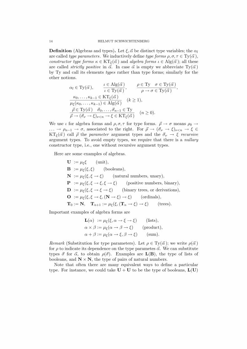
Definition (Algebras and types). Let ξ, ~α be distinct type variables; the αlare called type parameters. We inductively define type forms ρ, σ, τ ∈ Ty(~α ),constructor type forms κ ∈ KTξ(~α ) and algebra forms ι ∈ Alg(~α ); all theseare called strictly positive in ~α. In case ~α is empty we abbreviate Ty(~α )by Ty and call its elements types rather than type forms; similarly for theother notions.
αl ∈ Ty(~α ),ι ∈ Alg(~α )ι ∈ Ty(~α )
,ρ ∈ Ty σ ∈ Ty(~α )ρ→ σ ∈ Ty(~α )
,
κ0, . . . , κk−1 ∈ KTξ(~α )µξ(κ0, . . . , κk−1) ∈ Alg(~α )
(k ≥ 1),
~ρ ∈ Ty(~α ) ~σ0, . . . , ~σn−1 ∈ Ty~ρ→ (~σν → ξ)ν<n → ξ ∈ KTξ(~α )
(n ≥ 0).
We use ι for algebra forms and ρ, σ, τ for type forms. ~ρ → σ means ρ0 →. . . → ρn−1 → σ, associated to the right. For ~ρ → (~σν → ξ)ν<n → ξ ∈KTξ(~α ) call ~ρ the parameter argument types and the ~σν → ξ recursiveargument types. To avoid empty types, we require that there is a nullaryconstructor type, i.e., one without recursive argument types.
Here are some examples of algebras.
U := µξξ (unit),
B := µξ(ξ, ξ) (booleans),
N := µξ(ξ, ξ → ξ) (natural numbers, unary),
P := µξ(ξ, ξ → ξ, ξ → ξ) (positive numbers, binary),
D := µξ(ξ, ξ → ξ → ξ) (binary trees, or derivations),
O := µξ(ξ, ξ → ξ, (N→ ξ)→ ξ) (ordinals),
T0 := N, Tn+1 := µξ(ξ, (Tn → ξ)→ ξ) (trees).
Important examples of algebra forms are
L(α) := µξ(ξ, α→ ξ → ξ) (lists),
α× β := µξ(α→ β → ξ) (product),
α+ β := µξ(α→ ξ, β → ξ) (sum).
Remark (Substitution for type parameters). Let ρ ∈ Ty(~α ); we write ρ(~α )for ρ to indicate its dependence on the type parametes ~α. We can substitutetypes ~σ for ~α, to obtain ρ(~σ). Examples are L(B), the type of lists ofbooleans, and N×N, the type of pairs of natural numbers.
Note that often there are many equivalent ways to define a particulartype. For instance, we could take U + U to be the type of booleans, L(U)

MINLOG REFERENCE MANUAL 15
to be the type of natural numbers, and L(B) to be the type of positivebinary numbers.
For every constructor type κi(ξ) of an algebra ι = µξ(~κ ) we providea (typed) constructor symbol Ci of type κi(ι). In some cases they havestandard names, for instance
ttB, ffB for the two constructors of the type B of booleans,
0N,SN→N for the type N of (unary) natural numbers,
1P, SP→P0 , SP→P
1 for the type P of (binary) positive numbers,
nilL(ρ), consρ→L(ρ)→L(ρ) for the type L(ρ) of lists,
(inlρσ)ρ→ρ+σ, (inrρσ)σ→ρ+σ for the sum type ρ+ σ.
We denote the constructors of the type D of derivations by 0D (axiom) andCD→D→D (rule).
One can extend the definition of algebras and types to simultaneouslydefined algebras: just replace ξ by a list ~ξ = ξ0, . . . , ξN−1 of type variablesand change the algebra introduction rule to
κ0, . . . , κk−1 ∈ KT~ξ(~α )
(µ~ξ (κ0, . . . , κk−1))j ∈ Alg(~α )(k ≥ 1, j < N).
with each κi of the form
~ρ→ (~σν → ξjν )ν<n → ξj .
The definition of a “nullary” constructor type is a little more delicate here.We require that for every ξj (j < N) there is a κij with final value typeξj , each of whose recursive argument types has a final value type ξjν withjν < j. — Examples of simultaneously defined algebras are
(Ev,Od) := µξ,ζ(ξ, ζ → ξ, ξ → ζ) (even and odd numbers),
(Ts(ρ),T(ρ)) := µξ,ζ(ξ, ζ → ξ → ξ, ρ→ ζ, ξ → ζ) (tree lists and trees).
T(ρ) defines finitely branching trees, and Ts(ρ) finite lists of such trees; thetrees carry objects of a type ρ at their leaves. The constructor symbols andtheir types are
EmptyTs(ρ), TconsT(ρ)→Ts(ρ)→Ts(ρ),
Leafρ→T(ρ), BranchTs(ρ)→T(ρ).
However, for simplicity we often consider non-simultaneous algebras only.An algebra is finitary if all its constructor types (i) only have finitary
algebras as parameter argument types, and (ii) have recursive argumenttypes of the form ξ only (so the ~σν in the general definition are all empty).
16 HELMUT SCHWICHTENBERG
Structure-finitary algebras are defined similarly, but without conditions onparameter argument types. In the examples above U, B, N, P and D areall finitary, but O and Tn+1 are not. L(ρ), ρ × σ and ρ + σ are structure-finitary, and finitary if their parameter types are. An argument position ina type is called finitary if it is occupied by a finitary algebra.
An algebra is explicit if all its constructor types have parameter argumenttypes only (i.e., no recursive argument types). In the examples above U, B,ρ× σ and ρ+ σ are explicit, but N, P, L(ρ), D, O and Tn+1 are not.
We will also need the notion of the level of a type, which is defined by
lev(ι) := 0, lev(ρ→ σ) := max{lev(σ), 1 + lev(ρ)}.
Base types are types of level 0, and a higher type has level at least 1.To add and remove names for type variables, we use
(add-tvar-name name1 ...)
(remove-tvar-name name1 ...)
We need a constructor, accessors and a test for type variables.
(make-tvar index name) constructor(tvar-to-index tvar) accessor(tvar-to-name tvar) accessor(tvar? x)
To generate new type variables we use
(new-tvar type)
To introduce simultaneous free algebras we use
add-algebras-with-parameters, abbreviated add-param-algs .
An example is(add-param-algs
(list "labtree" "labtlist") ’alg-typeop 2’("LabLeaf" "alpha1=>labtree")’("LabBranch" "labtlist=>alpha2=>labtree")’("LabEmpty" "labtlist")’("LabTcons" "labtree=>labtlist=>labtlist" pairscheme-op))
This simultaneously introduces the two free algebras labtree and labtlist,both finitary, whose constructors are LabLeaf, LabBranch, LabEmpty andLabTcons (written as an infix pair operator, hence right associative). Theconstructors are introduced as “self-evaluating” constants; they play a spe-cial role in our semantics for normalization by evaluation.
MINLOG REFERENCE MANUAL 17
In case there are no parameters we use add-algs, and in case there is noneed for a simultaneous definition we use add-alg or add-param-alg.
For already introduced algebras we need constructors and accessors
(make-alg name type1 ...)
(alg-form-to-name alg)
(alg-form-to-types alg)
(alg-name-to-simalg-names alg-name)
(alg-name-to-token-types alg-name)
(alg-name-to-typed-constr-names alg-name)
(alg-name-to-tvars alg-name)
(alg-name-to-arity alg-name)
We also provide the tests
(alg-form? x) incomplete test(alg? x) complete test(finalg? type) incomplete test(sfinalg? type) incomplete test(ground-type? x) incomplete test
We require that there is at least one nullary constructor in every freealgebra; hence, it has a “canonical inhabitant”. For arbitrary types thisneed not be the case, but occasionally (e.g., for general logical problems,like to prove the drinker formula) it is useful. Therefore
(make-inhabited type term1 ...)
marks the optional term as the canonical inhabitant if it is provided, andotherwise creates a new constant of that type, which is taken to be thecanonical inhabitant. We also have
(type-to-canonical-inhabitant type),
which returns the canonical inhabitant.To remove names for algebras we use
(remove-alg-name name1 ...)
Examples. Standard examples for finitary free algebras are the type natof unary natural numbers, and the algebra of binary trees. The domain Inatof unary natural numbers is defined (as in [4]) as a solution to a domainequation.
We always provide the finitary free algebra unit consisting of exactly oneelement, and boole of booleans; objects of the latter type are (cf. loc. cit.)
18 HELMUT SCHWICHTENBERG
true, false and families of terms of this type, and in addition the bottomobject of type boole.
Tests:
(arrow-form? type)
(star-form? type)
(object-type? type)
We also need constructors and accessors for arrow types
(make-arrow arg-type val-type) constructor(arrow-form-to-arg-type arrow-type) accessor(arrow-form-to-val-type arrow-type) accessor
and star types
(make-star type1 type2) constructor(star-form-to-left-type star-type) accessor(star-form-to-right-type star-type) accessor.
For convenience we also have
(mk-arrow type1 ... type)
(arrow-form-to-arg-types type <n>) all (first n) argument types(arrow-form-to-final-val-type type) type of final value.
To check and to display a type we have
(type? x)
(type-to-string type)
(pp type).
2.4. Coercion. To develop analysis we use a subtype relation generatedfrom pos < nat < int < rat < real < cpx. We view pos, nat, int, rat,real, cpx as algebras with the following constructors and destructors.
pos : One, SZero, SOne (positive numbers written in binary)nat : Zero, Succint : IntPos, IntZero, IntNeg
rat : RatConstr (written # infix) and destructors RatN, RatD
real : RealConstr and destructors RealSeq, RealMod
cpx : CpxConstr (written ## infix) and destructors RealPart, ImagPart
We provide
(alg-le? alg1 alg2)
MINLOG REFERENCE MANUAL 19
(type-le? type1 type2)
(algebras-to-embedding type1 type2)
(types-to-embedding type1 type2)
(types-lub type . types)
type-match-modulo-coercion checks whether a given pattern can be trans-formed modulo coercion by a substitution into a given instance. It returns#f, if this is impossible, and the substitution otherwise. We provide
(type-match-modulo-coercion pattern instance)
3. Variables
A variable of an object type is interpreted by a continuous functional (ob-ject) of that type. We use the word “variable” and not “program variable”,since continuous functionals are not necessarily computable. For readablein- and output, and also for ease in parsing, we may reserve certain stringsas names for variables of a given type, e.g., n, m for variables of type nat.Then also n0, n1, n2, . . . , m0, . . . can be used for the same purpose.
In most cases we need to argue about existing (i.e., total) objects only.For the notion of totality we have to refer to [25, Chapter 8.3]; particularlyrelevant here is exercise 8.5.7. To make formal arguments with quantifiersrelativized to total objects more managable, we use a special sort of variablesintended to range over such objects only. For example, n0, n1, n2, . . . , m0, . . .range over total natural numbers, and n^0, n^1, n^2, . . . are general vari-ables. We say that the degree of totality for the former is 1, and for thelatter 0.
To add and remove names for variables of a given type (e.g., n, m forvariables of type nat), we use
(add-var-name name1 ... type)
(remove-var-name name1 ... type)
(default-var-name type).
The first variable name added for any given type becomes the default vari-able name. If the system creates new variables of this type, they will carrythat name. For complex types it sometimes is necessary to talk about vari-ables of a certain type without using a specific name. In this case one canuse the empty string to create a so called numerated variable (see below).The parser is able to produce this kind of canonical variables from typeexpressions.
We need a constructor, accessors and tests for variables.
(make-var type index t-deg name) constructor

20 HELMUT SCHWICHTENBERG
(var-to-type var) accessor(var-to-index var) accessor(var-to-t-deg var) accessor(var-to-name var) accessor(var-form? x) incomplete test(var? x). complete test
It is guaranteed that equal? is a valid test for equality of variables. More-over, it is guaranteed that parsing a displayed variable reproduces the vari-able; the converse need not be the case (we may want to convert it into somecanonical form).
For convenience we have the function
(mk-var type <index> <t-deg> <name>).
The type is a required argument; however, the remaining arguments areoptional. The default for the name string is the value returned by
(default-var-name type)
If there is no default name, a numerated variable is created. The default forthe totality is “total”.
Using the empty string as the name, we can create so called numeratedvariables. We further require that we can test whether a given variablebelongs to those special ones, and that from every numerated variable wecan compute its index:
(numerated-var? var)
(numerated-var-to-index numerated-var).
It is guaranteed that make-var used with the empty name string is a bijec-tion of the product of Ty, N, and the degrees of totality to the set of numer-ated variables, with inverses var-to-type, numerated-var-to-index andvar-to-t-deg.
Although these functions look like an ad hoc extension of the interfacethat is convenient for normalization by evaluation, there is also a deeperbackground: these functions can be seen as the “computational content”of the well-known phrase “we assume that there are infinitely many vari-ables of every type”. Giving a constructive proof for this statement wouldrequire to give infinitely many examples of variables for every type. Thisof course can only be done by specifying a function (for every type) thatenumerates these examples. To make the specification finite we require theexamples to be given in a uniform way, i.e., by a function of two arguments.To make sure that all these examples are in fact different, we would have
MINLOG REFERENCE MANUAL 21
to require make-var to be injective. Instead, we require (classically equiva-lent) make-var to be a bijection on its image, as again, this can be turnedinto a computational statement by requiring that a witness (i.e., an inversefunction) is given.
Finally, as often the exact knowledge of infinitely many variables of everytype is not needed we require that, either by using the above functions orby some other form of definition, functions
(type-to-new-var type)
(type-to-new-partial-var type)
are defined that return a (total or partial) variable of the requested type, dif-ferent from all variables that have ever been returned by any of the specifiedfunctions so far.
Occasionally we may want to create a new variable with the same name(and degree of totality) as a given one. This is useful, for instance for boundrenaming. Therefore we supply
(var-to-new-var var)
(var-to-new-partial-var var)
Implementation. Variables are implemented as lists:
(var type index t-deg name).
4. Constants
Every constant (or more precisely, object constant) has a type and de-notes a computable (hence continuous) functional of that type. We have thefollowing three kinds of constants:
(i) constructors, kind constr,(ii) constants with user defined rules (also called program(mable) constant,
or pconst), kind pconst,(iii) constants whose rules are fixed, kind fixed-rules.
The latter are built into the system: recursion operators for arbitrary al-gebras, equality and existence operators for finitary algebras, and existenceelimination. They are typed in parametrized form, with the actual type (orformula) given by a type (or type and formula) substitution that is also partof the constant. For instance, equality is typed by α → α → B and a typesubstitution α 7→ ρ. This is done for clarity (and brevity, e.g., for large ρ inthe example above), since one should think of the type of a constant in thisway.

22 HELMUT SCHWICHTENBERG
For constructors and for constants with fixed rules, by efficiency reasonswe want to keep the object denoted by the constant (as needed for norma-lization by evaluation) as part of it. It depends on the type of the constant,hence must be updated in a given proof whenever the type changes by atype substitution.
4.1. Rewrite and computation rules for program constants. For ev-ery program constant (or defined constant) Dρ we assume that some rewriterules of the form D ~K 7→ N are given, where FV(N) ⊆ FV( ~K) and D ~K, Nhave the same type (not necessarily a ground type). Moreover, for any tworules D ~K 7→ N and D ~K ′ 7→ N ′ we require that ~K and ~K ′ are of the samelength, called the arity of D. The rules are divided into computation rulesand proper rewrite rules. They must satisfy the requirements listed in [4].The idea is that a computation rule can be understood as a description ofa computation in a suitable semantical model, provided the syntactic con-structors correspond to semantic ones in the model, whereas the other rulesdescribe syntactic transformations.
There a more general approach was used: one may enter into componentsof products. Then instead of one arity one needs several “type informations”~ρ → σ with ~ρ a list of types, 0’s and 1’s indicating the left or right part ofa product type. For example, if D is of type τ → (τ → τ → τ) × (τ → τ),then the rules Dy0xx 7→ a and Dy1 7→ b are admitted, and D comes withthe type informations (τ, 0, τ, τ → τ)→ τ and (τ, 1)→ (τ → τ). – However,for simplicity we only deal with a single arity here.
Given a set of rewrite rules, we want to treat some rules - which we callcomputation rules - in a different, more efficient way. The idea is that acomputation rule can be understood as a description of a computation ina suitable semantical model, provided the syntactic constructors correspondto semantic ones in the model, whereas the other rules describe syntactictransformations.
In order to define what we mean by computation rules, we need the notionof a constructor pattern. These are special terms defined inductively asfollows.
(i) Every variable is a constructor pattern.(ii) If C is a constructor and P1, . . . , Pn are constructor patterns (or pro-
jection markers 0 or 1), such that C~P is of ground type, then C~P is aconstructor pattern.
From the given set of rewrite rules we choose a subset Comp with the fol-lowing properties.
(i) If D~P 7→ Q ∈ Comp, then P1, . . . , Pn are constructor patterns orprojection markers.
MINLOG REFERENCE MANUAL 23
(ii) The rules are left-linear, i.e., if D~P 7→ Q ∈ Comp, then every variablein D~P occurs only once in D~P .
(iii) The rules are essentially non-overlapping, i.e., for different rules D ~K 7→M and D~L 7→ N in Comp the left hand sides D ~K and D~L are eithernon-unifiable, or else for the most general unifier ξ of ~K and ~L we haveMξ = Nξ.
We write D ~M 7→comp Q to indicate that the rule is in Comp. All other ruleswill be called (proper) rewrite rules.
In our reduction strategy computation rules will always be applied first,and since they are essentially non-overlapping, this part of the reduction isunique. However, since we allowed almost arbitrary rewrite rules, it mayhappen that in case no computation rule applies a term may be rewrittenby different rules /∈ Comp. In order to obtain a deterministic procedure wethen select the first applicable rewrite rule (this is a slight simplification of[4], where special “select”-functions were used for this purpose).
4.2. Recursion over simultaneous free algebras. We now explain whatwe mean by recursion over simultaneous free algebras. The inductive struc-ture of the types ~ι = µ~ξ ~κ corresponds to two sorts of constants. With theconstructors C~ιi : κi[~ι ] we can construct elements of a type ιj , and with therecursion operators R~ι,~τιj we can construct mappings from ιj to τj by recur-sion on the structure of ~ι. So in (Rec arrow-types), arrow-types is a listι1 → τ1, . . . , ιk → τk. Here ι1, . . . , ιk are the algebras defined simultaneouslyand τ1, . . . , τk are the result types.
For convenience in our later treatment of proofs (when we want to nor-malize a proof by (1) translating it into a term, (2) normalizing this termand (3) translating the normal term back into a proof), we also allow all-formulas ∀xι11 A1, . . . ,∀xιkk Ak instead of arrow-types: they are treated asι1 → τ(A1), . . . , ιk → τ(Ak) with τ(Aj) the type of Aj .
Recall the definition of types and constructor types in section 2, and theexamples given there. The (structural) higher type recursion operators Rτι(introduced by Godel [11]) are used to construct maps from the algebra ιto τ , by recursion on the structure of ι. For instance, RτN has type N →τ → (N→ τ → τ)→ τ . The first argument is the recursion argument, thesecond one gives the base value, and the third one gives the step function,mapping the recursion argument and the previous value to the next value.For example, RN
Nnmλn,p(Sp) defines addition m+ n by recursion an n.Generally, in order to define the type of the recursion operators w.r.t.
ι = µξ (κ0, . . . , κk−1) and result type τ , we first define for each constructortype
κ = ~ρ→ (~σν → ξ)ν<n → ξ ∈ KTξ
24 HELMUT SCHWICHTENBERG
the step type
δ := ~ρ→ (~σν → ι)ν<n → (~σν → τ)ν<n → τ.
The recursion operator Rτι then has type
ι→ δ0 → . . .→ δk−1 → τ
where k is the number of constructors. The recursion argument is of typeι. In the step type δ above, the ~ρ are parameter types, (~σν → ι)ν<n arethe types of the predecessor components in the recursion argument, and(~σν → τ)ν<n are the types of the previously defined values.
For some common algebras listed in 2.3 we spell out the type of theirrecursion operators:
RτB : B→ τ → τ → τ,
RτN : N→ τ → (N→ τ → τ)→ τ,
RτP : P→ τ → (P→ τ → τ)→ (P→ τ → τ)→ τ,
RτO : O→ τ → (O→ τ → τ)→ ((N→ O)→ (N→ τ)→ τ)→ τ,
RτL(ρ) : L(ρ)→ τ → (ρ→ L(ρ)→ τ → τ)→ τ,
Rτρ+σ : ρ+ σ → (ρ→ τ)→ (σ → τ)→ τ,
Rτρ×σ : ρ× σ → (ρ→ σ → τ)→ τ.
One can extend the definition of the (structural) recursion operators tosimultaneously defined algebras ~ι = µ~ξ (κ0, . . . , κk−1) and result types ~τ .Then for each constructor type
κ = ~ρ→ (~σν → ξjν )ν<n → ξj ∈ KT~ξ
we have the step type
δ := ~ρ→ (~σν → ιjν )ν<n → (~σν → τjν )ν<n → τj .
The jth simultaneous recursion operator R~ι,~τj has type
ιj → δ0 → . . .→ δk−1 → τj
where k is the total number of constructors. The recursion argument is oftype ιj . In the step type δ, the ~ρ are parameter types, (~σν → ιjν )ν<n arethe types of the predecessor components in the recursion argument, and(~σν → τjν )ν<n are the types of the previously defined values. We will oftenomit the upper indices ~ι, ~τ when they are clear from the context. Noticethat in case of a non-simultaneous free algebra we write Rτι for Rι,τ1 . —An example of a simultaneous recursion on tree lists and trees will be givenbelow.

MINLOG REFERENCE MANUAL 25
Definition. Terms of Godel’s T are inductively defined from typed vari-ables xρ and constants for constructors C~ιi and recursion operators R~ι,~τj byabstraction λxρM
σ and application Mρ→σNρ.
4.3. Conversion. To define the conversion relation for the structural recur-sion operators, it will be helpful to use the following notation. Let ~ι = µ~ξ ~κ,
κi = ρ0 → . . .→ ρm−1 → (~σ0 → ξj0)→ . . .→ (~σn−1 → ξjn−1)→ ξj ∈ KT~ξ,
and consider C~ιi ~N of type ιj . We write ~NP = NP0 , . . . , N
Pm−1 for the para-
meter arguments Nρ00 , . . . , N
ρm−1
m−1 and ~NR = NR0 , . . . , N
Rn−1 for the recursive
arguments N~σ0→ιj0m , . . . , N
~σn−1→ιjn−1
m+n−1 , and nR for the number n of recursivearguments.
We define a conversion relation 7→ρ between terms of type ρ by
(λxM(x))N 7→M(N),(1)
λx(Mx) 7→M if x /∈ FV(M) (M not an abstraction),(2)
Rj(C~ιi ~N) ~M 7→Mi~N((Rj0 · ~M) ◦NR
0
). . .((Rjn−1 · ~M) ◦NR
n−1
).(3)
Here we have written Rj · ~M for λxιj (R~ι,~τj xιj ~M); ◦ denotes ordinary com-
position. The rule (1) is called β-conversion, and (2) η-conversion; their lefthand sides are called β-redexes or η-redexes, respectively. The left handside of (3) is called R-redex ; it is a special case of a redex associated with aconstant D defined by “computation rules” (cf. 4.1), and hence also calleda D-redex .
Let us look at some examples of what can be defined in Godel’s T. Wedefine the canonical inhabitant ερ of a type ρ ∈ Ty:
ειj := C~ιijε~ρ(λ~x1
ειj1 ) . . . (λ~xnειjn ), ερ→σ := λxε
σ.
The projections of a pair to its components can be defined easily:
M0 := Rρρ×σMρ×σ(λxρ,yσxρ), M1 := Rσρ×σMρ×σ(λxρ,yσyσ).
The append -function ∗ for lists is defined recursively as follows. We writex :: l as shorthand for cons(x, l).
nil ∗ l2 := l2, (x :: l1) ∗ l2 := x :: (l1 ∗ l2).
It can be defined as the term
l1 ∗ l2 := RL(α)→L(α)L(α) l1(λl2 l2)λx, ,p,l2(x :: (pl2))l2.
Here “ ” is a name for a bound variable which is not used.Using the append function ∗ we can define list reversal Rev by
Rev(nil) := nil, Rev(x :: l) := Rev(l) ∗ (x :: nil).

26 HELMUT SCHWICHTENBERG
The corresponding term is
Rev(l) := RL(α)L(α)l nilλx, ,p(p ∗ (x :: nil)).
Assume we want to define by simultaneous recursion two functions on N,say even, odd: N→ B. We want
even(0) := tt, odd(0) := ff,
even(Sn) := odd(n), odd(Sn) := even(n).
This can be achieved by using pair types: we recursively define the singlefunction evenodd: N→ B×B. The step types are
δ0 = B×B, δ1 = N→ B×B→ B×B,
and we can define evenoddm := RB×BN m〈tt, ff〉λn,p〈p1, p0〉.
Another example concerns the algebras (Ts(N),T(N)) simultaneouslydefined in 2.3 (we write them without the argument N here), whose con-structors C(Ts,T)
i for i ∈ {0, . . . , 3} are
EmptyTs, TconsT→Ts→Ts, LeafN→T, BranchTs→T.
Recall that the elements of the algebra T (i.e., T(N)) are just the finitelybranching trees, which carry natural numbers on their leaves.
Let us compute the types of the recursion operators w.r.t. the result typesτ0, τ1, i.e., of R(Ts,T),(τ0,τ1)
Ts and R(Ts,T),(τ0,τ1)T , or shortly RTs and RT. The
step types areδ0 := τ0,
δ1 := Ts→ T→ τ0 → τ1 → τ0,
δ2 := N→ τ1,
δ3 := Ts→ τ0 → τ1.
Hence the types of the recursion operators are
RTs : Ts→ δ0 → δ1 → δ2 → δ3 → τ0,
RT : T→ δ0 → δ1 → δ2 → δ3 → τ1.
The internal representation of RT is
(const Rec δ′0 → δ′1 → δ′2 → δ′3 → T→ α0
(α0 7→ τ0, α1 7→ τ1))
withδ′0 := α0,
δ′1 := Ts→ T→ α0 → α1 → α0,
δ′2 := N→ α1,
δ′3 := Ts→ α0 → α1.
Here the fact that we deal with a simultaneous recursion (over tree andtlist), and that we define a constant of type T → . . . , can all be inferredfrom what is given: the type T → . . . is right there, and for tlist we canlook up the simultaneously defined algebras.
MINLOG REFERENCE MANUAL 27
For the external representation (i.e., display) we use the shorter notation
(Rec T→ τ0 Ts→ τ1).
4.4. Internal representation of constants. Every object constant hasthe internal representation
(const object-or-arity name uninst-type tsubst
t-deg token-type repro-data)
The type of the constant is the result of carrying out the type substitutiontsubst in uninst-type; free type variables may again occur in this type.The type substitution tsubst must be restricted to the type variables inuninst-type. Examples for object constants are
(const Compose (α→β)→(β→γ)→α→γ (α 7→ ρ, β 7→ σ, γ 7→ τ) ...)
(const Eq α→ α→ B (α 7→ finalg) ...)
(const E α→ B (α 7→ finalg . . . ))
object-or-arity is an object if this object cannot be changed, e.g., by allowinguser defined rules for the constant; otherwise, the associated object needsto be updated whenever a new rule is added, and we have the arity of thoserules instead. The rules are of crucial importance for the correctness of aproof, and should not be invisibly buried in the denoted object taken aspart of the constant (hence of any term involving it). Therefore we keepthe rules of a program constant and also its denoted objects (depending ontype substitutions) at a central place, a global variable PROGRAM-CONSTANTSwhich assigns to every name of such a constant the constant itself (withuninstantiated type), the rules presently chosen for it and also its denotedobjects (as association list with type substitutions as keys). When a new rulehas been added, the new objects for the program constant are computed,and the new list to be associated with the program constant is written inPROGRAM-CONSTANTS instead. All information on a program constant exceptits denoted object and its computation and rewrite rules (i.e., its type, degreeof totality, arity and token type) is stable and hence can be kept as part ofit. The token type can be either const (i.e., constant written as application)or one of: postfix-op, prefix-op, binding-op, add-op, mul-op, rel-op,and-op, or-op, imp-op and pair-op.
Repro-data are (only) necessary in proof.scm, for normalization of proofs:a (general) induction, efq, introduction or elimination axiom is translatedinto an appropriate constant, then normalized, and finally from the con-stant and its repro data the axiom is reproduced. The repro-data are of thefollowing forms.
(1) For a recursion constant.

28 HELMUT SCHWICHTENBERG
(a) A list of all-formulas. This form only occurs when translating anaxiom for (simultaneous) induction into a recursion constant, inorder to achieve normalization of proofs via term normalization.We have to consider the free variables in the scheme formulas,and let the type of the recursion constant depend on them. Thisis needed to have the allnc-conversion be represented in termnormalization. The relevant operation is
all-formulas-to-rec-const.
(b) A list of implication formulas I~x^→ A(~x^), where all idpcs aresimultaneously inductively defined. This form only occurs whentranslating an elimination axiom into a recursion constant, inorder to achieve normalization of proofs via term normalization.We again have to consider the free variables in the scheme formu-las, and let the type of the recursion constant depend on them.This is needed to have the allnc-conversion be represented interm normalization. The relevant operation is
imp-formulas-to-rec-const.
(2) For a cases constant. Here a single arrow-type or all-formula suffices.One uses
all-formula-to-cases-const.
(3) For a guarded general recursion constant: an all-formula. Thisform only occurs when translating a general induction axiom intoa guarded general recursion constant, in order to achieve normaliza-tion of proofs via term normalization. We have to consider the freevariables in the scheme formulas, and let the type of the guardedgeneral recursion constant depend on them. This is needed to havethe allnc-conversion be represented in term normalization. One uses
all-formula-and-number-to-grecguard-const.
(4) For an efq-constant (of kind ’fixed-rules): a formula. This formonly occurs when translating an efq-aconst into an efq-constant, inorder to achieve normalization of proofs via term normalization. Oneuses
formula-to-efq-const.
(5) For a constructor associated with an “Intro” axiom.(a) A number i of a clause for an inductively defined predicate con-
stant, and the constant idpc. One uses
number-and-idpredconst-to-intro-const.
MINLOG REFERENCE MANUAL 29
(b) An ex-formula for an “Ex-Intro” axiom. One uses
ex-formula-to-ex-intro-const.
(c) An exnc-formula for an “Exnc-Intro” axiom. One uses
exnc-formula-to-exnc-intro-const.
(6) For an Ex-Elim constant (of kind ’fixed-rules): an ex-formulaand a conclusion. One uses
ex-formula-and-concl-to-ex-elim-const.
(7) For an Exnc-Elim constant (of kind ’fixed-rules): an exnc-formulaand a conclusion. One uses
exnc-formula-and-concl-to-exnc-elim-const.
Constructor, accessors and tests for all kinds of constants:
(make-const obj-or-arity name kind uninst-type tsubst
t-deg token-type . repro-data)
(const-to-object-or-arity const)
(const-to-name const)
(const-to-kind const)
(const-to-uninst-type const)
(const-to-tsubst const)
(const-to-t-deg const)
(const-to-token-type const)
(const-to-repro-data const)
(const? x)
(const=? x y)
From these we can define
(const-to-type const)
(const-to-tvars const)
A constructor is a special constant with no rules. We maintain an as-sociation list CONSTRUCTORS assigning to every name of a constructor anassociation list associating with every type substitution (restricted to thetype parameters) the corresponding instance of the constructor. We pro-vide
(constr-name? string)
(constr-name-to-constr name <tsubst>)
30 HELMUT SCHWICHTENBERG
(constr-name-and-tsubst-to-constr name tsubst),
where in (constr-name-to-constr name <tsubst>), name is a string orelse of the form (Ex-Intro formula). If the optional tsubst is not present,the empty substitution is used.
For given algebras one can display the associated constructors with theirtypes by calling
(display-constructors alg-name1 ...).
We also need procedures recovering information from the string denotinga program constant (via PROGRAM-CONSTANTS):
(pconst-name-to-pconst name)
(pconst-name-to-comprules name)
(pconst-name-to-rewrules name)
(pconst-name-to-inst-objs name)
(pconst-name-and-tsubst-to-object name tsubst)
(pconst-name-to-object name).
One can display the program constants together with their current com-putation and rewrite rules by calling
(display-program-constants name1 ...).
To add and remove program constants we use
(add-program-constant name type <rest>)
(remove-program-constant symbol);
rest consists of an initial segment of the following list: t-deg (default 0),token-type (default const) and arity (default maximal number of argu-ment types).
To add and remove computation and rewrite rules we have
(add-computation-rule lhs rhs)
(add-rewrite-rule lhs rhs)
(remove-computation-rules-for lhs)
(remove-rewrite-rules-for lhs).
To generate our constants with fixed rules we use
(finalg-to-=-const finalg) equality(finalg-to-e-const finalg) existence(arrow-types-to-rec-const . arrow-types) recursion(ex-formula-and-concl-to-ex-elim-const

MINLOG REFERENCE MANUAL 31
ex-formula concl)
Similarly to arrow-types-to-rec-const we also define the procedureall-formulas-to-rec-const. It will be used in to achieve normalizationof proofs via translating them in terms.
Similarly we have arrow-types-to-cases-const and on the proof levelall-formulas-to-cases-const.
5. Predicate variables and constants
5.1. Predicate variables. A predicate variable of arity ρ1, . . . , ρn is aplaceholder for a formulaA with distinguished (different) variables x1, . . . , xnof types ρ1, . . . , ρn. Such an entity is called a comprehension term, written{x1, . . . , xn | A }.
Predicate variable names are provided in the form of an association list,which assigns to the names their arities. By default we have the predicatevariable bot of arity (arity), called (logical) falsity. It is viewed as apredicate variable rather than a predicate constant, since (when translatinga classical proof into a constructive one) we want to substitute for bot.
Often we will argue about Harrop formulas only, i.e., formulas withoutcomputational content. For convenience we use a special sort of predicatevariables intended to range over comprehension terms with Harrop formulasonly. For example, P^0, P^1, P^2, . . . range over comprehension terms withHarrop formulas, and P0, P1, P2, . . . , Q0, . . . are general predicate variables.We say that Harrop degree for the former is 1, and for the latter 0.
In the context of Godel’s Dialectica intepretation [11] we also need to dealwith “negative” computational content. Therefore we also need a “degreeof negativity” and denote it by n-deg, and we call the Harrop degree the“degree of positivity” denoted h-deg. We use P’0, P’1, P’2, . . . , Q’0, . . . forpredicate variables of h-deg 0 and n-deg 1, and P^’0, P^’1, P^’2, . . . forpredicate variables whose h-deg and n-deg are both 1.
We need constructors and accessors for arities
(make-arity type1 ...)
(arity-to-types arity)
To display an arity we have
(arity-to-string arity)
We can test whether a string is a name for a predicate variable, and if socompute its associated arity:
(pvar-name? string)
(pvar-name-to-arity pvar-name)

32 HELMUT SCHWICHTENBERG
To add and remove names for predicate variables of a given arity (e.g., Qfor predicate variables of arity nat), we use
(add-pvar-name name1 ... arity)
(remove-pvar-name name1 ...)
We need a constructor, accessors and tests for predicate variables.
(make-pvar arity index h-deg n-deg name) constructor(pvar-to-arity pvar) accessor(pvar-to-index pvar) accessor(pvar-to-h-deg pvar) accessor(pvar-to-n-deg pvar) accessor(pvar-to-name pvar) accessor(pvar? x)
(equal-pvars? pvar1 pvar2)
For convenience we have the function
(mk-pvar arity <index> <h-deg> <n-deg> <name>)
The arity is a required argument; the remaining arguments are optional.The default for index is −1, for h-deg and n-deg is 0 and for name it isgiven by (default-pvar-name arity).
It is guaranteed that parsing a displayed predicate variable reproducesthe predicate variable; the converse need not be the case (we may want toconvert it into some canonical form).
5.2. Predicate constants. We also allow predicate constants. The gene-ral reason for having them is that sometimes we wants predicates to beaxiomatized, which are not placeholders for formulas. Prime formulas builtfrom predicate constants do not give rise to extracted terms, and cannot besubstituted for.
Notice that a predicate constant does not change its name under a typesubstitution; this is in contrast to predicate (and other) variables. Noticealso that the parser can infer from the arguments the types ρ1 . . . ρn to besubstituted for the type variables in the uninstantiated arity of P .
To add and remove names for predicate constants of a given arity, we use
(add-predconst-name name1 ... arity)
(remove-predconst-name name1 ...)
We need a constructor, accessors and tests for predicate constants.
(make-predconst uninst-arity tsubst index name) constructor
MINLOG REFERENCE MANUAL 33
(predconst-to-uninst-arity predconst) accessor(predconst-to-tsubst predconst) accessor(predconst-to-index predconst) accessor(predconst-to-name predconst) accessor(predconst? x)
Moreover we need
(predconst-name? name)
(predconst-name-to-arity predconst-name).
(predconst-to-string predconst).
5.3. Inductively defined predicate constants. When we want to makepropositions about computable functionals and their domains of partial con-tinuous functionals, it is perfectly natural to take, as initial propositions,ones formed inductively. For example, in the algebra N we can inductivelydefine totality by the clauses
T0, ∀n(Tn→ T (Sn)).
Its least-fixed-point scheme will be taken in the form
∀n(Tn→ A(0)→ ∀n(Tn→ A(n)→ A(Sn))→ A(n)).
The reason for writing it in this way is that it fits better with the logical eli-mination rules. It expresses that every “competitor” {n | A(n) } satisfyingthe same clauses contains T . This is the usual induction schema for naturalnumbers, which clearly only holds for “total” numbers. Notice that we haveused a “strengthened” form of the “step formula”, namely ∀n(Tn→ A(n)→A(Sn)) rather than ∀n(A(n) → A(Sn)). In applications of the least-fixed-point axiom this simplifies the proof of the “induction step”, since we havethe additional hypothesis T (n) available. Totality for an arbitrary algebracan be defined similarly.
Generally, an inductively defined predicate I is given by k clauses, whichare of the form
∀~x( ~Ai → (∀~yiν ( ~Biν → I~siν))ν<ni → I~ti) (i < k).
Our formulas will be defined by the operations of implication A → B
and universal quantification ∀xρA from inductively defined predicates µX ~K,where X is a predicate variable, and the Ki are clauses. Formulas will betreated more extensively later in section 7. However, in principle predicatesand formulas are introduced simultaneously.
Definition (Predicates and formulas). Let X, ~Y be distinct predicate vari-ables; the Yl are called predicate parameters. We inductively define formula

34 HELMUT SCHWICHTENBERG
forms A,B,C,D ∈ F(~Y ), predicate forms P,Q, I, J ∈ Preds(~Y ) and clauseforms K ∈ ClX(~Y ); all these are called strictly positive in ~Y . In case ~Y isempty we abbreviate F(~Y ) by F and call its elements formulas; similarly forthe other notions. (However, for brevity we often say “formula” etc. whenit is clear from the context that parameters may occur.)
Yl~r ∈ F(~Y ),A ∈ F B ∈ F(~Y )
A→ B ∈ F(~Y ),
A ∈ F(~Y )
∀xA ∈ F(~Y ),
C ∈ F(~Y )
{ ~x | C } ∈ Preds(~Y ),
P ∈ Preds(~Y )
P~r ∈ F(~Y ),
K0, . . . ,Kk−1 ∈ ClX(~Y )
µX(K0, . . . ,Kk−1) ∈ Preds(~Y )(k ≥ 1),
~A ∈ F(~Y ) ~B0, . . . , ~Bn−1 ∈ F
∀~x( ~A→ (∀~yν ( ~Bν → X~sν))ν<n → X~t ) ∈ ClX(~Y )(n ≥ 0).
Here ~A → B means A0 → · · · → An−1 → B, associated to the right.For a clause ∀~x( ~A → (∀~yν ( ~Bν → X~sν))ν<n → X~t ) ∈ ClX(~Y ) we call ~A
parameter premises and ∀~yν ( ~Bν → X~sν) recursive premises. We require thatin µX(K0, . . . ,Kk−1) the clause K0 is “nullary”, without recursive premises.The terms ~r are those introduced in section 6, i.e., typed terms built fromconstants by abstraction and application, and (importantly) those with acommon reduct are identified.
A predicate of the form { ~x | C } is called a comprehension term. Weidentify { ~x | C(~x ) }~r with C(~r ). The letter I will be used for predicates ofthe form µX(K0, . . . ,Kk−1); they are called inductively defined predicates.
Remark (Substitution for predicate parameters). Let A ∈ F(~Y ); we writeA(~Y ) for A to indicate its dependence on the predicate parametes ~Y . Sim-ilarly we write I(~Y ) for I if I ∈ Preds(~Y ). We can substitute predicates ~P
for ~Y , to obtain A(~P ) and I(~P ), respectively.
An inductively defined predicate is finitary if its clauses have recursivepremises of the form X~s only (so the ~yν and ~Bν in the general definition areall empty).
To introduce inductively defined predicates we use
add-ids.
An example is(add-ids (list (list "Even" (make-arity (py "nat")) "nat"))
’("Even 0" "InitEven")

MINLOG REFERENCE MANUAL 35
’("allnc n^(Even n^ -> Even(n^ +2))" "GenEven"))
This simultaneously introduces the inductively defined predicate constantEven, by the clauses given. The presence of an algebra name after thearity (here nat) indicates that this inductively defined predicate constant isto have computational content. Then all clauses with this constant in theconclusion must provide a constructor name (here InitEven, GenEven). Wewill also allow special computationally irrelevant (c.i.) inductively definedpredicates.
An inductively defined predicate constant can only be understood fromits clauses and its elimination or least-fixed-point axiom.
Definition (Theory of Computable Functionals TCF). TCF is the systemin minimal logic for → and ∀, whose formulas are those in F above, andwhose axioms are the following. For each inductively defined predicate, thereare “closure” or introduction axioms, together with a “least-fixed-point” orelimination axiom. In more detail, consider an inductively defined predicateI := µX(K0, . . .Kk−1). For each of the k clauses we have an introductionaxiom, as follows. Let the i-th clause for I be
Ki(X) := ∀~x( ~A→ (∀~yν ( ~Bν → X~sν))ν<n → X~t ).
Then the corresponding introduction axiom is Ki(I), that is,
(4) ∀~x( ~A→ (∀~yν ( ~Bν → I~sν))ν<n → I~t ).
The elimination axiom is
(5) ∀~x(I~x→ (Ki(I, P ))i<k → P~x ),
where
Ki(I, P ) := ∀~x( ~A→ (∀~yν ( ~Bν → I~sν))ν<n →
(∀~yν ( ~Bν → P~sν))ν<n → P~t ).
We label each introduction axiom Ki(I) by I+i and the elimination axiom
by I−.
As an important example we now give the inductive definition of Leibnizequality. However, a word of warning is in order here: we need to distinguishfour separate, but closely related equalities.
(i) Firstly, defined function constants D are introduced by computationrules, written l = r, but intended as left-to-right rewrites.
(ii) Secondly, we have Leibniz equality Eq inductively defined below.(iii) Thirdly, pointwise equality between partial continuous functionals will
be defined inductively as well.

36 HELMUT SCHWICHTENBERG
(iv) Fourthly, if l and r have a finitary algebra as their type, l = r can beread as a boolean term, where = is the decidable equality defined in 6as a boolean-valued binary function.
Leibniz equality. We define Leibniz equality by
Eq(ρ) := µX(∀xX(xρ, xρ)).
The introduction axiom is∀xEq(xρ, xρ)
and the elimination axiom
∀x,y(Eq(x, y)→ ∀xPxx→ Pxy),
where Eq(x, y) abbreviates Eq(ρ)(xρ, yρ).
Lemma (Compatibility of Eq). ∀x,y(Eq(x, y)→ A(x)→ A(y)).
Proof. Use the elimination axiom with Pxy := (A(x)→ A(y)). �
Using compatibility of Eq one easily proves symmetry and transitivity.Define falsity by F := Eq(ff, tt). Then we have
Theorem (Ex-Falso-Quodlibet). For every formula A without predicate pa-rameters we can derive F→ A.
Proof. We first show that F → Eq(xρ, yρ). To see this, one first obtainsEq([if ff then x else y], [if ff then x else y]) from the introduction axiom,since [if ff then x else y] is an allowed term, and then from Eq(ff, tt) onegets Eq([if tt then x else y], [if ff then x else y]) by compatibility. HenceEq(xρ, yρ).
The claim can now be proved by induction on A ∈ F. Case I~s. LetKi be the nullary clause, with final conclusion I~t. By induction hypothesisfrom F we can derive all parameter premises. Hence I~t. From F we alsoobtain Eq(si, ti), by the remark above. Hence I~s by compatibility. Thecases A→ B and ∀xA are obvious. �
A crucial use of the equality predicate Eq is that it allows to lift a booleanterm rB to a formula, using atom(rB) := Eq(rB, tt). This opens up a con-venient way to deal with equality on finitary algebras. The computationrules ensure that for instance the boolean term Sr =N Ss or more precisely,=N(Sr, Ss), is identified with r =N s. We can now turn this boolean terminto the formula Eq(Sr =N Ss, tt), which again is abbreviated by Sr =N Ss,but this time with the understanding that it is a formula. Then (impor-tantly) the two formulas Sr =N Ss and r =N s are identified because thelatter is a reduct of the first. Consequently there is no need to prove theimplication Sr =N Ss→ r =N s explicitly.

MINLOG REFERENCE MANUAL 37
Pointwise equality =ρ. For every constructor Ci of an algebra ι we have anintroduction axiom
∀~y,~z(~yP =~ρ ~zP → (∀~xν (yRm+ν~xν =ι z
Rm+ν~xν))ν<n → Ci~y =ι Ci~z ).
For an arrow type ρ → σ the introduction axiom is explicit, in the sensethat it has no recursive premise:
∀x1,x2(∀y(x1y =σ x2y)→ x1 =ρ→σ x2).
For example, =N is inductively defined by0 =N 0,
∀n1,n2(n1 =N n2 → Sn1 =N Sn2),
and the elimination axiom is∀n1,n2(n1 =N n2 → P00→
∀n1,n2(n1 =N n2 → Pn1n2 → P (Sn1,Sn2))→Pn1n2).
The main purpose of pointwise equality is that it allows to formulate theextensionality axiom: we express the extensionality of our intended modelby stipulating that pointwise equality is equivalent to Leibniz equality.
Axiom (Extensionality). ∀x1,x2(x1 =ρ x2 ↔ Eq(x1, x2)).
We write E-TCF when the extensionality axioms are present. – One ofthe main points of TCF is that it allows the logical connectives existence,conjunction and disjunction to be inductively defined as predicates. Thiswas first discovered by Martin-Lof [15].
Existential quantifier.
Ex(Y ) := µX(∀x(Y xρ → X)).
The introduction axiom is
∀x(A→ ∃xA),
where ∃xA abbreviates Ex({xρ | A }), and the elimination axiom is
∃xA→ ∀x(A→ P )→ P.
Conjunction. We define
And(Y,Z) := µX(Y → Z → X).
The introduction axiom is
A→ B → A ∧Bwhere A ∧B abbreviates And({ | A }, { | B }), and the elimination axiom is
A ∧B → (A→ B → P )→ P.

38 HELMUT SCHWICHTENBERG
Disjunction. We define
Or(Y,Z) := µX(Y → X,Z → X).
The introduction axioms are
A→ A ∨B, B → A ∨B,
where A ∨B abbreviates Or({ | A }, { | B }), and the elimination axiom is
A ∨B → (A→ P )→ (B → P )→ P.
Remark. Alternatively, disjunction A ∨ B could be defined by the formula∃p((p→ A)∧(¬p→ B)) with p a boolean variable. However, for an analysisof the computational content of coinductively defined predicates it is betterto define it inductively.
We give some more familiar examples of inductively defined predicates.
The even numbers. The introduction axioms are
Even(0), ∀n(Even(n)→ Even(S(Sn)))
and the elimination axiom is
∀n(Even(n)→ P0→ ∀n(Even(n)→ Pn→ P (S(Sn)))→ Pn).
Transitive closure. Let ≺ be a binary relation. The transitive closure of ≺is inductively defined as follows. The introduction axioms are
∀x,y(x ≺ y → TC(x, y)),
∀x,y,z(x ≺ y → TC(y, z)→ TC(x, z))
and the elimination axiom is
∀x,y(TC(x, y)→ ∀x,y(x ≺ y → Pxy)→∀x,y,z(x ≺ y → TC(y, z)→ Pyz → Pxz)→Pxy).
It is defined by
(add-ids(list (list "TrCl" (make-arity (py "alpha") (py "alpha"))
"algTrCl"))’("allnc x^,y^(R x^ y^ -> TrCl x^ y^)" "InitTrCl")’("allnc x^,y^,z^(R x^ y^ -> TrCl y^ z^ -> TrCl x^ z^)"
"GenTrCl"))
MINLOG REFERENCE MANUAL 39
Accessible part. Let ≺ again be a binary relation. The accessible part of ≺is inductively defined as follows. The introduction axioms are
∀x(F→ Acc(x)),
∀x(∀y≺xAcc(y)→ Acc(x)),
and the elimination axiom is∀x(Acc(x)→ ∀x(F→ Px)→
∀x(∀y≺xAcc(y)→ ∀y≺xPy → Px)→Px).
Its definition in Minlog is(add-ids(list (list "Acc" (make-arity (py "alpha=>alpha=>boole")
(py "alpha"))"algAcc"))
’("allnc r^,x^(F -> Acc r^ x^)" "EfqAcc")’("allnc r^,x^(all y^(r^ y^ x^ -> Acc r^ y^) -> Acc r^ x^)""GenAccSup"))
We now come to the inductively defined totality predicates. The least-fixed-point axiom for Tι will provide us with the induction axiom. Let usfirst look at some examples. We already have stated the clauses definingtotality for the algebra N:
TN0, ∀n(TNn→ TN(Sn)).
The least-fixed-point axiom is
∀n(TNn→ P0→ ∀n(TNn→ Pn→ P (Sn))→ Pn).
As an example of a finitary algebra with parameters consider L(ρ). Theclauses for the predicate TL(ρ) expressing structure-totality are
TL(ρ)(nil), ∀x,l(TL(ρ)l→ TL(ρ)(x :: l)),
with no assumptions on x. The least-fixed-point axiom is
∀l(TL(ρ)l→ P (nil)→ ∀x,l(TL(ρ)l→ Pl→ P (x :: l))→ PlL(ρ)).
Generally, for arbitrary types ρ we inductively define predicates Gρ oftotality and Tρ of structure-totality, by induction on ρ. This definition isrelative to an assignment of predicate variables Gα, Tα of arity (α) to typevariables α.
Definition. In case ι ∈ Alg(~α ) we have ι = µξ(κ0, . . . , κk−1), with κi =~ρ→ (~σν → ξ)ν<n → ξ. Then Gι := µX(K0, . . . ,Kk−1), with
Ki := ∀~x(G~ρ~xP → (∀~yν (G~σν~yν → X(xRν ~yν)))ν<n → X(Ci~x )).
40 HELMUT SCHWICHTENBERG
Similarly, Tι := µX(K ′0, . . . ,K′k−1), with
K ′i := ∀~x((∀~yν (T~σν~yν → X(xRν ~yν)))ν<nR → X(Ci~x )).
For arrow types the definition is explicit, that is, the clauses have no recursivepremises but parameter premises only.
Gρ→σ := µX∀f (∀x(Gρx→ Gσ(fx))→ Xf),
Tρ→σ := µX∀f (∀x(Tρx→ Tσ(fx))→ Xf).
This concludes the definition.
In the case of an algebra ι the introduction axioms for Tι are
(Tι)+i : ∀~x((∀~yν (T~σν~yν → Tι(xRν ~yν)))ν<n → Tι(Ci~x ))
and the elimination axiom is
T−ι : ∀x(Tιx→ K0(Tι, P )→ · · · → Kk−1(Tι, P )→ Px),
whereKi(Tι, P ) := ∀~x((∀~yν (T~σν~yν → Tι(xRν ~yν)))ν<n →
(∀~yν (T~σν~yν → P (xRν ~yν)))ν<n → P (Ci~x )).
In the arrow type case, the introduction and elimination axioms are∀x(Tρx→ Tσ(fx))→ Tρ→σf,
Tρ→σf → ∀x(Tρx→ Tσ(fx)).
(The “official” axiom Tρ→σf → (∀x(Tρx → Tσ(fx)) → P ) → P is clearlyequivalent to one stated). Abbreviating ∀x(Tx → A) by ∀x∈T A allows ashorter formulation of these axioms:
(∀~yν∈T~σνTι(xRν ~yν))ν<n → Tι(Ci~x ),
∀x∈Tι(K0(Tι, P )→ · · · → Kk−1(Tι, P )→ Px),
∀x∈TρTσ(fx)→ Tρ→σf,
∀f∈Tρ→σ ,x∈TρTσ(fx))
where
Ki(Tι, P ) := ∀~xP ∀~xR∈T~ρ((∀~yν∈T~σνP (xRν ~yν))ν<n → P (Ci~x )).
Hence the elimination axiom T−ι is the induction axiom, and the Ki(Tι, P )are its step formulas. We write Indx,Pι or Indx,P for T−ι , and omit the indicesx, P when they are clear from the context. Examples are
Indp,P : ∀p∈T (P tt→ P ff → PpB),
Indn,P : ∀n∈T (P0→ ∀n∈T (Pn→ P (Sn))→ PnN),
Indl,P : ∀l∈T (P (nil)→ ∀x∀l∈T (Pl→ P (x :: l))→ PlL(ρ)),
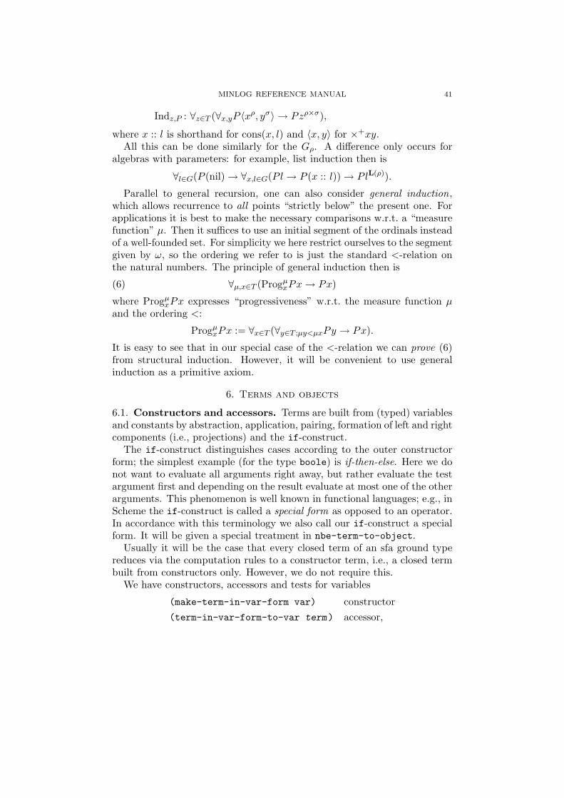
MINLOG REFERENCE MANUAL 41
Indz,P : ∀z∈T (∀x,yP 〈xρ, yσ〉 → Pzρ×σ),
where x :: l is shorthand for cons(x, l) and 〈x, y〉 for ×+xy.All this can be done similarly for the Gρ. A difference only occurs for
algebras with parameters: for example, list induction then is
∀l∈G(P (nil)→ ∀x,l∈G(Pl→ P (x :: l))→ PlL(ρ)).
Parallel to general recursion, one can also consider general induction,which allows recurrence to all points “strictly below” the present one. Forapplications it is best to make the necessary comparisons w.r.t. a “measurefunction” µ. Then it suffices to use an initial segment of the ordinals insteadof a well-founded set. For simplicity we here restrict ourselves to the segmentgiven by ω, so the ordering we refer to is just the standard <-relation onthe natural numbers. The principle of general induction then is
(6) ∀µ,x∈T (ProgµxPx→ Px)
where ProgµxPx expresses “progressiveness” w.r.t. the measure function µand the ordering <:
ProgµxPx := ∀x∈T (∀y∈T ;µy<µxPy → Px).
It is easy to see that in our special case of the <-relation we can prove (6)from structural induction. However, it will be convenient to use generalinduction as a primitive axiom.
6. Terms and objects
6.1. Constructors and accessors. Terms are built from (typed) variablesand constants by abstraction, application, pairing, formation of left and rightcomponents (i.e., projections) and the if-construct.
The if-construct distinguishes cases according to the outer constructorform; the simplest example (for the type boole) is if-then-else. Here we donot want to evaluate all arguments right away, but rather evaluate the testargument first and depending on the result evaluate at most one of the otherarguments. This phenomenon is well known in functional languages; e.g., inScheme the if-construct is called a special form as opposed to an operator.In accordance with this terminology we also call our if-construct a specialform. It will be given a special treatment in nbe-term-to-object.
Usually it will be the case that every closed term of an sfa ground typereduces via the computation rules to a constructor term, i.e., a closed termbuilt from constructors only. However, we do not require this.
We have constructors, accessors and tests for variables
(make-term-in-var-form var) constructor(term-in-var-form-to-var term) accessor,

42 HELMUT SCHWICHTENBERG
(term-in-var-form? term) test,
for constants
(make-term-in-const-form const) constructor(term-in-const-form-to-const term) accessor(term-in-const-form? term) test,
for abstractions
(make-term-in-abst-form var term) constructor(term-in-abst-form-to-var term) accessor(term-in-abst-form-to-kernel term) accessor(term-in-abst-form? term) test,
for applications
(make-term-in-app-form term1 term2) constructor(term-in-app-form-to-op term) accessor(term-in-app-form-to-arg term) accessor(term-in-app-form? term) test,
for pairs
(make-term-in-pair-form term1 term2) constructor(term-in-pair-form-to-left term) accessor(term-in-pair-form-to-right term) accessor(term-in-pair-form? term) test,
for the left and right component of a pair
(make-term-in-lcomp-form term) constructor(make-term-in-rcomp-form term) constructor(term-in-lcomp-form-to-kernel term) accessor(term-in-rcomp-form-to-kernel term) accessor(term-in-lcomp-form? term) test(term-in-rcomp-form? term) test
and for if-constructs
(make-term-in-if-form test alts . rest) constructor(term-in-if-form-to-test term) accessor(term-in-if-form-to-alts term) accessor(term-in-if-form-to-rest term) accessor
MINLOG REFERENCE MANUAL 43
(term-in-if-form? term) test,
where in make-term-in-if-form, rest is either empty or an all-formula.It is convenient to have more general application constructors and acces-
sors available, where application takes arbitrary many arguments and worksfor ordinary application as well as for component formation.
(mk-term-in-app-form term term1 ...) constructor(term-in-app-form-to-final-op term) accessor(term-in-app-form-to-args term) accessor,
Also for abstraction it is convenient to have a more general constructortaking arbitrary many variables to be abstracted one after the other
(mk-term-in-abst-form var1 ... term).
We also allow vector notation for recursion (cf. Joachimski and Matthes[13]).
Moreover we need
(term? x)
(term=? term1 term2)
(terms=? terms1 terms2)
(term-to-type term)
(term-to-free term)
(term-to-bound term)
(term-to-t-deg term)
(synt-total? term)
(term-to-string term).
6.2. Normalization. We need an operation which transforms a term intoits normal form w.r.t. the given computation and rewrite rules. Here webase our treatment on normalization by evaluation introduced in [5], andextended to arbitrary computation and rewrite rules in [4].
For normalization by evaluation we need semantical objects. For an ar-bitrary ground type every term family of that type is an object. For ansfa ground type, in addition the constructors have semantical counterparts.The freeness of the constructors is expressed by requiring that their rangesare disjoint and that they are injective. Moreover, we view the free algebraas a domain and require that its bottom element is not in the range of theconstructors. Hence the constructors are total and non-strict. Then by ap-plying nbe-reflect followed by nbe-reify we can normalize every term,where normalization refers to the computation as well as the rewrite rules.
44 HELMUT SCHWICHTENBERG
An object consists of a semantical value and a type.
(nbe-make-object type value) constructor(nbe-object-to-type object) accessor(nbe-object-to-value object) accessor(nbe-object? x) test.
To work with objects, we need
(nbe-object-apply function-obj arg-obj)
Again it is convenient to have a more general application operation available,which takes arbitrary many arguments and works for ordinary applicationas well as for component formation. We also need an operation composingtwo unary function objects.
(nbe-object-app function-obj arg-obj1 ...)
(nbe-object-compose function-obj1 function-obj2)
For ground type values we need constructors, accessors and tests. To makeconstructors “self-evaluating”, a constructor value has the form
(constr-value name objs delayed-constr),
where delayed-constr is a procedure of zero arguments which evaluates tothis very same constructor. This is necessary to avoid having a cycle (fornullary constructors, and only for those).
(nbe-make-constr-value name objs) constructor(nbe-constr-value-to-name value) accessor(nbe-constr-value-to-args value) accessor(nbe-constr-value-to-constr value) accessor(nbe-constr-value? value) test(nbe-fam-value? value) test.
The essential function which “animates” the program constants accordingto the given computation and rewrite rules is
(nbe-pconst-and-tsubst-and-rules-to-object
pconst tsubst comprules rewrules)
Using it we can the define an evaluation function, which assigns to a termand an environment a semantical object:
(nbe-term-to-object term bindings) evaluation.
Here bindings is an association list assigning objects of the same type tovariables. In case a variable is not assigned anything in bindings, by default

MINLOG REFERENCE MANUAL 45
we assign the constant term family of this variable, which always is an objectof the correct type.
The interpretation of the program constants requires some auxiliary func-tions (cf. [4]):
(nbe-constructor-pattern? term) test(nbe-inst? constr-pattern obj) test(nbe-genargs constr-pattern obj) generalized arguments(nbe-extract termfam) extracts a term from a family(nbe-match pattern term)
Then we can define
(nbe-reify object) reification(nbe-reflect term) reflection
and by means of these
(nbe-normalize-term term) normalization,
abbreviated nt.The if-form needs a special treatment. In particular, for a full normaliza-
tion of terms (including permutative conversions), we define a preprocessingstep that η expands the alternatives of all if-terms. The result containsif-terms with ground type alternatives only.
6.3. Substitution. Recall the generalities on substitutions in section 2.1.Under the conditions stated there on admissibility we define
(term-substitute term tosubst)
(term-subst term arg val)
(compose-substitutions subst1 subst2)
Display functions for substitutions are
(pp-subst topsubst)
(display-substitutions topsubst)
(substitution-to-string subst)
7. Formulas and comprehension terms
A prime formula has the form (predicate P r1 ... rn) with a pre-dicate variable or constant P and terms r1 . . . rn. Formulas are built fromprime formulas by
(i) (imp formula1 formula2) implication(ii) (all x formula) all quantification
46 HELMUT SCHWICHTENBERG
(iii) (impnc formula1 formula2) implication without computational con-tent
(iv) (allnc x formula) all quantification without computational content(v) (exca (x1 ...xn) formula) classical existential quantification (with
the arithmetical form of falsity F)(vi) (excl (x1 ...xn) formula) classical existential quantification (with
the logical form of falsity ⊥).(vii) (tensor formula1 formula2) tensor, for proper unfolding of formu-
las containing exca or excl.We allow that quantified variables are formed without ^, i.e., range overtotal objects only.
Formulas can be unfolded in the sense that the all classical existentialquantifiers are replaced according to their definition. Inversely a formulacan be folded in the sense that classical existential quantifiers are introducedwherever possible. Notice that, since ∃x∃yA unfolds into a rather awkwardformula, we have extended the ∃-terminology to lists of variables:
∃x1,...,xnA := ∀x1,...,xn(A→ ⊥)→ ⊥.In this context the tensor connective (written ∧) allows to abbreviate
∃x1,...,xn(A1 ∧ . . . ∧Am) := ∀x1,...,xn(A1 → · · · → Am → ⊥)→ ⊥.This way we stay in the→,∀ part of the language. Notice that ∧ only makessense in this context, i.e., in connection with ∃.
Leibniz equality, the existential quantifier, conjunction and disjunctionare provided by means of inductively defined predicates. Temporarily westill have built-in versions:
(i) (and formula1 formula2) conjunction(ii) (ex x formula) existential quantification
(iii) (exnc x formula) existential quantification without computationalcontent.
Temporarily we also allow prime formulas of the form (atom r) with aterm r of type boole. They can be replaced by Leibniz equality of r withthe boolean constant True, written True eqd r.
Comprehension terms have the form (cterm vars formula). Note thatformula may contain further free variables.
Tests:
(atom-form? formula)
(predicate-form? formula)
(prime-form? formula)
(imp-form? formula)

MINLOG REFERENCE MANUAL 47
(and-form? formula)
(tensor-form? formula)
(all-form? formula)
(ex-form? formula)
(allnc-form? formula)
(exnc-form? formula)
(exca-form? formula)
(excl-form? formula)
and also
(quant-prime-form? formula)
(quant-free? formula).
We need constructors and accessors for prime formulas
(make-atomic-formula boolean-term)
(make-predicate-formula predicate term1 ...)
atom-form-to-kernel
predicate-form-to-predicate
predicate-form-to-args.
We also have constructors for special atomic formulas
(make-eq term1 term2) constructor for equalities(make-= term1 term2) constructor for equalities on finalgs(make-total term) constructor for totalities(make-e term) constructor for existence on finalgstruth
falsity
falsity-log.
We need constructors and accessors for implications
(make-imp premise conclusion) constructor(imp-form-to-premise imp-formula) accessor(imp-form-to-conclusion imp-formula) accessor,
conjunctions
(make-and formula1 formula2) constructor(and-form-to-left and-formula) accessor
48 HELMUT SCHWICHTENBERG
(and-form-to-right and-formula) accessor,
tensors
(make-tensor formula1 formula2) constructor(tensor-form-to-left tensor-formula) accessor(tensor-form-to-right tensor-formula) accessor,
universally quantified formulas
(make-all var formula) constructor(all-form-to-var all-formula) accessor(all-form-to-kernel all-formula) accessor,
existentially quantified formulas
(make-ex var formula) constructor(ex-form-to-var ex-formula) accessor(ex-form-to-kernel ex-formula) accessor,
universally quantified formulas without computational content
(make-allnc var formula) constructor(allnc-form-to-var allnc-formula) accessor(allnc-form-to-kernel allnc-formula) accessor,
existentially quantified formulas without computational content
(make-exnc var formula) constructor(exnc-form-to-var exnc-formula) accessor(exnc-form-to-kernel exnc-formula) accessor,
existentially quantified formulas in the sense of classical arithmetic
(make-exca var formula) constructor(exca-form-to-var exca-formula) accessor(exca-form-to-kernel exca-formula) accessor,
existentially quantified formulas in the sense of classical logic
(make-excl var formula) constructor(excl-form-to-var excl-formula) accessor(excl-form-to-kernel excl-formula) accessor.
For convenience we also have as generalized constructors
(mk-imp formula formula1 ...) implication(mk-neg formula1 ...) negation
MINLOG REFERENCE MANUAL 49
(mk-neg-log formula1 ...) logical negation(mk-and formula formula1 ...) conjunction(mk-tensor formula formula1 ...) tensor(mk-all var1 ... formula) all-formula(mk-ex var1 ... formula) ex-formula(mk-allnc var1 ... formula) allnc-formula(mk-exnc var1 ... formula) exnc-formula
(mk-exca var1 ... formula) classical ex-formula (arithmetical)
(mk-excl var1 ... formula) classical ex-formula (logical)
and as generalized accessors
(imp-form-to-premises-and-final-conclusion formula)
(tensor-form-to-parts formula)
(all-form-to-vars-and-final-kernel formula)
(ex-form-to-vars-and-final-kernel formula)
and similarly for exca-forms and excl-forms. Occasionally it is convenientto have
(imp-form-to-premises formula <n>) all (first n) premises(imp-form-to-final-conclusion formula <n>)
where the latter computes the final conclusion (conclusion after removingthe first n premises) of the formula.
It is also useful to have some general procedures working for arbitraryquantified formulas. We provide
(make-quant-formula quant var1 ... kernel) constructor(quant-form-to-quant quant-form) accessor(quant-form-to-vars quant-form) accessor(quant-form-to-kernel quant-form) accessor(quant-form? x) test.
and for convenience also
(mk-quant quant var1 ... formula).
To fold and unfold formulas we have
(fold-formula formula)
(unfold-formula formula).

50 HELMUT SCHWICHTENBERG
To test equality of formulas up to normalization and α-equality we use
(classical-formula=? formula1 formula2)
(formula=? formula1 formula2),
where in the first procedure we unfold before comparing.Morever we need
(formula-to-free formula),
(formula-to-bound formula),
(nbe-formula-to-type formula),
(formula-to-prime-subformulas formula),
Constructors, accessors and a test for comprehension terms are
(make-cterm var1 ... formula) constructor(cterm-to-vars cterm) accessor(cterm-to-formula cterm) accessor(cterm? x) test.
Moreover we need
(cterm-to-free cterm)
(cterm=? x)
(classical-cterm=? x)
(fold-cterm cterm)
(unfold-cterm cterm).
Normalization of formulas is done with
(normalize-formula formula) normalization,
abbreviated nf.To check equality of formulas we use
(classical-formula=? formula1 formula2)
(formula=? formula1 formula2)
where the former unfolds the classical existential quantifiers and normalizesall subterms in its formulas.
Display functions for formulas and comprehension terms are
(pp formula)
(formula-to-string formula)
(cterm-to-string cterm).
MINLOG REFERENCE MANUAL 51
We can simultaneously substitute for type, object and predicate variablesin a formula or a comprehension term:
(formula-substitute formula topsubst)
(formula-subst formula arg val)
(cterm-substitute cterm topsubst)
(cterm-subst cterm arg val)
8. Assumption variables and constants
8.1. Assumption variables. Assumption variables are for proofs whatvariables are for terms. The main difference, however, is that assumptionvariables have formulas as types, and that formulas may contain free vari-ables. Therefore we must be careful when substituting terms for variables inassumption variables. Our solution (as in Matthes’ thesis [17]) is to consideran assumption variable as a pair of a (typefree) identifier and a formula, andto take equality of assumption variables to mean that both components areequal. Rather than using symbols as identifiers we prefer to use numbers(i.e., indices). However, sometimes it is useful to provide an optional stringas name for display purposes.
We need a constructor, accessors and tests for assumption variables.
(make-avar formula index name) constructor(avar-to-formula avar) accessor(avar-to-index avar) accessor(avar-to-name avar) accessor(avar? x) test(avar=? avar1 avar2) test.
For convenience we have the function
(mk-avar formula <index> <name>)
The formula is a required argument; however, the remaining arguments areoptional. The default for the name string is u. We also require that afunction
(formula-to-new-avar formula)
is defined that returns an assumption variable of the requested formula dif-ferent from all assumption variables that have ever been returned by any ofthe specified functions so far.
An assumption constant appears in a proof, as an axiom, a theorem ora global assumption. Its formula is given as an “uninstantiated formula”,

52 HELMUT SCHWICHTENBERG
where only type and predicate variables can occur freely; these are con-sidered to be bound in the assumption constant. In the proof the boundtype variables are implicitely instantiated by types, and the bound predicatevariables by comprehension terms (the arity of a comprehension term is thetype-instantiated arity of the corresponding predicate variable). Since wedo not have type and predicate quantification in formulas, the assumptionconstant contains these parts left implicit in the proof, as tpsubst.
So we have assumption constants of the following kinds:(i) axioms,(ii) theorems, and(iii) global assumptions.
To normalize a proof we will first translate it into a term, then normalizethe term and finally translate the normal term back into a proof. To makethis work, in case of axioms we pass to the term appropriate formulas: all-formulas for induction, an existential formula for existence introduction, andan existential formula together with a conclusion for existence elimination.During normalization of the term these formulas are passed along. Whenthe normal form is reached, we have to translate back into a proof. Thenthese formulas are used to reconstruct the axiom in question.
Internally, the formula of an assumption constant is split into an unin-stantiated formula where only type and predicate variables can occur freely,and a substitution for at most these type and predicate variables. The for-mula assumed by the constant is the result of carrying out this substitutionin the uninstantiated formula. Note that free variables may again occur inthe assumed formula. For example, assumption constants axiomatizing theexistential quantifier will internally have the form
(aconst Ex-Intro ∀xα(P (x)→ ∃xαP (x)) (α 7→ τ, P (α) 7→ { zτ | A }))
(aconst Ex-Elim ∃xαP (x)→ ∀xα(P (x)→ Q)→ Q
(α 7→ τ, P (α) 7→ { zτ | A }, Q 7→ { | B }))Interface for general assumption constants. To avoid duplication
of code it is useful to formulate some procedures generally for arbitraryassumption constants, i.e., for all of the forms listed above.
(make-aconst name kind uninst-formula tpsubst
repro-formula1 ...) constructor(aconst-to-name aconst) accessor(aconst-to-kind aconst) accessor(aconst-to-uninst-formula aconst) accessor(aconst-to-tpsubst aconst) accessor

MINLOG REFERENCE MANUAL 53
(aconst-to-repro-formulas aconst) accessor(aconst? x) test.
To construct the formula associated with an aconst, it is useful to separatethe instantiated formula from the variables to be generalized. The lattercan be obtained as free variables in inst-formula. We therefore provide
(aconst-to-inst-formula aconst)
(aconst-to-formula aconst)
We also provide
(aconst? aconst)
(aconst=? aconst1 aconst2)
(aconst-without-rules? aconst)
(aconst-to-string aconst)
8.2. Axiom constants. We use the natural numbers as a prototypical fini-tary algebra; recall Figure 1. Assume that n, p are variables of type N, B.Let ≈ denote the equality relation in the model. Recall the domain oftype B, consisting of tt, ff and the bottom element ⊥. The boolean valuedfunctions equality =nat : N → N → B and existence (definedness, totality)enat : N→ B need to be continuous. So we have
=(0, 0) ≈ tt
=(0, Sn) ≈ =(Sn, 0) ≈ ff e(0) ≈ tt
=(Sn1, Sn2) ≈ =(n1, n2) e(Sn) ≈ e(n)
=(⊥nat, n) ≈ =(n,⊥nat) ≈ ⊥ e(⊥N) ≈ ⊥=(∞nat, n) ≈ =(n,∞nat) ≈ ⊥ e(∞N) ≈ ⊥
Write T , F for atom(tt), atom(ff), r = s for atom(=(r, s)) and E(r) foratom(e(r)). We require the following axioms. Notice that all these axiomsbecome provable if we replace ≈ by the Leibniz equality (for Eq-Ext we needE-TCF).
T Truth-Axiom
x ≈ x Eq-Refl
x1 ≈ x2 → x2 ≈ x1 Eq-Symm
x1 ≈ x2 → x2 ≈ x3 → x1 ≈ x3 Eq-Trans
∀x(f1x ≈ f2x)→ f1 ≈ f2 Eq-Ext
x1 ≈ x2 → P (x1)→ P (x2) Eq-Compat

54 HELMUT SCHWICHTENBERG
Tρ→σ(f)↔ ∀x(Tρ(x)→ Tσ(f x)) Total
Tρ(c) Constr-Total
T (c~x )→ T (xi) Constr-Total-Args
and for every finitary algebra, e.g., nat
n1 ≈ n2 → E(n1)→ n1 = n2 Eq-to-=-1-nat
n1 ≈ n2 → E(n2)→ n1 = n2 Eq-to-=-2-nat
n1 = n2 → n1 ≈ n2 =-to-Eq-nat
n1 = n2 → E(n1) =-to-E-1-nat
n1 = n2 → E(n2) =-to-E-2-nat
T (n)→ E(n) Total-to-E-nat
E(n)→ T (n) E-to-Total-nat
Here c is a constructor. Notice that in T (c~x ) → T (xi), the type of (c~x )need not be a finitary algebra, and hence xi may have a function type.
Remark. (E(n1)→ n1 = n2)→ (E(n2)→ n1 = n2)→ n1 ≈ n2 is not validin our intended model (see Figure 1), since we have two distinct undefinedobjects ⊥nat and ∞nat.
We abbreviate
∀x(Tρ(x)→ A) by ∀xA,∃x(Tρ(x) ∧A) by ∃xA.
Formally, these abbreviations appear as axioms
∀xP (x)→ ∀x(T (x)→ P (x)) All-AllPartial
∀x(T (x)→ P (x))→ ∀xP (x) AllPartial-All
∃xP (x)→ ∃x(T (x) ∧ P (x)) Ex-ExPartial
∃x(T (x) ∧ P (x))→ ∃xP (x) ExPartial-Ex
and for every finitary algebra, e.g., nat
∀nP (n)→ ∀n(E(n)→ P (n)) All-AllPartial-nat
∃n(E(n) ∧ P (n))→ ∃nP (n) ExPartial-Ex-nat
Notice that AllPartial-All-nat i.e., ∀n(E(n)→ P (n))→ ∀nP (n) is prov-able (since E(n) 7→ T ). Similarly, Ex-ExPartial-nat, i.e., ∃nP (n) →∃n(E(n) ∧ P (n)) is provable.
Finally we have axioms for the existential quantifier
∀xα(P (x)→ ∃xαP (x)) Ex-Intro

MINLOG REFERENCE MANUAL 55
∃xαP (x)→ ∀xα(P (x)→ Q)→ Q Ex-Elim
The assumption constants corresponding to these axioms are
truth-aconst for Truth-Axiom
eq-refl-aconst for Eq-Refleq-symm-aconst for Eq-Symmeq-trans-aconst for Eq-Trans
ext-aconst for Eq-Exteq-compat-aconst for Eq-Compattotal-aconst for Total
(finalg-to-eq-to-=-1-aconst finalg) for Eq-to-=-1(finalg-to-eq-to-=-2-aconst finalg) for Eq-to-=-2(finalg-to-=-to-eq-aconst finalg) for =-to-Eq(finalg-to-=-to-e-1-aconst finalg) for =-to-E-1(finalg-to-=-to-e-2-aconst finalg) for =-to-E-2(finalg-to-total-to-e-aconst finalg) for Total-to-E(finalg-to-e-to-total-aconst finalg) for E-to-Total
all-allpartial-aconst for All-AllPartialallpartial-all-aconst for AllPartial-Allex-expartial-aconst for Ex-ExPartialexpartial-ex-aconst for ExPartial-Ex
(finalg-to-all-allpartial-aconst finalg) for All-AllPartial(finalg-to-expartial-ex-aconst finalg) for ExPartial-Ex
We now spell out what precisely we mean by induction over simultaneousfree algebras ~µ = µ~ξ ~κ, with goal formulas ∀
xµjjPj(xj). For the constructor
typeκi = ~ρ→ (~σ1 → ξj1)→ · · · → (~σn → ξjn)→ ξj ∈ KT~ξ
we have the step formula
Di := ∀yρ11 ,...,yρmm ,y
~σ1→µj1m+1 ,...,y
~σn→µjnm+n
(∀~x~σ1 Pj1(ym+1~x)→ · · · →
∀~x~σn Pjn(ym+n~x)→
Pj(C~µi (~y ))).

56 HELMUT SCHWICHTENBERG
Here ~y = yρ11 , . . . , yρmm , y
~σ1→µj1m+1 , . . . , y
~σn→µjnm+n are the components of the ob-
ject C~µi (~y ) of type µj under consideration, and
∀~x~σ1 Pj1(ym+1~x), . . . ,∀~x~σn Pjn(ym+n~x)
are the hypotheses available when proving the induction step. The inductionaxiom Indµj then proves the formula
Indµj : D1 → · · · → Dk → ∀xµjj Pj(xj).
We will often write Indj for Indµj .An example is
E1 → E2 → E3 → E4 → ∀xT1 P1(x1)
with
E1 := P1(Leaf),
E2 := ∀xTs(P2(x)→ P1(Branch(x))),
E3 := P2(Empty),
E4 := ∀xT1 ,xTs2
(P1(x1)→ P2(x2)→ P2(Tcons(x1, x2))).
Here the fact that we deal with a simultaneous induction (over tree andtlist), and that we prove a formula of the form ∀xT . . . , can all be inferredfrom what is given: the ∀xT . . . is right there, and for tlist we can look upthe simultaneously defined algebras. – The internal representation is
(aconst Ind E1 → E2 → E3 → E4 → ∀xT1 P1(x1)
(P1 7→ {xT1 | A1 }, P2 7→ {xTs
2 | A2 }))
A simplified version (without the recursive calls) of the induction axiomis the following cases axiom.
(aconst Cases E1 → E2 → ∀xT1 P1(x1) (P1 7→ {xT1 | A1 }))
with
E1 := P1(Leaf),
E2 := ∀Tsx P1(Branch(x)).
However, rather than using this as an assumption constant we will – parallelto the if-construct for terms – use a cases-construct for proofs. This doesnot change our notion of proof; it is done to have the if-construct in theextracted programs.

MINLOG REFERENCE MANUAL 57
The assumption constants corresponding to these axioms are generatedby
(all-formulas-to-ind-aconst all-formula1 ...) for Ind(all-formula-to-cases-aconst all-formula) for Cases
For the introduction and elimination axioms Ex-Intro and Ex-Elim forthe existential quantifier we provide
(ex-formula-to-ex-intro-aconst ex-formula)
(ex-formula-and-concl-to-ex-elim-aconst ex-formula concl)
and similarly for exnc instead of ex.To deal with inductively defined predicate constants, we need additional
axioms with names “Intro” and “Elim”, which can be generated by
(number-and-idpredconst-to-intro-aconst i idpc)
(imp-formulas-to-elim-aconst imp-formula1 ...);
here an imp-formula is expected to have the form I(~x)→ A.
8.3. Theorems. A theorem is a special assumption constant. Theoremsare normally created after successfully completing an interactive proof. Onemay also create a theorem from an explicitely given (closed) proof. Thecommand is
(add-theorem string . opt-proof) or save
From a theorem name we can access its aconst, its (original) proof and alsoits instantiated proof by
(theorem-name-to-aconst string)
(theorem-name-to-proof string)
(theorem-name-to-inst-proof string)
We also provide
(remove-theorem string1 ...)
(display-theorems string1 ...)
(pp theorem-name)
Initially we provide the following theorems
atom(p)→ p = tt Atom-True
(atom(p)→ F)→ p = ff Atom-False
F→ atom(p) Efq-Atom
((atom(p)→ F)→ F)→ atom(p) Stab-Atom

58 HELMUT SCHWICHTENBERG
and for every finitary algebra, e.g., nat
n = n =-Refl-nat
n1 = n2 → n2 = n1 =-Symm-nat
n1 = n2 → n2 = n3 → n1 = n3 =-Trans-nat
Proof of Atom-True. By Ind. In case tt use Eq-Compat with tt ≈ =(tt, tt) toinfer atom(=(tt, tt)) (i.e., tt = tt) from atom(tt). In case ff use Eq-Compatwith ff ≈ =(ff, tt) to infer atom(=(ff, tt)) (i.e., ff = tt) from atom(ff). �
Proof of Atom-False. Use Ind, and Truth-Axiom in both cases. – Noticethat the more general (atom(p)→ F)→ p = ff does not hold with ⊥ for p,since =(⊥, ff) ≈ ⊥. �
Proof of Efq-Atom. Again by Ind. In case tt use Truth-Axiom, and the caseff is obvious. �
Proof of Stab-Atom. By Ind. In case tt use Truth-Axiom, and the case ff isobvious. �
Remark. Notice that from Efq-Atom one easily obtains F → A for everyformula A all whose strictly positions occurrences of prime formulas are ofthe form atom(r), by induction on A. For all other formulas we shall makeuse of the global assumption Efq : F→ P (cf. section 8.4). Similarly, noticethat from Stab-Atom one again obtains ((A → F) → F) → A for everyformula A all whose strictly positions occurrences of prime formulas are ofthe form atom(r), by induction on A. For all other formulas we shall makeuse of the global assumption Stab : ((P → F)→ F)→ P (cf. section 8.4).
Proof of =-Refl-nat. Use Ind, and Truth-Axiom in both cases. – Noticethat n = n does not hold, since =(⊥,⊥) ≈ ⊥. �
Here are some other examples of theorems; we give the internal repre-sentation as assumption constants, which show how the assumed formula issplit into an uninstantiated formula and a substitution, in this case a typesubstitution α 7→ ρ, an object substitution fα→N 7→ gρ→N and a predicatevariable substitution P (α) 7→ { zρ | A }.(aconst Cvind-with-measure-11
∀α→Nf (∀xα(∀y(f(y)<f(x)→ P (y))→ P (x))→ ∀xP (x))
(α 7→ ρ, fα→N 7→ gρ→N, P (α) 7→ { zρ | A })).(aconst Minpr-with-measure-l11
∀fα→N(∃xαP (x)→ ∃x(P (x) ∧ ∀y(f(y)<f(x)→ P (y)→ ⊥)))
(α 7→ ρ, fα→N 7→ gρ→N, P (α) 7→ { zρ | A })).

MINLOG REFERENCE MANUAL 59
Here ∃ is the classical existential quantifier defined by ∃xA := ∀x(A→ ⊥)→⊥ with the logical form of falsity ⊥ (as opposed to the arithmetical formF). l indicates “logic” (we have used the logical form of falsity), the first1 that we have one predicate variable P , and the second that we quantifyover just one variable x. Both theorems can easily be generalized to moresuch parameters.
When dealing with classical logic it will be useful to have
(P → P1)→ ((P → ⊥)→ P1)→ P1 Cases-Log
The proof uses the global assumption Stab-Log (see below) for P1; hencewe cannot extract a term from it.
The assumption constants corresponding to these theorems are generatedby
(theorem-name-to-aconst name)
8.4. Global assumptions. A global assumption is a special assumptionconstant. It provides a proposition whose proof does not concern us pre-sently. Global assumptions are added, removed and displayed by
(add-global-assumption name formula) (abbreviated aga)(remove-global-assumption string1 ...)
(display-global-assumptions string1 ...)
We initially supply global assumptions for ex-falso-quodlibet and stability,both in logical and arithmetical form (for our two forms of falsity).
⊥ → P Efq-Log
((P → ⊥)→ ⊥)→ P Stab-Log
F→ P Efq
((P → F)→ F)→ P Stab
The assumption constants corresponding to these global assumptions aregenerated by
(global-assumption-name-to-aconst name)
9. Proofs
Proofs are built from assumption variables and assumption constants (i.e.,axioms, theorems and global assumption) by the usual rules of natural de-duction, i.e., introduction and elimination rules for implication, conjunctionand universal quantification. From a proof we can read off its context , whichis an ordered list of object and assumption variables.

60 HELMUT SCHWICHTENBERG
9.1. Constructors and accessors. We have constructors, accessors andtests for assumption variables
(make-proof-in-avar-form avar) constructor(proof-in-avar-form-to-avar proof) accessor,(proof-in-avar-form? proof) test,
for assumption constants
(make-proof-in-aconst-form aconst) constructor(proof-in-aconst-form-to-aconst proof) accessor(proof-in-aconst-form? proof) test,
for implication introduction
(make-proof-in-imp-intro-form avar proof) constructor(proof-in-imp-intro-form-to-avar proof) accessor(proof-in-imp-intro-form-to-kernel proof) accessor(proof-in-imp-intro-form? proof) test,
for implication elimination
(make-proof-in-imp-elim-form proof1 proof2) constructor(proof-in-imp-elim-form-to-op proof) accessor(proof-in-imp-elim-form-to-arg proof) accessor(proof-in-imp-elim-form? proof) test,
for and introduction
(make-proof-in-and-intro-form proof1 proof2) constructor(proof-in-and-intro-form-to-left proof) accessor(proof-in-and-intro-form-to-right proof) accessor(proof-in-and-intro-form? proof) test,
for and elimination
(make-proof-in-and-elim-left-form proof) constructor(make-proof-in-and-elim-right-form proof) constructor(proof-in-and-elim-left-form-to-kernel proof) accessor(proof-in-and-elim-right-form-to-kernel proof) accessor(proof-in-and-elim-left-form? proof) test(proof-in-and-elim-right-form? proof) test,

MINLOG REFERENCE MANUAL 61
for all introduction
(make-proof-in-all-intro-form var proof) constructor(proof-in-all-intro-form-to-var proof) accessor(proof-in-all-intro-form-to-kernel proof) accessor(proof-in-all-intro-form? proof) test,
for all elimination
(make-proof-in-all-elim-form proof term) constructor(proof-in-all-elim-form-to-op proof) accessor(proof-in-all-elim-form-to-arg proof) accessor(proof-in-all-elim-form? proof) test
and for cases-constructs
(make-proof-in-cases-form test alt1 ...) constructor(proof-in-cases-form-to-test proof) accessor(proof-in-cases-form-to-alts proof) accessor(proof-in-cases-form-to-rest proof) accessor(proof-in-cases-form? proof) test.
It is convenient to have more general introduction and elimination operatorsthat take arbitrary many arguments. The former works for implication-introduction and all-introduction, and the latter for implication-elimination,and-elimination and all-elimination.
(mk-proof-in-intro-form x1 ... proof)
(mk-proof-in-elim-form proof arg1 ...)
(proof-in-intro-form-to-kernel-and-vars proof)
(proof-in-elim-form-to-final-op proof)
(proof-in-elim-form-to-args proof).
(mk-proof-in-intro-form x1 ... proof) is formed from proof by firstabstracting x1, then x2 and so on. Here x1, x2 . . . can be assumption orobject variables. We also provide
(mk-proof-in-and-intro-form proof proof1 ...)
In our setup there are axioms rather than rules for the existential quan-tifier. However, sometimes it is useful to construct proofs as if an existenceintroduction rule would be present; internally then an existence introductionaxiom is used.
(make-proof-in-ex-intro-form term ex-formula proof-of-inst)
62 HELMUT SCHWICHTENBERG
(mk-proof-in-ex-intro-form .
terms-and-ex-formula-and-proof-of-inst)
Moreover we need
(proof? x)
(proof=? proof1 proof2)
(proofs=? proofs1 proofs2)
(proof-to-formula proof)
(proof-to-context proof)
(proof-to-free proof)
(proof-to-free-avars proof)
(proof-to-bound-avars proof)
(proof-to-free-and-bound-avars proof)
(proof-to-aconsts-without-rules proof).
(proof-to-aconsts proof).
To work with contexts we need
(context-to-vars context)
(context-to-avars context)
(context=? context1 context2).
9.2. Decorating proofs. In this section we are interested in “fine-tuning”the computational content of proofs, by inserting decorations. Here is anexample (due to Constable) of why this is of interest. Suppose that in aproof M of a formula C we have made use of a case distinction based onan auxiliary lemma stating a disjunction, say L : A ∨ B. Then the extractet(M) will contain the extract et(L) of the proof of the auxiliary lemma,which may be large. Now suppose further that in the proof M of C, theonly computationally relevant use of the lemma was which one of the twoalternatives holds true, A or B. We can express this fact by using a weakenedform of the lemma instead: L′ : A∨uB. Since the extract et(L′) is a boolean,the extract of the modified proof has been “purified” in the sense that the(possibly large) extract et(L) has disappeared.
We consider the question of “optimal” decorations of proofs: suppose weare given an undecorated proof, and a decoration of its end formula. Thetask then is to find a decoration of the whole proof (including a furtherdecoration of its end formula) in such a way that any other decoration“extends” this one. Here “extends” just means that some connectives havebeen changed into their more informative versions, disregarding polarities.
MINLOG REFERENCE MANUAL 63
We show that such an optimal decoration exists, and give an algorithm toconstruct it.
We denote the sequent of a proof M by Seq(M); it consists of its contextand end formula.
The proof pattern P(M) of a proof M is the result of marking in c.r.formulas of M (i.e., those not above a c.i. formula) all occurrences of impli-cations and universal quantifiers as non-computational, except the “unin-stantiated” formulas of axioms and theorems. For instance, the inductionaxiom for N consists of the uninstantiated formula ∀cn(P0 →c ∀cn(Pn →c
P (Sn))→c PnN) with a unary predicate variable P and a predicate substi-tution P 7→ {x | A(x) }. Notice that a proof pattern in most cases is not acorrect proof, because at axioms formulas may not fit.
We say that a formula D extends C if D is obtained from C by changingsome (possibly zero) of its occurrences of non-computational implicationsand universal quantifiers into their computational variants →c and ∀c.
A proof N extends M if (i) N and M are the same up to variants ofimplications and universal quantifiers in their formulas, and (ii) every c.r.formula of M is extended by the corresponding one in N . Every proof Mwhose proof pattern P(M) is U is called a decoration of U .
Notice that if a proof N extends another one M , then FV(et(N)) isessentially (that is, up to extensions of assumption formulas) a superset ofFV(et(M)). This can be proven by induction on N .
We assume that every axiom has the property that for every extension ofits formula we can find a further extension which is an instance of an axiom,and which is the least one under all further extensions that are instancesof axioms. This property clearly holds for axioms whose uninstantiatedformula only has the decorated→c and ∀c, for instance induction. However,in ∀cn(A(0) →c ∀cn(A(n) →c A(Sn)) →c A(nN)) the given extension of thefour A’s might be different. One needs to pick their “least upper bound” asfurther extension. To make this assumption true for the other (introductionand elimination) axioms we simply add all their extensions as axioms, ifnecessary.
One can define a decoration algorithm [20], assigning to every proof pat-tern U and every extension of its sequent an “optimal” decoration M∞ ofU , which further extends the given extension of its sequent.
Theorem. Under the assumption above, for every proof pattern U and everyextension of its sequent Seq(U) we can find a decoration M∞ of U such that(a) Seq(M∞) extends the given extension of Seq(U), and(b) M∞ is optimal in the sense that any other decoration M of U whose
sequent Seq(M) extends the given extension of Seq(U) has the propertythat M also extends M∞.

64 HELMUT SCHWICHTENBERG
The main function for decorating is
decorate proof . opt-decfla-and-name-and-altname
The default case for opt-decfla is the formula of the proof. If opt-decflais present, it must be a decoration variant of the formula of the proof. If theoptional argument name-and-altname is present, then in every recursivecall it is checked whether (1) the present proof is an application of theassumption constant op with name to some args, (2) op applied to argsproves an extension of decfla, and (3) altop applied to args and some ofdecavars is between op applied to args and decfla w.r.t. extension. If so,a proof based on altop is returned, else one carries on.
An important auxiliary function is proof-to-ppat. used to transform aproof into its proof pattern. It turns every →, ∀ formula in the given proofinto an →nc, ∀nc formula, including the parts of an assumption constantwhich come from its uninstatiated formula. It does not touch the c.i. partsof the proof, i.e., those which are above a c.i. formula. Recall that the proofpattern ppat is in general not a proof.
9.3. Normalization. Normalization of proofs will be done by reductionto normalization of terms. (1) Construct a term from the proof. To dothis properly, create for every free avar in the given proof a new variablewhose type comes from the formula of the avar; store this information. Notethat in this construction one also has to create new variables for the boundavars. Similary to avars we have to treat assumption constants which are notaxioms, i.e., theorems or global assumptions. (2) Normalize the resultingterm. (3) Reconstruct a normal proof from this term, the end formulaand the stored information. – The critical variables are carried along forefficiency reasons.
To assign recursion constants to induction constants, we need to associatetype variables with predicate variables, in such a way that we can later referto this assignment. Therefore we carry along a procedure pvar-to-tvarwhich remembers the assignment done so far (cf. make-rename).
Due to our distinction between general variables x^0, x^1, x^2, . . . andvariables x0, x1, x2, . . . intended to range over total objects only, η-conversionof proofs cannot be done via reduction to η-conversion of terms. To see this,consider the proof
∀xPx xPx∀xPx
∀xPx→ ∀xPx
MINLOG REFERENCE MANUAL 65
The proof term is λuλx(ux). If we η-normalize this to λuu, the proven for-mula would be all ∀xPx→ ∀xPx. Therefore we split nbe-normalize-proofinto nbe-normalize-proof-without-eta and proof-to-eta-nf.
Moreover, for a full normalization of proofs (including permutative con-versions) we need a preprocessing step that η-expands each ex-elim axiomsuch that the conclusion is atomic or existential.
We need the following functions.
(proof-and-genavar-var-alist-to-pterm pvar-to-tvar proof)
(npterm-and-var-genavar-alist-and-formula-to-proof
npterm var-genavar-alist crit formula)
(elim-npterm-and-var-genavar-alist-to-proof
npterm var-genavar-alist crit).
Then we can define nbe-normalize-proof, abbreviated np.
9.4. Substitution. In a proof we can substitute(i) types for type variables (by a type variable substitution tsubst),(ii) terms for variables (by a substitution subst),(iii) comprehension terms for predicate variables (by a predicate variable
substitution psubst), and(iv) proofs for assumption variables (by a assumption variable substitution
asubst).All these substitutions can be packed together, as an argument topasubstfor proof-substitute. It is assumed that topasubst is admissible, in thesense of section 2.1.
(proof-substitute proof topasubst)
If we want to substitute for a single variable only (which can be a type-, anobject-, a predicate- or an assumption-variable), then we can use
(proof-subst proof arg val)
The procedure expand-theorems expects a proof and a test whether astring denotes a theorem to be replaced by its proof. The result is the(normally quite long) proof obtained by replacing the theorems by theirsaved proofs.
(expand-theorems proof name-test?)
9.5. Display. There are many ways to display a proof. We normally usedisplay-proof for a linear representation, showing the formulas and therules used. When we in addition want to check the correctness of theproof, we can use check-and-display-proof, abbreviated cdp. We also

66 HELMUT SCHWICHTENBERG
provide a readable type-free lambda expression via proof-to-expr, andcan add useful information with one of proof-to-expr-with-formulas,proof-to-expr-with-aconsts.
To display proofs we use the following functions. In case the optionalproof argument is not present, the current proof of an interactive proofdevelopment is taken instead.
(display-proof . opt-proof) abbreviated dp
(check-and-display-proof . opt-proof) abbreviated cdp
(proof-to-expr . opt-proof)
(proof-to-expr-with-formulas . opt-proof)
(proof-to-expr-with-aconsts . opt-proof)
(display-pterm . opt-proof) abbreviated dpt
(display-proof-expr . opt-proof) abbreviated dpe
We also provide versions which normalize the proof first:
(display-normalized-proof . opt-proof) abbreviated dnp
(display-normalized-pterm . opt-proof) abbreviated dnpt
(display-normalized-proof-expr . opt-proof) abbreviated dnpe
9.6. Classical logic. (proof-of-stab-at formula) generates a proof of((A → F) → F) → A. For F, T one takes the obvious proof, and for otheratomic formulas the proof using cases on booleans. For all other prime orexistential formulas one takes an instance of the global assumption Stab:((P → F) → F) → P . Here the argument formula must be unfolded. Forthe logical form of falsity we take (proof-of-stab-log-at formula), andsimilary for ex-falso-quodlibet we provide
(proof-of-efq-at formula)
(proof-of-efq-log-at formula)
Using these functions we can then define (reduce-efq-and-stab proof),which reduces all instances of stability and ex-falso-quodlibet axioms in aproof to instances of these global assumptions with prime or existentialformulas, or (if possible) replaces them by their proofs.
With rm-exc we can transform a proof involving classical existential quan-tifiers in another one without, i.e., in minimal logic. The Exc-Intro andExc-Elim theorems are replaced by their proofs, using expand-theorems.
10. Interactive theorem proving with partial proofs
A partial proof is a proof with holes, i.e., special assumption variables(called goal variables) v, v1, v2 . . . whose formulas must be closed. We

MINLOG REFERENCE MANUAL 67
assume that every goal variable v has a single occurrence in the proof. Wethen select a (not necessarily maximal) subproof vx1...xn with distinctobject or assumption variables x1...xn. Such a subproof is called a goal .When interactively developing a partial proof, a goal vx1...xn is replacedby another partial proof, whose context is a subset of x1...xn (i.e., thecontext of the goal with v removed).
To gain some flexibility when working on our goals, we do not at eachstep of an interactive proof development traverse the partial proof searchingfor the remaining goals, but rather keep a list of all open goals together withtheir numbers as we go along. We maintain a global variable PPROOF-STATEcontaining a list of three elements: (1) num-goals, an alist of entries (numbergoal drop-info hypname-info), (2) proof and (3) maxgoal, the maximalgoal number used.
At each stage of an interactive proof development we have access to thecurrent proof and the current goal by executing
(current-proof)
(current-goal)
For interactively building proofs we need
(goal-to-goalvar goal)
(goal-to-context goal)
(goal-to-formula goal)
(goal=? proof goal)
(goal-subst proof goal proof1)
(pproof-state-to-num-goals)
(pproof-state-to-proof)
(pproof-state-to-formula)
(display-current-goal)
(display-current-goal-with-normalized-formulas)
(display-current-pproof-state)
We list some commands for interactively building proofs.
10.1. set-goal. An interactive proof starts with (set-goal formula), i.e.,with setting a goal. Here formula should be closed; if it is not, universalquantifiers are inserted automatically.
10.2. normalize-goal. (normalize-goal . ng-info) (short: ng) takesoptional arguments ng-info. If there are none, the goal formula and allhypotheses are normalized. Otherwise exactly those among the hypotheses
68 HELMUT SCHWICHTENBERG
and the goal formula are normalized whose numbers (or names, or just #tfor the goal formula) are listed as additional arguments.
10.3. assume. With (assume x1 ...) we can move universally quantifiedvariables and hypotheses into the context. The variables must be givennames (known to the parser as valid variable names for the given type), andthe hypotheses should be identified by numbers or strings.
10.4. use. In (use x . elab-path-and-terms), x is one of the following.(i) A number or string identifying a hypothesis form the context.(ii) A formula with free variables from the context, generating a new goal.(iii) The name of a theorem or global assumption.(iv) A closed proof.
It is checked whether some final part of this used formula has the form of (or“matches”) the goal, where if (i) x determines a hypothesis or is the formulafor a new goal, then all its free topvars are rigid, and if (ii) x determines aclosed proof, then all its (implicitely generalized) tpvars are flexible, exceptthe predicate variable ⊥ (written bot) from falsity-log. elab-path-and-terms is a list consisting of symbols left or right, giving directions in casethe used formula contains conjunctions, and of terms/cterms to be substi-tuted for the variables that cannot be instantiated by matching. Matching isdone for type and object variables first (via match), and in case this fails withhuet-match next. There is a similar (use2 x . elab-path-and-terms),which only applies huet-match.
10.5. use-with. This is a more verbose form of use, where the terms arenot inferred via unification, but have to be given explicitely. Also, for theinstantiated premises one can indicate how they are to come about. So in(use-with x . x-list), x is one of the following.
(i) A number or string identifying a hypothesis form the context.(ii) The name of a theorem or global assumption. If it is a global assump-
tion whose final conclusion is a nullary predicate variable distinct frombot (e.g. Efq-Log or Stab-Log), this predicate variable is substitutedby the goal formula.
(iii) A closed proof.(iv) A formula with free variables from the context, generating a new goal.
Moreover x-list is a list consisting of(i) a number or string identifying a hypothesis form the context,(ii) the name of a theorem or global assumption,(iii) a closed proof,(iv) the string “?” (value of DEFAULT-GOAL-NAME), generating a new goal,(v) a symbol left or right,
MINLOG REFERENCE MANUAL 69
(vi) a term, whose free variables are added to the context,(vii) a type, which is substituted for the first type variable,(viii) a comprehension term, which is substituted for the first predicate vari-
able.Notice that new free variables not in the ordered context can be intro-
duced in use-with. They will be present in the newly generated goals. Thereason is that proofs should be allowed to contain free variables. This isnecessary to allow logic in ground types where no constant is available (e.gto prove ∀xPx→ ∀x¬Px→ ⊥).
Notice also that there are situations where use-with can be applied but usecan not. For an example, consider the goal P (S(k+ l)) with the hypothesis∀lP (k + l) in the context. Then use cannot find the term Sl by matching;however, applying use-with to the hyposthesis and the term Sl succeeds(since k + Sl and S(k + l) have the same normal form).
10.6. inst-with. inst-with does for forward chaining the same as use-withfor backward chaining. It replaces the present goal by a new one, with oneadditional hypothesis obtained by instantiating a previous one. Notice thatthis effect could also be obtained by cut. In (inst-with x . x-list), xis
(i) a number or string identifying a hypothesis form the context,(ii) the name of a theorem or global assumption,
(iii) a closed proof,(iv) a formula with free variables from the context, generating a new goal.and x-list is a list consisting of
(i) a number or string identifying a hypothesis form the context,(ii) the name of a theorem or global assumption,
(iii) a closed proof,(iv) the string “?” (value of DEFAULT-GOAL-NAME), generating a new goal,(v) a symbol left or right,
(vi) a term, whose free variables are added to the context,(vii) a type, which is substituted for the first type variable,(viii) a comprehension term, which is substituted for the first predicate vari-
able.
10.7. inst-with-to. inst-with-to expects a string as its last argument,which is used (via name-hyp) to name the newly introduced instantiatedhypothesis.
10.8. cut. The command (cut A) replaces the goal B by the two new goalsA and A→ B, with A→ B to be proved first.

70 HELMUT SCHWICHTENBERG
10.9. assert. The command (assert A) replaces the goal B by the twonew goals A and A→ B, with A to be proved first.
10.10. strip. To move (all or n) universally quantified variables and hy-potheses of the current goal into the context, we use the command (strip)or (strip n).
10.11. drop. In (drop . x-list), x-list is a list of numbers or strings iden-tifying hypotheses from the context. A new goal is created, which differsfrom the previous one only in display aspects: the listed hypotheses arehidden (but still present). If x-list is empty, all hypotheses are hidden.
10.12. name-hyp. The command name-hyp expects an index i and a string.Then a new goal is created, which differs from the previous one only indisplay aspects: the string is used to label the ith hypothesis.
10.13. split, msplit. The command (split) expects as goal a conjunctionA ∧ B or an AndConst-atom, and splits it into two new goals A and B.We allow multiple split (msplit) over a conjunctive formula (all conjunctsconnected through & which are at the same level are split at once).
10.14. get. To be able to work on a goal different from that on top of thegoal stack, we have have to move it up using (get n).
10.15. undo. With (undo . n), the last n steps of an interactive proof canbe made undone. (undo) has the same effect as (undo 1).
10.16. ind. (ind) expects a goal ∀xιA(x) with x total and ι an algebra, or agoal ∀xι(STotal x→ A(x)) with x partial. Let c1, . . . , cn be the constructorsof the algebra. In the first case, n new goals ∀~xi(A(x1i) → · · · → A(xki) →A(ci~xi) are generated. In the second case, for every non-parameter variablexji the new goal has an additional assumption STotal xji.
(ind t) expects a goal A(t). It computes the algebra ι as type of theterm t. Then again the n new goals above are generated. If t is partial,another new goal STotal t is generated.
10.17. simind. (simind all-formula1 ...) expects a goal ∀xιA(x) withx total and ι an algebra, or ∀xι(STotal x→ A(x)) with x partial. We haveto provide as arguments the other all-formulas to be proved simultaneouslywith the goal.
10.18. gind. (gind h) expects a goal ∀~xA(~x ) with ~x total. It generates anew goal Progh{ ~x | A(~x ) } where h is a term of type ~ρ→ N, xi has type ρiand Progh{ ~x | A(~x ) } := ∀~x(∀~y(h~y < h~x→ A(~y ))→ A(~x )).
(gind h t1 ...tn) expects a goal A(~t ) and generates the same goal asfor (gind h) with the formula ∀~xA(x).
MINLOG REFERENCE MANUAL 71
10.19. intro. (intro i . terms) expects as goal an inductively definedpredicate. The i-th introduction axiom for this predicate is applied, via use(hence terms may have to be provided). (intro-with i . x-list) doesthe same, via use-with.
10.20. elim. Recall that I~r provides (i) a type substitution, (ii) a predicateinstantiation, and (iii) the list ~r of argument terms. In (elim idhyp) idhypis, with an inductively defined predicate I,
(i) a number or string identifying a hypothesis I~r form the context(ii) the name of a global assumption or theorem I~r;
(iii) a closed proof of a formula I~r;(iv) a formula I~r with free variables from the context, generating a new
goal.Then the (strengthened) elimination axiom is used with ~r for ~x and idhypfor I~r to prove the goal A(~r ), leaving the instantiated (with { ~x | A(~x ) })clauses as new goals.
(elim) expects a goal I~r → A(~r ). Then the (strengthened) clauses aregenerated as new goals, via use-with.
In case of simultaneously inductively defined predicate constants we canprovide other imp-formulas to be proved simultaneously with the given one.Then the (strengthened) simplified clauses are generated as new goals.
10.21. inversion, simplified-inversion. (inversion x . imp-formulas)assumes that x is one of the following.
(i) A number or string identifying a hypothesis I~r form the context.(ii) The name of a theorem or global assumption stating I~r.
(iii) A closed proof of I~r.(iv) A formula I~r with free vars from the context, generating a new goal.imp-formulas have the form J~s → B. Here I, J are inductively definedpredicates, with clauses K1, . . . ,Kn. Now one uses the elim-aconst for I~x→~x = ~r → A with A the goal formula and the additional implications J~y →~y = ~s→ B, with “?” for the clauses, ~r for ~x and proofs for ~r = ~r, to obtainthe goal. Then many of the generated goals for the clauses will containfalse premises, coming from substituted equations ~x = ~r, and are provedautomatically.
imp-formulas not provided are taken as J~x→ J~x. Generated clauses forsuch J are proved automatically from the intro axioms (the rec-prems arenot needed).
For simultaneous inductively defined predicates (simplified-inversionx . imp-formulas) does not add imp-formulas J~x→ J~x to form the elim-aconst. Then the (new) imp-formulas-to-uninst-elim-formulas-etcgenerates simplified clauses. In some special cases this suffices.

72 HELMUT SCHWICHTENBERG
10.22. ex-intro. In (ex-intro term), the user provides a term to be usedfor the present (existential) goal. (exnc-intro x) works similarly for theexnc-quantifier.
10.23. ex-elim. In (ex-elim x), x is(i) a number or string identifying an existential hypothesis from the con-
text,(ii) the name of an existential global assumption or theorem,(iii) a closed proof on an existential formula,(iv) an existential formula with free variables from the context, generating
a new goal.Let ∃yA be the existential formula identified by x. The user is then askedto provide a proof for the present goal, assuming that a y satisfying A isavailable. (exnc-elim x) works similarly for the exnc-quantifier.
10.24. by-assume-with. Suppose we are proving a goal G from an exis-tential hypothesis ExHyp : ∃yA. Then the natural way to use this hypothesisis to say “by ExHyp assume we have a y satisfying A”. Correspondinglywe provide (by-assume-with x y u). Here x – as in ex-elim – identi-fies an existential hypothesis, and we assume (i.e., add to the context) thevariable y and – with label u – the kernel A. (by-assume-with x y u)is implemented by the sequence (ex-elim x), (assume y u), (drop x).by-exnc-assume-with works similarly for the exnc-quantifier.
10.25. cases. (cases) expects a goal ∀xιA(x) with x total and ι an alge-bra, or a goal ∀xι(STotal x → A(x)) with x partial. Let c1, . . . , cn be theconstructors of the algebra. In the first case, n new goals ∀~xiA(ci~xi) aregenerated. In the second case, for every non-parameter variable xji the newgoal has an additional assumption STotal xji.
(cases t) expects a goalA(t). If t is a total boolean term, the goalA(t) isreplaced by the two new goals atom(t)→ A(tt) and (atom(t)→ F)→ A(ff),and if t is not total also STotal t. If t is a total non-boolean term, casesis called with the all-formula ∀x(x = t→ A(x)), and if t is a non-total non-boolean term, cases is called with the all-formula ∀x(STotal x→ x = t→A(x)).
(cases ’auto) expects an atomic goal and checks whether its booleankernel contains an if-term whose test is neither an if-term nor contains boundvariables. With the first such test (cases test) is called.
10.26. casedist. (casedist t) replaces the goal A containing a booleanterm t by two new goals atom(t) → A(tt) and (atom(t) → F) → A(ff), andif t is not total also STotal t.

MINLOG REFERENCE MANUAL 73
10.27. simp. In (simp opt-dir x . elab-path-and-terms), the optionalargument opt-dir is either the string “<-” or missing. x is
(i) a number or string identifying a hypothesis form the context,(ii) the name of a theorem or global assumption,(iii) a closed proof,(iv) a formula with free variables from the context, generating a new goal.
The optional elab-path-and-terms is a list consisting of symbols left orright, giving directions in case the used formula contains conjunctions, andof terms. The universal quantifiers of the used formula are instantiatedwith appropriate terms to match a part of the goal. The terms provided aresubstituted for those variables that cannot be inferred. For the instantiatedpremises new goals are created. This generates a used formula, which is tobe an atom, a negated atom or t ≈ s. If it as a (negated) atom, it is checkedwhether the kernel or its normal form is present in the goal. If so, it isreplaced by T (or F). If it is an equality t = s or t ≈ s with t or its normalform present in the goal, t is replaced by s. In case “<-” exchange t and s.
10.28. simp-with. This is a more verbose form of simp, where the termsare not inferred via matching, but have to be given explicitely. Also, forthe instantiated premises one can indicate how they are to come about. Soin (simp-with opt-dir x . x-list), opt-dir and x are as in simp, andx-list is a list consisting of
(i) a number or string identifying a hypothesis form the context,(ii) the name of a theorem or global assumption,
(iii) a closed proof,(iv) the string “?” (value of DEFAULT-GOAL-NAME), generating a new goal,(v) a symbol left or right,
(vi) a term, whose free variables are added to the context,(vii) a type, which is substituted for the first type variable,(viii) a comprehension term, which is substituted for the first predicate vari-
able.
10.29. simphyp-with. simphyp-with does for forward chaining the sameas simp-with for backward chaining. It replaces the present goal by anew one, with one additional hypothesis obtained by simplifying a previousone. Notice that this effect could also be obtained by cut or assert. In(simphyp-with opt-dir hyp . x-list), hyp is one of the following.
(i) A number or string identifying a hypothesis form the context.(ii) The name of a theorem or global assumption, but not one whose final
conclusion is a predicate variable.(iii) A closed proof.(iv) A formula with free variables from the context, generating a new goal.

74 HELMUT SCHWICHTENBERG
x-list is a list consisting of(i) a number or string identifying a hypothesis form the context,(ii) the name of a theorem or global assumption,(iii) a closed proof,(iv) the string “?” (value of DEFAULT-GOAL-NAME), generating a new goal,(v) a symbol left or right,(vi) a term, whose free variables are added to the context,
(vii) a type, which is substituted for the first type variable,(viii) a comprehension term, which is substituted for the first predicate vari-
able.This generates a used formula, which is to be an atom, a negated atom ort ≈ s. If it as a (negated) atom, it is checked whether the kernel or itsnormal form is present in the goal. If so, it is replaced by T (or F). If it isan equality t = s or t ≈ s with t or its normal form present in the goal, t isreplaced by s. In case “<-” exchange t and s.
10.30. simphyp-with-to. simp-with-to expects a string as its last argu-ment, which is used (via name-hyp) to name the newly introduced simplifiedhypothesis.
10.31. min-pr. In (min-pr x measure), x is(i) a number or string identifying a classical existential hypothesis from
the context,(ii) the name of a classical existential global assumption or theorem,(iii) a closed proof on a classical existential formula,(iv) a classical existential formula with free variables from the context,
generating a new goal.The result is a new implicational goal, whose premise provides the (classical)existence of instances with least measure.
We also provide exc-formula-to-min-pr-proof. It computes first agind-aconst (an axiom or a theorem) and from this a proof of the minimumprinciple.
10.32. by-assume-minimal-with. For convenience in classical argumentsthere is (by-assume-minimal-with exc-hyp . rest) where rest may becalled varnames-and-measure-and-minhyp-and-hyps. It is meant for the fol-lowing situation. Suppose we are proving a goal G from a classical existentialhypothesis ∃~x ~A. Then by the minimum principle we can assume that wehave ~x which are minimal w.r.t. a measure h such that ~A are satisfied.
We also provide make-gind-aconst. It takes a positive integer n and re-turns an assumption constant for general induction w.r.t. a measure functionof type α1 → . . .→ αn → N.

MINLOG REFERENCE MANUAL 75
Finally we provide make-min-pr-aconst. It takes positive integers m,nand returns an assumption constant for the minimum principle w.r.t. a mea-sure function of type α1 → . . .→ αn → N.
10.33. exc-intro. In (exc-intro terms), the user provides terms to beused for the present (classical existential) goal. Moreover we also providemake-exc-intro-aconst and exc-formula-to-exc-intro-aconst
10.34. exc-elim. In (exc-elim x), x is(i) a number or string identifying a classical existential hypothesis from
the context,(ii) the name of a classical existential global assumption or theorem,(iii) a closed proof on a classical existential formula,(iv) a classical existential formula with free variables from the context,
generating a new goal.
Let ∃~y ~A be the classical existential formula identified by x. The user isthen asked to provide a proof for the present goal, assuming that terms ~ysatisfying ~A are available. Moreover we also provide make-exc-elim-aconstand exc-formula-to-exc-elim-aconst.
10.35. pair-elim. In (pair-elim), a goal ∀pP (p) is replaced by the newgoal ∀x1,x2P (〈x1, x2〉).
10.36. admit. (admit) temporarily accepts the present goal, by turning itinto a global assumption.
11. Unification and proof search
We describe a proof search method suitable for minimal logic with higherorder functionals. It is based on Huet’s [12] unification algorithm for thesimply typed lambda calculus.
Huet’s unification algorithm does not terminate in general; this must bethe case, since it is well known that higher order unification is undecidable.However, non-termination can be avoided if we restrict ourselves to a certainfragment of higher order (simply typed) minimal logic. This fragment isdetermined by requiring that every higher order variable Y can only occurin a context Y ~x, where ~x are distinct bound variables in the scope of theoperator binding Y , and of opposite polarity. Note that for first order logicthis restriction does not mean anything, since there are no higher ordervariables. However, when designing a proof search algorithm for first orderlogic only, one is naturally led into this fragment of higher order logic, wherethe algorithm works as well.
76 HELMUT SCHWICHTENBERG
In this section we only present the algorithms and state their proper-ties. Proofs can be found in the accompanying document “A Theory ofComputable Functionals”, also in the Minlog distribution.
11.1. Huet’s unification algorithm. We work in the simply typed λ-calculus, with the usual conventions. For instance, whenever we write aterm we assume that it is correctly typed. Substitutions are denoted byϕ,ψ, ρ. The result of applying a substitution ϕ to a term r or a formula Ais written as rϕ or Aϕ, with the understanding that after the substitutionall terms are brought into long normal form.Q always denotes a ∀∃∀-prefix, say ∀~x∃~y∀~z, with distinct variables. We
call ~x the signature variables, ~y the flexible variables and ~z the forbiddenvariables of Q, and write Q∃ for the existential part ∃~y of Q. A variable iscalled rigid if it is either a signature variable or else a forbidden variable.
A Q-term is a term with all its free variables in Q, and similarly a Q-formula is a formula with all its free variables in Q. A Q-substitution is asubstitution of Q-terms.
A unification problem U consists of a ∀∃∀-prefix Q and a conjunction Cof equations between Q-terms of the same type, i.e.,
∧∧ni=1 ri = si. We may
assume that each such equation is of the form λ~xr = λ~xs with the same ~x(which may be empty) and r, s of ground type.
A solution to such a unification problem U is a Q-substitution ϕ suchthat for every i, riϕ = siϕ holds (i.e., riϕ and siϕ have the same normalform). We sometimes write C as ~r = ~s, and (for obvious reasons) call it alist of unification pairs.
We now define the unification algorithm. It takes a unification problemU = QC and produces a not necessarily well-founded tree (called matchingtree by Huet [12]) with nodes labelled by unification problems and verticeslabelled by substitutions.
Definition (Unification algorithm). We distinguish cases according to theform of the unification problem, and either give the transition done by thealgorithm, or else state that it fails.
Case identity, i.e., Q(r = r ∧ C). Then
Q(r = r ∧ C) =⇒ε QC.
Case ξ, i.e., Q(λ~xr = λ~xs ∧ C). We may assume here that the boundvariables ~x are the same on both sides.
Q(λ~x r = λ~x s ∧ C) =⇒ε Q∀~x(r = s ∧ C).
Case rigid-rigid, i.e., Q(f~r = g~s ∧ C) with both f and g rigid, that iseither a signature variable or else a forbidden variable. If f is different from
MINLOG REFERENCE MANUAL 77
g then fail. If f equals g,
Q(f~r = f~s ∧ C) =⇒ε Q(~r = ~s ∧ C).
Case flex-rigid, i.e., Q(u~r = f~s ∧ C) with f rigid. Then the algorithmbranches into one imitation branch and m projection branches, where r =r1, . . . , rm. Imitation replaces the flexible head u, using the substitution ρ =[u := λ~x(f(h1~x) . . . (hn~x))] with new variables ~h and ~x. This is only allowedif f is a signature (and not a forbidden) variable. For ri we have a projectionif and only if the final value type of ri is the (ground) type of f~s. Then thei-th projections pulls ri in front, by ρ = [u := λ~x(xi(h1~x) . . . (hni~x))]. Ineach of these branches we have
Q(u~r = f~s ∧ C) =⇒ρ Q′(u~r = f~s ∧ C)ρ,
where Q′ is obtained from Q by removing ∃u and adding ∃~h.Case flex-flex, i.e., Q(u~r = v~s ∧ C). If there is a first flex-rigid or rigid-
flex equation in C, pull this equation (possibly swapped) to the front andapply case flex-rigid. Otherwise, i.e., if all equations are between termswith flexible heads, pick a new variable z of ground type and let ρ be thesubstitution mapping each of these flexible heads u to λ~xz.
Q(u~r = v~s ∧ C) =⇒ρ Q∅.
This concludes the definition of the unification algorithm.
Clearly ρ is defined on flexible variables of Q only, and its value termshave no free occurrences of forbidden variables from Q. One can provecorrectness and completeness of this algorithm.
Theorem (Huet). Let a unification problem U consisting of a ∀∃∀-prefix Qand a list ~r = ~s of unification pairs be given. Then either(a) the unification algorithm can make a transition, and
(i) (correctness) for every transition U =⇒ρ U ′ and U ′-solution ϕ′ thesubstitution (ρ ◦ ϕ′)�Q∃ is a U-solution, and
(ii) (completeness) for every U-solution ϕ there is a transition U =⇒ρ
U ′ and U ′-solution ϕ′ such that ϕ = (ρ ◦ ϕ′)�Q∃, and moreoverµ(ϕ′) ≤ µ(ϕ) with < in case flex-rigid, or else
(b) the unification algorithm fails, and there is no U-solution, or else(c) the unification algorithm succeeds, and ~r = ~s is empty.Here µ(ϕ) denotes the number of applications in the value terms of ϕ.
Corollary. Given a unification problem U = QC, and a success node in thematching tree, labelled with a prefix Q′ (i.e., a unification problem U ′ with nounification pairs). Then by composing the substitution labels on the branchleading to this node we obtain a pair (Q′, ρ) with a “transition” substitution

78 HELMUT SCHWICHTENBERG
ρ and such that for any Q′-substitution ϕ′, (ρ ◦ ϕ′)�Q∃ is an U-solution.Moreover, every U-solution can be obtained in this way, for an appropriatesuccess node. Since the empty substitution is a Q′-substitution, ρ�Q∃ is aU-solution, which is most general in the sense stated.
11.2. The pattern unification algorithm. We restrict the notion of aQ-term as follows. Q-terms are inductively defined by the following clauses.
• If u is a universally quantified variable in Q or a constant, and ~r areQ-terms, then u~r is a Q-term.• For any flexible variable y and distinct forbidden variables ~z fromQ, y~z is a Q-term.• If r is a Q∀z-term, then λzr is a Q-term.
Explicitely, r is a Q-term iff all its free variables are in Q, and for everysubterm y~r of r with y free in r and flexible in Q, the ~r are distinct variableseither λ-bound in r (such that y~r is in the scope of this λ) or else forbiddenin Q.Q-goals and Q-clauses are simultaneously defined by
• If ~r are Q-terms, then P~r is a Q-goal as well as a Q-clause.• If D is a Q-clause and G is a Q-goal, then D → G is a Q-goal.• If G is a Q-goal and D is a Q-clause, then G→ D is a Q-clause.• If G is a Q∀x-goal, then ∀xG is a Q-goal.• If D[y := Y ~z ] is a ∀~x∃~y,Y ∀~z -clause, then ∀yD is a ∀~x∃~y∀~z -clause.
Explicitely, a formula A is a Q-goal iff all its free variables are in Q, and forevery subterm y~r of A with y either existentially bound in A (with y~r in thescope) or else free in A and flexible in Q, the ~r are distinct variables eitherλ- or universally bound in A (such that y~r is in the scope) or else free in Aand forbidden in Q.
A Q-substitution is a substitution of Q-terms.A pattern unification problem U consists of a ∀∃∀-prefix Q and a conjunc-
tion C of equations between Q-terms of the same type, i.e.,∧∧n
i=1(ri = si).We may assume that each such equation is of the form λ~xr = λ~xs with thesame ~x (which may be empty) and r, s of ground type.
A solution to such a unification problem U is a Q-substitution ϕ suchthat for every i, riϕ = siϕ holds (i.e., riϕ and siϕ have the same normalform). We sometimes write C as ~r = ~s, and (for obvious reasons) call it alist of unification pairs.
We now define the pattern unification algorithm. It takes a unificationproblem U = QC and returns a substitution ρ and another unification prob-lem U ′ = Q′C ′. Note that ρ will be neither a Q-substitution nor a Q′-substitution, but will have the property that
MINLOG REFERENCE MANUAL 79
(a) ρ is defined on flexible variables of Q only, and its value terms have nofree occurrences of forbidden variables from Q,
(b) if G is a Q-goal, then Gρ is a Q′-goal, and(c) whenever ϕ′ is a U ′-solution, then (ρ ◦ ϕ′)�Q∃ is a U-solution.
Definition (Pattern unification algorithm). We distinguish cases accordingto the form of the unification problem, and either give the transition doneby the algorithm, or else state that it fails.
Case identity, i.e., Q(r = r ∧ C). Then
Q(r = r ∧ C) =⇒ε QC.
Case ξ, i.e., Q(λ~xr = λ~xs ∧ C). We may assume here that the boundvariables ~x are the same on both sides.
Q(λ~xr = λ~xs ∧ C) =⇒ε Q(∀~x(r = s) ∧ C).
Case rigid-rigid, i.e., Q(f~r = f~s ∧ C) with f either a signature variableor else a forbidden variable.
Q(f~r = f~s ∧ C) =⇒ε Q(~r = ~s ∧ C).
Case flex-flex with equal heads, i.e., Q(u~y = u~z ∧ C).
Q(u~y = u~z ∧ C) =⇒ρ Q′(Cρ)
with ρ = [u := λ~y(u′ ~w)], Q′ is Q with ∃u replaced by ∃u′ , and ~w an enu-meration of those yi which are identical to zi (i.e., the variable at the sameposition in ~z ). Notice that λ~y(u′ ~w) = λ~z(u′ ~w).
Case flex-flex with different heads, i.e., Q(u~y = v~z ∧ C).
Q(u~y = v~z ∧ C) =⇒ρ Q′Cρ,
where ρ and Q′ are defined as follows. Let ~w be an enumeration of thevariables both in ~y and in ~z. Then ρ = [u, v := λ~y(u′ ~w ), λ~z(u′ ~w )], and Q′
is Q with ∃u,∃v removed and ∃u′ inserted.Case flex-rigid, i.e., Q(u~y = t ∧ C) with t rigid, i.e., not of the form v~z
with flexible v.Subcase occurrence check: t contains (a critical subterm with head) u.
Then fail.Subcase pruning: t contains a subterm v ~w1z ~w2 with ∃v in Q, and z free
in t but not in ~y.
Q(u~y = t ∧ C) =⇒ρ Q′(u~y = tρ ∧ Cρ)
where ρ = [v := λ~w1λzλ~w2
(v′ ~w1 ~w2)], Q′ is Q with ∃v replaced by ∃v′ .Subcase pruning impossible: λ~yt (after all pruning steps are done still)
has a free occurrence of a forbidden variable z. Then fail.

80 HELMUT SCHWICHTENBERG
Subcase explicit definition: otherwise.
Q(u~y = t ∧ C) =⇒ρ Q′Cρ
where ρ = [u := λ~yt], and Q′ is obtained from Q by removing ∃u. Thisconcludes the definition of the pattern unification algorithm.
One can prove that this algorithm indeed has the three properties statedabove. The first one (ρ is defined on flexible variables of Q only, and its valueterms have no free occurrences of forbidden variables from Q) is obvious fromthe definition. We now state the second one; the third one will be statednext.
Lemma (Q′-goals). If Q =⇒ρ Q′ and G is a Q-goal, then Gρ is a Q′-goal.
Let Q −→ρ Q′ mean that for some C,C ′ we have QC =⇒ρ Q
′C ′. WriteQ −→∗ρ Q′ if there are ρ1, . . . , ρn and Q1, . . . , Qn−1 such that
Q −→ρ1 Q1 −→ρ2 . . . −→ρn−1 Qn−1 −→ρn Q′,
and ρ = ρ1 ◦ · · · ◦ ρn.
Corollary. If Q −→∗ρ Q′ and G is a Q-goal, then Gρ is a Q′-goal.
Lemma. Let a unification problem U consisting of a ∀∃∀-prefix Q and a list~r = ~s of unification pairs be given. Then either
(a) the unification algorithm makes a transition U =⇒ρ U ′, and
Φ′ : U ′-solutions→ U-solutions
ϕ′ 7→ (ρ ◦ ϕ′)�Q∃
is well-defined and we have Φ: U-solutions → U ′-solutions such that Φ′
is inverse to Φ, i.e. Φ′(Φϕ) = ϕ, or else(b) the unification algorithm fails, and there is no U-solution.
It is not hard to see that the unification algorithm terminates, by defininga measure that decreases with each transition.
Corollary. Given a unification problem U = QC, the unification algorithmeither fails, and there is no U-solution, or else returns a pair (Q′, ρ) witha “transition” substitution ρ and a prefix Q′ (i.e., a unification problem U ′with no unification pairs) such that for any Q′-substitution ϕ′, (ρ◦ϕ′)�Q∃ isan U-solution, and every U-solution can be obtained in this way. Since theempty substitution is a Q′-substitution, ρ�Q∃ is a U-solution, which is mostgeneral in the sense stated.
MINLOG REFERENCE MANUAL 81
11.3. Proof search. A Q-sequent has the form P ⇒ G, where P is a listof Q-clauses and G is a Q-goal.
We write M [P] to indicate that all assumption variables in the derivationM are assumptions of clauses in P.
Write `n S for a set S of sequents if there are derivations MGii [Pi] in long
normal form for all (Pi ⇒ Gi) ∈ S such that∑
dp(Mi) ≤ n. Let `<n Smean ∃m<n `m S.
We prove correctness and completeness of the proof search procedure:correctness is the if-part of the two lemmata to follow, and completenessthe only-if-part.
Lemma. Let Q be a ∀∃∀-prefix, {P ⇒ ∀~x( ~D → A)} ∪ S Q-sequents with~x, ~D not both empty. Then we have for every substitution ϕ:
ϕ is a Q-substitution such that `n({P ⇒ ∀~x( ~D → A)} ∪ S
)ϕ
if and only if
ϕ is a Q∀~x-substitution such that `<n({P ∪ ~D ⇒ A} ∪ S
)ϕ.
Proof. “If”. Let ϕ be a Q∀~x-substitution and `<n({P ∪ ~D ⇒ A} ∪ S
)ϕ.
So we haveNAϕ[ ~Dϕ ∪ Pϕ].
Since ϕ is a Q∀~x-substitution, no variable in ~x can be free in Pϕ, or free inyϕ for some y ∈ dom(ϕ). Hence
M (∀~x( ~D→A))ϕ[Pϕ] := λ~xλ~u~DϕN
is a correct derivation.“Only if”. Let ϕ be a Q-substitution and `n
({P ⇒ ∀~x( ~D → A)} ∪ S
)ϕ.
This means we have a derivation (in long normal form)
M (∀~x( ~D→A))ϕ[Pϕ] = λ~xλ~u~Dϕ(NAϕ[ ~Dϕ ∪ Pϕ]).
Now dp(N) < dp(M), hence `<n({P ∪ ~D ⇒ A} ∪ S
)ϕ, and ϕ clearly is a
Q∀~x-substitution. �
Lemma. Let Q be a ∀∃∀-prefix, {P ⇒ P~r} ∪ S Q-sequents and ϕ a substi-tution. Then
ϕ is a Q-substitution such that `n({P ⇒ P~r} ∪ S
)ϕ
if and only if there is a clause ∀~x(~G → P~s ) in P such that the followingholds. Let ~z be the final universal variables in Q, ~X be new (“raised”) vari-ables such that Xi~z has the same type as xi, let Q∗ be Q with the existentialvariables extended by ~X, and let ∗ indicate the substitution [x1, . . . , xn :=X1~z, . . . , Xn~z ]. Then there is a result (Q′, ρ) of either Huet’s or the pattern

82 HELMUT SCHWICHTENBERG
unification algorithm applied to Q∗(~r = ~s∗) and a Q′-substitution ϕ′ suchthat `<n
({P ⇒ ~G∗} ∪ S
)ρϕ′, and ϕ = (ρ ◦ ϕ′)�Q∃.
Proof. “If”. Let (Q′, ρ) be such a result, and assume that ϕ′ is a Q′-substitution such that Ni `
(P ⇒ ~G∗
)ρϕ′. Let ϕ := (ρ ◦ ϕ′)�Q∃. From
unif(Q∗, ~r = ~s∗) = (Q′, ρ) we know ~rρ = ~s∗ρ, hence ~rϕ = ~s∗ρϕ′. Then
u(∀~x. ~G→P~s)ϕ(( ~Xρϕ′)~z ) ~N ~G∗ρϕ′
derives P~s∗ρϕ′ (i.e., P~rϕ) from Pϕ.“Only if”. Assume ϕ is a Q-substitution such that ` (P ⇒ P~r)ϕ, say by
u∀~x(~G→P~s)ϕ~t ~N ( ~Gϕ)[~x:=~t], with ∀~x(~G→ P~s) a clause in P, and with additional
assumptions from Pϕ in ~N . Then ~rϕ = (~sϕ)[~x := ~t]. Since we can assumethat the variables ~x are new and in particular not range variables of ϕ, with
ϑ := ϕ ∪ [~x := ~t]
we have ~rϕ = ~sϑ. Let ~z be the final universal variables in Q, ~X be new(“raised”) variables such that Xi~z has the same type as xi, let Q∗ be Q withthe existential variables extended by ~X, and for terms and formulas let ∗indicate the substitution [x1, . . . , xn := X1~z, . . . , Xn~z ]. Moreover, let
ϑ∗ := ϕ ∪ [X1, . . . , Xn := λ~zt1, . . . , λ~ztn].
Then ~rϑ∗ = ~rϕ = ~sϑ = ~s∗ϑ∗, i.e., ϑ∗ is a solution to the unification problemgiven by Q∗ and ~r = ~s. Hence by the corollary unif(Q∗, ~r = ~s∗) = (Q′, ρ) andthere is aQ′-substitution ϕ′ such that ϑ∗ = (ρ◦ϕ′)�Q∗∃, hence ϕ = (ρ◦ϕ′)�Q∃.Also, (~Gϕ)[~x := ~t ] = ~Gϑ = ~G∗ϑ∗ = ~G∗ρϕ′. �
A state is a pair (Q,S) with Q a prefix and S a finite set of Q-sequents.By the two lemmas just proved we have state transitions
(Q, {P ⇒ ∀~x( ~D → A)} ∪ S) 7→ε (Q∀~x, {P ∪ ~D ⇒ A} ∪ S)
(Q, {P ⇒ P~r} ∪ S) 7→ρ (Q′, ({P ⇒ ~G∗} ∪ S)ρ),
where in the latter case there is a clause ∀~x(~G → P~s ) in P such that thefollowing holds. Let ~z be the final universal variables in Q, ~X be new(“raised”) variables such that Xi~z has the same type as xi, let Q∗ be Q withthe existential variables extended by ~X, and let ∗ indicate the substitution[x1, . . . , xn := X1~z, . . . , Xn~z ], and unif(Q∗, ~r = ~s∗) = (Q′, ρ).
Notice that by the lemma on Q′-goals above, if P ⇒ P~r is a Q-sequent(which means that
∧∧P → P~r is a Q-goal), then (P ⇒ ~G∗)ρ is a Q′-sequent.
Theorem. Let Q be a prefix, and S be a set of Q-sequents. For everysubstitution ϕ we have: ϕ is a Q-substitution satisfying ` Sϕ iff there is a

MINLOG REFERENCE MANUAL 83
prefix Q′, a substitution ρ and a Q′-substitution ϕ′ such that
(Q,S) 7→ρ∗ (Q′, ∅),ϕ = (ρ ◦ ϕ′)�Q∃.
Examples. (a) The sequent ∀y(∀zRyz → Q),∀y1,y2Ry1y2 ⇒ Q leads firstto ∀y1,y2Ry1y2 ⇒ Ryz under ∃y∀z, then to y1 = y ∧ y2 = z under∃y∀z∃y1,y2 , and finally to Y1z = y ∧ Y2z = z under ∃y,Y1,Y2∀z, which hasthe solution Y1 = λzy, Y2 = λzz.
(b) ∀y(∀zRyz → Q),∀y1Ry1y1 ⇒ Q leads first to ∀y1Ry1y1 ⇒ Ryz under∃y∀z, then to y1 = y ∧ y1 = z under ∃y∀z∃y1 , and finally to Y1z =y ∧ Y1z = z under ∃y,Y1∀z, which has no solution.
(c) Here is a more complex example (derived from proofs of the Orevkov-formulas), for which we only give the derivation tree.
∀y(∀z(Ryz→⊥))→⊥∀z(R0z→⊥)→⊥
∀y(∀z1(Ryz1→⊥)→⊥)∀z1(Rzz1→⊥)→⊥
∀z(S0z→⊥)S0z1→⊥
(∗) R0z Rzz1S0z1
⊥Rzz1→⊥
∀z1(Rzz1→⊥)⊥
R0z→⊥∀z(R0z→⊥)
⊥where (∗) is a derivation from Hyp1 : ∀z,z1(R0z → Rzz1 → S0z1).
11.4. Extension by ∧ and ∃. The extension by conjunction is rather easy;it is even superfluous in principle, since conjunctions can always be avoidedat the expense of having lists of formulas instead of single formulas.
However, having conjunctions available is clearly useful at times, so let’sadd it. This requires the notion of an elaboration path for a formula (cf. [18]).The reason is that the property of a formula to have a unique atom as itshead is lost when conjunctions are present. An elaboration path is meant togive the directions (left or right) to go when we encounter a conjunction asa strictly positive subformula. For example, the elaboration paths of ∀xA∧(B ∧C → D ∧ ∀yE) are (left), (right, left) and (right, right). Clearly,a formula is equivalent to the conjunction (over all elaboration paths) ofall formulas obtained from it by following an elaboration path (i.e., alwaysthrowing away the other part of the conjunction). In our example,
∀xA ∧ (B ∧ C → D ∧ ∀yE)↔ ∀xA ∧ (B ∧ C → D) ∧ (B ∧ C → ∀yE).
In this way we regain the property of a formula to have a unique head, andour previous search procedure continues to work.
84 HELMUT SCHWICHTENBERG
For the existential quantifier ∃ the problem is of a different nature. Wechose to introduce ∃ by means of axiom schemata. Then the problem iswhich of such schemes to use in proof search, given a goal G and a set P ofclauses. We might proceed as follows.
List all prime, positive and negative existential subformulas of P ⇒ G,and remove any formula from those lists which is of the form of another one1.For every positive existential formula – say ∃xB – add (the generalizationof) the existence introduction scheme
∃+x,B : ∀x(B → ∃xB)
to P. Moreover, for every negative existential formula – say ∃xA – and every(prime or existential) formula C in any of those two lists, except the formula∃xA itself, add (the generalization of) the existence elimination scheme
∃−x,A,B : ∃xA→ ∀x(A→ B)→ B
to P. Then start the search algorithm as described in section 11.3. Thenormal form theorem for the natural deduction system of minimal logicwith ∃ then guarantees completeness.
However, experience has shown that this complete search procedure tendsto be trapped in too large a search space. Therefore in our actual implemen-tation we decided to only take instances of the existence elimination schemewith existential conclusions.
Moreover, it seems appropriate that – before the search is started – oneeliminates in a preprocessing step as many existential quantifiers as possible.
11.5. Implementation. Following Miller [18], Berger and [22], we haveimplemented a proof search algorithm for minimal logic. To enforce termi-nation, every assumption can only be used a fixed number of times.
We work with lists of sequents instead of single sequents; they all areQ-sequents for the same prefix Q. One then searches for a Q-substitutionϕ and proofs of the ϕ-substituted sequents. intro-search takes the firstsequent and extends Q by all universally quantified variables x1 . . . . Itthen calls select, which selects (using or) a fitting clause. If one is found,a new prefix Q′ (raising the new flexible variables) is formed, and the n(≥ 0) new goals with their clauses (and also all remaining sequents) aresubstituted with star ◦ ρ, where star is the “raising” substitution and ρ isthe most general unificator. For this constellation intro-search is calledagain. In case of success, one obtains a Q′-substitution ϕ′ and proofs of thestar ◦ ρ ◦ ϕ′ -substituted new sequents. Let ϕ := (ρ ◦ ϕ′)�Q∃, and take the
1To do this, for patterns the dual of the theory of “most general unifiers”, i.e., a theoryof “most special generalizations”, needs to be developed.

MINLOG REFERENCE MANUAL 85
first n proofs of these to build a proof of the ϕ-substituted (first) sequentoriginally considered by intro-search.
(search m (name1 m1) ...) expects for m a default value for multi-plicity (i.e., how often assumptions are to be used), for name1 . . .
(i) numbers of hypotheses from the present context or(ii) names for theorems or global assumptions,
and for m1 . . . multiplicities (positive integers for global assumptions ortheorems). A search is started for a proof of the goal formula from thegiven hypotheses with the given multiplicities and in addition from the otherhypotheses (but not any other global assumptions or theorems) with mor mult-default. To exclude a hypothesis from being tried, list it withmultiplicity 0.
11.6. Notes. I have benefitted from a presentation of Miller’s [18] given byUlrich Berger, in a logic seminar in Munchen in 1991. The type of restrictionto higher order terms described in the text has been introduced in [18]; ithas been called patterns by Nipkow [19]. Miller also noted its relevance forextensions of logic programming, and showed that the unification problemfor patterns is solvable and admits most general unifiers. The present treat-ment was motivated by the desire to use Miller’s approach as a basis for animplementation of a simple proof search engine for (first and higher order)minimal logic.
Compared with Miller [18], we make use of several simplifications, opti-mizations and extensions, in particular the following.
(i) Instead of arbitrarily mixed prefixes we only use those of the form∀∃∀. Nipkow in [19] already had presented a version of Miller’s patternunification algorithm for such prefixes, and Miller in [18, section 9.2]notes that in such a situation any two unifiers can be transformedinto each other by a variable renaming substitution. Here we restrictourselves to ∀∃∀-prefixes throughout, i.e., in the proof search algorithmas well.
(ii) The order of events in the pattern unification algorithm is changedslightly, by postponing the raising step until it is really needed. Thisavoids unnecessary creation of new higher type variables. – AlreadyMiller noted in [18, p.515] that such optimizations are possible.
(iii) The extensions concern the (strong) existential quantifier, which hasbeen left out in Miller’s treatment, and also conjunction(cf. 11.4). Thelatter can be avoided in principle, but of course is a useful thing tohave.

86 HELMUT SCHWICHTENBERG
12. Extracted terms
We assign to every formula A an object τ(A) (a type or the symbolnulltype). τ(A) is intended to be the type of the program to be extractedfrom a proof of A. This is done by
(formula-to-et-type formula)
In formula-to-et-type we assign type variables to the predicate variables.For to be able to later refer to this assignment, we use a global variablePVAR-TO-TVAR-ALIST, which memorizes the assigment done so far. Laterreference is necessary, because such type variables will appear in extractedprograms of theorems involving predicate variables, and in a given develop-ment there may be many auxiliary lemmata containing the same predicatevariable. A fixed pvar-to-tvar refers to and updates PVAR-TO-TVAR-ALIST.
When we want to execute the program, we have to replace the constantcL corresponding to a lemma L by the extracted program of its proof, andthe constant cGA corresponding to a global assumption GA by an assumedextracted term to be provided by the user. This can be achieved by addingcomputation rules for cL and cGA. We can be rather flexible here and en-able/block rewriting by using animate/deanimate as desired. Notice thatthe type of the extracted term provided for a cGA must be the extracted typeof the assumed formula. When predicate variables are present, one must usethe type variables assigned to them in PVAR-TO-TVAR-ALIST.
(animate thm-or-ga-name . opt-eterm)
(deanimate thm-or-ga-name)
We can define, for a given derivation M of a formula A with τ(A) 6=nulltype, its extracted term (or extracted program) et(M) of type τ(A).We also need extracted terms for the axioms. For induction we take recur-sion, for the proof-by-cases axiom we take the cases-construct for terms; forthe other axioms the extracted terms are rather clear. Term extraction isimplemented by
(proof-to-extracted-term proof)
The following table gives the symbols of Minlog’s output and the corre-sponding notation in the λ-calculus.

MINLOG REFERENCE MANUAL 87
Explanation Symbol Minlog’s outputλ-abstraction λxM ([x]M)pair 〈M,N〉 (M@N)left element of a pair (M 0) left Mright element of a pair (M 1) right Marrow for types → =>product for types × @@recursion operator R Rec
It is also possible to give an internal proof of soundness. This can be doneby
(proof-to-soundness-proof proof)
13. Computational content of classical proofs
13.1. Refined A-translation. In this section the connectives →, ∀ denotethe computational versions →c, ∀c, unless stated otherwise.
We will concentrate on the question of classical versus constructive proofs.It is known, by the so-called “A-translation” of Friedman [10] and Dragalin[8], that any proof of a specification of the form ∀x∃yB with B quantifier-free and a weak (or “classical”) existential quantifier ∃y, can be transformedinto a proof of ∀x∃yB, now with the constructive existential quantifier ∃y.However, when it comes to extraction of a program from a proof obtainedin this way, one easily ends up with a mess. Therefore, some refinements ofthe standard transformation are necessary. We shall study a refined methodof extracting reasonable and sometimes unexpected programs from classicalproofs. It applies to proofs of formulas of the form ∀x∃yB where B need notbe quantifier-free, but only has to belong to the larger class of goal formulas.Furthermore we allow unproven lemmata D to appear in the proof of ∀x∃yB,where D is a definite formula.
We now describe in more detail what this section is about. It is well knownthat from a derivation of a classical existential formula ∃yA := ∀y(A→ ⊥)→⊥ one generally cannot read off an instance. A simple example has beengiven by Kreisel: let R be a primitive recursive relation such that ∃zRxz isundecidable. Clearly – even logically –
` ∀x∃y∀z(Rxz → Rxy)
but there is no computable f satisfying
∀x∀z(Rxz → R(x, f(x))),
for then ∃zRxz would be decidable: it would be true if and only if R(x, f(x))holds.

88 HELMUT SCHWICHTENBERG
However, it is well known that in case ∃yG with G quantifier-free one canread off an instance. Here is a simple idea of how to prove this: replace ⊥anywhere in the proof by ∃yG. Then the end formula ∀y(G → ⊥) → ⊥ isturned into ∀y(G→ ∃yG)→ ∃yG, and since the premise is trivially provable,we have the claim.
Unfortunately, this simple argument is not quite correct. First, G maycontain ⊥, and hence is changed under the substitution of ∃yG for ⊥. Sec-ond, we may have used axioms or lemmata involving ⊥ (e.g., ⊥ → P ), whichneed not be derivable after the substitution. But in spite of this, the simpleidea can be turned into something useful.
Assume that the lemmata ~D and the goal formula G are such that we canderive
~D → Di[⊥ := ∃yG],(7)
G[⊥ := ∃yG]→ ∃yG.(8)
Assume also that the substitution [⊥ := ∃yG] turns any axiom into aninstance of the same axiom-schema, or else into a derivable formula. Thenfrom our given derivation (in minimal logic) of ~D → ∀y(G → ⊥) → ⊥ weobtain
~D[⊥ := ∃yG]→ ∀y(G[⊥ := ∃yG]→ ∃yG)→ ∃yG.Now (7) allows the substitution in ~D to be dropped, and by (8) the secondpremise is derivable. Hence we obtain as desired
~D → ∃yG.
We shall identify classes of formulas – to be called definite and goal formulas– such that slight generalizations of (7) and (8) hold.
This section is based on [3] and particularly [23, 7.3], where the theoryis developed in more detail and further references are given. Recall that werestrict to formulas in the language {⊥,→,∀}.
A formula is relevant if it ends with (logical) falsity. Definite and goalformulas are defined by a simultaneous recursion.
(atr-relevant? formula)
(atr-definite? formula)
(atr-goal? formula)
We need to construct proofs from F→ ⊥ of
DF → D,
G→ (GF → ⊥)→ ⊥,((RF → F)→ ⊥)→ R for R relevant and definite,
MINLOG REFERENCE MANUAL 89
I → IF for I irrelevant and goal.
This is done by
(atr-arb-definite-proof formula)
(atr-arb-goal-proof formula)
(atr-rel-definite-proof formula)
(atr-irrel-goal-proof formula)
The next task is to generalize G → (GF → ⊥) → ⊥ and construct a proofof (GF
1 → ...→ GFn → ⊥)→ G1 → ...→ Gn → ⊥, via
(atr-goals-F-to-bot-proof . goals)
Given a proof of ~A → ~D → ∀~y(~G → ⊥) → ⊥ with ~A arbitrary, ~D definiteand ~G goal formulas, we transform it into a proof of (F→ ⊥)→ ~A→ ~DF →∀~y(~GF → ⊥)→ ⊥. This is done via
(atr-min-excl-proof-to-bot-reduced-proof min-excl-proof)
Substituting the formula ∃~y ~GF for ⊥ in the proof given above of (F →⊥) → ~A → ~DF → ∀~y(~GF → ⊥) → ⊥, both the ex-falso-quodlibet premiseand the “wrong formula” ∀~y(~GF → ⊥) become provable and we obtain aproof of ~A′ → ~DF → ∃~y ~GF, where ~A′ is defined to be ~A[⊥ := ∃~y ~GF]. Thecorresponding function is
(atr-min-excl-proof-to-ex-proof min-excl-proof)
One can test with min-excl-proof? whether a given proof indeed is aproof in minimal logic of a classical (i.e., weak) existence formula. Moreover,atr-expand-theorems expands all non-definite theorems. This only makessense before substituting for ⊥.
See section 12 for an interpretation of the symbols of the extracted termsin Minlog’s output.
13.2. Godel’s Dialectica interpretation. In his original functional inter-pretation [11], Godel assigned to every formula A a new one ∃~x∀~yAD(~x, ~y )with AD(~x, ~y ) quantifier-free. Here ~x, ~y are lists of variables of finite types;the use of higher types is necessary even when the original formula A isfirst-order. He did this in such a way that whenever a proof of A say inPeano arithmetic was given, one could produce closed terms ~r such that thequantifier-free formula AD(~r, ~y ) is provable in his quantifier-free system T.
In [11] Godel referred to a Hilbert-style proof calculus. However, sincethe realizers will be formed in a λ-calculus formulation of system T, Godel’sinterpretation becomes more perspicuous when it is done for a natural de-duction calculus. The present implementation is based on such a setup.

90 HELMUT SCHWICHTENBERG
Then the need for contractions comes up in the (only) logical rule with twopremises: modus ponens (or implication elimination →−). This makes itpossible to give a relatively simple proof of the Soundness Theorem.
We assign to every formula A objects τ+(A), τ−(A) (a type or the “null-type” symbol ◦). τ+(A) is intended to be the type of a (Dialectica-) realizerto be extracted from a proof of A, and τ−(A) the type of a challenge for theclaim that this term realizes A.
τ+(P~s ) := ◦, τ−(P~s ) := ◦,τ+(∀xρA) := ρ→ τ+(A), τ−(∀xρA) := ρ× τ−(A),
τ+(∃xρA) := ρ× τ+(A), τ−(∃xρA) := τ−(A),
τ+(A ∧B) := τ+(A)× τ+(B), τ−(A ∧B) := τ−(A)× τ−(B),
and for implication
τ+(A→ B) := (τ+(A)→ τ+(B))× (τ+(A)→ τ−(B)→ τ−(A)),
τ−(A→ B) := τ+(A)× τ−(B).
Recall that (ρ → ◦) := ◦, (◦ → σ) := σ, (◦ → ◦) := ◦, and (ρ × ◦) := ρ,(◦ × σ) := σ, (◦ × ◦) := ◦.
In case τ+(A) (τ−(A)) is 6= ◦ we say that A has positive (negative) compu-tational content . For formulas without positive or without negative contentone can give an easy characterization, involving the well-known notion ofpositive or negative occurrences of quantifiers in a formula.
τ+(A) = ◦ ↔ A has no positive ∃ and no negative ∀,τ−(A) = ◦ ↔ A has no positive ∀ and no negative ∃,τ+(A) = τ−(A) = ◦ ↔ A is quantifier-free.
Both the positive and the negative type of a formula can be computed by
(formula-to-etdp-type formula)
(formula-to-etdn-type formula)
For every formula A and terms r of type τ+(A) and s of type τ−(A) wedefine a new quantifier-free formula |A|rs by induction on A.
|P~s |rs := P~s,
|∀xA(x)|rs := |A(s0)|r(s0)s1 ,
|∃xA(x)|rs := |A(r0)|r1s ,
|A ∧B|rs := |A|r0s0 ∧ |B|r1s1,
|A→ B|rs := |A|s0r1(s0)(s1) → |B|r0(s0)s1 .
The formula ∃x∀y|A|xy is called the Godel translation of A and is often de-noted by AD. Its quantifier-free kernel |A|xy is called Godel kernel of A; itis denoted by AD.

MINLOG REFERENCE MANUAL 91
For readability we sometimes write terms of a pair type in pair form:
|∀zA|fz,y := |A|fzy ,|∃zA|z,xy := |A|xy ,
|A ∧B|x,zy,u := |A|xy ∧ |B|zu,
|A→ B|f,gx,u := |A|xgxu → |B|fxu .
formula-to-d-formula calculates the Godel (or Dialectica) translation ofa formula.
To answer the question when the Godel translation of a formula A is equiv-alent to the formula itself, we need the (constructively doubtful) Markovprinciple (MP), for higher type variables and quantifier-free formulas A0, B0.
(∀xρA0 → B0)→ ∃xρ(A0 → B0) (xρ /∈ FV(B0)).
We also need the (less problematic) axiom of choice (AC)
∀xρ∃yσA(x, y)→ ∃fρ→σ∀xρA(x, f(x)).
and the independence of premise axiom (IP)
(A→ ∃xρB)→ ∃xρ(A→ B) (xρ /∈ FV(A), τ+(A) = ◦).
Notice that (AC) expresses that we can only have continuous dependencies.
Theorem (Characterization).
AC + IP + MP ` (A↔ ∃x∀y |A|xy).
Let Heyting arithmetic HAω in all finite types be the fragment of TCFwhere (i) the only base types are N and B, and (ii) the only inductivelydefined predicates are totality, Leibniz equality Eq, the (proper) existentialquantifier and conjunction. We can prove soundness of the Dialectica inter-pretation for HAω + AC + IP + MP, for our natural deduction formulationof the underlying logic.
Theorem (Soundness). Let M be a derivation
HAω + AC + IP + MP ` A
from assumptions ui : Ci (i = 1, . . . , n). Let xi of type τ+(Ci) be variablesfor realizers of the assumptions, and y be a variable of type τ−(A) for achallenge of the goal. Then we can find terms et+(M) =: t of type τ+(A)with y /∈ FV(t) and et−i (M) =: ri of type τ−(Ci), and a derivation in HAω
of |A|ty from assumptions ui : |Ci|xiri .
proof-to-extracted-d-terms returns the extracted realiser and a listof extracted challenges labelled with their associated assumption variables.

92 HELMUT SCHWICHTENBERG
14. Reading formulas in external form
A formula can be produced from an external representation, for examplea string, using the pt function. It has one argument, a string denoting aformula, that is converted to the internal representation of the formula. Forthe following syntactical entities parsing functions are provided:
(py string) for parsing types(pv string) for parsing variables(pt string) for parsing terms(pf string) for parsing formulas
The conversion occurs in two steps: lexical analysis and parsing.
14.1. Lexical analysis. In this stage the string is brocken into short se-quences, called tokens.
A token can be one of the following:(i) An alphabetic symbol: A sequence of letters a–z and A–Z. Upper and
lower case letters are considered different.(ii) A number: A sequence of digits 0–9
(iii) A punctuation mark: One of the characters: ( ) [ ] . , ;(iv) A special symbol: A sequence of characters, that are neither letters,
digits, punctuation marks nor white space.For example: abc, ABC and A are alphabetic symbols, 123, 0123 and 7
are numbers, ( is a punctuation mark, and <=, +, and ##:-^ are specialsymbols.
Tokens are always character sequences of maximal length belonging to oneof the above categories. Therefore fx is a single alphabetic symbol not twoand likewise <+ is a single special symbol. The sequence alpha<=(-x+z),however, consists of the 8 tokens alpha, <=, (, -, x, +, z, and ). Note thatthe special symbols <= and - are separated by a punctuation mark, and thealphabetic symbols x and z are separated by the special symbol +.
If two alphabetic symbols, two special symbols, or two numbers followeach other they need to be separated by white space (spaces, newlines, tabs,formfeeds, etc.). Except for a few situations mentioned below, whitespacehas no significance other than separating tokens. It can be inserted andremoved between any two tokens without affecting the significance of thestring.
Every token has a token type, and a value. The token type is one of thefollowing: number, var-index, var-name, const, pvar-name, predconst, type-symbol, pscheme-symbol, postfix-op, prefix-op, binding-op, add-op, mul-op,rel-op, and-op, or-op, imp-op, pair-op, if-op, postfix-jct, prefix-jct, and-jct,
MINLOG REFERENCE MANUAL 93
or-jct, tensor-jct, imp-jct, quantor, dot, hat, underscore, comma, semicolon,arrow, lpar, rpar, lbracket, rbracket.
The possible values for a token depend on the token type and are explainedbelow.
New tokens can be added using the function
(add-token string token-type value).
The inverse is the function
(remove-token string).
A list of all currently defined tokens sorted by token types can be obtainedby the function
(display-tokens).
14.2. Parsing. The second stage, parsing , extracts structure form the se-quence of tokens.
Types. Type-symbols are types; the value of a type-symbol must be a type.If σ and τ are types, then σ;τ is a type (pair type) and σ=>τ is a type (func-tion type). Parentheses can be used to indicate proper nesting. For exam-ple boole is a predefined type-symbol and hence, (boole;boole)=>booleis again a type. The parentheses in this case are not strictly necessary, since; binds stronger than =>. Both operators associate to the right.
Variables. Var-names are variables; the value of a var-name token mustbe a pair consisting of the type and the name of the variable (the samename string again! This is not nice and may be later, we find a way to givethe parser access to the string that is already implicit in the token). Forexample to add a new boolean variable called “flag”, you have to invoke thefunction (add-token "flag" ’var-name (cons ’boole "flag")). Thiswill enable the parser to recognize “flag3”, “flag^”, or “flag^14” as well.
Further, types, as defined above, can be used to construct variables.A variable given by a name or a type can be further modified. If it is
followed by a ^, a partial variable is constructed. Instead of the ^ a _ canbe used to specify a total variable.
Total variables are the default and therefore, the _ can be omitted.As another modifier, a number can immediately follow, with no white-
space in between, the ^ or the _, specifying a specific variable index.In the case of indexed total variables given by a variable name or a type
symbol, again the _ can be omitted. The number must then follow, with nowhitespace in between, directly after the variable name or the type.
Note: This is the only place where whitespace is of any significance inthe input. If the ^, _, type name or variable name is separated from the
94 HELMUT SCHWICHTENBERG
following number by whitespace, this number is no longer considered to bean index for that variable but a numeric term in its own right.
For example, assuming that p is declared as a variable of type boole, wehave:
(i) p a total variable of type boole with name p and no index.(ii) p_ a total variable of type boole with name p and no index.(iii) p^ a partial variable of type boole with name p and no index.(iv) p2 a total variable of type boole with name p and index 2.(v) p_2 a total variable of type boole with name p and index 2.(vi) p^2 a partial variable of type boole with name p and index 2.
(vii) boole a total anonymous variable of type boole with no index.(viii) boole_ a total anonymous variable of type boole with no index.(ix) boole^ a partial anonymous variable of type boole with no index.(x) boole_2 a total anonymous variable of type boole with index 2.(xi) boole2 a total anonymous variable of type boole with index 2.
(xii) boole^2 a partial anonymous variable of type boole with index 2.(xiii) (boole)_2 a total anonymous variable of type boole with index 2.(xiv) nat=>boole_2 a total anonymous variable of type function of nat to
boole with index 2.(xv) nat=>boole^2 a partial anonymous variable of type function of nat to
boole with index 2.(xvi) (nat=>alpha2) a total anonymous variable of type function of nat to
alpha2 with no index.(xvii) (nat=>alpha2)_2 a total anonymous variable of type function of nat
to alpha2 with index 2.(xviii) (nat=>alpha2)^2 a partial anonymous variable of type function of nat
to alpha2 with index 2.
Compare these with the following applicative terms.
(i) nat=>boole 2 a total anonymous variable of type function of nat toboole with no index applied to the numeric term 2.
(ii) nat=>boole_ 2 a total anonymous variable of type function of nat toboole with no index applied to the numeric term 2.
(iii) nat=>boole^ 2 a partial anonymous variable of type function of natto boole with no index applied to the numeric term 2.
(iv) nat=>boole_2 2 a total anonymous variable of type function of nat toboole with index 2 applied to the numeric term 2.
(v) nat=>boole^2 2 a partial anonymous variable of type function of natto boole with index 2 applied to the numeric term 2.
(vi) (nat=>alpha)2 a total anonymous variable of type function of nat toalpha with no index applied to the numeric term 2.

MINLOG REFERENCE MANUAL 95
(vii) (nat=>alpha)_ 2 a total anonymous variable of type function of natto alpha with no index applied to the numeric term 2.
(viii) (nat=>alpha)^ 2 a partial anonymous variable of type function of natto alpha with no index applied to the numeric term 2.
(ix) (nat=>alpha)_2 2 a total anonymous variable of type function of natto alpha with index 2 applied to the numeric term 2.
(x) (nat=>alpha)^2 2 a partial anonymous variable of type function ofnat to alpha with index 2 applied to the numeric term 2.
(xi) (nat=>alpha2)_2 2 a total anonymous variable of type function ofnat to alpha2 with index 2 applied to the numeric term 2.
(xii) (nat=>alpha2)^2 2 a partial anonymous variable of type function ofnat to alpha2 with index 2 applied to the numeric term 2.
Terms are built from atomic terms using application and operators.An atomic term is one of the following: a constant, a variable, a number,
a conditional, or any other term enclosed in parentheses.Constants have const as token type, and the respective term in inter-
nal form as value. There are also composed constants, so-called constantschemata. A constant schema has the form of the name of the constantschema (token type constscheme) followed by a list of types, the wholething enclosed in parentheses. There are a few built in constant schemata:(Rec <typelist>) is the recursion over the types given in the type list;(EQat <type>) is the equality for the given type; (Eat <type>) is the ex-istence predicate for the given type. The constant schema EQat can also bewritten as the relational infix operator =; the constant schemata Eat canalso be written as the prefix operator E.
For a number, the user defined function make-numeric-term is calledwith the number as argument. The return value of make-numeric-termshould be the internal term representation of the number.
To form a conditional term, the if operator if followed by a list of atomicterms is enclosed in square brackets. Depending on the constructor of thefirst term, the selector, a conditional term can be reduced to one of theremaining terms.
From these atomic terms, compound terms are built not only by appli-cation but also using a variety of operators, that differ in binding strengthand associativity.
Postfix operators (token type postfix-op) bind strongest, next in bindingstrength are prefix operators (token type prefix-op), next come bindingoperators (token type binding-op).
A binding operator is followed by a list of variables and finally a term.There are two more variations of binding operators, that bind much weakerand are discussed later.

96 HELMUT SCHWICHTENBERG
Next, after the binding operators, is plain application. Juxtaposition oftwo terms means applying the first term to the second. Sequences of appli-cations associate to the left. According to the vector notation conventionthe meaning of application depends on the type of the first term. Twoforms of applications are defined by default: if the type of the first term isof arrow-form? then make-term-in-app-form is used; for the type of a freealgebra we use the corresponding form of recursion. However, there is one ex-ception: if the first term is of type boole application is read as a short-handfor the “if. . . then . . . else” construct (which is a special form) rather thanboolean recursion. The user may use the function add-new-applicationto add new forms of applications. This function takes two arguments, apredicate for the type of the first argument, and a function taking the twoterms and returning another term intended to be the result of this form ofapplication. Predicates are tested in the inverse order of their definition, somore general forms of applications should be added first.
By default these new forms of application are not used for output; but theuser might declare that certain terms should be output as formal application.When doing so it is the user’s responsibility to make sure that the syntaxused for the output can still be parsed correctly by the parser! To do so thefunction (add-new-application-syntax pred toarg toop) can be used,where the first argument has to be a predicate (i.e., a function mappingterms to #t and #f) telling whether this special form of application can beused. If so, the arguments toarg and toop have to be functions mappingthe term to operator and argument of this “application” respectively.
After that, we have binary operators written in infix notation. In orderof decreasing binding strength these are:
(i) multiplicative operators, leftassociative, token type mul-op;(ii) additive operators, leftassociative, token type add-op;
(iii) relational operators, not associative, token type rel-op;(iv) boolean and operators, leftassociative, token type and-op;(v) boolean or operators, leftassociative, token type or-op;
(vi) boolean implication operators, rightassociative, token type imp-op;(vii) pairing operators, rightassociative, token type pair-op.
On the top level, we have two more forms of binding operators, one usingthe dot “.”, the other using square brackets “[ ]”. Recall that a bindingoperator is followed by a list of variables and a term. This notation canbe augmented by a period “.” following after the variable list and beforethe term. In this case the scope of the binding extends as far to the rightas possible. Bindings with the lambda operator can also be specified byincluding the list of variables in square brackets. In this case, again, thescope of the binding extends as far as possible.

MINLOG REFERENCE MANUAL 97
Predefined operators are E and = as described above, the binding operatorlambda, and the pairing operator @ with two prefix operators left and rightfor projection.
The value of an operator token is a function that will obtain the internalrepresentation of the component terms as arguments and returns the internalrepresentation of the whole term.
If a term is formed by application, the function make-gen-applicationis called with two subterms and returns the compound term. The defaulthere (for terms with an arrow type) is to make a term in application form.However other rules of composition might be introduced easily.
Formulas are built from atomic formulas using junctors and quantors.The simplest atomic formulas are made from terms using the implicit
predicate “atom”. The semantics of this predicate is well defined only forterms of type boole. Further, a predicate constant (token type predconst)or a predicate variable (token type pvar) followed by a list of atomic terms isan atomic formula. Lastly, any formula enclosed in parentheses is consideredan atomic formula.
The composition of formulas using junctors and quantors is very similarto the composition of terms using operators and binding. So, first postfixjunctors, token type postfix-jct, are applied, next prefix junctors, tokentype prefix-jct, and quantors, token type quantor, in the usual form:quantor, list of variables, formula. Again, we have a notation using a pe-riod after the list of variables, making the scope of the quantor as large aspossible. Predefined quantors are ex, excl, exca, and all.
The remaining junctors are binary junctors written in infix form. In orderof decreasing binding strength we have:
(i) conjunction junctors, leftassociative, token type and-jct;(ii) disjunction junctors, leftassociative, token type or-jct;
(iii) tensor junctors, rightassociative, token type tensor-jct;(iv) implication junctors, rightassociative, token type imp-jct.
Predefined junctors are & (and), ! (tensor), and -> (implication).The value of junctors and quantors is a function that will be called with
the appropriate subformulas, respectively variable lists, to produce the com-pound formula in internal form.

98 HELMUT SCHWICHTENBERG
References
[1] Pater Aczel, Harold Simmons, and Stanley S. Wainer (eds.), Proof theory. a selectionof papers from the leeds proof theory programme 1990, Cambridge University Press,1992. 21
[2] Ulrich Berger, Program extraction from normalization proofs, Typed Lambda Calculiand Applications (M. Bezem and J.F. Groote, eds.), LNCS, vol. 664, Springer Verlag,Berlin, Heidelberg, New York, 1993, pp. 91–106. iii
[3] Ulrich Berger, Wilfried Buchholz, and Helmut Schwichtenberg, Refined program ex-traction from classical proofs, Annals of Pure and Applied Logic 114 (2002), 3–25.iii, 13.1
[4] Ulrich Berger, Matthias Eberl, and Helmut Schwichtenberg, Term rewriting for nor-malization by evaluation, Information and Computation 183 (2003), 19–42. 1.1, 2.3,4.1, 4.1, 6.2
[5] Ulrich Berger and Helmut Schwichtenberg, An inverse of the evaluation functionalfor typed λ-calculus, Proceedings 6’th Symposium on Logic in Computer Science(LICS’91) (R. Vemuri, ed.), IEEE Computer Society Press, Los Alamitos, 1991,pp. 203–211. 6.2
[6] Stefan Berghofer, Proofs, programs and executable specifications in higher order logic,Ph.D. thesis, Institut fur Informatik, TU Munchen, 2003. 1.6
[7] Coq Development Team, The Coq Proof Assistant Reference Manual – Version 8.2,Inria, 2009. 1.6
[8] Albert Dragalin, New kinds of realizability, Abstracts of the 6th International Con-gress of Logic, Methodology and Philosophy of Sciences (Hannover, Germany), 1979,pp. 20–24. 1, 13.1
[9] Yuri L. Ershov, Model C of partial continuous functionals, Logic Colloquium 1976(R. Gandy and M. Hyland, eds.), North–Holland, Amsterdam, 1977, pp. 455–467. 1
[10] Harvey Friedman, Classically and intuitionistically provably recursive functions,Higher Set Theory (D.S. Scott and G.H. Muller, eds.), Lecture Notes in Mathematics,vol. 669, Springer Verlag, Berlin, Heidelberg, New York, 1978, pp. 21–28. 1, 13.1
[11] Kurt Godel, Uber eine bisher noch nicht benutzte Erweiterung des finiten Standpunkts,Dialectica 12 (1958), 280–287. 1, 4.2, 5.1, 13.2
[12] Gerard Huet, A unification algorithm for typed λ-calculus, Theoretical Computer Sci-ence 1 (1975), 27–57. 11, 11.1
[13] Felix Joachimski and Ralph Matthes, Short proofs of normalisation for the simply-typed λ-calculus, permutative conversions and Godel’s T , Archive for MathematicalLogic 42 (2003), 59–87. 6.1
[14] Alberto Martelli and Ugo Montanari, An efficient unification algorithm, ACM Trans-actions on Programming Languages and Systems 4 (1982), no. 2, 258–282. 2.2
[15] Per Martin-Lof, Hauptsatz for the intuitionistic theory of iterated inductive defini-tions, Proceedings of the Second Scandinavian Logic Symposium (J.E. Fenstad, ed.),North–Holland, Amsterdam, 1971, pp. 179–216. 5.3
[16] , Intuitionistic type theory, Bibliopolis, 1984. 1[17] Ralph Matthes, Extensions of System F by Iteration and Primitive Recursion on
Monotone Inductive Types, Ph.D. thesis, Mathematisches Institut der UniversitatMunchen, 1998. 8.1
[18] Dale Miller, A logic programming language with lambda–abstraction, function vari-ables and simple unification, Journal of Logic and Computation 2 (1991), no. 4,497–536. v, 11.4, 11.5, 11.6, i, ii

MINLOG REFERENCE MANUAL 99
[19] Tobias Nipkow, Higher-order critical pairs, Proceedings of the Sixth Annual IEEESymposium on Logic in Computer Science (Los Alamitos) (R. Vemuri, ed.), IEEEComputer Society Press, 1991, pp. 342–349. 11.6, i
[20] Diana Ratiu and Helmut Schwichtenberg, Decorating proofs, Proofs, Categories andComputations. Essays in honor of Grigori Mints (S. Feferman and W. Sieg, eds.),College Publications, 2010, pp. 171–188. 9.2
[21] Helmut Schwichtenberg, Proofs as programs, in Aczel et al. [1], pp. 81–113. (docu-ment)
[22] , Proof search in minimal logic, Artificial Intelligence and Symbolic Computa-tion, 7th International Conference, AISC 2004, Linz, Austria, September 2004, Pro-ceedings (B. Buchberger and J.A. Campbell, eds.), LNAI, vol. 3249, Springer Verlag,Berlin, Heidelberg, New York, 2004, pp. 15–25. 11.5
[23] Helmut Schwichtenberg and Stanley S. Wainer, Proofs and computations, Perspectivesin Mathematical Logic, Cambridge University Press, to appear 2010. 13.1
[24] Dana Scott, Outline of a mathematical theory of computation, Technical MonographPRG–2, Oxford University Computing Laboratory, 1970. 1
[25] Viggo Stoltenberg-Hansen, Edward Griffor, and Ingrid Lindstrom, Mathematical the-ory of domains, Cambridge Tracts in Theoretical Computer Science, Cambridge Uni-versity Press, 1994. 1.1, 1.2, 3
[26] Anne S. Troelstra and Helmut Schwichtenberg, Basic proof theory, 2nd ed., CambridgeUniversity Press, 2000. 1.5
Index
HAω, 91TCF, 35F, 4, 36⊥, 88∧, 46=-to-E-1, 55=-to-E-2, 55=-to-Eq, 55
aconst-to-formula, 53aconst-to-inst-formula, 53aconst-to-kind, 52aconst-to-name, 52aconst-to-repro-formulas, 53aconst-to-string, 53aconst-to-tpsubst, 52aconst-to-uninst-formula, 52aconst-without-rules?, 53aconst=?, 53aconst?, 53add-alg, 17add-algebras-with-parameters, 16add-algs, 17add-computation-rule, 30add-global-assumption, 59add-ids, 34add-new-application, 96add-param-alg, 17add-param-algs, 16add-predconst-name, 32add-program-constant, 30add-pvar-name, 32add-rewrite-rule, 30add-theorem, 57add-tvar-name, 16add-var-name, 19admissible, 11, 12admissible-substitution?, 13admit, 75aga, 59alg-form-to-name, 17alg-form-to-types, 17alg-form?, 17alg-le?, 18alg-name-to-arity, 17alg-name-to-simalg-names, 17alg-name-to-token-types, 17
alg-name-to-tvars, 17alg-name-to-typed-constr-names, 17alg?, 17algebra, 14
explicit, 16finitary, 15simultaneously defined, 15structure-finitary, 16
algebras-to-embedding, 19all quantification, 45
without computational content, 46All-AllPartial, 54, 55all-allpartial-aconst, 55All-AllPartial-nat, 54all-form-to-kernel, 48all-form-to-var, 48all-form-to-vars-and..., 49all-form?, 47all-formula-to-cases-aconst, 57all-formulas-to-cases-const, 31all-formulas-to-ind-aconst, 57allnc-form-to-kernel, 48allnc-form-to-var, 48allnc-form?, 47AllPartial-All, 54, 55allpartial-all-aconst, 55AllPartial-All-nat,, 54and-form-to-left, 47and-form-to-right, 48and-form?, 47animate, 86animation, 44argument type
parameter, 14recursive, 14
arityof a predicate variable, 31of a program constant, 22
arity-to-string, 31arity-to-types, 31arrow-form-to-arg-type, 18arrow-form-to-arg-types, 18arrow-form-to-final-val-type, 18arrow-form-to-val-type, 18arrow-form?, 18arrow-types-to-cases-const, 31arrow-types-to-rec-const, 30
100

MINLOG REFERENCE MANUAL 101
assert, 70assume, 68assumption constant, 52asubst, 10Atom-False, 57atom-form-to-kernel, 47atom-form?, 46Atom-True, 57atr-arb-definite-proof, 89atr-arb-goal-proof, 89atr-definite?, 88atr-expand-theorems, 89atr-goal?, 88atr-goals-F-to-bot-proof, 89atr-irrel-goal-proof, 89atr-min-excl-proof-to-bot-reduced-proof,
89atr-min-excl-proof-to-ex-proof, 89atr-rel-definite-proof, 89atr-relevant?, 88A-translation, 87avar-proof-equal?, 10avar-to-formula, 51avar-to-index, 51avar-to-name, 51avar=?, 10avar=?, 51avar?, 51axiom
independence of premise, 91of choice, 91of extensionality, 37
Barral, 3Benl, 3Berger, 3, 84Bopp, 3bottom, 31Buchholz, 3, 11by-assume-minimal-with, 74by-assume-with, 72by-exnc-assume-with, 72
canonical inhabitant, 25casedist, 72Cases, 56, 57cases, 72cases-construct, 56Cases-Log, 59
cdp, 65check-and-display-proof, 66check-and-display-proof, 65Chiarabini, 3classical-cterm=?, 50classical-formula=?, 50Compatibility, 53Compose, 27compose-substitutions, 45compose-substitutions-wrt, 10compose-t-substitutions, 11composition, 10comprehension term, 34, 46computation rule, 22, 25conjunction, 37, 46consistent-substitutions-wrt?, 10const-to-kind, 29const-to-name, 29const-to-object-or-arity, 29const-to-arrow-types-or..., 29const-to-t-deg, 29const-to-token-type, 29const-to-tsubst, 29const-to-tvars, 29const-to-type, 29const-to-uninst-type, 29const=?, 29const?, 29Constable, 62constant scheme, 95constr-name-and-tsubst..., 30constr-name-to-constr, 29constr-name?, 29Constr-Total, 54Constr-Total-Args, 54constructor, 29constructor symbol, 15constructor type
nullary, 14, 15context, 59context-to-avars, 62context-to-vars, 62context=?, 62conversion, 25D-, 25β-, 25η-, 25R-, 25
Coquand, 7

102 HELMUT SCHWICHTENBERG
cpx, 18CpxConstr, 18Crosilla, 3cterm-subst, 51cterm-substitute, 51cterm-to-formula, 50cterm-to-free, 50cterm-to-string, 50cterm-to-vars, 50cterm=?, 50cterm?, 50current-goal, 67current-proof, 67cut, 69Cvind-with-measure-11, 58
deanimate, 86decorate, 64decoration
algorithm, 63of proofs, 63
default-var-name, 19, 20degree
of negativity, 31of positivity, 31
degree of totality, 19Dialectica interpretation, 89disjunction, 38display-constructors, 30display-current-goal, 67display-current-goal-with..., 67display-current-num-goals..., 67display-global-assumptions, 59display-normalized-proof, 66display-normalized-proof-expr, 66display-normalized-pterm, 66display-program-constants, 30display-proof, 66display-proof-expr, 66display-pterm, 66display-substitutions, 45display-t-substitution, 11display-theorems, 57dnp, 66dnpe, 66dnpt, 66cdp, 66dp, 66dpe, 66
dpt, 66Dragalin, 4, 87drop, 70
E, 27E-to-Total, 55E-to-Total-nat, 54Eberl, 3Efq, 59Efq-Atom, 57Efq-Log, 59elaboration path, 83Elim, 57elim, 71elimination axiom, 35empty-subst, 10Eq, 27Eq-Compat, 55eq-compat-aconst, 55Eq-Ext, 55Eq-Refl, 53, 55eq-refl-aconst, 55Eq-Symm, 53, 55eq-symm-aconst, 55Eq-to-=-1, 55Eq-to-=-1-nat, 54Eq-to-=-2, 55Eq-to-=-2-nat, 54Eq-Trans, 53, 55eq-trans-aconst, 55equal-pvars?, 32=-Refl-nat, 58=-Symm-nat, 58=-Trans-nat, 58equality, 7
decidable, 36Leibniz, 4, 36, 37, 46, 53pointwise, 37
=-to-E-1-nat, 54=-to-E-2-nat, 54=-to-Eq-nat, 54Ex-Elim, 52, 55Ex-Elim, 57ex-elim, 72Ex-ExPartial, 54, 55ex-expartial-aconst, 55Ex-ExPartial-nat, 54ex-falso-quodlibet, 36ex-form-to-kernel, 48

MINLOG REFERENCE MANUAL 103
ex-form-to-var, 48ex-form-to-vars-and..., 49ex-form?, 47ex-for...-to-ex-elim-const, 31, 57ex-formula-to-ex-intro-aconst, 57Ex-Intro, 52, 54Ex-Intro, 57ex-intro, 72exc-elim, 75exc-formula-and-concl-to-exc-elim-aconst,
75exc-formula-to-exc-intro-aconst, 75exc-formula-to-min-pr-proof, 74exc-intro, 75exca, 46exca-form-to-kernel, 48exca-form-to-var, 48exca-form?, 47excl, 46excl-form-to-kernel, 48excl-form-to-var, 48excl-form?, 47existential quantification, 46
without computational content, 46exnc-elim, 72exnc-form-to-kernel, 48exnc-form-to-var, 48exnc-form?, 47exnc-intro, 72expand-theorems, 65ExPartial-Ex, 54, 55expartial-ex-aconst, 55ExPartial-Ex-nat, 54ext-aconst, 55Extensionality, 53extracted program, 86extracted term, 86
falsity, 47falsity F, 4, 36falsity-log, 47Filliatre, 8finalg-to-=-const, 30finalg-to-=-to-e-1-aconst, 55finalg-to-=-to-e-2-aconst, 55finalg-to-=-to-eq-aconst, 55finalg-to-all-allpartial-aconst, 55finalg-to-e-const, 30finalg-to-e-to-total-aconst, 55
finalg-to-eq-to-=-1-aconst, 55finalg-to-eq-to-=-2-aconst, 55finalg-to-expartial-ex-aconst, 55finalg-to-total-to-e-aconst, 55finalg?, 17fold-cterm, 50fold-formula, 49formula, 45
definite, 88folded, 46goal, 88negative content, 90positive content, 90prime, 45relevant, 88unfolded, 46uninstantiated, 51
formula-subst, 51formula-substitute, 51formula-to-bound, 50formula-to-d-formula, 91formula-to-et-type, 86formula-to-etdn-type, 90formula-to-etdp-type, 90formula-to-free, 50formula-to-prime-subformulas, 50formula-to-string, 50formula=?, 50Friedman, 4, 87
get, 70gind, 70global assumption, 59global-assdots-name-to-aconst, 59goal, 67goal-subst, 67goal-to-context, 67goal-to-formula, 67goal-to-goalvar, 67goal=?, 67Godel, 89
translation, 90ground-type?, 17
Harrop degree, 31Harrop formula, 31head, 83Hernest, 3Heyting arithmetic, 91
104 HELMUT SCHWICHTENBERG
Huber, 3Huet, 7huet-match, 68
if-construct, 41, 56ImagPart, 18imitation, 77imp-form-to-conclusion, 47imp-form-to-final-conclusion, 49imp-form-to-premise, 47imp-form-to-premises, 49imp-form?, 46imp-formulas-to-elim-aconst, 57implication, 45
without computational content, 46Ind, 56, 57Ind, 56ind, 70induction, 55, 70
general, 41, 70, 74simultaneous, 70strengthened form, 33
inductive definitionof conjunction, 37of disjunction, 38of existence, 37of totality, 33
inst-with, 69inst-with-to, 69int, 18IntNeg, 18IntPos, 18Intro, 57intro, 71intro-search, 84intro-with, 71IntZero, 18inversion, 71
Joachimski, 3
least-fixed-point axiom, 35Leibniz equality, 4, 36, 37, 46, 53Letouzey, 8lexical analysis, 92
make-=, 47make-aconst, 52make-alg, 17make-all, 48
make-allnc, 48make-and, 47make-arity, 31make-arrow, 18make-atomic-formula, 47make-avar, 51make-const, 29make-cterm, 50make-e, 47make-eq, 47make-ex, 48make-exc-elim-aconst, 75make-exc-intro-aconst, 75make-exca, 48make-excl, 48make-exnc, 48make-gind-aconst, 74make-imp, 47make-inhabited, 17make-min-pr-aconst, 75make-predconst, 32make-predicate-formula, 47make-proof-in-aconst-form, 60make-proof-in-all-elim-form, 61make-proof-in-all-intro-form, 61make-proof-in-and-elim-l..., 60make-proof-in-and-elim-r..., 60make-proof-in-and-intro-form, 60make-proof-in-avar-form, 60make-proof-in-cases-form, 61make-proof-in-ex-intro-form, 61make-proof-in-imp-elim-form, 60make-proof-in-imp-intro-form, 60make-pvar, 32make-quant-formula, 49make-star, 18make-subst, 9make-subst-wrt, 10make-substitution, 9make-substitution-wrt, 9make-tensor, 48make-term-in-abst-form, 42make-term-in-app-form, 42make-term-in-const-form, 42make-term-in-if-form, 42make-term-in-lcomp-form, 42make-term-in-pair-form, 42make-term-in-rcomp-form, 42make-term-in-var-form, 41
MINLOG REFERENCE MANUAL 105
make-total, 47Markov principle, 91Martin-Lof, 37matching tree, 76Matthes, 3match, 68Miller, 8, 84min-excl-proof, 89min-pr, 74minimum principle, 75Minpr-with-measure-l11, 58mk-all, 49mk-allnc, 49mk-and, 49mk-arrow, 18mk-ex, 49mk-exca, 49mk-excl, 49mk-exnc, 49mk-imp, 48mk-neg, 48mk-neg-log, 49mk-proof-in-and-intro-form, 61mk-proof-in-elim-form, 61mk-proof-in-ex-intro-form, 62mk-proof-in-intro-form, 61mk-quant, 49mk-tensor, 49mk-term-in-abst-form, 43mk-term-in-app-form, 43mk-var, 20msplit, 70
name-hyp, 70nat, 18nbe-constr-value-to-constr, 44nbe-constr-value-to-name, 44nbe-constr-value?, 44nbe-constructor-pattern?, 45nbe-extract, 45nbe-fam-value?, 44nbe-formula-to-type, 50nbe-genargs, 45nbe-inst?, 45nbe-make-constr-value, 44nbe-make-object, 44nbe-match, 45nbe-normalize-proof, 65nbe-normalize-term, 45
nbe-object-app, 44nbe-object-apply, 44nbe-object-compose, 44nbe-object-to-type, 44nbe-object-to-value, 44nbe-object?, 44nbe-pconst-...-to-object, 44nbe-reflect, 45nbe-reify, 45nbe-term-to-object, 44new-tvar, 16nf, 50ng, 67Niggl, 3Nipkow, 8normalize-formula, 50normalize-goal, 67np, 65nt, 45nullary clause, 34number-and-idpredconst-to-intro-aconst,
57numerated-var-to-index, 20numerated-var, 20
object-type?, 18One, 18osubst, 10
pair-elim, 75parameter premise, 34parsing, 93pattern, 85pattern unification problem, 78Paulin-Mohring, 7Paulson, 8pconst-name-to-comprules, 30pconst-name-to-inst-objs, 30pconst-name-to-object, 30pconst-name-to-pconst, 30pconst-name-to-rewrules, 30pf, 92Pol, van de, 3pos, 18pp, 18, 50, 57pp-subst, 45pp-subst, 11pproof-state-to-formula, 67pproof-state-to-proof, 67

106 HELMUT SCHWICHTENBERG
predconst-name-to-arity, 33predconst-name?, 33predconst-to-index, 33predconst-to-name, 33predconst-to-string, 33predconst-to-tsubst, 33predconst-to-uninst-arity, 33predconst?, 33predicate
inductively defined, 34predicate constant, 32predicate-form-to-args, 47predicate-form-to-predicate, 47predicate-form?, 46Presburger, 8prime-form?, 46progressive, 41projection, 77proof
pattern, 63proof-in-aconst-form-to-aconst, 60proof-in-aconst-form?, 60proof-in-all-elim-form-to-arg, 61proof-in-all-elim-form-to-op, 61proof-in-all-elim-form?, 61pr...all-intro-form-to-kernel, 61pr...all-intro-form-to-var, 61proof-in-all-intro-form?, 61proof-in-and-elim..., 60proof-in-and-elim-left-form?, 60proof-in-and-elim..., 60proof-in-and-elim-right-form?, 60pr...and-intro-form-to-left, 60pr...and-intro-form-to-right, 60proof-in-and-intro-form?, 60proof-in-avar-form-to-avar, 60proof-in-avar-form?, 60proof-in-cases-form-to-alts, 61proof-in-cases-form-to-rest, 61proof-in-cases-form-to-test, 61proof-in-cases-form?, 61proof-in-elim-form-to-args, 61pr...elim-form-to-final-op, 61proof-in-imp-elim-form-to-arg, 60proof-in-imp-elim-form-to-op, 60proof-in-imp-elim-form?, 60proof-in-imp-intro-form-to-avar, 60pr...-imp-intro-form-to-kernel, 60proof-in-imp-intro-form?, 60
proof-in-intro-form-to..., 61proof-of-efq-at, 66proof-of-efq-log-at, 66proof-of-stab-at, 66proof-of-stab-log-at, 66proof-subst, 65proof-substitute, 65proof-to-aconsts, 62proof-to-aconsts-without-rules, 62proof-to-bound-avars, 62proof-to-context, 62proof-to-expr, 66proof-to-expr-with-aconsts, 66proof-to-expr-with-formulas, 66proof-to-extracted-d-terms, 91proof-to-extracted-term, 86proof-to-formula, 62proof-to-free, 62proof-to-free-and-bound-avars, 62proof-to-free-avars, 62proof-to-ppat, 64proof-to-soundness-proof, 87proof=?, 62proof?, 62proofs=?, 62psubst, 10pt, 92pv, 92pvar-cterm-equal?, 10pvar-name-to-arity, 31pvar-name?, 31pvar-to-arity, 32pvar-to-h-deg, 32pvar-to-index, 32pvar-to-n-deg, 32pvar-to-name, 32pvar?, 32py, 92
Q-clause, 78Q-formula, 76Q-goal, 78Q-sequent, 81, 82Q-substitution, 76, 78Q-term, 76, 78quant-form-to-kernel, 49quant-form-to-quant, 49quant-form-to-vars, 49quant-form?, 49
MINLOG REFERENCE MANUAL 107
quant-free?, 47quant-prime-form?, 47
Ranzi, 3rat, 18RatConstr, 18RatD, 18Ratiu, 4RatN, 18real, 18RealConstr, 18realMod, 18RealPart, 18RealSeq, 18Rec, 26Rec, 95recursion, 23
operator, 23, 24operator, simultaneous, 24
recursion operator, 23recursive premise, 34reduce-efq-and-stab, 66relation
accessible part, 39remove-alg-name, 17remove-computation-rules-for, 30remove-global-assumption, 59remove-predconst-name, 32remove-program-constant, 30remove-pvar-name, 32remove-rewrite-rules-for, 30remove-theorem, 57remove-tvar-name, 16remove-var-name, 19restrict-substitution-to-args, 10restrict-substitution-wrt, 10rewrite rule, 22rm-exc, 66Ruckert, 4
save, 57Schimanski, 4search, 85Seisenberger, 4select, 84set-goal, 67sfinalg?, 17simind, 70simp, 73
simp-with, 73simp-with-to, 74simphyp-with, 73simplified-inversion, 71solution, 78
to a unification problem, 76SOne, 18soundness theorem
for Dialectica, 91special form, 41split, 70Stark, 4Stab, 59Stab-Atom, 57Stab-Log, 59star-form-to-left-type, 18star-form-to-right-type, 18star-form?, 18state, 82state transition, 82strictly positive, 14, 34strip, 70subst-item-equal-wrt?, 10substitution, 11, 45, 51, 52, 65, 76
admissible, 11, 12, 65substitution-equal-wrt?, 10substitution-equal?, 10substitution-to-string, 45Succ, 18synt-total?, 43SZero, 18
tensor, 46tensor-form-to-left, 48tensor-form-to-parts, 49tensor-form-to-right, 48tensor-form?, 47term
of Godel’s T, 25term-in-abst-form-to-kernel, 42term-in-abst-form-to-var, 42term-in-abst-form?, 42term-in-app-form-to-arg, 42term-in-app-form-to-args, 43term-in-app-form-to-final-op, 43term-in-app-form-to-op, 42term-in-app-form?, 42term-in-const-form-to-const, 42term-in-const-form?, 42
108 HELMUT SCHWICHTENBERG
term-in-if-form-to-alts, 42term-in-if-form-to-rest, 42term-in-if-form-to-test, 42term-in-if-form?, 43term-in-lcomp-form-to-kernel, 42term-in-lcomp-form?, 42term-in-pair-form-to-left, 42term-in-pair-form-to-right, 42term-in-pair-form?, 42term-in-rcomp-form-to-kernel, 42term-in-rcomp-form?, 42term-in-var-form-to-var, 41term-in-var-form?, 42term-subst, 45term-substitute, 45term-to-bound, 43term-to-free, 43term-to-string, 43term-to-t-deg, 43term-to-type, 43term=?, 43term?, 43terms=?, 43theorem-name-to-aconst, 57, 59theorem-name-to-inst-proof, 57theorem-name-to-proof, 57token, 92token type, 27Total, 54, 55total-aconst, 55Total-to-E, 55Total-to-E-nat, 54Trifonov, 4truth, 47truth-aconst, 55Truth-Axiom, 53, 55tsubst, 10tvar-to-index, 16tvar-to-name, 16tvar?, 16type, 14
base, 16higher, 16level of, 16
type constant, 9type parameter, 14type variable, 9type-le?, 19type-match, 13
type-match-list, 13type-match-modulo-coercion, 19type-subst, 11type-substitute, 10type-to-new-partial-var, 21type-to-new-var, 21type-to-string, 18type-unify, 13type-unify-list, 13type?, 18types-lub, 19types-to-embedding, 19
undo, 70unfold-cterm, 50unfold-formula, 49unification problem, 76use, 68use-with, 68use2, 68
var-form?, 20var-term-equal?, 10var-to-index, 20var-to-name, 20var-to-new-partial-var, 21var-to-new-var, 21var-to-t-deg, 20var-to-type, 20var?, 20variable
flexible, 76forbidden, 76rigid, 76signature, 76
Weich, 4
Zero, 18Zuber, 4