Document Revision History: Title of Document

Revision Date Section(s) Affected Reference Approval

C 1/07/02 Updates to 5.12 r3 C. Fitzgerald

B Modify Commands C. Fitzgerald

A All Sections C. Fitzgerald

Copyright ©2001, 2000 Digital Instruments Veeco Metrology GroupAll rights reserved.

Command Reference Manual

Software Version 5.12 r3Part Numbers

004-122-000 (Standard)004-122-100 (Cleanroom)

Notices:

The information in this document is subject to change without notice. NO WARRANTY OF ANY KIND IS MADE WITH REGARD TO THIS MATERIAL, INCLUDING, BUT NOT LIMITED TO, THE IMPLIED WARRANTIES OF MERCHANTABILITY AND FITNESS FOR A PARTICULAR PURPOSE. No liability is assumed for errors contained herein or for incidental or consequential damages in connection with the furnishing, performance, or use of this material. This document contains proprietary information which is protected by copyright. No part of this document may be photocopied, reproduced, or translated into another language without prior written consent.

Copyright:

Copyright © 2001 Veeco Metrology, LLC. All rights reserved.

Trademark Acknowledgments:

The following are registered trademarks of Veeco Instruments Inc. All other trademarks are the property of their respective owners.

Product Names:NanoScope®MultiMode™Dimension™BioScope™Atomic Force Profiler™ (AFP™)Dektak®

Software Modes:TappingMode™Tapping™TappingMode+™LiftMode™AutoTune™TurboScan™Fast HSG™PhaseImaging™DekMap 2™HyperScan™StepFinder™SoftScan™

Hardware Designs:

TrakScan™StiffStage™

Hardware Options:

TipX®Signal Access Module™ and SAM™Extender™TipView™Interleave™LookAhead™Quadrex™

Software Options:NanoScript™Navigator™FeatureFind™

Miscellaneous:NanoProbe®

Table of Contents

Chapter 1 Introduction 1

1.1 Conventions in this Manual . . . . . . . . . . . . . . . . . . . . . . . . . . . . . . . . . . . . 21.1.1 Page Content. . . . . . . . . . . . . . . . . . . . . . . . . . . . . . . . . . . . . . . . . . . . . . . . . . 31.1.2 NanoScope Command Icons . . . . . . . . . . . . . . . . . . . . . . . . . . . . . . . . . . . . . . 4

1.2 NanoScope Software Overview . . . . . . . . . . . . . . . . . . . . . . . . . . . . . . . . . 61.2.1 System Overview. . . . . . . . . . . . . . . . . . . . . . . . . . . . . . . . . . . . . . . . . . . . . . . 71.2.2 Starting Up the NanoScope Software . . . . . . . . . . . . . . . . . . . . . . . . . . . . . . . 71.2.3 Accessing Real-time . . . . . . . . . . . . . . . . . . . . . . . . . . . . . . . . . . . . . . . . . . . . 91.2.4 Control Monitor Mouse and Keyboard Functions. . . . . . . . . . . . . . . . . . . . . 111.2.5 Interfacing with the Display Monitor . . . . . . . . . . . . . . . . . . . . . . . . . . . . . . 141.2.6 Mouse Operations on the Display Monitor . . . . . . . . . . . . . . . . . . . . . . . . . . 16

1.3 Technical Support at Digital Instruments. . . . . . . . . . . . . . . . . . . . . . . . . 161.3.1 Submitting Bug Reports . . . . . . . . . . . . . . . . . . . . . . . . . . . . . . . . . . . . . . . . 161.3.2 Contact Information . . . . . . . . . . . . . . . . . . . . . . . . . . . . . . . . . . . . . . . . . . . 17

Chapter 2 DI System Menu 19

2.1 Overview of the DI Menu . . . . . . . . . . . . . . . . . . . . . . . . . . . . . . . . . . . . 20

2.2 About... . . . . . . . . . . . . . . . . . . . . . . . . . . . . . . . . . . . . . . . . . . . . . . . . . . 20

2.3 Real-time and Off-line . . . . . . . . . . . . . . . . . . . . . . . . . . . . . . . . . . . . . . . 20

2.4 Microscope Select . . . . . . . . . . . . . . . . . . . . . . . . . . . . . . . . . . . . . . . . . . 212.4.1 Microscope Select/Equipment Panel . . . . . . . . . . . . . . . . . . . . . . . . . . . . . . . 222.4.2 Equipment / Scanner Panel . . . . . . . . . . . . . . . . . . . . . . . . . . . . . . . . . . . . . . 232.4.3 Equipment / Advanced Panel. . . . . . . . . . . . . . . . . . . . . . . . . . . . . . . . . . . . . 232.4.4 Equipment / Serial Port Configuration Panel . . . . . . . . . . . . . . . . . . . . . . . . 242.4.5 Microscope Select/New Panel . . . . . . . . . . . . . . . . . . . . . . . . . . . . . . . . . . . . 252.4.6 Microscope Select/Delete Panel . . . . . . . . . . . . . . . . . . . . . . . . . . . . . . . . . . 25

2.5 NanoScript . . . . . . . . . . . . . . . . . . . . . . . . . . . . . . . . . . . . . . . . . . . . . . . . 26

2.6 Service Access . . . . . . . . . . . . . . . . . . . . . . . . . . . . . . . . . . . . . . . . . . . . . 26

2.7 Administrator Access . . . . . . . . . . . . . . . . . . . . . . . . . . . . . . . . . . . . . . . . 26

Rev. C Command Reference Manual i

ii

2.8 Customize . . . . . . . . . . . . . . . . . . . . . . . . . . . . . . . . . . . . . . . . . . . . . . . . 282.8.1 Customize Menus . . . . . . . . . . . . . . . . . . . . . . . . . . . . . . . . . . . . . . . . . . . . . 282.8.2 Auto Program Delay . . . . . . . . . . . . . . . . . . . . . . . . . . . . . . . . . . . . . . . . . . . 292.8.3 Color Settings . . . . . . . . . . . . . . . . . . . . . . . . . . . . . . . . . . . . . . . . . . . . . . . . 29

Chapter 3 Panels Menu 31

3.1 Overview of Control Panels . . . . . . . . . . . . . . . . . . . . . . . . . . . . . . . . . . 31

3.2 Scan Controls . . . . . . . . . . . . . . . . . . . . . . . . . . . . . . . . . . . . . . . . . . . . . 34

3.3 Feedback Controls. . . . . . . . . . . . . . . . . . . . . . . . . . . . . . . . . . . . . . . . . . 393.3.1 Parameters in the Feedback Controls Panel. . . . . . . . . . . . . . . . . . . . . . . . . . 39

3.4 Other Controls. . . . . . . . . . . . . . . . . . . . . . . . . . . . . . . . . . . . . . . . . . . . . 443.4.1 Parameters in the Other Controls Panel. . . . . . . . . . . . . . . . . . . . . . . . . . . . . 45

3.5 Interleave Controls . . . . . . . . . . . . . . . . . . . . . . . . . . . . . . . . . . . . . . . . . 493.5.1 Parameters in the Interleave Controls Panel . . . . . . . . . . . . . . . . . . . . . . . . . 50

3.6 Channel (1, 2, 3) . . . . . . . . . . . . . . . . . . . . . . . . . . . . . . . . . . . . . . . . . . . 57

3.7 Gain Adjust . . . . . . . . . . . . . . . . . . . . . . . . . . . . . . . . . . . . . . . . . . . . . . . 643.7.1 Parameters in the Auto Gain Panel . . . . . . . . . . . . . . . . . . . . . . . . . . . . . . . . 65

3.8 Drive Feedback Controls. . . . . . . . . . . . . . . . . . . . . . . . . . . . . . . . . . . . . 683.8.1 Parameters in the Drive Feedback Control Panel . . . . . . . . . . . . . . . . . . . . . 68

Chapter 4 Motor Menu 71

4.1 Engage. . . . . . . . . . . . . . . . . . . . . . . . . . . . . . . . . . . . . . . . . . . . . . . . . . . 714.1.1 Control Monitor Actions . . . . . . . . . . . . . . . . . . . . . . . . . . . . . . . . . . . . . . . . 714.1.2 Display Monitor Actions . . . . . . . . . . . . . . . . . . . . . . . . . . . . . . . . . . . . . . . . 724.1.3 Menu Items Affecting Results . . . . . . . . . . . . . . . . . . . . . . . . . . . . . . . . . . . . 72

4.2 Withdraw . . . . . . . . . . . . . . . . . . . . . . . . . . . . . . . . . . . . . . . . . . . . . . . . . 724.2.1 Withdraw Control Monitor . . . . . . . . . . . . . . . . . . . . . . . . . . . . . . . . . . . . . . 724.2.2 Withdraw Display Monitor . . . . . . . . . . . . . . . . . . . . . . . . . . . . . . . . . . . . . . 734.2.3 Menu Items Affecting Results . . . . . . . . . . . . . . . . . . . . . . . . . . . . . . . . . . . . 73

4.3 Step Motor. . . . . . . . . . . . . . . . . . . . . . . . . . . . . . . . . . . . . . . . . . . . . . . . 734.3.1 Step Motor Control Monitor . . . . . . . . . . . . . . . . . . . . . . . . . . . . . . . . . . . . . 734.3.2 Display Monitor Actions . . . . . . . . . . . . . . . . . . . . . . . . . . . . . . . . . . . . . . . . 744.3.3 Menu Items Affecting Results . . . . . . . . . . . . . . . . . . . . . . . . . . . . . . . . . . . . 74

4.4 Step XY. . . . . . . . . . . . . . . . . . . . . . . . . . . . . . . . . . . . . . . . . . . . . . . . . . 75

Chapter 5 View Menu 77

5.1 Image Mode . . . . . . . . . . . . . . . . . . . . . . . . . . . . . . . . . . . . . . . . . . . . . . 775.1.1 Image Mode Control Monitor . . . . . . . . . . . . . . . . . . . . . . . . . . . . . . . . . . . . 785.1.2 Image Mode Display Monitor . . . . . . . . . . . . . . . . . . . . . . . . . . . . . . . . . . . . 78

5.2 Scope Mode. . . . . . . . . . . . . . . . . . . . . . . . . . . . . . . . . . . . . . . . . . . . . . . 805.2.1 Scope Mode Display Monitor . . . . . . . . . . . . . . . . . . . . . . . . . . . . . . . . . . . . 80

5.3 Force Mode . . . . . . . . . . . . . . . . . . . . . . . . . . . . . . . . . . . . . . . . . . . . . . . 82

Command Reference Manual Rev. C

5.4 Force Calibrate . . . . . . . . . . . . . . . . . . . . . . . . . . . . . . . . . . . . . . . . . . . . . 825.4.1 Force Calibrate Control Monitor . . . . . . . . . . . . . . . . . . . . . . . . . . . . . . . . . . 825.4.2 Parameters on the Force Calibrate Main Controls Panel . . . . . . . . . . . . 835.4.3 Channel Panels and Force Mode . . . . . . . . . . . . . . . . . . . . . . . . . . . . . . . . . . 855.4.4 Channel Parameters Affecting Force Mode . . . . . . . . . . . . . . . . . . . . . . . . . . 865.4.5 Force Calibrate Control Monitor Menu Items . . . . . . . . . . . . . . . . . . . . . . . . 875.4.6 Force Calibrate Display Monitor . . . . . . . . . . . . . . . . . . . . . . . . . . . . . . . . . . 88

5.5 Force Mode / Advanced . . . . . . . . . . . . . . . . . . . . . . . . . . . . . . . . . . . . . . 915.5.1 Main Controls Panel Parameters . . . . . . . . . . . . . . . . . . . . . . . . . . . . . . . . . 915.5.2 Feedback Controls Panel in Force Mode . . . . . . . . . . . . . . . . . . . . . . . . . . . . 945.5.3 Feedback Controls Parameters in Force Mode . . . . . . . . . . . . . . . . . . . . . . . 945.5.4 Scan Mode Panel in Force Mode . . . . . . . . . . . . . . . . . . . . . . . . . . . . . . . . . . 955.5.5 Parameters in the Scan Mode Panel. . . . . . . . . . . . . . . . . . . . . . . . . . . . . . . . 965.5.6 Auto Panel in Force Mode . . . . . . . . . . . . . . . . . . . . . . . . . . . . . . . . . . . . . . . 985.5.7 Parameters in the Auto Panel . . . . . . . . . . . . . . . . . . . . . . . . . . . . . . . . . . . . . 995.5.8 Control Monitor Menu Bar and Toolbar . . . . . . . . . . . . . . . . . . . . . . . . . . . . 99

5.6 Force Step. . . . . . . . . . . . . . . . . . . . . . . . . . . . . . . . . . . . . . . . . . . . . . . . 100

5.7 Force Volume . . . . . . . . . . . . . . . . . . . . . . . . . . . . . . . . . . . . . . . . . . . . . 1015.7.1 Force Volume Control Monitor . . . . . . . . . . . . . . . . . . . . . . . . . . . . . . . . . . 1035.7.2 Force Volume Control Monitor Menu Items . . . . . . . . . . . . . . . . . . . . . . . . 1035.7.3 Force Volume Display Monitor . . . . . . . . . . . . . . . . . . . . . . . . . . . . . . . . . . 104

5.8 Sweep . . . . . . . . . . . . . . . . . . . . . . . . . . . . . . . . . . . . . . . . . . . . . . . . . . . 1075.8.1 Cantilever Tune . . . . . . . . . . . . . . . . . . . . . . . . . . . . . . . . . . . . . . . . . . . . . . 1075.8.2 Cantilever Tune Control Monitor . . . . . . . . . . . . . . . . . . . . . . . . . . . . . . . . 1085.8.3 Panels in the Cantilever Tune Screen. . . . . . . . . . . . . . . . . . . . . . . . . . . . . . 1095.8.4 Auto Tune Controls Panel . . . . . . . . . . . . . . . . . . . . . . . . . . . . . . . . . . . . . . 1095.8.5 Sweep Controls Panel . . . . . . . . . . . . . . . . . . . . . . . . . . . . . . . . . . . . . . . . . 1105.8.6 Spring Constant Panel . . . . . . . . . . . . . . . . . . . . . . . . . . . . . . . . . . . . . . . . . 1125.8.8 Cantilever Tune Display Monitor . . . . . . . . . . . . . . . . . . . . . . . . . . . . . . . . 113

5.9 STS Plot i(v) (STM Only) . . . . . . . . . . . . . . . . . . . . . . . . . . . . . . . . . . . 1165.9.1 STS Plot i(v) Control Monitor. . . . . . . . . . . . . . . . . . . . . . . . . . . . . . . . . . . 1165.9.2 STS i(v) Plot Main Controls Panel . . . . . . . . . . . . . . . . . . . . . . . . . . . . . . . 1165.9.3 Feedback Controls, Auto Panel and Scan Mode Panels . . . . . . . . . . . . . . . 1195.9.4 STS i(v) Plot Display Monitor. . . . . . . . . . . . . . . . . . . . . . . . . . . . . . . . . . . 119

5.10 STS Plot i(s) (STM Only) . . . . . . . . . . . . . . . . . . . . . . . . . . . . . . . . . . 1205.10.1 Control Monitor . . . . . . . . . . . . . . . . . . . . . . . . . . . . . . . . . . . . . . . . . . . . . 1215.10.2 Parameters in the Main Controls STS i(s) Panel . . . . . . . . . . . . . . . . . . . . 1215.10.3 Feedback Controls, Auto Panel, Scan Mode Panels in STS i(v) Plot. . . . 1235.10.4 STS i(s) Plot Display Monitor . . . . . . . . . . . . . . . . . . . . . . . . . . . . . . . . . . 123

Chapter 6 Frame and Capture Menus 125

6.1 Capture . . . . . . . . . . . . . . . . . . . . . . . . . . . . . . . . . . . . . . . . . . . . . . . . . . 1256.1.1 Capture Control Monitor . . . . . . . . . . . . . . . . . . . . . . . . . . . . . . . . . . . . . . . 1266.1.2 Capture Display Monitor . . . . . . . . . . . . . . . . . . . . . . . . . . . . . . . . . . . . . . . 127

6.2 Abort . . . . . . . . . . . . . . . . . . . . . . . . . . . . . . . . . . . . . . . . . . . . . . . . . . . . 128

6.3 Continuous (Movie) Capture . . . . . . . . . . . . . . . . . . . . . . . . . . . . . . . . . 128

Rev. C Command Reference Manual iii

iv

6.3.1 Continuous Command Display Monitor . . . . . . . . . . . . . . . . . . . . . . . . . . . 128

6.4 AutoScan . . . . . . . . . . . . . . . . . . . . . . . . . . . . . . . . . . . . . . . . . . . . . . . . 1296.4.1 AutoScan Panel . . . . . . . . . . . . . . . . . . . . . . . . . . . . . . . . . . . . . . . . . . . . . . 1296.4.2 Buttons on the AutoScan Panel . . . . . . . . . . . . . . . . . . . . . . . . . . . . . . . . . . 1296.4.3 Scan Controls on the AutoScan Panel . . . . . . . . . . . . . . . . . . . . . . . . . . . . . 1306.4.4 Auto Controls in the AutoScan Panel . . . . . . . . . . . . . . . . . . . . . . . . . . . . . 130

6.5 Capture Plane . . . . . . . . . . . . . . . . . . . . . . . . . . . . . . . . . . . . . . . . . . . . 1336.5.1 Capture Plane Control Monitor . . . . . . . . . . . . . . . . . . . . . . . . . . . . . . . . . . 133

6.6 Capture Withdraw . . . . . . . . . . . . . . . . . . . . . . . . . . . . . . . . . . . . . . . . . 133

6.7 Capture Calibration . . . . . . . . . . . . . . . . . . . . . . . . . . . . . . . . . . . . . . . . 1346.7.1 Capture Calibration Panel . . . . . . . . . . . . . . . . . . . . . . . . . . . . . . . . . . . . . . 1356.7.2 Parameters and Buttons in the Capture Calibration Panel. . . . . . . . . . . . . . 135

6.8 Capture Filename . . . . . . . . . . . . . . . . . . . . . . . . . . . . . . . . . . . . . . . . . 138

6.9 Frame Commands . . . . . . . . . . . . . . . . . . . . . . . . . . . . . . . . . . . . . . . . . 1416.9.1 Up . . . . . . . . . . . . . . . . . . . . . . . . . . . . . . . . . . . . . . . . . . . . . . . . . . . . . . . . 1416.9.2 Down . . . . . . . . . . . . . . . . . . . . . . . . . . . . . . . . . . . . . . . . . . . . . . . . . . . . . . 1416.9.3 Reverse . . . . . . . . . . . . . . . . . . . . . . . . . . . . . . . . . . . . . . . . . . . . . . . . . . . . 1416.9.4 Line . . . . . . . . . . . . . . . . . . . . . . . . . . . . . . . . . . . . . . . . . . . . . . . . . . . . . . . 141

Chapter 7 Microscope Menu 143

7.1 Profile . . . . . . . . . . . . . . . . . . . . . . . . . . . . . . . . . . . . . . . . . . . . . . . . . . 1447.1.1 Profile Select Panel . . . . . . . . . . . . . . . . . . . . . . . . . . . . . . . . . . . . . . . . . . . 1447.1.2 Enabling Profile Commands . . . . . . . . . . . . . . . . . . . . . . . . . . . . . . . . . . . . 147

7.2 Scanner . . . . . . . . . . . . . . . . . . . . . . . . . . . . . . . . . . . . . . . . . . . . . . . . . 148

7.3 Microscope/Calibrate . . . . . . . . . . . . . . . . . . . . . . . . . . . . . . . . . . . . . . 1497.3.1 Calibrate Submenu Commands . . . . . . . . . . . . . . . . . . . . . . . . . . . . . . . . . . 149

7.4 Calibrate/Scanner . . . . . . . . . . . . . . . . . . . . . . . . . . . . . . . . . . . . . . . . . 1507.4.1 Buttons on the Scanner Calibration Panel . . . . . . . . . . . . . . . . . . . . . . . . . . 1517.4.2 Parameters in the Scanner Calibration Panel. . . . . . . . . . . . . . . . . . . . . . . . 151

7.5 Calibrate/Detector . . . . . . . . . . . . . . . . . . . . . . . . . . . . . . . . . . . . . . . . . 1597.5.1 Detector Calibration Panel. . . . . . . . . . . . . . . . . . . . . . . . . . . . . . . . . . . . . . 160

7.6 Calibrate/Z . . . . . . . . . . . . . . . . . . . . . . . . . . . . . . . . . . . . . . . . . . . . . . 1617.6.1 Z Calibration Panel . . . . . . . . . . . . . . . . . . . . . . . . . . . . . . . . . . . . . . . . . . . 161

7.7 Tapping Engage. . . . . . . . . . . . . . . . . . . . . . . . . . . . . . . . . . . . . . . . . . . 1637.7.1 Tapping Engage Panel . . . . . . . . . . . . . . . . . . . . . . . . . . . . . . . . . . . . . . . . . 1637.7.2 Parameters in the Tapping Engage Panel. . . . . . . . . . . . . . . . . . . . . . . . . . . 164

7.8 Leakage (STM and EC STM Only) . . . . . . . . . . . . . . . . . . . . . . . . . . . 169

7.9 Offset (STM Only) . . . . . . . . . . . . . . . . . . . . . . . . . . . . . . . . . . . . . . . . 170

7.10 Sensitivity Calibration. . . . . . . . . . . . . . . . . . . . . . . . . . . . . . . . . . . . . 171

7.11 Auto Gain Adjust. . . . . . . . . . . . . . . . . . . . . . . . . . . . . . . . . . . . . . . . . 171

7.12 Reset . . . . . . . . . . . . . . . . . . . . . . . . . . . . . . . . . . . . . . . . . . . . . . . . . . 171

Command Reference Manual Rev. C

7.13 Replace Tip (MM AFM Only) . . . . . . . . . . . . . . . . . . . . . . . . . . . . . . . 172

Chapter 8 Vision Menu 173

8.1 Vision Hardware . . . . . . . . . . . . . . . . . . . . . . . . . . . . . . . . . . . . . . . . . . . 1738.1.1 Hardware Additions Requirements . . . . . . . . . . . . . . . . . . . . . . . . . . . . . . . 174

8.2 Vision System Requirements . . . . . . . . . . . . . . . . . . . . . . . . . . . . . . . . . 1758.2.1 Recognizable Patterns . . . . . . . . . . . . . . . . . . . . . . . . . . . . . . . . . . . . . . . . . 1758.2.2 Illumination Control . . . . . . . . . . . . . . . . . . . . . . . . . . . . . . . . . . . . . . . . . . 1768.2.3 Rotational Alignment of Features . . . . . . . . . . . . . . . . . . . . . . . . . . . . . . . . 177

8.3 Vision System Interface . . . . . . . . . . . . . . . . . . . . . . . . . . . . . . . . . . . . . 178

8.4 Vision Control Menu Command. . . . . . . . . . . . . . . . . . . . . . . . . . . . . . . 1788.4.1 Vision Control Panel . . . . . . . . . . . . . . . . . . . . . . . . . . . . . . . . . . . . . . . . . . 1798.4.2 Buttons on the Vision System Realtime Control Panel . . . . . . . . . . . . . . . . 1808.4.3 Parameters on the Vision System Real-time Control Panel. . . . . . . . . . . . . 1808.4.4 Parms Submenu . . . . . . . . . . . . . . . . . . . . . . . . . . . . . . . . . . . . . . . . . . . . . . 1818.4.5 Helpers Submenu on the Vision Control Panel . . . . . . . . . . . . . . . . . . . . . . 197

Chapter 10 Offline File Menu 201

10.1 Overview . . . . . . . . . . . . . . . . . . . . . . . . . . . . . . . . . . . . . . . . . . . . . . . 202

10.2 Browse . . . . . . . . . . . . . . . . . . . . . . . . . . . . . . . . . . . . . . . . . . . . . . . . . 20410.2.1 Browse Panel . . . . . . . . . . . . . . . . . . . . . . . . . . . . . . . . . . . . . . . . . . . . . . . 20410.2.2 Browse Display Monitor . . . . . . . . . . . . . . . . . . . . . . . . . . . . . . . . . . . . . . 20510.2.3 File Menu Command . . . . . . . . . . . . . . . . . . . . . . . . . . . . . . . . . . . . . . . . . 20610.2.4 Select Menu Command . . . . . . . . . . . . . . . . . . . . . . . . . . . . . . . . . . . . . . . 20710.2.5 View Menu Commands . . . . . . . . . . . . . . . . . . . . . . . . . . . . . . . . . . . . . . . 20810.2.6 Auto Menu Commands . . . . . . . . . . . . . . . . . . . . . . . . . . . . . . . . . . . . . . . 20810.2.7 Page up Menu Command. . . . . . . . . . . . . . . . . . . . . . . . . . . . . . . . . . . . . . 20910.2.8 Page down Menu Command . . . . . . . . . . . . . . . . . . . . . . . . . . . . . . . . . . . 20910.2.9 Hints to optimize the Browse Command. . . . . . . . . . . . . . . . . . . . . . . . . . 20910.2.10 Procedure to Use the Browse Command . . . . . . . . . . . . . . . . . . . . . . . . . 210

10.3 Multi View . . . . . . . . . . . . . . . . . . . . . . . . . . . . . . . . . . . . . . . . . . . . . . 21110.3.1 Multi View Display Monitor . . . . . . . . . . . . . . . . . . . . . . . . . . . . . . . . . . . 211

10.4 Select . . . . . . . . . . . . . . . . . . . . . . . . . . . . . . . . . . . . . . . . . . . . . . . . . . 21210.4.1 Select Subcommand Menu . . . . . . . . . . . . . . . . . . . . . . . . . . . . . . . . . . . . 212

10.5 Sort . . . . . . . . . . . . . . . . . . . . . . . . . . . . . . . . . . . . . . . . . . . . . . . . . . . . 21310.5.1 Sort Subcommand Menu . . . . . . . . . . . . . . . . . . . . . . . . . . . . . . . . . . . . . . 213

10.6 Move. . . . . . . . . . . . . . . . . . . . . . . . . . . . . . . . . . . . . . . . . . . . . . . . . . . 213

10.7 Copy . . . . . . . . . . . . . . . . . . . . . . . . . . . . . . . . . . . . . . . . . . . . . . . . . . . 21510.7.1 Parameters in the Copy Panel . . . . . . . . . . . . . . . . . . . . . . . . . . . . . . . . . . 215

10.8 Delete . . . . . . . . . . . . . . . . . . . . . . . . . . . . . . . . . . . . . . . . . . . . . . . . . . 216

10.9 Rename . . . . . . . . . . . . . . . . . . . . . . . . . . . . . . . . . . . . . . . . . . . . . . . . . 21610.9.1 Parameters in the Rename Panel . . . . . . . . . . . . . . . . . . . . . . . . . . . . . . . . 217

10.10 Create Directory . . . . . . . . . . . . . . . . . . . . . . . . . . . . . . . . . . . . . . . . . 217

Rev. C Command Reference Manual v

vi

Chapter 11 Offline Image Menu 219

11.1 Image File Types . . . . . . . . . . . . . . . . . . . . . . . . . . . . . . . . . . . . . . . . . 220

11.2 Dual Section . . . . . . . . . . . . . . . . . . . . . . . . . . . . . . . . . . . . . . . . . . . . 22211.2.1 Section Panel . . . . . . . . . . . . . . . . . . . . . . . . . . . . . . . . . . . . . . . . . . . . . . . 22211.2.2 Section Display Monitor . . . . . . . . . . . . . . . . . . . . . . . . . . . . . . . . . . . . . . 22311.2.3 Section Display Monitor Menu Commands . . . . . . . . . . . . . . . . . . . . . . . 223

11.3 Select Left . . . . . . . . . . . . . . . . . . . . . . . . . . . . . . . . . . . . . . . . . . . . . . 225

11.4 Select Right . . . . . . . . . . . . . . . . . . . . . . . . . . . . . . . . . . . . . . . . . . . . . 225

11.5 Subtract Image . . . . . . . . . . . . . . . . . . . . . . . . . . . . . . . . . . . . . . . . . . 225

11.6 Amp/Phase to Amp SinPhase/Amp Cosphase . . . . . . . . . . . . . . . . . . 22611.6.1 Control Panel . . . . . . . . . . . . . . . . . . . . . . . . . . . . . . . . . . . . . . . . . . . . . . . 226

11.7 Split Images. . . . . . . . . . . . . . . . . . . . . . . . . . . . . . . . . . . . . . . . . . . . . 227

11.8 Offset. . . . . . . . . . . . . . . . . . . . . . . . . . . . . . . . . . . . . . . . . . . . . . . . . . 227

Chapter 12 Offline View Menu 229

12.1 Top View . . . . . . . . . . . . . . . . . . . . . . . . . . . . . . . . . . . . . . . . . . . . . . . 22912.1.1 Top View Control Monitor . . . . . . . . . . . . . . . . . . . . . . . . . . . . . . . . . . . . 23012.1.2 Parameters in the Top View Panel . . . . . . . . . . . . . . . . . . . . . . . . . . . . . . . 23012.1.3 Buttons on the Top View Panel . . . . . . . . . . . . . . . . . . . . . . . . . . . . . . . . . 23312.1.4 Top View Display Monitor . . . . . . . . . . . . . . . . . . . . . . . . . . . . . . . . . . . . 234

12.2 Line Plot . . . . . . . . . . . . . . . . . . . . . . . . . . . . . . . . . . . . . . . . . . . . . . . 23712.2.1 Parameters on the Line Plot Panel . . . . . . . . . . . . . . . . . . . . . . . . . . . . . . . 23712.2.2 Buttons in the Line Plot Panel . . . . . . . . . . . . . . . . . . . . . . . . . . . . . . . . . . 23912.2.3 Line Plot Display Monitor . . . . . . . . . . . . . . . . . . . . . . . . . . . . . . . . . . . . . 24012.2.4 Using the Line Plot Command . . . . . . . . . . . . . . . . . . . . . . . . . . . . . . . . . 240

12.3 Surface Plot . . . . . . . . . . . . . . . . . . . . . . . . . . . . . . . . . . . . . . . . . . . . . 24112.3.1 Buttons and Parameters in the Surface Plot Panel. . . . . . . . . . . . . . . . . . . 24112.3.2 Surface Plot Display Monitor . . . . . . . . . . . . . . . . . . . . . . . . . . . . . . . . . . 24512.3.3 The View/Illumination Parameter . . . . . . . . . . . . . . . . . . . . . . . . . . . . . . . 246

12.4 Quick Surface Plot . . . . . . . . . . . . . . . . . . . . . . . . . . . . . . . . . . . . . . . 24712.4.1 Buttons and Parameters on Quick Surface Plot Panel . . . . . . . . . . . . . . . . 247

12.5 Parameter. . . . . . . . . . . . . . . . . . . . . . . . . . . . . . . . . . . . . . . . . . . . . . . 25012.5.1 Measurements in the Parameter Panel . . . . . . . . . . . . . . . . . . . . . . . . . . . . 25012.5.2 Buttons on the Parameter Panel . . . . . . . . . . . . . . . . . . . . . . . . . . . . . . . . . 25112.5.3 Parameter Display Monitor . . . . . . . . . . . . . . . . . . . . . . . . . . . . . . . . . . . . 252

12.6 Graph. . . . . . . . . . . . . . . . . . . . . . . . . . . . . . . . . . . . . . . . . . . . . . . . . . 25212.6.1 Graph Control Monitor . . . . . . . . . . . . . . . . . . . . . . . . . . . . . . . . . . . . . . . 25212.6.2 Buttons and Parameters in the Graph Panel . . . . . . . . . . . . . . . . . . . . . . . 25212.6.3 Display Monitor Graph Commands . . . . . . . . . . . . . . . . . . . . . . . . . . . . . 255

Chapter 13 Analysis Commands (A-L) 257

13.1 Theory . . . . . . . . . . . . . . . . . . . . . . . . . . . . . . . . . . . . . . . . . . . . . . . . . 257

Command Reference Manual Rev. C

13.1.1 FFTs, PSDs, Autocovariance and RMS. . . . . . . . . . . . . . . . . . . . . . . . . . . 25813.1.2 Why a Power Spectrum? . . . . . . . . . . . . . . . . . . . . . . . . . . . . . . . . . . . . . . 25913.1.3 Example . . . . . . . . . . . . . . . . . . . . . . . . . . . . . . . . . . . . . . . . . . . . . . . . . . . 26013.1.4 Autocovariance Theory . . . . . . . . . . . . . . . . . . . . . . . . . . . . . . . . . . . . . . . 263

13.2 Autocovariance . . . . . . . . . . . . . . . . . . . . . . . . . . . . . . . . . . . . . . . . . . . 26413.2.1 Parameters on the Autocovariance Panel . . . . . . . . . . . . . . . . . . . . . . . . . . 26413.2.2 Autocovariance Display Monitor. . . . . . . . . . . . . . . . . . . . . . . . . . . . . . . . 265

13.3 Auto Stepheight . . . . . . . . . . . . . . . . . . . . . . . . . . . . . . . . . . . . . . . . . . 26613.3.1 Auto Stepheight Control Monitor . . . . . . . . . . . . . . . . . . . . . . . . . . . . . . . 26813.3.2 Step Results Window . . . . . . . . . . . . . . . . . . . . . . . . . . . . . . . . . . . . . . . . . 26813.3.3 Auto Stepheight Panel . . . . . . . . . . . . . . . . . . . . . . . . . . . . . . . . . . . . . . . . 26913.3.4 Auto Stepheight Configure Panel. . . . . . . . . . . . . . . . . . . . . . . . . . . . . . . . 26913.3.5 Parameters in the Auto Stepheight Configure Panel . . . . . . . . . . . . . . . . . 27013.3.6 Auto Stepheight Auto Program Panel . . . . . . . . . . . . . . . . . . . . . . . . . . . . 27113.3.7 Auto Stepheight Display Monitor . . . . . . . . . . . . . . . . . . . . . . . . . . . . . . . 27313.3.8 Using the AutoStepheight Command . . . . . . . . . . . . . . . . . . . . . . . . . . . . 274

13.4 Bearing . . . . . . . . . . . . . . . . . . . . . . . . . . . . . . . . . . . . . . . . . . . . . . . . . 27513.4.1 Theory . . . . . . . . . . . . . . . . . . . . . . . . . . . . . . . . . . . . . . . . . . . . . . . . . . . . 27513.4.2 Preparation for Use . . . . . . . . . . . . . . . . . . . . . . . . . . . . . . . . . . . . . . . . . . 27613.4.3 Bearing Control Monitor . . . . . . . . . . . . . . . . . . . . . . . . . . . . . . . . . . . . . . 27613.4.4 Bearing Panel. . . . . . . . . . . . . . . . . . . . . . . . . . . . . . . . . . . . . . . . . . . . . . . 27813.4.5 Bearing Configure Panel . . . . . . . . . . . . . . . . . . . . . . . . . . . . . . . . . . . . . . 27913.4.6 Configuration File List Panel . . . . . . . . . . . . . . . . . . . . . . . . . . . . . . . . . . 28013.4.7 Zoom Settings . . . . . . . . . . . . . . . . . . . . . . . . . . . . . . . . . . . . . . . . . . . . . . 28013.4.8 Auto Program. . . . . . . . . . . . . . . . . . . . . . . . . . . . . . . . . . . . . . . . . . . . . . . 28113.4.9 Bearing Save . . . . . . . . . . . . . . . . . . . . . . . . . . . . . . . . . . . . . . . . . . . . . . . 28113.4.10 Bearing Display . . . . . . . . . . . . . . . . . . . . . . . . . . . . . . . . . . . . . . . . . . . . 28213.4.11 Bearing Display Menu Commands . . . . . . . . . . . . . . . . . . . . . . . . . . . . . 28213.4.12 Bearing Terms . . . . . . . . . . . . . . . . . . . . . . . . . . . . . . . . . . . . . . . . . . . . . 285

13.5 Bearing Compare . . . . . . . . . . . . . . . . . . . . . . . . . . . . . . . . . . . . . . . . . 28813.5.1 Theory . . . . . . . . . . . . . . . . . . . . . . . . . . . . . . . . . . . . . . . . . . . . . . . . . . . . 28813.5.2 Preparation. . . . . . . . . . . . . . . . . . . . . . . . . . . . . . . . . . . . . . . . . . . . . . . . . 28913.5.3 Bearing Compare Panel . . . . . . . . . . . . . . . . . . . . . . . . . . . . . . . . . . . . . . . 28913.5.4 Bearing Compare Procedure . . . . . . . . . . . . . . . . . . . . . . . . . . . . . . . . . . . 290

13.6 Depth . . . . . . . . . . . . . . . . . . . . . . . . . . . . . . . . . . . . . . . . . . . . . . . . . . 29213.6.1 Theory . . . . . . . . . . . . . . . . . . . . . . . . . . . . . . . . . . . . . . . . . . . . . . . . . . . . 29213.6.2 Depth Panels and Parameter . . . . . . . . . . . . . . . . . . . . . . . . . . . . . . . . . . . 29213.6.3 Depth Panel . . . . . . . . . . . . . . . . . . . . . . . . . . . . . . . . . . . . . . . . . . . . . . . . 29313.6.4 Depth Configure Panel. . . . . . . . . . . . . . . . . . . . . . . . . . . . . . . . . . . . . . . . 29413.6.5 Depth Auto Program Edit Panel . . . . . . . . . . . . . . . . . . . . . . . . . . . . . . . . 29613.6.6 Depth Display Monitor . . . . . . . . . . . . . . . . . . . . . . . . . . . . . . . . . . . . . . . 29813.6.7 Interpreting Depth Data . . . . . . . . . . . . . . . . . . . . . . . . . . . . . . . . . . . . . . . 300

13.7 Grain Size . . . . . . . . . . . . . . . . . . . . . . . . . . . . . . . . . . . . . . . . . . . . . . . 30213.7.1 Erosion and Dilation . . . . . . . . . . . . . . . . . . . . . . . . . . . . . . . . . . . . . . . . . 30313.7.2 Grain Size Panel . . . . . . . . . . . . . . . . . . . . . . . . . . . . . . . . . . . . . . . . . . . . 30513.7.3 The Grain Size Configure Panel . . . . . . . . . . . . . . . . . . . . . . . . . . . . . . . . 30613.7.4 Limits Window . . . . . . . . . . . . . . . . . . . . . . . . . . . . . . . . . . . . . . . . . . . . . 308

Rev. C Command Reference Manual vii

vii

13.7.5 Configuration File List Panel. . . . . . . . . . . . . . . . . . . . . . . . . . . . . . . . . . . 30913.7.6 Auto Program Edit Panel . . . . . . . . . . . . . . . . . . . . . . . . . . . . . . . . . . . . . . 31113.7.7 Grain Size Display Monitor. . . . . . . . . . . . . . . . . . . . . . . . . . . . . . . . . . . . 31213.7.8 Menu Commands on the Grain Size Display Monitor . . . . . . . . . . . . . . . 31213.7.9 Procedure for using the Grain Size Command . . . . . . . . . . . . . . . . . . . . . 31513.7.10 Using the Zoom Function . . . . . . . . . . . . . . . . . . . . . . . . . . . . . . . . . . . . 31513.7.11 Interpreting Grain Size Data . . . . . . . . . . . . . . . . . . . . . . . . . . . . . . . . . . 316

13.8 Grain Size Average . . . . . . . . . . . . . . . . . . . . . . . . . . . . . . . . . . . . . . . 31713.8.1 Average Grain Size Panel . . . . . . . . . . . . . . . . . . . . . . . . . . . . . . . . . . . . . 31813.8.2 Display Monitor. . . . . . . . . . . . . . . . . . . . . . . . . . . . . . . . . . . . . . . . . . . . . 31913.8.3 Using Average Grain Size . . . . . . . . . . . . . . . . . . . . . . . . . . . . . . . . . . . . . 32113.8.4 Interpreting Grain Size Average Data . . . . . . . . . . . . . . . . . . . . . . . . . . . . 322

Chapter 14 Aanalysis Commands (M-Z) 323

14.1 Analyze Commands M-Z Overview . . . . . . . . . . . . . . . . . . . . . . . . . . 323

14.2 Particle Analysis . . . . . . . . . . . . . . . . . . . . . . . . . . . . . . . . . . . . . . . . . 32514.2.1 Example of Particle Analysis and Area . . . . . . . . . . . . . . . . . . . . . . . . . . . 32514.2.2 Erosion and Dilation . . . . . . . . . . . . . . . . . . . . . . . . . . . . . . . . . . . . . . . . . 32614.2.3 Particle Analysis Panels Overview . . . . . . . . . . . . . . . . . . . . . . . . . . . . . . 32714.2.4 Particle Analysis Panel . . . . . . . . . . . . . . . . . . . . . . . . . . . . . . . . . . . . . . . 32814.2.5 Particle Analysis Configure Panel . . . . . . . . . . . . . . . . . . . . . . . . . . . . . 32814.2.6 Limits Window Panel . . . . . . . . . . . . . . . . . . . . . . . . . . . . . . . . . . . . . . . . 33014.2.7 Configuration File List . . . . . . . . . . . . . . . . . . . . . . . . . . . . . . . . . . . . . . . 33114.2.8 Auto Program Edit Panel . . . . . . . . . . . . . . . . . . . . . . . . . . . . . . . . . . . . . . 33214.2.9 Particle Analysis Display Monitor. . . . . . . . . . . . . . . . . . . . . . . . . . . . . . . 33314.2.10 Procedure for Using Particle Analysis. . . . . . . . . . . . . . . . . . . . . . . . . . . 33814.2.11 Interpreting Particle Analysis Data . . . . . . . . . . . . . . . . . . . . . . . . . . . . . 339

14.3 Pattern Recognition . . . . . . . . . . . . . . . . . . . . . . . . . . . . . . . . . . . . . . . 33914.3.1 Pattern Recognition Panel . . . . . . . . . . . . . . . . . . . . . . . . . . . . . . . . . . . . . 34014.3.2 Parameters in the Pattern Recognition Panel. . . . . . . . . . . . . . . . . . . . . . . 34114.3.3 Buttons in the Pattern Recognition Panel . . . . . . . . . . . . . . . . . . . . . . . . . 34114.3.4 Helpers Drop-Down Menu . . . . . . . . . . . . . . . . . . . . . . . . . . . . . . . . . . . . 346

14.4 Power Spectral Density . . . . . . . . . . . . . . . . . . . . . . . . . . . . . . . . . . . . 34714.4.1 NanoScope PSD Measurements . . . . . . . . . . . . . . . . . . . . . . . . . . . . . . . . 34714.4.2 PSD and Surface Features . . . . . . . . . . . . . . . . . . . . . . . . . . . . . . . . . . . . . 34814.4.3 PSD and Flatness . . . . . . . . . . . . . . . . . . . . . . . . . . . . . . . . . . . . . . . . . . . . 34914.4.4 Power Spectral Density Panel . . . . . . . . . . . . . . . . . . . . . . . . . . . . . . . . . . 35014.4.5 Parameters in the Spectral Density Panel . . . . . . . . . . . . . . . . . . . . . . . . . 35114.4.6 Buttons on the Spectral Density Panel . . . . . . . . . . . . . . . . . . . . . . . . . . . 35214.4.7 Power Spectral Density Display Monitor . . . . . . . . . . . . . . . . . . . . . . . . . 352

14.5 PSD Compare . . . . . . . . . . . . . . . . . . . . . . . . . . . . . . . . . . . . . . . . . . . 35414.5.1 PSD Compare Panel . . . . . . . . . . . . . . . . . . . . . . . . . . . . . . . . . . . . . . . . . 35514.5.2 Buttons on the PSD Compare Panel . . . . . . . . . . . . . . . . . . . . . . . . . . . . . 35514.5.3 PSD Compare Display Monitor. . . . . . . . . . . . . . . . . . . . . . . . . . . . . . . . . 35614.5.4 Reference Data . . . . . . . . . . . . . . . . . . . . . . . . . . . . . . . . . . . . . . . . . . . . . 357

14.6 Roughness . . . . . . . . . . . . . . . . . . . . . . . . . . . . . . . . . . . . . . . . . . . . . . 35814.6.1 Roughness Parameters . . . . . . . . . . . . . . . . . . . . . . . . . . . . . . . . . . . . . . . . 358

i Command Reference Manual Rev. C

14.6.2 Navigating Control Panels in Roughness Analysis . . . . . . . . . . . . . . . . . . 36014.6.3 Roughness Panel . . . . . . . . . . . . . . . . . . . . . . . . . . . . . . . . . . . . . . . . . . . . 36114.6.4 Auto Program Edit Panel . . . . . . . . . . . . . . . . . . . . . . . . . . . . . . . . . . . . . . 36214.6.5 Screen Layout Panel . . . . . . . . . . . . . . . . . . . . . . . . . . . . . . . . . . . . . . . . . 36314.6.6 Roughness Display Monitor . . . . . . . . . . . . . . . . . . . . . . . . . . . . . . . . . . . 36414.6.7 Troubleshooting the Roughness Function . . . . . . . . . . . . . . . . . . . . . . . . . 36914.6.8 Roughness Data Definitions . . . . . . . . . . . . . . . . . . . . . . . . . . . . . . . . . . . 37014.6.9 Example of Using Roughness Analysis. . . . . . . . . . . . . . . . . . . . . . . . . . . 377

14.7 Section . . . . . . . . . . . . . . . . . . . . . . . . . . . . . . . . . . . . . . . . . . . . . . . . . 37814.7.1 About Sectioning of Surfaces . . . . . . . . . . . . . . . . . . . . . . . . . . . . . . . . . . 37914.7.2 Navigating Control Monitor Panels in Section Analysis . . . . . . . . . . . . . . 38014.7.3 Section Panel . . . . . . . . . . . . . . . . . . . . . . . . . . . . . . . . . . . . . . . . . . . . . . . 38114.7.4 Section Auto Program Edit Panel . . . . . . . . . . . . . . . . . . . . . . . . . . . . . . . 38314.7.5 Section Display Monitor . . . . . . . . . . . . . . . . . . . . . . . . . . . . . . . . . . . . . . 38414.7.6 Troubleshooting the Section Command . . . . . . . . . . . . . . . . . . . . . . . . . . 38714.7.7 Section Data Definitions . . . . . . . . . . . . . . . . . . . . . . . . . . . . . . . . . . . . . . 38814.7.8 Example—Section Analysis of a Diffraction Grating . . . . . . . . . . . . . . . . 389

14.8 Stepheight . . . . . . . . . . . . . . . . . . . . . . . . . . . . . . . . . . . . . . . . . . . . . . . 39014.8.1 Stepheight Panel . . . . . . . . . . . . . . . . . . . . . . . . . . . . . . . . . . . . . . . . . . . . 39114.8.2 Parameters on the Stepheight Panel. . . . . . . . . . . . . . . . . . . . . . . . . . . . . . 39114.8.3 Buttons on the Stepheight Panel . . . . . . . . . . . . . . . . . . . . . . . . . . . . . . . . 39214.8.4 Stepheight Configure Panel . . . . . . . . . . . . . . . . . . . . . . . . . . . . . . . . . . . . 39214.8.5 Configuration File List Panel . . . . . . . . . . . . . . . . . . . . . . . . . . . . . . . . . . 39314.8.6 Auto Program Edit Panel . . . . . . . . . . . . . . . . . . . . . . . . . . . . . . . . . . . . . . 39314.8.7 Stepheight Display Monitor. . . . . . . . . . . . . . . . . . . . . . . . . . . . . . . . . . . . 39414.8.8 Example—Stepheight Analysis of a Thin Film . . . . . . . . . . . . . . . . . . . . . 396

14.9 Auto Tip Qualify. . . . . . . . . . . . . . . . . . . . . . . . . . . . . . . . . . . . . . . . . . 39814.9.1 Using macros to run Auto TipQual and Tip Exchange . . . . . . . . . . . . . . . 39914.9.2 Selection of Probes . . . . . . . . . . . . . . . . . . . . . . . . . . . . . . . . . . . . . . . . . . 39914.9.3 Tip Artifacts . . . . . . . . . . . . . . . . . . . . . . . . . . . . . . . . . . . . . . . . . . . . . . . . 39914.9.4 Tip Estimation Theory . . . . . . . . . . . . . . . . . . . . . . . . . . . . . . . . . . . . . . . . 40014.9.5 Auto Tip Qual Display Monitor. . . . . . . . . . . . . . . . . . . . . . . . . . . . . . . . . 40314.9.6 Auto Tip Qual Panel. . . . . . . . . . . . . . . . . . . . . . . . . . . . . . . . . . . . . . . . . . 40614.9.7 Auto Tip Qual Display Monitor. . . . . . . . . . . . . . . . . . . . . . . . . . . . . . . . . 41014.9.8 Tip Qualification Parameters . . . . . . . . . . . . . . . . . . . . . . . . . . . . . . . . . . . 41014.9.9 Example: Using the Auto Tip Qualification Command. . . . . . . . . . . . . . . 41114.9.10 Running ETD-based Tip Qualification . . . . . . . . . . . . . . . . . . . . . . . . . . 412

14.10 Trench . . . . . . . . . . . . . . . . . . . . . . . . . . . . . . . . . . . . . . . . . . . . . . . . . 41314.10.1 Trench Panel . . . . . . . . . . . . . . . . . . . . . . . . . . . . . . . . . . . . . . . . . . . . . 41414.10.2 Trench Configure Panel . . . . . . . . . . . . . . . . . . . . . . . . . . . . . . . . . . . . . 41514.10.3 Trench Auto Program Edit Panel . . . . . . . . . . . . . . . . . . . . . . . . . . . . . . 41714.10.4 Trench Display Monitor. . . . . . . . . . . . . . . . . . . . . . . . . . . . . . . . . . . . . 418

14.11 Width . . . . . . . . . . . . . . . . . . . . . . . . . . . . . . . . . . . . . . . . . . . . . . . . . 41814.11.1 Width Panel . . . . . . . . . . . . . . . . . . . . . . . . . . . . . . . . . . . . . . . . . . . . . . . 41914.11.2 Width Configure Panel. . . . . . . . . . . . . . . . . . . . . . . . . . . . . . . . . . . . . . 42014.11.3 Parameters on the Width Configure Panel . . . . . . . . . . . . . . . . . . . . . . . . 42114.11.4 Auto Program Edit Panel . . . . . . . . . . . . . . . . . . . . . . . . . . . . . . . . . . . . 42414.11.5 Width Display Monitor . . . . . . . . . . . . . . . . . . . . . . . . . . . . . . . . . . . . . 425

Rev. C Command Reference Manual ix

x

14.11.6 Width Example . . . . . . . . . . . . . . . . . . . . . . . . . . . . . . . . . . . . . . . . . . . 42714.11.7 Interpreting Width Data . . . . . . . . . . . . . . . . . . . . . . . . . . . . . . . . . . . . . 428

14.12 MSM and HFMFM . . . . . . . . . . . . . . . . . . . . . . . . . . . . . . . . . . . . . . 43114.12.1 MSM and HFMFM Panels . . . . . . . . . . . . . . . . . . . . . . . . . . . . . . . . . . . 43114.12.2 MSM and HFMFM Configure Panel. . . . . . . . . . . . . . . . . . . . . . . . . . . 432

Chapter 15 Modify Menu 439

15.1 Overview of the Modify Commands. . . . . . . . . . . . . . . . . . . . . . . . . . 43915.1.1 Contents of the Modify Menu . . . . . . . . . . . . . . . . . . . . . . . . . . . . . . . . . 43915.1.2 Modify Command Applications . . . . . . . . . . . . . . . . . . . . . . . . . . . . . . . . 440

15.2 Image Filtering using Data Matrix (Kernel) Operations. . . . . . . . . . . 442

15.3 Clean Image . . . . . . . . . . . . . . . . . . . . . . . . . . . . . . . . . . . . . . . . . . . . 44415.3.1 Clean Image Panel . . . . . . . . . . . . . . . . . . . . . . . . . . . . . . . . . . . . . . . . . . . 44415.3.2 Clean Image Auto Program Edit Panel . . . . . . . . . . . . . . . . . . . . . . . . . . . 447

15.4 Contrast Enhancement . . . . . . . . . . . . . . . . . . . . . . . . . . . . . . . . . . . . 44715.4.1 Contrast Enhancement Panel . . . . . . . . . . . . . . . . . . . . . . . . . . . . . . . . . . . 44815.4.2 Contrast Enhancement Auto Program Edit Panel . . . . . . . . . . . . . . . . . . . 449

15.5 Convolution . . . . . . . . . . . . . . . . . . . . . . . . . . . . . . . . . . . . . . . . . . . . . 45115.5.1 Convolution Panel . . . . . . . . . . . . . . . . . . . . . . . . . . . . . . . . . . . . . . . . . . . 45115.5.2 Convolution Auto Program Edit Panel . . . . . . . . . . . . . . . . . . . . . . . . . . . 453

15.6 Detrend . . . . . . . . . . . . . . . . . . . . . . . . . . . . . . . . . . . . . . . . . . . . . . . . 45415.6.1 Detrend Filter Panel. . . . . . . . . . . . . . . . . . . . . . . . . . . . . . . . . . . . . . . . . . 45415.6.2 Detrend Auto Program Edit Panel . . . . . . . . . . . . . . . . . . . . . . . . . . . . . . . 45515.6.3 Detrend Display Monitor. . . . . . . . . . . . . . . . . . . . . . . . . . . . . . . . . . . . . . 456

15.7 Edge Enhance . . . . . . . . . . . . . . . . . . . . . . . . . . . . . . . . . . . . . . . . . . . 457

15.8 Erase Scan Lines . . . . . . . . . . . . . . . . . . . . . . . . . . . . . . . . . . . . . . . . . 45915.8.1 Erase Scan Lines Panel . . . . . . . . . . . . . . . . . . . . . . . . . . . . . . . . . . . . . . . 45915.8.2 Erase Scan Lines Display Monitor . . . . . . . . . . . . . . . . . . . . . . . . . . . . . . 46015.8.3 Procedure in Using the Erase Scan Lines Command . . . . . . . . . . . . . . . . 462

15.9 Flatten . . . . . . . . . . . . . . . . . . . . . . . . . . . . . . . . . . . . . . . . . . . . . . . . . 46315.9.1 Flatten Panel . . . . . . . . . . . . . . . . . . . . . . . . . . . . . . . . . . . . . . . . . . . . . . . 46315.9.2 Flatten Auto Program Edit Panel . . . . . . . . . . . . . . . . . . . . . . . . . . . . . . . . 46515.9.3 Flatten Display Monitor . . . . . . . . . . . . . . . . . . . . . . . . . . . . . . . . . . . . . . 465

15.10 Gaussian . . . . . . . . . . . . . . . . . . . . . . . . . . . . . . . . . . . . . . . . . . . . . . 46715.10.1 Single Axis Gaussian Filter Panel . . . . . . . . . . . . . . . . . . . . . . . . . . . . . . 46815.10.2 Gaussian Auto Program Edit Panel . . . . . . . . . . . . . . . . . . . . . . . . . . . . . 47115.10.3 Gaussian Kernel Algorithm . . . . . . . . . . . . . . . . . . . . . . . . . . . . . . . . . . . 47115.10.4 Lowpass-type Single Axis Gaussian Filtering . . . . . . . . . . . . . . . . . . . . . 47215.10.5 Highpass-type Single Axis Gaussian Filtering . . . . . . . . . . . . . . . . . . . . 474

15.11 Geometric . . . . . . . . . . . . . . . . . . . . . . . . . . . . . . . . . . . . . . . . . . . . . 47615.11.1 Geometric Panel . . . . . . . . . . . . . . . . . . . . . . . . . . . . . . . . . . . . . . . . . . . 47615.11.2 Geometric Command Display Monitor . . . . . . . . . . . . . . . . . . . . . . . . . . 478

15.12 Highpass . . . . . . . . . . . . . . . . . . . . . . . . . . . . . . . . . . . . . . . . . . . . . . 480

Command Reference Manual Rev. C

15.12.1 Highpass Panel. . . . . . . . . . . . . . . . . . . . . . . . . . . . . . . . . . . . . . . . . . . . . 48015.12.2 Highpass Display Monitor. . . . . . . . . . . . . . . . . . . . . . . . . . . . . . . . . . . . 481

15.13 Invert. . . . . . . . . . . . . . . . . . . . . . . . . . . . . . . . . . . . . . . . . . . . . . . . . . 48215.13.1 Invert Panel . . . . . . . . . . . . . . . . . . . . . . . . . . . . . . . . . . . . . . . . . . . . . . . 48315.13.2 Invert Command Display Monitor. . . . . . . . . . . . . . . . . . . . . . . . . . . . . . 483

15.14 Lowpass . . . . . . . . . . . . . . . . . . . . . . . . . . . . . . . . . . . . . . . . . . . . . . . 48415.14.1 Lowpass Panel . . . . . . . . . . . . . . . . . . . . . . . . . . . . . . . . . . . . . . . . . . . . . 48415.14.2 Lowpass Auto Program Edit Panel . . . . . . . . . . . . . . . . . . . . . . . . . . . . . 48515.14.3 Display Monitor. . . . . . . . . . . . . . . . . . . . . . . . . . . . . . . . . . . . . . . . . . . . 48515.14.4 Example . . . . . . . . . . . . . . . . . . . . . . . . . . . . . . . . . . . . . . . . . . . . . . . . . . 486

15.15 Median . . . . . . . . . . . . . . . . . . . . . . . . . . . . . . . . . . . . . . . . . . . . . . . . 48615.15.1 Median Panel . . . . . . . . . . . . . . . . . . . . . . . . . . . . . . . . . . . . . . . . . . . . . . 48615.15.2 Median Auto Program Edit Panel . . . . . . . . . . . . . . . . . . . . . . . . . . . . . . 48715.15.3 Median Display Monitor . . . . . . . . . . . . . . . . . . . . . . . . . . . . . . . . . . . . . 488

15.16 Parameter . . . . . . . . . . . . . . . . . . . . . . . . . . . . . . . . . . . . . . . . . . . . . . 48815.16.1 Parameter Panel . . . . . . . . . . . . . . . . . . . . . . . . . . . . . . . . . . . . . . . . . . . . 488

15.17 Plane Fit Auto . . . . . . . . . . . . . . . . . . . . . . . . . . . . . . . . . . . . . . . . . . . 49015.17.1 Fitted Polynomials . . . . . . . . . . . . . . . . . . . . . . . . . . . . . . . . . . . . . . . . . . 49015.17.2 Plane Fit Auto Panel . . . . . . . . . . . . . . . . . . . . . . . . . . . . . . . . . . . . . . . . 49115.17.3 Planefit Auto Auto Program Edit Panel . . . . . . . . . . . . . . . . . . . . . . . . . . 49215.17.4 Plane Fit Display Monitor . . . . . . . . . . . . . . . . . . . . . . . . . . . . . . . . . . . . 49315.17.5 Procedure for Using Plane Fit Auto. . . . . . . . . . . . . . . . . . . . . . . . . . . . . 494

15.18 Plane Fit Manual . . . . . . . . . . . . . . . . . . . . . . . . . . . . . . . . . . . . . . . 49515.18.1 Plane Fit Manual Panel . . . . . . . . . . . . . . . . . . . . . . . . . . . . . . . . . . . . . . 49615.18.2 Planefit Auto Manual Program Edit Panel. . . . . . . . . . . . . . . . . . . . . . . . 49715.18.3 Plane Fit Manual Display Monitor . . . . . . . . . . . . . . . . . . . . . . . . . . . . . 497

15.19 Resize . . . . . . . . . . . . . . . . . . . . . . . . . . . . . . . . . . . . . . . . . . . . . . . . . 50015.19.1 Resize Panel. . . . . . . . . . . . . . . . . . . . . . . . . . . . . . . . . . . . . . . . . . . . . . . 50015.19.2 Resize Display Monitor . . . . . . . . . . . . . . . . . . . . . . . . . . . . . . . . . . . . . . 501

15.20 Rotate . . . . . . . . . . . . . . . . . . . . . . . . . . . . . . . . . . . . . . . . . . . . . . . . . 50115.20.1 Rotate Image Panel . . . . . . . . . . . . . . . . . . . . . . . . . . . . . . . . . . . . . . . . . 50115.20.2 Rotate Image Auto Program Edit Panel. . . . . . . . . . . . . . . . . . . . . . . . . . 502

15.21 Spectrum 2D. . . . . . . . . . . . . . . . . . . . . . . . . . . . . . . . . . . . . . . . . . . . 50315.21.1 Spectrum 2D Procedures . . . . . . . . . . . . . . . . . . . . . . . . . . . . . . . . . . . . . 50315.21.2 Spectrum 2D Pane . . . . . . . . . . . . . . . . . . . . . . . . . . . . . . . . . . . . . . . . . . 50415.21.3 Two-Dimensional FFT. . . . . . . . . . . . . . . . . . . . . . . . . . . . . . . . . . . . . . . 50415.21.4 Spectrum 2D Display Monitor . . . . . . . . . . . . . . . . . . . . . . . . . . . . . . . . 50615.21.5 Example 1—Simplifying an Image . . . . . . . . . . . . . . . . . . . . . . . . . . . . . 50815.21.6 Example 2—Highlighting Features Using 2D Spectrum Modification. . 50915.21.7 Example 3—Removing External Noise. . . . . . . . . . . . . . . . . . . . . . . . . . 511

15.22 Subtract Images . . . . . . . . . . . . . . . . . . . . . . . . . . . . . . . . . . . . . . . . . 51215.22.1 Subtract Images Panel . . . . . . . . . . . . . . . . . . . . . . . . . . . . . . . . . . . . . . . 513

15.23 Zoom . . . . . . . . . . . . . . . . . . . . . . . . . . . . . . . . . . . . . . . . . . . . . . . . . 51415.23.1 Zoom Panel . . . . . . . . . . . . . . . . . . . . . . . . . . . . . . . . . . . . . . . . . . . . . . . 515

Rev. C Command Reference Manual xi

xii

15.23.2 Zoom Auto Program Edit Panel. . . . . . . . . . . . . . . . . . . . . . . . . . . . . . . . 51615.23.3 Zoom Display Monitor . . . . . . . . . . . . . . . . . . . . . . . . . . . . . . . . . . . . . . 517

Chapter 16 Utility Menu 519

16.1 Overview . . . . . . . . . . . . . . . . . . . . . . . . . . . . . . . . . . . . . . . . . . . . . . . 51916.1.1 Utility Menu . . . . . . . . . . . . . . . . . . . . . . . . . . . . . . . . . . . . . . . . . . . . . . . 519

16.2 Print . . . . . . . . . . . . . . . . . . . . . . . . . . . . . . . . . . . . . . . . . . . . . . . . . . . 520

16.3 Auto Program File . . . . . . . . . . . . . . . . . . . . . . . . . . . . . . . . . . . . . . . . 521

16.4 Recipe Auto Program File. . . . . . . . . . . . . . . . . . . . . . . . . . . . . . . . . . 522

16.5 Auto Result File . . . . . . . . . . . . . . . . . . . . . . . . . . . . . . . . . . . . . . . . . 524

16.6 Autocalibration . . . . . . . . . . . . . . . . . . . . . . . . . . . . . . . . . . . . . . . . . . 52416.6.1 Autocalibration Control Monitor . . . . . . . . . . . . . . . . . . . . . . . . . . . . . . . . 52416.6.2 The Autocalibration Panel . . . . . . . . . . . . . . . . . . . . . . . . . . . . . . . . . . . . . 52516.6.3 Autocalibration Display Monitor. . . . . . . . . . . . . . . . . . . . . . . . . . . . . . . . 527

16.7 TIFF Export. . . . . . . . . . . . . . . . . . . . . . . . . . . . . . . . . . . . . . . . . . . . . 528

16.8 TIFF Import. . . . . . . . . . . . . . . . . . . . . . . . . . . . . . . . . . . . . . . . . . . . . 529

16.9 ASCII Export. . . . . . . . . . . . . . . . . . . . . . . . . . . . . . . . . . . . . . . . . . . . 530

16.10 ASCII Import. . . . . . . . . . . . . . . . . . . . . . . . . . . . . . . . . . . . . . . . . . . 531

16.11 JPEG Export . . . . . . . . . . . . . . . . . . . . . . . . . . . . . . . . . . . . . . . . . . . 532

16.12 Profile Import . . . . . . . . . . . . . . . . . . . . . . . . . . . . . . . . . . . . . . . . . . 53316.12.1 Profile Import Panel. . . . . . . . . . . . . . . . . . . . . . . . . . . . . . . . . . . . . . . . . 534

16.13 Color Table . . . . . . . . . . . . . . . . . . . . . . . . . . . . . . . . . . . . . . . . . . . . 53516.13.1 The Color Table Panel . . . . . . . . . . . . . . . . . . . . . . . . . . . . . . . . . . . . . . 53516.13.2 Color Table Display Monitor . . . . . . . . . . . . . . . . . . . . . . . . . . . . . . . . . 536

Appendix A Tip Selection Guide 539

1.1 Deflection Mode Cantilevers. . . . . . . . . . . . . . . . . . . . . . . . . . . . . . . . . 539

1.2 Cantilever Data Specifications . . . . . . . . . . . . . . . . . . . . . . . . . . . . . . . 539

Appendix B File Formats 547

B.1 Overview . . . . . . . . . . . . . . . . . . . . . . . . . . . . . . . . . . . . . . . . . . . . . . . 547

B.2 File Compatibility. . . . . . . . . . . . . . . . . . . . . . . . . . . . . . . . . . . . . . . . . 548

B.3 Data File Organization . . . . . . . . . . . . . . . . . . . . . . . . . . . . . . . . . . . . . 549B.3.1 Header Files . . . . . . . . . . . . . . . . . . . . . . . . . . . . . . . . . . . . . . . . . . . . . . . . 549B.3.2 Parameters. . . . . . . . . . . . . . . . . . . . . . . . . . . . . . . . . . . . . . . . . . . . . . . . . . 551B.3.3 Control-Z (Ctrl-Z) Character . . . . . . . . . . . . . . . . . . . . . . . . . . . . . . . . . . . 552B.3.4 Padding . . . . . . . . . . . . . . . . . . . . . . . . . . . . . . . . . . . . . . . . . . . . . . . . . . . . 552B.3.5 Raw Data. . . . . . . . . . . . . . . . . . . . . . . . . . . . . . . . . . . . . . . . . . . . . . . . . . . 552

B.4 Converting Data . . . . . . . . . . . . . . . . . . . . . . . . . . . . . . . . . . . . . . . . . . 553B.4.1 Preparing Data for Spreadsheets (Summary) . . . . . . . . . . . . . . . . . . . . . . . 553B.4.2 Preparing Data for Image Processing (Summary) . . . . . . . . . . . . . . . . . . . 553

Command Reference Manual Rev. C

B.4.3 Converting Data Files into ASCII . . . . . . . . . . . . . . . . . . . . . . . . . . . . . . . . 553

B.5 Converting Raw Data [Versions 4.3 - 5.12] . . . . . . . . . . . . . . . . . . . . . . 555B.5.1 Control Input and Output (CAIO). . . . . . . . . . . . . . . . . . . . . . . . . . . . . . . . 555B.5.2 Calculating Height Data Values . . . . . . . . . . . . . . . . . . . . . . . . . . . . . . . . . 555B.5.3 Calculating Raw Data Values . . . . . . . . . . . . . . . . . . . . . . . . . . . . . . . . . . . 555B.5.4 Force Curve File Format Information . . . . . . . . . . . . . . . . . . . . . . . . . . . . . 556B.5.5 Force Volume File Format Information. . . . . . . . . . . . . . . . . . . . . . . . . . . . 558

B.6 General Format for a CIAO Parameter Objects. . . . . . . . . . . . . . . . . . . 558B.6.1 Procedures to find Z scale CIAO Parameter Objects . . . . . . . . . . . . . . . . . 560

Glossary 563

A-E. . . . . . . . . . . . . . . . . . . . . . . . . . . . . . . . . . . . . . . . . . . . . . . . . . . . . . . . 564

F-J . . . . . . . . . . . . . . . . . . . . . . . . . . . . . . . . . . . . . . . . . . . . . . . . . . . . . . . . 574

K-O . . . . . . . . . . . . . . . . . . . . . . . . . . . . . . . . . . . . . . . . . . . . . . . . . . . . . . . 581

P-T . . . . . . . . . . . . . . . . . . . . . . . . . . . . . . . . . . . . . . . . . . . . . . . . . . . . . . . . 585

U-Z . . . . . . . . . . . . . . . . . . . . . . . . . . . . . . . . . . . . . . . . . . . . . . . . . . . . . . . 602

Rev. C Command Reference Manual xiii

xiv

Command Reference Manual Rev. C

List of Figures

Figure 1.1a. . . . . . . . . . . . . . . . . . . . . . . . . . . . . . . . . . . . . . . . . . . . . . . . . . . . . 1

Figure 1.1b . . . . . . . . . . . . . . . . . . . . . . . . . . . . . . . . . . . . . . . . . . . . . . . . . . . . 1

Figure 2.2a. . . . . . . . . . . . . . . . . . . . . . . . . . . . . . . . . . . . . . . . . . . . . . . . . . . . . 1

Figure 2.3a. . . . . . . . . . . . . . . . . . . . . . . . . . . . . . . . . . . . . . . . . . . . . . . . . . . . . 1

Figure A.2a . . . . . . . . . . . . . . . . . . . . . . . . . . . . . . . . . . . . . . . . . . . . . . . . . . . . 1

Figure A.2b . . . . . . . . . . . . . . . . . . . . . . . . . . . . . . . . . . . . . . . . . . . . . . . . . . . . 1

Chapter 1 Introduction . . . . . . . . . . . . . . . . . . . . . . . . . . . . . . . . . . . . . . . . . . . . . 1

Figure 1.1a Screen Elements:. . . . . . . . . . . . . . . . . . . . . . . . . . . . . . . . . . . . . . 4Figure 1.2a Control Monitor Start Up Screen . . . . . . . . . . . . . . . . . . . . . . . . . 8Figure 1.2b Display Monitor Start Up Screen . . . . . . . . . . . . . . . . . . . . . . . . 9Figure 1.2c Real-time Control Monitor . . . . . . . . . . . . . . . . . . . . . . . . . . . . . 10Figure 1.2d Off-line Control Monitor . . . . . . . . . . . . . . . . . . . . . . . . . . . . . . 11Figure 1.2e Off-line Display Window . . . . . . . . . . . . . . . . . . . . . . . . . . . . . . 11Figure 1.2f The Dialog Box Drop-down Menu . . . . . . . . . . . . . . . . . . . . . . . 13

Chapter 2 DI System Menu. . . . . . . . . . . . . . . . . . . . . . . . . . . . . . . . . . . . . . . . . 19

Figure 2.1a DI Menu . . . . . . . . . . . . . . . . . . . . . . . . . . . . . . . . . . . . . . . . . . . 20Figure 2.2a About Nanoscope Panel . . . . . . . . . . . . . . . . . . . . . . . . . . . . . . . 20Figure 2.3a Real-time and Off-line Icons. . . . . . . . . . . . . . . . . . . . . . . . . . . . 21Figure 2.4a Microscope Select Panel. . . . . . . . . . . . . . . . . . . . . . . . . . . . . . . 21Figure 2.4b Equipment Panel Configured for a MultiMode . . . . . . . . . . . . . 22Figure 2.4c Scanner Select Panel . . . . . . . . . . . . . . . . . . . . . . . . . . . . . . . . . . 23Figure 2.4d Advanced Equipment Panel . . . . . . . . . . . . . . . . . . . . . . . . . . . . 24Figure 2.4e Serial Port Configuration Panel . . . . . . . . . . . . . . . . . . . . . . . . . 24Figure 2.4f Equipment-New Panel. . . . . . . . . . . . . . . . . . . . . . . . . . . . . . . . . 25Figure 2.4g Equipment Delete Warning Panel . . . . . . . . . . . . . . . . . . . . . . . . 26Figure 2.7a Administrator Access Dialog Box. . . . . . . . . . . . . . . . . . . . . . . . 27Figure 2.7b Administrator Password Control Dialog Boxes . . . . . . . . . . . . . 27Figure 2.8a Customize Menus Panel . . . . . . . . . . . . . . . . . . . . . . . . . . . . . . . 28Figure 2.8b Customize Menus Panel . . . . . . . . . . . . . . . . . . . . . . . . . . . . . . . 28

Rev. C Command Reference Manual xv

xv

Figure 2.8c Auto Program Delay . . . . . . . . . . . . . . . . . . . . . . . . . . . . . . . . . 29Figure 2.8d Color Settings Panel . . . . . . . . . . . . . . . . . . . . . . . . . . . . . . . . . 29

Chapter 3 Panels Menu . . . . . . . . . . . . . . . . . . . . . . . . . . . . . . . . . . . . . . . . . . . 31

Figure 3.1a Real-time Control Panels . . . . . . . . . . . . . . . . . . . . . . . . . . . . . . 32Figure 3.1b Panel Drop-down Menu. . . . . . . . . . . . . . . . . . . . . . . . . . . . . . . 32Figure 3.1c "Show All Items" in the Scan Controls Panel . . . . . . . . . . . . . . 33Figure 3.2a Units Parameter Sub-menu . . . . . . . . . . . . . . . . . . . . . . . . . . . . 34Figure 3.2b Aspect Ratio Example . . . . . . . . . . . . . . . . . . . . . . . . . . . . . . . . 35Figure 3.2c Scan Angle Rotated Example. . . . . . . . . . . . . . . . . . . . . . . . . . . 36Figure 3.2d Example of Slow Scan Axis. . . . . . . . . . . . . . . . . . . . . . . . . . . . 38Figure 3.3a Feedback Controls Panel . . . . . . . . . . . . . . . . . . . . . . . . . . . . . . 39Figure 3.4a Other Controls Panel (D5000/Tapping Mode). . . . . . . . . . . . . . 45Figure 3.5a Interleave Controls Panel for MultiMode TM . . . . . . . . . . . . . . 50Figure 3.5b Interleave Lift Mode . . . . . . . . . . . . . . . . . . . . . . . . . . . . . . . . . 55Figure 3.5c Retrace Lift Mode . . . . . . . . . . . . . . . . . . . . . . . . . . . . . . . . . . . 56Figure 3.5d Lift Scan Height Illustrated . . . . . . . . . . . . . . . . . . . . . . . . . . . . 56Figure 3.5e Lift Start Height Illustrated.. . . . . . . . . . . . . . . . . . . . . . . . . . . . 57Figure 3.7a Auto Gain Panel . . . . . . . . . . . . . . . . . . . . . . . . . . . . . . . . . . . . . 65Figure 3.8a Drive Feedback Controls Panel . . . . . . . . . . . . . . . . . . . . . . . . . 68

Chapter 4 Motor Menu . . . . . . . . . . . . . . . . . . . . . . . . . . . . . . . . . . . . . . . . . . . . 71

Figure 4.0a Motor Menu . . . . . . . . . . . . . . . . . . . . . . . . . . . . . . . . . . . . . . . . 71Figure 4.3a Motor Control Panel . . . . . . . . . . . . . . . . . . . . . . . . . . . . . . . . . 73Figure 4.4a Step XY Panel . . . . . . . . . . . . . . . . . . . . . . . . . . . . . . . . . . . . . . 75

Chapter 5 View Menu . . . . . . . . . . . . . . . . . . . . . . . . . . . . . . . . . . . . . . . . . . . . . 77

Figure 5.2a TappingMode AFM Scope Trace . . . . . . . . . . . . . . . . . . . . . . . . 80Figure 5.4a Force Calibrate Panels . . . . . . . . . . . . . . . . . . . . . . . . . . . . . . . . 83Figure 5.4b Example: Z Scan.. . . . . . . . . . . . . . . . . . . . . . . . . . . . . . . . . . . . 84Figure 5.4c Control Panel—Channel 1, 2, 3 . . . . . . . . . . . . . . . . . . . . . . . . . 86Figure 5.4d Force Calibrate Menu Bar and Toolbar . . . . . . . . . . . . . . . . . . . 87Figure 5.4e Motor Control Panel . . . . . . . . . . . . . . . . . . . . . . . . . . . . . . . . . 87Figure 5.4f Illustration of a Force Calibration Plot. . . . . . . . . . . . . . . . . . . . 89Figure 5.5a Advanced Force Calibrate Screen . . . . . . . . . . . . . . . . . . . . . . . 91Figure 5.5b Control Panel—Feedback Controls . . . . . . . . . . . . . . . . . . . . . . 94Figure 5.5c Control Panel—Scan Mode . . . . . . . . . . . . . . . . . . . . . . . . . . . . 96Figure 5.5d Control Panel—Auto Panel . . . . . . . . . . . . . . . . . . . . . . . . . . . 98Figure 5.5e Advanced Force Calibrate Menu Bar and Toolbar. . . . . . . . . . . 99Figure 5.7a Standard Force Curve and Force Volume Display . . . . . . . . . . 102Figure 5.7b Force Volume Panels . . . . . . . . . . . . . . . . . . . . . . . . . . . . . . . . 103Figure 5.7c Schematic of Force Volume Data Set. . . . . . . . . . . . . . . . . . . . 105Figure 5.7d Force Volume Display . . . . . . . . . . . . . . . . . . . . . . . . . . . . . . . 106

i Command Reference Manual Rev. C

Figure 5.8a Tapping Cantilever in Mid-air. . . . . . . . . . . . . . . . . . . . . . . . . .107Figure 5.8b Tapping Cantilever on Sample Surface . . . . . . . . . . . . . . . . . . .108Figure 5.8c Cantilever Tune Controls Screen. . . . . . . . . . . . . . . . . . . . . . . .109Figure 5.8d Sweep Controls Panel . . . . . . . . . . . . . . . . . . . . . . . . . . . . . . . .111306.5g Sweep Mode Screen . . . . . . . . . . . . . . . . . . . . . . . . . . . . . . . . . . . . .112Figure 5.8a Cantilever Tune Display . . . . . . . . . . . . . . . . . . . . . . . . . . . . . .114Figure 5.9a STS i(v) Plot Screen. . . . . . . . . . . . . . . . . . . . . . . . . . . . . . . . .116Figure 5.9b STS i(v) Spectroscopic Mode . . . . . . . . . . . . . . . . . . . . . . . . . .119Figure 5.10a STS i(s) Plot Screen . . . . . . . . . . . . . . . . . . . . . . . . . . . . . . . .121

Chapter 6 Frame and Capture Menus . . . . . . . . . . . . . . . . . . . . . . . . . . . . . . .125

Figure 6.1a Capture Control Monitor and Status Bar . . . . . . . . . . . . . . . . .126Figure 6.1b Capture Display Menu Bar . . . . . . . . . . . . . . . . . . . . . . . . . . . .127Figure 6.4a AutoScan Panel . . . . . . . . . . . . . . . . . . . . . . . . . . . . . . . . . . . . .129Figure 6.4b Square Patterns . . . . . . . . . . . . . . . . . . . . . . . . . . . . . . . . . . . . .131Figure 6.6a Capture Withdraw Menu . . . . . . . . . . . . . . . . . . . . . . . . . . . . . .133Figure 6.6b Capture and Withdraw Prompt . . . . . . . . . . . . . . . . . . . . . . . . .134Figure 6.7a Capture Calibration Panel . . . . . . . . . . . . . . . . . . . . . . . . . . . . .135Figure 6.7b Capture Control Panel . . . . . . . . . . . . . . . . . . . . . . . . . . . . . . .137Figure 6.8a Capture Filename Panel . . . . . . . . . . . . . . . . . . . . . . . . . . . . . .139

Chapter 7 Microscope Menu . . . . . . . . . . . . . . . . . . . . . . . . . . . . . . . . . . . . . .143

Figure 7.1a Profile Select Panel . . . . . . . . . . . . . . . . . . . . . . . . . . . . . . . . . .145Figure 7.1b Profile Edit panel. . . . . . . . . . . . . . . . . . . . . . . . . . . . . . . . . . . .146Figure 7.1c Delete Confirm Panel . . . . . . . . . . . . . . . . . . . . . . . . . . . . . . . .146Figure 7.1d Save Master As Panel . . . . . . . . . . . . . . . . . . . . . . . . . . . . . . . .146Figure 7.2a Scanner Select Panel . . . . . . . . . . . . . . . . . . . . . . . . . . . . . . . . .148Figure 7.3a Microscope/Calibrate Submenu . . . . . . . . . . . . . . . . . . . . . . . .149Figure 7.4a Scanner Calibration Panel . . . . . . . . . . . . . . . . . . . . . . . . . . . . .150Figure 7.5a Detector Calibration Panel . . . . . . . . . . . . . . . . . . . . . . . . . . . .160Figure 7.6a Z Calibration Panel . . . . . . . . . . . . . . . . . . . . . . . . . . . . . . . . . .161Figure 7.7a Tapping Engage Panel . . . . . . . . . . . . . . . . . . . . . . . . . . . . . . . .164Figure 7.8a Head Leakage Test Panel . . . . . . . . . . . . . . . . . . . . . . . . . . . . .169Figure 7.9a Head Offset Calibration Test Panel . . . . . . . . . . . . . . . . . . . . . .170Figure 7.10a Sensitivity Calibration Pane . . . . . . . . . . . . . . . . . . . . . . . . . .171Figure 7.11a Auto Gain Adjustment Panel . . . . . . . . . . . . . . . . . . . . . . . . . .171Figure 7.13a Replace Tip Prompt Panels . . . . . . . . . . . . . . . . . . . . . . . . . . .172

Chapter 8 Vision Menu . . . . . . . . . . . . . . . . . . . . . . . . . . . . . . . . . . . . . . . . . . .173

Figure 8.1a Vision Hardware . . . . . . . . . . . . . . . . . . . . . . . . . . . . . . . . . . . .174Figure 8.1b Optical Standard . . . . . . . . . . . . . . . . . . . . . . . . . . . . . . . . . . . .175Figure 8.2a Selection of Visual Model . . . . . . . . . . . . . . . . . . . . . . . . . . . . .176Figure 8.3a Navigating in the Vision Menu . . . . . . . . . . . . . . . . . . . . . . . . .178

Rev. C Command Reference Manual xvii

xv

Figure 8.4a Vision Control Panel . . . . . . . . . . . . . . . . . . . . . . . . . . . . . . . . 179Figure 8.4b Abort Prompt . . . . . . . . . . . . . . . . . . . . . . . . . . . . . . . . . . . . . . 180Figure 8.4c Parms Submenu on Real-time Control Panel. . . . . . . . . . . . . . 181Figure 8.4d General Vision Parameters Dialog Box . . . . . . . . . . . . . . . . . 182Figure 8.4e Box Search Iterations Example . . . . . . . . . . . . . . . . . . . . . . . . 183Figure 8.4f AutoFocus Parameters Panel . . . . . . . . . . . . . . . . . . . . . . . . . . 186Figure 8.4g Low Mag Optics Parameters Panel . . . . . . . . . . . . . . . . . . . . . 190Figure 8.4h High Mag Optics Parameters Panel . . . . . . . . . . . . . . . . . . . . . 192Figure 8.4i DarkField Optics Parameters Panel . . . . . . . . . . . . . . . . . . . . . 196Figure 8.4j LargeField Optics Parameters Panel . . . . . . . . . . . . . . . . . . . . 197Figure 8.4k Edge Detection Parameters Panel . . . . . . . . . . . . . . . . . . . . . . 197Figure 8.4l Helpers Submenu on Vision System Real-time Control Panel 197

Chapter 10 Offline File Menu . . . . . . . . . . . . . . . . . . . . . . . . . . . . . . . . . . . . . . . 201

Figure 10.1a Off-line File Drop-down Menu . . . . . . . . . . . . . . . . . . . . . . . 202Figure 10.1b Off-line Files Screen . . . . . . . . . . . . . . . . . . . . . . . . . . . . . . . 203Figure 10.2a Browse Image Files Types . . . . . . . . . . . . . . . . . . . . . . . . . . . 204Figure 10.2b Browse Panel . . . . . . . . . . . . . . . . . . . . . . . . . . . . . . . . . . . . . 205Figure 10.2c Browse Display Window . . . . . . . . . . . . . . . . . . . . . . . . . . . . 206Figure 10.2d Move File Panel . . . . . . . . . . . . . . . . . . . . . . . . . . . . . . . . . . . 206Figure 10.2e Copy Files Panel . . . . . . . . . . . . . . . . . . . . . . . . . . . . . . . . . . 207Figure 10.2f Rename Panel . . . . . . . . . . . . . . . . . . . . . . . . . . . . . . . . . . . . . 207Figure 10.2g Select By Name Panel . . . . . . . . . . . . . . . . . . . . . . . . . . . . . . 208Figure 10.2h Auto Output File Panel . . . . . . . . . . . . . . . . . . . . . . . . . . . . . 209Figure 10.3a Multi View Panel . . . . . . . . . . . . . . . . . . . . . . . . . . . . . . . . . . 211Figure 10.4a File/Select Drop-down Menu. . . . . . . . . . . . . . . . . . . . . . . . . 212Figure 10.4b Select By Name Panel . . . . . . . . . . . . . . . . . . . . . . . . . . . . . . 212Figure 10.5a File/Sort Drop-down Menu . . . . . . . . . . . . . . . . . . . . . . . . . . 213Figure 10.6a Move Panel . . . . . . . . . . . . . . . . . . . . . . . . . . . . . . . . . . . . . . 214Figure 10.7a Copy Panel . . . . . . . . . . . . . . . . . . . . . . . . . . . . . . . . . . . . . . . 215Figure 10.8a File Delete Panel . . . . . . . . . . . . . . . . . . . . . . . . . . . . . . . . . . 216Figure 10.9a Rename Panel. . . . . . . . . . . . . . . . . . . . . . . . . . . . . . . . . . . . . 216Figure 10.10a Create Directory Panel . . . . . . . . . . . . . . . . . . . . . . . . . . . . . 217

Chapter 11 Offline Image Menu. . . . . . . . . . . . . . . . . . . . . . . . . . . . . . . . . . . . . 219

Figure 11.1a Browse Image Files Types . . . . . . . . . . . . . . . . . . . . . . . . . . . 220Figure 11.1b Dual-Image Drop-down Menu . . . . . . . . . . . . . . . . . . . . . . . 221Figure 11.1c Three-Image Drop-down Menu . . . . . . . . . . . . . . . . . . . . . . . 221Figure 11.2a Section Panel . . . . . . . . . . . . . . . . . . . . . . . . . . . . . . . . . . . . . 222Figure 11.2b Image Section Display. . . . . . . . . . . . . . . . . . . . . . . . . . . . . . 223Figure 11.5a Image Relative Z Scale Pane . . . . . . . . . . . . . . . . . . . . . . . . . 225Figure 11.6a Save As File Panel . . . . . . . . . . . . . . . . . . . . . . . . . . . . . . . . . 227Figure 11.7a Split Images Panel . . . . . . . . . . . . . . . . . . . . . . . . . . . . . . . . . 227

iii Command Reference Manual Rev. C

Chapter 12 Offline View Menu. . . . . . . . . . . . . . . . . . . . . . . . . . . . . . . . . . . . . .229

Figure 12.1a View Menu . . . . . . . . . . . . . . . . . . . . . . . . . . . . . . . . . . . . . . .229Figure 12.1b Top View Panel . . . . . . . . . . . . . . . . . . . . . . . . . . . . . . . . . . . .230Figure 12.1c Note Panel. . . . . . . . . . . . . . . . . . . . . . . . . . . . . . . . . . . . . . . .233Figure 12.1d Auto Program Edit Panel . . . . . . . . . . . . . . . . . . . . . . . . . . . .234Figure 12.1e Top View Display Monitor. . . . . . . . . . . . . . . . . . . . . . . . . . . .235Figure 12.2a Line Plot Panel . . . . . . . . . . . . . . . . . . . . . . . . . . . . . . . . . . . .237Figure 12.2b Line Plot Display . . . . . . . . . . . . . . . . . . . . . . . . . . . . . . . . . .240Figure 12.3a Surface Plot Panel . . . . . . . . . . . . . . . . . . . . . . . . . . . . . . . . . .241Figure 12.3b Surface Plot Display . . . . . . . . . . . . . . . . . . . . . . . . . . . . . . . .245Figure 12.3c View/Illumination Controller Operation . . . . . . . . . . . . . . . . .246Figure 12.4a Quick Surface Plot Panel. . . . . . . . . . . . . . . . . . . . . . . . . . . . .247Figure 12.5a Parameter Panel. . . . . . . . . . . . . . . . . . . . . . . . . . . . . . . . . . . .250Figure 12.5b Parameter File Panel. . . . . . . . . . . . . . . . . . . . . . . . . . . . . . . .251Figure 12.6a Graph of Force Plot Panel . . . . . . . . . . . . . . . . . . . . . . . . . . . .252

Chapter 13 Analysis Commands (A-L) . . . . . . . . . . . . . . . . . . . . . . . . . . . . . . .257

Figure 13.1a Sample Surfaces Example. . . . . . . . . . . . . . . . . . . . . . . . . . .259Figure 13.1b "Rules" Image . . . . . . . . . . . . . . . . . . . . . . . . . . . . . . . . . . . . .260Figure 13.1c X and Y Period (Wavelength) . . . . . . . . . . . . . . . . . . . . . . . . .260Figure 13.1d Power Spectral Density Plot . . . . . . . . . . . . . . . . . . . . . . . . . .261Figure 13.1e Wave Forms . . . . . . . . . . . . . . . . . . . . . . . . . . . . . . . . . . . . . . .261Figure 13.1f “Rings” Image . . . . . . . . . . . . . . . . . . . . . . . . . . . . . . . . . . . .262Figure 13.1g “Rings” Image 2D Spectrum Plot . . . . . . . . . . . . . . . . . . . . . .262Figure 13.1h Power Spectral Density Plot of “Rings” Image . . . . . . . . . . .263Figure 13.1i “Graf01” Image Autocovariance Example . . . . . . . . . . . . . . .264Figure 13.2a Autocovariance Panel . . . . . . . . . . . . . . . . . . . . . . . . . . . . . . .264Figure 13.2b Autocovariance Display . . . . . . . . . . . . . . . . . . . . . . . . . . . . .265Figure 13.3a Navigating in Auto Stepheight Analysis . . . . . . . . . . . . . . . . .267Figure 13.3b Step Results Window and Auto Stepheight Panels . . . . . . . . .268Figure 13.3c Auto Stepheight Configure Panel . . . . . . . . . . . . . . . . . . . . . .269Figure 13.3d Slot Dimensions . . . . . . . . . . . . . . . . . . . . . . . . . . . . . . . . . . .271Figure 13.3e Auto Stepheight Auto Program Edit Panel . . . . . . . . . . . . . . .272Figure 13.3f Relationship: Data in the Step Results Window and the Image

Window . . . . . . . . . . . . . . . . . . . . . . . . . . . . . . . . . . . . .273Figure 13.4a Bearing Analysis Illustration. . . . . . . . . . . . . . . . . . . . . . . . . .275Figure 13.4b Bearing Analysis Display . . . . . . . . . . . . . . . . . . . . . . . . . . . .276Figure 13.4c Navigating in Bearing Analysis. . . . . . . . . . . . . . . . . . . . . . . .277Figure 13.4d Bearing Panel . . . . . . . . . . . . . . . . . . . . . . . . . . . . . . . . . . . . .278Figure 13.4e Bearing Configure Panel . . . . . . . . . . . . . . . . . . . . . . . . . . . . .279Figure 13.4f Bearing Configuration File List Panel . . . . . . . . . . . . . . . . . . .280Figure 13.4g Bearing Zoom Limits Panel . . . . . . . . . . . . . . . . . . . . . . . . . .280Figure 13.4h Bearing Auto Program Panel . . . . . . . . . . . . . . . . . . . . . . . . .281

Rev. C Command Reference Manual xix

xx

Figure 13.4i Bearing Save Panel . . . . . . . . . . . . . . . . . . . . . . . . . . . . . . . . . 282Figure 13.4j Bearing Display . . . . . . . . . . . . . . . . . . . . . . . . . . . . . . . . . . . 282Figure 13.4k Bearing Box Area . . . . . . . . . . . . . . . . . . . . . . . . . . . . . . . . . 285Figure 13.4l Bearing Line Length. . . . . . . . . . . . . . . . . . . . . . . . . . . . . . . . 286Figure 13.4m Bearing Area . . . . . . . . . . . . . . . . . . . . . . . . . . . . . . . . . . . . . 286Figure 13.4n Bearing Length . . . . . . . . . . . . . . . . . . . . . . . . . . . . . . . . . . . 287Figure 13.4o Bearing Volume . . . . . . . . . . . . . . . . . . . . . . . . . . . . . . . . . . . 287Figure 13.5a Bearing Compare Panel . . . . . . . . . . . . . . . . . . . . . . . . . . . . . 289Figure 13.5b Bearing Compare Advisory . . . . . . . . . . . . . . . . . . . . . . . . . . 290Figure 13.5c Bearing Compare Panel . . . . . . . . . . . . . . . . . . . . . . . . . . . . . 290Figure 13.5d Bearing Compare Analysis Display. . . . . . . . . . . . . . . . . . . . 291Figure 13.6a Navigating Panels in Depth Analysis. . . . . . . . . . . . . . . . . . . 293Figure 13.6b Depth Panel . . . . . . . . . . . . . . . . . . . . . . . . . . . . . . . . . . . . . . 293Figure 13.6c Depth Configure Panel . . . . . . . . . . . . . . . . . . . . . . . . . . . . . . 294Figure 13.6d Determining the Exact Depth of a Peak . . . . . . . . . . . . . . . . 295Figure 13.6e Depth Thresholds Display . . . . . . . . . . . . . . . . . . . . . . . . . . . 296Figure 13.6f Auto Program Edit Pane . . . . . . . . . . . . . . . . . . . . . . . . . . . . . 297Figure 13.6g Depth Auto Program Set Limits Panel. . . . . . . . . . . . . . . . . . 297Figure 13.6h Depth Display . . . . . . . . . . . . . . . . . . . . . . . . . . . . . . . . . . . . 299Figure 13.6i Depth Histogram . . . . . . . . . . . . . . . . . . . . . . . . . . . . . . . . . . 299Figure 13.6j Depth Display Data Box. . . . . . . . . . . . . . . . . . . . . . . . . . . . . 300Figure 13.7a Grain Size Illustration . . . . . . . . . . . . . . . . . . . . . . . . . . . . . . 302Figure 13.7b . . . . . . . . . . . . . . . . . . . . . . . . . . . . . . . . . . . . . . . . . . . . . . . . 302Figure 13.7c Chemically Etched Hard Disk Image . . . . . . . . . . . . . . . . . . 303Figure 13.7d Navigating Grain Size Analysis. . . . . . . . . . . . . . . . . . . . . . . 304Figure 13.7e Grain Size Panel. . . . . . . . . . . . . . . . . . . . . . . . . . . . . . . . . . . 305Figure 13.7f Grain Size Configure Panel . . . . . . . . . . . . . . . . . . . . . . . . . . 306Figure 13.7g Grain Size Display. . . . . . . . . . . . . . . . . . . . . . . . . . . . . . . . . 307Figure 13.7h Grain Size Correlation Histogram . . . . . . . . . . . . . . . . . . . . . 308Figure 13.7i Limits Window Panel . . . . . . . . . . . . . . . . . . . . . . . . . . . . . . 308Figure 13.7j Limits Window Error Message . . . . . . . . . . . . . . . . . . . . . . . . 309Figure 13.7k Configuration File List Menu . . . . . . . . . . . . . . . . . . . . . . . . 310Figure 13.7l Grain Size Auto Program Edit Panel . . . . . . . . . . . . . . . . . . . 311Figure 13.7m Grain Size (Executed) Display . . . . . . . . . . . . . . . . . . . . . . . 312Figure 13.8a Grain Size Average Illustration . . . . . . . . . . . . . . . . . . . . . . . 317Figure 13.8b Chemically Etched Hard Disk Image . . . . . . . . . . . . . . . . . . 318Figure 13.8c Grain Size Average Menu . . . . . . . . . . . . . . . . . . . . . . . . . . . 318Figure 13.8d Average Grain Size Panel . . . . . . . . . . . . . . . . . . . . . . . . . . . 319Figure 13.8e Grain Size Average Display . . . . . . . . . . . . . . . . . . . . . . . . . . 319Figure 13.8f Grain Size Average (Executed) Display . . . . . . . . . . . . . . . . 320

Chapter 14 Aanalysis Commands (M-Z). . . . . . . . . . . . . . . . . . . . . . . . . . . . . . 323

Figure 14.2a Particles Isolated by Height . . . . . . . . . . . . . . . . . . . . . . . . . . 326

Command Reference Manual Rev. C

Figure 14.2b Navigating in Particle Analysis. . . . . . . . . . . . . . . . . . . . . . . .327Figure 14.2c Particle Analysis Panel . . . . . . . . . . . . . . . . . . . . . . . . . . . . . .328Figure 14.2d Particle Analysis Configure Panel. . . . . . . . . . . . . . . . . . . . . .329Figure 14.2e Particle Analysis Limits Window Panel . . . . . . . . . . . . . . . . .330Figure 14.2f Configuration File List. . . . . . . . . . . . . . . . . . . . . . . . . . . . . . .331Figure 14.2g Auto Program Edit Panel . . . . . . . . . . . . . . . . . . . . . . . . . . . .332Figure 14.2h Particle Analysis Display . . . . . . . . . . . . . . . . . . . . . . . . . . . .333Figure 14.2i Particle Analysis Image . . . . . . . . . . . . . . . . . . . . . . . . . . . . . .334Figure 14.2j Example of Particle Data Display . . . . . . . . . . . . . . . . . . . . . .339Figure 14.3a AFM Pattern Recognition Panel . . . . . . . . . . . . . . . . . . . . . . .340Figure 14.3b Teach Pattern Alert Box . . . . . . . . . . . . . . . . . . . . . . . . . . . . .342Figure 14.3c Pattern Recognition Site File Panel. . . . . . . . . . . . . . . . . . . . .342Figure 14.3d Unidentified Pattern Error Box . . . . . . . . . . . . . . . . . . . . . . . .343Figure 14.3e Shift Image Panel . . . . . . . . . . . . . . . . . . . . . . . . . . . . . . . . . .343Figure 14.3f Auto Program Edit Panel . . . . . . . . . . . . . . . . . . . . . . . . . . . . .344Figure 14.3g Auto Program Edit Parameters . . . . . . . . . . . . . . . . . . . . . . . .345Figure 14.3h Helpers Menu on Pattern Recognition Panel . . . . . . . . . . . . .346Figure 14.3i Off-line Pattern Rec - Advanced Panel . . . . . . . . . . . . . . . . . .346Figure 14.4a Waveform Surfaces . . . . . . . . . . . . . . . . . . . . . . . . . . . . . . . . .348Figure 14.4b Progressive Data Sampling . . . . . . . . . . . . . . . . . . . . . . . . . . .349Figure 14.4c Epitaxial Gallium Arsenide Image . . . . . . . . . . . . . . . . . . . . .350Figure 14.4d PSD Plot for Terraced Sample . . . . . . . . . . . . . . . . . . . . . . . .350Figure 14.4e Spectral Density Panel . . . . . . . . . . . . . . . . . . . . . . . . . . . . . .351Figure 14.4f Power Spectral Density Export Panel . . . . . . . . . . . . . . . . . . .352Figure 14.4g Power Spectral Density Display . . . . . . . . . . . . . . . . . . . . . . .353Figure 14.5a Power Spectral Density Compare Panel . . . . . . . . . . . . . . . . .355Figure 14.5b PSD Compare Display . . . . . . . . . . . . . . . . . . . . . . . . . . . . . .356Figure 14.6a Navigating in Roughness Analysis . . . . . . . . . . . . . . . . . . . . .361Figure 14.6b Roughness Panel. . . . . . . . . . . . . . . . . . . . . . . . . . . . . . . . . . .361Figure 14.6c Auto Program Edit Panel. . . . . . . . . . . . . . . . . . . . . . . . . . . . .362Figure 14.6d Screen Layout Panel . . . . . . . . . . . . . . . . . . . . . . . . . . . . . . . .363Figure 14.6e Roughness Display . . . . . . . . . . . . . . . . . . . . . . . . . . . . . . . . .364Figure 14.6f Peak Threshold Panel . . . . . . . . . . . . . . . . . . . . . . . . . . . . . . .365Figure 14.6g Area Threshold Panel. . . . . . . . . . . . . . . . . . . . . . . . . . . . . . .366Figure 14.6h Surface Area Calculation . . . . . . . . . . . . . . . . . . . . . . . . . . . .366Figure 14.6i Basic Roughness Measurements . . . . . . . . . . . . . . . . . . . . . . .370Figure 14.6j Summit Illustrations. . . . . . . . . . . . . . . . . . . . . . . . . . . . . . . . .375Figure 14.7a Section Analysis Illustrated. . . . . . . . . . . . . . . . . . . . . . . . . . .379Figure 14.7b Section Command Profile . . . . . . . . . . . . . . . . . . . . . . . . . . . .380Figure 14.7c Navigating in Section Analysis . . . . . . . . . . . . . . . . . . . . . . . .381Figure 14.7d Section Panel. . . . . . . . . . . . . . . . . . . . . . . . . . . . . . . . . . . . . .381Figure 14.7e Section Save Note Panel . . . . . . . . . . . . . . . . . . . . . . . . . . . . .382Figure 14.7f Section Auto Program Edit Panel . . . . . . . . . . . . . . . . . . . . . .383Figure 14.7g Section Display Monitor . . . . . . . . . . . . . . . . . . . . . . . . . . . . .384

Rev. C Command Reference Manual xxi

xx

Figure 14.7h Mouse Drawing Line . . . . . . . . . . . . . . . . . . . . . . . . . . . . . . . 390Figure 14.8a Stepheight Panel. . . . . . . . . . . . . . . . . . . . . . . . . . . . . . . . . . . 391Figure 14.8b Stepheight Panel . . . . . . . . . . . . . . . . . . . . . . . . . . . . . . . . . . 392Figure 14.8c Configuration File List Panel . . . . . . . . . . . . . . . . . . . . . . . . . 393Figure 14.8d Auto Program Edit Panel . . . . . . . . . . . . . . . . . . . . . . . . . . . . 393Figure 14.8e Stepheight Display . . . . . . . . . . . . . . . . . . . . . . . . . . . . . . . . 394Figure 14.8f Level Option Profile . . . . . . . . . . . . . . . . . . . . . . . . . . . . . . . . 395Figure 14.8g Stepheight Analysis Image . . . . . . . . . . . . . . . . . . . . . . . . . . 397Figure 14.9a Example of Dull Probe on a Deep Feature . . . . . . . . . . . . . . 399Figure 14.9b Tip/Image Relationship . . . . . . . . . . . . . . . . . . . . . . . . . . . . . 400Figure 14.9c Wooden Block Analogy . . . . . . . . . . . . . . . . . . . . . . . . . . . . . 401Figure 14.9d A perfect spike on the sample surface yields a perfect tip estimate.

402Figure 14.9e A sample with no sharp features yields a dull tip estimate. . . 402Figure 14.9f A sample with feature sizes similar to the tip size yields a tip estimate

that combines tip and sample geometry. . . . . . . . . . . . 402Figure 14.9g Typical Tip Qualification Display Monitor . . . . . . . . . . . . . . 403Figure 14.9h Cross Sections on Tips. . . . . . . . . . . . . . . . . . . . . . . . . . . . . . 404Figure 14.9i Tip Estimation . . . . . . . . . . . . . . . . . . . . . . . . . . . . . . . . . . . . 404Figure 14.9j Aspect Ratio . . . . . . . . . . . . . . . . . . . . . . . . . . . . . . . . . . . . . . 405Figure 14.9k Auto Tip Qualification Panel . . . . . . . . . . . . . . . . . . . . . . . . . 406Figure 14.9l Tip Image Display . . . . . . . . . . . . . . . . . . . . . . . . . . . . . . . . . 407Figure 14.9m Spike Height . . . . . . . . . . . . . . . . . . . . . . . . . . . . . . . . . . . . . 409Figure 14.9n Height from Apex . . . . . . . . . . . . . . . . . . . . . . . . . . . . . . . . . 410Figure 14.10a Main Trench Analysis Panels . . . . . . . . . . . . . . . . . . . . . . . 413Figure 14.10b Trench Panel . . . . . . . . . . . . . . . . . . . . . . . . . . . . . . . . . . . . 414Figure 14.10c Trench Configure Panel . . . . . . . . . . . . . . . . . . . . . . . . . . . . 415Figure 14.10d Peaks Correlation Histogram. . . . . . . . . . . . . . . . . . . . . . . . 416Figure 14.10e Trench Auto Program Edit Panel . . . . . . . . . . . . . . . . . . . . . 417Figure 14.10f Trench Display Monitor . . . . . . . . . . . . . . . . . . . . . . . . . . . . 418Figure 14.11a Width Panel . . . . . . . . . . . . . . . . . . . . . . . . . . . . . . . . . . . . . 419Figure 14.11b Width Configure Panel. . . . . . . . . . . . . . . . . . . . . . . . . . . . . 421Figure 14.11c Peaks Correlation Histogram . . . . . . . . . . . . . . . . . . . . . . . . 422Figure 14.11d Width Display . . . . . . . . . . . . . . . . . . . . . . . . . . . . . . . . . . . 423Figure 14.11e Width Auto Program Edit Panel. . . . . . . . . . . . . . . . . . . . . . 424Figure 14.11f Width Display Screen . . . . . . . . . . . . . . . . . . . . . . . . . . . . . . 425Figure 14.11g Linear Measurement . . . . . . . . . . . . . . . . . . . . . . . . . . . . . . 426Figure 14.11h Side Angle Measurement. . . . . . . . . . . . . . . . . . . . . . . . . . . 427Figure 14.11i Electric Field Image . . . . . . . . . . . . . . . . . . . . . . . . . . . . . . . 427Figure 14.11j Width Histogram Analysis. . . . . . . . . . . . . . . . . . . . . . . . . . 428Figure 14.12a MSM and HFMFM Main Panels . . . . . . . . . . . . . . . . . . . . . 431Figure 14.12b MSM Configure Panel . . . . . . . . . . . . . . . . . . . . . . . . . . . . . 432Figure 14.12c MSM Defining Window Parameters . . . . . . . . . . . . . . . . . . 433Figure 14.12d MSM Data Display . . . . . . . . . . . . . . . . . . . . . . . . . . . . . . . 435

ii Command Reference Manual Rev. C

Chapter 15 Modify Menu. . . . . . . . . . . . . . . . . . . . . . . . . . . . . . . . . . . . . . . . . . .439

Figure 15.2a Median Filter Example . . . . . . . . . . . . . . . . . . . . . . . . . . . . . .442Figure 15.2b 3 x 3 Pixel Matrix . . . . . . . . . . . . . . . . . . . . . . . . . . . . . . . . . .443Figure 15.2c Gaussian Filter Example . . . . . . . . . . . . . . . . . . . . . . . . . . . . .444Figure 15.3a Clean Image Diagram . . . . . . . . . . . . . . . . . . . . . . . . . . . . . . .444Figure 15.3b Clean Image Panel . . . . . . . . . . . . . . . . . . . . . . . . . . . . . . . . .445Figure 15.3c Auto Program Edit Panel . . . . . . . . . . . . . . . . . . . . . . . . . . . .447Figure 15.4a Contrast Enhancement Panel . . . . . . . . . . . . . . . . . . . . . . . . .448Figure 15.4b Auto Program Edit Panel . . . . . . . . . . . . . . . . . . . . . . . . . . . .450Figure 15.5a Convolution Pane . . . . . . . . . . . . . . . . . . . . . . . . . . . . . . . . . .451Figure 15.5b Convolution Auto Program Edit Panel. . . . . . . . . . . . . . . . . .453Figure 15.6a Detrend Panel . . . . . . . . . . . . . . . . . . . . . . . . . . . . . . . . . . . . .454Figure 15.6b Detrend Auto Program Edit Panel . . . . . . . . . . . . . . . . . . . . .455Figure 15.6c The Original Image in Detrend Image Display. . . . . . . . . . . .456Figure 15.6d Filtered Detrend Image . . . . . . . . . . . . . . . . . . . . . . . . . . . . . .457Figure 15.7a Edge Enhance Example. . . . . . . . . . . . . . . . . . . . . . . . . . . . . .458Figure 15.7b Sobel Kernel in 3 x 3 Pixels . . . . . . . . . . . . . . . . . . . . . . . . . .458Figure 15.7c Edge Enhance Panel . . . . . . . . . . . . . . . . . . . . . . . . . . . . . . . .458Figure 15.8a Erase Scan Lines Example . . . . . . . . . . . . . . . . . . . . . . . . . . .459Figure 15.8b Erase Scan Lines Panel . . . . . . . . . . . . . . . . . . . . . . . . . . . . . .459Figure 15.9a Flatten Panel . . . . . . . . . . . . . . . . . . . . . . . . . . . . . . . . . . . . . .463Figure 15.9b Flatten Warning . . . . . . . . . . . . . . . . . . . . . . . . . . . . . . . . . . . .464Figure 15.9c Flatten Auto Program Edit Panel . . . . . . . . . . . . . . . . . . . . . .465Figure 15.9d Raw Image Epitaxial Gallium Arsenide . . . . . . . . . . . . . . . . .467Figure 15.9e Flattened Image Epitaxial Gallium Arsenide . . . . . . . . . . . . .467Figure 15.10a Larger Filter Cutoff . . . . . . . . . . . . . . . . . . . . . . . . . . . . . . . .468Figure 15.10b Smaller Filter Cutoff . . . . . . . . . . . . . . . . . . . . . . . . . . . . . . .468Figure 15.10c Single Axis Gaussian Filter Panel . . . . . . . . . . . . . . . . . . . . .469Figure 15.10d Gaussian Auto Program Edit Panel. . . . . . . . . . . . . . . . . . . .471Figure 15.10e Views of Defraction Grating . . . . . . . . . . . . . . . . . . . . . . . . .473Figure 15.10f Magnetic Domains in a Permalloy Specimen . . . . . . . . . . . .474Figure 15.10g Gaussian Highpass-Filtered Images . . . . . . . . . . . . . . . . . . .475Figure 15.11a Altering an Ellipse Geometry . . . . . . . . . . . . . . . . . . . . . . . .476Figure 15.11b Geometric Panel . . . . . . . . . . . . . . . . . . . . . . . . . . . . . . . . . .477Figure 15.12a Highpass Panel . . . . . . . . . . . . . . . . . . . . . . . . . . . . . . . . . . .480Figure 15.13a Invert Command Illustrated. . . . . . . . . . . . . . . . . . . . . . . . . .482Figure 15.13b Invert Panel . . . . . . . . . . . . . . . . . . . . . . . . . . . . . . . . . . . . . .483Figure 15.14a Lowpass Panel. . . . . . . . . . . . . . . . . . . . . . . . . . . . . . . . . . . .484Figure 15.14b Low Pass Auto Program Edit Panel . . . . . . . . . . . . . . . . . . .485Figure 15.15a Median Panel. . . . . . . . . . . . . . . . . . . . . . . . . . . . . . . . . . . . .486Figure 15.15b Median Auto Program Edit Panel . . . . . . . . . . . . . . . . . . . . .487Figure 15.16a Parameter Panel . . . . . . . . . . . . . . . . . . . . . . . . . . . . . . . . . .488Figure 15.17a Plane Fit Auto Panel . . . . . . . . . . . . . . . . . . . . . . . . . . . . . . .491

Rev. C Command Reference Manual xxiii

xx

Figure 15.17b Plane Fit Auto Program Edit Panel . . . . . . . . . . . . . . . . . . . 492Figure 15.17c Saddle Image . . . . . . . . . . . . . . . . . . . . . . . . . . . . . . . . . . . . 494Figure 15.17d Plane Fit Image . . . . . . . . . . . . . . . . . . . . . . . . . . . . . . . . . . 495Figure 15.18a Plane Fit Manual Panel . . . . . . . . . . . . . . . . . . . . . . . . . . . . 496Figure 15.18b Plane Fit Manual Auto Program Edit . . . . . . . . . . . . . . . . . 497Figure 15.19a Resize Panel . . . . . . . . . . . . . . . . . . . . . . . . . . . . . . . . . . . . . 500Figure 15.20a Rotate Image Panel . . . . . . . . . . . . . . . . . . . . . . . . . . . . . . . 501Figure 15.20b Rotate Image Auto Program Edit. . . . . . . . . . . . . . . . . . . . . 503Figure 15.21a Spectrum 2D Panel . . . . . . . . . . . . . . . . . . . . . . . . . . . . . . . 504Figure 15.21b Two-Dimensional FFT Spectrum 2D Panel. . . . . . . . . . . . . 505Figure 15.21c Horizontal Passband Box Illustration . . . . . . . . . . . . . . . . . 510Figure 15.21d Vertical Passband Box Illustration . . . . . . . . . . . . . . . . . . . . 511Figure 15.21e Spectrum 2D Hot Spots . . . . . . . . . . . . . . . . . . . . . . . . . . . . 512Figure 15.22a Effects of Image Subtraction . . . . . . . . . . . . . . . . . . . . . . . . 513Figure 15.22b Subtract Image Panel . . . . . . . . . . . . . . . . . . . . . . . . . . . . . . 513Figure 15.23a Zoom Command Illustrated . . . . . . . . . . . . . . . . . . . . . . . . . 515Figure 15.23b Zoom Panel . . . . . . . . . . . . . . . . . . . . . . . . . . . . . . . . . . . . . 515Figure 15.23c Zoom Auto Program Edit Panel . . . . . . . . . . . . . . . . . . . . . . 516

Chapter 16 Utility Menu . . . . . . . . . . . . . . . . . . . . . . . . . . . . . . . . . . . . . . . . . . . 519

Figure 16.1a Utility Menu. . . . . . . . . . . . . . . . . . . . . . . . . . . . . . . . . . . . . . 520Figure 16.2a Print Panel . . . . . . . . . . . . . . . . . . . . . . . . . . . . . . . . . . . . . . . 520Figure 16.3a Auto Program File List Panel. . . . . . . . . . . . . . . . . . . . . . . . . 521Figure 16.3b Auto Program Edit Panel . . . . . . . . . . . . . . . . . . . . . . . . . . . . 522Figure 16.4a Recipe Auto Program File List . . . . . . . . . . . . . . . . . . . . . . . 523Figure 16.5a Auto Result File List . . . . . . . . . . . . . . . . . . . . . . . . . . . . . . . 524Figure 16.6a Autocalibration Warning . . . . . . . . . . . . . . . . . . . . . . . . . . . . 525Figure 16.6b X-Y Piezo Calibration Panel . . . . . . . . . . . . . . . . . . . . . . . . . 525Figure 16.7a Tiff Export Panel . . . . . . . . . . . . . . . . . . . . . . . . . . . . . . . . . . 528Figure 16.8a TIFF Import Panel . . . . . . . . . . . . . . . . . . . . . . . . . . . . . . . . . 529Figure 16.9a ASCII Export Panel . . . . . . . . . . . . . . . . . . . . . . . . . . . . . . . . 530Figure 16.10a ASCII Import Panel . . . . . . . . . . . . . . . . . . . . . . . . . . . . . . . 532Figure 16.11a JPEG Export Panel . . . . . . . . . . . . . . . . . . . . . . . . . . . . . . . 533Figure 16.12a Profile Import Example . . . . . . . . . . . . . . . . . . . . . . . . . . . . 534Figure 16.12b Profile Import Panel . . . . . . . . . . . . . . . . . . . . . . . . . . . . . . . 534Figure 16.13a Color Table Panel. . . . . . . . . . . . . . . . . . . . . . . . . . . . . . . . . 535

Chapter A Tip Selection Guide . . . . . . . . . . . . . . . . . . . . . . . . . . . . . . . . . . . . 539

Chapter B File Formats. . . . . . . . . . . . . . . . . . . . . . . . . . . . . . . . . . . . . . . . . . . 547

Figure B.3a Single and Two-Image Data File Structure . . . . . . . . . . . . . . . 549Figure B.3b Example of a Two-image Header File . . . . . . . . . . . . . . . . . 550Figure B.4a ASCII Export Dialog Box . . . . . . . . . . . . . . . . . . . . . . . . . . . . 554

iv Command Reference Manual Rev. C

Figure B.6a Sample Parameter List . . . . . . . . . . . . . . . . . . . . . . . . . . . . . . .561

Chapter 1 Glossary . . . . . . . . . . . . . . . . . . . . . . . . . . . . . . . . . . . . . . . . . . . . . .563

No figures available

Rev. C Command Reference Manual xxv

xx

vi Command Reference Manual Rev. C

Chapter 1 Introduction

NanoScope ™ systems from Digital Instruments Veeco Metrology Group are technological leaders in the field of scanning probe microscopy (SPM). They provide fully digital software control of the SPM process, from Real time manipulation of the microscope system to Offline viewing, analysis and modification tools.

The focus of this manual is the software. It is a reference to the tasks related to your NanoScope system. The material covered provides an overview to all of the graphical interface, menus, toolbars, dialog boxes and parameters in the software for version 5.12.

This chapter includes the following topics:

• Conventions in this Manual Section 1.1

• Chapter Contents Section 1.1.1

• Command Panels Section 1.1.2

• NanoScope Command Icons Section 1.1.3

• NanoScope Software Overview Section 1.2

• Technical Support at Digital Instruments Section 1.3

Rev. C Command Reference Manual 1

IntroductionConventions in this Manual

2

1.1 Conventions in this Manual

Most chapters are named for top-level menu bar commands. The organization is by software command in the order they appear on the menus and dialog boxes. Every attempt has been made to include all possible NanoScope software commands in this manual even if they may not be accessible from your particular system. Digital Instruments, Veeco Metrology Group is continually updating software and product offerings to remain at the cutting edge of the rapidly changing SPM field. Appendices contain selected advanced technical topics.

Table 1.1a shows the general organization of this manual.

Table 1.1a Command Reference Manual Organization

Category Location DescriptionSystem-level Information

Chapter 1 Manual Conventions

Chapter 1 Software Overview

Chapter 1 Hardware Overview

Chapter 1 DI Contact and Technical Support

Real time Menu Commands

Chapter 2 DI System Menu

Chapter 3 Panels Menu: Control Dialog Boxes

Chapter 4 Motor Menu

Chapter 5 View Menu

Chapter 6 Frame and Capture Menus

Chapter 7 Microscope Menu

Chapter 8 Vision Menu

Chapter 9 Stage and Recipe Menus

Offline Menu

Commands

Chapter 10 File Menu

Chapter 11 View Menu

Chapter 12 Image Menu

Chapter 13 Analyze Commands A-M

Chapter 14 Analyze Commands N-Z

Chapter 15 Modify Menu

Chapter 16 Utility Menu

Appendices Appendix A Tip Selection Guide

Appendix B Data File Formats

Command Reference Manual Rev. C

IntroductionConventions in this Manual

1.1.1 Chapter Contents

Each chapter title signifies menu item(s) on the NanoScope software. The chapter details sub-menu commands and explanations of each dialog box accessed by selecting the command.

Note: If the menu item or subcommand is not listed on your system, it may be disabled or does not exist for your system.

Note: Parameters disabled or grayed-out may be administrator-access only.

Note: Some parameters are disabled due to mode of operation (e.g., tapping) or microscope profile (Real time > Microscope > Profile) selected.

1.1.2 Command Panels

Each panel (also referred to as Dialog Box) on the Control Monitor has basic elements that enable optimized scanning or analysis. The panels are unique in that they are vieable and changeable during microscope operations.

The parameters and buttons often lead to subsequent dialog boxes. Each section in this manual describes the panels, parameters, buttons and settings. Basic knowledge of using a computer is necessary to understand the parameters.

Panel Elements

Panel elements are those portions of a dialog box that you view to adjust parameters. Figure 1.1a details general panel elements and terms used in this manual.

Figure 1.1a Screen Elements:

Feedback Controls

Integral gain:

Proportional gain:

LookAhead gain:

Main Controls

0.4000

0.6000

0

Drive frequency: 300.0 kHz

Drive phase: 0 deg

Interleave Controls

Z modulation: 0

Amplitude setpoint: 2.000 V

Amplitude limit: 2.500 V

Window Text

Title Bar Active

Button

/ Inactive

Scroll Bar

Rev. C Command Reference Manual 3

IntroductionConventions in this Manual

4

1.1.3 NanoScope Command Icons

NanoScope icons in this manual correspond to the software command icons. Selecting the icon allows for an alternative method to execute a command. By clicking on the icon, certain dialog boxes appear or the system executes a command also found as a menu or sub-menu item.

Specific icons relate to Real time or Offline functions. They can be found on your Control Monitor toolbar. Table 1.1b lists the command icons on the real time and Offline toolbars.

Table 1.1b Real time NanoScope Icons

Real time Icon Function Offline Icon Function

Real time Mode Offline Mode

DI System Menu DI System Menu

Engage Browse Mode

Withdraw Tip Top View

Image Mode Surface Plot

Scope Mode Section Analysis

Frame Up Bearing Analysis

Command Reference Manual Rev. C

IntroductionConventions in this Manual

Frame Down Roughness

Force Calibrate Mode Flatten

Cantilever Auto Tune Plane Fit

Capture Image Auto Program

Abort Offline Mode

Focus Surface

Focus Tip

Real time Icon Function Offline Icon Function

Rev. C Command Reference Manual 5

IntroductionNanoScope Software Overview

6

1.2 NanoScope Software Overview

NanoScope systems provide digital software control of the SPM process, from real time manipulation of the microscope system to Offline viewing, analysis and modification tools. While the focus of this manual is the software, it is difficult to separate software from hardware, especially in integrated systems that have been designed to work as a unit.

NanoScope Scanning Probe Microscope systems consist of hardware and software elements. All hardware systems are controlled by the software elements (software dialog boxes, parameters and commands). The software displays on both a Control Monitor and a Display Monitor. More recent NanoScope SPM systems—including Dimension™ Series, MultiMode™, electrochemical scanning probe microscopes (ECs), and base-style atomic force microscopes (AFMs)—use the same basic software element, referred to as Version 5.x (i.e., 5.12 in this manual) NanoScope software.

1.2.1 System Overview

The NanoScope software system includes basic computer hardware—two-button mouse, keyboard, CPU, two monitors—and may or may not include a digital signal processor (DSP).

One monitor is configured as the Display Monitor (the NanoScope Image) and the other monitor as the Control Monitor (the NanoScope Control). All captured images display on the Display Monitor. The software mode (Offline or real time) and control panels display on the Control Monitor. Executing commands or changing parameters are done on both monitors. The design of the version 5.0+ NanoScope graphical user interface (GUI) allows you to easily move between these modes, and even to operate in more than one mode at a time.

Real time Mode Definition

The NanoScope software provides operation of the real time mode of the microscope and other hardware elements. The software also determines the type of data to be collected and how to store it.

Offline Mode Definition

The Offline software mode contains numerous commands for data analysis, modification, presentation and storage of images.

Image files for Offline analysis include:

• Data captured in real time

• Previously captured images stored as image files

• New image files created using Offline modification or analysis commands.

Command Reference Manual Rev. C

IntroductionNanoScope Software Overview

The user selects commands, enters and changes parameters, changes modes, selects files and otherwise interfaces with the software using a series of menu bars, drop-down menus, dialog boxes and icons.

Use the keyboard (e.g. quick keys), the mouse or a combination of both to make selections in the Control Monitor. In the Display Monitor, only the mouse may be used for selecting commands or parameters. For additional information on executing commands or entering parameters, see Section 1.2.4 and Section 1.2.5.

1.2.2 Starting Up the NanoScope Software

Start the NanoScope software by double-clicking on the desktop shortcut labeled NanoScope III 5.x. (If your system is being used to run the DOS version of the software, start the NanoScope software by entering “Z” at the DOS prompt from the appropriate directory.) You are presented with the initial NanoScope screen on the Control Monitor and the Digital Instruments NanoScope logo screen on the Display Monitor.

The start up screens and subsequent menu items parallel the organization of the software and NanoScope Command Reference Manual. Chapters of the Command Reference Manual are organized to parallel the software’s organization.

The following section "Accessing the Start Up Screens" provides more information for accessing commands and managing the flow of NanoScope software from the initial NanoScope screen.

Opening the Software

Start the NanoScope software by double-clicking on the desktop shortcut labeled NanoScope III 5.x. (If your system is being used to run the DOS version of the software, start the NanoScope software by entering “Z” at the DOS prompt from the appropriate directory.) You are presented with the initial NanoScope screen on the Control Monitor and the Digital Instruments NanoScope logo screen on the Display Monitor.

Accessing the Start Up Screens

Upon first entering the NanoScope software, the two monitors display Start Up screens.

The Control Monitor displays a blank screen with the three system icons. The three icons (i.e., real time mode, Offline mode and system level operations) parallel the organization of the software and NanoScope Command Reference Manual (See Figure 1.2a).

Note: The NanoScope Control is also referred as the Control Monitor in this manual.

Rev. C Command Reference Manual 7

IntroductionNanoScope Software Overview

8

Figure 1.2a Control Monitor Start Up Screen

Note: The initial screen appears only once for each time you enter the software.

The Display Monitor displays the NanoScope System information (See Figure 1.2b).

Note: The NanoScope Image is also referred as the Display Monitor in this manual.

Figure 1.2b Display Monitor Start Up Screen

1.2.3 Accessing Real time

Select the real time icon to access the real time screens. Once the selection is made, a menu bar will always be present across the top of the Control Monitor. The bar displays general real time menu items and a toolbar with command icons (See Figure 1.2c).

DI System

Real time Mode

Offline Mode

Menu “NanoScope Control”

“NanoScope Image”

Command Reference Manual Rev. C

IntroductionNanoScope Software Overview

Figure 1.2c Real time Control Monitor

Select the DI icon in the real time menu to make software mode selections (e.g., the Microscope Select command). For complete details on the commands in the DI menu, see DI System Menu, Chapter 2.

The default panels that appear on the Control Monitor have their own menu sub-command (e.g., Panels/Interleave Controls). Access sub-menu commands by selecting the menu item or icon. For example, access Cantilever Tune panels by the path: View/Sweep/Cantilever Tune or select the Cantilever Tune icon.

A thick black border around a button indicates a default button. Pressing ENTER selects the default button. A thick black border around a panel indicates that it is the active panel.

For further details on the Display Monitor, see Interfacing with the Display Monitor Section 1.2.5.

Offline Screens

Once in the NanoScope screen, select the Offline icon to access the Offline default screens. Figure 1.2d shows the default Control Monitor display.

Rev. C Command Reference Manual 9

IntroductionNanoScope Software Overview

10

Figure 1.2d Offline Control Monitor

The Display Monitor opens the last image file in use or the first file selected on the default file list (See Figure 1.2e).

Figure 1.2e Offline Display Window

1.2.4 Control Monitor Mouse and Keyboard Functions

All movement from command-to-command and mode-to-mode on the Control Monitor can be completed exclusively from the keyboard or with a combination of mouse and keyboard actions.

Using the Mouse

Directory of Files

Status Bar

Menu BarTool Bar Icons

Basic Scan Information

Image Note and File Name

Captured Image

Color Table

Command Reference Manual Rev. C

IntroductionNanoScope Software Overview

Mouse actions are similar to other common GUI applications and include clicking, double-clicking, click-and-drag, as well as specific actions that can be initiated only from the right or left mouse button.

In this manual, specific mouse actions are described and indicated with the heading Mouse Operations. For further procedures on using the mouse, see the desired section in this manual.

Accessing and Selecting Commands Using the Keyboard

There are many keystrokes and keystroke combinations for moving through the boxes, panels, windows and commands of the Control Monitor. These can be used exclusively or in combination with mouse operations (See Table 1.2a).

Table 1.2a Control Monitor Keystrokes

Use UP and DOWN (arrow keys) to scroll up or down the menu commands. The highlight bar indicates the currently selected command. Press ENTER to activate the highlighted command. Pressing ESC closes the open menu and returns you to the previous level.

Keystrokes Action

LEFT, RIGHT Within a control entry: increases or decreases a value or cy-cles through possible valuesWithin a menu or section: Moves the highlight left or right, or to a subordinate menuIn conjunction with Move or Size: controls the direction of movement or increase/decrease

UP, DOWN Within a menu: Moves the highlight up or down, and enters a value In conjunction with Move or Size: controls the direction of movement or increase/decrease

ENTER Enters a value, initiates a command or makes a selection

ESCCloses a window, menu, or dialog box and returns control to previous levelWithin a dialog box, cancels an edit in progress

ALT + QUICK KEYJumps to appropriate menu bar command and pulls down menu

ALT + / Opens DI System Menu

ALT + . Opens a system menu, for example, the “- button” at the up-per left of a window

SPACE BARFor entries with preset options: brings up a menu of available options

CTRL + TAB Cycles control from window to window

PAUSE Activates the Abort Manager

PRINT SCRN Prints the screen contents visible on the Display Monitor

CTRL + F4 Closes the current dialog box or window

TAB Moves the highlight from field to field within a dialog box.

SHIFT + TAB Reverses Tab movement

Rev. C Command Reference Manual 11

IntroductionNanoScope Software Overview

12

Quick Key Commands

Many commands have quick key commands (series of keys to enter in place of using the mouse). Open menus, access dialog boxes and execute commands with the keys or combination of keystrokes. In the NanoScope software, the quick keys are designated by an underlined letter in the command name (e.g., R is the quick key in Real time).

To activate a quick key command, press the ALT button then the quick key, or select the command with the mouse and press the indicated quick key.

Quick keys only apply when in an active box, menu, dialog box or window that is currently visible on the screen. Active dialog boxes are designated in color with a highlight on the dialog box title or with a heavy frame around the dialog box.

Procedure to Move Dialog Boxes Using Quick Keys

Move or relocate windows or dialog boxes on the control screen as follows:

1. With the dialog box selected, press the Alt key and the period key simultaneously (ALT + .) to open the drop-down menu in the upper left corner of each dialog box (See Figure 1.2f).

Figure 1.2f The Dialog Box Drop-down Menu

Note: The dialog box drop-down menu is noted by a dark hyphen (–) within a grey box in the upper left corner of the dialog box.

2. Press M to activate the Move option.

3. When the highlight appears around the dialog box, use LEFT, RIGHT, UP or DOWN to move the highlight to the desired new position.

4. Press ENTER to execute the dialog box to move.

Execute other options in the menu similarly (for example, to execute the Show All Items, the quick key stroke is A).

Procedure to Resize Dialog Boxes Using Quick Keys

The Size option allows for resizing the dialog box or screen. Resizable windows have bracketed corners; for example, the File List screen in the Offline mode is resizable. Use the following procedure to resize a window:

PanelDrop-downMenu

Command Reference Manual Rev. C

IntroductionNanoScope Software Overview

1. Be sure the window to be resized is the active one on the monitor, (i.e. has a thick border around it or highlighted top border on windows).

2. Press the ALT key and the period key simultaneously (ALT + .) to open the system menu in the upper left corner of the dialog box .

3. With the Move/Close drop-down menu open, press ALT + S or just S to activate the Size function.

4. Use the arrow keys to increase or decrease the size in either direction.

5. Press ENTER to set the new size.

1.2.5 Interfacing with the Display Monitor

In general, use the Display Monitor for the following functions:

• Displaying images as they are being scanned.

• Browsing through smaller versions of stored images.

• Displaying stored images.

• Presenting resulting images, data tables or graphs from modification and analysis functions.

• Receiving input from the user.

• Transmitting that input to the software.

• Initiating software functions.

• Making changes to the visible images and data.

One of the major productivity features of NanoScope software is its ability to interact in Real time with the user.

Note: All user interaction with the Display Monitor requires a two-button mouse.

Images on the Display Monitor remain on the Display Monitor, even after exiting the software, or until replaced by another image, mode or application.

Information shown on the Display Monitor is function- and mode- dependent, and is normally indicated by the title at the top of the display screen.

Display Monitor Interface

Rev. C Command Reference Manual 13

IntroductionNanoScope Software Overview

14

A menu bar contains menu selections and commands that immediately initiate a function or action. User choices are made from the menu bar and the bar reflects choices or modes selected. When a command on a Display Monitor menu bar is the same as a button on the Control Monitor, selection can be made from either location (the resulting software activity is identical).

The Display Monitor screen includes the following components:

• Scanning Image, Captured Image or Plot - While scanning, a cursor shows Real time data collection. Some views show a plot of the data. Captured images include stored data for analysis.

• Menu Bar - Often list function commands.

• Status Bar - Bottom bar lists items in use on display.

Note: Almost always, when a menu bar is present along the top of the screen, a status bar is visible along the bottom of the screen.

• Parameter Choices - Measurements or items specified for analysis.

Note: In many cases, following selection of applicable parameters, the user must select the EXECUTE command before function activity begins.

• Graphs - Histogram, Correlation graphs for analysis.

• User-entered Notes and/or Date - Captured data includes this reference information.

• Interactive Cursors - Line, Box, etc. that allow for specific analysis.

• Diagrams - Allows for further analysis of a sample image.

• Measurements or information relating to the current function - Relate to Parameter choices and graphs or diagrams on the display screen.

Cursor Types

The cursor types are as follows:

• Lines

• Solid boxes

• Outlined boxes

• Shapes (e.g., triangles and circle)

• Color coded—Corresponds to other information on the screen.

When a cursor is moved by the user, it can result in: changes in the image, graph, display data, viewing perspective, or many other functionally dependent actions.

Command Reference Manual Rev. C

IntroductionTechnical Support at Digital Instruments

1.2.6 Mouse Operations on the Display Monitor

1. To open a drop-down menu or initiate a function from the Display Monitor, simply point and click once with the mouse.

2. Point and click once to make a parameter selection.

3. To select and move a cursor, point to it and click once with the mouse (to “pick up” the cursor, box, line, etc). Move the mouse to the desired location, and click a second time to deselect (to “drop”) the cursor.

Note: In some instances, a third mouse click “picks up” and move the entire shape (i.e., box, triangle or circle).

4. When in Browse mode, or when dual images are presented, point and click once with the mouse to select one or more images. The selected images are indicated with an X and subsequent selection of a function allows manipulation of the selected images.

5. Functions that require specific left or right button actions, or actions different from what is listed in this chapter, are described within the manual as needed.

6. For precise positioning with the mouse, press and hold down the SHIFT key while moving the mouse.

Note: This causes the mouse to move with only one-quarter of its normal speed.

1.3 Technical Support at Digital Instruments

Your satisfaction and productivity regarding Digital Instruments, Veeco Metrology Group products and documentation are absolutely essential. You can obtain technical support in a variety of ways: via telephone, send a fax, send us an e-mail, access our World Wide Web site, or send bug reports or documentation change requests through normal mail processes.

1.3.1 Submitting Bug Reports

The NanoScope software includes the capability to automatically generate a bug report if the system should abort for any reason. This bug report consists of all the information generally requested by the programmer for analysis of the problem. If the system should abort, the next time the software is initiated, a form is displayed on the Control Monitor. The user should enter their name and a brief description of the functions in use when the crash occurred. Describe the situation as accurately as possible. When transmitted, a file labeled “bug.txt” will be created. If the NanoScope system in use has a drive labeled “Q,” the bug.txt file is automatically placed there. If another bug.txt file exists, the number on the file name is incremented or the information is appended to the previous file. If there is no Q drive, the software asks you where to place the file. Once the file is created, you can put it on a floppy diskette and mail it to the address below or attach it to an e-mail message and submit it to us that way.

Rev. C Command Reference Manual 15

IntroductionTechnical Support at Digital Instruments

16

Note: You may not get a response to your bug submittal, but be assured that our programmers will analyze the problem and fix it in a future release if necessary.

1.3.2 Contact Information

Mailing Address:

Technical Documents(or Technical Support Digital Instruments, Veeco Metrology Group112 Robin Hill Rd.Santa Barbara, CA 93117

Voice Phone:(805) 967-1400, (800) 873-9750Fax:(805) 967-7717

World Wide Web: http://www.di.com

Command Reference Manual Rev. C

Chapter 2 DI System Menu

2.1 Overview

DI System Menu for Real-time and Off-line modes offer the same commands with the exception of the Access Control and NanoScript commands. The purpose of this menu item is to designate Microscope settings, change password levels, customize menus and interface settings. Some menu items may be unique (e.g., Customize) to the microscope mode, but the main functions of the DI menu include the following:

• About... Command Section 2.2

• Real time and Offline Commands Section 2.3

• Microscope Select Command Section 2.4

• NanoScript Command Section 2.5

• Access Control Command Section 2.6

• Customize Command Section 2.7

2.1.1 Di Menu

The Digital Instruments logo (DI) in the upper-left corner of the Control Monitor opens a main system menu (See Figure 2.1a).

Figure 2.1a DI Menu

•

Rev. C Command Reference Manual 19

DI System MenuAbout... Command

20

2.2 About... Command

Clicking on the About... option displays information about the NanoScope software (See Figure 2.2a).

Figure 2.2a About Nanoscope Panel

This panel provides a version number for your software, its creation date, and a copyright notice. Before contacting technical support for telephone assistance, be sure to have the version number available. This will assist in identifying the specific features of your system. To remove the panel, click on the OK button.

2.3 Real time and Offline Commands

Select the Real-time and Off-line submenu items to enter that microscope mode. The menu option is available in both modes. You can also switch between modes by clicking on the icon in the top right corner of the display screen (See Figure 2.3a).

Figure 2.3a Real-time and Off-line Icons

2.4 Microscope Select Command

This option configures the software for the type of SPM used. If you have only one type of SPM, this parameter need only be configured once. Users with multiple SPMs will use this panel when switching SPMs. The panel features a list of available microscopes and a scroll bar (See Figure 2.4a).

Real-time Off-line

Command Reference Manual Rev. C

DI System MenuMicroscope Select Command

Figure 2.4a Microscope Select Panel.

To select a microscope that has already been configured, select the appropriate microscope name, then click Ok.

Note: If the microscope has not yet been configured, it will be necessary to click the EDIT button first.

Buttons on the Microscope Select Panel

• Edit—Accesses the Equipment panel containing details of the equipment configuration. These are usually configured during the initial installation, and seldom require changing (See Section 2.4.1).

• New—Accesses the Equipment New panel to configure new microscope settings.

• Delete—Accesses an Equipment Delete warning panel.

• Cancel—Exits the Microscope Select panel.

2.4.1 Microscope Select/Equipment Panel

In the Microscope Select panel, click the EDIT button to access the Equipment panel (See Figure 2.4b).

Figure 2.4b Equipment Panel Configured for a MultiMode

List ofButtons to Change orDelete MicroscopeSelection

AvailableMicroscopes

Rev. C Command Reference Manual 21

DI System MenuMicroscope Select Command

22

Note: The panel name includes a file name for the selected microscope parameters. This file (on the SPM/Equip directory) contains the same parameters in a text format.

Parameters in the Equipment Panel

• Description—Name assigned to the equipment configuration. Many users enter the microscope type (“AFM,” “STM,” etc.); however, any label may be used (“SPM#2,” “Dale’s MultiMode,” etc.). When the Equipment panel is closed, this name will be listed on the Microscope Select panel alongside others.

• Controller—Type of control box connected between the SPM and computer. Typical choices include: IIIA, IIIE, Metrology, etc.

• Microscope—SPM being configured, including AFM, MultiMode, BioScope, etc.

• Extender—Mode of the installed Extender Electronics Module. Range and Settings: None, Basic, Capacitance, Velveeta, and Creamy Velveeta.

• Vision—Type of automatic vision or pattern recognition system installed (not to be confused with the standard on-axis video system installed on all Dimension Series SPMs). On systems without an automatic vision system, select None. Other choices include Cognex and Frame Grabber.

• Motor Sensitivity (MultiMode only)—Distance of movement at each step toward the surface.

Note: Changing this parameter is not recommended.

• Zoom System—Type of Zoom System installed on the instrument. Types include: Motorized and 2-Camera.

• Air Table—Identifies the presence of an air table. Choices include: None or Basic.

Buttons on the Equipment Panel

• Scanner—Accesses the Scanner Select panel, which lists scanner files alphabetically (See Section 2.4.2).

• Cancel—Exits the Microscope Select/Edit option, and closes the window.

• Advanced—Displays the Equipment panel parameters and additional parameters (See Section 2.4.3).

• Serial—Displays the Serial Port Configuration panel. This panel allows the user to assign and configure the serial ports (See Section 2.4.4).

Command Reference Manual Rev. C

DI System MenuMicroscope Select Command

2.4.2 Equipment / Scanner Panel

In the Equipment panel, click on the SCANNER button to access the Scanner Select panel. (See Figure 2.4c).

Figure 2.4c Scanner Select Panel

To configure a scanner, select the scanner name from the list, then click on the OK button. Click the CANCEL button to exit the panel.

Note: Only files included within the SPM/EQUIP directory are listed on the Scanner Select panel.

See also Real-time/Microscope/Scanner.

2.4.3 Equipment / Advanced Panel

In the Equipment panel, click on the ADVANCED button to display additional microscope equipment parameters (See Figure 2.4d).

Figure 2.4d Advanced Equipment Panel

Advanced Equipment Parameters

AdvancedParameters

Rev. C Command Reference Manual 23

DI System MenuMicroscope Select Command

24

• Analog 2—Configures the Analog 2 signal to switch either manually (User defined) or by the Atten switch.

• Scanner file—Name of file assigned to the scanner.

• Profile name—Name (alias) assigned to the microscope profile (see Real-time / Microscope / Profile section in this manual).

• Controller ciao, Microscope ciao, Custom ciao—(Reserved for future use.)

2.4.4 Equipment / Serial Port Configuration Panel

In the Equipment panel, click on the SERIAL button to access the Serial Port Configuration panel (See Figure 2.4e).

Figure 2.4e Serial Port Configuration Panel

This panel allows the user to assign and configure the serial ports.

Buttons in the Serial Port Configuration Panel

• EDIT—Accesses the Edit Port Setup window when the user has Service Access to the system. The Port Setup Window allows the user to quickly configure each serial port for a particular equipment type.

Note: Each peripheral item attached to the computer via serial port has pre-assigned default values. Altering these values may affect system performance.

• VIEW—Opens the view menu, which allows the user to view the configuration of the items connected to the serial ports of the computer.

• DONE—Closes the Serial Port Configuration window and saves the changes.

2.4.5 Microscope Select/New Panel

In the Microscope Select panel, click the NEW button to access the Equipment-New panel (See Section 2.4g).

Command Reference Manual Rev. C

DI System MenuNanoScript Command

Figure 2.4f Equipment-New Panel

The Equipment-New panel allows configuring new equipment on a microscope. The parameters and buttons are the same as the Equipment panel. For details on the parameters, see Section 2.4.1.

Buttons on the Equipment-New Panel

• OK—Saves the new microscope settings.

• SCANNER—Accesses the Scanner panel to select a compatible scanner (See Section 2.4.2).

• CANCEL—Exits the Equipment-New panel without saving the changes.

• ADVANCED—Accesses additional items to configure the microscope (See Section 2.4.3).

• SERIAL—Displays the Serial Port Configuration panel. This panel allows the user to assign and configure the serial ports.

2.4.6 Microscope Select/Delete Panel

In the Microscope Select panel, click the DELETE button to access the Equipment Delete warning panel (See Figure 2.4g).

Figure 2.4g Equipment Delete Warning Panel

2.5 NanoScript Command

The NanoScript menu opens an interface to open, edit and load macro commands. Typically, this command, used for NanoLithography programming.

Rev. C Command Reference Manual 25

DI System MenuAccess Control Command

26

There are several familiar menus offered within the NanoScript option, including a simple file manager, edit, and a macro manager.

Note: The NanoLithography functionality is available as an optional package. For further information on running Lithography commands on Version 5.x software, contact your Digital Instruments, Veeco Metrology Group representative.

2.6 Access Control Command

The Access Control command allows for password only parameters or commands to be enabled. The password needs to be enabled (i.e., by an administrator) for this command to be active. Special functions, such as Z Exclusion and Scaling (Stage Menu) are also activated by logging out of Service Access.

In the DI system menu, a new menu item replaces the Service Access and Administrator Access menu items in previous software versions. The Technician level has been added in Access Control. The Technician level access allows access to NanoScope functionality without the ability to teach recipes (See Figure 2a).

Figure 308.2a Access Control Menu Item

You may enable or change passwords for either the technician or engineer levels. You may also turn on or change Service Access in the Access Control dialog box.

Engineer Access

The Engineer option on the Access Control panel controls user access to higher level, sensitive functions within the NanoScope environment, including calibration dialog boxes for robot alignment and automatic tip exchange. This access allows for the safeguarding of sensitive parameters from accidental or intentional damage.

Note: Special functions such as robot calibration and automatic tip exchange contain sensitive parameters used for hardware alignment. Entering parameters incorrectly may lead to

DI Menu

7206

Technician

7207

New Access Control Dialog Box

Command Reference Manual Rev. C

DI System MenuAccess Control Command

serious mechanical failures and/or damage to samples; these functions should be password protected.

When Engineer access is turned on, direct access to sensitive dialog boxes is allowed. When Engineer access is turned off, sensitive functions are disabled, appearing gray on dialog boxes.

Rev. C Command Reference Manual 27

DI System MenuCustomize Command

28

2.7 Customize Command

The Customize command accesses a screen to configure the menu commands, auto program delay time and the screen display settings (e.g., screen display and font size) (See Figure 2.7a).

Figure 2.7a Customize Menus Panel

2.7.1 Customize Menus

Not all commands are set by default. To access the available list, use the Customize function (Off-line/DI/Customize/View Menu). This function accesses a screen listing all main menu items in Off-line mode (See Figure 2.7b). Select the Menu item to access the list of available commands to view. Select the desired commands or Select all to view all commands in the selected menu item.

Figure 2.7b Customize Menus Panel

Command Reference Manual Rev. C

DI System MenuCustomize Command

2.7.2 Auto Program Delay

The Auto Program Delay function accesses a panel to enter a time in seconds for the Auto Program commands to delay before the saved commands begin. The default is 0.

Figure 2.7c Auto Program Delay

2.7.3 Color Settings

The Color Settings function accesses a panel to customize the display settings (See Figure 2.7d).

Figure 2.7d Color Settings Panel

Rev. C Command Reference Manual 29

DI System MenuCustomize Command

30

Command Reference Manual Rev. C

Chapter 3 Panels Menu

Real Time control Panel menu commands (Real Time/Panel) appear on the default screen upon entering Real Time mode. Each control panel contains parameters important for optimizing the scanning process. The large number of parameters (more than 2,000) allow adjustment and manipulation of the hardware.

Note: Most SPM operators use only a few of the parameters to obtain images. The parameters within each panel are often microscope-specific and may be hidden.

This chapter discusses the following control panel components:

• Overview of Control Panels Section 3.1

• Scan Controls Section 3.2

• Feedback Controls Section 3.3

• Other Controls Section 3.4

• Interleave Controls Section 3.5

• Channel (1, 2, 3) Section 3.6

• Gain Adjust Section 3.7

• Drive Feedback Controls Section 3.8

3.1 Overview of Control Panels

Generally, control panels are organized according to some common task. More than one panel is usually required to obtain a sought-after image. For this reason, NanoScope software allows all control panels to be viewed simultaneously (See Figure 3.1a).

Rev. A (variable) Document Title (variable, update from TP) 31

Panels MenuOverview of Control Panels

32

Figure 3.1a Real Time Control Panels

When a panel is selected from its menu (or by clicking on its icon), it appears on the Control Monitor. Move the panels by dragging them to desired locations within the NanoScope Control screen. To close a panel, click twice on the HYPHEN button at the upper-left corner, press CONTROL+F4 (See Figure 3.1b).

Note: Each panel also has CLOSE, EXIT or QUIT buttons.

Figure 3.1b Panel Drop-down Menu

Control panels replace the switches, knobs, and dials required in earlier, analog versions of SPMs. For example, Scan size, Scan angle, Scan rate, Feedback Gains and other important parameters can be adjusted on the control panel with the mouse.

Clicking on a parameter and then dragging the mouse back and forth controls the parameter much like an old analog slider. The significance, range of acceptable values, and specific information about control panel parameters are discussed in this chapter.

Parameters listed in the control panels depend on the microscope selected. Parameters necessary for one style of microscope are not applicable to another. For example, the Drive frequency and Drive Amplitude parameters are enabled on the Feedback Controls panel only when the microscope AFM mode is switched to TappingMode. Similarly, the Bias voltage applied to the sample only appears in the STM control panel.

Access to Panel

Select to Display AllItems

Drop-down menu.

Document Title (variable, update from TP) Rev. A (variable)

Panels MenuOverview of Control Panels

Some users find operating an SPM less confusing if the number of parameters is limited to only the most essential ones. Parameters can be selected for display by clicking on the “close” button, then selecting the Show all items option (See Figure 3.1b).

In each panel, select or deselect displayed parameters by clicking on the box next to each parameter For an example of “show all items” in the Scan Control Parameters, (See Figure 3.1c.

Figure 3.1c "Show All Items" in the Scan Controls Panel

Rev. A (variable) Document Title (variable, update from TP) 33

Panels MenuScan Controls

34

3.2 Scan Controls

The Scan Controls panel includes parameters influencing piezo movement and data acquisition, as well as the ability to execute non-square scans. This control panel is probably the most frequently used panel, as it controls what type of scan to run, how large the scan is, its angle, scan rate, and number of samples per scan line.

Non-square scans are set using the Aspect ratio parameter. Square scans have an aspect ratio of 1:1; therefore, any other setting (2:1; 4:1; 8:1; 16:1, etc.) will produce a non-square scan. Once selected, scans can be modified by adjusting other parameters on the Scan Controls panel.

Scan size

Determines the size of the scan by controlling the voltage applied to the X and Y piezos.

Range or Settings:

• 0 to 440 V

• 0 to XX microns (scanner-dependent)

Note: The units of this parameter are volts if the Units parameter (Other Controls panel) is set to Volts. The units are linear distance (nm or µm) if the Units parameter is set to Metric (See Figure 3.2a).

Figure 3.2a Units Parameter Sub-menu

Optimizing the Scan Size Parameter

• Higher voltages are required for slower piezo movement along the Slow scan axis. This is one reason why the maximum setting of the Scan size may be less than 440 volts.

• Non-zero X and Y offsets reduce the maximum Scan size. Each volt of X or Y offset reduces the maximum scan size by 2 volts.

• The Scan size and offsets can be set by using to control the Zoom and Offset subcommands on the Display Monitor.

• Having a non-zero Scan angle will reduce the maximum allowable Scan size.

• The maximum Scan size will also decrease as the Scan rate increases.

Document Title (variable, update from TP) Rev. A (variable)

Panels MenuScan Controls

Aspect ratio

Controls the width-to-height size ratio of scans. Set Aspect ratio to 1:1 for square scans. An Aspect ratio of 2:1 yields scanned images having width equal to twice the height.

Range or Settings: (depends upon the number of scan lines)

• 1:1, 2:1, 4:1, 8:1, 16:1, 32:1, 64:1, 128:1, 256:1

Figure 3.2b Aspect Ratio Example

X offset, Y offset

Controls the center position of the scan in the X and Y directions, respectively.

Range or Settings:

• ±220 Volts; ± XX Microns

Hints for Optimizing the X Offset, Y Offset Parameter

• The maximum amount of X and Y offset available depends upon the scanner being used.

• Non-zero X and Y offsets reduce the maximum Scan size. Each volt of X or Y offset reduces the maximum scan size by 2 volts.

• These parameters use the sample as the position reference. Therefore, a more negative X offset value will move a feature in the current image to the left on the Display Monitor. Similarly, a more negative Y offset moves a feature in the current image down on the Display Monitor.

• Using the left-arrow and right-arrow keys when the cursor is in these parameters will decrement and increment these parameters by 10% of the Scan size.

• Using the Zoom or Offset subcommands on the Display Monitor automatically changes the value of X and Y offsets.

1:1

4:1

8:1

16:1

Rev. A (variable) Document Title (variable, update from TP) 35

Panels MenuScan Controls

36

Scan angle

Controls the angle of the X (fast) scan relative to the sample.

Range or Settings:

• 0—359° (Any angular value can be entered with the keyboard)

Note: Changing this parameter can dramatically affect the quality of images due to tip effects (double tips, dull faces, etc.).

Note: Setting this parameter to a non-zero setting may reduce the maximum allowable Scan size 10-20 percent due to corner constraints (See Figure 3.2c).

Figure 3.2c Scan Angle Rotated Example.

Scan rate

The Scan Rate sets the number of fast scan lines performed per second.

Range or Settings:

• 0.1—244 Hz, depending on the Number of samples per line (See Table 3.2a).

Table 3.2a Scan Rate/ Number of Samples

Hints for Using the Scan Parameters

Number of Samples

Maximum Scan rate

128 244 Hz

256 122 Hz

512 61 Hz

Original maximum Scan size Scan rotated 45 degrees.Maximum Scan size is reduced.

Document Title (variable, update from TP) Rev. A (variable)

Panels MenuScan Controls

• The Scan size and height of features on the sample will affect the maximum Scan rate that should be used on a given sample.

• Ramping under NT is limited to approximately 27.9 Hz at 512 samples per line.

Lines

Selects the number of lines to scan in a frame. The Lines parameter reduces resolution along the Y axis. It also speeds imaging or "frame rate" and reduces the size of the resulting image file.

(See also, )

Range or Settings:

• 4, 8, 16,..., maximum. To determine the maximum number of lines allowed, divide Samples/line by Aspect ratio.

Tip velocity

Velocity of the tip (in µm/s) as it scans over the surface.

Note: When Tip Velocity changes, the Scan Rate adjusts automatically.

Samples/line

Selects the number of sample data points per scan line.

Note: When this parameter is changed, the number of scan lines per image (Scan Controls/Lines) are automatically adjusted to maintain the same ratio between the samples/line and lines per image.

Range or Settings:

• 128, 256, 512. This setting influences the size of captured files and image resolution (See Table 3.2b).

Table 3.2b File Size/Samples per line

Samples/line valueFile size (for square scans, including 8K

header)

128 40 Kbytes

256 136 Kbytes

512 520 Kbytes

Rev. A (variable) Document Title (variable, update from TP) 37

Panels MenuScan Controls

38

Samples/line should be kept at 512 for the highest resolution. To increase the frame rate (rate at which complete images are generated), the Lines parameter reduces. When the Lines parameter is reduced, file sizes in Table 3.2b are reduced accordingly.

Slow scan axis

Allows the slow scan to be disabled, causing the fast scan to be repeated continuously at the same position. This means that the image displays the same line continuously. Images may be presented either as “true” X-Y renderings of the sample surface (Enabled), or as “stretched” single-line scans of length equal to the Scan size (Disabled) (See Figure 3.2d).

The advantage of using the Slow Scan Axis/Disabled parameter is to empasize one area (line) to set SPM parameters accordingly. For example, an area of the image appears fuzzy (believing SPM parms are not optimized for the sample). Disable the Slow Scan Axis, view the image in Scope mode, and reconfigure scan parameters to optimize the scan.

For information on viewing the image in Scope Mode, see Chapter 5, Scope Mode Section 5.2.

Note: Disabling the Slow scan axis and viewing the Scope Mode display (View / Scope Mode ), is a convenient way of setting the Feedback Gain parameters.

Figure 3.2d Example of Slow Scan Axis.

The integrated circuit is scanned with the Slow scan axis parameter Enabled (left). When Disabled (right) the image consists of data taken along the fast scan line (dotted line). The user may arbitrarily Disable the Slow scan axis at any line along the scan.

Range or Settings:

• Enabled—Sample is scanned in the slow scan direction. (This is the normal setting of this parameter.)

• Disabled—No scanning of the sample in the slow direction is performed. The fast scan is repeated at the same position.

Note: Setting the Slow scan axis parameter to Disable stops the slow scanning of the piezo, but does not stop the movement of the Real Time display in Y. Lines are replicated in the Y direction.

Slow Scan Axis Enabled

d

(arbitrary

line)Slow Scan Axis Disabled

Document Title (variable, update from TP) Rev. A (variable)

Panels MenuFeedback Controls

3.3 Feedback Controls

The Feedback Controls parameters allow for monitoring the signals between the NanoScope Controller and the cantilever. These signals adjust the setpoint, oscillation frequency, drive voltage and output voltages. The purpose of the Feedback Controls is to maintain a constant current in the Feedback Loop for tip/sample control.

In the Panels menu, select Feedback Controls to access the Feedback Controls panel (See Figure 3.3a).

Figure 3.3a Feedback Controls Panel

3.3.1 Parameters in the Feedback Controls Panel

SPM feedback

Selects the signal to be used for tip feedback according to the selected Microscope mode parameter (Other Controls panel). For contact AFM, the choice defaults to Deflection; however, for TappingMode, you may select either Deflection or Amplitude. STM offers three choices of feedback: Linear, Log and Boost.

Range or Settings:

• TappingMode—Amplitude, Deflection-(Forcemod only)

• Contact Mode—Deflection only.

• STM—Linear, Log, Boost.

Linear—The linear difference between the instantaneous tunneling current and the Setpoint current is used in the feedback calculation.

Rev. A (variable) Document Title (variable, update from TP) 39

Panels MenuFeedback Controls

40

Log—The difference between the log of the instantaneous tunneling current and the log of the Setpoint current is used in the feedback calculation.

Boost—Optimizes the feedback performance for high Scan rates over rough surfaces. This is not intended for atomic images.

Hints to Optimize the SPM Feedback Parameters

• The Boost and Log modes are preferable for most STM samples, because the tip responds in a more symmetric manner (i.e., the same going up and coming down). Log and Boost modes tend to linearize the entire feedback loop since Z ≈ ln(i). The asymmetric response of the Lin setting distorts data.

• Use of Boost mode allows the Proportional gain and Integral gain values to be reduced and is preferable for large scans having high, vertical features (e.g., integrated circuits).

• When Boost mode is selected, the Integral and Proportional gains are often best set to lower values than when Log mode is used.

• While the user is ramping Z in Force Mode, the feedback parameters (i.e., type, count and value) are inactive.

Input Feedback

In the Feedback panel, this parameter is read only. Use the Input feedback in the Interleave Controls panel for Frequency Modulation (MFM or EFM) and Surface Potential.

Integral gain

Controls the amount of integrated error signal used in the feedback calculation.

Range or Settings:

• 0—1024

Gain settings vary, depending upon the scanner used, the sample and scanner sensitivity. See Table 3.3a for approximate, nominal values (assumes a Scan rate of ≈ 2.5 Hz).

Table 3.3a Typical Integral Gain Ranges:

Scanner Contact AFM and Forcemod TappingMode STM

Aa

a. For atomic-scale images, scan rate must be increased to approximately 60 Hz.

1.0 - 8.0 0.2 - 1.0 0.3 - 5.0

Document Title (variable, update from TP) Rev. A (variable)

Panels MenuFeedback Controls

Hints to Optimize the Integral Gain Parameter

• The Integral gain is usually the major contributor to the performance of the feedback loop due to its “long term” influence. For this reason, it is usually adjusted first.

• The integral term in the feedback calculation has the highest gain at low frequencies, and its effects diminish with increasing frequency.

• For contact AFM, a nominal Integral gain value may be obtained by slowly increasing the value until the piezo begins to oscillate, then decreasing the value 1-2 volts. Oscillation effects are best viewed using Scope Mode.

Proportional gain

Controls the amount of the proportional error signal used in the feedback calculation. The Proportional gain term in the feedback calculation has equal gain at all frequencies; therefore, it has a dominating effect over the Integral gain for high frequencies.

Range or Settings:

• 0—1024

Note: Typically, settings for the Proportional gain parameter are 35-100% more than Integral gain values.

Look Ahead Gain

Adjusts Z-axis tracking of the sample surface by “remembering” previous scan line data, then anticipating adjacent surface features on the current scan line. Look ahead gain is a valuable assist to the Integral gain parameter when scanning regular, steep features such as gratings and integrated circuits (e.g., by decreasing tip overshooting, etc.).

Range or Settings:

• 0—16

Hints for Optimizing the Look Ahead Gain Parameter

• Use Look ahead gain discretely. For many surfaces, 0.5—0.8 is nominal.

• Settings greater than 1.0 have a linear, multiplying effect on data. For example, a setting of 2.0 will double the tip’s anticipatory reaction to features; a setting of 3.0 will triple it, etc.

• Look ahead gain is applied to noise and features alike. Look ahead gains which are excessive for the sample surface being scanned can actually amplify noise, or lead to overdrive feedback problems.

Rev. A (variable) Document Title (variable, update from TP) 41

Panels MenuFeedback Controls

42

Setpoint

The meaning of this parameter depends on the operating mode of the microscope as follows:

Amplitude Setpoint (Tapping Mode)—The Setpoint parameter in TappingMode control panel defines the amplitude of the cantilever oscillation signal to be maintained by the feedback loop.

Range or Settings:

• 0.00—10.00 volts

Note: The closer the Setpoint is to the maximum cantilever oscillation amplitude, the lower the amount of force applied to the surface. Therefore, larger Setpoint values decrease the force applied to the sample surface. This is opposite from the situation in the AFM contact mode where increasing the Setpoint increases the contact force.

Note: Negative values can be entered but they are not valid control points. Zero volts is not a valid control point either.

Deflection Setpoint (Contact Mode)—The Setpoint parameter in the AFM control panel controls the deflection-signal level used as the constant desired voltage in the feedback loop.

Range or Settings:

• -10.00—10.00 Volts

Note: The Setpoint voltage is proportional to the contact force once the base-line deflection signal level has been subtracted (i.e., increasing the setpoint, increases the contact force). This is opposite from the situation in the AFM tapping mode where increasing the Setpoint decreases the force applied to the surface.

Note: In the Real Time/View menu,Force Mode/Calibrate can be used to help determine the optimal setting for the Setpoint parameter.

Setpoint—STM.The Setpoint parameter in the STM control panel controls the constant current to be maintained by the feedback loop.

Range or Settings:

• 0.031 through 100.0 nA

Hints to Optimize the Setpoint-STM Parameter:

• Typical settings for the Setpoint current parameter are 0.5 to 4.0 nA.

• For large scans over surfaces with high vertical features, increasing the Setpoint current can improve the feedback performance since it is essentially like raising the gain.

Document Title (variable, update from TP) Rev. A (variable)

Panels MenuFeedback Controls

• This parameter should be set to low values for poorly conducting surfaces.

Drive frequency (TappingMode and Force Mode only)

Selects the oscillation frequency applied to the piezoelectric crystal that vibrates the cantilever.

Range or Settings:

• 0.00 through 5.00 MHz

Note: The Center frequency is adjusted with the Cantilever Tune command to find the resonance frequency of the cantilever. The maximum cantilever oscillation amplitude occurs at its resonant frequency. The software sets the Drive frequency equal to the current Center frequency value when the Ok button in the Cantilever Tune control panel is pressed.

Drive amplitude (TappingMode and Force Mode only)

Selects the amplitude of the drive voltage applied to the piezoelectric crystal that vibrates the cantilever.

Range or Settings:

• 0.00 through 20.00 Volts

Note: The Drive amplitude is also adjusted with the Cantilever Tune command. Increasing the Drive amplitude increases the cantilever-oscillation amplitude. The cantilever-oscillation amplitude is increased to an appropriate level with the Cantilever Tune command.

Note: In AutoTune, the Drive Amplitude automatically adjusts to get a cantilever oscillation (rms amplitde) equivalent to the user’s "target amplitude".

Bias (STM only)

Controls the sign and magnitude of the bias voltage applied to the sample.

Range or Settings:

• -10.00 to 10.00 Volts

Note: Typical settings for the Bias voltage parameter are 20 to 100 mV for conductive samples and up to several volts with poorly conducting samples.

Note: Positive settings of the Bias voltage item correspond to negative current (electrons) tunneling from the tip into the sample on heads with the Bias applied to the sample.

Rev. A (variable) Document Title (variable, update from TP) 43

Panels MenuOther Controls

44

Analog 1 [V] (STM and standard contact AFM only)

This voltage has no effect on the operation of the standard microscope, but is useful in custom applications.

Range or Settings:

• -10.00 through 10.00 Volts

Analog 2 [V] (STM and AFM only)

Outputs two complementary, selectable voltages from the controller (See lines labeled AN2LV and AN2HV in the “Controller-Interface Signals” matrix in Appendix B of the Control System User's Manual). One output ranges between ±12 volts while the other output ranges between ±220 volts. These voltages have no effect on the operation of the standard microscope, but they may be useful in custom applications.

Range or Settings:

• ±12.00 Volts on the low voltage channel

• ±220 Volts on the high voltage channel.

Note: The same digital-to-analog converter controls both the low voltage and high voltage outputs. The high voltage output simply contains another amplifier. Therefore, the voltages are complementary, but they are scaled differently.

3.4 Other Controls

The Other Controls parameters set the type of microscopy, Z and deflection limits, units to use in measuring and other parameters specific the to microscope mode (i.e., the parameters that appear in the Other Controls panel will vary from one microscope to another). Not all parameters are available on all microscopes. The contents of the panel will depend on the microscope system.

In the Panels menu, select Other Controls to access the Other Controls panel (See Figure 3.4a).

Document Title (variable, update from TP) Rev. A (variable)

Panels MenuOther Controls

Figure 3.4a Other Controls Panel (D5000/Tapping Mode)

3.4.1 Parameters in the Other Controls Panel

Microscope mode

Selects the type of microscopy to be employed. Switching this parameter enables/disables other parameters. Also, on MultiMode SPMs, any change to the Microscope mode must be accompanied by use of the mode selector switch on the microscope’s base.

Range or Settings: Contact, Tapping or STM

Note: Settings for this parameter will also vary according to settings in the Real Time / Microscope / Profile.

Z limit

• Permits attenuation of maximum allowable Z voltage and vertical scan range for achieving higher resolution (smaller quantization) in the Z direction.

Range or Settings:

• 11—440 Volts

Note: Scanner dependent systems use metric measurements (nm and µm).

Hints for Optimizing the Z Limit Parameter

• The Z limit parameter allows the Z-axis digital-to-analog converter’s full 16 bits to be applied to the specified range.

Rev. A (variable) Document Title (variable, update from TP) 45

Panels MenuOther Controls

46

• The Data scale parameter is limited to maximum Z Limit value.

• Lowering the maximum scan voltage with this command is useful when performing atomic scale scans with long-range heads where the effects of quantization are greatest.

• The new Z range scales around the current Z center voltage.

• Pressing Enter or double-clicking on the Z limit parameter resets the Z center position value to the current Z average.

Deflection Limit

Use this parameter for attenuating the input voltage signal (appears only when performing contact AFM).

Range or Settings:

• 2.500 V for regular imaging

• 20.00 V in Force Mode only

Hints for Optimizing the Deflection Limit Parameter

• Attenuation was formerly adjusted using the Input attenuation parameter, whose settings of 1x and 8x correspond to settings of 2.50 V and 20.00 V on the Deflection limit parameter, respectively.

Amplitude Limit

Use this parameter for attenuating the input voltage signal (appears only for TappingMode or STM).

Range or Settings:

• 2.500 V for regular imaging

• 20.00 V in Force Mode only

FM igain

Integral gain for Frequency modulation. Controls the feedback loop that uses phase electronics.

FM pgain

Proportional gain for Frequency modulation. Controls the feedback loop that uses phase electronics.

Document Title (variable, update from TP) Rev. A (variable)

Panels MenuOther Controls

Illumination

Controls the fiber optic illumination of the sample in Dimension series microscopes.

Range or Settings: 0—100, recommended range is 20—50

Units

Selects whether the units of certain scan parameters are in Volts or in units of Metric distance (nm, etc.). Parameters affected include Scan size, X Offset, Lift start height and Lift scan height, Y Offset, Data Scale, Z Limit, Z Scan Start, Ramp Size, Column Step and Row Step.

Range or Settings:

• Volts—Parameters are in Volts.

• Metric—Parameters are in units of distance (nm, µm, etc.)

Color table

Selects the range of colors used to map Z data. Color tables can be created or altered using the Color Table command in the Offline/Utility menu.

Range or Settings:

• 0—21

Rev. A (variable) Document Title (variable, update from TP) 47

Panels MenuOther Controls

48

Bidirectional scan

When the Bidirectional scan parameter is Enabled, data from both Trace and Retrace scans are used to capture frames in half the normal time. Images have alternately shifted lines, which cause features to lose some of their lateral definition; however, data may be used for metrological analysis. Use to save time while capturing images.

Range or Settings:

• Enabled or Disabled

Note: When Enabled, features shown in images lose some lateral definition, making point-to-point measurements inadvisable. Vertical data, however, is unaffected.

Use the Scan line shift parameter to readjust images with the Bidirectional scan parameter Enabled. This will shift scan lines relative to one another to restore some lateral definition in features.

Scan line shift

Use the Scan Line Shift parameter to shift trace and retrace lines relative to one another by up to 5 pixels in either direction. Units are in pixels and range from -5 to +5. Scan line shift is used for readjusting images captured when the Bidirectional scan parameter is Enabled (see “Bidirectional scan").

Range or Settings:

• -5 to +5.

Note: This parameter is generally only for images that have been captured with the Bidirectional scan parameter set to Enabled.

Engage Setpoint (TappingMode only)

Allows the user to correct for loss of tracking on engage due to sample differences. The automatic Engage procedure establishes the setpoint voltage at the smallest possible value that detects the sample surface, resulting in a value that protects both the sample surface and the cantilever tip. However, this value may not be sufficient for optimal surface tracking on all samples. The setpoint voltage determined by the automatic Engage procedure will be multiplied by the Engage Setpoint value, increasing or decreasing tapping force.

Range or Settings: 0.5 through 2.0. A value of 1.0 results in no change to the tapping force. Values less than 1.0 increase the tapping force and values greater than 1.0 decrease the tapping force. A value of .9 is nominal for most samples.

Example. The Engage Setpoint for a particular sample may be empirically determined. Procedures are as follows:

1. Set the Engage Setpoint to 1.0 and engage on the sample.

Document Title (variable, update from TP) Rev. A (variable)

Panels MenuInterleave Controls

2. After engagement, make note of the Setpoint parameter.

3. While watching the scan, adjust the Setpoint value until the tip tracks the surface correctly. Calculate the following:

- Setpoint value/ Starting Setpoint value = Engage Setpoint (For optimal value, take the average of several engages on a selection of samples or different areas of the same sample).

Z Modulation (Fluid TappingMode only)

Allows the user to add the drive oscillation signal to the Z piezo voltage. This parameter is used to set up fluid cell oscillation in any Dimension system for Fluid TappingMode.

Range or Settings:

• 1—Enables Z modulation drive oscillation signal is added to Z piezo voltage. When enabled, the Z limit must be set ≤420 Volts.

• 0—Disables the Z modulation (i.e., no additional signal is added to Z piezo voltage).

Note: The desired Drive amplitude and Drive frequency voltages (Real Time/ View / Sweep / Cantilever Tune ) need to be set for Fluid TappingMode operation.

Tip Serial Number

Saves input in the image header (Ciao Scan List) for users who keep a tip filing system. This is to keep track of the tips used for certain images.

Serial Number: Scanner Calibration file.

Min. Engage Gain (STM only)

Allows user to engage tip in "constant height" mode. In constant height mode, the gains (feedback) is disabled. However, the Min. Engage Gain parameter provides for gain during engagement.

3.5 Interleave Controls

As the name implies, the Interleave Controls panel allows scan parameters for the main and interleaved scan lines to be set independently. Enable Interleave Control feedback parameters by clicking on the round “LED” enable light to the left of each highlighted interleave parameter. When the interleave parameter defaults to the same as the main parameter, the enable light appears gray.

In addition to having independent feedback controls, the tip may be lifted and have its feedback turned off during the interleaved scan lines. The Interleave Controls panel also contains

Rev. A (variable) Document Title (variable, update from TP) 49

Panels MenuInterleave Controls

50

parameters to adjust the height of the lifted tip. Although liftmode is used most commonly for magnetic force microscopy, it can be used in all operating modes.

When the Interleave mode is enabled, the system scans twice as many lines by alternating between the “main” and “interleave” scan lines. Having independent feedback controls allows a wider range of scanning possibilities.

In the Panel menu, select Interleave Controls to access the Interleave Controls panel (See Figure 3.5a).

Figure 3.5a Interleave Controls Panel for MultiMode TM

3.5.1 Parameters in the Interleave Controls Panel

SPM Feedback

Selects the signal used for tip feedback according to the selected microscope mode (Other Controls panel).

Document Title (variable, update from TP) Rev. A (variable)

Panels MenuInterleave Controls

The SPM Feedback settings are as follows:

Input Feedback [For Systems configured with an Extender™ Electronics Module]

Use the Input feedback parameter for Frequency Modulation (MFM or EFM) and Surface Potential.

Range or Settings:

• Off—Disables the parameter

• Frequency—Enables the frequency data from oscillating TappingMode tips for MFM (Magnetic Force Microscopy) or EFM (Electric Force Microscopy) to be displayed and captured.

• Potential—Enables the feedback signal for electrical surface potential data (EFM) to be displayed and captured.

Z Modulation [Fluid TappingMode only]

Allows to add the oscillation signal to the Z piezo voltage used to set up fluid cell oscillation in an Dimension system for Fluid TappingMode.

Range or Settings:

• 1—Enables Z modulation drive oscillation signal that is added to the Z piezo voltage.

• 0—Disables the Z modulation signal.

Note: Z limit (Other Controls panel) must be set to ≤ 420 for optimizing the Z Modulation parameter.

Integral gain

Controls the amount of integrated error signal used in the feedback calculation.

Range or Settings: 0—1024

Other Controls/Microscope Mode Range or Setting

Tapping Amplitude (TM Deflect only for Force Mode)

Contact Deflection only

STM Log, Linear, Boost

Rev. A (variable) Document Title (variable, update from TP) 51

Panels MenuInterleave Controls

52

Gain settings vary, depending upon the scanner used, the sample and scanner sensitivity. See Table 3.3a for approximate, nominal values (assumes Scan rate of ≈2.5 Hz).

Table 3.5a Typical Integral Gain Ranges:

Hints to Optimize the Integral Gain Parameter

• The Integral gain is usually the major contributor to the performance of the feedback loop due to its “long term” influence. For this reason, it is usually adjusted first.

• The integral term in the feedback calculation has the highest gain at low frequencies, and its effects diminish with increasing frequency.

• For contact AFM, a nominal Integral gain value may be obtained by slowly increasing the value until the piezo begins to oscillate, then decreasing the value 1-2 volts. Oscillation effects are best viewed using Scope Mode.

Proportional gain

Controls the amount of the proportional error signal used in the feedback calculation. The Proportional gain term in the feedback calculation has equal gain at all frequencies; therefore, it has a dominating effect over the Integral gain for high frequencies.

Range or Settings:

• 0—1024

Note: Typically, settings for the Proportional gain parameter are 35-100% more than Integral gain values.

Look Ahead Gain

Adjusts Z-axis tracking of the sample surface by “remembering” previous scan line data, then anticipating adjacent surface features on the current scan line. Look ahead gain is a valuable assist to the Integral gain parameter when scanning regular, steep features such as gratings and integrated circuits (e.g., by decreasing tip overshooting, etc.).

Range or Settings:

• 0—16

Scanner Contact AFM and Forcemod TappingMode STM

Aa

a. For atomic-scale images, scan rate must be increased to approximately 60 Hz.

1.0 - 8.0 0.2 - 1.0 0.3 - 5.0

Document Title (variable, update from TP) Rev. A (variable)

Panels MenuInterleave Controls

Hints for Optimizing the Look Ahead Gain Parameter

• Use Look ahead gain discretely. For many surfaces, 0.5—0.8 is nominal.

• Settings greater than 1.0 have a linear, multiplying effect on data. For example, a setting of 2.0 will double the tip’s anticipatory reaction to features; a setting of 3.0 will triple it, etc.

• Look ahead gain is applied to noise and features alike. Look ahead gains which are excessive for the sample surface being scanned can actually amplify noise, or lead to overdrive feedback problems.

Setpoint

The meaning of this parameter depends on the operating mode of the microscope as follows:

Amplitude Setpoint (Tapping Mode)—The Setpoint parameter in TappingMode control panel defines the amplitude of the cantilever oscillation signal to be maintained by the feedback loop.

Range or Settings:

• 0.00—10.00 volts

Note: The closer the Setpoint is to the maximum cantilever oscillation amplitude, the lower the amount of force applied to the surface. Therefore, larger Setpoint values decrease the force applied to the sample surface. This is opposite from the situation in the AFM contact mode where increasing the Setpoint increases the contact force.

Note: Negative values can be entered but they are not valid control points. Zero volts is not a valid control point either.

Deflection Setpoint (Contact Mode)—The Setpoint parameter in the AFM control panel controls the deflection-signal level used as the constant desired voltage in the feedback loop.

Range or Settings:

• -10.00—10.00 Volts

Note: The Setpoint voltage is proportional to the contact force once the base-line deflection signal level has been subtracted (i.e., increasing the setpoint, increases the contact force). This is opposite from the situation in the AFM tapping mode where increasing the Setpoint decreases the force applied to the surface.

Note: In the Real Time/View menu,Force Mode/Calibrate can be used to help determine the optimal setting for the Setpoint parameter.

Rev. A (variable) Document Title (variable, update from TP) 53

Panels MenuInterleave Controls

54

Setpoint—STM.The Setpoint parameter in the STM control panel controls the constant current to be maintained by the feedback loop.

Range or Settings:

• 0.031 through 100.0 nA

Hints to Optimize the Setpoint-STM Parameter:

• Typical settings for the Setpoint current parameter are 0.5 to 4.0 nA.

• For large scans over surfaces with high vertical features, increasing the Setpoint current can improve the feedback performance since it is essentially like raising the gain.

• This parameter should be set to low values for poorly conducting surfaces.

Drive frequency (TappingMode and Force Mode only)

Selects the oscillation frequency applied to the piezoelectric crystal that vibrates the cantilever.

Range or Settings:

• 0.00 through 5.00 MHz

Note: The Center frequency is adjusted with the Cantilever Tune command to find the resonance frequency of the cantilever. The maximum cantilever oscillation amplitude occurs at its resonant frequency. The software sets the Drive frequency equal to the current Center frequency value when the Ok button in the Cantilever Tune control panel is pressed.

Drive amplitude (TappingMode and Force Mode only)

Selects the amplitude of the drive voltage applied to the piezoelectric crystal that vibrates the cantilever.

Range or Settings:

• 0.00 through 20.00 Volts

Note: The Drive amplitude is also adjusted with the Cantilever Tune command. Increasing the Drive amplitude increases the cantilever-oscillation amplitude. The cantilever-oscillation amplitude is increased to an appropriate level with the Cantilever Tune command.

Note: In AutoTune, the Drive Amplitude automatically adjusts to get a cantilever oscillation (rms amplitde) equivalent to the user’s "target amplitude".

Interleave mode

Document Title (variable, update from TP) Rev. A (variable)

Panels MenuInterleave Controls

The Interleave mode parameter enables or disables the interleave scanning function.

1. When either Interleave, Lift, Linear, Retrace Lift are chosen, the number of scan lines doubles, with the slow axis running at half the normal (single trace-retrace) speed (i.e., capture time doubles).

Range or Settings:

• Interleave—Adds a second, interleaved set of lines to the scan, which can be accessed from the Channel panel and captured as data. Invoking Interleave reduces the slow axis’ speed by one-half and doubles the capture time.

• Lift—A variant of Interleave, the Lift option uses the first set of scan lines to detect the surface, then lifts the probe above the sample surface on the interleaved set of scan lines according to the Lift start height and Lift scan height parameter settings. During the Interleaved scan, the tip mimics the surface topography from the previous surface scan line (See Figure 3.5b).

Figure 3.5b Interleave Lift Mode

• Linear—Lifts the tip to a predetermined height and runs the interleave scan at that height.

• Disabled—Turns off the interleave scanning.

• Retrace Lift—Lifts after the trace scan in the retrace direction. This parameter is optimized with the rounding parameter (Microscope/Calibrate/Scanner/rounding). The suggested rounding setting is 0.2.

SampleSurface

Trace

Retrace

Lift

Rev. A (variable) Document Title (variable, update from TP) 55

Panels MenuInterleave Controls

56

Figure 3.5c Retrace Lift Mode

Hints for Optimizing the Interleave Mode Parameters

• Before starting an interleaved scan, be certain that parameters on the Interleave Controls panel are properly set to avoid crashing the probe.

• To display interleaved data, set the Scan line parameter on a Channel panel to Interleave. Channel panels having their Scan line parameters set to Main will display only data from the normal scan.

• The Lift start height and Lift scan height parameters control the height of the lifted scan and should be set prior to starting interleaved lift scanning.

Lift scan height

Specifies the tip’s height above the sample surface during interleaved scans. This parameter is in effect ONLY when the Interleave mode parameter is set to Lift and Linear.

Figure 3.5d Lift Scan Height Illustrated

Range or Settings:

• XX µm (Scanner dependent)

Trace

Lif

t

Retrace

Document Title (variable, update from TP) Rev. A (variable)

Panels MenuChannel (1, 2, 3)

Note: The maximum meaningful value of the parameter depends on the Z voltages applied in the Main scan line and the maximum voltage that the system can output. The maximum voltage that can be applied to the piezo is ±220 volts. It will be lower if the Z voltage is restricted by the Z limit parameter.

Lift start height

Specifies the height that the tip is to be lifted above the sample surface at the start of each interleaved scan. Generally, this parameter serves to lift the tip clear of any contamination layers present on the sample before assuming its Lift scan height during interleaved scans. This parameter is in effect ONLY when the Interleaved mode parameter is set to Lift. This parameter defines an offset from the Z voltage, or height, applied to the piezo on the Main scan line.

Figure 3.5e Lift Start Height Illustrated.

Range or Settings:

• XX µm (Scanner dependent)

Hints for Optimizing the Lift Start Height Parameter

• This value can be left at zero for TappingMode and STM. It is generally only used for contact AFM to break the tip free of the adhesive force produced by the water layer before settling to the final tip height.

• The maximum meaningful value of the parameter depends on the Z voltages applied in the Main scan line and the maximum voltage that the system can output. The maximum voltage that can be applied to the piezo is ±220 volts. It will be lower if the Z voltage is restricted by the Z limit parameter.

• The tip will go through this height at the start of every lifted scan line, then proceeds to the lift scan height for the rest of the scan line.

3.6 Channel (1, 2, 3)

Rev. A (variable) Document Title (variable, update from TP) 57

Panels MenuChannel (1, 2, 3)

58

Up to three data Channels may be opened simultaneously using the Real Time / Panels menu. Channels are numbered 1, 2 and 3 and feature their own control panels. When a Data type is selected on a Channel, its image is added to the Display Monitor. It is possible to have up to three separate images from each scan. For example, a TappingMode scan might simultaneously present a Height image on Channel 1, a Deflection image on Channel 2, and an Amplitude image on Channel 3.

Parameters shown on each Channel control panel vary slightly, depending upon the type of microscope selected and its operating mode. For example, a MultiMode SPM imaging in TappingMode will offer six choices for its Data type parameter: Height, Deflection, Amplitude. The same microscope operating in contact AFM does not offer Amplitude, but offers Friction. Microscopes imaging with STM offer the choice of Current.

Parameters offered on each Channel panel follow. Differences are noted where pertinent.

Data type

Settings vary, depending upon the microscope selected and operating mode. The Data type parameter may receive: no data (Off); sample-height data (Height); cantilever oscillation amplitude data for TappingMode (Amplitude); cantilever deflection data (Deflection); STM current data (Current); phase data in extended AFM mode.

Range or Settings:

• Amplitude (TappingMode and Force Mode only)—The RMS of the cantilever amplitude signal is displayed and captured.

• Current (STM only)—Data displayed and captured is the tunneling current generated by the preamplifier.

Note: When this parameter is set to Current, the units of the data are nA.

• Deflection—Cantilever deflection signal data is displayed and captured.

Note: When this parameter is set to Deflection, the units of the data are in distance or volts.

• Frequency—Frequency data from oscillating TappingMode tips, usually used with MFM and EFM, is displayed and captured. This setting appears only when an Extender™ Electronics Module is attached to the microscope.

• Friction—Torsional deflection signal data is displayed and captured.

• Height—The Z piezo voltage set by the feedback calculation in the Digital Signal Processor (DSP) is displayed and captured.

Note: If Height is selected, the displayed data comes from the voltage output to the Z piezo. When this parameter is set to Height, the units of the data are distance (e.g., nm, µm, etc.).

Document Title (variable, update from TP) Rev. A (variable)

Panels MenuChannel (1, 2, 3)

• Off—This setting will not appear unless more than one channel is being used.

• Phase—Phase data from oscillating TappingMode tips, generally used with MFM and EFM, is displayed and captured. This setting appears when the microscope is configured with an Extender™ Electronics Module.

• Potential—Electrical surface potential data (EFM) is displayed and captured. This setting appears only when an Extender™ Electronics Module is attached to the SPM and it is hardware-configured.

• Thermal—Temperature data from thermal tips is displayed and captured.

Note: This setting appears only when a Thermal Head is used and the Thermal Profile is selected.

Hints for Optimizing the Date Type Parameters

• The system displays up to three Real Time images on the Display Monitor, depending on the settings of Data type parameters.

• The Data type parameter does not switch the operating mode of the instrument, it simply changes the source of the data displayed.

• Nanometers of deflection are calculated using the Sensitivity parameter in the Force Calibrate panel.

Contact AFM

• To run in the Constant Force mode, increase the feedback gains so that the Z piezo actually tracks the surface while keeping the deflection signal almost constant.

Set this parameter to Height data to image the variation in Z required to keep the deflection signal “constant.”

To run in what is referred to as the “Constant Height” mode, set the feedback gains low (so that the Z piezo would not respond very well to the variations in deflection signal, keeping the sample height almost constant), and set this parameter to Deflection to image the variation in deflection signal as the sample height remained “constant”.

Tapping Mode

• To produce accurate Height data in TappingMode, feedback gains should be relatively high to force the piezo height to change in an effort to keep the amplitude of the cantilever oscillation as constant as possible.

• Calculate nanometers of cantilever oscillation amplitude using the Sensitivity parameter in the Force Mode/Calibrate/Main panel. Finally, note that the Setpoint amplitude, or the nominal amplitude, is not zero, so that only the change in amplitude voltage is displayed.

STM

Rev. A (variable) Document Title (variable, update from TP) 59

Panels MenuChannel (1, 2, 3)

60

• To run in “Constant Current” mode, set the feedback gains relatively high so that the Z piezo actually tracks the sample surface, keeping the current almost constant.

Set this parameter to Height to image the variation in Z required to keep the current “constant”.

• To run in what is referred to as the “Constant Height” mode, set the feedback gains low so that the Z piezo does not respond very well to the variations in current, keeping the height almost constant. Set this parameter to Current to image the variation in the current as the tip height remains “constant”.

• Current, “Constant Height”, imaging should only be done for small scans (less than 0.1µ) over relatively flat surfaces; for example, atomic imaging. Otherwise, the image will appear spiky and the relatively low gains will cause the tip to strike the surface.

Data scale

The Data Scale controls the vertical scale corresponding to the full height of the display and color bar.

Range or Settings:

• 0.0067—440 Volts (Data type set to Height, Units set to Volts).

• XX—XXX µm (Scanner dependent; where Data type set to Height, Units set to Metric).

• XX—XXX (Sensitivity dependent; where the Data type is set to Deflection or Amplitude; Units are set to Metric).

• 0.00003815 - 2.5 V or 20 V (Set to Amplitude; Units set to Volts).

• 0.001—XX Volts (Data type set to Deflection; Units are set to Volts).

• 0.031—200 nA (Data type set to Current; Units are set to Metric).

• 0.0003052V—20V (Units are set to Volts).

Hints for Optimizing the Data Scale Parameters

• Data beyond the setting of the Data scale is clipped for the Real Time display. Captured data, however, is not clipped. Independent of the settings of this parameter, the captured data will be correct, unless of course, it exceeds the maximum vertical range of the currently selected scanner.

• Retain separate settings for Data scale for all settings of the Data type parameter.

• The conversion of volts to nm or nA, is dependent on the value Sensitivity Detector parameters in the Microscope/Calibrate/Detector panel.

Document Title (variable, update from TP) Rev. A (variable)

Panels MenuChannel (1, 2, 3)

Data center

Offsets centerline on the color scale by the amount entered.

Note: The Data Center offset does not become a permanent part of the data.

Range or Settings:

• ± 220 V (Volts)

• ± XX nm (Metric)

Line direction

Selects the direction of the fast scan during data collection.

The feedback calculation is always performed regardless of the scan direction. This parameter simply selects whether the data is collected on the trace or the retrace. This parameter selects the relative motion of the tip to the sample.

Range or Settings:

• Trace—Data is collected when the relative motion of the tip is left to right as viewed from the front of the microscope.

• Retrace—Data is collected when the relative tip motion is right to left as viewed from the front of the microscope.

Scan line

The scan line controls whether data from the Main or Interleave scan line is displayed and captured.

Range or Settings:

• Main or Interleave

Note: This parameter is not selectable when the Interleave mode parameter is set to Disable. The system is locked on the Main scan lines whenever the interleaved mode is turned off.

Note: Either channel 1 or 2 can be selected for the Main display, but the other channel must be defined for the Interleave display. This setting appears only when an Extender™ Electronics Module is attached to the SPM and it is hardware-configured.

Real Time Planefit

Rev. A (variable) Document Title (variable, update from TP) 61

Panels MenuChannel (1, 2, 3)

62

Applies a software “leveling plane” to each Real Time image, thus removing up to first-order tilt. Five types of planefit are available to each Real Time image shown on the Display Monitor.

Range or Settings:

• None—Only raw, unprocessed data is displayed.

• Offset—Takes the Z-axis average of each scan line, then subtracts it from every data point in that scan line.

• Line—Takes the slope and Z-axis average of each scan line and subtracts it from each data point in that scan line. This is the default mode of operation, and should be used unless there is a specific reason to do otherwise.

• AC—Takes the slope and Z-axis average of each scan line across one-half of that line, then subtracts it from each data point in that scan line.

• Frame—Level the Real Time image based on a best-fit plane calculated from the most recent Real Time frame performed with the same frame direction (Up or Down).

• Captured—Level the Real Time image based on a best fit plane calculated from a plane captured with the Capture Plane command in the Real Time/ Capture menu. This selection will not appear until a valid plane is captured.

Note: The Real Time Planefit is applied only to display data at the time of the scan and does not apply to captured data. To planefit captured data, use the Offline Planefit parameter.

Offline Planefit

Applies a software “leveling plane” to each offline image for removing first-order tilt. Five types of planefit are available to each offline image.

Range or Settings:

• None—Only raw, unprocessed data is displayed.

• Offset—Captured images have a DC Z offset removed from them, but they are not fitted to a plane.

• Full—A best-fit plane which is derived from the data file is subtracted from the captured image.

Hints for Optimizing the Offline Planefit Parameter

• The None option should only be used in special cases. The Offset and Full options provide greater dynamic range in the data to reduce round-off and other errors in subsequent calculations.

Document Title (variable, update from TP) Rev. A (variable)

Panels MenuChannel (1, 2, 3)

• The Offline / Modify / Flatten and Planefit commands can also be used to level the data after it has been captured.

• The Captured option will not appear in the control panel until the Capture Plane command is used to collect a plane.

Highpass filter (Channel 1 TappingMode and contact AFM only)

The Highpass filter sets the cut-off frequency of a digital high-pass filter used on the Real Time and captured images. This feature is normally used only for imaging at atomic scales.

Range or Settings:

• Off

• 1—9

Hints for Optimizing the Highpass Filter Parameter

• Removes low-frequency effects from Real Time and captured images such as ripples in the image caused by torsional forces on the cantilever when the scan reverses direction.

Note: The Height information in the image will be distorted by the application of this filter.

• The Off setting results in no high-pass filtering of the image and increasing the settings from 1 through 9 increases the passband by lowering the cut-off frequency of the two-pole high-pass filter applied to the data stream.

• The keyboard can be used to turn off the Highpass filter by typing 0 when the parameter is highlighted.

Lowpass filter (Channel 1 TappingMode and contact AFM only)

Allows Real Time digital low-pass filtering of each line of data to remove the effects of high-frequency noise from the image without affecting the feedback.

Range or Settings:

• Off or 1 - 9

Hints for Optimizing the Lowpass Filter Parameter

• The Off setting results in no low-pass filtering of the image.

• Increasing the settings 1 through 9 decreases the passband by lowering the cut-off frequency of the one-pole low-pass filter applied to the data stream.

Rev. A (variable) Document Title (variable, update from TP) 63

Panels MenuGain Adjust

64

• This parameter only affects the displayed and captured data and does not affect the feedback loop.

• The keyboard can be used to turn off the low-pass filter by typing 0 when the parameter is highlighted.

3.7 Gain Adjust

Auto Gain automatically sets the feedback parameters (Proportional and Integral gain) for a given sample.

Auto Gain works by analyzing the difference between Trace minus Retrace (TMR). The analysis is used to choose a set of feedback parameters that minimizes the TMR value. By specifying the starting value of the Integral gain sweep, the ending value, and the size of the increments, Auto Gain may be used to calculate a set of useful feedback parameters.

For the purposes of this analysis, Proportional gain operates as a factor of Integral gain. The relationship is , where F is a factor defined as Pro. Gain factor.

Auto Gain only requires the input of the three Gain values in order to calculate an effective Integral gain.

In the Panels menu, select Gain Adjust to access the Auto Gain panel (See Figure 3.7a).

Figure 3.7a Auto Gain Panel

3.7.1 Parameters in the Auto Gain Panel

Gain start

The starting value of the integral gain sweep.

Range or Settings: Recommended settings are 0.10 for TappingMode, 0.5 for Contact Mode

Proportional gain F Integral gain×=

Document Title (variable, update from TP) Rev. A (variable)

Panels MenuGain Adjust

Gain end

The ending value of the integral gain sweep.

Range or Settings: Recommended settings are 1.0 for TappingMode, 10.0 for Contact Mode

Gain incr.

The increment step for each integral gain test.

Range or Settings: 0.0—5.0; recommended settings are 0.1 for TappingMode, 0.5 for Contact Mode.

Pro. Gain factor

Proportional gain is set to:

Range or Settings: 0.0—10.0; recommended value is 1.50

Max shift

The percentage of pixels to shift the Retrace line to match the trace line during the correlation routine. This more closely the Trace and Retrace lines match, the lower the TMR will be, and the more effective the Auto Gain feature.

Range or Settings: 0—0.2; recommended setting is 0.02 (or 2%)

Gain offset

Specifies the number that determines the final, best fit Integral gain. Allows a change in the value produced by Auto Gain.

Range or Settings: 0.0—2.0; recommended setting is 0.95 (or 95%)

Lines/gain

The number of lines to test and average for each integral gain step. Optimal settings are between 4 and 8. This, like Max shift, allows for a more accurate determination of TMR.

Range or Settings: 1—20, with a default setting of 8

Hints for Optimizing the Lines/gain Parameter

• Start and End values should bracket the expected value, but not enough to cause damage.

Pro. Gain factor Integral gain×

Rev. A (variable) Document Title (variable, update from TP) 65

Panels MenuGain Adjust

66

• The user should perform Auto Gain on the actual feature of interest. If the feature is large this will usually result in an aggressive gain setting, but it is the most effective method.

• If there are no significant features, the calculated Integral gain is set too low because it is trying to reduce the noise in the background.

The basic procedure for using the Auto Gain parameter is as follows:

1. Take a Trace/Retrace pair.

2. Remove horizontal shift in the Trace and Retrace to improve the match.

3. Calculate Trace minus Retrace (TMR).

4. Step the gains to the next value. Auto Gain repeats the process until the End Gain value (Gain end) is reached. The Integral gain value that generates the least difference between Trace and Retrace is the selected value.

Document Title (variable, update from TP) Rev. A (variable)

Panels MenuDrive Feedback Controls

3.8 Drive Feedback Controls

Many users are familiar with the difficulties of minimizing tip-sample forces on extreme surfaces (i.e., surfaces which are extremely hard or soft). Very hard surfaces tend to wear out silicon tips rapidly; very soft samples are easily damaged by the tips themselves. Minimizing tip-sample forces in TappingMode with a higher setpoint may also lead to a condition in which tips suddenly disengage from surfaces. The Drive Feedback Controls panel contains parameters for precisely maintaining feedback levels during TappingMode imaging. This protects tips and samples, and assists greatly in maintaining tip engagement.

In the Panel menu, select Drive to access the Drive Feedback Controls panel (See Figure 3.8a).

Figure 3.8a Drive Feedback Controls Panel

When enabled, Drive Feedback works by readjusting the drive amplitude at the beginning and end of each scan line. As the tip reaches either edge of the scan area, the tip is lifted off the surface by the Drive height amount and the drive amplitude is adjusted by a factor equal to the Drive gain times the drive error signal. This occurs for a duration of Drive time. The tip then turns around, descends to the surface, and resumes scanning.

3.8.1 Parameters in the Drive Feedback Control Panel

Use Drive feedback parameters only for TappingMode imaging and Disable during other types of imaging. Although automatic control of Drive Feedback is not required for most TappingMode imaging, it should be applied whenever imaging extreme surfaces and when making tip changes with automatic tip exchange.

Drive feedback

The Drive feedback parameter turns drive feedback parameters on and off. Enabled is on, Disabled is off.

Drive height

Distance tip is lifted during readjustment of drive feedback. Default is 5.00 nm.

Rev. A (variable) Document Title (variable, update from TP) 67

Panels MenuDrive Feedback Controls

68

Drive time

Time required for the tip to exit the scan boundary, turn off feedback, ascend to the Drive height and adjust drive feedback. Default is 10.00 ms.

Drive setpoint

Drive amplitude setpoint, expressed as a fraction of the free-air amplitude. Default is 0.90.

Drive gain

Integral gain applied to the feedback loop’s drive error signal. Once the tip resumes normal scan height, Drive gain is no longer applied. Default is 1.00.

Document Title (variable, update from TP) Rev. A (variable)

Chapter 4 Motor Menu

The commands in the Motor menu control the step motor responsible for gross movement of either tip or sample. Use the step motor to advance or retract the probe tip from the sample in the Z axis. The software takes the different microscope configurations of into account.

This chapter discusses the following Motor menu commands:

• Engage Section 4.1

• Withdraw Section 4.2

• Step Motor Section 4.3

• Step XY Section 4.4

On the Real-time menu bar, select Motor to open the Motor subcommands (See Figure 4.0a).

Figure 4.0a Motor Menu

4.1 Engage

The Engage command brings the tip into contact with the sample surface and starts the Real-time imaging process.

4.1.1 Control Monitor Actions

Engage may be initiated in one of two ways:

1. Click on the Engage icon on the Real-time tool bar.

2. Select Motor/Engage (CTRL-E).

Rev. C Command Reference Manual 71

Motor MenuWithdraw

72

4.1.2 Display Monitor Actions

• The Image of the sample appears on the Display Monitor along with a cursor. The cursor moves along the image vertically to show the engaged tip position on the surface.

Hints for Optimizing the Engage Command

• When used with stepper-motor-engagement microscopes (the Motor item in the Microscope/Calibrate/Z panel is set to Forward or Reverse), the tip is lowered under program control. While the tip is being engaged, the total tip travel distance is shown in the center of the status bar on the Control Monitor. For the AFM, the error signal (input - Setpoint) is also displayed in the status bar. When the surface is detected, the workstation beeps, starts the Real-time imaging process, and displays Engaged in the status bar on the Control Monitor.

• During automatic engagement, the tip will travel up to 250 µm for the STM A and D heads, and for the center-mounted STM G and J heads, and 125 µm for the AFM. If the sample surface is not detected in this distance, an error message will be displayed.

• If the tip is on the surface and the Z center voltage indicates that the piezo is near full extension or retraction, the tip may be withdrawn and re-engaged to center the Z center voltage. Alternatively, the Tip Up and Tip Down subcommands of the Motor command can be used to center the Z voltage.

• Pressing Ctrl-F after the Engage command has been executed will cause a false engage to occur, causing the Real-time software to start scanning independently of whether the surface has been detected or not.

4.1.3 Menu Items Affecting Results

Microscope/Calibrate panels: Scanner, Z, and Detector items.

4.2 Withdraw

The Withdraw command stops the scanning process and withdraws the tip from the surface.

4.2.1 Withdraw Control Monitor

Withdraw may be initiated in one of two ways:

1. Click on the Withdraw icon located on the Real-Time tool bar.

2. Select Motor/Withdraw (Ctrl-W).

Command Reference Manual Rev. C

Motor MenuStep Motor

4.2.2 Withdraw Display Monitor

• The cursor stops moving along the image.

ATTENTION: Do not unplug scan heads from the microscope or the microscope from the control unit when the TIP status is ENGAGED. If you do, you may damage the head, the microscope, and/or the controller, or suffer an electric shock.

4.2.3 Menu Items Affecting Results

• No menu items.

4.3 Step Motor

Step Motor may be initiated by selecting Motor/Step Motor. The Step Motor command allows the tip-to-sample spacing to be changed by incrementing the motor and leadscrew. The tip can be moved up (away from the sample) or down (towards the sample) in selectable step sizes.

4.3.1 Step Motor Control Monitor

The Motor Control panel allows control of the position of the tip relative to the sample (See Figure 4.3a).

Figure 4.3a Motor Control Panel

Buttons and Parameters on the Motor Control Panel

SPM Step size—The change in tip height per step.

Range and Settings:

• 25—1000 nm for the AFM

• 50—2000 nm for the STM "A" and "D" heads

• 25-1000 nm for the STM "G" and "J" heads

Rev. C Command Reference Manual 73

Motor MenuStep Motor

74

QUIT—Exits the Step Motor mode.

TIP UP—This has the effect of moving the tip or cantilever up (away from the sample) by the amount specified by Step size.

Range and Settings:

• Specified by the Step size value.

TIP DOWN—Moves the tip or cantilever down (towards the sample) by the amount specified by Step size.

Range and Settings:

• Specified by the Step size value.

4.3.2 Display Monitor Actions

• No action items.

Hints for Optimizing Step Motor Controls

• The Motor field in the Microscope / Calibrate / Z Calibration panel can cause the meanings of Tip up and Tip down to be reversed if not set correctly for the head being used. STM heads with front mounted tips (A and D) should have this item set to Forward. All AFM heads and STM heads with center-mounted tips (G and J) should have this item set to Reverse.

• The Step size should be kept small (less than 200 nm) when moving the tip while it is engaged.

• There is up to 2 µm backlash in the motor-leadscrew coupling; depending upon the step size, several steps may be required to see an effect when reversing step direction.

• The step sizes are not equal because the stepper motor operates in the half-step mode. If an exact step size is required, it should be an even multiple of the minimum step size.

4.3.3 Menu Items Affecting Results

Microscope/Calibrate/Z panel: Motor direction and Motor sensitivity items.

Example

1. If the Z center voltage puts the piezo near the fully extended or fully retracted position (± 220 V), use the Step Motor subcommands to move it closer to the center (0.0 V).

Command Reference Manual Rev. C

Motor MenuStep XY

2. If the Z center voltage is too low (i.e., tip extended past center point), you would use the Tip Down subcommand. Likewise, you would use the Tip Up subcommand when the Z center voltage is too high (tip retracted above centerpoint).

4.4 Step XY

The buttons in the Step XY panel move the sample in steps of approximately 25 percent of the full range of the particular scanner being used. The sample can be moved in the ±X and the ±Y directions.

Note: This command is only available for microscopes that move the sample during scanning (Small Sample, Contact AFM or MultiMode).

The Step XY panel allows the user to move the sample in one or ten steps in both the X and Y axes (See Figure 4.4a).

Figure 4.4a Step XY Panel

Buttons and Parameters on the Step XY Panel:

• QUIT: Exits the Step XY mode.

• CYCLE Y+: Moves the sample 10 steps in the +Y direction.

• Y+: Moves the sample one step in the +Y direction.

• CYCLE X-: Moves the sample 10 steps in the –X direction.

• X–: Moves the sample one step in the –X direction.

• X+ : Moves the sample one step in the +X direction.

• CYCLE X+: Moves the sample 10 steps in the +X direction.

• Y– : Moves the sample one step in the –Y direction.

Rev. C Command Reference Manual 75

Motor MenuStep XY

76

• CYCLE Y–: Moves the sample 10 steps in the –Y direction.

Note: The number of steps depends on the Cycles parameter.

• Step XY Size: Adjusts the size of the stepping signal applied to the scanner. This parameter controls the effectiveness in scanning.

• Cycles: Number of times the stepping signal is applied to the scanner.

Command Reference Manual Rev. C

Chapter 5 View Menu

The commands in the View menu alter the form of Real-time information shown on the display menu for specific microscope modes. For example, the spectroscopic modes are not applicable to AFM, so they do not appear in the View menu when an AFM head is selected. Similarly, the Force Calibrate mode is specific to the AFM, so the Force Calibrate command only appears when an AFM is selected.

In some of the View commands (e.g., Force Mode), the X-Y scanning stops.

This chapter discusses the following View commands:

• Image Mode Section 5.1

• Scope Mode Section 5.2

• Force Mode Section 5.3

• Force Calibrate Section 5.4

• Force Mode / Advanced Section 5.5

• Force Step Section 5.6

• Sweep Section 5.8

• STS Plot i(v) (STM Only) Section 5.9

• STS Plot i(s) (STM Only) Section 5.10

5.1 Image Mode

The Image Mode command displays scan data on the display screen using a Top View format; this is the usual mode to select during scanning. The Control Monitor displays the default Control panels.

Note: When the Control Monitor panels change (e.g., in Force Mode), toggle back to the default screen by clicking the Image icon or selecting the View menu and then Image Mode.

Rev. C Command Reference Manual 77

View MenuImage Mode

78

5.1.1 Image Mode Control Monitor

Default Control Panels display on the Control Monitor. Panel parameters vary slightly depending upon the selected microscope (Real-time/DI/Microscope Select) and microscope profile (Real-time/Microscope/Profile). For details on each panel, see Chapter 3.

General Functions of Control Panels in Image Mode

• Scan Controls—Affects the movement of the piezo.

• Other Controls—Adjusts general imaging parameters (i.e., Units).

• Feedback Controls—Directs the feedback response between the tip and sample.

• Drive Feedback Controls (TappingMode only)—Controls imaging of extremely hard or soft samples.

• Interleave Controls—Allows feedback parameters for interleaved, or in between, scans lines to be adjusted independently.

Up to three Channel panels may be displayed simultaneously, each presenting a separate image on the Display Monitor. If only one channel’s Data type is ON and the others are set to OFF, only a single image will be displayed. Setting Channel panel Data type parameters to something other than Off puts the system in multi-image mode where two or three images are shown side-by-side on the Display Monitor.

5.1.2 Image Mode Display Monitor

The Display Monitor presents the Real-time image(s), a color bar for interpreting height information, a graph of the Z position, and a menu bar. The Data type parameter defines the number of images displayed. The menu bar contains subcommands associated with the Real-time/Zoom In, Zoom Out and Offset functions. These commands enable the mouse to change the center of the scan and the Scan size to highlight regions of interest. The mouse may also be used to measure an X-Y distance directly on the Real-time image.

• Distance and angle measurement—The cursor can be placed on the image to measure the distance and angle between two points in the X-Y plane; distances and angles are displayed directly on the image. The mouse remains in this mode until another subcommand is selected.

Mouse Operations

• 1st click, left button—fixes one end of the line segment. The line segment then rubberbands out from this point.

• 2nd click, left button—fixes the other end of the line segment and displays the X-Y distance between the two points.

Command Reference Manual Rev. C

View MenuImage Mode

• 3rd click, left button—picks up the end of the line segment which is closest to the cursor.

Image Mode Menu Commands

Offset—Changes the center point of the scan. Cross hairs are used to define the new scan center point on the Real-time image.

Mouse Operations

• 1st click, left button—Drops the cross hair at its current position.

• 2nd click, left button (within the image)—Ties the cross hair to the mouse cursor.

• Click right button—Sets the cross hair position and moves the cursor to the Execute subcommand in the menu bar.

Note: Select Execute with right or left mouse button.

Zoom In—Displays an adjustable box over the Real-time image. The area within the box will fill the screen when the Execute command is given.

Zoom Out—Displays an adjustable box over the Real-time image. When the Execute command is given, the scanned area will be enlarged proportionally to the zoom box drawn on the current image.

Zoom Notes—Selecting either of the Zoom subcommands places a square box on the image. The position of the box is tied to the movement of the mouse.

Mouse Operations

• 1st click, left button—Allows the box size to be changed by moving the mouse.

• 2nd click, left button—Allows the box position to be changed by moving the mouse. Additional clicks of the left button switch between the box-translation and box-size-adjustment modes.

• Click right button—Freezes the box and moves the cursor to the Execute subcommand in the menu bar. The Execute subcommand can be given with either mouse button.

• Additional click left button—After the box is dropped, it may be “picked up” by clicking the left button within the image.

Execute—Completes the Offset and Zoom menu commands.

Clear—Removes the zoom box or cross hair from the Display Monitor.

Rev. C Command Reference Manual 79

View MenuScope Mode

80

Rotate—Rotates the image display.

Erase Image—Clears and resets the image display.

See also: Real-time/View menu; Scope Mode and Force Calibrate commands.

5.2 Scope Mode

The Scope Mode plots tip-sample interactions. Depending on the selected microscope and Data type (Channel 1, 2 or 3), the feedback signal (Deflection), Z data (Height), or auxiliary signal (A, B or C) displays as a plot versus the probe position in an oscilloscope-type format on the Display Monitor (See Figure 5.2a).

Note: A plot displays for each image (e.g., Two images scanning display two Scope plots).

Figure 5.2a TappingMode AFM Scope Trace

As with Image Mode, control panels for the selected microscope are available on the Control Monitor, allowing various parameters to be adjusted.

5.2.1 Scope Mode Display Monitor

The plot (or plots), Z center position graph, and menu bar appear on the Display Monitor. The “trace minus retrace” value (TMR) is displayed next to each scope display. TMR is the average distance between the trace and retrace values.

Note: The TMR value is a useful indicator of whether the tip is tracking the surface properly.

Scope Mode Menu Commands

Height0.20 µm/div.

TMR

Scan

0.01 µm

10.04 ms/div, 2.50 µm/div

Command Reference Manual Rev. C

View MenuScope Mode

The subcommands in the menu bar control the format of the Real-time scope trace display. The commands are:

• Single Trace—Displays a single trace corresponding to the Line direction parameter. The line will be white if Trace is selected and yellow if Retrace is selected.

• Dual Trace—Displays both trace and retrace where the left-to-right trace of the tip is shown in white and the right-to-left trace is shown in yellow.

Rev. C Command Reference Manual 81

View MenuForce Mode

82

5.3 Force Mode

In the View menu, the Force Mode commands include:

• Calibrate—See Section 5.4

• Advanced—See Section 5.5

• Step—See Section 5.6

• Volume—See Section 5.7

Note: X-Y scanning is halted during all Force Calibrate, Advanced, and Force Step operations.

The Force Calibrate and Force Step commands allow users to execute and plot controlled tip-sample interactions. Advanced (i.e., advanced Force Calibrate) allows for additional configurations in executing a Force curve for tip-sample interactions.

5.4 Force Calibrate

Also referred to as Force Curves or Force Plots, the Force Calibrate command modulates tip-sample separation and plots either the resulting deflection of the cantilever (contact AFM), or the amplitude of the cantilever oscillation (TappingMode), as a function of sample displacement. The cantilever deflection or oscillation amplitude is plotted relative to a user-designated input signal.

5.4.1 Force Calibrate Control Monitor

Clicking on the Calibrate command (Real-time / View / Force Mode / Calibrate) displays several control panels on the Control Monitor: Main Controls and Channel 1, 2 and 3 (See Figure 5.4a).

Note: The Drive frequency and Drive amplitude parameters are displayed only when the microscope is switched to TappingMode.

Note: The Feedback Controls panel parameters also affect changes to the Force Calibrate (See Section 5.5.2).

Command Reference Manual Rev. C

View Menuorce Calibrate

F

Figure 5.4a Force Calibrate Panels

5.4.2 Parameters on the Force Calibrate Main Controls Panel

Use these panels to view the force curve on the Display Monitor by manipulating various parameters found on the Control Monitor. In the View menu, select Force Mode and the subcommand Calibrate to access the Main Controls panel and specified Channel panels. For advanced Force Calibrate parameters, see Section 5.5.

Ramp size

Specifies the range of the Ramp channel. Visible only if the Ramp channel parameter is set to Z. Settings depend on the specified units.

Ramp offset—Obsolete

Z scan start

Visible only if the Ramp channel parameter is set to Z.

Rev. C Command Reference Manual 83

View MenuForce Calibrate

84

Z scan start is the bottom position of the Z-axis scan as represented on the Display Monitor’s bar graph (See Figure 5.4b). When the Force Calibrate command is first accessed during imaging, this value is automatically set to the Z Center Position. When returning to Image mode from the Force Calibrate command, the Z position value is initially set to this value. Z scan start is constrained such that Z scan start minus Z Scan size is greater than -220 Volts.

Note: The value of this parameter will need to be increased to move the sample closer to the cantilever in the case where there is no deflection of the cantilever for a displacement of the sample.

Figure 5.4b Example: Z Scan.

Range and Settings:

• -220 through 220 V. The units of this parameter are volts or nanometers, depending on the setting of the Units parameter.

Note: While the user is ramping Z in Force Calibrate, the feedback parameters (i.e., type, count and value) are inactive.

Scan rate

The rate at which the piezo extends and retracts in the Z direction (full cycle).

Note: The units for this value vary depending on the Ramp channel value. Very slow Scan rates (< 0.10 Hz) may prove too slow; the system completes the present scan before initiating parameter changes. For advanced users, this value also varies depending upon the Forward and Reverse Velocities (See Section 5.5.1).

Range or Settings:

• Min. 0.010; maximum value depends upon Number of samples.

Note: Ramping under NT is limited to approximately 30 Hz at 512 samples per line.

Number of samples

Retracted

Extended

Z Center

-10.72 VPosition

Z scan start

Ramp size

Command Reference Manual Rev. C

View MenuForce Calibrate

Number of data points collected during each upward (retraction) and downward (extension) travel cycle of the piezo. The Number of samples parameter sets the pixel density of the force curve. This parameter does not change the Z scan size.

Range or Settings

• 4—512 data points displayed per extension and retraction cycle.

Units

Switches parameters in the control panels between units of Volts (V) or Metric units (nm or µm). Changing this parameter also changes the setting of the Units parameter on the AFM control panel.

Range or Settings: Volts (V) or Metric (nm)

Deflection [Amplitude] setpoint

Defines the deflection or amplitude signal, and therefore the tip-sample force, maintained by the feedback loop.

Range or Settings:

• ± 10.0 V maximum, depending upon Deflection or Amplitude limit.

Hints for Optimizing the Deflection [Amplitude] Setpoint

• The setpoint parameter is the same as the setpoint voltage parameter on the Real-time Feedback Control panel. Therefore, changing the value in one place will change it in the other.

• Increasing this parameter by 1 volt has the effect of lowering the entire force curve by 1 volt.

• Exiting the program (DI system menu) from Force Calibration mode withdraws the tip automatically.

5.4.3 Channel Panels and Force Mode

The Channel 1,2,3 appear on the Control Monitor in Force Calibrate and advanced Force Mode (See Figure 5.4c). For details on all of the Channel parameters, see Chapter 3.

Rev. C Command Reference Manual 85

View MenuForce Calibrate

86

Figure 5.4c Control Panel—Channel 1, 2, 3

5.4.4 Channel Parameters Affecting Force Mode

The parameters in each Channel panel affecting Force Calibrate and advanced Force Mode is as follows:

Data type

Channels may be assigned to any input signal available including: Deflection, Amplitude, Phase, Friction, Aux A, B or C data. The Channel 3 panel displays Aux A, B or C data only. Any channel may be switched to Off, however, at least one channel is always on.

Data scale

Voltage range to be scaled along the vertical axis of the force curve plot.

Data center

Offsets centerline of scan by the amount entered.

Note: The Data center offset does not become a permanent part of the data.

Range or Settings:

• Depends upon the input signal, generally ± one-half of data scale maximum.

Command Reference Manual Rev. C

View MenuForce Calibrate

5.4.5 Force Calibrate Control Monitor Menu Items

Along with panels, a menu bar and icon toolbar (i.e., different than the Image Mode) appear after selecting the Calibrate command (See Figure 5.4d).

Figure 5.4d Force Calibrate Menu Bar and Toolbar

Motor

The Motor menu controls the tip movement.

ATTENTION: Use of Step Motor panel is not recommended while the surface is engaged—the tip and/or sample surface may be damaged.

The Motor menu commands include:

• Withdraw—Retracts the tip from moving toward the surface.

• Step Motor—Accesses a Motor Control panel and allows large, motorized movements of the tip to the surface (See Figure 5.4e).

Figure 5.4e Motor Control Panel

Parameters on the Motor Control Panel

• STEP SIZE—Distance to move the tip.

• TIP UP—Executes tip move up (away fromsample surface).

• TIP DOWN—Executes tip move down (i.e., toward sample surface).

• QUIT—Exits the Motor Control dialog box and returns user to the Force Calibrate or Force Step screen.

View Menu

Rev. C Command Reference Manual 87

View MenuForce Calibrate

88

The View menu contains the Image Mode command and returns the user to the Real-time / Image Mode screen. Image Mode may also be accessed by clicking on its icon.

Capture Menu

Stores the Force Calibrate or Force Step curve in the Capture directory. The Capture command is included among the Force Calibrate and Force Step commands to record the resulting force curve.

• Capture—Allows for saving the Force Curve in a directory.

• Abort—Exits the Capture command.

• Continuous—Saves multiple files of the Force Curve in a directory.

• Capture File Name—Designates the file name where the image is to be stored.

Probe

The Probe menu contains various tip control commands, including:

• Run Continuous—The tip is continuously lowered and raised by a distance equal to the Z scan size. This is the normal, default motion during Force Calibrate. “Raising” and “lowering” are relative to your system (e.g., On Dimension Series SPMs, the tip is raised and lowered to the surface; however, other SPMs raise and lower the sample beneath the tip).

• Run Single—Lowers and raises tip once by a distance equal to the Z scan size, then halts.

• Stop—Halts all tip movement.

Note: View additional menu subcommands by accessing the advanced Force Mode command (See Section 5.5).

5.4.6 Force Calibrate Display Monitor

After selecting the Force Calibrate command, the Display Monitor shows a Force Calibrate plot. The plot is an oscilloscope-like display of the cantilever-deflection signal plotted against the Z-axis piezo voltage (sample height).

Figure 5.4f illustrates a Force Calibration using the mouse to set the Sensitivity value.

Command Reference Manual Rev. C

View MenuForce Calibrate

Figure 5.4f Illustration of a Force Calibration Plot.

Procedures to Set the Sensitivity Value in the Force Plot

Use the mouse to set the Sensitivity parameter in the Force Calibrate control panel by tracing a line on the sloped portion of the force curve (See Figure 5.4f). Use the Sensitivity value to calculate the deflection of the cantilever in nanometers.

Note: To ensure accuracy, the Sensitivity should be recalculated every time the laser spot position or the photodiode position is changed.

Procedures to Define the Sensitivity

Complete the following steps to define the Sensitivity of the cantilever deflection voltage due to the change in the piezo position:

Note: The Sensitivity must be defined before the Metric version of Deflection type data is available and accurate.

1. Position the cursor on the curve near the top of the sloped portion of the force curve.

2. Click on the left button to lock the cursor position. A line segment expands from this position.

3. Fit the line segment to the sloped portion of the curve. Remember that the slope of the curve is the only concern.

4. Click on the left button to define the bottom end of the line segment. The slope of the line will be calculated and automatically entered as the Sensitivity parameter in the Force Calibrate control panel.

5. An additional click of the left button within the limits of the graph will remove the line from the screen allowing the calibration operation to be repeated.

Tip

0.25 V/div.

Setpoint

Force Calibration Plot

Z position - 8.44 V/div

Deflection

First Trace

Force curve

Mouse-drawn sensitivity trace

Rev. C Command Reference Manual 89

View MenuForce Calibrate

90

Procedures to Graph a Contact AFM Force Curve

This exercise demonstrates how to graph a contact AFM force curve using the View / Force Calibration function.

1. Prepare a Probe and Load the Calibration Standard

Samples may consist of the silicon calibration standard supplied with the microscope or a sample of some other choosing.

2. Engage the Surface

Follow the procedures to engage for contact AFM. If an experienced user is available, consult them for assistance.

3. Transfer to the Force Calibration Screen (Real-time/View/Force Mode/Calibrate)

At this point, the surface of the sample should be engaged in contact AFM; a good image of the surface should display on the monitor. Next, complete the following:

4. Align the Graph Window

To align the graph window with the active part of curve, it is necessary to make adjustments to three parameters shown on the Force Calibration screen:

• Z scan start—Positions the graph horizontally on the force curve.

• Graph range—Scales the vertical axis of the graph to show more or less of the force curve.

• Setpoint—Positions the graph vertically on the force curve by setting the horizontal center line at the setpoint value indicated.

Command Reference Manual Rev. C

View MenuForce Mode / Advanced

5.5 Force Mode / Advanced

Additional panels and parameters are available in the Force Mode /Advanced subcommand. Due to improvements in the software, it is now possible to select which output channel/signal to ramp or sweep (e.g., Force Calibrate ramps Z). The ramp channel is determined by the Ramp Channel parameter in the Main Controls panel.

After selecting the Advanced subcommand, a screen appears with a menu bar, toolbar, several additional parameters and a status bar (See Figure 5.5a).

Figure 5.5a Advanced Force Calibrate Screen

5.5.1 Main Controls Panel Parameters

Advanced parameters in the Main Controls panel allow for further detail in optimizing the Force Curve. See Section 5.4.2 for details on the basic Force Calibrate parameters.

The advanced Force Calibrate parameters are as follows:

Ramp channel

Defines the variable to be plotted along the X-axis of the Scope Trace.

Range or Settings:

Rev. C Command Reference Manual 91

View MenuForce Mode / Advanced

92

• Z—Plots Z

• Analog 1—Any analog channel. Units will vary depending on the channel output.

Bias—Appears only in STM mode.

Velocity, Forward or Reverse

For advanced users only; must be enabled from the di/Show all items selection. Forward and Reverse Velocity control the velocity of the piezo toward and away from the sample. These values vary depend upon the Ramp Channel and Scan Rate values. Velocities may be set at different values, however, changing the Scan Rate changes the velocities in the ratio of difference between the values. Changing the velocities adjusts the Scan Rate value.

X offset, Y offset

X, Y offset controls the center position of the scan in the X and Y directions, respectively.

Range or Settings:

• ±220 Volts; ± XX Microns (head-dependent)

Average count

Number of force calibration curves averaged to plot the displayed and captured curve.

Spring constant

Records the spring constant of the indentation cantilever that is currently being used. This parameter is input by the user and is recorded along with each force plot captured. It is used for Off-line analysis of the force plot only. It is not critical to set the Spring constant, since it can be altered in the Off-line analysis of the captured force plot. Also, use the Spring constant to display a graph of force vs. separation when conducting Off-line analysis of the force plot.

Display mode

The portion of a tip’s vertical motion to be plotted on the force graph.

Range or Settings:

• Extend—Plots only the extension portion of the tip’s vertical travel.

Command Reference Manual Rev. C

View MenuForce Mode / Advanced

• Retract—Plots only the retraction portion of the tip’s vertical travel.

• Both—Plots both the extension and retraction portions of the tip’s vertical travel.

• If a channel other than Z is chosen and the force curve is captured Off-line, Display mode will not be available in Off-line view.

X-rotate

X-rotate allows the user to move the tip laterally, in the X direction, during indentation. This is useful since the cantilever is at an angle relative to the surface. One purpose of X Rotate is to prevent the cantilever from plowing the surface laterally, typically along the X direction, while it indents in the sample surface in the Z direction. Plowing can occur due to cantilever bending during indentation or due to X movement caused by coupling of the Z and X axes of the piezo scanner. When indenting in the Z direction, the X Rotate parameter allows the user to add movement to scanner in the X direction. X Rotate causes movement of the scanner opposite to the direction in which the cantilever points. Without X Rotate control, the tip may be prone to pitch forward during indentation. Normally, it is set to about 22.0 degrees.

Range or Settings:

• 0 to 90 degrees; most effective values are between 15 and 25 degrees

Feedback type

The Feedback type option specifies the feedback site.

Range or Settings:

• None—No feedback taking place when ramping

• Pixel—Feedback done after every pixel encountered during the ramp (of the force curve)

• Ramp—Feedback takes place at the top and bottom of the ramp

• Cycle—One feedback takes place at the starting point after one complete cycle

Feedback counts

The Feedback counts option specifies the number of feedbacks to be reported at each feedback site. When Feedback type is set to Ramp, and Feedback counts is set to 3, then three counts are performed at each stop during the ramp cycle (i.e., A total of six).

Feedback value

Rev. C Command Reference Manual 93

View MenuForce Mode / Advanced

94

The Feedback value is useful only in scanning tunneling microscopy (STM) and allows adjustment of the feedback value to a different bias than is being used in Image Mode.

Note: While the user is ramping Z in Force mode, the feedback parameters (i.e., type, count and value) are inactive.

For further details on the basic Force Calibrate parameters, seeSection 5.4.2.

5.5.2 Feedback Controls Panel in Force Mode

Many parameters on the Feedback Controls panel are identical to those used on the Real-time / Feedback Controls panel. Several Feedback Controls parameters affect the quality of a force curve. Only parameters requiring further explanation are included in this section. For complete details on the Feedback Controls panel, see Chapter 3.

In advanced Force Mode (Real-time/View/Force Mode/Advanced), the Feedback Controls panel appears on the Control Monitor (See Figure 5.5b).

Figure 5.5b Control Panel—Feedback Controls

5.5.3 Feedback Controls Parameters in Force Mode

For details on all of the Feedback Controls parameters, see Section 3.3.

Integral Gain—Controls the amount of integrated error signal used in the feedbackcalculation.

Range or Settings for Force Mode:

• 1.0—8.0

Command Reference Manual Rev. C

View MenuForce Mode / Advanced

Proportional gain—Controls the amount of the proportional error signal used in the feedbackcalculation. The Proportional gain term in the feedback calculation has equal gain at allfrequencies; therefore, it has a dominating effect over the Integral gain for high frequencies.

Range or Settings:

• Typically, settings are 35 to100 percent more than Integral gain values.

Amplitude [Deflection] limit

Available on MultiMode and Dimension SPMs. Sets the input range of the photodetector signal. (Previously called Input Atten.) If set to 2.5, the Amplitude [Deflection] limit parameter gives less range but better resolution. In general, use 20 V for silicon nitride tips and 2.5 for crystal silicon tips.

Analog 1, 2, 3, 4

(STM and standard contact AFM only)—Outputs a selectable voltage to the microscope (see line labeled ANA1 in the “Controller-Interface Signals” matrix in Appendix B of the Control System User's Manual). This voltage has no effect on the operation of the standard microscope, but is useful in custom applications.

Range or Settings:

• -10.00 through 10.00 Volts

Setpoint 0 (button)

Sets the setpoint to zero (i.e., in Contact mode the deflection off the surface is no force, or 0).

5.5.4 Scan Mode Panel in Force Mode

The Scan Mode panel appears along with other Advanced panels to configure the Force plot (See Figure 5.5c).

Rev. C Command Reference Manual 95

View MenuForce Mode / Advanced

96

Figure 5.5c Control Panel—Scan Mode

5.5.5 Parameters in the Scan Mode Panel

Trigger mode

Limits the amount of force exerted by the tip upon the sample. It is possible to operate the trigger independent of drift (Relative) or at some arbitrarily fixed point (Absolute) depending on the trigger settings.

Trig channel

Specifies on which data channel that Trig threshold will trigger. Trig channel varies depending on the selected Ramp channel, microscope type and mode.

Note: If a channel other than Z is chosen and the force curve is captured Off-line, Display mode will not be available in Off-line view.

Trig threshold

The value of the cantilever deflection, as measured by the photodetector, desired for the indentation or scratch. The Trigger threshold defines the maximum force applied to the sample corresponding to the upper leftmost point on the force plot.

Range or Settings:

• 0 V to 1.250 V, but the recommended starting value depends on the Deflection Limit. Try 0.5 V to 1.0 V. The value may also be negative, depending on the desired deflection.

Command Reference Manual Rev. C

View MenuForce Mode / Advanced

Trig direction

Determines the direction of the trigger and allows for a Positive, Negative, or Absolute trigger slope. In this way, the trigger may be configured to activate on either the positive or negative direction of the force curve.

Start mode

Start mode allows the user to switch between the various force modes without returning to image mode.

Range or Settings:

• Indent—The normal start mode to use for nanoindentation. This uses TappingMode to find the surface.

• Scratch—The normal start mode to use for nanoscratching. This uses TappingMode to find the surface.

• Calibrate—Produces standard Force Mode force plots. Includes the ability to continuously cycle the tip up and down.

• Step—Produces standard Force Mode force plots, with added control to step the tip towards the surface.

End mode

Determines the location of the tip when the microscope is returned to Image mode. Choices include Extended, Retracted, or Surface.

Auto start

When Enabled, autostarts Force mode when entering from Image mode. If off, user must start ramping by clicking the Continuous or Single icon, or by selecting the proper menu selection under the Probe pull-down menu.

Negative Trigger Direction Positive Trigger Direction

Z position - 0.10 µm/div Z position - 0.10 µm/div

2745

-110

Rev. C Command Reference Manual 97

View MenuForce Mode / Advanced

98

Ramp delay

Specifies a delay when the tip reaches the trigger threshold or ramp end

Range or Settings:

• 0 to 250 seconds

Reverse delay

Similar to Ramp delay, this value specifies the duration of the delay when the piezo is at the top of the cycle (farthest away from the sample).

Range or Settings:

• 0 to 250 seconds

Auto offset

Because of Z drift (thermal drift, piezo drift, etc.), the sample will sometimes drift out of Z range. When Enabled, Auto offset uses the feedback value from Image mode to find the surface and resume Force imaging. The Auto offset feature is a form of drift correction.

5.5.6 Auto Panel in Force Mode

The Auto Panel allows you to define a matrix of sample points for Force Cal., STS Plot i(v), and STS Plot i(s). The Rows and Columns define the number of data acquisition points. Rows are points in the X axis, and Columns are points in the Y axis.

The Auto Panel appears in the Control Monitor for advanced Force Mode (See Figure 5.5d).

Figure 5.5d Control Panel—Auto Panel

Command Reference Manual Rev. C

View MenuForce Mode / Advanced

5.5.7 Parameters in the Auto Panel

Columns—Points in the Y axis.

Rows—Points in the X axis.

Column step—Offset distance between points in the X plane.

Row step—Offset distance between points in the Y plane.

Threshold step

The trigger point at which the deflection or the current activates the position change. In STS mode, the Threshold step is measured in current.

Capture

State is either Enabled or Disabled. When Enabled, the software records and stores the data for each data point in the matrix of rows and columns.

5.5.8 Control Monitor Menu Bar and Toolbar

In addition to the advanced Force Calibrate (Force Mode/Advanced) parameters, new menu bar subcommands and icons appears for optimizing the Force Calibrate command (See Figure 5.5d).

Figure 5.5e Advanced Force Calibrate Menu Bar and Toolbar

For details on the basic Force Calibrate menu items and icons, see Figure 5.4.5. The following additional menu items and icons appear for the advanced Force Calibrate command:

Probe

• Retract—The Z-axis piezo retracts to its limit in preparation for Approach Continuous. This command does not initiate motor movements.

• Approach Continuous—The tip lowers to the surface and raises in a controlled series of steps, then indexed by the Z step size (see Scan Mode panel) distance. This process continues downward until the tip encounters the surface. When tip deflection exceeds

Rev. C Command Reference Manual 99

View MenuForce Step

10

the Threshold Step amount, Approach Continuous halts and the resulting force curve displays.

• Approach Single—The tip is lowered to the surface and raised in a single, controlled step. This process is halted if the surface is encountered by the tip, causing deflection exceeding the Step threshold amount. The resulting force curve is displayed.

• Auto Ramp—Begins auto ramping as defined by the parameters specified in the Auto Panel (See Figure 5.5d)

Panels

• Ramp—Accesses the Ramp Channel parameter in the Main Controls panel.

• Feedback—Accesses the Feedback Controls panel.

• Mode—Accesses the Scan Mode panel.

• Auto—Accesses the Auto Mode panel.

• Channel (1,2,3)—Accesses up to three Channel panels.

5.6 Force Step

The Force Step command halts the X-Y scan and allows the user to extend the Z piezo in a highly controlled manner. It brings the tip and sample into contact one or more times, then plots either the resulting deflection of the cantilever (contact AFM) or the amplitude of the cantilever oscillation (TappingMode) as a function of sample displacement.

Force Calibrate and Force Step commands are similar; however, they differ slightly in the type of tip-sample interaction allowed. The main difference being that in Force Step the tip is carefully “stepped” down to the sample surface rather than continuously oscillated. Generally, use Force Calibrate to observe multiple tip-sample interactions (i.e., with the Z-axis piezo repeatedly oscillating up and down).

All commands detailed in the Section 5.4 apply to Force Step.

Note: After selecting the Force Step command, the tip and sample are initially fully separated (i.e., the Z-axis piezo is fully retracted).

0 Command Reference Manual Rev. C

View MenuForce Volume

5.7 Force Volume

Force Volume imaging with the atomic force microscope (AFM), combines force measurement and topographic imaging capabilities. A Force Volume data set can be used to map in two or three dimensions the interaction forces between a sample and the AFM tip and correlate the force data with topographic information.

Advantages of Force Volume imaging include the ability to collect distributions of forces at various Z-positions and at thousands of X-Y positions during a single image scan, correlation of surface topography to interaction force, better quantization of the interaction force, and new methods of analysis.

A single Force Curve records the force felt by the tip as it approaches and retracts from a point on the sample surface. A Force Volume image contains a topographic image of an area of a sample and an array of force curves over the same area. Each force curve is measured at a unique X-Y position in the area, and force curves from an array of X-Y points are combined into a three-dimensional array of force data (hence the term volume).

The value at a point (X,Y,Z) in the volume is the deflection (force) of the cantilever at that position in space. Typical AFM images depict the topography of a surface by measuring the response of a feedback loop to changes in the tip-sample interactions as the tip is scanned across the surface.

The Force Volume data set combines simultaneously measured topographic information (a constant force map of the surface) and force information into a single data set allowing to test for correlations between forces and surface features (See Figure 5.7a).

Rev. C Command Reference Manual 101

View MenuForce Volume

10

Figure 5.7a Standard Force Curve and Force Volume Display

Note: The XYZ arrows in the graph are an addition and are not visible on screen.

A Force Volume data set or an array of regularly spaced force curves yields three-dimensional force information. All the force curves are identical in the figure to simplify the diagram.

Note: In a Force Volume data set, the force curves will vary with XY position.

2 Command Reference Manual Rev. C

View MenuForce Volume

5.7.1 Force Volume Control Monitor

After selecting the Force Volume command a screen appears on the Control Monitor to allow for configuration of the data (See Figure 5.7b).

Figure 5.7b Force Volume Panels

5.7.2 Force Volume Control Monitor Menu Items

Motor—Withdraws or accesses the Motor Step panel. For details on the Motor menu, seeSection 5.4.5.

View—Toggles the screen to Image Mode.

Frame—Commands include: Up, Down, Reverse and Line to adjust the imaging direction inthe display frame.

Capture

Commands include: Capture, Abort, Auto Scan, Capture Plane, Capture Calibrate, Capture Withdraw, Capture Filename. For details on the commands, see “Image Mode Menu Commands”.

Probe—Commands include: Start and Stop. Controls the tip movement.

Rev. C Command Reference Manual 103

View MenuForce Volume

10

Panels—Accesses panels on the Control Monitor

• Scan—Accesses the Image Scan panel similar to the main Scan Controls panel.

• Main—Accesses the Z Scan Controls panel similar to the Main Controls panel in Force Calibrate.

• Feedback—Accesses the Feedback Controls panel.

• Channels—Accesses three types of Channel panels: Image, Force Plot and FV Image channels. Each configures specific windows seen on the Display Monitor.

Hints to Optimize the Force Volume Parameters

• The Z display parameter in the FV Channel panel chooses the slice of the volume displayed in the FV Image window. Changing this parameter during the collection of an image will allow the user to view different slices through the volume. Only the lines scanned after changing Z display correspond to the new slice. Lines scanned before the change correspond to the previous slice.

• Adjusting the Volume scale and Volume Offset parameters in the FV Channel panel allow the user to zoom in on certain force features in the Force Volume image. Setting these parameters in such a way as to mask all but the range of forces of interest may be helpful.

• The Height image adjusts the scale through the Z range parameter in the Image Controls panel. Also, the Z direction parameter determines whether the microscope collects the Trace or the Retrace of the scan line.

• As a rule, it is best to set the above parameters to values that allow for clear and unambiguous identification of the topographic and force features of the sample during the scan.

5.7.3 Force Volume Display Monitor

The Display Monitor includes three main parts: an image window displaying the Height Image, a FV Image window, and a Force Curve plot.

The windows interact to allow the user to inspect each slice in the volume (See Figure 5.7c).

4 Command Reference Manual Rev. C

View MenuForce Volume

Figure 5.7c Schematic of Force Volume Data Set

General Procedures to Display a Force Volume Slice

To display a Force Volume slice at a particular Z position complete the following:

1. Click the left mouse button on the Z position in the force plots window.

Note: The Z display parameter in the Graph dialog box contains the present Z position (the Z value of the slice, also a vertical green line in the force plots window).

2. Drag the mouse in the force plots window while holding down the left button to select consecutive slices (See Figure 5.7d).

Rev. C Command Reference Manual 105

View MenuForce Volume

10

Figure 5.7d Force Volume Display

Note: Multiple force curves, measured at points A, B, and C in the height image, display simultaneously Off-line. Also, individual curves can display.

Presently, the only way to save images of slices for later use is through the Utility menu. This will save (or export) an image of the Display Monitor to a directory. The images can then be modified in third party graphics software (IDL, NIH image, Canvas, etc.).

For further details on the Off-line Utility menu, see Chapter 16.

6 Command Reference Manual Rev. C

View MenuSweep

5.8 Sweep

5.8.1 Cantilever Tune

The Cantilever Tune command allows determination of the cantilever resonant frequency and the setting of the operating point for TappingMode feedback. In addition, it is possible to determine the spring constant of a Contact Mode cantilever quickly and easily. Cantilever Tune sweeps the cantilever drive frequency over a selectable range, then displays a plot of the cantilever amplitude versus drive frequency on the Display Monitor. This command is enabled only when the AFM mode parameter on the Other Controls panel is set to Tapping. On Small Sample MultiMode SPMs, verify that the switch located on the base is toggled to TM AFM before selecting the Cantilever Tune command.

Note: The sweep channel is determined in the Channel 1, Channel 2, or Channel 3 control panels.

Figure 5.8a Tapping Cantilever in Mid-air.

Return signal

Cantilever

Laser beam

Maximum amplitude is attained at the cantilever natural resonance

Rev. C Command Reference Manual 107

View MenuSweep

10

Figure 5.8b Tapping Cantilever on Sample Surface

MultiMode and Dimension Series microscopes rely on an optical lever technique to map sample topography. In TappingMode, the optical lever technique reflects a laser beam off the back of the oscillating cantilever, thence to a segmented photodiode. The differential signal between the top and bottom photodiode segments provides a sensitive measure of cantilever deflection. As the sample is scanned, analog circuitry determines the RMS value of the rapidly changing cantilever deflection signal. The RMS value of the cantilever deflection signal corresponds to the amplitude of the cantilever oscillation. Changes in amplitude of the cantilever oscillation is controlled by the feedback system to track the sample surface.

5.8.2 Cantilever Tune Control Monitor

Clicking on Panels /Auto Tune displays the Auto Tune Controls screen. Along with the menu bar and status bar, up to three control panels and two channel panels appear (See Figure 5.8c).

Return signal(deflected)

Laser beam

Sample surface

Note: Deflection of cantilever and return signal (exaggerated).

8 Command Reference Manual Rev. C

View MenuSweep

Figure 5.8c Cantilever Tune Controls Screen

5.8.3 Panels in the Cantilever Tune Screen

To tune the cantilever at its natural resonance, click on the Auto Tune icon on the toolbar prior to selecting the Cantilever Tune command. Otherwise, select the Cantilever Tune command to access screens that allow for configuring parameters to tune the cantilever. The Cantilever Tune control panels include:

• Auto Tune Controls—See Section 5.8.4

• Sweep Controls—See Section 5.8.5

• Spring Constant—See Section 5.8.6

5.8.4 Auto Tune Controls Panel

The Auto Tune command simplifies the TappingMode tuning procedure. This command initiates a user-defined frequency sweep, then automatically determines the cantilever natural, resonant frequency and sets the Drive frequency to that value.

Parameters in the Auto Tune Controls Panel

Start frequency—Starting point of the Auto Tune frequency sweep.

Rev. C Command Reference Manual 109

View MenuSweep

11

End frequency—Ending point of the Auto Tune frequency sweep.

Target amplitude—Targeted output signal amplitude at the photodiode detector. This value should not be confused with Drive amplitude, which is the amplitude applied directly to the cantilever itself (see Drive amplitude).

Range and Settings:

• 0.00—5.00 V

• Dimension Series SPMs, nominal = 2.00 V

• Small Sample MultiMode SPMs, nominal = 3.00 V

Peak offset—Percentage of cantilever’s free-air resonant frequency to be automatically offset. Peak offset is used to compensate for changes in resonance before engagement due to the tip’s interaction with the surface after engagement.

Range and Settings: 0—50 percent; typical value = 1—2 percent.

Note: Positive values offset the Drive frequency rightward on the graph.

Minimum Q—Q is the value defined by the amount of oscillation it takes for a wave to drop to 1/e of its amplitude value (i.e. a wave with an amplitude of ten would have a Q of 10/e, or 3.6788). Minimum Q establishes a minimum “width of peak” value allowed by the AutoTune function. Peaks not meeting the Minimum Q may be ignored by setting the Smash Q factor.

Smash Q factor—The width of the area beneath the wave “smashed” (set to zero) when a peak not meeting the Minimum Q requirement is found.

Buttons on the Auto Tune Control Panel

AUTO TUNE—Executes the automatic tuning procedure: the cantilever is excited through a range of frequencies beginning at the Start frequency and ending at the End frequency. A plot of the cantilever’s response curve is shown on the Display Monitor.

BACK TO IMAGE MODE—Returns the software to image mode.

5.8.5 Sweep Controls Panel

The Sweep Controls panel parameters adjust the frequency values applied to the cantilever. The parameters toggle to Interleave Controls parameters after selecting the INTERLEAVE CONTROLS button (See Figure 5.8d).

0 Command Reference Manual Rev. C

View MenuSweep

Figure 5.8d Sweep Controls Panel

Parameters in the Sweep Controls Panel

Graph Controls

Sweep width—Controls the range of frequencies applied to the cantilever. This value corresponds to the width of the frequency plot.

Drive frequency—Selects the oscillation frequency applied to the piezoelectric crystal that vibrates the cantilever.

Range and Settings: 0 through 25000 kHz

Sweep sample count—Controls the number of frequencies used to generate the Frequency Sweep plot on the Display Monitor.

Main Controls

Amplitude setpoint—Defines the desired cantilever oscillation amplitude voltage to be maintained by the feedback loop. The feedback loop continually compares the setpoint to the present value of the cantilever oscillation amplitude voltage to calculate the desired vertical change in the piezo position.

Range and Settings: ± 10 Volts

Drive amplitude—Selects the amplitude of the drive voltage applied to the piezoelectric crystal vibrating the cantilever.

Range and Settings: 0 through 20000 mV

Buttons on the Sweep Controls Panel

MOTOR—Displays the Motor Control panel used to control tip position relative to the sample with motor movements (See Figure 5.4e).

InterleaveControlsParameters

Rev. C Command Reference Manual 111

View MenuSweep

11

INTERLEAVE CONTROLS—Displays a duplicate set of parameters applied only to the interleaved portions of the scan (See Figure 5.8d). For further details on the Interleave Controls parameters, see Section 3.5.

5.8.6 Spring Constant Panel

The Spring Constant panel is a panel in the Cantilever Tune screen. The parameters (Tip factor, true Resonance and Spring Constant) are defined by the tip type (e.g., 100W/100N or 200W/200N). The spring constant calculates automatically by using the equation:

k = æ1 * f3 (Spring Constant = Tip factor * resonant frequency)

306.5g Sweep Mode Screen

Parameters in the Spring Constant Controls Panel

Tip type—The type of Contact mode tip used (e.g., 100 wide and 100 narrow).

Table 5.8a Suggested Sweep Controls Values

Tip type Drive frequency Sweep width

100W100N

50 50

200W200N

15 25

2 Command Reference Manual Rev. C

View MenuSweep

Tip factor—Value defined by the tip type; each tip has a different tip factor. Values of the coefficient for cantilever types are stored in the file cant.ins in the Equip directory.

Range and Settings: Tip type dependent

Resonant frequency—While in Sweep mode, the ADJUST button finds the resonant peak, measures the Resonant frequency value, enters this value, then recalculates the spring constant value of the cantilever.

Spring constant—Calculates automatically based on the values for Tip type, Tip factor, and Resonant frequency.

Buttons on the Spring Constant Controls Panel

ADJUST—Tunes the cantilever to the center, responsible for finding the Resonant Frequency and calculating the Spring Constant value.

SAVE—Saves the Sweep Controls values to a file.

RESET—Resets the Sweep Controls values to the defaults.

5.8.8 Cantilever Tune Display Monitor

The plots shown on the Display Monitor for Cantilever Tune graph cantilever oscillation amplitude versus the cantilever drive frequency. This plot allows the resonance frequency of the cantilever to be determined and the operating point for the feedback loop to be set. A menu bar at the top of the monitor contains commands to help tune the drive frequency and define the operating point.

The Frequency Sweep plot does not appear after the microscope is engaged, because the frequency cannot be swept after the microscope is engaged. The following commands appear in the menu bar of the Display Monitor during the Cantilever Tune process:

Rev. C Command Reference Manual 113

View MenuSweep

11

Figure 5.8a Cantilever Tune Display

Cantilever Tune Display Menu Commands

• Offset—The Center frequency shifts to the position of the center vertical cursor when the command is executed. This has the effect of shifting the curve on the plot.

• Zoom In—The Sweep width of the graph is set to values indicated by the two yellow vertical lines when the command is executed. This command expands the plot by adjusting the Center frequency and decreasing the Sweep width. The left mouse button toggles between this command and Zoom Out. Continuing to press the left mouse button toggles between the two modes if the cursor remains in the graph area.

• Zoom Out—The Sweep width will increase by the ratio of the graph width and the spacing between the two yellow vertical lines when the command is executed. This command compresses the plot by adjusting the Center frequency to the center point between the cursors and increasing the Sweep width. The left mouse button toggles between this command and Zoom In. Continuing to press the left mouse button toggles between the two modes if the cursor remains in the graph area.

• Execute—This command initiates the previously selected command. Pressing the right mouse button moves the pointer up to this command in the command bar. Press the right button a second time (or the left button) and the previously selected command will be executed.

• Clear—Eliminates the cursors from the display.

Procedures To Find the Spring Constant

To find the Spring Constant in Contact Mode, complete the following:

1. Determine the type of cantilever being used. Standard silicon nitride Contact mode cantilever types are listed in Table 4.1.

Resonant FrequencyOffset Cursor

4 Command Reference Manual Rev. C

View MenuSweep

2. Identify the cantilever in the Spring Constant control panel under Tip type. The Tip factor is a function of the cantilever type, and will appear when the cantilever type has been identified. The values are stored in the file cant.ins in the Equip directory.

3. Determine the resonant frequency of the particular cantilever as follows.

• Set the Drive amplitude to 0 (in the Sweep Controls panel)

• Set Sweep width and Drive frequency using values defined in Table 4.1

• Use the Offset cursor in the Display Monitor to center the thermal resonance noise envelope and determine the resonant frequency of the cantilever.

4. Input the resonant frequency in the Spring Constant panel and the spring constant appears in the “Spring Constant” box. The formula used to determine an approximate spring constant is as follows: where “k” is the spring constant, “α” is some coefficient stored in the NanoScope software based on Tip type, and “f” is the measured resonant frequency.

Mouse Operations

• Select the desired command (Offset, Zoom In, Zoom Out, Setpoint) by positioning the pointer on the command in the menu bar and pressing the left button of the mouse. The command will then be highlighted (white background), and the appropriate vertical or horizontal yellow lines will appear on the graph.

• Move the mouse in the proper axis (see the particular command discussion preceding this) to obtain the desired parameter value on the graph.

• Press the right mouse button. This will cause the horizontal or vertical lines (depending upon the command) to quit moving, and the mouse pointer will jump to the Execute command in the command bar.

• Press the right (or left) mouse button to execute the command. The proper parameter values on the Control and Display Monitors will change to the new values.

k α1 f3×=

Rev. C Command Reference Manual 115

View MenuSTS Plot i(v) (STM Only)

11

5.9 STS Plot i(v) (STM Only)

The STS Plot i(v) command places the STM in a spectroscopic mode. In most cases, the tip position is constant and the change in the tunneling current as a function of bias voltage is measured and plotted. However, it can also be used for BEEM (Ballistic Electron Emission Microscopy) with some additional hardware.

5.9.1 STS Plot i(v) Control Monitor

The STS Plot i(v) screen displays a menu bar, toolbar, up to four control panels and up to three Channel panels (See Figure 5.9a).

Figure 5.9a STS i(v) Plot Screen

5.9.2 STS i(v) Plot Main Controls Panel

Ramp Controls

Ramp channel—Defines the variable to be plotted along the X-axis of the Scope Trace.

Range or Settings:

6 Command Reference Manual Rev. C

View Menu(v) (STM Only)

STS Plot i

Z—Plots Z

Analog 1—Any analog channel. Units will vary depending on the channel output.

Bias—Appears only in STM mode.

Ramp Begin—Specifies the start of the Ramp channel scan. Units depend on the setting for Ramp channel.

Ramp End—Determines the end position of the output ramp.

Scan rate—Rate at which piezo extends in Z direction (toward surface). Note that the units for this value will vary depending on the Ramp channel value. Very slow Scan rates (< 0.10 Hz) may prove frustrating; the system completes the present scan before initiating parameter changes.

Range or Settings: min. 0.010; maximum value depends upon Number of samples.

Note: Ramping under NT is limited to approximately 30 Hz at 512 samples per line.

Velocity—Forward or Reverse, units will depend on the ramp channel. Controls the velocity of the piezo.

X offset, Y offset—Controls the center position of the scan in the X and Y directions, respectively.

Range or Settings:

• ±220 Volts; ± XX Microns (head-dependent)

Number of samples—Number of data points collected during each upward (retraction) and downward (extension) travel cycle of the piezo. The Number of samples parameter sets the pixel density of the force curve. This parameter does not change the Z scan size.

Range or Settings

• 4—60,000 data points displayed per extension and retraction cycle.

Average count—The Average count parameter in the STS Plot control panel controls how many values are averaged for each point displayed in the plot. The entire cycle repeats and the corresponding values from each cycle are averaged to reduce noise.

Range or Settings: 1 - 1024

Rev. C Command Reference Manual 117

View MenuSTS Plot i(v) (STM Only)

11

Hints to Optimize the Parameters in the Average count Parameter

• Increasing this parameter increases the signal-to-noise ratio by averaging out the random noise in the signal.

• Increasing this parameter also increases the total measurement time.

• This parameter defines the number of times the entire modulation cycle repeats. The cycle from +Bias scan/2 to -Bias scan/2 repeats Average count times. The corresponding data points from each scan are averaged to reduce noise.

Main Panel Display Parameters

Display mode—Portion of tip’s vertical motion to be plotted on the force graph.

Range or Settings

• Extend—Plots only the extension portion of the tip’s vertical travel.

• Retract—Plots only the retraction portion of the tip’s vertical travel.

• Both—Plots both the extension and retraction portions of the tip’s vertical travel.

Units—Switches parameters in control panels between units of Volts or Metric units (nm, etc.). Changing this parameter also changes the setting of the Units parameter on the AFM control panel.

Range or Settings

• Volts

• Metric

Feedback type—Specifies the feedback site.

Range or Settings:

• None—No feedback taking place when ramping

• Pixel—Feedback done after every pixel encountered during the ramp (of the force curve)

• Ramp—Feedback takes place at the top and bottom of the ramp

• Cycle—One feedback takes place at the starting point after one complete cycle

Feedback counts—Specifies the number of feedbacks to be reported at each feedback site. When Feedback type is set to Ramp, and Feedback counts is set to 3, then three feedbacks are performed at each stop during the ramp cycle (a total of six, in this case).

8 Command Reference Manual Rev. C

View MenuSTS Plot i(v) (STM Only)

Feedback value—Useful only in scanning tunneling microscopy, allows user to adjust the bias value to a different bias than is being used in Image Mode.

5.9.3 Feedback Controls, Auto Panel and Scan Mode Panels

The panels in the STS i(v) Plot screen are similar to the advanced Force Calibrate screen panels. For further details on the parameters in these panels, see Section 5.5.

5.9.4 STS i(v) Plot Display Monitor

A plot of tunneling current versus bias voltage, and the Z Center Position bar graph, are shown on the Display Monitor. No control operations are possible.

Hints for Optimizing the STS i(v) Plot Command

• Figure 5.9b depicts the operation of the STS i(v) spectroscopic mode when the Feedback parameter is set to Off. (See following note for the case when the Feedback parameter has a non-zero value).

Figure 5.9b STS i(v) Spectroscopic Mode

• An STS i(v) measurement of tunneling current versus Bias voltage involves a few steps. First, the feedback loop runs to establish the tip-to-sample separation for the settings of Bias voltage and Setpoint current; the Setpoint current is sampled here. The tip-to-sample voltage is then set to and ramped to . The tip-to-sample voltage is modulated by along the ramped portion and the following tunneling currents are measured:

V

t

+Bias scan/2

-Bias scan/2

Bias voltage(feedback activated)

0

Sample period

-Bias scan/2

+Bias scan2

-------------------------- Bias scan–2

--------------------------Bias modulation±

2-------------------------------------------

i+ tunneling current at VBias VrampBias modulation

2---------------------------------------+= =

i- tunneling current at VBias VrampBias modulation

2---------------------------------------–= =

Rev. C Command Reference Manual 119

View MenuSTS Plot i(s) (STM Only)

12

• The software combines these two quantities as shown to derive the various functions of i(v) spectroscopy:

• If the Feedback parameter is set to something other than Off, the system responds differently. This is the setting required for BEEM (Ballistic Electron Emission Microscopy). Additional hardware is required for BEEM experiments.

• When the Feedback parameter is not zero, the feedback runs for each setting of the bias voltage ramp. In this way the tunneling current is kept constant throughout the bias voltage ramp.

• The signal-to-noise ratio can be increased by increasing the Average count parameter; however, the total measurement time is also increased. The Average count item controls the number of times the ramp occurs per data point. A value of four implies that the same ramp pattern occurs four times. The corresponding four data points from each ramp would be averaged to improve the signal-to-noise ratio.

• The input sensitivity must be properly defined for the auxiliary channel if the data is input through an auxiliary channel.

ATTENTION: All parameters on the STS Plot i(v) control panel affect results.

5.10 STS Plot i(s) (STM Only)

The STS Plot i(s) command places the STM in a spectroscopic mode. The change in the tunneling current as a function of tip-to-sample separation is measured. Many control panel parameters are common to the STS Plot i(v) and STS Plot i(s) control panels.

i t( )i+ i-+

2--------------, or

in in 1++

2----------------------= if Bias Modulation = 0

∆i i+ i– -= , or in in 1+– if Bias Modulation = 0

∆v Bias modulation= , or Bias scan

Number of samples----------------------------------------------- if Bias Modulation = 0

where v = instantaneous Bias scan value

δiδv------ ∆i

∆v-------=

δliδlv-------- ∆i ∆v⁄

i t( ) v⁄----------------=

δliδlv-------- ∆i ∆v⁄

i t( )----------------=

0 Command Reference Manual Rev. C

View MenuSTS Plot i(s) (STM Only)

5.10.1 Control Monitor

The STS Plot i(s) control panel is shown on the Control Monitor, allowing the user to control the system operation. Each of the parameters in the STS i(s) Plot screen can be changed to vary the operation of the microscope. After selecting the STS i(s) Plot command, a new screen appears with a menu bar, toolbar, four control panels and up to three channel panels.

Figure 5.10a STS i(s) Plot Screen

5.10.2 Parameters in the Main Controls STS i(s) Panel

Ramp Controls

Ramp channel—Defines the variable to be plotted along the X-axis of the Scope Trace.

Range or Settings:

• Z—Plots Z

• Analog 1—Any analog channel. Units will vary depending on the channel output.

• Bias—Appears only in STM mode.

Ramp Begin—Specifies the start of the Ramp channel. Units depend on the setting for Ramp channel.

Rev. C Command Reference Manual 121

View MenuSTS Plot i(s) (STM Only)

12

Ramp End—Determines the end position of the output ramp.

Scan rate—Rate at which piezo extends in Z direction (toward surface). Note that the units for this value will vary depending on the Ramp channel value. Very slow Scan rates (< 0.10 Hz) may prove frustrating; the system completes the present scan before initiating parameter changes.

Range or Settings: min. 0.010; maximum value depends upon Number of samples.Ramping under NT is limited to approximately 30 Hz at 512 samples per line.

Velocity —Forward or Reverse, units will depend on the ramp channel. Controls the velocity of the piezo.

X offset, Y offset—Controls the center position of the scan in the X and Y directions, respectively.

Range or Settings:

• ±220 Volts; ± XX Microns (head-dependent)

Number of samples—Selects the number of data points reported per STS cycle. Lower values allow faster line rates.

Range or Settings: 4 - 60,000

Average count—Controls how many values are averaged for each point displayed in the plot. The entire cycle repeats and the corresponding values from each cycle are averaged to reduce noise.

Range or Settings:

• 1 through 1024

Hints to Optimize the Parameters in the Average Count Parameter

• Increasing this parameter increases the signal-to-noise ratio by averaging out the random noise in the signal.

• Increasing this parameter also increases the total measurement time.

• This parameter defines the number of times the entire modulation cycle repeats. The cycle from +Bias scan/2 to -Bias scan/2 repeats Average count times. The corresponding data points from each scan are averaged to reduce noise.

STS i(s) Main Panel Display Parameters

Display mode—Portion of tip’s vertical motion to be plotted on the force graph.

Range or Settings:

• Extend—Plots only the extension portion of the tip’s vertical travel.

2 Command Reference Manual Rev. C

View Menu(s) (STM Only)

STS Plot i

• Retract—Plots only the retraction portion of the tip’s vertical travel.

• Both—Plots both the extension and retraction portions of the tip’s vertical travel.

Units—Switches parameters in control panels between units of Volts or Metric units (nm, etc.). Changing this parameter also changes the setting of the Units parameter on the AFM control panel.

Range or Settings: Volts or Metric (nm)

Feedback type—Specifies the feedback site.

Range or Settings:

• None—No feedback taking place when ramping

• Pixel—Feedback done after every pixel encountered during the ramp (of the force curve)

• Ramp—Feedback takes place at the top and bottom of the ramp

• Cycle—One feedback takes place at the starting point after one complete cycle

Feedback counts—Specifies the number of feedbacks to be reported at each feedback site. When Feedback type is set to Ramp, and Feedback counts is set to 3, then three feedbacks are performed at each stop during the ramp cycle (a total of six, in this case).

Feedback value—Useful only in scanning tunneling microscopy, allows user to adjust the bias value to a different bias than is being used in Image Mode.

5.10.3 Feedback Controls, Auto Panel, Scan Mode Panels in STS i(v) Plot

The panels in the STS i(s) Plot screen are similar to the advanced Force Calibrate screen panels. For further details on the parameters, see Section 5.5.

5.10.4 STS i(s) Plot Display Monitor

A plot of tunneling current versus bias voltage, and the Z Center Position bar graph, are shown on the Display Monitor. No control operations are possible.

Rev. C Command Reference Manual 123

View MenuSTS Plot i(s) (STM Only)

12

4 Command Reference Manual Rev. C

Chapter 6 Frame and Capture Menus

The Capture menu allows images and parameters to be captured, then stored for future analysis. Captured image files are saved with the label assigned by the user.

The Frame menu (Up, Down, Reverse and Line) restarts the Real-time scan. These four commands facilitate data collection, especially when slower Scan rates are being used.

This chapter discusses the following Capture and Frame Commands:

• Capture Section 6.1

• Abort Section 6.2

• Continuous (Movie) Capture Section 6.3

• AutoScan Section 6.4

• Capture Plane Section 6.5

• Capture Withdraw Section 6.6

• Capture Calibration Section 6.7

• Capture Filename Section 6.8

• Frame Commands Section 6.9

6.1 Capture

The Capture command stores the image data of the current scan. During the image scanning process, the cursor moves up and down a square image frame (i.e., see image display in the Display Monitor). When the cursor moves across one complete frame the Capture is done and an image file is saved.

If the scan is in in the middle of the frame, the Capture command waits for the beginning of the next frame to begin storing the file.

Rev. C Command Reference Manual 125

Frame and Capture MenusCapture

12

Note: For multiple images, the Capture command collects each frame simultaneously. However, the channel 1 image is saved in the capture file ahead of channels 2 and 3.

To begin capturing, select the Capture icon, the Capture command (Capture/Capture) or CNTRL-C.

6.1.1 Capture Control Monitor

The Control Monitor displays the main menu bar, control panels and a status bar along the bottom of the screen. The status bar reflects the state of the Capture operation along with the status of the scan (See Figure 6.1a).

Figure 6.1a Capture Control Monitor and Status Bar

The Capture status bar options include:

• On—Indicates that the Capture mode is in progress.

• Off—Indicates that the Capture has stopped.

• Next—Indicates that the Capture mode is waiting for the next frame to begin capturing.

• Done—Displays when the Capture finishes.

• Movie—Displays when the Continuous Capture mode begins (See Section 6.3).

• Forced—Indicates a Forced capture. This is done by clicking the Capture command a second time. The advantage is that the capture begins or resumes without waiting for the start of a new frame.

"Capture: On"Status Bar

6 Command Reference Manual Rev. C

Frame and Capture MenusCapture

6.1.2 Capture Display Monitor

The Capture menu bar is visible on the Display Monitor. The menu bar commands allow the user to Offset, Zoom In, Zoom Out, Clear, Rotate, Erase Image and Execute the commands for the displayed image to (See Figure 6.1b).

Note: Initiating any command will postpone the image capture until the scan regains the beginning of the next frame.

Figure 6.1b Capture Display Menu Bar

Hints for Optimizing the Capture Command

• Captured images are modified according to the setting of the Off-line planefit parameter on each channel panel. See the descriptions of the control panel parameters for details about stored data options.

• If the SPM motor is moved while a capture is in progress, the capture aborts.

Rev. C Command Reference Manual 127

Frame and Capture MenusAbort

12

6.2 Abort

The Abort command stops the data collection of the Capture command. The Abort command stops all of the Capture operations except the Auto Scan command.

To abort the Capture command, press the Abort icon or select the ABORT command key (Real-time/Capture/Abort).

6.3 Continuous (Movie) Capture

The Continuous command allows for storing multiple images sequentially and automatically. This often proves invaluable when recording images of an evolving, dynamic process (e.g., electrochemical changes to materials).

Note: Changing a parameter aborts the Continuous Capture function.

6.3.1 Continuous Command Display Monitor

The menu bar is visible, but attempting operation aborts the Continuous Capture operation. The Continuous Capture mode captures and stores images until the Abort command is given or the system runs out of disk space in the Capture partition.

Note: Changing any control panel parameter or invoking the Offset or Zoom functions within the current frame will stop the Continuous Capture command until the next frame.

8 Command Reference Manual Rev. C

Frame and Capture MenusAutoScan

6.4 AutoScan

Use the Auto Scan command with any head or scanner to obtain multiple high-magnification images within the confines of the maximum allowable Scan size for the head or scanner.

Note: Locate the scanner parameters for your system in the EQUIPE Directory and then select filename *.scn.

Refer to the following sections on AutoScan:

• AutoScan Panel Section 6.4.1

• Buttons on the AutoScan Panel Section 6.4.2

• Scan Controls on the AutoScan Panel Section 6.4.3

• Auto Controls in the AutoScan Panel Section 6.4.4

6.4.1 AutoScan Panel

The AutoScan panel displays parameters to control automatic scanning.

Figure 6.4a AutoScan Panel

6.4.2 Buttons on the AutoScan Panel

Start

The START button initiates AutoScan.

Note: If you click the Abort button, capture and frame incrementing should stop. Clicking Continue resumes with the next frame. If Quit is clicked after Abort, scan will reset to X and Y offset values in use before AutoScan was started.

Rev. C Command Reference Manual 129

Frame and Capture MenusAutoScan

13

Continue

The CONTINUE button resumes capturing after it has been suspended.

Quit

The QUIT button halts AutoScan and returns to the Real-time/Image mode.

6.4.3 Scan Controls on the AutoScan Panel

X Separation

Center-to-center distance between successive captures in the X (horizontal) direction.

Range or Settings:

• 0 V through 440 V (the allowed range is dependent on the settings of the Scan size, X offset, Y offset, and Rotation parameters on your SPM.

Y separation

Center-to-center distance between successive images in the Y (vertical) direction.

Range or Settings:

• 0 through 440 V (the allowed range is dependent on the settings of the Scan size, X offset, Y offset, and Rotation parameters on your SPM.

Units

Selects whether X and Y separation are in Volts (V) or Metric distance units.

Range or Settings:

• Volts—Separation units are in volts.

• Metric—Separation units are in metric units of distance (nm, µm,).

6.4.4 Auto Controls in the AutoScan Panel

Pattern

Selects the geometrical arrangement of the images acquired.

0 Command Reference Manual Rev. C

Frame and Capture MenusAutoScan

Range or Settings:

• Square—Acquires a square pattern of images with the number of images on a side equal to the Capture number. Specify spacing between columns by the X separation and spacing between rows by the Y separation.

• Linear—Acquires images in a line (not necessarily horizontal or vertical) with the X and Y separations specifying the X and Y displacements between subsequent image centers.

Note: The linear array can be oriented diagonally.

Note: Square patterns are acquired by row (horizontal, X separation), and then by column (vertical, Y separation) order.

Example of Using the Linear Parameter

For example, auto scanning a square pattern with the Capture number set to 3 would acquire nine images in the order shown in Figure 6.4b. The first image captured is the left- and top-most frame for the linear array.

Figure 6.4b Square Patterns

The X and Y offsets on the Real-time / Scan Controls panel define the center of the scan pattern. The X and Y offsets define the center of the square when the Pattern parameter is set to Square (the center of frame 5 in the example pattern). When the Pattern parameter is set to Linear, the X and Y offsets define the center of the array.

Capture Number

Controls the number of images per side (for Square patterns), or the number of images per line (for Linear patterns). This represents the square root of the total number of images captured for square patterns.

Range or Settings:

• 2 to XX. The number of images captured depends on the settings of the Scan size, X offset, Y offset, and Rotation parameters on the appropriate STM or AFM control

1 2 3

4 5 6

7 8 9

Rev. C Command Reference Manual 131

Frame and Capture MenusAutoScan

13

panel. The number of images captured may also be limited by the space available in the Capture directory.

Capture Pre-lines

Sets the amount of image frame to be scanned before capturing each image, expressed as a percentage of the frame lines. For example, if 75 percent is entered, the probe will scan three-quarters of the frame lines before beginning a capture. (For a scan frame having 256 Lines, this would be 192.) This allows the scanner piezo time to stabilize between frame offsets, improving image quality.

Range or Settings: 0—100 percent

Capture direction

Direction of scan while capturing images. Capture direction is maintained for all capture frames, regardless of Capture number or Capture pre-lines settings.

Range or Settings:

• Up or Down.

Example of Using the Capture Direction Parameter

To capture a series of four, adjacent 1-micron scans with a "D" head arranged in a square pattern, you would set the Scan size to 1000 nm, then access the Auto Scan command. In the Auto Scan panel you would set the Pattern item to Square, the Capture number to 2 (2 x 2 = 4 total images), and the X and Y separation parameters to 1000 nm. Finally, click on the Start button to begin data acquisition. To provide a half-frame settling period between captures, set the Capture pre-lines parameter to 50 percent.

2 Command Reference Manual Rev. C

Frame and Capture MenusCapture Plane

6.5 Capture Plane

The Capture Plane command captures data from the current scan and calculates a best-fit plane for the data. The best-fit plane defines the plane for lithographic operations and to level captured real time images.

Note: For details on Lithographic operations, see Support Note 327, NanoLithography.

6.5.1 Capture Plane Control Monitor

The control panel is visible, but changing a parameter postpones the data capture until the scan has regained the beginning of the next frame.

Changing any control panel parameter or invoking the Offset or Zoom functions within the current frame postpones the Capture operation until the scan regains the beginning of the next frame.

Note: Use the Capture Plane command to define the plane of the sample surface prior to lithographic operations. Lithographic operations require the tip to be at a uniform distance from the sample surface to produce consistent effects on the sample surface.

6.6 Capture Withdraw

The Capture Withdraw command captures data being scanned and withdraws the tip upon completion of the capture.

Figure 6.6a Capture Withdraw Menu

A prompt appears to show the process (See Chapter 6.6b).

Select to Capture thenWithdraw.

Rev. C Command Reference Manual 133

Frame and Capture MenusCapture Calibration

Figure 6.6b Capture and Withdraw Prompt

6.7 Capture Calibration

The Capture Calibration command stores image data for future use with the Head Autocalibrate command in the Offline/Utility menu. Images may be captured individually or in groups to calibrate: (1) sensitivities and deratings; and, (2) coupling between the slow and fast scan wave forms.

The entire set of twelve images required to calibrate the head or scanner may be captured automatically.

Note: The system must be in single image mode with the Interleave mode set to Off to capture calibration images.

Refer to the following sections on Capture Calibration:

• Capture Calibration Panel Section 6.7.1

• Parameters and Buttons in the Capture Calibration Panel Section 6.7.2

134 Command Reference Manual Rev. C

Frame and Capture MenusCapture Calibration

6.7.1 Capture Calibration Panel

The Capture Calibration panel allows to name, select and capture the calibration images (See Figure 6.7a).

Figure 6.7a Capture Calibration Panel

6.7.2 Parameters and Buttons in the Capture Calibration Panel

Filename prefix

Defines the name prefix assigned to the calibration images. The default name is "calibrat" but any name up to eight characters in length can be entered.

cxx

Selects scan with 45° rotation to be used to calculate the X coupling terms.

cyy

Selects scan with 45° rotation to be used to calculate the Y coupling terms.

dxx

Selects scan with 19° rotation to be used to calculate the X coupling-derating terms.

dyy

Selects scan with 71° rotation to be used to calculate the Y coupling-derating terms.

Capture Calibration

Rev. C Command Reference Manual 135

Frame and Capture MenusCapture Calibration

13

sfx

Selects scan with no rotation to be used to calculate the X fast sensitivity.

sfy

Selects scan with 90° rotation to be used to calculate the Y fast sensitivity.

ssx

Selects scan with 90° rotation to be used to calculate the X slow sensitivity.

ssy

Selects scan with 0° rotation to be used to calculate the Y slow sensitivity.

dfx

Selects scan with 0° rotation to be used to calculate the X fast derating.

dfy

Selects scan with 90° rotation to be used to calculate the Y fast derating.

dsx

Selects scan with 0° rotation to be used to calculate the X slow derating.

dsy

Selects scan with 90° rotation to be used to calculate the Y slow derating.

Withdraw when completed

Acts similar to the Capture Withdraw command by capturing then withdrawing the tip after capturing an image.

Quit (button)

Ends the Capture operation.

6 Command Reference Manual Rev. C

Frame and Capture MenusCapture Calibration

Capture(button)

The CAPTURE button photographs the selected image(s) and stores them with the name defined in the Filename prefix field. The extensions "sfx", "sfy", "ssx", through "dyy" will be appended to the files. A panel similar to the one shown in Figure 6.7b appears on the screen during the Capture operation.

Note: The panel items change according to the parameter to be calibrated (i.e., y offset or x offset changes).

Figure 6.7b Capture Control Panel

Capturing at...

Defines the calibration image being captured.

Amplitude Setpoint

Adjusts the voltage applied in the Z direction for changes to the captured image.

Adjust Y Offset (Up) (Down) or Adjust X Offset (Left) (Right)

This item appears when capturing images required to calibrate the slow-fast coupling parameters. When the scan required to calibrate the X slow-fast coupling is captured, the Y scan is shut off, and this item is displayed as shown in the panel. When the scan required to calibrate the Y slow-fast coupling is captured, the X scan is shut off and this item reads ADJUST Y OFFSET (UP) (DOWN). In either case, the Left / Right or Up / Down buttons should be used to align the scan to features on the sample.

Skip

Delays the Capture operation until the next scan. Exercise this option if an anomaly appears in the current scan.

Rev. C Command Reference Manual 137

Frame and Capture MenusCapture Filename

13

Abort

Terminates the Capture operation.

Hints for Optimizing the Capture Commands

• The file name suffix appended to the file name is specific to the calibration operation performed with the Autocalibrate command in the Utility menu (Off-line/Utility).

• The Capture directory will be checked for conflicting file names before the Capture operation begins.

• The voltage applied during the Capture operations are fractions of the Piezo cal voltage in the microscope list. By reducing the Piezo cal voltage, something other than the maximum scan voltage can be used to calibrate the piezo. In most cases the Piezo cal parameter should be set to 440 volts.

• Some items in the Capture Calibration list will not be selectable for heads that do not allow rotation.

• The status bar reflects the status of the Capture operation when the Capture Calibration command is running. To allow time for the scan to settle, two images are skipped before the calibration image is captured.

• A two-dimensional calibration standard must be used, and it must be aligned with X and Y scan directions. The Scan angle parameter in the control panel should be set to 0 degrees.

6.8 Capture Filename

The Capture Filename command assigns file names to captured files. File names may include a user-defined name and/or date-time stamp.

The Capture Filename panel appears on the Control Monitor allowing a new file name and note to be entered (See Figure 6.8a).

8 Command Reference Manual Rev. C

Frame and Capture MenusCapture Filename

Figure 6.8a Capture Filename Panel

Rev. C Command Reference Manual 139

Frame and Capture MenusCapture Filename

14

Filename

Allows a custom filename to be appended to captured images. Enter the name in the Name field.The specified filename must be DOS compatible. The filename may now be up to 32 characters in length. A three-digit extension will be appended to the file name. The extension is sequentially numbered after each image is captured.

Note: If an extension is specified as part of the file name, the labeling will begin with the specified extension number.

The file name command checks for conflicts with existing files. The numerical extension appended to the file increments to avoid conflicts.

Date / Time stamp

The filename assigned to the captured file results from the month/day/hour/minute the file was captured. Format: MMDDHHMM.xxx

Use Note

Select to add a note to the captured file.

No Note

Deselects the option to add a note to the captured file.

Note Field

Field to add a message to the captured file.

OK

Quits the operation and saves the specified filename selection.

Capture

Resumes capturing.

Cancel

Quits the operation without saving changes to the filename selection.

Example

0 Command Reference Manual Rev. C

Frame and Capture MenusFrame Commands

Specify the file name "IC.023" to continue numbering the integrated circuit data files with the extension 023. If IC.023 already exists, the new file will be given the next available extension, e.g., .024.

6.9 Frame Commands

6.9.1 Up

The Up command restarts the Real-time scan at the bottom of the frame.

Note: The Up command can be used to view an entire Real-time frame as quickly as possible. When the Scan rates are low, it can take a fairly long time to scan an entire frame.

Example

With the Scan rate set to 0.5 Hz and the Number of samples set to 512, it can take over 17 minutes to capture a single image. Using the Up and Down commands will allow you to go right to the start of the frame and not have to wait for the previous frame to end.

6.9.2 Down

The Down command restarts the Real-time scan at the top of the frame.

Note: The Down command can be used to view an entire Real-time frame as quickly as possible. When the Scan rates are low, it can take a long time to scan an entire frame.

6.9.3 Reverse

The Reverse command switches the direction of the Real-time scan.

6.9.4 Line

The Line Frame command allows Frame Up/Down to be initiated arbitrarily from any designated line in the scan. Line “0” is the bottommost line in the scan.

Rev. C Command Reference Manual 141

Frame and Capture MenusFrame Commands

14

2 Command Reference Manual Rev. C

Chapter 7 Microscope Menu

The NanoScope system accommodates a wide range of SPM parameters that are saved in a file and interchanged. The commands in the Microscope menu allow microscopes with different Profiles (e.g., scan settings or tips) to be selected and calibrated then stored for later use.

Note: Changes made with any command resets the Real-time mode.

This chapter discusses the following Microscope menu items:

• Profile Section 7.1

• Scanner Section 7.2

• Microscope/Calibrate Section 7.3

• Calibrate/Scanner Section 7.4

• Calibrate/Detector Section 7.5

• Calibrate/Z Section 7.6

• Tapping Engage Section 7.7

• Leakage (STM and EC STM Only) Section 7.8

• Offset (STM Only) Section 7.9

• Sensitivity Calibration Section 7.10

• Auto Gain Adjust Section 7.11

Rev. C Command Reference Manual 143

Microscope MenuProfile

• Reset Section 7.12

• Replace Tip (MM AFM Only) Section 7.13

7.1 Profile

The Profile command in the Microscope menu works with the Microscope Select command (Real-time/DI/Microscope Select) to configure the microscope for specific imaging modes (e.g., Contact mode, Tapping mode or STM).

Note: The Profile command is similar to the Microscope/Settings command used in earlier software versions.

A Profile is a file that includes all the Real-time parameter settings. There are two copies of each Profile, a master copy and a temporary copy. The master copy can only be modified by selecting the SAVE AS MASTER button and accessing the Save as Master Profile panel.

The temporary copy is updated whenever the user exits the software or enters Off-line mode. Access the temporary copy using the LOAD button. Once the Load button is selected, the Master Profile overwrites the temporary copy.

Refer to the following sections on using the Profile functions:

• Profile Select Panel Section 7.1.1

• Enabling Profile Commands Section 7.1.2

7.1.1 Profile Select Panel

In the Microscope menu, select Profile to access the Profile Select panel (See Figure 7.1a).

144 Command Reference Manual Rev. C

Microscope MenuProfile

Figure 7.1a Profile Select Panel

The Profile Select panel includes a two-column window and command buttons. In the window, the left column names the profile description for reference.

The right column lists the corresponding file name for the Profile. The file includes settings for each Profile (e.g., parameter values, display and placement of panels).

The Profiles marked with an exclamation mark (!) designate read only master files and can not be modified by the user (See Figure 7.1a).

Note: Changing the Master Profile File Name to Contact, STM, or Tapping also changes the Microscope Mode setting in the Other Controls panel.

Once changes are made, they may be easily saved to the Profile, then recalled later. This avoids any need for readjusting parameters each time the microscope is switched to a new imaging mode.

Buttons on the Profile Select Panel

The buttons allow for loading the Profile, including a description of the file, saving the file in the SPM/Equip directory, deleting the file or exiting from the Profile command.

Load

The LOAD button loads the selected temporary copy of the Profile file from the di/SPM/par directory and sets panels and setting parameters to their preset values. Select Profiles with the mouse from the scroll bar list on the Profile Select panel.

Note: If a different scanner is being used along with the new microscope profile, use the Real-time/Microscope/Scanner option to install the appropriate scanner file. For details on Scanner selections, see Section 7.2).

Describe

The DESCRIBE button accesses the Edit panel to enter the file name description (i.e., the left column description in the Profile Select panel). The description attaches a user-defined note to each profile for easy identification. Descriptions may be up to 40 characters in length (See Figure 7.1b).

Profile Select

!Tapping AFM

Rev. C Command Reference Manual 145

Microscope MenuProfile

Figure 7.1b Profile Edit panel

Select OK to incorporate the description in to the profile .

Load Master

The LOAD MASTER button loads a Master Profile from the D:/SPM/PAR directory, which acts as a template and overwrites the temporary copy of the Profile of the same name. Selecting the LOAD MASTER button accesses the Delete Confirm panel (See Figure 7.1c).

Figure 7.1c Delete Confirm Panel

Save As Master

The SAVE AS MASTER button saves the Profile as a Master Profile. The new file name appears in the Profile Select panel (right column) and saves a preset file in the d:/directory.

Note: The system also saves a temporary copy of the Master Profile.

In the Save Master Profile panel, enter the Name in the Name field (See Figure 7.1d).

Figure 7.1d Save Master As Panel

146 Command Reference Manual Rev. C

Microscope MenuProfile

Note: If a previously used Name is entered, the old Profile will be updated.

Select the OK button to enter the description and corresponding file name to the Master Profiles.

Delete Master

The DELETE MASTER button deletes a Master Profile from the Profile Select panel and the D:/SPM/PAR directory.

Cancel

The CANCEL button exits the Profile Select panel (or/and any changes) and returns to the Real-time menus.

7.1.2 Enabling Profile Commands

Some profiles may appear disabled (i.e., greyed) in the Profile Select panel. This is due to the equipment restrictions for this profile that are set up in the *.pan files. Locate the *.pan files in your EQUIP directory and view the allowable configurations that enable viewing the profile.

To view the restrictions, complete the following:

1. Locate the EQUIP directory in Windows Explorer (e.g., c:\spm\equip).

2. Select the profile name (e.g., MFM.pan).

3. Locate the restrictions at the top of the profile.

4. To view the profiles in the Profile Select panel, enable these configurations.

Example: MFM.pan file

Therefore, in order to view the MFM profile on the Profile panel, you must be on a D3000 microscope configured with a Quadrex extender.

Restrictions:Extender = QuadrexMicroscope = D3000

Rev. C Command Reference Manual 147

Microscope MenuScanner

7.2 Scanner

Use the Scanner command to select a scanner calibration file. The Microscope/Scanner option displays the Scanner Select panel, which lists all available scanner files located within SPM/EQUIP directory that are compatible with the selected microscope configuration.

The SPM/EQUIP directory contains separate parameter files for each microscope and scanner. Files having an ".eqp" extension contain information about your microscope hardware and configuration. Files having a ".scn" extension contain information for a specific scanner. For example, if you operate a MultiMode SPM with a J scanner, there should be a MM.EQP file for the microscope base, and a XXXXJ.SCN file for the scanner (i.e., where xxxx is the serial number of the scanner).

To select a scanner listed in the SPM/EQUIP directory, open the Scanner Select panel. The scanners are listed alphabetically and are selected using the mouse (See Figure 7.2a).

Note: If a required scanner file is not listed, its *.scn file needs to be added to the SPM/EQUIP directory manually.

Figure 7.2a Scanner Select Panel

148 Command Reference Manual Rev. C

Microscope MenuMicroscope/Calibrate

7.3 Microscope/Calibrate

The Calibrate menu provides access to the scanner calibration and signal gains. The Scanner and Z submenus allow the scanner calibration parameters to be viewed and changed. The Detector submenu allows various signal sensitivity and polarity settings to be viewed and changed.

The calibration parameters for the heads and scanners purchased with the instrument are set prior to shipment. Calibration parameters for heads and scanners purchased after installation can be loaded directly from the disk shipped with these added parts.

Some parameters appear on panels according to the microscope selected (Real-time/DI/Microscope Select) and the microscope profile settings (Real-time/Microscope/Profile); however, every attempt has been made to include all parameters, including some from earlier software versions.

ATTENTION: Changes made to parameters in any of the Calibrate panels, immediately affects the operation of the microscope.

The parameters are saved in the appropriate microscope parameter file after selecting the OK button to exit the panel.

Note: All Calibrate parameters can only be changed by typing in a numeric value. Unlike parameters in other windows, it is not possible to change the values by scrolling the mouse OR incrementing with the arrow keys on the keyboard.

See also: Off-line/Utility menu: Auto calibration command.

7.3.1 Calibrate Submenu Commands

In the Microscope menu, select the Calibrate command to access the submenu items (See Figure 7.3a).

Figure 7.3a Microscope/Calibrate Submenu

Rev. C Command Reference Manual 149

Microscope MenuCalibrate/Scanner7.4 Calibrate/Scanner

For optimizing the scanner, parameters set the sensitivity, applied voltage, limits on scan rate, etc. for specific scanner types. The parameters vary by the scanner serial number entered.

The Scanner command accesses the Scanner Calibration panel (See Figure 7.4a).

Refer to the following Calibrate/Scanner sections:

• Buttons on the Scanner Calibration Panel Section 7.4.1

• Parameters in the Scanner Calibration Panel Section 7.4.2

Figure 7.4a Scanner Calibration Panel

150 Command Reference Manual Rev. C

Microscope MenuCalibrate/Scanner

7.4.1 Buttons on the Scanner Calibration Panel

Ok—The OK button exits the Calibrate/Scanner command and saves the changes made to the parameters.

Print— Accesses the Print panel, which allows printing of scanner calibration parameters on the system printer. Once parameters are satisfactorily set, it will prove helpful to print a copy of the parameters list and store it with the scanner as a future reference. Note that some parameters need to be altered slightly as the scanner ages.

7.4.2 Parameters in the Scanner Calibration Panel

The heads and scanners are factory calibrated. The values for this item are entered into the calibration panels for all heads and scanners shipped with the system. Sensitivity values are listed on the back of the head or scanner.

Following are parameters for calibrating typical scanners:

X fast sens

Sets the piezo deflection per volt when the fast scan waveform is applied to X-axis electrodes (as when the Scan angle parameter in the Scan Controls panel is set to 0.00 degrees).

Table 7.4a Typical Parameter Values (nm/V)

X fast derate

Sets the rate of decrease in the X fast sensitivity as the fast scan voltage applied to the X-axis is reduced.

Table 7.4b Typical Parameter Values

X slow sens

Scanner "A" "D" "E" "G" "J"

X fast sensitivity2.00 35.0 30.0 200 300

Scanner "A" "D" "G" "J"

X fast derating0.00 0.020 0.20 0.25

Rev. C Command Reference Manual 151

Microscope MenuCalibrate/Scanner

15

Defines the deflection in nanometers produced in the piezo per volt applied when the slow scan waveform is applied to the X electrodes (as when the Scan angle parameter in the Scan Controls panel is set to 90 degrees).

Table 7.4c Typical Parameter Values

Note: The values listed in the table are typical values; the sensitivities of individual scanners often vary.

X slow derate

The rate of decrease in the X sensitivity when the slow scan voltage applied to the X electrode is reduced from the maximum.

Table 7.4d Typical Parameter Values (nm/V2)

Xs-Xf coupling

Defines the degree of coupling between the slow and fast scan waveforms when they are both applied to the X electrode (as when the scan angle parameter in the control panel is set to a non-orthogonal angle).

Values are in units of nanometers/volt/volt.

Note: This item has no effect if the Scan angle parameter in the Scan Controls panel is set to 0, 90, 180, or 270 deg.

Note: This number is defined by the Off-line/Utility/Auto calibration command.

Xs-Xf coup der

The Xs-Xf coupling derate compensates for the decrease in the X coupling between the slow and fast waveform when the fast-scan voltage applied to the X electrode is reduced from the maximum (e.g., when the scan is rotated).

Values are in units of picometers/volt/volt/volt.

Scanner "A" "D" "G" "J"

X slow sensitivityNA NA 300 400

Scanner "A" "D" "G" "J"

X slow derating0.00 0.020 0.35 0.45

2 Command Reference Manual Rev. C

Microscope MenuCalibrate/Scanner

Note: This item has no effect if the Scan angle parameter in the Scan Controls panel is set to 0°, 90°, 180°, or 270 degrees.

Note: This number is defined by the Off-line/Utility/Autocalibration command.

Xs-Yf coupling

Xs-Xf coupling defines the degree of coupling between the slow X waveform and the fast Y waveform. The fast Y waveform enhances the effect of the slow waveform applied to the Y axis. This item compensates for that effect.

Values are in units of nm/V3.

Note: This number is defined by the Off-line/Utility/Autocalibration command.

Xs-Yf coup der

The Xs-Yf coupling derate compensates for the decrease in coupling between the slow X and the fast Y waveforms when the fast-scan voltage applied to the Y electrode is reduced from the maximum.

Values for the heads and scanners are in units of pm/V3.

Note: This number is defined by the Off-line/Utility/Autocalibration command.

Fast mag0, Fast mag1, Fast arg

These are correction factors which improve the linearity of the fast-scan waveform.

Table 7.4e Typical Values for Nonlinear Correction Factors

Note: A patented, nonlinear ramp is applied to the piezo to produce linear scans. A linear voltage ramp applied to many piezo scanners will not generate a linear response. The scan waveform applied to the piezo consists of a linear ramp added to a decaying exponential of varying magnitude and argument. The parameters Fast mag0, Fast mag1, and Fast arg define the magnitude and argument of the exponential. Fast arg determines the exponential decay of the

Scanner Type Fast mag0 Fast mag1 Fast arg

A0.00 0.00 1.00

D, E0.75 0.35 2.50

G1.35 0.65 2.75

J1.3 0.80 3.65

Rev. C Command Reference Manual 153

Microscope MenuCalibrate/Scanner

15

nonlinear term while Fast mag0 and Fast mag1 determine the amount of the exponential term to use and how that amount varies with Scan size.

Fast arg derate

The Fast arg derate creates fine adjustment of the Fast arg parameter as a function of the scan size. The value of the argument for a given scan size is as follows:

Therefore, the value of the argument used is actually arg when the scan size is equal to the Piezo cal, and is reduced for smaller scan sizes.

Note: This parameter is used only under very special circumstances and should normally be set to 0.00 (zero).

Fast cal freq

Fast cal freq is the frequency of the slow waveform when the scanner was calibrated.

Range and Settings:

• 2.44 Hz (typical value)

Note: This number is assigned by the Off-line/Utility/Autocalibration command.

Piezo cal

Piezo cal is the voltage used to calibrate the head or scanner.

Range and Settings:

• I V—440 V.

Note: For large area scanners this value will usually be 440 V.

Allow rotation

Allow rotation allows the scan direction to be rotated relative to the sample by using the Scan angle parameter on the Scan Controls panel.

Range and Settings: Allow or Disallow

Note: Only the STM "A" and "D" heads, which have front-mounted tips, require the Disallow setting. Scan rotation is allowed for all other STM heads and all AFM scanners.

arg Piezo cal scan size–( ) arg derate×–

4 Command Reference Manual Rev. C

Microscope MenuCalibrate/Scanner

Minimum scan rate

The Minimum scale rate sets a lower limit for the Scan rate parameter on the Scan Controls panel.

Range and Settings:

• 0.001—10 Hz; default = 0.100 Hz

Y fast sens

Y fast sens defines the deflection in nanometers produced in the piezo per volt applied when the fast scan waveform is applied to the Y electrodes (as when the Scan angle parameter in the control panel is set to 90.0 degrees).

Table 7.4f Typical Values (nm/V)

Y fast derate

Y fast derate is the rate of decrease in the Y sensitivity when the fast scan voltage applied to the Y electrode is reduced from the maximum.

Table 7.4g Typical Values (nm/V2)

Y slow sens

Y slow sens defines the deflection in nanometers produced in the piezo per volt applied when the slow scan waveform is applied to the Y electrodes (as when the scan angle parameter in the control panel is set to 0.00 degrees).

Table 7.4h Typical Values (nm/V)

Y slow derate

Scanner Type "A" "D" "G" "J"

Y fast sensitivity2.20 30.0 200 300

Scanner "A" "D" "G" "J"

Y fast derating0.00 0.020 0.20 0.25

Scanner type "A" "D" "G" "J"

Y slow sensitivity2.20 40.0 300 400

Rev. C Command Reference Manual 155

Microscope MenuCalibrate/Scanner

15

Y slow derate is the rate of decrease in Y sensitivity when the slow scan voltage waveform applied to the Y electrode is reduced from the maximum.

Table 7.4i Typical Values (nm/V2)

Ys-Yf coupling

Ys-Yf coupling defines the coupling between the slow and fast waveform when both waveforms are applied to the Y piezo electrode (e.g., when the scan is rotated).

Values are in units of nm/V2.

Note: This parameter has no effect if the Scan angle parameter in the Scan Controls panel is set to 0, 90, 180, or 270 degrees.

Note: This number is defined by the Off-line/Utility/Autocalibration command.

Ys-Yf coup der

Ys-Yf coupling derate compensates for the decrease in the Y coupling between the slow and fast waveform when the fast scan voltage applied to the Y electrode is reduced from the maximum (e.g.,

while rotating the scan). Values for heads and scanners are in units of pm/V3.

Note: This item has no effect if the Scan angle parameter in the Scan Controls panel is set to 0, 90, 180, or 270 degrees.

Note: This number is defined by the Off-line/Utility/Autocalibration command.

Ys-Xf coupling

Ys-Xf coupling defines the degree of coupling between the slow Y waveform and the fast X waveform.

Values for scanners are in units of nm/V2.

Note: The fast X waveform enhances the effect of the slow waveform applied to the Y axis. This parameter compensates for that effect.

Note: This number is defined by the Off-line/Utility/Autocalibration command.

Ys-Xf coup der

Scanner type "A" "D" "G" "J"

Y slow derating0.00 0.020 0.35 0.45

6 Command Reference Manual Rev. C

Microscope MenuCalibrate/Scanner

Ys-XF coupling derate compensates for the decrease in the coupling between the slow Y and the fast X waveforms when the fast-scan voltage applied to the X electrode is reduced from the maximum (e.g., when the scan is rotated).

Values for scanners are in units of pm/V2.

Note: This number is defined by the Off-line/Utility/Autocalibration command.

Slow mag0, Slow mag1, Slow arg

These items are correction factors which improve the linearity of the slow-scan waveform.

Table 7.4j Typical Values for Nonlinear Correction Factors

Note: A patented nonlinear ramp is applied to the piezo to produce linear scans. A linear voltage ramp applied to many piezo scanners will not generate a linear response. The scan waveform applied to the piezo consists of a linear ramp added to a decaying exponential of varying magnitude and argument. The parameters Slow mag0, Slow mag1, and Slow arg define the magnitude and argument of the exponential. Slow arg determines the exponential decay of the nonlinear term while Slow mag0 and Slow mag1 determine the amount of the exponential term to use, and how that amount varies with Scan size.

Slow arg derate

Slow arg derate makes fine adjustment of the Slow arg parameter as a function of the the scan size. The value of the argument for a given scan size is as follows:

Therefore, the value of the argument used is actually arg when the scan size is equal to the Piezo cal, and is reduced for smaller scan sizes.

Note: This parameter is used only under very special circumstances and should normally be set to 0.00 (zero).

Slow cal freq [mHz]

Scanner Type Slow mag0 Slow mag1 Slow arg

A0.00 0.00 1.00

D, E0.75 0.35 2.50

G1.35 0.60 2.75

J1.3 0.80 3.65

arg Piezo cal scan size–( ) arg derate×–

Rev. C Command Reference Manual 157

Microscope MenuCalibrate/Scanner

Slow cal freq is the frequency of the slow scan waveform used when the selected scanner was calibrated. The units are millihertz (i.e., thousandths of Hertz). This value represents the frequency of the slow waveform when the head or scanner was calibrated.

Range and Settings:

• 4.77 mHz represents a typical value.

Note: This number is in millihertz. This number is calculated by dividing the Fast cal freq by the number of data points (or scan lines), then dividing the result by two.

Note: This number is assigned by the Off-line/Utility/Autocalibration command.

Rounding

Rounding defines the percentage of the fast scan time not captured or shown on the Display Monitor. This function allows mechanical systems to stabilize after the scan direction changes. This function distorts the linearity corrections made on the head or scanner.

Range and Settings:

• 0 - 50%

Note: This parameter should be zero for long, slow scans and increased only for short, fast scans.

Note: This parameter should be set to 0.00 when using the LFM.

Orthogonality

Orthogonality is the angular value added or subtracted to achieve an X-Y axis orthogonality of 90.00 degrees.

Range and Settings:

• ± 10.0 deg

Note: X- and Y-axis piezo crystals cannot always be assembled at precisely 90 degrees to one another. This parameter is designed to compensate for whatever orthogonality error exists in the assembled scanner.

158 Command Reference Manual Rev. C

oscope Menubrate/Detector

MicrCali7.5 Calibrate/Detector

The Microscope/Calibrate/Detector panel allows the gain, polarity and units of some signals to be viewed and /or changed. The standard setting for most signals is 1.0.

CAUTION: Changing the sensitivity settings changes your data! An incorrect polarity setting can affect feedback operation.

Note: Listed items vary depending upon the configuration of the microscope.

ATTENTION: In version 4.42 and later software versions, units and polarity are entered directly by the user and conveyed to other panel parameters. For example, Deflection sens is normally entered in units of volt-per-volt (Volt/Volt).

In version 4.42 and later software, however, the user also has the option of entering whatever units they wish to use. Units should be entered directly with the numeric value (e.g., "2.54 Volt/Volt"). To set polarity, simply enter a positive value or insert a minus sign ("-") before the value to make it negative. Positive values are generally assigned to all normal settings (i.e., normal motor direction, normal piezo polarity). Negative values are generally assigned to abnormal settings (e.g., reverse polarized scanners, reverse motor direction, etc.).

Rev. C Command Reference Manual 159

Microscope MenuCalibrate/Detector

16

7.5.1 Detector Calibration Panel

Figure 7.5a Detector Calibration Panel

Buttons on the Detector Calibration Panel

Ok

The OK button exits the Detector command and saves changes made to parameters.

Print

The PRINT button accesses the Print panel, which allows printing of Detector parameters on the system printer.

0 Command Reference Manual Rev. C

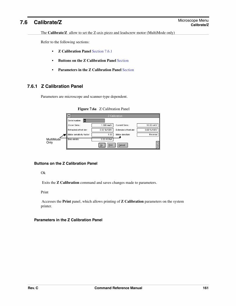
ope Menualibrate/Z

MicroscC7.6 Calibrate/Z

The Calibrate/Z allow to set the Z-axis piezo and leadscrew motor (MultiMode only)

Refer to the following sections:

• Z Calibration Panel Section 7.6.1

• Buttons on the Z Calibration Panel Section

• Parameters in the Z Calibration Panel Section

7.6.1 Z Calibration Panel

Parameters are microscope and scanner-type dependent.

Figure 7.6a Z Calibration Panel

Buttons on the Z Calibration Panel

Ok

Exits the Z Calibration command and saves changes made to parameters.

Print

Accesses the Print panel, which allows printing of Z Calibration parameters on the system printer.

Parameters in the Z Calibration Panel

MultiModeOnly

Rev. C Command Reference Manual 161

Microscope MenuCalibrate/Z

16

Serial number

The serial number is visible upon entering the panel.

Zscan sens

Z scan sens is the sensitivity of the piezo tube in the Z direction. The values are in units of nanometers of extension per volt applied to the electrodes.

Table 7.6a Typical Sensitivity Values (nm/V)

Note: Almost all SPM heads produced by Digital Instruments require positive Zscan sens values. A positive Zscan sens value extends the piezo element with positive voltage. In very rare instances, a Z piezo may exhibit reverse polarity properties (i.e., a positive voltage retracts the piezo element.) In these instances, a negative Zscan sens value should be entered.

Contact Digital Instruments/Veeco Metrology Group for more information on the Z scan sens.

Current Sens. [STM mode only]

Current Sens. specifies the current sensitivity in STM mode.

Range and Settings:

• Defaults to 10.00 nA/V (i.e., appropriate gain for standard STM pre-amp).

Retracted [Extended] offset der

Derating applied to the Z scan sensitivity as the Z piezo is offset by fixed voltages. This parameter corrects for Z-axis errors due to the piezo’s increased sensitivity at higher voltages, and is expressed as a percentage of the scanner’s Z-axis voltage above-below zero.

Range and Settings:

• 0—100%

Suggested Values:

• Retracted offset derating = 2.5 percent

• Extended offset derating = 7 percent

Scanner type "A" "D" "E" "G" "J"

Z Scan sensitivity

1.50 9.00 7.00 12.5 12.5

2 Command Reference Manual Rev. C

Microscope MenuTapping Engage

Bias derate [mV/nA] (STM only)

Corrects for the bias voltage drop which exists in some STM preamplifiers used on the NanoScope. This parameter only appears when an STM head is selected.

Range and Settings:

• 1 mV/nA for the standard preamplifier circuit

• 0 mV/nA for trans impedance low-noise preamplifier circuit

Note: This item ensures the accuracy of the Bias voltage parameter on the Real-time STM control panel.

For further instructions on calibrating offset deratings, see the Calibration chapter of your system manual.

7.7 Tapping Engage

The Calibrate/Tapping Engage commands are designed to assist users in controlling key parameters associated with surface engagement during TappingMode. In former software editions, these parameters were not subject to operator control, being optimized for engagement speed and tip safety under most conditions. By using the Calibrate/Tapping Engage panel, however, users may minimize engagement times or tapping forces for specific conditions (e.g., TappingMode in fluids, etc.).

CAUTION: Adjustment of the Tapping Engage parameters can decrease engagement times during TappingMode by speeding the tip’s travel to the surface and decreasing the number of test probes. Although this may save time, it also endangers the tip. You should always default to more conservative settings when in doubt; otherwise, you risk breaking tips.

7.7.1 Tapping Engage Panel

The Tapping Engage panel shown in Figure 7.7a illustrates recommended parameter values for most conditions. These setting yield an engagement time of 20 - 40 seconds.

Rev. C Command Reference Manual 163

Microscope MenuTapping Engage

Figure 7.7a Tapping Engage Panel

Setpoint values represent percentages of a setpoint established internally by the software for engagement purposes (generally, about 90 percent of the tip’s free-air amplitude). These values should not be confused with the Setpoint value indicated on the Feedback Controls panel.

7.7.2 Parameters in the Tapping Engage Panel

Engage delta setpoint

Amount the setpoint is adjusted during each false engage test.

Note: While in TappingMode, this tests for false engagement assist in engaging the tip on the sample surface. Tests for false engagement help to avoid artifacts produced by light scatter, fluid film damping, etc. Therefore, a setting of 0.00 (no test for false engagement) is not recommended.

Range and Settings:

164 Command Reference Manual Rev. C

Microscope MenuTapping Engage

• ± 0—0.10 (default: 0.02) A value of 0.10 (corresponds to ±10%) is the recommended maximum. If set to 0.00, the system will not test for false engagement.

Engage final delta setpoint

Percentage of setpoint value (internally set) to be used after tests for false engagement are concluded. This is the amount of temporary "overdrive" used by the system to verify whether the sample is, in fact, engaged by the tip. If this test is passed, the setpoint is restored to the last value used during false engagement tests.

Range and Settings:

• 0.00—0.10 (corresponding to 0 to 10 percent)

Note: This value is usually set equal to the Engage delta setpoint. It represents a cumulative value which is eventually reached in a series of Engage delta setpoint increments (rather than one, single test). For example, with an engage delta setpoint of 0.02 and a final delta of 0.10, five extra tests will be run after "engagement" to verify that the tip is actually on the surface (0.10 ÷ 0.02 = 5).

Note: If problems persist with false engagement, set the Engage final delta setpoint to a value that is 2-3 times the engage delta setpoint.

Engage test threshold

Slope value obtained by dividing the change in Z piezo voltage by the change in setpoint, which ultimately represents an envelope within which engagement is detected.

Range and Settings:

• 100—1000 (default: 100)

Note: Because changes in Z piezo voltage units occur approximately 200 times per unit change of setpoint, slope values tend to be between 100—1000.

Note: The higher the slope value, the greater the chance of "false engagement." Lower values are recommended for most applications. Using much lower values may reduce tip life.

Engage min setpoint [%]

Lowest allowable percentage of setpoint value (internally set) used during engagement, representing the "last word" in tip-sample force. This value overrides other parameters determining setpoint during engagement.

Range and Settings:

Rev. C Command Reference Manual 165

Microscope MenuTapping Engage

16

• 10—90. (typical value: 25).

Note: Lower values may endanger the tip and/or sample, as higher tip-sample forces will be employed.

Note: Higher values represent lower, more conservative tip-sample forces; however, very high values will increase false engagements.

TM engage gain

Integral gain value used during TappingMode engagement. Once the surface is engaged, gain values revert to those displayed on the Feedback Controls panel.

Range and Settings:

• 0.0100—10.00 (typical values: 0.5-2)

Hints for optimizing the TM Engage Gain

• As TM engage gain is increased, the tip’s vertical velocity downward increases. This parameter may be used to speed the engagement process and save time; however, if set too high, the tip and sample may be damaged.

• During engagement, gain values (Integral and Proportional) displayed on the Feedback Controls panel are not utilized. Instead, the software sets its own integral gain based on this parameter.

• With normal (non-fluid) samples, higher values tend to accelerate engagement speed at the cost of endangering tips and samples. Use of a higher gain may be recommended for TappingMode scanning of hard samples in fluid; however, gain should be increased cautiously.

• Use of lower gain values will tend to increase engagement times; however, lower values are recommended for soft, delicate samples where impact is to be minimized.

Sew tip

Controls use of sewing during the engagement process to detect the surface. Sewing consists of moving the tip vertically with the Z piezo while lowering it toward the surface. If the surface position is well known, Sewing may be triggered to save time.

Range and Settings:

• Yes—Turns sewing on. This is the normal, default mode.

• No—Turns sewing off.

Note: Only used for testing purposes; typically results in a damaged tip.

6 Command Reference Manual Rev. C

Microscope MenuTapping Engage

• Triggered—Turns sewing on when the RMS amplitude reaches the specified Sewing trigger value. The Triggered switch is used to protect tips and samples and to decrease engagement time.

• Ramped-Specifies the distance the motor travels toward the sample.

Sewing trigger [%]

Percentage of oscillation amplitude required to trigger sewing. This parameter is enabled only when the Sew tip parameter has been set to Triggered. Default setting is 98; not recommended at values less than 90.

Range and Settings:

• 1—100; default setting = 98.

Note: Regardless of setting, this parameter may be overridden by the Trigger safety parameter.

Trigger safety [for Dimension series microscopes only]

Minimum height above sample surface at which sewing is turned on. This parameter overrides the Sewing trigger parameter.

Range and Settings:

• 0—100 µm; typical setting = 20 µm

ATTENTION: To avoid damaging the tip or sample, the Trigger safety should be set to a value greater than the height of the tip, or the maximum peak-to-valley distance of surface features, whichever is greater. This parameter consists of a height above the surface as determined during the Real-time/Stage/Focus Surface command.

Pre engage setpoint [%]

Used to set the setpoint of the tip prior to engagement by reducing the setpoint relative to the RMS amplitude.

Range and Settings

• 50—100; default = 90.

Note: The usable range of this parameter is generally from 85 to 95. This represents the starting value for the engagement cycle (see beginning of this section).

Trig channel

Rev. C Command Reference Manual 167

Microscope MenuTapping Engage

Only active when the set top is set to ramped. The Trip channel specifies the data channel on which Trig threshold trigger. Trig channel choices will vary depending on the available inputs. Possible settings include Off (which disables the Trigger function), Deflection, Amplitude and Phase.

Trig threshold

Only active when the set top is set to ramped. The Trigger threshold is the change in value of the trigger channel that will determine when the tip contacts the surface.

Range and Settings:

• Dependent on selected channel.

Scan rate

Rate at which piezo extends in Z direction (toward surface). Very slow Scan rates (< 0.10 Hz) may prove frustrating; the system completes the present scan before initiating parameter changes.

Range or Settings:

• Min. 0.010; maximum value depends upon Number of samples; normal: 5-10Hz.

Note: Ramping under NT is limited to approximately 30 Hz at 512 samples per line.

Ramp step

Specifies the distance the motor will travel towards the sample when trying to find the surface (when Sew tip has been set to Ramped). This feature is used to increase the motor steps when ramped sewing has been activated.

168 Command Reference Manual Rev. C

Microscope MenuLeakage (STM and EC STM Only)

7.8 Leakage (STM and EC STM Only)

The Leakage command measures any current leakage between the tip and the Y electrode on the piezo tube of STM heads.

The Leakage test display appears on the Control Monitor:

Figure 7.8a Head Leakage Test Panel

As leakage tests are executed, the panel will display the results:

ATTENTION: Quit the panel when a sufficient number of tests have been run.

Hints for Optimizing the Leakage Command

• This command can only be executed if the head is withdrawn. Make sure the tip is not touching the sample when this command is executed.

• Null the preamplifier offset using the Real-time/Microscope/Offset command prior to running this command; otherwise, a Y offset will appear doubly as leakage.

• Select the Quit subcommand to exit the Leakage command.

• Head leakage is usually caused by an excess of moisture buildup in the area where the tip holder mounts to the piezoelectric scanner. This problem is greatest where etched tips (which can have some residual salts from the etching process) are used.

• If the measured leakage is greater than 0.2 to 0.5 nanoamps, then clean the area around the tip holder with a cotton swab and alcohol.

Note: Do not use more reactive solvents (i.e., acetone), as they will eat away the protective coating applied to the piezo scanner and tip holder.

• Head leakage can cause effects such as making the Z center voltage go off-scale when the Scan size is increased past a certain point. This is caused by domination of the tunneling current by the leakage current as the Y scan voltage increases.

• Each pass takes 8 seconds.

Rev. C Command Reference Manual 169

Microscope MenuOffset (STM Only)

17

7.9 Offset (STM Only)

The Offset command measures the voltage offset of the STM head preamplifier when the tip is withdrawn from the surface. This command allows the voltage offset to be measured and trimmed to zero for standard preamps. Low-noise preamps and Tipview preamps are not adjustable.

The Offset Calibration Test panel appears on the Control Monitor, allowing the offset in the head preamplifier to be nulled with the pot on the preamp board (See Figure 7.9a).

Figure 7.9a Head Offset Calibration Test Panel

Note: Execute only when the tip is withdrawn (use the Motor/Withdraw command several times).

Note: Unusually high offsets indicate that the tip is contacting the sample, that the head is disconnected from the base, the microscope is disconnected from the controller, or the controller is turned off or disconnected from the workstation.

See also: Real-time/Motor menu: Withdraw command. Real-time/Microscope menu: Leakage command.

Procedure to Adjust Head Offset

To adjust the preamplifier offset of a head, you would make sure the system is withdrawn, so that there are no high voltages applied to the head (using the Withdraw command several times). Connect the desired head to the microscope and make sure the tip was well away from the surface. Finally, after invoking the Offset command, adjust the head-offset potentiometer (accessible through the hole in the cover of the head) until the reading is close to zero.

0 Command Reference Manual Rev. C

Microscope MenuSensitivity Calibration

7.10 Sensitivity Calibration

The Sensitivity command measures the voltage offset of the STM head preamplifier when the tip is withdrawn from the surface. The Sensitivity Calibration Test panel appears on the Control Monitor, showing the sensitivity calibration (See Figure 7.10a).

Figure 7.10a Sensitivity Calibration Pane

7.11 Auto Gain Adjust

The Auto Gain Adjust command measures Integral Gain of STM head preamplifier when the tip is withdrawn from the surface. The Auto Gain Adjustment panel appears on the Control Monitor, displaying the measurements (See Figure 7.11a).

Figure 7.11a Auto Gain Adjustment Panel

7.12 Reset

The Reset command renews the Microscope settings to the default parameters. If the controller is turned off/on without restarting the software, this command needs to be executed.

Rev. C Command Reference Manual 171

Microscope MenuReplace Tip (MM AFM Only)

17

7.13 Replace Tip (MM AFM Only)

The Replace Tip command opens instruction panels when replacing a tip. The function of the panels is to assist the user with the hardware knobs and levers to optimize the tip replacement.

Selecting the Replace Tip command accesses a series of Replace Tip prompts (See Figure 7.13a).

Figure 7.13a Replace Tip Prompt Panels

See also: Real-time/Stage /Replace Tip for Dimension series microscopes.

2 Command Reference Manual Rev. C

Chapter 8 Vision Menu

This chapter describes the vision system hardware and software components for locating features on sample surfaces using a video camera.

The vision system components discussed in this chapter include:

• Vision Hardware: Section 8.1

• Vision System Requirements: Section 8.2

• Vision System Interface: Section 8.3

• Vision Control Menu Command: Section 8.4

For additional automated functions of the Vision System, see the Automation Supplement Rev A.

8.1 Vision Hardware

The standard on-axis, high magnification optical system supplied with all Dimension series SPMs is designed to align the probe with sample sites; however, these optics are unsuitable for conducting wide-angle searches. Therefore, a second, wide-angle, low magnification camera is added (as an option) to some microscopes for locating larger patterns with the Pattern Recognition option. The low magnification camera is used to align wafers with the microscope stage and to perform other wide-field tasks.

After large patterns are identified using the low magnification camera, the vision control system switches to the microscope’s high magnification camera to zoom in on finer features. These finer features are used to determine the wafer’s X-Y coordinate system and serve as reference points in all subsequent navigation of the sample.

In Figure 8.1a the high magnification system shown on the left side of the SPM is supplied with all Dimension series SPMs. Low magnification optics shown on the right side are supplied as a special option.

Rev. C Command Reference Manual 173

Vision MenuVision Hardware

17

Figure 8.1a Vision Hardware

8.1.1 Hardware Additions Requirements

Meteor Frame Grabber Board

The Frame Grabber board processes the output from up to four CCD (circuit cable devices) color NTSC cameras residing in the microscope and sends it to the display for viewing.

Low Magnification Optics

An optional set of low magnification optics is added to the right dovetail. The field of view of these optics is large enough (~8000 x 6500 µm) to handle the maximum wafer positioning error of the autoloader (<1000 µm). The low mag optics are offset from the tip high mag optics by about 1.25 inches.

Illumination System

A computer-controlled illumination system is added. This allows the system to save light levels during the macro teach process and restore them during the macro run process. The illumination system consists of a single halogen bulb illuminating two fiber bundles, one for each set of optics. The intensity of the bulb is controlled by a 6811 microprocessor. The 6811 communicates with the PC and NanoScope software through an RS-232 serial port.

Low Mag Camera

IlluminatorIlluminator

High Mag Camera(in rear)

High Magnification Optics Low Magnification Optics

SPM Head

4 Command Reference Manual Rev. C

Vision MenuVision System Requirements

Miscellaneous Hardware

Several small system changes have been made to accommodate the vision system:

• An Optical Standard is mounted to the right-rear of the chuck to provide a reference for calibrating both sets of optics. Note that the image is optically inverted (negative) from what is seen through the optics (See Figure 8.1b).

Figure 8.1b Optical Standard

• The illumination optics are upgraded to improve the contrast of the high magnification optics.

• A hard stop is added to the zoom to improve the repeatability of the zoom.

8.2 Vision System Requirements

8.2.1 Recognizable Patterns

The Cognex vision control system is capable of recognizing high-contrast features having a distinct, local appearance. These are referred to as “visual models”.

Rev. C Command Reference Manual 175

Vision MenuVision System Requirements

17

Many wafers are etched with distinct marks to serve as reference points. Corners, contact pads, trace intersections, etc. may all be used as visual models; however, they must be distinct from their surroundings.

Examples of poor visual models include non distinct pads located within a field of identical pads; wafer edges; parallel, identical traces, etc. Figure 8.2a shows one such example. Features within the box in the left illustration might easily be confused with each other. Features within the box in the right illustration are distinct from those immediately surrounding it.

A good visual model should have few transitions between dark and light, and the transitions should be far apart. T he model should have a distinct, local appearance that cannot be confused with any other area nearby.

When teaching a model, the upper-right of the video display shows the position (X-Y) and size (X-Y) of the model, and the total pixels within the model. Model size is limited to 65535 pixels or less. An error message is displayed if the model is 65536 pixels or greater. The optimum size of a model is in the range or 75 to 200 pixels on a side. A model that is too large takes a long time to save and load. A model that is too small requires a longer search time.

8.2.2 Illumination Control

Both the high magnification camera and the low magnification camera are equipped with on-axis, fiber optic illumination supplied by the same halogen lamp. The halogen lamp’s intensity is controlled by the Illumination software parameter. When a visual model is saved, the level of illumination is saved along with it.

The illumination intensity is crucial to the ability of the vision control system to distinquish features:

• The lower the magnification, the lower the illumination intensity required. Too much light at low magnification washes out features, making them impossible to see. Conversely, higher magnification requires more light.

Pattern

Figure 8.2a Selection of Visual Model

recognitionbox

6 Command Reference Manual Rev. C

Vision MenuVision System Requirements

• Illuminate features as brightly as possible without washing them out. You want features to be imaged with adequate contrast against their backgrounds and reduced tonal differences between one visual model and another.

8.2.3 Rotational Alignment of Features

The Cognex recognition system allows most features to be recognized within angular orientations of ± 7.5 degrees. The robot employed with Dimension series SPMs is designed to locate samples with an angular accuracy of ± 0.25 degrees. Therefore, rotation is normally not a problem with automatically loaded samples. When manually loading samples, you can reduce rotational alignment problems by ensuring that the samples are squarely positioned.

Rev. C Command Reference Manual 177

Vision MenuVision System Interface

17

8.3 Vision System Interface

Figure 8.3a illustrates the Vision menu panels and parameters associated with typical MultiMode and Dimension series microscopes. Additional parameters and menus appear for systems configured with automated features (i.e., robot functions).

Figure 8.3a Navigating in the Vision Menu

8.4 Vision Control Menu Command

From the Vision menu item, select Vision Control to display the Vision System Real Time Control panel. The purpose of the Vision System Control panel includes:

• Adjusts parameters for the currently selected camera and monitor.

• Assigns and recalls filenames for visual models and parameters.

Note: On a Dimension series microscopes that include a stage and the pattern recognition option, a number of additional parameters are available. See, The Automation Supplement (Version 5.13) for details on the parameters associated with automated systems.

Executes:"Intitialize

System"

VisionExecutes the"AutoFocus"Command

Accesses panelto move the stage and "AutoFocus"

5696

8 Command Reference Manual Rev. C

Vision MenuVision Control Menu Command

Refer to the following Vision Control sections:

• Vision Control Panel: Section 8.4.1

• Buttons on the Vision System Realtime Control Panel: Section 8.4.2

• Parameters on the Vision System Real-time Control Panel: Section 8.4.3

• Parms Submenu: Section 8.4.4

• General Parameters: Section

• AutoFocus Button [Auto Focus Parms Panel]: Section

• Helpers Submenu on the Vision Control Panel: Section 8.4.5

8.4.1 Vision Control Panel

Figure 8.4a Vision Control Panel

Rev. C Command Reference Manual 179

Vision MenuVision Control Menu Command

18

8.4.2 Buttons on the Vision System Realtime Control Panel

AutoFocus

Executes the Auto Focus command. If the stage is not initialized, you are informed of this condition and given the opportunity to ABORT or RESUME (See Figure 8.4b).

Figure 8.4b Abort Prompt

Selecting the ABORT button discontinues Vision Control and returns you to the Real Time environment (scan controls, channel controls, etc.). Selecting the RESUME button opens the Vision Control panel, but any vision system functions that require stage motion (e.g., Camera selection, MOVE STAGE button) do not operate properly.

Move Stage

The MOVE STAGE button accesses a panel allowing trackball stage control, stage control using the panel buttons and direct camera control.

8.4.3 Parameters on the Vision System Real-time Control Panel

Camera—Defines the current camera selection and allows the user to select a different camera.

Range or settings: Low Mag. or High Mag.

Zoom—Shows the current zoom setting and allows the user to select a different zoom setting.

Range or settings: Low Zoom or High Zoom

Illumination—SHows the current illumination (light) level and allows the user to select a different illumination setting.

Range or settings: 0 (min. light) - 100 (max. light).

Video Attenuation—Shows the current value of the video attenuation (hardware control over the video signal strength similar to the “Brightness” knob on a TV set) and allows the user to change the attenuation.

Range or settings: 0 attenuation is very bright - 100 attenuation (maximum) is very dark.

Hue—Controls the color value of the displayed image.

0 Command Reference Manual Rev. C

Vision MenuVision Control Menu Command

Saturation—Sets the value of the color intensity.

Contrast—Enhances or degrades the contrast in the image.

Range or settings: 0 (min. contrast) - 255 (max. contrast)

Cursor—Defines the color of the main cursor. Also allows the cursor to be disabled.

Cursor Hole (pixels)—Sets the number of pixels open at the center of the cursor where the horizontal and vertical lines meet.

Target Cursor—Defines the color of the “target cursor”. The target cursor controls the color of the box used to define models for pattern recognition.

8.4.4 Parms Submenu

The Parms pull-down menu on the Vision System Real-time Control panel provides access to additional parameter panels.

Figure 8.4c Parms Submenu on Real-time Control Panel

General Parameters

The General Vision Parameters dialog box contains parameters for controlling vision paths and general vision functions.

Note: All of the fields display, even if a particular parameter is not available.

Rev. C Command Reference Manual 181

Vision MenuVision Control Menu Command

18

Figure 8.4d General Vision Parameters Dialog Box

Parameters on the General Vision Parameters Panel

• Vision Debug

• The Vision Debug parameter is a diagnostic tool for controlling the quantity of information that is displayed in the Vision Debug box (Ctrl-Alt-V). The default value is 0 (no debug information). Increasing values cause more information to be displayed in the Vision Debug box when commands are sent to the vision system.

• Logger

• The Logger parameter allows you to enable or disable the logging function. If enabled, the Logger enters the vision errors in the Vision Debug file. If disabled, vision errors are not logged.

• IO Base Address—This field is obsolete.

• Baseline Path

• The Baseline Path parameter defines where the boot files for initializing the vision system are located on the NanoScope hard disk. The default directory is c:\spm\vision.

• Visual Models Path

2 Command Reference Manual Rev. C

Vision MenuVision Control Menu Command

• The Visual Models Path parameter defines the path for loading and saving visual models. The default path is c:\spm\vision\models.

• Last Booted File—This field is obsolete.

• Box Search Iterations

• The Box Search Iterations parameter defines the maximum number of boxes around the original search location which are allowed during a box search. A box search is conducted during a look if 1) the visual model is not found at the initial search location, and 2) the Box Search parameter is enabled for that look.

• The default is 2 boxes, with options of 0 to 10 boxes.

• With Box Search Iterations set to 1, the X-Y stage moves to obtain a series of images with the centerpoints of the images forming a square box (in the X-Y plane) around the original image center. The length of each side of the depicted box is twice the value of the Box Size (pixels) parameter. See the example in Figure 8.4e.

• The actual size of the box in microns depends on the camera, zoom, and the associated calibration parameter (microns per pixel) as set in the Low Mag Optics or High Mag Optics Parameters (See and ).

• When the parameter Box Search Iterations is greater than 1, each successive box increases in size such that the length of the side increases by:

• 2 × Box Size (pixels) × microns per pixel

Figure 8.4e Box Search Iterations Example

• Box Size (pixels)

• The Box Size parameter defines the X or Y distance in pixels of two successive looks during a box search. The size of the box through which the stage moves is defined by twice the value of Box Size (pixels). See the discussion of “Box Search Iterations” on page 8-183.

• Hit Selection Criteria

• The Hit Selection Criteria parameter determines the method used by the vision system when it finds multiple locations during the search for a model (i.e., two or more areas of the video correlate with the model).

• Best Score—Selects the location with the highest score. This is the default and is appropriate for most applications.

• Close to Original—Selects the location closest to the screen position of the model when the model was taught. This method is appropriate for regular use of pattern recognition on images that have repeated or ambiguous features. While pattern

Rev. C Command Reference Manual 183

Vision MenuVision Control Menu Command

18

recognition can dither between the ambiguous locations when aligning the pattern, the Close to Original option consistently uses the model closest to the original alignment.

• Accept Threshold

• When the software compares a location to the model it was taught, it uses the Accept Threshold minimum correlation score to determine if the location is acceptable.

• The default is 500, with a range of 1 to 1000.

• SPM Accept Threshold

• When the software compares a location to the model it was taught, it uses the SPM Accept Threshold minimum correlation score to determine if it is an acceptable SPM location.

1

2 3

4

5

67

8

9

Original search location

Box search site

The sequence of X-Y stage moves in a Box Search Iteration:

If High Mag Optics is selected with High Zoom (maximum), the calibrated pixel size is 0.2 µm/pixel, and the value of Box Size is 100 pixels.

-20 mm in X, 20 µm in Y (diagonal move to upper left corner of box) 20 mm in X, (top of box) 20 mm in X,-20 mm in Y, (right side of box)-20 mm in Y,-20 mm in X, (bottom of box)-20 mm in X, 20 mm in Y (left side of box)

Each of the above eight steps involves stage motion, the acquisition of a video image at the new stage location, and the search of that image for the previously trained visual model. If the model is located at any of the eight locations, the box search is terminated at that location, and alignment of the model is performed.

4 Command Reference Manual Rev. C

Vision MenuVision Control Menu Command

• The default is 500, with a range of 1 to 1000.

• Search Control

• The Search Control parameter establishes the type of correlation values used to determine acceptability.

• Normalized—Correlation values are acceptable from 0 to 1000. This is the default value.

• Absolute—The absolute value of the correlation score is acceptable; therefore, the software recognizes locations that are inverted or optical negative of the original model.

• Intensity Min

• The Intensity Minimum parameter determines the acceptable threshold for a location’s average pixel intensity (brightness).

• The default is 10, with a range of 0 to 255.

• Auto Reload Hardware —This field is obsolete.

• Disp Max Hor Size (pix)—This field is obsolete.

• Sync Workarkound (pixels)—This field is obsolete.

• Magic Parm—This field is obsolete.

• Display video on Multi chan image

• When capturing images in multi channels, the Display video on Multi channel image parameter enables or disables the video. If Disabled (default), only the channel captures display. If Enabled, the channel captures and the video screen are sized to display simultaneously.

• Video Based Stage Motion

• The Video Based Stage Motion parameter determines whether or not you can indicate stage position from the video screen. If Enabled, double-clicking on a point in the video display causes the stage to move so that the indicated point is aligned beneath the video display cross hair. To work well, this option requires good pixel calibration.

• The default is Disabled.

AutoFocus Parameters Panel [Parms Submenu Item]

Access the AutoFocus Parameters panel in the Vision System Control / Parms submenu. Select AutoFocus Parameters.

Rev. C Command Reference Manual 185

Vision MenuVision Control Menu Command

18

Figure 8.4f AutoFocus Parameters Panel

Max Z - Hi Mag, Hi Zoom (µm)

• This parameter defines the total Z (SPM) axis excursion during AutoFocus for the high mag camera at high zoom setting. The actual downward movement is half the value set in the parameter, after which it raises the full value gathering focus data. The default value is 200 µm, with a range of 0 to 2000 microns.

• At the default setting, the AutoFocus algorithm moves the SPM axis 50 µm down at maximum velocity, then move the SPM axis up slowly (defined by the Velocity % Hi Mag, Hi Zoom parameter) 100 µm during which focus data is gathered. If an optimum focus point is detected, the SPM axis is moved down to that point at maximum velocity.

Max Z - Lo Zoom & Lo Mag

• This parameter defines the maximum Z (SPM) axis excursion during AutoFocus when either the Low Mag camera is selected or the High Mag camera is selected at the Low Zoom setting. The default is 600 µm, with a range of 0 to 2000 microns.

Velocity % Hi Mag, Hi Zoom

• This parameter defines the Z (SPM) axis velocity for the data collection phase of AutoFocus when the Hi Mag camera and Hi Zoom settings are selected. The velocity is specified as a percentage of the maximum SPM axis velocity. The default is 7% (of maximum velocity), with a range of 0 to 100%

6 Command Reference Manual Rev. C

Vision MenuVision Control Menu Command

Velocity% Lo Zoom & Lo Mag

• This parameter defines the Z (SPM) axis velocity for the data collection phase of AutoFocus as a percentage of the maximum velocity when either Low Mag optics or High Mag optics is selected at the Low Zoom setting. The default is 25% (of maximum velocity), range of 0 to 100%

SPM Axis Backlash Comp

• This parameter defines the backlash compensation in microns during AutoFocus for the downward -Z (SPM) axis movement. The default value is 0.0 µm (no compensation), with a range of 0.0 to 100.0 µm.

Smoothing Pixels

• During data collection the AutoFocus algorithm repeatedly performs the following operations: 1) video acquisition, 2) windowing of acquired data, 3) smoothing of the windowed data, and 4) calculation of the differential-sum (sharpness) of the smoothed data.

• The number of pixels over which the data is smoothed is defined by the Smoothing Pixels parameter. The default is 8 pixels, with a range of 0 to 8.

Convergence

• After the AutoFocus data collection phase is complete, the resulting data relates focus (sharpness) to SPM axis position. This data is then fit to a Gaussian function using an iterative non-linear algorithm. The Convergence parameter determines how closely the Gaussian curve must fit. The default is 0.01, with a range of 0.00 to 1.00.

Max Chi Squared

• The Maximum Chi Squared parameter originally provided an iterative look for AutoFocus to aid in asymmetrical curves. This parameter is now obsolete.

Max Iterations

• The Max Iterations parameter defines the maximum number of attempts to make the AutoFocus data fit a Gaussian curve. If Convergence does not occur within this number of iterations, then the covariance of each of the Gaussian function parameters (height, width, center) is checked to determine if a fit has been obtained.

• The default is 100 iterations, range: up to 1000.

Rev. C Command Reference Manual 187

Vision MenuVision Control Menu Command

18

Max Acceptable Covariance

• At the completion of a curve fit, the covariance of the height, width, and center of the Gaussian function are provided by the curve fit algorithm. The Max Acceptable Covariance parameter defines the greatest tolerable covariance for a successful curve fit. If any of the three covariance are greater than the value of this parameter, AutoFocus fails.

Max Center Covariance

• The Maximum Center Covariance parameter defines the greatest tolerable covariance for a successful curve fit relative to only the center value. At the completion of a curve fit, the covariance of the height, width, and center of the Gaussian function are provided by the curve fit algorithm.The default is 0 iterations, range: 0 to 100.

Min Autofocus Samps

• The Minimum AutoFocus Samples parameter defines the number of pictures snapped during the AutoFocus routine. This parameter works in conjunction with the Minimum AutoFocus Velocity parameter. The higher the number of samples requested, the slower the AutoFocus.

• The default is 0 samples, with a range of 0 to 100.

Min Autofocus Vel (%)

• The Minimum AutoFocus Velocity parameter defines the minimum speed of the AutoFocus routine. This parameter works in conjunction with the Minimum AutoFocus Samples parameter. The slower the velocity, the slower the AutoFocus.

• The default is 0%, with a range of 0 to 100%.

AutoFocus Curve Fit

• The AutoFocus Curve Fit parameter determines the type of curve to apply to the data during AutoFocus.

• Gaussian—Fits the data to a smooth, symmetrical curve. This is the default value.

• Asymmetric—Recognizes asymmetry and fits the data appropriately to recognize the asymmetry. Use this type if the curve is known to be asymmetrical or if dealing with a dramatic step.

8 Command Reference Manual Rev. C

Vision MenuVision Control Menu Command

AutoFocus Button [Auto Focus Parms Panel]

The AUTOFOCUS button provides you with the ability to execute the AutoFocus algorithm from within the parameters adjustment box.

AutoFocus performs the following operations using the values set in AutoFocus Parameters panel:

AutoFocus moves the Z (SPM) axis down X microns, where X is determined by the Max Z parameter for the currently selected optics. The actual downward movement is half the value set in the parameter, after which it raises the full value gathering focus data.

Backlash compensation is used if the SPM Axis Backlash Comp parameter is non-zero (i.e., downward motion is 150 percent of the parameter’s value, then the Z axis moves upward by the amount of the backlash parameter).

AutoFocus commands the stage to move upward by Max Z amount at the percentage of maximum velocity defined by the appropriate Velocity % parameter.

Simultaneously, the vision system hardware repeatedly executes the following:

• Saves stage Z position for this pass.

• Acquires image in frame buffer.

• Identifies appropriate window of frame buffer image—center quarter of image for Low Mag optics or High Zoom, High Mag optics, or center (vertical), left (vertical) quarter of image for Low Zoom, High Mag optics.

• Checks window contrast and generates error if too low (<1.0).

• Smooths window according to Smoothing Pixels parameter value.

• Executes differential-sum algorithm on smoothed window (sharpness calculation).

• Repeats until stage motion completes.

AutoFocus then fits the acquired stage Z and sharpness data pairs to a Gaussian curve using the Levenberg-Marquardt method (nonlinear, steepest descent) and checks for convergence while iterating (Convergence and Max Iterations parameters).

AutoFocus verifies that the variances of the values that define the Gaussian curve (height, width, center) are sufficiently low (Max Acceptable Covariance parameter) and verifies that the computed center is within the range of motion through which the stage moved (Max Z).

If the settings for AutoFocus are met, the stage is moved downward in Z to the “sharpest” point, the center of the Gaussian curve. The downward motion includes backlash compensation if the backlash parameter is non-zero.

If any single constraint is not met, the Z stage is sent back to the position at which AutoFocus was initiated, and a failure message is displayed.

Rev. C Command Reference Manual 189

Vision MenuVision Control Menu Command

19

Low Mag Parameters [Parms Submenu]

Low magnification is available on systems with the Pattern Recognition option.

The Low Mag Optics Parameters panel provides access to parameters related to the behavior of the Low Mag optics within the vision system.

Figure 8.4g Low Mag Optics Parameters Panel

Low Mag Camera Enable

• The Low Mag Camera Enable parameter allows you to enable and disable the low mag optics. If set to Disabled, the other Low Mag Parameters are unavailable.

Low Mag Camera Port

• This parameter designates the port (either 1 or 2) to which the low mag camera is connected. Changes to this parameter take effect on initialization only (restart z.exe). The default is port 2.

Low Mag Stage X Location

• This parameter defines the X position (absolute) of the X-Y stage when the stage is at the Low Mag optics calibration position. The parameter is set when the Low Mag optics calibration function is executed or taught. This parameter is usually grayed-out and cannot be directly modified.

• The default is 0 counts (microns) range of -1000000 to 1000000 µm.

0 Command Reference Manual Rev. C

Vision MenuVision Control Menu Command

Low Mag Stage Y Location

• This parameter defines the Y position (absolute) of the X-Y stage when the stage is at the Low Mag optics calibration position.

• The parameter is set when the Low Mag optics calibration function is executed or taught. This parameter is usually grayed-out and cannot be directly modified.

• The default is 0 counts (microns)range of -1000000 to 1000000 µm.

Low Mag Stage Z Location

• This parameter defines the Z position (absolute) of the Z stage when the stage is at the Low Mag optics calibration position. The parameter is set when the Low Mag optics calibration function is executed or taught. This parameter is usually grayed-out and cannot be directly modified.

• The default is 0 counts (microns) range of -1000000 to 1000000 µm.

Low Mag Pixel X Size [µm]

• This parameter defines the size of a pixel in µm in the X direction for the low mag camera. The default is 10.0 µm, with a range from -1000 to 1000 µm.

• When coarse alignment occurs, the vision system determines the number of pixels along the X axis between the current location of the model and the taught location of the model. Using the value of this parameter, the number of pixels is converted to µm for subsequent stage motion to correct the alignment error in the X direction.

• You calculate this number by converting the video image of the 1000 µm square on the Optical Standard to a NanoScope image using the vision system function Video image->Nano3 image. Use the Off-line/View/Top View utility to measure the apparent width of the square, calculate the percent of error, and modify this parameter accordingly.

Low Mag Pixel Y Size [µm]

• This parameter defines the size of a pixel in µm in the Y direction for the low mag camera. The default is -10.0 µm, with a range from -1000 to 1000 µm.

• When coarse alignment occurs, the vision system determines the number of pixels along the Y axis between the current location of the model and the taught location of the model. Using the value of this parameter, the number of pixels is converted to µm for subsequent stage motion to correct the alignment error in the Y direction.

Rev. C Command Reference Manual 191

Vision MenuVision Control Menu Command

19

• You calculate this number by converting the video image of the 1000 microns square on the Optical Standard to a NanoScope image using the vision system function Video image->Nano3 image. Use the Off-line/View/Top View utility to measure the apparent width of the square, calculate the percent of error, and modify this parameter accordingly. This number is generally negative, because the positive Y direction of the X-Y stage is opposite that of the vision system.

Low Mag Stage Accuracy

• This parameter defines the accuracy threshold the vision system must meet when attempting to null errors during registration between the current screen location of the model and the taught location of the model.

• For example, if the vision system determines that the error between the current screen location of the video model and the taught location of the video model is 5 microns, and the Low Mag Stage Accuracy is set to 10 microns, then no error correction is attempted.

• This parameter applies to both the X and Y axes. Typically, the Low Mag Stage Accuracy should be greater than or equal to the pixel size of the camera.

High Mag Parameters [Parms Submenu]

The High Mag Optics Parameters panel gives you access to parameters related to the behavior of vision system High Mag optics (See Figure 8.4h).

Figure 8.4h High Mag Optics Parameters Panel

2 Command Reference Manual Rev. C

Vision MenuVision Control Menu Command

High Mag Camera Enable

• The High Mag Camera Enable parameter allows you to enable and disable the high mag optics. If set to Disabled, the other High Mag Parameters are unavailable.

High Mag Camera Port

• This parameter designates the port (either 1 or 2) to which the high mag camera is connected. Changes to this parameter take effect on initialization only (restart z.exe). The default is port 1.

High Mag Stage X Location

• This parameter defines the X position (absolute) of the X-Y stage when the stage is at the High Mag optics calibration position.

• (continued on next page...)

• The parameter is set when the High Mag optics calibration function is executed or taught. This parameter is usually grayed-out and cannot be directly modified.

• The default is 0 counts (microns), range of -1000000 to 1000000 µm.

High Mag Stage Y Location

• This parameter defines the Y position (absolute) of the X-Y stage when the stage is at the High Mag optics calibration position. The parameter is set when the High Mag optics calibration function is executed or taught. This parameter is usually grayed-out and cannot be directly modified.

• The default is 0 counts (microns), range: 1000000-1000000 µm

High Mag Stage Z Location

• This parameter defines the Z position (absolute) of the Z stage when the stage is at the High Mag optics calibration position. The parameter is set when the High Mag optics calibration function is executed or taught. This parameter is grayed-out and cannot be directly modified.

• The default is 0 counts (microns), range of -1000000 to 1000000 µm.

Rev. C Command Reference Manual 193

Vision MenuVision Control Menu Command

19

Move To Opt. Stand. X Offset (µm)

• The Move to Optical Standard X Offset (µm) parameter defines the X distance in microns from the center of the optical standard to the point which the stage must move after selecting the Move to Optical Standard command.

• The default is 1000 µm,range of -2000 to 2000

Move To Opt. Stand. Y Offset (µm)

• The Move to Optical Standard Y Offset (µm) parameter defines the Y distance in microns from the center of the optical standard to the point which the stage must move after selecting the Move to Optical Standard command.

• The default is -1000 µm, with a range of -2000 to 2000.

High Mag (Lo Zoom) Pixel X Size [µm]

• This parameter defines the High Mag (Low Zoom) camera’s X axis pixel size. The default is 1.0 µm, with a range from -1000 to 1000 µm.

• When coarse alignment occurs, the vision system determines the number of pixels along the X axis between the current location of the model and the taught location of the model. Using the value of this parameter, the number of pixels is converted to µm for subsequent stage motion to correct the alignment error in the X direction.

• You calculate this number by converting the video image of the 150 µm square on the Optical Standard to a NanoScope image using the vision system function Video image->Nano3 image. Use the Off-line/View/Top View utility to measure the apparent width of the square, calculate the percent of error, and modify this parameter accordingly.

High Mag (Low Zoom) Pixel Y Size [µm]

• This parameter defines the High Mag (Low Zoom) camera’s Y axis pixel size. The default is -1.0 µm, with a range from -1000 to 1000 µm.

• When coarse alignment occurs, the vision system determines the number of pixels along the Y axis between the current location of the model and the taught location of the model. Using the value of this parameter, the number of pixels is converted to µm for subsequent stage motion to correct the alignment error in the Y direction.

• You calculate this number by converting the video image of the 150 µm square on the Optical Standard to a NanoScope image using the vision system function Video image->Nano3 image. Use the Off-line/View/Top View utility to measure the apparent width of the square, calculate the percent of error, and modify this parameter accordingly. This number is generally negative because the positive Y direction of the X-Y stage is opposite the vision system.

4 Command Reference Manual Rev. C

Vision MenuVision Control Menu Command

High Mag, Low Zoom Stage Accuracy

• This parameter defines the accuracy threshold the vision system must meet when attempting to null errors during registration between the current screen location of the model and the taught location of the model. The default is 4.0 µm, with a range of 0 to 1000000 microns.

• For example, if the vision system determines that the error between the current screen location of the video model and the taught location of the video model is 2 microns, and the High Mag, Low Zoom Stage Accuracy is set to 4 microns, then no error correction is attempted.

• This parameter applies to both the X and Y axes. Typically, the High Mag, Low Zoom Stage Accuracy should be greater than or equal to the pixel size of the camera.

High Mag (Hi Zoom) Pixel X Size [µm]

• This parameter defines the High Mag (High Zoom) camera’s X axis pixel size. The default is 0.214 µm, with a range from -1000 to 1000 µm.

• When fine alignment occurs during registration, the vision system determines the number of pixels along the X axis between the current location of the model and the taught location of the model. Using the value of this parameter, the number of pixels is converted to µm for subsequent stage motion to correct the alignment error in the X direction.

• You calculate this number by converting the video image of the 20 µm square on the Optical Standard to a NanoScope image using the vision system function Video image->Nano3 image. Use the Off-line/View/Top View utility to measure the apparent width of the square, calculate the percent of error, and modify this parameter accordingly.

High Mag (Hi Zoom) Pixel Y Size [µm]

• This parameter defines the High Mag (High Zoom) camera’s Y axis pixel size. The default is -0.214 µm, with a range from -1000 to 1000 µm.

• When fine alignment occurs during registration, the vision system determines the number of pixels along the Y axis between the current location of the model and the taught location of the model. Using the value of this parameter, the number of pixels is converted to µm for subsequent stage motion to correct the alignment error in the Y direction.

• Calculate this number by converting the video image of the 20 µm square on the Optical Standard to a NanoScope image using the vision system function Video image->Nano3 image. Use the Off-line/View/Top View utility to measure the apparent width of the square, calculate the percent of error, and modify this parameter accordingly. This number is generally negative because the positive Y direction of the X-Y stage is opposite the vision system.

Rev. C Command Reference Manual 195

Vision MenuVision Control Menu Command

19

High Mag, High Zoom Stage Accuracy

• This parameter defines the accuracy threshold the vision system must meet when attempting to null errors during registration between the current screen location of the model and the taught location of the model. The default is 1.0 µm, with a range of 0 to 1000000 microns.

• For example, if the vision system determines that the error between the current screen location of the video model and the taught location of the video model is 0.5 microns, and the High Mag, High Zoom Stage Accuracy is set to 1 micron, then no error correction is attempted.

• This parameter applies to both the X and Y axes. Typically, the High Mag, High Zoom Stage Accuracy should be greater than or equal to 1 µm, the step size of the X-Y stage.

Camera AGC Delay (Secs)

• The Camera Automatic Gain Control parameter controls the time allowed for the camera iris and processor to determine acceptable brightness of the image.

• The default is 0 seconds, with a range of 0 to 1000.

DarkField Parameters [Parms Submenu]

Figure 8.4i DarkField Optics Parameters Panel

The DarkField parameters are similar to those for low magnification, as described on Page 190.

6 Command Reference Manual Rev. C

Vision MenuVision Control Menu Command

Large Field Parameters [Parms Submenu]

The Large Field parameters allow you to enable/disable the Large Field camera and to specify the port to which the Large Field camera is connected.

Figure 8.4j LargeField Optics Parameters Panel

Edge Detection

This function accesses a panel to enable the Vision system type (See Figure 8.4k).

Figure 8.4k Edge Detection Parameters Panel

8.4.5 Helpers Submenu on the Vision Control Panel

Several functions are available in the Helpers pull-down menu on the Vision System Real-time Control panel.

Figure 8.4l Helpers Submenu on Vision System Real-time Control Panel

Vision Image->Nano3 Image

The Vision Image->Nano3 Image function translates the vision image to a NanoScope compatible image for analysis.

For example, you can calculate a number by converting the video image of the 1000 µm square on the Optical Standard to a NanoScope image using the vision system function Video image->Nano3 image.

Then use the Off-line / View / Top View utility to measure the apparent width of the square, calculate the percent of error, or modify the image.

Enables PatMax (VisionSystem).

Rev. C Command Reference Manual 197

Vision MenuVision Control Menu Command

19

8 Command Reference Manual Rev. C

Chapter 9 Stage and Recipe Menus

The commands in the Stage menu pertain to the movement and calibration of stage systems. The commands in the Recipe menu control teaching the microscope to perform automated functions. For further details on the Recipe menu commands, see The Automation Supplement or your system manuals.

This chapter details the following Stage and Recipe commands:

• Overview of the Stage Command: Section 9.1

• Stage Menu Interface: Section 9.2

• Load New Sample Section 9.3

• Locate Tip Section 9.4

• Focus Surface Section 9.5

• Move To (x, y) (Dimension Series only) Section 9.6

• Set Reference (Dimension Series only) Section 9.7

• Programmed Move (Dimension Series Only) Section 9.8

• Replace Tip (D3000 Series) Section 9.9

• Scaling Section 9.10

• Set Image Center (Dimension 5000/9000 only) Section 9.11

• Initialize Section 9.12

• SPM Parameters Section 9.13

• Set Z Exclusion Section 9.14

• Recipe Commands Section 9.15

Rev. A (variable) Document Title (variable, update from TP) 1

Stage and Recipe MenusOverview of the Stage Command

9.1 Overview of the Stage Command

The Stage menu appears whenever Dimension™ Series microscopes are selected using the Microscope / Select command. The Dimension 3000 features two stage types: a manual (hand-cranked) version; and an open-loop, motorized version. Dimension 9000 microscopes feature a large sample stage having high-precision, closed-loop positioning for such materials as silicon wafers and computer hard drive media. These stages consist of stacked, perpendicular X- and Y-axis slides.

9.1.1 Mounting Samples

Stages come equipped with vacuum chucks, which are the usual choice employed for securing samples; an outside source of vacuum is required. Operators should be cautious when handling larger samples with the vacuum chuck—an 8-inch wafer held using 5 psi vacuum sustains a loading of 250 lbs. If debris is trapped between the stage and wafer, the wafer may become scratched or broken. Keep the stage clean at all times using isopropyl alcohol. When cleaning dust from the stage area, use a vacuum cleaner with a soft brush. DO NOT clean stages using compressed air.

Samples may also be secured to the stage using magnetic pucks, which are themselves magnetically attached to the stage. This system allows for easy mounting and removal of small samples.

Regardless of the method used, operators should verify that samples are mounted flat and parallel to the stage. This is especially important for larger samples being inspected over more than one site. Grossly tilted samples may require raising the head higher whenever the sample is indexed, increasing cycle time and the risk of probe-sample collision. Similarly, large numbers of identical samples should be mounted the same way whenever possible; this allows use of the same settings between samples.

9.1.2 Axis Orientation—X-Y Stages

Viewing the SPM from the front, stage movements are defined over two axes of motion: X (left-right), and Y (front-back). For X-axis movements, lesser (decreasing) coordinates are located to the left. For Y-axis movements, positive (increasing) coordinates are located toward the rear of the machine, negative values are located forward (see Figure 9.1a of a Dimension 5000/7000 stage; Dimension 3000 is similar).

2 Document Title (variable, update from TP) Rev. A (variable)

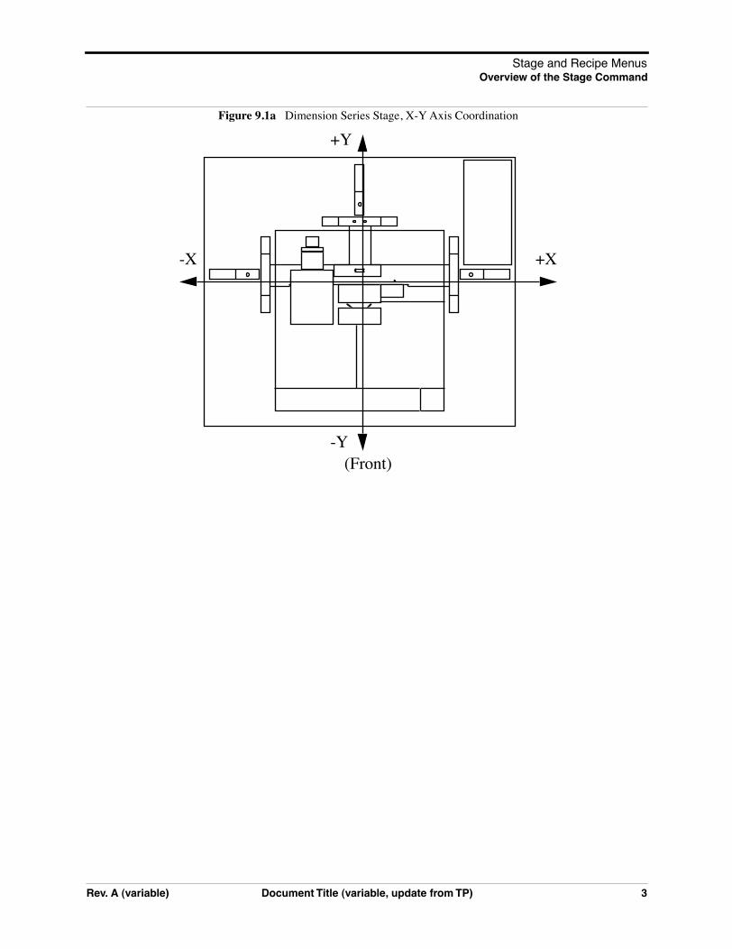
Stage and Recipe MenusOverview of the Stage Command

Figure 9.1a Dimension Series Stage, X-Y Axis Coordination

+X-X

+Y

-Y(Front)

Rev. A (variable) Document Title (variable, update from TP) 3

Stage and Recipe MenusStage Menu Interface

9.2 Stage Menu Interface

Stage software allows for manual or taught movement of the stage prior to scanning.

The stage menu allows for setting up stage parameters for optimal scanning. Prior to initializing the stage, menu commands appear disabled. This is to avoid head crashes and to properly set up locations for scanning. Enable some commands by entering the Service Access (e.g., Z exclusion) and enable the parameters set by logging out of Service Access. The software guides and prompts the user to complete the functions of each Stage command.

Figure 9.2a Stage Menu

9.3 Load New Sample

The Load New Sample command programs the probe to automatically lift from the sample surface, then index the stage to a preprogrammed location (usually front-center) from which samples may be rapidly reloaded.

Once a new sample has been placed on the stage and secured, the stage software is used to quickly and accurately relocate the sample to the previously used site. It is possible to establish a series of separate sites on any one sample, then repeatedly inspect these same sites on identical samples. This is the preferred method for inspecting integrated circuits and magnetic media

Refer to the following sections:

• Procedures to Load or Unload a Sample Section 9.3.1

9.3.1 Procedures to Load or Unload a Sample

1. Click on the Stage / Load New Sample option. The screen will display a panel:

4 Document Title (variable, update from TP) Rev. A (variable)

Stage and Recipe MenusLocate Tip

Figure 9.3a Stage Panel

2. To load the new sample, click the Ok option. The head will first be raised to the Load/Unload height, then the stage will index to the front-center position. The screen will display a reminder:

Figure 9.3b Stage Prompt

Note: Operators are advised to verify that the head’s tip is still usable. If the tip has been used for a lengthy period, or if damage is suspected, change the tip now per instructions provided in your Dimension Series manual.

3. When the tip has been changed, or if a tip change is not required, click Ok in the panel.

4. To release the vacuum chuck’s hold on a previous sample, use the pneumatic toggle switch located on the right side of the beam. The vacuum will be released; remove the sample.

5. Verify that the stage and vacuum chuck are clean of debris. If debris is noticed, clean using a lint-free wipe and isopropyl alcohol.

6. Place the new sample on the stage. Check that the sample is seated flat against the chuck’s contact points and centered. Actuate the vacuum chuck by toggling the vacuum chuck switch.

7. Click on the Stage / Load New Sample option. The screen will display an execute panel:

Figure 9.3c Stage Prompt

8. To load the new sample, click the Ok option. The stage will return the sample to its most recent position.

9.4 Locate Tip

Stage

Load/Unload?

Ok Cancel

Stage

Remember to locate a new tip before engaging

Ok

Stage

Load/Unload?

Ok Cancel

Rev. A (variable) Document Title (variable, update from TP) 5

Stage and Recipe MenusLocate Tip

This function is used as a prelude to focusing on the sample surface, and should be executed whenever new tips are installed before proceeding with engagement. It enables the operator to find the probe tip using the optical system.

Refer to the following sections:

• Procedure to Locate Tip Section 9.4.1

9.4.1 Procedure to Locate Tip

1. 1. Verify that a tip has been installed into the probe tipholder, then click on the Stage / Locate Tip option. The screen will prompt the operator to continue:

Figure 9.4a Stage Prompt

2. Click on Ok to continue. The screen will display a caution to the operator, indicating that the microscope objective is being maneuvered:

Figure 9.4b Stage Prompt

As the objective is positioned, the tip may begin to come into focus. When the focus position is attained, the screen will then display trackball instructions for achieving a focus:

Figure 9.4c Locate Tip Instructions Panel

Stage

Locate Tip

Ok Cancel

Stage

Moving to tip position

6 Document Title (variable, update from TP) Rev. A (variable)

Stage and Recipe MenusFocus Surface

3. Bring the tip into focus by holding down the left button while turning the trackball. The tip may be off from the center of the field of view (particularly if a new type of tip has been installed); however, this will be corrected shortly.

4. To center the tip in the field of view, rotate the small, metal knobs located on the front of the camera casing as indicated in the screen prompt. The tip should be centered in the frame’s field of view. You should verify that a sufficiently large field of view is being utilized to locate the tip. If locating the tip proves difficult, turn the metal knobs CW until they stop, then turn back CCW approximately 1.5 turns.

5. .When the tip has been brought into focus and centered in the field of view, click on Quit in the Locate Tip panel.

9.5 Focus Surface

The Focus Surface command accesses a panel to control the stage and view the surface. The purpose of this command is to optimize placement of the tip on the sample surface. Also, use this command for setting the Z-exclusion limit, (See Section 9.14).

In the Stage menu, access the Focus Surface panel (See Figure 9.5a).

Figure 9.5a Focus Surface Panel

9.5.1 Focus Surface Panel

Parameters on the Focus Surface Panel

Camera—Sets the level of magnification for viewing the surface (i.e., High Mag or Low Mag).

Illumination—Value for viewing the surface (i.e., 0 is darkest and 100 is brightest).

Focus On—Sets the focus designator (i.e., Surface or Tip).

Rev. A (variable) Document Title (variable, update from TP) 7

Stage and Recipe MenusMove To (x, y) (Dimension Series only)

Zoom In—Moves optics closer to the surface to enlarge a specified point on the sample surface.

Zoom Out—Distances the optics to enlarges the area on a sample surface.

Auto Focus—Automatically adjusts optics to find a position relative to the sample surface for setting engage values and SPM parameters.

Ok—Set the focus surface values and exits the Focus Surface command.

9.6 Move To (x, y) (Dimension Series only)

This option enables the operator to quickly index the stage to a defined X-Y coordinate. If the origin has not been preset using the Stage / Set Reference menu, the stage will automatically default to using its center point as the origin. (All subsequent X-Y moves are done from the origin).

Refer to the following sections:

• Procedure to Move the X-Y Stage Section 9.6.1

• CAUTION:, Page 9

9.6.1 Procedure to Move the X-Y Stage

1. Verify that the stage origin (position 0, 0) is either: a) at the default, center stage position; or, b) has been reset to a new position using the Stage / Set Reference menu.

2. Click on the Stage / Move To (x,y) option. The screen will present a panel having four parameters:

Figure 9.6a Move to (x, y) Panel

Note: The first two parameters define absolute moves relative to the currently set origin (0,0). The third and fourth parameters define relative moves from the current position.

3. Enter the X and Y coordinates of the position to be moved to, then click Move. The stage will move to the new position; meanwhile, the screen reminds the operator to monitor the Esc button:

Move To (x,y)

X position:

Y position:

X position change:

Y position change:

-49850 µm

49967 µm

0.00 µm

0.00 µm

MoveQuit Focus Surface

8 Document Title (variable, update from TP) Rev. A (variable)

Stage and Recipe MenusSet Reference (Dimension Series only)

Figure 9.6b Stage Screen

4. Should it become necessary to halt movement, press the Esc button.

Note: The software permits stage movement while the tip is engaged (using Focus Surface trackball controls); however, this is not generally advised.

CAUTION: Always verify that the tip is off the surface before attempting stage movements. If manual stage movements are attempted during engagement, the tip and/or sample may be damaged.

ATTENTION: Il est impératif de toujours s’assurer que la pointe ne touche pas la surface avant de bouger la platine porte-échantillons. Si le déplacement de la platine porte-échantillons est effectué manuellement, la pointe et/ou l’échantillon pourrai(en)t être endommagés.

WARNHINWEIS: Überprüfen Sie immer zunächst, daß die Meßspitze nicht mehr auf der Oberfläche ist, ehe Sie den XY-Verschiebetisch bewegen. Wenn der XY-Verschiebetisch von Hand bewegt wird, während sich das Mikroskop im Engage-Zustand befindet, können Meßspitze und/oder Probe beschädigt werden.

9.7 Set Reference (Dimension Series only)

Use the Set Reference command to set the origin point on the sample surface for all subsequent Move To and Programmed Move operations. Operators should verify the reference point (0,0) with programmed move sequences, since all moves are relative to the current origin. For example, a program designed to move the stage to the four corners of a square sample when the origin (0, 0) is set to the upper-left corner will not probe the same positions if the origin is changed to the lower-right corner. It will avoid confusion to select a standard position as the usual origin reference (e.g., lower-left corner), then reuse the same reference position with all samples.

On samples having a grid-like aspect (e.g., integrated circuits), the reference is initially defined from a line (two points) rather than a single point. The reference line is defined parallel to some feature on the sample surface (e.g., an electronic trace on an integrated circuit). This is done by defining two points: an origin and a second point.

Refer to the following sections:

• Procedure to Set a Reference Section 9.7.1

9.7.1 Procedure to Set a Reference

1. Select the Stage / Set Reference option. The screen will offer four options to the operator:

Stage

Press <Esc> to abort motion

Rev. A (variable) Document Title (variable, update from TP) 9

Stage and Recipe MenusSet Reference (Dimension Series only)

Figure 9.7a Set Reference Screen

2. Verify that the sample surface is in focus on the Display Monitor, then use the trackball to move the sample until the monitor cross-hairs are on the intended origin. Click Origin in the Set Reference panel; this is the first of two points to be used for defining a reference line on the coordinate grid.

3. Next, use the Focus Surface option and trackball to either:

a. Move the stage rightward to a second point on the linear feature. (This second point, along with the point set in Step 2 , will define the X-axis.) Now, click on the X Axis option. This will establish the (Y = 0) reference line.

b. Move the stage upward to a second point on the linear feature. (This second point, along with the point set in step Step 2, will define the Y-axis.) Now, click on the Y Axis option. This will establish the (X = 0) reference line.

Note: Accuracy will be improved if the two points defining a reference line are located at some distance to each other. For maximum angular accuracy, the two points should be located at opposite sides of the sample (See Figure 9.7b).

Figure 9.7b Stage Illustration

Set Reference

X Axis Y AxisOrigin ResetQuit

X XXXReference Points Reference Points

1 2 1 2

10 Document Title (variable, update from TP) Rev. A (variable)

Stage and Recipe MenusProgrammed Move (Dimension Series Only)

Figure 9.7c Scanning illustration

9.8 Programmed Move (Dimension Series Only)

The Stage / Programmed Move function allows the stage to be automatically positioned at a series of memorized positions. These positions are programmed into the controller’s computer, then called out automatically in sequence. The operator may run either the entire memorized sequence, or skip positions, as desired. This function is particularly useful for statistical quality assurance runs on large numbers of identical samples, and as a basic inspection aid.

Refer to the following sections:

• Programmed Move Panel Section 9.8.1

• Procedure for Teaching a Programmed Move Section 9.8.2

• Procedure to Remove a Programmed Option Section 9.8.3

• Procedure to Insert a Step into an Existing Program Sequence Section 9.8.4

• Procedure To Run a Series of Programmed Moves Section 9.8.5

X XReference Line

+X-X

+Y

-Y

Reference Line

1 2

Note: Left image uses two closely located points toimage is better—reference line defined by two,

shows the resultant reference line and axes.widely spaced points. This image

Rev. A (variable) Document Title (variable, update from TP) 11

Stage and Recipe MenusProgrammed Move (Dimension Series Only)

9.8.1 Programmed Move Panel

To access this option, select on Stage / Programmed Move. The screen will display a panel of short options:

Figure 9.8a Programed Move Panel

Definitions

• Program Name Field—Provides the name of the move program currently loaded (in this example, the program is called “move”). Moves are first programmed using the Teach option. Later they may be executed using the Run option.

• Quit (button)—Exits the Programmed Move panel.

• Run (button)—Executes the specified program name.Once a program sequence has been taught to the computer, the program can be run from the Programmed Move panel. The stage will move to each position in the same order it was taught, relative to the current origin point. At each program position, the sample will be scanned for 1.5 frames, captured, then indexed to the next position. Captured data from each position is stored on the hard disk; there should be sufficient memory to record 100 frames at 256 samples each.

• Teach (button)—Accesses a panel to crate a new program.

• Origin Points—Current origin at the time of programming.Programmed Move positions are memorized relative to the current origin at the time of programming. If the origin has been shifted from its original position since the time of programming, it will be necessary to reestablish the original origin point to locate the same positions on the sample. When generating maps of programmed moves, the origin point should always be indicated.

9.8.2 Procedure for Teaching a Programmed Move

To program (teach) a series of moves, do the following:

1. Click on the Program name option in the panel, then enter the name to be used. (Program names should be eight characters or less and follow DOS protocol.) From the Programmed Move panel, click on the Teach option. The screen will prompt with:

Programmed Move

Program name:

Run

move

Quit Teach

12 Document Title (variable, update from TP) Rev. A (variable)

Stage and Recipe MenusProgrammed Move (Dimension Series Only)

Figure 9.8b Programmed Move Panel

2. Click on Ok to proceed with programming moves. A new panel will be displayed, featuring the basic teaching commands:

Figure 9.8c Teach Program Panel

3. To add a first step, click on the Add Step option; this will, in turn, access the Teach Mode panel:

Figure 9.8d Teach Mode Panel

The operator may now use the controls to position the stage and sample to the desired location(s) to be programmed into the computer. (These controls are identical to the Focus Surface controls explained in Chapter 5 of this manual.)

4. The Move To (X,Y) command offers an alternative method to move the stage. Click on the Move To (X,Y) to access the Move To panel:

5. When the stage has been moved to a desired position, press Quit on the Teach Mode panel; to add another position, click again on the Add Step option. The Teach Mode panel will be displayed again, and the operator may again position the stage at the desired location, quit the Teach Mode panel, and click on Add Step. Each time the Teach Program panel is reentered, the Program step will increment by another count. This procedure may be repeated until all the desired positions have been programmed up to a maximum of 100 steps. Each position will be automatically assigned a program step number.

Programmed Move

Creating new program

Ok

Teach Program

Program step:

Save

0

Add Step Remove Step

Move to (x,y)

Quit

Teach Mode

Ok

Hold down the left button to move the SPM

Hold down the right button to zoom.

Hold down either top button to lock last move.

Zoom In Zoom Out

Rev. A (variable) Document Title (variable, update from TP) 13

Stage and Recipe MenusProgrammed Move (Dimension Series Only)

It will prove helpful to draw a simple map of the sample, along with each programmed position, before programmed moves are entered. If reducing cycle time is important, position order should be optimized to reduce stage travel. Also, note the origin point at the time of programming.

6. When all stage positions have been entered into the program, click on Save in the Teach Program panel, then Quit. The program should now be entered and saved under the name entered in Step 1.

Note: The operator must save steps before using Quit to exit the Teach Program panel; otherwise, programmed steps will be lost.

7. Additional programs are entered in the same manner, using a separate program name for each.

9.8.3 Procedure to Remove a Programmed Option

To remove a step from the programmed sequence:

1. Click on the Stage / Programmed Move / Teach Program panel.

2. Click on Program step field in the Teach Program panel.

3. Enter the step number to be removed into the keyboard, or drag the mouse to index to the step number. The stage will simultaneously move to the new step position.

4. Click on the Remove Step option. When individual program steps are removed, all subsequent steps are “moved up” by one count. (For example, after removing step #2 from a program, step #3 would become the new step #2, step #4 would become the new step #3, etc.)

5. Click on Save to save the edited version of program.

14 Document Title (variable, update from TP) Rev. A (variable)

Stage and Recipe MenusProgrammed Move (Dimension Series Only)

9.8.4 Procedure to Insert a Step into an Existing Program Sequence

1. Click on the Stage / Programmed Move / Teach Program option.

2. Click on Program step in the Teach Program panel.

3. Enter one less than the step number to be added to the sequence, or drag the mouse to index to the desired step number. (For example, if the operator wishes to add a new program step #7, while leaving all preexisting steps intact, they would enter “6” in the Program step field. The stage will simultaneously move to the preexisting step position #6.)

4. Click on the Add Step option. The Teach Mode panel will appear; at this point the operator should use the trackball to move the stage to the new position to be added. When new program steps are added, all preexisting steps beyond the new entry are “moved up” by one count.

5. Click on Quit to exit the Teach Mode panel. The new position should now be added.

6. Click on Save to save the edited version of program.

9.8.5 Procedure To Run a Series of Programmed Moves

1. Click on the Stage / Programmed Move panel.

2. Click on the Program name field, then enter the name of the program to be run.

3. Click on the Run option. If the program is being loaded and run from the beginning, the screen will prompt the operator whether to refocus the screen:

Figure 9.8e Stage Panel

4. Clicking on Yes will transfer the user to the Focus Surface panel; the user may then make focusing adjustments to better view the surface. Clicking on No will initiate the programmed move from step #1.

If the program was previously run without finishing (aborted), the screen will request whether to begin the program sequence at the aborted step; for example, if the operator left off at step #5:

Stage

Do you want to set the initial focus?

Yes No

Rev. A (variable) Document Title (variable, update from TP) 15

Stage and Recipe MenusProgrammed Move (Dimension Series Only)

Figure 9.8f Stage Panel

5. The operator may wish to run the entire program from its beginning (step #1); if this is the case, click No. Otherwise, click on Yes. The screen will display the current program step in progress:

Figure 9.8g Programmed Move Panel

If the operator wishes to initiate the program sequence from another starting point, it will be quickest to simply use the Teach Program panel to remove any unwanted step(s), then run the program again from the new “step 1” position.

Stage

Continue from step 5?

Yes No

Programmed Move

Program step 5 in progress

Abort

16 Document Title (variable, update from TP) Rev. A (variable)

Stage and Recipe MenusReplace Tip (D3000 Series)

9.9 Replace Tip (D3000 Series)

The Replace Tip command opens instruction panels when replacing a tip. The function of the panels is to assist the user with the hardware knobs and levers to optimize the tip replacement. Each prompt guides you through the process of replacing a tip on the Dimension 3000 series microscopes.

Select the Replace Tip command to access a series of Replace Tip prompts (See Figure 9.9a).

Figure 9.9a Replace Tip Prompts for the Dimension Series Microscopes

9.10 Scaling

Sets values according to the proportions of an established scale of measurement (e.g., wafer x, y or x and y dimensions). This function allows for locating features on the sample surface.

Rev. A (variable) Document Title (variable, update from TP) 17

Stage and Recipe MenusScaling

Refer to the following topics on Scaling:

• Procedures for Scaling Section 9.10.1

• Navigating in the Scaling Panels and Parameters Section 9.10.2

9.10.1 Procedures for Scaling

1. Select DI/SERVICE ACCESS and enter your Service password.

Note: Scaling is only available to engineers with Service Access.

2. Select Real-time/STAGE/SCALING. Select the coordinate(s) to be rescaled: X, Y or X+Y. Click OK.

3. Read the Ready? panel and select OK . Proceed or CANCEL to set up.

4. In the Scaling panel, enter X- and Y-coordinates for the FIRST REGISTRATION POINT, and X- and Y-coordinates of the SECOND REGISTRATION POINT, so that they are separated by the reference distance.

Figure 9.10a .

18 Document Title (variable, update from TP) Rev. A (variable)

Stage and Recipe MenusScaling

Note: If the two registration points are ≤50mm apart, a warning is displayed; select OK and proceed, or CANCEL and return to item 4.

5. Move to and align the crosshairs on the first target. Click OK.

6. Move to and align the crosshairs on the second target. Click OK.

7. Click OK to acknowledge the reminder.

8. Click OK to go to the Service Access log-off panel.

9. Log-off Service Access.

Rev. A (variable) Document Title (variable, update from TP) 19

Stage and Recipe MenusScaling

9.10.2 Navigating in the Scaling Panels and Parameters

A series of panels and prompts opens to set the X and Y registration points

Figure 9.10b Scaling Panels

9.10.3 Buttons on the Scaling Options Panel

X + Y AXIS: Sets the scale based on both X and Y coordi-nates.

X AXIS: Sets the scale based on the X coordinates only.

Y AXIS: Sets the scale based on the Y coordinates only.

RESET FACTORS: Resets the scale to previously saved values or default values.

Select to accept Scale values

Surface Select to Focus

20 Document Title (variable, update from TP) Rev. A (variable)

Stage and Recipe MenusSet Image Center (Dimension 5000/9000 only)

9.11 Set Image Center (Dimension 5000/9000 only)

Ideally, operators should be able to locate features on the surface of a sample using the optical system’s monitor, then engage the exact site of interest. Usually, this requires adjustment due to offsetting between camera optics, the tip, and the sample surface. The Set Image Center function of the Stage menu allows the operator to align images seen with the optical system with the SPM image seen on the Display Monitor. This requires scanning a frame, noting the offset difference between the optical system’s center and the scanned image’s center, then using the Set Image Center option to make a stage offset correction; subsequent engagements should locate the tip at the exact location(s) chosen from the optical system monitor.

9.11.1 General Procedures for Using Set Image Center

1. Verify that the tip has been located.

2. From the Stage / Focus Surface panel, use the SPM’s optical system to locate a prominent feature on the sample surface which is suitable for scanning. Examples include prominent holes and cornered features, etc. The camera should be zoomed out to maximum.

3. Center the screen’s cross-hairs exactly over the feature to be scanned, then click on Quit to exit the Focus Surface panel.

4. Verify that the X offset and Y offset values on the Main Controls screen are set to zero (0). Engage the sample surface and begin scanning until a full-frame view of the surface is obtained. The Scan size field should be sufficiently large (50—90 µm) to completely image the prominent feature(s) selected.

Survey the location of the prominent centering feature on the Display Monitor’s scanned image.

Note: If the feature is located at the center of the Display Monitor, the SPM is centered and will require no further adjustment. The operator may skip the Set Image Center procedure.

Note: If the feature is off-center, proceed to step #5.

5. Click on the Stage / Set Image Center option. A panel will display the various options for Set Image Center:

Figure 9.11a Set Image Center

6. Click the Locate option in the Set Image Center panel; a caution will be displayed on the screen:

Set Image Center

Set ResetLocate

Rev. A (variable) Document Title (variable, update from TP) 21

Stage and Recipe MenusInitialize

Figure 9.11b Set Image Center

Note: The prompt in Figure 9.11b is designed to remind operators not to use the Execute option at the top of the Display Monitor. If Execute is used, the computer will attempt centering the image with X and Y offsets, rather than by correcting from the stage; this will not correct the offset error.

7. Click on OK in the prompt panel to continue; a cursor (cross-hairs) will then appear on the Display Monitor.

8. Use the mouse to move the Display Monitor cursor (cross-hairs) onto the feature, then click the mouse to lock the cursor in place. Click on the Set option in the Set Image Center panel. This will establish the stage’s correction offset between the images centered in both the optical system and SPM Display Monitors; subsequent engagement of the surface should occur beneath the tip as viewed from the optical system monitor.

Clear an Image and Center Stage Offset

If the previously selected image center offset is no longer accurate due to tip replacement, etc., the operator may clear the offset by clicking the Clear option in the Set Image Center panel. This can be done before setting a new image center.

9.12 Initialize

The Initialize option is used by the system software to locate home pulses on the stage slides’ linear encoders. When executed, the stages are exercised to their limits of travel and the stage is parked in the center position. Initialization must be executed under the following conditions:

a. Use Initialize whenever the computer has been turned off.

b. Use Initialize whenever the stage has been manually moved while not under software control.

9.12.1 Procedures for Using the Initialize Command

1. Click on the Stage / Initialize option. The screen will offer a menu of short options:

Figure 9.12a Stage Panel

Set Image Center

Please do not use <Execute> on the image screen

Ok

Stage

CancelInitialize

22 Document Title (variable, update from TP) Rev. A (variable)

Stage and Recipe MenusSPM Parameters

2. Before beginning initialization, check that the stage is clear of loose items and debris, and that operators are clear. To begin initialization, click on Initialize. As the stage begins a series of motorized movements, the screen will indicate operating status:

Figure 9.12b Stage Panel

3. The initialization sequence may be aborted at any time by pressing the F12 key. When the stage has completed its initialization sequence, it will park at the load/unload position.

9.13 SPM Parameters

The SPM Parameters menu lists the most important Z-axis parameter values for loading/unloading the stage and engaging samples.

Select the SPM Parameters command to access the SPM Parameters panel (See Figure 9.13a).

Figure 9.13a SPM Parameters

Parameters on the SPM Parameters Panel

Sample Clearance: Sets the distance that the tip should be above the surface to allow reasonable clearance above the sample when moving the trackball.

Range or Settings:1000

SPM safety: Sets the distance of the tip above the sample surface where the fast approach segment of the engage process ends, and the slow approach begins.

Range or Setings:100

Stage

Initializing—Press <F12> to abort

Rev. A (variable) Document Title (variable, update from TP) 23

Stage and Recipe MenusZ Exclusion for Two Substrate Thicknesses [5.12 r1]

9.14 Z Exclusion for Two Substrate Thicknesses [5.12 r1]

The Z Exclusion Zone feature allows you to set two independent trackball protection, or exclusion, zones. You can run two thickness samples and teach an exclusion zone for each sample. When changing from one sample thickness to another, you can enable or set which exclusion zone setting is active.

There is a distinct menu option for enabling (that is, Enable Protection) and disabling (that is, Disable Protection) the Z Exclusion Zone settings (see Figure 9.14a).

9.14.1 Z Exclusion Submenu Items

The new Z Exclusion Zone functionality adds five submenu items to the Z Exclusion command (see Figure 9.14a).

Figure 9.14a Z Exclusion Menu After Stage Initialization and Service Access

• Teach Z Exclusion Zone(s)—Accesses the Set Z Exclusion dialog box.

• See Which Zone is Active—Accesses a dialog box to show the active zone.

• Set Which Zone is Active—Accesses a dialog box to change the active zone.

• Enable Protection—Activates the settings taught for Zone 1 or Zone 2.

• Disable Protection—Disables the settings taught for Zone 1 or Zone 2.

SPM engage step: Sets the step size (in microns) that is used while approaching the surface, dur-ing the slow engage portion of the engage (i.e., -1.0µm is safest).

Range and Settings: Less than 1µm

Load/Unload height: Sets the distance the tip should withdraw to, above the surface, when loading or unloading a sample (See Section 9.3).

SPM exclusion limit (Read-only):

Value in counts below the focus surface height (i.e., Sample Clearance height) below which trackball motion is excluded (disabled) to help protect against accidentally driving the tip in to the surface or tip-x cassette. This value is set by the Set Z Exclusion command (See Section 9.14).

7201

24 Document Title (variable, update from TP) Rev. A (variable)

Stage and Recipe MenusZ Exclusion for Two Substrate Thicknesses [5.12 r1]

9.14.2 Z Exclusion Warning Prompts

Upon entering the system, a warning prompts you to enable the Z Exclusion Zone settings. Also, if a thick and thin zone have been taught, a warning appears as a reminder to verify which sample is loaded.

Procedures to Disable the Warning Prompts

An added feature disables the warning prompts that appear when opening your NanoScope software. To disable these prompts complete the following:

1. In your NanoScope System files, locate the Par/STAGE.PAR file.

2. Locate the Exclusion Warning Level option.

3. Set the option to 0 for suppressing the warning prompts for Z Exclusion.

4. Setting the option to 1 enables the warning prompts.

9.14.3 Procedures to Enable Z Exclusion

1. Initialize the stage (Real Time > Stage > Initialize).

2. In the Stage menu, select Z Exclusion > Teach Z Exclusion Zone > Zone 1.

Figure 9.14b Teach Zone 1

Note: A reminder to load a sample and initialize the stage appears (see Figure 9.14c).

Figure 9.14c Teach Z Exclusion Prompt

3. Verify that your sample is on the chuck or stage.

7202

7203

Rev. A (variable) Document Title (variable, update from TP) 25

Stage and Recipe MenusZ Exclusion for Two Substrate Thicknesses [5.12 r1]

4. Verify that Locate Tip is complete.

5. Set the SPM parameters (Stage menu > SPM Parameters) appropriate for your sample.

Move the Tip with the Trackball

1. While looking at the probe and surface to verify a safe distance of tip to sample, roll the trackball slowly (that is, toward you) to lower the probe to approximately 5 mm above the surface.

2. Select the Focus Surface command (Stage > Focus Surface) (See Figure 9.14d).

Figure 9.14d Auto Focus/Trackball Settings Enabled

3. Set the Illumination setting (that is, percentage of lightness) to view the cantilever in your vision window.

4. Lower or raise the probe (that is, using the trackball) slowly to focus on the surface.

5. Bring the surface into sharp focus to set the Z Exclusion Zone level.

Note: This setting enables the system to remember the accepted level as the lowest point which the trackball can safely travel.

6. Click OK to accept this distance.

7. Select Z Exclusion > Enable Protection.

Verify Which Zone is Active

1. Select Z Exclusion > See Which Zone is Active.

2. Verify that Zone 1 is active.

CAUTION: Tip crashes can occur with the trackball fully enabled. Be careful when moving the tip toward the sample in focusing on the surface.

7204

26 Document Title (variable, update from TP) Rev. A (variable)

Stage and Recipe MenusZ Exclusion for Two Substrate Thicknesses [5.12 r1]

Figure 9.14e Verify Zone 1 is Active Prompt

For additional substrate thicknesses, follow the 9.14.3 for Setting the second Z distance (that is, Zone 2).

7207

Rev. A (variable) Document Title (variable, update from TP) 27

Chapter 10 Offline File Menu

The pull-down File menu features a number of basic commands to facilitate the preview, transfer, copy, and deletion of files. File commands in this chapter include:

• Browse Section 10.2

• Multi View Section 10.3

• Select Section 10.4

• Sort Section 10.5

• Move Section 10.6

• Copy Section 10.7

• Delete Section 10.8

• Rename Section 10.9

• Create Directory Section 10.10

Rev. C Command Reference Manual 201

Offline File MenuOverview

20

10.1 Overview

Select the File menu to execute commands to open, save, copy, rename or move to a specific folder menu (See Figure 10.1a).

Figure 10.1a Off-line File Drop-down Menu

Off-line files are displayed on the Control Monitor using the Files screen shown in Figure 10.1b. At the top of the panel, all available disk drives are displayed; drives are selected by clicking on them with the mouse. On the left side of the Files panel is a directory tree for the selected disk drive. A slider bar permits you to navigate through the tree and select directories. Files contained within the current directory display on the right side of the screen.

2 Command Reference Manual Rev. C

Offline File MenuOverview

Figure 10.1b Off-line Files Screen

In the File commands, select individual files by clicking on them with the mouse. To select more than one file, press the SHIFT or CONTROL keys simultaneously. The procedure for these functions are as follows:

Shift Key Function for Selecting Files

To select a serialized group of files, hold down the SHIFT key while dragging the mouse over the files to be selected. All selected files are highlighted. Release the mouse and SHIFT key after all selected files are highlighted.

Control Key Function for Selecting Files

To select a composite group of files, hold down the CONTROL key and click on individual files one-by-one with the mouse. All selected files are highlighted. Release the mouse and CONTROL key after all selected files are highlighted.

Rev. C Command Reference Manual 203

Offline File MenuBrowse

20

10.2 Browse

The Browse command previews up to twenty-four image files on the Display Monitor. Image files may take the form of single, dual, or triple images, depending on how many channels were enabled during Capture. The Browse command allows isolating and comparing two or three images within a single file, or comparing separate images from separate files.

Figure 10.2a Browse Image Files Types

Note: The two-image and three-image files are not distinguishable from each other on the browse screen.

Refer to the following Browse sections:

• Browse Panel Section 10.2.1

• Browse Display Monitor Section 10.2.2

• File Menu Command Section 10.2.3

• Select Menu Command Section 10.2.4

• View Menu Commands Section 10.2.5

• Auto Menu Commands Section 10.2.6

• Page up Menu Command Section 10.2.7

• Page down Menu Command Section 10.2.8

• Hints to optimize the Browse Command Section 10.2.9

• Procedure to Use the Browse Command Section 10.2.10

10.2.1 Browse Panel

The following panel is displayed on the Control Monitor, allowing the Color table, Color contrast, and Color offset of images to be adjusted (See Figure 10.2b).

AFMdata.000 AFMdata.002 AFMdata.003

Single-image file

CITSdata.000

Two-image file Three-image file CITS file

4 Command Reference Manual Rev. C

Offline File MenuBrowse

Figure 10.2b Browse Panel

Parameters in the Browse Panel

• Color Table—Number (0 - 21) designates color for the displayed images (e.g. 0 shows black and white image).

• Color Contrast—Number (0 - 10) designates contrast of colors in displayed image (e.g., 0 shows little change, while 10 shows highest contrast).

• Color Offset—Number (0 - 120) designates offset of colors in displayed image (e.g., 120 shows illuminated background on image).

• Browse Channel Pref—For multiple images, selects which channel image appears on top of the Browse Display Monitor.

10.2.2 Browse Display Monitor

Image files can be previewed quickly using Browse; the subcommands allow files to be selected and configured. The Display Monitor includes: menu bar, up to 24 thumbnail images and menu commands including (SeeFigure 10.2c): File, Select, View, Auto, Page Up, Page Down

Rev. C Command Reference Manual 205

Offline File MenuBrowse

20

Figure 10.2c Browse Display Window

10.2.3 File Menu Command

Move—Accesses the Move panel, allowing files to be moved from the current directory and/ordisk to another directory (See Figure 10.2d).

Figure 10.2d Move File Panel

Parameters in the Move Panel

• From and To—From refers to the current file name; To allows entry of the path where the file will be moved. The current directory displays at the top of the panel.

6 Command Reference Manual Rev. C

Offline File MenuBrowse

Copy—Accesses the Copy panel, allowing files to be copied (See Figure 10.2e).

Figure 10.2e Copy Files Panel

Parameters in the Copy Panel

• From refers to the current file name; To allows entry of the path where the file will be copied. The current directory displays at the top of the panel.

Delete—Removes selected image file(s) from the current directory.

Rename—Accesses the Rename panel. The Rename panel allows you to rename selectedfiles (See Figure 10.2f).

Figure 10.2f Rename Panel

Parameters in the Rename Panel

• From refers to the current file name; To allows entry of the new file name. The current directory displays at the top of the panel.

• Rename with sequential file extensions—Names file extensions with sequential extensions (i.e., *.000, *.001, *.002)

10.2.4 Select Menu Command

Contains the file handling subcommands All, None, Page, Name, and Invert.

• All—Selects all of the images within the directory.

Rev. C Command Reference Manual 207

Offline File MenuBrowse

20

• None—Deselects (removes the X marker) all of the images within the directory.

• Page—Selects the twenty-four images currently displayed on the page.

• Name—The Select By Name panel appears on the Control Monitor, allowing the selection of images by name (See Figure 10.2g).

Figure 10.2g Select By Name Panel

Note: Using one of the DOS “wild card” symbols allows you to select more than one file at a time. The * symbol allows selection of files with matching name strings. For example, typing image*.* selects all of the files beginning with the word “image”.

• Invert—Reverses the current command. For instance, if all the images in the directory are selected, the Invert command deselects all the images (removes the X marker).

10.2.5 View Menu Commands

Contains the file-handling subcommands Dual and Multi.

• Dual—Two images may be selected and displayed side-by-side in the dual-screen display. The two selected files may be composed of either single or dual images. If dual images are selected, only the front images is used.

• Multi—Displays from two to six images on the Display Monitor in 256 x 256 format. If more than six images are selected, the first six images are displayed in the selected order.

10.2.6 Auto Menu Commands

Initiates the currently selected Auto Program file. The file can be selected with the Auto Program File command in the Utility menu. The Auto Program file should be created by selecting the AUTO PROGRAM button in the desired commands in the desired order.

The panel in Figure 10.2h appears on the Control Monitor, allowing you to select the format of the output file.

8 Command Reference Manual Rev. C

Offline File MenuBrowse

Figure 10.2h Auto Output File Panel

The form of the output file selected depends on the type of printer that is available. If a Postscript compatible printer is to be used, select Postscript; otherwise ASCII is a more appropriate selection.

Note: If a custom report maco file is loaded on the system, the Auto Output File panel includes a Custom format.

The NOTE button accesses a panel to insert a message to be inserted in the output file.

10.2.7 Page up Menu Command

Pages to the previous images (twenty-four maximum).

10.2.8 Page down Menu Command

Pages to the next images (twenty-four maximum).

10.2.9 Hints to optimize the Browse Command

• Select the desired image(s) before selecting a command.

• Clicking on selected images a second time removes the X marker.

• DOS file conventions apply to filenames and directories.

• When renaming images, the extension can be specified to begin numbering at any specified value. For example, if the new base name “.055” is specified, the first image is renamed “.055,” the second “.056”...to the end of the images.

• Sequential images listed after the selected image are displayed. To view files out of sequential order, use the Multi View command described in Section 10.3.

• Spectroscopic and force plots are not displayed unless in Force Calibrate mode.

• Up to twenty-four images can be selected across page boundaries.

Rev. C Command Reference Manual 209

Offline File MenuBrowse

21

• The ESC key or space bar may be used to interrupt the preview of all twenty-four images. This can save time if the desired image previews early in the list.

• A Browse subdirectory is created in the currently selected directory. This subdirectory contains low-resolution forms of the browsed images to speed up subsequent browses.

10.2.10Procedure to Use the Browse Command

To perform any Browse command displayed on the Display Monitor’s menu bar, complete the following:

1. Select the first image in the file list on the Control Monitor.

2. Click the Browse command to view all the images in the directory (i.e.,twenty-four maximum).

Note: Image selection can be performed across pages.

3. Using the mouse, select the image or images that you want to configure.

4. Select the desired command.

See also: Off-line/View/Topview panel: Color table, Color offset, Color contrast, and Z range parameters; Offline /Image panel.

0 Command Reference Manual Rev. C

Offline File MenuMulti View

10.3 Multi View

The Multi View command is similar to the Browse command; however, Multi View allows you to choose specific files to preview rather than viewing all of the images after the selected file. Multi View previews up to six image files (256 x 256 format) on the Display Monitor. Use the CTRL key to choose single files and the SHIFT key to choose file ranges.

Figure 10.3a shows the Multi View panel, allowing you to adjust the Color table, Color contrast, Color offset and Browse Channel Pref.

Figure 10.3a Multi View Panel

Parameters in the Multi View Panel

• Color Table—Number (0 - 21) designates color for the displayed images (e.g. 0 shows black and white image).

• Color Contrast—Number (0 - 10) designates contrast of colors in displayed image (e.g., 0 shows little change, while 10 shows highest contrast).

• Color Offset—Number (0 - 120) designates offset of colors in displayed image (e.g., 120 shows illuminated background on image).

• Browse Channel Pref—For multiple images, selects which channel image appears on top of the Browse Display Monitor.

• Comment—Appends a comment to the saved Multi View images.

• Quit—Exits the Multi View panel.

10.3.1 Multi View Display Monitor

Up to six images in the 256 x 256 format are shown on the Display Monitor. The images are displayed without rotation and with the default Z range for that image.

If more than six images are selected, the first six images are displayed in the selected order.

Rev. C Command Reference Manual 211

Offline File MenuSelect

21

Example of Multi View Function

To quickly preview the images in a directory, use the CTRL key to select the desired images in the file list and use the Multi View command to view the selected images, up to six at a time.

10.4 Select

The Select command (File/Select) selects images within the open directory by using one of the Select subcommands (See Figure 10.4a).

Figure 10.4a File/Select Drop-down Menu

10.4.1 Select Subcommand Menu

All—Selects (highlights) all of the files in the directory.

None—Deselects any selected files in the directory.

Name—The Select By Name panel appears on the Control Monitor, allowing you to select images by name. Using one of the DOS “wild card” symbols to select more than one file at a time (e.g., Typing image*.* selects all of the files beginning with the word “image") (See Figure 10.4b).

Figure 10.4b Select By Name Panel

Invert

Reverses the current file selection. For instance, if one file is selected, the Invert command deselects that file and selects all of the remaining files in the directory. This command performs the opposite command.

image*.*

2 Command Reference Manual Rev. C

Offline File MenuSort

10.5 Sort

The Sort command sorts images within the open directory by using one of the Sort subcommands.

Figure 10.5a File/Sort Drop-down Menu

10.5.1 Sort Subcommand Menu

Name—Sorts files alphabetically by filenames.

Extension—Sorts files alphabetically by their three letter file suffix.

Date—Sorts files by file creation date.

None—Returns the files to their original order before using the Sort command.

10.6 Move

The Move command functions almost exactly the same as Copy; however, it also deletes moved files from their source directory. The Move command transfers the selected image to the drive and/or directory you specify.

Rev. C Command Reference Manual 213

Offline File MenuMove

21

The Move panel allows you to move a file.

From—The source drive\directory\filename to be moved.

To—The new location of the drive\directory\filename being moved.

Ok—Completes the Move command.

Cancel—Aborts the Move command.

Hints for Optimizing the Move Command

The following are hints to optimize the Move function:

• The default To filename is the same as the From filename. This default filename can be changed by selecting the To field and typing a new name.

• The desired partition and directory can be entered directly for the To directory; however, the entered directory must already exist, and the partition must be valid. The entry form should be partition:\directory.

• If a file with the same name already exists, the software asks whether to overwrite or supply a different filename.

Figure 10.6a Move Panel

4 Command Reference Manual Rev. C

Offline File MenuCopy

10.7 Copy

The Copy command duplicates the selected image and results in two identical images. An identical image with a new name can be created in the current directory, or a copy can be created in a new directory and/or partition with the same name or a new name.

Use the Copy panel shown in Figure 10.7a to copy files to/from any directory accessible by the microscope computer. Normal DOS file conventions should be observed.

Figure 10.7a Copy Panel

10.7.1 Parameters in the Copy Panel

From—The directory and name of file to be copied (e.g., C:\images\fileorig.001).

To—The directory and name of the file being assigned the file copy (e.g., C:\images\filecopy.001).

Ok—Completes the Copy command.

Cancel—Aborts the Copy command.

Hints for Optimizing the Copy Command

• The default To filename is the same as the source filename. When copying an individual file, the name of the copy can be changed by selecting the To field, then typing a new name.

• The desired partition and directory can be entered directly for the To directory; however, the entered directory must already exist, and the partition must be valid. The entry form should be partition:\Directory.

• If a file with the same name already exists, you are asked whether to overwrite or supply a different filename.

• You can also use the Copy subcommand of the Browse command to copy files.

Rev. C Command Reference Manual 215

Offline File MenuDelete

21

10.8 Delete

The Delete command eliminates the selected image from the disk.

The Delete panel allows you to delete a selected filename. Normal DOS file conventions should be observed.

Figure 10.8a File Delete Panel

Hints for Optimizing the File Delete Command

• Confirmation is requested for the Delete command to prevent accidental removal of files.

• The default name is the file selected when the command was given. A different file can be entered by selecting the filename and typing in another filename.

• The Delete command may also be used to delete empty directories.

• You can also use the Delete subcommand of the Browse command to delete files.

10.9 Rename

The Rename command changes the name of the selected file.

The Rename panel allows you to rename selected files.

Figure 10.9a Rename Panel

6 Command Reference Manual Rev. C

Offline File MenuCreate Directory

10.9.1 Parameters in the Rename Panel

From—Refers to the old file name.

To—Names the new file name.

Rename with sequential file extensions—If the To filename is given a numeric extension, subsequent files with the same filename are assigned incremental, sequential extensions.

Ok—Completes the name change.

Cancel—Aborts the Rename command, leaving the filename unchanged.

See also: Offline /File menu: Delete, Copy, and Move commands.

10.10Create Directory

The Create Directory command allows creation of additional directories in the Current directory. Directories created with this command are subsequently recognized by all MS-DOS commands.

The Create Directory panel shown in Figure 10.10a is displayed on the Control Monitor. Enter the directory to be added into the Name field, then click on the OK button.

Figure 10.10a Create Directory Panel

New directories are placed in the Current directory shown in the panel. If the new directory is to go to a different drive or directory other than the one displayed, Cancel the Create Directory panel, and use the Files panel on the Offline screen to specify a new Current directory. Reenter the Create Directory panel and enter the new directory name.

Note: You can also create a directory on a different drive by specifying the path as part of the directory name, using the format drive:\directory\filename

Rev. C Command Reference Manual 217

Offline File MenuCreate Directory

21

8 Command Reference Manual Rev. C

Chapter 11 Offline Image Menu

The Image menu commands allow the user to view two- or three-image files, and then select a single image for further analysis (e.g., Select Left Image, Subtract, and Offset).

Note: The Image menu only appears after multiple image files are selected.

This chapter includes the following Image commands:

• Dual Section Section 11.2

• Select Left Section 11.3

• Select Right Section 11.4

• Subtract Image Section 11.5

• Amp/Phase to Amp SinPhase/Amp Cosphase Section 11.6

• Split Images Section 11.7

• Offset Section 11.8

Rev. C Command Reference Manual 219

Offline Image MenuImage File Types

22

11.1 Image File Types

Image files may take the form of single, dual, or triple images, depending upon how many channels were enabled during Capture. It is sometimes necessary to isolate and compare two or three images within a single file, or to compare separate images from separate files. The commands in the Off-line/Image menu make image isolation and comparison possible. Look for the layered display of boxes denoting multiple images (See Figure 11.1a).

Figure 11.1a Browse Image Files Types

Displayed menu commands depend on the type of image file(s) selected (See Table 11.1a).

Table 11.1a Image File Types and Menu Commands

Note: The Image menu only appears in the Off-line mode when selecting the following:

• multiple (two or three) image files

• two (simultaneous) single-image files using the Browse screen

Figure 11.1b shows the menu for two-image files.

Image File Type Selected Image Menu Commands Displayed

Two-image files, or

two single-image files selected simulta-neously using the Browse command.

Dual Section

Select Left Image

Select Right Image

Subtract Images

AmpPHase to amp Sinphase/ampCosphase

Split Images

Offset

Three-image files Select First Image

Select Second Image

Select Third Image

Amp Phase to amp Sinphase/amp Cosphase

AFMdata.000 AFMdata.002 AFMdata.003

Single-image file

CITSdata.000

Two-image file Three-image file CITS file

0 Command Reference Manual Rev. C

Offline Image MenuImage File Types

Figure 11.1b Dual-Image Drop-down Menu

Figure 11.1c shows the drop-down menu for three-image files.

Figure 11.1c Three-Image Drop-down Menu

Rev. C Command Reference Manual 221

Offline Image MenuDual Section

22

11.2 Dual Section

The Dual Section command allows you to analyze surface profiles. When sectioning two images, the section profile is identical in each image (i.e., when cursor moves on one image, the identical position and size moves on the second image). This feature is similar to Section Analysis. For complete details on Section Analysis, see Chapter 14.

Refer to the following Dual Section topics:

• Section Panel Section 11.2.1

• Section Display Monitor Section 11.2.2

• Section Display Monitor Menu Commands Section 11.2.3

11.2.1 Section Panel

The Section panel appears to control the image colors and aspect ratio (See Figure 11.2a).

Figure 11.2a Section Panel

2 Command Reference Manual Rev. C

Offline Image MenuDual Section

11.2.2 Section Display Monitor

The Section monitor includes: the two images, a spectrum graph, two statistic boxes, a cross-sectional profile, a menu bar and a status bar (See Figure 11.2b).

Figure 11.2b Image Section Display

11.2.3 Section Display Monitor Menu Commands

The menu bar commands control specified areas of the image to be analyzed. The menu commands include:

Cursor

• Fixed—Allows a fixed line cursor to be drawn in area and displays this data in the Cross-sectional profile and Spectrum Graph.

• Moving—Allows a fixed-position line to be drawn on the images and places a moving reference line perpendicular to the fixed line. The Cross-sectional profile and FFT (Spectrum Graph) displays data from the reference line.

• Average—Allows a fixed-position reference line to be drawn on the image and places a box parallel to the reference line.

Spectrum Zoom

Controls the magnification of the Spectrum window:

Red Cursors

GreenReferenceMarkers

Statistics of Green Cursor Area

Menu Bar

Cross-Sectional

StatusBar

Profile

CursorsGreen

FFT (Spectrum)

Red CursorAreaMeasurements

Rev. C Command Reference Manual 223

Offline Image MenuDual Section

22

• 8:1—Interpolates data between reference markers in an 8 to 1 ratio

• 4:1—Interpolates data between reference markers in a 4 to 1 ratio

• 2:1—Interpolates data between reference markers in a 2 to 1 ratio

• 1:1—Interpolates data between reference markers in a 1 to 1 ratio

Center Line

Displays the calculated center line (local RMS) between cursors on the Cross-sectional profile. The center line displays in white with green and red reference markers.

Range and Settings:

• On and Off—Switches the center line on or off between cursors. If the Center Line subcommand is ON, each time the markers are repositioned a line appears (i.e., the first line is red for the red markers, then green and the last is white).

Offset

Allows the center line cursor to be arbitrarily moved so the viewing window can be shifted relative to the data. To move the center line, drag with the mouse:

Offset Range and Settings:

• On—Turns Offset on by displaying the t-cross reference markers positioned in the images.

• Off—Turns Offset off by anchoring the center line at “0.”

• Cursor Clear—Anchors the center line at its currently set position.

Clear

Removes the Profile and Spectrum windows and clears the reference marker measurements to allow new reference lines to be selected.

See also, Offline/Analyze/Section.

4 Command Reference Manual Rev. C

Image MenuSelect Left

Offline11.3 Select Left

The Select Left command appears only when dual-image files are selected. It places only the left image from the current file on the Display Monitor.

The Off-line menu bar appears when the single image is selected and displayed for individual analysis.

11.4 Select Right

The Select Right command appears only when dual-image files are selected. It places only the right image from the current file on the Display Monitor.

The Off-line menu bar appears when the single image is selected and displayed for individual analysis.

11.5 Subtract Image

The Subtract command appears when either a dual image file is selected, or two single-image files are selected by executing the Dual command from the Browse screen. It allows one image to be subtracted from another.

If the Data type for the images is different, panels appear, allowing you to enter Relative Z scale values for each image. In either case, another panel appears so the resultant file can be named and stored.

Figure 11.5a Image Relative Z Scale Pane

Hints for Optimizing the Subtract Command

• When Data types are the same, the second (right) image is subtracted from the first (left) image.

Rev. C Command Reference Manual 225

Offline Image MenuAmp/Phase to Amp SinPhase/Amp Cosphase

22

• When Data types are not the same, the calculation is performed as follows:

First (left) Relative Z scale * first (left) image – second (right) Relative Z scale * second (right) image = New Image

• The images must be the same Scan size and contain the same number of data points (i.e., Number of samples must be equal).

• The Relative Z scale parameter must be less than 10,000 and greater than 0.0001.

• Two separate images can be put together for the sake of this command with the Dual subcommand under the Off-line / Browse command.

• Limitations built into the command are not that stringent. Just because the command subtracts two images does not mean that the result is useful.

See also: Off-line/File menu: Browse/Dual subcommand.

11.6 Amp/Phase to Amp SinPhase/Amp Cosphase

In this function, dual images, which were obtained in Force Modulation appear on the Display Monitor. The left image is an amplitude image and the right is a phase image (i.e., Amp/Phase). The command creates two new images:

1. The left image is the amplitude image multiplied by the sine of the phase image.

New left Image = old left point * sin (old right point) (EQ 1)

2. The new right image is the amplitude image multiplied by the cosine of the phase image.

New right image = old left point * cos (old right point) (EQ 2)

11.6.1 Control Panel

After Amp/Phase to Amp Sinphase/Amp Cophase is selected, a Save As file panel appears to store the two new images (See Figure 11.6a).

Note: Open the new files in Windows Explorer using your local simpletext editor.

6 Command Reference Manual Rev. C

Offline Image MenuSplit Images

Figure 11.6a Save As File Panel

11.7 Split Images

The Split Images command appears only when a two or three image file is selected. It places all images from the current multiple image file on the Display Monitor in two- or three-image format. These separated images may then be saved as separate files.

Note: The Off-line menu bar is truncated by this command, because images must be processed individually.

Figure 11.7a Split Images Panel

11.8 Offset

The Offset command displays in the two or three-image file menus and allows for a comparison of visual data. Clicking on this function creates a center line reference marker on each image. Position a marker and drag the mouse to reposition markers for comparing data in the multiple images.

Rev. C Command Reference Manual 227

Offline Image MenuOffset

22

8 Command Reference Manual Rev. C

Chapter 12 Offline View Menu

View menu commands allow previously captured files to be displayed in various formats. This chapter includes the following View functions:

• Top View Section 12.1

• Line Plot Section 12.2

• Quick Surface Plot Section 12.4

• Parameter Section 12.5

• Graph Section 12.6

Not all commands are set by default. To access the entire list available, use the Customize function (Off-line/DI/Customize/View Menu).

Commands providing a top view and selectable oblique views are available for image files. The Graph command appears when force calibration curves are selected. The Image command appears when you select dual image files.

12.1 Top View

The Top View command displays the selected image from a top-down perspective. The X and Y information is in the plane of the monitor, and the height information is represented by the color at a given point. You can calculate the distance and angle between features, as well as the angle between planar features. Access Top View by clicking on the icon below the menu bar or entering the following path: Off-line/View/Top View.

Figure 12.1a View Menu

Rev. C Command Reference Manual 229

Offline View MenuTop View

23

12.1.1 Top View Control Monitor

The Top View panel is displayed on the Control Monitor, allowing the appearance of the image on the Display Monitor to be adjusted to your preference (See Figure 12.1b).

Figure 12.1b Top View Panel

12.1.2 Parameters in the Top View Panel

Plot type

Selects the mode in which the data is displayed: Height, Illuminate, or the contrast-enhanced Equal area mode.

Range and Settings:

• Equal area—Applies a contrast-enhancing function to the data.

• Height—The image is displayed with the height values at each point encoded according to the color table.

• Illuminate—The image is displayed as if a light source is shining on the sample surface from a selectable direction.

Note: In the Equal area mode, the Z range and Illuminate parameters have no effect on the display.

Note: The Illumination parameter on the Top View panel affects the display only if Illuminate is selected as Plot type.

Rotation

Selects the angular orientation of the displayed image relative to the captured image.

0 Command Reference Manual Rev. C

Offline View MenuTop View

Range & Settings:

• 0—No rotation.

• 90—Rotates image 90 degrees counterclockwise.

• 180—Rotates image180 degrees counterclockwise.

• 270—Rotates image 270 degrees counterclockwise.

Data scale

Controls the vertical range of the image, corresponding to the full extent of the color table.

Range & Settings:

• This parameter is head- and scanner-dependent, and the units vary according to the type of image (e.g., nm, nA, etc.).

• This parameter applies only to height data.

Color table

Selects which color table is used by the display commands to encode the Z information.

Range & Settings:

• 0—21

Note: Color tables 0 through 3 are built into the NanoScope software. Tables 4 through 21 are from color table files you can access and modify with the Off-line/Utility/Color table command.

Note: This parameter has an immediate effect on the image and any visible color bar.

Plot labels

Selects which axes and labels display with the image. This parameter is useful for generating hard copies for presentation. You can display and print images with the amount of information you choose to include.

Range & Settings:

• All—Includes plot axes, color bar, file name, and information label.

• Axes—Includes the plot axes and the color bar.

• None—Displays image by itself.

Rev. C Command Reference Manual 231

Offline View MenuTop View

23

• Big Note—Includes plot axes, color bar, and a double-sized label.

Illumination

Selects the position of the imaginary light source used to highlight features if you have selected Illuminate as the Plot type.

Range & Settings:

• Top—Illumination is from directly above the image.

• Right—Illumination is from above and to the right of the image.

• Front—Illumination is from above and to the front of the image.

• Left—Illumination is from above and to the left of the image.

• Back—Illumination is from above and to the back of the image.

Note: This parameter only takes effect when the Plot type parameter in the Top View panel is set to Illuminate.

Color contrast

Compresses or expands the color table about its center, effectively increasing or decreasing the image contrast.

Range & Settings:

• ± 10

Note: This parameter has an immediate effect on the image and any visible color bar.

Color offset

Adds or subtracts a constant offset from each color table index, shifting the color scale up or down.

Range & Settings:

• ±120 As the color table shifts upward or downward, the bottom or top color continues to fill in the offset.

2 Command Reference Manual Rev. C

Offline View MenuTop View

12.1.3 Buttons on the Top View Panel

Note

Allows a descriptive message and time stamp to be added to the display (See Figure 12.1c). The note can be up to 32 characters.

Figure 12.1c Note Panel.

Rev. C Command Reference Manual 233

Offline View MenuTop View

23

Auto Program

The AUTO PROGRAM button accesses the Auto Program Edit panel. In this panel, the Top View command is saved or deleted from the currently selected Auto Program file (See Figure 12.1d).

Figure 12.1d Auto Program Edit Panel

Note: The Auto Program File command in the Utility menu must be used to select or create an auto program file.

Use the Auto subcommand under the Browse command to select files to be processed and to execute the Auto Program file.

Quit

Exits the Top View command.

12.1.4 Top View Display Monitor

The Display Monitor includes the image, the color bar used to encode the height information, a menu bar, and a status bar (See Figure 12.1e).

4 Command Reference Manual Rev. C

Offline View MenuTop View

Figure 12.1e Top View Display Monitor.

Top View Menu Bar Commands

The commands in the menu bar let you use the mouse to determine point-to-point distances and angles on the captured image.

Height

Allows you to measure the change in height and the distance between points on an image. When more than one line is drawn, the sum of the line lengths and the average line length are reported in the status bar on the Display Monitor.

Mouse Operations

• 1st click, left button—Fixes the position of the first point. A line segment “rubberbands” from the point as the mouse is moved.

• 2nd click, left button—Fixes the position of the second point.

• Subsequent clicks—Pick up the end of the line closest to the cursor. A second click fixes the point.

• Click on Height again to remove line cursor.

Angle

Allows angular features to be measured on the image.

Mouse Operations

Note and/or

Color Bar Menu Bar to

Time Stamp

Execute TopView Analysis

Rev. C Command Reference Manual 235

Offline View MenuTop View

23

• 1st click, left button—Defines the vertex of the angle. A line segment expands from the point as you move the mouse.

• 2nd click, left button—Defines one leg of the angle. The other leg swings out as the mouse is moved.

• 3rd click, left button—Fixes the position of the second leg of the angle.

• Subsequent clicks—Pick up the leg of the angle closest to the cursor. Another click fixes the leg.

• Click on Angle again to remove angle from image.

Surface Normal

Calculates the angle between two planes you define. This subcommand performs a least-squares plane fit on the data in the two boxes, then calculates and reports the angle between vectors perpendicular to the calculated planes.

Mouse Operations

• 1st click, left button—Defines the corner of the first box (shown with red perimeter lines). A box expands from the point as the mouse is moved.

• 2nd click, left button—Defines and expands the opposite corner of the first box.

• 3rd click, left button—Defines the corner of the second box (shown with green perimeter lines). A box expands from the point as the mouse is moved.

• 4th click, left button—Defines and expands the opposite corner of the second box.

• Subsequent clicks—With cursor inside a box, picks up the entire box. With cursor on edge or corner, resizes box. Another click fixes the box position.

• Click on the Surface Normal command again to remove the boxes from the displayed image.

Clear Calculator

Zeros the sum and average values reported for the Height subcommand.

Note: In the typical color table, lighter colors represent taller positions while darker shades represent lower positions on the sample. However, this is flexible. A wide variety of color tables is available, and almost any color scheme can be used.

See also: Off-line/View menu: Line Plot and Surface Plot commands. Off-line/Utility menu: Color table command.

6 Command Reference Manual Rev. C

Offline View MenuLine Plot

12.2 Line Plot

The Line Plot command displays the selected image as a series of cross sections in an oblique view. Select View/Line Plot to access the Line Plot panel (See Figure 12.2a).

Figure 12.2a Line Plot Panel

12.2.1 Parameters on the Line Plot Panel

Line spacing

Controls the horizontal distance between lines in the displayed image.

Range & Settings:

• 2—16

Rotation

Selects the angular orientation of the displayed image relative to the captured image.

Range & Settings:

• 0—No rotation.

• 90—Rotates image 90 degrees counterclockwise.

• 180—Rotates image180 degrees counterclockwise.

• 270—Rotates image 270 degrees counterclockwise.

Data scale

Defines the vertical range of the color table used to encode the height information in the image.

Rev. C Command Reference Manual 237

Offline View MenuLine Plot

23

Range & Settings:

• This parameter is head- and scanner-dependent, and the units vary according to the type of image (e.g., nm, nA).

Color table

Selects the color table used to encode the Z information.

Range & Settings:

• 0—21 (Color schemes are numbered in no particular order.)

Hints for Optimizing the Color Table Command

• Colors used to construct images are rendered electronically and often bear little resemblance to the actual sample color. Most scan sizes are below the wavelengths of visible light.

• Color tables 0 through 3 are built into the NanoScope software. Tables 4 through 21 are from color table files which can be accessed and modified with the Off-line/Utility/Color table command.

• This parameter has an immediate effect on the image and any visible color bar.

Plot labels

Selects which axes and labels are displayed with the image.

Range & Settings:

• All—Includes plot axes, color bar, file name, and information label.

• Axes—Includes the plot axes and the color bar.

• None—Displays image by itself.

• Big Note—Includes plot axes, color bar, and a double-sized label.

Note: Regardless of the setting of this parameter, the color bar is not displayed when the Line plot shading parameter on the Line Plot panel is set to White.

Line plot shading

Allows the lines to be displayed in plain white or in color with the color representing the height at a given point in the image.

8 Command Reference Manual Rev. C

Offline View MenuLine Plot

Range & Settings:

• White—The cross sectional lines displayed are white.

• Height—The color table is applied to the cross sectional lines which form the image.

Pitch

Selects the pitch of the Y axis in the three-dimensional Line Plot image.

Range & Settings: 30 and 60

Color contrast

Compresses or expands the color table about its center, effectively increasing or decreasing the image contrast.

Range & Settings:

• ±10

Note: This parameter only has an effect when the Line plot shading parameter on the Line Plot panel is set to Height.

Color offset

Adds or subtracts a constant offset from each color table index, shifting the color scale up or down.

Range & Settings:

• ±120 This parameter has an immediate effect on the image and any visible color bar. As the color table is shifted upward or downward, the bottom or top entry is replicated to fill in the offset.

Note: This parameter only has an effect when the Line plot shading parameter on the Line Plot panel is set to Height.

12.2.2 Buttons in the Line Plot Panel

Note

Allows a descriptive message and/or a time stamp to be added to the displayed image.

Rev. C Command Reference Manual 239

Offline View MenuLine Plot

24

Quit

Exits the Line Plot command.

See also: Off-line/View menu: Top View and Surface Plot commands.

12.2.3 Line Plot Display Monitor

The Display Monitor includes an image, a color bar and a list of scan parameters (See Figure 12.2b). No menu items exist since the commands execute by using the Line Plot panel.

Figure 12.2b Line Plot Display

12.2.4 Using the Line Plot Command

To produce a hardcopy line plot of an image, complete the following:

1. Select the image with the mouse.

2. Access the Line Plot command.

3. Adjust the display parameters until the presentation is satisfactory.

4. Quit the Line Plot command and click on the Print subcommand (Off-line/Utility/Print) to print the displayed image.

ScanParameters

Color Bar

0 Command Reference Manual Rev. C

Offline View MenuSurface Plot

12.3 Surface Plot

The Surface Plot command displays the selected image with color-coded height information in a three-dimensional, oblique perspective. You can select the viewing angle and illumination angle for a modeled light source.

View the Surface Plot by clicking on the Surface Plot icon, or enter the following path: Off-line/View/Surface Plot.

The Surface Plot panel appears and allows formatting of image data on the Display Monitor (SeeFigure 12.3a).

Figure 12.3a Surface Plot Panel

12.3.1 Buttons and Parameters in the Surface Plot Panel

Plot Type

Selects data type displayed in Height, Illuminate, or a combination of the two.

Range & Settings:

• Height—Displays image with the height values encoded according to the color table.

• Illuminate—Displays image as if a light source is shining on the sample surface from a selectable direction.

• Mixed—A combination of height and illumination encoding is used on the displayed image. The relative weights of the height and illumination are determined by the Illumination weight parameter on the Surface Plot panel.

Note: The Illumination weight parameter only affects the display when the Plot type is set to MIXED.

Rev. C Command Reference Manual 241

Offline View MenuSurface Plot

24

Rotation

The Rotation parameter in the Surface Plot panel changes the viewing angle by rotating the displayed image about the Z axis relative to its captured orientation.

Range & Settings:

• 0—360°

Pitch

The Pitch parameter in the Surface Plot panel changes the viewing angle by selecting the pitch (in degrees) of the Y axis in the three-dimensional Surface Plot image.

Range & Settings:

• 0—90°

Light Hor Angle

The Light hor(izontal) angle parameter in the Surface Plot panel rotates the modeled incident light source in the horizontal plane (along the Z axis).

Range & Settings:

• 0—360°

Light Ver Angle

The Light ver(tical) angle parameter in the Surface Plot panel selects the vertical angle (in degrees) for the modeled, incident light source.

Range & Settings:

• 0—90°

Illumination Weight

Selects the percentage of the imaginary light source mixed with the color-encoded height information when the Plot type is set to Mixed.

Range & Settings:

• 0—100

Note: This parameter applied for Plot type set to MIXED.

2 Command Reference Manual Rev. C

Offline View MenuSurface Plot

Data Scale

The Data scale parameter in the Surface Plot panel defines the full range of the color bar used to encode the height information applied to the displayed image.

Range & Settings:

• This parameter is head- and scanner-dependent, and the units vary according to the type of image (e.g., nm, nA).

Color Table

The Color table parameter in the Surface Plot panel selects which color table is applied to the Z-axis data.

Range & Settings:

• 0—21: Color tables 0 through 3 are built into the NanoScope software. Tables 4 through 21 are from color table files which can be accessed and modified with the Off-line/Utility/Color table command.

Color Contrast

The Color contrast parameter in the Surface Plot panel compresses or expands the color table about its center, effectively increasing or decreasing the image contrast.

Range & Settings:

• ±10

Note: This parameter has an immediate effect on the image and any visible color bar.

Color Offset

The Color offset parameter in the Surface Plot panel changes the image color by shifting the range of the color table used to display the image. It adds/subtracts a constant offset from each color table index, shifting the color scale up/down.

Range & Settings:

• ±120

Note: As the color table is shifted upward or downward, the bottom or top entry continues to fill in the offset.

Label

Rev. C Command Reference Manual 243

Offline View MenuSurface Plot

24

The Label parameter in the Surface Plot panel selects whether labels, axes, and the view/illumination controller are displayed with the image.

Range & Settings:

• All—Includes the plot axes, scan parameters, and scale.

• Axes—Includes he plot axes and scale.

• None—Only the image is displayed.

Note

The Note parameter in the Surface Plot panel enables/disables the note appended to the image and changes its size on the Display Monitor.

Range & Settings:

• Big—Large font.

• Small—Small font.

• None—No message.

Target

The Target parameter in the Surface Plot panel turns the Display Monitor view/illumination controller on or off.

Range & Settings:

• On—Displays illumination controller with the image.

• Off—Does not display illumination controller.

Note

Allows a descriptive message to be added to the control monitor.

Quit

Exits the Surface Plot mode.

4 Command Reference Manual Rev. C

Offline View MenuSurface Plot

12.3.2 Surface Plot Display Monitor

The Display Monitor includes an image, a list of scan parameters and a View/Illumination controller (See Figure 12.3b).

Figure 12.3b Surface Plot Display

The View/Illumination controller, which consists of cross hairs in a circle, can be used to set the viewing angle and the angle of incidence from an imaginary light source (See Figure 12.3c).

View/ Illumination Controller

Basic Image Parameters

Rev. C Command Reference Manual 245

Offline View MenuSurface Plot

24

12.3.3 The View/Illumination Parameter

The light icon, which is used to position the angle of incidence of the imaginary light source, is the circle with radial lines. It affects the image if the Plot type is set to either Illuminate or Mixed (if the Illumination weight in the panel is greater than zero). Placing the light icon at the cross hairs in the center of the view/illumination controller places the light source directly above the sample. Moving the light icon toward the circumference of the circle moves the light source toward the horizon.

The nested square boxes constitute the view angle icon. Placing the view angle icon in the center of the view/illumination controller provides a top view perspective of the image. Moving the view angle icon radially toward the circumference of the circle reduces the pitch angle. Rotating the view angle icon around the circle changes the rotation of the sample.

Hints for Optimizing the Surface Plot Command

• Height-encoded surface plots (Plot type parameter set to Height) are less susceptible to high frequency noise and tend to look better than slope-shaded plots (Plot type parameter set to Illuminate) for images with a large number of features.

• The Rotation, Pitch, Light hor angle, and Light ver angle can be changed by changing the position of the appropriate symbol on the view/illumination controller or by changing the values in the Surface Plot panel.

See also: Off-line/View menu: Surface Plot, Top View, and Line Plot commands.

Figure 12.3c View/Illumination Controller Operation

light angle

view angle

0 deg

increasing rotation and horizontal light angle

increasing pitchand vertical ligh

angle

6 Command Reference Manual Rev. C

Offline View MenuQuick Surface Plot

12.4 Quick Surface Plot

The Quick Surface Plot command is similar to the Surface Plot command but has fewer parameters displayed.

Figure 12.4a Quick Surface Plot Panel

12.4.1 Buttons and Parameters on Quick Surface Plot Panel

Plot Type

Selects whether the data is displayed in the Height or Illuminate mode.

Range & Settings:

• Height—The image is displayed with the height values encoded according to the color table.

• Illuminate—The image is displayed as if a light source is shining on the sample surface from a selectable direction.

Rotation

The Rotation parameter in the Quick Surface Plot panel changes the viewing angle by rotating the displayed image about the Z axis relative to its captured orientation.

Range & Settings:

• 0—360°

Data Scale

Rev. C Command Reference Manual 247

Offline View MenuQuick Surface Plot

24

The Data scale parameter in the Quick Surface Plot panel defines the vertical range of the color table used to encode the height information in the image.

Range & Settings:

• This parameter is head- and scanner-dependent, and the units vary according to the type of image (e.g., nm, nA).

Color Table

The Color table parameter in the Quick Surface Plot panel selects which color table is applied to the Z-axis data.

Range & Settings:

• 0—21

Note: Color tables 0 through 3 are built into the NanoScope software. Tables 4 through 21 are from color table files you can access and modify with the Color table command.

Plot Labels

The Plot labels parameter in the Quick Surface Plot panel selects whether labels, axes, the view/illumination controller, or a note are displayed with the image.

Range & Settings:

• All—The plot axes, scan parameters, and scale are displayed with the image.

• Axes—The plot axes and scale are displayed with the image.

• None—Only the image is displayed.

• Big Note—A note with large font is appended to the image.

Illumination

Images displayed with the Illuminate Plot type appear to be illuminated by a light source. This parameter varies the position of the light source relative to the sample.

Range & Settings:

• Top—Places the light source directly above the sample.

• Right—Places the light source on the right side of the sample.

• Front—Places the light source in front of the sample.

8 Command Reference Manual Rev. C

ne View Menuk Surface Plot

OffliQuic

• Left—Places the light source on the left side of the sample.

• Back—Places the light source behind the sample.

Pitch

The Pitch parameter in the Surface Plot panel changes the viewing angle by selecting the pitch (in degrees) of the Y axis in the three-dimensional Surface Plot image.

Range & Settings:

• 30°, 60°

Color Contrast

The Color contrast parameter in the Quick Surface Plot panel compresses or expands the color table about its center, effectively increasing or decreasing the image contrast.

Range & Settings:

• ±10

Note: This parameter has an immediate effect on the image and any visible color bar.

Color Offset

The Color offset parameter in the Quick Surface Plot panel changes the image color by shifting the range of the color table used to display the image. It adds/subtracts a constant offset from each color table index, shifting the color scale up/down.

Range & Settings:

• ±120

Note: This parameter has an immediate effect on the image and any visible color bar. As the color table is shifted upward or downward, the bottom or top entry continues to fill in the offset.

Note [button]

Rev. C Command Reference Manual 249

Offline View MenuParameter

Adds a descriptive message and/or time stamp to the displayed image.

Quit

Exits the Quick Surface Plot mode.

12.5 Parameter

The Parameter command allows you to select a limited number of parameters which are subsequently shown on the Display Monitor with the image or force curve in all View formats.

A representative panel is shown in Figure 12.5a. The actual parameters listed depend on the type of file selected. The panel shows lists of parameters and their configured setting.

Figure 12.5a Parameter Panel

12.5.1 Measurements in the Parameter Panel

The Parameter panel displays parameters to be displayed with the image. All of the parameters from the header to the image file are shown, but only selected parameters may be displayed. You can scroll through the list of parameters by using the Page Up and

250 Command Reference Manual Rev. C

iew MenuParameter

Offline VPage Down keys, the Up and Down arrow keys, or by dragging the pointer on the side of the list.

12.5.2 Buttons on the Parameter Panel

Default

The selection defaults to a predefined set of parameters(Scan size, Setpoint, Scan rate, and Number of samples).

Save Selection

The selected parameters are displayed in a list with the image the next time a View command is used to display the image.

Save Listing

Accesses the Parameter File panel to create a new file that contains all of the parameters in the entire list (See Figure 12.5b).

Figure 12.5b Parameter File Panel.

Quit—Exits the Parameter command.

Rev. C Command Reference Manual 251

Offline View MenuGraph

12.5.3 Parameter Display Monitor

In several cases, the same parameter appears twice in the list, but the values may be different. Always use the parameter from the AFM or STM list for different values.

Note: For dual image files, the Parameter command is not available until one of the images is selected. The header for a dual image contains two image lists, one for each image. Both of the image lists are available with the Parameter command even after one image has been separated. The first image list corresponds to the left image while the second image list relates to the right image.

12.6 Graph

The Graph command appears in the View menu when a Force Calibrate function (also referred to as Force Curve) or Scope Trace is selected. For the Force Curve function, several formats of the graph axes can be selected.

12.6.1 Graph Control Monitor

The Graph panel displays on the Control Monitor, allowing you to adjust the appearance of the plot, sensitivity values, displayed units and Spring Constant value. For additional information on Force Curves, see Chapter 5, Force Mode Section 5.3.

Figure 12.6a Graph of Force Plot Panel

12.6.2 Buttons and Parameters in the Graph Panel

Range

252 Command Reference Manual Rev. C

View MenuGraph

Offline Controls the range of the vertical axis of the plot. The units of this parameter vary according to the type of image.

Force Offset

The distance to offset the plot along the deflection or force axis. This can be set with the Offset subcommand in the Display Monitor menu.

Display Mode

Changes the format of the displayed data. Several combinations of axes are available. The selections vary depending on the type of data.

Use the following Display mode options for TappingMode data:

• Amp v Z—Displays the RMS cantilever amplitude versus the Z position of the scanner.

• Amp v Sep(aration)—Displays the RMS cantilever amplitude versus the sample-to-tip separation.

• The following are for contact mode data:

• Def v Z—Displays the cantilever deflection versus the Z position of the scanner.

• Def v Sep(aration)—Displays the cantilever deflection versus the sample-to-tip separation.

• Frc v Sep(aration)—Displays the force on the cantilever versus the sample-to-tip separation. By first placing the cursor at the point of the start of deflection, the Frc v Sep mode gives a load versus penetration plot of the distance the tip moves versus force applied to the surface.

Sensitivity

Allows Sensitivity parameter to be determined graphically. Displays change in the cantilever deflection voltage-versus-piezo———voltage applied to the Z axis (the slope of the force curve between the cursors) when the probe is on the surface. This value has several important functions within the Graph command. It must be determined accurately before any data can be accurately represented.

Rev. C Command Reference Manual 253

Offline View MenuGraph

Tip Deflection depends on this value. Therefore, the Tip Force also depends on the Sensitivity. The tip-to-sample separation is defined by removing this slope from the deflection data.

Note: Both cursors should be placed on the sloped portion of the curve.

Mouse Operations:

Two arrow cursors appear on the plot. A left button click on either cursor picks it up. A second left button click drops the cursor. When a cursor stops, or is dropped, Sensitivity parameter changes to the slope of the least-squares fit of the data points between the cursors. The cursors should be positioned on the downward sloping section of the plot where the tip is in firm contact with the sample, encompassing as much good data as possible.

Units

Sets the units for all measurements.

Range & Settings:

• Volts or Metric

Spring Constant

Use the Spring Constant for converting deflection to force. This value must be set accurately to use the Frc v Sep display mode.

Note

Allows a descriptive message to be added to the display.

Quit

Exits the operation.

254 Command Reference Manual Rev. C

Offline View MenuGraph

12.6.3 Display Monitor Graph Commands

Sensitivity

Allows the Sensitivity parameter to be changed graphically.

Direction

This subcommand changes the plot line (trace or retrace) tracked by the Sensitivity and Offset cursors.

Offset

Allows the Offset parameter to be changed graphically.

Zoom in / Zoom out

Zooms the graph inward or outward.

Z Offset

Activates the center vertical cursor. Moving the cursor and Executing the move shifts the center of the plot to the cursor.

Execute

Completes the Z Offset command.

Reset

Resets the plot to its original display (erases any offsets and zooms).

Clear

Clears any offset lines (center vertical lines) in the Display Monitor.

Rev. C Command Reference Manual 255

Offline View MenuGraph

25

6 Command Reference Manual Rev. C

Chapter 13 Analysis Commands (A-L)

The commands in the Analyze menu provide methods for quantifying the surface properties of samples. You may skip though different sections of this chapter, according to your immediate interests. Commands beginning with the letters M-Z are listed in Chapter 14.

This chapter includes the following Analyze commands:

• Autocovariance Section 13.2

• Auto Stepheight Section 13.3

• Bearing Section 13.4

• Bearing Compare Section 13.5

• Depth Section 13.6

• Grain Size Section 13.7

• Grain Size Average Section 13.8

Note: Instructions for highly specialized Off-line Analyze commands (such as LZT Analysis) are not included in this manual. For more information on these features, please contact your local sales representative.

13.1 Theory

Rev. C Command Reference Manual 257

Analysis Commands (A-L)Theory

25

See Table 13.1a to review Analyze features and its applications in this chapter.

Numerous books are available which describe image processing with matrices, Fourier analysis and statistical methods such as autocovariance. Digital Instruments recommends two excellent books on the subject of image processing by John C. Russ—The Image Processing Handbook (1992, CRC Press, Inc., Boca Raton) and Computer-Assisted Microscopy, The Measurement and Analysis of Images (1992, Plenum Press, New York). You are also referred to author Jean M. Bennett as an excellent source of books and articles on Fourier analysis and statistical methods. Digital Instruments recommends her Introduction to Surface Roughness and Scattering (co-authored with Lars Mattsson, 1989, Optical Society of America, Washington, D.C.), among others.

13.1.1 FFTs, PSDs, Autocovariance and RMS

Two off-line NanoScope commands, Power Spectral Density (Analyze/PSD) and 2D Spectrum (Modify/2D Spectrum), use Fourier analysis to extract information from images. A third method, Autocovariance (Analyze/Autocovariance), uses a related, discrete method for analyzing images. Applications of all three features are discussed briefly in this section to assist the reader. Features are discussed further in their own sections.

Relating FFTs, PSDs, Autocovariance and Root Mean Square (RMS)

Fast Fourier transforms (FFTs), power spectral densities (PSDs), autocovariance and Root Mean Square (RMS) roughness are interrelated mathematically. Their relationship may be stated as follows:

The (one-dimensional) power spectral density (PSD) of a surface is equal to the square of its Fourier transform (FFT) and is also equal to the Fourier transform of its autocovariance function (ACF), or the RMS value squared. Both one- and two-dimensional PSDs are calculated automatically and displayed by the Analyze/ Power Spectral Density function; however, the spectral plot is presented only for the two-dimensional PSD.

Table 13.1a Analyze Commands & Applications

Analyze Command Measure Depth

Measure Roughnes

s

Measure Power

SpectrumGrain Size

Autocovariance √ √

Auto Stepheight √

Bearing √ √

Bearing Compare √ √

Bump Analysis

Depth √ √

Grain Size √ √

Grain Size Average √

PSD FFT2

FFT ACF RMS2

== =

8 Command Reference Manual Rev. C

Analysis Commands (A-L)Theory

13.1.2 Why a Power Spectrum?

Surfaces illustrated in Figure 13.1a may be characterized with roughness analysis, commonly using the RMS roughness, or Ra value. In the surfaces represented here, peaks and valleys are equidistant from the mean surface centerline. Although surface #A contains noticeably more peaks than surface frequency or wavelength also distinguish them apart for characterizing each surface’s feature. It would be helpful to know which wavelengths occur most often and which impart the greatest influence or “power” to the surface’s topography. This is presented in a power spectral density analysis.

Figure 13.1a Sample Surfaces Example

1543-110 #A #B

Mean

Surface

Rev. C Command Reference Manual 259

Analysis Commands (A-L)Theory

26

13.1.3 Example

Figure 13.1b is a synthetic image of an idealized, sinusoidal waveform having a wavelength of 63 nanometers. The waveform is pure and noise-free, and is not observed on natural surfaces; however, analysis is helpful in understanding spectral plots.

Figure 13.1b "Rules" Image

Figure 13.1c X and Y Period (Wavelength)

Notice that there is no Y component (the rules are perfectly parallel), and the Y Period is equal to DC (direct current) That is, the Y axis in this case cannot be expressed as a sinusoidal wave form and is, therefore, a flat wave form—as though produced by a fixed, direct current signal.

To further analyze, click on Analyze/ Power Spectral Density. The plot is shown on the Display Monitor (See Figure 13.1d).

63 nm

X Period = 0.0625 µmY Period = DC

0 Command Reference Manual Rev. C

Analysis Commands (A-L)Theory

Figure 13.1d Power Spectral Density Plot

The left (green) cursor is automatically positioned at the wavelength with the greatest power. The right (red) cursor is positioned rightward of the data plots. Specifications for both the green and red cursors are displayed below the plot. Notice that the most powerful wave form is detected at 62.5 nm, corresponding to the dominant wave form of the image. Additional spectra are plotted at shorter wavelengths (21, 13 and 9 nm); however, these contribute virtually no power to the image.

When considering complex images, the spectrum quickly broadens to include multiple wavelengths, see Figure 13.1e.

Figure 13.1e Wave Forms

The two-dimensional wave form at the top of Figure 13.1e (“Original wave form”) is an additive composite of the wave forms below it (“A” through “D”). A Fast Fourier Transform (FFT) algorithm separates the original wave form into its constituent parts, mapping each wavelength on the 2D spectral plot. Since SPM images are three dimensional, wave forms mapped on the 2D Spectrum may be oriented at any angle and density (power) to reconstruct the original image. Moreover, since the entire image is digitally comprised of a finite number of pixels, a finite number of wave forms suffice to reconstruct the image in toto. This and other aspects of FFT analysis are

1010

10-7

101 10-3

PSD

Wavelength (µm/cycle)

2D Isotropic PSD

1546

-110

Original wave form

Wave form “A”

Wave form “B”

Wave form “C”

Wave form “D”

Rev. C Command Reference Manual 261

Analysis Commands (A-L)Theory

26

discussed in a voluminous literature. Further reading is recommended to those seeking additional information.

Figure 13.1f shows another synthetic image having a wavelength of 100 nanometers. 2D Spectrum analysis of this image reveals a broad plot, consisting of many wavelengths.

Figure 13.1f “Rings” Image

Note: To better view the plot, use the Zoom command on the Display Monitor.

Figure 13.1g reflects the concentric symmetry of the data, with various wavelength densities plotted through 360° of rotation. As the cursor is positioned to various points on the plot, the X, Y and R Period and Angle reveal each wavelength’s position on the plot. Notice that wavelength values range from the original scan size (1 µm) to about 0.02 µm, and occur in various powers represented on the screen in terms of brightness and/or color.

Figure 13.1g “Rings” Image 2D Spectrum Plot

Power on the 2D Spectrum plot displays in pixel brightness and color, the Power Spectral Density plots each wavelength on a logarithmic scale. A Power Spectral Density (PSD) plot of the image confirms that the image consists of a composite of multiple wave forms (See Figure 13.1h).

100 nm

2 Command Reference Manual Rev. C

Analysis Commands (A-L)Theory

Figure 13.1h Power Spectral Density Plot of “Rings” Image

Notice that an exact wavelength of 100 nanometers is not plotted on the PSD. This is because the scan clip portions of the outermost annular waves, reducing the overall average. (The PSD’s most powerful wave form peaks at 91.4 nm.) Users of PSD should bear in mind that the graph includes all features within the image, not just those of immediate interest.

Relating PSDs, FFTs and Autocovariance

In the NanoScope III software environment, the FFT is the chief subroutine called in 2D Spectrum, Power Spectral Density and Autocovariance software routines. The FFT function consists of a common algorithm specially adapted to the NanoScope environment. It may be summarized as follows:

where and k varies from 0 to N. The expression is divided into two terms—one for even-numbered data points, the other for odd-numbered data points.

13.1.4 Autocovariance Theory

The Autocovariance function initiates an incremental correlation of the image data with itself. It is the product of two exact copies of the image data as they are shifted relative to one another. The amount of lateral shift between the two profiles is the lag length.

A related function of interest is the Analyze/ Autocovariance command. This runs a statistical covariance of the image data, yielding an image which highlights inherent, periodic features. Analysis of a sectioned autocovariance image provides information about the average size and separation of surface features. By comparing the lag-lengths and angular orientation of features in the autocovarianced image, it is possible to obtain information about “hidden” regularities in the surface.

The image in Figure 13.1i (graf01 on the tutorial disk) is shifted diagonally by the Autocovariance command until only one pixel is compared between the two copies.

109

101

101 10-3

PSD

Wavelength (µm/cycle)

2D Isotropic PSD

FFT e

2πikjN 2⁄

--------------

j 0=

N 2⁄ 1–

∑ f2 j Wk

e

2πikjN 2⁄

--------------

j 0=

N 2⁄ 1–

∑ f2 j 1+( )+=

W e

2πiN

--------

≡

Rev. C Command Reference Manual 263

Analysis Commands (A-L)Autocovariance

26

Figure 13.1i “Graf01” Image Autocovariance Example

13.2 Autocovariance

The Autocovariance command calculates the autocovariance function of the image and displays the results on the Display Monitor. The autocovariance function is calculated by taking the inverse Fourier transform of the product of the FFT of the image and the complex conjugate of the FFT. The Autocovariance command is performed on the currently loaded image when selected. To undo the command, Quit the panel and reload the image.

The Autocovariance panel displays parameters adjustable to the preferences of the user (See Figure 13.2a).

Figure 13.2a Autocovariance Panel

13.2.1 Parameters on the Autocovariance Panel

Data scale

Controls the vertical range of the image corresponding to the full extent of the Color table. The units of this item vary according to the type of image (e.g., nm, nA, etc.).

Color table

4 Command Reference Manual Rev. C

mands (A-L)utocovariance

Analysis ComA

Selects the Color table used to encode the Z information.

Color contrast

Controls the contrast in the image by compressing or expanding the Color table.

Color offset

Shifts the Color table used to display the image.

Save

Stores the autocovariance file to the specified directory, allowing it to be reviewed and processed.

Quit—Exits the Autocovariance command.

13.2.2 Autocovariance Display Monitor

The Autocovariance display includes an image, a note and/or time stamp and a Covariance Data Box (See Figure 13.2b).

Figure 13.2b Autocovariance Display

CovarianceData Box

Rev. C Command Reference Manual 265

Analysis Commands (A-L)Auto Stepheight

26

Mouse Operations:

A measurement cursor with the cross hair inside a box appears within the covariance image when the image is displayed.

• 1st click, left button—Attaches the measurement cursor to the cursor. As the cursor is moved around the image, the value of the relative covariance updates.

• 2nd click, left button—Drops the measurement cursor.

• Right mouse button—Clicking the right mouse button moves the mouse cursor out of the covariance window.

Note: The message prompt, AUTOCOVARIANCE IN PROGRESS - PLEASE WAIT, appears while the Autocovariance is calculated.

Covariance Data Box

• Covariance—Peak value of the Autocovariance command in µm2 or nm2.

• Cur[sor] covariance—Covariance value at the cursor (on Display Monitor).

• Rel covariance—Ratio of the covariance and the peak covariance at any point.

13.3 Auto Stepheight

The AutoStepheight command automatically makes relative height measurements between two levels (steps) on sample surfaces based on the entered parameters in the Configure panel (See Section 13.3.4).

AutoStepheight displays a top view of the image and two plots for displaying the averaged Height Profile and a derivative of the height value. For further details on the image display and the two plots, see Section 13.3.7.

Accessing Auto Stepheight Panels

In Off-line mode, select the image you want to measure. Then select Analyze/ AutoStepheight. The Auto Stepheight panel appears (See Figure 13.3a).

6 Command Reference Manual Rev. C

Analysis Commands (A-L)Auto Stepheight

Figure 13.3a Navigating in Auto Stepheight Analysis

Refer to the following Auto Stepheight sections:

• Auto Stepheight Control Monitor Section 13.3.1

• Step Results Window Section 13.3.2

• Auto Stepheight Panel Section 13.3.3

• Auto Stepheight Configure Panel Section 13.3.4

• Parameters in the Auto Stepheight Configure Panel Section 13.3.5

• Auto Stepheight Auto Program Panel Section 13.3.6

• Auto Stepheight Display Monitor Section 13.3.7

• Using the AutoStepheight Command Section 13.3.8

Rev. C Command Reference Manual 267

Analysis Commands (A-L)Auto Stepheight

13.3.1 Auto Stepheight Control Monitor

Along with the Offline list of files, the following panels appear in the control monitor for analyzing Auto Stepheight (See Figure 13.3b):

• Auto Stepheight panel, Section 13.3.3

• Step Results window, Section 13.3.2

Figure 13.3b Step Results Window and Auto Stepheight Panels

13.3.2 Step Results Window

The Step Results window shows all cursor placements measured in nanometers that fall within the parameters set in the Configure panel (See Section 13.3.4). These are measured from the left side of the profile. Highlighting a line of data in this window causes cursors representing this data to appear in the two image plots (e.g., Height Profile) on the Display Monitor (See Figure 13.3f).

Each line in the Step Results window contains the following data:

• Left x—The average of the placement of the two red cursors (i.e., the mid point between the red cursors).

StepResultsWindow

PanelAuto Stepheight

268 Command Reference Manual Rev. C

Analysis Commands (A-L)Auto Stepheight

• Right x—The average of the placement of the two green cursors (i.e., the mid point between the two green cursors).

• Width—The distance between the Left x and the Right x.

• Height—The z distance between the average of the data between the red cursors, and the average of the data between the green cursors.

• Sigma—The +\- error resulting from using averaged date to establish the z height.

13.3.3 Auto Stepheight Panel

The parameters in the Auto Stepheight panel are the same as in the Stepheight command (See Chapter 14).

Buttons on the Auto Stepheight Panel

Configure—Accesses parameters to adjust settings (See Section 13.3.4).

Note—Accesses a Note panel to append a note and/or time stamp to the displayed image.

AutoProgram—Accesses the Auto Program panel to add the Stepheight command to the Auto Program file (See

Quit—Exits the Auto Stepheight command.

13.3.4 Auto Stepheight Configure Panel

The Configure panel contains six Cut-off parameters, but usually requires only the Step height cutoff, Data variation cutoff, and Gaussian filter cutoff parameters.

Figure 13.3c Auto Stepheight Configure Panel

Three main parametersconfiguredforAuto Step-height.

Gaussian filter cutoff:

Step Height cutoff:

Data variation cutoff:

Rev. C Command Reference Manual 269

Analysis Commands (A-L)Auto Stepheight

13.3.5 Parameters in the Auto Stepheight Configure Panel

Cut Offs

Leveling Cutoff—Specifies a cutoff value for a low pass filter that is used to level the profile automatically. Most images are auto leveled with the default value (i.e., 4). Some types of images may require adjusting this parameter with a value of 2 or 3 (low pass at one-half or one-third of the profile length) to make the auto level work precisely.

Range and Settings—

• 0 to 512 (Default is 4)

Gaussian filter cutoff—Smooths the profile so that noise or small changes in the profile do not get identified as steps. The effective value is dependent on the profile and can be determined only by your experimentation.

Range and Settings—

• 0 nm to Scan Size value in nm (Default—100 nm.)

Step height cutoff—Specifies the minimum step height to be identified. Values below this cutoff are ignored in the data.

Range and Settings—

• 1 nm to infinity (Default—100 nm.)

Data variation cutoff—Sets the distance between the two cursors of a cursor pair. After finding the beginning of a step, the second cursor moves to one side (away from the step) and keeps going as long as the variation in the data encountered is not larger than the value of this parameter. If the cutoff value is 5 nm, the cursor continues moving until it encounters a variation greater than 5 nm, at which point the boundary of the cursor pair is set.

Note: All the data between the respective cursor pairs is averaged to determine the Left x and the Right x values.

Range and Settings—

• 0 nm to Scan Size value (Default—0 nm.)

Low band pass cutoff and High band pass cutoff—Profiles with nested steps, multiple levels of steps, or steps that do not have approximately horizontal levels may require a band pass filter to define the steps and place the cursors.

270 Command Reference Manual Rev. C

Analysis Commands (A-L)Auto Stepheight

Complicated profiles seems to respond to a Low band pass cutoff set to 2 (i.e., one-half scan length) and a High band pass cutoff set to 8 (i.e., one-eighth scan length). However, the optimum settings are dependent on the profile and must be determined through experimentation.

Range and Settings:

• 0 to 512 (Default—Low=0, High=256)

Slot Dimensions in the Auto Stepheight Configure Panel

The Slot dimensions appear below the cut off parameters in the Configure panel (SeeFigure 13.3d).

Figure 13.3d Slot Dimensions

The Slot Dimension parameters include:

• Between Inflection Points—Specifies the measurements to include data between the points on a curve that separates an arc concave upward from one concave downward and vice versa.

• Between Slot Edges—Specifies the measurements to include data between the openings in a groove on the sample surface.

Depth Scale (a + b*x) Parameters

Where a is usually 0 nm and b is a multiplier (usually 1 or 2) for the stepheight value x

• Step Scale Parameter a—Value of stepheight offset (default is 0 nm).

• Step Scale Parameter b—Value of multiplier (default is 1.00) for the reported stepheight value.

13.3.6 Auto Stepheight Auto Program Panel

The Auto Program Edit panel displays parameters to add to the Auto Program file (See Section 13.3e). Select parameters manually or by clicking the function buttons: SELECT ALL or CLEAR ALL.

Rev. C Command Reference Manual 271

Analysis Commands (A-L)Auto Stepheight

27

Figure 13.3e Auto Stepheight Auto Program Edit Panel

Buttons on the Auto Stepheight Auto Program Edit Panel

• Select All—Selects all of the parameters in the Auto Program Edit panel.

• Clear All—Removes all of the selected parameters in the Auto Program Edit panel.

• Note—Appends a note to the Auto Program file for reference.

• Save—Accesses a panel to save selected parameters to the Auto Program file (*.prg).

• Delete—Deletes selected parameters.

• Quit—Exits the Auto Program Edit panel.

2 Command Reference Manual Rev. C

ds (A-L)pheight

Analysis CommanAuto Ste

13.3.7 Auto Stepheight Display Monitor

The Display Monitor includes an image, a note and/or time stamp and two plots (See Figure 13.3f).

Figure 13.3f Relationship: Data in the Step Results Window and the Image Window

Figure 13.3f shows the sample image in the lower-left corner. In the center of this image is the reference line used to define the box cursor, and the step height is measured perpendicular to this line. Two pairs of cursors define the levels for the step.

The cursor pairs move to the pointhighlighted in the Step Results window.

In this example, thestepheight value is42.906434 mm.

Rev. C Command Reference Manual 273

Analysis Commands (A-L)Auto Stepheight

27

The lower graph displays the average of the line values. The position of the cursor pairs in the sample image are shown in the chart. The upper graph displays the derivative of the data shown it.

13.3.8 Using the AutoStepheight Command

1. Select Off-line.

2. Select the image to be measured.

3. Click on Analyze/ AutoStepheight on the menu bar.

4. Left click on the image, release and draw a reference line on the sample image, which appears in the lower-left of the image screen.

Note: Remember that image data is averaged perpendicular to the reference line. Therefore, you can draw the line in any direction.

5. In the sample image select the side border to size and position the box cursor to include the area you want measured

6. Configure the Auto Stepheight panel parameters.

7. Click on Configure and enter the appropriate parameters for your sample (See Section 13.3.4 for a description of these parameters).

Note: Notice that one pair of cursor lines is over the peak, and the other pair is over the pit. The data between the respective cursor pairs is averaged. Then the two averages are subtracted to calculate the step height. Refer to Figure 13.3f for an illustration of the relationship between the control screens and the image screens.

8. Click File to save the parameters; otherwise, click Quit.

4 Command Reference Manual Rev. C

Analysis Commands (A-L)Bearing

13.4 Bearing

Analyze/ Bearing provides a method of plotting and analyzing the distribution of surface height over a sample. This form of analysis may be applied to the entire image, or to selected areas of the image, using a rubberband box. Moreover, regions within the selected area can be blocked out by using “stopbands” to remove unwanted data from the analysis.

13.4.1 Theory

Bearing analysis reveals how much of a surface lies above or below a given height. This measurement provides additional information beyond standard roughness measurements. (Surface roughness is generally represented in terms of statistical deviation from average height; however, this gives little indication of height distribution over the surface.) By using bearing analysis, it is possible to determine what percentage of the surface (the “bearing ratio”) lies above or below any arbitrarily chosen height. In industries where materials are polished or chemically etched, this is a particularly useful tool. For example, bearing analysis is frequently used in silicon etching processes to observe changes in etched features over an interval of time.

Figure 13.4a Bearing Analysis Illustration

Figure 13.4a represents how Bearing analysis generates a histogram of feature height based upon the occurrence of pixels at various Z heights. At Z height “A,” virtually all of the surface is included (corresponding to a Bearing ratio of 100, or 100 percent of the area). At Z height “D,” the pixel count is much reduced, representing a smaller Bearing ratio (approximately 2-5 percent of area). By using Bearing Compare (See Section 13.5), you may compare sample regions before and after processing to reveal relative changes in surface height.

1552-110

Z Height

A

B

C

D

Rev. C Command Reference Manual 275

Analysis Commands (A-L)Bearing

27

13.4.2 Preparation for Use

Use Modify/Plane Fit to remove all tilt before running Analyze/ Bearing. When running Bearing Compare between two or more files, make certain that Z-scales are roughly equal; otherwise, comparisons cannot be generated.

The Bearing command displays a top view of the image, then calculates and displays bearing ratio curves and surface height histograms for lines or areas drawn on the image (See Figure 13.4b).

Figure 13.4b Bearing Analysis Display

The word bearing means the relative roughness of a surface in terms of high and low areas. The bearing ratio curve is the integral of the surface height histogram and plots the percentage of the surface above a reference plane as a function of the depth of that plane below the highest point in the image.

Plotted data includes all data points, noise spikes and holes. If noise is to be filtered out, it should be removed before using the Bearing command by executing one of the various filtering commands in Off-line/ Modify (e.g., Gaussian, Lowpass, Median).

13.4.3 Bearing Control Monitor

The Bearing panel displays on the Control Monitor. Each button on the panel leads to another panel to adjust bearing parameters to the preferences of the user. See Figure 13.4c for navigating in Bearing analysis.

0D

epth

[nm

]

Dep

th [

nm]

Bearing Analysis

3012

0

0 0.75 1.50Hist %

0 50 100

0

Bearing area %

Cursor Depth Scale Hist Cursr Stopband Depth Ref Zoom Execute Clear

Cursor—Box Depth—Auto Ref—Peak Scale—Full

130 Micron AFM Scan of Low-friction Surface

Box areaCenter line avBearing areaBearing area %Bearing depthBearing volumeHist areaHist%

1129.9 µm2

90.264 nm405.77 µm2 35.91374.011 nm

Hist depth 74.011 nm

Bearing area%

BA% 1 30.006BA% 2 19.987BA% 3 0BA% 4 0BA% 5 0BA% 6 0

52.89349051.293407

0.0000000.0000000.0000000.000000

Depth

9.155 µm3

244701 µm2

0.022

6090

3012

060

90

6 Command Reference Manual Rev. C

mands (A-L)Bearing

Analysis ComFigure 13.4c Navigating in Bearing Analysis

Rev. C Command Reference Manual 277

Analysis Commands (A-L)Bearing

27

13.4.4 Bearing Panel

The Bearing panel sets the image display parameters (See Figure 13.4d).

Figure 13.4d Bearing Panel

Parameters on the Bearing Panel

• Data scale—Controls the vertical range of the image corresponding to the full extent of the Color table. The units of this item vary according to the type of image (e.g., nm, nA, etc.).

• Color table—Selects the Color table used to encode the Z information.

• Color contrast—Controls the contrast in the image by compressing or expanding the Color table.

• Color offset—Shifts the Color table used to display the image.

Buttons on the Bearing Panel

• Configure—Allows the input of various bearing ratios (See Section 13.4.5).

• Zoom Settings—Expands or contracts the range about the center of data (See Section 13.4.7).

• Note—Allows you to add a descriptive message and time stamp to the display.

• Auto Program—Allows the Bearing command to be added to, or deleted from, the currently selected Auto Program file (See Section 13.4.8).

• Bearing Save—Saves the current bearing measurements (See Section 13.4.9).

• Quit—Cancels Bearing analysis and returns screen to Off-line mode.

8 Command Reference Manual Rev. C

Analysis Commands (A-L)Bearing

13.4.5 Bearing Configure Panel

The Configure panel allows the input of Bearing ratios (See Figure 13.4e).

Figure 13.4e Bearing Configure Panel

Parameters and Buttons on the Bearing Configure Panel

• Bearing Percent (1, 2, 3, 4, 5, 6)—Displays depth data for specifically entered bearing ratios. For example, if 50 is entered for the ratio, the box displayed on the image screen measures the depth above which 50% of the data points are above.

Up to six different ratios may be entered simultaneously. A red, triangular cursor is automatically located on the bearing area histogram to indicate the last entered Bearing ratio value.

• File (button)—Opens the Configuration file list panel (See Section 13.4.6) and allows for saved files to be opened.

Rev. C Command Reference Manual 279

Analysis Commands (A-L)Bearing

28

13.4.6 Configuration File List Panel

Figure 13.4f Bearing Configuration File List Panel

Buttons on the Configuration File List Panel

• Load—Loads the specified Bearing Configure file

• Save—Saves the current settings as a Bearing Config file

• Delete—Deletes the specified Bearing Configure file

• Quit—Exits the Configuration file list panel.

13.4.7 Zoom Settings

Expands or contracts the range about the center of data. For instance, if the Zoom factor is set to 2 and the current range is 100 nm (centered at 50 nm), the resulting zoomed range is 200 nm and extends from -50 to 150 nm (still centered at 50 nm). The Zoom factor is always applied to the current range; therefore, if the Zoom factor is set to 0.25 and applied to a range of 200, the new range is 50 (200 x 0.25) and extends from 25 to 75 nm (See Figure 13.4g).

Figure 13.4g Bearing Zoom Limits Panel

0 Command Reference Manual Rev. C

Analysis Commands (A-L)Bearing

13.4.8 Auto Program

The Auto Program panel allows the Bearing command to be added to, or deleted from, the currently selected Auto Program file. A selection of reportable values displays in the Bearing Auto Program panel (See Figure 13.4h).

Figure 13.4h Bearing Auto Program Panel

Buttons on the Bearing Auto Program Edit Panel

• Select All—Selects all of the parameters in the Auto Program Edit panel.

• Clear All—Removes all of the selected parameters in the Auto Program Edit panel.

• Note—Appends a note to the Auto Program file for reference.

• Save—Accesses a panel to save selected parameters to the Auto Program file (*.prg).

Note: A prompt appears to overwrite the existing Bearing program if the file is the same name.

• Delete—Deletes selected parameters.

• Quit—Exits the Auto Program Edit panel.

13.4.9 Bearing Save

Accesses the Bearing Save panel shown in Figure 13.4i to save the currently selected Bearing file to the Destination Directory and Destination File specified by the user. Files may be compared using Analyze/ Bearing Compare function (See Section 13.5).

Rev. C Command Reference Manual 281

Analysis Commands (A-L)Bearing

28

Figure 13.4i Bearing Save Panel

13.4.10Bearing Display

The Display Monitor includes: a menu bar, status bar, an image, two sets of measurements and two histograms. The histograms show the Z values in the image and the bearing ratio curve (See Figure 13.4j).

Figure 13.4j Bearing Display

13.4.11Bearing Display Menu Commands

The menu bar provides subcommands which modify and control the operation of the Bearing command.

BearingMenu

BearingDepthHist. %Measure-ments

BearingArea %Measure-ments

2 Command Reference Manual Rev. C

Analysis Commands (A-L)Bearing

Cursor

Determines whether the histogram and bearing ratio are calculated along a line or within a box.

• Line—Puts the system into line mode, allowing a reference line to be drawn on the image. The data along the line is used in the calculation of the bearing and histogram curves.

Mouse operations:

• 1st click, left button—Fixes one end of the reference line and “rubberbands” from the selected position, allowing the reference line to be drawn in any direction.

• 2nd click, left button—Fixes the position of the reference line and displays the Bearing Ratio and Histogram curves for the data along the line.

• Box—Puts the system into area mode, allowing a rectangular box to be drawn on the image. The data within the box is used in the calculation of the bearing and histogram curves.

Mouse operations:

• 1st click, left button—First, locate a corner or edge of the image and click once to allow the rectangle to be formed by moving the mouse.

• 2nd click, left button—Fixes the position of the box and displays the Bearing Ratio Curve and the Histogram for the enclosed area.

• 3rd click left button—The effect of the third depends on the position of the cursor when the click occurs.

• On box edge—Clicking the left button when the cursor is on an edge of the box allows that edge of the box to be repositioned by moving the mouse.

• On box corner—Clicking the left button when the cursor is on a corner of the box allows that corner of the box to be repositioned by moving the mouse.

• Inside the box—Clicking the left button when the mouse is inside the box allows the entire box to be repositioned by moving the mouse.

• Another click of the left button freezes the position and size of the box.

• Stop Add—This creates a user-defined rectangle (a “stopband”), having an “X,” whose area is not included in the bearing calculation. Click and drag on the image to draw the stopband. The stopband can be any size with any rectangular shape.

• Stop Remove—Removes stopbands which have already been drawn. Click on the particular rectangle to be removed.

• Stop Clear—Removes all currently drawn stopbands.

Rev. C Command Reference Manual 283

Analysis Commands (A-L)Bearing

28

Depth Scale

Sets the Z-axis scales (depth) of height histogram and bearing ratio curves.

• Z Scale—Scales the Z-axis on the height histogram and bearing ratio curves to the Data scale value entered in the panel on the control monitor. The lowest depth datum point is set to zero.

• Auto Scale—Automatically scales the Z-axis on the height histogram and bearing ratio curves over the entire data range.

Hist[ogram] Cursor

When the Hist Cursor subcommand is On, two reference markers are generated—one is red and the other is green.

Mouse and Cursor Operation—Clicking the left button when the cursor is on a reference marker attaches the reference marker to the cursor. Moving the mouse causes the reference marker to move and the relevant histogram values to be updated in the measurement chart. A second click of the left button drops the reference marker.

Depth Ref[erence]

Sets the Z-axis scale relative to one of two references—the peak (highest) height; or, the median (center line) height.

• Peak—When Peak is selected, the values are the difference between the tallest point in the selected region (i.e., the zero point of the Bearing Curve) and the cursor position.

• Center Line—When Center Line is selected, the values are the difference between Center line av (median height) and the cursor position.

Zoom

After executing Bearing analysis, subcommands under Zoom menu allow the height histogram between two green cursor lines to be magnified, and/or normalized. Zoomed plots may be zoomed again and again.

• On—Generates two green Zoom cursor lines on the height histogram. The portion to be zoomed lies between the green cursor lines. To adjust the zoom, drag the lines above and below the plotted data to be zoomed.

• Off—Removes the green Zoom cursor lines from the height histogram.

• Zoom—Expands the height histogram region between the green cursor lines to occupy the height histogram; vertical and horizontal axes are rescaled accordingly. This option may be used repeatedly for any given bearing data set. If the Zoom function is used

4 Command Reference Manual Rev. C

Analysis Commands (A-L)Bearing

without first activating the red cursor lines, the area zoomed lies above the triangular cursor indicated on the Bearing Area histogram.

• Normalize—Readjusts the bearing area% curve (horizontal axes) to fit to the zoomed height histogram.

• Full scale—Restores the height histogram and bearing ratio curve to their original forms (zoom range at 100%). Equivalent to another Execute of the bearing curve.

Thresh

Analysis tool, used to illustrate depths in the image. When activated, the percent (%) value indicates the top % of pixels that are turned red. 2% is the top two percent of pixels, 25% is the top twenty-five percent, etc.

13.4.12Bearing Terms

Depending on the image cursor selection, values for up to eight of the following terms are listed in the measurement windows:

Box area

Area of the box. This value is only displayed when the box cursor is selected.

Figure 13.4k Bearing Box Area

Line length

Length of the line. This value is only displayed when the line cursor is selected.

Box Area

Box Cursor

Rev. C Command Reference Manual 285

Analysis Commands (A-L)Bearing

28

Figure 13.4l Bearing Line Length

Center line av

Depth at which the number of points above and below the depth point are equal. This is the 50% point on the Bearing Curve.

Bearing area

Area covered by all of the points above the selected Bearing depth. This value is only displayed when the box cursor is selected.

Figure 13.4m Bearing Area

Bearing length

Length of cursor line above the selected Bearing depth. This value is only displayed when the line cursor is selected.

Line Length

Line Cursor

Bearing Depth Plane

Bearing Area

6 Command Reference Manual Rev. C

Analysis Commands (A-L)Bearing

Figure 13.4n Bearing Length

Bearing area %

The bearing area % curve is the integral of the Histogram curve. The bearing area % reported in the measurement list defines the percentage of the surface above the reference plane defined by the green cursor.

Bearing length %

When using the line cursor in the cursor menu, this value returns the length data along the line. Performs the same function as Bearing area %, but reduced to points along a line.

Bearing depth

The depth at the green bearing area cursor position relative to highest point in the image when Peak is selected in the Depth reference command and relative to the Center line av when Center Line is selected in the Depth reference command.

Bearing volume

Sample volume defined above the bearing depth plane.

Figure 13.4o Bearing Volume

Bearing Depth Plane

Line CursorBearing Length

Bearing Depth Plane

Bearing Volume (shaded)

Rev. C Command Reference Manual 287

Analysis Commands (A-L)Bearing Compare

28

Histogram area

The area covered by the points at the depth indicated by the red histogram cursor. This value is only displayed when the box cursor is selected.

Histogram length

The length of points along the cursor line at the depth indicated by the red histogram cursor. This value is only displayed when the line cursor is selected.

Histogram %

The percentage of the total number of points at the depth indicated by the red histogram cursor.

Histogram depth

The depth at the red histogram cursor position relative to highest point in the image when Peak is selected in the Depth subcommand and relative to the Center line av when Center Line is selected in the Depth subcommand. When both cursors are present, this value represents the depth difference between the two cursors, and this item is titled Hist rel depth.

Histogram relative depth

When the second histogram cursor is activated (in the Hist Cursor menu on Display Monitor), this value reports the distance between the two cursors.

Note: The Bearing command only operates on buffers with a “height” vertical scale.

13.5 Bearing Compare

Once Bearing analysis has been completed on two or more images, it becomes possible to compare results using the Bearing Compare function. This generates a composite height histogram and bearing ratio curve for the images being compared, and makes obvious any height differences between them.

13.5.1 Theory

Bearing Compare is designed to assist those interested in assessing height/depth changes on similar samples that have undergone a process, or for comparing dissimilar samples having surface features within a similar Z-axis scale. The Bearing feature is particularly useful for evaluating etched surfaces.

8 Command Reference Manual Rev. C

Analysis Commands (A-L)Bearing Compare

13.5.2 Preparation

Images to be compared must first undergo Bearing analysis (See Section 13.4) to obtain height histograms and bearing ratio curves. After Bearing analysis is obtained, files to be compared are saved to a common directory using the Bearing/ Bearing Save option.

Note: To ensure accurate comparisons between files, always prepare images to undergo Bearing analysis with Plane Fit modification first; otherwise, the surfaces to be compared may be at different attitudes. (That is, sample #1 may be “flat and level,” while sample #2 may appear wedged, “tilted, running downhill.” Whereas heights on the first, level sample appear relatively uniform, the second, wedged sample appears to have heights which diminish from one edge to the other. Use Modify/ Plane Fit (Auto or Manual) to correct this).

13.5.3 Bearing Compare Panel

On the Analyze menu, select Bearing Compare to access the Bearing Compare panel (See Figure 13.5a).

Figure 13.5a Bearing Compare Panel

Buttons in the Bearing Compare Panel

Execute—Executes Bearing Compare analysis between the files selected from the current directory.

Clear—Clears currently selected files in the Bearing Compare panel (removes all “X”s) without quitting the panel.

Save—Avg[average]—Saves the average values of compared files to a directory and file named by the operator.

Rev. C Command Reference Manual 289

Analysis Commands (A-L)Bearing Compare

29

Quit—Exits the Bearing Compare analysis without saving.

13.5.4 Bearing Compare Procedure

1. Analyze images to be compared using the Analyze/ Bearing function. Each image file should be saved to a common directory using Bearing Save in the Bearing panel. (See Section 13.4 for instructions on using Bearing Save.)

2. Exit the Bearing panel. Using the Files window, transfer to the directory where the bearing files to be compared are saved.

3. Click on Analyze/ Bearing Compare. The control screen displays a prompt during bearing file location (See Figure 13.5b).

Figure 13.5b Bearing Compare Advisory

When all bearing files are located, the control monitor then displays the Bearing Compare panel (See Figure 13.5c).

Figure 13.5c Bearing Compare Panel

4. Use the mouse to select all files to be compared. An “X” appears in the box of each file selected. When all desired files are selected, click on the Execute button.

5. The Display Monitor displays the results of the Bearing Compare analysis shown in Figure 13.5d.

Wait

Scanning directory.

Abort

0 Command Reference Manual Rev. C

Analysis Commands (A-L)Bearing Compare

Figure 13.5d Bearing Compare Analysis Display

The two files compared are listed in the File List box near the upper-left corner of the screen (i.e., “test_1.brg” and “test_2.brg” in Figure 13.5d). The Display Monitor includes Average values and Difference values for the first two files compared. On the right half of the screen are displayed the Average and Difference bearing ratio curves.

The Difference bearing ratio curve is computed as file #1 minus file #2; thus, curves to the left of the green center line represent areas where file #1 was lower than file #2, curves to the right of the green center line represent areas where file #1 was higher than file #2.

By manipulating the triangle cursors with the mouse, it is possible to change the Bearing depth, Bearing ratios, and Bearing areas for Average and/or Difference curves, then obtain bearing ratios for any given depth.

6. To exit the Bearing Compare panel, click on Quit.

0D

epth

[µm

]

Dep

th [

µm]

Bearing Compare

0.25

0.50

0 50 100Bearing area %

-100 0 100

0.50

0.25

0

Bearing area %

Bearing depthBearing area %Bearing areaFile1File2

130.31-3.125-16224test_1.brgtest_2.brg

nm2

nm

Bearing depthBearing area %Bearing areaFile count

130.31-3.125-162242

nm2

nm

Difference (File1 - File2)

Average

test_1.brgtest_2.brg

File List

Average Difference

Rev. C Command Reference Manual 291

Analysis Commands (A-L)Depth

29

13.6 Depth

To analyze the depth of features you have numerous choices which measure the height difference between two dominant features that occur at distinct heights. Depth was primarily designed for automatically comparing feature depths at two or more similar sample sites (e.g., when analyzing etching depths on large numbers of identical silicon wafers). The depth commands are also useful on unique samples.

The Section (Section 14.7) and Bearing (Section 13.4) commands are designed for analyzing unique samples. It is recommended that those tools be examined as well to determine which analysis is most appropriate for a particular image or sample.

13.6.1 Theory

The term “depth” often proves troublesome when analyzing features which undergo change. For example, silicon wafers undergo a cyclical building-up of deposition, etching, planarization, etc. to create multiple layers. Evaporated films on surfaces often alternate between one material and another to yield a multi-layer of many films. With normal probing to such surfaces, the SPM sometimes has no base-line reference from which to judge feature depth, giving rise to the question, “How deep is the feature, relative to what?”

One solution is to saw sections from samples to reveal layering, then scan the entire cross-section; this is accurate but destructive. Another is to compare all depths to some feature of unchanging depth (e.g., a substrate); however, such datum features are not always available, or may be located too far away from the imaging site to be of use.

The Depth command is designed to accumulate depth data within a specified area, apply a Gaussian low-pass filter to the data to remove noise, then rapidly obtain depth comparisons between two or more dominant features (for example, the depth of a single feature and its surroundings). Although this method of depth analysis does not substitute for direct, cross-sectioning of the sample, it does afford a means for comparing feature depth between two or more similar sites in a consistent, statistical manner.

13.6.2 Depth Panels and Parameter

In the Analyze menu, select the Depth command to access the Depth panels and parameters (See Figure 13.6a).

Note: Always plane fit images before performing Depth analysis.

2 Command Reference Manual Rev. C

Analysis Commands (A-L)Depth

Figure 13.6a Navigating Panels in Depth Analysis

13.6.3 Depth Panel

The Depth panel parameters set the image display parameters (See Figure 13.6b).

Figure 13.6b Depth Panel

Parameters in the Depth Panel

• Data scale—Controls the vertical range of the image corresponding to the full extent of the Color table. The units of this item vary according to the type of image (e.g., nm, nA).

• Color table—Selects the Color table used to encode the Z information.

• Color contrast—Controls the contrast in the image by compressing or expanding the Color table.

• Color offset—Shifts the Color table used to display the image.

Buttons on the Depth Panel

Rev. C Command Reference Manual 293

Analysis Commands (A-L)Depth

29

• Configure—Accesses the Configure panel (See Section 13.6.4).

• Auto Program—Accesses the Auto Program panel (See Section 13.6.5).

• Note—Allows for a descriptive message to be added to the display (up to 32 character).

• Quit—Exits the Depth command.

13.6.4 Depth Configure Panel

Cursors applied to the filtered data histogram serve two functions—1) to identify surface features for measurement and comparison; 2) to facilitate rapid recognition of curve components by the computer. The CONFIGURE button in the Depth panel accesses the Configure panel. This box displays, loads and deletes preexisting configuration files, and initiates new ones (See Figure 13.6c).

Figure 13.6c Depth Configure Panel

Parameters in the Depth Configure Panel

Peaks—Controls the smoothing of the data in the Correlation Histogram. Also controls the method of how the exact depth of the peaks is chosen. See Figure 13.6d for determining the exact depth of a Correlation Histogram.

4 Command Reference Manual Rev. C

Analysis Commands (A-L)Depth

Figure 13.6d Determining the Exact Depth of a Peak

Thresholds—Sets how much of a peak is used when calculating the centroid to determine its depth (or position)

• Highest Peak—Topmost peak in the Correlation Histogram. Value used to define how much of the Highest peak is included when calculating the centroid. At 0 percent, only the maximum point on the curve is included. At 25 percent, only the maximum 25% of the peak is included in the calculation of the centroid.

• Lowest Peak—Peak closest to the bottom in the Correlation Histogram. Value used to define how much of the Lowest peak is included when calculating the centroid. At 0 percent, only the maximum point on the curve is included. At 25 percent, only the maximum 25 percent of the peak is included in the calculation of the centroid.

0%

Centroid at 0%

Centroid at 25%

Centroid at 75%

Highest peak or Lowest peak value

0Correlation

Dep

th (

nm)

25%75%

2708

-110

1. Centroid—A weighted average of points on a curve.

1

Rev. C Command Reference Manual 295

Analysis Commands (A-L)Depth

29

Figure 13.6e Depth Thresholds Display

Histogram filter cutoff—Lowpass filter which smooths out the wavelengths below the cutoff. Use to reduce noise in the Correlation histogram.

Min peak to peak—Sets the minimum distance between the maximum peak (green cursor) and the second peak (red cursor). The second peak is the next largest peak to meet this distance criteria.

Depth Scale (a + bx)—Modifies the height data where A is the offset and B is the multiplier to the height data. Adjustments to the default values changes the data. Use this feature with caution unless manipulated data is desired.

• Depth scale parameter A—Offset value.

• Depth scale parameter B—Multiplier to the height data x.

Ranges and Settings: A=0, and B=1.0 (Changed values from the default values, modifies the data.)

13.6.5 Depth Auto Program Edit Panel

The Auto Program Edit panel adds or deletes the Depth command from the currently selected Auto Program file. A panel listing measurements reported by the Depth command is displayed (See Figure 13.6f). Selecting a measurement stores it in the Auto Results file when Auto Program is run.

6 Command Reference Manual Rev. C

Analysis Commands (A-L)Depth

Figure 13.6f Auto Program Edit Pane

Parameters in the Auto Program Edit Panel

• Peak to Peak—Depth between the two data peak centroids as shown by the green and red line cursors.

• Total Peaks—Total number of peaks included within the data histogram.

• Filter Cutoff—Reports the value from Histogram filter cutoff in the Configure menu.

• Depth at Max.—Depth of maximum (lowest) pixel from shallowest pixel.

Buttons in the Auto Program Edit Panel

• Select All—Selects all the parameters.

• Clear All—Clears all the parameters.

• Note—Allows you to insert a command note in the Auto Program file.

• SET LIMITS—Sets specific limits on the peak to peak measurements in an Auto Program (See Figure 13.6g).

Note: The Set Limit panel only appears if PEAK TO PEAK on the Auto Program Edit panel is enabled.

Figure 13.6g Depth Auto Program Set Limits Panel

Parameters and Buttons in the Set Limits Panel

Rev. C Command Reference Manual 297

Analysis Commands (A-L)Depth

29

Peak to Peak

• Check these limits—If enabled, the limits specified in the Set Limits panel apply to the Auto Program. If not selected, the limits are ignored.

• Pk to Pk Min—If the measured peak to peak value of a file analyzed in an Auto Program is less than the peak to peak minimum , then that measurement is not included in the calculation of the peak to peak statistics (average standard deviation, minimum). The measurement is then reported in the Auto Result file with an L- before the file name indicating that is was below the limit).

• Pk to Pk Max—If the measured peak to peak value of a file analyzed in an Auto Program is greater than the peak to peak maximum, then that measurement is not included in the calculation of the peak to peak average standard deviation. The measurement is then reported in the Auto Result file with an L+ before the file name indicating that is was above the limit.

• Percent of Pk to Pk—The peak to peak minimum and maximum

• Save—Saves selected measurements to the Auto Program file. If the Depth command is already in the current Auto Program file, it retains its position in the file.

• Delete—Removes the Depth command from the Auto Program file.

• Quit—Exits the Auto Program Edit mode without making changes to the Auto Program file.

13.6.6 Depth Display Monitor

The display screen includes a top view image and two histograms; depth data is displayed near the lower-left corner of the screen. Unconfigured files are displayed with a presized, white cursor box on other edge of the image. The mouse is used to resize and position the box cursor over the area to be analyzed. The left histogram displays the raw depth data. The right histogram displays a Gaussian-filtered version of the same data. In both histograms, depth data is distributed proportional to its occurrence within the defined bounding box. For example, in Figure 13.6h, the data peak indicates large numbers of features at a depth of about 60 nm.

8 Command Reference Manual Rev. C

Analysis Commands (A-L)Depth

Figure 13.6h Depth Display

Raw Data Histogram

The leftmost histogram displays raw depth data. Depending upon the range and size of depth data, the curve may appear jagged in profile, with noticeable levels of noise. Data spikes on the histogram correspond to specific depths of features on the sample surface.(See Figure 13.6i).

Figure 13.6i Depth Histogram

Correlation Histogram

The Correlation Histogram is a filtered version of the Raw Data Histogram. Filtering is done using the Histogram filter cutoff parameter in the Depth Configure panel.The larger the filter cutoff, the more data is filtered into a Gaussian (bell-shaped) curve. Large filter cutoffs average so much of the data curve that peaks corresponding to specific features are unrecognizable. On the other hand, if the filter cutoff is too small, the filtered curve may appear noisy.

Green Line Cursor

Red Line Cursor

Raw Data Hist. Correlation Hist.0

Dep

th [

nm]

0 1.00 2.00Hist %

3060

120

90

3.00

Rev. C Command Reference Manual 299

Analysis Commands (A-L)Depth

30

The Correlation Histogram presents a lowpass, Gaussian-filtered version of the left histogram. The low-pass Gaussian filter removes noise from the data curve and averages the curve’s profile. Peaks which are visible in the curve correspond to features in the image at differing depths.

Peaks do not show on the correlation curve as discrete, isolated spikes; instead, peaks are contiguous with lower and higher regions of the sample, and with other peaks. This reflects the reality that features do not all start and end at discrete depths.

When using the Depth command for analysis, each peak on the filtered histogram is measured from its statistical centroid (i.e., its statistical center of mass).

Green Line Cursor—The green line cursor identifies the centroid of the largest (maximum) peak.

Red Line Cursor—The red line cursor identifies the centroid of the next largest (minimum) peak that is no closer to the maximum peak than the distance specified by the Min peak to peak value set in the Configure panel.

Note: Both line cursors may be moved using the mouse to manually select their positions.

The Configure panel generates a configuration file, which sets parameters within the Depth feature that control many important aspects of the analysis (See Section 13.6.4) It records where the box cursor is located and how big it is sized, and records the selection of data peaks.

Because configuration files are so closely tied to the location of feature(s) within the image, it is imperative that images be carefully located the same way each time. If Depth analysis is being used to compare identical image files (such as captured from magnetic media and integrated circuits) for monitoring purposes. It is important that each image be captured with features of interest located in the same area where the cursor is drawn on the configuration file. For automated SPMs, this can be achieved by registering a representative sample and using a macro routine to process identical samples. On other SPMs, image sites need to be located manually. It may prove helpful to scan a larger-than-necessary site, then use the Off-line/ Modify/ Zoom feature to crop the scan to the same size each time before analyzing it.

13.6.7 Interpreting Depth Data

The Display Monitor lists all depth analysis results within the data box (See Figure 13.6j).

Figure 13.6j Depth Display Data Box

Note: Any or all of these values may be incorporated into the AutoProgram feature (See Section 13.6.5).

0 Command Reference Manual Rev. C

Analysis Commands (A-L)Depth

Parameters in the Depth Display Data Box

Peak to peak

Depth between two data peak centroids as selected using the horizontal, green line cursors.

Filter cutoff

Reports the value from Histogram filter cutoff in the Configure menu. Histogram filter cutoff acts as a lowpass filter which smooths out the wavelengths that lie below the cutoff. Used to reduce noise in the Correlation histogram.

Total peaks

Total number of peaks included within the data histogram.

Depth at max

Depth of maximum (lowest) pixel from shallowest pixel.

Note: Be aware of an image shifting on automatically captured images. If image features are shifted outside of the configured cursor box, results are inconsistent. To automate Depth analysis with optimal results, try using the Off-line/Analysis/ Pattern Recognition feature to ensure proper location of all image features.

Rev. C Command Reference Manual 301

Analysis Commands (A-L)Grain Size

30

13.7 Grain Size

The Grain Size command defines grain boundaries based on the height of pixel data. A histogram of grain size can be produced and used to identify specific grains by size. The mean area and standard deviation of the grain sizes, and the total number of grains are calculated and displayed. Grains may be analyzed singly or in aggregates. Grains, as used here, are defined in terms of conjoined pixels having a height above or below a given Threshold height.

Figure 13.7a Grain Size Illustration

Figure 13.7b

The illustration in Figure 13.7a reflects how grains can be isolated by height. This is especially true of certain materials where grain size or type is linked to height. Consider the chemically etched hard disk shown in Figure 13.7c.

1552-110

Threshold height

Grain size

2 Command Reference Manual Rev. C

ds (A-L)rain Size

Analysis CommanG

Figure 13.7c Chemically Etched Hard Disk Image

Materials which exhibit grain structure but which are very flat (e.g., polished refractories) may require pre-processing to assist the Grain Analysis software. The Contrast Enhance, or Invert functions on the modify menu are often useful. The software analyzes grains by height thresholding from above (normal, default setting) or below (enable Reverse Thresholding within the Limits window). Grains may also be differentiated by manually drawing lines to separate them (Cursor/ Line), and by using digital erosion (Erode) and dilation (Dilate) to further separate or conjoin them.

13.7.1 Erosion and Dilation

As applied to the Grain Size function in digital NanoScope images, erosion and dilation are used to clump grains together (dilation), or separate them (erosion). Pixels comprising an image are evaluated in square matrices (i.e., neighborhoods), sized according to the Erode Neighborhood size and Dilate Neighborhood size parameters shown on the Limits window (See Section 13.7.4).

Erosion—The effect of digital erosion is to separate grains which otherwise touch or conjoin one another. If all values in a neighborhood are ON, erosion is not applied. If N pixels are OFF in a neighborhood of ON pixels (where N is specified by the Num. pix. off for erode parameter), the center pixel is turned OFF and the result written to the eroded image file.

If the Num. pix. off for erode parameter is set to 1, the erosion process is triggered if even one pixel is off, making erosion more sensitive at a setting of 1. Furthermore, if the Erode Neighborhood size is large, erosion is applied to larger areas of the image. Therefore, maximum erosion is obtained with a large Erode Neighborhood size setting and a small Num. pix. off for erode setting.

Low-lying grains

Raised grains

Rev. C Command Reference Manual 303

Analysis Commands (A-L)Grain Size

Minimum erosion is attained with a small Erode Neighborhood size setting and a large Num. pix. off for erode setting.

Dilation—The effect of digital dilation is to conjoin otherwise separate grains, and to mend broken grains. If all values in a neighborhood are “off,” dilation is not applied. If N pixels are “on” in a neighborhood of “off” pixels (where N is specified by the Num. pix. on for dilate parameter), the center pixel is turned “on” and the result written to the dilated image file. Note that if the Num. pix. on for dilate parameter is set to 1, the dilation process is triggered if even one pixel is on, making dilation more sensitive at a setting of 1. Furthermore, if the Dilate Neighborhood size is large, dilation is applied to larger areas of the image. Therefore, maximum dilation is attained with a large Dilate Neighborhood size setting and a small Num. pix. on for dilate setting. Minimum dilation is attained with a small Dilate Neighborhood size setting and a large Num. pix. on for dilate setting.

For navigating in the Grain Size panels, see Figure 13.7d.

Figure 13.7d Navigating Grain Size Analysis

304 Command Reference Manual Rev. C

Analysis Commands (A-L)Grain Size

13.7.2 Grain Size Panel

The Grain panel appears and sets the image display parameters (See Figure 13.7e).

Figure 13.7e Grain Size Panel

Parameters in the Grain Size Panel

Data scale

Controls the vertical range of the image corresponding to the full extent of the Color table. The units of this item vary according to the type of image (e.g., nm, nA, etc.).

Color Table

Selects the color table used to encode the Z information.

Color Contrast

Controls the contrast in the image by compressing or expanding the Color table.

Color Offset

Shifts the Color table used to display the image.

Buttons in the Grain Size Panel

Configure

Accesses the Configure panel and defines the values to be applied in the various grain size functions. For details on the Configure panel, see Section 13.7.3.

Auto Program

Accesses the Auto Program Edit panel and adds or deletes the Grain Size command from the currently selected Auto Program file. For details on the Auto Program panel, see Section 13.7.6.

Save—Saves Grain Size data to a directory and file name specified by the user.

Note: Saves only the image of the grains and not the numeric information. To save any numeric results, use the Export command.

Rev. C Command Reference Manual 305

Analysis Commands (A-L)Grain Size

Export—Exports Grain Size data in ASCII format to a directory and file name defined by the user.

TQuit—Exits the Grain Size analysis feature.

13.7.3 The Grain Size Configure Panel

The Configure panel defines the values to be applied in the various grain size functions. In the Grain Size panel, click on the CONFIGURE button to access the Configure panel (See Figure 13.7f).

Figure 13.7f Grain Size Configure Panel

Parameters in the Grain Size Configure Panel

Thresholds

Sets amount of a peak is used for calculating the centroid (weighted average of points on a curve).

• Highest Peak—Value used to define how much of the highest peak (i.e., topmost peak in the Correlation histogram) is included when calculating the

306 Command Reference Manual Rev. C

Analysis Commands (A-L)Grain Size

centroid. At 0%, only the maximum point on the curve is included. At 25%, only the maximum 25% of the peak is included in the calculation of the centroid.

• Lowest Peak—Value used to define how much of the lowest peak (i.e., peak closest to the bottom in the Correlation histogram) is included when calculating the centroid. At 0 percent, only the maximum point on the curve is included. At 25 percent, only the maximum 25 percent of the peak is included in the calculation of the centroid.

Reference

• Highest Peak—Topmost peak in the Correlation histogram

• Lowest Peak—Peak closest to the bottom in the Correlation histogram

• Min peak—Shortest (smallest) peak in the curve

• Max peak—Tallest peak in the Correlation histogram

Figure 13.7g Grain Size Display

Figure 13.7h represents the data box measurements in Figure 13.7g.

Substrate DepthThreshold Hgt.

Grain Height

Rev. C Command Reference Manual 307

Analysis Commands (A-L)Grain Size

30

Figure 13.7h Grain Size Correlation Histogram

Histogram filter cutoff

Lowpass filter which smooths out the wavelengths that lie below the cutoff. Used to reduce noise in the Correlation histogram.

Threshold height

Sets threshold height used to differentiate grain boundaries, exactly as the cursor slider does on the height histogram. Unlike the slider cursor, this parameter allows for precise pinpointing of threshold values.

13.7.4 Limits Window

In the Configure panel, click on the LIMITS button to access the Limits Window panel. The Limits Window parameters define limits to be applied to the various Grain Size functions (See Figure 13.7i).

Figure 13.7i Limits Window Panel

Parameters in the Limits Window

Substrate Depth

Red Slider Green Slider

Threshold Height

Grain Height

Depth

Corre

latio

n

8 Command Reference Manual Rev. C

Analysis Commands (A-L)Grain Size

Erode Neighborhood size—N x N square pixel matrix used to erode a binary image where N equals the Erode Neighborhood size. (E.g., an Erode Neighbor-hood size of 3 uses a 3 x 3 matrix to evaluate local erosion in the binary image).

If even numbers are entered in Erode and Dilate parameters, an error panel appears (See Figure 13.7j).

Figure 13.7j Limits Window Error Message

Dilate Neighborhood size—Pixel size of matrix used to define image dilation. E.g., a value of 3 uses a 3 x 3 matrix to evaluate local dilation in the binary image. If all values in a 3 x 3 neighborhood are off, no change is effected. If any one pixel is on, the center pixel is turned on and the result is written to the dilated image file. The larger the neighborhood size, the less “tolerant” the dilation process becomes.

Num. pix. off for erode—Number of “off” pixels required in a square matrix of Erode Neighborhood size to apply erosion.

Num. pix. on for dilate—Number of “on” pixels required in a square matrix of Dilate Neighborhood size to apply dilation.

# of Size Hist. bins—Number of histogram points used to plot grain size data, varying from 1 to 370. As this parameter is reduced, histogram shape becomes coarser and grain sizes are clustered together into larger and larger (and fewer and fewer) data “bins” or “buckets,” with a correspondingly larger standard deviation.

Use Boundary grains—When selected, includes grains along the boundary of the cursor box. When not selected, includes only those grains which fall entirely within the boundary of the cursor box.

Reverse Thresholding—Selects sample areas below the height histogram, rather than above; this parameter should be selected when analyzing low-lying grains.

Note: Another way to analyze low-lying grains is to apply the Off-line/ Modify/ Invert command to the image first, then use Grain Size analysis in the normal fashion.

13.7.5 Configuration File List Panel

In the Configure panel, click on the FILE button to access the Configuration file list menu (See Figure 13.7k).

Rev. C Command Reference Manual 309

Analysis Commands (A-L)Grain Size

Figure 13.7k Configuration File List Menu

The panel allows saved Configure files to be opened, deleted or created.

Buttons on the Configuration File List Panel

LOAD—Loads the specified Grain Size Configure file.

SAVE—Saves the current settings as a Grain Size Config file.

DELETE—Deletes the specified Grain Size Configure file.

QUIT—Quits the Configuration file list window .

310 Command Reference Manual Rev. C

Analysis Commands (A-L)Grain Size

13.7.6 Auto Program Edit Panel

Adds or deletes the Grain Size command from the currently selected Auto Program file. A panel listing measurements reported by the Grain Size command is displayed (See Figure 13.7l).

Figure 13.7l Grain Size Auto Program Edit Panel

Note: See the end of this section for a definition of the measurements reported in Grain Size (Mean @ cursor, Number of grains, Max grain size, etc.).

Parameters and Buttons on the Auto Program Edit Panel

A list of parameters (i.e., measurements) add or delete to the grain size specifications. Selecting a measurement stores it in the Auto Result file when Auto Program is run.

Select All

Selects all the measurements simultaneously.

Clear All

Clears all the measurements simultaneously.

Note

Allows a command prompt to be inserted into the AutoProgram file. Text input is printed in the result file with the measurements.

Save

Saves selected measurements to the Auto Program file. If the Grain Size command is already in the current Auto Program file, it asks to retain or append the new grain size.

Delete

Removes the Grain Size command from the Auto Program file.

Quit

Rev. C Command Reference Manual 311

Analysis Commands (A-L)Grain Size

31

Exits the Auto Program Edit mode without making changes to the Auto Program file.

Note: The Auto Program File command in the Utility menu must be used to select, or create, an Auto Program file. The Auto subcommand under the Browse command selects the files to be processed and executes the Auto Program file.

13.7.7 Grain Size Display Monitor

When Grain Size is applied to an image, the image and an area histogram are first displayed on the Display Monitor (See Section 13.7g). The area histogram allows you to select individual grain sizes by sliding the red, triangular cursor horizontally. The measurement values of the selected grain(s) are displayed in red; measurements for all the grains in a given analysis are displayed in white.

Figure 13.7m Grain Size (Executed) Display

13.7.8 Menu Commands on the Grain Size Display Monitor

Image

Switches the displayed image between either a Binary or Normal mode. In the Binary mode, grains are shown in white against a black background. In the Normal mode, grains are assigned their normal, Color table hues against a black background. While adjusting the Threshold histogram, it is generally best to view the image in Binary mode to more easily differentiate grains.

2 Command Reference Manual Rev. C

Analysis Commands (A-L)Grain Size

Threshold hist[ogram]

Displays pixel height correlation and a pixel height histogram on the right side of the screen. The height correlation has two sliders that determine the thresholds of grain size. In the normal, default mode (with Reverse Thresholding disabled) as the red slider is moved to the right, sample areas below the threshold are removed from the image (black), leaving only the raised area of the grains behind. This effect reverses when Reverse Thresholding is enabled, blacking out image features above the threshold.

Again in normal, default mode, the green slider shows the position of the centroid of the largest peak (See Section 13.7g).

After grains are defined with the red threshold slider, the Execute command should be selected to obtain information about the grains.

Execute

Initiates grain size analysis and displays statistics for the grains defined by the height threshold on the area histogram. The default position of the red line cursor on the area histogram is the area bin containing the most grains.

Cursor

Offers several different types of cursors, which may be applied to the sample image.

• Box—Box cursor for selecting rectangular regions of the image. When Execute is selected, only the region within the box is analyzed.

• Grain select—Selects one specific grain from the analyzed region. The selected grain is highlighted in red, its dimensions are displayed in red characters, and its corresponding plot is indicated on the grain size histogram by a red line cursor.

• Grain remove—Removes selected grains from the image. This feature may be used to eliminate unwanted grains and noise.

• Grain accumulate—Restricts analysis to selected grains. As more grains are chosen, the display reflects the new accumulated statistics.

• Line—The line cursor may be used to cut portions of fragmented grains.

• Clear—Removes all cursors from the image and recalculates the grains and the grain-size histogram.

Erode

Performs a digital erosion on the image. For a definition of Erode, see Section 13.7.1.

Dilate

Rev. C Command Reference Manual 313

Analysis Commands (A-L)Grain Size

31

Performs a digital dilation on the image. For a definition of Dilate, see Section 13.7.1.

Zoom

Applies a “zoom in” to the grain size histogram by rescaling its horizontal axis to display only plots included within a green box cursor. Unzoomed portions of the histogram are not displayed and their corresponding grains are removed from the image. For a description of using Zoom, see also Section 13.7.10.

• On—Enables the Zoom command. A red zoom box cursor is displayed on the grain size histogram. To zoom a portion of the histogram, use the mouse to stretch and position the cursor box over the selected region of the plot, then click on Zoom/ Zoom. When Zoom is on, the data in the lower display reflects those grains within the Zoom lines.

• Off—Disables the Zoom command.

• Zoom—Applies the Zoom command to the portion of the histogram included within the green box cursor.

• Full scale—Restores the grain size histogram to its original (“zoomed out”) form, showing all plots.

Mouse Operations on the Display Monitor

Red Slider (cursor)—Defines the threshold.

Green Slider (cursor—Defines the substrate

Using the slider

• 1st click, left button—Placing the cursor on the red, triangular slider and clicking the left mouse button frees the slider horizontally. The slider can then be dragged by rolling the mouse left and right.

• 2nd click, left button—Fixes the slider and height histogram threshold.

Within the image

• 1st click, left button—Fixes one corner of a box cursor (or one end of a line cursor) and “rubberbands” to the opposite corner or end. Also enables the various Cursor options.

• 2nd click, left button—Fixes the opposite end of the box or line cursor.

4 Command Reference Manual Rev. C

nds (A-L)Grain Size

Analysis Comma13.7.9 Procedure for using the Grain Size Command

The Off-line/Analysis/Grain Size function is designed to detect and measure granularity on sample surfaces.

1. Load image.

2. Select area of interest in image by drawing a box cursor (Cursor/ Box).

3. Use Threshold hist. to define grain boundaries by manipulating the height thresholds in the correlation box (move the red slider). If the grains to be analyzed are low-lying areas of the image (e.g., pits), select the Reverse Thresholding command within the Limits window.

4. If more grain definition is required, apply Erode or Dilate to the image. Separate conjoined grains using Erode, or manually separate them using the Cursor/Line feature.

5. Click on Execute to perform grain analysis and generate data.

6. Use Zoom to isolate grains of a specific size. Use Cursor/Grain Select, Grain Accumulate or Grain Remove to manually isolate grains of interest and obtain data.

After grain size analysis is executed, statistics are displayed below the histogram for each plot pointed to by the sliding cursor. If statistics are sought for more than one grain, use the Zoom command to specify the size range to be analyzed (See Section 13.7.10).

In Figure 13.7g, a white box cursor has been drawn with the mouse to define the area of interest. Grain Size is performed by clicking on Execute. A histogram of the various grains is displayed to the right of the image, and various statistics such as average size are displayed in the lower-right corner.

By sliding the cursor laterally along the bottom of the histogram, you can highlight each grain plotted. If the Cursor/Grain option is selected, the mouse may be used to manually select specific grains from the image; the histogram slider automatically moves to the corresponding plot (See Figure 13.7m).

13.7.10Using the Zoom Function

Once an image has been analyzed using the Grain Size function, it is possible to isolate grains of a particular size range and compile statistics by using the Zoom function. In Grain Size analysis, size zooming enables you to isolate grains of a specified size range. To use the Zoom function, complete the following:

Rev. C Command Reference Manual 315

Analysis Commands (A-L)Grain Size

1. Load the image to be analyzed and execute the Grain Size function.

2. Click on the Zoom/ On option. Two red, vertical lines (line cursors or sliders) are displayed on the histogram.

3. Use the mouse to move the red, vertical lines on the histogram. The lines should encompass the grain size range of interest. Simultaneously, the sample image highlights all grains falling within the selected range.

Note: No extra plane fitting is applied to the data during the grain-size calculations. Some type of plane fitting may be needed beforehand.

Note: You can divide a grain into multiple grains by drawing edit lines (Cursor/ Line) through the grains on the image.

13.7.11Interpreting Grain Size Data

The data is divided into two sets, separated by boxes. The data set for a specific grain or group of grains identified by the red arrow slider in the area histogram is shown in red. The data for the entire area enclosed by the box cursor is shown at the bottom in white.

Data for a specific (highlighted) grain or group of grains:

• Grain size mean—Mean size of all highlighted grains in the group

• Grain size std dev—The standard deviation of the grain size for all the highlighted grains

• Number of grains—Number of grains in the group.

• Histogram %—percent of total number of grains

Data for the area enclosed by the box cursor:

• Grain size mean—Mean size of all grains enclosed in the box cursor (data set)

• Grain size std. dev.—Standard deviation for all the grains enclosed in the box cursor

• Number of grains—Total number of grains enclosed in the box cursor

• Min grain size—The size of the smallest grain in the data set

• Max grain size—The size of the largest grain in the data set

316 Command Reference Manual Rev. C

Analysis Commands (A-L)Grain Size Average

13.8 Grain Size Average

The Grain Size Average command defines grain boundaries based on the height of pixel data. It is nearly identical to the Grain Size command, although it returns a more true and accurate measurement of all the grains. Grain Size is used to measure and analyze individual grains. Grain Size Average is better suited for analyzing larger numbers of grains and grain groups. It does this by making calculations based on two thresholds. One threshold contains the maximum number of grains, and another is the maximum surface area (above a user-defined threshold plane). A histogram of grain size can be produced and used to identify specific grains. The mean size and diameter, total number of peaks, and the total number of grains are calculated and displayed. Grains may be analyzed singly or in aggregates. “Grains,” as used here, are defined in terms of conjoined pixels having a height above or below a given Threshold height.

Figure 13.8a Grain Size Average Illustration

Grains can be isolated by height. This is especially true of certain materials where grain size or type is linked to height. Consider the chemically etched hard disk shown in Figure 13.8b.

1552-110

Threshold height

Grain size

Rev. C Command Reference Manual 317

Analysis Commands (A-L)Grain Size Average

31

Figure 13.8b Chemically Etched Hard Disk Image

Materials which exhibit grain structure but which are very flat (e.g., polished refractories) may require pre-processing to assist the Grain Size Average software. The contrast enhance, or invert functions on the Modify menu are often useful. The software analyzes grains by height thresholding from above (normal, default setting) or below (enable Reverse Thresholding within the Limits window). Grains may also be differentiated by manually drawing lines to separate them (Cursor/Line), and by using digital erosion (Erode) and dilation (Dilate) to further separate or conjoin them.

To access Average Grain Size, select the Analyze/Average Grain Size command (See Figure 13.8c).

Figure 13.8c Grain Size Average Menu

The Average Grain Size panel is displayed allowing the display parameters to be adjusted to the preferences of the user (See Figure 13.8d).

13.8.1 Average Grain Size Panel

For details on the panels and parameters in the Average Grain Size command, refer to Grain Size Section 13.7.

Low-lying grains

Raised grains

8 Command Reference Manual Rev. C

Analysis Commands (A-L)Grain Size Average

Figure 13.8d Average Grain Size Panel

13.8.2 Display Monitor

When Grain Size Avg is applied to an image, the image and an area histogram are first displayed on the Display Monitor (See Figure 13.8e). The area histogram allows you to select individual grain sizes by sliding the red, triangular cursor horizontally.

Figure 13.8e Grain Size Average Display

The measurement values of the selected grain(s) are displayed in red; measurements for all the grains in a given analysis are displayed in white (See Figure 13.8f).

Rev. C Command Reference Manual 319

Analysis Commands (A-L)Grain Size Average

32

Figure 13.8f Grain Size Average (Executed) Display

Menu Commands in the Display Monitor

Threshold hist[ogram]

Displays pixel height correlation and a pixel height histogram on the right side of the screen. The height correlation has two sliders that determine the thresholds of grain size. In the normal, default mode (with Reverse Thresholding disabled) as the red slider is moved to the right, sample areas below the threshold are removed from the image (black), leaving only the raised area of the grains behind. This effect is reversed when Reverse Thresholding is enabled, blacking out image features above the threshold.

Again in normal, default mode, the green slider determines the maximum threshold height of the grains.

The histogram filter cutoff in the Configure panel determine the size of the Gaussian distribution. A larger cutoff value produces a more gaussian (bell-shaped) curve.

After grains are defined with the red threshold slider, the Execute command should be selected to obtain information about the grains.

Execute

Initiates grain size analysis and displays statistics for the grains defined by the height threshold on the height histogram. The default position of the red line cursor on the area histogram is the area bin containing the most grains.

0 Command Reference Manual Rev. C

ands (A-L)ze Average

Analysis CommGrain Si

Mouse operations on the Display Monitor

Using the slider:

• 1st click, left button—Placing the cursor on the red, triangular slider and clicking the left mouse button frees the slider horizontally. The slider can then be dragged by rolling the mouse left and right.

• 2nd click, left button—Fixes the slider and height histogram threshold.

Using the cursor within the image:

• 1st click, left button—Fixes one corner of a box cursor (or one end of a line cursor) and expands to the opposite corner or end. Also enables the various Cursor options.

• 2nd click, left button—Fixes the opposite end of the box or line cursor.

13.8.3 Using Average Grain Size

The Off-line/Analysis/Grain Size Average function is designed to measure the true size of grains on the sample surface. Generally, the procedure for using Grain Size Average is as follows:

1. Load image.

2. Select area of interest in image by drawing a box cursor (Cursor/ Box).

3. Use Threshold hist. to define grain boundaries by manipulating the height thresholds in the correlation box (move the red and green sliders). If the grains to be analyzed are low-lying areas of the image (e.g., pits), select the Reverse Thresholding command within the Limits window.

4. Click on Execute to perform grain analysis and generate data.

After grain size analysis is executed, statistics are displayed below the histogram for each plot pointed to by the sliding cursor.

A histogram of the various grains is displayed to the right of the image, and various statistics such as average size are displayed in the lower-right corner.

By sliding the cursor laterally along the bottom of the histogram, you can highlight each grain plotted. If the Cursor/Select grain option is selected, the mouse may be used to manually select specific grains from the image; the histogram slider automatically moves to the corresponding plot.

Rev. C Command Reference Manual 321

Analysis Commands (A-L)Grain Size Average

32

Note: You can divide a grain into multiple grains by drawing edit lines (Cursor/ Line) through the grains on the image.

13.8.4 Interpreting Grain Size Average Data

The data is divided into two sets, separated by boxes. The data set for a specific grain or group of grains identified by the red arrow slider in the area histogram is shown in red. The data for the entire area enclosed by the box cursor is shown at the bottom in white.

Data for a specific (highlighted) grain or group of grains

• Grain size mean—Mean size of all highlighted grains in the group

• Grain size std dev—The standard deviation of the grain size for all the highlighted grains

• Number of grains—Number of grains in the group (minimum of 1)

• Histogram %—Percent of the total area comprised by the selected grain

Data for the area enclosed by the box cursor

• Number of grains—Number of grains enclosed in the box cursor

• Grain height—Average height of grain relative to Threshold plane

• Mean size—The average size (area) of all the grains enclosed in the box cursor

• Mean diameter—The average diameter of all the grains enclosed in the box cursor

• Number of peaks—Number of peaks in the Correlation histogram used to calculate the true Grain size average.

2 Command Reference Manual Rev. C

Chapter 14 Aanalysis Commands (M-Z)

The commands in the Analyze menu provide methods for quantifying the surface properties of samples. See Chapter 13 for referencing commands beginning with the letters A-L.

Refer to the following sections:

• Analyze Commands M-Z Overview Section 14.1

• Particle Analysis Section 14.2

• Pattern Recognition Section 14.3

• Power Spectral Density Section 14.4

• PSD Compare Section 14.5

• Roughness Section 14.6

• Section Section 14.7

• Stepheight Section 14.8

• Auto Tip Qualify Section 14.9

• Trench Section 14.10

• Width Section 14.11

• MSM and HFMFM Section 14.12

14.1 Analyze Commands M-Z Overview

See Table 14.1a to review the Analyze features and its applications in this chapter.

Rev. C Command Reference Manual 323

Aanalysis Commands (M-Z)Analyze Commands M-Z Overview

32

Table 14.1a Analyze Commands and Applications

Analyze Command

Measurement/Applications

Depth Roughness

Power Spectrum Width Area

Particle Analysis X X X

Pattern Recognition

Power Spectral Den-sity

X

PSD Compare X

Roughness X

Section X X X X

Stepheight

Auto Tip Qual

Width X X X

Trench X X X

4 Command Reference Manual Rev. C

Aanalysis Commands (M-Z)Particle Analysis

14.2 Particle Analysis

The Particle Analysis command defines particles based on the height of pixel data. This analysis was designed for analyzing well isolated particles. Particles may be analyzed singly or in quantities. Particles in this context, are conjoined pixels above or below a given threshold height. The Particle Analysis functions are similar to analyzing grains (Analyze menu/Grain Size). .

The analysis includes a histogram of particle size, which can be used to identify specific particles by size. Measurements on this analysis include: the mean area and standard deviation of the particle sizes, the total number of particles, a correlation histogram, a bearing ratio curve and a depth histogram.

Refer to the following sections on Particle Analysis:

• Example of Particle Analysis and Area Section 14.2.1

• Erosion and Dilation Section 14.2.2

• Particle Analysis Panels Overview Section 14.2.3

• Particle Analysis Panel Section 14.2.4

• Particle Analysis Configure Panel Section 14.2.5

• Limits Window Panel Section 14.2.6

• Configuration File List Section 14.2.7

• Auto Program Edit Panel Section 14.2.8

• Particle Analysis Display Monitor Section 14.2.9

• Procedure for Using Particle Analysis Section 14.2.10

• Interpreting Particle Analysis Data Section 14.2.11

14.2.1 Example of Particle Analysis and Area

The illustration in Figure 14.2a reflects how particles can be isolated by height. This type of analysis works well on materials in which particle size or type is linked to height.

Rev. C Command Reference Manual 325

Aanalysis Commands (M-Z)Particle Analysis

32

Figure 14.2a Particles Isolated by Height

14.2.2 Erosion and Dilation

As applied to the Particle Analysis function in digital NanoScope images, erosion and dilation are used to clump particles together (dilation), or separate them (erosion). Pixels comprising an image are evaluated in square matrices (“neighborhoods”), sized according to the Erode Neighborhood size and Dilate Neighborhood size parameters shown on the Limits window.

Erosion—The effect of digital erosion is to separate particles which otherwise touch or conjoin one another. If all values in a neighborhood are “on,” erosion is not applied. If N pixels are “off” in a neighborhood of “on” pixels (where N is specified by the Num. pix. off for erode parameter), the center pixel is turned “off” and the result written to the eroded image file. Note that if the Num. pix. off for erode parameter is set to 1, the erosion process is triggered if even one pixel is off, making erosion more sensitive at a setting of 1. Furthermore, if the Erode Neighborhood size is large, erosion is applied to larger areas of the image. Therefore, maximum erosion is obtained with a large Erode Neighborhood size setting and a small Num. pix. off for erode setting. Minimum erosion is attained with a small Erode Neighborhood size setting and a large Num. pix. off for erode setting.

Dilation—The effect of digital dilation is to conjoin otherwise separate particles, and to mend broken particles. If all values in a neighborhood are “off,” dilation is not applied.If N pixels are “on” in a neighborhood of “off” pixels (where N is specified by the Num. pix. on for dilate parameter), the center pixel is turned “on” and the result written to the dilated image file. Note that if the Num. pix. on for dilate parameter is set to 1, the dilation process is triggered if even one pixel is on, making dilation more sensitive at a setting of 1. Furthermore, if the Dilate Neighborhood size is large, dilation is applied to larger areas of the image. Therefore, maximum dilation is attained with a large Dilate Neighborhood size setting and a small Num. pix. on for dilate setting. Minimum dilation is attained with a small Dilate Neighborhood size setting and a large Num. pix. on for dilate setting.

1552-110

Threshold height

Particle size

6 Command Reference Manual Rev. C

Aanalysis Commands (M-Z)Particle Analysis

14.2.3 Particle Analysis Panels Overview

For navigating in Particle Analysis, see Figure 14.2b.

Figure 14.2b Navigating in Particle Analysis

Rev. C Command Reference Manual 327

Aanalysis Commands (M-Z)Particle Analysis

32

14.2.4 Particle Analysis Panel

Access the Particle Analysis panels by selecting Off-line/Analyze/Particle Analysis (See Figure 14.2c).

Figure 14.2c Particle Analysis Panel

Parameters in the Particle Analysis Panel

Data scale—Controls the vertical range of the image corresponding to the full extent of the color table. The units of this item vary according to the type of image (e.g., nm, nA, etc.).

Color table—Selects the color table used to encode the Z information.

Color contrast—Controls the contrast in the image by compressing or expanding the color table.

Color offset—Shifts the color table used to display the image.

Buttons on the Particle Analysis Panel

Configure—Defines the values to be applied in the various particle size functions (See Section 14.2.5).

Auto Program— Adds or deletes the Particle Analysis command from the currently selected Auto Program file (See Section 14.2.8).

Save—Saves Particle Analysis image to a directory and filename you specify.

Export—Exports Particle Analysis data in ASCII format to a directory and file name you define.

Quit— Exits the Particle Analysis command.

14.2.5 Particle Analysis Configure Panel

In the Particle Analysis panel, click the CONFIGURE button to access the Configure panel (See Figure 14.2d).

8 Command Reference Manual Rev. C

Aanalysis Commands (M-Z)Particle Analysis

Figure 14.2d Particle Analysis Configure Panel

Parameters in the Particle Analysis Configure Panel

Histogram filter cutoff—Lowpass filter which smooths out the wavelengths that lie below the cutoff in the depth correlation histogram. Used to reduce noise in the Correlation histogram.

Min Peak to Peak—Specifies a minimum placement of the green and red cursors for particles configured to the specified distance (nm) between the red and green cursors (threshold height distance).

Threshold Height—Sets threshold height (distance between the green “substrate” and red “threshold” slider cursors) used to differentiate particle boundaries, exactly as the Red Slider cursor does on the Correlation histogram. Unlike the slider cursor, this parameter allows for precise pinpointing of threshold values.

Bearing Percentage—Displays the percentage of the surface that lies above the threshold height indicated by the red arrow on the bearing ratio curve.

Buttons on the Configure Panel

Limits—The Limits Window parameters define limits to be applied to the various Particle Analysis functions. For details on the Limits Window panel, see Section 14.2.6.

File—Opens a Configuration File List panel to save configure parameters. Allows saved Configure files to be opened and saved. For details on the Configuration File List, see Section 14.2.7.

Quit—Exits the Configure panel

Rev. C Command Reference Manual 329

Aanalysis Commands (M-Z)Particle Analysis

33

14.2.6 Limits Window Panel

Figure 14.2e Particle Analysis Limits Window Panel

Parameters in the Limits Window

Erode Neighborhood size—N x N square pixel matrix used to erode a binary image where N equals the Erode Neighborhood size. (For instance, an Erode Neighborhood size of 3 uses a 3 x 3 matrix to evaluate local erosion in the binary image.) For details on Erosion, see Section 14.2.7.

Dilate Neighborhood size—Pixel size of matrix used to define image dilation. E.g., a value of 3 uses a 3 x 3 matrix to evaluate local dilation in the binary image. If all values in a 3 x 3 neighborhood are off, no change is effected. If any one pixel is on, the center pixel is turned on and the result is written to the dilated image file. The larger the neighborhood size, the less “tolerant” the dilation process becomes. For details on Dilation, seeSection 14.2.7.

Num. pix. off for erode—Number of “off” pixels required in a square matrix of Erode Neighborhood size to apply erosion.

Num. pix. on for dilate—Number of “on” pixels required in a square matrix of Dilate Neighborhood size to apply dilation.

# of Size Hist. bins—Number of histogram points used to plot particle size data (default is 420).

Note: As this parameter is reduced, histogram shape becomes coarser and particle sizes are clustered together into larger and larger (and fewer and fewer) data “bins” or “buckets,” with a correspondingly larger standard deviation.

Use Boundary grains—When selected, includes particles along the boundary of the cursor box. When deselected, includes only those grains which fall entirely within the boundary of the cursor box.

Reverse Thresholding—Selects sample areas below the height histogram, rather than above; this parameter should be selected when analyzing low-lying areas or depressions rather than particles.

Note: Another way to analyze depressions is to apply the Off-line / Modify / Invert command to the image first, then use Particle Analysis in the normal fashion.

0 Command Reference Manual Rev. C

Aanalysis Commands (M-Z)Particle Analysis

14.2.7 Configuration File List

The FILE button in the Configure panel, opens the Configuration file list menu in Figure 14.2f. The panel allows saved Configure files to be opened.

Figure 14.2f Configuration File List

Buttons on the Configuration File List Panel

Load—Loads the specified Configure file.

Save—Saves the current settings as a Particle Analysis Configure file (*.prt).

Delete—Deletes the specified Configure file (*.prt).

Quit—Exits the Configuration file list window.

Rev. C Command Reference Manual 331

Aanalysis Commands (M-Z)Particle Analysis

33

14.2.8 Auto Program Edit Panel

Adds or deletes the Particle Analysis command from the currently selected Auto Program file. A panel listing measurements reported by the Particle Analysis command is displayed (See Figure 14.2g). Selecting a measurement stores it in the results file when Auto Program is run.

Note: Measurements not shown: Width min, Width max, and Width sigma.

Figure 14.2g Auto Program Edit Panel

Buttons on the Auto Program Edit Panel

Select All—Selects all the measurements simultaneously.

Clear All—Clears all the measurements simultaneously.

Note—Allows a descriptive message to be added to the display and the Auto Program Results file.

Save—Saves selected measurements to the Auto Program file. If the Particle Analysis command is already in the current Auto Program file, it retains its position in the file.

Note: An option exists to overwrite the command or add this as a second particle analysis command in the program.

Delete—Removes the Particle Analysis command from the Auto Program file.

Quit—Exits the Auto Program Edit mode without making changes to the Auto Program file.

Note: The Auto Program File command in the Utility menu must be used to select, or create, an Auto Program file. The Auto subcommand under the Browse command selects the files to be processed and executes the Auto Program file.

2 Command Reference Manual Rev. C

Aanalysis Commands (M-Z)Particle Analysis

14.2.9 Particle Analysis Display Monitor

In addition to a menu bar and status bar, Particle Analysis displays a selected image, a Bearing Ratio Curve (Bearing area %) and Correlation (pixel height) histogram to execute particle analysis (See Figure 14.2h).

Figure 14.2h Particle Analysis Display

Figure 14.2h displays three histograms on the right side of the display screen. The top histogram is a Bearing area percent or Bearing Ratio curve showing the Bearing percent or data to be analyzed above this percent (e.g., for a Bearing percent = 20, the top 80% of data is included in the analysis).

The middle correlation histogram shows data in pixel height for measuring the substrate depth, threshold height and the absolute threshold height. This histogram has two sliders that determine the thresholds of particle size. In the normal, default mode (with Reverse Thresholding disabled) as the red slider is moved to the right, sample areas below the threshold are removed from the image (black), leaving only the raised area of the particles behind. This effect is reversed when Reverse Thresholding is enabled, blacking out image features above the threshold.

The green line in the height histogram determine the size of the gaussian distribution. A larger area within the box produces a more gaussian (bell-shaped) curve.

The bottom graph displays the depth histogram % for read only analysis.

Measurements Calculated in the Display Monitor

As the cursor highlights a specific particle (or group of particles), measurements for that particle are displayed at the bottom of the screen.

Thresholdheight

Particle Analysismatching

Bearing percent

Substrate depth

Threshold height

AbsThres. height

cursor

BearingRatioCurve

CorrelationHistogram

DepthHistogram

Rev. C Command Reference Manual 333

Aanalysis Commands (M-Z)Particle Analysis

33

• Substrate depth—Distance between the the substrate peaks (green slider cursor) and the highest peak.

• Threshold height—Distance between the threshold (red cursor) and the substrate (green cursor) peaks.

• Abs Thres. height—Distance between the threshold (red cursor) and the lowest peak.

• Bearing Percent—Percent of data that has occurred above the depth indicated by the Bearing cursor.

• Particle height—Height of specific particles or group of particles for the cursor placements.

Display Monitor after Executing Particle Analysis

After selecting a group of particles to analyze, click Execute to calculate the Mean, minimum, maximum and sigma values of the isolated particles. A new screen appears that includes a menu bar, the selected particles, a Diameter histogram, a Height histogram and two data boxes (See Figure 14.2i).

Figure 14.2i Particle Analysis Image

Menu Bar Commands

Image

4 Command Reference Manual Rev. C

Aanalysis Commands (M-Z)Particle Analysis

Switches the displayed image between either a Binary or Normal mode. In the Binary mode, grains are shown in white against a black background. In the Normal mode, grains are assigned their normal, color table hues against a black background. While adjusting the Threshold histogram, it is generally best to view the image in Binary mode to more easily differentiate particles.

Threshold hist[ogram]

Returns the display to the original Particle Analysis Display (See Figure 14.2h) where the threshold is set on the depth correlation histogram.

Execute

Initiates particle analysis and displays statistics for the particles defined by the height threshold on the height histogram. Red arrows below the diameter and height histograms default to most numerous particle type (See Figure 14.2i).

Rev. C Command Reference Manual 335

Aanalysis Commands (M-Z)Particle Analysis

33

Cursor

Offers several different types of cursors applicable to the sample image.

• Box—Use for selecting rectangular regions of the image. When Execute is selected, only the region within the box is analyzed. The cross-hair cursor defines the center of the pattern.

• Grain select—Selects one specific particle from the analyzed region. The selected particle is highlighted in red, its dimensions are displayed in red characters, and its corresponding position on the diameter and height histograms indicated by a red arrow cursor.

• Grain remove—Removes selected grains from the image. This feature may be used to eliminate unwanted particles.

• Grain accumulate—Restricts analysis to selected particles. As more particles are chosen, their accumulated statistics are displayed.

• Line—Used to divide a particle in to 2 pieces. Two particles are created from the original “cut” particle.

• Clear—Removes all cursors from the image and recalculates the particle and the particle-size histogram.

Erode

Performs a digital erosion on the image (For definitions of erosion, see Section 14.2.2).

Dilate

Performs a digital dilation on the image (For definitions of dilation, see Section 14.2.2).

Zoom

Applies a “zoom-in” to the particle height histogram by rescaling its horizontal axis to display only plots included within a white box cursor. Unzoomed portions of the histogram are not displayed and their corresponding grains are removed from the image For details on using the Zoom command, see Procedures for Using the Zoom Function.

• On—Enables the Zoom command. A red zoom box cursor is displayed on the particle height histogram. To zoom a portion of the histogram, use the mouse to stretch and position the cursor box over the selected plots, then click on Zoom / Zoom.

• Off—Disables the Zoom command.

6 Command Reference Manual Rev. C

Aanalysis Commands (M-Z)Particle Analysis

• Zoom—Applies the Zoom command to the portion of the histogram included within the white box cursor. Particles within the zoomed height box are highlighted in red and the statistical data reflects only the selected particles.

• Full scale—Restores the particle histogram to its original (“zoomed out”) form, with all particles showing on the plots.

Mouse operations on the Display Monitor:

Using the slider:

• 1st click, left button—Placing the cursor on the red, triangular slider and clicking the left mouse button frees the slider horizontally. The slider can then be dragged by rolling the mouse left and right.

• 2nd click, left button—Fixes the slider position on the histogram.

Within the image:

• 1st click, left button—Fixes one corner of a box cursor (or one end of a line cursor) and “rubberbands” to resize the box as the mouse is rolled. Also enables the various Cursor options.

• 2nd click, left button—Fixes the opposite corner of the box or end of the line cursor.

Procedures for Using the Zoom Function

Once an image has been analyzed using the Particle Analysis function, it is possible to isolate particles of a particular size range and compile statistics by using the Zoom function. In Particle Analysis, size zooming enables you to isolate particles of a specified size range. To use the Zoom function, do the following:

1. Load the image to be analyzed and execute the Particle Analysis function. The particle diameter and height histograms appear to the right of the image.

2. Click on the Zoom / On option. Two red, vertical lines are displayed on the histogram.

3. Use the mouse to move the red, vertical lines on the histogram. The lines should be set to either side of the particle size range to be zoomed. Simultaneously, the sample image highlights all particles falling within the zoomed size range. The data displayed in the box below the histogram changes, depending upon the width of the zoom. If a single histogram plot is zoomed on, the number of particles (displayed as Count in the data box below the height histogram) is set to 1; if seven histogram plots are zoomed on, the count is set to 7, etc.

For images having a broad range of particle sizes, the Zoom / Zoom function expands the histogram scale for plots lying between the vertical, red cursors.

Rev. C Command Reference Manual 337

Aanalysis Commands (M-Z)Particle Analysis

33

14.2.10Procedure for Using Particle Analysis

The Off-line/Analysis/Particle Analysis function is designed to detect and measure the lateral and vertical dimensions of isolated particles on the sample surfaces. Generally, the procedure for using Particle Analysis is as follows:

1. Load image.

2. Select area of interest in image by drawing a box cursor (Cursor/Box).

3. Define particle boundaries by sliding the red and green sliders in the correlation box. If the particles to be analyzed are low-lying areas of the image (e.g., pits), select the Reverse Thresholding command within the Limits window.

4. Click on Execute to perform particle analysis and generate data.

5. Use Zoom to isolate particles of a specific size. Use Cursor/Grain Select, Grain Accumulate or Grain Remove to manually isolate particles of interest and obtain data.

6. Separate conjoined particles using the Cursor/Line feature.

After particle analysis is executed, statistics are displayed below the histogram for each plot pointed to by the sliding cursor. If statistics are sought for more than one particle, use the Zoom command to specify the size range to be analyzed or use the Grain Accumulate function (Analyze menu/Grain Size)

In the image below, a white box cursor has been drawn with the mouse to define the area of interest. Particle Analysis is performed by clicking on Execute. The diameter and height histograms of the various particles are displayed to the right of the image, and various statistics such as average height are displayed at the bottom of the screen.

By sliding the cursor laterally along the bottom of the histogram, you can highlight each particle plotted. If the Cursor/Select Grain option is selected, the mouse may be used to select specific grains from the image; the histogram slider automatically goes to the corresponding plot. Data for each particle is displayed in Figure 14.2j.

8 Command Reference Manual Rev. C

Aanalysis Commands (M-Z)Pattern Recognition

Figure 14.2j Example of Particle Data Display

14.2.11Interpreting Particle Analysis Data

* Length = the longest axis in a particle.** Width = the perpendicular bisector to the length.

14.3 Pattern Recognition

Mean Minimum Maximum Sigma

Height Average height of all particles in data set

Minimum height of all particles in data set

Maximum height of all particles in data set

Standard deviation of height of all particles in data set

Area Average area of all particles in data set

Minimum area of all particles in data set

Maximum area of all particles in data set

Standard deviation of area of all particles in data set

Diameter Average diameter of all particles in data set

Minimum diameter of all particles in data set

Maximum diameter of all particles in data set

Standard deviation of diameter of all particles in data set

Length * Average length of all particles in data set

Minimum length of all particles in data set

Maximum length of all particles in data set

Standard deviation of length of all particles in data set

Width ** Average width of all particles in data set

Minimum width of all particles in data set

Maximum width of all particles in data set

Standard deviation of width of all particles in data set

Rev. C Command Reference Manual 339

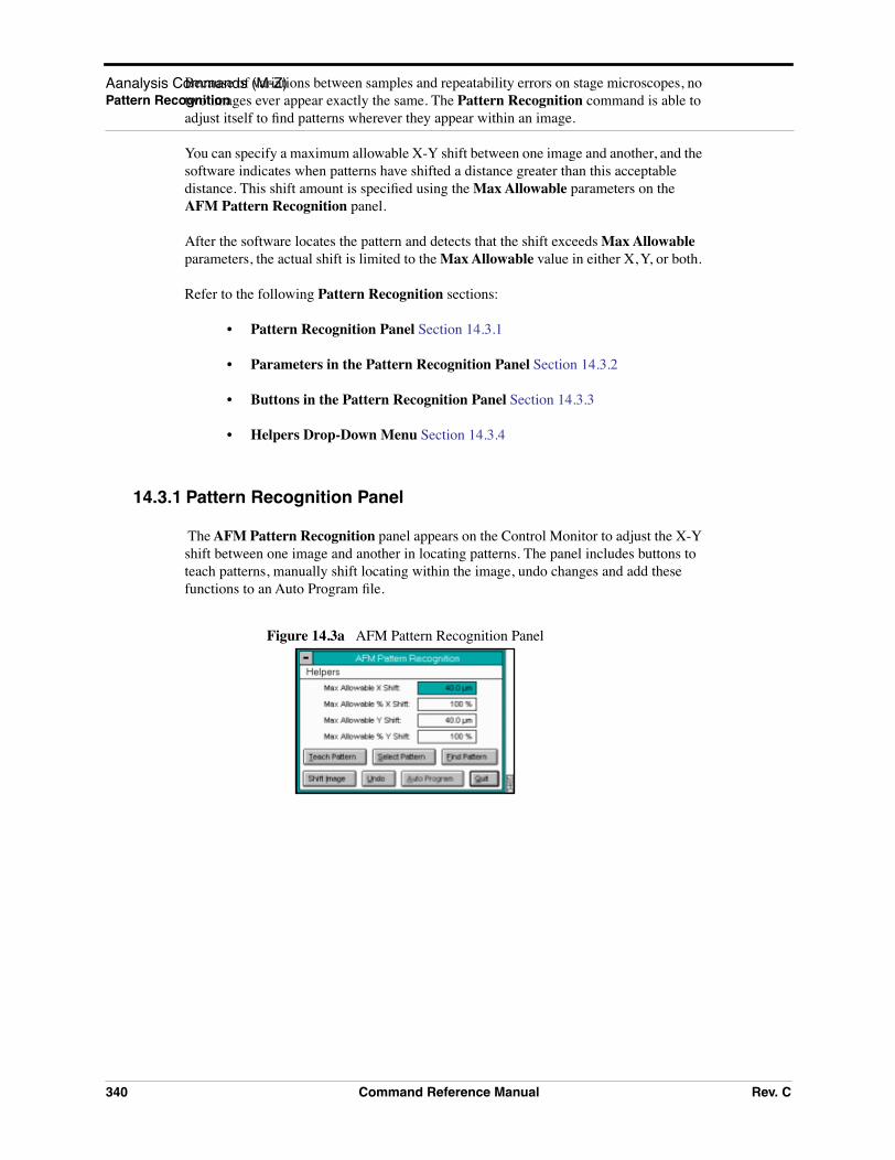
Aanalysis Commands (M-Z)Pattern Recognition

Because of variations between samples and repeatability errors on stage microscopes, no two images ever appear exactly the same. The Pattern Recognition command is able to adjust itself to find patterns wherever they appear within an image.

You can specify a maximum allowable X-Y shift between one image and another, and the software indicates when patterns have shifted a distance greater than this acceptable distance. This shift amount is specified using the Max Allowable parameters on the AFM Pattern Recognition panel.

After the software locates the pattern and detects that the shift exceeds Max Allowable parameters, the actual shift is limited to the Max Allowable value in either X, Y, or both.

Refer to the following Pattern Recognition sections:

• Pattern Recognition Panel Section 14.3.1

• Parameters in the Pattern Recognition Panel Section 14.3.2

• Buttons in the Pattern Recognition Panel Section 14.3.3

• Helpers Drop-Down Menu Section 14.3.4

14.3.1 Pattern Recognition Panel

The AFM Pattern Recognition panel appears on the Control Monitor to adjust the X-Y shift between one image and another in locating patterns. The panel includes buttons to teach patterns, manually shift locating within the image, undo changes and add these functions to an Auto Program file.

Figure 14.3a AFM Pattern Recognition Panel

340 Command Reference Manual Rev. C

Aanalysis Commands (M-Z)Pattern Recognition

14.3.2 Parameters in the Pattern Recognition Panel

Max Allowable X Shift

This parameter sets the maximum amount of shift on the X axis that is acceptable for locating a model from image to image. It is specified in microns.

Changes to the Max Allowable % X Shift parameter (described below) automatically adjust this parameter.

Max Allowable % X Shift

This parameter defines the maximum acceptable X axis shift for locating a model from image to image as a percentage of the Scan size (displayed in the Scan Controls panel on the control monitor). For instance, an image with a Scan size of 10 µm and a Max Allowable % X Shift value of 25% would be acceptable if the image shift did not exceed 2.5 microns.

Changes to the Max Allowable X Shift parameter (described above) automatically adjust this parameter.

Max Allowable Y Shift

This parameter sets the maximum amount of shift on theY axis that is acceptable for locating a model from image to image. It is specified in microns.

Changes to the Max Allowable % Y Shift parameter (described below) automatically adjust this parameter.

Max Allowable % Y Shift

This parameter defines the maximum acceptable Y axis shift for locating a model from image to image as a percentage of the Scan size (displayed in the Scan Controls panel on the control monitor). For instance, an image with a Scan size of 10 µm and a Max Allowable % Y Shift value of 25% would be acceptable if the image shift did not exceed 2.5 microns.

Changes to the Max Allowable Y Shift parameter (described above) automatically adjust this parameter.

14.3.3 Buttons in the Pattern Recognition Panel

Teach Pattern

If the pattern you wish to locate has not been taught, draw a box around the desired feature, then select the TEACH PATTERN button.

An Error prompt appears asking you to specify the area of interest on the image if you select the TEACH PATTERN button before drawing the box (See Figure 14.3b).

Rev. C Command Reference Manual 341

Aanalysis Commands (M-Z)Pattern Recognition

34

Figure 14.3b Teach Pattern Alert Box

Troubleshooting Teach Pattern:

1. Use the mouse to draw a box around the feature to be used as the pattern. The cursor box should encompass the specific feature of interest.

2. After locating the pattern and sizing the box appropriately, click again on the TEACH PATTERN button.

3. Return to the AFM Pattern Recognition panel (See Figure 14.3a).

Select Pattern

If the pattern you wish to locate has already been taught, click on the SELECT PATTERN button to find it and other patterns that have previously been taught. The control monitor displays a listing of all saved pattern files (See Figure 14.3c).

Note: Pattern Recognition files have an *.ovs (Off-line Vision Site) file extension.

Figure 14.3c Pattern Recognition Site File Panel

Find Pattern

After designating the pattern you wish to find (using SELECT PATTERN, above), click on the FIND PATTERN button to locate it in the image. A cursor box identifies it in the currently loaded image.

You may find it necessary to use the SHIFT IMAGE button to make minor adjustments to the image center (See “Shift Image” on page 14-343).

2 Command Reference Manual Rev. C

mands (M-Z)n Recognition

Aanalysis ComPatter

If the pattern is not found, an error message appears.

Figure 14.3d Unidentified Pattern Error Box

If the recognition system does not find the pattern, but you are sure it is within the image, check for the following conditions:

• The pattern may provide a poor visual model because of bad definition or contrast. Patterns must have a distinct, local appearance while remaining relatively simple. Remember, a plain square or cross is a better pattern than a complex curvilinear pattern. The pattern is rejected if the model does not satisfy the Accept Threshold parameter located in the Advanced Features found on the Helpers menu of the AFM Pattern Recognition panel (See Advanced Features).

• The sample may be rotated so that its pattern presents an unrecognizable model to the vision system. Be sure that samples are loaded each time with the same angular orientation. Autoloaded samples rarely have this problem, but manually loaded samples can be loaded at any angle. The use of registration pins or a stage jig on manually loaded stages helps maintain consistent angular orientation.

Shift Image

Use the SHIFT IMAGE button to make minor adjustments to the image’s center if it has been captured away from an ideal center point for your pattern.When you select the SHIFT IMAGE button, an instruction panel appears (See Figure 14.3e).

Figure 14.3e Shift Image Panel

Use the mouse to move the crosshair cursor to the desired image center, then click on Ok. The captured image is shifted on the Display Monitor to place the new image center point at the center of the scan’s field of view.

Rev. C Command Reference Manual 343

Aanalysis Commands (M-Z)Pattern Recognition

34

Undo

The Undo button restores the currently loaded image to its saved version. The image is cleared of any cursors and returned to its unshifted position (if you have used the SHIFT IMAGE command or the image was shifted during execution of FIND PATTERN).

Auto Program

The Auto Program command appends the pattern recognition routine to the list of automatic routines performed on captured images. When the button is selected, the Auto Program Edit panel (See Figure 14.3f) appears.

Figure 14.3f Auto Program Edit Panel

This panel can also be used to update the current Auto Program. If, after you click the SAVE button, the software finds an Auto Program step, you are asked if you want to update it. If not, the software appends the routine.

The Auto Program Edit panel contains several parameters that may be written to the auto result file during Auto Program execution. Click on the box next to each of the parameters you want written to the results file. The Auto Program Edit parameters are illustrated in Figure 14.3g.

4 Command Reference Manual Rev. C

Aanalysis Commands (M-Z)Pattern Recognition

•Delta X—The distance (µm) along the X axis over which the found pattern has shifted from the location of the original, taught pattern.

•Delta Y—The distance (µm) along the Y axis over which the found pattern has shifted from the location of the original, taught pattern.

•Image Name—The name of the image used to teach the pattern recognition step in the Auto Program.

•Model Name—The filename of the model.

•Model Pos X—The X axis location of the pattern relative to the left side of the image.

•Model Pos Y—The Y axis location of the pattern relative to the bottom of the image.

•Model Size X—Width (X-axis dimension) of the model.

•Model Size Y—Height (Y-axis dimension) of the model.

Buttons on the Auto Program Edit Panel

Select All—Selects all parameters on the panel.

Clear All—Deselects all parameters on the panel.

Note—Allows you to make notations to the file.

Save—Saves the pattern recognition data to the Auto Program file.

Delete—Deletes the pattern recognition data from the Auto Program file.

Quit—Exits the Auto Program Edit panel.

Delta X

Delta Y Found pattern

Original,taughtpattern

Model Pos Y

Found pattern

Model Pos X

3472

Figure 14.3g Auto Program Edit Parameters

Rev. C Command Reference Manual 345

Aanalysis Commands (M-Z)Pattern Recognition

34

14.3.4 Helpers Drop-Down Menu

The Helpers drop-down menu (See Figure 14.3h) on the AFM Pattern Recognition panel provides access to functions that configure and modify the pattern recognition process.

Figure 14.3h Helpers Menu on Pattern Recognition Panel

View Pattern Recognition Models

Loads a previously taught video model and displays it on the video monitor.

Advanced Features

The Off-line Pattern Rec - Advanced panel (See Figure 14.3i) enables you to change threshold parameters.

Figure 14.3i Off-line Pattern Rec - Advanced Panel

Display Hit List

A list of X-Y coordinate positions at which the pattern was found in the image the last time Find Pattern was run.

6 Command Reference Manual Rev. C

Aanalysis Commands (M-Z)Power Spectral Density

14.4 Power Spectral Density

The Power Spectral Density (PSD) function is useful in analyzing surface roughness. This function provides a representation of the amplitude of a surface’s roughness as a function of the spatial frequency of the roughness. Spatial frequency is the inverse of the inplane spatial wavelength of the roughness features.

The PSD function reveals periodic surface features that might otherwise appear “random” and provides a graphic representation of how such features are distributed. On turned surfaces, this is helpful in determining speed and feed data, sources of noise, etc. On ground surfaces, this may reveal some inherent characteristic of the material itself such as grain or fibrousness. At higher magnifications, PSD is also useful for determining atomic periodicity or lattice.

Refer to the following Power Spectral Density sections:

• NanoScope PSD Measurements Section 14.4.1

• PSD and Surface Features Section 14.4.2

• PSD and Flatness Section 14.4.3

• Power Spectral Density Panel Section 14.4.4

• Parameters in the Spectral Density Panel Section 14.4.5

• Buttons on the Spectral Density Panel Section 14.4.6

• Power Spectral Density Display Monitor Section 14.4.7

14.4.1 NanoScope PSD Measurements

The Power Spectral Density function computes the following information for the image:

• Total power spectrum - Power is roughness amplitude squared, so power is in units of length squared. Power spectrum is a plot of power as a function of spatial wavelength or frequency.

• 1D PSD - A one dimensional power spectral density. Power spectral density is a plot of the density, in spatial frequency space, of the power spectrum. Its units are length squared divided by a one dimensional frequency, or 1 over length, which is length cubed. A 1D PSD can be calculated in either the X direction of the data or in the Y direction.

• 1D isotropic PSD - A different version of a one dimensional power spectrum.

• 2D isotropic PSD - A two dimensional power spectral density. Its units are length squared divided by a two dimensional frequency, or 1 over length squared, which is length to the fourth power. This is isotropic in the sense that it is an average taken over all directions in the data.

Rev. C Command Reference Manual 347

Aanalysis Commands (M-Z)Power Spectral Density

34

• RMS roughness values - Since the RMS roughness is the square root of the integral of the PSD, over some wavelength or frequency interval, this calculation can be conveniently done when one has the PSD.

14.4.2 PSD and Surface Features

Consider the image in Figure 14.4a.

Figure 14.4a Waveform Surfaces

This synthetic surface consists of essentially two dominant wave forms: a long period waveform along the X-axis, and a shorter period waveform along the Y-axis. A 2 dimensional power spectral density plot consists of two dominant spikes (one for each dominant wavelength), plus some number of extra wavelengths inherent within the image. (These extra wavelengths may appear due to fine surface features and/or side bands of the dominant wave forms.) Because of the sinusoidal nature of the composite wave form, a relatively small set of spectral frequencies suffices to describe the entire surface. By contrast, an image comprised of angular (saw-toothed or square) waveform contains more spatial frequency components.

Over a given range of spatial frequencies the total power of the surface equals the RMS roughness of the sample squared. The frequency distribution for a digitized profile of length L, consisting of N points sampled at intervals of d0 is approximated by:

1564

-110

XY

PSD(f) = 2do

N-------- e

i 2πN

---------- n 1–( ) m 1–( )z n( )

n 1=

N

∑2

for f = m 1–Ndo

-------------

8 Command Reference Manual Rev. C

Aanalysis Commands (M-Z)Power Spectral Density

Where i = √-1, and frequencies, f, range from to . Practically speaking, the algorithm used

to obtain the PSD depends upon squaring the FFT of the image to derive the power. Once the power, P, is obtained, it may be used to derive various PSD-like values as follows:

The terms used in the denominators above are derived by progressively sampling data from the image’s two-dimensional FFT center (See Figure 14.4b).

Figure 14.4b Progressive Data Sampling

Each sampling swings a “data bucket” of given frequency f. Since samples are taken from the image

center, the sampling frequency, f, is limited to , where N is the scan size in pixels. This forms

the upper bandwidth limit (i.e., the highest frequency) of the PSD plot. The lower bandwidth limit is defined at 1/L.

14.4.3 PSD and Flatness

PSD is used increasingly as a metrology tool for evaluating extremely flat surfaces, such as polished or epitaxial silicon. Generally, the desired surface is expected to adhere to certain PSD thresholds, signifying it meets a specified flatness criterion. The main advantage gained over traditional RMS specifications is that PSD flatness is qualified through the full spectral range of interest. For example, one may specify spectral thresholds at frequencies measured on the atomic scale, thus ensuring surfaces consist largely of uniform lattices. Setting the precise thresholds for various materials remains a matter of debate.

Consider the image of epitaxial gallium arsenide in Figure 14.4c (See file “gaas.epi” on the images disk).

1L---

N 2⁄L

-----------

1D PSD P∆f------=

1D isotropic PSD P2πf---------=

2D isotropic PSD P2πf ∆f( )--------------------=

f = 1 pixel f = 2 pixels f = 3 pixels f = 4 pixels

∆f

N 2⁄L

-----------

Rev. C Command Reference Manual 349

Aanalysis Commands (M-Z)Power Spectral Density

35

Figure 14.4c Epitaxial Gallium Arsenide Image

This surface is comprised of “terraces” formed from the material’s natural lattice structure; each terrace is one atomic monolayer thick and is spaced at fairly regular intervals. This degree of flatness is handily evaluated with PSD, as the terraces produces a spectral spike corresponding to their spacing wavelength. A PSD plot for this type of surface generally takes the form shown in Figure 14.4d.

Figure 14.4d PSD Plot for Terraced Sample

This tapered PSD plot is characteristic of flat, isotropic surfaces. Longer wavelengths are present up to the scan width, and are accompanied by uniformly decreasing powers of shorter wavelengths down to 2 pixels. On the plot shown above a spike stands out, corresponding to the wavelength spacing of the terraced features. Depending upon the qualitative standards of the person evaluating such a plot, this spike may exceed a threshold standard of flatness.

14.4.4 Power Spectral Density Panel

The Spectral Density panel allows items on the Display Monitor to be adjusted to your preferences.

104

10-1

101 10-2

PSD

Wavelength (µm/cycle)

2D Isotropic PSD

Spectral spike corresponding to "terrace" spacings on surface

0 Command Reference Manual Rev. C

ands (M-Z)tral Density

Aanalysis CommPower Spec

Figure 14.4e Spectral Density Panel

14.4.5 Parameters in the Spectral Density Panel

Data Scale

Controls the vertical range of the image corresponding to the full extent of the color table.

Color Table

Selects the color table used to encode Z information.

Export Data

Sets the type of data to be exported from the display screen parameters. Data is exported in a spreadsheet format readable by most third-party applications. Generally, data is exported in two-column x N/2 rows, where N equals the scan size in pixels. Each row is separated by a carriage return; columns are separated with a space.

Range and Settings:

• Power, 1D PSD, 1D iso PSD, 2D iso PSD

Color Contrast

Controls the contrast in the image by compressing or expanding the color table.

Color Offset

Changes the image color by shifting the range of the color table used to display the image.

Rev. C Command Reference Manual 351

Aanalysis Commands (M-Z)Power Spectral Density

35

14.4.6 Buttons on the Spectral Density Panel

2D—Executes a two-dimensional Power Spectral Density analysis.

X—Executes a one-dimensional Power Spectral Density analysis along the X-axis.

Y—Executes a one-dimensional Power Spectral Density analysis along the Y-axis.

Note—Allows a descriptive message to be added to the display.

Export—Saves current PSD data to a directory and file name you define (See Figure 14.4f).

Figure 14.4f Power Spectral Density Export Panel

Save—Saves current PSD analysis to a directory and file you specify.

Note: The PSD Compare function may only be performed on PSD data files that have been saved to a common directory.

Quit—Exits the Power Spectral Density function.

14.4.7 Power Spectral Density Display Monitor

The Display Monitor generates a histogram of wavelength versus power. Both wavelength and power are indicated on logarithmic scales (See Figure 14.4g).

2 Command Reference Manual Rev. C

mands (M-Z)ectral Density

Aanalysis ComPower Sp

Figure 14.4g Power Spectral Density Display

The calculation begins as soon as the command is selected from the menu. The PSD and a table of values from the graph are shown on the Display Monitor.

Display Table Parameters

• Wavelength—The wavelength in µm/cycle units at current cursor positions.

• Frequency—The frequency in cycles per µm at current cursor positions.

• Power—Power measured in nm2 at current cursor positions.

• 1D PSD—One-dimensional power spectral density. (See Section 14.4.2 for mathematical definition.) Power measured in nm3 at current cursor positions.

• 1D isotropic PSD—One-dimensional, isotropic power spectral density. (See Section 14.4.2 for mathematical definition.) Power measured in nm3 at current cursor positions.

• 2D isotropic PSD—Two-dimensional, isotropic power spectral density. (See Section 14.4.2 for mathematical definition.) Power measured in nm4 at current cursor positions.

Note: The 2D isotropic PSD is the power function that is plotted on the Display Monitor histogram.

109

101

101 10-3

PSD

Wavelength (µm/cycle)

2D Isotropic PSD

Wavelength (µm/cycle):Frequency (cycles/µm):Power (nm2):

Total Power:Equivalent RMS:Power Between Cursors:Equivalent RMS:

rings

0.091410.95.28e+004

0.007911260.0789

0.000566 nm4

0.0238 nm0.000503 nm4

0.0224 nm

Power Spectral Density

1D PSD (nm3): 5.28e+007 78.91D isotropic PSD (nm3): 8.53e+005 0.104

2D isotropic PSD (nm4): 8.53e+008 104

Rev. C Command Reference Manual 353

Aanalysis Commands (M-Z)PSD Compare

35

• Total power—The sum of the power contained in the entire spectrum.

• Equivalent RMS—The root-mean-square (RMS) roughness of the sample. It is calculated as the square root of the total power.

• Power Between Cursors—The sum of the power contained in the portion of the spectrum between the cursors.

• Equivalent RMS—The root-mean-square (RMS) roughness of the sample contributed by the frequencies between the cursors. It is calculated as the square root of the integral of the Power Between Cursors (above).

Plot

Specifies the vertical axis of the PSD plot.

• Power—Power (nm2 units) is plotted against wavelength.

• 1D PSD—One-dimensional power (nm3 units) is plotted against wavelength.

• 1D ISO—One-dimensional, isotropic power (nm3 units) is plotted against wavelength.

• 2D ISO—Two-dimensional, isotropic power (nm4 units) is plotted against wavelength.

Mouse operations on the Display Monitor

The cursors in the power spectrum can be moved by clicking on a cursor and dragging the mouse.

Note: The ASTM E-42.14 STM/AFM Subcommittee report on “Standard Practices for Analyzing and Reporting Surface Roughness as Measured by STM/AFM” describes the basic method for quantifying the surface roughness of materials imaged by STM and AFM.

14.5 PSD Compare

The PSD Compare command permits one-to-one comparison between PSD data files (as saved from the Analyze/Power Spectral Density command). The power spectral density plot for each compared file is presented on a graph so that overlapping power data may be directly compared; PSD data is displayed in a table below. Plots are displayed and compared for: power, 1-dimensional PSD, 1-dimensional isotropic, or 2-dimensional isotropic data.

To utilize PSD Compare, it is necessary to collect all PSD files in a common directory and transfer to that directory beforehand. When the PSD Compare command is accessed, the software searches

RMS W∫ p,q( )δpδq=

4 Command Reference Manual Rev. C

Aanalysis Commands (M-Z)PSD Compare

the current directory for PSD files. If none are found, an error message (“Warning: Directory has no files with .psd extension”) displays.

Refer to the following PSD Compare sections:

• PSD Compare Panel Section 14.5.1

• Buttons on the PSD Compare Panel Section 14.5.2

• PSD Compare Display Monitor Section 14.5.3

• Reference Data Section 14.5.4

14.5.1 PSD Compare Panel

Clicking on the Analyze / PSD Compare command displays the PSD Compare panel (See Figure 14.5a).

Figure 14.5a Power Spectral Density Compare Panel

All saved PSD data files are listed for the current directory and feature a “.psd” extension. To change directories, use the Off-line file manager panel. To select files for comparison, click on the box to the left of each file; an “X” indicates that the file is to be compared. Up to six PSD data files may be selected and compared at one time.

14.5.2 Buttons on the PSD Compare Panel

Execute—Plots the selected data (where an “X” has been placed) to the Display Monitor histogram and displays each data set’s PSD information.

Clear—Deselects all previously selected files (removes all “X”s).

Rev. C Command Reference Manual 355

Aanalysis Commands (M-Z)PSD Compare

35

Quit—Quits PSD Compare command.

14.5.3 PSD Compare Display Monitor

On the Display Monitor, the selected files are plotted relative to one another. If the PSD data is similar between files, plots may be overlapping.

Figure 14.5b PSD Compare Display

Sliding the line cursor back and forth on the plot histogram displays new data for each point. Where a plot has no data, the value reads “NA” (not available).

Display Monitor Commands

Plot

Commands listed here present different types of data histograms on the Display Monitor. Choices are outlined below.

• Power—Total PSD power data is plotted.

• 1D PSD—One-dimensional PSD data is plotted.

• 1D ISO—One-dimensional isotropic PSD data is plotted.

• 2D ISO—Two-dimensional isotropic PSD data is plotted.

106

10-13

101 10-2

ISO

Wavelength (µm/cycle)

FilenamePSD TypePower (nm2)

Delta 2D PSDDelta PowerWavelength (µm)Frequency (/µm)

data12D

0.0114

data22D

0.00367

-1.16e+003-0.0077

0.2384.2

PSD Compare

1D PSD (nm3) 45.5 14.71D iso PSD (nm3) 0.429 0.139

2D iso PSD (nm4) 1.71e+003 554

2D

::::::::::

00

Reference

Click left button on fieldentry to select Ref. File

or turn plot on/off

Reference Plotyesyes

*data1data2

Plot Graph

Plot: 2D ISO Graph: Both

Click here with mouseto select reference data.

6 Command Reference Manual Rev. C

Aanalysis Commands (M-Z)PSD Compare

Graph

Commands listed here determine the manner in which data is plotted to the histogram. Choices are outlined below.

• Curves—Plots data as a series of curves.

• Lines—Plots data as a series of lines (bar graph).

• Both—Plots data with both curves and lines simultaneously.

14.5.4 Reference Data

Clicking on the Reference column in the upper-left corner of the Display Monitor allows a file to be designated as the reference data set. An asterisk (*) is placed alongside the selected file name and REFERENCE is displayed above the data column. Each data set is also assigned a separate color to assist in organization. Two values are generated from the reference data:

• Delta 2D PSD—Difference in two-dimensional PSD value between reference data and selected data.

• Delta Power—Difference in total power between reference data and selected data.

Rev. C Command Reference Manual 357

Aanalysis Commands (M-Z)Roughness

35

14.6 Roughness

The Roughness command generates a wide variety of statistics for surfaces, including classical roughness values, peak and summit (texture) data and surface area calculations. “Image” statistics are reported for the entire image. “Box” statistics are reported only for the region you define within a cursor box. In addition, the area included within a box cursor can be augmented with passbands and stopbands to isolate specific features.

Most industrial standards for roughness measurement call for planefitting of data before values are calculated. Digital Instruments’ Roughness routine applies a temporary, first-order planefit before calculating roughness statistics. On many surfaces, especially those which are tilted, this yields different values from those seen in raw (unplanefitted) data. Moreover, peripheral features included within the analyzed region may produce cumulative results uncharacteristic of the feature(s) of interest. To ensure the best results, you should observe the following rules when using Roughness analysis:

• If the image shows signs of second- or third-order distortion (e.g., bow due to large scans areas on large scanners), apply a second- or third-order Flatten (Off-line/Modify/Flatten) and Planefit (Off-line/Modify/Planefit) to the image before using Roughness analysis.

• Isolate your analysis to specific areas of the image. This may be accomplished by using Off-line / Modify / Zoom to limit the entire image, or by using the box cursor in Roughness to analyze only select portions of the image.

For further details on the Roughness panels and parameters, refer to the following sections:

• Roughness Parameters Section 14.6.1

• Navigating Control Panels in Roughness Analysis Section 14.6.2

• Roughness Panel Section 14.6.3

• Auto Program Edit Panel Section 14.6.4

• Screen Layout Panel Section 14.6.5

• Roughness Display Monitor Section 14.6.6

• Troubleshooting the Roughness Function Section 14.6.7

• Roughness Data Definitions Section 14.6.8

• Example of Using Roughness Analysis Section 14.6.9

14.6.1 Roughness Parameters

There are currently forty-five parameters available from the Roughness routine; however, only parameters selected from the Screen Layout menu are actually displayed and reported. In addition,

8 Command Reference Manual Rev. C

Aanalysis Commands (M-Z)Roughness

some parameters are reported only when certain subroutines are turned on from the command bar of the Display Monitor. For example, Surface area is displayed only when it has been selected from the Screen Layout panel AND the “Surface Area” subroutine is turned On.

Table 14.6a lists all parameters available within the Roughness routine, along with subroutines required (if any) to be turned On for their display.

To display a parameter, select it from the Screen Layout panel first, then turn On the required subroutine.

Note: Only 21 parameters can be selected an on time. If the box gets too big, the image statistics after 21 do not display.

Refer to Section 14.6.8 for Roughness parameter definitions.

Table 14.6a Roughness Parameters

ParameterRequired Subroutine

“Peak” “Surface Area” “Summit”

10 pt mean (Rz)

Area Thresh abs X

Area Thresh ref X

Area Thresh (%rms) X

Av max depth (Rvm) X

Av max ht (Rpm) X

Box x dimension

Box y dimension

Img. Mean

Img. Ra

Img. Raw mean

Img. Rmax

Img. RMS (Rq)

Img. Srf. area

Img. Srf. area diff

Img. Z range

Kurtosis

Line density

Max depth (Rv) X

Max height (Rmax)

Max peak ht (Rp) X

Mean

Mean roughness (Ra)

Peak count X

Peak Threshold X

Rev. C Command Reference Manual 359

Aanalysis Commands (M-Z)Roughness

36

14.6.2 Navigating Control Panels in Roughness Analysis

Off-line/Analyze/Roughness accesses the Roughness panel. After selecting the captured image, you can configure and program commands that allow for specific Roughness Analysis. For an overview of the navigational path in this analysis, see Figure 14.6a.

Peak Thresh ref X

Peak Thresh (%rms) X

Raw mean

RMS (Rq)

Skewness

Summit count X

Summit curvature X

Summit Cutoff X

Summit Cutoff ref X

Summit Cutoff (%rms) X

Summit density X

Summit diameter X

Summit Threshold X

Summit Thresh ref X

Summit Thresh (%rms) X

Summit rad. curv. X

Summit slope X

Surface area X

Surface area diff X

Z range

Table 14.6a Roughness Parameters

ParameterRequired Subroutine

“Peak” “Surface Area” “Summit”

0 Command Reference Manual Rev. C

Aanalysis Commands (M-Z)Roughness

Figure 14.6a Navigating in Roughness Analysis

14.6.3 Roughness Panel

The Roughness panel includes familiar display parameters and buttons to control the image display and set parameters (See Figure 14.6b).

Figure 14.6b Roughness Panel.

Parameters in the Roughness Panel

Data Scale

Controls the vertical range of the image corresponding to the full extent of the color table. This is the difference between the highest and lowest points within the image.

The units of this item vary according to the type of image (e.g., nm, nA, etc.).

Note: This value does not correct for tilt in the plane of the data; therefore, plane fitting or flattening the data changes the data while the data scale remains the same value.

Rev. C Command Reference Manual 361

Aanalysis Commands (M-Z)Roughness

36

Color Table

Selects the color table used to encode the image (e.g., Z information).

Color Contrast

Controls the contrast in the image by compressing or expanding the color table.

Color Offset

Shifts the color table used to display the image.

Buttons in the Roughness Panel

Note—Appends a descriptive message to the image file and the bottom of the displayed image.

Auto Program—Accesses the Auto Program Edit panel and allows Roughness parameters to be selected and stored in the Auto Program file list. For details on the Auto Program Edit panel, see Section 14.6.4.

Screen Layout—Accesses the Screen Layout panel and allows you to select the Roughness parameters to display. For details on the Screen Layout panel, see Section 14.6.5.

Quit—Exits the Roughness command.

14.6.4 Auto Program Edit Panel

The Auto Program Edit panel allows Roughness parameters to be selected and stored in the Auto Program file list. When the Auto Program file is run, the selected Roughness parameters are computed and listed in a report file along with any other functions selected (See Figure 14.6c).

Figure 14.6c Auto Program Edit Panel

Note: Select up to 21 parameters to be added to the output result file.

2 Command Reference Manual Rev. C

Aanalysis Commands (M-Z)Roughness

Buttons in the Auto Program Edit Panel

Select All—Selects all the measurements simultaneously.

Clear All—Clears all the measurements simultaneously.

Set Limits—Sets specific measurement limits for an AutoProgram result. You may specify the Min, Max ,and % of Section values for each result available in the Set Limits window.

Note—Allows a descriptive message to be added to the display and the Auto Program Results file.

Save—Saves selected measurements to the Auto Program file. If the Roughness Analysis command is already in the current Auto Program file, it retains its position in the file.

An option exists to overwrite the command or add this as a second particle analysis command in the program.

Delete—Removes the Roughness command from the Auto Program file.

Quit—Exits the Auto Program Edit mode without making changes to the Auto Program file.

Note: The Auto Program File command in the Off-line/ Utility menu must be used to create and edit Auto Program files. The Auto subcommand under the Browse command selects the currently selected files to be processed and executes the Auto Program file (Utility menu/Auto Program File).

14.6.5 Screen Layout Panel

The Screen Layout panel allows you to select which Roughness parameters display. Because of the limited size of the Display Monitor, it shows a maximum of twenty-one parameters at any one time; however, the current Auto Program files still contains all selected parameters.

Figure 14.6d Screen Layout Panel

Buttons and Parameters on the Screen Layout Panel

Rev. C Command Reference Manual 363

Aanalysis Commands (M-Z)Roughness

36

To select a parameter, use the mouse to place an “X” in the box next to it. Deselect a parameter by removing its “X” with the mouse.

Save—Finalizes the selected Roughness parameters. Once the Save button is clicked, the selected parameters appear on the Display Monitor.

Quit—Exits the Screen Layout panel without changing the parameter selection.

14.6.6 Roughness Display Monitor

The Display Monitor shows the image alongside Roughness parameters selected from the Screen Layout panel. Parameters chosen from the Screen Layout panel are displayed in two data boxes (i.e., Box Statistics and Image Statistics). Values listed in the Box Statistics apply only to the area within the box cursor; if no box cursor is drawn, no values appear there. Image Statistics apply to the entire image. Commands on the menu bar control the operating mode (See Figure 14.6e).

Figure 14.6e Roughness Display

Roughness Display Menu Bar Commands

Peak

The Peak feature, when switched On, isolates specified height portions of the image (peaks) from background data. Peaks are specified using the Peak Threshold panel, either in terms of their absolute height or their deviation from the RMS value of all surface data, and relative to either the highest data point (Peak) or the lowest (Zero). When Peak is turned On, portions of the image contained within the box cursor and falling within the specified boundaries are retained; all other data is removed.

ParametersFor BoxedArea on Image

ImageFor Whole Statistics

4 Command Reference Manual Rev. C

Aanalysis Commands (M-Z)Roughness

• On—The following statistical parameters are turned on: Peak Threshold; Peak Thresh ref.; Peak Thresh (%rms); 10 Pt Mean (Rz); Peak count; Max peak ht (Rp); Ave. Max ht (Rpm); Max depth (Rv); and, Ave. max depth (Rvm). All Peak parameters are calculated from the threshold you define with the Threshold subcommand.

• Off—Peak statistics are not calculated.

• Threshold—Defines a height threshold for the Peak measurement (See Figure 14.6f).

Figure 14.6f Peak Threshold Panel

Peak Threshold Panel

The Reference options select whether the threshold is defined relative to the Zero (lowest) value, or the tallest Peak in the selected region.

The Value Type options select whether the threshold is defined as an absolute distance (Absolute value) from the reference point or a percentage of the root-mean-square (RMS %) of the Z values.

Surface Area Menu Command

Controls the surface area statistical calculations. Disable Surface Area functions on the Area Threshold panel (i.e., unlike Peak functions that are enabled in the Menu commands).

Range and Settings:

• On—The following statistical parameters are turned on: Surface area; Surface area diff; Area Thresh (% rms); and, Area Thresh abs. Parameters are calculated based on the threshold you define with the Threshold subcommand.

• Off—Surface area statistical parameters are not calculated.

• Threshold—The Area Threshold panel allows a height threshold for surface area statistics (See Figure 14.6g).

ReferenceOptions

Value TypeOptions

Rev. C Command Reference Manual 365

Aanalysis Commands (M-Z)Roughness

36

Figure 14.6g Area Threshold Panel.

Area Threshold Panel

When Threshold is On, the surface area is calculated for the surface above the threshold. The threshold is applied according to the Reference and Value Type parameters in the panel. When Threshold is Off, the surface area of the entire selected area is calculated.

The Reference options determine whether the threshold is defined relative to the Zero value of the data or the tallest Peak within the selected region.

The Value Type options determine whether the threshold is defined as an absolute distance from the reference point in nanometers (Absolute value) or a percentage of the root-mean-square (RMS %) of the Z values.

Note: Surface area is calculated as a sum of triangles over the surface of the analyzed area defined within two-by-two pixel kernels (See Figure 14.6h).

Figure 14.6h Surface Area Calculation

Summit

A summit is any surface data point which is higher than its four nearest neighbors by a height you specify. The Summit subroutine allows you to isolate summits according to the Threshold settings. See also, Section 14.6.8 for specific descriptions of summit parameters.

Range and Settings:

Pixels

Triangular areas

6 Command Reference Manual Rev. C

mands (M-Z)Roughness

Aanalysis Com• On—The number of summits within the box cursor is determined based on the threshold you define with the Threshold subcommand. The number of summits is reported as the Summit count. The number of summits is divided by the area of the box cursor and reported as the Summit density.

• Off—The Summit determination is not performed.

• Threshold—The Summit Threshold panel appears on the control monitor, allowing a height threshold for the summit determination to be defined.

• The Reference selection defines whether the threshold is defined relative to the zero value of the data or the tallest peak in the selected region.

• The Value Type selects whether the threshold is defined as an absolute distance from the reference point or a percentage of the root-mean-square of the Z values.

• Cutoff—The Summit Cutoff panel appears on the control monitor, allowing a cutoff threshold for the summit determination to be defined.

• Summit disp. on/off—Allows you to display the summit.

Zero crossing

A zero crossing is a point where the Z values go through zero regardless of slope. This value is the total number of zero crossings along both the X and Y center lines divided by the sum of the box dimensions.

Range and Settings:

• On—The number of zero crossings along the X and Y center lines of the box cursor is determined. The number of zero crossings is divided by the sum of the lengths of the X and Y center lines and reported as the Line density.

• Off—The zero crossing determination is not performed.

Rev. C Command Reference Manual 367

Aanalysis Commands (M-Z)Roughness

36

Stopband

Excludes covered regions of the image from analysis.

Range and Settings:

• Add—This creates a rectangle you define containing an X whose area is excluded from the roughness calculation. Click on the image to create the stopband.

• Remove—Removes stopbands which have already been drawn. Click on the stopband(s) to be removed.

• Clear—Removes all stopbands.

Execute—Calculates roughness values for the region you define.

Cursor—Controls the type of cursor to be used.

• Clear—Removes all cursors from the image.

• Box—Places the cursor into box mode, which is the normal, default cursor mode. Boxes are defined by dragging the cursor from one corner to another. To switch the cursor to summit mode, select the Summit option.

• Summit—Allows summits to be selected and analyzed individually. Selected summits are distinquished by a small X. Summit statistics on the Display Monitor pertain only to the selected summit. To switch the cursor back to box mode, select the Box option.

Mouse Operation on the Display Monitor

Within the image

• 1st click, left button—Locates a corner of a rectangle and allows the rectangle to be formed by moving the mouse.

• 2nd click, left button—Fixes the position of the opposite corner of the box. After selecting the Execute command, the 2nd click, left button calculates the roughness values for the area confined by the box, and displays the values in the measurement chart.

• 3rd click, left button—The effect of the third depends on the position of the cursor when the click occurs.

• On box edge—clicking the left button when the cursor is on an edge of the box allows that edge of the box to be repositioned by moving the mouse.

• On box corner—Clicking the left button when the cursor is on a corner of the box allows that corner of the box to be repositioned by moving the mouse.

8 Command Reference Manual Rev. C

Aanalysis Commands (M-Z)Roughness

• Inside the box—Clicking the left button when the mouse is inside the box allows the entire box to be repositioned by moving the mouse.

• 4th click, left button—Freezes the position and/or size of the box.

• Right mouse button—Clicking the right mouse button when the cursor is in any of the windows moves the cursor to the menu bar.

14.6.7 Troubleshooting the Roughness Function

• All Roughness parameters are affected by offline filters applied to the data beforehand. When qualifying roughness statistics, be certain to evaluate the impacts of previous operations.

• Some statistics calculated by the Roughness routine are also calculated by other routines. (For example, RMS roughness is also calculated by the Offline / Analyze / Section and PSD routines).

If statistics differ slightly from routine-to-routine, it may be because they are calculated for a line rather than an area, or because planefitting was utilized. Check the appropriate sections in this manual to determine how values are calculated.

• Regarding the Effects of Planefitting on Roughness Statistics—When Roughness analysis is applied to an image, statistical values are calculated according to the relative heights of each pixel in the image. Planefitting—used to correct images for tilt and bow—reorients these pixels in a manner which can affect roughness statistics dramatically on some surfaces. This is especially true of surfaces having broad, coplanar features. Planefitting can be applied at the time of file capture using Real-time planefit and Off-line planefit from a Channel panel, or via either of the two Modify / Plane Fit functions.

• When Roughness analysis is applied to an image, the image data is automatically planefit beforehand. This is done to accord with ASME and ISO metrological standards. (Only the Raw mean parameter is exempt from this operation, being calculated from raw data only.) To avoid unexpected results due to planefitting, be certain to apply Roughness analysis only to the surface(s) of interest by utilizing a cursor box, or by scanning just the specific site of interest. Including peripheral features within an analyzed area may produce cumulative results uncharacteristic of the feature(s) of interest.

• The relationship between the zero plane and the data also changes according to the setting of the Off-line planefit parameter. If the Off-line planefit parameter is set to None the offset is not removed from the data and it is very possible that the zero plane does not intersect the data. The other settings of the parameter subtract the average Z value from every point in the image so the data varies around the zero plane.

• Regarding Basic Roughness Measurements—Average roughness (Ra) is one of the most commonly used roughness statistics. Figure 14.6i represents two surfaces having the same “average roughness”.

Rev. C Command Reference Manual 369

Aanalysis Commands (M-Z)Roughness

37

Similarly, a number of other roughness values are based upon least-squares calculations (e.g., RMS roughness, or Rq), and their algorithms are more concerned with a best fit of all height points than with the spatial frequency of features.

Figure 14.6i Basic Roughness Measurements

The surface of image A is represented as having a high frequency profile of features. Image B represents a separate surface having the same average feature height, but distributed at wider (lower-frequency) intervals. In terms of average and RMS roughness, both surfaces are “equally rough.” If you are interested in differentiating between the two, you must rely upon more precise statistical parameters. Refer to the Analyze / Bearing and Power Spectral Density functions, which analyze surface features in terms of depth-versus-occurrence and wavelength-versus-power, respectively.

14.6.8 Roughness Data Definitions

Statistics used by the Roughness routine are defined in this section. The terms are listed alphabetically. Most are derived from ASME B46.1 (“Surface Texture: Surface Roughness, Waviness and Lay”) available from the American Society of Mechanical Engineers, which should be consulted.

10 pt mean (Rz)

This is the average difference in height between the five highest peaks and five lowest valleys relative to the Mean Plane. In cases where five pairs of peaks and valleys do not exist, this value is based on fewer points.

1567-110

A B

Best-fit plane

0 Command Reference Manual Rev. C

mands (M-Z)Roughness

Aanalysis ComArea Thresh abs

The threshold absolute value in terms of height.

Area Thresh ref

The reference point for the area threshold.

Area Thres (%rms)

The threshold value as a percentage of the root-mean-square of the Z values.

Av max depth (Rvm)

Average distance between the five lowest profile points and the mean data plane.

Av max ht (Rpm)

Average distance between the five highest profile points and the mean data plane.

Box x dimension

The width of the Lx box cursor you define.

Box y dimension

The length of the Ly box cursor you define.

Img. Mean

Mean value of data contained within the image.

Img. Ra

Rev. C Command Reference Manual 371

Aanalysis Commands (M-Z)Roughness

37

Arithmetic average of the absolute values of the surface height deviations measured from the mean plane.

Img. Raw mean

Mean value of image data without application of plane fitting.

Img. Rmax

Maximum vertical distance between the highest and lowest data points in the image.

Img. RMS Rq

Root mean square average of height deviations taken from the mean data plane, expressed as:

Img. Srf. area

The three-dimensional area of the analyzed region. This value is the sum of the area of all of the triangles formed by three adjacent data points.

Img. Srf. area diff

Difference between the image’s three-dimensional Surface area and its two-dimensional, footprint area.

Img. Z range

Maximum vertical distance between the highest and lowest data points in the image. (Same as Img. Rmax).

Kurtosis

This is a non dimensional quantity used to evaluate the shape of data about a central mean. It is calculated as follows:

Ra1n--- Zj

j 1=

n

∑=

Zi2∑

n--------------- Rq=

Kurtosis1

Rq4

--------- 1n--- Zj

4

j 1=

n

∑=

2 Command Reference Manual Rev. C

Aanalysis Commands (M-Z)Roughness

Graphically, kurtosis indicates whether data are arranged flatly or sharply about the mean.

Line Density

The number of zero crossings per unit length on the X and Y center lines of the box cursor. A zero crossing is a point where the Z values go through zero regardless of slope. This value is the total number of zero crossings along both the X and Y center lines divided by the sum of the box dimensions.

Max Depth (Rv)

Lowest data point in examined region.

Max height (Rmax)

Maximum vertical distance between the highest and lowest data points within the cursor box.

Max peak ht (Rp)

Maximum peak height within the analyzed area with respect to the mean data plane.

Mean

The average of all the Z values within the enclosed area. The mean can have a negative value because the Z values are measured relative to the Z value when the microscope is engaged. This value is not corrected for tilt in the plane of the data; therefore, plane fitting or flattening the data changes this value.

Mean Roughness (Ra)

Arithmetic average of the absolute values of the surface height deviations measured from the mean plane within the box cursor:

Peak Count

The number of Surface peaks taller than the threshold.

Peak Threshold

Ra1n--- Zj

j 1=

n

∑=

Rev. C Command Reference Manual 373

Aanalysis Commands (M-Z)Roughness

37

The threshold value in terms of height.

Peak Thresh ref

The reference point for the peak threshold.

Peak Thresh(%rms)

The threshold value as a percentage of the root-mean-square of the Z values.

Raw Mean

Mean value of image data within the cursor box you define without application of plane fitting.

RMS (Rq)

This is the standard deviation of the Z values within the box cursor and is calculated as:

where Zi is the current Z value, and N is the number of points within the box cursor. This value is

not corrected for tilt in the plane of the data; therefore, plane fitting or flattening the data changes this value.

Skewness

Measures the symmetry of surface data about a mean data profile, expressed as:

where Rq is the RMS roughness. Skewness is a non dimensional quantity which is typically evaluated in terms of positive or negative. Where Skewness is zero, an even distribution of data around the mean data plane is suggested. Where Skewness is strongly non-zero, an asymmetric, one-tailed distribution is suggested, such as a flat plane having a small, sharp spike (> 0), or a small, deep pit (< 0).

Summit Count

Number of summits within the analyzed area having the defined “Threshold” and “Cutoff” values.

Note: Summits are identified on the image with special markers:

Rq

Zi( )∑ 2

n-------------------=

Skewness1

Rq3

--------- 1n--- Zj

3

j 1=

n

∑=

4 Command Reference Manual Rev. C

Aanalysis Commands (M-Z)Roughness

Summit Curvature

Measure of the peak’s sharpness using the summit and one of its nearest neighbors.

Summit Cutoff

Distance where a summit is recognized, referenced either from the mean Zero data plane or the highest Peak. The cutoff is measured in terms of an Absolute value, or as a percentage of the total data range (% of Range) within the analyzed area.

Figure 14.6j Summit Illustrations

Summit Cutoff ref

Summit

Summit Threshold

Summit (individual pixel)

Neighboring pixel (1 of 4)

Maximum data point

Summit Cutoff

Summit slope

Summit Cutoff

(referenced from Peak)

(referenced from Zero)

Summitdiameter

[Max peak ht (Rp)]

X

Summit base (+X)

Summit base (-X)

Maximum data point[Max peak ht (Rp)]

Z

X

Z

Rev. C Command Reference Manual 375

Aanalysis Commands (M-Z)Roughness

Reference from which the Summit Cutoff is measured. There are two choices: the Zero data plane, and the Peak (maximum) data point.

Summit Cutoff (%rms)

Summit Cutoff measured in terms of a percentage of the root mean square.

Summit Density

Number of summits found within the analyzed image area expressed as peaks per square micron.

Summit Diameter

Diameter of summit as measured from one summit base to another.

Summit Threshold

Minimum distance a pixel must rise above all four of its nearest neighbors to be identified as a summit.

Note: Usually, this value must be small to work effectively (e.g., < 500 nm Absolute value, or< 2% of Range), as many summits prove to be relatively flat on top.

Summit Thresh ref

Reference from which the Summit Threshold is measured.

Summit Thresh (% range)

Summit Threshold expressed as a percentage of height range.

Summit Rad. Curv.

Radius of curvature expressed as the inverse of the summit curvature found by using a summit and one of its nearest neighbors.

376 Command Reference Manual Rev. C

Aanalysis Commands (M-Z)Roughness

Summit Slope

Slope of a line connecting a summit and one of its bases along one of its axes.

Surface Area

The three-dimensional area of the region enclosed by the cursor box. This value is the sum of the area of all of the triangles formed by three adjacent data points.

Surface Area Diff

Difference between the analyzed region’s three-dimensional Surface area and its two-dimensional, footprint area.

Surface Area Ratio

The percentage of the three-dimensional surface area (as defined above) to the two-dimensional surface area produced by projecting surface onto the threshold plane. The calculation is as shown below.

When the threshold is lower than the lowest point in the image, the projected area equals the two-dimensional image area for the image calculations and the area of the box cursor for the box calculations.

Z Range

Peak-to-valley difference in height values within the analyzed region.

14.6.9 Example of Using Roughness Analysis

For general Roughness Analysis, complete the following procedures:

1. Select the captured image in the list of files.

2. Select the Roughness command (Off-line/Analyze/Roughness).

3. When the Roughness panel appears, configure the image display settings for desired color settings.

Note: The color settings are computer generated and should not be confused with actual sample colors.

surface area diffΣ surface areai( )

Σ projected areai( )-------------------------------------------- 1– 100%×=

Rev. C Command Reference Manual 377

Aanalysis Commands (M-Z)Section

37

4. Set Auto Program settings for multiple task settings and to save settings in a file for later use.

5. In Display Monitor, select Cursor commands to enable or disable desired areas to be calculated (e.g., enable box cursor to create a box area within image).

6. In Display Monitor, select Execute to calculate roughness statistics.

7. Note calculations and continue process of Roughness Analysis.

14.7 Section

The Section command displays a top view image, upon which three types of reference lines may be drawn. The cross-sectional profiles and fast Fourier transform (FFT) of the data along those reference lines are shown in separate windows on the Display Monitor. Roughness measurements are made of the surface along the reference line(s) you define.

Section is probably the most commonly used Analyze command; it is also one of the easiest commands to use. To obtain consistently accurate results, ensure your image data is corrected for tilt, noise, etc. before analyzing with Section.

If you wish to analyze the depth of features, you have three choices from the Analyze menu: Bearing, Depth and Section. This portion of the chapter is devoted to the Section command, which is designed for analyzing unique, one-of-a-kind surfaces.

To compare feature depth at two or more similar sample sites (e.g., when analyzing etched depths on large numbers of identical silicon wafers), use the Depth command (See Depth Section 13.6).

For statistical analysis (histograms) of depth data, use the Bearing command (See Bearing Section 13.4 and Bearing Compare Section 13.5).

For further information, refer to the following sections on Section Analysis:

• About Sectioning of Surfaces Section 14.7.1

• Navigating Control Monitor Panels in Section Analysis Section 14.7.2

• Section Panel Section 14.7.3

• Section Auto Program Edit Panel Section 14.7.4

• Section Display Monitor Section 14.7.5

• Troubleshooting the Section Command Section 14.7.6

• Example—Section Analysis of a Diffraction Grating Section 14.7.8

8 Command Reference Manual Rev. C

Aanalysis Commands (M-Z)Section

14.7.1 About Sectioning of Surfaces

Samples are sectioned to learn about their surface profiles. The Section command does not reveal what is below the surface—only the profile of the surface itself. When sectioning samples, you should first ascertain surface topology. Depending upon the topology and orientation of the sample, the results of Section analysis may vary tremendously (See Figure 14.7a).

Figure 14.7a Section Analysis Illustrated

In Figure 14.7a, the sample surface (a diffraction grating) is sectioned along three axes. Sections 1 and 2 are made perpendicular to the grating’s rules, revealing their blaze and spacings. (Sections 1 and 2 may be compared simultaneously using two fixed cursor lines, or checked individually with a moving cursor.) Section 3 is made parallel to the rules, and reveals a much flatter profile because of its orientation.

The Section command produces a profile of the surface, then presents it on the Display Monitor.

1

2

3

3

2

1

1568

-110

Rev. C Command Reference Manual 379

Aanalysis Commands (M-Z)Section

38

Figure 14.7b Section Command Profile

Generally, Section analysis proves most useful for making direct depth measurements of surface features. By selecting the type of cursor (fixed, moving, or average), and its orientation to features, you may obtain the following analysis:

• Vertical distance (depth), horizontal distance and angle between two or more points.

• Roughness along section line: RMS, Ra, Rmax, Rz.

• FFT spectrum along section line

See also, Section Data Definitions Section 14.7.7 and Roughness Section 14.6 for additional information on Section data and information regarding roughness calculations.

14.7.2 Navigating Control Monitor Panels in Section Analysis

The Section panels allow for definitions of image display, changing data for specific analysisof the sample surface. For an overview in navigating in this analysis, see Figure 14.7c.

1569-110

0 Command Reference Manual Rev. C

Aanalysis Commands (M-Z)Section

Figure 14.7c Navigating in Section Analysis

14.7.3 Section Panel

The Section panel displays parameters to define the image display.

Figure 14.7d Section Panel

Rev. C Command Reference Manual 381

Aanalysis Commands (M-Z)Section

38

Parameters in the Section Panel

1 x 1 Aspect Ratio

Selecting this option adjusts the Data scale to display the section profile with its true X-Y-Z aspect and proportions. On very flat samples, profiles may be imperceptible with 1 x 1 Aspect Ratio selected; however, section cursors and other functions may still be used.

Data scale

Controls the vertical range used to display the top view image and the cross-sectional profile along the reference line. The units of this item vary according to the type of image (e.g., nm, nA, etc.).

Color table

Selects the color table used to encode Z information.

Color contrast

Controls image contrast by compressing or expanding the color table.

Color offset

Changes image color by shifting the image’s color table range.

Buttons on the Section Panel

Note—Appends a note to the display. The note may include a time stamp.

Auto Program—Adds or deletes the Section command from the currently selected Auto Program file. For details on the Auto Program panel, see Section 14.7.4.

Save—Saves Section data to a directory and file name you specify. Once the Section file is saved, the screen prompts you whether to append the file name with a note (See Figure 14.7e).

Figure 14.7e Section Save Note Panel

Note: Comments may be up to 32 characters in length.

Quit—Exits the Section command.

2 Command Reference Manual Rev. C

Aanalysis Commands (M-Z)Section

14.7.4 Section Auto Program Edit Panel

The Auto Program panel adds or deletes the Section command from the currently selected Auto Program file. A panel listing measurements reported by the Section command is placed on the screen. Selecting a measurement stores it in the data file when Auto Program is run (See Figure 14.7f).

Figure 14.7f Section Auto Program Edit Panel

Buttons on the Auto Program Edit Panel

Select All—Selects all the measurements simultaneously.

Clear All—Clears all the measurements simultaneously.

Set Limits—Sets specific limits for the peak result. You may specify the Rmax Min (high peak), Rmax Max (low peak) , and % of Section Rmax values.

Note: If the data does not fit within the set limits, the file is flagged with an “L” in the Auto Result file.

Note: For Section data definitions, see Section 14.7.7.

Note—Allows you to insert a command note in the Auto Program file.

Save—Saves selected measurements to the Auto Program file. If the Section command is already in the current Auto Program file, and option appears to overwrite the current file or add a new Section analysis to the Auto Program file.

Delete—Removes the Section command from the Auto Program file.

Quit—Exits the Auto Program Edit mode without making changes to the Auto Program file.

Rev. C Command Reference Manual 383

Aanalysis Commands (M-Z)Section

38

Note: The Auto Program File command in the Utility menu can be used to select, or create, an Auto Program file. The Auto subcommand under the Browse command selects the files to be processed and executes the Auto Program file.

14.7.5 Section Display Monitor

The Display Monitor includes (See Figure 14.7g):

• Menu Bar (Cursor, Marker, Spectrum Zoom, Center Line, Offset, Clear)

• Cross-Sectional Profile

• Small image (lower left corner)

• Spectrum (FFT) (Next to image)

• Upper-right date box (defined by reference markers)

• Lower-right data box (defined by all reference markers in the Cross-sectional profile and Spectrum).

• Status bar

Figure 14.7g Section Display Monitor

Display Monitor Explanation. The menu, status bar and five windows are shown on the Display Monitor. An image is displayed in the lower-left window, allowing the cross-sectional line you specify to be drawn on the image. When the line is drawn, the cross-sectional profile is displayed in the upper-left window, and the FFT (Spectrum) along the line is displayed in the lower-center window. The extra points are generated by interpolation.

Measurementsfrom all of the markers. (Red

.markers onlyshown in this example).

FFT (Spectrum)

Cross-SectionalProfile

MeasurementsRoughness

4 Command Reference Manual Rev. C

Aanalysis Commands (M-Z)Section

The upper-right window lists roughness information based on the position of the presently selected reference markers. The lower-right window displays measurements from all of the reference markers in the Cross-sectional Profile window and the Spectrum window. The menu bar provides the subcommand list for the Section mode while the status bar reflects the subcommands that have been selected.

Display Monitor Menu Commands

Cursor

Five cross-sectional line types are available:

• Fixed—Allows a fixed-position line to be drawn on the image and shows the cross-sectional profile and FFT of the data along that line.

• Mouse operations for a Fixed cursor are as follows:

• 1st click—Anchors the origin of the reference line and expands from the selected position, allowing a reference line to be drawn in any direction.

• 2nd click—Anchors the terminal point of the reference line, then displays the cross-sectional profile and the FFT of the data along this line.

• Moving—Allows a fixed-position line to be drawn on the image and places a moving reference line perpendicular to the fixed line on the screen. The cross-sectional profile and FFT of the data along the moving reference line is displayed.

• Mouse operations for a Moving cursor:

• 1st click—Anchors the origin of a line segment and expands from the selected position, allowing a line segment to be drawn in any direction.

• 2nd click—Anchors the terminal point of the first (dashed) line segment and draws a moving reference line perpendicular to the fixed-line segment. The cross-sectional profile and the FFT along the reference line are displayed at this time. The position of the moving reference line tracks the movements of the mouse. When the mouse is stationary, the cross-sectional profile and the FFT of the data along the moving reference line is updated on the Display Monitor.

• 3rd click—Fixes the position of the reference line.

• 4th click—Recouples the reference line to the movement of the mouse.

• Average—Allows a fixed-position reference line to be drawn on the image and places a box parallel to the reference line.

The average of all the cross-sectional profiles perpendicular to the reference line and constrained by the box is displayed. The FFT of the average profile is also displayed.

• Mouse Operations for Average

Rev. C Command Reference Manual 385

Aanalysis Commands (M-Z)Section

38

• 1st click—Anchors the origin of a line segment and “rubberbands” from the selected position, allowing the line segment to be drawn in any direction.

• 2nd click—Anchors the terminal point of the first line segment and draws a box along the fixed-line segment. The average profile of the lines perpendicular to the segment and confined by the box is displayed. The FFT along the average cross-section is also displayed at this time.

• As a reference, the cursor positions also show up as red lines in the box.

• 3rd click—Allows the box to be moved (cursor inside box), or resized (cursor on edge of box). Clicking on the corner allows the box to be resized in two directions.

• 4th click—Fixes the box position or size.

• Fixed Two—Allows two fixed-position reference lines to be drawn on the image, showing the cross-sectional profiles of the data along those lines. Cross-sectional profiles may be shifted relative to one another by dragging the profile’s handle (tiny box on reference line) with the mouse.

• Fixed Three—Allows three fixed-position reference lines to be drawn on the image, showing the cross-sectional profiles and FFTs of the data along those lines. Cross-sectional profiles may be shifted relative to one another by dragging the profile’s handle (tiny box on reference line) with the mouse.

Marker

Adds or deletes pairs of reference markers (inverted colored triangles) from the cross-sectional profile window.

• Draw—Adds another pair of reference markers on the cross-sectional profile window if all three pairs are not already visible. Reference markers are added in the following order: Red-Green-White.

• Erase—Removes a pair of reference markers from the cross-sectional profile window. Reference markers are removed in the opposite order that they are added: White-Green-Red.

Spectrum Zoom

Controls the magnification of the Spectrum window. Eight-to-one, four-to-one, two-to-one, and one-to-one options are available.

Center Line

Displays the calculated center line (RMS) between cursors on the cross-sectional profile window. The center line is displayed in red with equal areas above and below.

Range and Settings:

6 Command Reference Manual Rev. C

Aanalysis Commands (M-Z)Section

• On—Switches the center line on between cursors. The cutoff length (lc) defined on the FFT plot, changes the calculation of the center line.

• Off—Switches the center line off between cursors.

Offset

Allows the center line cursor in the Section plot on the Display Monitor to be arbitrarily moved up-down so the viewing window can be shifted relative to the data. To move the center line, drag with the mouse.

Range and Settings:

• On—Turns Offset on by making center line available for moving (green center line).

• Off—Turns Offset off by anchoring the center line at “0” (yellow center line).

• Cursor Clear—Anchors the center line at its currently set position.

Mouse Operations for Offset:

• 1st click—Once the Offset subcommand is On, clicking on the green center line cursor in the section plot picks up the green line. Moving the mouse moves the green line cursor and defines the value of the new center line. When the mouse movement stops, the values on the vertical axis shift to make the position of the green line the new center of the graph.

• 2nd click—Fixes the center line of the plot.

Clear

Removes the cross-sectional profile window and the Spectrum window and clears the reference-marker measurements to allow new reference lines to be selected.

14.7.6 Troubleshooting the Section Command

• Reference (Triangle) Markers—When in the cross-sectional profile window or Spectrum window, reference markers can be 'picked-up' by clicking the left button when the cursor is on the desired marker. Moving the mouse changes the position of the marker. A second click drops the marker. The horizontal separation, vertical separation, and angle between the reference markers in the cross-sectional profile window are listed in the lower-right measurement window.

• Jumping between Windows—After selecting a cursor type from the Cursor menu, the cursor jumps to the image window. After selecting Marker / Draw, the cursor jumps to the cross-sectional profile window and is attached to one of the added reference markers. When Spectrum Zoom is selected, the cursor jumps to the Spectrum window and is attached to the reference marker.

Rev. C Command Reference Manual 387

Aanalysis Commands (M-Z)Section

38

• Clicking the right mouse button when the cursor is in one of the windows moves the cursor to the menu bar.

14.7.7 Section Data Definitions

Roughness Measurements

The standard deviation (RMS), mean Roughness (Ra), the maximum height (Rmax), and the 10-

point roughness (Rz) for the segment between the reference markers are also listed in the

measurement (upper right) window. This is the roughness data. These four parameters are calculated based upon the following definitions and criteria:

• L—Length of the roughness curve.

• RMS (Standard Deviation)—Standard deviation of the Z values between the reference markers, calculated as follows:

• where Zi is the current Z value, Zave is the average of the Z values between the reference markers, and N is the number of points between the reference markers.

• lc—Cutoff length (in nanometers) of the high-pass filter used in creating the roughness curve. The FFT period is equal to lc.

• Ra (Mean Roughness)—Mean value of the roughness curve relative to the center line, calculated as:

• where L is the length of the roughness curve and f(x) is the roughness curve relative to the center line.

• Rmax (Maximum Height)—Difference in height between the highest and lowest points on the cross-sectional profile relative to the center line (not the roughness curve) over the length of the profile, L.

• Rz (Ten-Point Mean Roughness)—Average difference in height between the five highest peaks and five lowest valleys relative to the center line over the length of the profile, L. In cases where five pairs of peaks and valleys do not exist, this is based on fewer points.

Profile

Cross-sectional data between the two reference markers.

RMS σZi Zave–( )∑ 2

n-------------------------------------= =

Ra1L--- f x( ) xd

0

L

∫=

8 Command Reference Manual Rev. C

Aanalysis Commands (M-Z)Section

Roughness Curve

Cross-sectional data between the two reference markers that have been high-pass filtered with a two-pole filter having a gain of 75% at the cutoff length, lc.

Mean Line of Profile

Calculated straight line based upon the profile that has a minimum variance about this line.

Center Line of Roughness Curve

Calculated straight line based upon the roughness curve data that has equal area (bounded by the roughness curve) above and below the line.

Profile Peak, Profile Valley

Continuous area above and below the mean line of the profile, respectively. Bounded by the profile and between the two intersection points.

Peak, Valley

Highest and lowest points, respectively, in the profile peaks and profile valleys.

Changing the cursor on the FFT changes lc, the cut-off length of the high-pass filter applied to the

data. The filter is applied before the roughness data is calculated; therefore, the position of the cut-off affects the calculated roughness values.

14.7.8 Example—Section Analysis of a Diffraction Grating

This example uses Section to analyze a diffraction grating (file name “grating” on the images disk). The Section command profiles peaks and valleys, as well as the blaze angle and other features in the grating.

Note: The file “grating” is included with the images disk which accompanies this manual. It may be loaded from the B: floppy drive.

1. Transfer to the Off-line screen, then use File / Open to access the image grating on the images disk.

2. Open the file by double-clicking on grating, or using Off-line/File/ Open to load the file. The image should appear on the display screen.

3. Use View / Surface Plot (or click on the Surface Plot icon) to obtain a surface plot view of the grating surface. Study the image—notice that the grating consists of parallel, ruled lines which are etched into the surface. These lines are used to diffract white light into light having

Rev. C Command Reference Manual 389

Aanalysis Commands (M-Z)Stepheight

39

narrower wavelengths. (You may have seen diffraction gratings used as colorful reflectors on ornaments and packages.) Depending upon the incident angle of the light falling on the grating’s surface and spacing between rules, different colors are produced. Manufacturers of gratings are especially concerned with maintaining a fixed, definite spacing between lines and the angle (or “blaze”) of the rulings.

4. Click on the Quit button to exit from the Surface Plot panel.

5. Before doing a sectional analysis of the grating, ensure that the image is properly oriented by removing any tilt or bow. This is especially important if a high level of precision is to be employed in measuring the blaze angle.

6. To remove any tilt which might be present, click on Off-line / Modify / Plane Fit Auto. Set the Planefit order parameter in the panel to 1, then click on the Execute button. The image is fitted to a plane (“leveled”) by fitting each scan line to a first-order equation, then fitting each scan line to others in the image. At this point, the image has not been appreciably altered, it has only been reoriented slightly.

7. Click on the Quit button to exit from the Plane Fit Auto panel.

8. To use the Section command, click on Offline / Analyze / Section, or use the Section icon. The Section panel is displayed on the control monitor, and the “grating” image is displayed on the Display Monitor.

9. To make a single-line section of the image, use the mouse to draw a line through the image, as in Figure 14.7h.

Figure 14.7h Mouse Drawing Line

See also, Dual Section Section 11.2 for Section Analysis on two and three images simultaneously.

14.8 Stepheight

Use the mouse to drag a linecursor across the image.

0 Command Reference Manual Rev. C

Aanalysis Commands (M-Z)Stepheight

The Stepheight command makes relative height measurements between two regions (steps) on sample surfaces. Typical applications include measuring film thickness and etch depths. Stepheight works similarly to a Section command with an averaging box cursor, but its operation is simplified.

Stepheight displays a top view of the image, then a reference line is drawn across the regions to be measured. A height profile is generated from averaged data on either side of the reference line. Cursors—which are moved along the profile—define specific regions (steps). These may be measured (Measure button) relative to each other, with or without data leveling (Level button).

Refer to the following Stepheight sections:

• Stepheight Panel Section 14.8.1

• Parameters on the Stepheight Panel Section 14.8.2

• Buttons on the Stepheight Panel Section 14.8.3

• Stepheight Configure Panel Section 14.8.4

• Configuration File List Panel Section 14.8.5

• Auto Program Edit Panel Section 14.8.6

• Stepheight Display Monitor Section 14.8.7

• Example—Stepheight Analysis of a Thin Film Section 14.8.8

14.8.1 Stepheight Panel

The Stepheight panel displays parameters for adjusting the image display, as well as buttons to Configure and Auto Program the Stepheight analysis.

Figure 14.8a Stepheight Panel

14.8.2 Parameters on the Stepheight Panel

Data scale

Rev. C Command Reference Manual 391

Aanalysis Commands (M-Z)Stepheight

39

Controls the vertical range used to display the top view image and the cross-sectional profile along the reference line. The units of this item vary according to the type of image (e.g., nm, nA, etc.).

Color table

Selects the color table used to encode Z information.

Color contrast

Controls image contrast by compressing or expanding the color table.

Color offset

Changes image color by shifting the image’s color table range.

Show tutorial

When selected, this displays a help box on the Display Monitor. The help box consists of several pages of useful information describing how to use the Stepheight command.

14.8.3 Buttons on the Stepheight Panel

Configure—Accesses the Configure panel and displays the Current File being used in the Stepheight function (See Section 14.8.4).

Note—Appends a note or timestamp to the display. The note may include a time stamp.

Auto Program—Adds or deletes the Stepheight command from the currently selected Auto Program file. For details on the Auto Program Edit panel, see Section 14.8.6.

Quit—Exits the Stepheight command.

14.8.4 Stepheight Configure Panel

Figure 14.8b Stepheight Panel

The Configure panel opens and shows the CURRENT FILE for running the Stepheight Analysis function. Click the FILE button to access a new file in the Configuration File List panel (See Section 14.8.5) or QUIT to exit the Configure panel.

2 Command Reference Manual Rev. C

Aanalysis Commands (M-Z)Stepheight

14.8.5 Configuration File List Panel

Figure 14.8c Configuration File List Panel

Buttons in the Configuration File List Panel

Load—Loads the specified Stepheight Configure file.

Save—Saves the current settings as a Stepheight Configure file.

Delete—Deletes the specified Stepheight Configure file.

Quit—Exits the Configuration File List panel.

14.8.6 Auto Program Edit Panel

The Auto Program Edit panel adds or deletes the Stepheight command from the currently selected Auto Program file. The Auto Program Edit panel is displayed. To include Stepheight within the auto program file, click on the box next to STEP HEIGHT, then click on the SAVE button (See Figure 14.8d).

Note: If you do not place an “X” within the “Step height” box, the command is executed but no results are recorded.

Figure 14.8d Auto Program Edit Panel

Note: The Auto Program File command in the Utility menu must be used to select, or create, an Auto Program file. The Auto subcommand under the Browse command selects the files to be processed and executes the Auto Program file.

Rev. C Command Reference Manual 393

Aanalysis Commands (M-Z)Stepheight

39

Buttons on the Auto Program Edit Panel

Select All—Selects all the measurements simultaneously.

Clear All—Clears all the measurements simultaneously.

Note—Allows you to insert a command note in the Auto Program file.

Save—Saves selected measurements to the Auto Program file. If the Section command is already in the current Auto Program file, it retains its position in the file.

Delete—Removes the Section command from the Auto Program file.

Quit—Exits the Auto Program Edit mode without making changes to the Auto Program file.

14.8.7 Stepheight Display Monitor

Figure 14.8e Stepheight Display

The image appears in the lower-left corner of the display screen. The mouse is used to draw a reference line across the image, which orients a white box cursor. The box is sized and positioned to define the measured area. In the profile above the image, the averaged height of features lying within the box are shown. Two pairs of cursors (one red and one green) are moved across the profile to define the steps to be measured. (The region between each cursor pair defines a “step.”) In the box labeled “Step height,” the relative height between steps is displayed in large numerals.

Stepheight Display Menu Commands

Level

"Show Tutorial"

4 Command Reference Manual Rev. C

Aanalysis Commands (M-Z)Stepheight

Reorients the profile so that the average height of each step region is equal.

Figure 14.8f Level Option Profile

Measure

Displays the relative height between steps.

Restore

Returns the profile to its original, unleveled form. (Deselects the Level option.)

Mouse Operation (within image)

• 1st click—Anchors the origin of a line segment and “rubberbands” from the selected position, allowing the line segment to be drawn in any direction.

• 2nd click—Anchors the terminal point of the first line segment and draws a box along the fixed-line segment. The average profile of the lines perpendicular to the segment and confined by the box is displayed.

• As a reference, the cursor positions also show up as red and green lines in the box.

• 3rd click—Allows the box to be moved (cursor inside box), or resized (cursor on edge of box). Clicking on the corner allows the box to be resized in two directions.

• 4th click—Fixes the box position or size.

Original profile

Level option applied

Rev. C Command Reference Manual 395

Aanalysis Commands (M-Z)Stepheight

14.8.8 Example—Stepheight Analysis of a Thin Film

This example uses Stepheight to analyze metal lines on a gallium arsenide substrate. The Stepheight command is used to profile adjacent lines and measure their height above the substrate.

Note: This example uses the file "gaas" included with the images disk which accompanies most recent software versions and may be loaded from the B: floppy drive. You may also download it from Digital Instrument’s “Public” FTP site folder.

1. Transfer to the Off-line screen, then use File / Open to access the image “gaas” on the images disk.

2. Open the file by double-clicking on “gaas,” or using Off-line / File / Open to load the file. The image should appear on the display screen.

3. Use View / Surface Plot (or click on the Surface Plot icon) to obtain a surface plot view of the grating surface. Study the image—notice that the image consists of parallel, metal lines atop a gallium arsenide substrate. The lines and substrate have been fractured through the center of the image, making two sets of juxtaposed lines.

4. Click on the Quit button to exit from the Surface Plot panel.

5. Before doing a Stepheight analysis of the image, it may prove helpful to ensure that the image is properly oriented by removing any tilt or bow. To remove any tilt which might be present, use the Off-line / Modify / Plane Fit Auto command. At this point, the image has not been appreciably altered, it has only been reoriented slightly.

6. To use the Stepheight command, click on Offline / Analyze / Stepheight. The image appears in the lower-left corner of the display screen. Use the mouse to draw a vertical reference line on the image between to parallel lines. (Remember, image date is averaged perpendicular to this line, which is why we are drawing it vertically.) Next, use the mouse to size and position the box cursor to include at least one complete line and a substrate region.

The image should appear similar to the one in Figure 14.8g.

396 Command Reference Manual Rev. C

Aanalysis Commands (M-Z)Stepheight

Figure 14.8g Stepheight Analysis Image

Notice that one pair of cursor lines have been moved over the substrate; another pair are centered on a line. The measured height difference is displayed prominently. (The step height in the example above indicates a relative height difference of 44.230 nm.)

7. You may continue to experiment with other images. Characteristics of a good image for Stepheight analysis include prominent, flat (planar) features. The Stepheight command is less useful for measuring features having rounded or uneven surfaces.

Rev. C Command Reference Manual 397

Aanalysis Commands (M-Z)Auto Tip Qualify14.9 Auto Tip Qualify

The Off-line / Analyze / Auto Tip Qual function actually incorporates two separate capabilities in one software feature: tip estimation and tip qualification. Tip estimation generates a composite image of the tip (as seen looking straight down on to the apex) based upon the tip’s interaction with a sample, and is displayed in the lower-left corner of the display screen. Tip qualification uses the estimate to determine whether the tip is acceptable for use. This is useful in at least two ways:

• Tips may be checked periodically for signs of wear, then changed when found to be unacceptably worn.

• By using tip estimation and qualification to enforce an envelope of tip acceptability, metrological values can be compared from image to image, ensuring consistent, long-term analysis of samples.

The Auto Tip Qualify command allows the user to qualify a tip before proceeding with the Real-time scan.

For Auto. Tip Exchange and Auto Tip Qual, see also, the Automation Supplement (Version 5.13).

Refer to the following Auto Tip Qualify sections:

• Using macros to run Auto TipQual and Tip Exchange Section 14.9.1

• Selection of Probes Section 14.9.2

• Tip Artifacts Section 14.9.3

• Tip Estimation Theory Section 14.9.4

• Auto Tip Qual Display Monitor Section 14.9.5

• Auto Tip Qual Panel Section 14.9.6

• Auto Tip Qual Display Monitor Section 14.9.7

• Tip Qualification Parameters Section 14.9.8

• Example: Using the Auto Tip Qualification Command Section 14.9.9

• Running ETD-based Tip Qualification Section 14.9.10

398 Command Reference Manual Rev. C

Aanalysis Commands (M-Z)Auto Tip Qualify

14.9.1 Using macros to run Auto TipQual and Tip Exchange

When run under macro control, the Auto TipQual software can be combined with Automatic Tip Exchange. If ETD-based tip qualification is selected while teaching the macro program, then when the tip qualification software determines that a tip is worn or bad, it will cause the system to execute an Exchange Tip function, which replaces the used cantilever with a fresh one or, if the system does not have Automatic Tip Exchange, it prompts the user to change the tip manually.

14.9.2 Selection of Probes

An important prelude to tip estimation and qualification is the correct choice of a suitable tip. There will be little gained in estimating and qualifying a tip if it is improperly sized for the features it will encounter. Specifically, a tip cannot resolve the linear and angular aspects of any feature sharper than itself.

Note: Even a blunt tip can still resolve height accurately. Therefore, select a tip which is sufficiently sharp, depending upon what you are attempting to measure with it.

14.9.3 Tip Artifacts

AFM measurements are limited by the shape of the tip used to probe the sample surface. Depending upon sample features, this may lead to “tip artifacts” in the image. In the simplest case, the finite size of the AFM tip will not let it probe narrow, deep features on a sample as shown in Figure 14.9a where the tip’s radius R, is greater than the radius of the recess, r.

Figure 14.9a Example of Dull Probe on a Deep Feature

In addition, sharp sample features will appear broadened in AFM images due to the finite width of the tip. Consequently, image measurements such as surface roughness and surface area are affected by the shape of the AFM tip. An image captured with a very sharp tip will show a greater roughness and a larger surface area than an image captured with a dull tip (See Figure 14.9b).

Rev. C Command Reference Manual 399

Aanalysis Commands (M-Z)Auto Tip Qualify

40

Figure 14.9b Tip/Image Relationship

Note: It is often desirable to discard a tip when it is no longer sufficiently sharp.

The Tip Estimation software provides tools for characterizing the apparent size and shape of the tip, based on captured sample images. Tip Qualification software can then use the apparent size and shape of the tip to decide whether or not a tip and/or the image data should be discarded.

Based on thresholds set by the user, the Tip Qualification software will usually return one of the following tip statuses: GOOD, WORN, or BAD. A tip status of GOOD indicates that the tip is still sufficiently sharp and that the image data should be acceptable. A tip status of WORN indicates that the tip is becoming dull and should be changed, but previous image data taken with this tip should still be acceptable. If a BAD status is returned, the tip should be changed and the current image data discarded. In cases where imaging errors are suspected, Tip Qualification may return one of two other statuses: SUSPECT or NO TIP.

Auto Tip Qual describes multiple operations, including:

• Estimation of tip shape from measured samples and designated characterizers.

• Qualifying tips as “good,” “worn,” or “bad,” depending upon their estimated shapes.

14.9.4 Tip Estimation Theory

Tip Estimation uses measured images of a sample to construct a 3-dimensional estimate of the apparent tip shape. The model of the tip is constructed by analyzing a collection of different features from the image data. The software first identifies a series of local peaks (neighborhood maxima) in the image data and then successively analyzes each peak, refining the tip estimate as it does so. At the top of each of these peaks, the software effectively determines the rate at which surrounding data slopes down in all directions. The degree of the slope determines the tip sharpness, as no data in the image can have a slope steeper than the slope of the tip. As this basic process is repeated for each local peak, any feature sharper than corresponding features from all previously analyzed peaks will cause the tip model to update to a new, sharper estimate.

A Physical Analogy: Carving a Wooden Model of the Tip

0 Command Reference Manual Rev. C

mands (M-Z)uto Tip Qualify

Aanalysis ComA

Try to carve a wooden model of the tip based on collected image data. Start with a simple wooden block. Now consider a sample image that has a series of small peaks (bumps) in the image data. This is the typical image for many samples with grain-like structure. Pick one of the peaks in the image data and measure the shape of the peak in all directions as you move down from the top of the peak. The tip must be at least as sharp as this measured shape. So your first estimate of the tip shape is to carve the same shape as the first peak into the wooden block. Now, move on to the next peak in the image data and compare this to the wooden model. If there are any features that are duller than the current model (that is, they fall away more slowly), ignore them.

Figure 14.9c Wooden Block Analogy

You already know that the tip is sharper than the dull parts of the second feature. But if there are any regions of the second peak that are sharper than on the last peak, you will carve away regions of the tip model that have the smaller slopes of the previous peak. You will repeat this for each peak in the image data.

Each peak will typically make the model of the tip more and more accurate since different peaks will often reflect contact between the sample and different parts of the tip. You keep carving away material from the model as necessary based on the sharpness of each new peak. The final model is the aggregate of all the shapes of all the peaks found in the image. Mathematically, the result is called the geometric intersection of all the individual peaks analyzed in the image data. A simplified progression of constructing the tip model is shown above. (You can see this same basic process occurring dynamically while running the Tip Estimation software—turn on the Dynamic Tip Update function described later in this chapter).

The Tip Model is Sample-dependent

The model generated by Tip Estimation is not, in general, the actual shape of the tip. Since the tip model is constructed by analyzing the shapes of peaks in the image data, the accuracy of the model is limited by the sharpness of features on the sample. A surface with infinitely sharp features will produce an accurate model of the tip. Conversely, a surface having large rounded features will impart its shape to the tip’s estimation. Here are a few examples:

Rev. C Command Reference Manual 401

Aanalysis Commands (M-Z)Auto Tip Qualify

40

Figure 14.9d A perfect spike on the sample surface yields a perfect tip estimate.

Figure 14.9e A sample with no sharp features yields a dull tip estimate.

Figure 14.9f A sample with feature sizes similar to the tip size yields a tip estimate that combines tip and sample geometry.

For this reason it is always important to consider the effects of the sample features on the calculated tip model. Samples that provide the most accurate estimate of tip size and shape are those with many fine protrusions. Very flat samples will not provide a very useful estimate of tip shape.

Despite the dependence on the sample characteristics, Tip Estimation and Tip Qualification software can often provide a reliable method of tracking tip wear and ensuring that probes are changed when they become dull. Example: When making repeated measurements on suitable rough samples, Tip Estimation can provide very reproducible estimates of tip size and shape, which change in a predictable and consistent fashion as the tip wears.

2 Command Reference Manual Rev. C

Aanalysis Commands (M-Z)Auto Tip Qualify

14.9.5 Auto Tip Qual Display Monitor

Figure 14.9g Typical Tip Qualification Display Monitor

The top-left frame is the image data being analyzed. The lower-left frame is a top view image of the software model of the tip (looking down onto the apex).

Once a tip model has been generated, the Tip Estimation software extracts quantitative measurements of the tip’s size and shape.

The software cuts cross-sections at two different heights through the tip model as shown in Figure 14.9h.

Rev. C Command Reference Manual 403

Aanalysis Commands (M-Z)Auto Tip Qualify

40

Figure 14.9h Cross Sections on Tips

These cross-sections show the apparent size and shape of the tip at two different distances from the apex of the tip. Typical cross-sections are shown in the two right frames labeled “level 1 etd” and “level 2 etd.” In the level 1 cross-section, the apparent tip shape is shown as a light gray shape (in this case, roughly circular). In the lower-right frame, the level 1 cross-section is shown again (light gray) and the additional tip area in the cross-section at level 2 is shown as a darker color. (The actual colors of the tip cross-section depend on the color table selected).

The Tip Estimation software then provides two numerical measurements of the tip size and shape: Estimated Tip Diameter (ETD) and aspect ratio (AR). The Estimated Tip Diameter is the diameter of a circle having the same area as the measured tip cross-section (See Figure 14.9i).

Figure 14.9i Tip Estimation

The Aspect Ratio (AR) is calculated as the ratio of the vertical (y) and horizontal (x) size of the tip as shown in Figure 14.9j.

4 Command Reference Manual Rev. C

Aanalysis Commands (M-Z)Auto Tip Qualify

Figure 14.9j Aspect Ratio

Tip Qualification Status

The Tip Qualification software will generate a tip status, depending on the calculated values of Estimated Tip Diameter (ETD), the Aspect Ratio (AR) and user-selected threshold and limit values. For the ETD values, there are two thresholds that affect the tip status:

• Good/Worn ETD Threshold— If the ETD is smaller than this number, the tip will usually be characterized as GOOD. The threshold diameters are shown as green circles on the Display Monitor.

• Bad/Worn ETD Threshold— If the ETD is smaller than this threshold, but bigger than the Good/Worn ETD Threshold, it is characterized as WORN. If the ETD is larger than this number, it is characterized as BAD. These threshold diameters are shown as red circles on the Display Monitors.

There are two separate sets of ETD thresholds for the two tip levels (ETD 1 at Height 1, and ETD 2 at Height 2). There are also minimum and maximum limits for the tip Aspect Ration (AR) at each level. These limits will detect when the image data produces a tip model of an oblong shape that is not likely to be physically correct. (Usually, induced by an imaging artifact, such as a noise streak not removed by discontinuity rejection.) In most cases these thresholds should not require adjustment.

Setting ETD Thresholds

It takes some experimentation with a particular tip and sample type to find appropriate values for the various thresholds. The basic idea is to find the maximum ETDs (the diameters of the dullest tips) that provide reliable image data. Then set the Bad/Worn ETD Thresholds based on these diameters. Then it is usually desirable to set the Good/Worn ETD Thresholds slightly smaller than the Bad/Worn ETD thresholds.

An additional limit MIN ETD SIZE is used to reject Tip Qualification results if the estimated tip shape is unreasonably small (indicating a tip that is sharper than physically likely). This is usually induced by imaging artifacts, such as noise spikes which were not removed by spike rejection. In most cases, this can be set at or near the same value as the Height (from Apex) for each different level. So, if Height 1 = 10 nm, a reasonable value for the Min ETD size is also 10 nm.

Rev. C Command Reference Manual 405

Aanalysis Commands (M-Z)Auto Tip Qualify

40

Since the tip estimate is valid only where the tip contacted the sample, ETD heights should be selected to ensure that the tip made “frequent” contact with the sample at those heights. Thus, the ETD heights should be below the sample’s peak-to-valley values. If the ETD heights are too high for the sample, the resultant ETD will tend to be very large and multiple apparent peaks will be found at that height.

14.9.6 Auto Tip Qual Panel

Access the Automatic Tip Qualification panel by using the Off-line / Analyze / Auto Tip Qual command. However, before accessing the Auto Tip Qual command, a qualification image must be loaded first. The sample image must have sufficient surface relief to make tip qualification possible, and produce an ETD that changes in a consistent and predictable fashion as the tip wears.

After the image is loaded, the Auto Tip Qualification panel is used to analyze image data and qualify the tip based on parameters set by the user. In the Off-line/Analyze menu, select Auto Tip Qual to access the AutoTip Qualification panel (See Figure 14.9k).

Figure 14.9k Auto Tip Qualification Panel

Parameters in the Auto Tip Qualification Panel

Parameters at the top of the panel control how the top view image on the left side of the Display Monitor is presented. These function the same as with other Off-line features.

Data Scale— Controls the vertical range of the image corresponding to the full extent of the Color Table. The units of this item vary according to the type of image (e.g., nm, µm, etc.).

Color Contrast— Controls the contrast in the image by compressing or expanding the Color Table.

6 Command Reference Manual Rev. C

Aanalysis Commands (M-Z)Auto Tip Qualify

Color Table— Selects the color scheme used to render Z-axis data.

Color Offset— Shifts the Color Table used to render Z-axis data up and down.

Buttons on the Auto Tip Qualification Panel

Estimate Tip— Performs a new tip estimation. A rendering of the tip as seen looking down on to the apex is shown in the lower left-hand corner of the Display Monitor. In the upper left hand corner of the screen is shown the original image, with green markers (+) indicating the data peaks used for the estimation. If the Save Tip button is selected, the estimated tip image is saved to a directory. This image can be loaded and analyzed the same as other NanoScope images.

Qualify Tip— Selecting this button results in the following actions:

1. If any “Tip Estimation” parameter or the analysis region has been changed, a new tip estimation is performed.

2. The tip cross sections and qualification results are displayed on the graphics window.

3. Tip status is determined based upon the estimated tip shape.

Save Tip— This saves the estimated tip image as a NanoScope image file, allowing it to be analyzed using the standard NanoScope Off-line / Modify and Analyze functions. Because tip images have fewer data points than a standard image, saved tip images are centered in a large, uniform field of flat data (See Figure 14.9l).

Figure 14.9l Tip Image Display

Quit— This will cause the current parameter settings to be written out to the ATIPQUAL.PAR file and exit the AutoTip Qualification panel.

Tip Estimation Parameters

Tip imageFlat data

Rev. C Command Reference Manual 407

Aanalysis Commands (M-Z)Auto Tip Qualify

40

Tip Image Size— The Tip Image Size sets the size of the image displayed in the lower-left corner of the Display Monitor. The calculated tip size will be the smallest size greater than or equal to Tip Image Size, as determined by the sample resolution. For example, Tip Image Size = 120 nm will result in a tip image approximately 120 nm x 120 nm square.

Tip Image Size also defines the neighborhood size which is used to select the maxima points used for the tip calculation. For example, for Tip Image Size = 120 nm, each selected maxima point is the maximum of approximately 120 nm x 120 nm centered about that point. Therefore selected maxima have to be at least 120 nm apart.

Note: Larger Tip Sizes results in a smaller number of selected points.

Because more points provide more tip information, it is best to select Tip Image Size to be as small as possible while still satisfying the following conditions:

• Tip Image Size should encompass a tip shape as far up the shaft of the tip as required to obtain measurements. This can be determined experimentally by varying the Tip Image Size and observing the image which results in the lower-left corner of the Display Monitor.

Note: A good starting point for this value is the sum of the maximum allowable tip diameter plus the diameter of a typical feature in the characterizer.

• If and when “double tip” peaks arise due to rough wear, their apexes should be no farther apart than one-half the Tip Image Size. This ensures that multiple peaks from a “double tip” feature are not treated as separate features from the same peak (which would produce erroneous results and no longer guarantee an outside tip envelope).

LPF [low pass filter] for max select— Determines whether a Gaussian lowpass filter is applied to the data before identifying selected points. The filtered data is only used for point selection, not for the actual tip calculation. This filter has the effect of reducing noise sensitivity. It is recommended that the filter be turned on (Yes).

Sigma mult[iplier] for spike rejection—Sets a threshold for rejection of isolated (upward) noise spikes by distributing data over a Gaussian curve, then rejecting that portion of the data lying beyond xσ of the average, where x is the Sigma mult[iplier] for spike rejection value and σ is equal to the standard deviation of the spike heights. (See Figure 14.9m).

8 Command Reference Manual Rev. C

Aanalysis Commands (M-Z)Auto Tip Qualify

Figure 14.9m Spike Height

In Figure 14.9m, image data is shown normalized in a Gaussian distribution. With the Sigma mult for spike rejection value set to 1, all outlying data beyond one standard deviation (shaded regions) would be rejected for purposes of tip estimation.

If Sigma mult for spike rejection = 0, noise spike rejection is not performed. If the parameter is > 0, noise spike rejection is performed as follows: for each point x,y in the selected region, the difference δx,y between that point and the average of its 8 neighbors is determined. The mean (µ) and standard deviation (σ) of all such positive differences δx,y is calculated and all outliers are rejected via the following formula:

where x,y is a noise spike datum and M is the specified sigma multiplier. A point identified as a noise spike is disqualified from the selected point set S.

Sigma Mult[iplier] for Discontinuity Rejection— Similar to Sigma mult for spike rejection (above), this parameter is used to set a threshold for rejection of an entire line of data where a statistical discontinuity is detected, such as when a tip “trips” over features. If Sigma mult for discontinuity rejection = 0, discontinuity rejection is not performed. If the parameter is > 0, discontinuity rejection is performed as follows: for each row y in the selected region, the average absolute difference δy between each point and its immediate neighbor on the next line is calculated. The mean (µ) and standard deviation (σ) of all such average differences δy is calculated and all outliers are rejected via the following formula:

where row y is a discontinuity and M is the specified sigma multiplier.

Points which fall within a (tip-sized) neighborhood centered on a discontinuity row are disqualified from the selected point set S. Thus detected discontinuities cannot contribute to the tip estimation. Discontinuity rows are displayed as red horizontal lines on the image display.

Note: Tip Qualification returns SUSPECT status whenever discontinuities are detected. In this case, the ETD values will provide additional tip size information.

δx,y µ M∗ σ+>

δy µ M∗ σ+>

Rev. C Command Reference Manual 409

Aanalysis Commands (M-Z)Auto Tip Qualify

41

14.9.7 Auto Tip Qual Display Monitor

Parameters on the Display Monitor control how the graphics display looks whenever tip estimation is performed (See Section 14.9.5). During tip estimation the tip is successively refined as each point in the selected point set S is analyzed. For diagnostic purposes it is often helpful to see the tip shape evolve as it is refined and/or have a visual indication of which selected points in the image are contributing to certain features in the estimated tip shape.

Sample Row Increment— This parameter controls how frequently the row marker is incremented during the tip calculation on the image display. This marker is a yellow line which is updated every Ith line, where I is the specified Sample Row Increment. The line corresponds to the current line being analyzed; any selected points in S on this line will be analyzed when the marker is on this line. If this parameter is set to zero, no row marker is displayed.

Dynamic Tip Update— If this option is selected (Yes) the tip display updates after processing each image line. If this option is deselected (No) the tip shape is displayed only after it has been completely estimated. Dynamic Tip Update slows down the tip estimation process but when used in conjunction with Sample Row Increment it is possible to get a good idea of which features in the image are contributing to significant tip features.

14.9.8 Tip Qualification Parameters

Tips are cross-sectionally analyzed by the software at two separate heights above the apex to determine the tip Status. These heights occur at Cross Section 1 and Cross Section 2. Parameters are appended with either a “1” or a “2,” depending upon which cross section they describe, (e.g., Height 1 and Height 2, respectively).

Note: If cross-sectional analysis is desired at only one height, set Height 1 to 0.00 nm, and set Height 2 to the desired value.

Height 1 [Height 2] (From Apex)— Height above the tip apex at which the cross section is defined.

Figure 14.9n Height from Apex

Min ETD1 [ETD2] Size— Minimum estimated tip diameter (ETD) at Cross Section 1 [2]. If the calculated ETD is smaller than Min ETD Size, then TipStatus = SUSPECT.

0 Command Reference Manual Rev. C

Aanalysis Commands (M-Z)Auto Tip Qualify

Good/Worn ETD1 [ETD2] Threshold— If ETDX is smaller than Good/Worn ETD1 [ETD2] Threshold (but greater than Min ETD Size) then Tip Status = GOOD (assuming that no other conditions such as a bad aspect ratio or the presence of discontinuities result in a SUSPECT TipStatus).

Worn/Bad ETD1 [ETD2] Threshold— If ETDX is greater than Good/Worn ETD Threshold but smaller than Worn/Bad ETD Threshold then TipStatus = WORN. If ETDX is greater than Worn/Bad ETD Threshold then TipStatus = BAD.

Min y/x Aspect Ratio 1 [Ratio 2]— If ARX is less than Min y/x Aspect Ratio X, then TipStatus = SUSPECT.

Max y/x Aspect Ratio 1 [Ratio 2]— If ARX is greater than Max y/x Aspect Ratio X, then TipStatus = SUSPECT.

14.9.9 Example: Using the Auto Tip Qualification Command

1. Select Tip Size and Filtering

With the image loaded, enter the Tip Image Size desired for the currently loaded tip and characterizer image. Next, select whether or not to apply a low pass filter to the image by selecting either Yes or No from the LPF for max select parameter. NOTE: It is generally a good idea to use a low pass filter to ensure that small noise artifacts are removed beforehand. If noise is left in the image, the software may mistake it for an actual feature and render a poor image of the tip. Additionally, large noise artifacts can be selectively removed by adjusting the Sigma mult for spike rejection and Sigma mult for discontinuity rejection parameters.

2. Enable “Display” Parameters (Optional)

Optionally, parameters within the “Display” box may be used to: 1) detect which features in the image contribute to significant tip features; or, 2) assist with diagnosing any problems that derive from the image. The Dynamic Tip Update parameter, in conjunction with the Sample row increment, identifies which portion of the image is being analyzed during the Estimate Tip command using a horizontal line. Meanwhile, tip shape is dynamically rendered within the “tip” window on the Display Monitor. If a sudden, abrupt change is noted in tip shape, the user should note which portion of the image was being analyzed at the time, then closely examine this portion of the image for noise. If noise is noted, it may be excluded by moving the cursor box to another, noise-free portion of the image, or by adjusting the Sigma mult for spike rejection and Sigma mult for discontinuity rejection parameters and rerunning the Estimate Tip command.

Sample Row Increment— Spacing of rows used to dynamically display the tip estimate.

Range and Settings: 0—100 (in multiples of 5 rows).

Dynamic Tip Update— Enables dynamic tip updating.

Range and Settings: Yes = enabled, No = disabled.

3. Select Cross Section 1 and 2 parameters

Rev. C Command Reference Manual 411

Aanalysis Commands (M-Z)Auto Tip Qualify

41

The selection of tip qualification parameters must be researched beforehand by the user. Each parameter will influence how the tip is qualified and whether or not it is rejected. Depending upon how parameters are set, they will result in one of the following flags. Evaluated in the following order:

• SUSPECT— Tips will be qualified as SUSPECT under any of the following conditions:

• A discontinuity has been found in the data that exceeds the Sigma mult[iplier] for discontinuity rejection.

• One of the aspect ratios of the tip exceeds Y/X or X/Y thresholds.

• One of the ETDs (ETD1 or ETD2) is smaller than its minimum threshold.

• GOOD— Both ETDs are less than the Good/Worn ETD Threshold parameter setting.

• BAD— At least one of the ETDs is greater than its WORN/BAD threshold or one of the cross-sections intersects a large portion of the tip image boundary.

• WORN— At least one of the ETDs falls between its GOOD/WORN and WORN/BAD limits.

14.9.10 Running ETD-based Tip Qualification

ETD-based tip qualification may be run either manually using the Off-line / Analyze / Auto Tip Qual function above, or from a recipe file. For more information on automated capabilities using this feature, see the Automation Supplement (Version 5.13) or your system manual.

2 Command Reference Manual Rev. C

Aanalysis Commands (M-Z)Trench

14.10Trench

Trench is designed to measure long narrow features on the sample image. The parameter functions are similar to the Depth command (See Section 13.6) and the Width command (See Section 14.11).

For navigating in the Trench panels, see Figure 14.10a.

Figure 14.10a Main Trench Analysis Panels

Rev. C Command Reference Manual 413

Aanalysis Commands (M-Z)Trench

41

14.10.1 Trench Panel

Figure 14.10b Trench Panel

Parameters and Buttons on the Trench Panel

Data scale

Controls the vertical range of the image corresponding to the full extent of the color table. The units of this item vary according to the type of image (e.g., nm, nA, etc.).

Color table

Selects the color table used to encode the Z information.

Color contrast

Controls the contrast in the image by compressing or expanding the color table.

Color offset

Shifts the color table used to display the image.

Configure—Accesses the Width Configure panel (See Section 14.11.2).

Auto Program—Accesses the Auto Program Edit panel (Section 14.11.4).

Note—Adds a descriptive message and time stamp to the display.

Quit—Exits the Width analysis feature.

4 Command Reference Manual Rev. C

Aanalysis Commands (M-Z)Trench

14.10.2 Trench Configure Panel

Figure 14.10c Trench Configure Panel

Peaks

Adjusts the minimum and maximum search values in the Trench Correlation histogram by adjusting the threshold heights (See Figure 14.10d).

Note: The Correlation histogram defines which peak to use for a reference height.

Rev. C Command Reference Manual 415

Aanalysis Commands (M-Z)Trench

41

Figure 14.10d Peaks Correlation Histogram

Thresholds

Establishes the height and depth thresholds when calculating the centroid.

• Highest Peak—Value defines how much of the Highest peak is included when calculating the centroid. At 0%, only the maximum point on the curve is included. At 25%, only the maximum 25% of the peak is included in the calculation of the centroid.

• Lowest Peak—Value used to define how much of the Lowest peak is included when calculating the centroid. At 0%, only the maximum point on the curve is included. At 25%, only the maximum 25% of the peak is included in the calculation of the centroid.

Reference

You may specify a reference point for the green cursor. This feature is useful for repeated, identical measurements on similar samples. For example, the green slider cursor is moved to a specific point on the Correlation histogram. That point is remembered (saved) as a distance from whatever reference peak you choose.

• Highest Peak—Topmost peak in the Correlation histogram

• Lowest Peak—Peak closest to the bottom in the Correlation histogram

• Min peak—Shortest (smallest) peak in the curve

• Max peak—Tallest peak in the Correlation histogram

Histogram filter cutoff

Lowpass filter which smooths out the wavelengths that lie below the cutoff. Used to reduce noise in the Correlation histogram.

0%

Centroid at 0%

Centroid at 25%

Centroid at 75%

Highest peak or Lowest peak value

0Correlation

Dep

th (

nm)

25%75%27

08-1

10

6 Command Reference Manual Rev. C

Aanalysis Commands (M-Z)Trench

Min peak to peak

Sets the minimum distance between the maximum peak (green cursor) and the second peak (red cursor). The second peak is the next largest peak to meet this distance criteria.

Locate Feature

Saves location information to a configuration file.

• By location only—Saves location information only in one parameter (location in X, Y, and Z). Note that this function analyzes the feature CLOSEST to the feature position established during the original configuration.

Use all parameters—Saves location information based on several parameters, including: location, area, width, length, and height. This function searches the entire image and finds the feature most closely matching the size of the feature established during the original configuration.

14.10.3 Trench Auto Program Edit Panel

Adds or deletes the Trench command from the currently selected Auto Program file. A panel listing measurements reported by the Trench command is displayed. Selecting a measurement stores it in the data file when Auto Program is run.

Note: The measurement selections vary depending on the setting of the Measure feature in the display screen.

Figure 14.10e Trench Auto Program Edit Panel

Buttons in the Auto Program Edit Panel

Select All—Selects all the measurements simultaneously.

Clear All—Clears all the measurements simultaneously.

Rev. C Command Reference Manual 417

Aanalysis Commands (M-Z)Width

41

Note—Allows you to insert a command note in the Auto Program file.

Set Limits—Sets specific limits for a given value, as well as a % limit on the total. Limits may be set only for non-planar, non-circular Width measurements.

Save—Saves selected measurements to the Auto Program file. If the Trench command is already in the current Auto Program file, it retains its position in the file.

Delete—Removes the Width command from the Auto Program file.

Quit—Exits the Auto Program Edit mode without making changes to the Auto Program file.

14.10.4 Trench Display Monitor

The Trench Display Monitor includes a menu bar command (Cursor) for selecting features on the image to analyze, two Histograms, a data box and status bar. The histograms include a Correlation and Trench Histogram for determining the exact measurements for specified features (e.g., Depth at Max[imum] and Width) (See Figure 14.10f).

Figure 14.10f Trench Display Monitor

14.11 Width

To analyze the width of features, you have two choices from the Analyze menu: Width and Section. It is also possible to measure features on images loaded into the Off-line / View / Top

8 Command Reference Manual Rev. C

Aanalysis Commands (M-Z)Width

View feature. This portion of the chapter is devoted to the Width command, which is designed to automatically measure the width of features on large numbers of identical images (e.g., silicon wafers). The Section command (discussed in the “Section” portion of this chapter) is better suited for analyzing unique, one-of-a-kind sample surfaces.

The Width command is designed to automatically measure width between features distinguished by height, such as trenches and raised features. This algorithm utilizes many of the same functions found in Depth and Grain Size analysis by accumulating height data within a specified area, applying a Gaussian low-pass filter to the data (to remove noise), then rapidly obtaining height comparisons between two dominant features. For example, 1) the depth of a single feature and its surroundings; or, 2) depth differences between two or more dominant features. Although this method of width measurement does not substitute for direct, cross-sectioning of the sample, it does afford a means for comparing feature widths between two or more similar sites in a consistent, statistical manner. The Width command is best applied when comparing similar features on similar sites. Width measurement on dissimilar sites is better performed using the Section command, or from View / Top View.

Refer to the following section on Width analysis:

• Width Panel Section 14.11.1

• Width Configure Panel Section 14.11.2

• Auto Program Edit Panel Section 14.11.4

• Width Display Monitor Section 14.11.5

• Width Example Section 14.11.6

• Interpreting Width Data Section 14.11.7

14.11.1Width Panel

Clicking on the Analyze / Width command accesses the Width panel.

Figure 14.11a Width Panel

Parameters on the Width Panel

Rev. C Command Reference Manual 419

Aanalysis Commands (M-Z)Width

42

Data scale

Controls the vertical range of the image corresponding to the full extent of the color table. The units of this item vary according to the type of image (e.g., nm, nA, etc.).

Color table

Selects the color table used to encode the Z information.

Color contrast

Controls the contrast in the image by compressing or expanding the color table.

Color offset

Shifts the color table used to display the image.

Buttons on the Width Panel

Configure—Accesses the Width Configure panel (See Section 14.11.2).

Auto Program—Accesses the Auto Program Edit panel (Section 14.11.4).

Note—Adds a descriptive message and time stamp to the display.

Quit—Exits the Width analysis feature.

14.11.2 Width Configure Panel

Cursors applied to the filtered data histogram serve two functions: 1) to identify surface features for measurement and comparison; 2) to facilitate rapid recognition of curve components by the computer. The Configure button in the Width panel accesses the Configure panel. This box displays, loads and deletes preexisting configuration files, and initiates new ones (See Figure 14.11b).

0 Command Reference Manual Rev. C

Aanalysis Commands (M-Z)Width

Figure 14.11b Width Configure Panel

Buttons on the Width Configure Panel

File—Accesses the Configuration file list panel. The list button commands are as follows:

• Load—Loads the specified Depth Configure file.

• Save—Saves the current settings as a Depth Config file.

• Delete—Deletes the specified Depth Configure file.

• Quit—Quits the Configuration file list window.

Quit—Exits the width Configure panel.

14.11.3Parameters on the Width Configure Panel

Locate Feature

Saves location information to a configuration file.

Rev. C Command Reference Manual 421

Aanalysis Commands (M-Z)Width

42

• By location only—Saves location information only in one parameter (location in X, Y, and Z). Note that this function analyzes the feature CLOSEST to the feature position established during the original configuration.

• Use all parameters—Saves location information based on several parameters, including: location, area, width, length, and height. This function searches the entire image and finds the feature most closely matching the size of the feature established during the original configuration.

Peaks

Adjusts the minimum and maximum search values in the Width Correlation histogram by adjusting the threshold heights (See Figure 14.11c).

Note: The Correlation histogram defines which peak to use for a reference height.

Figure 14.11c Peaks Correlation Histogram

Thresholds

Establishes the depth threshold when calculating the centroid.

• Highest Peak—Value defines how much of the Highest peak is included when calculating the centroid. At 0%, only the maximum point on the curve is included. At 25%, only the maximum 25% of the peak is included in the calculation of the centroid (See Figure 14.11d).

0%

Centroid at 0%

Centroid at 25%

Centroid at 75%

Highest peak or Lowest peak value

0Correlation

Dep

th (

nm)

25%75%

2708

-110 Note: Centroid is a weighted

average of points on a curve.

2 Command Reference Manual Rev. C

Aanalysis Commands (M-Z)Width

Figure 14.11d Width Display

• Lowest Peak—Value used to define how much of the Lowest peak is included when calculating the centroid. At 0%, only the maximum point on the curve is included. At 25%, only the maximum 25% of the peak is included in the calculation of the centroid.

Reference

You may specify a reference point for the green cursor. This feature is useful for repeated, identical measurements on similar samples. For example, the green slider cursor is moved to a specific point on the Correlation histogram. That point is remembered (saved) as a distance from whatever reference peak you choose.

• Highest Peak—Topmost peak in the Correlation histogram

• Lowest Peak—Peak closest to the bottom in the Correlation histogram

• Min peak—Shortest (smallest) peak in the curve

• Max peak—Tallest peak in the Correlation histogram

Histogram filter cutoff

Lowpass filter which smooths out the wavelengths that lie below the cutoff. Used to reduce noise in the Correlation histogram.

Peak Average Factor

Highestpeak

Max peak

Rev. C Command Reference Manual 423

Aanalysis Commands (M-Z)Width

Another method of averaging the height histogram data to eliminate extraneous peaks. When Peak Avg. Factor is set to 4, the height histogram data of four peaks is averaged out and displayed as one peak in the correlation data.

14.11.4 Auto Program Edit Panel

Adds or deletes the Width command from the currently selected Auto Program file. A panel listing measurements reported by the Width command is displayed. Selecting a measurement stores it in the data file when Auto Program is run.

Note: The measurement selections vary depending on the setting of the Measure feature in the display screen. The following values are for the Linear Dimensions setting (See Figure 14.11e).

Figure 14.11e Width Auto Program Edit Panel

Buttons in the Auto Program Edit Panel

SELECT ALL—Selects all the measurements simultaneously.

CLEAR ALL—Clears all the measurements simultaneously.

NOTE—Allows you to insert a command note in the Auto Program file.

SET LIMITS—Sets specific limits for a given value, as well as a % limit on the total. Limits may be set only for non-planar, non-circular Width measurements.

SAVE—Saves selected measurements to the Auto Program file. If the Width command is already in the current Auto Program file, it retains its position in the file.

DELETE—Removes the Width command from the Auto Program file.

QUIT—Exits the Auto Program Edit mode without making changes to the Auto Program file.

424 Command Reference Manual Rev. C

Aanalysis Commands (M-Z)Width

14.11.5 Width Display Monitor

Figure 14.11f Width Display Screen

The display screen includes a top view image and two histograms. Statistical width data is displayed near the lower-left corner of the screen. By using the mouse, the topview image allows a bounding box to be superimposed over it, defining the area where width is to be analyzed. The left histogram displays the raw depth data as depth-vs-histogram area. The right histogram displays a Gaussian-filtered version of the same data. In both histograms, depth data is distributed proportional to its occurrence within the defined bounding box. For example, in the example shown above, most of the surface (where the histogram peaks horizontally) lies near a depth of approximately 75 and120 nm.

When the Width command is opened, the most recent configuration file sets the Threshold plane and measure a feature. Temporary adjustments to the Width measurement functions may be made by adjusting the box cursor and/or sliders on the Display Monitor.

These adjustments are not saved and are immediately reset to the current configuration file while in the function. If these settings need to be saved, a new configuration file may be created.

Width Display Menu Commands

Cursor

Allows to select different types of cursors for different types of image data selection.

Rev. C Command Reference Manual 425

Aanalysis Commands (M-Z)Width

42

• Box cursor—The mouse draws a white box on the image. Area within the box is analyzed.

• Feature select—The mouse is used to include a feature in Width analysis.

• Feature de-select—The mouse is used to exclude a feature from Width analysis.

• Line—Allows you to cut a portion of a feature or allows you to divide one feature in to two parts.

Mode

Switches Width analysis between single and multiple features.

• Single feature—Width analysis is performed on one feature only.

• Multiple feature—Width analysis is performed on two or more features.

Measure

Determines the manner in which features are to be measured using Width analysis.

• Circular dimensions—Measures features in terms of area and diameter. This form of measurement may be preferable for certain types of features, such as grains and holes.

• Linear dimensions—Measures features in the X or Y direction (width and length) and calculates the mean value.

Figure 14.11g Linear Measurement

• Height—For raised features (bumps)—measures vertical distance between highest point of the selected feature and the reference peak. For depressed features (holes, trenches)—measures vertical distance between lowest point of the selected feature and the reference peak.

• Side angle—Measures angles on right and left sides selected feature (See

X Linear Dimensions = X Y Linear Dimensions = Y

X1

X3

X2

X4X5

X6X7

X1

Y1Y2 Y 3Y4 Y5 Y6Y7

6 Command Reference Manual Rev. C

Aanalysis Commands (M-Z)Width

Figure 14.11h Side Angle Measurement

14.11.6 Width Example

Figure 14.11i Electric Field Image

The 35.12-micron image above reveals metal lines on a gallium arsenide sample. The sample is broken, creating four separate height levels. For this example, we are measuring a series of lines in the upper portion of the image. Width is to be measured from the left to right sides of a raised feature.

Sample Width Procedures for Electric Field Sample

1. Load the image “e_field.tm” in the images directory.

Note: The file “e-field.tm” is included with the images disk which accompanies most recent software versions.

2. Before doing any Width analysis, first ensure the image is plane fit by clicking on Modify / Plane Fit (Manual or Automatic). Use a plane fit along the image’s X- and Y-axes (Planefit order = 1).

Z

Cross Section of Feature

XSide Angle

Green Cursor on Plane

Red Cursor on Pit

Rev. C Command Reference Manual 427

Aanalysis Commands (M-Z)Width

42

Note: To obtain accurate depth comparisons between two or more identical images, each image must be plane fit before commencing Width analysis. Tilted images introduce inconsistencies to measurements.

3. Next, load the plane fitted image into the Analyze / Width function by clicking on Analyze / Width. .

4. Click on the Configure button to begin configuring for the image. Select the appropriate parameters for measurement (See Figure 14.11b).

5. Click on Measure/Linear dimensions and then select Mode/Multiple features.

6. Use the mouse to move the cursor to the Display Monitor, then draw a box cursor on the top view image similar to the one in the example figure above.

Histograms for depth data are presented on the right side of the screen. The histogram peaks correspond to the different parts of the image (See Figure 14.11j).

Figure 14.11j Width Histogram Analysis

7. Move the green cursor in the right Gaussian Filtered histogram to define a threshold where the desired raised lines are separated from the lower areas between the lines.

8. Select Cursor in the display menu, then select Feature select. Click on the desired lines (features) to be measured. The linear width values (X mean) display in the lower-left data box.

14.11.7 Interpreting Width Data

The Display Monitor lists all information regarding width analysis within the bounding box. The information varies depending on the selection in the Measure menu (at the top of the Display Monitor).

Dep

th [

nm]

0 0.50 1.00

160

800

Correlation

4012

0

Analyzed area

1

2 Surface

Pit

8 Command Reference Manual Rev. C

Aanalysis Commands (M-Z)Width

Note: Define the Threshold plane value. Except for the Side Angle value, all other values in the Measure menu are calculated or measured values. If no Threshold plane is set, a default value is set by the software.

Height

• Threshold plane—Depth from the selected peak to the plane which defines the cutoff level of continuous features.

• Pk to LocMax—Depth from reference peak to the highest point in the feature selected by the Threshold plane and Feature select.

• Pk to LocMin—Depth from reference peak to the lowest point in the feature selected by the Threshold plane and Feature select.

Side Angle

• Threshold plane—Depth from the selected peak to the plan which defines the cutoff level of continuous features. Also defines one pair of X-Z data points for slope calculation.

• Bottom plane—Depth from selected peak to the level at which the second set of X-Z data points are measured.

• Left side angle—Left wall angle of feature

• Right side angle—Right wall angle of feature

Linear Dimensions

• Threshold plane—Depth from the selected peak to the plan which defines the cutoff level of continuous features.

• X mean—The average of all the highlighted X values within the enclosed area.

• X sigma—The standard deviation of the measured X values.

• Y mean—The average of all the highlighted Y values within the enclosed area.

• Y sigma—The standard deviation of the measured Y values.

Circular Dimensions

• Threshold plane—Depth from the selected peak to the plan which defines the cutoff level of continuous features.

• Area—The area of the circle defined by the feature.

Rev. C Command Reference Manual 429

Aanalysis Commands (M-Z)Width

• Diameter—Diameter of the circle defined by the feature.

430 Command Reference Manual Rev. C

Aanalysis Commands (M-Z)MSM and HFMFM

14.12MSM and HFMFM

MSM and HFMFM are AFM measurement tools typically used to measure magnetic field characteristics and the Magnetoresistive (MR) read sensitivity of data storage products (write/read heads used in disk and tape mass storage).

14.12.1MSM and HFMFM Panels

In the Analyze menu, select MSM and HFMFM for navigating in the MSM and HFMFM Track Width Analysis (See Figure 14.12a).

Figure 14.12a MSM and HFMFM Main Panels

MSM and HFMFM Track Width Analysis Panel

This panel allows to configure the display image colors, contrast and offset of colors for interpreting the analysis. The buttons on the panel access a Configure panel to define an area to

Rev. C Command Reference Manual 431

Aanalysis Commands (M-Z)MSM and HFMFM

43

analyze (See Section 14.12.2), save trace and correlation parameters, and set limits in an Auto Program file.

14.12.2 MSM and HFMFM Configure Panel

Figure 14.12b MSM Configure Panel

Parameters and Buttons on the Configure Panel

Searching Window Parameters—Defines the area of data to be analyzed for Reader width and amplitude within a 1:1 aspect ratio image. A rectangular window is determined from the coordinates assigned by the Lower Left Corner X-Y to the Upper Right Corners X-Y (See Figure 14.12c).

• Input Image ID—Selects the image to be analyzed. 0 is default, 1 is the left image, 2 and 3 are the middle and right images.

2 Command Reference Manual Rev. C

Aanalysis Commands (M-Z)MSM and HFMFM

• Lower Left Corner X—The pixel location of the lower left corner of the search window on the X-axis. Range: 0-512

• Lower Left Corner Y—The pixel location of the lower left corner of the search window on the Y-axis. Range: 0-512.

• Upper Right Corner X—The pixel location of the upper right corner of the search window on the X-axis. Range: 0-512.

• Upper Right Corner Y—The pixel location of the upper right corner of the search window on the Y-axis. Range: 0-512.

Figure 14.12c MSM Defining Window Parameters

Figure 14.12c represents HF MFM and MSM images captured in a single scan of an active GMR disk head with the inductive write portion of the head indicated by the left image and the Magneto Resistive reader indicated by the right. MSM and HF MFM Analysis (Off-line / Analyze / MSM and HF MFM) is used to analyze both scans individually and return width, amplitude and position information. Position information is useful in determining Y offset values between the write and read elements of the head.

Track Width Analysis Parameters—Defines the location of the top edge of the Mid Shield (See Figure 14.12d).

• Analysis Band Width—Width of the searching box in pixels. Range: 1-512.

• Analysis Band Height—Height of the searching box in pixels. Range: 10-512.

Rev. C Command Reference Manual 433

Aanalysis Commands (M-Z)MSM and HFMFM

43

• Analysis Band X Offset—Offsets the analysis band in the X direction, by the number of pixels specified. A negative number offsets the band to the left of the peak value. Range: 0-512.

• Top Cut Off Factor—Percent of data excluded at top for best-fit line calculation from high reference to low reference. Range: 0.05-0.950.

• Bot Cut Off Factor—Percent of data excluded at bottom for best-fit line calculations from the low reference to high reference. Range: 0-1.00.

• Target Threshold—Threshold, in percent, to find the edge between the high and low reference levels. Range: 0.05-0.950.

Other Parameters

• Correlation Slope—A gain value that can be applied to track width results to fine tune different systems into agreement. The ‘M’ in MX+B. Range: –1000-1000.

• Correlation Offset—An offset value that can be applied to track width results to fine tune different systems into agreement. The ‘B’ in MX+B. Range: –2000-2000.

• Min Spec Limit—Acceptance criteria lower value. Range: 0-1000.

• Max Spec Limit—Acceptance criteria upper value. Range: 0-1000.

Reference Preferences

• Use 0 (Zero) As Low Reference—If selected, the low reference value is the average of the two end values of the analysis band.

• Use Top_Average As High Reference—If selected, the high reference value is the average of the data in the area of the Analysis Band determined by Top Cut Off Factor (2d). If unchecked, the high reference value is the maximum data value in the Analysis Band.

• Use Best_Fit_Line TW With Spec Limits—If selected, the specification limits set in 3c,d are applied to best-fit line track width for failure codes. If unchecked o, the specification limits are applied to trace track width.

• Search Target Y Position First—If selected, the system searches the image for the peak value of each scan line in the Ydirection. If not selected, images are searched in the direction. For example in Figure 14.12d X direction search is appropriate (i.e., not selected) if the image was rotated 90º, Y direction (selected) search would be appropriate.

4 Command Reference Manual Rev. C

Aanalysis Commands (M-Z)MSM and HFMFM

Figure 14.12d MSM Data Display

Failure Codes on the MSM and HFMFM Display Monitor

• 0—Failed to find a target in any of the search windows or analysis bands.

• 20—Failed to derive a Track Width result.

• 100—Failed the lower Spec. Limit.

• 200—Failed the upper Spec. Limit.

Rev. C Command Reference Manual 435

Aanalysis Commands (M-Z)MSM and HFMFM

43

6 Command Reference Manual Rev. C

Aanalysis Commands (M-Z)MSM and HFMFM

Rev. C Command Reference Manual 437

Aanalysis Commands (M-Z)MSM and HFMFM

438 Command Reference Manual Rev. C

Chapter 15 Modify Menu

The commands in the Modify menu enhance image features, eliminate noise, correct for bow and tilt and isolate specific features. These operations process the captured/stored image, then produce another (modified) version.

Note: Before modifying images, always make a backup copy of the original. This allows more freedom to experiment with images without the risk of losing them.

A number of books have been written on the subject of image processing. Digital Instruments Veeco Metrology Group recommends two excellent books on the subject by John C. Russ: The Image Processing Handbook, 1992, CRC Press, Inc., Boca Raton; and, Computer-Assisted Microscopy, The Measurement and Analysis of Images, 1992, Plenum Press, New York.

15.1 Overview of the Modify Commands

15.1.1 Contents of the Modify Menu

This chapter discusses the following Modify menu commands:

• Clean Image Section 15.3

• Contrast Enhancement Section 15.4

• Convolution Section 15.5

• Detrend Section 15.6

• Edge Enhance Section 15.7

• Erase Scan Lines Section 15.8

• Flatten Section 15.9

• Gaussian Section 15.10

• Geometric Section 15.11

Rev. C Command Reference Manual 439

Modify MenuOverview of the Modify Commands

44

• Highpass Section 15.12

• Invert Section 15.13

• Lowpass Section 15.14

• Median Section 15.15

• Parameter Section 15.16

• Plane Fit Auto Section 15.17

• Plane Fit Manual Section 15.18

• Resize Section 15.19

• Rotate Section 15.20

• Spectrum 2D Section 15.21

• Subtract Images Section 15.22Zoom Section 15.23

15.1.2 Modify Command Applications

See Table 15.1a to review each Modify feature and its application.

[Fix this table prior to next print]

Table 15.1a

Modify Commands Reduce Noise Isolate Small Features Isolate Large Features Detect Edges

0 Command Reference Manual Rev. C

Modify MenuOverview of the Modify Commands

Clean Image

Contrast Enhancement

w/ Background Remove.

Convolution

Detrend

Erases Scan Lines

Flatten: Order = 0

Order = 1

Order = 2, 3

Gaussian

Geometric

Highpass

Invert

Low Pass

Median

Plane Fit:Auto

Plane Fit - Manual

Resize

Rotate

Spectrum 2D

Subtract

Zoom

Modify Commands Reduce Noise Isolate Small Features Isolate Large Features Detect Edges

Rev. C Command Reference Manual 441

Modify MenuImage Filtering using Data Matrix (Kernel) Operations15.2 Image Filtering using Data Matrix (Kernel) Operations

A number of Offline / Modify image filters use matrix operations to achieve their effects. The matrix operations include:

• Clean Image

• Convolution

• Gaussian

• Highpass

• Lowpass

• Median

In each of these commands, data is analyzed in kernels (matrices), with every pixel individually recalculated based upon its neighboring values. For example, data which is undergoing a Median filter applies a 3 x 3 or 5 x 5 matrix operation to each image pixel. (Most filters utilize 3 x 3 matrices.)

Figure 15.2a Median Filter Example

In the example in Figure 15.2a, each pixel is individually evaluated within its own local, 5 x 5 “neighborhood.” Neighborhood “A“ has pixel a2a3 at its center. For a Median filter, the 25 pixels in neighborhood A are evaluated to locate the median value pixel. The median value of neighborhood A is then mapped to a

2746

-110

Pixel a2a3 (height datum) Pixel a2a4

Neighborhood A Neighborhood B

Image data

Shift neighborhoodone column right

442 Command Reference Manual Rev. C

Modify Menuel) Operations

Image Filtering using Data Matrix (Kern

new pixel a2a3 in a separate data set.

The matrix is shifted over one column to define a new neighborhood (“B”) with pixel a2a4 at its center. The median value for neighborhood “B” is found, then mapped to pixel a2a4 in the separate data set. The filtering process is repeated until all pixels have been remapped.

Note: In this and all other matrix operations, pixels are mapped to the new, separate data set without changing pixel values in the original image data until saved. (Matrices do not operate cumulatively on previously filtered data.) Filters include averaging (e.g., Lowpass filter) and non-averaging (e.g., Highpass) types.

Most filters utilize 3 x 3 pixel matrixes, which tend to confine any averaging effects to smaller areas. They process image data in a manner similar to the 5 x 5 matrix example in Figure 15.2b.

Figure 15.2b 3 x 3 Pixel Matrix

Gaussian filters utilize a 1 x N matrix, where N is determined by the Filter size parameter. In this instance, image data is analyzed in two-dimensional matrices which are shaped to a Gaussian curve where the sigma value (σ) is determined by the Filter cutoff parameter. (See Section 15.10.)

2748-110

Pixel a2a2

Rev. C Command Reference Manual 443

Modify MenuClean Image

44

Figure 15.2c Gaussian Filter Example

15.3 Clean Image

The Clean Image command is used to smooth noisy image data within the cursor box you specify. The Spike cut off and Streak cut off commands define sigma cut-offs for spikes and streaks, respectively. Data points lying beyond the mean ± designated sigma values (σ) are replaced with the mean data value.

15.3.1 Clean Image Panel

The Clean Image panel allows filter and display parameters to be adjusted (See Figure 15.3b).

2749

-110

2750-110

µ

−σ+σ

Affected dataAffected data

+2σ−2σ

+3σ−3σ

User-specifiedcut off values

Figure 15.3a Clean Image Diagram

4 Command Reference Manual Rev. C

Modify MenuClean Image

Figure 15.3b Clean Image Panel

Rev. C Command Reference Manual 445

Modify MenuClean Image

44

Parameters on the Clean Image Panel

Data scale

Controls the vertical range of the image corresponding to the full extent of the color table. The units of this item vary according to the type of image (e.g., nm, nA, etc.)

Color table

Selects the color table used to encode the Z information.

Color contrast

Controls the contrast in the image by compressing or expanding the Color Table.

Color offset

Shifts the color table used to display the image.

Spike cut off

Number of sigma values to use as the cut off point for spike data. Data points lying outside the mean ± Spike cut off sigma value(s) are replaced by the mean data value.

Range and Settings:

• 0—10

Streak cut off

Number of sigma values to use as the cut off point for streak data. Data points lying outside the mean ± Streak cut off sigma value(s) are replaced by the mean data value.

Range and Settings:

• 0—10

Remove Spikes

Enables the Spike cut off value and applies it to data within the cursor box you specify.

Remove Streaks

Enables the Streak cut off value and applies it to data within the cursor box you specify.

Buttons on the Clean Image Panel

Execute—Executes the filter.

Undo—Restores the image to its original form.

6 Command Reference Manual Rev. C

Modify MenuContrast Enhancement

Auto Program—Accesses the Auto Program Edit panel on the Control Monitor, allowing the Clean Image command to be added to, or deleted from, the currently selected Auto Program file (See Section 15.3.2).

Save—Allows the converted image to be saved to the disk.

Quit—Exits the Clean Image command.

15.3.2 Clean Image Auto Program Edit Panel

The Auto Program Edit panel allows the Clean Image command to be added or deleted to the currently selected Auto Program file (See Figure 15.3c)

Figure 15.3c Auto Program Edit Panel

Buttons on the Auto Program Edit Panel

Select All—Selects all the measurements simultaneously.

Clear All—Clears all the measurements simultaneously.

Note—Allows you to insert a command note in the Auto Program file.

Save—Saves selected measurements to the Auto Program file. If the Lowpass command is already in the current Auto Program file, it retains its position in the file.

Delete—Removes the Clean Image command from the Auto Program file.

Quit—Exits the Auto Program Edit mode without making changes to the Auto Program file.

Note: The Auto Program File command in the Utility menu must be used to select or create an Auto Program file.

Note: The Auto subcommand under the Browse command selects the files to be processed and executes the current Auto Program file.

15.4 Contrast Enhancement

The Contrast Enhancement command runs a statistical differencing filter on the current image. This filter can bring all the features of an image to the same height and equalize the contrast between all the features. This allows all features of an image to be seen simultaneously. Contrast

Rev. C Command Reference Manual 447

Modify MenuContrast Enhancement

44

Enhancement distorts height information, so quantitative measurements performed after running this filter are inaccurate.

15.4.1 Contrast Enhancement Panel

The Contrast Enhancement panel allows filter and display parameters to be adjusted (See Figure 15.4a).

Figure 15.4a Contrast Enhancement Panel

Buttons on the Contrast Enhancement Panel

Execute—Executes the filter.

Undo—Restores the image to its original form.

Save—Allows the converted image to be saved to the disk.

Auto Program—Allows the Contrast Enhancement command to be added or deleted to the currently selected Auto Program file (See Section 15.4.2).

Quit—Exits the Contrast Enhancement command.

Parameters in the Contrast Enhancement Panel

Data scale

Controls the vertical range of the image corresponding to the full extent of the color table. The units of this item vary according to the type of image (e.g., nm, nA, etc.)

Color table

Selects the color table used to encode the Z information.

Color contrast

8 Command Reference Manual Rev. C

Modify MenuContrast Enhancement

Controls the contrast in the image by compressing or expanding the Color Table.

Color offset

Shifts the color table used to display the image.

Contrast equalization

Degree to which the filter attempts to equalize the image contrast. The Contrast equalization parameter is a filter coefficient which is trying to drive the standard deviation of each neighborhood to the same value. The larger the number, the more aggressively it is driven. Values as low as 2 and 3 can have dramatic effects. This processes an image with tall features in some areas and shorter features in other areas so that all the features become closer to the same size and can be seen simultaneously. It can also have many other effects, including edge enhancement.

Range and Settings:

• 0—9

Background removal

Amount of background to be removed. The Background removal parameter is a filter coefficient which brings the mean of each neighborhood towards the same value. A value of 0 has no effect and a value of 9 makes the mean for each neighborhood the same. This allows an image that has small features on large features to be essentially stripped of the larger features so that all of the smaller features can be seen simultaneously. The neighborhood size should be set larger than the size of the features you wish to preserve.

Range and Settings:

• 0—9

Neighborhood size

Sets the size in pixels of the neighborhoods to used for background removal and contrast equalization. The Neighborhood size parameter specifies the size in pixels of square regions (kernels) the image is divided into for Contrast equalization and Background removal. This should be set near to, or larger than, the pixel size of features in the image you are trying to enhance.

Range and Settings:

• 2, 4, 8, 16, 32, 64

15.4.2 Contrast Enhancement Auto Program Edit Panel

The Auto Program Edit panel allows the Contrast Enhancement command to be added or deleted to the currently selected Auto Program file (See Figure 15.4b).

Rev. C Command Reference Manual 449

Modify MenuContrast Enhancement

45

Figure 15.4b Auto Program Edit Panel

Buttons on the Auto Program Edit Panel

Select All—Selects all the measurements simultaneously.

Clear All—Clears all the measurements simultaneously.

Note—Allows you to insert a command note in the Auto Program file.

Save—Saves selected measurements to the Auto Program file. If the Contrast Enhancement command is already in the current Auto Program file, it retains its position in the file.

Delete—Removes the Contrast Enhancement command from the Auto Program file.

Quit—Exits the Auto Program Edit mode without making changes to the Auto Program file.

Note: The Auto Program File command in the Utility menu must be used to select or create an Auto Program file.

Note: The Auto subcommand under the Browse command selects the files to be processed and executes the current Auto Program file.

0 Command Reference Manual Rev. C

Modify MenuConvolution

15.5 Convolution

The Convolution filter incorporates filters similar to the Highpass and Lowpass commands (See Section 15.12 and Section 15.14), plus a third, User filter having an assignable 3 x 3 kernel. This third option enables you to apply a custom-designed, non-averaging filter to the image data and can prove very useful in enhancing edge features. Filter kernels are applied to the image data pixel-by-pixel to construct an entirely new image.

Selecting the Convolution function displays a panel shown in Figure 15.5a featuring a 3 x 3 kernel (matrix). The kernel values alter, depending upon which filter is selected in the Filter option box. A brief discussion of each filter follows.

15.5.1 Convolution Panel

Figure 15.5a Convolution Pane

Buttons on the Convolution Panel

Execute—Executes the filter.

Undo—Restores the image to its original form.

Save—Allows the converted image to be saved to the disk.

Auto Program—Allows the Convolution command to be added or deleted to the currently selected Auto Program file (See Section 15.5.2).

Quit—Exits the Convolution command.

Parameters in the Convolution Panel

Filter—Lowpass

This is the only averaging filter in the Convolution command and is similar to the Modify/Lowpass function (See Section 15.14). It is designed to filter out high frequency noise, and imparts

Rev. C Command Reference Manual 451

Modify MenuConvolution

45

a “smoothing” effect to surface features, averaging each pixel with the pixels around it. When selected, its kernel defaults to the following values:

This filter treats each pixel of the image data according to the following algorithm:

Each pixel in the image data, , is incrementally multiplied by every pixel immediately adjacent

to it; the product is divided by 9 (averaged), and the result, , is plotted to the modified image.

This averaging effect removes high frequency noise from the image and has a “smoothing” effect on sharp surface features.

Filter—Highpass

This filter is similar to the Modify / Highpass function (See Section 15.14). It is designed to filter out low frequency noise and accentuate high frequency features. When selected, its kernel defaults to the following values:

This filter treats each pixel of the image data according to the following algorithm:

Each pixel in the image data, , is multiplied by eight (8) and incrementally added to every pixel

immediately adjacent to it, then the result, , is plotted to the modified image. Notice that this

1

1

1

1

1

1

1

1

1

1 1 1

1 1 1

1 1 1

a11 a12 a13

a21 a22 a23

a31 a32 a33

⇒

a ′22

aiia33

a11

∑9

-------------=

a22

a ′22

-1

-1

-1

-1

8

-1

-1

-1

-1

1– 1– 1–

1– 8 1–

1– 1– 1–

a11 a12 a13

a21 a22 a23

a31 a32 a33

⇒

a ′22 a– iia21

a11

∑ 8a22 a– iia33

a23

∑+ +=

a22

a ′22

2 Command Reference Manual Rev. C

Modify MenuConvolution

algorithm is non-averaging; therefore, it accentuates differences in adjacent pixels rather than smooth them (as does the Lowpass filter).

Filter—User

The third filter option is labeled User. This option allows you to custom-design the image filter by assigning values to the 3 x 3 kernel. When this option is selected, its values default to those of the Highpass option . To change the filter, click on any of nine kernel values with a cursor, then enters the new value.

Note: Whole numbers (integers) must be used for all values.

Note: If any negative values are entered into the User kernel, the sum of all values must equal zero (0).

The user-defined kernel operates upon the image data in a manner similar to the Highpass filter:

Experimentation with various values on a known sample surface provide the best indication of how the user-defined kernel impacts image data.

15.5.2 Convolution Auto Program Edit Panel

The Auto Program Edit panel allows the Convolution command to be added or deleted to the currently selected Auto Program file (See

Figure 15.5b Convolution Auto Program Edit Panel

Buttons on the Auto Program Edit Panel

Select All—Selects all the measurements simultaneously.

Clear All—Clears all the measurements simultaneously.

x11 x12 x13

x21 x22 x23

x31 x32 x33

a11 a12 a13

a21 a22 a23

a31 a32 a33

⇒

a ′22 xiiaiia x, 33

a x, 11

∑=

User-defined kernel

Rev. C Command Reference Manual 453

Modify MenuDetrend

45

Note—Allows you to insert a command note in the Auto Program file.

Save—Saves selected measurements to the Auto Program file. If the Convolution command is already in the current Auto Program file, it retains its position in the file.

Delete—Removes the Convolution command from the Auto Program file.

Quit—Exits the Auto Program Edit mode without making changes to the Auto Program file

15.6 Detrend

The Detrend command modifies the displayed image by accessing spatial frequency data for imaging features with slowly changing topography and for viewing the image for sharp changes in topography. The lower spatial frequency includes data at a “lower frequency” and correlates to a lower Eigenvalue input in the Detrend Filter panel.

The original image can be thought of as a sum of 100 Eigenvalues numbered from 1 (lowest spatial frequencies) to 100 (highest spatial frequencies).

15.6.1 Detrend Filter Panel

Select Modify/Detrend to access the Detrend panel (See Figure 15.6a).

Figure 15.6a Detrend Panel

Parameters and Buttons on the Detrend Panel

Save—Saves the modified data.

Auto Program—Allows the Detrend command to be added or deleted to the currently selected Auto Program file (See Section 15.6.2).

Quit—Exits the Detrend command without saving.

Data scale

Controls the vertical range of the image corresponding to the full extent of the color table. The units of this item vary according to the type of image (e.g., nm, nA, etc.)

4 Command Reference Manual Rev. C

Modify MenuDetrend

Color table

Selects the color table used to encode the Z information.

Color contrast

Controls the contrast in the image by compressing or expanding the Color Table.

Color offset

Shifts the color table used to display the image.

Number of Eigenvalues

Controls the displayed image when entered and Execute is the Display Monitor is run.

Range and Settings:

• 1—Displays the lowest spatial frequency data.

• 2-100—Displays increasing spatial frequency data of the original image.

15.6.2 Detrend Auto Program Edit Panel

The Auto Program Edit panel allows the Detrend command to be added or deleted to the currently selected Auto Program file (See Figure 15.6b).

Figure 15.6b Detrend Auto Program Edit Panel

Parameters and Buttons on the Auto Program Edit Panel

Select All—Selects all the measurements simultaneously.

Clear All—Clears all the measurements simultaneously.

Note—Allows you to insert a command note in the Auto Program file.

Save—Saves selected measurements to the Auto Program file. If the Detrend command is already in the current Auto Program file, it retains its position in the file.

Delete—Removes the Detrend command from the Auto Program file.

Quit—Exits the Auto Program Edit mode without making changes to the Auto Program file.

Rev. C Command Reference Manual 455

Modify MenuDetrend

45

15.6.3 Detrend Display Monitor

The Display Monitor displays the original image, the scan parameters and a command menu.

Detrend Display Menu Commands

View—Displays the Original image, Trend (image based on Eigenvalues) and the Detrended Image (the sum of the detrended image and the trended image and the Eigenvalues equals the original image) (See Figure 15.6c).

Figure 15.6c The Original Image in Detrend Image Display

Note: For 1 Eigenvalue, the image displays lower spatial frequency data (i.e., the image shows slower changes in topography) (See Figure 15.6d).

Menu

ScanParameters

Status

OriginalImage

Color Table

6 Command Reference Manual Rev. C

Modify MenuEdge Enhance

Figure 15.6d Filtered Detrend Image

Execute—Runs the Detrend command.

Undo—Resets the Detrend settings to the original image without saving.

Cursor—Allows a box cursor to specify an area on the image to be modified. The Delete command detrends the specified area. The Clear command clears the cursor box(es).

Note: To reset the image, select the Undo command.

15.7 Edge Enhance

Edge Enhance is used to accentuate boundaries (edges) between dissimilar areas of an image. This is accomplished at some loss of height resolution; therefore, images should be copied and processed with edge enhancement separately if height data needs to be preserved.

Image changewith “1” Eigen-value showslow frequencyimage.

Rev. C Command Reference Manual 457

Modify MenuEdge Enhance

45

Figure 15.7a Edge Enhance Example

The Edge Enhance routine detects edges in images by applying Sobel kernels to 3 x 3 pixel cells. These kernels are of the form where edge enhancement is achieved by summing the absolute value of the results of both kernels. This routine is applied to the center pixel in each 3 x 3 kernel of the image (See Figure 15.7b).

Figure 15.7b Sobel Kernel in 3 x 3 Pixels

There are no parameter controls associated with the Edge Enhance command; however, the command may be applied repeatedly to the same image by clicking on the Re-execute button. Images may be restored by clicking on the Undo button.

The Edge Enhance panel allows display parameters to be adjusted to your preferences (See Figure 15.7c)

Figure 15.7c Edge Enhance Panel

Re-execute—Reapplies edge enhancement.

Before After

-1 -2 -1

0 0 0

1 2 1

-1 0 1

-2 0 2

-1 0 1

8 Command Reference Manual Rev. C

Modify MenuErase Scan Lines

Note: Edge Enhance may be applied as many times as desired; however, image definition may be lost if used excessively.

Undo—Restores the image to its original form.

Save—Allows the converted image to be saved to the disk.

Quit—Exits Edge Enhance.

15.8 Erase Scan Lines

The Erase Scan Lines command removes noisy scan lines from an image. This operation replaces the specified line or lines by interpolation. For example, the image in Figure 15.8a includes noisy scan lines. Erasure lines are positioned over the noisy lines to remove them. Where noise is larger, the erasure line is widened (bottom).

15.8.1 Erase Scan Lines Panel

The Erase Scan Lines panel allows display parameters to be adjusted to your preferences (See Figure 15.8b).

Figure 15.8b Erase Scan Lines Panel

Noisy scan lines

Erasure band (widened)

Erasure bands

Figure 15.8a Erase Scan Lines Example

Rev. C Command Reference Manual 459

Modify MenuErase Scan Lines

46

Parameters and Buttons in the Erase Scan Lines Panel

Execute—Initiates the command.

Undo—Restores the image to its original form.

SAVE—Allows the converted image to be saved to the disk.

Quit—Exits the operation.

Data scale

Controls the vertical range of the image corresponding to the full extent of the color table. The units of this item vary according to the type of image (e.g., nm, nA, etc.).

Color table

Selects the color table used to encode the Z information.

Color contrast

Controls the contrast in the image by compressing or expanding the Color Table.

Color offset

Shifts the color table used to display the image.

15.8.2 Erase Scan Lines Display Monitor

The standard top view of the image, plus the menu and status bar are shown on the Display Monitor.

Erase Scan Lines Menu Bar Commands

Add

Allows a horizontal reference line to be placed over a scan line to remove it from the image. Reference lines can also be moved in the Add mode by clicking on a previously placed line. The first click ties the line to the mouse movement; the second click drops the line.

Mouse Operations—Add mode

• Use the left button.

0 Command Reference Manual Rev. C

Modify MenuErase Scan Lines

• 1st click—Places a horizontal line which is tied to the mouse on the image. The line can be positioned by moving the mouse.

• 2nd click—Drops the line generated by the first click.

Delete

Removes a line previously placed with the Add subcommand.

Mouse Operations—Delete mode

• Position the cursor over a previously added line and click the left button to remove the line.

Move

Moves a reference line previously placed with the Add subcommand.

Mouse Operations—Move mode

• Use the left button.

• 1st click—Position the cursor over a previously added line and click the left button to tie the line to the movement of the mouse. The line can be repositioned by moving the mouse.

• 2nd click—Drops the line picked up by the first click.

Widen

Increases the width of a reference line previously placed with the Add subcommand.

Mouse Operations—Widen mode

• Position the cursor over a previously added line and click the left button to increase the width of the line in both directions.

Clear

Removes all of the reference lines from the image.

Execute

Removes the scan line or lines beneath the reference lines added to the image.

Rev. C Command Reference Manual 461

Modify MenuErase Scan Lines

46

Undo

Restores the image to its original form.

Mouse Operations—All modes

• A click of the right mouse button completes the operation and positions the cursor over the Execute subcommand in the menu bar. At this point, clicking either mouse button executes the command. Therefore, once the lines are positioned properly, two clicks of the right mouse button execute the command.

Note: The operating modes, Add, Delete, Move, or Widen, are shown in the status bar. Once a mode has been selected, repeated operations can be performed. For example, after the Delete subcommand has been selected, any number of lines can be deleted with multiple clicks of the left button. The Add mode is the default mode for this command.

Note: The data for the adjoining scan lines is used to interpolate new data for the removed scan lines. Therefore, this command does not change the number of scan lines in the image.

See also: Off-line / Modify menu: Median, Lowpass, and Spectrum 2D commands.

15.8.3 Procedure in Using the Erase Scan Lines Command

1. Load a captured image from the SPM/IMAGES DIRECTORY.

2. Click on the Offline / Modify / Erase Scan Lines command.

3. Move the cursor to the Display Monitor, then click on Add. Next, move the cursor to the top view image.

4. Locate a noisy scan line (See Figure 15.8a for locating noise on an image), then use the cursor to click on it. A white erasure line is drawn.

5. Drag the white erasure line to a position where it is covering the offending scan line, then click the mouse again to drop the line.

6. Click on Add again and place another white erasure line over a wider noisy scan line. Drop the line and click on Widen, then return to the line once more and click on it. The erasure line is widened. (You may continue to widen the line by clicking on it again and again.)

7. To erase the covered lines, click on Execute (use either the display or Control Monitor). The covered lines is reconstructed (“erased”) by interpolating from neighboring data.

2 Command Reference Manual Rev. C

Modify MenuFlatten

15.9 Flatten

The Flatten command eliminates unwanted features from scan lines. It uses all unmasked (stopbanded) portions of scan lines to calculate individual least-squares fit polynomials. The polynomials are subtracted from each scan line. This is useful for samples that have sporadic, tall features in predominantly flat areas. (Only featureless area of the scan should be used to calculate the polynomial. All other features should be covered with a stopband.)

15.9.1 Flatten Panel

The Flatten panel is displayed, allowing the order of the equation to be selected and display parameters to be adjusted to your preferences.

Figure 15.9a Flatten Panel

Parameters and Buttons on the Flatten Panel

Execute—Initiates the command.

Undo—Restores the image to its original form.

Auto Program—Allows the Flatten command to be added or deleted to the currently selected Auto Program file (See Section 15.9.2).

Save—Allows the converted image to be saved to the disk.

Quit—Exits the operation.

Flatten order

Selects the order of the polynomial calculated and subtracted from each scan line.

Range and Settings:

Rev. C Command Reference Manual 463

Modify MenuFlatten

46

• Zero order (0) removes the Z offset between scan lines by subtracting the average Z value for the selected segment from every point in the scan line.

• First order (1) removes the Z offset between scan lines, and the tilt in each scan line, by calculating a first order, least-squares fit for the selected segment then subtracting it from the scan line.

• Second order (2) removes the Z offset between scan lines, and the tilt and bow in each scan line, by calculating a second order, least-squares fit for the selected segment then subtracting it from the scan line.

• Third order (3) removes the Z offset between scan lines, and the tilt and bow in each scan line, by calculating calculates a third order, least-squares fit for the selected segment and subtracts it from the scan line.

Show warning

When enabled (click on the box to place an “X”), the following warning is displayed before access to the Flatten panel is granted (See Figure 15.9b).

Figure 15.9b Flatten Warning

Data scale

Controls the vertical range of the image corresponding to the full extent of the color table. The units of this item vary according to the type of image (e.g., nm, nA, etc.).

Color table

Selects the color table used to encode the Z information.

Color contrast

Controls the contrast in the image by compressing or expanding the color table.

Color offset

Shifts the color table used to display the image.

4 Command Reference Manual Rev. C

Modify MenuFlatten

15.9.2 Flatten Auto Program Edit Panel

The Auto Program Edit panel allows the Flatten command to be added or deleted to the currently selected Auto Program file (See Figure 15.9c).

Figure 15.9c Flatten Auto Program Edit Panel

Parameters and Buttons in the Flatten Auto Program Edit Panel

Select All—Selects all the measurements simultaneously.

Clear All—Clears all the measurements simultaneously.

Note—Allows you to insert a command note in the Auto Program file.

Save—Saves selected measurements to the Auto Program file. If the Flatten command is already in the current Auto Program file, it retains its position in the file.

Delete—Removes the Flatten command from the Auto Program file.

Quit—Exits the Auto Program Edit mode without making changes to the Auto Program file.

15.9.3 Flatten Display Monitor

The standard top view of the image, and the menu and status bars, are shown on the Display Monitor.

Flatten Menu Bar Commands

Clear

Removes stopband(s) from the image.

Execute

Initiates the flattening operation.

Undo

Restores the image to its original form.

Rev. C Command Reference Manual 465

Modify MenuFlatten

46

Mouse Stopband Operations

• 1st click, left button—Drops the first corner of the stopband.

• 2nd click, left button—Drops the second corner of the stopband.

• Subsequent clicks, left button—Additional clicks can be used to draw additional stopbands, or pick up, resize or reposition.

• Clicking the right button moves the cursor to the Execute subcommand in the top menu bar.

Note: The Flatten command uses only those data points which have not been stopbanded to generate each least-squares fit polynomial; however, all data is subtracted from polynomials.

Note: Use of the Flatten command modifies the file’s height information. If you need to keep the height information, save a separate, unflattened copy of the image file before using Flatten.

See also: Off-line / Modify menu: Geometric, Plane Fit Auto, and Plane Fit Manual commands.

Procedures for the Flatten Command

For an image that contains a number of noisy scan lines, use the Flatten command to correct the problem.

1. Load the image. Before using Flatten, examine the image using Surface Plot. Click on View / Surface Plot, or use the Surface Plot icon. Notice that the image contains disjointed scan lines which are misaligned along the Z-axis (some are high and some are low). This effect somewhat resembles an unshuffled deck of cards when viewed on-edge. The image also has bow along its Y-axis. When finished examining the image, click on Quit.

Note: Figure 15.9d shows an image file “gaas.epi” in its original, raw form as an example for the Flatten command. Many of the image’s scan lines are disjointed along the Z-axis. The image also has a slight bow along the Y-axis.

6 Command Reference Manual Rev. C

Modify MenuGaussian

Figure 15.9d Raw Image Epitaxial Gallium Arsenide

2. Click on Flatten. Set the Flatten order value to 2. This removes both the scan line misalignment and the Y-axis bow.

3. Click on Execute to initiate the Flatten command. The flattened image appears on the display screen.

Note: Figure 15.9e shows the same image file after using a second-order Flatten (Flatten order = 2). The scan lines are now aligned and the Y-axis bow is removed.

Figure 15.9e Flattened Image Epitaxial Gallium Arsenide

4. To see a variety of effects using the Flatten command, enter different Flatten order values. Each new version may be undone by clicking on the Undo button.

15.10Gaussian

Rev. C Command Reference Manual 467

Modify MenuGaussian

46

The Single Axis Gaussian Filter permits analysis of images along either the X or Y axis with a 1-by-X kernel you define specified in Gaussian terms. The Filter size value in the panel corresponds to the kernel size, with the symmetric Gaussian curve centered over the operated-upon pixel. The Filter cutoff value corresponds to the sigma (σ) value of the Gaussian curve, encompassing approximately 68 percent of the data. By varying these two values, you are able to effectively shape the Gaussian curve.

Larger Filter cutoff values distribute the curve broadly (See Figure 15.10a). During Lowpass filtering, this lends greater weight to values farther away from the pixel and increases the Gaussian filter’s averaging effects upon the image. During Highpass filtering, this subtracts a decreased average from each pixel, lessening the filter’s impact.

Smaller Filter cutoff values concentrate curve data around the center value (See Figure 15.10b).

During Lowpass filtering, this lends less weight to pixels distant from the center, decreasing the Gaussian filter’s ability to average local pixels with distant ones—the filter’s impact is lessened. During Highpass filtering, the larger and more localized pixel average being subtracted from the operated-upon pixel value yields an enhanced impact upon the image.

Note: Filter size and Filter cutoff are specified in units of Distance, Spatial frequency, Time , Temporal frequency, and Pixel size.

15.10.1Single Axis Gaussian Filter Panel

The Single Axis Gaussian Filter panel is shown in Figure 15.10c.

µ−σ +σLarger Filter cutoff

Filter size

Figure 15.10a Larger Filter Cutoff

Figure 15.10b Smaller Filter Cutoff

The Flatten Warning prompt reminds you that flattening permanently alters the height characteristics of your data. If you do not wish to see the warning when Flatten is used,

8 Command Reference Manual Rev. C

Modify MenuGaussian

Figure 15.10c Single Axis Gaussian Filter Panel

Parameters and Buttons in the Gaussian Filter Panel

Auto Program—Allows the Gaussian command to be added or deleted to the currently selected Auto Program file (See Section 15.10.2).

Execute—Applies the Single Axis Gaussian Filter to the currently loaded image.

Undo—Undoes the Single Axis Gaussian Filter command and restores the file to its original form.

Save—Saves the filtered image file to the directory and file name you specify.

Quit—Quits the Single Axis Gaussian Filter panel.

Data scale

Controls the vertical range of the image corresponding to the full extent of the color table. The units of this item vary according to the type of image (e.g., nm, nA, etc.).

Color table

Selects the color table used to encode the Z information.

Color contrast

Controls the contrast in the image by compressing or expanding the Color Table.

Color offset

Shifts the color table used to display the image.

Filter size

Rev. C Command Reference Manual 469

Modify MenuGaussian

47

Size of the scan line to be operated upon by the Gaussian filter kernel. This value is expressed in the Cutoff units specified (See below).

Range and Settings:

• Minimum = 3 pixels

• Maximum = one-half scan size

#pixels

The current Filter size in pixel units. This value may be used to both enter and monitor the Filter size.

Range and Settings:

• Minimum = 3

• Maximum = one-half scan size.

Filter cutoff

Portion of the scan line to be included within filtered computations. This value represents a statistical sigma (σ) value and is applied to both sides of the center, average data point (i.e., µ ± σ); therefore, the filtered area equals twice the Filter cutoff value.

Range and Settings:

• ≥ 0.01 nm

Cutoff units

Selected units are applied simultaneously to both the Filter size and the Filter cutoff. (The #pixels field displays the pixel equivalent of the current Filter size value.)

Range and Settings:

• Distance

• Spatial frequency

• Time

• Temporal frequency

Type: Low Pass and High Pass

Low Pass filtering allows through longer wavelength features while filtering out shorter wavelength features. The net effect is to remove noise in the form of spikes and fuzz on the image. (For a more thorough discussion on Low Pass, See Section 15.14.)

0 Command Reference Manual Rev. C

Modify MenuGaussian

Conversely, High Pass filtering allows shorter wavelength features through while filtering out longer wavelength features. (For a more thorough discussion, See Section 15.12.)

15.10.2Gaussian Auto Program Edit Panel

The Auto Program Edit panel allows the Gaussian command to be added or deleted to the currently selected Auto Program file (See Figure 15.10d).

Figure 15.10d Gaussian Auto Program Edit Panel

Buttons on the Gaussian Auto Program Edit Panel

Select All—Selects all the measurements simultaneously.

Clear All—Clears all the measurements simultaneously.

Note—Allows you to insert a command note in the Auto Program file.

Save—Saves selected measurements to the Auto Program file. If the Gaussian command is already in the current Auto Program file, it retains its position in the file.

Delete—Removes the Gaussian command from the Auto Program file.

Quit—Exits the Auto Program Edit mode without making changes to the Auto Program file.

15.10.3Gaussian Kernel Algorithm

The general equation used to generate a 1-by-(N+1) Gaussian kernel is as follows:

Where , is in units of pixels, and is set by the Filter cutoff value. Using this kernel, the filter output is as follows:

f i1

σ 2π--------------e

12---–

iσ---

2

=

i σ

a0' ai f iN–2

-------

N2----

∑

=Lowpass pixel value

Rev. C Command Reference Manual 471

Modify MenuGaussian

The actual impact of filtering on an image is best demonstrated by reviewing examples of images before and after filtering. In the following example, both Lowpass and Highpass Gaussian filter capabilities are demonstrated.

15.10.4Lowpass-type Single Axis Gaussian Filtering

During Lowpass filtering, the Single Axis Gaussian Filter has a unique ability to average features oriented orthogonally to the scan frame. For example, the Gaussian filter can average features running parallel to an image’s Y scan axis while leaving features relatively unchanged along the X axis, or vice versa. This is a similar capability to the Modify / Spectrum 2D function; however, it is more unidirectional (i.e., strictly operating along the X or Y axis). One such example is provided in the three views of a diffraction grating in Figure 15.10e.

The "grating" image Scan size is 1.872 microns. Applying a Single Axis Gaussian Filter with Filter size of 500 nm and a Filter cutoff of 250 nm along the Y Filter axis results in view B. Notice that rulings running parallel to the Y axis are smoothed along their length by the filter, while features oriented orthogonal to the Y axis remain relatively unchanged. This results in an idealized (averaged) profile of the X axis. In this instance, the Filter cutoff is large with respect to the Filter size, giving rise to a significant impact upon the image. (Decreasing the Filter cutoff value reduces this impact.)

In view C, the Filter size and Filter cutoff values are unchanged; however, the Filter axis has been rotated 90° to the X axis. The filter’s impact upon the image here is very dramatic, destroying the ruling features in the image by averaging across their profile. The result is an almost flat surface.

a0' a0 ai f iN–2

-------

N2----

∑

–=Highpass pixel value

472 Command Reference Manual Rev. C

Modify MenuGaussian

Figure 15.10e Views of Defraction Grating

B. Filter axis = Y.

C. Filter axis = X.

A. Original image.

Rev. C Command Reference Manual 473

Modify MenuGaussian

47

15.10.5Highpass-type Single Axis Gaussian Filtering

Applications for Highpass filtering are limited to detecting smaller features. Generally, higher frequency (shorter wavelength) features are enhanced, while sacrificing lower frequency (longer wavelength) features and height data.

One example of applying a Gaussian Highpass filter is provided in Figure 15.10f.

This 27.41-micron, MFM image reveals magnetic domains in a permalloy specimen. Although magnetic domains are visible on the original image, you may apply a Gaussian highpass filter to highlight boundaries between domains.

Figure 15.10f Magnetic Domains in a Permalloy Specimen

Figure 15.10f shows the magnetic force microscopy (MFM) image in its original form. This is an early MFM image of a permalloy specimen, and contains artifacts which are significantly reduced in phase analyzed images using the Extender™ Electronics Module. Magnetic force is represented in the image as height data. Suppose the microscopist wanted to highlight the magnetic boundaries without regard to magnetic force (height data). A Gaussian Highpass filter here would be appropriate.

Procedures for the Gaussian Filter Command

1. Select a captured *.mfm image.

2. Load into the Gaussian filter by clicking on Off-line / Modify / Gaussian.

3. If the image is fairly large image (e.g.,27.41 microns), the Filter size may be set to 1.00 micron; set the Filter cutoff to 250 nm. (These values can be experimented with to observe how the filter’s effects alter.)

4. Set the filter Type to Highpass.

Example Explanation. First, the image is filtered along the X-axis by setting the Filter axis to X. Clicking on Execute activates the Gaussian filter, and the result is shown on the display screen (See Figure 15.10g, View A). Notice that features running parallel to the X-axis (e.g., the tips of each

4 Command Reference Manual Rev. C

Modify MenuGaussian

oval area) are washed out, while features running perpendicular to the X-axis are enhanced. This image can be saved by clicking on Save and entering a file name.

Figure 15.10g Gaussian Highpass-Filtered Images

Next, reload the image and filter along the Y-axis by setting the Filter axis to Y. Clicking on Execute activates the Gaussian filter, and the result is shown on the display screen (See Figure 15.10g, View B). Notice that features running parallel to the Y-axis (e.g., the sides of each oval area) are washed out, while features running perpendicular to the Y-axis are enhanced. Again, this image can be saved by clicking on Save and entering a file name.

To construct a composite image of the two Gaussian-filtered images, add them together. (This can be accomplished by subtracting an inverted image from another image.) A composite of the two filtered images is shown in Figure 15.10g, View C. This shows the domain boundaries clearly; however, all Highpass filtered images have lost their height data, including the composite.

For more information regarding Highpass filtering, See Section 15.12.

+ =

X Filter Axis Y Filter Axis (Composite Image)

A. B. C.

Rev. C Command Reference Manual 475

Modify MenuGeometric

47

15.11Geometric

The Geometric function is designed to perform unique Lowpass and Highpass filtering on image files. What makes the Geometric function unique is that it sections images, then analyzes the sectioned profiles either from above or below their surfaces.

In addition, the Geometric function also features a "roller" which allows filtering to be selectively applied. The roller—which can also be thought of as the tip of profilometer—is represented on the right side of the Display Monitor. By manipulating its shape with the mouse, its geometry may be changed from a sharp ellipse, through a circle, to a blunt ellipse.

Figure 15.11a Altering an Ellipse Geometry

The Geometric command can perform Lowpass as well as Highpass filtering. The envelope of the data corresponds to the position of the center point of an ellipsoid as the ellipsoid scans over, or under, the sample surface. The envelope contains the low frequency components of the data. A Lowpass filter is performed by replacing the data with the envelope. When used as a Highpass filter, the data are replaced with the difference between data and the envelope. The size of the ellipsoid defines the cutoff frequency of the filter.

15.11.1Geometric Panel

The Geometric panel is displayed allowing the display parameters to be adjusted to your preference.

Roller Geometry

Roller Geometry

A “sharp” ellipse.

A “blunt” ellipse.

6 Command Reference Manual Rev. C

ify Menueometric

ModG

Figure 15.11b Geometric Panel

Parameters and Buttons on the Geometric Panel

Execute—Applies the geometric filter based on the specified ellipse size.

Undo—Restores the original image.

Save—Allows the converted image to be saved to the disk.

Quit—Exits the operation.

Hor size

Defines the horizontal size of the elliptical roller used for finding the envelope as a percentage of the image size.

Data scale

Controls the vertical range used to display the top view image. The units of this item vary according to the type of image (e.g., nm, nA, etc.).

Color table

Selects the color table used to encode the Z information.

Ver size

Defines the vertical size of the elliptical roller used for finding the envelope as a percentage of the image size.

Color contrast

Controls the contrast in the image by compressing or expanding the Color Table.

Rev. C Command Reference Manual 477

Modify MenuGeometric

47

Color offset

Changes the image color by shifting the range of the color table used to display the image.

15.11.2Geometric Command Display Monitor

The menu bar, image, and status bar are shown on the Display Monitor. The mouse is used to define an arbitrary cross-section on the image as described below. At this point, the subtleties of the command operation become important.

After the position of the cross-section has been defined, Section subcommand displays the cross-section data in two windows. The window labeled "Roller Geometry" shows the relationship between the roller size and the section data. The window labeled Section shows the cross-section, the envelope, and the difference between the two.

On the Section plot, the red trace is the section data. The white trace represents the envelope created by the elliptical roller. The green trace is the data with the envelope removed (i.e., red trace minus white trace). Note that the green trace is the result of the Highpass filter on the section data and the white trace is the result of the Lowpass filter. The cursor in this window allows the data to be scrolled by the ellipse in the Roller Geometry window.

Geometric Display Menu Bar Commands

Envelope

Defines whether the elliptical roll runs over the top of the data or the bottom of the data to produce the Upper or Lower envelope, respectively. If Mean is selected, the average of the two envelopes is used.

Averaging

Defines the spacing between the data points that are compared to the roller. If 1 Pixel is selected, every data point in every line is compared. If 2 Pixels is selected, every other data point in every other line is compared.

Default

Value depends on the number of data points in the image. If default is selected, every data point is compared in 128 x 128 images; every other data point in every other line is compared in 256 x 256 images; and every fourth data point in every fourth line is compared in 512 x 512 images.

Filter

Defines whether a Low pass filter is performed by replacing the data with the envelope or High pass filter in which the data are replaced with the difference between data and the envelope.

8 Command Reference Manual Rev. C

Modify MenuGeometric

Section

Draws the cross-section, envelope, and the difference between the two on the "Section" plot and draws the cross section on the "Roller Geometry" plot.

Execute

Filters and redisplays the image based on the current subcommand settings.

Clear

Removes the section from the image and the corresponding windows from the Display Monitor allowing a new cross-section to be defined.

Mouse Operation —Geometric

There are three main functions that the mouse performs in the Geometric command.

1. Define the cross section on the image.

• The first click of the left mouse button when the cursor is on the image anchors a "rubber band" line.

• The second click fixes the direction of the line, and draws a cross-sectional profile in the "Section" and "Roller Geometry" windows. The "Section" window also displays the line envelope and the filtered-line data.

2. Scroll the section in the "Roller Geometry" window.

• The cursor in the Section window can be grabbed and released with the mouse.

• As the cursor is moved, the section in the "Roller Geometry" window scrolls past the elliptical roller.

3. Change the size of the elliptical roller.

• The size of the elliptical roller can be changed by clicking and dragging the elliptical cursor in the "Roller Geometry" window. As the roller size changes, the envelope is recalculated and the "Section" and the "Roller Geometry" windows are updated.

Note: The geometric filter can be used as a Highpass as well as a Lowpass filter. The cutoff frequency is essentially determined by the roller size. As the size increases, the cutoff frequency decreases.

Example for Using the Geometric Command

The Geometric command can be very helpful in removing saddle-type bowing from an image. A Highpass operation with relatively large ellipse works quite well.

Rev. C Command Reference Manual 479

Modify MenuHighpass

48

15.12Highpass

The Highpass command replaces each data point in the image with the weighted difference between that data point and each of its eight neighbors. This operation is useful in highlighting edges or areas with rapidly changing height in images. Note that it does not make any sense to apply this filter more than once to an image.

15.12.1Highpass Panel

The Highpass panel allows the display parameters to be adjusted to your preferences.

Figure 15.12a Highpass Panel

Parameters and Buttons on the Highpass Panel

Re-execute—Applies the Highpass filter to the data again.

Undo—Restores the image to its original form.

Save—Allows the converted image to be saved.

Quit—Exits the operation.

Data scale

Controls the vertical range of the image corresponding to the full extent of the color table. The units of this item vary according to the type of image (e.g., nm, nA, etc.).

Color table

Selects the color table used to encode the Z information.

Color contrast

Controls the contrast in the image by compressing or expanding the color table.

Color offset

Shifts the color table used to display the image.

0 Command Reference Manual Rev. C

Modify MenuHighpass

15.12.2Highpass Display Monitor

The Highpass filter is applied to the data as soon as the Highpass command is selected. (When the image is displayed after selecting the command, it has already been filtered once.)

Example for Using the Highpass Command

The Highpass command can be used to bring out edges in images, since it essentially takes the derivative of the image, thus highlighting areas with rapidly changing surface height.

Rev. C Command Reference Manual 481

Modify MenuInvert

48

15.13Invert

The Invert command Inverts image data along the Z-axis, effectively turning valleys into mounds and vice versa. The inverted image retains the symmetry and orientation of the original (it does not produce a reverse or "mirrored" image).

Figure 15.13a Invert Command Illustrated

2773-110

Original Image

Inverted Image

2 Command Reference Manual Rev. C

Modify MenuInvert

15.13.1Invert Panel

The Invert panel features a Re-execute button and allows display parameters to be adjusted.

Figure 15.13b Invert Panel

Parameters and Buttons on the Invert Panel

Re-execute—Runs the command again.

Undo—Restores the image to its original form.

Quit—Exits the operation.

Save—Allows the converted image to be saved to the disk.

Data scale

Controls the vertical range of the image corresponding to the full extent of the color table. The units of this item vary according to the type of image (e.g., nm, nA, etc.).

Color table

Selects the color table used to encode the Z information.

Color contrast

Controls the contrast in the image by compressing or expanding the Color Table.

Color offset

Shifts the color table used to display the image.

15.13.2Invert Command Display Monitor

The original image is displayed in its inverted form when Invert is first selected. Use the Re-execute button to restore the image to its original form.

Rev. C Command Reference Manual 483

Modify MenuLowpass

48

The Invert command can be used to add two images by subtracting an inverted version from an original. If image A is to be added to image B, invert image B first, then use the Modify / Subtract Images command to subtract image B from image A. (That is, .)

15.14Lowpass

The Lowpass command replaces each data point in the image with the weighted average of the 3 x 3 cell of points surrounding and including the point. This command is faster than Fourier filtering, and it can be applied to the same image a number of times.

15.14.1Lowpass Panel

The Lowpass panel allows display parameters to be adjusted to your preferences.

Figure 15.14a Lowpass Panel

Parameters and Buttons on the Lowpass Panel

Re-execute—Applies the Lowpass filter again.

Undo—Restores the image to its original form.

Auto Program—Allows the Lowpass command to be added to, or deleted from, the currently selected Auto Program file (See Section 15.14.2).

Save—Allows the converted image to be saved to the disk.

Quit—Exits the operation.

Data scale

Controls the vertical range of the image corresponding to the full extent of the color table. The units of this item vary according to the type of image (e.g., nm, nA, etc.).

Color table

Selects the color table used to encode the Z information.

A B+ A B–( )–≡

4 Command Reference Manual Rev. C

Modify MenuLowpass

Color contrast

Controls the contrast in the image by compressing or expanding the color table.

Color offset

Shifts the color table used to display the image.

15.14.2Lowpass Auto Program Edit Panel

Accesses the Auto Program Edit panel and allows the Lowpass command to be added to, or deleted from, the currently selected Auto Program file.

Figure 15.14b Low Pass Auto Program Edit Panel

Buttons on the Lowpass Auto Program Edit Panel

Select All—Selects all the measurements simultaneously.

Clear All—Clears all the measurements simultaneously.

Note—Allows you to insert a command note in the Auto Program file.

Save—Saves selected measurements to the Auto Program file. If the Lowpass command is already in the current Auto Program file, it retains its position in the file.

Delete—Removes the Lowpass command from the Auto Program file.

Quit—Exits the Auto Program Edit mode without making changes to the Auto Program file.

Note: The Auto Program File command in the Utility menu must be used to select or create an Auto Program file.

Note: The Auto subcommand under the Browse command selects the files to be processed and executes the current Auto Program file.

15.14.3Display Monitor

The Lowpass filter is applied to the data when the Lowpass command is selected from the Modify menu. The first time the data displays, it has already been filtered once.

Rev. C Command Reference Manual 485

Modify MenuMedian

48

See also: Off-line / Modify menu: Median, Spectrum 2D, and Erase Scan Lines commands.

15.14.4Example

To remove high frequency noise from images, try several passes with the Lowpass filter. For images with a large number of features across the screen (more than 10 to 20), the Lowpass filter attenuates those features even on a single pass.

15.15Median

The Median command replaces each data point in the image with the median value of either a 3 x 3 or 5 x 5 cell of surrounding points. The data point forms the center of the cell and is included in the calculation. The operation removes spot noise, and it can be applied repeatedly.

15.15.1Median Panel

The Median panel is displayed allowing the display parameters to be adjusted to your preferences.

Figure 15.15a Median Panel

Parameters and Buttons on the Median Panel

3x3—Executes the operation for the 3 x 3 cell.

5x5—Executes the operation for the 5 x 5 cell.

Undo—Restores the image to its original form.

Save—Allows the converted image to be saved to the disk.

Auto Program—Allows the Median command to be added to, or deleted from, the currently selected Auto Program file (See Section 15.15.2.

Quit—Exits the operation.

Data scale

6 Command Reference Manual Rev. C

Modify MenuMedian

Controls the vertical range of the image corresponding to the full extent of the color table. The units of this item vary according to the type of image (e.g., nm, nA, etc.).

Color table

Selects the color table used to encode the Z information.

Color contrast

Controls the contrast in the image by increasing or decreasing the contrast of colors in the Color Table.

Color offset

Shifts the Color Table used to display the image.

15.15.2Median Auto Program Edit Panel

Accesses the Auto Program Edit panel and allows the Median command to be added to, or deleted from, the currently selected Auto Program file.

Figure 15.15b Median Auto Program Edit Panel

Parameters and Buttons on the Median Auto Program Edit

Select All—Selects all the measurements simultaneously.

Clear All—Clears all the measurements simultaneously.

Note—Allows you to insert a command note in the Auto Program file.

Save—Saves selected measurements to the Auto Program file. If the Median command is already in the current Auto Program file, it retains its position in the file.

Delete—Removes the Median command from the Auto Program file.

Quit—Exits the Auto Program Edit mode without making changes to the Auto Program file.

Rev. C Command Reference Manual 487

Modify MenuParameter

48

15.15.3Median Display Monitor

This operation is particularly useful in removing spot noise from images, but it can have a rather degrading effect on the image resolution. For optimal effect, this operation should be performed before the Lowpass operation if both are to be used.

See also: Off-line / Modify menu: Lowpass, Spectrum 2D, and Erase Scan Lines commands.

Example for Using the Median Command

This operation would be particularly useful on an image with randomly located sharp spike noise. The Lowpass Filter would require too many applications to remove the noise. A 3x3 or 5x5 Median operation would eliminate the spikes.

15.16Parameter

The Parameter command allows the Z range and Scan size of a captured image to be rescaled based on new sensitivity information.

15.16.1Parameter Panel

The Parameter panel allows the Z range and Scan size to be adjusted to change the dimensions of a stored image.

Figure 15.16a Parameter Panel

Parameters and Button on the Parameter Panel

Quit—Performs and exits the operation.

Data Scale—Allows Z distance to be entered.

Scan Size—Allows scan size to be entered.

Hints for Optimizing the Parameter Command

8 Command Reference Manual Rev. C

Modify MenuParameter

• The numbers and units shown in the panel when the command is first called are the values used to collect the data.

• The operation of this command is different than changing the Z range in the Off-line / View panels. Changing the Z range in the panels changes the range of the color bar used to display the Z data; this command changes the numerical values of the Z range and the Scan size.

• An image captured with incorrect piezo sensitivities can be corrected with this command.

• The correction does not show until the image is redisplayed.

• For offline profiler data files, an added feature allows you to change the data scale, in terms of length, by entering a new Scan size.

Rev. C Command Reference Manual 489

Modify MenuPlane Fit Auto

49

15.17Plane Fit Auto

The Plane Fit Auto command calculates a single polynomial of a selectable order for an image and subtracts it from the image. The plane fit operation can be applied to either the X , Y or XY direction.

15.17.1Fitted Polynomials

Refer to Table 15.17a to view the inherent software polynomials that calculate the best plane fit for the images in the Plane Fit Auto function.

Table 15.17a Plane Fit Auto Equations

Box cursors in the software functions, allow specific points to be used in the calculation of the polynomial. The calculation uses the average value of the columns in the box to determine the polynomial for X and the average across rows when Y is selected. One point is used for each column, or row, in every box. The command fits a polynomial of the selected order to the points and subtracts this same polynomial from each line in the image.

For further details on the Plane Fit Auto command, refer to the following sections:

• Plane Fit Auto Panel Section 15.17.2

Order Variable Polynomial Equation

0

X z = a

Y z = a

XY z = a

1

X z = a + bx

Y z = a + by

XY z = a + bx + cy + dxy

2

X z = a + bx + ex2

Y z = a + cy + fy2

XYz = a + bx + cy + dxy + ex2 + fy2+ gxy2 + hx2y +

ix2y2

3

X z = a + bx + ex2 + jx3

Y z = a + cy + fy2 + ky3

XYz = a + bx + cy + dxy + ex2 + fy2+ gxy2 + hx2y +

ix2y2 + jx3 + ky3 + lxy3 + mx2y3 +nx3y3 +ox3y +

px3y2

0 Command Reference Manual Rev. C

Modify MenuPlane Fit Auto

• Planefit Auto Auto Program Edit Panel Section 15.17.3

• Plane Fit Display Monitor Section 15.17.4

• Procedure for Using Plane Fit Auto Section 15.17.5

15.17.2Plane Fit Auto Panel

The Plane Fit Auto panel allows the display parameters and the Planefit order to be adjusted to your preferences.

Figure 15.17a Plane Fit Auto Panel

Parameters and Buttons on the Plane Fit Auto Panel

X—Applies the plane fit operation along the X axis.

Y—Applies the plane fit operation along the Y axis.

XY—Applies the plane fit operation along the X and Y axis

Undo—Restores the image to its original form.

Auto Program—Accesses the Auto Program Edit panel allowing the Plane Fit Auto command to be added to, or deleted from, the currently selected Auto Program file (See Section 15.17.3).

Save—Allows the converted image to be saved to the disk.

Quit—Exits the operation.

Planefit order

Selects the order of the plane calculated and subtracted from the image.

Planefit Z offset

If Apply offsets is activated, the image is offset by the absolute value of Planefit Z offset in the negative direction.

Rev. C Command Reference Manual 491

Modify MenuPlane Fit Auto

49

Planefit Tilt

If Apply offsets is activated, the image is offset by the absolute value of Planefit Tilt in the negative direction.

Color offset

Shifts the color table used to display the image.

Data scale

Controls the vertical range of the image corresponding to the full extent of the color table. The units of this item vary according to the type of image (e.g., nm, nA, etc.).

Color table

Selects the color table used to encode the Z information.

Color contrast

Controls the contrast in the image by compressing or expanding the Color table.

Apply offsets

When box is checked, the Planefit Auto offsets are applied.

15.17.3Planefit Auto Auto Program Edit Panel

Accesses the Auto Program Edit panel allowing the Plane Fit Auto command to be added to, or deleted from, the currently selected Auto Program file.

Figure 15.17b Plane Fit Auto Program Edit Panel

Parameters and Buttons on the Plane Fit Auto Program Edit

Select All—Selects all the measurements simultaneously.

Clear All—Clears all the measurements simultaneously.

Note—Allows you to insert a command note in the Auto Program file.

2 Command Reference Manual Rev. C

Modify MenuPlane Fit Auto

Save—Saves selected measurements to the Auto Program file. If the Plane Fit Auto command is already in the current Auto Program file, it retains its position in the file.

Delete—Removes the Plane Fit Auto command from the Auto Program file.

Quit—Exits the Auto Program Edit mode without making changes to the Auto Program file.

Note: The Auto Program File command in the Utility menu must be used to select or create an Auto Program file.

The Auto subcommand under the Browse command selects the files to be processed and executes the current Auto Program file.

15.17.4Plane Fit Display Monitor

The standard top view of the image plus the menu and status bars are shown on the Display Monitor.

Plane Fit Menu Bar Commands

Mode

Selects the orientation of the plane fit.

• X—Selects the horizontal direction for the polynomial curve-fit.

• Y—Selects the vertical direction for the polynomial curve-fit.

Mouse Operations—X and Y subcommands.

• 1st click—fixes the corner of the box cursor. It "rubber bands" out as the cursor is moved.

• 2nd click—fixes the position of the box cursor.

• Subsequent clicks—Clicks inside of an existing box picks up the box so it can be repositioned. Clicks outside of the box allow additional boxes to be drawn.

Cursor

Allows the mouse to be used to draw box cursors.

Rev. C Command Reference Manual 493

Modify MenuPlane Fit Auto

49

• Delete—Allows the mouse to remove individual box cursors.

• Clear—Removes all of the cursors from the image.

Mouse Operations —Delete subcommand

• Clicking on a box removes it.

Execute—Initiates the plane fit operation.

Undo—Restores the image to its original form.

See also: Off-line / Modify menu: Flatten, Geometric, and Plane Fit Manual commands.

15.17.5Procedure for Using Plane Fit Auto

Use Plane Fit (Auto or Manual) to correct the image distortion as follows:

1. Load and study a captured image before modifying it by clicking on View / Surface Plot (or use the Surface Plot icon). Notice any the strong saddle appearances as shown in Figure 15.17c.

Figure 15.17c Saddle Image

2. Click on the Modify / Plane Fit Manual command (Plane Fit Auto is similar). The Plane Fit Manual panel appears on the Control Monitor; the top view image of the file is shown on the Display Monitor. For this image, the Plane Fit order value should be set to 3.

3. Next, select the X cursor option on the display screen menu bar, then click on the image. A movable, white X-axis line cursor is displayed. Position the X line cursor to intersect the center of the bulge, between rows of pits. Click on the Execute button to plane fit the image along its X axis. The image is now corrected along the X axis, but not along the Y axis.

4. Repeat the process for the Y axis: select the Y cursor option on the display screen menu bar, then click on the image. A movable, white Y-axis line cursor is displayed. Position the Y line cursor between rows of pits. Click on the Execute button to plane fit the image along its Y

X

Y

4 Command Reference Manual Rev. C

Modify MenuPlane Fit Manual

axis. The image is now fully plane fit along both X and Y axes, and appears as shown in Figure 15.17d.

Figure 15.17d Plane Fit Image

5. Notice that the image’s distortion is removed almost entirely, reflecting a flat, planar profile. Checking a section of the pits’ depth before and after Plane Fit reveals that the pit depth is relatively unchanged before and after, even near the most severely rolled-off edges.

Now, experiment with this image to explore the range of Plane Fit capabilities. Try the following:

• Change the Planefit order value to see its effects. Notice that there is a vast difference between a value of 1, 2 or 3.

• Try plane fitting in one axis (e.g., X), but not the other. This generally keeps whatever errors are presently oriented along the unused axis. For example, the image can be straightened along its Y axis, while leaving the X axis strongly bowed.

• Try using a different Planefit order for the X and Y axis. (For example, a setting of 3 for X, but a setting of 1 for Y.) This is similar to using one axis, but not the other.

• Compare the effect of Plane Fit with Flatten. Notice that each command has a significantly different impact upon this image; although, the difference is less noticeable for some other types of images.

15.18 Plane Fit Manual

The Plane Fit Manual command allows either a vertical or horizontal line placed anywhere on the image to specify the data used for calculating the best-fit polynomial. Furthermore, sections of the line can be eliminated from the calculation and the order (first, second, or third) of the polynomial can be specified.

Rev. C Command Reference Manual 495

Modify MenuPlane Fit Manual

49

15.18.1Plane Fit Manual Panel

The Plane Fit Manual panel allows display parameters to be adjusted to your preferences.

Figure 15.18a Plane Fit Manual Panel

Parameters and Buttons on the Plane Fit Manual Panel

Execute—Initiates the command.

Undo—Restores the image to its original form.

Auto Program—Accesses the Auto Program Edit panel and places the Plane Fit Manual functions on the Auto Program file (Section 15.18.2).

Save—Allows the converted image to be saved to the disk.

Quit—Exits the operation.

Planefit order

Specifies the order of the polynomial used to fit the cross section of the image. First, second, and third-order polynomials can be selected.

Data scale

Controls the vertical range of the image corresponding to the full extent of the color table. The units of this item vary according to the type of image (e.g., nm, nA, etc.).

Color table

Selects the color table used to encode the Z information.

Color contrast

Controls the contrast in the image by compressing or expanding the Color Table.

Color offset

Shifts the color table used to display the image.

6 Command Reference Manual Rev. C

Modify MenuPlane Fit Manual

15.18.2Planefit Auto Manual Program Edit Panel

Accesses the Auto Program Edit panel allowing the Plane Fit Manual command to be added to, or deleted from, the currently selected Auto Program file.

Figure 15.18b Plane Fit Manual Auto Program Edit

Parameters and Buttons on the Plane Fit Manual Auto Program Edit

Select All—Selects all the measurements simultaneously.

Clear All—Clears all the measurements simultaneously.

Note—Allows you to insert a command note in the Auto Program file.

Save—Saves selected measurements to the Auto Program file. If the Plane Fit Manual command is already in the current Auto Program file, it retains its position in the file.

Delete—Removes the Plane Fit Manual command from the Auto Program file.

Quit—Exits the Auto Program Edit mode without making changes to the Auto Program file.

Note: The Auto Program File command in the Utility menu must be used to select or create an Auto Program file.

Note: The Auto subcommand under the Browse command selects the files to be processed and executes the current Auto Program file.

15.18.3Plane Fit Manual Display Monitor

The standard top view of the image plus the menu and status bars are shown on the Display Monitor.

Plane Fit Manual Display Menu Bar

X

Selects the horizontal direction for the polynomial curve-fit and places a horizontal line to be positioned by the mouse on the image.

Y

Rev. C Command Reference Manual 497

Modify MenuPlane Fit Manual

49

Selects the vertical direction for the polynomial curve-fit and places a vertical line to be positioned by the mouse on the image.

Move

Allows the mouse to be used to reposition the horizontal or vertical reference line.

Draw

Allows the mouse to be used to add segments to previously erased portions of either the horizontal or vertical reference line.

Erase

Allows the mouse to be used to delete segments from either the horizontal or vertical reference line.

Clear

Removes the line from the image.

Execute

Initiates the plane fit operation.

Undo

Restores the image to its original form.

Mouse Operations—X, Y, Mover, Draw, Erase

X—Places a horizontal line on the image. The line position is tied to the mouse; therefore, the line can be positioned by moving the mouse up and down.

• 1st click—drops the line.

Y—Places a vertical line on the image. The line position is tied to the mouse; therefore, the line can be positioned by moving the mouse left and right.

• 1st click—drops the line.

Move:

• 1st click—picks up the line and ties the line position to the mouse movement.

• 2nd click—drops the line.

Draw—Places the cursor in the desired position

• 1st click—begins drawing along the reference line. Moving the mouse adds a new line segment where a portion of the reference line was previously deleted.

8 Command Reference Manual Rev. C

Modify MenuPlane Fit Manual

• 2nd click—ends the new line segment.

Erase—Places the cursor in the desired position

• 1st click—begins erasing the previously drawn line. Moving the mouse deletes a segment of the line.

• 2nd click—ends the erase process.

Hints for Optimizing the Mouse Operations

• The status bar reports the line orientation, X for horizontal or Y for vertical, and the line manipulation mode, Move, Erase, or Draw.

• After a Clear or Undo operation, a new line can be placed on the image in the orientation indicated in the status bar by clicking the left mouse button on the image.

• The Move, Draw, and Erase operations can be initiated by clicking the left button of the mouse in the image whenever the respective mode is highlighted in the status bar.

See also: Off-line / Modify menu: Plane Fit Auto, Geometric, Flatten commands.

Rev. C Command Reference Manual 499

Modify MenuResize

50

15.19Resize

The Resize command converts images collected with one number of data points, the Number of samples parameter, to another number of data points. Images captured in the 512 x 512 or 256 x 256 format can be reduced to smaller formats. Images captured in the smaller 128 x 128 or 256 x 256 formats can be expanded through interpolation to larger formats.

15.19.1Resize Panel

The Resize panel is displayed allowing the display parameters to be adjusted to your preferences.

Figure 15.19a Resize Panel

Parameters and Buttons on the Resize Panel

Execute—Initiates the command.

Undo—Restores the image to its original form.

Quit—Exits the operation.

Save—Allows the converted image to be saved to the disk.

New size

Specifies the size of the image after the conversion operation.

Data scale

Controls the vertical range of the image corresponding to the full extent of the color table. The units of this item vary according to the type of image (e.g., nm, nA).

Color table

Selects the color table used to encode the Z information.

Color contrast

0 Command Reference Manual Rev. C

Modify MenuRotate

Controls the contrast in the image by compressing or expanding the Color Table.

Color offset

Shifts the color table used to display the image.

15.19.2Resize Display Monitor

Images can be stored in smaller sizes to reduce the disk space required to store the image. Resizing to a larger format does not increase image resolution. The added pixels are interpolated from the original data.

Example for Using the Resize Command

The Resize command can be handy for seeing how 512 x 512 images would appear if stored in 256 x 256 format. Use this to see if there is any perceptible loss of image quality.

15.20Rotate

Rotate serves to rotate an image in ninety degree increments. Occasionally, a scan is captured that would be easier to analyze if it were oriented a different way (a scan of a penny, for example). Rotate allows you to re-orient the scan. Note that the relative data remains unchanged, only the orientation of the data is altered.

15.20.1Rotate Image Panel

The Rotate panel allows display parameters to be adjusted to your preferences.

Figure 15.20a Rotate Image Panel

Parameters and Buttons on the Rotate Image Panel

Data scale

Rev. C Command Reference Manual 501

Modify MenuRotate

50

Controls the vertical range of the image corresponding to the full extent of the color table. The units of this item vary according to the type of image (e.g., nm, nA, etc.).

Color table

Selects the color table used to encode the Z information.

Color contrast

Controls the contrast in the image by compressing or expanding the Color Table.

Color offset

Shifts the color table used to display the image.

Rotate image

Rotates the image in 90° increments, in either the positive or negative direction.

Execute—Initiates the Rotate image operation.

Undo—Restores the image to its original form.

Save—Allows the converted image to be saved to the disk.

Auto Program—Places the Auto Program Edit panel on the Control Monitor allowing the Rotate command to be added to, or deleted from, the currently selected Auto Program file (SeeSection 15.20.2).

Quit—Exits the Rotate Image command.

15.20.2Rotate Image Auto Program Edit Panel

Places the Auto Program Edit panel on the Control Monitor allowing the Rotate command to be added to, or deleted from, the currently selected Auto Program file.

0°

90° (-270°)

180°

270° (-90°)

2 Command Reference Manual Rev. C

Modify MenuSpectrum 2D

Figure 15.20b Rotate Image Auto Program Edit

Buttons on the Rotate Image Auto Program Edit

Select All—Selects all the measurements simultaneously.

Clear All—Clears all the measurements simultaneously.

Note—Allows you to insert a command note in the Auto Program file.

Save—Saves selected measurements to the Auto Program file. If the Rotate command is already in the current Auto Program file, it retains its position in the file.

Delete—Removes the Rotate command from the Auto Program file.

Quit—Exits the Auto Program Edit mode without making changes to the Auto Program file.

15.21Spectrum 2D

The Spectrum 2D (two-dimensional) function transforms images into a 2D fast Fourier transform (FFT) plot, then allows you to selectively pass or remove specific frequencies from the image. After selected frequencies are passed or removed, the image is reconstructed, yielding an improved version. The Spectrum 2D function is extremely useful in removing electrical and acoustic noise from images, and may also be used to isolate certain surface features (e.g., lathe lines on turned surfaces, load marks on ground or polished surfaces, etc.)

Noise is removable using the Spectrum 2D function generally consists of two types: 1) high frequency electrical noise (most visible at atomic resolution); 2) lower-frequency acoustic noise from floor vibrations, air blowers, etc. The 2D spectral display is scaled according to the scan size of the original image

15.21.1Spectrum 2D Procedures

Before beginning, it is advisable to make a backup copy of the original image file. The Spectrum 2D function is capable of making major changes to the image which, if saved, can destroy the original data.

The Spectrum 2D command allows filtering of images in the frequency domain through the 2-dimensional fast Fourier transform (FFT). The 2-D FFT (power spectrum) of the image is calculated and displayed. Rectangular boxes representing either frequencies to pass (multiply by 1.0), passband, or frequencies to stop (multiply by 0.0), stopband, are selected. Finally, the inverse transform is performed on the filtered transform data to reconstruct a new filtered image.

Rev. C Command Reference Manual 503

Modify MenuSpectrum 2D

50

15.21.2Spectrum 2D Pane

The Spectrum 2D panel allows display parameters to be adjusted to your preferences.

Figure 15.21a Spectrum 2D Panel

Parameters and Buttons on the Spectrum 2D Panel

Execute—Initiates the two-dimensional FFT calculation.

Undo—Restores the image to its original form.

Save—Allows the converted image to be saved to the disk.

Quit—Exits the operation.

Data scale

Controls the vertical range of the image corresponding to the full extent of the color table. The units of this item vary according to the type of image (e.g., nm, nA, etc.).

Color table

Selects the color table used to encode the Z information.

Color contrast

Controls the contrast in the image by compressing or expanding the Color Table.

Color offset

Shifts the color table used to display the image.

15.21.3Two-Dimensional FFT

When the two-dimensional FFT (2D FFT) is calculated and shown on the Display Monitor, a new panel is displayed on the Control Monitor (See Figure 15.21b). It allows the filtering process to continue by performing the inverse FFT after the desired passbands and stopbands have been selected.

4 Command Reference Manual Rev. C

Modify MenuSpectrum 2D

Figure 15.21b Two-Dimensional FFT Spectrum 2D Panel

Parameters and Buttons on the 2D FFT Spectrum 2D Panel

Execute—Initiates the inverse FFT calculation.

Undo—Restores the image to its original form.

Quit—Exits the operation.

FFT attenuation band

Controls the pixel width of the attenuation band used to ramp the passband boxes to zero and the stopband boxes to one. This enables the effect of stopbands and passbands to be either gently "feathered" into the image spectral data (by using larger values, e.g., 16), or directly applied (by using smaller values, e.g., 0).

Range or Settings:

• 0, 2 ,4 ,6 ,8 ,10 ,12 ,14 ,16

If FFT attenuation band values are set smaller than the stopband’s box size in pixels, the stopband DOES NOT WORK. Stopbands that are to be applied directly to very small spectral "hot spots" should have their FFT attenuation band values set at 0.

Color table

Selects the color table used to encode the Z information.

Color contrast

Controls the contrast in the image by compressing or expanding the color table.

Color offset

Shifts the color table used to display the image.

Rev. C Command Reference Manual 505

Modify MenuSpectrum 2D

50

15.21.4Spectrum 2D Display Monitor

In addition to the menu and status bars, the power spectrum, a color bar which reflects the amplitude of the power spectrum, and a measurement chart are shown on the Display Monitor. The subcommands available in the menu bar of the Display Monitor allow you to select different areas of the power spectrum. The status bar indicates which options are currently selected. The measurement chart contains data from the power spectrum.

Spectrum 2D Display Menu Bar Commands

Cursor

Controls the mode of the cursor and mouse in the Display Monitor.

Range or Settings:

• Stopband—Puts the mouse in the stopband mode. This allows placement of stopband boxes which set the frequency data within the boxes to zero. The data outside of the boxes is passed. Stopbands appear on the top view image as "X-ed rectangles.

• Passband—Puts the mouse in the passband mode. This allows placement of passband boxes which set the frequency data outside the boxes to zero. Data inside the boxes is passed.

Mode

Controls the Mode of the Stopband and Passband boxes.

• Add—Allows stopband or passband boxes to be placed on the image of the power spectrum.

• Delete—Allows stopband or passband boxes to be removed from the image of the power spectrum.

• Clear—Removes all of the stopband or passband boxes from the image of the power spectrum.

Mouse operations—Add mode

• 1st click—Fixes the position of a corner of the box and allows the mouse to drag out the desired shape of the box. A mirror image of the box is also drawn due to the symmetry of the calculation.

• 2nd click—Fixes the position of the opposite corners of the boxes.

Mouse Operation—Delete mode

6 Command Reference Manual Rev. C

Modify MenuSpectrum 2D

• Each click erases from the power spectrum display any passband or stopband boxes that enclose the location where the click occurred. The complimentary box in the opposite quadrant is also removed.

Mouse Operations—Any mode

• Clicking the right mouse button completes the current operation and moves the cursor to the Execute subcommand in the menu bar.

• While the FFT transform is displayed, moving the cursor within the image and briefly stopping displays the period, angle, amplitude, and spectral density at the cursor position.

Execute

Initiates the calculation of the power spectrum, FFT, from the original image and the calculation of the image, inverse FFT, from the modified power spectrum.

Undo

Restores the image to its original form.

Zoom

Provides three levels of magnification for the power spectrum

Range and Settings:

• 1 : 1—shows all of the available spectral frequencies

• 2 : 1—zooms the display 2:1, showing the lowest one-half of X and Y spectral frequencies.

• 4 : 1—zooms the display 4:1, showing the lowest one-quarter of X and Y spectral frequencies.

Hints for Optimizing the Spectrum 2D Command

• It is possible to negate the effect of a small stopband box or passband box by using a large value for the FFT attenuation parameter.

• If any passband boxes exist on the display, then data outside the passband boxes is deleted. Thus, it is superfluous to have a stopband box completely outside the confines of a passband box.

• Due to the symmetry of the transformed data about the line , all stopband and passband boxes drawn actually produce two boxes on the display.

See also: Off-line/Modify menu: Lowpass and Highpass commands.

fx f– y=

Rev. C Command Reference Manual 507

Modify MenuSpectrum 2D

50

15.21.5Example 1—Simplifying an Image

Regarding data contained within an image, more data is not always better. Sometimes it is desirable to eliminate components of an image to better isolate and accentuate another component of direct interest. The following example demonstrates how to utilize the Spectrum 2D function to simplify an image for analysis. The image utilized here is of lathed plastic used in the manufacture of contact lenses.

1. Load an image from the SPM/IMAGES DIRECTORY (or in the IMAGES folder on your installed system). Examine the image using the Offline / Surface Plot function.

Supposing you want to make a general, cross-sectional inspection of the sample’s lathe lines, it may prove helpful to remove spikes and smaller, jagged features on the surface. Notice the surface topology may be analyzed in terms of two dominant influences: 1) lathe lines running parallel to the image’s Y-axis; 2) a contiguous, jagged aspect to each lathe line (i.e., the lines themselves are not smooth streaks, but present a jagged profile along their length). Since the parallel lathe lines occur at longer wavelengths than the short-wavelength, jagged bumps and spikes, it is possible to separate these components using 2D spectral analysis.

2. With the image selected, click on Offline / Modify / Spectrum 2D. The Spectrum 2D panel appears on the Control Monitor; the image appears on the Display Monitor. Click on the Execute button.

The 2D spectrum of the image appears on the Display Monitor as a clustering of data having a narrow, horizontal band. This horizontal band reveals the prominence of the parallel lathe lines, and the fact that they are distributed uniformly along the X-axis of the image.

As the cursor is moved through the 2D plot, the X period, Y period and R period values are displayed in a box to the right of the plot. Moving the cursor through the data cluster reveals that shorter wavelengths lie around the periphery of the plot, while longer wavelengths lie near the plot’s center. Notice that the plot is bandwidth limited at its exact center; that is, nothing larger than the scan size of the image may be plotted here. The centermost point of the plot (best viewed by using the Zoom / 4:1 function on the Display Monitor) is labeled “DC.” This reference to “direct current” is another way of saying that the longest wavelengths, when considered in terms of alternating current, approach infinite periods such as observed in a fixed (DC) waveform.

Note: The term “wavelength” as used throughout applies to actual surface features, NOT the color of light used to represent those features.

The trick to using 2D spectral filtering lies in first identifying wavelength components of interest to you. This requires some interpretive ability on your part and is perfected with practice. When the sought-after component is identified, all that remains is to remove everything else.

One use of 2D spectral modification is in removing high frequency components, commonly referred to as “noise.” (Whether the component is referred to as “noise,” or simply as “high frequency features” of an image is analogous to whether or not to call unwanted plants “weeds.”) High frequency components are rendered on images as finely spaced, jagged lines, spikes and fuzz.

Assuming you want to remove high frequency noise, they would seek to eliminate outer portions of the plot. This is easily done with the

8 Command Reference Manual Rev. C

Modify MenuSpectrum 2D

Spectrum 2D function by enclosing the central cluster of the plot within a passband drawn on the Display Monitor.

The objective here is to pass (allow) the central, longer wavelength portions of the plot, while stopping (disallowing) the shorter wavelength components located around the periphery of the plot. The X period and Y period of the enclosed area are displayed to the right as the boxes are drawn.

3. Click on Cursor / Passband, then draw a passband box around the central portion of the 2D spectral plot. Click on Execute to reconstruct the image with the high frequency components removed. To obtain the best view of the image, quit the 2D Spectrum panel, then click on the View / Surface Plot function (or Surface Plot icon button). Changes to the image are most obvious when viewing from an elevated angle.

When the image is reconstructed with its high frequency components removed, the most obvious change is smoother, more contiguous image features. Jagged lines and spikes are reduced, accentuating the longer wavelength features.

Note: Filtering may also be accomplished by utilizing the Offline / Modify / Lowpass filter, although without selective wavelength controls.

15.21.6Example 2—Highlighting Features Using 2D Spectrum Modification

Another use of the Spectrum 2D function is in highlighting certain surface features by filtering out unwanted wavelengths. Continuing with the example of the lathed plastic, it is possible to isolate and accentuate lathe lines. (This might prove useful to an analyst intending to examine how cutting tool geometry imparts features to the surface of the plastic.) Conversely, it may also be used to isolate and accentuate smaller surface features inherent within lathe lines, while reducing the separation between lines.

1. Reload the image file used in Section 15.21.5; but do not save the previously filtered version of the image. When the image is reloaded, select the Modify / Spectrum 2D function, then click on the Execute button. As before, the 2D spectrum of the image is plotted. To isolate

Rev. C Command Reference Manual 509

Modify MenuSpectrum 2D

51

the lathe lines, draw a thin, horizontal passband box across the center of the plot (See Figure 15.21c).

Figure 15.21c Horizontal Passband Box Illustration

The intent is to pass most wavelengths inherent in the horizontally distributed lathe lines, while stopping those wavelengths inherent in the vertically distributed features of each line (i.e., the jagged contour running along each individual line). After the passband box is drawn, click on the Execute button to reconstruct the image. Quit the Spectrum 2D panel, then use the View / Surface Plot function to look closer at the reconstituted image. The change in the image quickly becomes evident; lathe lines stand out more dramatically and have been smoothed along their length. By analyzing a section across the lathe lines (Offline / Analyze / Section), a cleaner profile of lathe lines in the plastic is obtained.

The vertically distributed features of the lathe lines may be similarly examined by filtering out the horizontal components. By drawing a passband box vertically, it is possible to isolate and accentuate the features running along each individual lathe line. (See Figure 15.21d)

Note: This type of analysis might prove helpful in a study of how tool chatter affects the surface, without regard to tool geometry.

0 Command Reference Manual Rev. C

Modify MenuSpectrum 2D

Figure 15.21d Vertical Passband Box Illustration

15.21.7Example 3—Removing External Noise

In Example 1 above (See Section 15.21.5), high frequency surface noise was removed by drawing a passband around the center spectral plot of the image. This type of noise tends to be evenly distributed across the surface and is inherent to the surface itself. Another type of noise is externally introduced, either due to electrical noise (especially during extremely high resolution, atomic scans), or due to acoustic noise introduced from air blowers, loud sounds, etc. Distinquishing one type of noise from another requires some experience. Here are a few guidelines.

• Steady acoustic noise (such as from a constant pitch sound or moving air) and steady electronic noise, introduce diagonal bands to the image. These bands run parallel and are produced when the noise is introduced in sync with the scan. If the bands change their angle of orientation when the Scan size or Scan rate is altered, they are probably from this source. This type of noise can be easily removed from the image by using the Spectrum 2D function.

• Sporadic noise (such as from sudden, loud noises and/or powerful EMF spikes) introduce isolated “noise lines” which run partially or completely across the image. These may arise sporadically and without pattern. This type of noise cannot be removed from the image using the Spectrum 2D function; however, another function (Modify / Erase Scan Lines) easily removes this type of noise.

• To remove the diagonal bands characteristic of steady acoustic and electronic noise using the Spectrum 2D function, do the following:

1. Load the image, then click on the Modify / Spectrum 2D function. Click on the Execute button to obtain the image’s 2D spectral plot. If the image is of a more or less isotropic surface, search the spectral plot for bright “hot spots”—small islands of high spectral concentration—near its center.

Rev. C Command Reference Manual 511

Modify MenuSubtract Images

51

Figure 15.21e Spectrum 2D Hot Spots

Note: Click on the Zoom / 4:1 function to obtain a closer view of the "hot spots."

Depending upon the distribution and orientation of the noise bands, the hot spots should be distributed at the same angle in the spectral plot as they are on the image. There may also exist other spectral hot spots which are actually part of the surface features; however, these are usually distributed at some other orientation. If the surface is anisotropic and includes some type of banding features naturally, isolating the noise bands proves more difficult, especially if they run parallel to the noise bands.

2. Verify that the FFT attenuation band value is set to 0. When the hot spots are located, draw a stopband box around them, then click on the Execute button to reconstruct the image. The image should now appear without the noise bands. If noise bands are still present, click on the Undo option and try again by stopbanding different hot spots.

15.22Subtract Images

The Subtract Images command enables data from one image to be subtracted from another. This proves most useful when comparing two or more images from a surface to determine changes over time, or to compare completely different images. The Subtract Images command cannot be directly applied to images having different pixel sizes (Number of samples value). For example, a 256 x 256 pixel image cannot be directly subtracted from a 512 x 512 image. Images may be resized, however, using the Modify / Resize command, then subtracted.

Figure 15.22a diagrams an image subtraction and its effects. Surface 2, when subtracted from surface 3, yields surface 1 (“3” - “2” = “1”). Conversely, surface 1 plus surface 2 yields surface 3 (“1” + “2” = “3”).

Spectral “Hot Spots”

2 Command Reference Manual Rev. C

Modify MenuSubtract Images

15.22.1Subtract Images Panel

Access the Subtract Images panel by clicking on the Modify / Subtract Images command. The command assumes that one of the two images (the minuend) is already selected when choosing this command. The panel requests a file to subtract (the subtrahend). Enter the file to subtract in the Image to sub field, then clicks on Execute. The result is shown on the Display Monitor.

Figure 15.22b Subtract Image Panel

2

3

1 2771-110

Figure 15.22a Effects of Image Subtraction

Rev. C Command Reference Manual 513

Modify MenuZoom

51

Parameters and Buttons on the Subtract Image Panel

Select File—Presents a panel for rapid selection of the file to be subtracted (subtrahend). To select a file, highlight the file name with the mouse, then click on Ok.

Execute—Subtracts the selected file from the currently loaded file. The resulting image is displayed.

Undo—Undoes the Subtract Images command. The originally loaded file (minuend) is restored to the Display Monitor.

Auto Program—Accesses the Auto Program Edit panel on the Control Monitor, allowing the Subtract Images command to be added to, or deleted from, the currently selected Auto Program file.

Save—Saves the subtracted image to the disk.

Quit—Exits the Subtract Images panel.

Data scale

Controls the vertical range of the image corresponding to the full extent of the color table. The units of this item vary according to the type of image (e.g., nm, nA, etc.).

Color table

Selects the color table used to encode the Z information.

Color contrast

Controls the contrast in the image by compressing or expanding the Color Table.

Color offset

Shifts the color table used to display the image.

Image to sub

The disk drive, directory and file being subtracted (subtrahend) away from the currently loaded file. Enter this filename, automatically, by using the Select File field .

15.23Zoom

The Zoom command expands selected areas of a captured image to fill the display screen. Selected features of captured images can be magnified using the Zoom command; however, they do not gain increased resolution beyond the original image. Image data is interpolated when magnifying to a larger size.

4 Command Reference Manual Rev. C

Modify MenuZoom

15.23.1Zoom Panel

The Zoom panel controls the operation of the Zoom command (See Figure 15.23b).

Figure 15.23b Zoom Panel

Parameters and Buttons on the Zoom Panel

Zoom & Plane Fit—Expands the region defined by the Zoom box to the size of the regular top view display and includes a plane fit operation as described under the Plane Fit Auto command.

Zoom Only—Expands the region defined by the Zoom box to the size of the regular top view display.

Execute—Performs the selected zoom operation.

Undo—Restores the image to its original form.

Auto Program—Allows the Zoom command to be added to, or deleted from, the currently selected Auto Program file (See Section 15.23.2).

2772

-110

Figure 15.23a Zoom Command Illustrated

Rev. C Command Reference Manual 515

Modify MenuZoom

Save—Allows the converted image to be saved to the disk.

Quit—Exits the operation.

Data scale

Controls the vertical range of the image corresponding to the full extent of the color table. The units of this item vary according to the type of image (e.g., nm, nA, etc.).

Color table

Selects the color table used to encode the Z information.

Color contrast

Controls the contrast in the image by compressing or expanding the Color Table.

Color offset

Shifts the color table used to display the image.

15.23.2Zoom Auto Program Edit Panel

The Auto Program Edit panel allows the Zoom command to be added to, or deleted from, the currently selected Auto Program file. The Auto Program File command in the Utility menu must be used to select, or create, an Auto Program file. The Auto subcommand under the Browse command (File/Browse) selects the files to be processed and executes the current Auto Program file.

Figure 15.23c Zoom Auto Program Edit Panel

Buttons on the Zoom Auto Program Edit Panel

Select All—Selects all the measurements simultaneously.

516 Command Reference Manual Rev. C

Modify MenuZoom

Clear All—Clears all the measurements simultaneously.

Note—Allows you to insert a command note in the Auto Program file.

Save—Saves selected measurements to the Auto Program file. If the Zoom command is already in the current Auto Program file, it retains its position in the file.

Delete—Removes the Zoom command from the Auto Program file.

Quit—Exits the Auto Program Edit mode without making changes to the Auto Program file.

15.23.3Zoom Display Monitor

The standard top view of the selected image, the Zoom menu and status bars appear on the Display Monitor.

Zoom Display Menu Bar Commands

Zoom & Plane Fit

This selection followed by Execute expands the region defined by the Zoom box to the size of the regular top view display and includes a plane fit operation as described under the Plane Fit Auto command.

Zoom Only

This selection followed by Execute expands the region defined by the Zoom box to the size of the regular top view display.

Clear

Removes the Zoom box from the image.

Execute

Begins the selected operation.

Undo

Restores the image to its original form.

Mouse Operations

• 1st click, left button. Clicking within the image places the cursor box on the image.

Rev. C Command Reference Manual 517

Modify MenuZoom

51

• Successive clicks of the left button, toggles the Zoom box between expansion mode (where movement of the mouse causes expansion/contraction of the box) and translation mode (where movement of the mouse causes translation of the box).

• Click of the right button, Freezes the Zoom box and transfers the cursor to the menu bar allowing the desired subcommand to be initiated with a click of either mouse button.

See also: Zoom operations in the Real-time / Image Mode.

8 Command Reference Manual Rev. C

Chapter 16 Utility Menu

The Utility menu includes basic commands to Print, Export, Import, alter the image for saving, and access the Auto Program and Auto Result files.

This chapter includes the following Utility commands:

• Overview Section 16.1

• Print Section 16.2

• Auto Program File Section 16.3

• Recipe Auto Program File Section 16.4

• Auto Result File Section 16.5

• Autocalibration Section 16.6

• TIFF Export Section 16.7

• TIFF Import Section 16.8

• ASCII Export Section 16.9

• ASCII Import Section 16.10

• JPEG Export Section 16.11

• Color Table Section 16.13

16.1 Overview

16.1.1 Utility Menu

Select Off-line/Utility to access the Utility menu (See Figure 16.1a).

Rev. A Command Reference Manual 519

Utility MenuPrint

52

Figure 16.1a Utility Menu

16.2 Print

The Print command outputs the Display Monitor screen data to the printer based on the selected options in the Print panel.

Computers running NanoScope software under Windows NT™ use the NT print panels and drivers. You can specify the NT printer, set the number of copies, and set the collation (if available). For more information on the NT print panels, consult the appropriate Windows NT documentation. Select the Print command to open the Print panel (See Figure 16.2a).

Figure 16.2a Print Panel

The Print panel shown on the Control Monitor allows you to select various printer options.

0 Command Reference Manual Rev. A

Utility MenuAuto Program File

16.3 Auto Program File

The Auto Program File command contains several subcommands for creating and manipulating Auto Program files. Auto Program files are programmed from the individual commands. As the command is selected it can be inserted into the file. Auto Program files are run with the Auto subcommand in the Browse command. Up to 32 images can be processed with the Top View, Section, Bearing, Roughness, Zoom, Lowpass, Flatten Auto, Planefit Auto, and Print commands. Each command can be used once per file. The order of the commands depends on the order in which they are selected and edited into the auto program file.

The Auto Program file creates an output file that can be viewed and printed from the Auto Result File command.

The Auto Program File panel allows you to select an auto program file or create a new one. Buttons allow for reviewing and printing auto program files (See Figure 16.3a).

Figure 16.3a Auto Program File List Panel

Parameters and Buttons on the Auto Program File List

• File name and List—Lists the selected auto program file. The Up and Down arrow keys and the Page Up and Page Down keys help move through the list.

Ok—Exits the Auto Program command.

Cancel—Exits the Auto Program File List panel without executing the file.

Edit—Accesses the selected file name in the SPM/PAR Directory. The panel opens the list of parameters to view a specified line, cut, copy, paste, save changes and create a new file (i.e., Save As) (See Figure 16.3b).

Rev. A Command Reference Manual 521

Utility MenuRecipe Auto Program File

52

Figure 16.3b Auto Program Edit Panel

Print—Prints the auto program file to a selectable printer and port.

New—Creates a new auto program file.

Delete—Removes the currently selected file from the list.

Procedures for Running the Auto Program File

General procedures for creating and running an Auto Program file are as follows:

1. Create the file in the Auto Program File command.

2. Select auto programs in the Auto Program panel and enter them into the Auto Program file from each Off-line/Menu/Command.

3. Select the image files, and run the Auto Program file from the Browse command.

Note: The program files are automatically stored in the C:\AUTO\PROGRAM directory with a .PRG extension.

Note: The result files are automatically stored in the C:\AUTO\RESULT directory with a .RES extension.

See also: Off-line/View menu: Top View command. Off-line/Analyze menu: Section, Bearing, and Roughness commands. Off-line/Modify menu: Zoom, Lowpass, Flatten Auto and Planefit Auto commands. Off-line/Utility menu: Print and Auto Result File commands.

16.4 Recipe Auto Program File

2 Command Reference Manual Rev. A

Utility MenuRecipe Auto Program File

The Recipe Auto Program File command displays, prints, and deletes output files created in Automation Recipe Programming. For complete details on recipe programming, see the Automation Supplement manual, V. 5.13.

Select the Recipe Auto Program File command to access the Auto Program File List. When accessing this panel after creating a recipe, the recipe file being configured should appear in the File Name field as *.prg (i.e. your selected filename with the extension prg) (See Figure 16.4a).

Figure 16.4a Recipe Auto Program File List

Rev. A Command Reference Manual 523

Utility MenuAuto Result File

52

16.5 Auto Result File

The Auto Result File command displays, prints, and deletes the output files created by previously run auto program files.

The Auto Result File panel on the Control Monitor allows you to select an output file and review the contents, print the file, or delete the file (See Figure 16.5a).

Figure 16.5a Auto Result File List

Buttons on the Auto Result File List Panel

• View—Lists the selected auto result file.

• Print—Prints the auto result file to a selectable printer and port.

• Delete—Removes the currently selected file from the list.

• Ok—Exits the Auto Result File command.

16.6 Autocalibration

Because of the nonlinear electrical response of piezo materials, the electrical signals applied to SPM scanners must be carefully calibrated to ensure accuracy. Use the Autocalibration command to calibrate microscope scanners. It is based upon carefully measuring images of calibration standards captured with the Capture Calibration command in the Real-time/Capture menu. Sensitivities of the piezo to applied voltages and the derating of piezo sensitivity at low voltages are determined. The calibration of coupling parameters that maintain accuracy with rotated scans and account for changes in scan rate are also determined. This command automatically changes the parameter values stored in the parameter file (e.g. AFMJ.PAR) in the C:\EQUIP directory.

16.6.1 Autocalibration Control Monitor

The Autocalibration commands include:

• Calibrate individual parameters.

4 Command Reference Manual Rev. A

Utility MenuAutocalibration

• Sequentially calibrate the sensitivities and deratings .

• Calibrate the couplings.

• Calculate all calibration parameters.

For details on the command options, see Section 16.6.2.

16.6.2 The Autocalibration Panel

The user must initialize the microscope or a warning appears (See Figure 16.6a).

Figure 16.6a Autocalibration Warning

In the Off-line/Modify menu, select Autocalibration to access the X-Y Piezo Calibration panel (See Figure 16.6b).

Figure 16.6b X-Y Piezo Calibration Panel

Parameters and Buttons in the X-Y Piezo Calibration Panel

Filename Prefix

Defines the prefix of the name of the calibration images. The default name is the prefix of the currently selected file, but the name used to capture the images with the Capture/Capture Calibration command must be used.

Ssx & Dsx & Cxy & Dxy

Rev. A Command Reference Manual 525

Utility MenuAutocalibration

52

Selects the proper images to calibrate the sensitivity of the piezo and derating of the piezo sensitivity in the X direction when the slow waveform is applied. The X Y coupling parameters are also calibrated with this selection.

Ssy & Dsy & Cyx & Dyx

Selects the proper images to calibrate the sensitivity of the piezo and derating of the piezo sensitivity in the Y direction when the slow waveform is applied. The X Y coupling parameters are also calibrated with this selection.

Sfx & Dfx

Selects the proper images to calibrate the sensitivity of the piezo and derating of the piezo sensitivity in the X direction when the fast waveform is applied.

Cxx & Dxx

Selects the proper images to calibrate the coupling between the slow X and fast X waveforms and the derating of the coupling between the slow X and fast X waveforms.

Sfy & Dfy

Selects the proper images to calibrate the sensitivity of the piezo and derating of the piezo sensitivity in the Y direction when the fast waveform is applied.

Cyy & Dyy

Selects the proper images to calibrate the coupling between the slow Y and fast Y waveforms and the derating of the coupling between the slow Y and fast Y waveforms.

CALIBRATE—Begins the calibration operation. The image for the selected calibration operation is shown on the Display Monitor, and a panel appears on the Control Monitor for each parameter being calibrated.

QUIT—Exits the Autocalibrate command and saves any changes made to the calibration parameters of the selected head or scanner.

Hints for Optimizing the Autocalibration Command

• After the horizontal or vertical line is drawn on the image between features of known spacing, a best guess of the distance based on the current value of the parameter displays in the panel. If the best guess is incorrect, enter a new value based on the known spacing of the features in the sample.

6 Command Reference Manual Rev. A

Utility MenuAutocalibration

• The value of the parameter for the head or scannerupdates automatically in the corresponding parameter file.

• When drawing lines, it is best to span as many features as possible. This has the effect of averaging values across the scan, thus improving accuracy.

• DO NOT draw lines between different portions of features (such as the top of one feature to the bottom of another, or the left side of one feature to the right side of another). It is easier to calculate distances between features based upon their even, regular spacing.

• Images are made using a DI-supplied calibration standard (e.g., 10-micron standard) with the Capture Calibration command. At least one-third of the captured images appear distorted (that is, elongated and/or angled) due to the unusual manner in which the image is scanned.

Note: Lines should be drawn on the image and distances entered without regard to this distortion. Do not “compensate” for any perceived angularity.

• The file name specified must match the file name used to capture the calibration images using the Capture Calibration command.

• For best results, the features on the calibration standard should be parallel to the scan directions.

• The Autocalibrate command automatically enters the new calibration parameters in the parameter file (e.g., afmj.par) for the scanner used to collect the calibration images. These numbers should be transferred to other parameter files that rely on the same scanner.

16.6.3 Autocalibration Display Monitor

For each parameter to be calibrated, a top view of the selected image appears on the Display Monitor. The direction “Draw a horizontal (or vertical) line” also appears. The following mouse operations should be used to draw a line between two features which are separated by a known distance.

Mouse Operations:

• 1st click, left button: Fixes one end of the reference line at the cursor position and extends from that position allowing either a horizontal or vertical line to be drawn.

• 2nd click, left button: Fixes the other end of the reference line at the current position.

Note: The images used to calibrate a particular head or scanner must have been captured with the head or scanner to be calibrated.

Rev. A Command Reference Manual 527

Utility MenuTIFF Export

52

See also: Real-time/Capture menu: Capture Calibration command. Real-time/Microscope menu: Select and Calibrate commands.

16.7 TIFF Export

The TIFF Export command creates and stores a TIFF (Tagged Image File Format) file. A TIFF file is one of the industry-standard formats for stored image files. If a given file contains image-type data, then the file can be converted into a TIFF file. The file can then be integrated into documents with an application program capable of reading the TIFF format.

The following TIFF Export panel is displayed when the file selected is an image file.

Figure 16.7a Tiff Export Panel

Parameters and Buttons in the Tiff Export Panel

• OK—Executes the conversion operation.

• CANCEL—Exits the TIFF Export command.

Source

Selects the source of the file for the conversion.

Range & Settings:

• Screen—Results in a bit mapped version of the screen.

• File—Produces a top view of the image from the raw image data.

Background

Selects the color of the background in the converted file.

Range & Settings:

8 Command Reference Manual Rev. A

Utility MenuTIFF Import

• Normal—Black.

• Reverse—White.

Destination DOS Directory

Specify the directory that the file is to be stored in.

Destination file

The name of the file to be created must be entered.

See also: Off-line/Utility menu: Data Export, Print, and Printer File commands.

16.8 TIFF Import

The TIFF Import command displays a TIFF (Tagged Image File Format) file list. The Print and Printer File commands can then be used to print or create a file for subsequent printing.To import the file, it must be in the TIFF 5.0 format, and it may not be compressed.

The TIFF Import panel specifies the TIFF file to display (See Figure 16.8a).

Figure 16.8a TIFF Import Panel

Parameters and Buttons on the Tiff Import Input Panel

• OK—Executes the conversion operation.

• CANCEL—Exits the TIFF Import command.

File Name—Specifies the source TIFF file to be displayed.

Directories—Directory containing the TIFF file to be displayed.

Rev. A Command Reference Manual 529

Utility MenuASCII Export

53

Hints for Optimizing the Tiff Import Command

• You can import TIFF versions of NanoScope screen or image files. You can import files from any other source as long as the files are uncompressed and in the TIFF 5.0 format.

• You can display NanoScope screen or image files that have been converted to TIFF format with the TIFF Export command and modified with desk-top publishing programs to be displayed within the NanoScope program. You can then print the modified files.

• Photostyler™ and Adobe Photoshop™ have been used to modify NanoScope TIFF files.

• Images that have been reduced in size are displayed at the center of the Display Monitor. The program does not display imported images that are larger than the screen.

See also: Off-line/Utility menu: TIFF Export, Print, and Printer File commands.

16.9 ASCII Export

The ASCII Export command converts the selected binary file to an ASCII file in either Raw Units or nanometers.

In the Off-line/Utility menu, select ASCII Export to access the Ascii Export panel (See Figure 16.9a).

Figure 16.9a ASCII Export Panel

Parameters and Buttons on the ASCII Export Panel

Format

Determines how exported data will be separated. You should set this according to the requirements of third-party software accepting the data.

0 Command Reference Manual Rev. A

Utility MenuASCII Import

• ASCII—Each data value is separated with a space.

• Spreadsheet—Each data value is separated with a comma.

Save Header

Specifies whether the file header is retained or not.

• Yes—Retains the file header.

• No—Removes the file header. File consists only of raw data.

Number of Columns

Specifies the number of columns applied to the exported data.

Destination DOS Directory

Specifies the directory where the converted file is to be stored.

Destination File

Specifies the name of the destination ASCII file.

Note: The converted file contains the same ASCII header as the binary file.

Note: Specified Destination DOS Directory should be appended with a slash (for example, B:\).

See also: Off-line/Utility menu: ASCII Import command.

16.10ASCII Import

The ASCII Import command converts a previously converted ASCII file back to the binary format. The ASCII Import panel displays on the Control Monitor (See Figure 16.10a).

Rev. A Command Reference Manual 531

Utility MenuJPEG Export

53

Figure 16.10a ASCII Import Panel

Source DOS directory

Specifies the name of the DOS directory containing the ASCII file to be imported.

Source File

Specifies the name of the ASCII file to be imported.

Destination DOS directory

The name of the DOS directory where the binary data file is to be stored.

Destination file

The name of the binary data file to be created.

Hints for Optimizing the ASCII Import Command

• The full menu bar is not available when an ASCII file (or any other non-NanoScope image file) is selected.

• Most of the commands in the Off-line menus are designed specifically for image data and do not operate on anything but image data.

See also: Off-line/Utility menu: ASCII Export command.

16.11JPEG Export

The JPEG Export utility command allows the storing of file images or screen shots as a jpeg compressed file. The compression reduces the TIFF (.tiff) or bitmap (.bmp) image file by 20 percent (a typical image file of 34 KB reducesto ~27 KB). View the JPEG images in your browser, save in any file or print.

2 Command Reference Manual Rev. A

Utility MenuProfile Import

In the Utility menu, access the JPEG Export panel (See Figure 16.11a).

Figure 16.11a JPEG Export Panel

Parameters and Buttons on the JPEG Export Panel

Source—Designates the image source or location of specified image.

• Screen: Choose this option when image is displayed on the screen.

• File: Choose this option if image is saved in a file.

Background—Designates background display of specified image.

• Normal: Choose this option for image to display as shown on screen or in file.

• Reverse: Choose this option for image to display reverse of image shown on the screen or in the file (i.e., For image displayed with black background, exported image displays with white background).

Destination DOS Directory—Designates destination to a DOS directory.

Destination File—Designates image destination to a file.

Ok—Executes the JPEG Export command.

Cancel—Exits the JPEG Export command without saving.

16.12Profile Import

The Profile Import command is for profiler-enabled systems (i.e. the Vx Profiler microscope). The Profiler microscopes are systems configured with a profilometer (scanning hardware) in addition to NanoScope SPMs. Although profilometers cannot reconfigure at the same magnitude as an SPM, they quickly and conveniently scan much larger areas. The profilometer files (here after referred to as profiles) include 128, 256 or 512 consecutive lines of data. When configuring the set of profiles, that data matches to essentially create the entire image file as one file. For complete details on profiling, see Support Note 256, Profile Analysis and Support Note 299, 3D Profiling.

Rev. A Command Reference Manual 533

Utility MenuProfile Import

53

The Utility/Profile Import command is designed to import profiles then convert them to NanoScope III files, as shown in Figure 16.12a. The files may be viewed, modified and analyzed in exactly the same manner as a microscope image.

Figure 16.12a Profile Import Example

You should bear in mind that profile scans are usually conducted at much coarser raster spacings than SPM scans; therefore, much of the data must be interpolated to generate the more finely resolved NanoScope III file.

16.12.1Profile Import Panel

Clicking on the Utility/Profile Import command accesses the Profile Import panel (See Figure 16.12b).

Figure 16.12b Profile Import Panel

Parameters and Buttons on the Profile Import Panel

• Source DOS Directory—The directory from which the profiles are imported.

• Source File—The name of the profilometry file to be converted. The file name entered should include the base name characters, plus the data files’ extension (usually ".PIP").

4 Command Reference Manual Rev. A

Utility MenuColor Table

• Destination DOS Directory—The Directory to which the converted file(s) are sent.

• Destination File—New name to be assigned to the converted file.

Note: The program automatically sorts through all the profiles to construct the single NanoScope file.

• Ok—Button to accept configured parameters.

• Cancel—Button to exit Profile Import panel without saving changes.

16.13Color Table

The Color Table command allows the operator to modify existing color tables or to create new color tables. The red, green, blue, or gray intensities at a given Z position can be adjusted individually with this command.

16.13.1 The Color Table Panel

A list of the available color tables appears on the Control Monitor. The color composition of the listed color tables can be viewed and modified. A modified table can be saved or the modification can be ignored by quitting without saving. The desired color table can be selected with the mouse.

Figure 16.13a Color Table Panel

Rev. A Command Reference Manual 535

Utility MenuColor Table

53

16.13.2 Color Table Display Monitor

In addition to the status and menu bars, a plot of the color intensity versus the length of the color bar (Z height), as well as a plot of the image, is shown on the Display Monitor. The intensities of the individual color components can be adjusted on the plot to create a color table that accentuates the important information in the image. The sum of the individual color intensities is displayed in a color bar across the bottom of the intensity plot. The image is also shown so the color table can be tailored to highlight features in a particular image.

Color Table Menu Bar Commands

Edit mode

• Move—Allows points placed on the plot to be rearranged.

• Add—Allows new points to be added to the plot.

• Delete—Allows points to be removed from the plot.

Color Select

Selects the color for the editing mode.

Range & Settings:

• Red, Green, Blue, Gray

Color Restore

Returns the selected curve to its original shape.

Range & Settings:

• Red, Green, Blue

Mouse Operations—All edit modes:

• Clicking the right button from the intensity plot moves the cursor to the menu bar.

Mouse Operations—Move mode:

• 1st click, left button—positioning the cursor on an existing point and clicking the left button picks up the point and tie its position to the mouse movement.

• 2nd click, left button—drops the point. The system automatically recalculates and draws the best curve-fit through the existing points.

Mouse Operations—Add mode:

6 Command Reference Manual Rev. A

Utility MenuColor Table

• each click of the left button places a new point at the cursor position. The system calculates and draws the best curve-fit through the points as each point is placed.

Mouse Operations—Delete mode:

• Positioning the cursor over an existing point and clicking the left button removes the point from the plot.

• The system automatically recalculates and draws the best curve-fit through the existing points.

Hints for Optimizing the Color Table Command

• The sum of the individual color intensities is shown in the color bar under the intensity plot. This is the same color bar that is displayed along side of the image in the Real-time Image Mode and the Off-line View modes.

• You cannot modify Color tables 0 through 3. They are not included in the list.

• The system calculates the best curve-fit through the points as they are placed and draws the curve through the points. It updates the color bar along the bottom of the plot and the color of the image as each change is made to the plot.

• Either mouse button can be used to select subcommands.

• After an item is selected from a pull-down menu, the cursor moves to the center of the intensity plot.

See also: Off-line/View: Color table, Color offset, and Color contrast items.

Procedures for the Color Table Command

Suppose you have an image with features that are not highlighted well by any of the existing color tables. The Color table command can be used to create a new color table while viewing the image. The new color table can be adjusted until the image highlights are improved.

Rev. A Command Reference Manual 537

Utility MenuColor Table

53

8 Command Reference Manual Rev. A

Appendix A Tip Selection Guide

Refer to the following sections and tables in determining tip selection:

• Deflection Mode Cantilevers: Section 1.1

• Cantilever Data Specifications: Section 1.2

1.1 Deflection Mode Cantilevers

The following tables provide information to help guide your selection of cantilever tips. Table 1.2a, Table 1.2b, and Table 1.2c list deflection mode cantilevers for use with standard atomic force microscopes (AFM), MultiMode™ AFMs (MMAFM), lateral force microscopes (LFM), BioScope™ and Dimension™ Series SPMs.

1.2 Cantilever Data Specifications

Table 1.2d and Table 1.2e lists Cantilever specifications called, "Diving Board Data in Air". Table 1.2f and Table 1.2g lists Cantilever specifications called, "Diving Board Data in Water".

The Digital Instruments Web Site at http://www.di.com/ maintains a NanoProbe™ Tip Guide on the Products page. Reference the NanoProbe Tip Guide for the latest information on cantilevers available from Digital Instruments.

Rev. A (variable) Document Title (variable, update from TP) 539

Tip Selection GuideCantilever Data Specifications

54

Table 1.2a

Model Number NP SP-S DNP NDP-S NP-STT

Description Standard Silicon Nitride

Oxide Sharpened Silicon Nitride

Standard Silicon Nitride

Oxide Sharpened Sili-con Nitride

Oxide Sharpened Silicon Nitride Ori-ented Twin Tip

Force or Spring Constant(s) - Typical

0.01-0.6 N/m 0.01-0.6 N/m 0.01-0.6 N/m 0.01-0.6 N/m 0.01-0.6 N/m

Resonant Frequency -Typical

5 - 50 KHz 5 - 50 KHz 5 - 50 KHz 5 - 50 KHz 5 - 50 KHz

Nominal Tip Radius of Curvature

20 - 40 nm 20 - 40 nm 20 - 40 nm 20 - 40 nm 20 - 40 nm

Nominal Tip Height 3µm 3µm 3µm 3µm 2nd tip height clearance ≈ 100 nm (for single tip image)

Tip 1/2 Cone Angle 35° 35° 35° 35° 35°

Reflective Coating Gold Gold Gold Gold Gold

Cantilever Length 120 or 200µm 120 or 200µm 120 or 200µm 120 or 200µm 120 or 200µm

Cantilever Width per Leg-Perpendicular

15 - 40 µm 15 - 40 µm 15 - 40 µm 15 - 40 µm 15 - 40 µm

Cantilever Thickness 0.4 - 0.6 µm 0.4 - 0.6 µm 0.4 - 0.6 µm 0.4 - 0.6 µm 0.4 - 0.6 µm

Cantilever Configura-tion

V-Frame V-Frame V-Frame V-Frame V-Frame

Used in Microscope Models

AFM, LFM, MMAFM

AFM, LFM, MMAFM

BioScope, Dimension

BioScope, Dimension

AFM, LFM, MMAFM, BioScope, Dimension

0 Document Title (variable, update from TP) Rev. A (variable)

Tip Selection GuideCantilever Data Specifications

Table 1.2b

Model Number AFTS ESP(W) FESP(W) TESP(W) MESP(W)

Description Experimental Fluid Taping Sam-pler

Contact Etched Silicon

Fore Modulation Etched Silicon

TappingMode Etched Silicon

Magnetic Reso-nant Etched Sili-con

Force or Spring Con-stant(s)

0.004 - 0.125 N/m (soft)

0.02 - 0.1 N/m 1 - 5 N/m 20 - 100 N/m 1 - 5 N/m

Resonant Frequency Various (includes 90 Lever types)

6 - 20 Khz 6 - 100 KHz 200 - 400 KHz 60 - 100 KHz

Nominal Tip Radius of Curvature

5 - 40 nm 5 - 20 nm 5 - 10 nm 5 - 10 nm 25 - 50 nm

Nominal Tip Height 3 µm 10 - 15 µm 10 - 15 µm 10 - 15 µm 10 - 15 µm

Tip 1/2 Cone Angle 35º 18º side, 25 º front, 10 º back

18º side, 25 º front, 10 º back

18º side, 25 º front, 10 º back

18º side, 25 º front, 10 º back

Reflective Coating Gold Aluminum Uncoated Uncoated Gold

Cantilever Length Various (includes 90 lever types, 35 -195 µm

450 µm 225 µm 125 µm 225 µm

Cantilever Width per Leg-Perpendicular

3 - 20 µm 30 - 40 µm 30 µm 30 - 40 µm 30 µm

Cantilever Thickness 0.4 - 0.6 µm 1 - 3 µm 2 - 3 µm 3.5 - 5.0 µm 2 - 3 µm

Cantilever Configuration

Various (V-Frame, Single Beam,Torsional)

Single Beam Single Beam Single Beam Single Beam

Used in Microscope Models AFM, LFM,

MMAFM, BioScope, Dimension

AFM, LFM, MMAFM, BioScope, Dimension

MMAFM, Dimension

MMAFM, BioScope, Dimension

MMAFM, Dimension

Rev. A (variable) Document Title (variable, update from TP) 541

Tip Selection GuideCantilever Data Specifications

54

Table 1.2c

Refer to the following key in reading Table 1.2d, Table 1.2e, and Table 1.2f:

Model Number MESP-LM(W) MESP-LC(W) FIBLADE FISPIKE

Description Low Moment Magnetic Force Etched Silicon

Low Coercivity Magnetic Force Etched Silicon

TappyMode™ Etched Silicon FIB Blade

TappingMode™ Etched Silicon FIB Spike

Force or Spring Con-stant(s)

1 - 5 N/m 1 - 5 N/m 20 - 100 N/m 20 - 100 N/m

Resonant Frequency 60 - 100 KHz 60 - 100 KHz 200 - 400 KHz 200 - 400 KHz

Nominal Tip Radius of Curvature

20 - 40 nm 20 - 40 nm 75 - 100 nm 75 - 100 nm

Nominal Tip Height 10 - 15 µm 10 - 15 µm Tip 10 - 15 µm, End Blade 1.5 - 2 µm

Tip 10 - 15 µm, End Spike 1.5 - 2 µm

Tip 1/2 Cone Angle 18º side, 25º front, 10 º back

18º front to back (asymmetric) 3º side to side, 18º front to back (asymmetric)

3º on spike

Reflective Coating Gold Gold Uncoated Uncoated

Cantilever Length 225 µm 225 µm 125 µm 125 µm

Cantilever Width per Leg-Perpendicular

30 µm 30 µm 30 - 40 µm 30 - 40 µm

Cantilever Thickness 2 - 3 µm 2 - 3 µm 3.5 - 5 µm 3.5 - 5 µm

Cantilever Configuration

Single Beam Single Beam Single Beam Single Beam

Used in Microscope Models MMAFM,

Dimension MMAFM, DimensionMMAFM, BioScope

Dimension

MMAFM, BioScope, Dimension

2 Document Title (variable, update from TP) Rev. A (variable)

Tip Selection GuideCantilever Data Specifications

Table 1.2d Diving Board Data in Air

Table 1.2e Diving Board Data in Air continued...

Width (µm)

Nominal Length (µm) Length Air RMS AirFit RMS AirRes

FreqAirFreqError

12 18 2.260e-05 8.28e-12 3.36e-11 643671 46

16 25 2.950e-05 2.64e-11 5.33e-11 379264 46

20 34 3.910e-05 5.50e-11 6.93e-11 233771 39

20 46 5140e-05 8.76e-11 9.83e-11 143835 40

20 57 6.270e-05 1.34e-10 1.32e-10 98994 43

20 72 7.780e-05 1.60e-10 1.59e-10 64759 18

20 98 1.047e-04 2.44e-10 2.32e-10 37821 21

20 124 1.306e-04 3.56e-04 3.26e-10 24466 30

20 156 1.645e-04 5.10e-10 4.49e-10 15984 18

20 194 2.030e-04 6.96e-10 6.03e-10 10472 28

Width (µm)

Nominal Length (µm) AirQ AirQ-Error AirNoise-as

ResAir-

Thermalk AirSens

12 18 138.6 3.48 4.87e-13 3.6122 3.032e+08

16 25 76.7 1.70 6.10e-13 1.4316 1.827e+08

20 34 57.9 1.28 8.71e-13 0.8476 2.927e+08

20 46 36.4 1.53 1.25e-12 0.4213 2.578e+08

20 57 27.7 1.33 1.77e-12 0.2321 1.889e-08

20 72 20.2 0.29 2.09e-12 0.1613 1.768e-08

20 98 12.5 0.21 3.24e-12 0.0754 1.523e-08

All data is in MKS units:

Length, RMS, FitRMS - (m)

ResFreq, ResFreqError - (Hz)

NoiseAtRes - (mHz 1/2)

ThermalK - (N/m)

Sens - (V/m)

Rev. A (variable) Document Title (variable, update from TP) 543

Tip Selection GuideCantilever Data Specifications

54

Table 1.2f Diving Board Data in Water

Table 1.2g Diving Board Data in Water continued...

20 124 9.3 0.23 4.96e-12 0.0383 1.196e-08

20 156 7.2 0.12 7.46e-12 0.0202 9.844e-07

20 194 4.5 0.17 9.95e-12 0.0112 7.193e-07

Nominal Length Length Water-RMS WaterFitRMS

WaterResFreq Water Freq Error Water Q

18 2.260e-05 3.42e-11 4.29e-11 261823 245 3.5

25 2.950e-05 4.81e-11 4.94e-11 141771 191 3.2

34 3.910e-05 6.31e-11 6.62e-11 77155 151 2.6

46 5.140e-05 9.94e-11 9.73e-11 43730 179 2.2

57 6.270e-05 1.42e-10 1.25e-10 29199 133 1.7

72 7.780e-05 1.78e-10 1.70e-10 18252 114 1.5

98 1.047e-04 2.65e-10 2.52e-10 10207 118 1.0

124 1.306e-04 3.62e-10 3.23e-10 6214 170 0.8

156 1.645e-04 4.98e-10 4.62e-10 3660 145 0.6

194 2.030e-04 6.99e-10 5.88e-10 1961 273 0.5

Nominal Length Length WaterQ Error

Water Noise at

Res

Water-Thermal

kWater Sens

18 2.260e-05 0.022 1.27e-13 2.2075 1.290e+08

25 2.950e-05 0.028 1.86e-13 1.6651 2.190e+08

34 3.910e-05 0.028 3.09e-13 0.9296 3.663e+08

46 5.140e-05 0.035 5.51e-13 0.4300 3.162e+08

57 6.270e-05 0.028 7.66e-13 0.2598 2.739e+08

72 7.780e-05 0.028 1.21e-12 0.1410 1.952e+08

98 1.047e-04 0.025 1.98e-12 0.0640 1.642e+08

Width (µm)

Nominal Length (µm) AirQ AirQ-Error AirNoise-as

ResAir-

Thermalk AirSens

4 Document Title (variable, update from TP) Rev. A (variable)

Tip Selection GuideCantilever Data Specifications

124 1.306e-04 0.034 2.89e-12 0.0391 1.401e+08

156 1.645e-04 0.036 4.71e-12 0.0191 1.092e+08

194 2.030e-04 0.085 7.72e-12 0.0118 1.001e+08

Nominal Length Length WaterQ Error

Water Noise at

Res

Water-Thermal

kWater Sens

Rev. A (variable) Document Title (variable, update from TP) 545

Tip Selection GuideCantilever Data Specifications

54

6 Document Title (variable, update from TP) Rev. A (variable)

Appendix B File Formats

This appendix details file format information for NanoScope software Version 5.12. Customers often upgrade to newer software, therefore, this appendix also includes compatibility and conversion information for earlier software versions (i.e., 4.3 - 5.12).

Note: For details on earlier file format information, refer to Support Note 330 File Formats, which includes versions 3.0 - 5.12.

This appendix includes the following information:

• Overview: Section B.1 on Page 547

• File Compatibility: Section B.2 on Page 548

• Data File Organization: Section B.3 on Page 549

• Converting Data: Section B.4 on Page 553

• Converting Raw Data [Versions 4.3 - 5.12]: Section B.5 on Page 555

• General Format for a CIAO Parameter Objects: Section B.6 on Page 558

WARNING: Before attempting data extraction on files, always make backup copies of the originals. If files become damaged due to loss of data, they may be irrecoverable.

AVERTISSEMENT: Toujours effectuer une copie des fichiers originaux avant d’en extraire des données. Si la perte de données endommageait des fichiers, ceux-ci pourraient être irrécupérables.

WARNUNG: Machen Sie bitte immer Backup-Files Ihrer Originaldaten, ehe Sie versuchen, Datenfiles selbst zu bearbeiten. Wenn Files durch Datenverlust beschädigt werden, könnten die Daten unwiederbringlich verloren sein.

B.1 Overview

File formats in the NanoScope software are of concern to users for at least two reasons:

• Compatibility—Processing older files using newer NanoScope software

Rev. C Command Reference Manual 547

File FormatsFile Compatibility

• Converting file data—Exporting data into third-party applications such as spreadsheets and statistical packages to evaluate data in unique ways.

The ability to extract data from files is for the purpose of applying third-party software packages and analyze data in other formats. This may include displaying data in spreadsheets (e.g., Excel), statistical packages and expert systems. Typically, you extract data from the image files, then filter the data according to the requirements of their software. This section discusses how data files are organized to assist in extracting the file data.

B.2 File Compatibility

Digital Instruments, Veeco Metrology Group updates file formatting to ensure cross-compatibility of files between different versions of the NanoScope software. There are some exceptions. For example, version 3.0 electrochemical files are not compatible with version 4.23 or 5.12. Table 2.2a summarizes file compatibility by file type and NanoScope software version.

Note: Versions 3.0 and 4.1 software versions were written using DOS commands.

Table 2.2a File Compatibility

Almost all software can open earlier versions of software. Conversely, image files captured and saved on an earlier version of software should run on any later version of software. However, once the files are open and re-saved on a newer version, they are no longer usable in older versions of software.For this reason, use Table 2.2a as a guide to make backup copies of the files before saving them into the newer software version.

WARNING: IMPORTANT! To analyze old files using newer software versions and then to return the files to the older software version, make backup copies of the files with the old software BEFORE loading them into the newer software.

AVERTISSEMENT: IMPORTANT! Les Utilisateurs désirant analyser d’anciens fichiers en utilisant une nouvelle version de logiciel, et désirant également les retraiter par la suite dans l’ancienne version, doivent effectuer des copies (backup) de leurs fichiers AVANT de les charger dans la nouvelle version.

WARNUNG: WICHTIG! Anwender, die alte Datenfiles mit neuerer Software analysieren und später die Files wieder mit der alten Software einlesen wollen, sollten Backup-Kopien ihrer Files mit der alten Softwareversion machen, EHE sie diese mit der neuen Software laden.

File Type 3.0 - 4.1 Versions of Software

4.3 - 5.12 Versions of Software

All data files Files captured in this soft-ware may be open in the same or newer versions of software only.

Files captured in this soft-ware may be open in this or newer versions of software only.

Electrochemical (EC) Data Not compatible with other versions.

Not compatible with other versions.

File FormatsData File Organization

B.3 Data File Organization

Images which are captured by the user are immediately stored in the NanoScope’s capture directory as binary files. Depending upon the Number of samples taken per scan line (128, 256 or 512), files will vary in size from about 41K to 532K per image. Multiple images may be two or three times larger. Regardless of size, all files include: 1) a “header,” containing various parameter settings used during the capture of the original image, a Ctrl-Z character to signal the end of the header, and “padding,” comprised of random data; and, 2)

data, stored two bytes (216) per pixel (2’s complement).

File organization includes the following:

• Header Files: Section B.3.1 on Page 549

• Parameters: Section B.3.2 on Page 551

• Control-Z (Ctrl-Z) Character: Section B.3.3 on Page 552

• Padding: Section B.3.4 on Page 552

• Raw Data: Section B.3.5 on Page 552

B.3.1 Header Files

The first portion of every image file contains a header file. The header file tells the software about the data which follows. The header file size depends upon the number of parameters used at the time that data is captured. Also, depending upon the type of file saved and the version of NanoScope software used when saving the file, the header may contain more than 2,000 parameters.

Each header is divided into separate lists (beginning with the characters \*). Users typically, manipulate only a few of the parameters for each application. See the Parameters section for a few of the most important parameters and characters.

The header is also crucial to interpreting the data. The header information provides crucial parameter and setting information for converting ASCII file data. The end of the header file reveals where the actual data begins. Figure B.3a shows the size and relationship of data file formats commonly found in software versions prior to version 5.12.

Figure B.3a Single and Two-Image Data File Structure

Two-Image Files

Parameters (Image #1)

“Ctrl-Z” Image data (#1)

Padding data

TWO-IMAGE DATA FILE

Header (4K or 8K)

Parameters

“Ctrl-Z”

Image dataPadding data

SINGLE IMAGE DATA FILE

Header (4K or 8K)

Parameters (Image #2)

Image data (#2)

File FormatsData File Organization

Files with two or more images contain separate parameter lists and image data. Figure B.3b illustrates data organization of a two-image files.

Figure B.3b Example of a Two-image Header File

Analysis of the Two-Image Header File

• Section 1 includes parameters common to both images (only a few are shown here). The parameters are included within various lists beginning with \*. The type of image and the NanoScope software version also affect the lists and parameters. For example, the \Data

\*File list\Version: 0x04 100201\Date: 05:32:38 PM Wed Apr19 1995\Data length: 8192

\*NCAFM list

\*Controller list

\*NCAFM image list\Data offset: 8192\Date length: 131072

\*NCAFM image list\Data offset: 139264\Date length: 131072

D3F87F311F35E22CE9F55A8D9AE4B74E9F55A8D6B4B7D111F35E22C297BA3F89AE4B74D3F87F31297BA3F81F35E22C

1F35E22C297BA3F89AE4B74D3F87F31E9F55A8D6B4B7D111F35E22C297BA3F8D3F87F311F35E22CE9F55A8D9AE4B74

9AE4B74D3F87F31

Image file

(common to

Image #1

Image #2

1

2

3

4 Control-Z

Padding data5 (random)

Image #1 data6

Image #2 data7

parameters

both images)

parameters

parameters

File FormatsData File Organization

length parameter in the \*File list of this section is generally either 4K, 8K or (rarely) 12K and includes the entire header.

• Section 2 contains parameters which are specific to image #1. In this example, only two are shown; however, there may be dozens. The \Data offset parameter is very important because it indicates the Nth byte where data for image #1 begins (here, it is 8192). The \Data length parameter indicates the length of data for image #1 in bytes (here, it is 131072). By adding the \Data offset and \Data length together, the data offset for image #2 is found.

• Section 3 contains parameters which are specific to image #2. The \Data offset parameter here indicates that data for image #2 begins at byte 139264 and is 131072 bytes in length.

• Section 4 is a Ctrl-Z character which denotes the end of parameter lists.

• Section 5 contains random padding data. This is added to the header to make it a predetermined length (specified in the first \Data length parameter at the start of the header) and is used to read the file into NanoScope software. Image files containing multiple images will have less padding than files containing only one image.

• Section 6 contains image data specific to image #1. In this example, it begins at byte 8192 and is 131072 bytes in length. Depending upon whether the image was captured at 128, 256 or 512 samples per scan line, the length of data will vary.

• Section 7 contains image data specific to image #2. In this example, it begins at byte 139264 and is 131072 bytes in length. The last data value in this section of the file denotes the end of the file.

B.3.2 Parameters

\* File List—Denotes the beginning of several parameter lists. For example, \*Image list, \*Microscope list, etc. Each image in the file has its own image list (e.g., \*AFM image list).

\Version—Describes the version of software currently in use.

\Data length—Length of header, Ctrl-Z character and padding in bytes.

\Samples/line—Number of pixels per scan line. This is the same as the Number of samples value on the Real-time / Scan Controls panel.

\Scan size—Height and width of the square scan area in nanometers.

\Z atten—Z-axis attenuation value. The total Z-axis range of data may be calculated from this number as follows:

The Z attenuation value is divided by 65,536 (steps of resolution for Z scanner crystal), then multiplied times the Z-axis scanner crystal’s voltage range (± 220 Volts) to yield the total Z-axis range of data.

\Data offset—Nth byte in the image file where raw data commences. This value is typically 8000 for version 2.3 and later NanoScope software.

Total Z-axis rangeZ atten value

65,536------------------------------- 440⋅=

File FormatsData File Organization

\Data length—Length of raw data stream in bytes. Divide this value by 2 to obtain the total number of pixels in the image.

\Z scale—Factor used to convert data to indicated units. E.g., for \Z scale: 20000 nm,

\Z sensitivity—Z-axis scanner sensitivity in nanometers per volt. To obtain the maximum Z-axis scanner travel, multiply this value by 440.

\Z scale magnify—Multiplier applied to Z-axis height data to render a NanoScope image on the display screen. For example, a value of 1.0 would render data on the display screen at the same scale as actual features. This value is generally of no use outside the NanoScope software environment.

B.3.3 Control-Z (Ctrl-Z) Character

A Ctrl-Z (ASCII value 26) character is used to show the end of the parameter lists and the beginning of padding. Users wishing to organize their data for spreadsheets may search for this character to locate the end of the parameter lists.

B.3.4 Padding

After the Ctrl-Z character, a quantity of random data—”padding”—is inserted into the file to make the header a fixed length specified in the first \Data length parameter at the start of the header. (Before version 2.3 NanoScope software, the header length was typically 4K.) Padding contains no information, and exists only to accommodate various lengths of parameter lists for different image files.

B.3.5 Raw Data

Comprising the bulk of every image file is the raw data of the image itself. At the time of Capture, image data is stored 16-bits per pixel in the capture directory on the computer’s hard drive. (Data is stored in 2’s complement, LSB). The 16 bits accorded each pixel allows a 32K Z-axis resolution.Whenever image files are exported using the Utility / ASCII Export command, data is presented in a converted form.

data (nm)pixel value

65,536-------------------------- 20000⋅=

File FormatsConverting Data

B.4 Converting Data

Refer to the following sections for preparing file data:

• Preparing Data for Spreadsheets (Summary): Section B.4.1 on Page 553

• Preparing Data for Image Processing (Summary): Section B.4.2 on Page 553

• Converting Data Files into ASCII: Section B.4.3 on Page 553

B.4.1 Preparing Data for Spreadsheets (Summary)

You may load data files into third-party, spreadsheet software (e.g., Excel, Igor Pro, Mathematica, etc.). To convert data in to a spreadsheet program, complete the following:

1. Convert the data into ASCII format—for example, by using the Off-line / Utility / ASCII Export command. (NOTE: This may increase the size of the file substantially.)

2. Load the file into a suitable editor where it may be prepared for third-party applications.

3. Locate and note important header parameters.

4. Locate the start of raw data, then separate raw data from the remainder of the file.

5. Load raw data into the third-party software program, then condition data according to important header parameters and requirements of third-party software application(s).

6. Analyze or modify conditioned data as required.

B.4.2 Preparing Data for Image Processing (Summary)

You may convert data files into third-party, image processing software (e.g., Photoshop, CorelDraw). To convert the data into image processing software, complete the following:

1. Convert the data into TIFF format—for example, by using the Off-line / Utility / TIFF Export command. TIFF screen files include everything shown on the Display Monitor, along with the actual image.

2. Load the TIFF file directly into the third-party, image processing software.

3. Process the image file. This may include cropping the image from the rest of the display screen, filtering the image, adjusting contrast, brightness, color, etc.

B.4.3 Converting Data Files into ASCII

When NanoScope image files are captured and stored, they are in 2-byte, binary (LSB—least significant bit) form. Although some programs import raw, binary files, most users find they must convert the files into ASCII form first to use them. The converted file allows users to read the header information directly and works with many third-party programs requiring ASCII formatting. (Some users prefer to download the

File FormatsConverting Data

original, raw binary files into their third-party program, while using their ASCII version of the file as a guide map.)

Note: Depending upon the software version used during capture of the image data, the actual file format and file size varies. Headers may include more than 2000 parameters, followed by Ctrl-Z, data padding, and raw data (i.e., for NanoScope software prior to 5.x).

Convert captured data in to ASCII format by using the Offline > Utility menu command To convert files, complete the following:

1. Make a backup copy of the file to be converted and save it to a safeguarded archive.

2. Select the file to be converted from the Offline file list by clicking on it in the file menu box.

3. Click on the Utility > ASCII Export command. The ASCII Export dialog box displays.

Figure B.4a ASCII Export Dialog Box

4. Set options on the ASCII Export dialog box according to the type of conversion required.

5. In the Format options, select ASCII to save the data in plain text.

a. See also, Section B.4.1 for converting data to a spreadsheet.

6. In the Save Header options, select Yes to display the header file information.

Note: In order to convert the ASCII data from binary (LSB) data to useful values (Phase, Frequency, Current, etc.), you must save the information in the header.

7. In the Image Units options, select Raw Units for displaying binary data numeric form.

a. For data to be converted to nanometers, select the nm option.

8. Select a Number of Columns for displaying the data (e.g., 512 displays all data in one column, 8 displays data in 8 columns).

Note: Data displays in rows from left to right. Total data points correspond to the number of data points per line selected in your parameter settings (i.e, 128, 256 or 512 data points per line) and the number of lines per scan (i.e., 128, 256 or 512 lines).

9. The Destination DOS Directory is the output directory to archive the ASCII file (e.g, SimpleText, NotePad).

10. Name the Destination File for retrieval and include a file extension (e.g., test.doc).

File FormatsConverting Raw Data [Versions 4.3 - 5.12]

B.5 Converting Raw Data [Versions 4.3 - 5.12]

Before bringing raw data into a third-party application, the user can first convert the data.

Note: In Version 5.12, the Utility menu includes Export commands (i.e., ASCII Export, JPEG Export, TIFF Export) to convert the raw data in to nanometers and pixel data.

Usually, this means simply multiplying all values by a constant to convert them into common measuring units. Once converted, the data becomes more meaningful to analyze.

By using parameters in the header, it is possible to convert and analyze data for various purposes. Users need only understand how parameters are related to extract the maximum amount of information from their files. In the raw data information, each numeric value is relative horizontally and vertically.

B.5.1 Control Input and Output (CAIO)

As of the release of Version 4.3, the NanoScope uses a format to simplify the interaction between the software and the microscope electronics. The new format, or Z scales, use a new format called CIAO (Control Input and Output). This comes from the complete redesign of the internal code of the software that makes it easier for Digital Instruments to describe to the software the microscope electronics capabilities.

B.5.2 Calculating Height Data Values

In order to calculate height data, it must be converted from LSB form by using the Z scale value. Recall that raw data recorded from each scan is scaled to the maximum resolution of the Z-axis scanner crystal (± 32,768). Whether features are related in terms of “height” or “depth” is irrelevant. What matters most is that features be accurately represented in meaningful units.

To convert raw data into metric units, use the following relation:

Note: The Z scale value in a parameter list includes the value and the units (for example, \Z scale: 1.57541 µm). In this example, the units of measure are in microns (µm).

Calculating X and Y Pixel Width from Raw Data

To obtain the X axis pixel width, use the following relation:

To obtain the Y axis pixel width, use the following relation:

B.5.3 Calculating Raw Data Values

Z heightdata point value( ) Z scale( ) Sens. Z scan( )

216----------------------------------------------------------------------------------------------------- =

X Scan sizeSamples/line( ) 1–

--------------------------------------------=

Y Scan sizeNumber of Lines( ) 1–

------------------------------------------------------=

File FormatsConverting Raw Data [Versions 4.3 - 5.12]

This section details equations to calculate values for analysis (e.g., height data, phase, etc.).

Note: Only one set of values may be found for each Z scale. That is, the Zscale units are different for each type of image (Hz for Frequency, or nA for Current), and the Zscale for a Height image (for example) may not be used to find values for Phase.

For software version 4.2x, the equations for converting the LSB data points into various values are as follows:

Height

Phase:

Frequency

Potential

Current (nA)

Amplitude (nm)

For LFM Aux data, the torsional deflection of the cantilever in volts (or whatever else, depending, on the definition of the input sensitivity) can be calculated by applying the following formula to each point in the data file:

In this formula, the parameter Aux A and In sensitivity aux A can be substituted with the corresponding parameters for Aux B, Aux C, and Aux D. In order to get the In sensitivity aux (A,B,C,D) parameters to appear in the header, you must select Microscope / Calibrate / Detector, highlight the parameter, and then press enter.

B.5.4 Force Curve File Format Information

The following Force Curve File Format information is for force curves captured with software version 4.3 - 5.12.

Heightdata point

65536------------------------ Z scale height value×=

PhaseData point

65536-------------------------

Z scale phase180°

65536---------------

××=

FrequencyData point

65536-------------------------

Z scale freq25e

6

232

-----------

××=

PotentialData point

65536-------------------------

Z scale pot2 In 2 max⋅

65536----------------------------

××=

CurrentData point

65536-------------------------

Z scale amplitude2 In 1 max⋅

65536----------------------------

In sensitivity×××=

AmplitudeData point

65536-------------------------

Z scale amplitude2 In 1 max⋅

65536----------------------------

× In sensitivityDetect sens

------------------------------ ××=

DeflectionData point

65536-------------------------

Z scale Aux A2 In 2 max⋅

65536----------------------------

× In sensitivity Aux A××=

File FormatsConverting Raw Data [Versions 4.3 - 5.12]

When exporting the force curve in ASCII format, it is recommended that the file be exported twice, once with the header and once without. The one without the header should be exported in Spreadsheet format (this makes it comma delineated).

When you import the file without the header into MS Excel each value should come up as a separate entry. In your file, there should be 1024 values, the first 512 are the retract curve and the next are the extend curve. The scan size in Z is calculated by looking at the Scan size value in the Force cal. list in the header and the Z sensitivity in the Microscope list. You then do the following calculation.

In the header, find the line "\*Force cal. list” and "\Scan Size". The Scan Size is in 16-bit values. Convert to nm by:

In some cases it may be necessary to calculate the force to determine the vertical (Deflection) axis of a curve. The following calculation may be used, as long as the microscope is in ContactMode and Input Atten is set to 1x.

Note that the above equation only works when calculating force vs. separation. When calculating force vs. Z, Z magnify force must be removed from the calculation. When calculating deflection vs. Z, the spring constant must also be removed from the calculation.

When interested only in the deflection of the curve, the calculation below will suffice. Divide by the number of samples to get the Z step per data point. This value is also found in the "\*Force Image list" near the header end.

Force Data Organization

In later versions, the data changes and is opposite from previous versions of software. For example, the first n samples of data includes the Extend curve from the closest aproach to the farthest distance. The next n samples are the Retract curve data from the closest to farthest distance.

Converting the Force Data to Volts [4.3 - 5.12]

The actual data is again in 16-bit values for the input signal. Convert to volts by:

The volt range is 20V for Contact Mode when In Atten is 8X. Its 2.5 for 1X In Atten. If you are in TappingMode looking at deflection (normal mode using Nanoindentation), it's 5V (see the table below).

The Detector Sensitivity is under the "\AFM list", as "\Detect Sens." in units of .

Microscope Mode InAtten / Deflection Volt Range

Contact mode 8X 10V

Contact mode 1X 1.25V

TappingMode (normal mode) 5V

Size (nm) Z Scan size Sens. Z scan⋅Number of Data points 1–( )

----------------------------------------------------------------------=

Value (nm) data point (LSB) Sens. Defl. Z scale ⋅ ⋅=

Value (V)Value (LSB)

32768------------------------------ (Full Volt Range)⋅=

V of detectornm of Z

-------------------------------

File FormatsGeneral Format for a CIAO Parameter Objects

B.5.5 Force Volume File Format Information

The curve data should be right after the image height data. The curve data is the data collected at each Z point as in a normal single force curve file. If deflection, volts is given by:

Using the value for deflection in volts (V), it is possible to calculate the deflection in nanometers (nm) using the equation:

The way force volume works, it gets tricky to figure which image pixel corresponds to which force curve data. The data and force curve are in the same order: bottom to top, left to right. There are three pixel numbers that are needed:

• Under “\*[NC]AFM” image list, “\Samps/line” gives the number of image pixels/line, 128, 256 or 512

• Under “\*Force” image list, “\Samps/line: n m”, where n is the number of samples per Force line.

• Under “\*Force cal.” list is the “\force/line: n m” parameter, where n is the number of force curves / image line.

Consider a square block of pixels that represents one force curve. Including the data in the bottom left corner, a simple analysis allows the identification of which pixel corresponds to which curve. If the number of samples/force line is 128 and the number of force curves/image data is 32 and there are 256 pixels/image data, then there is a curve every 256/32 or 8 pixels. The next image data line with force curves is the 8th one from that line. Since there are 128 samples/force curve, they are 256 pixels or 512 bytes each. Thus, the first image pixel matches the first force curve, the 8th pixel matches the second force curve 512 bytes later, etc.

Even though there are 3 data displays during Force Volume (Image, Force plot and FV Image), the FV image is NOT SAVED. It is calculated during both the Real-time and Off-line display from the force curve data as described above.

B.6 General Format for a CIAO Parameter Objects

In the file header some parameters start with '\@' instead of simply '\'. This is an indication to the software that the data that follows is intended for one of our new CIAO parameter objects. After the '@', you might see a number followed by a colon before the label. This number is what we call a "group number" and can generally be ignored.

Further, after the label and its colon, you will see a single definition character of 'V', 'C', or 'S'.

• V means Value – a parameter that contains a double and a unit of measure, and some scaling definitions.

• C means Scale – a parameter that is simply a scaled version of another.

• S means Select – a parameter that describes some selection that has been made.

Deflection (V)Data point (LSB)

32768(LSB)------------------------------------------ 10(V)

Input atten (1 or 8)---------------------------------------------⋅=

Defl (nm) Deflection (V)Detector Sensitivity (V/nm)-------------------------------------------------------------------=

File FormatsGeneral Format for a CIAO Parameter Objects

The Value (identified by the letter “V”) parameters have the following format.

[soft-scale] (hard-scale) hard-value

Example 1

LSB

Since the NanoScope is a digital device, all data is numeric. We call this number in its rawest form an LSB (i.e., scaling values on ADCs and DACs as Volts per Least-Significant-Bit). The LSB is the digital representation of volts or frequency.

Hard value

The hard value is the analog representation of a measurement. It is simply the value read on the parameter panel when you set the Units: to Volts. The hard-value is the value you would read with a voltmeter inside of the NanoScope electronics or inside the head. This value is always in volts with the exception of the Drive Frequency (which is in Hertz) and some STM parameters (which are in Amps).

Hard Scale

The hard scale is the conversion factor we use to convert LSBs into hard values. We use the prefix "hard-" in hard-scale and hard-value because these numbers are typically defined by the hardware itself and are not changeable by the user.

Note: Soft-scale and soft-value also exist for distinguishing units. A soft-value is what the user sees on the screen when the Units: are set to Metric. The soft-scale is what we use to convert a hard-value into a soft-value. Soft-scales are user defined, or are calibration numbers that the user divines. Soft-scales in the parameters are typically not written out – rather, another tag appears between the brackets, like [Sens. Zscan]. In that case, you look elsewhere in the plist for tag and use that parameter's hard-value for the soft-scale.

A value parameter might be missing a soft-scale or a hard-scale, but must always have a hard-value.

The Scale parameters (identified by the letter “C”) have the following format.

Example 2: [Soft-scale] hard-value

\@1:Z limit: V [Sens. Zscan] (0.006714 V/LSB) 440.0 V

CIAO Parameter Indicator

“Group” Number(usually ignored)

Parameter Parameter Type

Soft-Scale

Hard-Scale

Hard-Value

\@Z magnify: C [2:Z scale] 1.98

CIAO Parameter Indicator

Parameter Parameter Type

Soft-Scale

Hard-Value

File FormatsGeneral Format for a CIAO Parameter Objects

• The hard-value is almost always a scalar value.

• The soft-scale always points to another parameter – this parameter is the target of the scaling action.

• Most often used for the Z magnify parm to allow user to change scaling of Z scale in Off-line without actually affecting the real data in the file.

The Select parameters (identified by the letter “S”) have the following format:

Example 3: [Internal-designation for selection] "external-designation for selection"

B.6.1 Procedures to find Z scale CIAO Parameter Objects

To find the Z scale conversion factors, refer to Figure B.6a to complete the following calculation:

1. Find the soft scale by searching for a tag in brackets. Note that the parameter “Sens. Zscan” appears in brackets in some of the value parameters and defines a specific soft scale.

2. Locate the [Sens. Zscan in nm/V] in the Scanner List.

\@2:Image Data: S [Height] "Height"

CIAO Parameter Indicator

“Group” Number(usually ignored)

Parameter Parameter Type

Internal-Designationfor Selection

External-Designationfor Selection

File FormatsGeneral Format for a CIAO Parameter Objects

Figure B.6a Sample Parameter List

The hard scale (e.g., 0.006714 V/LSB) is the scale at which the file was originally captured. However, to help minimize round off errors in the off-line processing, the software automatically scales the image data to the full range of the data word. While the hard value of the Z scale is updated, the hard scale is not. Therefore, this hard scale should be ignored.

Following are two formulas that explain the relationship between the hard scale, the hard-value, and the soft-scale:

Using these two formulas, it is possible to figure out all one might want to know about the data.

Converting Raw Data into Height

The raw data in the file is assigned 2-byte number. The numbers in the data file are called LSBs (and, for our purposes, assigned a unit of ‘LSB’). In order to convert the raw data in the file, use the number from the file and multiply it by both the hard-scale and the soft-scale.

For example, using the above parameter list in Figure B.6a, the hard scale would be:

\*File list\Version: 0x04310000\Data length: 20480\*Equipment list\Description: D5000\Controller: IIIA\Scanner file: xxxg.scn\*Scanner list\Scanner type: Dimension\Serial number: xxxG\Piezo size: G\@Sens. Zscan: V 12.50 nm/V\*Ciao scan list\Scan size: 311.1 nm\Samps/line: 256\Lines: 256\Scan rate: 61.0352\@InterleaveList: S [InterleaveOffMode] "Disabled"\@MicroscopeList: S [TMMode] "Tapping"\@2:SPMFeedbackList: S [SPMFb] "Amplitude"\@3:SPMFeedbackList: S [SPMFb] "Amplitude"\@Sens. Deflection: V 1.000\@1:Z limit: V [Sens. Zscan] (0.006714 V/LSB) 440.0 V\*Ciao image list\Data offset: 20480\Data length: 131072\Bytes/pixel: 2\Samps/line: 256\Number of lines: 256\@2:Image Data: S [Height] "Height"\@Z magnify: C [2:Z scale] 1.98\@2:Z scale: V [Sens. Zscan] (0.006714 V/LSB) 202.2 V\*File list end

Soft scale, Sens. Zscan value

hard scalehard value

28 bytes( ) pixel( )⁄×( )-----------------------------------------------=

hard value soft-scale⋅ soft-value=

202.2V

28 2⋅( )------------------ 202.2V

65536------------------ 0.003085

VLSB-----------= =

File FormatsGeneral Format for a CIAO Parameter Objects

Now, if we had a value of 54 in the data file, the result would be:

Note: The same procedure may be used to calculate frequency, current, potential, amplitude data, etc., by using the appropriate Z scale. However, each data set requires a specific Z scale. For example, the Z scale for potential may not be used to calculate frequency.

What is the range of the data in the file?

The range of data in the file may be found by multiplying the hard-value by the soft-scale. Using the hard-value and soft-scale values from the example above:

Data is expanded in the NanoScope file after capture to prevent round-off in the Off-line calculations. The expansion procedure changes the Z scale to correspond with the new scale of the expanded data. Yet, in Off-line, the software displays the data with the original Z scale I used to capture it.

How can I calculate the displayed Z scale for use in my own analysis programs?

Use Z magnify to discover the displayed Z scale. The modified Z scale is 2.53 µm. Z magnify (from the Sample Parameter List) tells us there is a scale of 1.98 missing. So the data on the screen in the NanoScope off-line is displayed at 5.00 nm. This trick also works if the user changed the displayed Z scale in Off-line.

Force Curve File Format

To find the Z scan size and steps, refer to the Sample Parameter List and complete the following:

1. Under \*Ciao Force List are the parameters that describe Z:\@Z scan start: (last number is in volts)\@Z scan size: (last number is also in volts)

You can convert using the \@Sens. Zscan: which shows the value and units (typically 12.5 nm/V) under the \*Scanner list line.

2. Find the number of pixels/line of data is under the \*Ciao force image list (usually last) as:\Samps/line: nnn [where nnn is the number of pixels in each direction]

Also in the \*Ciao section is the Data Type:\@4: Image Data: S [data type] "data description"

Note: Data type is usually Deflection or Amplitude and can be "Deflection", "TM Deflect." or "Amplitude".

54LSB( ) 0.003085V

LSB-----------

12.5nmV

-------- ⋅ ⋅ 2.08nm=

202.2V 12.5nmV

--------⋅ 2.53µm=

Glossary

Abstract

This glossary defines terms used in the semiconductor and general purpose microscopy industries, as well as terms specific to Digital Instruments, Veeco Metrology Group. Some of the terms in this glossary are specific to SEMATECH. This version also includes terminology from other industry organizations, namely ASME, SIA, EIA, IEEE, ASTM, and SEMI. Sources are indicated at the end of each definition.

Reprint Permissions

SEMI definitions are reprinted by SEMATECH with permission from Semiconductor Equipment and Materials International. Copyright Semiconductor Equipment and Materials International, 805 E. Middlefield Road, Mountain View, CA, 94043.

Last updated July 9, 2001.

© Copyright 2001 Digital Instruments, Veeco Metrology Group

Quick Reference

A-E F-J K-O P-T U-Z

Rev. A (variable) Document Title 563

Glossary

56

Term DefinitionA-E

absolute pressure In mass flow controllers, the pressure measured relative to zero pressure (perfect vacuum). [SEMI E28-92]

accuracy In statistical process control, the compliance of the measured or observed value to the true value or accepted reference value. [EIA 557]

acetone A colorless, volatile, and extremely flammable liquid used as a sol-vent and as a reagent. [SEMATECH]

acoustic isolation The combination of a complete acoustic enclosure of the isolation platform and a multilayer foam design results in a complete acous-tic isolation system which effectively dampens acoustic noise sources.

actuation cycle The full operation of a valve, such as from a fully opened position to fully closed and back to fully opened. [SEMATECH]

adjusted decibel (dBa) A unit used to express the relationship between the interfering effect of a noise frequency and a noise power level. [SEMATECH]

AFM Atomic Force Microscope or atomic force microscopy.

air velocity (VA) In the thermal testing of semiconductor devices, the velocity of the cooling air at a specified location upstream from the device under test. Air velocity is measured in linear feet per minute. [SEMI G38-87]

aliasing Electronic image error due to differences in resolution between surface features and the pixels used to represent them.

alignment 1: The accuracy of the relative position of an image on a reticle with reference to an existing image on a substrate. [SEMATECH] 2: a procedure in which a wafer is correctly positioned relative to a reticle. [SEMATECH] 3: the mechanical positioning of reference points on a wafer or flat panel display substrate (also called align-ment marks or alignment targets) to the corresponding points on the reticle or reticles. The measure of alignment is the overlay at the positions on the wafer or substrate where the alignment marks are placed. [Adapted from SEMI P18-92 and D8-94]

4 Document Title Rev. A (variable)

Glossary

ambient pressure In mass flow controllers, the absolute pressure of the medium sur-rounding the device. [SEMI E28-92]

ambient temperature 1: the temperature of the surrounding medium, such as air or liq-uid, that comes into contact with the device or apparatus. [SEMATECH] 2: the temperature of the specified, surrounding medium (such as air, nitrogen, or a liquid) that comes into contact with a semiconductor device being tested for thermal resistance. [SEMI G38-87]

American National Standards Institute (ANSI)

An organization that compiles and publishes computer industry standards. [SEMATECH]

analog A signal in an electronic circuit that takes on a continuous range of values rather than only a few discrete values; a circuit or system that processes analog signals. [1994 National Technology Road-map for Semiconductors]

angstrom (Å) Unit of linear measure equal to one ten billionths of a meter (10-10 m). The preferred SI unit is nanometers. 10 Å = 1 nm. [SEMAT-ECH]

area contamination Foreign matter on localized portions of a wafer or substrate sur-face. [SEMI M3-88]

artifact 1: A physical standard against which a parameter is measured; for example, a test wafer used for testing parametric drift in a machine. [SEMATECH] 2: a superficial or unessential attribute of a process or characteristic under examination; for example, a piece of lint on a lens that appears through a microscope to be a defect on a die. [SEMATECH] 3: in surface characterization, any contri-bution to an image from other than true surface morphology (e.g., contamination, vibration, electronic noise, and instrument imper-fections). [SEMATECH]

aspect ratio 1: In etch, the depth-to-width ratio of an opening on a wafer. [SEMATECH] 2: in feature profile, the ratio of height to width of a feature. [SEMATECH]

atmosphere (atm.) A unit of pressure equal to the pressure exerted by a vertical col-umn of mercury 760 mm high, at a temperature of 0°C, and under standard gravity. One technical atmosphere equals 1 kg f/cm 2 (14.7 pounds per square inch). [ASTM D1356 REV A-73]

Term Definition

Rev. A (variable) Document Title 565

Glossary

56

atmospheric hood An enclosure for use with the MultiMode Scanning Probe Micro-scope (SPM) which enables control of the imaging environment. It is strongly recommended for users who need to control humidity or require specific environmental atmospheres during operation.

atomic force microscopy (AFM) A microscopy technique based on profilometry using an atomi-cally sharp probe that provides three-dimensional highly magnified images. During AFM, the probe scans across a sample surface. The changes in force between the sample and the probe tip cause a deflection of the probe tip that is monitored and used to form the magnified image. [SEMATECH] The three primary AFM modes used at Digital Instruments, Veeco Metrology Group are: Contact Mode, Non-Contact Mode and Tapping Mode.

Auto Step Height The process of collecting all relative height measurements along profile data between defined regions.

automated material handling system (AMHS)

Equipment that helps control the flow of material in a manufactur-ing facility; e.g., robots, computers, sensors, and protective carri-ers. [SEMATECH]

automatic valve A valve with an actuation device that can be operated remotely, such as a pneumatically or electrically controlled valve. [SEMAT-ECH]

bandwidth The difference between the highest and lowest values in a range of two pattern characteristics, such as efficiency, frequency, or imped-ance. The bandwidth of significant frequencies (frequencies that conform to standards or that are required for reliable frequencies) within a spectrum is expressed in hertz. [SEMATECH]

bay Of a cleanroom, a confined area that contains equipment used for one or more steps in a process. [SEMATECH]

BEEM Ballistic Electron Emission Microscopy.

bellows valve A packless valve that incorporates a statically sealed bellows to isolate the controlled medium from the atmosphere. [SEMI Chem-icals/Gases, Vol. 1, 1990 (no longer in print)]

bias Electrical potential applied to a tip or sample which causes elec-tron flow to ensue from one to the other (scanning tunnel micros-copy and electric force microscopy only).

Term Definition

6 Document Title Rev. A (variable)

Glossary

bidirectional In the bar code marking of silicon wafers, refers to a bar code that can be read successfully in either scanning direction, right to left or left to right. [Adapted from SEMI T1-93]

boiling point (bp) The temperature of a liquid at which the vapor pressure equals the prevailing atmospheric pressure. The normal boiling point is speci-fied at one atmosphere. [SEMI Chemicals/Gases, Vol. 1, 1990 (no longer in print)]

boot The process of starting or resetting a computer, from "pulling one-self up by the bootstraps"; the chicken and egg problem of a com-puter starting itself.

Bow Bow, which increases with scan size, is the result of 2nd order or 3rd order curvatures from an ideal plane. Bow can be removed from a captured image by using Modify >Planefit Auto.

browser Type of software that lets your computer read HTML documents and access related files and software on the Internet, intranets, or your local hard drive.

bug An error in coding or logic that causes a program to work incor-rectly (from the 50s when insects caused electrical shorts between vacuum tubes).

c-AFM-air Contact atomic force microscopy in air.

c-AFM-fluid Contact atomic force microscopy in fluid.

calibration Measurement of known features to ensure accuracy of SPM images.

cantilever Flexible portion of probe extending from the substrate and to which the tip is attached.

cantilever tune Process of finding a cantilever’s natural, resonant frequency by exciting the cantilever through a range of frequencies until maxi-mum amplitude is obtained. The frequency at which maximum amplitude is obtained is the resonant frequency.

cassette An open structure that holds one or more substrates. [SEMI E44-95]

Term Definition

Rev. A (variable) Document Title 567

Glossary

56

ceiling In safety threshold limit values, the concentration that should not be exceeded during any part of the working exposure. [SEMI S2-93]

check valve A flow-controlling device, installed in a tube or pipeline, that allows flow to occur in only one direction and positively prevents flow in the opposite direction. [SEMI International Standards 1990, Vol. 1, Glossary]

chemical-mechanical polishing (CMP)

A process for the removal of surface material from a wafer. The process uses chemical and mechanical actions to achieve a mirror-like surface for subsequent processing. [SEMI M1-94 and ASTM F1241]

child node A name for any subordinate node under another node found in a workspace.

child view Name representing view under a top view.

CITS Current Imaging Tunneling Spectroscopy.

Classic Control The name for the NanoScope Control display on the modal, dual display, version of software. The Classic Control displays menu bars, status bars, control panels and file lists.

Classic Control and Image The name for the NanoScope Control and Image displays com-bined (See also Classic Control and Classic Image).

Classic Image The name for the NanoScope Image display on the modal, dual display, version of software. The Classic Image displays imaging data, menu bars, data boxes and graphs.

Classic Interface The name for the NanoScope software configured for two displays: control monitor (Classic Control) and image monitor (Classic Image).

cleanroom A confined area in which the humidity, temperature, particulate matter, and contamination are precisely controlled within specified parameters. The class of the cleanroom defines the maximum num-ber of particles of 0.5 mm size or larger that may exist in one cubic foot of air in the designated area. For example, a class 1 cleanroom allows one such particle of any kind to exist in one cubic foot of space; a class 10 area may contain no more than 10 such particles in one cubic foot of space. [SEMATECH]

Term Definition

8 Document Title Rev. A (variable)

Glossary

clearance The minimum distance between the edges of sequentially applied images. [ASTM F127-84]

client window Central window for viewing all real time graphical displays, image processing graphical displays, dockable windows and views.

Cognex Third-party software used as the primary link in the NanoScope vision system.

compressed gas A gas or mixture of gases in a closed container having an absolute pressure exceeding 40 psi at 70°F. [SEMATECH]

configuration The definition of equipment and interfaces necessary for a given application. [SEMATECH]

contaminant An unwanted substance present in the cleanroom or on the prod-uct. [SEMATECH]

controlled work area A space within a building where hazardous production materials may be stored, handled, dispensed, or used. [SEMI F6-92]

coordinate system A means to specify location by mapping each dimension of a space onto the real number line. A point in the space is identified by its coordinates, the locator numbers in each dimension.

crater On the surface of a slice or wafer, an individually distinguishable bowl-shaped cavity. A crater is visible when viewed under diffused illumination. [SEMATECH]

creep The drift of the piezo displacement after a DC offset voltage is applied to the piezo.

critical dimension (CD) The width of a patterned line or the distance between two lines, monitored to maintain device performance consistency; that dimension of a specified geometry that must be within design tol-erances. [ASTM F127-84]

critical pressure The pressure at which a substance may exist as a gas in equilib-rium with the liquid at the critical temperature. [SEMI Chemicals/Gases, Vol. 1, 1990 (no longer in print)]

critical temperature The temperature above which gas cannot be liquefied by pressure alone. [SEMI Chemicals/Gases, Vol. 1, 1990 (no longer in print)]

Term Definition

Rev. A (variable) Document Title 569

Glossary

57

current In scanning tunneling microscopy, tunnel current, expressed in nanoamperes (nA), that flows across the tip surface gap. [SEMAT-ECH]

Cutoff The act of isolating or separating values to obtain data (e.g., cutoff filter).

data 1: information, including programs, program instructions, and the information used or produced by a computer. [SEMATECH] 2: any representation to which meaning is or might be assigned (for example, characters). [SEMI E13-91]

data integration 1:the degree to which tools can share data through a framework. The degree of integration is dependent on the granularity of data that a framework supports. [SEMATECH] 2: The means by which design data is transferred between computer-aided design applica-tions. [1994 National Technology Roadmap for Semiconductors]

datum point In wafer transport systems, the left rear corner of wafer transport equipment; formed by the intersection of the planes that define the left side, back side, and wafer plane. [SEMI E8-92]

design pressure Of a system or subsystem, the pressure at the most severe condi-tion of coincident internal or external pressure and temperature expected during normal service. The maximum pressure expected in any portion of a system or subsystem is typically determined by the maximum adjustable setting of the last pressure regulator that supplies it, the supply pressure to the regulator, or the actuation pressure of any relief device incorporated. [SEMI F1-90]

diameter Of a semiconductor wafer, the linear dimension across the surface of a circular wafer that contains the wafer center and excludes flats or other peripheral fiduciary geometries. [ASTM F1241]

diaphragm valve A packless valve that incorporates a statically sealed diaphragm with which to isolate the controlled medium from the atmosphere. [SEMI International Standards 1990, Vol. 1, Glossary]

dielectric A nonconductive material; an insulator. Examples are silicon diox-ide and silicon nitride. [SEMATECH] 2: a material applied to the surface of a ceramic or preformed plastic package to provide func-tions such as electrical insulation, passivation of underlying metal-lization, and limitations to solder flow. [SEMI G33-90]

Term Definition

0 Document Title Rev. A (variable)

Glossary

differential pressure In mass flow controllers, the difference in absolute pressure between two points of measurement in a system. Note—As it applies to a mass flow controller, differential pressure is usually the measured difference in pressures between the gas inlet and out-let fittings of the mass flow controller. [SEMI E28-92]

diffusion A high-temperature process in which desired chemicals (dopants) on a wafer are redistributed within the silicon to form a device component. [SEMATECH]

digital signal processor (DSP) Computer processor used to control Scanning Probe Microscope feedback loop.

Dimension Series Microscopes A series of scanning probe microscopes (i.e. 5000, 7000, 9000 and 9300) in which the stage moves under the probe. The Dimension 7000 - 9300 microscopes also include a robot for fully automated scanning.

drift In scanning tunneling microscopy or atomic force microscopy, movement of the sample surface with respect to a microscope tip or cantilever due to a lack of thermal equilibrium. [SEMATECH]

drive amplitude Amplitude of the signal used to oscillate a tip in TappingMode.

drive frequency Frequency of the signal used to oscillate a tip in TappingMode.

DSP Digital signal processor.

dump Presentation of intermediate results just prior to an error that stops a software procedure from completing.

dynamic port In automated material movement, a port with associated mecha-nisms capable of assisting with the physical movement of a trans-fer object or of interfering with the transfer of an object during the transfer. Such mechanisms may include doors, elevators, and robot arms. A transfer partner using a dynamic port for the transfer may be active or passive, as required. Note—The concepts of dynamic and static are associated with a port rather than equipment, as equipment may have both dynamic and static ports. [SEMI E32-94] Contrast with static port.

ECAFM Atomic force microscopy (AFM) in fluid with provision to control the potential difference (voltage) between the tip and sample to study electrochemistry (EC).

Term Definition

Rev. A (variable) Document Title 571

Glossary

57

ECLFM Lateral force microscopy (LFM) in fluid with provision to control the potential difference (voltage) between the tip and sample to study electrochemistry (EC).

ECM Electrochemical microscopy.

edge effect Localized structure about the edge of a specimen. [ASTM F1241]

edge sensor A sensor on automatic test equipment that determines the location of the edge of the wafer. [SEMATECH]

EFM Electric force microscopy.

electric force microscopy Electric field measurement at a fixed small distance from a surface. Surface topography is established first by atomic force microscopy (AFM).

electrochemical microscopy Use of a scanning probe microscope in a fluid with control over tip and sample voltages.

electromagnetic compatibility (EMC)

The ability of electronic equipment to function properly with respect to environmental electromagnetic interference and electro-static discharge. [SEMI E33-94]

electromagnetic interference (EMI) Any electrical signal in the nonionizing (suboptical) portion of the electromagnetic spectrum with the potential to cause an undesired response in electronic equipment. [SEMI E33-94]

electrostatic chuck (ESC) A mechanism for holding wafers using electrostatic attraction. [SEMATECH]

electrostatic discharge (ESD) A sudden electric current flow, such as between a human body and a metal oxide semiconductor, with potential damage to the compo-nent. [SEMATECH] 2: the transfer of electrostatic charge between bodies at different electrostatic potentials. [SEMI E33-94]

emergency off (EMO) Fail safe control switch or circuit that, when de-energized, will stop the operation of associated equipment and will shut off all potential hazards outside the main power enclosure. [SEMI E20-91]

Term Definition

2 Document Title Rev. A (variable)

Glossary

emergency off (EMO) circuit In facilities and safety, a control circuit that, when deactivated, places the equipment into a safe shutdown condition and will restrict all hazardous potentials to the main power enclosure. This is a condition in which all hazardous voltage has been removed from the equipment, all hazardous production materials flow has been stopped, any radiation sources have been de-energized or totally contained, any capacitors have been grounded, all moving parts stopped, internal and external heat sources shut off, and the equipment presents minimum hazard to personnel or the facility. [Adapted from SEMI S2-93]

emergency off (EMO) interface The location at which a process or cassette module EMO cable is connected into the cluster tool circuit. [SEMI E20-91]

enabled Refers to one of the two major SECS communication states (enabled and disabled). The enabled state has two sub-states, com-municating and not communicating. In the enabled state, the equipment will periodically attempt to establish communication with a host computer or uphold communications with the host. [SEMI E30-94]

enclosure In mini environments, a physical barrier between the localized environment and its surroundings. [SEMI E44-95]

end effector In cluster tools, a physical location attached to a transport resource, capable of holding a wafer during an end-to-end material transfer. [SEMATECH]

engagement Process of bringing a probe tip and sample together in a controlled manner such that useful information about the surface is obtained without damaging either the tip or the sample.

environmental isolation Separation from the ambient atmospheric environment. [SEMI E21-94]

equipment cycle One complete operational sequence of processing, manufacturing, and testing steps. In single-unit processing systems, the number of cycles equals the number of units processed. In batch systems, the number of cycles equals the number of batches processed. [SEMI E10-92]

equipment downtime The hours when the equipment is not in a condition or is not avail-able to perform its intended function; does not include any portion of nonscheduled time. [SEMI E10-92]

Term Definition

Rev. A (variable) Document Title 573

Glossary

57

equipment failure Any interruption or variance from the specifications of equipment operation that requires the replacement of a component (other than specified consumables) because of degradation or failure. Also includes assists that interrupt operation and require more than six minutes. [SEMI E10-92]

equipment uptime The amount of time when the equipment is in a condition to per-form its intended function, including productive, standby, and engineering time; does not include any portion of nonscheduled time.

ergonomics The science that deals with adapting the work environment to the needs of the worker.

error Difference between actual tip-sample force measured at the detec-tor and the setpoint force.

etch A category of lithographic processes that remove material from selected areas of a die. Examples are nitride etch and oxide etch. [SEMATECH] 2: in the manufacture of silicon wafers, a solution, a mixture of solutions, or a mixture of gases that attacks the sur-faces of a film or substrate, removing material either selectively or nonselectively. [SEMI M1-94 and ASTM F1241]

excess flow valve (EFV) A valve inserted in a supply line designed to shut off the flow posi-tively in the event its predetermined flow is exceeded. [SEMI S2-93]

exposure The process of subjecting a photosensitive material to light or other radiant energy. [SEMATECH] 2: the amount of light or other radiant energy received per unit area of sensitized material. [ASTM F127-84]

Extender Electronics Module Offers phase and frequency detection capabilities for enhanced magnetic and electric force microscopy that eliminate artifacts and improve image quality. Also allows measurement of sample sur-face potential. It is recommended for all users performing mag-netic or electric force measurements and for specialized applications requiring microscopic measurement of surface volt-age.

F-J

fab The main manufacturing facility for processing semiconductor wafers. [SEMATECH]

Term Definition

4 Document Title Rev. A (variable)

Glossary

fail safe A system so designed that a failure of any component in the system will stop the equipment and prevent unsafe operation of the equip-ment. [SEMI S2-93]

false engagement Condition due to surface effects or insufficient setpoint (too low during contact AFM; too high during TappingMode) in which the feedback controller attempts imaging a sample that is not engaged with the tip.

false negative A measurement that indicates the failure to count a particle that is present. [SEMATECH]

false positive A measurement that indicates the presence of particles when no particles are present. [SEMATECH]

fast axis In optics, of a doubly refracting crystal, the direction in which the velocity of light is a maximum. [ASTM F1241]

fast scanning The ability to scan a sample at speeds up to 10 times faster than possible with conventional Atomic Force Microscope and Scan-ning Probe Microscope systems (available in TappingMode and Contact Mode). This translates to complete scans in seconds ver-sus minutes while maintaining integrity and accuracy

feature An area within a single continuous boundary (for example, an aggregate image) that has an optical-density value (gray-level range) that is distinct from the background area outside the feature; for example, the simplest element of a pattern such as a single line, space, or L-bar. [SEMI P19-92]

feature height In scanning tunneling microscopy and atomic force microscopy, the height of features on a surface profile; the distance in the Z-direction of any point in a microscope’s scan area, relative to the lowest point in the scan area, as derived from measurement fluctu-ations during raster. [SEMATECH]

feedback In atomic force microscopy, a process by which the cantilever is moved in the Z-direction relative to the sample to maintain a con-stant force during scanning. 2: in scanning tunneling microscopy, a process by which the tip is moved in the Z-direction relative to the sample to maintain a constant current during scanning. [SEMAT-ECH].

fiber optics A technique for transmitting light through very fine, flexible glass rods by means of internal refraction. [SEMATECH]

Term Definition

Rev. A (variable) Document Title 575

Glossary

57

field The printed pattern from a reticle. [SEMATECH]

field rotation The rotation of a printed reticle pattern with respect to previously exposed fields. [SEMATECH]

flammable liquid A liquid that has a flash point below 37.8°C (100°F) and a vapor pressure not exceeding 40 psi (absolute) at 37.8°C. [ASTM E772-87]

flange In plastic and metal wafer carriers, the material on the exterior of a wafer carrier and perpendicular to the side walls. [SEMI E1-86]

flatness 1: for wafer surfaces, the deviation of the front surface, expressed in total indicator reading (TIR) or maximum focal plane deviation (FPD), relative to a specified reference plane when the back sur-face of the wafer is ideally flat, as when pulled down by a vacuum onto an ideally clean, flat chuck. [SEMI M1-94 and ASTM F1241] Contrast bow and warp. Also see global flatness, site flatness, total indicator reading, and focal plane deviation. 2: in a ceramic pack-age or lead frame, the allowable deviation of a surface from a defined reference plane. The tolerance zone is defined by two par-allel planes within which the surface must lie. [SEMI G61-94]

floating menu Pop-menu appearing on top of a specific window for configuring window elements. Also known as properties menu.

flow coefficient (Cv) The number of standard cubic meters of air per minute that can flow through a valve at a pressure drop of 1 psi. [SEMATECH]

flow rate Measurement of the amount of fluid or gas that passes one point at a given time. [SEMATECH]

flow velocity (V) In equipment exhaust systems, the average speed at which the effluent stream travels through the exhaust duct. It is measured in meters per second (m/s) or feet per minute (fpm). [SEMI S6-93]

flow volume (Q) In equipment exhaust systems, the volumetric flow rate of the effluent stream passing a given location in the exhaust system per unit of time. It is measured in cubic meters per second (m 3 /s) or cubic feet per minute (cfm). [SEMI S6-93]

fluid cell Accessory used for imaging materials in fluid, consisting of a spe-cialized tipholder and o-ring.

Term Definition

6 Document Title Rev. A (variable)

Glossary

fluid cell A container for electrochemically interesting fluids with provision for admitting a scanning probe microscope (SPM) probe and pos-sibly allowing fluid to circulate.

flux The number of particles flowing through a given area per unit time. [ASTM 1296-92]

FM Frequency modulation.

focal plane The plane perpendicular to the optical axis of an imaging system that contains the focal point of the imaging system. [SEMI M1-94]

focal plane deviation (FPD) The distance parallel to the optical axis from a point on the wafer surface to the focal plane of the optical system. [SEMI M1-94 and ASTM F1241]

focal range In the measurement of photolithographic instruments, the total dis-tance of defocus in which, over the whole of the processed image field, the processed image is sufficiently resolved for practical use. [SEMI P25-94]

focal surface In the measurement of photolithographic instruments, the surface determined by finding the focus for each point-like object in the optical image field, with the object fixed with respect to the lens. The focal surface is then the map of Z-axis displacements for the highest contrast at each point in the optical image field as a func-tion of the (x, y) or (r, j) coordinates. [SEMI P25-94]

focussed ion beam An imaging tool that can be used to deposit or etch materials on wafers. A focussed ion beam is often used in the etch mode to selectively cleave structures for failure analysis. It is also used in photomask repair for removing or adding material, as necessary, to make the photomask defect free. [SEMATECH]

footprint The floorspace (in square feet) that a piece of equipment occupies. [SEMATECH] 2: on a semiconductor package, the pattern of the metallized pads, leads, or pins used to make contact between the internal metallization of the package and the connecting external circuitry. [SEMI G22-86]

force For atomic force microscopy, interactions in the nanometer scale leading to movement of the cantilever relative to the sample sur-face. [SEMATECH]

force curves Also referred to as force plots. The force acting vertically on a probe tip as a function of its distance above the sample.

Term Definition

Rev. A (variable) Document Title 577

Glossary

57

force modulation Force modulation imaging is a scanning probe microscopy (SPM) technique that identifies and maps differences in surface stiffness or elasticity.

force volume An array of force plots taken at different locations on a sample.

fork In cluster tools, a two-prong transport module end effector designed to hold the wafer around its periphery. [SEMI E22-91]

functions menu Pop-up menu found only in a workspace (permit multiple views, add new views, etc.).

FV Force volume.

gas A material that is shipped in compressed gas cylinders or acts as a gas upon release at normal temperatures and pressure, or is used or handled as a gas, whether or not in strict accordance with the defi-nition of a compressed gas as set forth in Article 9 of the Uniform Fire Code. [SEMI S4-92]

gas temperature In a mass flow controller, the actual temperature of the flowing gas at the primary flow standard. [SEMI E18-91]

gauge pressure In mass flow controllers, the differential pressure measured rela-tive to ambient pressure. For example, when the pressure within a system equals the prevailing ambient pressure, the gauge pressure equals zero. [SEMI E28-92]

Generic Equipment Model (GEM) 1: a generalized model that describes a recommended implementa-tion of the SEMI Equipment Communications Standard II. [SEMATECH] 2: in communications and control of semiconduc-tor manufacturing equipment, a reference model for any type of equipment. It contains functionality that can apply to most equip-ment, but does not address unique requirements of specific equip-ment. [SEMI E30-94]

gowning A procedure that includes hand washing and the donning of gloves, head covering, masks, shoe covering, and other specialized garments before workers enter the cleanroom. [SEMATECH]

graphical user interface (GUI) The area on the display monitor that includes all information dis-played graphically. A graphical user interface is a combination of icons, scroll bars, windows, help systems, menus, views, dialog boxes and other services to make a program easier to use. [SEMATECH]

Term Definition

8 Document Title Rev. A (variable)

Glossary

groove In a semiconductor wafer, a shallow scratch with rounded edges that is usually the remnant of a scratch not completely removed by polishing. [SEMI M1-94 and ASTM F1241]

hazard A set of recognizable conditions with the potential for initiating an event that could result in death, injury, or illness to people, and/or facility/equipment damage. [SEMI S1-90]

hazardous materials 1: those chemicals or substances that are physical hazards or health hazards as defined and classified in National Fire Protection Asso-ciation (NFPA) 704, whether the materials are in use or in waste conditions. [SEMI S2-93] 2: substances or mixtures having prop-erties capable of producing adverse effects on the health or safety of a human. [SEMATECH]

help interface A menu item for initializing the help files and Follow Along Help. The help is displayed or hidden using the View>Help command. The help interface allows you to view documentation related to using the NanoScope software.

HEPA See high-efficiency particulate air (HEPA) filter.

hermetic seal A coat applied in the final stage of thermal processing to seal the ceramic package and to protect the device from the external envi-ronment. [SEMATECH]

hertz (Hz) A term applied to the number of repetitions of a periodic wave per second. [SEMATECH]

heterogeneous environment An environment that contains a collection of platforms having both similar and significantly different parts. [SEMATECH]

HF MFM High Frequency Magnetic Force Microscopy.

high pressure isolation (HPI) valve A shutoff valve located on the high-pressure side of a gas piping system that, when closed, isolates the purged volume from the pressure regulator and other downstream components. [SEMI F13-93]

High Temperature Heater Accessory for the MultiMode Scanning Probe Microscope that allows imaging at temperatures up to 250°C, which covers the melting range of most common polymers

high-efficiency particulate air (HEPA) filter

A replaceable extended media, dry-type filter in a rigid frame and having a minimum particle-collection efficiency of 99.97% on all particles larger than 0.3 mm. [SEMATECH]

Term Definition

Rev. A (variable) Document Title 579

Glossary

58

histogram A graph obtained by dividing the range of the data set into equal intervals and plotting the number of data points in each interval. [EIA 557]

icon A small image (e.g., displayed on a computer screen) representing something (e.g. an item on the computer that the user can access).

IFM Interfacial force microscopy.

image 1: any single geometric form appearing in a layout as a part of a master drawing or layout (image, drafting) projected on a screen or viewed, usually at some magnification or reduction (image, opti-cal) etched in the silicon dioxide layer on an oxidized silicon wafer (image, oxide) in a photomask or in the emulsion of a photo-graphic film or plate (image, photographic) an exposed and devel-oped coating on a substrate (image, photoresist) [ASTM F127-84 and SEMI P25-94] 2: in scanning tunneling microscopy, represen-tation of surface topography obtained using the signal from the tip or surface during rastering and runder tunneling conditions. [SEMATECH] 3: in atomic force microscopy, representation of surface topography obtained by using the signal from the cantile-ver or surface during rastering in constant force conditions. [SEMATECH]

image display Window of the realtime scan or captured image.

image processing The process of analyzing, modifying or reconstructing real time data (e.g., AFM images or profiles).

input parameters A grid of parameters in the image processing commands allowing for editing parameters settings.

inputs window Window within image processing commands allowing for editing parameters settings.

insoluble Not capable of being dissolved. [SEMATECH]

integral gain Amount of correction applied in response to the average error between setpoint force and actual force measured by the detector.

integrated circuit (IC) 1: two or more interconnected circuit elements on a single die. [SEMATECH] 2: a fabrication technology that combines most of the components of a circuit on a single-crystal silicon wafer. [SEMI Materials, Vol. 3, Definitions for Semiconductor Materials]

Term Definition

0 Document Title Rev. A (variable)

Glossary

integrated mini-environment A mini-environment that is an integral part of the tool. [SEMI E44-95]

integrated standard mechanical interface (SMIF)

A unit that includes a SMIF port and a mechanism for indexing the port door, and which is entirely incorporated within the tool. [SEMI E44-95]

interconnect A highly conductive material, usually aluminum or polysilicon, that carries electrical signals to different parts of a die. [SEMAT-ECH] 2: the wiring between elements on a die, package, or board. [1994 National Technology Readmit for Semiconductors]

isolation valve 1: in cluster tools, a mechanical component used at an interface plane to permit environmental isolation between the transport module and an attached module. There is always one isolation valve under the control of the transport module. [SEMATECH] 2: in the pressure testing of fluorocarbon tube fittings, a valve used to separate high-temperature fluid from high-pressure fluid, or to sep-arate the samples from each other. [SEMI F10-93]

K-O

label A piece of paper or other material affixed to a container or article, on which is printed information concerning the product or addresses. It may also be printed directly on the container. [ASTM D996-90]

laminar air flow A flow of air uniformly parallel from ceiling to floor, or wall to wall in a room or workstation, moving with uniform velocity and a minimum of turbulence. [SEMATECH]

latent image A condition produced and persisting in the image receptor by exposure to radiation that is able to be converted into a visible image by processing. [ASTM E586 REV A-90]

lateral force microscopy (LFM) A scanning probe microscopy (SPM) technique that identifies and maps relative differences in surface frictional characteristics

leak In the measurement of mass flow controller leak rates, a path or paths in a sealed system that will pass helium when a partial pres-sure differential exists. A partial pressure differential can exist for helium even though a total gas pressure differential may not exist. A leak may be a mechanical leak or a permeation leak, or it may have both mechanisms operating in parallel. [Adapted from SEMI E16-90]

Term Definition

Rev. A (variable) Document Title 581

Glossary

58

life cycle The stages beginning with original requirements specifications and ending with the final retirement of a program, application, or tool. [SEMATECH]

lift access In quartz and high temperature carriers, the clearance space in which an implement is inserted to pick up a wafer carrier. [SEMI E2-93]

lift access height In quartz and high-temperature wafer carriers, the distance from the horizontal center line of the lift access opening to the bottom plane. [SEMI E2-93]

lift access opening In quartz and high-temperature wafer carriers, the size of the open-ing provided for the insertion of an implement that picks up the wafer carrier. [SEMI E2-93]

LiftMode™ Two-part, proprietary method of imaging surfaces consisting of a surface scan to obtain height data, followed by a second scan to extract other information about the surface (such as magnetic force or elasticity) while the tip profiles the previous Z path at a constant height. The two images are subtracting from each other to yield an image uninfluenced by topography.

linearity In the linearity of mass flow devices, the closeness to which a curve approximates a straight line. It is measured as a nonlinearity and expressed as a linearity. [SEMI E27-92]

lithography A process in which a masked pattern is projected onto a photosen-sitive coating that covers a substrate. [SEMATECH] Also called photolithography.

load (verb) To place a cassette on the cassette stage of the equipment. [SEMI E23-91]

load height The distance from the bottom of the cassette or container to the floor on which the tool is installed. [SEMI E15-91]

look 1: (noun) An image displayed by the vision system which (poten-tially) includes a model or a scanning site. Registration of a single point (e.g., origin only) entails at least one look. Registration of two points (e.g., origin and deskew) entails at least two looks. 2: (verb) The process of detecting a model in an image and adjusting the relative positions of the sample and probe such that the model occupies the same area of the video image (i.e., same pixel coordi-nates) as when the user taught the model.

Term Definition

2 Document Title Rev. A (variable)

Glossary

LookAhead gain Amount of correction applied in response to the error signal between setpoint force and actual force measured by the detector, based upon recorded information from the adjacent scan line.

low pressure isolation (LPI) valve A shutoff valve located on the low pressure side of a gas system that, when closed, isolates the purged volume from the distribution piping and all other downstream components. [SEMI F13-93]

LTG Light-modulated tunneling gap.

machine vision The automatic acquisition of graphical information.

Magnetic Actuated Drive TappingMode

Option for the MultiMode Scanning Probe Microscope specifically designed for TappingMode in fluids. The option offers easy setup and operation, including AutoTune automatic cantilever tuning.

maintenance The act of sustaining equipment in a condition to perform its intended function. [SEMI E10-92]

manual override A mechanism incorporated into a remotely actuated valve that pro-vides for manual closing and locking. [SEMI F4-90]

material data safety sheet (MSDS) 1: written or printed material concerning a hazardous material that is prepared in accordance with the provisions of 29 CFR 1910.1200. (See UFC “88” 9.115.) (Form OSHA 20) [SEMI S2-91] 2: the descriptive data provided on a data sheet recommended by the Occupational Safety and Health Administration (OSHA) to provide information regarding the hazards of materials to prevent and respond to emergency situations. [SEMATECH]

MDM Magnetic dissipation microscopy

median surface Of a semiconductor wafer, the locus of points in the wafer equidis-tant between the front and back surfaces. [ASTM F1241]

menu A list of options visually presented on a terminal by a computer program to allow a user to select a course of action. [SEMATECH]

metrology The science of measurement to ascertain dimensions, quantity, or capacity; the techniques and procedures for using sensors and measurement equipment to determine physical and electrical prop-erties in wafer processing. [SEMATECH]

MFM Magnetic force microscopy

Term Definition

Rev. A (variable) Document Title 583

Glossary

58

micro environment Ambient conditions in a very small region. [SEMATECH]

micrometer (µm) A metric unit of linear measure that equals 1/1,000,000 meter (10 -6 m), or 10,000 angstroms. The diameter of a human hair is approximately 75 micrometers. [SEMATECH] Also called micron.

micron See micrometer.

mini environment A localized environment created by an enclosure to isolate the product from contamination and people.

MMAFM-ECAFM Electrochemical atomic force microscopy (AFM) on MultiMode Atomic Force Microscope (AFM)

MMAFM-ECSTM Electrochemical scanning tunneling microscopy on MultiMode Atomic Force Microscope (AFM).

model A region within a displayed image that is favorable for pattern rec-ognition due to subregions of high contrast.

module 1: a program unit that is discrete and identifiable with respect to compiling, combining with other units, and loading. For example, the unit may be the input to, or output from, an assembler, com-piler, linkage editor, or executive routine. [SEMATECH] 2: a logi-cally separable part of a program. [SEMATECH] 3: in modular equipment, an independently operable unit that is part of a tool or system. [SEMI E21-94] 4: in the calibration of mass flow devices, the number of moles per unit of time flowing in a closed channel. [SEMI E29-93]

monitor A graphical display device for pointing to or selecting individual pixels within a monitor display.

MSDS See material safety data sheet.

MSM Magnetoresistance sensitivity mapping.

MultiMode The most compact Digital Instruments Scanning Probe Micro-scope.

NanoScope™ Trademark name applied to Digital Instruments’ scanning probe microscopy products.

nc-AFM Non-contact atomic force microscopy.

Term Definition

4 Document Title Rev. A (variable)

Glossary

node Corresponds to the names found in a workspace allowing to view captured images, microscope settings, or views (e.g., Realtime, Recipe, Setup).

normal operating differential pressure

In a mass flow controller, the range of differential pressure required by the device to meet its stated performance specifica-tions. [SEMI E28-92]

normal operating temperature In a mass flow controller, the temperature range within which the influence of ambient temperature on the performance is stated. [SEMI E18-91]

NSOM Near-field scanning optical microscopy.

object-oriented Describes a perspective that views the elements of a problem or solution by decomposition into objects and object relationships. [SEMATECH]

objective Of a microscope, the primary magnifying system, consisting of a system (generally of lenses, less frequently of mirrors) forming a real, inverted, and magnified image of the object viewed. [ASTM E175-82]

operating temperature limits In a mass flow controller, the temperature range within which operation is permitted, but performance is not specified beyond the normal operating temperature. If the instrument is operated outside these limits, damage may occur. [Adapted from SEMI E18-91]

operator In communications and control of semiconductor manufacturing equipment, a human who operates the equipment to perform its intended function (for example, processing). The operator typi-cally interacts with the equipment through the equipment-supplied operator console. [SEMI E30-94]

origin Of a dot matrix, the physical center point of the dot in the cell com-mon to the primary border row and secondary border column. [SEMI T2-93]

orthogonality The measure of perpendicularity between the X- and Y-axis geom-etries printed on a substrate. [SEMATECH]

P-T

parent node A name for the highest level view found in a workspace corre-sponding to a captured image, microscope settings, group or view.

Term Definition

Rev. A (variable) Document Title 585

Glossary

58

parent view Name representing top view.

particle 1: a minute quantity of solid or liquid matter. [SEMATECH] 2: in the manufacture of photolithographic pellicles, material that can be distinguished from the film, whether on the film surface or embed-ded in the film. [SEMI P5-94] 3: the replating step in which a cata-lytic material, often a palladium or gold compound, is absorbed on a surface to act as sites for initial stages of deposition. [ASTM B374-93]

particulate Discrete particle of dirt or other material. [ASTM F1241] 2: dis-crete particle of material that can usually be removed by (nonetch-ing) cleaning. [SEMI M10-89] 3: describes material in small, discrete pieces; anything that is not a fiber and has an aspect ratio of less than 3 to 1. Examples are dusts, fumes, smokes, mists, and fogs. [SEMATECH]

particulate contamination On a semiconductor wafer, a particle or particles on the surface of the wafer. [ASTM F1241]

partition coefficient The quotient of the solubility of a compound in octanol and its sol-ubility in water. [SEMATECH]

pattern shift ratio In silicon wafers, the lateral distance between the center point of the pattern on the surface of the substrate and the center point of the pattern on the surface of the epitaxial layer, divided by the epi-taxial layer thickness. [SEMI M18-94]

pattern step height In silicon wafers, the difference in vertical position of the diffused (buried layer) surface and the original substrate surface, after removal of oxide. [SEMI M18-94]

pattern surface In flat panel display, that surface of a substrate that has, or will have, patterns applied. [SEMI D4-94]

patterning The process of photolithography; formation of geometrical shapes by the use of photosensitive resists, masks, and etching techniques. [SEMATECH]

pedestal A support pillar axially symmetric to the wafer transport position in a process or cassette module. [SEMI E22-91]

Term Definition

6 Document Title Rev. A (variable)

Glossary

permissible exposure limit (PEL) 1: a time-weighted average exposure limit (typically 8 hours) or a ceiling exposure limit for employees to any material listed in Occupational Safety and Health Administration (OSHA) Regula-tion 29 CFR, Air Contaminants. [SEMATECH] 2: the maximum permitted eight-hour time-weighted average concentration of an airborne contaminant. The maximum permitted time-weighted average exposures to be used are those published in 29 CFR 1910, Subpart Z. [SEMI S2-93]

phase imaging Provides nanometer-scale information about surface structure often not revealed by other scanning probe microscopy (SPM) techniques by mapping the phase of the cantilever oscillation dur-ing the TappingMode scan.

photolithography See lithography.

photomask A structure comprising functional pattern images produced on a film, plastic, or glass-based material and accurately positioned so as to be useful for selective exposure of a photoresist coating. [ASTM F127-84]

photomask, negative A photomask having an opaque background and transparent images. [ASTM F127-84]

photomask, positive A photomask having transparent background and opaque images. [ASTM F127-84]

photomask, reverse polarity A photomask that maintains the same geometric orientation of the array on its surface as that of a referenced photomask, but is of the opposite polarity, as a correct positive mask to a correct negative mask. A correct negative mask is a reverse polarity mask of a cor-rect positive mask. [ASTM F127-84]

photomasking An operation in which patterns or images are produced on a glass plate to create a mask. [SEMATECH] 2: the practice of photoli-thography. [SEMATECH] 3: the name of an area or a group that performs photolithography. [SEMATECH]

physical interlock Mechanical connection through which interlock conditions are verified. [SEMATECH]

piezoelectric A material property such that an applied voltage causes a change in object size and, inversely, expansion or contraction induces a volt-age across the object.

Term Definition

Rev. A (variable) Document Title 587

Glossary

58

pin In plastic and metal wafer carriers, part of a wafer carrier that enters the hole or slot of another wafer carrier for alignment when wafers are transferred. [SEMI E1-86]

pit 1: in a wafer surface, a depression in a wafer surface that has steeply sloped sides which meet the surface in a distinguishable manner, in contrast to the rounded sides of a dimple. [ASTM F1241] 2: in semiconductor packages, plastic or ceramic, or in the leadframes, a shallow depression or crater. The bottom of the depression must be visible in order for the term to apply. A pit is formed during the component manufacture. [SEMI G61-94] Con-trast chip. 3: in flat panel display substrates, a small indentation on the glass substrate surface. [SEMI D9-94]

pitch The distance between a point on an image and a point on the corre-sponding image in an adjacent functional pattern that lies in either a row or column on a photomask or reticle. [SEMATECH]

planarization A process that smooths the contours of the wafer surface by mini-mizing the step heights. [SEMATECH] 2: minimizing the differ-ence in depth of the test probe pin with respect to the bond pads of a die. [SEMATECH]

pod A box having a standard mechanical interface (SMIF). [SEMI E44-95]

polar transmission A method of transmitting teletypewriter signals when current flows in opposite directions. Direct current flowing in one direction iden-tifies the marking signal, and an equal current flowing in the oppo-site direction identifies the spacing signal. [SEMATECH]

polarization In optics, the term used to describe the orientation of the electric field vector in an electromagnetic wave. [ASTM F1241]

polarized light In optics, light that exhibits different properties in different direc-tions at right angles to the line of propagation. [ASTM F1241]

pop-up menu A floating menu that appears when right-clicking on each window or screen. Configures the properties found on that screen or win-dow (e.g., cursor type, color table in the image display).

Term Definition

8 Document Title Rev. A (variable)

Glossary

port 1: a terminal of a semiconductor device or component at which information can be extracted or inserted. [SEMATECH] 2: in auto-mated material movement, a point on the equipment at which a change of equipment ownership of a transfer object occurs, includ-ing any dedicated mechanisms that either prepare for, facilitate, or are capable of interfering with the transfer. [Adapted from SEMI E32-94]

position reference point In cluster tools, a location defined in an attached module’s local coordinate system, through which an end effector will pass during a wafer exchange sequence. [SEMATECH]

positive mask See photomask, positive.

power dissipation (PH) In the measurement of the thermal resistance of a semiconductor device, the heating power applied to the device to cause a junction to specified reference point (possibly case) temperature difference. PH is measured in watts. [SEMI G38-87]

practical resolution The minimum linewidth that reproduces the mask (or drafting) dimensions faithfully. [SEMI P25-94]

precision The measure of natural variation of repeated measurements. [EIA 557]

probe Integrated mechanical device used to image surfaces, including a substrate, cantilever and tip.

probe A cantilever, typically several hundred microns in length, with an atomically-sharp tip attached to the free end for use in scanning probe microscopy imaging.

probe damage 1: on a substrate, local damage caused by mechanical probing or measurement. Probe damage consists of pitted areas that have spacing equal to that of the probe array. [SEMI Materials, Vol. 3, Definitions for Semiconductor Materials and SEMI M10-89] 2: in gallium arsenide technology, any damage to the wafer surface caused by mechanical probing or measurement. [SEMI M10-89]

probe holder A removable fixture where consumable scanning probe micros-copy probes are mounted for use.

process control The ability to maintain specifications of product and equipment during the manufacturing operations. [SEMATECH]

Term Definition

Rev. A (variable) Document Title 589

Glossary

59

process time The length of time required to process one wafer or one batch (for sequential and batch tools, respectively) at a given workstation or through an entire process. [SEMATECH]

processed image In the measurement of photolithographic instruments, any single geometric form that appears in the realized pattern or topographi-cal variation of a material surface or material constitution, and that is obtained by a physical process of pattern transference from an optical image. [Adapted from SEMI P25-94]

properties menu Pop-up menu appearing on each window or screen that configures the properties of elements found on that screen or window (e.g., cursor type, color table in the image display). Also known as float-ing menu.

proportional gain Correction applied in response to the error signal between setpoint force and actual force measured by the detector, in direct propor-tion to the error.

protective clothing Articles of apparel to prevent gases, vapors, liquids, and solids from contacting the skin and to prevent them from being inhaled or ingested. This clothing includes self-contained breathing appara-tus. [SEMATECH]

PSTM Photon scanning tunneling microscopy.

radio frequency (RF) Electromagnetic energy with frequencies ranging from 3 kHz to 300 GHz. Microwaves are a portion of radio frequency extending from 300 MHz to 300 GHz. [SEMI S2-93]

ramp-down The portion of a maintenance procedure required to prepare the equipment for hands-on work. It includes purging, cool-down, warm-up, etc. Ramp-down is included only in scheduled and unscheduled downtime. [SEMI E10-92]

ramp-up The portion of a maintenance procedure required, after the hands-on work is completed, to return the equipment to a condition in which it can perform its intended function. It includes pumpdown, warm-up, stabilization periods, initialization routines, etc. It does not include equipment or process test time. Ramp-up is included only in scheduled and unscheduled downtime. [SEMI E10-92]

range The region between the limits within which a quantity is measured, expressed by stating the lower and upper range values. [SEMI E27-92]

Term Definition

0 Document Title Rev. A (variable)

Glossary

rapid thermal processing (RTP) A process in which a wafer is heated to a specified temperature for short periods of time.

raster The movement or area defined by repetitively scanning (with a microscope) in the X-direction while moving stepwise in the Y-direction. [SEMATECH]

reach The distance measured from the interface plane to the wafer cen-troid (center of mass) within a process module or a cassette mod-ule of a cluster tool. [SEMI E21-94]

reactivity The tendency of a substance to undergo chemical reaction, either by itself or with other materials, and to release energy. [SEMAT-ECH]

reactor A sealed isolation chamber in which a reaction occurs. [SEMAT-ECH]

reagent In the semiconductor industry, a chemical that is suitable for use in the manufacture of semiconductors or in the performance of chem-ical tests. The purity of a reagent solution is higher than the purity of a standard solution. [SEMATECH]

realtime Pertaining to a system designed to control a dynamic process within the timing constraints of the process. [SEMATECH]

recipe The computer program, rules, specifications, operations, and pro-cedures performed each time to produce a wafer that contains functional die. Examples are the setup recipe and the process rec-ipe. [SEMATECH]

reference plane In semiconductor technology, a plane defined by one of the follow-ing: three points at specified locations on the front surface of a wafer; the least squares fit to the front surface of a wafer using all points within the fixed quality area (FQA); the least squares fit to the front surface of a wafer using all points within a site; or an ideal back surface (equivalent to the ideally flat chuck surface that contacts the wafer). [SEMI M1-94]

refractive index The ratio of the velocity of light in the first of two media to its velocity in the second as it passes from one into the other. The first medium is usually a vacuum. [SEMATECH]

Term Definition

Rev. A (variable) Document Title 591

Glossary

59

registration 1: the accuracy of the relative position of all functional patterns on any reticle with the corresponding patterns of any other reticle of a given device series when the reticles are properly superimposed. [ASTM F127-84] 2: a vector quantity defined at every point on the wafer. It is the difference, R, between the vector position, P1, of a substrate geometry and the vector position of the corresponding point, P0, in a reference grid. [SEMATECH] 3: in the overlay capabilities of wafer steppers, a vector quantity defined at every point on the wafer. It is the difference, R, between the vector posi-tion, P1, of a substrate geometry, and the vector position of the cor-responding point, P0, in a reference grid. [SEMI P18-92]

regulator A valve designed to reduce a high incoming pressure (for example, from a cylinder) to a lower outlet pressure by automatically open-ing to allow flow until a desired, preset pressure on the outlet side is reached and then automatically throttling closed to stop further pressure increase. [SEMI International Standards 1990, Vol. 1, Glossary]

relative humidity (RH) The quantity of water vapor present in the atmosphere as a percent-age of the quantity that would saturate at the existing temperature. [SEMATECH]

relative minimum In optics, a minimum in the amount of light transmitted through a polarizer and analyzer combination that results when either the polarizing angle or the analyzing angle is varied (with the other angle fixed). [ASTM F1241]

reliability Of equipment, the probability that the equipment will perform its intended function, within stated conditions, for a specified period of time. [SEMI E10-92]

relief valve A pressure-relieving device, installed in a line or control compo-nent, designed and adjusted to release pressure that could damage other components in the system. [SEMI International Standards 1990, Vol. 1, Glossary]

residue Any undesirable material that remains on a substrate after any pro-cess step. [ASTM F127-84 and SEMI P3-90]

resistivity (ρρρρ) 1: of a semiconductor, the ratio of the potential gradient parallel with the current in the material to the current density. Units are Ωcm. [SEMI M4-88] 2: the resistance that a unit volume of semi-conductor material offers to the passage of electricity when the electric current is perpendicular to two parallel faces. [SEMI M1-94] 3: the measure of difficulty with which charge carriers flow through a material. Resistivity is the reciprocal of conductivity. [ASTM F1241]

Term Definition

2 Document Title Rev. A (variable)

Glossary

resolution The fineness of detail revealed by an optical device. Resolution is usually specified as the minimum distance by which two lines in the object must be separated before they can be revealed as sepa-rate lines in the image. [ASTM E7-90]

results data A grid of measurements within the image processing commands displaying resulting data from the configured input parameters, cursor placement and histogram slider cursor placement.

results window Window within the image processing commands displaying data from the configured inputs window settings and cursor placement.

reticle A very flat glass plate that contains the patterns to be reproduced on a wafer; the image may be equal to or larger than the final pro-jected image. Typical reticle substrate material is quartz, and typi-cal magnifications are 10, 5, and 1 times final size. The reticle is used in a stepper. [SEMATECH]

RMS amplitude Root mean square (RMS) signal measured at the detector (Tap-pingMode only).

rotation In dielectrically isolated (DI) wafers, the angle of deviation between the primary flat of the DI wafer and the X axis of the pho-tolithography pattern. [SEMI M22-92]

roughness 1: the more narrowly spaced components of surface texture. [ASTM F1241] 2: in flat panel display substrates, the criterion for the smoothness of the sheet surface. [SEMI D9-94]

roughness average In surface profilometry, the arithmetic average of the absolute val-ues of the measure profile height deviations taken within the sam-pling length and measured from the graphical center line. [ASME B46.1-85]

safe Free of conditions that can cause occupational illness, injury, or death to personnel, damage to or loss of equipment or property, or damage to the environment. [SEMI S2-93]

sample angle In electron spectroscopy for chemical analysis, the angle of the surface with respect to a horizontal axis, which is defined as zero. [SEMATECH]

sample flow rate In particle contribution testing, the volumetric flow rate drawn by the counter for particle detection. The counter may draw higher flow for other purposes (for example, sheath gas). [SEMATECH]

Term Definition

Rev. A (variable) Document Title 593

Glossary

59

sample tilt angle In scanning electron microscopy, the angle that the sample plane makes with a line normal to the incoming electron beam. [SEMATECH]

sample volume flow The actual amount of liquid being monitored in an optical particle counter, measured in units of liters or milliliters per minute. [SEMATECH]

sampling distance The lateral distance between areas to be measured for characteriz-ing a surface. [SEMATECH]

SAWM Surface acoustic wave microscopy.

scan In scanning tunneling microscopy, movement of the microscope tip relative to sample surface, continuously in one direction. Con-trast raster. [SEMATECH] 2 v to move the microscope tip continu-ously in one direction. [SEMATECH]

scan area In scanning tunneling microscopy, area defined by successive, side-by-side scan lengths. [SEMATECH]

scan direction In scanning tunneling microscopy, the direction in which the tip or sample is continuously scanned, orthogonal to the Y-direction, in the sample plane. [SEMATECH]

scan length In scanning tunneling microscopy, the distance from start to end of a single scan. [SEMATECH]

scan path A linkage of registers in an integrated circuit with associated con-trol mechanisms that enables the registers to be operated as a shift register in addition to their normal mode of operation. This permits the registers to be controlled and observed during test mode, greatly enhancing testability. [1994 National Technology Roadmap for Semiconductors]

scan rate In scanning tunneling microscopy and atomic force microscopy, the speed at which the tip or cantilever moves relative to the sur-face. [SEMATECH]

scanning probe microscopy (SPM) Generation of graphical portraits of the control signal needed to maintain a particular tip/sample interaction while scanning a sam-ple surface with an atomically-sharp tip. The two primary forms of SPM are scanning tunneling microscopy (STM) and atomic force microscopy (AFM).

Term Definition

4 Document Title Rev. A (variable)

Glossary

scanning tunneling microscope (STM)

An instrument for producing surface images with atomic scale lat-eral resolution, in which a fine probe tip is raster scanned over the surface and the resulting tunneling current is monitored. [SEMAT-ECH]

scheduled downtime The total time during which equipment is not available to perform its intended function because of planned downtime events.

SCM Scanning capacitance microscopy.

scope display Window that toggles with the video display and shows a scope trace of the realtime scanning image.

score The rank of a correlation between a saved model and an image. When the model and a portion of an image correlate perfectly, the score is 1000.

SEM Scanning electron microscopy.

SEMI Equipment Communications Standard 1 (SECS-I)

A SEMI Equipment Communications Standard (SEMI E4) that addresses the mechanism for conveying information over an elec-trically controllable medium such as wire, fiber-optic cable, or electromagnetic transmission. [SEMATECH] 2: a standard that specifies a method for a message transfer protocol with electrical signal levels based on EIA RS232-C. [SEMI E30-94]

SEMI Equipment Communications Standard 2 (SECS-II)

A SEMI Equipment Communications Standard (SEMI E5) that addresses how information should be structured for conveyance; provides syntax and semantics. [SEMATECH] 2: a standard that specifies a group of messages and the respective syntax and semantics for those messages relating to semiconductor manufac-turing equipment control. [SEMI E30-94]

semiconductor An element that has an electrical resistivity in the range between conductors (such as aluminum) and insulators (such as silicon dioxide). Integrated circuits are typically fabricated in semicon-ductor materials such as silicon, germanium, or gallium arsenide. [SEMATECH]

Semiconductor Equipment and Materials International, Inc. (SEMI)

An international trade organization with membership from compa-nies that supply equipment, materials, and services used in the semiconductor manufacturing industry. [SEMATECH]

sensitivity Amount of movement produced by a scanner piezo for a given amount of voltage.

Term Definition

Rev. A (variable) Document Title 595

Glossary

59

server A computer in a network that stores programs and files that other computers in the network can access.

servos Electromechanical devices for effecting control based on feedback from a process.

setpoint 1: Operator-selected force threshold between tip and sample used as the feedback control loop’s target. 2: In mass flow controller testing, the electrical input signal to the device that sets the desired value of the controlled flow. [SEMI E17-91]

sharpness The visual impression of distinctness in a photographic reproduc-tion, such as the edge of an image; the subjective effect of the physical property acutance. [ASTM F127-84]

shutdown The time required to put the equipment in a safe condition when entering a nonscheduled state. It includes any procedures neces-sary to reach a safe condition. Shutdown is included only in non-scheduled time. [SEMI E10-92]

shutoff valve A valve designed for and capable of positive closure to prevent flow within a piping system. Typical shutoff valves include, but are not limited to, manually-actuated, power-actuated, or spring-actu-ated fail-safe shutoff valves. Usually excluded are self-actuated valves, such as check valves, pressure regulators, flow controllers, and other devices that are not intended to provide positive shutoff for safety isolation. [SEMI F1-90]

SI Abbreviation for the International System of Units (in its original French, le Système International d’Unités), which is a modernized metric system accepted as the standard by (among others) the American Society for Testing and Materials (ASTM), Semicon-ductor Equipment and Materials, International (SEMI), and the Institute of Electrical and Electronics Engineers (IEEE). [SEMAT-ECH]

Signal Access Module (SAM™) An in-line hardware utility that lets you access or interrupt every signal going into and out of your NanoScope controller for experi-mentation and diagnostic evaluation.

silicon probes Electrical probes on an integrated circuit testing system that have been etched monolithically from a silicon wafer using a variation of integrated circuit processing technology. [1994 National Tech-nology Roadmap for Semiconductors]

Term Definition

6 Document Title Rev. A (variable)

Glossary

site On the front surface of a wafer, a rectangular area, the sides of which are parallel and perpendicular to the primary flat or to the notch bisector and the center of which falls within the fixed quality area (FQA). [SEMI M1-94]

slot The area in which a wafer is situated within a wafer carrier. [SEMATECH] 2: a two-sided support for a standard wafer carrier when the carrier is oriented with its axis in a vertical attitude. [SEMI E22-91] 3: in cluster tools, a wafer location within a cas-sette module associated with the function of wafer I/O. Wafers enter or leave the intratool environment through slots. Generally, a slot, through its slot group, corresponds to a carrier location within a wafer carrier. [SEMATECH]

SMIF See integrated standard mechanical interface.

software interlock Data exchange between two programs in order to verify that inter-lock conditions are met. [SEMATECH]

solvent A substance capable of dissolving another substance, or sub-stances, to form a solution. Examples are isopropyl alcohol, methyl alcohol, and xylene. [SEMATECH]

SPC Statistical process control.

specification A detailed, precise description of a tool, material, process, method, or procedure. [SEMATECH] 2: a detailed definition of the logic used by an application or a program. [SEMATECH]

spike In an epitaxial wafer surface, a tall, thin dendrite or crystalline fila-ment that often occurs at the center or recess. [ASTM F1241] 2: an extreme structure that has a large ratio of height-to-base width and no apparent relation to epitaxial film thickness. [SEMATECH]

spring constant Ratio of resultant force to deflection for a given cantilever or spring.

standard A method, rule, or description subscribed to by the consensus of the appropriate industry and under control of the issuing organiza-tion for document revision. [SEMATECH]

Term Definition

Rev. A (variable) Document Title 597

Glossary

59

standard coordinates In the measurement of photolithographic instruments, a system of Cartesian coordinates with the Z axis along the optical axis of the system and with the X and Y axes in the flat plane perpendicular to the optical axis. The system user or vendor will specify the X and Y directions in this plane for any particular equipment studies. [SEMI P25-94]

standard deviation A measure of the spread of the process output or the spread of a sampling statistic from the process. The true standard deviation (represented by the Greek letter sigma) is estimated by calculating the difference of each individual observation from the average of the observations, squaring the differences, finding the sum of the squares, dividing by one less than the number of observations, and finding the square root of the result. 2: a measure of the variation among the members of a statistical sample. [SEMATECH] 3: in the pressure testing of fluorocarbon tube fittings, a measure of the variation among the members of a statistical sample. [SEMI F8-92]

standard pressure In the calibration of mass flow devices, the pressure, in pascals, specified as a reference for measurement and comparison. In the semiconductor industry, this pressure is defined as 101.32 kPa (760 torr). [SEMI E29-93]

standard temperature 1: defined as 21°C– 5°C (70°F–10°F). [SEMI F4-90] 2: in the cali-bration of mass flow devices, the temperature, in degrees Celsius, specified as a reference for measurement and comparison. In the semiconductor industry, this temperature is defined as 0.0°C. [SEMI E29-93]

standby state One of the six equipment states or conditions; a period other than nonscheduled time, in which the equipment is not operated, although it is in a condition to perform its intended function, and the chemicals and facilities are available. [SEMI E10-92]

standby time The total time (other than nonscheduled time) during which equip-ment is not operated, although it is in a condition to perform its intended function, and the chemicals and facilities are available. [SEMI E10-92] Also see standby state and nonscheduled time.

statistical process control Area of software that reports statistical deviations from recipe pro-gram configurations.

step A single action in the performance of an operation, procedure, or process. [SEMATECH] 2: the transitions from lower levels of a wafer pattern to upper layers; the topography of a patterned wafer. [SEMATECH]

Term Definition

8 Document Title Rev. A (variable)

Glossary

Step Height The value of relative height measurements between two regions (steps) on sample surfaces.

step response time In mass flow controller testing, the time between the set point step change and the moment the actual flow first enters the specified band. [SEMI E17-91]

stepper Equipment used to transfer a reticle pattern onto a wafer. [SEMAT-ECH]

SthM Scanning thermal microscopy.

STM Scanning tunneling microscopy.

stress test Exposure of components to extreme mechanical, temperature, humidity, and biased conditions. [SEMATECH]

STS Scanning tunneling spectroscopy.

submenu Name for a drop-down menu resulting from hovering over a main menu item.

substrate In the manufacture of semiconductors, a wafer that is the basis for subsequent processing operations in the fabrication of semicon-ductor devices or circuits. [ASTM F1241]

surf To browse among Internet websites or TV channels.

surface The boundary that separates an object from another object, sub-stance, or space. [ASME B46.1-85] 2: in electron spectroscopy for chemical analysis (ESCA), that volume from which the photoelec-trons can escape. [SEMATECH]

surface imaging Multilayer resists on which the image to be transferred is focused onto a thin resist layer on the surface when developed. This thin layer serves as a mask to pattern a thick resist layer that is employed for forming the image on the wafer. [1994 National Technology Roadmap for Semiconductors]

surface profile The contour of the surface in a plane perpendicular to the surface, unless some other angle is specified. [ASME B46.1-85]

Term Definition

Rev. A (variable) Document Title 599

Glossary

60

surface roughness The finer irregularities of the surface texture, usually including those irregularities that result from the inherent action of the pro-duction process. Examples include traverse feed marks and other irregularities within the limits of the roughness sampling length. [ASME B46.1-85]

surface texture The topographic deviations of a real surface from a reference sur-face. NOTE—Surface texture includes roughness, waviness, and lay. [ASTM F1241]

symmetrical valve A valve bilaterally identical with respect to its center line and hav-ing similar flow and pressure characteristics in either direction. [SEMATECH]

TappingMode™ Proprietary mode of scanning probe microscopy exclusive to Digi-tal Instruments which utilizes an oscillating probe to obtain nano-metric images. Advantages include negligible surface impacts, high resolution and sensing of magnetic, electric and chemical forces.

teach To program an automated system to perform a sequence of opera-tions and give the sequence a name so it may be subsequently called to enact the sequence automatically.

temperature coefficient (Kt) In regulator performance testing, the average rate of change of the regulator’s set point per degree of temperature change, that is, Pa per 1°C. The temperature coefficient may be positive (set point increases with increasing temperature) or negative (set point decreases with increasing temperature) or both. [SEMATECH]

Thermal Accessory This accessory provides controlled heat to the bottom of the sam-ple from ambient temperature to 50°C. It can be used with any scanning technique (TappingMode™, contact mode, force mea-surements, etc.) and in liquid, ambient air, or controlled gaseous environments.

thermal deposition A process in which chemical dopants are introduced onto a silicon wafer in a controlled atmosphere at temperatures typically greater than 950°C. [SEMATECH]

thermocouple (TC) A pair of dissimilar metal wires; used for accurate measurement of temperature. [SEMATECH]

Term Definition

0 Document Title Rev. A (variable)

Glossary

thickness Of an epitaxial layer, the distance from the surface of the wafer to the layer-substrate interface. [SEMI M2-94 and ASTM F1241] 2: of a semiconductor wafer, the distance through the wafer between corresponding points on the front and back surfaces. [ASTM F1241]

throughput The number of wafers per hour through a machine, assuming 100% equipment uptime and a fully loaded machine. The number is adjusted downward for any detracting factors one wants to con-sider (for example, downtime, setup time, idle time, etc.)[SEMAT-ECH]

tilt A small angle of offset from the normal horizontal or vertical sur-faces of a cassette or container, designed to preferentially align or keep wafers in their normal places. [SEMI E15-91] 2: the loss of parallelism between the die pad and the Z-plane formed by the dambars of a semiconductor devices leadframe. [SEMI G2-87]

tip In a scanning tunneling microscope probe, a sharpened, nonoxi-dized, or minimally oxidized conductive point at the end. [SEMATECH]

Tip Estimation Refers to the approximation of current tip sharpness based on peri-odic checking of images generated by scanning with that tip.

tip holder Removable appliance for mounting scanning probe microscope probes. On MultiMode Scanning Probe Microscopes, the tipholder is installed within the head of the microscope. On Dimension Series Scanning Probe Microscopes, the tipholder plugs onto the end of the scanner tube.

Tip Qualification Software generates a tip status by comparing the estimated tip diameter and aspect ratio with user-selected threshold and limit values. The software will usually return one of the following tip statuses: good, worn, or bad.

tm-AFM-air TappingMode atomic force microscopy in air.

tm-AFM-fluid TappingMode atomic force microscopy in fluid.

tm-AFM-pi TappingMode atomic force microscopy phase imaging.

toggle To switch a transistor between “off” and “on” states. [SEMAT-ECH]

Term Definition

Rev. A (variable) Document Title 601

Glossary

60

tool An instrument, machine, or device used to perform a task or to measure a characteristic or quality. [SEMATECH] 2: any piece of semiconductor fabrication or inspection equipment designed to process wafers delivered in cassettes or cassettes in containers intended for use with an automated material transport system. [SEMI E15-91]

toxic Describes a chemical or material that has the ability to seriously injure biological tissue. Examples of toxic substances are phos-phine, diborane, and arsine. [SEMATECH]

trackball A ball mounted on a console and rotated to control the movement of a cursor or mechanical motion (e.g., probe height).

transfer envelope In automated material movement, the three-dimensional space occupied during the transfer by the transfer object and all associ-ated transfer mechanisms of both transfer partners. This defines the space in which transfer activity occurs, and in which the potential for physical interference with the transfer exists. [SEMI E32-94]

transfer job In automated material movement, the set of atomic transfers con-structed by the host to accomplish a cohesive material movement objective. [SEMI E32-94]

transfer object In automated material movement, a physical object that is trans-ferred to and from equipment, such as a product material, an empty carrier, or a carrier containing material to be processed. Tools, such as stepper reticles, and expendable materials also may be transfer objects. [SEMI E32-94]

transfer standard In the calibration of mass flow devices, a device typically cali-brated against a primary standard that can guarantee sufficient accuracy to, in turn, calibrate another device. [SEMI E29-93]

trench A deeply etched area used to isolate one area from another or to form a storage capacitor on a silicon wafer. [SEMATECH]

U-Z

UFM Ultrasonic force microscopy.

unload To remove a cassette from the cassette stage of the equipment. [SEMI E23-91]

Term Definition

2 Document Title Rev. A (variable)

Glossary

unscheduled downtime The total time during which equipment is not in a condition to per-form its intended function because of unplanned downtime events. [SEMI E10-92]

user In communications and control of semiconductor manufacturing equipment, a human or humans who represent the factory and enforce the factory operation model. A user is considered to be responsible for many setup and configuration activities that cause the equipment to best conform to factory operations practices. [SEMI E30-94]

vacuum An absence of air or other gas. [SEMATECH]

vacuum wand A tool that uses suction on the back of an individual wafer to pick up the wafer. [SEMATECH]

vapor pressure The pressure exerted when a solid or liquid is in equilibrium with its own vapor. Vapor pressure is a function of the substance and of the temperature. [SEMI Chemicals/Gases, Vol. 1, 1990 (no longer in print)]

vibration isolation Provides the high damping needed for optimum isolation of high ground noise sources.

video display Window that displays the surface or tip during realtime scanning (toggles with the scope display).

view Name for a specific screen that appears in the client window for configuring the settings to run the microscope or image processing commands.

viscosity Measurement of the flow properties of a material expressed as its resistance to flow. [SEMATECH]

Vx Series Microscopes An Atomic Force Microscope combined with a stylus profiler for 2-dimensional scans (larger than the range of the Atomic Force Microscope’s piezoelectric actuators). Also referred to as the Atomic Force Profiler (AFP).

wafer In semiconductor technology, a thin slice with parallel faces cut from a semiconductor crystal. [ASTM F1241]

wafer carrier 1: any vessel or supporting structure used to contain or transfer wafers during processing. [SEMATECH] 2: a device for holding a wafer for various processing steps in semiconductor manufactur-ing. [SEMI E1-86]

Term Definition

Rev. A (variable) Document Title 603

Glossary

60

wafer environment The atmosphere contained within a chamber in which the wafers are exposed. [SEMATECH]

wafer height In quartz and high-temperature wafer carriers, the distance from the horizontal center line of a wafer to the bottom plane of the wafer carrier. [SEMI E2-86]

wafer tilt In plastic and metal wafer carriers, the possible unparallel position of a wafer in relation to the crossbar end of a wafer carrier when the wafer carrier is resting on the crossbar end. [SEMI E1-86]

wafer transfer The act of relocating wafers from one carrier into another. [SEMI E1-86]

waviness The more widely spaced component of surface texture. NOTE-Waviness may be caused by such factors as machine or work piece deflections, vibration, and chatter. Roughness may be considered as superimposed on a wavy surface. [ASTM F1241]

working distance In scanning electron microscopy, the distance between the bottom of the objective lens and the sample. [SEMATECH]

workspace A hierarchical arrangement of nodes. Each node corresponds to a captured image, microscope settings, group or view. If a node cor-responds to a view, clicking on the node displays a window that contains information about the most immediate parent node. A dockable window used for configuring a hierarchy of views.

X Series Microscopes Similar to the Atomic Force Profiler with additional automated features.

X-direction See scan direction.

Y-direction In characterizing surface roughness, the direction over which suc-cessive scans are taken by a microscope, orthogonal to the scan direction, in the sample plane. [SEMATECH]

Z-direction In characterizing surface roughness, the direction perpendicular to the sample plane, orthogonal to the X and Y directions. [SEMAT-ECH] Also called feature height direction.

zero effect In flat panel displays, the change in zero due to a change in ambi-ent temperature from one normal operating temperature to a sec-ond normal operating temperature. All other conditions must be held within the limits of reference operating conditions. [SEMI E18-91]

Term Definition

4 Document Title Rev. A (variable)

Index

AAbort, Capture Control panel 138Abort, Capture menu 128About...,di menu 20Accept Threshold 184, 343Administrator Access

definition 26panel 26

Administrator Access panelChange 27Password 27

Administrator Access, di menu 26Adobe Photoshop™ 530Advanced

Force Mode 91Advanced Features

Pattern Recognition 346Advanced Features dialog box 346Advanced, Microscope Select panel 23AFM Control Panel

Highpass filter 41, 53, 58Image mode 43, 95Z range 41, 53, 58

Allow rotation, Scanner Calibration panel 154Alt

See quick keyalt

See keystrokesAmplitude limit, Feedback Controls panel 95Amplitude setpoint, Main Controls panel 85Amplitude setpoint, Sweep Controls panel 111AN2HV 44AN2LV 44ANA1 95Analog 95Analog 2, Microscope Select panel 24Analysis commands 257Approach Continuous, Probe menu 99

Rev. C Command Refe

Approach Single, Probe menu 100Area Thresh (%rms), Roughness 359, 371

Area Thresh abs, Roughness 359

Area Thresh ref, Roughness 359, 371

Area Threshold, Roughness 371arrow keys

See keystrokesASCII Export 530ASCII Import 531Aspect ratio, Scan Controls panel 35ASTM E-42.14, reference to roughness 354

Auto Program Delay Panel 29Auto Program Edit dialog box 344Auto Program File 521Auto Program, Depth 296

Auto Program, Grain Size 311

Auto Program, Particle Analysis 332

Auto Program, Roughness 362

Auto Program, Section 382, 383

Auto Program, Stepheight 393

Auto Program, Width 417, 424

Auto Reload Hardware 185Auto Result File 524Auto Scan, Capture menu 129Auto Stepheight

Depth Scale 271Slot Dimensions 271

Auto Tune Control panelPeak offset 110

Auto Tune Controls panelAuto Tune 110End frequency 110Start frequency 109

Auto Tune Controls panelsTarget amplitude 110

Auto Tune, Auto Tune Controls panel 110Autocovariance 258, 264–266

AutoFocus 189

rence Manual 605

description 189AutoFocus Curve Fit 188AutoFocus Parameters dialog box 185Av max depth (Rvm), Roughness 359, 371

Av max ht (Rpm), Roughness 359, 371

Average count, STS Plot i(s) panel 122Average count, STS Plot i(v) panel 117Average count, Z Scan Controls panel 92Average cursor, Section 385

BBallistic Electron Emission Microscopy 116Ballistic Electron Emission Microscopy (BEEM)

120Baseline Path 182Bearing 275–288

Bearing area, Bearing 286

Bearing Compare 288–291

Bearing depth, Bearing 287

Bearing length, Bearing 286

Bearing Percentage, Particle Analysis 329

Bearing ratio, Bearing 275, 279, 287

Bearing Save, Bearing 281

Bearing volume, Bearing 287

BEEM 116BEEM (Ballistic Electron Emission Microscopy)

120Bias derate, Z Calibration panel 163Bias, Feedback Controls panel 43Bidirectional scan 48Bidirectional scan, Other Controls panel 48box 12, 15Box area, Bearing 285

Box Search Iterations 183Box Size (pixels) 183Box x dimension, Roughness 371

Box y dimension, Roughness 371

Browse 16, 204CCalibrate, Microscope menu 149calibration standard 90Camera AGC Delay 196Cancel, Profile Select panel 147Cantilever Tune Control Panel

Drive amplitude 111Interleave Controls 112Motor 111

Cantilever Tune panels 107–115

606 Command Refere

Cantilever Tune panels (display monitor)Clear 114Execute 114Offset 114Zoom In 114Zoom Out 114

Capture 125–141

Capture Calibrationpanel 135Capture direction, AutoScan panel 132Capture Filename 138Capture Filename, Capture menu 138Capture number, AutoScan panel 131Capture Plane, Capture menu 133Capture pre-lines, AutoScan panel 132Capture, Capture Calibration panel 137Center line av, Bearing 286

Center Line of Roughness Curve, Section 389

Center Line, Section 386

Change, Administrator Access panel 27Channel panels 57–64

Data center 61, 86Data scale 60, 86Data type 58, 86Highpass filter 63Line direction 61Offline planefit 62Realtime Planefit 62Scan line 61

Clear, Bearing Compare 289

Clear, Cantilever Tune panels (display monitor) 114

Clear, Section 387

Color contrast 232, 239, 243Color offset 232, 239, 243, 249Color Settings 29Color Table 535Color table 231, 243, 248Color table, Other Controls panel 47Commands

Off-line FileBrowse 204, 211

Copy 215

Delete 216

Dir Make 217

Move 213

Rename 216Off-line Modify

nce Manual Rev. C

Contrast Enhance 447

Flatten Manual 463

Highpass 480

Invert 482

Lowpass 484

Median 486

Parameter 488

Planefit Auto 490

Planefit Manual 495

Remove Scan Lines 459

Resize 500

Spectrum 2D 503

Zoom 514Off-line Utility

ASCII Export 530

ASCII Import 531

Auto Program File 521

Auto Result File 524

Color Table 535

Print 520

TIFF Export 528

TIFF Import 529Off-line View

Graph 252

Line Plot 237

Surface Plot 241, 247

Top View 229Real-time Image

Split 227

Subtract 225Real-time Motor

Engage 71

Step Motor 73

Withdraw 72

Configure, Depth 294

Configure, Width 420Contact AFM

Setpoint 42, 53Continue, AutoScan panel 130Continuous, Capture menu 128control monitor

See monitor, controlController, Microscope Select panel 22Convergence 187Copy 215

Rev. C Command Ref

Covariance, Autocovariance 266

CPU 7Create Directory 217ctrl

See keystrokesCtrl-E 72Cursor 283cursor 15, 16Cursor covariance, Autocovariance 266

Cursor, Bearing 283

Cursor, Grain Size 313

Cursor, Particle Analysis 336

Cursor, Roughness 368

Cursor, Section 385

Cursor, Width 425

Curves, PSD Compare 357

Customize Menus 28, 229cxx, Capture Calibration panel 135cyy, Capture Calibration panel 135DDarkField Optics Parameters dialog box 196Data center, Channel panels 61, 86Data scale, Channel panels 60, 86Data type, Channel panels 58, 86Date / Time stamp, Capture Filename panel 140default button 10Deflection limit, Other Controls panel 46Deflection setpoint, Main Controls panel 85Delete 216Delta 345Delta 2D PSD, PSD Compare 357

Delta Power, PSD Compare 357

Delta X/Y 345Depth 292–301

Depth at max, Depth 301

Depth Reference, Bearing 284Depth Scale

and Auto Stepheight 271Depth Scale, Bearing 284

Describe, Profile Select panel 145Description, Microscope Select panel 22Detector, Microscope / Calibrate menu 159dfx, Capture Calibration panel 136dfy, Capture Calibration panel 136DI Menu

Auto Program Delay 29Color Settings 29

erence Manual 607

Customize 28Customize Menus 28

di menu 20About... 20Administrator Access 26Microscope Select 21–25NanoScript 26

dialog boxAdvanced Features 346Auto Program Edit 344AutoFocus Parameters 185DarkField Optics Parameters 196Edge Detection Parameters 197General Vision Parameters 181High Mag Optics Parameters 192LargeField Optics Parameters 197Low Mag Optics Parameters 190Pattern Recognition 340Shift Image 343Vision System Real-time Control 180

Dialog BoxesASCII Export 530ASCII Import 531Auto Program File 521Auto Result File 524Clean Image 444Contrast Enhance 448Copy Files 215Delete 216Flatten Manual 463Highpass 480Invert 483Lowpass 484Median 486Motor Control 73Move Files 214Parameter 488Planefit Auto 491Planefit Manual 496Print 520Remove Scan Lines 459Rename 207, 216Resize 500Roughness 361Section 381Spectrum 2D, Box 1 504Spectrum 2D, Box 2 504

608 Command Refere

Surface Plot 241TIFF Export 528TIFF Import 529Top View 230Zoom 515

digital signal processorSee DSP

Dilate Neighborhood size, Grain Size 309

Dilate Neighborhood size, Particle Analysis 330

Dilation, effects on Grain Size analysis 304Dilation, effects on Particle Analysis See Grain

SizeDisp Max Hor Size (pix) 185Display Hit List 346Display mode, Z Scan Controls panel 92, 118,

122display monitor

See monitor, displayDisplay Monitor menu bar

2D FilterMode 506

Zoom 507

Display video on Multi chan image 185DOS prompt 7, 8Down 141down

See keystrokesDown, Capture Control panel 137Down, Capture menu 141Drive amplitude, Feedback Controls panel 43,

54Drive Feedback Controls panel 68–69

Drive feedback 68Drive gain 69Drive height 69Drive setpoint 69Drive time 69

Drive feedback, Drive Feedback Controls panel 68

Drive frequency, Feedback Controls panel 42, 54Drive frequency, Sweep Controls panel 111Drive gain, Drive Feedback Controls panel 69Drive height, Drive Feedback Controls panel 69Drive setpoint, Drive Feedback Controls panel 69Drive time, Drive Feedback Controls panel 69DSP 7dsx, Capture Calibration panel 136dsy, Capture Calibration panel 136Dual Trace, Scope Mode menu 81

nce Manual Rev. C

dual-image 252dxx, Capture Calibration panel 135dyy, Capture Calibration panel 135EEdge Detection Parameters dialog box 197Edge Enhance 458Edit, Microscope Select panel 21Edit, Serial Port Configuration panel 24End frequency, Auto Tune Controls panel 110Engage 71Engage delta setpoint, Tapping Engage panel 164Engage final delta setpoint, Tapping Engage panel

165Engage min setpoint, Tapping Engage panel 165Engage Setpoint, Other Controls panel 48Engage test threshold, Tapping Engage panel 165enter 12Equivalent RMS, Power Spectral Density 354

Erase Scan Lines 459Erode Neighborhood size, Grain Size 309

Erode Neighborhood size, Particle Analyis 330

Erosion, effects on Grain Size analysis 303Erosion, effects on Particle Analysis. See Grain

SizeEsc 12esc 12Execute, Cantilever Tune panels (display

monitor) 114Execute, Grain Size 313

Export Data, Power Spectral Density 351

Export, Particle Analysis 328

Extended offset der, Z Calibration panel 162Extender, Microscope Select panel 22FF4

See keystrokesFast arg derate, Scanner Calibration panel 154Fast arg, Scanner Calibration panel 153Fast cal freq, Scanner Calibration panel 154Fast fourier transform (FFT) 258Fast mag0, Scanner Calibration panel 153Fast mag1, Scanner Calibration panel 153Feedback Controls panel 39–44

Amplitude limit 95Bias 43Drive amplitude 43, 54Drive frequency 42, 54

Rev. C Command Ref

Integral gain 40, 51Look ahead gain 41, 52Proportional gain 41, 52Setpoint 41, 53SPM feedback 39

file manager 13Filename prefix, Capture Calibration panel 135Filename, Capture Filename panel 140Filter cutoff, Depth 301

Find Pattern 342Fixed cursor, Section 385

Fixed Three cursors, Section 386

Fixed Two cursors, Section 386

Flatten Manual 463Fluid Tapping Mode 49Force Cal Control Panel

Number of samples 85, 117Force Calibration panels 82–90Force Mode

Integral gain 94Proportional gain 95

Force Mode / Advanced 91Force Mode options 82Force Step panels 100Frame Grabber board 174Frequency, Power Spectral Density 353

GGeneral Vision Parameters dialog box 181Geometric 476Grain height 322Grain Size 302–316

Grain Size Average 317–322

Grain size mean 316, 322Grain size std dev 316, 322Graph

Off-line View menu 252graph 15graph range 90graph window 90Graph, PSD Compare 357

GUI 7See also graphical user interface 7

Hhardware 6

vision 173Head Autocalibrate 524Helpers

erence Manual 609

Pattern Recognition 346Helpers menu

Vision System Real-Time Control 197High Mag (Hi Zoom) Pixel X/Y Size 195High Mag (Lo Zoom) Pixel X/Y Size 194High Mag Camera Enable 193High Mag Camera Port 193High Mag Optics Parameters dialog box 192High Mag Stage X/Y/Z Location 193High Mag, High Zoom Stage Accuracy 196High Mag, Low Zoom Stage Accuracy 195Highest Peak, Grain Size 307

Highpass 480Highpass filter, Channel panels 63Histogram %, Bearing 288

Histogram area, Bearing 288

Histogram Cursor, Bearing 284

Histogram depth, Bearing 288

Histogram filter cutoff, Depth 296

Histogram filter cutoff, Grain Size 308

Histogram filter cutoff, Particle Analysis 329

Histogram filter cutoff, Trench 416

Histogram filter cutoff, Width 423

Histogram length, Bearing 288

Hit Selection Criteria 183IIcons

Software System 4Icons

Off-line 3Real-time 6

IconsOff-line 6Real-time 5

icons 7Illumination 232illumination control 176illumination system 174Illumination weight 242image 14

dual 16Image Mode menu 77–80

Offset 79Zoom In 79Zoom Out 79

Image Mode options 88Image Name 345

610 Command Refere

Img. Mean, Roughness 371

Img. Ra, Roughness 371

Img. Raw mean, Roughness 372

Img. Rmax, Roughness 372

Img. Rms (Rq), Roughness 372

Img. Srf. area diff, Roughness 372

Img. Srf. area, Roughness 372

Img. Z range, Roughness 372

Integral gain, Feedback Controls panel 40, 51Integral gain, Force Mode panel 94Intensity Min 185Interleave Controls panel 49

Interleave mode 54Lift scan height 56Lift start height 57

Interleave mode, Interleave Controls panel 54Invert 482IO Base Address 182Kkeyboard 7, 11keystrokes 12

pause 12print scrn 12

Kurtosis, Roughness 372

LLabel 243, 248LargeField Optics Parameters dialog box 197Last Booted File 183lc, Section 388

Leakage (STM Only) 169Leakage, Microscope / Calibrate menu 169Left 222Left, Capture Control panel 137left, right (arrow keys)

See keystrokesLevel, Stepheight 394

Lift scan height, Interleave Controls panel 56Lift start height, Interleave Controls panel 57LiftMode 55Light hor angle 242Light ver angle 242Limits, Grain Size 308

Limits, Particle Analysis 330

Line density, Roughness 373

Line direction, Channel panels 61Line length, Bearing 285

Line Plot 237

nce Manual Rev. C

Line plot shading 238Line spacing 237Line, Capture menu 141Lineplot Dialog Box

Z range 248Lines, PSD Compare 357

Lines, Scan Controls panel 37Load, Profile Select panel 145Locate Feature, Width 421

Logger 182Look ahead gain, Feedback Controls panel 41,

52Low Mag Camera Enable 190Low Mag Camera Port 190Low Mag Optics Parameters dialog box 190Low Mag Pixel X Size 191Low Mag Stage Accuracy 192Low Mag Stage X/Y/Z Location 190low magnification optics 174Lowest Peak, Grain Size 307

Lowpass 484MMagic Parm 185Main Controls panel

Amplitude setpoint 85Deflection setpoint 85

Marker, Section 386

Max Acceptable Covariance 188Max Allowable % X/Y Shift 341Max Allowable X/Y Shift 341Max Center Covariance 188Max Chi Squared 187Max depth (Rv), Roughness 359, 373

Max height (Rmax), Roughness 373

Max Iterations 187Max peak ht (Rp), Roughness 359, 373

Max peak, Grain Size 307

Max Z - Hi Mag, Hi Zoom 186Max Z - Lo Zoom & Lo Mag 186Mean diameter 322Mean Line of Profile, Section 389

Mean Roughness (Ra), Roughness 373

Mean size 322Mean, Roughness 373

Measure, Stepheight 395

Measure, Width 426

Median 486

Rev. C Command Ref

menu bar 2, 7, 9, 15Microcope Select, di menu 21–25microscope

AFM 90Microscope / Calibrate menu

Detector 159Leakage 169Offset 170Tapping Engage 163Z 161

Microscope menuCalibrate 149Profile 144Scanner 148

Microscope mode, Other Controls panel 45Microscope Select panel

Advanced 23Analog 2 24Controller 22Description 22Edit 21Extender 22Microscope 22Profile name 24Scanner 23Scanner File 24Serial 23, 24Vision 22

Microscope, Microscope Select panel 22Min Autofocus Samps 188Min Autofocus Vel (%) 188Min peak, Grain Size 307

Min. Peak to Peak 329Minimum Q 110Minimum scan rate, Scanner Calibration panel

155mode 7, 10Mode, Width 426

Model Name 345Model Pos X/Y 345Model Size X/Y 345monitor 7, 11

control 7, 9–14, 15display 7, 14menu bar 15status bar 15

Motor Control panel

erence Manual 611

Step size 87Tip Down 87Tip Up 87

mouse 11, 16hardware 7operations 16two-button 14

Move 212Move To Opt. Stand. X/Y Offset 194Moving cursor, Section 385

MSM and HFMFM 431NNanoScope software 6, 7, 8NanoScript

definition 26NanoScript, di menu 26Note 244Note, Section 382

Note, Stepheight 392notes

user entered 15Num. pix. off for erode, Grain Size 309

Num. pix. off for erode, Particle Analysis 330

Num. pix. on for dilate, Grain Size 309

Num. pix. on for dilate, Particle Analsyis 330

Number of grains 316, 322Number of peaks 322Number of samples, STS Plot i(s) panel 122Number of samples, Z Scan Controls panel 84,

117, 122OOff-line

definitionicons 4

Offline planefit, Channel panels 62Offset (STM Only) 170Offset, Cantilever Tune panels (display monitor)

114Offset, Image Mode menu 79Offset, Microscope / Calibrate menu 170Offset, Section 387

1D ISO, PSD Compare 356

1D isotropic PSD, Power Spectral Density 347, 353

1D PSD, Power Spectral Density 347, 353

1D PSD, PSD Compare 356

Optical Standard 175Orthogonality, Scanner Calibration panel 158

612 Command Refere

Other Controls panel 44–49Bidirectional scan 48Color table 47Deflection limit 46Engage Setpoint 48Microscope mode 45Scan line shift 48Units 47Z limit 45Z Modulation 49

PParameter 247, 488parameter 7Parms menu

Vision System Real-Time Control 181Particle Analysis 325–339

Passband,Spectrum 2DDisplay Monitor 506Password, Administrator Access panel 27pattern recognition 175Pattern Recognition dialog box 340pause

See keystrokesPeak count, Roughness 359, 373

Peak offset, Auto Tune Controls panel 110Peak Thresh (%rms), Roughness 360, 374

Peak Thresh ref, Roughness 360, 374

Peak Threshold, Roughness 359, 373

Peak to peak, Depth 301

Peak, Roughness 364

Peak, Valley, Section 389

Peaks, Depth 294

Photostyler™ 530Piezo cal, Scanner Calibration panel 154Pitch 239, 242, 249Plane Fit, effects on roughness measurements 369

Planefit Auto 490Planefit Manual 495Planefit Tilt, Plane Fit Auto 492

Planefit Z offset, Plane Fit Auto 491

Plot labels 231, 238Plot type 230, 241, 247Plot, PSD Compare 356

Power Between Cursors, Power Spectral Density 354

Power Spectral Density 347–??Power spectral density (PSD) 258Power, Power Spectral Density 353

nce Manual Rev. C

Power, PSD Compare 356

Pre engage setpoint, Tapping Engage panel 167Print 520print screen

See keystrokesProbe menu

Approach Continuous 99Approach Single 100Retract 99Run Continuous 88Run Single 88Stop 88

Profile name, Microscope Select panel 24Profile Peak, Section 389Profile Select panel

Default 145, 147Load 145

Profile Valley, Section 389

Profile, Microscope menu 144Profile, Section 388

Proportional gain, Feedback Controls panel 41, 52

Proportional gain, Force Mode panel 95PSD Compare 354–357

pull-down menu 7Qquick key 12, 13RRa (Mean Roughness), Section 388

Ra, Roughness 369

Ramp channel, Z Scan Controls panel 116Raw mean, Roughness 374

Real-time 7definitionicons 4

Real-time Control Panels 34–69Realtime Planefit, Channel panels 62Reference, Grain Size 307

Relative covariance, Autocovariance 266

Rename 216Resize 500Restore, Stepheight 395

Retract, Probe menu 99Retracted offset der, Z Calibration panel 162Reverse Thresholding, Grain Size 309

Reverse Thresholding, Particle Analysis 330

Right, Capture Control panel 137

Rev. C Command Ref

right, left (arrow keys)See keystrokes

Rmax (Maximum Height), Section 388

RMS (Rq), Roughness 374

RMS roughness, Power Spectral Density 348

Root mean square (RMS) 258Rotate 501

Rotate image, Rotate 502

rotated scans 524Rotation 230, 237, 242, 247rotational alignment 177Roughness 358–377

Roughness Curve, Section 389

roughness measurements, Section 388

Roughness, effects of plane fitting on 369

Rounding, Scanner Calibration panel 158Run Continuous, Probe menu 88Run Single, Probe menu 88Rz 370Rz (Ten-Point Mean Roughness), Section 388

SSamples/line, Scan Controls panel 37Save Average, Bearing Compare 289

Scan angle, Scan Controls panel 36Scan Controls panel 34–38Scan Controls panel

Aspect ratio 35Lines 37Samples/line 37Scan angle 36Scan rate 36Scan size 34, 36, 37Slow scan axis 38Tip velocity 37X offset 35Y offset 35

Scan line shift 48Scan line shift, Other Controls panel 48Scan line, Channel panels 61Scan rate 84, 117, 122, 168Scan rate, Scan Controls panel 36Scan size, Scan Controls panel 34, 36, 37Scanner

sensitivity 16Scanner Calibration panel

Allow rotation 154Fast arg 153

erence Manual 613

Fast arg derate 154Fast cal freq 154Fast mag0 153Fast mag1 153Minimum scan rate 155Orthogonality 158Piezo cal 154Rounding 158Slow arg 157Slow arg derate 157Slow cal freq 157Slow mag0 157Slow mag1 157X fast derate 151X fast sens 151X slow derate 152X slow sens 151Xs-Xf coup der 152Xs-Xf coupling 152Xs-Yf coup der 153Xs-Yf coupling 153Y fast derate 155Y fast sens 155Y slow derate 155Y slow sens 155Ys-Xf coup der 156Ys-Xf coupling 156Ys-Yf coup der 156Ys-Yf coupling 156

Scanner File, Microscope Select panel 24Scanner, Microscope menu 148Scanner, Microscope Select panel 23Scanning Tunneling Microscopy (STM)

Boost feedback 40Linear feedback 39Log feedback 40

Scope Mode menu 80–??Dual Trace 81Single Trace 81

Screen Layout, Roughness 362, 363

Search Control 185Section 378–390

Select Pattern 342Serial number, Z Calibration panel 162Serial Port Configuration panel

Edit 24View 25

614 Command Refere

Serial, Microscope Select panel 23, 24Setpoint

Contact AFM 42, 53STM 42, 54TappingMode 42, 53

setpoint 90Setpoint, Feedback Controls panel 41, 53Sew tip, Tapping Engage panel 166Sewing trigger, Tapping Engage panel 167sfx, Capture Calibration panel 136sfy, Capture Calibration panel 136Shift Image 343Shift Image dialog box 343shift key

See keystrokesshift parameters 340Show tutorial, Stepheight 392

Single Trace, Scope Mode menu 81Skewness, Roughness 374

Skip, Capture Control panel 137Slot Dimensions

and Auto Stepheight 271Slow arg derate, Scanner Calibration panel 157Slow arg, Scanner Calibration panel 157Slow cal freq, Scanner Calibration panel 157Slow mag0 157Slow mag0, Scanner Calibration panel 157Slow mag1, Scanner Calibration panel 157Slow scan axis, Scan Controls panel 38Smash Q factor 110Smoothing Pixels 187space bar

See keystrokesSpectrum 2D 503Spectrum Zoom, Section 386

Split 227SPM Accept Threshold 184SPM Axis Backlash Comp 187SPM feedback, Feedback Controls panel 39ssx, Capture Calibration panel 136ssy, Capture Calibration panel 136Stage Not Initialized alert box 180Start frequency, Auto Tune Controls panel 109Start, AutoScan panel 129Step Motor 73Step scale

Parameter a 271Parameter b 271

nce Manual Rev. C

Step size, Motor Control panel 87Step XY 75Stepheight 391–397STM

Bias 43Setpoint 42, 54

Stop, Probe menu 88Stopband, Roughness 368

Stopband, Spectrum 2DDisplay Monitor 506STS Plot i(s) 120–123STS Plot i(s) panel

Number of samples 122STS Plot i(v) 116–120

Subtract 225Summit area diff, Roughness 360

Summit area, Roughness 360

Summit count, Roughness 360, 374

Summit curvature, Roughness 360, 375

Summit Cutoff (%rms), Roughness 360, 376

Summit Cutoff ref, Roughness 360, 375

Summit Cutoff, Roughness 360, 375

Summit density, Roughness 360, 376

Summit diameter, Roughness 360, 376

Summit rad. curv. 376Summit rad. curv., Roughness 360, 376

Summit slope, Roughness 360, 377

Summit Thresh (% range), Roughness 376

Summit Thresh (%rms), Roughness 360

Summit Thresh ref, Roughness 360, 376

Summit Threshold, Roughness 360, 376

Summit, Roughness 366

Surface area diff, Roughness 377

Surface area ratio, Roughness 377

Surface Area, Roughness 365

Surface area, Roughness 377

Surface Plot 241Surface Plot Dialog Box

Color contrast 243, 249Color offset 243, 249Color table 243, 248Light hor angle 242Light ver angle 242Pitch 242, 249Rotation 242, 247Z range 243

Sweep Controls panelAmplitude setpoint 111

Rev. C Command Ref

Drive frequency 111Sweep sample count 111Sweep width 111

Sweep sample count, Sweep Controls panel 111Sweep width, Sweep Controls panel 111Sweep, View menu 107Sync Workarkound (pixels) 185system

icons 8Ttab

See keystrokesTapping Engage panel

Engage delta setpoint 164Engage final delta setpoint 165Engage min setpoint 165Engage test threshold 165Pre engage setpoint 167Sew tip 166Sewing trigger 167TM engage gain 166Trigger safety 167

Tapping Engage, Microscope / Calibrate menu 163

TappingModeAmplitude feedback 39Deflection feedback 39Engage Setpoint 48Setpoint 42, 53Z Modulation 49

Target 244Target amplitude, Auto Tune Controls panels 110Teach Pattern 341Technical Support 1610 pt mean (Rz), Roughness 370

Thermal imaging 59Threshold height, Grain Size 302, 308

Threshold height, Grain Size Average 317

Threshold height, Particle Analysis 325, 329

TIFF 528, 529TIFF Export 528TIFF Import 529time stamp

user entered 15Tip Down, Motor Control panel 87Tip Up, Motor Control panel 87Tip velocity, Scan Controls panel 37

erence Manual 615

tip-sample force 85TM engage gain, Tapping Engage panel 166Top View 229Total peaks, Depth 301

Total power spectrum, Power Spectral Density 347

Total power, Power Spectral Density 354

Trench Analysis 418Trench Analysis 413Trench Configure Panel 415Trench Panel 414triangle

See cursorTrigger safety, Tapping Engage panel 1672D Filter

add 506clear 506delete 506See also Spectrum 2D

2D, Power Spectral Density 352

2D ISO, PSD Compare 356

2D isotropic PSD, Power Spectral Density 347, 353

UUndo 344Units, AutoScan panel 130Units, Other Controls panel 47Units, Z Scan Controls panel 85, 118, 123Up, Capture Control panel 137Up, Capture menu 141up, down (arrow keys)

See keystrokesUse Boundary grains, Grain Size 309

Use Boundary grains, Particle Analysis 330

VVelocity % Hi Mag, Hi Zoom 186Velocity % Lo Zoom & Lo Mag 187Video Based Stage Motion 185View menu

Force Mode/Advanced 91View menu

Sweep 107View Pattern Rec Models 346View, Serial Port Configuration panel 25Vision Debug 182vision hardware 173Vision Image->Nano3 Image 197Vision System

and AutoFocus 180

616 Command Refere

Vision System Real-time Control 181, 197Helpers menu 197Parms menu 181

Vision, Microscope Select panel 22Visual Models Path 182WWavelength, Power Spectral Density 353

Width 419–430

Withdraw 72world wide web 16XX fast derate, Scanner Calibration panel 151X fast sens, Scanner Calibration panel 151X offset, Scan Controls panel 35X offset, Z Scan Controls panel 92, 117, 122X separation, AutoScan panel 130X slow derate, Scanner Calibration panel 152X slow sens, Scanner Calibration panel 151X, Power Spectral Density 352

Xs-Xf coup der, Scanner Calibration panel 152Xs-Xf coupling, Scanner Calibration panel 152Xs-Yf coup der, Scanner Calibration panel 153Xs-Yf coupling, Scanner Calibration panel 153YY fast derate, Scanner Calibration panel 155Y fast sens, Scanner Calibration panel 155Y offset, Scan Controls panel 35Y offset, Z Scan Controls panel 92, 117, 122Y separation, AutoScan panel 130Y slow derate, Scanner Calibration panel 155Y slow sens, Scanner Calibration panel 155Y, Power Spectral Density 352

Ys-Xf coup der 157Ys-Xf coup der, Scanner Calibration panel 156Ys-Xf coupling 157Ys-Xf coupling, Scanner Calibration panel 156Ys-Yf coup der, Scanner Calibration panel 156Ys-Yf coupling, Scanner Calibration panel 156ZZ Calibration panel

Bias derate 163Extended offset der 162Retracted offset der 162Serial number 162Zscan sens 162

Z command 7, 8Z limit, Other Controls panel 45

nce Manual Rev. C

Z Modulation, Other Controls panel 49Z range 231, 237, 243Z range, Roughness 377Z Scan Controls panel

Average count 92Display mode 92, 118, 122Number of samples 84, 117, 122Ramp channel 116Units 85, 118, 123X offset 92, 117, 122Y offset 92, 117, 122Z scan start 83

Z scan start 90Z scan start, Z Scan Controls panel 83Z, Microscope / Calibrate menu 161Zero crossing, Roughness 367

Zoom 514Zoom In, Cantilever Tune panels (display

monitor) 114Zoom In, Image Mode menu 79Zoom Out, Cantilever Tune panels (display

monitor) 114Zoom Out, Image Mode menu 79Zoom Settings, Bearing 280

Zoom, Bearing 284

Zoom, Grain Size 315, 337

Zscan sens, Z Calibration panel 162

Rev. C Command Ref

erence Manual 617