FAST Survey

Reference Manual

For ProMark 500& Z-Max.Net

Important Notice:

The Magellan FAST Survey software version 2.3 is derived from the Carlson SurvCE software version 2. So is its documentation. The present Magellan documentation is a facsimile of the Carlson documentation. Only the legal sections and the cover pages of the original copy have been swapped for Magellan legal mentions and cover pages. Because FAST Survey and SurvCE are similar in many respects, all explanations provided in this manual for SurvCE are also valid for FAST Survey. Copyright Notice

Copyright 2003-2008 Magellan Navigation Inc. All rights reserved. Original Publication

08/01/2001 Last Revised for Technical Content

06/07/2007 Trademarks

All product and brand names mentioned in this publication are trademarks of their respective holders. Magellan Professional Products - Limited Warranty (North, Central and South America)

Magellan Navigation warrants their GPS receivers and hardware accessories to be free of defects in material and workmanship and will conform to our published specifications for the product for a period of one year from the date of original purchase. THIS WARRANTY APPLIES ONLY TO THE ORIGINAL PURCHASER OF THIS PRODUCT. In the event of a defect, Magellan Navigation will, at its option, repair or replace the hardware product with no charge to the purchaser for parts or labor. The repaired or replaced product will be warranted for 90 days from the date of return shipment, or for the balance of the original warranty, whichever is longer. Magellan Navigation warrants that software products or software included in hardware products will be free from defects in the media for a period of 30 days from the date of shipment and will substantially conform to the then-current user documentation provided with the software (including updates thereto). Magellan Navigation's sole obligation shall be the correction or replacement of the media or the software so that it will substantially conform to the then- current user documentation. Magellan Navigation does not warrant the software will meet purchaser's requirements or that its operation will be uninterrupted, error-free or virus-free. Purchaser assumes the entire risk of using the software. PURCHASER'S EXCLUSIVE REMEDY UNDER THIS WRITTEN WARRANTY OR ANY IMPLIED WARRANTY SHALL BE LIMITED TO THE REPAIR OR REPLACEMENT, AT MAGELLAN NAVIGATION'S OPTION, OF ANY DEFECTIVE PART OF THE RECEIVER OR ACCESSORIES WHICH ARE COVERED BY THIS WARRANTY. REPAIRS UNDER THIS WARRANTY SHALL ONLY BE MADE AT AN AUTHORIZED MAGELLAN NAVIGATION SERVICE CENTER. ANY REPAIRS BY A SERVICE CENTER NOT AUTHORIZED BY MAGELLAN NAVIGATION WILL VOID THIS WARRANTY. To obtain warranty service the purchaser must obtain a Return Materials Authorization (RMA) number prior to shipping by calling 1-800-229-2400 (press option #1) (U.S.) or 1-408-615-3981 (International), or by submitting a repair request on-line at: http://professional.magellangps.com/en/support/rma.asp. The purchaser must return the product postpaid with a copy of the original sales receipt to the address provided by Magellan Navigation with the RMA number. Purchaser’s return address and the RMA number must be clearly printed on the outside of the package. Magellan Navigation reserves the right to refuse to provide service free-of-charge if the sales receipt is not provided or if the information contained in it is incomplete or illegible or if the serial number is altered or removed. Magellan Navigation will not be responsible for any losses or damage to the product incurred while the product is in transit or is being shipped for repair. Insurance is recommended. Magellan Navigation suggests using a trackable shipping method such as UPS or FedEx when returning a product for service. EXCEPT AS SET FORTH IN THIS LIMITED WARRANTY, ALL OTHER EXPRESSED OR IMPLIED WARRANTIES, INCLUDING THOSE OF FITNESS FOR ANY PARTICULAR PURPOSE, MERCHANTABILITY OR NON-INFRINGEMENT, ARE HEREBY DISCLAIMED AND IF APPLICABLE, IMPLIED WARRANTIES UNDER ARTICLE 35 OF THE UNITED NATIONS CONVENTION ON CONTRACTS FOR THE INTERNATIONAL SALE OF GOODS. Some national, state, or local laws do not allow limitations on implied warranty or how long an implied warranty lasts, so the above limitation may not apply to you. The following are excluded from the warranty coverage: (1) periodic maintenance and repair or replacement of parts due to normal wear and tear; (2) batteries and finishes; (3) installations or defects resulting from installation; (4) any damage caused by (i) shipping, misuse, abuse, negligence, tampering, or improper use; (ii) disasters such as fire, flood, wind, and lightning; (iii) unauthorized attachments or modification; (5) service performed or attempted by anyone other than an authorized Magellan Navigations Service Center; (6) any product, components

p. 2

or parts not manufactured by Magellan Navigation; (7) that the receiver will be free from any claim for infringement of any patent, trademark, copyright or other proprietary right, including trade secrets; and (8) any damage due to accident, resulting from inaccurate satellite transmissions. Inaccurate transmissions can occur due to changes in the position, health or geometry of a satellite or modifications to the receiver that may be required due to any change in the GPS. (Note: Magellan Navigation GPS receivers use GPS or GPS+GLONASS to obtain position, velocity and time information. GPS is operated by the U.S. Government and GLONASS is the Global Navigation Satellite System of the Russian Federation, which are solely responsible for the accuracy and maintenance of their systems. Certain conditions can cause inaccuracies which could require modifications to the receiver. Examples of such conditions include but are not limited to changes in the GPS or GLONASS transmission.) Opening, dismantling or repairing of this product by anyone other than an authorized Magellan Navigation Service Center will void this warranty. MAGELLAN NAVIGATION SHALL NOT BE LIABLE TO PURCHASER OR ANY OTHER PERSON FOR ANY INCIDENTAL OR CONSEQUENTIAL DAMAGES WHATSOEVER, INCLUDING BUT NOT LIMITED TO LOST PROFITS, DAMAGES RESULTING FROM DELAY OR LOSS OF USE, LOSS OF OR DAMAGES ARISING OUT OF BREACH OF THIS WARRANTY OR ANY IMPLIED WARRANTY EVEN THOUGH CAUSED BY NEGLIGENCE OR OTHER FAULT OFMAGELLAN NAVIGATION OR NEGLIGENT USAGE OF THE PRODUCT. IN NO EVENT WILL MAGELLAN NAVIGATION BE RESPONSIBLE FOR SUCH DAMAGES, EVEN IF MAGELLAN NAVIGATION HAS BEEN ADVISED OF THE POSSIBILITY OF SUCH DAMAGES. This written warranty is the complete, final and exclusive agreement between Magellan Navigation and the purchaser with respect to the quality of performance of the goods and any and all warranties and representations. This warranty sets forth all of Magellan Navigation's responsibilities regarding this product. This limited warranty is governed by the laws of the State of California, without reference to its conflict of law provisions or the U.N. Convention on Contracts for the International Sale of Goods, and shall benefit Magellan Navigation, its successors and assigns. This warranty gives the purchaser specific rights. The purchaser may have other rights which vary from locality to locality (including Directive 1999/44/EC in the EC Member States) and certain limitations contained in this warranty, including the exclusion or limitation of incidental or consequential damages may not apply. For further information concerning this limited warranty, please call or write: Magellan Navigation, Inc., 471 El Camino Real, Santa Clara, CA 95050-4300, Phone: +1 408 615 5100, Fax: + +1 408 615 5200 or Magellan Navigation SAS - ZAC La Fleuriaye - BP 433 - 44474 Carquefou Cedex - France Phone: +33 (0)2 28 09 38 00, Fax: +33 (0)2 28 09 39 39. Magellan Professional Products Limited Warranty (Europe, Middle East, Africa)

All Magellan Navigation global positioning system (GPS) receivers are navigation aids, and are not intended to replace other methods of navigation. Purchaser is advised to perform careful position charting and use good judgment. READ THE USER GUIDE CAREFULLY BEFORE USING THE PRODUCT. 1. MAGELLAN NAVIGATION WARRANTY Magellan Navigation warrants their GPS receivers and hardware accessories to be free of defects in material and workmanship and will conform to our published specifications for the product for a period of one year from the date of original purchase or such longer period as required by law. THIS WARRANTY APPLIES ONLY TO THE ORIGINAL PURCHASER OF THIS PRODUCT. In the event of a defect, Magellan Navigation will, at its option, repair or replace the hardware product with no charge to the purchaser for parts or labor. The repaired or replaced product will be warranted for 90 days from the date of return shipment, or for the balance of the original warranty, whichever is longer. Magellan Navigation warrants that software products or software included in hardware products will be free from defects in the media for a period of 30 days from the date of shipment and will substantially conform to the then-current user documentation provided with the software (including updates thereto). Magellan Navigation's sole obligation shall be the correction or replacement of the media or the software so that it will substantially conform to the then- current user documentation. Magellan Navigation does not warrant the software will meet purchaser's requirements or that its operation will be uninterrupted, error-free or virus-free. Purchaser assumes the entire risk of using the software. 2. PURCHASER'S REMEDY PURCHASER'S EXCLUSIVE REMEDY UNDER THIS WRITTEN WARRANTY OR ANY IMPLIED WARRANTY SHALL BE LIMITED TO THE REPAIR OR REPLACEMENT, AT MAGELLAN NAVIGATION'S OPTION, OF ANY DEFECTIVE PART OF THE RECEIVER OR ACCESSORIES WHICH ARE COVERED BY THIS WARRANTY. REPAIRS UNDER THIS WARRANTY SHALL ONLY BE MADE AT AN AUTHORIZED MAGELLAN NAVIGATION SERVICE CENTER. ANY REPAIRS BY A SERVICE CENTER NOT AUTHORIZED BY MAGELLAN NAVIGATION WILL VOID THIS WARRANTY. 3. PURCHASER'S DUTIES To obtain service, contact and return the product with a copy of the original sales receipt to the dealer from whom you purchased the product.

p. 3

Magellan Navigation reserves the right to refuse to provide service free-of-charge if the sales receipt is not provided or if the information contained in it is incomplete or illegible or if the serial number is altered or removed. Magellan Navigation will not be responsible for any losses or damage to the product incurred while the product is in transit or is being shipped for repair. Insurance is recommended. Magellan Navigation suggests using a trackable shipping method such as UPS or FedEx when returning a product for service. 4. LIMITATION OF IMPLIED WARRANTIES EXCEPT AS SET FORTH IN ITEM 1 ABOVE, ALL OTHER EXPRESSED OR IMPLIED WARRANTIES, INCLUDING THOSE OF FITNESS FOR ANY PARTICULAR PURPOSE OR MERCHANTABILITY, ARE HEREBY DISCLAIMED AND IF APPLICABLE, IMPLIED WARRANTIES UNDER ARTICLE 35 OF THE UNITED NATIONS CONVENTION ON CONTRACTS FOR THE INTERNATIONAL SALE OF GOODS. Some national, state, or local laws do not allow limitations on implied warranty or how long an implied warranty lasts, so the above limitation may not apply to you. 5. EXCLUSIONS The following are excluded from the warranty coverage: (1) periodic maintenance and repair or replacement of parts due to normal wear and tear; (2) batteries; (3) finishes; (4) installations or defects resulting from installation; (5) any damage caused by (i) shipping, misuse, abuse, negligence, tampering, or improper use; (ii) disasters such as fire, flood, wind, and lightning; (iii) unauthorized attachments or modification; (6) service performed or attempted by anyone other than an authorized Magellan Navigations Service Center; (7) any product, components or parts not manufactured by Magellan Navigation, (8) that the receiver will be free from any claim for infringement of any patent, trademark, copyright or other proprietary right, including trade secrets (9) any damage due to accident, resulting from inaccurate satellite transmissions. Inaccurate transmissions can occur due to changes in the position, health or geometry of a satellite or modifications to the receiver that may be required due to any change in the GPS. (Note: Magellan Navigation GPS receivers use GPS or GPS+GLONASS to obtain position, velocity and time information. GPS is operated by the U.S. Government and GLONASS is the Global Navigation Satellite System of the Russian Federation, which are solely responsible for the accuracy and maintenance of their systems. Certain conditions can cause inaccuracies which could require modifications to the receiver. Examples of such conditions include but are not limited to changes in the GPS or GLONASS transmission.). Opening, dismantling or repairing of this product by anyone other than an authorized Magellan Navigation Service Center will void this warranty. 6. EXCLUSION OF INCIDENTAL OR CONSEQUENTIAL DAMAGES MAGELLAN NAVIGATION SHALL NOT BE LIABLE TO PURCHASER OR ANY OTHER PERSON FOR ANY INDIRECT, INCIDENTAL OR CONSEQUENTIAL DAMAGES WHATSOEVER, INCLUDING BUT NOT LIMITED TO LOST PROFITS, DAMAGES RESULTING FROM DELAY OR LOSS OF USE, LOSS OF OR DAMAGES ARISING OUT OF BREACH OF THIS WARRANTY OR ANY IMPLIED WARRANTY EVEN THOUGH CAUSED BY NEGLIGENCE OR OTHER FAULT OFMAGELLAN NAVIGATION OR NEGLIGENT USAGE OF THE PRODUCT. IN NO EVENT WILL MAGELLAN NAVIGATION BE RESPONSIBLE FOR SUCH DAMAGES, EVEN IF MAGELLAN NAVIGATION HAS BEEN ADVISED OF THE POSSIBILITY OF SUCH DAMAGES. Some national, state, or local laws do not allow the exclusion or limitation of incidental or consequential damages, so the above limitation or exclusion may not apply to you. 7. COMPLETE AGREEMENT This written warranty is the complete, final and exclusive agreement between Magellan Navigation and the purchaser with respect to the quality of performance of the goods and any and all warranties and representations. THIS WARRANTY SETS FORTH ALL OF MAGELLAN NAVIGATION'S RESPONSIBILITIES REGARDING THIS PRODUCT. THIS WARRANTY GIVES YOU SPECIFIC RIGHTS. YOU MAY HAVE OTHER RIGHTS WHICH VARY FROM LOCALITY TO LOCALITY (including Directive 1999/44/EC in the EC Member States) AND CERTAIN LIMITATIONS CONTAINED IN THIS WARRANTY MAY NOT APPLY TO YOU. 8. CHOICE OF LAW. This limited warranty is governed by the laws of France, without reference to its conflict of law provisions or the U.N. Convention on Contracts for the International Sale of Goods, and shall benefit Magellan Navigation, its successors and assigns. THIS WARRANTY DOES NOT AFFECT THE CUSTOMER'S STATUTORY RIGHTS UNDER APPLICABLE LAWS IN FORCE IN THEIR LOCALITY, NOR THE CUSTOMER'S RIGHTS AGAINST THE DEALER ARISING FROM THEIR SALES/PURCHASE CONTRACT (such as the guarantees in France for latent defects in accordance with Article 1641 et seq of the French Civil Code). For further information concerning this limited warranty, please call or write: Magellan Navigation SAS - ZAC La Fleuriaye - BP 433 - 44474 Carquefou Cedex - France. Phone: +33 (0)2 28 09 38 00, Fax: +33 (0)2 28 09 39 39

p. 4

p5

Table of Contents

End-User License Agreement 7Installation 10 Using the Manual 10 System Requirements 10 Microsoft ActiveSync 11 Installing SurvCE 16 Authorizing SurvCE 20 Hardware Notes 22 Color Screens 22 Memory 22 Battery Status 23 Save System 24 Carlson Technical Support 24User Interface 25 Graphic Mode 25 View Options 28 Quick Calculator 29 Hot Keys & Hot List 31 Instrument Selection 36 Input Box Controls 36 Keyboard Operation 40 Abbreviations 41FILE 43 Job 43 Job Settings (New Job) 44 Job Settings (System) 46 Job Settings (Options) 47 Job Settings (Format) 52 Job Settings (Stake) 53 List Points 63 Raw Data 67

p6

Feature Code List 89 Data Transfer 101 Import/Export 107 Delete File 111 Add Job Notes 113 Exit 113EQUIP 115 Instrument Setup 115 Setup (Total Station) 123 Setup (GPS) 128 GPS Base 131 GPS Rover 141 GPS Utilities 150 Configure (General) 153 Configure (View Pt) 158 Configure (Sets) 159 Localization 162 Monitor/SkyPlot (GPS) 180 Check Level (Total Station) 184 Tolerances 185 Peripherals 187 About SurvCE 193SURV 195 Orientation (Instrument Setup) 195 Orientation (Backsight) 199 Orientation (Remote Benchmark) 201 Orientation (Robotics) 203 Store Points (TS) 205 Store Points (TS Offsets) 210 Store Points (GPS) 213 Store Points (GPS Offsets) 216 Stake Points 222 Stake Line/Arc 228 Stake Offset 245 Elevation Difference 250

p7

Grid/Face 258 Resection 262 Set Collection 266 Leveling 276 Auto By Interval 288 Remote Elevation 290 Log Raw GPS 292COGO 312 Keyboard Input 312 Inverse 313 Areas 315 Intersections 317 Point Projection 323 Station Store 327 Transformation 328 Calculator 332 Manual Traverse 339ROAD 344 Centerline Editor 344 Draw Centerline 352 Profile Editor 353 Draw Profile 356 Template Editor 357 Draw Template 363 Utilities 364 Stake Slope 386 Store Sections 412 Stake Road 427MAP 438 Basics 438 FILE 442 VIEW 454 DRAW 460 COGO 472 TOOLS 487

p8

Tutorials 500 Tutorial 1: Calculating a Traverse (By Hand) withSurvCE

500

Tutorial 2: Performing Math Functions in CarlsonSurvCE Input Boxes

502

Tutorial 3: Performing a Compass Rule Adjustment 503 Tutorial 4: Defining Field Codes, Line/LayerProperties & GIS Prompting

509

Tutorial 5: Standard Procedures for Conducting GPSLocalizations

531

Instrument Setup by Manufacturer 543 Total Station (Geodimeter/Trimble) 543 Total Station (Leica TPS Series) 549 Total Station (Leica Robotic) 554 Total Station (Leica/Wild Older Models) 563 Total Station (Nikon) 564 Total Station (Pentax) 565 Total Station (Sokkia Set) 567 Total Station (Sokkia Robotic) 571 Total Station (Topcon 800/8000/APL1) 572 Total Station (Topcon GTS) 580 GPS (Allen-Osbourne) 580 GPS (CSI - DGPS Max) 580 GPS (DataGrid) 581 GPS (Leica 500/1200) 581 GPS (Leica GIS System 50) 585 GPS (Navcom) 585 GPS (NMEA) 590 GPS (Novatel) 592 GPS (Septentrio) 593 GPS (Magellan/Ashtech) 593 GPS (Sokkia) 597 GPS (Topcon) 599 GPS (Trimble) 605GPS Utilities by Manufacturer 611

p9

GPS Utilities (Leica 500/1200) 611 GPS Utilities (Navcom) 613 GPS Utilities (Sokkia and Novatel) 620 GPS Utilities (Magellan/Ashtech) 620 GPS Utilities (Topcon) 625 GPS Utilities (Trimble) 626Troubleshooting 627 GPS Heights 627 Handheld Hardware 627 Miscellaneous Instrument Configuration 630 Supported File Formats 630Raw Data 633 File Format 633

p10

InstallationThis chapter describes the system requirements and installation instructions forCarlson SurvCE.

Using the ManualThis manual is designed as a reference guide. It contains a complete description ofall commands in the Carlson SurvCE product.

The chapters are organized by program menus, and they are arranged in the orderthat the menus typically appear in Carlson SurvCE. Some commands are onlyapplicable to either GPS or total station use and may not appear in your menu.

Look for the icons for either GPS mode and/or total station mode, found at thestart of certain chapters. These icons will be located at the top (header) of thesepages, or at the start of a chapter.

For some commands both icons will be shown, indicating that the SurvCEcommand can be used in both GPS and total station modes.

System RequirementsThe information below describes the system requirements and installationinstructions for Carlson SurvCE.

Software Windows CE® version 3.0 or later. Handheld PC. Microsoft ActiveSync 3.7 and later.

p11

RAM and Hard Disk Space Requirements 64 MB of RAM (recommended) 16 MB of hard disk space (minimum)

Hardware (Required) StrongARM, XScale or compatible processor (hardware must be supported by

the Microsoft operating system being used)

Hardware (Optional) Serial cable for uploading and downloading data.

Microsoft ActiveSyncMicrosoft® ActiveSync® provides support for synchronizing data between aWindows-based desktop computer and Microsoft® Windows® CE based portabledevices. Microsoft ActiveSync 3.7.1 supports Microsoft Windows 98 (includingSecond Edition), Windows NT Workstation 4.0 SP 6, Microsoft Windows ME,Windows 2000 Professional Edition, and Windows XP.

You should have a serial cable that was included with your mobile device. Attachthis cable from your desktop PC to the mobile device.

Before you can install Carlson SurvCE, your desktop PC must have MicrosoftActiveSync installed and running. If you have ActiveSync on your desktop PC,you should see the ActiveSync icon in your system tray. If you do not see this iconin the tray, choose the Windows Start button, choose Program s and then chooseMicrosoft ActiveSync. If you do not have ActiveSync installed, insert the CarlsonSurvCE CD-ROM and choose “Install ActiveSync”. You may also choose todownload the latest version from Microsoft. After the ActiveSync installationstarts, follow the prompts. If you need more assistance to install ActiveSync, visitMicrosoft’s web site for the latest install details.

Auto ConnectionIf the default settings are correct, ActiveSync should automatically connect to themobile device. When you see a dialog on the mobile device that asks you if youwant to connect, press Yes.

Manual Connection

p12

If nothing happens when you connect the cable, check to see if you have theActiveSync icon in your system tray. If you see this icon, right click on it andchoose “Connection Settings”. You should see the following dialog:

Be sure that you have selected the appropriate COM port or USB options.Assuming that you are using a COM port connection, you will choose the COMport (usually this will be COM1). Click Connect at the top right. You will now seethe Get Connected dialog.

p13

You now need to manually "link" to the remote device. Focus on the mobile devicewhile still observing your PC screen. Observe the above dialog and, with yourdevice properly connected to the PC, be prepared to click the Next button at thebottom. Now look at the mobile device screen for the "PC Link" icon.

First, click Next on the PC. Then immediately double-tap the PC Link icon. (Youmay have to do the double-tap more than once.) If successful, after you press Nex t,the following screen will appear and the connection will be made.

p14

In ActiveSync, you will then see the New Partnership dialog. Click No to settingup a partnership, and click Next. When you see the icon in the system tray, and itis green with no "x" through it, you are connected. Once you are connected, youshould see the following dialog. It should say "Connected":

p15

TroubleshootingIf you cannot get connected, make sure that no other program is using the COMport. Programs to check for include any Fax/Modem software and other datatransfer software. If you see anything you think may be using the COM port, shut itdown and retry the connection with ActiveSync.

Enabling COM Port Communication for ActiveSync on Allegro, Panas onicToughbook 01 and other CE devicesIn order for ActiveSync to communicate, it may be necessary to direct the CEdevice to utilize the COM port as a default. Some may come set default to USB. Go to Start (on Allegro, blue key and Start button), then Settings, and open theControl Panel. Next choose the Communications icon, then PC Connection. Choose COM1 at a high baud rate, such as 57,600 baud. This will downloadprograms and files at a high rate of speed. On the Allegro, use PC Link to connectto PC with ActiveSync. On the Panasonic Toughbook, do Start, Run, and in theOpen window, type in “autosync –go” (autosync then spacebar then “m inus” go).Then go to Start, then Settings, and open the Control Panel. Choose theCommunications icon, then PC Connection. Change Connection to Serial Port @115K. Make sure “Enable direct connections to the desktop computer” is checked.

p16

Note: When using SurvCE’s Data Transfer option, you will need to disable SerialPort Connection (uncheck Allow Serial Cable). This is done in the ConnectionSettings in ActiveSync. This option must be enabled again in order to useActiveSync.

Installing SurvCEBefore you install Carlson SurvCE, close all running applications on the mobiledevice.

1. Connect the mobile device to the desktop PC and ensure that the ActiveSyncconnection is made.

2. Insert the CD into the CD-ROM drive on the desktop PC. If Autorun isenabled, the startup program begins. The startup program lets you choose theversion of SurvCE to install. To start the installation process without usingAutorun, choose Run from the Windows Start Menu. Enter the CD-ROMdrive letter, and setup. For example, enter d:\setup (where d is your CD-ROMdrive letter).

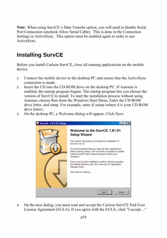
3. On the desktop PC, a Welcome dialog will appear. Click Next.

4. On the next dialog, you must read and accept the Carlson SurvCE End-UserLicense Agreement (EULA). If you agree with the EULA, click "I accept ..."

p17

and then select Install. If you do not agree with the EULA, click "I do notaccept ..." and the installation program will quit.

5. The next dialog asks you to confirm the installation directory. Press Y es.

6. At this point, the necessary files will be copied to the mobile device. A dialogwill appear to show installation progress.

p18

p19

7. You are given a final chance to check your mobile device. Click OK when youare ready.

8. After this has completed, the next figure will appear on the mobile deviceshowing the installation progress. When this dialog disappears, theinstallation is complete.

How-To Update Carlson SurvCE Using a Memory CardThis process requires that you have a memory card with sufficient free space andWinZip installed on the desktop computer.1. Download the appropriate Carlson SurvCE executable to your desktop PC.

There are several executables, therefore it is important to get the right onebased on the type of hardware you own.

2. Make sure that you have exited Carlson SurvCE on the handheld.3. Launch WinZip on the PC.4. In WinZip, select “File Open Archive”.5. In the WinZip “Open Archive” dialog, choose “Archives and .ex e Files” from

the “Files of type” drop list and navigate to the location of the downloaded

p20

Carlson SurvCE executable.6. Still in the “Open Archive” dialog, highlight the downloaded Carlson SurvCE

executable and select the “Open” button.7. Highlight the file that has the .CAB extension and select the “Extract” button.

There should only be one .CAB file.8. Close WinZip.9. Remove the memory card and put it into the handheld device.10. Turn on the handheld device.11. Using “My Computer” on the desktop of the handheld device, navigate to the

memory card and locate the .CAB file.12. Double-Click to open the .CAB file and answer “OK” or “YES” to all of the

prompts and dialogs.13. Carlson SurvCE should be installed or updated and the .CAB file will remove

itself from the memory card.14. Launch Carlson SurvCE and verify the version number and date by selecting

“Equip About Carlson SurvCE”.

Authorizing SurvCEThe first time you start SurvCE, you are prompted to register your license of thesoftware. If you do not register, SurvCE will remain in demo mode, limiting eachjob file to a maximum of 30 points.

Choose Yes to start the registration process, or No to register later.

p21

SurvCE registration is done via the Internet at the following address:

http://update.carlsonsw.com/regist_survce.php

You will be required to enter your company name, phone number, email address,your SurvCE serial number, and the registration code that the program willgenerate. After you submit this information, your change key will be displayedand emailed to the address that you submit. Keep this for your permanent records.

If you do not have access to the Internet, you may fax the above information to606-564-9525. Your registration information will be faxed back to you within 48hours. During this time, you may continue to use the program without restriction.After you receive your Change Key, enter it, and press OK.

After you register SurvCE, you should perform a RAM Backup or a System Save.If you do not do this, then your authorization code could be lost the nex t time thecomputer reboots.

p22

If you cannot find this on your Start menu, then open the Control Panel, andchoose RAM Backup.

Hardware NotesIf SurvCE quits responding, you can reset the hardware by following theapplicable procedures described in the hardware documentation.

Color ScreensSurvCE 1.21 or greater enables viewing of color. Any red, green, blue or othercolored entities in DXF files will retain their color when viewed within SurvCE. Points will appear with black point numbers, green descriptions and blueelevations. Dialogs and prompting will utilize color throughout SurvCE.

MemoryMemory on most CE devices can be allocated for best results. We recommendsetting “Storage Memory” to a minimum of 16,000 KB. The following discussionis an example for setting that memory . An equivalent process should be used for

p23

other CE devices, as available.

The SurvCE controller will function better during topo and stakeout with the"Storage Memory" set to around 18,000 KB. Use the following process to checkand/or change the settings:

Go to the start menu by simultaneously hitting the Blue Key and Start .Choose Settings, then Control Panel , then double click on System. Touchthe Memory tab and slide the pointer toward the left, which is the StorageMemory side, so that Allocated is around 18,000 KB .

Keep in mind that to upgrade software, this setting may need to be changed back,so that the Program Memory has more available. To change, do as above but slidethe pointer toward the right, which is the Program side, so that Allocated isaround 18,000 KB. This assures that there is enough Program memory, so that thenew updates can be saved.

Once the upgrade or additional software is added, you can change it back so thatthe pointer is more toward the Storage Memory -- around 18,000 KB.

After changing these settings, or updating software, it's a good idea to do a "SaveSystem".

Battery StatusThe black icon that appears at the top of every screen is designed to indicatebattery status. Full black should indicate full battery. As battery levels decreasethe black recedes to full white (out of battery).

On some CE devices, there is no way to detect battery status, so the battery icondoes not change. On some devices such as the Jett CE (Carlson Ex plorer), apartial indication of battery status is detected as follows:

p24

Good - 100% Low - 50% Critical – 10%

Save SystemAfter installing SurvCE or making any system level changes (e.g. memorysettings), its highly recommended that you perform a Save System on the device.

Examples:

Carlson ExplorerStart Programs SaveReg

AllegroStart Programs Utilities Save System

Carlson Technical SupportContact information for tech support for SurvCE is provided below:

Carlson Software, Inc .Corporate HeadquartersMaysville, KY, USATel (606) 564-5028Fax (606) 564-6422e-mail: support@carlsonsw.com

Customer Service, Technical Support, Repair:If you need assistance with your Carlson Software products, please call bytelephone, or send an e-mail to the address above. Support hours are Mondaythrough Friday, 7:00 A.M. to 9:00 P.M. (EST, GMT -5 hours).

p25

User InterfaceThis chapter describes the general user interface features of SurvCE.

Graphic Mode

p26

IconsSurvCE 2.0 can be configured to show either the traditional letter icons or newgraphical icons for several functions. To set this option, go to the EQUIP tab,select Configure and toggle the "Use Graphic Icons" check box .

This icon will Read a measurement (ALT-R).

Total Station Only. This icon will Traverse to the measured pointby advancing your setup (ALT-T).

This icon will Store a point. This function is also performed viathe Enter key. (ALT-S).

This icon will lead to a dialog where the user can Average up to999 epochs of GPS readings (ALT-A).

This icon leads to Offset reading screens with options forkeyed-in offsets as well as offsets taken by laser devices that measure distanceonly, or distance and azimuth (ALT-O).

This icon will take you to the Configure dialog, also found on theEQUIP tab. Here you set many preferences in SurvCE such as the number ofreadings to average, function of the Store icon, and whether to display theHgt/Desc prompt on Save (ALT-C).

This icon will advance stake location incrementally to the Nextpoint or station (ALT-N).

This icon returns to the previous stakeout settings dialog whereyou can Modify the current design stake data.

This icon allows the user to override the design Elevation(ALT-E).

OK: This icon will accept the dialog.

Back: This icon will return you to the previous dialog.

p27

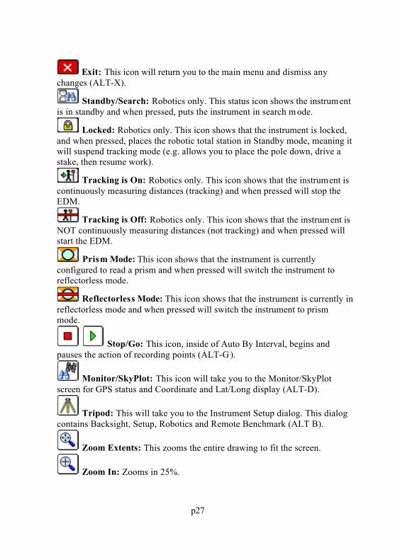
Exit: This icon will return you to the main menu and dismiss anychanges (ALT-X).

Standby/Search: Robotics only. This status icon shows the instrumentis in standby and when pressed, puts the instrument in search m ode.

Locked: Robotics only. This icon shows that the instrument is locked,and when pressed, places the robotic total station in Standby mode, meaning itwill suspend tracking mode (e.g. allows you to place the pole down, drive astake, then resume work).

Tracking is On: Robotics only. This icon shows that the instrument iscontinuously measuring distances (tracking) and when pressed will stop theEDM.

Tracking is Off: Robotics only. This icon shows that the instrument isNOT continuously measuring distances (not tracking) and when pressed willstart the EDM.

Prism Mode: This icon shows that the instrument is currentlyconfigured to read a prism and when pressed will switch the instrument toreflectorless mode.

Reflectorless Mode: This icon shows that the instrument is currently inreflectorless mode and when pressed will switch the instrument to prismmode.

Stop/Go: This icon, inside of Auto By Interval, begins andpauses the action of recording points (ALT-G).

Monitor/SkyPlot: This icon will take you to the Monitor/SkyPlotscreen for GPS status and Coordinate and Lat/Long display (ALT-D).

Tripod: This will take you to the Instrument Setup dialog. This dialogcontains Backsight, Setup, Robotics and Remote Benchmark (ALT B).

Zoom Extents: This zooms the entire drawing to fit the screen.

Zoom In: Zooms in 25%.

p28

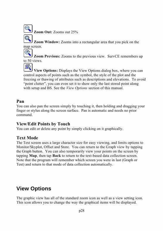
Zoom Out: Zooms out 25%

Zoom Window: Zooms into a rectangular area that you pick on themap screen.

Zoom Previous: Zooms to the previous view. SurvCE remembers upto 50 views.

View Options: Displays the View Options dialog box, where you cancontrol aspects of points such as the symbol, the style of the plot and thefreezing or thawing of attributes such as descriptions and elevations. To avoid“point clutter”, you can even set it to show only the last stored point alongwith setup and BS. See the View Options section of this manual.

PanYou can also pan the screen simply by touching it, then holding and dragging yourfinger or stylus along the screen surface. Pan is automatic and needs no priorcommand.

View/Edit Points by TouchYou can edit or delete any point by simply clicking on it graphically.

Text ModeThe Text screen uses a large character size for easy viewing, and limits options toMonitor/Skyplot, Offset and Store. You can return to the Graph view by tappingthe Graph button. You can also temporarily view your points on the screen bytapping Map, then tap Back to return to the text-based data collection screen.Note that the program will remember which screen you were in last (Graph orText) and return to that mode of data collection automatically.

View OptionsThe graphic view has all of the standard zoom icon as well as a view setting icon.This icon allows you to change the way the graphical items will be displayed.

p29

Show Only Last Stored Point (ALT-F): This toggle will result in SurvCEonly displaying the linework collected, the instrument and backsight points,and the last point collected. This is a popular setting to reduce the clutter ofnumerous points displayed all at once.

Freeze All: This toggle will freeze (hide from view) the point attributes (e.g.Point ID, Elevation and Description). Each attribute can be toggled offseparately as well.

Decimal in Point Location: This toggle will adjust the text location so thatthe point location is the decimal point of the elevation.

Redraw: After adjusting the settings, exit and commit your changes byselecting redraw.

Set Color Attributes: This button will allow users to specify the colors of thepoint text (color units only).

Quick CalculatorFrom virtually any dialog entry line in the program, the ? command will go to theCalculator routines and allow copying and pasting of any selected calculationresult back into the dialog entry line.

For example, if you were grading a site that had 19.5” of subgrade, and hadmodeled the top surface, you need to grade to the top surface with a vertical offsetof -19.5/12. You could quickly obtain the value in feet by entering ? in theVertical Offset field within the Elevation Difference dialog, as shown in this nextfigure.

p30

This leads immediately to the Calculator dialog, with its four tabs, or options,many with sub-options. Using the Standard tab, we can enter 19.5/12 and get1.625 as shown. Then select the Copy button, which places the value in thebanner line at the very top of the screen. Then choose Paste in the upper right topaste the value back into the Vertical Offset dialog edit box. These calculationscan also be done directly from the edit box within the Vertical Offset dialog. Youcould enter "19.5 in" for inches, which would auto-convert to feet or the currentunits setting. In this same edit box, you could also enter 19.5/12, which would dothe division directly in the edit box. This figure shows the Calculator screen.

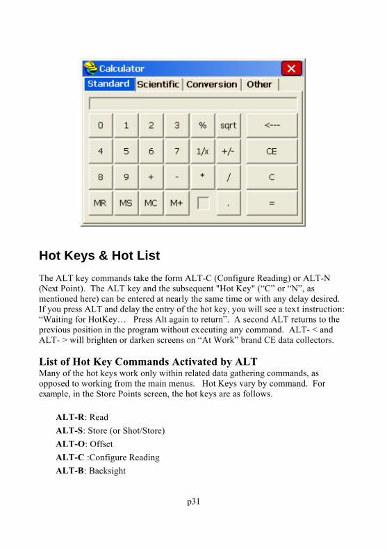
p31

Hot Keys & Hot ListThe ALT key commands take the form ALT-C (Configure Reading) or ALT-N(Next Point). The ALT key and the subsequent "Hot Key" (“C” or “N”, asmentioned here) can be entered at nearly the same time or with any delay desired. If you press ALT and delay the entry of the hot key, you will see a text instruction: “Waiting for HotKey… Press Alt again to return”. A second ALT returns to theprevious position in the program without executing any command. ALT- < andALT- > will brighten or darken screens on “At Work” brand CE data collectors.

List of Hot Key Commands Activated by ALTMany of the hot keys work only within related data gathering commands, asopposed to working from the main menus. Hot Keys vary by command. Forexample, in the Store Points screen, the hot keys are as follows.

ALT-R: Read ALT-S: Store (or Shot/Store) ALT-O: Offset ALT-C :Configure Reading ALT-B: Backsight

p32

Here is a list of other common hot keys:

ALT-E: Target Elevation — From the stakeout screen in any StakeoutLine/Arc command, Offset Stakeout, Elevation Difference and virtually allstakeout commands except Stakeout Points, ALT-E will allow the user to enteran alternate design elevation different from the computed current designelevation.

ALT-F: Foresight Only Toggle. When in the Store Points graphic screen andtaking new shots, ALT-F will freeze all but the setup point number, backsightpoint number and current foresight shot. This is helpful when points aredensely located. Alt F again returns to the full point plot. Linework remains.

ALT-H: Help. Takes you to the Help menu. ALT-I: Inverse. Does a quick inverse, and upon exit, returns you to the

command you were in. ALT-J: Joystick. Applies only to robotic total station. Takes you to the

Settings option. ALT-J typically only functions if you are configured for arobotic total station. ALT-J will work from within data gathering commandsand from the main menus.

ALT-L: List, as in Feature Code List. When entered in any Description field,this will recall the Feature Code List, which displays the characteristics(layer/linework) of the feature code. This serves not only as a way to select thecode and apply it to the description, but it also serves as a handy rem inder ofthe code’s properties.

ALT-M: Menu. Returns you to the dialog of the local command, keeping allcurrent inputs. For example, in Intersection, you are returned to the entrydialog, with all entered point numbers, distances and azimuths intact, allowingyou to alter one or more and re-calculate. Except when used as a “local”menu return, ALT-M will switch to the map screen.

ALT-N: Next. Moves you to the Next point or station in the Stakeoutcommands.

ALT-T: Traverse. Takes a reading and advances the setup to the measuredpoint. The instrument setup dialog is presented for verification.

ALT-V: Shortcut to View the Raw Data, Point Data, Feature Codes andCutsheets.

ALT-W: Write a Note anytime with this command. Notes store to the RawFile.

ALT-X: Shortcut to Exit most commands. Similar to Esc (escape key). ?: The ‘?’ character can be used in any field that requires a numerical entry to

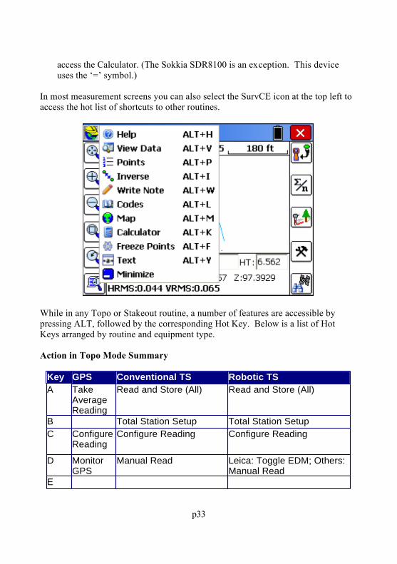
p33

access the Calculator. (The Sokkia SDR8100 is an exception. This deviceuses the ‘=’ symbol.)

In most measurement screens you can also select the SurvCE icon at the top left toaccess the hot list of shortcuts to other routines.

While in any Topo or Stakeout routine, a number of features are accessible bypressing ALT, followed by the corresponding Hot Key. Below is a list of HotKeys arranged by routine and equipment type.

Action in Topo Mode Summary

Key GPS Conventional TS Robotic TSA Take

AverageReading

Read and Store (All) Read and Store (All)

B Total Station Setup Total Station SetupC Configure

ReadingConfigure Reading Configure Reading

D MonitorGPS

Manual Read Leica: Toggle EDM; Others:Manual Read

E

p34

F FreezePoints

Freeze Points Freeze Points

G Start/StopIntervalRecording

Start/Stop IntervalRecording

H Help Help HelpI Inverse Inverse InverseJ Sokkia Motorized:

JoystickJoystick

K Calculator Calculator CalculatorL Feature

Code ListFeature Code List Feature Code List

M View Map View Map View MapNO Offset

PointCollection

Offset Point Collection Offset Point Collection

P List PointsList Points List PointsQ Toggle

PromptforHgt/Desc

Toggle Prompt forHgt/Desc

Toggle Prompt for Hgt/Desc

R Read Read and StoreS Store Store StoreT Traverse TraverseUV View Raw

FileView Raw File View Raw File

W Write JobNotes

Write Job Notes Write Job Notes

X Exit toMainMenu

Exit to Main Menu Exit to Main Menu

Y ToggleGraphics/TextMode

Toggle Graphics/TextMode

Toggle Graphics/Text Mode

Z Zoom toPoint

Zoom to Point Zoom to Point

p35

Action in Stakeout Mode Summary

Key GPS Conventional TS Robotic TS

AB Total Station Setup Total Station SetupC Configure

ReadingConfigure Reading Configure Reading

D Monitor GPS Leica: Toggle EDME Set Target

ElevationSet Target Elevation Set Target Elevation

F Freeze Points Freeze Points Freeze PointsGH Help Help HelpI Inverse Inverse InverseJ Sokkia Motorized:

JoystickJoystick

K Calculator Calculator CalculatorL Feature Code

ListFeature Code List Feature Code List

M View Map View Map View MapN Next

Point/Station toStake

Next Point/Station toStake

Next Point/Station toStake

OP List Points List Points List PointsQR Read Read and StoreS Store Store StoreTUV View Raw File View Raw File View Raw FileW Write Job Notes Write Job Notes Write Job NotesX Exit to Main

MenuExit to Main Menu Exit to Main Menu

p36

Y ToggleGraphics/TextMode

Toggle Graphics/TextMode

Toggle Graphics/TextMode

Z Zoom to Point Zoom to Point Zoom to Point

Instrument Selection

The user can switch between current instruments using the Instrum ent Selectionflyout on the top bar of the SurvCE.

Input Box ControlsWhen point IDs are used to determine a value, the program will search for thepoint IDs in the current job. If not found it will then search in the control job, ifactive.

Formatted Distance/Height EntriesEntries for distances or heights that include certain special or commonlyunderstood measurement extensions are automatically interpreted as a unit ofmeasurement and converted to the working units as chosen in job setup. Forexample, a target height entry of 2m is converted to 6.5617 feet if units areconfigured for feet. The extension can appear after the number, separated by aspace (2 m), or can be directly appended to the number (2m). For feet and inchconversion, the second decimal point informs the software that the user is enteringfractions (See Below). Recognized text and their corresponding units are shownbelow:

f or ft: US Feet

p37

i or ift: International Feet in: Inches cm: Centimeters m: Meters #.##.#: Feet and Inches (e.g. 1.5.3.8 = 1'5 3/8" either entry format is

supported)

These extensions are automatically recognized for target heights and instrumentheights, and within certain distance entry dialogs. Entries are not case sensitive.

Formatted Bearing/Azimuth EntriesMost directional commands within SurvCE allow for the entry of both azimuthsand bearings. Azimuth entries are in the form 350.2531 (DDD.MMSS),representing 350 degrees, 25 minutes and 31 seconds. But that same directioncould be entered as N9.3429W or alternately as NW9.3429. SurvCE will acceptboth formats. Additional directional entry options, which might apply tocommands such as Intersection under Cogo, are outlined below:

If options in Job Settings are set to Bearing and Degrees (360 circle), the user canenter the quadrant number before the angle value.

Example120.1234

The result is N20°12’34’’E.

Quadrants1 NE 2 SE 3 SW4 NW

In the case where Job Settings have been set for Bearing, and the user would liketo enter an Azimuth, the letter A can be placed before the azimuth value and theprogram will convert it to a Bearing.

ExampleA20.1234

The result is N20°12’34’’E.

p38

In the case where Job Settings is set to Azimuth and the user would like to enter abearing, the quadrant letters can be used before the bearing value.

ExampleNW45.0000

The result is 315°00’00”.

Formatted Angle EntriesInterior Angle: The user can compute an angle defined by three points by enteringthe point IDs as <Point ID>,<Point ID>,Point ID>. The program will return theinterior angle created by the three points using the AT-FROM-TO logic. Suchentries might apply to the Angle Right input box in Store Points when configuredto Manual Total Station.

Example1,2,3

Using the coordinates below, the result is 90°00’00”. Point 2 would be the vertexpoint.

Pt. North East1 5500 50002 5000 50003 5000 5500

Mathematical ExpressionsMathematical expressions can be used in nearly all angle and distance edit box es. For example, within the Intersection routine, an azimuth can be entered in the form255.35-90, which means 255 degrees, 35 minutes minus 90 degrees. Additionally,point-defined distances and directions can be entered with a comma as separator,as in 4,5. If point 4 to point 5 has an azimuth of 255 degrees, 35 minutes, then thesame expression above could be entered as 4,5-90. For math, the program handles“/”, “*”, “-“ and “+”. To go half the distance from 103 to 10, enter 103,10/2.

Point RangesWhen ranges of points are involved, such as in stakeout lists, a dash is used. Y oucan enter ranges in reverse (e.g.. 75-50), which would create a list of points from75 down to 50 in reverse order.

p39

Survey Data Display ControlsANGLEThe angle control will display the angle as defined by the current settings in JobSettings.

Options are available for Azimuth (North or South) or Bearing combined with theoption of Degrees or Grads.

FormatThe display format of degrees uses the degree, minute, and second symbols. Forthe case of a bearing we display the quadrant using the characters N, S, W, E.

Example BearingN7°09'59"EExample Azimuth7°09'59"

All angular values entered by the user should be in the DD.MMSS format.

Example7.0959The result is 7°09'59".

FormulasFormulas can be entered for working with angles. The format must have theoperator after the angle value.Example90.0000 * 0.5The result would be 45°00’00”

DISTANCEThe distance control will display the value using the current Job Settings unit. Y oucan enter a formula using the mathematical operators as described above.

InverseYou can compute a distance from a point-to-point inverse by entering <PointID>,<Point ID>.Example1,2Using the coordinates listed below, the result is 500 ’.Pt. North East

p40

1 5500 50002 5000 5000

STATIONThe station control will display the value using the current Job Settings format.The same options described above for distance input box es apply.

SLOPEThe slope control will display the value using the current Job Settings format.

Keyboard OperationCarlson SurvCE allows the user to operate the interface entirely from keyboardnavigation, as well as touch screen navigation. The rules for keyboard navigationare outlined below:

Controls Button (Radio Buttons, Check Boxes and Standard Buttons )

o Enter: Select the button.o Right/Left Arrows: Move to the next tab stop.

Right [Tab] Left [Shift+Tab]

o Up/Down Arrows: Move to the next tab stop. Down [Tab] Up [Shift+Tab]

o Tab: Move to the next tab stop.

Drop Listo Enter: Move to the next tab stop.o Right/Left Arrows: Move to the next tab stop.

Right [Tab] Left [Shift+Tab]

o Up/Down Arrows: Move through the list items.o Tab: Move to the next tab stop.

Edit Boxo Enter: Move to the next tab stop. For any measurement screen,

p41

if focus is in the description edit box , take a reading. For allother edit boxes, ENTER moves through the tab stops.

o Right/Left Arrows: Move through the text like standardwindows.

o Up/Down Arrows: Move to the next tab stop. Down [Tab] Up [Shift+Tab]

o Tab: Move to the next tab stop.

Tabo Enter: Move to the next tab stop.o Right/Left Arrows: Move through the tabs.

Right Next Tab Left Previous Tab

o Up/Down Arrows: Move to the next tab stop. Down [Tab] Up [Shift+Tab]

o Tab: Move to the next tab stop.

Abbreviations

Adr: Address AR: Angle Right Avg: Average Az: Azimuth Bk: Back Calc: Calculate Char: Character Chk: Check cm: Centimeter Coord(s): Coordinate(s) Ctrl: Control Desc: Description Dev: Deviation

p42

Diff: Difference Dist: Distance El: Elevation Fst: Fast ft: Foot Fwd: Forward HD: Horizontal Distance HI: Height of Instrument. Horiz: Horizontal Ht: Height or Height of Antenna with GPS. HT: Height of Target. ID: Identifier ift: International Foot in: Inch Inst: Instrument Int: Interval L: Left m: Meter No: Number OS: Offset Prev: Previous Pt: Point ID Pts: Points R: Right Rdg: Reading SD: Slope Distance Sta: Station Std: Standard Vert: Vertical ZE: Zenith

p43

FILEThis chapter provides information on using the commands from the File menu.

JobThis command allows you to select an existing coordinate file for your job or tocreate a new coordinate file. The standard file selection dialog box appears forchoosing a coordinate file, as shown in the next figure. Buttons for moving up thedirectory structure, creating a new folder, listing file names and listing file detailsappear in the upper right corner of the dialog box .

p44

All data points you collect are stored in the coordinate (.crd) file you select orcreate. The .crd file extension will automatically be appended to the file name.

Select Existing JobTo select an existing job, browse to and select an existing file, then select OK (thegreen check icon).

Create a New JobTo create a new job, simply enter a new name and select OK. You can controlwhere your job is saved by browsing to the desired folder where the job is to becreated before entering the new name and selecting OK. You can also create a newfolder for this new file name. Following job creation, you will be asked to enter inJob Attribute information. This feature lets you set up prompting for each new jobwith job-related attributes like Client, Jurisdiction, Weather Conditions and thelike. This is discussed in detail in the Job Setting section.

Note: If you key in a coordinate file that already exists, it will load the file insteadof overwriting it with a new file. This benefit to this feature is that you cannotaccidentally overwrite an existing coordinate file from within Carlson SurvCE.

Job Settings (New Job)

p45

This tab allows you to configure how all new jobs will be created.

Prompt for First Pt: This option specifies whether or not SurvCE willprompt you to specify a starting point when starting a new job. If enabled, youspecify the default starting point coordinates in the left column. This appliesfor total station use only.

Prompt for Units: This option specifies whether or not SurvCE will promptyou to set the units when you start a new job.

Use Last Job Localization: If this feature is enabled, each new job will usethe previous job’s localization file and project scale. If this feature isdisabled, each new job will start out with no localization and a project scale of1.0. The default value is off.

Attach Last Control Data: This allows the user to use the same control fileon all new jobs. With this option off, the control file will automatically bedeactivated during new job creation.

Cutsheets: Auto-Save by job will automatically create cutsheet files (in thelast format used) for each new job. If your job was named Macon1.crd, thenthe 3 cutsheet files created would be Macon1-Pt.txt (for non-alignment,point-only stakeout), Macon1-CL.txt (for stakeout involving alignments) andMacon1-Sl.txt (for slope staking). Recall Previous will allow the user to usethe same cutsheets on all new jobs. With Manual, the control file willautomatically be deactivated during new job creation and you will need tocreate cutsheet files within the Stake tab of Job Settings.

p46

Use Template DXF: This allows users to create an empty DXF file thatcontains all of the layers and colors that will be used and displayed in thefield. The advantage of this is in particular with use of Feature Codes forlinework. If you designate code 201, for example, as a pavement edge in thelayer BitPav, you could make a blank DXF drawing with BitPav layer created,set to color blue. Then using that "template dxf" file, everytime you code a201, you will see the blue linework as an extra confirmation of correct coding.This color-coding could be repeated for other often used layers.

Define Job Attributes: This lets you set up prompting, for each new job, forjob-related attributes like Client, Jurisdiction, Weather Conditions, PartyChief and other notes. These will prompt when each new job is started, andthe attributes and entries will appear in the raw file (.rw5) file. Select Add toenter new attributes.

Job Settings (System)This tab allows you to define the units for the current job.

p47

Distance: Select the units that you want to use. Choices include US Feet,International Feet, and Metric. If US Feet or International Feet is selected, youhave the option to display distances as decimal feet (Dec Ft) or Feet andInches (Inches). This is a display property only and will not change the formatof the data recorded to the raw file.

Angle: This offers the option of degrees (360 circle, 60 minutes to a degreeand 60 seconds to a minute) or gons (also refered to as grads- 400 circle andfully decimal). An angle of 397.9809 gons is equivalent to 358 degrees, 10minutes and 58 seconds. (Note: you can verify this in Cogo, Calculator,Conversion tab). The Angle Unit configuration impacts commands such asInverse, Traverse, Sideshot, Input-Edit Centerline and other commands wherea direction is displayed or entered.

Zero Azimuth Setting: Allows you to specify the direction for zero azimuth,North or South.

Job Settings (Options)This tab allows you to set configuration options for the current job.

p48

Time Stamp Each Point: When enabled, a date and time stamp will be notedin the raw file beside each point. Raw files in Carlson SurvCE have a .RW5extension and are nearly identical to the TDS .RW5 format. See the imagebelow for simple SurvCE .RW5 file.

Store GPS Accuracy in Raw File : This option is available when configured

p49

to any GPS equipment. If enabled, the horizontal and vertical quality asreported by the GPS will be stored to the raw file with each point (RMS orCEP/SEP typically).

Auto Load Map and Auto Save Map: Maps can be viewed in the MAP andGraphic views within Carlson SurvCE. These maps can be created by usingthe command IDXF which imports a DXF drawing file. AutoCad DXFformats 12 through 2000 are fully compatible and will import. Micros tationDXF files and DXF files from other CAD programs will also work. Linework(referred to as polylines) can be produced within the MAP view by using thePL (polyline) command, or other commands such as Offset (O2 and O3). Inaddition, use of Feature Codes, where linework is associated with field codessuch as EP for edge-of-pavement, will lead to the drawing of polylines in theMap view. These maps can then be auto-saved whenever you ex it acoordinate file, and auto-loaded whenever you load a particular coordinatefile. The maps are saved in DXF format. It is typical to enable both AutoLoad Map and Auto Save Map if you want to auto-recall your latest map. IfAuto Load Map is on and Auto Save Map is turned off, you will recall themap that was saved previously—when Auto Save Map was on. If you want tostart your map from a clean slate (from the point plot only —which alwaysappears in map view), you can turn off Auto Load Map and re-enter theprogram. Then add polylines, use IDXF to import maps (polylines), then clickon Auto Save Map and Auto Load Map and you will store and recall only thenew linework.

p50

Note: The above graphic display is non-default. In the Map screen, thenormal display includes pull down menus. These can be disabled by selectingPreferences under the Tools menu. The screen shown below will appear withdisplay options. The pull down menu format is recommended, since itcontains the same graphic space, and also responds identically to keyed-incommands (such as PL for polyline).

Recall Job Road Files: This command only applies to Stakeout Centerline,Offset Stakeout, and Point Projection in the non-roading version of CarlsonSurvCE. When enabled, this option will recall the last roading files(centerlines, profiles, templates, superelevation files, etc.) used in roadstakeout. Routines in the Road menu such as Stake Road and Slope Stakingwill automatically recall the last-used roading files

Recall Job Localization: Enabling this option is advisable if you are workingon the same job with GPS equipment for several days. It allows you to set upthe base in the same location, change only the base antenna height inConfigure Base (if applicable), then continue to work. You must have at least1 point in the file (which initiates the RW5, “raw”, file) for the GPSlocalization to be auto-recalled. With this option disabled, you would have togo to Localization within the Equip menu and Load the stored localization(.dat) file. Even with the option turned on, you can always move to a new joband create or load another localization file. The localization file (*.dat file) isrecalled as long as there is at least one coordinate point in the job.

p51

Use Code Table for Descriptions : This feature will cause the codes in thefeature code list to appear as selectable options when storing points. Whenenabled, Configure Reading is set to Ht/Desc Prompt on Save. If the codetable includes FL, EP, IP and LP for example, these appear within the StorePoint routine.

Use Control File: The control file is used for selecting and using points thatdon’t exist in your current working file.

Select File: You need to select a file for the control file. The chosen fileappears, and will remain as the default control file, even when the control fileoption is disabled (in which case it is grayed out). Control files remainassociated with active coordinate files.

General Rule: Carlson SurvCE will always look for the defined point inthe current working file first, and then the control file. If the point is notfound in either file, a warning that the point does not ex ist will bedisplayed. You can force a point to come from the control file or thecurrent file, regardless of settings, by using the List icon to the right ofthe point ID input box. While in the point list selection window, selectthe Control file radio button prior to selecting the desired point.Stakeout Option: Control files work similarly in stakeout. However,you can go to the STAKEOUT tab in Job Settings and set the program togive priority to the control file points when duplicate points ex ist. If this

p52

option is turned on, and the selected point is found in both files, you willactually be staking out the point from the control file.Coordinate File Rule: At no time will a point be automatically copiedfrom the control file into the current file. This allows users to avoid largegaps in coordinate files and eliminates the potential for conflicting points.Raw Data File Rule: Any time a point is occupied, the occupationrecord (OC) is written to the raw file for processing purposes. There willnot be an SP record written for control file points, only an OC record.Note that if the raw file is reprocessed, the point will be written to thecurrent coordinate file.

Job Settings (Format)This tab allows you to select the viewing format of the data displayed and enteredin the current job.

Coordinate Display Order: This option allows you to display coordinateswith the order of North then East or East then North.

Angle Entry and Display: Options are Bearing or Azimuth. This applies tonumerous commands, such as prompting and displays in Sideshot Traverse

p53

(the backsight as azimuth or bearing), Intersections, and Inverse. Vertical Observation Display: Allows you to set the default prompting to

Zenith (0 degrees up, 90 degrees level), Vertical Angle (90 degrees up, 0degrees level) or Elevation Difference (up is positive in absolute units, downis negative). Normally combine Elevation Difference with HorizontalDistance. If combined with Slope Distance, the non-zero Elevation Differencewill be used to compute the equivalent zenith angle and will reduce the SlopeDistance to a lesser Horizontal Distance. (Applies to entries in Manual TotalStation mode).

Distance Observation Display : Options are Slope or Horizontal. Thisapplies to the values displayed from total station readings.

Slope Entry and Display: Whenever slopes are reported or prompted, youhave the option to specify the default in Percent, Degrees or Ratio; however,some commands such as 3D Inverse will automatically report both slope andratio and are unaffected.

Station Display: This option impacts the display of centerline stationing,sometimes referred to as “chainage”. In the U.S., for example, roads designedin feet are “stationed” by every 100 feet, so that a road at linear position14280.5 is given a station of 142+80.50. Metric roads in the U.S. are oftenstationed by kilometers, where the same road position has a station of14+280.500. You can configure the placement of the “+” as desired,independent of your configuration for metric vs feet units. You can alsoconfigure for a purely decimal display of stationing/chainage, as in 14280.500. This display form shows up in such commands as Input-Edit Centerline,within the Start Station dialog box. Please note that you should still input thestationing in purely numeric form, without the “+” convention. Only thedisplay is impacted by this option.

Job Settings (Stake)This tab allows you to set configuration options for the stakeout routines.

p54

Precision: Use this to control the decimal precision reported during stakeoutroutines.

Store Data Note File: This option specifies whether or not to store thestakeout data in the note file (.NOT) for the current job. At the end of stakingout a point, there is an option to store the staked coordinates in the currentjob. Note (.NOT) files are associated with points, so you must store the pointto also store the cutsheet note. This additional data includes the targetcoordinates for reference. Keep in mind that the cut and fill data is alsostored in the raw file. You can also store an ASCII cutsheet file using thebutton at the bottom of the dialog, so storing into the note file is somewhatredundant. SurvCE does not show the cutsheet note within List Points (notesturned on), since this feature only shows notes that begin with “Note:”  Theone advantage of the note file is that notes are viewable in association withpoints using Carlson Software office products such as Carlson SurvCadd,Carlson Survey, or Carlson Survey Desktop. See command Cutsheet Report,option Note File.

Control File Points have Priority for Stakeout : This option, which appliesto both total stations and GPS, will give priority to the control file pointduring stakeout, when the point requested ex ists in both the current file andthe control file.

p55

Note: Use this option with care.  You may not realize that this optionis set, and will discover that directions to your expected stakeout pointof 10 are really based on a point 10 from another file altogether – thecontrol file.

Use Automatic Descriptions: This allows you to have descriptionsautomatically entered for staked locations based on the settings defined bythe Auto Descriptions dialog.

Stake Offset DescThis allows you to define what the ID is called for each offset location in the StakeOffset routine.

Auto DescriptionsThis button allows you to configure the point description when you store points instakeout.  The very act of storing a staked point is optional.  You can stake a pointor a station and offset, but must click Store Point within the stakeout screens toactually store a point.  If you do choose to store the point, the description isconfigurable.  See image below.

p56

A user in Australia or Great Britain might want to change the STA for“Station” to CH for “Chainage”.  An example of a typical stakedescription, based on your configuration settings, is shown at thebottom left of the screen.  The first line (STK1317 CB#22 CUT2.100) represents a typical Stake Point description, where CB#22 isthe description you would enter, and the rest is governed by yourStake Description settings.  Similarly, if centerline-based stakeout isbeing conducted, then the lower line would apply.  The description(CL in this case) is the only aspect entered by the user in the fieldduring stakeout.  All the rest is reported based on your StakeDescription settings.  If you turn off an item, note how it will notappear in the reported “sample” description.  The “+” in the stationcan also be configured to appear or not appear, but this is set globallywithin the Units Tab of Job Settings.  The behavior of the On/Off,Up/Down and Update buttons is identical to that discussed above inthe Cutsheet discussion.

Other routines, particularly Cross Section Survey and Slope Staking(part of the Roading features), have their own settings fordescriptions.  When any automatic description for stakeout is turnedon, the program will no longer default to the last-entered description; it will use the “automatic” description instead.  If you type a newdescription, you will turn off the “automatic” stakeout description.  Ifyou delete the default (new) description, the program will return to

p57

using the automatic stakeout description.  To delete, you can simplyplace the cursor in the description field and hit the delete key — thereis no need to first highlight the description.

Alignment SettingsThis dialog allows the user to define how all alignments and roads are staked.

Alignments Tab Increment from Starting Station: For centerlines that start on an “odd”

station such as 1020 (10+20 in U.S. stationing format), this option wouldconduct stakeout by interval measured from station 1020.  So a 50 intervalstakeout, instead of being 1050, 1100, 1150 would be 1020, 1070, 1120, etc.

Extend Alignments: This projects a tangent line off of the first and lastsegments of the alignment for extending them beyond their defined limits.

Stake Start and End Stations: This instructs the software to stop at thesecritical locations even when they do not fall on the even station.

Stake CL Alignment Points: This instructs the software to stop at thesecritical locations even when they do not fall on the even station.

Stake Profile Points: This instructs the software to stop at these criticallocations even when they do not fall on the even station.

Stake High and Low Points: This instructs the software to stop at thesecritical locations even when they do not fall on the even station.

p58

Combine Station Equations: This allows the user to overlap the stationequations.

Apply Station Equations: This allows the user to ignore the station equationsso that the station reflects the length of the alignment.

Offset Gap Type: Fillet: This allows the user to define the offset gap typeused when defining offsets within Stakeout Line/Arc routine at a straightcorners as: radius fillet or radius zero fillet.

Limit Station Range: When selected, the program will not automaticallyadvance beyond the natural start and end of a given centerline.

Use Station and Offset List: Use this option to load a predefined list ofstations and offsets. This allows the Stake Offset  routine to use a pre-definedlist of station, offset, and elevation information as defined by the user.  This issometimes referred to as “Cutsheet” list. An ASCII file with a .CUT fileextension is required.  The file format is shown below:

Station, Offset, Elevation, Description, as in20100, -11.5, 102.34, 20109.23, -11.5, 102.35, PC

Road Tab

Next icon advances to: This defines how the "Next" icon will behave. It canadvance to the next station or the next offset location.

p59

Stake Section File Locations: This instructs the software to stop at thesecritical locations even when they do not fall on the even station.

Sections Include Catch Points: This instructs the software whether or notthe design sections were extracted to the shoulder or the design catchlocation. If the design catch location is included in the section, the softwarewill automatically determine the pivot point at the next interior section pointfor slope staking purposes. The design slope ratio will be determined by thelast two points in the section.

Always Zoom All: This zooms the preview window automatically to fit theextents of the current section.

Zoom In/Out: This determines the zoom increment of the preview window. Vertical Scale: This allows the user to exaggerate the scale vertically. Degree of Curvature: This allows the user to define the value of the base

value used to define the degree of curvature: 100 ft it is the default valueused for US Feet or US International Feet.

Use Railroad Type Curves: This allows the user to define the use ofrailroad definition for the curves present within the alignment used inside theStakeout Line/Arc routine.

CutsheetsThere can be as many as three cutsheet files active at one time, one for pointstaking cutsheets, one for centerline staking cutsheets and one for slope stakecutsheets.  All three cutsheet files can be given distinct names, and any of the threecan be turned on or off for purposes of storing.  It is even possible to have a fourth,named, cutsheet file if cutsheets are turned on within Cross Section Survey in theRoading menu.  And finally, if cutsheets are reported from the raw file, a distinctnew name can be assigned prior to recalling the raw file and creating the cutsheetfile.  All cutsheet files are ASCII and can be viewed in a tex t editor or an ExcelSpreadsheet.

The Cutsheets button leads to the following options:

p60

Point Stakes: Toggling this option on enables writing to the selectedcutsheet file. The buttons allow the user to select the file, customize the PointCutsheet report format as well as edit and view the current point cutsheetfile. This applies to the command Stake Points.

Alignment Stakes: Toggling this option on enables writing to the selectedcutsheet file. The buttons allow the user to select the file, customize theAlignment Cutsheet report format, and edit and view the current alignmentcutsheet file. This applies to commands within Stake Line/Arc, and to OffsetStakeout, Point Projection and Stake Road (in Roading) and includes stationand offset options in the stored file, as well as cut/fill.  A special“centerline-style” cutsheet file, containing station and offset information, canbe named and saved within the Roading command, Cross Section Survey. This file is viewable in the editor within Set Cl Cutsheet Format, but has nocut/fill values, just “as-built” data. Centerline-based cutsheets have moreconfigurable options in the report, such as Stake Station, Staked Offset,Design Station and Design Offset.  The Design Point ID is one of theconfigurable items to report, and since commands such as Offset Stakeout,Point Projection and Stake Road do not stake out Point IDs, the programuses either the command name (CL for Stake Centerline, PP for PointProjection), offset reference, or template ID as the “design point name”.“RCurb”, for example, would be the name given to the design point in OffsetStakeout for top of curb, right side. This might lead to a variety of ID namesfor the design point.

Slope Stakes: Toggling this option on enables writing to the selected

p61

cutsheet file. The buttons allow the user to select the file, customize theSlope Stake Cutsheet report format as well as edit and view the current slopestake cutsheet file. This applies only to the commands Stake Slope and StakeRoad available within Roading. Slope Stake Cutsheets have an ex tra optionto “Include progressive offsets report”, and also have different options suchas “Pivot Offset” , “Slope Ratio” and “Elevation: PP/CP” (Elevation of PivotPoint and/or Offset Point).  Note that columns can serve a dual purpose inthe slope stake report.  If progressive offsets are enabled, the header lines(such as Design Station) are ignored for the additional information, and youobtain the incremental, delta distance and elevation from each point on thesection or template from the offset stake to the catch and then all the wayinto centerline. These last three options allow you to customize therespective output report. To change an item label, highlight the item, changethe Header Label field, then tap Update Item. You can select an item in thelist and turn it ON or OFF (no reporting). You can also control the order ofthe report items by using the Move Down and Move Up buttons. Changesmust be made prior to starting a new cutsheet file.

Select File: Tap this button to select the output file. The file name is shownbelow this button.

FormatSelect the format button to configure each cutsheet to your liking. Column orderand column headers are completely user-defined and any column can be turned offif not useful.

p62

Header Label: You can substitute header text of your own choice for thedefaults.   Here, the text Pt ID was substituted for Design Pt#.  Tap UpdateItem after changing a Header Label.  These changes should be done prior tostarting a new cutsheet file—they cannot be applied retroactively to a filethat already contains information.  However, the header line in that file (e.g.Market.txt) can always be edited using Notepad or any tex t editor toaccomplish the change.

Down-Up: Items in the list can be moved up and down to change theirorder.  For example, if you prefer Fill before Cut in the report, just move Cutdown below Fill.

Cutsheet from Raw: SurvCE automatically stores cutsheet data and headerinformation to the raw file for the job.  You can capture and report thecutsheet information directly from the raw file.  Before doing this, it isrecommended that you start a new cutsheet file, configure the header lines,and order of information as desired, then run “Cutsheet from Raw”.

Edit FileSelect this option to edit and review the cutsheet file.  Shown below is a pointcutsheet file as viewed in the Edit File option. Notice that the vertical bars of thespreadsheet can be moved left and right to condense the display and who more ofthe header lines.  Just pick them in the title line and move them. The Cutsheeteditor also includes the ability to insert and delete lines.  If you insert a line andenter a Design Elevation and a Stake Elevation, the program will compute the cutor fill.  Using the Special button, you can increase or decrease the Pt ID, DesignElevation or Stake Elevation by any desired amount, and the cut or fill will becomputed.  Do not use the Special button to directly modify the cut or fill.

p63

List PointsThis command will list all of the points in the current coordinate (.crd) file. Youcan also edit any point in the list.

p64

The above figure shows the List Points dialog. The point list includes Point ID,Northing, Easting, Elevation, and Description. Columbs can be shifted to condensethe display, as desired. The new positions, however, are not stored.

Details: The number of points and highest point number in the file willnow appear in the Details option.

Settings: Select the Settings button to customize the List Pointsdisplay. The next figure shows the Settings dialog for List Points.

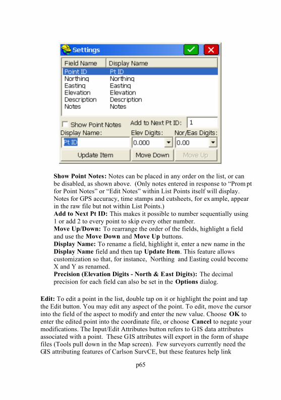
p65

Show Point Notes: Notes can be placed in any order on the list, or canbe disabled, as shown above. (Only notes entered in response to “Prom ptfor Point Notes” or “Edit Notes” within List Points itself will display. Notes for GPS accuracy, time stamps and cutsheets, for ex ample, appearin the raw file but not within List Points.)Add to Next Pt ID: This makes it possible to number sequentially using1 or add 2 to every point to skip every other number.Move Up/Down: To rearrange the order of the fields, highlight a fieldand use the Move Down and Move Up buttons.Display Name: To rename a field, highlight it, enter a new name in theDisplay Name field and then tap Update Item. This feature allowscustomization so that, for instance, Northing and Easting could becomeX and Y as renamed. Precision (Elevation Digits - North & East Digits): The decimalprecision for each field can also be set in the Options dialog.

Edit: To edit a point in the list, double tap on it or highlight the point and tapthe Edit button. You may edit any aspect of the point. To edit, move the cursorinto the field of the aspect to modify and enter the new value. Choose OK toenter the edited point into the coordinate file, or choose Cancel to negate yourmodifications. The Input/Edit Attributes button refers to GIS data attributesassociated with a point. These GIS attributes will export in the form of shapefiles (Tools pull down in the Map screen). Few surveyors currently need theGIS attributing features of Carlson SurvCE, but these features help link

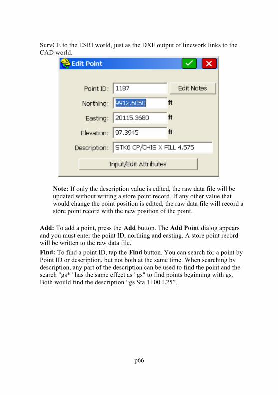
p66

SurvCE to the ESRI world, just as the DXF output of linework links to theCAD world.

Note: If only the description value is edited, the raw data file will beupdated without writing a store point record. If any other value thatwould change the point position is edited, the raw data file will record astore point record with the new position of the point.

Add: To add a point, press the Add button. The Add Point dialog appearsand you must enter the point ID, northing and easting. A store point recordwill be written to the raw data file.

Find: To find a point ID, tap the Find button. You can search for a point byPoint ID or description, but not both at the same time. When searching bydescription, any part of the description can be used to find the point and thesearch "gs*" has the same effect as "gs" to find points beginning with gs. Both would find the description “gs Sta 1+00 L25”.

p67

Delete: To delete a point, highlight a point ID and tap the Delete button. Youwill be asked to confirm this choice before the point is actually deleted.

Control File: When a control file is specified, List Points offers the option toselect the control file and to list the control file points. This feature enablesthe From List option found throughout SurvCE to access Control Points. Thenumber of points and highest point number in the control file will now appearin the Details option.

Raw DataCarlson SurvCE creates a raw file (.RW5) that contains various lines of surveydata similar to a surveyors' field book. The data contained in the RW5 file willvary depending upon whether a total station, robotic total station, or G PS is usedduring the survey. The name of the RW5 file will default to the specified job name(jobname.RW5). This command enables viewing and editing of the raw surveydata, as well as traverse closure and adjustment computations for the survey, forboth total station and GPS raw data. If total station shots are involved, a graphicalrepresentation of the traverse can also be viewed using this command.

p68

Total Station and GPS UseTotal station adjustments are conducted differently from GPS adjustments (Process GPS). If you wish to adjust your GPS first for control, and then calculateyour total station traverse, first select Process GPS. Then use Process No Adjust, or Compass , as desired.

Process Raw File Operations: Total Station, GPS, Reporting,EditingSurvCE has made available four different types of raw file processing. You canprocess or draw your total station traverse, report out the Direct-Reversemeasurements, Process GPS, and Review and Edit the RW5 file.

Note that for all processing where new coordinates are calculated, beginning withSurvCE 2.0, upon exit the program will prompt you whether or not to store thenewly calculated points into the coordinate file. This provides the flexibility toexperiment with different processing settings and options without impacting theactual stored coordinates, until you deliberately choose to do so.

Total Station AdjustmentsIf you wish to adjust or draw a total station traverse, you would choose any of thefollowing: Process No Adjust, Angle Balance, Transit, Compass , Crandall orDraw Traverse Lines . All of these commands have the same four-tab menusystem, outlined below.

p69

Total Station Tab: Reduce to Grid Coordinates will perform a “ground togrid” calculation based on your GPS projection used, viewable in theprojection tab. The Scale setting will multiply all distance measurements bythe entered scale factor. Apply Curvature and Refraction will computecurvature and refraction distinctly on all raw measurements and adjustaccordingly.

p70

GPS Projection Tab: This tab, critical for GPS calculation, only applies fortotal station work when Reduce to Grid Coordinates is set on within theTotal Station Tab. To change the active projection, go to the GPS tab underJob Settings.

Redundancies Tab: This screen covers the handling of multiple

p71

measurements to the same point, known as redundancies. There are threeoptions for Method: Use First, Use Last or Average. For example, if youshot point 10 a total of four times, you could choose to use the first reading,the last reading or average them all. If you select Average, then the AverageType option becomes available. Here you can choose from coordinate ordistance measurement. If you shot point 10 four times, twice from twodifferent setups, and then chose coordinate under the Average Optionsdrop-down, then the 4 northings and eastings computed would be averaged. Ifyou chose instead Distance Measurement, then the two measurements wouldfirst be averaged, and then the two distinct coordinates calculated for point 10(using the averaged measurements) would themselves be averaged.

The Backsight Reciprocal option provides special treatment for reciprocals.A foresight to point 15 from a setup on 14, followed by a backsight from 15 to14, makes a pair of “reciprocal” readings. The backsight reciprocal readingcan be ignored (for its impact on recalculating the occupied point), or theElevation component of the reciprocal measurements can be averaged, or boththe Elevation and Distance can be averaged, to recalculate the setup (occupiedpoint) coordinates. The program will calculate reciprocals for backsight direct(BD) records. First set Backsight Reciprocals to Average Elevation. Then ifyou foresight from 2 to 3, for example, then occupy 3 and backsight 2, thestored BD record will lead to an averaged delta Z calculation for point 3within Process No Adjust or any of the other adjustment options. If theTolerances entered above are exceeded, then warning screens appear duringthe processing.

Note: If there are significant redundancies in a traverse (reciprocalreadings, D&R sets, multiple measurements to the same point fromdifferent setups, multiple tie shots into control) then it is recommendedthat the raw file be processed in a Network Least Squares program backat the office, such as SurvNet which is an add-on to Carlson Survey orCarlson Civil.

p72

Other Tab (for D&R Measurements): This tab contains settings for how touse direct and reverse (D&R) measurements. For the vertical angles, you canbalance the direct and reverse measurements or use Direct-Only. When youhave Foresight measurements and Backsight measurements (e.g. slopedistance/zenith angles) between the same points (e.g. reciprocals) in Directand Reverse surveys, you can Balance Foresight-Backsight measurements(apply reciprocals) or use the Foresight data only. For purposes of warningscreens, you can also set the Angle Tolerance and Distance Tolerance forDirect and Reverse measurement processing.

Process No AdjustThis command processes the RW5 file and computes coordinate values for thesurveyed data. No angle balance or traverse adjustment is applied. The ProcessRaw Data Options dialog shown below appears after selecting Process NoAdjust.

p73

You can report the traverse only or compute all measurements by clicking on Report Sideshots. If you click on Report Closure, then you need to specify aReference Closing Point ID , which is the point that the last traverse point isclosing to, or trying to match. The Reference Closing Point ID is not a point inthe traverse—it is the point the traverse is trying to close on. It can be entered as apoint ID or a coordinate.

Note: To preserve coordinate values of the initial setup and backsight, particularlywith D&R measurements involved, it is recommended that Redundancies be setto Average by Distance Measurement , if averaging is used.

Pressing OK leads to the calculation and the report screen for Process No Adjust.

p74

Angle BalanceThis method of processing applies an angle balance to the traverse lines whencalculating the coordinates. The angle balance takes the angular error divided bythe number of traverse lines and adjusts the angle of each traverse line by thecalculated amount. The angular error is the difference between the angle balanceshot and a reference angle. The program will prompt you to enter the traverse shotto use as the angle balance shot. The measured direction between the occupiedpoint and the foresight point in the specified angle balance shot is then comparedto a reference angle. The reference angle is specified as a bearing, azimuth or by atraverse line defined by entering a From Point and a To Point. The angle balanceprocess is initiated by selecting the angle balance option from the process raw filemenu.

p75

The Angle Balance Measurement dialog appears in the figure. Suppose a giventraverse started at 24, traversed up to 25, then around a loop and back to 24 (point45). If point 45 was the end point or closing shot, the traverse leg from 45 to 46could be the angle balance shot. It is very common, for example, in closed-looptraversing to take a closing angle shot from the closing point (45) by measuring theangle along the first traverse leg (24 to 25). That is what occurred in the case ofthis sample traverse.

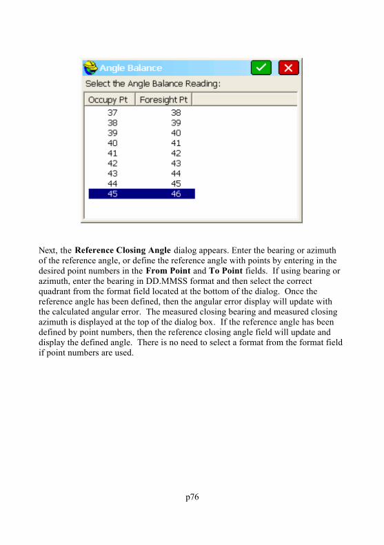
p76

Next, the Reference Closing Angle dialog appears. Enter the bearing or azimuthof the reference angle, or define the reference angle with points by entering in thedesired point numbers in the From Point and To Point fields. If using bearing orazimuth, enter the bearing in DD.MMSS format and then select the correctquadrant from the format field located at the bottom of the dialog. Once thereference angle has been defined, then the angular error display will update withthe calculated angular error. The measured closing bearing and measured closingazimuth is displayed at the top of the dialog box. If the reference angle has beendefined by point numbers, then the reference closing angle field will update anddisplay the defined angle. There is no need to select a format from the format fieldif point numbers are used.

p77

Pressing the OK button, or the enter key, will execute the angle balance process,and the process results will be displayed. The results display shows the closureresults before angle balance and after angle balance.

p78

The angular adjustment applied to each traverse leg is also displayed, along withunadjusted angles and adjusted angles for each traverse leg. The adjustedcoordinates are written to the coordinate file replacing the unadjusted coordinatevalues.

Transit, Compass, Crandall AdjustmentsThese methods apply the selected rule to the traverse lines when calculating thecoordinates. After adjusting the traverse points, the sideshots can also berecalculated. The closure error is calculated as the difference between thespecified ending point and a reference point. The ending point is specified in theinitial dialog.

p79

You can change the ending point to correspond to the point in the traverse thatcloses back to the existing reference point. In the current example, point 26 is thefinal shot, and is closing to an existing point, 10.

The reference point is specified by point ID or by entering the northing, eastingand elevation of the reference point.

p80

The process results show varying information depending on selected options fromthe Process Raw Data Options dialog box.

Reference Closing Point ID: The desired closing point number must beentered into this field. If the closing point does not exist in the coordinate file,the known coordinates can be entered into the North, East and Elevation fieldson the dialog box.

Apply Angle Balance: This option performs an angle balance on the traverselines before the selected adjustment routine is processed. With this optionenabled, the Angle Balance Shot must be chosen from the Angle BalanceMeasurement Dialog box. The adjustment method is applied without anglebalance computations.

Vertical Error Adjustment: The vertical error between the starting andending points will be calculated and displayed in the results screen. Anadjustment value is determined and applied to the traverse points proportionalto their measured distance.

Report Point Adjustment: The adjusted point coordinates and the originalpoint coordinates will be displayed in the results display under the adjustedpoint comparison section.

Report Unadjusted Points : Displays the unadjusted points in the resultsscreen.

Report Sideshots: Displays sideshot data, original and adjusted, in theresults screen.

If Angle Balance is enabled, you will be asked for the closing angle shot, and thereference closing angle screen will appear, which you complete as described in theAngle Balance section above. The closure method will be applied to thecoordinates before or after angle balance, depending upon whether angle balance isenabled.

The routine will conclude, for all three closure methods, by displaying the final,adjusted angles, distances and coordinates. The coordinate values in the CRD filewill change as a result of the closure adjustment.

Draw Traverse LinesThis command employs the same four-tab screen as Process No Adjust and theother adjustment routines. It displays a preview of the traverse configuration bydrawing lines between the traverse points. To start the command, select DrawTraverse Lines from the Process Raw Menu. Inside the dialog, enter thebeginning and ending points to be drawn and press enter. The figure below shows

p81

an example of the results. To exit the preview screen, select the MENU button atthe top right of the screen.

Direct-Reverse ReportThis command creates a report of direct and reverse shots along with the resultingaveraged shots. The residuals are the difference between the measurement and thefinal average. Shown below is a direct and reverse report for a shot taken frompoint 1, backsighting point 4 and foresighting point 100.

Direct-Reverse ReportObservationsType Setup FSight HorzAngle Distance VerticalBD 1 4 359.5958 279.8760 89.4827BR 1 4 179.5945 279.9490 270.1114FD 1 100 336.1603 211.2160 75.0056FR 1 100 156.1601 211.2150 284.5848

BD 1 4 359.5948 279.9500 89.4824BR 1 4 179.5942 279.9500 270.1111FD 1 100 336.1608 211.2150 75.0052FR 1 100 156.1601 211.2170 284.5850

Reduced SetsHorzAngle Residual FS Diff. BK Diff.

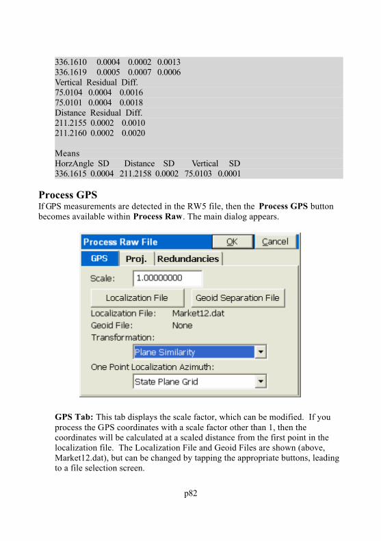
p82

336.1610 0.0004 0.0002 0.0013 336.1619 0.0005 0.0007 0.0006 Vertical Residual Diff.75.0104 0.0004 0.0016 75.0101 0.0004 0.0018 Distance Residual Diff.211.2155 0.0002 0.0010 211.2160 0.0002 0.0020

MeansHorzAngle SD Distance SD Vertical SD336.1615 0.0004 211.2158 0.0002 75.0103 0.0001

Process GPSIf GPS measurements are detected in the RW5 file, then the Process GPS buttonbecomes available within Process Raw. The main dialog appears.

GPS Tab: This tab displays the scale factor, which can be modified. If youprocess the GPS coordinates with a scale factor other than 1, then thecoordinates will be calculated at a scaled distance from the first point in thelocalization file. The Localization File and Geoid Files are shown (above,Market12.dat), but can be changed by tapping the appropriate buttons, leadingto a file selection screen.

p83

The Transformation Types are Plane Similarity (recommended default) andRigid Body , or No Scale . For One Point Localizations, north can be definedby State Plane Grid or Geodetic North.

Projection Tab: Displays selectable GPS grid system projections. Thisprojection list is created on the GPS tab under Job Settings.

p84

Redundancies Tab: For multiple GPS measurements on the same point ID,you can Use First, Use Last or Average all Readings.

When all settings are correct, select OK. The results appear in the Review Filedialog.

Edit Raw (RW5) Survey File

p85

The Raw Survey Notes can be reviewed and edited by selecting Edit Rw5 File. Atypical application of this feature is to edit or add rod height records. This isuseful in the event that changes in rod heights were not recorded at the tim e thatthey were changed. The editor allows changes to virtually all measured data, butwill record the original data as a note (that cannot be deleted). Entries can beAdded, Edited or Removed, but even if removed, original data is retained in anote.

To edit, highlight the desired line.

Tap the Edit button, and the line will appear in a specially formatted Edit dialog,tailored to the type of data selected.

p86

For example, to change the foresight point to 101, click into the Foresight Pointdialog box, enter "101", then press OK. The data will be changed and a note addedshowing the original data and indicating when it was edited.

If you click Add, you may then to select from a variety of record types.

p87

The Network Least Squares tab is a special option that allows you to designatemeasurements for eventual processing in the Carlson SurvNet program (officenetwork least squares software).

If, for example, you pick Measure Standard Error , you can enter errorsappropriate for your instrument. This will reduce the entries required to process thenetwork least squares adjustment when back in the office.

p88

The Find option lets you globally change any set of characters in the raw file. It isuseful for changing a series of descriptions to a new description for purposes offield-to-finish drawing. It is also useful for finding a particular shot that you recallby number or description. For example, assume that you learned that the rodheight you noted as 4.700 was actually 4.833 due to an extra attachment measuring0.133 in length. This feature would allow you to easily change all 4.700 rodheights to 4.833. Direction “Up” would replace all occurrences of HR4.700 priorto the currently highlighted line in the raw file. You can limit the search by use ofthe In Field option by selecting only Descriptions, Notes or Points, or search Allrecords.

p89

Feature Code ListThis command allows you to define default, ready-to-use descriptions. You cancreate multiple feature code lists and each list can contain an unlimited number ofcodes. Each feature code consists of a short code, a longer description, a polylinetoggle, and a polyline type setting. The initial dialog is shown below.

p90

Add a Feature Code Add: To add a code to the list, select this button. The Add Code dialog will

appear.

Select a Feature Code File Load: The Load button allows you to select a file to open or edit. Choose an

existing file or enter a new file name to create a new Feature Code List.Feature Code List files have a *.FCL file extension.

Edit an Existing Code Edit: If you wish to edit an existing code, double tap on the code or highlight

it and tap Edit. It will appear in the Edit Code dialog.

Saving the Feature Code List Save As: Select the Save As button to save the file. Choose an existing file or

enter a new file name to create a new feature code list.

Remove an Existing Code Remove: To remove a code from the list, highlight an existing code and press

the Remove button. SurvCE will ask you to confirm deletion of the code.

The Add Code dialog is shown below. Below the figure is a description list of thevarious options and buttons available in the dialog.

p91

Code: Enter the name of the Feature Code. For example, you might useEP for edge of pavement.Full Text: Enter a description for the code. This is only for yourinformation. It will not be added to the point description. It isparticularly helpful when using numeric codes, to remind you of whatthey refer to.Polyline ON: This setting determines whether points with this code arejoined together with linework when the points are plotted.Polyline is 3D: Choose whether the polyline should be 3D or 2D. If youchoose YES, then each polyline vertex is located at the elevation of thepoint. If you choose NO, then the entire polyline is constructed onelevation 0, regardless of each point’s elevation. This setting is notapplicable if Polyline On is set to NO.New Attributes: This option leads to GIS type attributing, where you canfurther describe the code (e.g. fence) with additional attributes. Forexample, one attribute might be Fence Type, and there may be 4 options,with a default option. These can be set up, one time, by using the Addoption within New Attributes. Once setup, whenever a fence is chosen,the attributes can be selected from a list. These attributes will be storedin the raw file and most importantly, will output to an ESRI Shape file(Map Screen, File pull down, Export SHP File). You can even controlthe prompt and what the default attribute is (in this example, “barbedwire”) and whether each attribute entry is required, or just optional. Withthis setting, any shot to “FL” for fence will jump into the GIS attribute

p92

screen. The setup screen for attributes is shown below.

Fence type is a user-defined attribute. But many attributes of the featureare known by Carlson SurvCE (e.g. the current instrument being used, thedate and time, etc.). These types of known attributes appear in a list ofspecial codes, selectable above, and shown in the figure below.

p93

Now, when you are collecting the points with an “FL” code, and theprogram detects that you have shot a “point-only” feature, or if you areshooting a line, that you have ended the line (e.g. FL END), then you willbe prompted for the attributes.

If there are several attributes associated with the fence (eg. height,condition, etc.), then the Next and Previous buttons will be active. Ifyou have just taken three points along a fence line with GPS, the raw datafile will appear, within FILE Raw Data Edit RW5 File.

You also have the option not to save the attribute information, in whichcase it will not appear in the raw file or be convertible to shape files usingthe command Export SHP File found under File in the Map screen.

Special Code Suffixes Special Codes: In addition to the codes that you add to the Feature Code List,

there are some predefined code suffixes that you may use to end lines or startcurves. For example, FL END could end the fence line, with “END” being apredefined special code. The need to append codes is one reason that the"END" button on your data collector is useful, to move to the END of theexisting description so you can append a special code. Y ou can substitute newcodes for default codes, such that “..” can be substituted for “END” to end aline. The special code suffixes can also be entered as prefix es, as in PC EP(for start curve) rather than EP PC. Special Codes should be separated fromyour actual feature codes by a space. However, the alias of “..” can go rightup against the feature code as in “FL..”. The special codes are describedbelow.

PC & PT: Used to specify the point of curvature (PC) and point oftangency (PT) of a curve. If you are taking shots on a curve, use PC tospecify the beginning of the curve and PT to specify the end of the curve.The PC special code will activate a 3-point arc automatically, so use ofthe PT code in a 3-point arc is redundant and therefore it is not necessary.You can even do a reverse curve by entering the PT instead as PC. However, if you are picking up a meandering stream or tree line, PT isuseful to end the curving feature, and the program will “best fit” a curvethrough all the surveyed points between the PC and PT codes.

p94

CLO: Use this code to close a figure. This tells the software to closefrom the last point coded as CLO back to the first point of the figure. Note that after using a special code such as "CLO", appended with aspace to the description code "BLD", that the program automaticallyremoves the special code as it defaults the next description to "BLD". The "CLO" code also has the effect of ending the line and starting a newline. It only works with codes defined as 2D or 3D polylines.

p95

SMO: Use this code to smooth the line through all of the points. Thiscode must occur on the first point of the line.

JPN: Use this code followed by a point ID to create a new line segmentbetween the current point and the entered point ID.END (or ..): Use this code to end the line. You can also set any code for

p96

Begin Line, but keep in mind with SurvCE you only need to end a line,and the next point with the same description will begin a new line.RECT: This special code can be used in 2 different ways. You can takemeasurements to 3 sides of a building and on the third side, add thespecial code RECT, and the program will create a 4-sided building. Oryou can measure two sides of a building and enter the distance right(RECT30) or distance left (RECT-20) to create the other, parallel sides. Both methods are illustrated below.

OH and OV: You can also create horizontal offset lines and you canoffset these same lines vertically as well by combining OH and OV as inEP OH0.5 OV0.5 (which might create a 6" over, 6" up back of curbparallel 3D polyline). You can even do multiple offset lines as shownbelow:

p97

This example here leads to a series of 4 parallel lines (for railroad tracksin this case), all offset to the left (negative) of the direction of the points120 through 126.

The OH and companion OV commands are flexible in that they can beentered after the first point measured, such as on point 121 or 122.

p98

Using Short-Cut Icons to Append Special CodesWith the Prompt for Height and Description turned on within Configure,you have the opportunity to choose from your ex isting descriptions savedin your Feature Code List, whenever you store points. You also have theability to select icons for the special codes as shown here:

These codes going from top to bottom, starting at the left, represent startline, end line, close line, select active line (when multiple lines are beingdrawn with the same code), start curve, end curve, rectangle, "more", andin the next screen, you obtain Offset Horizontal and Offset V ertical.

Pre-Formatted Special CodesSurvCE has several pre-made files of codes used by certain highwaydepartments and others. These can be selected from the drop list byselecting Special Codes within the Feature Code command.

p99

When a specified format is selected such as Geopak (MO DOT), thestandard codes all change, including the separator code. Whereas fornormal coding, a space is used to separate a description from a specialcode (eg. EP PC), with MO DOT coding, a "-" (dash) would be used asthe separator, as in EP-EC. The users of these systems need to befamiliar with the required coding. For example, with Geopak (MO DOT)coding, a typical edge of bituminous survey might be coded: 201-BS,201, 201, 201-C, 201-C, 201-EC, 201, 201-ES. Note that Geopakrequires a start line and end line and requires coding on all arc points (Cor EC). This coding will process correctly in SurvCE, but SurvCE willalso process this coding if the "-BS" is omitted on the first measurement. Use of the special icons within the Hgt/Description prompt screen willappend the correct special codes that are active. Geopak also requirespoints to process linework, so it will not respond to the OH feature andthe CLR feature, which create lines without always creating points foreach vertice. With Geopak-style configurations, you can click the

p100

Settings button at the top of the screen (left of the green checkmark) andrequire that all linework be created with associated points, for processingin Geopak.

The upper 3 items in Settings appear for all feature code list scenarios,and are default off when SurvCE is shipped.

Use FCL Path to Store *.GIS: If GIS attributing is being used, you canstore the GIS data directly into any special subdirectory used for theapplicable Feature Code List. So if you maintain several feature code lists,each with attributing specified for certain descriptions, the GIS attribute datacan be placed in the directory of the associated feature code file.

Store GIS Line Data to Vertices : When lines are created by field coding,points at the vertices are also created (except for features created by RECTand OH). In addition to associating attribute data with the linework itself, youcan click this option to store the GIS attribute data to each point on the linethat was surveyed.

Use FCL Only: If this option is selected, you will be prompted with awarning screen if you use a field code that is not found in the feature code list.This is a more rarely used feature, and will lead to a lot of ex tra prompting inthe field if field crews choose new codes as they work.

Reprocessing the Field Codes

p101

Using the command Field to Finish, found under the Tools pulldown menu in theMap screen, you can reprocess your field codes after editing any aspect of yourpoint data. So if you left off an "end line" command, you can edit the point,change the description, and re-process the linework. In the example using the codeRECT25 above, if you edited that point and changed it to RECT50, it would drawa twice as large building when you run Field to Finish, and RECT-25 would drawthe same building but instead in the opposite direction.

Data TransferThis command prepares Carlson SurvCE for transferring data to and from adesktop PC. Data Transfer requires that a companion program on the PC is runningto receive and send files. SurvCE, using the Data Transfer option, must“handshake” with the program on the PC in order for the transfer to be successful. A serial cable must connect the PC to the handheld device running SurvCE. COMports must be identified correctly, as well as baud rates.

Carlson/C&G Transfer: This option is designed to work with CarlsonSoftware and C&G office products (SurvCADD/Carlson Civil, CarlsonSurvey, Carlson Survey Desktop, Carlson Connect in Autodesk products,X-Port, CG Survey and CG SurvNET). It also works with the standaloneSurvCom program that is included with the purchase of SurvCE. The

p102

handshake is designed for simplicity and robustness. Carlson Softwareproducts use the same native file formats as SurvCE, so no file conversionoccurs — only transfer.

Kermit Transfer: This command leads to a send and receive screen thatworks with the Kermit program on the PC. This is a readily available datatransfer program.

SDR Transfer: This command is designed to work with existing programsthat communicate with the SDR. For example, if you have LDD, Intergraph,SurvCADD/Carlson Civil, SelectCAD or other software that contains anSDR33 transfer routine, then this option is designed to mimic that protocol. When an RW5 file is selected, it is automatically converted to a Sokkia RAWfile and downloaded to the PC. When a CRD file is selected, it isautomatically converted to a Sokkia RAW file with “08” records for points. This allows you to use and process the data in SurvCE similarly to the data inthe SDR33. You can also upload into the SurvCE field computer SokkiaRAW files that contain point records. All the points will be stored in a CRDfile on SurvCE.

TDS Transfer: This command is used to transfer data from SurvCE to TDSForesight or other programs that have a TDS Link routine.

Sending data to a computer using the Carlson Transfer Option1. Connect your serial cable to your PC. Select Data Transfer from the File

menu. Choose Carlson/C&G Transfer. This leads to a File Transfer screenon SurvCE, which prompts “Awaiting Connection”. All further action takesplace on the PC side. There is no time delay in this handshake. SurvCE willwait for the PC program to catch up. When you connect the cable fromSurvCE to the PC, Microsoft ActiveSync may interfere and display “Connectto PC?” If you get this question, select No and on your PC, disable theMicrosoft ActiveSync serial linkage if it is on.

2. Execute SurvCom, or for Carlson Survey or SurvCADD/Carlson Civil us ers(July, 2001 build or later), choose Tools, Data Collectors, SurvCE/SurvStaroption. If you get “Failed to open COM 1 error code -3”, the most likelyerrors are lack of cable connection or interference by Microsoft ActiveSync. If connection is automatically established, SurvCE will display, “Connected toPC”.

p103

3. If only the left side of the screen on the PC displays data, then you do not havea connection yet. Press the Connect button located at the bottom left of thefile transfer dialog. The transfer program will respond with "Retrieving FileList". Once the file list has been retrieved, the left side of the dialog box willshow files located in the specified path on the PC, and the right side of thedialog will show the files located in the designated path on the remote. Youcan change directories by scrolling to the top of the file list and choosing UpOne Level (just like in Windows). In the above dialog, a filter is applied sothat only files in the form of *.crd are displayed. Filters such as this can be setup using the Options button.

4. To transfer one or more files, simply select or highlight the desired files andselect the Transfer button. More than one file can be transferred from theremote to the PC or from the PC to the remote during the transfer process. Standard Windows selection options apply. For example, selecting one fileand then, while pressing the shift key on the PC, selecting another file deeperon the list, will select all the files in between the first and last selected. Youcan also select the first file to transfer and press and hold down the shift keyand use the down arrow to specify the range of files to transfer. Pressing andholding the control key on the keyboard allows for the selection of multiplefiles in any selection order, by picking the files with the left mouse button.

p104

5. After the files have been selected, press the Transfer button. When thetransfer is complete, the program will display the "Transfer Complete"message and will then proceed to update the file lists on the PC and theRemote.

Note: The process of importing points to the data collector mimics the process ofexporting points to the office computer, but in reverse. If a point is found toalready exist on the data collector, options appear to Overwrite All (Yes All) orCancel All (No All).

SurvCom Commands These commands are found and can be seen in the SurvCom dialog box shownabove. Connect: After selecting Data Transfer from the File menu, press this button

to connect to the PC. Once connection is made, the status line on the filetransfer utility dialog box will show "Connected to the remote machine".

Transfer: Pressing this button transfers selected files from either the Remoteto the PC, or the PC to the Remote.

Set Path: This option allows for the specification of the desired source anddestination drives and folders for both the PC and the Remote device. Forexample, if you were downloading, or copying files from the Remote device tothe PC, to specify a source path on the remote device, select the RemoteMachine toggle and then type in the desired path in the path field. To specifya destination path on the PC, select the Local PC toggle and type in thedesired path the path field. When a change to either path is made, the transferutility will retrieve a new file list from the specified paths.

Make Dir: This option allows for creation of directories on both the PC andthe Remote device. Specify the machine to create the directory on and thenenter the directory name.

Delete: This option allows you to delete the tagged files. Rename: Select a file and rename it. Options: This command allows you to set various options for data transfer.

The dialog shown in the figure below will appear.

p105

Com Port: You must select which com port on the PC to use.File Mask: You must select a file filtering syntax.Directory Sort: You must select how to sort the list of files.Display Special Files: Toggle whether or not you should see specialfiles.Confirm Overwrite: Check this to confirm before overwriting files.Baud Rate: You must choose the baud rate for transferring data.Protect Remote Files: Check this to protect files on the mobile device.Archive RW5 Files: Toggle YES or NO.

Geoid: This command will carve out a portion of the Geoid 99, EGM96,Canadian CGG2000, Canadian HT2.0, Canadian HT1.01, Australian GDA94and Great Britain OSG-MO2 grid files and send it to SurvCE. Since thes egeoid grids are very large, the program carves out a precise portion of it andavoids overloading the memory on the remote device running SurvCE. You

p106

will be prompted for the directory, on the PC, of the source Geoid grid file,and the approximate latitude and longitude of the job, and the size of the areadesired in miles, kilometers or degrees of latitude and longitude.

F2F Conversion: This converts the more thorough and detailed CarlsonSurvey field code file (for field-to-finish work) to the more simplified FeatureCode List that runs in SurvCE. The Feature Code List in SurvCE handlesLinework (on or off), Line Type (2D or 3D), Layer (= Code) and Full Text(Description).

Send Points: The command allows for the sending of a range of points. Exit: This command will exit the File Transfer Utility

Note: The following two options appear in the Data Transfer dialog only ifdetected or available:

Infrared Transfer: This command leads to a send and receive screen thatworks with the Window Socket IrDA server/client objects only between twoCE mobile devices. This is a readily available data transfer program. It works,for example, from Ranger to Ranger. Please make sure you align your devicesso that the infrared transceivers are within one meter of each other, and thetransceivers are pointing at each other. For an easy connection it is preferableto start first the server (the device that will receive the data file) and after that

p107

the client (the device from which the data file will be sent). Bluetooth Transfer: If the mobile device has a Bluetooth emulated serial

COM port, the user will be able to select it from the list, and transfer datafrom/to another device that has Bluetooth available.

Import/ExportThis command allows you to import an ASCII file to job data or export job data toan ACSII file. When you choose this command, you will see a secondary dialog inwhich you will be prompted to choose to Import or Export.

Import ASCII File This command converts point data from an ASCII tex t file into the SurvCE format.The source ASCII file can contain any combination of point number, northing,easting, elevation, and description. You may select any of the predefined formatsor create your own custom format. Since some of these source file formats (likeCarlson CRD and TDS CR5) are not ASCII but are actually binary, Import ASCIIfile can be used to import points from certain non-ASCII type files . This nextfigure shows the Import ASCII dialog box.

p108

Source File Format: You must choose the format of the source file. Thechoices include

User Defined: For importing most .TXT and .ASC files. The coordinateorder in the Choice field is used.Traverse PC: For importing Traverse PC .TRV files .TDS: For importing TDS .CR5 files. Note that CR5 files can containpoint numbers in excess of 32760. If point IDs exceed that value, it isbest to set Alphanumeric as the point ID type under New Job in JobSettings prior to importing.Geodimeter: For importing Geodimeter .OBS files .Trimble POS: For importing Trimble .POS files.CRD File: Allows you to import a SurvCE CRD file into the current,active CRD file, and set the range of points to import. Note that thismethod can be used to move a subset of points from one CRD file over toanother file, as shown below.

p109

SDR File: For importing point data within Sokkia SDR files.

File: You may type in the file name to import. Select: Choose this button to browse for the file name. Common Formats: If your Source File Format is set to User Defined,

choosing one of these settings copies the contents into the Choice field, whichwill be used to import the file.

Choice: If you are importing an ASCII file with a special form (e.g.A,Survey,1254552.123,498135.12,1109.23,iron pin,54) then you want aformat that skips the first two columns (A and Survey) and does Easting (X),Northing (Y), Elevation (Z), Description (D) and Point ID (P), so your formatwill be: S,S,X,Y,Z,D,P. If there is no point ID in the ASCII file, you s implyomit the P in the entered format, and the program will prompt for a startingpoint number or ID and will number each subsequent point sequentially.

Preview: Shows you a preview of the first line of the ASCII file. This ishelpful in determining the correct coordinate order format.

Header Lines: Specifies the number of header lines to skip in the ASCII file. Add to Pt ID’s: Specifies a value to be added to each point ID during the

import process. Pt Protect: Specifies whether or not to check each point ID to see if it already

exists in the current CRD file. If this is toggled ON and you attempt to importpoint ID’s that already exist, you will then be prompted to overwrite each

p110

existing point or to cancel the operation.

Export ASCII FileThis command converts SurvCE point data to an ASCII tex t file. The next figureshows the Export ASCII dialog box. Choose a coordinate order, type of delimiter,range of points and precision. After choosing the settings in this dialog box , press OK. A standard file dialog will appear. In this dialog, choose a name for yourASCII file and then press OK. After the file is written, a dialog will appear tellingyou that the conversion if finished.

Coordinate Order: You must specify the output format for the ASCII file.There are seven different formats to choose from. Each can either be space orcomma delimited, giving you a total of fourteen choices. Two of the optionsinclude quotes around the description field so that your descriptions caninclude spaces and/or commas.

Type of Delimiter: You must specify the character used for delimiting thefields in the output ASCII file. You may choose either a space or a comma.

Range: You must specify the range of points to output. Ranges can beseparated with commas, as in 1-40,101-199,A1-A44.

Export Notes: When this option is enabled, any point notes associated withthe current job will be exported to a .NOT file. These files are used withSurvCADD (and other Carlson office software products).

p111

Export Attributes : GIS attributes can be assigned to points that are storedbased on settings in the Feature Code List. If a point that is shot is a manhole(e.g. MH) and attributes such as concrete, 5 rungs, 2 inlets are entered for thispoint, these attributes will be exported to an ASCII file for use by externalprograms when this option is enabled.

Decimals: You must specify the output precision for northings, eastings, andelevations. This setting does not affect point IDs or descriptions. Afterchoosing the settings in this dialog box , press OK. A standard file dialog willappear. In this dialog; choose a name for your ASCII file and then press OK.After the file is written, a dialog will appear to let you know that the process isfinished. This next figure shows the result of exporting a job to an ASCII file.

Delete FileThis command allows you to remove any existing file from any directory to free upmemory. This figure below shows the standard file selection dialog, where you canchoose the file name to delete.

Note: It is always a good idea to back-up your data by transferring it to a PCbefore deleting files. Carlson SurvCE does not require you to back-up your databefore deleting.

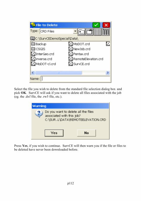
p112

Select the file you wish to delete from the standard file selection dialog box andpick OK. SurvCE will ask if you want to delete all files associated with the job(eg. the .dxf file, the .rw5 file, etc.).

Press Yes, if you wish to continue. SurvCE will then warn you if the file or files tobe deleted have never been downloaded before.

p113

Press Yes, if you wish to continue. You will be asked to confirm your file selectiononce more. Press Yes to accept the deletion of the file or files, or No to cancel theselection.

Add Job NotesThis command allows you to enter job notes as ASCII text. These notes are savedwith the job in the raw data file.

ExitThis command will exit the Carlson SurvCE program. The software presents the

p114

confirmation dialog.

If you choose Yes, SurvCE will exit and your data files are saved. If you chooseNo, SurvCE does not exit.

p115

EQUIPThis chapter provides information on using the commands from the Equip menu.

Instrument Setup

p116

The Total Station routine allows the user to configure their total stationcommunication and operation settings. The tabs shown are configured based on theselected instrument (see specific instrument for details).

CurrentThe routine also provides an instrument recall feature that allows the user to storeand recall all instrument related settings as a user named configuration. Configureall of the settings as desired, and select the save button to nam e and store thecustom configuration. Settings that will be retained are as follows:

Instrument Settings

Communication Settings

Configure Settings

Stakeout Reference Settings

Load: This button will load all settings defined by the selected icon.

Save: This button will save the current settings and allows the user to

p117

enter the name of new icons that will be created to represent the instrumentsettings.

Rename: This button will allow the user to rename the selected icon.

Delete: This button will remove the selected icon.

CommsThe Comms tab allows you to specify communication parameters for the datacollector. For certain equipment, a “Bluetooth” wireless serial connection ispossible.  The user can detect if there is any Bluetooth emulated serial COM portavailable on the CE device by using the “Set Port to Bluetooth” button. SurvCEcan use Bluetooth to communicate only with instruments that have Bluetoothincorporated on it. Also, the user can change the name and the password for theBluetooth present on the instrument end by using the “Bluetooth Settings” button.The dialog shown below will allow the user to change the existing name andpassword for the Bluetooth on the remote device.

Port Number:  You must select the COM port to use. This is the commport of the data collector.

p118

This is a Bluetooth Port: For some of the newer equipment, a“Bluetooth” wireless serial connection is possible.  SurvCE can use Bluetoothto communicate only with instruments that have Bluetooth incorporated onthem. Do not use this toggle unless you are certain that you have Bluetooth.

Baud Rate:  You must select the baud rate for data transfer.

Parity:  You must select the parity setting.

Char Length:  You must select the character length setting.

Stop Bits:  You must select the stop bits setting.

Defaults: Clicking Defaults will utilize the standard default settings forthe configured instrument.

Bluetooth WirelessBluetooth is automatically detected.  The com port settings to use Bluetooth varyfrom unit to unit.  For example, Com3 is typical for the Compaq Ipaq and Com5 istypical for the Topcon FC1000, though it may use any of Com 4, 5 or 6.  On theAllegro, the Bluetooth port is typically Com 4, 5, 8 or 9.  The Bluetooth serial comport settings can be found in the “My Bluetooth Device” m enu selection.

Bluetooth connection is available, for ex ample, with Thales ZMax.  ForThales/Ashtech, set the baud rate in Comms Setup to match the baud rate set forPort C on the ZMax receiver which is typically used for Bluetoothcommunication. 

For Topcon, set the baud rate in Comm Setup to match the baud rate for Port B onthe Hiper receiver, which is typically used for Bluetooth.

If Bluetooth is available, and the Bluetooth option is clicked on, when you OK theComm Setup screen, the Bluetooth port will be searched for and if found, aconfirmation screen is presented.

p119

The program then proceeds to the Bluetooth Manager screen.  This screen givesyou the option to choose which GPS receiver you would like to connect to viaBluetooth. If you click Cancel, no Bluetooth connection will be established.  Selecta receiver and click Connect.

First time into this routine, no receivers will be listed.  Select Find Receiver and

p120

you can add the connected receiver to the list.  Find Receiver will “ghost” ifbluetooth is not an active Bluetooth connection to a receiver.  Find Receiver willonly work on ARM processor devices, which includes the Allegro and Symbol8100. 

Find ReceiverWhen you click Find Receiver to add another receiver to the list, a dialog pops up. The dialog below is for a Socket Bluetooth driver.

p121

Delete ReceiverHighlight a Bluetooth Receiver and click Delete Receiver button to remove thedevice. You will be prompted before removing the device.

Set Receiver PINYou can enter the receiver PIN by clicking “Set Receiver PIN”, and you canchange the receiver name by clicking “Set Receiver Name”.

p122

The default PIN is different for each manufacturer and ex amples for PINs arebelow. Please see your equipment manuals for your equipment PINS.

Topcon        11111Leica             00000Thales          12345

Bluetooth ManagerThe Bluetooth Manager will appear in many places: entry into the program,clicking OK from Comm Setup, Configure Base, and Configure Rover (it worksthe same from all of them). After making a successful connection, the software willlet the user know. If the connection fails, there will be a warning.

p123

Trouble-shooting Note:   Be sure the GPS receiver is turned on before trying toconnect, and that you are within 30 feet of the receiver.  If the user can ’t see thedevice from the Bluetooth Devices program, it is not going to work in SurvCE.The Bluetooth Manager works somewhat better with a passkey but it is not strictlynecessary. Sometimes the Bluetooth registry settings don’t work correctly with anempty passkey. A pass key is the name the Bluetooth driver uses for a password.This is always used on Thales/Ashtech and can be used on Topcon.  It m akes theBluetooth connection more reliable.

Setup (Total Station)

Settings/Search

p124

EDM Mode: Available methods are Standard (1.5 to 2 seconds), Fast, andReflectorless. In all modes of data collection, you are in “Rapid Tracking”mode. Clicking that icon goes to the “No Distance” or “Tracking Only Mode”(no distance measurements). Avoiding taking distance measurements willsave battery usage. So the “Dist” button refers to the selectable mode you will“go to,” not the mode you are currently in. In Rapid Tracking mode, the store

p125

icon will always take a “Rapid Tracking” shot, and pressing enter will take aRapid Tracking shot if Enter is configured to Store only (to mimic the storeicon). Pressing the read icon will always cause configured reading to betaken, as will Enter when set to Read and Store. The next figure shows theRapid Tracking mode, which follows the movement of the prism by takingrapid distance measurements, much like RTK GPS.

Note that in the above figure we are in “Fast” read mode for a configuredreading, and in “Rapid Tracking” mode for display and quick readings by S. Clicking the “No Dist” icon leads to angle measurement only, as shown inthis figure:

p126

Foresight/Backsight Prism Offset : This drop down menu provides a list ofstandard prism offsets. Whenever a prism constant is changed, a note iswritten to the raw (RW5) file. When you select one of the prisms from the list(Circle, Mini, etc), the value that is shown in parenthesis is the actual valuesent to the instrument. i.e. 0.0 for Circular, 17.5 for Mini. If you select"30mm" or "40mm", we send - 4.4 and 5.6 respectively (30-34.4 and 40-34.4). The user may also type in any value they choose. In this case, we willsend that value exactly, unmodified, to the instrument.

(360) (23.1): Prism offset of 23.1 (Leica model). Circle (0.0): Standard Leica round prism. Mini (17.5): Leica mini prism. ReflTape (34.4): Equates to zero offset (wall, surface). 30mm: Other manufactures (Sokkia, Seco). 40mm: Other manufacturers.

Use ATR: When this feature is enabled, ATR (Auto Target Recognition) willbe used when configured to standard or fast reading. When running the roboticin remote mode with ATR turned on, and when performing a “Set Angle andRead” in the backsight screen (a standard measured backsight), the ATRconnection will be taken into consideration, so that the angle set is relative tothe center of the prism, not necessarily the crosshairs of the instrument. The“Set Angle” and “Check Angle” functions will still be relative to thecrosshairs.

Laser Pointer: Ideal for indoor or dark evening surveying, this feature causes

p127

the instrument to emit a red beam. It is often used when doing reflectorlesswork and makes a red mark on the wall, floor or object being surveyed. Thisis useful for confirming the position prior to the shot. The beam should not bedirected into someone’s vision or eye.

Power Search Enabled: The Power Search option may be available withmotorized total stations. This option activates the “PowerSearch” button inthe “banner line” at the top of the survey and stakeout screens. When PowerSearch is pressed, the total station will typically find the prism in 10 secondsregardless of the direction it is initially pointed. If it has found one prism andyou hit “Power Search” again, it will leave that prism and find the nex t one. Ifyou have only two prisms on the job (foresight and backsight), it willconveniently rotate from the foresight to the backsight and back again eachtime it is pressed.

Work Area: This will define a limiting area for searching. This can speedup both the standard ATR Search and the PowerSearch. The Work area angleranges apply to both searches. The Show button will show the two positionsof the search window, first by moving immediately to Position 1. Y ou will beprompted to press OK to see Position 2. Having defined a “window” ofsearching, Center will move that window to a new center position. Y ou willbe prompted to “Sight on Centered Position and Press OK”. The Definebutton prompts you to shoot the lower left and upper right positions, which arethen displayed above under “Work Area”. If the Work Area is set to start at0.0000 horizontal, for example, searching would send the instrument to thebacksight point.

Tracking and Reflectorless: The upper left of the screen controls the ATRSearch, and the upper right controls the PowerSearch. The Work area angleranges apply to both searches. The Show button will show the two positionsof the search window, first by moving immediately to Position 1. Y ou will beprompted to press OK to see Position 2. Having defined a “window” ofsearching, Center will move that window to a new center position. Y ou willbe prompted to “Sight on Centered Position and Press OK”. The Definebutton prompts you to shoot the lower left and upper right positions, which arethen displayed above under “Work Area”. If the Work Area is set to start at0.0000 horizontal, for example, searching would send the instrument to thebacksight point.

p128

Manufacturer Setup InstructionsFor manufacturer specific information, please consult with the Instrument Setup byManufacturer section.

Setup (GPS)

Both Base and Rover GPS are configured with Receiver and RTK inthe same manner. Base GPS requires additional setup and is coveredin the GPS Base section. GPS Rovers section covers theconfiguration of GPS networks and internet corrections.

Receiver TabThis tab is used to Configure the receivers Antenna, set the elevationmask and for some gps position rates.

p129

Receiver Model: SurvCE will auto-detect the receiver model and display it inthis list. It will also auto-detect the port setting for data and the port baud.

Antenna Type: The entire list of supported antennas is available for selection.To select an antenna press the "List" button and search the list bymanufacturer. In this dialog, the user can also verify the antenna offset valuesor create custom antenna types.

Antenna Height: Entered as a either "vertical" or "slant" height in the currentjob units. The slant height is the distance from the base of the pole or fromthe “hub and tack” up to a mark or defined slant measurement point on theedge of the antenna (See NGS for more details). The vertical height ismeasured plumb, straight down from the base (where it screws into theantenna) of the antenna to the ground.

Use Internal Antenna: Many GPS units now have internal antennas. Selectthis option if not using an external antenna.

Elevation Mask: This specifies the cutoff vertical angle above the horizon.Any satellites below this angle will be left out of calculations.

Position Update Rate: This option allows the user to set the position updaterate for the GPS readings. 1 Hz will display one reading per second, while 5Hz is 5 times per second.

p130

RTK TabThe RTK tab is used to configure the GPS RTK communications.

Device: This list contains the supported devices that deliver or receive RTKmessages, such as a radio or IP modem. If an External Radio is selected, theuser will need to specify the Port, Baud, Parity and Stop Bits that the radiomanufacturer requires. For internal radios, SurvCE will detect the propersettings.

Network: This list allows you to configure and connect to various networks(e.g. NTRIP).

Message Type: You must select the RTK message type that you wish tobroadcast and receive. This is the format of the RTK message that is eithersent from the base and received by the rover.

Base ID: This is typically used to isolate paired devices. The user specifiesthat the base is "ID 1", then the rover should be set to only listen for "ID 1" sothat other base stations that might be in the area do not interfere.

Send Rover Position to Network: This will output a NMEA GGA messagefor networks that require it.

Manufacturer Setup InstructionsFor manufacturer specific information, please consult with the Instrument Setup byManufacturer section.

p131

GPS Base

GPS BaseFor GPS equipment, it is necessary to set up the base antenna and record thecorrect antenna height, the antenna type (for certain equipment), and the m ethodsused for localizing (obtaining the desired coordinates).

Much of GPS Base is common to most instruments. For example, the Base Ant.Height would be entered in feet or meters, depending on the setting specified inUnits within Job Settings. Vertical or Slant height refers to the method used tomeasure the height of the base antenna. Vertical refers to the distance from theground point to the antenna disk, measured plumb. Slant refers to the distancefrom the edge of the antenna disk down to the ground point directly beneath thecenter of the antenna. Elevation Mask refers to the degrees above the horizonabove which satellites will be used for GPS “correction” calculations, and belowwhich satellites will be ignored. Keep in mind that it is not always better to lowerthe elevation mask below 10 or 15 degrees. Satellites closer to the horizon than 10degrees will often degrade the calculation of coordinates.

The “alternative” to GPS Base is GPS Rover. GPS receivers can usually functionas either type, but must be “configured” for the role they will serve. You will bewarned when you switch receiver configuration from Base to Rover and vice versa,to confirm that is what is intended.

With all RTK GPS Equipment selections (except GPS Simulation), GPS Base willfirst bring up settings and then proceed to the 6-option G PS Base screen which“locates” the base position. After completing the GPS communications setup and clicking on the Ok button theBase Configure dialog will be presented. These button options "locates" the baseposition. The 6-button GPS Base options (3 buttons per “tab”), common to all, arediscussed first, followed by equipment-specific settings.

p132

GPS Base for All RTK GPS BrandsFor all brands of GPS, the GPS Base button is the command that configures thebase receiver for broadcasting GPS corrections to the rover. You must click theGPS Base button in while you are connected to the base receiver. The base needsa set of coordinates to use as its stationary position. G iven that you are configuredfor a particular coordinate system, there are 2 main “types” of localizations: (1)Enter an Accurate Base Position and work from that point outward on the scaleand “true north” of that system (no rover localization), (2) Enter an Accurate orSemi-Accurate (Read from GPS) Base Position and then localize to known roverpoints that transform to the local coordinate system (required if the local system isnot true GPS north). There is also a “mixed” base-rover approach. To use thebase in the localization, you should configure the base with the "Use LocalCoordinates" option under "From Known Position". Here, you configure the baseby entering the local point (5000, 5000,100) and start a new localization file (oruse an existing one if it applies). Then, at your rover, you can add more points tothe localization as necessary. In this case, a single rover point within Localizationwill produce a scale factor and best fit to the local coordinates.

There are six methods to set the stationary base position, organized into 2categories: From New Position includes Read from GPS, Enter Lat/Long andEnter Grid System Coordinates. The From Known Position tab includesPreviously Surveyed Point, Use Local Coordinates and Read From File. Whenyou are starting a new job (no information in the raw RW5 file yet), always use theoptions in From New Position.

p133

From New Position Options Read from GPS - This method takes a specified number of GPS readings

from the base receiver’s autonomous position and uses it as its “true” position.The autonomous position can be off of the actual position by 150 feet. Thebase will calculate corrections based on this autonomous position. If you setup the base with this method, the rover points must be used for localizationsince the corrections they are using are based on the approx imate position ofthe base antenna. Read GPS, combined with rover-based localization, is oneof the most common methods used to start a GPS survey. When Read fromGPS is used, the program will present the current position, as shown:

p134

Latitude: N 42d21 ’28.35882”Longitude: W 71d08 ’12.87540”Elevation: 116.376

Continue with Base Setup?Yes No

If you like the result, press Yes and continue on. You will then be prompted forthe Reference Station Number. This is an “ID” that will store to the raw file andpermit post-processing of the raw GPS data. A typical entry is 0001. The finalprompt will say,

Base Configuration Successful. Save Settings to File?Yes No

Answering Yes will bring up an entry screen for the reference file name. Reference files are stored with a “.ref” extension. It is important to save areference file if you plan to return to the job at another date. Without re-localizingto control points, you can set up over the same base position, recall the referencefile, and enter the new antenna height for the base position, and start working.

The Read from GPS option is sometimes referred to as “Find Me”. This option isaccurate to about 10 to 50 meters, typically, and it enables the corrections tobroadcast with enough accuracy to permit localization and sub-centimeter real-time

p135

work. Be sure that your GPS zone in Job Settings is set correctly before using thisoption. Also, give the base enough time to find itself. When first set up, the basereceiver has to “collect” satellites and “resolve ambiguities”. If you Read fromGPS too early, you may find a position, but one that is not fully resolved and endsup slowing down the speed at which the rover fixes.

Enter Lat/Lon - Requires you to enter the latitude and longitude for theposition of the base antenna. This is useful if you are setting up over amonument whose latitude and longitude is known. It can also be used over acontrol point whose position is known from GPS post-processing. This willput you on the NAD83, NAD27, UTM or other coordinate system specified inJob Settings, GPS Tab. You can still do a rover-based alignment to transformto a local system. Rover-based localizations are always improved by moreaccurate base positioning. If the GPS detects that your entered Lat/Long isnot near the current GPS readings, the program will warn the user.

This method should be used if you are reasonably sure of the accuracy of thelatitude and longitude—it should be at least as accurate as the “Read fromGPS” option, or otherwise you will have difficulty getting a “fix” on the rover.If it is a very accurate latitude and longitude, you will get the best results.Pressing OK leads to the option of store the base position as a reference file,similar to Read from GPS.

p136

Enter Grid System Coordinates : Requires you to enter the grid systemnorthing and easting for the point that the base is occupying. This applies toany projection that you have configured, including U.S. state plane, worldwideUTM or any individual country or user-defined grid system. This is useful ifyou are setting up over a monument whose coordinates you know. Anaccurate base position, either by entry of Lat/Long or Grid SystemCoordinates, will enable immediate data collection without rover-basedlocalization, but also will improve rover-based localization.

The Coordinate method is similar to the Lat/Lon method, since Lat/Longs convertto Grid Coordinates based on the current coordinate system set in Job Settings,GPS option. The Grid Coordinates will convert back to the Lat/Long coordinatesneeded by SurvCE to configure the base.

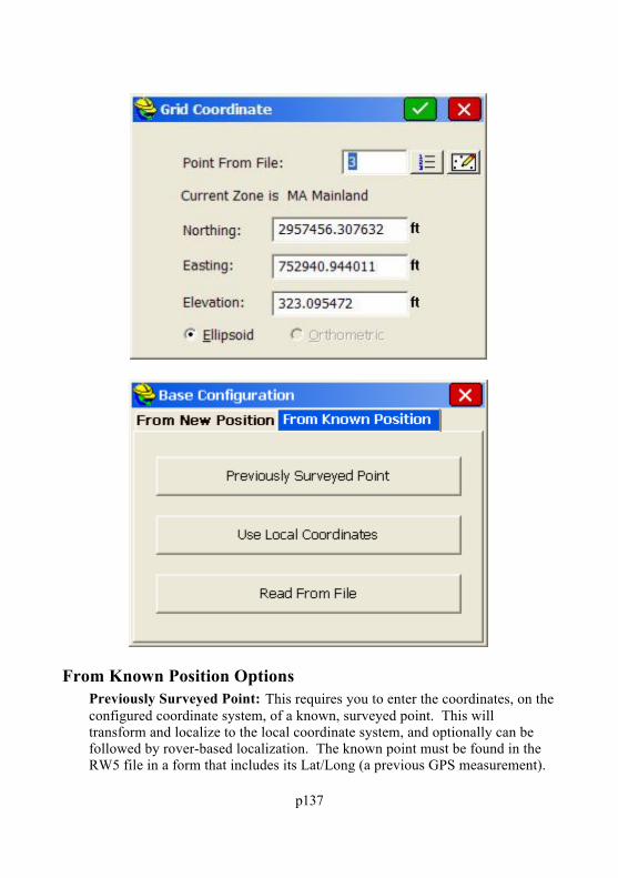
p137

From Known Position Options Previously Surveyed Point: This requires you to enter the coordinates, on the

configured coordinate system, of a known, surveyed point. This willtransform and localize to the local coordinate system, and optionally can befollowed by rover-based localization. The known point must be found in theRW5 file in a form that includes its Lat/Long (a previous GPS measurement).

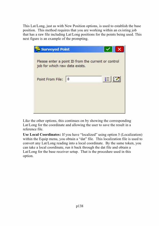
p138

This Lat/Long, just as with New Position options, is used to establish the baseposition. This method requires that you are working within an ex isting jobthat has a raw file including Lat/Long positions for the points being used. Thisnext figure is an example of the prompting.

Like the other options, this continues on by showing the correspondingLat/Long for the coordinate and allowing the user to save the result in areference file.

Use Local Coordinates: If you have “localized” using option 5 (Localization)within the Equip menu, you obtain a “dat” file. This localization file is used toconvert any Lat/Long reading into a local coordinate. By the same token, youcan take a local coordinate, run it back through the dat file and obtain aLat/Long for the base receiver setup. That is the procedure used in thisoption.

p139

When OK is pressed, you will be asked to load the associated “.dat” file, in adialog similar to below:

Read From File - Reads a previously saved base position file. All of the othermethods of setting up the base let you save the base position at the end ofsetup. If you return to a site, set up the base in exactly the same position, use

p140

Read From File to use the same base position and you don ’t have to re-alignthe rover: the old alignment is still valid.

This option recalls a reference file in a dialog similar to that above. Then youwill receive the standard prompting.

This is followed by the Reference Station ID prompt (showing the default ID).The “new” base antenna height, which will change with each new set up, isentered back at the first set of dialogs. A message is displayed after successfulconfiguration from a file. Only if you set the base antenna on the samehorizontal and vertical position each day would the base antenna heightremain fixed. If the base antenna height and x,y position is the same from dayto day, then you do not need to do GPS Base each day. You would simplypower up the base, power up the rover and start working in that case. Keep inmind that in certain power surge conditions, receivers can lose their settings,and a re-configuration may be necessary, even if the base receiver antenna hasnot been moved.

Note: In SurvCE 1.50.006 or later, a “quick connect” is performed when youexit and re-enter the SurvCE program. In earlier versions of SurvCE (beforeAugust 20, 2004) and after the release of SurvCE 1.50 in May, 2004, it wasnecessary to conduct a fresh GPS Base after exiting SurvCE.

Note: One method of obtaining Latitude/Longitude and state plane

p141

coordinates in the U.S. is to occupy a point, any point, for two hours or more,logging the static data, then submit the Rinex file to the NGS “OPUS”program accessible on the web. You must log the data with dual frequencyequipment. The OPUS program is fully automated, and will return the x,y,z,lat, long, ellipsoidal height and orthometric height. This data can then beentered in during base localization. Though most post-processing programs(Trimble Geomatics Office, Leica SKI-Pro) use proprietary post-processingfile formats, they will output the ASCII “Rinex” format needed by OPUS.

GPS Rover

GPS RoverFor many brands of GPS, receiver perform differently depending on whether theyare set as base or rover. Even though the receivers are identical, they performdifferently depending on whether they are configured as a base or a rover. Multiple rover receivers can communicate with a single base receiver. The GPSRover command is used to set the rover receiver to the correct parameters and toinstruct the receiver that it is, in fact, a rover.

Connecting a GPS Rover to a Modem or BaseNetwork

There are several methods for connecting to an available network.  The RTK tab inthe GPS Rover dialog configures the modems and network settings.

p142

The dialog is designed to be filled out from the top to bottom, and from left toright.  First select the device you will use to connect to the remote modem ornetwork.

If a particular receiver model supports an internal modem or radio, meaning it isintegrated into the receiver; those devices are shown first in the list.  When aninternal device is shown in the list, it means that model could have the device

p143

inside, but does not guarantee it.  The user will have to know if the receiver waspurchased with an integrated radio or modem.

External radios and modems are shown next and then one of the last options is“Data Collector Internet”, which is a special case explained below where the datacollector provides access to the internet instead of a modem inside the receiver orconnected to the receiver..

Once a device that is capable of connecting to the internet is selected, the Networkcombo box is enabled.  Select the type of network connection you will use.

Here is a brief summary of the different network types available:

TCP Direct: For connecting to a single modem at a base or to a VRSnetwork or another network that doesn’t require a special login.

The configure button for TCP Direct brings up this window:

p144

To add a new base or network address, select <New> in the Name field andreplace the “<New>” text with what you want to call the connection and fill out theAddress and Port fields.  Most modems support either an IP address (Ex :192.202.228.252) or a URL addres s (Ex: www.basenetwork.com).

UDP Direct:  This works exactly like the TCP Direct option but uses UDPprotocol instead of TCP.  Most networks use TCP.

NTRIP:  This option is for base networks that support NTRIP protocol.  Pressingthe Configure button shows the NTRIP Broadcasters (Also called Casters) thathave been previously connected to.

p145

The default is for rtcm-ntrip.org which if connected to will download informationabout many Broadcasters (casters) all over the world.  They will be shown the nex ttime NTRIP Configure is selected.  Select an existing caster or select <New> inthe Name combo box and replace with a different name and fill out the otherinformation.  If the Default User and Password fields are filled out, they will beused as the default user name and password for all the bases at that caster.

When the green checkbox is selected, SurvCE will have the modem connect to theaddress of the Broadcaster and establish a connection.  The Broadcaster thensupplies a table of bases (also known as mountpoints) available at thatBroadcaster.  SurvCE puts the table of bases into the next window that comes up.

p146

If you don’t like the name of the base supplied by the Broadcaster, you can changeit to something else you prefer and SurvCE will remember your preference but stillask the Broadcaster for the correct base.

Select the base you want to use and press the green check box .  You are broughtback to the RTK tab with the base you selected as the current Base ID.  You canchange the Base ID in the RTK tab without going back to the NTRIP Configure

p147

button.

Note that with NTRIP, SurvCE already knows if the base wants the rover positionsent and what type of corrections are being sent.  Those settings are shown in theRTK tab and are grayed out to guarantee that they stay on the correct setting.

SpiderNet:  Networks that require that a GPUID message be sent to the networkshould use the SpiderNet option.  The SpiderNet Configure window comes upwhen the Configure button to the right of the SpiderNet option is pressed.

p148

Add a new network by selecting <New> in the Name combo box and typing in thename of the network and filling out the other fields.  If the User Name andPassword fields are left empty, the GPUID message is not sent to the network.

Just like when using a radio, the RTK Port combo box is to identify which port onthe receiver should be configured to accept RTK corrections.  The Baud, Parity,and Stop Bits combo boxes specify the settings for the RTK port.  Message Typeidentifies what type of RTK correction message the receiver should be ex pecting.

Base ID when using a network is a combo box to select the name of the network orbase the modem should connect to.  Use the Network Configure button to changethe bases available in this list.

“Send Rover Position to Network” if turned on will cause the receiver toperiodically send GGA messages out of the RTK port to the base or network.

Connecting a Data Collector to the Internet

There are several ways of connecting a data collector to the internet – Cell phonecards inserted into the data collector, connections to a cell phone with a data plan,etc. These instructions assume that an internet connection has already beenestablished to the data collector. One way to tell that the data collector isconnected to the internet is to browse the internet using Internet Ex plorer. For

p149

information about how to connect a data collector to the internet using an Enforacell card in an Explorer 600+, search Carlson Knowledge Base for “Enfora”.

Once the connection to the internet has been established, start SurvCE and selectConfigure Rover in the Equip tab.

Press the Configure button to the right of the Data Collector Internet option.

p150

Select the COM port on the data collector that is connected to the RTK port of theGPS rover receiver. It cannot be the same port that is used to control the receiverand is selected in the GPS Rover Comms tab. It may be a serial port or a BT portwith a connection that has already been established.

After selecting the port and pressing the green check to accept the input, select thenetwork type in the RTK tab. Other settings are just like using the other modemselections as explained in the section “Connecting a GPS Rover to a Modem orBase Network”.

GPS Utilities

p151

Every GPS manufacturer and model has a different set of G PS Utilities. Theprimary purpose of the Receiver Utilities is reset and/or troubleshoot the GPSreceiver.

Common GPS Utilities Reset Receiver: This command performs a soft reset of the GPS receiver. Soft

p152

resets will reinitialize the receiver like a power cycle. Soft reset does notdelete the memory.

Factory Reset or Hard Reset: This command will erase the memory of thereceiver and restore the setting to a factory settings.

Power Off Receiver: This will power down the receiver. Save Settings to Receiver: Stores receiver settings to internal memory. Beep Off: Turns off the receiver alarms. Radio Channel: Change the channel radio channel of the GPS. Configure RTK Device: Use this page to change your RTK data port

settings. This can also be done during base or rover configuration. Check RTK: This tells the user why they aren’t in RTK fixed. Send Command to Receiver: You can send what are known as “pash”

commands, internal Thales/Ashtech codes, to the receiver. This should bedone only in consultation with your Thales dealer.

Reset RTK Engine: This resets the carrier phase ambiguities. This is a usefulcommand if you are having difficulty obtaining lock and want to start theprocess of fixing over again. Receiver settings are retained (so you can thinkof it as a “soft reset”).

Bluetooth Settings: The Bluetooth settings in SurvCE ’s Bluetooth Manager(discussed in Comm Setup) do not actually change anything in the receiveritself. In order to make changes to the receiver ’s internal Bluetooth settings, itis necessary to go into Receiver Utilities and click on Bluetooth Settings.

GPS Utility for GPS SimulationIf running GPS simulation, the starting point can be reset using the special GPSutility. Enter the new Lat/Lon for the position.

p153

GPS Utilites by Manufacturer SetupManufacturer specific information is available in the G PS Utilities byManufacturer section.

Configure (General)This tab allows you to select settings and preferences that apply to observationstaken in the field. These options remain set from job to job. If an option is notapplicable, it is grayed out. Configure is accessible from within any routine wherethe C or Configure Icon is present. These options can also be accessed bypressing ALT-C on the keyboard.

p154

Store Fixed Only: When enabled, only data gathered in the fixed (locked)status will be stored to the point file. If you attempt to store data when thereceiver is not fixed, a message will appear stating, "Position is not fix ed!Continue storing?" The program will prompt to store the point anyway. Thisallows for overwriting the Store Fixed Only option without having to go backto the Configure menu.

p155

Prompt for Total Station Setup: This option determines whether or not thesoftware will display the current setup and orientation values each time theuser enters a survey routine.

Prompt for Height and Description: When this option is enabled, you willbe prompted after each shot to enter the target height and description. Thoughthis adds an extra prompt screen to each shot, it can reduce errors, as you nolonger have to anticipate the shot and get the correct information enteredahead of time. This prompt screen is shown in the figure below. When itappears, you will have the option to enter a point description and change thepoint number and the target height. Note that all the field codes identified inthe Feature Code List under File are available for touch or arrow keyselection, provided this option is activated in Job Settings (Use Code Tablefor Descriptions). Also, if you enter the first character of a code (for ex ample,"I" for IP), the first field code starting with that character will be highlighted,allowing you to arrow key to the one you want, or accept the highlightedoption. This entry is not case-sensitive. Disable the Prompt For Height andDescription option to save time while taking points, or if you are certain thatyour height and description will not change from shot to shot. If the option isdisabled, you must be sure that the correct target height and description havealready been entered.

Note: In the Height/Description Prompt screen, you will see pre-definedFeature Code points indicated with a large dot. 2D polylines will show as a simpleline, 3D polylines will show as a line with a "Z" indicator, and descriptions entered

p156

that are not found in the feature code list will appear with the "fieldbook" symbolabove.

Prompt for Point Notes: Point Notes are additional descriptions that can bestored with a point. A regular point consists of a point ID (number oralphanumeric), northing, easting, elevation, and description (up to 32characters). Point Notes are a way to add an unlimited number of lines of tex tto a point. With this toggle enabled, you will be prompted for notes aftercollecting a point. The notes are stored in a file with the same name as thecoordinate file, but with a .NOT extension. For example, a job calledTOPO.CRD would have a note file called TOPO.NOT.

3D Mode: This option allows you to toggle between 2D or 3D data. In 2Dmode, all elevations will be stored as 0.0

Use Virtual Keyboard: This option provides a software keyboard for datacollectors without keyboards.

Use Graphic Icon: This option toggles between the traditional letter icons (inversions prior to SurvCE 2.0) and the new graphic icons.

Use Audible Alerts: Turn on or off data collector sound alarms. Use Alphanumeric Format: When this option is enabled, SurvCE will allow

alphanumeric point numbers such as 2A or T1105. When this option isdisabled, SurvCE will only allow numeric point number entry. Note: thissetting only affects new jobs, not existing ones. Using purely numeric filescan increase operation speed in very large files, however, this option limitspoints to just over 32,000. An alphanumeric format will be necessary for fileslarger than 32,000 points. A comment will be added in the Rw5 file “ —CRD:Alphanumeric” or “—CRD:Numeric”, based on the format used.

Show Continuous Total Station Angles: This allows you to display anglescontinuously within SurvCE. This option is especially useful when usingOn-board versions of SurvCE.

No. of Readings to Avg (TS & GPS) : Specifies the number of readings thatwill be taken and averaged on each observation. Values between 1 and 9 areaccepted for Total Stations and 1-999 for GPS. If the tolerance is ex ceededbetween readings, a warning screen will appear.

Note: The Num Dist Readings setting does not apply to Manual TotalStation mode. In this mode, you can use the Calculator to averagedistances. When prompted for Slope Distance, enter “ ?” to bring up thecalculator. Choose the Scientific Tab. Follow the tutorial below toaverage three values:

p157

141.213 Enter141.211 Enter141.220 Enter

Now press + on the keyboard twice and with the first +, 141.220 is addedto 141.211 to get 282.431, then with the second + you get 423.6440.

Then enter 3 and type “/”(backslash) for divide. This gives the result:141.2147.

Choose the Copy button at the bottom of the screen, then Paste at thetop.

Enter/Store Icon (TS & RTS/GPS) : Since the Enter key is a convenientand popular way to take shots in the Store Points command, SurvCE allowsyou to specify the effects of this key. These different functions of the Enterkey apply not only to Store Points but also to Elevation Difference . Thefunction of the Enter key is set separately for Total Stations and GPS. Thedifferent options are described below. Note: Most users choose Read thenStore.

Store Then Read: This option similar to the effects of the Read key onthe original SDR data collectors. After a backsight, the first time Enter isused, it will take the shot and display the results. Then when youforesight the next point, Enter will “Store Last, Read Next”. Thisprocedure is best used with the above Hgt/Desc Prompt on Savedisabled. If that option is on, then when you turn to the new shot andpress Enter, the new shot doesn’t take right away, but instead, you areprompted for the target height and description of the previous shot. Thatcould cause some confusion. But with Hgt/Desc Prompt turned off, thismethod can be very efficient. You press Enter and take your first shot. You see the results displayed, and can alter descriptions or target heightsor point numbers for that shot. You sight your next foresight, and pressEnter and the previous shot is correctly stored and the nex t is taken. Theinformation is displayed. You can review and alter it. You sight yournext foresight, press Enter and store the last shot and shoot the nex t, etc.

Read then Store: With this option, the Enter key takes the shot andstores the point. This option works very well with the Hgt/Desc Prompton Save turned on, in which case Enter key takes the shot, then displays

p158

the results and provides an opportunity for editing as in the Store Pointdialog shown above.

Read or Store: The first Enter key takes the reading and the secondEnter key stores the reading.

Configure (View Pt)These settings control the reporting appearance of the stakeout navigationinformation. The Method setting allows you to choose the stakeout informationthat is most appropriate for your situation and personal preference. The optionsfor Method are described in detail below.

Method Options: North-South, East-West: When total stations are used, the direction to go in

stakeout can be North-South, East-West. For instance, the program mightadvise, "North 3.582, East 1.917." This method is better suited to GPS workand is subject to having a sense, in the field, of the north direction.

In-Out, Left-Right: Nearly all surveyors choose this method. If you arestaking a point located 100 meters from the instrument, and take ameasurement at 97 meters, the program will respond, “Out 3”. If the In-Out,Left-Right method is selected, then the Ref. Object and Directions From

p159

options become available to further define left-right. The Ref. Object boxallows you to choose a stationary point by which the directions will bereferenced. This point can be either the instrument or a known point. If Ref.Object is set as instrument, then left is defined as left of the line between theinstrument and the rod. Likewise, if Ref. Object is point then left is defiinedas left of the line between the point and the rod. The second option, Directions From, allows you to decide whether the directions are relative tothe stationary point selected in Ref. Object or to the moving Rod.

Direction to Point—Azimuth, Distance: This directs you to the point forstakeout by the total distance and the azimuth, in either the 360 degree circleor a 400 degree circle if configured to grads. The Use Horizontal Clocksystem option converts the 360 (or 400) circle into a 12-hour circle with 60minutes per hour, and is used in certain military applications. North is 12 o ’clock.

CL In-Out, Forward-Back if Alignment available : This option overridesthe settings above, and if the stakeout involves a centerline, the program willdirect the user by distance in to or out from the centerline and forward or backalong the centerline.

Configure (Sets)This tab allows the user to define how the software will handle angle sets,reciprocals, and direct and reverse.

p160

D&R: The user can choose to measure direct and reverse readings forbacksight, traverse, resection, topography, or stakeout routines. If the usermeasures direct and reverse for the backsight readings, all foresight readingsthat also are recorded direct and reverse will be recorded and computed asangle sets. If the backsight reading is only measured direct, then foresightpoints that are measured direct and reverse are then combined to produce an

p161

average observation record for the vertical circle, which is stored in the .rw5file as a sideshot (SS) record. For calculation purposes, the routine onlyaverages the distances using both vertical circle readings, and uses the directhorizontal reading for the direction. Both the direct and reverse readings arestored in the .rw5 file as a note record. When disabled, (default setting) onlythe direct foresight shot will be taken. This option improves accuracy onelevation measurements and mimics a feature found on the SDR datacollectors. The Resection D&R will also apply to Remote Benchmark.

Reciprocal Calc: The Reciprocal Calculation option has three settings: No,Prompted, and Always. It governs the calculation of the elevation of foresightpoints taken with a total station, where a backsight measurement is also taken. When set to Always, the program will calculate the distance to the foresightpoint and delta elevation by combining the foresight and backsightmeasurements. When set to Prompted, the program will detect the backsightmeasurement and ask the user if the occupied point should be calculated usingboth previous foresight and current backsight. If set to No, the programcalculates foresight points based only on the foresight measurement. If, forexample, you had a vertical difference of +1.2 going up to the foresight, andthen when you backsighted the difference was -1.0, the program wouldcalculate the average difference (1.1) and would lower your occupied point by0.1 “on-the-fly”, prior to conducting foresights. This is useful for multi-setuptopo work, in particular, where no further adjustment is anticipated. Forclosed traverse or high-precision work, it is recommended that you run withReciprocals off and use the adjustment options found in your office softwareor within Cogo, Process Raw File, in SurvCE. Reciprocals, because theyre-calculate your occupied point by combining the backsight with the priorforesight information, should be used with care, because they will degrade theprecision of the work if backsights are not precisely measured, with correcttarget heights.

Reverse Face Angles Only: When taking Face 1 and Face 2 foresights, orwhen doing Set Collection, the program will use the distance from the directreading only, but will use the horizontal and vertical angles from both thedirect and reverse face readings. This setting is repeated and displayed within Configure in Set Collection. Any change in either location controls thesetting. (Note that in Manual Total Station, you will be prompted for reverseface distance, but the entry will not be used.) When using robotic totalstations, which do not take distance measurements in reverse face, settingReverse Face Angles Only is necessary to use motorized direct and reversereadings.

Reverse Face - Auto Turn: This option is for motorized instruments only andwhen enabled will automatically turn the instrument to the reverse face.

p162

Reverse Face - Auto Read: This option will immediately take a reading afterthe instrument has turned to the reverse face. You must make sure that theauto targeting option is on.

LocalizationThis command allows you to define the project coordinate system, geoid usage,and scale factors, as well as align on a local coordinate system for GPS. Furtherdiscussions on localization are found in Tutorial 2 near the end of the manual.

System TabClick Edit Projection List to add to the list and to create user-defined projections.The user may select a predefined or ceate a user-defined coordinate projection system

p163

Projection: If you click the arrow to the right of the current projection, youcan select from a list of projections that you have previously created. But toselect a projection that you haven’t previously used, choose Edit ProjectionList.

Edit Projection List: Click this button to select a predefined projection ordefine a new projection.

Add Predefined: If you click Add Predefined, you can set thecountry/projection to use at the top of the dialog, then choose the zone withinthe projection. For example, in the United States, State Plane 83 is a commonprojection, with various grids available covering all states. If Austria isselected, options for that country appear.

p164

Country: Some of the projections available for selection in the Countrycategory are discussed below:

NAD 27: When selecting this coordinate system, you will also need tospecify a state plane zone. SurvCE will use data files to perform aNADCON datum shift from WGS84 to NAD27 coordinates. By default,only data files for the continental U.S. are loaded to the data collector. Ifyou are working outside this region, please load the appropriate filesfrom your CD to the SurvStar\NADConv directory. NAD27 uses theClarke 1866 ellipsoid.NAD 83: When selecting this coordinate system, you will also need tospecify a state plane zone. NAD 83 uses the G RS80 ellipsoid.UTM: The ellipsoid used in the Universal Transverse Mercatorcalculation is determined by the Datum selection. If you choose theoption, “WGS 84/Automatic Zone Selection”, the zone is determined bythe lat/lon values read in from the receiver. If you know your UTM zone,you can also select it. Whenever SurvCE does a reverse calculation(from UTM to WGS84) you will be prompted to enter a zone number.3TM (Canada): This system is also referred to as “MTM”. It is a 3degree zone width Transverse Mercator calculation. You may selectbetween the Clarke 1866 ellipsoid and the WGS84 ellips oid.New Zealand: You may select between “NZGD2000” and “NZGD49”.Both use the Transverse Mercator calculation. NZGD2000 uses theGRS80 ellipsoid. NZGD49 uses the International 1924 ellipsoid. You

p165

may specify a Meridional Circuit with either datum. To select the circuit,press the Define button. You will see a pull-down list with allMeridional Circuits as well as the option to pick None.RGF 93 (France): This system requires that you have the file named“Predef1.csl” in the SurvStar directory on the data collector. If this file isnot found, please re-install SurvCE. NTF (France): This system requires that you have the file named“Predef1.csl” in the SurvStar directory on the data collector. If this file isnot found, please re-install SurvCE. NTF is an approx imation of theNTF-GR3DF97A grid transformation.NTF-GR3DF97A: This system is a grid transformation that requires thefiles “Predef1.csl” and “gr3df97a.bin” to be in the SurvStar directory onthe data collector. The “Predef1.csl” file is part of the default installation.You will need to use Data Transfer to copy the “gr3df97a.bin” file fromyour CD to your data collector.OSTN02 (UK): This system is a grid transformation that requires thefiles “Predef1.csl”, “ostn02_x.bin” and “ostn02_y.bin”. The“Predef1.csl” file is part of the default installation. You will need to use Data Transfer to copy the “ostn02_x.bin” and “ostn02_y.bin” files fromyour CD to your data collector.RD2000: This is the RD NAP transformation for the Netherlands. Thissystem is a grid transformation that requires the file “Predef1.csl”,“X2C.grd” and “Y2C.grd”. The “Predef1.csl” file is part of the defaultinstallation. You will need to use Data Transfer to copy the “X2C.grd”and “Y2C.grd” files from your CD to your data collector.Denmark 34: Used for all cadastral mapping and for most technicalmapping carried out in Denmark. System 34 is a two dimensional -horizontal - coordinate system. System 34 is based on the NationalGeodetic Reference Network and is divided into two different zones, onecovering Jutland and Fuen, and the other covering Sealand. The island ofBornholm has its own coordinate system called System 45.

Add User Defined: To define a new coordinate system, go to the Localizationunder the EQUIP tab. You will find the Edit Projection List button underthe SYSTEM tab. Then select the Add User Defined button. Enter a name foryour system (e.g. PRVI for Puerto Rico/Virgin Islands), then select aprojection (in the example below, Lambert_Conformal_Conic_2SP) and enterthe appropriate parameters. Note that all latitude and longitude values are indecimal degrees and False Northing and False Easting are always presented inmeters. All entries involving degree must be in decimal degrees based on a360 circle.

p166

New Datum: You may select a predefined Ellipsoid or set your ownparameters by typing in a new ellipsoid name and entering values for aand 1/f. The values for dX, dY, dZ, rot X, rot Y, rot Z and scale are “toWGS84”.

If the values you have are “from WGS84”, simply reverse the sign of

p167

each value (positive becomes negative and vice versa). You will need tosave the system to a file. You may save the system to a “.sys” file or a“.csl” file. Sys files contain only one system definition. Csl files containmultiple system definitions. Both files are ASCII text files usingOpenGIS WKT (Well Known Text) format.

Load File: To load a user-defined coordinate system from a file, Clickunder the Edit Projection List button under the SYSTEM tab inLocalization. Select Add User Defined and then Load File. Change theFile Type at the top to “.sys” or “.csl” depending on the type of file youare loading. A “.sys” file will be associated with each job. You can loadthe projection last used on a survey job by loading its “.sys” file. Selectyour file and hit OK. If you have selected a ".csl" file, you will be askedto choose from a list of system definitions found in the file. For the “.csl”type, you may verify that the details of your system have been loadedcorrectly by clicking the edit option.

TS TabThe TS tab is where you specify the total station scale and adjustment options.

p168

C & R (Curvature and Refraction) : This option applies only to total stationconfigurations and will be unavailable when your instrument is configured toany GPS option. This factor causes an adjustment in distance measurement. Effects are negligible except over long distances. It is recommended that thistoggle be enabled, except in those very rare cases where the instrument factorsin curvature and refraction.

Sea Level Correction: If the sea level correction toggle is enabled, thehorizontal distance at the source point's elevation is reduced to the sea levelchord using the mean height of the vector. Typically this value is negligibleunless measuring very long distances.

Scale Factor (TS): For most applications, the Scale Factor should be set to1.0 to work on the ground with a total station. The scale factor represents thecombined grid/elevation factor that reduces ground distances to grid. Therefore, for total stations, the scale factor acts as a multiplier. All distancemeasurements taken by a total station will be multiplied by the scale factor.Because there are two potential uses of the scale factor (to adjust G PSmeasurements and to adjust total station measurements), two distinct scalefactors are stored and recalled for any job, one for total stations located on theTS tab and one for GPS located on the GPS tab.

Calculate: This routine will calculate the combined factor based on enteredcoordinates. The coordinates must fall within the selected grid system, and theelevation must be orthometric.

p169

GPS TabThe GPS tab is where you define the RTK methods, geoid file, and GPS scalefactor.

RTK Method (Transformation Types): The transformation can be by planesimilarity, rigid body, or seven-parameter Helmert methods. Plane Similarity

p170

and Rigid Body both use a best-fit least-squares transform ation. Thedifference is that the rigid body method does a transformation with atranslation and rotation, without scale. The plane similarity does a rotation,translation and scale. These two methods only apply when two or more pointsare held horizontally in the points tab. The Helmert method requires the userto enter the seven parameters on the BY HELMERT tab.

RTK Method (North Type) : This option applies to the rotation when usingone-point localization. For this alignment method, the state plane coordinate istranslated to the local coordinate. Then the rotation can use either state planegrid north or geodetic north.

Scale Factor (GPS): For most applications, the Scale Factor should be set to1.0 to work on the grid coordinate system using GPS. The scale factorrepresents the “combined” grid/elevation factor that reduces ground distancesto grid. Therefore, for GPS, the scale factor acts as a divisor. All GPScoordinates will also be divided by the scale factor. In this way, the same“ground to grid” number can be used to convert total station shots to the grid,or alternately to convert GPS shots to the ground.

To match the coordinates of any standard transform ation (e.g. UTM, NAD83),the scale factor should be set to 1.0. When configured to total stations, the Calculate option will calculate the combined grid/elevation factor from anyentered coordinate—based on your current state plane zone setting. This can

p171

allow you to go “ground to grid,” to reduce the distance measured by totalstation to the sea level grid distance of GPS. If set to a GPS configuration, Calculate becomes Read GPS . The Read GPS option is grayed out if amulti-point localization is active. In that case, the scale factor is fixed by thelocalization itself, and is the inverse of the value appearing in localization,because within Units , we display the “ground to grid” number, whereas inlocalization, we display the “grid to ground” multiplier. For base or one-pointrover localizations, Read GPS applies. After converting the LAT/LONGfrom the GPS to the state plane coordinates and computing the grid andelevation factors, the Scale Factor is applied as the final adjustment to thecoordinates. This adjustment is used on the X and Y coordinates, but not Z. InGPS, the Scale Factor is applied by dividing the distance between thecoordinate and a base point by the Scale Factor. The coordinate is then set bystarting from the base point and moving in the direction to the coordinate forthe adjusted distance.

The base point is the first point appearing in the GPS Localization option. Ifthere are no points specified in Localization, then 0,0 is used as base point.The Scale Factor can be entered directly or calculated using the grid factorand elevation for the current position. When using the current position, theprogram will read the LAT/LONG from the GPS receiver. The scale factor isthen calculated as: (State Plane Grid Factor - (Elevation/Earth Radius)). Ascale factor can be used to make grid-to-ground conversions between identicalpoints. This is useful if you want to adjust the lesser sea level distances ofGPS to the ground (greater) distances measured by total stations whenever youare above sea level. The grid to ground scale factor is lower at higherelevations because it acts as a divisor (the scale factor is always defined as“ground to grid”). In summary, when configured to GPS, the scale factor(typically <1) can be used to go “grid to ground” through division, and whenconfigured to total stations, the scale factor (typically <1) can be used to go“ground to grid” through multiplication. It can also be used for any otherscaling purpose desired, but be advised that any scale factor used for G PS isused as a divisor. Because there are two potential uses of the scale factor (toadjust GPS measurements and to adjust total station measurements), twodistinct scale factors are stored and recalled for any job, one for total stationslocated on the TS tab and one for GPS located on the GPS tab.

Geoid Separation File : This option will incorporate the geoid undulation indetermining the orthometric elevation of the measurement. The definition ofthe geoid model as currently adopted by the National Geodetic Survey is theequipotential surface of the Earth's gravity field which best fits, in a least

p172

squares sense, global mean sea level. Orthometric elevation measurements areused in survey calculations. In order to convert ellipsoid heights (He) asmeasured by GPS into orthometric elevations (Eo), you must provide for acorrection between the GPS-measured ellipsoid (reference ellipsoid) and aconstant level gravitational surface, the geoid. This correction is the geoidundulation (Ug). Use XPort or SurvCOM to download the Geoid SeparationFile. This option only has significant impact with one-point alignments. Thezip file containing the Geoid Files (GSF, Geoid99 or EGM) is found on theSurvCE installation CD, and a portion of any such file can be specified (bysize and center point) for downloading to the data collector using CarlsonX-Port or Carlson SurvCom.

How To Use Geoid Files with Carlson SurvCE1. Download and/or install either Carlson X-Port or SurvCOM to the desktop

computer.2. Download and/or install “CarlsonGeoidGrids.exe” to a location on your

desktop computer (Typically installed to the “…\Program Files\CarlsonX-Port\” directory).

3. If you have Microsoft ActiveSync already installed on your computer, makesure that it is not currently occupying the COM port.

To do this:Launch ActiveSync and select Connection Settings from the File menu. Remove the check box that refers to the port you intend to use withCarlson X-Port (Typically COM1). Select OK to exit Connection Settings and close ActiveSync.

4. Connect your handheld device to your desktop com puter using a serial cable.

p173

5. Run Carlson SurvCE on the handheld device and select Data Transfer fromthe FILE tab.

6. From within the Data Transfer dialog, select the SurvCADD(CarlsonCivil)/Carlson Survey Transfer option.

7. Leave the data collector waiting for communications as shown by theresulting File Transfer dialog.

8. Launch either Carlson X-Port or SurvCOM from your desktop computer. Ifyou are using Carlson X-Port, select Carlson SurvCE/SurvStar/G2 from theTools menu to launch SurvCOM.

9. From within SurvCOM, and while connected to the handheld computer via aserial cable, you should be able to see the contents of the handheld device onthe right and the contents of the desktop computer on the left sim ultaneously.If you do not see the handheld device on the right, you are not connected.

10. Select the Geoid icon located at the bottom of the SurvCOM dialog.11. From within the Set Geoid Area dialog, verify the path to the geoid files is set

to the installed location of these files as defined in step 2 of this document(Typically “…Program Files\Carlson X-Port\”).

12. Select the desired geoid model to extract an area from.13. Key in the approximate latitude and longitude of the center of the area.14. Define the grid size for the area you want the model to cover (Supported sizes

are 50-250 miles, 80-400 kilometers and 1-5 degrees, however, keep the s ize100 miles or smaller for better performance).

15. Name the geoid model with any name that you want (e.g. "geoid"). Y ou maywant to name this file with a logical name for the location of the area forfuture reference (e.g. "geoid-LA").

16. Select the OK button to automatically transfer the file to the “…\Survstar\”directory of the handheld device. A copy of the file will also be created onyour desktop computer in the currently selected folder.

17. On the handheld device, go to the FILE tab and select Job Settings, thenchoose the GPS tab.

18. Select the Geoid Separation File button and choose the geoid file you createdand transferred with SurvCOM.

19. You have now completed the definition and selection of the geoid file. Select OK to exit the Job Settings dialog.

Points TabThis tab is where the user adds pairs of positions to create a localization.

p174

View: The local coordinates are shown in the POINTS tab by default.Pressing View will switch the view to show the geodetic, Lat/Loncoordinates.

Scale: The Scale Factor, shown in the Localization dialog when two or morelocalization points are used, is a multiplier and represents “grid to ground”. When configured to GPS in release 1.50.004 or higher of SurvCE, any GPSlocalization scale factor is displayed within the UNITS tab of Job Settings ininverse form to represent “ground to grid”.

Add: Enter the alignment or localization points by coordinate values or byentering a point number. If you choose the point number method, you canenter a point number or select them from the point list. If you choose the From List method, you can access points in the Control File, if a Control Fileis active (See Job Settings, Options). You can average as many readings asyou like when you add points, and view the range and residuals. It isrecommended that you use the point number option and carefully hand-enteryour local grid system coordinates first, using either List Points, option Add,or Keyboard Input. Entry of coordinates “on-the-fly”, in the field, providesopportunity for error. Once you click OK in the coordinate dialog, you willhave three options for establishing the GPS position for the named local point.

Add Method 1--Read GPS: This allows you to collect measurementsfrom the GPS receiver and average as many readings as you choose.Once the readings are complete, the software will present a dialog that

p175

displays the range and residuals of the averaged readings.

Add Method 2--Enter Latitude/Longitude: This allows you tohand-enter known geodetic coordinates for the local position. Theelevation should be the ellipsoid elevation in the current job units if ageoid model is not applied. If a geoid model is applied, then the elevationshould be the orthometric elevation in the current job units. This methodallows manual entry of a localization file without occupying points in thefield. Note that you do not enter the decimal point for decimal seconds.

If you use manual entry of a localization data set, it is important that youeither utilize an existing base GPS receiver with the fixed antennalocation that was used to survey the original geodetic positions, or thatyou set up your base on a known GPS position measured previouslyusing that localization data set. Good survey practice would includechecking into known positions to verify the quality of your hand-enteredGPS localization and verifying low residuals in the Localization screen. With all data pairs used for both horizontal and vertical control (noneturned off), the resolutions for this data set will appear.

Add Method 3--From Raw File: This allows you to use a point from theraw data file that has been previously collected via GPS. This is just like Read from GPS except you are recalling a point previously measuredand stored in the raw file. For this to work, you must have the base

p176

antenna in the same position as when the original raw file was collected,or you need to set your base antenna over a known coordinate from theoriginal survey, and enter those original coordinates and the new baseantenna height within the command Configure Base.

Delete: Allows you to delete the selected item from the list. Note that it is notnecessary to delete a localization point if you simply want to avoid using it. You can disable both the horizontal and vertical component of the point, butkeep it available for use later.

Edit: Allows you to edit the selected item in the list. It will display thenorthing, easting and elevation of the localization point, which can bechanged.

On/Off: Allows you to remove the horizontal or vertical components of yourlocalization points. This is a frequently used feature that enables the use ofone point for vertical control only (turn off its horizontal component) andother points for horizontal control (turn off their vertical, if appropriate). Points with no known elevation (0 for example), would obviously be usedonly for horizontal control, as shown in this ex ample.

Note that in this example, it takes three horizontal control points, active “H On= Y” to get horizontal residual results, and four vertical control points, active“V On = Y” to get vertical residual results. You can employ trial and error toremove different points from consideration both vertically and horizontally

p177

and watch the residuals of the remaining control points improve or degrade. In this way, if you have four or more total control points, you can determinethe best combination to use as horizontal and vertical control.

Load: This allows you to load any localization file for modifying or for thepurpose of associating it to the current job. Note that the OK button must beused if the intention is to associate the loaded file to the current job.

Monitor: Goes to the standard Monitor screen. This is particularly useful toverify the quality of your satellite coverage and your fixed or float status. Youalways want the best possible fixed status when conducting a rover-basedlocalization.

Save: Allows you to save the control points in a file. 2 pt Rotate Only: Allows you to use the second point in the localization file

for direction but not for scaling. In this case, any scale factor set on theUNITS tab in Job Settings would be active.

OK: Pressing OK will temporarily recall the current Localization as youwork. If you change the Localization file, Save, then Cancel, the originalLocalization file will still be active. Pressing OK is what makes it active, andcurrent. In this case, you would need to Load the new Localization file andpress OK to make it active. You can choose to Add localization pointsmidway on a job, and not actually use them by pressing Save, then Cancel.Then when the job is complete, you can recall the Localization file with all theold and added localization points, go to Process Raw File, and re-calculate allsurveying points according to the new Localization.

Discussion of Localization TechniquesIf you do a base localization by entering Latitude and Longitude or knowncoordinates on the designated coordinate system , then you do not need to addlocalization points. A base localization would put you on grid north and grid scaleand would work for any new job where you are not trying to match ex istingcoordinates. However, any time you are working on a project that has ex istingcoordinates, you will most likely need to do a Localization. Even if that ex istingjob is supposedly on state plane, UTM or another known coordinate system , theproject coordinates often fail to match grid scale and grid north ex actly, requiringlocalization. When localizing, it is advisable to use at least three points forhorizontal control and four points for vertical control, in order to get a measure ofresiduals (or accuracy). The program will “best fit” a plane through all activated(H=On and/or V=On) control points. The residuals are how much each activatedpoint is off of the plane surface. Because multiple elevation points may create aslightly tilted plane, some surveyors will verify that the vertical control has lowresiduals and is accurate using multiple vertical control points, then turn off all but

p178

one (V=Off) and use only the nearest vertical (elevation) as they progress throughthe job.

Note: The Scale Factor chosen in UNITS under Job Settings will cause allGPS measurements to be adjusted by the scale factor. For GPS, scale factorscan only be entered for one-point localizations (base or rover). Formulti-point rover localizations, the scale factor is computed by the localizationand fixed. It appears grayed out under UNITS in Job Settings . When a scalefactor is used for one-point localizations, scaling occurs along the vectoroutward from the single localization point in the direction of the measuredpoint. For GPS, the scale factor acts as a divisor. A scale factor of 0.9 willcalculate the measured point 1/0.9 units further away from the singlelocalization point. Therefore, it is recommended that you keep the scale factorset to 1.0. When configured to total station, the scale factor is sometimes usedto go “ground to grid”. When configured to GPS, the scale factor in issometimes used to go “grid to ground”, to better match total station scaling. The scale factor is defined as “ground to grid”. To go “ground to grid” fromhigh elevations, for example, it would be less than 1. It would multiply totalstation measurements and reduce them to grid. It would divide GPSmeasurements and expand them to ground. If your goal is to work on thespecified state plane, UTM or other grid coordinate system, and you areplanning to use a one-point localization, then the scale factor should be set to1, unless you are trying to match “ground” coordinates, where the coordinatesare “true north” but not “true scale”. In all other cases, matching groundcoordinates with GPS is best accomplished with a multi-point rover-basedlocalization. The resulting “effective” scale factor multiplier will appear inthe localization screen, such as the 0.999779 value shown in the last figure.

After a change in a localization file, any points measured in the field by G PS willbe converted from Lat/Long to local coordinates by using the new localization file.For this reason, it is a good idea to re-convert older GPS measurements to thesame, compatible coordinate system by going to Process Raw Data, optionProcess GPS, within the COGO tab.

Geoid FilesThe Geoid file is loaded onto SurvCE using Carlson X-Port. You first select thearea of interest, then X-Port “carves out” the geoid for that area and downloads itto SurvCE. You set the Geoid file to use in the GPS tab of Job Settings. TheGeoid should be used principally with one-point localizations. Starting with aknown position for the base (or using a one-point rover localization andapproximate base position), the program will add or deduct the geoidal separation

p179

from the computed Z value on all measurements, and will match more closely togeoid-based surface elevations. The Geoid can also be used with multiple-pointrover localizations, since the added accuracy provided by the geoidal calculationcan reduce vertical residuals. This is true, however, only if the points beingmatched had Z values that, themselves, considered the geoid. Since you will get abest-fit plane that minimizes vertical residuals with or without use of the geoid, itis often not used with rover-based localizations.

Changing or Updating the Localization FileThere are two ways to change a localization file. One method is to edit an ex istingfile by deleting elements, and the second is to add additional localization points. In either case, whenever a change in the “.dat” localization file is detected, you areprompted whether you would like to re-process any previously stored GPS pointsfound in the raw file. The dialog below appears.

If you answer Yes, you will be directed to the Process GPS command foundwithin COGO, Process Raw File.

Recalculating Stored GPS PointsThere is no requirement to survey all localization points first, unless you are doingstakeout. For simple topo or data gathering, you can set up your base, survey inone or two localization points with the rover, then gather data in Store Points asneeded. As you move cross country and encounter another known, or unex pected,control point, you can localize on it and add it to the list. The nex t step would beto verify residuals, and if the results are good, you can reprocess the raw file andkeep your entire survey fully updated. If the residuals are disappointing, you canchoose not to include the new point in the localization file. Either remove it orturn its H and V components off. You can also choose Process Raw File torecalculate all GPS measurements at any time.

Including the Base Position in the Localization File

p180

To use the base in the localization, you should configure the base with the UseLocal Coordinates option under From Known Position. Here, you configure thebase by entering the local point (5000,5000,100, etc.) and start a new localizationfile (or use an existing one if it applies). Then, at your rover, you can add morepoints to the localization as necessary.

Localization and the Raw FileIf the scale for GPS is determined from the localization, a “GPS Scale” record of1.0 and a “Localization Scale” equal to the calculated scale appearing in theLocalization screen will be written to the RW5 file.

Using the Localization File to Improve Base Localizationsthrough Logging Static DataThe Localization File (.dat) typically applies to rover-based localizations. But ifyou did a Read GPS on your base antenna position and then took G PS shots withno rover localization, and logged static data on the base in the meantime, it ispossible to submit that logged information to the OPUS program and obtain anaccurate base position. At this point, it is still possible to recalculate all the fieldshots taken earlier from the less accurate base. To do so, follow the procedureoutlined below.1. Store the Base Point (Reference Tab in the Monitor screen). 2. Add a point to the now-empty Localization File. For the local point, enter the

grid system coordinate computed by OPUS or other program. For thegeodetic Lat/Lon point, review the raw file and select the point you stored forthe base.

3. Reprocess the raw file through the localization. All CRD points should thenbe relative to the new calculated (eg. OPUS-generated) coordinate .

Monitor/SkyPlot (GPS)The Monitor/Skyplot command allows you to review local position and quality ofdata.

Quality: Under the QUALITY tab you monitor the status and number ofsatellites. You can also see values for horizontal and vertical RMS values, aswell as HDOP, VDOP, PDOP, TDOP and GDOP values. Some instrumentsrefer to RMS values as CEP and SEP. For the CSI DGPS and the Sokkia Axis3 receivers using OmniStar, the BER value will be shown in order to giveindication of the strength of corrections received. When set to CSI DGPS, the

p181

age of corrections is also displayed. The number of satellites (SATS) isshown.

The Status is shown as either:

AUTONOMOUS: No radio communication between base and rover.DGPS: Corrections from a differental sources such as WAAS or SBAS.FLOAT: Communication has been established, but ambiguities have notbeen resolved.FIXED: Position has been resolved.

Position: Under the POSITION tab you see the current position given inlatitude, longitude, ellipsoid elevation, geoid separation, and orthometricelevation. You will also see the local grid coordinates here.

p182

SATView: Under the SATView tab, the spatial orientation of the satelliteconstellation is shown. Click on any satellite number to see details. You canalso toggle satellites on and off if supported by the GPS.

SATInfo: This tab shows information on Satellites. PRN is the satellite reference numbers. * indicates satallite in use for position

p183

calculation. AZI: is the satellite azimuth. ELV: is the satellite elevation above the horizon. S/N: is the signal to noise ratio indicating quality of satellite signal.

Ref: The REF tab to the right of SAT Info appears with most G PSconfigurations (not with GPS Simulation). The REF tab will show the basestation information stored to the reference file, which is created during baseconfiguration. The Magellan/Ashtech GPS, for ex ample, will show thedistance from rover to base. The base coordinates can also be stored bypressing the Store button.

You simply enter a point number and description, and the precise basecoordinates are stored in north, east and elevation, according to thelocalization file settings. Then the base coordinate point can be used for totalstation work as a setup or backsight. If a base position of 0,0,0 is detected,representing in invalid base setup, the Store button will be grayed out.

p184

With Leica GPS, it also shows the status of the radio signal in the middle twolines. If the radio signal is interrupted, a “No Radio” message will appear. The Utilities button associated with the Leica GPS configuration takes youstraight to the radio settings, including cell modem configuration.

Check Level (Total Station)This feature is only available on instruments that provide information fromelectronic compensators. It allows the user to Check the level of the instrumentfrom within the software.

p185

Tilt T: Shows the compensator value. Tilt L: Shows the compensator value.

TolerancesThis command allows you to set operating tolerances for the collection of points.

Total Station Tolerances:

p186

H. Obs: This specifies the horizontal observation tolerance as an angle field.A tolerance of zero is not allowed.

V. Obs: This specifies the vertical observation tolerance as an angle field. Atolerance of zero is not allowed.

Edm tol (mm): EDM fixed tolerance in millimeters specifies the EDM errorthat is independent of the length of the line measured.

Stakeout Tol: This specifies the maximum difference between the targetlocation and actual staked point. When the staked point is beyond thetolerance, SurvCE displays a warning dialog. The Stakeout Tolerance issystematically applied to all stakeout commands. The program will respondwith a warning screen such as “Stakeout is beyond the Tolerance Setting. Doyou wish to continue storing?” The angle and distance tolerances are appliedto multiple distance measurements (when Configure Reading specifiesmultiple Num Dist Readings) and when multiple angle measurements aretaken in Set Collection or processed in Process Raw File.

GPS Tolerances:

p187

CEP/HRMS Tol: A measurement of accuracy defined by the radius of thecircle containing 50 percent of the individual measurements being made, orthe radius of the circle within which there is a 50 percent probability of beinglocated.

SEP/VRMS Tol: A measurement of accuracy defined by a sphere withinwhich there is a 50 percent probability of locating a point or being located.SEP is the three-dimensional analogue of CEP.

Stakeout Tol: This specifies the maximum difference between the targetlocation and actual staked point. When the staked point is beyond thetolerance, SurvCE displays a warning dialog.

Note: CEP tolerance and SEP tolerance are only used by Trimble. All others referto it as HRMS and VRMS Tolerance.

Note: Even if you are fixed, if you attempt to store points and your GPS tolerancevalues are exceeded, you will obtain a warning screen.

PeripheralsA Peripheral is a device that must be used in tandem with a GPS receiver or a totalstation. Peripherals can all be configured from the Peripherals menu under the

p188

EQUIP tab. Lasers, Light Bars, and Depth Sounders are all supported asperipherals. If a peripheral is not currently in use, it is strongly recommended thatyou deactivate it, so it does not slow down other operations. Lasers such as theLeica Disto can be used for horizontal offsets, and can be set to supplement the rodheight for data collection “at the pole” using robotic total stations or GPS formarine or ATV surveys.

LasersCurrently supported lasers are Laser Atlanta, Leica Disto, Laser Impulse IP200,Laser Impulse CR400, and Sokkia Contour. If you have a different laser, contactCarlson Software to discuss adding support for it. With GPS enabled, a laser canbe used to provide an offset from a GPS reading. For more information, see the GPS Offset section of the manual. With a robotic total station enabled, a laser canbe used to automatically measure the rod height of each total station reading.

To activate a laser for use with GPS, follow these steps:1. Plug in your laser to any of your device’s COM ports; make sure that it is

adequately charged, and turn it on.2. Enter the Peripherals menu, and select the LASER tab, as shown above.3. Check Active4. Select the type of laser you are using.5. Enter the height of your laser from the ground. This value will be added to the

vertical offset returned by your laser. For accuracy, this value should bespecified with respect to the same ground elevation that your GPS rod height

p189

was specified.6. Directions for aligning your laser will be given in a different section. For now,

leave the laser alignment value set to 0.7. If you want GPS to be automatically updated between each laser read, enable

Auto GPS Update. If you want the Read Laser button to automaticallytrigger the laser, enable Auto Laser Read.

8. Set appropriate COM port settings. To load the default settings for the laseryou specified, select the Default button. However, you will still need to setyour COM port number manually.

9. Click OK to save settings, or Cancel to revert back to your old settings.

Activating a laser for use with a robotic total station follows a similar procedure.Attach the laser to the prism, pointing towards the ground. Every total station readwill automatically trigger the laser, and the read value will be used as the rodheight.

Using the Laser1. Once the laser has been properly set up, enter the GPS Offset method and

press Read Laser.

2. A progress window should pop up, indicating that Carlson SurvCE is ready toread from the laser. Aim the laser and fire at a target point. Keep firing untilyour laser returns a valid reading, and the progress window disappears.

3. To test whether your shot was successful, verify that the values on your screencorrespond to the values on your laser’s internal display. Note that not alllasers return azimuth and vertical offset data, in which case this informationwill have to be entered manually.

Laser AlignmentThis option is only relevant to lasers with internal compasses. The purpose of thisoption is to allow you to compensate for any discrepancy between the laser ’s

p190

internal compass and the North determined by G PS. The alignment factor will beautomatically added to all azimuth values returned by the laser. The alignmentfactor can either be entered manually, or calculated using the laser and GPS. Tocalculate this factor using the laser, follow these steps:1. If you don’t already have two known points in your vicinity, use GPS to store

two points within 50 feet of each other.2. From the LASER tab of the Peripherals window, select Align Laser.

3. Choose an Occupied Point from your point list, and prepare to fire your laserfrom that point.

4. Choose a Target Point from your point list, and prepare to fire your laser atthat point.

5. Click Read Laser, and when the "Reading Laser" progress bar appears, fireyour laser at the target point from your occupied point. An azimuth readingwill appear in the Laser Reading box, and two values will be calculated. TheReference Angle is the azimuth of the vector from the occupied point to thetarget point. The Alignment Factor is the difference between the azimuth readby the laser and the Reference Angle.

6. Press OK, and the Alignment Factor that was calculated will appear in theLaser Alignment box.

7. Click OK again to save the new alignment settings.

Laser-Specific ConfigurationsIf you’re having trouble establishing communication with the laser, you may need

p191

to change certain settings on your laser’s instrument panel. Here are laser-specificsetup instructions for some of the lasers supported by SurvCE.

Laser Atlanta: Make sure your Laser Atlanta baud-rate and message formatsagree with those you specified in SurvCE. Also, make sure the laser format isset to Laser Atlanta Original (LA1KA). Consult your Laser Atlanta manualfor instructions on how to do this.

Laser Impulse: Make sure your Laser Impulse baud-rate and message formatsagree with those you specified in SurvCE. Supported formats are IP200, andCR400. Consult your Laser Impulse manual for instructions on how to do this.

Leica Disto: Make sure your Leica Disto’s baud-rate agrees with those youspecified in SurvCE. Consult your Laser Impulse manual for instructions.

Sokkia Contour: Make sure your Sokkia Contour’s baud-rate agrees withthose specified in SurvCE. Consult your Sokkia Contour manual forinstructions.

MDL LaserAce: Using SurvCE 1.50.008 (or higher), you can use theLaserAce, but should configure your peripherals screen to Impulse (CR400).Using the MDL selection will invert the inclination. Use 9600 baud rate. Usea Topcon/Sokkia data cable (not a Nikon cable!). The laser must beconfigured to the same units as the job since SurvCE does not convert themeasurement.

Depth SoundersCurrently supported depth sounders are Horizon, Hydrotrac, Innerspace, andOdom Digitrace. If you have a different depth sounder, contact Carlson Softwareto discuss adding support for it. You can use a depth sounder with GPS to map anunderwater surface. When the depth sounder is enabled, SurvCE will alternatebetween reading from GPS and reading from the depth sounder, so if you aren ’tusing a depth sounder, you must be sure this feature has been deactivated, or youmay experience slow GPS readings. When active, incoming Depth readings areviewable in Monitor/Skyplot. Elevation values in the Store Point screen areautomatically depth adjusted.

p192

To activate the Depth Sounder, follow these steps:1. Plug in your Depth Sounder to any of your device ’s unused COM ports and

turn it on.2. Enter the Peripherals menu, and select the DEPTH SOUNDER tab, as shown

above.3. Check Active4. Select the Type of Depth Sounder you are using.5. If the Unit Mode radios are not grayed, you will have to set the units to

correspond to those output by the depth sounder.6. Specify the Port the Depth Sounder is plugged in to.

Light BarsCurrently supported light bars are Mikrofyn and Apache. Light bars can be usedwith either GPS or total stations to provide prominently displayed directionarrows, when staking out a polyline/centerline, or in the Elevation Differenceroutine, when trying to cut or fill toward a target elevation.

p193

To activate the light bar, follow these steps:1. Plug in the light bar to any of your device’s unused COM ports and turn it on.2. Enter the Peripherals menu, and select the Light Bar tab, as shown above.3. Check Active4. Select the Type of light bar you are using.5. Set the Grading Tolerance to the maximum permissible deviation from the

target path or elevation.6. Specify the Port the Light Bar is plugged in to.

About SurvCEThis command allows you to view information about Carlson SurvCE and yourregistration.

p194

Change RegistrationThe Change Registration button will open the SurvCE product registration dialogbox. This dialog will allow the user to register SurvCE.

p195

SURVThis chapter provides information on using the commands from the Survey menu.

Orientation (Instrument Setup)

p196

The instrument setup dialog is displayed upon entering every active survey routine,unless "Prompt for Total Station Setup" is clicked off within Configuration. Youalso go directly to the Orientation screen whenever you click the tripod icon in allsurvey and stakeout routines. So if "Prompt for Total Station Setup" is clicked off,but your occupied point has changed, then within the survey routine, tap the tripodicon (lower right) to update the occupied point and other setup information.

When simply confirming the backsight information, if the OK button (greencheckmark) is active, you can simply press Enter or click OK to move on to theactive survey screen. If the OK button is grayed out, that means the program hasdetected a new occupied point (or the first one of the survey). Then you must clickthe Backsight screen and take an angle and/or distance measurement to thebacksight.

When configured to robotic total stations, the Tripod icon takes you first to therobotics control screen for quick adjustments, and then back to more foresights.From there, you can tab to the backsight screen to access all of the backsightfunctions, then easily return when you are finished to the Foresight Screen.

Occupy Point: You can manually enter the occupied point ID (occupied/setuppoint) or click the List icon and select the point from a list of points. You canalso choose the point by clicking the Map icon and selecting the point fromthe map itself by tapping a specific point. Finally, a third icon offers the

p197

ability to occupy a station and offset on a known horizontal alignment, withoutknowing a point number.

In the Station/Offset method, you must load a horizontal alignment (centerline) fileand then specify a station and offset. If you click the "store to disk" icon, it willstore the station and offset and after clicking OK in this dialog, you will beprompted for a description, and the next available point will automatically beassigned. If you enter a station and offset that is equivalent to a known point, thatpoint will populate in the Pt ID field. And if you enter a point in the Pt ID field, itwill confirm to you the station and offset. In road work, this option can be usedsimply for confirmation of the correct station and offset for any entered point.

Instr. Height: This is the height of the instrument from the center ofmeasurement (typically middle of the lens) to the tack in the hub,or groundelevation over which the instrument is set. Units for the instrument heightwill be set according to the options in Job Settings. The units for the job aredisplayed (ft, ift or m). If you brought a feet and inches tape to the field, andyou are set in decimal feet units, you can enter the instrument height as 63" (inwhich case 5.25 will be computed) or as 5.6.3.8 (5 feet 6 and 3/8", in whichcase 5.5313 will be computed).

Backsight point: Here you enter your backsight point ID, or pick it from a listor from the map itself, using the icons to the right. You can also click thestation and offset icon, as with the occupied point. A backsight point ID isrequired, even if you choose to enter an azimuth or bearing only.

p198

Backsight Bearing or Azimuth : This displays the bearing or azimuthbetween the two entered points, when both points have coordinates. If AngleType, in Job Settings, is set to bearing, then a backsight bearing will appear.If set to azimuth, then the backsight azimuth is shown. (Azimuth shouldalways be used with a 400 circle/gons configuration). When both point IDshave coordinates, the backsight is fixed and predetermined and therefore thebearing/azimuth field is disabled since it cannot be altered. However, if thebacksight point has no coordinates, then you must enter a backsight bearing orazimuth, which will be used to calculate the null or zero coordinate point ID.

Target Height: This is the height in feet or meters (depending on yourconfiguration) of the target, from ground elevation to the center of the lens forexample. Even if working in English units, you can enter a 2 meter targetheight using 2m. This converts to 6.5617 feet automatically after you pressEnter.

Note: The backsight target height will default to the previous backsighttarget height on future setups. The foresight target height is kept distinctand will default to previous foresight target heights, but will notautomatically match the backsight target height. If you prefer to surveyby setting the prism pole to a fixed height for both backsights andforesights, be aware that you will have to put in 2 initial target heights: one for the first backsight in the backsight screen and one for the firstforesight in the foresight screen, in order to get both “remembered”values established.

Use Backsight Ht for Foresights: This option will link the backsight heightand the foresight height to accommodate the use of a single prism for both thebacksight and foresight readings, rather than a fixed tripod at the backsightand roving pole scenario.

Confirm NEZ: This option will display the full coordinates and description ofboth the setup and backsight points. By default, the Setup coordinates will bedisplayed. You can tab to the backsight coordinates. Press Enter or tap OK toexit this dialog.

Configure: This accesses the Configure screen for a variety of condition orsettings changes (e.g. Hgt/Desc prompt on save).

Backsight: Continues to the Take Backsight screen. OK or pressing Enter: Continues straight to the Foresight screen. If OK is

not highlighted and not ghosted, pressing OK will still go to the Foresightscreen, even if Enter does not.

p199

Orientation (Backsight)The backsight dialog has Setup and Results tabs showing the results of ameasurement to the backsight.

Set Angle Option List: There are three options for setting the reference anglein backsight. They are found in the options list at the upper left of the TakeBS screen:

Set to Zero: This is the most commonly used option. A message is sentto the instrument to set it to zero, then the backsight is taken at a zeroreference angle. Angles are then typically turned to the right from zero.Set to Backsight Azimuth: In this scenario, the backsight direction inthe gun is set to the azimuth of the backsight. For ex ample, if thebacksight azimuth is 180 degrees, then an angle to the right of 10 degreeswould read 190 degrees from the instrument. This is useful inunderground mine surveying because it ensures that the readingsdisplayed by the total station always refer to true azimuth. Somesurveyors are “azimuth” surveyors and others prefer “set zero”.Use Current (Do Not Set Angle): Uses whatever direction reading isalready in the instrument.

p200

Set Angle and Read: This button will set the horizontal angle and read thedistance to the backsight. The program defaults to the Set Angle and Readoption (the large, lower button), on the assumption that in most cases, you willbe taking a distance measurement to the backsight.

Set Angle: This button will only set the horizontal angle. If you are justbacksighting an object or plumb bob without a measurement, choose SetAngle. You can tap Set Angle on the screen or, using the keyboard, enterALT-S. (Note: On most buttons, the underlined letter in the name is thehotkey which, in combination with the ALT key, will access the function ofthe button. On this menu, for instance, ALT-A would go to Check Angle.)

Check: This enables the surveyor to determine whether the instrument hasdrifted off the point. Based on what is presented here, the surveyor m ay decideto reset the BS angle, or to actually re-level and re-shoot the BS point. Morecommonly, you would do a Check Backsight after taking a large set offoresights. You may want to be sure that you haven’t bumped the instrumentor experienced settlement in the tripod legs.

Check Angle: This button will simply read the angle currently in theinstrument and compare it to the reference angle. Choose Check Angle tore-sight on the backsight and obtain an angular error report (no distancecomparisons are made).

Turn to BS: With robotic total stations, you have the option to automaticallyturn to the backsight. This button will turn the instrument to the previously setbacksight angle so that a Check Angle or Set Angle can be performed. Onceyou press OK to go back to the foresight screen, the instrument willautomatically prompt if you want to return to the previous foresight position.

Whether in a conventional or Manual Total Station configuration, pressing SetAngle and Read or pressing Enter will cause a backsight to be taken. In ManualTotal Station configuration, a dialog will appear for you to manually input theangle and distance measurements.

Pressing Enter or OK completes the backsight setup and leads to the foresightscreen, where shots are taken, readings are presented, and points are plottedgraphically.

Types of Total Station Backsights - Handling MissingInformationThe SurvCE backsight procedure will allow last minute entry of the backsightcoordinate values if none are found, or will calculate the backsight coordinatesusing the azimuth and distance of the measurement. If both the Station and

p201

Backsight have coordinates (non-zero northings, eastings and elevations), thebacksight azimuth is computed, and the coordinate values are not altered.

Known Station and Backsight Azimuth to Backsight Point ofUnknown CoordinatesIn the case that the coordinates of the station are known and you shoot a backsightpoint of unknown coordinates, a backsight point will be calculated. Note thatwhen a zero-coordinate backsight point is encountered, the program will promptthe user to "Enter Coordinates or Use Azimuth". This prompt appears only whenthe Use Azimuth option has been selected. If you choose only to Set Angle, thebacksight point will not be calculated, but is still a viable entry in the raw file. Some raw file processing programs make use of this backsight point with zerocoordinates as a backsight azimuth reference. It is recommended that you usedistinct new point IDs for all foresight points. Don’t re-use a backsight point IDthat served as a “dummy” point to initiate the “set zero” backsight, unless you planto re-use it for the same backsight again.

Orientation (Remote Benchmark)This is a command for total station applications only, in which the elevation of oneor more remote, but known, points is used to compute the elevation of theoccupied Station. The Remote BM tab is the 2nd to the right in the Backsightscreen. The main screen is shown below.

p202

Read: You have the option to transfer the elevation from a single benchmarkby taking a reading on it, any number of times, in any face. You may also usemultiple benchmark points, any number of times, in any face. If you turn onDirect and Reverse for Resection in Configuration, Sets tab, roboticinstruments will perform a D&R automatically for remote elevation readingsas well.

p203

Results: The readings taken on the benchmark are reported in the Resultsdialog. All of the readings taken will determine an average instrument pointelevation.

Store: Click Store to update the instrument point elevation. A store pointrecord will be recorded to the raw data file.

Orientation (Robotics)The term “Robotics” applies to Geodimeter, Trimble 5600, Leica, Sokkia andTopcon robotic instruments. The Robotics tab has some variations per equipmenttype.

Arrow Keys for JoystickALT-J will take you directly to the robotics dialog from elsewhere in the program. The arrow-key motion is sometimes referred to as the Joystick Speed.

Leica: Tapping once in the direction you want (e.g. up) causes the instrument tomove slowly, two taps medium, and 3 taps fast speed. Tapping the other direction(e.g. down) stops the movement.

Geodimeter/Trimble: Press the arrow key once. After a small delay, the

p204

instrument will move an incremental amount. Do not rush too many presses as theyall will be completed.

Topcon: Holding down the arrow keys on the keypad of the CE data collectorallows you to move the base instrument up and down, left and right. When yourelease the key, the motion stops.

Search: This button will initiate a search to look for the prism or reflector.For Leica, Search initiates an ATR search. Pressing the Search orQuick-Lock buttons will lock the instrument to the prism and put theinstrument back into tracking mode.

PowerSearch: For Leica, the PowerSearch option will conduct a fast search,typically less than 10 seconds. PowerSearch will find the prism regardless ofthe original direction the instrument is pointing.

QuickLock: Topcon has an additional search option called Quick-Lockwhich appears when configured for Topcon 800/8000 Remote using RC2. A Quick-Lock search will find the prism in less than 15 seconds.

Standby: This button takes the instrument out of tracking mode. This isuseful, for example, in allowing the user to set the prism pole down to drive astake.

Turn to Angle: This button opens an additional dialog that prompts you forthe angle to turn (which can be entered, picked from the Map, or point-based).See the figure below. You can turn to a known point number or to an enteredhorizontal and zenith angle using Turn Angle. When enabled, the SearchAfter Turn option, searches and locks on a prism after turning the angle(potentially changing slightly the computed angle). Change Face reverses theface. The lower three buttons (Turn Left 90, Turn 180 and Turn Right 90)are common angle turns and minimize user entry when needed.

p205

Settings: This button leads to a series of settings screens that allow you to dialin the speed of motion, range of motion, and other factors governingarrow-key driven movement and automatic searching.

Store Points (TS)This command is designed for total stations and manual entry. It is the principaldata collection routine with total stations. Store Points interacts with numeroussettings, including the feature codes that will draw line work. All settings in Configure Reading will impact Store Points, including the Number of DistanceReadings, Average Direct & Reverse, Hgt/Desc Prompt on Save, Angle Only inReverse Face and Function of Enter Key.

ForesightsThe Foresight screen is entered automatically after exiting the Backsight screen.In the backsight screen, if the green checkmark ("OK") is active, you can godirectly to the Foresight screen by pressing Enter or clicking the icon itself. And ifyou turn off "Prompt for Total Station Setup" within Configure, you go directly tothe foresight screen if there is already a valid backsight. There are two major typesof Foresight Screens: (1) Standard Total Station, (2) Robotic Total Station. Seethe Store Points (GPS) section of this manual for more information on GPS. Onlytotal station screens will be discussed here.

p206

Standard Total Station Foresight ScreenStore Points (standard sideshots and traverses) can be run in either full graphicsmode or full text mode. The Text screen is accessed by tapping the helmet in theupper left and selecting Text. To go back to graphics, click the helmet and selectGraph. Graphic backgrounds can include linework that you create yourself usingcommands such as PL and 2DP and O2 (offset) in the Map view. Graphics canalso include drawings that you import from DXF using the command IDXF (“in”DXF) found in the Map view of SurvCE. When you ex it SurvCE, this lineworkcan be configured to “save on exit” and stay associated with your point file. Notethat linework drawn by feature codes or IDXF is on layers which can be “frozen”(hidden) or “thawed” (shown) by the Layer command under View in the Mapscreen. The Text and Graphic screens are shown below.

Enter saves the measurement immediately. If you do a Read, you can review thedata within the Text view. If you re-enter the rod height, it re-calculates the Zelevation of the measured point. As you enter the description, a pulldown appearsof your Feature Code List or previously entered descriptions. As each letter isentered, such as "e" for edge of pavement, every description beginning with "e" or"E" appears, enabling quick selections. Some users prefer the tex t screen to takereadings because of the larger buttons and tex t size. The program remains in theText mode until Graphic mode is chosen again.

p207

Unless the rod hgt/description prompt is enabled, the Store Points screen isdesigned to “quick-store” points, where the user is expected to enter, ahead oftime, the correct description and rod heights in the edit boxes shown at the bottomof the dialog.

Note: SurvCE is designed to produce a 1 keystroke point store, by pressing Enter. If you experience more prompts storing a point, it is because you have certain

p208

settings active that cause additional prompts. These settings include 2 optionswithin Configure (Prompt for Height and Description, Prompt for Point Notes), Store FCL Only within Feature Codes, Special Codes, Settings (will prompt ifdescription does not match a feature code), the use of GIS attributes as set inFeature Codes, or the use of "Read or Store" rather than "Read and Store" withinConfigure. "Read or Store" will turn the first Enter into Read (to review the shot)and the second Enter into Store. Set to "Read and Store" with no Prompt forHeight/Description, points are typically stored as fast as you press Enter.

Sokkia-Style: The SDR33 and earlier SDR data collectors have a convenientconcept for “Store Last, Read Next”. In this method, you get yourdescriptions set up and take a shot. The reading is displayed at the bottom lineof the screen. You examine it, satisfy yourself it is correct, move to the nex tpoint, and take another shot. This was done on the SDR collectors with the Read key, but with SurvCE, can be accomplished with Enter.

Normal Foresight Style: The most typical method is the "Read and Store"procedure as set in Configure. This takes a one keystroke measurement. Butyou must remember to enter the height and description ahead of time, beforepressing Enter. If you want an "after-shot" chance to change the height anddescription, turn on "Prompt for Height/Description Prompt" within Configure. The Enter key can also be used for Read First, Store Later. Thisis the “Read or Store” version. Your first Enter is a read, only (like pressingR or entering ALT-R). Your second Enter is a store, which can be followedby the Hgt/Desc Prompt on save. This is the most cautious designation of theuse of the Enter key for taking shots. Note below that after the read, the pointis displayed with a question mark, and the raw data is displayed. It is savedonly when Enter is pressed again (or S is pressed, or even Alt S—all of whichstore a previous Read). In the final Store Point dialog (with Rod Hgt/Descprompt turned on), you will find the Point Description field. Along with thedesignated Feature Code list, all descriptions entered for the current job willaccumulate in the available Point Description List, allowing the user to selectthe text graphically, arrow key to the desired text, or highlight and select thecorrect text after entering the first character in the edit box . An entry of “P”goes right to all text starting with the letter “P”. Then you can select the oneyou want. The Enter key will continue on at this point.

Height/Description PromptWhen this option is turned on within Configure (EQUIP menu), you obtain thefull list of Feature Codes plus any descriptions you have entered that are notincluded in the Feature Code list. Shown below is a reflectorless shot (rodheight=0) with Height/Description Prompt on.

p209

Symbols are shown as circles, and polyline features as lines. Polylines that are 3Dinclude the "Z". As a short-cut to entering the special codes to start and stop lines,you can use the icons that appear at right. Of the 8 icons shown, going left to rightstarting at the top, they represent start polyline, start curve, end polyline, endcurve, close polyline, close rectangle, designate specific "unfinished" active line,and "more options", leading to icons for Offset Horizontal and Offset V ertical.

Robotic FeaturesThe status of the robot is displayed in the upper left-center, nex t to TEXT andabove the Map. Status modes include: Tracking: Locked onto the prism and following it (shows a lock symbol). Standby: Stopped in the last position it was in and ready to resume Tracking. Searching: Looking for the prism (shows a binoculars symbol). No Data: Brief mode between losing the prism and beginning an automatic

search.

The search/s tandby and lock icons let you initiate a Search after a lost lockcondition, or go to Standby if currently locked (to drive a hub and stop the gunfrom moving), or go back to Lock, from Standby (after driving the hub). In thegraphic shown above, you are in Prism Mode (as opposed to reflectorless, whichwould show a line through the prism). You are locked and "tracking" real-time,meaning distance measurements are being taken.

p210

The tracking icon, takes the EDM signal on and off. With the signal on, morepower is used, but you gain a lot by seeing continuous, real-time distance readingsand by seeing your position on the screen, in the form of a triangle. Shots arenearly instantaneous, but respond to the “fast-tracking” m ode of the EDM(typically 10mm). If taken out of EDM Tracking, you lose your real-timemovement on the screen, but measurements will respond to the accuracy of yourEquipment Settings, which may call for standard or fine mode.

Note: The response to losing lock when taking foresights with robotic totalstations is for the instrument to stop where it is. If you have enabled Search whenLost Lock in instrument settings, the instrument will start searching immediatelyon loss of lock. Alternately, when running remotely, you can use thejoystick-arrow controls to move the instrument towards you and obtain lock again.

Store Points (TS Offsets)Making offset points using a total station requires entry of ALT-O or selection ofthe O/Offset button within the Store Points Foresight Screen. If you are set to thegraphical icons in Configure, you would select the "offset to tree" icon. Thisworks from both the Graphic and Text screens when foresighting. There is nodistinct total station "Offset” command—it is an offshoot (literally) of standardStore Points. The total station Offset command must be selected each time it isused. It has three options:

Distance/Angle (sometimes referred to as “Shoot a Big Tree”): TheDistance/Angle method requires two measurements. The first measurement isthe distance, followed by the prompt to read the angle. Note that the dialog,shown in the next figure, prompts you to Read Distance first.

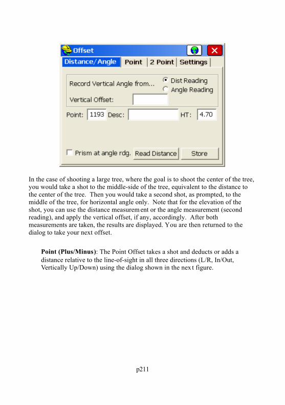
p211

In the case of shooting a large tree, where the goal is to shoot the center of the tree,you would take a shot to the middle-side of the tree, equivalent to the distance tothe center of the tree. Then you would take a second shot, as prompted, to themiddle of the tree, for horizontal angle only. Note that for the elevation of theshot, you can use the distance measurem ent or the angle measurement (secondreading), and apply the vertical offset, if any, accordingly. After bothmeasurements are taken, the results are displayed. You are then returned to thedialog to take your next offset.

Point (Plus/Minus): The Point Offset takes a shot and deducts or adds adistance relative to the line-of-sight in all three directions (L/R, In/Out,Vertically Up/Down) using the dialog shown in the nex t figure.

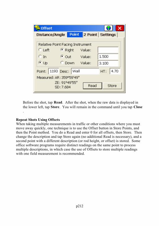
p212

Before the shot, tap Read. After the shot, when the raw data is displayed inthe lower left, tap Store. You will remain in the command until you tap Close.

Repeat Shots Using OffsetsWhen taking multiple measurements in traffic or other conditions where you mustmove away quickly, one technique is to use the Offset button in Store Points, andthen the Point method. You do a Read and enter 0 for all offsets, then Store. Thenchange the description and tap Store again (no additional Read is necessary), and asecond point with a different description (or rod height, or offset) is stored. Someoffice software programs require distinct readings on the same point to processmultiple descriptions, in which case the use of Offsets to store multiple readingswith one field measurement is recommended.

p213

2-Point Offset: This creates a 2-point 3D “vector”, where the offset direction,distance, and vertical offset are computed from the delta N, delta E and DeltaZ of the two points that are measured or entered. If Read Inst is enabled, thenthe two points are measured in the field. If, instead, you wish to obtain theoffset vector from two points, then disable Read Inst and enter the two pointnumbers. The offset entered will extend the vector from point “P2” in thedirection of “P1” to “P2”. The vector offset will also impact the elevation thatis calculated. This might be used to calculate a point at the top of a cliff, forexample, where you stand above the cliff top, pick up two points on the slopeto the cliff edge, and estimate the distance to the cliff face from the secondpoint. The offset by two points routine will write an SS record in the RW5file (raw file), which enables re-processing.

Settings: The Settings tab appears with robotic total stations running remotely(from the prsim) and permits reading the target height from a laser andaccesses the entire range of laser devices found in the Peripherals menuoption under Equip.

Store Points (GPS)Store Points is the principal data collection routine for GPS equipment. Store

p214

Points interacts with numerous settings, including the feature codes, and will drawline work. The Store Points screen in GPS shows the cursor moving on the screenin real-time. Shots can be taken anytime by pressing Enter. The screen will panautomatically, so you are always in view as you move. Points will plot on thescreen as shots are taken.

In GPS mode, Enter has only one function: Read & Store. The after-shot antennaheight and description prompt can be enabled in Configure (C or ALT-C from theStore Pints screen.). If you don't have the height and description prompt turned on,then each shot is a single press of Enter, and you must enter antenna height,description, or point ID changes prior to pressing Enter and taking the shot.

For GPS, coordinates, status (Fixed, Float, Autonomous) and HRMS and VRMSaccuracy estimates are displayed at all times. The icons at the left are for zoomingand panning. From top to bottom, they are: zoom ex tents, zoom in, zoom out,zoom window, zoom previous and point display control. If you prefer to work in apure text screen, without graphics, you can tap the helmet icon and select TEXT. The following dialog will appear.

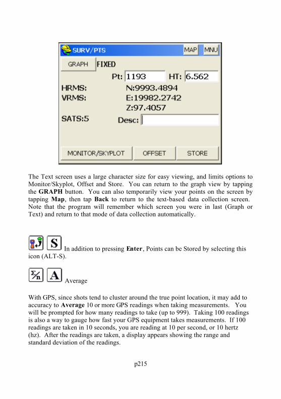
p215

The Text screen uses a large character size for easy viewing, and limits options toMonitor/Skyplot, Offset and Store. You can return to the graph view by tappingthe GRAPH button. You can also temporarily view your points on the screen bytapping Map, then tap Back to return to the text-based data collection screen. Note that the program will remember which screen you were in last (Graph orText) and return to that mode of data collection automatically.

In addition to pressing Enter, Points can be Stored by selecting thisicon (ALT-S).

Average

With GPS, since shots tend to cluster around the true point location, it may add toaccuracy to Average 10 or more GPS readings when taking measurements. Youwill be prompted for how many readings to take (up to 999). Taking 100 readingsis also a way to gauge how fast your GPS equipment takes measurements. If 100readings are taken in 10 seconds, you are reading at 10 per second, or 10 hertz(hz). After the readings are taken, a display appears showing the range andstandard deviation of the readings.

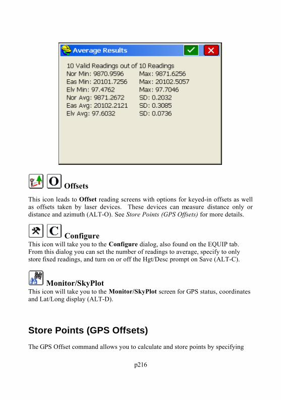
p216

OffsetsThis icon leads to Offset reading screens with options for keyed-in offsets as wellas offsets taken by laser devices. These devices can measure distance only ordistance and azimuth (ALT-O). See Store Points (GPS Offsets) for more details.

ConfigureThis icon will take you to the Configure dialog, also found on the EQUIP tab.From this dialog you can set the number of readings to average, specify to onlystore fixed readings, and turn on or off the Hgt/Desc prompt on Save (ALT-C).

Monitor/SkyPlotThis icon will take you to the Monitor/SkyPlot screen for GPS status, coordinatesand Lat/Long display (ALT-D).

Store Points (GPS Offsets)The GPS Offset command allows you to calculate and store points by specifying

p217

an offset from a GPS position. Offsets can either be entered manually or readautomatically from a laser. There are three GPS offset methods: Distance/Angle,Intersection, and Two Point. The current method can be set from the Method tab.

Distance/Angle OffsetIn the Distance/Angle method, offsets can be specified manually by choosing theOFFSET tab, or with a laser, by choosing the LASER tab.

Manual Offset: Under the OFFSET tab, offsets are specified by enteringazimuth, vertical, and horizontal distance offset values as show below. Theazimuth can either be specified with respect to north, or with respect to aspecified point. Current GPS coordinates are shown at the bottom, and can beupdated via the Read GPS button. When all necessary data has been entered,you’ll be able to store by tapping Store, or preview the point you’re storing byselecting Map, or Results.

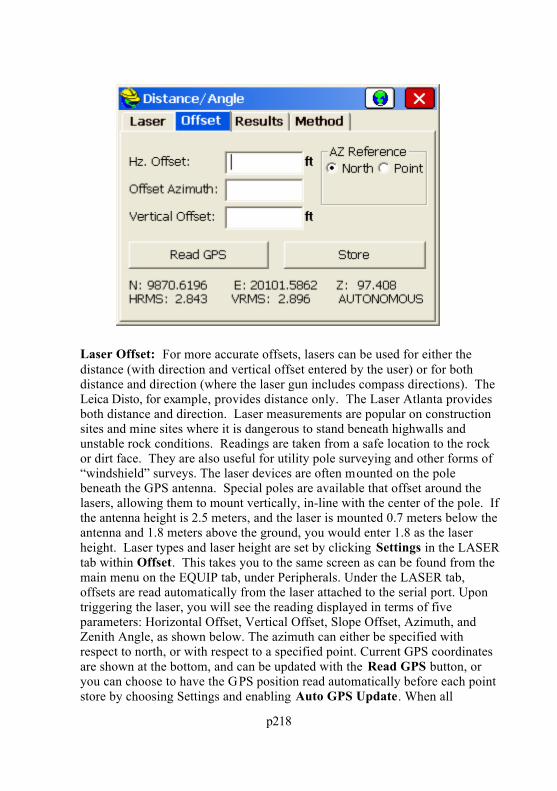
p218

Laser Offset: For more accurate offsets, lasers can be used for either thedistance (with direction and vertical offset entered by the user) or for bothdistance and direction (where the laser gun includes compass directions). TheLeica Disto, for example, provides distance only. The Laser Atlanta providesboth distance and direction. Laser measurements are popular on constructionsites and mine sites where it is dangerous to stand beneath highwalls andunstable rock conditions. Readings are taken from a safe location to the rockor dirt face. They are also useful for utility pole surveying and other forms of“windshield” surveys. The laser devices are often mounted on the polebeneath the GPS antenna. Special poles are available that offset around thelasers, allowing them to mount vertically, in-line with the center of the pole. Ifthe antenna height is 2.5 meters, and the laser is mounted 0.7 meters below theantenna and 1.8 meters above the ground, you would enter 1.8 as the laserheight. Laser types and laser height are set by clicking Settings in the LASERtab within Offset. This takes you to the same screen as can be found from themain menu on the EQUIP tab, under Peripherals. Under the LASER tab,offsets are read automatically from the laser attached to the serial port. Upontriggering the laser, you will see the reading displayed in terms of fiveparameters: Horizontal Offset, Vertical Offset, Slope Offset, Azimuth, andZenith Angle, as shown below. The azimuth can either be specified withrespect to north, or with respect to a specified point. Current GPS coordinatesare shown at the bottom, and can be updated with the Read GPS button, oryou can choose to have the GPS position read automatically before each pointstore by choosing Settings and enabling Auto GPS Update. When all

p219

necessary data has been entered, you’ll be able to store by clicking Store, orpreview the point you’re storing by clicking Map or Results. Before you canbegin using the Laser offset feature, you must configure the laser, either byclicking Settings, or by selecting Peripherals from SurvCE’s main menu.Under the peripherals menu, you will have to activate your laser, select yourlaser type, and choose a COM port. It is also recommended that you deactivateall other peripherals except GPS while using the laser. For more details onlaser setup, see the Peripherals section of this manual. Once you haveactivated a laser, you may click Read Laser to begin collecting data from thelaser. In order to expedite the data collection process, the methodology forreading an offset from the laser has been optimized so that you do not need totouch your data collector between shots. This option can be enabled byselecting Multiread Laser. If you are a first-time user, it is recommended thatyou disable this option. If Multiread Laser is disabled, pressing Read Laserwill pop up a dialog asking you to trigger the laser, as shown below. Fromhere, you can either cancel, or fire the laser to record the shot. If MultireadLaser is enabled, when you press Read Laser, a dialog will appear asking youto trigger the laser, as shown below. Each time you trigger the laser, a newshot will be collected, and if there was a previous shot, it will be automaticallystored. Between shots, the laser reading and the offset-adjusted position to bestored are displayed. If Auto GPS Update is enabled during peripheral setup, anew GPS position will be read for each shot. If a bad reading is taken, you canprevent it from being stored by pressing Reject Last Shot. When finished,click Exit Shot Sequence .

p220

Results: Before storing, you can preview the data by selecting the RESULTStab. If valid data has been entered in the LASER or OFFSET tab, the resultwill appear as shown below. In this window, you can also change the G PSantenna height, or specify a vertical difference for your target point. You canalso specify the point ID and description for the point that will be stored.

Offset by IntersectionUse Offset by Intersection to calculate a point based on two GPS positions and twodistance offsets. The distance values can either be manually entered or input with alaser. To use a laser, you must first activate it by selecting Settings. For moreinformation on laser setup, see the Peripherals section of this manual.

Offset: Under the OFFSET tab, press Read Point 1 to read the first pointfrom GPS. Now enter the distance of the point to be stored, or press ReadDist 1 to read this distance from a laser. Repeat this process for the secondpoint. Switch to the RESULTS tab to see your solution. If your distances andGPS can’t be triangulated, you may have to return to this tab to adjust thevalues.

Results: After you have two GPS positions and two distances that form avalid triangle, click on the RESULTS tab to view the resulting point. If validdata has been entered in the OFFSET tab, the result will appear as shownbelow. In this window, you can adjust the GPS antenna height, or specify a

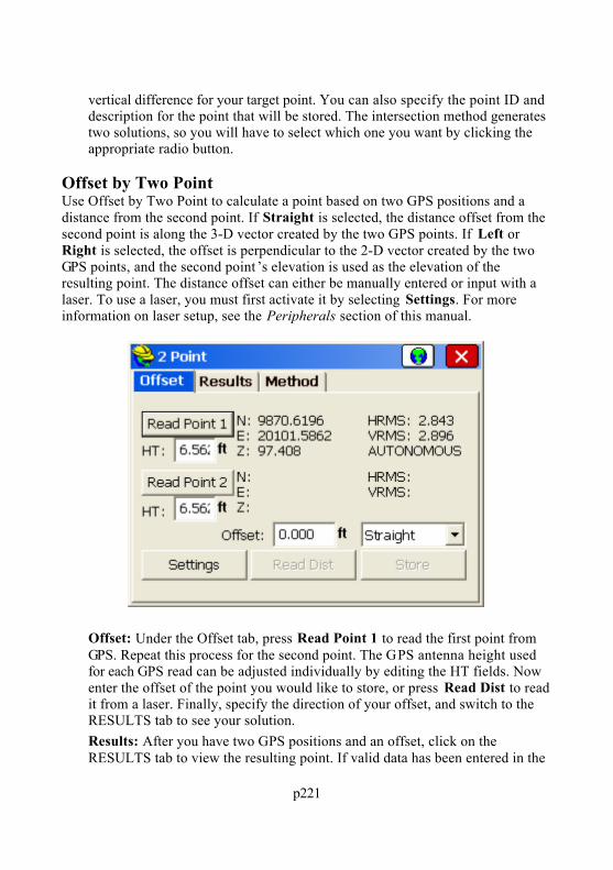
p221

vertical difference for your target point. You can also specify the point ID anddescription for the point that will be stored. The intersection method generatestwo solutions, so you will have to select which one you want by clicking theappropriate radio button.

Offset by Two PointUse Offset by Two Point to calculate a point based on two GPS positions and adistance from the second point. If Straight is selected, the distance offset from thesecond point is along the 3-D vector created by the two GPS points. If Left orRight is selected, the offset is perpendicular to the 2-D vector created by the twoGPS points, and the second point ’s elevation is used as the elevation of theresulting point. The distance offset can either be manually entered or input with alaser. To use a laser, you must first activate it by selecting Settings. For moreinformation on laser setup, see the Peripherals section of this manual.

Offset: Under the Offset tab, press Read Point 1 to read the first point fromGPS. Repeat this process for the second point. The GPS antenna height usedfor each GPS read can be adjusted individually by editing the HT fields. Nowenter the offset of the point you would like to store, or press Read Dist to readit from a laser. Finally, specify the direction of your offset, and switch to theRESULTS tab to see your solution.

Results: After you have two GPS positions and an offset, click on theRESULTS tab to view the resulting point. If valid data has been entered in the

p222

OFFSET tab, the result will appear as shown below. In this window, you canspecify a vertical difference for your target point. You can also specify thepoint ID and description for the point that will be stored.

Stake PointsThis command allows you to stakeout a selected point by guiding you to the pointwith a series of commands and directions. Various options can be set in EQUIP,Configure, View Point to adjust how the directions are provided to best suit yourneeds. You should also review the Job Settings under FILE before staking. Thedialogs are varied slightly with respect to total station or G PS equipment. Bothtypes are documented here, illustrating the differences between the dialogs.

Note: While in graphics mode stakeout, if you press the down arrow key, you canincrease the plan view size and eliminate some of the text information. Pressingthe up arrow key again reveals the cut and fill.

After selecting OK, the main stakeout window appears in MAP view. In manualtotal station mode, the angle to turn to and the distance to the stake point will bedisplayed at the bottom of the screen. Shown below are the graphic icons, setunder EQUIP, Configure, using a robotic total station in prism mode (notreflectorless).

p223

A read function is required to update the directional display information. Youshould see your points in the map with an icon showing your target location (thecircle with the X inside).

Shots are taken typically by pressing Enter. Enter also transitions automaticallyfrom the Stake Points entry screen to the Stk Pt shot screens above. Point Stakeoutcan be conducted without touching the screen. Both screens are ex plained below,starting with the graphic Stk Pt screen.

Total Station Only: After reading and taking the shot, the display will beupdated with a distance and direction to the stakeout point. Buttons on theright from top to bottom are Read, Store, Next, Menu, Configure and Setup.

GPS or Robotic Total Station with Tracking On: Your current position isread immediately (no Read button needed).

Point ID: This is the point which you are staking. You can enter it in here andhit the enter key to view the elevation, northing and easting before selectingOK. If you want to stake out a range of points, you can enter in the points inthe following format: 3-10,2,15-20. This would stake out the points from 3-10sequentially, then point 2, then 15 through 20 sequentially. If you are using acontrol file in total station mode, and you enter a point number which also ispresent in the current job file, it will choose the control file point if ControlFile Has Priority is enabled in the stakeout section of Job Settings. If youenter a point number that is not in the control file, but is in the current job ’s

p224

coordinate file, then that point will be used. You can also select the points tostakeout from a list by selecting the List icon. If you select the List option,you can select the points for stakeout from the active job file or the controlfile. To do this, you must toggle between the files using the Job and Controltoggles at the top of the dialog. You can select a range of points by selectingthe first point to stake then pressing the shift key and selecting the last point tostake. All points between the two selected points will be staked in sequentialorder. You can also add to the selection of points to be staked by pressing andholding the CTRL button and individually selecting the points to be staked.The final way to select an individual point to be staked is by selecting the Map icon and tapping on the point to be staked.

Add to List, Pick from List: When you select or enter multiple points, theyappear in the Point ID dialog window. You can then pick Add to List andcreate a list of these points in the order they were selected. When you Add toList, the Point ID dialog is cleared, and you can select more points, place themin the dialog and click Add to List again. Then you can stake any of themusing Pick from List, where the points appear as shown below:

Source: When you press Enter after selecting the point (or points), theprogram will display the source of the points, either as Current Job or ControlFile. The display of the source is important for verification. You maydiscover, for example, that someone has turned on Control File Points havePriority in the stakeout settings, and this is a way to catch the m istake.

p225

Northing, Easting, Elevation: You must have a northing, easting andelevation entered for the point you are staking out. If you type in the pointnumber of an existing point and hit OK, these values wiill appearautomatically. The description of existing points is displayed at the bottom ofthe dialog.

Point by Direction: In addition to staking a point ID or entered coordinate,you can stake a point defined by a direction and distance, and even slope,from the entered point coordinate. This allows you to stake points withoutcalculating point numbers or point IDs for the target point. Simply enter thebearing/azimuth, horizontal distance and also slope, if applicable. If thedistance entry is not known but must be computed, the calculator is accessiblefrom the distance dialog box by hitting the ? button. Shown below is astakeout of a point calculated at NE45 degrees, 100 feet, from point 10.

View PtDepending on your settings in the View Pt tab of Configure (in the EQUIP tab),the direction to stake will either be Right/Left Distance, Azimuth and Distance, orNorth/South East/West Distances. The cut or fill is the elevation differencebetween the point read and the point being staked. Normally, you take a shotsimply by pressing Enter. After a total station shot is taken, you will see your“In-Out” distance to the target point. For total station stakeout, the direction of thereference is shown by a little arrow in the lower right of the screen.

p226

Store Point DialogSelecting S to Store will display the Stakeout Report. You can turn off the StorePoint option, and just reference the Stakeout Report screen for information. If thetolerance distance is exceeded for staking out, you will be notified and asked if youwant to continue storing. (Stakeout Tolerances are set under Tolerances in the EQUIP menu).

p227

The coordinates for the Stake Point and the Target Point are displayed. The deltaNorth, East and the elevation difference (Cut/Fill) are also displayed. The verticaloffset input boxes allow for elevation calculations based on the input vertical offsetvalues. The vertical offsets can be entered in inches in English units in two forms(10" using the inch designator, or 0.10.3.8 for 0 feet 10 and 3/8ths inches). Thesecond form requires 3 decimals to be used.

If Store Carlson Cutsheet Data in Note File has been enabled, the verticaloffset(s) specified will be recorded in the .not file for the job. If under SetCutsheet Format in the Stakeout section of Job Settings, a Set Pt Cutsheet Formathas been established with a named file for storage, then cut and fill data will besaved to a cutsheet ASCII file. If using GPS, the HRMS, VRMS, and PDOPvalues are also displayed. Fields for Point number and point description input arealso displayed. If, for example, you choose not to store a staked point, but onlyreport the design point, design elevation, surveyed elevation and the cut and fill,you could produce a simple cutsheet report as shown below. One vertical offsetper shot was recorded (-10"). The cutsheet can be reviewed from within the activestakeout screen using Alt V. You can also click on the helmet and go to V iewData, when actively staking out, and you will be returned to the stakeout screen. Cutsheet data is always stored to the raw file, so if you forgot to store the cutsheetinformation, you could create a new point cutsheet file and select "Cutsheets fromRaw File".

Pressing OK (which optionally will Store Point if enabled) will return to the

p228

Stakeout Points dialog to select the next point for staking. If the Use Control Fileoption is set under the Job Settings, you have the option of staking control filepoints. If you enter in a point number to store that is the same as a point number inthe control file, the point in the control file will remain unchanged. It will onlymodify the point in the current coordinate file. If the point being stored is the sameas one in the current job file, the Point Protect dialog box appears stating that thepoint you chose is already used. The next available point number is listed with theoption to overwrite the current point, or use the new number.

Stake Line/ArcThis command opens a secondary dialog where you can choose between DefineLine, Define Alignments, Define Arc (3 points), and Define Arc (PC, PT, Value).Define Line is documented below.

Define LineThis command allows you to stakeout to a line between two points by guiding youto the point with a series of commands and directions.

This option is for setting out points along a line including the cut or fill, or forstaking out points relative to the line. One application, for ex ample, would bestaking a pipe between two known points (inlet and outlet), where offset stakes canbe set with cut/fill noted. Station Store might even be used to calculate, in

p229

advance, the inlet and outlet points based on a known station, offset and elevation. For all staking, there are configuration settings that govern the type of instructionsyou receive in stakeout. You should review the settings in the Stake tab under JobSettings, as well as the Configure option within Equip before staking. Thedialogs are varied slightly with respect to total station or G PS equipment. Bothtypes are documented here, illustrating the differences between the dialogs.

Stakeout by Define Line also has a Point On Line tab that enables, in total stationmode, staking of the intersect with the specified line on the current line-of-sight. This is often used to set stakes or flagging along a property line that is obscured bytrees. The surveyor finds a gap in the line, takes a reading to the prism and isadvised how far to Move In or Move Out to stake the line at the currentline-of-sight. The Point on Line tab also includes the standard perpendicularmethod, where any measurement is used to compute the direction and distance tomove to go to the point on the line perpendicular to the measured point. For G PSconfigurations, Point On Line offers only the Perpendicular method.

The Define Line dialog gives you the following options:

First Point ID: This is the starting point of the line. You can enter the pointhere by point ID. The first button brings up the list points dialog where youcan select the starting point of the line from a list. The button directly to theright allows you to choose your point from the map instead. If you pick apoint from the map in a crowded area of points, you will be directed to the list

p230

points dialog to select the desired point among those near to your chosenposition.

Second Point ID: Pressing Enter from the first point moves the curser to thesecond point. This is the ending point on the line that is only available forentry if Method is set as two Point for defining the line. The procedure forselecting this point is the same as for the first point.

Azimuth: This option will be available for input only if Method is set toAzimuth. If Method is set to Two Point, then the Azimuth is inactive, but stilldisplays the azimuth or bearing between the two points of the line. TheAzimuth method will prompt for bearing if Angle Type is set to bearing inthe Format section of Job Settings.

Slope (%): Just like the Azimuth, this option will be available for input onlyif Method is set to Azimuth. If Method is set to Two Point, then the slope isinactive, but still displays the slope between the two points of the line.

Method: This options lets you choose how to define your line. The availableoptions are by two points, or one point and an azimuth and slope.

Start Station: This option defaults to 0 within Stakeout Line, but can bechanged to any starting station.

Confirm NEZ: Selecting this button brings up the Confirm NEZ dialog box.This screen displays each point as a tab at the top of the screen. Listed is thepoint number, Northing, Easting, Elevation and Description of the point(s)selected for the line. After you confirm the points, selecting the back arrowwill take you back to the line definition screen. Pressing Enter after ConfirmNEZ automatically continues to the next screen.

Define Alignments (Horizontal)Stakeout Centerline only requires a horizontal alignment, but you have the optionto specify a vertical alignment which will lead to cut and fill results as well.Additionally, you can specify a reference alignment. This feature allows you tostake the offset off of one alignment (e.g. curb) and report the station of a referencealignment (e.g. centerline).

p231

Centerline File: Select a centerline file defined in the Roads Menu oruploaded and converted to “.cl” format.

Select Polyline: Select a polyline on the screen to define the alignment. Define Point List: Enter a sequence of points to define the alignment. Use Ref. CL: Toggle this on to enable the use of a reference alignment. This

will be the alignment from which the stationing is reported. The offsets andcritical locations will remain relative to the main centerline alignment.

Select: Use this option to select the reference alignment file. Preview: Displays the alignment graphically. Edit: Use this to edit the selected alignment. Save As: If an alignment was defined by points or a polyline, you can

optionally save it as a centerline file. Start Station: Enter the starting station unless it was pre-determined by a

centerline file. End Station: This shows the ending station of the selected alignment.

Defining Alignment (Vertical)This is optional in this command. If your goal is to ignore elevations and you areauto-recalling roading files, the Vertical Alignment will be used and cut/fill willappear unless you turn off Apply Vertical Alignment.

p232

Profile File: Select a profile file defined in the Roads Menu or uploaded andconverted to “.pro” format.

Select Polyline: Select a 3D polyline on the screen to define the profile. Define Point List: Enter a sequence of points that have elevations to define

the profile. Preview: Displays the profile graphically. Edit: Use this to quickly edit the selected profile. Save As: If the profile was defined by points or a polyline, you can optionally

save it as a profile file. Start Station: Enter the starting station unless it was pre-determined by a

profile file. End Station: This shows the ending station of the selected alignment. Apply Vertical Alignment: Toggles on/off the vertical alignment for 2D or

3D staking.

Note : For file names to be recalled, Recall Job Road Files needs to be enabledwithin Job Settings, Options .

Shown below is an example of what will you see when you tap Preview in eithertab. Notice that the centerline is shown, along with any existing point numbers inthe vicinity.

p233

As with all options, the alignment selection screen continues into the Station/Offsetscreen where you select your station and offset to stake out. Using DefineAlignments, the Point on Line option becomes Point on CL in the screen thatfollows. With both horizontal and vertical alignments defined, the final stakeoutscreen (eg. station 375) includes cut and fill values. Shown below is an ex ample inGPS mode. The centerline was picked from the screen (Select Polyline) and thevertical alignment was selected from a file.

p234

Define Arc (3 Points)This routine requests three points to define a unique arc, which is then used forstakeout by station and offset. The first point becomes the beginning of the arc.The prompting is shown below.

The points can be entered in, chosen from the list points button, or selected from

p235

the map. After selecting the three points, choose OK (green checkmark) to go tothe Stakeout Arc dialog. The special stations are limited to PC (start) and PT(end). After choosing a station and offset to stake and selecting OK, the mainstakeout window appears in map view. In total station mode, an angle to turn toand a distance to go will be displayed at the bottom of the screen. Taking areading to the current target position will update the display with a new out/indistance and a right/left distance depending upon your job settings. Y ou shouldsee your points and centerline or curve in the map with an icon of the point youneed to stakeout to (the circle with the X inside). When using GPS, after selecting OK to the Stakeout Arc dialog, you will be placed in the Map screen at yourcurrent position with directional instructions to the target point continuallyupdating. You can click "RR" to stake out a 3-point arc by railroad definition.

Define Arc (PC, PT Value)This option for defining the arc requires four input parameters: the Start point, EndPoint, Curve Direction, and any of the following: Radius Point, Radius Length,Arc Length, Delta Angle or Degree of Curvature. The starting station defaults to0, but can also be changed. See the figure below.

When selecting the PC point, option Radius Point and PT point, enter the point ID,choose the point from the list points screen button, or pick the point from the mapbutton. After selecting OK you will be directed to the Stakeout Arc dialog. Afterselecting OK to the Stakeout Arc dialog, the main stakeout window appears inmap view. Here we are staking station 75 at 0 offset. In total station mode, an

p236

angle to turn to and a distance to go will be displayed at the bottom of the screen. Taking a reading to the current target position will update the display with a newout/in distance and a right/left distance depending upon your reference settings in Configure Reading. You should see your points and arc in the map with an iconof the point you need to stakeout to (the circle with the X inside). When usingGPS, after selecting OK to the Stakeout Arc dialog, you will be placed in theMap screen at your current position with continuously updating instructions to thestakeout point.

Stake Line/Arc (Station/Offset)Selecting OK on the Define Line, Define Alignments or Define Arc dialogspresents the Stake Line dialog for defining the stake location parameters (e.g.offset or elevation).

p237

Station: This is where you enter the station to stakeout.

Station +: You can advance to the next station as defined by thealignment points or station interval using the right green arrow icon.

Station -: You can go back to the previous station as defined by thealignment points or station interval using the left green arrow icon.

Station List: Select a specific station using the station list icon. Interval: This is where you choose the distance by which to increment the

stations.

Calculate Interval: This is used to divide the entire line into equalparts, which results in a calculated, non-rounded, incremental station.

Offset/Skew List: This is where you enter in the offset distance from the line.Select one of the left/right radio buttons to determine the offset side. This listalso provides additional methods of offsetting, such as Skewed Offsets,Bisectors, Intersections and PI or Radius Points. A Skew Forward angle ismeasured forward from the perpendicular, and a Skew Back angle is measuredback from the perpendicular. So looking forward down a tangent centerline, apipe with a skew of 70 degrees (in DD.MMSS) from the forward tangentwould be a Forward Skew Angle of 20 degrees, as measured forward from theperpendicular (normal) offset.

Elevation: This is the design elevation. If the defined geometry is 2D, then

p238

this option will be active. Override Design: This allows the user to override the design elevation of 3D

geometry. Off. Inc: This is for entering an optional incremental offset along the line.

This is a rarely used feature that would trend the offsets away or in to thecenterline.

Segment: This defines the current segment of the alignment based on theentered station.

Cutsheet: This shows the currently selected Alignment Cutsheet file.

Settings: This icon takes you to the Job Settings that apply to alignm entstaking. See Job Settings (Stake) for more details. Note that this is where youinstruct the software to include and stop at critical alignment locations.

Stake Line/Arc (Point On Line)The Point On Line option appears when Define Line or Define Alignments isselected. It offers a Perpendicular to Line method for total stations and G PS. Thismethod projects any shot onto the alignment perpendicular or radial in curves, andprompts for the distance and direction to move to the alignment intersect point. However, only if you select Define Line as the method to define the alignment andyou are set to total stations, is there a "Find Intersect to Line" option, whichenables “line-of-sight” staking of lines. This is often used by surveyors who aresetting line in tree lines, moving to gaps in the trees for readings, then movingin-out along the line-of-sight and driving stakes when perfectly on line. It is usefulfor any line or boundary staking, such as property lines, right-of-ways andconstruction lines. For GPS, only the Perpendicular method is available.

Total Stations: The Offset to Line option is grayed out when the Find Intersect toLine method is selected and available only when the Perpendicular option ischosen.

p239

Total Stations, Define Line, Point On Line, Inters ect to Line: The IntersectMethod is used to set line by moving in or out at the current line of sight. A majorapplication is setting line where the line is largely blocked by trees or obstructions,and you must set the line in gaps where you do have a line of sight.

In the Intersect mode, the first screen always displays the target point on the line(or the extension of the line), perpendicular to the setup or station point. When thefirst reading is taken, the program will display the In-Out distance to the line along

p240

the line-of-sight.

When staking a line defined by points with zero elevation, the cut or fill values willbe displayed but should be ignored. Notice that the screen ex pands to show moregraphics by pressing the down arrow key.

p241

Total Stations/GPS, Perpendicular to Line: When configured for thePerpendicular to Line method, the program will show the direction and distance tomove to find the nearest point on the line to the measured point. The instructionreceived (In/Out versus North/South or Azimuth/Distance) will depend on thesetting within Configure Reading.

The “Turn to AR” advice at the top of the screen refers to the angle to turn tointersect the defined line at 90 degrees from the instrument location. For GPS, thePoint-On-Line screen instructions are similar.

p242

Stake Line/Arc (Point on Arc)Both the Stake Arc (3 Points) and the Stake Arc (PC, PT, Value) routines have aPoint On Arc option similar to the Point On Line option. In the dialog below, wehave chosen to calculate a left 25 offset from the arc. Any measured point willthen be translated radially onto the arc that is 25 units left of the specified arc.

p243

When a measurement or GPS reading is taken, the target point will be radial to thecurve, at 25 units offset from the curve, as shown below.

The above example might be useful for setting stakes at a 25 ’ building setbackfrom the right-of-way line. For GPS, information is provided “real-time”. As youmove, you see the instructions to contact the nearest point on the arc (or offset tothe arc). For total stations, you are first instructed to measure to the nearest pointon the arc (or arc offset) from the instrument setup. Then after you take any shot,the instruction refers to that measurement.

Note: The Turn to AR advice refers to the angle to turn to contact the centerline at90 degrees (right angles) to the instrument setup.

After selecting OK, the main stakeout window appears in map view. In totalstation mode, it will be waiting for a shot or reading. You should see your pointsin the map with an icon showing the location of your target (the circle with the Xinside).

Note: If the points defining the line are at zero elevation, the program will stillreport a cut and fill -- in this case a cut from the GPS elevation of 839.52 all theway to zero. If the points defining the line are at a known elevation, the elevationwill be interpolated to determine the design and target elevation of the point tostake, and will be applied to a zero offset or non-zero offset stakeout position.

p244

Store a reading and the coordinates for the Stake Point and the Target Point aredisplayed. Store by pressing Enter or S to Store. The delta North, East and theelevation difference (Cut/Fill) are also displayed. The Vert Offset 1 and VertOffset 2 allow for elevation calculations based on the input vertical offset values.In English units, a vertical offset of -10" can be entered for ex ample in that form,and the program will auto-calculate -0.833 as the offset. If Vertical Offsets aredetected, and a point is stored, you are prompted for additional descriptions for thevertical offsets. If "Alignment Cutsheet" storage is on (as set in Job Settings, Staketab), an additional cutsheet "row" will be created for each vertical offset. Shownbelow is a stakeout of station 125, Right 12, and the resulting Report screen.

p245

Note that you have the option to store a point in stakeout. If the point being storedis the same as one in the current job file, the Point Protect dialog box appearsstating that the point you chose has already been used. The nex t available pointnumber is listed with the option to overwrite the current point, or use the newnumber. If you "Show Station/Offset", you will see the Station and Offset of thedesign (1+25.000 R12.000) and staked point (1+25.000 R11.979), for example.

All cut and fill data, including vertical offsets, will be stored in the AlignmentCutsheet File if named and turned on within Job Settings, Stake tab, Cutsheets .Finally, the data is always stored to the raw (.rw5) file as cut/fill (cutsheet)information. If you forgot to create a cutsheet file, you can make a new one, andwhen formatting the cutsheet, select "Cutsheets from Raw" as one of the options.You can review the cutsheet with the shortcut, Alt V, from the active stakeoutscreen. This will return you directly to stakeout. If using G PS, the HRMS,VRMS, and PDOP values are also displayed, as are Fields for Point ID and pointdescription input. After the point has been stored, you are taken back to theStation/Offset dialog to select the next point for staking.

When you return to the Stakeout Line screen after storing a point, there is a taboption for Next Alignment that allows you to define a new alignment, withoutexiting the command.

Stake Offset

p246

This command will stake out up to two user-defined horizontal offsets to acenterline at any station, as well as an unlimited number of offsets per station, ifyou are using a predefined Cutsheet Station and Offset List (loaded using theSettings button). It will also stake out the centerline itself. Station intervals can beentered, and the program will auto-detect, at the user ’s option, special stations suchas the TS, SC, PC, PT, CS, ST and vertical curve points (including high and lowpoints). Because individual stations and offsets can be entered, and also becausepre-made station and offset lists can be recalled in the field, Offset Stakeout can beapplied to virtually any offset point along a centerline.

Prerequisites and ProceduresStake Offset requires both a horizontal and vertical alignment. If total stations areinvolved, Stake Offset passes through the normal backsight confirmation screensthat Store Points and other forms of Stakeout require.

The Offset Stakeout command is a three-screen routine. The first screen identifiesand loads in the alignment files. The second screen identifies the offset points tostake (slopes and distances) and the intervals or lists of stations/offsets to stake.The final screen goes to the standard graphics, shows the target points, and guidesyou to the destination, with N for Next continuing onto the next station in theinterval or list.

Identifying the AlignmentsThe first screen has tabs for selecting both the horizontal and vertical alignments.See Stake Line/Arc for more detail.

Settings Use this button in the upper part of the screen to select predefined station lists andcritical stopping points along the alignments.

p247

Within this option, you can click the Stake tab and edit your default Stake OffsetDescriptions shown below. See Job Settings (Stake) for more details.

Entering the Offset Points as Slopes and DistancesThe Offset Stakeout screen allows you to enter one or two offsets from thecenterline. The first offset requires a presentage slope and a distance. The second

p248

offset is for a curb or ditch, and is prompted in the form of “distance over” and“elevation change up or down”.

Settings: The Settings button returns to the Settings dialog, allowing you toload another cutsheet list or specify more or less special stations. Note that inSettings, if you called for a Station and Offset List, then most of the options inthe Offset Stakeout dialog are fixed, and your only choice is to stake theparticular offsets named in the list. Also note that Offset Stakeout, when notusing a List, allows for the staking of three points on the Left or Right Side: Center, Curb (or Ditch) and EOP. On the left, it becomes LEOP, LCurb orLDitch. On the right, it becomes REOP, RCurb or RDitch. You must enterdata for the right as well as the left if you are staking both sides of a road. Sothere are five points total that can be staked when you use the dialog entry,since the centerline is covered in both the Left and Right scenarios.

Back: The Back button returns to the first screen. Station: This is where you enter the station you wish to stakeout.

Station +: You can advance to the next station as defined by thealignment points or station interval using the right green arrow icons.

Station -: You can go back to the previous station as defined by thealignment points or station interval using the left green arrow icon.

Station List: Select a specific station using the station list icon.

p249

Interval: This is where you enter the distance by which the stations should beincremented.

Calculate Interval: This is used to divide the entire line into equalparts, which results in a calculated, non-rounded, incremental station.

Next Offset: The green arrow found to the right of the offset entry boxwill switch from RCurb to REOP to CL and back, and the large solid circlewill move and highlight the correct location. These abbreviations are definedin the Settings dialog or the Stakeout tab of Job Settings.

Left/Right: You can specify whether to stake the left or right side of the road.The offsets are applied symmetrically. If you have a special case on a specificside of the road, do the right and left separately, with separate slope anddistance entries.

Offset: This is the first offset from centerline. Units are as configured in JobSettings (feet or meters).

X-Slope: This is the first offset slope. Negative represents downhill. Stake Curb/Ditch: This will allow the user to input and activate a second

offset defined by offset distance and height from the first offset. Stake Curb/Ditch (Height): This is the vertical difference from the first

offset to the second offset. A positive entry is interpreted as a curb and anegative (downhill) entry is interpreted as a ditch.

p250

Stake Curb/Ditch (Offset): This is the distance from the first offset to thesecond (outer) offset.

When using a Cutsheet Station and Offset list, you must select the List button,highlight the offset you wish to use and press Select. The routine will stay on thisoffset as it progresses through the stations until the user selects List again andspecifies a new offset.

The Stake Offset command will store to the Alignment Stakes cutsheet file formatif the file is named and made active for storing. The data can include station andoffsets as formatted.

Elevation DifferenceThis routine will report a cut/fill in comparison to a design surface at any locationwithin a project. The Elevation Difference command will save cutsheet data ifcutsheet files are named and made active within Job Settings, Stake tab. For anysurface where a centerline is defined (Road Design and Section, orGrid/Triangulation/Elevation with centerline defined), the routine will not onlyreport, but optionally store cuts, fills and centerline position data into analignment-style cutsheet file. With no centerline defined, the Road, G rid and

p251

Elevation methods will store cut and fill data into a point-style cutsheet file. Elevation Difference can also be used with a light bar.

Prerequisites and ProceduresThere are five types of data that can be used to define the design surface. Grid File : You may use a .GRD file that has been created using software

packages including Carlson Civil or Carlson Survey. You must transfer thisfile to the collector via the File Transfer routine prior to running thiscommand.

Triangulation File: You may use a .TIN file created within SurvCE using theTriangulate & Contour command found in the Map screen under Tools,Surface. You can also use a .TIN or .FLT file that has been created inCarlson Civil or Carlson Survey office products, in which case you musttransfer this file to the collector via the File Transfer routine prior to runningthis command. Note that triangulation files can be imported from LandXMLor DXF format using the command File, DTM Import, found in the Mapscreen.

Elevation: You may use known elevation that you specify in the SetElevation field.

Road Design: This method requires a Template, Centerline and Profile file ata minimum, and can utilize superelevation and template transition files.

Section: This method requires a Cross Section file and a Centerline file. Select Type of Surface Model : Specify the type of surface to be used. With

the exception of the Elevation method, the 4 other methods allow the option tospecify a vertical offset (such as to subgrade) and lead to a follow-up fileselection dialog.

Set Elevation: This option is available when the Elevation method is used fordefining the surface model. Enter the desired elevation of your surface in thisfield.

p252

Vertical Offset: This is used in conjunction with grid, triangulation, roadingand section files. It allows the user to vertically offset the surface (as definedin the file) by the amount specified in the box.

Use Centerline for Station-Offset : This allows the user to specify ahorizontal alignment file (.cl file) for reporting station and offset of yourcurrent location to the reference alignment. With total stations this is reportedwhenever a shot is taken. Using GPS or robotic total stations, with trackingon, your current position is updated in real time as the rover or prism ismoved. This option is available with Grid, Triangulation and Elevation typesof surface models. (A centerline is required for Road Design and Section-typesurfaces).

Stakeout Grid Pattern (GPS Only) :The first prompt asks if you want to usethe last stakeout pattern. To make a new pattern, you specify, in effect, thelower left corner (“left side” option) or the lower right corner (“right side”option) of a rectangle, and specify the starting point, direction point. Shownin the figure below is a 10x10 layout at 50’ interval (10 rows and columns areadded to the starting point, producing 11x11 grid points). The number of cellsin the grid ranges from 1x1 to 20x20, and are laid out in a grid beginning atthe starting point going towards the direction point.

p253

The program will then show the grid point nearest to your GPS position.

Light Bar Settings: This button allows you to specify parameters for enablingthe light bar, setting the grading tolerance, and specifying the COM port. Thetwo light bars currently supported are Mikrofyn and Apache. SurvCE canactually drive the grading process, as shown below, where an Apache light bar

p254

is used on a motor grader. In effect, this offers extremely low cost "gradeindicate" machine control.

Pressing OK from the main Elevation Difference dialog will first prompt the userto load the surface files involved (unless elevation method was selected). Then,when OK is pressed again, the ELEV DIFF screen in the following figure willappear. This screen provides the user with a plan view of the project. When a shotis taken, cut or fill from the current vertical location to the design surface isreported in the lower left portion of the screen. The computed design surfaceelevation for your current location is also reported.

p255

When Road Design Files are selected, there is an ex tra Settings option at the topof the screen that is used for setting the location of the Profile position on thetemplate.

p256

In road design, the position of the profile is sometimes placed on an insideedge-of-pavement or at some other offset from centerline, as defined by a fix edoffset, a template ID or even a completely distinct reference horizontal alignment. Even when specified, the application of the special profile can be turned off andon. Note that the "Off" status is equivalent to the default condition of profile gradeat Template ID "Center". If the Profile positioning is set to "On" in Settings, youwill always be promped with the Settings dialog after loading the Roading files, sothat you are reminded of any unusual, active profile offset before continuing bypressing Enter (OK) or changing a setting.

If you click the helmet icon in the upper left of the screen and select View Datafrom the Help options, or enter Alt V, you can select Cutsheets and the Edit Fileoption to review the stored cut and fill data at any time, assuming a "cutsheet" filehas been named and set active. The data might appear as follows:

p257

The order of the columns in the cutsheet is set by the user when the cutsheet file isnamed. In this case, the "Use Centerline for Station-Offset" was clicked on, andthe shots were stored to the "alignment-based" cutsheet because a centerline wasactive. All shots were cut, so if you scrolled right to the fill column, it would beblank. Columns can be extended and compressed by moving the vertical barbetween columns. In addition, cut and fill data is also stored to the Raw Fileassociated with the job name. Then when a new cutsheet file is named, you canchoose, "Cutsheets from Raw File". For those users who always want a cutsheetfile to be made in commands such as Elevation Difference, you can auto-create anew cutsheet with the job name as the prefix, whenever you start a new job, by thefollowing selection within Job Settings, New Job tab:

p258

Grid/FaceThis command enables points on both vertical and non-vertical planes to becoordinated by angle-only observations. This feature is m ost often used to pick updetails of a building where the prism cannot be placed. You first establish theplane, then take angle-only observations for features such as windows.

The building face is defined by observing three accessible points on the building orby entering their known coordinates. After angle-only observations are made,SurvCE then calculates and stores coordinates of the angle intersection observationwith the plane. You can use SurvCE to survey the vertical face of a building orother vertical planes.

Vertical Plane SurveyThe Define Plane dialog can be accessed by selecting the Grid/Face option fromthe SURVEY tab of the main menu.

p259

Point 1, Point 2, Point 3 : These fields indicate the points that define thebuilding face plane. Both Point 1 and Point 2 must have horizontalcoordinates to properly define the building face. For a vertical plane survey,point 3 is not required and can be left blank.

Get Coords : This function allows for three methods to define the coordinatesof a point. The coordinates of the points can be manually entered into theNorthing, Easting and Elevation fields. Manually entered coordinates will notbe stored in the coordinate file.

p260

Existing point IDs can be entered into the Point ID field. These points must bedefined by coordinate data. As soon as you enter the point ID, press enter and thecoordinates will appear in the Northing, Easting, and Elevation fields. Ex istingpoints can be selected from a points list by selecting the Point List icon. Highlightthe desired point and press enter or tap OK.

Existing points can be selected from the map screen by selecting the map icon. To

p261

select a point, tap it on the screen. If two or more points are close together on thescreen, you will be asked to select the intended point from the point list.

Lastly, the points can be taken with the total station by pressing Read.

After you have specified the two defining points for the building face plane,SurvCE will determine the available solution. One of the following messages willbe displayed in the dialog box.

Vertical - SurvCE has enough data to fix a vertical plane (the verticalexample is shown in this above figure).

3D - SurvCE has enough information to fix an arbitrary plane.

Press OK , and the following dialog will appear. The building face or verticalplane is drawn as a solid line, and any measurement taken by angle only reading(eg. angle right of 270, zenith angle of 83 degrees), will plot as a point withcalculated x,y,z position, such as point 20.

Non-Vertical Plane SurveySurveying a non-vertical plane is similar to surveying a vertical plane. Once theplane has been defined, picking up detailed observations follows the same generalprocess detailed above. All three points must be defined for a non-vertical planesurvey. When defining a non-vertical plane, the three points cannot be in a line.

p262

ResectionThis command allows you to calculate coordinates of an unknown instrument setuppoint given the angles and distances from up to 20 distinct reference points. Thereference points are recalled from your working job file. If a control file is activein Job Settings, and the entered point ID is not found in the current workingcoordinate file, then the point will be recalled from the control file automatically. You can also access points from the control file by using the from list icon.

Direct and Reverse measurements can be activated within the Configure screen inResection. The options within Configure expand (eg. for "Auto Turn" capability)if you are using motorized or robotic total stations versus conventional totalstations. If you choose Direct & Reverse, then the reverse measurements count aspart of the 20 allowable measurements, so the max imum number of referencepoints becomes 10. As long as you have at least 2 distinct points, you can shootthe same point twice or more with a direct or D&R measurement.

Elevations can be ignored on any measurement. Angle Only Readings can bemixed in as well. This is useful when sighting radio towers and church steepleswith known coordinates. In fact, all of your resection points can be measured byangle only, in which case 3 or more points are necessary for an accuratecalculation. Sometimes if the 3 angle-only points are in the same quadrant of view,

p263

a solution won't be found, requiring additional points. When elevations are used,measurements will contribute to the calculation of the setup point elevation. Afterentering the routine, the first screen appears as follows:

The points can also be selected from the point list or directly from the map screenby pressing either the list or map icons. You will also be prompted for theInstrument Height and a Target Height. On reading #1, you will be asked if youwant to Set Zero on the first resection point (optional).

If you press Configure, you can set standard errors for the measurements, asshown below. These settings allow you to take advantage of network least squaresand weighting in the calculation performed by SurvCE. The default values areshown. You can also enable Direct & Reverse measurements here, in addition tousing EQUIP, Configure .

p264

Press Read when you are ready to take a measurement. The angle right, zenithangle, and slope distance are recorded.

Repeat this process for all measurements of the resection. After the secondmeasurement, there is enough information to conduct the resection calculation, sothe Calculate button at the top of the dialog becomes active and can be selected.If you select Calculate, you can review the data, then return to taking more shotsby hitting Cancel rather than OK, which would prompt to store the point.

Any time Calculate is selected, the Review Resection screen appears. The inputdata is displayed in a list structure, and you have the ability to turn certainmeasurements on/off and recalculate the solution, without the necessity ofre-measurement. You can also edit point numbers, instrument and rod heights, andmore here. When satisfied with your edits and the solution, you can store theresults of the resection.

Since there is redundant data, the final calculated coordinate differs slightly fromthe individual measurements. The command reports the calculated coordinate ’snorthing, easting, and elevation, and the difference between the calculatedcoordinate and the individual solutions as residuals, which indicate the quality ofthe data. High residuals suggest a problem with the input data. If you select thered X in the Review Resection Screen, you are returned to the Read screen in caseyou want to collect more shots. Here in the Read screen you can truly Cancel ifthat is your intention. Shown here is a resection to 2 points using D&R (direct and

p265

reverse), with angle only in the reverse face. Note that even in a 2-point resection,a closure calculation is presented.

In the “Store this Point?” dialog box shown below, you are prompted for thepoint number and description of the calculated point (the occupied station/setuppoint). With three or more resection points, residuals are presented showing theaccuracy of the calculation. When you press OK from the "Store this Point?"dialog, you will be setup on the calculated point backsighting the first point shot inthe resection.

p266

Set CollectionThe Set Collection routine allows you to collect and average sets of angles tomultiple foresights.

SetupThe opening dialog is the standard setup dialog shown below that allows the userto specify the instrument and backsight information.

p267

Confirm NEZ: This button allows you to quickly verify the instrument andbacksight coordinate values.

Configure: This button displays the dialog shown below, and allows you tospecify options available for the way the angle sets are to be collected.

p268

For robotic total stations, the Robotic Set option is available.

Number of Sets: This input box allows you to define the number ofangle sets that are to be collected to each point. An angle set is definedas a direct and reverse reading to the backsight and the foresight (i.e.BD-FD/FR-BR). If multiple foresights are defined, only a singlebacksight-direct and backsight-reverse set of readings will be collectedfor all foresight points.Num Dist Rdgs: This input box allows you to specify the number ofdistance measurements that are to be taken during each sighting.Obs Order: This drop list allows you to specify the order the angles areto be completed. The definition for the abbreviations are BacksightDirect (BD), Backsight Reverse (BR), Foresight Direct (FD) andForesight Reverse (FR). Since the backsight dialog is the first reading inall cases, only the following options are available:

Robotic Set: Only available for motorized, auto targetinginstruments. This option will turn all reverse sightings without anyassistance from the user. The order will be the same asBD-FD/FR-BR. BD-FD/FR-BR BD-BR/FD-FR BD-FD/BR-FR BD-BR/FR-FD

p269

Angle Only in Reverse Face: This toggle is intended for use withnon-coaxial instruments. Only direct face readings will be measured, andall reverse face readings will be for angles only.Auto-Turn: This toggle will allow the motorized instrument toautomatically advance to the next position if it was previously measured.The software will pause at the next location and wait for the user toinitiate the reading.Review Individual Reading Data: This toggle will pause the softwareafter every reading and display the measured data.

Backsight: This button is required to initiate the first reading and backsightorientation for the set collection process. The following dialog will bedisplayed. The user must measure either an angle only or an angle anddistance to the backsight in order to proceed with the OK button. It isrecommended that the Set Angle or Set Angle and Read buttons be used torecord the initial backsight reading.

Define Foresight PointsAfter the Backsight dialog is accepted, the next step in the process is to enter inthe point IDs for all of the foresight points that you intend to sight. The dialogshown below is intended to receive predefined point IDs. To enter points, begin inthe top left input box and work your way down to the bottom of the left column,then start at the top of the right column and work down to the end.

p270

Take ReadingsOnce the foresight points have been specified, the nex t dialog will be determinedby the set order. If the next reading was to be FD, since the BD was alreadyrecorded, then the dialog will prompt as shown below. Pay attention to the promptsin these dialogs as they inform you as to which point and which face is expectedbased on your configured set order. Press the Enter button or select the OK buttonto record the reading.

p271

Reading ReviewUnless robotic sets are involved, after each measurement an optional ReadingReview dialog appears where the measurement can be accepted or rejected. Thisoption is set in Configure.

p272

The sequence of shots continues.

p273

Completed SetAt the end of the set collection process the Set Report dialog will be presented.

If you had specified 2 points (or more) in the initial "Set Collection Point Order"screen, you would obtain a tabbed dialog of all the points to review.

p274

After all of the Reciprocal Calculation and Store Point dialogs have beenaccepted, the dialog below will be presented.

Change Station: This button will take you to the Instrument Setup dialogand advance the point numbers so that the original occupied point is thebacksight and the last foresight point is now the occupied point.

p275

Collect More Sets: This button will take you to the Backsight dialog andmaintain all of the previous setup information.

Review Direct-Reverse Report: This button will allow you to select theoccupied point ID from a list of points that were used with set collection. Thesoftware will then generate a report of all of the sets measured from thespecified occupation point.

In the figure above, select a point number and tap OK to view the report. Thereport is shown below.

p276

LevelingThis routine allows you to run trigonometric level loops using a total station ordigital level loops using a digital level. There are also manual entry modesavailable for both types of level loops. The raw data collected for a total station isslope distance, zenith angle and prism height. For digital levels, the verticaldifference and if available, the horizontal distance is stored in the raw data file.

The calculation routines assume there is only one loop per level file. A benchmarkis required at the beginning of the loop (BM+) and a benchmark is required at theend of the loop (BM-). After the BM+, measurements back to a known elevation(TP-) and measurements forward to establish an elevation (TP+) are alternated. Any number of side shots to points (SS-) or stations (STA-) is allowed whiletraversing. Spurs (series of TP+ and TP- measurements off the main loop) areallowed and will be adjusted correctly. A spur after the BM- is allowed.

The opening dialog is where you set up the level loop. If road files are used, anadditional tab in the leveling measurement screen will be made available forentering station and offset data. To use a digital level instead of the current totalstation, click the Select button to the right of the Instrument and choose from theavailable options, which include Manual 3-Wire, Manual 1-Wire, Manual DigitalLevel and Sokkia SDL. Manual Total Station entry can also be done by choosing Manual Total Station on the EQUIP tab. 

p277

Click the Select button to the right of the Level File to open an existing loop orstart a new loop. The user will be prompted to enter loop data, such as projectname and operator, when creating a new loop.

Use the Select Road button to choose the horizontal and vertical alignments you

p278

wish to associate.

Click the Use Road Files toggle to enable the use of the selected files. If UseRoad Files is turned off, the STA+ tab will not be shown.

After the loop has been opened or created, select the G reen Check button (OK) toadvance to the measuring screens. The first reading of the loop must be abenchmark (plus) reading to establish the instrument height. Enter the point ID orknown benchmark elevation, the prism height (trig levels), and a description. Thenpress the Read icon or Enter to measure. Once the reading has been taken, selectthe Store icon to keep it. You can take as many readings on a single point in anyface that you like. You can also review the readings, and disable any that you don'tlike prior to storing.

Trig Leveling

p279

Conventional Leveling

Some of the fields below only apply to one of the Leveling types. See screen shotsabove to see which apply.

Pt ID: Use this field to retrieve the elevation from an existing point in thecoordinate file.

HT: Use this to enter the prism height. If using a digital level, this field willbe gray, and will be populated with the rod reading from the level.

BM Elev: Enter a known elevation for the benchmark. This field willauto-populate if a point ID is selected.

Desc: Enter the point description.

Review Readings: This allows you to enable or disable specific readingsprior to storing.

Robotics: Use this to control the robot.

Read: Use this icon to take a reading.

p280

Store: Use this icon to store the reading.

Configure: Use this icon to setup direct and reverse settings andreview options.

Avg Direct & Reverse: This option will allow you to determine whichreadings take direct and reverse pairs. (only applies to Trig Leveling)

Review before storing: This toggle forces the Review Readings dialog priorto storing. This is the same dialog that comes up when the Review Readingbutton is pressed except the Review Reading dialog has a Store Point buttonthat stores the shown measurements

p281

Trig Leveling

Conventional Leveling

The Status field shows if the measurement is turned on or off. Measurements thatare off will not be used in any calculations. Elev shows the calculated elevationwhich will be the elevation at the total station or level on a plus shot (BM+ orTP+) or the elevation at the rod on a minus shot (BM-, TP-, SS- or STA-).

p282

Any measurement can be highlighted by clicking on the measurement. Ameasurement must be selected before using Edit Reading or the ON/OFF button.

All the values in the Results section are about the elevation calculations. The SelError field shows how different the calculated elevation of the currently selectedmeasurement is from the mean of all the measurements that are on.

Once a benchmark (plus) reading has been taken and stored, the Minus Readingdialog will be shown. This dialog allows you to read the minus reading to a turningpoint (TP), benchmark (BM), sideshot (SS), or a sideshot on an alignment (STA).Turning points advance the setup while sideshots do not. A reading to thebenchmark in the minus screen will end the loop.

Level Reading Mode: This icon switches the interface betweentaking plus or minus readings.

At any time during the loop, you can edit a reading using the Edit Levels icon tothe left of the red X (Cancel) button.

p283

Once the minus reading on a benchmark has been recorded, you can then processthe loop using the Process icon which is to the left of the Edit Levels icon. Onceyou've processed the loop, a Review File dialog will be displayed. At this pointyou can choose to save the report or proceed to the Processing Options screen.

The Processing Options screen allows you to update all ex isting points in thecoordinate file with the leveled elevations. It also allows you to overwrite the point

p284

descriptions using what was entered during the level loop and will computecoordinates for any points that were defined by station and offset.

Manual 1-Wire Example

If you select the 1-Wire method of Leveling, the graphic below may be helpful inselecting the options to conduct a simple level loop:

p285

You "+" to your "backsight" and you "-" up to your foresight, and you nam e thepoints as you go.  You start by referencing a benchmark, and you close the loop byreferencing the starting point or a second benchmark.

After entering the example, pressing the Edit Levels icon shows all themeasurements made. All the horizontal distances (HD) are shown as 100 because1-wire leveling does not provide a horizontal distance. Giving all the segments thesame distance causes the level adjustment to give all the segments the sam eweight.

p286

Pressing the Process icon shows the results.

Scrolling to the end shows the adjustments that will be applied to the last twomeasurements.

p287

Pressing the green check icon brings up the Update Points in Job dialog.

Save Report will put the information shown in the Update Points in Job dialoginto a text file for your records.

Update Job saves the new elevations to the points in the job. Skip Existing willnot replace a point’s elevation if it already exists but Replace Existing will.

p288

Auto By IntervalAuto by Interval allows you to acquire and store data at a set interval value ofeither distance or time. This function is available with all GPS or certain robotictotal stations only. When the routine is selected using a robotic total station withPrompt for Setup within Configure on, you will be directed to a ConfirmOrientation dialog, in which you will be asked to confirm your orientation. Theopening or main dialog appears as shown below.

After the backsight is confirmed or measured, the Auto Store by Interval dialogwill appear as shown in the figure below. In GPS mode, you will see the AutoStore by Interval dialog immediately. In the Auto Store by Interval dialog box , youset the type of interval (distance or time) and the value of the interval. You alsoset the starting point number for the data set. You can assign a point descriptionfor all points acquired with this command. During actual data collection, you canchange the description.

p289

Data is acquired in the standard collection MAP view screen. The point ID,description, and rod height fields can all be changed while the command is active. For example, to change your point description from td (top of ditch) to gr (groundshot), simply type "gr" over the "td" in the Desc field without interrupting yourcollection.

p290

Store: Pressing the Store icon immediately stores the point at your currentlocation, overriding the interval.

GPS Start and Stop: This button alternates between stop (square, red) andplay (arrow, green) icons. While the GPS is running or the robotic total stationis tracking, the stop icon allows you to stop the surveying equipment fromtaking readings. When the button is pressed, the G PS or robotic total stationstops, and the button switches to the play icon, which can be pressed toresume the readings.

Monitor/Skyplot: This button can be found on the bottom right of the MAPscreen for GPS. This "binocular" icon opens the Monitor/Skyplot dialog.

Note: In GPS mode, if you run Auto Points at Interval and points do notstore, check that your RMS tolerances for storing are not set too low. Pointswill be stored only when your RMS values are less than those specified intolerances under the EQUIP tab.. Also note that you may find that the pointsstore at a distance apart exceeding that specified by your interval due tolatency and your speed of movement.

Remote ElevationThis command allows you to observe a point that cannot be reached vertically,such as a power line, building top, etc. The routine uses two observations - one forthe base point and one for the vertical angle to the target object. The routine thencalculates the target point's elevation.

By placing the prism below or above the desired point, Carlson SurvCE storesinformation about the base point. Then you can take a second reading, observingonly the zenith/vertical angle to the true target point. Using these twoobservations, SurvCE calculates the intersection of the extended zenith/verticalangle with a vertical line from the base point to determine the elevation. Reportingincludes the elevation of the target object as well as the elevation differencebetween the prism and the target object.

Steps to take a remote elevation reading are as follows:1. Select Remote Elevation from the S URVEY tab of the main menu.2. Confirm your orientation, and re-shoot the backsight as necessary.3. Press Enter to observe base point (see the figure below). Point the instrument

toward the target and press Enter.

p291

4. Press Enter to shoot target elevation (see the figure below). Sight instrumenton the desired point (such as a wire or top of pole or point on a building) andpress Enter.

Back in the REM ELEV screen, your angle, zenith, and distance are shown, alongwith the remote height and remote elevation.

Read Icon: This allows the user to take additional shots above or below thepreviously defined base point. Pressing the Enter key will also repeat this

p292

command. Store Icon: This button stores the current target offset point to the job file Configure Icon: This takes you to the Configure settings also found on the

EQUIP tab. Instrument Icon: This takes you to the standard Instrument Setup dialog.

Log Raw GPSThis command allows you to log static data to the receiver or a data card(depending on instrument type) for use with post processing software.

Post Processing (Logging Static Data) for NovAtel/SokkiaRadian/Sokkia Radian ISGo to the SURVEY tab, and select the Log Static Data button. You will see ascreen with three buttons (see the figure below), or an error message stating thatthe data collector could not connect to the receiver. If you receive an errormessage, check connections and the data card.

If you want to change the groups you already have on the device, select GroupEditor. It will take up to five seconds for a dialog with group information to

p293

appear. This dialog box will be covered later, as it is only necessary for postprocessing if you have no groups.

Tap on the Log Raw Data button to start logging raw data. From this point, youcan choose the File Manager button to see what files are on the receiver’s card.You can delete files here if memory is low. More information on the FileManager dialog will be covered later.

The Log Raw Data dialog contains a list of groups (or a message that no groupswere found), three buttons, and a place to enter a file name. In order to continue,select a group, enter a file name, and tap Use Selected Group For File . If youhave no groups (or wish to see/change the groups you already have) you will needto click Edit Groups, and add a group, as shown below.

Next is the Tagging Site dialog. To start tagging a site, enter the informationrequested including site name, site code, and antenna height (changing isoptional--see Changing the Antenna). You will also decide here whether youwant the site to stop automatically after a duration of your choice, or when EndSite is selected. Tap Start Site, and all the information entered will be grayed outuntil the site is ended. Stop the site at any time by clicking End Site. Beforeending the site, you will have the option to change the antenna information (in caseyou made a mistake). View the satellite status at any time using the View Statusbutton. This will not affect the tagging of the site.

p294

You can tag as many sites as you wish. When you are done, click the Exit button.SurvCE will ask you if you want to continue logging the file. If you do, click Yes,and the next time you select Log Raw Data, you will go directly to the dialog boxshown above. The file name will appear in the main post process screen if it isbeing logged. If you wish to leave the receiver logging, you can exit the setup, andthe next time you come back to post processing, the software will know you arestill logging a file.

File ManagerUnder the SURVEY tab of the main menu, select the Log Static Data button. Youwill either see a screen with three buttons, or an error message stating that the datacollector could not connect to the receiver. If you receive an error message, checkconnections and the data card. Click on the File Manager button to see what filesare on the receiver’s card. In this dialog, you see a list of files, along with theirrespective sizes.

p295

At the bottom of the dialog, the free memory is shown, along with a cancel and adelete button. If you are running low on memory, you can delete files here. Todelete a file, click on the file from the list and the tap the delete button. You willbe asked to verify that you want to delete the file. To ex it this dialog, click Exit.

Group EditorGo to the SURVEY tab, and select the Log Static Data button. You will see ascreen with three buttons, or an error message stating that the data collector couldnot connect to the receiver. If you receive an error message, check connections andthe data card.

If you want to change the groups you already have on the device, choose GroupEditor. It will take up to five seconds for a dialog to appear with groupinformation.

p296

If the Group Name is “NewGroup,” there are currently no groups on the receiver.To add one, fill out the information and click the Save button. If there are alreadygroups you may add a new one by selecting New, filling in the requiredinformation, and hitting Save.

To see other groups, click Prev or Next. To delete a group, click on the Delbutton.

To edit a group, make any changes, and click the Save button. If a group name ismodified, it may take slightly longer to make the change. In order to change theantenna, click the Change Antenna button (see Changing the Antenna).

When you are satisfied with the groups, click Close. You will be asked if you wishto start logging data. If you click yes, you will enter the Log Raw Data dialogs.

Post Processing (Logging Static Data) for TopconGo to the Survey Menu, and select the Log Static Data button. You will see ascreen with four buttons.

p297

If you want to manage the files (to see how much memory they are using and todelete files) on the receiver, click the File Manager button. If a file is open, youcan now tag sites. Otherwise, open a file by clicking the Start File button.

The file name can be chosen from a list of existing file names using the suggestedfile name, or a file name of your choice. The antenna height and antenna type canbe changed using the Change Antenna button (see Changing the Antenna). Theinterval can be selected from the list, or you can enter your own, in seconds.

p298

After starting a file, you will be returned to the main screen. From here you canleave the file recording, manage files, exit, or start tagging sites. To tag a site, clickthe Tag Site button.

The Tag New Site dialog shows the available space on the receiver, and gives youthe ability to enter a site name, change the interval, and change the antenna. Youcan choose to have SurvCE stop logging the site automatically after a specifiedtime period, or stop it manually. Even if you choose to stop logging automatically,you will still have the option to stop it manually using the Stop Point Loggingbutton.

p299

After you exit this screen (automatically or manually), you will be returned to themain post processing screen. From here, you may tag more sites, close the file, ormanage your files.

When you are ready to close the file, hit the Close File button.

Post Processing (Logging Static Data) for Leica System 500 GPSSetting Up Post Processing as a BaseIn order to do post processing as a base, you m ust start when you configure thebase. From the EQUIP tab select Configure Base and enable the Log Static Datato PC Card check box.

p300

Proceed through the Configure Base screens as normal until reaching a dialogasking for a job name and interval. After entering these, the job will startrecording. To end the job, turn off the receiver. Your next job should start upwithout complication.

p301

Setting Up Post Processing as a RoverFrom the SURVEY tab choose Log Static Data. The data collector will check tosee that the receiver is connected and has satellites (if the receiver doesn ’t havesatellites, no post processing is possible). If successful, a screen with four buttonswill appear.

p302

To manage jobs, click the Job Manager button (more information on this featurewill be covered later in the documentation). To start a post processing job, clickthe Start Job button. Select a job name from the existing jobs, or create a newone. To change the antenna settings, click the Change Antenna button.

After starting a job, you will return to the Post Processing menu. Now, you will beable to log points, close the job, or manage jobs.

To start logging a point, click the Start Point Logging button. The current job, the

p303

available memory, the interval, and the antenna height (which can be changed byclicking the Change Antenna button) are shown. Here you will need to enter a sitename and choose whether to stop logging the point autom atically or manually.

The dialog below will appear to show information about the point being logged. Itcan be exited without stopping the point.

After exiting the screen, you will return to the menu. You can choose to end thejob, log more points, or just leave it running while you do other things. To end thejob, click the Close Job button.

p304

File ManagerGo to the SURVEY tab again and click the Log Static Data button. Again, youwill see a screen with four buttons. This time, click on the File Manager button tosee what files are on the receiver's card. In the dialog box, you see a list of filesalong with their respecive sizes.

At the bottom of the dialog, free memory is shown, along with a Delete button. Ifyou are running low on memory, you can delete files using this dialog box . Todelete a file, click on the file from the list and select the Delete button. You willthen be asked to confirm that you wish to delete the file. You can also format thecard here using the Format Card button. This will destroy all the data on the card!Make sure you don’t need any of the data on the card before formatting it. To ex itthis dialog, choose Exit.

Changing the Antenna for Post ProcessingClicking on Change Antenna from various SurvCE Post Processing dialogs leadsyou to this dialog. Here you can change the antenna height by choosing eitherVertical Height or Slant Height.

p305

For Vertical Height, click on the radio button for Vertical Height, enter a height,and choose OK. For Slant Height, click on the radio button for Slant Height andenter the slant height. Then, click on Load From List. Choose the antenna andclick OK. The radius should be filled in for the antenna. If your antenna is notlisted, choose Manual, click OK, and enter the radius in the edit box on the mainAntenna Height dialog.

When you are finished, click OK. The program will calculate an antenna height ifyou chose slant height. Antenna height is displayed in the original dialog.

Post Processing (Logging Static Data) for Thales/Ashtech inSurvCEThere are two methods to log static data with a Thales/Ashtech receiver. The firstis from the Log Static Data button under the SURVEY tab of the main menu. Thesecond is using Configure Rover and Configure Base, as described below.

Logging Static Data from the Survey MenuGo to the SURVEY tab, and select the Log Static Data button. The result is adialog with six buttons, or an error message stating that the data collector could notconnect to the receiver. (If you receive the error message, check connections onthe data card.) From here, one can start a file, leave the file recording (ex it),manage files, pause recording (stop processing), resume recording (startprocessing), or start tagging sites. To manage files, see below. If a file is open, butpaused, you can choose to resume it here.

p306

If a file is open, you can now tag sites. Otherwise, open a file by clicking the StartFile button. The receiver chooses the file name based on the names of the last sitein the file. The antenna height and type can be changed via the Change Antennabutton (see Changing the Antenna). The interval can be selected from the list, oryou can enter your own, in seconds, using the edit field.

After starting a file, the software returns to the main screen. From there, you canleave the file recording (exit), manage files, or start tagging sites. To tag a site,click the Tag Site button.

p307

The Tag New Site dialog shows the available space on the receiver, and allowsyou to enter the site name (which must be four characters) and site attribute. Youmay also change the interval and the antenna height here. You can choose to haveSurvCE stop logging the site automatically after a specified time period, ormanually. If you choose to stop the logging automatically, you will still have theability to stop it manually using the Stop Point Logging button.

The Recording Site screen can be exited by clicking the Stop Point Loggingbutton or the Exit-Continue Logging button (which leaves the site running butexits the dialog). You will return to the main post processing screen. From hereyou may exit, tag more sites, manage files, or close the file by clicking the Close

p308

File button.

Start Processing/Stop ProcessingThese buttons pause and resum e recording to the file. If the file is recording, StopProcessing will pause the recording. If the file is not recording, Start Processingwill resume the file. When the file first starts, it is recording.

File ManagerGo to the SURVEY tab, and click the Log Static Data button. You will see ascreen with six buttons, or an error message stating that the data collector could notconnect to the receiver. If there is an error message, check connections on the datacard.

Click on the File Manager button to see what files are on the receiver’s card. Thenext screen contains a list of files and their respective sizes.

At the bottom of the dialog, free memory is shown, along with a Delete button. Ifyou are running low on memory, you can delete files using this dialog box . Todelete a file, click on the file from the list and select the Delete button. You willthen be asked to confirm that you wish to delete the file. You can also format thecard here using the Format Card button. This will destroy all the data on the card!Make sure you don’t need any of the data on the card before formatting it. To ex itthis dialog, choose Exit.

Thales/Ashtech File Types & Logging Static for RTK Points

p309

The Thales/Ashtech receivers log data into various files on the receiver during LogStatic Data. These files are all contained in a U-file, which is what the FileManager will list from the PC Card. When these files are decompressed on thecomputer intended to do post processing (using the Ashtech Download program ),they are split into the following files: an almanac file, a B-file (raw data), a D-file(description and antenna information), an E-file (ephemeris data), and an S-file(session information). D-files are created automatically from the antenna and siteinformation.SurvCE creates O-files automatically on the data collector from receiverinformation. The O-file is named the same as the coordinate file name, with an.obn extension, and placed in the data directory. This file is needed for GNSSStudio, as it contains vector information. However, this information can only beadded if the point stored has a GPS fixed position.

To store an RTK point into the O-file, go into Store Points with the GPS positionfixed. Enter information for point (site id), description (site attribute), and antennaheight, and click the Average button to store an OBEN average. For every readingtaken by GPS Average, an OBEN measurement will be taken to be averaged intothe final measurement. The final measurement is stored in the crd file and theO-file on the data collector, as well as the static data files on the receiver.

Remember, the file must be recording in order to log static data from Store Points.If a point is stored, and no site is logged, to log one, go to the Log Static DataMenu, select Start Processing, and return to Store Points. It is now possible tolog a point from Store Points.

p310

Note : In one reported instance, a damaged PC card caused the equipment todisplay a “Card Full” message. Use the File Manager within Log StaticData to review data on the PCMCIA card in the receiver and use FileManager to re-format the PCMCIA card on the receiver if the card appears tobe causing errors. Be sure to copy any useful information from the PC cardbefore re-formatting, or install a new PC card.

Logging Static Data with Navcom ReceiverThe Navcom Receiver supports logging of static data to a file. The files generatedwith this option can be post-processed to increase the accuracy of your Surveyusing software produced by third parties such as Way Point. SurvCE allows you toturn Navcom static data logging on and off, and manipulate files on the receiver,but you will still need third party software to post-process the resulting files. Tobegin logging static data, go to the SURVEY tab and click the Log Static DataButton. If an error message appears, stating that the data collector could notconnect to the receiver, check connections and the data card. Y ou have threechoices on the setup screen.

Start/Resume File: To start a new file on the receiver or to append to anexisting file, select Start/Resume File. In the next menu, type the name of thenew file, or select the name of an existing file from the drop list, and press OK.

Close File: Select this to close a file that is open for logging.

p311

File Manager: To manipulate files on the receiver, choose this button.

All of the files on the receiver, along with their sizes and creation dates, aredisplayed in the list. Also, the total memory used is displayed in the lower leftcorner of the dialog. To delete a file, select the file and press Delete. To downloada file to your data collector, select the file and press Download File. To format theMMC data card on your receiver, press format card. Formatting the card will eraseall existing data.

p312

COGOThis chapter provides information on using the commands from the COGO menu.

Keyboard InputThis feature allows you to manually enter or edit coordinates in the current job fileor the current control file. The option to edit points in the control file only appearsif Use Control File is enabled in Job Settings. There are fields for Point ID,Northing, Easting, Elevation and Description. If adding a point to an existing job,SurvCE displays a point ID one greater than the highest in the file. If starting witha new job, the point ID will default to 1.

p313

Previous and Next: These buttons move back and forth through thecoordinate file, skipping points with zero coordinates. The Next button willnot store the current data to the file.

Store: This writes the entered data to the file and advances the display to thenext point. If you are editing an existing point, when you press Store, SurvCEwill warn you that the point number has already been used. You then have achoice to overwrite this point number or use a new number.

Delete: The Delete button allows the user to delete a point or range of pointsfrom the file.

If you want to create a duplicate point, simply change the point number and press Enter or Store to save it.

If you want a duplicate point with a different elevation, change the point ID andelevation and press Enter or Store to save it.

InverseThis command reports the bearing and horizontal distance between any twouser-specified points that are contained within the current job. If under Units inJob Settings, Angle is set to Azimuth, then inverse will display azimuths insteadof bearings. You can override the display settings in Job Settings by choosing

p314

between Bearing (Brg N,E or Brg E,N), North Azimuth (NAz N,E, NAz E,N) andSouth Azimuth (SAz N,E or SAz E,N) at the bottom right of the Inverse screen.

Inverse can be run in either 2D or 3D mode as selected at the top of the screen. In2D mode, the program displays only the bearing and distance between the twopoints. As many as four inverses can be viewed at once, as shown below.

In 3D mode, the report also displays the slope distance, elevation difference, slopein percent, and slope as a ratio, between each point. The Northing, Easting,Elevation and description of the specified points are also shown.

p315

To run the inverse routine, enter the first point number at the bottom (you may alsoselect from a point list or select from the map screen). Press Enter, and then enterthe second point and press Enter again.

If a control file is specified in Job Settings, then when you run inverse, you canchoose the List icon at the bottom center of the screen and then select points fromthe control file. In this way, you can inverse between points in your current fileand your control file as needed.

If under Units in Job Settings, Angle Unit is set to Grads/Gons, then the Inversecommand will default to the 400 circle and will display North azimuths.

Clear Dialog: Use this icon to clear the results window.

AreasThis command calculates the area of a closed figure that is defined internally byuser-entered point numbers contained within the current job, or by a polylinepicked from the screen.

p316

You may specify individual point numbers or type in a range of point numbers todefine the area. Individual point numbers can be entered as 142,143,148,149 oreach number followed by Enter. This will calculate the area from point 142 to 143to 148 to 149 back to 142. The area is reported at the bottom of the map screen. Atemporary polyline is also drawn between the points. Results are reported in squarefeet and acres when units are set to feet, and square meters when units are set tometric.

p317

If the polyline is used to solve the area, the program will bring up the MAP screenafter you pick a polyline. When you are certain that you have selected the desiredpolyline, press OK, and the graphic screen presents the area. Since thepoint-defined area is a straight point inverse, the advantage of the pick polylineapproach is that the polyline may contain arcs.

At the end of each area calculation, you are asked if you would like to “Writeresult to raw file?” This will write a line in the raw file as "Calculate area ofpolyline 142,143,148,149: Area = 1813.6316SF, 0.0416 acres." For point-definedfigures in metric, the raw file record would read "Calculate area of polyline142,143,148,149: Area = 168.4918 SM".

IntersectionsThis command allows for the calculation and storing of points based upon standardsurveying practices of Bearing-Bearing, Bearing-Distance, or Distance-DistanceIntersection calculations. Data can be entered manually or defined by selectingpoints from a point list or map. The kind of intersection calculation to beperformed determines the number of possible solutions. With a Bearing-Bearingcalculation, there will be only one possible solution. Bearing-Distance, andDistance-Distance calculations will have two possible solutions prompting the userto pick the desired solution. Note that in intersection calculations ofBearing-Distance and Distance-Distance there may be no solution for the inputdata. In these cases, Carlson SurvCE will display the message, "No V alidSolution."

p318

From the COGO Menu, select Intersections. Fill out the appropriate data fields toperform the desired calculation. The Enter key moves forward through the editboxes. The current Angle setting in Job Settings, Units, dictates whether anglesare prompted as azimuth or bearings.

Off: Use these edit controls to create intersections that are defined by paralleloffsets to the defined or computed direction.

All Intersect routines create SP records in the raw file, storing the calculatedcoordinates for each new point. This SP record is identical to records created bykeyboard input.

Bearing-BearingThis method locates a point at the intersection of two lines. Select Point 1 byentering the desired point number, or pressing the Point List icon and selecting thedesired point. Pressing the Map icon will allow for selection of the desired pointdirectly from the screen. Note that when selecting a point from the screen, if thedesired point cannot be determined from the picked point on the screen, a listing ofthe nearest points to the desired location will appear allowing for verification ofthe targeted point. If the list appears, select the desired point from the list byclicking on it.

Define the bearing from the first point by typing in the bearing or by specifyingtwo point IDs. Repeat the procedures for defining the bearing from the second

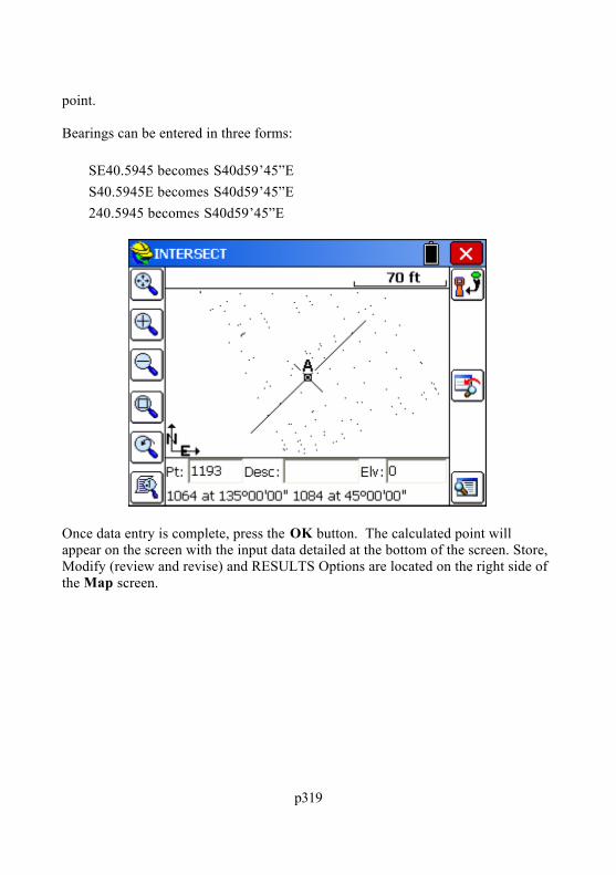
p319

point. Bearings can be entered in three forms:

SE40.5945 becomes S40d59’45”E S40.5945E becomes S40d59’45”E 240.5945 becomes S40d59’45”E

Once data entry is complete, press the OK button. The calculated point willappear on the screen with the input data detailed at the bottom of the screen. Store,Modify (review and revise) and RESULTS Options are located on the right side ofthe Map screen.

p320

Save: Use this icon to save a report of the inverse.

The results screen will display the coordinates of the base points, the inversebearing, the distance from the base points to the calculated INT1 point (and INT2for distance intersections), and the coordinate data for the calculated points. Notethat calculated points are labeled as Int1 and Int2 until the points are stored. TheseOption Buttons are present on all Map screens displayed while in the Intersectionsroutine. Once Store is selected or the Enter key pressed, the stored point willinherit the specified point number, description, and the elevation displayed at thebottom of the screen (optional). There can be only one solution for abearing-bearing intersection.

All Intersect routines handle the 400 circle, if configured to grads/gons within JobSettings, Units.

Bearing-DistanceDefine the Bearing from the first point, then define the known horizontal distancefrom the second point.

p321

Select OK and the map screen will appear showing a circle radiating from thedistance base point and a line from the bearing base point, defined by the enteredbearing. The line is extended to intersect the circle at the two possible solutions.

Pressing Enter or Store will display the prompt "Pick a Solution". To select thepoint, simply pick it from the screen. Picking near the desired solution issufficient. The program will select the nearest solution position. Pressing Enteragain will accept the second possible solution for the intersection.

p322

Distance-DistanceEnter the known horizontal distances from both points.

Select OK, and the map screen will display showing circles radiating from the firstand second selected base points. Lines leading from both base points to the twopossible intersections of the circles are also shown.

p323

Pressing Enter or Store will display the prompt "Pick a Solution". Select thedesired calculated solution. To select the point, simply pick it from the screen. Picking near the desired solution is sufficient. The program will select the nearestsolution position. Pressing Enter again will accept the second possible solutionfor the intersection. If there was no solution for the input data, SurvCE willdisplay "No Valid Solution".

Point ProjectionThis command allows you to calculate the station and offset of any entered orsurveyed point relative to a known centerline or baseline. Note that the StationStore command will calculate a point at a given station and offset. PointProjection does just the reverse — it calculates a station and offset for any givenpoint. It also will calculate the “Intersect”, or the projection of that offset point onthe baseline. This baseline “intersect”, or perpendicular projection point, can bestaked out and stored. The application of the routine is shown below.

p324

The coordinates from which to project can be entered in three ways:

By point number By entering the coordinate values By taking a GPS or total station reading

The station, offset, and vertical difference of the point is then calculated, and the Intersect button (see the above figure) will calculate the projected perpendicularintersect point on the baseline. This Intersect can also be staked out using theStake button.

You must first define the baseline. You can define the baseline by one of thefollowing methods:

Define Line: Select two points to define the line. Define Alignment: Select a predefined centerline file (.cl file), graphically

pick a polyline or enter a sequence of points. Define Arc (3 Points): Select three points on the arc. Define Arc (PC, PT, Value): Select the start and end points of the arc and

enter the radius length.

p325

If you choose two points, you must then define the line in the Point Projectiondialog box as shown below.

With the two points method, you simply enter two point numbers, or choose themfrom the point list or MAP. The azimuth and slope between the two points iscalculated, along with the ending station, based on the entered start station. Withthe Azimuth method, you define the line by entering a first point and then entering

p326

an azimuth and slope. You can confirm the coordinate values of the points bychoosing Confirm NEZ. When the line is defined, choose Continue. You mustnow define, or designate, the point that is offset from the line in the PointDefinition dialog.

You can enter a point ID, select one from the list, or select one from the map. Y oucan also enter coordinates to define a new point, or read values from theinstrument. As soon as enough information is entered, the station, offset andvertical difference is displayed or the message "OFF CENTERLINE" is displayed. This message lets you know that a station/offset cannot be com puted for thecoordinates entered.

Read: This command reads the instrument to gather coordinates for pointprojection.

Intersect: This command will project the coordinates entered perpendicular,back to the centerline and enter these new coordinates into the PointProjection dialog. From there you can store or stakeout the intersect points.

Stake: This command will allow you to stakeout the displayed coordinates(typically used to stakeout the intersect points).

Store: Pressing Store after Read stores the offset coordinate. Store afterIntersect is selected stores the coordinates for the intersect point on thecenterline (perpendicular from the offset point). Store after enteringcoordinates or a point number for the offset point, without selecting Intersect,

p327

will simply store the offset point coordinates again as a new point number. Store is most often used to save the calculated intersect points to thecoordinate file. Pressing Store will save an SP (store point) record in the rawfile, and a note record will indicate that the point was calculated within PointProjection.

Station StoreStation Store is a pure calculation routine that will create points based on a stationand offset from an alignment. The alignment may be defined as a centerline, a3-point arc, an arc defined by a PC, Radius and PT, a selected polyline, or asequence of points. The user may also assign an elevation to the calculated point. Station Store might be used to enter elevations of pipe culverts, for ex ample, whereinlets and outlets are located at distinct stations, offsets, and elevations. Then thetwo calculated points at the inlet and outlet can be used within Stakeout Line tostake any point along the culvert, with the cut/fill calculated. Although thecommand Stake Centerline, found within Stakeout Line/Arc, will directly stakeouta particular station and offset to a centerline, some users prefer to pre-calculate thestation and offset and assign a point ID, then stake by point ID. Station Storepermits this pre-calculation of points at any station and offset.

The very first screen within Station Store offers several methods of defining analignment.

p328

The following screen is where you enter the station, offset, and elevation tocompute and store a point location.

Pressing Enter will move through the dialog and store the point, leaving the screenup for more entries, while defaulting to the previous data and the nex t point ID. The description is fixed as the station and offset, but can be edited using thecommand Keyboard Input.

TransformationThis command allows you to translate, rotate, and/or scale points in the currentjob. Any point drawn on the map screen will be updated automatically in additionto updating the coordinates.

All three transformations can be performed individually or all at once if desired. You first fill out the options in one or more of the tabs (Translate, Rotate andScale), and then you press Enter and obtain a second screen where you fill out therange of points to transform.

p329

Range of Points: Enter the range of points to translate. Ranges can be entered inthe following format: 1-20,32,40-45, etc..Add to Point Numbers: Enter a number to add to existing point numbers whencreating new point numbers. This option is not available when overwriting yourexisting point numbers. Seeexample below under Use New Point Numbers.Overwrite Existing Point Numbers : Overwrites the existing point coordinatedata with the new coordinate data.Use New Point Numbers: Uses new point numbers for the new coordinatepositions while keeping the existing point numbers and coordinate data. Each timea point is to be overwritten, you will be prompted whether to overwrite or use anew point number. This method is only recommended when you are transformingvery few points and wish to give each a specific point number assignment.Store in New CRD File: This option writes the transformed points to a new CRDfile while keeping the existing point numbers and coordinate data. Y ou may alsochoose to input a number for Add to Point Numbers, but this is not required.

TranslateOn the translate dialog, enter in the Delta North, Delta East, and the DeltaElevation. These values represent the change in the original coordinate values andthe desired coordinate values. When complete, select the OK button on the dialog,or navigate to the ROTATE or SCALE Tabs for further data input.

The lower portion of the screen shows an alternate method of defining a translation

p330

by comparing an original point to a destination point. Data entered here, as pointID or directly entered northing, easting and elevation, will lead to computation anddisplay of the delta N, delta E and delta Z in the upper portion of the screen.

When OK is pressed, a second screen appears which controls the range of pointsto be translated.

Assuming you have 55 points in your file, you could "preserve" these 55 points byadding 100 to the point numbers, and saving the transformed points as 101 through155. If you choose Overwrite Existing Point IDs , the Add to Point Numbersoption is not available. If you choose Use New Point Numbers, then you will beprompted to enter a new point number for each existing point to be overwritten(recommended only when you are overwriting a few points). You can even storethe transformed points in a completely new CRD file by selecting Store in NewCRD File.

Raising and Lowering Elevations: Users often ask, "How do I raise or lowerelevations on a range of points?" The answer is the Translate option in theTransformation routine. To adjust elevation only, enter only the delta elevation(leave Northing and Easting at 0 translation).

RotateThe ROTATE tab is used to rotate points in a coordinate file. Enter the desireddegree of rotation into the degree of rotation data field. Specify the rotation base

p331

point. This can be accomplished by either entering the point number of the desiredpoint manually, or by selecting the point using the List or Map icon. You may alsoenter in coordinates for the rotation point if the point is not present in thecoordinate file. Lastly, you can define the rotation by referencing two points (suchas "From 1, To 2"), then specifying the desired new bearing for these points. Eventhe new bearing itself can be computed from two points used as a reference.

The second screen appears, which allows you to set the range of points totransform and choose how to store the newly calculated points. For all rotations,the rotation value is written into the RW5 file as dd.mmss (the current angleformat).

ScaleThe scale tab is used to scale the points in a coordinate file. The northing, easting,and optionally, the elevation, are multiplied by the specified scale factor. Enter thedesired scale factor in the scale factor field. Select the base point by entering thepoint number of the desired point manually, or by selecting the point using the List or Map icon. You may also enter coordinates for the scale base point if the basepoint for scaling is not present in the coordinate file. The coordinate of the basepoint will remain unchanged. All other points will scale. If the Ignore Elevationstoggle is enabled, then only the northing and easting values are scaled. Note thatyou can scale your points from base coordinate 0,0,0 by entering a scale factor andanswering Yes to the warning screen.

Raw Data RecordsThe transformation raw data records are expressed as one string per command withthe values separated by spaces. These records will be recorded to the raw data filefor processing purposes so that all Carlson processors will recognize the recordsand perform the transformation during re-processing.

TRANSLATE: Range Dx Dy Dz Process_Zero_Z ROTATE: Range Angle Base_Y Base_X SCALE: Range Scale Base_Y Base_X Use_Z ALIGN: Range From1 To1 From2 To2

Example:

CC,Translate,8-9 200 50 0 0

CC,Rotate,7 33.1234 79613.662 15619.725

p332

CC,Scale,7 1.5 79613.662 15619.725

CC,Align,8-9 8 6 9 7

CalculatorThis command eliminates the need to carry a separate calculator in the field. Thecalculator can be used to do scientific computations, standard calculations,conversions, triangle calculations, including angles, and curve calculations.

Standard CalculatorMost basic calculations can be performed using this tab in the calculator. Memoryfunctions are also available.

Scientific CalculatorValues can be entered on the X register by typing on the keypad. The values can berolled up and down with the up and down arrow keys and the Roll and RollDbuttons on the screen. The Enter key finishes the entry of a number and pushes thestack. The C on the touch screen clears an entry. Additional functions on the

p333

screen can be obtained through touching the scroll [<] and [>] area of the screen.

Conversion CalculatorConversion values can be entered for various unit types and scenarios. M to Ft: This option provides for conversion between many units. Enter a

value in any field and press Enter to find the conversion value. The followingunits are available in Feet, Meters and International Feet Degrees, Minutes,Seconds and Gons/Grads and Decimal Degrees

p334

Slope Distance to Horizontal Distance: This option allows you to convertslope distances with zenith angles to horizontal distances and verticaldifferences, and vice versa. See figure.

Lat/Lon-SP: This option allows you to convert from Latitude/Longitude togrid system coordinates and vice versa. If you are configured for U.S. State

p335

Plane Coordinates, the routine conveniently displays your zone, and you caneven change zones for quick calculations without altering your G PS zonesettings in Job Settings. Otherwise, the calculation is based on your JobSettings GPS Zone. To solve for northing and easting, fill in the latitude andlongitude and press Solve N/E. To solve for latitude and longitude, fill in thenorthing and easting and press Solve Lat/Long. You can set the state planezone at the bottom of this dialog.

After completing a conversion, you may enter a point ID and press Save tosave the coordinates to the current job. You can also change the type oftransformation or zone system used. If you don ’t want NAD 83 (primarilyused in the U.S.) you can go to Job Settings , GPS and change theTransformation type. For example, you could change the Transformation toUTM or NTF-France. Then, back in Calculator, your coordinate to Lat/Longcalculation would be based on the configured transformation. Note that whenconverting Grid System Coordinates to WGS84 coordinates and goingWGS84 to Grid, the geoid separate file (if any) is applied to the calculation.

Az-Br: This does a straight, simple calculation converting azimuths tobearings. A prime example, shown below, would be converting an azimuth of119.2547.

p336

Other CalculationsThere are two types of calculations that can be performed from the OTHER tab. Click the large, square icons to go to the Triangle or Curve calculator.

Triangle Calculator

p337

The figure below shows the Triangle calculator. The top of the dialog boxindicates the mode of calculation. To change the mode, simply use the pull-downand to selec the desired mode.

Side-Side-Side Angle-Side-Angle Side-Angle-Angle Side-Angle-Side Side-Side-Angle

After choosing a mode, simply apply the values to the appropriate blank and hit Solve. Points from your current job can be selected to fill out the blanks as well.The points can be selected from the screen or from the point list by picking theappropriate button icon. After the calculations have been performed, you will seethe Clear, Results, and View Triangle buttons. Clear will clear the entry fields.Results will show the results dialog again. View Triangle will draw the triangleon the screen connecting the points chosen for the calculation. The trianglecalculator, using 3 points, is a convenient way to calculate the interior anglebetween 3 points. For example, if you were setup on 1, backsighting 10, andturned a 90 degree angle to 21, then the triangle defined by 10 to 1 to 21 wouldindicate a 90 degree angle at point 1.

p338

Curve CalculatorThe figure below shows the Curve calculator. Simply use the pull-down at theupper left to select the desired method of curve calculation.

Radius-Delta Angle Radius-Chord Length Radius-Arc Length Deg. of Crv.-Delta Angle Deg. of Crv.-Chord Length Deg. of Crv.-Arc Length Delta Angle-Chord Length Delta Angle-Arc Length Chord Length-Arc Length

p339

The type of curve can be toggled between roadway and railroad. Values can beentered into the blanks by keyboard entry, by selecting points from the current job,from a point list, from the screen, or by selecting an arc drawn on the screen. Oncethe values are entered, the results are displayed on the screen. The results can beviewed by selecting the Results button. The curve can be viewed on the screen byselecting the View Curve button.

Manual TraverseThis command allows for manual entry of angles and distances, and calculatessideshots or traverses from a known occupied point. If the direction is defined bya bearing or azimuth, a backsight point is not required. If the direction is definedby angle left or right or a deflection angle left or right, then a backsight point isrequired.

Manual Traverse is actually one of three options for manual traverse and sideshotentry. A second option is to go to the Map screen, and at the command line(Cmd:) enter "I" for inverse, to inverse to an occupied point, or from backsightpoint to occupied point, then "T" for traverse or "S" for Sideshot, using anglecodes 1-NE, 2-SE, 3-SW, 4-NW, 5-AZ, 6-AL, 7-AR following the prompting forangle and distance entry. This style works strictly off the keyboard and does notrequire any screen tapping to switch from traverse to sideshot to inverse. Thepoints plot on the screen as you go. A third option for traverse and sideshot entry

p340

is to set the equipment type to Manual Total Station, and enter the traverse andsideshot data within the Store Points command. All three of the methods willstore data to the raw survey file for re-processing, and will allow entry ofinstrument heights and target heights. In the Map screen, Traverse Defaults (TD)will turn instrument and target height prompting on and off. All three methodsallow for zenith angle prompting as an option.

The command centers around one main entry screen. You must enter an occupiedpoint for traversing. You must also enter a target point number to calculate.

Horizontal Angle: You must select a horizontal angle method. Options hereare AR (angle right), NE, SE, SW, NW, AZ, SAZ (south azimuth), AL (angleleft), deflection left, and deflection right. If a bearing or azimuth is selectedfor traversing, the backsight point number will become inactive. Only anoccupied point is required to traverse forward by bearing or azimuth. Allother turned-angle methods will require a backsight point number. The storeddescriptions for the occupied point and backsight point will display as shownabove (TRV MAG and TRV N in this case). Occupied points and backsightpoints can be selected from the list or the map using the appropriate icons. You can also enter point-defined angles, as in 6,7 for the direction from 6 to 7,or 6,7+90 for 90 degrees to the right of the direction of 6 to 7.

Elevation/Vertical Angle Method : There are many ways to calculate avertical differential between the occupied point and target point. The mostcommon method is zenith angle (ZE). Manual Traverse also offers vertical

p341

angle, delta Z (elevation difference), slope by percent (SP), slope by ratio(SR), and known elevation (Z). To get the slope from point 6 to point 7,switch to SP mode and enter 6,7 for the slope.

Distance Method: There are four methods of distance entry: HorizontalDistance (in which case the elevation line is inactive), Slope Distance; SlopeDistance, No Elevation; and Horizontal Distance, No Elevation. . BothSlope Distance methods will prompt for vertical angle/zenith angle, etc., butSlope Distance, No Elevation will calculate a zero-elevation for the targetpoint number and will reduce the slope distance by the effect of the verticalangle/zenith angle. You can also enter the distance in the form of 6,7 for thedistance from 6 to 7, or as 6,7/2 as half the distance from 6 to 7. Note that ifyou wanted to interpolate a point 12 midway between 6 and 7, you can use all3 edit boxes to accomplish this. The azimuth or bearing could be entered as6,7. The slope would be entered as 6,7, and the distance would be entered as6,7/2. So if point 6 is elevation 100 and point 7 is elevation 101, point 12 willhave elevation 100.5.

Enter Elevation: If Enter Elevation is enabled, a check screen is activatedto display the calculated elevation. From here you can override the calculatedelevation with a new elevation. This option is useful in combination withHorizontal Distance for calculating points at a known distance and fix edelevation.

TR Mode: Enabling Traverse Mode will cause the routine to “traverse up”

p342

to the target point number, so that the new occupied point number willautomatically change to the last target point number, and the new backsightwill change to the last occupied point. You can always manually change thefields for occupied point and backsight point and “force” a traverse, butenabling Traverse Mode will update these fields automatically, so that youimmediately “move up”, and are awaiting the next angle and distance entries. With TR Mode disabled, Manual Traverse defaults to sideshot mode.

When you are entering in the horizontal angle, distance, or elevation/vertical angleinformation, the program displays the current mode as an extra confirmation at thebottom of the screen. Hitting Enter from the last entry line, or tapping Calculate,or entering a C for calculate, will solve for the coordinates and display them at thebottom of the screen. Hitting Enter again, tapping Store, or entering S will storethe points. Before storing, you can also tap the Map icon to see the location of thecalculated point, in reference to the occupied point and backsight point.

Click Back to return. You always have the option to enter new angle and distanceinformation, Calculate, check the Map, then Store, as desired. Point in Directionoffers the flexibility to check point locations graphically prior to storing.

El/Off: If El/Off is clicked on for Elevation mode, a “check screen” isactivated that allows you to see the calculated elevation and potentiallyoverride it with a new elevation. This option is useful in combination with

p343

Horizontal Distance for calculating points at a known distance and fixedelevation. This screen also allows you to offset the point perpendicular to thecomputed traverse leg. Enter positive for right and negative for left.

p344

ROADThis chapter provides information on using the commands from the Road menu.

Centerline EditorThis command allows you to enter new centerlines, as well as recall and editexisting centerline files. Centerline files in SurvCE are ASCII files with a .CLextension. When the routine is selected, a dialog will appear in which you canload existing centerlines or begin entry of new centerline information.

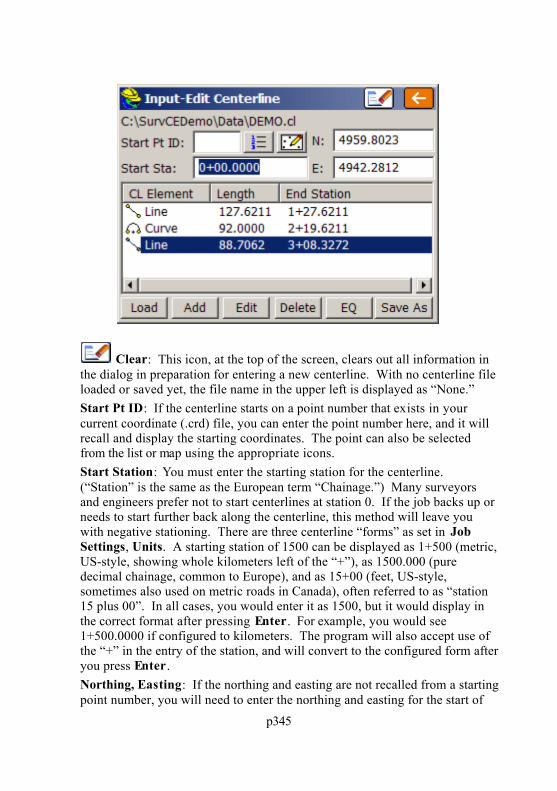
p345

Clear: This icon, at the top of the screen, clears out all information inthe dialog in preparation for entering a new centerline. With no centerline fileloaded or saved yet, the file name in the upper left is displayed as “None.”

Start Pt ID: If the centerline starts on a point number that exists in yourcurrent coordinate (.crd) file, you can enter the point number here, and it willrecall and display the starting coordinates. The point can also be selectedfrom the list or map using the appropriate icons.

Start Station: You must enter the starting station for the centerline.(“Station” is the same as the European term “Chainage.”) Many surveyorsand engineers prefer not to start centerlines at station 0. If the job backs up orneeds to start further back along the centerline, this method will leave youwith negative stationing. There are three centerline “forms” as set in JobSettings, Units. A starting station of 1500 can be displayed as 1+500 (metric,US-style, showing whole kilometers left of the “+”), as 1500.000 (puredecimal chainage, common to Europe), and as 15+00 (feet, US-style,sometimes also used on metric roads in Canada), often referred to as “station15 plus 00”. In all cases, you would enter it as 1500, but it would display inthe correct format after pressing Enter. For example, you would see1+500.0000 if configured to kilometers. The program will also accept use ofthe “+” in the entry of the station, and will convert to the configured form afteryou press Enter.

Northing, Easting: If the northing and easting are not recalled from a startingpoint number, you will need to enter the northing and easting for the start of

p346

the centerline. It is not necessary to enter the northing and easting if you usethe Pick PL (pick polyline) option for defining a centerline, since the startingcoordinates of the selected polyline are automatically used, and wouldoverwrite anything previously entered.

Load: This command allows you to load an existing centerline for review oredit.

Edit: Use this button to edit the highlighted element. Delete: Use this button to remove the highlighted element. Add: Returning to the starting dialog, you can add elements to get a

centerline started. Typically, you will start with a line or tangent segment, butyou can also start on a curve or spiral curve element. When you select Add,you get to choose which element to use. These options include:

Add (Line): A tangent section of the alignment. This option allows you toenter a point ID or coordinates to define the end of the tangent, or enter thestation, or distance and the direction. To force the element to be tangent to theprevious element, toggle on the Tangential to the previous elem option. Thiswill gray out the direction field and will compute the tangent direction andenter it for you.

p347

Add (Curve): A typical circular curve section of the alignment. The firstelement of the curve defines what the options for the second element can be(See Lists Below). The RR toggle allows the user to use Railroad definitions.The Review button allows you to verify the Tangent In and Tangent Outbearings or azimuths (depending on Job Settings, Format, Angle Displaysettings), as well as confirm PC and PT coordinates. For ex ample, this allowsyou to verify computed Tangent Out bearings against paper plans, beforecontinuing entry of new elements.

p348

Add (Spiral-Curve-Spiral): The Spiral-Curve-Spiral element is really justtwo implementations of Spiral Only (line-spiral-curve and curve-spiral-line). The advantage of Spiral-Curve-Spiral is that it completes three elements at

p349

once and is a fairly common application on high-speed highways. This routinealso allows the user to define the spiral-curve-spiral using known points aslong as the spiral in and spiral out lengths are entered first.

Add (Spiral Only): The Spiral Only element will handle a spiral between anyline and arc segment (e.g. line-spiral-arc or arc-spiral-arc).

p350

Pick PL: This option is only visible if you Clear the dialog. With this option,you can pick a centerline from any screen polyline, including polylines witharcs. When you choose Pick PL, you are immediately presented with thegraphic screen, where you can pan by dragging your finger across the screen,or zoom using the many zoom options. You can choose not to select apolyline (maybe there were none to select!) by pressing OK or Enter. Whenyou select a polyline, it will highlight as a darkened polyline. After selecting apolyline and pressing OK or Enter you will see the polyline elements. Notethat if you change the start station to 500, all the stationing for the polylineelements will change accordingly. This is also true regarding the startingnorthing and easting. If these are changed, all element coordinates willchange accordingly, as can be verified using the Edit option.

p351

EQ: The EQ button allows you to enter station equations.

Save As: This saves the file. Enter a name.

Note : You can create new points with Input-Edit Centerline. When youenter and save a centerline, it will prompt “Do you want to save

p352

centerline points?” You may answer Yes and save point IDs for the start,end, PI, PC, radius point, PT and any key spiral points found in the file. In the same way, a centerline that you load can be re-saved with newcoordinate IDs assigned to all key points, as long as you make somechange, like adding a point number to one of the Pt ID fields for a CLElement. If you answer Yes to Save Centerline Points, the dialog boxbelow appears. If you have entered point IDs of your own choosing in theInput-Edit dialogs, use the upper option. The lower option willauto-number from the starting point ID without regard to any numbersyou’ve entered, but will respect and not overwrite used points in the file.Points are not stored to the centerline file itself, so after loading a storedcenterline, no point IDs will appear.

Draw CenterlineDraw Centerline will draw the selected centerline on the screen. All the zoomingcommands [Zoom In, Zoom Out, Zoom Window, Zoom Previous and Pan] areavailable to you in the Draw Centerline command. The program willautomatically zoom to the extent of the centerline when drawn. If there are pointnumbers and polylines on the screen in that area, they will appear as well. This

p353

command only temporarily displays the centerline for reference and does not drawit on the screen as part of the dxf file associated with the job. To actually draw thecenterline as a permanent feature (unless erased later), use Map (globe icon),Tools, Centerline, CL to Polyline .

Profile EditorThis routine allows field entry of vertical alignment files for roads, sewers andother types of alignments. Vertical alignments can also be loaded and edited. Inaddition, high and low points can be calculated and the elevations of individualstations can be calculated. Vertical alignments are stored as files with a .PROextension. Vertical alignments are typically referred to as profiles. In CarlsonSurvCE, the station ranges of the profile and centerline do not need to match. Aslong as they have station ranges in common, any profile can be used with anycenterline for all advanced Roading commands as well as Survey menu routinessuch as Offset Stakeout and Elevation Difference by Road Design files.

Profile EntryProfiles are extremely easy to enter. When the command is selected, if no priorprofile has been entered, you will encounter the blank Input-Edit Profile dialog. You can also obtain a blank screen and start a new profile by tapping the Clearicon (eraser) at the top of the screen.

p354

PVI Station: PVI stands for Point of Vertical Intersection, similar to a PI(Point of Intersection) for the horizontal alignment. In some locations, theterm VPI is used (Vertical Point of Intersection). You can start immediatelyby typing in the starting station under the PVI column. For our highwayexample, the starting station is 10078.69.

PVI Elevation: The starting elevation is 526.49. So simply press Enter andmove from the PVI column to the PVI Elev. column and enter 526.49. Pressing Enter again moves onto the next PVI field, where you can enter10600 for the next station, then 529.10 for the next PVI elevation.

Slope %: Once a second station and elevation are entered, the program willcalculate the percent slope. Alternately, if you enter under the Slope % beforeentering the PVI elevation, then the program will calculate the PV I elevation. The slope column is a nice check against bad entries in the PV I elevationcolumn. In other words, you often expect even slopes, and you can check thecomputed slopes against the plans. Slopes can be entered as ratios when thatoption is clicked, and if you click "Show Zeroes", the dialog will show aconsistent number of decimals (typically 4) in all columns, causing the dataand decimal places to line up vertically.

VC Lng: For road jobs, you can enter the vertical curve length in thiscolumn. This is the total length of the vertical curve. If the length entered is600, this means that the vertical alignment transitions through a curve(parabola) beginning 300 units (feet or meters) before the PV I and ending 300

p355

units after the PVI. If a vertical curve is uneven, that is, it transitions from,say, 400 feet before the PVI to 200 feet after the PVI, then the curve must beentered using the form 400-200 (the before and after distances separated by adash). SurvCE assumes all vertical curves are parabolas (U.S. road industrystandard). However, you can tap the circular curve option when that applies. For sewer and water line alignments, there is typically no vertical curvetransition, so this column can be left blank, or 0s can be entered for verticalcurve lengths.

Check Station: When the profile for a highway job has been entered in adialog, you can also enter a value to Check Stations. This feature is at thebottom of the dialog. This will check the grades at any desired station. Whenentering stations, you may include the “+” that is often used, as in 12+680.5(English) and 126+80.5 (metric).

Load: The Load command presents a list of all previously stored profiles.When one is selected, it displays the profile information in the dialog. To loada stored file, you simply enter the name (for ex ample, "Demo"). No fileextension is necessary. Alternatively, you can select a name from the list andaccept it by pressing OK or Enter.

Add: The Add button will create a new row at the curser position with 0entries (with the exception of slope, which will compute based on the 0entries). If, for example, you touch line 1 (to move the blinking cursor to line1--the first row), the Add command will allow you to insert a new row in thefront of your profile. This would be necessary if you needed to start theprofile at an earlier station. To add to the end of your profile, just click thedown arrow key at the right until a blank line becomes available and makeyour new entries.

Remove: This button deletes the current line. High-Low: This button can be used to calculate high and low points.

p356

Save As: This command will save your profile to a specified file name.There is no need to enter a file extension. If you want to save the file asBaker.pro, just enter "Baker". The Save As command will default to thecurrent profile name. If you are entering a new profile, it will default to thecurrent coordinate file name.

Draw ProfileThe Draw Profile command will draw the selected profile on the screen. Theprofile will be exaggerated (typically 10:1 or 20:1) in order to maximize detail. You can control the vertical exaggeration by selecting the vertical scale icon,located at the lower left of the Draw Profile screen. All the zooming commands[Zoom In, Zoom Out, Zoom Window, Zoom Previous and Pan] are available toyou in the Draw Profile command.

p357

If you want to change the display scale, click the icon in the lower left corner. Thedialog shown below will appear. Change the scale and tap OK.

Template EditorTemplates for roads, levees, ditches and other earthwork can be created in CarlsonSoftware products such as Carlson Civil or Carlson Roads, or alternately they canbe entered in the field using Input/Edit Template. These templates can then beused in Carlson SurvCE in the Stake Slope command, where the template is one ofthe design files for slope staking, along with the centerline and the profile. Templates are also used in Stake Road (for staking those portions of the road

p358

from left shoulder to right shoulder) and for Elevation Difference by Road DesignFiles. Templates can be reviewed graphically using the command Draw Template. Templates are not necessary for the command Stake Offset, found on theSURVEY tab. In Offset Stakeout, road or other cross slopes from centerline areentered within the command itself.

Currently, SurvCE uses only templates created in Carlson Civil and Carlson Roadsor entered directly within SurvCE using the command Template Editor. Everypoint on a template has an ID such as “EP” and “SH” or “CB1”. Templates inSurvCE have only one surface—the surface you are staking. To stake out asubgrade, you could enter the surface grade information, then use a vertical offsetin Stake Road or enter the subgrade surface directly as a template.

After selecting Template Editor, you are presented immediately with the inputdialog shown in the figure below. If an existing template is loaded (based on thelast template used), you can clear the screen by clicking the clear icon (eraser) inthe upper right.

Template grades are entered top to bottom, and ex tend out from the middleposition of the template. If you are dealing with a symmetrical template, keep the Right Side Same as Left option enabled. This will reduce entries by half.Otherwise, you must select the appropriate side and use Add to add entries, orEdit to revise. One trick, if you have non-symmetrical grades, is to keep RightSide Same as Left on and enter the symmetrical portion (perhaps the pavement

p359

lanes and first shoulder lane), then when you get to the outside shoulder or otherlane where one side is different than the other, disable Right Side Same as Leftand complete the non-symmetrical portion of the template. With the Right SideSame as Left turned off, you can click the words Left SURFACE or RightSURFACE and the left or right columns become active for editing. Alternatively,you may simply click into the items in the columns and edit or add.

In the curb-and-gutter template shown below, the Add option is used to enter thegrade breaks from centerline out to the back of shoulder.

Since templates used in Slope Staking help define all grades into the centerlinefrom the slope stake, it makes sense to focus on the subgrades that are built by thedozer, motor grader or trimmer. Thus, despite all the surface grades involved,there are only three distinct grades in this example curb and gutter templatebetween centerline and the pivot point of the cut and fill slopes: 12.00 at -2%(subgrade at back of curb), 0.01 horizontal and 1 vertical, and 8.00 at 4%. For the Vertical method, some positive horizontal distances must be entered, such as 0.01or 0.001. By pressing Add in the dialog, we can enter the first two grades.

p360

Downhill slopes, going out from the middle of the template, are entered asnegatives. Note that it is necessary to enter an ID for each break point in thetemplate. This helps identify the description of the grade on the progressive slopestake report (e.g. from the outside going in, 8 ’ at -4% to TC, 0.01’ at -1 vertical toEP, 12’ at 2% to CL). The shoulder slope going out (8 ’ at 4%) is enteredsimilarly, as above. The Input-Edit Template dialog now appears.

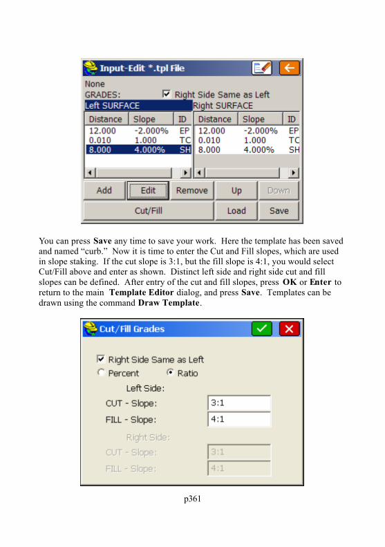
p361

You can press Save any time to save your work. Here the template has been savedand named “curb.” Now it is time to enter the Cut and Fill slopes, which are usedin slope staking. If the cut slope is 3:1, but the fill slope is 4:1, you would selectCut/Fill above and enter as shown. Distinct left side and right side cut and fillslopes can be defined. After entry of the cut and fill slopes, press OK or Enter toreturn to the main Template Editor dialog, and press Save. Templates can bedrawn using the command Draw Template.

p362

For highway projects or subdivision roads with cut slopes down to a ditch line,four template definitions may be necessary for slope staking: (1) Cut Left, FillRight, (2) Cut Left, Cut Right, (3) Fill Left, Cut Right, (4) Fill Left, Fill Right. The appropriate template can then be used for any condition. Shown below is theCut Left, Fill Right for a 2-slope (pavement and shoulder) road. The last slope ineach column acts as the "pivot point" for the slope stake calculation. The fill slopeis set at 4:1 and the cut slope at 3:1.

p363

Using this template, cut slopes on the left side of the road will find the pivot at thebase of ditch, while fill slopes on the right side of the road will pivot from the edgeof shoulder.

Draw Template

p364

The Draw Template command will draw the selected template on the screen. Allthe zooming commands [Zoom In, Zoom Out, Zoom Window, Zoom Previous andPan] are available to you in the Draw Template command. Tap the Menu button toexit this command. The figure below illustrates this command using the “demo.tpl”template.

UtilitiesRoad Utilities includes necessary routines to convert centerlines, profiles andcross sections from other formats to the formats used by SurvCE. SurvCE usesASCII file formats for centerlines (“.cl” files), profiles (“.pro” files) and crosssections (“.sct” files). These same formats are used by other Carlson products suchas Carlson Civil (formerly SurvCADD), Carlson Survey, and Carlson Roads.

Road Utilities will also scale up or down centerlines and profiles, usually toconvert between metric and English units. In addition, Road Utilities includes acommand for entering a superelevation file (“.sup”). This file can serve as anoptional input file and react with templates in commands such as Stake Road,Slope Staking and Elevation Difference . Finally, Road Utilities has an option fora Template Series file (".tsf" file). This file will transition from one template toanother automatically, as long as the templates share identical IDs. The TemplateSeries file can be substituted for a standard template file in Slope Staking and

p365

Stake Road, wherever design files are applied.

File Conversion and LandXML: The LandXML file format is quickly becomingan encouraged standard of many departments of transportation (DOTs). Thisstandard is also recommended by Autodesk, Microstation., and several othersoftware companies such as Carlson and G eopak. LandXML files have an “.xml”extension and may contain various road design files including centerlines, profiles,and cross sections. The “header” lines within the “.x ml” file will indicate whatdesign files are included. In some cases, several files of the same type, such asthree or four centerlines or profiles, may appear in the same LandXML file. Asmore and more software companies offer LandXML file output, this file type maybecome the preferred form of data exchange. Be aware that each company tends toimplement the LandXML format in slightly different ways, much like DXF filesfor drawing data exchange were sometimes slightly different in format betweenAutodesk and Microstation, or from release to release. Therefore, if a LandXMLfile containing centerlines, profiles or cross section files fails to convert, it isrecommended that the file be emailed to Carlson Software so changes can be madein SurvCE to enable conversion. LandXML is an evolving format that is likely tosolidify in the near future.

Centerline ConversionThis command converts horizontal alignment files to and from the Carlsoncenterline format (*.CL). Supported file types include:

p366

ASCII Inroads (.ASC) ASCII LDD (.TXT) CLIP (.PLA) Geopak (.OSD) ISPOL (.ALI) LandXML (.XML) Leica (.GSI) MOSS (.INP) SDMS (.ALI) SDR (.SDR) TDS (.RD5) Terramodel/Geodimeter (.RLN, .ALN and .ARE formats )

The SurvCE format has a “.CL” extension. These source files can be loaded intoSurvCE using Data Transfer, located in the File menu options. When performingthe conversion, and selecting a particular format, SurvCE automatically looks forthe corresponding file extension.

Report Icon for LandXML Files : If you are importing a LandXML filespecifically, you can click the Report icon left of the "Return" icon in the upperright of the dialog, and review the source of the data as shown:

p367

Conversion: Clicking Existing File in the upper right (in the Land XML section)will load the file, and clicking Select New under the CL File section will save thecenterline file in the correct format for use in SurvCE. To convert in the oppositedirection, select Existing File under the CL section to recall a SurvCE centerlinefile, and then click New File in the upper left (under LandXML file) to save itback to a LandXML file, for use in other software.

For file types in which both Import and Export options are available, theconversion procedure forms a “criss-cross”: You bring the files into SurvCE bygoing upper right (“Existing”) to lower left (“Select New”). You send the filesback to the “non-SurvCE” format by going lower right (“Select Existing”) to upperleft “New”.

When the files have been selected, the appropriate action is highlighted below,"Import to CL" or "Export to <type>". When the process is completed, theprogram announces “Process Done,” and you are free to move on to the nex tcommand. Most formats only convert to SurvCE and not back again, and thereforeonly have “one-way” dialogs. These include ASCII-Inroads, ASCII-LDD,Geopak, Moss, TDS and Terramodel/Geodimeter.

Importing TDS RD5 FilesImporting TDS RD5 Files: If TDS is selected, centerlines can be convertedone-way to SurvCE centerlines (centerline files CANNOT be converted back toTDS files). It is important to note that the TDS RD5 file is a dual centerline andprofile file. Because the TDS RD5 file does not display the starting station, anextra dialog will appear requesting starting coordinates (which can be recalled

p368

from a point) and a starting station.

Verify the ConversionIt is recommended that after converting centerlines, profiles or cross section filesto SurvCE format, you go to the Editor and Draw options for these file types andreview the data to verify that the correct file was converted and that the conversionwas successful. So, for example, after converting a centerline from Inroads formatto SurvCE “.cl” format, go directly to Centerline Editor in the Roads menu andverify the data.

Recognizing File FormatsFor reference, portions of four of the file types are shown below, as they mightdisplay in a Text Editor. The LandXML, SurvCE and SDR examples all referencethe file DOT1.CL. These displays may help you recognize these file types in thefuture. The new LandXML format, endorsed by many Departments ofTransportation in the United States, may soon become the standard in the futurefor internet transfer of roading and other types of design files.

p369

p370

Centerline TransformationThis routine is designed primarily to convert centerline data from Metric to SurveyFeet or from Survey Feet to Metric. The image below shows the dialog and scalefactor when converting from Metric to Survey Feet.

Apply scale factor for start station: If this option is enabled then the startingstation will be converted using the scale factor. For example, a start station of1000 would become 3280.833. If disabled, the start s tation would remain at 1000. If the goal is to change the starting station by a certain amount unrelated to thescale factor, then you must use Input-Edit Centerline and enter a new start stationin the initial dialog. This will automatically translate all stations in the centerlineby the appropriate amount.

When Apply Scale Factor for start station is enabled, the centerline is adjustedby the scale factor, after a confirming warning screen.

Profile ConversionThis command converts vertical alignments to and from the Carlson profile format(*.PRO). Supported file types include: ASCII-LDD (.TXT) Caice (.KCP) CLIP (.ALZ)

p371

ISPOL (.RAS) LandXML (.XML) Leica (.GSI) MOSS (.INP) SDR (.SDR) TDS (.RD5) Terramodel/Geodimeter (.RLN, .ALN and .ARE)

The SurvCE format has a .PRO extension. These source files can be loaded intoSurvCE using the Data Transfer feature in the FILE tab. The conversion screenis similar to Centerline Conversion, with the characteristic “criss-cross” logic for2-way conversion (LandXML and Leica) and one-way conversion for the otheroptions.

The SurvCE Profile File Format: It should be noted that of all the SurvCE filetypes that are ASCII and therefore viewable in standard text editors, the profile(.pro) file has the simplest format. The format is station, elevation, length ofvertical curve, and description for road profiles. For ex ample, the Demo.pro filethat is typically provided with the software has the following four lines (which canbe viewed in Notepad):

0.0000, 997.0000 , 0.0000,

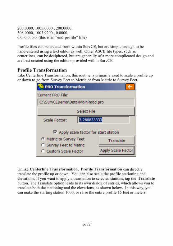
p372

200.0000, 1005.0000 , 200.0000, 308.0000, 1003.9200 , 0.0000, 0.0, 0.0, 0.0 (this is an “end-profile” line)

Profile files can be created from within SurvCE, but are simple enough to behand-entered using a text editor as well. Other ASCII file types, such ascenterlines, can be deciphered, but are generally of a more complicated design andare best created using the editors provided within SurvCE.

Profile TransformationLike Centerline Transformation, this routine is primarily used to scale a profile upor down to go from Survey Feet to Metric or from Metric to Survey Feet.

Unlike Centerline Transformation, Profile Transformation can directlytranslate the profile up or down. You can also scale the profile stationing andelevations. If you want to apply a translation to selected stations, tap the Translatebutton. The Translate option leads to its own dialog of entries, which allows you totranslate both the stationing and the elevations, as shown below. In this way, youcan make the starting station 1000, or raise the entire profile 15 feet or meters.

p373

By default, the entire range of stations is selected. If you wish to only translate arange, highlight the beginning station, then click End Station and highlight theend station. Next enter the amount to translate in the Change Station box. Youmay also translate the elevation using the Change Elevation box. Tap OK whenyou are finished.

Section File ConversionThis command converts section files to and from the Carlson section file format(*.SCT). Supported file types include: Caice (.FFF) CLIP (.TRV) Geopak (.XRS, .XSR, .SOE & .TXT) IGRDS (.LIS, .RDS & .TXT) ISPOL (.SC1 & .RAS) LandXML (.XML) Columnar Text (.TXT, CSV & .ASC) Terramodel/Geodimeter (.XSC)

The SurvCE format is “.SCT”. Section files are used for Stake Slope, StakeRoad and Elevation Difference . Cross Section Survey also has the ability tooutput section files. TDS will store cross sections in an RD5 format that behave as

p374

a series of templates, following "rules" for slopes coming from the design profilegrade. You can import TDS-style cross sections using Input-Edit TemplateSeries within Road Utilities, and for "Files of Type", select TDS.

Note that if you select XML Info at the top of the screen, you’ll see some of the“header” information associated with the XML file to be exported or imported.

To export to LandXML, you need to load a LandXML file that already contains acenterline covering all or part of the station range in the SCT cross section file. Otherwise, you will see an error message.

p375

Despite the message, you can add the horizontal alignment portion to theLandXML file after creating the file with sections only. However, if you firstcreate a LandXML file containing one or more alignments, then choose thatexisting LandXML file to export to, you can select among those centerlinealignments when making the cross section file.

Section files in SurvCE can contain descriptions useful for reference in otherroutines such as Stake Road. If descriptions are found in the source section file,they will be captured by the import process into the “.sct” file for use in SurvCE.

Input-Edit Section FileThis routine is a convenient cross section editor. It can be used for entering new

p376

sets of cross sections or for editing and reviewing an ex isting set of cross sections. One nice application is Slope Staking. If you know the left and right “pivotpoints” on stations to be slope staked, you can enter very sim ple, two-point crosssections consisting of the left pivot offset and elevation, and the right pivot offsetand elevation. Then, without taking a cheat sheet into the field, you can slopestake by cross section method, and the program will seek these pivot points, andeven interpolate the correct pivot points between entered cross sections.

A better approach would be to include all break points in the sections from pivotleft to pivot right, along with descriptions. Then Slope Staking will report theprogressive information to grade each point from the catch all the way intocenterline. This “section-based slope staking” is a cross between user-defined(where you need the cheat-sheet!) and design files, where the pivot offsets andelevations are taken from the pivot points in the template as they react with theprofile and superelevation files. Sections used in Stake Road should be completecross section files, with all offsets, to enable precise, interpolated stakeout withinthe left-to-right range of the sections, on station, or at interpolated stations.

The Input-Edit Section File routine begins by prompting for a cross section filename. If you wish to start a new cross section file, just enter a new name.

If you choose to select an existing cross section file, such as DEMO.sct, afterselecting the file, you will see the “Section List” dialog.

p377

From this dialog, you can Add stations, Edit existing stations, Remove stations,Load entire new cross section files, Save As (to save your changes to the currentloaded file or to a new cross section file), and Clear the list of stations (notrecommended unless you want to start from scratch). Select Edit to review astation.

In this dialog, you can Add , Edit , Remove , Rearrange , or Clear existing offsets

p378

and elevations. Note that cross section offsets are negative for left of centerline andpositive for right of centerline, and can have descriptions such as SH, EOP, CL,Ditch, 21, 22, 23, etc. These descriptions, where they exist, are potentially usefulfor description-based interpolation between stations, as applied in Stake Road . Ifyou want to add an offset at -42.867 called RP, click Add . You don ’t have tohighlight the correct offset to add above — the software will sort and place thenew entry appropriately.

When you click OK , your new entry will be in the list.

The Edit box leads to the same entry dialog as Add. Remove will provide awarning and then delete the highlighted offset and elevation. Up and Down shouldnot be used unless a file conversion led to out-of-order listing of offsets andelevations. When you click OK from the station edit dialog, you can save therevised cross section file back in the section list dialog.

Input-Edit SuperelevationRoads can contain one or more curves, and each curve can have its ownsuperelevation data. This data includes start station for super transition, stationfor full super, percent of full super, station for end full super, and station forending the super transition back to normal crown. In SurvCE, each superelevationdata set for each curve would be entered as a “line” of superelevation data in the“.sup” file.

p379

If we had two curves, both with superelevation, then we would do two Adds usingthis dialog. Let’s say, for simplicity, that we have a road with a 2% “normalcrown” which has one curve to the left followed by one curve to the right, with thefollowing information:

Curve 1 Curve 2

Start Super Pivot Sta: 100 Sta: 2200Full Super Sta: 600 Sta: 2500Full Super %: 3% Left 4% RightEnd Super: Sta: 1400 Sta: 3500End Super Pivot: Sta: 1900 Sta: 3800

The first curve to the left goes through three stages as it pivots into full super: (1) the right side pivots to “flat”, (2) the right side pivots to “reverse crown”, wherethe slope is the same across the template and (3) both the right and left sides pivotfrom the hinge point (centerline) into full super. All of these key pivot points areentered in the superelevation dialog.

p380

You enter all these key stations (begin, flat outside lane, reverse crown, full super)both going up to full super and transitioning back down to normal crown. Recognizing that the normal crown of -2% transitions from station 100 through aslope of 5%, the transition is 1% per 100 feet, assuming an even rate of transition. Therefore, a “flat” outside slope occurs at station 300, reverse crown at station 500and full super at station 600, as shown. You will need to compute these stations inadvance. These intermediate stations are entered in the superelevation dialog toallow for different rates of transition from normal crown to flat to reverse crown tofull super. Normally, the rates of transition are consistent. Note that super left orright is always entered as a positive percent slope — the road centerline curvedirection will control the direction of pivot. You are now ready to click Add andenter in Curve 1.

p381

When you click OK, the first line of the superelevation dialog is filled in. Curve 1is complete. Next, we enter Curve 2 as follows, using similar logic.

When OK is clicked, the two curves are complete and the summary dialogappears. There is one line (or row) for each curve.

Note: If any of the columns are too narrow to display all the text, you can

p382

“grip” the vertical line separating columns, much like in programs such asExcel, and make the column wider.

The superelevation file is one of the optional “roading” or “design” files in StakeSlope, Stake Road and Elevation Difference . After a superelevation file hasbeen entered and saved, it will appear as the default superelevation file in all ofthese commands, unless removed from the design file list by the user.

Input-Edit Template SeriesSurvCE allows for two types of transitioning: (1) a single template can transitionby being “acted upon” by template transition files (made in Carlson Roads,Topsite, Leica Site Manager or Carlson Civil) and superelevation files, or (2) atemplate series file can transition between several templates sharing identical IDs,but having different slopes and widths between ID points within the templates.

You can load an existing TDS template series file, in the RD5 format, by clickingLoad, then clicking the down arrow for Type of File, and selecting TDS format. TDS templates always have IDs and the same number of template points per crosssection, so once imported, they behave exactly like SurvCE-defined templates. Using the Draw Template option, any particular template in a template series filecan be selected and displayed as shown:

p383

The Template Series approach can even be used to transition from normal crownto superelevation, avoiding the need to use superelevation files. The TemplateSeries approach is commonly used to expand the width of a lane to accommodate,for example, a passing lane. Since template IDs must match, if a “special slope”lane “appears” for a certain station range, then the Template Series approach canstill be used as long as you add the ex tra ID point (e.g. EP2) to the normaltemplate, perhaps making that point 0.001 units in dimension initially. In thesecond, transitional template, the EP2 lane can have the full width of 3.5 meters or12 feet or whatever applies. If the transition starts at station 500 and ends atstation 600, EP2, will be 1.75 meters or 6 feet or exactly half the full dimension atstation 550.

Starting with the demo.tpl file, with a 10’ lane to ID “EP” followed by a 6’shoulder lane to ID “SH”, you can make another template called Road.tpl, with a12’ lane to “EP” and an 8’ shoulder to “SH”. Note how we have made sure to usethe same ID for the road lane (“EP”) and the shoulder lane (“SH”).

p384

If the demo.tpl is used from station 0 to 500, and the Road.tpl is used from 600 tothe end of the project at station 1000, then the entry process for a Template Seriesis as follows:

Click Add and you will obtain the next dialog.

p385

Choose Select File and pick the first template (demo.tpl). Click OK. Back in themain dialog, click Add again and specify the ending station for demo.tpl as station500. Then click Add again and specify the first station for Road.tpl as station 600. You do not need to specify an end station, as Road.tpl will be used for theremainder of the project.

You then Save the Template Series File. When running Stake Road, Stake Slope

p386

or Elevation Difference by Roading Design Files and recalling a template file,you now have the option to recall a Template Series File and process a set oftransitioning templates.

Stake SlopeThe Stake Slope command calculates and stakes out the location of the “catchpoint” where fill slopes or cut slopes contact the original ground. The commandwill also set offset stakes to the catch point and will produce a report of the slopestake information. The location of the slope stake is dependent on the position ofthe “pivot” point where the slope begins and on the slope itself (eg. 2:1, 3:1, 4:1,etc.). Slope stakes are typically used in highway work to locate the top of slope ortop of cut. If design file information is available for the road template and profile,then the slope stake routine will calculate distance and offset information for all“break points” on the template from the slope stake itself back to the centerline. This also applies to slope staking conducted by section files, and descriptionsassociated with the break points on templates and/or sections are identified byname in the slope stake report.

Note: Slope Staking can be conducted within the Stake Slope command from thefixed "pivot point" of the template, the end-points of cross sections, or thecenterline points of a horizontal and vertical alignment (as for a ditch). Slopestaking, however, can also be conducted directly within the command Stake Road

p387

from any picked pivot point on the template or cross section. One of theadvantages of the Stake Slope command is the ability to obtain catch pointinformation "real-time" using the "non-interval" method of walking parallel tocenterline. Stake Slope will also automatically detect the ditch pivot point in cutscenarios using templates defined by Carlson Civil and Carlson Roads. Plus StakeSlope knows which side of the centerline you are on and slopes stakesautomatically to that side. The main advantage of Stake Road is the ability toslope stake from any picked point going either Left or Right as specified, for"staged" or partial roadwork design, or for finding catch points towards the interiorof the template (eg. central median). Stake Road also has a cross section viewoption (within the Helmut Help). All slope staking is improved if the instruction tothe user is In-Out from centerline and Forward-Back along the axis of thecenterline. For this reason, it is best to set the View Point within FILE, Configureto In-Out and Left-Right, but also click on "Use Centerline for Reference Object".

There are “rules” for slope staking. The slope stake is measured from a pivotpoint, which is user-entered, or starts at the centerline itself in “point-defined”alignments, or starts at the last template point before the cut or fills when templatesare involved, or starts at the left and right end-points of sections when usingsection files. Note that in the command Stake Road (which works with bothsections and templates), slope staking can be initiated from any desired point. Thisallows for slope staking of interior, central median catch points and slope stakingof any side of an eventual divided highway, being built in stages. Slope stakingcan be interval based, or accomplished based on where you are standing right now,independent of station interval.

Although office plans may predict the position of the catch points, slope staking isnecessary to accurately determine the catch points based on actual field conditions.Slope stakes are often set at an offset to the actual catch points, since stakes at theprecise top of slope or bottom of fill are likely to be knocked out by earthmovingactivity. Furthermore, slope stakes are often marked with information on theslopes and distances in toward centerline or in toward the building pad or otherfeature. The information on the slope stake is often written in “progressive” form: distance and slope from offset stake to slope stake, distance and slope from slopestake to outside shoulder, distance and slope from outside shoulder to edge ofpavement, on into centerline. Thus, the slope stake, placed safely beyond the areaof construction, tells the story of the cuts and fills in toward centerline or towardthe center of the work.

Catch points for both cut and fill are shown in the typical section graphics below.

p388

See these two figures.

Note in the “cut” example above (bottom figure) how the catch point may be closeror farther from the pivot point based on the slope of the original ground. With flatground at virtually the same elevation as the centerline of the road, the catch isfound approximately 15 feet from the pivot point in the base of the ditch. But withground sloping slightly uphill, it takes a full 30 feet or so to find the catch point. The program helps find the catch quickly by modeling the surface of the groundwith each shot taken. Thus, by projecting the ground slope outward, the programadvises the user how far to go to find the anticipated catch point. Unless theground slope changes dramatically, the catch point is usually staked within just afew tries. With GPS, the process is even more automatic, since the groundelevation is being computed continuously as you walk toward the catch point. No“shot” has to be taken until you are positioned right on the catch point itself. Thisnext figure shows a cut condition slope stake in 3D. The “catch” is located at thetop of the cut.

p389

Four Methods of Slope Staking User-Defined: This is the most commonly used method of slope staking.

Here, you simply enter the station, offset and elevation of the pivot point. Donot enter a minus sign for a left offset as in –25, since the program detectswhether you are left or right of centerline. The only prerequisite is theselection of a centerline file. Cut and fill slopes are entered in the field.

Point-Defined Alignments: This method is often used for staking the top ofcut for a ditch, particularly a V-ditch. You can select the centerline by any ofthe three classic methods of centerline file, a picked polyline on the screen, ora sequence of points. The vertical alignment can be derived from any picked3D polyline or from the elevations on the sequence of points, or you canseparately enter a profile. This method is useful for slope staking ex istingflow lines, where you simply take two shots at either end, create an alignmentby point number, then set the slope stakes at the user-entered slope ratio.

Design Files: This is the most “formal” way of slope staking, but typicallyonly applies to uniform, simple road, drainage ditch or levee projects wherethe pivot offset positions do not vary from station to station. While allmethods require that a centerline be selected, the design file methodadditionally requires, at a minimum, a template file and a profile (verticalalignment). For more complex roads, superelevation files and template lanewidth transition files may also be entered. With the exception of thecenterline, profiles and simple templates, the other files are usually created atthe office using Carlson Civil, Carlson Roads or TakeOff, and thendownloaded onto the field computer.

p390

Note: Whenever the Road Design File option is selected, templates canbe selected as a single “TPL” file, or as a series of templates organized asa “TSF” file (Template Series File). The TSF file can be entered withinRoad Utilities. If the left pavement lane of a road expanded from 10’ to20’ for a passing lane, from station 1100 to 1200, you can create twotemplates, Road1 with the 10’ lane and Road2 with the 20’ lane. Then ifyou create the Template Series File shown below, the program willauto-calculate a 15’ left pavement width at station 1150. This samefeature can be accomplished by using one template and applying aTemplate Transition File, which instructs on the changing dimensions ofportions of a single template. Unlike the Template Series File, thealternate Template Transition File can only be created at the office usingCarlson Civil, Carlson Roads or Carlson TakeOff.

One advantage of the design files method is that since each templatepoint has an “ID”, the slope stake report will include information tolocate all ID’d template points from the slope stake back in to thecenterline. In this way, the entire road can be built from the informationmarked on the slope stake, which is placed outside the construction areaat a user-specified (eg. 5’) offset to the actual catch point.

A report might appear as follows:

p391

HDIST VDIST SLOPE

OFFSET to CATCH 5.02 -0.17 CUT 3.4%, 29.5:1

CATCH to PIVOT 32.20 16.10 FILL 50.0%, 2.0:1

PIVOT to SHLDR 14.00 33 FILL 16.7%, 6.0:1

SHLDR to EOP 12.00 0.48 FILL 4.0%, 25:1

EOP to CL 12.00 0.24 FILL 2.0%, 50:1

Within the program itself, the report might appear as shown here:

Progressive or Total: The above report is sometimes referred to as a“progressive” report, since it lists the incremental information from eachbreak point to the next, going in toward the centerline. In some areas, thestake is referred to as a “story stake” or “progressive story stake”,because it tells the whole story of the gradework. The program is able toidentify the names of the break points (eg. “SHLDR” and “EOP”)because the templates used by the program must have pre-defined IDs forall break points. Specifically with office-defined templates where cutconditions can have downslopes for ditches followed by upslopes, theprogram will auto-detect whether to pivot into fill or to create a cutcondition, and pivot from the ditch line. You can also click the "Total"option and get offset distances to all break points as totals measured fromthe offset stake. In either case, the report is issued only if you stake the

p392

offset point to the catch.

Section Files: Section files can be used to identify the pivot points left andright and minimize fieldwork. Consider the sections shown below.

Shown are stations 0+20 and 0+40, with the pivot points for slope stakingidentified on station 0+40. For the section approach to work, theleft-most point in the cross section must be the left pivot, and similarly,the right-most point in the cross section must be the right pivot point. The section should only be entered from pivot left to pivot right (the“designed” catch points should be dropped). But since the interiorsection points have no bearing on the slope staking, they can be om itted,too. So in the case of station 0+40, a 2-point cross section could beentered, consisting of pivot left and pivot right. That 2-point section isalso shown in the graphic above. It is just as effective for slope stakingas a section containing all the break points between pivots. The oneexception is if you have entered descriptions for your section points, youcan obtain a progressive slope stake report, just as with the templates. Note that if descriptions do not exist, the report leaves them out. Section-based slope staking requires selection of a centerline file andfield-entry of the cut and fill slopes.

Section-based slope staking is useful when the pivot points for stakeoutvary unpredictably and don’t conform to a fixed template. Section-basedslope staking has 2 advantages. First, all sections can be entered in theoffice as 2-point sections (left and right pivot), minimizing fieldpaperwork and reference material. Secondly, odd stations can be stakedout (eg. station 0+27.5), since the pivot points can be straight-line

p393

interpolated by the program.

Note: Section files can be used for slope staking within the commandStake Road . In this routine, you can choose sections or templates tostake, and you can pick any point to slope stake from —so any point onthe section can become the pivot point. The advantage of slope stakingby section file within Stake Road is that you can pick any point (greaterflexibility). The advantage of slope staking by section file within the Stake Slope routine is that it automatically uses the left and right endpoints of the section as pivot points, which means less screen picks areinvolved (greater speed).

Section files may be entered in Road Utilities, or in an external programsuch as Carlson Civil, Roads or TakeOff.

Choosing the Slope Staking MethodWhen Slope Staking is selected, you are presented with a Definition Methodscreen, where you choose among the 4 methods of Slope Staking: User-Defined,Point-Defined Alignments, Design Files or Section Files. The application of thesemethods is discussed above.

Stake Station Interval: When clicked on, your slope stake target is always afixed point. It is the slope stake at the specified station in the input dialog inall 4 methods. But if clicked off, the slope stake target point moves

p394

forward/back station as you move. In User-Defined, the pivot offset andelevation is used regardless of station position. In the other methods, the pivotelevation is recalculated dynamically as you move based on the knowninformation (3D points, profile, sections).

Round Station: This option applies only if you turn off “Stake StationInterval” and move to “fluid” slope staking. If you “round” to an interval,such as 5, then the elevation to stake from is calculated to the rounded stationvalue, as is the up-down station position for the offset. Rounding only appliesto the stored report—the target still moves fluidly as you walk forward or backparallel to the alignment.

Load Road Net File/Select Road Element: Carlson Civil 2008 and CarlsonRoads 2008 have the option to output an "RNF" file, or "Road Net File", fromthe RoadNet feature. This file contains every centerline, cul-de-sac and roadintersection "curve return" treatment for an entire road network. For ex ample,a complete subdivision road system can be output as a single RNF file, andthen SurvCE can stakeout any element of the RoadNet file that is loaded. Since the RNF file contains both templates and final sections, the LoadRoadNet File option is accessible when slope staking by Design Files andSection Files. If you select, "Load RoadNet File", it merely loads the files,announces "Process Done" and all road files are placed into a temporarydirectory. You then need to click "Select RoadNet Element" to choose theelement of interest. The three choices are centerlines, cul-de-sacs and thecurve returns at intersections. For centerlines, the Center ID of the designtemplate (if that method is used) is applied to the horizontal alignment. Keepin mind that for cul-de-sacs and curve-returns, the position of the horizontalalignment is set in RoadNet within Carlson Civil and Carlson Roads, andtypically is set to the edge-of-pavement alignment position. Slope staking willtherefore use just the outer part of the template, for ex ample, from EP IDoutward, to find that pivot point. If you re-load the same RoadNet File, theprogram warns you that the prior temprorary files will be erased and new onescreated. This is done in case you actually modified a profile or other files inthe temporary files, in which case you should use SaveAs in the appropriatecommand to preserve the changes in a new file name. When you SelectRoadNet Element after loading an "RNF" file, you can highlight any elementto stake, which then appear "dashed" when highlighted:

p395

When you click out of the opening dialog that offers the 4 methods of SlopeStaking, you obtain additional input screens.

User-Entered Dialog: If the User-Entered method is selected, you are firstprompted for a centerline, and a dialog appears.

p396

At each station, you can enter a specific pivot offset, pivot elevation and thecut and fill slope ratio that governs. Slope ratios can be entered as percent aswell, is "Display As Ratio" is clicked off. Pivot offsets should be entered aspositive numbers even left of centerline, since the program will detect whichside of centerline you are on from the first total station or GPS reading. Theprogram will take the absolute value of the pivot offset entry, in any case. Youcan obtain the position to stake from “Read Instrument”, which calculates thestation, offset and pivot elevation from a measured position. Or you can entera point number to obtain a station, offset and pivot elevation.

Point-Defined Alignment Dialog: The selection of the Point-Defined methodleads to the classic alignment selection screen, familiar to users of OffsetStakeout and Stake Centerline.

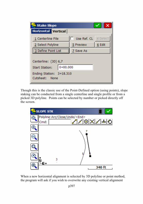
p397

Though this is the classic use of the Point-Defined option (using points), slopestaking can be conducted from a single centerline and single profile or from apicked 3D polyline. Points can be selected by number or picked directly offthe screen.

When a new horizontal alignment is selected by 3D polyline or point method,the program will ask if you wish to overwrite any existing vertical alignment

p398

selection. The typical answer is yes—you want it for both, and you are readyto stake any station at any interval based on user-entered slopes. Think ofpoints 6 to 7 as the flow line of a ditch with steep side slopes, and the goal isto lay the slopes back at 2:1 —a perfect application for Point-Defined SlopeStaking.

Design File Dialog: If you select Design Files, a dialog appears.

Centerlines, profiles and templates can be made using SurvCE. In fact,centerlines and profiles can be imported from a variety of file formats usingthe commands within Road Utilities. Note that templates can be either singletemplate “.tpl” files or multiple templates with transitions in a Template Series“.tsf” file. If the roads have superelevation, the “super” files can be made inRoad Utilities. If template transition files are to be used for lane changes, thenthis file type must be made using external software such as Carlson Civil orCarlson Roads. Note that “sets” of Roading Files can be saved and loadedusing the buttons at the bottom of the screen. The Settings icon at the top ofthe screen, to the left of the checkmark, allows you to place the profile gradeat an offset to centerline, such as at the inside edge-of-pavement for dividedhighways, as shown below:

p399

Section File Dialog: If Section Files are selected, a dialog appears.

The Section file (which has an “sct” file extension) can be entered in RoadUtilities or imported from the LandXML format using Section FileConversion, also in Road Utilities. Note that for all roading design files, thereis no requirement that starting and ending stations (chainage) m atch. All thatis necessary is that they have a station range in comm on (in the above case,

p400

10+00 through 20+00 is common to all files). Roading File sets (as in theabove Boneta files) can also be saved to a named set and then re-loaded laterfor convenience. With cross sections, the profile is not required, but includingthe profile will lead to more accurate slope staking between known crosssections, such as at high and low points in the road.

Setting the Station and Interval for StakeoutThe next screen sets the station to stakeout and the interval and will appear in someform in all cases except section and design files slope staking with interval turnedoff. In effect, there are 8 ways of going into Slope Staking: 4 methods times 2interval options (on=fixed station/off=fluid, real-time). You also have 3 moremethods if you include the Stake Road routine which offers Slope Staking bySection, Template or Sections Cut from DTM, all fixed station.

The station to stake can also be read from the GPS or total station measurement,allowing you to slope stake "where you are". You can also get the station byentering a point number, in which case it projects the point onto the centerline todetermine the station. In the non-interval method, the above screen does notappear. You slope stake wherever you are all the time, and are freed of theconstraints of staking a specified station.

The User-Defined and Point-Defined Alignment methods have their own pair of“follow-up” screens for the location to stake.

p401

For flow line or V-ditch staking, a 0 pivot offset would be entered from thepoint-defined alignment. If the ditch were a trapezoidal ditch with a 2 meterbottom width, and the alignment was the centerline, each side of the ditch could beslope staked using a pivot offset of 1 (1/2 of the ditch width from center to pivotpoint).

Both the Road Design Files and Section Files methods go straight to the navigation(stakeout) screens if no interval is selected (Stake Station Interval turned off). Thepivot offset is built into these methods based on the “rules” outlined earlier -- youstake from the pivot to cut or fill in templates, and from the ex treme left and rightpoints of cross sections. With interval turned off, slope staking by "User-Entered"method simply asks for the pivot offset and elevation at the current location, andslope staking by point-defined alignment asks only for pivot offset, obtaining theelevation from the vertical alignment.

Slope staking cannot occur outside the station range of the horizontal alignment. Ifyour horizontal alignment runs from station 0 to 308, you can ’t stake station -10,either by interval method (naming the station) or by the non-interval, fluid“where-you-are” method.

p402

In live stakeout mode, you will get “Off Centerline” when beyond the range of thehorizontal alignment.

All paths lead on to the navigation or stakeout (som e call it “set out”) screen.

The Navigation (Stakeout) ScreenWhen configured for GPS, the navigation screen then appears.

Note that because the GPS reads continuously and models the ground surface, theprogram calculates immediately where the catch point (the circle with the X) islocated. You simply walk right to it. If the ground goes uphill or downhill as youapproach the point, then the X will move closer or move away, until you are righton it.As you get closer to the point (within the stake tolerance distance) the program willpresent a bullseye screen.

p403

When you are satisfied with the accuracy of the slope stake position, you thentouch S for Store (or press Enter to take the shot). In this case, its time to drive thestake.

Interval and Non-Interval Methods Impact Stakeout ScreenThe stakeout screens above are for the interval method. In the non-interval, “fluid”slope staking, where you can drive the stake anywhere, the “Forward-Back”portion of the screen becomes vertical “Current Fill” or "Current Cut". In thisfluid stake-out mode, you simply move in or out from the centerline to set theslope stake—there is no correct or incorrect forward or back station. So theprogram instead reports the vertical up to the fill slope above you or down to thecut below you.

p404

If you are moving out to the catch point along the ground, you would get a reportof “CrtF 1.25” or some such number, and the “Current Fill” amount to the groundwould decrease as you approach the catch. The actual stakeout screen wouldappear as shown below. Note that some surveyors will watch the lower line (1.6:1for 3.65) and just keep moving out until they see 2:1 (or the desired slope) anddrive the stake. Others will watch the “CrtF” value decrease to 0 and drive thestake, or watch “OUT” decrease to 0.

Storing the Slope Stake and Offset Stake PointsWhen S for Store is pressed, you may store the actual slope stake point. Y ou canalso store a first offset point (since the slope stake itself can be removed byconstruction). The slope stake information is typically written on the first offsetstake. Then you can also stake a second offset point, to obtain “line” to reset theslope stake if it is knocked out. The first and second offset stakes provide adirection back to the slope stake. When the slope stake is set, the program promptsfor setting the first offset stake. When the first offset stake is set, the programprompts for setting the second offset stake. Both offset stakes are optional.

p405

The storage of the slope stake points is an option turned on by clicking “StorePoint to CRD File”. With this clicked off, you can simply slope stake and avoidstoring any points. The Description for the point will default to the station andoffset. Slope Staking will not respond to settings in Configure Reading for theHeight/Description prompt screen. If you are using a named “Slope Stake File”(set in File, Job Settings, Stake tab, Cutsheets option), you can still control at thepoint of staking whether you choose to append data to the file by clicking on or off“Store Data to Report File”.

p406

Note that there are two options for the slope stake report: Elevation and Offset. The standard option is the Elevation method. This assumes you were able tosurvey the actual slope stake point with reasonable accuracy, and it reports theactual stake to pivot point results. If you were staking a 2:1 cut slope, it reportsyour actual slope (as 1.997:1 in this case), and you can choose to round the resultand write "Cut 2:1, 9.25 V, 18.48 H" on the stake. But if at the catch point thereare boulders in the way, you can walk out and away from centerline in cut and intoward centerline in fill, and drive the stake where you can. In this case, youwould choose the Offset method. In the Offset example above, we had to walk past

p407

the catch point about 2 units (from 36.50 to 38.56). We drive the stake, and notethat the catch is at 956.03 rather than 955.01, so we measure up 1.02 on the stake,and draw a horizontal line there as the catch point. An extra line appears in thereport that tells us to write "Cut 2:1, 10.28 V, 20.56 H" on the stake. In cases offill where there are obstructions, walk into centerline so when you drive the stake,you can mark where the fill intersects the stake. Note that this same level ofreporting occurs with "non-interval" staking, where you get real-time cut and fill atany point, also allowing you to drive the stake to avoid obstructions.

When Enter or OK is pressed, you are prompted for whether to stake the firstoffset stake.

If you are doing “User-Defined” or “Point-Defined Alignment” methods, you areshown the horizontal distance and vertical fill or cut difference to the pivot point,which can be written on the Slope Stake. Additional break-point informationappears if you are using the “Design File” or “Section File” method. If you trustthat the Slope Stake will not be knocked out, then you are done —no need to set anoffset stake.

Pressing OK leads to the prompt to set the first offset stake. If you choose to setthe first offset stake, then you can set the offset distance.

p408

Press OK and then you are in a standard stakeout screen. The offset point is afixed location and the stakeout procedure is similar to point stakeout. This leads toa report of information that can be written on the Slope Stake. Finally, you will beprompted for staking out a second Slope Stake, to establish “line.” After the firstoffset stake is set, and before the prompt for the optional second offset stake, asummary screen will appear. If you have used the Road Design File or SectionFile methods, you will be presented with every break point into centerline.

p409

Finally, you will be prompted for staking out a second Slope Stake, a more rarelyused option whose purpose is to establish “line” (the direction) from the first offsetstake to the slope stake itself. This permits accurate replacement of the slopestake when it is knocked out by construction activity.

Note : When using Road Design or Section Files in Slope Staking, setting thefirst offset point is the recommended procedure, as it produces the full report,referenced to cross section and template IDs, for all break points all the wayinto the centerline point.

Procedure for Slope Staking with Total StationsThe procedure is nearly identical for Total Stations, except that you must press Rfor Read (or Enter) to take shots and allow the program to begin calculating theSlope Stake position. Unlike the GPS, SurvCE cannot predict the location of thetarget slope stake point until at least one measurement is taken.

p410

Note: When using either GPS or total stations for slope staking, you canobtain more graphics and less screen information by pressing the down arrowkey. It literally has the effect of bringing the graphic screen down (see below).Pressing the up arrow key will pull the screen back up and show the full text. This works in all modes except GPS Simulation, where the up arrow movesthe cursor faster, down arrow slower.

p411

The Slope Stake Report and Writing on the Slope StakeSurveyors doing slope staking have the option to write the information on the stakeas each is surveyed, or to come back at a later time, refer to the slope stake report,and write on all the stakes after the surveying is complete. The slope stake reportfile is a comma-separated “.txt” file, configured in Job Settings, Stake, Cutsheets, which might appear as follows if formatted in Excel or another spreadsheet form:

#Des Sta Des Off Des Elv Staked Sta Staked Off Staked Elv Desc

1+00.000 L33.849 998.075 0+99.966 L33.453 998.075 CatchPoint

1+00.000 L38.849 ------ 1+00.019 L38.866 998.15 FirstOffsetPoint

Here is another example as viewed in the Edit mode within Job Settings, Stake,Cutsheets, Edit Slope Stake.

The columns are configurable with the Slope Stake formatting in Job Settings. Shown above is a "total" report (as opposed to "progressive"). No offset stake wasset. The template involved was flat from centerline for 12', then had a 2:1 slopefor 6' into a ditch point (ID="BD" for "base of ditch). This cut downslopecondition was created within an office-entered template using Carlson Civil or

p412

Carlson Roads, and SurvCE automatically detected the cut condition and used theditch points as pivot points, offset 18 with elevations 945.75 at station 6+00 and946.50 at station 6+50. Some survey teams use one person to set the slope stakesand another to enter data on the stakes, which is easily done using the stored slopestake report above.

Store SectionsThis function collects as-built cross sections of roads or other alignm ents andstores them optionally as points, as cross sections or as an ASCII file organized bystation. The station and offset can be stored into the description field of the points.The station itself can be set to automatically round to the nearest 5, 10 or otherstation interval (eg. a shot at 177+98.23 would round to 180+00 if a rounding of 5or 10 is used). The information can be stored into a “.tx t” ASCII file in addition tothe points themselves, if "Store Comma Separated File" is turned on, and if pointstorage is turned on, you can save a ".not" file of the station and offset. Y ou cansave the cross section data to a cross section file in .SCT or RAW/G eodimeterformat. Store Sections can also be used simply to verify your current station andoffset as you move along a centerline using GPS or taking total station shots.

This routine is often combined with office software to check as-built road crosssections against desired grade and to calculate quantities for payment. The fieldcrew begins by taking shots along each desired cross section, as shown in thisfigure.

If, for example, four sets of cross sections were taken from station 0+75 to 1+50,

p413

the points would appear as shown in the plan view below, and the 3D view shownbelow that. There is an option to turn off point number storing, in which case theshots can still be stored to a cross section (.sct) file and report file (.tx t).

Here, below, we see the 3D view of this area.

p414

The command begins with a screen where you select the method for defining acenterline.

p415

The next screen allows you to choose whether or not to store a file summarizingcross section data. Because the SCT method requires that you choose analignment, the option for no alignment (“None”) only applies to theRaw/Geodimeter method, in which case a named file is required. Except for thiscase of option “None”, the Section output file is optional because the informationwill be stored with the points. When you click Select File, you have two file typeoptions when using a horizontal alignment.

The Raw file format is a design that is compatible with the old Geodimeter sectionfile format, and includes special prompting for job type. It is discussed in detailbelow (see the discussion of “None” as centerline option). It leads to a differentset of screen options than the SCT format.

Unless you are looking for Geodimeter file format compatibility, you shouldconsider storing a section output file in the “.SCT” format, since it can beconverted, using Road Utilities, to LandXML form and then imported to severaldifferent roading software packages for plotting and computation of volumes. The“.SCT” section files can also be used directly for volume calculations with CarlsonRoads, Leica Site Manager, Topcon Topsite and Carlson Civil. You can also setthe rounding—here, a rounding of 10 units (feet or meters) has been selected. Thestation and offset can also be stored as the point description and as a note file, ifthe lower options are clicked on.

p416

Note that the rounding is fully automatic. If you choose a 5-unit rounding, and aretargeting station 0+75, but take a shot at 0+77.93, it will round up to 0+80.

Before collecting the cross sections, it is important to click X-SCT Settings nearthe top of the dialog, and set the stations you wish to capture. This way, if thestation rounds, per the above screen, to a station that doesn ’t exist in your list, youare warned before proceeding with storing. This list also includes the left and right“tolerances” for the offsets, which will lead to warnings if you exceed that distancefrom centerline. If you set a tighter “Station Tolerance” in X-SCT Settings (optionEdit) than the “Rounding” Tolerance, you will be warned even though therounding is correct. In the screen shown below, station 16+70.000 has beenadded as a special station. Clicking the first line (10+00.000-23+00.000) allowsyou to set the standard interval, and the additional stations in the list would be forspecial stations in addition to the standard interval.

p417

The below, smaller dialog appears when you tap Add Odd Stations, shown in theabove figure.

With the first line highlighted, selecting Edit leads to the settings options for thefull range of stations.

p418

With an interval set of 50, and Start/End Stations turned on, the program will onlyexpect you to capture stations at 50 units intervals starting at 10+00 through to23+00, but also including 10+11.57 and 16+70 in this case. The Offset fromalignment to X-Section option lets you, in effect, use an alternate, parallelcenterline at a left (negative) or right offset from the main centerline. Unless theRaw/Geodimeter method is used, a station “warning” screen is used if the roundedstation is not in the list or pre-selected stations. A capture of station 1075 wouldround to 1080, but since 1080 is not in “the list”, you will be warned beforestoring. A station of 1667 would round to 1670, which is in the list, leading to nowarning screen. Since the rounding was set to 10 in this example, data collected at45 to 55 would round to 50 (station 1053 would not round up to 1055), andtherefore only “even 10” stations will be collected to begin with. So the additional“Station Tolerance”, which rounds the collected station data to the listed stations,will not activate.

When OK (green check mark) is clicked from the Store Sections dialog, theprogram immediately proceeds to a point collection mode, with continuouspresentation of station and offset (if running GPS or robotic total stations).

p419

Storing Points using GPS: There are two methods for storing points inreal-time GPS mode: Press the S icon at right (or pick Alt S) or simply pressEnter. The “binoculars” icon will bring up the Monitor/Skyplot dialog. Youcan survey as many cross sections as desired within the command. Unlike inSlope Staking, Store Sections will respond to the setting for Hgt/Descriptionprompt on save, found in Configure Reading, allowing you to arrow key todesired descriptions or change your rod height after taking the shot. Option Cgoes to the Configure Reading directly from the data gathering screen. Whendone, simply select the Menu button, and you are returned to the Road menu. When exiting by pressing Menu, if you have opted to store to an SCT file, youwill be prompted to store the cross section information in SCT form.

Storing Points using Total Stations : After confirming the occupied stationand backsight, as with all total station work, proceed through the same optionsabove until you reach the store point dialog. In the ex ample below, ourcenterline is metric, starting at station 0+000.

p420

Here, your options are R for read, followed by S for Store, or simply Enter toRead and Store. The backsight icon can be pressed to set a new occupiedpoint or backsight point. Note that we have a very “busy” screen of points. Ifyou just want to see your setup, backsight and last point that was measured,press Alt F. This produces the screen below. You will stay in this mode untilyou press Alt F again and toggle back to the presentation of all points.

p421

If a shot is taken that doesn’t round to a station in the list of “approved” crosssection stations (X-SCT Settings), then a warning screen appears. In the warningdialog shown below, the tolerance has been exceeded on two accounts. We roundto 0+80, which is not in the list, and our offset is 186.891 left, which ex ceeds ouranticipated maximum offsets of 100 left and right.

Points Store with Station/Offset Descriptions, as shown below:29 0+125 L23.58

30 0+150 L33.24

31 0+150 L19.39

32 0+150 R1.98

33 0+150 R18.12

The comma-separated file would appear as follows if presented in a tab-delimitedform:

#PointID

Station Offset Elevation Description

p422

29 0+125 Left 23.5759 991.2901 0+125 L23.58

30 0+150 Left 33.2363 989.9193 0+150 L33.24

31 0+150 Left 19.3923 996.8921 0+150 L19.39

32 0+150 Right 1.9816 998.2340 0+150 R1.98

33 0+150 Right18.1201

997.0731 0+150 R18.12

When you exit the routine by clicking Menu from the data gathering screen, andhave Store SCT file turned on, you will be asked if you want to “process” or addthe last shots you collected to the named SCT file. You have the choice to“Process” (use the data) or “Discard”.

The program will even keep the section data “on file”, so that if you Cancel theabove screen, and re-enter Store Sections, you will be prompted again whether tosave (process) or discard the cross section data collected earlier.

Options When Storing in Raw/Geodimeter FormatDifferent options present themselves when the Raw/G eodimeter Format, or FileType, is chosen.

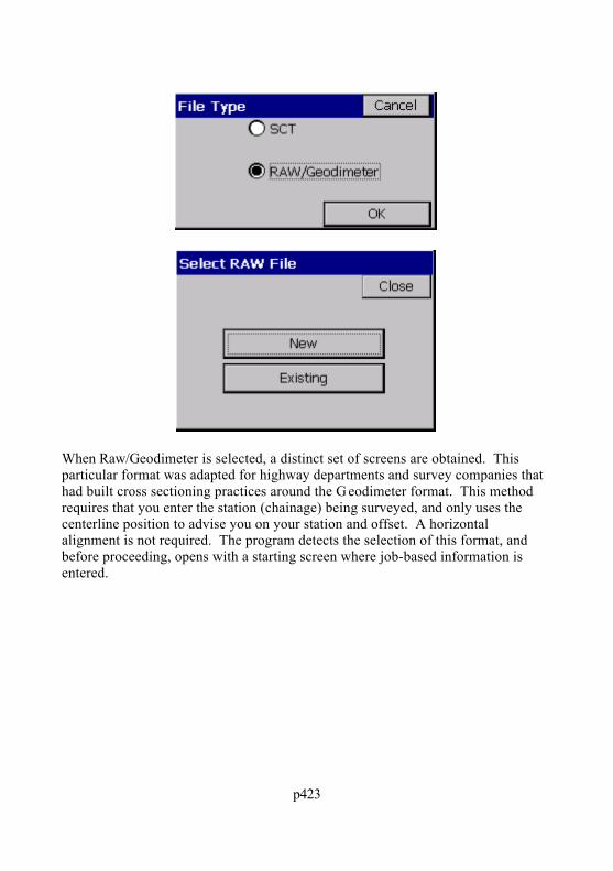
p423

When Raw/Geodimeter is selected, a distinct set of screens are obtained. Thisparticular format was adapted for highway departments and survey companies thathad built cross sectioning practices around the G eodimeter format. This methodrequires that you enter the station (chainage) being surveyed, and only uses thecenterline position to advise you on your station and offset. A horizontalalignment is not required. The program detects the selection of this format, andbefore proceeding, opens with a starting screen where job-based information isentered.

p424

There are pre-set job categories and tasks, which save into defined numbercategories in the old Geodimeter raw file format. Whereas the SCT methodrecognizes the station you are on and automatically rounds to it when you arewithin tolerance, the Raw/Geodimeter method requires that you click the Stationbutton, and set your target station for collection of cross section data.

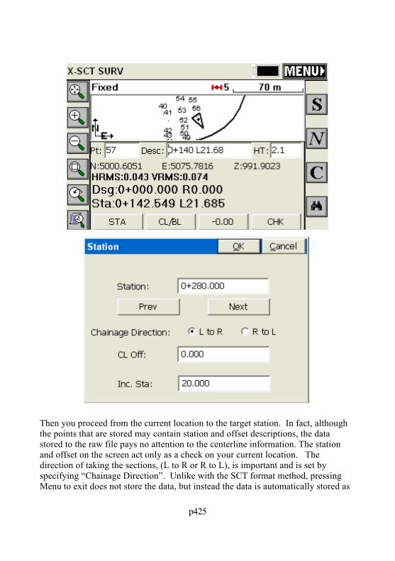
p425

Then you proceed from the current location to the target station. In fact, althoughthe points that are stored may contain station and offset descriptions, the datastored to the raw file pays no attention to the centerline information. The stationand offset on the screen act only as a check on your current location. Thedirection of taking the sections, (L to R or R to L), is important and is set byspecifying “Chainage Direction”. Unlike with the SCT format method, pressingMenu to exit does not store the data, but instead the data is automatically stored as

p426

you go, as a series of 37 (N), 38 (E) and 39 (Z) record types (Geodimeter format),with header line records, as shown below:

50=XSEC154=104 North0=As-Builts 240-30053=VF90=297=051=3-28-200456=65.074=30.1055=396=26=2.10080=280.00091=137=5105.85738=5069.09139=991.90537=5104.09138=5074.93139=990.724

Starting left to right, the data points begin with a 91=1 record. A right to leftsection would begin with 91=2. When you “cross 0” or are on the centerline orbaseline, you click the CL/BL button which sets a 92=1 record for centerline and92=2 for baseline, and the next shot is the centerline/baseline shot. If you selectthe “-0.00” button, this indicates whether the next shot is a tie-in (catch) orextension beyond the tie-in. This sets a 93=1 record for the catch and 93=2 for theextension prior to the subsequent coordinate record. In effect, you tell theprogram where the centerline or baseline is by shooting that point. Then thestation and offsets of the shots for that cross section are determined relative to thatcenter-of-alignment shot. It does not use a horizontal alignment combined withrounding to determine the station and offset of the shots (like the SCT methoddoes). You tell it the station, the direction of measurement (left to right or viceversa) and you tell it which one is the center shot. This is why theRaw/Geodimeter method is the only method that works with no centerline (the“None” option). For each section, you tell it the station and center shot, and allother measurements are used to determine the left and right offsets relative to thecenter shot. If the L to R method was used, shots before the center shot are on theleft, for example, and their offset is determined by the inversed distance to the

p427

center shot. The centerline file or other form of horizontal alignment, if selected,is academic and only used to advise you on your current station and offset. TheCHK button will allow checking into known points to be sure that tight coordinatecontrol is maintained. N moves onto the next station as defined by the interval setusing the Sta button.

Note: The .SCT file method is the standard Store Sections method. TheRAW/Geodimeter method is a flexible routine designed to adapt to customerswho have built their cross section processing systems around the G eodimeterraw file format.

Stake RoadStake Road is one of four major commands used in highway work. Thiscommand is designed to stakeout specific stations and offsets along a centerline. For example, if your goal is to stakeout the break points at station 87+80 on agiven road centerline, you would use Stake Road. Stake Road, therefore, is usedprimarily to lay out road surfaces for construction. Stake Road is typically used toset cut and fill stakes or “blue tops” at specific stations and offsets. The elevationused to determine the cut or fill at each offset is derived from either design files(the template interacting with the profile and centerline) or from cross sections orfrom sections that are “cut” from alignments. At any specific station, you will beguided to the desired offset and will get a cut or fill. By contrast, if the goal wereto simply set random cut and fill stakes along an alignment, at no particular stationor offset, then the command Elevation Difference would be used. If the goal is tostake out the “catch” in cut and fill, where cut slopes and fill slopes meet ex istingground, then Stake Slope would be used. However, you can also Slope Stakewithin Stake Road. The fourth, major highway-oriented feature is Store Sections,which is used to gather “as-built” information on a road. In this command, youtake cross sections of data points along the road, at random or specific stations. Insummary, Stake Slope starts the cut and fill work, Stake Road directs the preciseroadbed work and fine grading, Elevation Difference acts as a quick grade check,and Store Sections produces the final confirmation of the as-built road forpayment and certification. It is highly recommended for all road stakeout that youset on "Use CL for Reference Object" within Configure, View Point tab.

Defining the RoadThe first dialog that comes up when you select Stake Road is where you define theroad by selecting one of the following options.

p428

Design Files: In Carlson SurvCE, design files include templates, centerline,profile and optionally, superelevation and template transition files. If you wishto “clear” a file such as a superelevation file, just click it and choose Cancel.The definitions for each of these files is covered in their own sections of thismanual. Design files are recommended for subdivision streets, access roadsand simpler highway designs.

Section Files: Sections are made up of simple offsets and elevations that canhave descriptions such as “EOP”, “DL” or “SH” and must be accompanied bya horizontal alignment file (centerline). Every cross section is a “snapshot” ofthe template at a given station. SurvCE supports using multiple surfacessimultaneously in Stake Road by using multiple section files or by extractingthe section for each surface when all surfaces are within a single file. Eachsurface can exist on its own layer with its own color for easy identificationwhile in the Stake Road dialog. For complex designs, with non-conformingintersections, transition lanes, special ditches, etc., it is recommended to usecross section data if available.

Cut Section from Alignments: Provides the ability to extract cross sectionsdirectly from 3D polylines that exist within SurvCE. The first thing you needto define is the horizontal and vertical alignment files. These form the basisfor cutting the sections and determining left and right offsets from thehorizontal alignment or centerline. The centerline-defining screen is similar tothe screens found in Stakeout Line and other commands.

p429

This just starts the process. With both horizontal and vertical alignmentsdefined, click OK. You will then be asked to define a template pointalignment (TPA) file. In this process, you must either pick or identify bypoint number or file each alignment “pair” (H and V) that define anedge-of-pavement or other feature of the sections. It takes a 3D polyline,or a pair of horizontal and vertical files, or any mixture of points,polylines and files, to define a single offset feature.

Click on Left Surface, for example, then Click Add. This brings up thesame screen used to define the centerline. If you have a drawing of 3Dpolylines (brought in as a DXF file, for example), it is very easy toillustrate this command by the Pick Polyline option. When chosen, youobtain the next screen, where you can pick the EP.

p430

Now click OK, say Yes to Overwrite vertical alignment (if the polyline is3D), and simply OK the screen (no need to save the file as a namedalignment). This brings up the name template ID dialog.

Repeat for the outer polyline (SH, left side), then for the EP on the rightside and SH on the right side. You now have a centerline and 4 offsetalignments from which to cut sections. When you get the full contingentof alignments defined, click Save As to save the TPA file . Now anydesign offset at any station will be automatically interpolated, and normaltemplate/section stakeout can proceed.

Save Roading Files: This button will save the selected set of roading files asan RDF file for recalling later.

Load Roading Files: This button loads all of the files previously saved to anRDF file. The files must still be present in the original locations.

InterpolationIf descriptions are provided, “intelligent” interpolation is performed betweensimilar descriptions on slope transitions or widening lanes as well as verticalcurves for all methods described above.

Stake Road

p431

The next screen is the heart of the program. Here is where you select the stationand offset to stake out. You can even launch into a slope stake and then return tostake out other template points.

Settings: The “Additional Stake Stations” that appear in the List are set in thelower portion of the dialog. The Vertical Scale option will allow for“exaggeration” of the vertical on the template graphic. Though defaulting to1, we can double the exaggeration by setting this to 2. In fact, an ex aggerationof 5 works fine for the “demo.tpl” template file. The “Next Station Method”governs how “N” for next, from the stakeout graphic screen, moves you up. When set to “None”, N for Next will stay put until you change your entries. But if set to “Next Offset (Left to Right)”, Next will stay on the current stationand move to the next offset. The “Next” in the dialog below, however, alwaysincrements the current station by the next station in the List. Don’t confusethe Next button on this screen, with the N button on the graphic screen tofollow, which is influenced by “Settings”, and moves you along after youcomplete each point stakeout.

Station: The value of the Station to Stake. Interval: The horizontal distance to increment the stationing when using the

Next and Previous buttons. Play/Pause: This button allows the user to play through the road file like

watching a drive-through movie. List: Depending on the settings and specified interval, “List” will list the

p432

defined stations including intervals and critical stations. List Offsets: This dialog allows the user to pick from the known offsets by a

list rather than using the graphic screen below. It also allows the user to selectan optional second point of "Reference" for reporting cut/fill informationwhile staking. So you could stake the shoulder but also reference cut and fill tothe centerline, as an option.With this option, the selected offset and thesecondary reference offset will both be reported to.

The resulting plan view in stakeout shows cut and fill to both thereference and the target point.

p433

Design Offset: Any offset can be entered, even if it is not a “break point” onthe template. For example, an offset of Left 5 (-5) or Right 7.23 could beentered. For every design offset point selected, the elevation is calculated andpresented. You can select the offset point from the offset list or literally pickit on the screen. The touchscreen is active in the graphic, so you can select the-12 (EP) just by picking it. Picking on the graphic screen will take you to the“Offset List” screen for verification, where you can confirm your pick bypressing Enter or selecting another offset.

Stk Off(H): Horizontal offset from the design offset. If you enter an stakeoffset of 2 and the design offset point was at 12, then the stake would go in atoffset 14 off of CL, but the cut/fill would refer to the elevation at the designoffset location of 12. The stake offset and Off. to CL inter-react. A stakeoffset entry of 15 with a design offset of 12 left calculates to a setback of 3. Ifyou click the "Stake Off" button, you can choose from a variety of methods tocreate an offset point, including extend current slope, apply next slope,vertical offset, or user-defined slope.

p434

Your offset is then computed and shown graphically:

Note that you can zoom and pan in the dialog above. Pan using yourfinger or stylus.

Stake Off Button: This button allows the user to specify the horizontal andvertical offsets relative to the design offset. Various methods can be used for

p435

computing the offsets based on the template or section points and theirelevations.

Off to CL: This is the total distance that the stakeout position is from thedefined road centerline.

Vert. Off (V): Vertical offset from the design elevation. Elevation: Elevation to be staked. This value is based on the combined design

elevation and vertical offset. Run Slope Stake: This feature allows for dynamic slope staking in the

middle of the Stake Road routine. This option is very useful for road staging,and also for staking interior catch points like central median ditches. Whenthe slope stake is completed, the program returns to the main Stake Roaddialog. Any point in the template or section can be used for running in a slopestake. You are asked to specify the desired cut-and-fill slope ratios. The slopecan be auto-defined or user defined as follows:

Define Slope by Next Section Point: This option allows you to selectthe edge of the road and use the proposed design catch point forauto-determining the slope rate.

Define Slope by Previous Section Point: This option allows you toselect the proposed design catch point and then use the nex t point towardCL for auto-determining the slope rate.

Extend Current Slope: This option will allow you to pick the edge of

p436

the road or catch point and use the next point toward CL to end the slopebetween then away from CL.

User Defined Slope: Allows you to enter the slope ratio by hand foron-the-fly slope changes.

Slopes by Template: This option extracts the slope definitions from thetemplate file itself.

If you click Slope Stake, you can stake by the template slope for the ditchshown on the left side, or you can enter a user-defined slope to overridewhat is in the template.

Pivot Point: This option allows the user to perform on-the-fly offsets relativeto the stakeout position.

Stakeout ViewsStake Road now allows you to navigate to the point in either plan view or crosssection view. Select the helmet icon and choose Section to see a section view andchoose Plan to return to plan view.

p437

CutsheetsStake Road will produce Alignment-style cutsheets that include the option toreport station and offset as well as the cut and fill to any point. These are fullydescribed in Stake Line/Arc, Elevation Difference and in Job Settings, Stake Tab. If using Slope Stake within Stake Road, a slope stake report, including"progressive" and "total" distances to all template or section points, can be output.

p438

MAPThis chapter describes the use of the MAP screen. The MAP screen commands areavailable in the pull down menus or at the command prompt. The MAP screen isuseful for drawing, COGO, creating points for stakeout, and for the import andexport of DXF and shape files. No measurements are taken from the MAP screen.

BasicsThe basic operations of the MAP screen are described here.

Map View IconsThe commands associated with the MAP View Icons are described in the figurebelow:

p439

Executing commands in Carlson MAPThe MAP screen defaults to a pull down menu format containing approx imately 60additional commands, virtually doubling the number of commands found in theMenu Screens. Many of the commands in MAP offer CAD-like features such aslayer freeze and thaw, predetermined area, polyline offsets and even contouring. One of the most important commands is Polyline to Points, which allows you tocreate points for stakeout (set out) from any selected polyline. The MAP screenalso includes a command line format that can be set using Preferences. SeveralMAP screen pull down menu commands involve “fly out” options, as shownbelow.

p440

Alternatively, you can enter the command name, or command alias, at thecommand prompt and press ENTER. In many cases, the user can start a commandwhile using another command. The newly started command is called a"transparent" command. Each command from the left-toolbar menu is a"transparent" command.

Usually, a command does not immediately execute. Carlson MAP either displays adialog box or displays prompts at the command line requesting more informationfrom the user. Typically, the user can select objects on the screen or enter data onthe command line. Many commands consist of a series of options, structured asfollows:

Cmd:Command name-Option1/oPtion2/opTion3/.../<default option>

To select one of the options, the user can enter the entire option name or only thecapitalized letters, and then press ENTER. If available, the default option alwaysappears in angle brackets (<>). To select the default option, just press ENTER. Ifno command is active, the user can repeat the previous command by pressingENTER.

Panning the ScreenThe user can move the drawing display (PAN) anytime. To use this command, theuser must hold down and slide a finger — or the proper pointing device — on thescreen. The drawing display is moved in the same direction as the pointing device.

p441

When you release the pointing device, the panning stops. Only the display m ovesand all objects retain their correct coordinates. Be careful to start the pan bypicking in “empty” space. If you hold down on a point, you may obtain the “PointDetails” screen, or you may see a list of points to select from (to see Point Details).

Point DetailsUnless you are in the middle of a MAP screen command, you can click on a pointand see a Point Details dialog. If you tap near several points, a list of nearbypoints will appear from which you can select the target point. Otherwise, you willgo straight to Point Details, and see a screen such as this:

If you are in total station mode, and actively surveying (with a setup and backsightspecified), clicking on the setup or backsight point will lead to a special graphic, asshown here:

If you have assigned attributes to the points (e.g. Description Pole, Type-Metal,

p442

Wires-4, etc.) by use of the Feature Code capabilities, these attributes can bereviewed. The Point Details option works both within the MAP screen (when youare not being prompted for entering points or selecting objects) and in all graphicscreens within the Menu options. It is not as transparent and available as thedynamic pan option, but nearly so.

Notes: All polyline vertices and all points contain x, y and z coordinates.Also, the user can move the drawing display (PAN) anytime. To use thiscommand the user must hold down and move the pointer device on the screen.The drawing display is moved in the same direction as the pointer device.When the user release the pointer device, panning stops.

FILEDXF File - Import DXF (IDXF)Similar to the AutoCAD DXFIN command, will bring in polylines from AutoCAD,Microstation and other CAD formats that can ex port data into a DXF file format.Points, text and blocks such as symbols are not imported. However, manysoftware packages such as Carlson Civil (formerly SurvCADD) allow tex t to beconverted into polylines – in which case the text will import for reference.

DXF File - Export DXF (EDXF): The EDXF command, similar to AutoCAD’s DXFOUT command, will export a

p443

DXF file. It captures not only 2D and 3D polylines and their layer names but alsoexports all visible (layer on) points from the CRD file into AutoCAD “Point”entities form (layer PNTS). All points and polylines that are visible (layers on)would be exported, not based on the current screen zoom, but based on the fullextent of the drawing.

LandXML - CRD from Land XML (XML2CRD): This command allows you to import points from LandXML format to SurvCE.

LandXML - CRD to Land XML (CRD2 XML): This command allows you to export points from SurvCE to LandXML format.

LandXML - Export Chain File to LandXML (CHAINXML): This command allows you to export all the polylines from the current drawingcreated using Feature Codes, as LandXML chain objects into a LandXML file. For example, if you made strictly 3D polylines for break lines using descriptionssuch as EP for edge-of-pavement or DL for ditch line, then the 3D polylines can beexported as a LandXML chain file and used as break lines for contouring in otherCAD programs. The combination of points and break lines can lead to optimalcontouring. Most CAD packages will import linework using the DXF fileapproach, but many now recognize linework in LandXML “Chain” file format.

SHP File - Import Shape File (ISHP) (e.g. from ESRI): This command allows you to import entities and also the associated attributes

p444

values from a SHP file. The routine displays "Import from SHP" dialog box. If theSHP file has POINT or POINTZ type, the entities will be stored into a CRD file.In the cases of an ARC, ARCZ, POLYGON or POLYGONZ SHP type, the entitieswill be stored into the current drawing. The attribute values will be stored into a*.vtt file. The routine requires a feature code name from the user, which will beused to store the name and the type of the attributes from the SHP file.

SHP File - Quick Import SHP (QISHP): This command allows you to import entities from SHP files (used by mostprograms produced by ESRI). The routine displays the Import from SHP dialogshown below. POINT or POINTZ type entities will be stored in a CRD file. ARC,ARCZ, POLYGON, or POLYGONZ entities will be stored in the current drawingas POLYLINES.

Current SHP: Displays the name of the SHP file that will be importedwhen this command is completed. Read-only, you must use the SelectSHP button to specify the file name.Select SHP: Tap this button to select a SHP file name.Current Job: Available when importing coordinate data. Specifywhether to Overwrite Exiting Point Numbers or Use New PointNumbers. Attribute used to fill Description : Available when importing coordinatedata. Lists the attributes in the currently selected SHP file. Select whichattribute to use to fill out the Description field in the CRD file.

p445

Layer used to store new entities : Available when importing geometry.Select the layer to store the new entities.Process: Tap this button to begin the import process. If you are importinga large file, a progress bar at the bottom of the dialog will indicate theprogress of the import.

SHP File - Export SHP File (ESHP): This command allows you to export entities from the current drawing and also theassociated attributes values, into a SHP file (or more accurately, multiple shapefiles). The routine will allow the user to select which entities will be exported,based on entity type and also based on the feature code name. The routine displays"Export to SHP" dialog box.

Click on Export All and include special attributes and optionally the Z coordinates.If you have point, arcs (non-closed polylines in ESRI terminology) and polygons(closed polylines), all with one attribute, you will obtain up to nine files as shownbelow:

Ascot1_11.dbfAscot1_11.shpAscot1_11.shxAscot1_13.dbfAscot1_13.shpAscot1_13.shx

p446

Ascot1_15.dbfAscot1_15.shpAscot1_15.shx

The selection of the Z coordinate places the 1 after the underline character. Otherwise, the file form would be, for example, Ascot1_1.shx (special attributesonly). The “1” group represent points, the “3” group represent arcs (unclosedpolylines) and the “5” group represent polygons (closed polylines). Within Ex portShape file, the field name in the dbf file is expanded to handle up to 254characters.

SHP File - Quick Export SHP (QESHP): This command allows you to export polylines and/or points to an SHP file. Thedialog that displays will have the following options:

Current SHP: Displays the name of the SHP file that will be createdwhen this command is completed. Read-only, you must use the Selectnew SHP button to specify the file name.Select new SHP: Tap this button to select a SHP file name.Do not export points: When this option is checked, only polylines areexported to the SHP file.Export entities from selected Layers : Lists the layers in the currentmap. You may select certain layers for export.Select All: Selects all layers in the list.

p447

Clear All: Clears all selected layers in the list.Remove Arcs (offset cutoff): Specifies the maximum distance that avertex on a polyline segment will deviate from the original arc.Include Z Coordinates: When this option is checked, elevation data (orZ coordinates) will be included in the SHP file.Process: Tap this button to begin the export process. If you are exportinga large file, a progress bar at the bottom of the dialog will indicate theprogress of the export.

DTM Import - DTM from DXF (TDXF): Allows you to import 3DFACE entities from a DXF File and save them as atriangulation (FLT) file and also draw them as 3D faces.

DTM Import - DTM from Land XML (TXML): Allows you to import 3DFACE entities from an XML File and save them as atriangulation (FLT) file and also draw them as 3D faces.

p448

The DTM file is stored in SurvCE as an FLT file and can be used for commandssuch as Elevation Difference (obtaining cut/fill by comparing field measurementsto the DTM).

The 3DFaces are placed on a layer (TRI_FACE by default), and that layer can beturned off and removed from view. If you choose E for Erase, you can pick the 3DFace entities and erase them on command. There is no particular value to seeing

p449

the 3D Faces, so it is not recommended that they be drawn. The main value is tocapture the FLT (triangulation) file for use in Elevation Difference.

Preferences (SETT): This allows the user to turn on/off the pull-down MAP menus. The graphic screenstyle of normal or reverse (solid dark) background is set here.

Command Aliases (AL): Brings up a list of commands in the MAP mode for which the user can substitutean alias. If you would prefer to type A for Area rather than AR, you can substitute“A” as an alias for AR. Three commands will not accept substitutes: Inverse,Traverse and Sideshot (I, T and S). In addition to commands, you can toggle overto the “Linework special code” option, and substitute aliases codes for the defaultspecial codes such as PC, PT and END (used to control linework using featurecodes). As an example, you could choose the “X” or “..” to End a line, or use“CS” for curve start instead of PC.

p450

p451

p452

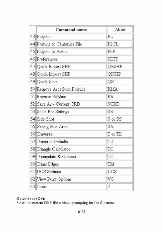
p453

Quick Save (QS): Saves the current DXF file without prompting for the file name.

p454

Save As(CRD): Saves the current coordinate file to the location you choose as a backup copy.

Exit (X): This exits the MAP and CAD session and brings you back to the Menu screen.

Help (H): Launches the interactive Help screen describing various MAP screen commands. Scroll up and down to review.

VIEWThe View menu is found next to the File menu in MAP view. Below you will findeach feature described.

p455

Zoom (Z): Increase or decrease the apparent size of polylines and distances between points, indrawing area. The Zoom command options can also be accessed using the first 5buttons from left-toolbar menu. The order of buttons, starting with the first topbutton, is: Extents, In, Out, Window, Previous. The menu also has Num which letsyou enter in a point number and zoom to it.

Layer (LA): This command manages layers and layer properties.

p456

To add a new layer: Type in a new name into the New Layer edit box.The New button will appear at the bottom. Tap this button. If you type ina new layer name and the New button does not appear, then the layername you entered contains invalid characters.To set a layer current: Highlight the layer name in the list and then tapthe Set button. You cannot set a layer current if that layer is turned Off.Turn the layer On first and then set it current.To delete a layer: Highlight the layer name in the list and tap the Deletebutton. You cannot delete layers that contain objects. If you select a layerand the Delete button is not visible, then this layer contains objects.To turn a layer On/Off: Highlight the layer name and tap the On/Offbutton. Objects on layers that are On will be visible, objects on layersthat are Off are not visible.On all: This button will turn all layers onOff all: This button will turn all layers except the current layer off.Color: Clicking on the color bar will bring up the color palette allowingyou to set or change the layer color of the highlighted layer.

One of the main purposes of the Layer command is to permit the import, by DXF,of a drawing containing all possible polyline work to stake out (set out). Then youcan reduce clutter on the drawing by turning layers off, leaving only the layers youwant. You can then do the command Cogo, Interpolate Points, Polylines to Pointsand make point numbers out of all vertices (corners) of polylines where you needto set stakes. Then proceed with Stakeout by Points.

p457

View Options (VO): This command controls the appearance of point objects on screen. This is ex actlythe same as touching the lower left graphic icon. The routine displays the ViewPoint Options dialog. Pt#, Description and Elevation toggles control whether theseattributes are labeled with the points. If Freeze All is on, the points are placed onthe map, without attributes. Available point symbols are: ".", "+", "x ". The“Decimal is point location” toggle determines if the decimal point used in thedisplay of elevations represents simultaneously the point location and symbol. Thisslightly reduces screen clutter.

Small and Large toggles determine the size of font used to display the point objecton screen. Set Color Attributes brings up the color palette (available only on colorCE devices). This lets you choose the color of the point symbol, elevation anddescription text. The Traverse Defaults button brings up a dialog that has thesettings for prompting each time for instrument and rod height and the verticalangle. This applies to the T for Traverse and SS for Sideshot commands that allowpoint calculation within the MAP Screen. For Cogo work, turn off Instrument/RodHeight and Vertical Angle prompting. For manual entry of actual fieldmeasurements, turn them back on.

p458

Isolate Points (ISO): This is another useful command to reduce screen clutter. If you have 500 pointson the screen, you can isolate to only those points you wish to see, by entering adistinct point range, in the form 1-10, 22, 25-30, or a certain description. Thiswould isolate to points 1 through 10, point 22 and points 25 to 30, and other pointsare “frozen”. Repeat the ISO command and enter the full point file range (or “all”)to restore all points.

Isolate Layer (IL):Select any polyline layer and isolate it to keep that layer. Other polyline layers areturned off (frozen), but point layers are retained. Use the Layer command to turn

p459

layers back on as needed.

Aperture (AP): Controls the size of the rectangle area used to select points or polylines fromscreen. Initially, the size in pixels is 40 units for points selection and 10 units forpolylines selection. The routine displays the Aperture size dialog.

UCS (UCS) User Coordinate System Indicator: This toggles the visibility of the UCS icon shown in the MAP screen.

Find Point (FND): This command allows you to find a point on the MAP screen. Enter the point youwant to find and a zoom height. If you enter a point that is not on the map, thedialog will warn you and allow you to enter another point number.

p460

Click Find and the SurvCE zooms to the selected point at the entered scale.

Scale Bar (SB): This toggles the visibility of scale bar on or off. The scale bar is normally shown atthe bottom of the MAP screen.

List (LI): This lists the layer, 2D or 3D status, Closed or Open status, perimeter (length), andarea or projected area (if not closed).

DRAWThe Draw menu is found next to the View menu in MAP view. Below you willfind each feature described.

p461

2D Polyline (PL) (AutoCAD style): This command allows you to draw a polyline between points. You can pick pointsfrom the screen or type in point numbers. First, pick your starting point then youhave several options on the command line. The default option is to keep pickingpoints and the other options are described below.

Cmd:Polyline-Arc/Close/Undo/<End>A: Starts an arc segment. See below for details.C: Closes the polyline (you must have at least two polyline segmentsdrawn before you can close)U: Will undo the last segment drawn.E: Will end the Polyline command.

Constructing an arc segmentAfter choosing A, the command line will change to:Cmd: Polyline-Arc CEn/Len/Sec/<Rad>You have various options for constructing an arc as part of your polyline.CEn: Allows you to specify the center point (or radius point) for the arc.After picking the center point, you must specify the arc end point andthen the arc direction.Len: Allows you to specify the arc length. First you pick the arc endpoint and then you can enter the arc length. The minimum arc length isgiven to you.Sec: Allows you to specify the second point and end point to define the

p462

arc.Rad: Allows you to specify a radius length. First you pick the arc endpoint and then you can enter the radius length. The minimum radiuslength is given to you.

2D Polyline (Road) :This command allows you to draw a 2D Polyline. This command is similar to the polyline command described above with the following additions:

+/-: The +/- options activate an additional prompt that allows you to plotline segments at a 90 degree deflection angle from the last line. [+] is aright deflection and [–] is a left deflection.Len: This option prompts you for the length of a line segment. Enter thelength and a line segment will be drawn that length using the samebearing as the previous line segment. If the previous segment is an arc,then the new segment will be tangent to that arc.

3D Polyline (3DP): The 3D Polyline command is similar to the 2D polyline command. It will evendraw arcs, but will create a polyline on the screen with many vertices at different Zelevations which are linearly interpolated around the arc. If the start of the arc ispoint 17 at elevation 100 and the end of the arc is point 9 at elevation 90, thenusing View, List, you would see intermediate vertices (note that the segment lengthbetween vertices is about 0.05 units).

p463

If you select 3D Polyline but pick points that are all at 0 elevation, you will createa 2D polyline.

Circle (CR): This command draws a circle entity, based on diameter defined by two points orbased on a center point and a radius.

Erase (E): Erases all selected polylines. It will not erase points. Note that you can erase anentire area by drawing a Window through the polylines (picking first a lower leftpoint in “blank space”, then picking an upper right point). If you even contact orenclose any polylines with this window selection, they will be erased. So the“window” erase procedure mimics the “crossing” selection method of AutoCAD.

Delete Layer (DL): Select from a list one or more layers, then the routine will delete all the polylineson those layers.

p464

Change Layer (CHG): This changes the layer of the selected polylines. One form of selection is to type Land press Enter in order to select last created polyline from the drawing. Theroutine displays the "Change entities to layer" dialog box . When the dialog appearson the screen, the selection in the layer list will be set to the current layer. Clickingthe color bar brings up the color palette, letting you change the color by picking orByLayer.

p465

Offset - 2D (O2): Mimics the AutoCAD Offset command, and only works with 2D polylines. Enterthe offset distance and pick the left or right offset amount.

Offset - 3D (O3): This offsets 3D polylines both horizontally and vertically. It is great incombination with road/utility centerlines to create offset polylines to stake. If youdo the “segment” option versus the “continuous” option, it will break the cornersand offset the projection of the line. This creates vertices that can be turned intopoints using the command P2P, and is useful for building offsets.

p466

Modify - Remove Arcs (RMA): Pick any polyline with an arc, specify the “offset cutoff” spacing, and turn the arcinto chords. Offset cutoff refers to the maximum separation between the chord andthe original arc. If you enter a small cutoff distance of 0.1, then at no point do thechord segments differ from the arc than 0.1. Be careful with this command – thereis no “Undo” to restore the arcs (though you can im mediately start a new job and“re-load” the last, saved DXF file of the drawing).

Modify - Fillet (F): Similar to AutoCAD’s Fillet command. It prompts: Cmd: Fillet -Ra/Pl/eXit/Firstseg 25.00. If you are trying to inscribe a curve at the corner of a polyline, youenter the desired radius first (at the above prompt). Then you choose the P option. This leads to the prompt, Cmd: Fillet -Ra/Pl/eXit/Select pl 25.00. Select thepolyline near the vertex where you want the curve to go. This completes theprocess. If you wish to change the radius, enter R. If you want to fillet the cornerof 2 distinct polylines, then just pick them as prompted (do not do the P forPolyline option). This command will only work with 2D polylines, completed withthe command 2DP, or imported from a DXF file as 2D polylines, or convertedfrom 3D using the command C2D.

p467

See the above two figures. Because in the top figure, from 1 to 2 to 3 was onecontinuous polyline, after the radius was set at 15, P was entered to set up theone-pick approach for polylines, leading to the completed fillet command and theresult as shown in the bottom figure. Now you can do Cogo, Interpolate Points,Polylines to Points (P2P) and solve for the points for the beginning of the arc,radius and end of arc, for purposes of stakeout (set out).

p468

Modify - Join (JN):

This command allows you to join polylines. Enter D to specify a new max imumseparation distance, then select the polylines on the MAP screen. The advantageof joining polylines is that they can then be offset as a unit, and the vertices of theoffset polylines can be turned into points for stake out. The offset command, ineffect, does all the complicated bearing-bearing intersects for you. For ex ample, ifthe resulting polyline were a pipeline with a 20 meter total right-of-way, then tostake the right-of-way points, you would offset the polyline 10 units left, then 10units right, then turn both offset polylines into points.

p469

Modify - Trim (TM): This allows you to trim polylines to the edge of other polylines just like inAutoCAD. Then the command Polyline to Points (P2P) will turn all vertices,including the trimmed end points, into points for stakeout.

p470

Modify - Reverse Polyline (RV): When you turn a polyline into points, it will start the point numbering at thebeginning of the polyline. Thus it may be useful to control the direction of thepolylines. This is done with the command Reverse Polyline. Each time you pick apolyline using this command, you reverse its direction, and little temporary arrowsare displayed along the polyline indicating the current direction. If it is not thedirection you want, reverse again.

p471

Place (Draw) GRID (DG): This command toggles a horizontal and verticle grid display over your drawing,allowing you to set the grid resolution in drawing units.

Transform (MOV, ROT, COP, SCL, MIR):This command allows you to reposition polylines in the drawing to new locationsbased on your point geometry. The transformation options are Move, Rotate,Copy, Scale, Mirror. These work much like they do in AutoCAD, with inputbeing the base point, and the destination or target point. Note: This command onlymoves the graphics and does NOT reposition the corresponding points in thedrawing.

p472

(Centerline moved from Pt 4 to Pt 8)

COGO

p473

The COGO menu is found next to the Draw menu in MAP view. Below you willfind each feature described.

Inverse (I): Inverse command Inverses and presents the bearing and distance between pointnumbers. It has the added benefit that the previous point inversed becom es thebacksight, and the current point inversed becomes the occupied point, allowingyou to sequence directly into the Traverse or Sideshot commands. (Use angle code7 to turn an angle right from the backsight to the foresight.)

Traverse (T) (also TR): Similar to the Sideshot command, the Traverse command will “move up” to thelast point traversed, holding the previous occupied points as the backsight. Ex itwith Esc.

Sideshot (SS) (also S): This allows for sideshots from any point that is “occupied”by use of the inverse command. For ex ample, if you inverse from 126 to 150, youare “on” 150 and backsighting 126. Then at the prompt: Cmd: Inverse –Tr/Ss/Pick point or point No: You can enter S for Sideshot. The first prompt is theAngle-Bearing Code: Sideshot-eXit/I/Tr/H/Angle-BC(1-7)<7>, which can be any

p474

of the following:

1-NE (0 through 90 if degrees, 0 through 100 if gons/grads)2-SE (same as above)3-SW (same as above)4-NW (same as above)5-Azimuth (360 circle if degrees, 400 circle if gons/grads)6-Angle Left (degrees or gons)7-Angle Right (degrees or gons)

Note that at the Angle/Bearing prompt, you can transition back to inverse (fromyour occupied point) or to traverse, which would move you up to the nex ttraversed point. Within Sideshot, you stay on your current point, holding thebacksight, and foresighting (calculating) as many points as desired. X returns tothe MAP screen as does Esc.

The remaining prompts are the angle itself (as in 85.3522, DDD.MMSS), zenithangle, slope distance, description and point number. Exit with Esc anytime. Ingons/grads, angles are also in decimal form, and angles such as 397.9871 are valid.

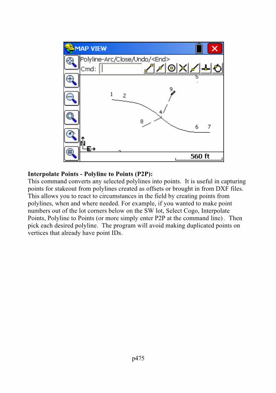
p475

Interpolate Points - Polyline to Points (P2P): This command converts any selected polylines into points. It is useful in capturingpoints for stakeout from polylines created as offsets or brought in from DXF files. This allows you to react to circumstances in the field by creating points frompolylines, when and where needed. For example, if you wanted to make pointnumbers out of the lot corners below on the SW lot, Select Cogo, InterpolatePoints, Polyline to Points (or more simply enter P2P at the command line) . Thenpick each desired polyline. The program will avoid making duplicated points onvertices that already have point IDs.

p476

The new points are shown in “large” format, for emphasis.

Interpolate Points - Divide Along Entity (DVS): This divides a polyline into the number of segments entered. A dialog will allowyou enter in the number of segments. There are settings to prompt for descriptionsand elevations and to create points at the end points of the polyline.

p477

The command will create new vertices along the polyline, but can also create pointnumbers starting at the entered Point ID, and you can elect to be prompted fordescriptions and/or elevations at each new point. If a property line were dividedinto two segments, you would create three new points.

Interpolate Points - Interval Along Entity (DVI):

p478

This divides a polyline by the distance entered. Curves can have a differentinterval. There are settings to prompt for descriptions and elevations and to createpoints at the end points of the polyline.

This command is often used for creating points on centerlines. Note the programresets the interval at break points like PI ’s and PC’s.

p479

Triangle Calculator (TC): Goes directly from the MAP view to the Triangle calculator. See COGO -Calculator for detail.

Curve Calculator (CC): Shortcut to the curve calculator, then returns to MAP. See COGO - Calculator fordetail.

Area (AR): This will report the area of any picked polyline. If you pick an unclosed polyline,the program will draw a temporary line for the closing segment and report the area.

Hinged Area (HA): This command can be used to determine the dimensions of a figure when the areais fixed and three or more sides are known. The figure must be defined by a closedpolyline. After executing the command, select the polyline. Next, select the hingepoint, the polyline segment clockwise from your hinge point will be the segment tomove. SurvCE will then ask you if you want to keep the existing polyline. If youanswer Yes, a new polyline with the desired area is created, if you answer No, thepolyline you pick is modified. Next, the current area of the polyline is shown. Atthis point, enter the new area in the units specified under Job Settings. (If yourunits are set to feet, the area will be specified in square feet). See the top figurebelow.

p480

p481

Note how the hinged side occurred on the clockwise side of the polygon perimeter(side 57 to 43). If we erase the new polyline, reverse the original polyline (RV)and repeat the command, this time answering “No” to “Keep existing” and againtargeting 24000 s.f. area, we get the following:

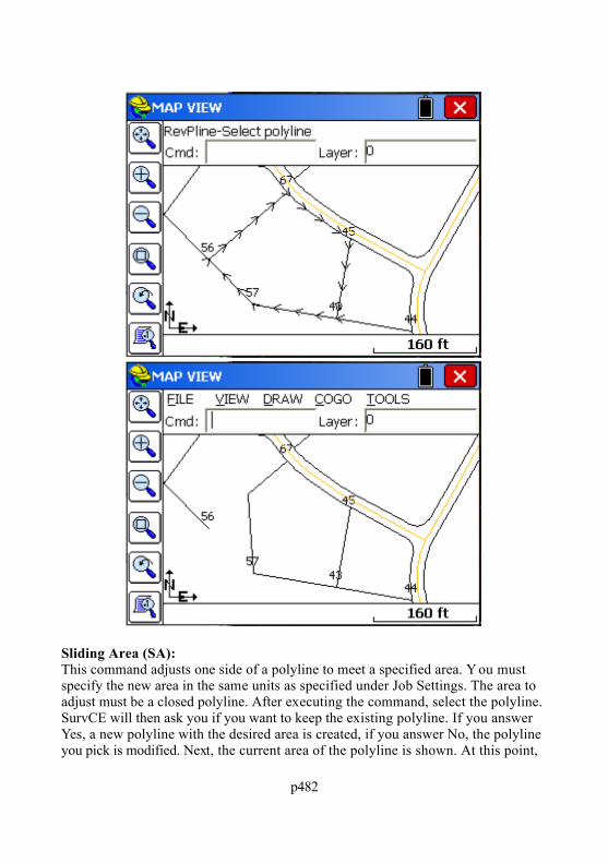
p482

Sliding Area (SA): This command adjusts one side of a polyline to meet a specified area. Y ou mustspecify the new area in the same units as specified under Job Settings. The area toadjust must be a closed polyline. After executing the command, select the polyline.SurvCE will then ask you if you want to keep the existing polyline. If you answerYes, a new polyline with the desired area is created, if you answer No, the polylineyou pick is modified. Next, the current area of the polyline is shown. At this point,

p483

enter the new area in the units specified under Job Settings. (If your units are set tofeet, the area will be specified in square feet). Let's choose to divide our newparcel into two equal areas of 12,000 square feet each.

p484

Slope Report (SR): This command reports the horizontal area along with the slope area of a figuredefined by a range of points. The command actually executes theTRIANGULATION command to compute the slopes within the defined area.There are options to include breaklines, use a predefined TIN model, and promptfor inclusion/exclusion areas.

Consider the figure defined by points numbered 570, 97, 569, 584, 585, 75, andback to 570 as shown below. From the COGO AREA command, we see that thehorizontal area of the enclosing polygon is 11,653.4122 Sq Ft. Performing theSLOPE REPORT yields the same horizontal results, but also reports the slopearea, and the maximum, minimum, and average elevations and the average slopewithin the area.

p485

p486

Bearing & 3D Distance (3D): This command reports the horizontal distance, elevation difference, slope distance,vertical angle, percent slope, slope ratio, bearing and azimuth between two 3Dpoints. The user can pick or enter the number of two points, select a polylinesegment or pick two points on any polylines from MAP.

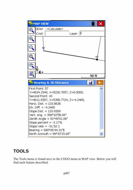
p487

TOOLSThe Tools menu is found nex t to the COGO menu in MAP view. Below you willfind each feature described.

p488

Polyline to CL (P2CL): Converts any polyline into a centerline file for use in the Roading commands andin Centerline, Curve and Offset Stakeout. You will be prompted for startingstation and you will obtain a centerline report. Use Reverse Polyline (RV ) andrepeat the command to change the direction of the stationing. If we choose theexisting polyline as shown, we obtain the following CL file report:

p489

CL to Polyline (CL2P): This command draws a POLYLINE entity using the data from a centerline file. You can practice this command by selecting the file Demo.cl, provided with theprogram.

Convert Polylines to 2D (C2D): Pick any 3D polyline and convert it to 2D (elevations of vertices are set to 0).

Edit - Polyline (EDP): Remove vertices, insert vertices and update (alter) the coordinates of any vertex . For example, if we pick the centerline that was used above, we obtain the editdialog, with options to add or remove segments or arcs, edit curve information, etc.Saving changes updates the graphics on the screen.

p490

Edit - Input-Edit GIS Data (EGIS): This command allows you to input or edit GIS attributes associated with an entity.Select the entity from the screen or for the case of a closed polyline, pick inside thearea defined by that entity.

Only polylines (open or closed) can be selected. This command does not apply to

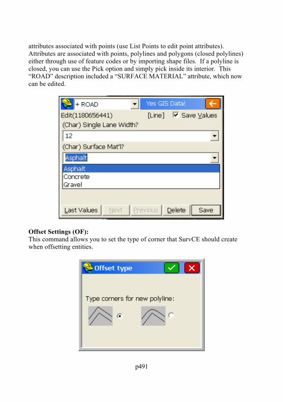
p491

attributes associated with points (use List Points to edit point attributes). Attributes are associated with points, polylines and polygons (closed polylines)either through use of feature codes or by importing shape files. If a polyline isclosed, you can use the Pick option and simply pick inside its interior. This“ROAD” description included a “SURFACE MATERIAL” attribute, which nowcan be edited.

Offset Settings (OF): This command allows you to set the type of corner that SurvCE should createwhen offsetting entities.

p492

Traverse Defaults (TD): This sets the elevation prompting (none, zenith, vertical, elevation difference),within the Traverse and Sideshot commands within the MAP view. Also enables aprompt for Instrument and Rod Height. Default setting is no instrument or rodheights and no vertical angle prompting, so inputs are simplified as angle/bearingcode, angle/bearing, distance, description, point number. Traverse and Sideshotentries within the MAP screen are stored to the RW5 file.

Note: 3D MODE must be enabled in Equip/Configure for this dialog to becomeactive. Otherwise, choices are "grayed out."

Triangulate & Contour (TRGC): Triangulate and Contour can create a final contour map based on user given data:points, polylines. This function has many options which are specified in its dialogbox. The routine will prompt also for inclusion and exclusion polylines. To deleteentities drawn with this command, turn off all of the drawing options andreprocess.

p493

Volume (VOL):Volumes can be computed by several methods, using point ranges and/or layers todefine existing and final surfaces. Perimeters can be used to further limit the areaof the volume calculation.

p494

Referring to the graphic below, which illustrates a stockpile, the “Final” pointrange could be defined as ALL points, and the “Original” point range could bedefined as the base points of the stockpile or points 1-15.

So using the settings above in the Volume routine, you would verify your two pointranges, then click OK. For example, the “Original” surface point range would beset as follows within the “Define” button for “Original”.

p495

Clicking OK moves forward to a shrink and swell factor screen. Only if you areset to English units do you get the option for tons based on a density factor. Inmetric units, the volume is presented in cubic meters.

Clicking OK continues on to the Volume Report.

p496

The report can be saved to a text file using the “Save to Disk” icon at the top of thescreen within “Volume Report”. Click the “Return” arrow to continue back to theMap screen. If you draw a 3D polyline perimeter connecting points with elevationrepresenting the outer limits of the volume calculation (using Draw, Polyline, 3D),then you can click on Inclusion and use the polyline as an inclusion perimeter. You can also use drawn elements on different layers as part of the volumecalculation, if they are 3D, by moving them over to the right-colume using the“Define” button. Volumes can also be conducted between “File” surfaces, TINfiles made with Triangulate & Contour or within the Volume command itself usingthe option “Save Surface to File.”

p497

Finally, if you are doing a stockpile and make the effort to put this outer perimeterin the “Perimeter” layer, then you can select the “Stockpile” option within V olumeand it goes directly to the shrink/swell factor screen and then to the report, withoutany other selections by the user. This is because the Perimeter layer will defineboth the inclusion perimeter and the original surface in this case.

p498

List Elevation (LELV): This command allows the user to pick on an entity and retrieve the elevation ofthat point.

Field to Finish (F2F): This command will redraw the linework created with Feature Codes based on thecurrent coordinates of the points. So if a GPS file was “processed” using a newlocalization, or a total station survey was adjusted, the ex isting linework made byuse of Feature Codes will erase and redraw by connecting to the adjustedcoordinates. In this way, polylines on the MAP screen created by field surveyingwill be redrawn to recapture their association with the adjusted point coordinates.

Place World Image:This command will attach an image database to the SurvCE drawing. Imagedatabases are georefenced aerial photography or image maps. These imagedatabases can contain mulitple large images that have been processed for quickdisplay in SurvCE. The boundary for the image-set is shown by a dashed line. Images are inserted in coordinate system and units of the image. Image databasesare processed with the Image X-Port utility of Carlson X-Port.

p499

p500

Tutorials

This chapter contains five tutorials designed to assist you in learning CarlsonSurvCE.

Tutorial 1: Calculating a Travers e (By Hand) with SurvCETo do a hand traverse with SurvCE, go to the MAP screen. To get there, click theicon in the upper right corner of your screen labeled MAP. Once there, you will setyour defaults for traversing.

Tutorial 2: Performing Math Functions in SurvCE Input BoxesVarious input boxes in SurvCE allow the user to calculate math functions"on-the-fly". The basic steps for getting started are shown here.

Tutorial 3: Performing a Compass Rule AdjustmentThis tutorial shows a compass rule adjustment, with various SurvCE screencaptures to guide you.

Tutorial 4: Defining Field Codes, Line/Layer Properties & GIS PromptingThis tutorial will assist users in defining Field Codes in SurvCE. SurvCE can haveone pre-defined FCL (Feature Code List) file loaded with the job coordinate CRDfile. The Feature Code List file stores pre-defined field codes that defineLine/Layer drawing properties and, optionally, GIS prompting. More than oneFCL file can exist, but only one can be loaded at a time per job coordinate CRDfile. The operator builds this FCL file using option 5 “Feature Code List” in theFile main menu.

Tutorial 5: Standard Procedures for Conducting GPS LocalizationsThis tutorial is intended to assist users with the recommended localization methodfor SurvCE. Other methods can be used, and it is up to the individual users todetermine which is best for them.

Tutorial 1: Calculating a Traverse (By Hand) withSurvCEIn order to do a hand traverse with SurvCE, go to the MAP screen by clicking theicon in the upper right corner labeled MAP. While in the map screen, select theMap Settings icon to set your Traverse Defaults

p501

.

Traverse Steps:

1 To begin, you must key in the command for inverse by typing “I”. This willestablish your occupied and backsight points. The command prompt willdisplay the following:

Cmd:Inverse - Tr/Ss/Pick point or point No2 Key in the backsight point number followed by the [ENTER] key.3 Key in the occupied point number followed by the [ENTER] key.4 Key “T” for Traverse or “S” for Sideshot followed by the [ENTER] key.5 If you keyed in “T” for traverse, the command prompt will be waiting for an

angle code by displaying the following:

Cmd:Traverse - eXit/I/Ss/Angle-BC(1-7)<7>

If you keyed in “S” for sideshot, the command prompt will also be waitingfor an angle code by displaying the following:

Cmd:Sideshot - eXit/I/Tr/Angle-BC(1-7)<7>

The code choices you can key in are as follows:

1 - Northeast Bearing

2 - Southeast Bearing

3 - Southwest Bearing

4 - Northwest Bearing

5 - Azimuth

6 - Angle Left

7 - Angle Right6 Key in the angle code of choice followed by the [ENTER] key7 Key in the angular value in the dd.mmss format followed by the [ENTER]

key.8 If you selected a vertical prompt under Traverse Defaults, then key in the

p502

appropriate value followed by the [ENTER] key.9 Key in the slope distance followed by the [ENTER] key.10 Key in the point description followed by the [ENTER] key.11 Press the [ENTER] key to accept the next available point number or key in

a new point number followed by the [ENTER] key.12 If you traversed, then you are now occupying the new point and are

backsighting the previous point of occupation. If you sideshot the newpoint, then you are still at the previous setup and ready to compute the nextpoint.

13 Options at the command prompt when presented with the messages listed instep 5 are as follows:

X - Exit

I - Inverse

S - Sideshot

T - Traverse

Note: in order to establish new occupied and backsight point information, youmust use the “I” (Inverse) command and define the backsight point first and theoccupied point second.

Tutorial 2: Performing Math Functions in CarlsonSurvCE Input BoxesMany input boxes in SurvCE allow the user to calculate math functions"on-the-fly".

To enter rod heights while in a GPS setup screen that is not in your current units(e.g. you’re using a 2 meter pole but working in U.S. feet), key in the following:

The Rod Height followed by “m” for Meters, “ft” for Feet and “ift” forInternational Feet followed by the [ENTER] key will convert the measurementinto your current units (e.g. 2m = 6.5617).

To compute the azimuth from one point to another to automatically enter in theazimuth while using the Point by Direction option in Point Store, key in thefollowing:

p503

Point ID,Point ID (e.g. "1,2")

To add or subtract a value from the computed azimuth, key in the following:

Point ID,PointID+Angle (e.g. "1,2+90")

Or

Point ID,Point ID-Angle (e.g. "1,2-90")

Tutorial 3: Performing a Compass RuleAdjustmentIn the example below, as shown in the next figure, the traverse was performed byoccupying point 1 located at the NW corner of the block. The initial backsight wasestablished by azimuth, measured and stored as point 2 shown NW along thehanging leg. Angles and distances were measured in a clockwise direction. Pointnumbers 6 and 1 are at the same location and point numbers 7 and 2 are at thesame location. This method allows for the closing of the angles and themeasurement of all traverse legs.

Process Raw FileSelect “Process Raw File” from the “COGO” tab, as shown below in this figure.

p504

Select Raw FileThe next figure below shows the standard Windows file selection dialog. Select theRW5 file you want to process followed by the “OK” button.

Select “Compass” from the adjustment options dialog box as shown in this figurebelow.

p505

Reference Closing PointKey in the initial occupied point number for the “Reference Closing Point #:” andtoggle on the “Apply Angle Balance” option, followed by the “OK” button, asshown in the next figure below.

Closed TraverseIn a closed traverse scenario, the reference closing point will always be your initial

p506

occupied point name.

Note that you will need two known points, or one point and a known azimuth, for aclosed traverse. The angle balance point will be the same location as the originalbacksight and will not be adjusted.

Open TraverseIn an open traverse scenario, the reference closing point will be a stored pointname or coordinates that represents the known values for the last occupied point inthe traverse.

Note that you will need two known points, or one point and a known azimuth, atthe beginning and at the end of an open traverse; one point at the end will be usedto close on and other will be used for angle balance (when Angle Balance isapplied). The angle balance point will be the same as the last foresight point in thetraverse and will not be adjusted.

Traverse PointsYou’ll notice in the Angle Balance Measurement figure below, since you keyed inthe data yourself, that the number of traverse points in this survey is 7. Since point7 was only measured to avoid and record the closing angle balance measurementby hand, in this example the traverse is only from points 1 through 6. Replace the7 in the “Ending Point Number” input box with a 6, as shown in this next figureimmediately below, followed by the “OK” button.

Note that point 6 should be the same location as point number 1 in a closedtraverse.

p507

Angle Balance

Select the foresight shot from the last occupied point to the original backsightlocation. In this example we would select the leg measured from point 6 to point 7,since point 7 was our foresight angle balance shot to point 2. Press the “OK”button. In an open traverse, this would be the measured leg that represents theknown azimuth or bearing at the end of the traverse.

p508

Reference Closing Angle

Finally we need to provide the reference closing angle (record). This is the originalbacksight azimuth. Key in point 1 and point 2, or key in the known azimuth orbearing, followed by the “OK” button.

In an open traverse, key in the stored point numbers that represent the values forthe known control points at the end of the traverse, or key in the known azimuth orbearing.

The adjustment report should be presented, and the adjustment should becomplete. The angle balance point number 7 will not be adjusted to fit pointnumber 2, and can be discarded.

p509

Tutorial 4: Defining Field Codes, Line/LayerProperties & GIS PromptingSurvCE can have one pre-defined FCL (Feature Code List) file loaded with the jobcoordinate CRD file.

The Feature Code List file stores pre-defined field codes that define Line/Layerdrawing properties and optionally GIS prompting. (More than one FCL file canexist but only one can be loaded at a time per job coordinate CRD file.)

The operator builds this FCL file using option 5 “Feature Code List” in the Filemain menu. See the figure below.

p510

After you select 5 Feature Code List, the following Code List pop-up box isdisplayed. See the figure below.

FCL (Feature Code List) files can be created, edited or reviewed on a PC usingCarlson X-Port or any Carlson Surveying office software. (SurvCE’s FCL file isequivalent to Carlson’s Field-to-Finish FLD Table used in their PC office software. Transfer all PC Field-to-finish FLD table files using SurveyCOM or Carlson

p511

Export. Select the Field Code Table option to upload the FLD file to SurvCE as aFLC file.)

Defining Field Code Line/Layer PropertiesTo define codes with line/layer drawn features and, optionally, GIS prompting,select in the Code List pop-up box “Add” (as shown in the previous figure). Thefollowing Add Code pop-up box allows the operator to define Field CodeLine/Layer drawing properties.

Code: Input one-word Field Code

Layer Name: Defines the layer the linework 2D & 3D will draw in usingStore Points

Full Text: User defined full text description for code

Polyline On: Yes or No defines to draw or not to draw between similar codese.g. EP, EP1

Polyline is 3D: Yes or No Yes draws in 3D, No in 2D

New Attributes: This highlights after inputting all the Line/Layer drawingproperties

p512

The following EP code has been input in the FCL file. When Surveying usingStore Points in the Survey menu, inputting field codes EP, EP1, EP2 and so on willdraw 3D Polylines between these similar codes in the EOP layer. A 3D Polylinewill be drawn in real-time when collecting data and inputting EP or EP# codes inSurveyed points descriptions.

As mentioned above, “New Attributes” becomes highlighted after inputting all theLine/Layer drawing properties. GIS prompting information can be added for thisfield code. If no GIS prompting is applicable for this field code, simply pick OKand create another field code, or exit and store the FCL file.

Defining Field Code GIS PromptingTo add GIS prompting to a defined Line/Layer code, select “New Attributes”. Thisbutton can be seen in the above figure at the bottom of the dialog. The followingGIS Feature pop-up box is displayed. See the next figure below. To define GISprompting for the EP field code, select “Add” in the Feature dialog shown below.The next pop-up box that appears, titled New attribute, is then displayed (shownbelow, underneath the Feature dialog). The New attribute dialog creates GISprompting.

p513

Load will load any existing Field Code GIS prompting for reuse. Edit reviews orrevises existing GIS prompting. Add creates individual GIS prompting, as shownin the figure immediately above (New attribute dialog). Remove deletes anyhighlighted GIS attribute. Up and Down reorders the sequence of GIS attributeprompting. Save stores input or edited GIS prompting and exits to Line/Layerdrawing properties.

p514

Defining GIS Prompting

Feature Code Name: No spaces GIS title for database

Codes: Special codes, e.g. Date, Time, Lat, Long.

GIS Prompt: Including spaces full name for GIS

Default Value: Most common GIS value/default value

Set: Lets the operator highlight and select the default value if there is a List ofattribute Values.

Type: Offers 4 options CHAR, INT, REAL and Code. Code Type will defaultto character type corresponding to special Codes. Codes can be Char, Int. orReal automatically.

Req: Requisite/required entry. Operator cannot leave any GIS prompt emptywhen this field is set to Yes.

To add GIS attribute prompting for List Values, select the “Add” button within theNew attribute dialog, as shown immediately below. The figure below that showsthe New value pop-up box. The operator inputs, after selecting Add again, foreach possible material (e.g. macadam, concrete, brick, stone cobbles and so on).

p515

The data input for all GIS List Values is shown in following figure below. Notethat Macadam is highlighted and will be the default value. If there are more thansix attribute List Values, scroll bars will appear. This defines only one GIS entryMaterial for the EP field code. Each GIS prompt for the field code EP (e.g.Material, Location, Condition, Width, Slope and so on) will require being createdusing Add in the Feature pop-up box, as shown earlier in this tutorial.

Add, Remove, Up and Down pertain to GIS List Values prompting. Add andRemove create or delete List Values entries. Up or Down reorders the highlightedList Value up or down. OK exits the GIS prompting screen retaining the GIS

p516

prompting entries and Cancel exits and discards all new inputs. The completed GISfield code for EP is shown below in the Feature dialog.

With all of the GIS Features input – Material, Location, Condition, Width andSlope – the operator can now select Save to store the GIS prompting for the fieldcode EP. When storing points in the Survey menu in Store Points with EP or EP#,3D linework when ended will prompt for EP GIS data as defined here. If 2D or3D linework is created the GIS data will be attached to the linework. Note thatLocation, Condition and Width are required input GIS fields. Load allowsselecting any existing field codes GIS prompting for reuse. Edit reviews or revisesexisting GIS prompting. Remove deletes highlighted GIS attribute prompting. The Up and Down buttons will reorder GIS attribute prompting. Save stores andexits.

Importing & Exporting GIS Information from SurvCESurvCE imports and exports ESRI SHP files. SurvCE solely uses ESRI SHP filesto interface with all GIS programs. ESRI SHP files are open architecture and are awidely used and accepted GIS format for most common GIS packages. To importor export GIS data to or from SurvCE, select in MAP – File – SHP File – Importor Export SHP File (Quick Import or Export only reads and writes the drawingentities and doesn’t include the GIS info). There are two figures later in thistutorial that depict this.

p517

SurvCE Creates Three ESRI GIS Drawing Objects: Points, Arcs (Polylines)and Polygons (Closed Polylines)There are only three types of drawing entries in ESRI SHP files points, arcs (open2D or 3D Polylines) and polygons (closed 2D or 3D Polylines). The EP field codecreates points and arcs and/or polygons. GIS information is stored only to the arcsor polygons and not the EP points. All GIS information for EP will be attached tothe 3D Polylines. The second Field Code UP in the FCL job file creates pointsonly with no linework. The UP field code attaches GIS information to the UPpoints. See the next two figures below.

p518

Save Feature Code List FileWith two field codes (EP and UP) with GIS information input and stored, usingoption 5 “Feature Code List” (in the File main menu), let’s collect some Surveydata in Store Points with GIS information. First, Save As these two codes into aFeature Code List file, as shown below.

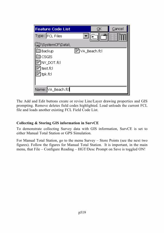
p519

The Add and Edit buttons create or revise Line/Layer drawing properties and GISprompting. Remove deletes field codes highlighted. Load unloads the current FCLfile and loads another existing FCL Field Code List.

Collecting & Storing GIS information in SurvCETo demonstrate collecting Survey data with GIS information, SurvCE is set toeither Manual Total Station or GPS Simulation.

For Manual Total Station, go to the menu Survey – Store Points (see the next twofigures). Follow the figures for Manual Total Station. It is important, in the mainmenu, that File – Configure Reading – HGT/Desc Prompt on Save is toggled ON!

p520

For GPS Simulation, go to the menu Survey – Store Point (see the next twofigures) and follow figures for GPS Simulation.

p521

See these Manual Total Station example screen captures, shown here in the nex tfour figures.

p522

p523

GPS Simulation screen capture examples are shown in these nex t four figures.

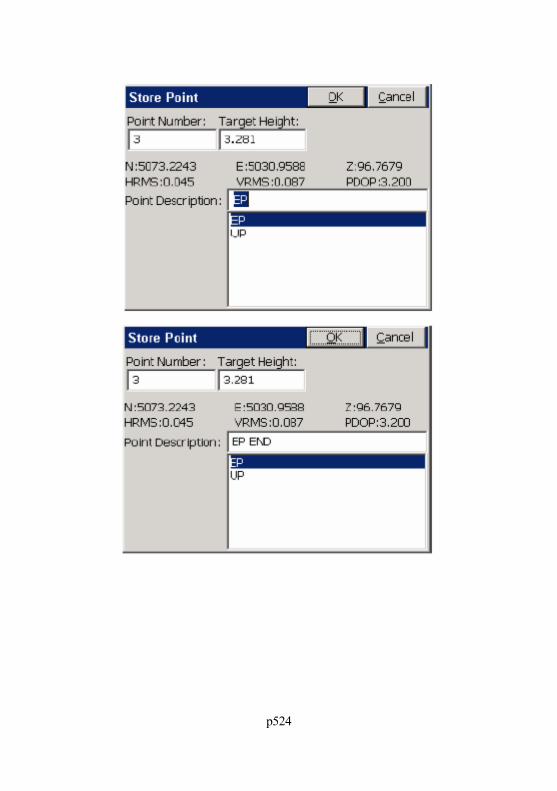
p524

p525

The sequence of shoots started with G PS Simulation storing points 2 and 3 as EPcodes. Point 3 was stored as EP END. A 3D Polyline was drawn between 2 to 3and GIS prompting popped-up after point 3 was stored shown above. Note in theCondition field the operator input data not found in the default settings. Point 4was stored using manual total station as a UP point code. Point 4 ’s UP GISprompting appeared after point 4 was stored. Points 5 through 7 were stored as aclosed polygon. This was done by storing point 7 as EP1 CLO to close back to thestart point 5 of the EP1 3D Polyline. The GIS prompting appeared for EP1 (not

p526

shown) and entered. The last sequence above was to ex it Store Points and selectMAP.

Editing GIS Information on Arcs and Polygons – Input-Edit GIS DataTo edit existing GIS information stored on Arcs (2D/3D Polylines) or Polygons(closed 2D/3D Polylines) in the MAP pop-up box, select Tools – Edit – Input/EditGIS Data, and pick any polyline or polygon. There are two figures below. The topfigure shows how the closed 3D Polyline between points 5, 6 and 7 was selectedusing this command. GIS data for the closed 3D Polygon is shown in the secondfigure.

The above figure displays the nex t EP code EP2 stored using GPS Simulation. When ended with a END or CLO description after EP2 SurvCE will prompt for EPGIS data to attach to the polyline as defined above.

p527

The figure above displays the ease of reviewing, creating or editing GIS data usingInput-Edit GIS Data. From the MAP screen Input-Edit GIS Data was selected andthe closed 3D Polyline picked on the screen. The GIS data stored prior wasdisplayed for review or editing. Any data point, polyline or closed polyline couldbe selected using the Input-Edit GIS Data command in MAP and new GIS attachedto this entity or existing GIS data reviewed and edited.

Editing GIS Information on Points using Lis t PointsInput-Edit GIS Data only works creating, reviewing or editing GIS information onArcs or Polygons. To create, review or edit GIS information on points use ListPoints shown below under File – 3 List Points.

p528

Highlight point 4 and select Edit (see figure immediately above). Point 4 is theonly Surveyed number with GIS data stored to the point. The Edit Point pop-upbox appears, and can be seen in the next figure below. To create, review or editGIS information select Input/Edit Attributes (See Figure 9-32).

Note: At the +UP box on top the down arrow can be selected and one or moreGIS field codes could attach GIS data to this same point. Points, Arcs or

p529

Polygons can all have one or more GIS field codes attached to these entities.

Exporting SurvCE GIS Data as ESRI SHP files

p530

These final two figures, above, display the exporting of our VA_Beach MAP andGIS data. The ESRI SHP file consists of 9 points, 2 arcs and 1 polygon (closedpolyline). Only one point, point 4, has UP GIS data. Two arc polylines and onepolygon have EP GIS information attached. Note that Include special attributes ischecked. This adds to polyline arcs and closed polygons the polylines length andarea to the GIS data automatically. Process with Export All checked stores the

p531

VA_Beach three SHP files automatically to a user defined subdirectory and afourth SHP file with 8 points without GIS data.

Tutorial 5: Standard Procedures for ConductingGPS LocalizationsThis tutorial is intended to assist users with the recommended localization methodfor SurvCE. Other methods can be used and it is up to the individual users todetermine which is best for them.

File ExtensionsLocalization File: *.datGeoid Model File: *.gsfCoordinate File: *.crdRaw Data File: *.rw5

ProjectionsIt is essential that the proper plane coordinate projection is selected prior tocreating a localization file. This should be the first step performed during thecreation of the job file and be performed easily through File Job Settings GPS.

Geoid ModelAn important item to note is if the user intends to use a geoid model (typical forlocalizations that contain less that 3 control points), the geoid model must beapplied prior to the creation of the localization file.

A local portion of the geoid grid must be extracted from the Carlson Geoid Modelusing Carlson X-Port, SurvCOM, Survey or Civil/SurvCADD, and the geoidmodel file must be installed prior to the creation of the local geoid file. It is alsohighly recommended that the local geoid file grid size does not exceed 100 miles.

Web Link to the Geoid Fileshttp://update.carlsonsw.com/public/CarlsonGeoidGrids.exe

Transfer or Enter the Known (local) PointsIt’s a good idea to simplify the process by transferring the known (local) points tothe data collector prior to going to the field. Conversely, the user can keyboard

p532

enter the known coordinates for these points into the CRD file, one at a time, usingFile List Points Add. It is not recommended that the user keys in the localcoordinates from within the localization process as transpositions can occur easily.However, this can be done as well.Collect the GPS Locations with AveragingUsing the Survey Store Points routine, specify your point ID. It is good to usesomething that will relate to the original known point. Example, if the known pointfor the first control point is 1, then you may want to collect the measured locationas 1001.Use the average reading icon <A> to collect several epochs of data at each point.Typically when using a 1 Hz receiver, 10 to 30 readings will be collected to ensurethat the RTK solution is consistently reporting the same position for 10 to 30seconds. On a 5 Hz receiver, the user may want to collect 50 or more readings as50 readings would be 10 seconds.Create the Localization FileOnce the data collector has points that represent the known (local) coordinates andthe measured data for these points, the localization file can be created.Select Equip Localization Add to enter each point into the localization file.Local PointThe first dialog presented to the user will be the Local Point dialog shown below.Enter the known (local) coordinate point ID or coordinates. If the point does notexist in the CRD file and coordinates are entered into this dialog, do not enter apoint ID. Select OK when the known (local) position has been defined.

p533

GPS CoordinatesThe next dialog presented will be the GPS Coordinates dialog shown below. Sincethe measured locations for each point has already been recorded, the user will wantto use the option From Raw File in this dialog. Select OK to continue.

p534

Surveyed PointNext, the user will be presented with the Surveyed Point dialog shown below (topimage). This dialog allows the user to select or enter the GPS measured point thatrepresents the known (local) point. If the user selects the GPS measured pointusing the list icon, they should ignore the current coordinates displayed in the ListPoints dialog shown below (bottom image), as they only reflect the non-localizedposition at this point. The important thing to remember is that if the local point was1, and the GPS measured point was 1001, the user must enter 1001 in this dialog.

p535

Save the Localization File

p536

Once all of the points have been added to the localization dialog, save thelocalization file before exiting using the Save button.Reprocess Raw File and Update CoordinatesAt this point all of the coordinates in the CRD file that represent the measuredpositions need to be updated to reflect the newly created localization. To do this,select COGO Process Raw File and process the raw file through the localizationfile. This will update the previously measured GPS points. Verify that the positionslook valid by viewing the points in File List Points. You should be able tocompare the known and measured positions to see if they look right. Depending onthe localization method, the measured values may not be exactly the same as theoriginal known positions due to error that may have existed in the originalpositions.Additional GPS MeasurementsOnce the localization is defined, all of the GPS points measured after its creationwill be recorded to the CRD file based on this localization.Changing the LocalizationIf the user determines that they want to redefine the current localization during ajob, they must reprocess the entire raw file after making any changes to thelocalization file. It may be prudent to simply define a new localization file fromscratch, leaving the original intact, and reprocess the raw file through this newlocalization file. Just remember that the last localization loaded, will be the currentlocalization.Selecting Projections for use in LocalizationWhenever you select a projection or coordinate system, you can place it in a “mostused” list of coordinate systems to choose from under the GPS tab in Job Settings. This list can contain one projection system or many different systems the userselects.

p537

This is a special list of either predefined (eg. KY North NAD83) or user-definedcoordinates systems. To get the list started or add to the list, select Edit ProjectionList and click Add Predefined. In the U.S., for example, surveyors might want tokeep the UTM (WGS84) system plus the NAD83 and NAD27 “state plane” zonesin the list for quick access, covering the region of your work. European and otherworldwide zones can be added. When setting up a UTM selection, you can chooseyour zone, referencing the graphic below for the US:

p538

You can see a map of the UTM zones online at:

http://www.dmap.co.uk/utmworld.htm

To edit the list of saved projections, click on Edit Projection List. Here we select auser-defined UTM system from the list to Delete or Edit.

p539

Choosing Edit will bring you to the screen below:

From this screen, you can select the Projection calculation method as well ascalculation parameters. Projections include: Lambert Conformal_Conic_2SP, Transverse_Mercator, Oblique_Sterographic (Double), Lambert_Conformal_Conic_1SP,

p540

Oblique_Mercator_83, Stereographic, Oblique_Mercator_27, Transverse_Mercator_OSTN02, Oblique_Stereographic_RD2000, Oblique_Mercator, Cassini_Soldner, Transverse_Mercator_27, Lambert_Conformal_Conic_27, Transverse_Mercator_Alaska_27 Transverse_Mercator_34.

You may also use the buttons on this screen to edit the ex isting datum or create anew datum definition.

The Datum definition screen is where you select the ellipsoid and Helmertparameters to apply.

If you select Add User Defined within the Coordinate Projection List screen, youproceed to the screen below:

p541

Here you enter the name of the new system and select the projection type andparameters, or you can “Load File” to load a pre-defined system stored earlier (inthe form *.sys or *.csl).

If you select “Add Predefined” to create a new, stored projection system, you willbe presented with this screen:

p542

Here you can select the country and then the corresponding system for your area. There is a very extensive list of European and Asian systems including in the list.

The “quick-access” short list of most used projections enhances job efficiency.

p543

Instrument Setup by Manufacturer

Total Station (Geodimeter/Trimble)The following information describes the various options available for theGeodimeter 600 and Trimble 5600 total stations. It's important to note thatfirmware 696-03.xx or later is required. To check firmware version, select Menu 5,4, 1 on the instrument.

CommsGeodimeter/Trimble default communication settings in SurvCE are 9600,8,None,1.To check these settings on the instrument, do the following:

1. Select MNU, ENT, 4 (Data com), 1 (Select device), 2 (Serial) 2. At prompt “Serial ON?”, select ENT 3. Verify COM=1.8.0.9600 followed by ENT

The software allows you to run the instrument in several modes, depending on thecapabilities of the instrument. Selecting a model that says DR informs the softwarethat the instrument is a reflectorless (Direct Reflex) model, and the reflectorlessEDM mode will be made available.

Settings/Search (Station)If the instrument is not robotic or you want to operate it as a standard total station,the Station mode should be used.

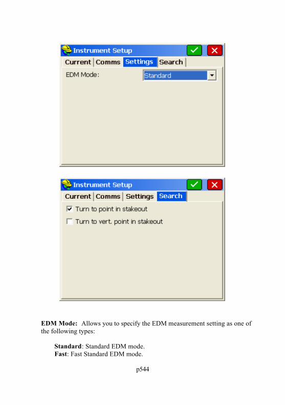
p544

EDM Mode: Allows you to specify the EDM measurement setting as one ofthe following types:

Standard: Standard EDM mode.Fast: Fast Standard EDM mode.

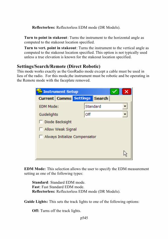
p545

Reflectorless: Reflectorless EDM mode (DR Models).

Turn to point in stakeout: Turns the instrument to the horizontal angle ascomputed to the stakeout location specified.

Turn to vert. point in stakeout: Turns the instrument to the vertical angle ascomputed to the stakeout location specified. This option is not typically usedunless a true elevation is known for the stakeout location specified.

Settings/Search/Remote (Direct Robotic)This mode works exactly as the GeoRadio mode except a cable must be used inlieu of the radio. For this mode,the instrument must be robotic and be operating inthe Remote mode with the faceplate removed.

EDM Mode: This selection allows the user to specify the EDM measurementsetting as one of the following types:

Standard: Standard EDM mode.Fast: Fast Standard EDM mode.Reflectorless: Reflectorless EDM mode (DR Models).

Guide Lights: This sets the track lights to one of the following options:

Off: Turns off the track lights.

p546

Low: Turns on the track lights on low power.High: Turns of the track lights on high power.

Allow Weak Signal: This will allow the instrument to return a distance whenthe signal is weak.

Always Initialize Compensator: This will reset the compensator every timethe instrument is restarted.

Search on Read: This setting will force the instrument to perform a searchbefore initiating a reading if the instrument is not locked on the prism.

Diode Backsight: This setting allows the user to specify if the backsight hasan active diode prism or not.

Horizontal/Vertical Range: These input boxes allow the user to specify therange to search for the prism when a search function is initialized.

Minimum/Maximum Distance: Determines the range by distance that theinstrument will search for or track a prism.

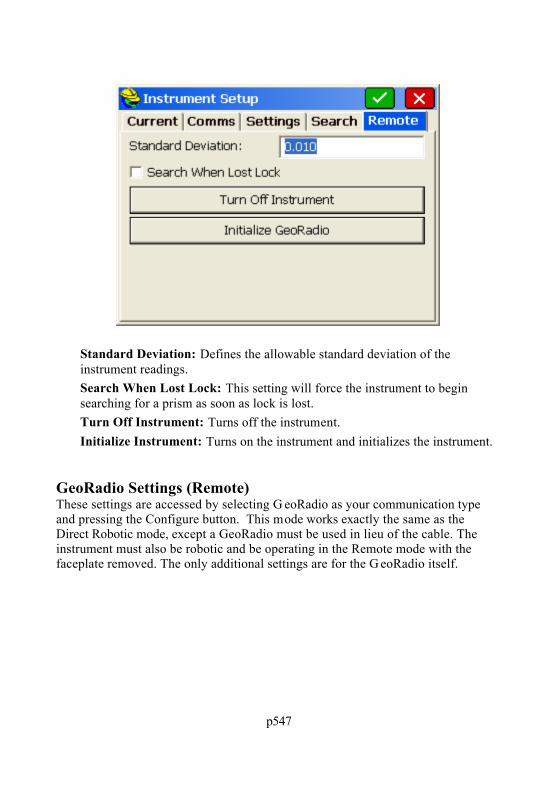
p547

Standard Deviation: Defines the allowable standard deviation of theinstrument readings.

Search When Lost Lock: This setting will force the instrument to beginsearching for a prism as soon as lock is lost.

Turn Off Instrument: Turns off the instrument. Initialize Instrument: Turns on the instrument and initializes the instrument.

GeoRadio Settings (Remote)These settings are accessed by selecting G eoRadio as your communication typeand pressing the Configure button. This mode works exactly the same as theDirect Robotic mode, except a GeoRadio must be used in lieu of the cable. Theinstrument must also be robotic and be operating in the Remote mode with thefaceplate removed. The only additional settings are for the G eoRadio itself.

p548

Channel: Specifices the channel of the GeoRadio. Station Address: Specifies the station address of the GeoRadio. Remote Address : Specifies the remote address of the instrument's radio.

Putting the 600 in the “Remote Mode”1. # Power the 600 on.2. # Answer the initial questions.3. # If you have not selected the Radio Channels and Address, do the following:4. # Press <Menu>.5. # <1> for Set.6. # <5> for Radio.7. # Select Channel (1-8).8. # Select Station Address (1-99).9. # Select Radio Address (1-99).10. # Press <RPU>.11. # Press <3> for Remote.12. # Press <1> for OK.13. # Press <No> for Sector.14. # Press <No> for Measure Ref Object.15. # Press any key when prompted. You do not have to remove the keyboard as

prompted unless you are using the Direct Robotic option instead of GeoRadio.SurvCE will control the total station.

p549

Total Station (Leica TPS Series)This series covers most of the current Leica total stations such as TPS 100, TPS300, TPS 700, TPS 700 auto, Builder, TPS 400, TPS 800, TPS 1000 (includingTC1010 and TC1610,) TPS 1100,and TPS 1200. For the older 600 and 900, turnoff ATR and use the TPS 100/300 configuration. Many of these units include the“motorized” option. Some settings may vary by model.

Comm Setup: Default settings for these instruments are a baud rate: 19200,none parity, Char Length: 8 and Stop Bits:1

Instrument Series: Instruments supported are TPS 100, TPS 300, TPS 700,TPS 700 auto, Builder, TPS 400, TPS 800, TPS 1000 (including TC1010 andTC1610,) TPS 1100,and TPS 1200

Read Method: The available read methods are Fast, Tracking, User-Defined,and Reflectorless. The default setting is Fast. The "Standard" optionproduces a 3-second reading while the “Fast” setting produces a 1-secondreading. One application of Reflectorless is to toggle between a 0 prism offset(shooting a rock face or brick wall) versus shooting a prism with a non-zeroprism offset. When set to Reflectorless, the rod height and prism offsetautomatically change to zero. When returned to Standard, the previousnon-zero prism offset is recalled, and the original rod height is restored. Turn

p550

to Point for stakeout and PowerSearch are disabled in Reflectorless mode. The Read Method (Std, Fast, Reflectorless) will appear in the upper right ofthe graphic screen for most types of Leica total stations, in commands such asStore Points, Stakeout Point, etc.

Foresight/Backsight Prism Offset : Here is the list of standard prism offsets.Note that Leica prisms default zero to equate to -34.4 mm. So a prism offsetof 34.4 equals a zero “net” offset. Whenever a prism constant is changed, anote is written to the raw (RW5) file. When you select one of the prisms fromthe list (Circle, Mini, etc), the value that is shown in parenthesis is the actualvalue sent to the instrument. i.e. 0.0 for Circular, 17.5 for Mini. If you select"30mm" or "40mm", - 4.4 and 5.6 are sent, respectively (30-34.4 and 40-34.4). You may also type in any value you choose. In this case, we will sendthat value exactly, unmodified, to the instrument.

23.1 (360): Leica Model 4.4 Mini (360) 34.4 (0mm) 0.0 (circle): Standard Leica round prism. 17.5 (mini): Leica mini prism. 34.4 (ReflTape): Equates to zero offset (wall, surface). 4.4 (30mm): Other manufactures (Sokkia, Seco). -5.6 (40mm): Other manufacturers.

Laser Pointer: Ideal for indoor or dark evening surveying, this feature causesthe instrument to emit a red beam. It is often used when doing reflectorlesswork and makes a red mark on the wall, floor or object being surveyed. Thisis usefule for confirming the position prior to the shot. The beam should notbe directed into someone’s vision or eye.

p551

Motorized: When this option is disabled, many other options will also not beavailable. These options are ATR, Power Search, Turn to Point in Stakeout,and Turn to Vertical point in stakeout.

ATR (Auto Target Recognition) : For the TPS 700, TPS 1000 and TPS1100, this option will find the prism after you point in the approx imatedirection. It searches over a fixed range of motion and detects all prism typesand locks on to the exact center of the prism. Saves “dial in” time.

Power Search Enabled: The Power Search option can be purchased with allmotorized Leica total stations. This option activates the “PowerSearch”button in the “banner line” at the top of the survey and stakeout screens. When Power Search is pressed, the total station will typically find the prism in10 seconds regardless of the direction it is initially pointed. If it has found oneprism and you hit “Power Search” again, it will leave that prism and find thenext one. If you have only 2 prisms on the job (foresight and backsight), it willconveniently rotate from the foresight to the backsight and back again eachtime it is pressed.

Turn to Point in Stakeout: This option should always be enabled with amotorized total station. In stakeout (with the exception of slope staking), theprogram knows the angle and distance to turn. When enabled, this feature willautomatically rotate to correct horizontal angle for the stake point. When on,the associated "Turn to Vertical Point in Stakeout" option will also be madeavailable. Turn to Point in Stakeout is disabled when in Reflectorless mode,since staking out should require the certainty of a prism placed vertically over

p552

the target point. Turn to Vertical in Stakeout : When auto-turning to stakeout points, you

have the option to turn horizontally but not vertically. If “Turn to Vertical” isdisabled, you would need to manually dial in the vertical position of the prismin stakeout. However, if rod heights are unchanging, this feature can beenabled, and will turn the gun to the correct vertical position as well, factoringin the current rod height setting.

For Leica TPS equipment that offers the reflectorless option, screens such as StorePoints and Stakeout now have a handy icon which, when toggled, switches fromnon-reflectorless to reflectorless and back. The button appears in both the graphicsand text modes of these screens. Rod heights and prism constants willautomatically be adjusted when switching from one mode to the other.

Leica 1200 RoboticThe new Leica robotic total station requires the activation of the “Ex tendedGeoCOM” option before it will allow the use of third party data collectionsoftware (i.e. SurvCE or Carlson Field).

Activation Information: The following information was provided by Leica indocument Su11-05G.

TPS1200 Instruments (TCA, TCP, TCRA, TCRP) require a special key codeto operate in Robotic mode when using an AllegroCE/RCS running SurvCEVersion 1.5. The following table lists the part number for the code:

Product Part Number DescriptionTPS1200 734754 GeoCOM Robotics License

Note: When ordering a TPS1200 Robotic Instrument, AllegroCE/RCS andSurvCE, you must order part number 734754 – this is a no charge item.

Procedures for Checking Activation Status : A simple way to determinewhether the “Extended GeoCOM” option is activated is to enter the Roboticsdialog of SurvCE and attempt a power search. If the instrumentcommunicates, but the power search feature fails, the "Ex tended GeoCOM"option is not activated. If you suspect that this is the case, you can verify thatthe feature is on in the instrument using the following steps:

o Power on the instrument.

p553

o Select the “User” button on the keyboard.o Select the F3 button for “STAT”.o Select list item number 3 for “System Information”.o Use the down arrow key to scroll to the bottom of the

“Instrument” page.o Verify that “Extended GeoCOM” is on.

Defining the Port: The Leica 1200 needs to know that you intend to use theGeoCOM interface through the external port. The following steps will set theLeica to communicate with SurvCE:

o Power on the instrument.o Select “Config”.o Select menu item 4 for “Interfaces”.o Arrow down to “GeoCOM Mode” and select F3 for “Edit”.o Select F5 for “DEVCE”.o Select “RS232 Geocom”o Select F3 for “Edit” and verify the communication settings.

Baud Rate: 19,200 Parity: None Data Bits: 8 Stop Bit: 1

o Select F1 for “STORE”.o Select F1 for “CONT” and verify the following option on the

GeoCOM Mode page: Use Interface: Yes Port: Port 1 Device: RS232 GeoCOM Protocol: RS232 GeoCOM

o Select F1 for “CONT”.o Verify that the only device active is RS232 GeoCOM and select

F1 for “CONT”.

Prediction Settings: The Leica 1200 has several prediction modes for whenthe instrument has lost lock. The following are the recommended settingswhile using SurvCE:

o Select 3 for “Manage”.o Select 5 for “Configuration Sets”

p554

o Pick New or Edit (Recommend New for First Time) New - Input Name, Desc and Creator Initials then F1

Store/Conto Select F1 for “CONT” 8 times until the "Automatic Prism

Search" screen appears.o Select the down arrow one time and set "After Prediction Search

With:" to "No Search" by tapping the right arrow key one time.o Select F1 for “CONT”.o Select F1 for “CONT” 2 more times until the "Interfaces" screen

appears.o Select the down arrow key to highlight GeoCOM mode and

press F5 for “Use”. Make sure no other mode is set. To toggleoff any other mode highlight and press F5 for “Use” to toggleoff.

o Select F1 for “CONT” 5 times to save and exit to the MainMenu.

TC1010/1610For the Leica TC1010/1610 series instruments, it's important that the followingsettings are true: Communications Settings (SurvCE & Instrument): 9600,7,even,1 Communication Mode: Make sure you set the instrument to communicate

RS232 mode, not module.

SurvCE Settings Instrument: Leica TPS Series Instrument Series: TPS 1000/1100

Make sure all of the toggles in the settings dialog are off.

Total Station (Leica Robotic)This series covers most of the current Leica standard total stations including theTPS 1000, TPS 1100 and TPS 1200 series. For best results, set the instrument toGeocom Online mode. From the Main Menu, go to Configuration/CommunicationMode/GeoCom Online Mode.

Comms

p555

The default communication settings are baud rates 19200, Parity None, CharLength 8, and Stop Bits 1.

Wireless Connection: Using the Juniper Allegro CE/RCS, a built-in radiomodem and internal antenna is included which permits wirelesscommunication with the robotic total station when using the RM2410 radio. This wireless connection is through the Leica propriety radio and does notinvolve Bluetooth per the Comm Setup screen. The Comm port for theinternal radio on the Allegro is COM 3. For one-man operation, the pole andprism become “freed” from wire connection and can be placed anywhere for ashot or reading, with the process driven “remotely” by the data collectorcommunicating with the robotic total station.

Settings/Search

p556

EDM Mode: Available methods are Standard (1.5 to 2 seconds), Fast, andReflectorless. In all modes of data collection, you are in “Rapid Tracking”mode. Clicking that icon goes to the “No Distance” or “Tracking Only Mode”(no distance measurements). Avoiding taking distance measurements willsave battery usage. So the “Dist” button refers to the selectable mode you will“go to,” not the mode you are currently in. In Rapid Tracking mode, the storeicon will always take a “Rapid Tracking” shot, and pressing enter will take aRapid Tracking shot if Enter is configured to Store only (to mimic the storeicon). Pressing the read icon will always cause configured reading to betaken, as will Enter when set to Read and Store. The next figure shows theRapid Tracking mode, which follows the movement of the prism by takingrapid distance measurements, much like RTK GPS.

Foresight/Backsight Prism Offset : This drop down menu provides a list ofstandard prism offsets. Note that Leica prisms default zero to equate to -34.4mm. So a prism offset of 34.4 equals a zero “net” offset. Whenever a prismconstant is changed, a note is written to the raw (RW5) file. When you selectone of the prisms from the list (Circle, Mini, etc), the value that is shown inparenthesis is the actual value sent to the instrument. i.e. 0.0 for Circular, 17.5for Mini. If you select "30mm" or "40mm", we send - 4.4 and 5.6 respectively(30-34.4 and 40- 34.4). The user may also type in any value they choose. Inthis case, we will send that value exactly, unmodified, to the instrument.

23.1 (360): Leica Model 4.4 Mini (360)

p557

34.4 (0mm) 0.0 (circle): Standard Leica round prism. 17.5 (mini): Leica mini prism. 34.4 (ReflTape): Equates to zero offset (wall, surface). 4.4 (30mm): Other manufactures (Sokkia, Seco). -5.6 (40mm): Other manufacturers.

Guide Lights: This setting causes the instrument to show flashing lights. Thismakes it easy to tell when the instrument has turned towards you in trackingmode. Can be set to Off, On, or Auto.

Laser Pointer: Ideal for indoor or dark evening surveying, this feature causesthe instrument to emit a red beam. It is often used when doing reflectorlesswork and makes a red mark on the wall, floor or object being surveyed. Thisis usefule for confirming the position prior to the shot. The beam should notbe directed into someone’s vision or eye.

Power Search Enabled: The Power Search option can be purchased with allmotorized Leica total stations. This option activates the “PowerSearch”button in the “banner line” at the top of the survey and stakeout screens. When Power Search is pressed, the total station will typically find the prism in10 seconds regardless of the direction it is initially pointed. If it has found oneprism and you hit “Power Search” again, it will leave that prism and find thenext one. If you have only two prisms on the job (foresight and backsight), itwill conveniently rotate from the foresight to the backsight and back againeach time it is pressed.

p558

Work Area: This will define a limiting area for searching. This can speedup both the standard ATR Search and the PowerSearch. The Work area angleranges apply to both searches. The Show button will show the two positionsof the search window, first by moving immediately to Position 1. Y ou will beprompted to press OK to see Position 2. Having defined a “window” ofsearching, Center will move that window to a new center position. Y ou willbe prompted to “Sight on Centered Position and Press OK”. The Definebutton prompts you to shoot the lower left and upper right positions, which arethen displayed above under “Work Area”. If the Work Area is set to start at0.0000 horizontal, for example, searching would send the instrument to thebacksight point.

Use ATR: When this feature is enabled, ATR (Auto Target Recognition) willbe used when configured to standard or fast reading. When running the roboticin remote mode with ATR turned on, and when performing a “Set Angle andRead” in the backsight screen (a standard measured backsight), the ATRconnection will be taken into consideration, so that the angle set is relative tothe center of the prism, not necessarily the crosshairs of the instrument. The“Set Angle” and “Check Angle” functions will still be relative to thecrosshairs.

Work Area Settings

More settings appear when you press the "Work Area Settings" button from theSEARCH tab.

p559

The upper left of the screen controls the ATR Search, and the upper right controlsthe PowerSearch. The Work area angle ranges apply to both searches. The Showbutton will show the two positions of the search window, first by movingimmediately to Position 1. You will be prompted to press OK to see Position 2.Having defined a “window” of searching, Center will move that window to a newcenter position. You will be prompted to “Sight on Centered Position and PressOK”. The Define button prompts you to shoot the lower left and upper rightpositions, which are then displayed above under “Work Area”. If the Work Areais set to start at 0.0000 horizontal, for example, searching would send theinstrument to the backsight point.

Tracking

The instrument can also easily switchin between tracking and non-tracking modefrom the store points screen by toggling the icon of the man in the upper right handcorner. In the image below, we are in tracking mode.

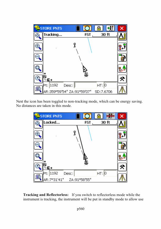
p560

Next the icon has been toggled to non-tracking mode, which can be energy saving. No distances are taken in this mode.

Tracking and Reflectorless: If you switch to reflectorless mode while theinstrument is tracking, the instrument will be put in standby mode to allow use

p561

of the tangent screws. For all Leica robotic total stations and for the Leica1200 Direct (TPS Series), the timeout for reflectorless mode is 30 seconds. You always have the option to Cancel from a reflectorless reading and if youdo, the measurement will not be automatically re-initialized.

Leica 1200 RoboticThe new Leica robotic total station requires the activation of the “Ex tendedGeoCOM” option before it will allow the use of third party data collectionsoftware (i.e. SurvCE or Carlson Field).

Activation Information: The following information was provided by Leica indocument Su11-05G.

TPS1200 Instruments (TCA, TCP, TCRA, TCRP) require a special key codeto operate in Robotic mode when using an AllegroCE/RCS running SurvCEVersion 1.5.

The following table lists the part number for the code:

Product Part Number DescriptionTPS1200 734754 GeoCOM Robotics License

Important Note:When ordering a TPS1200 Robotic Instrument, AllegroCE/RCS and SurvCE,you must order part number 734754 – this is a no charge item.

Procedures for Checking Activation Status : A simple way to determinewhether the “Extended GeoCOM” option is activated is to enter the Roboticsdialog of SurvCE and attempt a power search. If the instrumentcommunicates, but the power search feature fails, the "Ex tended GeoCOM"option is not activated. If you suspect that this is the case, you can verify thatthe feature is on in the instrument using the following steps:

o Power on the instrument.o Select the “User” button on the keyboard.o Select the F3 button for “STAT”.o Select list item number 3 for “System Information”.o Use the down arrow key to scroll to the bottom of the

“Instrument” page.

p562

o Verify that “Extended GeoCOM” is on.

Defining the Port: The Leica 1200 needs to know that you intend to use theGeoCOM interface through the external port. The following steps will set theLeica to communicate with SurvCE:

o Power on the instrument.o Select “Config”.o Select menu item 4 for “Interfaces”.o Arrow down to “GeoCOM Mode” and select F3 for “Edit”.o Select F5 for “DEVCE”.o Select “RS232 Geocom”o Select F3 for “Edit” and verify the communication settings.

Baud Rate: 19,200 Parity: None Data Bits: 8 Stop Bit: 1

o Select F1 for “STORE”.o Select F1 for “CONT” and verify the following option on the

GeoCOM Mode page: Use Interface: Yes Port: Port 1 Device: RS232 GeoCOM Protocol: RS232 GeoCOM

o Select F1 for “CONT”.o Verify that the only device active is RS232 GeoCOM and select

F1 for “CONT”.

Prediction Settings: The Leica 1200 has several prediction modes for whenthe instrument has lost lock. The following are the recommended settingswhile using SurvCE:

o Select 3 for “Manage”.o Select 5 for “Configuration Sets”o Pick New or Edit (Recommend New for First Time)

New - Input Name, Desc and Creator Initials then F1Store/Cont

o Select F1 for “CONT” 8 times until the "Automatic PrismSearch" screen appears.

p563

o Select the down arrow one time and set "After Prediction SearchWith:" to "No Search" by tapping the right arrow key one time.

o Select F1 for “CONT”.o Select F1 for “CONT” 2 more times until the "Interfaces" screen

appears.o Select the down arrow key to highlight GeoCOM mode and

press F5 for “Use”. Make sure no other mode is set. To toggleoff any other mode highlight and press F5 for “Use” to toggleoff.

o Select F1 for “CONT” 5 times to save and exit to the MainMenu.

Troubleshooting: If your Leica robotic total station has any communicationissues, it is typically a matter of verifying firmware and configuration settings. Investigate and note down the firmware version of the various components on yourinstrument.

Total Station (Leica/Wild Older Models)

Data Collector Model: Many of the older instrument could be set to operateas different models. These include T1000, T1600 and T2000 modes . SetSurvCE to match your instrument. Two different models are available forT1000 with a one-row keyboard, and T1000 with two-row keyboard. Choosethe appropriate one.

p564

Total Station (Nikon)Nikon 310/500 SeriesThis configuration covers such instruments as the Nikon 520, 521, 522 and 552.

Although the Nikon total stations have their own configuration, they also can beset to Sokkia emulation. If set to Sokkia emulation, they should be configured asSokkia Set. In this mode, you can turn on the “2-way” communication mode. Thisenables the Nikons to “turn to zero” in stakeout (set out) mode. In this setting,when you stake point 10 and the angle right to turn is 75 degrees, 15 minutes, theinstrument panel will display 75 degrees, 15 minutes, and as you turn towards thepoint, the display will count down to zero. So without looking at your datacollector, you watch the screen until you obtain zero degrees — this means you areon target. In a sense, the performance of the Nikon total stations is enhanced inSokkia emulation mode.

Nikon 800 SeriesThe 800 Series configuration will also apply to the older 700 series. To use thatproduct the user must select SET mode on the instrument and have the connectionspeed set at 1200 baud then select the Nikon 800.

Trimble TS415Users who own this instrument can use SurvCE by selecting the Nikon 800 Series

p565

configuration.

Total Station (Pentax)Pentax PTS3 SeriesFor Pentax instruments, select the "PTS3" checkbox if you are using a PTS3 seriesinstrument.

PTS3 instruments will first send out the last reading before sending the currentreading. For some users, you may wish to choose to record the 3rd reading for themost accuracy.

Pentax ATS SeriesThe following information outlines the settings for the Pentax ATS Seriesinstruments.

p566

This information was compiled using an ATS-105.

1. Power up the Unit & Level it up.

2. Set the baud rate in the instrument. Hold down the Blue “S” key and press thenumber 6 key in the upper right. This will open the Configuration Menu for BaudSettings.

3. Set the baud rate in SurvCE by selecting the Equip tab, and then select theComm Setup button. SurvCE defaults to 1200 / None / 8 / 1. Match the Baud,Parity, Char Length & Stop Bits with whatever the instrument is currently set to.

4. Connect the data collector, hold down the Blue "S" key and press the "F5"button. This puts the Total Station into Remote Mode for use with ex ternal datacollectors. [RM] blinks in the upper left corner.

NOTE: SurvCE has advanced options for setting the Read Method, Number ofReadings & use of the instrument lights. Not all models or firmware support thesefeatures. If these options do not work, you might be able to update the firmware, ormanually adjust the settings using the instrument.

p567

Total Station (Sokkia Set)

The following information describes the various options available for the SokkiaSet total stations.

1-Way vs 2-Way: The 1-Way option mimics the operation of most totalstation instruments using SurvCE.  The 2-Way option has the one bigadvantage of sending the angle to turn into the instrum ent during stakeout,so that looking at the instrument panel, you “turn to zero” to aim at thetarget point. It is recommended that Nikon instruments be run in SokkiaSet emulation mode, enabling the 2-Way communication.

EDM Mode: Available methods are rapid and fine. Target Offset: Enter the prism offset here. Zero Hz Angle to Target: This option specifies whether or not SurvCE will

set the horizontal angle of the total station to zero in the direction towards thestakeout point. When stakeout is completed, the horizontal angle is set back tothe original value. This option only applies to Sokkia total stations or to totalstations such as Nikon which have a “Sokkia emulation” mode.

The driver applies to all current Sokkia total stations, including the 110M when

p568

used in manual mode.  It also applies to many non-Sokkia instruments which havea Sokkia or “Set” emulation mode, including Nikon, Pentax and Topcon.  Theadvantage of Sokkia emulation is that the Sokkia driver includes a “2-way” settingthat will upload configuration settings into the instrument such as units, prismconstant and the backsight circle.  Most important, for stakeout, the “2-way”setting will upload the angle to turn, so that you turn to zero to get on target.  TheSokkia Series 30R is reflectorless.

The “On” key is the upper right, which takes you to the “Measure” screen where itis ready to work with SurvCE.  Commands would not be accepted, for ex ample, ifyou were in the “Config” screen.  Use the instrument to activate reflectorlessmode, and in SurvCE, be sure to set target height to zero.  The gun will controlprism offset in non-prism modes

Sokkia Motorized SeriesThis driver is necessary to utilize the motorized features of the motorizedinstruments.  For example, in stakeout, it will turn to the point automatically.  Themotorized features will turn to the appropriate horizontal and vertical angle in mostcommands when the instrument  is set to “Remote” mode.

p569

Note that baud rates on motorized instruments  must be set to 9600 in remote modebut are typically set to 1200 baud in direct mode.  Change on the instrument and inSurvCE, Equip, Com Setup. The Settings options for the motorized instruments areshown below:

p570

Joystick speeds are 1 to 6 (for arrow key response turning gun).  For reference 6 isapproximately 6 degrees per arrow press.  Search types are Sight (field of view ofgun, or 1 degree, 30 minutes or 10 meters at 100 meters), H Wide, V Wide andHV Wide.  The wide views are 6 times field of view.  Auto Search before Readfinds the prism center exactly before taking a measurement (useful in SetCollection, for example, and in Stakeout).  Run Remotely sets the left and right

p571

turning of the gun, referenced from the pole, and not from the instrument.  This isdistinct from left and right referencing for stakeout which refers to movement ofthe rod.  For the Sokkia instruments with RMC search device, there are 2 buttonsin the joystick screen for RC Search:  “RC Left” and “RC Right”.  Left and rightwill be determined by the Run Remotely setting.

Total Station (Sokkia Robotic)

The following information describes the various options availablefor the Sokkia Robotic total stations.

The instrument  “Measure” screen should be shown on the totalstation in order to work with SurvCE.  Commands will not beaccepted, for example, if you were in the “Config” screen.

Note that baud rates on the Sokkia robotic  must be set to 9600.  TheSettings options for the Sokkia robotic are shown below:

p572

Joystick speeds are 1 to 6 (for arrow key response turning gun).  Forreference 6 is approximately 6 degrees per arrow press.  Search typesare Sight (field of view of gun, or 1 degree, 30 minutes or 10 metersat 100 meters), H Wide, V Wide and HV Wide.  The wide views are6 times field of view.  Auto Search before Read finds the prismcenter exactly before taking a measurement (useful in Set Collection,for example, and in Stakeout).  Run Remotely sets the left and rightturning of the gun, referenced from the pole, and not from theinstrument.  This is distinct from left and right referencing forstakeout which refers to movement of the rod.  Use RC Unit willenable the RMC search option in SurvCE..

Total Station (Topcon 800/8000/APL1)

The following information describes the various options available for the Topcon800/8000 total stations.

p573

Carlson SurvCE supports the Topcon 800 s eries (800, 802, 800A, 8000, 8200),when running in direct mode (measurements taken from the instrument, no radioconnection to the prism).  All 800 series instruments are motorized.  The Topcon8000 is a reflectorless unit.  The Topcon 800A is motorized but not fully robotic. The 800AR is motorized and robotic.  The Topcon 802 refers to a “2-second”version of the 800 series, for example.

To operate either direct or remote, press the Power button to turn the instrumenton.  After you level, the instrument will go through a motorized self-test.  Y ouobtain a 6-icon menu.  To run direct, press F2 for Standard.  This puts you in themeasure screen.  Note that in Direct mode, the Topcon 800 typically ex pects 1200,E, 7, 1 for communication, but 9600, N, 8, 1 in Remote mode. Note that theTopcon 820 and 8200 are a new series of instruments, where Topcon 822 indicatesa “2-second” version of the 820 series.  Running Direct, the Topcon roboticinstruments that have the reflectorless option offer a handy, one-click reflectorlessoff-on icon at the top of the screen, as shown above in the discussion of the LeicaTPS series where it also applies.

DirectThe following settings are presented by selecting the Topcon 800/8000 Directinstrument.

EDM Mode: Choose between coarse, tracking, fine and reflectorless. Turn to point in stakeout: Turns the instrument to the horizontal angle as

computed to the stakeout location specified. Turn to vert. point in stakeout: Turns the instrument to the vertical angle as

computed to the stakeout location specified. This option is not typically usedunless a true elevation is known for the stakeout location specified.

Use CR/LF: If set, this must match the settings on the instrument. Auto Aim: This forces the instrument to lock onto the prism before a

configured read. This is particularly useful when turning robotic sets. AutoAim is not available in reflectorless mode.

p574

RemoteThis configuration works for the Topcon 800 series running in remote mode (radiolink active, equipment operation driven from the prism). The optional RC unit,mounted on the prism pole, provides a “quick lock” feature for rapidly guiding theinstrument to the prism.  Additionally, the RC provides an alternative to radios

p575

allowing limited remote communication between the data collector andinstrument.  Be sure that the RC unit is pointed directly at the instrument beforeexecuting a “quick lock.”

To operate in remote mode, on the instrument obtain the 6-icon menu, press F1 forProgram, F6 for More, then F3 for External Link.  Press F2 to verify your currentssettings, then hit Escape and press F1 to execute the remote settings.

Type: Topon Remote has two types in addition to the standard Cable, Bluetooth,and Radio options.  The two additional types support RC Only communicationusing either Bluetooth or Cable.  If RC Only is selected use the RC tab (describedbelow) to specify which type of RC unit is in use. 

p576

EDM Mode: Choose between Fine 0.1mm, Fine 1mm, Tracking 1mm andTracking 10mm EDM settings.

Guide Lights: Turns on and off the guide lights.

Lock on Read: For the Topcon 800/8000 remote, there is a “Lock on Read”option which behaves similarly to the Auto Aim for direct mode, but is not as

p577

precise as Auto Aim. Search Pattern: Defines the pattern the instrument will search. Joystick Speed: This option defines how fast the instrument will turn when

using the arrow keys to steer it.

The RC tab refers to the configuration of the RC unit.  This tab allows you tospecify which type of RC device is being used and whether there is a connectionbetween SurvCE and the RC unit.  If there is a connection please use the configurebutton to set communication parameters for the RC unit.  Note that the RC “quicklock” function has a maximum range of 1500ft, while the two way remotecommunication is limited to 800ft. 

Topcon provides distinct cables for radio communication and RC communication. The “Y” cable is used with radios and RC in combination, but is not required.  Youcan press the yellow button on top of the RC to initiate a “quick lock”.  The “Y ”cable is not used for RC only communication.  The advantages of using both radioand RC are range (works remotely over 800ft), speed (faster reading), and ease ofoperation.

Within SurvCE, go to Equipment, select Topcon 800 Remote, use default port andbaud settings.

p578

The recommended settings are as follows: Tracking: 10mm Search Pattern: Normal Track Sensitivity: High (best with Quick Lock) Search Scan Range: Middle (applies to APL1 only) Tracking Speed: Middle Joystick: Middle (this changes the response of the arrow keys) Vertical Range: 10 Horizontal Range:10 Wait Time (how soon it starts searching when you lose the link): 3 to 5

seconds (low traffic areas) and 120 (2 minutes, in high traffic areas) Guide Lights: User choice

SurvCE will track the prism in the fastest mode (10mm), then switch to configuredreading when a shot is taken.  Note, configured reading was also set to Tracking10mm, which will take a nearly instantaneous shot.  If configured for Fine (1mm),the shot will take 2-3 seconds.  Here we have taken a foresight to point 3 and havemoved in tracking mode to a new position, ready for a configured reading on point4.  “Configured Reading” shots are taken with Enter or R for Read.  The “S”button will take a “fast read” or Tracking Read, no matter what the ConfiguredReading mode.

If using RC, Select QuickLock button.  Otherwise, use arrow keys to turn theinstrument, look for the 2 blinking lights (if track lights are turned on) and then tapSearch.  Above, we set the vertical and horizontal search ranges to 10 degrees. When you obtain lock, you will get 3 beeps from the RC, and in all cases, SurvCEwill say Tracking, meaning you are locked on.

Pressing the Search icon does an RC “quick lock” search  if you are configured forRC.  Standby let’s the instrument hold its position and stop tracking allowing you,for example, to place the rod on the ground and drive a stake, then get on lineagain and use Search icon to regain the link. 

With robotic total stations, commands such as Turn to Angle, Set Collection(choose “robotic” sets) and Check Backsight will turn robotically.

Set Collection Notes

p579

Set Collection works best with radio linkage (radio alone or radio with RC), buthas limited functionality in RC only mode.  Robotic sets use BD-FD/FR-BRobservation order.  Note, “non-robotic” sets can be done with a robotic totalstation.  The “Angle Only in Reverse Face” can be toggled on for faster Face 2readings.  “Auto Turn,” available for all observation orders but Robotic Set, willturn the gun automatically to all known points. An hourglass will appear whenRobotic Sets is selected, during which time SurvCE initiates constantly streamingdata.  When in robotic Set Collection, an option to obtain the Robotic screen(search and joystick features) is available. After all sets are collected, the user isprompted whether to move to a new setup station, collect still more sets, or reviewthe set data.  Close this dialog and Set Collection is complete for that backsightand foresight.

Topcon APL1This is an older Topcon robotic total station with ex cellent tracking.

It’s a larger instrument often used in construction and machine controlapplications.  It communicates only by radio with the 2ASx type radios. You mustset the Com parameters on APL1. You only have to do this once.

1. Turn the APL1 on.2. Press <Menu>.3. Press <F1> for Parameters.4. Press <F3> for COM.5. Press <F3> for Terminate.6. Select ETX (ONLY) and press <Ent> to accept.7. Select F2 for Transfer Speed.8. Select 9600 and press <Ent> to accept.9. Select F1 for Bit Format.10. Set to BS, S1, and NONE, Press <ENT> to accept.

Putting the APL1 in the “Remote Mode”:

1. Turn the APL1 on.2. Press <Menu>.3. Press <F3> for Remote.4. Press <F1> for Remote.

The total station is now in the Remote Mode.

p580

Total Station (Topcon GTS)Most standard Topcon total stations will work configured to Topcon G TS Series. This includes the Topcon 200,300,600,700,2000 and 3000 series ins truments, andnewer models such as the Topcon 230 (which uses Bluetooth wirelesscommunication). This driver does support the reflectorless capability of the“thousand” series instruments (Topcon 2000 and 3000, for ex ample). Typicalbaud rates for instruments in this group are 1200, E, 7, 1.

Topcon 200 SeriesThis is another option that can be tried when the GTS Series or other configurationdoes not communicate. It uses a different speed and mode of linkage.

Topcon 300/600/700/2000Similar to the Topcon GTS Series, these drivers offer the reflectorless option. Typical baud rates for instruments such as the Topcon 303 and Topcon 313, forexample, are 1200, E, 7, 1.

Topcon GTS 3/3B SeriesThis driver supports the older Topcon GTS 3 and GTS 3B standard total stations. Some of the GTS Series Topcon instruments offer Reflectorless, and in stakeoutroutines and Store Points (both graphics and tex t modes), there is a convenientreflectorless icon at the top of the screen to turn on/off reflectorless and showcurrent status. (See discussion of Leica TPS above.)

GPS (Allen-Osbourne)The first time into this selection, as with most other setup procedures, the programshows the Comms Setup screen.

There is no Configure Base, Configure Rover or Receiver Utilities forAllen-Osbourne. SurvCE reads the NEMA string characters and all of the setup isdone on the instrument itself.

GPS (CSI - DGPS Max)This GPS system is typically used for GIS-type surveys with 1 to 3 meter accuracy.Corrections are obtained from Omnistar, WAAS, U.S. Corps of Engineersbeacons, or by RTCM message string from an RTK unit. The rover setup offers

p581

the ability to set elevation mask and the DGPS Max Age.

GPS (DataGrid)

Using DataGrid with SurvCE

DataGrid GPS can be connected using either a bluetooth or cable connection. TheGPS switches to bluetooth communications when the cable is disconnected and thereceiver is powered on. DataGrid receivers communicate at a baud rate of 115200. DataGrid uses ARWest UHF radios for RTK corrections.

Connecting with BluetoothTo use DataGrid GPS in bluetooth mode remove data cables prior to powering onthe receiver. The GPS will automatically switch over to bluetooth. No PIN isrequired for bluetooth communications.

Radio ConfigurationDataGrid uses ARWest UHF radios for RTK corrections. The base G PS has anexternal radio connected to a radio port on the receiver and the rover uses a built inradio. DataGrid uses one message type for RTK corrections. RTK messageselection in SurvCE will show the default message selection and be greyed out.Radio channel selection displayed on the GPS unit and is selectable on the unit. Setting the radios to channel 0 will set the radio selection to an automatic mode.

GPS (Leica 500/1200)Default values in Comm Setup are 9600, Parity None, Char Length 8, Stop Bits 1. These can be set by hitting “Defaults”. For the G X1200 series GPS, the defaultbaud rate is 115200.

Warning

For Leica 1200 GPS units, only firmware versions 2.12 and higher are supported!

p582

GPS BaseThis command opens the Base Configuration dialog.

Base Antenna: This option allows the user to specify the antenna in use. Themost common setting for the base antenna is AT502 Tripod type.

Antenna Height: Input the base antenna height. The AT501 Tripod, AT502Tripod, AT503 Tripod and AT504 Tripod settings will all prompt to“Measure to Base of 36cm Height Hook”.

When the height hook is used, the Antenna Height is measured down to thehub and tack elevation from the fixed mounting position of the height hook. The measurement is typically in meters, so if you are configured to units infeet, you can enter the Antenna Height in meters with the “m” suffix, as shownabove, and the program will do the conversion automatically. You can omitthe “m” suffix if you are configured to metric units.

p583

Other Antenna settings for Leica GPS are AT201, AT202/302,AT202/302GP, AT303, AT501, AT501 Pole, AT502, AT502 Pole, AT503,AT504, SR299/399 Internal, AX1201, AX201 Pole, AX1201 Tripod,AX1202, AX1202 Pillar, AX1202 Pole, AX1202 Tripod and “Other”. In allthese cases, the antenna height is measured from the ground elevation to thebase of the antenna (the “base” is where it would rest if you removed it andplaced it on a table —the “base” is the lowest point).

Elv Mask : This specifies the cutoff vertical angle above the horizon. Anysatellites below this angle will be left out of calculations. An elevation maskof 10 degrees is typical. It is advisable to use some elevation mask between 5and 15 degrees. Satellites low to the horizon can actually degrade theresolving of the GPS position.

Log Static Data to PC Card : This option will log static data in binary formto the PC Card in the GPS receiver whether or not you choose to conductRTK GPS work. The static data can be processed using the Leica SKI-Proprogram.

Use Glonass : This option will only apply for System 1200 instruments thatsupport Glonass.

GPS RoverThis command is used primarily to set the appropriate antenna height and antennatype for the rover. Leica typically offers a 2-meter pole, so for antenna height, themost common entry is 2m or 6.5617 feet. The default antenna is the AT502 Pole.

p584

Antenna Height: Input the rover antenna height. The AT501 Tripod, AT502Tripod, AT503 Tripod and AT504 Tripod settings will all prompt to“Measure to Base of 36cm Height Hook”. When the height hook is used, theAntenna Height is measured down to the hub and tack elevation from the fix edmounting position of the height hook. The measurement is typically in meters,so if you are configured to units in feet, you can enter the Antenna Height inmeters with the “m” suffix, as shown above, and the program will do theconversion automatically. You can omit the “m” suffix if you are configuredto metric units. Other Antenna settings for Leica GPS are AT201, AT202/302,AT202/302GP, AT303, AT501, AT501 Pole, AT502, AT502 Pole, AT503,AT504, SR299/399 Internal, AX1201, AX201 Pole, AX1201 Tripod,AX1202, AX1202 Pillar, AX1202 Pole, AX1202 Tripod and “Other”. In allthese cases, the antenna height is measured from the ground elevation to thebase of the antenna (the “base” is where it would rest if you removed it andplaced it on a table—the “base” is the lowest point).

Elv Mask : This specifies the cutoff vertical angle above the horizon. Anysatellites below this angle will be left out of calculations. An elevation maskof 10 degrees is typical. It is advisable to use some elevation mask between 5and 15 degrees. Satellites low to the horizon can actually degrade theresolving of the GPS position.

Log Baseline Data: This option stores raw vector data and Cartesiancoordinate data for both the base and the rover and stores to the SurvCE datacollector, in the “Data” directory. The file will be Jobname_SKI.ASC,depending on the name of the coordinate file. This vector file can be further

p585

processed in the Leica SKI-Pro program. Use Glonass : This option will only apply for System 1200 instruments that

support Glonass. Rover Antenna: This option allows the user to specify the antenna in use.

The most common setting for the rover antenna is AT502 Pole type. Base Antenna: For best results, specify here the type of antenna used at the

base.

GPS (Leica GIS System 50)The Leica System 50 gets its corrections from the Corps of Engineer ’s beacons(free) or you can sign up for an annual subscription and pick up corrections fromthe Racal satellite at a rate of approx imately $800 per year. You would need toorder a special part with your GS50 system to read the satellite corrections. Though the Corps beacons are free, they are not available everywhere, andcoverage is typically up to about 100 miles from each beacon. There are alsoline-of-sight issues, and you can “lose” the Corps beacons when in deep valleys,for example. Typical accuracies are 0.3 to 1 meter horizontal and 1 to 2 metersvertical. Configure Base, Configure Rover and Receiver Utilities do not apply, butthe Localization command can be used to translate (1-point) or transform(multi-point) from the configured coordinate system to local coordinates. It is stillimportant, under Job Settings, GPS tab, to set the correct Transformation (eg.NAD83) and Zone (eg. KY North) so that the Lat/Longs are converted tocoordinates on the local system.

GPS (Navcom)

Using Navcom with SurvCE

Always connect the data collector to COM1 on the Navcom receiver. The baudrates are searched after selecting Navcom in the Instrument dialog. The receivermodel is automatically detected. Models that start with SF are capable of Starfire,but that does not mean that the Starfire license is active. Models that are capable ofRTK have “RTK” put after the model name.

Configure Base

p586

GPS Rover

p587

RTK Tab Device: This list contains the supported devices that deliver or receive RTK

messages, such as a radio or IP modem. If an External Radio is selected, theuser will need to specify the Port, Baud, Parity and Stop Bits that the radio

p588

manufacturer requires. For internal radios, SurvCE will detect the propersettings.

Network: This list allows you to configure and connect to various networks(e.g. NTRIP).

Message Type: You must select the RTK message type that you wish tobroadcast and receive. This is the format of the RTK message string that iseither sent from the base or received at the rover.

Base ID: This is typically used to isolate paired devices. The user specifiesthat the base it ID 1, then the rover should be set to only listen to ID 1 so thatother base station that might be in the area do not interfere.

Send Rover Position to Network: This will output a NMEA GGA messagefor networks that require it.

Navcom GPS handles “QuickStart”. When QuickStart is used, RMS values inMonitor and elsewhere will be displayed as “0.0” as valid numbers will not bereported from the receiver in this mode.

When configuring the rover -- even if the message “Failed to clear Navcom baseposition” appears -- the software will continue to configure the rover. Thismessage should not affect the operation of the rover.

There are three sets of three LED's on the front panel of the Navcom receiver. TheGPS lights indicate the quality of the receiver's GPS position reading. One or morebase lights will be on if the receiver is acting as a base. These lights will alsoindicate the RTK message type being broadcast. When functioning as a rover, allbase lights should be off. The number of link lights indicates the strength of thesignal the receiver is getting from a base. Blinking link lights, or no link lights,indicates that a base has not been found. For a full description of the meanings ofthese LED's, read below and also consult your Navcom User's Manual.

Navcom Receiver LED LightsNavCom receivers have three groups of LED lights labeled LINK, BASE andGPS. Each group contains a green, amber, and red light. They are very useful forquickly understanding what state the receiver is in.

GPS LED LightsWhatever GPS LED lights are on, they blink at the rate of position calculation(1Hz, 5Hz, etc.). If the red LED is on then there are not enough satellites tocalculate a position. The amber LED blinking by itself indicates that anon-differential position is being calculated. Blinking green and amber means

p589

there is a differential position (WAAS, DGPS, Starfire, or RTK Float). If thereceiver has Starfire capability, then when the green LED is the only GPSLED blinking, the receiver has a Starfire position. If the receiver does nothave Starfire, the single green LED indicates RTK Fixed mode. If thereceiver has both Starfire and RTK ability, then a single green LED indicateseither Starfire or RTK Fixed mode.

Base LED LightsThe Base LED lights blink at the rate RTK corrections are being sent. If thereceiver is configured as a rover, all Base LED lights will be off. Which colorof LED is blinking depends on the RTK correction format being sent. Greenindicates Navcom proprietary format, amber indicates CMR and red indicatesRTCM.

Link LED LightsCarlson Software programs the behavior of the Link LED lights to depend onwhether the receiver is configured as a base or rover and whether using aninternal or external radio for RTK corrections. The following tablesummarizes the possible configurations:

  Base Rover

Internal Radio LED’s off Signal Strength

External Radio Sent correction Received correction

When using an internal radio on a rover, the LED ’s show radio signal strength.Full strength is shown by all Link LED ’s being on and not blinking. As signalstrength fades, The green LED will start blinking then turn off, then the amberLED will start blinking and turn off, then the red LED will blink when signalis lost.

Every time a correction is sent or received when using an external radio, aLink LED blinks. The color of the Link LED that blinks depends on the RTKcorrection format. Green indicates Navcom proprietary format, amberindicates CMR and red indicates RTCM.

Troubleshooting

Not able to establish connection to receiver

p590

If the data collector is connected to COM2 and configures COM1 to receive CMRcorrections, the receiver will no longer recognize commands on COM1. Tocorrect the problem, connect the data collector to COM2, go to the ConfigureRover window, set the correction type to Navcom and press OK. Now connect toCOM1, go to the Comm Setup window and press OK. It will then search throughthe baud rates to find the right one.

Unable to update Navcom firmwareA common problem people have when updating the firmware on the Navcom isthey connect the computer to COM1 on the Navcom instead of COM2. They mustconnect to COM2 to update the firmware. The transfer will go faster if they setCOM2 to run at 115200 baud before starting the firmware update utility.

GPS (NMEA)This GPS configuration is typically used to pick up the standard, commonly outputNMEA string from a variety of receivers, including Thales MobileMapper CE,Magellan, the Sokkia GPS01 Toughbook and some brands of Trimble equipment.

Thales MobileMapper CE

To use the internal GPS of the MobileMapper CE unit from Thales, set thefollowing:

InstrumentNMEA GPS Receiver

CommunicationsPort Number: COM2Baud Rate: 57600Parity: NoneChar Length: 8Stop Bits: 1

Configure ReadingMake sure that you toggle off the option to Store Fixed Only.

p591

Sokkia GPS01

The Sokkia GPS01 Toughbook, for example, has an integrate L1 GPS receiverusing WAAS for corrections and has accuracies of 1 to 2 meters. That same unitcan be connected to real-time GPS or total stations and therefore functions as adual-use device, locating on-the-ground positions (Lat/Long, state plane, UTM)and permitting standard precision surveying. The GPS receiver is powered onwhenever the Toughbook 01 is on, and uses COM3 as the GPS port. Note the“stabilizer bar” which effectively secures the com port connection for use in thefield.

p592

Some low-accuracy (10 to 50 meter) GPS outputs NMEA Lat/Long data by defaultand has no accurate “setting” or method. Alternately, certain accurate RTK brandsof GPS, if setup with their proprietary equipment to run RTK, will transmit theNMEA string and allow GIS-CE to pick up the message from the rover receiver. For this reason, NMEA has no Configure Base, Configure Rover or ReceiverUtilities option. It is a “plug and play” method, which will pull from the receiverwhatever position it is outputting. That Lat/Long position will respond to thetransformation defined in Job Settings, GPS and will also respond to anylocalization file to transform it further to local coordinates.

GPS (Novatel)

p593

This is the driver for the original Sokkia Radian “real-time” GPS with centimeteraccuracy. Sokkia Radian GPS, like all real-time, high-accuracy GPS requires abase receiver sending corrections to a rover receiver. Most commonly used GPSantenna types include the SK600 and SK502. All Sokkia GPS receivers willaccept and transmit RTCM, RTCA and CMR message strings.

GPS (Septentrio)

Using Septentrio with SurvCE

Septentrio PolarRx2 GPS is a 48-channel dual-frequency GNSS receiver.There are several variants for this GPS line supporting differentfeatures including SBAS, DGPS and GLONASS. SurvCE supportsthe general GPS functions of this unit.

GPS (Magellan/Ashtech)The following information describes the various options available forMagellan/Ashtech GPS.

SurvCE works with the following high precision, centimeter accurate RTK GPSequipment produced by Thales/Ashtech: Z12/Sensor, ZSurveyor, GG 24, Z-Xtremeand Z-Max. SurvCE also works with the Ashtech Reliance USCG/DGPS RTCMsub-meter RTK GPS receivers.

Shown below is the front panel view of the Ashtech Z-Xtreme, as it appears in thetop of the backpack.

p594

Shown in the next photo is the cabling for the Z-Xtreme, looking at the back panel.

Configure Base or Rover Current tab - Model: You must specify the model of Magellan/Ashtech

equipment to be used.

p595

Receiver tab - Antenna Type : A pull down list that includes approximately50 different antenna types. Shown in the below photo is the Geodetic 4antenna.

Receiver tab - Antenna Height : This is entered as a "vertical" or "slant"height in the current job units. The slant height is the distance from the baseof the pole or from the “hub and tack” up to a mark or defined slantmeasurement point on the edge of the antenna (See NGS for more details).The vertical height is measured plumb, straight down from the base of theantenna (where it screws into the antenna).

Receiver tab - Elevation Mask : This specifies the cutoff vertical angle above

p596

the horizon. Any satellites below this angle will be left out of calculations. Receiver tab - Log OBEN Data for Averaged RTK Readings: This setting

specifies that the software will log the standard Thales OBEN file as specifiedby Thales during averaged readings.

Ports tab - RTK Port: You must select the data port on the GPS receiver thatis connected to the radio modem. The default setting is A. Changing thissetting will change the internal setting of the receiver.

Ports tab - Radio Type: This allows the user to specify the various supportedradios.

Ports tab - Message Type : You must specify the message type. For highprecision centimeter RTK GPS, set this to Ashtech (CPD). For USCG/RTCMDGPS sub-meter accuracy, set this to RTCM.

Ports tab - Baud: This setting allows you to change Pacific Crest radio baudsettings through the receiver. The default baud rate is 9600. (Note: If thereare communication problems with either port A or B on the AshtechZSurveyor receiver, turn off receiver and turn it back on with both keysdepressed to reset receiver to factory defaults.)

For more information on this tab, see "Connecting G PS"

Configure Rover (Parameters)

p597

Multipath Type: You must specify this setting in order to filter outinterference in the satellite signals caused by nearby objects.

Dynamics: This setting is applied to all Thales equipment types with theexception of the Z-Max. Here you may specify the dynamics setting. Static isselected only when the Rover receiver is stationary. The default is Walking.When set to Static, the HRMS and VRMS values (measurements of accuracy)will fall to very low numbers (high accuracy), but lock will not hold unless theantenna is motionless. Static is recommended when the antenna and pole aresecured by a tripod or bipod.

Ambiguity Fixing Parameter: This controls the confidence level of fixedpositions. The default is 99.0. At a lower confidence interval the system solvesmuch faster. If the system incorrectly solves the position, then the positionerror will be much greater than the reported RMS value.

Fast CPD: This option specifies whether or not the program will allowapproximating the rover’s position if your position is lost briefly. Off is thedefault. Fast CPD is generally toggled on when Dynamics is set toAutomobile.

GPS (Sokkia)Sokkia GSR 2700 IS - What do I do when I get the Bluetooth pass keyprompt?

p598

This receiver does not require a pass key. If you are prompted for one, do a factoryreset on the receiver by holding the power key down until the message displayed isFactory Reset. Then turn the device off and back on again. In Carlson SurvCE,clear the receiver from the Bluetooth connections list and add it back in.

Sokkia RadianThis is the driver for the original Sokkia Radian “real-time” GPS with centimeteraccuracy. Sokkia Radian GPS, like all real-time, high-accuracy GPS requires abase receiver sending corrections to a rover receiver. Most commonly used GPSantenna types include the SK600 and SK502. All Sokkia GPS receivers willaccept and transmit RTCM, RTCA and CMR message strings.

Sokkia Radian ISThe Radian IS is an “integrated” GPS receiver with a fixed antenna type, theSK600. Antenna height on the integrated Radian IS with built-in SK600 antenna ismeasured to the base of the rubber bumper around the antenna. Sokkia provides ameasuring tape that connects to the rectangular indentations for precise heightmeasurement. A diagram of the phase center offset (antenna height) is included onthe receiver. Similar “hook points” exist on all Sokkia antennas.

Sokkia GSR2600 GPSThe GSR2600 is a modular version of the Radian IS, with a variety of antenna

p599

types available. The Log Static Data routine in SurvCE will initialize the storingof raw data to the receiver. This raw data can be post-processed in SokkiaSpectrum Survey.

Sokkia Axis/Axis 3 GPSThe Sokkia Axis 3 is the current GIS-level GPS product from Sokkia and obtainscorrections from Coast Guard beacons, WAAS and OmniStar. There is nosubscription fee for beacons or WAAS, but there is for OmniStar. Thesubscription can be by month or year or any other time period (even “weekend”use). Accuracy varies on correction method used, but is typically sub-meter to 3meters. For example, 0.5 meter accuracy (1.5 feet) is common with beaconcorrections when located within 60 miles of a Coast Guard beacon. The Ax is 3 isdesigned for GIS and environmental applications, which are effectively addressedby SurvCE through use of attributing on feature codes and through ESRI importand export features.

GPS (Topcon)This configuration covers all Topcon GPS receiver types. Some of these receiversutilize Glonass satellites as well as the standard U.S. satellites. In the ConfigureBase routine for Topcon GPS, the firmware version of the receiver will be checkedand the correct message for setting the base position will be sent according to thefirmware version in use.

Note: Glonass refers to the Russian satellite constellation (Global NavigationSatellite System). There are approximately 24 U.S. satellites active (more willlaunch over time) and there are approximately 10 Glonass satellites currentlyactive. A full “24 satellite constellation” is anticipated by 2006 for theGlonass satellites. With a minimum of 2 Glonass satellites available or “seen”by the base and rover receivers, satellite coverage is improved, and work issometimes possible in canopy, urban or deep pit environments wherenon-Glonass receivers do not have coverage. All Topcon GPS receivers havea "stat" light on the front panel that flashes green indicating number of U.S.satellites and orange indicating the number of Russian satellites.

Comm Setup Port Number: This drop list allows the user to select the communications

port of the data collector. This is a Bluetooth Port: This toggle allows the user to specify that the

selected port number is in fact the communications port that the Bluetooth

p600

device in the data collector is assigned to. Find Bluetooth Port: This button will auto-detect the Bluetooth port number

in most devices. Bluetooth Type: Select the manufacturer of the Bluetooth device if known.

Typically, Socket will be the preferred brand and often the installed brand, butif the brand is not known, select Other.

Baud Rate: Set this value to match the data baud rate of the GPS serial port.Typically this will be 115200 but may also be 9600 or 38400.

Character Length: Set this value to match the data Character Length of theGPS serial port. Typically this will be 8.

Parity: Set this value to match the data Parity of the GPS serial port.Typically this will be None.

Stop Bits: Set this value to match the data Stop Bits of the GPS serial port.Typically this will be 1.

BluetoothIn addition to the discussion of Bluetooth (wireless) connection found under thehelp subject Equip - Comm Setup, there are additional trouble-shootingconsiderations with Topcon Bluetooth. Note that the PIN for all Topcon devices is 11111. If the OAF file is not current the Bluetooth will not work. An OAF file is used

by Topcon for the firmware of their receivers. With an ex pired OAF file,many features (including Bluetooth) will not work.

Normally the Bluetooth port (usually B) must be enabled in the OAF file forthe Bluetooth to work.

It is possible to set the Bluetooth port baud rate. Normally it is 9600, 38400 or115200. This can be checked from the “A” com port using GRIL (commandmanual for Topcon receivers) commands. The baud rate in the Com Setupshould be the same.

Configure Base Station Receiver Type: You must select the receiver type (e.g. Hiper Lite). Antenna Type: You must select the Antenna Type (e.g. Hiper Lite). See the

figure below.

p601

p602

Antenna Height: This is entered as a vertical or “slant” height in the jobunits. The Vertical option is measured from the tip of the pole to the unit'sARP (For the Hiper series GPS units, this is the bottom of the unit where thepole screws in). Vertical is typically used for fixed height poles and tripods.For the Hiper series, the Slant option is measured from the point on the groundto the bottom edge of the square housing. This point is approx imately30.50mm higher than the ARP and is located at the bottom edge of thereceiver's metal housing and is marked by a small arrow. For detailedinformation on antenna heights, please seehttp://www.ngs.noaa.gov/ANTCAL/.

Elevation Mask: This value establishes the cutoff value above the horizon indegrees where satellites will not be considered.

Configure Base Radio Radio Type: There are two options available, PDL or Spread Spectrum.

When using PDL, you must define the radio port, baud and RTK message

p603

type. When using Spread Spectrum, you only have to define the RTK messagetype. Most of the modern Hiper series units come with Spread Spectrumradios. When using PacCrest radios, a “TX” light blinks about every secondindicating the radio is transmitting. The “RX” light would blink if you weregetting interference.

Radio Port: You must select the radio port. This setting on the TOPCONbase and rover receiver is usually C. Data Port is always A when using acable and B when using Bluetooth. When using Pacific Crest radios,TOPCON recommends the new PDL Pacific Crest radios. These must be setto 38,400 baud rate. TOPCON can also use Spread Spectrum radios, whichwork at 115,200 baud rate. The HiperLite GPS uses Spread Spectrum radiosrunning at 57,600 baud. The standard Hiper uses Pacific Crest PDL.

Radio Baud: This defines the over-the-air baud rate that the radio will use. Inmany cases, the user must know what the radio expects this setting to be basedon the radio's firmware or pre-programming.

RTK Message Type: You must select the RTK message type that you wish tobroadcast.

Configure Rover Station Receiver Type: You must select the receiver type (e.g. Hiper Lite). Antenna Type: You must select the Antenna Type (e.g. Hiper Lite). Antenna Height: This is entered as a vertical or “slant” height in the job

units. The Vertical option is measured from the tip of the pole to the unit'sARP (For the Hiper series GPS units, this is the bottom of the unit where thepole screws in). Vertical is typically used for fixed height poles and tripods.For the Hiper series, the Slant option is measured from the point on the groundto the bottom edge of the square housing. This point is approx imately30.50mm higher than the ARP and is located at the bottom edge of thereceiver's metal housing and is marked by a small arrow. For detailedinformation on antenna heights, please seehttp://www.ngs.noaa.gov/ANTCAL/.

Elevation Mask: This value establishes the cutoff value above the horizon indegrees where satellites will not be considered.

Configure Rover Radio Radio Type: There are two options available, PDL or Spread Spectrum.

When using PDL, you must define the radio port, baud and RTK messagetype. When using Spread Spectrum, you only have to define the RTK messagetype. Most of the modern Hiper series units come with Spread Spectrum

p604

radios. When using PacCrest radios, a “TX” light blinks about every secondindicating the radio is transmitting. The “RX” light would blink if you weregetting interference.

Radio Port: You must select the radio port. This setting on the TOPCONbase and rover receiver is usually C. Data Port is always A when using acable and B when using Bluetooth. When using Pacific Crest radios,TOPCON recommends the new PDL Pacific Crest radios. These must be setto 38,400 baud rate. TOPCON can also use Spread Spectrum radios, whichwork at 115,200 baud rate. The HiperLite GPS uses Spread Spectrum radiosrunning at 57,600 baud. The standard Hiper uses Pacific Crest PDL.

Radio Baud: This defines the over-the-air baud rate that the radio willreceive. In many cases, the user must know what the radio expects this settingto be based on the radio's firmware or pre-programming.

RTK Message Type: You must select the RTK message type that you wish toreceive.

Configure Rover Parameters Position Update Rate: In Configure Rover, the RTK Calculation Mode

should be set to Delay, which forces a fresh reading, as opposed toExtrapolate, which will project the next reading by your direction ofmovement, and may apply to difficult shots in tree lines.

Ambiguity Fixing Parameter: This determines how tight the ambiguities ofthe RTK solution must be before a fixed position is achieved. It isrecommended that High be used for greater accuracy.

RTK Calculation Mode: In Configure Rover, the RTK Calculation Modeshould be set to Delay, which forces a fresh reading, as opposed toExtrapolate which will project the next reading by your direction ofmovement. Extrapolate may apply to difficult shots near obstructions such astrees or buildings.

Receiver Utilities Power Cycle Receiver: Use this button to power cycle the receiver. At times

this may help if communications fail and cannot be restarted by ConfigureBase or Rover.

Restore Factory Defaults: Use this button to re-boot the receiver back tofactory default settings.

Clear Non-Volatile Memory: Use this option to clear the unit's non-volatilememory.

Send Command to Receiver: This button allow the user to send command

p605

directly to the receiver if necessary. Set Base/Rover Radio: Use Set Base Radio and Set Rover Radio to be sure

that both radios are on the same channel. Recommended settings are base onlow “digisquelch” (low sensitivity) and rover on medium or high digisquelch.

Set Satellite Status: This command enables you to “turn off” particularsatellites, both U.S. and Russian. In SurvCE's Monitor/SkyPlot command,located on the Equip tab, the Sat Info screen displays the Russian satellitesnumbered 45 and up and the U.S. satellites numbered from 1 to 24.

Initialize to Known Point: Use this option to speed up the initializationprocess.

Post-ProcessingAll Topcon GPS receivers can be used for post processing and will store raw GPSdata on the on-board RAM in the receiver. The post-processing can be activatedby the Log Static Data command found in the Survey menu of SurvCE. On everyreceiver, you can also activate logging purely through hardware by holding downthe FN key, watch the light turn orange to green, then release. To turn off byhardware, press FN until the light turns off. Since SurvCE will prompt for antennaheight, type and other parameters, it is recommended that software be used toinitiate logging. Topcon logging files typically start off with the word “Log”followed by the date, and are post-processed using Topcon Tools. Topcon Toolswill output a Rinex ASCII file of the logging data for use with programs such asNGS’s OPUS.

GPS (Trimble)Trimble 4000 GPSThe Trimble GPS 4000 is an older series of GPS receiver. The panel on thereceiver itself can be used on the Trimble 4000 to configure for RTK. There is noConfigure Base or Configure Rover in SurvCE for the Trimble 4000.

p606

Trimble GPS General (4700, 5700 and 5800)This configuration is used for most current brands of Trimble GPS, including theTrimble 5700 and Trimble 5800. The Trimble 5700 is often used as a base inconjunction with the Trimble 5800, which has the wireless “Bluetooth”communication feature. To use the Bluetooth feature, the Trimble TSCe isoutfitted with an adapter on one of its serial ports which includes the internal radio.For use with SurvCE, the standard serial cable is recommended. To use the cable,disable “Bluetooth”.

p607

The Trimble 5800 with Zephyr antenna has a panel that includes an On-Off buttonat right.

p608

There are three LCD lights. From left, the first round light is yellow and flashes orpulses at 1 per second when sufficient satellites have been acquired for RTK, andflashes quickly when insufficient satellites are available. The second round light isa pulsing green light indicating radio linkage. When the pulse is intermittent, radioconnection is being interrupted. The third, rectangular light is green and indicatesbattery status. It is steady on when there is sufficient battery power.

p609

Note on the Trimble 5700 that the power on-off button is on the right, the nex t twobuttons to the left show the usage of battery 1 and an optional battery 2. ThreeLCD lights appear along the bottom left of the 5700 panel. The middle buttonpulses red and is a satellite indicator: steady 1 second pulse means good satellitereception and fast pulsing means insufficient satellites. The LCD to the left issteady on amber if static data is being logged to the receiver. When you configurethe base with the Trimble data loggers, you can set it to do RTK with PPInfill,which will do both RTK and static logging. SurvCE can be used to configure thebase or will drive the rover when the base has been configured by the Trimble datalogger. A typical antenna usage would be the Zephyr Geodetic for the base(mitigates multi-path) and the Zephyr for the 5800 rover. Consult your Trimblereference manuals for more detailed information.

p610

Trimble PathfinderThis is another “GIS-level” receiver, which typically gets corrections from either aBeacon or a dedicated satellite in space (Racal), and has an approx imate accuracyof 1 meter. An option to read OmniStar has been added. There is no ConfigureBase or Receiver Utilities option, but there is a Configure Rover option.

p611

GPS Utilities by Manufacturer

GPS Utilities (Leica 500/1200)This command is used to configure the GPS radios and set the message type to use.This command is used to set radio configurations for both base and roverreceivers. If SurvCE is used in conjunction with the Red Controller from Leica, aserial port to radio baud rate of 38400 is often pre-set. SurvCE should be set toconform to that baud rate. A useful feature of the Receiver Utilities is to verify thestatus of the receiver as either a Base or a Rover (bottom status line).

Power On/Off Receiver : The receiver can be turned off and on in thecommand “Receiver Utilities”, option “Power On/Off Receiver”. TheConfigure Base and Configure Rover commands will typically turn on thereceiver automatically. Sometimes, turning off and turning on the receiver canbe used as a “troubleshooting” technique to clear conditions and start from aclean slate.

Radio Type: The Pacific Crest PDL radio type is the default setting, operatingat 38400 baud rate. Older Pacific Crest radios are often type RFM96W,defaulting to 9600 baud rate. Other options include Satel radios, Modems,

p612

RS232 and User Defined Modem. Phone numbers for cell modems willaccept up to 49 characters. When using Freewave or Tait “spread spectrum”radios, the radio type doesn’t matter, but can be set to “User DefinedModem”. Baud rate for Freewave is often 19200 baud.

Connections: With Freewave and other spread spectrum radio linkages,communication must occur within a line-of-sight distance, typically nomore than 2 to 5 kilometers except in very flat terrain. With PacCrestradios, the signal can “bend” somewhat, and achieve maximum distancesof 10 kilometers, typically. Cell phone linkage allows corrections to betransmitted within the coverage of the cell phones themselves andmaintains accuracy up to as much as 50 kilometers. Contact your LeicaGPS vendor for appropriate cables for connectivity details. When youselect a modem configuration, the “Set Radio Channel” button becomes“Connect Modem”, and when tapped, you are prompted for a PhoneNumber or IP address and port (for the rover to call the base). The basemust also be hooked to a cell phone or modem. The base can actually beset to both cell phone and radio linkage, with the rover set to either cellor radio as preferred. The rover will go from autonomous to float (cellphones are communicating) to fixed with cell phones just like with radiolinkage.Note: Base and rover GPS receivers must have matching radioconfigurations. If cell phones are used for the rover, then the base mustbe configured for cell phone use. If PacCrest PDL radios are used on therover, than PacCrest PDL radios must be used on the base. Also note thatcell phone switching is made possible through the C icon or Alt C “on thefly” from commands such as Store Points or Stakeout Points. This isbecause of the availability of a “Utilities Tab” in Configure Readingwhen configured Leica GPS.Reference Station: To obtain corrections from a reference station to asingle rover, you typically must set to cell phone or modem linkage,depending on what is required by the reference station.

Set Radio Channel: This is normally set to channel 0 or channel 1. SurvCEallows up to 16 radio channels (0 to 15). The procedure is to pick the channel,then tap “Set Radio Channel”. Radios on base and rover must be set to thesame channel.

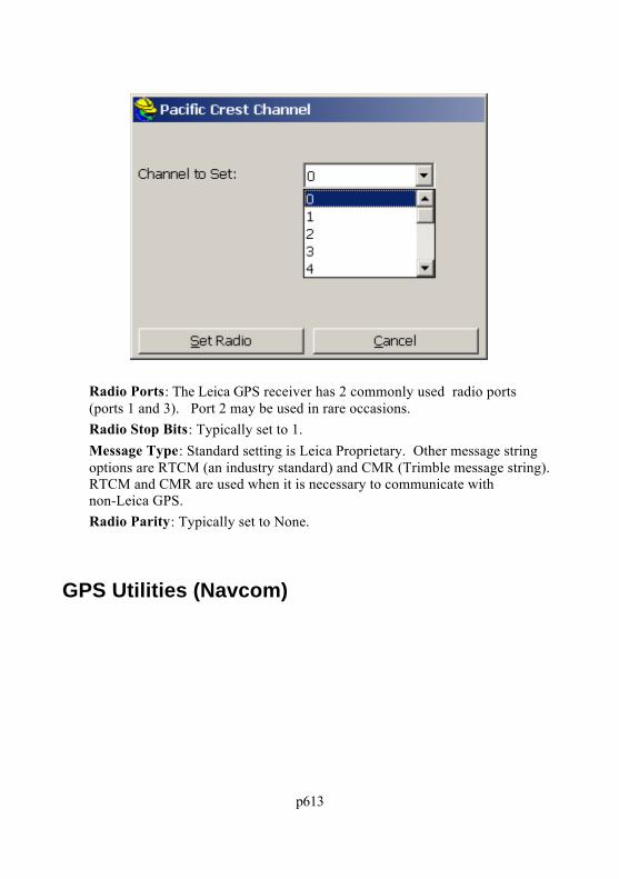
p613

Radio Ports: The Leica GPS receiver has 2 commonly used radio ports(ports 1 and 3). Port 2 may be used in rare occasions.

Radio Stop Bits: Typically set to 1. Message Type: Standard setting is Leica Proprietary. Other message string

options are RTCM (an industry standard) and CMR (Trimble message string). RTCM and CMR are used when it is necessary to communicate withnon-Leica GPS.

Radio Parity: Typically set to None.

GPS Utilities (Navcom)

p614

Configure RTK Device: Use this page to change your RTK data portsettings. This can also be done during base or rover configuration.

Check RTK: This tells the user why they aren’t in RTK fixed. QuickStart (Starfire Only): Starfire corrections often take some time to

acquire high levels of accuracy. If you’re returning to a previously surveyedarea, you can save time by storing a known position to a reference file. Thenyou can initialize the Starfire system with this position upon returning to thesite by performing a QuickStart.

At the end of the first day, verify that you’re receiving Dual-FrequencyStarfire corrections (RTG or WCT) by entering the Navigation Statusutility. Enter the QuickStart menu, and press Read GPS. Be sure tophysically mark this position in some way so that the exact position canbe returned to later. When you have a GPS position, click Save to savethe position to a reference file. When you return to the site, first ensurethat you’re receiving dual-frequency Starfire corrections, and that you'reset up on the position marked the previous day. Then enter the QuickStartmenu and choose Load to select the previously stored reference file.Press Initiate to input the loaded starting position to the receiver. Todisable an input position, press Disable. Note that if the input position isinaccurate, using the QuickStart routine will slow down the processing ofacquiring an accurate position.

p615

Reset Receiver: Use this tool to reset your receiver (soft reset) Factory Reset: Use this tool to reset your receiver (factory reset).

The buttons available in Receiver Utilities depends on the capabilities of thereceiver. If a Starfire license is not active, the QuickStart button is not shown.

Check RTK is a very useful tool. It tells the user why they aren ’t in RTK fixed and,if connected to a base when pressed, it determines if the base is transmittingcorrections, and if not, tells the user why. If connected to the rover, it tells the userif in RTK Fixed and if not, and it tells the user why. Configure RTK Device is thesame as the Configure button in the RTK tab of the Base and Rover dialogs.

“QuickStart” allows the user to save a QuickStart point or to QuickStart from apreviously saved QuickStart point.

Starfire and QuickStartStarfire is a space-based GPS correction system capable of 10 cm horizontalaccuracy. Vertical will be 1.5 to 2 times as much. It is kind of like WAAS onsteroids. The positions that it calculates are ITRF 2000. This is different from the

p616

positions calculated in RTK surveys. Since the RTK survey is based on a basepoint on the ground and the Starfire position is a space based position, they do notmatch. A localization created from an RTK system cannot be used by a Starfirereceiver. The localization must be created using Starfire positions.

It normally takes about an hour to get to the 10cm accuracy. The receiver does nothave to be stationary during that time. QuickStart is a method of reducing the“pull in” time to 50 seconds. If a QuickStart point has been saved using theQuickStart dialog, it can be loaded and used to perform a QuickStart. Best resultsare obtained by performing the QuickStart 5 minutes after turning on the receiver.

Performing a QuickStart to point with a position that is wrong will increase the“pull in” time to 2-3 hours. It will start at the bad position and then drift towardthe correct position. It is better to not perform a QuickStart if the receiver hasalready been on for 30-40 minutes.

RTK Extend™

IntroductionAn industry first from Navcom, RTK Extend™ enables continuous RTK positionaccuracy during radio communication outages by utilizing Navcom ’s globalStarfire™ corrections. Traditionally, when an RTK rover loses communicationwith the base station, it is unable to continue to provide position updates for morethan a few seconds, resulting in user down-time and reduced productivity. ANavcom Starfire receiver, operating in RTK mode, can transition to RTK Extendmode and maintain centimeter accurate positioning during communication loss forup to 15 minutes or in some cases even longer. RTK Extend allows the user towork more efficiently and without interruption, thus enabling them to concentrateon the work rather than the tools.

The ConceptUsing a receiver capable of Starfire and RTK at both the base and the roverlocations allows the receivers to compute Starfire and RTK solutions (orcorrections) simultaneously. If a communication outage occurs and the rover stopsreceiving RTK corrections from the base station, the receiver automatically andseamlessly transitions to RTK Extend mode by employing the Starfire signal.

Using RTK Extend, the receiver is able to compute an RTK equivalent position forup to 15 minutes. If the receiver remains in RTK extend mode for more than 15

p617

minutes, the position solution will slowly degrade to the typical 10cm accuracy ofthe Starfire system. Once the communication link is restored, the roverautomatically switches back to the standard RTK solution. The break incommunications and the seamless mode transition of RTK Extend is designed togo unnoticed by the user with the exception of the mode flag indicating thereceiver is operating in the Starfire-aided RTK Extend mode rather than standardRTK.

How it WorksTo enable the RTK Extend process, the base station must compute a Starfiresolution and constantly difference this position against the known RTK basestation position. This difference information is transmitted to the rover as anadditional RTK message. The difference results from two different sources: 1)The Starfire system inherently operates on the ITRF coordinate system and thesolution will differ for the known base station position if it was entered using adifferent coordinate system. 2) Because RTK and Starfire use different techniquesto compute a position solution at any given time there will be a few centimetersdifference between the two solutions. The rover uses this difference information toprevent any position jumps from occurring when transitioning into or out of RTKExtend mode such that the geodetic datum of the rover position will always be thesame as the RTK base station position.

The RTK extend process works by continually forcing agreement between theStarfire and RTK rover solutions at every epoch while receiving a signal from thebase station. Prior to initializing Starfire at each epoch, the RTK solution ismodified by the delta received from the base station. By first applying the delta,Starfire is initialized to a true Starfire position but with a known offset from thedesired RTK position.

When the system transitions to the RTK extend mode all that is required is tosubtract the delta prior to outputting the position. Had the delta not first beenapplied to the RTK position prior to initialization, Starfire would immediatelyattempt to return to the correct Starfire position once it was no longer locked to theRTK position. In addition to the loss of accuracy that would result if the Starfiresolution diverged from the RTK position there would also be a sudden positionjump when the link to the base station was restored. Thus by making use of thisadditional information, the rover is able to extend RTK through position gaps thatwould normally result from loss of communication with the base station.

SetupSetting up an RTK system to take advantage of RTK Extend involves very little

p618

additional effort. The Starfire-activated receiver at the base station is setup ex actlythe same as if it were a standard RTK receiver using an external communicationlink with the addition of two key steps:

1. The unit will be configured to navigate as a Starfire™ rover in addition tooperating as an RTK base station.

2. The unit will be configured to output a third RTK message , namely Navcom ’sbinary 0x5D message, which carries the Delta between the fixed RTK positionand the Starfire-aided navigation position to the rover.

The rover, being able to translate and adjust for the bias mentioned in item twoabove, is able to instantaneously QuickStart to the Starfire-aided navigationsolution when standard RTK corrections are unavailable. While the receiver isnavigating in Starfire mode, the position is flagged in its binary output indicatingthat the Starfire solution is actually “coasting” through an RTK communicationdropout.

Frequently Asked Questions

Q: How long are the near-RTK level accuracies maintained if the communicationlink is lost?A: To allow a Starfire receiver to work anywhere in the world, rather than justwithin a few kilometers of an RTK base station, unique processing techniques mustbe used and the typically obtainable accuracy is around 10 cm rather than the 1-2cm obtainable with an RTK system. The errors that cause Starfire to fluctuatearound the true position by a few centimeters change very slowly. As a result,once Starfire is initialized to a known position, it will stay within 1-2 cm of truthfor many minutes, but within an hour or so will begin varying from the trueposition by a greater amount. Testing has determined that once initialized theStarfire position will stay within 1-2 cm of the true position for at least 15 minutesand in many cases even longer depending on the num ber of satellites visible andtheir geometry. Every time the receiver reestablishes the link to the base stationand is able to compute an RTK position the 15 minute period is restarted. ThusRTK Extend will coast through several back to back outages as long as none ofthem are longer than 15 minutes.

Q: Does the base station send more than standard RTK messages to the rover?A: Yes. The RTK Extend base outputs an additional correction which allows therover to resolve any biases between the Starfire and RTK solutions. The rover

p619

makes use of this information to seamlessly transition between modes ofoperation.

Q: Can another manufacturer’s receiver or Navcom receiver without Starfirecapability be used as a base station? A: Entering precise ITRF00 Starfire coordinates for the base position will allowthe rover to make use of the RTK Extend feature although at a reduced level ofperformance. In this mode of operation, RTK Extend may only be able to coastthrough short outages of a few minutes. Depending on the length of the outagethere is the possibility of a small position jump when transitioning from RTKExtend back to RTK. The coordinate transformation required to convert the localposition into an ITRF00 position can be difficult, and if not done correctly willcause the RTK Extend position to rapidly diverge from truth. As such, a G PSreceiver capable of navigating in Starfire mode coupled with the ability to outputthe bias between these two sets of coordinates is the best approach to ensuringseamless operation.

Q: Which Navcom products are capable of RTK Extend?A: Navcom’s SF-2040 and SF-2050 product lines are capable of employing RTKExtend. In order to be used in this mode, each receiver (base and rover) must havethe RTK option enabled as well as an active Starfire license.

Q: Can a user define whether they want the RTK Extend™ feature to be active?A: Yes. Each receiver is fully configurable to ignore or accept a variety ofcorrection types. As such, the user may choose to disable the Starfire navigationability, making the receiver a primary host to RTK, or vice versa.

Q: What is Starfire™ convergence or “pull-in”, and why is it necessary to achieveadvertised accuracies from Starfire?A: When positioning with GPS, there are two types of error sources that affect theaccuracy obtainable 1) the errors generated by the GPS satellite system and 2)errors created by the receiver when processing the GPS signal.

The Starfire system is designed to compensate for all satellite based errors bycontinuously tracking the GPS satellites and calculating the clock and orbit errorsin real-time. These errors affect all GPS receivers, but are removed by applyingthe Starfire corrections. Correcting for the remaining error created by the G PSreceiver, involves a different process that must be done by the receiver itself. Theprocess of eliminating these errors involves smoothing the code measurements forup to an hour during which time sufficient satellite geometry changes occurallowing these errors to be estimated. This process is called convergence or

p620

“pull-in”.

Q: What is Starfire QuickStart?A: Navcom offers the unique feature called QuickStart where an accurately knownITRF00 position can be used to initialize Starfire navigation and eliminate theconvergence period. This is typically a position previously surveyed and convertedto ITRF00 prior to initialization. It can also be a position obtained from theStarfire receiver while in steady state (or fully converged) navigation. Forexample, vehicular installations can be initialized using the last position from whenit was parked and powered down. Employing QuickStart from a position that isnot geodetic truth will be followed by a longer-term convergence to geodetic truth,so entering false coordinates into this function is not a recommended approach.

Note: RTK Extend™ is an “automated extension” of QuickStart.

GPS Utilities (Sokkia and Novatel)The NovAtel and Sokkia GPS options, like Ashtech, allow for hard and soft resets,permit sending commands to the receiver (consult your dealer) and allow thereview and re-setting of base and rover radio channels for Pacific Crest PDL andRFM series radios. Additional options check the communication status (shows thequality of the message string). The Review REF File will display the reference file(which stores the GPS base position information), which also helps introubleshooting.

GPS Utilities (Magellan/Ashtech)The Magellan/Ashtech Receiver Utilities screen has the following options:

p621

Base and Rover Radio/GSM Setup: The Base and Rover Radio/GSM setupoptions will read the receiver, display the current radio channel, and allow theuser to change to another channel. This feature is available for Pacific CrestPDL and RFM Series radios and Ashtech internal radios. Be sure that youhave the right Radio Port set under the Configure Rover or Configure Base“Ports” tab. For GSM, see discussions under Configure Rover. The Base andRover radio buttons work similarly. It is important for the user to choose theright button (base radio setup for base receiver and rover radio setup for roverreceiver) to ensure that the software will try to connect to the radio on thecorrect port.

Thales/Ashtech Radio Setup – PDLIf the radio is an American PDL radio, it will appear as shown below.

p622

The user can change the channel, the digisquelch (sensitivity), and the over airradio link baud rate. If it is a European radio, channels are not available. Instead,the user will be able to set the frequency, the digisquelch, and the over air radiolink baud rate. The digisquelch is best high on rovers and low on bases. To setchanges, click on the Set Radio button and the following screen appears:

Magellan/Ashtech Radio Setup – Thales UHF

p623

Select the appropriate button (see above). The following screen will appear.

Change the frequency to the desired frequency and click Set Radio.

Magellan/Ashtech Radio Setup – CableNo configuration options are available when the software is configured to cable.

Magellan/Ashtech Radio Setup – Older ReceiversCurrently, the only radio option available for non-ZMAX Thales/Ashtech receiversis a PDL radio. The Base/Rover radio setup options will assume the radio is a PDLradio on these receivers, and try to configure them accordingly. All the samesettings (channel, digisquelch, over air link rate) should still be available,however.

Hard Reset: Shuts down the receiver and brings it up again with defaultsettings. Resets all port baud rates to 9600 and resets the internal memory.

Set Factory Defaults: Resets the receiver and changes all parameters to thefactory defaults. It is useful in troubleshooting problems.

Save Settings to Receiver: Use this command is issued as part of theConfigure Base and Configure Rover operations. However, you can run thiscommand at any time as an extra “confirmation” of your settings changes(including settings changes within Receiver Utilities). This sends the$PASHS,SAV,Y command to the receiver.

p624

Beep Off: This disables the Beep sound that emanates from the Receiverwhen it is turned on.

Send Command to Receiver: You can send what are known as “pash”commands, internal Thales/Ashtech codes, to the receiver. This should bedone only in consultation with your Thales dealer.

Reset RTK Engine: This resets the carrier phase ambiguities. This is a usefulcommand if you are having difficulty obtaining lock and want to start theprocess of fixing over again. Receiver settings are retained (so you can thinkof it as a “soft reset”).

Bluetooth Settings: The Bluetooth settings in SurvCE ’s Bluetooth Manager(discussed in Comm Setup) do not actually change anything in the receiveritself. In order to make changes to the receiver ’s internal Bluetooth settings, itis necessary to go into Receiver Utilities and click on Bluetooth Settings.

In this dialog, the user can change the Bluetooth receiver name (Receiver IDin Bluetooth Manager), the Bluetooth passkey (PIN in Bluetooth Manager), orthe country code (currently the only choices are France and other countriesbecause France has unique Bluetooth specifications). To change the name,change it in the appropriate text field and click Set New Bluetooth Name. Amessage confirming success will appear.

p625

To change the passkey, change it in the appropriate tex t field and click SetNew Bluetooth Passkey. A similar message confirming success will appear.To change the country code, click the appropriate radio button for the countryand click Set Bluetooth Country Code. A similar message confirming successwill appear.

Power Off Receiver: Sends a command to power off the receiver. Update Clock from GPS: This will update the clock on your CE device

based on the time recieved from the GPS satellites.

GPS Utilities (Topcon)

Power Cycle Receiver: This command is the same as turning the TOPCONreceiver off and then on.

Restore Factory Defaults : This command resets the TOPCON receiver tofactory settings and the receiver stops acting as base or rover. The baud rateof Port A will be set to 115,200. Reset this to 9600 by turning the receiver offand then on while holding down the FN button. Watch the REC light go fromorange to green to red and then let up the FN button. This method can be usedif SurvCE cannot establish communications at any time.

Clear Non-Volatile Memory : This command does everything RestoreFactory Defaults does and also clears the almanac data that tells it where to

p626

look for the satellites. The receiver then downloads a new almanac from thesatellites.

Send Command to Receiver: This command allows experienced users totype in commands using TOPCON GPS receiver commands to set or reportinternal settings. (See the TOPCON operations manuals for a complete list ofTOPCON GPS receiver commands).

Set Satellite Status: This feature allows the user to disable a satellite ifnecessary.

Initialize to Known Point: The Topcon GPS has a special feature toInitialize to a Known Point which can greatly speed up “move ups” from onebase position to another.

GPS Utilities (Trimble)

Reset Receiver: This will reset the receiver. Select Rover Input: If you choose Select Rover Input, you can identify the

“station id” of the base to avoid picking up inappropriate base correctionsfrom the wrong base receiver.

Check Battery: This will display the condition of the receiver's battery. Power On/Off Receiver: This will turn on and off the receiver.

p627

TroubleshootingThis chapter contains troubleshooting tips for Carlson SurvCE, and the varioushardware devices supported by SurvCE.

GPS HeightsSurvCE records GPS heights as the ellipsoid height, expressed in meters, at eitherthe phase center or the ARP of the antenna, depending on the GPS manufacturer. Ifthe position is recorded to the ARP, then the LS record (antenna height) will onlyreflect the user-entered value. If the position is recorded to the phase center, thenthe LS record (antenna height) will reflect the user-entered value plus the phasecenter offset.

SurvCE records the ARP position for the following GPS manufacturers: Leica Geodetics

Handheld Hardware

How do I reset the computer after a lock up?RangerHold down the power button until the computer resets or instructs you to hold it for5 more seconds to reset.

AllegroHold down the power button until the computer resets.

Why can’t I load the software?The computer may disconnect from ActiveSync when there is not enough memoryallocated to “Storage Memory”. In the control panel, select the “System” iconfollowed by the Memory tab. Position the slider so that there is 5mb (5120 kb)allocated and not in use (i.e. if the “In Use” value says 1024 kb then add 1024 &5120 to determine what the “Allocated” value should be).

How do I clear the RAM backup and why?Clearing the RAM backup seems to improve performance on the Ranger platform

p628

after new programs have been installed or removed. Make sure that all softwareapplications are closed and select the “RAM Backup” icon from the control panel.Select the Delete button and answer Yes to the three resulting message boxes.

Why can’t I communicate through the COM port?If you cannot communicate with the instrument, verify all COM settings in SurvCEand make sure that they match the COM settings on the instrument. Ifcommunication has previously been working and the COM settings have not beenaltered, try one of the following to clear up the COM port:

Exit SurvCE, turn off the computer, Restart the computer and re-enterSurvCE.

Exit SurvCE and perform a soft reset on the device (V erify that allapplications have been closed).

Exit SurvCE and perform a hard reset on the device (Verify that allapplications have been closed).

How do I set the CAPS LOCK status?Ranger1) Hold down the yellow shift button [ ^ ] and the [ALT] buttons, then press andrelease the power button.2) A small keyboard should be showing. On the small keyboard, press the [CAPS]button then repeat step 1 to dismiss the keyboard.

AllegroPress and release the blue function button followed by the CapLk/Shift buttonlocated at the lower left side of the keyboard.

How frequently should I charge the device?We recommend starting every day with a fully-charged battery. Refer to yourhardware manual for specifics on charging your battery.

How do I calibrate the touch screen?In the control panel of the CE device, select the “Stylus” icon to configure the“Double Tab” and “Calibration” of the touch screen.

How do I turn on/off the back light?RangerHold down the shift button [ ^ ] and then press and release the power button.

p629

AllegroPress and release the yellow function button followed by the F3/F8 button locatedat the top center of the keyboard.

How can I speed up the Allegro performance?In the control panel of the Allegro, select the “System” icon and then the“Memory” tab. Set your “Storage Memory” allocation to 8000 KB or 8 MB +/-.This should provide more RAM to the system for operating the programs andincrease performance.

How can I Recover the SurvCE Icon if it Disappears?It may be possible to lose the SurvCE Icon off the desktop if, for ex ample, thepower drains out of the CE device. There are safeguards against this, but if ithappens, follow these steps to restore the icon:1. Select Start (lower left on most CE devices, Ctrl Esc on the Ranger) and

choose Windows Explorer under Programs.2. Navigate to the SurvStar directory (the directory containing SurvCE), which

on some devices is \Disk\SurvStar.3. Look for the SurvCE Shortcut and highlight it.4. Choose the Edit pull down in Windows Explorer and choose Copy.5. Then return to the desktop where the icons are visible and press ALT then tap

into blank space on the screen (sometimes referred to as ALT-Click).6. Choose Paste Shortcut. That should restore it.

If the icon disappears, this indicates some problem in the original installation ofSurvCE, since a process occurs to make the icon permanent. You can help ensurethat your restored icon is permanent by going to Start, Settings, Control Panel andchoosing Perform Ram Backup. Select Backup Now, as prompted. This shouldmake the SurvCE icon remain even after full loss of battery.

Can I lose data or get bad data if I Re-Boot my CE device?If you re-boot your Allegro or Carlson Explorer or Ipaq or any other CE deviceyou are using, you can lose your antenna height or prism height information,because SurvCE does not store to memory changes in antenna height or prismheight, except in the following scenarios:

The hard save of antenna/prism heights is done when you ex it the program, whenyou save a configuration from the instrument icon at the top of the screen, whenyou say OK to Configure Rover, Configure Base or Equip/Settings (for TS), whenyou change jobs, and when you enter Equip/Comm Settings.  Prior to release

p630

1.50.007, in November, 2004, even Configure Rover did not save the heightinformation "to disk".

Therefore, if you re-boot, perform a hard reset, or otherwise ex it the program byany method other than the normal File, Exit method, recent changes to the prismheight or antenna height may not be saved.  On re-entering the program, the X,Yposition for GPS work, for example, will very likely be correct, but elevations mayhave been lost.  When using GPS, it is recommended, after a re-boot, that you dothe command Configure Rover to re-establish the correct elevations, and in allcases (GPS and Total Station) it is recommended that you double-check yourantenna or prism heights before proceeding.

Miscellaneous Instrument ConfigurationLeica Robotic - Do I need to be in RCS (Remote Control) mode?You must verify that you are NOT in RCS mode when using SurvCE with Leicarobotic equipment. It will appear as though you are not communicating with theinstrument if this mode is active. Refer to the Leica documentation for how to ex itRCS mode.

Leica GPS - What firmware will allow radio channel changing?Firmware version 3.52 or later is required for SurvCE to have radio channelchanging functionality.

Geodimeter 600 - What firmware version is required?Firmware version 696-03.xx or later is required for SurvCE to operate with thisinstrument. To check the firmware on the instrument, follow the key strokes:Menu, 5, 4, 1. The Geodimeter 640, for example, does not take measurements inreverse face. Therefore, when doing D&R, set reverse face to angle only.

Sokkia GSR 2700 IS - What do I do when I get the Bluetooth pass keyprompt?This receiver does not require a pass key. If you are prompted for one, do a factoryreset on the receiver by holding the power key down until the message displayed isFactory Reset. Then turn the device off and back on again. In Carlson SurvCE,clear the receiver from the Bluetooth connections list and add it back in.

Supported File Formats

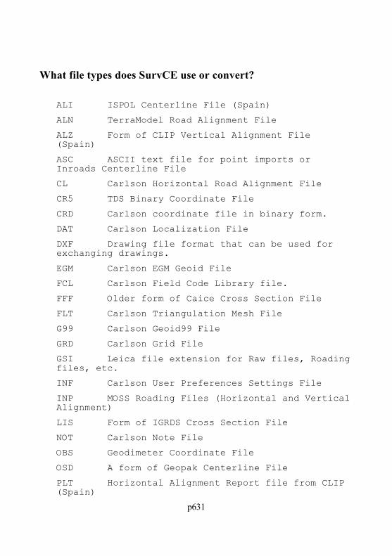
p631

What file types does SurvCE use or convert?

ALI ISPOL Centerline File (Spain)

ALN TerraModel Road Alignment File

ALZ Form of CLIP Vertical Alignment File

(Spain)

ASC ASCII text file for point imports or

Inroads Centerline File

CL Carlson Horizontal Road Alignment File

CR5 TDS Binary Coordinate File

CRD Carlson coordinate file in binary form.

DAT Carlson Localization File

DXF Drawing file format that can be used for

exchanging drawings.

EGM Carlson EGM Geoid File

FCL Carlson Field Code Library file.

FFF Older form of Caice Cross Section File

FLT Carlson Triangulation Mesh File

G99 Carlson Geoid99 File

GRD Carlson Grid File

GSI Leica file extension for Raw files, Roading

files, etc.

INF Carlson User Preferences Settings File

INP MOSS Roading Files (Horizontal and Vertical

Alignment)

LIS Form of IGRDS Cross Section File

NOT Carlson Note File

OBS Geodimeter Coordinate File

OSD A form of Geopak Centerline File

PLT Horizontal Alignment Report file from CLIP

(Spain)

p632

POS Sokkia or Trimble Coordinate File

PRO Carlson Vertical Road Alignment File

RAS ISPOL Vertical Road Alignment File (Spain)

RD5 TDS Road Alignment File

RDS IGRDS Cross Section File

REF Carlson Base Station Reference File

RLN TerraModel Road Alignment File

RW5 Carlson Raw Data File, TDS Raw Data File

SC1 ISPOL Cross Section File (Spain)

SCT Carlson Cross Section File

SDR Sokkia file extension for Raw Files,

Roading files, etc.

SHP ESRI Shape File

SUP Carlson Road Superelevation File

TPL Carlson Road Template File

TPT Carlson Road Template Transition File

TRV Traverse PC Coordinate File and CLIP Format

for Sections (Spain)

XML LandXML File may contain a variety of file

types (eg. Roading/DTM)

XRS Form of Geopak Cross Section File

p633

Raw DataThis section outlines the Carlson SurvCE RW5 format.

File Format

Carlson SurvCE RW5 Format

This document outlines the Carlson SurvCE RW5 format in detail. The format is acomma delimited ASCII file containing record types, headers, recorded data andcomments.

The format is based on the RW5 raw data specification, with the exception ofangle sets. Angle sets are recorded as BD, BR, FD and FR records to allowreduction of all possible data that can be recorded by Carlson SurvCE using the Set Collection routine. Essentially, these records are identical to a sideshot record.

With the exception of the aforementioned angle set records, if the RW5specification is modified to provide enhanced functionality, the added or modifieddata will reside in comment records to avoid incompatibility with ex istingsoftware.

Backsight RecordRecord type: BK

Field headers:

OP Occupy Point

BP Back Point

BS Backsight

BC Back Circle

Sample(s):

BK,OP1,BP2,BS315.0000,BC0.0044

Job RecordRecord type: JB

Field headers:

NM Job Name

DT Date

TM Time

Sample(s):

JB,NMSAMPLE,DT06-27-2003,TM14:21:53

p634

Line of Sight RecordRecord type: LS

Field headers:

HI Height of Instrument

HR Height of Rod*

*GPS heights may be recorded to phase center or ARP

depending on GPS make.

Sample(s):

LS,HI5.000000,HR6.000000

LS,HR4.000000

Mode Setup RecordThe mode setup will be recorded at the beginning of the

raw data file.

Record type: MO

Field headers:

AD Azimuth direction ( 0 for

North, 1 for South)

UN Distance unit (0 for feet, 1

for meter)

SF Scale factor

EC Earth Curvature (0 for off, 1

for on)

EO EDM offset(inch)

Sample(s):

MO,AD0,UN0,SF1.00000000,EC1,EO0.0,AU0

Occupy RecordRecord type: OC

Field headers:

OP Point Name

N Northing (the header is N

space)

E Easting (the header is E

space)

EL Elevation

-- Note

Sample(s):

OC,OP1,N 5000.00000,E 5000.00000,EL100.000,--CP

p635

Off Center Shot RecordRecord type: OF

Field headers:

AR Angle right

ZE Zenith (actual)

SD Slope Distance

Sample(s):

OF,AR90.3333,ZE90.0000,SD25.550000

OF,ZE90.3333,--Vert Angle Offset

Store Point RecordRecord type: SP

Field headers:

PN Point Name

N Northing

E Easting

EL Elevation

-- Note

Sample(s):

SP,PN100,N 5002.0000,E 5000.0000,EL100.0000,--PP

Traverse / Sideshot Record / Backsight Direct / BacksightReverse / Foresight Direct / Foresight ReverseRecord type: TR / SS / BD / BR / FD / FR

Field headers:

OP Occupy Point

FP Foresight Point

(one of the following)

AZ Azimuth

BR Bearing

AR Angle-Right

AL Angle-Left

DR Deflection-Right

DL Deflection-Left

(one of the following)

ZE Zenith

VA Vertical angle

CE Change Elevation

(one of the following)

SD Slope Distance

HD Horizontal Distance

-- Note

Sample(s):

p636

TR,OP1,FP4,AR90.3333,ZE90.3333,SD25.550000,--CP

SS,OP1,FP2,AR0.0044,ZE86.0133,SD10.313750,--CP

BD,OP1,FP2,AR0.0055,ZE86.0126,SD10.320000,--CP

BR,OP1,FP2,AR180.0037,ZE273.5826,SD10.315000,--CP

FD,OP1,FP3,AR57.1630,ZE89.4305,SD7.393000,--CP

FR,OP1,FP3,AR237.1612,ZE270.1548,SD7.395000,--CP

GPSRecord type: GPS

Field headers:

PN Point Name

LA Latitude (WGS84)

LN Longitude (WGS84, negative

for West)

EL Ellipsoid elevation in

meters*

-- Note

*GPS heights may be recorded to phase center or ARP

depending on GPS make.

Sample(s):

GPS,PN701,LA42.214630920,LN-71.081409184,EL-21.8459,--C

P /Brass Disk

Alphabetical listing of Record TypesBD Backsight Direct

BK Backsight

BR Backsight Reverse

FD Foresight Direct

FR Foresight Reverse

GPS GPS Position in Lat (dd.mmss) Lon (dd.mmss -

Negative for West) and WGS84 Ellipsoid Elevation in

meters

JB Job

LS Line of Sight

MO Mode Setup

OC Occupy

OF Off Center Shot

SP Store Point

SS Side Shot

TR Traverse

-- Note Record

p637

Alphabetical listing of Field HeadersAD Azimuth Direction ( 0 for North, 1 for South)

AL Angle-Left

AR Angle-Right

AZ Azimuth

BC Back Circle

BP Back Point

BR Bearing (this field will be recorded as

N123.4500W)

BS Backsight (when back point is not defined)

CE Change Elevation

DL Deflection-Left

DR Deflection-Right

DT Local Date (MM-DD-YYYY)

E Easting (the header is E space)

EC Earth Curvature (0 for off, 1 for on)

EL Elevation (GPS value is ellipsoid elevation

in meters)

EO EDM Offset

FE Foresight Elevation

FP Foresight Point

HD Horizontal Distance

HI Height of Instrument

HR Height of Rod

LA Latitude

LN Longitude

N Northing (the header is N space)

OC Occupy Point Coordinates

OP Occupy Point

PN Point Name

SD Slope Distance

SF Scale Factor

TM Local Time (HH:MM:SS)

UN Distance Unit (0 for feet, 1 for meter, 2 for

US feet)

VA Vertical Angle

ZE Zenith

-- Note

p638

Index

- A -Abbreviations 41About SurvCE 193Add Job Notes 113Areas 315Authorizing SurvCE 20Auto By Interval 288

- B -Basics 438Battery Status 23

- C -Calculator 332Carlson Technical Support 24Centerline Editor 344Check Level (Total Station) 184COGO 472Color Screens 22Configure (General) 153Configure (Sets) 159Configure (View Pt) 158

- D -Data Transfer 101Delete File 111DRAW 460Draw Centerline 352Draw Profile 356Draw Template 363

- E -

p639

Elevation Difference 250End-User License Agreement 7Exit 113

- F -Feature Code List 89FILE 442File Format 633

- G -GPS (Allen-Osbourne) 580GPS (CSI - DGPS Max)GPS (Leica 500/1200) 581GPS (Leica GIS System 50) 585GPS (Magellan/Ashtech) 593GPS (Navcom) 585GPS (NMEA) 590GPS (Novatel) 592GPS (Sokkia) 597GPS (Topcon) 599GPS (Trimble) 605GPS Base 131GPS Heights 627GPS Rover 141GPS Utilities 150GPS Utilities (Leica 500/1200) 611GPS Utilities (Magellan/Ashtech) 620GPS Utilities (Navcom) 613GPS Utilities (Sokkia and Novatel) 620GPS Utilities (Topcon) 625GPS Utilities (Trimble) 626Graphic Mode 25Grid/Face 258

- H -Handheld Hardware 627Hardware Notes 22Hot Keys & Hot List 31

p640

- I -Import/Export 107Input Box Controls 36Installing SurvCE 16Instrument Selection 36Intersections 317Inverse 313

- J -Job 43Job Settings (Format) 52Job Settings (New Job) 44Job Settings (Options) 47Job Settings (Stake) 53Job Settings (System) 46

- K -Keyboard Input 312Keyboard Operation 40

- L -Leveling 276List Points 63Localization 162Log Raw GPS 292

- M -Manual Traverse 339Memory 22Microsoft ActiveSync 11Miscellaneous Instrument Configuration 630Monitor/SkyPlot (GPS) 180

- O -Orientation (Backsight) 199Orientation (Instrument Setup) 195Orientation (Remote Benchmark) 201

p641

Orientation (Robotics) 203

- P -Peripherals 187Point Projection 323Profile Editor 353

- Q -Quick Calculator 29

- R -Raw Data 67Receiver (GPS)Remote Elevation 290Resection 262

- S -Save System 24Set Collection 266Setup (GPS) 128Setup (Total Station) 123Stake Line/Arc 228Stake Offset 245Stake Points 222Stake Road 427Stake Slope 386Station Store 327Store Points (GPS Offsets) 216Store Points (GPS) 213Store Points (TS Offsets) 210Store Points (TS) 205Store Sections 412Supported File Formats 630System Requirements 10

- T -Template Editor 357

p642

Tolerances 185TOOLS 487Total Station (Geodimeter/Trimble) 543Total Station (Leica Robotic) 554Total Station (Leica TPS Series) 549Total Station (Leica/Wild Older Models ) 563Total Station (Nikon) 564Total Station (Pentax)Total Station (Sokkia Robotic) 571Total Station (Sokkia Set) 567Total Station (Topcon 800/8000/APL1) 572Total Station (Topcon GTS) 580Transformation 328Tutorial 1: Calculating a Traverse (By Hand) with SurvCE 500Tutorial 2: Performing Math Functions in Carlson SurvCE Input Boxes 502Tutorial 3: Performing a Compass Rule Adjus tment 503Tutorial 4: Defining Field Codes, Line/Layer Properties & GIS Prompting 509Tutorial 5: Standard Procedures for Conducting G PS Localizations 531

- U -Using the Manual 10Utilities 364

- V -VIEW 454View Options 28

FAST Survey

Reference Manual

MagellanSurvey Solutions Contact Information:In USA +1 408 615 3970 � Fax +1 408 615 5200Toll Free (Sales in USA/Canada) 1 800 922 2401In South America +56 2 273 3214 � Fax +56 2 273 3187Email surveysales@magellangps.com

In Singapore +65 9838 4229 � Fax +65 6777 9881In China +86 10 6566 9866 � Fax +86 10 6566 0246Email surveysalesapac@magellangps.com

In France +33 2 28 09 38 00 � Fax +33 2 28 09 39 39In Russia +7 495 980 5400 � Fax +7 495 981 4840In the Netherlands +31 78 61 57 988 � Fax +31 78 61 52 027Email surveysalesemea@magellangps.comwww.pro.magellanGPS.com

Magellan follows a policy of continuous product improvement; specifications and descriptions are thus subject to change without notice. Please contact Magellan for the latest product information.©2003-2008 Magellan Navigation, Inc. All rights reserved. All product and brand names are trademarks of their respective holders. P/N 630884-B