熊本大学学術リポジトリ

Kumamoto University Repository System

Title Miniature Open Channel Scrubber for Gas Collection

Author(s) Toda, Kei; Tomoko, Koga; Toshinori, Tanaka; Shin-

Ichi, Ohira; Jordan, M. Berg; Purnendu, K. Dasgupta

Citation Talanta, 82(5): 1870-1875

Issue date 2010-10-15

Type Journal Article

URL http://hdl.handle.net/2298/18151

Right © 2010 Elsevier B.V.

- 1 -

Miniature open channel scrubbers for gas collection

Kei Toda 1*, Tomoko Koga

1, Toshinori Tanaka

1, Shin-Ichi Ohira

1, Jordan M. Berg

2, Purnendu

K. Dasgupta 3

1 Department of Chemistry, Kumamoto University, Kurokami 2-39-1, Kumamoto 860-8555,

Japan

2 Department of Mechanical Engineering, Texas Tech University, Lubbock, TX 79409-1021, USA

3 Department of Chemistry and Biochemistry, University of Texas at Arlington, Arlington, TX

76019-0065, USA

* Tel: +81-96-342-3389; Email: todakei@sci.kumamoto-u.ac.jp (K. Toda)

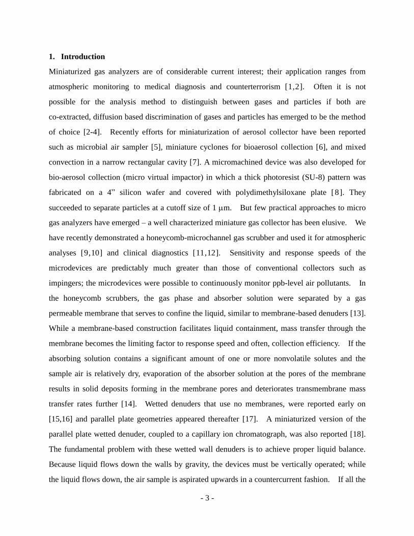
Abstract

An open channel scrubber is proposed as a miniature fieldable gas collector. The device is 100

mm in length, 26 mm in width and 22 mm in thickness. The channel bottom is rendered

hydrophilic and liquid flows as a thin layer on the bottom. Air sample flows atop the

appropriately chosen flowing liquid film and analyte molecules are absorbed into the liquid.

There is no membrane at the air-liquid interface: they contact directly each other. Analyte

species collected over a 10 min interval are determined by fluorometric flow analysis or ion

chromatography. A calculation algorithm was developed to estimate the collection efficiency a

priori; experimental and simulated results agreed well. The characteristics of the open channel

scrubber are discussed in this paper from both theoretical and experimental points of view. In

addition to superior collection efficiencies at relatively high sample air flow rates, this geometry

is particularly attractive that there is no change in collection performance due to membrane

fouling. We demonstrate field use for analysis of ambient SO2 near an active volcano. This is

basic investigation of membraneless miniature scrubber and is expected to lead development of

an excellent micro gas analysis system integrated with a detector for continuous measurements.

*Revised Manuscript

- 2 -

Keywords: Planar channel gas scrubber, miniature device for gas collection, theoretical

simulation of gas collection, sulfur dioxide, hydrogen sulfide, ammonia

- 3 -

1. Introduction

Miniaturized gas analyzers are of considerable current interest; their application ranges from

atmospheric monitoring to medical diagnosis and counterterrorism [1,2]. Often it is not

possible for the analysis method to distinguish between gases and particles if both are

co-extracted, diffusion based discrimination of gases and particles has emerged to be the method

of choice [2-4]. Recently efforts for miniaturization of aerosol collector have been reported

such as microbial air sampler [5], miniature cyclones for bioaerosol collection [6], and mixed

convection in a narrow rectangular cavity [7]. A micromachined device was also developed for

bio-aerosol collection (micro virtual impactor) in which a thick photoresist (SU-8) pattern was

fabricated on a 4” silicon wafer and covered with polydimethylsiloxane plate [8]. They

succeeded to separate particles at a cutoff size of 1 m. But few practical approaches to micro

gas analyzers have emerged – a well characterized miniature gas collector has been elusive. We

have recently demonstrated a honeycomb-microchannel gas scrubber and used it for atmospheric

analyses [9,10] and clinical diagnostics [11,12]. Sensitivity and response speeds of the

microdevices are predictably much greater than those of conventional collectors such as

impingers; the microdevices were possible to continuously monitor ppb-level air pollutants. In

the honeycomb scrubbers, the gas phase and absorber solution were separated by a gas

permeable membrane that serves to confine the liquid, similar to membrane-based denuders [13].

While a membrane-based construction facilitates liquid containment, mass transfer through the

membrane becomes the limiting factor to response speed and often, collection efficiency. If the

absorbing solution contains a significant amount of one or more nonvolatile solutes and the

sample air is relatively dry, evaporation of the absorber solution at the pores of the membrane

results in solid deposits forming in the membrane pores and deteriorates transmembrane mass

transfer rates further [14]. Wetted denuders that use no membranes, were reported early on

[15,16] and parallel plate geometries appeared thereafter [17]. A miniaturized version of the

parallel plate wetted denuder, coupled to a capillary ion chromatograph, was also reported [18].

The fundamental problem with these wetted wall denuders is to achieve proper liquid balance.

Because liquid flows down the walls by gravity, the devices must be vertically operated; while

the liquid flows down, the air sample is aspirated upwards in a countercurrent fashion. If all the

- 4 -

influent liquid is not fully aspirated out, the excess drops down unto the sampling conduit below

and removes soluble gases from the influent sample. On the other hand, if influent liquid flow

is too small, dry spots develop on the denuder walls, gas collection efficiency decreases and air is

aspirated into the liquid aspiration lines at the bottom that creates problems with some analysis

systems. These problems have never been fully solved. An Y-inlet miniature gas collector has

been reported by Timmer et al. [19] in which the sample gas and the absorber liquid form

alternating segments and the gas bubbles are removed prior to conductivity measurement of the

liquid stream. The response time of this device is good but the attainable gas/liquid volumetric

ratio is too low for the device to be of general practical interest.

Problems with membrane interfaces between gas and liquid or two liquid phases are

also encountered in other areas of endeavor. In gas diffusion flow injection analysis [20], a

membrane separates a donor from an acceptor stream and analytes that can be converted to the

vapor phase by pH adjustment (e,g., NH3, CO2, SO2, H2S etc.) or redox transformation (OCl-,

As3+

, etc.) are transferred from the donor to the acceptor phase. To allow unmodified samples

that can foul a membrane, “pervaporation” arrangements where a headspace exists between the

donor stream and the membrane has been advocated [21]. More recently it has also been

realized that a membraneless arrangement where the donor and acceptor streams flow side by

side may be superior [22,23], following a larger scale earlier demonstration that a wetted denuder

can be operated with one wall bearing a donor fluid stream and the opposite wall bearing an

acceptor stream [24].

A logical progression of these approaches adapted to gas sampling would be a

miniaturized open channel scrubber, can be operated horizontally and will obviate the

aforementioned problems with the vertical wetted denuder geometry. We introduce such a

device, compare its performance with theoretical simulations, and demonstrate its field use near

the Mt. Aso volcanic region.

2. Principles

- 5 -

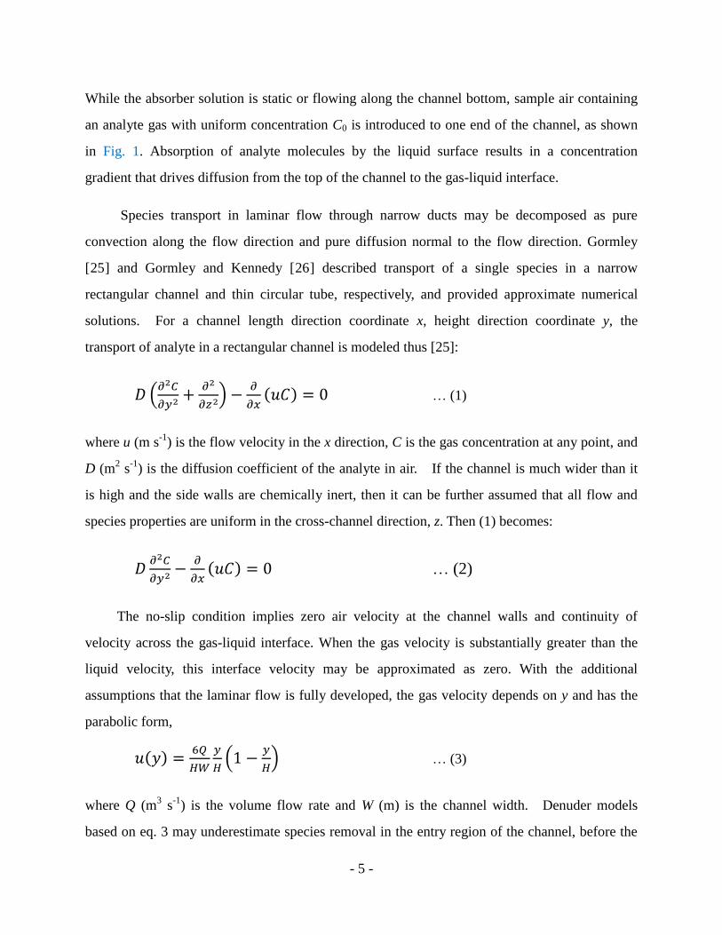
While the absorber solution is static or flowing along the channel bottom, sample air containing

an analyte gas with uniform concentration C0 is introduced to one end of the channel, as shown

in Fig. 1. Absorption of analyte molecules by the liquid surface results in a concentration

gradient that drives diffusion from the top of the channel to the gas-liquid interface.

Species transport in laminar flow through narrow ducts may be decomposed as pure

convection along the flow direction and pure diffusion normal to the flow direction. Gormley

[25] and Gormley and Kennedy [26] described transport of a single species in a narrow

rectangular channel and thin circular tube, respectively, and provided approximate numerical

solutions. For a channel length direction coordinate x, height direction coordinate y, the

transport of analyte in a rectangular channel is modeled thus [25]:

… (1)

where u (m s-1

) is the flow velocity in the x direction, C is the gas concentration at any point, and

D (m2 s

-1) is the diffusion coefficient of the analyte in air. If the channel is much wider than it

is high and the side walls are chemically inert, then it can be further assumed that all flow and

species properties are uniform in the cross-channel direction, z. Then (1) becomes:

… (2)

The no-slip condition implies zero air velocity at the channel walls and continuity of

velocity across the gas-liquid interface. When the gas velocity is substantially greater than the

liquid velocity, this interface velocity may be approximated as zero. With the additional

assumptions that the laminar flow is fully developed, the gas velocity depends on y and has the

parabolic form,

… (3)

where Q (m3 s

-1) is the volume flow rate and W (m) is the channel width. Denuder models

based on eq. 3 may underestimate species removal in the entry region of the channel, before the

- 6 -

parabolic flow profile is fully established.

Gormley [25] treats only the case where both the top and bottom bounding surfaces are

perfect sinks for the analyte. More accurate numerical solutions for this case, as well as

consideration of the present case where only one surface is a sink are reported by McCuen [27]

and Lundberg et al. [28]. Lundberg et al. also provide solutions for annular flow with a variety

of geometries and boundary conditions. While these calculations were intended for heat

transfer problems, they apply equally well to mass transfer problems. For the uninitiated,

however, the use of the original tables from Lundberg et al. is difficult; solutions directly relevant

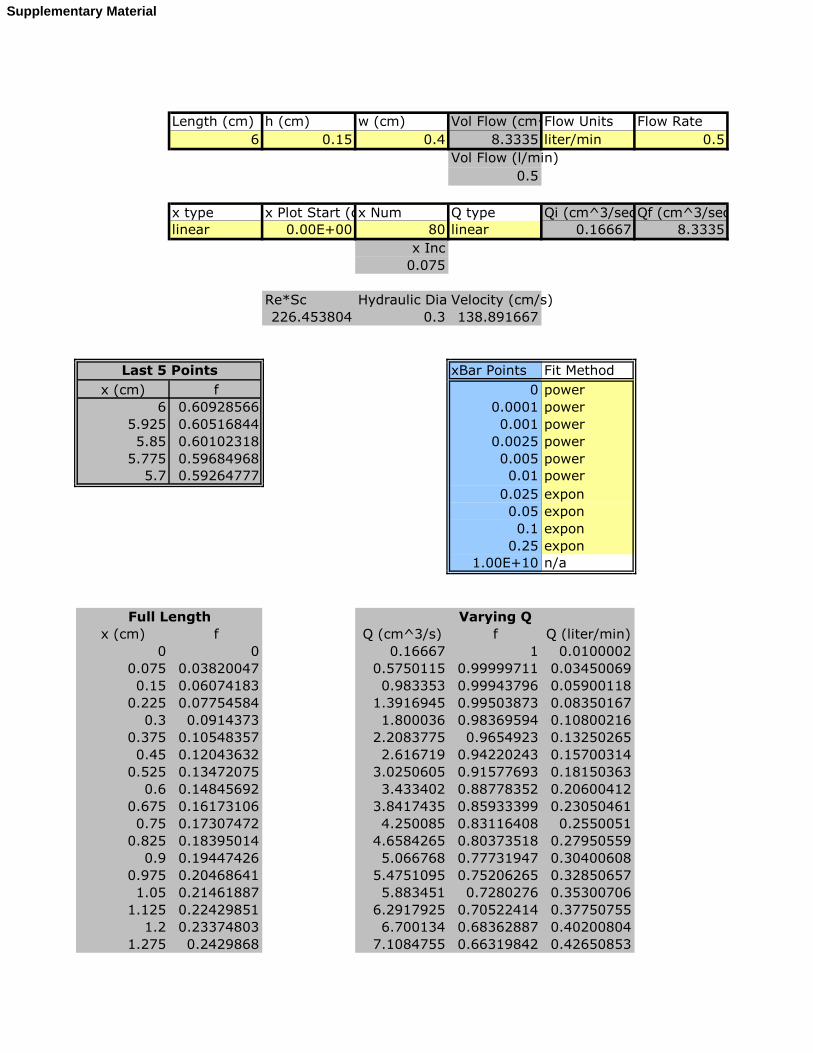
to the annular denuder geometry have recently been made available in spreadsheet form [29].

We similarly use here a spreadsheet implementation of the solutions for the planar geometry; the

spreadsheet included in supporting information (PlanarDenuderEfficiencyCalculator.xls).

3. Experimental

3.1. Planar open channel scrubber

Structure of the planar open channel scrubber is shown in Fig. 2. The device constitutes of a

gas channel plate and a solution channel plate both made of transparent polyvinylchloride (PVC)

that lie above each other, each bearing a 4 mm wide channel. The length and the depth of the

liquid channel were 60 and 0.5 mm, respectively. The gas channel made on the top PVC plate

extended 10 mm beyond the length of the liquid channel at each end (to allow laminar flow to

develop prior to liquid contact), thus totaling 80 mm and to accommodate the substantially

greater gas flow rate, the gas channel depth was made 1.5 mm, except as stated. The exterior

total dimensions of each plate was 26 mm in width and 100 mm in length. Total height of the

device was 22 mm when 1.5 mm deep air channel was used. The bottom of the liquid flow

channel was made hydrophilic by placing a thin (100 m) cotton mesh. Thin filter paper was

also found to work but since analyte retention is a possibility, it was not used. We also carried

out some experiments by coating with liquid glass (sodium silicate, Nacalai Tesque, Kyoto,

Japan) and baking but over a period of time the layer dissolves. For comparison purposes, we

- 7 -

also carried out experiments where a thin porous membrane was placed between the top and

bottom plates to provide more conventional membrane-based scrubber. Porous

polytetrafluoroethylene (pPTFE), (30 m thick, pore size 0.45 m, Poreflon® HP-010-30,

Sumitomo Fine Polymer, Osaka, Japan), porous polypropylene. (pPP), (94 m thick, Accurel®

PP 1E, Membrana, Wuppertal, Germany) and silicone (50 m thick, Asone, Tokyo, Japan) were

each tested.

3.2. Procedure

The sample gas was aspirated though the scrubber device at 25 – 500 mL min-1

by a diaphragm

airpump, DA-5S (ULVAC Kiko, Saito, Japan) with flow rate control by a mass flow controller

(MFC), SEC-B40 (500 mL air/min full scale, Horiba STEC, Kyoto, Japan) and with a liquid mist

trap before the flow controller. The absorbing solution was pumped (50 L min-1

) into the

liquid channel by a peristaltic pump (Minipuls 3, Gilson International) with 0.25-mm i.d. PVC

pump tube (15.0 rpm) and aspirated from the liquid outlet at a higher aspiration rate (~100

L/min, 0.38 mm i.d. pump tube); some air is obligatorily aspirated but the entire channel

remains wet. The pump transfers the aspirated solution into a 10 mL volumetric flask. After 1.0

L of air is sampled, the liquid and air flows are stopped and the liquid volume is made up to 10

mL with distilled deionized water. The respective absorbing solutions were 0.1 M NaOH with

0.02% w/v ascorbic acid for the measurement of H2S, 0.03% H2O2 + 10 M H3PO4 for SO2 and 5

mM H2SO4 for NH3. For H2S and NH3, the collected absorber solution was measured by flow

injection analysis (FIA), respectively using 5-M fluorescein mercuric acetate (FMA) in 0.1 M

NaOH [30] and 2-mM o-phthalaldehyde (OPA) + 3-mM Na2SO3 (pH 11 adjusted with Na2B4O7

+ NaOH) [31]. The carrier and reagent streams flowed at 0.15 mL min-1

, respectively, and 100

L of the collected absorber (after make-up to 10 mL) was injected into the carrier stream.

Sulfur dioxide was measured as SO42-

by ion chromatography under chromatographic conditions

previously described [32].

3.3. Field application

In order to evaluate this method, the system was put in a plastic box (35 cm x 29 cm x 17 cm)

- 8 -

including an air pump (DA-5S, ULVAC Kiko) and a small peristaltic liquid pump (high

performance roller pump, Ogawa Shokai, Kobe, Japan) with PharMed® tubing (0.5 mm i.d. x 3.7

mm o.d. for introduction and 1.0 mm i.d. x 3.0 mm o.d. for aspiration, at 5 rpm) and MFC setup.

The entire package was 6.2 kg (5.0 kg without air pump) in weight. The system was much

lighter than the commercial pulsed UV fluorescence instrument (APSA-370, Horiba, Kyoto,

Japan) used for concurrently measuring atmospheric SO2 (19 kg). For the scrubber, air was

sampled through a dust filter (Balston DFU

model 9900-05, Grade BK, Parker) at a flow rate of

100 mL min-1

. Gaseous SO2 absorber and absorber flow rate were the same as in-lab

experiments. The effluent absorber was collected into 1.5-mL vials, changed every 10 min.

The collected samples were analyzed by ion chromatography upon return to the laboratory on the

same day. The instruments were powered by a generator (EU-9i entry, Honda, Japan) placed 20

m downwind from the samplers.

4. Results and discussion

4.1. Membraneless device collection efficiency

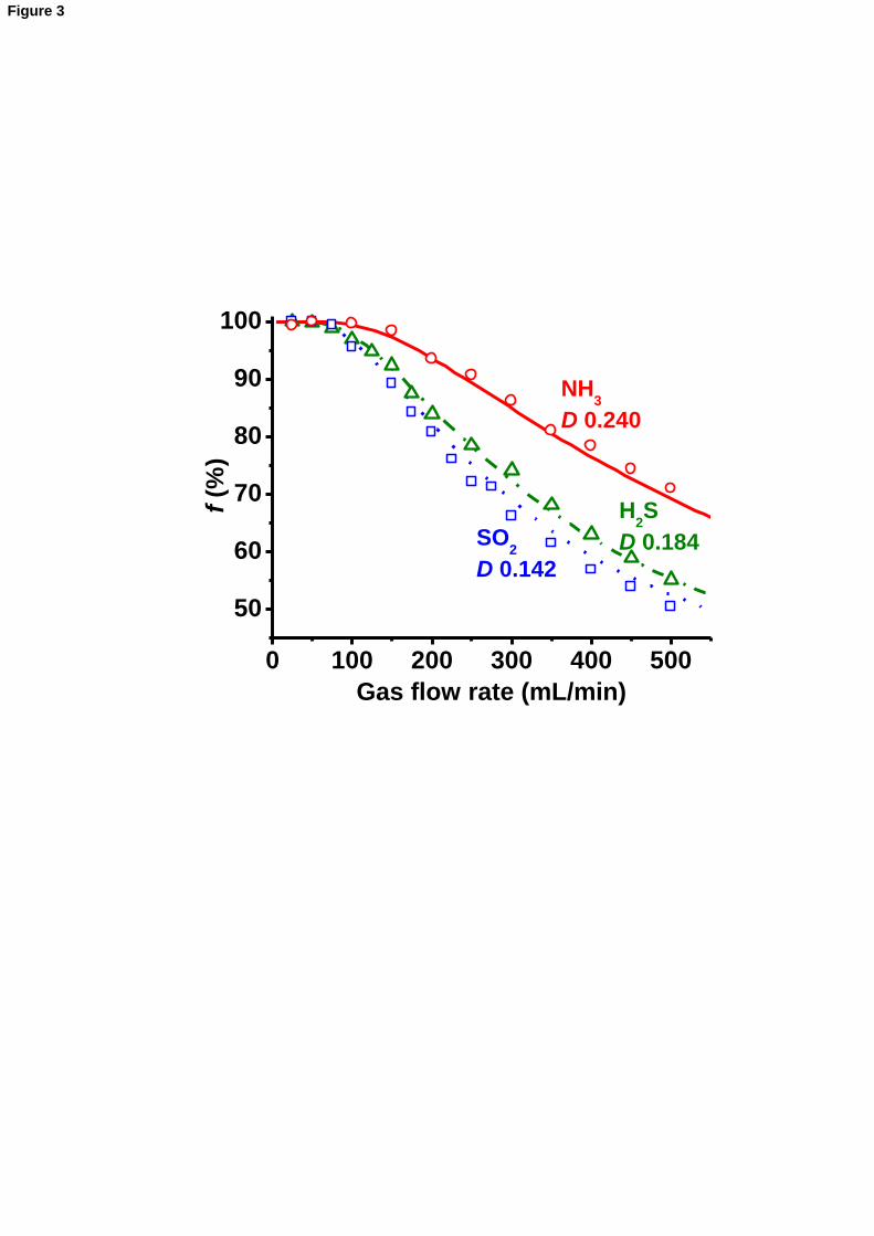
Collection efficiencies (f) for NH3, H2S and SO2 are shown in Fig. 3, the respective diffusion

coefficients (D) being 0.240, 0.184 and 0.142 cm2 s

-1, respectively, at 298K and 1.00 atm

obtained by Fujita’s equation [33,34]. Molecular weights of these gases range from 17 to 64.

Lighter molecules predictably have a higher D and result in higher f values. As shown in Fig. 3,

the experimental values for the three gases agreed quite well with the theoretical estimates.

This provides confidence that collection efficiencies for such devices can be estimated very well

a priori.

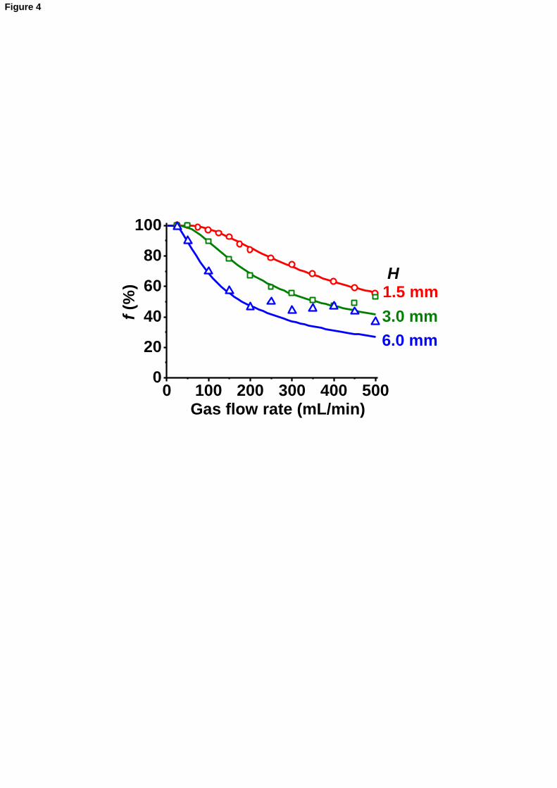
Figure 4 shows variation of f against gas flow rate obtained for H2S for three different

channel depths. The residence time of the sample gas in the scrubber was proportional to the

channel depth but a greater counteracting effect was increased mean diffusion distance to the

absorber surface. The net result was that a smaller channel depth was the most advantageous,

as correctly predicted by theory. At higher gas flow rates and larger channel depths, the

observed collection efficiencies were significantly greater than those theoretically predicted.

- 9 -

We used a gas inlet perpendicular to the channel (Fig. 2); with larger channel depths and higher

flow rates, laminar flow was not fully developed – for a simple tube the inlet length Li needed for

laminar flow development is approximately (98% accuracy) given by [35]:

Li = 0.2 Q / () …(3)

Where Q is the volumetric sampling rate, is the sample gas density and is its viscosity. The

need for a greater inlet length thus directly increases with the sampling rate.

4.2. Comparison with membrane-based scrubbers

In all membrane-based collectors, mass transport through the membranes is generally the factor

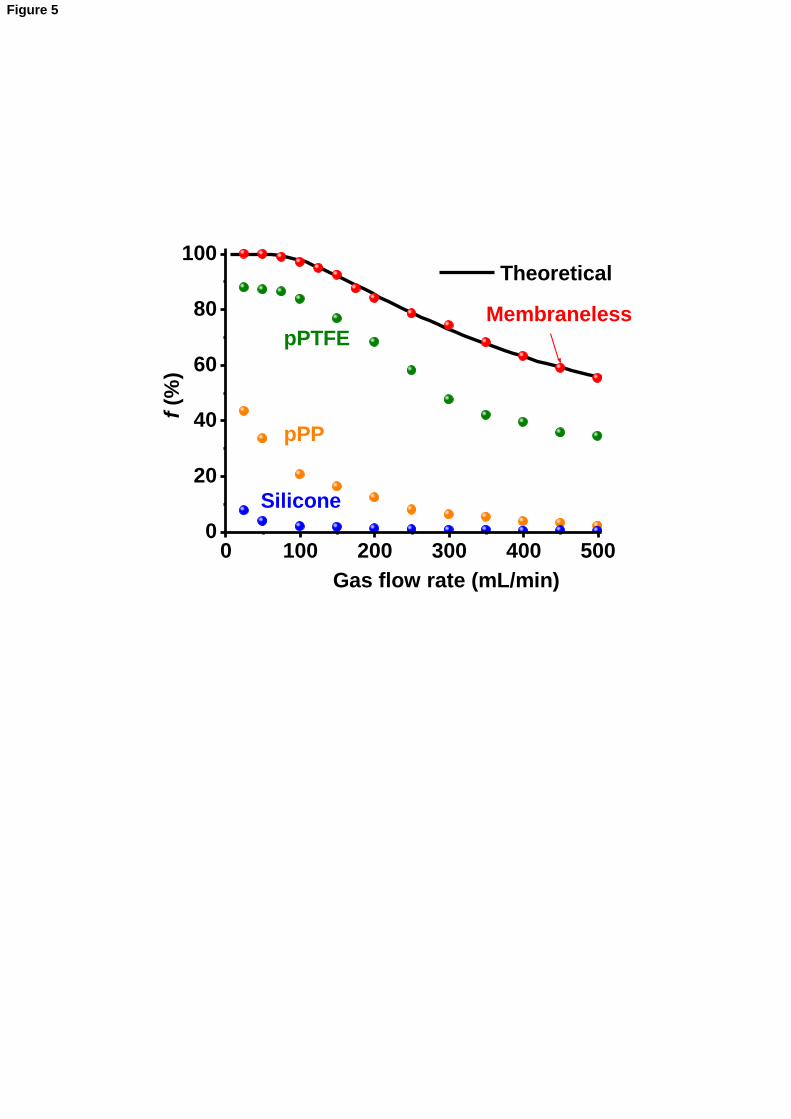
that limits how much of the sample gas is collected. The results are presented in Fig. 5. With

silicone membrane, f was only 7.7% even at 25 mL min-1

and decreased to 0.25% at 500 mL

min-1

. The pPTFE membrane was the best among the tested membranes. However, the

observed collection efficiency was less than that of the membraneless/theoretical case throughout

the flow rate range, ranging from 87% of the membraneless device efficiency at low flow rates

(25 mL min-1

) to 60% at high flow rates (500 mL min-1

). The pPP membrane was significantly

worse, ranging from 43% to 4% of the membraneless device efficiency at the same flow rates

above. The membraneless device not only provided the highest f values, it provided

reproducible f values as the device was assembled and disassembled and reassembled whereas

the f values of the membrane devices varied on a daily basis and whenever a new but otherwise

identical membrane was put in. The membraneless scrubber was therefore the superior device

in all respects with theoretical predictions closely matching the experimental results.

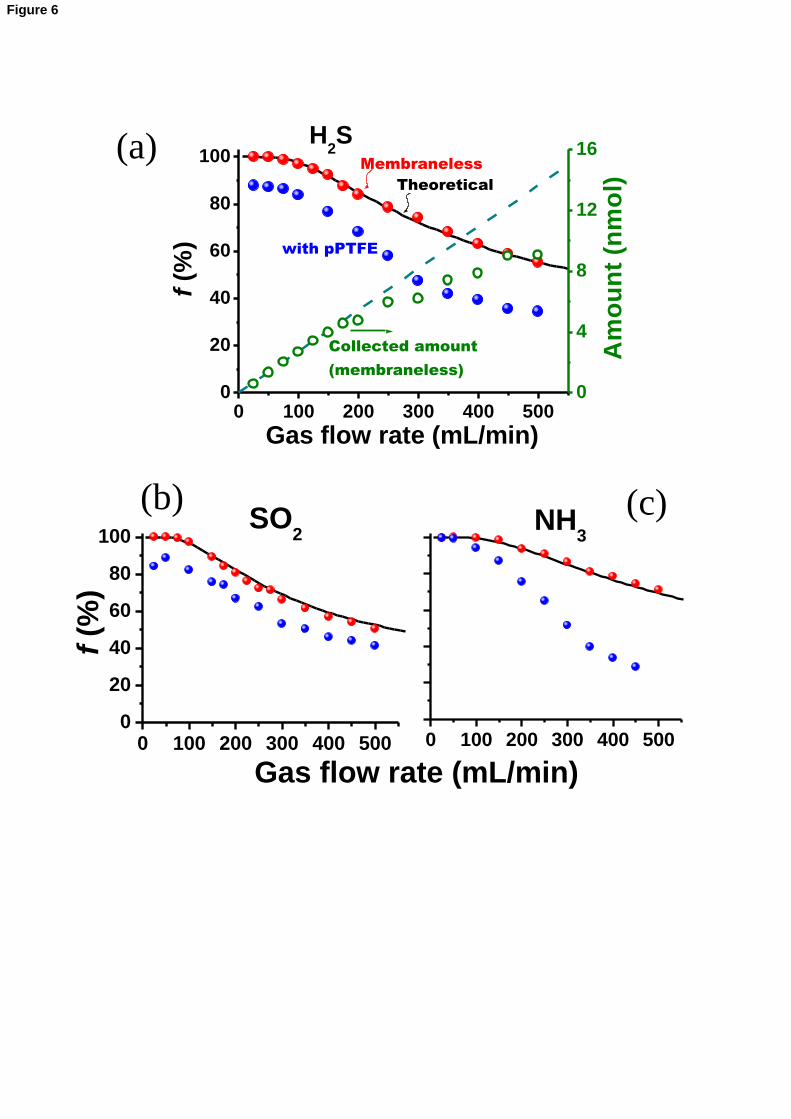
The best membrane device, namely the pPTFE device was tested for all three gases: H2S,

SO2 and NH3. The results are shown in Fig. 6. The pPTFE device performed with uniformly

lower efficiency than the membraneless device for SO2, much like that for H2S. However, at

low flow rates it exhibited quantitative collection for NH3, much as the membraneless device.

We believe that this is due to the strong affinity of NH3 for surfaces where water is already

adsorbed. The porous membrane surface not only has water in the pores but there is adsorbed

- 10 -

layer of water across the membrane surface. For a gas like NH3, this is sufficient to provide an

effective sink at lower flow rates but at higher flow rates, the difference with the membraneless

device increases dramatically. For all tested gases, the amount of the analyte gas collected

increases with the sampling rate but the collected fraction decreases with increasing flow rate.

The net result, shown in Fig. 6a for H2S is that the collected amount initially increases linearly

with flow rate but eventually plateaus out to an essentially constant value nearly independent of

the flow rate. This general behavior is true for membraneless scrubbers as well.

There are thus two flow regions advantageous for sampling – one in which the analyte gas

is collected essentially quantitatively. For the membraneless scrubber, all three test gases of our

interest could be collected nearly quantitatively at flow rates up to ~100 mL min-1

(experimental

f = 99.6% for NH3, 98.8% for H2S, and 97.3% for SO2) and 100 mL min-1

is thus a desirable

sampling rate for the miniature membraneless scrubber and we used this in the following

experiments. Note that there is another sampling rate range around 0.5 L min-1

that can be

useful; at this sampling rate the amount collected becomes essentially independent of the flow

rate and very accurate control of the flow rate is not essential. The amount collected

nevertheless will remain proportional to the analyte gas concentration. We did not further

explore this strategy at this time.

Using a sampling rate of 100 mL min-1

, 10 min sample collection, volume make-up to 1.0

mL and subsequent analysis by flow injection as described in the experimental section, the three

gases could be determined and the respective S/N=3 limits of detection were 1.8 ppbv for SO2,

1.7 ppbv for H2S (with 5 M FMA), and 0.29 ppbv for NH3. Parts per billion of these gases

can be measured with relatively short (10 min) sampling time while conventional impingers

require from half to a few hours gas collection.

4.3. Field application

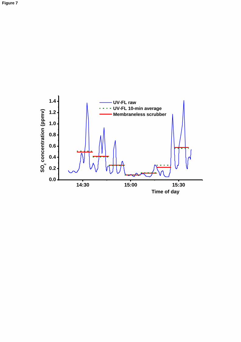
The membraneless scrubber was used for sampling around the Mt. Aso volcanic region. The

instrument package containing the membraneless scrubber as well as the pulsed fluorescence

SO2 instrument was carried to the ridge of the volcanic crater; this involved a 2-km walk through

- 11 -

an undeveloped trail. The pulsed fluorescence instrument monitored SO2 continuously while

the membraneless scrubber effluent was collected every 10 min. Collected samples were

analyzed on the same day by ion chromatography with calibration by aqueous sulfate standard

solutions (the S/N=3 limit of detection was 73 nM SO42-

, equivalent to 1.8 ppbv SO2 for the

amount of the air sampled). The results obtained from the field experiments are shown in Fig. 7.

The monitoring site was in the restricted area and we entered with a special permission for the

academic purpose. High level of SO2 was observed and sometimes it exceeded 1 ppmv in this

area. Gas mask was necessary for the survey. There is excellent agreement between the two

approaches. The collection device including the flow system was much easier to deploy in the

field compared to the commercial instrument and our previous instrument used in volcanic gas

analysis [36].

5. Conclusions

An open-channel scrubber device has been explored for the collection and analysis of gaseous

atmospheric species. The collection channel was rendered hydrophilic and a thin liquid film

formed thereupon to collect water soluble species effectively. The membraneless open-channel

device had predictably superior gas collection efficiency compared to its membrane-interfaced

counterparts and thus could provide better sensitivity or time resolution in the same analysis

system. In this work, a thin cotton screen was used to obtain a hydrophilic bottom surface.

Other hydrophilic surfaces inert for the purpose include anodically treated stainless steel [37], or

titanium [38]; silica-treated glass [15] can also be used. An open channel miniature scrubber

exhibits near-quantitative collection up to 100 mL min-1

sampling rates, permits calibration with

aqueous standards, allows near-exact theoretical prediction of the collection efficiency if the

diffusion coefficient of the analyte gas is known and its small size facilitates field deployment.

We hope to report in the near future integral systems where the analysis system has been

integrated with the collector.

Newly developed spreadsheet for calculation of collection efficiency is available from the

journal’s website (PlanarDenuderEfficiencyCalculator.xls).

- 12 -

References

[1] S. Ohira, K. Toda, Anal. Chim. Acta 619 (2008) 143.

[2] K. Toda, P.K. Dasgupta, Compr. Anal. Chem. 54 (2008) 639.

[3] P.K. Dasgupta, Compr. Anal. Chem. 37 (2002) 97.

[4] K. Toda, Anal. Sci. 20 (2004) 19. [5] W. Whyte, G. Green, A. Albisu, J. Aerosol Sci. 38 (2007) 101.

[6] K. Pant, C.T. Crowe, P. Irving, Power Technol. 125 (2002) 260.

[7] G. Rosengarten, G.L. Morrison, M. Behnia, Heat Fluid Flow 22 (2001) 168.

[8] D. Park, Y.-H. Kim, C.W. Park, J. Hwang, Y.-J. Kim, J. Aerosol Sci. 40 (2009) 415.

[9] S. Ohira, K. Toda, Lab Chip 5 (2005) 1374.

[10] K. Toda, T. Obata, V. A. Obolkin, V.L. Potemkin, K. Hirota, M. Takeuchi, S. Arita, T.

Khodzher, M. Grachev, Atmos. Environ. 44 (2010) 2427.

[11] K. Toda, Y. Hato, S. Ohira, T. Namihira, Anal. Chim. Acta 603 (2007) 60.

[12] K. Toda, T. Koga, J. Kosuge, M. Kashiwagi, H. Oguchi, T. Arimoto, Anal. Chem. 81 (2009)

7031.

[13] M. Takeuchi, J. Li, K. J. Morris and P. K. Dasgupta, Anal. Chem. 76 (2004) 1204.

[14] P.K. Dasgupta, ACS Adv. Chem. Ser. 232 (1993) 41.

[15] P.K. Simon, P.K. Dasgupta, Z. Vecera, Anal. Chem. 63 (1991) 1237.

[16] Z. Vecera, P.K. Dasgupta, Anal. Chem. 63 (1991) 2210.

[17] P.K. Simon, P.K. Dasgupta, Anal. Chem. 65 (1993) 1134.

[18] C.B. Boring, S.K. Poruthoor, P.K. Dasgupta, Talanta 48 (1999) 675.

[19] B. Timmer, W. Olthuis, A. v. d. Berg, Lab Chip 4 (2004) 252.

[20] V. Kuban, Crit. Rev. Anal. Chem. 23 (1992) 323.

[21] S. Satienperakula, S.Y. Sheikheldina, T.J. Cardwell, R.W. Cattrall, M.D. Luque de Castro,

I.D. McKelvie, S.D. Kolev, Anal. Chim. Acta 485 (2003) 37.

[22] N. Choengchan, P. Wilairat, P.K. Dasgupta, S. Motomizu, D.A. Nacapricha, Anal. Chim.

Acta 579 (2006) 33.

[23] P. Mornane, J. van den Haaka, T.J. Cardwell, R.W. Cattrall, P.K. Dasgupta, S.D. Kolev,

Talanta 72 (2007) 741.

[24] Z. Genfa, T. Uehara, P.K. Dasgupta, T. Clarke, W. Winiwater, Anal. Chem. 70 (1998) 3656.

[25] P.G. Gormley, Proc. Roy, Ir. Acad. A 45 (1938) 59.

[26] P.G. Gormley, M. Kennedy, Proc. Roy. Ir. Acad. A 52 (1949) 163.

[27] P.A. McCuen, Heat transfer with laminar and turbulent flow between parallel planes with

constant and variable wall temperature and heat flux. Ph.D. Dissertation, Stanford University,

1961.

[28] R.E. Lundberg, W.C. Reynolds, W.M. Kays, 1963. NASA Technical Note D-1972, National

Aeronautics and Space Administration: Washington D.C.

[29] J.M. Berg, D.L. James, C.F. Berg, K. Toda, P.K. Dasgupta, Anal. Chim. Acta 664 (2010) 56.

[30] K. Toda, P.K. Dasgupta, J. Li, G.A. Tarver, G.M. Zarus, Anal. Chem. 73 (2001) 5716.

[31] Z. Genfa, P.K. Dasgupta, Anal. Chem. 61 (1989) 408.

[32] S. Ohira, K. Toda, J. Chromatogr. A 1121 (2006) 280.

[33] S. Fujita, Kagaku Kogaku 28 (1964) 251 – 254.

[34] Kagaku Kogaku Binran, 4th

ed.: Kagaku Kyokai Ed.; Maruzen: Tokyo, 1978; pp.66 – 69.

[35] McKays, W.; Crawford, M. E. Covective heat and mass transfer. 2nd

ed., McGraw-Hill, 1980

- 13 -

pp. 66-68.

[36] K. Toda, S. Ohira, T. Tanaka, T. Nishimura, P.K. Dasgupta, Environ. Sci. Technol. 38 (2004)

1529.

[37] K. Toda, J. Li, P.K. Dasgupta, Anal. Chem. 78 (2006) 7284.

[38] J. Premkumar, Chem. Mater. 17 (2005) 944.

- 2 -

Figure captions

Fig. 1. Diffusion of gas molecules in a planar open channel. Decrease of gas concentration is shown

as gradation. See text for details.

Figure 2. Structure of the planar open channel scrubber. In the left, only channels for soltution and

air are drawn to simplify the figure and they are attached to a bottom plate and a top plate, respectively.

Actual membrane device and membraneless device were shown back side and front side, respectively,

in the picture. A membrane (shown in dotted outline) was used only in selected comparison

experiments. Dimensions are all expressed in mm.

Fig. 3. Experimental and computed collection efficiency vs. sampling rate for NH3, H2S and SO2.

The lines (solid, dashed and dotted) respectively depict the theoretical curves for the three gases. Gas

channel depth: 1.5 mm.

Fig. 4. Effect of gas channel height. Symbols and lines respectively depict experimental data and

theoretical estimates. Test gas: H2S.

Fig. 5. Collection efficiencies of membrane scrubbers utilizing three different membrane types

compared to a membraneless device of identical dimensions. Test gas 1 ppmv H2S, 1.5-mm gas

channel depth. For the silicone membrane, 100 ppmv H2S had to be used to make the measurement of

the collected analyte possible.

Fig. 6. Collection efficiency obtained with the membraneless (●) and pPTFE (●) devices for 1 ppmv

H2S (a), 1 ppmv SO2 (b) and 100 ppmv NH3 gases (c). Open circles ○ shown in panel (a) are the

experimental amounts of H2S collected (in nmol) and the dashed line indicates the total amount of H2S

sampled.

Fig. 7. Field data obtained around Mt. Aso Volcano, September 1, 2009. Thick horizontal lines are

- 3 -

SO2 level obtained from membraneless scrubber collection and subsequent ion chromatography

analysis. Solid (blue) continuous trace and the horizontal dashed lines are raw signals obtained by the

commercial UV-fluorescence instrument and its 10-min averages, respectively.

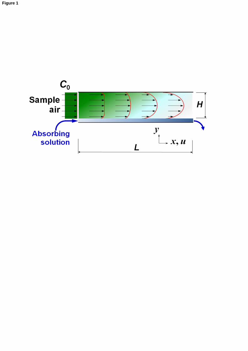
Figure 1

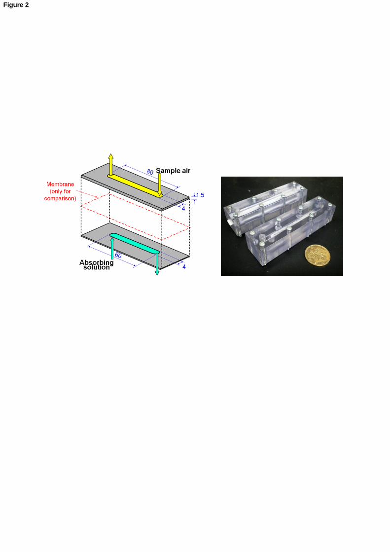
Figure 2

0 100 200 300 400 500

50

60

70

80

90

100

f (%

)

Gas flow rate (mL/min)

SO2

D 0.142

H2S

D 0.184

NH3

D 0.240

Figure 3

0 100 200 300 400 5000

20

40

60

80

100

Gas flow rate (mL/min)

H

6.0 mm

1.5 mm

3.0 mmf (%

)

Figure 4

0 100 200 300 400 5000

20

40

60

80

100

Gas flow rate (mL/min)

Silicone

pPP

pPTFEMembraneless

Theoretical

f (%

)

Figure 5

0 100 200 300 400 500

NH3

0 100 200 300 400 5000

20

40

60

80

100

with pPTFE

Membraneless

Theoretical

Gas flow rate (mL/min)

H2S

f (%

)

0

4

8

12

16

Collected amount

(membraneless)

Am

ou

nt

(nm

ol)

(a)

(b) (c)

0 100 200 300 400 5000

20

40

60

80

100

f (%

)

SO2

Gas flow rate (mL/min)

Figure 6

14:30 15:00 15:300.0

0.2

0.4

0.6

0.8

1.0

1.2

1.4 UV-FL raw

UV-FL 10-min average

Membraneless scrubber

SO

2 c

on

ce

ntr

ati

on

(p

pm

v)

Time of day

Figure 7

Length (cm) h (cm) w (cm) Vol Flow (cm^3/s)Flow Units Flow Rate

6 0.15 0.4 8.3335 liter/min 0.5

Vol Flow (l/min)

0.5

x type x Plot Start (cm)x Num Q type Qi (cm^3/sec)Qf (cm^3/sec)

linear 0.00E+00 80 linear 0.16667 8.3335

x Inc

0.075

Re*Sc Hydraulic Diam (cm)Velocity (cm/s)

226.453804 0.3 138.891667

xBar Points Fit Method

x (cm) f 0 power

6 0.60928566 0.0001 power

5.925 0.60516844 0.001 power

5.85 0.60102318 0.0025 power

5.775 0.59684968 0.005 power

5.7 0.59264777 0.01 power

0.025 expon

0.05 expon

0.1 expon

0.25 expon

1.00E+10 n/a

x (cm) f Q (cm^3/s) f Q (liter/min)

0 0 0.16667 1 0.0100002

0.075 0.03820047 0.5750115 0.99999711 0.03450069

0.15 0.06074183 0.983353 0.99943796 0.05900118

0.225 0.07754584 1.3916945 0.99503873 0.08350167

0.3 0.0914373 1.800036 0.98369594 0.10800216

0.375 0.10548357 2.2083775 0.9654923 0.13250265

0.45 0.12043632 2.616719 0.94220243 0.15700314

0.525 0.13472075 3.0250605 0.91577693 0.18150363

0.6 0.14845692 3.433402 0.88778352 0.20600412

0.675 0.16173106 3.8417435 0.85933399 0.23050461

0.75 0.17307472 4.250085 0.83116408 0.2550051

0.825 0.18395014 4.6584265 0.80373518 0.27950559

0.9 0.19447426 5.066768 0.77731947 0.30400608

0.975 0.20468641 5.4751095 0.75206265 0.32850657

1.05 0.21461887 5.883451 0.7280276 0.35300706

1.125 0.22429851 6.2917925 0.70522414 0.37750755

1.2 0.23374803 6.700134 0.68362887 0.40200804

1.275 0.2429868 7.1084755 0.66319842 0.42650853

Last 5 Points

Varying QFull Length

Supplementary Material