Microwave Emission and Scattering From Deserts: Theory Compared With Satellite Measurements

IEEE TRANSACTIONS ON GEOSCIENCE AND REMOTE SENSING, VOL. 46, NO. 2, FEBRUARY 2008 361

Microwave Emission and Scattering From Deserts:Theory Compared With Satellite Measurements

Norman C. Grody and Fuzhong Weng

Abstract—The emission and scattering from desert surfaces areanalyzed using simulations and measurements from the SpecialSensor Microwave/Imager (SSM/I) and the Advanced MicrowaveSounding Unit (AMSU) microwave satellite instruments. Desertsare virtually free of vegetation, so the satellite radiometers are ableto observe the emissivities of different minerals, such as limestoneand quartz. Moreover, since deserts contain little moisture, thethermal emission originates below the surface at a depth of manywavelengths. At high frequencies, where the penetration depth ofradiation is smallest, the radiometric measurements display thelarge diurnal variation in surface temperature, which reaches itsmaximum at around 1 P.M. Conversely, at low frequencies, wherethe penetration depth is largest, the radiation measurements dis-play the small diurnal variation of subsurface temperature, whichreaches a minimum at around 6 A.M. In addition to these emissionsignals, sand particles also scatter microwave radiation. Volumescattering causes the measurements to decrease as the frequencyincreases; although compared to other scattering media (snowcover and precipitation), the larger absorption and fractional vol-ume (i.e., solidity) of sand reduce the scattering. Although the scat-tering effect is small, SSM/I measurements between 19 and 85 GHzshow that deserts scatter the upwelling microwave radiation ina manner similar to light precipitation, which makes it difficultto uniquely identify precipitation over arid regions. Interestingly,the higher frequency AMSU measurement at 150 GHz is nearlythe same as at 89 GHz for deserts, whereas the 150-GHz mea-surement is much lower than at 89 GHz for precipitation. Thesedifferent spectral features at high frequencies can provide a meansof separating the scattering from desert surfaces from that ofprecipitation.

Index Terms—Dense media application, desert scattering, emis-sion, microwave desert properties, microwave remote sensing.

I. INTRODUCTION

AN ANALYSIS on the microwave radiation characteris-tics of desert surfaces is presented. Sand is basically

rock that has been degraded through various physical/chemical

Manuscript received March 14, 2007; revised August 7, 2007. This workwas supported by the I. M. Systems Group, Inc. National Oceanic andAtmospheric Administration, National Environmental Satellite, Data, andInformation Service, Center for Satellite Applications and Research (STAR)under Contract/Task DG133E-06-CQ-0030/8003-025. The content of this paperis solely the opinion of the author and does not constitute a statement of policy,decisions, or position on behalf of NOAA or the U.S. Government.

N. C. Grody is with the I. M. Systems Group, National Oceanic andAtmospheric Administration, National Environmental Satellite, Data, andInformation Service, Office of Research and Applications, Camp Springs, MD20746 USA (e-mail: [email protected]).

F. Weng is with the National Oceanic and Atmospheric Administration,National Environmental Satellite, Data, and Information Service, Center forSatellite Applications and Research (STAR), Camp Springs, MD 20746 USA(e-mail: [email protected]).

Color versions of one or more of the figures in this paper are available onlineat http://ieeexplore.ieee.org.

Digital Object Identifier 10.1109/TGRS.2007.909920

TABLE ISOME PHYSICAL CHARACTERISTICS OF SAND. THE DIELECTRIC

CONSTANTS WERE OBTAINED FROM [1]

processes. The composition of sand varies according to localrock sources and conditions, with the most common constituentbeing silicon dioxide, which is usually in the form of quartz.The density of pure crystalline quartz (single crystal) is about2.65 g/cm3, while the density of sand can range from about1.4–2 g/cm3, so the fractional volume or solidity of the sandgrains is between 0.53 and 0.75. In addition, according to theU.S. Department of Agriculture, the particle diameter of sandgrains ranges from 0.05 mm for fine sand to 2 mm for coarsesand. Since sand particles can have millimeter-size diameterswith fractional volumes of less than unity, they can scatteras well as absorb high-frequency microwave radiation. Theseparameters are listed in Table I(a) for reference.

While much is known about the mineralogy and sizes of sandgrains, less is known about the radiation absorption properties.Table I(b) lists the real part or refractive component of thedielectric constant εR for four of the most abundant desertmaterials. As shown in the table, the dielectric constant rangesfrom a maximum of about 7.5 for limestone to a minimum of3.0 for quartz, which is similar to that of ice (e.g., [4], [10],and [16]). These different minerals were first observed usingmicrowave observations at 19 and 37 GHz from the ElectricallyScanning Microwave Radiometers (ESMRs) on the Nimbus-5and Nimbus-6 National Aeronautics and Space Administration(NASA) satellites [1]. Both sensors were used to identify lime-stone and quartz deposits over Saudi Arabia from the spatialvariation of the brightness temperature measurements, i.e., thesurface emissivity is high for quartz and low for limestone.More recently, the low microwave emissivities of carbonate

U.S. Government work not protected by U.S. copyright.

362 IEEE TRANSACTIONS ON GEOSCIENCE AND REMOTE SENSING, VOL. 46, NO. 2, FEBRUARY 2008

Fig. 1. Real εR and imaginary εI parts of the dielectric constant of desertsand based on laboratory measurements [9].

rocks such as limestone have been studied by Prigent et al. [15].Other studies measured the dielectric constant [9] and thepenetration depth of radiation in sand [2], [14], which forsolid media is given by L = λ

√εR/2πεI , where εI is the

imaginary part of the dielectric constant, and λ is the free-spacewavelength.

Unlike the real part of the dielectric constant, the imaginarypart is less certain since it strongly depends on impuritieswithin the sand mixture and within the minerals. An early studyused microwave radiometers aboard a truck-supported platformto determine the penetration depth of geological materials byplacing the materials over a reflecting aluminum plate and mea-suring the surface-emitted radiation as a function of layer thick-ness [2]. The penetration depth of the different materials wasdetermined as a function of particle size and moisture content.For a coarse-grained lakeshore deposit sand (0.18% moistureby weight), which is composed of quartz with a mean particlesize of 0.46 mm, they obtained penetration depths of 130, 20,and 6 cm at frequencies of 1.4, 10, and 30 GHz, respectively.More recently, Matzler [9] used microwave resonant cavitymeasurements on a small sample of dry sand (0.2% moisture byweight) collected from the Sahara to show that the frequencydependence of the dielectric constant is characterized by aDebye-type model with a relaxation frequency of 0.27 GHz.As shown in Fig. 1, εR

∼= 2.63 for frequencies greater than1 GHz, while εI decreases from 0.056 at 1.4 GHz to 0.009for frequencies greater than 2 GHz. For solid media, the cal-culated penetration depth at 1.4 GHz is 91 cm, and it reducesto 88 cm at the highest measurement frequency of 10 GHz.Satellite measurements from the Special Sensor Microwave/Imager (SSM/I) instrument, which was developed as part of theDefense Meteorological Satellite Program (DMSP), have alsobeen used to estimate the penetration depths over the Africandesert. Prigent et al. [14] found that the penetration depths werehighly variable, i.e., with maximum values of about 15, 8, and4 cm at 19, 37, and 85 GHz, respectively. As shown in Fig. 2,the laboratory, ground-based, and satellite estimates all exhibita decrease of penetration depth with increasing frequency.However, the penetration depth based on Matzler’s dielectricconstant shows very little frequency variation compared to theground-based measurements, which appears more consistentwith the satellite estimates. As discussed later, the differencesin the three penetration depth measurements shown in the figurecan be due to the different solidity of the sand in addition to im-purities in the sand mixture, which affect the dielectric constant.

Fig. 2. Penetration depth of desert sand as a function of frequency based onsatellite radiometer measurements (Prigent et al. [14]), ground-based radiome-ter measurements (Blinn et al. [2]), and calculations (see text) using laboratorymeasurements of the dielectric constant (Matzler [9]).

This paper uses additional SSM/I brightness temperaturemeasurements, in conjunction with simulations, to arrive ata physically based emissivity model for deserts. To validatethe emissivity model, comparisons are made between the sim-ulations and measurements. These comparisons include boththe spectral and temporal variations of brightness temperature.In addition to the SSM/I observations at 19–85 GHz, themeasurements from the National Oceanic and AtmosphericAdministration (NOAA) Advanced Microwave Sounding Unit(AMSU) are used to extend the measurements up to 150 GHz.Large changes in the spectral characteristics are found forfrequencies between 85 and 150 GHz, and possible explana-tions are given based on the emissivity model. For reference,Table II lists the channel frequencies, field of views, and satel-lite observation times associated with the SSM/I and AMSUinstruments.

II. SURFACE EMISSIVITY MODEL

A physically based model is developed using the two-streamradiative transfer equation in conjunction with the dense mediatheory. Fig. 3 shows the schematic representation of the scene,which consists of a deep nonisothermal surface bound by theEarth’s atmosphere above. As shown in the Appendix, thebrightness temperature observed by an Earth-viewing satelliteradiometer can be written as [see (A12)]

TB(ν, t) = Tu(ν) + τν [εS(ν)Teff(ν, t) + 1 − εS(ν)Td(ν)](1)

where the atmospheric terms consist of the upwelling radiationTu, downwelling radiation Td, and atmospheric transmittanceτν , while the surface contribution consists of the surface emis-sivity εS and the effective temperature Teff , which approxi-mately corresponds to the temperature at the penetration depth.While all of these quantities depend on the frequency ν, theeffective temperature has the strongest diurnal variation and isso indicated.

Equation (1) can be simplified for window channels byrecognizing that the upwelling and downwelling radiations arenearly the same and can be approximated as TM (1 − τν), whereTM is the mean atmospheric temperature near the surface [5].As such, (1) becomes

TB(ν, t) ∼= TM

[1 − τ2

ν 1 − εS(ν)]

+ τνεS(ν) [Teff(ν, t) − TM ] . (2)

GRODY AND WENG: MICROWAVE EMISSION AND SCATTERING FROM DESERTS 363

TABLE IISSM/I AND AMSU OBSERVATION TIMES, CHANNELS, AND FIELDS OF VIEW

Fig. 3. Schematic representation of desert surfaces. Medium 1 consists of theupward Tu and downward Td atmospheric radiation, the downward-reflectedradiation R12Td, and the radiation transmitted from medium 2 across the inter-face (1 − R21)T+

B . Medium 2 consists of the upward T+B and downward T−

Bradiation, the upward-reflected radiation R21T+

B , and the radiation transmittedfrom medium 1 across the interface (1 − R12)Td.

Of all the parameters in (1) and (2), the emissivity is the mostdifficult to characterize. A relatively simple approach is takenhere by considering the desert surface to be infinitely deep,which is composed of low-loss sand particles (i.e., moisturefree), and all having the same geometry and dielectric constant.The emissivity is then the same as that for a homogeneous

isothermal surface [21], which can be concisely written as[see (A13)]

εS(ν) = (1 − RS)[

2a

(1 + a) − (1 − a)RS

](3a)

with

a =√

1 − ω

1 − ωg. (3b)

Equation (3a) combines the surface interface and the subsurfacevolumetric properties into a single expression. The leading termin (3a), i.e., 1 − RS , is the transmissivity at the air/surfaceinterface, where RS is the reflectivity that refracts the upwellingradiation generated below the surface. The reflectivity alsoreflects the downwelling atmospheric radiation incident to thesurface. For smooth surfaces, the reflectivity is determinedusing Fresnel equations1 with the dielectric constant, viewing

1(RS)V H = |rV H |2, where rV = −tan(θ − θ′)/ tan(θ + θ′), rH =sin(θ − θ′)/ sin(θ + θ′), and sin θ′ = sin θ/

√ε. Natural surfaces do not ap-

pear perfectly smooth at microwave frequencies, so the reflectivity is modifiedby the effects of surface roughness. As a result, (RS)V is generally less and(RS)H is higher than that obtained from the Fresnel equations.


Fig. 4. (Top) Emissivity and (bottom) penetration depth for a dielectricconstant of 4.0 + i0.08 and fractional volume of 0.6. Calculated for the SSM/Iviewing angle of 53.1 at V-Pol. The emissivity and penetration depth areplotted as a function of frequency with particle radius as a parameter. Onlythe emissivity strongly depends on the particle radius. The bottom figure alsoshows the SSM/I measurements of maximum penetration depth at 19, 37, and85 GHz (see text).

angle, and polarization as input parameters. Table I(b) showsthe calculated transmissivity for the different minerals. Asshown later, the transmissivity accounts for much of the spatialvariation of brightness temperature (i.e., emissivity) observedby satellite radiometers. In fact, it has been customary to di-rectly equate transmissivity with emissivity for many snow-freesurfaces. However, the second bracketed term in (3a) accountsfor volume scattering, which can be important at high frequen-cies. It contains the similarity parameter a defined by (3b),which is a function of the single-particle albedo ω (ratio ofscattering to extinction coefficient) and the asymmetry parame-ter g (forward minus back-scattered energy divided by 2). Bothof these quantities (ω and g) are defined in the Appendix anddepend on the dielectric constant, fractional volume, and sizeof the sand grains in addition to the microwave frequency. Thesimulations are compared later with the satellite measurementsto show that the fractional volume of sand ranges between 0.5and 0.7 with corresponding dielectric constants of 0.11 and0.06 for the imaginary part. Using a mean dielectric constant of4 + i0.08 and a fractional volume of 0.6, Fig. 4 (top) displaysthe vertically polarized (V-Pol) emissivity as a function offrequency for the SSM/I viewing angle of 53.1, where eachplot is for a different particle radius (0.3 and 0.5 mm). Notethat volumetric scattering causes the emissivity to decreasewith increasing frequency and particle radius. In addition toemissivity, Fig. 4 (bottom) shows the corresponding penetra-tion depth, which is essentially independent of the particleradius.

The brightness temperature (2) also contains the effectivetemperature of the medium, which depends on the subsurfacetemperature profile and the penetration depth of radiation. Anaccurate representation of the temperature profile is obtained

TABLE IIITHERMAL PROPERTIES FOR NATURAL MATERIALS. THE SCALE

HEIGHT IS DETERMINED FROM THE THERMAL

DIFFUSIVITY K USING h = (2 K/Ω)0.5

using the 1-D equation of heat transfer, whose general solutionis [17]

T (z, t)=T0+∞∑

n=1

Tne(z/h)√

n cos[nΩ(t−tn)+(z/h)

√n].

(4)

Using only the first term in the series expansion, the tem-perature is

T (z, t) = T0 + T1ez/h cos [Ω(t − t1) + z/h] (5)

where T0 = 0.5(Tmx + Tmn), and T1 = 0.5(Tmx − Tmn),where Tmx is the maximum surface temperature, which occursat time t1, and Tmn is the minimum surface temperature,which occurs 12 h later. Equation (5) also contains the scaleheight h, which defines the rate of temperature decrease withdepth. Table III lists the scale height for different materials ascalculated from the thermal diffusivity [12]. For desert sand, thescale height is about 8 cm. The diurnal variation of temperaturedue to solar heating is given by the cosine term in (5), whichcontains the Earth’s rotational frequency (Ω = 2π/24 rad/h).As an example, Fig. 5 compares the diurnal variation of surfacetemperature represented by (5) with the actual measurementsover the Central Sahara desert ([13]; also [12, p. 82]). Thecoefficients T0, T1, and t1 shown in the figure were obtained byfitting the time series of the surface temperature measurementsto a Fourier series. Fig. 5 also shows the improved fit obtainedby using the first and second harmonic components in (4),where the coefficients T0, T1, T2, t1, and t2 were again deter-mined by Fourier analysis. However, to simplify the brightnesstemperature model, only the first harmonic component given by(5) is used in the Appendix to obtain the effective temperature[see (A11c)]

Teff(ν, t) = T0 + T1[C1 cos ψ + C2 sinψ], ψ = Ω(t − t1)(6a)


Fig. 5. Comparison between measured and modeled surface temperatureswithin a sand dune for the Central Sahara desert in mid-August. The modelfunctions are obtained using the first Fourier harmonic as well as the first andsecond Fourier harmonics.

with

C1 =1 − b + 2b3

1 + 4b4C2 =

b − 2b2 + 2b3

1 + 4b4(6b)

where

b =µL

hL =

a

ka. (6c)

The coefficients C1 and C2 are functions of the b-parameter,which depends on the ratio of penetration depth L to temper-ature scale height h and the cosine of the transmitted angle(µ = cos θ′), as shown in Fig. 3. As shown in the Appendix,for solid media, the albedo is zero so that a = 1, and theabsorption coefficient is ka = 2πεI/λ

√εR, where λ is the

free-space wavelength. The penetration depth then reduces tothe well-known result L = 1/ka = λ

√εR/2πεI . In general,

however, for granular media, the penetration depth also dependson the fractional volume and particle radius. Using the effec-tive dielectric constant from dense media theory [19, p. 498],which accounts for the coherent wave–particle interactions, thepenetration depth is in general a function of the particle ra-dius, fractional volume, and dielectric constant of the particles.However, for the range of parameters associated with desertsand (f = 0.5–1, r = 0.3–0.5 mm, and εI = 0.02–0.10), thepenetration depth can be approximated by

L ∼=λ√

εR

2πεIf1.7(7)

where Fig. 6 (top) compares this equation with the exact modelcalculations. The scatter about the one-to-one line is mainlydue to the dependence on particle radii, which is neglectedin (7) since it is mainly important at high frequencies, wherethe penetration depth is small. Note also that for densely packedparticles (i.e., f = 1), the equation reduces to that obtainedfor solid media. The SSM/I estimates of the penetration depthmentioned in Section I and described in the next section areused in conjunction with (7) to obtain an equation relating theimaginary part of the dielectric constant to the fractional vol-ume. This hyperbolic relationship is shown in Fig. 6 (bottom)

Fig. 6. (Top) Penetration depth compared with an empirical fit given by (7) forthe SSM/I frequencies and the parameter range associated with desert surfaces.(Bottom) Relationship between the imaginary part of the dielectric constantand the fractional volume obtained using (7) with the real part of the dielectricconstant set at 4.0 and the penetration depth set at 15, 8, and 4 cm by the SSM/Imeasurements at 19, 37, and 85 GHz, respectively (see text).

for each of the SSM/I frequencies and will be used later toestimate the dielectric constant and fractional volume based oncomparisons between simulations and SSM/I measurements.

Equation (6a) is simplified when b 1 since C1≈ 1,C2≈ b, and Teff ≈ T (z = −µL, t), so Teff is approximatelythe temperature at the penetration depth. This simplificationis mainly applicable to high frequencies, since the penetrationdepth is much smaller than the scale height and b 1. Ingeneral, however, the difference between Teff and T can be aslarge as 4.5 K when b = 1.8 and when the surface temperatureis at its maximum or minimum. It is also found that uponequating Teff with T , the penetration depths based on (5)and (6) can differ by up to 5 cm. Nevertheless, as discussednext, the approximation Teff ≈ T (z = −µL, t) has been usedto estimate the penetration depth from SSM/I measurements.

III. SSM/I EMISSION MEASUREMENTS

In [14], the penetration depth and emissivity were derived atthe SSM/I frequencies (19, 37, and 85 GHz) over North Africaand Saudi Arabia by first representing the temperature profileby the first two harmonics in (4). As in the case of Fig. 5,the coefficients (T0, T1, T2, t1, and t2) were obtained usingFourier analysis of the surface skin temperature (derived usinggeostationary satellite infrared (IR) measurements obtainedeight times daily). The daily SSM/I brightness temperaturemeasurements were then used to estimate the penetration depthand emissivity at each SSM/I frequency by fixing the thermaldiffusivity to 0.002 cm2/s (i.e., h = 7.5 cm) and assuming


Fig. 7. (Top) SSM/I V-Pol 37-GHz (ascending F-13) measurements for July 1996. Quartz has the highest brightness temperatures, while limestone has the lowestmeasurements. (Bottom, left) Emissivity calculated as a function of dielectric constant. (Bottom, right) Map of limestone deposits over Saudi Arabia.

Teff(ν, t) = T (z = −µL, t) in (1). Moreover, the atmosphericterms in (1) are also required, which were obtained usingthe atmospheric temperature and water vapor from numericalweather analysis models. Note that the derived penetrationdepths do not require any assumption regarding the emissivityor penetration depth models. However, the calculated pene-tration depths considerably varied over the different desertareas, presumably due to the different dielectric properties andfractional volume, or solidity, of sand. At all the frequencies,the minimum was found to be near zero, while the maximumpenetration was about 4, 8, and 15 cm at 85, 37, and 19 GHz,respectively. Since the penetration depths at 19 and 37 GHz canbe greater than the 7.5-cm scale height, the assumption Teff ≈T (z = −µL, t) is less accurate at these two lower frequencies.However, the resulting penetration depths and emissivity mapsgenerated by Prigent et al., [14] appear reasonable. Further-more, as shown in Fig. 4 (bottom), the SSM/I maximum pene-tration depths are consistent with the model calculations using adielectric constant of 4 + i0.08 and a fractional volume of 0.6.As discussed in the next section, these chosen parameters arealso consistent with other independent SSM/I measurements.

In addition to the contribution from the effective temperature,the brightness temperature also depends on the emissivity term.As previously mentioned, the leading term (1 − RS) in (3a) re-sults in the transmissivities listed in Table I. For a more detaileddescription, Fig. 7 (bottom left) shows this emissivity compo-nent as a function of the real part of the dielectric constant fornadir viewing as well as at the SSM/I viewing angle of 53.1.The figure also identifies the different surfaces listed in Table I

based on their dielectric constants. Note that the emissivity forquartz and sandstone approaches unity, while limestone hasthe lowest emissivity at V-Pol. As an example of these surfacefeatures, Fig. 7 (top) shows the monthly averaged SSM/I V-Polbrightness temperature measurements at 37 GHz imaged overNorth Africa and Saudi Arabia for July 1996. In addition, a1963 geological surface map of the Arabian Peninsula from theU.S. Geological Survey/American Oil Company is also shown(bottom right) delineating the areas containing large limestonedeposits. Observe how well the lowest SSM/I brightness tem-peratures (≈265 K) follow the limestone deposits shown in thesurface map. Note in particular the “crescent-like feature” of thelimestone deposit in the middle of Saudi Arabia that appears inboth the SSM/I measurements and the surface map. This samefeature was first identified by Allison [1] using early microwavesensors (ESMRs on Nimbus-5 and Nimbus-6 satellites). Theemissivity maps presented by Prigent et al. [15] also showthese same surface features using the 19-GHz V-Pol SSM/Imeasurements. From these comparisons, it appears that muchof the brightness temperature variation over deserts is due toemissivity changes and not to surface temperature variations.

Interestingly, the same spatial variation of surface featuresseen at microwave frequencies has also been observed in the IR[1]. As a more recent example, Fig. 8 shows the latest imageof emissivity obtained in the 8.4- to 8.7-µm band from mea-surements [11] by the Moderate Resolution Imaging Spectro-radiometer (MODIS) instrument aboard the Earth ObservationSystem satellites operated by NASA. The physical mechanismassociated with radiation absorption by molecules is quite


Fig. 8. IR image of North Africa and Saudi Arabia showing the surface-emitted radiation in the 8.4- to 8.7-µm band. Quartz has the lowest emissivity, whilelimestone has the highest emissivity.

Fig. 9. Brightness temperature Tb as a function of transmittance τ withemissivity εS as a parameter, which is obtained using (2) with TM = 280 Kand Teff = 300 K. The transmittances at 19 and 22 GHz are shown for watervapor amounts ranging between 5 and 30 mm at the SSM/I viewing angleof 53.1. For εS > 0.95, Tb increases with τ so that Tb(19) > Tb(22).Conversely, for εS < 0.95, Tb decreases with τ so that Tb(19) < Tb(22).

different at microwave frequencies (i.e., rotational modes ofexcitation) and IR wavelengths (i.e., vibrational modes). Assuch, the emissivity of quartz and sandstone is near unity atmicrowave frequencies but has a very low emissivity (0.7) inthe 8- to 9-µm IR band. Moreover, the microwave emissivityfor limestone is very low compared to other desert minerals butis near unity in the 8- to 9-µm IR band.

The regions of high brightness temperature in Fig. 7 were at-tributed to the high-emissivity surfaces listed in Table I, namelythat of quartz or sandstone. However, besides being supportedby the IR image, these high-emissivity regions can also be val-idated using the SSM/I V-Pol channels at the 19- and 22-GHzchannels. The surface emissivity is virtually identical for theseclosely spaced channels, so the main difference is due to thelarger atmospheric water vapor absorption at 22 GHz comparedto 19 GHz. As a result, the 22-GHz brightness temperature mea-surements are less than at 19 GHz for high-emissivity surfaces,whereas the opposite occurs for low-emissivity surfaces. Toillustrate this feature, Fig. 9 shows a plot of (2) as a function of

atmospheric transmittance with the emissivity as a parameter.The emissivity is set at 0.90, 0.95, and 1.0 with a meantemperature of 280 K and an effective temperature of 300 K.For reference, the figure also shows the nominal range of trans-mittance due to water vapor for the 19- and 22-GHz channels.While the brightness temperatures vary with the water vaporand the difference between the effective and mean atmospherictemperature, the 19-GHz brightness temperature is alwayslarger than at 22 GHz for emissivities greater than 0.95, whereasthe opposite occurs for smaller emissivities. This split-windowapproach is used here as an independent means of identifyinghigh-emissivity surfaces such as quartz by differencing thesetwo closely spaced SSM/I channels in Fig. 10 and only imagingdifferences greater than 3 K.

As expected from the above discussion, the color imageof Fig. 10 clearly shows that the same regions having veryhigh brightness temperatures at 37 GHz (bottom) also have thelargest positive differences between the 19- and 22-GHz V-Polchannels (top left). After examining other regions around theglobe using this split-window technique, it is found that desertshave the highest emissivity at V-Pol of all the surfaces. Asshown in Fig. 10, even the vegetated and heavily forested areasover central Africa, which are generally considered to havethe highest emissivity, result in split-window channel measure-ments less than 3 K. This latter result occurs due to the rela-tively smooth characteristic of deserts compared to vegetationand forests whose roughness reduces the V-Pol emissivity dueto cross-polarization effects.

IV. SSM/I SCATTERING MEASUREMENTS

Satellite-based microwave radiometers have been used tomeasure the intensity of scattering using an index. Over land,the scattering index can be defined as the positive difference


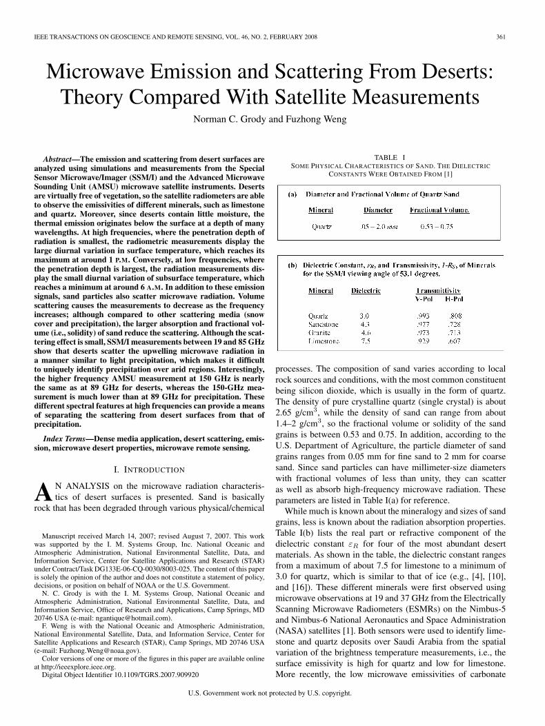
Fig. 10. SSM/I measurements over Africa and Saudi Arabia for July 1996. Difference between (top) 19- and 22-GHz V-Pol channels and (bottom) 37-GHzchannel measurements. Note that the large differences in the top image (≥ 3 K) correspond to the highest brightness temperature measurements in thebottom image.

TABLE IVSCATTERING INDEX FOR DIFFERENT MATERIALS

in brightness temperature measurements Tb at two frequencies,e.g., Tb(ν1) − Tb(ν2), where ν2 > ν1. Table IV shows therange of the scattering index TB(22v) − TB(85v) obtained fordeserts, snow cover, and precipitation using the V-Pol SSM/Ichannels at 22 and 85 GHz. The measurements over Africawere used to obtain the maximum scattering values over deserts(Sahara) and arid land (Sahel and Kalahari). Intense rain eventsover the U.S. were used to obtain the maximum value forprecipitation. The scattering index is largest for V-Pol [6], sofor highly polarized surfaces (e.g., deserts), the index is about25% less for AMSU, which has similar channels to that ofSSM/I (see Table II), but measures the average between theV-Pol and horizontally polarized brightness temperatures at23 and 89 GHz.

As shown in Table IV, the range of scattering indices fordifferent materials overlaps at the low end of the scale. As such,one must use additional channel relationships as well as auxil-iary information to discriminate among them [7]. For example,snow cover is approximately separated from precipitation byrecognizing that its physical temperature is generally less thanthat of precipitation. In the case of AMSU, the lowest frequencychannel at 23.8 GHz is used to infer the temperature beneaththe snow pack. Since the emissivity of frozen soils is about0.96, brightness temperatures of less than 262 K are associatedwith snow cover. This same temperature threshold also filters

out most cold deserts (e.g., Tibet and Mongolia). However,additional conditions are needed to filter out the scatteringsignal due to warmer deserts and arid land such as that foundover Africa. As noted in Table III, these more solid surfaceswith higher fractional volumes generally scatter less than snowcover and precipitation. Increasing the lower limit of the scatter-ing index can remove these remaining surfaces, although lightrainfall events will also be removed. It is therefore necessary tocome up with a compromising set of conditions to retain mostof the precipitation.

The reduction in scattering shown in Table IV for desertscompared to precipitation and snow cover is due to the largerfractional volume, which reduces the albedo, and the increasedabsorption by desert sand compared to ice particles. Due to thesmaller scattering signal, all previous studies have concentratedon larger emission signals over deserts. However, in addition tothe emission measurements, the SSM/I also displays scatteringsignatures over deserts. To identify the scattering features insome detail, we first examine the difference between two of thelowest frequency SSM/I channels, i.e., TB(19v) − TB(37v),and compare these results with the higher frequency differenceTB(37v) − TB(85v). Fig. 11 shows the images generated forMay 1998 after taking the difference between the 19- and37-GHz V-Pol measurements and averaging only positive dif-ferences for the month. The left image is from the F-13 de-scending satellite orbits at 6:00 A.M., while the rightmostimage is from the F-14 descending satellite orbits at 9:30 A.M.(see Table II). Note that the 6:00 A.M. early morning imagedisplays positive differences (TB(19v) > TB(37v)) over thedeserts of Saudi Arabia, Tibet, China, and South America, witha maximum difference of 10 K. However, these areas of positivedifference over deserts nearly vanish at 9:30 A.M. Only themuch larger signal (> 10 K) due to the scattering by snow coverremains at the higher latitudes, which is constant independentof time.


Fig. 11. Difference between the 19- and 37-GHz SSM/I V-Pol measurements at (left) 6:00 A.M. and (right) 9:30 A.M. for May 1998. Bottom image shows thetime series of the temperature at different depths within a sand dune for the Central Sahara in mid-August.

Fig. 12. Difference between the 37- and 85-GHz SSM/I V-Pol measurements at (left) 6:00 A.M. and (right) 9:30 A.M. for May 1998.

The diurnal feature exhibited over the deserts in Fig. 11 hasbeen studied in [14], where the physical basis can be obtainedby referring to the temperature measurements shown at thebottom of the figure. This plot shows the temperature abovethe surface, at the surface, and below (30 and 75 cm) duringmid-August for a sand dune over the Central Sahara ([13];also [12, p. 82]). These same surface temperature data wereused in the analysis presented in Fig. 5 and vary by almost25 K between 6:00 A.M. and 9:30 A.M., while the deeperlevel temperatures remain constant. Since the 19-GHz channelresponds to temperature at a greater depth than at 37 GHz (seeFig. 4, bottom), the quantity TB(19v) − TB(37v) is positive at6:00 A.M. and reverses sign at 9:30 A.M., which is in agreement

with the two SSM/I images. Based on this consideration, whichonly accounts for thermal emission, one would expect a similardiurnal variation for TB(37v) − TB(85v).

Fig. 12 shows the corresponding images for TB(37v) −TB(85v), where again the left image is from the F-13 descend-ing satellite orbits at 6:00 A.M., while the rightmost image isfrom the F-14 descending satellite data at 9:30 A.M. However,unlike the previous results in Fig. 11, both images in Fig. 12look similar, with relatively little change in the “positive” desertareas for the two time periods. As such, the positive differencefor TB(37) − TB(85) cannot be entirely attributed to thermalemission. This is explained next using simulations that includethe effect of volume scattering.


Fig. 13. Surface temperature using (5) with the parameters derived from themeasurements in Fig. 5, i.e., Tmx = 329 K, Tmn = 298 K, and t1 = 13.6 h.The two dots on the plot correspond to the satellite observation times of6:00 A.M. and 9:30 A.M. (see Figs. 11 and 12).

V. SSM/I SIMULATED MEASUREMENTS

Simulations are used to examine the relationship between theSSM/I measurements and the surface parameters. The bright-ness temperatures are calculated using (1), (3a), (3b), (5), (6a),(6b), and (6c) by applying realistic atmospheric and surfaceparameters. To represent dry desert climates, the water vaporis varied between 10 and 20 mm, and the temperature profileis given by (5) with the parameters shown in Fig. 4 (Tmx =329 K, Tmn = 298 K, and t1 = 13.6 h). Using these para-meters, Fig. 13 shows the temperature at the surface with thetwo periods of SSM/I observation (6:00 A.M. and 9:30 A.M.)highlighted by vertical lines. The simulated brightness tem-perature differences at these two time periods are shown inFig. 14 and plotted as a function of fractional volume. As inFigs. 11 and 12, the leftmost plots show TB(19) − TB(37)and TB(37) − TB(85) at 6 A.M., while the rightmost plotscorrespond to the later time of 9:30 A.M. Each display showsthe brightness temperature difference plotted against the frac-tional volume, which ranges between 0.5 and unity in six equalintervals. The particle radius for the data set has values between0 and 0.5 mm, where the increase in TB(37) − TB(85) forlow fractional volumes is due to the increase in particle radius.At each fractional volume, the imaginary part of the dielectricconstant is set to the indicated values, which is based on therelationship shown in Fig. 6 (bottom). This approximately fixesthe penetration depth to the SSM/I estimates of 15, 8, and 4 cmat 19, 37, and 85 GHz, respectively.

Compared to the scatter-free results (i.e., f = 1), the bright-ness temperature difference TB(37) − TB(85) substantiallyincreases as the fractional volume decreases. Although thebrightness temperature difference diurnally varies, it remainsmostly positive for the two time periods for fractional volumesof 0.7 and smaller. Such fractional volumes are required forthe simulations to be consistent with the SSM/I measurementsin Fig. 12. Furthermore, the brightness temperature differenceTB(19) − TB(37) is positive at 6:00 A.M. but changes signby 9:30 A.M. This diurnal variation occurs for all fractionalvolumes, although the largest negative values occur for highfractional volumes. From these simulations, it is concluded thatthe inclusion of scattering effects in the emissivity model isrequired to explain the high-frequency SSM/I measurementsshown in Fig. 12.

Additional comparisons are shown in Fig. 15 by plottingthe complete diurnal cycle of TB(19) − TB(37) and TB(37) −

TB(85) for a scatter-free surface (i.e., f = 1 and ε = 4 +i0.03), and that obtained when including the scattering ef-fects using a fractional volume of 0.6 with ε = 4 + i0.08. Forreference, the vertical lines are shown along the time axisto highlight the satellite observation times corresponding tothat in Figs. 11 and 12. This figure shows that the brightnesstemperature differences, i.e., TB(19) − TB(37) and TB(37) −TB(85), both display the diurnal variations resulting from theeffective temperature in (1). This emission component mod-ulates the scattering contribution, which causes the emissiv-ity to decrease with increasing frequency and particle size(see Fig. 4). Note that if scattering effects are neglected, thehigher frequency difference TB(37) − TB(85) is underesti-mated and results in a zero to negative difference during thetime period from about 8:00 A.M. to 6:00 P.M. when the surfacetemperature is higher than the subsurface temperature.

As mentioned in the previous section, the desert scatteringseen at higher frequencies makes it difficult to identify theatmospheric scattering due to precipitation. However, aninteresting effect occurs for frequencies greater than 85 GHz.Fig. 16 compares the NOAA-15 AMSU measurements overAfrica on January 3, 2000, at 7:30 P.M. with a coincidentIR image from the METEOSAT geostationary satellite. TheAMSU consists of three separate modules, which are calledAMSU-A1, AMSU-A2, and AMSU-B [8], where the A2-module contains channels at 23.8, 31.4, and 89 GHz with50-km resolution at nadir, while the B-module contains an89- and 150-GHz channel with 15-km resolution at nadirviewing (see Table II). The IR imager is particularly usefulfor monitoring precipitation, where clouds are screened basedon the brightness temperature and temporal variability of themeasurements. However, for IR brightness temperatures of240 K and lower (yellow and light green), the measurementsare directly associated with precipitation. Such low brightnesstemperature measurements are seen as a diagonal line overNorth Africa centered around 22 N, 16 E. This same region ofvery low IR temperatures also shows large positive values forboth the AMSU-A 23- and 89-GHz channel difference (top left)and the AMSU-B 89- and 150-GHz channel difference (bottomleft), where a threshold of 5 K is used. However, unlike theisolated precipitation feature shown in the AMSU-B image, theAMSU-A image also displays a number of large-scale irregularareas having IR brightness temperatures higher than 280 K(purple and pink), which are not due to precipitation. Theseregions in the AMSU-A image are due to desert scattering andcan lead to false areas of precipitation if not accounted for.

The difference between the AMSU-B 89- and 150-GHzchannels uniquely identifies the isolated precipitation eventover North Africa, with no false signatures resulting from thedesert surface. Only over the vegetated and heavily forestedareas of central Africa are the precipitation events identifiedby both the AMSU-A and AMSU-B channel differences. Thisexample shows that the higher frequency portion of the mi-crowave spectrum measured by AMSU-B removes the desert-scattering features seen by the AMSU-A channels. For a moredetailed understanding, Fig. 17 displays the brightness tem-perature spectrum in the rain and rain-free (see triangle) areasshown in Fig. 16. Note that while the brightness temperatures


Fig. 14. Simulated V-Pol brightness temperature differences 19v − 37v (top) and 37v − 85v (bottom) as a function of fractional volume. The simulations are atthe satellite overpass times of (left) 6 A.M. and (right) 9:30 A.M. At low fractional volumes, the higher frequency difference increases with particle radius, whichranges between 0 and 0.5 mm. For each fractional volume, the imaginary part of the dielectric constant is set to the indicated values based on the relationship inFig. 6 (bottom).

Fig. 15. Simulated diurnal cycle of simulated V-Pol brightness temperature difference. (Left) 19v37v. (Right) 37v85v. Vertical lines indicate the satelliteoverpass times of about 6 A.M. and 9:30 A.M. The results are shown for a fractional volume of (top) unity and (bottom) 0.6. The imaginary part of the dielectricconstant (0.3 and 0.8) is obtained from the relationship in Fig. 6 (bottom). As in Fig. 14, the particle radius is between 0 and 0.5 mm, where the increase in thehigher frequency difference for high fractional volume is due to the larger particle radius.

continuously decrease up to 150 GHz for precipitation, it flat-tens out beyond 89 GHz for the rain-free area. The possibleexplanations include the effects of water vapor, which is muchlarger at 150 GHz than at 89 GHz, thereby attenuating theradiation emitted by the desert surface. However, it is alsopossible that for a large grain size (radii > 0.5 mm), scatteringapproaches the geometric optics limit for frequencies largerthan 89 GHz so that the emissivity and brightness temperature

remain nearly constant up to 150 GHz. To investigate thesepossibilities through simulations, the surface emissivity shownin Fig. 4 must be extended to higher frequencies and largerparticle size. However, the dense media model used here isapplicable for size parameters (kr = 2πr/λ) less than unity,so an empirical adjustment is needed for the 150-GHz channel.Further analysis is therefore needed before reaching a finalconclusion on this issue.


Fig. 16. Comparisons between NOAA-15 AMSU measurements on January 3, 2000 and the METEOSAT-IR image at the same time (7:30 P.M.) over Africa.The IR image on the right shows regions having brightness temperatures of 240 K and lower (yellow and light green) associated with heavy precipitation. Ofparticular interest is the line of precipitation over North Africa centered around 22 N, 16 E. This region shows large positive values for both the AMSU-A 23-and 89-GHz channel difference (top, left) and the AMSU-B 89- and 150-GHz channel difference (bottom, left). However, the AMSU-A image also displays anumber of areas having IR brightness temperatures higher than 280 K (purple and pink), which is not due to precipitation but mainly due to desert scattering.

Fig. 17. Brightness temperature spectrum from AMSU-A and AMSU-Bmeasurements for the heavy precipitation region of north central Africa(22.3 N, 16.4 E) as well as the rain-free area shown in Fig. 16 by the trianglesymbol.

VI. CONCLUSION

Several unique microwave characteristics have been iden-tified over deserts using simulated and observed V-Polmeasurements at SSM/I frequencies of 19, 22, 37, and 85 GHz.The spatial variation of the 37-GHz V-Pol measurements inFig. 7 has been found to be mainly due to emissivity variations,with quartz having an emissivity near unity, while limestone hasthe lowest emissivity. These same minerals have been observedto have completely opposite emissivity characteristics in the8- to 9-µm IR band. Regions having emissivities greater than0.95 (i.e., quartz, granite, and sandstone) were also identified bymeans of a split-window technique, which uses the differencebetween the 19- and 22-GHz V-Pol channels (see Fig. 10).

The split-window technique also showed that deserts have thehighest V-Pol emissivity of any surface, including vegetatedand forested land. Deserts can therefore provide a very highemissivity target for the validation of emissivity retrievals aswell as the vicarious calibration of microwave radiometers.While the emissivity is constant, the 37-GHz brightness temper-ature follows the diurnal variation of the effective temperature(i.e., temperature near the penetration depth). The differencebetween the 19- and 37-GHz V-Pol measurements in Fig. 11is also shown to follow the diurnal variation of the effectivetemperature, which is different at the two frequencies due totheir different penetration depths.

In addition to the above emission effects, deserts also scattermicrowave radiation. The volume-scattering contribution ofemissivity is constant and decreases the emissivity and bright-ness temperature as the frequency and grain size is increased(see Fig. 4). Scattering from coarse grain sand was observedby differencing the 37-and 85-GHz V-Pol SSM/I channels inFig. 12 and noting the stationary features for the two satelliteobservation periods. The SSM/I measurements were also com-pared with a simplified emissivity and brightness temperaturemodel, which includes volume scattering as well as thermalemission. Scattering, which depends on the fractional volumeand grain size of sand, is considered to be more significantthan the neglected geometric surface effects due to small-scaleroughness [3] or large-scale variation due to dunes [18]. Directcomparisons are made between model simulations and SSM/Imeasurements to show the important role that scattering playsin defining the spectral characteristics of the V-Pol emissivityand brightness temperature. An analysis of the SSM/I mea-surements in conjunction with model simulations suggests that


the average fractional volume of sand is about 0.6 with animaginary dielectric component of 0.08. Not determined at thistime is the spatial distribution of the fractional volume anddielectric constant.

In addition to SSM/I observations, the AMSU instrumentwas used to extend the frequency range of measurements upto 150 GHz. AMSU observations over the Sahara show thatthe spectral response of desert surfaces markedly changes be-tween 89 and 150 GHz. Unlike the atmospheric scattering dueto precipitation, whose brightness temperature monotonicallydecreases with frequency, the radiation from desert surfaceschanges relatively little between 89 and 150 GHz comparedto the lower frequency segment between 23 and 89 GHz (seeFig. 17). Possible explanations include the effect of water vaporabsorption, which is larger at 150 GHz, or the fact that for alarge grain size (> 0.5 mm), scattering approaches the geomet-ric optics limit so that the emissivity and brightness temperatureremain nearly constant between 89 and 150 GHz. Althoughthe exact physical mechanism has not been established at thistime, the flatter response at high frequencies for deserts enablesone to uniquely identify precipitation (see Fig. 16). This is incontrast to the SSM/I measurements between 19 and 85 GHz,which can be similar for deserts and precipitation, which makesit difficult to identify precipitation over arid regions.

APPENDIX

This Appendix derives the brightness temperature seen by anEarth-viewing satellite-based radiometer. As shown in Fig. 3,the scene consists of an emitting atmosphere above a non-isothermal deep scattering medium. The brightness temperatureobserved at the satellite altitude (z = ∞) is

TB = Tu(∞) + τ[(1 − R21)T+

B (0) + R12Td(0)]

(A1)

where Tu and Td are the atmospheric radiation contributions.The interface at z = 0 reflects the downward atmosphericradiation, where R12 is the reflectivity. This reflectivity alsorefracts the upwelling radiation generated from below the sur-face T+

B (0), where 1 − R21 is the transmissivity. For a smoothinterface, the reflectivity is derived using Fresnel equations byapplying the effective dielectric constant of the medium, whereeffects due to surface roughness can be included by modifyingthe Fresnel equations.

To obtain a concise analytic solution, the radiation in thescattering medium is obtained using the two-stream radiativetransfer equation, where T+

B and T−B are the upward- and

downward-propagating radiations along the two stream direc-tions (see Fig. 3), respectively. For the SSM/I viewing angle of53.1, the two-stream solution accurately approximates the fullmultistream radiative transfer equation [20]. The coupled set ofequations along the two streams can be rewritten as

[(1+a2

2a

)± µL

d

dz

]T±

B (z, t)=(

1−a2

2a

)T∓

B (z, t)+ aT (z, t)

(A2)

where a is the similarity parameter, L is the penetration depth,and µ is the cosine of the transmitted angle θ′, as shown in

Fig. 3. The similarity parameter and the penetration depth aregiven by

a =√

1 − ω

1 − ωgL =

a

ka(A3)

which contains the single-particle albedo ω (which is the ratioof the scattering coefficient to the extinction coefficient) andthe asymmetry parameter g (which is the difference betweenthe forward and back-scattered energy divided by 2). Both ofthese parameters will be determined later.

The two coupled (A2) are combined to obtain separateequations for the upward and downward brightness tempera-tures, viz.,[

1 − µ2L2 d2

dz2

]T±

B (z, t) =[1 ∓ aµL

d

dz

]T (z, t) (A4)

where the boundary condition at the interface z = 0 is

T−B (0) = R21T

+B (0) + (1 − R12)Td(0) (A5)

with the interface reflectivity R12 being complimentary so thatR12(θ) = R21(θ′) ≡ RS .

The solution of (A4) is

T±B (z) = A±ez/µL + T±

p (z) (A6)

where the complementary solution contains the undeterminedcoefficients A+ and A−, and the particular solution Tp sat-isfies (A4). The particular solution depends on the verticaltemperature profile, which varies exponentially with depth anddiurnally in time, and to first order is approximated by (5), i.e.,

T (z, t) = T0 + T1ez/h cos [Ω(t − t1) + z/h] . (A7)

The particular solution then becomes

T±p (z)= T0 + [C± cos ψ′ + D± sin ψ′] T1e

z/h

ψ′= Ω(t − t1) + z/h (A8a)

with

C± =1 ∓ ab(1 − 2b2)

1 + 4b4D± = −2b2 ∓ ab(1 + 2b2)

1 + 4b4(A8b)

where b = µL/h.Substituting (A6) into (A2) and setting z = 0, one obtains

[1 +

1 + a2

2a

]A+ =

1 − a2

2aA− (A9)

where a second equation for the coefficients is obtained byapplying the boundary condition (A5) to (A6) so that

A− + T−p (0) = RS

[A+ + T+

p (0)]+ (1 − RS)Td(0). (A10)

Solving for the coefficients using (A9) and (A10), and substi-tuting them into (A6), we obtain the following equation for theupwelling brightness temperature T+

B at z = 0:

T+B (0) = ETeff + (1 − E)Td(0) (A11a)


where

E =2a

(1+a)−(1−a)RS(A11b)

Teff =T0+T1[C1 cos ψ+C2 sin ψ] ψ = Ω(t−t1) (A11c)

and where

C1 =1 − b + 2b3

1 + 4b4C2 =

b − 2b2 + 2b3

1 + 4b4. (A11d)

Substituting (A11a) into (A1), the brightness temperaturebecomes

TB = Tu + τ [εSTeff + (1 − εS)Td] (A12)

where the emissivity is

εS =(1 − RS)E =(1−RS)[

2a

(1+a)−(1−a)RS

]. (A13)

Equation (A12) has the same form and the same emissivity,which is obtained for isothermal surfaces. The difference be-ing that for an isothermal surface, the effective temperaturebecomes the surface temperature.

For dense media such as desert surfaces, the particle separa-tion is small compared to the microwave wavelength. As such,the scattering and absorption coefficients contained in (A3) arederived from the dense media theory [19], which accounts forthe near-field interactions due to closely spaced particles. Forsize parameters (kr = 2πr/λ) less than unity, the coefficientscan be written in terms of the absorption efficiency Qa andscattering efficiency QS for monodisperse particles, i.e.,

ka = n0πr2Qa kS = n0πr2QS (A14a)

with

Qa = 4(kr)yI

[1

(1 − fyR)3/2(1 + 2fyR)1/2

](A14b)

QS =83(kr)4y2

R

[(1 − f)4

(1 + 2f)2(1 − fyR)3/2(1 + 2fyR)1/2

]

(A14c)

where f = (4/3)πr3n0 is the fractional volume of sphericalparticles, where r is the particle radius, and no is the number ofparticles per unit volume. The y-parameters are also containedin (A14b) and (A14c), which for low-loss particles are given by

yR =εR − 1εR + 2

yI =3εI

(εR + 2)2(A15)

where εR is the real part and εI is the imaginary part ofthe dielectric constant. Note that for small fractional volumes,the bracketed terms in (A14b) and (A14c) approach unityso that QS = (8/3)(kr)4y2

R and Qa = 4(kr)yI , which is theclassical Rayleigh result obtained for isolated noninteractingparticles. Conversely, for a unity fractional volume, QS = 0and Qa = 4(kr)εI/3

√εR, so ka = 2πεI/λ

√εR, which is the

well-known result obtained for solid media.

Using (A14a), (A14b), and (A14c), the single-particle albedoin (A3) is

ω =kS

kS + ka=

(1 − f)4(kr)3y2R

(1 − f)4(kr)3y2R + 1.5(1 + 2f)2yI

(A16)

which is maximum for a small fractional volume (i.e., diffusemedia) and becomes zero when f = 1 (i.e., for dense, solidmedia). The asymmetry parameter g is also contained in (A3),which for an isolated spherical particle is approximately givenas 0.23 (kr)2.

ACKNOWLEDGMENT

The authors would like to thank Dr. T. Schmugee for hisreview of this paper and valuable suggestions.

REFERENCES

[1] L. J. Allison, “Geologic applications of nimbus radiation data in theMiddle East,” NASA, Washington, DC, NASA Tech. Note, NASA TND-8469, 1977.

[2] J. C. Blinn, III, J. E. Conel, and J. G. Quade, “Microwave emission fromgeological materials: Observation of interference effects,” J. Geophys.Res., vol. 77, pp. 4366–4378, 1972.

[3] B. J. Choudhury, T. J. Schmugge, R. W. Newton, and A. T. C. Chang,“Effect of surface roughness on microwave emission of soils,” J. Geophys.Res., vol. 84, no. C9, pp. 5699–5706, Sep. 1979.

[4] S. P. Clark, Ed., Handbook of Physical Constants. Boulder, CO: Geol.Soc. Amer., 1966. Memoir 97.

[5] N. C. Grody, A. Gruber, and W. C. Shen, “Atmospheric water contentderived from the Nimbus-6 scanning microwave spectrometer over thetropical pacific,” J. Appl. Meteorol., vol. 19, pp. 986–996, 1980.

[6] N. C. Grody, “Classification of snow cover and precipitation using theSpecial Sensor Microwave Imager,” J. Geophys. Res., vol. 96, no. D4,pp. 7423–7435, Apr. 1991.

[7] N. C. Grody and A. Basist, “Global identification of snowcover usingSSM/I measurements,” IEEE Trans. Geosci. Remote Sens., vol. 34, no. 1,pp. 237–249, Jan. 1996.

[8] N. C. Grody, N. J. Zhao, and R. Ferraro, “Determination of precipitablewater and cloud liquid water over oceans from the NOAA 15 AdvancedMicrowave Sounding Unit,” J. Geophys. Res., vol. 106, no. D3, pp. 2943–2953, Feb. 2001.

[9] C. Matzler, “Microwave permittivity of dry sand,” IEEE Trans. Geosci.Remote Sens., vol. 36, no. 1, pp. 317–319, Jan. 1998.

[10] S. O. Nelson, D. P. Lindroth, and R. L. Blake, “Dielectric properties ofselected materials at 1 to 22 GHz,” Geophysics, vol. 54, pp. 1344–1349,1989.

[11] K. Ogawa, T. Schmugge, and S. Rokugawa, “Estimating broadband emis-sivity of arid regions and its seasonal variations using thermal infraredremote sensing,” IEEE Trans. Geosci. Remote Sens., vol. 46, no. 2,pp. 334–343, Feb. 2008.

[12] T. R. Oke, Boundary Layer Climates. London, U.K.: Methuen,1987.

[13] R. F. Peel, “Isolation and weathering: Some measures of diurnal temper-ature change in exposed rocks in the Tibesti region, central Sahara,” Zeit,Fur Geomorph., pp. 19–28. Suppl. 21.

[14] C. Prigent, C. W. Rossow, E. Matthews, and B. Marticorena, “Microwaveradiometric signatures of different surface types in deserts,” J. Geophys.Res., vol. 104, no. D10, pp. 12 147–12 158, 1999.

[15] C. Prigent, J.-M. Munier, B. Thomas, “Microwave signatures over carbon-ate sedimentary platforms in arid areas: Potential geological applicationsof passive microwave observations,” Geophys. Res. Lett., vol 32, L23 405,2005.

[16] D. A. Robinson, S. P. Friedman, “A method for measuring the solidparticle permittivity or electrical conductivity of rocks, sediments,and granular materials,” J. Geophys. Res., vol. 108, no. B2, 2076.DOI:10.1029/2001JB000691.

[17] A. Sommerfeld, Partial Differential Equations in Physics, vol. 6.London, U.K.: Academic, 1964.

[18] H. Stephen and D. Long, “Modeling microwave emissions of erg surfacesin the Sahara desert,” IEEE Trans. Geosci. Remote Sens., vol. 43, no. 12,pp. 2822–2830, Dec. 2005.


[19] L. Tsang, J. A. Kong, and R. T. Shin, Theory of Microwave RemoteSensing. Hoboken, NJ: Wiley, 1985.

[20] F. Weng and N. Grody, “Retrieval of ice cloud parameters using a mi-crowave imaging radiometer,” J. Atmos. Sci., vol. 57, no. 8, pp. 1069–1081, Apr. 2000.

[21] F. Weng, F. B. Yan, and N. Grody, “A microwave land emissivity model,”J. Geophys. Res., vol. 106, no. D17, pp. 20 115–20 123, 2001.

Norman C. Grody received the B.E.E. degree fromthe City College of New York, New York, in 1962and the M.S. and Ph.D. degrees in electrical engi-neering from New York University, New York, in1964 and 1972, respectively.

From 1964 to 1966 he was a Research Associate atNew York University with the Department of Electri-cal Engineering. He then joined C.B.S. Laboratoriesin Stamford, CT, from 1966 to 1967, where he stud-ied electro-optic effects in crystals for applications inlaser imaging systems. The following year he joined

ITT Federal Laboratories in Nutley, NJ, as a Microwave Engineer, designing an-tennas and components for aircraft and ground-based communication systems.From 1968 to 1971 he returned to New York University to complete researchon the linear and nonlinear impulse responses from laboratory plasmas, whichlead to his Ph.D. degree. Upon receiving his Ph.D in 1972, he joined theNASA Goddard Space Flight Center, Greenbelt, MD. as an Electrical Engineer,where he was first introduced to the application of microwave radiometry fromspace platforms for monitoring the Earth. Following 1972, until his retirementin September 2005, he has been with the National Oceanic and AtmosphericAdministration (NOAA) National Environmental Satellite, Data, and Infor-mation Servvice, Camp Springs, MD, where he developed algorithms forretrieving atmospheric and surface parameters from satellite-based microwaveradiometers, and was instrumental in the design of the Microwave SoundingUnit (MSU) and Advanced Microwave Sounding Unit (AMSU). Throughouthis 34 years at NOAA he performed research using data from almost everypassive microwave instrument developed by NOAA, NASA, and the U.S.Department of Defense, and studied all aspects of microwave radiometry.Contributions have included the publication of more than 50 peer-reviewedarticles in the scientific literature, many of which describe unique applicationsof microwave radiometer data in meteorology, oceanography, and hydrology.

Dr. Grody was awarded two Silver Medals and a Bronze Medal from theU.S. Department of Commerce for his many achievements. He also servedon a National Research Council panel for Reconciling Observations of GlobalTemperature Change, and was a member of the Microwave Operational Algo-rithm Team to provide scientific guidance to the Integrated Program Office fordeveloping a Conical Microwave Imager Sounder.

Fuzhong Weng received the M.S. degree in radarmeteorology from the Nanjing Institute of Mete-orology, Nanjing, China, in 1985 and the Ph.D.degree from Colorado State University, Fort Collins,in 1992.

He is currently with the National Oceanicand Atmospheric Administration (NOAA), NationalEnvironmental Satellite, Data, and InformationService, Center for Satellite Applications andResearch (STAR), Camp Springs, MD. He is aleading expert in developing various NOAA oper-

ational satellite microwave products and algorithms such as Special SensorMicrowave/Imager and Advanced Microwave Sounding Unit cloud and pre-cipitation algorithms, land surface temperature, and emissivity algorithms. Heis developing new innovative techniques to the advance uses of satellite mea-surements under cloudy and precipitation areas in numerical weather predictionmodels.

Microwave Emission and Scattering From Deserts: Theory Compared With Satellite Measurements

Documents

Transcript of Microwave Emission and Scattering From Deserts: Theory Compared With Satellite Measurements