Microsoft® Office Excel® 2019: Part 2

Microsoft® OfficeExcel® 2019: Part2

STUDENT MANUAL

Licensed For Use Only By: Todd Raines [email protected] Sep 13 2021 10:40AM

Microsoft® OfficeExcel® 2019: Part

2


Microsoft® Office Excel® 2019: Part 2Part Number: 091079Course Edition: 1.01

AcknowledgementsPROJECT TEAM

Author Media Designer Content Editor

William KellyTamara Hagen

Brian Sullivan Joe McElveney

Logical Operations wishes to thank the Logical Operations Instructor Community, and in particular Mickey Curry, Dawn Hunter,Gary Leenhouts, Carol Marion, and Elizabeth Robinson, for their instructional and technical expertise during the creation of thiscourse.

NoticesDISCLAIMERWhile Logical Operations, Inc. takes care to ensure the accuracy and quality of these materials, we cannot guarantee theiraccuracy, and all materials are provided without any warranty whatsoever, including, but not limited to, the implied warranties ofmerchantability or fitness for a particular purpose. The name used in the data files for this course is that of a fictitious company. Anyresemblance to current or future companies is purely coincidental. We do not believe we have used anyone's name in creating thiscourse, but if we have, please notify us and we will change the name in the next revision of the course. Logical Operations is anindependent provider of integrated training solutions for individuals, businesses, educational institutions, and government agencies.The use of screenshots, photographs of another entity's products, or another entity's product name or service in this book is foreditorial purposes only. No such use should be construed to imply sponsorship or endorsement of the book by nor any affiliation ofsuch entity with Logical Operations. This courseware may contain links to sites on the Internet that are owned and operated by thirdparties (the "External Sites"). Logical Operations is not responsible for the availability of, or the content located on or through, anyExternal Site. Please contact Logical Operations if you have any concerns regarding such links or External Sites.

TRADEMARK NOTICESLogical Operations and the Logical Operations logo are trademarks of Logical Operations, Inc. and its affiliates.Microsoft® and Excel® are registered trademarks of Microsoft Corporation in the U.S. and other countries. The other Microsoftproducts and services discussed or described may be trademarks or registered trademarks of Microsoft Corporation. All otherproduct and service names used may be common law or registered trademarks of their respective proprietors.Copyright © 2019 Logical Operations, Inc. All rights reserved. Screenshots used for illustrative purposes are the property of thesoftware proprietor. This publication, or any part thereof, may not be reproduced or transmitted in any form or by any means,electronic or mechanical, including photocopying, recording, storage in an information retrieval system, or otherwise, withoutexpress written permission of Logical Operations, 3535 Winton Place, Rochester, NY 14623, 1-800-456-4677 in the United Statesand Canada, 1-585-350-7000 in all other countries. Logical Operations’ World Wide Web site is located atwww.logicaloperations.com.This book conveys no rights in the software or other products about which it was written; all use or licensing of such software orother products is the responsibility of the user according to terms and conditions of the owner. Do not make illegal copies of booksor software. If you believe that this book, related materials, or any other Logical Operations materials are being reproduced ortransmitted without permission, please call 1-800-456-4677 in the United States and Canada, 1-585-350-7000 in all other countries.


Microsoft® Office Excel®2019: Part 2

Lesson 1: Working with Functions...................................1Topic A: Work with Ranges............................................................. 2Topic B: Use Specialized Functions............................................... 14Topic C: Work with Logical Functions........................................... 21Topic D: Work with Date and Time Functions................................34Topic E: Work with Text Functions................................................41

Lesson 2: Working with Lists.........................................51Topic A: Sort Data........................................................................ 52Topic B: Filter Data....................................................................... 60Topic C: Query Data with Database Functions...............................69Topic D: Outline and Subtotal Data...............................................74

Lesson 3: Analyzing Data..............................................83Topic A: Create and Modify Tables............................................... 84Topic B: Apply Intermediate Conditional Formatting..................... 96Topic C: Apply Advanced Conditional Formatting....................... 103

Lesson 4: Visualizing Data with Charts....................... 113Topic A: Create Charts............................................................... 114


Topic B: Modify and Format Charts.......................................................123Topic C: Use Advanced Chart Features..................................................135

Lesson 5: Using PivotTables and PivotCharts...................... 147Topic A: Create a PivotTable.................................................................148Topic B: Analyze PivotTable Data..........................................................159Topic C: Present Data with PivotCharts................................................. 170Topic D: Filter Data by Using Timelines and Slicers...............................177

Appendix A: Mapping Course Content to Excel Associate (Office 365and Office 2019): Exam MO-200................................................ 187

Appendix B: Mapping Course Content to Excel Expert (Office 365 andOffice 2019): Exam MO-201....................................................... 189

Appendix C: Microsoft® Excel® 2019 Common Keyboard Shortcuts.... 191

Appendix D: Financial Functions......................................................... 193

Appendix E: Working with Graphical Objects.......................................199Topic A: Insert Graphical Objects..........................................................200Topic B: Modify Graphical Objects........................................................ 207Topic C: Work with SmartArt.................................................................214

Appendix F: Using Array Formulas...................................................... 219Topic A: Use Array Formulas................................................................ 220

Mastery Builders................................................................................. 229Glossary............................................................................................. 235Index..................................................................................................239

| Microsoft® Office Excel® 2019: Part 2 |


About This Course

Whether you need to crunch numbers for sales, inventory, information technology, humanresources, or other organizational purposes and departments, the ability to get the rightinformation to the right people at the right time can create a powerful competitiveadvantage. After all, the world runs on data more than ever before and that's a trend notlikely to change, or even slow down, any time soon. But with so much data available andbeing created on a nearly constant basis, the ability to make sense of that data becomesmore critical and challenging with every passing day. You already know how to getMicrosoft® Office Excel® to perform simple calculations and how to modify yourworkbooks and worksheets to make them easier to read, interpret, and present to others.But, Excel is capable of doing so much more. To gain a truly competitive edge, you need tobe able to extract actionable organizational intelligence from your raw data. In other words,when you have questions about your data, you need to know how to get Excel to providethe answers for you. And that's exactly what this course aims to help you do.This course builds upon the foundational knowledge presented in the Microsoft® Office Excel®2019: Part 1 course and will help start you down the road to creating advanced workbooksand worksheets that can help deepen your understanding of organizational intelligence. Theability to analyze massive amounts of data, extract actionable information from it, andpresent that information to decision makers is at the foundation of a successful organizationthat is able to compete at a high level.This course covers Microsoft Office Specialist Program exam objectives to help you preparefor the Excel Associate (Office 365 and Office 2019): Exam MO-200 and Excel Expert(Office 365 and Office 2019): Exam MO-201 certifications.

Course DescriptionTarget StudentThis course is designed for students who already have foundational knowledge and skills inExcel 2019 and who wish to begin taking advantage of some of the higher-levelfunctionality in Excel to analyze and present data.

Course PrerequisitesTo ensure success, students should have completed Logical Operations’ Microsoft® OfficeExcel® 2019: Part 1 or have the equivalent knowledge and experience.

Course ObjectivesUpon successful completion of this course, you will be able to leverage the power of dataanalysis and presentation in order to make informed, intelligent organizational decisions.You will:


• Work with functions.• Work with lists.• Analyze data.• Visualize data with charts.• Use PivotTables and PivotCharts.

The CHOICE Home ScreenLogon and access information for your CHOICE environment will be provided with your classexperience. The CHOICE platform is your entry point to the CHOICE learning experience, ofwhich this course manual is only one part.On the CHOICE Home screen, you can access the CHOICE Course screens for your specificcourses. Visit the CHOICE Course screen both during and after class to make use of the world ofsupport and instructional resources that make up the CHOICE experience.Each CHOICE Course screen will give you access to the following resources:• Classroom: A link to your training provider's classroom environment.• eBook: An interactive electronic version of the printed book for your course.• Files: Any course files available to download.• Checklists: Step-by-step procedures and general guidelines you can use as a reference during

and after class.• LearnTOs: Brief animated videos that enhance and extend the classroom learning experience.• Assessment: A course assessment for your self-assessment of the course content.• Social media resources that enable you to collaborate with others in the learning community

using professional communications sites such as LinkedIn or microblogging tools such asTwitter.

Depending on the nature of your course and the components chosen by your learning provider, theCHOICE Course screen may also include access to elements such as:• LogicalLABS, a virtual technical environment for your course.• Various partner resources related to the courseware.• Related certifications or credentials.• A link to your training provider's website.• Notices from the CHOICE administrator.• Newsletters and other communications from your learning provider.• Mentoring services.Visit your CHOICE Home screen often to connect, communicate, and extend your learningexperience!

How to Use This BookAs You LearnThis book is divided into lessons and topics, covering a subject or a set of related subjects. In mostcases, lessons are arranged in order of increasing proficiency.The results-oriented topics include relevant and supporting information you need to master thecontent. Each topic has various types of activities designed to enable you to solidify yourunderstanding of the informational material presented in the course. Information is provided forreference and reflection to facilitate understanding and practice.Data files for various activities as well as other supporting files for the course are available bydownload from the CHOICE Course screen. In addition to sample data for the course exercises, thecourse files may contain media components to enhance your learning and additional referencematerials for use both during and after the course.


| About This Course |


Checklists of procedures and guidelines can be used during class and as after-class references whenyou're back on the job and need to refresh your understanding.At the back of the book, you will find a glossary of the definitions of the terms and concepts usedthroughout the course. You will also find an index to assist in locating information within theinstructional components of the book. In many electronic versions of the book, you can click linkson key words in the content to move to the associated glossary definition, and on page references inthe index to move to that term in the content. To return to the previous location in the documentafter clicking a link, use the appropriate functionality in your PDF viewing software.

As You ReviewAny method of instruction is only as effective as the time and effort you, the student, are willing toinvest in it. In addition, some of the information that you learn in class may not be important to youimmediately, but it may become important later. For this reason, we encourage you to spend sometime reviewing the content of the course after your time in the classroom.

As a ReferenceThe organization and layout of this book make it an easy-to-use resource for future reference.Taking advantage of the glossary, index, and table of contents, you can use this book as a firstsource of definitions, background information, and summaries.

Course IconsWatch throughout the material for the following visual cues.

Icon Description

A Note provides additional information, guidance, or hints about a topic or task.

A Caution note makes you aware of places where you need to be particularly carefulwith your actions, settings, or decisions so that you can be sure to get the desiredresults of an activity or task.

LearnTO notes show you where an associated LearnTO is particularly relevant tothe content. Access LearnTOs from your CHOICE Course screen.

Checklists provide job aids you can use after class as a reference to perform skillsback on the job. Access checklists from your CHOICE Course screen.

Social notes remind you to check your CHOICE Course screen for opportunities tointeract with the CHOICE community using social media.


| About This Course |


Working with FunctionsLesson Time: 1 hour, 30 minutes

Lesson IntroductionYou already know how to get Microsoft® Office Excel® 2019 to perform simplecalculations to make your job easier. However, manually entering formulas will take youonly so far. The most commonly used functions in Excel may not be enough to handlecomplex data analysis needs. As you progress with Excel, and as you are called upon toprovide a deeper understanding of your organization's data to decision makers, you'll needto know how to ask Excel more complex questions about your data and how to get theanswers you expect.Of course, the more complex your data analysis tasks are, the more complexity you're likelyto need in your formulas and functions. This means that you'll need to know how to "talk"to Excel at a higher level to get the most out of your data. As with mathematics in general,and all forms of computer programming, understanding the language Excel speaks is thekey to having productive conversations with Excel and getting the answers you need.

Lesson ObjectivesIn this lesson, you will:

• Use range names in formulas.

• Use specialized functions.

• Analyze data with logical functions.

• Work with date and time functions.

• Work with text functions.

1


TOPIC AWork with RangesWorking with formulas and functions that calculate results from cells within one worksheet can bedifficult enough; working with multiple worksheets and workbooks can seem downright impossible.To make it easier for you and others that utilize the work you do, Excel 2019 enables you to nameranges for use in functions and formulas. This provides a way for you to read a formula or functionmore naturally because these names are often based on existing titles used in the worksheet. Inaddition, with very large worksheets, navigation can take some time, and cell and range names giveyou a way to navigate the worksheet much faster.

Cell and Range NamesCell names and range names are exactly what they sound like. They are meaningful names youassign to a given cell or range to make it easier to both understand what calculations are beingperformed in a formula and to reuse the references for a number of purposes. Take a look at thefollowing image, which shows two versions of the same formula: one using cell references and oneusing names.

Figure 1-1: The same formula using cell references and names.

Now imagine that you open this workbook months, or even years, after you created it. At firstglance, which formula is easier to interpret? And if you share this workbook with a colleague, whichwould make it clearer to the workbook recipient what he or she is looking at? It's pretty clear howpowerful a feature this is.

Note: Cell and range references aren't the only items you can name in Excel. You can nameother objects, such as tables and even formulas themselves. Collectively, the names you assign toall of these items are known as defined names.

In short, cell and range names are concise, descriptive names you can assign to cells or ranges forthe purpose of making formulas easier to read and maintain. You can assign a name to bothcontiguous ranges and noncontiguous ranges. Names refer to absolute references by default, but youcan change those to relative references to facilitate the reuse of formulas.

Note: It may be a good idea to indicate in a name whether the reference is absolute or relative,as the name will be displayed precisely as you created it, regardless of which type of reference itcontains.

Although you can come up with an incredible array of different names, there are some rules youmust follow:• Names must begin with a letter, an underscore, or a backslash.• After the first character, names can contain letters, numbers, periods, and underscores.• Names cannot contain spaces.

2 | Microsoft® Office Excel® 2019: Part 2

Lesson 1: Working with Functions | Topic A

Cell and Range Names


• Names cannot be the same as a cell or a range reference. For example, you cannot use A1 as aname.

• Names have a defined scope, either to a worksheet or a workbook, and must be unique withinthat scope.

• Names can contain up to 255 total characters.• Excel does not recognize casing differences for names. So, within the same scope, you cannot,

for example, create both SalesTotals and salestotals as names.• You can use a single letter as a name, but you cannot use either C or R (either uppercase or

lowercase) as these are used as shorthand for selecting an entire row or an entire column in otherExcel features.

Names and the Name BoxThere are several methods you can use to create names in Excel 2019. The most direct of these is touse the Name Box. To name a cell or a range, you can simply select the desired cell or range andtype the desired name in the Name Box.Once you've created named cells and ranges, you can access those cells and ranges from the NameBox drop-down menu. This is a quick way to select a cell or range that you've already named.Additionally, if you manually select a named cell or range on a worksheet, the name—not the cellreference—appears in the Name Box. Names created in the Name Box, by default, have"Workbook" as their scope.

Figure 1-2: Named ranges in the Name Box.

The New Name Dialog BoxYou can also name cells or ranges by using the New Name dialog box. The advantage here is thatyou have greater control over configuring precisely what the name refers to. You can access theNew Name dialog box by selecting Formulas→Defined Names→Define Name.

Microsoft® Office Excel® 2019: Part 2 | 3


Names and the NameBox

The New Name DialogBox


Figure 1-3: The New Name dialog box gives you greater control over naming cells and ranges.

The following table describes the various elements of the New Name dialog box.

New Name Dialog BoxElement

Enables You To

Name field Enter a name for the cell or range.

Scope drop-down menu Assign a scope to the name. This can be either the entire workbookor a particular worksheet. You cannot create two identical nameswithin the same scope. You can, however, create identical names forboth a worksheet and the workbook containing that worksheet. Onthe worksheet, the name that has the worksheet as its scope will takeprecedence. On all other worksheets, the name that has theworkbook as its scope will take precedence.

Comment field Enter a brief description of the named cell or range to help clarify itspurpose.

Refers to field View or edit the name's reference. Whatever cell or range is selectedwhen you open the New Name dialog box will be displayed as anabsolute reference in the Refers to field by default.

The Create from Selection CommandAnother method you can use to name ranges is the Create from Selection command. Thiscommand enables you to quickly and easily create a single range name or multiple range names atonce, based on the range you currently have selected. The Create from Selection command doesnot work for naming individual cells. By default, named ranges you create by using this commandhave "Workbook" as their scope.When you select a range and then select the Create from Selection command, Excel opens theCreate Names from Selection dialog box, which enables you to select the cells from which Excelwill create the names. This feature works best for ranges with clearly defined content types andappropriately labeled rows and columns. You may get unexpected results or error messages if labelsdon't align with Excel's naming conventions.If you use the Create from Selection command when a range in a single row or column is selected,Excel will create a single named range. If a range that covers multiple rows and columns is selected,Excel will create a series of named ranges based on the cell selection and the option you check in theCreate Names from Selection dialog box. The cells from which Excel creates the names are notincluded in the range reference for the named ranges.



The Create fromSelection Command


The Create from Selection command is available in the Defined Names group on the Formulastab. You can also use the Ctrl+Shift+F3 keyboard shortcut to open the Create Names fromSelection dialog box.

Figure 1-4: Use the Create from Selection command to quickly create multiple named ranges.

The Name Manager Dialog BoxAs most workbooks are dynamic, changing documents, it stands to reason that you will likely haveto edit named cells and ranges from time to time. For example, if you need to add rows to a range ofdata, you will likely want your named ranges to include the new rows. Excel 2019 includes theName Manager dialog box, a tool you can use to view and manage all of the named objects in yourworkbooks. From here, you can rename, edit, and delete existing defined names, and access theNew Name dialog box to create new named cells or ranges.

Figure 1-5: The Name Manager dialog box.



The Name ManagerDialog Box


You cannot, however, change the scope of an existing cell or range name by using the NameManager dialog box. To do this, you can delete the existing name and create a new one with thedesired scope. The Name Manager dialog box also displays a Filter command, which you can useto filter the display of existing names. Use the Filter command, for example, to view only thosenames that have the entire workbook as their scope, names that have a particular worksheet as theirscope, or names containing errors. You can access the Name Manager dialog box by selectingFormulas→Defined Names→Name Manager.

Access the Checklist tile on your CHOICE Course screen for reference information andjob aids on How to Name and Edit Ranges.




ACTIVITY 1-1Naming and Editing Ranges

Data FileC:\091079Data\Working with Functions\Current Projects.xlsx

Before You BeginYou are on the Windows 10 desktop.

ScenarioYou are a regional sales manager at Develetech Industries, a manufacturer of home electronicsbased in the fictitious city and state of Greene City, Richland (RL). Develetech is known as aninnovative designer and producer of high-end televisions, video game consoles, laptop and tabletcomputers, and mobile phones. Develetech is a mid-sized company, employing approximately 2,000residents of Greene City and the surrounding area. Develetech also contracts with a number ofoffshore organizations for manufacturing and supply-chain support.You have been asked to total the regional data by quarter. To help yourself and others quicklyidentify the data being totaled, you decide to use range names in order to create the totals for eachregion and quarter.

Note: Activities may vary slightly if the software vendor has issued digital updates. Yourinstructor will notify you of any changes.

1. Open Excel and the Current Projects.xlsx workbook.a) Open Excel 2019.b) From the Start screen, select Open Other Workbooks.c) Select Browse.d) Navigate to C:\091079Data\Working with Functions and open the file Current Projects.xlsx.

Verify that you are on the Region worksheet.

2. Use the New Name dialog box to create a named range in the Quarter 1column.a) Select cell B4 and press Ctrl+Shift+Down Arrow to select the entire range in column B.b) Select Formulas→Defined Names→Define Name.c) In the New Name dialog box, in the Name field, verify Quarter_1 is listed.d) From the Scope drop-down menu, ensure that Workbook is selected.e) Ensure that the Refers to field displays the following range reference: =Region!$B$4:$B$7.f) Select OK.

3. Use the Name Box to create a named range in the Quarter 2 column.a) Select cells C4:C7 and select the Name Box, and then type Quarter_2 and press Enter.



ActivityInform students that theywill be using the sameworkbook for multipleactivities. This is done toconsolidate the numberof data files studentswould have to open foreach activity.

Notify students of anychanges to activitiesbased on digital softwareupdates issued by thesoftware vendor.

Let students know thatCtrl+Shift+Down Arrowis the keyboard shortcutfor selecting allcontiguously populatedcells below the selectedcell or range.This is a goodopportunity to quiz theclass to see if they knowwhat the significance ofthe text "Region!" isbefore the rangereference. The answer:It is the worksheetreference for the range.


b) Verify the new range name Quarter_2 is listed in the Name Box.

4. Use the Create from Selection command to create a named range in theQuarter 3 and Quarter 4 columns.a) Select the range D3:E7 and select Formulas→Defined Names→Create from Selection.b) Ensure that the Top row check box is checked and select OK.c) Select the Name Box drop-down arrow and verify that the two additional named ranges exist,

confirming that the names appear as expected.

5. Use the Create from Selection command to create named ranges for theRegion rows simultaneously.a) Select the range A4:E7.b) Select Formulas→Defined Names→Create from Selection.c) Ensure that the Left column check box is checked and select OK.d) Verify that Excel created four unique named ranges for the Region rows.



In step 4a, ensure thatstudents select therange D3:E7, includingthe headings for Quarter3 and Quarter 4.


6. Navigate to a range and verify the correct total.a) From the Name Box drop-down list, select South.

Note: You may also use the Go To dialog box to navigate to ranges bypressing F5.

b) Verify that Excel selected the quarterly values for the range South in B5:E5.c) With this range selected, note the Total for the range in cell F5 and verify that the same total

appears on the Status Bar for the Sum function.

7. Edit the range names for the quarterly columns to make them a bit shorter.a) Select Formulas→Defined Names→Name Manager.b) Select the Quarter_1 named range and select Edit.c) In the Name field, type Qtr_1 and select OK.d) Change the named range Quarter_2 to Qtr_2e) Edit the Quarter_3 and Quarter_4 named ranges to Qtr_3 and Qtr_4, respectively.f) Close the Name Manager dialog box.g) Examine the Name Box and verify that the names have changed as expected.

8. Save the workbook to the C:\091079Data\Working with Functions folder asMy Current Projects.xlsx



In steps 7c–7e, ensurethat students use anunderscore character, asthere are cells forQTR1:QTR4.


Cell and Range Names in FormulasAlthough it's certainly helpful to be able to name a range or a cell for easy navigation, the real powerof this feature lies in its ability to easily identify references in formulas and to quickly and accuratelyinsert references into multiple formulas. Once you've defined a name, you can simply use the namein place of a standard cell or range reference in any formula or function.

Figure 1-6: Named cells and ranges make it easy to identify the purpose of formulas and to entercell and range references accurately.

As with many of the features and functions in Office applications, Excel provides several ways toperform a task. In Excel, inserting cell and range names in formulas and functions is one such task.The most common, though certainly not the only, methods for entering cell and range names aremanually typing the name in a formula or function, using the Use in Formula command, and usingthe Formula AutoComplete feature. Let's look at each of these in some detail.

Manually Entering Cell or Range NamesThe most direct method for including cell or range names instead of references in formulas orfunctions is to simply type them. Wherever you would normally enter a cell or range reference, youcan type a defined name instead. The formula will reference the cell or range by name, just as itwould if you typed the cell or range reference, and your calculation results will be the same.

Note: It is important to note that you can still type the cell or range references for a named cellor range in a formula, and they will still appear as cell or range references.

You can also manually select a cell or range that you've applied a name to directly on a worksheet toenter it into a formula, just as you would with any unnamed range or cell. When you do this, Excelautomatically displays the name, not the reference, though.

The Use in Formula Command MethodExcel 2019 includes a ribbon command you can use to insert cell and range names into formulasand functions: the Use in Formula command. As with manually typing a cell or a range name, youcan use this method anywhere you would normally enter a range or cell reference in a formula.Instead of typing the name, you simply select the Use in Formula command and select the desireddefined name from the drop-down menu. You can access the Use in Formula command byselecting Formulas→Defined Names→Use in Formula.

Figure 1-7: The Use in Formula command displays all valid defined names for use in formulasand functions.



Cell and Range Namesin Formulas

The Use in FormulaCommand Method


From the Use in Formula drop-down menu, you can also select Paste Names, which opens thePaste Name dialog box. This provides you with yet another option for selecting a named cell orrange. The added benefit here is that there is a keyboard shortcut, F3, that you can use to quicklyopen the Paste Name dialog box.

The Formula AutoComplete MethodYou already know the Formula AutoComplete feature can help you enter functions into worksheetcells without having to type the full function name. Well, the Formula AutoComplete feature canalso help you enter range and cell names into formulas and functions, and it works in the exact sameway. As you type a formula or a function into a cell, whether directly into the cell or by using theFormula Bar, and you begin to type a cell or range name, the Formula AutoComplete featureautomatically opens the same pop-up menu that appears when you type a function name. You canselect any valid named cells or ranges from the pop-up menu to enter into the formula or function.The pop-up menu automatically filters the available defined names, just as it would filter Excelfunctions.You can differentiate between functions and defined names in the Formula AutoComplete feature

by viewing the icon next to each option. Functions will display the Insert Function icon

whereas defined names will display an icon that looks like a highlighted spreadsheet row. Onceyou've entered the cell or range name, you simply continue entering the rest of the formula orfunction as you normally would.

Figure 1-8: Adding a range name by using the Formula AutoComplete feature.

Access the Checklist tile on your CHOICE Course screen for reference information andjob aids on How to Use Defined Names in Formulas and Functions.



The FormulaAutoComplete Method


ACTIVITY 1-2Using Defined Names in a Formula

Before You BeginThe My Current Projects.xlsx workbook is open.

ScenarioNow that you have created named ranges for the various columns, you will use them to enterfunctions to provide your supervisor with the total sales by representative for the first quarter. Thismakes it easier for any person reviewing your work to identify where the values originate in theworksheet.

1. Use an existing range in a function.a) Verify that you are on the Region worksheet, select cell F4, and type =SUM(b) Select Formulas→Defined Names→Use in Formula→North.c) Type ) and press Enter to complete the function.d) Verify that the total for the North region is entered.

2. Enter a range name with the Formula AutoComplete method.a) Select cell F5, if necessary.b) Type =SUM(soc) From the Formula AutoComplete pop-up menu, double-click South or press Tab.

d) Type ) and press Enter to complete the function.

3. Replace cell references with range names.a) Select the range F6:F7.b) Select Formulas→Defined Names→Define Name drop-down arrow→Apply Names.c) Deselect Qtr_4.

Note: The Apply Names dialog box has a built-in sticky function. This meansthat more than one range name may be selected. Simply deselect any rangename not needed, or select all ranges and allow Excel to choose the correctrange name.



Activity


d) Select East and West and select OK.e) Verify that the range names East and West are applied to cells F6 and F7, respectively.

4. Save the workbook and keep the file open.




TOPIC BUse Specialized FunctionsYou are already familiar with the most basic functions and formulas in Excel. You're also likelyaware that there are far more complex tasks you can perform in Excel beyond adding up rows andcolumns and multiplying the sum by some other figure. To that end, you will need to use specializedfunctions to perform advanced calculations.Excel contains a large set of built-in functions in several categories that will allow you to go beyondbasic mathematics and perform operations on specialized types of data such as text, dates, andtimes. In this topic, you will use the syntax of specialized functions to perform calculations on avariety of worksheet data.

Function CategoriesYou will find every built-in Excel function in the Function Library group on the Formulas tab.Here, the vast collection of available functions is organized into task-related categories. Thesecategories can be expanded by installing certain Excel add-ins.

Note: You have to access several of these categories via the More Functions drop-down menuin the Function Library group, as well as by selecting the Insert Function command.

The Excel Function ReferenceWhile it is certainly advantageous to be familiar with the purpose and syntax of functions youregularly work with, you will likely run into situations in which you need to use functions you areunfamiliar with or in which you need to identify which function serves a given purpose. In thesecases, you'll want a fast, easy way to look up such information. Fortunately, Excel 2019 provides youwith a powerful resource to do so: the Excel function reference.The function reference is not a separate, discrete tool; it is a Help resource available online. Thefunction reference is basically a Help article that lists all Excel functions by category and describeseach in detail. Each function's entry includes a general description of the function's task, any specialconsiderations you should keep in mind regarding its use, a description of the function's syntax andarguments, and examples of the function in use.You can access the function reference by searching for Excel functions by category using eitherthe Tell Me field on the ribbon or the Search field in the Help task pane. The Help task pane isaccessible by pressing F1.


Lesson 1: Working with Functions | Topic B

Remind students thatthey can explore allfunction categories inthe Function Library andthrough Insert Function.

The Excel FunctionReference


Figure 1-9: Use the Excel function reference to examine any function in detail.

Note: The Insert Function dialog box also provides some assistance for identifying the correctfunction to use for particular tasks, although it is much less detailed than what is available in thefunction reference. Because of this, you may find it helpful to use the Insert Function dialogbox to identify the correct function and then look up that function in the function reference tosee detailed information about it.

Access the Checklist tile on your CHOICE Course screen for reference information andjob aids on How to Locate Functions by Using the Excel Function Reference.

Comparison Operator BasicsBefore examining the syntax of more Excel functions, there is a group of operators you may not yetbe familiar with in terms of Excel: comparison operators. You might, however, remember these asthe mathematical symbols that indicate conditions such as one figure being greater than or less thananother.As you advance in your understanding of Excel functions, you will find that these comparisonoperators form the basis for using many of Excel's functions and take advantage of many of itsfeatures. For now, it will be enough to simply understand what these comparison operators mean.The following table briefly describes what each of the operators means in Excel functions.



Inform the students thatyou will be coveringcomparison operators ingreater detail in the topicon using logicalfunctions. Thisintroduction is justenough for the studentsto be able to understandusing functions such asCOUNTIF.


Comparison Operator Meaning

= Equal to

< Less than

> Greater than

<= Less than or equal to

>= Greater than or equal to

<> Not equal to

Function SyntaxBy now, you have likely familiarized yourself with the syntax for a number of basic Excel functionsand have had some opportunity to use them regularly. You'll remember that a function's syntaxdefines the structure of the function and identifies the required and optional arguments you can useto complete it. As you advance in your Excel proficiency, you'll want to add to your lexicon offamiliar functions so you don't have to frequently look up functions as you develop yourworkbooks. Here is an overview of some of the most commonly used Excel functions you may notalready be familiar with.Remember that, in Excel function syntax, arguments in bold are required and arguments withinsquare brackets ( [ ] ) are optional. In addition, remember that all arguments are separated bycommas.

The COUNTIF FunctionSyntax: =COUNTIF(range,criteria)Use COUNTIF, one of the statistical functions, to count the number of cells that meet a criterion.For example, suppose you have a list of customers and one of the columns includes the city whereeach customer is located. With the COUNTIF function, you can count the number of times aparticular city appears in the list.

Figure 1-10: The COUNTIF function calculating the number of times Greene City appears in thecustomers list.

Note: The criteria argument must be enclosed in quotation marks ( " " ) if it contains text,mathematical operators, or comparison operators. This is common among the various functionsthat contain the criteria argument.

The TODAY FunctionSyntax: =TODAY()This function enters the current date in a cell. Unlike other functions, the TODAY function doesnot have any arguments. This functions result is termed volatile, which means that it changes everytime the worksheet recalculates. For example, you may need to calculate the difference between agiven date (order date, shipping date, or hire date) and today's date. Each time the workbook isopened, the function updates to the current date, thus updating the difference between the dates.

Criteria Argument SyntaxThe criteria argument for COUNTIF (the condition that must be met for the cell to be counted) iswritten as a text string, enclosed in quotation marks. That text string can combine text, numbers,



Function SyntaxThis is a goodopportunity to facilitate adiscussion on the valueof some of the morespecialized Excelfunctions. Of keyimportance here is thedifference betweenusing Excel as a simplecalculator and using it asa data analysis tool.Let students know this isonly an introduction tofunction syntax and thatmore functions will bediscussed later in thecourse.

Criteria ArgumentSyntax


mathematical operators, and comparison operators. For example, you would write "<=12" if youwanted to count all the cells that had a value less than or equal to 12.Things get more complex if you want to combine text, mathematical operators, and comparisonoperators with cell references. If you enclose the cell reference inside the quotation marks, itbecomes part of the text string. So if you write a criteria statement "<=F3", Excel will look for allcells that literally contain that phrase, which is probably not in any of your cells.In this example, the function returns a count of zero, even though you can see with the conditionalformatting that five cells in the range have values less than 12.

Figure 1-11: A criteria argument with incorrect syntax.

Instead, you need to use the ampersand (&) operator to combine the mathematical operator "<"with the value of the cell. The proper way to write the criterion is "<="&F3. You enclose thecomparison operator inside quotation marks, follow it with the ampersand, and finish with the cellreference.

Figure 1-12: A criteria argument with correct syntax.

Using a cell reference in the criteria allows you to change your criteria dynamically when you areexploring your data. When F3 contains the number 12, Excel will return a count of all cells that areless than or equal to 12. If you change the value in F3 to be 100, then Excel will return a count of allcells that are less than or equal to 100.




Automatic Workbook CalculationBy default, Excel 2019 automatically recalculates the values returned by a formula or function if thedata feeding the formula or function changes. In many cases, this functionality is preferred by users.However, in large workbooks with thousands of rows or columns of data and a large number ofinterdependent formulas, automatic recalculation can take anywhere from a few seconds to morethan a minute. If you need to update multiple values in such a workbook, the automatic calculationfunctionality can actually hinder your efforts; while Excel is recalculating, you are unable to work inyour worksheets.In these cases, you may want to temporarily disable automatic workbook calculations, revise thenecessary data, and then update the workbook calculations. You can also choose to keep automaticworkbook calculations turned off and manually update calculations by using the Calculate Nowcommand found on the ribbon in the Calculation group of the Formulas tab when updates arenecessary.The following table describes Excel's calculation options.

Calculation Option Description

Automatic Recalculates all dependent formulas every time you make a change toa value, formula, or name. This is the default calculation setting.

Automatic Except forData Tables

Recalculates all dependent formulas, except data tables, every timeyou make a change to a value, formula, or name.

Manual Turns off automatic recalculation and recalculates open workbooksonly when you explicitly do so.

Calculate Now Manually recalculates all open worksheets, including data tables, andupdates all open chart sheets when Manual calculation is selected.

Calculate Sheet Manually recalculates the active worksheet and any charts and chartsheets linked to the active worksheet.

Access the Checklist tile on your CHOICE Course screen for reference information andjob aids on How to Use Specialized Functions.




ACTIVITY 1-3Locating and Using Specialized Functions


ScenarioYou are an HR Generalist for Develetech Industries. You have been provided with an Excelworkbook containing the hire dates of various employees. Your manager has asked you to find outwhat functions to use in order to determine the years of each employee's tenure. You have tworeasons you need to calculate the tenure: employees with over 20 years with the company are gettingan award, and employees with fewer than 5 years of employment need to attend a required safetytraining. You need to first find a function that will insert today’s date, and then calculate the numberof years an employee has been with the company based on that date, and count the number ofemployees that meet the tenure criteria.

1. Determine which function will insert the current date.a) Select the Employees worksheet and verify that cell B3 is selected.b) On the ribbon, select the Tell Me search box and type insert current datec) Select Get Help on "insert current date".d) Select the Help topic Insert the current date and time in a cell.e) Read the Help topic on inserting the current date and close the Help task pane.f) In cell B3, type =TODAY() and press Enter.

2. Calculate the years of service value for each employee.a) Select cell C10.b) Enter the formula =($B$3-B10)/365 and press Enter.c) Select cell C10 and double-click the AutoFill handle to fill in the remaining years of service through

cell C39.

Note: Remember, the AutoFill handle is the black square in the bottom-rightcorner of any cell or range, and when you place your mouse on it, it turns intoa black plus sign.

3. Determine the number of employees with over 20 years of service.a) Select cell B5.b) Select Formulas→Function Library→Insert Function.c) Select the Or select a category drop-down arrow and select Statistical.d) From the Select a function list box, select COUNTIF and select OK.e) In the Function Arguments dialog box, verify that your cursor is in the Range text box. Select the

range C10:C39 and then press Tab.f) In the Criteria text box, type >=20 and select OK.

Note: Note that Excel will enclose your criteria in double quotes.



ActivityThis activity focuses onlocating and usingspecialized functions.These functions will bediscussed in more detaillater in the lesson.

If necessary, directstudents to resize andexpand the Help taskpane.

Activity DateCalculations

Verify that you areselecting the COUNTIFfunction and not theCOUNTIFS function.Note that we are firstusing >=20 because wewant students tounderstand how theCOUNTIF functionworks. We will use a cellreference in the nextstep.


g) Verify that seven employees have a tenure over 20 years.

Note: Because the current date changes, there may be more than sevenemployees with a tenure over 20 years on the date you are completing thecourse activity.

4. Determine the number of employees who need to attend the safety training.a) Select cell B7.b) On the Formula Bar, select Insert Function.c) From the Select a function list box, select COUNTIF and select OK.d) In the Range text box, select the range C10:C39 and press Tab.e) In the Criteria text box, type "<"&B6

The ampersand (&) character used here is combining the less than (<) operator enclosed in quotesand the value of cell B6 together, for the criteria "<5".

f) Select OK.





TOPIC CWork with Logical FunctionsComparing and testing values—whether numbers, text, dates, or times—can be a useful tool toanalyze data. The logical functions in Excel provide a method for testing various conditions tocalculate a result of a value, text, or a calculation, which enables you to ask questions of your data. Inthis topic, you will analyze data with logical functions.

Logical FunctionsOne of the keys to data analysis is the ability to ask Excel questions about your data and get theanswers you need. Perhaps the most foundational set of tools to do this is the collection of logicalfunctions available in Excel. Logical functions enable you to ask questions of your data for whichExcel can return one of two values: TRUE or FALSE. Logical functions also enable you to performcalculations when certain conditions are met or to perform different calculations based on a varietyof criteria.By adding simple logical decision making to your formulas and functions, you can begin to gain awhole new perspective on the information available in your raw data. Before diving into theoperators and syntax associated with logical functions, you'll need to look at a new type of cell data:logical values.

Logical ValuesYou are already familiar with the four basic types of data that can be entered into Excel cells:numeric values, text/labels, formulas/functions, and dates and times. When working with logicalfunctions and comparison operators in Excel, you will encounter a new type of data: logical values.The only values that Excel can return when you apply a logical test to your data are TRUE andFALSE. This actually forms the basis for all logic used in computer programming and is the reasonwhy the binary numbering system is so critical to how computers operate. In Excel, these logicalvalues serve the same purpose as they do for programmers: establishing whether or not givencriteria have been met.Logical values may look like text, but they are quite different in both appearance (for the most part)and behavior. First, logical values are always displayed in capital letters, which distinguishes themfrom standard text strings. In fact, if you enter "true," "false," "True," or "False" in a cell, Excelautomatically converts the text to logical values and displays it in uppercase letters. In order to evenbe able to enter these as standalone text strings, you must format the cell for text only or use textfunctions/formulas to enter the text.Second, logical values behave similarly to numeric values in functions and formulas, and in somecases are treated as either a 1 or a 0. And, logical values can be used as arguments in certainfunctions, as well as be returned by Excel as the result of a function performing a logical test.

Note: The IF, AND, and OR functions discussed later in this topic all perform logical tests andcan result in either TRUE or FALSE.

Comparison OperatorsOne other key component of working with logical functions that you need to examine before divinginto specific logical functions and their syntax is comparison operators. Comparison operatorsbehave similarly to mathematical and reference operators in that they tell Excel which specific taskto perform.


Lesson 1: Working with Functions | Topic C

Logical Values

Comparison Operators


You use comparison operators to examine two values to see if they meet a specific logical condition.If the values meet the logical condition, the operation returns a logical value of TRUE; if the valuesdo not meet the logical condition, the operation returns a logical value of FALSE.Say you have the value 10 in cell A1, and the value in B1 is 15. If you use comparison operators toask Excel if the value in cell A1 is greater than the value in cell B1, Excel would return the logicalvalue FALSE.The following table describes the syntax and purpose of the comparison operators in Excel.

Name ComparisonOperator

This Comparison Operator Determines Whether or Not

Equal to = The specified values are the same.

Greater than > The first value is greater than the second value.

Less than < The first value is less than the second value.

Greater than or equalto

>= The first value is greater than or equal to the secondvalue.

Less than or equal to <= The first value is less than or equal to the second value.

Not equal to <> The specified values are different.

IF FunctionSyntax: =IF(logical_test,value_if_true,value_if_false)The IF function returns one value if the logical test you enter as an argument is true, and it returns adifferent value if the logical test is not true. You would use this function, for example, to determinea sales rep's commission if, and only if, he or she met a particular sales goal.In the function's syntax, logical_test is the condition you would like to test. For example, areemployee X's sales more than $1 million? You can use any item that returns a logical value for thisargument: cells, ranges, or arrays populated with logical values; simple logical statements; or evenother logical functions. Excel returns the result of the value_if_true argument if the logicalcondition is met. It returns the result of the value_if_false argument if the logical condition is notmet. Either of these arguments can contain numeric values, references, text, or even formulas andfunctions. Text strings in either the value_if_true or the value_if_false argument must be enclosedin double quotation marks ( " " ). If you do not enter a value in these arguments, they return thenumeric value zero (0).Let's take a look at a couple of examples of the IF function in worksheets. In this first example, salesreps will receive a 9-percent commission on their annual sales if those sales meet or exceed a $6,500threshold. Otherwise, they will not receive the commission.



This section is a morecomplete examination ofthe comparisonoperators than theComparison OperatorBasics section in theprevious topic.

The IF Function


Figure 1-13: The IF function performing a calculation as a result of the test.

Note: Note the use of absolute cell references for both the Sales Goal and Commission Rate. Ifyou do not use absolute cell references for these cells, when the formula is copied from one rowto the next, they will shift to the next row as well. You should also be aware that you can use celland range names instead, as they act as absolute cell references as well.

In this example, the logical_test argument asks Excel to examine the value in cell F7 to determineif it is greater than or equal to the sales goal in B3. If it is, Excel should multiply the value in cell F7by the commission rate in cell B4. If it is not, Excel should display the text "No Commission". Asthe logical test returns a value of TRUE, Excel performs the calculation in the value_if_trueargument and returns the result in the cell. Now let's see what happens when the formula is copiedto the next rep's row. In this case, as the value in cell F8 is less than the sales goal, meaning thelogical test returns a value of FALSE, Excel displays the "No Commission" text.

Figure 1-14: The IF function displaying text as a result of a false test.

Keep in mind that you don't always need an IF function to perform a calculation. You could simplyuse it to answer the question, "Does each sales rep get a commission?" Here's what you would enter.




Figure 1-15: The IF function displaying text answering a yes/no question.

Or, you can simply ask the IF function to return the value in a particular cell if the condition is met.In this last example, assume the sales reps get a flat $500 commission only if their sales exceed$6,500.

Figure 1-16: The IF function displaying a value as a result.

Here, because the value_if_true argument contains a cell reference, the function returns the valuein cell B4 when the logical test returns the value TRUE. Also, as the value_if_false argument hasbeen left off, the function returns a value of zero (0) in cases where the logical condition was notmet.

Note: You must include the second comma in the IF function arguments if you want thefunction to return 0 when the logical condition isn't met. Otherwise, it will return a value ofFALSE.

Functions Similar to the IF FunctionThere are several other useful functions that can perform calculations based on the logicalcomparisons.

Function Name Function Definition Function Arguments

SUMIF You use the SUMIF function to sumthe values in a range that meet criteriathat you specify.

SUMIF(range,criteria, [sum_range])




Function Name Function Definition Function ArgumentsSUMIFS The SUMIFS function, one of the

math and trig functions, adds all of itsarguments that meet multiple criteria.

SUMIFS(sum_range,criteria_range1,criteria1,[criteria_range2,criteria2],...)

COUNTIF Use COUNTIF, one of the statisticalfunctions, to count the number of cellsthat meet a criterion.

COUNTIF(range,criteria)

COUNTIFS Use COUNTIFS to count cells usingmultiple criteria.

COUNTIFS(criteria_range1,criteria1,[criteria_range2,criteria2],...)

AVERAGEIF Use the AVERAGEIF function toreturn the average of all the cells in arange that meet a given criterion.

AVERAGEIF(range,criteria,[average_range])

AVERAGEIFS Use the AVERAGEIFS function toreturn the average of all the cells thatmeet multiple criteria.

AVERAGEIFS(average_range,criteria_range1,criteria1,[criteria_range2,criteria2],...)

In the function's syntax, range is the range of cells to which the criteria is applied, criteria is thecondition that must be met, and sum_range or average_range is the range of cells from which toadd or average values if you want that range to differ from the one specified in the range argument.If you do not specify a range for the optional sum_range or average_range argument, thefunction sums or averages the qualifying values from the cells specified in the range argument.

AND FunctionSyntax: =AND(logical1,[logical2],...,[logical30])The AND function returns the logical value TRUE when all arguments entered in the function aretrue and returns the logical value FALSE if any one or more of the arguments are not true. Youwould use this function, for example, to determine if a sales rep has fulfilled all requirements toreceive a commission bonus or to determine if an applicant has met all requirements to qualify for aloan.In the function's syntax, logical1 is the first logical test you wish to apply. Technically, only oneargument is required in the AND function, but typically more than one is used; if you wish toperform only a single logical test, you could simply enter a formula containing the single logical test.The AND function can contain up to 30 arguments, all of which must either return a logical value,or be a cell or range reference or an array containing logical values. In addition to using comparisonoperators to return a logical value, you can also use mathematical statements as arguments. Forexample, 1+1=2 would return a logical value of TRUE.For the following examples, assume cell A1 contains the value 10, cell A2 contains the value 15, andcell A3 contains the value 20.

Figure 1-17: Various AND function examples.



The AND Function

Let students know thatthe AND function is oftenused in conjunction withthe IF function as anested function, whichwill be discussed later inthis topic.


OR FunctionSyntax: =OR(logical1,[logical2],...,[logical30])The only difference between the OR function and the AND function is that the OR function willreturn a logical value of TRUE if any one of the arguments evaluates to TRUE. It contains the samearguments, it can support the same number of arguments, and the arguments can be the same itemsas with the AND function. If all of the arguments in an OR function are not true, the function willreturn the logical value FALSE. You would use this function, for example, if you wanted to identifysales reps who achieved at least one out of a set of multiple sales targets.For the following examples, assume cell A1 contains the value 10, cell A2 contains the value 15, andcell A3 contains the value 20.

Figure 1-18: Various OR function examples.

NOT FunctionSyntax: =NOT(logical1)The NOT function is a logical function used to reverse the value determined by a logicalcomparison. If the comparison within the NOT function is determined to be true, the NOTfunction returns a value of FALSE. If the comparison is determined to be false, the function returnsa value of TRUE. A common example of the NOT function is to reverse the behavior of anotherfunction.For the following examples, assume cell A1 contains the value 10, cell A2 contains the value 15, andcell A3 contains the value 20.

Figure 1-19: Various NOT function examples.



The OR Function

Let students know thatthe OR function is oftenused in conjunction withthe IF function as anested function, whichwill be discussed later inthis topic.

The NOT Function


ACTIVITY 1-4Working with Logical Functions


ScenarioHeading the sales team at Develetech, you have recommended a compensation structure such that a1 percent bonus on their total sales will be given to all salespersons who exceed their sales goals.Additionally, for each category with sales greater than $85,000, they will be given a bonus of 1percent of that category's sales. You also want to count the number of times an employee achievesthe category goal. You will use logical functions to quickly and easily calculate these bonuses.

1. Enter a function to calculate the 1 percent goal bonus for employees.a) Select the Bonus worksheet.b) Verify that cell J8 is selected and type =IF(c) On the Formula Bar, select Insert Function.d) In the Logical_test text box, type G8>H8 and press Tab.e) In the Value_if_true text box, type G8*$C$4 and press Tab.f) In the Value_if_false text box, type 0 and select OK.g) AutoFill the formula in cells J9:J11 to calculate the goal bonus for the remaining employees.h) Verify that a goal bonus has been earned by all but one employee.

2. Enter a formula to calculate the category bonus, 1 percent of the sales foreach category above $85,000, for the employees.a) Select cell K8 and type =$C$4*SUMIF(b) On the Formula Bar, select Insert Function.c) In the Function Arguments dialog box, in the Range text box, type C8:F8 and press Tab.d) In the Criteria text box, type >85,000 and select OK.e) AutoFill the formula in cells K9:K11 to calculate the category bonus for the remaining employees.



Activity

You may wish to instructstudents to move theFunction Argumentsdialog box just below therow you are working onto act as a guide.

Note that we are using>85,000 because wewant students tounderstand how theSUMIF function workswithout the complexity ofusing operators toreference the cell.


f) Verify that all employees except one received a category bonus.

3. Enter a function to calculate the number of times each employee received acategory bonus.a) In cell L8, type =COUNTIF(C8:F8,">"&$C$5) and press Enter.

Note: The ampersand (&) character used here concatenates the greater than(>) operator enclosed in quotes and the value of the cell C5 together, joiningthe criteria argument for Excel to evaluate as >85,000.

b) AutoFill the formula in cells L9:L11 to calculate the number of category bonuses for the remainingemployees.

c) Verify the counts of each category bonus.


NestingThe key to combining multiple calculations into a function in a single cell is nesting. Nesting is,simply, using a function as an argument within another function. Whatever value the nestedfunction returns becomes the value the main function uses for the argument. This works much likeincluding a reference to the value in a cell in a formula or function. Nesting enables you to crafthighly complex functions that perform a wide variety of calculations or perform multiple logicaltests in order to achieve a single result in a single cell.Excel enables you to nest more than one function within the same larger function, and you can nestfunctions within nested functions. In fact, Excel 2019 supports up to 64 levels of nesting. Afunction nested within another function is referred to as a second-level function. A function nestedwithin the nested function is called a third-level function, and so on.



Nesting


Figure 1-20: Nesting enables you to use the value returned by one function as an argument inanother function.

Nested Function SyntaxAs is the case with all other Excel functions, the key to understanding nested functions isunderstanding nested function syntax. Because the particular syntax of any one nested functiondepends on the particular syntax of the first-level function and all of the other functions you wish tonest, this section will focus on presenting a couple of examples of nested functions and thenbreaking down the syntax into chunks to examine the specific calculation.Before looking at a few examples, however, there are some important points to keep in mindregarding nested functions in general:• Any function used as an argument must return a value of the same data type as is required for

the argument.• You do not include the equal sign ( = ) before a nested function, but all remaining function

syntax is the same as it usually is for the function. You still must include the equal sign before thefirst-level function.

• Each function, both the first-level function and all nested functions, must have a complete set ofparentheses. These can become tricky to track, but they must all be present.

Example 1Now, let's take a look at two examples.In this first example, the user is trying to determine if members of a group of sales reps qualify for abonus. The bonus is based on meeting two criteria: having sales greater than $3,000 and having soldmore than 2,000 units of product. It's easy to use an IF function to determine whether or notsomeone qualifies for a bonus based on a single criterion, but what about two criteria? For this, youcan nest an AND function within an IF function.

Figure 1-21: And AND function with two logical tests nested within an IF function.

Here, we are simply using the AND function as the logical_test argument in the IF function. Sothe logical test includes both conditions stipulated by the AND function. As Jack has met only oneof the conditions set out in the AND function, the IF function returns a value of FALSE.



Nested Function Syntax


Remember that the logical_test argument can be either a logical test or a logical value. As theargument evaluates to the logical value FALSE, the IF function returns the value_if_false value,which in this case is "No Bonus."

Note: Note that the AND function contains a complete set of parentheses and is fully containedwithin the space between the IF function's opening parenthesis and the IF function's firstcomma. This makes sense, as the entire AND function is the IF function's first argument. TheIF function ignores the comma within the AND function's parentheses, as it is only looking forthe value returned by the AND function.

Example 2In this second example, the user is calculating commission payments for a group of sales reps. Butthe particular commission rate depends on the sales volume generated by each rep. If the rep's salesare less than $2,000, he or she receives a 5-percent commission. If sales are between $2,000 and$4,999, the commission rate is 7 percent. If sales are $5,000 or more, the rep receives a 9-percentcommission. If this were only a matter of two different rates, a simple IF function would suffice.But how do you add the second logical test? You nest one IF function within another.

Figure 1-22: An example of a nested IF function in the value_if_false argument.

Let's break down the function's syntax. If this had been a case of applying one of two commissionrates, say either 5 or 7 percent, the function would have looked like this:=IF(B2<2000,B2*0.05,B2*0.07)But there is a third condition. Instead of telling Excel to multiply any value greater than $2,000 by asingle value, you have to specify a second logical test. This second logical test, on its own, wouldtypically look something like this:=IF(B2<5000,B2*0.07,B2*0.09)This function should be included as the third argument in the original function, without the leadingequal sign, to get this:=IF(B2<2000,B2*0.05,IF(B2<5000,B2*0.07,B2*0.09))If you were to read this function aloud, it would sound something like, "If the value in cell B2 is lessthan 2,000, then multiply it by 5 percent; else, if the value is less than 5,000, multiply it by 7 percent;otherwise, multiply it by 9 percent." You do not need to include a logical argument for the valuebeing greater than or equal to 5,000, as the first two logical arguments already include all values thatdon't match that description.It is easy to see how nesting can quickly become highly complex. If you break down the first-levelfunction and all nested functions into chunks and carefully think about what each function's syntaxis asking Excel to do, you can read or write nearly any combination of nested functions.




Guidelines for Combining Functions

Note: All of the Guidelines for this lesson are available as checklists from the Checklist tile onthe CHOICE Course screen.

Combining FunctionsAs long as you understand the syntax of all functions you wish to nest, you can combine up to 64levels of functions within a single first-level function. But you must carefully follow and understandthese guidelines:• To nest a function within another, include the nested function as an argument in the first-level

function. Subsequent, lower-level functions can be nested within the nested function(s).• You must include the equal sign ( = ) for the first-level function.• Do not include an equal sign for any of the nested functions. The rest of the syntax for all nested

functions remains the same.• All functions, nested or otherwise, must include a full set of parentheses.• Higher-level functions ignore the commas within the parentheses of nested functions. Those

commas separate only the arguments for the associated function.• Any function used as an argument must return a value of the same data type required for the

argument.• You can combine nested functions and other calculations within a single argument. For example,

an argument that needs to be a numeric value can be made up of a function multiplied by aconstant or by the value in a cell.

• You can include more than one nested function within a single argument.



Guidelines forCombining Functions


ACTIVITY 1-5Combining Functions


ScenarioYou are pleased with the progress of your bonus worksheet. Now that you have calculated the goaland category bonuses, as well as counted the number of category bonuses, you want to test to seewhich employees will be awarded with a Winner's Circle vacation. If employees exceed their targetsand get a bonus in two or more business categories, they will be rewarded with a Winner's Circlevacation.

1. Begin a nested formula to test whether employees receive the Winner's Circlevacation.a) Verify that the Bonus worksheet is selected and select cell N8.b) Type =IF(AND( and then, on the Formula Bar, select Insert Function.c) In the Function Arguments dialog box, in the AND function, verify that your cursor is in the Logical1

text box.d) Type J8>0 and press Tab.e) In the Logical2 text box, type L8>1

2. Add the arguments for the IF portion of the nested function.a) On the Formula Bar, select the IF function.

Note: The Function Arguments dialog box will change from the AND functionarguments to the IF function arguments.

b) In the Function Arguments dialog box, in the IF function, select the Value_if_true text box, type"Winner's Circle" and press Tab.



Activity


c) In the Value_if_false text box, type ""

Note: There are no spaces between the double quotes.

d) Select OK.e) AutoFill the formula in cells M9:M11 to calculate the honor for the remaining employees.

3. Verify that only Mullins is awarded the Winner's Circle achievement.





TOPIC DWork with Date and Time FunctionsExcel's date and time functions are often used by business analysts, human resources professionals,and project managers, who all frequently deal with scheduling and analyzing data for particularperiods of time. But there are also a couple of handy functions for simply entering the current dateor time. In this topic, you will work with some of the more commonly used date & time functions.

The TODAY FunctionSyntax: =TODAY()This function enters the current date in a cell. This function has no arguments; as such, thisfunction's results are known as volatile. This means that whenever the workbook is opened andExcel calculates all formulas and functions within the workbook, the date will update to the currentdate. Simply enter it into a cell to return the current date in whatever date format you have appliedto the cell. You can use the value returned by this function to perform other calculations related todurations of time.Excel uses a serial number system to represent dates and times. January 1, 1900 is represented by thenumber 1. Each day after that increases by one whole number. So, January 12, 1900 is representedby the number 12. This is how Excel is able to display dates in a number of different formats, as theunderlying serial number is always the same.

Figure 1-23: The TODAY function in cell B1.

Note: If you do not wish the date to update when the workbook is opened, simply enter a staticdate or press CTRL+; to insert the current date.

The NOW FunctionSyntax: =NOW()Like the TODAY function, the NOW function has no arguments; it simply returns the current dateand time in the cell you enter it into. You can use the value returned by this function to performother calculations related to durations of time.

Figure 1-24: The NOW function is entered in cell B1.


Lesson 1: Working with Functions | Topic D

The TODAY Function

The NOW Function


Note: When you enter the NOW function in a cell, Excel automatically formats the cell with acustom cell format used to accommodate both the date and the time. Here is the format: m/d/yyyy h:mm. Although the format displays only a single m for month and a single d for day, dateswill appear in cells with both numbers for months and dates that contain two digits. If you alterthe format to a different date or time format, you will alter the value in the cell.

The DATE FunctionSyntax: =DATE(Year,Month,Day)A function similar to TODAY and NOW is the DATE function. The DATE function returns theserial number for the date entered in the arguments. Although the DATE function technicallyreturns the specified date's serial number, it displays the date in whatever date format is applied toyour worksheet cells.In the DATE function's syntax, the Year argument is the four-digit year you wish to enter, theMonth argument is the calendar month represented in numbers from 1 to 12, and the Dayargument is the desired date. You use the DATE function largely to make calculations using otherdate and time functions, as using plain text or simply entering the date and time values can returnerrors.

Figure 1-25: The serial number of the date 9/24/2018.

Note: Cell references for year, month, and day can be used instead of a static year, month, andday. This gives you the ability to change any of the arguments to suit your needs.

The NETWORKDAYS FunctionSyntax: =NETWORKDAYS(start_date,end_date,[holidays])The NETWORKDAYS function returns a count of the number of work days between two specificdates. You would use this function, for example, to determine how many working days you'll haveto complete a project from now until a specific date in the future or to calculate how much of aparticular benefit employees have accrued. In the function's syntax, the start_date argument is thefirst date of the range for which you wish to count the number of work days. The end_dateargument is the last day of the range. The optional holidays argument enables you to excludeknown holidays so they are not counted as work days. The NETWORKDAYS functionautomatically excludes weekends from the calculation.

Note: In the United States, typical work days are Monday–Friday, and the weekend days areSaturday and Sunday. If you need to specify different working and weekend days, use theNETWORKDAYS.INTL function.



The DATE Function

The NETWORKDAYSFunction


In the following example, the number of working days are being counted in a project that starts onJuly 18, 2018 and ends on December 19, 2018. The project team will all be off every other Friday,beginning at the end of July and running through August. The cells in the range B2:B8 have all beenentered manually, but you can just as easily use the DATE function.

Figure 1-26: The number of working days between the project start and end dates, accountingfor holidays.

The WEEKDAY FunctionSyntax: =WEEKDAY(serial_number,[return_type])Description: Returns the day of the week corresponding to a date. The day is given as an integer,ranging from 1 (Sunday) to 7 (Saturday), by default. You can specify what day of the week isassigned 1.Required argument:• serial_number: A sequential number that represents the date of the day you are trying to find.

Dates should be entered by using the DATE function, or as results of other formulas orfunctions. For example, use DATE(2018,5,23) for the 23rd day of May, 2018. Problems canoccur if dates are entered as text.

Optional argument:• return_type: A number from 1 to 7 identifying the day of the week that is marked as day 1, the

day of the week marked as day 2, and so on. The first three return types are described in thefollowing list; the remaining return types are 11, 12, 13, 14, 15, 16, and 17. Each one changes thedesignated first day of the week.• 1 or omitted returns the numbers 1 for Sunday through 7 for Saturday.• 2 returns the numbers 1 for Monday through 7 for Sunday.• 3 returns the numbers 0 for Monday through 6 for Sunday.

In the following example, the date (10/17/2018), which is a Wednesday, is entered into cell B1.What day of the week is this date, assuming you count from Sunday? The answer would be 4, asseen in cell B3. This is the default action of Excel; however, you can change the day of the week thatyou begin counting from by adding a return type. For example, the return type of 2 begins countingon Monday, instead of the default Sunday. In this example, the day of the week would be 3, as seenin cell B4.



The WEEKDAYFunction


Figure 1-27: The WEEKDAY function.

The WORKDAY FunctionSyntax: =WORKDAY(start_date,days,[holidays])Description: Returns a number that represents a date that is the indicated number of working daysbefore or after a date (the starting date). Working days exclude weekends and any dates identified asholidays.Required arguments:• start_date: A date that represents the start date.• days: The number of non-weekend and non-holiday days before or after start_date. A positive

value for days yields a future date; a negative value yields a past date.Optional argument:• holidays: An optional list of one or more dates to exclude from the working calendar, such as

state and federal holidays and floating holidays. The list can be either a range of cells that containthe dates or an array constant of the serial numbers that represent the dates.

Use the WORKDAY function to exclude weekends or holidays when you calculate invoice duedates, expected delivery times, or the number of days of work performed. While most people willenter dates as text, this can cause problems, so it is recommended that you enter dates using theDATE function.In the following example, the start date of a project is entered in cell B2, and the project length is150 days, as entered in cell B3. Additional non-working days are entered in B4:B6. Excel uses theWORKDAY function to calculate the end date of the project (B7).



The WORKDAYFunction


Figure 1-28: The WORKDAY function.

The ISOWEEKNUM FunctionSyntax: =ISOWEEKNUM(Date)The ISOWEEKNUM function returns the number of the week in the year for the date entered. Allweeks begin on a Monday. Week 1 starts on Monday of the first week of the calendar year thatcontains a Thursday. Generally, this means that week 1 is the week that contains January 1st. If youare in a manufacturing industry, you might use this function to know the week number, or youmight see it beside the weeks of a monthly calendar.

Figure 1-29: The ISOWEEKNUM of a date.



The ISOWEEKNUMFunction


ACTIVITY 1-6Working with Date and Time Functions


ScenarioBased on the excellent work you did to calculate employee bonuses, you have now been asked tocalculate the number of work days between the start and end of a project taking into account severalseasonal shut down days that will occur within the project dates. In order to do this, you will use theNETWORKDAYS function.

1. Verify that the project dates are in the workbook.a) Select the Project Details worksheet and verify that the project dates match the following:

2. Enter the NETWORKDAYS function to calculate the total work days for theproject.a) Verify that cell B9 is selected.b) On the Formula Bar, select Insert function.c) In the Insert Function dialog box, from the Or select a category drop-down list, select the Date &

Time category.d) From the Select a function list box, select the NETWORKDAYS function.e) Select OK.f) In the Start_date text box, type or select cell B4 and press Tab.g) In the End_date text box, select cell B5 and press Tab.



Activity


h) In the Holidays text box, select the range B6:B8 and select OK.Verify the total work days for the project.




Time permitting, instructstudents on creatingadditional date functionsby calculating thenumber of weeks ormonths for the total workdays.


TOPIC EWork with Text FunctionsAs you work with Excel, you will either enter data yourself or be provided with raw data from variedsystems. You will be asked to perform calculations to produce the desired results for yourself ormanagement. Excel's text functions let you manipulate text in cells to extract portions of text toother cells or combine them to produce full names or addresses.

The LEFT FunctionSyntax: =LEFT(text,[num_chars])The LEFT function returns the first character or characters in a text string, based on the number ofcharacters you specify. For example, if the full name Mark Thompson was in cell A2, you could usethe LEFT function in cell B2 to extract the first four characters of that text, resulting in a cell withthe first name Mark.

Figure 1-30: The LEFT function returns the first four characters from cell A2.

The FIND FunctionSyntax: =FIND(find_text,within_text,[start_num])To extract text from cells that contain values of varying characters, Excel also includes the FINDfunction. The FIND function locates one text string within a second text string and returns thenumber of the starting position of the first text string from the first character of the second textstring.For example, if a cell contains a full name in the format Last name, First name, with the FINDfunction nested within the [num_char] argument of the LEFT function, you can locate the comma(,) separating each name and return the comma and all characters before the comma. Normally, youwould want to remove the comma from the result; therefore, you modify the LEFT function's[num_char] by subtracting one character from the result (the comma) by entering -1.


Lesson 1: Working with Functions | Topic E

The LEFT Function

The FIND Function


Figure 1-31: The FIND function locates the comma and returns the text before the comma.

The RIGHT FunctionSyntax: =RIGHT(text,[num_chars])The RIGHT function returns the first character or characters in a text string, based on the numberof characters you specify. For example, if the full name Timothy Darius was in cell A3, you coulduse the RIGHT function in cell C3 to extract six characters from the right of that text, resulting in acell with the last name Darius.

Figure 1-32: The RIGHT function displaying the result of the last six characters of text.

The Text to Columns FeatureThe Text to Columns command in the Data Tools group on the Data tab of the ribbon isanother method of splitting text. This feature splits a single column of text into multiple columns.For example, you can create first name and last name columns from one column of full names.When used, this feature starts the Convert Text to Columns Wizard. The wizard's three steps let youselect how the text should be treated as a group, what character separates the text, and thedestination of the text in other columns.



The RIGHT Function


Figure 1-33: The Convert Text to Columns Wizard.

The MID FunctionSyntax: =MID(text,start_num,num_chars)The MID function returns the characters from the middle of a text string, starting at the positionyou specify, based on the number of characters you specify. For example, various acronyms orcodes can be separated into their respective parts.Imagine your organization has multiple campuses and several multi-floor buildings on each campus.A campus/building/floor code could be built, such as C1BAFL01, and you could be asked toextract the building identifier (BA) from a list of codes. The MID function can perform thisoperation by looking at the text in cell A2 starting at the third character and returning the next twocharacters.

Figure 1-34: The MID function extracting characters from the middle of text.



Convert Text to ColumnsWizard

The MID Function


The CONCAT FunctionSyntax: =CONCAT(text1,[text2], ...)One of the most powerful text functions available in Excel 2019 is the CONCAT function. It servesthe same purpose as the CONCATENATE function, which is still available for backwardscompatibility with old files. This function enables you to concatenate, or join together, text stringsfrom multiple cells into a single cell. This function can save you massive amounts of time when youneed to pull together data from multiple cells that already exist in your worksheets.Say you've been placed in charge of updating your organization's personnel records, which the HRdepartment saves in Excel workbooks. You've been asked by HR to change the format in whichnames are entered. Previously, first and last names were entered into separate columns within theworksheets, but now HR would prefer full names entered into a single column. The CONCATfunction is perfect for tasks such as this.In the function's syntax, text1 is the only required argument, which represents the first string of textyou wish to include in the new cell. You can add up to 254 other arguments for a total of 255 joinedtext strings. You can manually type text or numerical values as arguments, and you can use cellreferences to include text entered into cells. The CONCAT function will include empty spaces(leading spaces, trailing spaces, and spaces between words and values in cells) when it joins textstrings together. If you wish to include spaces where none are present in the original data, you canuse an empty space enclosed in double quotation marks ( " " ) as an argument.The following examples illustrate several methods of using the CONCAT function.

Figure 1-35: The CONCAT function joining first and last names without spaces.

In this first example, notice the CONCAT function joined the text strings from cells A2 and B2together in cell C2, and that there is no space between the first name and the last name. This isbecause there are no leading or trailing spaces in either cell A2 or B2, and because no space isincluded in the function. Now let's modify this function to include a space between the names.

Figure 1-36: The CONCAT function joining first and last names with a space.

Here, the CONCAT function placed a space between the first name and the last name because theempty space has been included as an argument. In this last example, you see the CONCAT functionused to join text from more than two cells and add a character manually.



The CONCAT Function

Explain to students thatspaces are importantwith this function, andnote the spaces in theexamples and how theywill affect theconcatenate results.


Figure 1-37: The CONCAT function joining first name, last name, and suffix with spaces andpunctuation.

Text Concatenation with the AmpersandRemember, another way to concatenate text strings and numeric values from worksheet cells is touse the ampersand ( & ) operator in formulas. By using this method, you can include a mix of eithercell references or text and values entered in double quotation marks to join text strings. This is howthe aforementioned first and third examples would work if you used the ampersand operator informulas, instead of the CONCAT function.

Figure 1-38: The ampersand character joining first and last names with a space.

Figure 1-39: The ampersand character joining first name, last name, and suffix with spaces andpunctuation.

Other Text FunctionsMany times, data that comes from sources such as text files, mainframes, or databases can store datain various formats. When this data is rendered in Excel, it can often make reading the data difficultbecause the data can be combined with other text or simply displayed in uppercase or lowercaseletters. Excel contains three text functions that are very useful for formatting text to display it in thedesired format: the UPPER, LOWER, and PROPER functions. These functions are all similar inthat they only have a text argument. In addition, these functions are extremely helpful when nestedin the CONCATENATE function.

The UPPER FunctionSyntax: =UPPER(text1)Description: The UPPER function converts a text string to uppercase or capitalizes all the text in astring.



Text Concatenation withthe Ampersand

The UPPER Function


Figure 1-40: The UPPER function capitalizing all text.

The LOWER FunctionSyntax: =LOWER(text1)Description: The LOWER function converts a text string to lowercase or makes all the text in astring lowercase. The LOWER function does not change characters in text that are not letters.

Figure 1-41: The LOWER function displaying all text in lowercase.

The PROPER FunctionSyntax: =PROPER(text1)Description: The PROPER function converts a text string to proper case, meaning that the functioncapitalizes the first letter in a text string and converts the other letters to lowercase.

Figure 1-42: The PROPER function capitalizing the first letter of text and making all other letterslowercase.



The LOWER Function

The PROPER Function


ACTIVITY 1-7Working with Text Functions


ScenarioYou are an HR generalist at Develetech Industries. Your company has a large campus with multi-floor buildings. In order to locate an employee in any building of the campus, you have been askedto extract various parts of data from text provided to you by your manager. The first two charactersof the code represent campus notation, the next two characters represent the building code, and thelast four characters represent the floor location. In order to do this, you will use text functions.

1. Select the Campus Information worksheet.

2. Extract the campus code, the first two characters, from the combined field.a) Verify that cell D2 is selected.b) Select Formulas→Function Library→Text→LEFT.c) In the Text text box, type C2 and press Tab.d) In the Num_chars text box, type 2 and select OK.

Verify that the campus code was extracted.

3. Extract the building code, the third and fourth characters, from the combinedfield.a) Select cell E2.b) Select Formulas→Function Library→Text→MID.c) In the Text text box, type C2 and press Tab.d) In the Start_num text box, type 3 and press Tab.e) In the Num_chars text box, type 2 and select OK.

Verify that the building code was extracted.



Activity

The images in the finalsubstep of steps 2-4provide the completefunction in the formulabar if students prefer tomanually type it.


4. Extract the floor code, the last four characters, from the combined field.a) Select cell F2.b) Select Formulas→Function Library→Text→RIGHT.c) In the Text text box, type C2 and press Tab.d) In the Num_chars text box, type 4 and select OK.

Verify that the floor code was extracted.

5. Concatenate the first name and last name in a single field.a) Select cell G2.b) Type =CONC and press Tab to use Formula AutoComplete.c) In the text1 argument, select or type A2 and type a comma ( , )d) In the [text2] argument, type " " and type a comma ( , )

Note: There is a space between the two quotation marks.

e) In the [text3] argument, select or type B2 and type a right parenthesis ) to complete the function andpress Ctrl+Enter.Verify that the employee name appears in the full name format.

6. AutoFill in the remaining rows of data.a) Select cells D2:G2 and double-click the AutoFill handle of cell G2.




b) Verify that the campus, building, floor, and full names are listed for all personnel.

7. Save the workbook and close the file.




SummaryIn this lesson, you created advanced formulas by using range and cell names, instead of references;by examining the syntax of commonly used specialized functions; and by writing logical, date &time, and text functions. You are just beginning to unlock Excel's potential as a data analysis tool,which will take you far beyond using Excel as a mere calculator and data storage tool. By buildingthis foundational knowledge of Excel formula syntax, you are taking the first steps to true Excelmastery.

How do you think using defined names will benefit you as you create futureworkbooks?A: Answers will vary, but many students will likely find using defined names faster and easier than typing

or selecting ranges. Also, organizations that consistently encourage people to use defined names willenjoy the benefit of users being able to share workbooks that are easy to interpret. This could be aboon to productivity by preventing unnecessary meetings, emails, and phone calls.

How do you plan to incorporate the use of varied functions in your workbooks?A: Answers will vary because you can use Excel for various reasons, so the data can be text based or

value based. In addition, the analysis of various data types means that you will need to use manyspecialized functions to extract or calculate results, based on testing the data.

Note: Check your CHOICE Course screen for opportunities to interact with your classmates,peers, and the larger CHOICE online community about the topics covered in this course orother topics you are interested in. From the Course screen you can also access availableresources for a more continuous learning experience.


Lesson 1: Working with Functions |

Encourage students touse the socialnetworking toolsprovided on the CHOICECourse screen to followup with their peers afterthe course is completedfor further discussionand resources to supportcontinued learning.


Working with ListsLesson Time: 1 hour, 30 minutes

Lesson IntroductionOrganizing and presenting your data in a logical and coherent manner is just as important asworking with functions to analyze that data. In this lesson, you will use Microsoft® OfficeExcel® 2019 to sort, filter, and subtotal data. These functions help you organize your datafor better analysis and presentation, in addition to the functions you used previously.


• Sort data.

• Filter data.

• Query data with database functions.

• Outline and subtotal data.

2


TOPIC ASort DataRaw data is often entered into Excel worksheets in random order, or at least not in the order youneed for a particular data analysis task. For example, sales data may be entered chronologically, butyou may need to examine information related to particular products or store locations. Or you mayneed to review employee data based on hire date, but the entries are listed alphabetically byemployee last name.In this topic, you will sort data. By reordering your data, you can more easily locate and interact withspecific entries, even in massive worksheets with tens of thousands of entries. Your raw data can bein many formats, such as text, dates, and values that Excel can sort alphabetically or numerically.

SortingSorting is, quite simply, reordering the data in your worksheets based on some defined criteria, suchas alphabetically or from highest value to lowest value. Sorting enables you to put data entries in asequence that makes sense for performing a particular task.In Excel, you can sort by row or by column, but an overwhelming majority of sorting is done bycolumn because of the way most people enter worksheet data. You can sort on a single row orcolumn, or apply multiple sorts to the same set of data. Additionally, you can sort either range ortable data. Excel can sort data based on a number of different values, such as numeric, alphabetical,date and time, and even by cell color or conditional formatting criteria. If you add data to a sortedrange or table, you can re-sort it to accommodate the new entries.

Figure 2-1: The same Excel worksheet both unsorted and sorted.

It is important to keep in mind that when you sort data, you are not changing the raw data in yourworksheets; you are merely changing the display of the data. So, while you may sort on oneparticular column in a worksheet, say by numeric value, after the sort, each entry (individual row)will have the same data across the entire row. The rows will just appear in a different order, basedon the sort criteria. This preserving of data integrity is what makes sorting a powerful, useful feature.

Note: It's a best practice to select only a single cell within a column or row when sorting. Whenyou do this, Excel will automatically preserve the integrity of your data as described. However, ifyou select an entire column or row and then sort, Excel prompts you to include the surroundingdata in the sort. If you do not expand the selection to include the surrounding data, Excel willnot maintain your data integrity.


Lesson 2: Working with Lists | Topic A

Sorting


There are a couple of things about sorting that you should keep in mind. First, you cannot clearsorting, but you can use the Undo command to revert sorted data to its previous state. Second,when you save and close a workbook file, you save sorts along with it. So, if you want to undo asort, you must do it before saving and closing the file or before performing more actions than yourundo settings allow you to undo. You can access the sort commands in the Sort & Filter group onthe Data tab.

Clean DataWhen performing sorting or any other list-related function, it is best to have clean data. You willsometimes need to clean your data before you can sort it.The list should have a header row, and the header row should be formatted differently than the restof the data. Adding bold formatting to the headings is sufficient to prevent Excel from accidentallytreating your heading row as a row of data to sort.The list should have no blank rows or columns separating sections of the data. Excel will stopsorting a list at the point where it finds a blank row or column. Keeping your list contiguous is agood example of having clean data.

Multiple Column/Row SortingWhen you sort on multiple columns or rows, it's important to consider that all of the columns orrows on which you're sorting, except for the last one you sort on, should contain some duplicateentries. Otherwise, the sort is of no value. Consider the simple example in the following figure.

Figure 2-2: Sorting on multiple columns or rows enables you to organize your data inincreasingly meaningful ways.

In this example, the dataset is sorted in ascending order in three different columns. First, it is sortedby Department, then by Office Location, and then by Extension. This sort can provide someanalytical value because there are multiple entries with duplicate values in the first two columns thedata is sorted on. For example, you can quickly find an employee's extension by locating theirDepartment and Office Location quickly.



Multiple Column/RowSorting


Quick SortsQuick sorts enable you to easily sort the data in a range according to a set of predefined criteria. Byusing quick sorts, you can sort data one column at a time, in ascending or descending order,according to the type of content stored in the column.For example, if the column contains text, you can sort by alphabetical order. If the cells containnumeric values, you can sort lowest to highest, or highest to lowest. If the cells contain dates, youcan sort based on chronological order.

Figure 2-3: Use quick sorts to easily reorder your range data.

Note: Ranges or lists of data that need to be sorted should have a distinct heading row so thatExcel does not inadvertently sort the heading row along with the rest of the data. Formatting theheading row bold is all that is needed to avoid problems.

Custom SortsTo sort your range data by using more highly defined criteria than is possible by using quick sorts,you can define a custom sort.Custom sorting enables you to sort by row or column, to sort on multiple rows or columnssimultaneously, and to define specific sort criteria. In addition to the sort criteria that are available byusing quick sorts, custom sorts enable you to sort based on cell and font color, and based onconditional formatting icons.Each specific criterion you assign to a custom sort is called a level. Excel evaluates and sorts yourdata based on the order in which you assign sort levels to the data. You can add, delete, edit, andreorder sort levels. Custom sorting is only possible by using ribbon commands.

Note: You cannot apply both column and row sorting to the same data range.

The Sort Dialog BoxYou use the Sort dialog box to define and manage your custom sorts. You can access it by selectingData→Sort & Filer→Sort.



Quick Sorts

Although users canaccess quick sortingoptions for data rangeswhen filtering is turnedon, that is not mentionedhere. This is becausefiltering isn't introduceduntil the next topic. Thisfunctionality will beaddressed there.

The Sort Dialog Box


Figure 2-4: The Sort dialog box displaying multiple sort levels for a data range.

Note: Because sorting is such a useful function, you can also access the Sort dialog box byselecting Home→Editing→Sort & Filter→Sort.

The following table describes the functions of the various Sort dialog box elements.

Sort Dialog Box Element Description

Add Level button Adds new blank sort levels to a custom sort.

Delete Level button Removes the currently selected sort level from a custom sort.

Copy Level button Creates a copy of the currently selected sort level and places itimmediately after the selected level.

Move Up/Move Down buttons Enables you to reorder the sort levels in a custom sort.

Options button Opens the Sort Options dialog box.

Column/Row drop-down menu Use this to select the column or the row upon which to sortyour data. Setting your sort options determines whether yousort by row or column.

Sort On drop-down menu Use this to select the criteria by which you want to sort yourdata.

Order drop-down menu Use this to determine the order in which Excel will displaysorted data (for example, alphabetical or oldest to newest). Theoptions that the Order drop-down menu displays depend onthe selections you make in the Column/Row drop-downmenus and the Sort On drop-down menus.

Defined sort levels The sort levels appear in the order in which Excel will evaluateand apply data sorting.

The Sort Options Dialog BoxUse the Sort Options dialog box to determine whether Excel will sort by column or row and todefine the precedence Excel applies to capitalization while sorting.When the Case sensitive check box is unchecked, Excel gives precedence to capital letters. When itis checked, it gives precedence to lowercase letters.The Orientation section has two options. The default, Sort top to bottom, sorts by column, andthe Sort left to right option sorts by row.You can access the dialog box by selecting the Options button in the Sort dialog box.



The Sort Options DialogBox


Figure 2-5: Use the Sort Options dialog box to assign sorts to rows or columns and to define theprecedence Excel applies to capitalization.

Access the Checklist tile on your CHOICE Course screen for reference information andjob aids on How to Sort Data.




ACTIVITY 2-1Sorting Data

Data FileC:\091079Data\Working with Lists\Develetech Lists.xlsx

Before You BeginExcel 2019 is open.

ScenarioYou are an HR generalist with Develetech Industries and your manager has asked you to organizethe employees list. You want to quickly look up employees in various ways by sorting data. Theemployees list contains data that will allow you to sort by name, date, department, and officelocation.

1. Sort the employees list by Last Name.a) In Excel, open the workbook Develetech Lists.xlsx.

Verify that the Employees worksheet is selected.

b) Verify that cell A1 is selected, and on the Data tab, in the Sort & Filter group, select Sort A to Z. Confirm that the employees list is sorted by Last Name.

2. Sort the employees list by Department.a) Select cell D1 and select Data→Sort & Filter→Sort.

Observe that Excel maintained the previous sort on Last Name.b) Select the Sort by drop-down arrow and select Department.



Activity

Inform students that theywill be using the sameworkbook for multipleactivities. This is done toconsolidate the numberof data files studentswould have to open foreach activity.


c) Select OK.Verify that the employees list is sorted by Department.

3. Sort the employees list by Last Name, then by Department, and then byExtension.a) Select Data→Sort & Filter→Sort.b) Select the Sort by drop-down arrow and select Last Name.c) Select Add Level.d) Select the Then by drop-down arrow and select Department.e) Select Add Level again.f) Select the last Then by drop-down arrow and select Extension.




g) Select OK.Confirm that the employees list has been sorted by Last Name, then by Department, and then byExtension.

4. Save the workbook as My Develetech Lists.xlsx and keep the file open.




TOPIC BFilter DataThough sorting can help you locate and review data in large worksheets, it does nothing to cut downon the number of displayed entries. Even with ordered data, you may often still need to sift throughlarge volumes of data to find what you're looking for, which can be challenging and time consuming.In this topic, you will filter data, which limits the rows of data you have to review in order to findwhat you are looking for.

FilteringAs with the sorting feature, you can use the filtering feature to make data far easier to work with.While sorting rearranges your data based on particular defined criteria, filtering removes from viewany data entries that do not match the specified criteria.When you filter data in Excel, you do not affect the actual data entries; you alter only how Exceldisplays your data. It is important to note that filtering affects entire worksheet rows. If you havedata in a range or a table next to data that you filter, rows that are suppressed from view in the datayou're filtering are also suppressed from view in the adjacent tables or ranges.You can filter data ranges in Excel, and you can filter on more than one column. However, you canfilter only by column, and not by row.

Figure 2-6: Filtering data removes all non-pertinent entries from view, making it easier to reviewand work with your data.

You can combine sorting and filtering to fine-tune the display of your data. Typically, when youcombine sorting and filtering, it's a best practice to filter first and then sort only the data you wish towork with.You can toggle filtering on and off for ranges by selecting any cell within the desired range andselect Data→Sort & Filter→Filter.

Note: When you turn on filtering for a data range, you also activate quick sorting functionalityfor the range. Be sure that you select either only a single cell within the range or the entire datarange when turning on filtering for a range. If you select only certain columns within a rangewhen turning on filtering, when you use quick sorts to sort the range, columns not included inthe selection when you turned on filtering will not sort with the rest of the data. Remember thatthe Filter command is also located on the Home tab by selecting Home→Editing→Sort &Filter→Filter.


Lesson 2: Working with Lists | Topic B

Filtering


Unlike sorting, filtering can be cleared at any time to re-display all rows that the filtering temporarilysuppressed.When you apply functions to or search through filtered data, Excel applies the function to orsearches through only the data that is displayed. When you clear filters, Excel applies the function toor searches through the entire dataset.

Caution: Filtering data and hiding rows or columns can have a wide range of effects on the Cutand Copy commands. When cutting or copying and then pasting data from filtered datasets ordatasets with hidden columns or rows, always ensure that your pasted values appear as expected.

AutoFiltersAutoFilters enable you to quickly filter range data or datasets based on unique cell entries orapplied cell formatting in a column.AutoFilter options appear in two ways: as check boxes or as pop-up menu options in the headerrow drop-down menu of ranges that have filtering turned on. You use the list of check boxes tofilter based on cell values. Checked items will appear in the filtered dataset; unchecked items willnot. You can check or uncheck any number of entries for each column, and you can search forspecific entry values to pare down the list of AutoFilter options. The search functionality forAutoFilter values is dynamic, so Excel filters the AutoFilter options as you type each character ofyour search term.

Figure 2-7: AutoFilters enable you to quickly filter datasets based on unique column entries orcell formatting.

You use the pop-up menu options to filter cells based on font or fill color, or based on icon sets.Again, for whichever formatting criteria you select in the pop-up menu, Excel will display rowscontaining that particular formatting; all other rows are hidden. You can use AutoFilters to filterblended criteria. In other words, you can filter by cell value and by formatting in the same column,but you can filter based on only one formatting criterion at a time.



AutoFilters


The AutoFilter feature is most useful in columns that contain multiple duplicate entries orformatting options. Excel will display only one check box for each unique data entry (up to 10,000unique values) in the column and one formatting option for each unique formatting element.Columns that you have applied filtering to will display a slightly different header row drop-down

arrow. For unfiltered columns, the header row drop-down arrow looks like this: ; in filtered

columns, it looks like this: .

Note: Two visual changes appear in Excel to let you know that filtering has been applied. Therow labels change color to blue, and the status bar indicates the number of records found afterapplying a filter.

Custom AutoFiltersIn addition to using the default AutoFilters available in Excel, you can customize AutoFilters tofilter datasets according to specific criteria. You can use custom AutoFilters to filter by suchcriteria as a particular range of numerical values, text entries that begin with a particular character, orall entries made before or after a particular date.The custom AutoFilter options available to you depend on the type of data stored in the column.You can access these options by selecting either Text Filters, Number Filters, or Date Filtersfrom the header row drop-down menu of ranges that have filtering turned on.Selecting any of these options from the drop-down menu opens a secondary menu. In the secondarymenu, some of the filter options have no configurable parameters, such as filtering for the top orbottom 10 percent of numerical values, so selecting them will simply apply the filter. Others do needto be configured, so when you select them, Excel opens the Custom AutoFilter dialog box.

The Custom AutoFilter Dialog BoxUse the Custom AutoFilter dialog box to configure the parameters for some of Excel's customAutoFilters. The options available in the dialog box vary depending on the type of data in thecolumn. You can set one or two parameters. For example, if you'd like to filter for a certain range ofnumerical values, you would enter the top and bottom values of the desired range.You can also select whether Excel should filter data based on entries that meet both defined criteriaor based on meeting only one of the two criteria. If you don't enter a value in the lower fields, Excelignores them.

Figure 2-8: Use the Custom AutoFilter dialog box to set the parameters for custom AutoFilters.

The following table describes the function of the various elements of the Custom AutoFilter dialogbox.



The Custom AutoFilterDialog Box


Custom AutoFilter Dialog BoxElement

Allows You To

Filter selection drop-downmenus

Select the specific custom AutoFilters you wish to apply to yourdataset. Typically, Excel automatically populates the top menuwith the filter you selected to open the Custom AutoFilterdialog box.

And/Or radio buttons Choose between requiring both filter parameters or applying thefilter to entries matching either one or the other. Choosing Andwill narrow the results, and choosing Or will expand the results.

Parameter entry text fields/drop-down menus

Define the specific criteria for the search. You can manually typethe entries or select them from the drop-down menu, which ispopulated with the column's data entries.

Advanced FilteringExcel's built-in AutoFilter functionality is a fast and easy way to pare down large volumes of datainto manageable, easy-to-view chunks. However, there will likely be times when you will need tofilter your data based on much more complex criteria than the AutoFilter options can support. Inthese cases, you can create advanced filters.When you filter data by using Excel's Advanced filtering command, you enter filter criteria directlyon the worksheet containing the dataset you want to filter. Advanced filtering uses a set of filteroperators that are similar to Excel's comparison operators. You can access the Advanced filtercommand by selecting Data→Sort & Filter→Advanced.Although you can filter the original dataset in its original location, you can also ask Excel to returnthe filtered dataset in a different location within the workbook. This provides you with both anunfiltered and a filtered view of your data simultaneously.

Figure 2-9: The Advanced filtering command enables you to filter your data using highlycomplex, user-defined criteria.

Note: Applying advanced filtering to a range with filtering (AutoFilter) turned on automaticallyturns off filtering.



Advanced Filtering


The Criteria RangeAs previously mentioned, to use advanced filtering, you enter the desired filter criteria directly onthe worksheet containing the dataset you wish to filter. The area on the worksheet in which you dothis is called the criteria range. To properly enter filter criteria in the criteria range, you must followthe correct protocol. Here are the requirements for creating a valid criteria range:• It is a best practice to have the criteria range be located directly above the dataset you wish to

filter.• The criteria range must contain the same column headings as the columns in the dataset.• Criteria entered into cells on the same row in the criteria range use the AND operator. In other

words, rows displayed in the filtered dataset must meet all of the specified criteria in the criteriarange row.

• Criteria entered in different rows use the OR operator.• Each criterion that you wish to include by using the OR operator must be in its own row in the

criteria range.• You can enter more than one filter operator in the same column. Not all columns have to

include a filter operator.• There must be at least one blank row between the criteria range and the dataset you wish to

filter.

Figure 2-10: Use the criteria range to specify advanced filtering criteria.

This advanced filter reads (State = FL AND Level = >=2) OR (State = TN AND Level = 1).

Filter OperatorsTo define the criteria for advanced filtering, you use filter operators. These function very much likethe comparison operators you use to create logical functions. Filter operators help you narrow yoursearch for specific data, and you can use these in nearly any combination.

Filter Operator What It Does

= Filters data based on an exact content match. As Excel interprets the equal signas the beginning of a formula or function, you must enclose the = operator in aset of double quotation marks ( " " ). So, if you want to filter for all entries thatinclude the text "NY," you must enter the filter criteria as "=NY". To filter foran exact numerical match, you can simply enter the numerical value.

< Filters for numerical or date and time values that are less than the definedcriteria.

> Filters for numerical or date and time values that are greater than the definedcriteria.

<= Filters for numerical or date and time values that are less than or equal to thedefined criteria.



The Criteria Range


Filter Operator What It Does>= Filters for numerical or date and time values that are greater than or equal to the

defined criteria.

<> Filters for numerical, textual, or date and time values that are not equal to thedefined criteria.

? Serves as a wildcard character for a single character in the same position as thequestion mark. So, if you want to filter a list of employee numbers that beginwith "100" but can have any number as the last digit, you could type 100? as thefilter criterion.

* Serves as a wildcard character for multiple characters in the same position as theasterisk. So, if you want to filter a list of product names for entries that beginwith the letter S and end with the letter L, you could enter "=S*L" as thecriterion. In this case, both "sail" and "stool" would appear in the filtereddataset.

Note: You cannot use cell or range references to define advanced filter criteria. You mustmanually enter values in the criteria range.

Note: Be aware that there may be some occasions where you do not need to enter an equal sign( = ) operator. Simply entering your criteria may constitute that the criteria equal what you arelooking to find.

Access the Checklist tile on your CHOICE Course screen for reference information andjob aids on How to Filter Data.




ACTIVITY 2-2Filtering Data

Before You BeginThe My Develetech Lists.xlsx file is open.

ScenarioAs an HR generalist at Develetech Industries, you were asked to sort the employees list. Now youare being asked which employees are in specific offices and departments. In order to find thisinformation, you will filter the employees list.

1. Filter the data for all employees in the PB4 Office Location.a) Select cell A1 and select Data→Sort & Filter→Filter.b) Select the Office Location AutoFilter drop-down arrow and uncheck Select All.c) Select PB4 and select OK.d) Verify that only the Office Location PB4 is shown.

2. Filter for Management and Marketing employees.a) Select the AutoFilter drop-down arrow for Office Location and select Clear Filter from "Office

Location".b) Select the Department AutoFilter drop-down arrow and uncheck Select All.c) Select Management and Marketing and select OK.d) Verify that the Management and Marketing departments are shown.

3. Create a custom filter for employees in either Engineering or Facilities.a) Select the Department AutoFilter drop-down arrow and select Clear Filter from "Department".



Activity


b) Select the Department AutoFilter drop-down arrow again and select Text Filters→Custom Filter.

c) Select the Parameter fields drop-down arrow on the first row and select Engineering.d) Select the Or radio button.e) Select the Filter selection drop-down arrow on the second row and select equals.f) Select the Parameter fields drop-down arrow on the second row and select Facilities.

g) Select OK.




h) Verify that the employees list has been filtered for the Engineering and Facilities departments.





TOPIC CQuery Data with Database FunctionsAfter sorting and filtering your data, you may want to perform calculations on the data. Similar tousing advanced filters, you can use database functions. These functions allow you to find the datayou are looking for and perform calculations all in one step. If your company has thousands ofproducts, customers, or data entries of any kind, database functions can help you find specific itemsin the dataset and perform calculations to sum or average subsets of that data. In this topic, you willquery data with database functions.

Database FunctionsExcel 2019 provides you with a powerful set of functions that can help you drill down into yourdata to ask highly focused questions: database functions. Database functions enable you toperform calculations on ranges of data based on specific criteria. Essentially, these allow you toperform calculations on particular data by incorporating a database-query-like level of functionality.You query the dataset to find a particular value or set of values, and then perform some calculationon only the specific data.Mathematically speaking, the calculations that database functions perform are similar to theirstandard counterparts. Database functions, essentially, combine the functionality of Excel functionswith the functionality of advanced filters. Database functions use the same operators that advancedfilters use to identify the specific data you wish to perform a calculation on. To enter criteria fordatabase functions, you must follow the same rules as you do for creating advanced filters.A flat file list in Excel can also be considered a database. A column of data in a database is known asa field, and a row of data is known as either an entry or a record.

Figure 2-11: The database function in cell G5 returns the average sales for sales greater than orequal to a quantity of 100 and a unit price greater than $5.00.

The following table lists all of the database functions in Excel 2019.

Function Name Function Definition

DAVERAGE Averages the values in a column in a list or database that match yourcriteria.

DCOUNT Counts the cells containing numbers in the field (column) in the databasethat match your criteria.

DCOUNTA Counts nonblank cells in the field (column) in the database that matchyour criteria.


Lesson 2: Working with Lists | Topic C

Database Functions


Function Name Function DefinitionDGET Extracts from a database a single record that matches your criteria.

DMAX Returns the largest number in the field (column) in the database thatmatches your criteria.

DMIN Returns the smallest number in the field (column) in the database thatmatches your criteria.

DPRODUCT Multiplies the values in the field (column) in the database that matchyour criteria.

DSTDEV Estimates the standard deviation based on a sample from selecteddatabase entries.

DSTDEVP Calculates the standard deviation based on the entire population ofselected database entries.

DSUM Adds the numbers in the field (column) in the database that match yourcriteria.

DVAR Estimates the variance based on a sample from the selected databaseentries.

DVARP Calculates variance based on the entire population of selected databaseentries.

Database Function SyntaxYou can distinguish database functions from their counterparts because the function names all beginwith the letter "D." The database function equivalent of the SUM function is the DSUM function,and the database function equivalent of the AVERAGE function is the DAVERAGE function. Alldatabase functions have the same three arguments, which are all required. Let's look at the DSUMfunction as an example.Syntax: =DSUM(database,field,criteria)The DSUM function calculates the sum of values within a range that all meet the specified criteria.In the function's arguments, database is the reference to the range of cells that make up the entiredataset. This range should include column labels (headers). In addition, you can use range names inplace of the database argument.The field argument specifies the column that the function will perform a calculation on. You caninclude this argument in one of three ways. The first is by enclosing the column label in doublequotation marks (for example, "Total Sales"). The second is by entering the cell reference of the cellcontaining the column label. Or, in the third and final way, you can simply refer to the column by itsnumerical place in the dataset. So, if you want the function to perform the calculation on the thirdcolumn in a table or dataset, you could enter 3 as the field argument.The criteria argument specifies the criteria range. You enter this argument as a range of cells; therange must include the duplicate header row and all criteria you wish to include. It does not have toinclude the empty row between the criteria range and the dataset.

Note: All the database functions in Excel contain the same arguments.

Let's take a look at an example using the DAVERAGE function.As you can enter the field argument in three different ways, this function could be entered in any ofthe following ways:=DAVERAGE(A4:E62,E4,A1:E2)=DAVERAGE(A4:E62,"Total Sales",A1:E2)



Database FunctionSyntax


=DAVERAGE(A4:E62,5,A1:E2)In the first example, the field argument is specified by the cell name. The second example uses thecolumn's label. The third example specifies the argument by the column's position in the dataset. Asthe Total Sales column is the fifth column in the dataset, you can simply enter 5 to define the fieldargument.

Access the Checklist tile on your CHOICE Course screen for reference information andjob aids on How to Use Database Functions.




ACTIVITY 2-3Using Database Functions


ScenarioAs a sales manager at Develetech Industries, you want to analyze the second quarter sales figures inorder to identify the impact of sales in various regions across the nation. You want to know the totalsales and average sales in the quarter where sales in the Northeast and Southeast were less than$10,000. In addition, calculating the total and average sales for the month of May will aid in yournational sales analysis. You decide to use database functions to calculate the totals and averagesutilizing the range name Q2Sales to simplify the formula.

1. Calculate the total and average sales in the Northeast and Southeast wheresales were less than $10,000.a) Select the Quarter 2 Sales worksheet.b) Verify that cell J2 is selected and type =DSUM(c) From the Formula Bar, select Insert Function.d) In the Function Arguments dialog box, in the Database text box, select Formulas→Defined

Names→Use in Formula→Q2Sales.e) Press Tab, and in the Field text box, select or type H4 and press Tab.

Note: Remember that the field is the column of data you wish to summarize. Inthe data file, you can also total any region.

f) In the Criteria text box, select or type A1:H2 and select OK.

Note: Advanced queries and database functions set up the criteria area in thesame manner. The criteria area comprises at least three rows above the listwith the headings from the list copied into row one. The following rows areused for the comparison criteria. Be sure to leave a blank row between thecriteria area and the list.

g) Verify that total sales for the Northeast and Southeast regions, where sales were less than $10,000,is $257,470.

h) Select cell K2 and enter =DAVERAGE(Q2Sales,H4,A1:H2)



Activity


i) Verify that the average total sales for the Northeast and Southeast regions, where sales were lessthan $10,000, is $64,368.

2. Edit the criteria to calculate the total and average sales for May.a) Select cells C2:D2 and press Delete.b) Select cell B2 and enter Mayc) If necessary, adjust the width of column J and verify the total and average sales for May.





TOPIC DOutline and Subtotal DataAs you have worked with Excel, you have learned how to hide rows and columns of data to presenta summary view of the data for reporting purposes. In addition, as you enter data, you may want toperiodically summarize the data, by region or quarter for example, rather than create a grand totalfor all regions or quarters. In this topic, you will outline and subtotal your data, which may beespecially useful when you are working on a spreadsheet with a large amount of data.

OutlinesOutlining is the process of grouping rows and columns to create a hierarchy called an outline. In anoutline, subtotaled datasets are arranged into groups of varying levels of detail that you can expandor collapse, depending on how much detail you want to see. For example, if you want to carefullyanalyze individual data entries for the worksheet, you would want to expand all levels in thehierarchy so that all populated cells appear in the worksheet. But if you want to present summarydata to your supervisor on a per-region basis, you may want to display only the subtotal rows thatcontain the summary information.

Figure 2-12: Outlines enable you to control how much detail is displayed in worksheetscontaining subtotals.

Outlines can contain up to eight levels of detail. Each level is nested within the previous level. Thelevel buttons along the top of the Outline panel enable you to instantly change the view of yourworksheet to display only the summary information of that level. The higher the number of the levelbutton, the more detailed a view of your data you will see. Data subsets are represented in the


Lesson 2: Working with Lists | Topic D

Outlines


outline by square brackets. These brackets display plus and minus buttons that enable you tocollapse and expand individual data subsets as desired.The commands to manually create outlines are found on the Data tab, in the Outline group.

The SUBTOTAL FunctionBefore you look at two key elements of Excel functionality that will help you analyze your data on amore granular level, it will be helpful to look at a different type of Excel function, one that lies at thecore of this functionality: the SUBTOTAL function. SUBTOTAL functions are a specific set ofExcel functions that perform calculations on subsets of data.

Note: Although it is important to have an understanding of how SUBTOTAL functions work interms of syntax, most users take advantage of them through ribbon commands and other UI-based functionality, as opposed to manually typing them into cells.

Technically speaking, the SUBTOTAL function is a single function that calls one other function outof a set of available functions, such as SUM, AVERAGE, MAX, and MIN, depending on thespecific calculation you want Excel to perform. It then performs the selected function on the rangeor ranges you stipulate in the arguments. Here is the function's syntax:=SUBTOTAL(function_num,ref1,[ref2],...,[ref254])In the function's syntax, the reference arguments, ref1, ref2, and so on, simply tell the functionwhich ranges to perform the calculations on. The function_num argument calls the specificfunction you want to use to calculate your subtotals. You express this argument as a single numericvalue of 1 to 11, or 101 to 111. Of the available functions the SUBTOTAL function can call, thereare two different groups, hence the two sets of possible values for the function_num argument.These are two identical sets of functions. If you enter a value from 1 to 11 as the argument, theselected function will include hidden values (because of hidden rows or columns in your worksheet).If you enter a value from 101 to 111 as the argument, the selected function will ignore hiddenvalues.The following table outlines the functions each value in the function_num argument calls.

function_num Argument(Includes Hidden Values)

function_num Argument(Ignores Hidden Values)

Called Function

1 101 AVERAGE

2 102 COUNT

3 103 COUNTA

4 104 MAX

5 105 MIN

6 106 PRODUCT

7 107 STDEV

8 108 STDEVP

9 109 SUM

10 110 VAR

11 111 VARP

So, if you have a large set of data in column A of a worksheet and you want the subtotal for the first20 values, you would enter the following function: =SUBTOTAL(9, A1:A20).If you wanted to find the average value of that same range, you would enter=SUBTOTAL(1,A1:A20).



The SUBTOTALFunction

If students ask, informthem that the focus ofmuch of the rest of thistopic is on usingSUBTOTAL functionsthrough the ribbon andthe user interface.


If that range contained hidden rows that you wanted to ignore while performing the samecalculations, you would use 109 and 101 for the function_num arguments, respectively.

The Subtotals FeatureAs previously mentioned, although it's good to have a grasp of the SUBTOTAL function's syntax, itisn't necessary to manually enter these functions. This is because Excel 2019 includes severalfeatures that enter the appropriate function for you automatically. One of these is the Subtotalsfeature. Selecting the Subtotals command enables you to automatically perform SUBTOTALfunction calculations on subsets of data within a particular dataset. The Subtotals feature does notwork on tables.In this example, a range of sales data has been sorted by quarter. To find the sales totals by quarter,extra rows have been added in the worksheet. Normally, you would simply use the SUM function tocalculate each quarter's total sales, which are subtotals of the company's overall sales. This is simpleenough to do if you're dealing with a relatively small worksheet, but this could quickly become quitea chore in larger ones. So, having a function that can perform the subtotal calculation on a very largedataset can be quite advantageous. The example shown here shows the SUBTOTAL function usedin place of the SUM function.

Figure 2-13: The Subtotals feature applied to a dataset. Here, the data is sorted by quarter andthe Subtotals feature has applied the SUM function to the values in the Total Sales column.



The Subtotals Feature


Two of the most important things to remember about the Subtotals feature are that it is mosteffective when you have included column headers in the dataset and when you have already sortedyour data by some specific criteria, such as a region or financial period for which you wish tocalculate subtotals. This is because the Subtotals feature looks for changes in the column entries ofone column, and then performs the desired calculation on the corresponding values in anothercolumn.

The Subtotal Dialog BoxYou can use the Subtotal dialog box to perform SUBTOTAL function calculations on data rangeswithout having to manually enter the desired SUBTOTAL function. From here, you specify thecriteria by which Excel will organize subsets of data, select the desired function, and select thecolumn on which the calculation will be performed. The Subtotal dialog box also includes severaloptions for configuring the display of subtotals. You can access the Subtotal dialog box by selectingData→Outline→Subtotal.

Figure 2-14: Use the Subtotal dialog box to configure your subtotal calculations.

The following table describes the function of the various elements of the Subtotal dialog box.

Subtotal Dialog BoxElement

Enables You To

At each change in drop-down menu

Select the criteria by which to organize subsets of data. You do thisby selecting the column that contains the desired entries. Forexample, you can tell Excel to perform subtotal calculations on dataentries based on a particular region, department, or product.Remember to first sort your data on the column you will select in theAt each change in drop-down menu, and then apply the subtotalcalculation.

Use function drop-downmenu

Select the desired SUBTOTAL function.



The Subtotal Dialog Box


Subtotal Dialog BoxElement

Enables You To

Add subtotal to menu Select the column on which you wish to perform the calculation.Like the At each change in drop-down menu, this drop-downmenu is populated with the column headers in the selected dataset.

Replace current subtotalscheck box

Decide between replacing existing subtotals with new subtotalcalculations and including multiple subtotals in your dataset.

Page break betweengroups check box

Place a page break after each subtotal so you can print each subset ofdata separately.

Summary below datacheck box

Include a summary row at the bottom of the dataset. This willinclude the grand total from all of the individual subtotals.

Remove All button Clear all subtotals and subsets from the original dataset.

Access the Checklist tile on your CHOICE Course screen for reference information andjob aids on How to Summarize Data with the Subtotal Feature.




ACTIVITY 2-4Using Subtotals to Summarize Data


ScenarioAs a data analyst for Develetech Industries, it is your responsibility to analyze the 2018 sales data.You have been asked to provide subtotals for the total sales of each region. You decide to use theSubtotal feature to group each region and sum total sales.

1. Use the Subtotal feature to sum total sales for each region.a) Select the 2018 Sales worksheet.

b) Select cell B1 and select Data→Sort & Filter→Sort A to Z. c) Select Data→Outline→Subtotal.d) From the At each change in drop-down menu, select Region.e) In the Use function field, verify that Sum is selected.f) In the Add subtotal to field, verify that Total Sales is selected.

g) Select OK.

2. Manipulate the subtotal outline to show only the regional totals.

a) Next to row 18, select the minus button.

b) Select the outline level in the rows outline area.



Activity


c) AutoFit column F, if necessary, and verify the subtotals for each region and grand total of sales.

3. Save the workbook and close the file.




SummaryIn this lesson, you sorted, filtered, and subtotaled data. Extracting subsets of your raw data can bean invaluable analysis tool. When data is organized in smaller groups, it is often easier and faster toanalyze.

How do you think sorting and filtering will benefit you with current or futureworkbooks?A: Answers will vary, but filtering data quickly to find answers to simple questions can be very useful.

How do you plan to incorporate the Subtotals feature in future workbooks?A: Answers will vary, but data that is limited to the number of items in a category—such as account types,

regions, states, or products—are good candidates for sorting and grouping your data in order toprovide totals or averages to your values.



Lesson 2: Working with Lists |



Analyzing DataLesson Time: 1 hour

Lesson IntroductionAs you progress with the features of Microsoft® Office Excel® 2019, you see that many ofits features build on the concepts and topics introduced in the previous lessons. You havealready seen that data analysis is an integral part of what you can do with Excel.Manipulating raw data for analysis can be done in many ways, and each method has itsmerits. In this lesson, you will create tables to make reviewing data easier. In addition, youwill format data in order to show highs, lows, or trends.


• Create and modify tables.

• Apply intermediate conditional formatting.

• Apply advanced conditional formatting.

3


TOPIC ACreate and Modify TablesWhile most work in Excel does not require much formatting to present a well-organized, good-looking worksheet, one feature—known as tables—can have a huge visual impact on how your datais presented. In the previous lesson, you worked with lists by sorting and filtering. This topic oncreating and modifying tables builds on that knowledge. By converting your raw data into tables, youwill be able to take advantage of additional reporting features without affecting any of the data youhave entered into your worksheets.

TablesIn Excel, a table is simply a dataset composed of contiguous rows and columns that Excel treats asa single, independent object. Excel tables contain robust functionality that enables you to organize,change the display of, and perform calculations on worksheet data quickly and easily. Regardless ofhow many ways you manipulate your table data, the raw data you initially entered remains intact.You can create tables from existing ranges, or create empty tables and then populate them. You canalso revert tables to simple ranges.As with cells and ranges, you can apply defined names to tables for ease of reference. When youcreate a table, Excel automatically assigns it a generic name, such as Table1 or Table2, but you canchange this to suit your needs.You can also expand existing tables to accommodate additional data, and you can insert or deletecolumns and rows within tables, just as you can in a range.

Figure 3-1: Data in an Excel table.

Note: Named tables must adhere to the same naming conventions as other named elements.

Table ComponentsThere is a basic set of table components that Excel tables can, but don't necessarily have to, contain.By default, Excel tables contain a header row and appear with banded rows. You can toggle thedisplay of these and other components on or off to suit your needs and to provide access to orsuppress various functionality.


Lesson 3: Analyzing Data | Topic A

Tables

Table Components


Figure 3-2: An Excel table with most of its components displayed.

The following table describes the various components of Excel tables, along with their functions.

Excel Table Component Description

Header row Displays column labels for the table and provides you with access tosome of Excel's table-organization functionality.

Header row drop-downarrow

Displays a drop-down menu that provides you with access to sorting andfiltering commands you can use to organize and change the display ofyour table data.

Total row Displays the results of column-specific calculations. The drop-downarrow provides you with access to some of Excel's built-in tablesummary function capabilities, as well as other functions forperforming calculations on table-column data.

Calculated column Enables you to enter a formula in one cell and have the formula beinstantly applied to the remainder of cells in the column.

Sizing handle Enables you to manually increase or decrease the size of a table.Generally speaking, changing the size of an Excel table does not affectthe entries in any of the cells you either add to or remove from the table.But, cell formatting is affected.For example, if you add cells to a table by using the sizing handle toincrease the size of a table, the new cells inherit the table's formatting. Ifyou remove those same cells from the table using the sizing handle, theformatting reverts. This only applies, however, to the table's formatting;formatting you manually added to the cells may not change.




The Create Table Dialog BoxYou can use the Create Table dialog box to convert simple ranges of data into tables. From here,you can confirm the range selection you wish to convert into a table or modify that range to ensurethat the correct data becomes part of the table. The dialog box also enables you to decide whetheror not you wish to include the top row of the selected range in the new table as a header row.Typically, you would do this if the selected range contains column labels in the top row. You canaccess the Create Table dialog box by selecting Insert→Tables→Table.

Figure 3-3: Use the Create Table dialog box to convert raw data into a table.

Note: Another way to create a table is to use the Format as Table command located on theHome tab in the Styles group. This command lets you format a list as a table by choosing thestyle first and then confirming where the data is for your table. The only difference between thetwo commands is that Format as Table lets you choose a table style before the table is created.

The Table Tools Design Contextual TabThe Table Tools contextual tab group contains only one tab, the Design tab, which is divided intofive command groups. The Design contextual tab contains various commands and options that arespecific to working with tables. It appears when you select a worksheet table, or any part of a table,and it disappears when you select outside of the table.The following table identifies the types of commands and options contained in the various groupson the Table Tools Design contextual tab.

Figure 3-4: The Table Tools Design contextual tab.

Table Tools Design ContextualTab Group

Contains Commands or Options For

Properties Resizing and naming worksheet tables. This group also displaysthe name of the currently selected table.

Tools Removing duplicate values from tables; converting tables backinto ranges; creating PivotTables out of tables; and addingfiltering objects, known as slicers, to tables.

External Table Data Exporting table data to external applications and managing datalinks with external sources.

Table Style Options Toggling the display of table components on or off.

Table Styles Applying styles to Excel tables.



The Create Table DialogBox

The Table Tools DesignContextual Tab


Table Styles and Quick StylesLike cell styles, table styles are particular configurations of formatting options you can apply toyour worksheet tables. Table styles help make your tables more visually appealing and easier to read.Table styles can include font, border, and fill formatting, and you can create your own customizedtable styles or select from among a variety of preconfigured table styles, known as quick styles.Some of the Table Style Options are automatically incorporated when you insert a table. Thefollowing table describes the remaining options, which impact the readability of the informationthrough visual formatting.

Table Style Option Description

Banded Rows Makes it easier to view individual rows of data by applying differentformatting to alternating table rows.

Banded Columns Makes it easier to view individual columns of data by applying differentformatting to alternating table columns.

First Column Sets off the display of the first column of data by applying specificformatting (typically bold) to it.

Last Column Sets off the display of the last column of data by applying specificformatting (typically bold) to it.

The New Table Style Dialog BoxYou can use the New Table Style dialog box to create and save custom table styles. From here, youcan select which table component you wish to apply formatting to; access the Format Cells dialogbox to configure the desired font, border, and fill formatting; and name and save your custom styles.To access the New Table Style dialog box, on the Design tab of the Table Tools contextual tab,in the Table Styles group, select the Table Styles gallery's More button, and then select NewTable Style.



Table Styles and QuickStyles

The New Table StyleDialog Box


Figure 3-5: The New Table Style dialog box.

Quick AnalysisYou've likely already noticed the little icon that appears whenever you select multiple populatedcells, or a combination of populated and empty cells, on your worksheets. This icon is the QuickAnalysis button, which provides you with access to a set of commands for quickly performing avariety of common data-analysis tasks. Among these is the ability to quickly convert a range to atable.Excel 2019's Quick Analysis tools appear in a pop-up gallery when you select the Quick Analysisbutton. This gallery is divided into a series of five tabs that each display a set of Quick Analysiscommands related to a particular type of analysis. These commands are, to a degree, contextspecific, and so can change depending on the current selection. Pointing the cursor at the variouscommands in the Quick Analysis gallery displays a live preview of what applying that option wouldlook like.



Quick Analysis


Figure 3-6: Quick Analysis tools display live previews when you point the mouse pointer at them.

Note: When you create a table using the Quick Analysis tools, Excel does not display theCreate Table dialog box, which enables you to verify or change the cells that will be included inthe table. Using the Quick Analysis method automatically coverts the entire selected range into atable.

The following table describes the types of Quick Analysis tools you will find on the various QuickAnalysis gallery tabs.

Quick Analysis GalleryTab

Contains Commands For

Formatting Applying conditional formatting to the current selection.

Charts Creating charts out of the current selection.

Totals Automatically inserting various functions to perform calculations on thecurrent selection.

Tables Converting the current selection to a table or inserting a PivotTable.




Quick Analysis GalleryTab


Sparklines Inserting graphical data-analysis objects into the selected cells, based ontheir values.

Access the Checklist tile on your CHOICE Course screen for reference information andjob aids on How to Use Quick Analysis Tools.

Access the Checklist tile on your CHOICE Course screen for reference information andjob aids on How to Create and Modify Tables.




ACTIVITY 3-1Creating and Modifying Tables

Data FileC:\091079Data\Analyzing Data\Develetech Sales.xlsx


ScenarioAs an administrative assistant to the vice president of sales at Develetech Industries, you have beenasked to create a report of the third quarter sales. The third quarter sales report should delineateeach of the quarter's records. You decide the best way to present this data is to create a table fromthe data.

1. In Excel, open the workbook Develetech Sales.xlsx.

2. Convert the data for the third quarter sales into a table.a) On the Quarter 3 Sales worksheet, verify that there are no blank rows or columns within the dataset.b) With cell A1 selected, select Insert→Tables→Table.c) In the Create Table dialog box, ensure that the range listed is =$A$1:$E$21.d) Verify that the My table has headers check box is checked and select OK.

3. Apply a quick style to the table.a) If necessary, select any cell within the table to display the Table Tools Design contextual tab.b) Select the Table Tools Design contextual tab, then in the Table Styles group, select the More button.





c) In the Table Styles gallery, from the Medium section, select Table Style Medium 12.

4. Add a new sales entry and a new column to the table.a) Select cell A22 and type Q3 and press Tab.

Note: As you enter the new record, Excel automatically formats the rowaccording to the table style.

b) Enter the remaining values for the entry in row 22.• B22: West• C22: Desktops• D22: 327• E22: 668

Note: While a cell in the table is selected, when you scroll down theworksheet, Excel will change the column headings from A–F into the columnheadings of your table.

c) Select cell F1 and enter Total Sales

5. Remove the duplicate Northeast region data for cameras from the table.a) Verify that the table is selected and select Table Tools Design→Tools→Remove Duplicates.



Mention to students thatthey may choose theirown table style.


b) In the Remove Duplicates dialog box, verify that My data has headers is selected and that allcolumns are selected.

c) Select OK.d) Verify that one duplicate value was found and removed from the table and select OK.

6. Create a defined name for the table.a) Select the Table Tools Design contextual tab, if necessary, and then in the Properties group, select

the Table Name text box and type Q3Sales_tbl

b) Press Enter.

7. Save the workbook as My Develetech Sales.xlsx and keep the file open.




ACTIVITY 3-2Using Summary Functions in Tables

Before You BeginThe workbook My Develetech Sales.xlsx is open.

ScenarioThe vice president is pleased with your work on the third quarter sales. Now the vice presidentwants to know the total sales for each row of the table and for the Southwest region, and by eachproduct in the Southwest region. You decide the best way to accomplish this is to enable the totalrow for the table and to filter for the Southwest region.

1. Calculate the Total Sales for each table row, multiplying quantity times price.a) Select cell F2 and type = and select cell D2.b) Type * and then select cell E2 and press Enter.c) Verify that Excel automatically calculated the formula for the remaining table rows.

Note: When you create an Excel table, Excel assigns a name to the table andto each column in the table. When you add formulas to an Excel table, thosenames can appear automatically as you enter the formula and select the cellreferences in the table, instead of manually entering them. These are calledstructured references.

2. Enable the Total Row for the table.a) With any cell of the table selected, select Table Tools Design and in the Table Style Options group,

select the Total Row check box.b) Select cell F22 and select the Total Row drop-down arrow.c) Verify that the function Sum is selected.d) Select any cell within the table to close the drop-down menu.



Activity


e) Verify that the total for the quarter is $2,816,773.

3. Filter the third quarter sales for the Southwest region.a) Select the Region AutoFilter drop-down arrow in cell B1 and uncheck the Select All check box.b) Check the Southwest check box and select OK.c) Verify the third quarter totals for the Southwest region.





TOPIC BApply Intermediate Conditional FormattingIn Microsoft® Office Excel ® 2019: Part 1, you applied basic conditional formatting to ranges of data tohighlight data outliers and compare data as a set. Using additional conditional formatting optionsbeyond the basics is the next step to help you analyze data trends. In this topic, you will applyintermediate conditional formatting.

Custom Conditional FormatsIn addition to the preconfigured conditional formatting options available in Excel 2019, you havethe option of creating completely custom conditional formats to suit your needs. The tools availablein Excel enable you to create specific rules you can use to apply conditional formatting and to tailorthe display of conditionally formatted cells using an incredible array of options.You can start with one of Excel's pre-formatted options and then adjust it to better suit your needs.Or, you can create sets of rules and formatting options completely from scratch.In addition to the built-in cell formatting options and the data bars, color scales, and icon sets, youcan use nearly any of Excel's cell formatting options, such as number, font, and border formatting,to format cells that meet the conditions you set. The only cell formatting options not available foruse as conditional formats are those on the Alignment and Protection tabs in the Format Cellsdialog box.

The New Formatting Rule Dialog BoxThe New Formatting Rule dialog box enables you to create fully customized conditionalformatting rules and to customize the display of cells that meet the given criteria. The dialog box isdivided into two sections: the Select a Rule Type list and the Edit the Rule Description section.The dialog box is accessible by selecting Home→Styles→Conditional Formatting→New Rule.

Figure 3-7: Add new conditional formatting rules by using the New Formatting Rule dialog box.


Lesson 3: Analyzing Data | Topic B

The New FormattingRule Dialog Box


The Select a Rule Type list displays six categories of rule types from which you can select thegeneral kind of rule you wish to use to apply conditional formatting. The following table providessome detail on what these categories represent.

Rule Type Will Apply Formatting to Cells

Format all cells based ontheir values

Based on the relative values of the data in a range. This is the samerule type used by data bar, color scale, and icon set conditionalformatting.

Format only cells thatcontain

Based on both the type of data contained in a specified range andthe specific values. You can use this rule type to format cells basedon criteria such as numerical values, specific text entries, particulardates, or cell errors.

Format only top or bottomranked values

Containing values that fall within a specified percentage of the topor bottom range of values. For example, you can apply formattingto the top 5 percent of values or the bottom 22 percent of values.

Format only values thatare above or below average

Containing values that are either above or below the average valueof all data in the selected range. You can also use this rule type toapply formatting to values that fall either above or below the first,second, or third standard deviation.

Format only unique orduplicate values

Containing data that is either unique in the specified range or thatduplicates values in other cells in the specified range.

Use a formula todetermine which cells toformat

That pass a logical test specified by a formula or function.

The Edit the Rule Description section displays the commands and options you will use toconfigure the parameters of whichever rule you select and to customize the display of cellformatting. The commands and options that appear in this section vary dramatically, depending onthe rule type you select in the Select a Rule Type list. Typically, you will be presented with optionsfor setting the particular values or content types Excel will use as thresholds/identifiers to apply theselected formatting.The specific formatting options also vary greatly, but selecting several of the rule types will promptExcel to display the Format button in the Edit the Rule Description section. Selecting theFormat button opens the Format Cells dialog box, providing you with access to a wide array offormatting options.

The Conditional Formatting Rules Manager Dialog BoxYou can use the Conditional Formatting Rules Manager dialog box to add, delete, edit, andmanage conditional formatting rules in your workbooks. The dialog box contains a number ofcommands, components, and options that provide you with a high level of control over yourconditional formatting rules. From here, you can simultaneously manage all conditional formattingrules present in an entire workbook. You can access it by selecting Home→Styles→ConditionalFormatting→Manage Rules.



The ConditionalFormatting RulesManager Dialog Box


Figure 3-8: Use the Conditional Formatting Rules Manager dialog box to manage all conditionalformatting within a particular workbook.

The following table describes the various elements of the Conditional Formatting RulesManager dialog box.

Conditional FormattingRules Manager Dialog BoxElement

Description

Show formatting rulesfor drop-down menu

Enables you to select which workbook element to display appliedformatting rules for. This can be for the currently selected range ofcells, for any of the worksheets in the workbook, and for particularobjects like tables.

New Rule button Opens the New Formatting Rule dialog box, which you can use tocreate a new conditional formatting rule.

Edit Rule button Opens the Edit Formatting Rule dialog box, which enables you toedit the currently selected rule. This is essentially the same as the NewFormatting Rule dialog box, only you use it to edit existingconditional formatting rules.

Delete Rule button Deletes the currently selected rule.

Move Up and MoveDown buttons

Use these to change the order of rule precedence.

Rule (applied in ordershown) column

Displays all of the specific rules applied to the selection in the Showformatting rules for drop-down menu.

Format column Displays a preview of the specific formatting associated with eachrule.

Applies to column Displays the cell or range to which each rule applies.

Stop If True check boxes Enables you to select how far down the list of displayed rules to stopapplying formatting. You use this feature if you need to open aworkbook in an earlier version of Excel that does not support thesame type or the same number of conditional formatting rules. Forexample, if you have five conditional formatting rules applied to aparticular worksheet, but you have the workbook containing thatworksheet open in an older version of Excel that supports only threerules, you could check the Stop If True check box for the third ruleto tell Excel to apply only the top three rules.




Rule PrecedenceThe Conditional Formatting Rules Manager dialog box displays all rules applied to the selectionin the Show formatting rules for drop-down menu in order of rule precedence. This is the orderin which Excel evaluates and applies conditional formatting to the cells. Rules that appear aboveother rules have a higher precedence.Where there are no conflicts, all conditional formatting applied to the same range of cells will appearsimultaneously. Where there are conflicts, Excel will default to displaying the formatting with ahigher precedence.For example, let's say you apply two conditional formatting rules to the same cell, and both of theformats indicate applying a background fill, one blue and one red, to the cells. In cells containingdata that matches the criteria of both rules, Excel will display the formatting that has a higherprecedence in the Conditional Formatting Rules Manager dialog box. This is because a cellcannot have two different background fills applied to it at the same time. However, you can, forexample, display a data bar on top of a cell background. If those are the two formats applied to acell, both will appear in the cell and the precedence is moot.

Figure 3-9: Here, most cells meet the criteria for the rule applying blue fill formatting, but onlytwo cells meet the criteria for the red fill formatting. As the red fill formatting rule hasprecedence, the red fill appears in cells that meet its rule's condition.

Access the Checklist tile on your CHOICE Course screen for reference information andjob aids on How to Apply Intermediate Conditional Formatting.



Rule Precedence


ACTIVITY 3-3Applying Intermediate Conditional Formatting


ScenarioAs the vice president of sales for Develetech Industries, you have collected the 2018 sales data andorganized it for each of the quarters, regions, and products. You want to find out which regions andproducts are above the average. In order to accomplish this task, you decide to apply conditionalformatting.

1. Apply conditional formatting in order to see total sales that are above theaverage.a) Select the Total Sales worksheet.b) Select the range C2:C21.c) Select Home→Styles→Conditional Formatting→New Rule.d) In the New Formatting Rule dialog box, from the Select a Rule Type list, select Format only values

that are above or below average.e) In the Edit the Rule Description section, in the Format values that are drop-down list, verify that

above is selected.f) Select the Format button.g) In the Format Cells dialog box, select the Fill tab.h) Select the Fill Effects button.i) In the Fill Effects dialog box, in the Shading styles section, select the option Vertical.j) In the Variants section, select the upper right variant and select OK.k) In the Format Cells dialog box, select OK.



Activity


l) In the New Formatting Rule dialog box, select OK.

m) Verify that the conditional formatting has been applied to the sales data that are above the average

of $620,529.

Note: Note that the average of the selected range will appear on the status barif Average is enabled. Right-click the status bar to customize its settings.




TOPIC CApply Advanced Conditional FormattingApplying conditional formatting to worksheets is a convenient way to help users quickly make senseof the data in a particular column. But applying conditional formatting using some of the morecommon methods can be limiting. Many users simply apply conditional formatting to the samerange of cells they ask Excel to evaluate. But, what if you want Excel to examine and evaluate thedata in one column, but then apply the specified conditional formatting to another column? Or,suppose you wish to format the cells in numerous columns based on criteria in a different column.In Excel, you can create a formula to evaluate a condition, and when that condition is met, you canapply formatting. In this topic, you will apply conditional formatting based on formulas.

The Use a Formula to Determine Which Cells to Format RuleTypically, when you apply conditional formatting to a range of cells, say a particular column of data,you're asking Excel to evaluate the entries in that range and then apply the specified formatting toany cell that meets the specified criteria. Any of the basic, preconfigured conditional formattingrules, and most of the rules available in the New Formatting Rule dialog box, are well suited toperforming this task.But applying formatting to cells based on the data entered in other cells will require the use offormulas or functions. This means you'll need to select the Use a formula to determine whichcells to format option in the New Formatting Rule dialog box when you go to define theconditional formatting rule.

Figure 3-10: Excel enables you to define your own custom rules for the application of conditionalformatting.

This option is, essentially, an IF function that Excel uses to determine which cells to applyformatting to. Excel treats any formula or function you enter in the Format values where this


Lesson 3: Analyzing Data | Topic C

The Use a Formula toDetermine Which Cellsto Format Rule (2Slides)


formula is true field like the logical_test argument in a standard IF function. The difference hereis that the value_if_true argument is the application of the specified conditional formatting,whereas the value_if_false argument is not applying the specified formatting.To get a better idea of how this works, let's take a look at a simple example, one in which we askExcel to highlight annual sales less than $500,000.

Figure 3-11: An example of highlighting annual sales less than $500,000.

Note: As with entering formulas or functions in worksheet cells, you must add the equal sign( = ) before the formula or function in the Format values where this formula is true field.

Here, we are using a formula to apply formatting to the same cell Excel is evaluating. In thisexample, if you were to read aloud the IF function Excel is applying, it would sound something like,"If the value in cell E2 is less than 500,000, then apply the formatting. Otherwise, don't apply theformatting." Obviously, this is a task Excel could easily perform using one of the preconfiguredHighlight Cells Rules from the Conditional Formatting drop-down menu.But, let's say we want to use the value in cell E2 to apply the formatting to the sales rep's nameinstead of the value itself. That would look something like the following image:

Figure 3-12: An example of highlighting the sales rep's name if their annual sales were less than$500,000.

The only difference between the first example and this example is that we highlighted cell A2, notcell E2, before creating the conditional formatting rule. So, although the formula is still looking tocell E2 to perform the logical test, Excel is applying the conditional formatting to cell A2. Thisforms the basis for using formulas to apply conditional formatting to cells other than those thatExcel evaluates. In order to apply the same formatting across a much wider range of cells, you'll firstneed to consider how absolute and relative references come into play.




Note: Although the main focus of this topic is on using formulas and functions to applyconditional formatting to multiple columns simultaneously and to cells other than the ones Excelevaluates, it is important to understand that you can also use formulas and functions to createcustom formatting rules when the existing conditional formatting options don't suit your needs.

Cell References and Conditional FormattingExcel provides you with several options for applying a conditional formatting rule to more than onecell, row, or column at a time. You can select the entire range to which you wish to apply theformatting before defining the rule, or you can use the Format Painter or the Paste Specialoptions to copy and paste the formatting to other cells once you've already defined the rule.There is an extremely important consideration to keep in mind when doing this: whether you selectthe entire range first or you copy the formatting later, Excel treats the operation as if you weredragging (or copying and pasting) the formatting to the new cells. This means that, as with reusingformulas and functions themselves, absolute and relative cell references become extremelyimportant once you begin to reuse conditional formatting rules. When you define your conditionalformatting rule, you must think in these terms or you won't get the results you desire. Let's take alook at a few examples to see how this works.In this example, we are trying to apply a conditional formatting rule to highlight the names of salespeople that have been with the company more than 10 years. We created the conditional formattingrule for the first cell in the first column and used the Format Painter to apply it to the remainingcells in the column.

Figure 3-13: Using Format Painter to apply conditional formatting.

Clearly, there is an issue, as salespersons who have been with the company less than 10 years are stillhighlighted. This is because the reference to cell D2 in the formula is an absolute reference. Excel islooking to that cell for all of the cells in column A when applying the rule. To resolve this, simplychange the reference to cell D2 from an absolute reference to a relative reference and use theFormat Painter again to copy the formatting to the remainder of the column.



Cell References andConditional Formatting(2 Slides)


Figure 3-14: Changing an absolute reference to a relative reference.

Now the rule is behaving as you'd expect it to. However, things get a bit more complex when youtry to apply the same conditional formatting rule to more than one column at a time. Continuingwith this example, let's say we now want to use the same rule to apply formatting to both theSalesperson name and Employee ID, based on the values in column D. If we simply copy theformatting to the second column without changing the formula, the result would look like thefollowing figure:

Figure 3-15: Applying conditional formatting to more than one column at a time.

Although Excel applied the correct formatting in column A, it did not do so in column B. This isbecause both the column and the row are relative references for cell D2 in the formula. Keep inmind that regardless of how you apply the conditional formatting rule to the range, Excel treats it asif you entered it in cell A2 and then dragged it down column A and then across to column B.For all of the cells in column B, Excel is looking to the values in column E, not column D. As all ofthose values are well above 10, Excel applied the formatting to all of the cells in column B.In this example, we want Excel to always look in column D to find the value to evaluate. We alsowant it to look for the values per salesperson, so the row will need to change. Because of this, weneed to use a mixed reference that locks the column reference but allows the row reference tochange. The following figure shows the formula to get this example working the way we want.




Figure 3-16: Using a mixed reference to apply conditional formatting.

When using formulas or functions to apply conditional formatting across ranges of cells, alwaysthink in terms of dragging the formula or function from the first cell to all others, and then writeyour cell and range references accordingly.

Access the Checklist tile on your CHOICE Course screen for reference information andjob aids on How to Use Formulas and Functions to Apply Conditional Formatting.

Guidelines for Applying Conditional Formatting to Cells Basedon Values in Other Cells


Applying Conditional Formatting to Cells Based on Other Cell ValuesAlthough you can use formulas and functions to apply conditional formatting to wide ranges ofdata, when doing so based on data in other cells, you must keep absolute and relative references inmind. Excel treats all conditional formatting rules applied in this manner as if they were entered intoa single cell and then dragged across the rest of the range. When applying conditional formatting tocells based on data stored in other cells:• You must use a formula or a function to define the conditional formatting rule.• You must enter the formula or function in the Format values where this formula is true field

in the New Formatting Rule dialog box.• The formula or function must begin with an equal sign ( = ).• If you are applying the rule to a single cell, you can use either a relative or an absolute reference

to the evaluated cell in the formula or function.• If you are applying the rule to multiple cells in a single column and the rule will be evaluating the

data in only a single cell, you must use an absolute reference to the evaluated cell in the formulaor function.

• If you are applying the rule to multiple cells in a single column and the rule will be evaluating theassociated data stored in multiple rows in another column, you must use a mixed reference thatlocks the column for the evaluated cells, but that is relative for rows, in the formula or function.

• If you are applying the rule to a range that includes multiple rows and columns and the rule willbe evaluating the associated data stored in a single cell, you must use an absolute reference forthe evaluated cell in the formula or function.

• If you are applying the rule to a range that includes multiple rows and columns and the rule willbe evaluating the associated data stored in multiple rows in another column, you must use amixed reference that locks the column for the evaluated cells, but that is relative for rows, in theformula or function.



Guidelines for ApplyingConditional Formattingto Cells Based onValues in Other Cells (2Slides)


ACTIVITY 3-4Using Logical Functions to Apply ConditionalFormatting


ScenarioAs the sales manager for Develetech Industries, you want to recognize sales personnel that havebeen with the company for 10 or more years. You have created a worksheet with each of thesalespersons and their calculated tenure. You decide to use a formula to apply conditionalformatting to the salesperson names and employee IDs.

1. Apply conditional formatting to the salesperson names based on their tenurewith the company.a) Select the Sales Tenure worksheet.b) Select cells A2:A11.c) Select Home→Styles→Conditional Formatting→New Rule.d) From the Select a Rule Type list box, select the Use a formula to determine which cells to format

rule.e) Select the Format values where this formula is true text box and type =$D2>10

Note: Using the mixed reference in this formula prevents the column fromchanging when this rule is copied to the employee IDs later in this activity.

f) Select the Format button.g) In the Format Cells dialog box, select the Fill tab, if necessary, and in the last row of the Background

Color section, select Light Green (the fifth color from the left) and select OK.



Activity


h) In the New Formatting Rule dialog box, select OK.

i) Verify that correct fill formatting has been applied to the salesperson names who have been with the

company greater than 10 years.

2. Apply the same formatting to the employee IDs.




a) If necessary, reselect A2:A11, and select the AutoFill handle and drag it to the right to B2:B11.

Note: Remember that the AutoFill handle is in cell A11 after the range A2:A11is selected.

b) Select the AutoFill icon and select Fill Formatting Only.

c) Verify that the correct fill formatting has been applied to the employee IDs.

3. Verify that the Conditional Formatting Rules Manager updated the rule toinclude the range B2:B11.a) If necessary, select A2:B11, and select Home→Styles→Conditional Formatting→Manage Rules.




b) Verify that in the Show formatting rules for drop-down list Current Selection is selected, and in theApplies to section, the range =$A$2:$B$11 is displayed.

c) Select Close.

4. Save the workbook and then close the file.




SummaryIn this lesson, you created and modified tables, and you used multiple ways to apply conditionalformatting. The ability to create and summarize data quickly using tables to present that data in aprofessional manner is an important skill. Another important skill is the ability to highlight keyvalues in your data through the use of conditional formatting. Excel provides many differentmethods of analyzing your data because every business need is different.

What advantages do you see tables providing in addition to data ranges?A: Answers will vary, but students are likely to find the built-in sorting, filtering, and summary functions of

tables easier to use than the alternative options for data ranges. Students may wish to apply their ownformatting, instead of relying on Excel's table style options.

What tasks will Excel's advanced conditional formatting options make easier foryou in your current role?A: Answers will vary, largely depending on the student's role and organization. Some users will find it

useful to be able to easily display overall data patterns to a general audience. Others will likely useconditional formatting to search for and identify anomalies in their data that could affect calculationaccuracy for critical computations. Some users may find the ability to apply multiple rules to the samedataset helpful when looking to assign resources to particular issues or projects or to identifypersonnel who require various levels of training or support.



Lesson 3: Analyzing Data |



Visualizing Data withChartsLesson Time: 1 hour

Lesson IntroductionMicrosoft® Office Excel® 2019 provides you with powerful features to help you organizeand analyze your data. As you become more familiar with these features, you'll find you canask Excel a vast array of questions and get the answers you need. However, not everyonewho you report to or present data to will have the same comfort level or expertise when itcomes to viewing worksheets. Viewing information in the form of ranges of data entries issimply not natural for many people. You may find yourself presenting information to largeaudiences on a regular basis. In these cases, you don't want people scanning lines of data ona worksheet when you're trying to present. You want to give them a simple, easy-to-digestview of relevant data so they can quickly understand what's really important.In short, you need a way to generate visual representations of your data. Excel 2019 includessome handy functionality that can convert your raw or analyzed data into visually clear, easy-to-interpret diagrams with just a few steps. Taking the time to understand how thisfunctionality works will give you the ability to generate high-impact visuals to present tonearly any audience, nearly any time, almost instantly.


• Create charts.

• Modify and format charts.

• Use advanced chart features.

4


TOPIC ACreate ChartsCharts are a great way to interpret data, as many people need to see data visually to comprehend itbetter. Plotting data in charts can make spreadsheets less confusing. In this topic, you will createcharts.

ChartsCharts are graphical representations of the numeric values and relationships in a dataset. Chartshelp worksheet viewers to quickly and easily interpret the data in a worksheet. Excel charts updateautomatically when you update the data feeding them. And, some chart types contain animationfunctionality that helps worksheet viewers more easily discern overall patterns in the changing dataas you update it.

Figure 4-1: A pie chart on an Excel worksheet.

In this figure, while you can tell from the values in the Total Sales (in millions) column what thesales are for each market, the pie chart to the right of the data is much easier to interpret. With just aglance, you can tell that sales in the West region are greater than the sales in the other three regions,and that they account for more than a third of all sales. Getting this information from the raw datawould require a bit of analysis and some calculating.

Chart BasicsAlthough there is a wide variety of charts available to display a number of different types of data inExcel 2019, most of the chart types follow the same basic conventions.Most of the commonly used chart types in Excel plot data along two axes: the X axis and the Y axis.The X axis is the one that runs horizontally along the chart. It is typically used to represent acategory of information, such as a fiscal quarter or a department. The Y, or vertical, axis is typicallyused to represent values within your dataset, such as sales totals or the number of products shipped.The objects displayed in the chart, such as bars, columns, or lines, typically represent the individualitems, or series, for which you wish to represent the data, such as particular regions or individualsales reps.Because Excel pulls data from your worksheets to create charts, it's important to understand howExcel reads your data in order to create them. Excel pulls the elements plotted along the X axis, or


Lesson 4: Visualizing Data with Charts | Topic A

Charts

Chart Basics


the categories, from your column labels. It identifies a data series based on the row labels from theselected dataset. Excel reads the values in the remaining cells as the values to plot against the Y axis.

Figure 4-2: Using simple sales data to chart relative sales by region.

Note that, in the figure, the categories along the X axis correspond to the worksheet column labels,which in this case are fiscal quarters. The data series, represented by the columns on the chart,represent different regions, which Excel pulled from the row labels. The data entered into theremaining cells are the values against which the series are plotted.Of course, not all charts work exactly like this, but most of the commonly used charts do. The mostnotable exceptions are the pie chart, which you will typically use only to chart a single column ofdata, and the bar chart, which essentially turns a column chart on its side.

Chart Insertion MethodsBefore inserting a chart into a worksheet, you should select the dataset the chart will be based on. Ifyou select a single cell within the desired dataset, Excel will try to guess at the proper range. Thisdoes not always generate the desired outcome, however, so it's a best practice to manually select thedesired dataset.It's important to remember to include row and column labels in your selection and to have your dataentered correctly. For example, the categories you want plotted along the X axis should be yourcolumn labels, and the desired data series should be the row labels.Once you have ensured that your data is properly entered on the worksheet, and you have selectedthe desired range, you have four general options for inserting a chart: the Quick Analysis tools,ribbon commands, the Insert Chart dialog box, or inserting the default chart type. For either of themiddle two methods, simply select the desired chart type and subtype from the Insert Chart dialogbox or from the chart type drop-down menus in the Charts group on the Insert tab.If you know you will be inserting the same type of chart a number of times in your workbook, youcan set that chart type as the default chart type. Then you can use one of two keyboard shortcuts toinstantly create the default chart type out of any selected dataset.

Keyboard Shortcut Inserts

Alt+F1 The default chart type on the same worksheet the dataset is on.

F11 The default chart type on a new worksheet.



Chart Insertion Methods


Note: You set the default chart type for Excel by right-clicking the desired chart subtype fromthe Insert Chart dialog box and selecting Set as Default Chart. This is an application-levelsetting, so what you set here will be the default chart type for any workbook file until you changethe default chart type.

The Insert Chart Dialog BoxAs previously mentioned, the Insert Chart dialog box is one of the methods you can use to insertcharts into a worksheet. The dialog box is divided into two tabs.From the Recommended Charts tab, you can view a list of the chart subtypes Excel recommendsfor you, based on the dataset you select. You can also view a live preview of what each of therecommendations would look like if you inserted them.The All Charts tab enables you to browse through all of the available chart types and subtypes soyou can select the appropriate chart subtype yourself. The tab also displays a live preview of each ofthe choices. These live previews also include variations on the chart subtypes with variousformatting options applied to them.

Chart TypesExcel 2019 includes 17 different chart types, each of which is ideal for displaying a particular type ofdata or set of relationships. Each type of chart contains a variety of specific subtypes that you canuse to tailor the presentation of your data. You can access the chart types and subtypes in the InsertChart dialog box, which you can use to insert charts into your worksheets. You can access theInsert Chart dialog box by selecting Insert→Charts→Dialog Box Launcher, or by selecting theMore option from any of the chart type drop-down menus in the Charts group on the Insert tab.



It may be a good idea tocaution students thatsome of therecommended chartsExcel displays couldcontain functionality theyare not yet familiar with,such as PivotCharts.

Chart Types


Figure 4-3: Use the All Charts tab in the Insert Chart dialog box to select the desired chart typeand subtype to suit your needs.

The following table describes the ideal uses for the various Excel chart types.

Chart Type Is Best Used to Display

Column Relationships among values in a number of categories or changes in valuesover time.

Line Trends in data over a period of time at consistent intervals (for example,quarterly or annually).

Pie The relative size of values, compared to the whole and to other parts of thewhole. This is the best chart to use when you are charting only a singlecolumn or row of data.

Bar Relationships among values in a number of categories.

Area Relationships among values in a number of categories over time with visualemphasis on the magnitude of each data category.

X Y (Scatter) The relationship between two categories of measured data, as opposed toone category of measured data across evenly spaced periods of time. Use thischart type to determine if there is a trend in the relationship between twosets of variables.

Map Data comparisons across geographic regions.

Stock The change in stock prices over time or other similar fluctuating sets ofvalues, such as daily or annual temperatures.




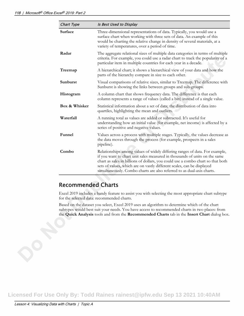
Chart Type Is Best Used to DisplaySurface Three-dimensional representations of data. Typically, you would use a

surface chart when working with three sets of data. An example of thiswould be charting the relative change in density of several materials, at avariety of temperatures, over a period of time.

Radar The aggregate relational sizes of multiple data categories in terms of multiplecriteria. For example, you could use a radar chart to track the popularity of aparticular item in multiple countries for each year in a decade.

Treemap A hierarchical chart; it shows a hierarchical view of your data and how theparts of the hierarchy compare in size to each other.

Sunburst Visual comparisons of relative sizes, similar to Treemap. The difference withSunburst is showing the links between groups and sub-groups.

Histogram A column chart that shows frequency data. The difference is that eachcolumn represents a range of values (called a bin) instead of a single value.

Box & Whisker Statistical information about a set of data; the distribution of data intoquartiles, highlighting the mean and outliers.

Waterfall A running total as values are added or subtracted. It's useful forunderstanding how an initial value (for example, net income) is affected by aseries of positive and negative values.

Funnel Values across a process with multiple stages. Typically, the values decrease asthe data moves through the process (for example, prospects in a salespipeline).

Combo Relationships among values of widely differing ranges of data. For example,if you want to chart unit sales measured in thousands of units on the samechart as sales in billions of dollars, you could use a combo chart so that bothsets of values, which are on vastly different scales, can be displayedsimultaneously. Combo charts are also referred to as dual-axis charts.

Recommended ChartsExcel 2019 includes a handy feature to assist you with selecting the most appropriate chart subtypefor the selected data: recommended charts.Based on the dataset you select, Excel 2019 uses an algorithm to determine which of the chartsubtypes would best suit your needs. You have access to recommended charts in two places: fromthe Quick Analysis tools and from the Recommended Charts tab in the Insert Chart dialog box.



Recommended Charts


Figure 4-4: You can access recommended charts from the Quick Analysis tools or from the InsertChart dialog box.

Access the Checklist tile on your CHOICE Course screen for reference information andjob aids on How to Create Charts.




ACTIVITY 4-1Creating Charts

Data FileC:\091079Data\Visualizing Data with Charts\Annual Sales.xlsx


ScenarioAs a marketing analyst for Develetech Industries, you have received the Annual Sales workbookfrom the sales team. The sales manager has asked you to build charts for the data in the workbookto be used in the annual company meeting.

1. In Excel, open the workbook Annual Sales.xlsx.

2. Create a clustered column chart from the quarterly sales data.a) Verify that the Quarterly Sales worksheet is selected and select the range A1:E5.b) Select Insert→Charts→Dialog Box Launcher.c) Explore the Recommended Charts by selecting the chart thumbnails.d) Select the first recommended chart, a Clustered Column chart, and select OK.





e) Verify that the clustered column chart was created.

3. Create a line chart from the monthly sales of laptops.a) Select the Sales Trends worksheet and select the range A1:A13.b) Hold Ctrl and select C1:C13.

c) Select Insert→Charts→Insert Line or Area Chart and select Line, the first 2-D line chart variant.

4. Create a pie chart from the sales comparison data.a) Select the Sales Comparison worksheet and select the range A1:B5.

b) Select the Quick Analysis button and select the Charts tab.




c) Hover over the various chart types and select the Pie chart type.

5. Save the workbook as My Annual Sales.xlsx and keep the file open.




TOPIC BModify and Format ChartsAlthough you can create charts with just a few mouse clicks, the default chart configurations aren'talways exactly what you need to present your data. Depending on your audience and the venue, youmay want to include more or less information than the default configurations include, present yourdata with organizational branding, or simply make your charts larger or easier to read.Excel 2019 provides you with a vast array of options when it comes to modifying and formattingyour charts. By configuring the display of your charts, you take full control over the message yourcharts convey and their overall visual impact. A well-formatted chart can mean the differencebetween simply delivering information and making an impact on your audience.

Modification vs. FormattingModifying and formatting charts go hand-in-hand. Although many people use these termssynonymously, they are actually two different things.Modifying a chart includes making changes such as moving chart elements, adding or removingchart elements, turning the display of particular data on or off, and changing the chart type. Think ofmodifying a chart as working with the display of data. You modify a chart to change the audience'sunderstanding of the information you're presenting.

Figure 4-5: This chart has been modified to make the data easier to interpret.

Formatting refers to altering the overall look and feel of a chart. Formatting a chart typicallyincludes tasks such as changing the color scheme or the font, and altering the size of the chart. Youformat a chart to comply with branding standards or to convey a particular mood or feel.


Lesson 4: Visualizing Data with Charts | Topic B

Chart Modifications


Figure 4-6: This chart has been formatted to comply with branding guidelines.

Chart ElementsChart elements are the individual objects that can appear on charts and that convey some level ofinformation to a viewer about the chart's data. While all Excel charts contain at least one chartelement by default, the various chart types display different chart elements. Each chart elementserves a different role in visually communicating information about data and trends.For example, while bar and column charts typically display an X axis and a Y axis, surface chartsdisplay three axes. Pie charts don't contain axes, as they deal with only a single column of data.

Figure 4-7: Chart elements help the audience interpret chart data.



Chart Formatting

Chart Elements


Guidelines for Modifying Chart Elements


Modifying Chart ElementsFormatting charts has relatively little impact on an audience's ability to interpret your data.Modifying chart elements, on the other hand, can have a significant impact. As a general rule, it'sbest to include only those chart elements that are absolutely necessary for conveying meaning.Cluttered charts can muddy your main point and make your charts confusing to view, and avoidingconfusion is exactly why you created them in the first place.However, some chart elements do actually help add meaning. Until you gain an intuitive sense ofwhat chart elements to include for various purposes, you may want to consider adding chartelements that you feel will help your target audience interpret your data, analyzing your chart, andthen removing anything that doesn't directly contribute to the message you intend to deliver. Whenanalyzing your charts, ask yourself questions such as:• If I remove the gridlines, will the chart still convey meaning?• Do I need a legend? Can I remove the legend and use data labels instead?• How much precision do I need for axis labels?• Do the axes really need titles?• Will using a three-dimensional layout enhance visual appeal or distort proportions?• Does including the data table aid understanding?• Do I really need major and minor tick marks on the axes?

Note: Before finalizing your charts, keep the old adage "less is more" in mind. If theaudience needs an element to acquire meaning, keep it. Otherwise, remove it.

The Chart Tools Contextual TabYou can access many of the commands you will use to modify and format your charts on the ChartTools contextual tab, which appears whenever you select a chart or a chart element and disappearswhen you select a worksheet element outside the chart. This contextual tab contains two tabs thateach contain task-related groups and commands for working with your charts. Let's take a look atthe various command groups on both of these tabs.

Figure 4-8: The Design tab.

Use the commands on the Design tab to quickly change the overall look and feel of your charts.

Design Tab CommandGroup


Chart Layouts Adding or removing individual chart elements, and quickly configuringthe display of all chart elements according to predefined configurations.

Chart Styles Quickly formatting a chart by using predefined sets of formattingoptions.



Guidelines for ModifyingChart Elements

The Design Tab


Design Tab CommandGroup


Data Changing the chart's dataset range and switching the row and columndata. Keep in mind that this does not switch the data that is displayed onthe X axis with the data that is displayed on the Y axis. This switches thecategories with the data series.

Type Changing the chart type.

Location Moving charts to different worksheets within a workbook.

Figure 4-9: The Format tab.

Use the commands on the Format tab to configure chart formatting.

Format Tab CommandGroup


Current Selection Selecting particular chart elements and accessing the Format task pane.

Insert Shapes Inserting or changing shapes on worksheets.

Shape Styles Configuring formatting options for chart elements.

WordArt Styles Configuring formatting options for chart text.

Arrange Changing the front-to-back placement of chart elements and configuringthe orientation of chart elements.

Size Changing the size of charts and chart elements.

The Format Task PaneYou can use the commands available in the Format task pane to fine-tune the overall formatting ofyour charts. Excel 2019 opens this task pane when you select Format→CurrentSelection→Format Selection from the Chart Tools contextual tab.It will display with a slightly different name, depending on the chart element you currently haveselected. For example, if you have one of the axes selected, it will appear as the Format Axis taskpane; if you have the chart title selected, it will appear as the Format Chart Title task pane.The Format task pane also displays a different configuration of tabs and commands, based on thechart element you have selected. At the highest level, depending on your current selection, it maydisplay two tabs that essentially divide the formatting commands between text and other objects.Under each of these tabs is a series of other tabs that further divide the commands into functionalgroups. Within these lower-level tabs is a series of expandable sections that display the commandsand options you will use to apply specific formatting to the selected chart element.



The Format Tab

The Format Task Pane


Figure 4-10: The Format task pane displays different sets of commands and options dependingon which chart element you currently have selected.

The following table describes the various elements of the Format task pane.

Format Task PaneElement

Description

Title Displays variations of the Format task pane's title, depending on thechart element that is currently selected.

Task Pane Optionsdrop-down arrow

Provides you with access to options for moving, resizing, or closing theFormat task pane.

Options drop-downarrow

Opens a drop-down menu that enables you to select different chartelements for formatting purposes. This is essentially the same menu youcan access by selecting the Format→Current Selection→ChartElements drop-down arrow from the Chart Tools contextual tab.Changing the selection changes the task pane's title and the displayedtabs and commands.

High-level tabs Divide the formatting commands into functional groups at the highestlevel. Essentially, these divide the formatting commands and optionsbetween object formatting tasks and text formatting tasks. If a chartelement doesn't contain text, the Format task pane displays only a singleoption at this level of the hierarchy.

Low-level tabs Divide the formatting commands and options at a more granular levelthan the high-level tabs. The low-level tabs available are dependent uponyour current selection.




Format Task PaneElement

Description

Command sections You can expand or collapse these task-specific sections to access or hidethe specific commands and options you will use to format chartelements.

Commands and options Enable you to apply formatting options to the selected chart element.

The Chart Tools ButtonsWhenever you select a chart in Excel, Excel displays a set of three buttons near the top-right cornerof the chart area. You can use these three buttons to quickly access some of the most commonlyused commands for formatting and modifying Excel charts. Selecting any of these three buttonsopens either a menu or a gallery containing commands or options for configuring the currentlyselected chart.

Figure 4-11: Use the chart tools buttons to quickly access common formatting and modificationoptions.

The following table describes the commands or options available from each of the chart toolsbuttons.

Chart Tools Button Selecting This Button

Chart Elements button Opens a menu that enables you to toggle on or off, as well as modify,various chart elements.

Chart Styles button Opens a gallery providing you with quick access to various chartstyles and color schemes.

Chart Filters button Opens a menu that enables you to quickly toggle on or off the displayof chart series, chart categories, or individual elements within eitherof these. From this menu, you can also toggle on or off the display ofseries labels and category labels.

The Select Data Source Dialog BoxYou will use the Select Data Source dialog box to manage Excel chart data. From here, you canedit the entire dataset feeding the chart or you can edit the data feeding any of the individual dataseries. You can also remove from or add back to the chart any of the individual data series, reorderhow the data series appear on the chart, or switch the chart's X and Y axes. You can access the



The Chart Tools Buttons

The Select Data SourceDialog Box


Select Data Source dialog box from the Chart Tools contextual tab by selectingDesign→Data→Select Data.

Figure 4-12: Use the Select Data Source dialog box to manage the data displayed by Excel charts.

Chart AnimationsAs previously mentioned, when you update the data associated with a chart, the chart itself alsoupdates. In Excel 2019, these changes are animated to help worksheet developers and viewers get aclearer sense of how the changes affect the overall values and relationships in the chart. Thisfunctionality can also enable you to create dynamic, animated charts by using some of the add-insavailable for Excel 2019.

Access the Checklist tile on your CHOICE Course screen for reference information andjob aids on How to Modify and Format Charts.




ACTIVITY 4-2Modifying and Formatting Charts

Before You BeginThe workbook My Annual Sales.xlsx is open.

ScenarioAs a marketing analyst, you have shared your initial charts with your manager. Your manager hassuggested you modify and format these charts for a better presentation at the annual companymeeting.

1. Change the layout of the clustered column chart on the Quarterly Salesworksheet.a) Select the Quarterly Sales worksheet and, if necessary, select the clustered column chart.b) On the Chart Tools contextual tab, select Design→Chart Layouts→Quick Layout and select Layout 9

from the gallery.

Notice the new axis titles and that the legend was moved from the bottom to the right.

2. Change the default titles on the column chart.



Activity


a) On the Chart Tools contextual tab, select Format→Current Selection→Chart Elements drop-downarrow and select Chart Title.

b) Select the Formula Bar and type Quarterly Sales and press Enter.c) Select the vertical Axis Title label on the left side of the chart, type Sales and press Enter.

Note: You may notice that the text is entered in the Formula Bar.

d) Select the horizontal Axis Title label at the bottom of the chart, type 2018 and press Enter.

3. Move and resize the Quarterly Sales clustered column chart.

a) Point to the chart area surrounding the chart. Using the move pointer click and drag the chart sothat the upper-left of the chart covers cell G3.

Note: It is good practice to leave at least one row and one column of spacearound the edges of charts.

b) Point the cursor to the bottom-right resize handle until the mouse changes to a resize pointer. c) Click and drag to enlarge the chart to cover cell P20.




4. Modify the chart style of the Laptops line chart on the Sales Trendsworksheet.a) Select the Sales Trends worksheet and, if necessary, select the line chart.

b) On the Chart Tools contextual tab, select Design→Chart Styles→More button and from thegallery, select Style 12.

5. Change the labels on the line chart to a currency format.

a) Select the Chart Elements button and hover over Data Labels. Select the arrow that appears tothe right and select More Options from the menu.

b) In the Label Options section, scroll down and select Number to expand the formatting options.

c) In the Category menu, select Currency.d) In Decimal places, type 0




e) Close the Format Data Labels task pane.

6. Change the chart type of the pie chart on the Sales Comparison worksheet toa 3-D pie chart.a) Select the Sales Comparison worksheet and, if necessary, select the pie chart.b) On the Chart Tools contextual tab, select Design→Type→Change Chart Type.c) From the Pie category, select the second variant, 3-D Pie, and select OK.

7. Apply a chart style to the pie chart.

a) Select the Chart Styles button.




b) Select Style 1.

c) Select the Chart Elements button and hover over Data Labels. Select the arrow that appears tothe right and select More Options from the menu.

d) In the Format Data Labels task pane, in the Label Options section, check the Percentage check boxand uncheck the Value check box.

e) Close the Format Data Labels task pane.f) Select Home→Font→Font Size pull down and select 14.





TOPIC CUse Advanced Chart FeaturesHave you ever needed to graphically display two widely different sets of data simultaneously? Forexample, you may wish to show how unit sales correlate to overall sales totals within the same chart.It's likely that the figures for total sales are much higher than they are for the number of units sold;after all, many items cost far more than a dollar these days. Putting both figures on the same chartwould likely make at least one of the data series difficult to read. Or, suppose you want to displayfuture projections for your datasets on the same chart where you display the data itself. Without thefuture data, how can you create chart elements that visually convey the information you wish toshare? What if you have to create a lot of these charts? Does all of this mean a lot of extra dataentry, calculation, and formatting?Fortunately, Excel 2019 includes a wide range of advanced charting features that enable you todisplay widely varying sets of data together, include forecasting trends on your charts, and reusehighly stylized or formatted charts again and again. It almost goes without saying that this level offunctionality means you can quickly make an impact on nearly any presentation without having toput a lot of time and effort into doing so.

Dual-Axis ChartsA dual-axis chart is, simply, a chart that displays two sets of information on the same chart. This canbe in the form of a dual-Y-axis chart, which displays two data series simultaneously, or a dual-X-axischart, which displays two sets of categories simultaneously. By far, dual-Y-axis charts are used morefrequently than dual-X-axis charts. But dual-X-axis charts can be useful for particular types ofcharts, such as bubble charts or XY (scatter) charts.The main advantage to dual-axis charts is the ability to not only display two different sets of datasimultaneously, but also to format the different sets of data independently of each other. This meansyou can make the various data series easily visually distinguishable from each other and display themwithin the same amount of space using different scales.

Figure 4-13: Dual-axis charts enable you to simultaneously display and independently formatvarious sets of data within the same space.


Lesson 4: Visualizing Data with Charts | Topic C

Dual-Axis Charts


For example, you can simultaneously display unit sales figures, which may range in the thousands,with total sales figures, which could range in the billions of dollars for expensive equipment. Clearlythe data that is expressed in billions of units would be far easier to see within the same Y-axis scalethan the data with figures in the thousands. In fact, those figures may not even be visible with such adrastic difference in scale.When you format one or more data series as a different chart type than the original data series, thechart is known as a combo chart. Excel 2019 automatically adjusts the scale of secondary Y axeswhen the data values for the series you use to create them are drastically different than the values inthe remaining series. But, you must apply other visual formatting manually.Excel supports dual-axis charts only for 2-D chart types; they do not work with 3-D chart types.Additionally, you can create a chart with a secondary X axis, but only if it already has a secondary Yaxis.

Note: To learn more about using your Excel charts in external applications, presentations, orother forms of media, check out the LearnTO Save an Excel Chart as a Picture presentationfrom the LearnTO tile on the CHOICE course screen.

Access the Checklist tile on your CHOICE Course screen for reference information andjob aids on How to Create a Dual-Axis Chart.

ForecastingIn addition to creating secondary axes to display various data series or categories simultaneously,Excel includes a chart feature that can help you forecast trends in your data. Forecasting is theprocess of using the trends that exist within past data to predict future outcomes. By its nature,forecasting can never be entirely accurate, as one can never precisely predict all possible futureoutcomes. As a general rule, the farther you forecast out into the future, the less accurate yourforecasts become.

TrendlinesIn Excel, trendlines are chart elements that can graphically represent both the current trends thatexist within your data and future forecasts of those trends. You can add trendlines to any of thefollowing non-stacked, 2-D chart types: column, line, bar, area, stock, XY (scatter), and bubble. Youcan name and format trendlines to make them easier to view on charts or to adhere toorganizational branding standards. To access the options for adding trendlines to your charts, selectthe desired chart to display the chart tools buttons, select the Chart Elements button, point thecursor at the Trendlines check box, and then select the arrow that appears to the right of it.



The LearnTO Save anExcel Chart as a Picturepresentation is availablefrom the LearnTO tile onthe CHOICE Coursescreen. You may chooseto include it in yourinstructional plans, oryou can remind studentsabout the tile and thesupplementalinformation it contains.

Forecasting

Trendlines


Figure 4-14: Trendline on an Excel chart.

Trendline TypesYou can use different types of trendlines to display and forecast data trends depending on the typeof data you wish to analyze. Excel provides you with six options for adding trendlines to yourcharts.

Trendline Type Use This to Display or Forecast Data That

Exponential Increases in rate of change at an ever-faster rate over time.

Linear Has a proportional relationship. When you graph linear relationships, theresulting graph is a straight line that represents a trend that holds steady or thatincreases or decreases by a steady rate.

Logarithmic Has a rapidly increasing or decreasing rate of change that eventually levels out.

Polynomial Fluctuates over time.

Power Increases in rate of change at a steady rate over time.

Moving average Fluctuates randomly over time. Use this type of trendline to smooth outrandom patterns of values to give viewers a sense of the overall average changein values over time.

The Format Trendline Task PaneYou will use the Format Trendline task pane to apply formatting and effects to your charttrendlines and to change the type of trendlines in your charts. You can access the task pane byselecting the desired trendline; then, on the Chart Tools contextual tab, select Format→CurrentSelection→Format Selection.



The Format TrendlineTask Pane


Figure 4-15: The Format Trendline task pane.

Access the Checklist tile on your CHOICE Course screen for reference information andjob aids on How to Work with Trendlines.




ACTIVITY 4-3Creating a Dual-Axis Chart with a Trendline


ScenarioIn addition to the previous charts you have created, your manager has asked you to build some morecomplex charts. You have been provided with a worksheet that contains the second and thirdquarter monthly totals and their percentage of total sales for the year thus far. Your manager hasheard about combo charts and wants you to display total sales on one axis and percentage of totalsales on another. In addition, with only six months of recorded data, your manager would like to seea projection of what the next three months might look like. You decide to add a trendline toforecast this trend.

1. Create a combo chart from the monthly totals.a) Select the Monthly Totals worksheet.b) Select the range A1:C7.c) Select Insert→Charts→Dialog Box Launcher.d) In the Insert Chart dialog box, select the All Charts tab, and select Combo.e) In the Choose the chart type and axis for your data series section, in the % of Total Sales row,

check the check box for Secondary Axis.



Activity


f) Select OK.

2. Modify the chart title and include axis titles for each Y axis.

a) Select the Chart Elements button and hover over Axis Titles. Select the arrow that appears tothe right and select Primary Vertical and Secondary Vertical.

b) On the left side of the chart, select the Vertical (Value) Axis Title. Type = and select cell B1, then

press Enter.c) On the right side of the chart, select the Secondary Vertical (Value) Axis Title. Type = and select cell

C1, then press Enter.




d) Select the Chart Title, type Monthly Totals and press Enter.

3. Add a trendline to the total sales series.a) On the Chart Tools contextual tab, select Format→Current Selection→Chart Elements drop-down

arrow and select Series "Total Sales".

b) Select the Chart Elements button and hover over Trendline. Select the arrow that appears to theright and select More Options.

c) In the Format Trendline task pane, verify that the Trendline Options high-level tab is selected and

then, if necessary, select the Trendline Options low-level tab. d) In the Trendline Options section, verify that Linear is selected. In the Forecast group, select the

Forward text box, type 3 and press Enter.




e) Verify that the trendline has been added to the chart, forecasting three periods forward.


Chart TemplatesWorking with advanced charting features can require quite a bit of chart formatting andmodification. And, it's likely you'll need to reuse at least some of your charts for multiple purposes,projects, or periods. So, you would certainly benefit from the ability to save all of the formatting andmodification work that went into creating your charts for use in future workbooks. This can beespecially helpful if you've painstakingly formatted chart elements to adhere to organizationalbranding guidelines and will frequently need to create charts that follow them. Fortunately, Excelprovides you with the ability to save charts as chart templates that you can apply to other datasets inthe same workbook or to datasets in other workbooks.Like other Excel templates, a chart template is a type of file that stores a chart type and all of theassociated formatting you've applied to it. The file extension for Excel 2019 chart templates is .crtx.Excel stores chart templates in a subfolder in the Microsoft Templates folder named Charts. Oncesaved, you can access chart templates from the Templates tab in either the Insert Chart dialog boxor the Change Chart Type dialog box, just as you can any other chart type. This is true only if yousave your chart templates in the Charts folder. Do not save chart templates in any other folder ifyou wish to access them from the dialog boxes.



Chart Templates


Figure 4-16: Chart templates available for use in the Change Chart Type dialog box.

Access the Checklist tile on your CHOICE Course screen for reference information andjob aids on How to Create and Use Chart Templates.




ACTIVITY 4-4Creating a Chart Template


ScenarioYou like the look and feel of the chart you created to forecast monthly sales. You know that you'llbe creating similar charts for other sales periods. Instead of creating and manually adding elementsto your charts each time you create them, you decide to create a chart template from the chart thatyou can apply to future datasets. You decide to test it on some data from the prior year, just to makesure the template works.

1. Verify that you are on the Monthly Totals worksheet, and if necessary, selectthe Monthly Totals combo chart.

2. Save the chart as a template.a) Right-click the chart and then select Save as Template.b) In the Save Chart Template dialog box, ensure the Charts folder is selected.

Note: Excel should automatically direct you to the Charts folder. The label<User> in the chart templates path image will be your user name. TheAppData folder is typically a hidden system folder, so you will not see thefolder when browsing through File Explorer. However, you can type AppDatain the address path to go to that folder directly.

c) In the File name field, type Trendline Chart Template.d) Verify that the Save as type is Chart Template Files(*.crtx), and then select Save.

3. Test the new chart template.a) Select the 2017 Sales worksheet.b) Select the range A1:C7.c) Select Insert→Charts→Dialog Box Launcher.d) In the Insert Charts dialog box, select the All Charts tab, and select the Templates category.



Activity


e) In the My Templates section, select the Trendline Chart Template and select OK.

f) Verify that Excel created a dual-axis combo chart with a trendline.

4. Save and close the workbook.



You may wish to pointout that the axis titleswere not carried overinto the templatebecause they includedreferences to a specificworksheet.


SummaryIn this lesson, you presented your data graphically using charts. You did this by creating charts todisplay your data in various types. You initially created basic charts like column, bar, line, and piecharts. You then formatted and modified those charts. You also built advanced charts (such ascombo charts) and included trendlines to make charts easier to read and interpret. Providing youraudience members with a visual snapshot of your data enables them to quickly recognize trends inyour raw data, make easy comparisons, and focus on your message.

What are a couple of reasons for which you anticipate including charts in yourworkbooks?A: Answers will vary, but many users will likely find charts useful for regular meetings at which status

updates are frequently presented. The use of charts is a quick and easy way to demonstrateprogress. Also, users are likely to find charts helpful when breaking down overall and periodic figures(such as at end-of-year events) or when reviewing the success of a particular initiative or product.

What uses will you have for Excel's advanced chart features in your currentrole?A: Answers will vary, and some students may not have a need to use advanced chart features currently.

Now that students are aware of these chart features, they may use them in the future. Users whofrequently track multiple figures simultaneously, especially figures that vary drastically in scale, willlikely wish to present quarterly or annual figures to large audiences by using combo or dual-axischarts. For users in industries that track long-term performance (such as with financial or investmentfirms) including trendlines in charts will be a simple way to display estimated future trends.



Lesson 4: Visualizing Data with Charts |



Using PivotTables andPivotChartsLesson Time: 1 hour, 30 minutes

Lesson IntroductionYou've already seen the way Microsoft® Office Excel® 2019 works and how features suchas sorting, filtering, and summary functions can help you drill down into your data to getanswers to very specific questions. Although using these features is often a good option forattaining specific answers, these aren't necessarily the best options if you need to frequentlychange the questions you're asking of your data. To change the question you're asking whenusing functions, sorting, and filtering, you often need to rewrite functions, adjust criteria, orre-filter you data; sometimes, you even need to use several of these methods at the sametime. You certainly could take this route, but it isn't the most efficient way to re-query yourdata to get the variety of answers you need. If you work in a high-paced, data-intensiveenvironment, you simply may not have the time needed to recalculate every time asupervisor asks you a different question. You need something a little more dynamic.Excel 2019 includes a powerful feature that enables you to ask any number of questions ofyour data; get detailed, specific answers; and do it all over again in just a matter of moments.By taking advantage of this functionality, you can get critical, time-sensitive organizationalintelligence to the people who need it quickly, easily, and with a high-level of flexibility.


• Create a PivotTable.

• Analyze PivotTable data.

• Present data with PivotCharts.

• Filter data using timelines and slicers.

5


TOPIC ACreate a PivotTableTo take advantage of the functionality and flexibility of PivotTables, you must first understand howto create them. Although this is a relatively simple process, you must also know a bit about the typeof data that works best for PivotTables. By taking a few moments to gain this foundational level ofunderstanding, you'll be preparing yourself to create useful, effective PivotTables that you can use toanalyze your raw data in incredibly fine detail.

PivotingSimply put, pivoting, in Excel, is a way to manipulate, rotate, or turn large amounts of data into asummarization of that data. You and your organization collect and track data for the expresspurpose of gaining insight and information from that data to make decisions. When you askquestions of your data, you get information about which products or services your customers preferand which ones they do not. In this course, you have created functions and sorted, filtered,summarized, and subtotaled data in order to gain perspective on your data. Pivoting enables you toview your data from a variety of new perspectives.To pivot your data, Excel summarizes your values by row and column. Data that can be grouped(such as company names, cities, states/provinces, product codes, and names) are good examples ofitems that can be used as row or column headings. Values are data that can be summarized,averaged, or calculated for a percentage. Examples of values include quantities, prices, and counts ofvalues, both numeric and text-based.Take the following example: the raw data on the left contains a list of data, and each row in that data(which can be called a record) identifies a unique entry to the list. When Excel pivots the raw data,the state/province data are grouped as row labels and the values of total sale are summarized. Thisprovides a concise report of your data that can also be formatted, sorted, and filtered further to gainmore insight. This report quickly answers the question of what the total sales are for each state orprovince.Here's a look at how the previous example would work in a worksheet. The list is a set of ordertransactions by various companies in different locations purchasing items with different quantitiesand price.


Lesson 5: Using PivotTables and PivotCharts | Topic A

Pivoting


Figure 5-1: Pivoted data provides sales totals at a glance.

Note: As with filtering and sorting, pivoting does not affect your raw data; it only modifies yourview of the data.

PivotTablesA PivotTable is a dynamic Excel data object that enables you to analyze data by pivoting columnsand rows of raw data without altering the raw data.PivotTables are effective for summarizing large volumes of data according to two or more criteria toreturn specific answers to your questions. PivotTables combine some of the most powerful anduseful types of Excel functionality (such as sorting, filtering, summary functions, and subtotals) togive you an incredible level of control over how you view your data.When you create a PivotTable, Excel allows you to place it on the same worksheet as the originaldata or insert it on a new worksheet. Once the PivotTable is created, you can re-pivot, re-sort, re-summarize, and re-filter your data any number of times without affecting the original dataset.In addition to pivoting columns and rows, you can nest columns and rows within one another tocreate a hierarchy, much as you do when using subtotals. You can expand or collapse levels of thehierarchy to view more or less detail in your PivotTables. And you can use any of the availablesummary functions to summarize your pivoted data for a variety of purposes. You can also createPivotTables out of either data in the same workbook, or data from other workbooks and externaldata sources.



PivotTables


Figure 5-2: A PivotTable containing a hierarchy of raw data. In this example, Company, TotalSale, State/Province, and Months are all column labels in the original dataset.

Recommended PivotTablesA quick way to get started with PivotTables is to use recommended PivotTables. When you use thisfeature, Excel determines PivotTable layouts based on your data. From this starting point, you canchange the arrangement of fields in the PivotTable for additional analysis of your data. Therecommended PivotTables are accessible from Insert→Tables→Recommended PivotTables.




Figure 5-3: Examples of recommended PivotTables.

Transactional DataThere is an extremely important consideration for you to keep in mind when creating and workingwith PivotTables: your data format. PivotTables are designed to work with, and work best with, rawtransactional data.Transactional data is not summarized in any way, so it does not contain row labels, only columnlabels. Columns in a transactional dataset are also known as fields. The best way to visualizetransactional data is to examine the root word "transaction." In a transactional dataset, eachtransaction, or entry, is located in its own separate row.To carry on the example from earlier of sales transactions at a variety of locations, each sale,regardless of when or where it took place, would be entered as an individual row of data. Thedataset columns represent the specific elements of each transaction: date, time, location, amount,and so on.In a summarized dataset, even a raw one, the data has already been compiled in some way and willhave both row labels and column labels. For example, you may have raw sales data for each sales repin your organization. Because each rep has his or her own row of data, the dataset would likelycontain the total of each person's sales, as opposed to each sale regardless of the rep. Although youcan create PivotTables from summary data, they will never give you as much granular insight intoyour data as PivotTables created from transactional data.



Transactional Data


Figure 5-4: Transactional data shows each event, whereas summary data compiles it in someway.

Note: It makes more sense to view your data as two types: values to summarize and values togroup. Values of dates, times, quantity, price, etc. are good examples of values that can besummarized. Values of cities, states, companies, accounts, etc. are examples of values that can begrouped.

The Create PivotTable Dialog BoxYou use the Create PivotTable dialog box to insert PivotTables into your worksheets. From here,you can select the desired dataset, include a reference to a named range or table, or select aconnection to an external data source. You can also select a location for the PivotTable, which canbe on the same worksheet as the dataset or on another worksheet in the same workbook. You canaccess the dialog box by selecting Insert→Tables→PivotTable.

Figure 5-5: The Create PivotTable dialog box.



The Create PivotTableDialog Box


The PivotTable Fields Task PaneOnce you create a PivotTable, you will use the PivotTable Fields task pane to configure thePivotTable and perform data analysis tasks. Excel automatically opens the task pane when you inserta PivotTable in a worksheet.The top half of the pane, the Choose fields to add to report list, displays a list of all of the fields(columns) from the original dataset; Excel pulls the names for these from the column labels.The bottom half of the pane, the Drag fields between areas below section, displays a series offour areas that you use to configure the PivotTable. By dragging the various fields to the variousareas, you configure the structure of the PivotTable and select the values upon which Excelperforms calculations.As PivotTables are, by default, dynamic, you can drag fields to the various areas of the PivotTableFields task pane as necessary and your PivotTable will update automatically. You can move thefields around as often as you like, and you can include more than one field in each area. When youdrag more than one field into the same area, Excel creates a hierarchy in the PivotTable with itemson top of the area representing higher levels in the hierarchy. This works much like using subtotalsand outlines in ranges.Each field that you have dragged into an area displays a field drop-down arrow. This provides youwith access to context menus and dialog boxes that enable you to configure your PivotTablesfurther.

Figure 5-6: Use the elements of the PivotTable Fields task pane to configure the structure ofPivotTables.



The PivotTable FieldsTask Pane


The following table provides a brief description of the various elements of the PivotTable Fieldstask pane.

PivotTable Fields TaskPane Element

Description

Tools drop-down arrow Provides you with access to a menu that contains variouspreconfigured PivotTable Fields task pane layouts. Select fromamong these options to customize the PivotTable Fields task paneto suit your needs. From the Tools drop-down menu, you can alsoalter the order in which your fields appear within the Choose fieldsto add to report section of the PivotTable Fields task pane.

Field check boxes These enable you to add or remove fields from the various areas.Checking a field's check box adds it to an area, whereas unchecking itremoves the field from all areas. You have no control over whereExcel places a field when you check its check box, so many usersprefer to simply drag the fields to the desired areas.

Field drop-down arrow Selecting a field's drop-down arrow displays a context menu thatprovides you with various options for configuring your PivotTables.For example, you can move fields to another area (again, this can alsobe done simply by dragging the field to another area), move fieldswithin a hierarchy, or access the Field Settings or Value FieldSettings dialog boxes.

Filters area Drag fields here to include field values as filter criteria for thePivotTable.

Columns area Drag fields here to create columns out of the unique entries in a field.

Rows area Drag fields here to create rows out of the unique entries in a field.

Values area Drag fields here to have Excel perform calculations on or summarizetheir values.

Note: To learn more about how to use field entries to filter your PivotTable data, check out theLearnTO Add a Report Filter to an Excel PivotTable presentation from the LearnTO tileon the CHOICE course screen.

Access the Checklist tile on your CHOICE Course screen for reference information andjob aids on How to Create a PivotTable.



The LearnTO Add aReport Filter to an ExcelPivotTable presentationis available from theLearnTO tile on theCHOICE Course screen.You may choose toinclude it in yourinstructional plans, oryou can remind studentsabout the tile and thesupplementalinformation it contains..


ACTIVITY 5-1Creating a PivotTable

Data FileC:\091079Data\Using PivotTables and PivotCharts\Sales Data.xlsx


ScenarioAs the sales manager, you need to track sales. Because Develetech's products are sold across manyregions, you want to be able to analyze the sales data in a number of ways. You decide the best wayto answer your questions now and in the future is to create a PivotTable.

1. In Excel, open the workbook Sales Data.xlsx.

2. Create a PivotTable from the data.a) Verify that cell A1 is selected.b) Select Insert→Tables→PivotTable.c) In the Choose the data that you want to analyze section, verify that the Select a table or range

option is selected.d) In the Choose where you want the PivotTable report to be placed section, verify that the New

Worksheet option is selected and select OK.





e) Observe that the PivotTable framework is created on a new worksheet.

3. Build the PivotTable report.a) In the PivotTable Fields task pane, in the Choose fields to add to report section, check the check

boxes for Region and Total Sales.b) Verify that Excel builds a PivotTable on Sheet1 depicting the sum of total sales for each region.

Note: Notice that Excel does not retain cell formatting from the original datawhen creating PivotTable reports.




4. Create a recommended PivotTable from the sales data.a) Select the Data worksheet and verify that cell A1 is selected.b) Select Insert→Tables→Recommended PivotTables.c) Examine the various PivotTable options in the Recommended PivotTables dialog box. Select the

second variant, Sum of Total Sales by Region and select OK.

d) Verify that Sheet2 contains the new PivotTable.

Note: This action builds the same PivotTable report on Sheet2 as the firstPivotTable report on Sheet1. Recommended PivotTables are a good way toget started building your own PivotTable reports.

5. Modify the PivotTable on Sheet2 to include products.a) In the PivotTable Fields task pane, in the Choose fields to add to report section, select Products.




b) Verify that the PivotTable is updated to include total sales for products in each region.

6. Save the workbook as My Sales Data.xlsx and keep the file open.




TOPIC BAnalyze PivotTable DataNow that you have created your PivotTable, you're ready to dive right in and crunch the numbers togain the organizational insight that can help you succeed. As with all Excel data analysis tasks,creating and configuring effective PivotTables is a matter of asking the right questions to glean thenecessary information. When working with PivotTables, this all boils down to structure. You alreadyknow that PivotTables enable you to reorganize and re-analyze your data as many times as necessaryto get all of the answers you're looking for. But, how do you translate your questions into aPivotTable structure? Actually, it's relatively simple.Excel 2019 provides you with a number of different tools and commands you can use to organizethe structure of your PivotTables. Knowing how these tools work and understanding howPivotTable structure translates into actionable intelligence are the keys to getting the answers youseek.

Start with Questions, End with StructureTo create PivotTables that will be useful to you, begin by thinking about the types of questions youwould like your raw data to answer. This is precisely that same type of initial analysis you performwhen determining which functions or formulas to include in worksheets. The only difference here isthat you will use your questions as a basis for organizing your PivotTables, not to enter a function ora formula. Once you've determined what question you want Excel to answer, you can begin todesign your PivotTable's structure.There are a couple of items to keep in mind before beginning this process. First, it's typically best tocreate rows and columns out of fields that have a fairly finite set of entries, such as sales reps,regions, or products—in other words, data that can be grouped easily. You may not, for example,find it very useful to create rows out of dates that occurred over a 10-year span of time, as you couldend up with thousands of rows of data. Second, you should create rows out of the field for whichyou are primarily interested in determining some fact and create columns out of your secondarycriterion.For example, if you want to know the total sales per product for each sales rep in your department,you would typically create rows out of sales reps (your primary concern) and columns out of theproducts (the items for which you are measuring performance). Then you would ask Excel to usethe SUM function to total the sales for each rep per product.Let's take a look at a simple example. This is the beginning of a large table of transactional sales data.


Lesson 5: Using PivotTables and PivotCharts | Topic B

Start with Questions,End with Structure (3Slides)

While it is a general ruleof thumb to create rowsand columns from fieldswith relatively smallnumbers of uniqueentries, you can letstudents know that it issometimes necessary tocreate PivotTables thatcontain large numbers ofrows or columns.


Figure 5-7: Example of a table with over 1,500 entries.

Now, here's a PivotTable created from the entire dataset that answers this question: What are thetotal sales for each sales rep by product?

Figure 5-8: Example of PivotTable showing total sales for each sales rep by product.

Notice that the sales reps are listed by row and the products are listed by column. The PivotTablereturns the total sales, indicating the use of the SUM function, for each sales rep for each product.Now, let's say you'd like Excel to answer the following question: How many of each product wassold in each region? As you are primarily concerned with what is happening on a per-region basis,you would put the regions in rows and keep the products in columns. Then you would ask Excel tototal the quantity sold of each product in each region, indicating the use of the SUM function.

Figure 5-9: Example of PivotTable showing number of each product sold by region.




Notice that the rows and columns in each of these examples represent two of the criteria on whichyou are analyzing the data. The values throughout the rest of the table represent the third criterion:the values you are asking Excel to calculate, based on the other two criteria. This is the basicstructure you will use to create most PivotTables. The three keys to structuring your PivotTables areto determine the question you want Excel to answer, visualize the table you wish to create, anddetermine what calculation you want Excel to perform.

The Value Field Settings Dialog BoxWhen you select the drop-down arrow of a field in the Values area of the PivotTable Fields taskpane, Excel provides you with access to the Value Field Settings dialog box. You will use thecommands and options in the dialog box to configure the calculations Excel performs on field datain PivotTables and to configure how Excel displays the results of those calculations. The dialog boxis divided into two tabs: the Summarize Values By tab and the Show Values As tab.

Figure 5-10: The Summarize Values By tab of the Value Field Settings dialog box.

The Summarize Values By tab enables you to select which function Excel uses to summarize thedata in your PivotTables. The available functions here are the same as those available for creatingsubtotals and for summarizing table data. For example, you could use the SUM function to find thetotal of all values that meet the criteria outlined in the PivotTable rows and columns. Or, you coulduse the AVERAGE function to find the average values of the entries that meet the criteria.

Note: The default summary function for numerical values is the SUM function. The defaultsummary function for all other values is the COUNT function.



The Value Field SettingsDialog Box


Figure 5-11: The Show Values As tab of the Value Field Settings dialog box.

The Show Values As tab provides you with access to options for how you wish to display yoursummarized PivotTable data. By default, the value here is No Calculation, which means thePivotTable will simply summarize your data according to the function selected on the SummarizeValues By tab.You can also choose to have Excel display the summary data in a variety of other ways. Forexample, you may wish to show the summarized data as a percentage of the grand total or as apercentage of column or row totals. This could be helpful if you want to know what percentage ofyour total sales came from a particular region or which sales rep generated the highest percentage ofyour total or regional sales. Or, you may wish to show a relative comparison between values. Forexample, you may wish to see how far behind the sales leader other sales reps are in terms of totalsales.One other handy feature of the Value Field Settings dialog box is the Number Format button.Selecting this will open a scaled-down version of the Format Cells dialog box, which contains onlythe Number tab. Use this to change the cell formatting in your PivotTables to accommodate thevarious types of values you ask Excel to calculate.

Summarize and Show CombinationsCombining the options from the Summarize Values By tab and the Show Values As tab enablesyou to gain a deeper understanding of the information in your raw data. Here is a simple examplethat shows how the summary functions and the Show Values As tab options work together to giveyou new perspectives on your data.Take a look at this PivotTable that displays sales totals for sales reps per region. Here, the salesfigures have been dragged to the Values area of the PivotTable Fields task pane, and the defaultSUM function and No Calculation option are selected.




Figure 5-12: SUM function only.

Now take a look at how selecting the % of Grand Total option from the Show Values As tabchanges your view of the data; the summary function is still the SUM function.

Figure 5-13: % of Grand Total option.

Now you can see what percentage of all sales is composed of each rep's sales in each region. Noticealso that the grand totals for each row and for each column add up to 100 percent of all total sales.You now have a clear picture of which regions and which sales reps are generating your sales.Now take a look at what happens when you change the summary function to the AVERAGEfunction and change the Show Values As tab option to Difference From. Here, all sales reps' salesaverages are being compared to Cooper's sales, as this rep was selected in the Value Field Settingsfor having the highest percentage of grand total in the prior PivotTable. You could, however,compare the values to any individual sales rep.



SUM Function Only

Percentage of Total


Figure 5-14: Difference From option.

Notice that there are no values for Cooper, as this rep's values are the ones the PivotTable iscomparing the other values to. By looking at this PivotTable, you can see how far behind or aheadof the this rep all other reps are in terms of average regional and overall sales. Here, you see thatCooper is between the highest and lowest ranges in average total sales. Combining summaryfunctions with the Show Values As options is an effective way to gain a deep, granularunderstanding of the information hidden in your raw data.

Note: To learn more about additional methods for manipulating your PivotTable data, checkout the LearnTO Customize the View of a PivotTable and LearnTO Enhance a PivotTableWith Conditional Formatting presentations from the LearnTO tile on the CHOICE coursescreen.

The PivotTable Tools Contextual TabThe PivotTable Tools contextual tab displays commands and options that are specific to workingwith PivotTables. It appears when you select a PivotTable and disappears when you select outsidethe PivotTable. The contextual tab contains two tabs: the Analyze tab and the Design tab.

Figure 5-15: The Analyze tab.

The following table identifies the types of commands you will find in the various groups on theAnalyze tab.

Analyze Tab Group Contains Commands For

PivotTable Accessing the PivotTable Options dialog box, which enables you to changeglobal PivotTable settings. This group also displays the name of the currentlyselected PivotTable.

Active Field Accessing the Field Settings and Value Field Settings dialog boxes,expanding or collapsing hierarchies in your PivotTables, and drilling down orup in PivotTables created from databases.

Group Grouping various elements within a PivotTable and managing those groups.

Filter Accessing and managing filtering commands and options.



Difference From OptionThe LearnTO Customizethe View of a PivotTableand LearnTO Enhance aPivotTable WithConditional Formattingpresentations areavailable from theLearnTO tile on theCHOICE Course screen.You may choose toinclude these in yourinstructional plans, oryou can remind studentsabout the tile and thesupplementalinformation it contains.

The Analyze Tab


Analyze Tab Group Contains Commands ForData Refreshing PivotTable data when the source dataset has been updated and

modifying the dataset that feeds PivotTables.

Actions Clearing filtering, selecting elements of a PivotTable, and moving PivotTablesin your workbooks.

Calculations Configuring PivotTable calculations.

Tools Creating PivotCharts and accessing recommended PivotTables.

Show Toggling the display of PivotTable elements on or off.

Figure 5-16: The Design tab.

The following table identifies the types of commands you will find in the various Design tabgroups.

Design Tab Group Contains Commands For

Layout Toggling particular functionality on or off, and for modifying theoverall layout of PivotTables.

PivotTable StyleOptions

Toggling the display of PivotTable elements on or off.

PivotTable Styles Selecting and configuring PivotTable formatting options.

The GETPIVOTDATA FunctionOnce you have a PivotTable report, you may wish to extract a small portion or generate a summaryof that data if the PivotTable is large. Fortunately, Excel provides the GETPIVOTDATA functionas a way to show data from a PivotTable elsewhere in Excel. For example, you may have configureda PivotTable to show product sales for your regions and then someone asks you what the laptopsales were in the Southwest region. While you can look at the PivotTable and determine the answer,you can also use the GETPIVOTDATA function to show this answer in a report on anotherworksheet.Syntax: =GETPIVOTDATA(data_field,pivot_table,[field1,item1,field2,item2], ...)Description: Use the GETPIVOTDATA function to retrieve data from a PivotTable reportprovided that the data is visible in the report.Required arguments:• data_field: The name, enclosed in quotation marks, for the data field that contains the data that

you want to retrieve (for example, "Total Sales").• pivot_table: A reference to any cell, range of cells, or named range of cells in a PivotTable

report. This information is used to determine which PivotTable report contains the data that youwant to retrieve.

Optional arguments:• field1,item1,field2,item2: One to 126 pairs of field names and item names that describe the data

that you want to retrieve. The pairs can be in any order. Field names and names for items otherthan dates and numbers are enclosed in quotation marks (for example, the pairing of the Region



The Design Tab

The GETPIVOTDATAFunction


field and the item Southwest as "Region","Southwest", and the pairing of the Products fieldand the item Laptop as "Products","Laptop").

In the following example, the GETPIVOTDATA function entered in B14 retrieves the total salesfor the laptops in the Southwest region.

Figure 5-17: The GETPIVOTDATA function.

Access the Checklist tile on your CHOICE Course screen for reference information andjob aids on How to Analyze PivotTable Data.




ACTIVITY 5-2Analyzing PivotTable Data

Before You BeginThe workbook My Sales Data.xlsx is open.

ScenarioYou are pleased with the PivotTable reports you have created. You now want to see what otherinformation you can glean from the PivotTable. You decide to see if you can answer the followingquestions:• What are the fourth quarter sales?• What are the total sales for each quarter by region?• What are the total sales for each region by product?

1. Modify the PivotTable report on Sheet1 to answer the question, "What are thefourth quarter sales values?"a) Select Sheet1 and verify that the PivotTable is selected.b) In the PivotTable Fields task pane, in Choose fields to add to report, drag and drop Quarter to the

Filters area.Verify that Quarter is in cell A1 and a filter is in cell B1.

c) Select the drop-down arrow in cell B1, select Quarter 4, and then select OK.Verify that Quarter 4 total sales are 1,842,121.272.

2. Clear the filter from Quarter and modify the PivotTable report to answer thequestion, "What are the total sales by region for each quarter?"a) Select the AutoFilter drop-down arrow in cell B1, select All, and then select OK.



Activity


b) In the PivotTable Fields task pane, in the Drag fields between areas below section, drag and dropQuarter from the Filters area to the Columns area.Verify that the PivotTable report updates to show you total sales for each region by quarter.

3. Modify the PivotTable on Sheet2 to answer the question, "What are the totalsales for each region by product?"a) Select Sheet2 and verify that the PivotTable is selected.b) In the PivotTable Fields task pane, in the Drag fields between areas below section, drag and drop

Products from the Rows area to the Columns area.Verify that the PivotTable report updates to show you regional sales for each product.

4. Modify the formatting of the PivotTable report.a) In the PivotTable Fields task pane, in the Drag fields between areas below section, in the Values

area, select the Sum of Total Sales drop-down arrow and select Value Field Settings.

b) In the Value Field Settings dialog box, select the Number Format button.c) In the Format Cells dialog box, from the Category list box, select Currency.d) In the Decimal places spin box, type 0 and then select OK.




e) In the Value Field Settings dialog box, select OK.Verify that the PivotTable updated the total sales values with the currency format.

5. Sort the Grand Total values in smallest to largest order.a) Select one of the Grand Total values in column K.b) Select Home→Editing→Sort & Filter→Sort Smallest to Largest.

Verify that the Grand Totals are sorted in smallest to largest order.





TOPIC CPresent Data with PivotChartsAlthough PivotTables provide you with an amazing array of options for analyzing your data, theyhave one downfall in common with other worksheet data: they can be difficult to read. You knowyou can convert the data in your worksheet ranges and tables into visually appealing, easy-to-interpret charts. You also know that doing so makes it easier for your audience to gather meaningfrom all of that data with just a glance. Wouldn't it be nice if you could do the same with PivotTabledata?The good news is that Excel 2019 provides you with a quick and easy way to translate yourPivotTable data into charts just as you can do with your other data. Taking the time to familiarizeyourself with this functionality will provide you with all of the benefits of Excel charts when itcomes to presenting the data you analyze by using PivotTables.

PivotChartsLike standard Excel charts, PivotCharts are graphical representations of numerical values andrelationships among those values. The main difference is simply that PivotCharts are linked toPivotTable data, whereas standard charts are linked to either a range of data or a table.

Figure 5-18: A PivotChart and its associated PivotTable.

As with charts, when you alter the data in a PivotTable, PivotCharts update automatically to reflectthe changes. As you drag fields from one area to another, update the PivotTable data, and modifythe summary function and Show Values As options, your PivotCharts will dynamically change toreflect the changes in the PivotTable.Excel provides you with many of the same options for formatting your PivotCharts, including theability to change chart types, as it does with charts. And, the same considerations apply for decidingwhich chart type to select and which chart elements you should include in your PivotCharts. Tocreate a PivotChart, you can access the Insert Chart dialog box from the Charts group on the


Lesson 5: Using PivotTables and PivotCharts | Topic C

PivotCharts


Insert tab, or by selecting Analyze→Tools→PivotChart from the PivotTable Tools contextualtab.

The PivotChart Fields Task PaneWhen you select a cell within a PivotTable, Excel displays the PivotTable Fields task pane.Likewise, when you select a PivotChart or a PivotChart element, Excel displays the PivotChartFields task pane. These task panes are essentially the same. The only notable difference is that, onthe PivotChart Fields task pane, the Rows area appears as the Axis (Categories) area and theColumns area appears as the Legend (Series) area. Functionally, the two task panes are virtuallyidentical.

Figure 5-19: The PivotChart Fields task pane.

PivotChart FiltersOne of the added benefits of PivotCharts is that they include their own set of filters, which arelinked to the filters on the associated PivotTable. These filters correspond to the fields you drag tothe Columns and Rows areas in the PivotTable Fields task pane (or the corresponding areas inthe PivotChart Fields task pane), and they display the same filter and sorting options available onthe PivotTable.Whether you filter or sort your data by using the options on the PivotTable or the options on thePivotChart, Excel updates both objects simultaneously. By right-clicking the PivotChart filters, youhave access to the same context menus that open when you select fields in the various areas at thebottom of the PivotTable Fields task pane or the PivotChart Fields task pane.



The PivotChart FieldsTask Pane

PivotChart Filters


Figure 5-20: Changes made with either the PivotTable filters or the PivotChart filters reflected inboth objects.

Access the Checklist tile on your CHOICE Course screen for reference information andjob aids on How to Create and Work with a PivotChart.




ACTIVITY 5-3Presenting Data with PivotCharts


ScenarioYou are pleased with the modifications you have made to the PivotTable reports you have created.You know that when you present this data to management they will want to see the data representedvisually. You decide to create a PivotChart from one of your PivotTable reports.

1. Create a PivotChart from the PivotTable on Sheet1.a) Select Sheet1 and verify that the PivotTable is selected.b) On the PivotTable Tools contextual tab, select Analyze→Tools→PivotChart.c) In the Insert Chart dialog box, verify that the Column chart category is selected, select the fourth

subtype, 3-D Clustered Column, and select OK.d) Verify that a 3-D clustered column chart depicts total sales for each region by quarter.

e) Move the PivotChart next to the PivotTable, as necessary.

2. Examine the Southwest region, as you can see the total sales in this regionare lower than in other regions.a) On the PivotChart, select the Region field button drop-down arrow and deselect (Select All). Then,

select Southwestand select OK.



Activity


b) You see that there is a decline in sales after the second quarter in the Southwest region.

Note: When filtering is applied to a PivotChart, the same filtering is applied tothe PivotTable.

3. Create a PivotChart for the PivotTable on Sheet2.a) Select Sheet2 and verify that the PivotTable is selected.b) On the PivotTable Tools contextual tab, select Analyze→Tools→PivotChart.c) In the Insert Chart dialog box, verify that the Column chart category is selected, select the fourth

subtype, 3-D Clustered Column, and select OK.d) Move the PivotChart next to the PivotTable, as necessary.

4. Examine the product sales for the Southwest.




a) In cell A4 on the PivotTable, select the Row Labels AutoFilter drop-down arrow and deselect (SelectAll). Then, select Southwestand select OK.

b) Verify that the filtering of the PivotTable updated the PivotChart to display total sales of products in

the Southwest region. You can see that sales of Bluetooth speakers, music players, and printers arelow in this region.

5. Modify the design of the PivotChart on Sheet1 to further explore details of theSouthwest region.a) Select Sheet1 and select the PivotChart, if necessary.b) On the PivotChart Tools contextual tab, select Design→Chart Styles→Style 8.

Note: You may have to select the More button on the Chart Styles gallery.




c) Double-click any column of the PivotChart.d) In the Show Detail dialog box, select State and select OK.

e) Observe that the PivotChart and PivotTable are updated with the states in the Southwest region.





TOPIC DFilter Data by Using Timelines and SlicersThe ability to filter your PivotTables enables you to drill down into your raw data to view the finedetail that lies within. As you likely have many questions to ask of your data, it can quickly becometedious to have to open drop-down menus, determine what items are filtered out, clear the filtering,and then re-filter your data to find the next answer. This is especially true if data analysis is one ofyour key functions. If you fall into this category of Excel users, you'll likely appreciate the ability toquickly and easily re-filter your PivotTables on any number of fields. In addition, the ability toquickly view the filters applied to the current dataset could come in handy if you're returning to aworksheet after having not worked in it for a while.In short, you need some type of tool that gives you a high level of control over PivotTable filtering—one that is easy to work with and easy to interpret regardless of how many filters you apply toyour PivotTables. Excel 2019 includes such a tool. Gaining an understanding of how this featureworks will give you a greater level of control over your PivotTable filtering and the peace of mind ofknowing that you have filtered your data in precisely the manner you meant to.

SlicersSlicers are PivotTable filtering tools that you can link to various PivotTables in your worksheets.You can create a slicer out of any of the fields associated with a PivotTable and then use thoseslicers to filter each field by any of its unique entries.Although a slicer is typically associated with a single PivotTable, you can link slicers to multiplePivotTables; this is typically done for PivotTables that are associated with the same raw dataset. Thiscan be handy, for example, if you want to create multiple versions of the same PivotTable, create aunique structure for each to answer various questions about your data, and then filter them by thesame criteria simultaneously.Each unique value in a field appears as a separate button on the associated slicer. By default, slicerbuttons appear highlighted in blue when the filter is inactive, meaning the associated value willappear in the PivotTable. When the filter is active, meaning the value has been removed from thePivotTable, the button appears white. When you first create a slicer, all filters are inactive, so all ofthe buttons are highlighted in blue.Selecting a slicer button activates all of the other filters, meaning only the value you selected willappear in the table. This may seem counterintuitive at first, but it makes sense when you think aboutit in this way: selecting a button displays the associated value in a PivotTable.To select multiple slicer buttons simultaneously, enable the Multi-Select button or press and holddown Ctrl while making your selections. Selecting the Clear Filter button deactivates all filters on aslicer, meaning all values will appear in the PivotTable.

Note: As PivotTables and their associated PivotCharts are connected, any filtering you apply toone using slicers applies to both automatically.

Slicer buttons may also appear slightly grayed out. Excel does this when some active filter hasremoved the associated values from view. Grayed-out slicer buttons are inactive, as you cannot filteron values that do not appear in the PivotTable. Clearing the filter that is suppressing the values fromview will reactivate the associated slicer button(s).The default slicer formatting is blue and white, but you can customize the display of slicers to matchyour worksheet formatting. You can place slicers anywhere on your worksheets or resize them asyou like. You can even place copies of slicers in multiple locations. The original slicer and the copiesremain linked, so whatever you do to one affects the others. This is true only of filtering tasks, notof visual formatting.


Lesson 5: Using PivotTables and PivotCharts | Topic D

Slicers


Figure 5-21: Use slicers to quickly and easily apply multiple filters to your PivotTables.

The Insert Slicers Dialog BoxYou use the Insert Slicers dialog box to create slicers out of the various fields in your PivotTables.Each field appears as a check box option in the dialog box. To create a slicer out of a particularfield, check the associated check box. You can access the dialog box on the PivotTable Toolscontextual tab by selecting Analyze→Filter→Insert Slicer.

Figure 5-22: The Insert Slicers dialog box enables you to create slicers out of any PivotTablefield.



The Insert Slicers DialogBox


The Slicer Tools Contextual TabYou can access the commands you will use to work with PivotTable slicers on the Slicer Toolscontextual tab. The contextual tab appears when you select a slicer and disappears when you selectany non-slicer object. It contains only a single tab: the Options tab.If you select multiple slicers simultaneously, some of the commands on the Slicer Tools contextualtab remain active and others become deactivated. For example, you can typically resize or applyformatting to multiple slicers at the same time, but you can manage slicer connections only one at atime.

Figure 5-23: The Slicer Tools contextual tab.

The following table describes the types of commands you will find in the command groups on theSlicer Tools contextual tab.

Slicer Tools ContextualTab Group


Slicer Renaming slicers, accessing slicer options, and managing slicerconnections to PivotTables.

Slicer Styles Applying formatting to slicers.

Arrange Configuring the arrangement of slicers on the screen. You can use thecommands in this group to order slicers from front to back, alignslicers with other objects, group slicers, and rotate the display ofslicers.

Buttons Modifying the size and alignment of slicer buttons. Changes you makehere can also affect the size of the slicers themselves.

Size Modifying the size of slicers. Changes you make here can also affectthe display of slicer buttons.

The Report Connections Dialog BoxYou can use the Report Connections dialog box to manage slicer connections. All PivotTables thatare associated with the same raw dataset can share slicers. These shared slicers affect allPivotTables that share them, so what you filter in one PivotTable is filtered in all PivotTables thatshare the slicer.It is important to note that PivotTables that are associated with the same raw dataset do not have toshare slicers. You can create unique slicers for each one that filter the same fields independently. It isonly the slicers that you connect to multiple PivotTables that will affect them all simultaneously.You can access the Report Connections dialog box from the Slicer Tools contextual tab byselecting Options→Slicer→Report Connections. The name of the field associated with thecurrently selected slicer appears in the Report Connections dialog box's title bar.



The Slicer ToolsContextual Tab

The Report ConnectionsDialog Box


Figure 5-24: Use the Report Connections dialog box to manage slicer connections.

TimelinesAs with slicers, timelines are PivotTable filtering tools that you can link to various PivotTables inyour worksheets. You can create a timeline out of any date field associated with a PivotTable, andthen use timelines to filter by any of its unique date entries.Although a timeline is typically associated with a single PivotTable, you can link timelines to multiplePivotTables; this is typically done for PivotTables that are associated with the same raw dataset. Usethe Report Connections dialog box to associate a timeline with more than one PivotTable. Fromthe Timeline Tools contextual tab, select Options→Timeline→Report Connections.

Note: As PivotTables and their associated PivotCharts are connected, any filtering you apply toone using timelines applies to both automatically.

The default timeline formatting is blue and white, but you can customize the display of timelines tomatch your worksheet formatting. You can place timelines anywhere on your worksheets or resizethem as you like.

Figure 5-25: Use timelines to quickly and easily apply date filters to your PivotTables.

The Insert Timelines Dialog BoxYou use the Insert Timelines dialog box to create a timeline out of the date fields in yourPivotTables. Each field appears as a check box option in the dialog box. To create a timeline out ofa particular field, check the associated check box. You can access the dialog box from thePivotTable Tools contextual tab by selecting Analyze→Filter→Insert Timelines.



Timelines

The Insert TimelinesDialog Box


Figure 5-26: The Insert Timelines dialog box enables you to create a timeline out of anyPivotTable date field.

The Timeline Tools Contextual TabYou can access the commands you will use to work with PivotTable timelines on the TimelineTools contextual tab. The contextual tab appears when you select a timeline and disappears whenyou select any non-timeline object. It contains only a single tab: the Options tab.

Figure 5-27: The Timeline Tools contextual tab.

The following table describes the types of commands you will find in the command groups on theTimeline Tools contextual tab.

Timeline ToolsContextual Tab Group


Timeline Renaming a timeline and managing timeline connections toPivotTables.

Timeline Styles Applying formatting to timelines.

Arrange Configuring the arrangement of timelines on the screen. You can usethe commands in this group to order timelines from front to back, aligntimelines with other objects, and group timelines.

Size Modifying the size of the timeline.

Show Showing or hiding various elements on the timeline.

Access the Checklist tile on your CHOICE Course screen for reference information andjob aids on How to Insert and Work with Slicers and Timelines.



The Timeline ToolsContextual Tab


ACTIVITY 5-4Filtering Data by Using Slicers and Timelines


ScenarioYou are pleased with the modifications you have made to the PivotTable reports and the newPivotCharts you have created. You realize that the initial questions you asked to analyze your datawere from your own perspective. In order to make the PivotTables and PivotCharts more flexible,you decide to create a timeline and insert slicers. This will enable you and anyone else to view salesdata in many ways.

1. Insert a timeline to view fourth quarter sales values for the Southwest region.a) Select the Sheet2 worksheet and move the PivotChart to clearly see the PivotTable, if necessary.b) Select the PivotTable, and on the PivotTable Tools contextual tab, select Analyze→Filter→Insert

Timeline.c) In the Insert Timelines dialog box, check Order Date and select OK.d) Move the timeline to clearly see all worksheet objects, if necessary.e) Select the Time Level drop-down arrow and select Quarters.

Note: Excel groups months into quarters based on the calendar year.

f) Select Q4 of 2018 and verify that both the PivotTable and PivotChart update to show only Q4values.

2. Insert slicers to filter the PivotTable and PivotChart.a) Select the PivotTable, if necessary, and on the PivotTable Tools contextual tab, select

Analyze→Filter→Insert Slicer.b) In the Insert Slicer dialog box, check State and Salesperson, and then select OK.c) Move the Salesperson and State slicers as necessary to clearly see all worksheet objects.



Activity


3. Using the slicers, filter for sales in New Mexico and Texas for the salespersonAnderson.

a) In the State slicer, select Multi-Select. b) Select AZ and OK to disable those states.

c) In the Salesperson slicer, select Anderson.d) Verify that the PivotTable and the PivotChart update to show total sales for Anderson in TX in Q4,

noting that Anderson does not have sales in NM.

4. Save and close the workbook.




SummaryIn this lesson, you used PivotTables, PivotCharts, slicers, and timelines to analyze and present yourdata. The ability to crunch and re-crunch your numbers, ask incredibly detailed questions of yourdata, present your results in an easily digestible manner, and do it all over again without affectingyour raw data puts the power of information right in your hands. As the volume of data and thespeed at which organizations generate it continues to grow, your ability to mine actionableintelligence from it becomes increasingly critical and can give you the competitive edge needed tosucceed.

How do you see PivotTables and PivotCharts helping you with your regulartasks?A: Answers may vary, but most students will find the power and flexibility in these tools to be a huge

benefit over manually entering formulas and then re-entering them to find answers to a differentquestion.

When might you use slicers?A: Answers may vary, but users who often analyze complex datasets with a large number of fields will

likely find quick access to filtering tools and easy-to-read filter indicators to be a huge help whenlooking for multiple answers to a variety of questions about their data.



Lesson 5: Using PivotTables and PivotCharts |



Course Follow-UpCongratulations! You have completed the Microsoft® Office Excel® 2019: Part 2 course. You have usedpowerful functions to manipulate your data and to sort, filter, and query the data to summarize it inmeaningful ways. In addition, you have created tables, applied conditional formatting, and createdcharts to show data in a visual way. And finally, you created PivotTables and PivotCharts as a way tocontinually analyze your data from many viewpoints.To gain a competitive edge in today's market, decision makers need to have a keen understanding ofwhat's happening within their organizations. They need to be able to ask specific questions and getspecific answers even when sifting through massive amounts of data. Becoming proficient atengaging your data in an ongoing dialogue to find these answers means you'll be able to provide thedecision makers within your organization with the intelligence they need to keep you ahead of thecompetition. The more you know about Excel's analysis tools and formula and function syntax, thebetter you'll be able to analyze and examine your raw data to find the nuanced patterns andopportunities that could mean the difference between running with the pack and staying one stepahead of everyone else.

What's Next?Microsoft® Office Excel® 2019: Part 3 is the next course in this series. In that course, you will buildupon the skills you have acquired by working with multiple worksheets and workbooks, use lookupfunctions and formula auditing to troubleshoot your workbooks and fix errors, and share andprotect workbooks from unwanted changes. You will also automate Excel functions, createsparklines and map data, as well as forecast future data.You are also encouraged to explore Excel further by actively participating in any of the social mediaforums set up by your instructor or training administrator through the Social Media tile on theCHOICE Course screen.


Course Follow up


Mapping Course Contentto Excel Associate (Office365 and Office 2019):Exam MO-200Obtaining Microsoft Certified Excel Associate Certification requires candidates to pass theExcel Associate (Office 365 and Office 2019) certification exam.To assist you in your preparation for the exam, Logical Operations has provided a referencedocument that indicates where the exam objectives are covered in the Logical OperationsMicrosoft® Office Excel® 2019: Part 2 courseware.The exam-mapping document is available from the Course page on CHOICE. Log on toyour CHOICE account, select the tile for this course, select the Files tile, and downloadand unzip the course files. The mapping reference will be in a subfolder named Mappings.Best of luck in your exam preparation!

A


Mapping Course Contentto Excel Expert (Office365 and Office 2019):Exam MO-201Obtaining Microsoft Certified Excel Expert Certification requires candidates to pass theExcel Expert (Office 365 and Office 2019) certification exam.To assist you in your preparation for the exam, Logical Operations has provided a referencedocument that indicates where the exam objectives are covered in the Logical OperationsMicrosoft® Office Excel® 2019: Part 2 courseware.The exam-mapping document is available from the Course page on CHOICE. Log on toyour CHOICE account, select the tile for this course, select the Files tile, and downloadand unzip the course files. The mapping reference will be in a subfolder named Mappings.Best of luck in your exam preparation!

B


Microsoft® Excel® 2019Common KeyboardShortcutsThe following table lists common keyboard shortcuts you can use in Microsoft® OfficeExcel® 2019.

Function Shortcut

Switch between worksheet tabs, from left to right. Ctrl+PgDn

Switch between worksheet tabs, from right to left. Ctrl+PgUp

Select the region around the active cell (requires there to becontent in the surrounding cells).

Ctrl+Shift+*orCtrl+* (from thenumber pad)

Select the cell at the beginning of the worksheet or pane. Ctrl+Home

Select the cell at the end of the worksheet. Ctrl+End

Select the cell at an edge of the worksheet. Ctrl+Arrow keys

Insert the current time. Ctrl+Shift+:

Insert the current date. Ctrl+;

Display the Insert dialog box. Ctrl+Shift++

Display the Delete dialog box. Ctrl+-

Display the Format Cells dialog box. Ctrl+1

Select the entire worksheet. Ctrl+A

Apply or remove bold formatting. Ctrl+B

Apply or remove italic formatting. Ctrl+I

Copy the selected cells. Ctrl+C

Cut the selected cells. Ctrl+X

Paste copied content. Ctrl+V

Display the Find and Replace dialog box. Ctrl+F

Display the Insert Hyperlink or Edit Hyperlink dialog box. Ctrl+K

C


Function Shortcut

Create a new workbook. Ctrl+N

Close an open workbook. Ctrl+W

Display the Open tab on the Backstage view. Ctrl+O

Display the Print tab on the Backstage view. Ctrl+P

Save the file. Ctrl+S

Repeat the last command or action, if possible. Ctrl+Y or F4 (when theinsertion point is not inthe Formula Bar)

Undo the last command or action. Ctrl+Z

Redo the last undo. Ctrl+Y

Enter data in a cell while keeping it the active cell. Ctrl+Enter

Select all contiguously populated cells in a column from theselected cell to the end of the range.

Ctrl+Shift+Up ArroworCtrl+Shift+DownArrow

Select all contiguously populated cells in a row from the selectedcell to the end of the range.

Ctrl+Shift+RightArroworCtrl+Shift+Left Arrow

Toggle among relative, absolute, and mixed references when theinsertion point is in or next to a cell reference in the FormulaBar.

F4

Open the Save As dialog box. F12

Activate the Tell Me text box. Alt+Q


Appendix C : Microsoft® Excel® 2019 Common Keyboard Shortcuts |


Financial FunctionsFinance and accounting professionals are most likely to use Excel's financial functions.These specialized functions are useful for calculating a variety of financial values, such aspayments, interest, and investment values over time. The following are overviews of someof the more commonly used financial functions not directly covered in the course.

Note: These function overviews assume some prior knowledge of finance.

The FV FunctionSyntax: =FV(rate,nper,pmt,[pv],[type])Description: This function calculates the future value of an investment with fixed, periodicpayments and a fixed interest rate. Here is a breakdown of the function's syntax.Required arguments:• rate: The interest rate per period. As with some of the other financial functions, it's

important to be specific about the period here. If the interest rate is 10 percent andpayments are made monthly, the rate value should be 10 percent divided by 12, or0.10/12. If payments are annual, the rate value would simply be 10 percent, or 0.10.

• nper: The number of periods from now for which you wish to calculate the future value.Make sure the periods for this argument are the same as those used in the rate argument.

• pmt: The payment made each period. For example, if you invest $200 a month fromyour paycheck toward a retirement investment for 20 years, the pmt value should be 200and the nper value should be 240 (12 months × 20 years).

Note: Although the pmt argument is considered to be required, that's not exactlytrue. You could also use the FV function to calculate the future value of a lump-sum investment. For example, if you put $10,000 in a fixed-rate investment, withoutmaking additional periodic contributions, you could simply enter 10000 in the pvargument, and leave the pmt argument blank. The FV function would then returnthe future value of that lump sum if it sat untouched in the same investment.

Optional arguments:• pv: The present value of the investment. Use this argument to determine the future value

of a one-time, lump-sum investment into a fixed-rate asset. Or, you can use this inaddition to the pmt argument to determine the future value of an investment in whichyou already have money, but plan to add to on a regular basis over time.

• type: Designates when payments are made within a particular period. This argument canhave one of two values: 0 or 1. A value of 0 indicates payments are made at the end ofthe given period; for example, the last day of the month. A value of 1 indicates paymentsare made at the beginning of the period; for example, the first day of the year. If you donot enter a value, Excel treats it as 0.

In the following example, assume the investor put $10,000 into an investment with anannual fixed-rate of return of 8 percent. Also assume the investor plans to contributeanother $1,500 each month for 30 years with payments made at the end of each month.

D


The IPMT FunctionSyntax: =IPMT(rate,per,nper,pv,[fv],[type])Description: This function returns the interest payment due for a particular period on an investmentor a loan with regular payments and a fixed interest rate. Here is a breakdown of the function'ssyntax.Required arguments:• rate: The interest rate per period. It's important to be specific about the payment period here. If

your interest rate is 10 percent and payments are made monthly, the rate value should be 10percent divided by 12, or 0.10/12. If payments are annual, the rate value would simply be 10percent, or 0.10.

• per: The period for which you wish to calculate the interest. Take note that this is not a range ofdates or a specific date, but rather the payment number itself. So if payments are monthly on afour-year investment, the per value will have to be somewhere between 1 and 48. If you'recalculating the interest for the first month of year 2, the per value is 13.

• nper: The total number of payments for the investment. For example, if payments are monthlyon a five-year investment, the nper value is 60. Literally, this is the number of payment periodsfor the duration of the investment.

• pv: The principal, or lump sum, value. This is the present value of all remaining payments.

Note: For all arguments in the IPMT function, use negative numbers for any money youmust pay out, and use positive numbers for any money you take in.

Optional arguments:• fv: The future value of the investment after all payments have been made. If you do not enter a

value for the fv argument, Excel treats it as zero. This may be easier to think of in terms of aloan. Typically, you are interested in values associated with paying a loan off in full, so the final,or future, value is 0.

• type: Designates when payments are due within a particular period. This argument can have oneof two values: 0 or 1. A value of 0 indicates payments are due at the end of the given period; forexample, the last day of the month. A value of 1 indicates payments are due at the beginning ofthe period; for example, the first day of the year. If you do not enter a value, Excel treats it as 0.

In the following example, how much interest a borrower would owe in the first month of thesecond year of a five-year, $10,000 loan is being calculated. Payments are due at the end of eachmonth.


Appendix D : Financial Functions |


If you were making the same calculation from the bank's perspective, you would have entered -$10,000 for the principal, as you would have paid the money out to the borrower. Excel wouldreturn $62.50, not -$62.50, because the interest payment would be owed to you from the borrower.The value 13 is entered for the per argument because the first month of the second year representsthe 13th payment period.

The IRR FunctionSyntax: =IRR(values,[guess])Description: Returns the internal rate of return for a series of cash flows represented by thenumbers in values. These cash flows do not have to be even, as they would be for an annuity.However, the cash flows must occur at regular intervals, such as monthly or annually. The internalrate of return is the interest rate received for an investment consisting of payments (negative values)and income (positive values) that occur at regular periods.Required argument:• values: An array or reference to cells that contain numbers for which you want to calculate the

internal rate of return.Optional argument:• guess: A number that you guess is close to the result of the internal rate of return; 0.1 (10

percent) if omitted.In the following example, cash flow has been recorded for five years including the initial cost ofbusiness. The internal rate of return is calculated over the first three years of business.

The NPER FunctionSyntax: =NPER(rate,pmt,pv,[fv],[type])Description: Returns the number of periods for an investment based on periodic, constantpayments and a constant interest rate.Required arguments:• rate: The interest rate per period.• pmt: The payment made each period that cannot change over the life of the annuity.• pv: The present value of the investment.Optional arguments:• fv: The future value, or a cash balance you want to attain after the last payment is made. If fv is

omitted, it is assumed to be 0.• type: The number 0 or omitted indicates payments are due at the end of the period; 1 indicates

the payments are due at the beginning of the period.




In the following example, the number of periods is calculated based on payments made at thebeginning of each payment period with an annual interest rate of 12 percent, a payment of $100 perperiod with an initial payment of $1,000, and a future value of the investment of $10,000.

The NPV FunctionSyntax: =NPV(rate,value1,[value2], ..., [value254])Description: The NPV function calculates the net present value of an asset or an investment giventhe estimated or known future cash flows and the discount rate per period. In the function's syntax,rate is the discount rate per period, and the valueX arguments represent the future cash flows. Forthis function, the cash flow, or value argument, period must be fixed and the cash flows must occurat the end of each period.

Note: The NPV function does not take into account the initial cost of the investment, or thecash flow at Time 0. You must subtract this from the value returned by the NPV functionmanually to calculate the actual increase or decrease in net value from the investment.

In the following example, assume an annual discount rate of 9 percent and the given estimated cashflows.

Notice that the initial cost is not included in the function; this is not factored in. To calculate thetrue NPV of the investment, you must subtract the initial cost of the investment from the valuereturned by the NPV formula. In this case, the NPV for the investment is $29,589.21.

The PMT functionSyntax: =PMT(rate,nper,pv,[fv],[type])Description: This function calculates the payments for a loan with a fixed interest rate and fixedpayment periods. You can use this function, for example, to calculate your payments for a fixed-ratemortgage, auto loan, or student loan. In the function's syntax, here are the required arguments: rateis the loan's fixed interest rate, nper is the total number of payments for the loan (for example,monthly payments for a three-year loan occur 36 times), and pv is the present value (principal) ofthe loan. There are two optional arguments for the function: fv (future value of the loan) and type.




The fv argument is used to indicate the remaining balance on the loan at the end of the specifiedperiod. Typically, this will be 0 (meaning the loan is fully paid off), which is the value if you omit thisargument. If you want to calculate the payments to partially pay off the loan, use the fv argument toindicate how much should be left over once all of the payments are made. The type argumentindicates whether the payment is due at the end of each payment period (indicated by a 0 or byomitting the argument), or at the beginning of each pay period (indicated by a 1).

Note: When using the PMT function, you must account for how often you plan to makepayments when you enter the values for the rate and nper arguments. So, if the interest rate is 9percent and you're making monthly payments for three years, the value for rate should be .09/12, and the value for nper should be 36. If you make annual payments on the same loan,rate would be .09 and nper would be 3.

In the following example, you want to find the monthly payments for a five-year loan for $50,000,with a fixed 5 percent interest rate.

The PPMT FunctionSyntax: =PPMT(rate,per,nper,pv,[fv],[type])Description: The PPMT function calculates the amount owed against the principal for a particularperiod on an investment or a loan with regular payments and a fixed interest rate. The arguments forthe PPMT function are exactly the same as those for the IPMT function. If you add the valuesreturned for the same period of the same loan by the IPMT function and the PPMT function, youwill calculate the total payment, less any fees, for the period.Using the previous example, this is what the PPMT function would return for the principal paymentdue in the same period.

The PV FunctionSyntax: =PV(rate,nper,pmt,[fv],[type])Description: This function calculates the present value of a loan or an investment, based on aconstant interest rate.Required arguments:• rate: The interest rate per period.• nper: The total number of payment periods in an annuity.• pmt: The payment made each period that cannot change over the life of the annuity.Optional arguments:




• fv: The future value, or a cash balance you want to attain after the last payment is made. If fv isomitted, it is assumed to be 0.

• type: The number 0 or omitted indicates payments are due at the end of the period; 1 indicatesthe payments are due at the beginning of the period.

In the following example, the present value of an annuity is calculated from an interest rate of 8percent over 20 years with 12 payments each year, and a month-end payment of $500.




Working with GraphicalObjects

Appendix IntroductionAlthough data is king in Microsoft® Office Excel ® 2019, there are a number of reasons youmay need to add graphical objects, outside of charts or PivotCharts, to your worksheets.You may want to simply enhance the visual appeal of your worksheets, or you may wish toinclude some type of "infographic" that simply can't be created with a chart. Perhaps youwant to include your company logo in a visible location when sharing your screen withpotential clients. Or, you may wish to include screenshots of relevant computer applicationsor websites when presenting related information.Whatever the case, at some point you'll likely need to rely on graphical support for the datain your workbooks. Excel 2019 provides you with a number of tools for inserting,modifying, and even editing a variety of graphical objects that can enhance the visual appealof a document and serve as interactive data objects. Understanding what these objects are,how they work, and how you can integrate them with your data can help you elevate yourworkbooks to a new level of sophistication.

E


TOPIC AInsert Graphical ObjectsBefore you can use graphical objects to enhance the visual appeal of your workbooks or presentyour data with greater impact, you must first be able to insert them into your worksheets. Excel2019 provides you with a variety of tools and commands that enable you to add numerous graphicalobjects to your worksheets. Understanding the differences among the types of graphical objects andthe various methods for inserting them is a key first step in using graphical objects to enhance yourworkbooks.

Graphical ObjectsThere are eight basic types of graphical objects that you can insert into your workbooks: pictures,online pictures, shapes, icons, 3D models, SmartArt, WordArt, and screenshots. Each of these issuited to particular purposes.It's important to understand that these objects, much like charts, are separate objects that lie on topof worksheets; you do not insert them in cells.All of these graphical objects can be resized, modified, and moved. Some of them can also containtext or display the content of worksheet cells. You can access the commands for inserting mostgraphical objects in the Illustrations group on the Insert tab. You insert WordArt, however, byselecting Insert→Text→WordArt.

Figure E-1: Graphical objects enable you to add appeal to your worksheets and present datavisually.

The following table describes each of the types of graphical objects in some detail.

Graphical ObjectType

Description

Pictures Photographs, graphics, and art saved as image files.


Appendix E : Working with Graphical Objects | Topic A

Graphical Objects (2Slides)


Graphical ObjectType

Description

Online Pictures Simple artwork graphics or images that are available online, found via anembedded Bing® image search window.

Shapes Simple graphical objects, such as circles, text callouts, and arrows that aregenerated within Excel and that you manually draw on your worksheets. Shapescan also display text or the contents of worksheet cells.

Icons Scalable two-dimensional vector graphics that are representative symbols ofthings like technology, people, and weather. They can be colored and resizedwith no loss of image quality.

3D Models Three-dimensional objects that can rotate and tilt to show specific features onthe object.

SmartArt Preconfigured graphics that you can use as graphical representations of textualcontent such as processes or hierarchies. SmartArt can display text, but youcannot link cell content to SmartArt graphics.

WordArt Preconfigured sets of text formatting that you can apply to the text in certaingraphical objects. You cannot apply WordArt to text or data in worksheet cells.

Screenshots Images captured from within Excel of the current display of your computermonitor.

The Insert Picture Dialog BoxYou will use the Insert Picture dialog box to insert images saved to OneDrive®, your computer, ornetwork directories in your worksheets. Excel 2019 supports a variety of common image fileformats. From here, you can navigate to and select the image files you wish to insert. To access theInsert Picture dialog box, select Insert→Illustrations→Pictures.

Figure E-2: The Insert Picture dialog box.

The Insert Online Pictures WindowYou can use the Insert Online Pictures window to add online images, including photographs, clipart, line drawings, and animated GIFs to your worksheets. Excel uses Bing Image Search on the



The Insert Picture DialogBox

The Insert OnlinePictures Window


web, which uses a copyright filter based on the Creative Commons licensing system. The windowdisplays a gallery of thumbnail images for the items that match your search query. You can filteryour search by size, type, layout (square, wide, or tall), and color. You can access the window byselecting Insert→Illustrations→Online Pictures.

Figure E-3: Use the Insert Online Pictures window to search for, preview, and insert pictures andclips.

ShapesYou will select the particular shapes you wish to add to your worksheets by using the Shapesgallery. Once you select the desired shape, you draw it in Excel using your mouse.The gallery is divided into a series of eight categories of related shape types. These include simplelines and arrows, basic geometric shapes, flow chart elements, and text callout boxes. Shapes youhave recently used in your workbooks appear in the Recently Used Shapes section at the top ofthe gallery. You can access the gallery by selecting Insert→Illustrations→Shapes.



Shapes


Figure E-4: The Shapes gallery.

IconsExcel 2019 includes a set of vector graphic icons that are divided into 19 categories of commonsymbols. You have to scroll through the sets, as there is no search function. You can select andinsert multiple icons at the same time. You can access the Insert Icons dialog box by selectingInsert→Illustrations→Icons.



Icons


Figure E-5: The Insert Icons dialog box.

3D ModelsExcel 2019 has the ability to insert three-dimensional models into your Excel files. Anyone who hasthe spreadsheet can rotate and tilt the model to see it from all angles.You can download models created and shared by artists from the community space Remix 3D. Youcan also create your own 3D models in Windows 10 using Paint 3D and add them to Excel as a file.You can access the Insert 3D Models dialog box by selecting Insert→Illustrations→3D Modelsdrop-down arrow→From Online Sources.

Figure E-6: The Insert 3D Models dialog box.

ScreenshotsThe Take a Screenshot command enables you to capture an image from an open application onyour computer. You can capture either an entire application window or a particular region of thescreen. The screenshot tool enables you to screen capture open applications that are not minimizedto the task bar.



3D Models

Screenshots


When you select the Take a Screenshot command, Excel opens the Available Windows gallery,from which you can select an open application to capture. This method captures an image of theentire window of the selected application.To capture only a portion of the application window, select the Screen Clipping command fromthe bottom of the Available Windows gallery. Excel then activates the screen clipping tool,enabling you to select the particular region of your screen that you wish to capture.You cannot capture an image of Excel from within Excel, unless you have two instances of Excelopen, or you minimize the app and use the screen clipping tool on the desktop. You can access thescreenshot tool by selecting Insert→Illustrations→Take a Screenshot.

Figure E-7: The Take a Screenshot command.

Text BoxesTechnically speaking, text boxes are essentially a special kind of shape. The main differences withtext boxes are that they contain no formatting when you insert them, and they display an insertionpoint (cursor) when selected, indicating they are ready for you to enter text. You can type text oryou can type a cell reference. Use text boxes to include additional information on your worksheetsor to call attention to some fact or worksheet element. To insert a text box, selectInsert→Text→Text Box.

Figure E-8: A text box on an Excel worksheet.

WordArtWordArt is a type of text formatting that you can apply to the text in certain graphical objects withinExcel. By default, when you insert WordArt, Excel inserts it as a text box with the selected WordArtformatting applied to the text. You can, however, apply WordArt styles to some of the text in someother graphical objects, such as chart labels and text in shapes. Excel 2019 comes loaded with asmall selection of preconfigured WordArt styles, and you can create custom WordArt styles. Toinsert a default WordArt text box, select Insert→Text→WordArt.



Text Boxes

WordArt


Figure E-9: WordArt formatting applied to the text in a text box.

Access the Checklist tile on your CHOICE Course screen for reference information andjob aids on How to Insert Graphical Objects.




TOPIC BModify Graphical ObjectsInserting graphical objects is a great way to enhance the visual appeal and impact of yourworkbooks. However, many of the raw images or basic shapes you insert may not suit yourparticular needs. For instance, you may need to ensure that all shapes adhere to your organization'sbranding guidelines. Or you may want to remove distracting background elements from images tofocus your audience's attention on only the most important aspects of pictures. Whatever thereason, taking the time to gain the foundational knowledge needed to modify and edit your graphicalobjects will give you the flexibility you need to ensure that your images deliver the proper messageand have the desired impact.

Note: While there are no formal activities for this section, a sample data file has been providedto you so that you can practice adding shapes and connecting them to cell data in the C:\091079Data\Appendix E folder. Use the graphic_objects.xlsx file to practice adding,modifying, and connecting data to shapes; one has been included in the workbook as anexample. You can also practice adding images or SmartArt as well.

The Picture Tools Contextual TabExcel displays the Picture Tools contextual tab when you select a graphical object it considers to bea picture. Excel considers photographs, screenshots, and the clip art you insert from the InsertOnline Pictures dialog box to be pictures.The contextual tab contains only one tab, the Format tab, which displays the tools and commandsyou will use to edit, modify, and add effects to the pictures in your workbooks.

Figure E-10: The Picture Tools contextual tab.

The Format tab on the Picture Tools contextual tab is divided into five command groups. Each ofthese groups displays functionally related commands for working with pictures in Excel.

Format Tab Group Contains Commands For

Adjust Performing image-correction tasks, compressing the size of pictures, addingartistic effects to pictures, and removing picture backgrounds.

Picture Styles Adding a variety of style elements to pictures, such as placing bordersaround them, adding drop shadows, and adding 3D rotation and beveleffects.

Accessibility Adding alternate text to describe the object in one or two sentences forsomeone who is visually impaired and using a screen reader.

Arrange Changing the placement of pictures on worksheets, arranging multipleimages front-to-back, grouping images together, and rotating images.

Size Modifying the size of and cropping pictures.


Appendix E : Working with Graphical Objects | Topic B

The Picture ToolsContextual Tab


The Image EditorThe Adjust group on the Format tab of the Picture Tools contextual tab contains a set ofcommands and tools sometimes referred to collectively as the image editor. These commands andtools enable you to perform image editing tasks, such as adjusting the brightness, contrast, orsharpness of a picture, that you might otherwise need a separate application to perform.

Figure E-11: The Adjust group's image editing tools.

The following table describes the type of image-correction and modification tasks you can performby using the tools and commands available in the image editor.

Image Editor Command/Tool

Use This To

Remove Background tool Remove unwanted background elements from a picture. TheRemove Background tool will attempt to guess at the main subjectof an image and remove all other background elements. You canalso manually select which regions of an image Excel will keep andwhich elements it will remove.

Corrections command Adjust the sharpness, brightness, or contrast of an image.

Color command Adjust the color tone or saturation of an image, recolor an image, orselect a particular color to make transparent in an image.

Artistic Effects command Apply a particular artistic effect to an image, such as making animage look like a pencil sketch, adding a blur effect, adding apixelated effect, or turning a color image into a black-and-whiteimage.

Compress Picturescommand

Reduce the overall file size of your Excel workbook by compressingthe images it contains.

Change Picture command Replace a picture with another image file.

Reset Picture command Remove any formatting changes you've made to a picture.

The Drawing Tools Contextual TabExcel displays the Drawing Tools contextual tab when you select a graphical object it considers tobe a drawing. This includes shapes, text boxes, and WordArt.

Note: Although technically the individual elements of a SmartArt graphic are the same asshapes, SmartArt has a separate set of tools that you will use to modify your SmartArt graphics.

The contextual tab contains only one tab, the Format tab, which displays the tools and commandsyou will use to edit, modify, and add effects to the drawings in your workbooks.



The Image Editor

The Drawing ToolsContextual Tab


Figure E-12: The Drawing Tools contextual tab.

The Format tab on the Drawing Tools contextual tab is divided into six command groups. Eachof these groups displays functionally related commands for working with drawings in Excel.


Insert Shapes Inserting additional shapes, changing the outline (shape) of a shape, andinserting text boxes.

Shape Styles Applying a variety of preconfigured or custom styles to drawings.

WordArt Styles Applying a variety of preconfigured or custom styles to text you add todrawings.


Arrange Changing the placement of drawings on worksheets, arranging multipledrawings front-to-back, grouping drawings together, and rotatingdrawings.

Size Modifying the size of drawings.

The Graphics Tools Contextual TabExcel displays the Graphics Tools contextual tab when you select a Microsoft icon. The contextualtab contains only one tab, the Format tab, which displays the tools and commands you will use toedit, modify, and add effects to the icons in your workbooks.

Figure E-13: The Graphics Tools contextual tab.

The Format tab on the Graphics Tools contextual tab is divided into five command groups. Eachof these groups displays functionally related commands for working with icons in Excel.


Change Replacing the icon with a different graphic and converting the icon to ashape so you can modify it further using the Drawing Tools contextualtab.

Graphics Styles Adding a variety of style elements to icons, such as changing the fill color,changing the outline color, and adding 3D rotation and bevel effects.


Arrange Changing the placement of icons on worksheets, arranging multiple iconsfront-to-back, grouping icons together, and rotating icons.

Size Modifying the size of and cropping icons.



The Graphics ToolsContextual Tab


The 3D Model Tools Contextual TabExcel displays the 3D Model Tools contextual tab when you select a three-dimensional model. Thecontextual tab contains only one tab, the Format tab, which displays the tools and commands youwill use to edit, modify, and add effects to the 3D models in your workbooks.

Figure E-14: The 3D Model Tools contextual tab.

The Format tab on the 3D Model Tools contextual tab is divided into five command groups. Eachof these groups displays functionally related commands for working with 3D models in Excel.


Adjust Replacing the model with a different 3D model and resetting the modelback to its original rotation, or rotation and size.

3D Model Views Rotating the 3D model to preset orientations such as top or left.


Arrange Changing the placement of 3D models on worksheets, arranging multiple3D models front-to-back, and grouping 3D models together.

Size Modifying the size of a 3D model, and controlling how it fits within theframe. Panning moves it left and right, and zooming makes the model seemlarger or smaller inside the frame.

The Selection Task PaneAlthough you can use the Arrangecommands on the contextual tabs to arrange graphical objectsfront-to-back on your worksheets, Excel 2019 includes a tool that makes doing so easier when youhave different types of objects: the Selection task pane. It enables you to easily view the front-to-back order of graphical objects on your worksheets, view which objects are grouped together,change the order of objects and groups (and individual objects within groups), and hide from viewor display any of the graphical objects on your worksheets.It may not appear as such when objects are separated from each other, but all objects on aworksheet are arranged in a front-to-back order as if each exists on its own plane. This fact becomesevident, however, when you overlap objects onscreen. Objects that are in front of other objects willobscure the view of the objects behind them.Objects appear in the Selection pane from top to bottom as they appear on the worksheet fromfront to back. In other words, the object at the top of the Selection task pane is in front of all otherobjects on the worksheet.When you group objects together, they behave as one independent object that you can move,arrange, resize, or modify collectively. You are, however, able to select individual objects within agroup to perform modifications on them separate from the group. Grouped objects appear in theSelection task pane in a hierarchical fashion with the group existing at the same level as otherindependent objects, and the objects in the group appearing one level down in the hierarchy withinthe group.



The 3D Model ToolsContextual Tab

The Selection TaskPane


Figure E-15: The Selection task pane.

The following table describes the functions of the various elements of the Selection task pane.

Selection Task PaneElement

Description

Objects list Displays the order of all objects and groups on a worksheet, as well asthe order in which individual objects appear within a group.

Eye buttons Enable you to hide or show any object or group.

Show All button Turns on the display of all objects and groups on a worksheet.

Hide All button Turns off the display of all objects and groups on a worksheet.

Bring Forward and SendBackward buttons

Enable you to move objects or groups up or down in the objects list,which changes their order on the worksheet.

The Format Task PanesExcel 2019 also provides you with access to task panes that you can use to fine-tune the formattingand modification of your graphical objects. Like other task panes, these are organized into ahierarchical structure of tabs and expandable command sections. Only the Format Shape task paneincludes high-level tabs, because the other types of graphical objects can't contain text.You can access the task panes by selecting the Dialog Box Launchers from the command groups inthe contextual tabs.



The Format Task Panes


Figure E-16: Use the commands and the options available in the Format Shape and FormatPicture task panes to work with the graphical objects on your worksheets.

Object PropertiesAs objects on an Excel worksheet don't exist within worksheet cells, it may seem odd that when youmodify the size of or hide and unhide columns or rows, your objects move or resize along with thecells. This is actually a default setting that you can change using object properties.Configuring object properties enables you to control the behavior of objects on worksheets relativeto the cells beneath them, whether or not objects print on printouts, and how worksheet protectionaffects the objects on your worksheets. You set object properties using the commands in theProperties command section on the Size & Properties tab of the task panes.

Figure E-17: Modify object properties to affect the behavior of objects relative to worksheet cells,when printing worksheets, and when applying worksheet protection.

The following table describes the various options in the Properties command section.

Object Property Option Description

Move and size with cells radiobutton

With this option selected, objects on your worksheets willchange size and position when you make adjustments to the cellsbeneath them.

Move but don't size with cellsradio button

This option allows objects to move as you adjust cells beneaththem, but maintains their current dimensions.

Don't move or size with cellsradio button

This option enables you to make adjustments to the cellsbeneath worksheet objects without affecting either theplacement or the size of the objects.



Object Properties


Object Property Option DescriptionPrint object check box Determines whether or not objects will print on printed

worksheets.

Locked check box Protects objects from user changes if you have appliedworksheet protection to the worksheet.

Lock text check box Protects the text on objects from user changes if you haveapplied worksheet protection to the worksheet.

Access the Checklist tile on your CHOICE Course screen for reference information andjob aids on How to Modify Graphical Objects.




TOPIC CWork with SmartArtCreating complex graphical representations of textual information can be a daunting task. You mustdecide what shapes to include, how to size and format them, and how to arrange them on thegraphic so they make sense. You may know what you would like to communicate but be unsure ofhow to say it visually. So, how do you go about designing and building your graphic? Well, the goodnews is that you don't have to do all of the work yourself.The SmartArt tools within Excel 2019 give you a vast array of options for creating graphics that arewell-suited to a variety of needs. Understanding how to insert SmartArt into your workbooks andhow to decide which layout to use will save you the effort of tirelessly adding and formattingindividual shapes to create a complex graphic.

SmartArt GraphicsSmartArt graphics are visual representations of textual content that typically represent a process, acycle, a hierarchy, or relationships. Common uses of SmartArt include creating organizational chartsand representing sales or business cycles.Excel 2019 contains eight different categories of SmartArt graphics that you can use to display avariety of textual information. In addition, you can download a number of other SmartArt templatesfrom Office.com. Like other objects, SmartArt graphics are individual objects that can be moved,resized, arranged, and formatted in a variety of ways.

Figure E-18: A SmartArt graphic.

The following table describes some of the common uses for SmartArt graphics in the variousSmartArt graphic categories.


Appendix E : Working with Graphical Objects | Topic C

SmartArt Graphics


SmartArt Category Is Used to Create Diagrams for Displaying

List Information that does not need to be shown in sequential order. Lists areideal for content such as bulleted lists.

Process Information that needs to be shown in sequential order, such as amanufacturing process or a task procedure.

Cycle A continuous process, such as an annual performance-review system orannual sales cycles.

Hierarchy Steps in a decision process or an organizational chart.

Relationship How various elements of a system interconnect with each other.

Matrix How various elements of a system relate to the system as a whole.

Pyramid How elements of varying degrees of importance or size relate,proportionally, to each other as part of the whole.

Picture Content as a combination of text and graphics.

SmartArt ShapesThe individual elements of a SmartArt graphic are known as shapes. This can be a bit confusing asthey share a name with the shapes you manually draw onto your Excel worksheets. Essentially, theindividual elements of SmartArt are the same type of objects as shapes. But to differentiate the two,from this point forward, the term "shapes" will be used to refer to the objects you manually draw,and the elements of SmartArt graphics will be referred to as "SmartArt shapes."It is the SmartArt shapes that display the text in SmartArt graphics. And, although they are typicallyformatted in much the same way as other SmartArt shapes in a SmartArt graphic, you canindividually format, move, and resize them to suit your needs. Much as with grouped objects, toselect a SmartArt shape, you first select the SmartArt graphic it is a part of, and then select theindividual SmartArt shape you wish to interact with.

Figure E-19: A SmartArt shape.



SmartArt Shapes


The Choose a SmartArt Graphic Dialog BoxYou will use the Choose a SmartArt Graphic dialog box to insert SmartArt graphics into yourworkbooks. The dialog box is divided into a series of tabs that organize the available SmartArtgraphics by category.As you select the various categories of SmartArt in the left pane, the dialog box displays theavailable SmartArt graphic layouts in the middle pane as thumbnail images. Selecting one of thethumbnail images displays a preview of the selected SmartArt layout along with a brief descriptionof its common uses in the right pane. To display the dialog box, selectInsert→Illustrations→Insert a SmartArt Graphic.

Figure E-20: The Choose a SmartArt Graphic dialog box.

The Text PaneThere are two methods you can use to add text to your SmartArt graphics. The first is to simplyselect the default text on the SmartArt shapes and then enter the text.The second method is to use the Text pane. With the Text pane open, you can still select the textplaceholders directly in the SmartArt shapes to enter or edit text, but you can also place the insertionpoint in the various text placeholders within the Text pane to do the same.Many SmartArt graphics are hierarchical in nature. This is especially beneficial when creatinggraphics for bulleted list content and organizational charts. As such, Excel provides you withfunctionality to control and arrange the hierarchical relationships among the various bits of text inyour SmartArt graphics. Once you enter text in the Text pane, pressing the Enter key will add anew text placeholder at the same hierarchical level, both in the Text pane and in the SmartArtgraphic. You can also promote or demote text in the graphic's overall hierarchy. Depending on theparticular SmartArt graphic you're working with, adding more lines of text may simply add bulletitems within a SmartArt shape, or it may add new SmartArt shapes to contain the text. To open theText pane, select the SmartArt graphic and then select the control.



The Choose a SmartArtGraphic Dialog Box

The Text Pane


Figure E-21: The Text pane.

The SmartArt Tools Contextual TabYou will find the commands and tools specific to working with and modifying SmartArt graphics onthe SmartArt Tools contextual tab. The contextual tab is divided into two tabs.The Design tab contains the commands you will use to configure the overall structure of yourSmartArt graphics, and to apply particular style elements to entire SmartArt graphics.

Figure E-22: The SmartArt Design tab.

The Design tab on the SmartArt Tools contextual tab is divided into four command groups.

Design Tab Group Contains Commands For

Create Graphic Adding SmartArt shapes to SmartArt graphics, adding additional textpanes to SmartArt shapes, and managing the hierarchical structure ofSmartArt graphics.

Layouts Modifying the overall layout of SmartArt graphics.

SmartArt Styles Changing the overall color scheme of SmartArt graphics and applyingstylistic elements, such as 3D effects, beveling, and drop shadows, toSmartArt graphics.

Reset Removing customization from SmartArt graphics and convertingSmartArt graphics to standard Excel shapes.

The Format tab contains the commands you will use to apply formatting to the individual SmartArtshapes and their text within your SmartArt graphics.



The SmartArt ToolsContextual Tab


Figure E-23: The SmartArt Format tab.

The Format tab on the SmartArt Tools contextual tab is divided into six functional groups.


Shapes Changing the shape of and modifying the size of individual SmartArtshapes.

Shape Styles Applying preconfigured or customized formatting to individual SmartArtshapes.

WordArt Styles Applying preconfigured or customized formatting to the text withinSmartArt shapes.


Arrange Configuring the placement of, arranging, and rotating SmartArt shapes.

Size Modifying the size of overall SmartArt graphics or individual SmartArtshapes.

Access the Checklist tile on your CHOICE Course screen for reference information andjob aids on How to Insert and Modify SmartArt.




Using Array Formulas

Appendix IntroductionIn addition to the functions discussed in the course, Microsoft® Office Excel® provides atype of function to help you easily reuse formulas throughout thousands of cells.

F


TOPIC AUse Array FormulasAs you have used Excel for some time, you're likely well aware of the advantages of reusingformulas in worksheets. By copying a formula down a column or across a row, you save yourself theeffort of manually typing the formula in each cell, or even of pasting the formula over and overagain. This works well in smaller worksheets, but what if you had to drag a formula down a columnwith 10,000 rows? Although that would be much easier than manually typing a formula 10,000times, it would still be awkward and time consuming. It seems there should be an easier way toperform a calculation on a large number of cells simultaneously.Excel 2019 contains a powerful, yet largely underused, feature that enables you to perform taskssuch as this, and a number of other seemingly complex computations, quickly, easily, and accurately:array formulas. Gaining a foundational understanding of how to use these powerful Excel formulaswill open new doors to you, help you protect the integrity of your data, and generally make yourExcel working life much easier.

ArraysIn order to understand how array formulas work, you'll need to know what an array is. An array, inthe most basic sense, is simply a group of items. In Excel, an array is composed of the entries in agroup of cells. An array can be made up of cell values from a single row or a single column, whichare referred to as one-dimensional horizontal arrays and one-dimensional vertical arrays,respectively. An array can also include cell values from multiple rows or columns, in which case it isknown as a two-dimensional array.You may be thinking that arrays sound exactly like ranges, and, in a sense, that's correct. The keydifference between an array and a range is that an array is the representation of the values in a rangein a computer's memory. Put another way, when an array formula acts upon a range, the rangebecomes an array. It is the range stored in the machine's memory so that the machine can performcalculations on it. It is important to keep in mind that arrays can also exist solely in a computer'smemory without first being entered into cells.

Note: You can store arrays by using defined names just as you can create named cells andranges.

Array FormulasArray formulas enable you to perform multiple calculations on cells in an array simultaneously. Toillustrate the power and effectiveness of array formulas, consider the following image.


Appendix F : Using Array Formulas | Topic A

Arrays

Array Formulas


Figure F-1: Example using formulas and functions.

Here, a formula has been entered in cell D2 to multiply the author's sales by the commission rate.The formula was copied down the column from cell D2 to cell D7 and then the SUM function wasused in cell D9 to total the commission payments for all authors. This is likely the method youwould have used in the same situation. However, imagine you were trying to do the same for apublishing company with 5,000 authors. It's easy to see how this could become quite a chore.You can reach the same total without taking all of the extra steps as in the first example. So, howdoes one do this? By using array formulas. With an array formula, Excel will multiply the figures incolumn B by the figures in column C, and then add the products together and display the total incell D9. And this will be done by using a single formula. Let's take a closer look at how this works.There are actually two general types of array formulas: single-cell array formulas and multi-cellarray formulas. Let's first look at multi-cell array formulas, as they may illustrate a little bit betterhow array formulas work.

Multi-Cell Array FormulasAs you may have guessed, you enter multi-cell array formulas in multiple cells, which yields multipleresults for the calculation. Look back at the first example and consider the steps it took to calculatethe commission payment for all authors. First, a simple multiplication formula was entered, and thenit was dragged down so that it could be pasted into the remaining cells in the column. What if youdidn't have to do that? Using multi-cell array formulas, you can calculate the commission paymentfor all authors at once, but you have to know how to tell Excel to do this.Because array formulas work on arrays (stored values from ranges) instead of just single cells, youcan enter a single array formula into all of the cells in the range D2:D7 at once, and Excel willcalculate the commission payment for all authors simultaneously. To do this, you would select theentire range D2:D7 and then enter the following formula in the Formula Bar:=B2:B7*C2:C7Here, you're telling Excel to multiply the corresponding set of cells from each row together andplace the associated results in the corresponding cells in the range D2:D7.But there's a catch: if you simply press Enter or Tab to enter the formula, Excel will calculate theresult for the active cell only, leaving the others blank. To enter an array formula in worksheet cells,you must press Ctrl+Shift+Enter. For this reason, array formulas are often referred to as Ctrl-Shift-Enter, or CSE, formulas. When this array formula is entered properly, the worksheet will looklike the following example.




Figure F-2: Example using a CSE array formula.

There are a couple of key points to mention here. First, notice the curly brackets. Excelautomatically placed them around the formula when it was entered. Those brackets designate anarray in Excel (more on that later). Second, Excel entered the exact same formula in each cell in therange D2:D7. You cannot change any of the array formulas without changing all of them, and youmust press Ctrl+Shift+Enter if you wish to modify the array formula. This adds a level ofprotection for the formulas in your worksheets. Again, there will be more on this later.

Single-Cell Array FormulasSingle-cell array formulas perform multiple calculations on arrays and display the result in a singlecell. In the second example in the previous section, a single-cell array formula was used to bothmultiply the sales figures by the rates for each author, and to add those results together to get thetotal payment figure, all with a single formula in cell D9.

Figure F-3: Example using single-cell array formula.

Notice here that Excel automatically added the curly brackets around the formula, indicating it is anarray formula. Also take note that the SUM function was used with the range references asarguments to complete the calculation. The array formula performed the first part of the calculationjust as the aforementioned multi-cell array formula example did, and then it used the SUM functionto add all of the results together. This illustrates the true power of the array formula.You can use array formulas to save time, ensure formula accuracy, create leaner workbooks that takeup less storage space and refresh calculations more quickly, use less real estate on your worksheets,and add a level of protection to your workbook calculations.



Single-Cell ArrayFormula


Array ConstantsAs previously mentioned, arrays are similar to ranges but they exist in a computer's memory asopposed to existing in a series of worksheet cells. Although you can reference cell ranges in arrayformulas, you can also create arrays that exist only in memory. These arrays are known as arrayconstants. An array constant is simply a series of values, logical values, or text entries stored inmemory (as defined names) or entered directly into array formulas, as opposed to being entered incells. Once created, array constants can be used in array formulas just as a constant can be used in astandard formula. There are four key points of array constant syntax:• Array constants must be enclosed in curly brackets, which must be manually typed.• To separate entries into columns in an array constant, use commas.• To separate entries into rows in an array constant, use semicolons.• If you include text entries in an array constant, they must be enclosed in double quotation marks

( " " ).Consider the following example:

The array constant equivalent of this range is {10,15,20; 12,56,32; 11,98,78}.

Note: Keep in mind that array constants don't exist in actual, "physical" cells, so cell and rangereferences do not apply.

So, rather than taking up worksheet space by populating the numerical values, you can simply usethe array constant. Remember that you can also save an array by using a defined name so you canreuse it in multiple array formulas.

Note: Array constants saved as defined names do not appear in the Name Box drop-downmenu, but you can manually enter them into formulas or functions, and they do appear in theFormula AutoComplete drop-down menu.

Array Formula SyntaxAs is the case with any formula or function in Excel, understanding array syntax and array formulasyntax lies at the core of mastering array formulas. You'll first look at array syntax and then examinehow that applies to array formula syntax.You create array formulas by using any formula operators or existing functions you would use tocreate standard formulas and functions in Excel. The key difference in the syntax of array formulas,as opposed to standard formulas and functions, is the set of curly brackets that enclose the formula.Excel automatically places brackets around a formula or function when you enter it by pressing Ctrl+Shift+Enter.One other main difference is that you can include ranges and array constants as arguments in arrayformulas in order to perform multiple calculations using formula and function operatorssimultaneously, without having to copy formulas in multiple cells. Let's look at one more example toillustrate this point.



Array Constants

Array Formula Syntax


Figure F-4: Example of array formula syntax.

This example is slightly more complex than the first one examined. Here, the number of units eachsales rep sold is being multiplied by the cost of the product each rep sells, and then that number ismultiplied by each sales rep's commission rate. This is all enclosed in a SUM function, so in onestep, the total sales commissions the organization will have to pay out has been calculated. Let'sbreak down the syntax:• The curly brackets tell Excel that this is an array formula, so it can perform operations on related

values from a series of arrays (in this case, ranges).• The SUM function tells Excel to add a series of values.• The set of parentheses enclose the arguments for the SUM function as they would for a standard

SUM function.• The arguments for the SUM function, as this is an array formula, are telling Excel to multiply the

corresponding values in the various columns for each rep. For example, for Fred, the formulamultiplies 12 by 1,250 and then multiplies the product of that calculation by 9 percent. For Amu,the formula multiplies 87 by 1,250, and then multiplies the product by 8 percent. This carries onfor each rep, and then Excel sums all of those values to provide the total commissions paid of$23,850.00.

It is also important to remember that you can simply include array constants in array formulas, andthese can be used in place of or in conjunction with range references. Let's say you need to presentthe information from the previous example at a sales meeting and you don't want to revealcommission rates for sales reps to the other people in the room. By using array constants, you cancreate the same array formula without the need to display the commission rate data in cells.

Figure F-5: Example using array constants in array formulas.




Notice here that the range reference D2:D6 was simply replaced with the array constant{0.09;0.08;0.12;0.07;0.09}. This way, the data doesn't need to appear in the worksheet but the arrayformula performs the same calculation. Remember that you must manually type the curly bracketsaround array constants in array formulas. You must also press Ctrl+Shift+Enter to enter theformula as an array formula; again, Excel automatically places the outside curly brackets around theentire array formula.Let's look at one more example of how array formulas can work on entire ranges (arrays) of data.Let's say you want to multiply one range of values by another range of values, but the values arecontained in multiple rows and columns as in this worksheet.

Figure F-6: Example of array formulas and ranges of data.

Here, the array formula is multiplying the corresponding values from the range A1:C3 and the rangeE1:G3 and returning the products in the cells in A5:C7. The formula systematically multiplies thevalue in A1 by the value in E1 and places the result in cell A5. Then it does the same for B1 and F1and places the result in B5. This carries on until all nine values are calculated and the results arereturned in the associated cells. And it's all done with a single array formula.

Array Formula RulesYou must follow some pretty specific rules when working with arrays and array formulas. Whilesome of these have been touched upon in the previous sections, here is a recap of the rules thathave already been covered and a few rules that haven't been mentioned yet.

General Array Formula Rules• You must press Ctrl+Shift+Enter to enter an array formula. This is perhaps the most important

rule you should remember about array formulas.• Excel automatically places the curly brackets around an array formula when you press Ctrl+Shift

+Enter. If you type them in the formula yourself, Excel treats the formula like text. Rememberthat all formulas must begin with an equal sign. If you begin a formula with an open curlybracket, Excel won't know you want to enter a formula.

• You can use any of the built-in functions in Excel as array formulas.

Multi-Cell Array Formula Rules• You must first select all cells into which you wish to place a multi-cell array formula, and then

enter the formula.• You cannot edit or delete a multi-cell array formula in just one or only some of the cells

containing it. You must delete or change it in all cells at once.• You can move an entire multi-cell array formula, but you cannot move only some of the cells

included in the formula.• You cannot insert or delete rows, columns, or cells in a multi-cell array formula, but you can add

rows or columns to the end of one.



Array Formula with DataRanges

Array Formula Rules (2Slides)


Array Rules• You must manually enter the curly brackets around array constants.• In arrays, commas separate entries into columns and semicolons separate entries into rows.• Arrays can contain numerical values, text, or logical values.• In arrays, text must be enclosed in double quotation marks ( " " ).• Array constants cannot contain other arrays, formulas, or functions.• You can save array constants as defined names, and use those defined names in formulas and

functions just as you would a named cell or range.

Access the Checklist tile on your CHOICE Course screen for reference information andjob aids on How to Use Array Formulas.




ACTIVITY F-1Using Array Formulas

Data FileC:\091079Data\Using Array Formulas\Author Data.xlsx


ScenarioCompany leadership is interested in knowing more about how much value they're receiving from thecompany's relationships with its authors. In addition to the information you've already provided,your supervisor is now asking for detailed information about income, based on the number of titleseach of the authors has published and the average income the company has earned per contractyear. Specifically, she wants to know:• How much income has the company generated from each author per title?• What is the average income per year under contract for all authors?

You'd like anyone viewing your workbook to be able to easily tell how you arrived at these figures,so you decide not to use the calculated totals in the Income Earned column to perform thecalculations to answer the first question. You also decide to use array formulas to answer bothquestions to avoid unnecessary copying of formulas.

1. In Excel, open the workbook Author Data.xlsx.

2. Label a column for income per title and add a new label for average incomeper contract year.a) If necessary, select cell H1, type Income Per Title and press Enter.b) Select cell J4, type Average Income/Contract Year and press Enter.c) If necessary, adjust the width of column J to accommodate the new label.

3. Use a multi-cell array formula to determine the income per title for eachauthor.a) In the Name Box, type h2:h94 and press Enter.

Note: Please follow these steps precisely as written. After you type the rangeand press Enter, you can simply begin typing the text in the following step.You do not need to select anything on the screen first.

b) Type =(nc) From the pop-up menu, double-click No_of_Books_Sold.d) Type *see) From the pop-up menu, double-click Sell_Price.



Activity

The purpose of not usingthe calculated values inthe Income Earnedcolumn in thecalculations for theIncome Per Title columnis two-fold. First, it willmake the array formulaseasier for otherworkbook viewers tointerpret (as stated in thescenario). Second, itfacilitates the use of anarray formula asopposed to simplydividing values in theIncome Earned columnby values in the Numberof Titles in Print columnand copying the formuladown the Income PerTitle column.Let students know theyare using the Name Boxto select the rangeH2:H94 because the Ctrl+Shift+Down Arrowshortcut will select theentire column, as it is notpopulated.


f) Type )/no and, from the pop-up menu, double-click No_of_Titles_in_Print.

g) Press Ctrl+Shift+Enter.h) Verify that Excel placed curly brackets around the formula and entered it into all of the selected

cells.

i) Apply the Currency number format to the cells in column H.

4. Use a single-cell array formula to determine the overall average of income percontract year.a) Select cell K4.b) Enter the following formula: =average(Income_Earned/Years_Under_Contract)c) Press Ctrl+Shift+Enter.d) Verify that Excel placed curly brackets around the function and entered it in cell K4.

e) Apply the Currency number format to cell K4.

5. Save the workbook as My Author Data and close it.



This is a goodopportunity to have oneof the students explainthe syntax of the arrayformula.

This is a goodopportunity to ask one ofthe students to explainthe syntax of the arrayfunction. Reach out toremote students for theirinput as well.


Mastery Builders

Mastery Builders are provided for certain lessons as additional learning resources for thiscourse. Mastery Builders are developed for selected lessons within a course in cases whenthey seem most instructionally useful as well as technically feasible. In general, MasteryBuilders are supplemental, optional unguided practice and may or may not be performed aspart of the classroom activities. Your instructor will consider setup requirements, classroomtiming, and instructional needs to determine which Mastery Builders are appropriate for youto perform, and at what point during the class. If you do not perform the Mastery Buildersin class, your instructor can tell you if you can perform them independently as self-study,and if there are any special setup requirements.


Mastery Builder 1-1Working with Functions

Activity Time: 10 minutes

Data FileC:\091079Data\Working with Functions\Employee Summary.xlsx

ScenarioYou are the sales manager for your organization. You are preparing a summary ofemployee location information and their hire dates. The company is awarding a gasgrill to all employees with 10 years or more of service and a telescope to those with 25years or more of service. You need to figure out which employees on your list will beawarded which gift.

1. Open Excel 2019 and open the workbook EmployeeSummary.xlsx.

2. Enter a function in B1 to insert today's date.

3. Create range names for the columns in the dataset, based on thecolumn labels.

4. Enter a function to join Campus, Building, and Floor to createLocation Code.

5. Enter a function to join First Name and Last Name with a spacebetween them.

6. Enter a function to calculate the Years of Service.

7. Enter a nested function to calculate the award to be given, basedon years of service. If an employee has greater than or equal to 25years of service, they will be awarded a telescope. If they havegreater than or equal to 10 years service, they will be awarded agrill.

8. Save the workbook to the C:\091079Data\Working with Functionsfolder as My Employee Summary.xlsx and close the file.


Mastery Builders


Mastery Builder 2-1Working with Lists


Data FileC:\091079Data\Working with Lists\All Employees.xlsx

ScenarioIn your role as an HR generalist, you have a listing of all employees. This list was created in theorder in which the employees were added. You want to sort the employees list to put it in order bylast name. You also want to find out how many employees are from Alaska. In addition, you want aset of employees that are from either Carbon Creek or Carlin. You decide to perform an advancedfilter and copy the results to another area in order to leave the original list unchanged.

1. Open the workbook All Employees.xlsx.

2. Sort the employees list by last name.

3. Filter the list for employees living in Alaska.

4. Clear the filter from State.

5. Insert three rows at the top of the worksheet.

6. Create a criteria area to search for employees that live in either Carbon Creekor Carlin using the asterisk ( * ) wildcard.

7. Perform an advanced filter using the new criteria area and copy the results tocell J4.

8. Save the workbook to the C:\091079Data\Working with Lists folder as My AllEmployees.xlsx and close the file.


Mastery Builders


Mastery Builder 3-1Analyzing Data


Data FileC:\091079Data\Analyzing Data\European Sales.xlsx

ScenarioAs the European sales manager, you are analyzing quarterly sales across Europe. Youwant to create a table from the listed data and add in totals for each country, as well asfor each quarter. In addition, you want to highlight the countries with the highest totalsales.

1. Open the workbook European Sales.xlsx.

2. Insert a table for the European sales data.

3. Enter a Total heading after Quarter 4.

4. Enter a function that will total each country's quarterly sales.

5. Enable the Total Row option for the table and sum each quarter.

6. Apply conditional formatting to the country names when total salesfor the countries are over $20,000.

7. Save the workbook to the C:\091079Data\Analyzing Data folder asMy European Sales.xlsx and close the file.


Mastery Builders


Mastery Builder 4-1Visualizing Data with Charts


Data FileC:\091079Data\Visualizing Data with Charts\Sales Summary.xlsx

ScenarioAs the sales manager preparing for the upcoming annual sales meeting, you want to create somecharts to include in your discussions. You have totaled the raw sales data by region across eachquarter and want to see the trend for the next two quarters. In addition, you have total sales andaverage sales per quarter, and you think it would be a good idea to present this data on the samechart. You decide to create a dual-axis combo chart for this data.

1. Open the workbook Sales Summary.xlsx.

2. Verify that the Summary worksheet is selected, create a 2-D clustered columnchart from the data in A1:E6, and then move it to G1.

3. Insert a linear trendline for Quarter4 data, forecasting forward two periods.

4. Create a dual-axis combo chart from the data in A8:E10.

5. Set the Average/Quarter values on the secondary axis and move the chart toB18.

6. Save the workbook to the C:\091079Data\Visualizing Data with Charts folderas My Sales Summary.xlsx and close the file.


Mastery Builders


Mastery Builder 5-1Using PivotTables and PivotCharts


Data FileC:\091079Data\Using PivotTables and PivotCharts\Quarterly Data.xlsx

ScenarioAs the sales manager preparing for the upcoming annual sales meeting, you want to beable to answer any question from the audience regarding sales performance from anyregion, product line, or date. In order to accomplish this task, you decide to create aPivotTable and PivotChart. To add additional flexibility, you also want to includeslicers and a timeline.

1. Open the workbook Quarterly Data.xlsx.

2. Use the values on the Data worksheet to create a new PivotTableon a new worksheet.

3. Add the following fields to the PivotTable report: Region, ProductLine, Line Manager, and Total Sale.

4. Move the Line Manager field to the Columns area.

5. Create a 3-D clustered column PivotChart from the PivotTable andmove the chart to I3.

6. In the bottom-right corner of the chart, select the Collapse EntireField button to collapse the detail of the report.

7. Insert a timeline for the Date field of the PivotTable and move it tocell I18.

8. Adjust the time level on the timeline to Quarters and select Q1 of2018.

9. Insert slicers for Region and Sales Rep and move them to cellsB12 and E12, respectively.

10.Using the Sales Rep slicer, filter for the sales rep Anderson.

11.Save the workbook to the C:\091079Data\Analyzing Data withPivotTables and PivotCharts folder as My Quarterly Data.xlsx andclose the file.


Mastery Builders


Glossary

arrayA range of data that can be entered into acomputer's memory and accessed by Excelfor data analysis that does not necessarilyhave to exist within worksheet cells.

array constantsA series of values, logical values, or textentries that are stored in memory orentered directly into array formulas, asopposed to being entered in cells.

array formulasA type of Excel formula that allows usersto perform multiple calculations on cells inan array simultaneously.

AutoFiltersPreconfigured, common filtering optionsthat enable Excel users to quickly removefrom view all data that does not meet somespecified criteria.

cell namesMeaningful names users can assign toparticular cells to make it easier to bothunderstand what specific calculations arebeing performed in a formula and to reusethe references for a number of purposes.

chart elementsThe individual objects that can appear oncharts and that convey some level ofinformation to a viewer about the chart'sdata.

chartsGraphical representations of the numericalvalues and relationships in a dataset.

combo chartIn Excel, a chart that contains data seriesof differing chart types.

comparison operatorsA type of Excel operator used to compareparticular values to determine whether ornot they meet some specified criteria.

criteria rangeIn terms of Excel advanced filtering anddatabase functions, the worksheet rangethat contains the user-defined criteria toperform a particular operation.

Ctrl-Shift-Enter formulasAlso known as CSE formulas. An alternatename for Excel array formulas, as usersmust press Ctrl+Shift+Enter to enter anarray formula.

custom AutoFiltersUser-defined Excel AutoFilters.

custom sortA user-defined sort that can be applied toeither rows or columns, that can be appliedto multiple rows or columnssimultaneously, and that can be highlycustomized.


database functionsA set of Excel functions that enable usersto perform calculations on ranges of databased on specific criteria.

entryAn individual row of data in a transactionaldataset. An entry represents one singletransaction, such as a sale.

Excel function referenceA Help article that lists all Excel functionsby category and describes each in detail.

fieldsThe columns in a transactional dataset.

filteringThe process of removing from view anydata entries that do not match somespecified criteria.

forecastingThe process of using the trends that existwithin past data to predict futureoutcomes.

levelIn terms of Excel custom sorting, anindependent, specific criterion by which adataset is sorted. Users can specify multiplelevels for a custom sort.

logical valuesAn Excel data type that expresses whetheror not particular data meets some specifiedcriteria. There are only two logical values inExcel: TRUE and FALSE.

multi-cell array formulaAn array formula that performs multiplecalculations on arrays and displays theresults in multiple cells.

nestingThe process of using a function as anargument in another function or as part ofa formula's expression.

object propertiesParticular Excel object settings that enableyou to control the behavior of objects on

worksheets relative to the cells beneaththem.

outlineAn Excel feature that enables users toorganize datasets into hierarchical groupsof varying levels of detail that they canexpand or collapse depending on howmuch detail they want to see.

PivotChartsSimilar to standard Excel charts, these aregraphical representations of numericalvalues and relationships among thosevalues. The key difference between chartsand PivotCharts is that PivotCharts arelinked to the data in PivotTables.

pivotingIn Excel, a form of data manipulation thatcan take a column of data and pivot it intoa row and vice versa.

PivotTableA dynamic Excel data object that enablesusers to perform data analysis by pivotingcolumns and rows of raw data withoutaltering the raw data.

quick sortsPreconfigured sorting options that enableworkbook users to quickly sort data basedon common criteria.

quick stylesPreconfigured table styles.

range namesMeaningful names users can assign toparticular ranges to make it easier to bothunderstand what specific calculations arebeing performed in a formula and to reusethe references for a number of purposes.

rule precedenceThe order in which Excel evaluates andapplies conditional formatting rules tocells.

shared slicersSlicers that are connected to and that filtermultiple PivotTables based on a commondataset simultaneously.


Glossary


single-cell array formulaAn array formula that performs multiplecalculations on arrays and displays the result ina single cell.

slicersIndividual Excel objects used to filter the datain PivotTables.

sortingThe process of reordering worksheet databased on some defined criteria, such asalphabetically or from highest value to lowestvalue.

SUBTOTAL functionsA specific set of Excel functions that performcalculations on subsets of data.

Subtotals featureAn Excel feature that enables users toautomatically perform SUBTOTAL functioncalculations on subsets of data within aparticular dataset.

summary functionAn Excel feature that automatically performsSUBTOTAL function calculations in tables.Users can access this functionality from thetotal row down arrows in each column.

tableA dataset composed of contiguous rows andcolumns that Excel treats as a single,independent object.

table stylesParticular configurations of formatting optionsusers can apply to worksheet tables.

Text paneAn element of the Excel user interface thatenables users to add and edit text on SmartArtgraphics.

timelinesIndividual Excel objects used to filter date-related data in PivotTables.

transactional dataData that represents each individualtransaction, or event, in a series of transactions,and that is not summarized in any way, shape,

or form. Transactional data does not typicallycontain row labels; it includes only columnlabels.

trendlineA chart element that can graphically representboth the current trends that exist within yourdata and future forecasts of those trends.


Glossary


Index

3D graphics 204, 2103D Model Tools contextual tab 210

AAND function 25arrays

constants 223defined 220formula rules 225formulas 220, 223syntax 223

AutoFilterscustom 62defined 61

automatic workbook calculation 18

Ccell names

defined 2entering manually 10in formulas 10Name Box 3Name Manager dialog box 5New Name dialog box 3Use in Formula command 10

chartsanimations 129basics 114combo 135dual-axis 135elements 124forecasting 136Format task pane 126Format Trendline task pane 137

Insert Chart dialog box 116insertion methods 115modification vs. formatting 123overview 114recommended 118templates 142tools buttons 128trendlines 136, 137types 116

Chart Tools contextual tab 125Choose a SmartArt Graphic dialog box216comparison operators 15, 21CONCAT function 44conditional formatting

cell references 105custom 96custom rules using formulas 103managing rules 97New Formatting Rule dialog box 96rule precedence 99

Conditional Formatting Rules Managerdialog box 97, 99COUNTIF function 16Create from Selection command 4Create Table dialog box 86CSE formulas 221Ctrl-Shift-Enter formulas, See CSEformulasCustom AutoFilter dialog box 62

Ddata

analysis 88filtering 177


sorting 52transactional 151

database functionsnames of 69overview 69syntax 70

date and time functions 34DATE function 35Drawing Tools contextual tab 208

EExcel function reference 14

Ffiltering

advanced 63AutoFilters 61criteria range 64custom 62filter operators 64overview 60slicers 177

FIND function 41Format task panes 211Formula AutoComplete feature 11formulas

cell names 10multi-cell array 221range names 10single-cell array 222

functionsAND 25categories 14comparison operators 15CONCAT 44COUNTIF 16DATE 35Excel function reference 14financial 193FIND 41FV 193GETPIVOTDATA 165IF 22IPMT 194IRR 195ISOWEEKNUM 38LEFT 41logical 21LOWER 46MID 43

nesting 28NETWORKDAYS 35NOT 26NOW 34NPER 195NPV 196OR 26PMT 196PPMT 197PROPER 46PV 197RIGHT 42SUBTOTAL 75syntax 16TODAY 16, 34UPPER 45WEEKDAY 36WORKDAY 37

FV function 193

GGETPIVOTDATA function 165graphical objects

image editor 208types of 200

Graphics Tools contextual tab 209

Iicons 203IF function 22Insert Chart dialog box 116Insert Icons dialog box 203Insert Online Pictures window 201Insert Picture dialog box 201IPMT function 194IRR function 195ISOWEEKNUM function 38

LLEFT function 41logical functions

comparison operators 21logical values 21overview 21

LOWER function 46

MMID function 43multi-cell array formulas 221


Index


NName Box 3Name Manager dialog box 5nesting

defined 28function syntax 29

NETWORKDAYS function 35New Formatting Rule dialog box 96New Name dialog box 3New Table Style dialog box 87NOT function 26NOW function 34NPER function 195NPV function 196

Oobject properties 212OR function 26outlines 74

PPaste Name dialog box 11Picture Tools contextual tab 207PivotCharts

filters 171overview 170PivotChart Fields task pane 171

pivoting 148PivotTables

Create PivotTable dialog box 152creating/structuring 159customizing 162overview 149PivotTable Fields task pane 153slicers 177transactional data 151Value Field Settings dialog box 161

PivotTable ToolsAnalyze tab 164Design tab 165

PMT function 196PPMT function 197PROPER function 46PV function 197

QQuick Analysis tools 88

Rrange names

Create from Selection command 4defined 2entering manually 10in formulas 10Name Box 3Name Manager dialog box 5New Name dialog box 3Use in Formula command 10

RIGHT function 42

SSelect Data Source dialog box 128Selection task pane 210Shapes gallery 202single-cell array formulas 221slicers

Insert Slicers dialog box 178overview 177Report Connections dialog box 179shared slicers 179Slicer Tools contextual tab 179

SmartArtgraphics 214shapes 215SmartArt Tools contextual tab 217

sortingcustom sorts 54multiple column/row 53overview 52quick sorts 54Sort dialog box 54sort levels 54Sort Options dialog box 55

Subtotal dialog box 77SUBTOTAL function 75, 77Subtotals feature 76summary functions 85

Ttables

components 84, 85Create Table dialog box 86defined 84

table stylesNew Table Style dialog box 87quick styles 87

Table Tools Design contextual tab 86


Index


Take a Screenshot command 204text boxes 205text functions 41, 45Text pane 216Text to Columns feature 42timelines

Insert Timelines dialog box 180overview 180Timeline Tools contextual tab 181

TODAY function 16, 34transactional data

entry 151fields 151

UUPPER function 45Use in Formula command 10

VValue Field Settings dialog box 161

WWEEKDAY function 36WordArt 205WORKDAY function 37


Index


ISBN-10 1-4246-3881-XISBN-13 978-1-4246-3881-9

091079S rev 1.01


Microsoft® Office Excel® 2019: Part 2

Documents

Transcript of Microsoft® Office Excel® 2019: Part 2