metrics to guide riparian shade management in river catchments

This item was submitted to Loughborough's Research Repository by the author. Items in Figshare are protected by copyright, with all rights reserved, unless otherwise indicated.

Seeing the landscape for the trees: metrics to guide riparian shadeSeeing the landscape for the trees: metrics to guide riparian shademanagement in river catchmentsmanagement in river catchments

PLEASE CITE THE PUBLISHED VERSION

http://dx.doi.org/10.1002/2014WR016802

PUBLISHER

© American Geophysical Union

VERSION

VoR (Version of Record)

PUBLISHER STATEMENT

This work is made available according to the conditions of the Creative Commons Attribution-NonCommercial-NoDerivatives 4.0 International (CC BY-NC-ND 4.0) licence. Full details of this licence are available at:https://creativecommons.org/licenses/by-nc-nd/4.0/

LICENCE

CC BY-NC-ND 4.0

REPOSITORY RECORD

Johnson, Matthew F., and Robert L. Wilby. 2019. “Seeing the Landscape for the Trees: Metrics to GuideRiparian Shade Management in River Catchments”. figshare. https://hdl.handle.net/2134/18294.

https://lboro.figshare.com/

http://dx.doi.org/10.1002/2014WR016802

RESEARCH ARTICLE10.1002/2014WR016802

Seeing the landscape for the trees: Metrics to guide riparianshade management in river catchmentsMatthew F. Johnson1 and Robert L. Wilby2

1School of Geography, University of Nottingham, Nottingham, UK, 2Department of Geography, Loughborough University,Leicestershire, UK

Abstract Rising water temperature (Tw) due to anthropogenic climate change may have serious conse-quences for river ecosystems. Conservation and/or expansion of riparian shade could counter warming andbuy time for ecosystems to adapt. However, sensitivity of river reaches to direct solar radiation is highly het-erogeneous in space and time, so benefits of shading are also expected to be site specific. We use a networkof high-resolution temperature measurements from two upland rivers in the UK, in conjunction with topo-graphic shade modeling, to assess the relative significance of landscape and riparian shade to the thermalbehavior of river reaches. Trees occupy 7% of the study catchments (comparable with the UK national aver-age) yet shade covers 52% of the area and is concentrated along river corridors. Riparian shade is most ben-eficial for managing Tw at distances 5–20 km downstream from the source of the rivers where discharge ismodest, flow is dominated by near-surface hydrological pathways, there is a wide floodplain with little land-scape shade, and where cumulative solar exposure times are sufficient to affect Tw. For the rivers studied,we find that approximately 0.5 km of complete shade is necessary to off-set Tw by 18C during July (themonth with peak Tw) at a headwater site; whereas 1.1 km of shade is required 25 km downstream. Furtherresearch is needed to assess the integrated effect of future changes in air temperature, sunshine duration,direct solar radiation, and downward diffuse radiation on Tw to help tree planting schemes achieveintended outcomes.

1. Introduction

Water temperature (Tw) is critical to the survival, growth, and development of poikilothermic fauna such asfish and invertebrates [Thackeray et al., 2010; Martins et al., 2011; Dallas and Rivers-Moore, 2012; Everall et al.,2015]. Global and regional assessments suggest that river Tw is rising due to climate change [Isaak et al.,2010; van Vleit et al., 2011; Orr et al., 2015a]. Changes to catchment land use and hydrology, including theremoval of riparian vegetation that shades channels from solar radiation, can also elevate Tw [Rutherfordet al., 2004; Richardson and B�eraud, 2014]. Riparian vegetation has many impacts on waterways and, as aresult, riparian buffer strips have long been a focus of river management and restoration [e.g., Osborne andKovacic, 1993; Everall et al., 2012; Wilby et al., 2010; Sweeney and Newbold, 2014].

The thermal impact of riparian vegetation is widely recognized by the forestry sector in North America [seeMoore et al., 2005] and is attracting attention in the UK as a possible climate adaptation option [e.g., Nisbetet al., 2011; Environment Agency, 2012]. Tree canopies increase long-wave radiation reaching the forest floor,but this only partially offsets substantial reductions in short-wave solar radiation, which may be 80% lessthan in open areas [e.g., Davies-Colley et al., 2000]. A meta-analysis by Bowler et al. [2012] found that riverswith riparian trees had lower mean and maximum Tw than those without trees. Experimental work involv-ing artificial shading of rivers also demonstrates the potential significance of shade in reducing Tw [Johnson,2003]. Ultimately, daily and seasonal solar energy receipts depend on orbital variations and latitude.

Energy balance studies reveal that short-wave solar radiation is the major heat component of rivers, withother sources (including long-wave radiation, sensible, and latent heat transfers and frictional effects) beingrelatively minor [Evans et al., 1998]. River discharge indirectly affects Tw by controlling water surface areaavailable for energy exchanges; river flow velocity controls the length of time water is exposed to energyexchanges; and water volume determines heat capacity and thermal inertia [Moore et al., 2005]. Other prop-erties, such as suspended sediment load also affects the energy balance of the water column. Hence,

Key Points:� Temperature over long stretches of

river will not be affected by riparianshade� Midreaches of headwater streams are

most responsive to riparian shade� To offset a 18C temperature rise, 1 km

of trees is necessary in UK smallstreams

Correspondence to:M. F. Johnson,[email protected]

Citation:Johnson, M. F., and R. L. Wilby (2015),Seeing the landscape for the trees:Metrics to guide riparian shademanagement in river catchments,Water Resour. Res., 51, 3754–3769,doi:10.1002/2014WR016802.

Received 14 DEC 2014

Accepted 2 MAY 2015

Accepted article online 6 MAY 2015

Published online 27 MAY 2015

VC 2015. American Geophysical Union.

All Rights Reserved.

JOHNSON AND WILBY METRICS FOR GUIDING RIPARIAN SHADE MANAGEMENT 3754

Water Resources Research

PUBLICATIONS

http://dx.doi.org/10.1002/2014WR016802

http://onlinelibrary.wiley.com/journal/10.1002/(ISSN)1944-7973/

http://publications.agu.org/

moving downstream, rivers tend to be increasingly buffered against Tw change as discharge increases andthe drainage network is progressively decoupled from the surrounding landscape.

Sensitivity of rivers to solar energy inputs may be further moderated by mixing of water of differing temper-ature, for example, from groundwater sources or tributaries [Story et al., 2003]. The base flow index providesa useful proxy for groundwater flow and was found to be a significant factor reducing maximum streamtemperatures in the Columbia River basin [Chang and Psaris, 2013]. Projected changes in river flow regimesunder climate change also have the potential to indirectly affect Tw by modifying the relative dominance ofdifferent hydrological pathways and flow volumes. For example, under a warming scenario, transition froma snowmelt dominated to pluvial regime would be expected to diminish influxes of cool meltwater inspring and cause more severe low flows in summer [Mantua et al., 2010; Null et al., 2013; Ficklin et al., 2014].In turn, decreased spring/summer flows and rising stream temperatures reduce dissolved oxygen concen-trations and sediment transport in snowmelt-dominated systems [Ficklin et al., 2013].

Daily mean and maximum Tw can be predicted from air temperature (Ta) using logistic regression analysis[e.g., Kelleher et al., 2012; Chang and Psaris, 2013; Johnson et al., 2014]. The relationship between Ta and Twis not causal but is informative because of the high explanatory power of regressions (typically r2> 0.8) andavailability of long-term, high-resolution Ta records. Moreover, logistic regression parameters can be usedto infer controls of thermal sensitivity. For example, Johnson et al. [2014] found that the gradient of regres-sions was significantly correlated with cumulative upstream shade and groundwater inputs. Similarly, Changand Psaris [2013] report that stream order and forest cover controlled regression parameters. In contrast,systematic measurement of all components of Tw heat budgets can be prohibitively expensive and logisti-cally complex to collect over large numbers of sites or for extended field campaigns.

The effects of thermal inertia (due to water volume) and impact of advected heat from upstream, can beexplored using coupled energy-hydrological models running at high spatial and temporal resolutions [e.g.,Cole and Wells, 2002; Chapra et al., 2008]. Such models typically depend on extensive data inputs and proc-essing times even for small areas. Here, the aim is to derive robust metrics to identify reaches whereincreased riparian shade might counter rising Tw given data that are widely available and/or inexpensive tocollect. In order to achieve this outcome, we have the following research questions in mind. (1) What is therelative amount of tree and landscape shade over the surface drainage network in our study catchments?(2) What temporal and spatial factors govern thermal inertia and heat advection with distance downstream?(3) Where and by how much should riparian shade be increased to offset a unit rise in summer maximumTw under climate change?

First, we combine landscape analysis in ArcGIS with Tw records for the River Dove and Manifold catchments,English Peak District to quantify; (i) the extent and distribution of tree cover, (ii) the relative significance oflandscape and tree shade in reducing solar energy inputs to the river network, and (iii) the sensitivity ofriver reaches to shading. Second, the location of trees and their significance in the context of rising Tw wasassessed by considering variations in river heat capacity. Third, logistic regression parameters derived fromlong-term Tw monitoring were used to interpret sensitivity of sites to future climate change. Finally, theimplications of the study are discussed for other catchment types in order to inform planting schemes andTw management more generally.

2. Methods

2.1. LUTEN Site Location and Field SurveysThe Loughborough University TEmperature Network (LUTEN) has been described previously by Toone et al.[2011], Johnson et al. [2014], and Wilby et al. [2014]. LUTEN is an array of 37 paired Ta-Tw monitoring sitesalong the Rivers Dove and Manifold, English Peak District (Figure 1). The catchments are located in anupland region (450 m above sea level), with an altitudinal range over the monitored reaches of 150 m. Bothcatchments receive over 1000 mm/yr rainfall and have annual average Ta 5 8.98C at site D10 (for the years2010–2013). Land use is mainly cattle-grazed pasture. The Manifold is underlain by Millstone Grit whereasthe Dove comprises a Millstone Grit-Carboniferous Limestone transition (Figure 1). The area of the Dovecatchment is 83 km2, and the Manifold is 64 km2 upstream of the most downstream monitoring site in eachcase. Both river morphologies develop from narrow, incised channels in the headwaters to wider channels

Water Resources Research 10.1002/2014WR016802


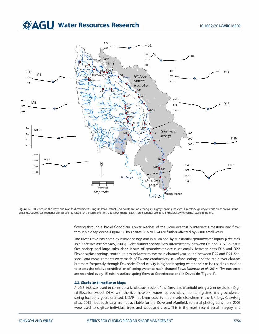
flowing through a broad floodplain. Lower reaches of the Dove eventually intersect Limestone and flowsthrough a deep gorge (Figure 1). Tw at sites D16 to D24 are further affected by �100 small weirs.

The River Dove has complex hydrogeology and is sustained by substantial groundwater inputs [Edmunds,1971; Abesser and Smedley, 2008]. Eight distinct springs flow intermittently between D6 and D16. Four sur-face springs and large subsurface inputs of groundwater occur seasonally between sites D16 and D22.Eleven surface springs contribute groundwater to the main channel year-round between D22 and D24. Sea-sonal spot measurements were made of Tw and conductivity in surface springs and the main river channelbut more frequently through Dovedale. Conductivity is higher in spring water and can be used as a markerto assess the relative contribution of spring water to main channel flows [Johnson et al., 2014]. Tw measuresare recorded every 15 min in surface spring flows at Crowdecote and in Dovedale (Figure 1).

2.2. Shade and Irradiance MapsArcGIS 10.3 was used to construct a landscape model of the Dove and Manifold using a 2 m resolution Digi-tal Elevation Model (DEM) with the river network, watershed boundary, monitoring sites, and groundwaterspring locations georeferenced. LiDAR has been used to map shade elsewhere in the UK [e.g., Greenberget al., 2012], but such data are not available for the Dove and Manifold, so aerial photographs from 2003were used to digitize individual trees and woodland areas. This is the most recent aerial imagery and

D2 D3D4 D5D6

D10

D11

D12

D13

D14

D15

D16

D17

D18

D20

D21D22

D23

D24

M16

M15M14

M13

M12

M10M11

M9

M8M6

D9Dove

Manifold

N

0 1 2 3

kilometres

Izaak Walton

Hollinsclough

Ilam

M17

R. Hamps

M2M3

D1

D1

D6

D10

D13

D16

D23

M3

M9

M13

M16

Map scale

First-order

Hillslope-channel separa�on

Ephemeral springs

Limestone gorge

Figure 1. LUTEN sites in the Dove and Manifold catchments, English Peak District. Red points are monitoring sites; gray-shading indicates Limestone geology; white areas are MillstoneGrit. Illustrative cross-sectional profiles are indicated for the Manifold (left) and Dove (right). Each cross-sectional profile is 3 km across with vertical scale in meters.



represents a snap-shot in time. However, no major forestry operations have taken place since 2003, mapswere ground validated at river monitoring sites and found to be consistent. In addition, tree cover at LUTENsites was monitored over the course of the three year experiment, with minimal change observed. Syntheticshade maps were then generated from the footprint of observed tree cover for heights of 10, 20, and 30 m.These represent juvenile, adult, and mature Ash (Fraxinus excelsior), respectively—the dominant tree speciesin the study area.

Shade maps were produced using the solar radiation function of Fu and Rich [2002], which uses globalstandard solar geometry equations to calculate solar radiation receipt across a DEM, based on site latitudeand longitude, date, time of day, and slope angle. Calculation resolution was set to 14 days with the visiblesky (skysize) divided into 512 discrete solar regions, which was deemed sufficient for monthly, catchment-scale radiation maps [see Fu and Rich, 2002 for more details]. Only direct solar radiation was considered inour analysis and the simplifying assumption made that trees allow no light penetration through the canopy.In reality, some light would penetrate the foliage, depending on species, age, canopy structure, and season,so our evaluation of the potential impact of trees on river shade is an upper bound estimate. Shade andradiation maps were generated for surfaces with no trees, juvenile, adult, and mature trees for each monthand year as a whole. Comparisons were made between the duration of shade and the amount of solarenergy incident over the catchments and along the river network.

To estimate maximum solar radiation incident on the river channel at higher temporal resolutions (5 min)than for GIS layers covering the whole catchment (monthly), solar elevation angles (i.e., height of the sunabove the horizon he) and azimuth angles (i.e., compass direction us) at any given time at site latitude(528 N) were calculated using the algorithm of NOAA [2014], which is a global function, based on solargeometry. The solar radiation incident on the Earth’s atmosphere is known as the Solar Constant andapproximates 1.353 kW m22. However, the amount of radiation reaching the Earth’s surface varies due totwo main factors. First is the reduction in the power as solar energy passes through the Earth’s atmospheredue to absorption by air and dust, quantified using the global function:

IA51:353 x 0:7ðAM0:678ÞÞ (1)

where IA (W m22) is solar irradiance incident on a perpendicular surface, 1.353 is the solar constant, 0.7 rep-resents the fact that 70% of solar radiation incident on the atmosphere reaches the Earth’s surface, 0.678 isderived empirically from measured data, and AM is the ‘‘air mass,’’ which is equal to:

AM51

cos hzð Þ10:50572ð96:079952hzÞ21:6364 (2)

where hz is the Zenith Angle (which is the complimentary angle to he). Second, when the angle of incidence(which is elevation angle, he) is not 908 vertical, solar radiation is spread over a larger area, effectively dilut-ing intensity. This effect is quantified as:

IAD5IA sin he (3)

where IAD (W m22) is the solar irradiance on a horizontal surface. Note that this estimate does not accountfor cloud cover or water vapor in the atmosphere, both of which have substantial impacts on solar irradi-ance by casting shade and reducing solar energy receipt at the Earth’s surface. The value of IAD does notaccount for surface albedo (i.e., reflectance), nor for diffuse radiation. Consequently, equation (3) is the max-imum possible amount of direct solar radiation striking a horizontal surface at a given latitude. The river sur-face was also considered to be horizontal at this resolution, so the effect of channel slope on radiationreceipt was ignored. However, sensitivity testing using channel gradients in the Dove (maximum 2.38, mean0.48) and the Manifold (maximum 1.08, mean 0.58) indicates that river slope adds locally no more than 4% todirect radiation receipt. At the catchment-scale, ArcGIS layer outputs do account for nonhorizontal slopes.To convert IAD (W m22), calculated at 5 min resolution, into solar energy (J m22), IAD was multiplied by300 s.

2.3. River Discharge and Thermal Sensitivity AnalysisMetrics were derived for thermal inertia and advection to explore the sensitivity of sites to shade. Thermalinertia due to increasing water volume with distance downstream was estimated by standardizing at-a-site



irradiance by upstream catchment area, a widely used surrogate for discharge [e.g., Hannah et al., 2008]that is readily derived from the DEM. Heat advection was estimated by standardizing at-a-site irradiance byall radiation incident over the upstream river network. The heat capacity (C) of water (�4180 kg J8C) wasthen used to estimate the length of continuous shade required to change Tw by 18C at the two sites on theDove, coinciding with river flow gauges maintained by the Environment Agency of England and Wales (EA).These sites are Hollinsclough (D4, 4.1 km from source) and Izaak Walton (D24, 31.2 km from source). Thegauges record discharge every 15 min through a fixed cross section. Volume of flow (product of channelwidth (w m), depth (d m), and length (l m)) at these sites was used to estimate the energy (E J) required tochange Tw by 18C as:

E5 ½w3d3l�31000ð Þ3C (4)

where 1000 converts water volume (m3) to mass (kg). The time (T s) taken to accumulate radiative energy(E) over the surface w.l was calculated from NOAA solar estimates and ArcGIS layer outputs as:

T5E=IAD (5)

The velocity of water (v m s21) at the gauge was then used to determine how far a parcel of water wouldflow in the time taken to reach E, as:

L5v3T (6)

indicating the length (L m) of tree cover required to shade a river from radiation that is equivalent to a 18Cchange in Tw. Note, this lower bound estimate does not account for heat from other sources, diffuse, orreflected radiation or for the fraction of direct radiation that penetrates the tree canopy.

2.4. Regression Modeling and Parameter AnalysisMaximum, mean, and minimum Ta and Tw were monitored with Gemini Aquatic II Tinytag thermistors ateach monitoring site (Figure 1). Tinytags have a quoted accuracy of 0.28C, which has been confirmed in lab-oratory experiments [Johnson and Wilby, 2013]. Data were recorded at 15 min resolution and are availablefor 3 years at 20 sites, and 2 years at a further 17 sites (Figure 1). Daily maximum Tw at each site was mod-eled given daily maximum Ta using logistic regression models, following Mohensi et al. [1998]:

TW5a

11expc b2Tað Þð Þ (7)

where a is the model asymptote, b is the Ta where the gradient is steepest, and c is the gradient term.Regression models were constructed for all sites for each year, as well as for all years combined. Detailedanalysis of LUTEN data reveals that regression models perform well (r 5 0.82 to 0.97) even when calibratedand validated with data reflecting contrasting weather conditions [Johnson et al., 2014; Wilby et al., 2014].Spatial variations in these regression parameters are reinterpreted below in the context of the shade andheat analyses.

3. Results

3.1. Location and Extent of Tree CoverTrees cover 6.8% of the Dove and 7.5% of the Manifold catchment. Average patch size across both catch-ments is 681 m2 (S.D 5 4563 m2) but 16% of patches consist of single trees. The largest unbroken patch sizewas 0.26 km2, comprising of an Ash woodland running through Dovedale. Trees bound the main channel ofthe Dove and Manifold for 44% and 35% of their lengths (13.7 km and 7.0 km), respectively. Patches border-ing the rivers are typically just a few trees deep.

3.2. Location and Extent of ShadeAdult trees reduce annual radiation receipt over 51% and 55% of the surface area of the Dove and Manifoldcatchments but 92% and 89% of the main channel length of Dove and Manifold, respectively (Table 1).Approximately 7% of the Dove and Manifold catchments receive less than half of the solar radiation thatwould accrue if there were no trees. However, landscape shade is concentrated along drainage lines with32% of Dove river network and 22% of the Manifold receiving less than 50% (Figure 2). Landscape providesmost shade in the headwaters with much less for downstream reaches once floodplain development



begins. Treeless reaches of the Dove(between 5 and 25 km from source) receivenearly 100% of potential direct solar radiation.Equivalent distances on the Manifold are9–17 km from source. Beyond 25 km alongthe Dove and 17 km along the Manifold, theLimestone gorge increases landscape shade,decreasing solar radiation receipt by 16% and7%, respectively (Figure 3).

Solar radiation is greatest at midday insummer, when solar angles are high and solarazimuth is south (Figure 4). Over 69% of the

total radiation received at 528 N is from solar angles greater than 308, despite the fact that these anglesoccur only 37% of the time. Landscape shades all solar angles in the headwaters of the Dove and Manifold,but only relatively low solar angles at more downstream sites (Figure 5). Conversely, trees shade a similarrange of angles to the landscape in the headwaters, but shade higher solar angles than the landscapedownstream (Figure 5). Due to variations in solar radiation intensity, the proportion of time in shadeexceeds the proportion of radiation reduced by shade (Figure 3).

Preferential shading at certain solar angles leads to seasonality in shade, and to differences in shade pro-vided by trees and the landscape (Figure 3). The difference in radiation receipt between landscape only andlandscape plus trees is less than 15% of the annual total irradiance across 73% of the catchment area. Mostof this difference occurs in spring and summer, when solar angles, and therefore solar radiation, are greatest(at the latitude of the catchment) (Figure 2). In autumn and winter, the difference in shading between treesand the landscape is minimal, even when leaf fall is neglected.

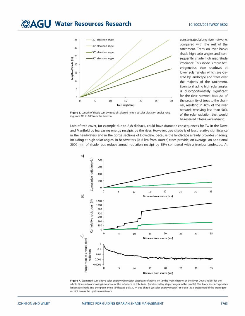
In order to block, solar angles greater than 308 and thereby reduce the majority of solar irradiance requirestrees to be sited near rivers (Figure 6). For example, a 10 m high tree casts 17.6 m of shade at 308 solar ele-vation angles, whereas at 608 angles (responsible for 23% of solar energy in the catchments) the shadowcast is 5.8 m long. Although a larger area is shaded in winter, when solar angles are lower, the benefit ofshading is greatest in summer, when solar angles and intensities are highest. To put these values into con-text, the maximum channel widths of the Dove and Manifold are 14 and 12 m, respectively. The Dove is lessthan 6 m wide for the first 24 km from source, therefore requiring a single line of 10 m tall trees on eachbank to shade the width of the river. The transition to partial shade is due to increased channel width aswell as the north-south orientation of the river.

3.3. Sensitivity of River Reaches to ShadingCumulative direct solar energy received by the drainage network increases with distance downstream (Fig-ure 7a). A channel without trees, shaded only by the landscape receives substantially more radiation thanreaches shaded by trees: each year treeless reaches of the Dove accumulate 1.54 3 106 MJ/km comparedwith 0.39 3 106 MJ/km when trees are present. This also means that more heat is advected from upstreamwhen the landscape is treeless. Moreover, there are step changes in heat with distance downstream due totributary inputs which for the Dove contribute 43% of the energy received by a network without trees and41% with adult trees (Figure 7b). Tributaries contribute 88% of the energy received by the Manifold networkboth with and without adult trees. Standardizing annual energy received at a site by total cumulativeupstream energy receipt reveals the significance of heat advection. After 50 m, local radiation adds lessthan 1% to the heat gained from upstream in the Dove network and less than 0.1% after 300 m (Figure 7c).

Catchment area increases from 2.1 km2 at site D2 to 82.5 km2 at site D24 at an average rate of �3 km2 perkilometer of river length in the Dove (Figure 8b) and 3.4 km2 per kilometer in the Manifold (not shown).Heat capacity calculations suggest that to reduce Tw by 18C at Hollinsclough (6.7 km from source) at mid-day on the solar equinox would require 0.5 km of adult tree cover. Under the same conditions, it wouldrequire 1.1 km of tree cover at Izaak Walton (31.2 km from source). Table 2 shows the length of riparianshade theoretically required to cool Tw by 18C at midday on the 15th day of each month at the two gaugingstations. We pay particular attention to June–July because this is the month during which maximum Tw istypically experienced in the Dove and Manifold [Wilby et al., 2012].

Table 1. Surface Area of Tree Canopy and Tree Shade in the Dove andManifold Catchments

Catchment Dove Manifold

Surface area shaded by landscape (%) 50.7 54.7Total area covered by tree canopy (km2) 5.7 4.8Fraction of area covered by tree canopy (%) 6.8 7.5Number of discrete tree patches 6770 8630Average patch size (km2) 0.0008 0.0006Standard deviation of area (km2) 0.006 0.003Total area shaded (10 m trees) (km2) 37.4 40.3Total area shaded (20 m trees) (km2) 49.8 48.0Total area shaded (30 m trees) (km2) 63.1 56.3



3.4. Logistic Regression AnalysisLogistic regression models describe the Ta-Tw relationship well at all LUTEN sites (the lowest r2 value is still0.86 at site D20 despite the substantial influence of groundwater). The three model parameters are: a whichis the asymptote of the model, indicating the maximum predicted Tw due to evaporative cooling at highTa; b which is the Ta where the gradient is greatest, and; c which is the model gradient at b.

Spring Summer

Autumn WinterWinterAutumn

No change

< 10%

10% - 20%

20% - 30%

30% - 40%

ii

i

iii

iv

ii

i

iii

iv

ii

i

iii

iv

ii

i

iii

iv

Figure 2. Difference in solar radiation receipt due to 30 m tall vegetation cover shown as a percentage of the potential annual total.Summer is June–August, Spring is March–May, Autumn is September–November, and Winter is December–February. White areas indicateno change. Horizontal hatching indicate area overlying limestone. Dashed lines indicate the four distinct hydrological regimes of theDove; (i) first-order, (ii) hillslope-channel decoupling, (iii) ephemeral groundwater, and (iv) limestone gorge.



Values of a increase with distance downstream until D22 and drop off markedly at D23 (Figure 8d). For thefirst 19 km of the River Dove (D1 to D17), a increases by 0.58C for every 1 km of downstream distance(r2 5 0.98). At sites D20 and D22 (26 and 28 km), a remains at 248C but is more variable between years thanupstream sites (Figure 8d). Values of c are highest in the headwater (D1 and D2) and decline with distancedownstream to 19 km (D17) where they begin to increase. Regression model parameters vary betweenyears according to weather conditions, but the general pattern remains the same (see Figure 8d).

0

100000

200000

300000

400000

500000

600000

1

16

1

32

1

48

1

64

1

80

1

96

1

11

21

12

81

14

41

16

01

17

61

19

21

20

81

22

41

24

01

25

61

27

21

28

81

30

41

32

01

33

61

35

21

36

81

38

41

0

500

1000

1500

2000

2500

3000

3500

4000

1

16

1

32

1

48

1

64

1

80

1

96

1

11

21

12

81

14

41

16

01

17

61

19

21

20

81

22

41

24

01

25

61

27

21

28

81

30

41

32

01

33

61

35

21

36

81

38

41

Irra

dia

nce

Su

nli

gh

t d

ura

�o

n (

ho

urs)

0

100000

200000

300000

400000

500000

600000

1

11

3

22

5

33

7

44

9

56

1

67

3

78

5

89

7

10

09

11

21

12

33

13

45

14

57

15

69

16

81

17

93

19

05

20

17

21

29

22

41

23

53

24

65

25

77

26

89

Direct

Dura�on

Dove Manifold

2.16

1.80

1.44

1.08

0.72

0.36An

nu

al

Ra

dia

�o

n (

GJ m

-2)

Irra

dia

nce

2.16

1.80

1.44

1.08

0.72

0.36An

nu

al

Ra

dia

�o

n (

GJ m

-2)

0

0 5 10 15 20 25 30 35

0 5 10 15 20 25 30 35

0

200 5 10 15

Distance from source (km)



0

500

1000

1500

2000

2500

3000

3500

4000

1

13

25

37

49

61

73

85

97

10

9

12

1

13

3

14

5

15

7

16

9

18

1

19

3

20

5

21

7

22

9

24

1

25

3

26

5

27

7

28

9

Su

nli

gh

t d

ura

�o

n (

ho

urs)

205 10 15


0

Figure 3. Downstream profiles of estimated annual direct solar radiation (Gigajoules) (upper panels) and time in shade (hours) (lower panels) for landscapes with trees (green) and with-out trees (black) in the Dove (left) and Manifold (right).

60

50

40

30

20

10

0

0 25 50 75 100 125 150 175 200 225 250 275 300 325 350

N SE W

2%

12%

18%

22%

24%

23%

0.04%0.7% 5% 11% 14% 15% 15% 15% 13% 8% 2%

So

lar a

l�tu

de

an

gle

(°)

Solar azimuth angle (°)

% Annual Total

6

0

1

2

3

4

5

Figure 4. The elevation angle (e.g., angle of incidence) and azimuth angle (i.e., compass direction) of the sun over a year at 528 latitude.Shading indicates relative proportion of solar radiation occurring at that solar position over a year. Percentages of the total solar radiationbudget at each azimuth or elevation angle are denoted.



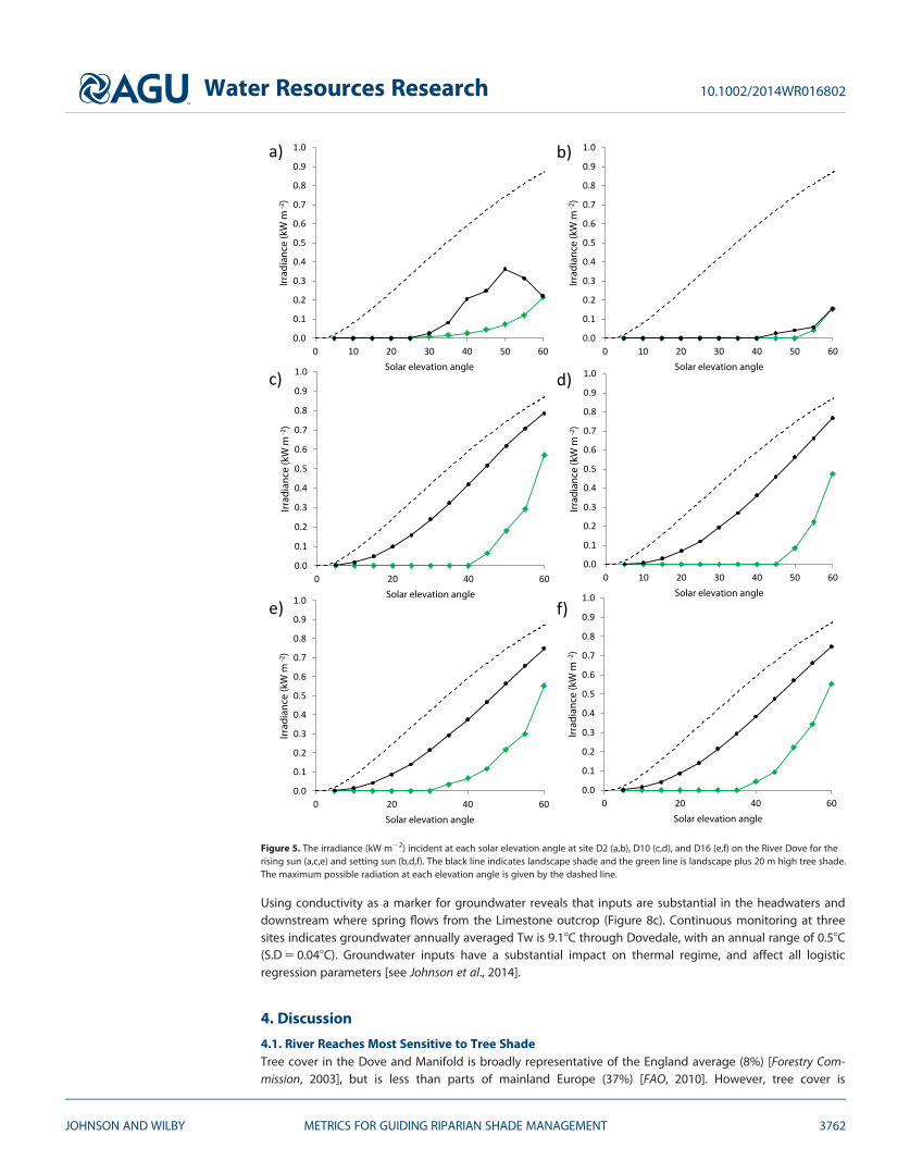
Using conductivity as a marker for groundwater reveals that inputs are substantial in the headwaters anddownstream where spring flows from the Limestone outcrop (Figure 8c). Continuous monitoring at threesites indicates groundwater annually averaged Tw is 9.18C through Dovedale, with an annual range of 0.58C(S.D 5 0.048C). Groundwater inputs have a substantial impact on thermal regime, and affect all logisticregression parameters [see Johnson et al., 2014].

4. Discussion

4.1. River Reaches Most Sensitive to Tree ShadeTree cover in the Dove and Manifold is broadly representative of the England average (8%) [Forestry Com-mission, 2003], but is less than parts of mainland Europe (37%) [FAO, 2010]. However, tree cover is

0.0

0.1

0.2

0.3

0.4

0.5

0.6

0.7

0.8

0.9

1.0

0 10 20 30 40 50 60

Irrad

ianc

e (k

W m

-2)

Solar elevation angle

0.0

0.1

0.2

0.3

0.4

0.5

0.6

0.7

0.8

0.9

1.0

0 10 20 30 40 50 60

Irrad

ianc

e (k

W m

-2)


0.0

0.1

0.2

0.3

0.4

0.5

0.6

0.7

0.8

0.9

1.0

0 20 40 60

Irrad

ianc

e (k

W m

-2)


0.0

0.1

0.2

0.3

0.4

0.5

0.6

0.7

0.8

0.9

1.0

0 10 20 30 40 50 60Irr

adia

nce

(kW

m- 2

)


0.0

0.1

0.2

0.3

0.4

0.5

0.6

0.7

0.8

0.9

1.0

0 20 40 60

Irrad

ianc

e (k

W m

-2)


0.0

0.1

0.2

0.3

0.4

0.5

0.6

0.7

0.8

0.9

1.0

0 20 40 60

Irrad

ianc

e (k

W m

-2)


a) b)

c) d)

e) f)

Figure 5. The irradiance (kW m22) incident at each solar elevation angle at site D2 (a,b), D10 (c,d), and D16 (e,f) on the River Dove for therising sun (a,c,e) and setting sun (b,d,f). The black line indicates landscape shade and the green line is landscape plus 20 m high tree shade.The maximum possible radiation at each elevation angle is given by the dashed line.



concentrated along river networkscompared with the rest of thecatchment. Trees on river banksshade high solar angles and, con-sequently, shade high magnitudeirradiance. This shade is more het-erogeneous than shadows atlower solar angles which are cre-ated by landscape and trees overthe majority of the catchment.Even so, shading high solar anglesis disproportionately significantfor the river network because ofthe proximity of trees to the chan-nel, resulting in 40% of the rivernetwork receiving less than 50%of the solar radiation that wouldbe received if trees were absent.

Loss of tree cover, for example due to Ash dieback, could have dramatic consequences for Tw in the Doveand Manifold by increasing energy receipts by the river. However, tree shade is of least relative significancein the headwaters and in the gorge sections of Dovedale, because the landscape already provides shading,including at high solar angles. In headwaters (0–6 km from source) trees provide, on average, an additional2000 min of shade, but reduce annual radiation receipt by 15% compared with a treeless landscape. At

0

5

10

15

20

25

30

35

0 5 10 15 20 25 30

Leng

th o

f Sha

de (m

)

Tree height (m)

30° eleva�on angle




Figure 6. Length of shade cast by trees of selected height at solar elevation angles rang-ing from 308 to 608 from the horizon.

0

50000000

100000000

150000000

200000000

1

11

21

31

41

51

61

71

81

91

10

1

11

1

12

1

13

1

14

1

15

1

16

1

17

1

18

1

19

1

20

1

21

1

22

1

23

1

24

1

25

1

26

1

27

1

28

1

29

1

30

1

31

1

Distance from source (km)0

0

50000000

100000000

150000000

200000000

250000000

300000000

350000000

1

11

21

31

41

51

61

71

81

91

10

1

11

1

12

1

13

1

14

1

15

1

16

1

17

1

18

1

19

1

20

1

21

1

22

1

23

1

24

1

25

1

26

1

27

1

28

1

29

1

30

1

31

1


0.0001

0.001

0.01

0.1

1

1

11

21

31

41

51

61

71

81

91

10

1

11

1

12

1

13

1

14

1

15

1

16

1

17

1

18

1

19

1

20

1

21

1

22

1

23

1

24

1

25

1

26

1

27

1

28

1

29

1

30

1

31

1


0

180

360

540

720

180

360

540

720

900

1080

1260

0

0

Cu

mu

la�

ve

ra

dia

�o

n (

GJ)

Cu

mu

la�

ve

ra

dia

�o

n (

GJ)

Pro

po

r�

on

of a

nn

ua

l to

ta

l

ra

dia

�o

n

0 5 10 15 20 25 30 35

0 5 10 15 20 25 30 35

0 5 10 15 20 25 30 35

a)

b)

c)

Figure 7. Estimated cumulative solar energy (GJ) receipt upstream of points on (a) the main channel of the River Dove and (b) for thewhole Dove network taking into account the influence of tributaries (evidenced by step changes in the profile). The black line incorporateslandscape shade and the green line is landscape plus 30 m tree shade. (c) Solar energy receipt ‘‘at-a-site’’ as a proportion of the aggregatereceipt across the upstream network.



intermediate reaches (6–20 km from source), with floodplain, the landscape provides little shade at highsolar angles, resulting in the river receiving nearly 100% of the potential solar radiation. In these locations,tree cover would reduce radiation receipts by 25%.

4.2. Relative Significance of Shade in Context of River RegimeWhile tree cover and radiation maps show spatial variations in riparian shade, they do not indicate whichriver reaches might benefit most from increased canopy cover. Thermal inertia and advected heat from

0

10

20

30

40

50

60

70

80

90

0 5 10 15 20 25 30 35

Ups

trea

m c

atch

men

t are

a (k

m2 )

200000

250000

300000

350000

400000

450000

500000

550000

600000

0 5 10 15 20 25 30 35

Radi

a�on

(GJ)

0

100

200

300

400

500

600

0 5 10 15 20 25 30 35

Cond

uc�

vity

First-order Hillslope channel separa�on Limestone gorgeEphemeral springs

10

12

14

16

18

20

22

24

26

28

30

0.04

0.06

0.08

0.1

0.12

0.14

0.16

0 5 10 15 20 25 30 35

α(°C)γ

(°C)


2.16

1.80

1.44

1.08

0.72

a)

b)

c)

d)

Figure 8. (a) Radiation receipt with distance from source in the River Dove without trees; (b) upstream catchment area of the Dove; (c) con-ductivity of water in the main channel of the River Dove; (d) the asymptote (a; blue) and gradient (c; black) term of logistic regression mod-els constructed on daily maximum Ta and Tw data from March 2011 to February 2013 (thick lines) and values for individual years (dashedlines).



upstream quickly render local solar radiation receipt insignificant to Tw variations at that site. Instead, Tw isdriven by the cumulative energy advected from upstream. Consequently, as distance downstreamincreases, shading over longer reaches is required to influence local Tw. Therefore, for all but the first few100s meters of river, shading has limited impact on the site of planting but can contribute to downstreamcooling. For example, at Hollinsclough direct solar radiation would have to be completely intercepted over0.5 km to change Tw by 18C at midday in July. At Izaak Walton (where discharge is on average five timesgreater than at Hollinsclough), the equivalent figure is 1.1 km of shade. It should also be noted that theseare likely to be lower bound estimates given our assumptions that no radiation penetrated trees and ofmaximum possible radiation receipt, under continuous clear sky conditions.

Several studies have measured higher rates of change of Tw (8C/km) for the opposite case when riversemerge from areas of native vegetation to open pasture. For example, Rutherford et al. [1997] find that dailymaximum Tw in summer can change by 3–48C in 600 m for a river in Hamilton, New Zealand (388S; averagewidth 1.2 m); similarly, Hopkins [1971] obtains 3–48C in 500 m for second-order streams in Wellington, NewZealand (418S; 1.5–2.0 m wide). Even higher rates of change in maximum Tw of 108C/km are reported byRutherford et al. [2004] for streams in Western Australia and south-east Queensland (26–358S; 1.3–3.3 mwide). However, all these field sites are closer to the equator than the River Dove (528N; average width6.9 m; range 0.5–11.7 m) so receive more intense solar radiation (equation (3)). Reported discharges of< 30Ls21 also mean that the volumes of flow being heated are less than those in the Dove, even for summerminima (typically >50 Ls21 at the Hollinsclough gauge).

Tributary influences are a further consideration because they increase the water surface receiving directsolar radiation and input point sources of heat to the main channel. The Dove has little surface drainageand, consequently, tributaries contribute 43% of the cumulative heat whereas in the Manifold, with a dense,dendritic channel network, tributaries provide 88%. As a result, the Dove gains only 36% of the energy thatthe Manifold accumulates a year, despite the Dove draining a larger catchment. Overall, the significance ofa tributary to the thermal regime of a river network depends on the ratio of catchment area to that of themain channel upstream recognizing that groundwater inputs, abstraction, reservoirs, and other factors mayfurther influence Tw.

Table 2. Estimated Length of Continuous 20 m High Tree Shade Required to Change Tw by 18C at 11 A.M. on the 15th Day of EachMontha

Discharge(m3)

Heat Capacity(kg J8C)

Time to ReachCapacity (s)

Average Velocity(m s21)

RequiredShade (km)

D4 January 0.42 1,328,166 9,600 0.67 6.4February 0.36 1,188,790 4,200 0.63 2.7March 0.33 1,110,618 2,700 0.62 1.7April 0.25 908,214 1,800 0.57 1.0May 0.18 717,255 1,200 0.53 0.6June 0.14 598,873 1,050 0.49 0.5July 0.14 586,403 1,050 0.49 0.5August 0.16 650,092 1,200 0.51 0.6September 0.18 726,491 1,800 0.53 1.0October 0.32 1,103,218 3,000 0.61 1.8November 0.41 1,301,353 6,600 0.66 4.4December 0.41 1,297,365 1,140 0.66 7.5

D24 January 3.09 2,205,427 15,600 0.98 15.2February 2.912 2,149,313 8,100 0.94 7.6March 2.61 2,043,625 4,500 0.89 4.0April 2.18 1,881,096 3,000 0.81 2.4May 1.59 1,622,111 2,400 0.68 1.6June 1.28 1,476,224 2,100 0.61 1.3July 1.07 1,370,258 1,950 0.55 1.1August 0.98 1,323,391 2,100 0.52 1.1September 1.00 1,333,703 2,700 0.52 1.4October 1.51 1,585,399 4,500 0.66 2.9November 2.20 1,889,172 9,900 0.81 8.0December 2.81 2,114,340 N/A 0.93 N/A

aEstimates were made by calculating the heat capacity of the monthly-averaged water volume for the past 34 years at flow gaugesat Hollinsclough (D4) and Izaak Walton (D24) on the River Dove. Note that in December, at site D24, solar radiation receipt is insufficientto achieve the heat capacity.



Shade has greatest effect where water volumes are small and where there is little upstream channel length,such as in headwaters. However, countering this is the fact that headwaters have limited exposure time tosolar radiation, limited surface area over which to receive radiation and are strongly influenced by ground-water inputs [D’Angelo et al., 1993]. River sources are also more likely to be affected by landscape and micro-topographic shade, reducing the relative significance of riparian shade. It is, therefore, likely in the Doveand Manifold that tree shade will have effect over only relatively short reaches of river, supporting the find-ings of Chang and Lawler [2011] for streams in Oregon, USA. In other catchments, wide, shallow streams setin broad floodplains could benefit, provided that the channel is shaded at high solar angles. However, closerto the equator, shadow length is smaller due to high solar angles, reducing the potential significance ofriparian shading.

Logistic regression models support these findings. Increased tree cover is expected to be of greatest benefitwhere a and c are both relatively high, indicating sensitivity to Ta (the proxy for solar radiation) enabling riv-ers to reach high Tw. However, the model asymptote (a) increases with distance downstream as exposuretime to solar radiation increases, reflecting increased advection of heat with distance downstream, whereasthe gradient parameter (c) decreases as water volumes (thermal inertia) increase. At intermediate distances(5–19 km from source in the Dove), where both parameters are relatively high, riparian shade is likely to bemost beneficial for Tw management. Therefore, logistic Ta-Tw regression parameters (a and c) can helpinform site selection for tree planting but this presupposes existence of sufficient Tw and Ta samplingpoints to detect spatial variations in these metrics [Johnson et al., 2014; Wilby et al., 2014].

4.4. Other Heat Sources and Future ChangeTrees increase long-wave radiation reaching the ground and also modify latent and sensible heat fluxes byaltering the microclimate above rivers flowing through riparian woodland [see Moore et al., 2005 review].However, these heat sources are relatively insignificant for much of the time [e.g., Evans et al., 1998] and theimpact of riparian shade in reducing short-wave radiation more than offsets potential increases in energyfrom these other sources [Moore et al., 2005]. It is unclear whether riparian shade would alter other sourcesof heat in rivers, such as from precipitation. Although rainfall typically contributes less than 1% of the totalenergy input to a stream [Webb and Zhang, 1997; Evans et al., 1998] intense summer storms can producemore rapid rises in Tw than intense solar heating under clear sky conditions [Wilby et al., 2015].

To place our estimated shade lengths (0.5–1.1 km) in context, the UKCP09 central estimate of projectedchange in the warmest day in summer is 158C by the 2080s under medium emissions [Murphy et al., 2009].Logistic regression models for D4 and D24 predict that the corresponding change in maximum daily Twwould be 10.78C and 10.58C, respectively. This in turn suggests that less than 1 km of additional riparianshade would be sufficient to offset projected anthropogenic warming to century end. Again, this assumesno radiation penetrates the canopy and that changes in solar radiation may be neglected (despite the possi-bility of reduced summer mean cloud cover). On the other hand, an outlook of lower river flow volumes insummer implies that the associated changes in Tw (and attendant need for tree planting) are conservative[Prudhomme et al., 2012].

The UKCP09 projections suggest substantial increases in sunshine duration and solar radiation, but lessdownward diffuse radiation [Tham et al., 2011]. Further research is needed to establish how these changesmight combine in future Tw and hence to ascertain the rivers and reaches that would benefit most fromriparian shade management. A more sophisticated approach is needed to interpret the great variability instream Tw responses to rising global temperatures, including for example recent cooling trends in many riv-ers of the Pacific continental U.S. [Arismendi et al., 2012]. For example, Kibler et al. [2013] report that clearfelling in one headwater of southwest Oregon resulted in marked cooling of the stream. Similarly, Janischet al. [2013] found Tw response to clear felling in headwaters in western Washington, USA, was small andhighly variable between sites. Other works suggests that the relationship between canopy cover and Twmay be moderated by intermittency in surface flow [Janisch et al., 2013]. These disparate results underlinethe importance of local context in shaping energy receipts and hydrological controls of Tw.

4.5. Wider Implications for River ManagementThe potential benefit of shade is determined by channel characteristics. At the most fundamental level, inthe northern hemisphere vegetation should be located on the south bank of rivers to maximize shading of



the channel [Larsen and Larsen, 1996]. Channels aligned north-south will not be shaded at midday, whenthe sun is most powerful, except by overhanging vegetation. In order to reduce the radiation receipt of a10 m wide stream by more than 50% at 528N latitudes, a tree on the south bank of a river and 5 m from itsedge must be at least 12 m tall. Ash requires �20 years to attain this height and at least 50 years under idealcondition to reach 30 m [Dobrowolska et al., 2011]. Recalling that at least 0.5 km of complete shade wouldbe required to cool the Dove by 18C, riparian buffer zones would have to be several trees deep in order toprovide complete shade. In practical terms, it may be challenging to persuade landowners to allow suchwidespread tree planting, particularly in Europe where the average agricultural land holding is only0.14 km2 [EU Agricultural Census, 2010]. Therefore, the cooperation of multiple land-owners and a relativelylarge percentage of their holding would need to be given over to tree cover if this adaptation strategy is tohave a discernible impact.

Tree planting to cool rivers may be a more tenable proposition in the UK for major land owners such as theChurch of England, Crown Estate, Ministry of Defence, or National Trust. Nonetheless, all planting schemesshould recognize the potential detrimental impacts on ecosystems caused by altering the light regime,increasing flood hazard, modifying the geomorphic functioning and local water balance of the river.Enhanced rainfall interception and transpiration along woodland edges could increase local water demand,lessen soil moisture, and reduce recharge, particularly during dry summers [Harding et al., 1992]. In addition,some habitats could be fundamentally altered by shade with negative impacts on biomass and ecologicalcommunities [Wood et al., 2014]. Therefore, patchy shade may be more beneficial to the river ecosystem asa whole, but this implies a longer reach given over to trees to achieve the same predicted cooling.

Increased direct solar radiation penetrating the water column, and warming the body of fish or other organ-isms may cause more stress than increased Tw, per se. However, the impact of direct radiation on aquaticorganisms is rarely considered and Tw monitoring conventionally seeks to minimize this factor in measure-ments [Johnson and Wilby, 2013]. There has also been relatively little consideration of the potential impactsof tree planting on nocturnal Tw [Wilby et al., 2014]. Whereas large areas of tree cover are required to alterTw, individual trees, and patches can still be of biological importance by providing fauna local protectionfrom direct solar radiation or highly localized cool refugia [Everall et al., 2012]. More research is needed toassess the specific thermal variables that are of significance to aquatic animals and how these conditionsmight change in the future under climate change with or without more tree cover [Orr et al., 2015b].

5. Conclusions

The thermal regimes of exposed river channels are undoubtedly very different to those under tree cover.However, increased riparian shade is not a panacea for climate change and there will be large areas of riverthat would be little affected by the addition (or removal) of vegetation because of advected heat fromupstream, landscape shade, (cool) groundwater, reservoir releases, and/or snowmelt inputs. In addition, fur-ther research is needed into how regional climate change could be manifested directly in Tw (due to plausi-ble combinations of changing Ta, radiation balance, cloud cover, magnitude and frequency of extremeevents, and precipitation regime). Potential indirect impacts of climate change on Tw through modified vol-umes of flow in stream and shifting contributions from surface, subsurface, groundwater, and/or snow/icemelt also merit further investigation.

The topographic indices developed herein could provide means of identifying river reaches that are mostsensitive to thermal forcing by the atmosphere, and/or potentially most responsive to active shade manage-ment. We show that standardizing direct radiation by upstream catchment area provides a useful proxy forheat accumulation along the profile of a river and hence a basis for estimating riparian buffer lengthsneeded to achieve a unit reduction in Tw. We show that river reaches dominated by surface water but withrelatively small discharges, large width: depth ratios and limited landscape shade benefit most from shad-ing. These zones tend to occur in the midreaches of headwater systems (and are further characterized byrelatively large a and c logistic regression parameters). Channel morphology, river orientation, and the pres-ence of wetland areas, ponds, or artificial structures may also be locally significant considerations. Other fac-tors such as slope, stream order, and percent grassland area are known to affect the net benefit of forestland cover on maximum Tw in nival systems [Chang and Psaris, 2013], whereas greater storm sewer pipelengths and network densities moderate Tw in urban environments [Sabouri et al., 2013].



In the case of the River Dove, it is estimated that at least 0.5 km of complete shade would be required tooff-set each 18C rise in Tw. In addition, bankside trees over 12 m tall are needed to shade the river, taking atleast 20 years to grow. To implement tree planting on this scale in the UK typically requires coordination ofmany riparian land-owners and interest groups. Any tree planting would also need to assess potentialimpacts (positive and negative) on river habitat, hydrology, and geomorphology beyond simply reducingTw. This research underlines the need for shade management to be considered in a much broader,catchment-wide context, and provides evidence of the scale and time needed to achieve intended thermalbenefits for small (�100 km2), natural catchments in temperate zones. Further work would be necessary toextend the approach to other catchment types such as urban environments where tree planting could helpto manage thermal pollution by runoff from paved surfaces.

ReferencesAbesser, C., and P. L. Smedley (2008), Baseline groundwater chemistry: The carbonferous limestone aquifer of the Derbyshire Dome, Br.

Geol. Surv. Open Rep. OR/08/028, British Geological Survey, Keyworth, U. K.Arismendi, I., S. L. Johnson, J. B. Dunham, R. Haggerty, and D. Hockman-Wert (2012), The paradox of cooling streams in a warming world:

Regional climate trends do not parallel variable local trends in stream temperature in the Pacific continental United States, Geophys.Res. Lett., 39, L10401, doi:10.1029/2012GL051448.

Bowler, D. E., R. Mant, H. Orr, D. M. Hannah, and A. S. Pullin (2012), What are the effects of wooded riparian zones on stream temperature?Environ. Evid., 1, doi:10.1186/2047-2382-1-3.

Chang, H. and K. Lawler (2011), Impacts of climate variability and change on water temperature in an urbanizing Oregon basin, in Proceed-ings of Symposium H04 IUGG2011: Water Quality Trends and Expected Climate Change Impacts, IAHS Publ., edited by N. Peters et al.,vol. 348, pp. 123–128, Melbourne, Australia.

Chang, H., and M. Psaris (2013), Local landscape predictors of maximum stream temperature and thermal sensitivity in the Columbia RiverBasin, USA, Sci. Total Environ., 461–462, 587–600.

Chapra, S. C., G. J. Pelletier, and H. Tao (2008), QUAL2K: A Modelling Framework for Simulating River and Stream Quality, version 2.11: Docu-mentation and User’s Manual, Civ. and Environ. Eng. Dep., Tufts Univ., Medford, Mass.

Cole, T. M., and S. A. Wells (2002), CE-QUAL-W2: A two-dimensional, laterally averaged, hydrodynamic and water quality model, version 3.1,Inst. Rep. EL 03-1, U.S. Army Corps of Eng., Vicksburg, Miss.

Dallas, H. F., and N. A. Rivers-Moore (2012), Critical thermal maxima of aquatic macroinvertebrates: Towards identifying bioindicators ofthermal alteration, Hydrobiologia, 679, 61–76.

D’Angelo, D. J., J. R. Webster, S. V. Gregory, and J. L. Meyer (1993), Transient storage in Appalachian and Cascade mountain streams asrelated to hydraulic characteristics, J. N. Am. Benthol. Soc., 12, 223–235.

Davies-Colley, R. J., G. W. Payne, and M. van Elswijk (2000), Microclimate gradients across a forest edge, N. Z. J. Ecol., 24, 111–121.Dobrowolska, D., S. Hein, A. Oosterbaan, S. Wagner, J. Clark, and J. P. Skovsgaard (2011), A review of European ash (Fraxinus excelsior L.):

Implications for silviculture, Forestry, 84, 133–148.Edmunds, W. M. (1971), Hydrogeochemistry of groundwaters in the Derbyshire Dome with special reference to trace constituents, Rep.

Inst. Geol. Sci. 71/7, Br. Geol. Surv., Keyworth, U. K.Environment Agency (2012), Keeping Rivers Cool: Getting Ready for Climate Change by Creating Riparian Shade, Bristol, U. K.EU Agricultural Census (2010). [Available at http://ec.europa.eu/eurostat/statistics-explained/index.php/Agricultural_census_2010_-_main_

results, last accessed 29 Sept. 2014]Evans, E. C., G. McGregor, and G. E. Petts (1998), River energy budgets with special reference to river bed processes, Hydrol. Processes, 12,

575–595.Everall, N. C., A. Farmer, A. F. Heath, T. E. Jacklin, and R. L. Wilby (2012) Ecological benefits of creating messy rivers, Area, 44, 470–478.Everall, N. C., M. F. Johnson, R. L. Wilby, and C. J. Bennett (2015), Detecting phenology change in the mayfly Ephemera danica: Responses to

spatial and temporal water temperature variations, Ecol. Entomol., 40, 90–105.FAO (2010), Global Forest Resources Assessment 2010: Main Report, Food and Agriculture Organization of the United Nations, Rome FAO

For. Pap. 163.Ficklin, D. L., I. T. Stewart, and E. P. Maurer (2013), Effects of climate change on stream temperature, dissolved oxygen, and sediment con-

centration in the Sierra Nevada in California, Water Resour. Res., 49, 2765–2782, doi:10.1002/wrcr.20248.Ficklin, D. L., B. L. Barnhart, J. H. Knouft, I. T. Stewart, E. P. Maurer, S. L. Letsinger, and G. W. Whittaker (2014), Climate change and stream

temperature projections in the Columbia River basin: Habitat implications of spatial variation in hydrologic drivers, Hydrol. Earth Syst.Sci., 18, 4897–4912.

Forestry Commission (2003), National Inventory of Woodland and Trees, Edinburgh, U. K.Fu, P., and P. M. Rich (2002), A geometric solar radiation model with applications in agriculture and forestry, Comput. Electron. Agric., 37,

25–35.Greenberg, J. A., E. L. Hestir, D. Riano, G. J. Scheer, and S. L. Ustin (2012), Using LIDAR data analysis to estimate changes in insolation under

large-scale riparian deforestation, J. Am. Water Resour. Assoc., 48, 939–948.Hannah, D. M., I. A. Malcolm, C. Soulsby, and A. F. Youngson (2008), A comparison of forest and moorland stream microclimate, heat

exchanges and thermal dynamics, Hydrol. Processes, 22, 919–940.Harding, R. J., R. L. Hall, C. Neal, J. M. Roberts, P. T. W. Rosier, and D. G. Kinniburgh (1992), Hydrological implications of broadleaf woodlands:

Implications for water use and water quality, Proj. Rep. 115/03/ST, Natl. Rivers Auth., Bristol, U. K.Hopkins, C. L. (1971) The annual temperature regime of a small stream in New Zealand, Hydrobiologia, 37, 397–408.Isaak, D. J., C. H. Luce, B. E. Rieman, D. E. Nagal, E. E. Paterson, D. L. Horan, S. Parkes, and G. L. Chandler (2010), Effects of climate change

and wildfire on stream temperatures and salmonid thermal habitat in a mountain river network, Ecol. Appl., 20, 1350–1371.Janisch, J. E., S. M. Wondzell, and W. J. Ehinger (2013), Headwater stream temperature: Interpreting response after logging, with and with-

out riparian buffers, Washington, USA, For. Ecol. Manage., 270, 302–313.Johnson, S. L. (2003), Stream temperature: Scaling of observations and issues for modelling, Hydrol. Processes, 17, 497–499.

AcknowledgementsAll LUTEN data are freely available fordownload from www.luten.org.uk.Other data used, including ArcGISlayers, are available by contacting theauthors. We appreciate funding fromthe Wild Trout Trust and access to sitesgranted by landowners. Thanks to JuliaToone for assistance in the field andDapeng Yu for analysing GIS layers.



http://www.luten.org.uk

http://dx.doi.org/10.1186/2047-2382-1-3

http://ec.europa.eu/eurostat/statistics-explained/index.php/Agricultural_census_2010_-_main_results

http://ec.europa.eu/eurostat/statistics-explained/index.php/Agricultural_census_2010_-_main_results

http://dx.doi.org/10.1002/wrcr.20248

http://www.luten.org.uk

Johnson, M. F. and R. L. Wilby (2013), Shield or not to shield: Effects of solar radiation on water temperature sensor accuracy, Water, 5,1622–1637.

Johnson, M. F., R. L. Wilby, and J. A. Toone (2014), Inferring air-water temperature relationships from river and catchment properties, Hydrol.Processes, 28, 2912–2928.

Kelleher, C., T. Wagener, M. Gooseff, B. McGlynn, K. McGuire, and L. Marshall (2012), Investigating controls on the thermal sensitivity ofPennsylvania streams, Hydrol. Processes, 26, 771–785.

Kibler, K. M., A. Skaugset, L. M. Ganio, and M. M. Huso (2013), Effect of contemporary forest harvesting practices on headwater stream tem-peratures: Initial response of the Hinkle Creek catchment, Pacific Northwest, USA, For. Ecol. Manage., 310, 680–691.

Larsen, L. L. and S. L. Larsen (1996), Riparian shade and stream temperature: A perspective, Rangelands, 18, 149–152.Mantua, N., I. Tohver, and A. Hamlet (2010), Climate change impacts on streamflow extremes and summertime stream temperature and

their possible consequences for freshwater salmon habitat in Washington State, Clim. Change, 102, 187–223.Martins, E. G., S. G. Hinch, D. A. Patterson, M. J. Hague, S. J. Cooke, K. M. Miller, M. F. Lapointe, K. K. English, and A. P. Farrell (2011), Effects of

river temperature and climate warming on stock-specific survival of adult migrating Fraser River sockeye salmon (Oncorhynchus nerka),Global Change Biol., 17, 99–114.

Mohensi, O., H. G. Stefan, and T. R. Erickson (1998), A nonlinear regression model for weekly stream temperatures, Water Resour. Research,34, 2685–2692.

Moore, R. D., D. L. Spittlehouse, and A. Story (2005), Riparian microclimate and stream temperature response to forest harvesting: A review.J. Am. Water Resour. Assoc., 41, 813–834.

Murphy, J. M., et al. (2009), UK Climate Projections Science Report: Climate Change Projections, Met Off. Hadley Cent., Exeter, U. K.Nisbet, T., M. Silgram, N. Shah, K. Morrow, and S. Broadmeadow (2011), Woodland for Water: Woodland measures for meeting Water

Framework Directive objectives, For. Res. Monogr. 4, For. Res., Surrey, U. K.NOAA (2014). [Available at http://www.esrl.noaa.gov/gmd/grad/solcalc/calcdetails.html, last accessed 30 Sept 2014.]Null, S. E., J. H. Viers, M. L. Deas, S. K. Tanaka, and J. F. Mount (2013), Stream temperature sensitivity to climate warming in California’s Sierra

Nevada: Impacts to coldwater habitat, Clim. Change, 116, 149–170.Orr, H. G., et al. (2015a), Detecting changing river temperatures in England and Wales. Hydrol. Processes, 29, 752–766.Orr, H. G., M. F. Johnson, R. L. Wilby, T. Hatton-Ellis, and S. Broadmeadow (2015b), What else do managers need to know about warming riv-

ers? WIRES Water, 2, 55–64.Osborne, L. L., and D. A. Kovacic (1993), Riparian vegetated buffer strips in water-quality restoration and stream management. Freshwater

Biol., 29, 243–258.Prudhomme, C., A. Young, G. Watts, T. Haxton, S. Crook, J. Williamson, H. Davies, S. Dadson, and S. Allen (2012), The drying up of Britain? A

national estimate of changes in seasonal river flows from 11 Regional Climate Model simulations, Hydrol. Processes, 26, 1115–1118.Richardson, J. S., and S. B�eraud (2014), Effects of riparian forest harvest on streams: A meta-analysis, J. Appl. Ecol., 51, 1712–1721.Rutherford, J. C., S. Blackett, C. Blackett, L. Saito, and R. J. Davies-Colley (1997), Predicting the effects of shade on water temperature in

small streams, N. Z. J. Mar. Freshwater Res., 31, 707–721.Rutherford, J. C., N. A. Marsh, P. M. Davies, and S. E. Bunn (2004) Effects of patchy shade on stream water temperature: How quickly do

small streams heat and cool?, Mar. Freshwater Res., 55, 737–748.Sabouri, F., B. Gharabaghi, A. A. Mahboubi, and E. A. McBean (2013), Impervious surfaces and sewer pipe effects on stormwater runoff tem-

perature, J. Hydrol., 502, 10–17.Story, A., R. D. Moore, and J. S. Macdonald (2003), Stream temperatures in two shaded reaches below cutblocks and logging roads: Down-

stream cooling linked to subsurface hydrology, Can. J. For. Res., 33, 1383–1396.Sweeney, B. W., and J. D. Newbold (2014), Streamside forest buffer width needed to protect stream water quality, habitat, ad organisms: A

literature review, J. Am. Water Resour. Assoc., 50, 560–584.Thackeray, S. J., et al. (2010), Trophic level asynchrony in rates of phonological change for marine, freshwater and terrestrial environments,

Global Change Biol., 16, 3304–3313.Tham, Y., T. Muneer, G. J. Levermore, and D. Chow (2011), An examination of UKCIP02 and UKCP09 solar radiation data sets for the UK cli-

mate related to their use in building design, Build. Serv. Eng. Res. Technol., 32, 207–228.Toone, J. A., R. L. Wilby, and S. Rice (2011), Surface-water temperature variations and river corridor properties, in Water Quality: Current

Trends and Expected Climate Change Impacts, edited by N. Peters et al., vol. 348, pp. 129–134. IAHS Publ.van Vleit, M. T. H., F. Ludwig, J. J. G. Zwolsman, G. P. Weedon, and P. Kabat (2011), Global river temperatures and sensitivity to atmospheric

warming and changes in river flow, Water Resour. Res., 47, W02544, doi:10.1029/2010WR009198.Webb, B. W., and Y. Zhang (1997), Spatial and seasonal variability in the components of the river heat budget, Hydrol. Processes, 11, 79–101.Wilby, R. L., et al. (2010), Evidence needed to manage freshwater ecosystems in a changing climate: Turning adaptation principles into

practice, Sci. Total Environ., 408, 4150–4164.Wilby, R. L., M. F. Johnson, and J. A. Toone (2012), The Loughborough University TEmperature Network (LUTEN): Rationale and analysis of

stream temperature variations, in Proceedings of Earth Systems Engineering 2012: Systems Engineering for Sustainable Adaptation toGlobal Change, Centre for Earth Systems Engineering Research, Newcastle, U. K.

Wilby, R. L., M. F. Johnson, and J. A. Toone (2014), Nocturnal river water temperatures: Spatial and temporal variations, Sci. Total Environ.,482–483, 157–173.

Wilby, R. L., M. F. Johnson and J. A. Toone (2015), Storm induced thermal shockwaves in an upland river, Weather, 70, 92–100.Wood, K. A., R. A. Stillman, R. T. Clarke, F. Daunt, and M. T. O’Hare (2014), Understanding plant community response to combinations of

biotic and abiotic factors in different phases of plant growth cycle, PLOS One, 7, e49824.



http://www.esrl.noaa.gov/gmd/grad/solcalc/calcdetails.html

http://dx.doi.org/10.1029/2010WR009198

metrics to guide riparian shade management in river catchments

Documents

Transcript of metrics to guide riparian shade management in river catchments