Methodology for the Development of a Highway Asset Management System for Indiana
293
Final Report FHWA/IN/JTRP-2003/21 MULTICRITERIA HIGHWAY PROGRAMMING INCORPORATING RISK AND UNCERTAINTY: A METHODOLOGY FOR HIGHWAY ASSET MANAGEMENT SYSTEM by Zongzhi Li Graduate Research Assistant and Kumares C. Sinha Professor of Civil Engineering Purdue University School of Civil Engineering Joint Transportation Research Program Project No.: C-36-78G File No.3-10-7 SPR-2384 Prepared in Cooperation with the Indiana Department of Transportation and The U.S. Department of Transportation Federal Highway Administration The contents of this report reflect the views of the authors who are responsible for the facts and the accuracy of the data presented herein. The contents do not necessarily reflect the official views of the Federal Highway Administration and the Indiana Department of Transportation. This report does not constitute a standard, a specification, or a regulation. Purdue University West Lafayette, Indiana 47907 November 2004
Transcript of Methodology for the Development of a Highway Asset Management System for Indiana

Final Report
FHWA/IN/JTRP-2003/21
MULTICRITERIA HIGHWAY PROGRAMMING INCORPORATING RISK AND UNCERTAINTY: A METHODOLOGY FOR HIGHWAY ASSET
MANAGEMENT SYSTEM
by
Zongzhi Li Graduate Research Assistant
and Kumares C. Sinha
Professor of Civil Engineering
Purdue University School of Civil Engineering
Joint Transportation Research Program Project No.: C-36-78G
File No.3-10-7 SPR-2384
Prepared in Cooperation with the
Indiana Department of Transportation and The U.S. Department of Transportation
Federal Highway Administration
The contents of this report reflect the views of the authors who are responsible for the facts and the accuracy of the data presented herein. The contents do not necessarily reflect the official views of the Federal Highway Administration and the Indiana Department of Transportation. This report does not constitute a standard, a specification, or a regulation.
Purdue University West Lafayette, Indiana 47907
November 2004

13-3 11/04 JTRP-2003/21 INDOT Division of Research West Lafayette, IN 47906
INDOT Research
TECHNICAL Summary Technology Transfer and Project Implementation Information
TRB Subject Code: 13-3 Forecasting Methodologies November 2004 Publication No.: FHWA/IN/JTRP-2003/21, SPR-2384 Final Report Multicriteria Highway Programming Incorporating Risk
and Uncertainty: A Methodology for Highway Asset Management System
Introduction Highway asset management, a systematic
process aimed at efficient and cost-effective preservation and operation of highway assets (pavements, bridges, traffic control devices, ITS installations, etc.), necessarily incorporates an analytical tool for rational and integrated decision-making. A key component of any highway asset management system is multicriteria decision-making which involves tradeoff analysis, and project selection and programming. Most existing management systems deal with individual highway assets and also focus primarily on analysis of outcomes that are assumed to be certain. In a departure from such state of practice, this study adopts holistic and probabilistic approaches that incorporate risk and uncertainty towards the management of overall physical highway assets and usage of such assets.
A set of highway asset management system
goals was first identified and their relative weights were determined, and a set of performance indicators under each goal were
classified. Benefits achieved under asset goals as a result of project implementation are typically measured with non-commensurable units under different goals, but need to be converted into non-dimensional units so that tradeoffs can be carried out under equal footings. Where such conversion processes involve certainty and risk, utility theory was adopted to form the basis of tradeoff analysis under certainty and risk. Due to the limitation of utility theory for situations under uncertainty, an alternative approach based on Shackle’s model was introduced. Multiattribute utility functions and standardized focus gain-over-loss ratio functions based on utility theory and Shackle’s model were calibrated for each asset management program, respectively, using data collected through a series of questionnaire surveys. Also, a system optimization model and its solution algorithm were formulated to facilitate the selection and programming of constituent (pavement, bridge, safety, and ITS) projects.
Findings A methodology was developed and
utilized in a case study for system-wide project selection based on information on candidate projects proposed for state highway programming in Indiana during 1998-2001.
The study revealed that, regardless of
decision-making under certainty, risk, or uncertainty, a higher total number of contracts was selected in the proposed approach under the multiyear budget scenario for the entire analysis period. However, as no constraints
were imposed for each year under the multiyear budget scenario, the number of projects selected in each year tended to be less balanced as opposed to that of the carryover budget scenario. For instance, for case under uncertainty the number of contracts selected on the basis of multiyear budget scenario was higher than that on the basis of carryover budget scenario for 1999 and 2000 and was lower for 1998 and 2001. On the other hand, irrespective of budget scenarios, less number of projects was selected under certainty as

13-3 11/04 JTRP-2003/21 INDOT Division of Research West Lafayette, IN 47906
compared to number of projects being selected under risk and uncertainty.
The study also revealed that project
selection was sensitive to the budget level for a given analysis period. However, the relative weights of the agency and user decision groups appeared to be not as significant, which suggested that the agency and the user
maintained consistent perceptions on asset management system goals.
For all given years and regardless of the
tradeoff decision under certainty, risk, or uncertainty, using budget scenarios based on annual budget with carryover and multiyear budget for the entire analysis period, the software outputs matched with the results of actual highway programming at least 85 percent of the time.
Implementation The developed software can be used
for programming purposes. The incorporation of risk and uncertainty will assist in an objective evaluation of programming decisions.
However, uncertainty considerations will introduce added complexity. The proposed methodology and study findings can be adopted not only by the Indiana Department of Transportation by also by other transportation agencies for highway asset management practice.
Contacts For more information: Prof. Kumares Sinha Principal Investigator School of Civil Engineering Purdue University West Lafayette IN 47907 Phone: (765) 494-2211 Fax: (765) 496-7996 E-mail: [email protected]
Indiana Department of Transportation Division of Research 1205 Montgomery Street P.O. Box 2279 West Lafayette, IN 47906 Phone: (765) 463-1521 Fax: (765) 497-1665 Purdue University Joint Transportation Research Program School of Civil Engineering West Lafayette, IN 47907-1284 Phone: (765) 494-9310 Fax: (765) 496-7996 E-mail: [email protected]
ii
TECHNICAL REPORT STANDARD TITLE PAGE 1. Report No.
2. Government Accession No.
3. Recipient's Catalog No.
FHWA/IN/JTRP-2003/21
4. Title and Subtitle Multicriteria Highway Programming Incorporating Risk and Uncertainty: A Methodology for Highway Asset Management System
5. Report Date November 2004
6. Performing Organization Code 7. Author(s) Zongzhi Li and Kumares C. Sinha
8. Performing Organization Report No. FHWA/IN/JTRP-2003/21
9. Performing Organization Name and Address Joint Transportation Research Program 1284 Civil Engineering Building Purdue University West Lafayette, IN 47907-1284
10. Work Unit No.
11. Contract or Grant No.
SPR-2384 12. Sponsoring Agency Name and Address Indiana Department of Transportation State Office Building 100 North Senate Avenue Indianapolis, IN 46204
13. Type of Report and Period Covered
Final Report
14. Sponsoring Agency Code
15. Supplementary Notes Prepared in cooperation with the Indiana Department of Transportation and Federal Highway Administration. 16. Abstract Highway asset management is a systematic process that aims to preserve, expand, and operate highway assets in the most cost-effective manner. It is an analytical tool that facilitates organized, logical, and integrated decision-making in asset management practice. This study proposes a methodology for the development of a highway asset management system that addresses asset valuation, performance modeling, marginal benefit analysis, and multicriteria decision-making, including tradeoff analysis as well as project selection and programming. While most existing management systems deal with individual physical highway assets or system usage only under certainty or risk, this research focuses on the management of an entire highway network that also incorporates tradeoff decisions involving uncertainty. Systemwide multiattribute utility functions and standardized focus gain-over-loss ratio functions based on utility theory and Shackle’s model, respectively, are calibrated using data collected through a series of questionnaire surveys. A system optimization model, along with a solution algorithm, is formulated to facilitate project selection and programming. A Highway Asset Management System software program is developed and utilized in a case study for systemwide project selection based on information for candidate projects proposed for state highway programming in Indiana during 1998-2001. For all given years and regardless of the tradeoff decision under certainty, risk, or uncertainty, the software outputs match with the results of actual highway programming at least 85 percent of the time. The case study results validate the proposed methodology and research findings and also reveal the advantages of using the algorithm for overall highway asset management practice.
17. Key Words Multicriteria, Highway Programming, Risk, Uncertainty,
Asset Management
18. Distribution Statement No restrictions. This document is available to the public through the National Technical Information Service, Springfield, VA 22161
19. Security Classif. (of this report)
Unclassified
20. Security Classif. (of this page)
Unclassified
21. No. of Pages
272
22. Price
Form DOT F 1700.7 (8-69)


iv
IMPLEMENTATION REPORT
A methodology has been developed for a systematic management of the state highway assets
in Indiana. The methodology focuses on asset valuation, performance modeling, marginal benefit
analysis, and multicriteria decision-making, including trade-off analysis as well as projection selection
and programming. A comparison with the historical programming practice in the Indiana Department
of Transportation (INDOT) indicated that the use of the methodology gave a high total number of
contracts, regardless of the type of decision-making, certainty, risk, or uncertainty. On the other hand,
irrespective of budget scenarios, a lower number of projects was selected under certainty as compared
to the number of projects selected under risk and uncertainty. As such, risk and uncertainty should be
incorporated into the overall asset management decision-making process. The current study results
also revealed, as can be expected, that project selection was sensitive to the budget level for a given
analysis period. However, the relative weights of the agency and user decision groups appeared to be
not as significant, which suggested that the agency and the user maintained consistent perceptions on
asset management system goals. The findings demonstrated that the proposed methodology provided
reliable results and it could indeed be used for state highway programming and management.
The methodology developed in the study can be used by the INDOT Program Development
Division to evaluate the programming decisions made by traditional procedures. The methodology
and study findings can also be adopted by other transportation agencies for highway asset
management practice. However, additional research will be necessary for implementation of the
methodology. The implementation project would provide specific procedures and guidelines,
including readily usable software.


1
1 CHAPTER 1 INTRODUCTION
Transportation facilities constitute one of the most valuable public assets and account for a
major share of public sector expenditure worldwide. These investments serve to build, operate, and
preserve infrastructure that supports movements of people and goods by various modes. Efficient,
economical, and safe transportation is critical to a society in meeting its goals toward economic
progress, social welfare, and emergency preparedness. Given the ever-increasing personal and
commercial travel demands vis-à-vis limited resources, changes in public expectations, and
extraordinary advances in technology, the task of providing transportation services becomes more
critical than ever. Most recently, transportation agencies throughout the world are increasingly
adopting a strategic approach, referred to as transportation asset management, to make investment
decisions for system preservation, expansion, and operation, based on comprehensive information and
in a holistic and proactive way. Defined as a systematic process of maintaining, upgrading, and
operating physical assets cost-effectively, highway asset management combines engineering
principles with sound business practices and economic theory, and provides a tool to facilitate an
organized, logical, and integrated approach to highway investment decision-making [FHWA, 1999].
1.1 Current Highway Asset Management Practice
1.1.1 Highway Asset Management Worldwide
A study to address the current practice in highway asset management was conducted by the
Organization for Economic Cooperation and Development’s (OECD) expert group of engineers,
economists, and road administrators [OECD, 2000]. The study defined asset management as a

2
systematic process supported by procedures of data collection, storage, management, and analysis;
asset valuation and depreciation methods; and the use of performance indicators. The benefits of
implementing an asset management system, according to this study, included improved internal and
external agency communication, the condition and levels of service of the asset inventory, road
network performance, asset management tools, budget process, and staff development.
Australia and New Zealand have national legislation requiring government agencies to utilize
asset management systems. AUSTROADS, a cooperative association formed to provide strategic
direction for the integrated development, management, and operation of Australian and New Zealand
highways, published documents on asset management guidelines and strategies that defined the
composition of road assets and pointed out that asset management decisions were generally made at
the collective level for local, regional, or national road system [AUSTROADS, 1997]. The strategies
identified a programmed set of management actions that directed physical treatments to assets, or
controls on the use of assets, so as to affect their physical or operational performance, consequent
levels of service provided to the highway user and benefit to the community, including accessibility,
economic development, social justice, security, and environment.
The Transportation Association of Canada (TAC) published an asset management primer that
characterized asset management as a comprehensive process that employed people, information, and
technology to allocate funds effectively and efficiently among competing asset needs [TAC, 1999].
The principal components of an asset management system classified in the primer included asset
inventory, performance prediction models, project-specific analytical tools, and decision-aid tools.
The primer further stated the key steps for asset management implementation, including definition of
objectives, review of current process and gap analysis, framework scoping, benefit-cost analysis,
internal expertise assessment, management changes, and assessment of functional performance and
investment strategies. Subsequently, a detailed study was conducted focusing on the calculation of
highway asset value using performance indicators to assess facility condition and performance, and
3
effectively communicating the implications of performance indicators to external audiences [TAC,
2000].
The English Highways Agency (EHA) was mandated by legislation emanating from the
United Kingdom to adopt an asset management-oriented approach to infrastructure development and
maintenance. The agency is currently making efforts to develop a geographically referenced database
to support an online pavement management system. This system will serve as the basis of a
comprehensive asset management system to be developed in the future [Cambridge Systematics et al.,
2002].
1.1.2 Highway Asset Management in the United States
The public road system in the United States has nearly four million miles of highways and
streets and over 550,000 bridges. Constituting the largest government-owned assets in the country,
highways are associated with annual investment levels exceeding one trillion dollars nationwide
[FHWA and AASHTO, 1996]. Recognizing the growing importance of asset management to
transportation agencies, a task force formed by the American Association of State Highway and
Transportation Officials (AASHTO) in 1997 developed a 10-year strategic plan outlining goals,
strategies, and tasks needed to implement transportation asset management within the United States.
The American Public Works Association (APWA) also commissioned a task force for asset
management. In August 1998, the task force delivered a report titled “Asset Management for the
Public Works Manager: Challenges and Strategies” to the APWA Board of Directors [Danylo and
Lemer, 1998].
In February 1999, the Federal Highway Administration (FHWA) created an Office of Asset
Management within the Office of Infrastructure and developed an asset management primer to build a
foundation for discussion throughout the FHWA and among other interested parties regarding asset
management [FHWA, 1999]. The Office of Asset Management has key responsibilities that include

4
providing national leadership in asset management principles for highway programming, developing
asset management policies for system preservation, and cooperating with AASHTO, other FHWA
offices, and others to conduct nationwide programs.
While transportation asset management is still a growing discipline, some state transportation
agencies have taken a proactive approach to asset management as an overall departmental initiative.
For instance, the New York Department of Transportation (DOT) has had an active asset management
program focusing on system preservation since 1998. Michigan DOT has pursued several business
process and information technology advances for asset management since the mid-1990s. Arizona
DOT, Indiana DOT (INDOT), and Pennsylvania DOT are currently developing asset management
plans and strategies and in the past have undertaken programs that conform to good asset management
practice [Neumann, 1997].
1.2 Recent Trends in Highway Financial Management
In June 1999, the Governmental Accounting Standards Board (GASB) approved Statement
No. 34 (GASB34) titled “Basic Financial Statements and Management's Discussion and Analysis for
State and Local Governments,” which updated standards for state and local agencies in preparing
reports of their financial condition. According to GASB34, governmental agencies need to determine
infrastructure asset categories for asset valuation and reporting. There are two approaches to asset
valuation and reporting. The first is a depreciation approach, with which the historical cost of an asset
is adjusted in accordance with accepted depreciation methods. The second is a modified approach, an
alternative to depreciation, which requires maintaining an inventory of current assets, establishing the
minimum acceptable condition levels, periodically conducting asset condition assessments, and
comparing the expected and actual maintenance and preservation expenditure [GASB, 1999]. The key
elements of infrastructure reporting are an inventory of assets in terms of type and extent and a
valuation of assets. [Dornan, 2000].

5
1.3 Dimensions of Highway Asset Management
Sinha and Fwa [1989] defined the concept of a comprehensive highway asset management as
a three-dimensional matrix structure, with dimensions representing highway facilities, system goals,
and operational functions, as shown in Figure 1.
Figure 1: Dimensions of Highway Asset Management
A highway system includes a number of physical facilities such as pavements, bridges,
drainage systems, traffic control devices, and roadside furniture. Each facility plays a unique role in
the delivery of transportation services. For instance, pavements and bridges carry traffic; drainage
ensures drivability and safeguards water quality; traffic control devices foster smooth traffic flow; and
roadside furniture enhance convenience, aesthetics, and safety. Each physical highway facility is
associated with one or more component management system of highway asset management. The
overall effectiveness of a highway system depends on the levels of service provided by individual
facilities.
6
System goals are specified levels of selected performance measures relating to the condition
or usage of physical highway facilities. Such goals may include preservation of facility condition at or
above a desired level, minimization of agency and user cost, energy use, and environmental impacts,
and maximization of safety and socio-economic benefits. To facilitate the task of highway
programming and management, system goals may be assessed quantitatively by means of highway
performance indicators that provide indications of the degree of fulfillment of system goals.
An operational function is an activity carried out on highway facilities in order to achieve a
system goal, which may include planning, design, construction, system evaluation, maintenance, and
rehabilitation. Each operational function is related to one or more component management systems of
highway asset management. The planning phase involves the preparation of capital expenditure
programs for highways based on overall needs, demand analysis, and estimation of facility needs. The
design phase generates, analyzes, and evaluates alternative facility configurations. The construction
phase involves quality, progress, and cost control to transform designs into physical realities.
Operational functions of system evaluation and facility maintenance and rehabilitation are currently
the main focus of most facility management systems.
A highway asset management system explicitly considers its three dimensions in order to
select projects that can maximize the attainment of system goals. For example, the operational
function of maintenance activities is carried out on pavement facilities to achieve the goal of condition
preservation. For this task to be carried out properly, it is necessary to determine any tradeoff
relationships that may exist between various operational functions, for a given facility or across
facility types, to yield maximum system benefits. An example of such analysis is the tradeoff between
routine maintenance level and rehabilitation interval [Labi, 2001].
1.4 Current Component Management Systems
7
In order to enhance the ability to diagnose existing and potential problems throughout a
highway network and evaluate and prioritize alternative strategies, most state transportation agencies
have developed various highway-related management systems, which mainly deal with pavements,
bridges, congestion, and safety. In addition, many states have developed systems for maintenance
management to aid in planning and evaluation of maintenance work on pavements, bridges, drainage
systems and roadside furniture. Systems for the management of pavements, bridges, and maintenance
activities are oriented towards the physical state of highway assets, as their primary purpose is to
inventory, track, and address the condition of various components of the highway network and to
assist in establishing cost-effective strategies to sustain an acceptable condition of such facilities. On
the other hand, systems dealing with congestion and safety are mainly focused on the operation and
performance of the transportation network. The various management systems are briefly described in
the following sections.
1.4.1 Pavement Management System
A Pavement Management System (PMS) is a set of tools to find optimal strategies for
preserving pavements in a serviceable condition over a given period of time [AASHTO, 1990]. In its
broad sense, pavement management includes all activities involved in planning and programming,
design, construction, maintenance, and rehabilitation of highway pavements. There are three principal
components in a PMS: data collection and management, analysis, and feedback and updates [FHWA,
1991]. At the network level, agency-wide pavement programs for new construction, maintenance, or
rehabilitation are developed such that overall cost-effectiveness is maximized over a given analysis
period. At the project level, detailed consideration is typically given to alternative design,
construction, maintenance, or rehabilitation activities for a particular pavement section or project
within the overall program that will provide the desired benefits or service levels at the least total cost
over the analysis period.

8
1.4.2 Bridge Management System
A Bridge Management System (BMS) is a systematic approach to assist in making decisions
regarding cost-effective maintenance, rehabilitation, and replacement plans for bridges [FHWA,
1987]. Such a system seeks to identify current and future deficiencies, estimate the backlog of
investment requirements, and project future requirements. A BMS also helps to identify the optimal
program of bridge investments over time periods, given particular funding levels. A BMS generally
includes four basic components: a database, cost and deterioration models, project selection and
programming, and updating functions. The database component contains information from regular
field inspections. Deterioration models predict the future condition of bridge elements. Agency cost
models are associated with maintenance and improvements of bridge components, while user cost
models relate more directly to bridge safety and serviceability. Using results from cost and
deterioration modeling, an optimization model can help determine the least-cost strategies for bridge
elements.
1.4.3 Maintenance Management System
Maintenance activities carried out in-house by highway agencies are associated with
significant levels of resources. A Maintenance Management System (MMS) seeks to utilize limited
resources for in-house maintenance cost-effectively and improve the coordination of maintenance and
rehabilitation programs so that tradeoffs between maintenance and rehabilitation activities can be
evaluated. A MMS incorporates a number of features, including a maintenance activity definition and
list, an asset inventory, performance standards, work programs, a performance budget, a work
calendar, resource requirements, scheduling, work reporting, and management reports; and typically

9
includes components of database development, maintenance needs assessment, resource needs
assessment, cost analysis, optimal programming, scheduling, and budgeting [Markow et al., 1994].
1.4.4 Congestion Management System
Traffic congestion has become a major concern on existing highways and the situation is
deteriorating at an alarming rate. Detrimental consequences of traffic congestion include longer travel
time, higher fuel consumption, and increased air pollution. The proposed Indiana Congestion
Management System (CMS) is an example of a statewide system that provides information on
transportation system performance and alternative strategies to alleviate congestion and to enhance
mobility of people and goods in a state highway network [Choocharukul and Sinha, 2000]. Congestion
management implies a direct customer orientation to planning and investment and can be tailored to
provide a mechanism to measure the economic and environmental consequences of current system
performance and to propose future investments.
1.4.5 Safety Management System
High rates of highway vehicle collisions make it necessary to identify highway facility
problematic areas so that necessary safety improvement investments can be carried out. A Safety
Management System (SMS) integrates vehicle, driver, and roadway elements with the goal of
reducing the number and severity of vehicle collisions by ensuring that all opportunities to improve
highway safety are identified, considered, implemented, and evaluated in all phases of highway
planning, design, construction, maintenance, and operation, and by providing information for selecting
and implementing effective highway safety strategies and projects [Farooq et al., 1994]. A SMS
generally consists of the following elements: identification of hazardous locations, development and

10
evaluation of safety enhancing measures, estimation of costs and benefits, implementation of safety
improvement projects, and review of the safety management system on a continuing basis.
1.5 Need for an Analytical Tool for Overall Highway Asset Management
Since the early 1990s, transportation agencies in the United States have shifted their focus
from major construction and expansion to preservation and operation of the existing system. At the
same time, public sentiment has grown about government accountability, as well as expectations
regarding levels of service. In response to these challenges, transportation agencies are making efforts
to improve efficiency and productivity and to increase the value of their services and products to the
highway user. In this environment new tools and procedures are needed that can assist in making
overall highway investment decisions; considering changing system demands, budget constraints,
accountability requirements, integrated programming needs, and coordination of planning,
programming, and budgeting [FHWA, 1999].
As procedures for data gathering and analysis of system inventory and needs for preservation
and new capacities become increasingly automated, integration of information generated from the
existing management systems to an overall asset management framework for programming and
financial management becomes not only possible and but also necessary. There are three primary
functions that can be viewed as common to all state and local transportation agencies: long-range
planning and programming. Deployment of an asset management system enables coordination among
the three functions. However, an overall highway asset management system shall not be considered as
the replacement of the existing component management systems. The highway asset management
system will, however, make use of information generated from individual management systems and
assist in overall investment decision-making to achieve maximum benefits for an entire highway
system.

11
1.6 Problem Definition
1.6.1 Highway Asset Management System Components
A framework for highway asset management is presented in Figure 2. The components of a
highway asset management system generally cover system goals, asset inventory, asset valuation,
performance modeling, marginal benefit analysis, multicriteria decision-making, implementation and
feedback [FHWA, 1999].
Figure 2: Key Components of a Highway Asset Management System
System goals are general statements that define priority areas and reflect a holistic, long-term
view of asset performance and cost. Policy formulation allows the agency latitude in arriving at
performance-driven decisions on resource allocation. An integrated system data inventory allows
Highway Asset Management System Goals
Asset Inventory
Performance Modeling
Multicriteria Decision Making - Tradeoff Analysis - Project Selection and
Programming
Program Implementation
Monitoring and Feedback
Asset Valuation
Marginal Benefit Analysis

12
displaying and analyzing multiple program requirements. As program implementation is a continuous
process, monitoring of system performance must be done periodically. The resulting information is
used to inform and to update other stages of the overall asset management process. One of the key
functions of a highway asset management system is to conduct tradeoff analysis. Tradeoff decisions
can be made either within or across various asset management programs that serve the purpose of
managing various physical highway assets and system usage. Based on tradeoff analysis, decisions
can be made on recommended capital projects and levels of service for maintenance and operational
activities. In addition, risk and uncertainty can be incorporated into the tradeoff decision process.
Highway asset management is an evolutionary process that is expected to be responsive to the needs
of the highway agency and the user. It is important that highway asset management systems be made
flexible to keep abreast of the changing needs of highway transportation, yet robust enough to be
applicable in a wide variety of areas related to asset management.
1.6.2 Development of Highway Agency and User Goals and Objectives
1.6.2.1 Categories of Goals and Objectives
A goal is a general statement of a desired state or ideal function of a highway transportation
system. An objective is a concrete step towards achieving a goal, stated in measurable terms. Goals
and objectives are related to system performance in that they reflect different perceptions of what the
transportation system should achieve and are often developed through extensive public outreach
efforts. As such, goals and objectives incorporate a broad user perspective on what elements of system
performance are important. Understanding different goals and objectives is critical to identifying the
different types of performance indicators that might be included in a highway asset management
system.
13
1.6.3 Highway Asset Management Programs
Highway asset management programs are a set of general programs for the preservation and
expansion of physical highway assets and sustaining levels of service of a highway network. For a
typical highway system, general programs may cover those for the preservation of pavements and
bridges, safety and roadside improvements, major or new construction, and so forth. It is practical to
divide each of those program categories into more detailed subcategories.
1.6.4 Establishment of Highway Performance Indicators
Performance is defined as the execution of a required function. Performance indicators are
quantitative or qualitative measures that directly or indirectly reflect the degree to which results meet
expectations or goals [Poister, 1997]. The impetus to link government agencies with performance
indicators results from two aspects. Externally, the need for meaningful performance indicators in
government has been underscored by resolutions made by professional organizations, such as GASB
[1989], the National Academy of Public Administration (NAPA) [1991], and the American Society
for Public Administration (ASPA) [1992]. The U.S. Congress also passed two pieces of legislation,
Public Law 101-576 and Public Law 103-62, to build performance measurement into federal
management processes. Internally, strategic management or total quality management processes
within a governmental agency is impossible without the development and use of performance
indicators to track progress in achieving strategic goals or to evaluate the success of continuous
process improvement activities.

14
1.7 Scope and Objectives of the Research
Similar to the traditional highway planning process, a highway asset management system is
goal-driven. It focuses on the performance of physical highway assets, as well as system usage, and
provides an analytical tool for systemwide highway project selection and programming. The primary
beneficiary of highway asset management is the highway agency, as the agency aims at extending
asset service lives at the minimum cost. The highway user also stands to benefit directly as the user
receives improved riding quality, mobility, and safety.
The present study will focus on proposing a methodology for the development of a highway
asset management system that will assist in system-wide highway programming. To assist in tradeoff
decisions under certainty, risk, and uncertainty, models will be calibrated on the basis of the proposed
methodology using field data. A system optimization model, along with a solution algorithm, will also
be formulated. The key research issues that will be investigated include the following:
- Network-level highway user cost computation and modeling
- Pavement and bridge performance modeling
- Establishment of highway asset management system goals and their relative weights
- Models for tradeoff decisions incorporating risk and uncertainty
- System optimization model along with solution algorithm for systemwide highway
project selection and programming
- Development of a highway asset management system software using the study findings
1.8 Dissertation Organization
The dissertation is comprised of 10 chapters. Chapter 1 discusses the increasing need for a new
analytical tool for overall highway asset management and the main components of a highway asset
management system, as well as the scope and objectives of the research. Chapter 2 provides

15
background information on methods for asset valuation, highway asset management system goals and
performance indicators, performance modeling, life-cycle cost analysis, and multiple criteria decision-
making. Chapter 3 elaborates on the study design and proposed methodology, and Chapter 4
concentrates on network-level highway user cost computation and models. Chapter 5 focuses on
modeling the performance of physical pavements and bridges. Using the information from the
calibrated models, Chapter 6 establishes the marginal effects of different types of projects in achieving
various highway asset management system goals. Chapter 7 focuses on the tradeoffs of different types
of projects involving certainty, risk, or uncertainty, and a system optimization model along with a
solution algorithm is provided in Chapter 8. Chapter 9 begins with a brief introduction to a highway
asset management system software, and a case study using the software package then follows to
validate the proposed methodology and study findings. Finally, Chapter 10 provides a summary of the
study findings and discusses areas for future research.

16
1.1.1.1.1
2 CHAPTER 2 BACKGROUND INFORMATION
This chapter provides a review of the existing literature on highway asset management in the
following areas: highway asset valuation, highway system goals and performance indicators,
performance modeling, life-cycle cost analysis, and multicriteria decision-making. These topics are
discussed sequentially in the following sections.
2.1 Highway Asset Valuation
Highway facilities constitute an interconnected system that has crucial impacts on the
economy, the environment, and the quality of life in general. As these facilities are a public asset,
managers of such assets have a stewardship role to play in ensuring that maximum benefits are
produced from public expenditure through the use of cost-effective practices. In order to provide more
comprehensive cost information upon which to make informed judgments about the ability of
governments to repay their debts and properly manage physical assets, GASB34 requires that physical
assets must be included in the governmentwide annual financial statements [Dornan, 2000]. More
specifically, the cost of existing major physical assets acquired, removed, restored, or improved in the
fiscal year ending after June 30, 1980 must be reported retrospectively, while physical assets acquired,
renovated, restored, or improved after the effective date of implementing GASB34 must be reported
on a prospective basis [GASB, 1999]. State transportation agencies are among those governmental
agencies required to report on the cost of physical assets within their jurisdiction. However, highway
asset management should not only focus on the management of physical highway assets, but also on
the management of asset usage. Toward this end, highway user cost information is also needed to
further support a transportation agency’s service obligations. As such, highway asset valuation in the
17
current study covers valuation of physical highway assets and network-level highway user cost
computation.
2.1.1 Approaches for the Valuation of Physical Highway Assets
GASB defines infrastructure assets as long-lived capital assets associated with governmental
activities that normally are stationary in nature and can be preserved for a significant number of years
[GASB, 1999]. Two approaches are applicable for the valuation of highway assets: the depreciation
approach and the modified approach. The depreciation approach assumes gradual deterioration of an
asset over its service life and consequently reduces the recorded value of the asset on the balance
sheet, using appropriate methods for depreciation. The commonly used depreciation approaches
include net book value, replacement cost, perpetual inventory, and discounted value approaches
[Lemer and McCarthy, 1997]. The common methods for depreciation include straight line, declining
balance, sum-of-years digits, and sinking fund methods [Canada et al., 1996]. The modified approach
assumes that the asset is preserved at or above prescribed condition standards through timely
maintenance and rehabilitation. Agencies that use this approach do not have to account for
depreciation if, however, they can demonstrate that the asset is being properly preserved by
maintaining up-to-date records of asset inventory, condition, and expenditure to preserve the asset
[GASB, 1999].
2.1.2 Previous Studies on Highway User Cost Computation
A number of studies developed project level models for highway user cost estimation. One of
the most widely accepted is the “1977 AASHTO Manual on User Benefit Analysis and Bus-Transit
Improvements” [AASHTO, 1977]. This manual provides cost factors, nomographs, and guidelines for
economic analysis of most types of highway and bus transit improvements, including curve

18
elimination, widening or added travel lanes, reducing gradients, new construction, intersection
improvements, and deciding bus lanes. A number of physical and cost data on highway capacity,
traffic condition, transit patronage, vehicle travel, and traveling speed are required to conduct benefit-
cost analysis and economic assessment.
Based on the concept of economic analysis using the techniques of benefit-cost ratio, net
present value, and internal rate of return, the Texas Transportation Institute (TTI) developed the
MicroBENCOST software for user benefit-cost analysis on highway projects, such as intersection
improvements, roadway upgrading, new constructions, and safety improvements [TTI, 1993]. A
number of input data, including characteristics of existing, proposed, and alternative facilities, cost,
and traffic are needed for the analysis. The program can compute average speed, congestion and
delays, accidents, air pollution, and reduction in user cost as project benefits.
StratBENCOST, the sister tool of MicroBENCOST, was developed by HLB Decision
Economics [2001] to assist in comparing large numbers of project options. It forecasts the benefits of
candidate highway investments in terms of highway user cost and the environmental effects and
compares the benefits with the capital and ongoing cost in terms of their net present value the agency
will incur in constructing, maintaining, and operating the project. StratBENCOST is also capable of
conducting risk analysis, which provides both the median estimates for variables relevant to highway
user cost estimation and a probability range for the variables resulting from different methods and data
sources.
The Highway Development and Management System (HDM-4) is a software program for
highway investment decisions produced by the International Study of Highway Development and
Management (ISOHDM) [2000]. The system is capable of conducting strategic planning on a highway
network and economic assessments at the project level. The strategic planning application involves an
analysis of network level cost estimation, together with pavement performance prediction and user
effects, for highway development and maintenance under various budgetary and economic scenarios.
19
The Highway Economic Requirements System (HERS) software was developed by FHWA in
the mid-1990s. The software simulates the effects of future highway improvements by comparing the
relative benefit and cost associated with alternative improvement options on the basis of information
about existing highways [FHWA, 2000]. It begins by assessing the current condition of highway
segments and then projects the future condition and performance in terms of congestion of the
highway segments based on expected changes in traffic, pavement condition, and average speed. For
each segment identified as deficient according to FHWA deficiency criteria, the model assesses the
relative benefit and cost associated with improvement options to determine whether improving the
segment is economically justified. The cost calculated includes improvement expenditure, and the
benefit is computed as reductions in vehicle operating cost, travel time, and accidents over the service
life of the improvement.
Ozbay et al. [2001] described a methodology for estimating full marginal highway
transportation cost. The full marginal highway transportation cost for each origin-destination pairs was
defined as a function of the average highway transportation cost and the congestion-related cost
imposed by an additional trip to the rest of the traffic. For the marginal cost estimations, the authors
first classified highway transportation cost as user cost, infrastructure cost, and environmental cost.
User cost was further broken down into vehicle operating, accident and congestion costs.
Infrastructure cost covered all long-term expenditures of facility construction, material, labor, and
administration, as well as right-of-way (ROW) costs. Environmental cost included air pollution and
noise costs. Regression analysis was then conducted to develop the cost functions for each cost
category, and the marginal cost functions were determined simply by taking the first order derivative
of the respective cost functions. The one-route marginal cost was generalized as the sum of individual
marginal costs.

20
2.1.2.1 Critiques
The AASHTO Manual was used extensively in the 1980s and a large part of the estimated
parameters have become obsolete. Both the MicroBENCOST and the StratBENCOST are very
comprehensive programs, but a large amount of input data is required. The HDM-4 system also uses a
large default data set, and was designed for use at project level. The major strength of the HERS
model is its application of benefit-cost analysis in estimating investment options at network level.
However, the lifetime benefits associated with a given improvement is computed only for the first
five-year period, and an estimate of an improvement’s construction cost is used as a proxy for its
remaining future benefits. The Ozbay model was calibrated for each origin-destination pair, which
may not be transferable for use at network-level. It is therefore desirable to explore an alternative
approach to estimate aggregated network-level highway user cost without having to carry out user cost
estimation for the individual highway segments that comprise such a network.
2.2 Highway Asset Management System Goals and Performance Indicators
2.2.1 General Highway Asset Management System Goals
The goals of an asset management system are related to highway system performance in that
they reflect different perceptions of what the highway system should achieve. Understanding different
goals is critical to identifying different types of highway performance indicators that need to be
included into the management process. Table 1 summarizes an example set of goals and objectives
identified by Cambridge Systematics [2000] that were found to provide a solid and broad basis for the
highway asset management process.

21
Table 1: Example Goals and Objectives by Category
Category Goal Objective
System Preservation Preserve highway infrastructure cost-effectively to protect the public investment
Improve construction techniques and materials to minimize construction delays and improve service lives of highway assets
Operational Efficiency
Develop strategies that improve the transfer of people and goods by reducing delays and minimizing discomforts
Utilize economies of scale by providing for joint use of inter-modal facilities
Accessibility Ensure reasonable accessibility for all residences
Maintain access to population that can reach specified services
Mobility
Ensure basic mobility for all residences by providing safe, efficient, and economical access to employment, educational opportunities, and essential services
Make public transportation travel time competitive with automobiles
Economic Development Address anticipated demand from increase in trade
Improve access to passenger and freight facilities to serve trade
Quality of Life
Ensure that highway investments are cost-effective, protect the environment, promote energy efficiency
Provide opportunity for safe, enjoyable, and low environmental impact recreation
Safety Ensure high standards of safety in the transportation system
Reduce motor vehicle-related fatalities, injuries, and property damages
Resource and Environment Develop projects that are environmentally acceptable
Improve air quality through transportation measures
2.2.2 Performance Indicators under System Goals
The purpose of establishing performance indicators is to enable transportation agencies to
assess the degree to which the selected investment program has been successful in terms of improved
system benefits. Setting clear performance indicators and using the results of this evaluation to inform
future investment choices and management decisions are essential to ensure that an agency’s
investment is producing intended outcomes. Table 2 summarizes highway performance indicators
currently used by state transportation agencies [Poister, 1997].

22
Table 2: Highway Performance Indicators Utilized by State Transportation Agencies
Category Performance Indicator State Percent highway miles built to target design OR
Average roughness or overall pavement index valuefor state highway, by functional class
CT, FL, IN, MN, NC, NY, PA, RI, VA
Percent of highways rated good to excellent IN, MN, NY Percent roads with score of 80 or higher on overallhighway maintenance rating scale
FL, IN, MN, OR
Percent of total lane miles rated fair or better OR
Pavement
Miles of highway that need to be reconstructed MN, NY, WAPercent of highway bridges rated good or better IN Percent of highway mainline bridges rated poor IN, WA
System Preservation
Bridge Number of bridges that need to be rebuilt FL, IN, WA Cost per lane-mile of highway constructed AL, GA, FL Construction,
maintenance, and operation
Cost per unit of highway maintenance work completed; labor cost per unit completed
AZ, NC, MN, PA, WA
Cost per percentage point increase in lane miles rated fair or better on pavement condition CA, VA
Operational Efficiency Cost-
effectiveness Cost per accident avoided by safety projects CA, VA Automobile/ roadway
Percent of population residing within 10 minutes or 5 miles of state aided public roads MN, OR
Percent of bridges with weight restrictions AZ Accessibility Roadway Miles of bicycle compatible highway rated as good
or fair IN
Travel speed Average speed versus peak-hour speed MN Hours of delay MN, NY Delay,
congestion Percent of limited access highways in urban areas not heavily congested during peak hours IN, OR, NY
Vehicle miles of travel on state highways PA Percent VMT on roads with high v/c ratios AZ, NJ, PA
Mobility
Amount of travel Percent PMT in private vehicles and public transit
buses on roads with high v/c ratios NJ
Economic Development
Support of economy by transportation
Percent of wholesale and retail sales occurring in significant economic centers served by unrestricted market artery routes
MN
Quality of Life
Accessibility, mobility related
Percent motorists indicating they are satisfied with travel times for work and other trips IN, MN, PA

23
Table 2: Highway Performance Indicators Utilized by State Transportation Agencies (Continued)
Vehicular accidents per million VMT CA, IN, KS
Fatalities or injury per 100 vehicle miles of travel CA, IN, KS, OR
Accidents involving injuries per 1,000 residents KS Accidents involving pedestrians or bicyclists IN
Number of vehicle collisions
Number of pedestrians killed on state highways IN Percent change in miles in high accident locations PA Percent accident reduction due to highway construction or reconstruction projects CA, OR, VA
Reduction in highway accidents by safety improvement projects IL
Number of railroad crossing accidents CA, IN
Roadway condition related
Percent of motorists satisfying with snow and ice removal, or roadside appearance MN
Safety
Construction related Number of accidents in highway workzones IN, NC
Resource and Environment Fuel usage Highway vehicle miles of travel per gallon of fuel IN
Note: VMT- vehicle mile of travel; PMT- person mile of travel.
2.2.3 Discussions on Highway Performance Indicators
State transportation agencies, as can be seen from the above table, tend to maintain a variety
of performance indicators for a number of goals ranging from system preservation, agency cost,
operational efficiency, mobility, and safety, to the environment. In the present study, we will look
into the details of performance indicators identified, refine the content, and also consider the data
collection efforts needed to establish a final set of performance indicators under the study framework.
2.3 Modeling of Physical Highway Asset Performance
2.3.1 Introduction
System performance refers to the manner in which the assets of a highway system deteriorate
after cumulative use. Pavements and bridges are the primary physical assets in a highway network,

24
and over the years, state transportation agencies responsible for the preservation of a highway network
have committed significant amounts towards collecting and analyzing data on condition of pavements
and bridges. One of the purposes of this effort is to determine historical trends and to develop models
for forecasting future performance so that the information can be used to identify maintenance and
rehabilitation strategies for these highway assets. The present section mainly focuses on a review of
performance modeling of pavements and bridges based on deterministic and probabilistic models.
2.3.2 Review of Studies Using Deterministic Models
2.3.2.1 Regression Models
Over the past two decades, regression analysis has been used for pavement performance
modeling in a number of studies. For instance, Sharaf et al. [1998] used regression analysis to model
pavement condition trends at selected U.S. Army installations. New York DOT also used regression
analysis to model pavement condition over a period of time [Gepffrey and Shufon, 1992]. Twelve
years of data were used to develop pavement performance curves in Ontario, Canada, using regression
analysis [Ponniah, 1992]. Statistical regression was used in a Strategic Highway Research Program
(SHRP) study to obtain predictive pavement performance models for various pavement types, traffic
levels, and environmental conditions, among others [Daleiden et al., 1993]. Al-Mansour and Sinha
[1994] used regression to obtain a relationship between pavement performance in terms of PSI and
pavement age. A study conducted by Geoffroy et al. [1996] suggested that the actual pavement
performance curve could be determined by performing a regression analysis of time-condition data.
Ullidtz [1999] presented a number of mechanistic-empirical deterioration models for managing
flexible pavements, in which a simple mechanistic method using the critical stresses and strains in
pavement materials was combined with deterioration models to predict pavement deterioration in
terms of roughness, rutting, and cracking, respectively, as a function of traffic loading, climate, and
age.

25
Regression models are often used in model development because they are fairly easy to
develop with commonly available analysis packages. The results are also easy to interpret. There are,
however, limitations with regression analysis. The use of regression techniques assumes that the errors
are normally distributed and their variance is homogeneous, which does not systematically vary with
the variation of the predicted value of the dependent variable. The underlying assumptions for the use
of regression must be verified with the data before such an analysis can be used [Mouaket and Sinha,
1990]. Furthermore, the accuracy of regression models can be adversely affected by any correlated
independent variables. For example, a model that has pavement age and cumulative Equivalent Single
Axle Loads (ESALs), without correcting for biases, could suffer because the greater the age of a
pavement, the greater the likelihood of a high cumulative ESALs.
2.3.2.2 Econometric Models
The past decade has seen a rise in the use of econometric analysis for pavement and bridge
performance modeling. Most of such studies have generally been limited to research purposes, but the
results they provide have been shown to be more consistent with actual observation, compared to
those offered by regression analysis. Using econometric models, the multicollinearity between
explanatory variables, heteroscedasticity of the error variances, selectivity bias including simulteneity
and endogeneity biases from sample selection procedures can be adequately addressed.
Econometric analysis commonly uses single equation and mixed equation approaches. In the
single equation approach, an underlying assumption is that past maintenance has a unilateral and
exogenous effect on performance. For example, the pavement condition may currently be acceptable
but may become unacceptable in the future if no action is taken. To forestall pavement deterioration to
an unacceptable level, a decision may be made to perform a work activity. The effect of the work
activity on performance can be modeled using the single equation approach. Examples of the single
equation approach were found in the work of Ramaswamy and Ben-Akiva [1997], who developed
26
simultaneous models to represent the interaction of pavement performance and maintenance; and of
Madanat et al. [1997], who developed a random effect probit model with state dependence for bridge
deck deterioration modeling. The mixed equation approach is applicable to situations where discrete
choices are involved in the investment process and performance modeling needs to be carried out as a
result of a given investment decision. An example of the mixed equation approach is contained in the
study by Mohamad et al. [1997] who investigated the relationship between maintenance and
performance. In that study, a discrete model was developed to examine the impact of pavement
performance levels on the decision to perform maintenance on pavement segments. A continuous
model was then formulated to investigate the effect of maintenance on the level of pavement
performance. It was found that the mixed logit approach produced much better results than the single
equation method in specifying the models in terms of coefficient signs and their significances.
2.3.2.3 Heuristic Optimization Approach
Deterioration models may also be categorized as linear or nonlinear. Linear models generally
have simple equation forms and are relatively easy to use, but such models may have their own
disadvantages of not being able to serve many purposes. In recent years, researchers also started to
develop nonlinear models through optimization techniques as a solution. One example is the work of
Shekharan [2000], who used genetic algorithms as a tool for the development of nonlinear
deterioration models.
2.3.3 Review of Studies Using Probabilistic Models
Probabilistic models include Markovian process models, Bayesian decision models, and
survivor curves. Markov theory assumes that a change in condition from one state to another is only
dependent on its current state. Bayesian theory allows for combining both subjective and objective

27
data to develop predictive models using regression analysis [Butt, 1991]. Survivor curves represent the
percent of highways that remain in service as a function of time [McNeil et al., 1992].
2.3.3.1 Markovian Process Models
Markovian process models are developed from estimates of probability that a given condition
state will either stay the same or move to another state. The probability of each of these events is
estimated based on historical field data or the experience of agency personnel. For instance,
Washington DOT started to use Markov transition probabilities of pavement condition states in the
early 1970s; INDOT used the Markov chain for bridge performance prediction for bridge management
in 1980s [Jiang et al., 1988]; Arizona DOT used the Markovian process for pavement performance
prediction in the 1980s and improved the transition probability matrices by introducing the concept of
pavement probabilistic behavior curves [Wang et al., 1994]; and Ohio DOT developed Markovian
deterioration models using Monte Carlo simulation for pavement performance analysis [Tack and
Chou, 2001]. Pavement or bridge conditions can be predicted at any point in the future as long as the
initial condition state and transition matrix are known. Using the probability transition matrices, an
agency can also develop pavement performance models by calculating plotted points based on matrix
multiplication. Markovian process assumes time homogeneity of the transition probabilities, which
may not be realistic for pavement or bridge performance. One remedying measure to this limitation is
to incorporate the use of zones within which the transition process is stationary [FHWA, 1987].
2.3.3.2 Bayesian Regression Analysis
In Bayesian regression analysis, both subjective and objective data are used to develop
prediction models. An example of this approach was provided in a research project in the State of
Washington [Kay et al., 1993]. By using both the subjective opinions of experienced personnel and

28
objective data obtained from mechanistic models, new models were developed to relate pavement
fatigue life as a function of asphalt consistency, asphalt content, asphalt concrete proportion, and base
course density. Using Bayesian regression analysis, the model parameters were found to be random
variables with associated probability distributions.
2.3.4 Summary of Review on Modeling of Physical Asset Performance
Over the past several decades, deterministic models, especially regression models, have
served performance prediction needs reasonably well. In recent years there is a trend to explore other
methods of performance modeling in order to achieve an improved level of accuracy. An example of
these efforts is the use of econometric models. Although econometrics involve mathematical rigor,
with increasingly available econometric modeling software packages, it is possible to adopt these
techniques for predicting the performance of physical highway assets such as pavements and bridges.
Probabilistic models are also gaining attention, as they facilitate the prediction of pavement
condition on a network level. Significant progress has been made in probabilistic modeling of
pavement and bridge performance. The relationship between deterministic and probabilistic models
was investigated by Li et al. [1997]. The successful use of probabilistic models largely depends on
establishing transition probability matrices and incorporating pavement and bridge history into the
model development, which is a difficult task.
2.4 Modeling of Asset Usage Performance
In a highway network, asset usage performance is represented by highway user cost. User
cost savings are considered benefits when conducting economic analysis. Therefore, the determination
of highway user cost is one of the most important issues in highway programming and management.
Extensive user cost studies have been carried out throughout the world in recent years to establish user

29
cost models as a function of road condition. For instance, Du Plessis and Schutte [1991] developed
vehicle operating cost as a function of PSI separately for different vehicle types. Models of highway
user cost including vehicle operating cost, crash-related cost, and user delay cost during maintenance
and rehabilitation operations at workzones were established by Vadakpat et al. [2000]. The existing
user cost models are mainly for use at the project level. As a highway asset management system is to
be used to assist in systemwide highway investment decisions, network level user cost models are
needed.
2.5 Life-Cycle Cost Analysis
Life-cycle cost analysis for highway assets such as pavements and bridges is a process that
evaluates the total economic worth of the initial cost and the discounted future cost of maintenance,
rehabilitation, and reconstruction associated with the assets. Many state transportation agencies have
started to use life-cycle cost analysis for asset management in recent years [FHWA, 1991]. FHWA has
made a concerted effort for the use of life-cycle cost analysis in highway design [FHWA, 1998]. A
life-cycle cost analysis can use a deterministic approach by incorporating a single point value or a
probabilistic approach, which includes mean, variance, and probability distribution for the concerning
variables used. Tighe [2001] conducted probabilistic life-cycle cost analysis for highways and
concluded that typical construction variables, such as thickness and cost, follow a lognormal
distribution rather than a normal distribution. Ignoring the lognormal nature of these variables can
introduce significant biases in the overall life-cycle cost estimation. As highway asset management
involves various physical assets that have different service lives, life-cycle costing needs to be carried
out to allow comparison of investments on the assumption of an equal basis.

30
2.6 Multicriteria Decision-Making
2.6.1 Tradeoff Analysis
Highway asset management entails a comprehensive view across a range of physical highway
assets and their usage. The management process encourages developing the most cost-effective mix of
projects under various program categories and examining the implications of shifting funds between
different program categories. Insufficient attention has been given in the past to explicit program
evaluation and examination of tradeoffs between program categories within a mode, between modes,
and between jurisdiction levels [Cambridge Systematics, 2001]. Through tradeoff analysis, the
economic benefit and cost of shifting funds from one program category to another can be assessed. In
addition, the service level possible at different program funding levels can also be defined.
A highway asset management system involves multiple system goals, including system
preservation, agency and user cost, mobility, safety, and the environment. These goals have non-
commensurable measurement units. For instance, system preservation could be reflected in terms of
the remaining service life in years, cost could be represented in dollars, and environmental impacts
could be shown by vehicle emission quantities in tons. To validate the tradeoff decision process
involving multiple, non-commensurable goals, relative weights between the system goals must first be
established; then the non-commensurable units under individual goals can be scaled into
dimensionless values. The dimensionless values under individual system goals can finally be
combined into a systemwide dimensionless value. The above three steps are commonly termed as
weighting, scaling, and amalgamation. The following sections present a review of techniques currently
available for dealing with these issues encountered in the tradeoff decision process.

31
2.6.1.1 Methods of Weighting
Because the values of relative weights can make a large difference in the resulting ranks of
alternative projects, the determination of weights should be approached carefully. The common
weighting methods include equal weights, observer-derived weights, direct weighting, Analytical
Hierarchy Process, and the gamble method. These are briefly discussed below.
The use of equal weights is simple and straightforward and easy to implement, but it does not
capture the preference among different attributes. Observer-derived weights [Hobbs and Meier, 2000]
estimate relative weights of multiple goals by analyzing unaided subjective evaluations of alternatives
using regression analysis. For each of the given alternatives, the decision-maker is asked to assign
scores to benefits under individual goals and a total score on a scale of 0 to 100. A functional
relationship is then established using the total score as a response variable and the scores assigned
under individual goals as explanatory variables through regression analysis. The calibrated
coefficients of the model thus become the relative weights of the multiple goals. Psychologists and
pollsters prefer this method because it yields the weights that best predict unaided opinions.
Direct weighting methods [Dodgson et al., 2001] ask the decision-maker to specify numerical
values directly for individual goals between 1 and 10 on an interval scale. There are two ways of
scaling. One possibility is global scaling, which is to assign a score of 1 to represent the worst level of
performance that is likely to be encountered and 10 to represent the best level. Another option is
called local scaling, which associates 1 with the performance level of the alternative in the currently
considered set of alternatives that performs least well and 10 with that which performs best. The
global scaling more easily accommodates new alternatives at a later stage if their performances lie
outside those of the original set. However, it requires additional judgments in defining the extremes of
the scale, and is less easily used than local scaling to construct relative weights for the different goals.
The Analytic Hierarchy Process (AHP) can consider both objective and subjective factors in
assigning weights to multiple goals [Saaty, 1977]. The AHP technique is based on three principles:

32
decomposition, comparative judgments, and synthesis of priorities. The relative weights of individual
decision-makers that reflect their importance are first established, and then the relative weights of
individual decision-makers for the multiple goals are assessed. The local priorities of the goals with
respect to each decision-maker are finally synthesized to arrive at the global priorities of the goals.
One criticism to this technique is the rank reversal of goals when an extra goal is introduced.
The gamble method [Keeney and Raiffa, 1993] chooses a weight for one goal at a time by
asking the decision-maker to compare a “sure thing” and a “gamble”. The first step is to determine
which goal is most important to move from its worst to its best possible level. Then, two situations
must be considered. First, the most important goal is set at its best level and other goals are at their
least desirable levels. Second, the chance of all goals being at their most desirable levels is set to p,
and chance of (1-p) for all goals is at their worst values. If the two situations are equally desirable, the
weight for the most important goal will be precisely p. The same approach is repeated to derive the
weights for remaining goals with decreasing relative importance. The hypothetical probabilities for all
goals in their best or worst cases will likely vary with different assessors.
2.6.1.2 Methods of Scaling
For tradeoff analysis with multiple, non-commensurable goals, the decision-maker must scale
the attributes. Value scaling can be viewed as a value function that translates a social, economic, or
environmental attribute into an indicator of worth or desirability. A value function usually describes a
decision-maker’s preferences regarding different levels of an attribute under certainty, with which the
most preferred outcome is assigned a value of one and the worst outcome a value of zero. As a more
specific type of the value function, a utility function reflects both the innate value of different levels of
the attributes as well as the decision-maker’s attitudes toward risk, i.e., risk prone, risk neutral, and
risk averse. The utility function is often applied in three steps: create a single attribute utility function
for an attribute; characterize the probability distribution of the attribute for each alternative; and

33
calculate the expected utility of the attribute for each alternative. The alternative with a higher
expected utility value is the more preferred by the decision-maker.
The assessment of a utility function can be carried out by the following five steps: prepare for
assessment, identify relevant qualitative characteristics, specify quantitative restrictions, choose a
utility function, and check for consistency [Keeney and Raiffa, 1993]. At the early stage of the
assessment, it is needed to determine whether the utility function is monotonic and whether the utility
function is risk prone, risk neutral, or risk averse. After identifying the relative shape of the utility
function, quantitative utility values corresponding to some attribute values, normally on five points,
need to be assessed. This can be done by first choosing attribute values at their lowest, first quarter,
half, third quarter, and highest levels, and then finding the corresponding utility values. The
calibration can also be conducted by fixing utility values at zero, one quarter, half, three quarters, and
one, and then determining the attribute values associated with these utility values. Before finishing the
whole evaluation process, some simple consistency checks need to be conducted. For instance, the
decision-maker’s certainty equivalent can be assessed using three consecutive points in a five-point
assessment procedure.
2.6.1.3 Methods of Amalgamation
Amalgamation is a process applied to yield a single value index for an alternative that
involves multiple goals, which allows the alternatives to be ranked. Amalgamation methods can be
categorized as no-preference, prior, posterior, interactive, and evolutionary methods. The classical
methods with no-preference include the ε-constraint method [Goicoechea et al., 1982] and weighted
sum and weighted Tchebycheff method [Steuer, 1989]. Prior methods can be either continuous or
discrete with prior articulation of preferences and mainly include goal programming [Charnes and
Cooper, 1961], the multiattribute utility function method [Keeney and Raiffa, 1993], the surrogate
worth tradeoff method [Haimes and Hall, 1974], and the outranking method [Benayoun et al., 1966;

34
and Roy and Bertier, 1971]. The method based on posterior articulation of preferences includes data
envelopment analysis [Charnes et al., 1978]. Interactive methods are used for situations where
minimum knowledge is needed for a prior, and are often termed as methods of progressive articulation
of preferences. Popular interactive methods include the step method [Benayoun and Tergny, 1969]
and compromise programming [Zeleny, 1973]. Evolutionary algorithms mimic natural evolutionary
principles to constitute optimization processes. These algorithms are well suited for situations where
nonlinearities and complex interactions among problem variables are present. The most commonly
used evolutionary algorithms are genetic algorithms [Holland, 1975]. The following section briefly
discusses each of these methods.
The ε-constraint methods [Goicoechea et al., 1982] allow the user to arbitrarily select an
objective function for maximization and at the same time specify bounds on the remaining objectives,
which alleviates the difficulties faced by the weighted sum method in solving problems having non-
convex solution space. Motivation for specifying bounds on the objective functions is often provided
by the formulation requirements of the problem. As the solution technique is used to solve for one
objective function at a time, this method only leads to an intermediate non-dominated solution, and the
global non-dominated solution can only be obtained under some specific conditions.
The weighted sum method is the most widely used procedure that scales multiple objectives
into a single objective by multiplying a weight to each objective. Setting relative weights for
individual objectives becomes a central issue in applying this method. It should be noted that setting
up a weight vector for the multiple objectives depends highly on the magnitude of each objective
function, and it is desirable to normalize them so that each has more or less the same scale of
magnitude. Instead of using a simple weighted sum of the multiple objectives, the weighted
Tchebycheff method [Steuer, 1989] uses distance metrics for the amalgamation process:
pM
m
p
mmmp zxfwl/1
1
*)( ⎥⎦
⎤⎢⎣
⎡⎟⎠⎞⎜
⎝⎛ −∗= ∑
=
, where fm(x) is the single objective function, zm* is the ideal solution for

35
fm(x), m = 1, 2, …, M for number of objectives, and p is the metric parameter that takes values
between 1 and ∞. This is the basic idea of goal programming, which will be discussed below.
Goal programming [Charnes and Cooper, 1961] is an approach to solve multicriteria
optimization problems when the relationship between multiple conflicting goals and decision variables
can be expressed mathematically. This method requires the decision-maker to provide relative weights
for the conflicting goals and the target level of each goal to be achieved. Alternatives are then ranked
according to the weighted deviation from the goal, i.e., the smaller the deviation, the more preferred
the alternative. The idea is to choose an alternative closest to the goals by minimizing a distance
measure. A variation of goal programming is compromise programming [Zeleny, 1973], which
identifies solutions closest to the ideal solution as determined by some measure of distance. The
solutions identified are called compromise solutions and constitute the compromise set. If the
compromise set is small enough to allow the decision-maker to choose a satisfactory solution, then the
process is terminated. Otherwise, the ideal solution is redefined and the whole process is repeated.
Multiattribute utility functions [Keeney and Raiffa, 1993] capture a decision-maker’s
preferences regarding levels of attributes and also the attitude towards risk for several attributes
simultaneously. This is accomplished by weighting and synthesizing single attribute utility functions
to a multiattribute utility function, either in additive or multiplicative form. The expected values of the
multiattribute utility function are then used to rank the alternatives, and the alternative with the
maximum expected utility value is then chosen. Two assumptions are made for the multiattribute
utility functions: utility independence and preference independence. Utility independence means that
each attribute’s utility function does not depend on the levels of other attributes. Preference
independence assumes if the tradeoffs between two attributes do not depend on the levels of other
attributes.
The surrogate worth tradeoff method [Haimes and Hall, 1974] assumes that the decision-
maker maintains a multiattribute utility function with continuous variables and twice differentiable.
The method is applied systematically and compares two objectives at a time. Application of the

36
method is facilitated by the following: (i) generate a representative subset of non-dominated solutions;
(ii) obtain relevant tradeoff information for each generated solution; (iii) construct surrogate worth
tradeoff functions by assessing each time the decision-maker’s own marginal rate of substitution for a
pair of non-dominated solutions; and (iv) use optimal tradeoffs relative to the decision-maker’s
preferences to identify the best compromise solution.
Outranking methods are a class of multicriteria decision-making techniques that provide an
ordinal ranking (sometimes only a partial ordering) of the alternatives. The Elimination and (et)
Choice Translating Algorithm (ELECTRE) method [Benayoun et al., 1966; and Roy and Bertier,
1971] falls into the category of outranking methods, and its purpose is to establish a set of outranking
relationships among alternatives using the following procedure. One alternative is found to outrank
another only if two conditions are satisfied. First, the sum of normalized weights in which the first
alternative is better, i.e., concordance index, exceeds a predetermined threshold value. Second, the
number of attributes in which the second alternative is better by an amount greater than a tolerable
threshold value, i.e., discordance index, is zero. An extension of the ELECTRE method by
incorporating uncertainty was provided by Mahmassani [1981].
The Data Envelopment Analysis (DEA) method [Charnes et al., 1978] is used to analyze the
relative efficiency of each of a set of alternatives by constructing the efficiency frontier. The most
commonly used DEA models are based on a linear programming formulation that uses a pair of primal
and dual linear programming models. Given the input and output for a set of alternatives, the primal
and dual pairs are solved. When the optimal objective functions for both the primal and dual reach
zero, then the corresponding alternative is on the efficient frontier. The values of the dual variables for
efficient alternatives provide the rates of substitution of the input for the output along the efficiency
frontier.
The Step Method (STEM) [Benayoun and Tergny, 1969] was the first interactive method
introduced to solve for linear and nonlinear problems. The method assumes that the best
compromising solution has the minimum combined deviation from the ideal point, and the decision-

37
maker has a pessimistic view of the worst component of all individual deviations from the ideal point.
The technique essentially consists of two steps. First, a non-dominated solution in the minimax sense
to the ideal point for each objective function is sought, and a payoff table is constructed to obtain the
ideal criterion vector. The decision-maker then compares the solution vector with the ideal vector of a
payoff table by modifying a constraint set and the relative weights of objective functions. The process
terminates when the decision-maker is satisfied with the current solution.
Over the last decade, Genetic Algorithms (GA) [Holland, 1975] have been widely used as
analytical tools to handle optimization problems with heuristic solutions. In principle, a genetic
algorithm begins a search with a random set of solutions. Once a random population of solutions is
created, the solutions are evaluated by calculating the objective function values and constraint
violations, by which a metric is defined to assign relative merits, called fitness, corresponding to the
solutions. The population of the solutions is updated through operations of reproduction, crossover,
and mutation to maintain and combine good binary strings, as well as to create a better string. A better
population of random solutions may be created with additional iterations. The algorithm stops when
the termination criterion is met.
2.6.1.4 Incorporation of Risk and Uncertainty into the Tradeoff Decision Process
The concept of risk comes from the inability to know what the future will bring in response to
a given action today. Risk can be subjective or objective. Subjective risk is based on personal
perception that may be related to the consequences of the failure as well as the ability or inability to
control the situation. Objective risk is based on theory, experiment, or observation [FHWA, 1998]. In
the case of risk, the decision-maker is ignorant of possible outcomes but the range and distribution of
possible outcomes are known. For uncertainty, on the other hand, either the range or distribution of
possible outcomes, or both, are not known.

38
Most existing decision-making tools for highway asset management treat input variables as
discrete fixed values, i.e., the values are certain. In fact, the majority of input variables inherit a certain
amount of uncertainty. For instance, uncertainties are involved in conducting a life-cycle cost analysis
and quantifying the benefits of investments. In addition, a wide range of factors are also likely to
change over time, some of which are beyond the control of state transportation agencies. For example,
changes in project cost and scheduling and changes in federal and state funding levels have a
potentially significant impact on a program in terms of policy direction and priority [Neumann, 1997].
2.6.1.5 Review Summary for Tradeoff Analysis
In this section, a number of methods for tradeoff analysis were discussed. These methods
generally deal with setting parameters for three major aspects encounted in tradeoffs involving
multiple, non-commensurable goals: weighting, scaling, and amalgamation. Properly selecting and
implementing these methods are critical to the quality of the final solution. For instance, some of the
amalgamation methods, such as the outranking methods and the DEA procedure, are less popular than
others and can only be applicable to problems involving a small number of alternatives. Highway
asset programming and management involve multiple, non-commensurable goals and also deal with a
large number of candidate projects associated with different asset types. Therefore the relative weights
of multiple goals must first be determined, benefits under individual goals associated with a candidate
project must be scaled into dimensionless values, and the respective values synthesized to come up
with a systemwide nondimensional value. Tradeoffs of projects can then be conducted on the basis of
the nondimensional value. For these reasons, multiattribute utility functions based on the utility
theory appear to be a suitable approach for tradeoff decision-making in highway asset management.

39
2.6.2 Project Selection and Programming
2.6.2.1 Current Practices in State Transportation Agencies
Most transportation agencies have established procedures for identifying deficiencies, needs,
and candidate projects within the planning function. The information is then used as the input in the
programming process. Needs assessment and project identification are carried out through a
combination of methods: facility management systems; system usage management systems;
sufficiency ratings or deficiency threshold criteria; review of accident, traffic, or ridership statistics;
and suggestions by agency staff or elected officials. After the needs are identified, specific projects
can be developed for consideration in the project priority setting phase. Ranking, prioritization, and
optimization offer an approach that allows for analysis and comparison of different types of projects in
the priority setting process [FHWA, 1991].
Ranking is the simplest form of priority setting for the selection of highway projects for a
single year period, which is also called single year prioritization. The ranking procedure mainly
includes two steps. The first step is to determine project items of a highway asset type that should be
considered for preservation or improvement. For each set of candidate projects, the best alternative for
each candidate project is identified and the corresponding cost is determined. The next step involves
prioritization of candidate projects according to a given set of criteria. The ranking procedure may be
implemented by using single criterion, such as distress, condition, initial cost, least present cost and
timing, life-cycle cost, benefit-cost ratio, cost-effectiveness, or composite criteria such as a ranking
function combining condition, geometry, traffic, maintenance, and safety factors [Zimmerman, 1995].
The ranking procedure produces a ranked list of projects to be carried out, the cost associated with
each project, and a cut-off line established based upon the level of funding available. As the timings of
alternative projects are not considered in the ranking process, the long-term impacts of delaying or
accelerating projects from one year to another cannot easily be evaluated.

40
Multi-year prioritization is a more sophisticated approach to project selection that is closer to
an optimal solution for addressing highway network scheduling and budgeting needs. This method
requires the use of performance prediction models, or remaining service life estimates. It also requires
the definition of trigger points to identify needs and provisions that allow the acceleration or deferral
of treatments during the analysis period. Common approaches used to perform prioritization include
marginal cost-effectiveness, incremental benefit-cost, and remaining service life analysis. Multi-year
prioritization differs from the ranking procedure in a number of ways. First, different strategies that
include alternatives and timings are considered in multi-year prioritization. Another difference lies in
the complexity of the analysis. In the ranking procedure, the most common criteria considered are
current condition and existing traffic levels. In a multi-year prioritization, an agency is able to
simulate future conditions through the use of performance models and consider other factors in the
analysis. Furthermore, with multi-year prioritization, the option of timing of maintenance,
rehabilitation, or reconstruction can be included in the analysis process. The impact of various funding
levels can also be assessed [FHWA, 1991].
Through the use of mathematical programming techniques, such as linear programming,
integer programming, and dynamic programming, an optimal solution can be developed in accordance
with goals established, such as maximizing total agency benefits or minimizing agency cost to achieve
certain condition levels [Zimmerman, 1995]. Unlike prioritization, optimization analysis can yield
outputs that are provided in terms of percentage of miles of roads or bridges that should be improved
from one condition to another, rather than identifying candidate projects. Optimization addresses
several important considerations that are not covered in prioritization analysis. These include the
incorporation of tradeoff analysis among candidate projects during strategy selection. Optimization
also guarantees that the selection of strategies adheres to budgetary limits. Furthermore, optimization
allows multi-year network level planning and programming aimed at moving the overall system
towards a defined performance level. Table 3 summarizes programs and project selection tools used
by state transportation agencies [Cambridge Systematics, 2000].

41
Table 3: Program Categories and Project Selection Tools Used by State Transportation Agencies
State Program Category Project Selection Criterion
Arizona
- Interstate construction and reconstruction - Non-Interstate major construction - Bridge, railroad crossing, hazard elimination - Transportation system management
Prioritization by - Benefit-cost analysis - Sufficiency ratings - Engineer’s recommendations
California - Highway Operation and Protection Program - Transportation Improvement Program - Traffic Systems Management Plan
Technical and policy screen, scoring based on technical merits, policy priority, and air quality control measures
Indiana
- Bridge preservation - Pavement preservation - Safety and roadside improvements - System expansion - ITS improvements - Maintenance
- Ranking by utility values - Prioritization by incremental
benefit-cost analysis - Optimization by mix-integer
programming
Minnesota
- Preservation - Management and operations - Replacement - Expansion
Ranking by - Sufficiency/ deficiency ratings - Benefit-cost analysis - Cost-effectiveness analysis
Montana - Maintenance - Rehabilitation - Expansion
- Ranking - Prioritization by incremental
benefit-cost analysis - Optimization
New York - State pavement - Statewide congestion/ mobility
Ranking by - Sufficiency/ deficiency ratings - Life-cycle cost - Cost-effectiveness - Benefit-cost analysis
Oregon - Preservation - Modernization - Operations Safety
- Technical ranking and scoring
Pennsylvania
- Bridge rehabilitation and replacement - Interstate/ expressway restorations - Congestion reduction - Safety, mobility, and congestion - New facilities and services
Ranking by - Sufficiency ratings
Texas
- Added capacity and new location - Highway rehabilitation and construction - Bridge replacement and rehabilitation - Maintenance
Ranking by - Cost-effectiveness, - Sufficiency/deficiency ratings
Washington - Maintenance - Preservation and improvement - Operations
Ranking by - Benefit-cost analysis
Wisconsin
- Maintenance - Rehabilitation, restoration, and reconstruction - Interstate - Bridge
- Ranking by deficiency ratings, benefit-cost analysis
- Multi-objective optimization

42
2.6.2.2 Algorithms for Project Selection and Programming in Highway Asset Management
Similar to project selection and programming process used in pavement and bridge
management systems, the optimization process for overall highway asset management can also be
treated as a Capital Budgeting Problem (CBP) [Lorie and Savage, 1955] because a subset of mixed
projects is selected from a systemwide candidate project list to yield maximum system benefits subject
to budget constraints. However, the optimization process is more complicated for highway asset
management because multiple asset types are involved and additional budget constraints by asset
category may be required. Furthermore, as projects are implemented by contracts in which multiple
projects may come from different asset types, a project inter-dependence relationship must be
considered. In this case, the project selection and programming process for overall highway asset
management evolves to a Multi-Choice Multidimensional Knapsack Problem (MCMDKP), where the
budget is achievable from different sources and the analysis is conducted for multiple periods.
The MCMDKP problem is considered as NP-hard in the sense that no non-deterministic
polynomial algorithm exists, i.e., the time requirement for the optimal solution grows exponentially
with the size of the problem instances. Algorithms for these problems can be classified into two group,
exact algorithms and heuristic algorithms. The exact algorithms are mainly based on branch-and-
bound, dynamic programming, and are a hybrid of the two techniques. Heuristic algorithms may solve
the problem close to optimal in polynomial time but do not guarantee optimality. Notable algorithms
are largely based on dual simplex and Lagrangian relaxation techniques [Martello and Toth, 1990].
Algorithms developed during the past two decades for solving the MCMDKP problem, including the
Multichoice Knapsack Problem (MCKP), where multiple budget sources and a single analysis period
are invloved and the Multidimensional Knapsack Problem (MDKP), where a single budget source and
multiple periods for the analysis are considered, are briefly discussed as follows.
43
2.6.2.2.1 Exact Algorithms
Sinha and Zoltners [1979] presented a branch-and-bound algorithm for the MCKP problem
that resided with quick solution of linear programming relaxation and its efficient, subsequent re-
optimization as a result of branching. This algorithm performed well on the basis of a large set of test
problems. Armstrong et al. [1983] conducted a computational study based on the brach-and-bound
algorithm developed by Sinha and Zoltners, wherein, data list structures, sorting techniques, and
fathoming criteria were investigated. These researchers further improved the algorithm by inserting a
heap sort in the algorithm, which resulted in a substantial reduction in computational time. Aggarwal
et al. [1992] proposed a two-stage algorithm based on Lagrangian relaxation and branch-and-bound.
In this algorithm, the first stage was aimed at determining in polynomial time an optimal Lagrangian
multiplier, which was then used in the second stage within a branch-and-bound scheme to rank order
solutions and finally lead to an optimal solution in a relatively low depth of search. A hybrid
algorithm that combined dynamic programming and the branch-and-bound algorithm was developed
by Dyer et al. [1995] to solve the MCKP problem. In this algorithm, Lagrangian duality was used in a
computationally efficient manner to compute tight bounds on every active node in the search tree.
Computational experience indicated that the resulting algorithm ran fast and was simple to code.
Klamroth and Wiecek [2001] also proposed a dynamic programming approach to find all
nondominated solution to the MCMDKP problem. Osorio and Glover [2001] presented a method of
logic cuts from dual surrogate constraint analysis before solving the MDKP problem with branch-and-
bound, and computational testing showed that the approach solved different problems in a reasonable
amount of time.

44
2.6.2.2.2 Heuristic Algorithms
Frieze and Clarke [1984] described a polynomial time approximation scheme for the MDKP
problem based on the used of a dual simplex algorithm for linear programming. Toyoda [1975]
suggested a simplified heuristic algorithm based on Lagrangian relaxation for an approximate solution
to the MCMDKP problem. Magazine and Oguz [1984] presented a polynomial time-generalized
Lagrangian Multiplier approach based on Toyoda’s algorithm. Volgenant and Zoon [1990] further
extended the algorithm, which also enabled the determination of an upper bound to the optimal
solution by allowing more multipliers to be computed simultaneously and sharpened the upper bound
by changing some multiplier values. Lee and Guignard [1988] presented an approximation algorithm
for the MDKP problem that was controlled by three user-controllable parameters affecting the tradeoff
between solution quality and computational time. Zemel [1984] presented a linear time algorithm for
the linear MCKP problem and its D-dimensional generalization based on Megiddo’s algorithm. In the
same period, Dyer [1984] also suggested a linear time algorithm for the MCKP problem with solution
quality within a constant factor of optimality. Freville and Plateau [1994] introducted a subgradient
heuristic algorithm for the MDKP problem that provided sharp lower and upper bounds on the optimal
value and also a tighter equivalent representation by reducing the continuous feasible set and by
eliminating constraints and variables. Moser et al. [1997] introducted a heuristic algorithm based on
the Lagrangian multiplier method for a solution to the MCMDKP problem with polynomial time
complexity. Teng and Tzeng [1996] suggested an effective distance heuristic optimization algorithm
for the MDKP problem involving a project inter-dependence relationship. The algorithm was able to
provide a near optimal solution. Chu and Beasley [1998] presented an algorithm that incorporated
problem-specific knowledge into the standard genetic algorithm for the MDKP problem.
Computational results showed that the genetic algorithm gave superior solutions to a number of other
heuristics with only a modest amount of computational efforts. Akbar et al. [2001] developed two
heuristic algorithms for solving the MCMDKP problem based on sorting the items of each group in

45
non-decreasing order according to the value associated with each item. The study’s experimental
results suggested that the heuristic algorithms find near optimal solutions with much less
computational complexity.
2.6.2.3 Review Summary for Project Selection and Programming
Project selection and programming in highway asset management is consistent with the
standard MCMDKP problem. However, additional constraints need to be included to capture the
project inter-dependence effects. Because the MCMDKP problem is NP-hard and no exact algorithm
with polynomial computational time exists, using a heuristic algorithm is a viable choice. In the
present study an efficient heuristic algorithm for the MCMDKP problem incorporating project inter-
dependence relationships will be developed.
2.7 Chapter Summary
Asset valuation, highway asset management system goals and performance indicators,
performance modeling, and multicriteria decision-making as a part of highway asset management
were discussed in this chapter. Approaches for valuation of physical highway assets and highway user
cost computation in previous studies were briefly discussed as well, and a summary of highway
performance indicators currently being used by state transportation agencies was given. Different
highway pavement performance modeling techniques and their advantages and limitations, as well as
methods for weighting, scaling, and amalgamation for tradeoff analysis were presented. Finally, the
current practices of project selection and programming in state transportation agencies and an
algorithm for system optimization were reviewed.

46
1
2
3 CHAPTER 3 STUDY METHODOLOGY
3.1 Introduction
This chapter discusses the methodology adopted for addressing various tasks involved in a
highway asset management system. These tasks include asset valuation, performance modeling,
marginal benefit analysis, tradeoff analysis, and project selection and programming, and an overview
of study methodology is shown in Figure 3. The process begins with defining a set of highway asset
management system goals and programs. A set of performance indicators associated with various
programs under individual system goals is then classified. Historical data on annual expenditure
incurred on various highway assets, and measurements of highway system physical and operational
characteristics are acquired based on random sampling. This information is used for the computation
of network-level highway user cost and development of user cost models to evaluate the extent to
which the system goals associated with asset usage are achieved. Analysis of the highway system
characteristics enables modeling of the performance of physical highway assets including pavements
and bridges. By combining the expenditure information with the system performance characteristics,
the benefits of individual projects to achieve individual system goals and the impacts of these projects
on the performance indicators under individual system goals are also quantified. To facilitate project
tradeoffs under certainty and risk and uncertainty, systemwide multiattribute utility functions and
standardized focus gain-over-loss ratio functions are separately developed for each program. These
functions are the basis for converting project impacts into a dimensionless unit, allowing for the
comparison of different projects on an equal basis. A mathematical optimization model along with a
solution algorithm is then formulated to assist in systemwide project selection and programming at a
certain budget level in a given analysis period.
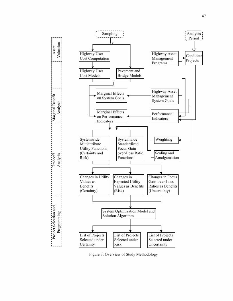
47
Figure 3: Overview of Study Methodology
System Optimization Model and Solution Algorithm
Systemwide Standardized Focus Gain-over-Loss Ratio Functions
Systemwide Mutiattribute Utility Functions (Certainty and Risk)
Highway User Cost Models
Pavement and Bridge Models
Marginal Effects on System Goals
Marginal Effects on Performance Indicators
Highway User Cost Computation
Scaling and Amalgamation
Weighting
Changes in Utility Values as Benefits (Certainty)
Changes in Expected Utility Values as Benefits (Risk)
Changes in Focus Gain-over-Loss Ratios as Benefits (Uncertainty)
List of Projects Selected under Certainty
List of Projects Selected under Risk
List of Projects Selected under Uncertainty
Candidate Projects
Performance Indicators
Highway Asset Management Programs
Highway Asset Management System Goals
Sampling Analysis Period
Proj
ect S
elec
tion
and
Prog
ram
min
g Tr
adeo
ff
Ana
lysi
s M
argi
nal B
enef
it A
naly
sis
A
sset
V
alua
tion

48
3.2 Study Design
The present study is designed in such a manner as to simplify and elucidate the entire
analytical approach. A brief discussion of each stage of the analytical framework follows in the
subsequent sections.
3.3 Highway Asset Management System Goals and Objectives
In the present study, both agency and highway user goals are considered. On the basis of the
literature survey and meetings with officials responsible for statewide highway planning,
programming, budgeting, and engineering in Indiana, the following goals were classified for the
highway asset management system: system preservation, agency cost, user cost, mobility, safety, and
the environment. The objectives and measurement units for individual system goals were established
and are listed in Table 4.
Table 4: Highway Asset Management System Goals and Objectives
Asset Management System Goal
Asset Management System Objective Measurement Unit
System Preservation
Extension of asset service life Preservation of asset condition
Number of years Life-cycle annual average condition rating
Agency Cost Decrease of agency cost Life-cycle equivalent uniform annual agency cost in service life
User Cost Reduction in VOC Life-cycle equivalent uniform annual VOC per VMT
Mobility Reduction in travel time Life-cycle annual average vehicle-hours per VMT
Safety Reduction in collision rate Life-cycle annual average no. of collision per million VMT
Environment Reduction in air pollution rate Life-cycle annual average emission quantities per VMT

49
3.4 Project Types under Highway Asset Management Programs
The primary state highway asset management programs in Indiana include the preservation of
physical facilities and system expansion. However, there are four different program codes that exist
within INDOT, which are the Long Range Plan Code, the Budgetary Code, the Program Management
Groups (PMG) Code, and the Engineering Code. The asset management system to be developed in the
present study will ultimately be utilized to serve the need of highway programming so the PMG Code
was adopted here. Efforts were made in the present study to unify the four coding systems so that
there is flexibility in the use of the research products, as shown in Appendix A1. Project types under
individual PMG programs (“programs” hereafter) are listed in Table 5, and project definitions are
provided in Appendix A2.
Table 5: Project Types under Various Highway Asset Management Programs
General Category Program Category Project Type
Bridge Preservation Rehabilitation Replacement Bridge
Preservation Historic Bridges Preservation
Non-Interstate Resurfacing Rehabilitation/ reconstruction/replacement Pavement
Preservation Interstate
Resurfacing Rehabilitation/ reconstruction/replacement
Intersection Improvements Intersection improvements Railroad Crossing Improvements Railroad crossing projects
Safety Improvements
Guardrail improvements Sight distance improvements Lighting improvements Traffic signs Pavement markings
Safety Improvements
Traffic Signals Traffic signals
Enhancements Bicycles/ pedestrians Other transportation enhancements
Roadside Improvements Roadside
Improvements
Landscaping/ wildflower program Environmental mitigation/ improvement Erosion/ landslide control Access control

50
Table 5: Project Types under Various Highway Asset Management Programs (Continued)
General Category Program Category Project Type
New Weigh Station/Rest Area New weigh station New rest area
Weigh Station/ Rest Area Modernization
Weigh station modernization Rest area modernization
Roadside Improvements (Continued)
Small Structures/ Drainages Small structure replacement Drainage problem correction
New/ Major Construction Expansion
New road construction Added travel lanes New interchange construction Interchange modifications
Department of Natural Resources Facilities
Park roads Park bridges Cooperative access projects
Forest Land Highways Forest land highways Other State Facilities
Other State Institution Facilities Institution roads Institution bridges Other projects
Intelligent Transportation Systems (ITS)
ITS Installations
ITS traveler information systems ITS management systems ITS monitoring systems ITS operations and maintenance
Command and Control Category
Congestion mitigation and air quality (Pre-committed) bonding projects Bridge “watch list” Shelf projects Suspended projects Other command guidance projects
Local Bridge Inspections Local bridge inspections Local Public Agency Program State administered Federal aid projects
Maintenance Routine maintenance Periodic maintenance
Multimodal
Inter-modal management projects Inter-modal connectors Airport facilities Passenger rail Railroad corridor preservation Railroad right-of-way preservation Railroad track preservation Transit facilities
Noise Abatement Noise abatement projects Relinquishments Transfer of route from state to local level Studies Feasibility/corridor studies
Miscellaneous
Utilities Utility relocation

51
3.5 Highway Asset Valuation
3.5.1 Introduction
The state-maintained physical highway assets identified for fulfilling GASB34 asset value
reporting requirements include roads, bridges, weigh stations, rest areas, railroad crossings, and
highway drainage systems. The procedure for assessing physical highway assets is well defined and
most state transportation agencies have addressed this issue well. However, little attention has been
given to the computation of network-level asset usage cost. The present study, therefore, focuses on
filling the gap of computing the network-level highway user cost. This information will assist in
evaluating the impacts of highway investment decisions on various highway system usage goals.
3.5.2 Network-Level Highway User Cost Computation and Models
3.5.2.1 Network-Level Highway User Cost Computation
The computation of network-level user cost components in the present study followed a
procedure similar to that used in the MicroBENCOST software for estimating user cost, with the
exception that the present study was geared towards an entire highway network. Highway user cost
components classified include vehicle operation, travel time, vehicle collisions, and vehicle air
pollution, and the quantities of different user cost components are associated with the use of the
Indiana state highways. Network parameters included the amount of travel, traffic volume, speed, road
condition, and geometric characteristics including grade and curvature, and the data used were for the
period 1990-2000. The vehicle and highway classes used for the computation are listed in Tables 6
and 7, respectively.

52
Table 6: Vehicle Classes for Highway User Cost Computation
Vehicle Class Description Axle Configuration
1 2 3 4 5 6 7 8 9
10 11 12 13
Unclassified vehicle types Passenger Cars Two-axle, 4-tire single units Buses Two-axle, 6-tire single units Three-axle single units Four or more axle single units Four or less axle single trailers Five-axle single trailers Six or more axle single trailers Five or less axle multiple trailers Six-axle multiple trailers Seven or more axle multiple trailers
1 steering, 1 single 1 steering, 1 single 1 steering, 1 single 1 steering, 1 single 1 steering, 1 single 1 steering, 1 tandem 1 steering, 1 tridem 1 steering, 2 or 3 single 1 steering, 2 tandem 1 steering, 1 tandem, 1 tridem 1 steering, 3 or 4 single 1 steering, 3 single, 1 tandem 1 steering, 2 single, 2 tandem
Table 7: Highway Classes for Highway User Cost Computation
Highway Class Description 1 2 3 4 5 6 7 8 9
10
Rural interstate Rural principal arterial Rural minor arterial Rural major collector Rural minor collector Urban interstate Urban freeway and expressway Urban principal arterial Urban minor arterial Urban collector
Vehicle operating cost is the mileage-dependent cost of using vehicles, including the
expenses for fuel, tires, engine oil, maintenance, and vehicle depreciation, which are attributable to
highway mileage traveled. Travel time is measured in terms of vehicle-hours. Delays are considered
additional travel time and may be due to congestion and incidents, as well as delays at intersections,
railroad crossings, and at workzones. Delay is defined as when the level of travel speed falls under
normal traffic conditions because of capacity, geometric, or operational constraints. A county-by-
county congestion analysis was performed for the State of Indiana to identify congestion from 1995 to
2015 [Whitford and Opsuth, 1996]. The respective benchmark volume-to-capacity ratios used were

53
0.9 for urban interstates, 0.8 for urban freeways, arterials and collectors, and 0.7 for rural highway
classes. Intersection delay was calculated separately for intersections with stop signs and signalized
intersections. Delay at railroad crossings was quantified based on the number of railroad crossings, the
number of affected vehicles at each railroad crossing, and the duration of stop time per vehicle at each
railroad crossing. Incident delay was estimated in accordance with the FHWA’s Traffic Control
Systems Handbook, which recommended eight incidents per million VMT when blocking one or more
travel lanes [FHWA, 1985]. Details of Indiana workzone characteristics, such as the number of
workzones, the length and duration, and the spatial distribution over the highway network were
obtained from INDOT construction records, and this information was then processed along with the
typical number of vehicles affected and the average travel speed to obtain the total workzone delay.
Vehicle collision statistics were extracted from the annual highway safety facts reported in three
categories of decreasing severity: fatalities, injury, or property damage by the National Highway
Traffic Safety Administration (NHTSA). The major pollutants emitted by vehicles are carbon dioxide
(CO2), non-methane hydrocarbons (NMHC), carbon monoxide (CO), nitrogen oxides (NOX), total
suspended particles (TSP) and sulfur dioxide (SO2), and emission rates for these pollutants and their
respective costs were quantified on the basis of the FHWA’s Costs of Air Pollution Abatement Study
[FHWA, 1992]. The computation of individual highway user cost components was carried out based
on Equations (1)-(8).
∑= ⎥
⎥⎥
⎦
⎤
⎢⎢⎢
⎣
⎡
⎟⎟⎟
⎠
⎞
⎜⎜⎜
⎝
⎛∑=
=13
1i
10
1j)
ijSpeedijVMT
(TimeTravel
∑= ⎥
⎥
⎦
⎤
⎢⎢
⎣
⎡
⎟⎟
⎠
⎞
⎜⎜
⎝
⎛∑=
∑=
⎟⎠⎞⎜
⎝⎛ ⋅=
13
1i
10
1j
L
1l jlDelayAveragejlNonsintersectiDelay
(1)
(2)
(3)
∑=
∑= ⎥
⎥⎦
⎤
⎢⎢⎣
⎡⋅⎟
⎟⎠
⎞⎜⎜⎝
⎛∑=
=13
1i
10
1j ijVMT5
1k ijkUVOCVOC

54
where
VOC = Annual vehicle operating cost, in dollars/year
Travel Time = Annual total travel time, in hours/year
Delayintersections = Annual vehicle delay at intersections and interchanges, in hours/year
Delayrailroad crossings= Annual vehicle delay at railroad crossings, in hours/year
Delayincidents = Annual vehicle delay due to incidents, in hours/year
Delayworkzones = Annual vehicle delay at work zones, in hours/year
Vehicle Collisions = Annual number of vehicle collisions, in no. of collisions/year
Air Pollution = Annual air pollution quantities, tons/year
VMTij = Annual vehicle miles of travel for vehicle class i on highway class j
∑= ⎥
⎥⎦
⎤
⎢⎢⎣
⎡⎟⎟⎠
⎞⎜⎜⎝
⎛∑=
⋅=13
1i
M
1m mTSDmKcrossingsrailroadDelay
∑=
∑= ⎥
⎥
⎦
⎤
⎢⎢
⎣
⎡
⎟⎟
⎠
⎞
⎜⎜
⎝
⎛⋅⋅=
13
1i
10
1j 1,000,000ijVMT
ijRateIncidentijDelayIncidentIncidentsDelay
∑= ⎥
⎥
⎦
⎤
⎢⎢
⎣
⎡
⎟⎟⎟
⎠
⎞
⎜⎜⎜
⎝
⎛∑=
⎟⎟
⎠
⎞
⎜⎜
⎝
⎛⋅⎟
⎟
⎠
⎞
⎜⎜
⎝
⎛∑=
=10
1j
10
1i 1,000,000ijVMT3
1p jpRateCollisionCollisionsVehicle
∑=
∑= ⎥
⎥
⎦
⎤
⎢⎢
⎣
⎡⋅⎟
⎟
⎠
⎞
⎜⎜
⎝
⎛∑=
=13
1i
10
1j ijVMT6
1q iqRateEmissionPollutionAir
∑=
∑= ⎥
⎥⎥
⎦
⎤
⎢⎢⎢
⎣
⎡
⎟⎟⎟
⎠
⎞
⎜⎜⎜
⎝
⎛−⋅⋅⋅=
13
1i
N
1n in(2)Speed1
in(1)Speed1
nLengthWZnDurationWZinVehiclesAffectedZonesWorkDelay
(4)
(5)
(6)
(7)
(8)

55
UVOCijk = Unit vehicle operating cost of VOC component k for vehicle class i on
highway class j, in $/VMT
Speedij = Annual average travel speed for vehicle class i on highway class j
Njl = Number of intersections of type l on highway class j
Average Delayjl = Average delay at intersection of type l on highway class j, in hours/vehicle
Km = Number of trains passing railroad crossing m per year
TSDm = Total stopped delay time per train at railroad crossing m, in hours/train
Incident Delayij = Delay time per incident by vehicle class i on highway class j, in
hours/vehicle
Incident Rateij = Number of incidents per million VMT by vehicle class i on highway class j
Affected Vehiclesin= Number of affected vehicles of vehicle class i at workzone n
WZ Durationn = Duration of work zone n, in days/year
WZ Lengthn = Length of work zone n, in miles
Speedin(1) = Speed of vehicle class i approaching work zone n, in mph
Speedin(2) = Speed of vehicle class i in work zone n, in mph
Collision Ratejp= Number of vehicle collisions of type p per million VMT on highway class j,
in no. of collisions/MVMT
Emission Rateiq = Quantities of pollutant type q emitted by vehicle class i, in tons/VMT
i = Vehicle class 1 to 13
j = Highway class 1 to 10
k = VOC component 1 to 5 for fuel consumption, oil consumption, tire wear,
vehicle depreciation, and maintenance and repair

56
l = Intersection type 1 to L
m = Railroad crossing 1 to M
n = Workzone 1 to N
p = Collision type 1 to 3 for fatality, injury, and property damage
q = Pollutant type 1 to 6 for CO2, NMHC, CO, NOX, TSP, and SO2.
The unit costs of fuel, oil, tire wear, vehicle depreciation, and maintenance and repair were
adjusted to reflect the effects of grade, curvature, speed change, and road condition. In order to obtain
dollar value of the annual network-level highway user cost, the annual travel time, vehicle collision,
and air pollution quantities were first converted into dollar amounts according to the respective unit
costs and then added to the annual vehicle operating cost to arrive at the annual total user cost. The
unit costs used for the conversion process were updated in each year based on the Consumer Price
Index (CPI) for passenger cars and the Producer Price Index (PPI) for trucks accordingly. Details of
these computations are discussed in Chapter 4.
3.5.2.2 Network-Level Highway User Cost Models
Network-level highway user cost models were calibrated separately for vehicle operating
cost, travel time, vehicle collisions, and air pollution. In order to facilitate model calibration, the
individual highway user cost components were first normalized by dividing the estimated annual
quantities with the annual amount of travel. In the normalization process, three factors were
considered: land use (rural and urban), route type (interstate and non-interstate), and vehicle class (car,
single unit truck, and multiple unit truck). For each of the four highway user cost components, a large
number of possible combinations among the three factors exist, which would make the entire
modeling process quite lengthy. It was necessary to determine whether some aggregation to the

57
normalized user cost values could be made. As such, an Analysis of Variance (ANOVA) was carried
out as a preliminary step. The three-factor factorial model used was of the following form:
Yijkm= µ+ Li+ HCj+ L.HCij+ VCk+ (L.VC)ik+ (HC.VC)jk+ (L.HC.VC)ijk+ em(ijk)
where
Yijkm = User cost component associated with land use i and route type j for vehicle class
k in year m
µ = Average value of user cost component
Li = Land use, i = 1, 2 for rural/urban
HCj = Highway class, j = 1, 2 for interstate/non-interstate
VCk = Vehicle class, k = 1, 2, 3 for car/ single unit/multiple unit truck
em(ijk) = Error terms within each of the 12 treatments.
Statistical models for the normalized vehicle operating cost, travel time, vehicle collision rate,
and air pollution rate were then carried out as a function of network condition, travel speed, and other
factors, with levels of aggregation in terms of land use, route type, and vehicle class based on the
results of the ANOVA analysis. Results are presented in Chapter 4.
(9)

58
3.6 Modeling of Physical Highway Asset Performance
Pavements and bridges dominate the construction activities of a highway transportation
agency, and as shown in Table 8, approximately ninety percent of the total construction budget in
Indiana involves pavements and bridges. Consequently, modeling the performance of physical
highway assets in the present study focused on pavements and bridges.
Table 8: Share of Expenditure on Pavements and Bridges in Annual Construction Budget in Indiana (in millions, current dollars)
Bridge and Pavement Budget Fiscal Year Bridge
Preservation Pavement
PreservationNew
Construction Subtotal Total
Budget % Total
1996 1997 1998 1999 2000 2001
68.9 68.6 79.9 73.3 62.9 99.3
238 239 278 227 365 242
161 163 190 257 166 389
468 471 548 557 594 730
516 523 654 652 717 849
91% 90% 84% 85% 83% 86%
Source: INDOT Annual Reports.
3.6.1 Pavement Performance Modeling
The pavement performance analysis focused on two aspects, the effects of traffic loading on
rehabilitation and routine maintenance expenditure and relationship between routine maintenance and
the rehabilitation interval. The effect of traffic loading on pavement rehabilitation and routine
maintenance expenditure was quantified using data collected on state highways in Indiana from a
recent study [Li and Sinha, 2000], which established the load and non-load shares of the rehabilitation
and routine maintenance expenditure. The findings from that study were adopted for the current
research. The relationship between rehabilitation interval and annual maintenance, traffic loading, and
weather condition was also determined in another recent study in Indiana [Labi and Sinha, 2001] and
these findings were utilized for the tradeoff analysis in the present study.
59
3.6.2 Bridge Performance Modeling
Bridge performance modeling in the current study focused on two aspects, the impacts of
work activities on bridge deck, superstructure, substructure, and wearing surface condition, and the
bridge life-cycle agency and user cost. For the bridge condition models, the relationship of changes in
the bridge wearing surface and the deck, superstructure, and substructure condition as a function of a
work activity, which were represented by a certain level of expenditure, bridge age, and traffic
condition at the time of implementing the work action, was established. The cost models sought to
express changes in the bridge life-cycle user cost as a function of variables that included expenditure
of a work activity, bridge physical condition, age, traffic condition, and load inventory rating. As
different types of bridges generally follow different performance trends and have different service
lives, model development was conducted separately by bridge type.
3.7 Marginal Benefit Analysis
3.7.1 Marginal Benefit of System Preservation
For physical highway assets, the direct benefit of system preservation was an extension in
asset service lives. For instance, tradeoff relationships were found to exist between pavement
rehabilitation intervals and the annual maintenance expenditure, traffic loading, and weather severity.
Assuming the traffic loading and weather condition remain constant, an increase in maintenance
expenditure would result in an extension in the rehabilitation interval. Marginal effects could be
determined based on the calibrated pavement performance models. Similarly, in the course of bridge
performance modeling, relationships between changes in the bridge wearing surface, deck,
superstructure, and substructure structural conditions and the work activities applied to highway
bridges were also established. Thus, the marginal effects of various work activities to changes in
bridge condition could be quantified.

60
3.7.2 Marginal Benefit of Agency Cost
A reduction in life-cycle cost for highway pavements and bridges is a direct result of
extending the asset service lives. Because, in the long run, less frequent rehabilitation or
reconstruction is needed.
3.7.3 Marginal Benefit of Vehicle Operating Cost, Travel Time, Vehicle Collision Rate and Air Emission Rate
In the present study, network-level user cost models were calibrated to relate vehicle
operating cost, travel time, vehicle collision rate, and air pollution rate per vehicle mile of travel,
respectively, as a function of average traveling speed, road condition, and other factors. The calibrated
coefficients were then used to establish the marginal effects of change in vehicle speed and other
factors to individual user cost components.
3.8 Tradeoff Analysis
3.8.1 Tradeoff Decision-Making under Certainty
The tradeoff analysis encompasses a number of programs focusing on physical highway
assets and asset usage, and it can be conducted for candidate projects under a specific program or
across different programs in order to achieve various asset management system goals. As non-
commensurable goals are involved, multiattribute utility functions were developed. In addition,
projects under different programs are normally implemented for different types of assets or to serve
different needs of the system operation. Systemwide multiattribute utility functions were developed
separately for individual programs. The calibrated utility functions could then be used to scale benefits
associated with a specific project in achieving various asset management system goals into a
dimensionless value. Tradeoffs between different types of projects could thus be made on the basis of

61
these dimensionless values. The following items were used sequentially to establish systemwide
multiattribute utility functions for individual programs:
- Relative weights of highway asset management system goals
- Performance indicators for various programs under each system goal
- Weights of performance indicators for individual programs under each goal
- Single attribute utility functions associated with individual performance indicators
- Multiattribute utility functions for individual programs under each goal
- Systemwide multiattribute utility functions for each program.
In order to accomplish the weighing and scaling steps, a series of questionnaire surveys were
organized. As a highway asset management system considers the perspectives of not only the agency
but also of the highway user, questionnaire surveys about the relative weights of system goals and
performance indicators, as well as the utility functions for individual performance indicators, were
conducted with both groups. Furthermore, to make the calibrated utility functions both theoretically
sound and robust, two different approaches were adopted in the course of developing the utility
functions. Details of these surveys are presented in Chapter 7.
3.8.1.1 Performance Indicators for Highway Asset Management Programs
Having established the goals and programs of a highway asset management system, a set of
performance indicators for various highway asset management programs was established in
consultation with the INDOT officials, as shown in Table 9.

62
Table 9: Performance Indicators for Various Highway Asset Management Programs
Asset Management System Goal Program Category Preservation Agency Cost User Cost Mobility Safety Environment
Bridge Preservation
Struct condition Surf condition Remain life
Construction RehabilitationMaintenance
Detour condition Speed
Speed Detour length
Load inventory Deck width Vert clearance (over/under) Hor clearance
Speed
Historical Bridges
Struct condition Surf condition Remain life Bridge age Bridge length
Construction RehabilitationMaintenance
Detour condition Speed
Speed Detour length
Load Inventory Deck width Vert clearance (over/under) Hor clearance
Speed
Non-Interstate Pavements Condition
Construction RehabilitationMaintenance
Condition Speed Speed
Speed Skid resistance Lane width Shoulder width
Speed
Interstate Pavements Condition
Construction RehabilitationMaintenance
Condition Speed Speed
Speed Skid resistance Lane width Shoulder width
Speed
Intersection Improvements Condition
Construction RehabilitationMaintenance
- Intersect delay Collision rate -
Railroad Crossing Improvements
Condition Remain life
Construction RehabilitationMaintenance
- - RR adequacy Collision rate -
Safety Remain life Construction Maintenance - - Sight distance
Luminance -
Traffic Signals Remain life Construction Maintenance - Intersect
delay Speed Collision rate -
Enhancements - - - - Collision rate - Roadside Improvements - Construction
Maintenance Speed Speed Speed Speed
Weigh Station/Rest Area Remain life Construction
Maintenance - - Collision rate -
Small Structures/ Drainages
Remain life Construction Maintenance - - - -
Roads: Condition Remain life
Construction Condition Speed Speed
Speed Skid resistance Lane width Shoulder width
Speed
Expansion Bridges: Struct condition Surf condition Remain life
Construction
Detour condition Speed
Speed Detour length
Load inventory Deck width Vert clearance (over/under) Hor clearance
Speed

63
Table 9: Performance Indicators for Various Highway Asset Management Programs (Continued)
Asset Management System Goal Program Category Preservation Agency Cost User Cost Mobility Safety Environment
Roads: Condition Remain life
Construction RehabilitationMaintenance
Condition Speed Speed
Speed Skid resistance Lane width
Speed DNR Facilities/ Forest Land Highways/ Other State Institutions
Bridges: Struct condition Surf condition Remain life
Construction RehabilitationMaintenance
Detour condition Speed
Speed Detour length
Load inventory Deck width Vert clearance (over/under) Hor clearance
Speed
Bridge Inspection - - - - Collision rate -
ITS Projects Remain life Procurement Maintenance Speed Speed Collision rate Speed
CMAQ Projects - Construction
Maintenance Speed Speed Speed Speed
Maintenance Condition Remain life Maintenance Condition - Skid resistance -
Multi-modal Remain life Construction Maintenance Speed Speed Collision rate Speed
Note: Struct- Structure, Surf- Surface, Vert- Vertical, and Hor- Horizontal.
3.8.1.2 Relative Weights of System Goals and Multiple Performance Indicators under Each Goal
The Delphi technique [Dalkey and Helmer, 1963] was used to establish relative weights for
system goals and performance indicators. As mentioned earlier, two decision groups representing both
the agency and the user perspectives participated in the survey. The sequential steps for applying the
questionnaire to individual survey groups are listed below:
Step 1 concerned with applying survey questionnaire to the respondents. An example was
first provided to allow respondents to comprehend the survey approach.
Step 2 involved analysis of the completed questionnaire and preparation of a concise
summary of survey results.

64
Step 3 focused on presenting the survey summary to each respondent and solicited comments
expressing agreement, disagreement, and clarification of the results.
Step 4 dealt with the second survey, using the same questionnaire, and preparation of an
updated summary of survey results.
In the summary of survey results, the summary statistics, such as mean and standard
deviations associated with the relative weights assigned for system goals and performance indicators,
were listed. However, the average weights assigned might not be consistent with the consensus
weights because of the differences in the standard deviations among the weights. The raw data were
further processed to derive the consensus weights separately for the two groups using the AHP
technique [Saaty, 1977].
3.8.1.3 Single Attribute Utility Functions for Individual Performance Indicators
Similar to the procedure used for establishing relative weights for system goals and
performance indicators, questionnaire surveys were also used to develop single attribute utility
functions for individual performance indicators. In order to acquire input from both the agency and the
user perspectives and also maintain the robustness of the derived utility functions, two survey groups
and two approaches were utilized. The two groups classified were the agency and the user, with
representatives randomly selected. Two approaches were used for the preparation of two different
questionnaires as well, the direct questioning approach and the certainty equivalency approach
[Keeney and Raiffa, 1993]. The concepts of these approaches are illustrated as follows:
Approach 1: Direct Questioning Approach
- For attribute X, denote its best level as XH, and worst as XL; and assign U(XL)= 0, and
U(XH)= 1.

65
- Consider following situations
(i) Risky prospect of obtaining XL with probability p and XH with probability (1-p)
(ii) Prospect of obtaining X= 0.5.(XH-XL) for certain
The value of p is varied until the decision-maker is indifferent between two choices.
- Repeat the same process (twice) by changing X value to 0.25.(XH-XL), and 0.75.(XH-XL),
find corresponding p values, respectively. Graphic illustration of the procedure is below:
Figure 4: Illustration of Direct Questioning Approach for Establishing Utility Values
Approach 2: Certainty Equivalency Approach
- For attribute X, denote its best level as XH, and worst level as XL; and assign U(XL)= 0, and
U(XH)= 1.
- Step 1, consider following situations
p1 XH ∼ 1 X1= 0.5.(XH-XL) Given XH, XL, and X1, determine p1. 1-p1 XL (a) p2 XH ∼ 1 X2= 0.25.(XH-XL) Given XH, XL, and X2, determine p2. 1-p2 XL (b) p3 XH ∼ 1 X3= 0.75.(XH-XL) Given XH, XL, and X3, determine p3. 1-p3 XL (c)

66
(i) Risky prospect of obtaining XL with probability 0.5 and XH with probability 0.5
(ii) Prospect of obtaining X0.5 for which U(X0.5)= 0.5 for certain
The value of X0.5 is varied until decision-maker is indifferent between the two choices.
- Step 2, consider following situations
(i) Risky prospect of obtaining XH with probability 0.5 and X0.5 with probability 0.5
(ii) Prospect of obtaining X0.25 for which U(X0.25)= 0.25 for certain
The value of X0.25 is varied until decision-maker is indifferent between the two choices.
- Step 3, consider following situations
(i) Risky prospect of obtaining X0.5 with probability 0.5 and XL with probability 0.5
(ii) Prospect of obtaining X0.75 for which U(X0.75)= 0.75 for certain
The value of X0.75 is varied until decision-maker is indifferent between the two choices.
- Step 4, consistency check between the two situations
(i) Risky prospect of obtaining X0.25 and X0.75 both with probability 0.5
(ii) Prospect of obtaining X0.5 for which U(X0.5)= 0.5 for certain
The decision-maker should be indifferent with the two situations. Otherwise, Steps 1-3
need to be repeated. Graphic illustration of the procedure is below:

67
Figure 5: Illustration of Certainty Equivalency Approach for Establishing Utility Values
As two approaches were used by two decision groups to establish utility values, it was needed
to investigate whether the results between the decision groups and the approaches used were
statistically different. As such, an ANOVA analysis was carried out to determine the level of
aggregation for the raw data prior to calibrating the utility functions using OLS techniques. The two-
factor factorial ANOVA model adopted was of the following form:
Uijm= µU+ Gi+ Aj+ (G.A)ij+ em(ij)
where
Uijm = Utility value assigned by decision-maker m in group i using approach j
µU = Average utility value assigned by all decision-makers using all approaches
0.5 XH ∼ 1 X0.5 with U(X0.5)= 0.5 Given XH, XL, and p= 0.5, determine X0.5. 0.5 XL (a) 0.5 XH ∼ 1 X0.25 with U(X0.25)= 0.25 Given XH, X0.5, and p= 0.5, determine X0.25. 0.5 X0.5 (b) 0.5 X0.5 ∼ 1 X0.75 with U(X0.75)= 0.75 Given X0.5, XL, and p= 0.5, determine X0.75. 0.5 XL (c) 0.5 X0.25 ∼ 1 X0.5 with U(X0.5)= 0.5 Check 0.5*U(X0.25)+0.5*U(X0.75) with 0.5 . 0.5 X0.75 (d)
(10)
68
Gi = Decision group, i = 1, 2 for the agency and the highway user
Aj = Approach used, j = 1, 2 for direct weighting approach and the certainty equivalency
approach
em(ij) = Error terms within each of the 4 group and approach combinations.
3.8.1.4 Systemwide Multiattribute Utility Functions for Individual Programs
Systemwide multiattribute utility functions for individual programs were established by
synthesizing the single attribute utility functions in two steps. The first step was to obtain
multiattribute utility functions under each system goal from single utility functions, while the second
step synthesized the goal-specific multiattribute utility functions into a systemwide multiattribute
utility function for each program.
Prior to synthesizing the single attribute utility functions, the underlying assumptions were
verified, which included utility independence, additive independence, and preference independence if
more than two utility functions were to be combined. Utility independence inferred that each single
attribute utility function was not a function of the level of other attributes (i.e., performance
indicators). Under this assumption, the underlying multiattribute utility function might be of the
additive form, the multilinear form (a special case of multiplicative form), or the multiplicative form.
Additive independence applied if, and only if, all single attribute functions were directly additive.
Preference independence remained valid if the tradeoffs a decision-maker was willing to make among
any two attributes were not dependent on the levels of other attributes.

69
3.8.2 Incorporation of Risk and Uncertainty into Tradeoff Decision Process
The tradeoff decision process discussed earlier assumed that the expected level of each
performance indicator after project implementation would occur under certainty. However, this
assumption might not hold true because of the uncertain and dynamic nature of a highway network.
Risk and uncertainty associated with performance indicators were incorporated into the tradeoff
analysis to further strengthen the robustness of the decision-making process. As the performance
indicators relevant to geometric characteristics, such as lane width, and vertical and horizontal
clearance, were deterministic in nature, they were excluded for consideration in risk and uncertainty
analyses. Performance indicators involving risk and uncertainty in the tradeoff decision process are
listed in Table 10.
Table 10: Performance Indicators Involving Risk and Uncertainty in Tradeoff Decision Process
Asset Management System Goal Performance Indicator
System Preservation
Bridge structural condition Bridge wearing surface condition Pavement surface condition Remaining service life
Agency Cost Construction cost Rehabilitation cost Maintenance cost
User Cost Mobility Environment
Vehicle speed Detour condition Detour length Intersection delay time
Safety
Vehicle speed Bridge load inventory rating Skid resistance Collision rate

70
3.8.3 Tradeoff Decision-Making under Risk
For tradeoffs under risk, the multiattribute utility functions developed for tradeoffs under
certainty were valid for the conversion of project benefits into dimensionless units. However, in this
case, utility values corresponding to the levels of performance indicators after project implementation
were replaced by expected utility values to account for the range and distribution of possible outcomes
of underlying performance indicators. In order to establish the expected utility values, it was needed to
characterize the types of probability distributions and select and calibrate distribution parameters.
3.8.3.1 Categorization of Probability Distributions for Performance Indicators
This step involved identifying whether the possible outcomes of the performance indicators
were discrete or continuous. Because discrete values were used to measure the bridge deck,
superstructure, substructure, and wearing surface conditions, discrete probability distribution was
appropriate. On the other hand, since the remaining performance indicators in risk analysis were
measured by continuous values, continuous distributions were used.
3.8.3.2 Selection of Probability Distributions for Performance Indicators
After defining the basic properties of probability distributions for the relevant performance
indicators, the next step involved selecting appropriate distributions that best fit the possible outcomes
of the respective performance indicators. For discrete performance indicators such as bridge deck,
superstructure, substructure, and wearing surface condition, the respective possible outcomes as a
result of project implementation might range from a condition rating of 3 (worst) to 9 (best). It was
reasonable to assume that there was equal opportunity that the probability would occur at each
condition rating, and that this probability was not affected by any knowledge of the previous condition

71
rating. It was therefore needed to first determine the probabilities of occurrence of outcomes that fall
into condition rating 3 only; ratings 3 and 4; ratings 3, 4, and 5; and finally 3, 4, …, and 9,
respectively. Under these circumstances, the binomial distribution was considered to be appropriate.
The binomial distribution function with parameters n, p, and x is given by
( ) ( ) xnx p1pxnx,p,nb −−⋅⋅⎟
⎠⎞
⎜⎝⎛=
with mean and variance: µ= np, and σ2= np(1-p)
where
n = Number of possible outcomes
p = Probability of occurrence of an outcome
x = Number of occurrences over all possible outcomes (i.e., exactly x possible outcomes
occurred over n Bernoulli trials).
In practice, Poisson distribution is used as an approximation to the binomial distribution when
the parameter n is relatively large (n ≥ 30). As bridge deck, superstructure, substructure, and wearing
surface conditions range from 3 to 9, it is therefore needed to subdivide the six condition intervals into
more subintervals to apply Poisson approximation. The justification for Poisson approximation is as
follows. For bridge deck, superstructure, substructure, and wearing surface condition with conditions
from 3 to 9, it can be imagined that the range of extreme conditions between 3 and 9 is further divided
into n subintervals of equal length, i.e., the length of interval between any two consecutive condition
levels is further divided into n/6 subintervals of equal length. If the subintervals are sufficiently short,
it can be assumed that, in each subinterval, there is either 0 or 1 occurrence with the probability of
occurrence p. This means that the sequence of subintervals can be thought of as a sequence of
Bernoulli trials, with a success corresponding to an occurrence in the subinterval. Suppose that the
(11)

72
average rate of occurrences in a condition interval between 3 and 9 is λ, the probability of occurrence
in each subinterval thus becomes p = λ/n. This yields the following:
( ) ( ) λ−≈⎟⎠⎞
⎜⎝⎛ λ
−=−⋅⋅⎟⎠⎞
⎜⎝⎛=== e
n1p1p0
n0,p,nb)0X(Pn
n0
In general, Poisson approximation of the binomial distribution is obtained as follows:
( ) ( ) npx
λx
ex!
npex!λxp,n,bx)P(X −− =≈==
In addition to creating subintervals between two consecutive condition ratings, it is also
needed to consider the existing condition rating at the time of project implementation so that the total
number of subintervals can be established. The underlying assumption is that the distribution of
condition ratings after project implementation will spread from the existing level upward to the best
condition rating of 9, as illustrated in Figure 6. In the present study, each two-consecutive condition
rating levels is equally divided into 10 subintervals. This brings about a total number of subintervals
of 60, 50, 40, 30, 20, 10, 0 corresponding to an existing condition rating of 3, 4, 5, 6, 7, 8, and 9,
respectively.
(12)
(13)
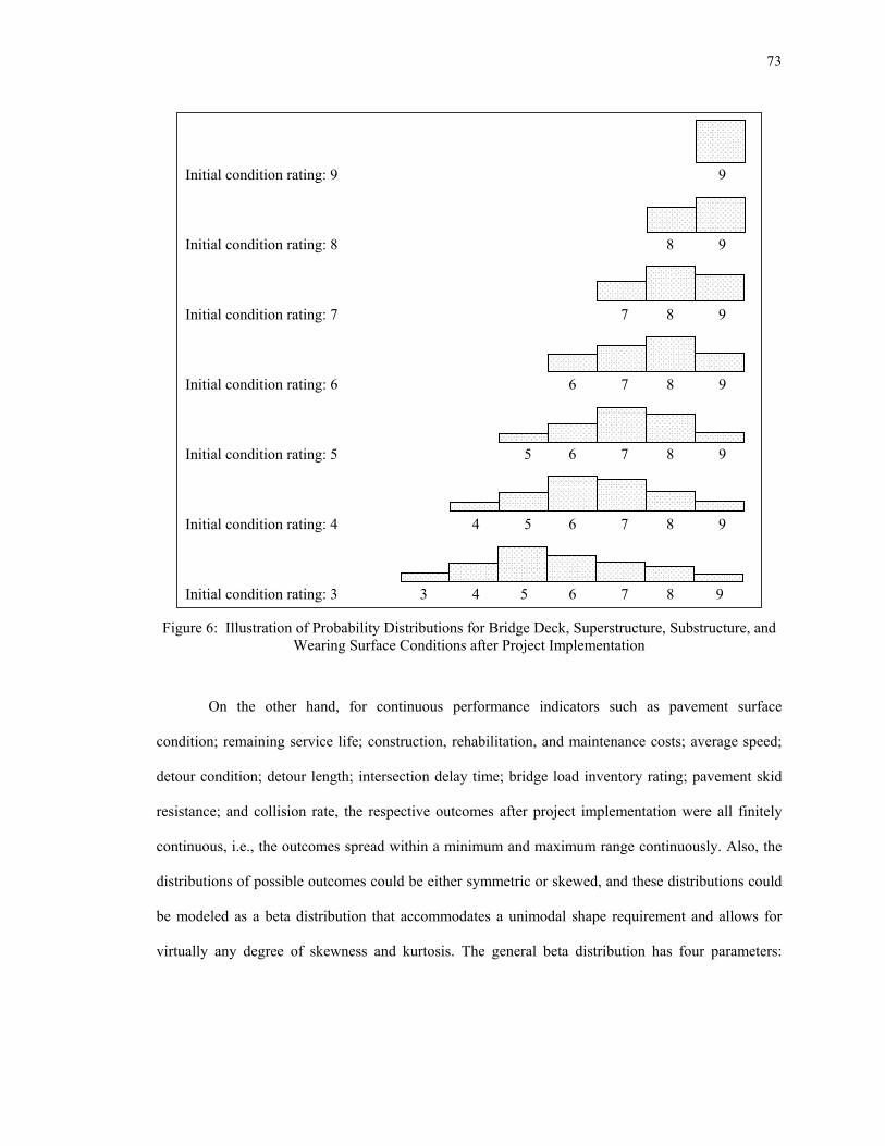
73
Figure 6: Illustration of Probability Distributions for Bridge Deck, Superstructure, Substructure, and Wearing Surface Conditions after Project Implementation
On the other hand, for continuous performance indicators such as pavement surface
condition; remaining service life; construction, rehabilitation, and maintenance costs; average speed;
detour condition; detour length; intersection delay time; bridge load inventory rating; pavement skid
resistance; and collision rate, the respective outcomes after project implementation were all finitely
continuous, i.e., the outcomes spread within a minimum and maximum range continuously. Also, the
distributions of possible outcomes could be either symmetric or skewed, and these distributions could
be modeled as a beta distribution that accommodates a unimodal shape requirement and allows for
virtually any degree of skewness and kurtosis. The general beta distribution has four parameters:
Initial condition rating: 9 9 Initial condition rating: 8 8 9 Initial condition rating: 7 7 8 9 Initial condition rating: 6 6 7 8 9
Initial condition rating: 5 5 6 7 8 9
Initial condition rating: 4 4 5 6 7 8 9
Initial condition rating: 3 3 4 5 6 7 8 9

74
lower range (L), upper range (H), and two shape parameters referred to as α and β. The beta density
function is given by
( ) ( ) ( ) ( )( ) ( ) ( )
( )HxL1βαLHβΓαΓ
1βxH1αLxβαΓHL,β,α,xf ≤≤−+−⋅⋅
−−⋅−−⋅+=
where the Γ -function factors serve to normalize the distribution so that the area under the
density function from L to H is exactly 1. The mean and variance for the beta distribution are given by
the following: β+α
α=µ and
( ) ( ).
122
+β+αβ+α
αβ=σ
It is seen that the mean of the distribution is a weighted average of L and H such that when
0<α<β the mean is closer to L and the distribution is skewed to the right; whereas for α>β>0 the mean
is closer to H and the distribution is skewed to the left. When α = β the distribution is symmetric. Also
note that for a given α/β ratio, the mean is constant and the variance varies inversely with the absolute
magnitude of α+β. Thus, by increasing α and β by proportionate amounts, the variance may be
decreased while holding the mean constant; and conversely, by decreasing α and β by proportionate
amounts, the variance may be increased while leaving the mean unchanged. In practice, the skewness
and variance (kurtosis) can be categorized as high, medium, or low based on the magnitude of α and
β. Table 11 presents the resulting combinations of skewness and variance (kurtosis) for beta
distributions that best approximate the risk situation of possible outcomes of the continuous
performance indicators.
(14)

75
Table 11: Approximate Values of Shape Parameters for Beta Distributions under Different Skewness and Variance Combinations
Combination Type Skewness Variance (Kurtosis) α β 1 2 3 4 5 6 7 8 9
Skewed to the left Symmetric Skewed to the right Skewed to the left Symmetric Skewed to the right Skewed to the left Symmetric Skewed to the right
High High High Medium Medium Medium Low Low Low
1.50 1.35 0.50 3.00 2.75 1.00 4.50 4.00 1.50
0.50 1.35 1.50 1.00 2.75 3.00 1.50 4.00 4.50
3.8.3.3 Expected Utility for Performance Indicators Involving Risk in Tradeoff Decision Process
In the tradeoff decision process involving risk situations, the binomial distribution and beta
distribution were selected for discrete and continuous performance indicators, respectively, to model
the possible outcomes after project implementation. The expected utility values corresponding to the
possible outcomes of respective performance indicators were computed separately.
For discrete performance indicators, the initial condition rating was a key factor that needed
to be explicitly considered. As stated in the previous section, Poisson approximation was applied for
the binomial distribution where the number of subintervals (Nk) corresponding to initial condition
ratings of 3, 4, 5, 6, 7, and 8 were 60, 50, 40, 30, 20, and 10, respectively. The expected utility values
for the possible outcomes of individual performance indicators were calculated as below:
( )[ ] ( )[ ] ( ) ( )∑∑=
−
= ⎪⎭
⎪⎬⎫
⎪⎩
⎪⎨⎧
⎥⎥⎦
⎤
⎢⎢⎣
⎡⋅==⋅=
kk
k N
0x
pNx
kN
0xe
x!pN
xuxXPu(x)XuE
For continuous performance indicators, it was difficult to assign a single, fixed lower and
upper range for the possible outcomes of individual performance indicators after project
implementation. This was because the possible range deviated significantly under different
(15)
76
circumstances. For each performance indicator, the beta distribution parameters were first calibrated
for a fixed lower and higher range. Truncated beta distributions that allowed varying the minimum
and maximum ranges (denoted by “min” and “max”) of possible outcomes of an underlying
performance indicator were then used to establish the expected utility values. The formula used was as
follows:
( )[ ] ( ) ( )
( ) ( )[ ]( )
( ) ( )( ) ( ) ( )
( ) ( )
( )( ) ( ) ( )
( ) ( )∫
∫
∫∫
∫
−−−+
−−−+
−⋅−⋅−⋅⋅
+⎪⎭
⎪⎬⎫
⎪⎩
⎪⎨⎧
⎥⎦
⎤⎢⎣
⎡−⋅−⋅
−⋅⋅+
⋅
=
⋅=
<<⋅=
max
min
1β1α1βα
max
min
1β1α1βα
max
min
max
min
max
min
dxxHLxLHβΓαΓ
βαΓ
dxxHLxLHβΓαΓ
βαΓxu
dxHL,|xβ, α,Beta
dxHL,|xβ, α,Betaxu
dxmaxxmin|xfxuXuE
3.8.4 Tradeoff Decision-Making Involving Uncertainty
3.8.4.1 Introduction
Common to the concept of expected utility is that it employs a weighted average to arrive at
an evaluation of outcomes. The underlying assumption made is that the probability or utility
associated with a particular outcome is independent of the degree of uncertainty associated with that
outcome. However, for a situation where the probability attached to the implementation of a project
depends both on the outcome and measure of uncertainty, the need for an alternative approach
becomes apparent. In the present study, Shackle’s model, which constituted one of the most original
approaches to decision-making under uncertainty, was adopted [Shackle, 1949].
(16)

77
3.8.4.2 Shackle’s Model
Shackle’s model is different from the expected utility approach which uses weighted averages
of outcomes and their probabilities, and it is based on three main elements. The first is the replacement
of probability as a measure of uncertainty by degree of surprise. The second is the priority index as a
mechanism to evaluate different outcomes and the corresponding degrees of surprise. The third is the
standardized focus gain-over-loss ratio as the basis of comparing different projects. The main steps for
applying Shackle’s model are discussed below.
1) Degree of Surprise Function
Degree of surprise indicates the decision-maker’s degree of uncertainty as to the hypothetical
outcomes resulting from project implementation with gains (positive returns) and losses (negative
returns) from the expectation. Suppose that there are a range of outcomes xi from an action (i = 1, 2,
..., n), and assign a value as the degree of surprise y, which reflects the decision-maker’s degree of
belief for a given outcome, ranging from 0 (no surprise) to 10 (extremely surprised), the degree of
surprise function y = y(x) can be as shown in Figure 7.
Figure 7: Diagram of Degree of Surprise Function

78
2) Priority Function and Focus Values
Priority function indicates the weighting index φ (0 for lowest priority and 10 for highest
priority) that the decision-maker assigns to any given outcome/degree of surprise pair (x, y). The
priority function denoted by φ = φ(x, y) possesses properties of 0y
0;x
⟨∂∂
⟩∂∂ φφ (namely, higher
priorities will be given as gaining of outcomes from expectation increases, or as degree of surprise
decreases). There also exists an indifference curve φ[x, y(x)] that traces out different combinations of
outcome/degree of surprise pair (x, y) where weight φ is kept constant. It is obvious that the priority
function is defined by points at which the degree of surprise function y = y(x) intersects the priority
indifference curves φ[x, y(x)] ≡ 0, 1, 2,…, 10. The priority indifference curves and priority function
can then be illustrated as in Figure 8.
Figure 8: Diagram of Priority Function
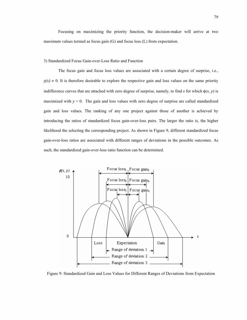
79
Focusing on maximizing the priority function, the decision-maker will arrive at two
maximum values termed as focus gain (G) and focus loss (L) from expectation.
3) Standardized Focus Gain-over-Loss Ratio and Function
The focus gain and focus loss values are associated with a certain degree of surprise, i.e.,
y(x) ≠ 0. It is therefore desirable to explore the respective gain and loss values on the same priority
indifference curves that are attached with zero degree of surprise, namely, to find x for which φ(x, y) is
maximized with y = 0. The gain and loss values with zero degree of surprise are called standardized
gain and loss values. The ranking of any one project against those of another is achieved by
introducing the ratios of standardized focus gain-over-loss pairs. The larger the ratio is, the higher
likelihood the selecting the corresponding project. As shown in Figure 9, different standardized focus
gain-over-loss ratios are associated with different ranges of deviations in the possible outcomes. As
such, the standardized gain-over-loss ratio function can be determined.
Figure 9: Standardized Gain and Loss Values for Different Ranges of Deviations from Expectation

80
3.9 Project Selection and Programming
As tradeoff analysis between candidate projects was carried out under certainty, risk, and
uncertainty, project selection and programming were separately conducted for the three cases. More
specifically, project selection was made on the basis of systemwide benefits resulting from project
implementation in terms of changes in utility values, expected utility values, and standardized focus-
gain-over-loss ratios, respectively. Systemwide programming involved selecting a subset from all
candidate projects in an optimal manner under budget constraints for a given analysis period. A
system optimization model was formulated on the basis of the MCMDKP problem. A solution
algorithm was also developed accordingly.
3.10 Chapter Summary
This chapter provided a summary of the methodological framework used in the present study.
A graphic overview of the study methodology was first provided, which was followed in sequence by
the technical details that dealt with key components of a highway asset management system, including
network-level highway user cost, asset management goals and programs, performance modeling,
marginal benefit analysis, and multicriteria decision-making including tradeoff analysis, and project
selection and programming.

81
1
2
3
4 CHAPTER 4 NETWORK-LEVEL HIGHWAY USER COST COMPUTATION AND MODELS
4.1 General Information
The physical condition of a highway network and the extent to which the network is being
used affect network level highway user cost. All things being equal, as the number of physical
facilities on a network such as bridges, intersections, railroad crossings, and workzones increases, the
overall average speed of the highway network will decrease. This may lead to an increased vehicle
operating cost, travel time, and vehicle air pollution, and thus a high total highway user cost for each
unit distance of travel. Also, a high vehicle operating cost will result from a highway network with
deteriorated overall road condition. Furthermore, the percentage of trucks in the traffic stream is a key
factor affecting total user cost. General information about physical highway assets and their condition,
as well as usage of the state highway network in Indiana from 1990 through 2000 is presented in
Appendices B and C. Models were calibrated separately for vehicle operating cost, travel time, vehicle
collision, and vehicle air pollution.
4.2 Data Collection and Processing of for Highway User Cost Computation
Data items collected for the computation of annual user cost associated with state highways in
Indiana are listed in Table 12. These data were mainly acquired from INDOT Highway Performance
and Monitoring System (HPMS) reports, FHWA Highway Statistics, Purdue Joint Transportation
Research Program (JTRP) reports, Indiana Bureau of Motor Vehicles, and U.S. Bureau of Labor
Statistics. In order to utilize the user cost information for development of the network-level user cost

82
model, data were collected for a relatively long period, from 1990 through 2000. In the course of data
collection, it was found that some data items were either not directly available from the original data
source or not available for all years, and the missing data were generated through extrapolation or
interpolation based on available data.
Table 12: Data Items Used for Highway User Cost Computation
Data Category Data Item Data Source
Physical Asset Characteristics
Road mileage Pavement surface condition Bridge surface and structural condition Number of lanes Number of grade separations Number of interchanges Number of intersections Number of stops Number of railroad crossings Number of workzones Distribution of horizontal alignment Distribution of vertical alignment Distribution of length of curves Distribution of length of grades Distribution of signalization Distribution of green time
INDOT HPMS Reports
Vehicle Characteristics
Vehicle registration Gas, diesel, other engine type Engine fuel efficiency Vehicle engine emission rate
Indiana Bureau of Motor Vehicles FHWA Highway Statistics
Traffic and Travel Safety
Annual Average Daily Traffic (AADT) Daily vehicle miles of travel Average traveling speed Directional factors Peak capacity Volume-to-capacity ratio Congested vehicle miles of travel Vehicle collisions
INDOT HPMS Reports Purdue JTRP Reports NHTSA Reports
Price Index Consumer price index Producer price index
U.S. Bureau of Labor Statistics

83
4.3 Annual Quantities of Individual Highway User Cost Components
Table 13 presents cost items classified under individual user cost components as well as
factors considered affecting each of these items. The computation was carried out on the basis of
vehicle miles traveled by various types of vehicles on different highway functional classifications.
Vehicle traveling speed is one of the key factors that affect fuel and oil consumption rates and thus the
vehicle emission rate, average travel time, and vehicle collisions. Further adjustment was made to
these items by factors including speed change cycles and the curvature pattern of the highway network
according to the procedure in MicroBENCOST software program [TTI, 1993].
Table 13: Condition and Usage of Indiana State Highway Network
User Cost Component Item Influencing Factor
Vehicle Operation
Fuel Oil Tire wear Depreciation Maintenance
Engine type Vehicle type Speed by highway class Speed change cycles Curvature Vehicle idling
Travel Time Average travel time Delays
Speed by highway class Congestion Stops Intersections/interchanges Railroad crossings Incidents and workzones Discomfort adjustments
Vehicle Collision
Fatality Injury Property damage
Highway class
Air Pollution CO2, NMHC, CO, NOX, TSP, SO2
Engine type Vehicle type Speed by highway class
84
4.3.1 Quantification of Vehicle Operating Cost Components
Vehicle operating cost items, including fuel consumption, engine oil consumption, tire wear,
annual depreciation, and annual maintenance and repair, were first quantified on the basis of vehicles
traveling at uniform speed at grade. Extra fuel consumption, maintenance, and repair were then
calculated according to horizontal curvature, vehicle speed change cycles, and idling. Similarly, extra
oil consumption was determined based on horizontal curvature and idling. Extra tire wear was
calculated for curvature and speed change cycles. Excess depreciation was obtained for speed change
cycles and idling.
Information regarding vehicle speed by highway functional classification and distribution of
horizontal curvature of the state highway network was retrieved from the annual INDOT HPMS
reports. For the computation of the total number of speed change cycles, the number of speed change
cycles per vehicle mile of travel as a function of volume-to-capacity ratio developed in NCHRP report
7-12, Microcomputer Evaluation of Highway User Benefits, was adopted. The unit running cost of
speed change cycles based on a study by Zaniewski et al. [1982] was updated and used for the present
study. Vehicle delays due to congestion, incidents, stops signs, intersections, railroad crossings, and
workzones are the cause of vehicle hours of idling, and fuel consumption rates for each vehicle type
during idling were taken from the Zaniewski et al. study. Extra oil consumption, tire wear,
maintenance and depreciation were considered by road surface condition based on the Zaniewski et al.
study as well. The annual total of fuel and oil consumption, tire wear, depreciation, and maintenance
from 1990-2000 are given in Table 14.

85
Table 14: Annual Quantities of Vehicle Operating Cost Items Associated with Indiana State Highway Network (in millions)
Year Fuel (gallon)
Oil (quarter)
Tire Wear (no.)
Depreciation (% new cost)
Maintenance (dollar)
1990 1991 1992 1993 1994 1995 1996 1997 1998 1999 2000
3,245 3,336 3,759 4,062 3,912 4,034 4,126 5,490 4,596 4,703 4,885
93 95
100 108 117 124 125 131 126 127 131
3.5 3.5 3.5 3.9 4.0 4.4 4.5 3.8 4.0 4.0 4.0
14 14 15 16 16 17 17 18 17 17 18
40.0 39.6 38.7 49.9 53.0 56.2 55.4 72.2 58.5 75.5 80.5
The individual vehicle operating cost items were converted into dollar amounts using unit
rates for different vehicle classes. The original unit rates were extracted from the Zaniewski et al.
study [1982] and updated on the basis of annual CPI for passenger cars and annual PPI for trucks,
respectively. The updated unit rates and price indices are listed in Appendices D and E, respectively.
The annual vehicle operating cost associated with state highways in Indiana is listed in Table
15. The annual total vehicle operating cost, as shown in the table, increased from 8.9 billion dollars in
1990 to 12.3 billion dollars in 2000, with a net increase of 3.4 billion dollars or an annual average
increase of 3.4 percent. As shown in Appendices B and C, annual traffic volume and travel on state
highways increased 3.3 percent and 2.1 percent, respectively, and at the same time road surface
condition deteriorated by 5.4 percent in each year. The combined effect of increased use and
deteriorating network led to an increase in vehicle operating cost.

86
Table 15: Annual Vehicle Operating Cost Associated with Indiana State Highway Network (1990$, in billions)
Category Land Area Year Fuel Oil Tire Depreciation Maintenance Rural Urban
Total
1990 1991 1992 1993 1994 1995 1996 1997 1998 1999 2000
3.7 3.9 4.3 4.7 4.6 4.7 4.9 6.5 5.3 5.5 5.7
0.2 0.2 0.3 0.3 0.3 0.3 0.3 0.3 0.3 0.3 0.3
2.8 2.8 2.9 3.3 3.3 3.6 3.6 3.5 3.3 3.3 3.4
2.2 2.3 2.4 2.6 2.7 2.8 2.9 3.0 2.8 2.8 2.9
0.04 0.04 0.04 0.05 0.05 0.05 0.05 0.06 0.05 0.06 0.06
5.4 5.6 6.1 6.6 6.7 7.0 7.1 8.1 6.7 6.9 7.0
3.6 3.6 3.8 4.3 4.2 4.5 4.7 5.2 5.0 5.1 5.4
8.9 9.2 9.9
10.9 10.9 11.5 11.8 13.4 11.8 12.0 12.3
4.3.2 Travel Time Spent on Indiana State Highway Network
Annual total travel time was quantified separately for travel time under uniform speed at
grade and excess travel time caused by delays. For each vehicle type and each highway class, daily
travel time was determined by dividing the average daily distance of travel by the average traveling
speed. The annual travel time of the entire highway network was then obtained on the basis of daily
travel time. In a study conducted by Whitford and Opsuth [1996], link-by-link congested VMT of the
state highway network was classified. The extra travel time was then quantified based on the
congested VMT quantities.
The annual total travel time spent on the state highway network is presented in Table 16.
Travel time on the state highway network has increased on an average of 2.3 percent annually since
1990. It can be seen in the table that, even though the annual delay increased by approximately 3.3
percent, the delay portion of travel time out of the total network travel time was still low, which was
on the order of 3 percent.

87
Table 16: Annual Travel Time Associated with Indiana State Highway Network (in million vehicle-hours)
Category Land Area Year Travel Time Delay Rural Urban Total
1990 1991 1992 1993 1994 1995 1996 1997 1998 1999 2000
553.2 555.4 582.0 621.1 647.1 667.0 677.8 722.1 674.4 674.5 686.8
16.5 18.6 18.5 19.3 21.4 20.9 21.7 22.1 21.5 21.8 22.5
338.5 341.3 357.9 375.3 396.6 404.5 413.9 436.4 388.6 390.7 391.8
231.1 232.7 242.7 265.1 271.9 283.3 285.6 307.8 307.3 305.7 317.4
569.7 574.0 600.5 640.5 668.5 687.9 699.5 744.2 695.9 696.3 709.2
4.3.3 Vehicle Collisions on Indiana State Highway Network
Vehicle collision rates per million VMT in Indiana were obtained from the NHTSA’s Annual
State Traffic Data Reports. The total numbers of fatal, injury, and property damage collisions were
then established by multiplying the respective collision rates by the total VMT. The annual total
number of vehicle collisions is listed in Table 17. As shown in the table, the total number of vehicle
collisions on the state highway network increased slightly from 1990 to 1994, and then began to
decrease until 2000. One obvious change was related to fatal collisions, in that while injury and
property damage collision totals remained steady, the fatality number decreased consistently by about
2.4 percent each year.

88
Table 17: Annual Number of Vehicle Collisions on Indiana State Highway Network
Collision Category Land Area Year Fatality Injury Property
Damage Rural Urban Total
1990 1991 1992 1993 1994 1995 1996 1997 1998 1999 2000
604 586 512 516 568 552 562 532 523 476 464
28,155 26,117 28,579 30,485 31,648 30,335 30,378 30,598 28,985 28,337 28,136
80,962 75,529 95,356
102,231 107,278 101,159 102,019 103,461
98,663 97,086 97,011
66,181 61,898 75,364 79,626 83,911 78,615 79,449 80,062 72,155 70,947 69,563
43,541 40,334 49,083 53,606 55,583 53,431 53,510 54,530 56,016 54,952 56,049
109,721 102,233 124,447 133,232 139,493 132,046 132,959 134,592 128,171 125,899 125,611
4.3.4 Air Pollution Quantities due to Vehicle Emissions
The relative impact of vehicle air pollution in rural and urban areas was estimated by FHWA
in a study that established emission rates of various pollutants including CO2, NMHC, CO, TSP, NOX,
and SO2 by different vehicle type [FHWA, 1982]. The corresponding emission rates were adopted and
multiplied by the annual total VMT to establish the annual vehicle air pollution quantities. As shown
in Table 18, CO2 was the dominant vehicle-emitted pollutant. For each pollutant type, the respective
quantity increased by 2 percent in each year, which generally matched with the annual VMT growth
rate.

89
Table 18: Annual Vehicle Air Pollution Associated with Indiana State Highway Network (in million tons)
Pollutant Category Land Area Year CO2 NMHC CO NOX TSP SO2 Rural Urban Total
1990 1991 1992 1993 1994 1995 1996 1997 1998 1999 2000
30.04 30.20 31.55 34.08 34.66 36.10 36.72 38.94 36.00 35.94 36.47
0.11 0.11 0.11 0.12 0.12 0.13 0.13 0.14 0.13 0.13 0.13
0.47 0.47 0.49 0.53 0.54 0.56 0.57 0.61 0.56 0.56 0.57
0.48 0.48 0.50 0.54 0.55 0.57 0.58 0.62 0.57 0.57 0.58
0.04 0.04 0.04 0.05 0.05 0.05 0.05 0.06 0.05 0.05 0.05
0.03 0.03 0.03 0.04 0.04 0.04 0.04 0.04 0.04 0.04 0.04
19.24 19.42 20.30 21.65 22.17 22.84 23.31 24.62 21.55 21.53 21.48
11.89 11.87 12.39 13.67 13.76 14.57 14.75 15.74 15.77 15.73 16.33
31.13 31.30 32.70 35.32 35.93 37.41 38.06 40.36 37.32 37.26 37.81
4.4 Conversion of Quantities of User Cost Components into Dollar Values
After establishing the quantities of respective user cost components, it was desirable to further
establish the relative shares of the individual user cost components within the context of total network-
level highway user cost. The individual user cost components were therefore converted into constant
dollar terms to enable comparison.
4.4.1 Determination of Unit Rates
Since annual vehicle operating cost was already established in monetary values, conversion
centered on travel time, vehicle collisions, and air pollution. The unit value of travel time was
established after updating the estimates developed by Chui and McFarland [1986] using a speed-
choice model. For the unit cost of injuries by category, the Rice and MacKenzie [1989] accident cost
estimations were updated. Similarly, the urban and rural air pollution cost by vehicle type based on the
1982 FHWA study was adopted, and updated. The updating processes were separately carried out
using CPI for passenger cars and PPI for trucks, which were then converted to 1990 constant dollars.

90
4.4.2 Conversion of Quantities of User Cost Components into Dollar Values
Table 19 shows the constant dollar values of the annual value of travel time, the cost of
vehicle collisions and the cost of vehicle air pollution. During 1990-2000, the total highway user cost
on the Indiana state highways increased from 25.4 billion dollars to 35.3 billion dollars, resulting in an
average increase of 4 percent each year. This value could be well justified by the combined effects of
increases in traffic volume, truck traffic percent, age, and network deterioration.
Table 19: Annual User Cost Components Associated with Indiana State Highway Network (in billions, 1990 constant dollar)
VOC Travel Time Vehicle Collisions Air Pollution User Cost Year Rural Urban Total RuralUrbanTotalRuralUrban Total RuralUrbanTotal Rural Urban Total1990 1991 1992 1993 1994 1995 1996 1997 1998 1999 2000
5.4 5.6 6.1 6.6 6.7 7.0 7.1 8.1 6.7 6.9 7.0
3.6 3.6 3.8 4.3 4.2 4.5 4.7 5.2 5.0 5.1 5.4
8.9 9.2 9.9
10.9 10.9 11.5 11.8 13.4 11.8 12.0 12.3
3.63.73.94.14.34.44.54.84.24.24.3
2.32.42.52.72.82.93.03.23.23.23.3
5.96.16.46.87.17.47.58.07.37.47.6
2.42.32.42.62.82.72.82.82.62.62.6
1.61.51.61.71.81.91.91.92.02.02.1
4.03.94.04.34.64.64.74.84.74.64.6
2.22.32.52.72.93.03.13.43.13.13.2
4.3 4.4 4.7 5.3 5.5 6.0 6.2 6.8 6.9 7.1 7.5
6.6 6.7 7.2 8.0 8.3 9.0 9.3
10.2 10.0 10.2 10.7
13.6 13.9 14.9 15.9 16.7 17.1 17.6 19.1 16.6 16.8 17.0
11.811.912.614.114.415.215.717.117.217.418.3
25.425.927.530.031.132.433.336.233.834.335.3
4.4.3 Discussion of Results
The relative shares of vehicle operating cost, value of travel time, vehicle collision cost, and
air pollution cost are illustrated in Figure 10. Of the total highway user cost, vehicle operating cost
held the largest share, while vehicle collisions were the lowest. The cost of air pollution and travel
time fell in between the two. The relative shares were quite stable over the 11-year period, which were
36 percent for vehicle operation, 23 percent for travel time, 14 percent for vehicle collisions, and 28
percent for vehicle-related air pollution, respectively.
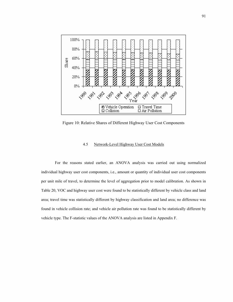
91
Figure 10: Relative Shares of Different Highway User Cost Components
4.5 Network-Level Highway User Cost Models
For the reasons stated earlier, an ANOVA analysis was carried out using normalized
individual highway user cost components, i.e., amount or quantity of individual user cost components
per unit mile of travel, to determine the level of aggregation prior to model calibration. As shown in
Table 20, VOC and highway user cost were found to be statistically different by vehicle class and land
area; travel time was statistically different by highway classification and land area; no difference was
found in vehicle collision rate; and vehicle air pollution rate was found to be statistically different by
vehicle type. The F-statistic values of the ANOVA analysis are listed in Appendix F.

92
Table 20: Results of ANOVA Analysis for the Preparation of Network-Level Highway User Cost Modeling (Level of significance: 0.005)
Component Source VOC Travel Time Collision Rate Air Pollution User Cost
L HC L.HC VC L.VC HC.VC L.HC.VC
Yes No No
Yes No
Yes No
Yes Yes Yes
Marginal No
Yes No
No No No No No No No
No No
Marginal Yes No
Yes No
Yes Marginal
No Yes Yes Yes No
Note: L- Land use, HC- Highway class, and VC- Vehicle class.
The descriptive statistics for VOC, travel time, vehicle collision rate, and air pollution rate per
VMT are summarized in Appendix G. The independent variables considered for model calibration
were grouped into two sets. The first set was mainly related to the level of physical highway assets,
which include network mileage, surface condition, and density of stop controlled intersections,
signalized intersections, interchanges, railroad crossings, and workzone characteristics. The second set
was associated with network usage, including average speed, traffic volume, truck traffic percent, etc.
The following OLS models were selected as being most appropriate to fit in the existing data:
SPEEDCONDITIONVMT/VOC 210 α+α+α=
SPEEDVMT/TT 20 α+α=
SPEEDMVMT/COL 20 α+α=
SPEEDVMT/POL 20 α+α=
SPEEDCONDITIONVMT/UC 210 α+α+α=
where
VOC/VMT = Vehicle operating cost for per vehicle mile of travel, in 1990$/VMT
(21)
(20)
(19)
(18)
(17)

93
TT/VMT = Average travel time for per vehicle mile of travel, in veh-hour/VMT
COL/VMT = Vehicle collision rate for per million vehicle miles of travel, in
number/millionVMT
POL/VMT = Vehicle air pollution rate for per vehicle mile of travel, in kg/VMT
UC/VMT = Highway user cost for per vehicle mile of travel, in 1990$/VMT
CONDITION = Pavement surface condition measured in IRI, in inches/mile
SPEED = Average vehicle traveling speed, in miles per hour.
α0, α1, and α2 are calibrated coefficients for different bridge types as listed in Table 21.
Table 21: Coefficients of Significant Independent Variables for Calibrated Network-Level Highway User Cost Models (Observations: 11)
y = α0 +α1CONDITION+α2SPEED User Cost Component
Land Use
VC/ HC α0 (t-statistic) α1 (t-statistic) α2 (t-statistic)
Adj. R2
Vehicle Operating Cost (1990$/VMT)
Rural
Urban
Car SUT MUT
Car SUT MUT
0.5252 (6.26)0.2361 (7.92)1.0553 (5.77)
0.6680 (6.34)0.2166 (80.64)0.8525 (20.01)
0.0002 (1.27)0.0001 (1.93)0.0015 (5.55)
- 0.000013 (5.06)
0.0002 (5.52)
-0.0056 (-4.23) -0.0008 (-1.81) -0.0085 (-2.96)
-0.0073 (-3.86) -0.0003 (-6.64) -0.0012 (-1.77)
0.94 0.88 0.98
0.58 0.97 0.94
Travel Time (Hour/VMT)
Rural
Urban
IS NIS
IS NIS
0.0487 (11.41)0.0382 (11.66)
0.0433 (4.72)0.0253 (36.77)
- -
- -
-0.0005 (-7.49) -0.0004 (-5.88)
-0.0005 (-2.90) -0.0001 (-7.29)
0.85 0.77
0.43 0.84
Collision Rate (No./million VMT)
All -4.9542 (-3.32) - 0.1595 (5.74) 0.76
Air Pollution (Kg/VMT)
All Car SUT MUT
0.7307 (1,062.63)1.5880 (1,984.84)1.5908 (6,197.64)
- - -
0.0001 (10.03) 0.0001 (7.00) 0.0001 (18.32)
0.91 0.83 0.97
User Cost (1990$/VMT)
Rural
Urban
Car SUT MUT
Car SUT MUT
0.7526 (7.47)0.6506 (7.61)1.5719 (4.87)
1.1711 (6.25)1.2637 (6.69)1.9960 (8.19)
0.0009 (5.97)0.0012 (8.86)0.0025 (5.08)
0.0014 (7.95)0.0017 (9.45)0.0011 (5.02)
-0.0041 (-2.56) -0.0008 (-0.58) -0.0080 (-1.58)
-0.0078 (-2.56) -0.0062 (-2.02) -0.0075 (-1.90)
0.98 0.98
0.96
0.97 0.97 0.93

94
Model calibration was also conducted to establish the relationship between network level
vehicle delay and volume-to-capacity ratios separately for rural and urban interstate highways, as well
as non-interstate highways. The models using OLS techniques were in the following specification
Ratio)C-to-(VααDelay/VMTVehicle 10 +=
where
Vehicle Delay/VMT = Vehicle delay for per vehicle mile of travel, in vehicle-hour/VMT
V-to-C Ratio = Volume to capacity ratio.
α0 and α1 are calibrated coefficients for different bridge types as listed in Table 22.
Table 22: Coefficients of Significant Independent Variables for Calibrated Network-Level Vehicle Delay Models (Observations: 11)
Vehicle Delay: Hour/VMT = α0 + a1(V-to-C Ratio) Land Area Highway Class α0 (t-statistic) α1 (t-statistic)
Adj. R2
Rural
Interstate Non-Interstate
0.0001 (8.30) 0.0001 (18.94)
0.0001 (6.14) 0.0001 (8.69)
0.79 0.88
Urban Interstate Non-Interstate
0.00009 (8.44) 0.0017 (91.54)
0.0001 (8.50) 0.0002 (6.31)
0.88 0.80
Model coefficients obtained for vehicle operating cost, travel time, vehicle collisions, and air
pollution as well as total user cost per mile of travel were as expected. For a given level of travel
speed, deterioration in the system condition resulted in a higher level of cost for vehicle operation,
causing an increased overall highway user cost. Also, with no change in the system condition, higher
travel speed was associated with a reduction in travel time, a higher likelihood of vehicle collisions,
and increased vehicle air pollution. Regardless of the land area and highway classification, higher
volume-to-capacity ratios would lead to higher network-level vehicle delays.
(22)
95
4.6 Chapter Summary
This chapter focused on the computation of the network-level highway user cost. The basis of
this computation was the annual vehicle miles of travel associated with state highways in Indiana
during 1990-2000 by different vehicle classes on various highway functional classifications. The
highway user cost components classified included vehicle operation, travel time, vehicle collisions,
and vehicle air pollution, and factors that affected individual user cost components were identified. In
order to establish the relative shares of individual highway user cost components, the respective user
cost components were further converted into constant dollars using existing unit rates, updated by CPI
and PPI accordingly. The dominant user cost component found was vehicle operation cost. Network-
level highway user cost models were calibrated separately for the individual highway user cost
components; as well as the total highway user cost. Models for network delay were also developed.

96
1
2
3
4
5 CHAPTER 5 PERFORMANCE MODELING FOR PHYSICAL HIGHWAY ASSETS
5.1 Introduction
As pavements and bridges are the dominant asset types in a highway network, the
performance modeling was mainly focused on these assets, based on the methods discussed in
Chapter 3.
5.2 Data Collection and Preparation
5.2.1 Data Collection
The most common physical assets in a highway network are pavements and bridges.
Consequently, data collection in the current study was geared towards these assets and utilized the
following database.
The INDIPAVE2000 [JTRP, 2000] database consists of data from 1990 through 2000 on
various pavement attributes for the state highways in Indiana, and items in the database include road
segment identification, condition, traffic, age, design and construction features, subgrade material
characteristics, region and climatic features, and maintenance and rehabilitation history, as listed in
Table 23. This database was designed as a relational type to facilitate data management tasks such as
querying, sorting, and reporting, either for each of the 9,902 one-mile pavement segments or for
contract sections that were typically set between major intersections with lengths stretching up to 15
miles.

97
Table 23: Data Items Stored in INDIPAVE2000 Database
Data Category Data Item
Roadway Segment Identification
Starting and ending mileposts Functional class Segment ID number
Road Surface Condition
Roughness Rutting index Pavement quality index Present serviceability index Cracking index Faulting index
Traffic AADT Percentage of single and multiple unit trucks
Age Pavement age
Design and Construction Features
Pavement surface type Pavement layer thickness Asphalt content and air voids Concrete elasticity modulus Doweling
Subgrade Material Characteristics
Percent fines California Bearing Capacity Ratio (CBR)
Region and Climatic Features
Air temperature Precipitation Freeze-thaw cycles Freeze index
Maintenance History Treatment type, level, and expenditure Rehabilitation History Rehabilitation type, thickness, and expenditure
Data items associated with state highway bridges were mainly acquired from the Indiana
bridge inventory database. Key data items in the database include bridge identification, region, age,
traffic, design and construction features, bridge deck, superstructure, substructure, and wearing
surface conditions for the period 1996-2000, as listed in Table 24.
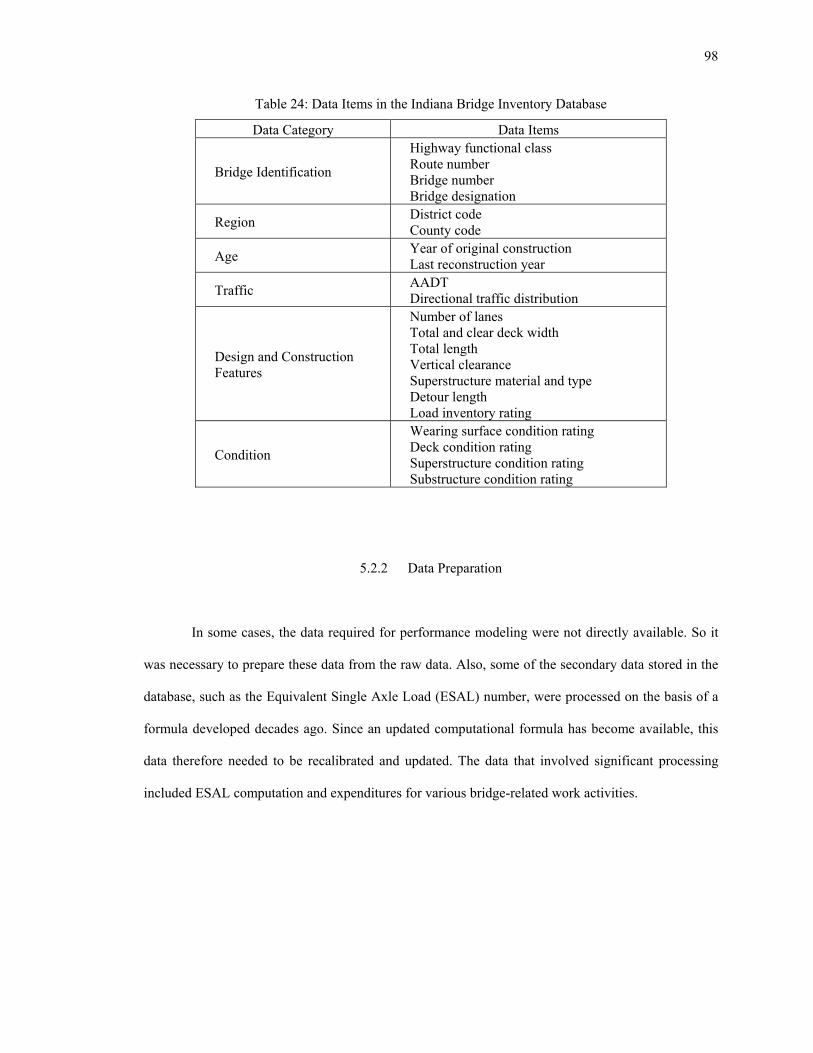
98
Table 24: Data Items in the Indiana Bridge Inventory Database
Data Category Data Items
Bridge Identification
Highway functional class Route number Bridge number Bridge designation
Region District code County code
Age Year of original construction Last reconstruction year
Traffic AADT Directional traffic distribution
Design and Construction Features
Number of lanes Total and clear deck width Total length Vertical clearance Superstructure material and type Detour length Load inventory rating
Condition
Wearing surface condition rating Deck condition rating Superstructure condition rating Substructure condition rating
5.2.2 Data Preparation
In some cases, the data required for performance modeling were not directly available. So it
was necessary to prepare these data from the raw data. Also, some of the secondary data stored in the
database, such as the Equivalent Single Axle Load (ESAL) number, were processed on the basis of a
formula developed decades ago. Since an updated computational formula has become available, this
data therefore needed to be recalibrated and updated. The data that involved significant processing
included ESAL computation and expenditures for various bridge-related work activities.

99
5.2.2.1 ESAL Computation
The AASHTO Design Guide [AASHTO, 1993] provided ESAL factors for flexible, rigid, and
composite pavements with traffic loading applied on pavements with different structural numbers or
thicknesses. In order to utilize the information for actual design practice, the axle-loading
configuration, including the number of steering, single, and tandem or tridem axles need to be
determined from the traffic stream. As this information is not available at the time of design, INDOT
developed in 1980’s an approximate procedure to estimate the ESAL factors for single and multiple
unit trucks for flexible and rigid pavements for pavement design. In 2000 INDOT updated the ESAL
factors using data from 35 Weigh-in-Motion (WIM) stations in Indiana. In the updating procedure, a
structural number of 5 and a slab thickness of 10 inches were used separately for flexible and rigid
pavements. A terminal PSI of 2.5 was assumed for both pavement types. In addition, these factors
were developed separately for single and multiple unit trucks. Table 25 presents the updated ESAL
factors established from the study [Gulen et al., 2000].
Table 25: Updated ESAL Factors for Highway Pavement Design in Indiana
Pavement Type Vehicle Class ESAL Factor
Flexible 5, 6, 7 8, 9, 10, 11, 12, 13
0.6 1.3
Rigid 5, 6, 7 8, 9, 10, 11, 12, 13
0.9 2.0
Following the concept of the AASHTO formula for ESAL computation, the total annual
ESAL values applied on a pavement segment were computed using ESAL factors from Table 25 and
by incorporating the adjustments of directional distribution and lane occupancy of the traffic as shown
below:
Annual ESALs = 365.AADT.Dd.Lf.[(%SUT.ESALSUT)+(%MUT.ESALMUT)]
(23)

100
where
Annual ESALs = Annual ESAL values applied on a pavement segment
AADT = Annual average daily traffic
Dd = Adjustment factor for traffic directional distribution
Lf = Adjustment factor for lane occupancy
%SUT = Percent of single unit trucks, vehicle classes 5, 6, 7
%MUT = Percent of multiple unit trucks, vehicle classes 8, 9, 10, 11, 12, 13
ESALSUT = ESAL factor for single unit trucks
ESALMUT = ESAL factor for multiple unit trucks.
To facilitate establishing the directional distribution, the lane occupancy factors, and the truck
percentage for various highway classes, statistical models were developed using traffic characteristics
data collected from WIM stations in Indiana. The descriptive statistics of the dependent variables are
provided in Appendix H, and the calibrated models are of the following specification:
)1990t(DD 10 −α+α=
)1990t(LOF 10 −α+α=
)1990t(SUT% 10 −α+α=
)1990t(MUT% 10 −α+α=
where
DD = Directional distribution factor, in %
LOF = Lane occupancy adjustment factor
% SUT = Percent of single unit trucks in traffic stream, in %
(24)
(25)
(26)
(27)

101
% MUT = Percent of multiple unit trucks in traffic stream, in %
t = Year of analysis.
α0, and α1 are calibrated coefficients for different highway classifications.
The calibrated coefficients as well as test results of goodness of fit of the proposed models are
presented in Table 26. It is shown that, except for rural interstate highways, fairly good fit was
achieved for directional distribution and lane occupancy factors. For the percentage of both single and
multiple unit trucks, apart from urban non-interstate highways, good fit was obtained. Even though the
goodness of fit, i.e., adjusted R2, was low for some models, the calibrated coefficients were significant
at least at 5 percent level of significance as indicated by t-statistic values.
Table 26: Calibrated Model Coefficients for Directional Distribution, Lane Occupancy Adjustment Factor, and Truck Percentage for ESAL Computation
y = α0 + α1(t-1990) Designation Highway Class α0 t-statistic α1 t-statistic
Adjusted R2
Directional Distribution (DD) (%)
Rural interstate Rural non-interstate Urban interstate Urban non-interstate
53 48 47 39
(752.99) (54.99)
(112.60)(68.27)
0.020.670.882.92
(1.91) (4.54)
(12.41) (30.17)
0.21 0.66 0.94 0.99
Lane Occupancy Adjustment Factor (Lf)
Rural interstate Rural non-interstate Urban interstate Urban non-interstate
0.76 0.82 0.70 0.42
(137.77) (319.45)(117.49)
(68.00)
-0.0021-0.00380.00320.0349
(-2.21) (-8.72)
(3.21) (33.71)
0.28 0.88 0.48 0.99
Single Unit Truck (%)
Rural interstate Rural non-interstate Urban interstate Urban non-interstate
15 21 15 17
(67.04)(30.91)
(35.49)(21.70)
0.900.530.81
-0.38
(23.00) (4.57)
(11.18) (-2.92)
0.98 0.67 0.93 0.43
Multiple Unit Truck (%)
Rural interstate Rural non-interstate Urban interstate Urban non-interstate
15 7
10 2
(24.60)(19.73)
(17.86)(20.72)
0.660.52
-0.16-0.05
(6.43) (8.06)
(-1.69) (-2.71)
0.80 0.86 0.66 0.39

102
5.2.2.2 Expenditures of Various Bridge Related Work Activities
From the Indiana bridge inventory database information was obtained on bridge location,
traffic, age, design characteristics, and condition for 4,907 bridges from 1996 through 2000. As shown
in Table 27, these bridges are distributed across various highway classifications and are further
classified by superstructure type. One challenge encountered for bridge model development was that
no bridge expenditure information was provided. The Indiana Bridge Management System (IBMS)
software was thus utilized to acquire the missing data relevant to bridge expenditure.
Table 27: Distribution of State Maintained Highway Bridges
Superstructure Type Road Type Functional Classification 1 2 3 4 5 6 Interstate (IS) (1,249)
Rural interstate Urban interstate 63 322 53 712 12 87National
Highway System (NHS) (2,382)
Non-IS (1,133)
Rural principal arterial Urban freeway Urban principal arterial
127 228 74 556 45 103
State (2,464)
Rural principal arterial Rural minor arterial Rural major collector Rural minor collector Urban principal arterial Urban minor arterial Urban collector
685 559 269 402 271 278Non-NHS (2,525)
Local (61)
Rural local Urban local 13 9 20 7 10 2
Total 4,907 888 1,118 416 1,677 338 470
Superstructure Type: 1- Concrete slab, 2- Concrete girder, 3- Steel girder, 4- Steel truss,
5- Concrete arch deck, and 6- Concrete channel beam.
The IBMS software is comprised of four modules: decision tree (DTREE), life-cycle cost
analysis (COST), multicriteria ranking (RANK), and optimization (OPT). In the present study, the
DTREE and COST modules were utilized to establish bridge expenditure information. Based on the
assessment of the condition of various elements and the safety status of a bridge, the DTREE module

103
recommends different improvement activities. The COST module then performs a life-cycle cost
analysis for each given activity according to an activity profile that depicts maintenance and other
improvements needed on a bridge throughout its service life. The computation is done for user cost in
constant dollars in the base year of analysis. In order to establish reliable information for changes in
bridge condition, and user cost as a result of implementing a recommended work activity, the cost
analysis was conducted using the IBMS software repetitively for a 10-year analysis period (2001-
2010).
5.3 Pavement Performance Modeling
Pavement performance modeling concentrated on pavement rehabilitation expenditure,
routine maintenance expenditure, and tradeoffs between the maintenance level and the rehabilitation
interval. Models were calibrated separately for flexible, rigid, and composite pavements. The
descriptive statistics of modeling data are summarized in Appendix I.
5.3.1 Pavement Rehabilitation Expenditure Models
Pavement rehabilitation expenditure models developed by Li and Sinha [2000] were used
in the present study. For a pavement segment that received rehabilitation, its service life was
considered to be the time interval between the last rehabilitation work and the start of a
rehabilitation activity that fell in the analysis period of the present study. The general functions of
OLS models for flexible, rigid and composite pavements are as below:
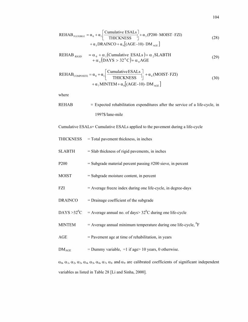
104
[ ]AGE95
310FLEXIBLE
DM10)-(AGEαDRAINCOα
FZI)MOIST(P200α THICKNESS
ESALs CumulativeααREHAB
⋅++
⋅⋅+⎥⎦⎤
⎢⎣⎡+=
( )
( ) AGEC32DAYS SLABTH ESALs CumulativeREHAB
80
6
210RIGID
α+>α+α+α+α=
[ ]AGE97
410COMPOSITE
DM10)-(AGEαMINTEMα
FZI)(MOISTα THICKNESS
ESALs CumulativeααREHAB
⋅++
⋅+⎥⎦⎤
⎢⎣⎡+=
where
REHAB = Expected rehabilitation expenditures after the service of a life-cycle, in
1997$/lane-mile
Cumulative ESALs= Cumulative ESALs applied to the pavement during a life-cycle
THICKNESS = Total pavement thickness, in inches
SLABTH = Slab thickness of rigid pavements, in inches
P200 = Subgrade material percent passing #200 sieve, in percent
MOIST = Subgrade moisture content, in percent
FZI = Average freeze index during one life-cycle, in degree-days
DRAINCO = Drainage coefficient of the subgrade
DAYS >320C = Average annual no. of days> 320C during one life-cycle
MINTEM = Average annual minimum temperature during one life-cycle, 0F
AGE = Pavement age at time of rehabilitation, in years
DMAGE = Dummy variable, =1 if age> 10 years, 0 otherwise.
α0, α1, α2, α3, α4, α5, α6, α7, α8 and α9 are calibrated coefficients of significant independent
variables as listed in Table 28 [Li and Sinha, 2000].
(28)
(29)
(30)

105
Table 28: Coefficients of Significant Independent Variables for Calibrated Pavement Rehabilitation Expenditure Models
Significant Independent
Variable
Calibrated Coefficient
Flexible (t-statistic)
Rigid-JCP (t-statistic)
Composite (t-statistic)
Constant Annual ESALs THICKNESS
SLABTH P200*MOIST*FZI MOIST*FZI DRAINCO DAYS >320C MINTEM AGE (AGE-10)*DMAGE
α0 α1
α2 α3 α4 α5 α6 α7 α8 α9
172,431 (5.45)0.3113 (50.66)
- 301 (5.43)-
-145,378 (-4.67)- - -
701 (3.38)
-628,986 (-3.09) 0.0380 (12.53)
-40,021 (-3.66)
- - -
13,274 (3.76) -
34,760 (3.97) -
540,918 (7.41)0.2409 (29.39)
- -
71 (39.55)- -
-10,393 (-6.82)-
10,593 (8.83)Goodness of Fit (R2) 0.96 0.96 0.90 Observations 202 49 621
5.3.2 Pavement Annual Routine Maintenance Expenditure Models
Tobit models developed by Li and Sinha [2000] were used to estimate the expenditure
function for pavement segments with routine maintenance work. Four different models were
estimated, one for each pavement type. Formulation of the models recognized the lagged relationship
between routine maintenance and pavement condition change; the pavement damage at the end of year
t was a function of load and non-load factors in year t; and maintenance decision (and hence,
expenditure) in year t+1 was influenced by pavement condition change in the previous year t. The
calibrated routine maintenance expenditure and pavement condition change functions for flexible,
Joint Concrete Pavements (JCP), Continuously Reinforced Concrete (CRC), and composite pavements
are as below:
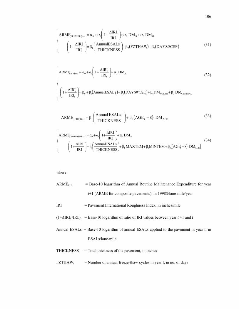
106
( )
( ) ( )⎪⎪⎩
⎪⎪⎨
⎧
°β+β+⎟⎠⎞
⎜⎝⎛β=⎟⎟
⎠
⎞⎜⎜⎝
⎛ ∆+
α+α+⎟⎟⎠
⎞⎜⎜⎝
⎛ ∆+α+α=+
t3t2t
1t
t
ST3IS2t
t101tFLEXIBLE
CSFDAYS0FZTHAWTHICKNESS
ESALs Annual IRIIRI1
DM DM IRIIRI1 ARME
( )
( ) ( )⎪⎪⎪⎪
⎩
⎪⎪⎪⎪
⎨
⎧
++°++=⎟⎟⎠
⎞⎜⎜⎝
⎛+
+⎟⎟⎠
⎞⎜⎜⎝
⎛++=+
CENTRAL7NORTH6t3t10t
t
IS2t
t101tJCP
DM βDMβCSFDAYS0βESALs AnnualββIRI∆IRI1
DM αIRI∆IRI1 ααARME
( ) ( ) AGEt8t
11tCRC DM 8AGEβTHICKNESS
ESALs AnnualβARME ⋅−+⎟
⎠
⎞⎜⎝
⎛=+
( )
( )[ ]⎪⎪⎩
⎪⎪⎨
⎧
⋅−+++⎟⎠⎞
⎜⎝⎛=⎟⎟
⎠
⎞⎜⎜⎝
⎛+
+⎟⎟⎠
⎞⎜⎜⎝
⎛++=+
AGEt8t5t4t
1t
t
IS2t
t101tCOMPOSITE
DM 8AGEβMINTEMβMAXTEM βTHICKNESS
ESALs AnnualβIRI∆IRI1
DM αIRI∆IRI1 ααARME
where
ARMEt+1 = Base-10 logarithm of Annual Routine Maintenance Expenditure for year
t+1 (ARME for composite pavements), in 1998$/lane-mile/year
IRI = Pavement International Roughness Index, in inches/mile
(1+∆IRIt /IRIt) = Base-10 logarithm of ratio of IRI values between year t +1 and t
Annual ESALst = Base-10 logarithm of annual ESALs applied to the pavement in year t, in
ESALs/lane-mile
THICKNESS = Total thickness of the pavement, in inches
FZTHAWt = Number of annual freeze-thaw cycles in year t, in no. of days
(31)
(32)
(33)
(34)

107
DAYS0°CSFt = Number of days of first min. of 0°C between last spring and current fall
MAXTEMt = Average annual maximum temperature in year t, in 0F
MINTEMt = Average annual minimum temperature in year t, in 0F
AGEt = Pavement age in year t, in years
DMIS = Dummy variable: 1 for Interstate roads, 0 otherwise
DMST = Dummy variable: 1 for state roads, 0 otherwise
DMNORTH = Dummy variable: 1 for northern Indiana, 0 otherwise
DMCENTRAL = Dummy variable: 1 for central Indiana, 0 otherwise
DMAGE = Dummy variable: 1 if pavement age is greater than 8 years, 0 otherwise.
α0, α1, α2, α3, β0, β1, β2, β3, β4, β5, β6, β7, and β8 are calibrated coefficients of significant
independent variables as listed in Table 29 [Li and Sinha, 2000].
Table 29: Coefficients of Significant Independent Variables for Calibrated Pavement Routine Maintenance Expenditure Models
Significant Independent
Variable
Calibrated Coefficient
Flexible (t-statistic)
Rigid-JCP (t-statistic)
Rigid-CRC (t-statistic)
Composite (t-statistic)
Constant % IRI Change DMIS DMST
α0 α1 α2 α3
0.3770 (3.48)46.02 (7.60)
0.8864 (11.86)0.2537 (3.80)
0.7924 (3.37)37.73 (2.80)
0.2627 (1.81)-
- - - -
-114.48 (-8.47)8,061.98 (13.97)
373.64 (20.06)-
Constant Annual ESALs THICKNESS
FZTHAW DAYS00CSF MAXTEM MINTEM DMNORTH DMCENTRAL (AGE-8)*DMAGE
β0 β1
β2 β3 β4 β5 β6 β7 β8
- 0.0052 (5.79)
0.0003 (7.25)-0.0002 (-6.82)
- - - - -
0.0756 (1.99)0.0081 (3.62)
- -0.0006 (-3.13)
- -
-0.0087 (-1.73)-0.0116 (-2.14)
-
- 0.4449 (17.64)
- - - - - -
0.2567 (1.74)
- 0.0062 (7.74)
- -
0.00035 (24.83)-0.0007(-12.41)
- -
0.0012 (3.53)Goodness of Fit (ρ2) 0.18 0.06 0.39 0.12 Observations 828 141 29 1,961

108
5.3.3 Tradeoffs between Routine Maintenance and Rehabilitation Interval
Tradeoff relationships between the rehabilitation interval and maintenance-load-weather were
extensively studied using field data from the Indiana state highways by Labi and Sinha [2001].
Models were calibrated using OLS techniques separately by highway functional classification for
different pavement types as listed in the following:
( )⎥⎦
⎤⎢⎣
⎡⋅⋅+= WSIESALsAnnual
ARME
cbaINTERVALREHAB
where
REHAB INTERVAL = Interval of rehabilitation of given pavement section, in years
ARME = Annual routine maintenance expenditure, in 1995$/lane-mile/year
Annual ESALs = Annual ESALs applied to the pavement, in million ESALs/lane-mile
WSI = A weighted index of precipitation (in millimeter), freeze index (in degree-
day), and freeze-thaw cycles (in number of days) with weights being 0.3,
0.35, and 0.35, respectively.
a, b, and c are calibrated coefficients for different pavement types by highway functional
classification as listed in Table 30.
Table 30: Calibrated Coefficients for Pavement Rehabilitation Interval Models
Highway Class Interstate Non-Interstate
Calibrated Coefficient
Rigid (t-statistic)
Composite (t-statistic)
Flexible (t-statistic)
Rigid (t-statistic)
Composite (t-statistic)
a b c
34.0793 (3.36)-19.8293 (-2.21)
0.2410 (1.46)
37.5909 (2.22)-23.3918 (-4.22)
0.5394 (1.77)
11.9249 (3.73)-8.2775 (-1.44) 0.7678 (2.45)
39.0608 (1.69) -27.0552 (-1.42)
0.9281 (8.61)
61.8719 (1.33)-50.7040 (-2.05)
0.9824 (4.87)R2 0.27 0.38 0.14 0.35 0.23
Observations 16 23 25 24 43
(35)

109
5.3.4 Discussions
Pavement expenditure models were considered separately for rehabilitation and routine
maintenance. In addition, the tradeoff relationship between rehabilitation interval and routine
maintenance was also included. The models developed in earlier studies were found applicable to the
present study. For rehabilitation expenditure and rehabilitation-routine maintenance relationship, OLS
models were used, while the routine maintenance expenditure models used Tobit analysis. Tobit
model was used because annual routine maintenance levels were restricted by budget constraints, and
econometric theory stated that in such cases the OLS model was not appropriate and the Tobit model
yielded more consistent estimates [Goldberger, 1964].
5.4 Bridge Performance Modeling
Model calibration focused on the impact of a bridge work activity, represented by a given
level of expenditure, on changes in bridge condition, life-cycle agency cost, and user cost.
Specifically, models were developed separately for concrete and steel bridges. Model forms are
discussed in the following sections and the descriptive statistics of modeling data are summarized in
Appendix J.
5.4.1 Impact of Work Activity on Bridge Deck, Superstructure, Substructure, and Wearing Surface Condition
Models were calibrated separately for changes in the deck, superstructure, substructure, and
wearing surface conditions for concrete and steel bridges using OLS techniques as a function of
traffic, age, and bridge expenditure. The general form of the calibrated models for concrete and steel
bridges is as below:

110
BOXBEAM8ARCH7GIRDER6SLAB5
IS43210
DMαDMαDMαDMαDMαEEXPENDITURαAGEαAADTααCHANGECONDITION
++++++++=
where
CONDITION CHANGE = Change in deck, superstructure, substructure, and wearing surface
condition of concrete or steel bridge as a result of a work activity, in %
EXPENDITURE= Expenditure associated with a specific work activity, in 1990$/ft2
AADT = Bridge traffic volume at time of work action, in vehicles
AGE = Bridge age at time of work action, in years
DMIS = Dummy variable, 1 for interstate, 0 otherwise
DMSLAB = Dummy variable, 1 for slab superstructure, 0 otherwise
DMGIRDER = Dummy variable, 1 for girder superstructure, 0 otherwise
DMARCH = Dummy variable, 1 for arch superstructure, 0 otherwise
DMBOXBEAM = Dummy variable, 1 for box beam superstructure, 0 otherwise.
α0, α1, α2, α3, α4, α5, α6, α7, and α8 are calibrated coefficients for concrete and steel bridges
as listed in Tables 31 and 32.
Table 31: Coefficients of Significant Independent Variables for Concrete Bridge Condition Models
Significant Independent
Variable
Calibrated Coefficient
Deck (t-statistic)
Superstructure (t-statistic)
Substructure (t-statistic)
Surface (t-statistic)
Constant AADT AGE EXPEND ($/ft2) DMIS DMSLAB DMGIRDER DMARCH
α0 α1 α2 α3 α4 α5 α6 α7
0.0084 (2.20)0.000003(16.52)
- 0.0006 (12.72)0.0370 (11.68)0.0093 (2.00)
-0.0204 (-6.47)-0.0273 (-5.81)
-0.0271 (-2.76)-0.000001(-1.84)
0.0042 (20.56)0.0006 (2.55)0.0496 (8.06)
-0.1155 (-10.42)-0.0347 (-4.95)-0.0260 (-2.70)
-0.6958 (-11.04) -0.00001 (-2.31)
-0.0202 (-103.29) 0.0512 (18.22)
- 0.3431 (223.43)
- -0.0177 (-16.50)
- 0.00001 (4.88)0.0090 (18.04)0.0067 (28.52)
-0.0686 (-3.78)-0.1980 (-7.30)0.1460 (8.32)0.0738 (2.81)
Goodness of Fit (R2) 0.20 0.53 0.90 0.81 Observations 3,796 648 15 3,796
(36)

111
Table 32: Coefficients of Significant Independent Variables for Steel Bridge Condition Models
Significant Independent Variable
Calibrated Coefficient
Deck (t-statistic)
Superstructure (t-statistic)
Surface (t-statistic)
Constant AADT AGE EXPENDITURE ($/ft2) DMIS DMBOXBEAM
α0 α1 α2 α3 α4 α8
0.1099 (34.06)0.0000004 (6.24)
0.0007 (9.01)0.0004 (13.02)
-0.0035 (-1.72)-0.0121 (-3.62)
0.0569 (3.37) -
0.0016 (4.90) 0.0025 (3.29)
- 0.0328 (3.29)
- -
0.0143 (31.19)0.0038 (13.83)0.0613 (3.67)
-0.0453 (-1.50)Goodness of Fit (R2) 0.11 0.20 0.79 Observations 2,946 183 2,946
It can be seen from the above tables that a fairly good fit was obtained for bridge substructure
and wearing surface condition models. Even though the goodness of fit, i.e., adjusted R2, was low for
bridge deck and superstructure models, the calibrated coefficients were significant at least at 5 percent
level of significance as indicated by t-statistic values. The signs of calibrated coefficients were
intuitive. All things being equal, a higher expenditure level would result in an increased rate of change
in the condition of individual bridge components. This was true for both concrete and steel bridges.
Also, the marginal effects of changes in bridge condition were higher as traffic volume and age
increased. However, the magnitude of the change was different for different types of bridges when
classified by bridge superstructure type.
5.4.2 Impact of Work Activity on Bridge Life-Cycle Agency and User Costs
Models were calibrated for concrete and steel bridges, respectively, using OLS techniques to
relate changes in bridge user cost as a function of traffic, age, bridge expenditure, load inventory
rating, and detour length. The general form of the calibrated user cost models for concrete and steel
bridges is as follows:

112
TURESUPERSTRUC12DECK11BOXBEAM10
ARCH9GIRDER8SLAB7IS65
43210
DMαDMαDMαDMαDMαDMαDMαGTHDETOUR_LENαTORYLOAD_INVENαEEXPENDITURαAGEαAADTααCHANGECOSTUSER
+++++++
++++=
where
USER COST CHANGE= Change in equivalent uniform annual user cost for concrete or steel
bridges as a result of a work activity, in %
AADT = Bridge traffic volume at time of work action, in vehicles
AGE = Bridge age at time of work action, in years
EXPENDITURE= Equivalent annual agency cost, in 1990$/ft2
LOAD_INVENTORY = Bridge load inventory rating at time of work action, in tons
DETOUR_LENGTH = Bridge detour length at time of work action, in miles
DMIS = Dummy variable, 1 for interstate, 0 otherwise
DMSLAB = Dummy variable, 1 for slab superstructure, 0 otherwise
DMGIRDER = Dummy variable, 1 for girder superstructure, 0 otherwise
DMARCH = Dummy variable, 1 for arch superstructure, 0 otherwise
DMBOXBEAM = Dummy variable, 1 for box beam superstructure, 0 otherwise
DMDECK = Dummy variable, 1 if work action conducted only on deck, 0 otherwise
DMSUPERSTRUCRUE = Dummy variable, 1 if work action conducted only on superstructure,
0 otherwise.
α0, α1, α2, α3, α4, α5, α6, α7, α8, α9, α10, α11, and α12 are calibrated coefficients for concrete
and steel bridges as listed in Table 33.
(37)
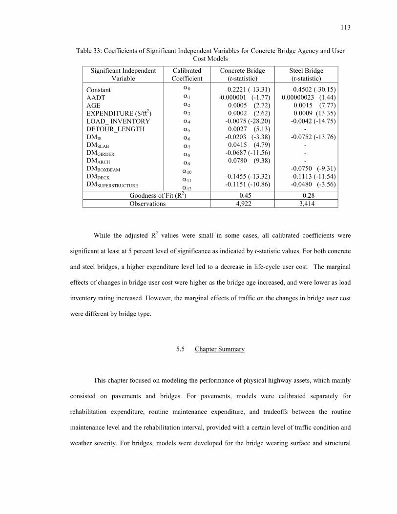
113
Table 33: Coefficients of Significant Independent Variables for Concrete Bridge Agency and User Cost Models
Significant Independent Variable
Calibrated Coefficient
Concrete Bridge (t-statistic)
Steel Bridge (t-statistic)
Constant AADT AGE EXPENDITURE ($/ft2) LOAD_ INVENTORY DETOUR_LENGTH DMIS DMSLAB DMGIRDER DMARCH DMBOXBEAM DMDECK DMSUPERSTRUCTURE
α0 α1 α2 α3 α4 α5 α6 α7 α8 α9 α10 α11 α12
-0.2221 (-13.31) -0.000001 (-1.77)
0.0005 (2.72) 0.0002 (2.62)
-0.0075 (-28.20) 0.0027 (5.13)
-0.0203 (-3.38) 0.0415 (4.79)
-0.0687 (-11.56) 0.0780 (9.38)
- -0.1455 (-13.32) -0.1151 (-10.86)
-0.4502 (-30.15)0.00000023 (1.44)
0.0015 (7.77)0.0009 (13.35)
-0.0042 (-14.75)-
-0.0752 (-13.76)- - -
-0.0750 (-9.31)-0.1113 (-11.54)-0.0480 (-3.56)
Goodness of Fit (R2) 0.45 0.28 Observations 4,922 3,414
While the adjusted R2 values were small in some cases, all calibrated coefficients were
significant at least at 5 percent level of significance as indicated by t-statistic values. For both concrete
and steel bridges, a higher expenditure level led to a decrease in life-cycle user cost. The marginal
effects of changes in bridge user cost were higher as the bridge age increased, and were lower as load
inventory rating increased. However, the marginal effects of traffic on the changes in bridge user cost
were different by bridge type.
5.5 Chapter Summary
This chapter focused on modeling the performance of physical highway assets, which mainly
consisted on pavements and bridges. For pavements, models were calibrated separately for
rehabilitation expenditure, routine maintenance expenditure, and tradeoffs between the routine
maintenance level and the rehabilitation interval, provided with a certain level of traffic condition and
weather severity. For bridges, models were developed for the bridge wearing surface and structural

114
conditions as well as life-cycle user cost, respectively. The calibrated models could be used to
establish the marginal effects of significant explanatory variables that affect the response variables
representing the performance of physical highway assets.

115
1
2
3
4
5
6 CHAPTER 6 MARGINAL BENEFIT ANALYSIS
6.1 Introduction
Marginal benefit analysis was conducted using the calibrated performance models for
physical highway assets and network usage. The key marginal effects were pavement rehabilitation
and routine maintenance expenditure needed to recover damages caused by load and non-load factors,
the pavement routine maintenance expenditure level on the rehabilitation interval, the bridge
expenditure level on a change in bridge surface and structural conditions as well as bridge life-cycle
agency and user costs, and the change in road condition and vehicle traveling speed on individual user
cost components. These effects were determined by taking the first-order derivative of relevant
functions with respect to appropriate variables on interest, as discussed in the following sections.
6.2 Marginal Effects Based on Physical Asset Performance Models
6.2.1 Marginal Effect of Traffic Loading on Pavement Rehabilitation Expenditure
Models relating rehabilitation expenditure as a function of a series of the load and non-load
factors given in Equations (28)-(30) in Chapter 5 were utilized to establish the marginal effect of
cumulative traffic loading on rehabilitation expenditure needs. Information regarding average
pavement thickness, cumulative traffic loading, and rehabilitation expenditure associated with these
models is provided in Table 34. As an example, a detailed computation using the rehabilitation
expenditure model for flexible pavements is provided below. Similar computations were done for
rigid and composite pavements.

116
According to Equation (22), we have
[ ]AGE
FLEXIBLE
DM10)-(AGE701DRAINCO145,378
FZI)MOIST(P200301 THICKNESS
ESALs Cumulative0.3113172,431REHAB
⋅⋅+⋅−
⋅⋅⋅+⎥⎦⎤
⎢⎣⎡⋅+=
Hence, ( )( ) THICKNESS
3113.0ESAL
REHABFLEXIBLE =∂
∂
Substituting THICKNESS = 13.76 into Equation (39), we get ( )
( ) 0226.0ESAL
REHABFLEXIBLE =∂
∂ (in
1997 constant dollar). As overall pavement damage is caused by load and non-load related factors, the
total marginal rehabilitation expenditure would thus be attributable to both load and non-load related
marginal rehabilitation expenditure. The load shares of rehabilitation expenditure for different
pavement types developed by Li and Sinha [2000] were utilized to establish the total marginal
rehabilitation expenditure, and the total marginal rehabilitation needs were adjusted to 1990 constant
dollars by CPI, and are presented in Table 35.
Table 34: Average Pavement Rehabilitation Expenditure, Pavement Thickness, and Cumulative
Traffic Loading in Indiana (1995-1997)
Item Unit Flexible Rigid Composite Rehabilitation Thickness Cumulative ESALs
1997 $/lane-mile inch ESAL
186,891 13.76
2,197,969
461,637 22.04
9,469,897
247,224 14.12
4,121,405
Table 35: Marginal Effect of Traffic Loading on Total Rehabilitation Expenditure
Pavement Type Load Related Marginal Rehab.
Expenditure (1997, $/lane-mile/ESAL)
Load ShareTotal Marginal Rehab.
Expenditure (1990, $/lane-mile/ESAL)
Flexible Rigid Composite
0.0226 0.0380 0.0200
28% 78% 38%
0.0671 0.0405 0.0437
(38)
(39)

117
6.2.2 Marginal Effect of Change in Pavement Condition on Routine Maintenance Needs
Models for annual pavement routine maintenance expenditure needs, as a function of a series
of load and non-load factors were calibrated using the Tobit approach as listed in Equations (31)-(34)
in Chapter 5. To obtain the marginal effect of change in pavement condition on routine maintenance
needs, only the first equation of the two-stage equation was required. Information about the average
pavement surface condition and the change in the condition as well as the annual average routine
maintenance expenditure needed is listed in Table 36. As an example, a detailed calculation using
models for flexible pavements on interstate highways is provided below. Similar computations were
done for PCC, CRC, and composite pavements.
( ) STISt
t101t10 DM0.2537DM0.8864
IRI∆IRI1log46.02010.3770ARMEog ⋅+⋅+⎟⎟
⎠
⎞⎜⎜⎝
⎛+⋅+=+l
For interstate highways, we therefore have
( ) ⎟⎟⎠
⎞⎜⎜⎝
⎛+⋅+=+
t
t101t10 IRI
∆IRI1log46.02011.2634ARMEogl
Hence, ( )( ) ( )⎥⎦
⎤⎢⎣
⎡
+⋅= =+
tt
1t
t
1t
IRI∆IRIARME46.0201
∆IRIdARMEd
Substituting ARMEt+1= 77.58, IRIt= 140.94, and ∆IRIt= 4.48 (3.18% change) for interstate
flexible pavements into Equation (42), we get ( )( ) 55.24
IRIdARMEd
t
1t =∆
+ (in 1998 constant dollar). The
marginal effects of pavement condition change on annual routine maintenance needs for different
pavement types by highway class were adjusted to 1990 constant dollars using CPI, and are listed in
Table 37.
(40)
(41)
(42)
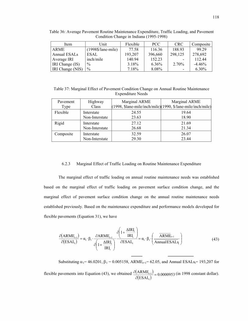
118
Table 36: Average Pavement Routine Maintenance Expenditure, Traffic Loading, and Pavement Condition Change in Indiana (1995-1998)
Item Unit Flexible PCC CRC CompositeARME Annual ESALs Average IRI IRI Change (IS) IRI Change (NIS)
(1998$/lane-mile) ESAL inch/mile % %
77.58 193,207
140.94 3.18% 7.18%
116.36 396,660
152.23 6.36% 8.08%
188.93 298,125
- 2.70%
-
99.29 278,692
112.44 -4.46% 6.30%
Table 37: Marginal Effect of Pavement Condition Change on Annual Routine Maintenance Expenditure Needs
Pavement Type
Highway Class
Marginal ARME (1998, $lane-mile/inch/mile)
Marginal ARME (1990, $/lane-mile/inch/mile)
Flexible
Interstate Non-Interstate
24.55 23.63
19.64 18.90
Rigid
Interstate Non-Interstate
27.12 26.68
21.69 21.34
Composite
Interstate Non-Interstate
32.59 29.30
26.07 23.44
6.2.3 Marginal Effect of Traffic Loading on Routine Maintenance Expenditure
The marginal effect of traffic loading on annual routine maintenance needs was established
based on the marginal effect of traffic loading on pavement surface condition change, and the
marginal effect of pavement surface condition change on the annual routine maintenance needs
established previously. Based on the maintenance expenditure and performance models developed for
flexible pavements (Equation 31), we have
( )( ) ⎟
⎟⎠
⎞⎜⎜⎝
⎛⋅⋅=
∂
⎟⎟⎠
⎞⎜⎜⎝
⎛+∂
⋅
⎟⎟⎠
⎞⎜⎜⎝
⎛+∂
∂⋅⋅=
∂∂ +++
t
1t11
t
t
t
t
t
1t11
t
1t
ESALsAnnualARMEβα
ESALIRI∆IRI1
IRI∆IRI1
ARMEβαESAL
ARME
Substituting α1= 46.0201, β1 = 0.005158, ARMEt+1= 62.05, and Annual ESALst= 193,207 for
flexible pavements into Equation (43), we obtained ( )( ) 0000953.0ESAL
ARME
t
1t =∂∂ + (in 1998 constant dollar).
(43)

119
The marginal annual routine maintenance needed to recover the portion of pavement damage caused
by traffic loading for different pavement types by highway class is listed in Table 38. As overall
pavement damage was caused by load and non-load related factors, the total marginal annual routine
maintenance expenditure would therefore be the load-related marginal maintenance expenditure being
normalized according to the load share of total routine maintenance expenditure. The load shares of
annual routine maintenance expenditure for different pavement types established by Li and Sinha
[2000] were utilized for the normalization process. The total marginal annual maintenance needs were
adjusted to 1990 constant dollars by CPI and are presented in Table 38.
Table 38: Marginal Effect of Traffic Loading on Annual Total Routine Maintenance Expenditure
Pavement Type
Load Related Marginal ARME(1998, $/lane-mile/ESAL) Load Share Total Marginal ARME
(1990, $/lane-mile/ESAL) Flexible Rigid-PCC Rigid-CRC Composite
0.0000953 0.0000897 0.0002820 0.0000780
26% 36% 63% 28%
0.000293 0.000199 0.000358 0.000223
6.2.4 Marginal Effect of Pavement Routine Maintenance Level on Rehabilitation Interval
According to the calibrated models shown in Equation (35) in Chapter 5, the pavement
rehabilitation interval would increase as the result of a higher level of routine maintenance
expenditure, provided that the traffic loading and weather condition are kept constant. However, the
magnitude of the marginal effect of routine maintenance expenditure on the extension of the
rehabilitation interval varies drastically for different traffic loading and weather combinations as well
as the existing routine maintenance levels. This argument is illustrated as below:
Given ( )⎥⎦⎤
⎢⎣
⎡⋅⋅+= WSIESALsAnnual
ARME
cbaINTERVALREHAB , we have
( )( ) ( )
( )⎥⎥⎦⎤
⎢⎢⎣
⎡
⋅⋅⋅
⋅⋅=∂
∂ WSIESALsAnnual
ARME
cWSIESALsAnnual
1lncbARME
INTERVALREHAB (44)

120
The average traffic loading and average weather severity index in 1995 as shown in Table 39
and routine maintenance expenditure levels ranging from 5 to 50 dollars per lane-mile per year were
utilized to illustrate the marginal effect of routine maintenance on the rehabilitation interval for
different types of pavements. The results are presented in Table 40. As an example, if the current
average routine maintenance expenditure for flexible pavements is $5/lane-mile/year, every dollar
increase in expenditure can be expected to add 0.143 year to the rehabilitation interval of these
pavements under average traffic loading and weather conditions.
Table 39: Annual Average Traffic Loading, Weather Severity Index, and Average Rehabilitation Interval in Indiana
Pavement Type
Highway Class
Annual ESALs (in million) WSI Average RI
(year) Flexible All 0.39 0.62 10.18
Rigid Interstate Non-interstate
0.71 0.26
0.72 0.68
26.76 24.71
Composite
Interstate Non-interstate
0.81 0.28
0.75 0.76
22.04 14.00
Table 40: Marginal Effect of Maintenance Level on Pavement Rehabilitation Interval under Average Traffic Loading and Average Weather Condition in Indiana (in number of years)
Pavement Type Flexible Rigid Composite Highway Class All Interstate Non-interstate Interstate Non-interstate
Exis
ting
Rou
tine
Mai
nten
ance
Lev
el
($/la
ne-m
ile/y
ear)
5 10 15 20 25 30 35 40 45 50
0.143 0.003 0.000 0.000 0.000 0.000 0.000 0.000 0.000 0.000
0.595 0.030 0.001 0.000 0.000 0.000 0.000 0.000 0.000 0.000
1.478 0.978 0.647 0.429 0.284 0.188 0.124 0.082 0.054 0.036
1.527 0.317 0.066 0.014 0.003 0.001 0.000 0.000 0.000 0.000
0.571 0.140 0.035 0.008 0.002 0.001 0.000 0.000 0.000 0.000
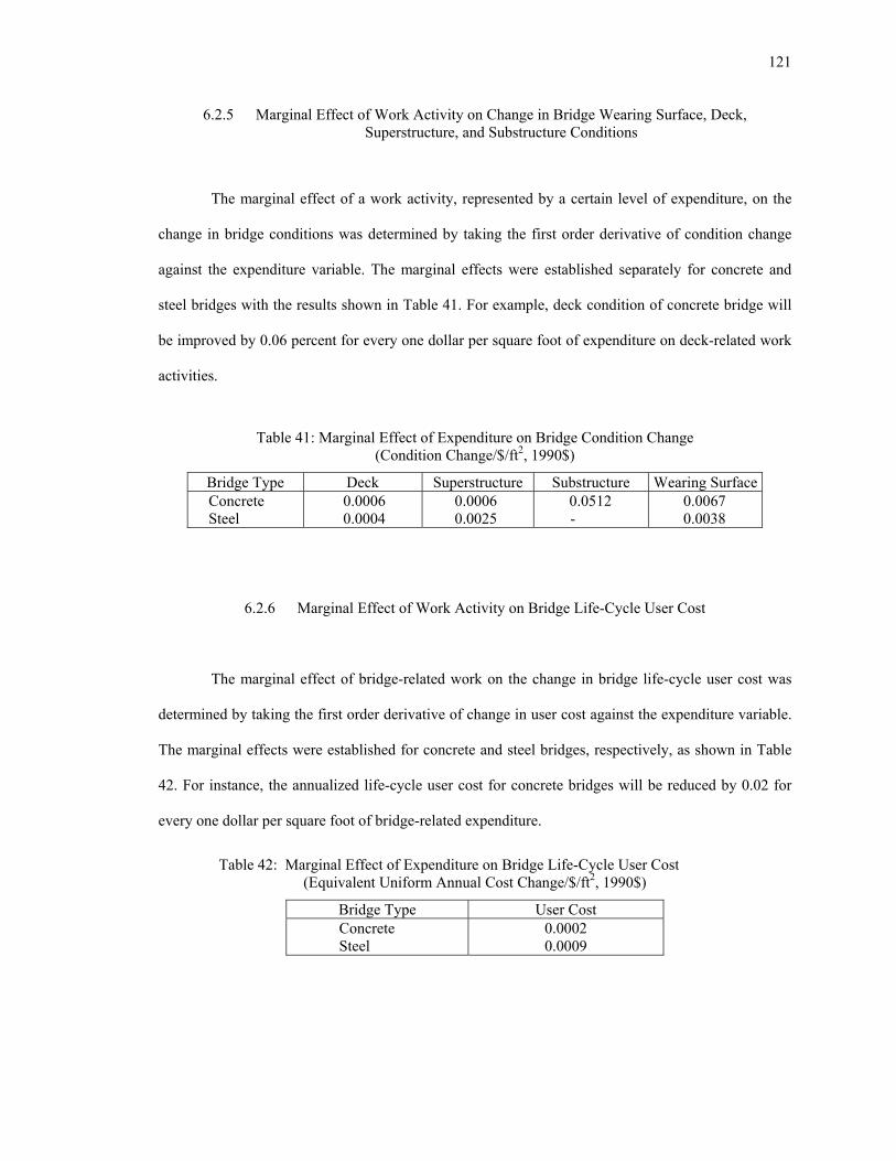
121
6.2.5 Marginal Effect of Work Activity on Change in Bridge Wearing Surface, Deck, Superstructure, and Substructure Conditions
The marginal effect of a work activity, represented by a certain level of expenditure, on the
change in bridge conditions was determined by taking the first order derivative of condition change
against the expenditure variable. The marginal effects were established separately for concrete and
steel bridges with the results shown in Table 41. For example, deck condition of concrete bridge will
be improved by 0.06 percent for every one dollar per square foot of expenditure on deck-related work
activities.
Table 41: Marginal Effect of Expenditure on Bridge Condition Change
(Condition Change/$/ft2, 1990$)
Bridge Type Deck Superstructure Substructure Wearing SurfaceConcrete Steel
0.0006 0.0004
0.0006 0.0025
0.0512 -
0.0067 0.0038
6.2.6 Marginal Effect of Work Activity on Bridge Life-Cycle User Cost
The marginal effect of bridge-related work on the change in bridge life-cycle user cost was
determined by taking the first order derivative of change in user cost against the expenditure variable.
The marginal effects were established for concrete and steel bridges, respectively, as shown in Table
42. For instance, the annualized life-cycle user cost for concrete bridges will be reduced by 0.02 for
every one dollar per square foot of bridge-related expenditure.
Table 42: Marginal Effect of Expenditure on Bridge Life-Cycle User Cost (Equivalent Uniform Annual Cost Change/$/ft2, 1990$)
Bridge Type User Cost Concrete Steel
0.0002 0.0009

122
6.3 Marginal Effects Based on Network-Level Highway User Cost Models
According to the calibrated models for individual user cost components, the significant
variables affecting user cost components were road condition and vehicle traveling speed. The
marginal effects of road condition and vehicle speed on respective user cost components were
therefore determined by taking the first-order derivative of the respective equations. The marginal
effects established are listed in Table 43. For instance, all other things being equal, vehicle operating
cost per mile for passenger cars traveling in rural areas will increase by 2 cents for 100 inches per mile
increase in IRI of pavement surface condition. Similarly, keeping other factors constant, vehicle
operating cost associated with passenger cars using rural highways will reduce by 5.6 cents for every
10 miles per hour increase in vehicle traveling speed.
Table 43: Marginal Effects of Pavement Surface Condition and Average Vehicle Speed on Individual
User Cost Components
Marginal Effect on User Cost Component
Land Use Vehicle Class/ Highway Class
Change in Pavement Condition
(per inch/mile increase)
Change in Speed (per mph increase)
Rural Passenger Car Single Unit Truck Multiple Unit Truck
0.0002 0.0001 0.0015
-0.0056 -0.0008 -0.0085 Vehicle
Operating Cost (1990$/VMT) Urban
Passenger Car Single Unit Truck Multiple Unit Truck
- 0.000013
0.0002
-0.0073 -0.0003 -0.0012
Rural Interstate Non-Interstate - -0.0005
-0.0004 Travel Time (hour/VMT) Urban Interstate
Non-Interstate - -0.0005 -0.0001
Collision Rate (No./MVMT) All Area All Vehicle Type - 0.1595
Air Pollution (kg/VMT)
All
Passenger Car Single Unit Truck Multiple Unit Truck
- 0.0001 0.0001 0.0001
Rural Passenger Car Single Unit Truck Multiple Unit Truck
0.0009 0.0012 0.0025
-0.0041 -0.0008 -0.0080 User Cost
(1990$/VMT) Urban
Passenger Car Single Unit Truck Multiple Unit Truck
0.0014 0.0017 0.0011
-0.0078 -0.0062 -0.0075

123
6.4 Project Benefits under Individual Asset Management System Goals
6.4.1 Benefits on Pavement Rehabilitation Interval and Life-Cycle Agency Cost
The direct benefit of an increased level of routine maintenance is a lengthening of the
rehabilitation interval. However, a higher rehabilitation interval will lead to a higher level of
cumulative traffic loading within the service interval under a steady traffic condition. As a result of
added cumulative traffic loading, a higher level of total rehabilitation expenditure is then required to
repair pavement damages caused by load and non-load factors. In order to determine the relative
benefits to the life-cycle agency cost, comprised of routine maintenance and rehabilitation
expenditure, the difference in life-cycle agency cost for two different levels of routine maintenance
and rehabilitation expenditures under two rehabilitation intervals was established using the concept of
Equivalent Uniform Annual Cost (EUAC). The method is illustrated as follows:
Denote
ARME1 = Annual routine maintenance level 1, in dollars/lane-mile/year
ARME2 = Annual routine maintenance level 2 (higher), in dollars/lane-mile/year
RI1 = Rehabilitation interval at routine maintenance level 1, in years
RI2 = Rehabilitation interval at routine maintenance level 2, in years
REHAB1 = Rehabilitation expenditure needed for rehabilitation interval 1,
in dollars/lane-mile
REHAB2 = Rehabilitation expenditure needed for rehabilitation interval 2,
in dollars/lane-mile
i = Discount rate, in %.

124
The benefits of service life and agency cost are therefore established as
1. Rehabilitation Interval: ∆RI = RI2-RI1
2. Routine Maintenance: ∆EUACARME = ARME2-ARME1
3. Rehabilitation: ( )nn i1
1REHABPW+
⋅=
( )
( ) ( ) ⎥⎦
⎤⎢⎣
⎡
−+
⋅=⎥
⎦
⎤⎢⎣
⎡
−++
⋅=1i1
iREHAB1i1
i1iPWEUAC nn
n
n
nn
( ) ( ) ⎥
⎦
⎤⎢⎣
⎡
−+
⋅−⎥
⎦
⎤⎢⎣
⎡
−+
⋅=
1i1
iREHAB
1i1
iREHAB∆EUAC
1
1
2
2
RIRI
RIRI
REHAB
6.4.2 Benefits of Vehicle Operating Cost, Travel Time, Collision Rate and Air Pollution Rate per Vehicle Mile of Travel during Road Service Life
As life-cycle cost analysis was conducted for maintenance and rehabilitation expenditures in
determining the system benefits, it was desirable to evaluate the vehicle operating cost, travel time,
collision rate, and vehicle air pollution rate per VMT for the same service life. The vehicle operating
cost per VMT was computed in dollars annually during the road service life. As such, it could be
discounted to present worth and then to an EUAC value over the road service life. However, the travel
time, vehicle collision rate, and air pollution rate per VMT in each year were calculated in terms of
hours, number of collisions, and kilograms per VMT, respectively. As these values were not converted
into dollars, they could not be discounted over the road service life. Therefore, to make the
comparison of benefits compatible with the concept of life-cycle cost analysis, the respective average
values for travel time, collision rate, and air pollution rate per VMT during the road service life were
computed. This procedure is illustrated as follows:
(45)
(46)
(49)
(48)
(47)
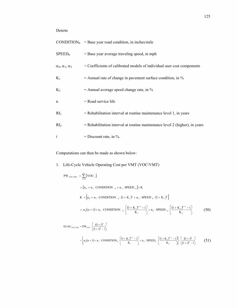
125
Denote
CONDITION0 = Base year road condition, in inches/mile
SPEED0 = Base year average traveling speed, in mph
α0, α1, α2 = Coefficients of calibrated models of individual user cost components
K1 = Annual rate of change in pavement surface condition, in %
K2 = Annual average speed change rate, in %
n = Road service life
RI1 = Rehabilitation interval at routine maintenance level 1, in years
RI2 = Rehabilitation interval at routine maintenance level 2 (higher), in years
i = Discount rate, in %.
Computations can then be made as shown below:
1. Life-Cycle Vehicle Operating Cost per VMT (VOC/VMT)
[ ]
[ ]
( ) ( )[ ]
( ) ( ) ( )⎥⎦
⎤⎢⎣
⎡ −+⋅⋅+⎥
⎦
⎤⎢⎣
⎡ −+⋅⋅++=
+⋅⋅++⋅⋅++
+⋅+⋅+=
=
++
=∑
2
1n2
021
1n1
010
n202
n1010
02010
n
0ttVOC/VMT
K1K1SPEEDα
K1K1CONDITIONα1nα
K1SPEEDαK1CONDITIONαα
SPEEDαCONDITIONαα
VOCPW
Κ
Κ
( )( )
( ) ( ) ( ) ( )( ) ⎥
⎦
⎤⎢⎣
⎡
−++
⋅⎪⎭
⎪⎬⎫
⎪⎩
⎪⎨⎧
⎥⎦
⎤⎢⎣
⎡ −+⋅⋅+⎥
⎦
⎤⎢⎣
⎡ −+⋅⋅++=
⎥⎦
⎤⎢⎣
⎡
−++
⋅=
++
1i1i1i
K1K1
SPEEDαK
1K1CONDITIONα1nα
1i1i1iPWEUAC
n
n
2
1n2
021
1n1
010
n
n
VOCVOC/VMT
(51)
(50)
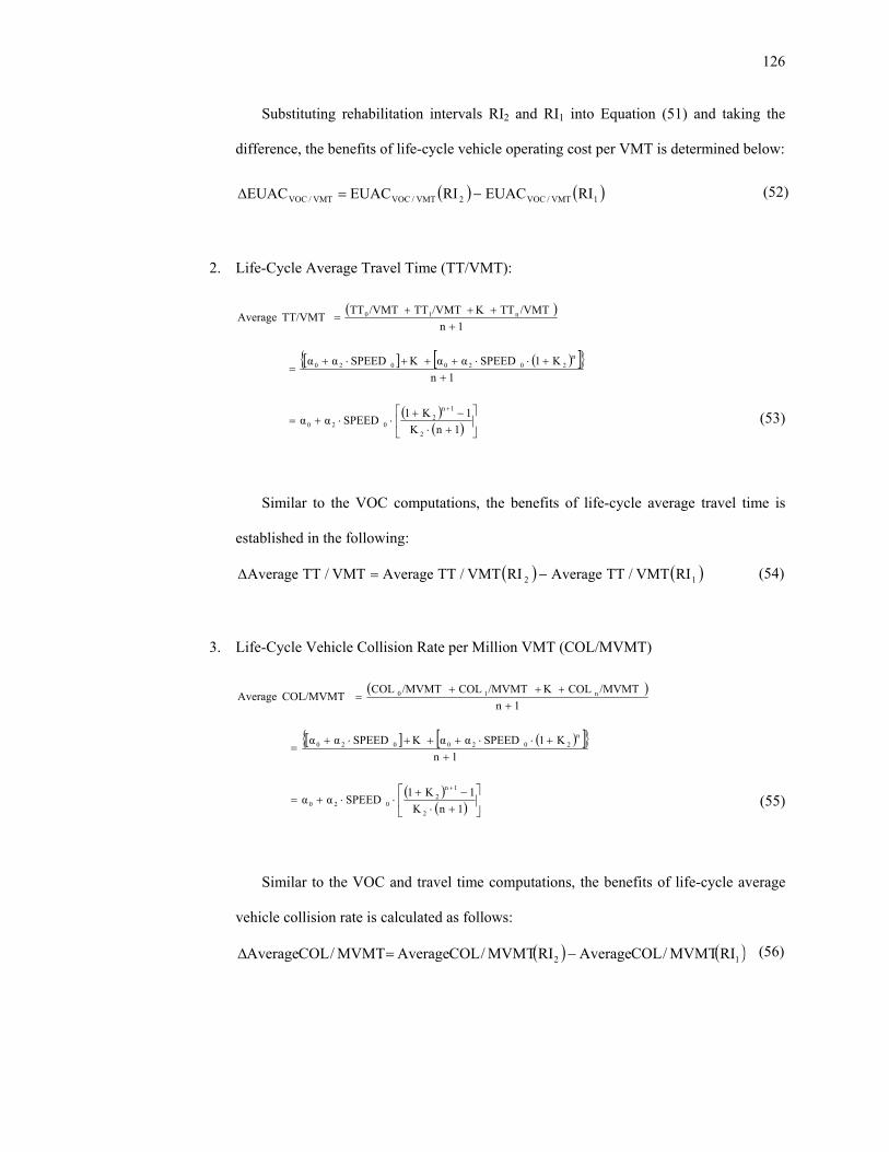
126
Substituting rehabilitation intervals RI2 and RI1 into Equation (51) and taking the
difference, the benefits of life-cycle vehicle operating cost per VMT is determined below:
( ) ( )1VMT/VOC2VMT/VOCVMT/VOC RIEUACRIEUACEUAC −=∆
2. Life-Cycle Average Travel Time (TT/VMT):
( )
[ ] ( )[ ]{ }
( )( ) ⎥
⎦
⎤⎢⎣
⎡
+⋅−+
⋅⋅+=
++⋅⋅+++⋅+
=
++++
=
+
1nK1K1SPEEDαα
1nK1SPEEDααSPEEDαα
1n/VMTTT/VMTTT/VMTTTTT/VMTAverage
2
1n2
020
n2020020
n10
Κ
Κ
Similar to the VOC computations, the benefits of life-cycle average travel time is
established in the following:
( ) ( )12 RIVMT/TTAverageRIVMT/TTAverageVMT/TTAverage −=∆
3. Life-Cycle Vehicle Collision Rate per Million VMT (COL/MVMT)
( )
[ ] ( )[ ]{ }
( )( ) ⎥
⎦
⎤⎢⎣
⎡
+⋅−+
⋅⋅+=
++⋅⋅+++⋅+
=
++++
=
+
1nK1K1SPEEDαα
1nK1SPEEDααSPEEDαα
1n/MVMTCOL/MVMTCOL/MVMTCOLCOL/MVMTAverage
2
1n2
020
n2020020
n10
Κ
Κ
Similar to the VOC and travel time computations, the benefits of life-cycle average
vehicle collision rate is calculated as follows:
( ) ( )12 RIMVMT/COLAverageRIMVMT/COLAverageMVMT/COLAverage −=∆
(53)
(55)
(52)
(54)
(56)

127
4. Life-Cycle Air pollution Rate per VMT (POL/VMT)
( )
[ ] ( )[ ]{ }
( )( ) ⎥
⎦
⎤⎢⎣
⎡
+⋅−+
⋅⋅+=
++⋅⋅+++⋅+
=
++++
=
+
1nK1K1SPEEDαα
1nK1SPEEDααSPEEDαα
1RI/VMTPOL/VMTPOL/VMTPOLPOL/VMTAverage
2
1n2
020
n2020020
2
n10
Κ
Κ
Similar to the vehicle operating cost, travel time, and vehicle collision rate
computations, the benefits of life-cycle average air pollution rate is calculated as follows:
( ) ( )12 RIVMT/POLAverageRIVMT/POLAverageVMT/POLAverage −=∆
These relationships were used to estimate impacts on individual highway asset management
system goals due to the implementation of various projects, as explained in Chapter 3.
6.5 Chapter Summary
This chapter focused on establishing the marginal effects of factors that influenced the
performance of physical highway assets as well as asset usage at the network level. The marginal
effects were established on the basis of calibrated performance models. The marginal benefit was then
determined on the basis of the marginal effects established. Specifically, marginal benefit analysis was
conducted for pavement and bridge-related projects and network level user cost components that
include vehicle operation, travel time, vehicle collision rate, and air pollution rate per mile of travel.
(57)
(58)

128
1
2
3
4 5
6
7 CHAPTER 7 TRADEOFF ANALYSIS
7.1 Introduction
In a highway asset management system, there are multiple, non-commensurable system goals.
In order to facilitate tradeoffs between different candidate projects under equal parameters, project
benefits that achieve individual system goals measured by various performance indicators require
conversion into a non-dimensional unit. In the present study, the conversion procedure was achieved
by developing systemwide multiattribute utility functions for individual highway asset management
programs of which the various candidate projects are a part.
Risk analysis was also incorporated into the tradeoff decision process. This study first
identified performance indicators involving risk occurrence, and for each performance indicator
identified, a probability distribution of its possible outcomes as a result of project implementation was
selected and the distribution parameters were then calibrated using existing Indiana state highways
data. In the course of tradeoff analysis for candidate projects under a risk situation, systemwide
multiattribute utility functions developed for tradeoffs under certainty were used to establish non-
dimensional units as project benefits. However, instead of using utility values, the expected utility
values were computed.
In addition to considering a risk situation, the present study further extended the tradeoff
analysis by incorporating uncertainty into the decision procedure. For tradeoff analysis under
uncertainty, the constraint of establishing a probability distribution for the possible outcomes of a
performance indicator was removed, which directly invalidated the application of the utility theory for
tradeoff decision-making. An alternative approach, based on Shackle’s model [Shackle, 1949], as
mentioned in Section 3.8.4, was then applied to derive a commensurable value from non-

129
commensurable benefits under various system goals associated with a specific candidate project. It
should be noted that, similar to tradeoff analysis under risk, the performance indicators included under
uncertainty were those also dealing with system usage, where uncertainty is normally encountered.
This chapter discusses a systematic procedure to develop systemwide mutiattribute utility functions
for tradeoff analysis under certainty and risk and focus gain-over-loss ratio functions for dealing with
uncertainty.
7.2 Preparation of Data Collection
In the course of establishing tradeoff relationships, a series of questionnaire surveys were
administered. These questionnaires were organized to acquire data to establish the relative weights of
asset management system goals, relative weights of multiple performance indicators under individual
system goals, single attribute utility functions for individual performance indicators, and degree of
surprise functions and priority functions for performance indicators involving uncertainty in the
tradeoff decision process.
Two factors were considered in the survey process: survey approach for the preparation of
questionnaires and decision group represented by survey participants. For the purpose of establishing
the relative weights of asset management system goals and performance indicators and also for
assigning weighting indices to reflect the decision-maker’s degree of surprise and priority, a direct
weighting approach was used to prepare survey questionnaires. A weighting scaling from 1 to 10 was
used to reflect increased order of importance. In addition, instead of using the direct weighting
approach, the certainty equivalency approach, as an alternative, was added to prepare the survey
questionnaires to assess the robustness of survey results. The lower and upper ranges of various
performance indicators considered for establishing the utility functions, and the deviations of
outcomes of performance indicators involving uncertainty are listed in Appendix K. During the course
of the questionnaire surveys, both the highway agency and the user groups were considered.
130
Specifically, survey attendants representing the agency group consisted of the INDOT leadership,
while participants representing the user group were randomly selected in the greater Lafayette area.
7.3 Relative Weights of Highway Asset Management System Goals
7.3.1 Data Collection
Twenty nine INDOT personnel, including executive staff, district directors and division
chiefs participated in the survey as a group in one session, while twenty eight Purdue employees,
including faculty members, staff, and students, participated in the survey in another session. The
Delphi technique discussed in Section 3.8.1.2 was followed for the two decision groups. A weighting
scale from 1 (least important) to 10 (most important) was adopted to establish the relative weights of
asset management goals.
7.3.2 Establishment of Relative Weights of Highway Asset Management System Goals
The descriptive statistics of the relative weights assigned in the final round are listed in
Appendix L1. It was found that, for participants within each group, the relative weights established in
the final round were quite consistent. Also, the standard deviations in the final round tended to be
narrower, indicating a higher level of consensus. However, there were differences in the average and
standard deviation values of the weights assigned by participants in the two decision groups. It was
therefore necessary to arrive at a set of consensus weights that simultaneously considered the mean
and standard deviation values of the assigned weights for each decision group. In this regard, the AHP
technique discussed in Section 2.6.1.1 was applied by conducting pairwise comparisons of the weights
assigned by individual survey participants within each decision group. As the survey participants were
given equal weights, the weights established through AHP technique provided the consensus weights.

131
As seen in Table 44, the order of final consensus weights assigned by the two decision groups
was different. For the agency group, safety received the highest weight, followed by system
preservation, mobility, agency cost, user cost, and the environment. For the user group, while safety
also received the highest weight, the relative weights of other system goals were in the following
order: mobility, environment, system preservation, user cost, and agency cost.
Table 44: Relative Weights of Highway Asset Management System Goals Assigned by the Agency and User Groups
Asset Management System Goal Agency Group User Group System Preservation Agency Cost Highway User Cost Mobility Safety Environment
0.2259 0.1922 0.1776 0.2112 0.2319 0.1715
0.1857 0.1625 0.1795 0.1956 0.2294 0.1911
7.4 Relative Weights of Multiple Performance Indicators under Individual Goals
7.4.1 Data Collection
For some asset management programs, multiple performance indicators were identified to
represent the extent to which a system goal was achieved through the implementation of a candidate
project. For instance, for projects under the bridge preservation program, such performance indicators
as bridge structural condition, wearing surface condition, and remaining service life, were selected to
represent the goal of system preservation. It was therefore necessary to establish the relative weights
of these performance indicators.
A new survey questionnaire was prepared following the similar procedure used for
establishing the relative weights of system goals. Nine additional participants in each decision group
were randomly selected to fill out the new questionnaire to solicit relative weights of multiple
performance indicators within each system goal. The survey was also administered using the Delphi

132
technique discussed in Section 3.8.1.2 based on a weighting scale from 1 (least important) to 10 (most
important).
7.4.2 Establishment of Relative Weights of Multiple Performance Indicators
The descriptive statistics of the relative weights assigned are listed in Appendix L2. The AHP
technique was again utilized to establish the consensus weights of the concerning performance
indicators, and the results are shown in Table 45.
Table 45: Relative Weights of Multiple Performance Indicators Assigned by the Agency and User Groups
Asset Management System Goal
Asset Management Program Performance Indicator Agency
Group User
Group
Bridge Preservation Bridge structural condition Bridge wearing surface condition Bridge remaining service life
0.3971 0.2679 0.3349
0.4162 0.3401 0.2437
Historical Bridge Preservation
Bridge structural condition Bridge wearing surface condition Bridge remaining service life Historical bridge age Historical bridge length
0.2372 0.1652 0.2012 0.2252 0.1712
0.2483 0.1788 0.1954 0.2384 0.1391
System Preservation
Pavement Preservation
Surface condition Remaining service life
0.5000 0.5000
0.5000 0.5000
Bridge Preservation
Bridge construction cost Bridge rehabilitation cost Bridge maintenance cost
0.3535 0.3581 0.2884
0.3769 0.3015 0.3216
Pavement Preservation
Pavement construction cost Pavement rehabilitation cost Pavement maintenance cost
0.3519 0.3565 0.2917
0.3547 0.3153 0.3300
Agency Cost
ITS Improvements Procurement cost Maintenance cost
0.7083 0.2917
0.6700 0.3300
Bridge Preservation Detour condition Vehicle speed
0.4609 0.5391
0.4748 0.5252 User Cost Pavement
Preservation Pavement surface condition Vehicle speed
0.5000 0.5000
0.4662 0.5338

133
Table 45: Relative Weights of Multiple Performance Indicators Assigned by the Agency and User Groups (Continued)
Asset Management System Goal
Asset Management Program Performance Indicator Agency
Group User
Group
Mobility Bridge Preservation Detour length Vehicle speed
0.4965 0.5035
0.5133 0.4867
Bridge Preservation
Bridge inventory rating Bridge clear deck width Bridge vertical clearance (over) Bridge vertical clearance (under) Bridge horizontal clearance
0.1935 0.2143 0.1905 0.2054 0.1964
0.2327 0.2170 0.1950 0.1698 0.1855
Pavement Preservation
Vehicle speed Skid resistance Lane width Shoulder width
0.2720 0.2605 0.2567 0.2107
0.2698 0.2619 0.2619 0.2063
Railroad Crossings Railroad crossing adequacy Occurrence of collisions
0.5267 0.4733
0.4863 0.5137
Safety Sight distance Luminance Occurrence of collisions
0.3709 0.2958 0.3333
0.3397 0.3014 0.3589
Traffic Signals Vehicle speed Occurrence of collisions
0.4589 0.5411
0.4604 0.5396
Safety
DNR/ Forest/ Other
Vehicle speed Skid resistance Lane width
0.3447 0.3301 0.3252
0.3400 0.3300 0.3300
7.5 Single Attribute Utility Functions for Individual Performance Indicators
7.5.1 Data Collection and Processing
In order to develop utility functions corresponding to individual performance indicators,
another survey was conducted with eighteen participants randomly selected from INDOT and Purdue
campus representing the agency and user groups, respectively. The survey was conducted in an
interactive manner. In response to the two questionnaires prepared using the approaches described in
Section 3.8.1.3, an example was illustrated before filling out each questionnaire to allow the
participants to become familiar with the survey approach. Further interactions were made as necessary
during the course of the survey. However, the survey participants were required to fill in the

134
questionnaires independently without having inter-personal discussions. By doing so, it was expected
that as much reliable information as possible could be extracted.
7.5.2 Development of Single Attribute Utility Functions
7.5.2.1 Preparation of Model Calibration
As discussed in Section 3.8.1.3, two different approaches were used to develop utility
functions, the direct questioning approach and the certainty equivalency approach. One of the main
reasons for two different approaches for the two decision groups in the survey process was to verify
whether the utility values assigned would be affected by the approaches used and whether the
interaction between the decision groups and the approaches was significant. These effects were
clarified by ANOVA tests based on a two-factor factorial model as stated in Section 3.8.1.3. The
ANOVA analysis was first conducted using all the data points from the four data sets. It was found
that neither the effects of decision groups, or the approaches, nor their interaction was significant at a
level of significance of 5 percent. This indicated that consistent utility values were assigned by survey
participants irrespective of the survey approaches. In order to further confirm this conclusion, a
second ANOVA test was carried out based on the four sets of data without having the extreme utility
values of 0 and 1. The same conclusion was also reached, given a level of significance of 5 percent,
with only one exception of the performance indicator of intersection delay time. The results of the
two ANOVA tests are listed in Table 46 with p-values given in Appendix M.

135
Table 46: Results of ANOVA Analysis for Utility Values Assigned by the Agency and User Groups Based on Two Approaches (Level of significance at 0.05 with 108 observations)
Factor ANOVA I ANOVA II
Highway Asset Management System Goal
Performance Indicator
Gro
up
App
roac
h
Inte
ract
ion
Gro
up
App
roac
h
Inte
ract
ion
System Preservation
Bridge structural condition Bridge wearing surface condition Historical bridge age Historical bridge length Pavement condition Remaining service life
No No No No No No
No No No No No No
No No No No No No
No No No No No No
No No No No No No
No No No No No No
User Cost Vehicle speed No No No No No No
Mobility Vehicle speed Detour length Intersection delay time
No No No
No No No
No No No
No No No
No No Yes
No No No
Safety
Bridge inventory rating Bridge deck width Bridge vertical clearance- over Bridge vertical clearance- under Bridge horizontal clearance Average speed Skid resistance Lane width Shoulder width Railroad crossing Sight distance Luminance
No No No No No No No No No No No No
No No No No No No No No No No No No
No No No No No No No No No No No No
No No No No No No No No No No No No
No No No No No No No No No No No No
No No No No No No No No No No No No
Environment
Vehicle speed for CO2, TSP, SO2 Vehicle speed for NMHC Vehicle speed for CO Vehicle speed for NOX
No No No No
No No No No
No No No No
No No No No
No No No No
No No No No
Figure 11 shows a plot that displays the difference in utility values assigned based on two
approaches. It can be seen that the direct questioning approach always yielded higher utility values as
opposed to those based on the certainty equivalency approach for the same amount of intersection
delay time. This may be due to the fact that the direct questioning approach is less complicated and
straightforward, while the certainty equivalency approach involves a more detailed and probing
procedure requiring in-depth judgments. Consequently, all four data sets for performance indicators

136
were combined to develop a single set of utility functions for all indicators except that two separate
utility functions were considered for the intersection delay time.
Figure 11: Comparison of Utility Values Assigned by Two Approaches
7.5.2.2 Calibration of Utility Functions and Discussions
The OLS technique was adopted for the calibration of single attribute utility functions.
Descriptive statistics of the utility function modeling data are listed in Appendix N. It was found from
data scatter plots that the basic shapes of the utility functions generally followed either a strict concave
or pseudo-concave pattern, strictly increasing or decreasing, as shown in Figure 12.
Util
ity V
alue

137
Figure 12: Functional Forms Selected for the Calibration of Single Attribute Utility Functions
The calibrated single attribute utility functions are listed in Table 47. As shown in the table,
the calibrated models generally fit well with the modeling data with the exceptions of bridge deck
width and pavement lane width, where the actual-over-desired width ratios exceeded one. Based on
the calibrated models, it was found that the utility values tended to decrease as the actual deck width
and lane width were in excess of the desirable width. This result was consistent with engineering sense
in that when lane width became overly wide it would confuse the highway user and thus would
receive a low utility value. However, given the fairly low adjusted R2 values achieved, it further
revealed that even though the highway user realized the disadvantage of having an extremely wide
lane width, the extent of its disadvantage was as reflected by varying utility values assigned from
person to person.

138
Table 47: Calibrated Utility Functions for Individual Highway Asset Management Performance Indicators (Observations: 108)
System Goal Performance Indicator (x)
Utility Function u(x)
Coefficienta (or b) (t-Statistic) Factor
k Adj.R2
System Preservation
Bridge structural condition Bridge wearing surface Historical bridge age Historical bridge length Pavement surface conditionRemaining service life
k[1 - eax2] k[1 - eax2) k[1 - ea(x-80)] k[1 - ea(x-40)] keax2 k[1 - eax2]
-0.0249 -0.025
-0.0144 -0.0112
-0.000044-0.0195
(-26.91) (-22.17) (-72.74) (-75.98) (-54.25) (-70.92)
1.15351.15211.21601.19991.07291.1659
0.980.980.990.990.990.99
User Cost Average speed k[1 - ea(x-15)] (x ≤ 55) k[1 - ea(75-x)] (x > 55)
-0.0486 -0.0778
(-83.90) (-72.13)
1.16701.1668
0.990.99
Mobility
Average speed Detour length Intersection delay time
k[1 - eax2] keax keax kebx
-0.0005 -0.2145 -0.0982 -0.1772
(-100.78) (-92.02) (-45.81) (-27.71)
1.04251.00001.00001.0000
0.990.990.990.99
Safety
Bridge load inventory ratingBridge deck width Bridge vertical clearance (o)Bridge vertical clearance (u)Bridge horizontal clearance Average speed Skid resistance Lane width Shoulder width Railroad crossing Sight distance Luminance
k[1 - eax2] k[1 - ea(x-0.8)] (x ≤ 1.0) k[1 - ea(1.1-x)] (x > 1.0) k[1 - ea(x-0.8)] k[1 - ea(x-0.8)] k[1 - ea(x-0.8)] keax2 k[1 - ea(x-10)] k[1 - ea(x-0.8)] (x ≤ 1.0) k[1 - ea(1.1-x)] (x > 1.0) k[1 - eax2] k[1 - eax] k[1 - ea(x-0.6)] k[1 - ea(x-0.6)]
-0.0404 -8.5113 -59.2952 -8.2612 -8.2672 -8.2278 -0.0004 -0.0437 -8.2827 -59.6314 -2.4343 -0.6963 -4.5181 -4.6399
(-14.42) (-93.07) (-2.04) (-56.64) (-57.41) (-61.91) (-75.73) (-53.05) (-71.83) (-2.24)
(-166.83) (-37.17) (-89.49) (-94.62)
1.00001.22291.00001.23701.23671.23901.00001.21081.23581.00001.09611.14131.19631.1853
0.950.990.510.990.990.990.990.990.990.570.990.990.990.99
Environment
Speed for CO2, TSP, SO2 Speed for NMHC Speed for CO Speed for NOx
k[1 - ea(x-15)] (x ≤ 55) k[1 - ea(75-x)] (x > 55) k[1 - eax] k[1 - eax] (x ≤ 35) k[1 - ea(65-x)] (x > 35) k[1 - eax] (x ≤ 15) k[1 - ea(65-x)] (x > 15)
-0.0478 -0.0816 -0.0338 -0.0618 -0.0609 -0.0949 -0.0366
(-76.72) (-33.23) (-84.00)
(-119.83) (-83.63)
(-826.00) (-46.96)
1.17341.14951.07171.12991.06901.31731.1021
0.990.990.990.990.990.990.99
Note: The functional forms of utility functions are illustrated in Figure 12, where a or b values are
calibrated coefficients and k values are adjustment factors to ensure a utility value of 1.0 when
performance indicators x are at the most desirable levels.

139
7.6 Probability Distribution Parameters for Performance Indicators Involving Risk in Tradeoff Decision Process
The underlying assumption of incorporating risk analysis into the tradeoff decision process
was that a probability distribution could be assigned to the possible outcomes of a performance
indicator as a result of implementing a certain project. Probability distribution parameters were
calibrated for discrete and continuous performance indicators based on binomial and beta
distributions, respectively. The field data available from INDOT were used to develop these
distribution parameters.
7.6.1 Data Preparation
For discrete performance indicators such as bridge deck, superstructure, substructure, and
wearing surface conditions, the respective histograms were first prepared. This information was then
utilized directly to calibrate the parameters for the binomial distribution on the basis of Poisson
approximation. For continuous performance indicators, the descriptive statistics, including mean,
minimum, maximum, and standard deviation, were first explored. Histograms corresponding to
individual performance indicators were comprised of five data points, i.e., two ranges below and two
ranges above the mean, were created according to the descriptive statistical information. Modeling
calibration was then conducted accordingly. The descriptive statistics of data values of individual
performance indicators are listed in Appendix O.
7.6.2 Calibration of Probability Distribution Parameters
The Slover tool in Excel spreadsheet was used to establish the parameters for binomial and
beta distribution parameters. The tool utilizes Newton’s search algorithm to find the optimal solution

140
by minimizing the sum of the squared deviations between the observed probability mass or density
function values and those calculated on the basis of the calibrated binomial or beta parameters. The
convergence level was set at 0.0001 with 1000 iterations each time. The calibrated parameters are
listed in Tables 48-54.
Table 48: Calibrated Parameters of Binomial Distribution for Bridge Structural and Wearing Surface Condition Ratings
Binomial Distribution Parameter (p) Bridge Type
Component Initial Condition Observations 3
(n= 60)4
(n= 50)5
(n= 40)6
(n= 30) 7
(n= 20) 8
(n= 10)
Concrete
Deck Superstructure Substructure Wearing Surface
4,230 1,097
464 4,230
0.009 0.167 0.167 0.089
0.200 0.200 0.028 0.100
0.046 0.056 0.022 0.173
0.031 0.063 0.017 0.040
0.015 0.025 0.017 0.018
0.018 0.012 0.069 0.069
Steel
Deck Superstructure Substructure Wearing Surface
3,218 422 252
3,218
0.167 0.167 0.167 0.114
0.180 0.200 0.200 0.112
0.125 0.054 0.017 0.077
0.133 0.057 0.043 0.042
0.150 0.018 0.069 0.049
0.154 0.050 0.030 0.069
Table 49: Calibrated Parameters of Beta Distribution for Bridge Remaining Service Life, Detour Length, and Load Inventory Ratings
Beta Distribution Parameters Bridge Type (Observations) Item
α β
Concrete (4,922)
AADT Age Remaining service life Load inventory rating Detour length Average expenditure Agency cost User cost
1.38 2.75 1.10 3.29 2.74 4.50 2.17 2.12
1.10 2.67 1.80 4.50 4.50 4.31 4.50 4.50
Steel (3,414)
AADT Age Remaining service life Load inventory rating Detour length Average expenditure Agency cost User cost
2.83 2.60 1.10 2.99 3.03 2.97 2.39 2.17
4.50 2.39 1.67 4.50 4.50 2.75 4.50 4.50

141
Table 50: Calibrated Parameters of Beta Distribution for Pavement Surface Condition
Beta Distribution Parameters Pavement Type Highway Class Observations
α β
Flexible Interstate Non-Interstate
172 1,884
3.09 2.83
4.50 2.80
Rigid Interstate Non-Interstate
172 303
4.36 2.35
4.50 2.19
Composite Interstate Non-Interstate
818 2,720
3.47 3.92
4.50 4.50
Table 51: Calibrated Parameters of Beta Distribution for Pavement Maintenance, Rehabilitation, and Construction Expenditures
Beta Distribution Parameters Pavement Type
Expenditure Category
Observations α β
Flexible Maintenance Rehabilitation Construction
1,343 202 218
2.27 2.56 2.49
4.50 4.50 4.50
Rigid Maintenance Rehabilitation Construction
226 49 74
3.10 2.41 2.25
4.50 4.50 4.50
Composite Maintenance Rehabilitation Construction
2,470 621 988
2.78 2.41 2.17
4.50 4.50 4.50
Table 52: Calibrated Parameters of Beta Distribution for Average Traveling Speed
Beta Distribution Parameters Land Area (Observations) Highway Class
α β
Rural (11)
Rural interstate Rural principle arterial Rural minor arterial Rural major collector
1.22 1.16 4.50 4.50
1.17 1.15 2.70 2.98
Urban (11)
Urban interstate Urban freeway and expressway Urban principal arterial Urban minor arterial Urban collector
1.16 1.17 1.15 1.43 1.30
1.36 1.15 1.12 1.18 1.20

142
Table 53: Calibrated Parameters of Beta Distribution for Intersection Delay Time
Beta Distribution Parameters Land Area (Observations)
Highway Class Vehicle Class
α β
Interstate Passenger car Single unit truck Multiple unit truck
1.22 3.11 1.24
1.14 2.99 1.15 Rural
(11) Non-Interstate
Passenger car Single unit truck Multiple unit truck
1.15 1.22 1.11
1.13 1.14 1.13
Interstate Passenger car Single unit truck Multiple unit truck
4.20 3.91 1.10
4.50 4.50 1.38 Urban
(11) Non-Interstate
Passenger car Single unit truck Multiple unit truck
1.32 1.16 1.14
1.37 1.30 1.18
Table 54: Calibrated Parameters of Beta Distribution for Vehicle Collision Rate
Beta Distribution Parameters Collision Type Observations α β
Fatality Injury Property Damage
11 11 11
2.40 1.18 2.56
2.37 1.15 2.48
All 11 1.26 1.13
7.6.3 Discussions
The calibrated parameters for binomial distribution were quite reasonable, as indicated by the
relatively low p-parameter values. In fact, most of the parameters were on the order of less than 0.1.
This generally validated the assumption of using Poisson approximation for binomial distribution in
that a relatively large number of variable levels and low parameter values were required. The binomial
parameters indicated that the distributions for bridge deck, superstructure, substructure, and wearing
surface conditions skewed to the left, which provided evidence that the condition ratings were
generally distributed above the average levels.

143
For pavement surface condition, agency cost, detour length and bridge load inventory rating,
the distributions skewed to the right, revealing that a higher portion of pavement segments in the
network had a condition rating better than network average and that maintenance, rehabilitation, or
construction expenditure was below network average. Additionally, a higher number of bridges were
found to have a detour length shorter than network average and that the load inventory rating was
below the network average. For the remaining service life, average speed, and collision rate, the
calibrated beta parameters indicated that the beta distributions skewed to the left, meaning that a
higher number of state-maintained highway bridges had remaining service lives that were above
network average, and that the vehicle speed and collision rate for a higher number of years were
slightly higher than the respective network average.
7.7 Standardized Focus Gain-over-Loss Functions for Performance Indicators Involving Uncertainty in Tradeoff Decision Process
7.7.1 Data Collection
In order to establish the decision maker’s degree of surprise and priority weighting indices
corresponding to different levels of deviations from the expected values for the underlying
performance indicators, another survey was prepared with two questionnaires. Thirteen people,
randomly selected from the Purdue campus, participated in the survey process.
Because of the long and involved nature of the two questionnaires, a relatively long time
(about two hours) was involved for each participant. Therefore, participants were compensated for
their time to complete the questionnaires. The theory behind the degree of surprise function was that
people were subject to assigning higher weights to reflect their degree of surprise when encountering
larger deviations in the possible outcomes, as compared to their expectations. On the other hand, when
the degree of surprise and outcome pair were considered simultaneously, the priority index to be
assigned would be different. Correspondingly, a priority function could thus be established. In the

144
course of preparing the two survey questionnaires, ten different ranges of deviations were considered
for each of the performance indicators. For a specific range of deviations, survey participants were
asked to assign a weight index using a scale from 0 (no surprise or least priority) to 10 (highest degree
of surprise or highest priority) to ten different outcome values of a specific performance indicator. The
ranges of deviations selected for individual performance indicators are listed in Appendix P.
7.7.2 Development of Degree of Surprise and Priority Functions
The OLS techniques were used to calibrate the degree of surprise and priority functions.
Based on the nature of these functions as discussed in Section 3.8.4.2, quadratic functional form was
selected to relate the degree of surprise with the possible outcomes of the underlying performance
indicator and also to establish relationship of priority indices with the outcomes and degree of surprise
pairs. The calibrated surprise and priority functions are presented in Appendices Q and R,
respectively.
7.7.3 Establishment of Standard Gain-over-Loss Ratios
The priority function followed a saddle shape with one maximum priority at the gain from the
expectation side and one maximum priority at the loss from the expectation side. The two outcomes of
the underlying performance indicator with the maximum priority values were focus gain and focus
loss values. As the focus gain and loss values were in fact associated with a certain degree of
uncertainty, it was therefore necessary to filter out the uncertainty attached. The standardized focus
gain and loss values with zero degree of surprise were obtained from the priority indifference curves
at both the gain and the loss sides where the priority weights were equivalent to the respective
maximum priorities. The standardizing process is illustrated in Figure 13 using the focus gain case.

145
Figure 13: Standardization of Focus Gain Value
Denote
f(∆x) = Degree of surprise function, set f(∆x) = c.∆x2
φ1(∆x, y) = Priority indifference function, set φ1(∆x, y) = α1.∆x0.5 - β1.y2 = k (k ≥ 0)
φ2(∆x, y) = Maximum priority indifference function, φ2(∆x, y) = α2.∆x0.5 - β2.y2 = φmax
∆x1 = Gain value on indifference curve φ1(∆x, y) with no surprise
∆xφmax = Focus gain value
∆xstd-φmax = Standardized focus gain value
A, B are points on φ1(∆x, y), and O is a point on φ2(∆x, y).
The purpose was to find the standardized focus gain ∆xstd-φmax from the underlying focus gain
∆xφmax on the same priority indifference curve φ2(∆x, y). As the maximum priority indifference curve
φ2(∆x, y) only intersects with the degree of surprise function f((∆x) once at point O, it would be

146
impractical to progress with the standardization process directly due to the fact that it is impossible to
calibrate two parameters α2 and β2 for φ2(∆x, y) based on one point on the curve. However,
information can be utilized from the indifference curve adjacent to φ2(∆x, y) to accomplish this
process. As shown in Figure 13, when the priority indifference curve φ1(∆x, y) comes close to φ2(∆x,
y), the standardized gain value ∆x1 for φ1(∆x, y) tends to merge with the standardized focus gain ∆xstd-
φmax. Hence, the problem reduces to establish a mathematical expression for the standardized gain
value ∆x1.
For points A and B on priority indifference curve φ1(∆x, y), we have
α1.∆xA
0.5 - β1.yA
2 = k
α1.∆xB
0.5 - β1.yB
2 = k
Substituting yA= ∆xA2 and yB= ∆xB
2 into Equations (59) and (60), and solving them
simultaneously, we obtain
( )( )4
15.0
25.0
142
41
42
1 xxxxxxk
∆⋅−⋅∆∆−∆
=α
For point (∆x1, 0) on φ1(∆x, y), we get φ1(∆x, y)= α1
.∆x10.5 -β1
.02 or φ1(∆x, y)= α1.∆x1
0.5, thus,
( ) 2
1
111
0,xx ⎥⎦
⎤⎢⎣
⎡α∆φ
=∆
Hence, ( )( )
2
41
42
41
5.02
5.01
42
max
2
1
maxmaxstd xxk
xxxxx ⎥⎦
⎤⎢⎣
⎡∆−∆
∆⋅−⋅∆⋅φ=⎥
⎦
⎤⎢⎣
⎡α
φ≈∆ −
Following this procedure, the maximum priority, φmax, and the corresponding standardized
focus gain and loss values, ∆xstd-φmax, were established as listed in Table 55.
(59)
(60)
(61)
(62)
(63)
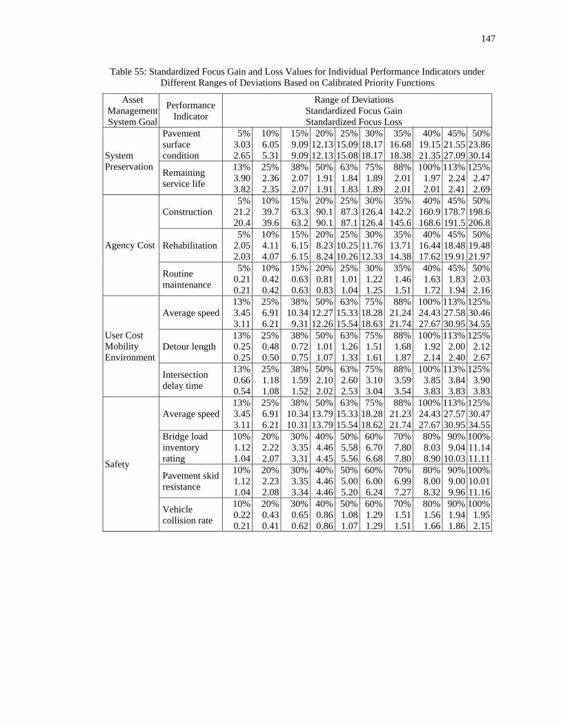
147
Table 55: Standardized Focus Gain and Loss Values for Individual Performance Indicators under Different Ranges of Deviations Based on Calibrated Priority Functions
Asset Management System Goal
Performance Indicator
Range of Deviations Standardized Focus Gain Standardized Focus Loss
Pavement surface condition
5%3.03 2.65
10%6.05 5.31
15%9.09 9.09
20%12.13 12.13
25%15.09 15.08
30%18.17 18.17
35% 16.68 18.38
40% 19.15 21.35
45%21.55 27.09
50%23.86 30.14 System
Preservation Remaining service life
13%3.903.82
25%2.362.35
38%2.072.07
50%1.911.91
63%1.841.83
75%1.891.89
88% 2.01 2.01
100% 1.97 2.01
113%2.242.41
125%2.472.69
Construction 5%
21.2 20.4
10%39.7 39.6
15%63.3 63.2
20%90.1 90.1
25%87.3 87.1
30%126.4 126.4
35% 142.2 145.6
40% 160.9 168.6
45%178.7 191.5
50%198.6 206.8
Rehabilitation 5%
2.05 2.03
10%4.11 4.07
15%6.15 6.15
20%8.23 8.24
25%10.25 10.26
30%11.76 12.33
35% 13.71 14.38
40% 16.44 17.62
45%18.48 19.91
50%19.48 21.97
Agency Cost
Routine maintenance
5%0.21 0.21
10%0.42 0.42
15%0.63 0.63
20%0.81 0.83
25%1.01 1.04
30%1.22 1.25
35% 1.46 1.51
40% 1.63 1.72
45%1.83 1.94
50%2.03 2.16
Average speed 13%3.45 3.11
25%6.91 6.21
38%10.34 9.31
50%12.27 12.26
63%15.33 15.54
75%18.28 18.63
88% 21.24 21.74
100% 24.43 27.67
113%27.58 30.95
125%30.46 34.55
Detour length 13%0.25 0.25
25%0.48 0.50
38%0.72 0.75
50%1.01 1.07
63%1.26 1.33
75%1.51 1.61
88% 1.68 1.87
100% 1.92 2.14
113%2.00 2.40
125%2.12 2.67
User Cost Mobility Environment
Intersection delay time
13%0.66 0.54
25%1.18 1.08
38%1.59 1.52
50%2.10 2.02
63%2.60 2.53
75%3.10 3.04
88% 3.59 3.54
100% 3.85 3.83
113%3.84 3.83
125%3.90 3.83
Average speed 13%3.45 3.11
25%6.91 6.21
38%10.34 10.31
50%13.79 13.79
63%15.33 15.54
75%18.28 18.62
88% 21.23 21.74
100% 24.43 27.67
113%27.57 30.95
125%30.47 34.55
Bridge load inventory rating
10%1.12 1.04
20%2.22 2.07
30%3.35 3.31
40%4.46 4.45
50%5.58 5.56
60%6.70 6.68
70% 7.80 7.80
80% 8.03 8.90
90%9.04
10.03
100%11.14 11.11
Pavement skid resistance
10%1.12 1.04
20%2.23 2.08
30%3.35 3.34
40%4.46 4.46
50%5.00 5.20
60%6.00 6.24
70% 6.99 7.27
80% 8.00 8.32
90%9.00 9.96
100%10.01 11.16
Safety
Vehicle collision rate
10%0.22 0.21
20%0.43 0.41
30%0.65 0.62
40%0.86 0.86
50%1.08 1.07
60%1.29 1.29
70% 1.51 1.51
80% 1.56 1.66
90%1.94 1.86
100%1.95 2.15

148
7.7.4 Development of Standardized Gain-over-Loss Ratio Functions
After obtaining standardized focus gain and focus loss values in accordance with the different
ranges of deviations of the outcomes from the expectation, it was necessary to further investigate the
relationship between the gain-over-loss ratios with the ranges of deviations for individual performance
indicators. To this end, standardized gain-over-loss ratios were first computed and standardized gain-
over-loss ratio functions were then calibrated using the OLS techniques. Descriptive statistics of the
ratios for individual performance indicators are listed in Appendix S, and the standardized gain-over-
loss ratio functions calibrated are shown in Table 56. It was found from the calibrated functions that
the standardized gain-over-loss ratio would decrease as the range of deviations became larger, which
indicated that people were inclined to pose a higher weight to losses from their expectations as the
deviation ranges became larger compared to gains. The models can be used to establish standardized
gain-over-loss ratios for a performance indicator provided that the range of deviations of possible
outcomes is given.
Table 56: Calibrated Standardized Gain-over-Loss Ratio Functions for Individual Performance Indicators (Observations: 10)
SGLR = α0 + α1. Range of Deviation Goal Performance Indicator α0 (t-statistic) α1 (t-statistic)
Adjusted R2
System Preservation
Pavement condition Remaining service life
1.1785 1.0380
(46.55)(72.61)
-0.7683-0.0759
(-9.42) (-4.12)
0.91 0.64
Agency Cost Construction Rehabilitation Routine maintenance
1.0382 1.0398 1.0132
(106.66)(106.12)(216.41)
-0.1847-0.2647-0.1538
(-5.89) (-8.38) (-0.19)
0.79 0.89 0.92
User Cost Mobility Environment
Vehicle speed Detour length Intersection delay time
1.1535 1.02511.1414
(58.04)(64.62)(38.17)
-0.2331-0.2070-0.1572
(-9.10) (-7.68) (-3.45)
0.90 0.87 0.55
Safety
Vehicle speed Bridge load inventory Skid resistance Collision rate
1.12481.09241.08341.0750
(56.36)(69.61)(76.77)(88.34)
-0.1330-0.1791-0.1887-0.1526
(-8.05) (-7.08) (-8.30) (-7.78)
0.88 0.85 0.88 0.87

149
7.8 Systemwide Multiattribute Utility Functions for Tradeoffs under Certainty and Risk
7.8.1 Multiattribute Utility Functions under Individual System Goals
Some individual system goals have a number of performance indicators. The utility and
preference values for these performance indicators are independent of each other. Therefore, an
additive form was selected to combine utility functions of performance indicators within a system goal
to establish the goal-specific function, as defined below:
∑=
⋅=iK
1kikiki )u(xw)U(X
where
U(Xi) = Goal-specific multiattribute utility function for a specific asset management
program, i = 1, 2, 3, 4, 5, and 6 for system preservation, agency cost, user cost,
mobility, safety, and environment
wik = Relative weight of performance indicator k under goal i
u(xik) = Single attribute utility function for performance indicator k under goal i
Ki = Number of performance indicators under goal i.
7.8.2 Systemwide Multiattribute Utility Functions
The additive form used for combining performance indicators under individual system goals
could not be used for combining all goals into systemwide utility functions. The reason is that strong
correlations exist between some of the system goals. For instance, a better preserved system condition
would result in reduced highway user cost and also a reduction in vehicle air pollution. Consequently,
(64)

150
a multiplicative form was adopted to establish systemwide multiattribute utility functions for
individual asset management programs. The utility functions were of the following specification:
[ ] [ ]∏=
+⋅⋅=+⋅6
1iii654321 1)X(UWc1)X,X,X,X,X,X(Uc
or [ ]⎭⎬⎫
⎩⎨⎧
−+⋅⋅⋅⎟⎠⎞
⎜⎝⎛= ∏
=
6
1iii654321 11)U(XWc
c1)X,X,X,X,X,U(X
where
U(X1, X2, X3, X4, X5, X6) = System-level multiattribute utility function for a specific asset
management program
Wi = Relative weight of asset management system goal i as listed in Table 54
U(Xi) = Goal-specific multiattribute utility function for an asset management program
c = Scaling constant.
At this stage, the scaling constant c needed to be determined. To do this, the special case
where U(Xi) = 1 for all six system goals was considered. As a result, Equation (65) was simplified
to [ ] [ ]∏=
+⋅=+6
1
1W1i
icc . The scaling constant for various weighting combinations between the
agency and user decision groups is given in Table 57. Having established systemwide maultiattribute
utility functions, project benefits could then be quantified as the difference between the utility values
before and after implementation of a project.
(65)
(66)

151
Table 57: Scaling Constants for Various Weight Combinations between the Agency and User Groups
Relative Weights of the Agency and User Groups Scaling Constant c
10:0 9:1 8:2 7:3 6:4 5:5 4:6 3:7 2:8 1:9 0:10
-0.3825 -0.3733 -0.3640 -0.3545 -0.3449 -0.3352 -0.3252 -0.3152 -0.3049 -0.2945 -0.2839
7.8.3 Incorporating Risk into Tradeoff Decision Process
In the process of conducting tradeoff decisions involving the risk situation for some of the
performance indicators, the systemwide mutiattribute utility functions developed were still valid.
However, the utility values associated with the performance indicators after project implementation
would be replaced by the expected utility values.
7.9 Systemwide Standardized Gain-over-Loss Functions for Tradeoffs under Uncertainty
For tradeoff analysis under uncertainty, the functional structure developed for tradeoff
decisions under certainty and risk was maintained. However, the corresponding single attribute utility
functions were replaced by standardized focus gain-over-loss ratio functions to arrive at systemwide
standardized gain-over-loss ratio functions for individual asset management system programs. Project
tradeoffs were then accomplished on the basis of project benefits in terms of differences in
systemwide standardized gain-over-loss ratio values before and after project implementation.

152
7.10 Chapter Summary
This chapter described the results of the proposed methodology for tradeoff analysis in
highway asset management. The analysis considered decision-making under certainty, risk, and
uncertainty and focused on developing systemwide mutiutility functions and calibrating probability
distribution parameters for tradeoffs under certainty and risk, as well as establishing systemwide
standardized focus gain-over-loss ratio functions to assist in tradeoffs under certainty. To accomplish
these tasks, a series of questionnaire surveys were conducted that focused on establishing the relative
weights of asset management system goals as well as for weights of multiple performance indicators,
single attribute utility functions, and also degree of surprise and priority functions. The collected data
were then used to calibrate those functions, which were in turn used to develop the systemwide
multiattribute utility functions as well as systemwide standardized focus gain-over-loss functions for
individual asset management programs. The systemwide functions developed would assist in the
tradeoff decision process and would be the basis for systemwide project selection and programming.

153
1
2 3
4
5
6
7
8 CHAPTER 8 SYSTEM OPTIMIZATION MODEL FOR PROJECT SELECTION AND PROGRAMMING
8.1 Introduction
To assist in highway project selection and programming at the network level incorporating
the research results, a system optimization model was formulated. A solution algorithm was also
developed for implementation of the optimization model as well.
8.2 Budget Scenarios in Project Selection and Programming
In the system optimization model, budget is the major constraint. As a practical matter, the
budget dollars available for individual asset management programs are not always transferable across
programs. For instance, the budget for the pavement preservation program can not be used for the
bridge rehabilitation program. In addition to this, within each program category, budget constraints
can be imposed in two ways, either annually or as a cumulative budget for all years in a given analysis
period. For the annual budget scenario, it may be possible that a small amount is left from a preceding
fiscal year that is not sufficient to select any single project, and the residual can then be carried over to
the next year. It should be noted that for both cases project timings are fixed. Therefore, the multiyear
budget scenario is in fact a special case of the annual budget with carryover scenario (“carryover
budget scenario” hereafter).

154
8.3 System Optimization Formulation
The system optimization model associated with carryover budget scenario was formulated as
the MCMDKP problem as mentioned in Section 3.9. The details of model formulation are provided
below.
8.3.1 Decision Variables
The decision required for project selection is a binary choice process: 1 for selecting the
project, and 0, otherwise. As projects are programmed, the decision process can involve single or
multiple projects in one contract. Correspondingly, the decision variables are denoted as below:
⎩⎨⎧
=otherwise0,
selectediscontractif,1 iYi
8.3.2 Objective Function
The objective is to maximize the gain in system utility or the standardized focus gain-over-
loss ratio values by selecting a subset from the candidate contract list. The factors affecting the
selection of a specific contract include the number of projects under the contract, the program
category of the projects, and the year for implementing the designated projects. The system objective
function was formulated as follows:
maximize ( )∑ ∑= = ⎪⎭
⎪⎬⎫
⎪⎩
⎪⎨⎧
⋅⎥⎥⎦
⎤
⎢⎢⎣
⎡⎟⎟⎠
⎞⎜⎜⎝
⎛⋅
N
1iii
N
1jijijkt Y/Nsa
i
(68)
(67)

155
where
aijkt = Gain in system utility associated with project j under contract i that belongs to
program category k and to be implemented in fiscal year t
sij = Scaling multiplier for project j under contract i, ⎟⎟⎠
⎞⎜⎜⎝
⎛ ⋅=
ij
ijijij Cost
LengthTraffics
Trafficij = Traffic volume that project j under contract i can serve during its service life
Lengthij = Length of project j under contract i
Costij = Cost of project j under contract i
Ni = Number of projects under contract i
i = Contract i, i = 1, 2, …N
j = Project j under contract i, j = 1, 2, …Ni
k = Program category k, k = 1, 2, 3, 4, 5, 6, 7, and 8 for bridge preservation, pavement
preservation, safety improvements, roadside improvements, new/major
construction, state facilities, ITS installations, and miscellaneous
t = Fiscal year t, t = 1, 2, …, M.
8.3.3 Constraints
The constraints considered were those imposed by budget by category in each year of the
analysis period. In addition, the decision variables only take zero-one integer values. The budget
constraints were constructed as follows:
kt
N
1ii
N
1jijkt BYc
i
≤⎥⎥⎦
⎤
⎢⎢⎣
⎡⋅⎟⎟⎠
⎞⎜⎜⎝
⎛∑ ∑= =
(69)

156
Yi = 0/1 integers.
where
cijkt = Cost of project j under contract i that used budget from budget category k in year t
Bkt = Budget for program category k in fiscal year t
k = Program category k, k = 1, 2, 3, 4, 5, 6, 7, 8
t = Fiscal year t, t = 1, 2, …, M.
8.4 Proposed Algorithm for Project Selection and Programming
8.4.1 Preparation
The system optimization model can be redefined as follows:
maximize z(Y) = ( )∑=
⋅N
1iii Yb
subject to
( )∑=
≤⋅N
1iktiikt BYc
Yi = 0/1 integers.
where
bi = Benefits associated with contract i, for i = 1, 2, …, N
cikt = Cost of contract i that uses money from budget category k in year t
Bkt = Budget for program category k in fiscal year t
k = Program category k, k = 1, 2, 3, 4, 5, 6, 7, 8
t = Fiscal year t, t = 1, 2, …, M.
(70)
(71)

157
Given non-negative, real Lagrangian multipliers λkt (for k = 1, 2,…, 8; and t = 1, 2,…, M), the
Lagrangian Relaxation of (70), zLR(λkt), can be written as
zLR(λkt) = maximize ( ) ( )⎪⎭
⎪⎬⎫
⎪⎩
⎪⎨⎧
⎥⎦
⎤⎢⎣
⎡⎟⎠
⎞⎜⎝
⎛⋅−⋅+⋅ ∑∑ ∑∑
= = ==
8
1k
M
1t
N
1iiiktktkt
N
1iii YcBλYb
= maximize ( ) ( ) ( )⎪⎭
⎪⎬⎫
⎪⎩
⎪⎨⎧
⋅+⎥⎥⎦
⎤
⎢⎢⎣
⎡⎟⎟⎠
⎞⎜⎜⎝
⎛⎟⎠
⎞⎜⎝
⎛⋅⋅−⋅ ∑∑∑∑ ∑∑
= == = ==
8
1k
M
1tktkt
8
1k
M
1t
N
1iiiktkt
N
1iii BλYcλYb
= maximize ( )⎪⎭
⎪⎬⎫
⎪⎩
⎪⎨⎧
⋅+⎥⎥⎦
⎤
⎢⎢⎣
⎡⎟⎟⎠
⎞⎜⎜⎝
⎛⋅⎟⎟⎠
⎞⎜⎜⎝
⎛⎟⎠
⎞⎜⎝
⎛⋅− ∑∑∑ ∑∑ ∑
= == = = =
8
1k
M
1tktkt
N
1ii
8
1k
M
1t
N
1iiktkti BλYcλb
subject to
Yi = 0/1 integers.
As the second term in Equation (72), ( )∑∑= =
⋅8
1k
M
1tktkt Bλ , is a constant, optimization process
can just be concentrated on the first term, namely, maximizing ⎥⎥⎦
⎤
⎢⎢⎣
⎡⎟⎟⎠
⎞⎜⎜⎝
⎛⋅⎟⎟⎠
⎞⎜⎜⎝
⎛⎟⎠
⎞⎜⎝
⎛⋅−∑ ∑∑ ∑
= = = =
N
1ii
8
1k
M
1t
N
1iiktkti Ycλb
The feasible solution to Equation (73) is Y* = (Y1*, Y2
*,…, YN*), where
⎪⎩
⎪⎨
⎧>⎟⎟
⎠
⎞⎜⎜⎝
⎛⎟⎠
⎞⎜⎝
⎛⋅−
= ∑∑ ∑= = =
∗
otherwise0,
0cλbif1,Y
8
1k
M
1t
N
1iiktkti
i
Then, Y* maximizes z(Y) = ( )∑=
⋅N
1iii Yb , subject to ( ) ( )∑∑
=
∗
=
⋅≤⋅N
1iiikt
N
1iiikt YcYc , and Yi =
0/1 (for i = 1, 2,…, N; k = 1, 2, 3, 4, 5, 6, 7, and 8; and t = 1, 2,…, M).
(72)
(73)
(74)

158
In order to maximize z(Y) = ( )∑=
⋅N
1iii Yb , only subject to Yi = 0/1 (i.e., to obtain an optimal
solution to the original MCMDKP problem), the following condition needs to be satisfied
( ) 0YcBλ8
1k
M
1t
N
1iiiktktkt =⎥⎦
⎤⎢⎣
⎡⎟⎠
⎞⎜⎝
⎛⋅−⋅∑∑ ∑
= = =
In this regard, the optimal solution to the underlying problem boils down to determining
Lagrangian multipliers λkt (for k = 1, 2,…, 8; and t = 1, 2,…, M) such that conditions (74) and (75) are
both satisfied.
8.4.2 Description of the Proposed Algorithm
The proposed algorithm, based on Lagrangian relaxation techniques, is comprised of two
parts. The first part deals with system optimization with budget constraints in each year, while the
second part focuses on budget carryover between consecutive years by repetitively using the algorithm
produced in the first part. The algorithm is described below.
Part I: Main Steps of the Proposed Algorithm prior to Carryover Budget by Year
The heuristic process has the following steps:
Step 0: Sort Benefits by Contract
- Sort benefit bi in descending order using quick sort.
Step 1: Initialize and Normalize Contract Cost and Budget by Category
- Denote λkt = 0, for k = 1, 2, 3, 4, 5, 6, 7, and 8; t = 1,2,…, M;
Yi = 1 for i = 1, 2,…, N.
(75)

159
- Normalize contract cost and budget by category in each fiscal year:
Set cikt’ = cikt/Bkt, Bkt =1 (for i = 1, 2,…, N; k = 1, 2, 3, 4, 5, 6, 7, 8; t = 1,2,…, M).
- Compute Ckt = ∑=
N
1iiktc for all k and t. If Ckt ≤ 1 for all k and t, then stop.
Step 2: Determine the Least Total Cost Constraint
- Determine Ckt’ = min {Ckt} for all k and t.
Step 3: Compute Increase in Lagrangian Multiplier Values λkt
- Let
( )
⎪⎪⎪
⎩
⎪⎪⎪
⎨
⎧
∞
>
⎥⎥⎦
⎤
⎢⎢⎣
⎡⎟⎟⎠
⎞⎜⎜⎝
⎛∗
⎥⎦
⎤⎢⎣
⎡∗−
=∑∑
∑∑
= =
= =
otherwise,
0c,
CC
c
cλb
θikt8
1k
M
1t'kt
kt'ikt
8
1k
M
1t
'iktkti
i
- Set θi’= min{θi | Yi = 1} for all i.
Step 4: Establish Values of Lagrangian Multipliers λkt
- Set λkt = ⎥⎥⎦
⎤
⎢⎢⎣
⎡⎟⎟⎠
⎞⎜⎜⎝
⎛∗+ '
'
kt
ktkt C
Ci
θλ for all i to ensure λ(i)kt > λ(i')kt for i ≠ i’.
- Let Yi = 0; and Ckt = Ckt – cikt’.
If Ckt ≤ 1 for all k and t, then go to Step 5, otherwise, go to Step 2.
Step 5: Improve the Solution
- For all Yi = 0 (Yi’s have already been sorted in descending order based on their
respective benefit bi’ in Step 0), check whether Yi can be changed from 0 to 1 without
violating the budget constraint Ckt ≤ 1. If it is feasible, choose the first Yi from the Yi’=
0 list.

160
- Repeat this step, until no such Yi = 0 can be added without violating the budget
constraint, and stop.
Part II: Algorithm for Budget Carryover by Program Category for Each Fiscal Year
Denote:
Skpt = Set of selected contracts in period p of category k and using budget from
period t, for t = 1, 2, ..., M
B(Skpt) = Budget used for Skpt
Bkt = Budget for program category k in fiscal year t
k = Program category k, k = 1, 2, 3, 4, 5, 6, 7, 8
t = Fiscal year t, t = 1, 2, …, M.
Step 1: For p = r, r + 1, … , M – 1, M (where r = 1, 2,…, M-1)
- Run the heuristic algorithm in Part I for M period starting with period p
- For period p, place the selected contracts in Skpt and remove Skqt for q = p+1, p+2, …, M
- For period p+1, increase budget Bk,p+1 by [Bkp – B(Skpp)]; and decrease budget for period
s (for s = p+1, p+2,…, M), Bks, by B(Skps)
Therefore, budget available for each general category in period s (for s = p+1, p+2,…,
M) then becomes:
Bk,p+1 + [Bkp – B(Skpp)] - B(Sk,p,p+1) for period p+1,
Bk,p+2 - B(Sk,p,p+2) for period p+2,
……, and
Bk,M - B(SkpM) for period M.
Step 2: Increase r to r+1. If r = M, then stop. Otherwise, repeat Step 1.

161
For the analysis under the multiyear budget scenario, the optimization formulation, including
decision variables, objective function, and constraints, remains to be the same, except for resetting the
total number of analysis periods into one, namely, M = 1. As such, the solution algorithm for the
multiyear budget scenario is exactly the same as Part I of the algorithm for optimization under the
carryover budget scenario with budget constraints for a single analysis period.
8.4.3 Computational Complexity of the Proposed Algorithm
During the execution of Steps 0 to 5 in Part I of the proposed algorithm, the operations
needed in each step are listed below:
Step 0 requires N. (log2N) operations using quick sort → O(N(log2N));
Step 1 needs (8. M + N + 2. 8. M. N) divisions and additions → O(NM);
Step 2 has at most 8. M comparisons → O(M);
Step 3 needs (8. M. N + N) operations → O(NM);
Step 4 has 8. M additions and comparisons → O(M);
Step 5 needs at most N operations → O(N).
For Steps 1 to 5 in Part I, at most N variables can be set to zero, the computation complexity
for Part I is thus O(N2M). The extended step for budget carryover in Part II requires at most M
iterations → O(M). In total, it leads to a computational complexity of O(N2M2). It shall be noted that
the value of M decreases by 1 when doing the carryover from one period to the next, until it
diminishes to 1 for the last period. In practice, the number of analysis period M is far smaller than the
number of candidate projects N for selection. The algorithm thus maintains a complexity of O(N2).

162
8.5 Chapter Summary
In this chapter the details of the system optimization formulation and also the solution
algorithm for project selection and programming were provided. The system optimization model was
formulated as the MCMDKP problem and the solution algorithm was prepared on the basis of
Lagrangian relaxation techniques. The computational complexity was also discussed.

163
1
2
3
4
5
6
7 8
9 CHAPTER 9 CASE STUDY
9.1 General
A highway asset management system software program was developed incorporating
multicriteria programming and system optimization under certainty, risk, and uncertainty. In order to
validate the procedure, a case study was conducted for project selection and programming using the
historical data on state highway programs in Indiana.
9.1.1 Highway Asset Management System Software Package
The Highway Asset Management System (HAMS) software is comprised of four functional
components: data input, benefit and utility computation, system optimization, and output and report
generation. These components work in a sequential order, and after data input each component uses
the output of the preceding component as its input. As seen in Figure 14, the oval shape represents
input data fields, the 3-D rectangular shape represents forms (except for “UserInputForm” that
maintains both form and module capabilities), the rectangular shape represents modules, and the
rounded rectangular shape represents output options.

164
Figure 14: Functional Components of HAMS Software
The data input component reads data from the database according to the project number that
is uniquely assigned to each candidate project. Data items contained in the software include: project

165
let fiscal year, project construction estimate, project length, average daily traffic, number of lanes,
project priority, district number, contract number, work category, work type, highway functional
classification, transportation system, bridge type, and county code. The data input component consists
of “UserInputData” input field, “INDOT Database” input field, “IN-HAMS: OptionForm” form set,
“IN-HAMS: AdditionalOptionForm” form set, “IN-HAMS: InputBudgetForm” form set,
“UserInputForm” form set and module, “DataReader” module, and “CompData” module.
A total of forty eight highway asset management programs are classified in the software and
the computations of project benefits are made separately for each program. The benefits are quantified
in two ways. The first type of benefits is the estimated benefits as measured by non-commensurable
units under individual asset management system goals. The second type is those benefits after
conversion of the estimated benefits under individual system goals into dimensionless units in terms
of changes in utility values or in standardized focus gain-over-loss ratios corresponding to tradeoffs
under certainty, risk, or uncertainty. The benefit and utility computation component consists of the
“ProjectItem” module containing equations for benefit and utility computations.
The project selection and programming tasks are undertaken in the system optimization
component of the software. To facilitate examining input data and computed benefit and utility values
prior to the optimization process, a printing function was added. As systemwide non-dimensional
benefits are quantified independent of project size, they are rescaled according to project size, the
cumulative traffic volume that the projects can accommodate during their respective service lives, and
the project construction cost.
The output and report generation component of the software deals with generating reports of
the optimization results both in tabular and graphic forms. The output information includes the
number and budget of the recommended and selected projects or contracts, the fiscal year budget, and
the systemwide gain in utility values or standardized focus gain-over-loss ratio values, as well as the
benefits under individual asset management system goals. The output and report generation
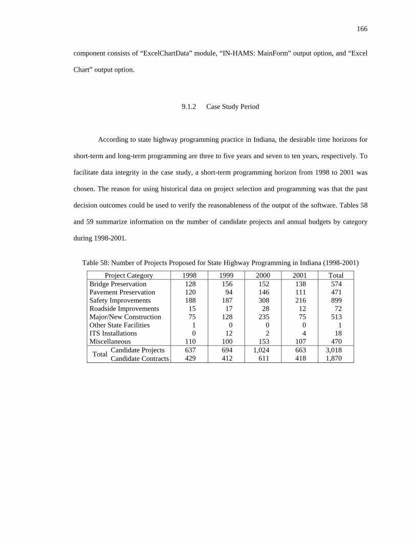
166
component consists of “ExcelChartData” module, “IN-HAMS: MainForm” output option, and “Excel
Chart” output option.
9.1.2 Case Study Period
According to state highway programming practice in Indiana, the desirable time horizons for
short-term and long-term programming are three to five years and seven to ten years, respectively. To
facilitate data integrity in the case study, a short-term programming horizon from 1998 to 2001 was
chosen. The reason for using historical data on project selection and programming was that the past
decision outcomes could be used to verify the reasonableness of the output of the software. Tables 58
and 59 summarize information on the number of candidate projects and annual budgets by category
during 1998-2001.
Table 58: Number of Projects Proposed for State Highway Programming in Indiana (1998-2001)
Project Category 1998 1999 2000 2001 Total Bridge Preservation Pavement Preservation Safety Improvements Roadside Improvements Major/New Construction Other State Facilities ITS Installations Miscellaneous
128 120 188 15 75
1 0
110
156 94
187 17
128 0
12 100
152 146 308 28
235 0 2
153
138 111 216 12 75
0 4
107
574 471 899 72
513 1
18 470
Candidate Projects Total Candidate Contracts637 429
694 412
1,024 611
663 418
3,018 1,870

167
Table 59: Annual Budget for State Highway Programming in Indiana (1998-2001) (Current dollars, in thousands)
Budget Category 1998 1999 2000 2001 Total Bridge Preservation Pavement Preservation Safety Improvements Roadside Improvements Major/New Construction Other State Facilities ITS Installations Miscellaneous
79,900 277,900
43,747 9,622
190,200 2,631 4,600
45,391
73,294 226,925
24,667 7,836
257,106 1,677
17,889 42,413
62,856 365,464
59,635 6,404
166,410 1,379 1,952
52,672
99,312 242,175
53,452 16,058
389,322 5,229 2,091
41,089
315,362 1,112,464
181,501 39,920
1,003,038 10,916 26532
181,565 Total 653,991 651,807 716,772 848,728 2,871,298
9.2 Case Study Results
9.2.1 Number of Contracts Selected
In the case study, project selection was conducted by contract separately for tradeoff
decisions involving certainty, risk, and uncertainty. Figures 15 and 16 present the number of candidate
contracts proposed by INDOT and selected by the HAMS software in each year and for all years in
total. Of the 429, 412, 611, and 418 contracts proposed respectively in each year for the period 1998-
2001, an almost identical number of contracts was selected under the three decision cases.
A higher total number of contracts was selected under the multiyear budget scenario for the
entire analysis period, which was not unexpected. All other things being equal, the multiyear budget
scenario had fewer constraints in the optimization process, which might yield a better solution.
However, as no constraints were imposed for each year under the multiyear budget scenario, the
number of projects selected in each year tended to be less balanced as opposed to that of the carryover
budget scenario. For instance, for case under uncertainty the number of contracts selected on the basis
of multiyear budget scenario was higher than that on the basis of carryover budget scenario for 1999
and 2000 and was lower for 1998 and 2001.

168
Figure 15(a): Selection under Certainty: Comparison of Contracts Selected by Carryover Budget and
Multiyear Budget Scenarios
Figure 15(b): Selection under Risk: Comparison of Contracts Selected by Carryover Budget and
Multiyear Budget Scenarios
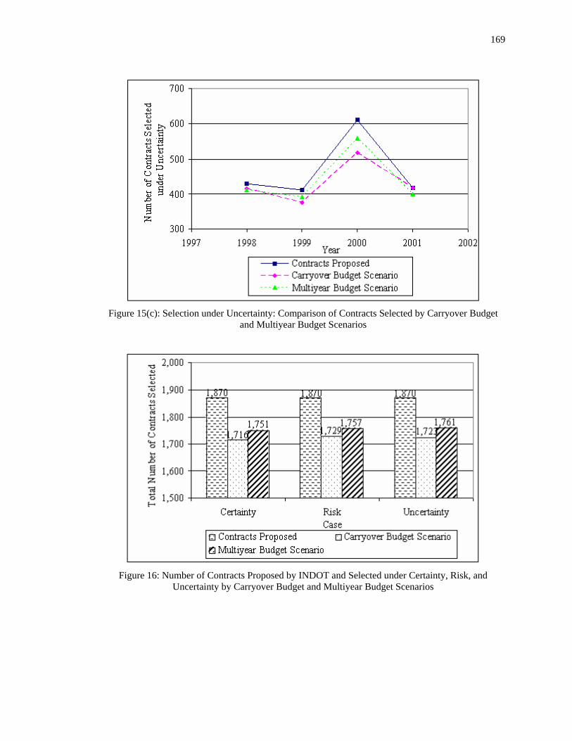
169
Figure 15(c): Selection under Uncertainty: Comparison of Contracts Selected by Carryover Budget
and Multiyear Budget Scenarios
Figure 16: Number of Contracts Proposed by INDOT and Selected under Certainty, Risk, and
Uncertainty by Carryover Budget and Multiyear Budget Scenarios

170
9.2.2 Systemwide Benefits of Selected Contracts
The systemwide benefits of the selected contracts in terms of the gain in system utility or
standardized focus gain-over-loss ratio values are shown in Table 60. These values are rescaled utility
gains per year from selected contracts in that year as represented by the objective function in Equation
(68). It was found that the difference between the quantified benefits for selected contracts under risk
and uncertainty was not as much as that between these benefits under certainty and risk or uncertainty.
Both the risk and uncertainty cases provided much higher benefits than the certainty case. This might
be explained by the fact that the benefits for individual contracts in terms of either expected utility
values or standardized gain-over-loss ratio values were slightly higher than those of utility values,
leading to a higher total benefits corresponding to all selected contracts.
Comparing the results of the two budget scenarios, the total benefits of all selected contracts
based on the multiyear budget scenario were slightly higher than those of the carryover budget
scenario, which could also be attributable to having fewer constraints in the optimization process of
the multiyear budget scenario.
Table 60: Benefits of Selected Contracts by Carryover Budget and Multiyear Budget Scenarios under Certainty, Risk, and Uncertainty (in Rescaled utility values/year)
Fiscal Year Case Carryover Budget Scenario
Multiyear Budget Scenario
1998
Certainty Risk Uncertainty
160 297 301
161 297 301
1999
Certainty Risk Uncertainty
212 324 331
212 324 331
2000
Certainty Risk Uncertainty
297 501 529
297 504 532
2001
Certainty Risk Uncertainty
301 416 430
301 416 430
Total Certainty Risk Uncertainty
977 1,539 1,591
979 1,542 1,594

171
9.3 Sensitivity Analysis
9.3.1 Sensitivity of Input Budget
After conducting the case study based on the available budget in each fiscal year, a sensitivity
analysis was carried out on the basis of two important factors that would affect the outcome of project
selection and programming. The first factor was the budget level in each fiscal year and the second
factor was the relative weights of the agency and the user decision groups.
The sensitivity analysis for budget level was done by changing the fiscal year budget in
increments up to ±20 percent. The impact of changes in the budget on the number of contracts
selected for cases under certainty, risk, or uncertainty was evaluated. Figure 17 presents the results of
the budget sensitivity analysis with two budget scenarios. The results were quite intuitive as the total
number of contracts selected increased as a result of a higher budget level. This was true for both the
carryover budget scenario and the multiyear budget scenario, however, both increased in a
diminishing rate as the budget was increased. For the same reason stated earlier, the multiyear budget
scenario yielded better results.
In the case of the number of contracts selected for tradeoff decisions under certainty, risk, and
uncertainty, there was an obvious gap when the budget level was decreased from the original level,
which was due to the fact that for relatively large-scale contracts in the candidate list, removal of the
entire contracts from the selection list was necessary when the budget level was reduced. The same
was true for the situation of higher budget levels so that only when the added budget reached a certain
level could new contracts be added.

172
Figure 17: Results of Budget Sensitivity in Programming
9.3.2 Weight Sensitivity
In the case study, equal weights were given to the agency and user groups. A series of tests
were conducted with various combinations of the relative weights of the two decision groups to assess
the impact of these weights on the program output. The weight sensitivity analysis was also carried
out under certainty, risk, and uncertainty, and the results are illustrated in Figure 18. As indicated in
the figure, changes in the relative weights between the agency and user groups did not significantly
affect the number of contracts selected. However, the specific contracts selected can differ
significantly due to a change in relative weights.
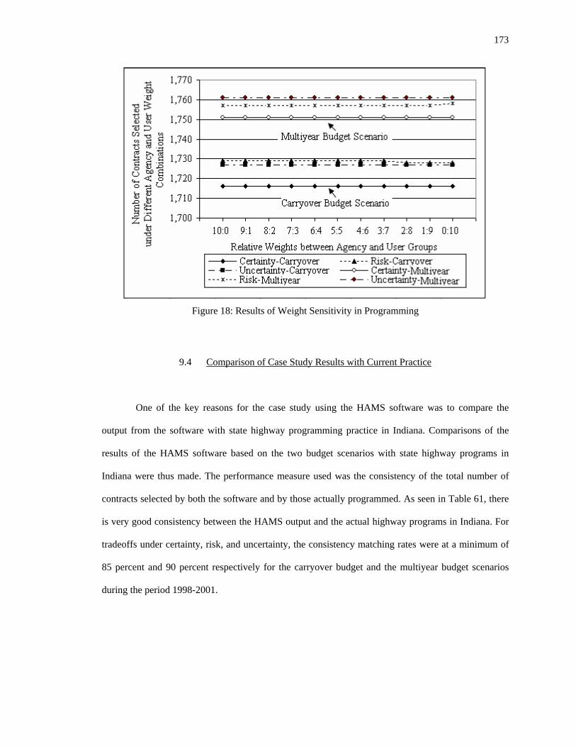
173
Figure 18: Results of Weight Sensitivity in Programming
9.4 Comparison of Case Study Results with Current Practice
One of the key reasons for the case study using the HAMS software was to compare the
output from the software with state highway programming practice in Indiana. Comparisons of the
results of the HAMS software based on the two budget scenarios with state highway programs in
Indiana were thus made. The performance measure used was the consistency of the total number of
contracts selected by both the software and by those actually programmed. As seen in Table 61, there
is very good consistency between the HAMS output and the actual highway programs in Indiana. For
tradeoffs under certainty, risk, and uncertainty, the consistency matching rates were at a minimum of
85 percent and 90 percent respectively for the carryover budget and the multiyear budget scenarios
during the period 1998-2001.

174
Table 61: Number of Contracts Proposed and Both Authorized and Selected by the HAMS Software
Same Contracts Selected by HAMS Package Fiscal Year
Contracts Proposed
Contracts Programmed Case Carryover
Budget % Match Multiyear Budget % Match
1998
429
152
Certainty Risk Uncertainty
139 143 142
91% 94% 93%
142 142 142
93% 93% 93%
1999
412
323
Certainty Risk Uncertainty
292 293 292
90% 91% 90%
305 306 302
94% 95% 93%
2000
611
583
Certainty Risk Uncertainty
496 496 497
85% 85% 85%
524 530 535
90% 91% 92%
2001
418
414
Certainty Risk Uncertainty
413 413 413
100% 100% 100%
397 395 397
96% 95% 96%
Total
1,870
1,472
Certainty Risk Uncertainty
1,340 1,345 1,344
91% 91% 91%
1,368 1,373 1,376
93% 93% 93%
9.5 Discussions
The case study results revealed that project selection was sensitive to the budget level for a
given analysis period. However, the relative weights of the agency and user decision groups appeared
to be not as significant, which suggested that the agency and the user maintained consistent
perceptions on asset management system goals. All things being equal, the multiyear budget scenario
selected a higher number of contracts and thus yielded slightly better system benefits than those from
the carryover budget scenario. However, the distribution of the total number of contracts selected and
the system benefits in each fiscal year associated with the multiyear budget scenario were less
balanced.

175
9.6 Chapter Summary
This chapter first provided a brief description of the HAMS software that can be used for state
highway project selection and programming. In order to validate the tradeoff analysis findings, as well
as the system optimization model along with the solution algorithm, a case study was carried out using
the information of past candidate projects for state highway programming in Indiana. A sensitivity
analysis was further conducted on the basis of two factors, the budget level and the relative weights of
the agency and user decision groups. Cross comparisons of the HAMS software outputs with actual
state highway programs practice in Indiana were also made. For the case study, the sensitivity
analysis, and result comparisons, tradeoff decisions were made separately under certainty, risk, and
uncertainty using two budget scenarios, carryover and multiyear. The findings demonstrated that the
HAMS software provided reliable results and it could indeed be used by for state highway
programming and management.
176
1
2
3
4
5
6
7
8 9
10 CHAPTER 10 CONCLUSIONS
10.1 Summary and Findings
In the present study, a methodology was proposed for highway asset management that
embraced the top-level agency functions of asset valuation, performance modeling, marginal benefit
analysis, and multicriteria decision-making. Models were developed to predict the performance of
physical highway assets, including pavements and bridges, and usage of the highway network. For
pavements, the models were calibrated based on rehabilitation expenditure, routine maintenance
expenditure, and the tradeoff relationship between the level of routine maintenance and the
rehabilitation interval at various levels of traffic loading and weather conditions. For bridges, the
models were developed based on the bridge wearing surface condition, structural condition, and
bridge life cycle user cost. Regarding network-level usage performance, user cost models were
calibrated separately for individual user cost components that included vehicle operating cost, travel
time, vehicle collisions, and vehicle air pollution per vehicle mile of travel, as well as total highway
user cost per vehicle mile of travel. For the pavement expenditure models, the variables found
significant were the pavement surface condition, traffic loading, thickness, freeze-thaw cycles,
ambient temperature, and pavement age. The variables found significant to bridge performance mainly
included traffic volume, bridge age, and superstructure type. For the network-level highway user cost
models, the significant variables were the road surface condition and the vehicle traveling speed.
The marginal effects of significant variables affecting asset condition, service life, and agency
cost, as well as the network-level highway user cost, were established on the basis of the calibrated
models. The marginal benefits were then determined accordingly. Marginal benefit analysis was

177
specifically carried out for pavement and bridge-related projects and the individual user cost
components based on the concept of life-cycle cost analysis.
The multicriteria decision-making process for highway asset management included a tradeoff
analysis and project selection and programming. A tradeoff analysis was done for cases under
certainty, risk and uncertainty as follows. First, a set of asset management system goals and
performance indicators were classified. The relative weights of system goals and multiple
performance indicators under individual system goals were then established. For cases of certainty and
risk, a utility theory was employed to establish systemwide multiattribute utility functions on the basis
of single attribute utility functions developed for various performance indicators. The systemwide
utility functions were utilized to establish a non-dimensional value for the benefits associated with a
candidate project. As the utility theory is not directly applicable to situations involving uncertainty, an
alternative approach based on Shackle’s model was employed. In particular, the degree of surprise
functions and priority functions were established to develop systemwide standardized focus gain-over-
loss ratio functions, which formed the basis of prioritizing candidate projects under uncertainty. A
series of questionnaire surveys were conducted to establish relative weights, single attribute utility
functions, degree of surprise functions, and priority functions. For the questionnaire surveys, two
decision groups and two separate survey approaches were used to assess the robustness of the results.
The two decision groups included the agency group and the user group, and the two survey
approaches used were the direct questioning approach and the certainty equivalency approach. It was
found that the utility functions and standardized focus gain-over-loss ratio functions were not
statistically different by decision group or by approach, and it should be noted that the non-
dimensional benefits in terms of changes in utility values or standardized gain-over-loss ratio values
were independent of project size. These values were rescaled according to the expected traffic during
the project life and the construction cost, as well as the number of projects involved in a specific
contract prior to the system optimization process. By making such adjustments, it ensured tradeoffs
between projects to be conducted equitably. Project selection and programming were conducted
178
separately using the results of tradeoffs under certainty, risk, and uncertainty. A system optimization
model was formulated on the basis of the MCMDKP problem, and a heuristic algorithm based on
Lagrangian relaxation techniques was prepared for system optimization using two budget scenarios,
annual budget with carryover and multiyear budget.
A Highway Asset Management System software was developed on the basis of the findings
of the tradeoff analysis and the system optimization model, as well as the solution algorithm
developed. In order to validate the research findings, a case study was carried out for project selection
and programming using information on past candidate projects in state highway programs in Indiana.
In addition, a sensitivity analysis was also conducted on two factors, the budget level and the relative
weights of the agency and the user decision groups. The case study results generated from the HAMS
software were then compared with actual state highway programs in Indiana. The comparison
revealed that, for tradeoff decisions involving certainty, risk, or uncertainty under both budget
scenarios, the consistency matching rate for candidate contracts selected both by the software and by
actual highway programs was 85 percent at minimum.
10.2 Implementation Issues
The products of this research are as follows:
- Models to predict the performance of physical highway assets
- Models to estimate network-level highway user cost
- Methodology that can be used by top-level management in INDOT to do tradeoff analysis
incorporating risk and uncertainty
- A software package to facilitate implementation of the research findings of present study.
When properly implemented by INDOT top-level management, it is expected that the results
of the present study will provide a reliable and objective basis upon which highway investment

179
decisions can be made. Implementation of the study findings will result in obtaining maximum return
from each dollar of investment, and overall savings to the state of Indiana in the long run, without
needlessly sacrificing asset performance. It is therefore expected that the implementation of the results
will result in changes in state-level highway programming.
Tools to facilitate implementation of the results of this research include training of top-level
personnel and organization of workshops to demonstrate the project selection and programming
methodology and the investigation of tradeoffs and marginal effects. Possible impediments to
successful implementation of the product of the study include inconsistency of inter-agency
terminology, peculiar nature of budgeting procedures, and the fact that some management systems
have not been fully implemented. However, with close cooperation between concerned parties,
improved public relations, and learning from the experiences of agencies that have experimented with
implementing different asset management policies, the impact of such barriers to implementation of
the study findings can be reduced.
10.3 Directions for Future Research
Asset management is an improved way of overall highway system management that responds
to an environment of increasing system demands, aging physical highway assets, and limited
resources. One of the major contributions of the present research is that it has incorporated asset usage
performance into the overall decision-making framework. Furthermore, tradeoff analysis methods
have been introduced to enable tradeoff scenarios being made not only within a specific asset
category, but also across various physical highway assets, thereby making the decision-making
process rational, objective, and holistic. The issue of uncertainty, which is commonly encountered in
highway investment decision process, is also successfully addressed in the research. The asset
management system software developed has proven to be a reliable analytical tool to conduct
statewide highway asset management decisions. Since the condition and performance of the highway
180
system change over time, however, it is desirable to refine the research findings so that decision-
making in the future can always be attuned to the current situation of the system. In addition, a large
part of the research findings for tradeoff analysis was established on the basis of questionnaire
surveys, and to some extent, subjective information was acquired based on relatively small sample
sizes. A refinement process may be needed, therefore, as a larger number of survey participants
becomes available. Finally, it may be worthwhile to explore a new approach that can bridge
inconsistencies between the utility theory used for certainty and risk and Shackle’s model used for
uncertainty.


190
Appendix A Project Coding Systems Used within Indiana Department of Transportation and Definition of Project
Types Classified for Highway Asst Management
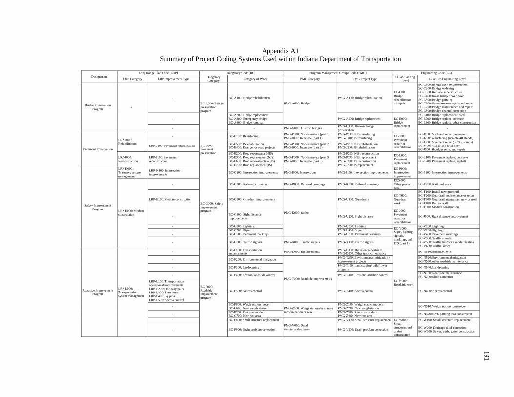
191
Appendix A1 Summary of Project Coding Systems Used within Indiana Department of Transportation
Long Range Plan Code (LRP) Budgetary Code (BC) Program Management Groups Code (PMG) Engineering Code (EC)
Designation LRP Category LRP Improvement Type Budgetary
Category Category of Work PMG Category PMG Project Type EC at Planning Level EC at Pre-Engineering Level
- BC-A100: Bridge rehabilitation PMG-A100: Bridge rehabilitation
EC-C000: Bridge rehabilitation or repair
EC-C100: Bridge deck reconstruction EC-C200: Bridge widening EC-C300: Replace superstructure EC-C400: Raise bridge/lower pave EC-C500: Bridge painting EC-C600: Superstructure repair and rehab EC-C700: Bridge maintenance and repair EC-C800: Bridge channel correction
- BC-A200: Bridge replacement BC-A300: Emergency bridge BC-A400: Bridge removal
PMG-A000: Bridges
PMG-A200: Bridge replacement EC-E100: Bridge replacement, steel EC-E200: Bridge replace, concrete EC-E300: Bridge replace, other construction
Bridge Preservation Program -
-
BC-A000: Bridge preservation program
- PMG-G000: Historic bridges PMG-G100: Historic bridge preservation
EC-E000: Bridge replacement
-
- BC-E100: Resurfacing PMG-P000: Non-Interstate (part 1) PMG-J000: Interstate (part 1)
PMG-P100: NIS resurfacing PMG-J100: IS resurfacing
EC-J100: Patch and rehab pavement EC-J200: Resurfacing (non 3R/4R stands) LRP-J000:
Rehabilitation LRP-J100: Pavement rehabilitation BC-E500: IS rehabilitation
BC-E400: Emergency road projects PMG-P000: Non-Interstate (part 2) PMG-J000: Interstate (part 2)
PMG-P210: NIS rehabilitation PMG-J210: IS rehabilitation
EC-J000: Pavement repair or rehabilitation
EC-J300: Pavement rehab (3R/4R stands) EC-J400: Wedge and level only EC-J600: Shoulder rehab and repair Pavement Preservation
LRP-I000: Reconstruction
LRP-I100: Pavement reconstruction
BC-E000: Pavement preservation BC-E200: Road reconstruct (NIS)
BC-E300: Road replacement (NIS) BC-E600: Road reconstruction (IS) BC-E700: Road replacement (IS)
PMG-P000: Non-Interstate (part 3) PMG-J000: Interstate (part 3)
PMG-P220: NIS reconstruction PMG-P230: NIS replacement PMG-J220: IS reconstruction PMG-J230: IS replacement
EC-L000: Pavement replacement
EC-L100: Pavement replace, concrete EC-L200: Pavement replace, asphalt
LRP-K000: Transport system management
LRP-K100: Intersection improvements BC-G100: Intersection improvements PMG-I000: Intersections PMG-I100: Intersection improvements
EC-P000: Intersection improvement
EC-P100: Intersection improvements
- BC-G200: Railroad crossings PMG-R000: Railroad crossings PMG-R100: Railroad crossings ECX000: Other project type
EC-X200: Railroad work
LRP-E100: Median construction BC-G300: Guardrail improvements PMG-U100: Guardrails EC-T000: Guardrail work
EC-T100: Install new guardrail EC-T200: Guardrail, maintenance or repair EC-T300: Guardrail attenuators, new or mod EC-T400: Barrier wall EC-T500: Median construction
- BC-G400: Sight distance improvements PMG-U200: Sight distance
EC-J000: Pavement repair or rehabilitation
EC-J500: Sight distance improvement
- BC-G800: Lighting PMG-U500: Lighting EC-V100: Lighting - BC-G700: Signs PMG-U400: Signs EC-V200: Signing - BC-G500: Pavement markings
PMG-U000: Safety
PMG-U300: Pavement markings EC-V400: Pavement markings
Safety Improvement Program LRP-E000: Median
construction
-
BC-G000: Safety improvement program
BC-G600: Traffic signals PMG-X000: Traffic signals PMG-X100: Traffic signals
EC-V000: Signs, lighting, signals, markings, and ITS (part 1)
EC-V300: Traffic signals EC-V500: Traffic hardware modernization EC-V600: Traffic, other
- BC-F100: Transportation enhancements PMG-D000: Enhancements PMG-D100: Bicycles/ pedestrians
PMG-D200: Other transport enhance EC-N510: Enhancements
- BC-F200: Environmental mitigation PMG-T200: Environmental mitigation / improvement projects
EC-N520: Environmental mitigation EC-N530: other roadside maintenance
- BC-F300; Landscaping PMG-T100: Landscaping/ wildflower program EC-N540: Landscaping
- BC-F400: Erosion/landslide control PMG-T300: Erosion/ landslide control EC-N100: Roadside maintenance EC-N200: Slide correction
LRP-L100: Transportation operational improvements LRP-L200: One-way pairs LRP-L300: Turn lanes LRP-L400: By pass LRP-L500: Access control
BC-F500: Access control
PMG-T000: Roadside improvements
PMG-T400: Access control EC-N400: Access control
- BC-F600: Weigh station modern BC-C600: New weigh station
PMG-Z100: Weigh station modern PMG-Z200: New weigh station EC-N310: Weigh station const/recon
- BC-F700: Rest area modern BC-C700: New rest area
PMG-Z000: Weigh stations/rest areas modernization or new PMG-Z300: Rest area modern
PMG-Z400: New rest area
EC-N000: Roadside work
EC-N320: Rest, parking area const/recon
- BC-F800: Small structure replacement PMG-V100: Small structure replacement EC-W100: Small structure, replacement
Roadside Improvement Program
LRP-L000: Transportation system management
-
BC-F000: Roadside improvement program
BC-F900: Drain problem correction PMG-V000: Small structures/drainages PMG-V200: Drain problem correction
EC-W000: Small structures and drains construction
EC-W200: Drainage ditch correction EC-W300: Sewer, curb, gutter construction

192
Appendix A1 Summary of Project Coding Systems Used within Indiana Department of Transportation (Continued)
Long Range Plan Code (LRP) Budgetary Code (BC) Program Management Groups Code (PMG) Engineering Code (EC) Designation
LRP Category LRP Improvement Type Budgetary Category Category of Work PMG Category PMG Project Type EC at Planning
Level EC at Pre-Engineering Level
LRP-H000: New road construction LRP-H100: New road construction
BC-C100: New road construction BC-C200: Completion of IS
PMG-E100: New road construction
EC-G100: New road, grading only EC-G200: New road, paving only EC-G300: New road construction
LRP-A000: Added travel lanes LRP-B000: Freeway update (part 1)
LRP-H100: Added travel lanes LRP-B100: Freeway construct LRP-B200: Added travel lane on freeways
BC-C300: Added travel lanes PMG-E200: Added travel lanes
EC-G000: Road construction EC-G400: Added travel lanes
EC-G500: Dual lane existing route EC-G600: Auxiliary lanes
LRP-F000: New bridge construction
LRP-F100: New bridge construction - -
EC-A000: New bridge construction
EC-A100: New bridge, steel construction EC-A200: New bridge, concrete construct EC-A300: New bridge, other construction EC-A400: New bridge, special
LRP-G000: New interchange construction
LRP-G100: New interchange construction
BC-C400: New interchange construction PMG-E300: New interchange construct EC-R100: New interchange construction
LRP-C000: Interchange modifications
LRP-C100: Interchange modifications BC-C500: Interchange modifications PMG-E400: Interchange modifications EC-R200: Interchange modifications
LRP-D000: Interstate interchanges
LRP-D100: IS interchange modifications LRP-D200: IS interchange construction
- - -
Major/New Construction Program
LRP-B000: Freeway update (part 2)
LRP-B300: New freeway interchange construction LRP-B400: New freeway GS construction
BC-C000: Major/new construction program
-
PMG-E000: Expansion
-
EC-R000: Interchange work
-
- BC-D100: Park roads PMG-C000: DNR Facilities (part 1) PMG-F000: Forest land highways PMG-Q000: Other state inst (part 1)
PMG-C100: Park roads PMG-F100: Forest land highways PMG-Q100: Institution roads
EC-J700: Pavement, other
- BC-D200: Park bridges PMG-C000: DNR Facilities (part 2) PMG-Q000: Other state inst (part 2)
PMG-C200: Park bridges PMG-Q200: Institution bridges EC-E400: Bridge replacement, special
Other State Facilities Program -
-
BC-D000: Park facilities program
BC-D300: Cooperative access projects PMG-C000: DNR Facilities (part 3) PMG-Q000: Other state inst (part 3)
PMG-C300: Cooperative access projects PMG-Q300: Other projects
-
-
- BC-B100: ITS traveler info systems PMG-H100: ITS traveler info systems EC-V710: ITS traveler info systems - BC-B200: ITS management systems PMG-H200: ITS management systems EC-V720: ITS management systems - BC-B300: ITS monitoring systems PMG-H300: ITS monitoring systems EC-V730: ITS monitoring systems
Intelligent Transportation Systems
Program -
-
BC-B000: ITS program
BC-B400: ITS operations and maintenance
PMG-H000: Intelligent transportation systems (ITS)
PMG-H400: ITS operations and maintenance
EC-V000: Signs, lighting, signals, markings, and ITS (part 2) EC-V750: ITS operations and maintenance
- PMG-K000: Local bridge inspections PMG-K100: Local bridge inspections EC-X300: Bridge inspections PMG-B100: CMAQ projects
BC-H400: CMAQ projects BC-H300: Toll road
PMG-B000: Command and control category
PMG-B200: Bonding projects PMG-B300: Bridge “watch list” PMG-B400: Shelf projects PMG-B500: Suspended projects PMG-B600: other command projects
- PMG-L000: LPA (local) program PMG-L100: State administered Federal aid projects PMG-M100: Routine maintenance BC-H100: Traffic maintenance
BC-H200: Maintenance PMG-M000: Maintenance PMG-M200: Periodic maintenance PMG-N100: Inter-modal mgmt projects PMG-N200: Inter-modal connectors PMG-N300: Airport facilities PMG-N400: Passenger rail PMG-N500: Railroad corridor preservation PMG-N600: Railroad right-of-way preservation PMG-N700: Railroad track preservation
- PMG-N000: Multi-modal
PMG-N800: Transit facilities - PMG-O000: Noise abasement PMG-O100: Noise abasement projects
-
- PMG-S000: Relinquishments PMG-S100: Transfer of route from State to local jurisdiction EC-X413: Relinquishments
BC-H500: Feasibility/corridor studies PMG-W000: Studies PMG-W100: Feasibility/corridor studies -
Miscellaneous LRP-M000: Undetermined LRP-M100: Undetermined
BC-H000: Unprogrammed/ projected
- PMG-Y000: Utilities PMG-Y100: Utility relocation
EC-X000: Other project type
EC-X000: Other project type EC-X111: Bridge removal EC-X112: Demolition, remove bld foundationEC-X113: Remove bridge abutments EC-X411: Protective buying EC-X414: Utility relocation

193
Appendix A2 Definition of Project Types Classified for Highway Asst Management
1. Access Control: Expenditures preserved to places where efficient movement of through
traffic is desired by acquiring the adjacent property's access rights and regulating the number of access points to the highways. This strategy will not only increases the free and efficient movement of through traffic, but also reduces highway accidents by minimizing the number of conflict points or entrances located along the highways.
2. Added Travel Lane: Construction of additional travel or through lanes to existing roadways
for increased capacity to obtain a more efficient and safer facility. The exiting pavement is usually reconstructed at the same time.
3. Bicycles/Pedestrians: Non-motorized projects aimed at providing bicycling or walking
facilities to assist concerns of traffic congestion, exhaust-pipe pollution, unsightly roadsides, and unceasing traffic noise.
4. (Pre-committed) Bonding Projects: Projects implemented with partial funding through a bond
issuance and the remaining cost with INDOT pre-committed matching funds. 5. Bridge Rehabilitation: Bridge rehabilitation involves major work required to restore the
structural integrity of a bridge as well as work necessary to correct its major safety defects. 6. Bridge Replacement: It refers to total replacement of a structurally deficient or functionally
obsolete bridge with a new facility constructed in the same general traffic corridor, resulting in increased capacity and safety.
7. Bridge “Watch List”: Specific bridge projects that for some reason (such as safety concerns)
must be implemented. 8. Congestion Mitigation & Air Quality Improvement Program (CMAQ): This program directs
funds toward transportation improvements on traffic flow, demand management, transit, and non-motorized transportation in clean air non-attainment areas for ozone and carbon monoxide. These projects will contribute to meeting the attainment of the National Ambient Air Quality Standards (NAAQS).
9. Cooperative Access Projects: INDOT involved public transportation projects aimed at
providing additional opportunities for access to employment, medical, social service and educational facilities for residents reliant on public transportation and outside the fixed route transit service areas.
10. Environmental Mitigation/Improvements: Alternative projects like transit and transportation
enhancement projects implemented to avoid, minimize, or mitigate environmental impacts. 11. Erosion/landslide control: Projects implemented during construction, and operation, and
maintenance stages to protect unstable soil along the side of highway embankment by control strategies like side slope vegetation, upper slope stabilization, and other feasible methods.
12. Feasibility / Corridor Studies: Studies that involve feasibility and corridor design of highway
projects. 13. Forestland Highways: Highway projects implemented at forestlands.

194
Appendix A2 Definition of Project Types Classified for Highway Asst Management (Continued)
14. Guardrail Improvements: These improvements consist of maintenance, repairs, and
rehabilitation of guardrails. Eligible projects include but not limit to installation of new guardrails, cleaning, painting, and repair of existing guardrails, guardrail attenuator installation or modernization.
15. Historic Bridge Preservation: Program mainly using Federal funds either to preserve the
existing historic bridges when the future traffic conditions are met or to build alternative alignments or new bridges on the existing structure alignments when the future traffic conditions could not be satisfied.
16. Institution Roads/ Bridges/ Other Projects: INDOT sponsored roads, bridges and other
projects at State institutions, such as roads and bridges at Purdue and Indiana University campuses.
17. Interchange Modifications: Construction of improvements to an interchange, ranging from
ramp terminal improvements, eliminating two-way ramps, or adding lanes to ramps to replace existing movements with loop ramps or directional ramps.
18. Inter-Modal Management Systems/ Connectors/ Airport / Passenger Rail/ Transit Facilities:
The multi-modal transportation management systems, connectors and facilities provide travelers with alternatives to serve regional communities and to connect local state to other states and other part of the world.
19. Intersection Improvements: Improvements result in a reduction in overall peak hour
congestion that provide the most efficient use of existing and future transportation facilities where congestion is occurring or is expected to occur.
20. ITS Incident Management Systems: The ITS freeway incident management systems (Hoosier
Helpers, Lane Merge system) can assist motorists and clear incidents from the roadway. 21. ITS Operations and Maintenance: These refer to toll road operation centers and maintenance
related to ITS infrastructures. 22. ITS Traffic Surveillance and Monitoring Systems: The ITS traffic surveillance and
monitoring systems (trafficwise) use computerized sensors and video cameras to quickly detect highway congestion and to determine reasons for it.
23. ITS Traveler Information Systems: The ITS traveler information systems, through Highway
Advisory Radio (HAR), Variable Message Signs (VMS), Pagers, are capable of providing real-time traffic information to the traveling public.
24. Landscaping/ Wildflower Program: Program mainly deals with safety of drivers, walkers and
horseback riders while preserving roadway area's character and scenic beauty. 25. Lighting Improvements: These improvements involve provision of continuous freeway
lighting, partial lighting of interchanges on unlighted freeways, and lighting of other streets and highways. These improvement projects are identified on the basis of average daily traffic, ratio of night to day crashes, local government participation in the cost, and other factors.
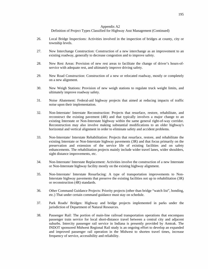
195
Appendix A2 Definition of Project Types Classified for Highway Asst Management (Continued)
26. Local Bridge Inspections: Activities involved in the inspection of bridges at county, city or
township levels. 27. New Interchange Construction: Construction of a new interchange as an improvement to an
existing roadway, generally to decrease congestion and to improve safety. 28. New Rest Areas: Provision of new rest areas to facilitate the change of driver’s hours-of-
service with adequate rest, and ultimately improve driving safety. 29. New Road Construction: Construction of a new or relocated roadway, mostly or completely
on a new alignment. 30. New Weigh Stations: Provision of new weigh stations to regulate truck weight limits, and
ultimately improve roadway safety. 31. Noise Abatement: Federal-aid highway projects that aimed at reducing impacts of traffic
noise upon their implementation. 32. Non-Interstate/ Interstate Reconstruction: Projects that resurface, restore, rehabilitate, and
reconstruct the existing pavement (4R) and that typically involves a major change to an existing Interstate or Non-Interstate highway within the same general right-of-way corridor. Reconstruction may also involve making substantial modifications to an older highway's horizontal and vertical alignment in order to eliminate safety and accident problems.
33. Non-Interstate/ Interstate Rehabilitation: Projects that resurface, restore, and rehabilitate the
existing Interstate or Non-Interstate highway pavements (3R) and that focus primarily on the preservation and extension of the service life of existing facilities and on safety enhancements. The rehabilitation projects mainly include wider travel lanes, wider shoulders, sight distance improvements, etc.
34. Non-Interstate/ Interstate Replacement: Activities involve the construction of a new Interstate
or Non-Interstate highway facility mostly on the existing highway alignment. 35. Non-Interstate/ Interstate Resurfacing: A type of transportation improvements to Non-
Interstate highway pavements that preserve the existing facilities not up to rehabilitation (3R) or reconstruction (4R) standards.
36. Other Command Guidance Projects: Priority projects (other than bridge “watch list”, bonding,
etc.) That under certain command guidance must stay on schedule. 37. Park Roads/ Bridges: Highway and bridge projects implemented in parks under the
jurisdiction of Department of Natural Resources. 38. Passenger Rail: The portion of main-line railroad transportation operations that encompass
passenger train service for local short-distance travel between a central city and adjacent suburbs. Intercity passenger rail service in Indiana is presently provided by Amtrak. The INDOT sponsored Midwest Regional Rail study is an ongoing effort to develop an expanded and improved passenger rail operation in the Midwest to shorten travel times, increase frequency of service, accessibility and reliability.
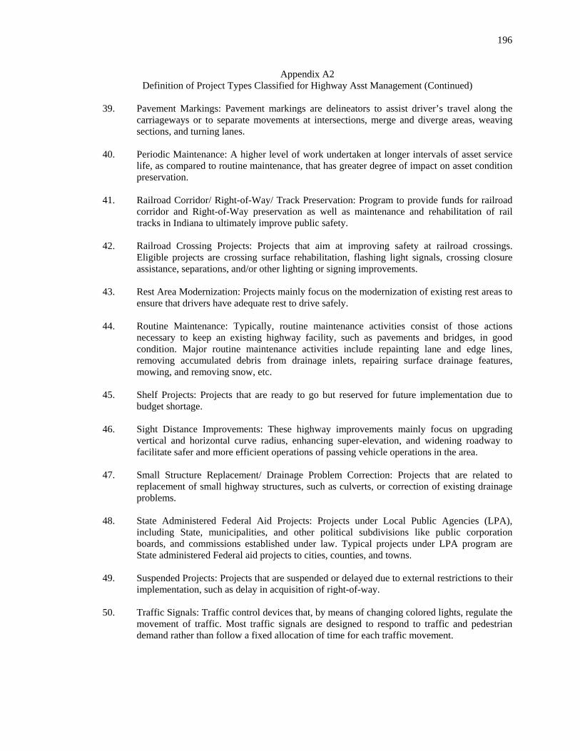
196
Appendix A2 Definition of Project Types Classified for Highway Asst Management (Continued)
39. Pavement Markings: Pavement markings are delineators to assist driver’s travel along the
carriageways or to separate movements at intersections, merge and diverge areas, weaving sections, and turning lanes.
40. Periodic Maintenance: A higher level of work undertaken at longer intervals of asset service
life, as compared to routine maintenance, that has greater degree of impact on asset condition preservation.
41. Railroad Corridor/ Right-of-Way/ Track Preservation: Program to provide funds for railroad
corridor and Right-of-Way preservation as well as maintenance and rehabilitation of rail tracks in Indiana to ultimately improve public safety.
42. Railroad Crossing Projects: Projects that aim at improving safety at railroad crossings.
Eligible projects are crossing surface rehabilitation, flashing light signals, crossing closure assistance, separations, and/or other lighting or signing improvements.
43. Rest Area Modernization: Projects mainly focus on the modernization of existing rest areas to
ensure that drivers have adequate rest to drive safely. 44. Routine Maintenance: Typically, routine maintenance activities consist of those actions
necessary to keep an existing highway facility, such as pavements and bridges, in good condition. Major routine maintenance activities include repainting lane and edge lines, removing accumulated debris from drainage inlets, repairing surface drainage features, mowing, and removing snow, etc.
45. Shelf Projects: Projects that are ready to go but reserved for future implementation due to
budget shortage. 46. Sight Distance Improvements: These highway improvements mainly focus on upgrading
vertical and horizontal curve radius, enhancing super-elevation, and widening roadway to facilitate safer and more efficient operations of passing vehicle operations in the area.
47. Small Structure Replacement/ Drainage Problem Correction: Projects that are related to
replacement of small highway structures, such as culverts, or correction of existing drainage problems.
48. State Administered Federal Aid Projects: Projects under Local Public Agencies (LPA),
including State, municipalities, and other political subdivisions like public corporation boards, and commissions established under law. Typical projects under LPA program are State administered Federal aid projects to cities, counties, and towns.
49. Suspended Projects: Projects that are suspended or delayed due to external restrictions to their
implementation, such as delay in acquisition of right-of-way. 50. Traffic Signals: Traffic control devices that, by means of changing colored lights, regulate the
movement of traffic. Most traffic signals are designed to respond to traffic and pedestrian demand rather than follow a fixed allocation of time for each traffic movement.

197
Appendix A2 Definition of Project Types Classified for Highway Asst Management (Continued)
51. Traffic Signs: Traffic control installations to provide regulatory, warning, and guiding traffic.
Regulatory signs mainly assign right-of-way, post speed limits, restrict parking, and allow pedestrian movements. Warning signs are used for curves, no passing zones, T- or Y-intersections, merging lanes, one-lane bridges, and steep grades. Guiding signs are usually used as route markers as well as providing destination and distance Information to travelers.
52. Transfer of Route from State to Local Jurisdiction: Relinquishments of route from State to
local jurisdiction. 53. Transportation Enhancements: Transportation-related activities that are designed to
strengthen the cultural, aesthetic, and environmental aspects of the Nation’s inter-modal transportation system. The transportation enhancement activities include: - Pedestrian and bicycle facilities - Pedestrian and bicycle safety and education activities - Acquisition of scenic or historic easements and sites - Scenic or historic highway programs including tourist and welcome centers - Landscaping and scenic beautification - Historic preservation - Rehabilitation and operation of historic transportation buildings, structures or facilities - Conversion of abandoned railway corridors to trails - Control and removal of outdoor advertising - Archaeological planning and research - Environmental mitigation of runoff pollution and provision of wildlife underpasses - Establishment of transportation museums
54. Utility Relocation: Program funds the relocation of utilities within the right-of-way of newly
implemented highway projects. 55. Weigh Station Modernization: Projects mainly focus on the modernization of existing weigh
stations to ensure that drivers do not carry loads over specified limits, and ultimately to improve roadway safety.

198
Appendix B Summary of Physical Highway Assets and Asset Usage of Indiana State Highway Network

199
Appendix B1 Summary of Physical Highway Assets of Indiana State Highway Network
Year Mileage Lane Bridge Stop
Controlled Intersection
Signalized Intersection
Grade Separation Interchange Railroad
Cross Workzone
1990 1991 1992 1993 1994 1995 1996 1997 1998 1999 2000
10,634 10,615 11,251 11,284 11,266 11,238 11,233 11,242 10,703 10,711 10,585
2.5 2.5 2.5 2.5 2.5 2.5 2.5 2.5 2.5 2.5 2.6
5,053 5,056 5,059 5,062 5,065 5,068 5,070 5,077 5,073 5,076 5,085
6,717 6,740 7,001 7,502 7,484 7,446 7,443 7,452 7,544 7,480 7,549
10,850 10,939 11,036 11,810 11,786 11,719 11,716 11,723 11,712 11,533 11,529
948 935
1,004 969 953 974
1,070 1,079 1,068 1,086 1,104
11,761 11,339 12,497 9,778 9,758 9,707 9,703 9,707 8,597 8,127 7,786
505 507 519 544 543 535 535 536 537 527 530
148 151 154 124 182 174 201 128 170 173 175

200
Appendix B2 Summary of Asset Usage of Indiana State Highway Network
Year Condition (inch/mile)
Bridge SD (%)
Bridge FO(%)
Speed (mph)
AADT (vehicle)
Truck (%)
SUT (%)
MUT (%)
VMT (billion)
1990 1991 1992 1993 1994 1995 1996 1997 1998 1999 2000
86 92 99 97
115 117 119 125 132 138 144
10% 10%
9% 8% 6% 6% 6% 5% 5% 3% 3%
21% 19% 19% 17% 11% 10% 12% 11% 11% 12% 12%
54.3 54.2 54.1 54.0 53.9 53.5 53.3 53.2 52.8 52.5 52.3
7,451 7,576 7,837 8,471 8,664 9,054 9,267 9,436 9,966
10,073 10,248
26% 26% 26% 27% 24% 26% 25% 27% 26% 27% 27%
23% 23% 22% 23% 21% 22% 20% 22% 21% 21% 21%
3% 3% 4% 4% 4% 4% 5% 5% 5% 6% 6%
31 31 32 35 36 37 38 40 37 37 38
Note: 1. SD- Structurally deficient 2. FO- Functionally obsolete 3. SUT- Single unit truck 4. MUT- Multiple unit truck 5. VMT- Vehicle mile of travel.

201
Appendix C Condition of Indiana State Highway Pavements and Bridges

202
Appendix C1 Condition of Indiana State Highway Pavements

203
Appendix C2 Condition of Indiana State Highway Bridges

204
Appendix D Unit Rates of Fuels, Time Value, Vehicle Collisions, and Vehicle Air Pollutants for Highway User
Cost Computation

205
Appendix D1 Unit Rates of Fuels for Various Vehicle Classes
Vehicle Class Year 2 3 4 5 6 7 8 9 10 11 12 13 1990 1991 1992 1993 1994 1995 1996 1997 1998 1999 2000
1.07 1.12 1.15 1.18 1.21 1.24 1.28 1.31 1.32 1.37 1.40
1.09 1.13 1.16 1.20 1.23 1.26 1.30 1.33 1.34 1.39 1.42
1.091.131.161.201.231.261.301.331.341.391.42
1.091.131.161.201.231.261.301.331.341.391.42
1.091.131.161.201.231.261.301.331.341.391.42
1.091.131.161.201.231.261.301.331.341.391.42
1.151.201.231.261.301.331.371.401.421.471.50
1.151.201.231.261.301.331.371.401.421.471.50
1.15 1.20 1.23 1.26 1.30 1.33 1.37 1.40 1.42 1.47 1.50
1.15 1.20 1.23 1.26 1.30 1.33 1.37 1.40 1.42 1.47 1.50
1.15 1.20 1.23 1.26 1.30 1.33 1.37 1.40 1.42 1.47 1.50
1.151.201.231.261.301.331.371.401.421.471.50
Source: Zaniewski, 1982; updated for the period 1990-2000.

206
Appendix D2 Unit Rates of Time Value for Various Vehicle Classes
Vehicle Class Year 2 3 4 5 6 7 8 9 10 11 12 13 1990 1991 1992 1993 1994 1995 1996 1997 1998 1999 2000
8.8 9.2 9.4 9.7 9.9
10.2 10.5 10.8 10.9 11.2 11.5
11.3 11.7 12.1 12.4 12.7 13.1 13.5 13.8 13.9 14.4 14.7
11.311.712.112.412.713.113.513.813.914.414.7
11.311.712.112.412.713.113.513.813.914.414.7
11.311.712.112.412.713.113.513.813.914.414.7
11.311.712.112.412.713.113.513.813.914.414.7
18.619.420.020.521.021.622.322.823.023.824.3
18.619.420.020.521.021.622.322.823.023.824.3
18.6 19.4 20.0 20.5 21.0 21.6 22.3 22.8 23.0 23.8 24.3
18.6 19.4 20.0 20.5 21.0 21.6 22.3 22.8 23.0 23.8 24.3
18.6 19.4 20.0 20.5 21.0 21.6 22.3 22.8 23.0 23.8 24.3
18.619.420.020.521.021.622.322.823.023.824.3
Source: Chui and McFarland, 1986; updated for the period 1990-2000.

207
Appendix D3
Unit Rates of Vehicle Collision by Category
Collision Category Fatal Injury Property Damage 1990 1991 1992 1993 1994 1995 1996 1997 1998 1999 2000
2,632,016 2,738,146 2,817,572 2,896,998 2,970,262 3,054,481 3,143,493 3,213,333 3,244,487 3,358,263 3,436,342
80,580 83,829 86,260 88,692 90,935 93,513 96,239 98,377 99,331
102,814 105,204
1,564 1,627 1,675 1,722 1,765 1,815 1,868 1,910 1,928 1,996 2,042
Source: Rice, MacKenzie, and Associates, 1989; updated for the period 1990-2000.

208
Appendix D4
Unit Rates of Various Vehicle Air Pollutants
Rural Area Urban Area Pollutant ($/kg) CO2 NMHC CO NOX TSP SO2 CO2 NMHC CO NOX TSP SO2
1990 1991 1992 1993 1994 1995 1996 1997 1998 1999 2000
0.10 0.10 0.10 0.10 0.11 0.11 0.11 0.12 0.12 0.12 0.12
7.20 7.49 7.71 7.92 8.13 8.36 8.60 8.79 8.88 9.19 9.40
0.000.000.000.000.000.000.000.000.000.000.00
0.060.060.060.060.060.060.070.070.070.070.07
0.000.000.000.000.000.000.000.000.000.000.00
0.00030.00030.00030.00030.00030.00030.00040.00040.00040.00040.0004
0.100.100.100.100.110.110.110.120.120.120.12
3.60 3.75 3.85 3.96 4.06 4.18 4.30 4.40 4.44 4.59 4.70
12.00 12.48 12.85 13.21 13.54 13.93 14.33 14.65 14.79 15.31 15.67
4.50 4.68 4.82 4.95 5.08 5.22 5.37 5.49 5.55 5.74 5.88
0.110.110.110.120.120.120.130.130.130.130.14
0.190.190.200.200.210.210.220.230.230.240.24
Source: Haugaard, 1981; FHWA, 1982; and Pace, 1990; updated for the period 1990-2000.

209
Appendix E Consumer and Producer Price Indices for State of Indiana
Consumer Price Index Construction Year Maintenance
Excavation Resurfacing Structures Composite
Producer Price Index
1978 1979 1980 1981 1982 1983 1984 1985 1986 1987 1988 1989 1990 1991 1992 1993 1994 1995 1996 1997 1998 1999 2000 2001
57.4 63.9 72.5 80.0 84.9 89.3 92.6 95.4 96.5
100.0 103.8 108.6 113.9 118.3 121.6 125.1 128.7 132.6 136.7 140.0 142.4 145.4 150.4 154.4
63.5 66.8 75.5 72.6 65.6 71.8 78.4 92.4 94.0
100.0 112.2
99.0 98.1 95.5 90.8
103.2 113.2 112.8 120.6 117.6 124.3 120.9 124.1 125.9
73.3 89.0
102.2 101.4
95.3 94.4
102.7 109.6 107.0 100.0
99.8 99.4
102.3 106.5 106.9 113.5 122.3 127.9 118.7 133.0 120.8 140.3 152.2 158.1
70.7 88.6
100.0 94.9 90.0 86.7 88.2 98.1 98.0
100.0 111.0 118.4 117.8 112.5 108.4 105.3 109.0 119.5 121.6 132.7 133.4 138.3 146.9 138.8
70.7 85.5 97.2 94.2 88.5 87.6 92.6
102.0 101.1 100.0 106.6 107.7 108.5 107.5 105.1 108.3 115.1 121.9 120.2 130.6 126.9 136.5 145.6 144.8
69.9 78.7 89.8 98.0
100.0 101.3 103.7 103.2 100.2 102.8 106.9 112.2 116.3 116.5 117.2 118.9 120.4 124.7 127.7 127.6 124.4 125.5 132.7 134.2
Note: 1. Highway user cost and maintenance constant dollars are calculated using Consumer Price
Index and Producer Price Index from U.S. Department of labor Bureau of Labor Statistics.
2. Construction constant dollars are calculated using Federal-Aid Highway Construction Index from Federal Highway Administration (see Highway Statistics 2001, Section IV, Table PT-1).

210
Appendix F The ANOVA Test Results for the Preparation of Network-Level Highway User Cost Modeling
Component Source F-statistic α = 0.005 Significant
Vehicle Operating Cost
L HC L.HC VC L.VC HC.VC L.HC.VC
10.7 0.8 0.7
6,716.4 4.8
62.5 1.0
8.18 8.18 8.18 5.54 5.54 5.54 5.54
Yes No No
Yes No
Yes No
Travel Time
L HC L.HC VC L.VC HC.VC L.HC.VC
107.5 1,169.6
70.8 7.4 4.9 9.8 4.7
8.18 8.18 8.18 5.54 5.54 5.54 5.54
Yes Yes Yes Yes No
Yes No
Collisions
L HC L.HC VC L.VC HC.VC L.HC.VC
0.00 0.00 0.00 0.00 0.01 0.01 0.01
8.18 8.18 8.18 5.54 5.54 5.54 5.54
No No No No No No No
Air Pollution
L HC L.HC VC L.VC HC.VC L.HC.VC
0.0 0.0
21.8 2.E+15
5.5 120.0
0.0
8.18 8.18 8.18 5.54 5.54 5.54 5.54
No No
Yes Yes No
Yes No
User Cost
L HC L.HC VC L.VC HC.VC L.HC.VC
1,570.7 13.2 0.3
3,958.5 21.2 27.6 0.5
8.18 8.18 8.18 5.54 5.54 5.54 5.54
Yes Yes No
Yes Yes Yes No
Note: L- Land use, HC- Highway class, and VC- Vehicle class.
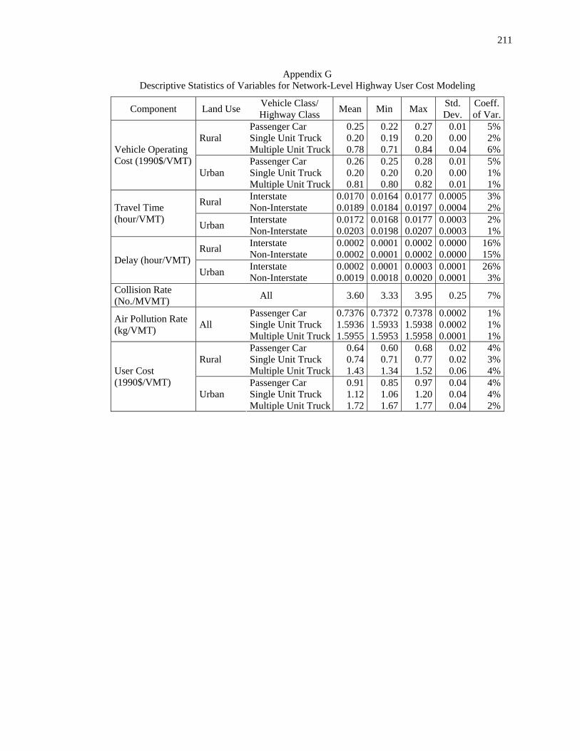
211
Appendix G Descriptive Statistics of Variables for Network-Level Highway User Cost Modeling
Component Land Use Vehicle Class/ Highway Class Mean Min Max Std.
Dev. Coeff. of Var.
Rural Passenger Car Single Unit Truck Multiple Unit Truck
0.250.200.78
0.220.190.71
0.27 0.20 0.84
0.010.000.04
5%2%6%Vehicle Operating
Cost (1990$/VMT) Urban
Passenger Car Single Unit Truck Multiple Unit Truck
0.260.200.81
0.250.200.80
0.28 0.20 0.82
0.010.000.01
5%1%1%
Rural Interstate Non-Interstate
0.01700.0189
0.01640.0184
0.0177 0.0197
0.00050.0004
3%2%Travel Time
(hour/VMT) Urban Interstate Non-Interstate
0.01720.0203
0.01680.0198
0.0177 0.0207
0.00030.0003
2%1%
Rural Interstate Non-Interstate
0.00020.0002
0.00010.0001
0.0002 0.0002
0.00000.0000
16%15%Delay (hour/VMT)
Urban Interstate Non-Interstate
0.00020.0019
0.00010.0018
0.0003 0.0020
0.00010.0001
26%3%
Collision Rate (No./MVMT) All 3.60 3.33 3.95 0.25 7%
Air Pollution Rate (kg/VMT) All
Passenger Car Single Unit Truck Multiple Unit Truck
0.73761.59361.5955
0.73721.59331.5953
0.7378 1.5938 1.5958
0.00020.00020.0001
1%1%1%
Rural Passenger Car Single Unit Truck Multiple Unit Truck
0.640.741.43
0.600.711.34
0.68 0.77 1.52
0.020.020.06
4%3%4%User Cost
(1990$/VMT) Urban
Passenger Car Single Unit Truck Multiple Unit Truck
0.911.121.72
0.851.061.67
0.97 1.20 1.77
0.040.040.04
4%4%2%

212
Appendix H Descriptive Statistics of Variables for Directional Distribution, Lane Occupancy Adjustment Factor,
and Truck Percentage Modeling
Designation Highway Class Mean Minimum Maximum Std. Dev. Coeff. of Var.
Directional Distribution (DD) (%)
Rural interstate Rural non-interstate Urban interstate Urban non-interstate
53 52 51 54
53 48 47 39
53 55 56 68
0 3 3
10
0% 5% 6%
18% Lane Occupancy Adjustment Factor (Lf)
Rural interstate Rural non-interstate Urban interstate Urban non-interstate
0.75 0.80 0.72 0.59
0.73 0.78 0.70 0.42
0.77 0.82 0.74 0.77
0.01 0.01 0.01 0.12
2% 2% 2%
20%
Single Unit Truck (%)
Rural interstate Rural non-interstate Urban interstate Urban non-interstate
20 24 19 15
16 21 15 12
25 26 23 18
3 2 3 2
15% 9%
14% 12%
Multiple Unit Truck (%)
Rural interstate Rural non-interstate Urban interstate Urban non-interstate
18 10
9 2
16 8 8 2
22 13 11
3
2 2 1 0
13% 18% 12% 12%

213
Appendix I Descriptive Statistics of Variables for Highway Pavement Performance Modeling

214
Appendix I1 Descriptive Statistics of Pavement Rehabilitation Expenditure in Indiana (1990$)
Pavement Type Mean Min Max Std. Dev. Coeff. of Var.
Flexible 155,287 29,147 1,119,863 242,260 156% Rigid 383,704 57,952 2,052,896 509,879 133% Composite 207,634 53,399 1,602,124 440,193 212%
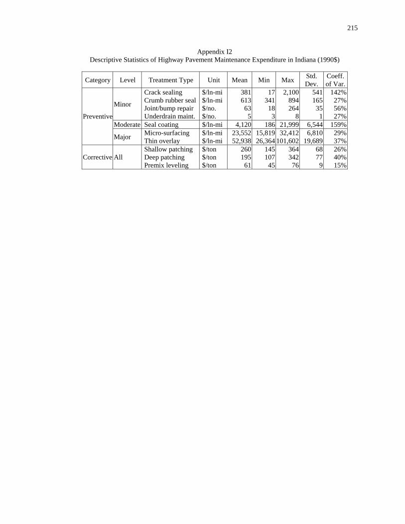
215
Appendix I2 Descriptive Statistics of Highway Pavement Maintenance Expenditure in Indiana (1990$)
Category Level Treatment Type Unit Mean Min Max Std. Dev.
Coeff. of Var.
Minor
Crack sealing Crumb rubber seal Joint/bump repair Underdrain maint.
$/ln-mi $/ln-mi $/no. $/no.
38161363
5
1734118
3
2,100 894 264
8
541 165 35
1
142%27%56%27%
Moderate Seal coating $/ln-mi 4,120 186 21,999 6,544 159%Preventive
Major Micro-surfacing Thin overlay
$/ln-mi $/ln-mi
23,55252,938
15,81926,364
32,412 101,602
6,810 19,689
29%37%
Corrective All Shallow patching Deep patching Premix leveling
$/ton $/ton $/ton
26019561
14510745
364 342 76
68 77
9
26%40%15%

216
Appendix I3 Descriptive Statistics of Annual ESAL on Various Highway Pavement Types in Indiana (in Millions)
Pavement Type Highway Class Mean Min Max Std. Dev. Coeff. of Var.
Flexible All 0.39 0.00 0.15 0.12 80%
Rigid Interstate Non-interstate
0.71 0.26
0.20 0.07
2.43 0.97
0.53 0.19
75% 73%
Composite Interstate Non-interstate
0.81 0.28
0.36 0.03
1.96 0.94
0.48 0.20
59% 69%

217
Appendix I4 Weather Severity Index for Individual Counties in Indiana
County Region WSI County Region WSI County Region WSI
Adams Allen BartholomewBenton Blackford Boone Brown Carroll Cass Clarke Clay Clinton Crawford Daviess Dearborn Decatur Dekalb Delaware Dubois Elkhart Fayette Floyd Fountain Franklin Fulton Gibson Grant Greene Hamilton Hancock Harrison
NE NE SE
NW NE
NW SE
NW NW SE
WC NW SW SW SE SE NE EC SW NE EC SE
WC EC
NW SW NE SW EC EC SE
0.72 0.78 0.63 0.77 0.75 0.73 0.70 0.72 0.77 0.59 0.70 0.70 0.61 0.58 0.60 0.66 0.84 0.78 0.59 0.83 0.68 0.58 0.69 0.71 0.79 0.59 0.77 0.61 0.72 0.76 0.55
Hendricks Henry Howard Huntington Jackson Jasper Jay Jefferson Jennings Johnson Knox Kosciusko Lagrange Lake LaPorte Lawrence Madison Marion Marshall Martin Miami Monroe Montgomery Morgan Newton Noble Ohio Orange Owen Parke Perry
WC EC
NW NE SE
NW NE SE SE EC SW NE NE
NW NW SW EC EC
NW SW NW SW WC WC NW NE SE
SW WC WC SW
0.74 0.74 0.78 0.82 0.64 0.72 0.75 0.59 0.63 0.70 0.58 0.81 0.83 0.86 0.81 0.64 0.83 0.75 0.82 0.65 0.82 0.59 0.78 0.71 0.79 0.85 0.50 0.63 0.69 0.71 0.54
Pike Porter Posey Pulaski Putnum Randolph Ripley Rush St. Joseph Scott Shelby Spence Starke Steuben Sullivan Switzerland Tippecanoe Tipton Union Vanderburg Vermilion Vigo Wabash Warren Warrick Washington Wayne Wells White Whitney
SW NW SW NW WC EC SE EC
NW SE EC SW NW NE SW SE
WC EC EC SW WC WC NE
WC SW SE EC NE
NW NE
0.59 0.80 0.55 0.76 0.76 0.77 0.62 0.71 0.85 0.60 0.71 0.54 0.79 0.85 0.63 0.58 0.70 0.82 0.70 0.55 0.68 0.62 0.83 0.71 0.54 0.61 0.73 0.79 0.72 0.81
Note: WSI- Weather severity index.

218
Appendix I5 Descriptive Statistics of Rehabilitation Intervals for Various Highway Pavement Types in Indiana
(in Years)
Pavement Type Highway Class Mean Min Max Std. Dev. Coeff. of Var.
Flexible All 16.00 6.00 10.18 3.03 30% Rigid
Interstate Non-interstate
26.76 24.71
12.00 13.00
38.40 34.00
7.94 5.13
30% 21%
Composite
Interstate Non-interstate
22.04 14.00
14.00 6.00
31.00 24.00
5.36 4.03
24% 28%

219
Appendix J Descriptive Statistics of Variables for Highway Bridge Performance Modeling

220
Appendix J1 Descriptive Statistics of Variable for Concrete Bridge Performance Modeling
Item Designation Mean Min Max Std. Dev. Coeff. of Var.
Deck
Condition rating % Condition change AADT Age (year) Average expenditure (1990, $/ft2)
77%
6,9393271
40%
011
1
9 25%
69,425 75
468
18%
7,6271327
14%118%110%42%38%
Superstructure
Condition rating % Condition change AADT Age (year) Average expenditure (1990, $/ft2)
614%
8,58844
143
30%10011
5
9 33%
44,235 75
273
18%
7,5421134
16%57%88%26%23%
Substructure
Condition rating % Condition change AADT Age (year) Average expenditure (1990, $/ft2)
415%
1,1264226
40%6743026
4 25%
2,050 49 28
013%362
70
0%85%32%16%
2% Wearing Surface
Condition rating % Condition change AADT Age (year) Average expenditure (1990, $/ft2)
493%
6,9393271
20%
011
1
7 167%
69,425 75
468
130%
7,6271327
20%32%
110%42%38%

221
Appendix J2 Descriptive Statistics of Variable for Steel Bridge Performance Modeling
Item Designation Mean Min Max Std. Dev. Coeff. of Var.
Deck
Condition rating % Condition change AADT Age (year) Average expenditure (1990, $/ft2)
616%
14,7784057
30%
013
0
9 33%
111,620 70
387
15%
16,9351230
17%31%
115%31%53%
Superstructure
Condition rating % Condition change AADT Age (year) Average expenditure (1990, $/ft2)
615%
13,8134097
30%
014
0
9 33%
69,780 70
305
18%
18,6611464
15%52%
135%36%66%
Substructure
Condition rating % Condition change AADT Age (year) Average expenditure (1990, $/ft2)
425%
5,7445027
425%
3,9914725
4 25%
17,618 53 29
00%
4,79822
0%0%
84%5%6%
Wearing Surface
Condition rating % Condition change AADT Age (year) Average expenditure (1990, $/ft2)
489%
14,7784057
30%
013
0
7 167%
111,620 70
387
131%
16,9351230
21%35%
115%31%53%

222
Appendix J3 Descriptive Statistics of Variable for Bridge Agency and User Cost Modeling
Bridge Type Designation Mean Min Max Std.
Dev. Coeff. of Var.
Concrete
AADT Age (year) Number of lanes Bridge length before work (ft) Bridge length after work (ft) Approach length (ft) Total deck width (ft) Clear deck width (ft) Vertical clearance (ft) Substructure height (ft) Detour length (mile) Load inventory rating (ton) Rehabilitation expenditure (1990$, in 1,000)Unit rehabilitation expenditure (1990$/ft2) Construction expenditure (1990$, in 1,000) Unit construction expenditure (1990$/ft2) EUAUC before work (1990$, in 1,000) EUAUC after work (1990$, in 1,000) EUAUC change (%)
7,05434
2124126
33735
186
333
30182
379225
10,1023,548-57%
011
0.022.022.00.02.95.80.00.0
00
7.00.91.60.30.00.0
47%
69,42575
61,2341,2341,250
989511
2242096
1,061468
1,023734
245,98792,169-100%
7,70014
110810834
992
1114
1115339
20391
17,6866,15471%
109%39%26%87%85%
1074%25%26%
347%129%126%32%51%47%53%40%
175%173%
-124%
Steel
AADT Age (year) Number of lanes Bridge length before work (ft) Bridge length after work (ft) Approach length (ft) Total deck width (ft) Clear deck width (ft) Vertical clearance (ft) Substructure height (ft) Detour length (mile) Load inventory rating (ton) Rehabilitation expenditure (1990$, in 1,000)Unit rehabilitation expenditure (1990$/ft2) Construction expenditure (1990$, in 1,000) Unit construction expenditure (1990$/ft2) EUAUC before work (1990$, in 1,000) EUAUC after work (1990$, in 1,000) EUAUC change (%)
14,50939
2284285
63936
3169
337
44760
516126
16,1675,317-63%
010
0.028.030.00.01.94.20.00.0
00
0.70.1
68.11.70.00.0
63%
117,22086
84,9324,932
92311410911
3,0212084
1,059387
1,058372
304,191117,991
-100%
16,99613
1268267401313
4154
610
19836
278100
27,1459,92417%
117%32%40%94%94%
652%34%35%
124%91%
213%26%44%59%54%79%
168%187%-27%

223
Appendix K Lower and Upper Ranges for the Development of Utility Functions Corresponding to Individual
Performance Indicators
Goal Performance Indicator Unit Lower Upper
System Preservation
Bridge structural condition Bridge wearing surface condition Historical bridge age Historical bridge length Pavement surface condition Remaining service life
rating scale rating scale year ft inch/mile year
3 3
80 40 40
2
9 9
200 200 240 10
User Cost Average speed (part 1) Average speed (part 2) mph 15
55 55 75
Mobility Average speed Detour length Intersection delay time
mph mile min/vehicle
0 0 0
80 10 20
Safety
Bridge load inventory rating Bridge clear deck width (part 1) Bridge clear deck width (part 2) Bridge vertical clearance- over Bridge vertical clearance- under Bridge horizontal clearance Average speed Skid resistance Lane width (part 1) Lane width (part 2) Shoulder width Railroad crossing Sight distance Luminance
ton ratio ratio ratio ratio ratio mph number ratio ratio ratio number ratio ratio
0 0.8 1.0 0.8 0.8 0.8
0 10
0.8 1.0
0 0
0.6 0.6
40 1.0 1.1 1.0 1.0 1.0 80 50
1.0 1.1 1.0
3 1.0 1.0
Environment
Average speed for CO2, TSP, SO2 (part 1) Average speed for CO2, TSP, SO2 (part 2) Average speed for NMHC Average speed for CO (part 1) Average speed for CO (part 2) Average speed for NOx (part 1) Average speed for NOx (part 2)
mph
15 55
0 0
35 0
15
55 75 60 35 65 15 65

224
Appendix L Descriptive Statistics of Relative Weights Assigned to Asset Management System Goals and
Performance Indicators

225
Appendix L1 Descriptive Statistics of Relative Weights Assigned to Asset Management System Goals
Agency Group User Group System Goal Mean Std. Dev. Mean Std. Dev.
System Preservation Agency Cost User Cost Mobility Safety Environment
9 8 7 8 9 7
1 1 1 1 1 1
7 7 7 8 9 8
2 2 2 2 1 2
Survey Participants 29 28

226
Appendix L2 Descriptive Statistics of Relative Weights Assigned to Performance Indicators under Various Asset
Management System Goals Agency Group User Group Asset
Management System Goal
Asset Management
Program
Weight Assigned Performance Indicator Mean Std.
Dev. Mean Std. Dev.
Bridge Preservation
Bridge structural condition Bridge wearing surface condition Bridge remaining service life
9 6 8
1 1 2
9 7 5
1 1 3
Historical Bridge Preservation
Bridge structural condition Bridge wearing surface condition Bridge remaining service life Historical bridge age Historical bridge length
9 6 7 8 6
1 1 2 1 2
8 6 7 8 5
2 2 3 2 2
System Preservation
Pavement Preservation
Surface condition Remaining service life
9 9
1 1
8 8
1 1
Bridge Preservation
Bridge construction cost Bridge rehabilitation cost Bridge maintenance cost
8 9 7
1 1 1
8 7 7
2 2 2
Pavement Preservation
Pavement construction cost Pavement rehabilitation cost Pavement maintenance cost
8 9 7
1 1 1
8 7 7
2 2 2
Agency Cost
ITS Improvements
Procurement cost Maintenance cost
9 4
1 1
8 4
2 1
Bridge Preservation
Detour condition Average travel speed
7 8
2 2
7 8
2 2 User Cost
Pavement Preservation
Pavement surface condition Average travel speed
8 8
1 1
8 9
2 1
Mobility Bridge Preservation
Detour length Average travel speed
8 8
1 1
9 8
1 2
Bridge Preservation
Bridge inventory rating Bridge clear deck width Bridge vertical clearance (over) Bridge vertical clearance (under) Bridge horizontal clearance
7 8 7 8 7
2 1 2 1 1
8 8 7 6 7
1 2 2 3 2
Pavement Preservation
Average speed Skid resistance Lane width Shoulder width
8 8 7 6
2 1 1 1
8 7 7 6
2 2 2 2
Railroad Crossings
Railroad crossing adequacy Occurrence of collisions
9 8
1 1
8 8
2 2
Safety
Sight distance Luminance Occurrence of collisions
9 7 8
1 1 1
8 7 8
2 2 2
Traffic Signals Average speed Occurrence of collisions
7 9
1 1
7 8
2 2
Safety
DNR/ Forest/ Other
Average speed Skid resistance Lane width
8 8 7
2 1 1
8 7 7
2 2 2
Survey Participants 9 9
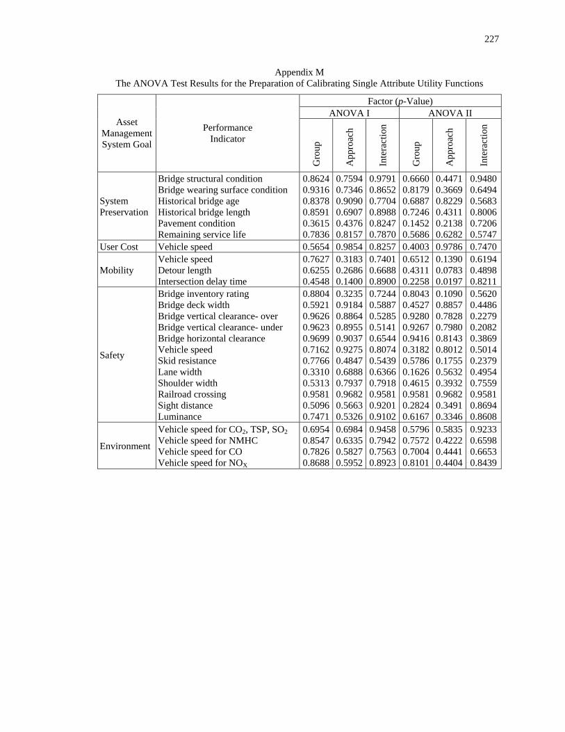
227
Appendix M The ANOVA Test Results for the Preparation of Calibrating Single Attribute Utility Functions
Factor (p-Value) ANOVA I ANOVA II
Asset Management System Goal
Performance Indicator
Gro
up
App
roac
h
Inte
ract
ion
Gro
up
App
roac
h
Inte
ract
ion
System Preservation
Bridge structural condition Bridge wearing surface condition Historical bridge age Historical bridge length Pavement condition Remaining service life
0.86240.93160.83780.85910.36150.7836
0.75940.73460.90900.69070.43760.8157
0.97910.86520.77040.89880.82470.7870
0.6660 0.8179 0.6887 0.7246 0.1452 0.5686
0.44710.36690.82290.43110.21380.6282
0.94800.64940.56830.80060.72060.5747
User Cost Vehicle speed 0.5654 0.9854 0.8257 0.4003 0.9786 0.7470
Mobility Vehicle speed Detour length Intersection delay time
0.76270.62550.4548
0.31830.26860.1400
0.74010.66880.8900
0.6512 0.4311 0.2258
0.13900.07830.0197
0.61940.48980.8211
Safety
Bridge inventory rating Bridge deck width Bridge vertical clearance- over Bridge vertical clearance- under Bridge horizontal clearance Vehicle speed Skid resistance Lane width Shoulder width Railroad crossing Sight distance Luminance
0.88040.59210.96260.96230.96990.71620.77660.33100.53130.95810.50960.7471
0.32350.91840.88640.89550.90370.92750.48470.68880.79370.96820.56630.5326
0.72440.58870.52850.51410.65440.80740.54390.63660.79180.95810.92010.9102
0.8043 0.4527 0.9280 0.9267 0.9416 0.3182 0.5786 0.1626 0.4615 0.9581 0.2824 0.6167
0.10900.88570.78280.79800.81430.80120.17550.56320.39320.96820.34910.3346
0.56200.44860.22790.20820.38690.50140.23790.49540.75590.95810.86940.8608
Environment
Vehicle speed for CO2, TSP, SO2 Vehicle speed for NMHC Vehicle speed for CO Vehicle speed for NOX
0.69540.85470.78260.8688
0.69840.63350.58270.5952
0.94580.79420.75630.8923
0.5796 0.7572 0.7004 0.8101
0.58350.42220.44410.4404
0.92330.65980.66530.8439

228
Appendix N
Descriptive Statistics of Variables for the Calibration of Utility Functions Associated with Individual Performance Indicators
Asset Management System Goal
Performance Indicator Mean Min Max Std. Dev. Coeff. of
Var.
System Preservation
Bridge structural condition Bridge wearing surface Historical bridge age Historical bridge length Pavement surface condition Remaining service life
0.5472 0.5359 0.4860 0.4977 0.5655 0.4759
0.0000 0.0000 0.0000 0.0000 0.0000 0.0000
1.0000 1.0000 1.0000 1.0000 1.0000 1.0000
0.3285 0.3390 0.3028 0.3041 0.3196 0.3051
60% 63% 62% 61% 57% 64%
User Cost Average speed 0.5002 0.5038
0.0000 0.0000
1.0000 1.0000
0.3071 0.2897
61% 58%
Mobility
Average speed Detour length Intersection delay time
0.5422 0.4884 0.5068 0.3622
0.0000 0.0000 0.0000 0.0000
1.0000 1.0000 1.0000 1.0000
0.2985 0.2815 0.2869 0.3133
55 % 58% 57% 87%
Safety
Bridge load inventory rating Bridge deck width Bridge vertical clearance (o) Bridge vertical clearance (u) Bridge horizontal clearance Average speed Skid resistance Lane width Shoulder width Railroad crossing Sight distance Luminance
0.5634 0.4619 0.9484 0.4837 0.4839 0.4825 0.4997 0.5074 0.4952 0.9513 0.4975 0.5581 0.4528 0.4448
0.0000 0.0000 0.9236 0.0000 0.0000 0.0000 0.0000 0.0000 0.0000 0.9167 0.0000 0.0000 0.0000 0.0000
1.0000 1.0000 1.0000 1.0000 1.0000 1.0000 1.0000 1.0000 1.0000 1.0000 1.0000 1.0000 1.0000 1.0000
0.3165 0.3083 0.0355 0.3032 0.3022 0.3023 0.2974 0.3072 0.3032 0.0352 0.3016 0.4296 0.3202 0.3286
56% 67 % 4%
63% 62% 63% 60% 61% 61% 4%
61% 77% 71% 74%
Environment
Speed for CO2, TSP, SO2 Speed for NMHC Speed for CO Speed for NOx
0.4947 0.5051 0.5534 0.5733 0.5336 0.5300 0.5110
0.0000 0.0000 0.0000 0.0000 0.0000 0.0000 0.0000
1.0000 1.0000 1.0000 1.0000 1.0000 1.0000 1.0000
0.3070 0.3038 0.2766 0.2783 0.2934 0.3557 0.2868
62% 60% 50% 49% 55% 67% 56%

229
Appendix O Descriptive Statistics of Performance Indicators Involving Risk in Tradeoff Decision Process
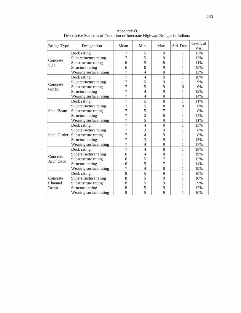
230
Appendix O1 Descriptive Statistics of Condition of Interstate Highway Bridges in Indiana
Bridge Type Designation Mean Min Max Std. Dev. Coeff. of Var.
Concrete Slab
Deck rating Superstructure rating Substructure rating Structure rating Wearing surface rating
7 7 6 6 7
5 5 5 0 4
9 9 8 9 9
1 1 1 1 1
13% 12% 11% 15% 13%
Concrete Girder
Deck rating Superstructure rating Substructure rating Structure rating Wearing surface rating
7 7 7 7 7
4 5 5 4 4
9 9 9 9 9
1 1 0 1 1
10% 9% 6%
12% 14%
Steel Beam
Deck rating Superstructure rating Substructure rating Structure rating Wearing surface rating
7 7 7 7 7
5 5 5 2 5
8 8 7 8 9
1 0 1 1 1
11% 6% 8%
14% 11%
Steel Girder
Deck rating Superstructure rating Substructure rating Structure rating Wearing surface rating
7 7 7 7 7
4 3 4 3 4
9 9 9 9 9
1 1 1 1 1
15% 8% 8%
13% 17%
Concrete Arch Deck
Deck rating Superstructure rating Substructure rating Structure rating Wearing surface rating
7 6 6 6 7
4 4 5 5 4
8 8 7 7 8
1 1 1 1 1
18% 19% 12% 14% 19%
Concrete Channel Beam
Deck rating Superstructure rating Substructure rating Structure rating Wearing surface rating
8 8 8 8 8
5 5 5 5 5
9 9 9 9 9
1 1 1 1 1
10% 10%
9% 12% 10%

231
Appendix O2 Descriptive Statistics of Condition of NHS Non-Interstate Highway Bridges in Indiana
Bridge Type Designation Mean Min Max Std. Dev. Coeff. of Var.
Concrete Slab
Deck rating Superstructure rating Substructure rating Structure rating Wearing surface rating
6 6 6 6 7
3 3 2 2 4
9 9 9 9 9
1 1 1 1 1
18% 18% 19% 22% 15%
Concrete Girder
Deck rating Superstructure rating Substructure rating Structure rating Wearing surface rating
7 7 7 7 7
4 4 5 4 4
9 9 9 9 9
1 1 1 1 1
11% 9% 9%
12% 14%
Steel Beam
Deck rating Superstructure rating Substructure rating Structure rating Wearing surface rating
7 7 6 7 7
4 2 3 2 4
9 9 9 9 9
1 1 1 1 1
14% 13% 18% 17% 14%
Steel Girder
Deck rating Superstructure rating Substructure rating Structure rating Wearing surface rating
7 7 7 7 7
4 1 3 2 3
9 9 9 9 9
1 1 1 1 1
14% 9%
10% 14% 16%
Concrete Arch Deck
Deck rating Superstructure rating Substructure rating Structure rating Wearing surface rating
7 7 7 7 7
5 6 5 5 5
9 8 9 9 9
1 1 1 1 1
10% 8%
11% 13% 13%
Concrete Channel Beam
Deck rating Superstructure rating Substructure rating Structure rating Wearing surface rating
7 8 7 7 7
5 5 0 5 5
9 9 9 9 9
1 1 1 1 1
11% 10% 12% 11% 15%

232
Appendix O3 Descriptive Statistics of Condition of Non-NHS State Highway Bridges in Indiana
Bridge Type Designation Mean Min Max Std. Dev. Coeff. of Var.
Concrete Slab
Deck rating Superstructure rating Substructure rating Structure rating Wearing surface rating
6 6 6 6 7
3 3 3 2 3
9 9 9 9 9
1 1 1 1 1
15% 16% 13% 21% 13%
Concrete Girder
Deck rating Superstructure rating Substructure rating Structure rating Wearing surface rating
7 7 7 7 7
4 3 4 2 4
9 9 9 9 9
1 1 1 1 1
13% 12% 10% 14% 14%
Steel Beam
Deck rating Superstructure rating Substructure rating Structure rating Wearing surface rating
7 6 6 6 7
3 3 3 2 3
9 9 9 9 9
1 1 1 1 1
16% 16% 15% 21% 14%
Steel Girder
Deck rating Superstructure rating Substructure rating Structure rating Wearing surface rating
7 7 7 7 7
3 3 3 2 3
9 9 9 9 9
1 1 1 1 1
15% 10% 11% 14% 16%
Concrete Arch Deck
Deck rating Superstructure rating Substructure rating Structure rating Wearing surface rating
7 7 7 6 7
4 4 3 0 4
9 9 9 9 9
1 1 1 2 1
12% 13% 18% 34% 13%
Concrete Channel Beam
Deck rating Superstructure rating Substructure rating Structure rating Wearing surface rating
7 7 7 7 7
4 4 4 2 3
9 9 9 9 9
1 1 1 1 1
11% 10% 10% 15% 15%

233
Appendix O4 Descriptive Statistics of Condition of Non-NHS Local Highway Bridges in Indiana
Bridge Type Designation Mean Min Max Std. Dev. Coeff. of Var.
Concrete Slab
Deck rating Superstructure rating Substructure rating Structure rating Wearing surface rating
6 7 6 6 7
4 5 4 4 4
9 9 7 8 9
1 1 1 1 1
18% 16% 13% 20% 18%
Concrete Girder
Deck rating Superstructure rating Substructure rating Structure rating Wearing surface rating
7 7 7 7 7
5 6 6 6 5
9 9 9 9 9
1 1 1 1 1
11% 12% 14% 14% 14%
Steel Beam
Deck rating Superstructure rating Substructure rating Structure rating Wearing surface rating
5 5 5 4 6
1 3 2 0 3
7 7 7 9 9
1 1 1 2 1
30% 24% 24% 55% 24%
Steel Girder
Deck rating Superstructure rating Substructure rating Structure rating Wearing surface rating
7 7 6 6 7
4 5 5 5 4
8 8 8 8 8
1 1 1 1 1
14% 14% 17% 17% 14%
Concrete Arch Deck
Deck rating Superstructure rating Substructure rating Structure rating Wearing surface rating
7 7 7 6 7
4 4 5 2 4
9 9 9 8 9
2 1 1 2 2
23% 20% 16% 36% 23%
Concrete Channel Beam
Deck rating Superstructure rating Substructure rating Structure rating Wearing surface rating
8 8 8 8 8
8 8 7 8 7
9 9 8 8 9
0 1 1 0 1
4% 6% 7% 0%
10%
Prestressed Concrete Box Beam
Deck rating Superstructure rating Substructure rating Structure rating Wearing surface rating
7 8 8 7 7
5 5 6 2 5
9 9 9 9 9
1 1 1 3 1
16% 18% 14% 38% 20%

234
Appendix O5 Descriptive Statistics of Usage of Interstate Highway Bridges in Indiana
Bridge Type Designation Mean Min Max Std. Dev. Coeff. of Var.
Concrete Slab
Age (year) AADT Detour length (mile) Load invent rating (ton)
39 18,465
2 41
26 763
1 32
52 78,250
18 59
5 13,698
3 6
14% 74%
167% 14%
Concrete Girder
Age (year) AADT Detour length (mile) Load invent rating (ton)
33 16,057
1 34
5 0 1
16
47 114,440
10 62
8 13,474
1 7
23% 84% 98% 20%
Steel Beam
Age (year) AADT Detour length (mile) Load invent rating (ton)
30 27,930
3 37
5 0 1 0
51 117,220
18 54
13 29,284
4 6
44% 105% 121% 17%
Steel Girder
Age (year) AADT Detour length (mile) Load invent rating (ton)
33 27,404
1 39
7 0 0
23
51 127,450
56 79
8 24,653
3 8
25% 90%
230% 20%
Concrete Arch Deck
Age (year) AADT Detour length (mile) Load invent rating (ton)
36 21,993
2 42
34 7,595
1 26
37 53,740
18 63
1 14,670
5 10
3% 67%
196% 23%
Concrete Channel Beam
Age (year) AADT Detour length (mile) Load invent rating (ton)
17 13,429
2 39
8 0 1
22
40 127,450
10 89
11 20,428
2 8
63% 152% 133% 21%

235
Appendix O6
Descriptive Statistics of Usage of NHS Non-Interstate Highway Bridges in Indiana
Bridge Type Designation Mean Min Max Std. Dev. Coeff. of Var.
Concrete Slab
Age (year) AADT Detour length (mile) Load invent rating (ton)
56 12,003
4 36
5 191
0 0
86 43,347
15 64
15 8,316
3 8
27% 69% 74% 21%
Concrete Girder
Age (year) AADT Detour length (mile) Load invent rating (ton)
35 6,564
3 35
5 0 0
19
74 44,036
11 58
11 6,508
2 7
31% 99% 73% 19%
Steel Beam
Age (year) AADT Detour length (mile) Load invent rating (ton)
35 13,772
7 37
5 763
1 28
85 69,127
40 59
18 13,231
11 6
52% 96%
168% 16%
Steel Girder
Age (year) AADT Detour length (mile) Load invent rating (ton)
31 8,146
4 38
5 0 0 0
72 74,912
52 80
10 11,640
4 7
32% 143% 115% 18%
Concrete Arch Deck
Age (year) AADT Detour length (mile) Load invent rating (ton)
34 11,576
3 42
7 219
1 23
78 30,621
10 68
24 8,625
3 12
69% 75% 76% 28%
Concrete Channel Beam
Age (year) AADT Detour length (mile) Load invent rating (ton)
27 8,576
3 39
5 1 1
21
93 27,500
40 73
19 7,234
5 9
69% 84%
142% 24%

236
Appendix O7 Descriptive Statistics of Usage of Non-NHS State Highway Bridges in Indiana
Bridge Type Designation Mean Min Max Std. Dev. Coeff. of Var.
Concrete Slab
Age (year) AADT Detour length (mile) Load invent rating (ton)
55 4,585
5 35
1 0 0 0
94 29,062
23 85
18 3,927
3 9
33% 86% 64% 26%
Concrete Girder
Age (year) AADT Detour length (mile) Load invent rating (ton)
23 4,401
4 33
3 152
1 0
76 41,882
23 68
16 4,703
2 6
69% 107% 58% 18%
Steel Beam
Age (year) AADT Detour length (mile) Load invent rating (ton)
44 7,298
4 31
4 0 0 0
100 992,572
40 70
25 56,465
5 17
57% 774% 135% 55%
Steel Girder
Age (year) AADT Detour length (mile) Load invent rating (ton)
33 6,257
5 37
4 0 0 0
90 40,846
98 77
17 6,702
7 8
51% 107% 146% 22%
Concrete Arch Deck
Age (year) AADT Detour length (mile) Load invent rating (ton)
44 3,260
4 34
4 0 0 0
90 54,570
15 96
24 4,813
3 19
54% 148% 57% 56%
Concrete Channel Beam
Age (year) AADT Detour length (mile) Load invent rating (ton)
25 3,871
5 36
4 0 1 0
100 24,086
26 75
16 3,886
4 8
64% 100% 69% 22%
Timber Stringer
Age (year) AADT Detour length (mile) Load invent rating (ton)
12 3,433
6 35
7 2,060
4 32
15 4,613
9 36
4 1,156
2 2
30% 34% 39%
5%
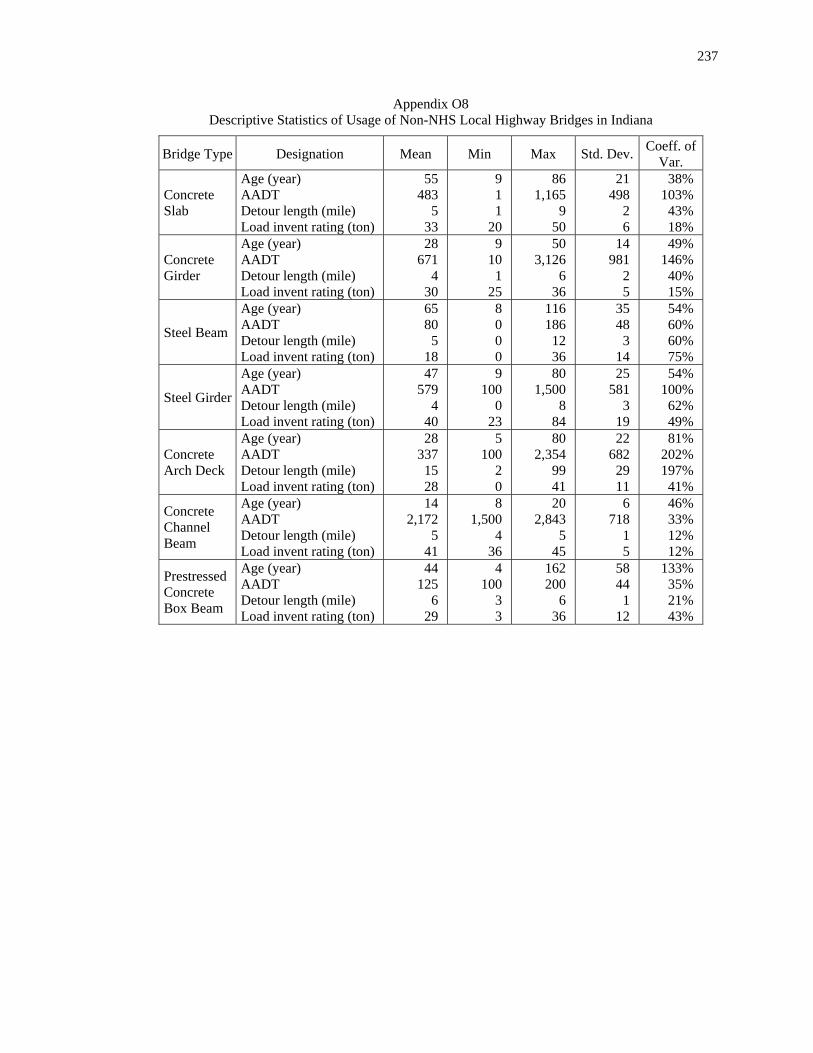
237
Appendix O8 Descriptive Statistics of Usage of Non-NHS Local Highway Bridges in Indiana
Bridge Type Designation Mean Min Max Std. Dev. Coeff. of Var.
Concrete Slab
Age (year) AADT Detour length (mile) Load invent rating (ton)
55 483
5 33
9 1 1
20
86 1,165
9 50
21 498
2 6
38% 103% 43% 18%
Concrete Girder
Age (year) AADT Detour length (mile) Load invent rating (ton)
28 671
4 30
9 10
1 25
50 3,126
6 36
14 981
2 5
49% 146% 40% 15%
Steel Beam
Age (year) AADT Detour length (mile) Load invent rating (ton)
65 80
5 18
8 0 0 0
116 186 12 36
35 48
3 14
54% 60% 60% 75%
Steel Girder
Age (year) AADT Detour length (mile) Load invent rating (ton)
47 579
4 40
9 100
0 23
80 1,500
8 84
25 581
3 19
54% 100% 62% 49%
Concrete Arch Deck
Age (year) AADT Detour length (mile) Load invent rating (ton)
28 337 15 28
5 100
2 0
80 2,354
99 41
22 682 29 11
81% 202% 197% 41%
Concrete Channel Beam
Age (year) AADT Detour length (mile) Load invent rating (ton)
14 2,172
5 41
8 1,500
4 36
20 2,843
5 45
6 718
1 5
46% 33% 12% 12%
Prestressed Concrete Box Beam
Age (year) AADT Detour length (mile) Load invent rating (ton)
44 125
6 29
4 100
3 3
162 200
6 36
58 44
1 12
133% 35% 21% 43%

238
Appendix O9 Descriptive Statistics of Condition, Service Life, Maintenance, Rehabilitation, and Traffic Loading of
Flexible, Rigid, and Composite Pavements in Indiana
Pavement Type
Highway Class Item Mean Min Max Std. Dev. Coeff.
of Var.
Flexible All
IRI (inch/mile) RI (year) AAME (1990$/ln-mi) Rehab. expenditure (1990$/ln-mi) Annual ESALs (in million)
14616
1,092155,287
0.39
416
1829,147
0.00
34710
4741,119,863
0.15
683
341242,260
0.12
46%30%72%
156%80%
IS
IRI (inch/mile) RI (year) AAME (1990$/ln-mi) Rehab. expenditure (1990$/ln-mi) Annual ESALs (in million)
12827
304383,704
0.71
481251
57,9520.20
30538
1,1712,052,896
2.43
428
304509,879
0.53
33%30%
100%133%75%
Rigid
Non-IS
IRI (inch/mile) RI (year) AAME (1990$/ln-mi) Rehab. expenditure (1990$/ln-mi) Annual ESALs (in million)
17825
758383,704
0.26
441341
57,9520.07
35434
3,3842,052,896
0.97
615
676509,879
0.19
34%21%89%
133%73%
IS
IRI (inch/mile) RI (year) AAME (1990$/ln-mi) Rehab. expenditure (1990$/ln-mi) Annual ESALs (in million)
9322
364207,634
0.81
351480
53,3990.36
31231
1,0521,602,124
1.96
325
278440,193
0.48
34%24%76%
212%59%
Composite
Non-IS
IRI (inch/mile) RI (year) AAME (1990$/ln-mi) Rehab. expenditure (1990$/ln-mi) Annual ESALs (in million)
12414
681207,634
0.28
406
6853,399
0.03
35524
4,4891,602,124
0.94
534
761440,193
0.20
42%28%
112%212%69%

239
Appendix O10 Descriptive Statistics of Unit Cost of Various Pavement Maintenance Treatments in Indiana (1990$)
Treatment Type Unit Mean Min Max Std. Dev. Coeff. of Var.
Crack Sealing Crumb Rubber Sealing Joint/Bump Repair Underdrain Maintenance Seal Coating Micro-Surfacing Thin HMA Overlay Shallow Patching Deep Patching Premix Leveling
$/lane-mile $/lane-mile $/Number $/Number $/lane-mile $/lane-mile $/lane-mile $/ton $/ton $/ton
381 613 63
5 4,120
23,552 52,938
260 195 61
17 341 18
3 186
15,819 26,364
145 107 45
2,100 894 264
8 21,999 32,412
101,602 364 342 76
541 165 35
1 6,544 6,810
19,689 68 77
9
142% 27% 56% 27%
159% 29% 37% 26% 40% 15%

240
Appendix O11 Descriptive Statistics of Average Traveling Speed on
Indiana State Highway Network (in mph)
Land Use Highway Class Mean Min Max Std. Dev.
Coeff. of Var.
Rural
Rural interstate Rural principle arterial Rural minor arterial Rural major collector
59.554.356.849.7
57.049.655.048.0
61.7 58.6 57.0 50.0
1.6 3.2 0.6 0.6
3% 6% 1% 1%
Urban
Urban interstate Urban freeway and expressway Urban principal arterial Urban minor arterial Urban collector
59.059.554.054.356.4
57.357.852.753.254.3
60.0 61.6 55.2 56.4 58.3
1.0 1.3 0.9 1.0 1.4
2% 2% 2% 2% 2%
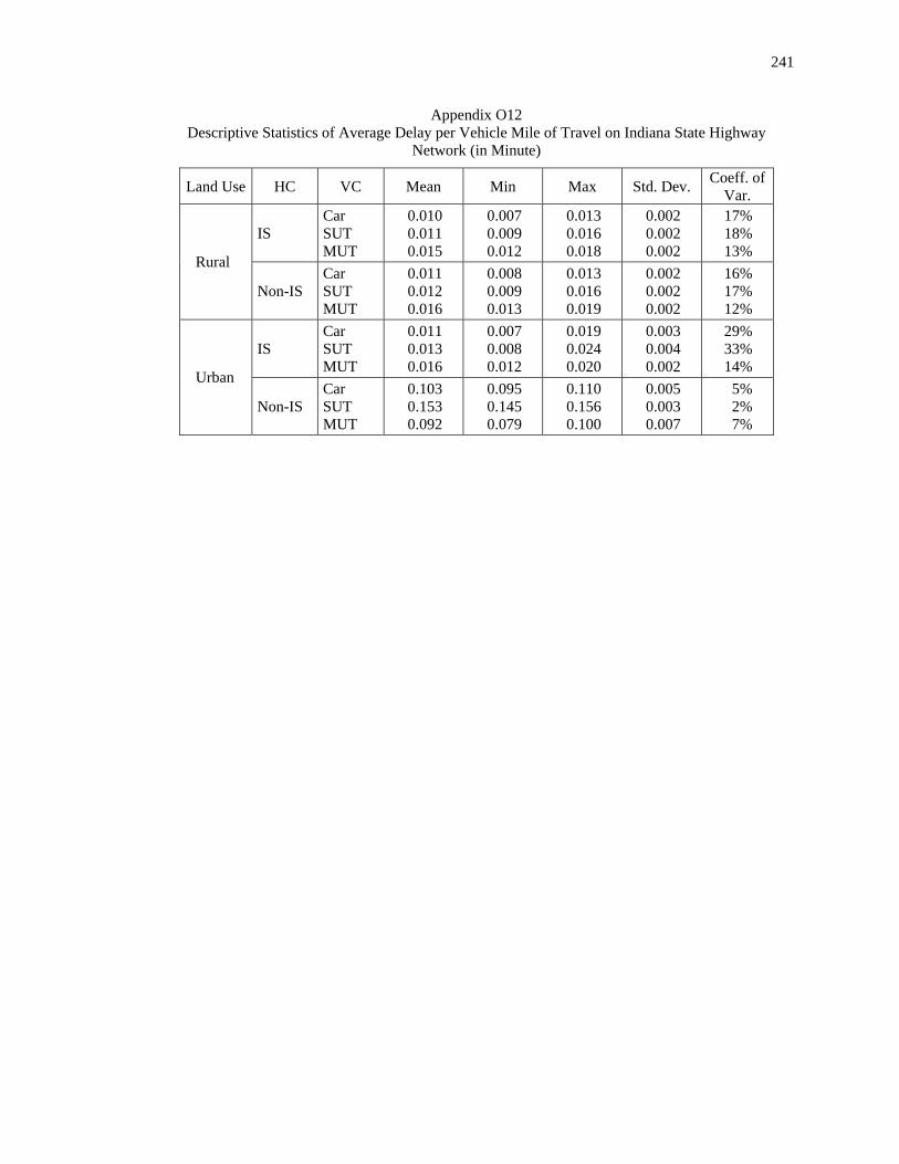
241
Appendix O12 Descriptive Statistics of Average Delay per Vehicle Mile of Travel on Indiana State Highway
Network (in Minute)
Land Use HC VC Mean Min Max Std. Dev. Coeff. of Var.
IS Car SUT MUT
0.010 0.011 0.015
0.007 0.009 0.012
0.013 0.016 0.018
0.002 0.002 0.002
17% 18% 13%
Rural
Non-IS Car SUT MUT
0.011 0.012 0.016
0.008 0.009 0.013
0.013 0.016 0.019
0.002 0.002 0.002
16% 17% 12%
IS Car SUT MUT
0.011 0.013 0.016
0.007 0.008 0.012
0.019 0.024 0.020
0.003 0.004 0.002
29% 33% 14%
Urban
Non-IS Car SUT MUT
0.103 0.153 0.092
0.095 0.145 0.079
0.110 0.156 0.100
0.005 0.003 0.007
5% 2% 7%
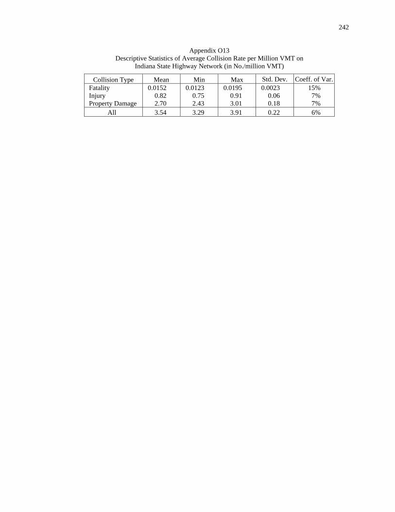
242
Appendix O13 Descriptive Statistics of Average Collision Rate per Million VMT on
Indiana State Highway Network (in No./million VMT)
Collision Type Mean Min Max Std. Dev. Coeff. of Var.Fatality Injury Property Damage
0.0152 0.82 2.70
0.0123 0.75 2.43
0.0195 0.91 3.01
0.0023 0.06 0.18
15% 7% 7%
All 3.54 3.29 3.91 0.22 6%

243
Appendix P Deviations of Outcomes of Performance Indicators Involving Uncertainty in Tradeoff Decision
Process
Range of Deviation (%) Asset Management System Goal Performance Indicator
Minimum Maximum Increment
(%)
System Preservation Pavement surface condition Remaining service life
5 12.5
50 125
5 12.5
Agency Cost Construction cost Rehabilitation cost Maintenance cost
5 5 5
50 50 50
5 5 5
User Cost Mobility Environment
Vehicle speed Detour length Intersection delay time
12.5 12.5 12.5
125 125 125
12.5 12.5 12.5
Safety
Vehicle speed Bridge load inventory rating Skid resistance Collision rate
12.5 10 10 10
125 100 100 100
12.5 10 10 10

244
Appendix Q Calibrated Degree of Surprise Functions for Performance Indicators Involving Uncertainty in Tradeoff
Decision Process

245
Appendix Q1 Calibrated Degree of Surprise Functions for Bridge Structural Condition
y(x) = c.(x-7)2 Range of Deviation Data Set
Coefficient c (t-statistic) Adjusted R2
57% All 0.6554 (6.45) 0.85

246
Appendix Q2 Calibrated Degree of Surprise Functions for Pavement Surface Condition
y(x) = c.(x-120)2 Range of Deviation Data Set
Coefficient c (t-statistic) Adjusted R2
5% All Loss
0.2488 0.2780
(9.62) (7.56)
0.89 0.90
10% All Loss
0.0622 0.0695
(9.62) (7.56)
0.89 0.90
15% All 0.0276 (9.62) 0.89 20% All 0.0155 (9.62) 0.89 25% All 0.0100 (9.62) 0.89 30% All 0.0069 (9.62) 0.89
35% Gain Loss
0.0045 0.0057
(7.02) (7.56)
0.89 0.90
40% Gain Loss
0.0034 0.0043
(7.02) (7.56)
0.89 0.90
45% Gain All
0.0027 0.0031
(7.02) (9.62)
0.89 0.89
50% Gain All
0.0022 0.0025
(7.02) (9.62)
0.89 0.89

247
Appendix Q3 Calibrated Degree of Surprise Functions for Remaining Service Life
y(x) = c.(x-5)2 Range of Deviation Data Set
Coefficient c (t-statistic) Adjusted R2
13% Gain All
22.1287 0.3666
(7.02) (1.89)
0.89 0.18
25% All 0.4038 (2.12) 0.24 38% All 0.4552 (2.62) 0.35 50% All 0.5018 (3.41) 0.49 63% All 0.5204 (4.56) 0.64 75% All 0.5002 (6.11) 0.77 88% All 0.4500 (7.77) 0.84
100% Gain Loss
0.3458 0.4296
(7.02) (6.34)
0.89 0.87
113% Gain All
0.2732 0.3268
(7.02) (8.9)
0.89 0.88
125% Gain All
0.2213 0.2737
(7.02) (8.38)
0.89 0.86

248
Appendix Q4 Calibrated Degree of Surprise Functions for Construction Expenditure
y(x) = c.(x-1000)2 Range of Deviation Data Set
Coefficient c (t-statistic) Adjusted R2
5% All 0.0038 (10.08) 0.90
10% Gain All
0.0010 0.0010
(7.45) (10.08)
0.90 0.90
15% Gain All
0.0004 0.0004
(7.45) (10.08)
0.90 0.90
20% All 0.0002 (10.08) 0.90 25% All 0.0002 (10.08) 0.90 30% All 0.0001 (10.08) 0.90
35% All Loss
0.0001 0.0001
(10.08) (6.95)
0.90 0.89
40% Gain Loss
0.0001 0.0001
(7.45) (6.95)
0.90 0.89
45% Gain Loss
0.00005 0.00005
(7.45) (6.95)
0.90 0.89
50% Gain Loss
0.00004 0.00004
(7.45) (6.95)
0.90 0.89

249
Appendix Q5 Calibrated Degree of Surprise Functions for Rehabilitation Expenditure
y(x) = c.(x-100)2 Range of Deviation Data Set
Coefficient c (t-statistic) Adjusted R2
5% All 0.3725 (9.74) 0.90 10% All 0.0931 (9.74) 0.90 15% All 0.0414 (9.74) 0.90 20% All 0.0233 (9.74) 0.90 25% All 0.0149 (9.74) 0.90
30% Gain All
0.0107 0.0103
(7.01) (9.74)
0.90 0.89
35% Gain All
0.0079 0.0076
(7.01) (9.74)
0.90 0.89
40% All Loss
0.0058 0.0056
(9.74) (6.83)
0.90 0.88
45% All Loss
0.0046 0.0044
(9.74) (6.83)
0.90 0.88
50% Gain Loss
0.0039 0.0036
(7.01) (6.83)
0.89 0.88

250
Appendix Q6 Calibrated Degree of Surprise Functions for Routine Maintenance Expenditure
y(x) = c.(x-10)2 Range of Deviation Data Set
Coefficient c (t-statistic) Adjusted R2
5% All 35.5678 (10.22) 0.90 10% All 8.8919 (10.22) 0.90 15% All 3.9520 (10.22) 0.90
20% Gain All
2.2882 2.2230
(7.88) (10.22)
0.91 0.90
25% Gain All
1.4644 1.4227
(7.88) (10.22)
0.91 0.90
30% Gain All
1.0170 0.9880
(7.88) (10.22)
0.91 0.90
35% All Loss
0.7259 0.7046
(10.22) (6.71)
0.90 0.88
40% Gain Loss
0.5720 0.5395
(7.88) (6.71)
0.91 0.88
45% Gain Loss
0.4520 0.4262
(7.88) (6.71)
0.91 0.88
50% Gain Loss
0.3661 0.3453
(7.88) (6.71)
0.91 0.88

251
Appendix Q7 Calibrated Degree of Surprise Functions for Vehicle Traveling Speed
(Where Higher Speed is Preferred)
y(x) = c.(x-55)2 Range of Deviation Data Set Coefficient c (t-statistic)
Adjusted R2
13% All Loss
0.2059 0.2301
(8.57) (5.88)
0.87 0.85
25% All Loss
0.0515 0.0575
(8.57) (5.88)
0.87 0.85
38% All Loss
0.0229 0.0256
(8.57) (5.88)
0.87 0.85
50% Gain Loss
0.0114 0.0144
(7.79) (5.88)
0.91 0.85
63% Gain Loss
0.0073 0.0092
(7.79) (5.88)
0.91 0.85
75% Gain Loss
0.0050 0.0064
(7.79) (5.88)
0.91 0.85
88% Gain Loss
0.0037 0.0047
(7.79) (5.88)
0.91 0.85
100% Gain All
0.0028 0.0032
(7.79) (8.57)
0.91 0.87
113% Gain All
0.0022 0.0027
(7.79) (8.57)
0.91 0.87
125% Gain All
0.0018 0.0023
(7.79) (8.57)
0.91 0.87

252
Appendix Q8 Calibrated Degree of Surprise Functions for Vehicle Traveling Speed
(Where Lower Speed is Preferred)
y(x) = c.(x-55)2 Range of Deviation Data Set
Coefficient c (t-statistic) Adjusted R2
13% All Loss
0.2059 0.2301
(8.57) (5.88)
0.87 0.85
25% All Loss
0.0515 0.0575
(8.57) (5.88)
0.87 0.85
38% All 0.0229 (8.57) 0.87 50% All 0.0129 (8.57) 0.87
63% Gain Loss
0.0073 0.0092
(7.79) (5.88)
0.91 0.85
75% Gain Loss
0.0050 0.0064
(7.79) (5.88)
0.91 0.85
88% Gain Loss
0.0037 0.0047
(7.79) (5.88)
0.91 0.85
100% Gain All
0.0028 0.0032
(7.79) (8.57)
0.91 0.87
113% Gain All
0.0022 0.0027
(7.79) (8.57)
0.91 0.87
125% Gain All
0.0018 0.0023
(7.79) (8.57)
0.91 0.87
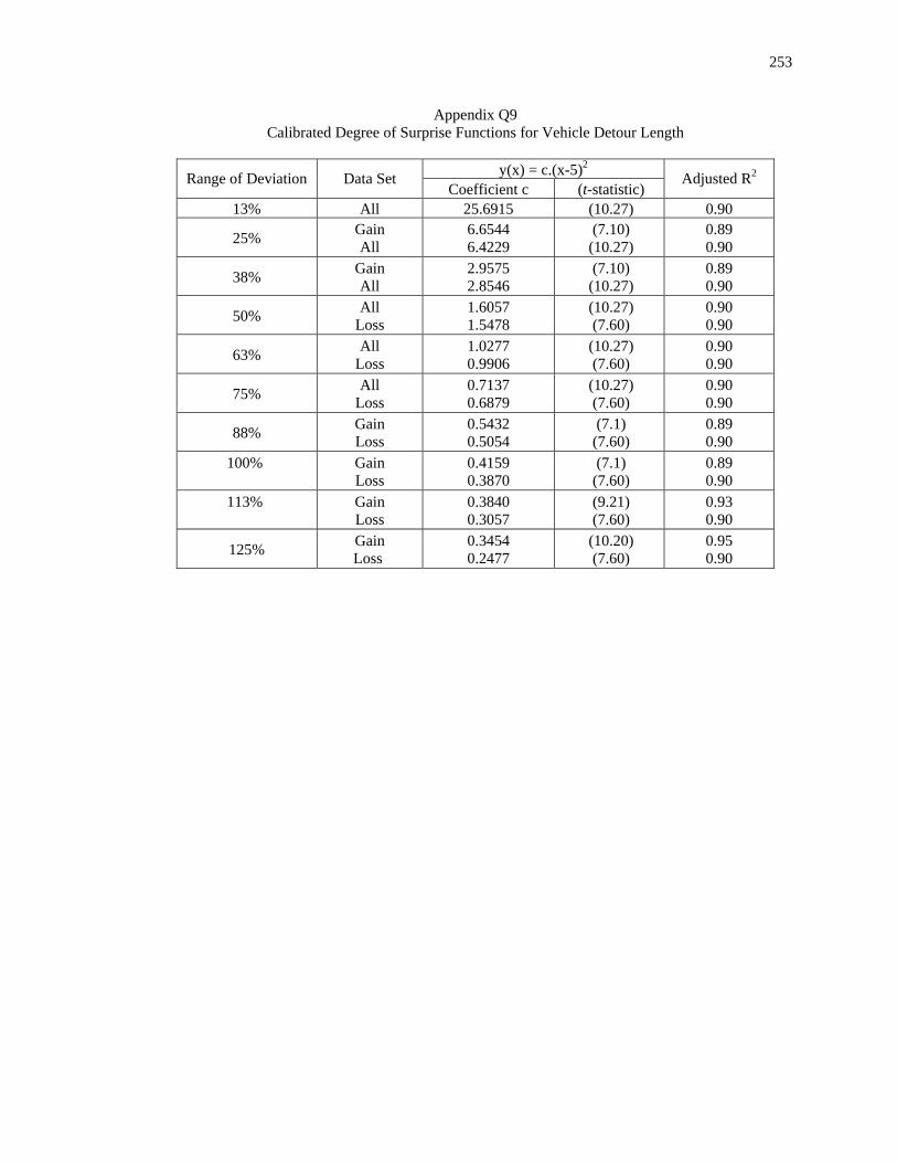
253
Appendix Q9 Calibrated Degree of Surprise Functions for Vehicle Detour Length
y(x) = c.(x-5)2 Range of Deviation Data Set
Coefficient c (t-statistic) Adjusted R2
13% All 25.6915 (10.27) 0.90
25% Gain All
6.6544 6.4229
(7.10) (10.27)
0.89 0.90
38% Gain All
2.9575 2.8546
(7.10) (10.27)
0.89 0.90
50% All Loss
1.6057 1.5478
(10.27) (7.60)
0.90 0.90
63% All Loss
1.0277 0.9906
(10.27) (7.60)
0.90 0.90
75% All Loss
0.7137 0.6879
(10.27) (7.60)
0.90 0.90
88% Gain Loss
0.5432 0.5054
(7.1) (7.60)
0.89 0.90
100%
Gain Loss
0.4159 0.3870
(7.1) (7.60)
0.89 0.90
113%
Gain Loss
0.3840 0.3057
(9.21) (7.60)
0.93 0.90
125% Gain Loss
0.3454 0.2477
(10.20) (7.60)
0.95 0.90

254
Appendix Q10 Calibrated Degree of Surprise Functions for Intersection Delay Time
y(x) = c.(x-10)2 Range of Deviation Data Set
Coefficient c (t-statistic) Adjusted R2
13% All Loss
6.4562 6.3221
(10.22) (7.93)
0.90 0.91
25% All Loss
1.6141 1.5805
(10.22) (7.93)
0.90 0.91
38% All 0.7174 (10.22) 0.90 50% All 0.4035 (10.22) 0.90 63% All 0.2582 (10.22) 0.90 75% All 0.1793 (10.22) 0.90 88% All 0.1318 (10.22) 0.90
100% All Loss
0.1009 0.0988
(10.22) (7.93)
0.90 0.91
113% Gain Loss
0.0951 0.0781
(8.5) (7.93)
0.92 0.91
125% Gain All
0.0855 0.0718
(9.27) (10.4)
0.93 0.91

255
Appendix Q11 Calibrated Degree of Surprise Functions for Bridge Load Inventory Rating
y(x) = c.(x-25)2 Range of Deviation Data Set
Coefficient c (t-statistic) Adjusted R2
10% All Loss
1.5855 1.7147
(9.99) (6.71)
0.90 0.88
20% All Loss
0.3964 0.4287
(9.99) (6.71)
0.90 0.88
30% All 0.1762 (9.99) 0.90 40% All 0.0991 (9.99) 0.90 50% All 0.0634 (9.99) 0.90 60% All 0.0440 (9.99) 0.90 70% All 0.0324 (9.99) 0.90
80% Gain All
0.0228 0.0248
(8.59) (9.99)
0.92 0.90
90% Gain All
0.0180 0.0196
(8.59) (9.99)
0.90 0.92
100% All 0.0159 (9.99) 0.90

256
Appendix Q12 Calibrated Degree of Surprise Functions for Pavement Skid Resistance
y(x) = c.(x-25)2 Range of Deviation Data Set
Coefficient c (t-statistic) Adjusted R2
10% All Loss
1.7545 1.8645
(9.18) (6.22)
0.88 0.86
20% All Loss
0.4386 0.4661
(9.18) (6.22)
0.88 0.86
30% All 0.1949 (9.18) 0.88 40% All 0.1097 (9.18) 0.88
50% Gain Loss
0.0658 0.0746
(7.25) (6.22)
0.90 0.86
60% Gain Loss
0.0457 0.0518
(7.25) (6.22)
0.90 0.86
70% Gain Loss
0.0336 0.0381
(7.25) (6.22)
0.90 0.86
80% Gain Loss
0.0257 0.0291
(7.25) (6.22)
0.90 0.86
90% Gain All
0.0203 0.0217
(7.25) (9.18)
0.90 0.88
100% Gain All
0.0164 0.0175
(7.25) (9.18)
0.90 0.88

257
Appendix Q13 Calibrated Degree of Surprise Functions for Vehicle Collision Rate
y(x) = c.(x-5)2 Range of Deviation Data Set
Coefficient c (t-statistic) Adjusted R2
10% All Loss
34.2739 37.6404
(11.86) (8.72)
0.93 0.93
20% All Loss
8.5685 9.4101
(11.86) (8.72)
0.93 0.93
30% All Loss
3.8082 4.1823
(11.86) (8.72)
0.93 0.93
40% All 2.1421 (11.86) 0.93 50% All 1.3710 (11.86) 0.93 60% All 0.9521 (11.86) 0.93 70% All 0.6995 (11.86) 0.93
80% Gain Loss
0.4829 0.5881
(9.66) (8.72)
0.94 0.93
90% All Loss
0.4231 0.4647
(11.86) (8.72)
0.93 0.93
100% Gain All
0.3091 0.3427
(9.66) (11.86)
0.94 0.93

258
Appendix R Calibrated Priority Functions for Performance Indicators Involving Uncertainty in
Tradeoff Decision Process

259
Appendix R1 Calibrated Priority Functions for Bridge Structural Condition Rating
φ(x) = a.(x-7)0.5 + b.y2 Range of
Deviation Data Set Coefficient a (t-statistic) Coefficient b (t-statistic)
Adjusted R2
57% All 1.2216 (3.37) -0.0198 (-1.42) 0.79

260
Appendix R2 Calibrated Priority Functions for Pavement Surface Condition
φ(x) = a.(x-120)0.5 + b.y2 Range of
Deviation Data Set Coefficient a (t-statistic) Coefficient b (t-statistic)
Adjusted R2
5% All Loss
0.6445 1.0977
(3.07) (6.56)
-0.0106 -0.0229
(-0.93) (-3.03)
0.71 0.95
10% All Loss
0.4557 0.7762
(3.07) (6.56)
-0.0106 -0.0229
(-0.93) (-3.03)
0.71 0.95
15% All 0.3721 (3.07) -0.0106 (-0.93) 0.71 20% All 0.3223 (3.07) -0.0106 (-0.93) 0.71 25% All 0.2882 (3.07) -0.0106 (-0.93) 0.71 30% All 0.2631 (3.07) -0.0106 (-0.93) 0.71
35% Gain Loss
0.3068 0.4149
(4.48) (6.56)
-0.0392 -0.0229
(-2.98) (-3.03)
0.83 0.95
40% Gain Loss
0.2870 0.3881
(4.48) (6.56)
-0.0392 -0.0229
(-2.98) (-3.03)
0.83 0.95
45% Gain All
0.2706 0.2148
(4.48) (3.07)
-0.0392 -0.0106
(-2.98) (-0.93)
0.83 0.71
50% Gain All
0.2567 0.2038
(4.48) (3.07)
-0.0392 -0.0106
(-2.98) (-0.93)
0.83 0.71

261
Appendix R3 Calibrated Priority Functions for Remaining Service Life
φ(x) = a.(x-5)0.5 + b.y2 Range of
Deviation Data Set Coefficient a (t-statistic) Coefficient b (t-statistic)
Adjusted R2
13% Gain All
3.4792 1.0613
(4.35) (1.05)
-0.0469 -0.0013
(-2.99) (-0.06)
0.81 0.35
25% All 2.0547 (2.37) -0.0307 (-1.35) 0.55 38% All 2.1274 (3.22) -0.0394 (-2.02) 0.66 50% All 1.8819 (3.50) -0.0376 (-2.14) 0.69 63% All 1.6246 (3.49) -0.0335 (-2.04) 0.69 75% All 1.4145 (3.40) -0.0296 (-1.87) 0.68 88% All 1.2498 (3.30) -0.0262 (-1.71) 0.67
100% Gain Loss
1.2301 2.0245
(4.35) (5.27)
-0.0469 -0.0469
(-2.99) (-3.39)
0.81 0.90
113% Gain All
1.1597 1.0169
(4.35) (3.11)
-0.0469 -0.0211
(-2.99) (-1.44)
0.81 0.65
125% Gain All
1.1002 0.9327
(4.35) (3.04)
-0.0469 -0.0192
(-2.99) (-1.33)
0.81 0.64

262
Appendix R4 Calibrated Priority Functions for Construction Expenditure
φ(x) = a.(x-1000)0.5 + b.y2 Range of
Deviation Data Set Coefficient a (t-statistic) Coefficient b (t-statistic)
Adjusted R2
5% All 0.5209 (6.94) -0.0460 (-4.33) 0.88
10% Gain All
0.2725 0.3683
(4.84) (6.94)
-0.0338 -0.0460
(-3.26) (-4.33)
0.85 0.88
15% Gain All
0.2225 0.3007
(4.84) (6.94)
-0.0338 -0.0460
(-3.26) (-4.33)
0.85 0.88
20% All 0.2604 (6.94) -0.0460 (-4.33) 0.88 25% All 0.2329 (6.94) -0.0460 (-4.33) 0.88 30% All 0.2127 (6.94) -0.0460 (-4.33) 0.88
35% All Loss
0.1969 0.2346
(6.94) (6.81)
-0.0460 -0.0544
(-4.33) (-3.84)
0.88 0.94
40% Gain Loss
0.1362 0.2195
(4.84) (6.81)
-0.0338 -0.0544
(-3.26) (-3.84)
0.85 0.94
45% Gain Loss
0.1285 0.2069
(4.84) (6.81)
-0.0338 -0.0544
(-3.26) (-3.84)
0.85 0.94
50% Gain Loss
0.1219 0.1963
(4.84) (6.81)
-0.0338 -0.0544
(-3.26) (-3.84)
0.85 0.94

263
Appendix R5 Calibrated Priority Functions for Rehabilitation Expenditure
φ(x) = a.(x-100)0.5 + b.y2 Range of
Deviation Data Set Coefficient a (t-statistic) Coefficient b (t-statistic)
Adjusted R2
5% All 1.3535 (6.58) -0.0386 (-3.95) 0.88 10% All 0.9571 (6.58) -0.0386 (-3.95) 0.88 15% All 0.7815 (6.58) -0.0386 (-3.95) 0.88 20% All 0.6768 (6.58) -0.0386 (-3.95) 0.88 25% All 0.6053 (6.58) -0.0386 (-3.95) 0.88
30% Gain All
0.4536 0.5526
(5.31) (6.58)
-0.0347 -0.0386
(-3.7) (-3.95)
0.87 0.88
35% Gain All
0.4199 0.5116
(5.31) (6.58)
-0.0347 -0.0386
(-3.7) (-3.95)
0.87 0.88
40% All Loss
0.4785 0.5102
(6.58) (6.92)
-0.0386 -0.0348
(-3.95) (-3.27)
0.88 0.96
45% All Loss
0.4512 0.4810
(6.58) (6.92)
-0.0386 -0.0348
(-3.95) (-3.27)
0.88 0.96
50% Gain Loss
0.3513 0.4563
(5.31) (6.92)
-0.0347 -0.0348
(-3.7) (-3.27)
0.87 0.96

264
Appendix R6 Calibrated Priority Functions for Routine Maintenance Expenditure
φ(x) = a.(x-10)0.5 + b.y2 Range of
Deviation Data Set Coefficient a (t-statistic) Coefficient b (t-statistic)
Adjusted R2
5% All 4.1599 (5.94) -0.0386 (-3.35) 0.86 10% All 2.9415 (5.94) -0.0386 (-3.35) 0.86 15% All 2.4017 (5.94) -0.0386 (-3.35) 0.86
20% Gain All
1.4465 2.0800
(6.37) (5.94)
-0.0282 -0.0386
(-4.00) (-3.35)
0.91 0.86
25% Gain All
1.2938 1.8604
(6.37) (5.94)
-0.0282 -0.0386
(-4.00) (-3.35)
0.91 0.86
30% Gain All
1.1810 1.6983
(6.37) (5.94)
-0.0282 -0.0386
(-4.00) (-3.35)
0.91 0.86
35% All Loss
1.5723 1.9730
(5.94) (8.93)
-0.0386 -0.0463
(-3.35) (-4.50)
0.86 0.97
40% Gain Loss
1.0228 1.8455
(6.37) (8.93)
-0.0282 -0.0463
(-4.00) (-4.50)
0.91 0.97
45% Gain Loss
0.9643 1.7400
(6.37) (8.93)
-0.0282 -0.0463
(-4.00) (-4.50)
0.91 0.97
50% Gain Loss
0.9148 1.6507
(6.37) (8.93)
-0.0282 -0.0463
(-4.00) (-4.50)
0.91 0.97
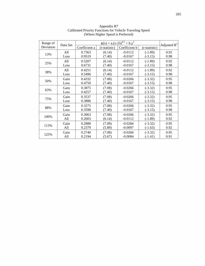
265
Appendix R7 Calibrated Priority Functions for Vehicle Traveling Speed
(Where Higher Speed is Preferred)
φ(x) = a.(x-55)0.5 + b.y2 Range of Deviation Data Set
Coefficient a (t-statistic) Coefficient b (t-statistic) Adjusted R2
13% All Loss
0.7363 0.9519
(6.14) (7.40)
-0.0112 -0.0167
(-1.89) (-3.15)
0.92 0.98
25% All Loss
0.5207 0.6731
(6.14) (7.40)
-0.0112 -0.0167
(-1.89) (-3.15)
0.92 0.98
38% All Loss
0.4251 0.5496
(6.14) (7.40)
-0.0112 -0.0167
(-1.89) (-3.15)
0.92 0.98
50% Gain Loss
0.4332 0.4759
(7.08) (7.40)
-0.0266 -0.0167
(-3.32) (-3.15)
0.95 0.98
63% Gain Loss
0.3875 0.4257
(7.08) (7.40)
-0.0266 -0.0167
(-3.32) (-3.15)
0.95 0.98
75% Gain Loss
0.3537 0.3886
(7.08) (7.40)
-0.0266 -0.0167
(-3.32) (-3.15)
0.95 0.98
88% Gain Loss
0.3275 0.3598
(7.08) (7.40)
-0.0266 -0.0167
(-3.32) (-3.15)
0.95 0.98
100% Gain All
0.3063 0.2603
(7.08) (6.14)
-0.0266 -0.0112
(-3.32) (-1.89)
0.95 0.92
113% Gain All
0.2888 0.2379
(7.08) (5.89)
-0.0266 -0.0097
(-3.32) (-1.63)
0.95 0.92
125% Gain All
0.2740 0.2194
(7.08) (5.67)
-0.0266 -0.0084
(-3.32) (-1.41)
0.95 0.91

266
Appendix R8 Calibrated Priority Functions for Vehicle Traveling Speed
(Where Lower Speed is Preferred)
φ(x) = a.(x-55)0.5 + b.y2 Range of Deviation Data Set
Coefficient a (t-statistic) Coefficient b (t-statistic) Adjusted R2
13% All Loss
0.7363 0.9519
(6.14) (7.40)
-0.0112 -0.0167
(-1.89) (-3.15)
0.92 0.98
25% All Loss
0.5207 0.6731
(6.14) (7.40)
-0.0112 -0.0167
(-1.89) (-3.15)
0.92 0.98
38% All 0.4251 (6.14) -0.0112 (-1.89) 0.92 50% All 0.3682 (6.14) -0.0112 (-1.89) 0.92
63% Gain Loss
0.3875 0.4257
(7.08) (7.40)
-0.0266 -0.0167
(-3.32) (-3.15)
0.95 0.98
75% Gain Loss
0.3537 0.3886
(7.08) (7.40)
-0.0266 -0.0167
(-3.32) (-3.15)
0.95 0.98
88% Gain Loss
0.3275 0.3598
(7.08) (7.40)
-0.0266 -0.0167
(-3.32) (-3.15)
0.95 0.98
100% Gain All
0.3063 0.2603
(7.08) (6.14)
-0.0266 -0.0112
(-3.32) (-1.89)
0.95 0.92
113% Gain All
0.2888 0.2379
(7.08) (5.89)
-0.0266 -0.0097
(-3.32) (-1.63)
0.95 0.92
125% Gain All
0.2740 0.2194
(7.08) (5.67)
-0.0266 -0.0084
(-3.32) (-1.41)
0.95 0.91

267
Appendix R9 Calibrated Priority Functions for Vehicle Detour Length
φ(x) = a.(x-5)0.5 + b.y2 Range of
Deviation Data Set Coefficient a (t-statistic) Coefficient b (t-statistic)
Adjusted R2
13% All 3.6590 (5.45) -0.0342 (-3.53) 0.80
25% Gain All
1.8368 2.5873
(3.89) (5.45)
-0.0266 -0.0342
(-2.94) (-3.53)
0.74 0.80
38% Gain All
1.4997 2.1125
(3.89) (5.45)
-0.0266 -0.0342
(-2.94) (-3.53)
0.74 0.80
50% All Loss
1.8295 2.0887
(5.45) (5.99)
-0.0342 -0.0340
(-3.53) (-3.13)
0.80 0.93
63% All Loss
1.6363 1.8682
(5.45) (5.99)
-0.0342 -0.0340
(-3.53) (-3.13)
0.80 0.93
75% All Loss
1.4938 1.7054
(5.45) (5.99)
-0.0342 -0.0340
(-3.53) (-3.13)
0.80 0.93
88% Gain Loss
0.9818 1.5789
(3.89) (5.99)
-0.0266 -0.0340
(-2.94) (-3.13)
0.74 0.93
100%
Gain Loss
0.9184 1.4769
(3.89) (5.99)
-0.0266 -0.0340
(-2.94) (-3.13)
0.74 0.93
113%
Gain Loss
0.8237 1.3925
(3.61) (5.99)
-0.0241 -0.0340
(-2.65) (-3.13)
0.71 0.93
125% Gain Loss
0.7472 1.3210
(3.39) (5.99)
-0.0221 -0.0340
(-2.43) (-3.13)
0.68 0.93

268
Appendix R10 Calibrated Priority Functions for Intersection Delay Time
φ(x) = a.(x-10)0.5 + b.y2 Range of
Deviation Data Set Coefficient a (t-statistic) Coefficient b (t-statistic)
Adjusted R2
13% All Loss
2.4699 2.8929
(5.01) (6.57)
-0.0316 -0.0312
(-3.16) (-3.37)
0.78 0.94
25% All Loss
1.7465 2.0456
(5.01) (6.57)
-0.0316 -0.0312
(-3.16) (-3.37)
0.78 0.94
38% All 1.4260 (5.01) -0.0316 (-3.16) 0.78 50% All 1.2350 (5.01) -0.0316 (-3.16) 0.78 63% All 1.1046 (5.01) -0.0316 (-3.16) 0.78 75% All 1.0083 (5.01) -0.0316 (-3.16) 0.78 88% All 0.9335 (5.01) -0.0316 (-3.16) 0.78
100% All Loss
0.8732 1.0228
(5.01) (6.57)
-0.0316 -0.0312
(-3.16) (-3.37)
0.78 0.94
113% Gain Loss
0.5432 0.9643
(3.99) (6.57)
-0.0227 -0.0312
(-2.88) (-3.37)
0.77 0.94
125% Gain All
0.4910 0.7572
(3.71) (5.1)
-0.0206 -0.0290
(-2.61) (-3.1)
0.74 0.79
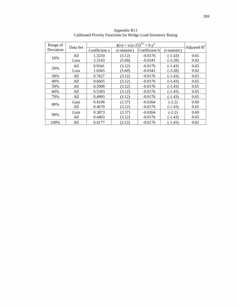
269
Appendix R11 Calibrated Priority Functions for Bridge Load Inventory Rating
φ(x) = a.(x-25)0.5 + b.y2 Range of
Deviation Data Set Coefficient a (t-statistic) Coefficient b (t-statistic)
Adjusted R2
10% All Loss
1.3210 2.3143
(3.12) (5.69)
-0.0176 -0.0341
(-1.43) (-3.28)
0.65 0.92
20% All Loss
0.9341 1.6365
(3.12) (5.69)
-0.0176 -0.0341
(-1.43) (-3.28)
0.65 0.92
30% All 0.7627 (3.12) -0.0176 (-1.43) 0.65 40% All 0.6605 (3.12) -0.0176 (-1.43) 0.65 50% All 0.5908 (3.12) -0.0176 (-1.43) 0.65 60% All 0.5393 (3.12) -0.0176 (-1.43) 0.65 70% All 0.4993 (3.12) -0.0176 (-1.43) 0.65
80% Gain All
0.4108 0.4670
(3.37) (3.12)
-0.0264 -0.0176
(-2.2) (-1.43)
0.69 0.65
90% Gain All
0.3873 0.4403
(3.37) (3.12)
-0.0264 -0.0176
(-2.2) (-1.43)
0.69 0.65
100% All 0.4177 (3.12) -0.0176 (-1.43) 0.65

270
Appendix R12 Calibrated Priority Functions for Pavement Skid Resistance
φ(x) = a.(x-25)0.5 + b.y2 Range of
Deviation Data Set Coefficient a (t-statistic) Coefficient b (t-statistic)
Adjusted R2
10% All Loss
1.0693 1.9070
(2.99) (6.63)
-0.0116 -0.0235
(-1.35) (-3.77)
0.69 0.95
20% All Loss
0.7561 1.3485
(2.99) (6.63)
-0.0116 -0.0235
(-1.35) (-3.77)
0.69 0.95
30% All 0.6174 (2.99) -0.0116 (-1.35) 0.69 40% All 0.5347 (2.99) -0.0116 (-1.35) 0.69
50% Gain Loss
0.4133 0.8528
(4.79) (6.63)
-0.0168 -0.0235
(-3.13) (-3.77)
0.85 0.95
60% Gain Loss
0.3773 0.7785
(4.79) (6.63)
-0.0168 -0.0235
(-3.13) (-3.77)
0.85 0.95
70% Gain Loss
0.3493 0.7208
(4.79) (6.63)
-0.0168 -0.0235
(-3.13) (-3.77)
0.85 0.95
80% Gain Loss
0.3268 0.6742
(4.79) (6.63)
-0.0168 -0.0235
(-3.13) (-3.77)
0.85 0.95
90% Gain All
0.3081 0.3564
(4.79) (2.99)
-0.0168 -0.0116
(-3.13) (-1.35)
0.85 0.69
100% Gain All
0.2923 0.3382
(4.79) (2.99)
-0.0168 -0.0116
(-3.13) (-1.35)
0.85 0.69

271
Appendix R13 Calibrated Priority Functions for Vehicle Collision Rate
φ(x) = a.(x-5)0.5 + b.y2 Range of
Deviation Data Set Coefficient a (t-statistic) Coefficient b (t-statistic)
Adjusted R2
10% All Loss
4.0647 6.4974
(3.34) (5.5)
-0.0366 -0.0559
(-1.76) (-3.24)
0.60 0.89
20% All Loss
2.8742 4.5944
(3.34) (5.5)
-0.0366 -0.0559
(-1.76) (-3.24)
0.60 0.89
30% All Loss
2.3468 3.7513
(3.34) (5.5)
-0.0366 -0.0559
(-1.76) (-3.24)
0.60 0.89
40% All 2.0324 (3.34) -0.0366 (-1.76) 0.60 50% All 1.8178 (3.34) -0.0366 (-1.76) 0.60 60% All 1.6594 (3.34) -0.0366 (-1.76) 0.60 70% All 1.5363 (3.34) -0.0366 (-1.76) 0.60
80% Gain Loss
1.3469 2.2972
(3.25) (5.5)
-0.0598 -0.0559
(-2.37) (-3.24)
0.63 0.89
90% All Loss
1.3549 2.1658
(3.34) (5.5)
-0.0366 -0.0559
(-1.76) (-3.24)
0.60 0.89
100% Gain All
1.2047 1.2854
(3.25) (3.34)
-0.0598 -0.0366
(-2.37) (-1.76)
0.63 0.60

272
Appendix S Descriptive Statistics of Data for the Calibration of Standardized Focus Gain-Over-Loss Ratio
Functions
Asset Management System Goal
Performance Indicator Mean Min Max Std. Dev. Coeff. of
Var.
System Preservation
Pavement condition Remaining service life
0.9672 0.9858
0.7917 0.9175
1.1400 1.0235
0.1214 0.0348
13% 4%
Agency Cost Construction cost Rehabilitation cost Maintenance cost
0.9874 0.9670 0.9709
0.9333 0.8864 0.9396
1.0400 1.0091 1.0013
0.0310 0.0423 0.0242
3% 4% 2%
User Cost Mobility Environment
Vehicle speed Detour length Intersection delay time
0.9933 0.9170 1.0499
0.8818 0.7941 1.0042
1.1125 1.0079 1.2170
0.0924 0.0634 0.0651
9% 7% 6%
Safety
Vehicle speed Bridge load inventory Skid resistance Collision rate
0.9824 0.9939 0.9796 0.9910
0.8820 0.9015 0.8970 0.9078
1.1124 1.0764 1.0738 1.0420
0.0831 0.0584 0.0604 0.0492
8% 6% 6% 5%