Metallurgical and mechanical modelling of Ti-6Al-4V ... - CORE
387
METALLURGICAL AND MECHANICAL MODELLING OF TI-6AL-4V FOR WELDING APPLICATIONS by MATTEO VILLA A thesis submitted to the University of Birmingham for the degree of DOCTOR OF PHILOSOPHY School of Engineering and Physical Sciences Department of Metallurgy and Materials University of Birmingham March 2016
-
Upload
khangminh22 -
Category
Documents
-
view
1 -
download
0
Transcript of Metallurgical and mechanical modelling of Ti-6Al-4V ... - CORE

METALLURGICAL AND MECHANICAL
MODELLING OF TI-6AL-4V FOR WELDING
APPLICATIONS
by
MATTEO VILLA
A thesis submitted to the University of Birmingham
for the degree of
DOCTOR OF PHILOSOPHY
School of Engineering and Physical Sciences
Department of Metallurgy and Materials
University of Birmingham
March 2016

University of Birmingham Research Archive
e-theses repository This unpublished thesis/dissertation is copyright of the author and/or third parties. The intellectual property rights of the author or third parties in respect of this work are as defined by The Copyright Designs and Patents Act 1988 or as modified by any successor legislation. Any use made of information contained in this thesis/dissertation must be in accordance with that legislation and must be properly acknowledged. Further distribution or reproduction in any format is prohibited without the permission of the copyright holder.

Abstract
Complex heat treatments and manufacturing processes such as welding involve a wide
range of temperatures and temperature rates, affecting the microstructure of the material
and its properties. In this work, a diffusion based approach to model growth and shrinkage
of precipitates in the alpha + beta field of Ti-6Al-4V alloys is established. Experimental
heat treatments were used to validate the numerical predictions of the model for lamellar
shrinkage, whilst data from literature have been used to evaluate the numerical model for
the growth of equiaxed microstructures. The agreement between measurements and
numerical predictions was found to be very good. Experimentally-based approaches were
used both to describe the growth of alpha lamellae and martensitic needles while cooling
down from temperatures above the beta transus, and beta grain growth for temperatures
remaining above the beta transus. Such models were coded in the commercial FE software
Visual-Weld for the prediction of microstructure evolution during welding simulations.
Experimental welding tests were carried out to validate the predictions. The metallurgical
models developed were linked with a mechanical physically based model to predict the
flow properties and the initial implementation of the coupled models in Visual-Weld is
discussed.

Acknowledgements
I am sincerely grateful to my supervisors Dr Mark Ward and Professor Jeffery Brooks for
the support and guidance they gave me throughout my PhD. This work would have not been
possible without their help.
ESI group, sponsor of my project, gave me also a great technical support and I cannot forget
to thank Dr Frédéric Boitout and Dr Rajab Said for their assistance.
I would like to thank also Professor Roger Reed as he offered to me the opportunity for this
PhD.
Thanks to Dr Hector Basoalto for the time spent together, even if I was not under his
supervision.
Thanks to Dr Richard Turner and Dr Hang Wang for the helpful conversations we had.
Last but not least, thanks to my girlfriend Nicoletta for the support during these years.

Contents
1 Introduction and objectives 1
2 Literature review 6
2.1 Introduction . . . . . . . . . . . . . . . . . . . . . . . . . . . 6
2.2 Welding . . . . . . . . . . . . . . . . . . . . . . . . . . . . . 7
2.2.1 Introduction . . . . . . . . . . . . . . . . . . . . . . . . . . . . . . . 7
2.2.2 Classical approach of computational welding mechanics . . . . . . . 8
2.2.3 Heat sources . . . . . . . . . . . . . . . . . . . . . . . . . . . . . . . 10
2.3 Ti-6Al-4V . . . . . . . . . . . . . . . . . . . . . . . . . . . . 18
2.3.1 Introduction . . . . . . . . . . . . . . . . . . . . . . . . . . . . . . . 18
2.3.2 Classication . . . . . . . . . . . . . . . . . . . . . . . . . . . . . . 19
2.3.3 Thermo-mechanical data . . . . . . . . . . . . . . . . . . . . . . . . 20
2.3.4 Phases and common microstructures obtainable . . . . . . . . . . . 26
2.3.5 Phases evolution . . . . . . . . . . . . . . . . . . . . . . . . . . . . 30
2.3.5.1 Heating . . . . . . . . . . . . . . . . . . . . . . . . . . . . 30
2.3.5.2 Cooling . . . . . . . . . . . . . . . . . . . . . . . . . . . . 30
2.3.5.3 Martensitic transformation . . . . . . . . . . . . . . . . . 35
2.3.6 Morphological and mechanical modelling . . . . . . . . . . . . . . . 36
2.3.6.1 Introduction on the relation between mechanical beha-
viour and material morphology . . . . . . . . . . . . . . . 36
i

Contents Contents
2.3.6.2 Modelling of the equiaxed and lamellar alpha phase evol-
ution . . . . . . . . . . . . . . . . . . . . . . . . . . . . . 42
2.3.6.3 Modelling of the beta grains evolution . . . . . . . . . . . 44
2.3.6.4 Modelling of the mechanical behaviour in relation to the
morphology . . . . . . . . . . . . . . . . . . . . . . . . . . 46
2.4 Welding of Ti-6Al-4V . . . . . . . . . . . . . . . . . . . . . . . 51
2.4.1 Modelling of welding on Ti-6Al-4V coupling metallurgical and mech-
anical behaviour of the material . . . . . . . . . . . . . . . . . . . . 57
2.4.2 Visual-Weld multi-phase code . . . . . . . . . . . . . . . . . . . . . 58
2.4.3 Summary . . . . . . . . . . . . . . . . . . . . . . . . . . . . . . . . 59
2.5 Surrogate models . . . . . . . . . . . . . . . . . . . . . . . . . 61
3 Characterization 64
3.1 Introduction . . . . . . . . . . . . . . . . . . . . . . . . . . . 64
3.2 Project plan . . . . . . . . . . . . . . . . . . . . . . . . . . . 65
3.3 Preliminary FE model . . . . . . . . . . . . . . . . . . . . . . . 65
3.4 Gleeble tests . . . . . . . . . . . . . . . . . . . . . . . . . . . 73
3.4.1 Microstructural analysis - procedure . . . . . . . . . . . . . . . . . 81
3.4.2 Microanalysis - technique . . . . . . . . . . . . . . . . . . . . . . . . 86
3.4.3 Heating rate eect on lamellar microstructure . . . . . . . . . . . . 88
3.4.4 Cooling rate eect on lamellar and martensitic microstructures . . . 97
3.4.5 Growth of nucleated lamellae in the α + β eld . . . . . . . . . . . 98
3.4.6 β transus . . . . . . . . . . . . . . . . . . . . . . . . . . . . . . . . 108
3.4.7 β grain growth . . . . . . . . . . . . . . . . . . . . . . . . . . . . . 112
3.5 Welding tests. . . . . . . . . . . . . . . . . . . . . . . . . . . 113
3.5.1 Temperature measurements . . . . . . . . . . . . . . . . . . . . . . 120
3.5.1.1 Plates with equiaxed microstructure . . . . . . . . . . . . 120
3.5.1.2 Plates with lamellar microstructure . . . . . . . . . . . . . 122
ii

Contents Contents
3.5.2 Microstructures . . . . . . . . . . . . . . . . . . . . . . . . . . . . 122
3.5.2.1 Plates with equiaxed microstructure . . . . . . . . . . . . 122
3.5.2.2 Plates with lamellar microstructure . . . . . . . . . . . . . 141
3.5.3 Chemical analysis . . . . . . . . . . . . . . . . . . . . . . . . . . . . 152
3.5.3.1 Plates with equiaxed microstructure . . . . . . . . . . . . 152
3.5.3.2 Plates with lamellar microstructure . . . . . . . . . . . . . 152
3.5.4 Deformation measurement . . . . . . . . . . . . . . . . . . . . . . . 157
3.6 Summary . . . . . . . . . . . . . . . . . . . . . . . . . . . . 157
3.6.1 Heating rate . . . . . . . . . . . . . . . . . . . . . . . . . . . . . . . 157
3.6.2 Cooling rate . . . . . . . . . . . . . . . . . . . . . . . . . . . . . . . 159
3.6.3 Welding tests . . . . . . . . . . . . . . . . . . . . . . . . . . . . . . 160
4 Numerical modelling 161
4.1 Introduction . . . . . . . . . . . . . . . . . . . . . . . . . . . 161
4.2 Alpha + Beta eld . . . . . . . . . . . . . . . . . . . . . . . . 162
4.2.1 Spherical particles . . . . . . . . . . . . . . . . . . . . . . . . . . . 165
4.2.1.1 Growth . . . . . . . . . . . . . . . . . . . . . . . . . . . . 165
4.2.1.2 Shrinkage . . . . . . . . . . . . . . . . . . . . . . . . . . . 168
4.2.2 Lamellar particles . . . . . . . . . . . . . . . . . . . . . . . . . . . . 168
4.2.2.1 Growth . . . . . . . . . . . . . . . . . . . . . . . . . . . . 168
4.2.2.2 Shrinkage . . . . . . . . . . . . . . . . . . . . . . . . . . . 171
4.2.3 Input data . . . . . . . . . . . . . . . . . . . . . . . . . . . . . . . . 171
4.2.4 Results and discussion . . . . . . . . . . . . . . . . . . . . . . . . . 175
4.2.4.1 Interdiusion coecient . . . . . . . . . . . . . . . . . . . 175
4.2.4.2 Spherical precipitates growth . . . . . . . . . . . . . . . . 176
4.2.4.3 Lamellar precipitates dissolution . . . . . . . . . . . . . . 188
4.3 Beta grain growth. . . . . . . . . . . . . . . . . . . . . . . . . 193
4.3.1 Results and discussion . . . . . . . . . . . . . . . . . . . . . . . . . 197
4.4 Lamellae nucleation . . . . . . . . . . . . . . . . . . . . . . . 199
iii

Contents Contents
4.4.1 Results and discussion . . . . . . . . . . . . . . . . . . . . . . . . . 199
4.5 Martensitic model . . . . . . . . . . . . . . . . . . . . . . . . 201
4.5.1 Results and discussion . . . . . . . . . . . . . . . . . . . . . . . . . 203
4.6 Welding simulations . . . . . . . . . . . . . . . . . . . . . . . . 203
4.6.1 Workpieces and operative conditions . . . . . . . . . . . . . . . . . 204
4.6.2 Thermal material properties . . . . . . . . . . . . . . . . . . . . . . 204
4.6.3 Model mesh . . . . . . . . . . . . . . . . . . . . . . . . . . . . . . . 205
4.6.4 Boundary conditions . . . . . . . . . . . . . . . . . . . . . . . . . . 207
4.6.5 Weld pool shape . . . . . . . . . . . . . . . . . . . . . . . . . . . . 210
4.6.5.1 Equiaxed microstructure . . . . . . . . . . . . . . . . . . . 210
4.6.5.2 Lamellar microstructure . . . . . . . . . . . . . . . . . . . 212
4.6.6 Implementation in Visual-Weld . . . . . . . . . . . . . . . . . . . . 216
4.6.7 Thermal comparison with experiments . . . . . . . . . . . . . . . . 219
4.6.7.1 Equiaxed microstructure . . . . . . . . . . . . . . . . . . . 219
4.6.7.2 Lamellar microstructure . . . . . . . . . . . . . . . . . . . 220
4.6.8 Microstructure comparison with experiments . . . . . . . . . . . . . 224
4.6.8.1 Equiaxed microstructure . . . . . . . . . . . . . . . . . . . 224
4.6.8.2 Lamellar microstructure . . . . . . . . . . . . . . . . . . . 228
4.7 Mechanical model . . . . . . . . . . . . . . . . . . . . . . . . . 238
4.8 Summary . . . . . . . . . . . . . . . . . . . . . . . . . . . . 243
4.8.1 Diusion based model . . . . . . . . . . . . . . . . . . . . . . . . . 243
4.8.2 Experimentally based models . . . . . . . . . . . . . . . . . . . . . 244
4.8.3 Welding models . . . . . . . . . . . . . . . . . . . . . . . . . . . . . 245
4.8.4 Mechanical model . . . . . . . . . . . . . . . . . . . . . . . . . . . . 245
5 Summary 247
6 Conclusions 263
7 Future work 265
iv

Contents Contents
A Gleeble numerical model 282
B Montages 292
B.1 Heating rate 5 °C/s . . . . . . . . . . . . . . . . . . . . . . . . 293
B.2 Heating rate 50 °C/s . . . . . . . . . . . . . . . . . . . . . . . 297
B.3 Heating rate 500 °C/s . . . . . . . . . . . . . . . . . . . . . . . 299
C Contact in welding 301
C.1 Welding jig . . . . . . . . . . . . . . . . . . . . . . . . . . . 301
C.2 Numerical modelling . . . . . . . . . . . . . . . . . . . . . . . 302
C.2.1 Chewing gum + contact elements (low preloads) . . . . . . . . . . . 305
C.2.2 Chewing gum + contact spring elements (high preloads) . . . . . . 305
C.2.3 Preliminary results . . . . . . . . . . . . . . . . . . . . . . . . . . . 306
C.3 Conclusions . . . . . . . . . . . . . . . . . . . . . . . . . . . 309
D Weld sequence optimization 311
D.1 Introduction . . . . . . . . . . . . . . . . . . . . . . . . . . . 311
D.2 Overview . . . . . . . . . . . . . . . . . . . . . . . . . . . . 312
D.3 DOE algorithm . . . . . . . . . . . . . . . . . . . . . . . . . . 315
D.4 Surrogate model . . . . . . . . . . . . . . . . . . . . . . . . . 325
D.5 Conclusions . . . . . . . . . . . . . . . . . . . . . . . . . . . 328
E Mechanical model 332
v

List of Figures
1.1 Representative chart of the percentage of titanium alloys usage in the Boe-
ing 787 Dreamliner [1, 2] . . . . . . . . . . . . . . . . . . . . . . . . . . . . 4
1.2 5 axis laser welding of a titanium duct for aerospace [3] . . . . . . . . . . 5
2.1 Welding processes ranked according to heat source intensity, where d/w is
the depth/width ratio of the weld pool, eciency represents the amount
of energy actually used to melt the material instead of preheating the sur-
rounding, HAZ size is the heat aected zone size, interaction is the inter-
action time between heat source and material, max speed is the maximum
speed allowed by the welding process and cost is the capital cost of the
equipment[4] . . . . . . . . . . . . . . . . . . . . . . . . . . . . . . . . . . . 9
2.2 Couplings in welding: the dominant ones are shown with bold lines, the
secondary ones are shown with thin lines [5]. . . . . . . . . . . . . . . . . 9
2.3 Schematic representation and description of the density power distribu-
tion of the Gaussian [6], Double ellipsoidal [7], TDC [8] and MTDC heat
sources [8] used to describe the heat distribution in FE analysis of welding
processes. Each heat source is suitable to describe a particular welding
processes, which is described in the 4th column . . . . . . . . . . . . . . . . 12
2.4 Schematic representation and description of the density power distribution
of the nail head heat source [9] used to describe the heat distribution in
FE analysis of high energy density welding processes . . . . . . . . . . . . 13
vi

List of Figures List of Figures
2.5 Graph showing an example of power density distribution obtained adopting
a double ellipsoidal heat source model (gure 2.3). In particular half of the
front section of the heat source is shown (symmetry plane x-y) . . . . . . . 14
2.6 Numerical weld pool shape and temperature distribution obtained in [9] for
a laser welding process on AISI304 adopting a nail head shape heat source 16
2.7 Comparison between the cross sections of the weld pool measured by ex-
periments and numerical models in a fusion welding process. Top row:
dierent welding pool shapes obtained experimentally changing the weld-
ing speed and keeping the power input constant. In the 2nd, 3rd, 4th rows
starting from the top, shapes of the weld pool obtained for dierent values
of the total power input (Pt), ctitious conductivities (λT effe) and Peclet
number at the initial time (Pe(0)) set as parameters for the nail head heat
source [9] . . . . . . . . . . . . . . . . . . . . . . . . . . . . . . . . . . . . 17
2.8 Graph of the Ti-6Al-4V density as a function of temperature obtained from
Mills [10] and the commercial software JMatPro . . . . . . . . . . . . . . . 21
2.9 Graph of the Ti-6Al-4V specic heat as a function of temperature obtained
from dierent sources: Basak [11], Boyer [12], CEA [13], University of
Birmingham [14], RVTP [10] e the commercial software JMatPro . . . . . . 22
2.10 Graph of the Ti-6Al-4V thermal conductivity as a function of the temper-
ature obtained from Boivineau [15], University of Birmingham [14], RVTP
[10] and thr commercial software JMatPro data . . . . . . . . . . . . . . . 23
2.11 Mean typical values of linear expansion for Ti-6Al-4V as reported in [12] . 24
2.12 Range values of Young's modulus as a function of the temperature for
Ti-6Al-4V and others titanium alloys [12] . . . . . . . . . . . . . . . . . . . 25
2.13 Young's modulus, Poisson's ratio and Shear modulus at dierent quenching
temperatures for Ti-6Al-4V [12] . . . . . . . . . . . . . . . . . . . . . . . . 25
2.14 Schematic pseudo-binary diagram of Ti-6Al-4V [13] . . . . . . . . . . . . . 26
vii

List of Figures List of Figures
2.15 Indicative microstructures obtainable by cooling down Ti-6Al-4V in three
dierent media (furnace, air and water) after soaking (time not reported
in source) at dierent temperatures (650 °C, 800 °C, 850 °C and 1050 °C) [12] 27
2.16 Micrographs of Ti-6Al-4V showing coarse lamellar structure (left) and a
ne lamellar structure (right) of α-phase obtained starting from a full β
structure and applying a slow and moderate cooling respectively [16] . . . 28
2.17 Micrographs of Ti-6Al-4V showing a α' martensitic structure obtained from
a full β structure and applying a water quenching (left); equiaxed micro-
structure (right) [16] . . . . . . . . . . . . . . . . . . . . . . . . . . . . . . 29
2.18 Micrograph of Ti-6Al-4V showing a duplex structure constituted by α
grains surrounded by transformed β obtained by a water quenching from
the α+β domain [17] . . . . . . . . . . . . . . . . . . . . . . . . . . . . . . 29
2.19 Graphs showing for a Ti-6Al-4V alloy a) temperature start (Tp) and nish
(Tk) of β transformation as a function of the heating rate, calculated and
measured experimentally by dilatometer; b) degree of transformation of
β phase (p) as a function of temperature and heating rate for the same
Ti-6Al[18] . . . . . . . . . . . . . . . . . . . . . . . . . . . . . . . . . . . . 31
2.20 Graph of the equilibrium β fraction as a function of temperature obtained
by Thermocalc for a Ti-6Al-4V alloy with the composition showed in table
2.2 [19] . . . . . . . . . . . . . . . . . . . . . . . . . . . . . . . . . . . . . . 31
2.21 Graph of the fraction of phase constituents after quenching as a function
of the temperature for a Ti-6Al-4V alloy [12] . . . . . . . . . . . . . . . . . 32
2.22 Two dierent TTT diagrams found in literature: a) TTT diagram obtained
keeping Ti-6Al-4V specimens at 1025 °C for 30 minutes then quenching
[20]; b) TTT diagram obtained after a solution annealing at 1020 °C then
quenching to reaction temperature [21] . . . . . . . . . . . . . . . . . . . . 33
2.23 Continuous Cooling Transformation diagram for Ti-6Al-4V, cooling from
1030 °C [22] . . . . . . . . . . . . . . . . . . . . . . . . . . . . . . . . . . . 33
viii

List of Figures List of Figures
2.24 Continuous Cooling Transformation diagram for Ti-6Al-4V, cooling from
1020 °C [23] . . . . . . . . . . . . . . . . . . . . . . . . . . . . . . . . . . . 34
2.25 a) Calculated rate parameter k as a function of the temperature for equation
2.1; b) experimental and calculated degrees of β to α transformed as a
function of the temperature and cooling rate applying the JMA approach
for a Ti-6Al-4V alloy[24] . . . . . . . . . . . . . . . . . . . . . . . . . . . . 35
2.26 Trend of the yield strength 0.2 % and ultimate stress in relation to the
platelet thickness measured in [25] and reported in table 2.3 and table 2.4 . 38
2.27 Graph showing the evolution of the platelet thickness reported in table 2.5
as a function of the peak temperature at which the Ti-6Al-4V alloy was
water quenched. The data points relative to the heat treated material
show that the alpha platelet dissolve with increasing the temperature [26] . 40
2.28 α lath thickness distribution as a function of the depth from the surface of
the Ti-6Al-4V specimen tested in [27]. Material far from is subjected to
slower cooling rates which allow growth of the α lath . . . . . . . . . . . . 41
2.29 Ultimate tensile strength as a function of the α lath thickness measured in
a Ti-6Al-4V Widmanstätten structure [28] . . . . . . . . . . . . . . . . . . 42
2.30 Graph comparing experimental data with model predictions of the eect
of cooling rate and size distribution on the variation of the total volume
fraction of the alpha phase in Ti-6Al-4V, cooling down from 955 °C [29] . . 43
2.31 Graphs showing measured and predicted variation of the volume fraction
of primary equiaxed, lamellar and total alpha as a function of temperature
and cooling rates from 982 °C in Ti-6Al-4V [30] . . . . . . . . . . . . . . . 45
2.32 Numerical beta grain size predictions obtained using equation 2.6 vs exper-
imental measurements as a function of temperature for a Ti-6Al-4V alloy.
PM makes reference to a rolled plate from 16 to 5 mm whilst SM refers
to a rolled plate from 16 to 2 mm, both plates had the same chemical
composition. Heating rate of 5 and 50 K/s have been tested . . . . . . . . 46
ix

List of Figures List of Figures
2.33 True stress-true strain curves obtained from Ti-6Al-4V hot compression
tests at 815 °C and strain rates of 0.001, 0.1, 1.0 s−1 with microstructures
having 3 dierent platelet thickness (reported in table 2.6) [31] . . . . . . 48
2.34 Average fusion zone and heat aected zone widths as a function of welding
speed and specic heat input in a laser welding process of Ti-6Al-4V [32] . 52
2.35 Micrographs showing dierent microstructures obtained in a Nd-YAG laser
welding process joining a 1mm thick Ti-6Al-4V plate (2.5kW, 7.5mm/min).
(b) fusion zone - acicular α′ martensite, (c)(d) heat aected zone - acicular
α′ + primary α, (e)(f) bulk material - α + β microstructure [33] . . . . . . 53
2.36 Graphs showing the mean values of the fusion zone hardness as function
(a) of the welding speed at dierent laser powers, (b) of the specic heat
input measured after laser welding of Ti-6Al-4V. Error bars indicate 80%
condence limits [32] . . . . . . . . . . . . . . . . . . . . . . . . . . . . . . 54
2.37 Comparison of simulation and experimental (hole-drilling) residual stresses
measured after a CO2 laser weld of Ti-6Al-4V at a maximum power of 3
kW. The welding plate size is 200 mm× 100 mm× 4 mm with heat input
of 115.7 J/mm in (a) and (b), 162.0 J/mm in (c) and (d) [34] . . . . . . . 55
2.38 Hardness measured using Nd-YAG laser on a Ti-6Al-4V sheet 1.6mm thick.
(a) location of microidentations, (b) hardness prole observed over the weld
cross section (0.8 kW, 17mm/s) [32] . . . . . . . . . . . . . . . . . . . . . 55
2.39 Micrographs showing: a) the microstructure developed in a Ti-6Al-4V plate
after electron beam welding process, it is possible to notice the coarse grains
developed in the fusion zone; b) a detail of the acicular colony structure
developed in the fusion zone, within the prior beta grains [35] . . . . . . . 56
2.40 Anatomy of surrogate modelling: model estimation + model appraisal.
The former provides an estimate of function f while the latter forecasts the
associated error [36] . . . . . . . . . . . . . . . . . . . . . . . . . . . . . . . 62
2.41 Key stages of the surrogate-based modelling approach [37] . . . . . . . . . 63
x

List of Figures List of Figures
3.1 Project plan . . . . . . . . . . . . . . . . . . . . . . . . . . . . . . . . . . 66
3.2 Graph showing the Ti-6Al-4V thermal conductivity data used to run a
preliminary FE welding simulation test . . . . . . . . . . . . . . . . . . . . 67
3.3 Graph showing the Ti-6Al-4V specic heat data used to run a preliminary
FE welding simulation test . . . . . . . . . . . . . . . . . . . . . . . . . . . 68
3.4 Graph showing the Ti-6Al-4V density data used to run a preliminary FE
welding simulation test . . . . . . . . . . . . . . . . . . . . . . . . . . . . . 69
3.5 Temperature distribution obtained by a numerical simulation of a laser
welding process on a Ti-6Al-4V plate using the commercial software Visual-
Weld. The inner black border highlights the fusion zone (temperature
higher than 1650°C) whilst the outer one highlights the area where Tβ transus <
T < Tfusion . . . . . . . . . . . . . . . . . . . . . . . . . . . . . . . . . . . 71
3.6 Cross section of the gure 3.5, starting from the centre of the weld pool
(weldline), point where the maximum temperature during the simulation
is measured, 6 other points have been sampled progressively farther from
the weldline (0.28, 0.62, 0.8, 1.23, 2.0, 2.6 mm), they are highlighted by red
dots. Fusion zone and area where Tβ transus < T < Tfusion are delimited by
black contours . . . . . . . . . . . . . . . . . . . . . . . . . . . . . . . . . 72
3.7 Graph of the temperature trends measured on some of the points reported
in gure 3.6, values measured at 0.28 and 0.62mm from the weldline have
been omitted for clarity . . . . . . . . . . . . . . . . . . . . . . . . . . . . . 72
3.8 Graph of the temperature rate trend measured on some of the points repor-
ted in gure 3.6, values measured at 0.28 and 0.62 mm from the weldline
have been omitted for clarity, the curve relative at 2.6 mm lies almost on
the x axis . . . . . . . . . . . . . . . . . . . . . . . . . . . . . . . . . . . . 73
xi

List of Figures List of Figures
3.9 Graph of the trend of temperatures (sux T in the legend) and tem-
perature rates (sux T.r. in the legend) measured in some of the points
shown in 3.6 have been reported in the same graph to highlight the possible
thermal conditions the material is subjected on during a welding process,
at dierent distances from the weldline. In particular, temperatures below
the Ti-6Al-4V melting temperature and temperature rates corresponding
to temperatures close to the beta transus temperature are shown . . . . . . 74
3.10 Point sampled for the evaluation of the strains and strain rates the material
is subjected on during the welding simulation . . . . . . . . . . . . . . . . 74
3.11 Graph of the equivalent Von Mises strain measured in the points showed
in gure 3.10 . . . . . . . . . . . . . . . . . . . . . . . . . . . . . . . . . . 75
3.12 Graph of the equivalent Von Mises strain rates measured in the points
showed in gure 3.10 of the numerical model. In a) it is possible to see
that the maximum values registered are in correspondence of the weldline,
where there are the highest gradient of temperature; at distances from the
weldline greater than 0.8 mm the strain rates are so small respect the y-
scale that the relative curves lie on the x axis. In b) it is possible to see
how after about 10 s the strain rates tend to converge toward zero, with
points farther from the weldline subjected to variations of strains higher
than points close to the weldline . . . . . . . . . . . . . . . . . . . . . . . 76
3.13 Tensile Gleeble specimens geometry. TC1, TC2 and TC3 represent the
location of the thermocouples xed on the specimens. Dimensions are in mm 77
3.14 Compressive Gleeble specimen geometry. Dimensions are in mm . . . . . . 77
3.15 Photograph of the assembly used for tension tests carried out by using the
testing system Gleeble 3500 . . . . . . . . . . . . . . . . . . . . . . . . . . 80
3.16 Photograph of the assembly used for compression tests carried out by using
the testing system Gleeble 3500 . . . . . . . . . . . . . . . . . . . . . . . . 80
xii

List of Figures List of Figures
3.17 From the top to the bottom: a) optical microscope micrograph showing
beta grains manually highlighted; b) beta grains thresholded; c) ellipses
inscribed in the beta grain shapes . . . . . . . . . . . . . . . . . . . . . . . 84
3.18 BEI micrograph showing the microstructure of the received Ti-6Al-4V. Al-
pha lamellae are represented by the darker areas, since they have lower
atomic weight. The thin white walls bounding the lamellae represent the
beta phase, with higher atomic weight . . . . . . . . . . . . . . . . . . . . 85
3.19 BEI micrograph showing ellipses inscribed to the lamellae of gure 3.18 . 86
3.20 Monte Carlo simulation of electron scattering due to the interaction between
an electron beam, dierent materials and acceleration voltage [38] . . . . . 88
3.21 BEI microhraphs showing representative microstructures obtained from all
the samples tested at the heating rate of 5 °C/s to dierent peak temper-
atures and water quenched. As a comparison, the original microstructure
of the material as received is also shown. The specimens heated up to
temperatures equal or higher than 976 °C and water quenched do not show
anymore the original lamellar morphology, but martensitic microstructure 91
3.22 BEI micrographs showing representative microstructures obtained from
each sample heated up at 50 °C/s to dierent peak temperatures and water
quenched. Specimens heated up till temperatures equal or higher than 982
°C have martensitic microstructure instead of the original lamellae one . . 92
3.23 BEI micrographs showing representative microstructures obtained from
each sample heated up at 500 °C/s till dierent peak temperatures and
water quenched. Specimens heated up till temperatures higher than 1020
°C have martensitic microstructure instead of the original lamellae one . . 93
3.24 Graphs showing the heating rate eect on the dissolution of lamellae (a),
growth of beta boundaries (b) and alpha volume fraction (c) as a function
of the peak temperature reached during the heating tests . . . . . . . . . . 94
xiii

List of Figures List of Figures
3.25 Same results shown in gure 3.24 but plotted as a function of time. The
duration ratio between the fastest and the slowest heat treatment is 1/100 95
3.26 Graphs showing the variation of the lamellae aspect ratio as a function of
(a) peak temperature and (b) time at dierent heating rates. In general, as
the reaction proceeds, the lamellae reduce their thickness (gure 3.24 and
3.25) thus their aspect ratio increases . . . . . . . . . . . . . . . . . . . . . 96
3.27 Graphs showing the cooling rate eect on lamellae growth as a function
of the temperature from which the cooling started (a), cooling rate eect
on lamellae beta boundaries growth as a function of the temperature from
which the cooling started (b) . . . . . . . . . . . . . . . . . . . . . . . . . 99
3.28 Graphs showing the cooling rate eect on lamellae growth as a function
of the beta grain size (a), cooling rate eect on lamellae beta boundaries
growth as a function of the beta grain size (b) . . . . . . . . . . . . . . . . 100
3.29 BEI micrographs showing an example of sample microstructures obtained
cooling down at 5 °C/s (a) and 50 °C/s (b) from the beta eld. The rst one
has a microstructure entirely lamellar, whilst in the second one martensite
has started to form . . . . . . . . . . . . . . . . . . . . . . . . . . . . . . . 101
3.30 BEI micrographs showing an example of sample microstructures obtained
cooling down at 100 °C/s (a) and 300 °C/s (b) from the beta eld. The
martensitic needles become progressively thicker as the cooling rate in-
creases (see also micrographs in gure 3.29) . . . . . . . . . . . . . . . . . 102
3.31 Graphs showing the cooling rate eect on the martensitic needles mean
thickness as a function of the peak temperature from which the cooling
started (a) and as a function of cooling rate (b). The data points shown
in graph (b), considering the error bars, can be interpolated by a straight
line, suggesting that a logarithmic function can well describe the needles
thickness as a function of the cooling rate (see also graph in gure 4.28) . 103
xiv

List of Figures List of Figures
3.32 Graph showing the amount of the alpha phase volume fraction formed
in Ti-6Al-4V when the material is cooled down with dierent cooling rates
starting from temperatures above the beta transus temperature (same data
points of gure 3.31) . . . . . . . . . . . . . . . . . . . . . . . . . . . . . . 104
3.33 BEI micrograph showing an example of a microstructure obtained in the α
+ β eld. Lamellar microstructure embedded in martensite obtained after
holding in the α + β eld and then quenching . . . . . . . . . . . . . . . . 106
3.34 Graphs showing growth of alpha lamellae in the α + β eld, cooling down
from the β eld at dierent cooling rates and soaking for 0, 10 and 20
seconds then water quenching the samples. Data points with arrows rep-
resent samples of 6mm diameter, the other ones represent samples of 12
mm diameter . . . . . . . . . . . . . . . . . . . . . . . . . . . . . . . . . . 107
3.35 Optical micrograph image of the sample soaked at 960 °C for the determ-
ination of the beta transus temperature. Parent alpha is still present thus
beta transus has not been passed . . . . . . . . . . . . . . . . . . . . . . . 109
3.36 Optical micrograph of the sample soaked at 970 °C for the determination
of the beta transus temperature. Parent alpha is still present thus beta
transus has not been passed . . . . . . . . . . . . . . . . . . . . . . . . . . 109
3.37 Optical micrograph of the sample soaked at 980 °C for the determination
of the beta transus temperature. Beta grains can be observed along the
entire section: the beta transus temperature has been passed . . . . . . . . 110
3.38 BEI micrograph of the samples tested at 960 °C for the determination of the
beta transus temperature. Parent alpha lamellae can be observed, meaning
the beta transus temperature has not been passed . . . . . . . . . . . . . 110
3.39 BEI micrograph of the samples tested at 970 °C for the determination of the
beta transus temperature. Parent alpha lamellae can be observed, meaning
the beta transus temperature has not been passed . . . . . . . . . . . . . 111
xv

List of Figures List of Figures
3.40 BEI micrograph of the sample tested at 980 °C for the determination of
the beta transus temperature. No parent alpha lamellae can be observed
as in gure 3.38-a and b, meaning the beta transus temperature has been
passed . . . . . . . . . . . . . . . . . . . . . . . . . . . . . . . . . . . . . . 111
3.41 Beta grains measurements as a function of the peak temperature and heat-
ing rate a), beta grains measurements as a function of the time and heating
rate b). . . . . . . . . . . . . . . . . . . . . . . . . . . . . . . . . . . . . . . 113
3.42 Drawing of the hole positions machined to keep in place the thermocouples
during welding tests. In the top face of the plates a series of holes at
dierent distances from the weld line have been machined, in the bottom
face the holes are at two dierent distances but with dierent depths . . . 117
3.43 Photograph of Ti-6Al-4V plate showing how the thermocouples were kept
in place by twisting two wires around them and the specimens . . . . . . . 118
3.44 Photographs showing a) the jig used to x the plates during welding tests
and b) the assembly placed in the welding chamber to operate in inert
atmosphere . . . . . . . . . . . . . . . . . . . . . . . . . . . . . . . . . . . 119
3.45 Photograph of a Ti-6Al-4V plate after welding . . . . . . . . . . . . . . . 120
3.46 Cropped photographs of the Ti-6Al-4V plate 5 mm thick, with equiaxed
microstructure, after welding tests - detail of the welding area. In this case
100% power was used at two dierent speeds, 2 m/min and 1.5 m/min. a)
Top view. b) Bottom view . . . . . . . . . . . . . . . . . . . . . . . . . . . 121
3.47 Graphs showing the temperatures measured at dierent distances from the
weldline, for the welding test conducted on a Ti-6Al-4V plate 5.8 mm thick
with initial equiaxed microstructure, using as operative parameters 100%
power and 2 m/min as welding speed. The bottom chart shows a zoom on
a time scale of 100 seconds . . . . . . . . . . . . . . . . . . . . . . . . . . . 123
xvi

List of Figures List of Figures
3.48 Graphs showing the temperatures measured at dierent distances from the
weldline, for the welding test conducted on a Ti-6Al-4V plate 5.8 mm thick
with initial equiaxed microstructure, using as operative parameters 100%
power and 1.5 m/min as welding speed. The bottom chart shows a zoom
on a time scale of 100 seconds . . . . . . . . . . . . . . . . . . . . . . . . . 124
3.49 Graphs showing the temperatures measured at dierent distances from the
weldline, for the welding test conducted on a Ti-6Al-4V plate 2mm thick
with initial equiaxed microstructure, using as operative parameters 60%
power and 2.0 m/min as welding speed. The bottom chart shows a zoom
on a time scale of 100 seconds . . . . . . . . . . . . . . . . . . . . . . . . . 125
3.50 Graph showing the temperatures measured at dierent distances from the
weldline, for the welding test conducted on a Ti-6Al-4V plate 3.75 mm
thick with initial lamellar microstructure, using as operative parameters
70% power and 2.0 m/min as welding speed. The bottom chart shows a
zoom on a time scale of 100 seconds . . . . . . . . . . . . . . . . . . . . . . 126
3.51 Graphs showing the temperatures measured at dierent distances from the
weldline, for the welding test conducted on a Ti-6Al-4V plate 3.06 mm
thick with initial lamellar microstructure, using as operative parameters
70% power and 2.0 m/min as welding speed. The bottom chart shows a
zoom on a time scale from 110 to 150 seconds . . . . . . . . . . . . . . . . 127
3.52 Montages for the Ti-6Al-4V plate 5.8 mm thick tested and the hardness
indentations, material with initial equiaxed microstructure. a) weld carried
out at 2 m/min 100% power; b) weld carried out at 1.5 m/min at 100%
power. The 0 point shows the rst hardness measurement referenced in
gure 3.54 and corresponds to the weld centreline . . . . . . . . . . . . . . 129
3.53 Montage of the Ti-6Al-4V plate 2 mm thick, material with initial equiaxed
microstructure. 2 m/min 60% power. The 0 point shows the rst hardness
measurement referenced in gure 3.55 . . . . . . . . . . . . . . . . . . . . 130
xvii

List of Figures List of Figures
3.54 Micro hardness measurements for the Ti-6Al-4V plate 5mm thick with
initial equiaxed microstructure. a) weld carried out at 2 m/min 100%
power; b) weld carried out at 1.5 m/min at 100% power. The triangle makes
reference to the indent in the HAZ/bulk material interface, represented by
a triangle also in gure 3.52. Distance 0 corresponds to the 0 point in
gure 3.52 . . . . . . . . . . . . . . . . . . . . . . . . . . . . . . . . . . . 131
3.55 Micro hardness measurements of the Ti-6Al-4V plate 2 mm thick with
initial equiaxed microstructure. 2 m/min 60% power. The triangle makes
reference to the indent in the HAZ/bulk material interface, represented by
a triangle also in gure 3.53. Distance 0 corresponds to the 0 point in
gure 3.53 . . . . . . . . . . . . . . . . . . . . . . . . . . . . . . . . . . . . 132
3.56 High magnication BEI micrographs of the microstructure developed in the
fusion zone of the Ti-6Al-4V plates with equiaxed microstructure welded.
a) 5 mm thick plate welded at 2 m/min, 100% power; b) 5 mm thick plate
welded at 1.5 m/min, 100% power; c) 2 mm thick plate welded at 2 m/min
60% power . . . . . . . . . . . . . . . . . . . . . . . . . . . . . . . . . . . . 133
3.57 BEI micrographs obtained observing the Ti-6Al-4V plate 5mm thick with
initial equiaxed microstructure welded at 2 m/min 100% power. Making
reference to the row of indentations of gure 3.52-a and considering as 1st
point the rst indent starting from the centre of the weld pool: a) 1st point,
b) 6th point, c) 8th point, d) 9th point, e) 11th point, f) 13th point . . . . . 135
3.58 BEI micrographs obtained observing the Ti-6Al-4V plate 5mm thick with
initial equiaxed microstructure welded at 1.5 m/min 100% power. Making
reference to the row of indentations of gure 3.52-b and considering as 1st
point the rst indent starting from the centre of the weld pool: a) 1st point,
b) 6th point, c) 8th point, d) 10th point, e) 12th point, f) 15th point . . . . 136
xviii

List of Figures List of Figures
3.59 BEI micrographs obtained observing the Ti-6Al-4V plate 2mm thick with
initial equiaxed microstructure welded at 2.0 m/min 60% power. Making
reference to the row of indentations of gure 3.53 and considering as 1st
point the rst indent starting from the centre of the weld pool: a) 1st point
1, b) 3rd point, c) 5th point, d) 7th point . . . . . . . . . . . . . . . . . . . 137
3.60 Graphs showing a) lamellae thickness and b) spherical alpha radius as a
function of the distance in the Ti-6Al-4V plate 5mm thick with initial
equiaxed microstructure welded at 2.0 m/min and 100% power. The dis-
tance makes reference to the ruler reported in the micrographs . . . . . . . 138
3.61 Graphs showing a) lamellae thickness and b) spherical alpha radius as a
function of the distance in the Ti-6Al-4V plate 5mm thick with initial
equiaxed microstructure welded at 1.5 m/min and 100% power. The dis-
tance makes reference to the ruler reported in the pictures . . . . . . . . . 139
3.62 Graphs showing a) lamellae thickness and b) spherical alpha radius as
a function of the distance in the Ti-6Al-4V plate 2mm thick with initial
equiaxed microstructure welded at 2.0 m/min and 60% power. The distance
makes reference to the ruler reported in the pictures . . . . . . . . . . . . . 140
3.63 Montages of the Ti-6Al-4V plates 3.75 mm (a) and 3.06 mm (b) thick
with initial lamellar microstructure welded at 2.0 m/min 70% power. The
specimens have been characterized by microhardness. The 0 point shows
the rst hardness measurement referenced in gure 3.64 and corresponds
to the weld centreline . . . . . . . . . . . . . . . . . . . . . . . . . . . . . 142
3.64 Micro hardness measurements graphs of the Ti-6Al-4V plate 3.75 mm (a)
and 3.06 mm (b) thick. In both cases the welding operative parameters
were set at 2 m/min and 70% power. The triangle makes reference to the
indent in the HAZ/bulk material interface, represented by a triangle also
in pictures 3.63 . . . . . . . . . . . . . . . . . . . . . . . . . . . . . . . . . 144
xix

List of Figures List of Figures
3.65 High magnication BEI micrographs of the microstructure developed in
the fusion zone of the Ti-6Al-4V plates with initial lamellar microstructure
welded. a) 3.75 mm thick plate welded at 2 m/min, 70% power; b) 3.06
mm thick plate welded at 2 m/min, 70% power . . . . . . . . . . . . . . . 145
3.66 BEI micrographs of the Ti-6Al-4V plate 3.75mm thick with initial lamellar
microstructure welded at 2 m/min 70% power. Making reference to the
row of indentations of gure 3.63-a and considering as 1st point the rst
indent starting from the centre of the weld pool: a) 1st point, b) 3rd point,
c) 4th point, d) 6th point, e) 8th point, f) 10th point . . . . . . . . . . . . . 146
3.67 BEI micrographs of the Ti-6Al-4V plate 3.06mm thick with initial lamellar
microstructure welded at 2 m/min 70% power. Making reference to the
row of indentations of gure 3.63-b and considering as 1st point the rst
indent starting from the centre of the weld pool: a) 1st point, b) 3rd point,
c) 4th point, d) 6th point, e) 8th point, f) 11th point . . . . . . . . . . . . . 147
3.68 Graphs showing a) the lamellae thickness of the original microstructure and
b) the thickness of new lamellae nucleated during welding of the Ti-6Al-
4V plate with initial lamellar microstructure 3.75 mm thick welded at 2.0
m/min and 70% power. The distance makes reference to the ruler reported
in the pictures . . . . . . . . . . . . . . . . . . . . . . . . . . . . . . . . . . 148
3.69 Graph showing the needles thickness of the martensitic microstructure
formed during welding of the Ti-6Al-4V plate with initial lamellar micro-
structure 3.75 mm thick welded at 2.0 m/min and 70% power. The distance
makes reference to the ruler reported in the picture . . . . . . . . . . . . . 149
3.70 Graphs showing a) the lamellae thickness of the original microstructure and
b) the thickness of new lamellae nucleated during welding of the Ti-6Al-
4V plate with initial lamellar microstructure 3.06 mm thick welded at 2.0
m/min and 70% power. The distance makes reference to the ruler reported
in the pictures . . . . . . . . . . . . . . . . . . . . . . . . . . . . . . . . . . 150
xx

List of Figures List of Figures
3.71 Graph showing the needle thickness of the martensitic microstructure formed
during welding of the Ti-6Al-4V plate with initial lamellar microstructure
3.06 mm thick welded at 2.0 m/min and 70% power. The distance makes
reference to the ruler reported in the picture . . . . . . . . . . . . . . . . . 151
3.72 Graphs showing the wt% of Al and V as a function of the distance from the
weldline (gure 3.60 and gure 3.61) for the Ti-6Al-4V plates 5 mm thick
with initial equiaxed microstructure. a) Plate welded at 2.0 m/min and 70%
power, b) plate welded at 1.5 m/min and 100% power. For some points the
errors bars are so small that they are not visible. The orange dotted line
indicates where the original microstructure of the material dissolves but it
is possible to notice still a local segregation related to the initial phases
distribution . . . . . . . . . . . . . . . . . . . . . . . . . . . . . . . . . . . 153
3.73 Graph showing the wt% of Al and V as a function of the distance from
the weldline (gure 3.62), starting from the rst indent in the centre of
the weld pool, for the Ti-6Al-4V plate 2 mm thick with initial equiaxed
microstructure. The orange dotted line indicates where the original micro-
structure of the material dissolves but it is possible to notice still a local
segregation related to the initial phases distribution . . . . . . . . . . . . 154
3.74 Graphs showing the wt% of Al and V as a function of the distance from the
weldline (gure 3.68 and gure 3.70) for the Ti-6Al-4V plates 3.75 mm a)
and 3.06 mm b) thick with initial lamellar microstructure. For some points
the errors bars are so small that are not visible. The orange dotted line
indicates where the original microstructure of the material dissolves but it
is possible to notice still a local segregation related to the initial phases
distribution . . . . . . . . . . . . . . . . . . . . . . . . . . . . . . . . . . . 156
xxi

List of Figures List of Figures
3.75 Deformation of the Ti-6Al-4V plates with initial lamellar morphology, be-
fore and after welding. The deformation shown is relative to the longit-
udinal centre line of the plates in their bottom side. The graph a) shows
the deformation of the plate 3.75 mm thick, whilst the graph b) shows the
deformation of the plate 3.06 mm thick . . . . . . . . . . . . . . . . . . . . 158
4.1 Schematic representation of the concentration eld during growth a) and
shrinkage b) [39] . . . . . . . . . . . . . . . . . . . . . . . . . . . . . . . . 165
4.2 Graph showing the parameter λ as a function of Ω of equations 4.6 and 4.8 166
4.3 Graph showing the inuence of the lamellar aspect ratio to the volume
fraction predictions for a Ti-6Al-4V alloy with an initial mean lamellae
thickness of 3.0 μm, subjected to a hypothetical heating rate of 60 °C/s, . 169
4.4 Graph showing delta (δ) as a function of omega (Ω) and aspect ratio gamma
(Γ ) of equation 4.18 . . . . . . . . . . . . . . . . . . . . . . . . . . . . . . 170
4.5 Gibbs free energy calculated both by a simplied equation for a Ti-Al-V
ternary system and using the actual composition by the Thermocalc database173
4.6 Ti-6Al-4V intrinsic diusion coecients for Vanadium, Aluminium and Ti-
tanium and interdiusion coecients considering either Al as diusing ele-
ment (Al interdiusion) or Vanadium (V interdiusion) . . . . . . . . . . . 176
4.7 Comparison of the equiaxed particle growth results obtained with or without
shrinkage, and with diusion controlled by either Al or V. Cooling from
955C at cooling rate of 11C/min. Equiaxed microstructure . . . . . . . . 179
4.8 Comparison between numerical (Al vs V diusing elements) and experi-
mental data [40] for a heat treatment consisting of a cooling at 11C/min
starting from 955C. Equiaxed microstructure with initial spherical particle
size 4.5 µm . . . . . . . . . . . . . . . . . . . . . . . . . . . . . . . . . . . 180
xxii

List of Figures List of Figures
4.9 Comparison between numerical (Al vs V diusing elements) and experi-
mental data [40] for a heat treatment consisting of a cooling at 11C/min
starting from 955C. Equiaxed microstructure with initial spherical particle
size 4.5 µm . . . . . . . . . . . . . . . . . . . . . . . . . . . . . . . . . . . 181
4.10 Comparison between numerical (Al vs V diusing elements) and experi-
mental data [40] for a heat treatment consisting of a cooling at 11C/min
starting from 955C. Equiaxed microstructure with initial spherical particle
size 4.5 µm . . . . . . . . . . . . . . . . . . . . . . . . . . . . . . . . . . . 182
4.11 Comparison between the dierent growth kinetics of an equiaxed micro-
structure resulting from an initial dierent spherical particle size. Soaking
temperature 955C then cooling at 11C/min. Vanadium considered as
diusing element . . . . . . . . . . . . . . . . . . . . . . . . . . . . . . . . 183
4.12 Lambda as a function of temperature considering Aluminium as the dius-
ing element. Heat treatment consisting of a cooling at 11C/min starting
from a soaking temperature of 955C. Equiaxed microstructure with initial
spherical particle size 4.5 µm . . . . . . . . . . . . . . . . . . . . . . . . . . 183
4.13 Lambda as a function of temperature considering Vanadium as diusing
element. Heat treatment consisting of a cooling at 11C/min starting
from a soaking temperature of 955C. Equiaxed microstructure with initial
spherical particle size 4.5 µm . . . . . . . . . . . . . . . . . . . . . . . . . . 184
4.14 Matrix Vanadium concentration for the growth of spherical alpha precip-
itate as a function of the time and distance from the particle interface
(initial particle radius 4.5 µm) for the heat treatment consisting of cooling
at 42C/min starting from 955 C (case of gure 4.9) . . . . . . . . . . . . 184
4.15 Vanadium concentration in the matrix as a function of the distance from
the precipitate interface at 1 and 13 seconds (gure a and gure b respect-
ively) from the beginning of the heat treatment reported in gure 4.14,
corresponding respectively to 954 °C and 945.9 °C . . . . . . . . . . . . . 185
xxiii

List of Figures List of Figures
4.16 Vanadium concentration in the matrix as a function of the distance from
the precipitate interface at 15 and 17 (gure a and gure b respectively)
seconds from the beginning of the heat treatment reported in gure 4.14,
corresponding respectively to 944.5 °C and 943 °C. It is possible to notice
the inversion of the Vanadium concentration eld that makes the precipit-
ate grow after an initial dissolution . . . . . . . . . . . . . . . . . . . . . . 186
4.17 Vanadium concentration in the matrix as a function of the distance from
the precipitate interface at 100 and 364 (gure a and gure b respectively)
seconds from the beginning of the heat treatment reported in gure 4.14,
corresponding respectively to 885 °C and 700 °C . . . . . . . . . . . . . . 187
4.18 Lamellar microstructure comparisons between the numerical model consid-
ering Vanadium as diusing element and the experimental measurements
at the heating rate of 5 °C/s. a) Lamellae thickness, b) volume fraction
lamellar microstructure . . . . . . . . . . . . . . . . . . . . . . . . . . . . . 190
4.19 Lamellar microstructure comparisons between the numerical model consid-
ering Vanadium as diusing element and the experimental measurements
at the heating rate of 50 °C/s. a) Lamellae thickness, b) volume fraction
lamellar microstructure . . . . . . . . . . . . . . . . . . . . . . . . . . . . . 191
4.20 Lamellar microstructure comparisons between the numerical model consid-
ering Vanadium as diusing element and the experimental measurements
at the heating rate of 500 °C/s. a) Lamellae thickness, b) volume fraction
lamellar microstructure . . . . . . . . . . . . . . . . . . . . . . . . . . . . . 192
4.21 Beta grain dimension data used for the calculation of the grain growth
equation parameters. They are the same as gure 3.41 with estimated
points at 1600 °C . . . . . . . . . . . . . . . . . . . . . . . . . . . . . . . . 194
4.22 Comparison between experimental data and numerical model prediction of
the beta grain growth at dierent heating rates . . . . . . . . . . . . . . . 195
xxiv

List of Figures List of Figures
4.23 Beta transus temperature predictions as a function of the heating rate and
chemical composition . . . . . . . . . . . . . . . . . . . . . . . . . . . . . 197
4.24 Beta grain growth predictions as a function of temperature and heating rates198
4.25 Graph showing the experimental data compared to the predictions obtained
applying the equation 4.48 . . . . . . . . . . . . . . . . . . . . . . . . . . . 200
4.26 Lamellae thickness predicted as a function of the cooling rate and beta
grain radius . . . . . . . . . . . . . . . . . . . . . . . . . . . . . . . . . . . 201
4.27 Martensitic phase fraction as a function of cooling rate. Comparison between
model predictions and experimental data . . . . . . . . . . . . . . . . . . . 202
4.28 Needle thickness as a function of the cooling rate. Experimental data
(points) and interpolating function (green line) . . . . . . . . . . . . . . . . 203
4.29 Graph showing the Ti-6Al-4V thermal conductivity as a function of tem-
perature used for the numerical simulations in Visual-Weld . . . . . . . . . 205
4.30 Graph showing the Ti-6Al-4V specic heat as a function of the temperature
used for the numerical simulations in Visual-Weld. Since the variation of
this dimension, in correspondence of the liquidus temperature, was too high
for the numerical convergence of the numerical simulations, the latent heat
of melting has been spread out on a wider range of temperatures . . . . . 206
4.31 Graph showing the Ti-6Al-4V density as a function of the temperature used
for the numerical simulations in Visual-Weld . . . . . . . . . . . . . . . . . 207
4.32 Mesh used for the welding simulations in Visual-Weld, made of 201,520
quad linear elements . . . . . . . . . . . . . . . . . . . . . . . . . . . . . . 208
4.33 Zoom close to the weld trajectory (green line) of the mesh shown in gure
4.32. Along the thickness, close to the weld line, 24 elements have been
used, passing then progressively to 6 going farther from it . . . . . . . . . . 208
4.34 Convection coecient as a function of the dierence of temperature between
the workpiece and ambient temperature assumed at 20 ºC (private com-
munication from prof Jeery Brooks) . . . . . . . . . . . . . . . . . . . . . 209
xxv

List of Figures List of Figures
4.35 Experimental (top) and numerical (bottom) weld pool fusion zones for
the Ti-6Al-4V plate with initial equiaxed microstructure 2.00 mm thick,
welded with a speed of 2 m/min and 60% power (2.4kW ). The fusion zone
is bounded in the micrograph by blue lines. In the FE model, the grey
colour shows locations where the maximum temperature during the welding
simulation passed 1650 °C (melting temperature), representing thus the
fusion zone. In the micrograph, depths and widths used for the tting of
the numerical heat source parameters are shown . . . . . . . . . . . . . . . 211
4.36 Comparison of the weld pool shape between numerical and experiment
results of the Ti-6Al-4V plate 2 mm thick with initial equiaxed microstruc-
ture (gure 4.35). Only one half is shown as the shape of the weld pool is
assumed to be symmetric . . . . . . . . . . . . . . . . . . . . . . . . . . . 212
4.37 Experimental (top) and numerical (bottom) weld pool fusion zones for the
Ti-6Al-4V plate with lamellar microstructure 3.76 mm thick, welded with
a speed of 2 m/min and 70% power (2.8 kW ). The fusion zone is bounded
in the micrograph by blue lines. In the FE model, the grey colour shows
locations where the maximum temperature during the welding simulation
passed 1650 °C (melting temperature), represents thus the fusion zone. In
the micrograph, depths and widths used for the tting of the numerical
heat source parameters are shown. At half depth of the weld pool, also the
beta grains around the heat aected zone are highlighted . . . . . . . . . . 213
4.38 Comparison of the weld pool shape between numerical and experiment
results of the Ti-6Al-4V plate 3.76 mm thick with lamellar microstructure
(gure 4.37). Only one half is shown as the shape of the weld pool is
assumed to be symmetric . . . . . . . . . . . . . . . . . . . . . . . . . . . 214
xxvi

List of Figures List of Figures
4.39 Experimental (top) and numerical (bottom) weld pool fusion zones for the
Ti-6Al-4V plate with lamellar microstructure 3.06 mm thick, welded with
a speed of 2 m/min and 70% power (2.8 kW ). The fusion zone is bounded
in the micrograph by blue lines. In the FE model, the grey colour shows
locations where the maximum temperature during the welding simulation
passed 1650 °C (melting temperature), and represents the fusion zone of
the numerical model. In the micrograph (top), depths and widths used
for the tting of the numerical heat source parameters are shown. At half
depth of the weld pool, also the beta grains around the heat aected zone
are highlighted . . . . . . . . . . . . . . . . . . . . . . . . . . . . . . . . . 215
4.40 Comparison of the weld pool shape between numerical and experiment
results of the Ti-6Al-4V plate 3.06 mm thick with lamellar microstructure
(gure 4.39). Only one half is shown as the shape of the weld pool is
assumed to be symmetric . . . . . . . . . . . . . . . . . . . . . . . . . . . . 216
4.41 Comprehensive numerical model ow chart for the description of the mi-
crostructure evolution in welding simulations . . . . . . . . . . . . . . . . 217
4.42 Diusion based model ow chart for the description of the alpha particle
growth/shrinkage . . . . . . . . . . . . . . . . . . . . . . . . . . . . . . . . 218
4.43 Comparison between experimental measured temperatures and numerical
results, for the Ti-6Al-4V plate with initial equiaxed microstructure and
2.00 mm thick. In a) and b) the same trends are reported but with dierent
x scales. The dierent lines make reference to the temperatures measured at
a series of distances from the weld line, in the experimental and numerical
case . . . . . . . . . . . . . . . . . . . . . . . . . . . . . . . . . . . . . . . 221
xxvii

List of Figures List of Figures
4.44 Comparison between experimental measured temperatures and numerical
ones, for the Ti-6Al-4V plate with initial lamellar microstructure and 3.76
mm thick. In a) and b) the same trends are reported but with dierent x
scales. The dierent lines make reference to the temperatures measured at
a series of distances from the weld line, in the experimental and numerical
case . . . . . . . . . . . . . . . . . . . . . . . . . . . . . . . . . . . . . . . 222
4.45 Comparison between experimental measured temperatures and numerical
ones, for the Ti-6Al-4V plate with initial lamellar microstructure and 3.06
mm thick. In a) and b) the same trends are reported but with dierent x
scales. The dierent lines make reference to the temperatures measured at
a series of distances from the weld line, in the experimental and numerical
case . . . . . . . . . . . . . . . . . . . . . . . . . . . . . . . . . . . . . . . 223
4.46 Ti-6Al-4V plate 2.0 mm thick with initial equiaxed microstructure. Com-
parison between the mean alpha equiaxed radius predicted by the numerical
model and the one experimentally measured for dierent distances from the
weld line . . . . . . . . . . . . . . . . . . . . . . . . . . . . . . . . . . . . . 225
4.47 Ti-6Al-4V plate 2.0 mm thick with initial equiaxed microstructure. Com-
parison between the mean martensitic needle thickness predicted by the
numerical model and the one experimentally measured for dierent dis-
tances from the weld line . . . . . . . . . . . . . . . . . . . . . . . . . . . . 225
4.48 Ti-6Al-4V plate 2.0 mm thick with initial equiaxed microstructure. Com-
parison between the mean beta grain radius predicted by the numerical
model and the one experimentally measured for dierent distances from
the weld line . . . . . . . . . . . . . . . . . . . . . . . . . . . . . . . . . . 226
4.49 Ti-6Al-4V plate 2.0 mm thick with initial equiaxed microstructure. Com-
parison between the equiaxed phase proportion predicted by the numerical
model and the one experimentally measured for dierent distances from
the weld line . . . . . . . . . . . . . . . . . . . . . . . . . . . . . . . . . . . 227
xxviii

List of Figures List of Figures
4.50 Ti-6Al-4V plate 2.0 mm thick with initial equiaxed microstructure. Com-
parison between the martensitic phase predicted by the numerical model
and the one experimentally measured for dierent distances from the weld
line . . . . . . . . . . . . . . . . . . . . . . . . . . . . . . . . . . . . . . . . 227
4.51 Ti-6Al-4V plate 2.0 mm thick with initial equiaxed microstructure. Com-
parison between the beta phase proportion predicted by the numerical
model and the one experimentally measured for dierent distances from
the weld line . . . . . . . . . . . . . . . . . . . . . . . . . . . . . . . . . . . 228
4.52 Ti-6Al-4V plates with initial lamellar microstructure, a) 3.75 mm thick and
b) 3.06 mm thick. Comparison between the mean alpha lamellae thickness
predicted by the numerical model and the one experimentally measured for
dierent distances from the weld line . . . . . . . . . . . . . . . . . . . . . 229
4.53 Ti-6Al-4V plates with initial lamellar microstructure, a) 3.75 mm thick
and b) 3.06 mm thick. Comparison between the mean martensitic needles
thickness predicted by the numerical model and the one experimentally
measured for dierent distances from the weld line . . . . . . . . . . . . . . 231
4.54 Ti-6Al-4V plates with initial lamellar microstructure, a) 3.75 mm thick and
b) 3.06 mm thick. Comparison between the mean beta grain dimension in
the HAZ zone predicted by the numerical model and the one experimentally
measured for dierent distances from the weld line . . . . . . . . . . . . . . 233
4.55 Beta grain distribution in the location around 0.8 mm far from the weld
line for the Ti-6Al-4V plate with initial lamellar microstructure and 3.75
mm thick . . . . . . . . . . . . . . . . . . . . . . . . . . . . . . . . . . . . 234
4.56 Beta transus temperature and nucleation beta grains temperature as a
function of the heating used for welding simulations of Ti-6Al-4V. The x
axis represents the heating rate dTdt
. . . . . . . . . . . . . . . . . . . . . . 235
xxix

List of Figures List of Figures
4.57 Ti-6Al-4V plates with initial lamellar microstructure, a) 3.75 mm thick and
b) 3.06 mm thick. Comparison between the alpha lamellar phase proportion
predicted by the numerical model and the one experimentally measured for
dierent distances from the weld line . . . . . . . . . . . . . . . . . . . . . 236
4.58 Ti-6Al-4V plates with initial lamellar microstructure, a) 3.75 mm thick and
b) 3.06 mm thick. Comparison between the martensitic phase proprtion
predicted by the numerical model and the one experimentally measured for
dierent distances from the weld line . . . . . . . . . . . . . . . . . . . . . 237
4.59 Ti-6Al-4V plates with initial lamellar microstructure, a) 3.75 mm thick
and b) 3.06 mm thick. Comparison between the beta phase proportion
predicted by the numerical model and the one experimentally measured
for dierent distances from the weld line . . . . . . . . . . . . . . . . . . . 238
4.60 Temperature and phase proportions used as input data for the prediction
of the stress-strain curve shown in gure 4.62. In this gure the rst 30
seconds of data obtained from a welding simulation with a total duration of
800 seconds are shown, to highlight the area of the chart where variations
of phase proportions occur . . . . . . . . . . . . . . . . . . . . . . . . . . 241
4.61 Temperature and and particle sizes used as input for the prediction of the
stress-strain curve shown in gure 4.62. In this gure the rst 30 seconds
of data obtained from a welding simulation with a total duration of 800
seconds are shown, to highlight the area of the chart where variations of
particle sizes occur . . . . . . . . . . . . . . . . . . . . . . . . . . . . . . . 242
4.62 Stress-strain curve predicted by the mechanical model for the temperature,
phase proportions and particle sizes shown in gure 4.60, 4.61 and strain
rate of 0.001 s−1. The section relative to the rst 30 seconds of computation
covers strains up to 0.007 . . . . . . . . . . . . . . . . . . . . . . . . . . . 243
xxx

List of Figures List of Figures
5.1 Experimental (top) and numerical (centre) weld pool fusion zones for the
2 mm thick Ti-6Al-4V plate with initial equiaxed microstructure, welded
with a speed of 2 m/min and 60% power (plate 1 in table 5.1). The fusion
zone is bounded in the micrograph by blue lines whilst it is identied by the
grey color in the FE model (see gure 4.36 for dimensional comparison).
The bottom picture shows the α equiaxed phase proportion obtained for
the same section of material, at the end of the FE simulation . . . . . . . 253
5.2 β phase proportion (top), martensitic phase proportion (centre) and radius
[µm] of the α equiaxed microstructure (bottom) obtained running the FE
welding simulation with conditions described in gure 5.1 (plate 1 in table
5.1) . . . . . . . . . . . . . . . . . . . . . . . . . . . . . . . . . . . . . . . 254
5.3 Martensitic needles thickness [µm] (top) and beta grain radius [µm] ob-
tained running the FE welding simulation with conditions described in
gure 5.1 (plate 1 in table 5.1) . . . . . . . . . . . . . . . . . . . . . . . . 255
5.4 Experimental (top) and numerical (centre) weld pool fusion zones for the
3.76 mm thick Ti-6Al-4V plate with initial lamellar microstructure, welded
with a speed of 2.0 m/min and 70% power (plate 2 in table 5.1). The fusion
zone is bounded in the micrograph by blue lines whilst it is identied by the
grey color in the FE model (see gure 4.38 for dimensional comparison).
The bottom picture shows the β phase proportion obtained for the same
section of material, at the end of the FE simulation . . . . . . . . . . . . . 256
5.5 Lamellar α phase proportion (top), martensitic phase proportion (centre)
and lamellar thickness [µm] of the alpha lamellar microstructure (bottom)
obtained running the FE welding simulation with conditions described in
gure 5.4 (plate 2 in table 5.1) . . . . . . . . . . . . . . . . . . . . . . . . 257
5.6 Martensitic needles thickness [µm] (top) and beta grain radius [µm] ob-
tained running the FE welding simulation with conditions described in
gure 5.4 (plate 2 in table 5.1) . . . . . . . . . . . . . . . . . . . . . . . . 258
xxxi

List of Figures List of Figures
5.7 Experimental (top) and numerical (centre) weld pool fusion zones for the
3.06 mm thick Ti-6Al-4V plate with initial lamellar microstructure, welded
with a speed of 2.0 m/min and 70% power (plate 3 in table 5.1). The fusion
zone is bounded in the micrograph by blue lines whilst it is identied by the
grey color in the FE model (see gure 4.40 for dimensional comparison).
The bottom picture shows the β phase proportion obtained for the same
section of material, at the end of the FE simulation . . . . . . . . . . . . . 259
5.8 Lamellar α phase proportion (top), martensitic phase proportion (centre)
and lamellar thickness [µm] of the alpha lamellar microstructure (bottom)
obtained running the FE welding simulation with conditions described in
gure 5.7 (plate 3 in table 5.1) . . . . . . . . . . . . . . . . . . . . . . . . 260
5.9 Martensitic needles thickness [µm] (top) and beta grain radius [µm] ob-
tained running the FE welding simulation with conditions described in
gure 5.7 (plate 3 in table 5.1) . . . . . . . . . . . . . . . . . . . . . . . . 261
A.1 DEFORM a) tensile numerical model and b) compression numerical model 283
A.2 To evaluate the temperature distribution across the thickness of the Ti-
6Al-4V tensile samples, points in two dierent sections were sampled. P1,
P2 and P3 were sampled in the centre of the sample and P4, P5 and P6
were sampled at 8 mm far from the centre . . . . . . . . . . . . . . . . . . 285
A.3 To evaluate the temperature distribution along the longitudinal direction
of Ti-6Al-4V tensile samples, points from P1 to P19 were sampled . . . . . 285
A.4 Temperature trends along the thickness of the Ti-6Al-4V tensile Gleeble
samples, applying a voltage potential of 1V (a) and 2V (b). Temperatures
relative to the points P1, P2 and P3 are all in the upper group of lines, vice
versa for points P4, P5 and P6. See gure A.2 for locations of the points
P1, P2, P3, P4, P5 and P6 . . . . . . . . . . . . . . . . . . . . . . . . . . . 286
xxxii

List of Figures List of Figures
A.5 Temperature trends along the longitudinal direction of the Ti-6Al-4V tensile
Gleeble samples, applying a voltage potential of 1V (a) and 2V (b). The
trends are not symmetrical because of a not a perfectly symmetrical mesh.
See gure A.3 for location of the sampled points: distance 0 is relative to
the point P1 . . . . . . . . . . . . . . . . . . . . . . . . . . . . . . . . . . . 287
A.6 Modelled temperature trends across the thickness of the Ti-6Al-4V tensile
Gleeble samples, during cooling. Temperatures relative to the points P1,
P2 and P3 are all in the upper group of lines, vice versa for points P4, P5
and P6. See gure A.2 for locations of the points P1, P2, P3, P4, P5 and P6289
A.7 Section view of the Gleeble compression model. To evaluate the temperat-
ure distribution across the thickness of the tensile samples, the points P1,
P2 and P3 were sampled in the centre of the sample . . . . . . . . . . . . 290
A.8 Modelled temperature distribution across the thickness of the compression
sample. The points at which the temperatures make reference are the ones
shown in gure A.7 . . . . . . . . . . . . . . . . . . . . . . . . . . . . . . 290
A.9 Longitudinal temperature distribution in the modelled numerical compres-
sion sample . . . . . . . . . . . . . . . . . . . . . . . . . . . . . . . . . . . 291
B.1 Montage of the sections taken at the optical microscope for the sample
tested at a heating rate of 5 °C/s till 1260 °C then water quenched. The
irregular surface close to the vertical hole is due to the spot welding of
thermocouples in that area . . . . . . . . . . . . . . . . . . . . . . . . . . . 293
B.2 Montage of the sections taken at the optical microscope for the sample
tested at a heating rate of 5 °C/s till 1188 °C then water quenched . . . . . 294
B.3 Montage of the sections taken at the optical microscope for the sample
tested at a heating rate of 5 °C/s till 996 °C then water quenched. At
this peak temperature, and magnication, the original morphology is not
visible anymore (gure B.4) as beta grains have taken is place . . . . . . . 295
xxxiii

List of Figures List of Figures
B.4 Montage of the sections taken at the optical microscope for the sample
tested at a heating rate of 5 °C/s till 996 °C then water quenched. At this
peak temperature the original morphology is still visible, with elongated
parent beta grains where lamellae are grown . . . . . . . . . . . . . . . . . 296
B.5 Montage of the sections taken at the optical microscope for the sample
tested at a heating rate of 50 °C/s till 1240 °C then water quenched . . . . 297
B.6 Montage of the sections taken at the optical microscope for the sample
tested at a heating rate of 50 °C/s till 1160 °C then water quenched . . . . 298
B.7 Montage of the sections taken at the optical microscope for the sample
tested at a heating rate of 500 °C/s till 1164 °C then water quenched . . . 299
B.8 Montage of the sections taken at the optical microscope for the sample
tested at a heating rate of 500 °C/s till 1123 °C then water quenched . . . 300
C.1 Welding assembly designed for displacement measurements during and
after a welding test. The two pictures show views from two opposite sides. 303
C.2 Chewing gum + contact elements adopted to model the contact of two
butts to be welded . . . . . . . . . . . . . . . . . . . . . . . . . . . . . . . 306
C.3 Chewing gum + contact spring elements adopted to model the contact of
two butts to be welded. The spring contact elements are represented by
blue lines connecting the sides of the chewing gum section . . . . . . . . . 307
C.4 Model used for the rst numerical investigation on the response of the
dierent techniques adopted to model the contact of the butts . . . . . . . 308
C.5 Displacements sampled in the right side of the model shown in gure C.4.
Type 6 represents the nomenclature for spring contact elements used in
Visual-Weld whilst Cont is for contact elements. The blue data are rel-
ative to the case where the junction is not modelled . . . . . . . . . . . . . 308
xxxiv

List of Figures List of Figures
C.6 Displacements sampled in the centre of the model shown in gure C.4.
Type 6 represents the nomenclature for spring contact elements used in
Visual-Weld whilst Contact is for contact elements. At 100 seconds the
right side of the model is unclamped . . . . . . . . . . . . . . . . . . . . . 309
D.1 Drawing of the model considered for the weld sequence optimization study 312
D.2 Mesh of the model studied for the weld sequence optimization. The 4 sub-
welds constituent the weld sequence to be optimized are shown. For each of
them it is possible to choose the direction, clockwise direction is identied
by the positive sign vice versa for the anti-clockwise direction . . . . . . . . 313
D.3 Model mesh. The area where the number of elements is not changed during
the mesh sensitivity study is highlighted by the red square . . . . . . . . . 315
D.4 Section view of gure D.3: in the right side of the red line the mesh density
is kept constant whilst in the left side the number of elements through the
thickness of the body is changed for the mesh sensitivity study . . . . . . . 316
D.5 Point sampled for the mechanical analysis. The coordinate system used for
the displacement measurement is shown in the bottom left side . . . . . . . 317
D.6 Mesh sensitivity study: displacements along X-Y-Z directions measured
in the point highlighted in gure D.5 changing the number of elements
through the thickness (gure D.4) . . . . . . . . . . . . . . . . . . . . . . 318
D.7 Mesh sensitivity study: zoom of the chart reported in gure D.6 . . . . . . 319
D.8 Mesh sensitivity study. Light blue rhombus represent the trend of the dis-
placement along the z coordinate at 250 s as a function of the number of
elements through the thickness. Red squares represent the dierence per-
centage between the various displacements, referred to the value registered
for the case with 2 elements through the thickness . . . . . . . . . . . . . 320
D.9 Flow chart of the 1st algorithm . . . . . . . . . . . . . . . . . . . . . . . . 322
xxxv

List of Figures List of Figures
D.10 First screen shot of the DOE algorithm used to get an initial list of se-
quences to analyse, in particular this case would be useful to study the
system shown in gure D.2 . In the red rectangle, the number of occurences
for the weld shown at the left side of each row, for each position withn the
sequences, is reported . . . . . . . . . . . . . . . . . . . . . . . . . . . . . . 323
D.11 Second screen shoot of the DOE algorithm. In the black rectangle, the
couples of all the welds formed within the list of sequences suggested by
the DOE algorithm if gure D.10 is shown D.10 . . . . . . . . . . . . . . . 324
D.12 Displacement measured along Y direction for the sequence -3,2,1,4 in the
point shown in gure D.5 . . . . . . . . . . . . . . . . . . . . . . . . . . . . 325
D.13 Flow chart of the 3rd algorithm . . . . . . . . . . . . . . . . . . . . . . . . 329
D.14 Screen shoot of the program for the calculation of the distortion using the
surrogate model . . . . . . . . . . . . . . . . . . . . . . . . . . . . . . . . . 330
D.15 Results obtained doing a FE analysis for the sequence suggested by the
program reported in gure D.14 . . . . . . . . . . . . . . . . . . . . . . . 330
E.1 Dislocations glide until they nd an obstacle. At this point they climb it
until they can return to their gliding direction . . . . . . . . . . . . . . . . 333
E.2 The backstress allows the stress calculated at the interface between particle-
matrix to be related to the stress applied to the matrix or to the particle . 337
xxxvi

List of Tables
2.1 a) Classication of U.S. technical Titanium multicomponent alloys [12]; b)
British technical commercial alloys [12] . . . . . . . . . . . . . . . . . . . . 19
2.2 Nominal composition of a Ti-6Al-4V ELI and chemical composition of the
relative α and β phases measured by micro probe analysis in [19] . . . . . . 20
2.3 Microstructural parameters measured for dierent cooling rates applied to
the same initial structure of Ti-6Al-4V, after soak at 1050 °C. From left
to right: cooling rate and microstructure obtained, mean β-prior grain
size, mean α Widmanstätten plates thickness and mean α Widmanstätten
colonies size [25] . . . . . . . . . . . . . . . . . . . . . . . . . . . . . . . . . 38
2.4 Strength measured for the dierent platelet thickness described in table 2.3
[25] . . . . . . . . . . . . . . . . . . . . . . . . . . . . . . . . . . . . . . . . 38
2.5 Mean platelet thickness (μm) at dierent hot working conditions (temper-
atures and strain rates) of a Ti-6Al-4V alloy. Numbers in parentheses rep-
resent the thickness of the martensitic platelet. Values under P column
are referred to the platelet thickness formed before the quenching follow-
ing the hot deformation process (compression at strain rates of 0.05 s−1,
0.1 s−1, 0.5 s−1 and 1.0 s−1), values under column S are platelet thick-
nesses formed after the quenching following the hot deformation process.
Under the column Heat-treated the mean values of the platelet thickness
obtained without hot deformation processing are reported [26] . . . . . . . 40
xxxvii

List of Tables List of Tables
2.6 Platelet thickness measured for three dierent Ti-6Al-4V microstructures
(A: 1040°C/1h + water quench; B: 1065°C/5min+940°C/5min+815°C/15min
+ air cool; C: 1040 °C/1h+ furnace cool to Tamb+970 °C/4h+ furnace cool
to Tamb) at 815, 900 and 955 °C [31] . . . . . . . . . . . . . . . . . . . . . . 48
2.7 Morphological characterization of the microstructure obtained in the fusion
zone of an electron beam process on a Ti-6Al-4V plate of 2.3 mm thickness
[35] . . . . . . . . . . . . . . . . . . . . . . . . . . . . . . . . . . . . . . . . 54
2.8 Microstructural parameters measured in EB and TIG welding processes of
a Ti-6Al-4V 6mm thick plate, GB is for grain boundary [41] . . . . . . . 56
3.1 Welding operative parameters used for welding tests. Ti-6l-4V plates with
two dierent initial microstructures and dierent thicknesses were welded,
using welding speeds of 2.0 or 1.5 m/min. The welding input power was
set as percentage of the maximum power (4 kW ) of the welding machine
used . . . . . . . . . . . . . . . . . . . . . . . . . . . . . . . . . . . . . . . 114
4.1 Parameters obtained from the current work by tting equation 4.39 to the
experimental results shown in gure 3.41 . . . . . . . . . . . . . . . . . . . 194
5.1 Welding test parameters used to run FE welding simulations. Experimental
welding tests with the same conditions were carried out to validate the nu-
merical models (chapter 3). Ti-6l-4V plates with two dierent initial mi-
crostructures, chemical compositions and dierent thicknesses were welded,
using a welding speed of 2.0 m/min. The welding input power was set as
percentage of the maximum power (4 kW ) of the welding machine used . . 252
D.1 Example of a minimum number of sequences for a case of 4 welds in which
it is possible to choose only one direction (+). The two condition all welds
coupled with all other welds and good distribution of every weld in every
position are satised . . . . . . . . . . . . . . . . . . . . . . . . . . . . . 317
xxxviii

List of Tables List of Tables
D.2 Results obtained running a FE analysis on the list of sequences shown in
gure D.10. Starting from the rst column on the left the following inform-
ation is reported: the sequence analyzed, the Δdisplacement measured for
each weld into the sequence and due to the cooling and nally the nal
deformation obtained by the algebraic sum of the previous contributions.
Saving the table as format csv, these data can be readable by the 3rd
algorithm . . . . . . . . . . . . . . . . . . . . . . . . . . . . . . . . . . . . 326
xxxix

Nomenclature
A Constant in the beta grain growth equation
B Constant in the beta grain growth equation
C0 Overall solute concentration
Cα Concentration in the alpha phase
C Solute concentration
CI Solute concentration in the matrix-particle interface at the matrix side
CM Solute concentration in the matrix
CP Solute concentration in the matrix-particle interface at the particle side
d0 Initial diameter
D∗A Intrinsic diusivity of element A
DβAl Intrinsic diusivity of Aluminium in the beta phase
D∗B Intrinsic diusivity of element B
D Diusion coecient
d Diameter
DβV Intrinsic diusivity of Vanadium in the beta phase
xl

Nomenclature Nomenclature
E Activation energy in the JMA equation for isochronal conditions
fi Fraction of i-phase
fα Alpha phase fraction
fα0 Initial alpha phase fraction
G0 Gibbs free energy of a mechanical mixture of the constituents of the phase
G0BCCx Gibbs free energy of the pure element x in the BCC phase
G Gibbs free energy
Gideal Entropy of mixing for an indeal solution
Gxs Excess Gibbs free energy
J Constant in the JMA equation for isochronal conditions
k0 Pre-exponential factor in the JMA equation for isochronal conditions
ki Coecient dependent on the temperature, composition of parent phase, and grain
size for the calculation of the fraction of i-phase fi
ks Hall-Petch constant
mi Coecient dependent on the type of phase transformation and grain growth, for the
calculation of the fraction of i-phase fi
L Lorentz number
l Platelet thickness
M Taylor factor
n Constant in the grain growth equation
Pi Equilibrium phase proportion of phase i
xli

Nomenclature Nomenclature
Pj→i Phase proportion in the transformation from phase j to i
p Exponential constant in the JMA equation for isochronal conditions
Q Activation energy
R0 Initial radius
F Thermodynamic correction factor
R Radius
r Radius considered in the calculation
S0 Initial lamellae thickness
s Constant in the JMA equation form used in Visual-Weld
t∗i Fictitious time
Tβφ Beta transus temperature at a specic temperature rate φ
T Temperature derivative respect the time
Tf Finish temperature
TR Shift time constant in the JMA equation form used in Visual-Weld
Ti Starting temperature
TMs Start temperature of martensitic transformation
T Temperature
t Time
Ve Equivalent volume lamellae
XA mol fraction of the element A
xlii

Nomenclature Nomenclature
XB mol fraction of the element B
x x position along the lamellae thickness considered in the calculation
ya Volume fraction of the material that can be converted to martensite
X Ellipsoid half length minor axis
Y Ellipsoid half length major axis
y Volume fraction of martensite
DβT i Intrinsic diusivity of Titanium in the beta phase
α Alpha phase
β Beta phase
δ Dimensionless parameter in the lamellar growth equation
∆Tβ Variation of the beta transus temperature respect a reference alloy
∆t Delta time
Γ Aspect ratio lamellae
κ Constant in the Koistinen equation
λT Thermal conductivity
λ Parameter related to the supersaturation in the diusion based model
Ω Supersaturation
Φ Temperature rate
ρel Electrical resistivity
σss Steady state stress
xliii

Nomenclature Nomenclature
∆σh Softening term due to the deformation heating
σp Peak stress
τ0 Friction lattice stress
Υ Gas constant
xliv

CHAPTER 1
Introduction and objectives
Titanium and titanium alloys are excellent candidates for high performance applications;
e.g. many aerospace structures airframes, skin, and engine components have be-
neted from the introduction of Titanium (gure 1.1), where the reduced weight and
increased performance permit lower fuel consumption and emissions, factors which are
becoming increasingly important [42]. Besides the choice of the right alloy, an important
aspect of the manufacturing process is the selection of the method for joining pieces of
material. Welding can produce components that are lighter and have better cost and
structural integrity than other methods can (e.g. rivetting) [43], in particular high energy
welding processes, such as laser beam welding (LBW) and electron beam welding (EBW),
oer shorter part-cycles time (3 times faster) and better overall assembled part quality
(smaller distortions, repeatability) than conventional welding processes (e.g. TIG, MIG,
spot welding). Their capability to focus onto a small area a beam with high energy dens-
ity allows the surface of the material to be brought quickly to the melting temperature,
reducing the interaction time between beam and material, thus decreasing the heat in-
troduced into the component which will produce a narrow heat aected zone and small
deformations. Though high energy welding processes have generally a higher capital cost
than conventional welding processes, they represent a competitive choice in sectors where
requirements of high quality and productivity (e.g. aerospace and automotive, gure 1.2)
1

CHAPTER 1. INTRODUCTION AND OBJECTIVES
balance the initial higher investment [44, 45, 46]. Nevertheless, in order to produce a
welded joint with excellent properties, it can be necessary to consider elds including
mechanics, metallurgy and uid dynamics to investigate and optimize the process.
The equations describing these phenomena, and the behaviour of many materials, are so
complex that simple analytical solutions are typically insucient to predict the behaviour
of a welding process with sucient accuracy to ensure the performance of the resulting
joint [43]. In particular, the mechanical properties of materials are typically strongly
dependent upon their microstructure, and the ways in which microstructure changes in
response to temperature and time are often complex. The need for more accurate solutions
is being met by methods such as those in which a structure is broken down into smaller
elements in which the governing equations are then solved numerically. Finite element
methods are an example of this, and their increasing use over the past 50 years, helped
by increasing computer power, gives users the chance to deeply analyse welding and other
processes. One of the nite element (FE) software codes for the simulation of welding
processes is Visual-Weld, in which the default model of microstructural development is
based on routines originally developed for steels [47, 48, 49, 50]. These microstructural
predictions are then used to calculate the mechanical properties of the material which are
then used in the elasto visco plastic models describing the weld behaviour. Despite this
widespread use, it will be shown in this work that the numerical approaches currently
used for the modelling of fusion welds in e.g. alpha-beta alloy Ti-6Al-4V have signicant
limitations. For a more accurate prediction of the mechanical behaviour of a Titanium
alloy, in particular for the description of the variation of the strength of the material
(which allows numerical simulations to predict the deformation of the component wel-
ded), besides the distribution of phases, it is necessary to predict also the morphology
of the microstructures developed during the process (i.e. dimensions of spherical, lamel-
lar and acicular particles). Moreover, it will be shown that using numerical physically
based approaches, instead of conventional experimental ones, the model developed will
be much more robust, self-adapting to dierent chemical compositions and initial micro-
2

CHAPTER 1. INTRODUCTION AND OBJECTIVES
structures of Ti-6Al-4V, not needing any tting parameter. Such models, even if based
on more complex equations and thus requiring higher eorts for their development, will
not require additional experiments for their calibration when new initial conditions of the
material have to be investigated, saving additional costs and time to the nal user. As a
disadvantage, more complex equations will require longer computational times.
Therefore the aim of this project is to develop improved methods for numerical model-
ling, by nite element analysis, of the metallurgical and mechanical behaviour of Ti-6Al-
4V when subjected to a high energy density welding process. In particular the current
multiphase code of Visual-Weld will be examined and if necessary extended, focusing
on the description and prediction of the dierent morphologies of microstructure obtain-
able in the material and relating them to their stress-strain relationships. The industrial
nature of Visual-Weld has to be maintained, in particular the code developed has to re-
turn results in reasonable running times and the user must be able both to set up a FE
welding simulation without a background in metallurgy and to check the results by using
the graphical interface of the software. The project will be focused on: a) describing
the evolution of the geometry of the microstructural particles, using a diusion-based
approach where possible or a more empirical method when the complexity of the process
makes this necessary; b) describing the strength of the material by dislocation-based ap-
proaches dependent on the microstructure from (a). To the best knowledge of the author,
the work available in literature on modelling of microstructural evolution in Ti-6Al-4V at
this fundamental level is currently centred on forging, with signicantly dierent thermal
and mechanical working conditions from welding processes. For validation, a comparison
will be made between numerical and experimental results of high energy density welding
processes on Ti-6Al-4V plates of dierent thicknesses, with dierent thermal loads. The
welding experiments will be carried out by using a LBW machine (Trumpf TLC1005)
available in University of Birmingham.
Along the main project some minor tasks associated with welding, but not directly
related to the material modelling, have been carried out. These topics are:
3

CHAPTER 1. INTRODUCTION AND OBJECTIVES
Figure 1.1.: Representative chart of the percentage of titanium alloys usage in the Boeing787 Dreamliner [1, 2]
(1) How the condition of contact in a butt-joint weld should be modelled numerically,
and whether the choice of representation signicantly aects the accuracy of the model.
(2) How to most eectively predict the nal properties (e.g. distortion at a point) from
a sequence of welds. This is extremely computationally expensive, as typically there are
many possible orders in which the welds could be done. Therefore a method for predicting
the outcomes of some sequences without having to do full models of every welding stage
would be extremely valuable.
In the author's opinion, they could present starting points for future research work,
deserving a mention in the appendices.
4

CHAPTER 1. INTRODUCTION AND OBJECTIVES
Figure 1.2.: 5 axis laser welding of a titanium duct for aerospace [3]
5

CHAPTER 2
Literature review
2.1 Introduction
The literature review, after a short introduction on the classication of the welding pro-
cesses, making a comparison between all of them, identies the problems of the numerical
computation of such processes.
The classical approach of computational welding mechanics is then introduced, as solu-
tion adopted in this project, such to simplify the description of certain physical aspects
on which the present work is not focused on.
By the classical approach of computation welding mechanics, the welding torch is simpli-
ed by a ctitious heat source, calibrated on the thermal prole experimentally measured
during a welding process. In this regard, the most relevant solutions found in literature,
to numerically schematise the heat source, are reviewed.
Successively, the attention is moved to the constitutive phases and microstructural
morphology evolution of Ti-6Al-4V during heating and cooling, the two thermal loads
characterizing a welding process. The current literature work to numerically model the
metallurgical behaviour of the material is then investigated.
Finally, the most interesting approaches to describe the strength of Ti-6Al-4V are re-
viewed, putting major attention on the dislocation based ones, where the mechanical
6

2.2. WELDING CHAPTER 2. LITERATURE REVIEW
response is directly related to the microstructural morphology of the material.
The chapter ends mentioning surrogate models techniques, adopted to optimize weld
sequences, problem investigated in the rst year of the PhD and discussed in appendix D.
2.2 Welding
2.2.1 Introduction
Welding processes, identied as processes of permanent junction of two workpieces, are
subdivided in two main families:
autogenous when the butts of the parts are joined by direct melting
non autogenous when an additional ller material is used.
Welding processes can also be classied by the intensity of the heat source used, as done
for some of them in gure 2.1 [4]. For a list of all the welding processes see [51]. This
ordering permits to understand the main characteristics of the high energy density fusion
welding processes, precisely electron beam and laser beam, in relation to the other ones:
very high penetration measured as the ratio of depth to width (d/w) given by a
very high intensity of the heat source; this allows both a smaller melted volume of
material to get the same penetration of other welding processes and higher welding
speeds;
high eciency and small heat aected zone, resulting in a stronger weld and lower
post-weld distortions;
high capital cost of the equipment, roughly proportional to the intensity of the heat
source.
EBW needs to operate under vacuum to control accurately the beam of electrons, con-
trarely to laser beam welding, which can operate in atmosphere except for special require-
ments due to the material to be welded (e.g. avoid oxidation). Generally, as reported in
[52, 53], electron beam welding is preferred with respect to laser beam welding when:
7

2.2. WELDING CHAPTER 2. LITERATURE REVIEW
the completed assembly must be sealed with internal components under vacuum;
weld penetrations exceed 1/2", as LBW cannot usually reach deeper penetrations;
the material is challenging to initiate laser coupling (e.g. material with high refrac-
tion);
when the weld must not be exposed to atmospheric conditions until it has cooled
to an acceptable temperature.
Laser beam welding is instead preferred when:
generation of X-rays is not desired (e.g. added capital cost for protections);
shorter cycles times are required (EBW requires to have the chamber under vacuum,
this produces waiting times not encountered in LBW);
big components have to be welded (EBW is limited by the size of the vacuum
chamber).
High energy density fusion welding processes, in general, are characterized by reaching in
a zone of the material fused, the boiling temperature, generating the so-called key hole.
From a point of view of this work, this phenomenon is not taken in consideration (major
details in the next section), but it gives the idea of which temperatures and gradient of
temperatures aect the material.
2.2.2 Classical approach of computational welding mechanics
Eects of welding processes on materials are very complicated to study and model, they
are sensitive to the close coupling between heat transfer, microstructure evolution and
thermal stress analysis (gure 2.2) moreover, a complete description of many of them,
should take in consideration also the magneto-hydrodynamics of the arc and the uid
ow of the weld pool, phenomena extremely complex to solve [54].
8

2.2. WELDING CHAPTER 2. LITERATURE REVIEW
Figure 2.1.: Welding processes ranked according to heat source intensity, where d/w is thedepth/width ratio of the weld pool, eciency represents the amount of energyactually used to melt the material instead of preheating the surrounding, HAZsize is the heat aected zone size, interaction is the interaction time betweenheat source and material, max speed is the maximum speed allowed by thewelding process and cost is the capital cost of the equipment[4]
Figure 2.2.: Couplings in welding: the dominant ones are shown with bold lines, thesecondary ones are shown with thin lines [5].
9

2.2. WELDING CHAPTER 2. LITERATURE REVIEW
Since the aim of the present work is to describe and code numerically the eects gen-
erated by the heat source of a fusion welding process on the microstructure and residual
stresses of the material, all phenomena related to the arc weld and uid dynamics of the
melted material, are schematised following the classical approach of computational welding
mechanics. In this approach, once the thermal properties of the material are known, the
heat input of the numerical model is calibrated using experiments, in general setting a
simplied heat source to have the same cross-section geometry of the fusion zone in the
numerical model (area where the temperature is higher than the Tfusion of the material)
as in the experimental test (microstructural analysis). It is possible to further validate
the numerical model through comparing the predicted temperature and experimentally
measured temperatures using thermocouples positioned along the component [55]. This
approach permits to get the same thermal load on the material between a hypothetical
workpiece welded and its corresponded numerical model, as long as the measurements are
suciently accurate, avoiding to describe the complexity of phenomena out of the aim of
this work, as previously mentioned.
2.2.3 Heat sources
By the previous paragraph, a classical approach of computational welding mechanics
needs:
a prior knowledge of the weld pool shape and thermal properties of the material,
thus reducing the predictive nature of the thermal solution;
the description of the heat input by a schematised shape and distribution of the
heat ux.
Regarding the rst point, the shape of the weld pool is determined by experiments, es-
sentially sectioning perpendicularly to the welding trajectory the material welded.
Depending on the welding process to be modelled, but also following a progressive
development the research eld of heat sources has met, dierent types of heat sources can
10

2.2. WELDING CHAPTER 2. LITERATURE REVIEW
be listed from literature. Hereinafter follows a brief analysis of:
Gaussian heat source [6];
double ellipsoidal [7], optimized also to take into account arc deection problems
caused by dierent kind of interference [56];
three-dimensional conical (TDC) [8];
modied three-dimensional conical (MTDC) [8];
nail head shape [9].
Figure 2.3 and 2.4 have been created to give a quick comparison between all of them,
showing the heat distribution they describe and reporting indicatively the best kind of
welding process they are suitable for.
A Gaussian heat source, represented by an axial symmetrical heat ux with a Gaussian
distribution, is used in [6] to simulate gas tungsten arc welding (GTAW) of lead. The
calculated penetration depths are in good agreement with the experimental data for low
power levels (325W and 650W ), whilst it becomes poor for higher power inputs (2000W )
of the heat source. For the authors, this is because the heat source model is not able
to take in account the eect of the uid motion in the weld pool at high temperatures.
Since this is one of the intrinsic limits of the classical approach of computational welding
mechanics, it is believed that, a distribution of the heat also along the thickness of the
work piece, instead of just on the top surface, would have been able to better describe
the shape of high depth weld pools. This kind of heat source has been developed in the
following years.
Goldak et al., in [7], proposed a double ellipsoidal three-dimensional heat source model,
demonstrating the improved capability to analyse the thermal history of deep penet-
ration welds like gas metal arc welding (GMAW), respect a two-dimensional Gaussian
heat source. In this model, a Gaussian distribution of the heat is spread across a three-
dimensional double ellipsoidal shape, along the thickness of the work piece (gure 2.3).
11

2.2. WELDING CHAPTER 2. LITERATURE REVIEW
Figure 2.3.: Schematic representation and description of the density power distributionof the Gaussian [6], Double ellipsoidal [7], TDC [8] and MTDC heat sources[8] used to describe the heat distribution in FE analysis of welding processes.Each heat source is suitable to describe a particular welding processes, whichis described in the 4th column
12

2.2. WELDING CHAPTER 2. LITERATURE REVIEW
Figure 2.4.: Schematic representation and description of the density power distributionof the nail head heat source [9] used to describe the heat distribution in FEanalysis of high energy density welding processes
However, when high energy density welding processes, with high ratio of the weld penet-
ration to width want to be modelled, this heat source still shows limitations, not being
able to describe the sharp weld pool shape in the opposite side to the application of the
heat source. This is related to the exponential nature of the equation used for this model,
that gives a rounded power distribution along the thickness of the workpiece.
Figure 2.5 shows an example of the power density distribution obtained coding a double
ellipsoidal heat source in the commercial software package Matlab. For clarity, only a
quarter of the heat source is shown. This picture shows clearly how high energy values
are localized very close to the surface (y=0), with very rounded shapes as the depth
increases (y<0).
For high energy density welding processes, TDC, MTDC or nail head heat sources have
been used with better results. These models, as shown in gures 2.3 and 2.4, have in
common the idea to describe higher power density distribution along the depth of the
component welded, contrarily to the ones previously described.
13

2.2. WELDING CHAPTER 2. LITERATURE REVIEW
Figure 2.5.: Graph showing an example of power density distribution obtained adoptinga double ellipsoidal heat source model (gure 2.3). In particular half of thefront section of the heat source is shown (symmetry plane x-y)
In [57] a TDC and a Gaussian heat sources have been compared modelling a laser
spot welding process. A good matching with experimental results has been obtained
using the TDC heat source whilst, as expected, the Gaussian one was unable to describe
accurately the thermal prole of the real heat source when high depths of the weld pool
were measured.
A MTDC heat source can still improve the capacity to describe the real temperature
prole in the weld pool of a high energy density welding process when a bugle-like weld
pool shape is obtained, as [8] shows for a plasma arc weld process.
In [9] a nail head shape heat source, constituted by a circular disk and a line heat sources,
has been used to describe a conical weld pool shape with a swelling at the top (gure 2.7)
obtained in a laser welding process. In this last case, the mathematical description of the
heat source becomes more physically based respect the other cases mentioned: instead
to use just geometrical parameters to distribute the heat source along dierent shapes,
some terms typical of the heat conduction have been adopted, like the Peclet number,
used in the form Pe = vrk2k
(v uni-axial velocity of the heat source, rk radius of the line
heat source, k thermal diusivity of the material) and a ctitious thermal conductivity
14

2.2. WELDING CHAPTER 2. LITERATURE REVIEW
(λT effe = δλT liq). The ctitious thermal conductivity λT effe has been used to relate the
thermal conductivity of the liquid metal (λT liq) to the speed of the heat source, by a user
dened coecient (δ).
For all the cases above mentioned, it is important to remember the salient characteristic
- and limit - of the classical approach of the computational welding mechanics. Making
reference again to the work presented in [9], where a laser fusion welding process has been
modelled (gure 2.6 and 2.7), and a relatively quite complicated heat source shape has
been adopted, can be noticed how the parameters of the model have been adapted by
direct comparison with the fusion zone measured by micrographs. Changing the actual
operative welding parameters like the welding speed, the shape of the real weld pool may
change (gure 2.7 a-b-c-d, top row), inducing to nd a new set of parameters for the
heat source, to match again the geometry of the real weld pool to the numerical one.
Looking at gure 2.7, sometimes, like for the case shown in column a), good matching
has been obtained, sometimes, like in case c) and d), the top of the weld pool has been
approximated badly. This underlines again how by this approach (section 2.2.2), the
temperature gradient measured in the numerical model is not an eect of a prediction,
but of an adjustment of the heat source parameters, such to t the weld pool shape
measured experimentally, sometimes accepting a good compromise.
In conclusion, some guidelines for the choice of the right heat source shape can be
identied, but the nal decision is especially related to the geometry of the weld pool
measured experimentally, in particular the transverse cross section, since it is not possible
to get a complete longitudinal cross section of the weld pool. The modeller can then
decide case by case the best heat source [58], in relation also to the complexity of the
model desired. In general, for a high energy density welding process, where a simple
conical prole of the weld pool is observed, a TDC heat source is the simplest model
to use; for curved proles of the weld pool section, in relation to the shape observed, a
MTDC or a nail head shape heat sources can be adopted.
15

2.2. WELDING CHAPTER 2. LITERATURE REVIEW
Figure 2.6.: Numerical weld pool shape and temperature distribution obtained in [9] fora laser welding process on AISI304 adopting a nail head shape heat source
All the heat sources described can be adopted and modied in the commercial software
package Visual-Weld used in this work. This software implements as default the double
ellipsoidal and the TDC models, for the usage of a MTDC or a nail head heat source it
is necessary to write user sub routines.
16

2.2. WELDING CHAPTER 2. LITERATURE REVIEW
Figure 2.7.: Comparison between the cross sections of the weld pool measured by experi-ments and numerical models in a fusion welding process. Top row: dierentwelding pool shapes obtained experimentally changing the welding speed andkeeping the power input constant. In the 2nd, 3rd, 4th rows starting from thetop, shapes of the weld pool obtained for dierent values of the total powerinput (Pt), ctitious conductivities (λT effe) and Peclet number at the initialtime (Pe(0)) set as parameters for the nail head heat source [9]
17

2.3. TI-6AL-4V CHAPTER 2. LITERATURE REVIEW
2.3 Ti-6Al-4V
2.3.1 Introduction
Ti-6Al-4V belongs to the family of titanium alloys. Although a higher cost than competing
materials, titanium alloys use, permits high operative temperature (Al, Ni, steel alloys
replacement), galvanic composite compatibility (Al replacement), corrosion resistance (Al
and low alloys steels replacement) together with weight saving (steel replacement) [42],
all aspects very important in competitive technological elds.
Pure titanium undergoes an allotropic transformation from hcp (α-phase) to bcc (β-
phase) as its temperature raises above 882.5 °C [12].
In titanium alloys, the single-phase α and single-phase β regions are not in contact in the
phase diagram as they are in pure titanium; they are instead separated by a two phase α
+ β region whose width increases with increasing solute concentration. The temperature
at which the alloys pass from the α + β region to the single phase β region is called beta
transus temperature.
Based on these considerations, alloys of titanium are classied as "α", "β" and "α + β",
based on the composition of the alloy and the resultant predominant room temperature
constituent phase(s). Within the last category are the subclasses near-α and near-β,
referring to alloys whose compositions place them near the α/(α + β) or (α + β)/β phase
boundaries [12]. In table 2.1 some common titanium alloys are reported, grouped by
family membership.
18

2.3. TI-6AL-4V CHAPTER 2. LITERATURE REVIEW
a) b)
Table 2.1.: a) Classication of U.S. technical Titanium multicomponent alloys [12]; b)British technical commercial alloys [12]
2.3.2 Classication
In the α+β family of titanium alloys, certainly the Ti-6A1-4V is the most widely used.
Designed primarily for high strength at low to moderate temperatures, Ti-6Al-4V has
a high specic strength, stability at temperatures up to 400 °C and a good corrosion
resistance but the cost continues to be an inhibitive factor if the previous mentioned
characteristics are not critical.
Ti-6Al-4V is produced in many dierent formulations, depending on the application, the
oxygen may vary from 0.08% to more than 0.2% (by weight), the nitrogen can be adjusted
up to 0.05 %, the aluminium content may reach 6.75 % and the vanadium content may
reach 4.5 %. The higher the content of these elements, particularly oxygen and nitrogen,
the higher the strength and the lower the ductility, fracture toughness, stress corrosion
resistance and resistance against crack growth [12]. Ti-6Al-4V is available in ELI (extra-
low interstitial) grades with high damage tolerance properties.
Ti-6Al-4V can acquire a large variety of microstructures, depending on the heat treat-
ment it is subjected to and content of interstitials elements, in turn, chemical composition
and thermal history of the base material inuence thermal and mechanical properties [59].
Aluminium, Oxygen and Nitrogen are α-stabilizer as they rise the temperature at which
the material develops 100 % of β phase; Vanadium, instead, is called β-stabilizer as it has
19

2.3. TI-6AL-4V CHAPTER 2. LITERATURE REVIEW
Table 2.2.: Nominal composition of a Ti-6Al-4V ELI and chemical composition of therelative α and β phases measured by micro probe analysis in [19]
the opposite eect of the α-stabilizer. An example of the composition of the two phases
in a Ti6Al4V ELI is reported in table 2.2.
In the following paragraphs, the dierent phases and microstructures obtainable in
Ti-6Al-4V as a function of temperature and cooling rates are dened schematically, un-
derlining the dierent mechanical properties that these could return. Possible relations
that permit to describe the strength of the material based on the microstructural features
of the material are then discussed. Before, some thermo-mechanical numerical data found
in literature or received by University of Birmingham during collaborations with external
businesses are listed; some of these data will be used for preliminary numerical simulations
presented in chapter 3.
2.3.3 Thermo-mechanical data
In this paragraph the main thermal and mechanical properties found in literature are
shown, both to give a further classication to the material and to see a rst variability of
certain dimensions in function of the dierent thermo-mechanical history and/or chemical
composition of the material.
The literature data are also compared with the data returned from the commercial soft-
ware JMatPro for a representative Ti-6Al-4V chemical composition chosen as (in weight
percent): 6.4 Al, 4.2 V, 0.14 Fe, 0.19 O, 0.016 C, 0.004 H, 0.005 N, balance Ti.
Melting temperature. Nominal value 1650− 1660 ± 15 °C [12].
Boiling temperature. 3260− 3285 °C [13].
Beta transus temperature. For a standard Ti-6Al-4V is 995 ± 15 °C, ELI grade
20

2.3. TI-6AL-4V CHAPTER 2. LITERATURE REVIEW
Figure 2.8.: Graph of the Ti-6Al-4V density as a function of temperature obtained fromMills [10] and the commercial software JMatPro
975 ± 15 °C [12].
Solidus temperature. Nominal value 1605 ± 15 °C [12].
Martensite start. 800 °C [12].
Density. Figure 2.8. Data on the original material conditions have not been
found. Trends between the two sources agree well except for the temperature at
which the step in correspondence of the liquidus temperature is noticed. This can
be related to the dierent chemical composition, measuring technique adopted and
interpolation code. As shown in gure 2.8, [10] does not report any variation in the
linear trend the density has where a phase change is expected (around 990 °C), this
due to the simplied equations form used to represent this dimension as a function
of temperature.
Specic heat. The specic heats at constant pressure (cp) and at constant volume
(cv) are nearly identical (within 3%), it depends on composition and heat treatment;
this is one of the cause generating the dierences noticed in the data extracted by
21

2.3. TI-6AL-4V CHAPTER 2. LITERATURE REVIEW
Figure 2.9.: Graph of the Ti-6Al-4V specic heat as a function of temperature obtainedfrom dierent sources: Basak [11], Boyer [12], CEA [13], University of Birm-ingham [14], RVTP [10] e the commercial software JMatPro
dierent sources (gure 2.9). The curves identied as CEA and RVTP do not
show almost any peak in correspondence of temperatures where phase transforma-
tions are expected, probably due to missing data in those ranges. No information
on the measurement technique has been found. The Basak's data [11], obtained by
pulsing heat technique, are the closest to the JMatPro one, even if no information
is given around liquidus temperature.
Thermal conductivity. Hereinafter the trend for this physical quantity in function
of the temperature obtained in [15] is described. It has been obtained applying
the Wiedemann-Franz law, hence indirectly measuring the electrical resistivity in
function of the temperature applying the following formula:
λT (T ) =LT
ρel(T )
22

2.3. TI-6AL-4V CHAPTER 2. LITERATURE REVIEW
Figure 2.10.: Graph of the Ti-6Al-4V thermal conductivity as a function of the temper-ature obtained from Boivineau [15], University of Birmingham [14], RVTP[10] and thr commercial software JMatPro data
where L is the Lorentz number, i.e., L = 2.45·10−8V 2K−2, ρel is the electrical resistivity.
The linear t for the β phase is found to be
λT = −0.32 + 1.46 · 10−2T with 1400 < T < 1850K
λT = −6.66 + 1.83 · 10−2T with 1950 < T < 2700K
where λT is in W ·m−1 ·K−1and T is in K.
In gure 2.10 others values found in literature are reported.
Thermal expansion. Typical values are reported in the table 2.11.
Young modulus. In [12] typical values at ambient temperature are given in the
range from 100 to 130 GPa . Figure 2.12 shows trends of the Young's modulus as a
function of the temperature for dierent Titanium alloys. At temperatures higher
23

2.3. TI-6AL-4V CHAPTER 2. LITERATURE REVIEW
Figure 2.11.: Mean typical values of linear expansion for Ti-6Al-4V as reported in [12]
than 200 ºC, for Ti-6Al-4V, it is possible to notice the dierent trend in case the
material is texture free or not.
Poisson's ratio. At ambient temperature α + β microstructures have a value of
0.27, martensitic microstructures (α' and α) have a value around 0.35, in gure 2.13
the inuence of the quenching temperature on the elastic properties of the material
is reported [12].
24

2.3. TI-6AL-4V CHAPTER 2. LITERATURE REVIEW
Figure 2.12.: Range values of Young's modulus as a function of the temperature for Ti-6Al-4V and others titanium alloys [12]
Figure 2.13.: Young's modulus, Poisson's ratio and Shear modulus at dierent quenchingtemperatures for Ti-6Al-4V [12]
25

2.3. TI-6AL-4V CHAPTER 2. LITERATURE REVIEW
2.3.4 Phases and common microstructures obtainable
To have a rst indicative idea of which phases are present, in equilibrium conditions (and
not in case of martensite) at dierent temperatures, a pseudo-binary phase diagram for
Ti-6Al-4V is shown in gure 2.14.
Above the β transus temperature the material has 100% β phase, below this temperature
rst α nuclei start to nucleate if the material is cooled down or the last α precipitates
completely dissolve if the material is heated up.
Indicative start and nish temperature of the martensitic transformation (metastable
form of the material) are represented respectively as Ms and Mf. If the material is cooled
down through these temperatures at a sucient fast cooling rate, possible existent beta
phase transforms to martensite.
The crystallographic structures of the two principal phases of the material are hexagonal
close packet for α phase and body centred cubic for β phase.
Figure 2.14.: Schematic pseudo-binary diagram of Ti-6Al-4V [13]
Subjecting Ti-6Al-4V to dierent thermal cycles, its microstructure assumes dierent
morphologies due to complex phenomena driving the solidication, like release of latent
heat of fusion, interaction with impurities, variable chemical composition in time and
26

2.3. TI-6AL-4V CHAPTER 2. LITERATURE REVIEW
Figure 2.15.: Indicative microstructures obtainable by cooling down Ti-6Al-4V in threedierent media (furnace, air and water) after soaking (time not reported insource) at dierent temperatures (650 °C, 800 °C, 850 °C and 1050 °C) [12]
space, mobility of the atoms, dierent growth rates in relation to the packing factors,
convection, etc. [60].
Some of the most signicant microstructures obtainable in Ti-6Al-4V are reported in
gure 2.15 and described hereinafter.
Lamellar structures can result in a fairly coarse plates often referred as plate-like
alpha (gure 2.16), when the material is subjected to slow cooling (e.g. in furnace
15K/min). By higher cooling rates, like air cooling, the microstructure results in a
ne needle-like alpha phase referred as acicular alpha. Certain intermediate cooling
rates develop Widmanstätten structures (basket-weave) [12].
Martensite (α') is another needle-like α structure with hexagonal close packed lattice,
it is obtained by quenching from above 900 °C and it has an acicular or sometimes
27

2.3. TI-6AL-4V CHAPTER 2. LITERATURE REVIEW
Figure 2.16.: Micrographs of Ti-6Al-4V showing coarse lamellar structure (left) and a nelamellar structure (right) of α-phase obtained starting from a full β structureand applying a slow and moderate cooling respectively [16]
ne-lamellar microstructure (gure 2.17). It is related crystallographically to the
alpha phase and has similar lattice parameters [12].
Orthorhombic martensite (α) is a rather soft martensite that forms during quench-
ing of beta phase with 10±2 wt% vanadium, from temperatures between 750 and
900 °C. The α martensite can also form as a stress-induced product by straining
metastable beta [12].
Equiaxed microstructures (gure 2.17) are obtained by extensive mechanical working
of the the material in the α + β phase eld, breaking up the the lamellar alpha [12].
Ti3Al precipitation (α2) has been experimentally veried in alloys containing less
than 0.2% oxygen and it occurs at aging temperatures from 500 to 600 °C when
oxygen concentrations (still within specication limits for Ti-6Al-4V) are increased
[12].
A bimodal morphology or duplex (gure 2.18) is formed of α phase grains in a β
phase matrix. A typical heat treatment by which obtains it, is annealing 1 h at
955°C following water quenching and aging at 600 °C. This microstructure is quite
often characteristic of commercial products like plates [12].
28

2.3. TI-6AL-4V CHAPTER 2. LITERATURE REVIEW
Figure 2.17.: Micrographs of Ti-6Al-4V showing a α' martensitic structure obtained froma full β structure and applying a water quenching (left); equiaxed micro-structure (right) [16]
Figure 2.18.: Micrograph of Ti-6Al-4V showing a duplex structure constituted by α grainssurrounded by transformed β obtained by a water quenching from the α+βdomain [17]
29

2.3. TI-6AL-4V CHAPTER 2. LITERATURE REVIEW
2.3.5 Phases evolution
2.3.5.1 Heating
During heating, the α + β structure existent at ambient temperature gradually changes:
initially, transformed β phase grows by diusional migration of α +β interface toward
the increase of β phase then, when the temperature is high enough, α phase starts to
transform to β phase too. Depending mainly on the heating rate, but also on the initial
microstructure, phases distribution and composition, the fraction of the α phase becomes
null in a range of temperatures more or less close to the β transus that the material would
show in equilibrium conditions.
In gure 2.19, an example of the heating rate eect on the beta transus temperature
shifting, is reported for a Ti-6Al-4V with an initial lamellar α structure and 10% β phase,
percentage of the principal alloying elements: 6.2% Al 4.5% V [18]: heating up the material
at 100 K/s rather than 0.01 K/s shifts up the beta transus temperature of about 50 K. The
beta phase proportion evolution for the heating rate of 0.01 K/s seems to be in reasonable
good agreement with the Thermocalc data obtained for equilibrium conditions reported
in [19] and shown in gure 2.20. As the heating rate rises, the beta transus shifts toward
higher and higher values (Tp) as well as the temperature at which rst growth of beta
phase is registered (Tk).
From experimental measurements of the beta transus temperature as a function of
heating rates, the beta transus temperature trend for unknown heating rates has been
predicted by applying the phenomenological Johnson-Mehl-Avrami equation (JMA) [61].
This approach has been adopted is this project and will be deepened in section 4.3, relative
to the beta grain growth prediction.
2.3.5.2 Cooling
Cooling Ti-6Al-4V, based on the type of cooling the material is subjected on, β phase
is transformed primarily in lamellar α phase or martensitic α' phase. In [12] the phase
30

2.3. TI-6AL-4V CHAPTER 2. LITERATURE REVIEW
a) b)
Figure 2.19.: Graphs showing for a Ti-6Al-4V alloy a) temperature start (Tp) and nish(Tk) of β transformation as a function of the heating rate, calculated andmeasured experimentally by dilatometer; b) degree of transformation of βphase (p) as a function of temperature and heating rate for the same Ti-6Al[18]
Figure 2.20.: Graph of the equilibrium β fraction as a function of temperature obtainedby Thermocalc for a Ti-6Al-4V alloy with the composition showed in table2.2 [19]
31

2.3. TI-6AL-4V CHAPTER 2. LITERATURE REVIEW
Figure 2.21.: Graph of the fraction of phase constituents after quenching as a function ofthe temperature for a Ti-6Al-4V alloy [12]
volume fractions obtainable after quenching from dierent temperatures have been in-
vestigated and well reassumed in the gure 2.21. In case of isothermal treatment, Time-
Temperature-Transformation (T-T-T) diagrams are probably the best charts to make
reference to. Examples are reported in gure 2.22, where two T-T-T diagrams for Ti-6Al-
4V are reported, respectively keeping for 30 minutes the temperature of 1025 °C (a) and
1020 °C (b) (over β transus), then rapidly cooling until a specied temperature, that is
kept constant throughout the course of the reaction.
Contrarily to the T-T-T curves, continuous cooling transformation (C-C-T) curves, are
widely used to describe the phases evolution during a constant cooling rate. In works like
[24, 62, 63], the modelling of the phases evolution during cooling in Ti-6Al-4V has been
described successfully using these charts. Examples of C-C-T diagrams are reported in
gure 2.23 and 2.24, obtained respectively after an annealing at 1030 °C for 30 minutes
[22] and after an annealing at 1020 °C of Ti-6Al-4V [23].
As above mentioned, in [24, 62, 64] the phases evolution in Ti-6Al-4V have been nu-
merically described making reference to CCT curves. In general, the models are primarily
based on the Johnson-Mehl-Avrami equation (JMA) [47, 48, 49], initially studied for iso-
thermal cases and then adapted to more generic thermal conditions. The procedure used
is describing the CCT curves by the sum of small, consecutive isothermal steps referred
32

2.3. TI-6AL-4V CHAPTER 2. LITERATURE REVIEW
a) b)
Figure 2.22.: Two dierent TTT diagrams found in literature: a) TTT diagram obtainedkeeping Ti-6Al-4V specimens at 1025 °C for 30 minutes then quenching [20];b) TTT diagram obtained after a solution annealing at 1020°C then quench-ing to reaction temperature [21]
Figure 2.23.: Continuous Cooling Transformation diagram for Ti-6Al-4V, cooling from1030 °C [22]
33

2.3. TI-6AL-4V CHAPTER 2. LITERATURE REVIEW
Figure 2.24.: Continuous Cooling Transformation diagram for Ti-6Al-4V, cooling from1020 °C [23]
to ctitious times (t∗) at which a fraction of phase (fi) would be transformed if the whole
transformation were at an isothermal temperature Ti, in particular, as reported in [24]:
fi = 1− exp(−ki · (t∗i + ∆t)mi) (2.1)
where
t∗i = mi
√ln(1− fi−1)−ki
(2.2)
with k is a coecient dependent on the temperature, composition of parent phase, and
grain size; m is a coecient dependent on the type of phase transformation and grain
growth; t∗i the isothermal time, Δt the length of the steps in which the transformation
has been divided. The solution to these equations has been found:
keeping n constant, since the authors arm this is reasonable for most transform-
ations over appreciable temperature ranges and that its value should be changed
only when the growth geometry changes;
writing an optimization program for the determination of the best values of k.
In gure 2.25 results obtained in [24] are shown, in particular the coecient k in function
34

2.3. TI-6AL-4V CHAPTER 2. LITERATURE REVIEW
a) b)
Figure 2.25.: a) Calculated rate parameter k as a function of the temperature for equa-tion 2.1; b) experimental and calculated degrees of β to α transformed as afunction of the temperature and cooling rate applying the JMA approachfor a Ti-6Al-4V alloy[24]
of the temperature, and the comparison between numerical and experimental results about
the amount of β to α phase transformed in function of the temperature at dierent cooling
rates.
In [62] this method has been implemented in a numerical code to predict phases distri-
bution in a laser deposition process of Ti-6Al-4V.
This approach can be used in the same way also to describe continuous heating trans-
formations, in fact, the nite element commercial Visual-Weld software adopts this idea
both for cooling and heating heat treatments.
2.3.5.3 Martensitic transformation
The kinetics of martensitic transformation takes place without diusion and the progress
of the transformation is independent by the cooling rate.
For steels, Koistinen [65] suggests an empirical relationship between the reduction of
temperature belowMs (start temperature of martensitic transformation) and the amount
of martensite formed:
y = ya 1− exp [−κ 〈TMs − T 〉] (2.3)
35

2.3. TI-6AL-4V CHAPTER 2. LITERATURE REVIEW
The equation 2.3 can therefore represent the progress of the martensitic reaction and it
is valid for all cooling rates and the parameters are:
y = volume fraction of martensite
ya = volume fraction of the material that can be converted
κ = constant, equal to 0.011 K−1 for most steels
〈x〉 = max (x, 0)
TMs = temperature of martensite start
T = temperature
The majority of people working on the prediction of the evolution of a tempering process,
also for Ti-6Al-4V, use equation 2.3 [63, 62].
2.3.6 Morphological and mechanical modelling
2.3.6.1 Introduction on the relation between mechanical behaviour and ma-
terial morphology
As it has been shown in section 2.3.4, the morphology of the material after a thermal
treatment can appear equiaxed, plate-like, Widmanstätten, acicular or martensitic, each
with own characteristics and variable geometrical parameters.
Understanding the microstructural evolution as a function of the heat treatments be-
comes particularly important when the mechanical behaviour of Ti-6Al-4V wants to be
described, since directly related to the evolution of some of the morphological features of
the microstructure.
From an experimental point of view, methods for a rapid characterization of the micro-
structural features have been presented in the last few years [27, 28], getting information
of: Widmanstätten α laths thickness and volume fraction, colony size, width of grain
boundary α, β grain size, mean edge length of α laths, volume fraction of basket-weave
36

2.3. TI-6AL-4V CHAPTER 2. LITERATURE REVIEW
structure, mean globular α grain size, volume fraction of globularized α, width of trans-
formed β laths and volume fraction of transformed β.
It is then theoretically possible to keep trace of all the properties of the microstructure
experimentally, actually, limiting factors like facilities, time available and complexity of
the material microstructure could prevent some measurements.
From a numerical point of view, modelling all the morphological features and dimensions
described would result a hard challenge. Since this work is focussed in the description of
the mechanical strength of the material, the most meaningful morphological characterist-
ics aecting this material property will be investigated, such to reduce both the amount
of modelling and the computational cost required.
From [25, 31, 66] it is clear how the platelet thickness of α lamellae has an important
eect on the plastic ow and fatigue life of the material, showing how thinner lamellae
return a higher plastic ow stress but also a reduced resistance to fatigue.
One of the main factors inuencing the platelet dimension is the cooling rate the material
is subjected to. In [25] specimens kept at 1050 °C (over β transus) for 1 hour then cooled
at dierent rates (0.23, 0.81, 3.40, 5.10 °C) show Widmanstätten structure, except for
the highest cooling rate where martensite is formed. The microstructural parameters
measured in [25] are summarised in table 2.3. It can be observed that the β-prior grain, α
platelet and α colony sizes, decrease progressively with the increasing of the cooling rate,
this because the available time for growth decreases. Within this study, some tensile tests
have been carried out (table 2.4), showing as the yield stress increases with the decreasing
of the laths thickness: passing from 7 to 12 µm of the platelet thickness, a variation of
about 10 % of the Yield strength is registered. The martensitic structure, obtained by a
relatively low cooling rate (gure 2.24), seems to have a small eect with respect to the
Widmanstätten structure with the smallest platelet thickness, except on the capacity of
the material to elongate, increasing hence the brittleness. A chart that relates the alpha
plate size reported in the table 2.3 and the strength of the material reported in table 2.4
is shown in gure 2.26.
37

2.3. TI-6AL-4V CHAPTER 2. LITERATURE REVIEW
Table 2.3.: Microstructural parameters measured for dierent cooling rates applied to thesame initial structure of Ti-6Al-4V, after soak at 1050 °C. From left to right:cooling rate and microstructure obtained, mean β-prior grain size, mean αWidmanstätten plates thickness and mean αWidmanstätten colonies size [25]
Table 2.4.: Strength measured for the dierent platelet thickness described in table 2.3[25]
Figure 2.26.: Trend of the yield strength 0.2 % and ultimate stress in relation to theplatelet thickness measured in [25] and reported in table 2.3 and table 2.4
38

2.3. TI-6AL-4V CHAPTER 2. LITERATURE REVIEW
Another factor aecting the microstructure and the particle dimensions is the temper-
ature at which the material before being cooled after a heat treatment is. In [26] samples
β-solution treated, forged and recrystallized just below β-transus, have been heated at ve
temperatures: 850, 900, 950, 1000 and 1050 °C then quenched in water (hence same cool-
ing rate, dierent initial temperatures). The average thickness of the α and martensitic
platelet after these heat treatments have been measured and reported in table 2.5 under
the column P (the column S reports the dimensions of the platelets after dierent
compression tests and successive quenching) and gure 2.27. In this case, it is possible
to see how the initial platelet dimension determines if shrinkage or growth occurs, driven
by the equilibrium lamellar dimension the material would have at the dierent temper-
atures. At 950 °C the platelet dimensions seem to converge to the same value. Even if
the authors report a high thickness variance of the prior platelets from grain to grain,
within the same sample and even from area to area in one grain, the trends seem to be
in good agreement. The value reported at 1000 °C is not signicant since representative
of new nucleated lamellae as the beta transus temperature was overpassed. The eect
of the cooling rate can be appreciated also comparing the results obtained in [25] (table
2.4) with the ones in [26] (table 2.5): cooling rates of 0.23, 0.81 and 3.40 °C/s returned
respectively a mean platelet thickness of 12, 10 and 7 µm, whilst water quenching (>100
°C/s) returned platelet thicknesses below 4 µm.
As the thermal history aects the dimension of the platelet, a dierent dimensional
particle distribution along the material can be seen as a function of the rate of the heat
dissipated through the workpiece, as demonstrated in [27]: it is signicant the example
of 10− 15% of variability measured in the lath thickness along the depth - few microns -
of the specimen investigated (gure 2.28).
The dispersion of the lamellae width, is reected in the dispersion of the strength of the
material, as shown in [28], where the ultimate tensile strength and yield strength are put
in relation with the Widmanstätten α-lath thickness. In gure 2.29 the ultimate tensile
strength is plotted as a function of the α lath thickness of the Widmanstätten structure
39

2.3. TI-6AL-4V CHAPTER 2. LITERATURE REVIEW
Table 2.5.: Mean platelet thickness (μm) at dierent hot working conditions (temperaturesand strain rates) of a Ti-6Al-4V alloy. Numbers in parentheses represent thethickness of the martensitic platelet. Values under P column are referred tothe platelet thickness formed before the quenching following the hot deforma-tion process (compression at strain rates of 0.05s−1, 0.1s−1, 0.5s−1 and 1.0s−1),values under column S are platelet thicknesses formed after the quenchingfollowing the hot deformation process. Under the column Heat-treated themean values of the platelet thickness obtained without hot deformation pro-cessing are reported [26]
Figure 2.27.: Graph showing the evolution of the platelet thickness reported in table 2.5 asa function of the peak temperature at which the Ti-6Al-4V alloy was waterquenched. The data points relative to the heat treated material show thatthe alpha platelet dissolve with increasing the temperature [26]
40

2.3. TI-6AL-4V CHAPTER 2. LITERATURE REVIEW
Figure 2.28.: α lath thickness distribution as a function of the depth from the surface ofthe Ti-6Al-4V specimen tested in [27]. Material far from is subjected toslower cooling rates which allow growth of the α lath
under examination and as it can be noticed, a variation of the lamellae thickness of about
1 µm brings a variation of the ultimate strength of about 10 %.
Further evidence of the impact of the platelet thickness on the strength of the material
will be given in section 2.3.6.4: in particular table 2.6 and gure 2.33, from work presen-
ted in [31], show the variation of the true stress true strain curves obtained from hot
compression tests, with three dierent platelet dimensions, at strain rates of 1.0, 0.1 and
0.001 s−1. Increased strength of the material was observed with thinner lamellae, and as
the strain rate was increased, the eect of the platelet dimension was more pronounced.
It is evident from this paragraph the strong relationship between morphological features
of the Ti-6Al-4V microstructure and its strength, in particular, in case of Widmanstätten
and martensitic structures, the thickness of the particles represents an important factor.
41

2.3. TI-6AL-4V CHAPTER 2. LITERATURE REVIEW
Figure 2.29.: Ultimate tensile strength as a function of the α lath thickness measured ina Ti-6Al-4V Widmanstätten structure [28]
2.3.6.2 Modelling of the equiaxed and lamellar alpha phase evolution
The previous section showed the relation between the variation of the microstructural mor-
phology and the mechanical behaviour of Ti-6Al-4V, suggesting the necessity to develop
numerical models to describe the microstructure evolution of the material. Literature
work investigating numerical approaches in this regard will be thus reviewed in this and
the following section.
Work based on the description of the diusion process driving the growth/shrinkage of
the particles has been carried out on equiaxed and lamellar structures that, in a welded
material, can both be present or developed.
A microstructural model for the prediction of the evolution of the equiaxed morphology
in Ti-6Al-4V has been developed in [40] then expanded in [29] adopting the approach
presented in [39]. A spherical particle growth diusion model has been used to analyse
how dierent primary-alpha particles of various sizes behave during cool-down from a
peak temperature. A classic one-dimensional diusion problem for a spherical particle of
radius R has been adopted as reference model, described by:
dR
dt= 2λ2D/R (2.4)
42

2.3. TI-6AL-4V CHAPTER 2. LITERATURE REVIEW
Figure 2.30.: Graph comparing experimental data with model predictions of the eectof cooling rate and size distribution on the variation of the total volumefraction of the alpha phase in Ti-6Al-4V, cooling down from 955 °C [29]
where R is the particle radius in function of time t, D is the diusion coecient and λ is
a parameter related to the supersaturation Ω which in turn is related to the ratio between
the solute concentration in the matrix side and in the precipitate side. The determination
of the single parameters of the equation 2.4, explained in [29], permitted good numerical
predictions for heat treatments consistent of a soaking at 955 °C and cooling rates at 1.6,
11, 42, 194 °C/min, considering both a distribution of dierent sizes of the alpha particles
and a mono-size distribution. The work shows an essentially identical behaviour between
the two dierent distributions of particles and agreement with experimental results (gure
2.30) about the prediction of the alpha volume fraction evolution. Another result showed
in [29] is the tendency of the particles with larger size to grow more rapidly than the ones
with bigger size, emphasizing this trend as the cooling rate becomes smaller and smaller.
The single particle diusion approach presented in [40] has been also used in [30] to
describe the growth of platelet thickness, approximating lamellae as ellipsoids, as origin-
ally developed in [67] and applied in [68, 69, 70]. Instead to use a more complicated
2-dimensional approach as it should be necessary to describe the growth of precipitates
with elongated shape (e.g. lamellar shape), the approach, considering to describe grow
43

2.3. TI-6AL-4V CHAPTER 2. LITERATURE REVIEW
of precipitates already nucleated and impinged, assumes constant aspect ratio of the pre-
cipitates allowing to treat the problem as one-dimensional. In [30], Ti-6Al-4V specimens
tested at temperatures of 971 and 982 °C and cooling rates of 11 and 42 °C/min, show
growth trends in good agreements with the numerical predictions, underlining also the
slower lamellar alpha volume fraction growth than the spherical particles, the behaviour
being justied by the larger equivalent radius of the platelets when the ellipsoid geometry
is converted to an equivalent spherical shape (see equation 2.4). In [30], both the spherical
and oblate spheroidal solutions have been used, as the material microstructure presented
both of them, and comparisons between numerical model and experimental tests seemed
to return trends in agreement (gure 2.31).
Regarding the dissolution, apparently in literature there is no work on Ti-6Al-4V, nev-
ertheless the same approach adopted for the equiaxed growth has been investigated also
for shrinkage in [39].
It seems instead, there is no solution in literature to the ellipsoidal approach applied to
the dissolution. The most interesting literature work found is relative to the description of
this phenomenon by the dissolution of an one-dimensional plate. This idea has been used
in [71] for modelling of Aluminium alloys but also in [72] for TiAl alloys. In particular
in the last work, one-dimensional lengthening has been coupled with the one-dimensional
thickening, switching from the rst type of growth to the second, when mechanical im-
pingement of lamellae was identied.
The current work will be carried out following the idea suggested in the works above
presented, trying to describe both for heating and cooling the evolution of the particles
dimensions when the temperature does not go above beta transus.
2.3.6.3 Modelling of the beta grains evolution
To model numerically the beta grain growth, the phenomenological expression shown in
equation 2.5 has been adopted to describe growth during preheating for temperatures close
to β-transus [66], for short times [73] and for continuous heating during beta annealing
44

2.3. TI-6AL-4V CHAPTER 2. LITERATURE REVIEW
Figure 2.31.: Graphs showing measured and predicted variation of the volume fraction ofprimary equiaxed, lamellar and total alpha as a function of temperature andcooling rates from 982 °C in Ti-6Al-4V [30]
[74].
dn − dn0 = A× t× exp(−Q/ΥT ) (2.5)
where d = nal grain size (μm), d0= starting grain size (μm), t = time (s), Q = activation
energy for grain growth (J/mol), Υ = gas constant (8.314 J/(mol*K)), T = temperature
(K) and A and n material specic constants.
Of particular interest is the approach shown in [74] since analysing continuous heat
treatments. In this work, the equation 2.5 has been converted in dierential form, where
the grain size (d) is a function of the initial and nal temperature (Ti and Tf ) of the
heat treatment, the temperature rate (T ), the initial grain size (d0) and the material
coecients (n, A, Q) that are assumed to be independent of temperature:
dn − dn0 =AΥ
TQ×[
T 2f exp
(− Q
ΥTf
)]−[T 2i exp
(− Q
ΥTi
)](2.6)
Comparisons between experiments and numerical predictions were made for heating
rates of 5 K/s and 50 K/s with good matching for temperatures below 1200 °C at the
fastest heating rate and temperatures below 1150 °C for the heating rate of 5 K/s. Above
45

2.3. TI-6AL-4V CHAPTER 2. LITERATURE REVIEW
Figure 2.32.: Numerical beta grain size predictions obtained using equation 2.6 vs exper-imental measurements as a function of temperature for a Ti-6Al-4V alloy.PM makes reference to a rolled plate from 16 to 5 mm whilst SM refers toa rolled plate from 16 to 2 mm, both plates had the same chemical compos-ition. Heating rate of 5 and 50 K/s have been tested
these temperatures, the authors claimed that discontinuous growth attributed to texture
aect made numerical predictions more dicult (gure 2.32).
2.3.6.4 Modelling of the mechanical behaviour in relation to the morphology
As stated in section 2.3.6.1, a relation between strength and morphology of the material
is evident and dierent works to establish a mechanism underlying the coupling between
plastic ow and microstructure phenomena of Ti-6Al-4V have been carried out. In general,
dierent levels of approximation of the phenomena are used, aecting the precision of the
prediction but also the range of validity of the model and the time of elaboration to get the
nal result. This last aspect, considering the noticeable time that a welding simulation
could take, for the number and the intrinsic complexity of the phenomena involved, will
be an important weighting factor in the elaboration of the nal mechanical model of the
project.
Besides works based on phenomenological models like for example [75], where a modied
46

2.3. TI-6AL-4V CHAPTER 2. LITERATURE REVIEW
Norton-Ho law has been used to describe the material behaviour within Tamb− 1, 000 °C
and 5 × 10⁻⁴ − 5 × 10⁻² s−1 as strain rates and [76], where a Johnson-Cook law with
temperature dependent parameters and able to describe strain softening has been used
for the description of mechanical stresses in cutting processes (strain rates evaluated
1−10, 000s−1), some more physically-based model have been developed too. Hereinafter,
some works sorted by increasing complexity are presented; common denominator is the
reference to the particles size of the microstructure for the determination of the strength
of the material.
In [31] the eect of the platelet thickness on plastic ow has been studied. Specimens
with three dierent microstructures, all colonies alpha but with dierent thickness of
the platelets (table 2.6), including a martensitic structure, have been subjected to hot
compression tests at dierent temperatures (815, 900, 955 °C) at a strain rates of 0.001,
0.01, 0.1, 1 or 10s−1(e.g. gure 2.33). For the higher strain rates (0.1, 1.0, 10.0s−1) where
the Hall-Petch phenomenon (dislocations pileup/slip) is shown and for the temperatures
of 815 and 900 °C, where the alpha volume fraction is greater than 0.5, the peak stress
measured in the hot compression tests has been expressed as sum of the single crystal
resolved shear stress and the Hall Petch eect, multiplied by the Taylor factor:
σp = M(τ0 + ksl−1/2) (2.7)
where M is the Taylor factor for specic alpha-phase texture (here taken equal to 3), τ0
is the friction lattice stress, ks the Hall-Petch constant and l the platelet thickness.
The work demonstrated also the dependence of the ow softening encountered during
the tests by the loss of the Hall-Petch strengthening, nding good agreement by expressing
the steady state stress as:
σss = Mτ0 −∆σh (2.8)
where ∆σh represents the softening due to the deformation heating.
47

2.3. TI-6AL-4V CHAPTER 2. LITERATURE REVIEW
Table 2.6.: Platelet thickness measured for three dierent Ti-6Al-4V microstructures (A:1040 °C/1h + water quench; B: 1065 °C/5min+940 °C/5min+815 °C/15min +air cool; C: 1040 °C/1h+ furnace cool to Tamb+970 °C/4h+ furnace cool toTamb) at 815, 900 and 955 °C [31]
Figure 2.33.: True stress-true strain curves obtained from Ti-6Al-4V hot compression testsat 815 °C and strain rates of 0.001, 0.1, 1.0 s−1 with microstructures having3 dierent platelet thickness (reported in table 2.6) [31]
48

2.3. TI-6AL-4V CHAPTER 2. LITERATURE REVIEW
A second order eect on the softening of the material seems to derive from its crystallo-
graphic texture, as stated in [77], where its eect has been studied both for colony alpha
and globular alpha microstructures, strengthening the thesis of the same author, in [31],
where the main eect of this phenomenon was attributed to the loosing of the Hall-Petch
strengthening.
In [78, 79] a constitutive model to describe the physics of the deformation between 100
and 1400K and strain rates between 10−3 and 10s−1has been presented, using as reference,
results obtained by compression tests on an initial equiaxed duplex microstructure. The
total stress was decomposed for temperatures below 1230K in a thermally activated and an
athermal stress: the rst contribute described by the superposition of a term related to the
interaction of dislocations with impurity atoms (C, N, H and O) and Ti3Al2 precipitates
(over 800 K Ti3Al2 precipitates dissolve and only the contribution of impurity atoms
remain) and one related to the interaction of dislocations with Aluminium solute atoms;
the second term described by the sum of the Hall-Petch factor and a contribution related
to the dislocation density evolution. Recrystallization and grain growth have not been
taken in to consideration since during the experimental tests they were not noticed. For
temperatures above 1230K the total stress has been described instead by only a thermally
produced interaction of dislocation with Al atoms in solid solution. A modied rule of
mixture in the α+β domain has been used to take in to account the contribution of each
phase.
In [80] the material behaviour at high temperatures (715 - 900 °C) of Ti-6Al-4V with
3 dierent thickness of lamellar structure (≈ 1µm, ≈ 4µm, ≈ 8µm) has been described
successfully using an inelastic-deformation equation, proposed originally in [81], referred
to the grain matrix deformation for low deformations (ε ≈ 0.5), together with grain
boundary sliding for high deformations (ε ≈ 1.2). The grain-matrix deformation in turn,
has been described by phenomena due to dislocation glide and dislocation climb. Each
eect, has been represented by an equation whose dierent parameters have been obtained
by non-linear regression with the experimental data.
49

2.3. TI-6AL-4V CHAPTER 2. LITERATURE REVIEW
For low strains (ε ≈ 0.5), the stress-strain rate experimental data of tests at 715 and
815 °C have been well described by the dislocation glide equation, whilst at 900 °C and
for strain rates ε ≤ 10−3s−1, the addition of the contribution due to dislocation climb
has been necessary to get a good match with the data of the experimental tests. An
inversion of the stress-strain rate curve trends has been highlighted in relation to the
eect of the platelet thickness, passing from low to high strain rates: at high strain rates
small platelets gave higher ow stresses and vice versa for small strain rates, justifying in
this last case, a thermal activated contribution typical of creep: thinner platelets, having
a higher surface for diusion with the alpha-beta interface can deform easier.
At high strains (ε ≈ 1.2), the stress-strain rates curves have been described by grain
boundary sliding, checked also experimentally, and dislocation glide contributes.
In [82] a set of dislocation density based constitutive equations for each phase of the
alloy have been used to describe the behaviours of Ti-6Al-4V and IMI834, putting also in
relation the interaction of the evolution of the phases within the alloys. Since the work
has been carried out for high temperatures and in a well dened range (800 - 1100 °C),
the authors justied with a low impact on the predictions the following simplications:
a) α-phase isotropic; b) neglecting of the twinning phenomenon whose contribution is
already decreased by the presence of a high percentage of aluminium in Ti-6Al-4V and c)
keeping constant the strain rate sensitivity factor for each constituent phase. The model
takes in consideration solution strengthening, Hall-Petch eect, dislocation interaction and
dynamic recrystallization, involving a high number of equations whose parameters have
been determined by the use of a genetic algorithm. The work reproduced successfully
many features of the hot-working of two-phase titanium alloys, like stress and strain
partitioning between α and β phases, dependence of ow stress on temperature, strain
rate and alloying elements.
As it can be seen, proceeding toward models more and more complicated, the authors
delimited the range of validity of the solutions to smaller amplitudes, this can be justied
by a simple consideration: the higher is the number of phenomena taken in considera-
50

2.4. WELDING OF TI-6AL-4V CHAPTER 2. LITERATURE REVIEW
tion the lower is the chance they are always valid, unless right corrections are taken in
consideration.
In all cases the parameters of the equations, determined initially by tting with experi-
mental data, has shown good results and capability to predict the strength of the material
for the dierent conditions studied.
In conclusion, it can be stated that for this work a dislocation based approach will be
preferred, considering the material as isotropic, and describing the strength of the material
as constituted by dierent contributions, in relation to the working temperature: for high
temperatures, where the volume of β phase is higher than 50% (about at 1230K), stress
will be considered mainly thermal, for lower temperatures, a thermal plus an athermal
eect related to the strain hardening will be take in account. Recrystallization and plastic
transformation induced by strain will not be considered since short times and relatively
small strains are involved in welding process. Eect of texture will be considered as having
a second order eect hence negligible.
2.4 Welding of Ti-6Al-4V
In this section the eect of welding processes on the microstructure and mechanical prop-
erties of the material has been investigated. Several works have studied experimentally
the microstructure and/or mechanical properties of Ti6Al4V in fusion welding processes
at dierent operative parameters [83, 34, 33, 32]. Some signicant results are reported in
gures 2.34 - 2.37 - 2.38 - 2.36.
In general, the smaller the heat introduced per unit volume of material, the smaller the
dimensions of the fusion and heat aected zones (FZ and HAZ respectively). Figures 2.34
b) and d) conrms this trend for a laser welding process.
Within the FZ and HAZ, the typical microstructures obtainable in a high energy density
welding process are shown in gure 2.35. Since the cooling rates in this areas are quite
high, the initial α+β microstructure results in mainly acicular α′ in the FZ and in acicular
and lamellar α in the HAZ.
51

2.4. WELDING OF TI-6AL-4V CHAPTER 2. LITERATURE REVIEW
Figure 2.34.: Average fusion zone and heat aected zone widths as a function of weldingspeed and specic heat input in a laser welding process of Ti-6Al-4V [32]
The acicular α′ microstructure has, as shown in gure 2.38, a higher hardness than the
base material and, the smaller the needles thickness (e.g. due to higher welding speeds
and relative higher cooling rates), the higher is the material hardness (gure 2.36).
The eect of the heat source is reected also in an introduction of residual stresses in
the material, as shown in gure 2.37, where by the hole-drilling technique, in proximity
of the weld line, tensile stresses due to the melting, solidication and contraction of the
material have been measured both in transversal and longitudinal direction.
Interlamellar spacing and a plate size of the Widmanstätten structure have been meas-
ured in [35], in a single and double pass electron beam welding process. The characterized
microstructure is summarized in table 2.7. The application of the second pass lower the
cooling rate, leading to a decreasing in the nucleation rate and an increasing in the growth
of the α lamellae. Relating this information with the structural eect described in para-
graph 2.3.6.4, it is clear how quite dierent mechanical behaviours of the material will
occur in dierent regions aected (or not) by a welding process.
52

2.4. WELDING OF TI-6AL-4V CHAPTER 2. LITERATURE REVIEW
Figure 2.35.: Micrographs showing dierent microstructures obtained in a Nd-YAG laserwelding process joining a 1mm thick Ti-6Al-4V plate (2.5kW, 7.5mm/min).(b) fusion zone - acicular α′ martensite, (c)(d) heat aected zone - acicularα′ + primary α, (e)(f) bulk material - α + β microstructure [33]
53

2.4. WELDING OF TI-6AL-4V CHAPTER 2. LITERATURE REVIEW
Figure 2.36.: Graphs showing the mean values of the fusion zone hardness as function(a) of the welding speed at dierent laser powers, (b) of the specic heatinput measured after laser welding of Ti-6Al-4V. Error bars indicate 80%condence limits [32]
Table 2.7.: Morphological characterization of the microstructure obtained in the fusionzone of an electron beam process on a Ti-6Al-4V plate of 2.3 mm thickness[35]
54

2.4. WELDING OF TI-6AL-4V CHAPTER 2. LITERATURE REVIEW
Figure 2.37.: Comparison of simulation and experimental (hole-drilling) residual stressesmeasured after a CO2 laser weld of Ti-6Al-4V at a maximum power of 3kW. The welding plate size is 200mm× 100mm× 4mm with heat input of115.7 J/mm in (a) and (b), 162.0 J/mm in (c) and (d) [34]
Figure 2.38.: Hardness measured using Nd-YAG laser on a Ti-6Al-4V sheet 1.6mm thick.(a) location of microidentations, (b) hardness prole observed over the weldcross section (0.8 kW, 17mm/s) [32]
55

2.4. WELDING OF TI-6AL-4V CHAPTER 2. LITERATURE REVIEW
a) b)
Figure 2.39.: Micrographs showing: a) the microstructure developed in a Ti-6Al-4V plateafter electron beam welding process, it is possible to notice the coarse grainsdeveloped in the fusion zone; b) a detail of the acicular colony structuredeveloped in the fusion zone, within the prior beta grains [35]
Table 2.8.: Microstructural parameters measured in EB and TIG welding processes of aTi-6Al-4V 6mm thick plate, GB is for grain boundary [41]
In [41], where the fatigue life resistance of a Ti-6Al-4V 6mm thick plate subjected
to TIG and EB welding process is studied, the eect of microstructural parameters are
investigated (table 2.8) experimentally. Alpha platelet, grain boundary alpha phase and
prior beta grains are larger in TIG compared to EB because of the slower cooling induced
during this process; although the latter results in higher tensile and yield stresses, the
formation of larger micro-pores induced by this process returns a lower resistance to high
cycle fatigue [41].
Comparing results shown in table 2.7 (column 1 pass) and 2.8 (row EB weld), referred
to two dierent thickness of plates (2.3 and 6mm respectively), it is possible to notice a
variation of about 20% in the thickness of the platelet, prior β grain 8 times larger and
grain boundary alpha doubled, main cause of this could be the dierent thickness of the
workpieces that results in dierent cooling rates of the materials and thus dierent times
available for grain growth.
56

2.4. WELDING OF TI-6AL-4V CHAPTER 2. LITERATURE REVIEW
Results presented above show how the microstructure of the material is greatly aected
by thermal history of the material hence, by the operative parameters of the welding
process. Within the same kind of morphology of the microstructure (e.g. lamellar in the
fusion zone, equiaxed far from the fusion zone), there can be dierences in the dimension
of the particles, that cause a dierent mechanical behaviour of the material, as discussed
previously. Aim of this work would be to catch these variations.
2.4.1 Modelling of welding on Ti-6Al-4V coupling metallurgical and mech-
anical behaviour of the material
Even though, as demonstrated previously in this chapter, the morphology of the micro-
structure in Ti-6Al-4V represents an important factor in the determination of the material
strength, in literature, to the best knowledge of the author, it is not possible to nd any
work on the modelling of welding processes coupling morphology and mechanical beha-
viour of Ti-6Al-4V. The past work is all based on the description of phases evolution by
the JMA equation (2.3.5) and, based on phases proportion, the strength of the material
is determined by a rule of mixture. The most meaningful works found in literature are
listed below.
In [63] the mechanical behaviour of the material, under a laser assisted process, has
been described as a function of the α, β distribution, each as a function only of the
temperature at a specic time and position, and α' by the equation 2.3. A mixture rule
has been used to compose the contribution of each phase, where the total strain was
decomposed in elastic strain, viscoplastic strain, thermal strain and phase transformation
strain. Deections measured at some points of the numerical and experimental model
were compared, showing an error on the prediction within 20− 40 %.
In [64] the distribution of phases, in a laser forming process, was predicted referring
to the solution proposed in the previously mentioned work in [24] (see equations 2.1,
2.2) and the ow behaviour was calculated by a rule of mixture between the stresses of
the single phases, considering the alpha phase as only equiaxed. The authors showed an
57

2.4. WELDING OF TI-6AL-4V CHAPTER 2. LITERATURE REVIEW
improvement in the deformation prediction of a weld on plate for the case where phases
transformation was used even though it is believed that a simple rule of mixture to
describe the strength of the material in the α + β eld is not correct, as shown also in [79]
where an exponential rule of mixture has been adopted. A comparison with experimental
data has been done regarding the prediction of the bending of the work piece, showing
good agreement; validation on the residual stresses has not been carried out, in this area
probably the model would have shown its limits.
2.4.2 Visual-Weld multi-phase code
The commercial software Visual-Weld is currently being used to simulate the welding
process. The diusional phase transformation model provided by Visual-Weld is based on
the Johnson-Mehl-Avrami equation (described also in section 2.3.5), with the limitations
mentioned previously. The form of the equation to which the software makes reference is
the following one:
Pj→i = Pi
1− exp
[(− t
TR
)s](2.9)
where:
Pj→i is the actual phase proportion in the transformation from the phase j to i - e.g.
to get the phase fraction of i at time t, the value of the phase fraction j at time t − ∆t
will be multiplied by Pj→i and added to the value of Pi at time t−∆t
Pi is the equilibrium phase proportion of phase i at the temperature under examination
t is the time
TR is a shift time constant for the phase i
s is a parameter related to the shape of the particles and the state of the reaction,
relative to the phase i
The parameters TR, n and Pi are loaded in Visual-Weld in tabular form as a function
of the temperature. The parameters are determined by tting of equation 2.9 to CCT
curves.
58

2.4. WELDING OF TI-6AL-4V CHAPTER 2. LITERATURE REVIEW
The martensitic reaction is described by equation 2.3 and it is attributed to only one
specic transformation of phase j to i (e.g. β to α') that, during cooling, once the Ms
temperature has been passed, starts following an exponential law. This reaction has
precedence on reactions specied by the equation 2.9 hence, for a hypothetical cooling
reaction from the beta eld, if the thermal conditions are satised, beta is transformed
to martensite following equation 2.3 then, if there is a residual dierence between Pβ→α
(eq. 2.9) and y (eq. 2.3) the relative amount of beta is transformed to alpha phase.
The main problem encountered by this process, besides the limits explained in the
previous paragraphs, due to the opportunity to work only on phase fractions, is the im-
possibility to activate dierent set of parameters as a function of the starting temperature
of the reaction: e.g. a cooling reaction for a specic phase is dened by a unique set of
tabular data that, for instance, could be ne for a transformation that starts from the
beta eld but not for a transformation that starts from the α+β eld.
2.4.3 Summary
In conclusion to this section, about the metallurgical and mechanical modeling of Ti-6Al-
4V subjected to a high energy density welding process, it can be stated that currently
there is not much work in literature and moreover, it is all based on the description of
the phase fraction evolution to describe the strength of the material.
It is believed that this approach, even though correct for steels, does not work correctly
for titanium alloys, where the main factor in determining the plastic ow of the mater-
ial is primarily the microstructure morphology, in particular the dimension of spherical
and lamellar particles. This probably explains the lack of works in literature and their
approximate ability to predict residual stresses in the material.
Another limiting factor of the approach used is that usually the description of the phase
fraction evolution is carried out using exponential laws like the JMA equation, making
reference to specic initial states of the material, for example a full β structure for cooling
transformations and, by tting to experimental data like CCT curves, the parameters
59

2.4. WELDING OF TI-6AL-4V CHAPTER 2. LITERATURE REVIEW
of the equation are found. This is an approximation that does not permit a correct
description of what happens in the material starting from a dierent initial condition
(e.g. α with a specic dimension of the grains + β).
This project will be based on a diusional approach to describe the evolution of the
particle dimensions, spherical and lamellar, during heating and cooling to describe in a
high energy density welding process the mechanical behaviour of the material as aected
by the morphological properties of the microstructure. Dierent works present in the
literature have been shown based on this idea, to describe the metallurgical and mechanical
behaviour of Ti-6Al-4V, but not applied to welding processes, hence this will be the main
challenge and innovation represented by this work.
Regarding the description of the martensitic transformation an empirical law, like the
one described in the paragraph 2.3.5.3, will be used to describe this diusionless process,
relating the acicular structure dimension to the cooling rate. In the literature, in fact,
other solutions to this idea have not been found besides the phase eld approach, which
is too complex for this project, that aims to be based on relatively simply equations to
avoid excessively long run times of the numerical simulations.
60

2.5. SURROGATE MODELS CHAPTER 2. LITERATURE REVIEW
2.5 Surrogate models
Surrogate models are approximation models constructed using a data-driven, bottom-up
approach. The exact, inner working of the system under evaluation is assumed not to be
known (or even understood) and just the input-output behaviour is considered important.
The aim of these models is to describe the response of a system by the initial evaluation
of a limited number of intelligently chosen cases, doing predictions and eventually self-
improving results.
A surrogate model is an engineering method that can be useful when:
an outcome of interest cannot be easily directly measured, so a model of the outcome
is used instead;
routine tasks such as design optimization, design space exploration, sensitivity ana-
lysis and what-if analysis become impossible since they require thousands or even
millions of simulation evaluations.
With reference to gure 2.40, surrogate modelling can be seen as a non-linear inverse
problem for which one aims to determine a continuous function (f ) of a set of design
variables from a limited amount of available data (f1). The available data f1 can represent
exact evaluations of the function f or noisy observations and in general cannot carry
sucient information to uniquely identify f. Thus, surrogate modelling deals with the twin
problems of: (a) constructing a model f from the available data f1 (model estimation),
and (b) assessing the errors ε attached to it (model appraisal). A general description of
the anatomy of inverse problems can be found in [36].
To construct a surrogate model it is necessary to pass through four major steps, as
summarized in [37] and in the gure 2.41:
1. DOE: the design of experiment is the sampling plan in design variable space. The
key question in this step is how to assess the goodness of such designs, considering
61

2.5. SURROGATE MODELS CHAPTER 2. LITERATURE REVIEW
Figure 2.40.: Anatomy of surrogate modelling: model estimation + model appraisal. Theformer provides an estimate of function f while the latter forecasts the asso-ciated error [36]
the number of samples is severely limited by the computational expense of each
sample;
2. Numerical simulations at selected locations. Here, the computationally expensive
model is executed for all the values of the input variables in the DOE specied in
the previous step;
3. Construction of surrogate model. Two questions are of interest in this step: (a)
what surrogate model(s) should we use (model selection) and, (b) how do we nd
the corresponding parameters (model identication)?
4. Model validation. This step has the purpose of establishing the predictive capabil-
ities of the surrogate model away from the available data (generalization error).
Dierent model estimation and model appraisal components of the prediction have been
shown to be eective in the context of surrogate based analysis and optimization (SBAO)
(see for example [84] [85][86]), namely polynomial regression (PRG), Gaussian radial basis
functions (GRF), and (ordinary) Kriging (KRG) as described in [87].
The scientic challenge of surrogate modelling is the generation of a surrogate that is
as accurate as possible, using as few simulation evaluations as possible.
62

2.5. SURROGATE MODELS CHAPTER 2. LITERATURE REVIEW
Figure 2.41.: Key stages of the surrogate-based modelling approach [37]
SBAO has been shown to be an eective approach for the design of computationally
expensive models such as those found in aerospace systems, involving aerodynamics, struc-
tures, and propulsion, among other disciplines. For example, SBAO has been applied to
rotor blade design and optimization [88], airfoil shape optimization [89], supersonic tur-
bine [90], and injectors [91].
63

CHAPTER 3
Characterization
3.1 Introduction
The experimental characterization of this work is focussed on:
the study of the microstructure evolution of a Ti-6Al-4V alloy when subjected to
heat treatments of heating or cooling at a constant temperature rate, trying to
investigate some of the thermal loads involved in a welding process, both to val-
idate the numerical models and to get some data for the parameters tting of the
experimentally based equations
running some welding tests to validate the numerical welding simulation predictions
made by coding the models described in chapter 4, in particular comparing particle
dimensions, phase proportions at dierent distances from the weld line.
The thermal treatments were decided by running a representative initial FE welding simu-
lation (section 3.3), by which thermal gradients along the material were captured and used
as reference to understand the data needed to characterize and study the microstructure
evolution of Ti-6Al-4V in welding processes.
Unfortunately, the thermal loads the material is subjected to during a welding process
are so extreme that a compromise with the limitations of the test instruments had to be
accepted.
64

3.2. PROJECT PLAN CHAPTER 3. CHARACTERIZATION
3.2 Project plan
To better understand the relation between the experimental work presented in this chapter
and the numerical models described in chapter 4, a scheme of the project plan is shown in
gure 3.1. By this gure, also the relationship between the metallurgical and mechanical
numerical models is highlighted.
3.3 Preliminary FE model
A preliminary numerical simulation of a laser welding process on a Ti-6Al-4V plate was
carried out using the commercial software Visual-Weld to get an indication of the thermal
conditions that the material is subjected to.
The parameters of the model were taken from previous work found in literature as a
reference [33] where a laser beam with a constant power of 2.5 kW was used to make
welding tests on Ti-6Al-4V plates of 1 and 2 mm thickness at dierent speeds (75, 100,
125, 150 mm/s). In this preliminary model a welding speed of 100 mm/s was assumed
for a Ti-6Al-4V plate 80× 60× 2mm3. With this geometry the weldline crossed the plate
in 0.6 s. The duration of the simulation was 600 s, to ensure a complete cooling of the
model.
A three dimensional conical heat source model was used (section 2.2.3) setting the
upper and lower diameters of the cone equal to the upper and lower width of the weld
pool measured experimentally in [33].
The thermal properties of the material used have been reported in the graphs shown
in gure 3.2, 3.3 and 3.4. As the aim of this simulation was not to simulate precisely
the thermal ow in the material, but to get an idea of the magnitude of the thermal
loads involved during the process, the thermal properties were considered constant above
1500 °C to avoid convergences problems due to the very high value the specic heat has
in correspondence of the melting temperature.
In gure 3.5 the distribution of the temperature along the workpiece is shown during
65

3.3. PRELIMINARY FE MODEL CHAPTER 3. CHARACTERIZATION
Figure 3.1.: Project plan
66

3.3. PRELIMINARY FE MODEL CHAPTER 3. CHARACTERIZATION
Figure 3.2.: Graph showing the Ti-6Al-4V thermal conductivity data used to run a pre-liminary FE welding simulation test
67

3.3. PRELIMINARY FE MODEL CHAPTER 3. CHARACTERIZATION
Figure 3.3.: Graph showing the Ti-6Al-4V specic heat data used to run a preliminaryFE welding simulation test
68

3.3. PRELIMINARY FE MODEL CHAPTER 3. CHARACTERIZATION
Figure 3.4.: Graph showing the Ti-6Al-4V density data used to run a preliminary FEwelding simulation test
69

3.3. PRELIMINARY FE MODEL CHAPTER 3. CHARACTERIZATION
the welding process, at a time when a steady state condition of the weld pool has been
reached. The fusion zone and the area where Tβ transus < T < Tfusion are highlighted by
black contours.
In gure 3.6 a cross section of the weld pool is shown together with the points where
the temperature has been sampled during the simulation. Graphs in gure 3.7 and 3.8
show trends of temperatures and heating/cooling rates sampled at the points showed in
gure 3.6, the x-scales have been reduced to put emphasis on the highest variations. It
can be seen there are very high gradients of temperatures along the workpiece as functions
of both space and time, that subject the material to a great range of dierent thermal
conditions.
The graph in gure 3.9 shows the rst second of the simulation is considered reporting,
in the same chart, both the trends of temperatures and their rates as a function of time.
The maximum temperature is reported to be at 1600 °C at approximately the solidus
for the material in equilibrium conditions; considering the eect of the supercooling this
value can be moved considerably toward lower values [19]. As a rst approximation, the
points where the temperature decreases passing through the β transus and then 700 °C
at rates higher than ∼ 20 °C/s (gure 2.24), will develop a full martensitic structure.
At a distance typically between 0.8 and 1.23 mm the maximum temperature goes under
1000°C and the corresponding cooling rates are about 1, 800°C/s: these values were taken
in consideration for the denition of the experimental tests.
Similarly, to gain an idea of the strains and strain rates the material could be subjected
to during welding, a mechanical simulation was also run. The points sampled for this
evaluation are represented in gure 3.10, they were chosen in an attempt to measure
within the area where the maximum equivalent Von Mises strains were predicted to be.
In gure 3.11 and 3.12 the equivalent Von Mises strains and strain rates predicted
are reported. The maximum value of strain is 0.2 mm/mm, whilst the higher values of
strain rates, measured when the temperature of the material is still very high, are such
that probably part of the real material is still molten, are considered to be ∼ 10 s−1.
70

3.3. PRELIMINARY FE MODEL CHAPTER 3. CHARACTERIZATION
Figure 3.5.: Temperature distribution obtained by a numerical simulation of a laser weld-ing process on a Ti-6Al-4V plate using the commercial software Visual-Weld.The inner black border highlights the fusion zone (temperature higher than1650°C) whilst the outer one highlights the area where Tβ transus < T < Tfusion
Looking at gure 3.12-b, where the strain rates after the application of the heat source
are highlighted, a minimum value of 10−4 s−1 can be considered for future evaluations,
lower values are not considered to be relevant to the timings involved in a welding process.
As shown by the charts in this section, the thermal loads on the material during a
welding process are represented by such high values that, in term of experimental char-
acterization, the temperature and temperature rate limits were established by the testing
machine used. In particular it was not allowed to keep temperatures higher than 1300 ºC
for few minutes to avoid damage to the specimen holders, the fastest heating rate at which
a sample was successfully tested was 500 ºC/s whilst, at 1000 ºC/s, the testing machine
showed limits controlling the temperature, melting the material. The maximum constant
cooling rate obtained till ambient temperature by water quenching was 300 ºC/s.
71

3.3. PRELIMINARY FE MODEL CHAPTER 3. CHARACTERIZATION
Figure 3.6.: Cross section of the gure 3.5, starting from the centre of the weld pool(weldline), point where the maximum temperature during the simulation ismeasured, 6 other points have been sampled progressively farther from theweldline (0.28, 0.62, 0.8, 1.23, 2.0, 2.6 mm), they are highlighted by red dots.Fusion zone and area where Tβ transus < T < Tfusion are delimited by blackcontours
Figure 3.7.: Graph of the temperature trends measured on some of the points reported ingure 3.6, values measured at 0.28 and 0.62mm from the weldline have beenomitted for clarity
72

3.4. GLEEBLE TESTS CHAPTER 3. CHARACTERIZATION
Figure 3.8.: Graph of the temperature rate trend measured on some of the points reportedin gure 3.6, values measured at 0.28 and 0.62 mm from the weldline havebeen omitted for clarity, the curve relative at 2.6mm lies almost on the x axis
3.4 Gleeble tests
The microstructural evolution of Ti-6Al-4V has been studied using the fully integrated
digital closed loop control thermal and mechanical testing system Gleeble 3500, produced
by Dynamic System Inc. This machine allows a compressive or tensile loading on a
specimen, whilst a controlled current is applied through it. By the Joule eect, the
component tested can then be heated following pre specied heat ramps and then cooling
can be applied using natural air cooling, forced air cooling or water quenching. Also
during cooling the current owing through the component can be controlled, thus allowing
specied cooling rates to be imposed.
Two dierent types of specimens have been used, according to the requirements for fast
(> 5 °C/s) or slow heating rates (≤ 5 °C/s). For high heating rates, tensile specimens
(gure 3.13) have been used, since in this mode it was possible to have better electrical
73

3.4. GLEEBLE TESTS CHAPTER 3. CHARACTERIZATION
Figure 3.9.: Graph of the trend of temperatures (sux T in the legend) and temperaturerates (sux T.r. in the legend) measured in some of the points shown in3.6 have been reported in the same graph to highlight the possible thermalconditions the material is subjected on during a welding process, at dierentdistances from the weldline. In particular, temperatures below the Ti-6Al-4Vmelting temperature and temperature rates corresponding to temperaturesclose to the beta transus temperature are shown
Figure 3.10.: Point sampled for the evaluation of the strains and strain rates the materialis subjected on during the welding simulation
74

3.4. GLEEBLE TESTS CHAPTER 3. CHARACTERIZATION
Figure 3.11.: Graph of the equivalent Von Mises strain measured in the points showed ingure 3.10
contact and smaller cross-sectioned area thus allowing a quicker control of the temperature
of the sample. For slow heating rates, compressive specimens have been used (gure
3.14), rstly because they were less expensive, having a simpler geometry. Secondly,
their dimension was not bounded by the geometry of the tensile jigs, allowing them to
be machined with a larger diameter. A wider section area was particularly important
for tests conducted at temperatures higher than the beta transus temperature and with
soaking, to ensure there were sucient beta grains to be measured for microstructural
analysis. In these conditions, in fact, the beta grain dimensions tends towards order of
millimetres.
Both kinds of specimens have been machined from a 16 mm Ti-6Al-4V thick plate,
supplied by Ti-Tek ltd., with chemical composition in weight percent Al 5.75, V 3.96, Fe
0.07, H 0.00445, N 0.013, O 0.11, Ti bal.
To let the Gleeble machine control the temperature, at which the samples were subjected
during the tests, a thermocouple had to be used to measure the temperature at a point
of interest in the specimen. Usually, the thermocouple is connected to the mid point of
the specimen using whichever technique is considered appropriate; in this regard, several
75

3.4. GLEEBLE TESTS CHAPTER 3. CHARACTERIZATION
a)
b)
Figure 3.12.: Graph of the equivalent Von Mises strain rates measured in the pointsshowed in gure 3.10 of the numerical model. In a) it is possible to seethat the maximum values registered are in correspondence of the weldline,where there are the highest gradient of temperature; at distances from theweldline greater than 0.8mm the strain rates are so small respect the y-scalethat the relative curves lie on the x axis. In b) it is possible to see how afterabout 10 s the strain rates tend to converge toward zero, with points fartherfrom the weldline subjected to variations of strains higher than points closeto the weldline
76
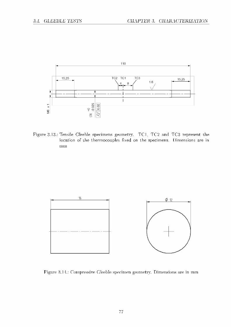
3.4. GLEEBLE TESTS CHAPTER 3. CHARACTERIZATION
Figure 3.13.: Tensile Gleeble specimens geometry. TC1, TC2 and TC3 represent thelocation of the thermocouples xed on the specimens. Dimensions are inmm
Figure 3.14.: Compressive Gleeble specimen geometry. Dimensions are in mm
77

3.4. GLEEBLE TESTS CHAPTER 3. CHARACTERIZATION
problems have been encountered.
The best way to get the quickest response time from a thermocouple is to spot-weld
it directly on the component to be measured. This ensures there are no further thermal
resistances between the surface measured and the thermocouple, while not modifying the
actual temperature measured and minimising delay due to the rise time of the measure-
ment system.
The most common type of thermocouple for this purpose, is the type K, since they can
operate at relatively high temperatures (1350°C max for short term) and they are cheaper
than other types. Unfortunately, the junction between Titanium and the thermocouple
materials (Nickel-Chromium for + wire and Nickel-Aluminum for - wire) seems to lose
strength at temperatures around 950 °C, breaking the junction. The cause of this phe-
nomenon could be explained by a possible eutectic transformation taking place at around
940-980 °C, between the binary system Ti-Ni, depending on the specic chemical compos-
ition of the junction formed [92]. As a rst solution to the problem, holes were drilled in
the specimens, then sheathed thermocouples type K were inserted, avoiding the necessity
to keep the sensors in position by spot welding. Besides a possible lower response time of
this solution, that would have been checked if really important for the testing conditions
used, the temperature read by the Gleeble machine was dierent from the value obtained
using a National Instrument acquisition box. This shift in temperature was a function of
the length of the thermocouple wires, probably due to poor design, low input impedance,
of the Gleeble acquisition instrumentation: sensors longer than about 30 cm introduced
there temperature shifts. Since it was not possible to nd sheathed thermocouples shorter
than 50 cm on the market, and considering also the unknown response time, bare type
B thermocouple wires were tried. These thermocouples (Platinum-30% Rhodium for +
wire and Platinum-6% Rhodium for - wire), able to work to relatively high temperatures
(max 1820 °C) did not show any junction trouble as encountered when the type K was
spot welded to Titanium. The downside of using this kind of thermocouple is, besides
a higher cost, the inability to work at temperatures below 60 °C, since the voltage re-
78

3.4. GLEEBLE TESTS CHAPTER 3. CHARACTERIZATION
turned becomes almost constant. For the purpose of these experiments, the limitation of
the minimum temperature was not a problem, since the material microstructure is not
aected by temperatures below 500 °C, for the heat treatment timings considered. The
higher cost was compensated by the certainty to get the best response time possible and
to avoid detachment of the junction at temperatures around 980 °C.
The only problem given by the type B thermocouples, when coupled with the acquisi-
tion instrumentation of the Gleeble, was a noisy signal, due to the low voltage returned
by the sensors, which was sensitive to other ambient signals. To solve this problem,
ferrite inductors were placed around each thermocouple wire, damping down the noise.
In conclusion, type B thermocouples have been the thermocouple type used for these
experiments, solving the potential possible problems related to using the type K ones.
To control the temperature in compression tests, a type B thermocouple was spot welded
in the middle of the length of each component (gure 3.16).
In the tensile specimens, another two type B thermocouples were spot welded on each
specimen, at about 4 mm and 8 mm from the middle, respectively one on the right side
and one on the left side (gure 3.13). It was then possible to control the temperature
at three dierent positions of each specimen and, since the temperature along the length
of the component has a parabolic trend, with a peak in the centre, three dierent peak
temperatures could be tested for each sample. A photograph of the assembly used is
shown in gure 3.15.
FE analysis has been carried out to assess any size eects and to ensure the samples
did not have a too high temperature gradient through their thickness, so there would be
no signicant dierence of temperature between the one measured by thermocouples spot
welded on the specimens surface and that in the centre (appendix A). This numerical
analysis did not attempt to be a full physical representation of the Gleeble tests but to
give an indicative guideline on the temperature gradient that could be expected along the
thickness of the components.
79

3.4. GLEEBLE TESTS CHAPTER 3. CHARACTERIZATION
Figure 3.15.: Photograph of the assembly used for tension tests carried out by using thetesting system Gleeble 3500
Figure 3.16.: Photograph of the assembly used for compression tests carried out by usingthe testing system Gleeble 3500
80

3.4. GLEEBLE TESTS CHAPTER 3. CHARACTERIZATION
3.4.1 Microstructural analysis - procedure
After each test, the samples were sectioned in correspondence with the thermocouple
positions, polished, etched in 2% HF and 10% HNO3 solution and analysed with:
optical microscopy using a Zeiss Axioskop 2 MAT mot microscope with software
AxioVision v 4.6.3.0
back scattered electron imaging (BEI) using an Oxford Instruments XL30 ESEM
EG
Using optical microscopy, montages of the entire section of each sample were composed,
and the beta grain dimensions measured.
From BEI, the thickness of lamellar microstructure, grain boundary and volume fraction
of alpha and beta phases were estimated using the open source image processing software
ImageJ. In general, alpha phase features were identied by darker colours since containing
lighter elements (more Aluminium, atomic mass 26.9 g/mol), vice versa for beta features
(more Vanadium, atomic mass 50.94 g/mol).
For the estimation of the dimensions of beta grains, the following procedure has been
adopted:
1. Identication of the grain boundaries by manually highlighting their boundaries
drawing black or white lines (gure 3.17-a).
2. Thresholding of the image (gure 3.17-b).
3. Using an ImageJ routine, ellipses were inscribed as best as possible in each beta
grain, such that the area of each ellipse was equivalent to the grain being evaluated
(gure 3.17-c).
4. For each ellipse, a ctitious oblate ellipsoid volume was calculated, using the two
smaller principal axis of the ellipsoid as the length of the minor axis of the ellipse,
while the major axis of the ellipsoid was equivalent to the major axis of the ellipse.
81

3.4. GLEEBLE TESTS CHAPTER 3. CHARACTERIZATION
5. The mean value of the distribution of ellipsoid volumes was calculated and used
as a representative value of the beta grain size obtained from the heat treatment
considered.
6. For each ellipsoid an equivalent sphere in volume was calculated and the relative
radius used as representative of the beta grain size distribution, thus simplifying the
particle geometry into spheres.
To estimate the evolution of the lamellae dimensions of the original microstructure of
the material tested (gure 3.18), ellipses were manually inscribed, to make the major
axis coincident with the length of the lamellae, and the minor axis coincident with the
thickest section of the lamellae considered (gure 3.19). From the mean of the minor axis
distribution, the mean lamellae thickness was calculated; by the ratio of the mean major
and minor axis, the aspect ratio was estimated. In this work, for the study of the lamellae
dimension evolution, only the lamellae colonies appearing with sharper boundaries and
slimmer shapes have been considered. This aimed to reduce the eect of the random
inclination of the sectioning plane used in studying the microstructure of the material.
Colonies sectioned not perpendicularly to their longitudinal direction, would appear with
wider and darker boundaries but also with an overall larger lamellae thickness. Thus,
from this consideration, the choice of evaluating colonies with well dened boundaries
would in general end up assessing colonies with a thinner lamellae thickness and hence
gives an underestimate.
In the literature, a common procedure adopted for lamellae thickness measurement, con-
sists of collecting a series of intercept readings by rotating a grid of parallel lines at many
angular steps, till a complete rotation of 360° has occurred [30, 28]. The mean length of
all the intersections of this grid, for each angular step, with each lamellae, multiplied by
a factor 1.5 and inverted, would return the hypothetical true mean value of the lamellae
measured. This approach conicted with the aim of the present work, where both lamellae
thickness and aspect ratio had to be measured. The intercept approach would have re-
turned only the thickness lamellae estimation. Moreover, a software solution to automate
82

3.4. GLEEBLE TESTS CHAPTER 3. CHARACTERIZATION
the intercept measurements was necessary to reduce the working time, but probably it
would still have needed a huge interaction from the user, in particular if, for consistency,
the same approach was used for the thickness measurement of lamellae nucleated during
cooling, where martensitic needles were also developed in the microstructure, introducing
signicant errors in the measurements on the lamellar microstructure.
To estimate the thickness of the lamellae beta boundaries, a set of perpendicular lines
to the sides of the grain boundaries were traced, and from their length distribution, the
mean grain boundary thickness was computed.
The volume fraction was estimated by thresholding pictures on the the grey scale of the
beta phase, that is represented by a whiter colour in BEI pictures.
For the estimation of the thickness of new lamellae nucleated during heat treatments
involving cooling, lines perpendicular to the longitudinal direction of the lamellae were
traced, from one side to the other of each lamellae.
All the values measured have been collected and their trend plotted in charts, reporting
when more measurements were involved, the error bar shown represent the standard
deviation.
The as received microstructure of the material used for the Gleeble tests was lamellar,
as shown in gure 3.18.
83

3.4. GLEEBLE TESTS CHAPTER 3. CHARACTERIZATION
a)
b)
c)
Figure 3.17.: From the top to the bottom: a) optical microscope micrograph showing betagrains manually highlighted; b) beta grains thresholded; c) ellipses inscribedin the beta grain shapes
84

3.4. GLEEBLE TESTS CHAPTER 3. CHARACTERIZATION
Figure 3.18.: BEI micrograph showing the microstructure of the received Ti-6Al-4V. Al-pha lamellae are represented by the darker areas, since they have loweratomic weight. The thin white walls bounding the lamellae represent thebeta phase, with higher atomic weight
85

3.4. GLEEBLE TESTS CHAPTER 3. CHARACTERIZATION
Figure 3.19.: BEI micrograph showing ellipses inscribed to the lamellae of gure 3.18
3.4.2 Microanalysis - technique
When necessary, to study the chemical composition of samples, in particular to analyse
its variation in function of position or thermal treatments, energy dispersive spectroscopy
(EDS) analysis was adopted by using the Oxford Instrument XL30 ESEM EG coupled
with the Oxford Instrument Inca software version 4.15.
The technique is based on the physical interaction between the microscope electrons
beam and the electrons of the material studied. When an electron of the beam hits an
electron of an atom of the material, this last escapes from its shell producing a vacancy.
If the vacancy is lled from a higher level orbital, an x-ray characteristic of that energy
transition is produced. Since energy levels are dierent for each elements of the periodic
table, the x-rays emitted can be related to the specic element generating it. In particular,
the EDS detector converts the energy of each individual x-ray into a voltage signal of
proportional size.
86

3.4. GLEEBLE TESTS CHAPTER 3. CHARACTERIZATION
The interactions produced between the electron beam and the material analysed can be
represented by a pear shape interaction volume located beneath the sample surface hit by
the beam (gure 3.20). This shape is function of the atomic number and crystallographic
structure of the material but also of the power of the beam used. As the atomic structure
of the atoms constituent the material is denser, the pear shape interaction volume will
have a smaller penetration and width as well as the power of the beam decreases.
To get in a relatively short time (minutes) a signicant interaction volume from EDS
analysis to identify properly the chemical composition of the area investigated, in a ma-
terial like the one studied in this work an acceleration voltage of 15 kV - 20 kV was needed,
thus expecting interaction volumes of 1− 2 µm3.
Considering sometimes the dimension of the particles investigated was fractions of mi-
crons, the chemical compositions reported in this chapter is, as already said, indicat-
ive of the mean composition of the area investigated but not the actual composition of
particles/phases.
87

3.4. GLEEBLE TESTS CHAPTER 3. CHARACTERIZATION
Figure 3.20.: Monte Carlo simulation of electron scattering due to the interaction betweenan electron beam, dierent materials and acceleration voltage [38]
3.4.3 Heating rate eect on lamellar microstructure
For the study of the eect of dierent heating rates on the dissolution of the original
lamellar microstructure of the material, and possible formation of beta grains when the
beta transus temperature was passed, tensile specimens were used (gure 3.13). Three
dierent heating rates (5, 50 and 500 °C/s) have been tested, bringing the specimens to
dierent peak temperatures and then water quenching them.
Representative microstructures, taken from each tested sample, are reported in gure
3.21 for heating rates of 5 °C/s, gure 3.22 for heating rates of 50 °C/s and gure 3.23 for
heating rates of 500 °C/s. Looking at the micrographs, going toward higher temperatures,
from the right to left and from bottom row to the top, it is possible to notice dissolution of
88

3.4. GLEEBLE TESTS CHAPTER 3. CHARACTERIZATION
the alpha phase lamellae (dark grey shapes) whilst the beta phase grows (white matrix).
When the lamellae are no longer recognizable, and needles appear, we can say the material
passed the beta transus temperature during the heat treatment. This can be deduced in
the micrographs due to the appearance of thin, long, white needles, formed by water
quenching from a temperature above the beta transus temperature.
Making reference to the gures 3.21, 3.22 and 3.23, the beta transus can be located
between 915 °C and 976 °C for the heating rate of 5 °C/s; between 966 °C and 982 °C for
the heating rate of 50 °C/s and between 1020 °C and 1123 °C for the heating rate of 500
°C/s.
The beta transus temperature, as the heating rate increases, shifts towards higher values.
This is due to the kinetics of the diusion process, that requires a certain amount of time
to let the metallurgical transformations occur. Moreover, in a quasi steady state process,
as the temperature rises, the original lamellae would dissolve, until a temperature where
they completely disappear, leaving the beta phase. In fast metallurgical reactions, like
the ones taken in consideration in this work, the time for a complete dissolution of the
lamellae is not sucient: the lamellae thickness, at temperatures close to the beta transus
temperature, is still quite large and the change of crystallographic structure from HCP
to BCC occurs before their complete dissolution. This also means that the concentration
eld of the constituent elements in the dierent phases, does not have time to change to
get the equilibrium concentration at a specic temperature. This is particularly visible in
micrographs where the temperature is slightly above the beta transus temperature and
the white and dark elds associated with the original concentration of the constituent
elements in the lamellar morphology can be still noticed. For example, in gure 3.21, for
the heat treatments with peak temperature of 976 °C and 1000 °C, besides the needles,
is possible to see an inhomogeneous background with darker and whiter areas, due to
remnants memory of the elemental distribution in the lamellar microstructure.
In section B.1, B.2 and B.3 optical microscope montages of the entire cross sections of
each sample tested are shown, in which it is possible to appreciate the disappearance of
89

3.4. GLEEBLE TESTS CHAPTER 3. CHARACTERIZATION
the original lamellar microstructure and the growth of the beta grains as the temperature
increases.
Graphs in gure 3.24 show the results of the image analysis conducted on the samples
tested, whose microstructures are shown in micrographs of gures 3.21, 3.22 and 3.23.
As the heating rate increases, the alpha lamellae dissolution and beta phase growth
tend to shift toward higher and higher temperatures as well as the alpha volume fraction.
This is due to the limited speed of the diusion kinetics, as already discussed.
The progressive reduction of time available for the diusion process can be visualised
by plotting the same data shown in the graph of gure 3.24 as a function of time (graph
in gure 3.25). The heat treatment durations between the fastest heating rate (500 °C/s)
and the slowest (5 °C/s) go from 180 seconds to 2 seconds. Thus the diusing process at
the fastest heating rate has 1/100 of the time to occur with respect to the slowest heat
treatment.
Graphs in gure 3.26 shows the evolution of the lamellae aspect ratio as a function of
the peak temperature and time. As the heat treatment advances and the temperature in-
creases, the lamellae thickness reduces and, as consequence, the aspect ratio progressively
increases.
90

3.4. GLEEBLE TESTS CHAPTER 3. CHARACTERIZATION
Figure 3.21.: BEI microhraphs showing representative microstructures obtained from allthe samples tested at the heating rate of 5 °C/s to dierent peak temperat-ures and water quenched. As a comparison, the original microstructure ofthe material as received is also shown. The specimens heated up to temper-atures equal or higher than 976 °C and water quenched do not show anymorethe original lamellar morphology, but martensitic microstructure
91

3.4. GLEEBLE TESTS CHAPTER 3. CHARACTERIZATION
Figure 3.22.: BEI micrographs showing representative microstructures obtained from eachsample heated up at 50 °C/s to dierent peak temperatures and waterquenched. Specimens heated up till temperatures equal or higher than 982°C have martensitic microstructure instead of the original lamellae one
92

3.4. GLEEBLE TESTS CHAPTER 3. CHARACTERIZATION
Figure 3.23.: BEI micrographs showing representative microstructures obtained from eachsample heated up at 500 °C/s till dierent peak temperatures and waterquenched. Specimens heated up till temperatures higher than 1020 °C havemartensitic microstructure instead of the original lamellae one
93

3.4. GLEEBLE TESTS CHAPTER 3. CHARACTERIZATION
a)
b)
c)
Figure 3.24.: Graphs showing the heating rate eect on the dissolution of lamellae (a),growth of beta boundaries (b) and alpha volume fraction (c) as a functionof the peak temperature reached during the heating tests
94

3.4. GLEEBLE TESTS CHAPTER 3. CHARACTERIZATION
a)
b)
c)
Figure 3.25.: Same results shown in gure 3.24 but plotted as a function of time. Theduration ratio between the fastest and the slowest heat treatment is 1/100
95

3.4. GLEEBLE TESTS CHAPTER 3. CHARACTERIZATION
a)
b)
Figure 3.26.: Graphs showing the variation of the lamellae aspect ratio as a function of(a) peak temperature and (b) time at dierent heating rates. In general, asthe reaction proceeds, the lamellae reduce their thickness (gure 3.24 and3.25) thus their aspect ratio increases
96

3.4. GLEEBLE TESTS CHAPTER 3. CHARACTERIZATION
3.4.4 Cooling rate eect on lamellar and martensitic microstructures
For the study of the cooling rate eect on the lamellae growth, during continuous cooling
from the beta eld, either Gleeble compression or tensile tests have been conducted, based
on the availability of the specimens and cooling rates required.
Graphs reporting trends of the data obtained are shown in gure 3.27, where the data
measured are reported as a function of the peak temperature from which the cooling
started.
Even though the number of data points is not very high to obtain precise trends, it seems
that the cooling rate from a specic temperature to ambient temperature does not have a
well dened eect on the lamellae thickness, while the starting temperature at which the
heat treatment happens is more important. This eect can be attributed to the dierent
beta grain size in which the lamellae grow: the larger the beta grains, the higher is the
probability to have a wider distance between nucleated lamellae, that can grow without
chemically/mechanically impinging on each other. To accurately verify this hypothesis,
another series of thermal tests should be carried out, testing for each cooling rate a wider
range of dierent starting temperatures/beta grain sizes. The relation between beta grain
dimension and lamellae thickness seems to be supported in literature, even if not much
work seems to be published about this relationship [72].
By plotting the data acquired for the lamellae thickness as a function of the beta grain
size where lamellae grew (graphs in gure 3.28), this hypothesis seems to be supported.
As a rst consideration the lamellae thickness seems really to not be related to the cooling
rate in continuous cooling heat treatments, if this statement was not true, at faster cooling
rates it would have been possible to observe thinner lamellae because of the shorter growth
time. A second consideration is that the thickest lamellae are measured for the fastest
cooling rate (300 °C/s), where the beta grains were noticeably larger than the ones at
the slower cooling rates (5 °C/s and 50 °C/s). Moreover, looking at the data relative to
the cooling rate of 100 °C/s, where a set of points with dierent beta grains has been
collected, the relationship between peak temperature/dimension of the beta grains and
97

3.4. GLEEBLE TESTS CHAPTER 3. CHARACTERIZATION
lamellae thickness is very clear. A last consideration can be made for the inter lamellae
beta phase as a function of the beta grains dimension, where the beta phase thickens as
the beta grains grow, such that the spacing between each lamella is driven by the beta
grain size where they nucleate. This further supports the original hypothesis.
The microstructures developed by the dierent cooling rates, besides diering in the
lamellar microstructure, in particular lamellae thickness, presented a higher amount of
martensite and thicker martensitic needles as the cooling rate increased (micrographs in
gures 3.29 and 3.30 and graphs in gure 3.31 and 3.32). Signicantly graph 3.31-b shows
a logarithmic relation between needle thickness and the cooling rate used to bring the
samples from the tested temperature to the ambient one.
Since the volume fraction measurement of the alpha and martensitic phases was very
dicult to carry out, due to the overlapping of the alpha lamellae and martensitic needles,
the graph reported in gure 3.32 should be taken as a qualitative indication only. A partial
martensitic microstructure at cooling rates of 300 °C/s seems to conrm Ahmed and Rack
in [93], where a cooling rate of 500 °C/s is claimed to be necessary to have a microstructure
completely transformed to martensite.
Regarding the observation of lamellar alpha even at 300 °C/s, reported in this work,
TEM investigations would be required to better classify it. In [93], the α microstruc-
ture present at cooling rates faster than 20 °C/s, following TEM study, was classied
as a second α morphology, with a heavily dislocated internal substructure and the same
hexagonal crystal structure as martensite. Since there was no time for this kind of invest-
igation, the lamellae noticed by SEM were all classied as of the same typology.
3.4.5 Growth of nucleated lamellae in the α + β eld
To study the isothermal growth of lamellae in the α+ β eld, nucleated by cooling down
from the beta eld, three series of tests have been carried out. Each of them consist of
cooling down samples from the beta eld at either 5, 25 or 50 °C/s to dierent temperat-
ures below the beta transus temperature, then water quenching directly or soaking for 10
98

3.4. GLEEBLE TESTS CHAPTER 3. CHARACTERIZATION
a)
b)
Figure 3.27.: Graphs showing the cooling rate eect on lamellae growth as a functionof the temperature from which the cooling started (a), cooling rate eecton lamellae beta boundaries growth as a function of the temperature fromwhich the cooling started (b)
99

3.4. GLEEBLE TESTS CHAPTER 3. CHARACTERIZATION
a)
b)
Figure 3.28.: Graphs showing the cooling rate eect on lamellae growth as a functionof the beta grain size (a), cooling rate eect on lamellae beta boundariesgrowth as a function of the beta grain size (b)
100

3.4. GLEEBLE TESTS CHAPTER 3. CHARACTERIZATION
a)
b)
Figure 3.29.: BEI micrographs showing an example of sample microstructures obtainedcooling down at 5 °C/s (a) and 50 °C/s (b) from the beta eld. The rst onehas a microstructure entirely lamellar, whilst in the second one martensitehas started to form
101

3.4. GLEEBLE TESTS CHAPTER 3. CHARACTERIZATION
a)
b)
Figure 3.30.: BEI micrographs showing an example of sample microstructures obtainedcooling down at 100 °C/s (a) and 300 °C/s (b) from the beta eld. Themartensitic needles become progressively thicker as the cooling rate increases(see also micrographs in gure 3.29)
102

3.4. GLEEBLE TESTS CHAPTER 3. CHARACTERIZATION
a)
b)
Figure 3.31.: Graphs showing the cooling rate eect on the martensitic needles meanthickness as a function of the peak temperature from which the coolingstarted (a) and as a function of cooling rate (b). The data points shownin graph (b), considering the error bars, can be interpolated by a straightline, suggesting that a logarithmic function can well describe the needlesthickness as a function of the cooling rate (see also graph in gure 4.28)
103

3.4. GLEEBLE TESTS CHAPTER 3. CHARACTERIZATION
Figure 3.32.: Graph showing the amount of the alpha phase volume fraction formed inTi-6Al-4V when the material is cooled down with dierent cooling ratesstarting from temperatures above the beta transus temperature (same datapoints of gure 3.31)
or 20 seconds then water quenching. Since the investigation of all the possible combina-
tions of temperatures, cooling rates and soaking times would have required an extensive
study, some combinations have been omitted.
This work was undertaken mainly to assess the feasibility of dierentiating between the
alpha formed on cooling through the transus and the martensite produced on quenching.
Although experimentally dicult, this is feasible, giving the possibility of quantifying the
alpha phase formation in the alpha-beta phase eld which is needed for predicting the
mechanical properties.
Measurement of the lamellae thickness for these particular tests was particularly ardu-
ous. Due to the particular heat treatment carried out (gure 2.24), a mixture of martensite
and alpha lamellar microstructures was obtained, returning complicated BEI images to
be studied. The amount of alpha lamellae recognizable per specimens was also very low,
which resulted in a poor sample population for calculating the means and standard devi-
ations (micrograph in gure 3.33). A further complication resulted from the use of tensile
104

3.4. GLEEBLE TESTS CHAPTER 3. CHARACTERIZATION
or compression specimens, with a dierent section area. From the considerations in sec-
tion 3.4.4, the thickness of the lamellae could be aected by a dierent sample size and
this could modify the real trend of the particle dissolution or growth.
With the previous considerations in mind, an indicative analysis of the trends obtained
from the measurements conducted (graphs in gure 3.34) is now described, giving partic-
ular attention to the heat treatments with more data points.
A rst observation comparing the results coming out from cooling down at 5 °C/s and
50 °C/s to the same temperature in the α+β eld, at time zero, is the very similar lamellar
thickness obtained. Also, it seems there is a clear relation between the cooling time and
the thicknesses of the lamellae: the lower the temperature at which the soaking starts,
the thicker are the lamellae developed.
In general the tendency for all the cases seems to be a slow growth as the soaking time
in the α + β eld becomes longer. For 50 °C/s the growth seems more pronounced at 20
s, but the low number of lamellae sampled per test and the dierent sample diameters
introduced uncertainty that, in the author's opinion, should be resolved by conducting a
wider campaign of tests.
With so few data points and the dierent specimen dimensions exact conclusions from
this part of the work cannot be done. As for the observation in section 3.4.4, approximately
the same lamellae thickness would be expected at time 0 for all the cooling rates and,
considering the dierent sample sections, this still seems reasonable. For the rst 10
seconds it also seems that lamellae do not have the time to grow considerably, even
though at 20 seconds it seems that growth is more appreciable.
105

3.4. GLEEBLE TESTS CHAPTER 3. CHARACTERIZATION
Figure 3.33.: BEI micrograph showing an example of a microstructure obtained in the α+ β eld. Lamellar microstructure embedded in martensite obtained afterholding in the α + β eld and then quenching
106

3.4. GLEEBLE TESTS CHAPTER 3. CHARACTERIZATION
a)
b)
c)
Figure 3.34.: Graphs showing growth of alpha lamellae in the α+β eld, cooling down fromthe β eld at dierent cooling rates and soaking for 0, 10 and 20 seconds thenwater quenching the samples. Data points with arrows represent samples of6mm diameter, the other ones represent samples of 12 mm diameter
107

3.4. GLEEBLE TESTS CHAPTER 3. CHARACTERIZATION
3.4.6 β transus
The beta transus temperature of the Titanium alloy used for the metallurgical study (see
section 3.4), has been established by soaking small cubic specimen 10× 15× 2mm3 in a
furnace for at least 20 minutes, at temperatures around the nominal beta transus, based
on the results obtained from heating up the material at 5 °C/s. This heating rate was the
slowest tested and thus was considered to be the closest to the response of the material
at isothermal conditions. The samples, glass coated before the heat treatment to reduce
the oxygen pick up at high temperatures, after soaking were water quenched to freeze the
microstructure.
The temperature was acquired from a thermocouple type K placed in contact with the
samples and controlled by a National Instrument acquisition box connected to a personal
computer, enabling temperature measurement in real time. The furnace temperature was
then manually set by small temperature steps, controlling each time the actual temper-
ature on the surface of the specimens.
The temperatures tested were 960 °C, 970 °C and 980 °C. To establish between which
range of temperatures the beta transus was located, optical microscopy and BEI investig-
ations were carried out, by checking if any primary alpha lamellae were still not dissolved.
In micrographs shown in gure 3.35, 3.36 and 3.37 optical microscope pictures are
shown, respectively a) for 960 °C, b) for 970 °C and c) for 980 °C.
In micrographs shown in gures 3.38, 3.39 and 3.40, in the same order of the previous
gures, a BEI image for each sample is shown. It is possible to see how at 980 °C
the microstructure was completely transformed to beta, since no parent lamellae can be
spotted and only martensite is observed.
The beta transus temperature can thus be estimated to be within 980 °C and 970 °C.
Using also results obtained from heating rates at 5 °C/s (micrographs in gure 3.21), the
beta transus temperature can be approximately assumed to be at 973 °C, as this is the
mean value between the two closest temperatures at which microstructures have been
studied and at which it is possible to see still parent material (970 °C) and only beta
108

3.4. GLEEBLE TESTS CHAPTER 3. CHARACTERIZATION
transformed phase (976 °C).
Figure 3.35.: Optical micrograph image of the sample soaked at 960 °C for the determ-ination of the beta transus temperature. Parent alpha is still present thusbeta transus has not been passed
Figure 3.36.: Optical micrograph of the sample soaked at 970 °C for the determination ofthe beta transus temperature. Parent alpha is still present thus beta transushas not been passed
109

3.4. GLEEBLE TESTS CHAPTER 3. CHARACTERIZATION
Figure 3.37.: Optical micrograph of the sample soaked at 980 °C for the determination ofthe beta transus temperature. Beta grains can be observed along the entiresection: the beta transus temperature has been passed
Figure 3.38.: BEI micrograph of the samples tested at 960 °C for the determination of thebeta transus temperature. Parent alpha lamellae can be observed, meaningthe beta transus temperature has not been passed
110

3.4. GLEEBLE TESTS CHAPTER 3. CHARACTERIZATION
Figure 3.39.: BEI micrograph of the samples tested at 970 °C for the determination of thebeta transus temperature. Parent alpha lamellae can be observed, meaningthe beta transus temperature has not been passed
Figure 3.40.: BEI micrograph of the sample tested at 980 °C for the determination of thebeta transus temperature. No parent alpha lamellae can be observed as ingure 3.38-a and b, meaning the beta transus temperature has been passed
111

3.4. GLEEBLE TESTS CHAPTER 3. CHARACTERIZATION
3.4.7 β grain growth
As described at the beginning of the chapter, beta grain dimensions have been measured,
in particular for the specimens tested at dierent heating rates, to understand and try to
get an analytical expression to describe their growth evolution.
The experimental results obtained are shown in graphs of gure 3.41, where the beta
grain dimension is reported both as a function of temperature and time for the three
heating rates tested (5, 50 and 500 °C/s).
As it can be noticed (gure 3.41), at the fastest heating rate the beta grain dimension
remains almost constant, limited by the short time the heat treatment required to reach
the test temperatures set. At the intermediate heating rate of 50 °C/s instead, comparing
at the same peak temperature, the kinetic of the diusion process driving the grain growth
seems instead to occur in timings long enough to return beta grain dimensions similar to
the ones obtained for the slowest heating rate (5 °C/s).
The asymptotic trends registered in these tests (gure 3.41-a) are in agreement with
the ones reported in literature [74] and they can be attributed to the beta grain growth
coarsening [94]. Moreover, a slower growth rate can be supported also by a progressive
homogenization of the chemical eld as the growth proceeds in non equilibrium conditions.
112

3.5. WELDING TESTS CHAPTER 3. CHARACTERIZATION
a)
b)
Figure 3.41.: Beta grains measurements as a function of the peak temperature and heatingrate a), beta grains measurements as a function of the time and heating rateb).
3.5 Welding tests
For the study of the microstructures obtained in laser welding of Ti-6Al-4V, and for the
application and validation of the numerical model developed in this work, a series of laser
welding tests on Ti-6Al-4V plates with either an initial equiaxed or lamellar morphologies
have been carried out.
The Titanium plates with equiaxed morphology had dimensions a) 51.62×149×5.80mm3
with a measured composition in weight percent of Al 6.05, V 3.99, Fe 0.19, H 0.00314, N
0.005, O 0.18, Ti bal and b) 46.95 × 151.5 × 2.00 mm3 with a measured composition in
weight percent of Al 5.82, V 4.00, Fe 0.06, H 0.00963, N 0.010, O 0.063, Ti bal.
113

3.5. WELDING TESTS CHAPTER 3. CHARACTERIZATION
Microstructure Thickness of the plate [mm] Power [%] Welding speed [m/min]
Equiaxed 5.80 100 2.0 - 1.5Equiaxed 2.00 60 2.0Lamellar 3.75 70 2.0Lamellar 3.06 70 2.0
Table 3.1.: Welding operative parameters used for welding tests. Ti-6l-4V plates with twodierent initial microstructures and dierent thicknesses were welded, usingwelding speeds of 2.0 or 1.5 m/min. The welding input power was set aspercentage of the maximum power (4 kW ) of the welding machine used
The Ti-6Al-4V plates with lamellar morphology had dimension 47.30×136.96×3.75mm3
and 47.31×137.05×3.06mm3 and they were made of a grade 5 Ti-6Al-4V with a measured
composition in weight percent of Al 5.75, V 3.96, Fe 0.07, H 0.00445, N 0.013, O 0.11, Ti
bal.
Two thickness have been used for the tests, with dierent welding parameters. The
power was set as a percentage of 4 kW, as this was the maximum power of the machine.
Regarding the equiaxed microstructure, for the 2.00mm thick plate, a power of 60% was
used whilst, for the 5.80 mm thick one, a power of 100% was set. For the plates with
an initial lamellar microstructure, a power of 70% was used. As explained in paragraph
2.2.2, the determination of the actual power going through the plates is beyond the aims
of the current work: thus for the data reported it will be make reference to the percentage
set in the machine rather than an actual power value.
The welding machine used for the welding tests was a Trumpf TLC1005.
The welding speeds tested for the plates with equiaxed microstructure were 1.5m/min
and 2.0 m/min for the plate 5.80 mm thick and 2.0 m/min for the plate 2.00 mm thick.
The plates with lamellar microstructure were instead welded with a speed of 2.0 m/min
(see table 3.1).
The nozzle of the welding machine was set at a distance of 6.8 mm from the top surface
of the plates.
Since temperature proles along the component are needed to set the heat source of
the numerical model correctly (section 2.2.2), the plates tested were machined to locate
114

3.5. WELDING TESTS CHAPTER 3. CHARACTERIZATION
the thermocouples. Holes were drilled at dierent distances from the weld line, and
thermocouples were placed in them.
Sheathed thermocouples type K were adopted for the following considerations:
a high number of thermocouples had to be used to get a good understanding of the
dierent temperature gradients along the component: with spot welding, there was
a high risk that some sensors would have disconnected while the plates were being
prepared for welding. In such a case, the component had to be removed from the
jig and brought again to the spot welder. By locating the thermocouples in place
with holes, they could be quickly repositioned if some of them came out;
initially, some welding tests were run with the thermocouples xed in the holes with
either glue or cement. Using glue, where the thermocouples were close enough to the
weld heat source, it burnt modifying the temperature readings and also signicantly
changing the shape of the weld pool. Instead, although the cement did not burn,
it changed the weld pool shape by absorbing in a dierent manner the heat ux
respect the workpiece material. A change in the weld pool shape would aect the
real thermal prole developed by the welding process, thus preventing the acquisition
of reliable information for the numerical model;
bare wires could not be located in the holes, since the thermocouple wires needed
to be bent so as to not touch the nozzle of the welding machine. Moreover by bend-
ing, the bare wires touched the upper edge of the holes and since the temperature
measured by thermocouples is where the rst electrical junction between the sensor
wires is formed, the temperature actually measured in this case, would have been
from the hole upper edge;
type B thermocouples would have allowed measurements at higher temperatures
but with the temperature rising so high close to the weld pool it was not possible
to place the sensor in positions where they could still measure temperature above
115

3.5. WELDING TESTS CHAPTER 3. CHARACTERIZATION
1400 °C (type K max temperature), but less than 1600 °C, without them moving
out of position when liquid was formed.
For each welding test of the plates with an equiaxed morphology, 14 thermocouples were
used, to measure seven dierent distances from the weld trajectory in one face, and to
study the thermal prole of the weld pool using the other seven thermocouples at two
distances very close to the weld pool and at dierent depths (gure 3.42). To save material,
each plate was used for 2 welding tests, while ensuring that the distance between the welds
was large enough to prevent any eect on the microstructures from the thermal load. In
gure 3.43 a photograph of a plate ready to be welded is shown. All the thermocouples
were kept in position by twisting a wire around them and the plate. In gure 3.44 a
photograph of the assembly used to x the plates for the welding tests is also shown.
The plates in the welding machine were xed using a jig designed previously (appendix
C), leaving one side free and clamping the other one as shown in gure 3.44-a. A ceramic
plate was placed below the specimens to protect the vice on which the jig was mounted,
in case of a full penetrating weld.
Because Titanium is very sensible to oxidation, all the instrumentation had to be placed
in a chamber to operate in inert atmosphere (Argon) (photograph in gure 3.44-b).
The surfaces of the plates were cleaned with Acetone before each welding tests, to
remove any grease or dirt which could aect the quality of the weld.
To measure the chamber temperature close to the specimens during welding, a further
thermocouple was placed at about 2 cm below the bottom surface of the plate.
After having run the rst weld, the plate was removed from the jig, cleaned with Acetone
(gure 3.45) and another 14 thermocouples were placed to measure temperatures for the
second welding test.
An example of how a welding plate looked at the end of the welding tests is shown in
gure 3.46.
116

3.5. WELDING TESTS CHAPTER 3. CHARACTERIZATION
Figure 3.42.: Drawing of the hole positions machined to keep in place the thermocouplesduring welding tests. In the top face of the plates a series of holes at dierentdistances from the weld line have been machined, in the bottom face the holesare at two dierent distances but with dierent depths
117

3.5. WELDING TESTS CHAPTER 3. CHARACTERIZATION
Figure 3.43.: Photograph of Ti-6Al-4V plate showing how the thermocouples were keptin place by twisting two wires around them and the specimens
Unfortunately, not all the thermocouples worked satisfactorily during the tests, thus
reducing the actual number of measurements available. Moreover, the row of thermo-
couples located very close to the weld pool, returned values not in agreement with values
expected from their position and depth, suggesting a high sensitivity of the measure-
ments to slightly dierent positions to the ones planned, caused by movements of the
thermocouples tip. Without any xing technique to keep the thermocouples in position
in the holes, small movements were unavoidable and this could be the explanation for the
problem.
Welding tests on plates with an initial lamellar morphology were carried out a second
time to measure distortion before and after welding, for the validation of the mechanical
model. For this purpose, each plate was welded only once, avoiding superimposition of the
eects of two welds on the distortion of the components. The temperature measurements
were carried out by using only the set of holes in the top surface of each plate tested (gure
118

3.5. WELDING TESTS CHAPTER 3. CHARACTERIZATION
a)
b)
Figure 3.44.: Photographs showing a) the jig used to x the plates during welding tests andb) the assembly placed in the welding chamber to operate in inert atmosphere
119

3.5. WELDING TESTS CHAPTER 3. CHARACTERIZATION
Figure 3.45.: Photograph of a Ti-6Al-4V plate after welding
3.42). This decision was because a) from previous welding tests, the set of holes in the
bottom surface did not return reliable results and b) at the time of the tests, the access
to the welding chamber was changed, only allowing a maximum of 5 thermocouples.
3.5.1 Temperature measurements
3.5.1.1 Plates with equiaxed microstructure
In the graphs of gure 3.47 and 3.48 results of the welding conducted on a 5.8mm plate
using as operative parameters 100% power and 2 m/min and 1.5 m/min respectively are
shown. The time at which the temperature rises does not correspond to the actual time
needed by the laser to heat up the thermocouples from the starting of the welding test.
The acquisition was launched some seconds before starting the experiments to check if
the acquisition system worked correctly.
In the graph of gure 3.49 results of welding tests on a 2mm thick plate with a 2 m/min
welding speed are shown.
Results shown in this section are all relative to the plates having an original microstruc-
120

3.5. WELDING TESTS CHAPTER 3. CHARACTERIZATION
a)
b)
Figure 3.46.: Cropped photographs of the Ti-6Al-4V plate 5 mm thick, with equiaxedmicrostructure, after welding tests - detail of the welding area. In this case100% power was used at two dierent speeds, 2 m/min and 1.5 m/min. a)Top view. b) Bottom view
121

3.5. WELDING TESTS CHAPTER 3. CHARACTERIZATION
ture with an equiaxed morphology.
3.5.1.2 Plates with lamellar microstructure
In the graph of gure 3.50 results are shown of the welding conducted on a 3.75 mm
plate using operative parameters of 70% power and 2 m/min. The time at which the
temperature rises does not correspond to the actual time needed by the laser to heat
up the thermocouples, since as before the acquisition was started earlier to check if the
acquisition system worked properly.
In the graph of gure 3.51 results of welding tests on a 3.06 mm thick plate at 2 m/min
as weld speed are shown.
Results shown in this section are all relative to the plates having as original microstruc-
ture equiaxed morphology.
3.5.2 Microstructures
To study the microstructures obtained from the welding processes described previously,
a series of micro indentations using a hardness machine allowed both the measurement
of the hardness of the material in dierent locations and to have a position reference at
which to take BEI images.
3.5.2.1 Plates with equiaxed microstructure
In gure 3.52 and 3.53 the montages of the micrographs shown correspond with the weld
zones of the plates tested.
It can be noticed that, at higher speed, the energy going through the plate per unit time
is less, thus giving rise to less penetration. Some porosity is also present, due probably to
the formation of gas bubbles. The holes used to x the thermocouples are also visible and,
122

3.5. WELDING TESTS CHAPTER 3. CHARACTERIZATION
Figure 3.47.: Graphs showing the temperatures measured at dierent distances from theweldline, for the welding test conducted on a Ti-6Al-4V plate 5.8 mm thickwith initial equiaxed microstructure, using as operative parameters 100%power and 2 m/min as welding speed. The bottom chart shows a zoom ona time scale of 100 seconds
123

3.5. WELDING TESTS CHAPTER 3. CHARACTERIZATION
Figure 3.48.: Graphs showing the temperatures measured at dierent distances from theweldline, for the welding test conducted on a Ti-6Al-4V plate 5.8 mm thickwith initial equiaxed microstructure, using as operative parameters 100%power and 1.5 m/min as welding speed. The bottom chart shows a zoom ona time scale of 100 seconds
124

3.5. WELDING TESTS CHAPTER 3. CHARACTERIZATION
Figure 3.49.: Graphs showing the temperatures measured at dierent distances from theweldline, for the welding test conducted on a Ti-6Al-4V plate 2mm thick withinitial equiaxed microstructure, using as operative parameters 60% powerand 2.0 m/min as welding speed. The bottom chart shows a zoom on a timescale of 100 seconds
125

3.5. WELDING TESTS CHAPTER 3. CHARACTERIZATION
Figure 3.50.: Graph showing the temperatures measured at dierent distances from theweldline, for the welding test conducted on a Ti-6Al-4V plate 3.75 mmthick with initial lamellar microstructure, using as operative parameters70% power and 2.0 m/min as welding speed. The bottom chart shows azoom on a time scale of 100 seconds
126

3.5. WELDING TESTS CHAPTER 3. CHARACTERIZATION
Figure 3.51.: Graphs showing the temperatures measured at dierent distances from theweldline, for the welding test conducted on a Ti-6Al-4V plate 3.06 mmthick with initial lamellar microstructure, using as operative parameters70% power and 2.0 m/min as welding speed. The bottom chart shows azoom on a time scale from 110 to 150 seconds
127

3.5. WELDING TESTS CHAPTER 3. CHARACTERIZATION
from the micrograph of gure 3.52-b), the inuence of these holes on the shape of the weld
pool can be seen by comparing its right side to the left one. Micro hardness measurements
and BEI images were taken on the opposite side to where the thermocouples were placed.
A prior beta columnar morphology can be observed in the centre of all the microstruc-
tures shown, with an orientation going from the heat aected zone, where the rst beta
nuclei formed from colder material, toward the centre where the hottest part of the mater-
ial is. These columnar grains, looking in the centre line of the weld pool, are also oriented
toward the colder side: in the upper side they grow going upward, in the bottom side
they grow downward. In the centre the elongated beta columnar microstructure becomes
more equiaxed.
In the micrograph of gure 3.53, is also possible to observe how the hole where a ther-
mocouple was placed, is deformed under the load induced by bending the thermocouples
wires (gure 3.43) that, at high temperatures, become high enough to plastically deform
the material. It is also possible to deduce, from the deformation of the hole, how the tip
of the thermocouple was not in the deepest position possible, potentially justifying the
inconsistent measurements described previously (section 3.5).
The hardness measurements for the samples shown in gures 3.52 and 3.53 are reported
in the graphs of gures 3.54 and 3.55. The weld centreline point at which the measure-
ments start is shown as 0, the indents then go progressively at steps of 0.2 mm, farther
from the centre.
As expected from the literature (gure 2.38), the hardness of the material is higher
in the fusion zone than the bulk, since a martensitic microstructure is developed during
cooling from the welding process. It is also interesting to point out the oscillation of the
hardness in the fusion zone, particularly noticed in gure 3.54-b, indicating regions with
dierent properties, due probably to the grain orientation eect.
The 5 mm plate welded at a speed of 2 m/min seems to have a slightly higher hardness
in the fusion zone than the plate 5 mm thick but welded at a speed of 1.5 m/min. This
is probably due to the faster cooling of the material being welded with a faster speed,
128

3.5. WELDING TESTS CHAPTER 3. CHARACTERIZATION
a)
b)
Figure 3.52.: Montages for the Ti-6Al-4V plate 5.8 mm thick tested and the hardnessindentations, material with initial equiaxed microstructure. a) weld carriedout at 2 m/min 100% power; b) weld carried out at 1.5 m/min at 100%power. The 0 point shows the rst hardness measurement referenced ingure 3.54 and corresponds to the weld centreline
129

3.5. WELDING TESTS CHAPTER 3. CHARACTERIZATION
Figure 3.53.: Montage of the Ti-6Al-4V plate 2 mm thick, material with initial equiaxedmicrostructure. 2 m/min 60% power. The 0 point shows the rst hardnessmeasurement referenced in gure 3.55
thus developing a fully martensitic structure, whilst the material welded at 1.5 m/min
had both martensite and lamellar microstructures (gures 3.56-a and 3.56-b) in the fusion
zone .
Even though the geometry and thermal load were dierent, the 2 mm thick plate shows
a hardness in the fusion zone similar to the 5 mm plate welded at 1.5 m/min, comparing
the microstructures in the fusion zone of these two samples, it is possible to observe
similarities in the presence of both lamellar and martensitic structures (gure 3.56-b and
3.56-c). Measurement of the lamellae thickness, shown later in the chapter (gure 3.61-a
and gure 3.62-a), will conrm the similarity in the lamellae thickness. This highlights
the strict relationship between microstructural features shape and mechanical response of
the material.
A further observation that can be done for all the samples, regards the drop in hardness
close to the interface between the bulk and the heat aected material, which is due
probably to the release of local residual stresses in the parent microstructure. In this
narrow area it could be supposed that the heating induced by the welding process is such
as bring the temperature to values sucient for annealing but not high enough to generate
harder lamellar or martensitic microstructures.
BEI images of the microstructure observed after welding, for some of the points shown in
130
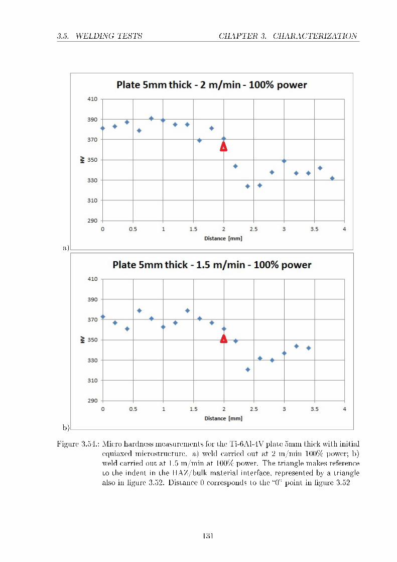
3.5. WELDING TESTS CHAPTER 3. CHARACTERIZATION
a)
b)
Figure 3.54.: Micro hardness measurements for the Ti-6Al-4V plate 5mm thick with initialequiaxed microstructure. a) weld carried out at 2 m/min 100% power; b)weld carried out at 1.5 m/min at 100% power. The triangle makes referenceto the indent in the HAZ/bulk material interface, represented by a trianglealso in gure 3.52. Distance 0 corresponds to the 0 point in gure 3.52
131

3.5. WELDING TESTS CHAPTER 3. CHARACTERIZATION
Figure 3.55.: Micro hardness measurements of the Ti-6Al-4V plate 2 mm thick with initialequiaxed microstructure. 2 m/min 60% power. The triangle makes referenceto the indent in the HAZ/bulk material interface, represented by a trianglealso in gure 3.53. Distance 0 corresponds to the 0 point in gure 3.53
132

3.5. WELDING TESTS CHAPTER 3. CHARACTERIZATION
a) b)
c)
Figure 3.56.: High magnication BEI micrographs of the microstructure developed in thefusion zone of the Ti-6Al-4V plates with equiaxed microstructure welded.a) 5 mm thick plate welded at 2 m/min, 100% power; b) 5 mm thick platewelded at 1.5 m/min, 100% power; c) 2 mm thick plate welded at 2 m/min60% power
133

3.5. WELDING TESTS CHAPTER 3. CHARACTERIZATION
gure 3.52 and 3.53 are reported (micrographs in gure 3.57, 3.58 and 3.59) and analysed.
Looking at the micrographs it is possible to observe the original beta particles (e.g.
white small spots in gure 3.57-f) dissolving gradually going toward the fusion zone and
being still visible at points where already new beta grains are nucleated and very close
to the liquid interface (e.g. gure 3.57-b) . This shows how Vanadium, which segregates
to the beta precipitates diuses through the matrix slower than Aluminium and, non
coincidentally, this element is considered the controlling diusing element in the numer-
ical model. Also, some residual local segregation related to the parent equiaxed alpha
precipitates are still noticeable where martensite is already present (e.g. gure 3.57-c),
indicating that even if the overall tendency of the crystallographic structure of the mater-
ial is to switch from HCP to BCC, the diusing elements are limited in their movement
speed by the diusion process.
Comparing gures 3.58 c) and a) it is possible to observe that going progressively
toward the centre of the weld pool, the beta grains become larger presumably as the
maximum temperature reached during the welding is higher (section 3.5.1). The length
of the transformed beta needles also increases as the beta grains grow.
In the graphs of gure 3.60, 3.61 and 3.62 the thickness of the lamellae and the radius of
the spherical alpha precipitates are reported as a function of the distance from the centre
of the weld pool. Going progressively toward the centre of the weld pool, the original
equiaxed microstructure evolves progressively, giving rise to the lamellar microstructure
originating from the beta phase. The thickness of the lamellae nucleated increases toward
the centre of the weld pool (e.g. in gure 3.60 from 1.8 to 0 mm), probably due to
the increasing size of the beta grains where they nucleate, associated with the higher
temperature at which the material is subjected.
As observed previously, the lamellae thickness of the 5 mm thick plate welded at 1.5
m/min is similar to the lamellae thickness developed in the 2 mm plate welded at 2.0
m/min, this resulted, as shown in gure 3.54-b and 3.55, in a similar hardness measure-
ment to that in the fusion zone.
134

3.5. WELDING TESTS CHAPTER 3. CHARACTERIZATION
a) b)
c) d)
e) f)
Figure 3.57.: BEI micrographs obtained observing the Ti-6Al-4V plate 5mm thick withinitial equiaxed microstructure welded at 2 m/min 100% power. Makingreference to the row of indentations of gure 3.52-a and considering as 1st
point the rst indent starting from the centre of the weld pool: a) 1st point,b) 6th point, c) 8th point, d) 9th point, e) 11th point, f) 13th point
135

3.5. WELDING TESTS CHAPTER 3. CHARACTERIZATION
a) b)
c) d)
e) f)
Figure 3.58.: BEI micrographs obtained observing the Ti-6Al-4V plate 5mm thick withinitial equiaxed microstructure welded at 1.5 m/min 100% power. Makingreference to the row of indentations of gure 3.52-b and considering as 1st
point the rst indent starting from the centre of the weld pool: a) 1st point,b) 6th point, c) 8th point, d) 10th point, e) 12th point, f) 15th point
136

3.5. WELDING TESTS CHAPTER 3. CHARACTERIZATION
a) b)
c) d)
Figure 3.59.: BEI micrographs obtained observing the Ti-6Al-4V plate 2mm thick withinitial equiaxed microstructure welded at 2.0 m/min 60% power. Makingreference to the row of indentations of gure 3.53 and considering as 1st
point the rst indent starting from the centre of the weld pool: a) 1st point1, b) 3rd point, c) 5th point, d) 7th point
137

3.5. WELDING TESTS CHAPTER 3. CHARACTERIZATION
a)
b)
Figure 3.60.: Graphs showing a) lamellae thickness and b) spherical alpha radius as a func-tion of the distance in the Ti-6Al-4V plate 5mm thick with initial equiaxedmicrostructure welded at 2.0 m/min and 100% power. The distance makesreference to the ruler reported in the micrographs
138

3.5. WELDING TESTS CHAPTER 3. CHARACTERIZATION
a)
b)
Figure 3.61.: Graphs showing a) lamellae thickness and b) spherical alpha radius as a func-tion of the distance in the Ti-6Al-4V plate 5mm thick with initial equiaxedmicrostructure welded at 1.5 m/min and 100% power. The distance makesreference to the ruler reported in the pictures
139

3.5. WELDING TESTS CHAPTER 3. CHARACTERIZATION
a)
b)
Figure 3.62.: Graphs showing a) lamellae thickness and b) spherical alpha radius as a func-tion of the distance in the Ti-6Al-4V plate 2mm thick with initial equiaxedmicrostructure welded at 2.0 m/min and 60% power. The distance makesreference to the ruler reported in the pictures
140

3.5. WELDING TESTS CHAPTER 3. CHARACTERIZATION
3.5.2.2 Plates with lamellar microstructure
In gure 3.63 the montages corresponding with the welded zones of the plates tested with
an initial lamellar microstructure are shown.
The two tests were dierent only in the plates thickness, since the operative parameters
were kept the same: 2.0 m/min as welding speed and 70% as power.
The resulting weld pool shapes were very similar with a classical hourglass shape.
The observations of the paragraph 3.5.2.1 in relation to the beta columnar morphology
observed in the centre of pictures are still valid for these cases.
The hardness measurements for the samples shown in gure 3.63 are reported in gure
3.64. The starting point at which the measurements begin is again at the centre and is
shown as 0, then go progressively at steps of 0.2 mm farther from the weld line.
As already observed previously, the material is harder in the fusion zone than the
bulk, because of the martensitic microstructure developed. Comparing with the results
obtained in section 3.5.2.2, the hardness values measured in the weld pool are very similar
(∼ 370 HV), whilst in the bulk material there is a dierence, with the plates with equiaxed
microstructure having a higher hardness (330-340 HV) than the material with the lamellar
microstructure (300-310 HV). From these data the chemical composition can be supposed
to have a relatively low impact on the hardness, as where the material melts, releasing
the residual stresses induced by the manufacturing processes, no relevant variation of the
hardness has been measured in all the plates tested even though the chemical compositions
of the plates in section 3.5.2.1 and 3.5.2.2 are dierent. In the bulk material instead,
appreciable dierences in hardness measurement have been encountered, suggesting that
the dierent microstructures give rise to the variation in hardness, together with, probably,
a dierent mechanical response of the two material microstructural morphologies tested.
The two plates shown in gure 3.64 are characterized by approximatively the same
hardness, suggesting their dierence in thickness is within the range that does not cause a
signicant variation in the gradient of temperatures in the specimens during the welding
process, or develop substantially dierent microstructures with a dierent mechanical
141

3.5. WELDING TESTS CHAPTER 3. CHARACTERIZATION
a)
b)
Figure 3.63.: Montages of the Ti-6Al-4V plates 3.75 mm (a) and 3.06 mm (b) thick withinitial lamellar microstructure welded at 2.0 m/min 70% power. The spe-cimens have been characterized by microhardness. The 0 point shows therst hardness measurement referenced in gure 3.64 and corresponds to theweld centreline
142

3.5. WELDING TESTS CHAPTER 3. CHARACTERIZATION
response. As it is shown in the high magnication BEI images reported in gure 3.65, the
microstructure is very similar at the centre of the fusion zone.
The hardness similarity of the parent material in the two plates, where the weld heat
source did not aect the material, is explained by the fact that the samples were machined
from the same plate, thus have the same initial microstructure.
BEI images of the microstructure observed after welding, for some of the points shown
in gure 3.63, are reported in gure 3.66 and gure 3.67 and hereinafter analysed.
Starting from the furthest locations from the application of the heat source, it is possible
to observe the gradual dissolution of the original lamellar microstructure, with the white
beta boundaries thickening and the dark alpha areas thinning. In locations where the
temperature reaches the beta transus and above on subsequent cooling, new lamellae
start to nucleate and grow (gure 3.66-e and 3.67-f) and martensitic needles form (gure
3.66-d and gure 3.67-d).
As already observed in the previous section, the speed of the welding process imposes
insucient time to allow homogenization of the dierent chemical species in the constitu-
ent alpha and beta phases and, in locations where the temperature should be such as to
have only beta phase, it is still possible to observe local segregations, as seen in the whiter
and darker areas in gure 3.66-c and 3.67-c, representing positions very close to the fusion
zone of the weld pool.
In gures 3.68 and 3.70 the alpha lamellae thicknesses measured for both plates are
reported, whilst in gure 3.69 and 3.71 the martensitic needles thickness is shown.
As expected, the lamellae thickness of the original microstructure tends to become
smaller moving toward the higher temperatures present closer to the centre of the weld
pool.
The nucleated lamellae thickness seems to be susceptible to the thickness of the plate,
as the thicker plate returns thicker nucleated lamellae, due probably to the slight slower
heat loss through the specimens (gure 3.50 and 3.51).
The needles thickness seem to be around the same values for both plates as probably
143

3.5. WELDING TESTS CHAPTER 3. CHARACTERIZATION
a)
b)
Figure 3.64.: Micro hardness measurements graphs of the Ti-6Al-4V plate 3.75 mm (a)and 3.06 mm (b) thick. In both cases the welding operative parameterswere set at 2 m/min and 70% power. The triangle makes reference to theindent in the HAZ/bulk material interface, represented by a triangle also inpictures 3.63
144

3.5. WELDING TESTS CHAPTER 3. CHARACTERIZATION
a) b)
Figure 3.65.: High magnication BEI micrographs of the microstructure developed in thefusion zone of the Ti-6Al-4V plates with initial lamellar microstructure wel-ded. a) 3.75 mm thick plate welded at 2 m/min, 70% power; b) 3.06 mmthick plate welded at 2 m/min, 70% power
driven by the same cooling rate.
145

3.5. WELDING TESTS CHAPTER 3. CHARACTERIZATION
a) b)
c) d)
e) f)
Figure 3.66.: BEI micrographs of the Ti-6Al-4V plate 3.75mm thick with initial lamellarmicrostructure welded at 2 m/min 70% power. Making reference to the rowof indentations of gure 3.63-a and considering as 1st point the rst indentstarting from the centre of the weld pool: a) 1st point, b) 3rd point, c) 4th
point, d) 6th point, e) 8th point, f) 10th point
146

3.5. WELDING TESTS CHAPTER 3. CHARACTERIZATION
a) b)
c) d)
e) f)
Figure 3.67.: BEI micrographs of the Ti-6Al-4V plate 3.06mm thick with initial lamellarmicrostructure welded at 2 m/min 70% power. Making reference to the rowof indentations of gure 3.63-b and considering as 1st point the rst indentstarting from the centre of the weld pool: a) 1st point, b) 3rd point, c) 4th
point, d) 6th point, e) 8th point, f) 11th point
147

3.5. WELDING TESTS CHAPTER 3. CHARACTERIZATION
a)
b)
Figure 3.68.: Graphs showing a) the lamellae thickness of the original microstructure andb) the thickness of new lamellae nucleated during welding of the Ti-6Al-4V plate with initial lamellar microstructure 3.75 mm thick welded at 2.0m/min and 70% power. The distance makes reference to the ruler reportedin the pictures
148

3.5. WELDING TESTS CHAPTER 3. CHARACTERIZATION
Figure 3.69.: Graph showing the needles thickness of the martensitic microstructureformed during welding of the Ti-6Al-4V plate with initial lamellar micro-structure 3.75 mm thick welded at 2.0 m/min and 70% power. The distancemakes reference to the ruler reported in the picture
149

3.5. WELDING TESTS CHAPTER 3. CHARACTERIZATION
a)
b)
Figure 3.70.: Graphs showing a) the lamellae thickness of the original microstructure andb) the thickness of new lamellae nucleated during welding of the Ti-6Al-4V plate with initial lamellar microstructure 3.06 mm thick welded at 2.0m/min and 70% power. The distance makes reference to the ruler reportedin the pictures
150

3.5. WELDING TESTS CHAPTER 3. CHARACTERIZATION
Figure 3.71.: Graph showing the needle thickness of the martensitic microstructure formedduring welding of the Ti-6Al-4V plate with initial lamellar microstructure3.06 mm thick welded at 2.0 m/min and 70% power. The distance makesreference to the ruler reported in the picture
151

3.5. WELDING TESTS CHAPTER 3. CHARACTERIZATION
3.5.3 Chemical analysis
Besides being microstructurally investigated at the locations adjacent to the micro hard-
ness indents, the samples were also been microanalysed by X-EDS and the wt% compos-
ition trends of Aluminium and Vanadium plotted as a function of the distance (graphs in
gure 3.72, 3.73 and 3.74).
The main observation from these results is the relatively small variation in composition
of the alpha phase with respect to the beta phase, in particular for Vanadium. This
could be indicative both of a slow diusivity within the alpha precipitates and of a high
diusivity in the beta matrix during heat treatment, in particular in this case, for welding.
Based on these observations, the numerical model will make some simplifying assumptions
for the description of the diusing process.
3.5.3.1 Plates with equiaxed microstructure
In graphs of gure 3.72 and gure 3.73 the chemical composition in term of weight percent
of Aluminium and Vanadium is reported as a function of the distance from the weld line,
for the plates with initial equiaxed microstructure. In both cases, as already mentioned,
it is noticeable the high variation in Vanadium content of the beta phase. Due to the
high speed of the welding process, the chemical composition along the material did not
have time to homogenise and the chemical composition of the phases present in the parent
microstructure was still noticeable after the formation of new morphological features (see
micrographs in gure 3.57-d, 3.58-d, 3.59-d, in particular white segregation related to the
original beta phase distribution), as alpha lamellae or martensitic needles. The appearance
of this phenomenon is identied in the charts by the line reporting local segregation.
3.5.3.2 Plates with lamellar microstructure
In gure 3.74 the chemical compositions in term of weight percent of Aluminium and
Vanadium are reported as a function of the distance from the weld line, for the plates
with initial lamellar microstructure. Also in these cases it is noticeable the high variation
152

3.5. WELDING TESTS CHAPTER 3. CHARACTERIZATION
a)
b)
Figure 3.72.: Graphs showing the wt% of Al and V as a function of the distance from theweldline (gure 3.60 and gure 3.61) for the Ti-6Al-4V plates 5 mm thickwith initial equiaxed microstructure. a) Plate welded at 2.0 m/min and70% power, b) plate welded at 1.5 m/min and 100% power. For some pointsthe errors bars are so small that they are not visible. The orange dottedline indicates where the original microstructure of the material dissolves butit is possible to notice still a local segregation related to the initial phasesdistribution
153

3.5. WELDING TESTS CHAPTER 3. CHARACTERIZATION
Figure 3.73.: Graph showing the wt% of Al and V as a function of the distance from theweldline (gure 3.62), starting from the rst indent in the centre of the weldpool, for the Ti-6Al-4V plate 2 mm thick with initial equiaxed microstruc-ture. The orange dotted line indicates where the original microstructure ofthe material dissolves but it is possible to notice still a local segregationrelated to the initial phases distribution
154

3.5. WELDING TESTS CHAPTER 3. CHARACTERIZATION
in Vanadium content of the beta phase. Due to the high speed of the welding process,
the chemical composition along the material did not have time to homogenise and the
chemical composition of the phases present in the original material was still noticeable
after the formation of new morphological features (see gure 3.66-d, 3.67-d, in particular
white segregation related to the original beta phase distribution), as alpha lamellae or
martensitic needles. The appearing of this phenomenon is identied in the charts by the
line reporting local segregation.
155

3.5. WELDING TESTS CHAPTER 3. CHARACTERIZATION
a)
b)
Figure 3.74.: Graphs showing the wt% of Al and V as a function of the distance from theweldline (gure 3.68 and gure 3.70) for the Ti-6Al-4V plates 3.75 mm a)and 3.06 mm b) thick with initial lamellar microstructure. For some pointsthe errors bars are so small that are not visible. The orange dotted lineindicates where the original microstructure of the material dissolves but itis possible to notice still a local segregation related to the initial phasesdistribution
156

3.6. SUMMARY CHAPTER 3. CHARACTERIZATION
3.5.4 Deformation measurement
Deection measurement of the plates with initial lamellar morphology were carried out
before and after welding, by a laser scanner Keyence LJ V7080.
The deformations are shown in the graphs of gure 3.75 and they are relative to the lon-
gitudinal centre line of the plates on their bottom side (the opposite side to the application
of the heat source).
The central spikes in the measurements after welding are due to the Ti-6Al-4V melting
and solidifying in the bottom part of the weld pool (gure 3.63).
The maximum deformation registered in both cases corresponds with the weld trajectory
(not considering the spikes) and they are about 0.22 mm for the plate 3.75 mm thick and
0.14 mm for the plate 3.06 mm thick.
The results obtained by these measurements were meant to validate the numerical pre-
dictions of a welding simulation in case the mechanical model described in section 4.7
would have been successfully implemented in the commercial software Visual-Weld.
3.6 Summary
In conclusion, the main results observed in the experiments described previously in this
chapter are listed below.
3.6.1 Heating rate
Alpha particles dissolution The alpha particles dissolve, during heating, as the heat
treatment becomes faster, has no time to occur completely because it is limited by the
speed of the diusion process. As a consequence, the chemical eld coupled to the distribu-
tion of the alpha and beta phases does not have time to reach the equilibrium conditions.
Using BEI analysis, in samples tested at sucient high temperatures, it is possible to
see the inhomogeneous chemical distribution above mentioned, resulting in ghost shapes,
memory of the parent microstructure, containing martensite. This indicates that before
157

3.6. SUMMARY CHAPTER 3. CHARACTERIZATION
a)
b)
Figure 3.75.: Deformation of the Ti-6Al-4V plates with initial lamellar morphology, be-fore and after welding. The deformation shown is relative to the longitudinalcentre line of the plates in their bottom side. The graph a) shows the deform-ation of the plate 3.75 mm thick, whilst the graph b) shows the deformationof the plate 3.06 mm thick
158

3.6. SUMMARY CHAPTER 3. CHARACTERIZATION
the water quenching, the material transformed from HCP to BCC thus, even if the chem-
ical diusion process does not have time to dissolve entirely the parent alpha precipitates,
transforming from HCP to BCC occurs as soon as the thermodynamic conditions allow
the transformation. In case of fast heat treatments, precipitate dissolution modelling that
assumes disappearing of the alpha phase only when the particle dimension becomes null
would make wrong predictions.
Experimental measurement of the volume fraction of the alpha and martensitic phase,
for fast heat treatments, results particularly dicult, for the overlapping of ghost shapes
above mentioned and martensitic needles. In this work, when martensite was observed,
alpha phase was considered to be completely disappeared.
Beta grain growth The nucleation temperature of beta grains shows a shift toward
higher values as the heating rate becomes faster, as expected from the literature. Moreover,
between nucleation temperature of beta grains and beta transus temperature, there is a
gap in temperature that seems to increase with the heating rate.
At high temperatures (>1100 °C) beta grain growth shows an asymptotic trend toward
constant values. This can be explained by mechanical impingement of highly misoriented
beta grains, that requires longer times and/or higher temperatures to let grains merge
together.
Beta transus temperature The equilibrium beta transus temperature for the material
tested can be located around 973±3 °C, with the considerations above mentioned for fast
heating rates.
3.6.2 Cooling rate
The experiments carried out suggest that continuous cooling from above the beta transus
temperature to ambient temperature has a relatively small eect on the lamellae growth,
compared to the dimension of the beta grains in which lamellae nucleate.
Even if the amount of data points collected is not very high, the fact that thicker lamellae
159

3.6. SUMMARY CHAPTER 3. CHARACTERIZATION
have been measured for faster cooling rates is a rst indication that the diusion process is
not the main driving factor in these kind of thermal loads. Plotting the lamellae thickness
as a function of the beta grains where they nucleate, makes explicit how a greater beta
grain volume allows grow of thicker lamellae, probably because being more statistically
spaced thus having availability of more solute for their growth.
3.6.3 Welding tests
Observations done for the Gleeble tests are conrmed in welding tests: thicker lamellae
seem to be associated with larger beta grains, thus thicker lamellae were measured closer
to the heat source.
Similar lamellae thickness, in dierent plates, returned similar hardness measurements.
Close to the interface between the bulk material and the heat aected zone a drop in
hardness is registered, probably associated with releasing of the residual stresses in the
parent material caused by the rising of temperature during welding. This increase of
temperature was not high enough to observe appreciable microstructural changes, but
probably was sucient to decrease the dislocation density in this portion of material.
The chemical composition of the beta matrix has a notable variation in Vanadium with
respect to the Aluminium, suggesting that the former element is the controlling factor in
the diusion process for particle growth and dissolution.
The maximum deformation registered for the plates with an initial lamellar morpho-
logy is approximately 0.22 mm and 0.14 mm for the plate 3.75 mm and 3.05 mm thick
respectively.
160

CHAPTER 4
Numerical modelling
4.1 Introduction
In this chapter, the physically and experimentally based models developed to describe the
evolution of the microstructure of Ti-6Al-4V for the temperatures and temperature rates
involved in a welding process are presented. The models described have been coded in
the commercial welding simulation software Visual-Weld and welding simulation results
for some cases are compared with the corresponding experimental data obtained for the
same operating conditions, material and workpiece geometries.
The choice to adopt physically or experimentally based models was driven by the com-
plexity of the phenomena investigated and by the level of understanding reached in liter-
ature to describe them.
A diusion based model has been adopted to describe the microstructure evolution in
the α + β eld, as this approach had already been shown to be successful in forging
applications, even though the thermal loads involved in this kind of process are much
simpler. Also, the numerical implementation of such a model in Visual-Weld, adopting
reasonable simplications, was possible and gave run times close to the currently used
approach in the welding simulation software (section 2.4.2), thus allowing this solution to
be eective for industrial applications.
161

4.2. ALPHA + BETA FIELD CHAPTER 4. NUMERICAL MODELLING
For the description of the microstructure evolution of the material in the beta eld
and molten zone (beta grain nucleation and coarsening) and for cooling from temper-
atures above the beta transus temperature (possible formation of martensite and alpha
lamellae), no physically based reasonable solutions were found in the literature that use
suciently simple models that could be implemented in welding simulations and still
return comparable running times to the conventional approach used in Visual-Weld. Ex-
amples of the complexity and relative approaches to physically describe these phenomena
have been investigated in [95, 96], where surface roughness and melted material uid dy-
namics aect the heat ow, solidication and the beta grains columnar shape. Also, in
the literature there are examples of martensitic transformation modelling that adopt the
phase eld approach [97, 98], but the computational power available nowadays is su-
cient to simulate only a few microns of material volume. Following these considerations,
empirical approaches were used for the beta grain and martensitic modelling based on the
experimental data presented in chapther 3.
4.2 Alpha + Beta eld
The kinetics of the growth and shrinkage of equiaxed and lamellar alpha in the α + β eld
has been modelled using a single element diusion analysis of an isolated particle in an
innite matrix [39], but adapted to a nite matrix case where the system overall solute
concentration is constant [71].
For an innitesimal time step, the two equations describing the solute ux in a particle
are [39, 67]:
1. Field equation
D∇2C =∂C
∂t(4.1)
2. Flux balance
(CP − CI)dR
dt= D
∂C
∂r
∣∣∣∣r=R
(4.2)
162

4.2. ALPHA + BETA FIELD CHAPTER 4. NUMERICAL MODELLING
Where D represents the interdiusion coecient considered independent of composition
for the time dt, C the solute concentration, t the time, R the radius of the particle, CP
the solute concentration in the matrix-particle interface at the particle side and CI the
solute concentration in the matrix-particle interface at the matrix side.
Assuming that the diusion process is driven mainly by a single diusing element that
acts as limiting element, is a simplication that for both Ti-6Al-4V and other alloys, has
been successfully adopted in literature [40, 30, 99]. In the experimental chapter (section
3.5.2) it has already been shown that actually in Ti-6Al-4V, Vanadium is the element
having the most noticeable variation in composition in the matrix during the dissolution
of alpha particles, indicating that this is the element with the highest mass transfer
during the diusing process. This hypothesis was then adopted and further validated by
comparing the numerical prediction of the model presented in the current paragraph with
experimental measurement.
When possible, the exact solutions of the eld equation (eq. 4.1) and ux balance
(eq. 4.2) have been used, otherwise simplied conditions have been applied to get a
solvable analytical solution. In gure 4.1, all the terms of the equations 4.1 and 4.2
are schematised, together with the solute concentration eld assumed for growth (gure
4.1-a) and dissolution (gure 4.1-b) of the diusion driving element. During growth, the
precipitate depletes the matrix immediately ahead of its interface [100, 101], since solute
is needed to increase the particle dimensions. Contrarily, during shrinkage, the precipitate
rejects solute, that moves toward the matrix, resulting in a gradual decrease in the solute
distribution from the particle to the matrix [101].
Assuming incoherent diusion controlled growth, local equilibrium at the interface can
be assumed [94], CI is then considered to be the equilibrium concentration of the matrix
phase. CP is considered as constant and equal to the value at the beginning of the heat
treatment. This last hypothesis implies that a) the diusion coecient in the precip-
itate is small compared to the one in the matrix and/or b) the solute concentration in
the precipitate is independent from the distance from the particle-matrix interface and
163

4.2. ALPHA + BETA FIELD CHAPTER 4. NUMERICAL MODELLING
temperature [101].
Hypothesis a) cannot be fully veried by literature data as the diusivity of Vanadium
in the alpha phase was not found. But it can be considered reasonable if the order of
magnitude of the Vanadium diusivity in alpha Titanium is assumed to be similar to
that for Aluminium reported in [102]. Semiatin et al [40] reported that the diusivity of
Aluminium in the beta phase is similar to that of Vanadium (equations 4.24 and 4.26).
Accepting the previous hypothesis, an approximate comparison of impurity diusion in
the alpha and beta phases can be made. In the alpha phase the impurity diusion goes
from 10−9(µm2/s) to 10−5(µm2/s) passing from 950 K to 1150 K, for the same range
of temperatures in the beta phase the diusivity goes from 6 × 10⁻⁴(µm2/s) to 2.5 ×
10−2(µm2/s). The diusivity in the beta phase seems, in the worst case, at least 3 order
of magnitude faster than in the alpha phase.
Hypothesis b) is supported by the small variation in concentration of Vanadium and
Aluminium measured experimentally in the alpha phase composition reported in section
3.5.2 with respect to that in the beta phase. In this case, the concentrations were measured
at dierent distances from the welding heat source, thus a wide range of temperatures were
involved, and the variation in composition in the alpha phase was very small compared
to the dierence seen in the beta phase.
Thus assuming that the hypotheses mentioned above are valid, the following boundary
conditions can be applied for the solution of equations 4.1 and 4.2:
C(r = R, t) = CI 0 < t ≤ ∞
C(r, t = 0) = CM r ≥ R
C(r =∞, t) = CM 0 ≤ t ≤ ∞
(4.3)
Where CM is the solute concentration in the matrix (gure 4.1).
164

4.2. ALPHA + BETA FIELD CHAPTER 4. NUMERICAL MODELLING
a) b)
Figure 4.1.: Schematic representation of the concentration eld during growth a) andshrinkage b) [39]
4.2.1 Spherical particles
4.2.1.1 Growth
The exact solution of equations 4.1 and 4.2, when applying the boundary conditions in
equation 4.3 and using spherical coordinates, expresses the concentration eld and the
radius variation in time as [40, 39]:
C(r, t)− CM =2λ(CI − CM)
exp(−λ2)− λ(π)1/2erfc(λ)×[
(Dt)1/2
rexp
(− r2
4Dt
)− 1
2(π)
1/2
erfc
(r
2(Dt)1/2
)](4.4)
dR
dt= 2λ2D/R (4.5)
where λ is a function of the supersaturation Ω:
λ2 exp(λ2) [(
exp(−λ2
))−(λπ
1/2erfc (λ))]
=Ω
2(4.6)
erfc(λ) =2√π
ˆ ∞λ
e−t2
dt (4.7)
165

4.2. ALPHA + BETA FIELD CHAPTER 4. NUMERICAL MODELLING
Ω =CM − CICP − CI
(4.8)
Since λ cannot be computed directly, a tting algorithm was used to give λ as a function
of the independent variable Ω. In this work a code has been written in the commercial
software Matlab. Figure 4.2 shows λ for of a range of supersaturation Ω values, from 0 to
1. At Ω = 1 λ tends asymptotically to innity.
Figure 4.2.: Graph showing the parameter λ as a function of Ω of equations 4.6 and 4.8
The solute concentration in the matrix CM is computed taking into consideration the
soft impingement on the far-eld composition, using a mass balance, where the overall
solute concentration of the alloy (C0) is given by the sum of the solute concentration in
the alpha phase (Cα) and in the matrix:
C0 = fαCα + (1− fα)CM (4.9)
From the equation 4.9, the solute concentration in the matrix as a function of the phase
166

4.2. ALPHA + BETA FIELD CHAPTER 4. NUMERICAL MODELLING
fraction of the precipitate (fα) can be expressed:
CM =C0 − fαCα
1− fα(4.10)
In equation 4.10 the precipitate composition (Cα) is considered equal to CP , in agree-
ment with the initial hypothesis, and the phase fraction of the precipitate fα is considered
proportional to its initial value (fα0) multiplied by the cube of the ratio between the cur-
rent radius of the particle and its original dimension (R0) [30]:
fα = fα0
(R
R0
)3
(4.11)
The assumptions involved for the calculation of CM in equation 4.10 neglect the precise
solute concentration in the region adjacent to the precipitate (gure 4.1). This simplic-
ation introduces an acceptable under prediction of the volume fraction of primary alpha
transformed of 0.5− 1.5% [30]. Phase eld calculations [103] support this hypothesis, in
particular for long annealing times.
The interdiusion coecient D, was determined as a function of the composition and
temperature at each delta time dt, using Darken's equation for a binary system [94]:
D = F (XBD∗A +XAD
∗B) (4.12)
This assumption has been made considering the diusion process to be driven by only
one element such as Aluminium or Vanadium diusing in a Titanium matrix, in an ana-
logous way to the growth model. Much recent work in the literature has adopted this
procedure, and has obtained good predictions when compared with experimental results
[40, 30, 71]. In equation 4.12 D∗A and D∗B are the intrinsic diusion coecients of the bin-
ary system of A and B elements, where in case of the current work A can be represented
by Vanadium or Aluminium and B is Titanium.
The term F of the equation 4.12 is the thermodynamic factor, i.e.
167

4.2. ALPHA + BETA FIELD CHAPTER 4. NUMERICAL MODELLING
F =XAXB
ΥT
d2G
dX2(4.13)
where X represents the mole fraction of the element A or B (as in equation 4.12), Υ is
the gas constant, T the temperature in Kelvin and d2GdX2 the second derivative of the Gibbs
free energy (see paragraph 4.2.3).
4.2.1.2 Shrinkage
Since for the physical reasons discussed in [39], the exact solution of equations 4.1 and
4.2 for a dissolving sphere is not possible, a stationary interface(∂R∂t
= 0)is assumed,
as suggested in [39, 104] as being a reasonable approximation. As observed in [101],
the stationary interface approximation can describe the kinetics satisfactorily when the
supersaturation is within 0.3 such that the growth rate is not particularly high. Equations
4.14 and 4.15 describe respectively the concentration eld around the particle and its
shrinkage rate.
C(r, t)− CM = [(CI − CM)R] /r erfc[(r −R) /2 (Dt)
1/2]
(4.14)
dR
dt=
ΩD
4R+
Ω
4
√D
πt(4.15)
All the terms have been already explained previously. The complementary error function
(erfc) has the form of equation 4.7.
4.2.2 Lamellar particles
4.2.2.1 Growth
The lamellar particles growth has been modelled using the solution proposed in [105, 67,
68] for an ellipsoidal shape, whose aspect ratio between minor and major axis remains
constant. In [30] it has been stated that this solution gives better results with respect to a
168

4.2. ALPHA + BETA FIELD CHAPTER 4. NUMERICAL MODELLING
Figure 4.3.: Graph showing the inuence of the lamellar aspect ratio to the volume fractionpredictions for a Ti-6Al-4V alloy with an initial mean lamellae thickness of3.0 μm, subjected to a hypothetical heating rate of 60 °C/s,
semi-innite plate solution, where the growth of the particle seems to be underestimated.
This approach does not consider the initial stage of the growth of lamellar particles,
where usually after nucleation a lengthening phase follows [68] until lamellae mechanically
impinge on themselves. Since nucleation is out of scope for this model, the assumption
of a constant aspect ratio is assumed to be reasonable for the description of growth and
shrinkage in the α + β eld.
Nucleation and lengthening could be considered using a further analytical model as in
[72] or an experimental/phenomenological approach could be used.
Moreover the experimental measurements (gure 3.26) show that the aspect ratio change
are relatively small as the lamellae thinning occurs. Consequently a sensitivity analysis of
the numerical model to this variation was conducted, conrming that the changes involved
have little appreciable eect on the nal predictions (gure 4.3).
The ellipsoidal approach describes the half length of the major (Y) and minor axis (X)
of the ellipsoid representing the lamellar particle by, respectively, the equations 4.16 and
4.17:
169

4.2. ALPHA + BETA FIELD CHAPTER 4. NUMERICAL MODELLING
Figure 4.4.: Graph showing delta (δ) as a function of omega (Ω) and aspect ratio gamma(Γ ) of equation 4.18
Y = 2Γ (δDt)1/2 (4.16)
X = 2 (δDt)1/2 (4.17)
Where Γ is the aspect ratio given by Y/X.
The dimensionless growth rate parameter δ is determined from equation 4.18, where Ω
is the supersaturation (equation 4.8).
Ω = exp δ[δ3/2Γ 2
]ˆ u=∞
u=δ
exp (−u) du
δ (Γ 2 − 1) + uu1/2(4.18)
The solution of equation 4.18 has been computed using the commercial software package
Matlab to obtain δ (Ω) and its behaviour is shown in gure 4.4.
The volume of the ellipsoid, considering equations 4.16 and 4.17 is then determined
from equation 4.19.
170

4.2. ALPHA + BETA FIELD CHAPTER 4. NUMERICAL MODELLING
dVedt
= 8πΓ 2δDX (4.19)
4.2.2.2 Shrinkage
To model the thinning of lamellar particles, the calculations have been based on diusional
shrinkage of a semi-innite plane [39]. The exact solution of the concentration eld is
represented in equation 4.20 whilst the thickness of the plate is described by equation
4.21, where λ1 and λ are described by the equations 4.22 and 4.23.
C (x, t)− CM = (CI − CM)erfc
[(x− S0) /2 (Dt)
1/2]
erfc (−λ)(4.20)
S = S0 − λ1 (Dt)1/2 (4.21)
λ1 = λ/2 (4.22)
(π)1/2 λeλ
2
erfc (−λ) = Ω/2 (4.23)
4.2.3 Input data
The intrinsic diusion coecients have been expressed as Arrhenius equations [40]:
DβV (µm2/s) = 105 exp(−17460/T (K)) (4.24)
DβT i(µm
2/s) = 2x10⁴ exp(−15000/T (K)) (4.25)
DβAl(µm
2/s) = 1.2x10⁵ exp(−18040/T (K)) (4.26)
171

4.2. ALPHA + BETA FIELD CHAPTER 4. NUMERICAL MODELLING
Where β means that the diusivity of the elements is considered in the beta Titanium
matrix.
For the calculation of d2GdX2 , the Gibbs free energy formulation in a beta matrix for a
Ti-Al-V ternary system has been used (eq. 4.27) [106]. The Gibbs free energy total
contribution is represented by the sum of the Gibbs free energy of a mechanical mixture
of the constituents of the phase (eq. 4.28), the entropy of mixing for an ideal solution (eq.
4.29) and the excess term (eq. 4.30) [107] :
Gβ = G0 +Gideal +Gxs (4.27)
G0 = XAlG0BCCAl +XT iG0BCCTi +XVG0BCCV (4.28)
Gideal = ΥT (XAl lnXAl +XT i lnXT i +XV lnXV ) (4.29)
Gxs = XAlXT i (−125485 + 36.8394T )+XAlXV [(−95000 + 20T ) + (−6000) (XAl −XV )]
+XTiXV
[(10500− 1.5T ) + 2000 (XT i −XV ) + 1000(XT i −XV )2
]+XAlXT iXV [XAl (116976.3− 9.067T ) +XT i (−175169 + 59T ) +XV (31107.3− 42.316T )]
(4.30)
Where Xx is the mole fraction of the element x at the temperature considered, G0BCCx
is the Gibbs free energy of the pure element x [108], T is the temperature in Kelvin. With
only considering a ternary system, the eect of other elements in the actual alloy, on the
Gibbs free energy, like O, Fe, C, etc., has not been considered and consequently their mole
fraction contribution, as predicted by Thermocalc®, was added to the Ti mol fraction,
to get the unity sum of the Ti, Al and V mol fractions. This simplication, for the case
under examination, was considered suciently precise as the errors in the prediction of the
172

4.2. ALPHA + BETA FIELD CHAPTER 4. NUMERICAL MODELLING
Figure 4.5.: Gibbs free energy calculated both by a simplied equation for a Ti-Al-Vternary system and using the actual composition by the Thermocalc database
actual Gibbs free energy were within 2%. These were compensated by the simplication
of the model and shorter running times when compared with the use of an interface with
Thermocalc® to get the actual Gibbs free energy values. Figure 4.5 shows a comparison
of the Gibbs free energy obtained using both the simplied ternary system solution and
the actual alloy composition from Thermocalc®, both referred to the beta matrix (BCC
structure). Furthermore, the small sensitivity noticed of the diusion growth model to
the variation of the thermodynamic factor (equation 4.13) justify the adoption of this
approach: when going from F = 2 to F = 4 the variation in the nal phase proportion
predicted is less than 3%.
All the considerations for the calculation of the interdiusion coecient D were con-
sidered valid for all the models presented in this work.
Even though the current model is thought to work only in the α+ β eld, the fast heat
cycles experienced in welding could bring the alpha precipitates to liquation temperatures.
Also, the transformation to liquid of the alpha precipitate and its local precipitate-matrix
interface, is assumed to occur suddenly [109]. To check if the material has reached the
173

4.2. ALPHA + BETA FIELD CHAPTER 4. NUMERICAL MODELLING
melting temperature in these regions, the Gibbs free energy equations for alpha (equations
4.31, 4.32, 4.33 and 4.34) and liquid (equations 4.35, 4.36, 4.37 and 4.38) are used [106,
110].
Gα = G0 +Gideal +Gxs (4.31)
G0 = XAlG0HCPAl +XT iG0HCPTi +XVG0HCPV (4.32)
Gideal = ΥT (XAl lnXAl +XT i lnXT i +XV lnXV ) (4.33)
Gxs = XAlXT i [(−123789 + 33.209T ) + (16034.9− 12.1827T ) (XAl −XT i)] +
XAlXV [(−95000 + 20T ) + (−6000) (XAl −XV )] +XT iXV [16500] +
XAlXT iXV [XAl (109690.9− 97.06T ) +XT i (−81024 + 38.06T ) +XV (104295.8− 96.27T )]
(4.34)
Gliq = G0 +Gideal +Gxs (4.35)
G0 = XAlG0liqAl +XT iG0liqT i +XVG0liqV (4.36)
Gideal = ΥT (XAl lnXAl +XT i lnXT i +XV lnXV ) (4.37)
Gxs = XAlXT i [(−105404 + 36.1159T ) + (7950.8) (XAl −XT i)] +
XAlXV [(−50725 + 9T ) + (−15000 + 8T ) (XAl −XV )]+XT iXV [(1400) + 4100 (XT i −XV )]
+XAlXT iXV [XAl (−11000) +XT i (−15000) +XV (−10000)] (4.38)
174

4.2. ALPHA + BETA FIELD CHAPTER 4. NUMERICAL MODELLING
4.2.4 Results and discussion
The models presented previously, for spherical and lamellar particles, are adopted de-
pending on the type of particle already existing in the microstructure under examination.
No nucleation/formation of new particles is considered. The sign of the supersaturation
determines if growth (positive sign) or shrinkage (negative sign) occurs.
Spherical and lamellar particles are treated as isolated with an independent supersat-
uration [30] if both are present in the material.
4.2.4.1 Interdiusion coecient
The intrinsic diusion coecients reported in equations 4.24, 4.25 and 4.26 are corrected
by the thermodynamic factor (eq. 4.13). The resulting interdiusion coecient is depend-
ent on the temperature and concentration of the beta matrix at the precipitate/matrix
interface, it is then not possible to get a unique value for a specic temperature. An
example of the magnitude of the intrinsic diusion and interdiusion coecients, for an
hypothetical heat treatment consisting of cooling down the material at 11C/min starting
from 955C is reported in gure 4.6. In this case, the eect of the concentration of the
elements on the diusivity is very important for the Aluminium whose value is almost
tripled for high temperatures, whilst the Vanadium one is a little reduced.
175

4.2. ALPHA + BETA FIELD CHAPTER 4. NUMERICAL MODELLING
Figure 4.6.: Ti-6Al-4V intrinsic diusion coecients for Vanadium, Aluminium and Ti-tanium and interdiusion coecients considering either Al as diusing ele-ment (Al interdiusion) or Vanadium (V interdiusion)
4.2.4.2 Spherical precipitates growth
Existing data from literatur [40, 30] for the study of the spherical particle growth was
used to validate the model. This allowed the experimental characterization carried out
in this project to instead focus on the study of the lamellar microstructure for which no
literature data was available.
The material conditions measured at the beginning of the heat treatments were used as
initial conditions for the numerical model: initial average radius of the spherical particles
4.5 µm, initial phase fraction of spherical particles 0.27, material composition (in weight
percent) of 6.4 Aluminium, 4.2 Vanadium, 0.14 Iron, 0.19 Oxygen, 0.016 Carbon, 0.004
Hydrogen, 0.005 Nitrogen and the balance Titanium. The alpha phase fraction of 0.27
was obtained by soaking the material at 955C for 1 hour then water quenching it.
The heat treatments tested consisted of cooling at 3 dierent cooling rates (11, 42 and
194 C/min) starting from a soaking temperature of 955C after a 20min hold.
176

4.2. ALPHA + BETA FIELD CHAPTER 4. NUMERICAL MODELLING
The CP value in equation 4.8 has been set as the equilibrium concentration of the
diusing element in the alpha phase, at the starting temperature of the heat treatment,
and it was kept constant during the heat treatment (see section 3.6). This assumption
gives negative values of the supersaturation for the rst stage of the heat treatments (gure
4.8, 4.9 and 4.10) because the initial α phase fraction (0.27) is higher than the equilibrium
value for 955C and, consequently, the particle tends initially to reduce its dimension. The
initial soaking of 20min before the heat treatments (the authors of the work in [40] sustain
it is equivalent to one of 60 min from the eects on the microstructure) is probably not
enough to obtain the equilibrium microstructure at 955C. A composition of the particle
(CP ) corresponding to the equilibrium value at about 900C would not give the initial
shrinkage but, since [40] does not report the actual initial value of CP , the original solution
presented has been preferred. A comparison with a hypothetical model where negative
supersaturation values give just null shrinkage has been made. In this manner the impact
of the dierent particle dimensions and relative solute concentrations has been evaluated
on the nal phase fraction predicted. In gure 4.7 this solution is compared with the
model describing both growth and shrinkage, considering either Al or V as the diusing
element. Since after a dierent initial evolution, the phase fraction predicted is the same
for both cases, the relative small variation in solute concentration, and relative possible
resulting initial shrinkage at the rst stage of the heat treatment is considered as not
having a big impact on the predictions and model validation.
In gure 4.8, 4.9 and 4.10, the eect of dierent cooling rates (11C/min, 42C/min,
194C/min) on the kinetics of growth has been investigated, starting from a peak temper-
ature of 955C and considering either Vanadium or Aluminium as the diusing element.
The numerical model, when compared with experimental results, describes the phase frac-
tion evolution well, in particular for Vanadium as the diusing element. The past work
in [111] and the experimental tests presented in chapter 3 conrm that Vanadium is the
limiting element in diusion driven processes in Ti-6Al-4V.
The eect of the estimation of a dierent initial diameter of the particle size (±0.5µm)
177

4.2. ALPHA + BETA FIELD CHAPTER 4. NUMERICAL MODELLING
on the alpha phase proportion kinetic is represented in gure 4.11, for the case of a cooling
rate of 11C/min and Vanadium as the diusing element. Such small variations in the
particle size are plausible both for microstructural variations within the material [27]
and instrument/measurement tolerance, but their impact on the growth kinetics seems
modest: for the case considered, a variation of ±12% on the diameter of the particle
returns a variation on the alpha phase growth of ±3%.
An interesting observation, is the smaller growth rate shown when Aluminium is con-
sidered to be the diusing element instead of Vanadium, even though its interdifusion
coecient is higher (gure 4.6). This is due to the smaller supersaturation related to
Aluminium, since it has a lower dierence in concentration between the alpha and beta
phases than Vanadium (gure 3.72 and 3.73), this in turn, is related exponentially to the
growth rate of the particle by the λ term (equation 4.5) (g. 4.12 and 4.13).
Figure 4.14 shows an example of the trend in the matrix of the Vanadium concentration
during particle growth, for the case of cooling down from 955C at 42C/min. The Va-
nadium concentration of the alpha precipitate is xed at 0.0129, the element equilibrium
concentration in alpha phase at 955 °C. The dierence of concentration acts as the driving
force to let the particle grow, after a short time where it shrinks, since the Vanadium con-
centration in the matrix is higher than in the precipitate. These trends are in agreement
with the experimental data reported in gures 3.60, 3.61, 3.62, 3.72 and 3.73 relative
to the equiaxed microstructure: as the precipitate grows the Vanadium concentration in
the matrix tends to increase since the alpha phase fraction, rich in Aluminium, increases
leaving less volume to the Vanadium.
In gures 4.15, 4.16 and 4.17 some meaningful timings relevant to welding from gure
4.14 are shown. After an initial shrinkage, at the 17th second the particle grows since the
Vanadium concentration in the matrix is higher than in the precipitate.
178

4.2. ALPHA + BETA FIELD CHAPTER 4. NUMERICAL MODELLING
Figure 4.7.: Comparison of the equiaxed particle growth results obtained with or withoutshrinkage, and with diusion controlled by either Al or V. Cooling from 955Cat cooling rate of 11C/min. Equiaxed microstructure
179

4.2. ALPHA + BETA FIELD CHAPTER 4. NUMERICAL MODELLING
Figure 4.8.: Comparison between numerical (Al vs V diusing elements) and experimentaldata [40] for a heat treatment consisting of a cooling at 11C/min start-ing from 955C. Equiaxed microstructure with initial spherical particle size4.5 µm
180

4.2. ALPHA + BETA FIELD CHAPTER 4. NUMERICAL MODELLING
Figure 4.9.: Comparison between numerical (Al vs V diusing elements) and experimentaldata [40] for a heat treatment consisting of a cooling at 11C/min start-ing from 955C. Equiaxed microstructure with initial spherical particle size4.5 µm
181

4.2. ALPHA + BETA FIELD CHAPTER 4. NUMERICAL MODELLING
Figure 4.10.: Comparison between numerical (Al vs V diusing elements) and experi-mental data [40] for a heat treatment consisting of a cooling at 11C/minstarting from 955C. Equiaxed microstructure with initial spherical particlesize 4.5 µm
182

4.2. ALPHA + BETA FIELD CHAPTER 4. NUMERICAL MODELLING
Figure 4.11.: Comparison between the dierent growth kinetics of an equiaxed micro-structure resulting from an initial dierent spherical particle size. Soakingtemperature 955C then cooling at 11C/min. Vanadium considered asdiusing element
Figure 4.12.: Lambda as a function of temperature considering Aluminium as the dius-ing element. Heat treatment consisting of a cooling at 11C/min startingfrom a soaking temperature of 955C. Equiaxed microstructure with initialspherical particle size 4.5 µm
183

4.2. ALPHA + BETA FIELD CHAPTER 4. NUMERICAL MODELLING
Figure 4.13.: Lambda as a function of temperature considering Vanadium as diusing ele-ment. Heat treatment consisting of a cooling at 11C/min starting from asoaking temperature of 955C. Equiaxed microstructure with initial spher-ical particle size 4.5 µm
Figure 4.14.: Matrix Vanadium concentration for the growth of spherical alpha precipit-ate as a function of the time and distance from the particle interface (ini-tial particle radius 4.5 µm) for the heat treatment consisting of cooling at42C/min starting from 955 C (case of gure 4.9)
184

4.2. ALPHA + BETA FIELD CHAPTER 4. NUMERICAL MODELLING
a)
b)
Figure 4.15.: Vanadium concentration in the matrix as a function of the distance from theprecipitate interface at 1 and 13 seconds (gure a and gure b respectively)from the beginning of the heat treatment reported in gure 4.14, corres-ponding respectively to 954 °C and 945.9 °C
185

4.2. ALPHA + BETA FIELD CHAPTER 4. NUMERICAL MODELLING
a)
b)
Figure 4.16.: Vanadium concentration in the matrix as a function of the distance fromthe precipitate interface at 15 and 17 (gure a and gure b respectively)seconds from the beginning of the heat treatment reported in gure 4.14,corresponding respectively to 944.5 °C and 943 °C. It is possible to noticethe inversion of the Vanadium concentration eld that makes the precipitategrow after an initial dissolution
186

4.2. ALPHA + BETA FIELD CHAPTER 4. NUMERICAL MODELLING
a)
b)
Figure 4.17.: Vanadium concentration in the matrix as a function of the distance fromthe precipitate interface at 100 and 364 (gure a and gure b respectively)seconds from the beginning of the heat treatment reported in gure 4.14,corresponding respectively to 885 °C and 700 °C
187

4.2. ALPHA + BETA FIELD CHAPTER 4. NUMERICAL MODELLING
4.2.4.3 Lamellar precipitates dissolution
For the validation of the numerical model used to describe the evolution of the lamellar
microstructure (see section 4.2.2), the experimental data reported in section 3.4.3 have
been used and for clarity briey listed below:
aspect ratio 7.0
initial lamellae thickness 3.0 µm
initial alpha lamellar phase fraction 0.95
mean Vanadium composition in the lamellar microstructure 2.47%
mean Aluminium composition in the lamellar microstructure 5.495%
overall Vanadium concentration 4.0479% in the material, as per the experimental
measurements.
Since the model that describes the lamellar microstructure evolution showed very low
sensitivity to small variations in the lamellae aspect ratio (gure 4.3), a value of 7 was
assumed to be constant for the entire thermal treatments tested.
For the experimental data reported, only one sample was tested for each thermal condi-
tion. Thus for the volume fraction measurement the standard deviations error bar could
not be computed, whilst for the lamellae thickness, since many particles were measured
in the same specimen, the standard deviation is available.
Figure 4.18 reports the comparison between the numerical model predictions consider-
ing Vanadium as diusing element and the experimental measurements carried out for
samples tested at the heating rate of 5 °C/s. Figures 4.19 and 4.20 report respectively the
comparisons for the heating rate of 50 °C/s and 500 °C/s. As shown, for temperatures
close to the complete dissolution of lamellae, and for fast heating rates, the model would
tend asymptotically to 0 in predicting the alpha lamellae thickness or phase fraction, this
is because of the low supersaturation at this stage of the transformation that slows down
188

4.2. ALPHA + BETA FIELD CHAPTER 4. NUMERICAL MODELLING
the shrinkage rate (section 4.2.2.2) and, for the very short times at fast heating rates, this
results in dissolution happening at still relatively high temperatures. As shown in section
3.4.3, the diusion process at fast heating rates does not allow sucient time to dissolve
completely the alpha phase but, it has also been shown that even though the local segreg-
ation is still visible in the SEM investigation, the switch in crystallographic structure from
HCP to BCC occurs anyway, when the temperature passes the beta transus temperature
of the material composition at the heating rate considered. For this purpose, the dissol-
ution model presented in this section has been integrated with an experimental equation
to predict the beta transus temperature as a function of the temperature rate (shown in
section 4.3), to determine when the alpha phase is completely transformed in beta phase.
This explains the sudden drop to 0 of the lamellae thickness and phase fraction shown in
gure 4.18, 4.19 and 4.20.
189

4.2. ALPHA + BETA FIELD CHAPTER 4. NUMERICAL MODELLING
a)
b)
Figure 4.18.: Lamellar microstructure comparisons between the numerical model consid-ering Vanadium as diusing element and the experimental measurementsat the heating rate of 5 °C/s. a) Lamellae thickness, b) volume fractionlamellar microstructure
190

4.2. ALPHA + BETA FIELD CHAPTER 4. NUMERICAL MODELLING
a)
b)
Figure 4.19.: Lamellar microstructure comparisons between the numerical model consid-ering Vanadium as diusing element and the experimental measurementsat the heating rate of 50 °C/s. a) Lamellae thickness, b) volume fractionlamellar microstructure
191

4.2. ALPHA + BETA FIELD CHAPTER 4. NUMERICAL MODELLING
a)
b)
Figure 4.20.: Lamellar microstructure comparisons between the numerical model consid-ering Vanadium as diusing element and the experimental measurementsat the heating rate of 500 °C/s. a) Lamellae thickness, b) volume fractionlamellar microstructure
192

4.3. BETA GRAIN GROWTH CHAPTER 4. NUMERICAL MODELLING
4.3 Beta grain growth
For the description of the beta phase microstructure evolution above the beta transus,
the phenomenological solution proposed in [73, 66] has been modied. In this approach,
the beta grain dimensions data obtained from isothermal heat treatments are tted to
equation 2.5, reported again below for clarity.
dn − dn0 = A× t× exp(−Q/ΥT ) (4.39)
As written in section 2.3.6.3, this method was also adopted to describe the beta grain
growth in Ti-6Al-4V for constant heating rate heat treatments, using the dierential form
of equation 2.6. Since the work only showed good agreement between experiments and nu-
merical predictions for relatively low temperatures, a correction term to equation 4.39 has
been applied to match the asymptotic trend shown by the grain growth. This correction
factor was introduced for numerical purposes and has no particular physical meaning. The
inverse tangent function was used to provide an asymptotic trend to equation 4.39, that
otherwise would predict exponential behaviours for non constant times and temperatures.
The new equation obtained is shown below:
dn − dn0 = A× t× exp(−Q/(ΥT2)) (4.40)
where
T2 = atan
(−TB
)∗ B
atan(1)(4.41)
Where T 2 represents the correction factor and B a constant to be tted to the experi-
mental data.
The experimental data obtained in this work, shown in gure 3.41, together with some
estimated data points at low and high temperatures (1600 °C) have been used to t the
193

4.3. BETA GRAIN GROWTH CHAPTER 4. NUMERICAL MODELLING
equation parameters B, Q and A in temperature ranges of interest for this work (gure
4.21). The author desires to point out that experimental tests at temperatures higher
than 1250-1300 °C were planned but, for a technical problem at the testing machine,
experiments could not be carried out in time for the end of this project.
Figure 4.21.: Beta grain dimension data used for the calculation of the grain growth equa-tion parameters. They are the same as gure 3.41 with estimated points at1600 °C
The set of parameters obtained tting the equation 4.40 to the data points of gure
4.21 is reported in the table 4.1 and the relative grain growth predictions for the same
heating rates of the experiments shown in gure 4.22.
n A Q M[µmn/s] [J/mol]
8 8.688x10⁹ 203,810 1140
Table 4.1.: Parameters obtained from the current work by tting equation 4.39 to theexperimental results shown in gure 3.41
Since equation 4.40 needs implicitly to know at which temperature beta grains start to
nucleate, the numerical approach presented in [61], based on isochronal conditions applied
194

4.3. BETA GRAIN GROWTH CHAPTER 4. NUMERICAL MODELLING
Figure 4.22.: Comparison between experimental data and numerical model prediction ofthe beta grain growth at dierent heating rates
195

4.3. BETA GRAIN GROWTH CHAPTER 4. NUMERICAL MODELLING
to the JMA equation 4.42 has been used, returning equation 4.44.
f = 1− exp(−ηp) (4.42)
η = kt = k0t exp
(− E
ΥT
)(4.43)
lnT 2βφ
Φ= ln
E
Υk0+
E
ΥTβφ+J
n2
ΥT 2βφ
E(4.44)
With k0 pre exponential factor, E activation energy of the phase transformation con-
sidered, Υ gas constant, T temperature in Kelvin, Φ temperature rate, J constant, p
exponential factor, Tβφ the beta transus temperature at a specic temperature rate φ.
Once equation 4.44 has been tted to the beta transus temperatures at dierent heating
rates for a Ti-6Al-4V alloy of known chemical composition, it is possible to predict the beta
transus temperature at a desired heating rate and, by applying an empirical relationship
with the alpha or beta stabilizer elements in a Ti-6Al-4V alloy, it is possible to predict
the beta transus temperature for the desired chemical composition.
The relationship used to describe the eect of the alloying elements was obtained by
running simulations of Ti-6Al-4V with dierent chemical compositions in the commercial
software JMatPro and quantifying their eect on the beta transus temperature. From
equations 4.45 and 4.46 the equivalent Aluminium and Vanadium content for a specic
alloy are calculated, thereafter multiplying the values obtained by 20 for Aleq and -20 for
V eq the total eect on the variation of the beta transus temperature with respect to the
reference alloy can be calculated (equation 4.47).
Aleq new alloy = Al + 10O + 40N (4.45)
Veq new alloy = V + 66H + 1.25Fe (4.46)
196

4.3. BETA GRAIN GROWTH CHAPTER 4. NUMERICAL MODELLING
∆Tβ = (Aleq reference alloy − Aleq new alloy) 20− (Veq reference alloy − V eq new alloy) 20 (4.47)
4.3.1 Results and discussion
In gure 4.23 the data obtained for the alloy experimentally studied in section 3.4 for
which the beta transus temperatures were known in ranges of heating rates from 5 K/s to
500 K/s is shown. The predictions of the beta transus for heating rates faster than 500
K/s were made by applying equation 4.44, whilst the beta transus temperatures for the
other two representative alloys, one with more alpha stabilisers and one with more beta
stabilisers, were made using equations 4.45, 4.46 and 4.47.
Figure 4.23.: Beta transus temperature predictions as a function of the heating rate andchemical composition
Once the beta transus temperature is known, for the alloy desired, equation 4.40 can be
applied to get predictions on the beta grain growth evolution as a function of the heating
rate, as for example, gure 4.24 shows.
197

4.3. BETA GRAIN GROWTH CHAPTER 4. NUMERICAL MODELLING
Figure 4.24.: Beta grain growth predictions as a function of temperature and heating rates
The predictions of beta grain growth have been done using a phenomenological equation
widely used in literature, for ease of use.
A physically based approach would have been necessary to describe nucleation and
growth competition of the beta grains. As a eld this is still not well developed in the
literature in the form of analytical expressions, requiring more experiments to set the
parameters for the nucleation equations. The fast heating rates involved in welding would
not have allowed model validation as facilities to apply the extreme thermal treatments
to the material are not readily available.
By the approach used in this work, the model can still predict the beta transus temper-
ature as a function of the alloy chemical composition and temperature rate, even if it is
necessary to carry out experiments to set the initial beta grain size for the beta transus
temperature of the alloy considered.
Thus although equation 4.40 is not able to self adapt to dierent alloy chemical compos-
itions, the disadvantages brought from its adoption were considered to be well balanced
by the advantages obtained. Furthermore it has been possible to set a model able to
198

4.4. LAMELLAE NUCLEATION CHAPTER 4. NUMERICAL MODELLING
predict reasonable beta grain growth values for extremely fast heating rates from a small
number of experiments.
4.4 Lamellae nucleation
As mentioned at the beginning of this chapter (section 4.1), the alpha lamellae nucleation
and growth, cooling down from the beta eld, has been described by an experimental
equation (equation 4.48).
Lamellae thickness [µm] = φ×−0.0013 + 0.0787× ln(d) (4.48)
Where φ represents the cooling rate of the heat treatment and d the mean beta grain
size diameter [µm] in which lamellae nucleate and grow.
The parameters of the equation 4.48 were obtained by tting to the experimental data,
adding some estimated points to the ones collected experimentally in this work, to provide
a suciently wide range of beta grain dimensions to let the tting algorithm work properly
(gure 3.28-a vs gure 4.25).
4.4.1 Results and discussion
The trends obtained from the equation 4.48, for cooling rates ranging from 5 °C/s to
300 °C/s are compared with the experimental data in gure 4.25. For faster cooling
rates and the same beta grain dimensions, the lamellae thickness obtained at the end
of the heat treatment is thinner than the one obtained at a slower cooling rate. This
can be related to the shorter time the lamellae have to grow at the faster cooling rates.
Also, for the same cooling rate, the bigger is the beta grain where lamellae nucleate and
grow, then the thicker the lamellae are at the end of the thermal process as, already
discussed and reported in section 3.4.4, a larger beta grain volume allows nucleation of
lamellae statistically more widely spaced and, as result, they hypothetically will impinge
on themselves at a later stage in the diusional growth process.
199

4.4. LAMELLAE NUCLEATION CHAPTER 4. NUMERICAL MODELLING
Figure 4.25.: Graph showing the experimental data compared to the predictions obtainedapplying the equation 4.48
Applying equation 4.48 to a series of beta grain radius, going from 0 to 900 µm, the
lamellae thickness predicted, for cooling rates of 5 °C/s, 100 °C/s and 300 °C/s, are
shown in gure 4.26. Even though this approach is not physically based, the lamellae
trends predicted seem to reect how the real behaviour (section 4.2.2), with a initial
faster lengthening and minimal growth in thickness until mechanically impingement of
the lamellae, than a slower thickening stage follows.
200

4.5. MARTENSITIC MODEL CHAPTER 4. NUMERICAL MODELLING
Figure 4.26.: Lamellae thickness predicted as a function of the cooling rate and beta grainradius
4.5 Martensitic model
The martensitic phase fraction evolution has been described as a function of the cooling
rate by tting an equation to the experimental data collected in section 3.4.4 and shown
in gure 3.32. This model is based on the hypothesis that on cooling the material from
temperatures above beta transus, the beta phase fraction not transformed to alpha phase
is entirely transformed to martensite, as the cooling rates considered are fast enough to
convert the residual beta phase into martensite.
α′vol fraction =
(2.6245− arctan
(dT
dt− 64.9971
))× 20.4014 (4.49)
The comparison between the experimental measurements of the martensitic phase frac-
tion and the numerical predictions from the tting equation 4.49, reported in gure 4.27,
shows a good matching between the two trends.
The coarsening of the martensitic needles has been described by another equation based
201

4.5. MARTENSITIC MODEL CHAPTER 4. NUMERICAL MODELLING
Figure 4.27.: Martensitic phase fraction as a function of cooling rate. Comparison betweenmodel predictions and experimental data
on the experimental data described in section 3.4.4. A logarithmic relationship with
cooling seems to t very well in this case. The results obtained by applying the tting
equation 4.50 compared with the experimental data are shown in gure 4.28.
Needle thickness = 0.0857 ln
(dT
dt
)− 0.1136 (4.50)
202

4.6. WELDING SIMULATIONS CHAPTER 4. NUMERICAL MODELLING
Figure 4.28.: Needle thickness as a function of the cooling rate. Experimental data(points) and interpolating function (green line)
4.5.1 Results and discussion
Since in literature there was no alternative solution to the phase eld approach for the
modelling of the martensitic microstructure evolution, which was considered too complex
to be adopted in this work, where acceptable running times represent an important nal
objective, an experimental approach has been used.
Fitting equations have been coded to model both the martensitic volume fraction and
needles thickness as a function of the cooling rate, obtaining a good match with experi-
mental data. In particular, the martensitic volume fraction is well tted by an arctangent
function with the knee between 50 and 100 °C/s, while the needles thickness is well de-
scribed by a logarithmic function.
4.6 Welding simulations
The numerical microstructure models developed and described previously in this chapter
have been coded in subroutines for the commercial software Visual-Weld, to run welding
203

4.6. WELDING SIMULATIONS CHAPTER 4. NUMERICAL MODELLING
simulations able to predict the microstructural evolution of the material during the joining
process. To validate the predictions of the welding simulations, the results have been
compared with the data obtained from the experimental welding tests described in detail
in section 3.5.
4.6.1 Workpieces and operative conditions
The dierent initial microstructures, chemical compositions of the material and geometries
of the workpieces tested are summarised hereinafter.
Chemical compositions
Plate 1 Equiaxed - Al 5.82, V 4.00, Fe 0.06, H 0.00963, N 0.010, O 0.063, Ti bal
Plate 1 and 2 Lamellar - Al 5.75, V 3.96, Fe 0.07, H 0.00445, N 0.013, O 0.11, Ti
bal
Plates tested geometry
Plate 1 Equiaxed -46.95× 151.5× 2.00mm3
Plate 1 Lamellar - 47.30× 136.965× 3.76mm3
Plate 2 Lamellar - 47.31× 137.05× 3.06mm3
Operative parameters
Plate 1 Equiaxed - 60% power, welding speed 2m/min
Plate 1 amd 2 Lamellar - 70% power, welding speed 2m/min
4.6.2 Thermal material properties
The material thermal properties, used for the numerical simulations, are based on the
mean values of thermal conductivity, specic heat and density obtained from several
literature sources (private communication from prof Jeery Brooks).
Making reference to the beta transus of the dierent materials, the thermal properties
due to phase change have been consequently shifted to coincide with the transition area.
204

4.6. WELDING SIMULATIONS CHAPTER 4. NUMERICAL MODELLING
Figure 4.29.: Graph showing the Ti-6Al-4V thermal conductivity as a function of temper-ature used for the numerical simulations in Visual-Weld
In gures 4.29, 4.30 and 4.31 the thermal conductivity, specic heat and density used
for the numerical simulations are shown, with the dimensions required by Visual-Weld.
In gure 4.30, it is possible to notice how the specic heat corresponding with the
liquidus temperature has been scaled over a wider range of temperatures, keeping constant
the area representing the latent heat of melting, this was needed to get stability of the
numerical simulations and reduce running times.
4.6.3 Model mesh
The mesh used for the welding simulations was made of 201,520 quad linear elements,
with a higher density close to area of the weld pool, to decrease the temperature gradient
along the elements subjected to very high variations of temperature in space and time.
Far from the weld pool, the number of elements along the thickness of the model was kept
to 6, as this value is the limit at which linear elements can correctly represent bending of
thin plates (gure D.6, D.7 and D.8). In gure 4.32 and 4.33 an entire view of the mesh
205
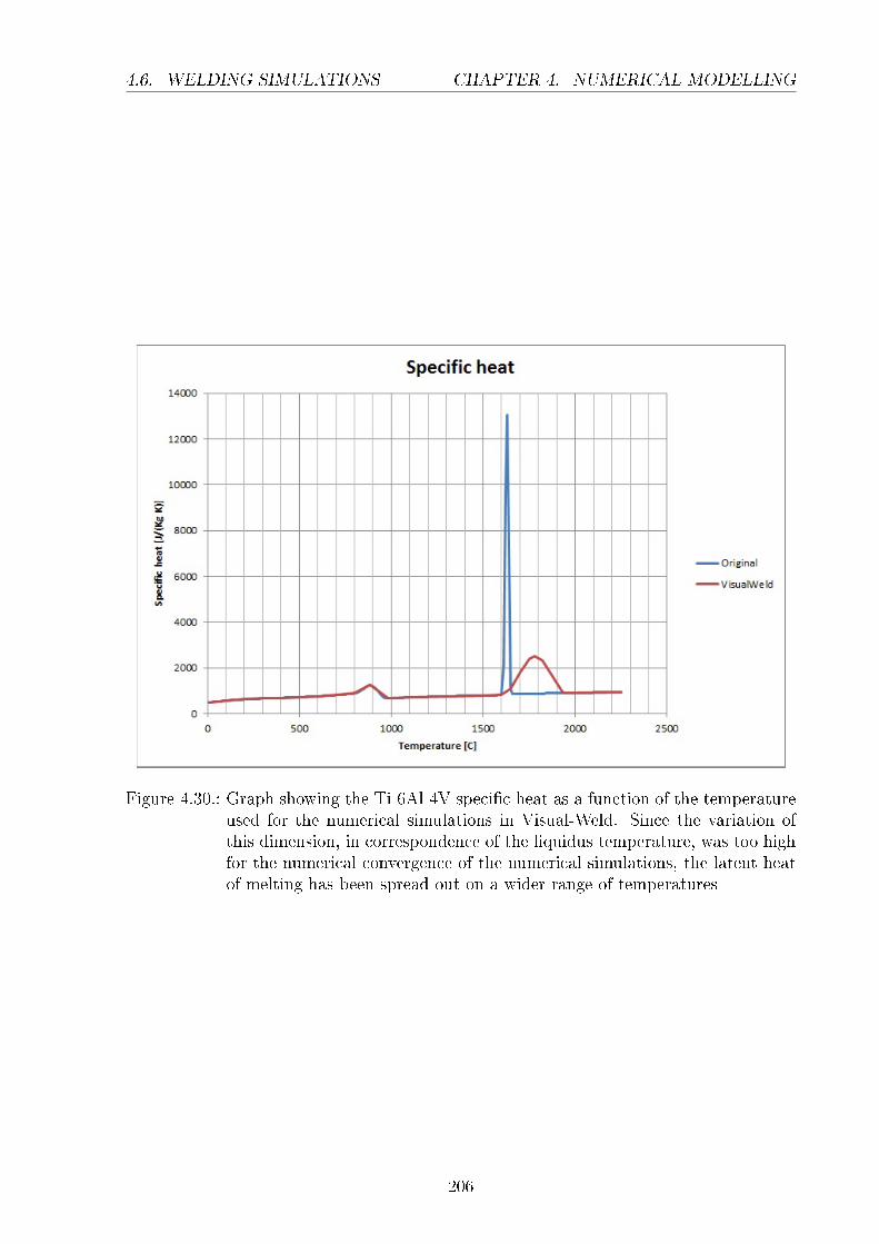
4.6. WELDING SIMULATIONS CHAPTER 4. NUMERICAL MODELLING
Figure 4.30.: Graph showing the Ti-6Al-4V specic heat as a function of the temperatureused for the numerical simulations in Visual-Weld. Since the variation ofthis dimension, in correspondence of the liquidus temperature, was too highfor the numerical convergence of the numerical simulations, the latent heatof melting has been spread out on a wider range of temperatures
206

4.6. WELDING SIMULATIONS CHAPTER 4. NUMERICAL MODELLING
Figure 4.31.: Graph showing the Ti-6Al-4V density as a function of the temperature usedfor the numerical simulations in Visual-Weld
of the model and a zoom close to the weld trajectory are shown respectively.
The mesh used for the welding simulation of the plate with equiaxed microstructure
was less ne in the weld pool area as, for this case, mechanical simulations were not run.
A ner mesh allows a reduction in the stress gradient along each mesh element, caused by
temperature gradient and the variation of the microstructure during the welding process.
4.6.4 Boundary conditions
The plates were clamped only on the left side as they were in the experiments.
All the external surfaces were set as in contact with air at 40 °C, as the temperature
measured at the end of the welding tests. In reality this temperature changes during the
welding tests but, as a simplication, it has been assumed constant.
The convection coecient has been assumed as a function of temperature, as shown in
gure 4.34.
The emissivity has been assumed constant and equal to 0.8.
207

4.6. WELDING SIMULATIONS CHAPTER 4. NUMERICAL MODELLING
Figure 4.32.: Mesh used for the welding simulations in Visual-Weld, made of 201,520 quadlinear elements
Figure 4.33.: Zoom close to the weld trajectory (green line) of the mesh shown in gure4.32. Along the thickness, close to the weld line, 24 elements have been used,passing then progressively to 6 going farther from it
208

4.6. WELDING SIMULATIONS CHAPTER 4. NUMERICAL MODELLING
Figure 4.34.: Convection coecient as a function of the dierence of temperature betweenthe workpiece and ambient temperature assumed at 20 ºC (private commu-nication from prof Jeery Brooks)
209

4.6. WELDING SIMULATIONS CHAPTER 4. NUMERICAL MODELLING
4.6.5 Weld pool shape
As described in the paragraph 2.2.2, by adopting the classical approach of computational
welding mechanics, the determination of the weld pool shape is a fundamental requirement
to get reliable predictions from a welding simulation.
The welding experiments were executed before the numerical simulations, the plates
welded were then sectioned and the weld pool shapes measured, in particular the fusion
zone width as a function of the depth.
The fusion zone dimensions of the numerical models were matched to the real ones, by
adapting the numerical models heat source shapes (paragraph 2.2.3). In particular, in this
work, a specic heat source has been coded [112], since the ones described in paragraph
2.2.3 were not suitable for matching the weld pool geometries measured experimentally.
The heat source was a modied three-dimensional conical heat source (gure 2.3), where
the heat intensity decay, instead of being described by a polynomial function was dened
using tabular data as a function of the weld depth.
To establish the boundaries of the fusion zone in the real case, pictures at high magni-
cations have been checked and, when ghost shapes of the original chemical segregation
disappeared, giving rise to a well dened lamellar/martensitic structure, the material was
considered to have reached the melting temperature (see for example pictures 3.66 b and
c).
4.6.5.1 Equiaxed microstructure
In gure 4.35 a section of the experimental and numerical model, after welding, of the
plate 2 mm thick with equiaxed microstructure, is shown. Temperatures above the melting
temperature are represented by the grey colour, showing the fusion zone of the weld pool.
In gure 4.36 the fusion zones widths of the experimental and numerical case are com-
pared for some some depths. The numerical fusion zone is in overall good agreement with
the experimental one, staying within a tolerance of about 0.1 mm.
210

4.6. WELDING SIMULATIONS CHAPTER 4. NUMERICAL MODELLING
Figure 4.35.: Experimental (top) and numerical (bottom) weld pool fusion zones for theTi-6Al-4V plate with initial equiaxed microstructure 2.00 mm thick, wel-ded with a speed of 2 m/min and 60% power (2.4 kW ). The fusion zoneis bounded in the micrograph by blue lines. In the FE model, the greycolour shows locations where the maximum temperature during the weldingsimulation passed 1650 °C (melting temperature), representing thus the fu-sion zone. In the micrograph, depths and widths used for the tting of thenumerical heat source parameters are shown
211

4.6. WELDING SIMULATIONS CHAPTER 4. NUMERICAL MODELLING
Figure 4.36.: Comparison of the weld pool shape between numerical and experiment res-ults of the Ti-6Al-4V plate 2 mm thick with initial equiaxed microstructure(gure 4.35). Only one half is shown as the shape of the weld pool is assumedto be symmetric
4.6.5.2 Lamellar microstructure
In gure 4.37 and 4.38 a section of the weld pool shape and the fusion zone width meas-
urements as a function of some depth values are shown for the 3.76 mm thick plate with
lamellar microstructure.
In gure 4.39 and 4.40 the ones for the 3.06 mm thick plate are instead shown.
In both cases, the numerical model was considered to describe accurately the shape of
the real weld pool as the boundaries of the model/real case matched within about 0.1
mm.
212

4.6. WELDING SIMULATIONS CHAPTER 4. NUMERICAL MODELLING
Figure 4.37.: Experimental (top) and numerical (bottom) weld pool fusion zones for theTi-6Al-4V plate with lamellar microstructure 3.76 mm thick, welded witha speed of 2 m/min and 70% power (2.8 kW ). The fusion zone is boundedin the micrograph by blue lines. In the FE model, the grey colour showslocations where the maximum temperature during the welding simulationpassed 1650 °C (melting temperature), represents thus the fusion zone. Inthe micrograph, depths and widths used for the tting of the numerical heatsource parameters are shown. At half depth of the weld pool, also the betagrains around the heat aected zone are highlighted
213

4.6. WELDING SIMULATIONS CHAPTER 4. NUMERICAL MODELLING
Figure 4.38.: Comparison of the weld pool shape between numerical and experiment res-ults of the Ti-6Al-4V plate 3.76 mm thick with lamellar microstructure (g-ure 4.37). Only one half is shown as the shape of the weld pool is assumedto be symmetric
214

4.6. WELDING SIMULATIONS CHAPTER 4. NUMERICAL MODELLING
Figure 4.39.: Experimental (top) and numerical (bottom) weld pool fusion zones for theTi-6Al-4V plate with lamellar microstructure 3.06 mm thick, welded witha speed of 2 m/min and 70% power (2.8 kW ). The fusion zone is boundedin the micrograph by blue lines. In the FE model, the grey colour showslocations where the maximum temperature during the welding simulationpassed 1650 °C (melting temperature), and represents the fusion zone of thenumerical model. In the micrograph (top), depths and widths used for thetting of the numerical heat source parameters are shown. At half depthof the weld pool, also the beta grains around the heat aected zone arehighlighted
215

4.6. WELDING SIMULATIONS CHAPTER 4. NUMERICAL MODELLING
Figure 4.40.: Comparison of the weld pool shape between numerical and experiment res-ults of the Ti-6Al-4V plate 3.06 mm thick with lamellar microstructure (g-ure 4.39). Only one half is shown as the shape of the weld pool is assumedto be symmetric
4.6.6 Implementation in Visual-Weld
The implementation in the commercial software Visual-Weld of the microstructural nu-
merical models presented in sections 4.2, 4.3, 4.4 and 4.5 is shown schematically in the
chart of gure 4.41, in which it is possible to see also the ow of the algorithm. The
diusion based model represented by the block Diusion based model lamellae/equiaxed
microstructure in gure 4.41 is then described more in detail by the ow chart shown in
gure 4.42.
The algorithm is solved each time step of the welding simulation, for each integration
point of the mesh.
As outputs, visible in the post processor, the following variables are saved for each
time step and integration point: equiaxed alpha phase, lamellar alpha phase, beta phase,
216

4.6. WELDING SIMULATIONS CHAPTER 4. NUMERICAL MODELLING
martensitic phases, equiaxed alpha mean radius, lamellar alpha thickness, needle thickness
and beta grain radius.
Figure 4.41.: Comprehensive numerical model ow chart for the description of the micro-structure evolution in welding simulations
217

4.6. WELDING SIMULATIONS CHAPTER 4. NUMERICAL MODELLING
Figure 4.42.: Diusion based model ow chart for the description of the alpha particlegrowth/shrinkage
218

4.6. WELDING SIMULATIONS CHAPTER 4. NUMERICAL MODELLING
4.6.7 Thermal comparison with experiments
In this section the temperature comparison between experiments and numerical predic-
tions, at dierent distances from the weld lines of the welding tests conducted on the
plates tested, is shown.
The temperatures measured in the numerical simulations were relatively sensitive to
the thermal properties adopted to model the material behaviour and, in a smaller part,
also to the temperature surrounding the workpieces and the convective coecient. Due
to time limitations, it was not possible in this work to investigate in detail the variations
of each of these factors, thus the xed values described in section 4.6.2 and 4.6.4 were
assumed.
4.6.7.1 Equiaxed microstructure
In gure 4.43 the temperature comparison between experiments and numerical predic-
tions, at dierent distances from the weld lines of the welding tests conducted on plates
with initial equiaxed microstructures, is shown.
The temperatures reported for the numerical model make reference approximatively
to the same positions where the thermocouples used for the experiments were located,
compatible with the locations of the mesh nodes of the numerical model. The depth of
the holes where the thermocouples were inserted was 1.5 mm, since the closest nodes of
the mesh at this distance were at 1.4 mm and 1.6 mm, the rst depth was used.
A good match with of the numerical results to the experimental ones was obtained,
in particular for the closest distances to the weld line, where the temperatures are high
enough to aect the material microstructure in the typical timings involved during weld-
ing.
The dierence of temperature between experimental and numerical results, measured at
20 mm far from the weld line, can be explained by the higher impact that the convection
coecient has at lower temperature. To verify this hypothesis, further measurements
and investigation on the variation of the heat ow dispersion during the cooling stage of
219

4.6. WELDING SIMULATIONS CHAPTER 4. NUMERICAL MODELLING
welding, should be carried out.
Considering the complexity of the problem to be modelled, the relatively good match
with the temperatures between numerical models and experimental ones conrms the
adoption of reasonable boundary conditions and material properties.
4.6.7.2 Lamellar microstructure
In gure 4.44 and 4.45 the temperature comparisons between experiments and numerical
predictions, at dierent distances from the weld lines of the welding tests conducted on
plates with initial lamellar microstructures, are shown.
The temperatures reported for the numerical model make reference approximatively
to the same positions where the thermocouples used for the experiments were located,
compatible with the locations of the mesh nodes of the numerical model. The depth of
the holes where the thermocouples were inserted was 2.5 mm, since the closest nodes of
the mesh at this distance were at 2.55 mm and 2.42 mm, the rst depth was used.
In both cases a good match with the numerical results to the experimental ones was
obtained, in particular for the closest distances to the weld line, where the temperatures
are high enough to aect the material microstructure in the typical timings involved
during welding.
The slightly lower temperatures measured in the numerical model with respect to the
ones measured experimentally, can be explained both by the higher thermal dissipation
given by the thermocouples wires with respect to the numerical model where they are
not present, and to the higher thermal inertia given by the ceramic insulation used in the
sensors to isolate the anode, cathode and sleeve from each other.
As for the equiaxed microstructure case, considering the complexity of the problem to be
modelled, the relatively good matching of the temperatures between numerical models and
experimental ones conrm the adoption of reasonable boundary conditions and material
properties.
220

4.6. WELDING SIMULATIONS CHAPTER 4. NUMERICAL MODELLING
a)
b)
Figure 4.43.: Comparison between experimental measured temperatures and numericalresults, for the Ti-6Al-4V plate with initial equiaxed microstructure and2.00 mm thick. In a) and b) the same trends are reported but with dierentx scales. The dierent lines make reference to the temperatures measured ata series of distances from the weld line, in the experimental and numericalcase
221

4.6. WELDING SIMULATIONS CHAPTER 4. NUMERICAL MODELLING
a)
b)
Figure 4.44.: Comparison between experimental measured temperatures and numericalones, for the Ti-6Al-4V plate with initial lamellar microstructure and 3.76mm thick. In a) and b) the same trends are reported but with dierent xscales. The dierent lines make reference to the temperatures measured ata series of distances from the weld line, in the experimental and numericalcase
222

4.6. WELDING SIMULATIONS CHAPTER 4. NUMERICAL MODELLING
a)
b)
Figure 4.45.: Comparison between experimental measured temperatures and numericalones, for the Ti-6Al-4V plate with initial lamellar microstructure and 3.06mm thick. In a) and b) the same trends are reported but with dierent xscales. The dierent lines make reference to the temperatures measured ata series of distances from the weld line, in the experimental and numericalcase
223

4.6. WELDING SIMULATIONS CHAPTER 4. NUMERICAL MODELLING
4.6.8 Microstructure comparison with experiments
In this paragraph a comparison between the microstructural morphologies, particle di-
mensions and phase proportions, between numerical predictions and experimental meas-
urements is carried out.
As already pointed out in the chapter 3, the experimental measurement of micro-
structural features was not always easy, particularly when many typology of phases and
particles were present in the same image analysed at the SEM. Sometimes, the welding
numerical simulations were used to understand what thermal load a specic portion of
material was subjected to, thus helping in qualifying the microstructure studied.
4.6.8.1 Equiaxed microstructure
In gure 4.46 experimental and numerical measurements of the mean radius of the equiaxed
alpha phase for the plate with initial equiaxed microstructures are shown as a function
of the distance from the weld line. A good match between numerical and experimental
results was obtained, capturing the location where the alpha particles dissolve.
In gure 4.47 experimental and numerical measurements of the mean martensitic needles
thickness for the plate with initial equiaxed microstructures are shown as a function of
the distance from the weld line. A relatively good matching between numerical and
experimental results was obtained even though the numerical model reports martensitic
needles till a distance from the weld line of 3.0 mm. Since BEI images were taken only
up to a distance of 1.7 mm, the possible formation of needles beyond this location was
not possible to be veried.
In gure 4.48 the comparison between the numerical prediction and experimental meas-
urements of the beta grains radius in the heat aected zone is shown. The numerical model
seems to over predict where the area of beta grains with a specic dimension is, with an
error of about 0.3 - 0.4 mm. Since the beta grain nucleation temperature for this material
was not investigated experimentally, the same temperature of the material with an initial
lamellar microstructure was assumed (gure 4.56). Consequently, these results suggest
224

4.6. WELDING SIMULATIONS CHAPTER 4. NUMERICAL MODELLING
Figure 4.46.: Ti-6Al-4V plate 2.0 mm thick with initial equiaxed microstructure. Com-parison between the mean alpha equiaxed radius predicted by the numericalmodel and the one experimentally measured for dierent distances from theweld line
Figure 4.47.: Ti-6Al-4V plate 2.0 mm thick with initial equiaxed microstructure. Com-parison between the mean martensitic needle thickness predicted by the nu-merical model and the one experimentally measured for dierent distancesfrom the weld line
225

4.6. WELDING SIMULATIONS CHAPTER 4. NUMERICAL MODELLING
Figure 4.48.: Ti-6Al-4V plate 2.0 mm thick with initial equiaxed microstructure. Compar-ison between the mean beta grain radius predicted by the numerical modeland the one experimentally measured for dierent distances from the weldline
that the nucleation temperature of the material with initial equiaxed microstructure is
higher than the lamellar one.
Figure 4.49, 4.50 and 4.51 show the comparison between the equiaxed alpha, martensitic
and beta phase proportions respectively. The numerical predictions match reasonably well
the experimental results, compatible with the availability of BEI images up to 2.0 mm far
from the weld line. The beta phase fraction prediction, even if the small scale of the y
axis seems to amplify the dierence with the experimental measurements, is still within
the errors of the other charts.
226

4.6. WELDING SIMULATIONS CHAPTER 4. NUMERICAL MODELLING
Figure 4.49.: Ti-6Al-4V plate 2.0 mm thick with initial equiaxed microstructure. Com-parison between the equiaxed phase proportion predicted by the numericalmodel and the one experimentally measured for dierent distances from theweld line
Figure 4.50.: Ti-6Al-4V plate 2.0 mm thick with initial equiaxed microstructure. Com-parison between the martensitic phase predicted by the numerical model andthe one experimentally measured for dierent distances from the weld line
227

4.6. WELDING SIMULATIONS CHAPTER 4. NUMERICAL MODELLING
Figure 4.51.: Ti-6Al-4V plate 2.0 mm thick with initial equiaxed microstructure. Compar-ison between the beta phase proportion predicted by the numerical modeland the one experimentally measured for dierent distances from the weldline
4.6.8.2 Lamellar microstructure
In gure 4.52 experimental and numerical measurements of the mean alpha lamellar thick-
ness for the plates with initial lamellar microstructures are shown as a function of the
distance from the weld line. The mean lamellar thickness of the original microstructure
and the thickness of nucleated lamellae are reported in dierent colours as they are recog-
nizable experimentally. When no lamellae were identied looking at the SEM pictures,
empty spaces were left in the charts.
Considering the possible errors in the positioning of the dierent measurements taken
by SEM analysis, measurement of the weld pool fusion zone dimensions and the tolerance
of about 0.1 mm in matching the numerical weld pool fusion zone to the experimental
one, a good match between numerical and experimental results was obtained, capturing
the transition between disappearing of the original lamellae and nucleation of new ones.
In gure 4.53 the comparison between numerical and experimental measurements of the
228

4.6. WELDING SIMULATIONS CHAPTER 4. NUMERICAL MODELLING
a)
b)
Figure 4.52.: Ti-6Al-4V plates with initial lamellar microstructure, a) 3.75 mm thick andb) 3.06 mm thick. Comparison between the mean alpha lamellae thicknesspredicted by the numerical model and the one experimentally measured fordierent distances from the weld line
229

4.6. WELDING SIMULATIONS CHAPTER 4. NUMERICAL MODELLING
mean martensitic needles thickness is shown as a function of the distance from the weld
line.
The numerical predictions are in reasonable agreement with the experimental measure-
ments, except for the very far locations from the weld line, where the numerical model
seems to over predict by about 0.5-1.0 mm the area where martensitic needles stop form-
ing. This is in agreement with the results obtained in section 4.6.8.1 and it shows that the
conditions for martensite formation adopted in the current model, deduced partially from
the experiments (gure 3.32) for the cooling rate, and from literature (gure 2.24) for the
temperatures range at which the transformation occurs, should to be investigated more in
detail. Currently, the minimum cooling rate and the range of temperatures at which the
transformation is supposed to happen are set at 30 ºC/s and 700 - 800 ºC respectively.
The comparison between numerical and experimental results seems to suggest that either
a higher minimum cooling rate or range of temperatures should be adopted.
In gure 4.54 the comparison between experimental and numerical measurements on
the mean beta grain radius dimension in the heat aected zone at dierent distances from
the weld line are shown.
For the numerical model results, two lines are reported, making reference to the beta
grain growth obtained considering nucleation directly after the passage of the beta tran-
sus temperature (line identied by FE in gure 4.56) or considering a further step in
temperature to allow nucleation of beta grains (line identied by FE nucleation in g-
ure 4.56). Trends of the nucleation temperature and beta transus temperature used, as
a function of the heating rate, are shown in gure 4.56. These trends were obtained
applying the approach explained in section 4.3 to the experimental data presented in
section 3.4.3. Precisely, the beta transus temperature was assumed to be passed when a
martensitic microstructure was observed within parent alpha lamellae at the end of the
heat treatments whilst, the lowest temperature at which beta grains were noticed, for a
specic heating rate, was assumed as the nucleation temperature of the beta grains.
As expected, with nucleation at the beta transus, larger dimensions obtained together
230

4.6. WELDING SIMULATIONS CHAPTER 4. NUMERICAL MODELLING
a)
b)
Figure 4.53.: Ti-6Al-4V plates with initial lamellar microstructure, a) 3.75 mm thick andb) 3.06 mm thick. Comparison between the mean martensitic needles thick-ness predicted by the numerical model and the one experimentally measuredfor dierent distances from the weld line
231

4.6. WELDING SIMULATIONS CHAPTER 4. NUMERICAL MODELLING
with nucleation at positions farther from the weldline, in respect to the case where nuc-
leation starts at higher temperatures.
The peak in the beta grain dimension shown in gure 4.54-a at 1 mm distance from
the weld line for the FE nucleation line, can be explained by a) the bigger area sampled
experimentally (∼ 0.2 × 0.2 mm2) than the corresponding numerical model mesh size of
this location (∼ 0.156 × 0.156 mm2), together with b) the relatively large dimension of
the beta grains noticed experimentally around this area mixed with smaller ones (gure
4.55) and c) the slight wider weld pool size returned by the numerical model (gure 4.38).
These factors could lead to the numerical model representing an area with a bigger beta
grains size and, since the mesh elements are smaller than the area experimentally sampled,
the mean value would not be lowered by other neighbouring smaller grains.
The trends of the lamellar phase shown in gure 4.57 are in good agreement with
the experiments, as are the ones of the martensitic phase shown in gure 4.58, with
the exception of positions very far from the weld line. As previously discussed, this
overestimation could be due to conditions, for the martensitic transformation to occur,
needing to be rened. Related to this result is the prediction of the beta phase, shown in
gure 4.59, with an under prediction at far locations from the weld line, as the martensitic
transformation still takes place.
232

4.6. WELDING SIMULATIONS CHAPTER 4. NUMERICAL MODELLING
a)
b)
Figure 4.54.: Ti-6Al-4V plates with initial lamellar microstructure, a) 3.75 mm thick andb) 3.06 mm thick. Comparison between the mean beta grain dimension inthe HAZ zone predicted by the numerical model and the one experimentallymeasured for dierent distances from the weld line
233

4.6. WELDING SIMULATIONS CHAPTER 4. NUMERICAL MODELLING
Figure 4.55.: Beta grain distribution in the location around 0.8 mm far from the weld linefor the Ti-6Al-4V plate with initial lamellar microstructure and 3.75 mmthick
234

4.6. WELDING SIMULATIONS CHAPTER 4. NUMERICAL MODELLING
Figure 4.56.: Beta transus temperature and nucleation beta grains temperature as a func-tion of the heating used for welding simulations of Ti-6Al-4V. The x axisrepresents the heating rate dT
dt
235

4.6. WELDING SIMULATIONS CHAPTER 4. NUMERICAL MODELLING
a)
b)
Figure 4.57.: Ti-6Al-4V plates with initial lamellar microstructure, a) 3.75 mm thick andb) 3.06 mm thick. Comparison between the alpha lamellar phase proportionpredicted by the numerical model and the one experimentally measured fordierent distances from the weld line
236

4.6. WELDING SIMULATIONS CHAPTER 4. NUMERICAL MODELLING
Figure 4.58.: Ti-6Al-4V plates with initial lamellar microstructure, a) 3.75 mm thick andb) 3.06 mm thick. Comparison between the martensitic phase proprtionpredicted by the numerical model and the one experimentally measured fordierent distances from the weld line
237

4.7. MECHANICAL MODEL CHAPTER 4. NUMERICAL MODELLING
Figure 4.59.: Ti-6Al-4V plates with initial lamellar microstructure, a) 3.75 mm thick andb) 3.06 mm thick. Comparison between the beta phase proportion predictedby the numerical model and the one experimentally measured for dierentdistances from the weld line
4.7 Mechanical model
The metallurgical model developed in this work can predict the evolution of the micro-
structure of the material during a welding process. In addition the mechanical models
238

4.7. MECHANICAL MODEL CHAPTER 4. NUMERICAL MODELLING
in [113, 114] will allow the variation of the strength of the material when subjected to
thermal treatments and mechanical loads to be investigated, with more accuracy than the
current models the commerical software Visual-Weld in based on (chapter 2).
A preliminary set of equations based on the work presented in [113] and fully described
in appendix E was gratefully accepted from the author to demonstrate the feasibility
of coupling two phyisically based models, one metallurgical and one mechanical, for the
description of the material behaviour. The author of this project did not develop this
mechanical model and will therefore limit the discussion to a simple analysis of the po-
tential of the approach, showing an example of the results that can be obtained.
The promise and advantage of such models is their capacity to adapt to dierent ini-
tial conditions of the material, such as microstructure and chemical composition. Thus
eliminating the requirement for iteratively determining a new set of stress-strain curves
and thus new experimental tests for each new variation. This allows the exploration of
any combination of intial conditions of the material and process parameters to optimize
the result desired, such as the nal deformation, strength or ductility of a component
subjected to a manufacturing process. A certain disadvantage of such physically based
approaches is the complexity represented by the necessity to study and dene appropriate
physical equations to describe the phenomena under investigation. This results in more
computational operations than is required when using simple tabular data, thus increas-
ing inevitably the simulation running time. The developer of such models has to consider,
when too complex models are obtained, reasonable simplications to reduce the number
of operations the computer has to cope with and, sometimes, to increase the stability of
the model.
When the present work was carried out, the above mentioned mechanical model was
still under development. Results of a preliminary version working in the α+β eld of the
material, for a lamellar microstructure, are shown in gure 4.62. As input data for the
model, values sampled from a welding simulation are used, in particular phase proportions
(alpha, beta and martensitic) and the particle dimensions (lamellae alpha and martensitic
239

4.7. MECHANICAL MODEL CHAPTER 4. NUMERICAL MODELLING
needles) have been extracted at each time step to compute the mechanical stress induced
as a function of the temperature and strain rate the material is subjected to. For this
example, a constant strain rate of 0.0001s−1 has been applied to the model, for a duration
of 800 seconds, giving a total strain of about 0.09. In gure 4.60 and 4.61 a zoom of the rst
30 seconds of the results obtained from the welding simulation is shown to highlight the
variation of phase proportions and particle sizes in correspondance with the temperature
peak reached in the point sampled of the model.
In this project there was no time left for the validation of the results returned from the
mechanical model, the chart shown is only for demonstrative purpose.
A rst attempt to embed the code of the model into the commercial FE software Visual-
Weld was carried out. Results for simple heat treatments returned by this software were
compared with the ones returned by the same mechanical model coded in the commercial
software Matlab and were in agreement. Coupling of metallurgical and mechanical welding
simulations was also feasible but the mechanical model showed to be still unstable when
used in computation of welding simulations. A ner tuning and investigation of the
behaviour of the model during welding processes is thus reccomended for future work.
240

4.7. MECHANICAL MODEL CHAPTER 4. NUMERICAL MODELLING
Figure 4.60.: Temperature and phase proportions used as input data for the predictionof the stress-strain curve shown in gure 4.62. In this gure the rst 30seconds of data obtained from a welding simulation with a total duration of800 seconds are shown, to highlight the area of the chart where variationsof phase proportions occur
241

4.7. MECHANICAL MODEL CHAPTER 4. NUMERICAL MODELLING
Figure 4.61.: Temperature and and particle sizes used as input for the prediction of thestress-strain curve shown in gure 4.62. In this gure the rst 30 seconds ofdata obtained from a welding simulation with a total duration of 800 secondsare shown, to highlight the area of the chart where variations of particle sizesoccur
242

4.8. SUMMARY CHAPTER 4. NUMERICAL MODELLING
Figure 4.62.: Stress-strain curve predicted by the mechanical model for the temperature,phase proportions and particle sizes shown in gure 4.60, 4.61 and strainrate of 0.001 s−1. The section relative to the rst 30 seconds of computationcovers strains up to 0.007
4.8 Summary
4.8.1 Diusion based model
A diusion based model has been developed and coded to describe growth and shrinkage
of alpha equiaxed and lamellar microstructures for Ti-6Al-4V alloys in the α + β eld.
The validation of the model has been carried out using data found from previous work
published in literature in the case of the equiaxed microstructure, and by experiments
in the case of the lamellar microstructure. In both cases the model returned predictions
aligned with the experimental results.
When fast heat treatments were studied, the diusion model showed a progressive tem-
perature overestimation of the complete dissolution of the lamellar microstructure. In
fact, from the experiments, a change in the crystallographic structure of the material,
243

4.8. SUMMARY CHAPTER 4. NUMERICAL MODELLING
from HCP to BCC, was noticed at temperatures lower than the ones predicted by the
diusion based model for complete dissolution of the alpha phase lamellae in the beta
matrix. This can be explained by the material reaching a suciently high internal energy
to allow a switch to the more stable crystallographic structure even with a non complete
dissolution of the alpha phase. With this consideration, to determine the beta transus
as a function of the heating rate, a JMA approach was adopted and applied to the diu-
sion based model, to establish when a complete transition from alpha to beta phase was
obtained, independent of the state of the alpha phase dissolution reached.
With the integration of the diusion and JMA models, a satisfactory prediction of the
microstructural evolution at the dierent heat treatments tested was obtained.
4.8.2 Experimentally based models
For the following phenomena
martensite formation
beta grains nucleation, growth and coarsening both starting from state and liquid
state
lamellae nucleation and growth cooling down from above the beta transus temper-
ature
No reasonable solutions were found in the literature to allow their physical modelling by
relatively simple equations, suitable for adoption in industrial applications where short
simulation running times are very important. Thus, phenomenological or experimental
equations were adopted.
Satisfactory results were obtained using these models even though, when applied to a
microstructure dierent to the one for which they were calibrated, a rise in the prediction
errors could occur. But this limitation is in the intrinsic nature of this approach.
A reasonable solution to physically model the lamellae nucleation was found in the
literature but there was no time to code, develop and validate such an approach.
244

4.8. SUMMARY CHAPTER 4. NUMERICAL MODELLING
The martensitic transformation seems to be over predicted at far locations from the weld
line, suggesting that the conditions leading to this transformation should be investigated
more in detail.
4.8.3 Welding models
Welding tests were carried out both on plates with an initial lamellar and an equiaxed mi-
crostructure. The samples welded were studied at dierent locations from the weld line,
analysing the phase proportions and morphology evolution of the material microstruc-
ture. The results were then compared with the predictions of welding simulations run for
the same conditions as the experiments and using the microstructural numerical models
presented in this work. Considering the complexity of the phenomena described and the
diculty in experimentally quantifying the microstructure investigated, good agreement
between experimental and numerical results was obtained.
The welding simulation run times obtained when adopting the models developed in this
work were double those for the conventional approach adopted in the commercial software
Visual-Weld, based on the phenomenological JMA approach.
The advantage of the solution proposed here, with respect to the JMA approach, is the
capability to self adapt to dierent chemical compositions and initial microstructures of
the material when predictions are made in the α+ β eld. Moreover, the microstructural
evolution of the particle dimensions are predicted, which is important for mechanical
strength prediction of Titanium alloys and also for possible future fatigue life modelling.
4.8.4 Mechanical model
A rst attempt trying to couple the metallurgical model developed in this work with a
mechanical physically based model able to describe the variation of the strength of the
material as a function of temperature and microstructure was carried out.
The mechanical model is promising and currently still under development. A prelim-
inary version has been coded in the commercial software Visual-Weld to interact with
245

4.8. SUMMARY CHAPTER 4. NUMERICAL MODELLING
results obtained from a metallurgical welding simulation computed using the diusion
based model presented in this work. The mechanical code showed still unstability and
needed very small time steps, this did not allow any full weld model to be completed, but
nonetheless it was possible to predict some stress-strain curves obtained by the interaction
of the mechanical and metallurgical models.
246

CHAPTER 5
Summary
Ti-6Al-4V thermo-mechanical-metallurgical behaviour. During welding, a mater-
ial is subjected to a very wide range of temperatures, highly varying as a function of
time and space, inducing high stress gradients, signicant changes in the microstructure
and thermo-mechanical behaviour of the material. Modelling all these material prop-
erty variations is complicated, particularly when coupling metallurgical and mechanical
behaviour.
Some useful data and work found in the literature on the modelling of the material
behaviour at dierent temperatures, stresses and with dierent microstructures have been
analysed and presented. Many works have been carried out on the modelling of Ti-6Al-
4V behaviour, adopting dierent approaches and levels of precision in the description of
dierent phenomena, however little work has been carried out applying these solutions to
welding simulations.
In an attempt to improve this situation, considering as a nal objective the necessity
to develop an industrially applicable model, with acceptable simulation running times, a
solution had to be chosen between ve fundamentally dierent ways in which the material
behaviour can be modelled. These progressively become more accurate but also more time
consuming:
1. usage of pure numerical data, usually in tabular form, as functions of temperature
247

CHAPTER 5. SUMMARY
and strain rate;
2. empirical equations without any physical meaning but able to describe the beha-
viour of the material in a continuous domain as functions of dierent variables, like
temperature and strain rate;
3. relations between some particular signicant properties of the material and its be-
haviour, like phase distribution and microstructure morphology;
4. internal constitutive equations describing actual physical phenomena in the material;
5. calculations based on the actual crystal physics.
Another important aspect of these choices was the progressively more accurate and specic
data required by the solutions going toward more and more physically based predictions.
The fourth option is currently not able to return results in a reasonable computation
time, if implemented in a FE code to simulate cases such as described in this work.
It was thus reasonable to develop a compromise solution between options 2, 3 and 4,
describing the evolution of the morphology of the material as functions of lamellae/grains
thicknesses, volume fractions of phases, temperature, strains and, then using a physically
based relationhip, incorporate the morphology changes into the model for the strength of
the material.
Previous to this work, the simulation of Ti-6Al-4V behaviour during welding processes
was based on the description of the evolution of metallurgical phases by the JMA phe-
nomenological equation, coupled to the mechanical behaviour by a rule of mixtures, in
which the stress-strain curve of each phase, at a specic temperature, gave a contribution
proportional to the relative amount of the phase in the material.
The capacity to predict residual stresses in the material or the ability to work with
dierent thermal histories of the microstructure was unclear and it was believed that a
model referring to the evolution of the microstructure could describe more accurately the
material behaviour during welding, without increasing excessively the computational cost
of a numerical simulation.
248

CHAPTER 5. SUMMARY
To adapt the microstructural model to the wide range of temperatures and conditions
encountered in a welding process, dierent approaches were adopted, based on the type
of microstructure evolving into the material and the solutions available in literature:
1. a single particle diusion based approach was developed for the metallurgical mod-
elling of the microstructure evolution in the α + β eld
2. an experimental approach was adopted to model the beta grain growth in the beta
eld, nucleation and growth of alpha lamellae and martensitic formation of needles
during cooling from temperatures above the beta transus temperature
3. a preliminary dislocation based approach was adopted for the mechanical behaviour
modelling, which was able to predict the strength of the material as a function of
the state of the microstructure.
The Gibbs free energy required to compute the diusivity of the diusing species was
obtained from the Gibbs free energy analytical expression for a ternary system Ti-Al-
V [106, 110]. This solution was within 2.5% of the Gibbs free energy calculated by
Thermocalc® for the actual alloy composition. This dierence was considered satisfactory
as the eect on the prediction of the numerical models was small. The work in literature
used discrete values of the Gibbs free energy at dierent temperatures and compositions
in the form of tabular data, which required new values every time the alloy changed; in the
solution developed in this work, the Gibbs free energy equation is based on the equilibrium
element composition, returning values as a function of the chemical composition and
temperature obtained during the solution of the diusion based model and does not need
new Gibbs free energy values to be input when the chemical composition of the alloy
changes.
The validation of the diusion based model was made using literature data for the
equiaxed microstructure, and by conducting experiments at heating rates close to the
ones involved in a welding process for the lamellar microstructure (5-500 °C/s). Welding
249

CHAPTER 5. SUMMARY
experiments considering either initially equiaxed or lamellar microstructures allowed a
further validation of the model, with typical thermal loads generated during welding.
Studying the evolution of lamellar microstructure at fast heating rates, the diusion
kinetics seemed to prevent complete dissolution of the alpha precipitates when reaching
the beta transus temperature, leaving typical ghost shapes, observable by SEM-BEI,
memory of the parent microstructure and relative chemical composition. When this mi-
crostructure was rapidly cooled down, martensite formed, conrming that the parent
alpha phase had transformed to beta phase, even if the alpha stabilised chemical eld was
still not completely dissolved. This phenomenon had not been reported in any literature
source investigated and thus would deserve further study to understand if the diusion
based process, in these situations, becomes a displacive transformation, more similar to
the martensitic transformation. Since this phenomenon could not be predicted by the dif-
fusion based model, a JMA approach was used to establish when, at temperatures close
to the beta transus temperature, a complete transformation of the alpha phase to the
beta phase occurred.
The validation of model 1), for a material starting with an initial lamellar microstruc-
ture, was made by an experimental characterization studying the eect of dierent thermal
loads on the material. The validation of the model, when an initial equiaxed microstruc-
ture was present in the material, used literature results.
For model 2), experimental characterization was used to obtain the trends of the micro-
structure evolution which was then modelled by tting the data to empirical equations.
The model 3) was based on the work published in [113] and is still under development
but nonetheless it has been possible to run some tests to evaluate the feasibility of coupling
the microstructure models with the ow stress evolution.
The metallurgical model provided a good matching between the numerical and exper-
imental results obtained, with the capability of the diusion based model to self adapt
to dierent chemical compositions of the material and initial microstructures, with no
need of any tting parameters. The models developed were coded into the commercial
250

CHAPTER 5. SUMMARY
software Visual-Weld and validated running welding simulations with the same conditions
of the experimental welding tests described in chapter 3 (reassumed in table 5.1). Good
matching between phase proportions, lamellae thickness and alpha and beta grain size
was obtained for all the cases investigated. The experimental approach used to describe
the beta grain size and beta phase proportion evolution showed the highest discrepancy
with the experimental measurements. Screenshots of the results obtained by running the
FE welding simulations, described in detail and validated against experimental data in
chapter 4, are shown:
in gure 5.1, gure 5.2 and gure 5.3 for the plate 1;
in gure 5.4, gure 5.5 and gure 5.6 for the plate 2;
in gure 5.7, gure 5.8 and gure 5.9 for the plate 3.
To run welding simulations using the numerical models developed and coded into Visual-
Weld, the user needs to input the chemical composition, the mean size of the α precipitates
and the phase proportions in the initial microstructure of the component studied. At the
end of the computation, the user can check the evolution of the microstructure (phase
proportions and particle sizes) into the component during the welding process and op-
timize the process in case standards are not respected. Computational run times were
increased by a factor of two when compared with a conventional simulation, meeting the
requirements for acceptable computational eciency.
The results of the metallurgical model when passed as input data to the mechanical
model will allow FE simulations that consider the eect of the variation of the thermal
loads on the evolution of the microstructure and mechanical strength of the material.
This combined approach will require some further validation against experiments.
251

CHAPTER 5. SUMMARY
Plate Microstructure Dimension plate [mm] Power [%] Welding speed [m/min]
1 Equiaxed 46.95× 151.5× 2.00 60 2.02 Lamellar 47.30× 136.965× 3.76 70 2.03 Lamellar 47.31× 137.05× 3.06 70 2.0
Plate Chemical composition
1 Al 5.82, V 4.00, Fe 0.06, H 0.00963, N 0.010, O 0.063, Ti bal2 Al 5.75, V 3.96, Fe 0.07, H 0.00445, N 0.013, O 0.11, Ti bal3 Al 5.75, V 3.96, Fe 0.07, H 0.00445, N 0.013, O 0.11, Ti bal
Table 5.1.: Welding test parameters used to run FE welding simulations. Experimentalwelding tests with the same conditions were carried out to validate the nu-merical models (chapter 3). Ti-6l-4V plates with two dierent initial micro-structures, chemical compositions and dierent thicknesses were welded, usinga welding speed of 2.0m/min. The welding input power was set as percentageof the maximum power (4 kW ) of the welding machine used
Weld sequence optimization (appendix D). An algorithm for the determination
of a initial DOE table was established. A surrogate model adopted from literature was
improved and provided reasonable optimization of the component nal deformation.
Further investigations are necessary to validate and possibly improve the model. The nu-
merical models adopted for this work returned very small nal deformations, comparable
to the convergence tolerance of the numerical simulation. Models with higher deforma-
tions are suggested to stay far from the convergence tolerance and for easier experimental
measurement.
The material data adopted for running the simulations of this part of work were in the
form of tabular thermo-mechanical properties as a function of temperature.
As described in chapter 2, when using this approach is not possible to describe the
variation of the behaviour of the material in function of its microstructure evolution and,
at the same time, by the usage of discrete tabular data, the FE solver could be required
to calculate properties of the material by interpolating between sudden variations of the
input data.
Currently, the inuence of the heat source on previous welds is taken in to consideration
just from the stresses induced by thermal load without considering any metallurgical eect.
Conversely when adopting more complex solutions, the computation time necessary for
252

CHAPTER 5. SUMMARY
Figure 5.1.: Experimental (top) and numerical (centre) weld pool fusion zones for the 2mm thick Ti-6Al-4V plate with initial equiaxed microstructure, welded witha speed of 2 m/min and 60% power (plate 1 in table 5.1). The fusion zoneis bounded in the micrograph by blue lines whilst it is identied by the greycolor in the FE model (see gure 4.36 for dimensional comparison). Thebottom picture shows the α equiaxed phase proportion obtained for the samesection of material, at the end of the FE simulation
253

CHAPTER 5. SUMMARY
Figure 5.2.: β phase proportion (top), martensitic phase proportion (centre) and radius[µm] of the α equiaxed microstructure (bottom) obtained running the FEwelding simulation with conditions described in gure 5.1 (plate 1 in table5.1)
254

CHAPTER 5. SUMMARY
Figure 5.3.: Martensitic needles thickness [µm] (top) and beta grain radius [µm] obtainedrunning the FE welding simulation with conditions described in gure 5.1(plate 1 in table 5.1)
255

CHAPTER 5. SUMMARY
Figure 5.4.: Experimental (top) and numerical (centre) weld pool fusion zones for the3.76 mm thick Ti-6Al-4V plate with initial lamellar microstructure, weldedwith a speed of 2.0 m/min and 70% power (plate 2 in table 5.1). The fusionzone is bounded in the micrograph by blue lines whilst it is identied by thegrey color in the FE model (see gure 4.38 for dimensional comparison). Thebottom picture shows the β phase proportion obtained for the same sectionof material, at the end of the FE simulation
256

CHAPTER 5. SUMMARY
Figure 5.5.: Lamellar α phase proportion (top), martensitic phase proportion (centre)and lamellar thickness [µm] of the alpha lamellar microstructure (bottom)obtained running the FE welding simulation with conditions described ingure 5.4 (plate 2 in table 5.1)
257

CHAPTER 5. SUMMARY
Figure 5.6.: Martensitic needles thickness [µm] (top) and beta grain radius [µm] obtainedrunning the FE welding simulation with conditions described in gure 5.4(plate 2 in table 5.1)
258

CHAPTER 5. SUMMARY
Figure 5.7.: Experimental (top) and numerical (centre) weld pool fusion zones for the3.06 mm thick Ti-6Al-4V plate with initial lamellar microstructure, weldedwith a speed of 2.0 m/min and 70% power (plate 3 in table 5.1). The fusionzone is bounded in the micrograph by blue lines whilst it is identied by thegrey color in the FE model (see gure 4.40 for dimensional comparison). Thebottom picture shows the β phase proportion obtained for the same sectionof material, at the end of the FE simulation
259

CHAPTER 5. SUMMARY
Figure 5.8.: Lamellar α phase proportion (top), martensitic phase proportion (centre)and lamellar thickness [µm] of the alpha lamellar microstructure (bottom)obtained running the FE welding simulation with conditions described ingure 5.7 (plate 3 in table 5.1)
260

CHAPTER 5. SUMMARY
Figure 5.9.: Martensitic needles thickness [µm] (top) and beta grain radius [µm] obtainedrunning the FE welding simulation with conditions described in gure 5.7(plate 3 in table 5.1)
261

CHAPTER 5. SUMMARY
the execution of simulations increases. This consideration assumes particular importance
when complex structures, big geometries or a process of optimization requires execution
of many simulations, like in the case of the weld sequence optimization problem.
However run times are already considerable using thermo-mechanical tabular data, typ-
ically three days for a simulation.
262

CHAPTER 6
Conclusions
1. A model for the evolution of microstructure during welding of Ti-6Al-4V has been
developed. The model has been coupled to a physically based constitutive equation
for the prediction of ow stress evolution.
2. The microstructural models have been implemented in the ESI FE solver Visual-
Weld and have met the requirement for acceptable computational eciency such
that run times are only increased by a factor of two when compared with a conven-
tional simulation.
3. An innovative method for determining the Gibbs Free energies, needed to model
the phase coarsening or dissolution, has been implemented which allows the model
to accommodate a wide range of compositions in a computationally fast and robust
way.
4. The changes in phase morphology that occur in welding have been quantied using
a comprehensive set of experimental tests carried out at temperatures and heating
rates relevant to welding. It was noted that at high heating rates not only the
beta transus temperature increased but also the beta phase remains segregated
in accordance with the original alpha-beta structure due to the short timescale
preventing diusion based homogenisation.
263

CHAPTER 6. CONCLUSIONS
5. The fusion zone shapes obtained using a series of instrumented autogenous test
welds were used to calibrate the heat source used in the models [112].
6. The microstructural model predictions were in good agreement with both literat-
ure data and the structural characterisation results obtained from the test welds
produced.
7. The preliminary simulations carried out using the coupled metallurgical and micro-
structural model gave reasonable results and it is recommended that this approach
is developed further in future work.
8. An instrumented test rig was designed and manufactured to facilitate the measure-
ment of the distortion that occurs in welding (gure C.1).
9. An optimised welding sequence for a multipass weld was demonstrated using the
approach developed in this work (described in appendix D).
264

CHAPTER 7
Future work
The work proposed for the future would be useful to ll the weak points, in the author's
opinion, of the current study and to better understand some unclear phenomena revealed
during this PhD.
A physically based approach to describe nucleation and growth of alpha lamellar mi-
crostructure, cooling down from temperatures above the beta transus temperature,
should be investigated and developed, instead of using the experimental approach
adopted in this work. A promising recent publication [72] tried to cope with this
phenomenon, obtaining good predictions, even when assuming the initial beta grain
dimensions. The experimental approach presented in this work to describe the beta
grain growth could be used as a rst step and then left, when a reasonable physical
solution becomes available.
A physically based approach to describe the formation of martensitic needles should
be developed to better describe the relation between their dimension with the heat
treatment and/or other factors. In this case, no work was available in literature
to describe this phenomenon, besides experimental or the phase eld approach. A
solution requiring shorter simulation times than the phase eld is, however, sugges-
ted, otherwise the nal objective to realize a solution for industrial applications will
not be anymore feasible.
265

CHAPTER 7. FUTURE WORK
Modelling of the beta grains nucleation cooling down from above the liquidus tem-
perature is currently investigated in literature by coupling CFD and cellular auto-
maton simulations. This approach, from the industrial application point of view, is
unfeasible, as the interaction between the two simulations is still manual and the
running times are too long to be considered for simulation of objects with industrial
dimensions. A simplied numerical approach would be required, to describe the
formation of the columnar beta grains in the weld pool area and, in the literature,
some work is being carried out in this direction.
More detailed characterization of the lamellae nucleation and growth, cooling down
from temperatures above beta transus, should be carried out, both to get valida-
tion data for the numerical model presented and to understand better the relation
with the beta grain dimensions. For this purpose, combinations of dierent mater-
ial chemical composition, initial beta grain dimensions, starting temperatures and
cooling rates followed by water quenching from dierent temperature are suggested.
A similar approach could be used to study the martensitic microstructure evolution
with the complication that the water quenching will form martensite not related to
the cooling rate preceding it. Thin and short needles were also observed in material
subjected to heat treatments that did not dissolve completely the initial microstruc-
ture (in this case lamellar), they were classied as martensitic by the the numerical
model but an experimental investigation by TEM could be useful to validate this
assumption.
Further characterization of the beta grain growth should be carried out to under-
stand the kinetics of the process, it would also be useful to establish and/or validate
a physical based model to describe this phenomenon. In the experiments carried
out in this work, nucleation of the beta grains was very dicult to observe. The
grains looked as if they were already mechanically impinged on each other as soon
as they nucleated. Moreover, as the heating rate increased, the rst beta grains
266

CHAPTER 7. FUTURE WORK
observed were at progressively higher temperatures than the relative beta transus
temperature, leaving a gap between complete dissolution of the alpha phase and
formation of beta grains where no particles seemed to be present in the material. An
investigation of this area, where local segregation of the previous alpha phase is still
present, but where no particles seem to characterize the microstructure should be
carried out, both from the metallurgical and mechanical (rather challenging) point
of view.
Temperature measurements within the weld pool, in dierent positions along the
length and width, should be carried out for a better understanding of the phenomena
occurring into it. This could help also the validation of CFD simulations.
Further development of the mechanical model adopted in this work is necessary
to validate its predictions for the Ti-6Al-4V alloys, improve its stability and allow
faster FE welding computations.
The surrogate model presented in the appendix could be tested and validated by
models with higher nal deformations, to avoid working within the small tolerance
values set for the solver convergence and to allow easier experimental measurements.
An approach using neural networks could also be attempted, even though the rela-
tion with mechanical phenomena caught by the current solution would be lost. The
material model developed in this work could be used in welding simulations to take
into consideration the dierent microstructure evolution for each sequence analysed.
The contact problem presented in appendix would deserve a deeper experimental
investigation, understanding when this problem has particular importance in the
nal deformation of the welded components. Currently, parts welded together are
modelled as a single body, already before the application of the welding process. This
does not reect the reality, where instead the junction is formed progressively and
during the welding process. In this work, dierent numerical approaches to take in
consideration the progressive formation of the joint during welding were adopeted,
267

CHAPTER 7. FUTURE WORK
showing dierent nal deformations between the conventional single body and
the two bodies approach. Experiments are suggested to compare the deformation
returned by welding a component machined as single piece and a component actually
made of two dierent bodies that are joint together by welding. In the author
opinion, more attention should be given to slim structures, where deections and
deformation at the interface of the butts are easier. In case experiments show a
dierent deformation between the two cases, numerical models able to describe the
formation of the junction during welding will be required.
268

Bibliography
[1] John P. Byrne. Conference Proceedings - 22nd Annual International Titanium
Association.
[2] Justin Hale. Boeing 787 from the Ground Up. AERO Magazine, (4):1723, 2006.
[3] MSM Aerospace. MSM aerospace fabricators.
[4] Thomas W. Eagar. Energy sources used for fusion welding. Massachusetts Institute
of Technology.
[5] L. Karlsson, L.-E Lindgren, and M. Jonsson. Mechanical eects of welding. Springer-
Verlag, 1991.
[6] M Salcudean, M. Choi, and R. Greif. A study of heat transfer during arc welding.
Heat Mass Transfer, 29(2):215225, 1986.
[7] John Goldak, Aditya Chakravarti, and Malcolm Bibby. A new nite element model
for welding heat sources. Metallurgical and materials transactions B, 15(June):299
305, 1984.
[8] C.S. Wu, H. G. Wang, and Y. M. Zhang. A new heat source model for keyhole
plasma arc welding in FEM analysis of the temperature prole. Welding Journal,
(December):284291, 2006.
[9] Komeil Kazemi and John a. Goldak. Numerical simulation of laser full penetration
welding. Computational Materials Science, 44(3):841849, 2009.
269

Bibliography Bibliography
[10] Kenneth C. Mills. Recommended values of thermophysical properties for selected
commercial alloys. Woodhead Publishing, 2002.
[11] D. Basak, R. a. Overfelt, and D. Wang. Measurement of specic heat capacity and
electrical resistivity of industrial alloys using pulse heating techniques. International
Journal of Thermophysics, 24(6):17211733, nov 2003.
[12] Rodney Boyer, Gerhard Welsch, and E.W. Collings. Materials Properties Handbook
- Titanium Alloys. ASM International, 1994.
[13] Yannick Robert. Simulation numérique du soudage du TA6V par laser YAG impul-
sionnel: caractérisation expérimentale er modélisation des aspects thermomécanique
associées à ce procédé. PhD thesis, Ecole des Mines de Paris, 2007.
[14] Jeery Brooks. Private Communication.
[15] M. Boivineau, C. Cagran, D. Doytier, V. Eyraud, M. H. Nadal, B. Wilthan, and
G. Pottlacher. Thermophysical properties of solid and liquid Ti-6Al-4V (TA6V)
alloy. International Journal of Thermophysics, 27(2):507529, mar 2006.
[16] Gerhard Welsch, Rodney Boyer, and E.W. Collings. Materials properties handbook:
titanium alloys. ASM International, 1994.
[17] Robert Pederson. Microstructure and phase transformation of Ti-6Al-4V. PhD
thesis, Lulea University of Technology, 2002.
[18] W Szkliniarz and G Smotka. Analysis of volume eects of phase transformation in
titanium alloys. Journal of Materials Processing Tech., 53(3):413422, 1995.
[19] J. W. Elmer. Phase transformation dynamics during welding of Ti-6Al-4V. Journal
of Applied Physics, 95(12):8327, 2004.
[20] B. Hocheid, R. Klima, C. Beauvais, M. Rapin, and C. Roux. Contribution à l'ètude
des transformations de l'alliage de titane TA6V en conditions isothermes. Mémoires
Scientique, LXVII(9), 1970.
270

Bibliography Bibliography
[21] L.E. Tanner. Time-Temperature-Trasnformation diagrams of the titanium sheet-
rolling-program alloys. Columbus, 1959.
[22] F. Le Maitre. Etude des transformation en refroidissement continu de l'alliage de
titane TA6V. Revue de Métallurgie, LXVII(9):563574, 1970.
[23] R. Dabrowski. The kinetics of phase transformations during continuous cooling of
Ti6Al4V alloy from the diphase α + β range. Archives of Metallurgy and Materials,
56(2):217221, 2011.
[24] S Malinov, Z Guo, W Sha, and A Wilson. Dierential Scanning Calorimetry Study
and Computer Modeling of β to α Phase Transformation in a Ti-6Al-4V Alloy.
32(April), 2001.
[25] F J Gil, J M Manero, M P Ginebra, and J A Planell. The eect of cooling rate on the
cyclic deformation of beta-annealed Ti-6Al-4V. Materials & Design, 349:150155,
2003.
[26] R. Ding, Z.X. Guo, and A. Wilson. Microstructural evolution of a Ti-6Al-4V al-
loy during thermomechanical processing. Materials Science and Engineering: A,
327(2):233245, 2002.
[27] T Searles, J Tiley, A Tanner, R Williams, B Rollins, E Lee, S Kar, R Banerjee,
and H L Fraser. Rapid characterization of titanium microstructural features for
specic modelling of mechanical properties. Measurement Science and Technology,
16(1):6069, 2005.
[28] J Tiley, T Searles, E Lee, S Kar, R Banerjee, J.C Russ, and H.L Fraser. Quanti-
cation of microstructural features in α/β titanium alloys. Materials Science and
Engineering: A, 372(1-2):191198, 2004.
[29] J D Miller and S L Semiatin. Eect of the Size Distribution of Alpha Particles
271

Bibliography Bibliography
on Microstructure Evolution during Heat Treatment of an Alpha/Beta Titanium
Alloy. Metallurgical and Materials Transactions A, 36(January):259262, 2005.
[30] S. L. Semiatin, T. M. Lehner, J. D. Miller, R. D. Doherty, and D. U. Furrer. Al-
pha/Beta Heat Treatment of a Titanium Alloy with a Nonuniform Microstructure.
Metallurgical and Materials Transactions A, 38(4):910921, 2007.
[31] S.L Semiatin and T.R Bieler. The eect of alpha platelet thickness on plastic
ow during hot working of TI-6Al-4V with a transformed microstructure. Acta
Materialia, 49(17):35653573, 2001.
[32] A. Squillace, U. Prisco, S. Ciliberto, and A. Astarita. Eect of welding parameters
on morphology and mechanical properties of Ti-6Al-4V laser beam welded butt
joints. Journal of Materials Processing Technology, 212(2):427436, 2012.
[33] X. Cao and M. Jahazi. Eect of welding speed on butt joint quality of Ti-6Al-4V
alloy welded using a high-power Nd:YAG laser. Optics and Lasers in Engineering,
47(11):12311241, 2009.
[34] Liu Chuan, Zhang Jianxun, and Niu Jing. Numerical and experimental analysis
of residual stresses in full-penetration laser beam welding of Ti6Al4V Alloy. Rare
Metal Materials and Engineering, 38(8):13171320, 2009.
[35] P. Wanjara, M. Brochu, and M. Jahazi. Ti-6Al-4V electron beam weld qualication
using laser scanning confocal microscopy. Materials Characterization, 54(3):254
262, 2005.
[36] Roel Snieder. The role of nonlinearity in inverse problems. Inverse Problems,
14(3):387404, 1998.
[37] Nestor V. Queipo, Raphael T. Haftka, Wei Shyy, Tushar Goel, Rajkumar Vaidy-
anathan, and P. Kevin Tucker. Surrogate-based analysis and optimization. Progress
in Aerospace Sciences, 41(1):128, 2005.
272

Bibliography Bibliography
[38] Jim Mabon, Wacek Swiech, Honghui Zhou, Matt Bresim, and Catalin Chiritescu.
Scanning Electron Microscopy (SEM) and Focused Ion Beams (FIB) in Materials
Research. 6th Advanced Materials Characterization Workshop, 2014.
[39] Howard B. Aaron. Diusion Limited Phase Transformations: A Comparison and
Critical Evaluation of the Mathematical Approximations. Journal of Applied Phys-
ics, 41(11):4404, 1970.
[40] S L Semiatin, S L Knisley, P N Fagin, F Zhang, and D R Barker. Microstruc-
ture Evolution during Alpha-Beta Heat Treatment of Ti-6Al-4V. Metallurgical and
Materials Transactions A, 34A(October):23772386, 2003.
[41] Jinkeun Oh, Nack J. Kim, Sunghak Lee, and Eui W. Lee. Correlation of fatigue
properties and microstructure in investment cast Ti-6Al-4V welds. Materials Science
and Engineering: A, 340(1-2):232242, 2003.
[42] R R Boyer. An overview on the use of titanium in the aerospace industry. Materials
Science and Engineering: A, 213:103114, 1996.
[43] Patricio F Mendez and Thomas W Eagar. Welding processes for aeronautics. Ad-
vance materials & processes, (May):3943, 2001.
[44] J. Blackburn. Laser welding of metals for aerospace and other applications. Wood-
head Publishing Limited, 2011.
[45] R. Freeman. New welding techniques for aerospace engineering. Woodhead Publish-
ing Limited, 2011.
[46] IPG Photonics. Benets of laser welding. FabShop Magazine Direct, pages 2731,
2015.
[47] Melvin Avrami. Kinetics of Phase Change. I General Theory. The Journal of
Chemical Physics, 7(12):11031112, 1939.
273

Bibliography Bibliography
[48] Melvin Avrami. Kinetics of Phase Change. II Transformation-Time Relations for
Random Distribution of Nuclei. The Journal of Chemical Physics, 8(2):212224,
1940.
[49] Melvin Avrami. Granulation, Phase Change, and Microstructure Kinetics of Phase
Change. III. The Journal of Chemical Physics, 9(2):177184, 1941.
[50] Esi-group. Sysweld 2013 Reference Manual. esi-group, 2012.
[51] ISO. ISO 4063:2009 Welding and allied processes Nomenclature of processes and
reference numbers.
[52] Rob Long. Electron Beam vs Laser Beam Welding, 2014.
[53] Tech Briefs. Laser Beam vs. Electron Beam Welding Which process works best for
what?, 2011.
[54] John A. Goldak and Medhi Akhlaghi. Computational welding mechanics. Springer,
2010.
[55] Lars-Erik Lindgren. Computational welding mechanics Thermomechanical and mi-
crostructural simulations. Woodhead Publishing and Maney Publishing, 2007.
[56] Fang Hongyuan, Meng Qingguo, Xu Wenli, and Ji Shude. New general double ellips-
oid heat source model. Science and Technology of Welding and Joining, 10(3):361
368, 2005.
[57] N. Siva Shanmugam, G. Buvanashekaran, and K. Sankaranarayanasamy. Some
studies on weld bead geometries for laser spot welding process using nite element
analysis. Materials & Design, 34:412426, 2012.
[58] Richard Turner, Jianglin Huang, Mark Ward, Matteo Villa, and Roger C Reed.
On the Modelling of a Pulsed TIG Weld process in a Nickel Superalloy. Material
Science Forum, 762:531537, 2013.
274

Bibliography Bibliography
[59] Øystein Grong. Metallurgical modelling of welding (2nd edition). Maney Publishing,
1997.
[60] Robert E. Reed-Hill. Physical Metallurgy Principles. D. Van Nostrand Company,
1973.
[61] E J Mittemeijer, A V A N Gent, and P J V A N D E R Schaaf. Analysis of
Transformation Kinetics by Nonisothermal Dilatometry. Metallurgical Transactions
A, 17(August):14411445, 1986.
[62] A. Suárez, M.J. Tobar, A. Yáñez, I. Pérez, J. Sampedro, V. Amigó, and J.J. Can-
del. Modeling of phase transformations of Ti6Al4V during laser metal deposition.
Physics Procedia, 12:666673, 2011.
[63] A. Longuet, Y. Robert, E. Aeby-Gautier, B. Appolaire, J.F. Mariage, C. Colin, and
G. Cailletaud. A multiphase mechanical model for Ti-6Al-4V: Application to the
modeling of laser assisted processing. Computational Materials Science, 46(3):761
766, 2009.
[64] Y. Fan, P. Cheng, Y. L. Yao, Z. Yang, and K. Egland. Eect of phase transforma-
tions on laser forming of Ti-6Al-4V alloy. Journal of Applied Physics, 98(1):013518,
2005.
[65] D.P. Koistinen and R.E. Marburger. A general equation prescribing the extent of
the austenite-martensite transformation in pure iron-carbon alloys and plain carbon
steels. Acta Metallurgica, 7(1):5960, 1959.
[66] G. Shen, D. Furrer, and J. Rollins. Microstructural development in a titanium alloy.
Advances in the Science and Technology of Titanium Alloy Processing, 1997.
[67] Frank S. Ham. Theory of diusion-limited precipitation. Journal of Physics and
Chemistry of Solids, 6:335351, 1958.
275

Bibliography Bibliography
[68] M. Ferrante and R. D. Doherty. Inluence of interfacial properties on the kinetics of
precipitation and precipitate coarsening in aluminium-silver alloys. Acta Metallur-
gica, 27(10):16031614, 1979.
[69] K. E. Rajab and R. D. Doherty. Kinetics of growth and coarsening of faceted
hexagonal precipitates in an FCC matrix - I Experimental observations. Acta Me-
tallurgica, 37(10):27092722, 1989.
[70] R.D. Doherty and K. E. Rajab. Kinetics of growth and coarsening of fa-
ceted hexagonal precipitates in an FCC matrix - II Analysis. Acta Metallurgica,
37(10):27232731, 1989.
[71] H. R. Shercli and O Grong. Microstructural modelling in metals processing. Pro-
gress in Material Science, 47:163282, 2002.
[72] A. Rostamian and A. Jacot. A numerical model for the description of the lamellar
and massive phase transformations in TiAl alloys. Intermetallics, 16(10):12271236,
2008.
[73] J C Soper, Materials Directorate, and Wright-patterson Air Force Base. Short-Time
Beta Grain Growth Conventional Kinetics Alloy. Acta Metallurgica, 44(5):1979
1986, 1996.
[74] O. M. Ivasishin, S. L. Semiatin, P. E. Markovsky, S. V. Shevchenko, and S. V.
Ulshin. Grain growth and texture evolution in Ti-6Al-4V during beta annealing
under continuous heating conditions. Materials Science and Engineering: A, 337(1-
2):8896, 2002.
[75] M. Vanderhasten, L. Rabet, and B. Verlinden. Ti-6Al-4V: Deformation map and
modelisation of tensile behaviour. Materials & Design, 29(6):10901098, jan 2008.
[76] Mohammad Sima and Tugrul Özel. Modied material constitutive models for ser-
rated chip formation simulations and experimental validation in machining of ti-
276

Bibliography Bibliography
tanium alloy Ti-6Al-4V. International Journal of Machine Tools and Manufacture,
50(11):943960, 2010.
[77] S L Semiatin, T R Bieler, and I Introduction. Eect of Texture and Slip Mode on the
Anisotropy of Plastic Flow and Flow Softening during Hot Working of Ti-6Al-4V.
Metallurgical and Materials Transactions A, 32A(July):1787, 2001.
[78] A Majorell, S Srivatsa, and R.C Picu. Mechanical behavior of Ti-6Al-4V at high
and moderate temperatures-Part I: Experimental results. Materials Science and
Engineering: A, 326(2):297305, 2002.
[79] R.C. Picu and A. Majorell. Mechanical behavior of Ti-6Al-4V at high and moderate
temperatures-Part II: constitutive modeling. Materials Science and Engineering: A,
326(2):306316, 2002.
[80] Jeoung Han Kim, S.L Semiatin, and Chong Soo Lee. Constitutive analysis of
the high-temperature deformation of Ti-6Al-4V with a transformed microstructure.
Acta Materialia, 51(18):56135626, 2003.
[81] T A E Kwon Ha and Young W O N Chang. An internal variable theory of structural
superplasticity. Acta Materialia, 46(8):27412749, 1998.
[82] X.G. Fan and H. Yang. Internal-state-variable based self-consistent constitutive
modeling for hot working of two-phase titanium alloys coupling microstructure evol-
ution. International Journal of Plasticity, 27(11):18331852, 2011.
[83] Shaogang Wang and Xinqiang Wu. Investigation on the microstructure and mech-
anical properties of Ti-6Al-4V alloy joints with electron beam welding. Materials &
Design, 36:663670, 2012.
[84] Timothy W. Simpson, John J. Korte, Timothy M. Mauery, and Farrokh Mis-
tree. Kriging models for global approximation in simulation-based multidisciplinary
design optimization. AIAA Journal, 39(12):22332241, 2001.
277

Bibliography Bibliography
[85] Chung Hyoung-Seog and Alonso AJuan J. Comparison of approximation models
with merit functions for design optimization comparison of approximation mod-
els with merit functions for design optimization. In Proceedings of the eigthth
AIAA/USAF/NASA/ISSMO symposium on multidisciplinary analysis and optim-
ization, Long Beach, CA, 2000.
[86] R Jin, W Chen, and T W Simpson. Comparative studies of metamodelling tech-
niques under multiple modelling criteria. (1998):113, 2001.
[87] Jerome Sacks, William J. Welch, Toby J. Mitchell, and Henry P. Wynn. Design and
analysis of computer experiments. Statistical Science. ® www.jstor.org, 4:409435,
1989.
[88] Andrew J. Booker, Dennis J.E., Paul D. Frank, David B. Serani, and Virginia Tor-
czon. Optimization using surrogate objective on a helicopter test example. Technical
report, Center for research on parallel computation, 1997.
[89] Man Mohan, K Madavan, and W Huber. Improving the unsteady aerodynamic
performance of transonic turbines using neural networks. NASA, (September), 1999.
[90] Nilay Papila, Wei Shyy, Lisa W Grin, Daniel J Dorney, and Lisa Grins. Shape
optimization of supersonic turbines using response surface and neural network meth-
ods. AIAA Journal, 2001.
[91] Wei Shyy, Nilay Papila, Rajkumar Vaidyanathan, and Kevin Tucker. Global design
optimization for aerodynamics and rocket propulsion components. Progress in
Aerospace Sciences, 37(1):59118, 2001.
[92] Thaddeus B. Massalski. Binary alloy phase diagrams. 1990.
[93] T. Ahmed and H.J. Rack. Phase transformations during cooling in α+β titanium
alloys. Materials Science and Engineering: A, 243(1-2):206211, mar 1998.
278

Bibliography Bibliography
[94] D.A. Porter and K.E. Easteriling. Phase transformations in metals and alloys.
Chapman & Hall, London, 2009.
[95] C. Panwisawas, C.L. Qiu, Y. Sovani, J.W. Brooks, M.M. Attallah, and H.C.
Basoalto. On the role of thermal uid dynamics into the evolution of porosity
during selective laser melting. Scripta Materialia, 105:1417, 2015.
[96] C. Panwisawas, Y. Sovani, R. Turner, B. Perumal, Ward R.P., J.W. Brooks, and
H.C. Basoalto. A Multi-scale, Multi-physics Approach to Modelling of Fusion Weld-
ing in Titanium Alloys. In The 3rd World Congress on Integrated Computational
Materials Engineering (ICME 2015), 2015.
[97] Tae Wook Heo and Long-Qing Chen. Phase-eld modeling of displacive phase
transformations in elastically anisotropic and inhomogeneous polycrystals. Acta
Materialia, 76:6881, sep 2014.
[98] Yuan Zhong and Ting Zhu. Phase-eld modeling of martensitic microstructure in
NiTi shape memory alloys. Acta Materialia, 75:337347, 2014.
[99] S. Zhu, H. Yang, L.G. Guo, and X.G. Fan. Eect of cooling rate on microstructure
evolution during α/β heat treatment of TA15 titanium alloy. Materials Character-
ization, 70:101110, 2012.
[100] Qing Chen, Ning Ma, Kaisheng Wu, and Yunzhi Wang. Quantitative phase eld
modeling of diusion-controlled precipitate growth and dissolution in Ti-Al-V.
Scripta Materialia, 50(4):471476, 2004.
[101] Howard B. Aaron and Gerald R. Kotler. Second phase dissolution. Metallurgical
Transactions, 2:393408, 1971.
[102] Y Mishin and Chr Herzig. OVERVIEW NO. 136 DIFFUSION IN THE Ti - Al
SYSTEM. Acta Materialia, 48(3):589623, 2000.
279

Bibliography Bibliography
[103] Y Wang, N Ma, Q Chen, F Zhang, S Chen, and Y A Chang. Predicting Phase
Equilibrium , Phase Transformation , and Microstructure Evolution in Titanium
Alloys. JOM, 57(September), 2005.
[104] M J Whelan. On the Kinetics of Precipitate Dissolution. Metal Science Journal,
3(4):9597, 1969.
[105] G Horvay and J. W. Cahn. Dendritic and spheroidal. Acta Metallurgica, 9:695705,
1961.
[106] H. Wang, N. Warnken, and R.C. Reed. Thermodynamic and kinetic modeling of
bcc phase in the Ti-Al-V ternary system. Materials Science and Engineering: A,
528(2):622630, 2010.
[107] Ursula R. Kattner. The thermodynamic modeling of multicomponent phase equi-
libria. Jom, 49(12):1419, 1997.
[108] A. T. Dinsdale. SGTE DATA FOR PURE ELEMENTS A T. CALPHAD,
15(4):317425, 1991.
[109] F. Tancret. Thermo-Calc and Dictra simulation of constitutional liquation of gamma
prime during welding of Ni base superalloys. Computational Materials Science,
41(1):1319, 2007.
[110] H. Wang, N. Warnken, and R.C. Reed. Thermodynamic assessment of the ordered
B2 phase in the Ti-V-Cr-Al quaternary system. Calphad, 35(2):204208, 2011.
[111] I. Katzarov, S. Malinov, and W. Sha. Finite element modeling of the morphology
of β to α phase transformation in Ti-6Al-4V alloy. Metallurgical and Materials
Transactions A, 33(4):10271040, 2002.
[112] R P Turner, M Villa, Y Sovani, C Panwisawas, B Perumal, R M Ward, J W Brooks,
and H C Basoalto. An Improved Method of Capturing the Surface Boundary of a Ti-
280

Bibliography Bibliography
6Al-4V Fusion Weld Bead for Finite Element Modeling. Metallurgical and Materials
Transactions B, 2015.
[113] H Basoalto and P L Blackwell. Slip induced strain rate sensitivity for superplastic
material. 11th International conference on Superplasticity in Advanced Materials,
2012.
[114] B. F. Dyson. Microstructure based creep constitutive model for precipitation
strengthened alloys: theory and application. Materials Science and Technology,
25(2):213220, 2009.
[115] R. A. Matula. Electrical resistivity of copper, gold, palladium and silver.pdf. Journal
of Physical and Chemical Reference Data, 8(4):11471298, 1979.
[116] R. W. Powell, C. Y. Ho, and P. E. Liley. Thermal conductivity of selected materi-
als.pdf. National Standard Reference Data Series, 1966.
281

APPENDIX A
Gleeble numerical model
To estimate the thermal gradients present in the specimens tested by the Gleeble machine
electrical-thermal simulations have been run in the FE software DEFORM. These simula-
tions rather than simulating accurately the physics behind the testing process, were used
particularly to understand the temperature distribution along the specimens and through
the thickness, during hypothetical heating and cooling in the Gleeble machine.
The results of these simulations were used to decide the sample diameter that could be
used in the heat treatments to ensure an acceptable temperature variation between the
surface and the centre, for a xed x coordinate (see gure A.1). For the microstructural
study, a wide section was desirable to ensure a higher amount of measurements, but if this
meant an eective dierent heat treatment across the section because of a big variation
of temperature, the microstructure studied could not be related to one specic thermal
load, thus losing signicance for this work.
Two dierent numerical models have been used (gure A.1), since two dierent kinds of
Gleeble tests were carried out (gure 3.16, 3.15): when faster heating rates were needed,
tensile tests were adopted, otherwise compression tests were preferred (section 3.4).
The Gleeble components thermal properties were taken from JMatPro for the Titanium
material and from literature for the electrical and thermal conductivity of Copper [115,
116]. Specimen and hexagonal bolts have been set as Titanium components, whilst the
282

APPENDIX A. GLEEBLE NUMERICAL MODEL
a)
b)
Figure A.1.: DEFORM a) tensile numerical model and b) compression numerical model
283

APPENDIX A. GLEEBLE NUMERICAL MODEL
holders have been set as Copper parts.
The geometry of the model used to simulate the tensile tests reected the geometry of
the real assembly while the geometry of the compression model was a simplication of the
real case. In the real compression assembly, the specimen was in contact with Tungsten
cylinders placed within the Copper holders. These parts have not been modelled since they
were considered not to be important, in the determination of the gradient of temperature
developed across the thickness of the samples, or in relation also to the complexity of the
geometry to be modelled.
The heat losses were represented in the models by convection and radiation. The rst
one was a function of temperature (private communication) while the second used an
emissivity of 0.7.
A voltage potential was applied between the right and left side of the Copper holders,
such that the specimens were heated up by the Joule eect and the temperature distribu-
tion could be investigated. Since the current DEFORM version does not allow a voltage
potential to be set as a function of the time, a constant value was used to get heating
similar to the experimental tests for the range of temperature of interest.
The points sampled for the tensile model are shown in gure A.2 and A.3, respectively
for the transverse and longitudinal directions. The relative temperatures measured are
reported in gure A.4 and A.5. The points in gure A.2 were representative of the
temperature across the specimen section, whilst the points represented in gure A.3 show
the longitudinal temperature trends.
Since in the real tensile experiments, temperatures were acquired at 3 dierent locations
along the samples (gure 3.13), the model temperatures were recorded at the centre
of the specimen and at about 8 mm far from it. This allowed an assessment of any
signicant temperature variations in the middle of the samples, with respect to the surface,
in correspondence with the actual thermocouples locations.
Simulations were run for a voltage potential of 1V and 2V, to check how the temperature
distribution changed with increasing heating rate: the rst voltage potential returned
284

APPENDIX A. GLEEBLE NUMERICAL MODEL
Figure A.2.: To evaluate the temperature distribution across the thickness of the Ti-6Al-4V tensile samples, points in two dierent sections were sampled. P1, P2and P3 were sampled in the centre of the sample and P4, P5 and P6 weresampled at 8 mm far from the centre
Figure A.3.: To evaluate the temperature distribution along the longitudinal direction ofTi-6Al-4V tensile samples, points from P1 to P19 were sampled
285

APPENDIX A. GLEEBLE NUMERICAL MODEL
a)
b)
Figure A.4.: Temperature trends along the thickness of the Ti-6Al-4V tensile Gleeblesamples, applying a voltage potential of 1V (a) and 2V (b). Temperaturesrelative to the points P1, P2 and P3 are all in the upper group of lines, viceversa for points P4, P5 and P6. See gure A.2 for locations of the points P1,P2, P3, P4, P5 and P6
286

APPENDIX A. GLEEBLE NUMERICAL MODEL
a)
b)
Figure A.5.: Temperature trends along the longitudinal direction of the Ti-6Al-4V tensileGleeble samples, applying a voltage potential of 1V (a) and 2V (b). Thetrends are not symmetrical because of a not a perfectly symmetrical mesh.See gure A.3 for location of the sampled points: distance 0 is relative to thepoint P1
287

APPENDIX A. GLEEBLE NUMERICAL MODEL
a heating rate of about 60 °C/s, the second voltage potential returned a heating rate
approximatively of 360 °C/s. Results of the rst test are shown in gure A.4-a, results
of the second case are shown in gure A.4-b. The maximum dierence of temperature
recorded, between surface and centre, for the 1V case was 14 °C, whilst for the 2V case
was 11 °C.
Considering the results obtained, the variation of temperature across the sections of
the sample was considered to be satisfactory and falling within errors of termocouples
measurements and numerical models predictions, so the tensile specimens were machined
with a diameter of 6 mm. The other diameter option was 12 mm but, the temperature
gradient across the sections would have been denitely higher than 14 °C, so this option
was discarded.
In gure A.5-a and A.5-b the representative temperature trends along the longitudinal
direction of the samples are shown. Even though a longitudinal temperature gradient
would aect the evolution of the microstructure of the material, for this work it has been
assumed that every section of the sample had a microstructure aected only by the local
temperature. This permitted, for the real tests, the study of 3 dierent heat treatments per
specimen by sectioning at 3 dierent distances from the centre thus allowing a reduction in
cost and time for the machining and experimental setting up and testing. Also, when the
specimens were sectioned, the tip of the thermocouples was still attached to them, reducing
errors in extracting samples in correspondance of actual thermal treatment measured.
For completeness, in gure A.6 the temperature trends across the thickness of the tensile
sample during cooling is reported. As during heating the temperature dierence between
surface and centre of the same section is maximum of around 15 °C.
To check the temperature along the thickness of the compression samples another model
was made as gure A.7 shows. Contrary to the previous case, only the points P1, P2
and P3 have been sampled across the specimen thickness as, in the real case, only one
temperature was acquired, in the centre of the specimen. A series of points linearly
connecting Ps and Pe have been sampled to check also the longitudinal temperature
288

APPENDIX A. GLEEBLE NUMERICAL MODEL
Figure A.6.: Modelled temperature trends across the thickness of the Ti-6Al-4V tensileGleeble samples, during cooling. Temperatures relative to the points P1, P2and P3 are all in the upper group of lines, vice versa for points P4, P5 andP6. See gure A.2 for locations of the points P1, P2, P3, P4, P5 and P6
distribution (gure A.7). The results are shown in gure A.8 and A.9. At the maximum
temperature, the dierence in temperature between surface and centre of the specimen was
26 °C, still acceptable, considering also that as the temperature decreases, this dierence
becomes smaller: around the beta transus it is 20 °C and these samples were used to study
the microstructure evolution for temperatures below the beta transus temperature after
soaking in the beta eld. For completeness the longitudinal temperature is also reported
but as stated before not taken in particular consideration.
289

APPENDIX A. GLEEBLE NUMERICAL MODEL
Figure A.7.: Section view of the Gleeble compression model. To evaluate the temperaturedistribution across the thickness of the tensile samples, the points P1, P2and P3 were sampled in the centre of the sample
Figure A.8.: Modelled temperature distribution across the thickness of the compressionsample. The points at which the temperatures make reference are the onesshown in gure A.7
290

APPENDIX A. GLEEBLE NUMERICAL MODEL
Figure A.9.: Longitudinal temperature distribution in the modelled numerical compres-sion sample
291

APPENDIX B
Montages
292

B.1. HEATING RATE 5 °C/S APPENDIX B. MONTAGES
B.1 Heating rate 5 °C/s
Figure B.1.: Montage of the sections taken at the optical microscope for the sample testedat a heating rate of 5 °C/s till 1260 °C then water quenched. The irregularsurface close to the vertical hole is due to the spot welding of thermocouplesin that area
293

B.1. HEATING RATE 5 °C/S APPENDIX B. MONTAGES
Figure B.2.: Montage of the sections taken at the optical microscope for the sample testedat a heating rate of 5 °C/s till 1188 °C then water quenched
294

B.1. HEATING RATE 5 °C/S APPENDIX B. MONTAGES
Figure B.3.: Montage of the sections taken at the optical microscope for the sample testedat a heating rate of 5 °C/s till 996 °C then water quenched. At this peak tem-perature, and magnication, the original morphology is not visible anymore(gure B.4) as beta grains have taken is place
295

B.1. HEATING RATE 5 °C/S APPENDIX B. MONTAGES
Figure B.4.: Montage of the sections taken at the optical microscope for the sample testedat a heating rate of 5 °C/s till 996 °C then water quenched. At this peaktemperature the original morphology is still visible, with elongated parentbeta grains where lamellae are grown
296

B.2. HEATING RATE 50 °C/S APPENDIX B. MONTAGES
B.2 Heating rate 50 °C/s
Figure B.5.: Montage of the sections taken at the optical microscope for the sample testedat a heating rate of 50 °C/s till 1240 °C then water quenched
297

B.2. HEATING RATE 50 °C/S APPENDIX B. MONTAGES
Figure B.6.: Montage of the sections taken at the optical microscope for the sample testedat a heating rate of 50 °C/s till 1160 °C then water quenched
298

B.3. HEATING RATE 500 °C/S APPENDIX B. MONTAGES
B.3 Heating rate 500 °C/s
Figure B.7.: Montage of the sections taken at the optical microscope for the sample testedat a heating rate of 500 °C/s till 1164 °C then water quenched
299

B.3. HEATING RATE 500 °C/S APPENDIX B. MONTAGES
Figure B.8.: Montage of the sections taken at the optical microscope for the sample testedat a heating rate of 500 °C/s till 1123 °C then water quenched
300

APPENDIX C
Contact in welding
During the rst year of the project, part of the time was spent getting information on the
actual behaviour of two butts joined by welding and comparing it to the predictions of a
numerical model.
Currently, in the commercial software Visual-Weld, the actual junction of two work-
pieces during a welding process is not simulated, as they are modelled already as a single
part. This could introduce errors in the deformation predictions that could become im-
portant when a) more components are welded together, b) uncontrolled preloads are used
to clamp the workpieces and c) thin structures, which are more prone to deect, are
joined.
The work carried out on this topic, consisted in the design and machining of the welding
assembly for the experimental validation and some preliminary FE analysis to investigate
the problem from a numerical point of view.
C.1 Welding jig
To experimentally clamp the workpiece in a way analagous to that usually practised in
numerical simulations, by either a) clamping both sides of the component in all the degrees
of freedom or b) fully clamping one side and imposing a displacement to the other side,
two jigs (gure C.1) were realized to be xed on a vice (gure 3.44). In this way it was
301

C.2. NUMERICAL MODELLING APPENDIX C. CONTACT IN WELDING
possible to keep the components to be welded aligned and, possibly, apply an external
displacement or load to them. Furthermore, a spacer was designed to avoid possible
movement of the clamps due to the stresses induced in the component during and after
welding. This, as mentioned, was to replicate as best as possible the clamping conditions
imposed in numerical simulations.
The workpiece considered in this stage is made of two plates to be joined together. After
the welding test, the plate on the left side would be unclamped by removing the cover of
the left jig and the deformation along Z and X directions can be measured by the laser
sensors 1 and 3 respectively.
The laser sensor 2, protected by a ceramic plate, measures the relative displacement of
the butt joint during the welding process, along the Z direction.
Part of the assembly was used also for the welding tests carried out for the study of the
microstructure evolution of Ti-6Al-4V (gure 3.44).
C.2 Numerical modelling
The work carried out on the numerical side was focussed on nding a solution for the actual
behaviour of two parts welded together and to compare the prediction of this approach
to the conventional one, and then validate and/or improve the model by comparison with
experimental tests.
The most realistic but complicated approach would be a) to update, every time step,
the nodes of the mesh corresponding to the part of the model that, during welding,
merge together, with relative change in the stiness matrix and, b) at the same time, the
contact between the two butts should also be modelled. Since Visual-Weld oered some
solutions for describing the contact problem, and as this was easier from the modelling
implementation point of view, for this phase of the work the ESI approach was preferred,
to get possible indications for future developments.
By mixing Visual-Weld built-in functionalities, two solutions were set up:
302

C.2. NUMERICAL MODELLING APPENDIX C. CONTACT IN WELDING
Figure C.1.: Welding assembly designed for displacement measurements during and aftera welding test. The two pictures show views from two opposite sides.
303

C.2. NUMERICAL MODELLING APPENDIX C. CONTACT IN WELDING
Chewing gum + contact elements
Chewing gum + contact springs elements
Chewing gum elements are elements of the model with:
very low Young's modulus (e.g. 1000 MPa )
relatively low yield stress to avoid convergence problems (e.g. linearly scaled from
280 MPa at T amb to 10 MPa at 1500 ºC)
thermal conductivity and specic heat set based on the actual conditions of the
contact, e.g. air properties if there is a gap between the butts or, as in this work,
the material of the component welded properties if the parts welded are pushed
against each other
thermal strains equal to zero
capacity to switch to the material properties of the components welded when the
melting temperature is reached
Contact elements are the usual contact properties set for elements of a model that can
be in touch with each other, slide relatively to each other if the tangential force is high
enough and a maximum interpenetration above which normal forces are transmitted is
allowed.
Contact spring elements are 1D elements whose:
stiness can be updated every time step to the mean stiness of the elements they
connect
stiness can be switched o and on when specic temperatures are reached
stiness in compression and tension can be set dierently
tangential stiness is zero
304

C.2. NUMERICAL MODELLING APPENDIX C. CONTACT IN WELDING
C.2.1 Chewing gum + contact elements (low preloads)
This approach consists in modelling the contact area both using chewing gum and contact
elements (gure C.2).
By this technique it is possible to describe the relative sliding and loss of contact of
the components not yet welded, as the chewing elements are very soft and the contact
elements do not apply any resistance in tension. At the same time, by using contact
elements it is possible to avoid squeezing the chewing gum when compressive loads are
applied. Obviously, the more chewing gum elements are used, the higher will be the
squeezing when compression is applied before welding but, also, the higher will be the
stiness of the joint when the parts have been welded.
This approach would be indicated when not too high compressive pre-loads are applied
to the structure before and during welding and, instead, relative tangential sliding is
supposed to occur. In this case, contact elements will avoid unrealistic inter penetration
of the two butts (allowed instead by the chewing gum elements) and will describe friction
as well as detachments. High compressive pre-loads would rise unrealistically the stresses
the contact elements are subjected to, imposing a higher local displacement than the real
case. The application of the heat source would cancel the local stresses of the elements, as
above melting temperature the elements are made stress-free, but the local displacement
of the nodes would remain, introducing errors in the numerical predictions.
C.2.2 Chewing gum + contact spring elements (high preloads)
This approach consists in modelling the contact area using chewing gum and contact
spring elements (gure C.3).
By this technique it is possible to describe the loss of contact of the components not
yet welded and the real stiness of the area of contact, as the contact spring elements
have the mean stiness of the material they connect at their side and do not apply any
resistance in tension and tangential direction. Using contact spring elements it is also
possible to avoid squeezing of the chewing gum when compressive loads are applied.
305

C.2. NUMERICAL MODELLING APPENDIX C. CONTACT IN WELDING
Figure C.2.: Chewing gum + contact elements adopted to model the contact of two buttsto be welded
This approach would be indicated when high compressive pre-loads are applied to the
structure before and during welding and, relative tangential sliding is supposed to be not
relevant.
When a specic temperature is reached, the stiness of the spring contact elements is
removed whilst the chewing gum is switched to the real material properties, simulating
the creation of a joint.
C.2.3 Preliminary results
The model used for the rst numerical investigation is shown in gure C.4.
The left side of the model was completely clamped in all directions, whilst a displacement
of 0.2 mm was applied to the right side along the Y direction avoiding, instead, movements
in the X and Z directions.
Two points were sampled, one on the side of the application of the displacement and
one close to the area where the heat source is applied and the junction is created, in the
306

C.2. NUMERICAL MODELLING APPENDIX C. CONTACT IN WELDING
Figure C.3.: Chewing gum + contact spring elements adopted to model the contact oftwo butts to be welded. The spring contact elements are represented by bluelines connecting the sides of the chewing gum section
opposite side to the application of the displacement. This last point was to check how
the forces passed through the junction. For comparison, values obtained running a weld
simulation with only chewing gum elements in the junction was also run.
Looking at the displacements sampled in the right side of the model (gure C.5), relative
to the Y direction, after the unclamping of the right side at 100 seconds, as expected the
model adopting only chewing gum elements shows a higher shrinkage due to the squeezing
during the preload, whilst the model without a description of the junction shows almost
no variation, since the possible expansion at the interface of the butts is avoided by having
a part actually already joined. The cases with spring contact elements + chewing gum
and contact elements + chewing gum show the tendency of the component to increase its
original length. This could be due to the expansion of the material during welding that
pushes the two butts one against the other.
The displacement along the Z direction toward positive values is related to the but-
tery shape usually observed after welding of plates. The higher amount of movement
registered for the solution with contact spring elements + chewing gum could again be
related to the higher freedom left to the butts during welding.
Figure C.6 shows identical behaviour of the plate after unclamping, except for the
307

C.2. NUMERICAL MODELLING APPENDIX C. CONTACT IN WELDING
Figure C.4.: Model used for the rst numerical investigation on the response of the dif-ferent techniques adopted to model the contact of the butts
Figure C.5.: Displacements sampled in the right side of the model shown in gure C.4.Type 6 represents the nomenclature for spring contact elements used inVisual-Weld whilst Cont is for contact elements. The blue data are rel-ative to the case where the junction is not modelled
308

C.3. CONCLUSIONS APPENDIX C. CONTACT IN WELDING
Figure C.6.: Displacements sampled in the centre of the model shown in gure C.4. Type6 represents the nomenclature for spring contact elements used in Visual-Weld whilst Contact is for contact elements. At 100 seconds the right sideof the model is unclamped
solution where only chewing elements are used, as the junction is easily prone to squeezing
and hence can absorb the deformation imposed from the right side of the plate. The left
side of the junction is thus free to deform and expand during welding, resulting in the
overall length of the left component slightly increasing.
C.3 Conclusions
Initial numerical simulations were run to investigate the numerical predictions returned
by models describing the contact of butts welded together, rather than considering them
already as a single part.
Modelling the contact between the parts welded seems to result in dierent nal de-
formations of the components that, even when absolute values are low, can result in 50%
variations between the dierent solutions.
309

C.3. CONCLUSIONS APPENDIX C. CONTACT IN WELDING
Experimental investigation is needed to understand better this phenomenon and to val-
idate possible numerical models as, probably, this problem could become more important
when more components of the same structure have to be welded together and/or thin
parts, that are more prone to deect, are joined.
310

APPENDIX D
Weld sequence optimization
D.1 Introduction
During the rst year of the PhD, an investigation of the weld sequence optimization was
carried out, in an attempt to understand the problem and to establish an initial approach
to a solution.
In industrial applications, when two parts have to be joined together by welding, it is
quite common to have weld paths constituted of many sub-welds and it is also normal
to join several parts together involving a still higher number of welds. As a rst approx-
imation, it is possible to say that these processes require as much time and material as
the number of welds increases. Also it is very important to understand and predict how
systems result in distortion at the end of a welding process to reduce costs and waste
of components, it is also an important requirement to optimize the order of the welds,
nding the weld sequence that returns the best results in terms, for example, of nal
deformation or residual stress.
The computational time needed to evaluate all the possible combinations of welds in-
volved in joining a mechanical system (e.g. by FE analysis) could become very high: the
usage of a surrogate model could thus be useful in trying to simplify this burden.
To approach this kind of problem, an optimization of a sequence of sub-welds used to
311

D.2. OVERVIEW APPENDIX D. WELD SEQUENCE OPTIMIZATION
Figure D.1.: Drawing of the model considered for the weld sequence optimization study
joint the parts showed in gure D.1 was studied: a disk has to be joined to a main body
with a toroidal form using a sequence of 4 sub-welds made by a TIG process.
D.2 Overview
The objective of the study was to optimize the weld path used to attach the disk to the
body shown in gure D.1, choosing the sequence of four sub-welds between those shown
in gure D.2 that deform the body the least amount possible at the point highlighted in
gure D.2.
The model was meshed following a mesh sensitivity study, in which the least number
of elements through the thickness of the body, that did not modify the deformation
prediction of the simulation, was determined. This was to reduce the computational time
required for running the simulations.
312

D.2. OVERVIEW APPENDIX D. WELD SEQUENCE OPTIMIZATION
Figure D.2.: Mesh of the model studied for the weld sequence optimization. The 4 sub-welds constituent the weld sequence to be optimized are shown. For each ofthem it is possible to choose the direction, clockwise direction is identiedby the positive sign vice versa for the anti-clockwise direction
313

D.2. OVERVIEW APPENDIX D. WELD SEQUENCE OPTIMIZATION
Close to the weld path, since there were high temperature and deformation gradients,
a high mesh density was localized and kept unchanged during the mesh sensitivity study
whilst, farther away, the number of elements through the body thickness was changed,
going from 2 to 6, to analyse the eect on the deformation predictions of the model (gure
D.3 and D.4).
Results of the mesh sensitivity study, obtained running simulations with the same welds
path but using dierent mesh densities, as described previously, are shown in gure D.6
and D.7, reporting the displacement along X, Y and Z directions measured in the point
highlighted in gure D.5.
The displacement measured at the end of the simulations along the Z direction, as a
function of the number of elements through the body thickness, is shown in gure D.8,
and considered as the main deformation to be optimized. From these data it is possible
to observe a pronounced asymptotic trend of the deformation around 5 and 6 elements,
the choice was thus for 5 elements along the body thickness, with the purpose of shorter
running times possible, with the smallest eect on the distortion prediction introduced
by the mesh.
A complete FE analysis for the case shown, with the mesh optimized, took about 3.5
days to be solved. Assuming that the results of all possible sub-welds orders are evaluated,
it would have taken (384 x 3.5)/(number of contemporaneous simulations launched) days.
This procedure would have allowed the identication of the best theoretical solution but
obviously it was not practically feasible, a compromise was thus needed to reduce the
number of simulations to obtain a reasonably good optimization of the weld sequence.
For this purpose a surrogate model was investigated and is presented in the next sections.
The work consisted of developing three main programs:
1. algorithm for the determination of the initial design of experiment (DOE) table;
2. algorithm for the automatic creation of all the les necessary to run FE analysis on
the sequences proposed in the DOE table (1);
314

D.3. DOE ALGORITHM APPENDIX D. WELD SEQUENCE OPTIMIZATION
Figure D.3.: Model mesh. The area where the number of elements is not changed duringthe mesh sensitivity study is highlighted by the red square
3. algorithm for the prediction of the best sequence(s) with respect to some conditions
specied by the user, using evaluations of results obtained in the previous points
and on possible further FE analysis.
D.3 DOE algorithm
This phase of the work, and the relative algorithm, has the important function of determ-
ining the minimum number (saving time) of signicant (getting useful information for the
surrogate model) sequences that should be evaluated, using FE analysis, to extract data
for a rst evaluation and optimization.
To identify the welds (or sub-welds) constituting the sequence, in this work numbers are
used (gure D.2); since it is possible to decide also the direction of the welds, the sign (+
or -) is used to discriminate between respectively the clockwise and the anti-clockwise
direction. The temporal order of a sequence is identied by reading numbers from the
315

D.3. DOE ALGORITHM APPENDIX D. WELD SEQUENCE OPTIMIZATION
Figure D.4.: Section view of gure D.3: in the right side of the red line the mesh densityis kept constant whilst in the left side the number of elements through thethickness of the body is changed for the mesh sensitivity study
316

D.3. DOE ALGORITHM APPENDIX D. WELD SEQUENCE OPTIMIZATION
Figure D.5.: Point sampled for the mechanical analysis. The coordinate system used forthe displacement measurement is shown in the bottom left side
right to the left (the rst number on the right is the rst weld occurring).
The algorithm searches the minimum number of random sequences that:
give all welds coupled with all other possible previous ones, in temporal order;
distribute as best as possible, every weld for every possible position inside a sequence.
In table D.1 a simple example of a good list of sequences, for an hypothetical case of welds
identied by 1-2-3-4, is shown.
1 2 3 4
3 1 4 2
2 4 1 3
4 3 2 1
Table D.1.: Example of a minimum number of sequences for a case of 4 welds in whichit is possible to choose only one direction (+). The two condition all weldscoupled with all other welds and good distribution of every weld in everyposition are satised
317

D.3. DOE ALGORITHM APPENDIX D. WELD SEQUENCE OPTIMIZATION
Figure D.6.: Mesh sensitivity study: displacements along X-Y-Z directions measured inthe point highlighted in gure D.5 changing the number of elements throughthe thickness (gure D.4)
318

D.3. DOE ALGORITHM APPENDIX D. WELD SEQUENCE OPTIMIZATION
Figure D.7.: Mesh sensitivity study: zoom of the chart reported in gure D.6
319

D.3. DOE ALGORITHM APPENDIX D. WELD SEQUENCE OPTIMIZATION
Figure D.8.: Mesh sensitivity study. Light blue rhombus represent the trend of the dis-placement along the z coordinate at 250 s as a function of the number ofelements through the thickness. Red squares represent the dierence per-centage between the various displacements, referred to the value registeredfor the case with 2 elements through the thickness
320

D.3. DOE ALGORITHM APPENDIX D. WELD SEQUENCE OPTIMIZATION
The two above conditions for the determination of the initial DOE table are desired
because, besides the numerical reason for having a good data dispersion, they also have
a thermo-mechanical meaning:
1. it is important to know the eect of any weld on all the possible next ones both for
the high eect on the temperature distribution and obviously for the change in the
system global stiness;
2. it is important to have data for every possible position occupied by every weld
inside a sequence because this is related to how many parts have already been
joined, thus changing the global system stiness; obviously this is a not very correct
statement because in two dierent sequences a weld can occupy the same position
but if the previous welds are dierent the global stiness will be dierent. This is
a simplication necessary to have a DOE table not too big; obviously the surrogate
model should keep in consideration these phenomena.
In gure D.9 the ow chart of the algorithm is shown.
In gure D.10 and D.11 two screen shoots of the algorithm output for the sequence of
four welds represented in gure D.2 are shown.
In gure D.10 it is possible to see that without optimization, 384 combinations (384 FE
analysis) would be necessary to be analysed whilst, using the algorithm presented in this
section, it is possible to begin the optimization of the problem by analysing 17 sequences.
The distribution of every weld in each sequence suggested is also shown, in this case there
are almost 2 occurrences for every weld and every position: within the red rectangle, the
amount of occurrences for the weld shown in the left side of the rows, for each position,
is reported.
In gure D.11, in the black rectangle, the list of all the couples of welds, within the list
of sequences suggested by the algorithm, is shown. In this case, every weld is preceded
by all the other possible welds, exactly once.
Once the initial DOE table is dened, all the FE analysis relative to the sequences
321

D.3. DOE ALGORITHM APPENDIX D. WELD SEQUENCE OPTIMIZATION
Figure D.9.: Flow chart of the 1st algorithm
322

D.3. DOE ALGORITHM APPENDIX D. WELD SEQUENCE OPTIMIZATION
Figure D.10.: First screen shot of the DOE algorithm used to get an initial list of sequencesto analyse, in particular this case would be useful to study the system shownin gure D.2 . In the red rectangle, the number of occurences for the weldshown at the left side of each row, for each position withn the sequences, isreported
323

D.3. DOE ALGORITHM APPENDIX D. WELD SEQUENCE OPTIMIZATION
Figure D.11.: Second screen shoot of the DOE algorithm. In the black rectangle, thecouples of all the welds formed within the list of sequences suggested by theDOE algorithm if gure D.10 is shown D.10
324

D.4. SURROGATE MODEL APPENDIX D. WELD SEQUENCE OPTIMIZATION
Figure D.12.: Displacement measured along Y direction for the sequence -3,2,1,4 in thepoint shown in gure D.5
suggested have to be run, then the data relative to the dimension to be optimized have
to be extracted, stored in a le (comma delimited format) that is going to be used by the
3rd algorithm of the surrogate model.
In gure D.12 the displacement measured along the Y direction for the sequence -3,2,1,4
is shown; the data sampled are the Δdisplacement between each weld within the sequence
(at 0, 10, 20, 30 and 40 seconds) and the one due to the cooling (between 40 and 600
seconds). In table D.2 the results obtained from carrying out the FE analysis on the
sequences proposed in gure D.10 are shown.
D.4 Surrogate model
In this section, the surrogate model used to nd the optimum weld sequence, from using
the data obtained running the simulations of the sequences suggested from the algorithm
325

D.4. SURROGATE MODEL APPENDIX D. WELD SEQUENCE OPTIMIZATION
Table D.2.: Results obtained running a FE analysis on the list of sequences shown in gureD.10. Starting from the rst column on the left the following information isreported: the sequence analyzed, the Δdisplacement measured for each weldinto the sequence and due to the cooling and nally the nal deformationobtained by the algebraic sum of the previous contributions. Saving the tableas format csv, these data can be readable by the 3rd algorithm
326

D.4. SURROGATE MODEL APPENDIX D. WELD SEQUENCE OPTIMIZATION
in section D.3 (identied hereinafter as initFEdata), is described.
This program, by searching the data passed to it, tries to predict the weld sequence that
returns the smallest deformation at the end of the simulation, between all the possible
sequences.
The nal deformation of a sequence is assumed to be given by the algebraic sum of the
eect of each weld plus the eect due to the cooling (table D.2).
The eect of each constituent weld of a sequence is calculated nding, in the initFEdata,
the weld satisfying one or some of the following characteristics. The following denitions
are made with respect to an hypothetical weld (identied hereinafter as WELD) belonging
to a SEQUENCE:
a weld into the initFEdata that is in the same position of the WELD is called of 1st
type, otherwise 2nd type;
the number of consecutive welds found in a sequence of initFEdata, in the same
order of the SEQUENCE, is identied by order;
the number of consecutive welds found in a sequence of initFEdata, in the same
order of the SEQUENCE but neglecting the sign, is identied by parents.
To understand using a practical case, supposing we have to predict the distortion of the
sequence (1,2,3,4,6,5) having data from FE analysis of the sequence (1,2-3,4,-5,6), there
are:
an occurrence of 1sttype, 2nd order and 4 parents 1
an occurrence of 1st type, 1storder, with 3 parents 2
an occurrence of 1st type, 1storder 4
an occurrence of 2nd type, 1storder 6
The program, for the estimation of the nal displacement of every possible sequence,
searches into the initFEdata the welds with the highest order and parents giving preced-
327

D.5. CONCLUSIONS APPENDIX D. WELD SEQUENCE OPTIMIZATION
ence to the ones of 1st type. In the case of two welds with the same properties, the mean
is calculated.
It is possible to load new FE results whenever they are available and the algorithm will
update the predictions with the new data.
In gure D.13 the ow chart of the surrogate model algorithm is shown .
In gure D.14 a screen shot of how the program interface is reported .
In gure D.15 the displacements measured for the sequence proposed by the surrogate
model is shown: the direction optimized is Y, the nal displacement is 0.009 mm (last
row of the table D.2) .
Even though the displacement obtained by the sequence suggested by the surrogate
model is not the best one compared to the results obtained for the other sequences run to
collect the initFEdata (table D.2), it is possible to appreciate a good level of optimization
of the nal deformation.
Further improvements have been evaluated to improve predictions and to propose new
sequences based on results obtained and the uncertainty of the predictions related to some
welds for which not satisfactory data were found in initFEdata.
However, the displacement to be optimized was already so small and falling within the
displacement convergence tolerance of the numerical simulations that, in the author's
opinion, it did not represent a valid case for further validation of the algorithm. Another
model was tested but the nal displacements were again too small falling within the
convergence displacement tolerance of the simulations. Further work was not able to dene
a system which returned sucient deformation to asses the method and consequently the
work was stopped.
D.5 Conclusions
A preliminary surrogate model was developed to optimize the order of welds to be applied
to a structure, so as to get the smallest possible deformation at a specic point.
To collect the information necessary for predicting the right weld order to minimize
328

D.5. CONCLUSIONS APPENDIX D. WELD SEQUENCE OPTIMIZATION
Figure D.13.: Flow chart of the 3rd algorithm
329

D.5. CONCLUSIONS APPENDIX D. WELD SEQUENCE OPTIMIZATION
Figure D.14.: Screen shoot of the program for the calculation of the distortion using thesurrogate model
Figure D.15.: Results obtained doing a FE analysis for the sequence suggested by theprogram reported in gure D.14
330

D.5. CONCLUSIONS APPENDIX D. WELD SEQUENCE OPTIMIZATION
the deformation, the optimization required the least number of numerical simulations as
possible, as the running time of a welding simulation could be considerable. In this case,
a single simulation required 3 days to be computed.
Three algorithms were written with this scope, trying also to minimise the amount of
time sent by the user doing repetitive tasks, as when several cases of the same simulation
have to be run.
In the rst algorithm, a DOE table is suggested to the user, from which a series of
simulations on the structure are analysed, using dierent weld sequences, to compute
data for the optimization.
The second algorithm helps the user run the simulations more quickly by not passing
through the simulation le generation process.
For each simulation of the DOE computed, the user has to measure the variation of
deformation given by each weld to the structure, and also the deformation during the
nal cooling. These values have to be stored in a le with a comma separated value
format (csv).
The third algorithm, reads the deformation results stored in the csv le and makes a
prediction on which weld sequence minimises the nal deformation of the structure.
The work showed the capacity to optimize the deformation of the structure, but the
result obtained for the weld sequence suggested was higher than some nal deformations
obtained from running simulations of the DOE table. These deformations were however
below the deformation tolerance set for the solver convergence of the numerical simula-
tions (<0.001 mm). This deformation was considered to be rather small for containing
simulation running times and also for possible experimental measurements (<1 μm).
Another structure was investigated in an attempt to obtain bigger nal deformations but
unfortunately, the simulations again showed very small distortions, below the tolerance
value mentioned.
At this point the work was stopped. The framework was set for further improvements
and case studies, where bigger deformations were involved.
331

APPENDIX E
Mechanical model
The physically based mechanical model used to describe the strength evolution of the
material, as a funciton of temperature and microstructure, is based on the Kocks Mecking
theory and further developed in [113, 114].
In this chapter the constitutive equations on which the model is based on are presented.
As the terms used in the equations have been kept unchanged from the ones of the
papers they made reference to, and since some of the symbols were already used in the
nomenclature of this thesis, the reader is advised to consider the terms of this appendix
as stand alone.
The shear strain rate in a material can be described by:
γ = bρmvg (E.1)
where γ represents the shear strain rate, b the burger vector, ρm the mean dislocation
density and vg the mean gliding disclocations velocity.
The mean dislocations density rate can be writtes as the sum of the rate of dislocations
generated ( ˙ρ+m) and dislocations annihilated ( ˙ρ−m):
˙ρm = ˙ρ+m − ˙ρ−m (E.2)
332

APPENDIX E. MECHANICAL MODEL
Figure E.1.: Dislocations glide until they nd an obstacle. At this point they climb ituntil they can return to their gliding direction
The mean dislocation density can also be expressed as the sum of the gliding (ρg) and
climbing (ρc) dislocations (gure E.1):
ρm = ρg + ρc (E.3)
Since it can be shown that the shear rate is driven mainly by the gliding dislocation:
γ = bρgvg (E.4)
To express the gliding dislocations evolution, the dislocations that meet an obstacle are
dened as trapped (-) whilst the dislocations that have just passed an obstacle are called
generated (+):
ρg =˙
ρ+g − ρ−g (E.5)
Now, the gliding dislocations generated can be described as a function of the number
of climbing dislocations (ρc) and the probability (P+) and the frequency (Γ+) that they
escape from an obstacle:
˙ρ+g = ρcP+Γ+ (E.6)
333

APPENDIX E. MECHANICAL MODEL
The trapped dislocation can, instead, be expressed as a function of the number of
gliding dislocations (ρc), the velocity of gliding (vg) and the mean free path the gliding
dislocations have between an obstacle and another one (λm):
ρ−g = ρcvgλm
(E.7)
Adding equation E.6 to equation E.7, the rate of dislocations generated can be written
as:
ρg = ρcP+Γ+ − ρc
vgλm
(E.8)
The solution of equation E.8 is:
ρg = ρcP+Γ+ vg
λm
(1− exp
(− vgλm
t
))(E.9)
Equation E.9, considering that λm increases faster than vg with increasing the shear
rate, can be simplied in:
vgρg = ρcP+Γ+λm (E.10)
Putting equation E.10 in equation E.4:
γ = bρcP+Γ+λm (E.11)
Dyson, in [114], dened the frequency of escpaing of dislocations from an obstacle as
Γ+ =cjDv
b2
exp
(τb2λpkT
)− 1
(E.12)
and the probability of a dislocation escaping from an obstacle as
P+ = φb
rp(E.13)
334

APPENDIX E. MECHANICAL MODEL
Where k is the Boltzman constant, T the temperature, cjthe jogs concentration, Dv the
diusivity and λp the pinning spacing, φ the volume fraction, rp the radius of the obstacle.
Putting equation E.12 and E.13 in equation E.11
γ = bρcλmφb
rp
cjDv
b2
exp
(τb2λpkT
)− 1
(E.14)
Considering positive and negative jogs the function exponential can be transformed into
the sinh function
γ = ρcλmφpcjDv
rp
sinh
(τb2λpkT
)(E.15)
Dyson in [114] proposes that λm = λp (where λp is pinning distance) and, considering
a square lattice spacing, λp can be expressed as
λp =2
√2
3rp
(√π
4φp− 1
)(E.16)
rp, λp and φp are parameters related to the microstructure and they can be seen as
related:
λmrp
=λprp
=2
√2
3rp
(√π
4φp− 1
)= F (φp) (E.17)
Putting equation E.17 in equation E.15:
γ = ρcφp2
√2
3rp
(√π
4φp− 1
)cjDv
sinh
(τb2λpkT
)(E.18)
If the particles are supposed to not deform plastically, the macroscopic rate is related
geometrically to the shear rate by
˙εpmatrix =γ
M(E.19)
Where M is the Taylor factor and εpmatrix is the plastic strain in the matrix. The overall
335

APPENDIX E. MECHANICAL MODEL
plastic strain can be expressed:
εp = φmεpmatrix = (1− φp)
γ
M(E.20)
Putting equation E.20 in equation E.18:
εp =φp (1− φp)F (φp) ρccj
MDv
sinh
(τb2λpkT
)(E.21)
Considering that, for most of the time, the dislocations climb, equation E.3 can be
approximated as ρc ∼ ρm and considering ε = γM
and τ = σM
εp =φp (1− φp)F (φp) ρmcj
MDv
sinh
(σmb
2λpMkT
)(E.22)
Where τ has been considered equiavelent to the shear stress applied to the matrix τm.
Applying the compatibility condition, the plastic stresses at the interface between
particle and matrix are the same. To change the stress applied at the interface to the
stress aplied to the particle and the matrix, a backstress is used (gure E.2):
σm = σ − σk (E.23)
Thus equation E.22 becomes
εp =φp (1− φp)F (φp) ρmcj
MDv
sinh
((σ − σk) b2λp
MkT
)(E.24)
The backstress is dened as
σk = φpE(
1− σkH∗σ
)ep (E.25)
Where H∗ is a function of the particle volume fraction and geometry, for spherical ones
it is
336

APPENDIX E. MECHANICAL MODEL
Figure E.2.: The backstress allows the stress calculated at the interface between particle-matrix to be related to the stress applied to the matrix or to the particle
H∗ =2φp
1 + 2φP(E.26)
Equations E.24, E.25 and E.26 are the constitutive equations on which the mechanical
model is based, in particular, for the FE implementation, a set of equations for the alpha
phase and one for the beta phase have been used, as reported below, with the alpha or
beta subscripts indicating dimensions relative to the alpha or beta phase respectively.
Martensitic phase was considered as alpha phase.
Eective stress on the alpha phase
σeffalpha = σalpha − σk alpha −Galphabalpha√ρm alpha (E.27)
Plastic strain rate on the alpha phase
˙εpalpha =φalphaρm alpha
M2alpha
Dv alpha
σeffalpha
Galpha
(λalphabalphs
)2
exp(σeffalpha
)b2λalpha
MkT
(E.28)
Backstress on the alpha phase
337

APPENDIX E. MECHANICAL MODEL
˙σk alpha = φbetaEalpha
(1− σk alpha
H∗σalpha
)˙εpalpha (E.29)
H∗ =2φhard
1 + 2φhard(E.30)
Where φhard is the volume of hard particle in the material considered, thus the ones
oering higher resistance to the stress applied.
Mean dislocation density rate in alpha phase
˙ρm alpha =Malpha
balphadalpha
(2√
3ρm alphad2alpha+ ηalpha
)˙εpalpha −
ρm alphaDv alphaσeffalphab
3alpha
2π (1− υalpha)MalphakT
(E.31)
Eective stress on the beta phase
σeffbeta = σbeta − σk beta −Gbetabbeta√ρm beta (E.32)
Plastic strain rate on the beta phase
˙εpbeta =φbetaρm beta
M2betaCbeta
Dv betaσeffbeta
Gbeta
(λbetabbeta
)2
exp(σeffbeta
)b2λbeta
MkTCbeta
(E.33)
Backstress on the beta
˙σk beta = φalphaEbeta
(1− σk beta
H∗σbeta
)˙εpbeta (E.34)
Mean dislocation density rate in beta phase
˙ρm beta =Mbeta
bbetadbeta
(2√
3ρm betad2beta
)˙εpbeta −
ρm betaDv betaσeffbetab
3beta
2π (1− νbeta)MkT(E.35)
Where dbeta is the mean beta grains size.
338

APPENDIX E. MECHANICAL MODEL
Cbeta = 1 + 0.1lalphawbeta
(E.36)
Where lalpha is the mean length of alpha particles and wb is the mean thicknes of beta
lamellae.
Total plastic strain
˙˙εptotal = φalphaεpalpha + φbeta ˙εpbeta (E.37)
Parameters used for the equations
Dv alpha = 1−3 exp(−320000
RT
) [m2
s
]Dv beta = 1−6 exp
(−240000
RT
) [m2
s
]νalpha = νbeta = 0.4
E = 105− 0.05461T + 0.00001263T 2 − 1.25× 10⁻⁸T 3
Galpha = Gbeta = 0.5 E1+ν
[Pa]
balpha = bbeta = 2.54× 10⁻¹⁰ [m]
Malpha = 2.54
Mbeta = 3.1
λalpha = λbeta = 60× 10−9 [m]
dalpha = walpha = lamellae thickness [m]
dbeta = 100× 10−6 [m]
wbeta = 1× 10⁻⁶ [m]
lalpha = 10−6 [m]
Initial conditions
ρm alpha = ρm beta = 0
εpalpha = εpbeta = 0
σk beta = σk alpha = 0
339