FUNDAMENTAL TOOL WEAR STUDY IN TURNING OF Ti-6Al ...

FUNDAMENTAL TOOL WEAR STUDY IN TURNING OF Ti-6Al-4V ALLOY (Ti64) AND NANO-ENHANCED MINIMUM QUANTITY LUBRICATION (MQL) MILLING

By

Trung Kien Nguyen

A DISSERTATION

Submitted to Michigan State University

in partial fulfillment of the requirements for the degree of

Mechanical Engineering - Doctor of Philosophy

2015

ABSTRACT

FUNDAMENTAL TOOL WEAR STUDY IN TURNING OF Ti-6Al-4V ALLOY (Ti64) AND NANO-ENHANCED MINIMUM QUANTITY LUBRICATION (MQL) MILLING

By

Trung Kien Nguyen

Titanium (Ti) alloy, in particular Ti-6Al-4V (Ti64), has been widely used in a variety of

industries such as automobile, aerospace, chemistry, biomedicine and other

manufacturing industries because of their desirable and unique mechanical properties.

The well-known properties of Ti alloys include light-weight, excellent strength even at

elevated temperatures, resistance to corrosion and biocompatibility, which cannot be

collectively and comprehensively satisfied by any other alloys in some applications. In

machining of Ti alloys, however, the low thermal conductivity and high hardness

exposes cutting tools to high temperatures and cutting forces, which often fracture the

cutting tools catastrophically. More importantly, the high chemical solubility of cutting

tools causes the high chemical wear leading to accelerated wear on cutting tools,

especially when cutting at high speeds. Polycrystalline diamond (PCD) and uncoated

carbide tools are the most widely used tool materials for machining Ti alloys. In order to

find the main reason for this puzzling behavior, this study revisits the fundamental wear

mechanisms in rake and flank faces using PCD and carbide tools in dry turning of Ti64

alloy. The original microstructure of work material was characterized using Orientation

Image Microscope (OIM) to explain the correlation of the wear pattern with the observed

microstructure. Based on the microstructure and the tool wear patterns, this study

claims that wear damages are caused primarily by the heterogeneity coming from not

only the presence of both α (hexagonal closed packed) and β (body centered cubic)

phases but also the hard orientation of the α−phases. In addition to the heterogeneities,

the adhesion layer detaching parts of the tool material also contributes to flank wear.

This thesis also considers improving tool life by adopting new lubrication techniques.

In particular, Minimum Quantity Lubrication (MQL)-based machining process was

chosen as it has many merits over not only conventional flood cooling machining but

also dry machining. However, few disadvantages make the MQL-based machining

process impractical to be adopted in many industrial production settings for more

aggressive cutting conditions. At high cutting speeds, for example, a minute amount of

oil used in MQL will simply evaporate or disintegrate as soon as the oil droplets strike

the tools already heated to high temperatures. Lamellar structured solid lubricants

(graphite and hexagonal boron nitride) in a platelet form have been mixed with a typical

vegetable MQL oils to mitigate this major deficiency of MQL process. When the mixture

of oil and these platelets are applied, the platelets are expected to provide additional

lubricity even after the oil droplets have been disintegrated at high temperature. Thus,

the enhancement achieved by adding these platelets allows us to expand the

processing envelope of MQL. In this research project, a comprehensive study on the

effect of the diameter and thickness of platelets was carried out. The results showed

that the presence of nano-platelets in the MQL oil decreased the tool wear and

improved the tool life compared to traditional MQL with pure oil as well as dry machining

1045 steel and Ti64 not only by providing lubricity at high temperature cutting condition

but also by reducing the micro-chipping and tool fracture.

iv

To my wife, Ha Dao, my children, Chi Nguyen, and An Nguyen,

and my beloved family

v

ACKNOWLEDGMENTS

I would like to gratefully and sincerely thank my advisor, Dr. Patrick Kwon for his

expertise, generous support, valuable encouragement, and excellent guidance for me to

proceed through my doctoral studies and the completion of this dissertation. My deepest

gratitude also goes for his patience, enlightening advice and help in improving my

scientific and writing skills. I also wish to thank my committee members, Dr. Bieler, Dr.

Feeny and Dr. Baek, for their support, valuable comments, and guidance to improve

and complete this dissertation. My appreciation especially goes to Dr. Bieler for

providing equipment for experiment that supported for analyzing data. A special thanks

to Mr. Lars Haubold at Franhoufer CCL, USA for his generous help in doing the

experiments and making equipment available for use. I would like to thank Brian Hoefler

at Sandvik Coromant for providing tools for experiments. Many thanks go to Mr. Steve

Allen at West Michigan Precision Machining for help in experiments.

A special acknowledgement goes to Dr. Tim K. Wong, and Dr. Kyung H. Park for

their encouragement and instruction at the beginning of my graduate studies. Many

thanks go to my colleagues, Xin Wang, Wang Mingang, David Schrock, Truong Do,

Sirisak Tooptong, Dinh Nguyen for valuable discussion and general support as friends

and co-workers. Furthermore, I am appreciative of my co-workers Di Kang for

assistance with conducting some of the experiments contained in this work.

Most importantly, I wish to thank my wife, my children, my parents and my parents in

law for their love, support and encouragement that provided my inspiration and was my

driving force during my PhD study.

vi

TABLE OF CONTENTS

Chapter 1: Tool wear of carbide and PCD inserts in turning of Ti64 ........................ 1

INTRODUCTION ................................................................................................ 1 I.1 Machining Titanium overview ...................................................................... 1 I.1.1 Motivation .................................................................................................... 6 I.1.2 Tool materials and tool wear mechanisms reported in literature .................. 7 I.1.3

Dominant tool wear mechanisms .......................................................... 9 I.1.3.1 TiC protection layer ............................................................................... 9 I.1.3.2 Cobalt diffusion ................................................................................... 10 I.1.3.3

Phases and microstructure of Ti alloys ...................................................... 10 I.1.4 Phases in Titanium alloys ................................................................... 10 I.1.4.1 Phase transformation in Titanium alloys. ............................................ 17 I.1.4.2 Microstructure of α + β Ti alloys .......................................................... 18 I.1.4.3

EXPERIMENTAL SETUP AND PROCEDURES .............................................. 20 I.2 Turning experiments of Ti64 alloy .............................................................. 20 I.2.1 Confocal Microscopy ................................................................................. 23 I.2.2 SEM picture and element mapping ............................................................ 27 I.2.3

EXPERIMENTAL RESULTS AND DISCUSSION ............................................ 28 I.3 Wear Characteristics of tools inserts at low DOC ...................................... 28 I.3.1

Crater wear at low DOC ...................................................................... 28 I.3.1.1 Nose wear at low DOC ........................................................................ 30 I.3.1.2

Wear characteristics of tools inserts at high DOC ..................................... 41 I.3.2 Crater wear at high DOC ..................................................................... 41 I.3.2.1 Nose wear and flank wear at high DOC .............................................. 52 I.3.2.2

I.3.3 SEM images and element mapping results ............................................... 59

I.3.4 Chip morphology ....................................................................................... 63

I.4 CUTTING TEMPERATURE PROFILES WITH FEM SIMULATION ................. 69

I.4.3 2D-FEM with the Johnson-Cook (JC) model ............................................. 69

I.4.4 2D-FEM JC model with heat transfer ......................................................... 71

I.4.5 Cutting temperature profiles with 2D-FEM simulation ................................ 73

Chapter 2: Evidence of phase change and root causes flank wear and scoring marks with orientation imaging microscopy (OIM) .................................................. 80

II.1 OIM SETUP FOR CRYSTAL ORIENTATION IN TI64 ALLOY AND CHIPS .... 80

II.2 OIM RESULTS AND DISCUSSION ................................................................. 83

II.2.1 Evidence of phase change (α →β) in machining of Ti64 ........................... 83

II.2.2 Root causes flank wear and scoring marks in Ti alloys machining ............ 90

Chapter 3: Driven process of thermochemical wear in Ti alloys machining ....... 105

III.1 BACKGROUND ON WEAR MECHANISMS .................................................. 105

III.1.1 Mechanical wear ...................................................................................... 106

III.1.2 Independent of dissolution and diffusion wear model by Kramer ............. 109

III.1.2.1 Dissolution wear ................................................................................ 111

vii

III.1.2.2 Diffusion wear ................................................................................... 116

III.1.3 Upper bound of diffusion wear model ...................................................... 119

III.2 DRIVEN PROCESS OF GENERALIZED THERMOCHEMICAL WEAR ........ 123

Chapter 4: Tool wear improvement in machining of Steel AISI 1045 with micro and nano-platelets enhanced MQL ................................................................................. 136

IV.1 INTRODUCTION ........................................................................................ 136

IV.1.1 Improved performance of MQL with alternative lubricants ................... 137

IV.1.2 Improved performance of MQL by adding solid lubricants ................... 139

IV.1.3 Improved performance of MQL by varying spray configuration ............ 144

IV.2 BACKGROUND .......................................................................................... 145

IV.2.1 Micro and nano-platelet characterizations ............................................ 147

IV.2.2 Vegetable oil Unist Coolube 2210 ........................................................ 153

IV.3 EXPERIMENTAL SETUP AND PROCEDURES......................................... 154

IV.3.1 Suspension Stability of Mixtures........................................................... 154

IV.3.2 Wetting angle measurement ................................................................ 155

IV.3.3 Surface characterization of two coated inserts using in tribotest and end-ball milling experiment .......................................................................................... 156

IV.3.4 Tribometer Tests .................................................................................. 157

IV.3.5 Ball Milling Experiments with steel AISI 1045 ....................................... 159

IV.4 EXPERIMENTAL RESULTS AND DISCUSSION ....................................... 163

IV.4.1 Stability of Mixtures .............................................................................. 163

IV.4.2 Wetting angle measurement ................................................................ 164

IV.4.3 Surface characterization of two coated inserts ..................................... 164

IV.4.4 Tribometer Tests .................................................................................. 166

IV.4.5 Tool Wear with Ball Milling Experiments .............................................. 171

IV.4.5.1 Optimal MQL spray angles for ball milling ......................................... 171

IV.4.5.2 Effectiveness of thickness and diameter of platelets to tool wear ..... 173

Chapter 5: ............ Tool wear improvement in machining of Ti64 with nano-platelets enhanced MQL .......................................................................................................... 178

V.1 EXPERIMENTAL SETUP AND PROCEDURES ............................................ 178

V.1.1 Ball Milling Experiments with Ti64 ........................................................... 178

V.1.2 Tool wear measurements ........................................................................ 180

V.2 EXPERIMENTAL RESULTS AND DISCUSSION .......................................... 182

V.2.1 Flank wear and chipping on cutting edges............................................... 182

V.2.1.1 Flank wear at low cutting speed (2500rpm) ...................................... 182

V.2.1.2 Flank wear at high cutting speed (3500rpm) ..................................... 186

V.2.1.3 Micro-chipping and tool fracture ........................................................ 188

V.2.2 Nose wear of insert .................................................................................. 190

V.2.3 Crater wear .............................................................................................. 192

Chapter 6: Conclusions ............................................................................................ 194

viii

BIBLIOGRAPHY ......................................................................................................... 197

ix

LIST OF TABLES

Table 1: Slip systems in alpha and beta phase ............................................................. 15

Table 2: Tool grades and DOC used ............................................................................. 21

Table 3: Cutting time for the second set of experiment at high DOC (dc= 1.2 mm) ....... 22

Table 4: Cutting time for the first set of experiment at low DOC (dc= 0.635 mm) .......... 23

Table 5: The maximum crater wear depth (µm) of the first turning tests with dc=0.635 [Schrock, 2012; 2014] .................................................................................. 29

Table 6: Johnson-Cooks coefficients for Ti-6Al-4V ....................................................... 70

Table 7: The parameters of air at 20°C and 1atm ......................................................... 72

Table 8: Reynolds, Nusselt number, and heat transfer coefficients for three cutting speeds ......................................................................................................... 73

Table 9: The area fraction of α-phase and the grain sizes of each phase in Bulk-Ti ..... 84

Table 10: The dimensions of the ‘hard’ α-cluster with Bulk-Ti ....................................... 94

Table 11: Typical damage on the flank face .................................................................. 97

Table 12: The hardness data of tool materials ............................................................ 108

Table 13: Estimated solubility of tool materials in α-Ti (at 800°C) and β-Ti (at 1000°C) ................................................................................................................... 115

Table 14: Diffusivity (m2/sec) of tool components in α-Ti and into β-Ti ........................ 117

Table 15: The distance from cutting edge to crater’s center and traveling time with carbide inserts ............................................................................................ 120

x

Table 16: Predicted upper bound of diffusion wear at cutting speed of 91 m/min ....... 121

Table 17: Predicted diffusion wear of carbide tool in which carbon is control elements. ................................................................................................................... 122

Table 18: Publication on optimal spray conditions in MQL machining with definition of Yaw and Pitch angle as shown in Figure 114 ............................................ 145

Table 19: Properties of graphite and hBN ................................................................... 149

Table 20: The diameters and thicknesses of various platelets .................................... 150

Table 21: Parameter for Tribometer tests .................................................................... 159

Table 22: Machining conditions for steel AISI 1045 .................................................... 160

Table 23: Ingot chemical analysis of Ti64 work material ............................................. 179

Table 24: Machining conditions for Ti64 ...................................................................... 180

xi

LIST OF FIGURES

Figure 1: Phase diagram of the titanium alloys [E. Gautier and B. Appolaire, Ecole de Mines de Nancy, France] ................................................................................ 3

Figure 2: Heat distribution of thermal load on tool and chip in turning [Konig, 1979] ....... 5

Figure 3: Phase diagram of titanium [Velsavjevic, 2012] ............................................... 11

Figure 4: Typical phase diagram of Ti alloys: a) α-stabilized system, b) β-stabilized isomorphous system, c) β-stabilized eutectoid system [Frees, 2011] ........... 12

Figure 5: Alpha phase and its slip systems ................................................................... 14

Figure 6: Beta phase and its slip systems ..................................................................... 15

Figure 7: Critical resolved shear stresses (CRSS) as function of temperature for slip systems in α phase [Lütjering, 2003] ............................................................ 16

Figure 8: a) Elasticity (E) and b) hardness as a function of the angle � between the c-axis of the unit cell and load direction [Lütjering, 2003; Britton, 2009] ........... 16

Figure 9: Elasticity (E) and shear (G) modulus of alpha phase as function of temperature [Lütjering, 2003] ........................................................................ 17

Figure 10: Schematically processing for bi-modal structure of two phase α + β Ti alloys[Lütjering, 2003]. ................................................................................. 19

Figure 11: Various types of microstructure of Ti64 alloys [Attanasio, 2013; Maciej Motyka, 2012; Meyer, 2008] ........................................................................ 19

Figure 12: Ti64 alloy turning configuration and chip flow direction ................................ 22

Figure 13: Operating principal of a confocal microscopy ............................................... 24

Figure 14: Flow chart of data collection with confocal microscopy ................................ 25

xii

Figure 15: Measurements of tool wear at the rake face, nose and flank face ............... 27

Figure 16: Types of tool wear according to standard ISO 3685:1993 ........................... 28

Figure 17: The maximum depth and wear rate of crater wear on carbide inserts (YD101) at low DOC ................................................................................................... 30

Figure 18: The geometric transformation on the nose of tool inserts in 3D view. ......... 32

Figure 19: Nose wear evolution of carbide inserts (YD101) at the cutting speed of 61m/min. ...................................................................................................... 33

Figure 20: Nose wear evolution of carbide inserts (YD101) at 91m/min. ...................... 34

Figure 21: Nose wear evolution of carbide inserts (YD101) at cutting speed of 122m/min. .................................................................................................... 35

Figure 22: Nose wear evolution of PCD1200 inserts at cutting speed of 61m/min. ....... 36

Figure 23: Nose wear evolution of PCD1200 inserts at cutting speed of 122m/min. ..... 37

Figure 24: The average nose wear land of the carbide inserts at the low DOC. ........... 38

Figure 25: The average nose wear land of the PCD inserts at the low DOC. ................ 38

Figure 26: Comparison of nose wear land on carbide and PCD inserts at low cutting speed (61 m/min or 200sfm) ........................................................................ 39

Figure 27: Comparison of nose wear land on carbide and PCD inserts at medium cutting speed (91 m/min) .............................................................................. 39

Figure 28: Comparison of nose wear land on carbide and PCD inserts at high cutting speed (122 m/min). ...................................................................................... 40

Figure 29: The scoring marks on the noses of YD101 inserts ....................................... 40

xiii

Figure 30: The evolution of crater wear on carbide inserts (YD101) at 61m/min (200sfm). ...................................................................................................... 43



Figure 33: The similarity of 2D crater wear profiles at different locations (88th and 108th) on carbide inserts (YD101) at 61m/min (200sfm). ........................................ 44

Figure 34: The evolution of 2-D crater wear profiles at 108th locations on carbide inserts (YD101) at 91m/min and 122m/min. ............................................................ 45

Figure 35: SEM image of smooth crater wear with YD101 inserts ................................ 45

Figure 36: The evolution of crater wear on PCD1510 inserts at 61m/min (200sfm). ..... 47

Figure 37: The evolution of crater wear on PCD1510 inserts at 91m/min (300sfm). ..... 47

Figure 38: The evolution of crater wear on PCD1510 inserts at 122m/min (400sfm). ... 48

Figure 39: SEM image of rough crater wear with PCD1510 inserts .............................. 48

Figure 40: The dissimilarity of 2-D crater wear profiles at different locations (88th and 108th) on PCD1510 inserts at 61m/min. ....................................................... 49

Figure 41: The evolution of crater wear on PCD1510 inserts at 91m/min and 122m/min. ..................................................................................................................... 49

Figure 42: The maximum depth and wear rate of crater wear on carbide inserts (YD101) at high DOC ................................................................................................. 51

Figure 43: Comparison in wear rate of crater wear on carbide inserts (YD101) at low DOC and high DOC ..................................................................................... 51

xiv

Figure 44: Nose wear on carbide YD101 inserts at the longest cutting time of three cutting speeds. ............................................................................................. 53

Figure 45: Nose wear on the nose of PCD1510 inserts at the longest cutting time of three cutting speeds. .................................................................................... 54

Figure 46: The flank wear on carbide YD101 inserts at the longest cutting time of three cutting speeds. ............................................................................................. 54

Figure 47: The flank wear on PCD1510 inserts at the longest cutting time of three cutting speeds. ............................................................................................. 55

Figure 48: Nose damage of the carbide inserts (YD101) .............................................. 55

Figure 49: The 2D profiles of nose and flank wear at 128th section of carbide YD101 and PCD1510 inserts at 61m/min. ...................................................................... 56

Figure 50: The 2D profiles of nose and flank at 148th section of carbide YD101 and PCD1510 inserts at 91m/min. ...................................................................... 56

Figure 51: The 2D profiles of nose and flank wear at 108th section of carbide YD101 and PCD1510 inserts at 122m/min. .................................................................... 57

Figure 52: The evolution of flank wear land on the flank face of YD101 and PCD1510 inserts at various cutting speeds. ................................................................. 57

Figure 53: The comparison of flank wear land of carbide and PCD1510 inserts. .......... 58

Figure 54: The comparison of flank wear land at low and high DOC. ........................... 58

Figure 55: The SEM images of adhesion layer on the PCD1510 and carbide inserts in the second set (high DOC). .......................................................................... 60

Figure 56: The elemental contents of adherent layers at white and dark area on PCD1510 inserts .......................................................................................... 60

xv

Figure 57: The elemental contents of adherent layers at white and dark area on carbide YD101 inserts............................................................................................... 61

Figure 58: The SEM images of chip-tool interface of chips generated with carbide and PCD1510 inserts. ......................................................................................... 62

Figure 59: Elemental content of chips with carbide and PCD1510 inserts for three cutting speeds .............................................................................................. 62

Figure 60: The SEM images of adhered particles on the chips. .................................... 63

Figure 61: Elemental content of adherent particles on the chips. .................................. 63

Figure 62: The chip morphology (top view). .................................................................. 64

Figure 63: Five parameters represented for chip morphology (side view) ..................... 65

Figure 64: Chip morphology with carbide and PCD1510 inserts at all cutting speeds .. 65

Figure 65: Statistical data for height of peaks. .............................................................. 66

Figure 66: Statistical data for height of valleys. ............................................................. 67

Figure 67: The comparison on chip morphology between carbide and PCD1510 inserts ..................................................................................................................... 68

Figure 68: 2D orthogonal cutting FEM with heat transfer .............................................. 71

Figure 69: Temperature profiles on the chip along tool-chip interface with PCD ........... 74

Figure 70: The temperature in Ti- turning with PCD rake angle: (A) Without heat transfer, (B) with heat transfer (friction µ=0.35) ............................................ 75

Figure 71: Effect of heat transfer to temperature profiles along the top surface of the chip with PCD............................................................................................... 75

xvi

Figure 72: Temperature profiles on the chip along tool-chip interface with PCD with and without heat transfer ..................................................................................... 76

Figure 73: Effect of JC parameter to temperature profiles on the chip along tool-chip interface with PCD. ...................................................................................... 76

Figure 74: Temperature profiles on the chip along tool-chip interface with PCD at various friction coefficients ........................................................................... 78

Figure 75: The chip contact length from experiment and simulation of PCD at various friction values ............................................................................................... 78

Figure 76: Temperature profiles on the chip with PCD inserts and µ=0.6 at various cutting speeds. ............................................................................................. 79

Figure 77: Samples for EBSD of material before (Bulk-Ti) and after (Chip) machining . 81

Figure 78: EBSD configuration ...................................................................................... 82

Figure 79: Microstructure of Ti64 alloy used in turning tests ......................................... 84

Figure 80: Grain size distribution of α-Ti in un-deformed work material (Bulk-Ti) .......... 85

Figure 81: The comparison of average diameter of grains in the bulk-Ti and in the deformed material (chips). ........................................................................... 85

Figure 82: Burgers’ orientation relationship in β → α transformation ............................. 87

Figure 83: Microstructures achieved at various intermediate temperatures by slowly cooling from above the β transus ................................................................. 87

Figure 84: The comparison of misorientation in α-Ti crystals in un-deformed (bulk-Ti) and deformed (chips) work material at low and high DOC ........................... 89

Figure 85: The comparison area fraction of β-Ti crystals in un-deformed (bulk-Ti) and deformed (chips) materials. .......................................................................... 89

xvii

Figure 86: The distribution of the β-Ti (dark) and the α-Ti (colored) in the chips at high DOC. ............................................................................................................ 90

Figure 87: Scoring marks on flank face of inserts in machining of Ti alloys .................. 91

Figure 88: Hardness of α-Ti as a function of the declination angles between c-axis to

vertical line [after Britton, 2009] and the ‘hard’ α-grains respect to flank face. ..................................................................................................................... 92

Figure 89: The distribution of α-crystal in hard orientation (red color) in Bulk-Ti sample respected to flank face of tool along feed direction ...................................... 93

Figure 90: The size of ‘hard’ α cluster in Bulk-Ti. ......................................................... 94

Figure 91: Interaction of the ‘hard’ α-cluster and the inserts.......................................... 95

Figure 92: The scoring marks on the carbides and PCD inserts at low DOC ................ 95

Figure 93. Adhesion layer on the rake face of carbide and PCD inserts ....................... 98

Figure 94: Width (µm) of ten scoring marks on YD101 ................................................. 99

Figure 95: Range and distribution of width of scoring marks of nose at low DOC respect to ‘hard’ α-cluster size ................................................................................ 101

Figure 96: Range and distribution of width of scoring marks on flank face at high DOC respect to ‘hard’ α-cluster size ................................................................... 102

Figure 97: Classifying of scoring marks on YD101 (Left: confocal image, Right: SEM image) ........................................................................................................ 103

Figure 98: Classifying of scoring marks on PCD1200 (Left: confocal image, Right: SEM image ......................................................................................................... 103

Figure 99: The hot hardness of Ti64 and typical tool materials ................................... 109

xviii

Figure 100: Distribution of velocity components of the chip in turning ......................... 110

Figure 101: Flow chart for calculation of solubility of tool material .............................. 114

Figure 102: Temperature dependence of the hardness and solubility of HfC tool ....... 115

Figure 103: Dissolution of carbide tool into chip .......................................................... 116

Figure 104: Diffusion of elements into α-Ti and into β-Ti. ............................................ 117

Figure 105: The diffusivity of carbon in α-Ti, β-Ti, Ti64 and TiCx ................................ 118

Figure 106: Generalized thermochemical wear [after Olortegui-Yume, 2007] ............. 123

Figure 107: Tool constituents diffused into chip .......................................................... 125

Figure 108 Dissolution and diffusion wear rate of carbide tool (WC) into β-Ti at 1000°C ................................................................................................................... 130

Figure 109: Dissolution and diffusion wear rate of TiN tool into α-Ti at 800°C ............ 131

Figure 110: Dissolution and diffusion wear rate of TiN tool into β-Ti at 1000°C ......... 132

Figure 111: Dissolution and diffusion wear rate of cBN tool into α-Ti at 800°C ........... 133

Figure 112: Process (dissolution and diffusion) controls thermochemical wear for machining of ferrous and Titanium with carbide tool. ................................. 134

Figure 113: Flow chart for calculation of relative thermochemical wear rate. .............. 134

Figure 114: Pitch and Yaw angle of the nozzle in End-ball milling .............................. 144

Figure 115: An illustration of hexagonal crystalline structures of ghraphite and hBN [Encyclopedia Britannica, Inc., 1995] ......................................................... 148

xix

Figure 116: Temperature range for lubrication of different solid lubricants [Chen N., 2004] .......................................................................................................... 149

Figure 117: SEM analysis ........................................................................................... 152

Figure 118: SEM images micro- and nano-platelets ................................................... 152

Figure 119: Diameter, thickness and aspect ratio of graphite platelets. ...................... 153

Figure 120: High-speed mixer DAC 150FVZ-K ........................................................... 154

Figure 121: Wetting Measurement system [Park, 2011].............................................. 156

Figure 122: Veeco Dektak 6M Surface Profiler ........................................................... 157

Figure 123: Linear ball-on-disc type tribometer ........................................................... 158

Figure 124: Profile of a cross-section of wear track. ................................................... 159

Figure 125: Experimental Set up for MQL ball milling ................................................. 162

Figure 126: The stability of the mixtures with 0.1wt% micro- and nano platelets after 3 days ........................................................................................................... 163

Figure 127: Wetting angle of MQL lubricants on the surface of TiAlN coated carbide inserts (left angle, right angle) .................................................................... 164

Figure 128: SEM surface images of tool surfaces ....................................................... 165

Figure 129: Roughness (Rz) and spacing parameters (Sm) ......................................... 165

Figure 130: Friction coefficients of various mixtures on tool A .................................... 167

Figure 131: Friction coefficients of mixtures with xGnP (M5) and hBN300 as function of sliding speeds. ........................................................................................... 168

xx

Figure 132: The wear track appearance with 0.1wt% of nano-platelets at a speed of 2.5cms and load of 10N after 35000cycles (Left: xGnP M5, Right: hBN300) ................................................................................................................... 169

Figure 133: Depth and Width of wear track under various lubricant conditions on tool A (Normal load: 10N, Speed: 2.5cm/s) .......................................................... 170

Figure 134: Depth and Width of wear track under various lubricant conditions on tool B (Normal load: 10N, Speed: 2.5cm/s) .......................................................... 170

Figure 135: Geometric Relationships of micro and nano-platelets on the tool surfaces ................................................................................................................... 171

Figure 136: Minimum pitch angle of MQL nozzle for oil mist entering the cutting zone172

Figure 137: Flank wear at 15° pitch angle and various yaw angles with tool B (dash-line: Tool chipping)............................................................................................. 173

Figure 138: Top View of MQL Experiment: The distribution of lubricant at 120° and -30° yaw angle ................................................................................................... 173

Figure 139: Central wear with MQL nano-platelet enhanced mixtures after milling 3 layers ......................................................................................................... 174

Figure 140: Flank Wear after milling 6 layers. ............................................................. 175

Figure 141: Nose wear at 3500 rpm after ball milling six layers with tool A ................. 175

Figure 142: Flank Wear at 3500rpm after ball milling six layers with tool A (dash-line: Tool chipping)............................................................................................. 176

Figure 143: Flank Wear at 3500 rpm after ball milling six layers with tool B ................ 177

Figure 144: Types of tool wear were measured on end-ball nose inserts ................... 181

Figure 145: The flank wear measurement in a) VB2 and b) VB1 on the cutting edge before and after etching the adhesion layer of titanium. ............................. 181

xxi

Figure 146: The flanks wear in VB1 on insert with Dry at 2500rpm. ............................ 183

Figure 147: The flank wear in VB1 on the insert with pure Unist oil at 2500rpm. ......... 183

Figure 148: The flank wear in VB1 on insert with xGnP C750 0.1wt% at 2500rpm...... 184

Figure 149: The flank wear in VB1 on insert with xGnP C750 1wt% at 2500rpm. ....... 184

Figure 150: Maximum flank wear with (VBmax) at 2500rpm (after etching) .................. 185

Figure 151: The average flank wear width (VBavg) at 2500rpm (after etching) ............ 185

Figure 152: The flank wear in VB1 after 1st layer with different lubrication conditions at 3500rpm. .................................................................................................... 186

Figure 153: The flank wear in VB1 after 2st layer with different lubrication conditions at 3500rpm. .................................................................................................... 186

Figure 154: Maximum flank wear width (VBmax) at 3500rpm (after etching) ................ 187

Figure 155: The average flank wear width (VBavg) at 3500rpm (after etching) ............ 187

Figure 156: Types of tool damage on ball nose end mill insert. .................................. 189

Figure 157: The first damage at the cutting edge with different lubrication conditions at 2500rpm. .................................................................................................... 189

Figure 158: The first damage at the cutting edge under various lubrication conditions at 3500rpm. .................................................................................................... 190

Figure 159: The largest damage at the cutting edge under various lubrication conditions at 2500rpm. ................................................................................................ 190

Figure 160: The largest damage at the cutting edge with different lubrication conditions at 3500rpm. ................................................................................................ 190

xxii

Figure 161: The effective diameter of the cut, De, for ball-nose end-mill insert ........... 191

Figure 162: The nose wear at the first and the last cutting layer under different lubrication conditions at 2500rpm. .............................................................. 191

Figure 163: The nose wear at the first and the last cutting layer under different lubrication conditions at 3500rpm. .............................................................. 192

Figure 164: The crater wear and damage on the tool at the last cutting layer with different lubrication conditions at 2500rpm. ................................................ 193

Figure 165: The crater wear and damage on the tool at the last cutting layer with different lubrication conditions at 3500rpm. ................................................ 193

1

Chapter 1: Tool wear of carbide and PCD inserts in turning of Ti64

INTRODUCTION I.1

Machining Titanium overview I.1.1

Titanium (Ti) industry was established in 1950s mainly to make aerospace parts

such as engine components, rockets, and spacecraft. Nowadays, Ti and its alloys

have become the essential materials for aerospace and medical device industries

due to its outstanding physical properties. The outstanding properties also make Ti

alloys extremely difficult-to-machine materials. In particular, high speed cutting of Ti

alloys is difficulty because of the extremely short tool life. For example, at the cutting

speed of 122 m/min, polycrystalline diamond (PCD) cutting tools can last for 2-4

minutes and only about 1-2 minutes for uncoated carbide tools [Schrock, 2013]. The

current recommended cutting speeds for Ti alloys are less than 30m/min with high

speed steel (HSS) and 60m/min with carbide tools in dry machining [Rahman, 2003].

Overall the machinability of Ti alloys is considered to be poor in terms of many

variables such as cutting forces, tool life, metal removal rate, and surface finish

[Jaffery, 2008].

Ti alloys have the low density of around 4.5g/cm3, high hot strengths [Oosthuizen,

2010] and extremely low thermal conductivities, somewhere between 6.6 and

20W/m.K depending on the alloys. The phase transformation temperature (β-transus

temperature or Ts) and the melting temperatures for pure titanium are around 882°C

[Yang, 1999] and 1650°C [Oosthuizen, 2010], respectively. These temperatures vary

depending on the content of alloy ingredients and pressure. For example, the beta

2

transus temperatures for Ti-5Al-2.5Sn, Ti-6Al-4V and Ti-5Al-2Sn-2Zr-4Cr-4Mo are

1040°C, 995°C, and 885°C, respectively [Semiatin, 1996]. The transus temperatures

of pure titanium are 1055, 1013, and 873 °K for pressure of 0, 5 and 10 GPa,

respectively [Velsavjevic, 2012]. Titanium is classified in two categories,

commercially pure titanium (at least 99.67 wt% of Ti) and alloyed titanium (Ti alloys).

Commercially pure titanium has low strength but outstanding corrosion resistance,

which has very limited applications except in the chemical process industries. Ti

alloys have higher strength and, thus, wider applications in aerospace and medical

device industries. The allotropic nature makes the classification of Ti alloys into three

categories, Alpha, Beta, and Alpha-Beta.

Alpha titanium alloys (Ti5Al2.5Sn, Ti8Al1Mo1V, etc.), hexagonal close packed

microstructures, have the α-phase stabilizers such as Al, O, B, N, Sn that raise the β-

transus temperature. Alpha and near-alpha alloys generally are not heat-treatable,

brittle and have low to medium tensile strengths, high corrosion resistance, and good

weldability. They are mainly used in corrosion resistance applications.

Beta alloys (Ti11.5Mo6Zr4.5Sn, Ti5553, etc.), body centered cubic

microstructures, contain the β phase stabilizers such as V, Nb, Ta, and Mo that

reduce the β-transus temperature. Alloys in this group are readily heat-treatable,

ductile and exhibit high strengths and have slightly higher density [Machado, 1990].

The alloys in this group show higher hardenability.

Alpha-beta alloys (Ti6Al4V, Ti5Al4V, etc.) contain the combination of both α and β

stabilizers. The mechanical properties of these alloys vary substantially depending on

the heat treatment schedule, which can lead to high strength between room

3

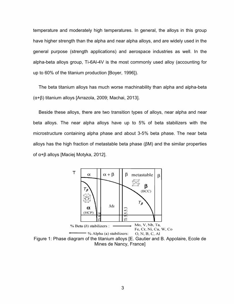
temperature and moderately high temperatures. In general, the alloys in this group

have higher strength than the alpha and near alpha alloys, and are widely used in the

general purpose (strength applications) and aerospace industries as well. In the

alpha-beta alloys group, Ti-6Al-4V is the most commonly used alloy (accounting for

up to 60% of the titanium production [Boyer, 1996]).

The beta titanium alloys has much worse machinability than alpha and alpha-beta

(α+β) titanium alloys [Arrazola, 2009; Machai, 2013].

Beside these alloys, there are two transition types of alloys, near alpha and near

beta alloys. The near alpha alloys have up to 5% of beta stabilizers with the

microstructure containing alpha phase and about 3-5% beta phase. The near beta

alloys has the high fraction of metastable beta phase (βM) and the similar properties

of α+β alloys [Maciej Motyka, 2012].

Figure 1: Phase diagram of the titanium alloys [E. Gautier and B. Appolaire, Ecole de

Mines de Nancy, France]

4

In machining metal, approximately 90% of the heat generation come from plastic

deformation [Boothroyd, 1975; Shahan, 1993]. However, the main distinction of Ti

compared to other metallic alloys is its low thermal conductivities. They have the

thermal conductivity around 6.6 W/m·K [Calamaz, 2008] compared to ferrous

materials around 50.7W/m·K [Andriya, 2012; Nandy, 2008] and aluminum alloys

around 200W/m·K [Toh, 2004] at room temperature. The thermal conductivity of

titanium could reach 20W/mK at high temperature [Calamaz, 2008]. This makes the

dissipation of the heat generated during machining extremely slow. Konig et al.

[1979] stated that about 80% of heat generation is absorbed by the cutting tool in

machining Ti alloys while only 50% for machining ferrous materials as shown in

Figure 2. Therefore, most of the heat is concentrated on the cutting edge of the tool

when machining Ti alloys. The effect of the low conductivity of Ti alloys can be

evident by comparing the reported cutting temperatures; ~1000°C [Ezugwu, 1997;

Hartung, 1982] when turning Ti alloys, 600°C when turning ferrous materials [Dhar,

2002; 2007] and 200°C when turning aluminum alloys [List, 2005]. The relatively

small chip-tool contact area (typically three times less than that of steels [Ramesh,

2008]) leads to high stress and stress gradient on the tool. The high cutting

temperature could be slightly relieved by reducing the cutting speed and using a

large amount of coolant. High thermal stress and cutting force with the confined

contact area result in extremely high stresses near the cutting edge (within 0.5mm

[Ezugwu, 1997]) as well as excessive tool deformation and failure. In addition, the

high temperature increases the wear rate of dissolution, diffusion, and chemical

reaction of a tool material with Ti alloys, often beyond the transus temperature

5

(882°C for pure titanium [Yang, 1999]) where the drastic change in physical

properties occurs .

Figure 2: Heat distribution of thermal load on tool and chip in turning [Konig, 1979]

The surface integrity is another reason for reduction of tool life. It not only causes

work hardening beneath the machined surface but also increases surface roughness.

In particular, because of the high chemical affinity with a tool material, Ti alloys have

a tendency to gall and weld to the tool, thus causing the fracture and tool geometry

failure and resulting in premature tool failure. Applying coolant at high pressure helps

overcome these problems. However, the high chemical reactivity of Ti with lubricants

and additives creates other problems such as additional reaction possibilities

[Andriya, 2012; Ezugwu, 1997; Rahman, 2003].

The low elastic modulus [Andriya, 2012; Machado, 1990] and high work

hardenability of Ti alloys are additional obstacles in machining. The low elastic

modulus of Ti alloys causes a higher deflection (twice as much as steels [Ezugwu,

1997; Machado, 1990]), which leads to chatter during machining.

6

Although most metals generates continuous chips in typical machining conditions,

Ti alloys are notorious for segmented chips, experiencing plastic instability and

discrete bursts of catastrophic thermoplastic shear in the primary shear zone. The

frequency of the chip segmentation in α−β alloys is higher than those in α-alloys and

β-alloys [Joshi, 2014]. Two shear bands was observed on each segmentation in -

alloys [Motonishi, 1987]. The chip morphology and serrated frequency of the chip

also depends on cutting speed and microstructure [Gente, 2001; Joshi, 2014;

Molinari, 2002; Rahim, 2008]. The lower chip segmentation frequency (larger spacing

between segments) was found in a higher cutting speed [Bayoumi, 1995].

The challenges mentioned above are the principal problems associated with

machining Ti alloys. When machining Ti alloys, the tool life dramatically decreases as

the cutting speed increases. Thus, the tool materials should provide (1) high hot

hardness, (2) good thermal resistance, (3) good thermal conductivity to reduce

thermal gradient (4) good chemical inertness to minimize galling and welding, (5)

high toughness to withstand vibration force, and localized stress and chip

segmentation. The development of advanced coated tool materials has improved the

machining productivity significantly in many materials such as ferrous and aluminum

alloys but not for Ti alloys.

Motivation I.1.2

In machining Ti alloys, beside PCD, the most successfully commercially available

tool material for cutting titanium is straight grade (uncoated) carbide tools (WC-Co or

WC). Even though many carbide tools with coatings are available in the market, the

coated carbide tools are not effective in machining Ti alloys. The reason behind this

7

is not clearly discovered at the present time. Therefore, the selection of tool materials

in machining Ti alloys is very difficult.

This thesis attempts to identify the wear mechanisms behind two main modes of

tool wear, crater and flank wear, by understanding metallurgical structure of a

selected Ti work material. This study can provide the fundamental knowledge in

designing effective tool materials for machining Ti alloys.

Tool materials and tool wear mechanisms reported in literature I.1.3

Over the past six decades, the production of Ti alloys has increased to meet the

increased usage in aerospace applications. Many researchers have studied heavily

the subject of machining Ti alloys to understand how to design effective tool materials

and develop techniques to minimize machining cost. Numerous studies on the

machinability of Ti alloys have been carried out. In fact, many hypotheses on tool

wear mechanisms in machining Ti alloys have been introduced. Many researchers

believe that both mechanical wear (abrasion, attrition) and chemical wear

(dissolution, diffusion) are the main wear mechanisms in machining Ti alloys.

Tool materials for machining Ti alloys can be mainly classified in three groups:

• High speed steel tools (HSS)

• Coated and uncoated carbide tools

• Super hard tool materials: PCD and CBN

Narutaki et al. [1983] conducted turning experiment on both alpha (Ti-5Al-2.5Sn)

and alpha-beta (Ti64) titanium alloys with straight carbide tools, CBN tools, cemented

TiN tools, sintered Al2O3 tools, sintered and natural diamond tools, and TiC coated

tools. He concluded that natural diamond tools offered excellent cutting performance

8

at the cutting speed of 1.67 m/s due to high thermal conductivity and low chemical

reactivity in both dry and water based coolant conditions. The cutting speed for these

diamond tools could go up to 3.33 m/s when applying sufficient coolant. Cemented

TiN, TiC-coated, and CBN tools were not recommended. In addition, CBN tools

caused very large and unusual groove marks on both the rake and flank faces. The

sinter diamond tools exhibited similar performances as the carbide tools at high

cutting speeds. Rahman et al. [2003] found that the binderless CBN tools without any

cobalt binder yielded significant improvement in tool life compared to regular CBN

tools, and even comparative to PCD tools at the cutting speed of 400m/min with high

pressure coolant.

With the turning experiment of Ti64 with multilayer coated (TiN-Al2O3-TiCN-TiN)

carbide tools, Ibrahim et al. [2009] stated that adhesive wear and welding were

predominant wear mechanisms both in flank and the rake face. The adhesion wear

took place after the coating had gone (worn out or flaked off). Corduan et al. [2003]

conducted the machining experiment of Ti64 with PCD, CBN and TiB2 coated

carbide. He recommended TiB2 coated carbide tools only for cutting speeds of less

than 100 m/min. While PCD tools showed the lowest wear rate, CBN tools were only

recommended for finishing cutting. He mentioned the delamination of TiB2 coating is

the main reason why the coated carbide tools did not work. Due to the mismatch in

thermal expansions between coating and substrate, internal stress is generated as

the temperature rises. The internal stress can intensify enough to break and flake off

the coating.

9

Dominant tool wear mechanisms I.1.3.1

In milling of Ti6246, Jawaid et al. [1999] claimed that the main wear mechanisms

were dissolution/diffusion and attrition wear with PVD-TiN and CVD-TiCN+Al2O3

coated carbide tools which caused the carbide grain to pull out. Nabhani et al. [2001]

conducted turning experiments of alpha-beta Ti48 with TiC/TiC-N/TiN coated WC,

CBN (Cubic Boron Nitride) and PCD tools with “quick-stop” device to capture the in-

situ tool condition during cutting process. By investigating tool wear appearance and

coherent metallic layer, they concluded that diffusion/dissolution and attrition were

the dominant tool wear mechanisms. The coating was not beneficial in resisting tool

wear since these layers were rapidly worn off, leading to immediate exposure of the

carbide substrate. The thickness of the protective adherent metal layer was strongly

influenced by the balance between the diffusion rate of tool material through layer

and the dissolution rate of the layer into work material.

TiC protection layer I.1.3.2

Hartung and Kramer [1982] carried out a comprehensive study on turning Ti64

with various tool materials (WC, TiC, CBN, Al2O3, TiCN, PCD, etc.) and various

coatings (HfO2, HfC, TiC, HfN, TiN, etc.) on carbide inserts. They reported that Al2O3

had the highest tool wear and PCD was the best in terms of wear resistance.

Uncoated carbide tools showed better performance than coated ones. A higher wear

rate was recorded with all coated carbide tools. Furthermore, they claimed that the

least soluble tool component controls the solubility of tool material. For example, the

solubility of WC was not greater than that of C (0.6 at%) and less than that of W (100

at%). Thus, they concluded that dissolution and diffusion wear models of tool

10

constituents in titanium were not sufficient to describe the tool wear in machining of Ti

alloys. They believed that, because of the high reactivity of Ti, the reaction layer,

titanium carbide (TiC), is formed, which becomes the main factor to control tool wear.

In the comparative research of turning Ti64 and Ti555.3 by Arrazola et al. [2009], the

results supported the conclusion by Hartung and Kramer [1982]. He showed that the

presence of TiC layer was less stable at the higher cutting speed (90m/min) which

accelerated tool wear.

Cobalt diffusion I.1.3.3

A cobalt-based diffusion tool wear model was introduced by Hua et al. [2005].

They carried out the turning experiment with Ti64 with uncoated carbide tools with

two distinct cobalt contents (6wt% and 10wt%). In the model, the wear rate was

calculated as the ratio of flux rate of diffused cobalt at tool-chip interface over density

of cobalt. He found that the results of the model agreed well with the experimental

data. Furthermore, the simulation indicated that the temperature increases with the

increase in cutting speeds while the chip contact length decreases, which leads to

rapid tool wear. The maximum depth of crater profile coincided with the peak

temperature which moved closer to the tool nose as the cutting speed increased.

Phases and microstructure of Ti alloys I.1.4

Phases in Titanium alloys I.1.4.1

It is known that the cementite phase (Fe3C) is present as the main abrasive

contributing to the flank wear in machining ferrous materials. Titanium can exist in

alpha, beta and rarely omega phases. Figure 3 shows the phase diagram as a

11

function of temperature and pressure. However, the phase diagram is strongly

influenced by the alloying elements and their content as shown in Figure 4. The

mechanical properties and hardness of Ti alloys influence the size, composition, and

volumetric fraction of α, β and ω-precipitated phases. No significant hard phase

exists in Ti alloys, which make hard to pinpoint the root cause of tool wear. In

addition, the microstructural features, which are affected by heat treatment and

alloying elements, also plays very important role in tool wear in machining Ti alloys.

Figure 3: Phase diagram of titanium [Velsavjevic, 2012]

12

Figure 4: Typical phase diagram of Ti alloys: a) α-stabilized system, b) β-stabilized

isomorphous system, c) β-stabilized eutectoid system [Frees, 2011]

Among the three phases of Ti, the α-phase with HCP structure is stable at room

temperature and pressure without any alloy stabilizer. At room temperature, the

hexagonal unit cell of the α-phase has the lattice parameters a (0.295 nm) and c

(0.468 nm) as shown in Figure 5. The c/a ratio for pure α-phase (1.587) is smaller

than the ideal ratio for the archetypal hexagonal crystal structure (1.633). Crystalline

structures accommodate plastic deformation along certain planes and directions

within the crystal lattice. As a general rule, the slip occurs in the densest packing

crystal planes (number of atoms/area) along the directions of the highest linear

density (atom/length). The α-phase has four slip planes, ({0001}, {1100}, {1101}, {1

1 22}, {1101}) and two slip directions (<1120>, <11 2 3>) making to 24 possible slip

systems as shown in Table 1. To determine which slip system is likely more active,

13

the critically resolved shear stress (CRSS) and the geometric relation between the

slip plane and the applied stress are used. The CRSS shown in Figure 7 is the in-

plane stress component required for dislocation movement as a function of

temperature. The predominant slip mode in the α phase is in {1100}, {0001}, {1101}

along <1120> direction. The highest CRSS is required for slip <11 2 3> direction.

Because of the intrinsically anisotropic character, the α phase has pronounced

variation of the elastic modulus (Ε) and hardness (H) as a function of the angle γ

between the c-axis of the unit cell and load direction. The elastic modulus and

hardness reach the highest values along the c-axis but the lowest in perpendicular

direction to the c-axis as presented in Figure 8. Furthermore, the elastic and shear

modulus and hardness decrease with the temperature as shown in Figure 9. The α-

phase has two variational phases, martensite structure (α′) and orthorhombic

martensite (α″).

The beta (β) phase is a metastable phase with body centered cubic (BCC)

structure. It has more slip systems than the α-phase making it more ductile and

easier to deform. The elastic modulus, shear modulus and hardness of the β phase

are well below that of the α phase [Meier, 1992].

The omega (ω) phase only presents in metastable β-alloys. The isothermal ω

particles have either an ellipsoidal or a cuboidal shape. It is well accepted that,

the ω phase has the highest elastic modulus and hardness followed by the α and α′,

phases [Zhou, 2004, 2008]. Many studies [Gabriel, 2013; Hickman B.S., 1969; Hsu,

2013; Jon, 1972; Jones, 2009] revealed that the ω (ellipsoidal) precipitates forms at

the beginning of the aging treatments and quenching β alloys from the beta field.

14

Although the ω-phase cannot be identified with optical analysis or the X-ray

diffraction (XRD) pattern, it can be investigated by the selected area diffraction

(SAED) patterns and bright-field image with transmission electron microscopy (TEM)

analysis.

Figure 5: Alpha phase and its slip systems

15

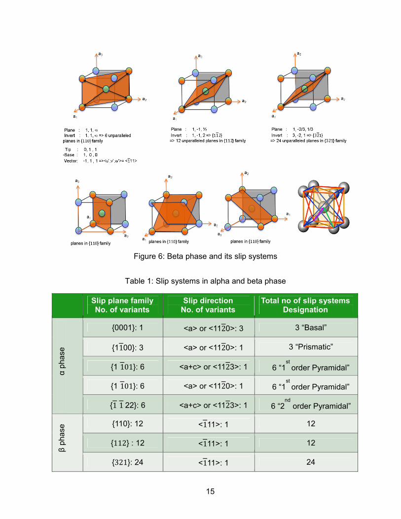
Figure 6: Beta phase and its slip systems

Table 1: Slip systems in alpha and beta phase

Slip plane family No. of variants

Slip direction No. of variants

Total no of slip systems Designation

α p

ha

se

{0001}: 1 <a> or <1120>: 3 3 “Basal”

{1100}: 3 <a> or <1120>: 1 3 “Prismatic”

{1 101}: 6 <a+c> or <1123>: 1 6 “1st

order Pyramidal”

{1 101}: 6 <a> or <1120>: 1 6 “1st

order Pyramidal”

{1 1 22}: 6 <a+c> or <1123>: 1 6 “2nd

order Pyramidal”

β p

ha

se {110}: 12 <111>: 1 12

{112} : 12 <111>: 1 12

{321}: 24 <111>: 1 24

16

Figure 7: Critical resolved shear stresses (CRSS) as function of temperature for slip

systems in α phase [Lütjering, 2003]

Figure 8: a) Elasticity (E) and b) hardness as a function of the angle � between the c-

axis of the unit cell and load direction [Lütjering, 2003; Britton, 2009]

17

Figure 9: Elasticity (E) and shear (G) modulus of alpha phase as function of

temperature [Lütjering, 2003]

Phase transformation in Titanium alloys. I.1.4.2

The phase transformation happens with the transition metals in the group IVB

such as Ti, Zr, Hf under applied pressure (p), temperature (T) or both (p, T). The α ⇔

β is more favorable with temperature while pressure is more critical for β ⇔ ω

transformation.

The α → β transformation happens when the temperature reaches transus

temperature (100% β phase). The transus temperature is strongly influenced by

interstitial and substitutional alloy ingredients.

The β phase transforms to α phase during continuous cooling of the α-β Titanium

alloys from above transus temperature. Depending on the cooling rate, the phase

transformation mechanism could be β → α for slow cooling rate and diffusionless

transformation β → α’ for fast cooling rate at temperatures below 700-750 °C.

18

Quenching Ti64 alloy from the 750–900 °C temperature range produces an

orthorhombic martensite (α″).

The β ⇔ ω transformation is reversible and diffussionless. The phase

decomposition mechanism of the metastable beta phase in this material follows the

classical behavior for this type of alloy: route 1 (β → β + ω + α → β + α) and route 2

(β → β + ω → β + ω +α → β + α) [Grabriel, 2013].

Microstructure of α + β Ti alloys I.1.4.3

The properties, hardness and machinability of each Ti alloy are directly related to

its microstructure. The dual phase (α + β) Ti alloys have different types of

microstructure depending on the heat treatment (solution treated and aged

temperatures; cooling rate and cooling rate. Four common microstructures are milled

annealed, equiaxed structure, fully lamellar structure and bi-modal (or duplex)

structure which is a combination of equiaxed and lamellar structure as shown in

Figure 11. Equiaxed structure has good creep and crack growth resistance, but

suffers from low tensile ductility and moderate fatigue properties. The bi-modal

structure is characterized by high ductility and fatigue strength, high yield and tensile

stress. High resistances to crack propagation and fracture toughness are the notable

properties of a fully lamellar structure [Zhang, 2014]. The bi-modal microstructure is

typical in the metallurgical processing of α + β alloys when heat-treated in the α + β

field as shown in Figure 10 [Lütjering, 2003]. The fully lamellar structure can be

achieved by heat treatment typically above beta-transus temperature (beta annealed)

then slowly cooled in furnace or in the air. In this microstructure, the thickness of

Widmanstätten α-laths, colony size, and prior grain size are important parameters

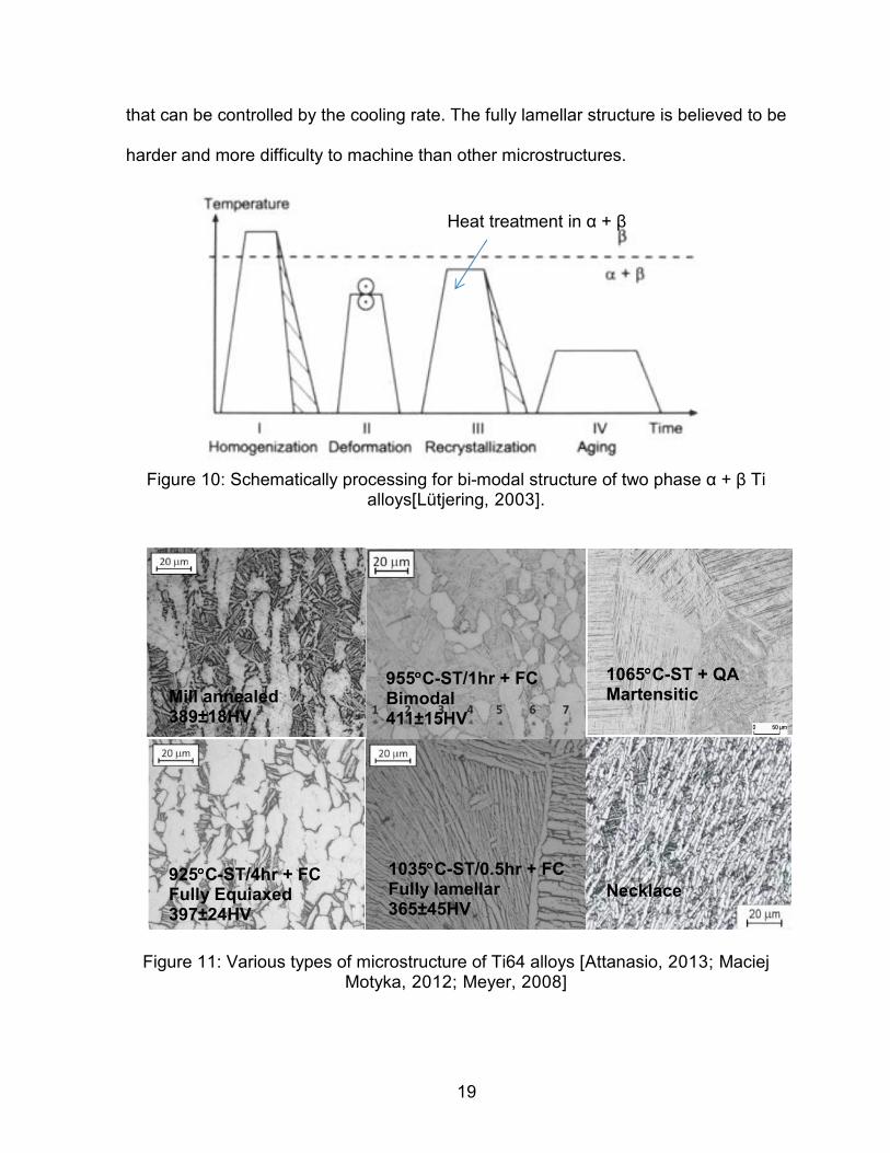
19

that can be controlled by the cooling rate. The fully lamellar structure is believed to be

harder and more difficulty to machine than other microstructures.

Figure 10: Schematically processing for bi-modal structure of two phase α + β Ti

alloys[Lütjering, 2003].

Figure 11: Various types of microstructure of Ti64 alloys [Attanasio, 2013; Maciej Motyka, 2012; Meyer, 2008]

Heat treatment in α + β

Mill annealed 389±18HV

955°°°°C-ST/1hr + FC Bimodal 411±15HV

925°°°°C-ST/4hr + FC Fully Equiaxed 397±24HV

1035°°°°C-ST/0.5hr + FC Fully lamellar 365±45HV

1065°°°°C-ST + QA Martensitic

Necklace

20

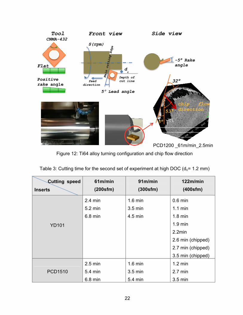
EXPERIMENTAL SETUP AND PROCEDURES I.2

Turning experiments of Ti64 alloy I.2.1

The turning experiments were conducted with Ti-6Al-4V with the average

hardness of 326HV on Yama Seiki GA-30 lathe using tungsten carbide (WC-

6wt%Co) and PCD inserts. The tests were in dry condition to understand the wear

mechanisms between Ti alloy and cutting tool. The tool insert geometry was ANSI

designation CNMA-432.

To investigate wear evolutions in both the rake and flank faces, all the inserts were

flat rake face without chip breaker. Two grades (YD101, YD201) of Zhuzhou

Cemented Carbide Cutting Tools, Co, LTD, (ZCCCT, Zhuzhou, Hunan, China) brand

uncoated carbide inserts were chosen for the test for their flat rake face. Grade

YD201 was a straight grade carbide containing approximately 94% WC and 6% Co.

The average grain size was 2µm. Carbide grade YD101 had a composition

consisting of 93.6% WC, 0.15%NbC, 0.25%TaC, and 6%Co. The average grain size

was 1µm.

Three PCD grades and two tungsten carbide grades were used as tool inserts in

this study. The PCD tips were Compax® 1200 and 1500 grades, 92% diamond by

volume, with average diamond grain size of 1.5 µm and 25 µm, respectively,

manufactured by Diamond Innovation. Shape-Master Tool Company, Kirkland, IL,

brazed each PCD tip onto an ISO CNMA120408 carbide base. The 1200 grade PCD

inserts with 0° rake angle had an average grain size of 1.5µm. Two grades, 1210 and

1510, of PCD inserts with a 10° positive rake angle. The feed rate remained constant

for all samples at 0.127 mm/rev (0.005 in/rev). Two sets of experiments with the

21

depth of cut (DOC) of 0.635 mm (low DOC) and 1.2 mm (high DOC), respectively,

were conducted to see the effects of DOC to cutting process and tool wear. The

information for tool grades and DOC was summarized in Table 2. The low DOC

showed wear at the nose while the high DOC showed traditional flank wear. Lead

angle refers to the angle between the imaginary line perpendicular to the direction of

feed and the line parallel to the cutting edge of the insert. Rake angle in this context

refers to the inclination angle in the tool holder that gives the insert its clearance with

respect to the work piece. For consistency, both of the inserts were run with a -5°°°°

lead angle and a -5°°°° rake angle with respect to the work material. The turning setup

and the chip flow direction respect to tool were presented in Figure 12. Tables 1 and

2 below lists the cutting time used in the turning tests for carbide and PCD inserts at

each cutting speeds.

Table 2: Tool grades and DOC used

Tool Grade

(Tool ID)

Rake angle

Grain size (µm)

Thermal conductivity

(W/m·K)

DOC

(mm)

Carbide YD101 0° 1 65 0.635 & 1.2

Carbide YD201 0° 2 75 0.635

PCD PCD1200 0° 1.5 450 0.635

PCD PCD1210 +10° 1.5 450 1.2

PCD PCD1510 +10° 25 450 1.2

22

Figure 12: Ti64 alloy turning configuration and chip flow direction

Table 3: Cutting time for the second set of experiment at high DOC (dc= 1.2 mm)

Cutting speed

Inserts

61m/min

(200sfm)

91m/min

(300sfm)

122m/min

(400sfm)

YD101

2.4 min

5.2 min

6.8 min

1.6 min

3.5 min

4.5 min

0.6 min

1.1 min

1.8 min

1.9 min

2.2min

2.6 min (chipped)

2.7 min (chipped)

3.5 min (chipped)

PCD1510

2.5 min

5.4 min

6.8 min

1.6 min

3.5 min

5.4 min

1.2 min

2.7 min

3.5 min

dc

feed

direction

5°°°° Lead angle

-5°°°° Rake angle

S(rpm)

Side view Front view

PCD1200 _61m/min_2.5min

chip flow

direction

32°°°°

5°°°°

53°°°°

Depth of

cut line

8

0

CNMA-432

Tool

Flat

Positive

rake angle

23

Table 4: Cutting time for the first set of experiment at low DOC (dc= 0.635 mm)

Cutting speed

Inserts

61m/min

(200sfm)

91m/min

(300sfm)

122m/min

(400sfm)

YD101

3 min (chipped)

6 min (chipped)

9 min

12 min

1 min

2 min

3 min (chipped)

4 min

30 sec

1 min (chipped)

2 min (chipped)

YD201

3 min (chipped)

6 min

9 min (chipped)

12 min

All Inserts

Chipped

30 sec

1 min (chipped)

2 min

PCD1200

6 min

12 min

18 min

24 min

30 min (chipped)

No Inserts

Tested

1 min (chipped)

2 min

3 min

4 min

PCD1210

6 min

12 min

24 min

4 min

6 min

8 min

2 min

3 min

4 min

Confocal Microscopy I.2.2

In this work, Ziess LSM 210 Confocal Laser Scanning Microscope (CSLM) was

used to capture both 2-D and 3-D images of crater and flank wear. This particular

confocal system can work in confocal, non-confocal and conventional optical modes.

24

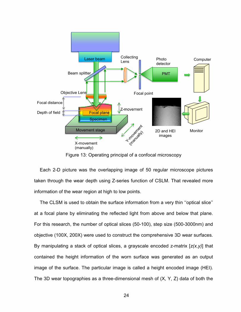
Figure 13: Operating principal of a confocal microscopy

Each 2-D picture was the overlapping image of 50 regular microscope pictures

taken through the wear depth using Z-series function of CSLM. That revealed more

information of the wear region at high to low points.

The CLSM is used to obtain the surface information from a very thin ‘‘optical slice’’

at a focal plane by eliminating the reflected light from above and below that plane.

For this research, the number of optical slices (50-100), step size (500-3000nm) and

objective (100X, 200X) were used to construct the comprehensive 3D wear surfaces.

By manipulating a stack of optical slices, a grayscale encoded z-matrix [z(x,y)] that

contained the height information of the worn surface was generated as an output

image of the surface. The particular image is called a height encoded image (HEI).

The 3D wear topographies as a three-dimensional mesh of (X, Y, Z) data of both the

Laser beam

Objective Lens

Focal plane

Specimen

PMT

Z-movement

X-movement (manually)

Monitor

Computer

Movement stage

Collecting Lens

Focal point

Depth of field

Focal distance

Beam splitter

Photo detector

2D and HEI images

25

rake and flank faces of the cutting tools were created from the HEI images. With the

similar process, the 2D images are generated in a much higher quality, which have

the detailed information to analyze the wear patterns on the inserts.

Figure 14: Flow chart of data collection with confocal microscopy

To reduce the noise in the capturing process, a wavelet filtering procedure

described by Olortegui-Yume and Kwon [Olortegui-Yume, 2010; Park, 2011] was

used to process the HEI images in Matlab. The main advantage of the wavelet

transform for image processing is to extract the surface topography clearly from the

raw image data without losing any surface details. In this work, the two-dimensional

discrete wavelet transform (2D-DWT) was used in a multi-resolution scheme with a

Objective, step size, number of optical slides,

current section

Collect points at current section (optical

slide)

Current section is

greater than number of optical slides?

Move to next optical slide (current section

+step size)

Finish collection of

data

2D & HEI images

Yes

No

26

two-channel filter bank, which consisted of a pair of filters, low-pass and high-pass,

based on the chosen mother wavelets, Daubechies7 (db7) [Rioul, 1991].

Finally, the combination of multiple 2D wear profiles extracted from the 3D

topographies for each cutting time provided the quantitative data on wear surfaces,

which can be accumulated to construct the wear evolution as a function of time. For

the crater wear on the rake face, the 2D crater wear profiles were taken in the

direction of chip flow to insure maximum wear profiles. For nose and flank wear, 2D

wear profiles were taken along the y direction at various x-positions (1st to 256th

section) as shown in Figure 15. The PCD inserts with +10° rake angle inserts were

placed on the 10° incline stage to measure them based on the horizontally flat plane.

The tool wear measurement was conducted both before and after an adhered

layer (most likely Ti and TiC) was removed with a weak hydrofluoric acid solution (HF

at 10 vol%).

27

Figure 15: Measurements of tool wear at the rake face, nose and flank face

SEM picture and element mapping I.2.3

The optical view and the element mapping of worn tools were captured and

characterized before and after cleaning the adhesion layer using JEOL 6610LV

Scanning Electron Microscope with Energy Dispersive X-ray Spectroscopy. The

accelerating voltage and working distance were 20kV and 15mm, respectively.

15 Flank face

Wavelet

Transform

(Matlab)

HEI

x (pixels)

y (pix

els

)

50 100 150 200 250

50

100

150

200

250

1st

section 128th

section 256th

section

HEIimage

Rake face

3Dwear

topographies

Geometric transformation

2Dwear

profiles

100 150 200 250 300 350 400 450-30

-25

-20

-15

-10

-5

0

5

10

The evolution of Nose wear of YD101 tool at 200sfm (-num80-num16-num17-num18-128sec)

Distance(µm)

Heig

ht(

µm

)

YD101_0min0sec_0m

YD101_2min24sec_146m



100 150 200 250 300 350 400 450-30

-25

-20

-15

-10

-5

0

5

10


Distance(µm)

Heig

ht(

µm

)

YD101_0min0sec_0m




100 150 200 250 300 350 400 450-30

-25

-20

-15

-10

-5

0

5

10


Distance(µm)

Heig

ht(

µm

)

YD101_0min0sec_0m




Cra

ter

Wear

No

se W

ear

Fla

nk W

ear

1st

section

128th

section

256th

section

Wavelet

Transform

(Matlab)

Wavelet

Transform

(Matlab)

128th

section

128th

section

128th

section

Nose

28

EXPERIMENTAL RESULTS AND DISCUSSION I.3

Wear Characteristics of tools inserts at low DOC I.3.1

The machining experiments were divided into two sets based on the DOC. The

crater wear characteristic of the first set with the low DOC was reported in detail

elsewhere [Schrock, 2012; 2014]. In this thesis, the flank wear of the first set was

studied and presented. Furthermore, the second set of the machining experiments

with high DOC was conducted to study the wear characteristics of both flank ad

crater wear. Figure 16 presents the definitions of crater and flank wear studied in this

research.

Figure 16: Types of tool wear according to standard ISO 3685:1993

Crater wear at low DOC I.3.1.1

The maximum crater depths of carbide and PCD inserts from the first set of

experiments are summarized in Table 5. The depths were calculated from the 2D-

profiles of craters reported in [Schrock, 2012; 2014] after excluding the fractured and

29

chipped inserts. These data were used to compare those of high DOC presented in

the next chapter.

Table 5: The maximum crater wear depth (µm) of the first turning tests with dc=0.635 [Schrock, 2012; 2014]

Tool

Cutting time

YD101 YD201 PCD1200 PCD1210

61 m/min (200sfm)

3min -- -- -- ---

6min 17 24 -- --

9min 26 33 -- --

12min 45 42 -- --

91 m/min (300sfm)

1min 11 -- -- --

2min 35 -- -- --

3min 50 -- -- --

4min 64 -- -- --

5min -- -- -- --

7min -- -- -- --

122 m/min (400sfm)

1min 15 14 -- --

2min 62 -- -- --

3min -- -- -- --

30

Figure 17: The maximum depth and wear rate of crater wear on carbide inserts

(YD101) at low DOC

Nose wear at low DOC I.3.1.2

Nose wear and flank wear land were also analyzed at various cutting conditions

(cutting speed and time). However, the first set generates notably the nose wear,

which is slight different from traditional flank wear. It should be noted that the depths

of nose wear along the tool curvature were much smaller than the tool radius.

Therefore, the evolution of nose wear was not clearly represented in 3D topographies

in its natural view. For a better representation, the 3D nose wear topographies are

presented after the curved surface has been flattened by the geometric

transformation as shown in Figure 18. In this transformation, the highest point for

each profile along X-axis direction in the unworn area was determined based on the

tool geometry. For each point along the X-profile, an addition in height (h) was

calculated based on the tool radius (r) and the difference in x direction between this

point and the highest point as shown in Figure 18. This transformation only affected

the 3D view of the nose wear. The 2D wear profiles nose wear were plotted from

initial data without any effect of geometric transformation.

Cutting Length (m)

0 100 200 300 400 500 600 700 800

We

ar

rate

(µ

m/m

in)

0

5

10

15

20

25

30

35

400sfm

300sfm

200sfm

YD101dc=0.635mm

Cutting Length (m)

0 100 200 300 400 500 600 700 800

De

pth

(µ

m)

0

10

20

30

40

50

60

70

400sfm

300sfm

200sfm

YD101dc=0.635mm

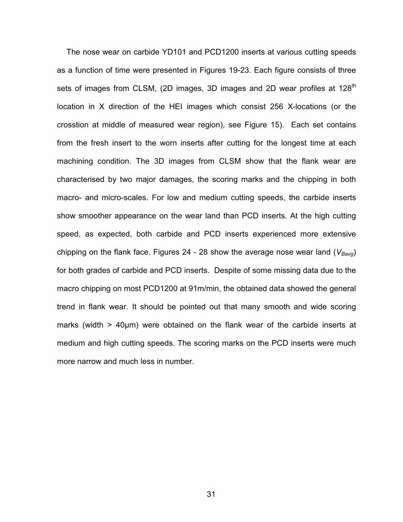
31

The nose wear on carbide YD101 and PCD1200 inserts at various cutting speeds

as a function of time were presented in Figures 19-23. Each figure consists of three

sets of images from CLSM, (2D images, 3D images and 2D wear profiles at 128th

location in X direction of the HEI images which consist 256 X-locations (or the

crosstion at middle of measured wear region), see Figure 15). Each set contains

from the fresh insert to the worn inserts after cutting for the longest time at each

machining condition. The 3D images from CLSM show that the flank wear are

characterised by two major damages, the scoring marks and the chipping in both

macro- and micro-scales. For low and medium cutting speeds, the carbide inserts

show smoother appearance on the wear land than PCD inserts. At the high cutting

speed, as expected, both carbide and PCD inserts experienced more extensive

chipping on the flank face. Figures 24 - 28 show the average nose wear land (VBavg)

for both grades of carbide and PCD inserts. Despite of some missing data due to the

macro chipping on most PCD1200 at 91m/min, the obtained data showed the general

trend in flank wear. It should be pointed out that many smooth and wide scoring

marks (width > 40µm) were obtained on the flank wear of the carbide inserts at

medium and high cutting speeds. The scoring marks on the PCD inserts were much

more narrow and much less in number.

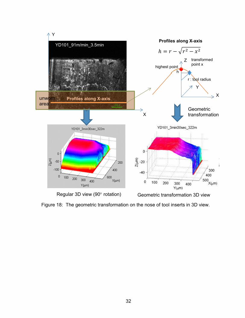
32

Figure 18: The geometric transformation on the nose of tool inserts in 3D view.

� � ��

transformed point x

Geometric transformation

YD101_91m/min_3.5min Profiles along X-axis

X

Y

Regular 3D view (90° rotation)

unworn area

Profiles along X-axis

r : tool radius

highest point

h

Geometric transformation 3D view

X

Z

Y

33

Figure 19: Nose wear evolution of carbide inserts (YD101) at the cutting speed of

61m/min.

-300 -250 -200 -150 -100 -50 0-60

-50

-40

-30

-20

-10

0

10

Nose wear at 61m/min

128thlocation

Distance to cutting edge(µm)

De

pth

( µm

)

YD101_0min0sec_0m


YD101_9min0sec_549m


Cutting edge

Rake face

Nose face

Depth of

scoring mark

a) 2D image b) 3D image

c) 2D profile of wear at 128th location

YD101 _61m/min_9min YD101 _61m/min_12min

YD101 _61m/min_~6min YD101 _61m/min_0min (fresh tool)

100µµµµm

Cutting edge 128

th

Scoring marks

1st

2D-profile

256th

100µµµµm

34

Figure 20: Nose wear evolution of carbide inserts (YD101) at 91m/min.

Dust

contamination

-300 -250 -200 -150 -100 -50 0-60

-50

-40

-30

-20

-10

0

10


128thlocation


De

pth

( µm

)

YD101_0min0sec_0m

YD101_2min0sec_122m


YD101_7min0sec_427m

Nosewearland

Chipping at the

cutting edge &

therakeface

YD101_91m/min_2min

100µµµµ

m YD101_91m/min_4min YD101_91m/min_7min

YD101_91m/min_0min

(freshtool)

100µµµµm 100µµµµm


Cuttingedge

128th

2D-profile

Scoringmarks


c) 2D profile of wear at 128th

location

35

Figure 21: Nose wear evolution of carbide inserts (YD101) at cutting speed of

122m/min.

YD101_122m/min_0min

(freshtool)

YD101_122m/min_2min

YD101_122m/min_3min YD101_122m/min_~4min

100µµµµm


100µµµµm

-300 -250 -200 -150 -100 -50 0-60

-50

-40

-30

-20

-10

0

10


128th

location


De

pth

( µm

)

YD101_0min0sec_0m

YD101_2min0sec_122m

YD101_3min0sec_183m


Chippingatthe

cuttingedge&

therakeface



location

36

Figure 22: Nose wear evolution of PCD1200 inserts at cutting speed of 61m/min.

PCD1200_61m/min_6min



(freshtool)




-300 -250 -200 -150 -100 -50 0-60

-50

-40

-30

-20

-10

0

10


128thlocation


De

pth

( µm

)

PCD1200_0min0sec_0m

PCD1200_6min0sec_363m



Scoringmarks



location

37

Figure 23: Nose wear evolution of PCD1200 inserts at cutting speed of 122m/min.

PCD1200_122m/min_3min PCD1200_122m/min_4min

PCD1200_122m/min_2.5minPCD1200_122m/min_0min

(freshtool)



-300 -250 -200 -150 -100 -50 0-60

-50

-40

-30

-20

-10

0

10


108thlocation


De

pth

( µm

)

PCD1200_0min0sec_0m




Scoringmarks


c) Wear profile at 128th location

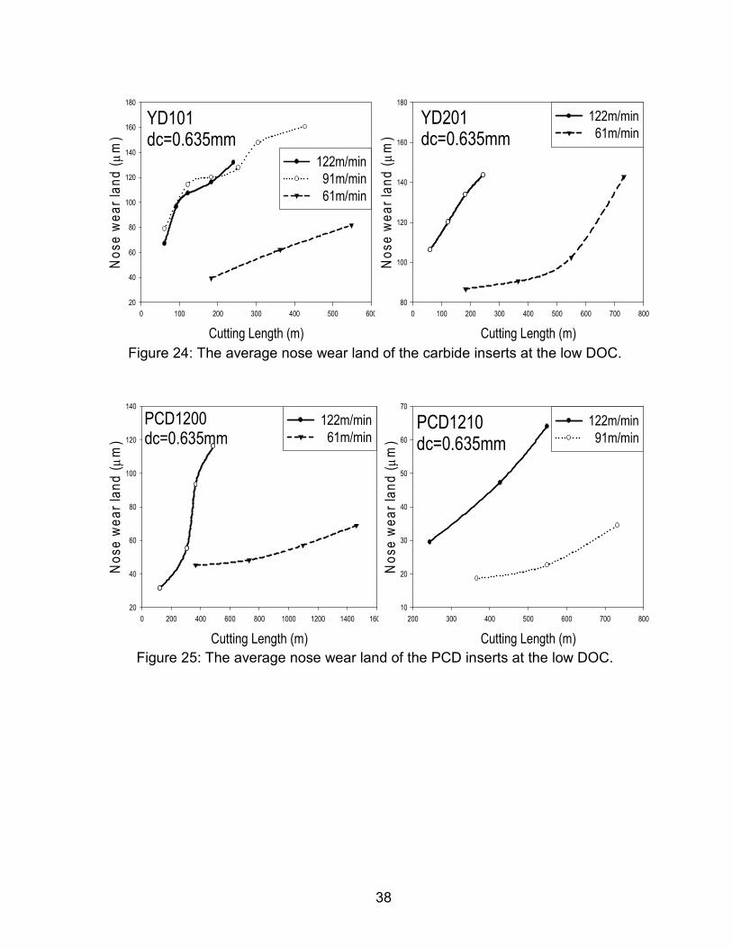
38

Figure 24: The average nose wear land of the carbide inserts at the low DOC.

Figure 25: The average nose wear land of the PCD inserts at the low DOC.

Cutting Length (m)

0 100 200 300 400 500 600

No

se

we

ar

lan

d (

µm

)

20

40

60

80

100

120

140

160

180

122m/min

91m/min

61m/min

YD101dc=0.635mm

Cutting Length (m)

0 100 200 300 400 500 600 700 800

No

se

we

ar

lan

d (

µm

)

80

100

120

140

160

180

122m/min

61m/minYD201dc=0.635mm

Cutting Length (m)

0 200 400 600 800 1000 1200 1400 1600

No

se

we

ar

lan

d (

µm

)

20

40

60

80

100

120

140

122m/min

61m/min

PCD1200dc=0.635mm

Cutting Length (m)

200 300 400 500 600 700 800

No

se

we

ar

lan

d (

µm

)

10

20

30

40

50

60

70

122m/min

91m/minPCD1210dc=0.635mm

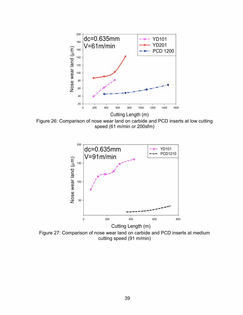
39

Figure 26: Comparison of nose wear land on carbide and PCD inserts at low cutting

speed (61 m/min or 200sfm)

Figure 27: Comparison of nose wear land on carbide and PCD inserts at medium

cutting speed (91 m/min)

Cutting Length (m)

0 200 400 600 800 1000 1200 1400 1600

No

se

we

ar

lan

d (

µm

)

20

40

60

80

100

120

140

160

180

200

YD101

YD201

PCD 1200

dc=0.635mmV=61m/min

Cutting Length (m)

0 200 400 600 800

No

se

we

ar

lan

d (

µm

)

50

100

150

200

YD101

PCD1210dc=0.635mmV=91m/min

40

Figure 28: Comparison of nose wear land on carbide and PCD inserts at high cutting

speed (122 m/min).

It should be pointed out that YD101 inserts at the medium cutting speed had larger

scoring marks (>60µm) on the nose in comparison to low and high cutting speeds. In

addition, all YD201 inserts at 91 m/min were fractured. The possible reason could be

chatter and vibration at this cutting condition. There were less and smaller scoring

marks observed on the nose of PCD inserts.

Figure 29: The scoring marks on the noses of YD101 inserts

Cutting Length (m)

0 100 200 300 400 500 600

No

se

we

ar

lan

d (

µm

)

20

40

60

80

100

120

140

160

180

200

PCD1200

PCD1210

YD101

YD201

dc=0.635mmV=12m/min

YD101_400fsm_num3_3min0sec_20x

YD101_91m/min_ 4min10sec

YD101_91m/min _5min0sec

YD101_91m/min _7min0sec

41

Wear characteristics of tools inserts at high DOC I.3.2

Crater wear at high DOC I.3.2.1

It is interesting that the catastrophic failure from tool fracture of the cutting edge

only happened after a cutting distance of more than 400m at high cutting speeds. At

a low cutting speed, the chipping happened randomly on both carbide and PCD

inserts of all grades at each cutting speed. Meanwhile, catastrophic fracture

happened on most of the YD201 and PCD1210 rake inserts at 91 m/min and 61

m/min with low DOC, respectively. The possible cause for chipping and fracture with

a low DOC was high temperature gradients and stress concentration along the short

chip-tool contact lengths as evident in the study of temperature and stress distribution

at the rake face of the tool using the FEM simulation to be discussed in the next

section.

The 2D and 3D images of fresh and worn carbide inserts are presented in Figures

30-32 for all three cutting speeds. Interestingly, the results from the second set show

smoother crater surface, a representative of thermochemical wear (dissolution and/or

diffusion) on the carbide inserts. The smooth crater surfaces were seen on carbide

inserts at even low cutting speed (200sfm) after cutting 5 min. The carbide inserts

with the cutting time of less than 5 minutes at 200sfm showed a few abrasive marks

but mainly dissolution/diffusion wear (insert after cutting 2.4min in Figure 30). The

crater surfaces became more even and shinier as the cutting speed increases. The

dissolution/diffusion may be more dominant at the medium and high cutting speed.

As reported in the literature [Ezugwu, 1997; Hartung, 1982; Narutaki, 1983], the

temperatures of medium and high cutting speeds with carbide tools were above the

42

transus temperature leading to acceleration of dissolution and diffusion rates. The

crater wear developed closer to the cutting edge on the inserts at all cutting speeds.

Therefore, the cutting edge of carbide inserts was weaken and chipped quickly. This

phenomenon resulted from the high temperature near the cutting edge. The stable

and sharp cutting edge was an important factor for long tool life in cutting Ti alloys. In

machining Ti, not only were the cutting temperatures higher but also the crater wear

occurred near the cutting edge alloys compared to machining ferrous materials

[Ezugwu, 1997].

To represent the crater depth information, the 2D crater wear profiles along chip

flow direction, where the maximum of crater was expected happen, were plotted

various locations (88th, 108th, 128th and 148th sections in Figure 30). These maximum

crater depths were obtained by taking the maximum depth value from the 2D wear

profiles. The 2D crater profiles of the carbide inserts were presented in Figures 33

and Figure 34. Figures 33 showed the 2D crater wear profiles at 88th and 108th

locations with the consistent depth of crater wear which presented the evidence of

smooth crater wear on carbide inserts.

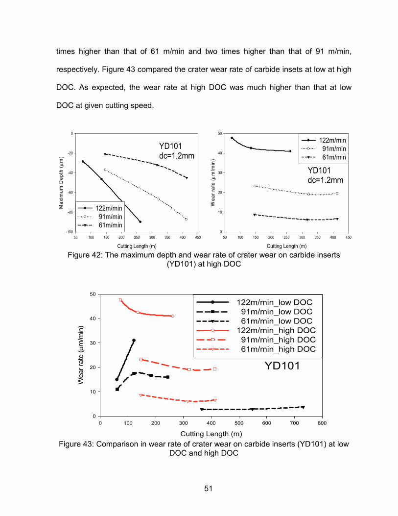
51

times higher than that of 61 m/min and two times higher than that of 91 m/min,

respectively. Figure 43 compared the crater wear rate of carbide insets at low at high

DOC. As expected, the wear rate at high DOC was much higher than that at low

DOC at given cutting speed.

Figure 42: The maximum depth and wear rate of crater wear on carbide inserts

(YD101) at high DOC

Figure 43: Comparison in wear rate of crater wear on carbide inserts (YD101) at low

DOC and high DOC

Cutting Length (m)

0 100 200 300 400 500 600 700 800

Wear ra

te (µm

/min

)

0

10

20

30

40

50

122m/min_low DOC

91m/min_low DOC

61m/min_low DOC

122m/min_high DOC

91m/min_high DOC

61m/min_high DOC

YD101

Cutting Length (m)

50 100 150 200 250 300 350 400 450

Ma

xim

um

De

pth

(µ

m)

-100

-80

-60

-40

-20

0

122m/min

91m/min

61m/min

YD101dc=1.2mm

Cutting Length (m)

50 100 150 200 250 300 350 400 450

We

ar

rate

(µ

m/m

in)

0

10

20

30

40

50

122m/min

91m/min

61m/min

YD101dc=1.2mm

52

Nose wear and flank wear at high DOC I.3.2.2

The nose and flank wear on the carbide and PCD1510 inserts at the longest

cutting time of three cutting speeds were presented in Figures 44-47. In appareance,

the carbide inserts showed even (in depth) nose and flank wear in appearance while

uneven nose and flank were observed on PCD1510 inserts at the low and medium

cutting speeds. In the literature, many researchers reported that titanium galls and

welds to tool material lead to the chipping of the cutting edge. The welded or

fractured chipping abraded the nose and flank face of tools causing scoring marks

when the tool travels along the feed direction. The scoring marks were observed with

both carbide and PCD1510 inserts. However, these scoring marks appeared more

frequently with smooth and clearly appearance than those of PCD1510. Obviously,

the temperatures at the flank face were much lower than those at the rake face.

Therefore, the dissolution and diffusion mechanisms which cause smooth wear

cannot be dominant in the flank face. Then, a question here is what causes these

scoring marks on the flank faces of the carbide and PCD1510 inserts, respectively.

The answer will be discussed in next section.

At the high cutting speed, as expected, with high temperature and less edge

stability on the rake face, both carbide and PCD1510 inserts experienced

catastrophic fracture. The inserts with a large fractured area suppressed the

appearances of the steady-state wear patterns observed in nose wear, flank wear

and crater wear. Figure 48 shows a very large damaged area on the carbide inserts

resulted from a large fracture. For the cutting speed of 122 m/min, the carbide inserts

last up to 2 minutes, and the PCD1510 tools withstand for up to 3.5 minutes.

53

Furthermore, the main failure of the carbide inserts was at the nose while the flank

face of PCD1510 was more damaged. The failure of the PCD1510 inserts at all

cutting speeds was affected by the notch wear as shown in Figure 47. The notch

wear occurred at most cutting speeds and cutting times. It happened in the earlier

stage of cutting and become more severe as the cutting speed increases.

Figure 44: Nose wear on carbide YD101 inserts at the longest cutting time of three

cutting speeds.

YD101_122m/min_

2.2min YD101_91m/min_

4.5min

YD101_0m/min_0min

(fresh tool)

YD101_61m/min_

5.2min

a) 2D images b) 3D images

100µµµµm

even(indepth)

wear

uneven(indepth)

wear

2Dprofile

at1st

section

256th

2D profile at

1st section

128th

256th

128th

YD101_0 m/min_0 min YD101_61 m/min_5.2 min

YD101_91 m/min_4.5 min

YD101_122 m/min_2.2 min

54

Figure 45: Nose wear on the nose of PCD1510 inserts at the longest cutting time of

three cutting speeds.

Figure 46: The flank wear on carbide YD101 inserts at the longest cutting time of

three cutting speeds.

PCD1510_91m/min_

5.4min

PCD1510_61m/min_

6.8min

PCD1510 _0m/min_

0min (fresh tool)

PCD1510_122m/min_

3.5min

100µµµµm


uneven(indepth)

wear

uneven(indepth)

wear

2Dprofile

at1st

section 128th

section

256th

2Dprofileat

1stsection

128th

256th

PCD1510_0 m/min_0 min PCD1510_61 m/min_6.8 min

PCD1510_91 m/min_5.4 min

PCD1510_122 m/min_3.5 min

YD101_91m/min_

4.5mim

YD101_0m/min_0min

(fresh tool) YD101_61m/min_

6.8min

100µm

YD101_122m/min_

2.2min


uneven(indepth)

wear

YD101_0 m/min_0 min



YD101_122 m/min_2.2 min

55

Figure 47: The flank wear on PCD1510 inserts at the longest cutting time of three

cutting speeds.

Figure 48: Nose damage of the carbide inserts (YD101)

The 2D nose and flank wear profiles were also plotted for each tool type as a

function of cutting distances for three cutting speeds. The 2D wear profiles provide

wear land as well as wear depth which was not determined with typical microscope

and SEM images reported in literatures. The nose and flank wear profiles of the

carbide and PCD1510 inserts can be compared in Figures 49-51. The 2D wear

profiles provided consistent data of nose and flank wear land at four different

locations (88th, 108th, 128th, 148th sections shown Figure 44). Because of the multiple

PCD1510_122m/min_

3.5min

PCD1510_91m/min_

5.5min

PCD1510_0m/min_

0min (fresh tool)

PCD1510_61m/min_

6.8min

Notch wear

100µµµµm

Notch

wear


uneven(indepth)

wear

PCD1510_0 m/min_0 min

PCD1510_61m/min_6.8 min



YD101_122m/min_2.7min YD101_122m/min_3.5min YD101_122m/min_2.6min 250µm

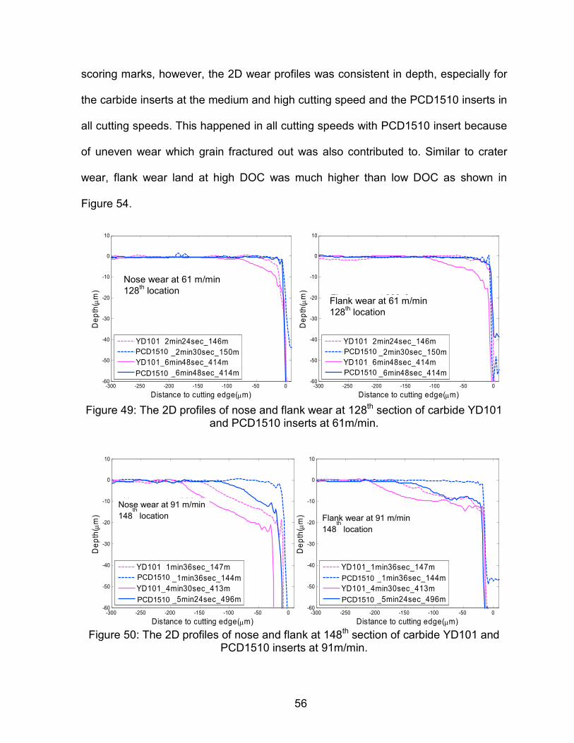
56

scoring marks, however, the 2D wear profiles was consistent in depth, especially for

the carbide inserts at the medium and high cutting speed and the PCD1510 inserts in

all cutting speeds. This happened in all cutting speeds with PCD1510 insert because

of uneven wear which grain fractured out was also contributed to. Similar to crater

wear, flank wear land at high DOC was much higher than low DOC as shown in

Figure 54.

Figure 49: The 2D profiles of nose and flank wear at 128th section of carbide YD101

and PCD1510 inserts at 61m/min.

Figure 50: The 2D profiles of nose and flank at 148th section of carbide YD101 and

PCD1510 inserts at 91m/min.

-300 -250 -200 -150 -100 -50 0-60

-50

-40

-30

-20

-10

0

10

Nose wear at 200sfm

128thlocation


De

pth

( µm

)





-300 -250 -200 -150 -100 -50 0-60

-50

-40

-30

-20

-10

0

10

Flank wear at 200sfm

128thlocation


De

pth

( µm

)





PCD1510

Nose wear at 61 m/min

128th location

Flank wear at 61 m/min

128th location

PCD1510

PCD1510

PCD1510

-300 -250 -200 -150 -100 -50 0-60

-50

-40

-30

-20

-10

0

10

Nose wear at 300sfm

148th

location


De

pth

( µm

)





-300 -250 -200 -150 -100 -50 0-60

-50

-40

-30

-20

-10

0

10


148th

location


De

pth

( µm

)





Nose wear at 91 m/min 148

th

location

Flank wear at 91 m/min 148

th

location

PCD1510

PCD1510

PCD1510

PCD1510

57

Figure 51: The 2D profiles of nose and flank wear at 108th section of carbide YD101

and PCD1510 inserts at 122m/min.

Figure 52: The evolution of flank wear land on the flank face of YD101 and PCD1510

inserts at various cutting speeds.

Cutting Length (m)

100 200 300 400 500 600

Fla

nk

we

ar

(µm

)

0

50

100

150

200

250

300

350

122m/min

91m/min

61m/min

dc=1.2mmPCD1510

Cutting Length (m)

50 100 150 200 250 300 350 400 450

Fla

nk w

ea

r ( µ

m)

50

100

150

200

250

300

350

122m/min

91m/min

61m/min

dc=1.2mmYD101

-300 -250 -200 -150 -100 -50 0-60

-50

-40

-30

-20

-10

0

10

Nose wear at 400sfm

108thlocation


De

pth

( µm

)

YD101_1min6sec_135m




-300 -250 -200 -150 -100 -50 0-60

-50

-40

-30

-20

-10

0

10


108thlocation


De

pth

( µm

)

YD101_1min6sec_135m




PCD1510

PCD1510

PCD1510

PCD1510

Nose wear at 122 m/min 108

th location

Nose wear at 122m/min 108

th location

58

Figure 53: The comparison of flank wear land of carbide and PCD1510 inserts.

Figure 54: The comparison of flank wear land at low and high DOC.

Cutting Length (m)

50 100 150 200 250 300 350 400 450

Fla

nk

we

ar

lan

d V

B (µ

m)

0

50

100

150

200

250

300

350

YD101


Cutting Length (m)

100 200 300 400 500 600F

lan

k w

ea

r la

nd

VB

(µ

m)

0

50

100

150

200

250

300

350

YD101


Cutting Length (m)

100 200 300 400 500

Fla

nk

we

ar

( µm

)

0

50

100

150

200

250

300

350

YD101


Cutting Length (m)

0 100 200 300 400 500 600

Fla

nk

we

ar

(µm

)

0

100

200

300

400

500

YD101_high DOC

YD101_low DOC

PCD1510_high DOC

PCD1210_low DOC

V=122m/min

Cutting Length (m)

0 100 200 300 400 500 600 700 800

Fla

nk

we

ar

(µm

)

0

100

200

300

400

YD101_high DOC

YD101_low DOC

PCD1510_high DOC

PCD1210_low DOC

V=91m/min

59

I.3.3 SEM images and element mapping results

Figure 55 shows the adhesion layers on the PCD1510 and carbide inserts for all

cutting speeds in the second set. Based on the images, the adhesion layers on

PCD1510 inserts were more stable and uniform. These layers are known to protect

the cutting edge during cutting process. Those layers strongly adhered to the rake

face and cutting edge of the inserts. Because of this, the fragments of a tool material

were pulled out when the layers were detached by the flowing chip. To determine the

possible reaction between work and tool materials, the elemental mapping was

conducted in the adhesion layers. Figures 56 and 57 represent the elemental

composition of the adhesion layer represented by the white and dark areas (shown in

Figure 55) for both PCD1510 and carbide inserts. Despite the deviation caused by

the carbon contamination, the weight content of carbon increased and that of titanium

decreased in the dark area as the cutting speed increased. The dark areas on the

inserts from the low and medium cutting speeds could be a compound of Ti and C

(TiCx). The standard atomic weight ratio of C:Ti is 12u: 47.68u (about 1:4). Based on

the weight content in the dark area, only adherent layer at low cutting speed with

PCD1510 had the weight ratio of C:Ti at 4:1 which converted into 1:1 in atom ratio (or

TiC). This result does not provide the definitive proof of the formation of TiC in the

adhesion layer at the low cutting speed. However, the results provided the low

possibility of the TiC formation at the medium and high cutting speeds because the

weight ratio C:Ti was less than 4:1 (or 1:1 in atom ratio) at the medium and high

cutting speed as shown in Figures 53 for PCD inserts and 54 for carbide inserts.

60

Hartung and Kramer [1982] and Arrazola et al. [2009] claimed that the TiC layer did

not form at the high cutting speed.

Figure 55: The SEM images of adhesion layer on the PCD1510 and carbide inserts in

the second set (high DOC).

Figure 56: The elemental contents of adherent layers at white and dark area on

PCD1510 inserts

C Al Ti V Co W

Weig

ht conte

nt (%

)

0

20

40

60

80

100

Unworn tool

Adherent layer at 200sfm (white)



Adherent layer at 200sfm (dark)



(dc=1.2mm)

PCD_61 m/min_5.4min PCD_91 m/min_5.4min PCD_122 m/min_3.5min

YD101_61m/min_6.8min YD101_122 m/min_2.2min YD101_91 m/min_4.5min YD101_unworn

PCD_unworn

white area

dark area

dark area

white area

dark area

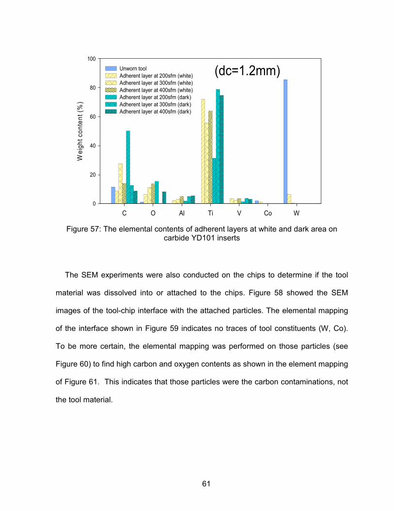
61

Figure 57: The elemental contents of adherent layers at white and dark area on

carbide YD101 inserts

The SEM experiments were also conducted on the chips to determine if the tool

material was dissolved into or attached to the chips. Figure 58 showed the SEM

images of the tool-chip interface with the attached particles. The elemental mapping

of the interface shown in Figure 59 indicates no traces of tool constituents (W, Co).

To be more certain, the elemental mapping was performed on those particles (see

Figure 60) to find high carbon and oxygen contents as shown in the element mapping

of Figure 61. This indicates that those particles were the carbon contaminations, not

the tool material.

C O Al Ti V Co W

We

igh

t c

on

ten

t (%

)

0

20

40

60

80

100

Unworn tool







(dc=1.2mm)

62

Figure 58: The SEM images of chip-tool interface of chips generated with carbide and

PCD1510 inserts.

Figure 59: Elemental content of chips with carbide and PCD1510 inserts for three

cutting speeds

Chip_PCD1510_61 m/min Chip_PCD1510_91 m/min Chip_PCD1510_122m/min

Chip_YD101_61 m/min Chip_YD101_122m/min Chip_YD101_91 m/min

attached particles

attached particles attached particles

attached particles

C Al Ti V W

Weig

ht

co

nte

nt

(%)

0

20

40

60

80

100

Bulk-Ti

Chip at 200sfm (PCD1500)



Chip at 200sfm (YD101)


Chip at 400sfm (YD101) (dc=1.2mm)

Chips

(PCD1510) (PCD1510) (PCD1510)

63

Figure 60: The SEM images of adhered particles on the chips.

Figure 61: Elemental content of adherent particles on the chips.

I.3.4 Chip morphology

Figure 62 presents SEM image of chip morphology with the carbide and PCD1510

inserts at three cutting speeds. The segmented chips were observed in all cutting

conditions with both carbide and PCD1510 inserts. Figure 63 presents five

parameters (height of peak, height of valleys, spacing of peaks, spacing of valleys,

and spacing of peak-to-valley) represented for chip morphology. The morphology of

Chip with PCD1510_122m/min Chip with YD101_122m/min

C O Al Ti V W

Weig

ht conte

nt (%

)

0

20

40

60

80

100

Particle on chip at 400sfm (PCD 1500)

Particle on chip at 400sfm (YD101)

(dc=1.2mm)

Chips(PCD1510)

High content of Ti from the background (chip)

64

chip generated with carbide and PCD1510 inserts was shown Figure 64. Statistical

analysis for height of peaks and valleys were presented in Figure 65 and Figure 66.

The higher height of peaks and valleys were found at the high cutting speed for both

carbide and PCD1510 inserts. The comparative data for chip morphology between

carbide and PCD1510 inserts was summarized in Figure 67. The carbide tool insert

showed segmented chips with higher peaks and shorter spacing of peaks as well as

spacing valleys (lower serrated frequency).

Figure 62: The chip morphology (top view).

Chip_PCD1510_

61 m/min Chip_PCD1510_

91 m/min

Chip_PCD1510_

122 m/min

Chip_YD101

_61 m/min

Chip_YD101_

122 m/min

100µµµµm

Chip_YD101

_91 m/min

65

Figure 63: Five parameters represented for chip morphology (side view)

Figure 64: Chip morphology with carbide and PCD1510 inserts at all cutting speeds

Height of valley

Spacing of peaks Height of peak

Spacing of valleys

Spacing of peak-to-valley

a) YD100 at 61 m/min b) YD100 at 91 m/min c) YD100 at 122 m/min

d) PCD1510 at 61 m/min e) PCD1510 at 91 m/min f) PCD1510 at 122 m/min

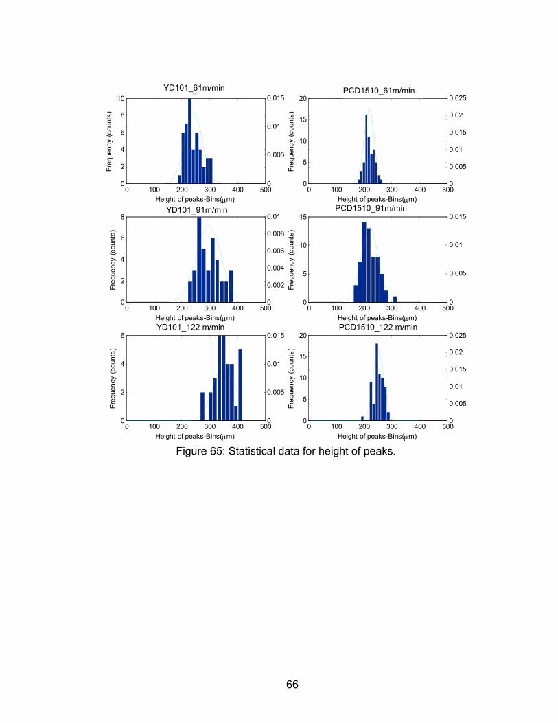
66

Figure 65: Statistical data for height of peaks.

0 100 200 300 400 5000

2

4

6

8

10YD101_200sfm

Fre

quency (

counts

)

Height of peaks-Bins(µm)

0

0.005

0.01

0.015

0 100 200 300 400 5000

5

10

15

20PCD1500_200sfm

Fre

quency (

counts

)


0

0.005

0.01

0.015

0.02

0.025

0 100 200 300 400 5000

2

4

6

8YD101_300sfm

Fre

quency (

counts

)


0

0.002

0.004

0.006

0.008

0.01

0 100 200 300 400 5000

5

10

15PCD1500_300sfm

Fre

quency (

counts

)


0

0.005

0.01

0.015

0 100 200 300 400 5000

2

4

6YD101_400sfm

Fre

quency (

counts

)


0

0.005

0.01

0.015

0 100 200 300 400 5000

5

10

15

20PCD1500_400sfm

Fre

quency (

counts

)


0

0.005

0.01

0.015

0.02

0.025

PCD1510_61m/min

YD101_91m/min PCD1510_91m/min

PCD1510_122 m/min YD101_122 m/min

YD101_61m/min

67

Figure 66: Statistical data for height of valleys.

0 100 200 300 400 5000

2

4

6

8

10YD101_200sfm

Fre

quency (

counts

)

Spacing of peaks-Bins(µm)

0

0.002

0.004

0.006

0.008

0.01

0 100 200 300 400 5000

5

10

15PCD1500_200sfm

Fre

quency (

counts

)


0

0.005

0.01

0.015

0 100 200 300 400 5000

2

4

6

8

10

12YD101_300sfm

Fre

quency (

counts

)


0

0.002

0.004

0.006

0.008

0.01

0 100 200 300 400 5000

5

10

15

20PCD1500_300sfm

Fre

quency (

counts

)


0

0.002

0.004

0.006

0.008

0.01

0.012

0 100 200 300 400 5000

2

4

6

8YD101_400sfm

Fre

quency (

counts

)


0

0.002

0.004

0.006

0.008

0.01

0 100 200 300 400 5000

2

4

6

8

10PCD1500_400sfm

Fre

quency (

counts

)


0

0.005

0.01

0.015

PCD1510_61m/min

YD101_91m/min PCD1510_91m/min

PCD1510_122 m/min YD101_122 m/min

YD101_61m/min

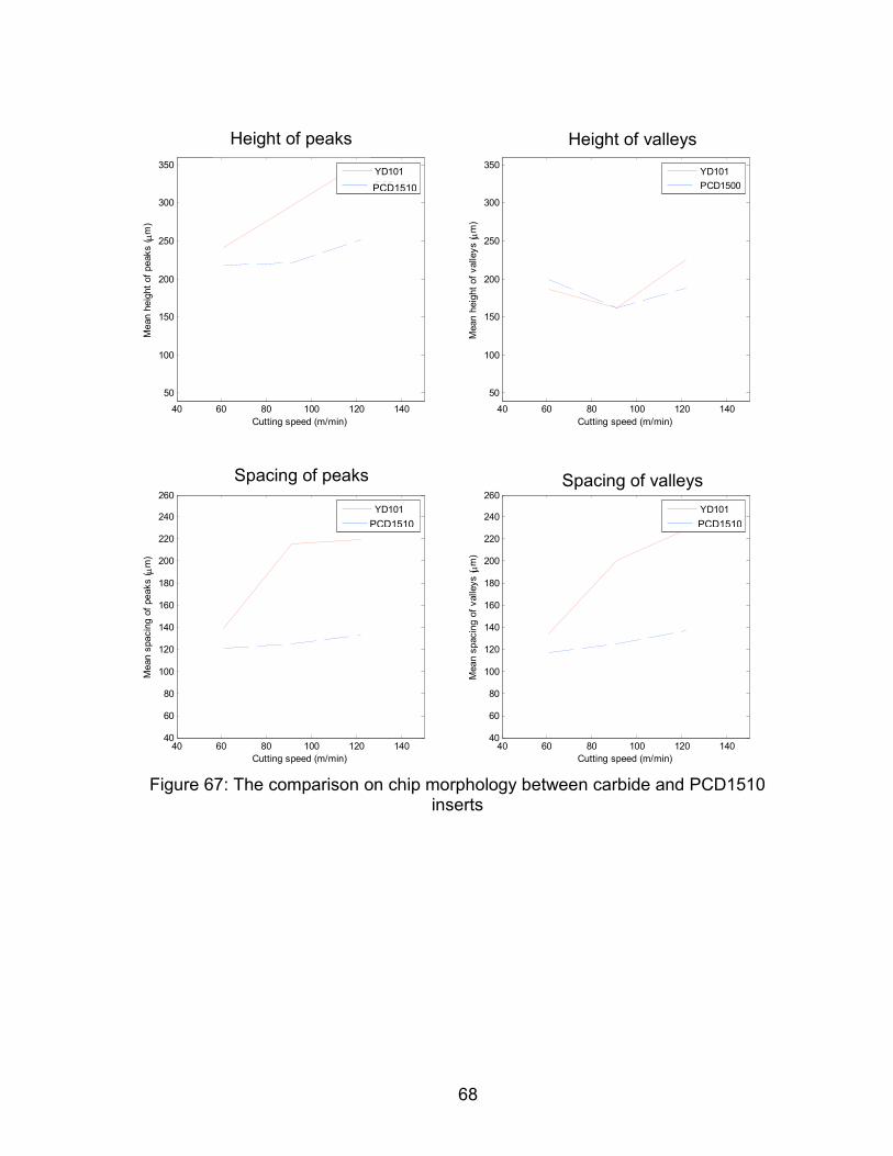
68

Figure 67: The comparison on chip morphology between carbide and PCD1510

inserts

40 60 80 100 120 140

50

100

150

200

250

300

350

Height of PeaksM

ean h

eig

ht

of

peaks (µm

)

Cutting speed (m/min)

YD101

PCD1500

40 60 80 100 120 140

50

100

150

200

250

300

350

Height of Valleys

Mean h

eig

ht

of

valleys ( µ

m)


YD101

PCD1500

40 60 80 100 120 14040

60

80

100

120

140

160

180

200

220

240

260Spacing of Peaks

Mean s

pacin

g o

f peaks (µ

m)


YD101

PCD1500

40 60 80 100 120 14040

60

80

100

120

140

160

180

200

220

240

260Spacing of Vaylleys

Mean s

pacin

g o

f valleys ( µ

m)


YD101

PCD1500

Height of peaks Height of valleys

Spacing of valleys Spacing of peaks

PCD1510

PCD1510 PCD1510

69

I.4 CUTTING TEMPERATURE PROFILES WITH FEM SIMULATION

I.4.3 2D-FEM with the Johnson-Cook (JC) model

The cutting temperature played a very important role in identifying the main wear

mechanisms involved in the cutting process. Both mechanical and thermochemical

wear (dissolution and diffusion) are functions of temperature which were discussed in

detail in Chapter 4. Thus, the temperature profiles along the chip thickness and rake

and flank faces on the workpiece needed to be determined. In spite of the

development of experimental techniques (thermocouple, infrared camera,

temperature indicating liquid, etc.), these techniques only measure in-situ local

temperatures. However, this study requires the estimation of temperature profiles on

both the tool and the workpiece. Therefore, Finite Element Analysis (FEA) software

was utilized. Many researchers have been using FEA simulation of cutting process to

predict the temperature distribution. This study also used 2D-FEM with the Johnson-

Cook (JC) model and Arbitrary Lagrangian-Eulerian (ALE) formulation to obtain the

temperature profile. The simulations were run with few sets of JC coefficients of the

Ti64 for comparison as shown in Table 6. However, the difference in the predicted

temperatures was minute. The developed model only simulated the case of

continuous chip as only rough estimation of the temperature profiles on tool and work

materials was required. The flow stress equation for the Johnson-Cook model is

given below.

(0.1) ( ) ( ) 0

0 0

, , 1 ln 1

m

n

m

T TT A B C

T T

εσ ε ε ε

ε

− = + + − −

&&

&

70

where:

and the Johnson-Cook coefficients:

Note there is no temperature effect to flow stress at melting

temperature.

Table 6: Johnson-Cooks coefficients for Ti-6Al-4V

Tm (°°°°C) A (Mpa) B (Mpa) C n m References

1650 880 695 0.04 0.36 0.8 This study [Meyer, 1998]

1650 870 990 0.028 0.25 0.8 Shivpuri et. al. [2002]

1630 783 498.4 0.028 0.28 1.03 Ozel et. al. [2004]

1600 870 990 0.008 1 1.4 Umbrello et. al. [2007]

1656 863 656 0.013 0.5 0.8 Meijer et. al. [2001]

( )( )

( )( )

1

1

0

: the plastic strain

: the strain rate

: the reference plastic strain rate ,

: the temperature of the work material °C ,

: the melting temperature of the work material 1399 °C

: th

m

s

s

T

T

T

ε

ε

ε

−

−

&

&

( )e room temperature 20 °C

: the initial yield strength (MPa)

: the hardening modulus (MPa)

: the strain rate sensitivity coefficient

: the hardening coefficient

: the thermal softening coefficient.

A

B

C

n

m

( ), , 0mTσ ε ε = →&

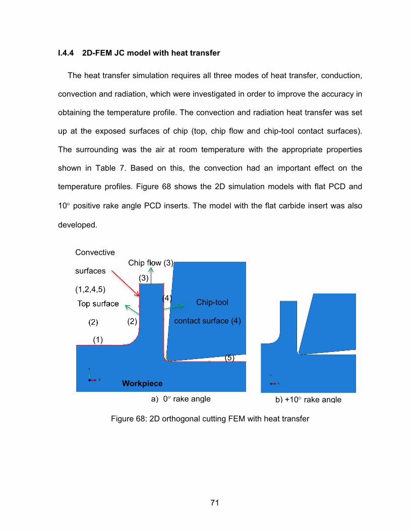
71

I.4.4 2D-FEM JC model with heat transfer

The heat transfer simulation requires all three modes of heat transfer, conduction,

convection and radiation, which were investigated in order to improve the accuracy in

obtaining the temperature profile. The convection and radiation heat transfer was set

up at the exposed surfaces of chip (top, chip flow and chip-tool contact surfaces).

The surrounding was the air at room temperature with the appropriate properties

shown in Table 7. Based on this, the convection had an important effect on the

temperature profiles. Figure 68 shows the 2D simulation models with flat PCD and

10° positive rake angle PCD inserts. The model with the flat carbide insert was also

developed.

Figure 68: 2D orthogonal cutting FEM with heat transfer

Tool

Top surface

(2)

a) 0° rake angle b) +10° rake angle

Convective

surfaces

(1,2,4,5)

Workpiece

Chip flow (3)

Chip-tool

contact surface (4)

(1)

(2)

(3)

(4)

(5)

72

Table 7: The parameters of air at 20°C and 1atm

The heat transfer coefficient for free convection to the air was 5–25 (W/m2K) while

the value for forced convection was 10-200 (W/m2K). In this simulation, the forced

convection was appropriate because of the chip travels up to 2.03 m/sec

approximated by the cutting speed. Table 8 reports the value for heat transfer

coefficients for each cutting speed calculated based on Reynolds, Nusselt, Pardtl

number, and chip flow using the equations (1.2) to (1.7).

(0.2)

(0.3)

(0.4)

Temperature DensitySpecific heat

capacity

Kinematic

viscosity

Thermal

conductivity

T (K) ρ (kg/m3) Cp (kJ/kg.K)

µ.107

(Ns/m3)

ν.106 (m

2/s)

k.103

(W/m.K)

α.106

(m2/s)

293.5 K 1.1614 1.0007 184.6 15.89 26.3 22.5

Local heat flux :

2( ) /sq h T T W m∞′′ = −

Total heat rate :

[ ]( )

( ) ;

s ss s s

A A

s s

q q dA T T hdA W

or

q hA T T

∞

∞

′′= = −

= −

∫ ∫

The average heat transfer coefficient :

1

ss

As

h hdAA

= ∫

73

The average heat transfer coefficient:

(0.5)

Reynolds number:

(0.6)

Nusselt number:

(0.7)

Table 8: Reynolds, Nusselt number, and heat transfer coefficients for three cutting speeds

Although the majority of the heat generated during the process was from plastic

deformation, the simulation results showed that the friction has some influence on the

temperature profile. The comparison of chip-tool contact length between experiment

data and those of the simulation model was made to determine a reasonable friction

coefficient to be used in this model.

I.4.5 Cutting temperature profiles with 2D-FEM simulation

The temperature profiles on the chip along the rake face and through the thickness

of the chip were the main interest. Figure 69 plots the temperature profile along the

LNu kh

L

⋅=

ReLu L u Lρν µ∞ ∞= =

( ) ( )1/2 1/30.664 Re PrL LNu = ⋅

Chip flow

(m/min)

Chip flow

(m/sec)

Chip's Length

(m)

Reynolds

number

Nusselt

numberh_avg

61 1.02 m/sec 0.0010 64.0 4.7 124.4

91.001.52 m/sec 0.0010 95.4 5.8 152.0

122.002.03 m/sec 0.0010 128.0 6.7 176.0

74

rake face starting at the end-point of the round corner (see Figure 69) with the friction

coefficient set at 0.8. The simulation results were adequate with the high temperature

profile for the high cutting speed. The maximum temperatures did not happen at the

cutting edge. The effects of heat transfer are reported in Figures 70-72 which show a

significant reduction of temperature. The maximum temperature from the simulations

without the heat transfer was along rake face while the simulations with the heat

transfer showed the maximum temperature close to the shear bands presented in

other publications [Sima, 2010; Y. C. Zhang, 2011; X. Zhang, 2011] with segmented

chips.

Figure 69: Temperature profiles on the chip along tool-chip interface with PCD

500

600

700

800

900

1000

1100

1200

0.0

3.9

31

.4

58

.9

86

.4

11

3.9

14

1.4

16

8.9

19

6.4

22

3.9

25

1.4

27

8.9

30

6.4

33

3.9

36

1.4

38

8.9

41

6.4

44

3.9

47

1.4

49

8.9

52

6.4

55

3.9

Tem

pe

ratu

re (°C

)

Distance from the end point (mm)

Temperature profile in the chip along rake face (µ=0.8)

122m/min

91m/min

61min/min

Temperature along this curve

End- point of the round corner

Cutting edge

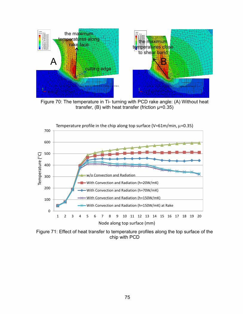
75

Figure 70: The temperature in Ti- turning with PCD rake angle: (A) Without heat

transfer, (B) with heat transfer (friction µ=0.35)

Figure 71: Effect of heat transfer to temperature profiles along the top surface of the

chip with PCD

0

100

200

300

400

500

600

700

1 2 3 4 5 6 7 8 9 10 11 12 13 14 15 16 17 18 19 20

Tem

pe

ratu

re (°C

)

Node along top surface (mm)

Temperature profile in the chip along top surface (V=61m/min, µ=0.35)

w/o Convection and Radiation

With Convection and Radiation (h=20W/mK)



With Convection and Radiation (h=150W/mK) at Rake

B

the maximum temperatures close

to shear band

A

the maximum temperatures along

rake face

cutting edge

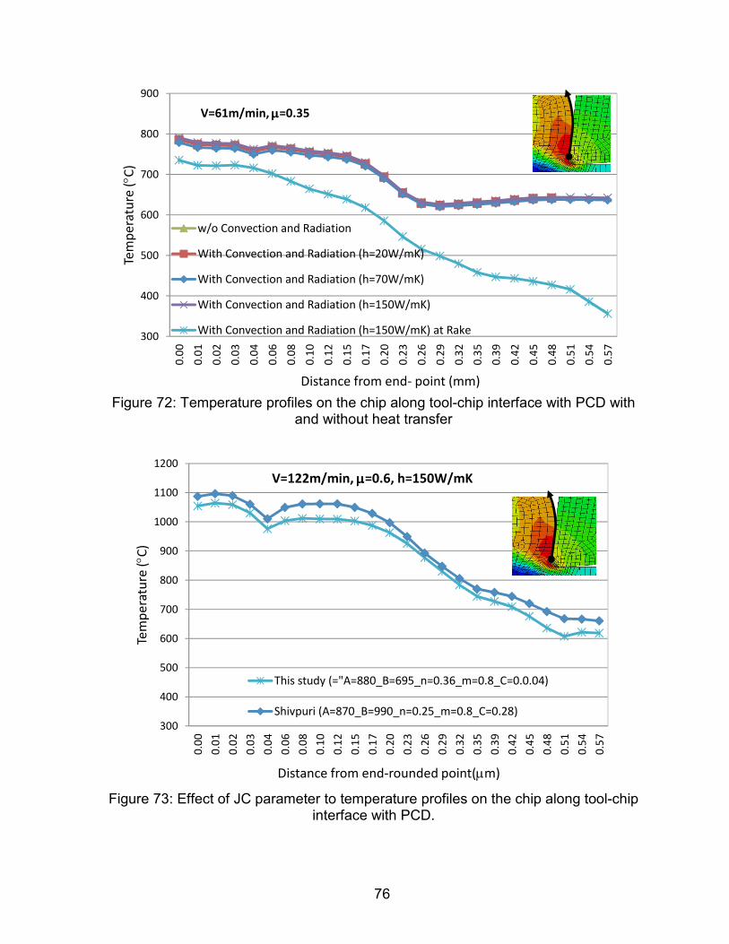
76

Figure 72: Temperature profiles on the chip along tool-chip interface with PCD with

and without heat transfer

Figure 73: Effect of JC parameter to temperature profiles on the chip along tool-chip

interface with PCD.

300

400

500

600

700

800

900

0.0

0

0.0

1

0.0

2

0.0

3

0.0

4

0.0

6

0.0

8

0.1

0

0.1

2

0.1

5

0.1

7

0.2

0

0.2

3

0.2

6

0.2

9

0.3

2

0.3

5

0.3

9

0.4

2

0.4

5

0.4

8

0.5

1

0.5

4

0.5

7

Tem

pe

ratu

re (°C

)

Distance from end- point (mm)

V=61m/min, µµµµ=0.35

w/o Convection and Radiation




With Convection and Radiation (h=150W/mK) at Rake

300

400

500

600

700

800

900

1000

1100

1200

0.0

0

0.0

1

0.0

2

0.0

3

0.0

4

0.0

6

0.0

8

0.1

0

0.1

2

0.1

5

0.1

7

0.2

0

0.2

3

0.2

6

0.2

9

0.3

2

0.3

5

0.3

9

0.4

2

0.4

5

0.4

8

0.5

1

0.5

4

0.5

7

Tem

pe

ratu

re (°C

)

Distance from end-rounded point(µm)

V=122m/min, µµµµ=0.6, h=150W/mK

This study (="A=880_B=695_n=0.36_m=0.8_C=0.0.04)

Shivpuri (A=870_B=990_n=0.25_m=0.8_C=0.28)

77

Figure 74 represents the significant effects of the friction coefficient in FE

simulation on the temperature profile along the rake face. To estimate the reasonable

friction coefficients for FEM simulation, the chip-tool contact lengths between

simulation results and experiments were compared. These values of experiment

were approximated by the maximum width of crater wear on the rake face of inserts.

The simulated results shown in Figure 75 also indicate that the chip-tool contact

length depended strongly on the friction coefficient. There was a small difference in

the length among three cutting speeds. As shown in Figure 75, the chip-tool contact

length of PCD and PCD+10° in the turning test was most likely close to those of the

simulation model with the friction coefficients of 0.6. For the simplicity, 0.6 was used

as friction coefficients for both PCD. The simulated temperature for all cutting speed

with friction coefficient of 0.6 was shown in Figure 76. The temperatures at tool-chip

interface were above transus temperature at medium and high cutting speed. The

maximum cutting temperatures of 2D FEM simulation with carbide insert were

reported at least 100 °C higher than those PCD at all cutting speeds [Schrock, 2012].

This thesis accepted that results although the FEM model was simulated without heat

transfer.

78

Figure 74: Temperature profiles on the chip along tool-chip interface with PCD at

various friction coefficients

Figure 75: The chip contact length from experiment and simulation of PCD at various

friction values

500

600

700

800

900

1000

1100

0.0

3.9

31

.4

58

.9

86

.4

11

3.9

14

1.4

16

8.9

19

6.4

22

3.9

25

1.4

27

8.9

30

6.4

33

3.9

36

1.4

38

8.9

41

6.4

44

3.9

47

1.4

49

8.9

52

6.4

55

3.9

Tem

pe

ratu

re (°C

)

Distance from end-point (mm)

V=61 m/min

0.8 friction 0.6 friction 0.35 frictionµ=0.8 µ=0.3µ=0.6

0.00

0.05

0.10

0.15

0.20

0.25

0.30

0.35

0.40

0.45

400sfm 300sfm 200sfm

Co

nta

ct le

ng

th (

mm

)

Cutting Speed (sfm)

Chip- Tool contact length vs. friction

0.35 friction 0.6 friction 0.8 friction PCD PCD10µ=0.35 µ=0.6 µ=0.8

122m/min 91m/min 61m/min

79

Figure 76: Temperature profiles on the chip with PCD inserts and µ=0.6 at various

cutting speeds.

400

500

600

700

800

900

1000

1100

0 0.1 0.2 0.3 0.4 0.5 0.6

Te

mp

era

ture

(°C

)


a) Temperature profile in the chip along tool-chip interface with PCD

(µ=0.6)

122 min/min

91 m/min

61 m/min

Transus temperature

400

500

600

700

800

900

1000

1100

0 0.05 0.1 0.15 0.2 0.25 0.3 0.35 0.4

Tem

pe

ratu

re (°C

)


b) Temperature profile in the chip along shear band with PCD (µ=0.6)

122 min/min

91 m/min

61 m/min

Transus temperature

80

Chapter 2: Evidence of phase change and root causes flank wear

and scoring marks with orientation imaging microscopy (OIM)

II.1 OIM SETUP FOR CRYSTAL ORIENTATION IN TI64 ALLOY AND CHIPS

To explain the wear mechanism on both rake and flank face, the microstructure of

Ti workpiece (before machining, to be called Bulk-Ti) and after machining (chip) was

investigated with Orientation Imaging Microscopy (OIM) based upon electron-

backscattered diffraction (EBSD). Two samples (Sample A and Sample B) were cut

out from the Bulk-Ti to study the microstructure before machining in DOC and feed

rate directions as shown in Figure 77a. The microstructure in the YZ plane is noted to

be Sample A (in Feed direction) while that in the XY plane is Sample B (in DOC

direction). To accurately obtain the original structure of the work material and limit

effects deformation and heat-affected zones and heat of the cutting process, Wire

Electron Discharge Machining (EDM) was applied to cut off these samples from the

round bar of Ti workpiece. With Wire-EDM cutting, the heat-affected zones from the

process can be easily removed [Hasçalık, 2007]. After polishing, EBSD scans were

conducted at various locations on both samples. With the Bulk-Ti samples, the EBSD

was scanned on the region of 800µmx800 µm, step size 2 µm, exposed time of

0.13sec. To have the reliable data, EBDS was conducted at various regions (named

A1, A2, A3, B1, B2, B3) on both samples as showed in Figure 77a.

81

Figure 77: Samples for EBSD of material before (Bulk-Ti) and after (Chip) machining

The microstructures of chips generated with carbide and PCD inserts at all speeds

were investigated to compare with those of bulk-Ti as shown in Figure 77b. The

difference in the microstructures between bulk-Ti and chip contains the information

about cutting temperature, stress, plastic deformation, phase change, etc. The

scanned regions of 200µm x 200µm were taken on the chips with step size 1µm and

exposed time of 0.13sec.

The EBSD studies shown in Figure 78 were carried out using a CamScan 44 FE

scanning electron microscope, with a field emission gun operated at 20 kV using

Z

Y

Bulk-Ti

X

Y

Sample

A

Feed direction

X

Z

Sa

mp

le B

Sample A

(YZ plane)

A1

A2

A3

B1

B2

Sample A & B in

Bulk-Ti

Sample B

(XY plane)

B3

a) Bulk -Ti

Lateral side of chips

Chips (PCD, dc=0.635 mm)

YD101

PCD

b) Chip

Chips (dc=1.2 mm)

Chip

Top of chip

tool-chip interface

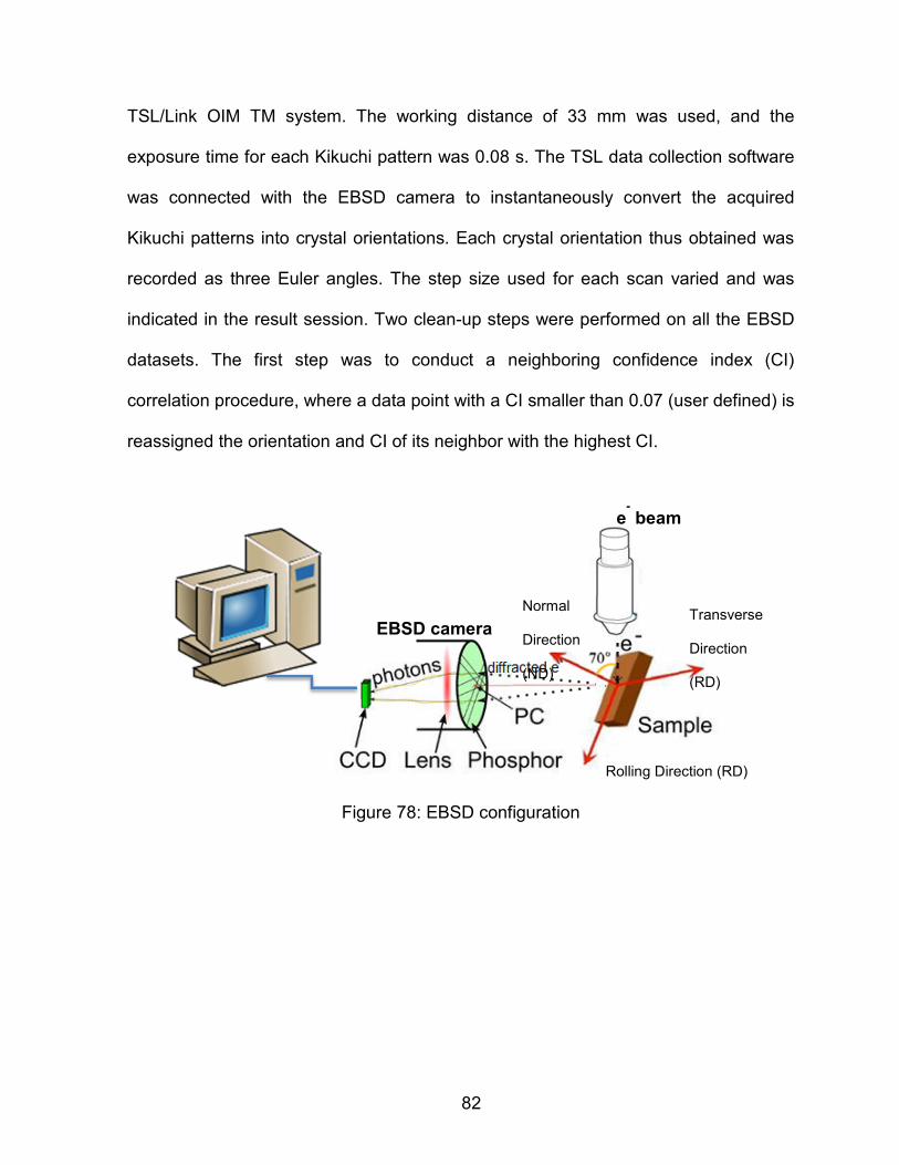
82

TSL/Link OIM TM system. The working distance of 33 mm was used, and the

exposure time for each Kikuchi pattern was 0.08 s. The TSL data collection software

was connected with the EBSD camera to instantaneously convert the acquired

Kikuchi patterns into crystal orientations. Each crystal orientation thus obtained was

recorded as three Euler angles. The step size used for each scan varied and was

indicated in the result session. Two clean-up steps were performed on all the EBSD

datasets. The first step was to conduct a neighboring confidence index (CI)

correlation procedure, where a data point with a CI smaller than 0.07 (user defined) is

reassigned the orientation and CI of its neighbor with the highest CI.

Figure 78: EBSD configuration

Rolling Direction (RD)

Normal

Direction

(ND)

Transverse

Direction

(RD)

EBSD camera

e-

beam

83

II.2 OIM RESULTS AND DISCUSSION

II.2.1 Evidence of phase change (α →→→→β) in machining of Ti64

The OIM scan of the microstructure is very important to indicate the indirect

evidence of phase change of titanium in the cutting process. Based on the average

results of six scan areas (A1, A2, A3, B1, B1, B2, B3) on the Bulk-Ti sample as

shown in Figure 79, the microstructure before machining was mostly the alpha phase

accounting for up to 99% of area fraction with the rest being the β-phase as

summarized in Table 9. The distribution of α-grain size in samples A and B was

plotted in Figure 80. It should be emphasized that that the average grain sizes of α-

phase and β-phase in the Bulk-Ti samples were 6.78 µm and 3.89µm, respectively.

However, the grain size in chips was much smaller, as shown in Figure 81. This was

likely the result of high deformation and recrystallization near the cutting zone on the

chips. The lateral side (see Figure 77b) of the chip recrystallized more than the chip-

tool interface as evident by the much smaller grain size on the side of chips. Only

small differences in the average grain size in relation to the cutting speeds and tool

materials were evident.

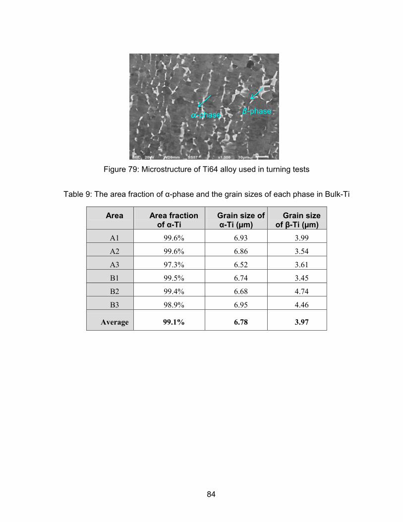
84

Figure 79: Microstructure of Ti64 alloy used in turning tests

Table 9: The area fraction of α-phase and the grain sizes of each phase in Bulk-Ti

Area Area fraction of α-Ti

Grain size of α-Ti (µm)

Grain size of β-Ti (µm)

A1 99.6% 6.93 3.99

A2 99.6% 6.86 3.54

A3 97.3% 6.52 3.61

B1 99.5% 6.74 3.45

B2 99.4% 6.68 4.74

B3 98.9% 6.95 4.46

Average 99.1% 6.78 3.97

aaaa-phase bbbb-phase

85

Figure 80: Grain size distribution of α-Ti in un-deformed work material (Bulk-Ti)

Figure 81: The comparison of average diameter of grains in the bulk-Ti and in the

deformed material (chips).

In Ti machining, the evidence of phase change is not easy to prove. Due to the

low thermal conductivity, the temperatures of chip are expected to be higher than the

transus temperature (Ts) at which the phase transformation (α to β) occurs. At

Grain Size (µm)

0 10 20 30 40 50 60 70

Are

a f

rac

tio

n (

%)

0

2

4

6

8

10

12

14

16

Region A1

Region A2

Region A3

Bulk-Ti (sample A)

α−Ti grains

Grain Size (µm)

0 10 20 30 40 50 60

Are

a f

rac

tio

n (

%)

0

5

10

15

20

25

30

35

Region B1

Region B2

Bulk-Ti (sample B)

α−Ti grains

alpha-crystals beta-crystals

Av

era

ge

Dia

me

ter

( µm

)

0

2

4

6

8

10

Bulk- Ti

Chip at 200sfm (PCD)



(dc=.635mm)

alpha-crystals beta-crystals

Av

era

ge

Dia

me

ter

( µm

)

0

2

4

6

8

10

Bulk- Ti







(dc=1.2mm)

Microstructure on the lateral side of chip

Microstructure on tool-chip interface of

chip

86

atmospheric pressure, the α-phase in Ti64 transformed to the β-phase when the

temperature increased above Ts = 995°C. The β-phase transformed back to the α-

phase when the temperature was cooled to below Ts. However, due to the low

thermal conductivities, the chips cooled slowly. This process helped the most of β-

phase to have enough time to transform back to the α-phase. Therefore, the amount

of β-phase formed during the cutting process cannot be determined directly. Because

the β→α transformation has a well-defined interphase misorientation relationship, it is

possible to see evidence of α →β phase by determining the misorientations in the α

phase.

In a polycrystalline material, the misorientation is defined as the difference in

crystallographic orientation between two adjacent crystals. When Ti64 is slowly

cooled below the beta transus temperature, α-plates form with their base planes

parallel to the transformation planes (110) of the β-phase as shown in Figure 82. The

α-plates grow relatively slowly in perpendicular direction to the planes and much

faster along the planes making acicular (plate-like) structures (see Figure 83).

Because of the symmetry of the β-phase, the transformation planes are oriented 60°

& 90° to each other resulting in alpha grains with precisely 60° & 90° misorientation

as shown in Figure 82. A high fraction of boundary in the α-phase with 60° & 90°

misorientations indicates proof of the phase change roughly.

87

Figure 82: Burgers’ orientation relationship in β → α transformation

Figure 83: Microstructures achieved at various intermediate temperatures by slowly

cooling from above the β transus

β-phase

α-phase

(110)

(110)

(110)

(110)

basal plane

90° misorientation

60° misorientation

88

Figure 84 shows the higher peak of 60° and 90° misorientations in the chips than

those in un-deformed work material. In addition, the portions of the β-phase in the

chips were greater than those in Bulk-Ti as presented in Figure 85. This evidence

provides a strong indication of the phase change during cutting process. It should be

noted that the determination of the phase change is valuable in predicting the

diffusion/dissolution wear. In observing the chips between low and high DOCs, a

higher fraction of the β-phase and the higher peak of 60° and 90° misorientations

with low DOC were observed. However, OIM scans were conducted on the side and

tool-chip interface of chips for low and high DOC, respectively. One possible

explanation is the higher and more uniform temperatures at the chip-tool interface

while the temperatures on the side were closer to the transus temperature and the

temperature gradients were greater due to the faster cooling on this side. The fast

cooling process retains more β-phase in the chip. 3D FEM simulation which was not

presented in this thesis may reveal the difference in terms of temperatures with two

DOCs in order to have a more convincing explanation. Figure 86 shows the

distribution of the β-phase among the α-phase in the underside of the chip at high

DOC for both carbide and PCD inserts for three cutting speeds. It was interesting to

see that, at high DOC, the β-phase crystals were distributed mostly at shear band

where the temperature was reported highest in most FEM simulation with serrated

chips.

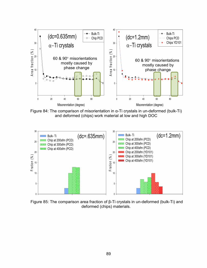
89

Figure 84: The comparison of misorientation in α-Ti crystals in un-deformed (bulk-Ti)

and deformed (chips) work material at low and high DOC

Figure 85: The comparison area fraction of β-Ti crystals in un-deformed (bulk-Ti) and

deformed (chips) materials.

Fra

tio

n (

%)

0

5

10

15

20

25

30

Bulk- Ti




(dc=.635mm)

Fra

tio

n (

%)

0

5

10

15

20

25

30

Bulk- Ti







(dc=1.2mm)

Misorenntation (degree)

0 20 40 60 80

Are

a f

rac

tio

n (

%)

0

10

20

30

40

Bulk-Ti

Chip PCD(dc=0.635mm)

α−Ti crystals

60 & 90° misorientations mostly caused by

phase change

(dc=1.2mm)

Misorenntation (degree)

0 20 40 60 80

Are

a f

rac

tio

n (

%)

0

10

20

30

40

Bulk-Ti

Chips PCD

Chips YD101α−Ti crystals

60 & 90° misorientations mostly caused by

phase change

90

Figure 86: The distribution of the β-Ti (dark) and the α-Ti (colored) in the chips at

high DOC.

II.2.2 Root causes flank wear and scoring marks in Ti alloys machining

Scoring marks were typically found on the flank wear in machining of Ti alloys

[Bermingham, 2011; Dearnley, 1986; Hughes, 2004; Narutaki, 1983; Venugopal,

2007; Wright, 1981] as shown in Figure 87. This section mainly focuses on the

microstructure of a work material in an attempt to determine the root cause for flank

wear and scoring marks on flank face.

β-Ti

PCD1510 at 61 m/min PCD1510 at 91 m/min PCD1510 at 122m/min

YD101 at 61 m/min YD101 at 91 m/min YD101 at 122m/min

91

Figure 87: Scoring marks on flank face of inserts in machining of Ti alloys

The α-Ti has the characteristic anisotropy in mechanical properties. The hardness

of α-Ti in the c-direction (0001) was reported to be much harder (~1.5 time) than any

other directions [Britton, 2009; Kwon, 2013]. Figure 6 shows the anisotropy in

hardness. Based on these data, the α-Ti with the c-axis within ±20° interacting with

the wear land of the inserts was chosen as the grains with ‘hard’ orientations or the

‘hard’ α-grains respect to the inserts. During machining, the tool will be worn or

damaged when the ‘hard’ α-grains interacts with the tool surfaces.

Venugopal, 2007 Bermingham, 2011 Narutaki, 1983

Dearnley, 1986 Wright, 1981

Hughes, 2004

92

Figure 88: Hardness of α-Ti as a function of the declination angles between c-axis to

vertical line [after Britton, 2009] and the ‘hard’ α-grains respect to flank face.

The results of EBSD scan showed that Bulk-Ti consists mostly of the α-Ti.

Therefore, the anisotropy in hardness of α-grain had significant effect to wear. As

shown in Figure 89, Sample A shows the distribution of the hard-orientation grains

considering the hard orientation within 90±20° to the rake face. It shows that the

clusters of hard α-grains in the Y-Z plane (the declination angle within ±20°) are

distributed in the direction of Z. Sample B has the hard-orientation grains

agglomerate more less at the 30° from the negative Y axis as shown in Figure 89.

Average

c-axis

‘hard’ αααα-grains

Tool

Flank face

93

Figure 89: The distribution of α-crystal in hard orientation (red color) in Bulk-Ti sample respected to flank face of tool along feed direction

The interaction with the tool in the hard α-grains can cause the abrasion, chipping

and the fracture. The size of the fracture may depend on the size of α-clusters in the

Bulk-Ti as well as the detailed interaction conditions (e.g. impact angle and

orientation). Table 10 summarizes the average dimensions of the ‘hard’ α-clusters

based on the microstructures in both XY and YZ faces. Based on these OIM

measurements, the size of the ‘hard’ α-clusters is roughly estimated and represented

in Figure 90. In this particular microstructure, the ‘hard’ α-cluster can be easily

approximated into an ellipsoid. Figure 91 shows how an ellipsoidal hard α-cluster

interacts with the flank surface, generating the flank wear. In addition, the ‘hard’

clusters happen to be in a certain plane, horizontally on the YZ face and on the 30°-

orientation on the XY face. Machining the same ‘hard’ α-cluster range in the Bulk-Ti,

however, the much harder PCD insert has much better wear resistance, resulting in

A1

A2

B1

B2

c-axis

α-Ti

90°

rotation

X

Y

Z

Bulk-Ti workpiece

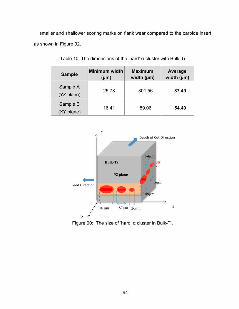
94

smaller and shallower scoring marks on flank wear compared to the carbide insert

as shown in Figure 92.

Table 10: The dimensions of the ‘hard’ α-cluster with Bulk-Ti

Sample Minimum width

(µm)

Maximum

width (µm)

Average

width (µm)

Sample A

(YZ plane) 25.78 301.56 87.49

Sample B

(XY plane) 16.41 89.06 54.49

Figure 90: The size of ‘hard’ α cluster in Bulk-Ti.

301µm 87µm 26µm

89µm

54µm

16µm

30° Bulk-Ti

Feed Direction

Depth of Cut Direction

Y

Z

X

YZ plane

95

Figure 91: Interaction of the ‘hard’ α-cluster and the inserts.

Figure 92: The scoring marks on the carbides and PCD inserts at low DOC

Obviously, because of the flank temperature being much lower than the crater

temperature and the ‘rough’ wear surface, the dissolution and diffusion rate is not

significant for the flank wear. Discounting the macro-fractures which may be more

YD101_91m/min

5min0sec YD101_91m/min

7min0sec

PCD1200_122m/min_4min0sec

100µm

YD101_91m/min

4min10sec

YD101_122m/min

7min0sec PCD1200_61m/min 6min0sec

96

related to the microstructural variations, two distinct types of steady-state wear

patterns were identified, (a) micro-fracture at the cutting edge and (b) scoring marks.

Both types of damage can be caused by the “hard” α-phase grains and clusters.

However, micro-fracture can be affected by additional mechanisms, the adhesion and

detachment of the work material. These two patterns on the flank face manifest

themselves into four main types of observed damage presented in Table 11. Type I

is the micro-fracture which occurs near the cutting edge most likely as a result of the

impact with the ‘hard’ grain or cluster, which are observed only on the PCD inserts.

Type II occurred near the cutting edge in both carbide and PCD. The distinction

between Type I and II is the inverted shape of the fracture.

Both Types I and II are expected to be caused by the larger ‘hard’ α-clusters in a

work material. Because the incidences of Type I damage are much rare and only

occurred to the PCD inserts in our experiment, more detailed interaction conditions

must be explained with the adhesion layer. Many researchers [Dhar, 2002; Ezugwu,

1997; Hartung, 1982; Rahman, 2003] reported that Ti adheres to a tool material,

which leads to the chipping when detached. Our observations indicated that not only

was the adhesion on carbide inserts substantially more extensive than PCD inserts

but the adhesion layers were also mostly located on the crater surface as shown in

Figure 93. Consequently, the cutting edge of the carbide inserts was more

extensively damaged while the edge of the PCD inserts remained sharper. The

difference in the adhesion layer between carbide and PCD inserts enabled Type I to

cause damage on PCD inserts. With Type II, additional damage may occur as the

loose fragments can further damage the surface evident by the damage at the trailing

97

end of the fracture. Type III was the scoring marks abraded by the ‘hard’ α-grains or

cluster. Type IV was the combination of the first and third types of damage. Besides

of Type III, the more common damage on PCD inserts were Type I and II while those

of carbides were Type II and IV.

Table 11: Typical damage on the flank face

Typical damage Explanation

Type I

Micro-fracture by the Impact of the hard α-cluster only on PCD

Type II

Micro-fractures by the Impact of the hard α-cluster

Type III

Scoring marks caused by the ‘hard’ α-crystal or cluster.

Type IV The Combination of Type I and

Type III

98

Figure 93. Adhesion layer on the rake face of carbide and PCD inserts

The scoring marks, Type II damage, were much more prevalent than any other

types on both carbide and PCD inserts. However, the scoring marks on the carbides

were not as distinct as those of PCD. Our hypothesis is that all four types of damage

were caused by the ‘hard’ α-crystals and the adhesion may enhance Type I and II

damage. To substantiate this claim, the widths were measured for at least ten scoring

marks on both carbide and PCD inserts at various cutting lengths as shown in Figure

94. The distribution of width was presented using a ‘box and whisker’ plot with the

minimum, maximum and average width as shown in Figure 95 for low DOC and

Figure 96 for high DOC. These data were compared to the size range of the ‘hard’ α-

clusters obtained in Sample B (mostly close to tool flank face) shown in the light gray

boxes in Figures 95 and 96. Notice that the widths of the damage were substantially

smaller as only a smaller part of each ellipsoidal cluster interacts with the tool during

the abrasion process. The width of the scoring marks was larger with longer cutting

distance for both carbide and PCD tool as demonstrated in Figures 95 and 96 as the

probability of encountering larger clusters increases. Typically wider scoring marks

PCD_200sfm_

5.4min

PCD_91

m/min_5.4min

PCD_400sfm_

3.5min

YD101_200sfm

_6.8min

YD101_400sfm_

2.2min

YD101_91

m/min_4.5min

YD101_unworn

PCD_unworn

Adhesion

layer

Adhesion

layer

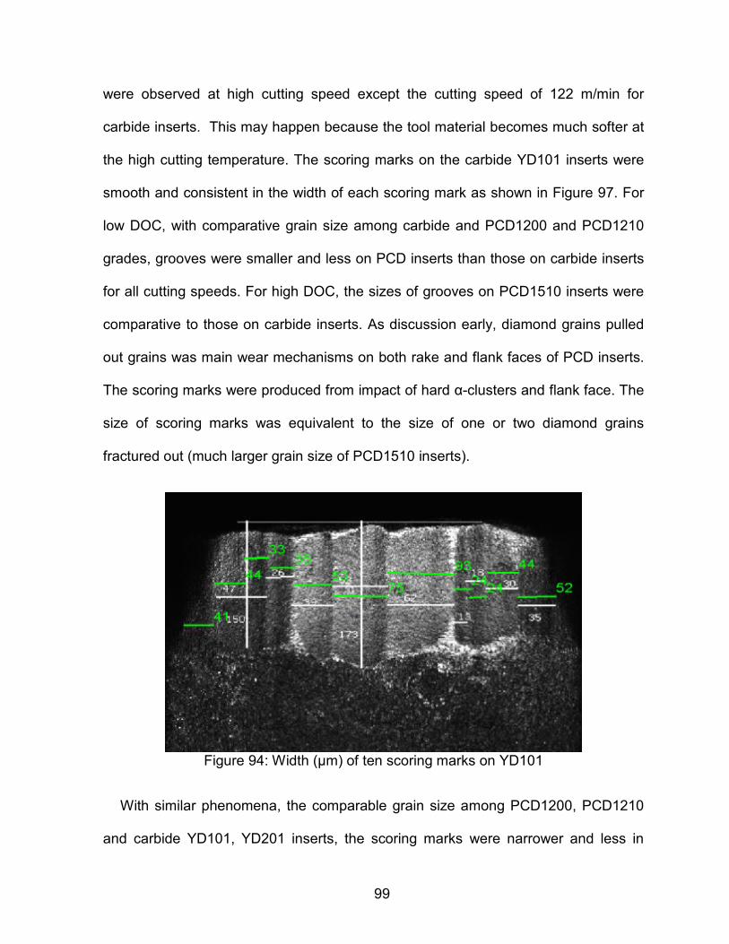
99

were observed at high cutting speed except the cutting speed of 122 m/min for

carbide inserts. This may happen because the tool material becomes much softer at

the high cutting temperature. The scoring marks on the carbide YD101 inserts were

smooth and consistent in the width of each scoring mark as shown in Figure 97. For

low DOC, with comparative grain size among carbide and PCD1200 and PCD1210

grades, grooves were smaller and less on PCD inserts than those on carbide inserts

for all cutting speeds. For high DOC, the sizes of grooves on PCD1510 inserts were

comparative to those on carbide inserts. As discussion early, diamond grains pulled

out grains was main wear mechanisms on both rake and flank faces of PCD inserts.

The scoring marks were produced from impact of hard α-clusters and flank face. The

size of scoring marks was equivalent to the size of one or two diamond grains

fractured out (much larger grain size of PCD1510 inserts).

Figure 94: Width (µm) of ten scoring marks on YD101

With similar phenomena, the comparable grain size among PCD1200, PCD1210

and carbide YD101, YD201 inserts, the scoring marks were narrower and less in

100

number for PCD inserts than those for carbide insert for all cutting speeds due to the

superior hardness of the PCD. For PCD inserts, the width of scoring marks was more

independent of cutting speed. PCD inserts have much higher hardness than the

carbide inserts and the ‘hard’ α-grain (6000kgf/mm2 for PCD, 1800kgf/mm2 for

carbides [Groover, 2007] and 550kgf/mm2 for α-grain in hard orientations [Britton,

2009] at room temperature) while their transverse rupture strength and fracture

toughness of PCD (1550MPa and 6.86MPa�m1/2 [Lammer, 1988]) were lower than

those of carbide insert (3133MPa and 10.18MPa�m1/2 [Fang, 2005]). Most of scoring

marks on PCD were rough with uneven width (and depth) as the pulled-out diamond

grains can abrade the tool surface, as shown in Figure 98. In addition, PCD inserts

were more prone to micro-fracture than the carbide inserts, an indication of lower

fracture toughness of PCD. The similar phenomenon was observed on the rake face

reported in [Schrock, 2014]. At high cutting speed, the micro-fractures are more

frequent and larger to suppress the appearances of the scoring marks on flank wear.

There is no difference between flat and positive tool in term of scoring marks due to

the end relief angle is the same for both inserts.

101

Figure 95: Range and distribution of width of scoring marks of nose at low DOC

respect to ‘hard’ α-cluster size

0

20

40

60

80

100

120

140

Wid

th o

f scoring

mark

s (

µm

)

a) Vc = 61m/min, DOC = 0.635 mm

hard α-Ti range 2Q Box 3Q Box Mean

0

20

40

60

80

100

120

140

Wiid

th o

f scoring

mark

s (

µm

)

b) Vc = 91 m/min, DOC = 0.635 mm


0

20

40

60

80

100

120

140

Wiid

th o

f scoring

mark

s (

µm

)

c) Vc = 122m/min, DOC = 0.635 mm


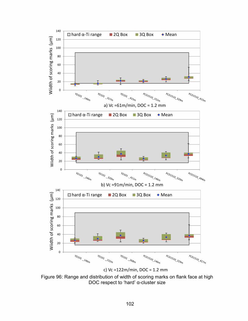
102

Figure 96: Range and distribution of width of scoring marks on flank face at high

DOC respect to ‘hard’ α-cluster size

0

20

40

60

80

100

120

140

Wii

dth

of

sco

rin

g m

ark

s (

µm

)

a) Vc =61m/min, DOC = 1.2 mm


0

20

40

60

80

100

120

140

Wii

dth

of

sco

rin

g m

ark

s (

µm

)

b) Vc =91m/min, DOC = 1.2 mm


0

20

40

60

80

100

120

140

Wii

dth

of

sco

rin

g m

ark

s (

µm

)

c) Vc =122m/min, DOC = 1.2 mm


103

Figure 97: Classifying of scoring marks on YD101 (Left: confocal image, Right: SEM

image)

Figure 98: Classifying of scoring marks on PCD1200 (Left: confocal image, Right:

SEM image

For both carbide and PCD inserts, the flank wear is directly related to the cutting

speed. The thermal conductivity and the hardness of PCD are much higher

compared to those of the carbide inserts, resulting in lower cutting temperatures and

superior resistance to abrasion wear. Therefore, the flank wear rates of PCD inserts

were much smaller than those of carbide inserts. The tool fracture started at 91m/min

for both PCD and carbide inserts. These fractures are caused by the large ‘hard’ α-

YD101_91 m/min 4min10sec

50µm 100µm

Crack

Tool fracture

Smooth scoring marks

Cutting edge fractured out on

rake face

PCD1200_200min 12min0sec

100µm

Rough

scoring marks

20µm

104

cluster and the detachment of the adhesion layer. The fractured fragments of the

inserts can also abrade the tool evident by the groove marking emanating from the

fracture area. On PCD inserts, the tool wear including crater wear did not progress as

rapidly as those of the carbide inserts and more importantly the cutting edge

remained sharp and stable throughout the cutting process. In other words, the edges

of PCD inserts were preserved while those of carbide inserts were destroyed.

Consequently, the fracture on the PCD inserts was less frequent than that of the

carbide inserts. This is an important factor to reduce cutting force and temperature in

machining of Ti alloys [Hosseini, 2014].

105

Chapter 3: Driven process of thermochemical wear in Ti alloys

machining

In thermochemical wear, beside the temperature, the wear rate of a tool material is

controlled by both the solubility and the diffusivity of a tool material into a particular

phase of a work material. The dominant wear mechanism may exist under a given

machining condition to determine if a process is limited by dissolution or diffusion.

Once determined, this information will help to design/select effective tool materials or

coating materials for machining Ti alloys. According to Olortegui-Yume and Kwon

[2007], the dissolution wear must take place prior to the diffusion wear. In ferrous

machining, the dissolution of a tool material is much lower than the diffusion and the

wear process is dominated by the dissolution. This has not been corroborated in

machining Ti alloys. This section focused the thermochemical wear process involved

in machining Ti alloys in order to determine which wear mechanism dominates the

wear process.

I.1 BACKGROUND ON WEAR MECHANISMS

In general, the comprehensive wear model was considered as a combination of

mechanical wear and thermochemical wear as:

(3.1)

where Wm and Wc are mechanical and thermochemical wear rates and η and ζ are

the weight factors for mechanical and thermochemical wear rates, respectively. The

weight factors, η and ζ must be determined from experimental data.

m cW W Wη ζ= ⋅ + ⋅

106

I.1.1 Mechanical wear

The abrasion wear is one of the primary mode of mechanical wear model for flank

wear in machining Ti alloys if harder inclusions are present. However, Ti alloys do not

have hard inclusions like cementite (Fe3C) in ferrous alloys. As shown in previous

chapters, the hard inclusions in Ti alloys are the α-grains or clusters in the hard

orientation. Depending on the general morphology of the hard α-phases, they can

exhibit both 2-body and 3-body abrasion. The 2- body abrasion model presented in

Rabinowicz et al. [1961] can be expressed as:

(3.2)

where

Although F and x is depended on the cutting condition, θ is influenced by the

roughness characteristics of the abrasives. They can be assumed to be the same for

given cutting condition and work material. Consequently, the relative abrasive wear

volume, RWm, can be expressed as a function of ratio of the hardness of a tool

material (2) and the reference tool material (1).

(3.3)

2

tanm

B

t

FV x

P

θπ

=

2 : wear volume ; F: load between interacting surface

: silding distance ; : roughness angle of abrasive

: the hardness of abraded surface (work material)

m

B

t

V

x

P

θ

21

2

2 1

2

m

tBm m

B t

PVRW

V P= =

107

If the hard inclusions are not constrained within the Ti matrix, an empirical

quantitative 3-body wear model abrasion introduced by Rabinowicz [1977] can be

used. In this model, hard particles can roll as well as slide between two surfaces. The

model indicates the strong dependency on the hardness ratio of abrasive and tool

material.

(3.4)

where is the wear volume and is hardness of the abrasives.

While the 2-body model is more relevant for large hard clusters of grains or the

hard particles with complex morphologies, the 3-body is expected to be more

relevant with small isolated grains in the regions experiencing high deformation and

recrystallizations. The α-phase has the hard orientation when the c-axis happens to

be perpendicular to the rake face. The hardness in the c-direction was reported to be

much harder (~1.5 time) than any other directions [Britton, 2009; Kwon, 2013]. To

compare tool materials at the same cutting condition, the parameters, x and θ, for the

hard clusters can be assumed to be the same. Therefore, the hardness ratio

determines the relative abrasive wear rate of a tool material. In addition, due to the

effects of thermal softening, the hardness of the tool and work materials were given

5/2

3

6

tanif 0.8

3

tanif 0.8 1.25

5.3

tanif 1.25

2.43

t

t a

m t tB

t a a

t t

t a a

PLx

P P

P PLV x

P P P

P PLx

P P P

θ

θ

θ

−

−

<

= < <

>

3

m

BV aP

108

as a function of temperatures, so called ‘hot hardness’, which are needed to predict

the relative abrasion wear rate. The hot hardness was introduced by the exponential

function of temperature.

(3.5)

where Po is hardness at 0°C, α is thermal softening factor, T is temperature. The

cutting tool temperature is much higher compared to the temperature of the hard

clusters as the workpiece undergoes a thermal transient condition.

Table 12: The hardness data of tool materials

Material Po

(Kg/mm2)

α x104

(/°°°°C)

Temperature

range(°°°°C)

Softening

temperature

(°°°°C)

References

WC 2350

7260

2.87

18.11

0 – 740

740 - 900

1100 Kwon et al. (1985)

pCBN 3500 7.56 0 - 1000 1500 Almond et al. (1982)

PCD 5500 8.12 0 -1000 1500 Almond et al. (1982)

Al2O3 2300 3.89 0 - 1000 1500 Kwon et al. (1985)

Ti64 255 29.3 0 - 800 NA Bilous et al. (2005)

T

oP P e α−=

109

Figure 99: The hot hardness of Ti64 and typical tool materials

I.1.2 Independent of dissolution and diffusion wear model by Kramer

The thermochemical wear includes chemical reaction, dissolution and diffusion.

The thermochemical wear occurs most likely on the rake face in the form of crater

wear. A quantitative dissolution wear model was first proposed by Kramer [1979].

The model was proved to be effective to predict the crater wear in machining ferrous

materials [Kramer, 1986; Wong, 2004].

0

1000

2000

3000

4000

5000

6000

0 °C 200 °C 400 °C 600 °C 800 °C 1000 °C

Ha

rdn

ess

(Kg

/mm

2)

Temperature (°C)

PCD pCBN

WC Al2O3

Ti64

110

Figure 100: Distribution of velocity components of the chip in turning

Suh [1986] stated that thermochemical wear is a combination of dissolution and

diffusion wear:

(3.6)

where :

c

0

dif dis

y

y

cW W W K S D V

y=

∂= + = ⋅ − + ∂

[ ]/ sec : thermochemical wear rate of the tool material

: diffusion wear rate of the tool material

: dissolution wear rate of the tool material

: ratio of molar volumes of the tool material and t

c

dif

dis

W cm

W

W

K he chip material

X Contact

length

X

Tool

Workpiece V

x

V

Y

\Chi

p

Vy

111

The first term represents diffusion wear, which is strongly influenced by the

concentration gradient and the diffusivity of the slowest diffusing tool constituents.

The second term is dissolution wear which depends on the solubility of a tool

material. At the present time, neither dissolution nor diffusion wear model has been

applied successfully in predicting tool wear in machining Ti alloys. In particular,

Hartung and Kramer [1982] showed the dissolution/diffusion wear model did not

correctly predict the crater wear in machining Ti alloys.

I.1.2.1 Dissolution wear

In the dissolution wear model, the tool material dissolves into the chips and its

solubility influenced by the cutting temperature affects the wear rate. The dissolution

wear becomes more dominant with higher cutting temperatures. The dissolution wear

is influenced by the bulk velocity term, Vy which cannot be easily determined. For the

simplicity, Vy is considered as constant for each combination of cutting condition and

tool material. Thus, the relative wear rate of two tool materials (1, 2) can be

expressed as:

[ ][ ]

2 / sec : diffusion coefficient of the slowest diffusing tool constituent in the chip

% : concentration of the tool material in the chip

% : equilibrium concentration (solubility) of the tool mate

D cm

c at

S at

[ ]rial in the chip

/ sec : bulk velocity of chip material at the tool-chip interface

perpendiclar to the interface

yV cm

112

(3.7)

where M, GMW and ρ are the molar volume, the gram molecular weight and the

density of a tool material, respectively.

Assuming the tertiary compounds as a tool material, AxByCz has three

constituents, A, B and C while x, y and z are their stoichiometric ratios, respectively.

The free energy of formation per mole of a tool material can be calculated as:

(3.8)

The relative partial molar energy can be determined from excess Gibbs free

energy, , and the solubility, Si, of component i in work material.

(3.9)

At the equilibrium state the solubility of tool constituents is given by

(3.10)

Substitute in Eq. (3.8)

1 1 1

2 2 2

W

W

disdis

dis

M SRW

M S

GMWM

ρ

= =

=

x y z

M M M

A B C A B CG x G y G z G∆ = ∆ + ∆ + ∆

where : relative partial m energy of component i olarM

iG∆

xs

iG∆

lnM xs

i i iG G RT S∆ = ∆ +

, ,x y z x y z x y zA A B C B A B C C A B CS x S S y S S z S= ⋅ = ⋅ = ⋅

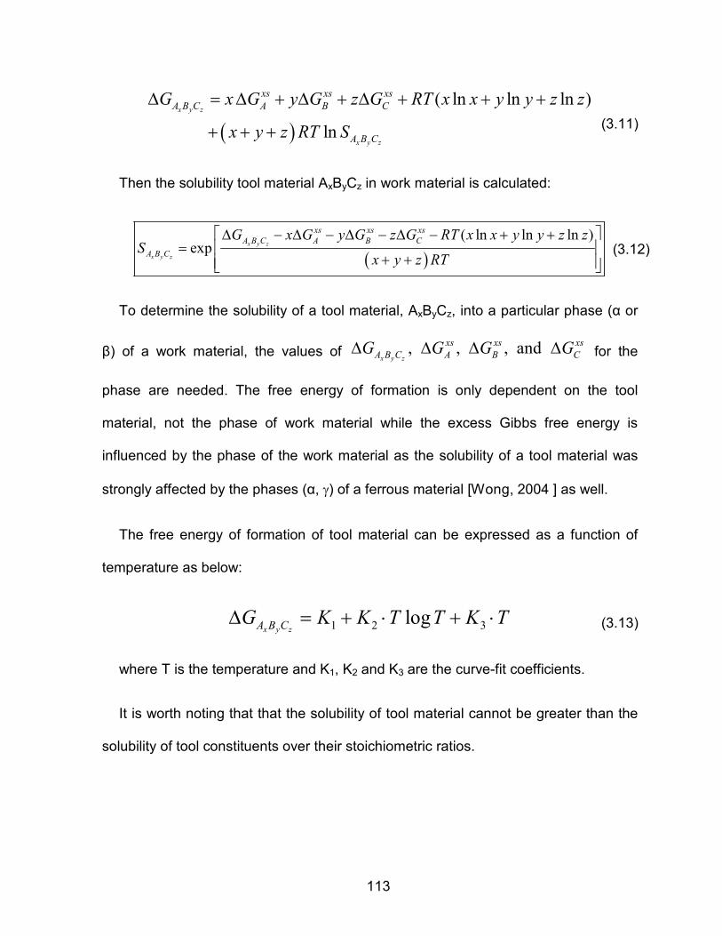
113

(3.11)

Then the solubility tool material AxByCz in work material is calculated:

(3.12)

To determine the solubility of a tool material, AxByCz, into a particular phase (α or

β) of a work material, the values of for the

phase are needed. The free energy of formation is only dependent on the tool

material, not the phase of work material while the excess Gibbs free energy is

influenced by the phase of the work material as the solubility of a tool material was

strongly affected by the phases (α, γ) of a ferrous material [Wong, 2004 ] as well.

The free energy of formation of tool material can be expressed as a function of

temperature as below:

(3.13)

where T is the temperature and K1, K2 and K3 are the curve-fit coefficients.

It is worth noting that that the solubility of tool material cannot be greater than the

solubility of tool constituents over their stoichiometric ratios.

( )

( ln ln ln )

ln

x y z

x y z

xs xs xs

A B C A B C

A B C

G x G y G z G RT x x y y z z

x y z RT S

∆ = ∆ + ∆ + ∆ + + +

+ + +

( )( ln ln ln )

expx y z

x y z

xs xs xs

A B C A B C

A B C

G x G y G z G RT x x y y z zS

x y z RT

∆ − ∆ − ∆ − ∆ − + +=

+ +

, , , andx y z

xs xs xs

A B C A B CG G G G∆ ∆ ∆ ∆

1 2 3logx y zA B CG K K T T K T∆ = + ⋅ + ⋅

114

(3.14)

Hence, the solubility of tool material was determined by following procedure:

Figure 101: Flow chart for calculation of solubility of tool material

The solubility of a tool material into a work material strongly depends on the

cutting temperature and the phase of a work material. As the cutting temperature

increases, the hardness decreases and the solubility increases, accelerating tool

wear. For example, Figure 102 presents the temperature dependence of hardness

x y z

x y z

x y z

A B C A

A B C B

A B C C

S S x

S S y

S S z

≤ ≤

≤

Given properties of tools constituents

Calculation of by eq. (*)

Yes

No

115

and solubility of hafnium carbide (HfC) into α-grain. However, these properties of only

few tool materials in α- and β- phases of titanium were available, which were used for

the calculation in this thesis as shown in Table 13..

Figure 102: Temperature dependence of the hardness and solubility of HfC tool

Table 13: Estimated solubility of tool materials in α-Ti (at 800°C) and β-Ti (at 1000°C)

Tool

(AxByCz)

SA in α-

Ti (at

800°C)

SA in β-

Ti (at

1000°C)

SB in α-

Ti (at

800°C)

SB in β-

Ti (at

1000°C)

SC in α-

Ti (at

800°C)

SC in β-

Ti (at

1000°C)

SAxByCy in

α-Ti (at

800°C)

SAxByCy in

β-Ti (at

1000°C)

Stool in α-

Ti (at

800°C)

Stool in β-

Ti (at

1000°C)

TiN 100.0 100.0 11.2 [1] 1.1 [1] 1.02E-04 2.49E-03 1.02E-04 2.49E-03

TiAlN 100.0 100.0 15.3 [2] 8.4 [2] 11.2 [1] 1.1 [1] 1.12E+01 1.10E+00

TiCN 100.0 100.0 0.9 [3] 0.6 [3] 11.2 [1] 1.1 [1] 9.00E-01 6.00E-01

cBN 0.1 [4] 0.3 [4] 11.2 [1] 1.1 [1] 7.69E+07 * 9.86E+07 * 1.00E-01 3.00E-01

Al2O315.3 [2] 8.4 [2] 15.3 [2] 8.4 [2] 1.04E+03 * 2.17E+03 * 5.10E+00 2.80E+00

WC 0.2 [5] 16.5 [5] 0.9 [3] 0.6 [3] 2.51E+04 * 1.07E+04 * 2.00E-01 6.00E-01

Ref : [1] Murray (1987) ; [2] CALPHAD ; [3] Bandyopadhyay (2000) ;[4] Rahaei ; [5] Murray (1981)

* solubility >100 (mol%) w as replaced by a modif ied solubility

116

I.1.2.2 Diffusion wear

The diffusion takes place as the atom moves from the regions of high

concentration to low concentration as shown in Figure 103. The diffusion is possible

only if the contact interface reaches high enough temperature for an adequate

amount of time. In high speed turning, the condition is favorable for the diffusion of

tool material into the chip [Trent, 1991]. Besides the temperature, the diffusivity of a

tool element is affected by the particular phase present in a work material during

machining. The diffusivities into the β-phase are reported two or three orders of

magnitude higher than those into the α-phase as shown in Figure 104 for some

selected tool materials. The diffusivity data of tool constituents in the α-phase at

800°C and the β-phase at 1000°C was represented in Table 14. The diffusion of tool

constituents in the β-phase is much faster than that into the α-phase leading to a

higher diffusion wear rate with the β-phase.

Figure 103: Dissolution of carbide tool into chip

X

Contact length X

WC Tool

Vx

Y

Chip at high

temperature C W

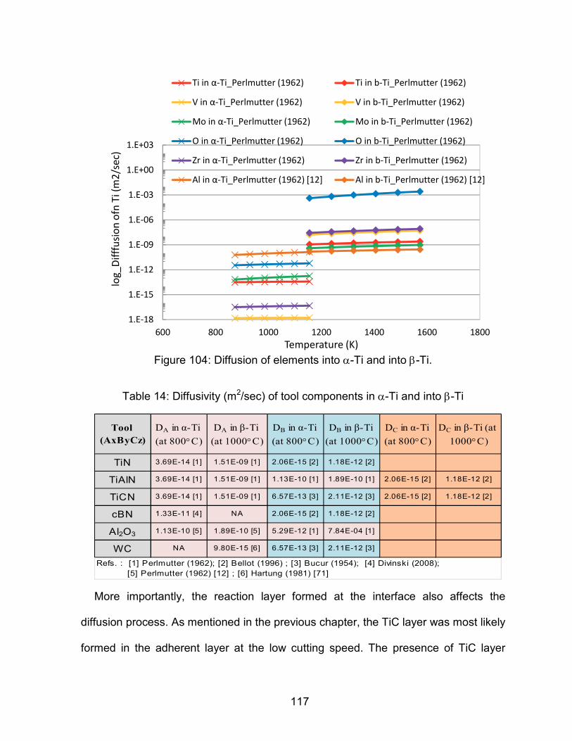
117

Figure 104: Diffusion of elements into α-Ti and into β-Ti.

Table 14: Diffusivity (m2/sec) of tool components in α-Ti and into β-Ti

More importantly, the reaction layer formed at the interface also affects the

diffusion process. As mentioned in the previous chapter, the TiC layer was most likely

formed in the adherent layer at the low cutting speed. The presence of TiC layer

1.E-18

1.E-15

1.E-12

1.E-09

1.E-06

1.E-03

1.E+00

1.E+03

600 800 1000 1200 1400 1600 1800

log

_D

ifff

usi

on

ofn

Ti (m

2/s

ec)

Temperature (K)

Ti in α-Ti_Perlmutter (1962) Ti in b-Ti_Perlmutter (1962)

V in α-Ti_Perlmutter (1962) V in b-Ti_Perlmutter (1962)

Mo in α-Ti_Perlmutter (1962) Mo in b-Ti_Perlmutter (1962)

O in α-Ti_Perlmutter (1962) O in b-Ti_Perlmutter (1962)

Zr in α-Ti_Perlmutter (1962) Zr in b-Ti_Perlmutter (1962)

Al in α-Ti_Perlmutter (1962) [12] Al in b-Ti_Perlmutter (1962) [12]

Tool

(AxByCz)

DA in α-Ti

(at 800°C)

DA in β-Ti

(at 1000°C)

DB in α-Ti

(at 800°C)

DB in β-Ti

(at 1000°C)

DC in α-Ti

(at 800°C)

DC in β-Ti (at

1000°C)

TiN 3.69E-14 [1] 1.51E-09 [1] 2.06E-15 [2] 1.18E-12 [2]

TiAlN 3.69E-14 [1] 1.51E-09 [1] 1.13E-10 [1] 1.89E-10 [1] 2.06E-15 [2] 1.18E-12 [2]

TiCN 3.69E-14 [1] 1.51E-09 [1] 6.57E-13 [3] 2.11E-12 [3] 2.06E-15 [2] 1.18E-12 [2]

cBN 1.33E-11 [4] NA 2.06E-15 [2] 1.18E-12 [2]

Al2O3 1.13E-10 [5] 1.89E-10 [5] 5.29E-12 [1] 7.84E-04 [1]

WC NA 9.80E-15 [6] 6.57E-13 [3] 2.11E-12 [3]

Refs. : [1] Perlmutter (1962); [2] Bellot (1996) ; [3] Bucur (1954); [4] Divinski (2008);

[5] Perlmutter (1962) [12] ; [6] Hartung (1981) [71]

118

substantially reduces the diffusion of tool constituents into the work material. Figure

105 shows the significant reduction of carbon diffusing into the TiC layer. The

adhesion layers (consisting of Ti and TiC) covered most of the contact zone on the

rake face of PCD inserts in all cutting speeds while the carbide inserts had fewer

localized areas covered by the adhesion layer. However, as discussed in pervious

section, the dominant wear mechanism with the carbide insert was dissolution and

diffusion while that for the PCD inserts is grain-pulled out. Hence, the diffusion wear

is mostly relevant to the carbide inserts.

Figure 105: The diffusivity of carbon in α-Ti, β-Ti, Ti64 and TiCx

The diffusion wear was influenced by the concentration gradient in y direction,

in Equation (3.6), of tool constituents in the chip, which cannot be accurately

determined. Therefore, the upper bound diffusion wear model was adopted by

1.0E-18

1.0E-16

1.0E-14

1.0E-12

1.0E-10

1.0E-08

600 800 1000 1200 1400 1600 1800

Dif

ffu

sio

n (

m^

2/s

ec)

Temperature (°K)

C in TiCx_Barros (1998)

C in α-Ti_Barros (1998)

C in Ti-6Al-4V_Barros (1998)

C in a-Ti_Bucur (1954)

C in b-Ti_Bucur (1954)

c

y

∂∂

119

Hartung and Kramer [1982] to simply predict the relative diffusion wear rate of tool

materials into titanium.

I.1.3 Upper bound of diffusion wear model

The upper bound calculation of diffusion wear model was introduced by Cook and

Nayak [1986] to predict the maximum diffusion wear rate with the assumption of no

chip deformation as it traverses across tool chip interface

(3.15)

The accuracy of this model depends on the diffusivity and solubility of tool

constituents used in the model. As the cutting time increases, the size of crater wear

grows. Hence, the distance from the cutting edge to the center of the crater wear

increases with cutting time for a given cutting speed. Then, the respective traveling

times can be calculated. Table 15 lists the traveling times after cutting for certain

amounts of times in all cutting speeds of carbide inserts. In fact, the difference in the

travelling times among various cutting times is relatively small. In this thesis, the

average value at 91m/min was used as the travel time for each cutting speed.

( )0.5/wearV K S D tπ= − ⋅

[ ]

2

where:

: ratio of molar volumes of the tool material and the chip material

/ sec : diffusion coefficient of the slowest diffusing tool constituent in the chip

% : equilibrium concentration of the t

K

D cm

S at

[ ]ool material in the chip

sec : travelling time, taken for the chip to move from the edge of the tool to the

center of the crater

t

120

Table 15: The distance from cutting edge to crater’s center and traveling time with carbide inserts

Cutting speed Cutting time

(min)

Distance to center

of crater (µm)

Time to

travel (sec)

Average

time (sec)

61 m/min

2.4 130 6.40E-05

7.71E-05 5.2 150 7.38E-05

6.8 190 9.35E-05

91 m/min

1.6 150 9.84E-05

1.14E-04 3.5 180 1.18E-04

4.5 190 1.25E-04

122 m/min

0.6 150 1.48E-04

1.48E-04 1.1 150 1.48E-04

2.2 150 1.48E-04

Table 16 shows the upper bounds of diffusion wear for a tool material used in

Hartung and Kramer (1982). The results were calculated with the diffusivity of the

slowest diffusing tool constituent, the solubility of the slowest dissolving tool

constituent and the same travelling time, t=1.14x10-4sec (see Table 15), at the cutting

speed of 91 m/min. For instance, the diffusivity of W and solubility of C were used to

calculate the diffusion wear rate of carbide. The results of predicted diffusion wear did

not agree with experiment data. For example, for turning Ti alloy with a high DOC,

carbide inserts showed that the crater wear rate was 20.6 µm/min at the cutting

speed of 91 m/min (see Figure 42), much higher than the predicted value.

Furthermore, the predicted wear rate of the carbide tool was much lower than those

of diamond tool. The experiment showed the opposite fact. It is worth stressing that

the wear mechanism (diffusion or dissolution) has not been well defined for titanium

machining. In general, the diffusion is known to be slower than the dissolution in Ti

alloys.

121

Table 16: Predicted upper bound of diffusion wear at cutting speed of 91 m/min

� The effects of reaction layer TiC to diffusion wear rate

In the case of the carbide insert, the diffusivity of tungsten is two or three orders of

magnitude lower than that of carbon into titanium [need reference]. Although the

diffusivity of Co is comparable to that of carbon, the amount of Co is very small in

comparison with W and C. In addition, tungsten, which was used as the wear

wear rate

(um/min)

least

consti

tuent

D

(cm2/sec)

REF

least

consti

tuent

C (at%) REFwith t=1e-4

(sec)

Diamond 0.321 C 2.28E-06Hartung

[11,12]C 0.6 98.44

NbC 1.266 Nb 3.66E-09Hartung

[11,12]C 0.6 15.56

TiC 1.147 Ti 4.82E-09Hartung

[11,12]C 0.6 16.17

VC 1.025 V 2.92E-09Hartung

[11,12]C 0.6 11.25

ZrC 1.472 Zr 1.40E-08Hartung

[11,12]C 0.6 35.37

TiN 1.082 Ti 4.82E-09Hartung

[11,12]Ni 23.5 597.54

ZrO2 2.068 Zr 1.40E-08Hartung

[11,12]O 17 1408.03

TiB2 1.492 Ti 4.82E-09Hartung

[11,12]B 0.5 17.53

WC 1.165 W 1.05E-10Hartung

[11,12]C 0.6 2.42

Diffusion coeff.

D(cm2/sec) of

Solubility C(at%) of

constituentsTool at

300sfm

Ratio molar

volumes (K)

Solubility of the slowest dissolving tool constituent

Diffusivity of the slowest diffusing tool constituent

122

controlling constituent in Hartung and Kramer [1982], diffuses slower than C in

titanium. However, the diffusivity data of tungsten and cobalt in α-Ti, β-Ti, Ti64 and

TiC is scarce. Thus, carbon was assumed to be the wear controlling constituent for

calculation of the upper bound diffusion wear of carbide tool to study the effect of TiC

reaction layer. Table 17 represents the upper bound of diffusion wear rate of carbide

tools in α-Ti at 1000°K, β-Ti at 1400°K, Ti64 and TiC at 1200°K for three cutting

speeds based on the diffusivity and solubility data of carbon in α-Ti, β-Ti, Ti64 and

TiC collected from few publications. The effect of the TiC reaction layer is significant

in controlling the wear rate of the carbide tool.

Table 17: Predicted diffusion wear of carbide tool in which carbon is control elements.

The experimental results from the high DOC showed the crater wear rates of

carbide inserts at 7.2, 20.6 and 43.7 µm/min (see Figure 42) for cutting speeds of 61

m/min, 91 m/min, and 122 m/min, respectively. In comparison with the predicted

diffusion wear of the carbide insert shown in Table 17, the diffusion wear observed in

the experiments behave similar to the diffusion prediction of the carbide into the TiC

least

constit

uent

D

(cm2/sec)

REF

least

consti

tuent

C (at%) REF 200sfm 300sfm 400sfm

C 8.02E-09 C in α-Ti_Barros (1998) 0.6 17.44 19.87 24.13

C 1.10E-07 C in Ti64_Barros (1998) 0.6 64.63 73.63 89.43

C 1.72E-10 C in TiCx_Barros (1998) 0.6 2.55 2.91 3.53

C 1.42E-09 C in α-Ti_Bucur (1954) 0.6 7.34 8.36 10.15

C 2.85E-06 C in β-Ti_Bucur (1954) 0.6 328.74 374.55 454.91

Diffusion coeff. D(cm2/sec) of

constituents

Solubility C(at%) of

constituents wear rate (µm/min)

123

reaction layers at the low cutting speed, into both Ti64 and the TiC reaction layers at

the medium cutting speed, and into Ti64 at the high cutting speed as the formation of

TiC reaction layer is deterred at higher cutting speeds.

I.2 DRIVEN PROCESS OF GENERALIZED THERMOCHEMICAL WEAR

Olortegui-Yume and Kwon [2007] have introduced a generalized thermochemical

wear where the tool constituent undergoes as a sequence of dissociation, chemical

reaction if possible, dissolution, and diffusion.

Figure 106: Generalized thermochemical wear [after Olortegui-Yume, 2007]

Diffusion

Diffusion of the dissociated species in work material

Dissolution

Atomic transport of the dissociated species that have not been consumed in the chemical across

the tool-chip interface (work material and reaction layer)

Chemical reaction

Chemical reaction ofdissociated species with work material

Dissociation of tool material

eg AxBy tools: AxBy = xA + yB

Solubility controls the dissolution rate

Diffusivity controls the diffusion rate

124

Assuming that the tool material, so called AxBy, dissociates into species, xA and

yB at the early stage of thermochemical wear process.

(3.16)

Then, the dissolution of tool constituents into a work material or the reaction layer

happened. The dissolution is controlled by the solubility (mol% or at%) of tool

material in work material. Therefore, at one instance of time, the specific mole of A

and B atoms in tool-chip interface, so called “dissolution mole limit”, ,

are present.

Considering a volume of chip, Vdis, in the dissolution zone as shown in Figure 107,

the mole of Ti can be calculated as:

(3.17)

where

x yA B xA yB= +

, is ,i

disn i A B

[ ]Ti

Ti Ti

disVn mol

Mρ=

⋅

[ ]Ti 3 Ti/ : density; / : molar massg cm M g molρ

125

Figure 107: Tool constituents diffused into chip

The solubility (mol%) of tool component i (A or B) in tool-chip interface is defined

as:

(3.18)

The mole of component i dissolved in dissolution zone of chip is calculated as:

[ ]i

i Ti Ticalled as "solubility mole limit"

1

i disdis

VSn mol

S Mρ= ⋅ →

− ⋅ (3.19)

Concentration of tool component i (A or B) in dissolution zone is obtained as:

i3

i Ti Ti

1/ called as "solubility concentration limit"

1

ii diss

dis

n Sc mol cm

V S Mρ = = ⋅ → − ⋅

(3.20)

The solubility concentration limit is also the fixed surface concentration at the

boundary of dissolution and diffusion zone.

[ ]i

Ti%

i

dis

i

dis

nS mol

n n=

+

hdidf

lc

AxBy Chemical

reaction

ht=f (chip thickness)

0

x

dc

126

Subsequently, the diffusion process takes place. Depending on how fast A

and B atoms diffuse in the work material, the numbers of A and B atoms at the tool-

chip interface are determined. Let, �� and ��

� are the moles of A and B’s

diffused into the work material in time t (sec). These numbers are functions of

diffusivity and temperature.

The net flux of atom passing through the unit area per unit time along x direction is

(Fick’s first law of diffusion):

(3.21)

The Fick’s second law of diffusion:

(3.22)

with a boundary condition of (0, ) i

sc t c const= = and initial condition of ( ,0) 0c x =

Hence, the diffusion concentration of component i (A or B) in diffusion zone at time

t and location x can be determined as:

(3.23)

2

2

( ); where is diffusivity

sec sec

dc x mol cmJ D D

dx cm

= − ⋅

2

2

( , ) ( , )c x t c x t

t x

∂ ∂=

∂ ∂

i3

i Ti Ti

1B.C: (0, ) / ; I.C : ( ,0) 0

1

i

s

Sc t c mol cm const c x

S Mρ = = ⋅ = = − ⋅

2

.

( , )( , ) 1 ( ) exp

2 2

iii i i s

s s

i i i

conc gradient

cdc x tx dz d xc x t c erf c erf z

dx dx dzD t D t D tπ

= − ⇒ = = − 14243

127

2

2

0

2 is characteristic distance for diffusion.

2erf ( ) ; erfc( ) 1 erfc( ) Error function

2erf

where

(0) 1; erf ( ) 1; erf (

is Gaus

)

s

i

z

z

a D t

z e d z z

dz e

dz

ζ ζπ

π

−

−

=

= = −

= ∞ = =

∫

The diffused mole of component i passed through cross-section, Ac, at location x

of diffusion zone at time t (sec) is:

[ ]( , ) ( , ) ; ;i

c c c cn x t mol c x t A dx A d l= ⋅ ⋅ = ⋅ (3.24)

, is depth of cuwhere is chip-tool contact length is thickness of a cross-sectt , ionc cl d dx

Hence, the total mole of the tool component i diffused in chip can be calculated as:

(3.25)

[ ]

2

1( ) erfc called as "diffusion mole limit"

th

ai i t tdiff c s

h h en t mol A c a

a a π

−

− = ⋅ ⋅ ⋅ + →

(3.26)

The average of diffusion rate limit the tool component i in chip at time t is defined

as:

0 0

/ /

0/ 0

( ) lim ( , ) lim 1 erf

lim 1 erf erfc( )

t t

diff diff

diff diff

t t

diff

diff

h h

i i i

diff c sh h

h h

h a z h a

i i

c s c sh

h a

xn t n x t dx A c dx

a

x xA c a d A c a z dz

a a

→ →

=

→

= = ⋅ −

= ⋅ ⋅ − = ⋅ ⋅

∫ ∫

∫ ∫

2

2/

0 /

1 1where erfc( ) z erfc( ) erf

t

t

t

h

z h a z a

t t

z h a

h he ez dz z

a aπ π

− = −

=

− − = ⋅ + = ⋅ +

∫

128

2

3

( ) 1erf

sec

th

i i adiffi c s t

diff t t

diff c

n t A c hmol eWR h h a t

cm V t A f t a π

−

⋅ − = = − ⋅ + ∝ ⋅ ⋅ ⋅ ⋅

(3.27)

whereas the dissolution rate limit the tool component i at time t is calculated as :

i

3 i Ti Ti

1

sec 1

ii idisdis dis

dis

nmol SWR c

cm V S Mρ = = = ⋅ ∝ ⋅ − ⋅

butx yA B

t S∝ (3.28)

The process that controls the thermochemical wear was determined by comparing

the diffusion rate limit, i

diffWR , and the dissolution rate limit, i

disWR . The process with a

smaller rate limit controls the thermochemical wear of tool constituents. Figures 108 -

111 compared the dissolution and diffusion wear rates of the constituents of WC, TiN

and cBN tool material into α-phase and β-phase using the data of solubility of tool

material,x y zA B C

S , in Table 13 and diffusivity tool constituents in Table 14. At the very

beginning stage (less than 1E-04 sec), the thermochemical wear is dominated by the

dissolution mechanism. Then, for most tool components such as W, C, Ti, B (exclude

N into β-phase at 1000°C), diffusion will control the thermochemical wear rate after

that. To summarize, traffic jam analogy was used and demonstrated the difference in

the thermochemical wear between ferrous and titanium alloys with the carbide tool on

Figure 112. The dissolution controls the thermochemical wear in machining ferrous

while thermochemical wear of mostly tool material in machining Ti will be restrained

by the diffusion the fastest tool constituent. Thermochemical wear of carbide into β-Ti

is an example of this. After dissociating from carbide tool, W and C dissolved and

diffused independently into chip in which diffusion is driven process for both W and C

129

as shown in Figure 108. The diffusion of W and C is influenced by solubility of

carbide which controls the dissociation of tool at tool-chip interface as the way how

solubility of tool was calculated. To put it more simply, diffusion of W and C control

both the dissociation of carbide and their dissolution. Therefore, thermochemical

wear of carbide depends on how fast W or C diffused in the chip. This means that C

with higher diffusion rate (see Figure 108) will control thermochemical wear of

carbide tool. The slower diffusion rate, a part of W will diffuse in chip while the other

left will be taken away with the chip flow. The relative thermochemical wear of tool 1

and tool 2 was determined by the chart shown in Figure 113.

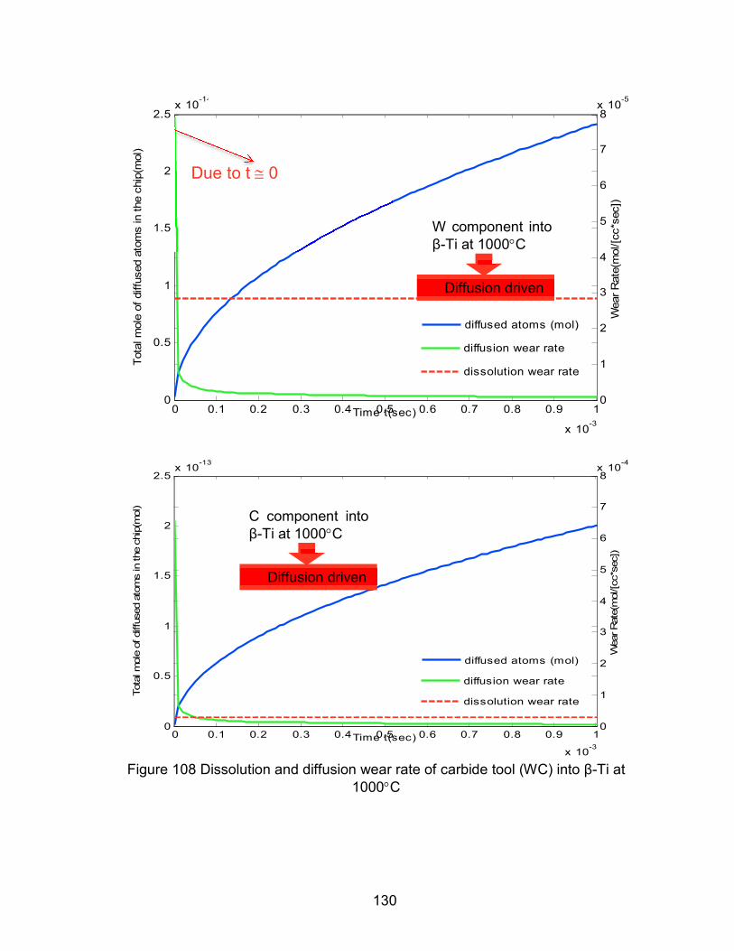
130

Figure 108 Dissolution and diffusion wear rate of carbide tool (WC) into β-Ti at

1000°C

0 0.1 0.2 0.3 0.4 0.5 0.6 0.7 0.8 0.9 1

x 10-3

0

0.5

1

1.5

2

2.5x 10

-14

Tota

l m

ole

of

diffu

sed a

tom

s in t

he c

hip

(mol)

diffused atoms (mol)

0

1

2

3

4

5

6

7

8x 10

-5

Time t(sec)

Wear

Rate

(mol/[c

c*s

ec])

The average wear rate of Tungsten (W) in the chip at 1220K

diffusion wear rate

dissolution wear rate

Due to t ≅ 0

W component into

β-Ti at 1000°C

Diffusion driven

0 0.1 0.2 0.3 0.4 0.5 0.6 0.7 0.8 0.9 1

x 10-3

0

0.5

1

1.5

2

2.5x 10

-13

Tota

l m

ole

of diffu

sed a

tom

s in the c

hip

(mol)


0

1

2

3

4

5

6

7

8x 10

-4

Time t(sec)

Wear R

ate

(mol/[c

c*s

ec])

The average wear rate of Carbon (C) in the chip at 1220K

diffusion wear rate


C component into

β-Ti at 1000°C

Diffusion driven

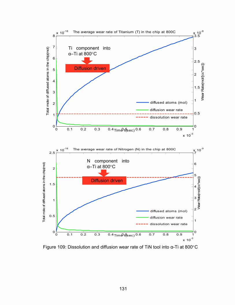
131

Figure 109: Dissolution and diffusion wear rate of TiN tool into α-Ti at 800°C

0 0.1 0.2 0.3 0.4 0.5 0.6 0.7 0.8 0.9 1

x 10-3

0

1

2

3

4

5

6

7

8x 10

-18

Tota

l m

ole

of diffu

sed a

tom

s in the c

hip

(mol)


0

0.5

1

1.5

2

2.5

3

3.5x 10

-8

Time t(sec)

Wear R

ate

(mol/[c

c*s

ec])

The average wear rate of Titanium (T) in the chip at 800C

diffusion wear rate


0 0.1 0.2 0.3 0.4 0.5 0.6 0.7 0.8 0.9 1

x 10-3

0

0.5

1

1.5

2

2.5x 10

-18

Tota

l m

ole

of diffu

sed a

tom

s in the c

hip

(mol)


0

1

2

3

4

5

6

7x 10

-9

Time t(sec)

Wear Rate

(mol/[c

c*s

ec])

The average wear rate of Nitrogen (N) in the chip at 800C

diffusion wear rate


Ti component into

α–Ti at 800°C

N component into

α–Ti at 800°C

Diffusion driven

Diffusion driven

132

Figure 110: Dissolution and diffusion wear rate of TiN tool into β-Ti at 1000°C

0 0.1 0.2 0.3 0.4 0.5 0.6 0.7 0.8 0.9 1

x 10-3

0

0.2

0.4

0.6

0.8

1

1.2x 10

-15

Tota

l m

ole

of diffu

sed a

tom

s in the c

hip

(mol)


0

0.5

1

1.5

2

2.5

3

3.5

4x 10

-6

Time t(sec)

Wear R

ate

(mol/[c

c*s

ec])


diffusion wear rate


0 0.1 0.2 0.3 0.4 0.5 0.6 0.7 0.8 0.9 1

x 10-3

0

0.5

1

1.5

2

2.5

3

3.5

x 10-14

Tota

l m

ole

of diffu

sed a

tom

s in the c

hip

(mol)


0

0.2

0.4

0.6

0.8

1

1.2

1.4x 10

-4

Time t(sec)

Wear R

ate

(mol/[c

c*s

ec])

The average wear rate of Titanium (T) in the chip at 1000C

diffusion wear rate


N component into

β-Ti at 1000°C

Ti component into

β-Ti at 1000°C

Dissolusion driven

Diffusion driven

133

Figure 111: Dissolution and diffusion wear rate of cBN tool into α-Ti at 800°C

0 0.1 0.2 0.3 0.4 0.5 0.6 0.7 0.8 0.9 1

x 10-3

0

0.2

0.4

0.6

0.8

1

1.2

1.4

1.6x 10

-13

Tota

l m

ole

of diffu

sed a

tom

s in the c

hip

(mol)


0

1

2

3

4

5

6x 10

-4

Time t(sec)

Wear R

ate

(mol/[c

c*s

ec])

The average wear rate of Boron (B) in the chip at 800C

diffusion wear rate


0 0.1 0.2 0.3 0.4 0.5 0.6 0.7 0.8 0.9 1

x 10-3

0

0.5

1

1.5

2

2.5x 10

-15

Tota

l m

ole

of diffu

sed a

tom

s in the c

hip

(mol)


0

1

2

3

4

5

6

7x 10

-6

Time t(sec)

Wear R

ate

(mol/[c

c*s

ec])


diffusion wear rate


B component into

α–Ti at 800°C

N component into

α–Ti at 800°C

Diffusion driven

Diffusion driven

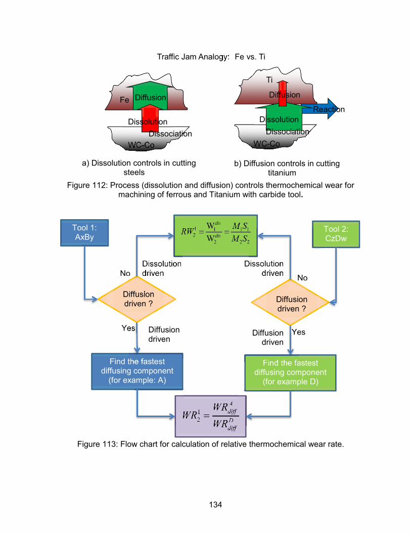
134

Figure 112: Process (dissolution and diffusion) controls thermochemical wear for

machining of ferrous and Titanium with carbide tool.

Figure 113: Flow chart for calculation of relative thermochemical wear rate.

Traffic Jam Analogy:

WC-Co

Fe

a) Dissolution controls in cutting steels

Fe vs. Ti

Diffusion

Reaction

Dissolution

Dissociation

Ti

Diffusion

b) Diffusion controls in cutting titanium

WC-Co

Dissolution

Dissociation

Tool 1: AxBy

Tool 2: CzDw

Diffusion driven ?

Dissolution driven

Yes

Diffusion driven ?

Find the fastest diffusing component

(for example D)

Find the fastest diffusing component

(for example: A)

Yes

No

Dissolution driven

No

Diffusion driven

Diffusion driven

135

According to the pervious chapters, the thermochemical (dissolution/diffusion) is

proven to be the dominant wear mechanism of carbide tools in machining Ti64. The

diffusion mechanism takes place by the diffusion action of W and C or Co from carbides

into Ti alloys. However, the diffusion process is hampered due to the presence of TiC

layer that forms by the reaction of Ti and C from carbides. The diffusivity of W and C in

TiC is fairly lower than in titanium and Ti64. The reaction layer TiC formed at tool-chip

interface helps to reduce wear rate. This can be proved with the nano-lubricants, which

can provide the additional carbon from graphitic platelets. However, providing the nano-

lubricants during turning is not always successful with MQL as the cutting tools is

always engaged with the workpiece. Instead, the nano-graphitic platelets can provide

additional lubricity at the tool-chip interface.

In next chapters, the study of tool wear improvement was conducted with MQL

machining with micro and nano-platelets of graphite added in MQL oil. However, due to

the difficulty in setting up MQL turning experiment, the ball mill was selected. The AISI

1045 steel was initially chosen for the workpiece to reduce the cost of the experiments.

Based on the MQL ball-mill experiments with the steel, the investigation was carried out

to find the effect of diameter and thickness of platelets and presented in in Chapter 4.

Finally, the performance of MQL experiment with nano graphite platelets was evaluated

with Ti64 in Chapter 5.

136

Chapter 4: Tool wear improvement in machining of Steel AISI

1045 with micro and nano-platelets enhanced MQL

IV.1 INTRODUCTION

Flood cooling has been the backbone of machining processes for manufacturing

industries. The traditional flood cooling, which uses and discards a large amount of

metal working fluid, is widely used in industrial machining operations. The primary

purposes of metalworking fluid (MWF) are to rapidly dissipate heat, reduce friction

between the tool and the chip and carry the chip away from the cutting zone.

Consequently, the reduction in force and power consumption and the improvement in

tool life and surface finish [1] are apparent. However, flood cooling has many

disadvantages due to its associated maintenance and disposal cost (7-17%) [Kajdas,

2010] as well as occupational hazards and environmental impacts. According to the

U.S. Occupational Safety and Health Administration (OSHA) [Aronson, 1995] and the

U.S. National Institute for Occupational Safety and Health (NIOSH) [U.S. DHHS, 1998],

the permissible exposure level (PEL) for metalworking fluid aerosol concentration is 5

mg/m3 and 0.5 mg/m3, respectively. The coolant mist level in U.S. automotive parts

manufacturing facilities has been estimated to be on the order of 20-90 mg/m3 with the

use of traditional flood cooling and lubrication [Bennett & Bennett, 1985]. As a result, the

need to reduce cutting fluid consumption is strong and the discrepancy in fluid aerosol

concentration needs to be aggressively addressed. Dry machining has offered an

alternative solution by completely eliminating cutting fluid. However, its applications are

limited due to the poor surface quality, the accelerated tool wear and the high

137

concentration of airborne particles on the factory shop floor [R Khettabi, 2008; 2009].

Recently, Minimum Quantity Lubrication (MQL)-based machining has been introduced

as an ideal alternative which provides a compromise between productivity and

environmental concerns. MQL machining refers to a class of machining processes

where the lubricant use is limited to only a extremely small amount – typically a flow rate

of 2.5 to 500 ml/h [Gaitonde, 2008; Shen, 2008]. This amount of lubricant is about three

to four orders of magnitude lower than the amount commonly used in flood cooling

which dispenses up to 60 l/h [Srikant, 2009]. Thus, MQL offers many benefits such as

the diminution of the environmental and occupational hazards and the reduction of

maintenance and disposal cost. A general study on the efficiency of MQL to dry

machining was introduced in Weinert et al. [2004]. In mild machining conditions, MQL

provides a great substitute for flood cooling. However, MQL-based machining

possesses have few major drawbacks such as chip disposal and limitation in machining

conditions. Chip disposal can be somewhat remedied by adding compressed air.

However, the lack of cooling capacity with MQL-based machining has been a major

drawback preventing this technology to reach its full potential in industrial applications.

To improve MQL performance and expand the range of MQL applications, many spray

configurations and cutting parameters are proposed and investigated while others study

to enhance the lubricity.

IV.1.1 Improved performance of MQL with alternative lubricants

Several works have been published to evaluate the characteristics of various

lubricants for finding optimum lubricants in MQL machining. The most common

138

lubricants in MQL are mineral oil [Braga, 2002; Brandao, 2011; Brinksmeier, 1999;

Shen, 2008; Varadarajan, 2002], emulsions (soluble or synthetic fluid) [Brinksmeier,

1999; Gaitonde, 2008; Wakabayashi, 2006], synthetic oils, esters [Brinksmeier, 1999;

Wakabayashi, 2006], neat oil [Sarhan, 2012; Thepsonthi, 2009] and vegetable oil [Cetin,

2011; Ozcelik, 2011; Shen, 2008; Singh, 2013; Wakabayashi, 2006]. Some researchers

used alcohol [Heinemann, 2006; Shen, 2008] and deionized water [Mao, 2012; Shen,

2008]. The mixture of water and oil-free synthetic lubricant provided longer tool life

compared to both synthetic ester with and without alcohol in deep-hole drilling due to its

high cooling ability and low viscosity of water [Heinemann et al., 2006]. A new approach

to enhance the cooling effect with the MQL process, oil-on-water droplets produced

through a new design nozzle system, reduced cutting forces in end milling [Itoigawa,

2006; Yoshimura, 2005]. Cutting performance in the tapping test as well as secondary

factors (biodegradability, oxidation, and storage stability) for synthetic polyor esters

were superior to vegetable oil [Wakabayashi, 2006; Suda, 2002].

In general, vegetable oil is favorable in MQL machining due to reduction in cutting

force [Sadeghi, 2008], better surface finish [Emami, 2014; Singh, 2013; Tai, 2011] and

improvement in tool life [Nguyen, 2012; Park, 2011] in comparison with MQL with other

lubricants. More importantly, the biodegradability makes it safe for the workers in the

environment. Thus, MQL offers many benefits such as the diminution of the

environmental and occupational hazards and the reduction of maintenance and disposal

costs. However, MQL lacks the ample cooling offered by flood cooling. Due to the

extremely small amount of a liquid lubricant, MQL mainly provides essential lubricant

function, which makes effective to only mild cutting conditions.

139

IV.1.2 Improved performance of MQL by adding solid lubricants

Solid lubricants have been used either to eliminate the use of cutting fluids or to mix

with cutting fluid to enhance its lubricity. Many of them have lamellar or layered crystal

structures where each layer readily slides against adjacent layers to provide lubricity.

Some examples of such solids include soft metals, graphite, hexagonal boron nitride,

boric acid, and the transition-metals dichalcogenides MX2 (M is molybdenum, tungsten

or niobium and X is sulfur, selenium or tellurium), such as MoS2 and

monochalcogenides (e.g., GaSe and GaS) [Erdemir, 2001]. However, no single solid

lubricant can provide the lubricity over a wide range of cutting conditions (different tool

and work materials). For example, molybdenum sulfide (MoS2) works well in vacuum or

dry conditions but degrades quickly in moist and oxidizing environments [Wiener, 1967].

Most transition metal dichalcogenides tend to oxidize at elevated temperatures, and

thus lose their lubricity. MoS2 can provide lubrication up to 350°C while WS2 endures up

to 500°C [Sliney, 1982]. In general, those with higher oxidation resistance or

chemical/structural stability perform the best at elevated temperatures. Oxide and

fluoride-based solid lubricants (e.g., CaF2, BaF2, PbO, and B2O3) [Sliney, 1993] as well

as some soft metals (e.g., Ag, Au) function quite well at elevated temperatures [Erdemir,

1990; Erdemir and Erck, 1996; Maillat, 1993), but all fail to provide low friction at room

or lower ambient temperatures. The lubricity of these solids at elevated temperatures is

largely controlled by their ability to soften and resist oxidation. Solid lubricants such as

molybdenum disulfide (MoS2), tungsten disulfide (WS2) graphite, hexagonal boron

nitride (hBN) and polytetrafluoroethylene (PTFE) have been used as dry powders or

coating materials [Donnet, 2004]. The effectiveness of the solid lubricant was

140

demonstrated in some publications. For example, the recent developments and future

trends of well-known solid lubricants were summarized at Donnet et al. [2004]. Yukhno

et al. [2001] reviewed the frictional behavior and wear resistance of solid lubricant

coatings at low temperatures. Prasad et al. [2010, 2005] inspected the effects of some

solid lubricants such as graphite, talc, MoS2, and lead suspended in oil on the wear

performance of cast iron and zinc–aluminum alloy. Hsu et al. [2004] discussed the

important characteristics of nano-lubricants such as being non-volatile, oxidation and

thermal decomposition resistant, and self-repairing as well as having a more effective

film organization of nano-lubricant compared to conventional lubrications. The effect of

the concentration of solid lubricants (MoS2 and graphite) were studied and the “optimal

concentrations” were found to be 3wt.% and 10wt.% for MoS2 and graphite, respectively

[Bartz, 1971]. Below the critical concentrations of MoS2 and graphite, they did not

effectively protect the surfaces against wear.

The main advantage of solid lubricants is the preservation of lubricity even under

extreme pressure and temperature. Thus, by mixing the solid lubricants into a MQL

lubricant, MQL-based machining can be enhanced for more aggressive conditions.

Several works were published to evaluate the effectiveness of MQL applications at

elevated temperatures by adding small amounts of solid lubricant to MQL oils.

However, to be effective in general machining applications, solid lubricants should

provide lubricity in a broader range of temperatures.

Molybdenum sulfide (MoS2)

141

Shen et al. [2008] used MoS2 to enhance grinding processes. By mixing MoS2 nano-

particles into MQL grinding fluid, the MQL-grinding process showed excellent

performance on cutting forces. However, its effectiveness, especially in traditional

machining applications, is questionable due to the low dissociation temperature of MoS2

(350°C in oxidizing environments). Kalita et al. [2012] added 2 and 8 wt.% of MoS2

nano-particles (40-70 µm) and micro-particles (3–5 µm) into paraffin and soybean oils

used in MQL grinding tests of cast iron and EN 24 steel. He concluded that the grinding

process was improved with MQL oil with added MoS2 (both nano- and micro- particles)

to flood cooling and MQL with pure oil. Furthermore, the nanoparticles less than 100nm

exhibited superior performance to micro-particles (3-5 µm), resulting in up to 30% and

50% reduction in the friction coefficient and grinding ratio, respectively. The increase in

the nano-particle content reduced the friction, energy consumption and cutting forces. In

milling tests of AL6061-T6 alloy, Rahmati [2013] used the MQL mixture with MoS2

nanoparticles (20–60 nm) added in ECOCUT HSG 905S neat cutting oil at various

concentrations. The machining experiment with the presence of MoS2 nanoparticles in

the MQL oil showed outstanding performance compared to pure MQL oil in term of

cutting force, temperature and surface finish. He claimed that optimum concentrations

for minimizing cutting force and temperature were 1 wt.% and 0.5 wt.%, respectively.

The surface roughness was minimized by applying the MQL oil mixed with 0.5 wt.% of

MoS2 nanoparticles.

142

Graphite (C)

The main advantage of graphite over MoS2 is that the dissociation of graphite is

much higher than that of MoS2. The graphite was found to start decomposing at

moderately high temperatures (e.g.: 500°C in oxidizing environments [Zhu, 1998]). The

nano-graphene platelet enhanced lubricants were studied under various conditions. Lee

et al. [2009] studied nano lubricants by mixing graphite nanoparticle additives (at 0.1

vol% and 0.5 vol%) with industrial gear oil to improve the lubrication properties in the

disk-on-disk tribo-test between two sliding grey cast iron plates which showed superior

performance in reducing the friction coefficient, sliding temperature, and surface

roughness. Huang et al. [2006] compared the performance of pure paraffin oil to

mixtures of paraffin oil with flake graphite (particle size: 48 µm) and with graphite nano-

sheets (average diameter: 500nm, thickness: 10-20nm) in pin-on-disk tests using steel

balls. He pointed out that the mixture with graphite nano-sheets formed a film on the

rubbing surface that not only improved the friction coefficient but also reduced the wear.

The pure graphite powder was used as solid lubricant to prolong the tool life and

improve the cutting force and surface quality in milling AISI 1045 [Reddy, 2006]. Amrita

et al. [2013] studied MQL turning of AISI 1040 steel using varying concentrations of

graphite nano-particles (particle size < 100nm) suspended in water soluble oil (20:1).

The cutting temperature, flanks wear and cutting force were significantly reduced

compared to those of dry, flood and pure MQL oil machining. Among the concentrations

of 0.1%, 0.3%, and 0.5 wt%, the higher content showed more improvement in the

cutting performance. In turning of hardened AISI 4340 steel with a MQL mixture of 10%

143

graphite added in semi-solid lubricant (composed of calcium and a sodium soap base

emulsified with mineral oil) [Paul, 2013], the machining process presented better cutting

performance (e.g. tool wear, cutting force and temperature, surface finish) compared to

dry machining and turning with pure MQL. In the MQL grinding process of a hardened

tool steel, Alberts et al. [2009] found that the mixture of exfoliated Graphite nano-

Platelet (xGnP) at 1wt% dispersed in isopropyl alcohol (IPA) was the optimal

concentration to reduce cutting forces, specific energy and surface roughness. Park et

al. [2011] showed that by using a very small amount (0.1wt%) of exfoliated graphite

nano-platelets (xGnP) added in MQL Unist Coolube® 2210 vegetable oil, the tool wear

was reduced by up to 50% in MQL ball milling of 1045 steel.

Boric acid (H3BO3)

Boric acid is a popular alternative solid lubricant added to MQL oils which have been

evaluated in a few publications. Rao et al. [2008] investigated turning of EN 28 steel

using compressed air and solid lubricant powders (graphite and boric acid) at different

particle sizes of 50, 100, 150 and 200µm . The reduction of cutting force and flank wear

was found when using solid lubricants compared to dry and wet conditions. He claimed

that a particle size of 50µm would be most effective for both graphite and boric acid.

Krishna [2012] examined the performance of boric acid nano-particle (100um)

suspensions at various concentrations (0.25, 0.5, 0.75, and 1.0 wt%) in coconut oil with

MQL turning AISI 1040 steel. In comparison to dry conditions, the turning process with

MQL oil showed significant reduction in cutting temperature, surface finish and tool flank

wear due to slight improvements in thermal conductivity and the heat transfer

144

coefficient. Among them, the 0.5wt% mixture showed the best cutting performance.

Using the same approach, Ramana [2011] studied MQL mixtures of boric acid particles

(50 nm, 60nm, 80nm and 0.5um) in canola oil in turning tests of AISI 1040 hardened

steel. Surprisingly, the experimental results revealed that MQL oil with boric acid

showed higher cutting force and tool temperature compared to dry and flood cooling

with pure canola oil. Furthermore, the smaller particles showed worse performance in

terms of cutting force, tool wear and surface quality of the machined surface.

IV.1.3 Improved performance of MQL by varying spray configuration

The effectiveness of MQL is directly dependent on the application angle of the

nozzle. Figure 114 depicts the illustration of spray angles (yaw and pitch angle) of an

external MQL nozzle in a ball-milling experiment. The experiment is set for the rotating

mill to travel along the Y axis. In this setup, the pitch angle is the angle between the Y

axis and nozzle spray while yaw angle is the angle between the table feed direction and

nozzle spray. Table 18 summarizes the findings from other works in determining the

optimal spray angles and other spray parameters for external MQL systems with

respect to the definitions of yaw and pitch angle in Figure 114.

Figure 114: Pitch and Yaw angle of the nozzle in End-ball milling

145

Table 18: Publication on optimal spray conditions in MQL machining with definition of Yaw and Pitch angle as shown in Figure 114

Ref. Machining Process

Cutting fluid

Additive Nozzle distance

Flow

rate

Yaw angle

Pitch angle

Improvement

Mao et al. [2012]

Grinding of AISI 52100

Deionized water

0.75wt% Al2O3particles (60nm)

20mm 60 ml/h 180° 15° 50% in surface roughness, 20% in grinding temperature

Yan et al. []

Milling of forged steel

Esters -- 20mm 43.8 ml/h 60° 60° 10% in Flank wear and surface roughness to other

yaw and pitch angles

Lacalle et al. [2006]

Milling of Aluminum 5083-

H112

Biodegradable oil

-- -- 0.06ml/min 45° -- 30% in flank wear to flood coolant with emulsion 95% of

water

Liu et al. [2011]

Milling Ti6Al4V Vegetable oil

-- 25mm 10 ml/h 45° -- Little lower cutting force and temperature to others

Ueda et al. [2006]

Turning and Milling of AISI

1045

Vegetable oil

-- 40 ml/h 45° 45° 10% in temperature

Tawakoli et al. [2010]

Grinding of hardened steel

100Cr6

Syntilo XPS

Castrol 5%

-- 40 100 ml/h 180° 10-12° Slightly improvement in grinding force and surface

finish to other positions and depend on material of wheel

Park et al. [2011]

Milling of AISI 1045 steel

Vegetable oil

xGnP 50-70 mm

1 ml/min -- 10° 40-50% in Flank improvements of xGnP

mixture in comparison to pure oil.

IV.2 BACKGROUND

Lamellar-type solid lubricants are readily available in the form of platelets. The

diameter and thickness of these platelets are typically to the scale of tens of microns

and only a few microns, respectively, which are classified in this thesis as micro-

platelets. Some of these platelets are also available as nano-platelets whose thickness

is well below a micron (even to a few nanometers). Clearly, the micro-platelets are not

as inexpensive. However, the mixtures with micro-platelets are not as stable as those

with nano-platelets. Another aspect of nano-particles is the worldwide excitement of

nanotechnology research. Many research findings are reporting on new processing

146

techniques, which will eventually make them cheaper and available for wide varieties of

applications. In this study, these micro- & nano-particles and platelets are used to

reduce friction and/or wear. It is also important to recognize that a wide variety of shape

and size distributions of these particles are now available.

In this chapter, we will explore the use of micro and nano platelets of graphite and

hBN mixed in the vegetable oil, Unist Coolube 2210 obtained from Unist, Inc. (Grand

Rapid, Michigan) in tribometer tests and MQL ball-milling tests. This study defines

‘nano-platelets’ to have a thickness of less than 0.1µm and ‘micro-platelets’ to have a

thickness of more than 0.1µm. The hBN phase is similar to graphite but quite different

from its related compound, cubic boron nitride (cBN). Like graphite, the hBN phase has

a layered structure where each layer is weakly bonded with adjacent layers. With the

application of a shear load, each layer can easily slide against other layers providing

lubricity. Both graphite and hBN can provide the lubricity desperately needed in more

severe machining conditions, even when the oil droplets can dissociate. The

dissociation temperature of hBN is even higher than that of the graphite. The main

advantage of the nano-platelet form of solid lubricants (hBN and graphite) is the aspect

ratio of diameter to thickness. When applied, the larger surface of the nano-platelets

will land on the tool surfaces and additional lubricity from these nano-platelets can be

provided in the MQL-machining. The nano-platelets have the thickness in nano-scale

and the diameter in micro-scale, which offers a unique advantage of being filtered by

nose hair and not being absorbed through human skin. This thesis intends to find the

effect of thickness and diameter on these platelets in MQL machining of AISI 1045 steel

and Ti64.

147

IV.2.1 Micro and nano-platelet characterizations

In the periodic table of elements, boron and nitrogen are the neighbors of carbon (C).

Boron Nitride (BN) was first founded in early 19th century. The compound has the same

number of outer shell electrons as graphite and diamond. BN has very similar properties

as carbon with both hexagonal and cubic crystal structures [Haubner, 2002]. Figure 115

illustrates the similarity in the hexagonal structure of graphite and hBN. While both

forms of carbon exist as graphite and diamond in nature, both forms of BN are synthetic

and exist as cubic boron nitride (cBN) and hexagonal boron nitride (hBN). The hBN

phase is more similar to graphite but quite different from its related compound, cubic

boron nitride (cBN). The electrical properties are recognized as the prominent

differences between carbon and BN. Due to its high electrical resistivity, BN is well-

known as dielectric and thermally conductive whereas carbon is electrically and

thermally conductive. The main difference in appearance is that hBN is white while

graphite is black. Like graphite, the hBN phase has a layered structure where each

layer is weakly bonded with adjacent layers. With the application of a shear load, each

layer can easily slide against other layers providing lubricity. hBN is expected to have

the similar lubricant properties to graphite. The main advantage of the mixtures of

graphite/oil and hBN/oil is that they can provide lubricity even if the oil droplets

dissociate due to a high cutting temperature. The hBN is stable up to 1000°C [Haubner,

2002], while graphite was known to start decomposing at moderately high temperatures

(500°C) [Zhu, 1998]. The hBN has good chemical inertness and is not wetted by most

molten metals [Haubner, 2002]. These advantages of hBN compared to graphite make

148

hBN a more promising solid lubricant in MQL processes where the cutting temperature

is expected to be very high.

Several research investigations on the lubricity of BN for various applications were

published. The early research on tribological properties of cubic, amorphous and

hexagonal boron nitride films by Watanabe et al. [1991] showed that BN films helped to

decrease the friction force and the friction coefficient as a function of normal load. The

curious behavior of hBN was discovered with a ring-on-roller tribometer when added to

lubricating oil as well as the effect of hBN concentration on friction and wear in Kimura

et al. [1999]. The sliding experiment of bearing steel vs. itself showed that the addition

of BN at as little as 1 wt% resulted in the reduction of wear. The wear was reduced as

concentrations of BN increased, although the friction coefficient was slightly increased.

Based on these investigations, BN was considered as a potential additive for the

lubricants.

Figure 115: An illustration of hexagonal crystalline structures of ghraphite and hBN

[Encyclopedia Britannica, Inc., 1995]

149

Table 19: Properties of graphite and hBN

Formula BN Graphite (C)

Molecular mass 24.82 g/mol 12.01 g/mol

Density (hexagonal) 2.27 g/cm3 2.23g/cm3

Density (cubic) 3.48 g/cm3 3.51 g/cm3

Melting range 2700-3000°C 3652 - 3697°C

Mohs hardness 1-2 1-2

Youngs Modulus (MPa) 20-102 8-15

Coefficient of Friction 0.15 to 0.70 0.2 to 0.6

Thermal conductivity 34 25-470

Temperature Stability 1000°C 500°C

Figure 116: Temperature range for lubrication of different solid lubricants [Chen N.,

2004]

The solid lubricant platelets examined in this study include micro-platelets (graphite

and hBN) and nano-platelets (xGnP and exfoliated hBN). The graphite micro-platelets

were obtained from Alfa Aesar Com., USA while the micro-platelets of hBN5 were

obtained from Changsung Corp. (South Korea). Four nano-platelets designated as

150

xGnP M5, xGnP M15, xGnP C300, xGnP C750 and one exfoliated hBN300 were

provided by XG Science, Inc., (Lansing, Michigan, USA) using their cost-effective

exfoliation process after being downsized by the pulverization process [Fukushima,

2003]. Among xGnP platelets, the Grade M5 and M15 have the same thickness with

distinct diameters while C300 and C750 have the same diameter with distinct

thicknesses. Table 20 summarizes the diameters and thicknesses of each platelet.

Some of these data have been interpreted based on surface area measurements or

based on SEM images. As presented in Table 20, a typical, commercially available hBN

powder has a surface area of around 2 m2/g while the surface area of XGS hBN is

246 m2/g. The surface area of hBN is quite larger than that of xGnP grade M5 (~120-

150 m2/g) but is smaller than that of xGnP grade C (300 and 750 m2/g for C300 and

C750, respectively).

Table 20: The diameters and thicknesses of various platelets

Platelets Diameter Thickness Aspect ratio

SBET(m2/g) Company

Mic

ro-

pla

tele

ts

Graphite 7µm 200 nm+ 35 4.8** Alfa Aesar

hBN5 5µm 1-2µm+ 3 1.27** Changsung

Nano-p

late

lets

xGnP M5 5µm 6-8 nm 714 ~120-150 XG Sciences

xGnP M15 15µm 6-8 nm 2143 ~120-150 XG Sciences

xGnP C300 2µm 3 nm* 667 300 XG Sciences

xGnP C750 2µm 1.2 nm* 1667 750 XG Sciences

hBN300 11 nm* 8.24 nm 1 246 XG Sciences

+ A estimation based on SEM image (See Figures 5 and 6)

* A calculated value based on the surface area BET (Brunauer–Emmett–Teller theory) data

** The calculated surface area based on diameter and thickness

151

The patent by Kwon and Drazl [2010] has been issued using xGnP platelets to

enhance the effectiveness of MQL machining. A wide variety of graphite platelets

varying in diameter and thickness are now produced by XG Science, Inc.. The main

advantage of xGnP over MoS2 is that the dissociation of graphite is much higher than

that of MoS2. In the paper by Park et al. [2011], the oil and the nano-platelets have

been mixed in a high-speed mixer to produce stable solutions, which have been

substituted for vegetable MQL oil in the MQL-based ball-milling experiments. The

diameter and thickness of the graphite platelets were approximately 1µm and 10nm in

average, respectively. The results were very encouraging in the reduction of tool wear.

Figure 5 presents the micrographs of some of the platelets at 1000x magnification.

Figure 6 shows the thickness of xGnP and graphite micro-platelets at 30,000x

magnification. Although both platelets have a similar particle diameter, the thicknesses

of xGnP and hBN are much smaller than those of micro-platelets. We expect that the

nano-platelets can facilitate a better lubricity and reduce wear even at the same

concentration levels in oil. Figure 119 presents the diameter versus thickness and the

aspect ratio for graphite platelets.

152

a) micro-platelet graphite b) nano-platelet xGnP (M5)

c) micro-platelet hBN5 d) nano-platelet hBN300

Figure 117: SEM analysis

a) xGnP M5 b) micro-platelet graphite c) hBN5

Figure 118: SEM images micro- and nano-platelets

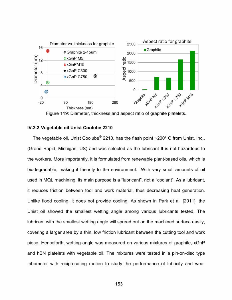
153

Figure 119: Diameter, thickness and aspect ratio of graphite platelets.

IV.2.2 Vegetable oil Unist Coolube 2210

The vegetable oil, Unist Coolube® 2210, has the flash point ~200° C from Unist, Inc.,

(Grand Rapid, Michigan, US) and was selected as the lubricant It is not hazardous to

the workers. More importantly, it is formulated from renewable plant-based oils, which is

biodegradable, making it friendly to the environment. With very small amounts of oil

used in MQL machining, its main purpose is a “lubricant”, not a “coolant”. As a lubricant,

it reduces friction between tool and work material, thus decreasing heat generation.

Unlike flood cooling, it does not provide cooling. As shown in Park et al. [2011], the

Unist oil showed the smallest wetting angle among various lubricants tested. The

lubricant with the smallest wetting angle will spread out on the machined surface easily,

covering a larger area by a thin, low friction lubricant between the cutting tool and work

piece. Henceforth, wetting angle was measured on various mixtures of graphite, xGnP

and hBN platelets with vegetable oil. The mixtures were tested in a pin-on-disc type

tribometer with reciprocating motion to study the performance of lubricity and wear

0

4

8

12

16

-20 80 180 280

Dia

me

ter

(µm

)

Thickness (nm)

Diameter vs. thickness for graphite

Graphite 2-15um

xGnP M5

xGnPM15

xGnP C300

xGnP C750

0

500

1000

1500

2000

2500

Asp

ect

ra

tio

Aspect ratio for graphite

Graphite

154

resistance. The ball-mill experiment is chosen to evaluate the applicability of the nano-

platelet enhanced MQL lubricant as the cutting edges of the tools are exposed each

revolution.

IV.3 EXPERIMENTAL SETUP AND PROCEDURES

IV.3.1 Suspension Stability of Mixtures

In practice, the stability of MQL mixtures – the segregation of particulates in a mixture

- is important. With the unstable mixture, the addition of solid lubricants will not provide

the intended function. The suspension stability is influenced by diameter, thickness of

platelets and mixing conditions such as mixing speed and mixing time. The suspension

stability test was conducted with the mixtures made with both micro- and nano-platelets

of graphite and hBN with vegetable oil. The mixtures were prepared on a high-speed

mixer DAC 150FVZ-K from FlackTek (Landrum, SC) as shown in Figure 120. The

mixing conditions were set at a speed of 2300rpm and durations of 4, 6 and 8 minutes

as the stabilities of the mixtures were achieved.

Figure 120: High-speed mixer DAC 150FVZ-K

155

IV.3.2 Wetting angle measurement

The wetting angle is one of the significant parameters determining lubricity of the

MQL lubricant. As the MQL droplets are applied to the spinning tool, the wetting angle

indicates how well the droplets will stick to the tool surface. A lubricant with a small

wetting angle shows good wettability on the surface. The wetting angle tests were

conducted with both micro- and nano-platelets of graphite and hBN platelet-mixtures at

various concentrations on the TiAlN-coated WC ball insert to be used in the ball-milling

tests. The mixtures include vegetable oil mixed with 0.1 and 0.5wt% of hBN300 and 0.1

wt% and 1.0 wt% of xGnP grade M5 and xGnP C300 and C750 grades. Figure 121

shows the equipment and setup for the wetting angle measurement. To generate

consistent amounts of droplets, the motorized syringe assembly (from AST Product,

Inc.) was used to dispense a droplet of 0.5, 1, or 2.0 µl on the tool surface. The CCD

camera was used to capture the image of the droplet produced by the LED black light.

The droplet image was processed to obtain the wetting angles based on the boundaries

of the droplet and the tool surface.

156

Figure 121: Wetting Measurement system [Park, 2011]

IV.3.3 Surface characterization of two coated inserts using in tribotest and end-

ball milling experiment

In the MQL milling experiments, two different types (denoted as A and B) of ball nose

end mill TiAlN-coated carbide inserts from two manufactures were used. To study the

effect of tool surface quality on the performance of solid lubricant platelet-enhanced

MQL mixtures, the topography of the surface of each tool was investigated. The surface

appearance and profile of these tool inserts were investigated by SEM images. The

roughness parameters such as the ten-point height mean roughness (Rz) and mean

spacing between peaks (Sm) were also measured with the Dektak 6M stylus surface

profilometer with the point-to-point resolution of 1 angstrom as shown in Figure 121.

FVS

: Solid-Vapor Interfacial Force

FLS

: Liquid-Solid Interfacial Force

FLV

: Liquid-Vapor Interfacial Force

θcosLVLSVSFFF =−

157

These data were attained at a horizontal resolution of 0.067µm/sample over the

average value of 30,000 data points on the 2mm evaluation length scan in the parallel

and perpendicular directions of the grinding marks on the tool inserts.

Figure 122: Veeco Dektak 6M Surface Profiler

IV.3.4 Tribometer Tests

The friction measurements on the mixtures were attained with the tribometer test.

The tests were performed with a linear ball-on-disc type tribometer (CSM Instruments)

as shown in Figure 123 where a steel 440c ball, with 6.35 mm in diameter, oscillated on

TiAlN-coated carbide flat and rough surfaces (tool A and B) to evaluate frictional

characteristics under various lubrication conditions. The software calculates the

coefficient of friction between two sliding objects at a given normal load. All the tests

were set at a track length of 6mm (with an amplitude of 3mm) while carrying a load of

1, 5 and 10N with a sliding speed of 1.0, 2.5 and 4.0 cm/s at room temperature as

summarized in Table 4. The lubrication conditions include dry, pure vegetable oil and

Camera

X Adjustment

Y Adjustment

Rotate Stage

Sample Stage

Stylus

158

mixtures of vegetable oil with 0.1, 1.0wt% of graphite and xGnP (M5); 0.1, 0.5wt% of

hBN300 and hBN5.

The wear characteristics under each lubricant condition were measured with a WC

ball instead of the 440C steel ball used in the friction tests in order to accelerate the

wear on the surfaces. The wear tests were conducted on both tool A and B, on which

depth and width measurements of the wear tracks were measured after 25,000, 35,000

and 50,000 cycles. However, since it is not possible to continue the wear test on the

exactly the same location, each wear cycle started from scratch. The average depth and

width on the wear tracks were measured on three cross-sections along a wear track

length of 6mm. Wear rate and volume of the wear track were calculated based on the

measurements from Dektak 6M Stylus Surface Profilometer. Figure 124 presents the

profile of a cross-section of the wear tracks using a Dektak 6M Surface Profiler which

the wear depth and width were measured.

Figure 123: Linear ball-on-disc type tribometer

Steel ball

L

Sample (Tool A & B)

Ball holder

Wear

W

Ball

Load

Sample Mounting

Reciprocating Actuator

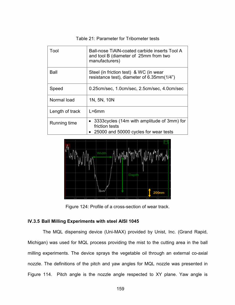
159

Table 21: Parameter for Tribometer tests

Tool Ball-nose TiAlN-coated carbide inserts Tool A and tool B (diameter of 25mm from two manufacturers)

Ball Steel (in friction test) & WC (in wear resistance test), diameter of 6.35mm(1/4”)

Speed 0.25cm/sec, 1.0cm/sec, 2.5cm/sec, 4.0cm/sec

Normal load 1N, 5N, 10N

Length of track L=6mm

Running time • 3333cycles (14m with amplitude of 3mm) for friction tests

• 25000 and 50000 cycles for wear tests

Figure 124: Profile of a cross-section of wear track.

IV.3.5 Ball Milling Experiments with steel AISI 1045

The MQL dispensing device (Uni-MAX) provided by Unist, Inc. (Grand Rapid,

Michigan) was used for MQL process providing the mist to the cutting area in the ball

milling experiments. The device sprays the vegetable oil through an external co-axial

nozzle. The definitions of the pitch and yaw angles for MQL nozzle was presented in

Figure 114. Pitch angle is the nozzle angle respected to XY plane. Yaw angle is

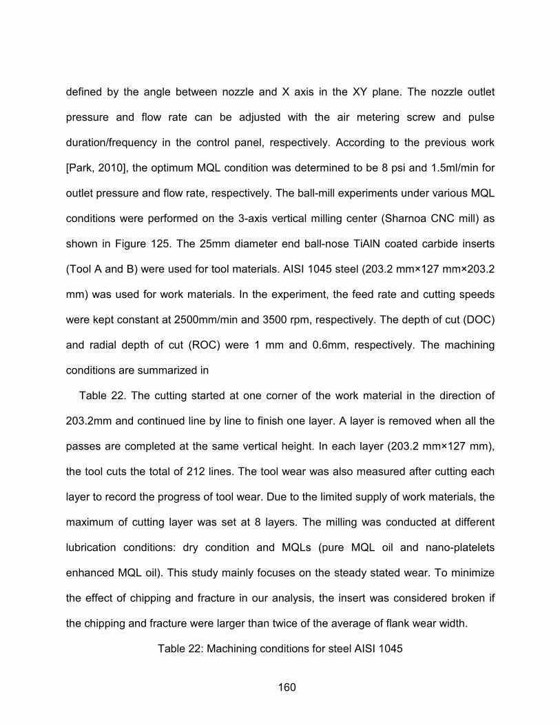
160

defined by the angle between nozzle and X axis in the XY plane. The nozzle outlet

pressure and flow rate can be adjusted with the air metering screw and pulse

duration/frequency in the control panel, respectively. According to the previous work

[Park, 2010], the optimum MQL condition was determined to be 8 psi and 1.5ml/min for

outlet pressure and flow rate, respectively. The ball-mill experiments under various MQL

conditions were performed on the 3-axis vertical milling center (Sharnoa CNC mill) as

shown in Figure 125. The 25mm diameter end ball-nose TiAlN coated carbide inserts

(Tool A and B) were used for tool materials. AISI 1045 steel (203.2 mm×127 mm×203.2

mm) was used for work materials. In the experiment, the feed rate and cutting speeds

were kept constant at 2500mm/min and 3500 rpm, respectively. The depth of cut (DOC)

and radial depth of cut (ROC) were 1 mm and 0.6mm, respectively. The machining

conditions are summarized in

Table 22. The cutting started at one corner of the work material in the direction of

203.2mm and continued line by line to finish one layer. A layer is removed when all the

passes are completed at the same vertical height. In each layer (203.2 mm×127 mm),

the tool cuts the total of 212 lines. The tool wear was also measured after cutting each

layer to record the progress of tool wear. Due to the limited supply of work materials, the

maximum of cutting layer was set at 8 layers. The milling was conducted at different

lubrication conditions: dry condition and MQLs (pure MQL oil and nano-platelets

enhanced MQL oil). This study mainly focuses on the steady stated wear. To minimize

the effect of chipping and fracture in our analysis, the insert was considered broken if

the chipping and fracture were larger than twice of the average of flank wear width.

Table 22: Machining conditions for steel AISI 1045

161

Tool Ball-nose TiAlN-coated carbide inserts Tool A and Tool B (diameter of 25mm)

Feed Rate 2500 mm/min

Axial DOC 1 mm

Radial DOC 0.6 mm

Cutting Speed 3500rpm (108 m/min)

Lubricants Dry,

MQL oil

Nano-platelets xGnP enhanced MQL oil at 0.1, 1, and 5 wt%

MQL spray parameter

Pitch angle: 15°

Yaw angle: -30, 60, 120 and 180°

Outlet pressure: 8 psi

Flow rate: 1.5ml/min

162

Figure 125: Experimental Set up for MQL ball milling

X axis

MQL

Nozzle Compressed air

Y axis

Z axis

Workpiece

CNC table

Outlet pressure gauge

Tool Holder

MQL oil Spindle

Vice

Tool Insert

Nose Wear

End ball milling

Insert

Workpiece

Outlet

Pressure

Gauge

Flank Wear

Tool

Holder

MQL

nozzle

Z

Yaw angle

Y Pitch angle

MQL

Nozzle

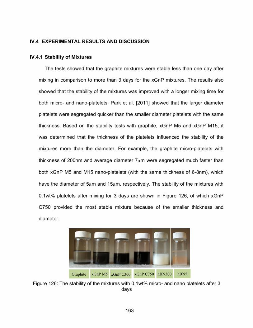
163

IV.4 EXPERIMENTAL RESULTS AND DISCUSSION

IV.4.1 Stability of Mixtures

The tests showed that the graphite mixtures were stable less than one day after

mixing in comparison to more than 3 days for the xGnP mixtures. The results also

showed that the stability of the mixtures was improved with a longer mixing time for

both micro- and nano-platelets. Park et al. [2011] showed that the larger diameter

platelets were segregated quicker than the smaller diameter platelets with the same

thickness. Based on the stability tests with graphite, xGnP M5 and xGnP M15, it

was determined that the thickness of the platelets influenced the stability of the

mixtures more than the diameter. For example, the graphite micro-platelets with

thickness of 200nm and average diameter 7µm were segregated much faster than

both xGnP M5 and M15 nano-platelets (with the same thickness of 6-8nm), which

have the diameter of 5µm and 15µm, respectively. The stability of the mixtures with

0.1wt% platelets after mixing for 3 days are shown in Figure 126, of which xGnP

C750 provided the most stable mixture because of the smaller thickness and

diameter.

Figure 126: The stability of the mixtures with 0.1wt% micro- and nano platelets after 3

days

Graphite xGnP M5 xGnP C300 xGnP C750 hBN300 hBN5

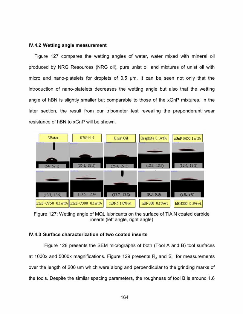
164

IV.4.2 Wetting angle measurement

Figure 127 compares the wetting angles of water, water mixed with mineral oil

produced by NRG Resources (NRG oil), pure unist oil and mixtures of unist oil with

micro and nano-platelets for droplets of 0.5 µm. It can be seen not only that the

introduction of nano-platelets decreases the wetting angle but also that the wetting

angle of hBN is slightly smaller but comparable to those of the xGnP mixtures. In the

later section, the result from our tribometer test revealing the preponderant wear

resistance of hBN to xGnP will be shown.

Figure 127: Wetting angle of MQL lubricants on the surface of TiAlN coated carbide

inserts (left angle, right angle)

IV.4.3 Surface characterization of two coated inserts

Figure 128 presents the SEM micrographs of both (Tool A and B) tool surfaces

at 1000x and 5000x magnifications. Figure 129 presents Rz and Sm for measurements

over the length of 200 um which were along and perpendicular to the grinding marks of

the tools. Despite the similar spacing parameters, the roughness of tool B is around 1.6

165

µm while the roughness of tool A is 0.6 µm. Thus, tool A has a smoother surface, which

we expected to yield a better sliding contact with less wear.

a) Tool A at 1000x b) Tool B at 1000x

c) Tool A at 5000x d) Tool B at 5000x.

Figure 128: SEM surface images of tool surfaces

Figure 129: Roughness (Rz) and spacing parameters (Sm)

601.81 686.84

1515.48

1688.12

0

400

800

1200

1600

2000

Parallel Perpendicular

Rz(n

m)

Rz (Ten Point Height Average) over the lengh of 2000um

Tool A Tool B

29.52

24.8326.59

44.93

0

10

20

30

40

50

Parallel Perpendicular

Sm

(um

)

Sm (Mean Spacing Between Peaks) over the lengh of 2000um

Tool A Tool B

Grinding marks

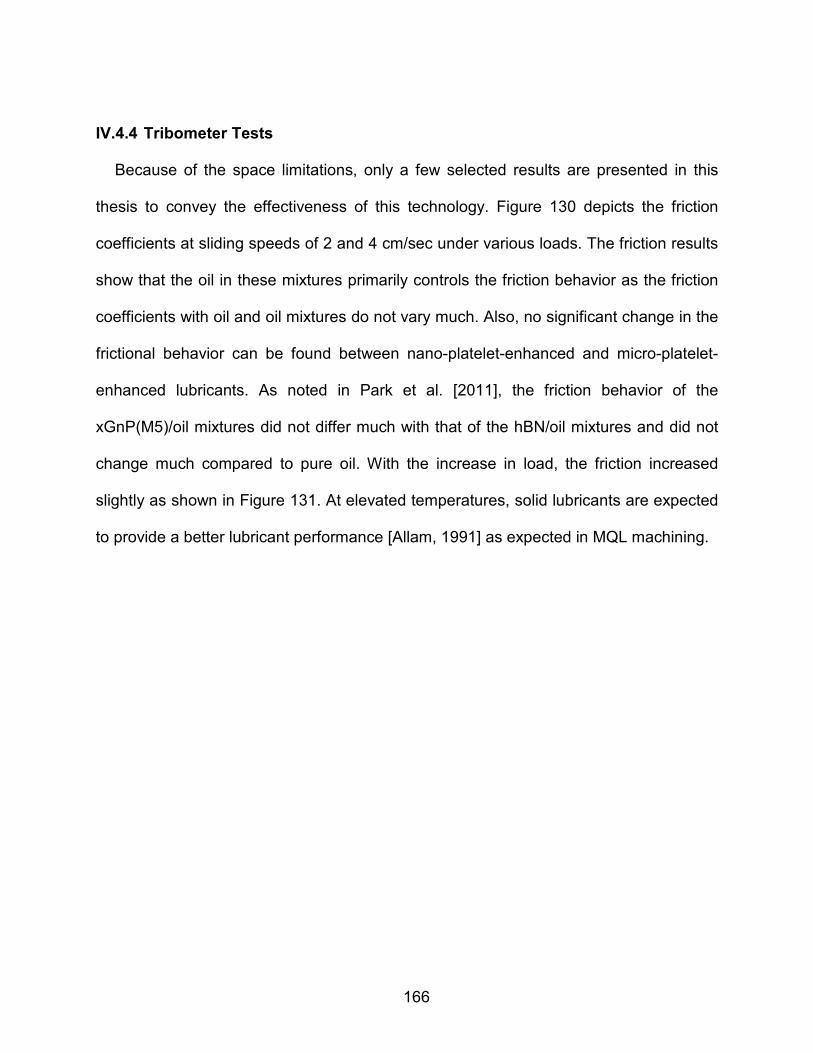
166

IV.4.4 Tribometer Tests

Because of the space limitations, only a few selected results are presented in this

thesis to convey the effectiveness of this technology. Figure 130 depicts the friction

coefficients at sliding speeds of 2 and 4 cm/sec under various loads. The friction results

show that the oil in these mixtures primarily controls the friction behavior as the friction

coefficients with oil and oil mixtures do not vary much. Also, no significant change in the

frictional behavior can be found between nano-platelet-enhanced and micro-platelet-

enhanced lubricants. As noted in Park et al. [2011], the friction behavior of the

xGnP(M5)/oil mixtures did not differ much with that of the hBN/oil mixtures and did not

change much compared to pure oil. With the increase in load, the friction increased

slightly as shown in Figure 131. At elevated temperatures, solid lubricants are expected

to provide a better lubricant performance [Allam, 1991] as expected in MQL machining.

167

Figure 130: Friction coefficients of various mixtures on tool A

0.3140.312 0.312

0.060 0.062 0.064

0.0

0.1

0.2

0.3

0.4

1N 5N 10N

Fri

ctio

n C

oe

ffic

ien

t

Load (N)

a) At sliding speed of 2.5cm/s

Dry Pure Unist oil Graphite 0.1wt%

xGnP-M5 0.1wt% xGnP- M5 1.0wt% xGnP-C300 0.1wt%

xGnP-C750 0.1wt% hBN300 0.1wt% hBN300 0.5wt%

hBN5 1.0wt%

0.0970.114

0.123

0.0120.016 0.020

0.0

0.1

0.2

0.3

0.4

1N 5N 10N

Fri

ctio

n C

oe

ffic

ien

t

Load (N)

b) At sliding speed of 4.0 cm/s

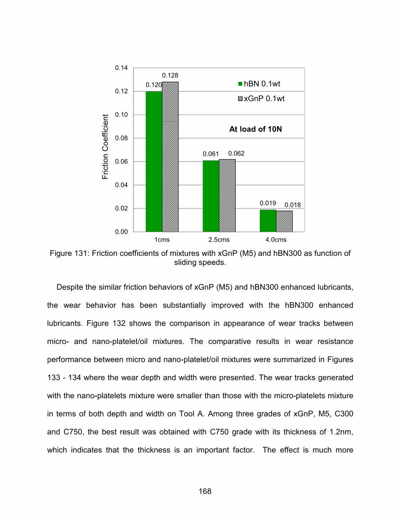
168

Figure 131: Friction coefficients of mixtures with xGnP (M5) and hBN300 as function of

sliding speeds.

Despite the similar friction behaviors of xGnP (M5) and hBN300 enhanced lubricants,

the wear behavior has been substantially improved with the hBN300 enhanced

lubricants. Figure 132 shows the comparison in appearance of wear tracks between

micro- and nano-platelet/oil mixtures. The comparative results in wear resistance

performance between micro and nano-platelet/oil mixtures were summarized in Figures

133 - 134 where the wear depth and width were presented. The wear tracks generated

with the nano-platelets mixture were smaller than those with the micro-platelets mixture

in terms of both depth and width on Tool A. Among three grades of xGnP, M5, C300

and C750, the best result was obtained with C750 grade with its thickness of 1.2nm,

which indicates that the thickness is an important factor. The effect is much more

0.120

0.061

0.019

0.128

0.062

0.018

0.00

0.02

0.04

0.06

0.08

0.10

0.12

0.14

1cms 2.5cms 4.0cms

Frict

ion

Co

eff

icie

nt

At load of 10N

hBN 0.1wt

xGnP 0.1wt

169

pronounced on the track depth than on the track width. Because of the thickness of the

nano-platelets, they can effectively cover the large area of the tool surface, which

facilitate sliding in their shear planar direction between the WC ball and tool surface. On

the other hand, due to its larger thickness and the associated low coverage area, the

micro-platelets did not perform as well. The wear track data on Tool B showed slight

improvement in wear resistance using nano-platelet mixtures compared to micro-

platelet mixtures as shown in Figure 133. One common lubrication condition between

Figures 133 and 134 is a mixture with nano-platelets of hBN300 at 0.5wt%. The wear

depth of Tool A is one fourth that of tool B, which cannot be completely explained by the

difference in surface roughness. This may be possibly due to the coating quality.

Figure 132: The wear track appearance with 0.1wt% of nano-platelets at a speed of

2.5cms and load of 10N after 35000cycles (Left: xGnP M5, Right: hBN300)

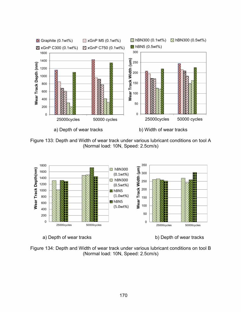
170

a) Depth of wear tracks b) Width of wear tracks

Figure 133: Depth and Width of wear track under various lubricant conditions on tool A (Normal load: 10N, Speed: 2.5cm/s)

a) Depth of wear tracks b) Depth of wear tracks

Figure 134: Depth and Width of wear track under various lubricant conditions on tool B (Normal load: 10N, Speed: 2.5cm/s)

0

200

400

600

800

1000

1200

1400

1600

25000cycles 50000 cycles

Wear

Tra

ck D

ep

th (

nm

)Graphite (0.1wt%) xGnP M5 (0.1wt%)

xGnP C300 (0.1wt%) xGnP C750 (0.1wt%)

0

50

100

150

200

250

300

25000cycles 50000 cycles

Wear

Tra

ck W

idth

(u

m)

hBN300 (0.1wt%) hBN300 (0.5wt%)

hBN5 (0.5wt%)

0

200

400

600

800

1000

1200

1400

1600

1800

25000cycles 50000cycles

Wear

Tra

ck D

ep

th(n

m)

hBN300

(0.1wt%)

hBN300

(0.5wt%)

hBN5

(1.0wt%)

hBN5

(5.0wt%)

0

50

100

150

200

250

300

350

25000cycles 50000cycles

Wear

Tra

ck W

idth

(µ

m)

171

Figure 135 presents two platelets, hBN5 and xGnP M5 in relation to the surface

characteristics of Tool A and B. The difference in the vertical and horizontal scales,

especially for the hBN5 platelet, should be noted. The xGnP M5 is very thin compared

to the surface characteristics of the tools. Only a few (1-2) hBN5 micro platelets filled in

a valley on tool surface. The larger area coverage by the nano-platelets enables them to

provide better lubricity and resistance to wear. Based on this primary finding, MQL ball

mill tests were conducted with both Tool A and B to evaluate the performance of the

nano- and micro-platelet lubricants in an experiment with MQL ball milling.

Figure 135: Geometric Relationships of micro and nano-platelets on the tool surfaces

IV.4.5 Tool Wear with Ball Milling Experiments

IV.4.5.1 Optimal MQL spray angles for ball milling

Based on the cutting geometry calculation with tool diameter and DOC, the pitch

angle of 11° is the minimum angle that the oil-mist flow can access the full cutting zone

-30 -20 -10 0 10 20 30-1

-0.8

-0.6

-0.4

-0.2

0

0.2

0.4

0.6

0.8

1

Mean spacing (Sm)

Rz

Platelets

Micro-platelets hBN5 on the tool surfaces

The cross-sections of Tool surfaces(µm)

He

igth

(µ

m)

Tool A

Tool B

-15 -10 -5 0

-0.8

-0.7

-0.6

-0.5

-0.4

-0.3

-0.2

-0.1

0

0.1

Platelets

Nano-platelets xGnP M5 on the tool surfaces

The cross-sections of Tool surfaces(µm)

He

igth

(µ

m)

Tool A

Tool B

a) hBN 5 on tool b) xGnP M5 on tool surfaces

172

at any yaw angle as shown in Figure 136. Thus, the pitch angle was fixed at 15° and the

MQL ball milling tests were conducted with Tool B to find the optimal yaw angle for our

MQL experiments. The vegetable oil mixed with 1.0wt% of xGnP (M5) was used for

these experiments. Various yaw angles, -30, 60, 120 and 180°, were chosen for the

experiment. Figure 137 shows the resulting flank wear at various yaw angles which

showed that the negative 30° yaw angle setup provided a relatively good lubrication

conditions for the cutting region while the 120° yaw angle configuration showed the

worst conditions. The results showed 180° is the optimal yaw angle contributing to

adequate lubrication. This finding is corroborated by the geometry calculation from

experiment setup with 30° and 120° yaw angle as shown in Figure 138. At 30°yaw

angle, the rake face, flank face and nose were lubricated by the oil-mist during the MQL

cutting process. In other words, the lubricant oil-mist was not blocked by tool as tool

entered into the cutting region. Based on this finding, a pitch angle of 15° and a yaw

angle of 180° were set for the MQL ball-mill tests.

Figure 136: Minimum pitch angle of MQL nozzle for oil mist entering the cutting zone

173

Figure 137: Flank wear at 15° pitch angle and various yaw angles with tool B (dash-line:

Tool chipping)

Figure 138: Top View of MQL Experiment: The distribution of lubricant at 120° and -30°

yaw angle

IV.4.5.2 Effectiveness of thickness and diameter of platelets to tool wear

A series of MQL ball-milling tests was carried out on AISI 1045 steel with the

vegetable oil mixed with nano- and micro-platelets to study the effects of the thickness

on the wear performance. The lubrication conditions include pure vegetable oil,

vegetable oil mixed with micro-platelet additives (0.1wt% of graphite, 0.5 and 5.0wt% of

40

60

80

100

120

140

160

180

25.81 51.61 77.42 103.23 129.03

Fla

nk

we

ar

(µm

)

Cutting Volume (cm3)

120deg -90deg 60deg

-150deg -30deg 180deg

174

hBN5) and vegetable oil mixed with nano-platelet additives (0.1 and 1.0 wt% of xGnP

M5, xGnP C300 and xGnP C750 and 0.5wt% of hBN300) used with Tool A and B.

Figures 139-140 showed nose wear and flank wear at various lubrication conditions. In

appearances, the nose wear and flank wear with MQL mixtures were much lower than

those of dry machining. Due to nose of the insert being in contact with the workpiece

during the cutting process and not exposed to MQL oil mist, the improvement in nose

wear of MQL mixtures with nano-platelets to MQL with pure oil was not significant and

consistent as summarized in Figure 141. To help discussion on flank wear without too

much information, Figure 142 for Tool A and Figure 143 for Tool B present some of the

flank wear results.

Figure 139: Central wear with MQL nano-platelet enhanced mixtures after milling 3

layers

a) Dry b) 0.1wt% xGnP M5 c) 0.1 wt% hBN300 d) 0.5 wt% hBN300

Nose wear

175

Figure 140: Flank wear after milling 6 layers.

Figure 141: Nose wear at 3500 rpm after ball milling six layers with tool A

0

10

20

30

40

50

60

70

1 2 3 4 5 6 7 8

No

se w

ea

r (µ

m)

Layers

Pure Oil hBN300 (0.1 wt%) hBN300 (0.5 wt%)

xGnPC750 (0.1wt%) xGnPC300 (0.1wt%) xGnPM5 (0.1wt%)

Flank wear a)

a) Dry b) 0.1wt% xGnP M5 c) 0.1 wt% hBN300 d) 0.5 wt%

hBN300

176

Figure 142: Flank Wear at 3500rpm after ball milling six layers with tool A (dash-line:

Tool chipping)

0

20

40

60

80

100

120

1 2 3 4 5 6

Fla

nk w

ea

r (µ

m)

Layers

Graphite (0.1wt%) hBN5 (0.5wt%)

Pure Oil xGnP M5 (0.1wt%)

xGnP C300 (0.1wt%) xGnP C750 (0.1wt%)

hBN300 (0.5 wt%)

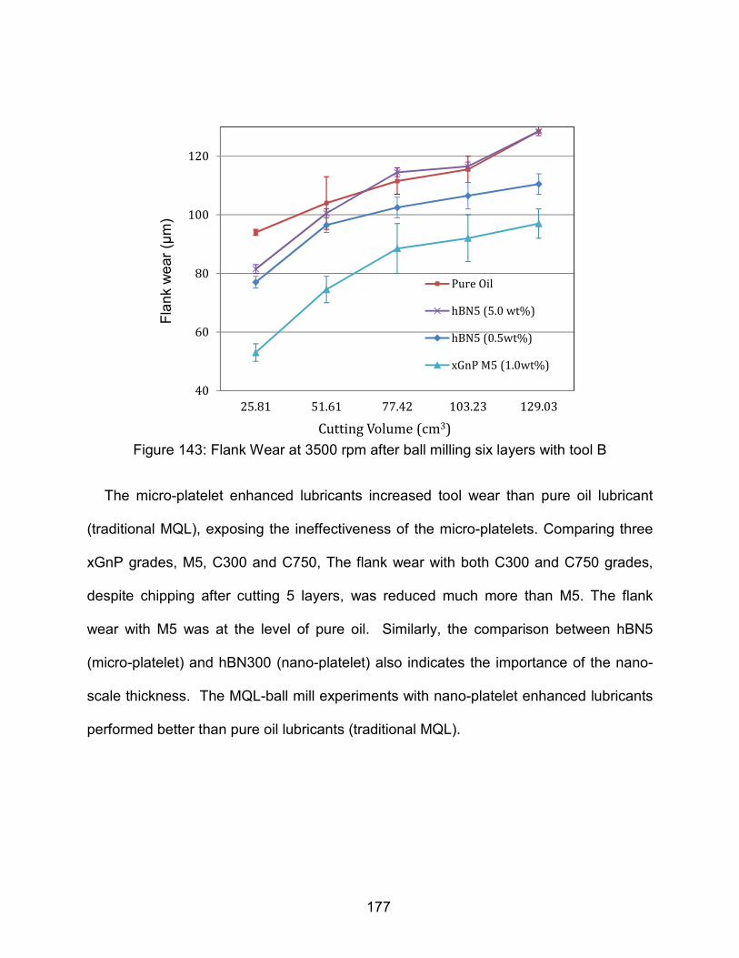
177

Figure 143: Flank Wear at 3500 rpm after ball milling six layers with tool B

The micro-platelet enhanced lubricants increased tool wear than pure oil lubricant

(traditional MQL), exposing the ineffectiveness of the micro-platelets. Comparing three

xGnP grades, M5, C300 and C750, The flank wear with both C300 and C750 grades,

despite chipping after cutting 5 layers, was reduced much more than M5. The flank

wear with M5 was at the level of pure oil. Similarly, the comparison between hBN5

(micro-platelet) and hBN300 (nano-platelet) also indicates the importance of the nano-

scale thickness. The MQL-ball mill experiments with nano-platelet enhanced lubricants

performed better than pure oil lubricants (traditional MQL).

40

60

80

100

120

25.81 51.61 77.42 103.23 129.03

Fla

nk

we

ar

(µm

)

Cutting Volume (cm3)

Pure Oil

hBN5 (5.0 wt%)

hBN5 (0.5wt%)

xGnP M5 (1.0wt%)

178

Chapter 5: Tool wear improvement in machining of Ti64 with

nano-platelets enhanced MQL

From the previous chapter (or Chapter 4), the thickness of both graphite and hBN

need to be in nano scale in order to be effective in MQL. Obviously, the cutting

conditions in machining Ti64 are more aggressive with higher cutting forces and

temperatures than machining steel AISI1045. The nano-platelet enhanced lubricant

found to be very effective in machining steel AISI1045 may not be effective. In this

chapter, thus, the performance of MQL with xGnP C750, which performed the best

among xGnP grade with steel AISI1045, was evaluated in machining Ti64. The

performance of the lubricant mixed with nano xGnP C750 could be better for crater

wear where TiC reaction layer act as a barrier to dissolution and diffusion of tool in the

chip. These wear mechanisms may not be operating in flank wear, which is more critical

in milling.

V.1 EXPERIMENTAL SETUP AND PROCEDURES

V.1.1 Ball Milling Experiments with Ti64

The MQL ball-milling setup with Ti64 was the same as that with AISI 1045 steel as

shown in Figure 125. The 25mm diameter end ball-nose TiAlN coated carbide inserts

(Tool B) were used for tool materials. The Ti workpiece was TIMETAL Ti64 block

(203.2mm×101.6mm×203.2mm) from Titanium Metals Corporation (Tomroto, OH),

whose ingot chemical analysis of the Ti64 sample is shown in Table 23. In the

experiment, the cutting speeds were set at 2500 rpm and 3500 rpm. The feed rate and

the radial depth of cutting (ROC) were kept constant at 2500mm/min and 0.6mm,

179

respectively. Due to the poor machinability of Ti64, the depth of cut (DOC) was set at

0.5mm, which is a half of the DOC used in milling of AISI 1045 steel. The machining

conditions for Ti64 are summarized in Table 24. The status of tool wear was captured

after cutting each layer (203.2mm×101.6mm) (170 lines of cutting for each layer) to

record the progress of tool wear. The maximum of cutting layer was set at 8 layers. The

milling was conducted at different lubrication conditions: dry, pure MQL oil and MQL oil

enhanced with nano-platelets xGnP C750. To study mainly the steady stated wear with

minimized effect of chipping and fracture in our analysis, the insert was considered

broken if the chipping and fracture were larger than twice of the average of flank wear

width.

Table 23: Ingot chemical analysis of Ti64 work material

Fe V Al C O N Y

Top 0.15 4.00 6.23 0.025 0.18 0.008 <0.0005

Bottom 0.16 3.89 6.19 0.026 0.19 0.008 <0.0005

180

Table 24: Machining conditions for Ti64

Tool 25mm diameter end ball-nose TiAlN coated carbide inserts (Tool B)

Feed Rate 2500 mm/min

Axial DOC 0.5mm

Radial DOC 0.6 mm

Cutting Speed 2500 rpm (55 m/min)

3500rpm (77m/min)

Lubricants Dry,

MQL oil

Nano-platelets xGnP enhanced MQL oil at 0.1, 1, and 5wt%

MQL spray parameter

Pitch angle: 15°

Yaw angle: 180°

Outlet pressure: 8 psi

Flow rate: 1.5ml/min

V.1.2 Tool wear measurements

Because chipping and tool fracture are common in machining of titanium alloys, flank

wear is characterized by capturing four areas,VB1, VB2, VB3, VB4 of the cutting edges,

as shown in Figure 144. Seven data points were taken for the flank wear width on each

area as shown in Figure 145. The maximum and average values of the flank wear width

(VBmax, VBavg) are reported based on a total of 28 data points.

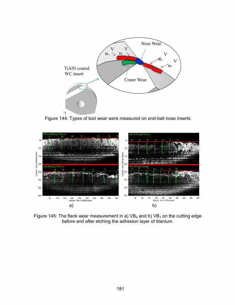
181

Figure 144: Types of tool wear were measured on end-ball nose inserts

a) b)

Figure 145: The flank wear measurement in a) VB2 and b) VB1 on the cutting edge before and after etching the adhesion layer of titanium.

TiAlN coated

WC insert

Nose Wear

V

B2

Crater Wear

V

B1

V

B4

V

B3

182

V.2 EXPERIMENTAL RESULTS AND DISCUSSION

V.2.1 Flank wear and chipping on cutting edges

V.2.1.1 Flank wear at low cutting speed (2500rpm)

As expected, the milling inserts used in MQL conditions cut more layers than under

dry conditions. Figures 146-149 presents the flank wear at VB1 on the inserts after

cutting the 1st to 8th layers under each lubrication condition at a cutting speed of

2500rpm. The maximum flank wear’s width, VBmax, and the average values of the flank

wear widths, VBavg are summarized in Figures 150 and 151. The MQL mixture with

1wt% of xGnP C750 is the best followed by the mixture with 0.1wt% of xGnP C750. In

the case of dry machining, the flank wear was not even due to the numerous chippings

and tool fractures. Consequently, the insert was only able to cut 5 layers. The flank

wear was more uniform when using the MQL mixture with 1wt% of xGnP C750. Only a

few minor chippings at the cutting edge were present with pure oil and the mixture with

0.1wt% of xGnP C750. Therefore, a certain concentration of nano-platelets of xGnP are

needed to substantially reduce both flank wear and chipping on the tool. In steady state

wear (VBavg), the mixture with 1wt% of xGnP C750 was most effective, which yielded

15% and 25% reduction in flank wear after cutting 5 layers. More importantly, machining

was stopped before reaching the life of each insert.

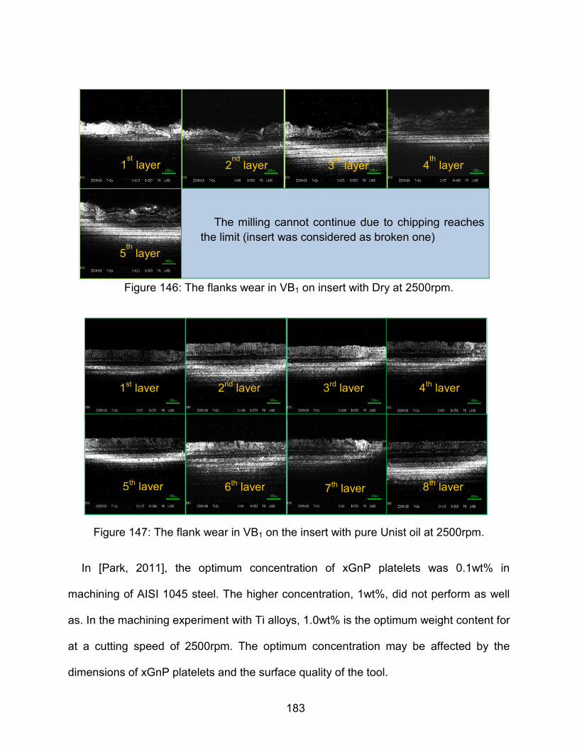
183

Figure 146: The flanks wear in VB1 on insert with Dry at 2500rpm.

Figure 147: The flank wear in VB1 on the insert with pure Unist oil at 2500rpm.

In [Park, 2011], the optimum concentration of xGnP platelets was 0.1wt% in

machining of AISI 1045 steel. The higher concentration, 1wt%, did not perform as well

as. In the machining experiment with Ti alloys, 1.0wt% is the optimum weight content for

at a cutting speed of 2500rpm. The optimum concentration may be affected by the

dimensions of xGnP platelets and the surface quality of the tool.

1st layer 2

nd layer 3

rd layer 4

th layer

5th

layer

The milling cannot continue due to chipping reaches the limit (insert was considered as broken one)

1st layer 2nd layer 3rd layer 4th layer

5th layer 6th layer 7th layer 8th layer

184

Figure 148: The flank wear in VB1 on insert with xGnP C750 0.1wt% at 2500rpm.

Figure 149: The flank wear in VB1 on insert with xGnP C750 1wt% at 2500rpm.

1st layer 3rd layer 4th layer

5th layer 7th layer 8th layer

2nd layer

6th layer

1st layer 3rd layer 4th layer

5th layer 7th layer 8th layer

2nd layer

6th layer

185

Figure 150: Maximum flank wear with (VBmax) at 2500rpm (after etching)

Figure 151: The average flank wear width (VBavg) at 2500rpm (after etching)

0

40

80

120

160

200

1 2 3 4 5 6 7 8

Th

e m

axi

mu

n F

lan

k w

ea

r V

Bm

ax

(µm

)

Cutting layer

Dry_Max Unist_Max

xGnP750 1wt%_Max xGnP750 0.1wt%_Max

30

40

50

60

70

80

90

1 2 3 4 5 6 7 8

Th

e a

vera

ge

Fla

nk

we

ar

VB

avg

(µm

)

Cutting layer

Dry_Avg Unist_Avg

xGnP750 1wt%_Avg xGnP750 0.1wt%_Avg

186

V.2.1.2 Flank wear at high cutting speed (3500rpm)

As shown in Figures 152 and 153, the enhancement of MQL solution is not as

pronounced because of the chipping under high impact conditions. It is important to

note that chipping occurred substantially more when cutting of the first few layers. The

higher concentration (5wt%) of xGnP nano-platelets was tested with an expectation of

more lubricity and/or damping due to more xGnP platelets in the lubricant. However, the

experimental results did not agree with the expectation. Among the MQL mixtures, the

mixture with 1wt % of xGnP C750 is the best followed by dry, Unist oil and 5wt% as

shown Figures 15 and 16. The reason why enhanced MQL solution at 5wt% did not

perform well is not clear at this time. It could be the poor wettability with the tool

surfaces or, the hindrance of the sliding actions at the high concentrations.

Figure 152: The flank wear in VB1 after 1st layer with different lubrication conditions at

3500rpm.

Figure 153: The flank wear in VB1 after 2st layer with different lubrication conditions at

3500rpm.

Dry Unist C750 - C750 -

Dry Unist C750 - C750 -

187

Figure 154: Maximum flank wear width (VBmax) at 3500rpm (after etching)

Figure 155: The average flank wear width (VBavg) at 3500rpm (after etching)

30

50

70

90

110

130

150

170

1 2 3 4

VB

ma

x(µ

m)

Cutting layer

Dry_Max Unist_Max

xGnP750 1wt%_Max xGnP750 5wt%_Max

30

40

50

60

70

80

90

100

1 2 3 4

VB

av

g (

µm

)

Cutting layer

Dry_Avg Unist_Avg

xGnP750 1wt%_Avg xGnP750 5wt%_Avg

188

V.2.1.3 Micro-chipping and tool fracture

Chipping and tool fracture are the common modes of tool damage in machining Ti

alloys. Especially for the consistently interrupted cutting process of milling, the tool

experiences high stress cycles and high impact leading to the cutting edges being

chipped frequently. In this work, the tool damage were classified into two categories:

micro-chipping and fracture, as shown in Figure 156. The elliptical shape represents

micro-chipping while the rectangular shape represents fracture. They were

distinguished based on the size; micro-chippings if the size was smaller than half of the

average flank wear width and tool fractures otherwise. To be more confident, the type of

chipping was evaluated based on the images from the flank face and the rake face. At

the low cutting speed, the MQL solutions (pure oil and the mixture with nano-platelets)

helped to reduce micro-chipping and prevent the propagation of micro-chipping into tool

fractures. Figures 157 and 158 represent the cutting layer on which the first damage

occurred at the cutting speeds of 2500rpm and 3550rpm, respectively, for various

lubrication conditions. The largest damage on tools under various lubrications was

presented in Figures 159 and 160 for cutting speeds of 2500rpm and 3550rpm

respectively. At low cutting speed, the tool fractures occurred at the first cutting layer

with dry milling while only micro-chippings were found with MQL mixtures even after

cutting 8th layers. At the cutting speed of 3500rpm, due to the high impact condition,

both micro-chippings and tool fractures occurred even with the MQL conditions. Tool

fractures happened after cutting only one layer under dry condition were more severe

than those under MQL mixtures which occurred after cutting 3-4 layers. The higher

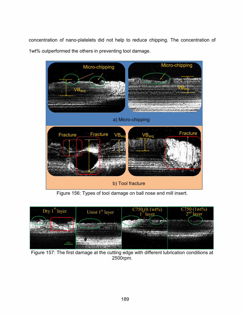
189

concentration of nano-platelets did not help to reduce chipping. The concentration of

1wt% outperformed the others in preventing tool damage.

Figure 156: Types of tool damage on ball nose end mill insert.

Figure 157: The first damage at the cutting edge with different lubrication conditions at

2500rpm.

VBavg

Micro-chipping

a) Micro-chipping

Micro-chipping

VBavg

Fracture Fracture VBavg Fracture

b) Tool fracture

VBavg

Dry 1st layer C750 (0.1wt%)

1st layer

C750 (1wt%) 2nd layer Unist 1

st layer

190

Figure 158: The first damage at the cutting edge under various lubrication conditions at

3500rpm.

Figure 159: The largest damage at the cutting edge under various lubrication conditions

at 2500rpm.

Figure 160: The largest damage at the cutting edge with different lubrication conditions

at 3500rpm.

V.2.2 Nose wear of insert

The cutting speed at the nose of the insert is very low due to the small effective

diameter (represented by De shown in Figure 161). Furthermore, the nose of the insert

being in contact with the workpiece during the cutting process is the least lubricated

region by the MQL oils in the contact zone. As expected, the effectiveness of MQL

mixture on nose wear was not significant as on flank and rake face. Figure 162 and

Unist 1st

layer

Dry 1st

layer

C750 (1wt%) 1

st

layer

C750 (5wt%) 1

st

layer

Unist 8th Dry 5

th

layer

C750 (0.1wt%) 8th layer

C750 (1wt%) 8th layer

Unist 2nd

layer

Dry 3rd C750

(1wt%) 4th

layer

C750 (5wt%) 3

rd

layer

191

Figure 163 present the center wear under certain lubrication conditions for low and high

cutting speeds, respectively. At low cutting speed, the nose wear under dry cutting was

higher than those MQL pure oil and MQL mixtures with xGnP C750. However, the

outperformance of MQL lubrication conditions to dry was reduced as high cutting

speeds increased.

Figure 161: The effective diameter of the cut, De, for ball-nose end-mill insert

Figure 162: The nose wear at the first and the last cutting layer under different

lubrication conditions at 2500rpm.

Dry

1st layer

Unist

1st layer

Unist

8th layer

C750 (1wt%)

1st layer

C750 (1wt%)

8th layer

Dry

5th layer

Nose wear

192

Figure 163: The nose wear at the first and the last cutting layer under different

lubrication conditions at 3500rpm.

V.2.3 Crater wear

In the milling process, the rake face of the tools did not experience the dramatic wear

unlike those in turning. In the milling experiment, only slight wear with a thin adhesion

layer was observed in the rake face of the inserts under all lubrication conditions.

Therefore, the MQL solution does not affect the rake face. The chipping at the cutting

edge had a more significant impact on the rake face than on the crater wear as shown

in Figures 164 and 165 for cutting speeds of 2500rpm and 3500rpm, respectively.

Fracture at the cutting edge was more frequent and larger in dry condition than the MQL

conditions at both low and high cutting speeds. Among MQL conditions, the lubricant

enhanced by nano-platelets helps to reduce the chipping at the cutting edge. The low

crater wear revealed the deformation of the tool is not as severe as in turning. A reason

for low crater wear is the cutting temperatures in milling were fairly lower than those in

Dry

1st

Unist

1st layer

Unist

2nd layer

C750 (1wt%)

C750 (1wt%)

Dry

3rd

Nose wear

193

turning which limited dissolution/diffusion. The abrasion of chip to rake face was less

compared with turning due to discontinuous chip in milling. In milling of Ti64 at low

cutting speed, cooling is not as critical as lubrication, which enhances the effectiveness

of MQL.

Figure 164: The crater wear and damage on the tool at the last cutting layer with

different lubrication conditions at 2500rpm.

Figure 165: The crater wear and damage on the tool at the last cutting layer with

different lubrication conditions at 3500rpm.

Unist 8th

layer

Dry 3rd

layer

C750 (0.1wt%) 8th

layer C750 (1wt%) 8

th

layer

chipped

crater

wear

crater

wear

chipped crater

wear

crater

wear chipped

Unist 2nd layer Dry 3

rd

layer

C750 (1wt%) 4th

layer C750 (5wt%) 3

rd

layer

chipped

crater

wear

crater

wear

chipped crater

wear

crater

wear

chipped chipped

194

Chapter 6: Conclusions

In the turning experiment of Ti64 with carbide and PCD inserts, the

dissolution/diffusion wear is the dominant wear mechanism on the rake face of carbide

insert while grain-pulled out is the main mode of tool wear on rake face of PCD insert.

These conclusions are corroborated by the smooth craters found on carbide inserts and

the rough and uneven crater on PCD inserts. Because the crater wear started away

from the cutting edge and progressed rapidly to cutting edge on carbide inserts, tool

fracture on cutting edge was more excessive than the PCD inserts. The cutting edge on

PCD inserts was intact, which enable them to have longer tool lives. Abrasion by the

hard α-clusters and tool fractures were the main causes for flank wear on both carbide

and PCD inserts. At the high cutting speed, PCD inserts were additionally damaged by

notch wear. Obviously, for both carbide and PCD inserts, the wear in low cutting speeds

is not as extensive as those from high cutting speeds. The thermal conductivity and

hardness of PCD are much higher compared to those of the carbide inserts, resulting in

lower cutting temperatures and superior resistance to abrasion wear. Therefore, the

wear rates of PCD inserts were much smaller than those of carbide inserts at each

cutting speed. PCD showed a better performance in resisting flank wear independent of

cutting speed. However, the performance of PCD is even more superior at high cutting

speed.

The OIM results of the microstructure analysis of work material and chip in the

turning experiments of Ti64 proved the evident of phase change and root cause flank

wear and scoring marks on flank face. The chips generated with carbides and PCD

inserts contain the higher β-phase faction and higher peaks at 60° and 90°

195

misorientations compared to the original work material indicated that the phase change

α→β happened during machining. This result agreed well with the FEM simulation,

which showed the cutting temperature reaching beyond the transus temperature. The

microstructure of the original work material revealed the heterogeneity in the

microstructure coming from the presence of both α and β grains and the cluster of the α-

grains in the hard orientations which abrade and fracture the tool surfaces,. In addition,

when the adhesion layers are detached from the inserts, some grains are pulled out of

the tool materials, further damaging the inserts. The hard α-clusters caused large,

steady and smoother scoring marks on ‘softer’ carbide surface and sometime fracture

with large ‘hard’ clusters. The hard α-clusters can damage the inserts in a more brittle

manner and the detached tool fragments further damaged mainly evident by the surface

patterns showing the grain fractured out from the flank surface with the scoring mark on

PCD inserts.

To enhance the machinability, the ball milling experiment of 1045 steel and Ti64 was

conducted with the MQL oil mixed with micro- and nano-platelets of graphite and hBN to

compare with dry and regular MQL cutting. Despite the fact that the friction of these

mixtures with micro and nano- platelets regardless of the thickness and concentrations

did not change from that of pure oil, the tribo-test clearly showed the advantage of

mixing nano-platelets of xGnP and hBN in reducing wear. These findings have been

corroborated with the experimental results from the ball milling experiment with 1045

steels. The MQL mixtures with micro-platelets (Graphite and hBN5) did not present any

advantage over the pure oil (traditional MQL) in reduction of flank wear while the

mixtures with only a small amount (0.1w% for xGnP M5, xGnP C300, xGnP C750 and

196

0.5wt% for HBN300) of nano-platelets presented a significant improvement in wear

performance. Among the xGnP grades, the thinner platelets showed better resisting

wear performances in both tribotest and MQL-ball mill test. In the milling of Ti64,

however, the content of nano-platelet C750 needed to be increased (up to 1wt%) to

provide significant improvement. MQL with nano-lubricants substantially outperforms to

dry and regular MQL machining by reducing flank wear and tool damage which consist

of micro chippings and fractures. At the cutting speed of 2500rpm, the tool fractured in

dry machining while only micro chippings occurred when the MQL mixtures were used.

At given cutting speed, cutting condition is more aggressive in machining Ti64 than

those in machining steel. As expected, the effectiveness of mixtures with nano-platelets

in MQL machining Ti64 was less significant at cutting speed of 3500rpm while those

mixtures showed outperformance at that cutting speed in machining 1045 steel.

Machining of Ti64 at the lower cutting speed, the nano-platelets enhanced MQL

presented much more effective. This nano-lubricant technology works because it

provides the necessary lubricity even when the oil dissociate due to the high cutting

temperature.

197

BIBLIOGRAPHY

198

BIBLIOGRAPHY

Alberts, M., Kalaitzidou, K., & Melkote, S. (2009). An investigation of graphite

nanoplatelets as lubricant in grinding. International Journal of Machine Tools and Manufacture, 49(12-13), 966–970.

Allam, I. (1991). Solid lubricants for applications at elevated temperatures. Journal of Materials, 26(15), 3977–3984.

Amrita, M., Srikant, R., Sitaramaraju, a., Prasad, M., & Krishna, P. V. (2013). Experimental investigations on influence of mist cooling using nanofluids on machining parameters in turning AISI 1040 steel. Proceedings of the Institution of Mechanical Engineers, Part J: Journal of Engineering Tribology, 227(12), 1334–1346.

Andriya, N., Rao, P. V., & Ghosh, S. (2012). Dry Machining of Ti-6Al-4V using PVD Coated TiAlN Tools. Proceedings of the World Congress on Engineering, III, 2–7.

Arrazola, P.-J., Garay, a., Iriarte, L.-M., Armendia, M., Marya, S., & Le Maître, F. (2009). Machinability of titanium alloys (Ti6Al4V and Ti555.3). Journal of Materials Processing Technology, 209(5), 2223–2230.

Attanasio, A., Gelfi, M., Pola, A., Ceretti, E., & Giardini, C. (2013). Influence of Material Microstructures in Micromilling of Ti6Al4V Alloy. Materials, 6(9), 4268–4283.

Bartz, W. J. (1971). Solid lubricant additives - effect of concentration and other additives on anti-wear performance. Wear, 17(5-6), 421–432.

Bayoumi, a. E., & Xie, J. Q. (1995). Some metallurgical aspects of chip formation in cutting Ti-6wt.%Al-4wt.%V alloy. Materials Science and Engineering: A, 190(1-2), 173–180.

Bermingham, M. J., Kirsch, J., Sun, S., Palanisamy, S., & Dargusch, M. S. (2011). New observations on tool life, cutting forces and chip morphology in cryogenic machining Ti-6Al-4V. International Journal of Machine Tools and Manufacture, 51(6), 500–511.

Boothroyd, G. (1975). Fundamentals of Metal Machining and Machine Tools. Washington. DC: Scripta Book Company.

Boyer, R. R. (1996). An overview on the use of titanium in the aerospace industry. Materials Science and Engineering: A, 213(1-2), 103–114.

199

Braga, D. U., Diniz, A. E., Miranda, G. W. ., & Coppini, N. L. (2002). Using a minimum quantity of lubricant (MQL) and a diamond coated tool in the drilling of aluminum–silicon alloys. Journal of Materials Processing Technology, 122(1), 127–138.

Brandao, L. C., Coelho, R. T., & Lauro, C. H. (2011). Contribution to dynamic characteristics of the cutting temperature in the drilling process considering one dimension heat flow. Applied Thermal Engineering, 31(17-18), 3806–3813.

Brinksmeier, E., Diersen, P., Zillmer, A., & Janssen, R. (1999). Cooling Lubrication Reduction when Machining Advanced Materials. Aspects of Cooling Lubrication Reduction in Machining Advanced Materials, 213(08), 769–778.

Britton, T. B., Liang, H., Dunne, F. P. E., & Wilkinson, a. J. (2009). The effect of crystal orientation on the indentation response of commercially pure titanium: experiments and simulations. Proceedings of the Royal Society A: Mathematical, Physical and Engineering Sciences, 466(2115), 695–719.

Calamaz, M., Coupard, D., & Girot, F. (2008). A new material model for 2D numerical simulation of serrated chip formation when machining titanium alloy Ti–6Al–4V. International Journal of Machine Tools and Manufacture, 48(3-4), 275–288.

Cetin, M. H., Ozcelik, B., Kuram, E., & Demirbas, E. (2011). Evaluation of vegetable based cutting fluids with extreme pressure and cutting parameters in turning of AISI 304L by Taguchi method. Journal of Cleaner Production, 19(17-18), 2049–2056.

Chen N. (2004). Coefficients of Friction for Graphite.

Cook, N. H., & Nayak, P. N. (1986). The thermal mechanics of tool wear. Journal of Manufacturing Science and Engineering, 88(1), 93–100.

Corduan, N., Himbart, T., Poulachon, G., Dessoly, M., Lambertin, M., Vigneau, J., & Payoux, B. (2003). Wear Mechanisms of New Tool Materials for Ti-6AI-4V High Performance Machining. CIRP Annals - Manufacturing Technology, 52(1), 73–76.

Dearnley, P. A., & Grearson, A. N. (1986). P. A. Dearnley A. N. Grearson, 2(January), 47–58.

Dhar, Ahmed, M. T., & Islam, S. (2007). An experimental investigation on effect of minimum quantity lubrication in machining AISI 1040 steel. International Journal of Machine Tools and Manufacture, 47(5), 748–753.

Dhar, N. R., Paul, S., & Chattopadhyay, A. B. (2002). Machining of AISI 4140 steel under cryogenic coolingÐtool wear, surface roughness and dimensional deviation. Journal of Materials Processing Technology, 123(3), 483–489.

200

Donnet, C., & Erdemir, a. (2004). Solid Lubricant Coatings: Recent Developments and Future Trends. Tribology Letters, 17(3), 389–397.

Emami, M., Sadeghi, M. H., Sarhan, A. A. D., & Hasani, F. (2014). Investigating the Minimum Quantity Lubrication in grinding of Al2O3 engineering ceramic. Journal of Cleaner Production, 66, 632–643.

Ezugwu, E. O., & Wang, Z. M. (1997). Materials Titanium alloys and their machinability. Journal of Materials Processing Technology, 68, 262–274.

Fang, Z. Z. (2005). Correlation of transverse rupture strength of WC–Co with hardness. International Journal of Refractory Metals and Hard Materials, 23(2), 119–127.

Fukushima, H. (2003). Graphite Nano-reinforcements in polymer Nanocomposites. Ph.D. Thesis, Michigan State University, East Lansing, MI, USA.

Gabriel, S. B., de Almeida, L. H., Nunes, C. a, Dille, J., & Soares, G. a. (2013). Maximisation of the ratio of microhardness to the Young’s modulus of Ti-12Mo-13Nb alloy through microstructure changes. Materials Science & Engineering. C, Materials for Biological Applications, 33(6), 3319–24.

Gaitonde, V. N., Karnik, S. R., & Davim, J. P. (2008). Selection of optimal MQL and cutting conditions for enhancing machinability in turning of brass. Journal of Materials Processing Technology, 204(1-3), 459–464.

Gente. (2001). Chip Formation in Machining_Ti64 (chip morphology vs CS).pdf. CIRP Annals - Manufacturing Technology, 50, 49–52.

Groover, M. P. (2007). Fundamentals of modern manufacturing: materials processes, and systems (3rd ed.). John Wiley & Sons.

Hartung, P. D., & Kramer, B. M. (1982). Tool Wear in Titanium Machining. Ann. CIRP, 31(1), 75–80.

Hasçalık, A., & Çaydaş, U. (2007). Optimization of turning parameters for surface roughness and tool life based on the Taguchi method. The International Journal of Advanced Manufacturing Technology, 38(9-10), 896–903.

Haubner, R., Wilhelm, M., Weissenbacher, R., & Lux, B. (2002). Boron Nitrides - Properties, Synthesis and Applications (Vol. 102, pp. 1–45). Springer Berlin Heidelberg.

Heinemann, R., Hinduja, S., Barrow, G., & Petuelli, G. (2006). Effect of MQL on the tool life of small twist drills in deep-hole drilling. International Journal of Machine Tools and Manufacture, 46(1), 1–6.

201

Hickman B.S. (1969). The Formation of Omega Phase in Titanium and Zirconium Alloys: A Review, 4, 554–563.

Hosseini, A., & Kishawy, H. A. (2014). Machining of Titanium Alloys. In J. P. Davim (Ed.), Machining of Titanium Alloys. Berlin, Heidelberg: Springer Berlin Heidelberg.

Hsu, H.-C., Wu, S.-C., Hsu, S.-K., Lin, T.-F., & Ho, W.-F. (2013). Structure and mechanical properties of as-cast Ti–5Nb–xCr alloys. Materials & Design, 51, 268–273.

Hsu, S. M. (2004). Nano-lubrication: concept and design. Tribology International, 37(7), 537–545.

Hua, J., & Shivpuri, R. (2005). A Cobalt Diffusion Based Model for Predicting Crater Wear of Carbide Tools in Machining Titanium Alloys. Journal of Engineering Materials and Technology, 127(1), 136.

Huang, H. D., Tu, J. P., Gan, L. P., & Li, C. Z. (2006). An investigation on tribological properties of graphite nanosheets as oil additive. Wear, 261(2), 140–144.

Hughes, J. I., Sharman, A. R. C., & Ridgway, K. (2004). The effect of tool edge preparation on tool life and workpiece surface integrity. Proc. IMechE Part B: J. Engineering Manufacture, 220, 1113–1123.

Ibrahim, G. A., CheHaron, C. H., & Ghani, J. A. (2009). Surface integrity of ti-6al-4v eli when machined using coated carbide tools under dry cutting condition. International Journal of Mechanical and Materials Engineering (IJMME), 4(2), 191–196.

Jaffery, S. I., & Mativenga, P. T. (2008). Assessment of the machinability of Ti-6Al-4V alloy using the wear map approach. The International Journal of Advanced Manufacturing Technology, 40(7-8), 687–696.

Jawaid, a, Che-Haron, C. ., & Abdullah, a. (1999). Tool wear characteristics in turning of titanium alloy Ti-6246. Journal of Materials Processing Technology, 92-93, 329–334.

Jon, M. C., Engineering, M., Science, M., & York, N. (1972). Omega-Phase Formation in Beta III Titanium Alloy, 150, 139–150.

Jones, N., Dashwood, R., Jackson, M., & Dye, D. (2009). Development of chevron-shaped α precipitates in Ti–5Al–5Mo–5V–3Cr. Scripta Materialia, 60(7), 571–573.

Joshi, S., Pawar, P., Tewari, A., & Joshi, S. S. (2014). Effect of β phase fraction in titanium alloys on chip segmentation in their orthogonal machining. CIRP Journal of Manufacturing Science and Technology, 7(3), 191–201.

202

Kajdas, C., Kanpsika, A., & Kulczycki, A. (2010). Chemistry and Technology of Lubricants. In R. M. Mortier, M. F. Fox, & S. T. Orszulik (Eds.), Chemistry and technology of lubricants (pp. 239–292). Dordrecht: Springer Netherlands.

Kalita, P., Malshe, A. P., Arun Kumar, S., Yoganath, V. G., & Gurumurthy, T. (2012). Study of specific energy and friction coefficient in minimum quantity lubrication grinding using oil-based nanolubricants. Journal of Manufacturing Processes, 14(2), 160–166.

Khettabi, R., Songmene, V., & Masounave, J. (2009). Effects of Speeds, Materials, and Tool Rake Angles on Metallic Particle Emission During Orthogonal Cutting. Journal of Materials Engineering and Performance, 19(6), 767–775.

Khettabi, R., Songmene, V., Masounave, J., & Zaghbani, I. (2008). Understanding the Formation of Nano and Micro Particles During Metal Cutting.pdf. International Journal of Signal System Control and Engineering, 1(3), 203–210.

Kimura, Y., Wakabayashi, T., Okada, K., Wada, T., & Nishikawa, H. (1999). Boron nitride as a lubricant additive. Wear, 232(2), 199–206.

Konig, W. (1979). Applied research on the machinability of titanium and its alloys. Proc. AGARD Conf. Advanced Fabrication Processes, Florence, Italy.

Kramer, B. M., & von Turkovich, B. F. (1986). A Comprehensive Tool Wear Model. CIRP Annals - Manufacturing Technology, 35(1), 67–70.

Kwon, J., Brandes, M. C., Sudharshan Phani, P., Pilchak, a. P., Gao, Y. F., George, E. P., a Mills, M. J. (2013). Characterization of deformation anisotropies in an α-Ti alloy by nanoindentation and electron microscopy. Acta Materialia, 61(13), 4743–4756.

Kwon, P., & Drzal, L. T. (2010). Nanoparticle graphite-based minimum quantity lubrication method and composition. US.

Lammer, A. (1988). Mechanical properties of polycrystalline diamonds. Materials Science and Technology, 4(November), 949–955.

Lee, C.-G., Hwang, Y.-J., Choi, Y.-M., Lee, J.-K., Choi, C., & Oh, J.-M. (2009). A study on the tribological characteristics of graphite nano lubricants. International Journal of Precision Engineering and Manufacturing, 10(1), 85–90.

List, G., Nouari, M., Géhin, D., Gomez, S., Manaud, J. P., Le Petitcorps, Y., & Girot, F. (2005). Wear behaviour of cemented carbide tools in dry machining of aluminium alloy. Wear, 259(7-12), 1177–1189.

203

Liu, Z. Q., Cai, X. J., Chen, M., & An, Q. L. (2011). Investigation of cutting force and temperature of end-milling Ti-6Al-4V with different minimum quantity lubrication (MQL) parameters. Proceedings of the Institution of Mechanical Engineers, Part B: Journal of Engineering Manufacture, 225(8), 1273–1279.

López de Lacalle, L. N., Angulo, C., Lamikiz, a., & Sánchez, J. a. (2006). Experimental and numerical investigation of the effect of spray cutting fluids in high speed milling. Journal of Materials Processing Technology, 172(1), 11–15.

Lütjering, G., & Williams, J. C. (2003). Titanium (2nd ed.). Berlin: Springer.

Machado, A. R., & Wallbank, J. (1990). Machining of titanium and its alloys-a. Proceedings of the Institution of Mechanical Engineers, Part B: Journal of Engineering Manufacture, 204(1), 53–60.

Machai, C., Iqbal, A., Biermann, D., Upmeier, T., & Schumann, S. (2013). On the effects of cutting speed and cooling methodologies in grooving operation of various tempers of β-titanium alloy. Journal of Materials Processing Technology, 213(7), 1027–1037.

Maciej Motyka, K. K. J. S. and W. Z. (2012). Titanium Alloys - Towards Achieving Enhanced Properties for Diversified Applications. (A. K. M. N. Amin, Ed.). InTech.

Mao, C., Tang, X., Zou, H., Huang, X., & Zhou, Z. (2012). Investigation of grinding characteristic using nanofluid minimum quantity lubrication. International Journal of Precision Engineering and Manufacturing, 13(10), 1745–1752.

Mao, C., Zou, H., Huang, X., Zhang, J., & Zhou, Z. (2012). The influence of spraying parameters on grinding performance for nanofluid minimum quantity lubrication. The International Journal of Advanced Manufacturing Technology, 64(9-12), 1791–1799.

Meyer, L. W., Krüger, L., Sommer, K., Halle, T., & Hockauf, M. (2008). Dynamic strength and failure behavior of titanium alloy Ti-6Al-4V for a variation of heat treatments. Mechanics of Time-Dependent Materials, 12(3), 237–247.

Molinari, a, Musquar, C., & Sutter, G. (2002). Adiabatic shear banding in high speed machining of Ti–6Al–4V: experiments and modeling. International Journal of Plasticity, 18(4), 443–459.

Motonishi, S., Isoda, S., Itoh, H., Tsumori, Y., & Terada, Y. (1987). Study on Machining of Titanium and Its Alloys. Kobelto Technology Review, 2, 28–31.

Nabhani, F. (2001). Machining of aerospace titanium alloys. Robotics and Computer-Integrated Manufacturing, 17(1-2), 99–106.

204

Nageswara Rao, D., & Vamsi Krishna, P. (2008). The influence of solid lubricant particle size on machining parameters in turning. International Journal of Machine Tools and Manufacture, 48(1), 107–111.

Nandy, a. K., & Paul, S. (2008). Effect of coolant pressure, nozzle diameter, impingement angle and spot distance in high pressure cooling with neat oil in turning Ti-6Al-4V. Machining Science and Technology, 12(4), 445–473.

Narutaki, N., Murakoshi, A., Motonishi, S., & Takeyama, H. (1983). Study on Machining of Titanium Alloys. CIRP Annals - Manufacturing Technology, 32(1), 65–69.

Narutaki, N., Murakoshi, A., Motonishi, S., & Takeyama, H. (1983). Study on Machining of Titanium Alloys. CIRP Annals - Manufacturing Technology, 32(1), 65–69.

Nguyen, T. K., Do, I., & Kwon, P. (2012). A tribological study of vegetable oil enhanced by nano-platelets and implication in MQL machining. International Journal of Precision Engineering and Manufacturing, 13(7), 1077–1083.

Olortegui-Yume, J. A., & Kwon, P. Y. (2007). Tool wear mechanisms in machining. Nternational Journal of Machining and Machinability of Materials, 2(3), 316–334.

Olortegui-Yume, J. a., & Kwon, P. Y. (2010). Crater wear patterns analysis on multi-layer coated carbides using the wavelet transform. Wear, 268(3-4), 493–504.

Oosthuizen, G. A., Akdogan, G., Dimitrov, D., & Treurnich, N. F. (2010). A Review of the Machinability of Titanium Alloys. R & D Journal of the South African Institution of Mechanical Engineering, 26(September), 43–52.

Ozcelik, B., Kuram, E., Huseyin Cetin, M., & Demirbas, E. (2011). Experimental investigations of vegetable based cutting fluids with extreme pressure during turning of AISI 304L. Tribology International, 44(12), 1864–1871.

Park, K.-H., & Kwon, P. Y. (2011). Flank wear of multi-layer coated tool. Wear, 270(11-12), 771–780.

Park, K.-H., Ewald, B., & Kwon, P. Y. (2011). Effect of Nano-Enhanced Lubricant in Minimum Quantity Lubrication Balling Milling. Journal of Tribology, 133(3), 031803.

Paul, P. S., & Varadarajan, a. (2013). Performance evaluation of hard turning of AISI 4340 steel with minimal fluid application in the presence of semi-solid lubricants. Proceedings of the Institution of Mechanical Engineers, Part J: Journal of Engineering Tribology, 227(7), 738–748.

205

Prasad, B. K. (2005). Effectiveness of an externally added solid lubricant on the sliding wear response of a zinc?aluminium alloy, its composite and cast iron. Tribology Letters, 18(2), 135–143.

Prasad, B. K., Rathod, S., Yadav, M. S., & Modi, O. P. (2010). Effects of Some Solid Lubricants Suspended in Oil Toward Controlling the Wear Performance of a Cast Iron. Journal of Tribology, 132(4), 041602.

Rabinowic, E., L.A., D., & Russell, P. G. (1961). A study of abrasive wear under three-body conditions. Wear, 4(5), 345–355.

Rabinowicz, E. (1977). Abrasive wear resistance as a materials test. Lubr. Eng., 33(7), 378–381.

Rahim, E. A., Kamdani, K., & Sharif, S. (2008). Performance Evaluation of Uncoated Carbide Tool in High Speed Drilling of Ti6Al4V. Journal of Advanced Mechanical Design, Systems, and Manufacturing, 2(4), 522–531.

Rahman, M., Wong, Y. S., & Zareena, A. R. (2003). Machinability of titanium alloys. JSME International Journal Series C, 46, 107–115.

Rahman, M., Wong, Y. S., & Zareena, A. R. (2003). Machinability of titanium alloys. JSME International Journal Series C, 46, 107–115.

Rahmati, B., Sarhan, A. a. D., & Sayuti, M. (2013). Investigating the optimum molybdenum disulfide (MoS2) nanolubrication parameters in CNC milling of AL6061-T6 alloy. The International Journal of Advanced Manufacturing Technology, 70(5-8), 1143–1155.

Ramesh, S., Karunamoorthy, L., & Palanikumar, K. (2008). Fuzzy Modeling and Analysis of Machining Parameters in Machining Titanium Alloy. Materials and Manufacturing Processes, 23(4), 439–447.

Reddy, N. S. K., & Rao, P. W. (2006). Experimental investigation to study the effect of solid lubricants on cutting forces and surface quality in end milling. International Journal of Machine Tools and Manufacture, 46(2), 189–198.

Rioul, O., & Vetterli, M. (1991). No Title. IEEE Signal Processing Magazine, 8, 14–38.

Sadeghi, M. H., Haddad, M. J., Tawakoli, T., & Emami, M. (2008). Minimal quantity lubrication-MQL in grinding of Ti–6Al–4V titanium alloy. The International Journal of Advanced Manufacturing Technology, 44(5-6), 487–500.

206

Sarhan, A. a. D., Sayuti, M., & Hamdi, M. (2012). Reduction of power and lubricant oil consumption in milling process using a new SiO2 nanolubrication system. The International Journal of Advanced Manufacturing Technology, 63(5-8), 505–512.

Schrock, D. J., & Kwon, P. (2012). Evidence of Phase Dependent Tool Wear in Ti-6Al-4V Turning Experiments Using PCD and Carbide Inserts. In ASME 2012 International Manufacturing Science and Engineering Conference (p. 371). ASME.

Schrock, D. J., Kang, D., Bieler, T. R., & Kwon, P. (2014). Phase Dependent Tool Wear in Turning Ti-6Al-4V Using Polycrystalline Diamond and Carbide Inserts. Journal of Manufacturing Science and Engineering, 136(4), 041018.

Semiatin, S. L., Seetharaman, V., & Weiss, I. (1996). The Thermomechanical Processing of Alpha/Beta Titanium Alloys. JOM, 49(6), 33–40.

Shahan, A. R., & Taheri, A. K. (1993). Adiabatic shear bands in titanium and titanium alloys: a critical review. Materials & Design, 14(4), 243–250.

Shen, B., Malshe, A. P., & Shih, A. J. (2008). Performance of novel mos 2 nanoparticles based grinding fluids in minimum quantity lubrication grinding. Transaxtions of NAMRI/SME, 36, 357–364.

Shen, B., Shih, A. J., & Tung, S. C. (2008). Application of Nanofluids in Minimum Quantity Lubrication Grinding. Tribology Transactions, 51(6), 730–737.

Sima, M., & Özel, T. (2010). Modified material constitutive models for serrated chip formation simulations and experimental validation in machining of titanium alloy Ti–6Al–4V. International Journal of Machine Tools and Manufacture, 50(11), 943–960.

Singh, G., Singh, S., Singh, M., & Kumar, A. (2013). Experimental investigations of vegetable & mineral oil performance during machining of en-31 steel with minimum quantity lubrication. International Journal of Research in Engineering and Technology, 02(06), 1030–1037.

Srikant, R. R., Rao, D. N., Subrahmanyam, M. S., & Vamsi Krishna, P. (2009). Applicability of cutting fluids with nanoparticle inclusion as coolants in machining. Proceedings of the Institution of Mechanical Engineers, Part J: Journal of Engineering Tribology, 223(2), 221–225.

Suh, N. P. (1986). Tribophysics. (Pretice-Hall, Ed.).

Tai, B. L., Dasch, J. M., & Shih, A. J. (2011). Evaluation and Comparison of Lubricant Properties in Minimum Quantity Lubrication Machining. Machining Science and Technology, 15(4), 376–391.

207

Tawakoli, T., Hadad, M. J., & Sadeghi, M. H. (2010). Influence of oil mist parameters on minimum quantity lubrication–MQL grinding process. International Journal of Machine Tools and Manufacture 50, 50(06), 521–531.

Thepsonthi, T., Hamdi, M., & Mitsui, K. (2009). Investigation into minimal-cutting-fluid application in high-speed milling of hardened steel using carbide mills. International Journal of Machine Tools and Manufacture, 49(2), 156–162.

Toh, C. K., & Kanno, S. (2004). Surface integrity effects on turned 6061 and 6061-T6 aluminum alloys. Proc. IMechE,Vol. 225, Part N: J. of Nano Engineering and Nano Systems, 225(1), 3–16.

Trent, E. M. (1991). Metal cutting. Butterworth-Heinemann Ltd, Oxford.

Ueda, T., Hosokawa, A., & Yamada, K. (2006). Effect of Oil Mist on Tool Temperature in Cutting. Journal of Manufacturing Science and Engineering, 128(1), 130.

Varadarajan, a. S., Philip, P. K., & Ramamoorthy, B. (2002). Investigations on hard turning with minimal cutting fluid application (HTMF) and its comparison with dry and wet turning. International Journal of Machine Tools and Manufacture, 42(2), 193–200.

Venugopal, K. a., Paul, S., & Chattopadhyay, a. B. (2007). Growth of tool wear in turning of Ti-6Al-4V alloy under cryogenic cooling. Wear, 262(9-10), 1071–1078.

Wakabayashi, T., Inasaki, I., & Suda, S. (2006). Tribological Action and Optimal Performance: Research Activities Regarding Mql Machining Fluids. Machining Science and Technology, 10(1), 59–85.

Watanabe, S., Miyake, S., & Murakawa, M. (1991). Tribological properties of cubic, amorphous and hexagonal boron nitride films. Surface and Coatings Technology, 49(1-3), 406–410.

Weinert, K., Inasaki, I., Sutherland, J. W., & Wakabayashi, T. (2004). Dry Machining and Minimum Quantity Lubrication. CIRP Annals - Manufacturing Technology, 53(2), 511–537.

Wong, T., Kim, W., & Kwon, P. (2004). Experimental support for a model-based prediction of tool wear. Wear, 257(7-8), 790–798.

Wright, P. K., & Bagchi, a. (1981). Wear mechanisms that dominate tool-life in machining. Journal of Applied Metalworking, 1(4), 15–23.

Yang, X., Liu, C. R., & Lafayette, W. (1999). Machining titanium and its alloys. Machining Science and Technology, 3(1), 107–139.

208

Yukhno, T. ., Vvedensky, Y. ., & Sentyurikhina, L. . (2001). Low temperature investigations on frictional behaviour and wear resistance of solid lubricant coatings. Tribology International, 34(4), 293–298.

Zhang, X. P., Shivpuri, R., & Srivastava, a. K. (2014). Role of phase transformation in chip segmentation during high speed machining of dual phase titanium alloys. Journal of Materials Processing Technology, 214(12), 3048–3066.

Zhang, X., Wu, S., Wang, H., & Liu, C. R. (2011). Predicting the Effects of Cutting Parameters and Tool Geometry on Hard Turning Process Using Finite Element Method. Journal of Manufacturing Science and Engineering, 133(4), 041010.

Zhang, Y. C., Mabrouki, T., Nelias, D., & Gong, Y. D. (2011). Chip formation in orthogonal cutting considering interface limiting shear stress and damage evolution based on fracture energy approach. Finite Elements in Analysis and Design, 47(7), 850–863.

Zhu, Q., Qiu, X., & Ma, C. (1998). The oxidation resistance improvement of matrix graphite of spherical fuel elements by slip-gelation process. Journal of Nuclear Materials, 254(2-3), 221–225.

FUNDAMENTAL TOOL WEAR STUDY IN TURNING OF Ti-6Al ...

Documents

Transcript of FUNDAMENTAL TOOL WEAR STUDY IN TURNING OF Ti-6Al ...