Meta-Analysis of Climate Change Data
59
Meta-Analysis of Climate Change Data Determination of High Effect Climate Factors Greenhouse Effect, Proxies and Reconstructions of Temperature and CO 2 (ppm), Instrumental Records of Temperature, Fossil Fuel Production, Solar Variation: Orbit, Magnetic and Sunspot Cycles, Irradiance, Radiation Bands, Albedo, Temperature Statistical Model, Ocean Currents, Sea and Glacier Levels, Climate Extremes, Climate Cycle Analysis, Climate Models, Search for Anthropogenic Climate Fingerprints, and Potential Solutions http://www.leapcad.com/Climate_Analysis/Meta-Analysis_of_Climate_Change_Data.xmcd Rev July 18, 2015 An Application of the LeapCad Methodology and Philosophy in providing a Virtual Laboratory for Learning, Exploring, and Developing Models using Tutorial Analytical Math Scripts. These analytic climate model Mathcad (Version14) scripts and data are directly accessible from LeapCad.com. Greenhouse Effect (GH), Anthropogenic Global Warming (AGW) Theory, and Evidence The earth receives mostly visible shortwave (< 1μm) energy from the sun, the majority of which passes through the atmosphere. The atmosphere near the surface is largely opaque to mid IR, thermal radiation (5-15μm) (with importan exceptions for "window" bands - See Section V. Solar Radiation Spectrum), and most heat loss from the surface is by sensible heat and latent heat transport. However, CO 2 radiative effects become increasingly important higher in the atmosphere as the higher levels become progressively more transparent to thermal radiation, largely because the atmosphere is drier and water vapor - an important greenhouse gas (GHG) - becomes less. GHG will absorb light only in a set of specific wavelengths, which show up as thin dark lines in a spectrum. In a gas at sea-level temperature and pressure, the countless molecules colliding with one another at different velocities each absorb at slightly different wavelengths, so the lines are broadened and overlap to a considerable extent. At low pressure the spikes become much more sharply defined, like a picket fence. There are gaps between the H2O lines where radiation can get through unless blocked by CO2 lines. Thus CO2 absorption in the stratosphere does not saturate. If the concentration of CO 2 is doubled, the GH effect model adds 4 W/sq. meter, which results in a global average temperature increase of 2.8C. It is more realistic to think of the greenhouse effect as applying to a "surface" in the mid-troposphere, which is effectively coupled to the surface by a temperature lapse rate. Within the mid-troposphere region where radiative effects are important, the presentation of the Idealized Greenhouse Model becomes more reasonable: a layer of atmosphere with greenhouses gases will re-radiate heat in all directions, both upwards and downwards, thereby warming the surface (324 W/m 2 ) and simultaneously cooling (195 W/m 2 ) the atmosphere by transmitting heat to deep space at 2.7K. Increasing the concentration of these gases increases the amount of radiation, and thereby warms the surface and cools the atmosphere more. GHG shift the balance between incoming shortwave solar radiation and IR thermal radiation. This GH effect increase the land & ocean by about 20 C. See the illustration below. AGW Mechanism: The Industrial Era has doubled CO 2 . CO 2 is only 0.04% of the atmosphere, (its highest atmospheric concentration in at least 650,000 years), but it modifies the balance of shortwave incoming and IR. It is a strong absorber of infrared wavelengths, so it traps energy that would otherwise escape to space and nudges upward the temperature at which the radiation balance occurs. Another critical factor is that CO 2 lingers for decades to centuries, while water vapor rains out. For the following discussion refer to the "Energy Balance Intensities" figure on page 2. If we average the incoming shortwave solar radiation that is absorbed by the earth’s climate over the surface of the earth we get around 235 W/m2. If we average the outgoing longwave radiation from the top of atmosphere we get the same value: 235 W/m2. If the atmosphere didn’t absorb any terrestrial radiation then the surface of the earth must also be emitting 235 W/m2. The only way that the surface of the earth could emit this amount is if the temperature of the earth was around 255K or -18°C. See Section IX-2. And yet we measure an average surface temperature of the earth around 15°C – which corresponds to an emission of radiation of 396 W/m2 from the surface of the earth. If the atmosphere wasn’t absorbing and re-radiating longwave then the surface of the earth would be -18°C. The actual warmer temperature of the earth results from the inappropriately-named “greenhouse” effect. In reality, of course, the situation is more complicated. Warmer air holds more water vapor, which is itself an important greenhouse gas. If we add carbon dioxide to the atmosphere, water vapor becomes more abundant and amplifies the temperature increase that would result from the carbon dioxide alone. Indeed, somewhat more than half of any AGW warming comes from this and other feedback processes. 1
-
Upload
khangminh22 -
Category
Documents
-
view
5 -
download
0
Transcript of Meta-Analysis of Climate Change Data
Meta-Analysis of Climate Change DataDetermination of High Effect Climate Factors
Greenhouse Effect, Proxies and Reconstructions of Temperature and CO2 (ppm),
Instrumental Records of Temperature, Fossil Fuel Production, Solar Variation:
Orbit, Magnetic and Sunspot Cycles, Irradiance, Radiation Bands, Albedo,
Temperature Statistical Model, Ocean Currents, Sea and Glacier Levels, Climate
Extremes, Climate Cycle Analysis, Climate Models, Search for Anthropogenic
Climate Fingerprints, and Potential Solutions http://www.leapcad.com/Climate_Analysis/Meta-Analysis_of_Climate_Change_Data.xmcd Rev July 18, 2015
An Application of the LeapCad Methodology and Philosophy in providing a Virtual Laboratory for
Learning, Exploring, and Developing Models using Tutorial Analytical Math Scripts. These analytic climate model Mathcad (Version14) scripts and data are directly accessible from LeapCad.com.
Greenhouse Effect (GH), Anthropogenic Global Warming (AGW) Theory, and Evidence
The earth receives mostly visible shortwave (< 1µm) energy from the sun, the majority of which passes through the
atmosphere. The atmosphere near the surface is largely opaque to mid IR, thermal radiation (5-15µm) (with important
exceptions for "window" bands - See Section V. Solar Radiation Spectrum), and most heat loss from the surface is by
sensible heat and latent heat transport. However, CO2 radiative effects become increasingly important higher in the
atmosphere as the higher levels become progressively more transparent to thermal radiation, largely because the
atmosphere is drier and water vapor - an important greenhouse gas (GHG) - becomes less. GHG will absorb light only
in a set of specific wavelengths, which show up as thin dark lines in a spectrum. In a gas at sea-level temperature and
pressure, the countless molecules colliding with one another at different velocities each absorb at slightly different
wavelengths, so the lines are broadened and overlap to a considerable extent. At low pressure the spikes become
much more sharply defined, like a picket fence. There are gaps between the H2O lines where radiation can get through
unless blocked by CO2 lines. Thus CO2 absorption in the stratosphere does not saturate. If the concentration of CO2
is doubled, the GH effect model adds 4 W/sq. meter, which results in a global average temperature increase of 2.8C.
It is more realistic to think of the greenhouse effect as applying to a "surface" in the mid-troposphere, which is
effectively coupled to the surface by a temperature lapse rate. Within the mid-troposphere region where radiative
effects are important, the presentation of the Idealized Greenhouse Model becomes more reasonable: a layer of
atmosphere with greenhouses gases will re-radiate heat in all directions, both upwards and downwards, thereby
warming the surface (324 W/m2) and simultaneously cooling (195 W/m2) the atmosphere by transmitting heat to deep
space at 2.7K. Increasing the concentration of these gases increases the amount of radiation, and thereby warms the
surface and cools the atmosphere more. GHG shift the balance between incoming shortwave solar radiation and IR
thermal radiation. This GH effect increase the land & ocean by about 20 C. See the illustration below.
AGW Mechanism: The Industrial Era has doubled CO2. CO2 is only 0.04% of the atmosphere, (its highest
atmospheric concentration in at least 650,000 years), but it modifies the balance of shortwave incoming and IR. It is a
strong absorber of infrared wavelengths, so it traps energy that would otherwise escape to space and nudges upward
the temperature at which the radiation balance occurs. Another critical factor is that CO2 lingers for decades to
centuries, while water vapor rains out.
For the following discussion refer to the "Energy Balance Intensities" figure on page 2.If we average the incoming shortwave solar radiation that is absorbed by the earth’s climate over the surface of the
earth we get around 235 W/m2.
If we average the outgoing longwave radiation from the top of atmosphere we get the same value: 235 W/m2.
If the atmosphere didn’t absorb any terrestrial radiation then the surface of the earth must also be emitting 235 W/m2.
The only way that the surface of the earth could emit this amount is if the temperature of the earth was around 255K
or -18°C. See Section IX-2. And yet we measure an average surface temperature of the earth around 15°C – which
corresponds to an emission of radiation of 396 W/m2 from the surface of the earth.
If the atmosphere wasn’t absorbing and re-radiating longwave then the surface of the earth would be -18°C. The
actual warmer temperature of the earth results from the inappropriately-named “greenhouse” effect.In reality, of course, the situation is more complicated. Warmer air holds more water vapor, which is itself an important
greenhouse gas. If we add carbon dioxide to the atmosphere, water vapor becomes more abundant and amplifies the
temperature increase that would result from the carbon dioxide alone. Indeed, somewhat more than half of any AGW
warming comes from this and other feedback processes.
1
Main Feedback Factors: Note - We currently have a poor understanding of these feedback factors.
1. Evaporation increases water vapor content of the atmosphere (provides both cloud shading, but water vapor is a
GHG). It causes both cooling from clouds reflecting sunlight and heating from the greenhouse effect.
2. Albedo is the ratio of reflected to absorbed sunlight. This is affected by the ratio of ice to dark land (ice is
reflective, while dark land absorbs sunlight). AGW causes increased heating and thus melting of polar ice.
3. Volcanic dust reflects sunlight and cools the planet. 4.Ocean currents/upwelling can change ocean heat flux.
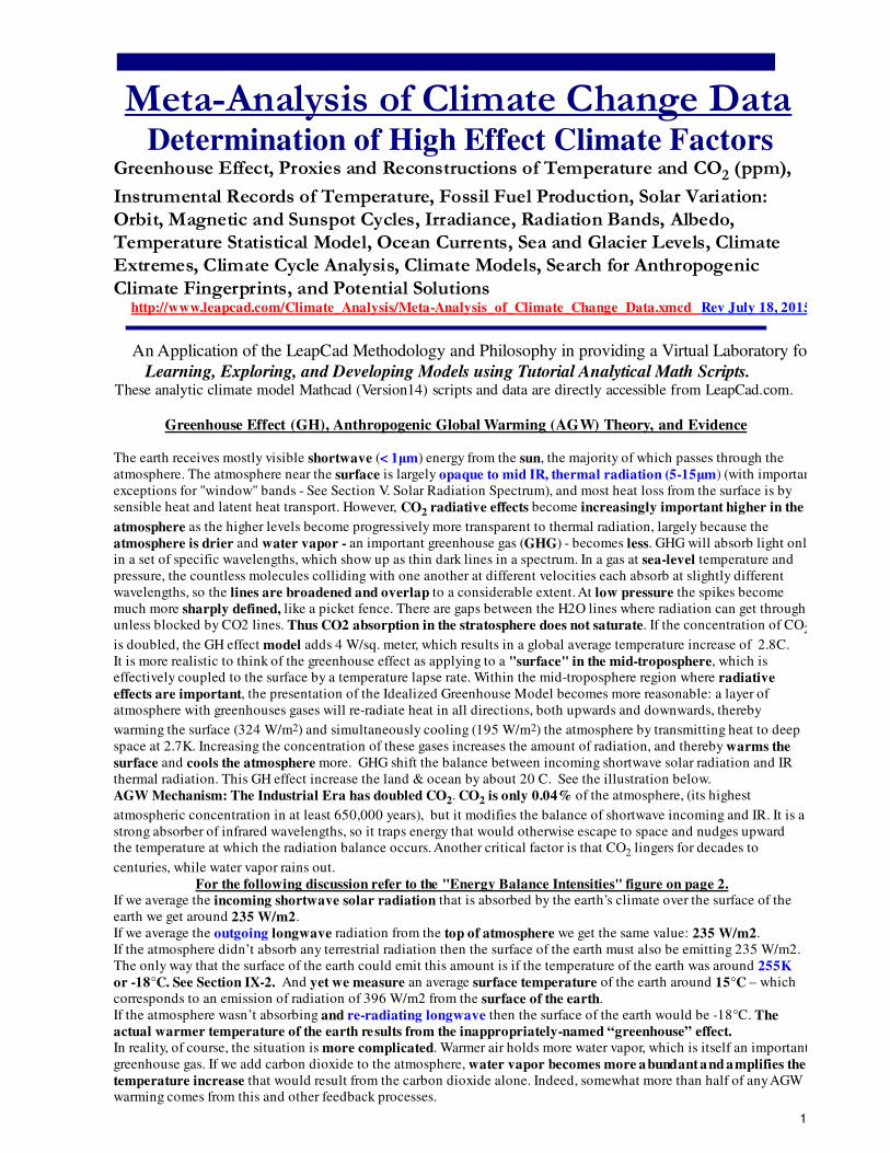
Graphic Illustrations for Greenhouse EffectThe earth is an isolated planet, that is, it is surrounded by the vacuum of space. The energy-in is by short wave
solar radiation and the only energy out must also be by radiation (longwave). For Energy Balance, the shortwave
solar heat coming in must equal the long wave IR re-radiated heat going out.
The energy out comes from the IR transparent region in the upper Troposphere, which is at a lower temperature (on
average, the temperature drops by 6.5 degrees C for every thousand meters of altitude you climb). If GHG is added,
then more energy is absorped in the lower atmosphere which cools the upper troposphere. According to the
Stefan-Boltzmann Law, the radiated power is proportional to T4. Thus the GHG IR molecules radiated less power to
space than they absorb from the surface. Thus the temperature must rise to maintain energy balance. This is the
greenhouse effect.
In the graph below, more that the energy leaving the earth, 452 W/m2, is much greater than the solar
radiation absorbed from the sun, 235 W/m2. The absorption and re-radiation by “greenhouse” gases in the
atmosphere is responsible. This is another indication of the greenhouse effect. The earth system
recirculates long wave mid IR
Energy Balance Intensities (Power Density)
2

TABLE OF CONTENTS A. INVESTIGATION OF CLIMATE CHANGE DATA - Pg. 3 of 59
B. CONCLUSIONS - EVALUATION OF EVIDENCE - Pg. 6
C. POTENTIAL SOLUTIONS - CLIMATE ENGINEERING
A. Investigation of Climate Change Data SECTION 0. Ice Age Climate Records: Billion and Million Year Cycles - Pg. 7 1. Ice Ages During the Past 2.4 Billion Years: Plot of Temperature vs. Millions Years
2. Cenozoic Era /Quaternary Period /Holocene Epoch: Plot Temperature and CO2 Levels vs. MYrs
SECTION I. Paleologicical Records -Paleoclimate Temp Proxies/Reconstructions - Ice Ages - Pg. 8
1. Paleozoic (Last 545,000,000 Years) Temperature and CO2:
2. Ice Ages and Vostok Ice Temperature (Blue) & CO2 (Black) over 420,000 Years
3. The Present Holocene Interglacial Period: Glaciers and Climate Change
4. The Little Ice Age and Medieval Warm Period in the Sargasso Sea Temp - from O18/O16 ratios.
5. Means of Temperature from 18 Non Tree Ring Series (30 Yr Running Means), Loehle 2007
6. Millennial Temperature Reconstructions (Last 1000 yrs from several sources)
7. Multi-Proxy Reconstructioned North Hemisphere Temperature Anomaly - Last 1000 Years
8. Multi-Proxy Reconstructioned North Hemisphere Temperature Anomaly - Last 2000 Years
9. 2010 Reconstructions shows 2 previous Warming Periods (Roman and Medieval) - Last 2000 Yrs.
SECTION II. Instrument Direct Temperature Records 1800 to Present - Continued - Pg. 14
1. National Climatic Data Center's NOA US website (1880 - present) and Berkeley Earth Records 2. NASA GISS US Aand Zonal Surface Temperature Analysis
3. Berkeley Earth Land Average 1750 to 2014 Data and Simple CO2 and Volcano Temp Fit - Pg. 15
4. Hemisphereic Temperature Change
5. Latest 2015 No Recent Global Warming Hiatus - Correct Buoy vs. ship and better spatial/Artic data
6. Satellite Global Temp Anomaly and Solar Insolation. UAH Satellite Temp of the Lower Atmosphere
7. Heat Content of Oceans - Indisputable evidence of global warming, but =>∆T ~ 0.025K from 1975
8. IPPC 2007: Comparison of models with natural versus anthropogenic forcing.
9. Analysis: Statistics of Climate Change - Temperature Rise is Non Monotonic - 70 Year Cycles
SECTION III-A. CO2 Concentration Records - Pg. 19
1. Global Temperature & CO2 ppm over Geologic Time (Paleozoic, Mesozoic, Cenozoic)600 MillionYr
2. The Keeling Curve- Mauna Loa Observation Hawaii CO2 Data (1958-2010): Seasonal & Monthly
CO2 Yearly ppm: Composite Ice Core & Shifted Keeling Curve (Hockey Stick) and Beck
3. CO2 - Neftel Siple Ice Station - 1847 to 1953 - Pg. 20
4. Vostok and Trend CO2 Concentration Data, Barnola et al - 160,000 Yrs. - Pg. 22 5. Temp and CO2 Hadcrut data:1860 to 2010
6. Does Temp track CO2? - Pg. 23
SECTION III-B. CO2 Production Projections, Scenarios, and Fossil Fuel Projections - Pg. 24
1. Yearly CO2 Emission & Atmospheric ppm Increases - 1850 to Present
2. Global Atmospheric CO2 Emission Scenarios (B1 to A1F1) - 1980 to 2100 - Pg. 25
3. World Energy Production Projection
SECTION III-C. Fossil Fuel Energy - Pg. 271. Main Areas of Human Energy Consumption in the US
2. Human Contribution Relative to Other Sources of CO2
3. Coal Usage and Factors
4. Oil Production - US Drilling Rigs - December 2014
3
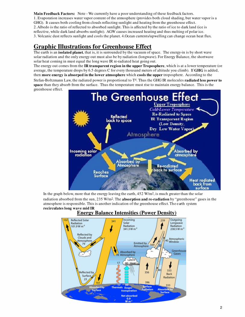
SECTION I V. Solar Variation: Wolf Number, Sunspots, C14 SS Extreme, Irradiance, Wind- Pg. 28 1. TCrut Temp, Solar Proxy: Changes C14 Concentration, Sunspot Extreme Periods, & #Sun Spots
NGDC-Table of smoothed monthly sunspot numbers 1700-present
2. Sun Spot Epochs (910 to 2010) - Maunder Minimum
3. Extended C14 Data (Red) Smoothed Data, Detrended Data, & Hallstadzeit Cycles
3. PMOD Total Solar Irradiance-31 Day Median Fit
4. The Sun's Total Irradiance: Cycles, Trends & Related Climate Change Uncertainties -1978 -PMOD
5. Reconstruction of solar irradiance since 1610, Lean 1995 (1600-1995) - Correlates to Temp
6. NASA OMNI2: Solar Wind Pressure and Decadal Trends
7. Solar Cycle Prediction - Solar Cycles # 24 and 25 -NASA - Influence of sun on climate - Pg. 32
8. Wilcox Solar Observatory - Solar Polar (North-South) Magnetic Field vs Sunspot Cycles - Pg. 33
9. Hathaway: Magnetic Conveyer Model - Sunspot Prediction - Pg. 34
10. Zharkova: Irregular Heartbeat of Sun driven by dual dynamo -Accurate Sunspots Prediction- Pg. 34
Predicts Lowest Sunspot Cycle Minimum in 370 Years, similar to Maunder Minimum
SECTION V . Incoming Solar Radiation Spectrum and GHG Adsorption Bands - Pg. 35 1. Top of Atmosphere and Sea Level (Greenhouse Gas Absorption Bands)
2. Comparison of MODTRAN Model to Nimbus 3 IRIS instrument (ClimateModels.UChicago.edu)
3. Measurements of the Radiative Surface Forcing of Climate
SECTION VI. Project Earthshine - Measuring the Earth's Albedo - Pg. 36 Earth’s average albedo is not constant from one year to the next; it also changes over decadal timescales.
The computer models currently used to study the climate system do not show such large decadal-scale
variability of the albedo.
SECTION VII . 70 Year Warming Cycles - Pg. 37 Analysis: Statistics of Climate Change -Temperature Rise is Not Monotonic - 70 Year Cycles
SECTION VIII. Milankovitch Astronomically Forced Glacial Insolation Cycles - Pg. 38 1. Astronomical Insolation Forcing: Early Pleistocene Glacial Cycles - Huybers
2. Milankovitch radiation for different latitudes and time periods
3. Total Solar Irradiance - 31 Day Median
See "Long-term numerical solution for the insolation quantities of the Earth.xmcd"
SECTION IX . Climate Cycle Analysis - Wavelets - Pg. 41 "Solar Forcing and Climate - A Multi-resolution Analysis.xmcd"
Empirical Analysis Mode Decomposition via Hilbert-Huang Transforms -> "EMD HHT.xmcd"
SECTION X . Atmosphere-Ocean Effects: EN SO and PDO - Pg. 41
ENSO - The Southern Oscillation: C onsistently dominant influence on mean global temperature 1. ENSO Index - 1950 to 2014
PDO - Pacific Decadal Oscillation - Pg. 41 1. PDO Index - 1900 to 2010
SECTION XI. Simple Climate Models and Wavelet Analysis of Global Temperature Anomaly - Pg. 42 1. Stefan-Boltzmann Law of Radiation: Calculation of Temp of Earth (w/o Greenhouse Effect)
2. Simple 1D Latitudinal Energy Balance Model - Pg. 42
3. Wavelet Adaptive Hilbert-Huang Transformation Analysis - Decomposition of Temp Data - Pg. 43
SECTION XII. More Complex Climate Models - Pg. 43
For details go to Link: http://www.leapcad.com/Climate_Analysis.html
Climate Model Papers: General Circulation Models (GCM)
4
Testing the Anthropogenic Greenhouse Gas Global Warming Model Looking for Unique Fingerprints of Global Warming
SECTION XIII. Global Temp Reproduced by CO 2 and Natural Forcing - Pg. 44
Use ENSO, Irradiance, Volcanic Aerosols, and Anthropogenic Effects to Create an Empirical Temp Model -
Compare Anthropogenic Forcing Component - (17 Year Lag) = b4*z4 (Green) of ∆T to D
SECTION XIV. Finding the Unique Anthropogenic Greenhouse Gas (CO2) Fingerprint - Pg. 45
Test# 1: Spectral signatures of climate change in IR spectrum between 1970 and 2000 - Pg. 45
Test #2: This Model is Interesting but Flawed: Miskolczi Saturated (Greenhouse Effect) Humidity Model
Test #3: GH Effect requires the lower and mid-troposphere to be warmer than the surface. True -Pg. 46Test #4 AGW requires the temperature of the stratosphere to decrease True - Pg. 47
Test #5 Asymmetric diurnal temp change - Nights warming faster than days True - Pg. 47
Test #6 Measure - Global Atmospheric Downward Longwave Radiation from 1973-2008 True - Pg. 48Test #7. Observational of surface radiative forcing (long wave downwelling IR) by CO2 2000-2010- Pg. 48
SECTION XV. Gelologic and Current Nonlinear Trends and Multiyear Cycles Sea Levels -Pg. 49 1. Geologic: Holocene Sea Level Rise - 8000 BP
2. Current Global Sea Level vs Time - 1800 to 2014 - Anomalous increased rate since 1990. -Pg. 50 3. Shutdown of thermohaline circulation
SECTION XVI. Glacier Records - Pg. 51 1. Glacier Global Temp Reconstruction & Ts - 1600 to 2000 (169 Records)
2. Glacier Mass Balance and Regime: Data of Measurements and Analysis 1950-2000
3. Vostok Ice Core Data, Ratio 18O/16O (High-->Warm) ==> Continental Glaciers over past 106 years -Pg 52
SECTION XVII : Snow Coverage in the Northern Hemisphere - Pg. 52 Snow cover, the whitest natural surface on the planet, reflects roughly 90 percent of the sunlight that
reaches it. Data from 1965 shows that snow coverage is decreasing, with PerCentSnowDecrease = 13.7%
SECTION XVIII . Cryosphere - Sea Ice Extent - Northern and Southern Hemispheres - Pg. 53 2.5% Loss of Global Sea Ice Extent since 1980
SECTION XIX. Model Predictions for Tropical Atmosphere Warming - Pg. 54 http://www.climatechange.gov.au/en/climate-change/science.aspx
http://www.drroyspencer.com/wp-content/uploads/Spencer_EPW_Written_Testimony_7_18_2013_updated.pdf
Test #5: Plots: All 73 climate models produce Too Much Tropical Atmospheric Warming During 1979 to 2012
SECTION XX. Is Extreme Climate (> 30 Years) Getting Worse? - Pg. 55 Test #6:
Models/Snow Extent, Very Hot/Cold, Droughts, Wetness, Sea Level Rise Prediction,
1. Simulated annual time series of January NA-Continental Scale Snow Coverage - 1850 to present
2. North Hemisphere Snow Cover Anomalies (December & January). Trend Line (Blue)
3. US Percentage Area Very Warm, Very Cold - Pg. 56 4. Extreme and Severe Drought Agricultural Land
5. NOAA: Rainfall/Wetness
6. IPCC Revisions: Sea Level Rise by 2100
7. Hurricane Frequency
8. US Tornadoes Frequency (Type) - Pg. 57 9. US Extreme Weather Index
10. Destabilzed Polar Vortex (USA Winters of 2009-2013)
APPENDIX
AI. TYPES OF GISS TEMPERATURE DATA SOURCES - Pg. 59
5
B. CONCLUSIONS - EVALUATION OF EVIDENCE"Science and skepticism are synonymous, and in both cases it's okay to change your mind if the evidence changes."
- Michael Shermer
"The first principle is that you must not fool yourself and you are the easiest person to fool." - Richard P. Feynman
1. The evidence clearly shows global warming over the last 300 years.
2. Section II. Warming over the last 100 years has been unusually rapid. Global +0.8 C for last 65 years.
3. Section XIII: Test 0: Regressions reproduce both natural fluctuations & CO2 trend line of global temp
4. Section XIV: Test 1, Tests 3, 4, and 5 show unique AGW fingerprint.
5. Section XIV: Measurements of downwelling long wave radiation vs time --> 0.2 W/m2 per decade.
Correlates with decadal 22 ppm CO2 increase - 10% of the trend in long wave downwelling radiation.
6. Section XV to XVIII show increased sea levels, decreased glacier mass, and decrease north sea ice.
7. 2009 to 2013 US winters show destabilized polar vortex.
Concern: Increased CO2 in the oceans causes increased carbonic acid, which attacks coral.
Summary: There is definitely a spike in the recorded global temperature over the last 100 years. Data has verified 7
unique fingerprints of AGW. The global temperature trend has been +0.8 C from 1950 to 2015.
Because of the chaotic nature of climate, climate models results must be presented as ensembles.
Therefore only probalistic conclusions are meaningful.
The evidence shows that AGW probably contributes significantly to the total Global Warming.
Increased acidity of the oceans are also a major anthropogenic concern.
There is still much we do not know about climate. We have a poor understanding of feedback factors.
They are at best guesses. IPCC Assesment Report, AR 5, Chapter 9.8.3 "Unlike shorter lead
forecasts, longer-term climate change projections push models into conditions outside the range
observed in the historical period used for evaluation."
Climate prediction is difficult because climate is chaotic. We also have limited data, e.g. volcanic, sun, and
cosmic ray activity, 3D data on clouds, threshold for convection, and aerosols.
It is possible that natural global warming may be occurring due to solar variation or other mechanisms
(cosmic rays, ocean currents, or unknown feedback factors).
However considering all the above factors, the evidence shows that antropogenic CO2 production is
causing a significant increase in downwelling long wave radiation power density with resultant global
warming. However, other causative effects, such as Solar Magnetic Field Variations, may modulate the
climate significantly.
C. POTENTIAL SOLUTIONS TO GLOBAL WARMING I. Alternative Energy Sources- See • Models: Other Energy Technology
II. Climate Engineering - Mitigating Climate Change:The observed spike in temperature carries risks such as increases in ocean heights. The outlook for
mitigating the AGW component by political change is very dim. Climate Engineering may target different
areas of the climate system; possess varying mechanics, costs, and feasibility; have diverse environmental
and societal impacts on varying scales; and create their own sets of risks, challenges, and unknowns. They
are commonly divided into two non-exhaustive suites:
• Carbon Dioxide Removal (CDR) methods attempt to absorb and store carbon from the atmosphere;
either by technological means, or by enhancing the ability of natural systems (e.g. oceans) to do so.
• Solar Radiation Management or Sunlight Reflection Methods (SRM) aims to reduce the amount of heat
trapped by greenhouse gases by reflecting sunlight back into space, either by increasing the reflectivity of
the earth's surfaces, or by deploying a layer of reflective particles in the atmosphere.
6
SECTION 0. Earliest Climate Records: Billion and Million Year Cycles
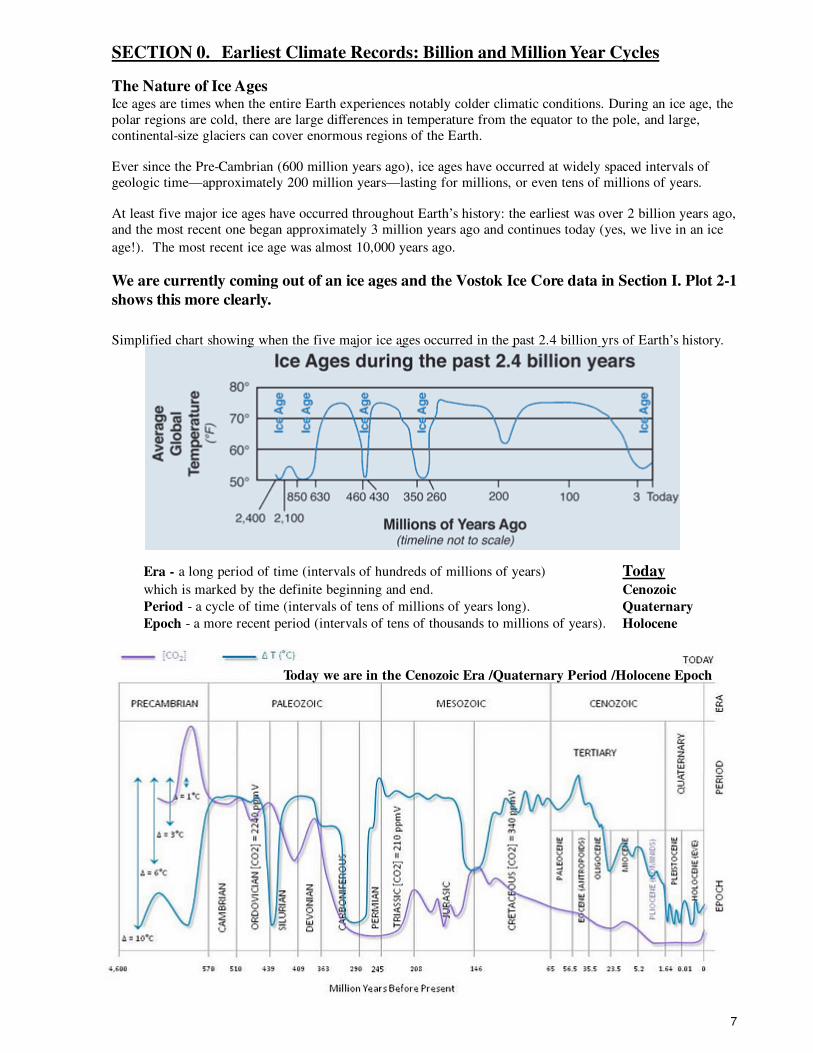
The Nature of Ice AgesIce ages are times when the entire Earth experiences notably colder climatic conditions. During an ice age, the
polar regions are cold, there are large differences in temperature from the equator to the pole, and large,
continental-size glaciers can cover enormous regions of the Earth.
Ever since the Pre-Cambrian (600 million years ago), ice ages have occurred at widely spaced intervals of
geologic time—approximately 200 million years—lasting for millions, or even tens of millions of years.
At least five major ice ages have occurred throughout Earth’s history: the earliest was over 2 billion years ago,
and the most recent one began approximately 3 million years ago and continues today (yes, we live in an ice
age!). The most recent ice age was almost 10,000 years ago.
We are currently coming out of an ice ages and the Vostok Ice Core data in Section I. Plot 2-1
shows this more clearly.
Era - a long period of time (intervals of hundreds of millions of years) Todaywhich is marked by the definite beginning and end. Cenozoic
Period - a cycle of time (intervals of tens of millions of years long). Quaternary
Epoch - a more recent period (intervals of tens of thousands to millions of years). Holocene
Today we are in the Cenozoic Era /Quaternary Period /Holocene Epoch
Simplified chart showing when the five major ice ages occurred in the past 2.4 billion yrs of Earth’s history.
7
SECTION I. Paleological Isotopic Temp Record - the Vostok Ice Core - 1999
http://www.heartland.org/publications/NIPCC%20report/PDFs/Chapter%203.1.pdf
http://en.wikipedia.org/wiki/Ice_core
Petit, "Climate and atmospheric history of the past 420,000 years from the Vostok ice core, Antarctica",
Nature 399: 429-436 CO2: Gas age CO2 (ppmv) File: co2vostokPetit.txt
Carbon Dioxide Information Analysis Center
http://cdiac.esd.ornl.gov/ftp/trends/temp/vostok/vostok.1999.temp.dat
Depth (m), Age of ice (yr BP), Deuterium content of the ice ( D), Temperature Variation (deg C)
CO2VosS
TS
TempVostok READPRN "vostok.1999.temp.txt"( ):= CO2Vostok READPRN "CO2vostokPetit.txt"( ):=
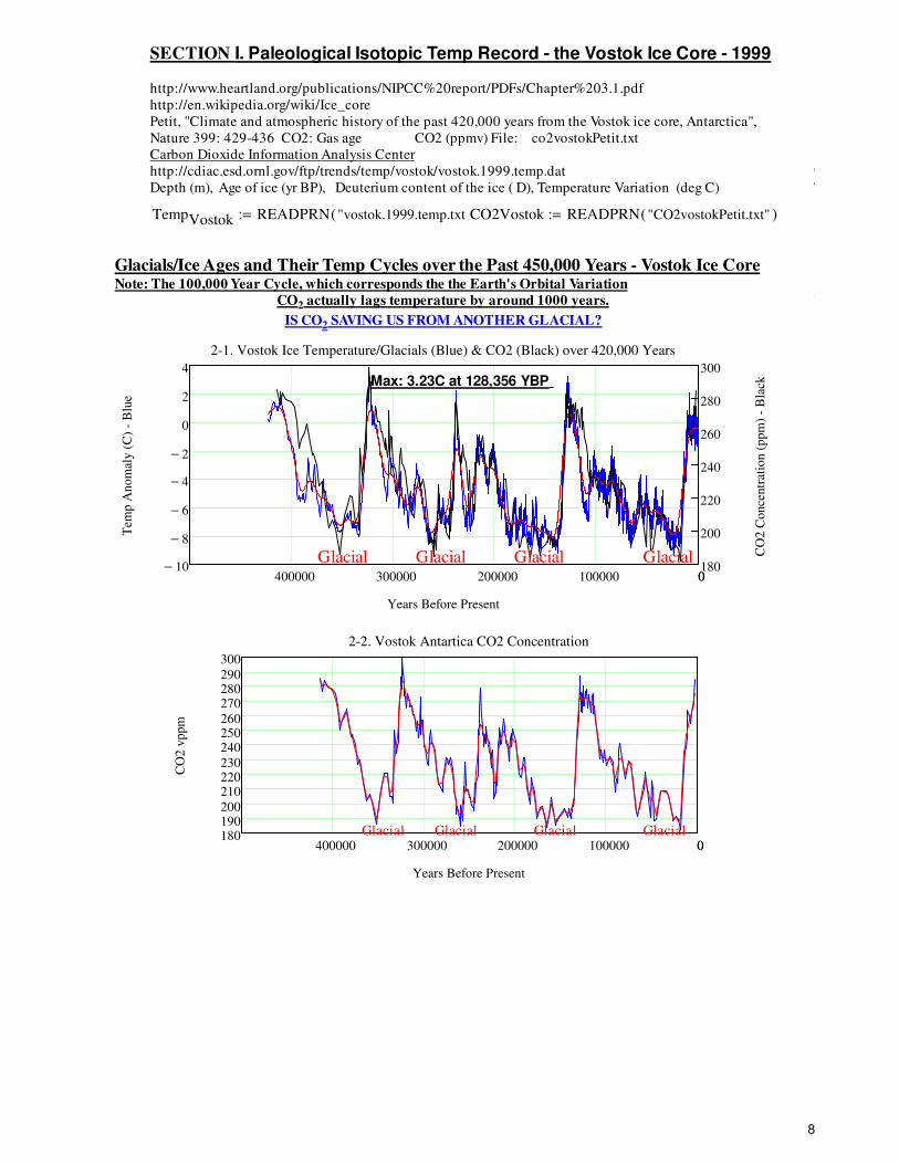
Glacials/Ice Ages and Their Temp Cycles over the Past 450,000 Years - Vostok Ice Core Note: The 100,000 Year Cycle, which corresponds the the Earth's Orbital Variation
CO2 actually lags temperature by around 1000 years.
IS CO 2 SAVING US FROM ANOTHER GLACIAL?
Years
0400000 300000 200000 100000 010−
8−
6−
4−
2−
0
2
4
180
200
220
240
260
280
300
2-1. Vostok Ice Temperature/Glacials (Blue) & CO2 (Black) over 420,000 Years
Years Before Present
Tem
p A
nom
aly (
C)
- B
lue
CO
2 C
once
ntr
atio
n (
ppm
) -
Bla
ck Max: 3.23C at 128,356 YBP
0400000 300000 200000 100000 0180190200
210220230
240250260
270280290
300
2-2. Vostok Antartica CO2 Concentration
Years Before Present
CO
2 v
ppm
Glacial Glacial Glacial Glacial
Glacial Glacial Glacial Glacial
8
080000 60000 40000 20000 010−
8−
6−
4−
2−
0
2
4
2.2-3. Vostok Antartica Temperature
Years Before Present
Tem
p (
C)
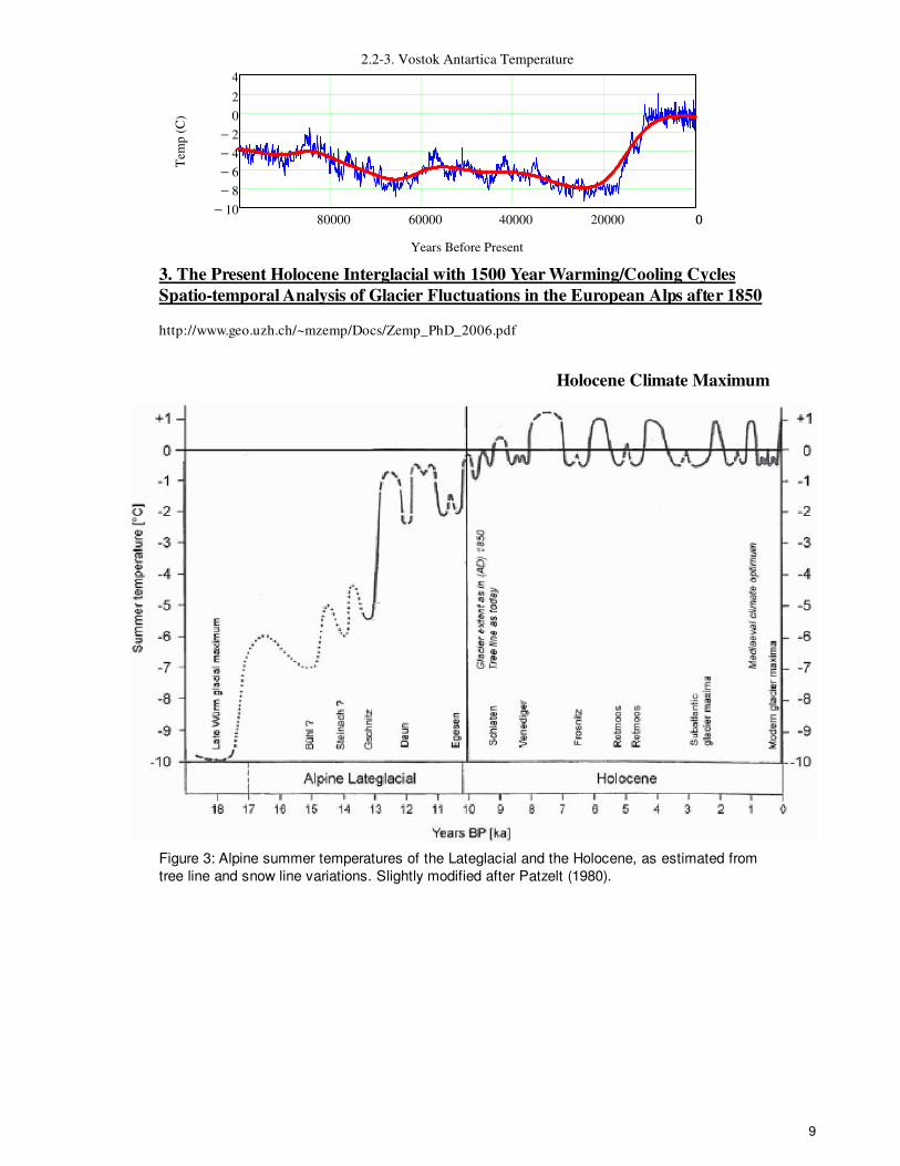
3. The Present Holocene Interglacial with 1500 Year Warming/Cooling Cycles
Spatio-temporal Analysis of Glacier Fluctuations in the European Alps after 1850
http://www.geo.uzh.ch/~mzemp/Docs/Zemp_PhD_2006.pdf
Holocene Climate Maximum
Figure 3: Alpine summer temperatures of the Lateglacial and the Holocene, as estimated from
tree line and snow line variations. Slightly modified after Patzelt (1980).
9
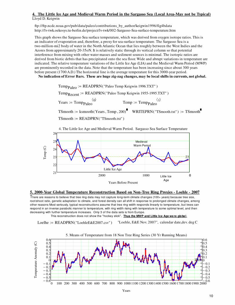
4. T he Little Ice Age and Medieval Warm Period in the Sargasso Sea (Local Area-May not be Typical)Lloyd D. Keigwin
ftp://ftp.ncdc.noaa.gov/pub/data/paleo/contributions_by_author/keigwin1996/fig4bdata
http://lv-twk.oekosys.tu-berlin.de/project/lv-twk/002-Sargasso-Sea-surface-temperature.htm
This graph shows the Sargasso Sea surface temperature, which was derived from oxygen isotope ratios. This is
an indicator of evaporation and, therefore, a proxy for sea-surface temperature. The Sargasso Sea is a
two-million-mi2 body of water in the North Atlantic Ocean that lies roughly between the West Indies and the
Azores from approximately 20-35oN. It is relatively static through its vertical column so that potential
interference from mixing with other water masses and sediment sources is minimal. The isotopic ratios are
derived from biotic debris that has precipitated onto the sea floor. Wide and abrupt variations in temperature are
indicated. The relative temperature variations of the Little Ice Age (LIA) and the Medieval Warm Period (MWP)
are prominently recorded in the data. Note that the temperature has been increasing since about 300 years
before present (1700 A.D.) The horizontal line is the average temperature for this 3000-year period.
No indication of Error Bars. These are huge zig-zag changes, may be local shifts in currents, not global.
TempPaleo READPRN "Paleo Temp Keigwin 1996.TXT"( ):=
TempRecent READPRN "Paleo Temp Keigwin 1955-1995.TXT"( ):=
Years TempPaleo0⟨ ⟩
:= Temp TempPaleo1⟨ ⟩
:=
TSmooth ksmooth Years Temp, 200, ( ):= WRITEPRN "TSmooth.txt"( ) TSmooth:=
TSmooth READPRN "TSmooth.txt"( ):=
02000 1000 021
22
23
24
25
26
4. The Little Ice Age and Medieval Warm Period. Sargasso Sea Surface Temperature
Years Before Present
Tem
p (
C)
23
Medieval
Warm Period
Little Ice Age
Little Ice
Age
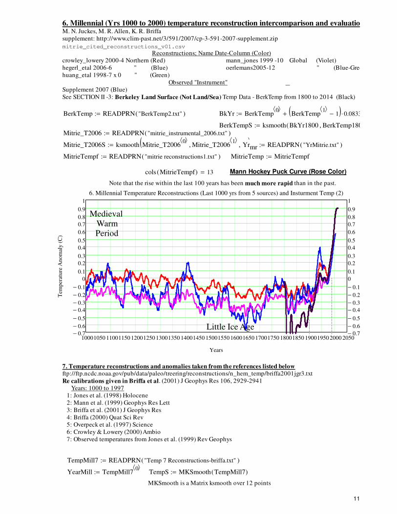
5. 2000-Year Global Temperature Reconstruction Based on Non-Tree Ring Proxies - Loehle - 2007
There are reasons to believe that tree ring data may not capture long-term climate changes (100+ years) because tree size,
root/shoot ratio, genetic adaptation to climate, and forest density can all shift in response to prolonged climate changes, among
other reasons Most seriously, typical reconstructions assume that tree ring width responds linearly to temperature, but trees can
respond in an inverse parabolic manner to temperature, with ring width rising with temperature to some optimal level, and then
decreasing with further temperature increases. Only 3 of the data sets is from Europe.
This reconstruction does not show the "hockey stick". Thus the MWP and Little Ice Age we re globa l .
Loelhe READPRN "LoehleE&E2007.csv"( ):= "Loehle, E&E Nov. 2007", calendar date,dev. deg C
0 100 200 300 400 500 600 700 800 900 1000 1100 1200 1300 1400 1500 1600 1700 1800 1900 20000.6−0.5−0.4−0.3−0.2−0.1−
00.10.20.30.40.50.6
0.6−0.5−0.4−0.3−0.2−0.1−
00.10.20.30.40.50.6
5. Means of Temperature from 18 Non Tree Ring Series (30 Yr Running Means)
Years
Tem
per
ature
Anom
aly (
C)
Zero
10
6. Millennial (Yrs 1000 to 2000) temperature reconstruction intercomparison and evaluationM. N. Juckes, M. R. Allen, K. R. Briffa
supplement: http://www.clim-past.net/3/591/2007/cp-3-591-2007-supplement.zip
mitrie_cited_reconstructions_v01.csv
Reconstructions; Name Date-Column (Color)
crowley_lowery 2000-4 Northern (Red) mann_jones 1999 -10 Global (Violet)
hegerl_etal 2006-6 " (Blue) oerlemans2005-12 " (Blue-Green)
huang_etal 1998-7 x 0 " (Green)
Observed "Instrument"
Supplement 2007 (Blue)
See SECTION II -3: Berkeley Land Surface (Not Land/Sea) Temp Data - BerkTemp from 1800 to 2014 (Black)
BerkTemp READPRN "BerkTemp2.txt"( ):= BkYr BerkTemp0⟨ ⟩
BerkTemp1⟨ ⟩
1−( ) 0.08333⋅+:=
BerkTempS ksmooth BkYr1800 BerkTemp1800, (:=
Mitrie_T2006 READPRN "mitrie_instrumental_2006.txt"( ):=
Mitrie_T2006S ksmooth Mitrie_T20060⟨ ⟩
Mitrie_T20061⟨ ⟩
, 12, ( ):= Yrmr READPRN "YrMitrie.txt"( ):=
MitrieTempf READPRN "mitrie reconstructions1.txt"( ):= MitrieTemp MitrieTempf:=
cols MitrieTempf( ) 13= Mann Hockey Puck Curve (Rose Color)
10001050 11001150 12001250 13001350 14001450 15001550 16001650 17001750 18001850 19001950 2000 20500.7−
0.6−
0.5−
0.4−
0.3−
0.2−
0.1−
0
0.1
0.2
0.3
0.4
0.5
0.6
0.7
0.8
0.9
1
0.7−
0.6−
0.5−
0.4−
0.3−
0.2−
0.1−
0
0.1
0.2
0.3
0.4
0.5
0.6
0.7
0.8
0.9
1
6. Millennial Temperature Reconstructions (Last 1000 yrs from 5 sources) and Insturment Temp (2)
Years
Tem
per
ature
Anom
aly (
C)
Note that the rise within the last 100 years has been much more rapid than in the past.
Medieval WarmPeriod
Little Ice Age
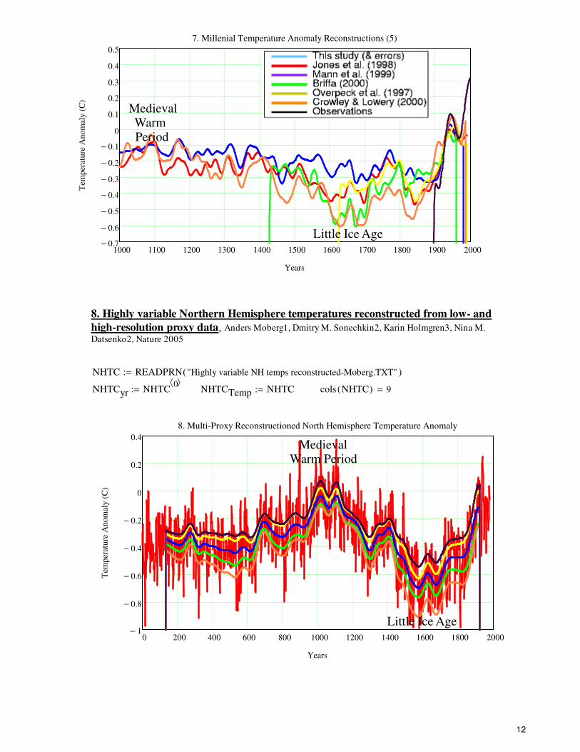
7. T emperature reconstructions and anomalies taken from the references listed belowftp://ftp.ncdc.noaa.gov/pub/data/paleo/treering/reconstructions/n_hem_temp/briffa2001jgr3.txt
Re calibrations given in Briffa et al. (2001) J Geophys Res 106, 2929-2941
Years: 1000 to 1997
1: Jones et al. (1998) Holocene
2: Mann et al. (1999) Geophys Res Lett
3: Briffa et al. (2001) J Geophys Res
4: Briffa (2000) Quat Sci Rev
5: Overpeck et al. (1997) Science
6: Crowley & Lowery (2000) Ambio
7: Observed temperatures from Jones et al. (1999) Rev Geophys
TempMill7 READPRN "Temp 7 Reconstructions-briffa.txt"( ):=
YearMill TempMill70⟨ ⟩
:= TempS MKSmooth TempMill7( ):=
MKSmooth is a Matrix ksmooth over 12 points
11
1000 1100 1200 1300 1400 1500 1600 1700 1800 1900 20000.7−
0.6−
0.5−
0.4−
0.3−
0.2−
0.1−
0
0.1
0.2
0.3
0.4
0.5
7. Millenial Temperature Anomaly Reconstructions (5)
Years
Tem
per
ature
Anom
aly (
C)
MedievalWarm Period
Little Ice Age
8. Highly variable Northern Hemisphere temperatures reconstructed from low- and
high-resolution proxy data, Anders Moberg1, Dmitry M. Sonechkin2, Karin Holmgren3, Nina M.
Datsenko2, Nature 2005
NHTC READPRN "Highly variable NH temps reconstructed-Moberg.TXT"( ):=
NHTCyr NHTC0⟨ ⟩
:= NHTCTemp NHTC:= cols NHTC( ) 9=
0 200 400 600 800 1000 1200 1400 1600 1800 20001−
0.8−
0.6−
0.4−
0.2−
0
0.2
0.4
8. Multi-Proxy Reconstructioned North Hemisphere Temperature Anomaly
Years
Tem
per
ature
Anom
aly (
C)
Medieval Warm Period
Little Ice Age
12
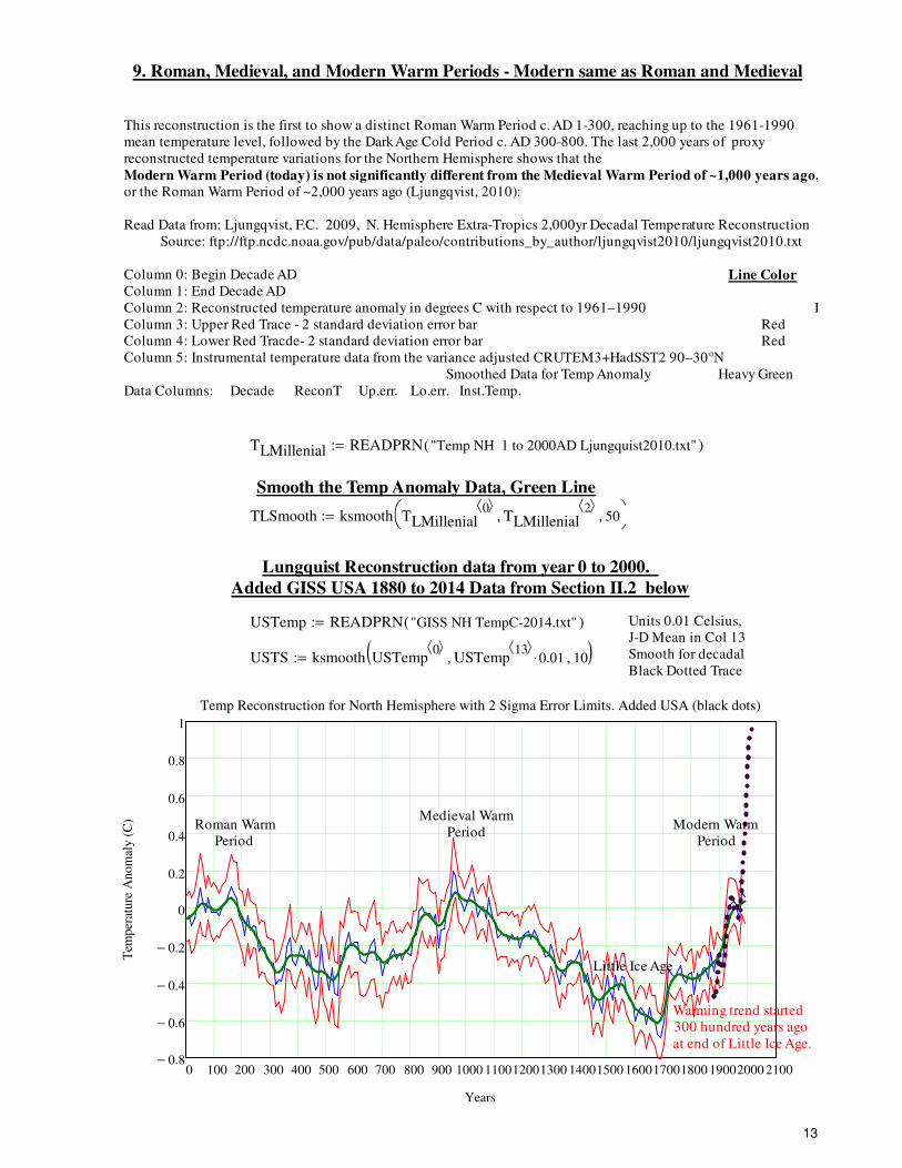
9. Roman, Medieval, and Modern Warm Periods - Modern same as Roman and Medieval
This reconstruction is the first to show a distinct Roman Warm Period c. AD 1-300, reaching up to the 1961-1990
mean temperature level, followed by the Dark Age Cold Period c. AD 300-800. The last 2,000 years of proxy
reconstructed temperature variations for the Northern Hemisphere shows that the
Modern Warm Period (today) is not significantly different from the Medieval Warm Period of ~1,000 years ago,or the Roman Warm Period of ~2,000 years ago (Ljungqvist, 2010):
Read Data from: Ljungqvist, F.C. 2009, N. Hemisphere Extra-Tropics 2,000yr Decadal Temperature Reconstruction
Source: ftp://ftp.ncdc.noaa.gov/pub/data/paleo/contributions_by_author/ljungqvist2010/ljungqvist2010.txt
Column 0: Begin Decade AD Line ColorColumn 1: End Decade AD
Column 2: Reconstructed temperature anomaly in degrees C with respect to 1961–1990 Blue
Column 3: Upper Red Trace - 2 standard deviation error bar Red
Column 4: Lower Red Tracde- 2 standard deviation error bar Red
Column 5: Instrumental temperature data from the variance adjusted CRUTEM3+HadSST2 90–30°N
Smoothed Data for Temp Anomaly Heavy Green
Data Columns: Decade ReconT Up.err. Lo.err. Inst.Temp.
TLMillenial READPRN "Temp NH 1 to 2000AD Ljungquist2010.txt"( ):=
Smooth the Temp Anomaly Data, Green Line
TLSmooth ksmooth TLMillenial0⟨ ⟩
TLMillenial2⟨ ⟩
, 50,
:=
Lungquist Reconstruction data from year 0 to 2000.
Added GISS USA 1880 to 2014 Data from Section II.2 below
USTemp READPRN "GISS NH TempC-2014.txt"( ):= Units 0.01 Celsius,
J-D Mean in Col 13
Smooth for decadal
Black Dotted TraceUSTS ksmooth USTemp
0⟨ ⟩USTemp
13⟨ ⟩0.01⋅, 10, ( ):=
0 100 200 300 400 500 600 700 800 900 1000 110012001300 14001500 160017001800 19002000 21000.8−
0.6−
0.4−
0.2−
0
0.2
0.4
0.6
0.8
1
Temp Reconstruction for North Hemisphere with 2 Sigma Error Limits. Added USA (black dots)
Years
Tem
per
ature
Anom
aly (
C) Medieval Warm
PeriodRoman Warm
Period
Modern Warm
Period
Little Ice Age
Warming trend started
300 hundred years ago
at end of Little Ice Age.
13
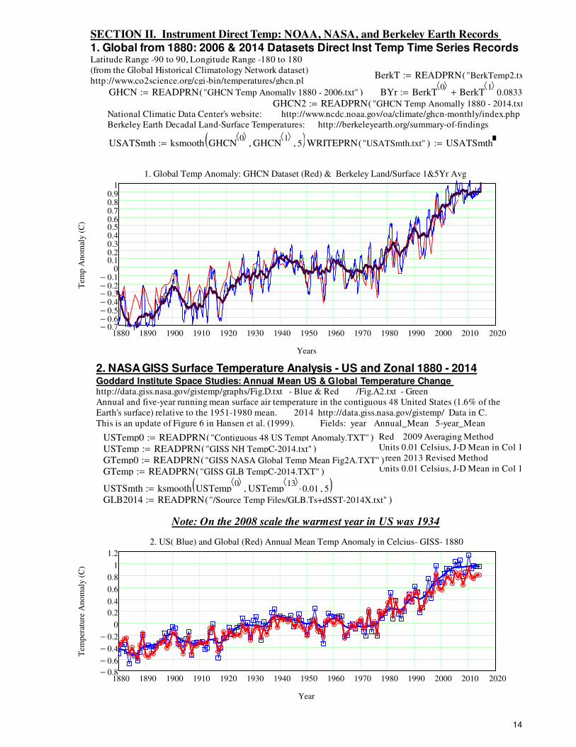
SECTION II. Instrument Direct Temp: NOAA, NASA, and Berkeley Earth Records 1. Global from 1880: 2006 & 2014 Datasets Direct Inst Temp Time Series RecordsLatitude Range -90 to 90, Longitude Range -180 to 180
(from the Global Historical Climatology Network dataset)
http://www.co2science.org/cgi-bin/temperatures/ghcn.plBerkT READPRN "BerkTemp2.txt"(:=
GHCN READPRN "GHCN Temp Anomally 1880 - 2006.txt"( ):= BYr BerkT0⟨ ⟩
BerkT1⟨ ⟩
0.08333+:=
GHCN2 READPRN "GHCN Temp Anomally 1880 - 2014.txt"(:=National Climatic Data Center's website: http://www.ncdc.noaa.gov/oa/climate/ghcn-monthly/index.php
Berkeley Earth Decadal Land-Surface Temperatures: http://berkeleyearth.org/summary-of-findings
USATSmth ksmooth GHCN0⟨ ⟩
GHCN1⟨ ⟩
, 5, ( ):= WRITEPRN "USATSmth.txt"( ) USATSmth:=
1880 1890 1900 1910 1920 1930 1940 1950 1960 1970 1980 1990 2000 2010 20200.7−0.6−0.5−0.4−0.3−0.2−0.1−
00.10.20.30.40.50.60.70.80.9
1
1. Global Temp Anomaly: GHCN Dataset (Red) & Berkeley Land/Surface 1&5Yr Avg
Years
Tem
p A
nom
aly (
C)
2. NASA GISS Surface Temperature Analysis - US and Zonal 1880 - 2014 Goddard Institute Space Studies: Annual Mean US & Global Temperature Change http://data.giss.nasa.gov/gistemp/graphs/Fig.D.txt - Blue & Red /Fig.A2.txt - Green
Annual and five-year running mean surface air temperature in the contiguous 48 United States (1.6% of the
Earth's surface) relative to the 1951-1980 mean. 2014 http://data.giss.nasa.gov/gistemp/ Data in C.
This is an update of Figure 6 in Hansen et al. (1999). Fields: year Annual_Mean 5-year_Mean
USTemp0 READPRN "Contiguous 48 US Tempt Anomaly.TXT"( ):= Red 2009 Averaging Method
Units 0.01 Celsius, J-D Mean in Col 13
Green 2013 Revised Method
Units 0.01 Celsius, J-D Mean in Col 13
USTemp READPRN "GISS NH TempC-2014.txt"( ):=
GTemp0 READPRN "GISS NASA Global Temp Mean Fig2A.TXT"( ):=
GTemp READPRN "GISS GLB TempC-2014.TXT"( ):=
USTSmth ksmooth USTemp0⟨ ⟩
USTemp13⟨ ⟩
0.01⋅, 5, ( ):=
GLB2014 READPRN "/Source Temp Files/GLB.Ts+dSST-2014X.txt"( ):=
Note: On the 2008 scale the warmest year in US was 1934
1880 1890 1900 1910 1920 1930 1940 1950 1960 1970 1980 1990 2000 2010 20200.8−
0.6−
0.4−
0.2−
0
0.2
0.4
0.6
0.8
1
1.2
2. US( Blue) and Global (Red) Annual Mean Temp Anomaly in Celcius- GISS- 1880
Year
Tem
per
ature
Anom
aly (
C)
14
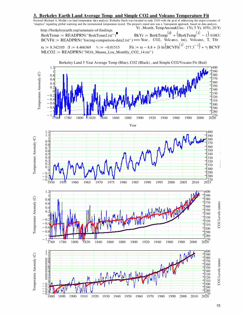
3. Berkeley Earth Land Average Temp and Simple CO2 and Volcano Temperature FitFocused (Richard A. Muller) on land temperature dat a analysis. B erkeley Earth was founded in early 2010 with t he goal of addressing the major concerns of
"skeptics" regarding global warming and the instrumental temperature record. The project's stated aim was a "transparent approach, based on data analysis.
Yr , Month, TempAnom&Unc: 1Yr, 5 Yr, 10Yr, 20 Yrhttp://berkeleyearth.org/summary-of-findings
BerkTemp READPRN "BerkTemp2.txt"( ):= BkYr BerkTemp0⟨ ⟩
BerkTemp1⟨ ⟩
1−( ) 0.08333⋅+:=
BCVFit READPRN "forcing-comparison-data2.txt"( ):= ==> Year , CO2, Volcano, ln(), Volcano, T, Tfit
α 8.342105:= β 4.466369:= γ 0.01515−:= Fit α 8.8− β ln BCVFit1⟨ ⟩
277.31−
⋅( )⋅+ γ BCVFit⋅+:=
MLCO2 READPRN "NOA_Mauna_Loa_Monthly_CO2_14.txt"( ):=
1760 1780 1800 1820 1840 1860 1880 1900 1920 1940 1960 1980 2000 20201.2−
1−0.8−0.6−0.4−0.2−
00.20.4
0.60.8
1
1.2
270280290300310320330340350360370380390400
Berkeley Land 5 Year Average Temp (Blue), CO2 (Black) , and Simple CO2/Vocano Fit (Red)
Year
Tem
per
ature
Anom
aly (
C)
1950 1955 1960 1965 1970 1975 1980 1985 1990 1995 2000 2005 2010 20150.3−0.2−0.1−
00.10.20.30.40.50.60.70.80.9
11.11.2
270280290300310320330340350360370380390400
Tem
per
ature
Anom
aly (
C)
CO
2 L
evel
s (p
pm
)
1760 1780 1800 1820 1840 1860 1880 1900 1920 1940 1960 1980 2000 20201.2−
1−0.8−0.6−0.4−0.2−
00.20.4
0.60.8
1
1.2
270280290300310320330340350360370380390400
Tem
per
ature
Anom
aly (
C)
CO
2 L
evel
s (p
pm
)
1880 1890 1900 1910 1920 1930 1940 1950 1960 1970 1980 1990 2000 2010 20200.5−0.4−0.3−0.2−0.1−
00.10.20.30.40.50.60.70.80.9
11.11.2
270280290300310320330340350360370380390400
Tem
per
ature
Anom
aly (
C)
CO
2 L
evel
s (p
pm
)
15
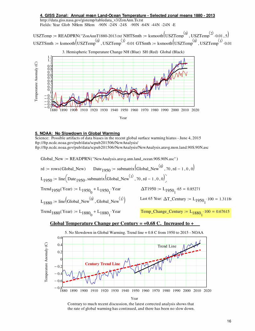
4. GISS Zonal: Annual mean Land-Ocean Temperature - S elected zonal means 1880 - 2013http://data.giss.nasa.gov/gistemp/tabledata_v3/ZonAnn.Ts.txt
Fields: Year Glob NHem SHem -90N -24N -24S -90N -64N -44N -24N -E
USZTemp READPRN "ZonAnnT1880-2013.txt"( ):= NHTSmth ksmooth USZTemp0⟨ ⟩
USZTemp2⟨ ⟩
0.01⋅, 5, ( ):=
USZTSmth ksmooth USZTemp0⟨ ⟩
USZTemp3⟨ ⟩
0.01⋅, 5, ( ):= GTSmth ksmooth USZTemp0⟨ ⟩
USZTemp1⟨ ⟩
0.01⋅, (:=
1880 1890 1900 1910 1920 1930 1940 1950 1960 1970 1980 1990 2000 2010 20200.5−0.4−0.3−0.2−0.1−
00.10.20.30.40.50.60.70.80.9
11.11.2
3. Hemispheric Temperature Change NH (Blue) SH (Red) Global (Black)
Year
Tem
per
ature
Anom
aly (
C)
5. NOAA: No Slowdown in Global WarmingScience: Possible artifacts of data biases in the recent global surface warming hiatus - June 4, 2015
ftp://ftp.ncdc.noaa.gov/pub/data/scpub201506/NewAnalysis/
ftp://ftp.ncdc.noaa.gov/pub/data/scpub201506/NewAnalysis/NewAnalysis.aravg.mon.land.90S.90N.asc
Global_New READPRN "NewAnalysis.aravg.ann.land_ocean.90S.90N.asc"( ):=
rd rows Global_New( ):= Date1950 submatrix Global_New0⟨ ⟩
70, rd 1−, 0, 0, ( ):=
L1950 line Date1950 submatrix Global_New1⟨ ⟩
70, rd 1−, 0, 0, ( ),
:=
Trend1950 Year( ) L19500
L19501
Year⋅+:= ∆T1950 L19501
65⋅ 0.85271=:=
Last 65 Year: ∆T_Century L19501
100⋅ 1.31186=:=L1880 line Global_New
0⟨ ⟩Global_New
1⟨ ⟩, ( ):=
Trend1880 Year( ) L18800
L18801
Year⋅+:= Temp_Change_Century L18801
100⋅ 0.67615=:=
Global Temperature Change per Century = +0.68 C. Increased to +
1880 1890 1900 1910 1920 1930 1940 1950 1960 1970 1980 1990 2000 2010 20200.8−
0.6−
0.4−
0.2−
0
0.2
0.4
0.6
5. No Slowdown in Global Warming. Trend line + 0.8 C from 1950 to 2015 - NOAA
Year
Tem
per
ature
Anom
aly (
C)
Trend Line
Century Trend Line
Contrary to much recent discussion, the latest corrected analysis shows that
the rate of global warming has continued, and there has been no slow down.
16
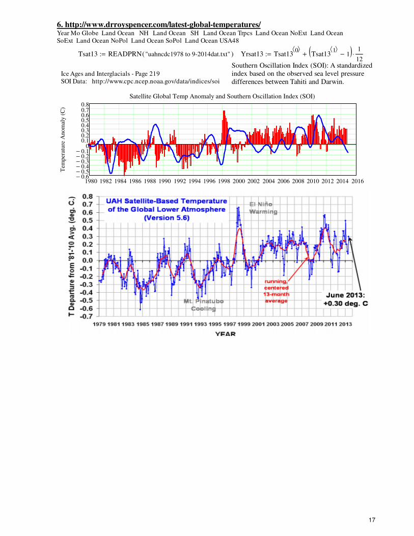
6. http://www.drroyspencer.com/latest-global-temperatures/Year Mo Globe Land Ocean NH Land Ocean SH Land Ocean Trpcs Land Ocean NoExt Land Ocean
SoExt Land Ocean NoPol Land Ocean SoPol Land Ocean USA48
Tsat13 READPRN "uahncdc1978 to 9-2014dat.txt"( ):= Yrsat13 Tsat130⟨ ⟩
Tsat131⟨ ⟩
1−( ) 1
12⋅+:=
Southern Oscillation Index (SOI): A standardized
index based on the observed sea level pressure
differences between Tahiti and Darwin.
Ice Ages and Interglacials - Page 219
SOI Data: http://www.cpc.ncep.noaa.gov/data/indices/soi
1980 1982 1984 1986 1988 1990 1992 1994 1996 1998 2000 2002 2004 2006 2008 2010 2012 2014 20160.6−0.5−0.4−0.3−0.2−0.1−
00.10.20.30.40.50.60.70.8
Satellite Global Temp Anomaly and Southern Oscillation Index (SOI)
Years
Tem
per
ature
Anom
aly (
C)
17
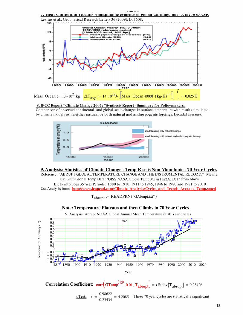
7. Heat Content of Oceans - Indisputable evidence of global warming, but ~∆Tavg= 0.025KLevitus et al., Geophysical Research Letters 36 (2009): L07608.
Mass_Ocean 1.4 1021
kg⋅:= ∆Tavg 14 1022
⋅ J Mass_Ocean 4000J kg K⋅( )1−
⋅ 1−
⋅ 0.025K=:=
8 . IPCC Report "Climate Change 2007: "Synthesis Report - Summary for Policymakers. Comparison of observed continental- and global-scale changes in surface temperature with results simulated
by climate models using either natural or both natural and anthropogenic forcings. Decadal averages.
9. Analysis: Statistics of Climate Change - Temp Rise is Non Monotonic - 70 Year CyclesReference: "ABRUPT GLOBAL TEMPERATURE CHANGE AND THE INSTRUMENTAL RECORD," Menne
Use GISS Global Temp Data: "GISS NASA Global Temp Mean Fig2A.TXT" from Above
Break into Four 35 Year Periods: 1880 to 1910, 1911 to 1945, 1946 to 1980 and 1981 to 2010
Use Analysis from: http://www.leapcad.com/Climate_Analysis/Cycles_and_Trends_Average_Temp.xmcd
Tabrupt READPRN "GAbrupt.txt"( ):=
1880 1890 1900 1910 1920 1930 1940 1950 1960 1970 1980 1990 2000 2010 20200.4−0.3−0.2−0.1−
00.10.20.30.40.50.60.70.80.9
9. Analysis: Abrupt NOAA Global Annual Mean Temperature in 70 Year Cycles
Year
Tem
per
ature
Anom
aly (
C) 1945
Note: Temperature Plateaus and then Climbs in 70 Year Cycles
Correlation Coefficient: corr GTemp13⟨ ⟩
0.01⋅ Tabrupt,
=corr GTemp
13⟨ ⟩0.01⋅ Tabrupt,
Stdev Tabrupt( ) 0.23426=
t Test: t0.98622
0.234344.2085=:= These 70 year cycles are statistically significant
18
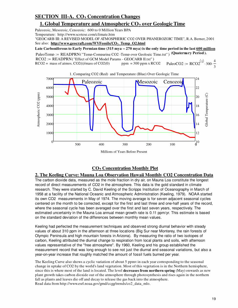
SECTION III-A. CO2 Concentration Changes
1. Global Temperature and Atmospheric CO2 over Geologic TimePaleozoic, Mesozoic, Cenozoic: 600 to 0 Million Years BPA
Temperature: http://www.scotese.com/climate.htm
"GEOCARB III: A REVISED MODEL OF ATMOSPHERIC CO2 OVER PHANEROZOIC TIME", R.A. Berner, 2001
See also: http://www.geocraft.com/WVFossils/CO2 _Temp_O2.html
Late Carboniferous to Early Permian time (315 mya -- 270 mya) is the only time period in the last 600 million
years when both atmospheric CO2 and temperatures were as low as they are today (Quaternary Period ).PaleoTemp READPRN "Temp-Comparing CO2 -Temp over Geologic Time.txt"( ):=
RCO2 READPRN "Effect of GCM Model Params - GEOCARB II.txt"( ):=RCO2 = mass of atmos. CO2(t)/mass of CO2(0) ppm = 300 ppm x RCO2 PaleoCO2 RCO2
1⟨ ⟩300⋅
4
3⋅:=
0500 400 300 200 100 00
1000
2000
3000
4000
5000
6000
7000
10
12
14
16
18
20
22
24
1. Comparing CO2 (Red) and Temperature (Blue) Over Geologic Time
Millions of Years Before Present
Atm
osp
her
ic C
O2 (
ppm
)
Glo
bal
Tem
per
ature
(C
)
Paleozoic Mesozoic Cenozoic
CO2 Concentration Monthly Plot
2. The Keeling Curve: Mauna Loa Observation Hawaii Monthly CO2 Concentration DataThe carbon dioxide data, measured as the mole fraction in dry air, on Mauna Loa constitute the longest
record of direct measurements of CO2 in the atmosphere. This data is the gold standard in climate
research. They were started by C. David Keeling of the Scripps Institution of Oceanography in March of
1958 at a facility of the National Oceanic and Atmospheric Administration (Keeling, 1979). NOAA started
its own CO2 measurements in May of 1974. The moving average is for seven adjacent seasonal cycles
centered on the month to be corrected, except for the first and last three and one-half years of the record,
where the seasonal cycle has been averaged over the first and last seven years, respectively. The
estimated uncertainty in the Mauna Loa annual mean growth rate is 0.11 ppm/yr. This estimate is based
on the standard deviation of the differences between monthly mean values.
Keeling had perfected the measurement techniques and observed strong diurnal behavior with steady
values of about 310 ppm in the afternoon at three locations (Big Sur near Monterey, the rain forests of
Olympic Peninsula and high mountain forests in Arizona). By measuring the ratio of two isotopes of
carbon, Keeling attributed the diurnal change to respiration from local plants and soils, with afternoon
values representative of the "free atmosphere". By 1960, Keeling and his group established the
measurement record that was long enough to see not just the diurnal and seasonal variations, but also a
year-on-year increase that roughly matched the amount of fossil fuels burned per year.
The Keeling Curve also shows a cyclic variation of about 5 ppmv in each year corresponding to the seasonal
change in uptake of CO2 by the world's land vegetation. Most of this vegetation is in the Northern hemisphere,
since this is where most of the land is located. The level decreases from northern spring (May) onwards as new
plant growth takes carbon dioxide out of the atmosphere through photosynthesis and rises again in the northern
fall as plants and leaves die off and decay to release the gas back into the atmosphere.
Read data from http://www.esrl.noaa.gov/gmd/ccgg/trends/co2_data_mlo.
19
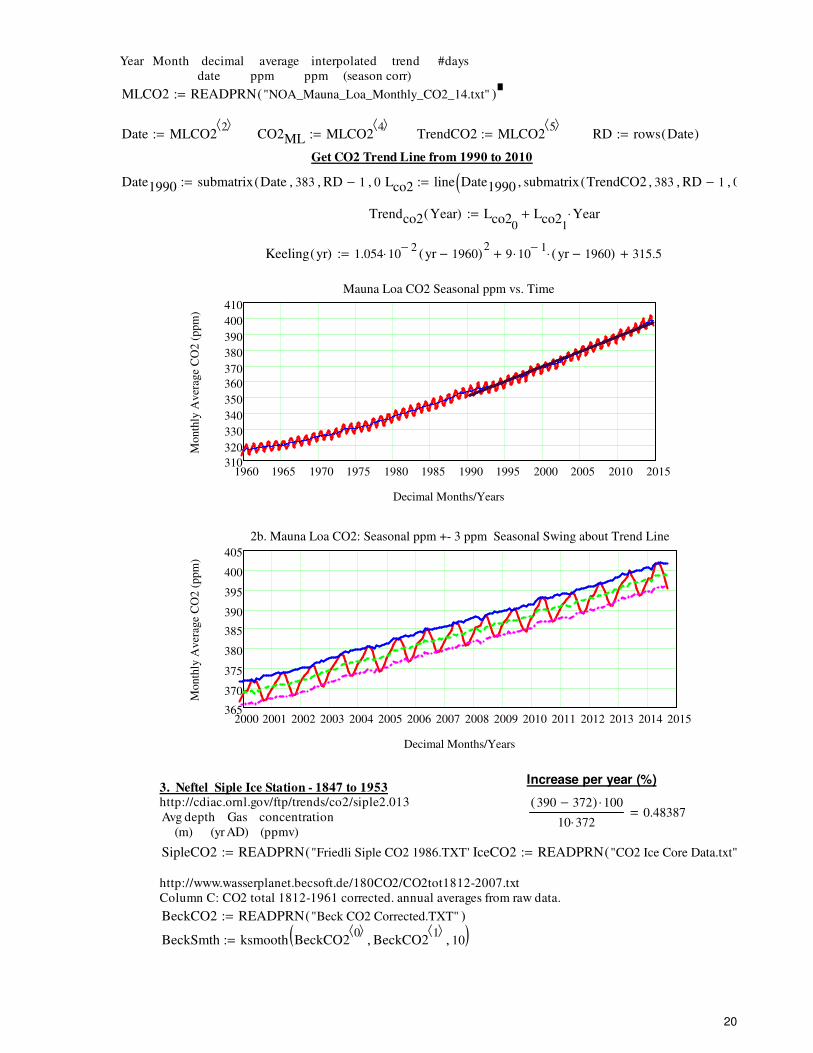
Year Month decimal average interpolated trend #days
date ppm ppm (season corr)
MLCO2 READPRN "NOA_Mauna_Loa_Monthly_CO2_14.txt"( ):=
Date MLCO22⟨ ⟩
:= CO2ML MLCO24⟨ ⟩
:= TrendCO2 MLCO25⟨ ⟩
:= RD rows Date( ):=
Get CO2 Trend Line from 1990 to 2010
Date1990 submatrix Date 383, RD 1−, 0, 0, ( ):= Lco2 line Date1990 submatrix TrendCO2 383, RD 1−, 0, (, (:=
Trendco2 Year( ) Lco20
Lco21
Year⋅+:=
Keeling yr( ) 1.054 102−
⋅ yr 1960−( )2
9 101−
⋅ yr 1960−( )⋅+ 315.5+:=
1960 1965 1970 1975 1980 1985 1990 1995 2000 2005 2010 2015310
320
330
340
350
360
370
380
390
400
410
Mauna Loa CO2 Seasonal ppm vs. Time
Decimal Months/Years
Month
ly A
ver
age
CO
2 (
ppm
)
2000 2001 2002 2003 2004 2005 2006 2007 2008 2009 2010 2011 2012 2013 2014 2015365
370
375
380
385
390
395
400
405
2b. Mauna Loa CO2: Seasonal ppm +- 3 ppm Seasonal Swing about Trend Line
Decimal Months/Years
Month
ly A
ver
age
CO
2 (
ppm
)
Increase per year (%) 3. Neftel Siple Ice Station - 1847 to 1953http://cdiac.ornl.gov/ftp/trends/co2/siple2.013
Avg depth Gas concentration
(m) (yr AD) (ppmv)
390 372−( ) 100⋅
10 372⋅0.48387=
SipleCO2 READPRN "Friedli Siple CO2 1986.TXT"( ):= IceCO2 READPRN "CO2 Ice Core Data.txt"(:=
http://www.wasserplanet.becsoft.de/180CO2/CO2tot1812-2007.txt
Column C: CO2 total 1812-1961 corrected. annual averages from raw data.
BeckCO2 READPRN "Beck CO2 Corrected.TXT"( ):=
BeckSmth ksmooth BeckCO20⟨ ⟩
BeckCO21⟨ ⟩
, 10, ( ):=
20
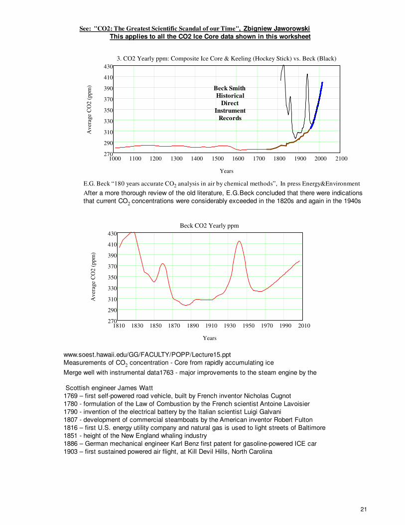
See: "CO2: The Greatest Scientific Scandal of our Time", Zbigniew Jaworowski
This applies to all the CO2 Ice Core data shown in this worksheet
1000 1100 1200 1300 1400 1500 1600 1700 1800 1900 2000 2100270
290
310
330
350
370
390
410
430
3. CO2 Yearly ppm: Composite Ice Core & Keeling (Hockey Stick) vs. Beck (Black)
Years
Aver
age
CO
2 (
ppm
)Beck Smith
Historical
Direct
Instrument
Records
E.G. Beck “180 years accurate CO2 analysis in air by chemical methods”, In press Energy&Environment
After a more thorough review of the old literature, E.G.Beck concluded that there were indications
that current CO2 concentrations were considerably exceeded in the 1820s and again in the 1940s
1810 1830 1850 1870 1890 1910 1930 1950 1970 1990 2010270
290
310
330
350
370
390
410
430
Beck CO2 Yearly ppm
Years
Aver
age
CO
2 (
ppm
)
www.soest.hawaii.edu/GG/FACULTY/POPP/Lecture15.ppt
Measurements of CO2 concentration - Core from rapidly accumulating ice
Merge well with instrumental data1763 - major improvements to the steam engine by the
Scottish engineer James Watt
1769 – first self-powered road vehicle, built by French inventor Nicholas Cugnot
1780 - formulation of the Law of Combustion by the French scientist Antoine Lavoisier
1790 - invention of the electrical battery by the Italian scientist Luigi Galvani
1807 - development of commercial steamboats by the American inventor Robert Fulton
1816 – first U.S. energy utility company and natural gas is used to light streets of Baltimore
1851 - height of the New England whaling industry
1886 – German mechanical engineer Karl Benz first patent for gasoline-powered ICE car
1903 – first sustained powered air flight, at Kill Devil Hills, North Carolina
21
0140000 120000 100000 80000 60000 40000 20000 0180
200
220
240
260
280
300
320
340
360
380
400
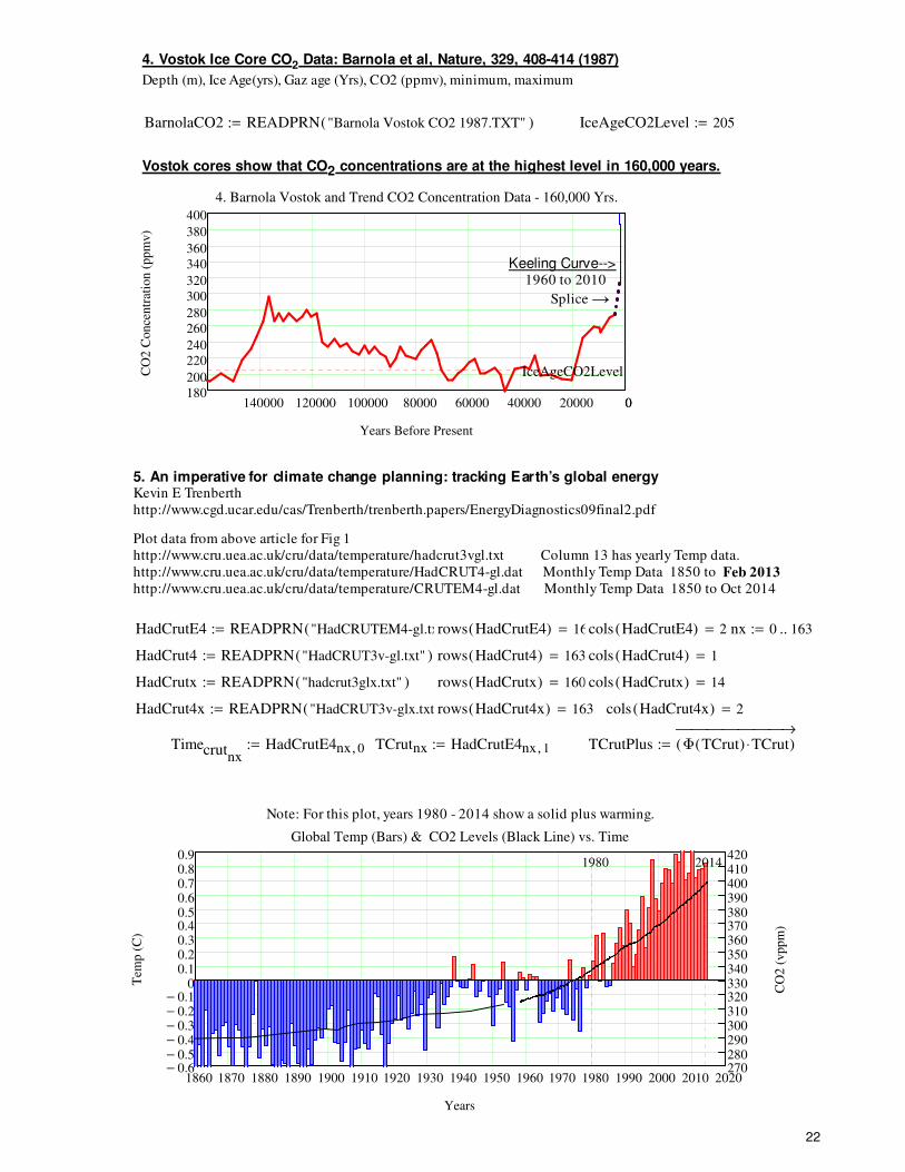
4. Barnola Vostok and Trend CO2 Concentration Data - 160,000 Yrs.
Years Before Present
CO
2 C
once
ntr
atio
n (
ppm
v)
IceAgeCO2Level
4. Vostok Ice Core CO2 Data: Barnola et al, Nature, 329, 408-414 (1987)
Depth (m), Ice Age(yrs), Gaz age (Yrs), CO2 (ppmv), minimum, maximum
BarnolaCO2 READPRN "Barnola Vostok CO2 1987.TXT"( ):= IceAgeCO2Level 205:=
Vostok cores show that CO2 concentrations are at the highest level in 160,000 years.
Keeling Curve-->1960 to 2010
Splice →
5. An imperative for climate change planning: tracking Earth’s global energyKevin E Trenberth
http://www.cgd.ucar.edu/cas/Trenberth/trenberth.papers/EnergyDiagnostics09final2.pdf
Plot data from above article for Fig 1
http://www.cru.uea.ac.uk/cru/data/temperature/hadcrut3vgl.txt Column 13 has yearly Temp data.
http://www.cru.uea.ac.uk/cru/data/temperature/HadCRUT4-gl.dat Monthly Temp Data 1850 to Feb 2013http://www.cru.uea.ac.uk/cru/data/temperature/CRUTEM4-gl.dat Monthly Temp Data 1850 to Oct 2014
HadCrutE4 READPRN "HadCRUTEM4-gl.txt"( ):= rows HadCrutE4( ) 164= cols HadCrutE4( ) 2= nx 0 163..:=
HadCrut4 READPRN "HadCRUT3v-gl.txt"( ):= rows HadCrut4( ) 163= cols HadCrut4( ) 1=
HadCrutx READPRN "hadcrut3glx.txt"( ):= rows HadCrutx( ) 160= cols HadCrutx( ) 14=
HadCrut4x READPRN "HadCRUT3v-glx.txt"( ):= rows HadCrut4x( ) 163= cols HadCrut4x( ) 2=
Timecrutnx
HadCrutE4nx 0, := TCrutnx HadCrutE4nx 1, := TCrutPlus Φ TCrut( ) TCrut⋅( )→
:=
1860 1870 1880 1890 1900 1910 1920 1930 1940 1950 1960 1970 1980 1990 2000 2010 20200.6−0.5−0.4−0.3−0.2−0.1−
00.10.20.30.40.50.60.70.80.9
270280290300310320330340350360370380390400410420
Global Temp (Bars) & CO2 Levels (Black Line) vs. Time
Years
Tem
p (
C)
CO
2 (
vppm
)
1980 2014
Note: For this plot, years 1980 - 2014 show a solid plus warming.
22
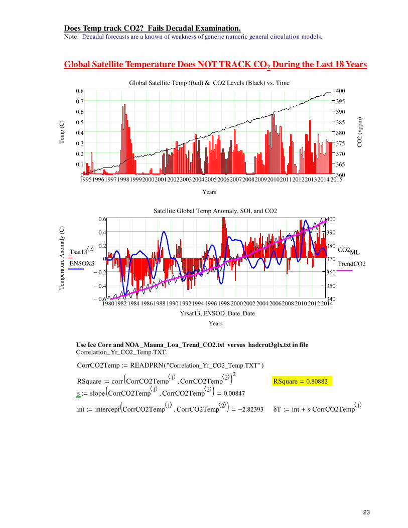
Does Temp track CO2? Fails Decadal Examination.Note: Decadal forecasts are a known of weakness of generic numeric general circulation models.
Global Satellite Temperature Does NOT TRACK CO 2 During the Last 18 Years
19951996199719981999200020012002200320042005200620072008200920102011201220132014 20150
0.1
0.2
0.3
0.4
0.5
0.6
0.7
0.8
360
365
370
375
380
385
390
395
400
Global Satellite Temp (Red) & CO2 Levels (Black) vs. Time
Years
Tem
p (
C)
CO
2 (
vppm
)
19801982 1984 19861988 1990 19921994 1996 1998 20002002 2004 20062008 2010 2012 20140.6−
0.4−
0.2−
0
0.2
0.4
0.6
340
350
360
370
380
390
400
Satellite Global Temp Anomaly, SOI, and CO2
Years
Tem
per
ature
Anom
aly (
C)
Tsat132⟨ ⟩
ENSOXS
CO2ML
TrendCO2
Yrsat13 ENSOD, Date, Date,
Use Ice Core and NOA _Mauna_Loa_Trend_CO2.txt versus hadcrut3glx.txt in fileCorrelation_Yr_CO2_Temp.TXT.
CorrCO2Temp READPRN "Correlation_Yr_CO2_Temp.TXT"( ):=
RSquare corr CorrCO2Temp1⟨ ⟩
CorrCO2Temp2⟨ ⟩
, ( )2
:= RSquare 0.80882=
s slope CorrCO2Temp1⟨ ⟩
CorrCO2Temp2⟨ ⟩
, ( ) 0.00847=:=
int intercept CorrCO2Temp1⟨ ⟩
CorrCO2Temp2⟨ ⟩
, ( ) 2.82393−=:= δT int s CorrCO2Temp1⟨ ⟩
⋅+:=
23
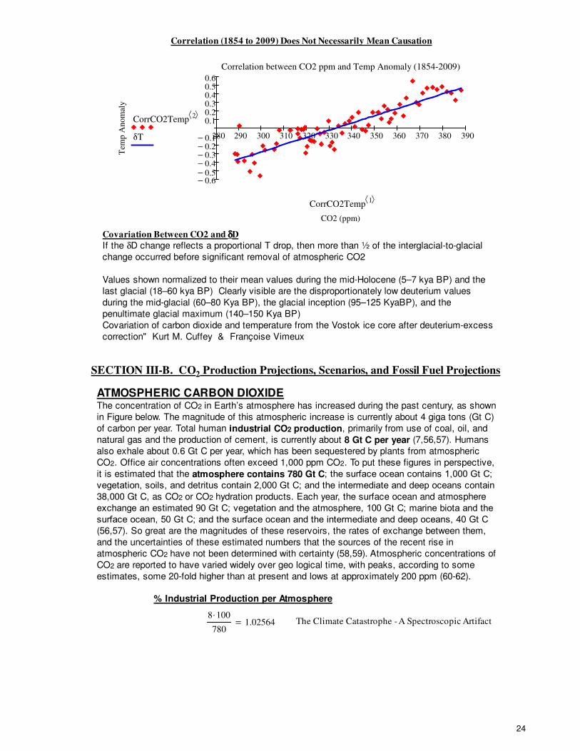
Correlation (1854 to 2009) Does Not Necessarily Mean Causation
280 290 300 310 320 330 340 350 360 370 380 390
0.6−0.5−0.4−0.3−0.2−0.1−
0.10.20.30.40.50.6
Correlation between CO2 ppm and Temp Anomaly (1854-2009)
CO2 (ppm)
Tem
p A
nom
aly
CorrCO2Temp2⟨ ⟩
δT
CorrCO2Temp1⟨ ⟩
Covariation Between CO2 and δδδδ D
If the δD change reflects a proportional T drop, then more than ½ of the interglacial-to-glacial
change occurred before significant removal of atmospheric CO2
Values shown normalized to their mean values during the mid-Holocene (5–7 kya BP) and the
last glacial (18–60 kya BP) Clearly visible are the disproportionately low deuterium values
during the mid-glacial (60–80 Kya BP), the glacial inception (95–125 KyaBP), and the
penultimate glacial maximum (140–150 Kya BP)
Covariation of carbon dioxide and temperature from the Vostok ice core after deuterium-excess
correction" Kurt M. Cuffey & Françoise Vimeux
SECTION III-B. CO2 Production Projections, Scenarios, and Fossil Fuel Projections
ATMOSPHERIC CARBON DIOXIDEThe concentration of CO2 in Earth’s atmosphere has increased during the past century, as shown
in Figure below. The magnitude of this atmospheric increase is currently about 4 giga tons (Gt C)
of carbon per year. Total human industrial CO2 production, primarily from use of coal, oil, and
natural gas and the production of cement, is currently about 8 Gt C per year (7,56,57). Humans
also exhale about 0.6 Gt C per year, which has been sequestered by plants from atmospheric
CO2. Office air concentrations often exceed 1,000 ppm CO2. To put these figures in perspective,
it is estimated that the atmosphere contains 780 Gt C; the surface ocean contains 1,000 Gt C;
vegetation, soils, and detritus contain 2,000 Gt C; and the intermediate and deep oceans contain
38,000 Gt C, as CO2 or CO2 hydration products. Each year, the surface ocean and atmosphere
exchange an estimated 90 Gt C; vegetation and the atmosphere, 100 Gt C; marine biota and the
surface ocean, 50 Gt C; and the surface ocean and the intermediate and deep oceans, 40 Gt C
(56,57). So great are the magnitudes of these reservoirs, the rates of exchange between them,
and the uncertainties of these estimated numbers that the sources of the recent rise in
atmospheric CO2 have not been determined with certainty (58,59). Atmospheric concentrations of
CO2 are reported to have varied widely over geo logical time, with peaks, according to some
estimates, some 20-fold higher than at present and lows at approximately 200 ppm (60-62).
% Industrial Production per Atmosphere
8 100⋅
7801.02564= The Climate Catastrophe - A Spectroscopic Artifact
24
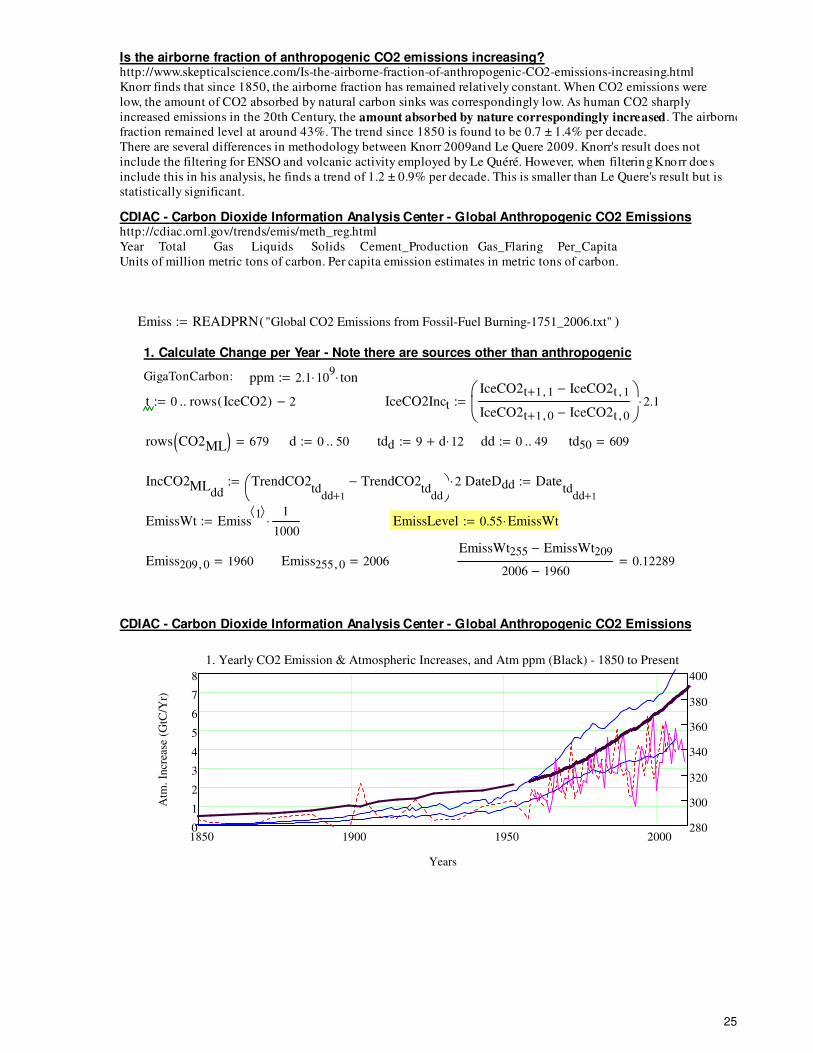
Is the airborne fraction of anthropogenic CO2 emissions increasing?http://www.skepticalscience.com/Is-the-airborne-fraction-of-anthropogenic-CO2-emissions-increasing.html
Knorr finds that since 1850, the airborne fraction has remained relatively constant. When CO2 emissions were
low, the amount of CO2 absorbed by natural carbon sinks was correspondingly low. As human CO2 sharply
increased emissions in the 20th Century, the amount absorbed by nature correspondingly increased. The airborne
fraction remained level at around 43%. The trend since 1850 is found to be 0.7 ± 1.4% per decade.
There are several differences in methodology between Knorr 2009and Le Quere 2009. Knorr's result does not
include the filtering for ENSO and volcanic activity employed by Le Quéré. However, when filtering Knorr does
include this in his analysis, he finds a trend of 1.2 ± 0.9% per decade. This is smaller than Le Quere's result but is
statistically significant.
CDIAC - Carbon Dioxide Information Analysis Center - Global Anthropogenic CO2 Emissionshttp://cdiac.ornl.gov/trends/emis/meth_reg.html
Year Total Gas Liquids Solids Cement_Production Gas_Flaring Per_Capita
Units of million metric tons of carbon. Per capita emission estimates in metric tons of carbon.
Emiss READPRN "Global CO2 Emissions from Fossil-Fuel Burning-1751_2006.txt"( ):=
1. Calculate Change per Year - Note there are sources other than anthropogenic
GigaTonCarbon: ppm 2.1 109
⋅ ton⋅:=
t 0 rows IceCO2( ) 2−..:= IceCO2Inct
IceCO2t 1+ 1, IceCO2t 1, −
IceCO2t 1+ 0, IceCO2t 0, −
2.1⋅:=
rows CO2ML( ) 679= d 0 50..:= tdd 9 d 12⋅+:= dd 0 49..:= td50 609=
IncCO2MLdd
TrendCO2td
dd 1+
TrendCO2td
dd
−
2.1⋅:= DateDdd Datetd
dd 1+
:=
EmissWt Emiss1⟨ ⟩ 1
1000⋅:= EmissLevel 0.55 EmissWt⋅:=
Emiss209 0, 1960= Emiss255 0, 2006=EmissWt255 EmissWt209−
2006 1960−0.12289=
CDIAC - Carbon Dioxide Information Analysis Center - Global Anthropogenic CO2 Emissions
1850 1900 1950 20000
1
2
3
4
5
6
7
8
280
300
320
340
360
380
400
1. Yearly CO2 Emission & Atmospheric Increases, and Atm ppm (Black) - 1850 to Present
Years
Atm
. In
crea
se (
GtC
/Yr)
25
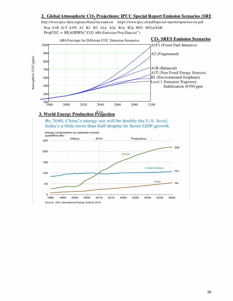
2. Global Atmospheric CO 2 Projections: IPCC Special Report Emission Scenarios (SRES)
http://www.ipcc-data.org/ancilliary/tar-isam.txt https://www.ipcc.ch/pdf/special-reports/spm/sres-en.pdf
Year A1B A1T A1FI A2 B1 B2 A1p A2p B1p B2p IS92 IS92a/SAR
ProjCO2 READPRN "CO2 AR4 Emission Proj-Data.txt"( ):=
1980 2000 2020 2040 2060 2080 2100300
400
500
600
700
800
900
1000
AR4 Forcings for Different CO2 Emission Scenarios
Year
Atm
osp
her
ic C
O2 (
ppm
)
CO 2 SRES Emission Scenarios
A1F1 (Fossil Fuel Intensive)
A2 (Fragmented)
A1B (Balanced)
A1T (Non Fossil Energy Sources)
B1 (Environmental Emphasis)Level 2 Emission Trajectory
Stabilization @550 ppm
3. World Energy Production Projection
26
SECTION III-C. Fossil Fuel Energy Sources - CO2 Emission Sources
1. Main Areas of Human Energy Consumption in the US
http://www.epa.gov/climatechange/ghgemissions/gases/co2.html
Electricity 38%, Transportation 32%, Industry 14%, Residential 9% and NonFossil Fuel 6%
Electricity is not a primary energy source. It is one of the most common energy carriers. generate 3 to 4
times more torque per unit energy input than all but the largest and most efficient house-sized diesel ship
engines (50 percent efficient).
2. Human Contribution Relative to Other Sources of CO 2
The burning of fossil fuels sends 7 gigatons (3.27 %) of carbon dioxide into the atmosphere each
year, while the biosphere and oceans account for 440 (55.28 %) and 330 (41.46 %) gigatons,
respectively—total human emissions have jumped sharply since the Industrial Revolution. Carbon is
emitted naturally into the atmosphere but that the atmosphere also sends carbon back to the land and
oceans and that these carbon flows have canceled each other out for millennia. Burning fossil fuels, in
contrast, creates a new flow of carbon that, though small, is not canceled.
3. Coal Usage and Factors
Source: http://www.nationalreview.com/article/392167/social-justice-coal-robert-bryce
Coal is perfectly suited for electricity production, it's abundant, its reserves are geographically
dispersed, prices are not affected by any canceled entities, and — above all — it's cheap. Coal-fired
generators provide about 40 percent of all global electricity. Coal is the most carbon intensive fossil fuel.
Coal is the world's fastest-growing form of energy and it has been since 1973. In 2013 alone, coal use
grew by about 2 million barrels of oil equivalent per day (boe/d). That was about three times the growth
seen in natural gas (which grew by about 700,000 boe/d), four times the rate of growth in wind (up by
about 500,000 boe/d), and 13 times the growth in solar (which was up by about 150,000 boe/d).
China has led the rush toward coal and now accounts for fully half of global coal consumption.
Increased use of hydrocarbons results in better living standards. Indeed, per capita carbon dioxide
emissions (like per capita electricity usage) are a reliable indicator of higher incomes.
4. Oil Production - US Drilling Rigs - December 2014
Why is the world market suddenly awash in oil? The answer: Over the past few years — thanks to rigs,
rednecks, and rights — the U.S. has added the equivalent of one Kuwait and one Iran to its domestic oil
and gas production.
Since 2004, U.S. oil production is up 56 percent, or about 3.1 million barrels a day, about the same
volume as Kuwait produced last year. The dimensions of the boom in natural gas can be seen by looking
solely at the Marcellus Shale in Pennsylvania, where output has jumped eight-fold since 2010 and is now
about 16 billion cubic feet per day, a volume roughly equal to Iran's current natural-gas production.
U.S. oil and gas numbers are soaring because of an abundance of rigs. More than half of all the
drilling rigs on the planet are operating in the United States. We have about 1,900 active rigs. The
rest of the world combined has about 1,300.
27
IV. Solar Variation: Wolf Number, Sunspots, C14 SS Extrema, Irradiance, WindSee Section XIIA for Solar Radiation Spectrum and XIIIB for Reflectance.
http://en.wikipedia.org/wiki/Solar_variation
The Sun and Climate http://pubs.usgs.gov/fs/fs-0095-00/fs-0095-00.pdf
Many geologic records of climatic and environmental change based on
various proxy variables exhibit distinct cyclicities that have been attributed to
extraterrestrial forcing. ... Another terrestrial observation was that the Maunder Minimum coincided
with the coldest part of the Little Ice Age.http://commons.wikimedia.org/wiki/File:Carbon-14_with_activity_labels.png
http://www.radiocarbon.org/IntCal04%20files/intcal04.14c
Read Carbon 14 Atmospheric Concentration Data# CAL BP, 14C age, Error, Delta 14C, Sigma,
YR BP ,YR BP, per mil , per mil
C14 READPRN "Atmospheric C14 Concentration.TXT"( ):= Yr C140⟨ ⟩
40+:=
SSSmooth ksmooth reverse Yr( ) reverse C143⟨ ⟩( ), 2000, ( ):=
Detrend reverse C143⟨ ⟩( ) SSSmooth−:=
SSCycle ksmooth reverse Yr( ) Detrend, 1000, ( ):= Yrss 2010 Yr−:=
Wolf numberThe Wolf number (also known as the International sunspot number, relative sunspot
number, or Zürich number) is a quan tity which measures the number o f sunspots and
groups of sunspots present on the surface of the sun.
http://en.wikipedia.org/wiki/Wolf_number
The Solar Physics Group at NASA's Marshall Space Flight Center Royal Greenwich Observatory - USAF/NOAA Sunspot Data
http://solarscience.msfc.nasa.gov/greenwch/spot_num.txt
Sunspot Monthly Averages -2013.txt: Spliced above with RecentIndices.txt data from
http://www.swpc.noaa.gov/ftpdir/weekly/RecentIndices.txt
Read Sunspot DataYEAR MON SSN DEV
SSpots READPRN "sunspot_num2015.txt"( ):= NumSS SSpots2⟨ ⟩
:=
YrDec SSpots0⟨ ⟩ SSpots
1⟨ ⟩1−
12+ 2014−
−:= SSpotYrly READPRN "SN_y_tot_V2.0-1690.txt"(:=
SSSmth ksmooth YrDec− NumSS, 11, ( ):= YrDec SSpots0⟨ ⟩ SSpots
1⟨ ⟩1−
12+:=
Solar Influences Data Analysis Center - SIDChttp://www.sidc.be/sunspot-data/ Updated 10-23-2014YrMon, Year_Decimal, Monthly, Monthly Smoothed Sunspot Number, 1749 to 2014
SSN READPRN "monthssn201409.dat"( ):= SSNYr READPRN "yearssn2013.dat"( ):=
SSNYrSmooth ksmooth SSNYr0⟨ ⟩
SSNYr1⟨ ⟩
, 11, ( ):= NGDC - Group Sunspot Numbers (Doug Hoyt re-evaluation) 1610-1995http://www.ngdc.noaa.gov/stp/SOLAR/ftpsunspotnumber.html#hoyt - 4bb. monthrg.dat
SSN_Hoyt READPRN "Grp SSN-monthrg-1610-1995.dat"( ):= SSNS ksmooth SSNYr0⟨ ⟩
SSNYr1⟨ ⟩
, 10, (:=
NGDC-Table of smoothed monthly sunspot numbers 1700-present
Year, SNN-Jan to SNN-Dec
SSNSm_Hoyt READPRN "SmoothMonthMeanHoyt-1749-2009.txt"( ):= R rows SSNSm_Hoyt( ):=
r 0 R 1−..:= SSHr
1
12
m
SSNSm_Hoytr m, 1
12⋅
∑
=
:=YearH SSNSm_Hoyt
0⟨ ⟩:=
Smooth Hadcrut over 11 year cycle Sun Spots: TKSmooth ksmooth Timecrut TCrut, 11, ( ):=
28
1690 1710 1730 1750 1770 1790 1810 1830 1850 1870 1890 1910 1930 1950 1970 1990 2010 20300
20
40
60
80
100
120
140
160
180
200
220
0.6−0.5−0.4−0.3−0.2−0.1−
00.10.2
0.30.40.5
0.60.70.8
0.9
Calendar Years BP
Num
ber
of
Sunsp
ots
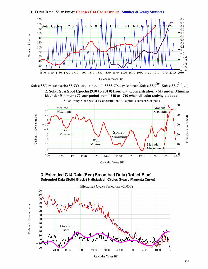
1. TCrut Temp, Solar Proxy: Changes C14 Concentration , Number of Yearly Sunspots
Solar Cycle #: 1 2 3 4 5 6 7 8 9 10 11 12 13 14 15 16 1718 19 20 21 22 23 24
SubsetSSN submatrix SSNYr 210, 313, 0, 1, ( ):= SSSSNDec ksmooth SubsetSSN0⟨ ⟩
SubsetSSN1⟨ ⟩
, 24, ( ):=
2. Solar Sun Spot Epochs (910 to 2010) from C14 Concentration - Maunder Minimum
920 1020 1120 1220 1320 1420 1520 1620 1720 1820 1920 202020
15
10
5
0
5−
10−
15−
20−
25−
30−
30
40
50
60
70
80
Solar Proxy: Changes C14 Concentration, Blue plot is current Sunspot #
Calendar Years BP
Car
bon 1
4 C
once
ntr
atio
n
#S
unsp
ots
(S
mooth
ed)
Maunder Minimum: 70 year period from 1645 to 1710 when all solar activity stopped
Medieval
Maximum
Modern
Maximum
Oort
MinimumSpörer
MinimumWolf
Minimum Maunder
Minimum
3. Extended C14 Data (Red) Smoothed Data (Dotted Blue) Detrended Data (Solid Black ) Hallstadzeit Cycles (Heavy Magenta Curve)
09000 8000 7000 6000 5000 4000 3000 2000 1000 020−
10−
0
10
20
30
40
50
60
70
80
90
100
110
120
Hallstadtzeit Cycles Periodicity ~2000Yr
Calendar Years BP
Car
bon 1
4 C
once
ntr
atio
n
Detrended
Data
29
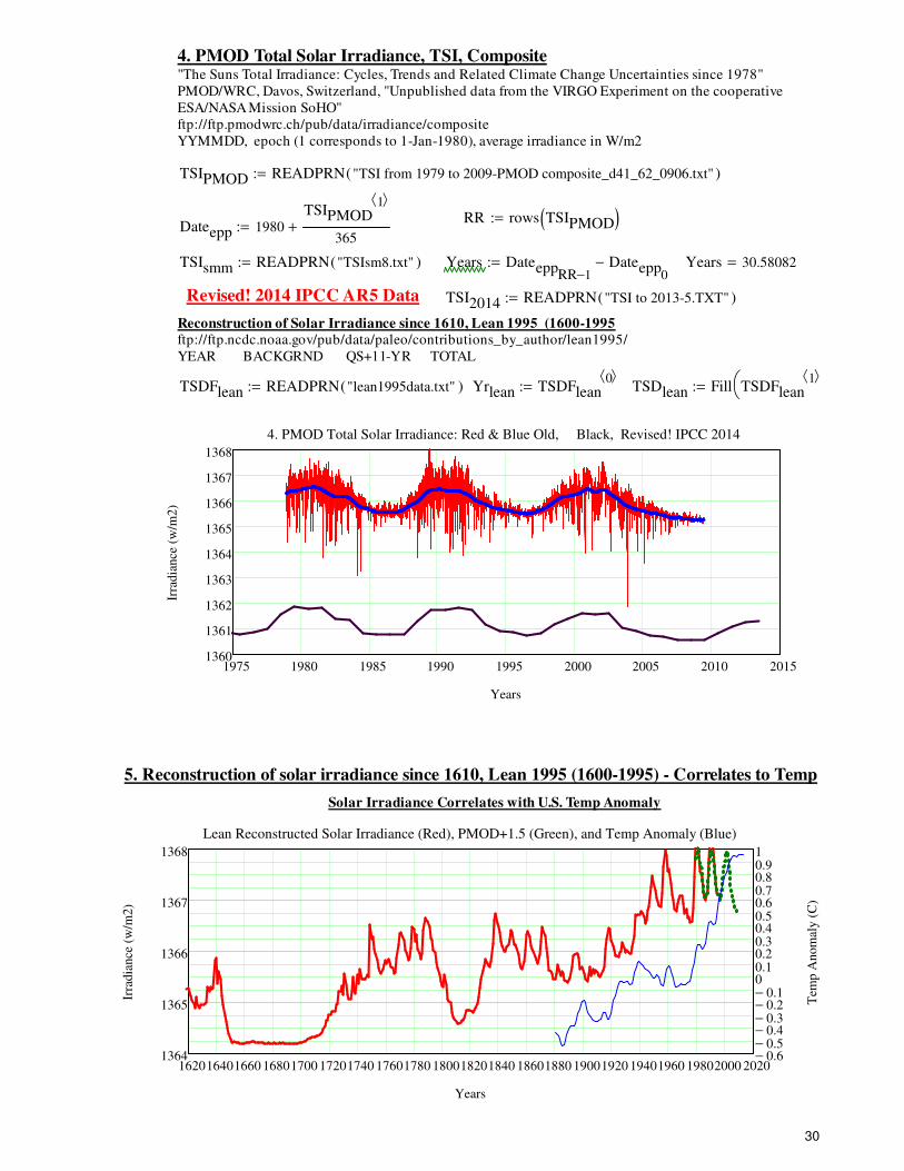
4. PMOD Total Solar Irradiance, TSI, Composite"The Suns Total Irradiance: Cycles, Trends and Related Climate Change Uncertainties since 1978"
PMOD/WRC, Davos, Switzerland, "Unpublished data from the VIRGO Experiment on the cooperative
ESA/NASA Mission SoHO"
ftp://ftp.pmodwrc.ch/pub/data/irradiance/composite
YYMMDD, epoch (1 corresponds to 1-Jan-1980), average irradiance in W/m2
TSIPMOD READPRN "TSI from 1979 to 2009-PMOD composite_d41_62_0906.txt"( ):=
RR rows TSIPMOD( ):=Dateepp 1980
TSIPMOD1⟨ ⟩
365+:=
TSIsmm READPRN "TSIsm8.txt"( ):= Years DateeppRR 1−
Dateepp0
−:= Years 30.58082=
Revised! 2014 IPCC AR5 Data TSI2014 READPRN "TSI to 2013-5.TXT"( ):=
Reconstruction of Solar Irradiance since 1610, Lean 1995 (1600-1995ftp://ftp.ncdc.noaa.gov/pub/data/paleo/contributions_by_author/lean1995/
YEAR BACKGRND QS+11-YR TOTAL
TSDFlean READPRN "lean1995data.txt"( ):= Yrlean TSDFlean0⟨ ⟩
:= TSDlean Fill TSDFlean1⟨ ⟩
:=
1975 1980 1985 1990 1995 2000 2005 2010 20151360
1361
1362
1363
1364
1365
1366
1367
1368
4. PMOD Total Solar Irradiance: Red & Blue Old, Black, Revised! IPCC 2014
Years
Irra
dia
nce
(w
/m2)
5. Reconstruction of solar irradiance since 1610, Lean 1995 (1600-1995) - Correlates to Temp
Solar Irradiance Correlates with U.S. Temp Anomaly
162016401660 16801700 17201740 17601780 180018201840 18601880 19001920 19401960 19802000 20201364
1365
1366
1367
1368
0.6−0.5−0.4−0.3−0.2−0.1−
00.10.20.30.40.50.60.70.80.91
Lean Reconstructed Solar Irradiance (Red), PMOD+1.5 (Green), and Temp Anomaly (Blue)
Years
Irra
dia
nce
(w
/m2)
Tem
p A
nom
aly (
C)
30
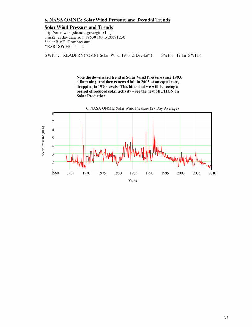
6. NASA OMNI2: Solar Wind Pressure and Decadal Trends
Solar Wind Pressure and Trendshttp://omniweb.gsfc.nasa.gov/cgi/nx1.cgi
omni2_27day data from 19630130 to 20091230
Scalar B, nT, Flow pressure
YEAR DOY HR 1 2
SWPF READPRN "OMNI_Solar_Wind_1963_27Day.dat"( ):= SWP Fillin SWPF( ):=
Note the downward trend in Solar Wind Pressure since 1993,
a flattening, and then renewed fall in 2005 at an equal rate,
dropping to 1970 levels. This hints that we will be seeing a
period of reduced solar activity - See the next SECTION on
Solar Prediction.
1960 1965 1970 1975 1980 1985 1990 1995 2000 2005 20101
2
3
4
5
6
7
8
6. NASA ONMI2 Solar Wind Pressure (27 Day Average)
Years
Sola
r P
ress
ure
(nP
a)
31
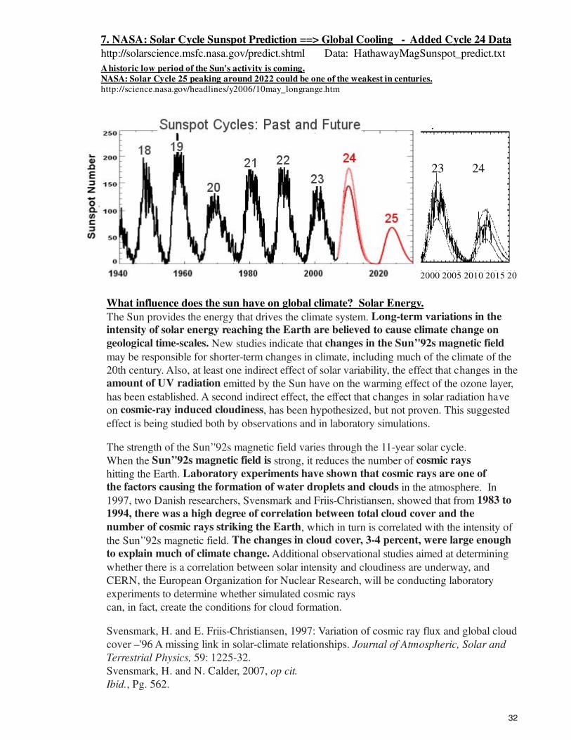
7. NASA: Solar Cycle Sunspot Prediction ==> Global Cooling - Added Cycle 24 Data
http://solarscience.msfc.nasa.gov/predict.shtml Data: HathawayMagSunspot_predict.txt
A historic low period of the Sun's activity is coming.
NASA: Solar Cycle 25 peaking around 2022 could be one of the weakest in centuries.http://science.nasa.gov/headlines/y2006/10may_longrange.htm
23 24
What influence does the sun have on global climate? Solar Energy.
The Sun provides the energy that drives the climate system. Long-term variations in the
intensity of solar energy reaching the Earth are believed to cause climate change on
geological time-scales. New studies indicate that changes in the Sun’'92s magnetic field
may be responsible for shorter-term changes in climate, including much of the climate of the
20th century. Also, at least one indirect effect of solar variability, the effect that changes in the
amount of UV radiation emitted by the Sun have on the warming effect of the ozone layer,
has been established. A second indirect effect, the effect that changes in solar radiation have
on cosmic-ray induced cloudiness, has been hypothesized, but not proven. This suggested
effect is being studied both by observations and in laboratory simulations.
The strength of the Sun’'92s magnetic field varies through the 11-year solar cycle.
When the Sun’'92s magnetic field is strong, it reduces the number of cosmic rays
hitting the Earth. Laboratory experiments have shown that cosmic rays are one of
the factors causing the formation of water droplets and clouds in the atmosphere. In
1997, two Danish researchers, Svensmark and Friis-Christiansen, showed that from 1983 to
1994, there was a high degree of correlation between total cloud cover and the
number of cosmic rays striking the Earth, which in turn is correlated with the intensity of
the Sun’'92s magnetic field. The changes in cloud cover, 3-4 percent, were large enough
to explain much of climate change. Additional observational studies aimed at determining
whether there is a correlation between solar intensity and cloudiness are underway, and
CERN, the European Organization for Nuclear Research, will be conducting laboratory
experiments to determine whether simulated cosmic rays
can, in fact, create the conditions for cloud formation.
Svensmark, H. and E. Friis-Christiansen, 1997: Variation of cosmic ray flux and global cloud
cover –'96 A missing link in solar-climate relationships. Journal of Atmospheric, Solar and
Terrestrial Physics, 59: 1225-32.
Svensmark, H. and N. Calder, 2007, op cit.
Ibid., Pg. 562.
2000 2005 2010 2015 2020
32
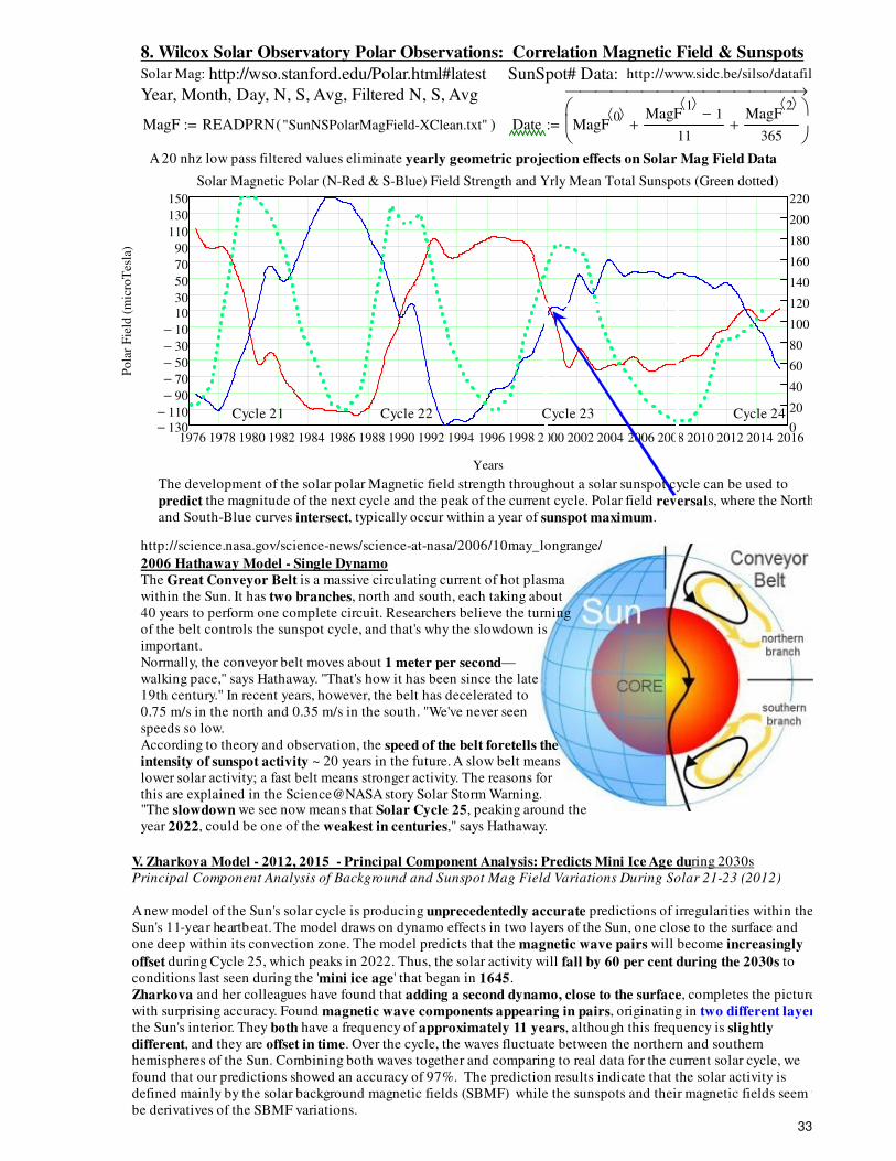
8. Wilcox Solar Observatory Polar Observations: Correlation Magnetic Field & Sunspots
Solar Mag: http://wso.stanford.edu/Polar.html#latest SunSpot# Data: http://www.sidc.be/silso/datafiles
Year, Month, Day, N, S, Avg, Filtered N, S, Avg
MagF READPRN "SunNSPolarMagField-XClean.txt"( ):= Date MagF0⟨ ⟩ MagF
1⟨ ⟩1−
11+
MagF2⟨ ⟩
365+
→
:=
1976 1978 1980 1982 1984 1986 1988 1990 1992 1994 1996 1998 2000 2002 2004 2006 2008 2010 2012 2014 2016130−110−
90−
70−
50−
30−
10−
10
30
50
70
90
110
130
150
0
20
40
60
80
100
120
140
160
180
200
220
Solar Magnetic Polar (N-Red & S-Blue) Field Strength and Yrly Mean Total Sunspots (Green dotted)
Years
Pola
r F
ield
(m
icro
Tes
la)
A 20 nhz low pass filtered values eliminate yearly geometric projection effects on Solar Mag Field Data
Cycle 21 Cycle 22 Cycle 23 Cycle 24
The development of the solar polar Magnetic field strength throughout a solar sunspot cycle can be used to
predict the magnitude of the next cycle and the peak of the current cycle. Polar field reversals, where the North-Red
and South-Blue curves intersect, typically occur within a year of sunspot maximum.
http://science.nasa.gov/science-news/science-at-nasa/2006/10may_longrange/
2006 Hathaway Model - Single DynamoThe Great Conveyor Belt is a massive circulating current of hot plasma
within the Sun. It has two branches, north and south, each taking about
40 years to perform one complete circuit. Researchers believe the turning
of the belt controls the sunspot cycle, and that's why the slowdown is
important.
Normally, the conveyor belt moves about 1 meter per second—
walking pace," says Hathaway. "That's how it has been since the late
19th century." In recent years, however, the belt has decelerated to
0.75 m/s in the north and 0.35 m/s in the south. "We've never seen
speeds so low.
According to theory and observation, the speed of the belt foretells the
intensity of sunspot activity ~ 20 years in the future. A slow belt means
lower solar activity; a fast belt means stronger activity. The reasons for
this are explained in the Science@NASA story Solar Storm Warning."The slowdown we see now means that Solar Cycle 25, peaking around the
year 2022, could be one of the weakest in centuries," says Hathaway.
V. Zharkova Model - 2012, 2015 - Principal Component Analysis: Predicts Mini Ice Age du ring 2030s
Principal Component Analysis of Background and Sunspot Mag Field Variations During Solar 21-23 (2012)
A new model of the Sun's solar cycle is producing unprecedentedly accurate predictions of irregularities within the
Sun's 11-year heartbeat. The model draws on dynamo effects in two layers of the Sun, one close to the surface and
one deep within its convection zone. The model predicts that the magnetic wave pairs will become increasingly
offset during Cycle 25, which peaks in 2022. Thus, the solar activity will fall by 60 per cent during the 2030s to
conditions last seen during the 'mini ice age' that began in 1645.
Zharkova and her colleagues have found that adding a second dynamo, close to the surface, completes the picture
with surprising accuracy. Found magnetic wave components appearing in pairs, originating in two different layersthe Sun's interior. They both have a frequency of approximately 11 years, although this frequency is slightly
different, and they are offset in time. Over the cycle, the waves fluctuate between the northern and southern
hemispheres of the Sun. Combining both waves together and comparing to real data for the current solar cycle, we
found that our predictions showed an accuracy of 97%. The prediction results indicate that the solar activity is
defined mainly by the solar background magnetic fields (SBMF) while the sunspots and their magnetic fields seem to
be derivatives of the SBMF variations.
33
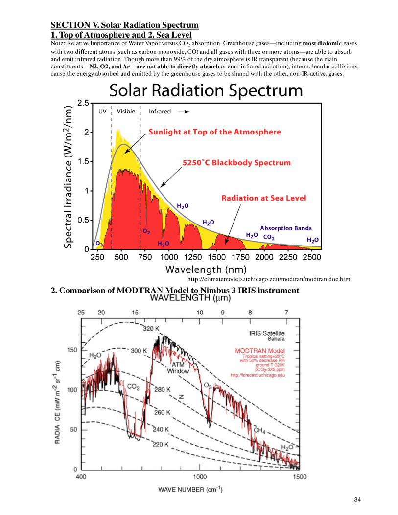
SECTION V. Solar Radiation Spectrum 1. Top of Atmosphere and 2. Sea LevelNote: Relative Importance of Water Vapor versus CO2 absorption. Greenhouse gases—including most diatomic gases
with two different atoms (such as carbon monoxide, CO) and all gases with three or more atoms—are able to absorb
and emit infrared radiation. Though more than 99% of the dry atmosphere is IR transparent (because the main
constituents—N2, O2, and Ar—are not able to directly absorb or emit infrared radiation), intermolecular collisions
cause the energy absorbed and emitted by the greenhouse gases to be shared with the other, non-IR-active, gases.
http://climatemodels.uchicago.edu/modtran/modtran.doc.html
2. Comparison of MODTRAN Model to Nimbus 3 IRIS instrument
34
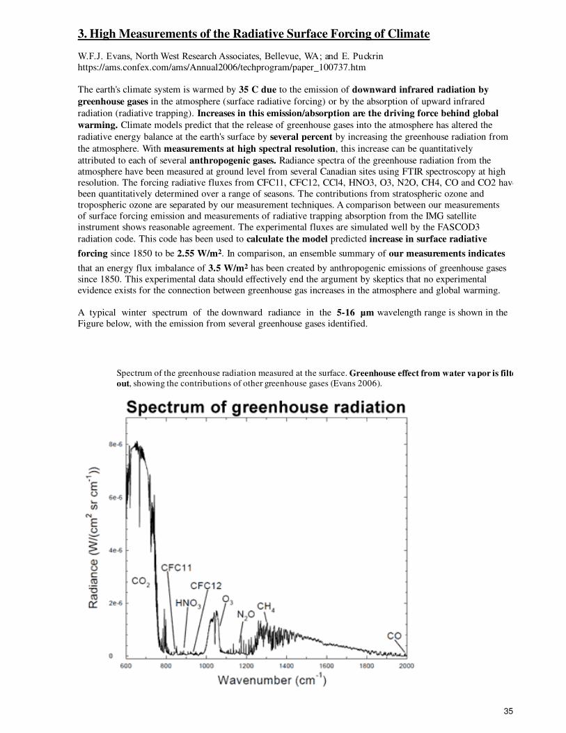
3. High Measurements of the Radiative Surface Forcing of Climate
W.F.J. Evans, North West Research Associates, Bellevue, WA; and E. Puckrin
https://ams.confex.com/ams/Annual2006/techprogram/paper_100737.htm
The earth's climate system is warmed by 35 C due to the emission of downward infrared radiation by
greenhouse gases in the atmosphere (surface radiative forcing) or by the absorption of upward infrared
radiation (radiative trapping). Increases in this emission/absorption are the driving force behind global
warming. Climate models predict that the release of greenhouse gases into the atmosphere has altered the
radiative energy balance at the earth's surface by several percent by increasing the greenhouse radiation from
the atmosphere. With measurements at high spectral resolution, this increase can be quantitatively
attributed to each of several anthropogenic gases. Radiance spectra of the greenhouse radiation from the
atmosphere have been measured at ground level from several Canadian sites using FTIR spectroscopy at high
resolution. The forcing radiative fluxes from CFC11, CFC12, CCl4, HNO3, O3, N2O, CH4, CO and CO2 have
been quantitatively determined over a range of seasons. The contributions from stratospheric ozone and
tropospheric ozone are separated by our measurement techniques. A comparison between our measurements
of surface forcing emission and measurements of radiative trapping absorption from the IMG satellite
instrument shows reasonable agreement. The experimental fluxes are simulated well by the FASCOD3
radiation code. This code has been used to calculate the model predicted increase in surface radiative
forcing since 1850 to be 2.55 W/m2. In comparison, an ensemble summary of our measurements indicates
that an energy flux imbalance of 3.5 W/m2 has been created by anthropogenic emissions of greenhouse gases
since 1850. This experimental data should effectively end the argument by skeptics that no experimental
evidence exists for the connection between greenhouse gas increases in the atmosphere and global warming.
A typical winter spectrum of the downward radiance in the 5-16 µm wavelength range is shown in the
Figure below, with the emission from several greenhouse gases identified.
Spectrum of the greenhouse radiation measured at the surface. Greenhouse effect from water vapor is filtered
out, showing the contributions of other greenhouse gases (Evans 2006).
35
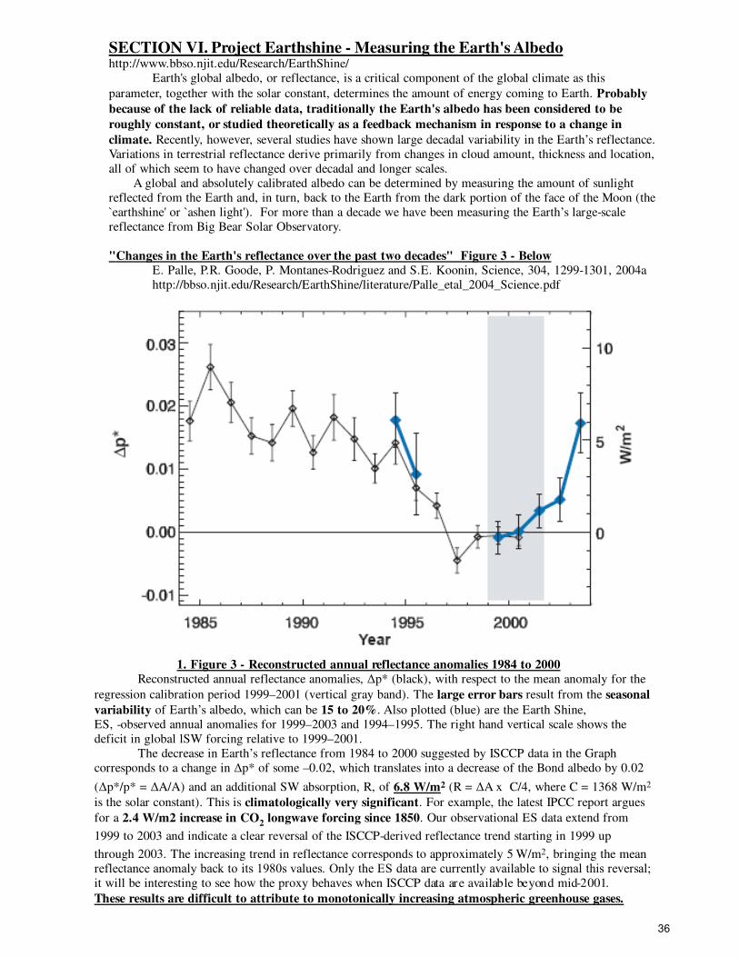
SECTION VI. Project Earthshine - Measuring the Earth's Albedohttp://www.bbso.njit.edu/Research/EarthShine/
Earth's global albedo, or reflectance, is a critical component of the global climate as this
parameter, together with the solar constant, determines the amount of energy coming to Earth. Probably
because of the lack of reliable data, traditionally the Earth's albedo has been considered to be
roughly constant, or studied theoretically as a feedback mechanism in response to a change in
climate. Recently, however, several studies have shown large decadal variability in the Earth’s reflectance.
Variations in terrestrial reflectance derive primarily from changes in cloud amount, thickness and location,
all of which seem to have changed over decadal and longer scales.
A global and absolutely calibrated albedo can be determined by measuring the amount of sunlight
reflected from the Earth and, in turn, back to the Earth from the dark portion of the face of the Moon (the
`earthshine' or `ashen light'). For more than a decade we have been measuring the Earth’s large-scale
reflectance from Big Bear Solar Observatory.
" Changes in the Earth's reflectance over the past two decades" Figure 3 - Below
E. Palle, P.R. Goode, P. Montanes-Rodriguez and S.E. Koonin, Science, 304, 1299-1301, 2004a
http://bbso.njit.edu/Research/EarthShine/literature/Palle_etal_2004_Science.pdf
1. Figure 3 - Reconstructed annual reflectance anomalies 1984 to 2000
Reconstructed annual reflectance anomalies, ∆p* (black), with respect to the mean anomaly for the
regression calibration period 1999–2001 (vertical gray band). The large error bars result from the seasonal
variability of Earth’s albedo, which can be 15 to 20%. Also plotted (blue) are the Earth Shine,
ES, -observed annual anomalies for 1999–2003 and 1994–1995. The right hand vertical scale shows the
deficit in global lSW forcing relative to 1999–2001.
The decrease in Earth’s reflectance from 1984 to 2000 suggested by ISCCP data in the Graph
corresponds to a change in ∆p* of some –0.02, which translates into a decrease of the Bond albedo by 0.02
(∆p*/p* = ∆A/A) and an additional SW absorption, R, of 6.8 W/m2 (R = ∆A x C/4, where C = 1368 W/m2
is the solar constant). This is climatologically very significant. For example, the latest IPCC report argues
for a 2.4 W/m2 increase in CO2 longwave forcing since 1850. Our observational ES data extend from
1999 to 2003 and indicate a clear reversal of the ISCCP-derived reflectance trend starting in 1999 up
through 2003. The increasing trend in reflectance corresponds to approximately 5 W/m2, bringing the mean
reflectance anomaly back to its 1980s values. Only the ES data are currently available to signal this reversal;
it will be interesting to see how the proxy behaves when ISCCP data are available beyond mid-2001.
These results are difficult to attribute to monotonically increasing atmospheric greenhouse gases.
36
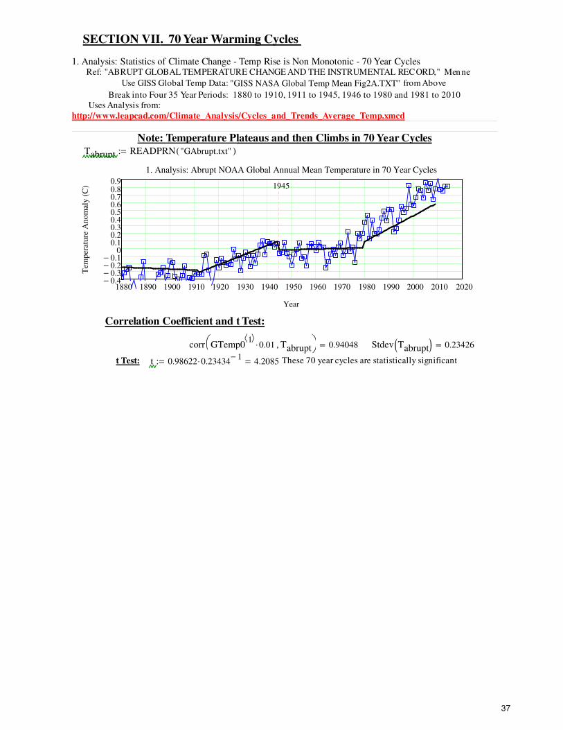
SECTION VII . 70 Year Warming Cycles
1. Analysis: Statistics of Climate Change - Temp Rise is Non Monotonic - 70 Year Cycles Ref: "ABRUPT GLOBAL TEMPERATURE CHANGE AND THE INSTRUMENTAL RECORD," Menne
Use GISS Global Temp Data: "GISS NASA Global Temp Mean Fig2A.TXT" from Above
Break into Four 35 Year Periods: 1880 to 1910, 1911 to 1945, 1946 to 1980 and 1981 to 2010
Uses Analysis from:
http://www.leapcad.com/Climate_Analysis/Cycles_and_Trends_Average_Temp.xmcd
Note: Temperature Plateaus and then Climbs in 70 Year Cycles
Tabrupt READPRN "GAbrupt.txt"( ):=
1880 1890 1900 1910 1920 1930 1940 1950 1960 1970 1980 1990 2000 2010 20200.4−0.3−0.2−0.1−
00.10.20.30.40.50.60.70.80.9
1. Analysis: Abrupt NOAA Global Annual Mean Temperature in 70 Year Cycles
Year
Tem
per
ature
Anom
aly (
C) 1945
Correlation Coefficient and t Test:
corr GTemp01⟨ ⟩
0.01⋅ Tabrupt,
0.94048= Stdev Tabrupt( ) 0.23426=
t Test: t 0.98622 0.234341−
⋅ 4.2085=:= These 70 year cycles are statistically significant
37
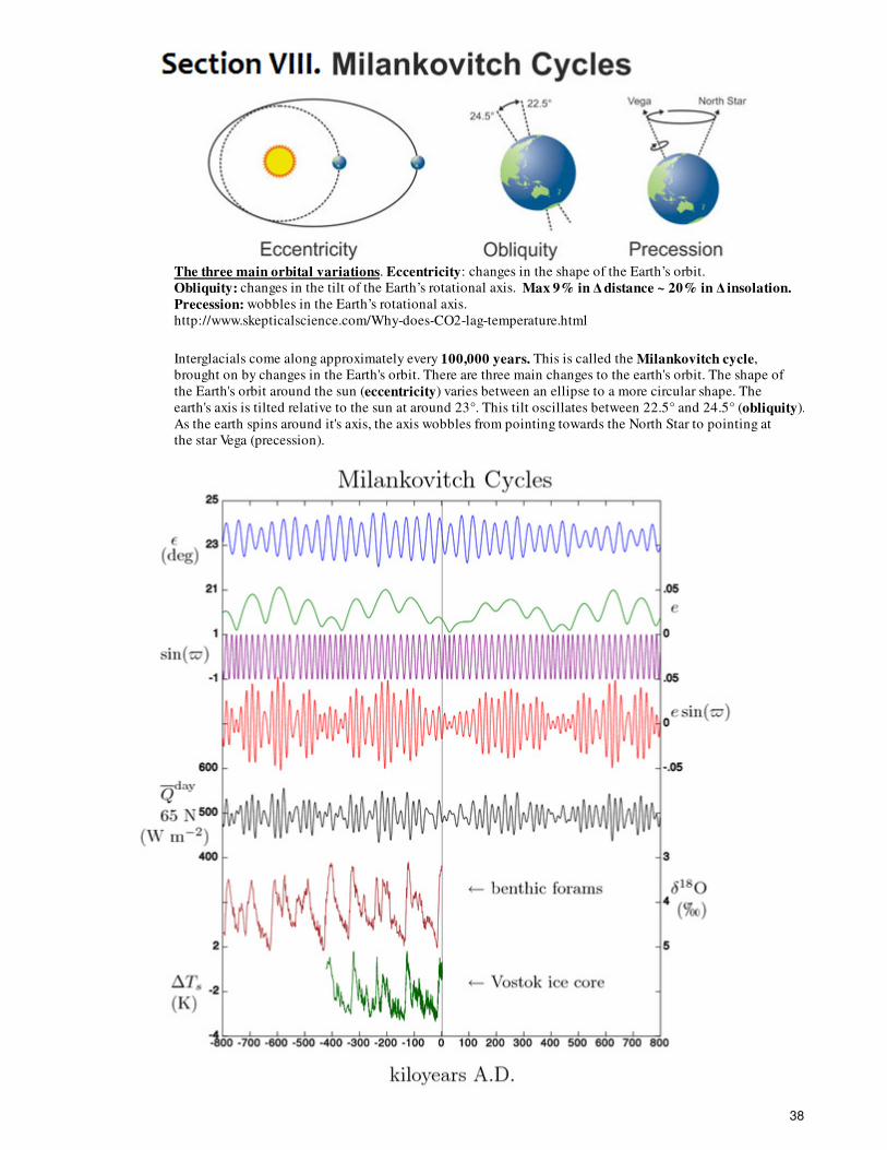
The three main orbital variations. Eccentricity: changes in the shape of the Earth’s orbit.
Obliquity: changes in the tilt of the Earth’s rotational axis. Max 9% in ∆ distance ~ 20% in ∆ insolation.
Precession: wobbles in the Earth’s rotational axis.
http://www.skepticalscience.com/Why-does-CO2-lag-temperature.html
Interglacials come along approximately every 100,000 years. This is called the Milankovitch cycle,
brought on by changes in the Earth's orbit. There are three main changes to the earth's orbit. The shape of
the Earth's orbit around the sun (eccentricity) varies between an ellipse to a more circular shape. The
earth's axis is tilted relative to the sun at around 23°. This tilt oscillates between 22.5° and 24.5° (obliquity).
As the earth spins around it's axis, the axis wobbles from pointing towards the North Star to pointing at
the star Vega (precession).
38
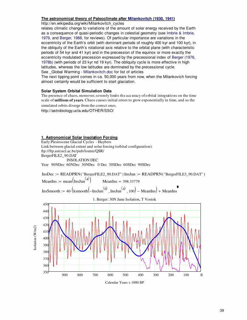
The astronomical theory of Paleoclimate after Milankovitch (1930 , 1941 )
http://en.wikipedia.org/wiki/Milankovitch_cycles
relates climatic change to variations of the amount of solar energy received by the Earth
as a consequence of quasi-periodic changes in celestial geometry (see Imbrie & Imbrie,
1979, and Berger, 1988, for reviews). Of particular importance are variations in the
eccentricity of the Earth’s orbit (with dominant periods of roughly 400 kyr and 100 kyr), in
the obliquity of the Earth’s rotational axis relative to the orbital plane (with characteristic
periods of 54 kyr and 41 kyr) and in the precession of the equinox or more exactly the
eccentricity modulated precession expressed by the precessional index of Berger (1976,
1978b) (with periods of 23 kyr nd 19 kyr). The obliquity cycle is more effective in high
latitudes, whereas the low latitudes are dominated by the precessional cycle.
See _Global Warming - Milankovitch.doc for list of articles
The next tipping point comes in ca. 50,000 years from now, when the Milankovich forcing
almost certainly would be sufficient to start glaciation.
Solar System Orbital Simulation DataThe presence of chaos, moreover, severely limits the accuracy of o rbital integrations on the time
scale of millions of years. Chaos causes initial errors to grow exponentially in time, and so the
simulated orbits diverge from the correct ones.http://astrobiology.ucla.edu/OTHER/SSO/
1. Astronomical Solar Insolation ForcingEarly Plesitocene Glacial Cycles - Huybers
Link between glacial extent and solar forcing (orbital configuration).
ftp://ftp.astr.ucl.ac.be/pub/loutre/QSR/
BergerFILE2_90.DAT
INSOLATION DEC
Year 90NDec 60NDec 30NDec 0 Dec 30SDec 60SDec 90SDec
InsDec READPRN "BergerFILE2_90.DAT"( ):= InsJun READPRN "BergerFILE3_90.DAT"( ):=
MeanIns mean InsJun4⟨ ⟩( ):= MeanIns 398.33779=
InsSmooth 40 ksmooth InsJun0⟨ ⟩
− InsJun4⟨ ⟩
, 100, ( ) MeanIns−( )⋅ MeanIns+:=
0900 800 700 600 500 400 300 200 100 0350
360
370
380
390
400
410
420
430
440
450
1. Berger: 30N June Isolation, T Vostok
Calendar Years x 1000 BP
Isola
tion (
W/m
2)
39
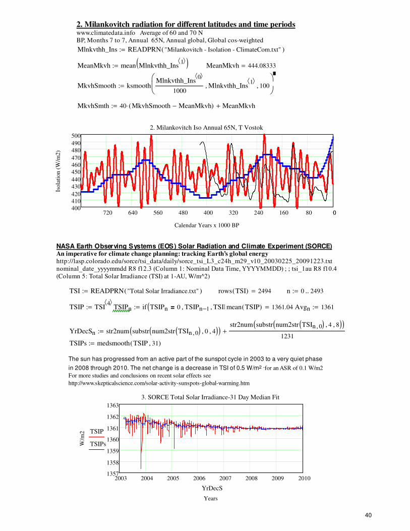
2. Milankovitch radiation for different latitudes and time periodswww.climatedata.info Average of 60 and 70 N
BP, Months 7 to 7, Annual 65N, Annual global, Global cos-weighted
Mlnkvthh_Ins READPRN "Milankovitch - Isolation - ClimateCom.txt"( ):=
MeanMkvh mean Mlnkvthh_Ins1⟨ ⟩( ):= MeanMkvh 444.08333=
MkvhSmooth ksmoothMlnkvthh_Ins
0⟨ ⟩
1000Mlnkvthh_Ins
1⟨ ⟩, 100,
:=
MkvhSmth 40 MkvhSmooth MeanMkvh−( )⋅ MeanMkvh+:=
0720 640 560 480 400 320 240 160 80 0400
410
420
430
440
450
460
470
480
490
500
2. Milankovitch Iso Annual 65N, T Vostok
Calendar Years x 1000 BP
Isola
tion (
W/m
2)
NASA Earth Observing Systems (EOS) Solar Radiation and Climate Experiment (SORCE)An imperative for climate change planning: tracking Earth’s global energyhttp://lasp.colorado.edu/sorce/tsi_data/daily/sorce_tsi_L3_c24h_m29_v10_20030225_20091223.txt
nominal_date_yyyymmdd R8 f12.3 (Column 1: Nominal Data Time, YYYYMMDD) ; ; tsi_1au R8 f10.4
(Column 5: Total Solar Irradiance (TSI) at 1-AU, W/m^2)
TSI READPRN "Total Solar Irradiance.txt"( ):= rows TSI( ) 2494= n 0 2493..:=
TSIP TSI4⟨ ⟩
:= TSIPn if TSIPn 0= TSIPn 1−, TSIPn, ( ):= mean TSIP( ) 1361.04101= Avgn 1361:=
YrDecSn str2num substr num2str TSIn 0, ( ) 0, 4, ( )( )str2num substr num2str TSIn 0, ( ) 4, 8, ( )( )
1231+:=
TSIPs medsmooth TSIP 31, ( ):=
The sun has progressed from an active part of the sunspot cycle in 2003 to a very quiet phase
in 2008 through 2010. The net change is a decrease in TSI of 0.5 W/m2 -for an ASR of 0.1 W/m2
For more studies and conclusions on recent solar effects see
http://www.skepticalscience.com/solar-activity-sunspots-global-warming.htm
2003 2004 2005 2006 2007 2008 2009 20101357
1358
1359
1360
1361
1362
1363
3. SORCE Total Solar Irradiance-31 Day Median Fit
Years
W/m
2 TSIP
TSIPs
YrDecS
40
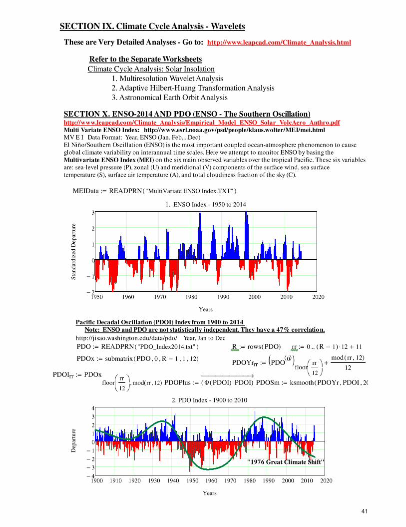
SECTION IX. Climate Cycle Analysis - Wavelets
These are Very Detailed Analyses - Go to: http://www.leapcad.com/Climate_Analysis.html
Refer to the Separate Worksheets
Climate Cycle Analysis: Solar Insolation
1. Multiresolution Wavelet Analysis
2. Adaptive Hilbert-Huang Transformation Analysis
3. Astronomical Earth Orbit Analysis
SECTION X . ENSO-2014 AND PDO ( ENSO - The Southern Oscillation) http://www.leapcad.com/Climate_Analysis/Empirical_Model_ENSO_Solar_VolcAero_Anthro.pdf
Multi Variate ENSO Index: http://www.esrl.noaa.gov/psd/people/klaus.wolter/MEI/mei.htmlMV E I Data Format: Year, ENSO (Jan, Feb,...Dec)
El Niño/Southern Oscillation (ENSO) is the most important coupled ocean-atmosphere phenomenon to cause
global climate variability on interannual time scales. Here we attempt to monitor ENSO by basing the
Multivariate ENSO Index (MEI) on the six main observed variables over the tropical Pacific. These six variables
are: sea-level pressure (P), zonal (U) and meridional (V) components of the surface wind, sea surface
temperature (S), surface air temperature (A), and total cloudiness fraction of the sky (C).
MEIData READPRN "MultiVariate ENSO Index.TXT"( ):=
1950 1960 1970 1980 1990 2000 2010 20202−
1−
0
1
2
3
1. ENSO Index - 1950 to 2014
Years
Sta
ndar
diz
ed D
epar
ture
Pacific Decadal Oscillation (PDOI) Index from 1900 to 2014
Note: ENSO and PDO are not statistically independent. They have a 47% correlation.
http://jisao.washington.edu/data/pdo/ Year, Jan to Dec
PDO READPRN "PDO_Index2014.txt"( ):= R rows PDO( ):= rr 0 R 1−( ) 12⋅ 11+..:=
PDOx submatrix PDO 0, R 1−, 1, 12, ( ):=PDOYrrr PDO
0⟨ ⟩( )floor
rr
12
mod rr 12, ( )
12+:=
PDOIrr PDOx
floorrr
12
mod rr 12, ( ),
:=
PDOPlus Φ PDOI( ) PDOI⋅( )→
:= PDOSm ksmooth PDOYr PDOI, 20, (:=
1900 1910 1920 1930 1940 1950 1960 1970 1980 1990 2000 2010 20204−
3−
2−
1−
0
1
2
3
4
2. PDO Index - 1900 to 2010
Years
Dep
artu
re
"1976 Great Climate Shift"
41
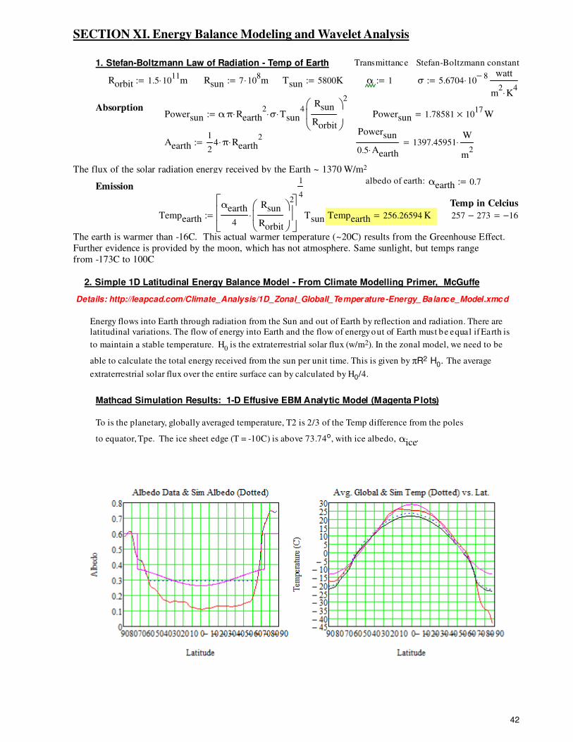
SECTION XI. Energy Balance Modeling and Wavelet Analysis
1. Stefan-Boltzmann Law of Radiation - Temp of Earth Transmittance Stefan-Boltzmann constant
Rorbit 1.5 1011
m⋅:= Rsun 7 108m⋅:= Tsun 5800K:= α 1:= σ 5.6704 10
8−⋅
watt
m2
K4
⋅
:=
Absorption Powersun απ Rearth
2⋅ σ⋅ Tsun
4⋅
Rsun
Rorbit
2
:= Powersun 1.78581 1017
× W=
Aearth1
24 π⋅ Rearth
2⋅:=
Powersun
0.5 Aearth⋅1397.45951
W
m2
⋅=
The flux of the solar radiation energy received by the Earth ~ 1370 W/m2
albedo of earth: αearth 0.7:=Emission
Temp in Celcius
Tempearth
αearth
4
Rsun
Rorbit
2
⋅
1
4
Tsun:= Tempearth 256.26594 K= 257 273− 16−=
The earth is warmer than -16C. This actual warmer temperature (~20C) results from the Greenhouse Effect.
Further evidence is provided by the moon, which has not atmosphere. Same sunlight, but temps range
from -173C to 100C
2. Simple 1D Latitudinal Energy Balance Model - From Climate Modelling Primer, McGuffe
Details: http://leapcad.com/Climate_Analysis/1D_Zonal_Globall_Temperature-Energy_Balance_Model.xmcd
Energy flows into Earth through radiation from the Sun and out of Earth by reflection and radiation. There are
latitudinal variations. The flow of energy into Earth and the flow of energy out of Earth must be equal if Earth is
to maintain a stable temperature. H0 is the extraterrestrial solar flux (w/m2). In the zonal model, we need to be
able to calculate the total energy received from the sun per unit time. This is given by πR2 H0. The average
extraterrestrial solar flux over the entire surface can by calculated by H0/4.
Mathcad Simulation Results: 1-D Effusive EBM Analytic Model (Magenta Plots)
To is the planetary, globally averaged temperature, T2 is 2/3 of the Temp difference from the poles
to equator, Tpe. The ice sheet edge (T = -10C) is above 73.74o, with ice albedo, αice.
42
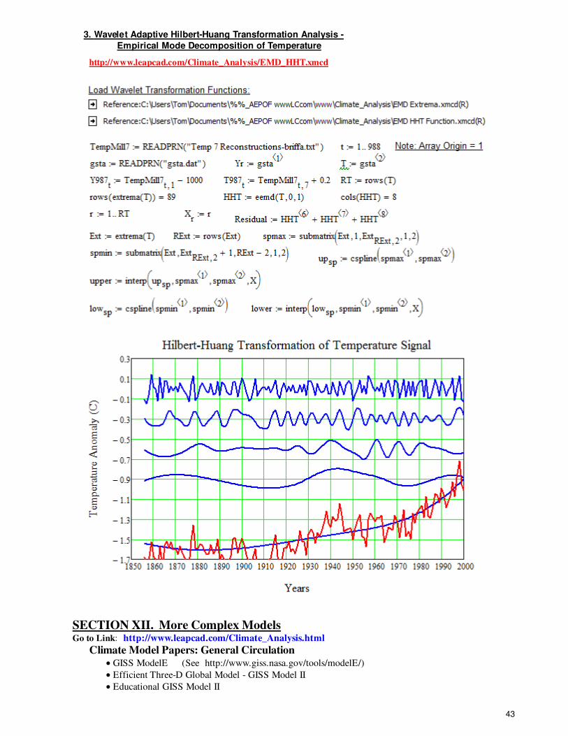
3. Wavelet Adaptive Hilbert-Huang Transformation Analysis -
Empirical Mode Decomposition of Temperature
http://www.leapcad.com/Climate_Analysis/EMD_HHT.xmcd
SECTION XII. More Complex ModelsGo to Link: http://www.leapcad.com/Climate_Analysis.html
Climate Model Papers: General Circulation
• GISS ModelE (See http://www.giss.nasa.gov/tools/modelE/)
• Efficient Three-D Global Model - GISS Model II
• Educational GISS Model II
43
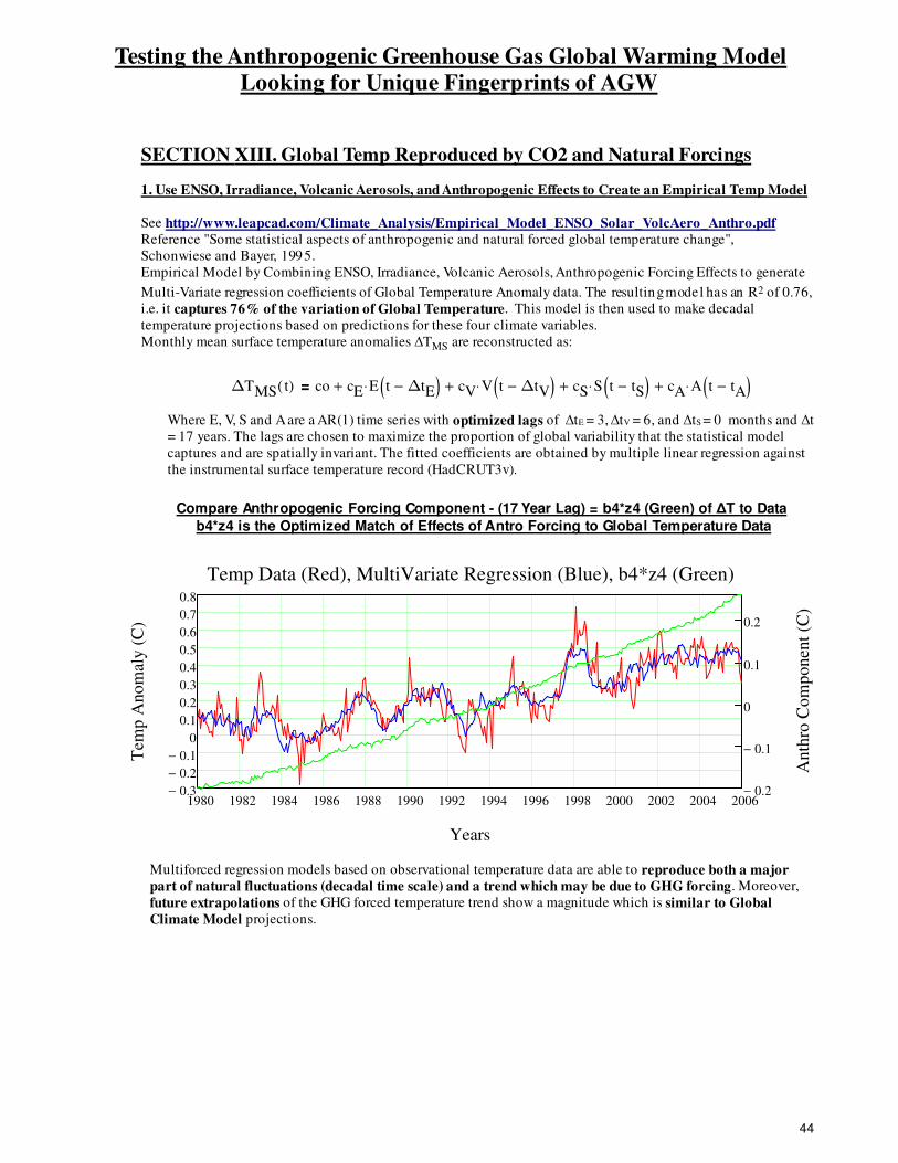
Testing the Anthropogenic Greenhouse Gas Global Warming Model
Looking for Unique Fingerprints of AGW
SECTION XIII. Global Temp Reproduced by CO2 and Natural Forcings
1. Use ENSO, Irradiance, Volcanic Aerosols, and Anthropogenic Effects to Create an Empirical Temp Model
See http://www.leapcad.com/Climate_Analysis/Empirical_Model_ENSO_Solar_VolcAero_Anthro.pdfReference "Some statistical aspects of anthropogenic and natural forced global temperature change",
Schonwiese and Bayer, 1995.
Empirical Model by Combining ENSO, Irradiance, Volcanic Aerosols, Anthropogenic Forcing Effects to generate
Multi-Variate regression coefficients of Global Temperature Anomaly data. The resulting model has an R2 of 0.76,
i.e. it captures 76% of the variation of Global Temperature. This model is then used to make decadal
temperature projections based on predictions for these four climate variables.
Monthly mean surface temperature anomalies ∆TMS are reconstructed as:
∆TMS t( ) co cE E t ∆tE−( )⋅+ cV V t ∆tV−( )⋅+ cS S t tS−( )⋅+ cA A t tA−( )⋅+=
Where E, V, S and A are a AR(1) time series with optimized lags of ∆tE = 3, ∆tV = 6, and ∆tS = 0 months and ∆t
= 17 years. The lags are chosen to maximize the proportion of global variability that the statistical model
captures and are spatially invariant. The fitted coefficients are obtained by multiple linear regression against
the instrumental surface temperature record (HadCRUT3v).
Compare Anthropogenic Forcing Component - (17 Year Lag) = b4*z4 (Green) of ∆T to Data
b4*z4 is the Optimized Match of Effects of Antro Forcing to Global Temperature Data
1980 1982 1984 1986 1988 1990 1992 1994 1996 1998 2000 2002 2004 20060.3−
0.2−
0.1−
0
0.1
0.2
0.3
0.4
0.5
0.6
0.7
0.8
0.2−
0.1−
0
0.1
0.2
Temp Data (Red), MultiVariate Regression (Blue), b4*z4 (Green)
Years
Tem
p A
no
mal
y (
C)
An
thro
Co
mp
on
ent
(C)
Multiforced regression models based on observational temperature data are able to reproduce both a major
part of natural fluctuations (decadal time scale) and a trend which may be due to GHG forcing. Moreover,
future extrapolations of the GHG forced temperature trend show a magnitude which is similar to Global
Climate Model projections.
44
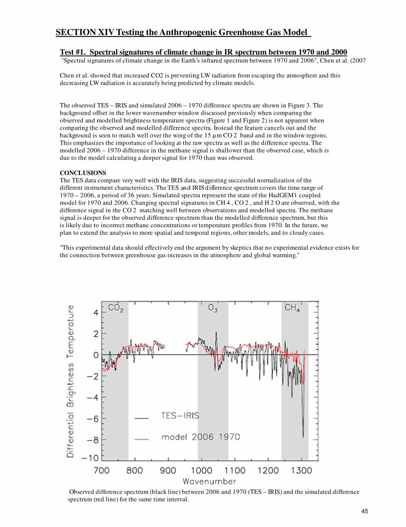
SECTION XIV Test ing the Anthropogenic Greenhouse Gas Model
Test #1. Spectral signatures of climate change in IR spectrum between 1970 and 2000 "Spectral signatures of climate change in the Earth’s infrared spectrum between 1970 and 2006", Chen et al. (2007
Chen et al. showed that increased CO2 is preventing LW radiation from escaping the atmosphere and this
decreasing LW radiation is accurately being predicted by climate models.
The observed TES – IRIS and simulated 2006 – 1970 difference spectra are shown in Figure 3. The
background offset in the lower wavenumber window discussed previously when comparing the
observed and modelled brightness temperature spectra (Figure 1 and Figure 2) is not apparent when
comparing the observed and modelled difference spectra. Instead the feature cancels out and the
background is seen to match well over the wing of the 15 µm CO 2 band and in the window regions.
This emphasizes the importance of looking at the raw spectra as well as the difference spectra. The
modelled 2006 – 1970 difference in the methane signal is shallower than the observed case, which is
due to the model calculating a deeper signal for 1970 than was observed.
CONCLUSIONS The TES data compare very well with the IRIS data, suggesting successful normalization of the
different instrument characteristics. The TES and IRIS d ifference spectrum covers the time range of
1970 – 2006, a period of 36 years. Simulated spectra represent the state of the HadGEM1 coupled
model for 1970 and 2006. Changing spectral signatures in CH 4 , CO 2 , and H 2 O are observed, with the
difference signal in the CO 2 matching well between observations and modelled spectra. The methane
signal is deeper for the observed difference spectrum than the modelled difference spectrum, but this
is likely due to incorrect methane concentrations or temperature profiles from 1970. In the future, we
plan to extend the analysis to more spatial and temporal regions, other models, and to cloudy cases.
"This experimental data should effectively end the argument by skeptics that no experimental evidence exists for
the connection between greenhouse gas increases in the atmosphere and global warming."
Observed difference spectrum (black line) between 2006 and 1970 (TES – IRIS) and the simulated difference
spectrum (red line) for the same time interval.
45
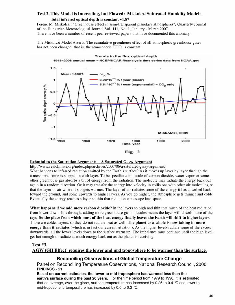
Test 2. This Model is Interesting, but Flawed: Miskolczi Saturated Humidity Model:
Total infrared optical depth is constant ~1.87
Ferenc M. Miskolczi, "Greenhouse effect in semi-transparent planetary atmospheres", Quarterly Journal
of the Hungarian Meteorological Journal,Vol. 111, No. 1, January - March 2007
There have been a number of recent peer reviewed papers that have documented this anomaly.
The Miskolczi Model Asserts: The cumulative greenhouse effect of all atmospheric greenhouse gases
has not been changed, that is, the atmospheric TIOD is constant.
Rebuttal to the Saturation Argument: A Saturated Gassy Argumenthttp://www.realclimate.org/index.php/archives/2007/06/a-saturated-gassy-argument/
What happens to infrared radiation emitted by the Earth’s surface? As it moves up layer by layer through the
atmosphere, some is stopped in each layer. To be specific: a molecule of carbon dioxide, water vapor or some
other greenhouse gas absorbs a bit of energy from the radiation. The molecule may radiate the energy back out
again in a random direction. Or it may transfer the energy into velocity in collisions with other air molecules, so
that the layer of air where it sits gets warmer. The layer of air radiates some of the energy it has absorbed back
toward the ground, and some upwards to higher layers. As you go higher, the atmosphere gets thinner and colder.
Eventually the energy reaches a layer so thin that radiation can escape into space.
What happens if we add more carbon dioxide? In the layers so high and thin that much of the heat radiation
from lower down slips through, adding more greenhouse gas molecules means the layer will absorb more of the
rays. So the place from which most of the heat energy finally leaves the Earth will shift to higher layers.
Those are colder layers, so they do not radiate heat as well. The planet as a whole is now taking in more
energy than it radiates (which is in fact our current situation). As the higher levels radiate some of the excess
downwards, all the lower levels down to the surface warm up. The imbalance must continue until the high levels
get hot enough to radiate as much energy back out as the planet is receiving.
Test #3.
AGW (GH Effect) requires the lower and mid troposphere to be warmer than the surface.
Reconciling Observations of Global Temperature Change
Panel on Reconciling Temperature Observations, National Research Council, 2000 FINDINGS - 21
Based on current estimates, the lower to mid-troposphere has warmed less than the
earth's surface during the past 20 years. For the time period from 1979 to 1998, it is estimated
that on average, over the globe, surface temperature has increased by 0.25 to 0.4 °C and lower to
mid-tropospheric temperature has increased by 0.0 to 0.2 °C.
46
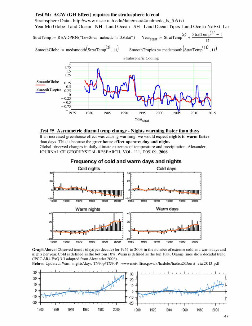
Test #4: AGW (GH Effect) requires the stratosphere to cool
Stratosphere Data: http://www.nsstc.uah.edu/data/msu/t4/uahncdc_ls_5.6.txt
Year Mo Globe Land Ocean NH Land Ocean SH Land Ocean Trpcs Land Ocean NoExt Land
StratTemp READPRN "LowStrat - uahncdc_ls_5.6.dat"( ):= Yearstrat StratTemp0⟨ ⟩ StratTemp
1⟨ ⟩1−
12+:=
SmoothGlobe medsmooth StratTemp2⟨ ⟩
11, ( ):= SmoothTropics medsmooth StratTemp11⟨ ⟩
11, ( ):=
1975 1980 1985 1990 1995 2000 2005 2010 20151−
0.75−0.5−
0.25−0
0.250.5
0.751
1.251.5
1.752
Stratospheric Cooling
SmoothGlobe
SmoothTropics
Yearstrat
Test #5 Asymmetric diurnal temp change - Nights warming faster than daysIf an increased greenhouse effect was causing warming, we would expect nights to warm faster
than days. This is because the greenhouse effect operates day and night.
Global observed changes in daily climate extremes of temperature and precipitation, Alexander,
JOURNAL OF GEOPHYSICAL RESEARCH, VOL. 111, D05109, 2006
Graph Above: Observed trends (days per decade) for 1951 to 2003 in the number of extreme cold and warm days and
nights per year. Cold is defined as the bottom 10%. Warm is defined as the top 10%. Orange lines show decadal trend
(IPCC AR4 FAQ 3.3 adapted from Alexander 2006).
Below: Updated: Warm nights/days, TN90p/TX90P www.metoffice.gov.uk/hadobs/hadex2/Donat_etal2013.pdf
47
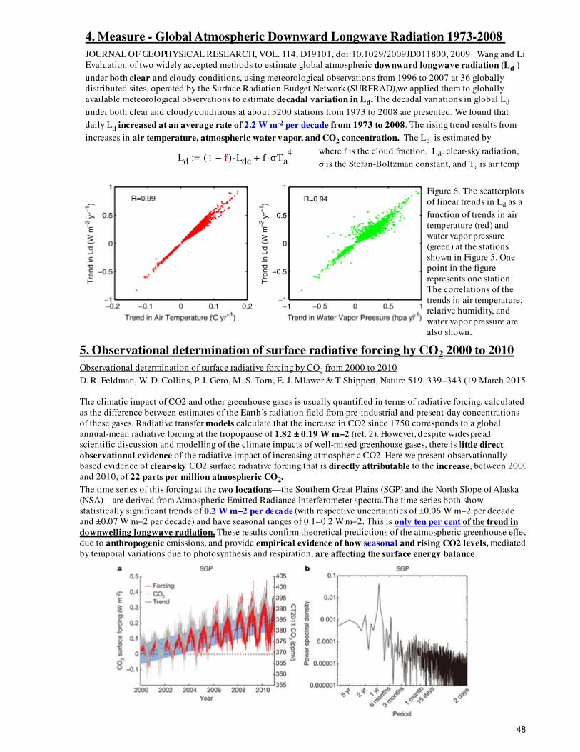
4. Measure - Global Atmospheric Downward Longwave Radiation 1973-2008
JOURNAL OF GEOPHYSICAL RESEARCH, VOL. 114, D19101, doi:10.1029/2009JD011800, 2009 Wang and Liang
Evaluation of two widely accepted methods to estimate global atmospheric downward longwave radiation (Ld )
under both clear and cloudy conditions, using meteorological observations from 1996 to 2007 at 36 globally
distributed sites, operated by the Surface Radiation Budget Network (SURFRAD),we applied them to globally
available meteorological observations to estimate decadal variation in Ld. The decadal variations in global Ld
under both clear and cloudy conditions at about 3200 stations from 1973 to 2008 are presented. We found that
daily Ld increased at an average rate of 2.2 W m-2 per decade from 1973 to 2008. The rising trend results from
increases in air temperature, atmospheric water vapor, and CO2 concentration. The Ld is estimated by
where f is the cloud fraction, Ldc clear-sky radiation,
σ is the Stefan-Boltzman constant, and Ta is air temp Ld 1 f−( ) Ldc⋅ f σTa
4⋅+:= f
Figure 6. The scatterplots
of linear trends in Ld as a
function of trends in air
temperature (red) and
water vapor pressure
(green) at the stations
shown in Figure 5. One
point in the figure
represents one station.
The correlations of the
trends in air temperature,
relative humidity, and
water vapor pressure are
also shown.
5. Observational determination of surface radiative forcing by CO 2 2000 to 2010
Observational determination of surface radiative forcing by CO 2 from 2000 to 2010
D. R. Feldman, W. D. Collins, P. J. Gero, M. S. Torn, E. J. Mlawer & T Shippert, Nature 519, 339–343 (19 March 2015)
The climatic impact of CO2 and other greenhouse gases is usually quantified in terms of radiative forcing, calculated
as the difference between estimates of the Earth’s radiation field from pre-industrial and present-day concentrations
of these gases. Radiative transfer models calculate that the increase in CO2 since 1750 corresponds to a global
annual-mean radiative forcing at the tropopause of 1.82 ± 0.19 W m−2 (ref. 2). However, despite widespread
scientific discussion and modelling of the climate impacts of well-mixed greenhouse gases, there is little direct
observational evidence of the radiative impact of increasing atmospheric CO2. Here we present observationally
based evidence of clear-sky CO2 surface radiative forcing that is directly attributable to the increase, between 2000
and 2010, of 22 parts per million atmospheric CO2.
The time series of this forcing at the two locations—the Southern Great Plains (SGP) and the North Slope of Alaska
(NSA)—are derived from Atmospheric Emitted Radiance Interferometer spectra.The time series both show
statistically significant trends of 0.2 W m−2 per decade (with respective uncertainties of ±0.06 W m−2 per decade
and ±0.07 W m−2 per decade) and have seasonal ranges of 0.1–0.2 W m−2. This is only ten per cent of the trend in
downwelling longwave radiation. These results confirm theoretical predictions of the atmospheric greenhouse effect
due to anthropogenic emissions, and provide empirical evidence of how seasonal and rising CO2 levels, mediated
by temporal variations due to photosynthesis and respiration, are affecting the surface energy balance.
48
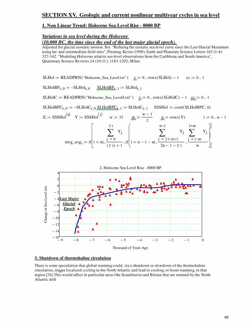
SECTION XV. Geologic and current nonlinear multiyear cycles in sea level
1. Non Linear Trend: Holocene Sea Level Rise - 8000 BP
Variations in sea level during the Holocene
(10,000 BC, the time since the end of the last major glacial epoch). Adjusted for glacial isostatic motion. See "Refining the eustatic sea-level curve since the Last Glacial Maximum
using far- and intermediate-field sites", Fleming, Kevin (1998). Earth and Planetary Science Letters 163 (1-4):
327-342. "Modeling Holocene relative sea-level observations from the Caribbean and South America",
Quaternary Science Reviews 24 (10-11): 1183-1202, Milne
SLHol READPRN "Holocene_Sea_Level.txt"( ):= r 0 rows SLHol( ) 1−..:= cc 0 1..:=
SLHolBPr 0, SLHolr 0, −:= SLHolBPr 1, SLHolr 1, :=
SLHolC READPRN "Holocene_Sea_Level4.txt"( ):= r 0 rows SLHolC( ) 1−..:= cc 0 1..:=
SLHolBPCr 0, SLHolCr 0, −:= SLHolBPCr 1, SLHolCr 1, := SSSHol csort SLHolBPC 0, ( ):=
X SSSHol0⟨ ⟩
:= Y SSSHol1⟨ ⟩
:= w 33:= mw 1−
2:= n rows Y( ):= i 0 n 1−..:=
mvg_avgi if i m<0
2 i⋅
j
Yj∑=
2 i⋅( ) 1+, if i n 1− m−>
2 i⋅ n− 1+
n 1−
j
Yj∑=
2n 1− 2 i⋅−,
i m−
i m+
j
Yj∑=
w,
,
:=
9− 8− 7− 6− 5− 4− 3− 2− 1− 016−
14−
12−
10−
8−
6−
4−
2−
0
2
4
2. Holocene Sea Level Rise - 8000 BP
Thousand of Years Ago
Chan
ge
in S
ea L
evel
(m
)
Last Major
Glacial
Epoch
3. Shutdown of thermohaline circulation
There is some speculation that global warming could, via a shutdown or slowdown of the thermohaline
circulation, trigger localized cooling in the North Atlantic and lead to cooling, or lesser warming, in that
region.[76] This would affect in particular areas like Scandinavia and Britain that are warmed by the North
Atlantic drift
49
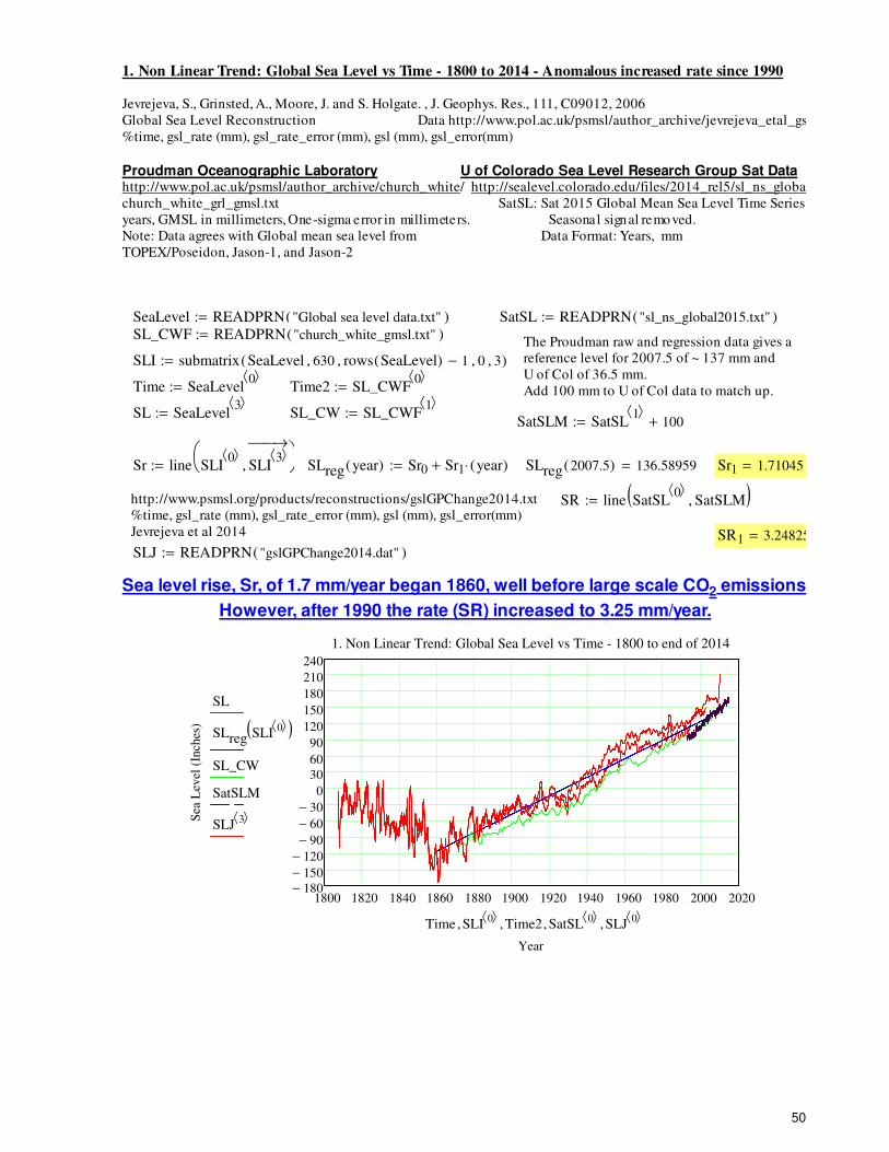
1. Non Linear Trend: Global Sea Level vs Time - 1800 to 2014 - Anomalous increased rate since 1990
Jevrejeva, S., Grinsted, A., Moore, J. and S. Holgate. , J. Geophys. Res., 111, C09012, 2006
Global Sea Level Reconstruction Data http://www.pol.ac.uk/psmsl/author_archive/jevrejeva_etal_gsl/
%time, gsl_rate (mm), gsl_rate_error (mm), gsl (mm), gsl_error(mm)
Proudman Oceanographic Laboratory U of Colorado Sea Level Research Group Sat Data http://www.pol.ac.uk/psmsl/author_archive/church_white/ http://sealevel.colorado.edu/files/2014_rel5/sl_ns_global.txt
church_white_grl_gmsl.txt SatSL: Sat 2015 Global Mean Sea Level Time Series
years, GMSL in millimeters, One-sigma error in millimeters. Seasonal signal removed.
Note: Data agrees with Global mean sea level from Data Format: Years, mm
TOPEX/Poseidon, Jason-1, and Jason-2
SeaLevel READPRN "Global sea level data.txt"( ):= SatSL READPRN "sl_ns_global2015.txt"( ):=
SL_CWF READPRN "church_white_gmsl.txt"( ):=The Proudman raw and regression data gives a
reference level for 2007.5 of ~ 137 mm and
U of Col of 36.5 mm.
Add 100 mm to U of Col data to match up.
SLI submatrix SeaLevel 630, rows SeaLevel( ) 1−, 0, 3, ( ):=
Time SeaLevel0⟨ ⟩
:= Time2 SL_CWF0⟨ ⟩
:=
SL SeaLevel3⟨ ⟩
:= SL_CW SL_CWF1⟨ ⟩
:=SatSLM SatSL
1⟨ ⟩100+:=
Sr line SLI0⟨ ⟩
SLI3⟨ ⟩→
,
:= SLreg year( ) Sr0 Sr1 year( )⋅+:= SLreg 2007.5( ) 136.58959= Sr1 1.71045=
http://www.psmsl.org/products/reconstructions/gslGPChange2014.txt
%time, gsl_rate (mm), gsl_rate_error (mm), gsl (mm), gsl_error(mm)
Jevrejeva et al 2014
SR line SatSL0⟨ ⟩
SatSLM, ( ):=
SR1 3.24825=
SLJ READPRN "gslGPChange2014.dat"( ):=
Sea level rise, Sr, of 1.7 mm/year began 1860, well before large scale CO 2 emissions
However, after 1990 the rate (SR) increased to 3.25 mm/year.
1800 1820 1840 1860 1880 1900 1920 1940 1960 1980 2000 2020180−150−
120−
90−
60−
30−
0
30
60
90
120
150
180
210
240
1. Non Linear Trend: Global Sea Level vs Time - 1800 to end of 2014
Year
Sea
Lev
el (
Inch
es)
SL
SLreg SLI0⟨ ⟩( )
SL_CW
SatSLM
SLJ3⟨ ⟩
Time SLI0⟨ ⟩
, Time2, SatSL0⟨ ⟩
, SLJ0⟨ ⟩
,
50
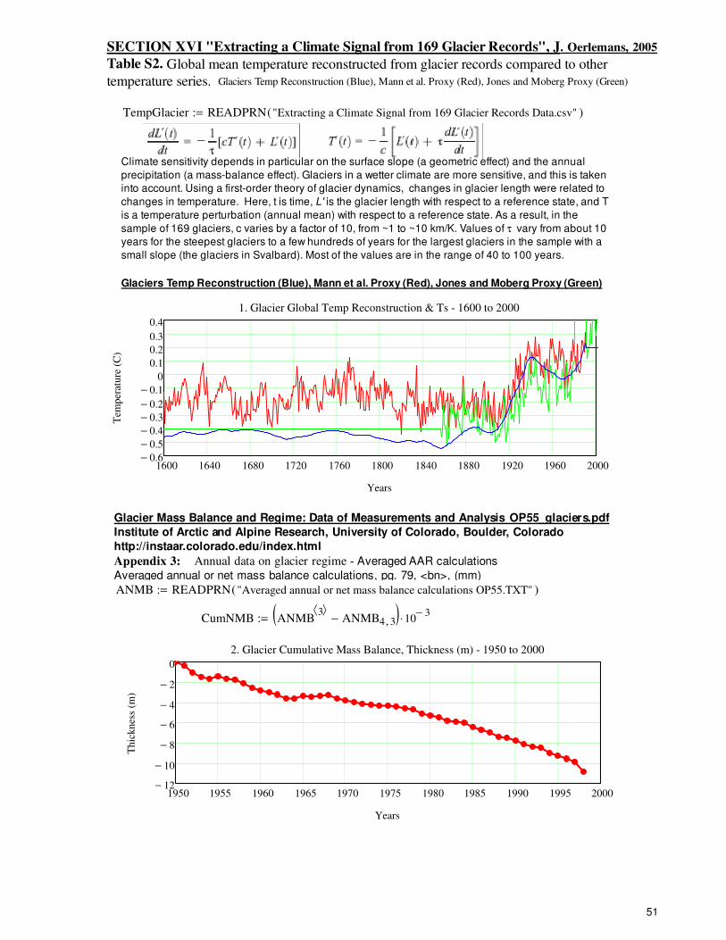
SECTION XVI "Extracting a Climate Signal from 169 Glacier Records", J . Oerlemans, 2005
Table S2. Global mean temperature reconstructed from glacier records compared to other
temperature series. Glaciers Temp Reconstruction (Blue), Mann et al. Proxy (Red), Jones and Moberg Proxy (Green)
TempGlacier READPRN "Extracting a Climate Signal from 169 Glacier Records Data.csv"( ):=
Climate sensitivity depends in particular on the surface slope (a geometric effect) and the annual
precipitation (a mass-balance effect). Glaciers in a wetter climate are more sensitive, and this is taken
into account. Using a first-order theory of glacier dynamics, changes in glacier length were related to
changes in temperature. Here, t is time, L' is the glacier length with respect to a reference state, and T
is a temperature perturbation (annual mean) with respect to a reference state. As a result, in the
sample of 169 glaciers, c varies by a factor of 10, from ~1 to ~10 km/K. Values of τ vary from about 10
years for the steepest glaciers to a few hundreds of years for the largest glaciers in the sample with a
small slope (the glaciers in Svalbard). Most of the values are in the range of 40 to 100 years.
Glaciers Temp Reconstruction (Blue), Mann et al. Proxy (Red), Jones and Moberg Proxy (Green)
1600 1640 1680 1720 1760 1800 1840 1880 1920 1960 20000.6−
0.5−
0.4−
0.3−
0.2−
0.1−
0
0.1
0.2
0.3
0.4
1. Glacier Global Temp Reconstruction & Ts - 1600 to 2000
Years
Tem
per
ature
(C
)
Glacier Mass Balance and Regime: Data of Measurements and Analysis OP55_glaciers.pdf
Institute of Arctic and Alpine Research, University of Colorado, Boulder, Colorado
http://instaar.colorado.edu/index.html
Appendix 3: Annual data on glacier regime - Averaged AAR calculations
Averaged annual or net mass balance calculations, pg. 79, <bn>, (mm)
ANMB READPRN "Averaged annual or net mass balance calculations OP55.TXT"( ):=
CumNMB ANMB3⟨ ⟩
ANMB4 3, −( ) 103−
⋅:=
1950 1955 1960 1965 1970 1975 1980 1985 1990 1995 200012−
10−
8−
6−
4−
2−
0
2. Glacier Cumulative Mass Balance, Thickness (m) - 1950 to 2000
Years
Thic
knes
s (m
)
51
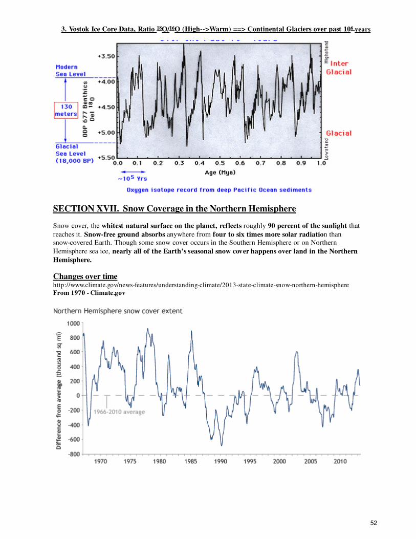
3. Vostok Ice Core Data, Ratio 18 O/ 16 O (High-->Warm) ==> Continental Glaciers over past 10 6 years
SECTION XVII. Snow Coverage in the Northern Hemisphere
Snow cover, the whitest natural surface on the planet, reflects roughly 90 percent of the sunlight that
reaches it. Snow-free ground absorbs anywhere from four to six times more solar radiation than
snow-covered Earth. Though some snow cover occurs in the Southern Hemisphere or on Northern
Hemisphere sea ice, nearly all of the Earth’s seasonal snow cover happens over land in the Northern
Hemisphere.
Changes over timehttp://www.climate.gov/news-features/understanding-climate/2013-state-climate-snow-northern-hemisphere
From 1970 - Climate.gov
52
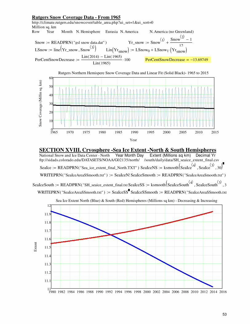
Rutgers Snow Coverage Data - From 1965http://climate.rutgers.edu/snowcover/table_area.php?ui_set=1&ui_sort=0
Million sq. km
Row Year Month N. Hemisphere Eurasia N. America N. America (no Greenland)
Snow READPRN "gsl snow data.dat"( ):= Yr_snow Snow1⟨ ⟩ Snow
2⟨ ⟩1−
12+:=
LSnow line Yr_snow Snow3⟨ ⟩
, ( ):= Lin Yrsnow( ) LSnow0 LSnow1 Yrsnow( )⋅+:=
PerCentSnowDecreaseLin 2014( ) Lin 1965( )−
Lin 1965( )100⋅:= PerCentSnowDecrease 13.69749−=
1965 1970 1975 1980 1985 1990 1995 2000 2005 2010 20150
10
20
30
40
50
60
Rutgers Northern Hemispere Snow Coverage Data and Linear Fit (Solid Black)- 1965 to 2015
Year
Snow
Cover
age
(Mil
lin s
q.
km
)
SECTION XVIII . Cryosphere - Sea Ice Extent -North & South HemispheresNational Snow and Ice Data Center - North Year Month Day Extent (Millions sq km) Decimal Yrftp://sidads.colorado.edu/DATASETS/NOAA/G02135/north/ /south/daily/data/SH_seaice_extent_final.csv
SeaIce READPRN "Sea_ice_extent_final_North.TXT"( ):= SeaIceNS ksmooth SeaIce4⟨ ⟩
SeaIce3⟨ ⟩
, 30, ( ):=
WRITEPRN "SeaIceAreaSSmooth.txt"( ) SeaIceNS:= SeaIceSmooth READPRN "SeaIceAreaSmooth.txt"( ):=
SeaIceSouth READPRN "SH_seaice_extent_final.txt"( ):= SeaIceSS ksmooth SeaIceSouth4⟨ ⟩
SeaIceSouth3⟨ ⟩
, 30, (:=
WRITEPRN "SeaIceAreaSSmooth.txt"( ) SeaIceSS:= SeaIceSSmooth READPRN "SeaIceAreaSSmooth.txt"(:=
1980 1982 1984 1986 1988 1990 1992 1994 1996 1998 2000 2002 2004 2006 2008 2010 2012 2014 201611
11.1
11.2
11.3
11.4
11.5
11.6
11.7
11.8
11.9
12
Sea Ice Extent North (Blue) & South (Red) Hemispheres (Millions sq km) - Decreasing & Increasing
Exte
nt
53
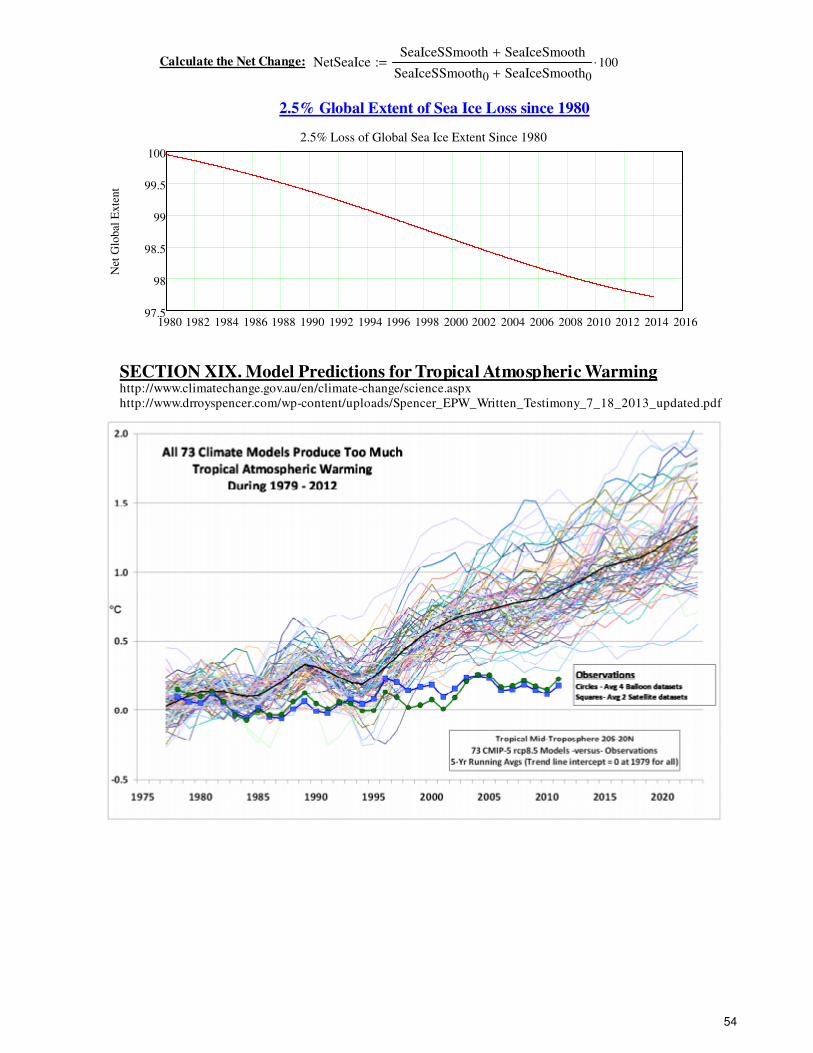
Calculate the Net Change: NetSeaIceSeaIceSSmooth SeaIceSmooth+
SeaIceSSmooth0 SeaIceSmooth0+100⋅:=
2.5% Global Extent of Sea Ice Loss since 1980
1980 1982 1984 1986 1988 1990 1992 1994 1996 1998 2000 2002 2004 2006 2008 2010 2012 2014 201697.5
98
98.5
99
99.5
100
2.5% Loss of Global Sea Ice Extent Since 1980
Net
Glo
bal
Exte
nt
SECTION XIX. Model Predictions for Tropical Atmospheric Warminghttp://www.climatechange.gov.au/en/climate-change/science.aspx
http://www.drroyspencer.com/wp-content/uploads/Spencer_EPW_Written_Testimony_7_18_2013_updated.pdf
54
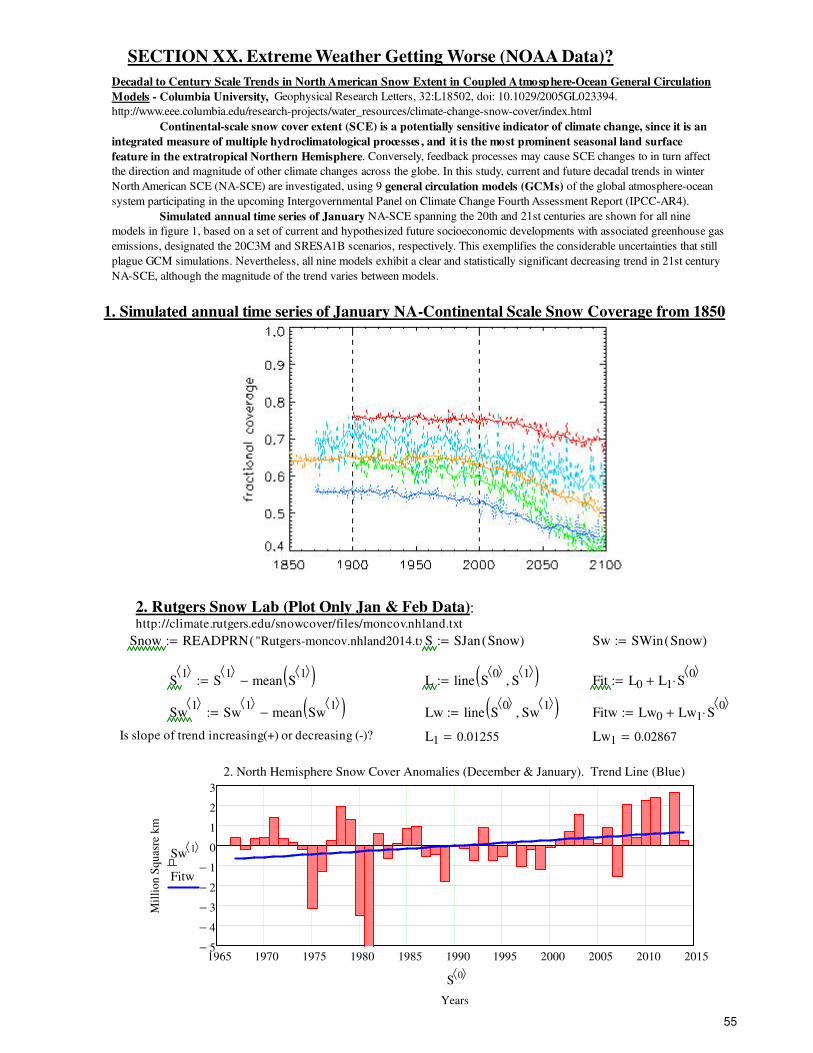
SECTION XX. Extreme Weather Getting Worse (NOAA Data)?
Decadal to Century Scale Trends in North American Snow Extent in Coupled Atmosphere-Ocean General Circulation
Models - Columbia University, Geophysical Research Letters, 32:L18502, doi: 10.1029/2005GL023394.
http://www.eee.columbia.edu/research-projects/water_resources/climate-change-snow-cover/index.html
Continental-scale snow cover extent (SCE) is a potentially sensitive indicator of climate change, since it is an
integrated measure of multiple hydroclimatological processes , and it is the most prominent seasonal land surface
feature in the extratropical Northern Hemisphere. Conversely, feedback processes may cause SCE changes to in turn affect
the direction and magnitude of other climate changes across the globe. In this study, current and future decadal trends in winter
North American SCE (NA-SCE) are investigated, using 9 general circulation models (GCMs) of the global atmosphere-ocean
system participating in the upcoming Intergovernmental Panel on Climate Change Fourth Assessment Report (IPCC-AR4).
Simulated annual time series of January NA-SCE spanning the 20th and 21st centuries are shown for all nine
models in figure 1, based on a set of current and hypothesized future socioeconomic developments with associated greenhouse gas
emissions, designated the 20C3M and SRESA1B scenarios, respectively. This exemplifies the considerable uncertainties that still
plague GCM simulations. Nevertheless, all nine models exhibit a clear and statistically significant decreasing trend in 21st century
NA-SCE, although the magnitude of the trend varies between models.
1. Simulated annual time series of January NA-Continental Scale Snow Coverage from 1850
2. Rutgers Snow Lab (Plot Only Jan & Feb Data):http://climate.rutgers.edu/snowcover/files/moncov.nhland.txt
Snow READPRN "Rutgers-moncov.nhland2014.txt"( ):= S SJan Snow( ):= Sw SWin Snow( ):=
S1⟨ ⟩
S1⟨ ⟩
mean S1⟨ ⟩( )−:= L line S
0⟨ ⟩S
1⟨ ⟩, ( ):= Fit L0 L1 S
0⟨ ⟩⋅+:=
Sw1⟨ ⟩
Sw1⟨ ⟩
mean Sw1⟨ ⟩( )−:= Lw line S
0⟨ ⟩Sw
1⟨ ⟩, ( ):= Fitw Lw0 Lw1 S
0⟨ ⟩⋅+:=
Is slope of trend increasing(+) or decreasing (-)? L1 0.01255= Lw1 0.02867=
1965 1970 1975 1980 1985 1990 1995 2000 2005 2010 20155−
4−
3−
2−
1−
0
1
2
3
2. North Hemisphere Snow Cover Anomalies (December & January). Trend Line (Blue)
Years
Mil
lion S
quas
re k
m
Sw1⟨ ⟩
Fitw
S0⟨ ⟩
55
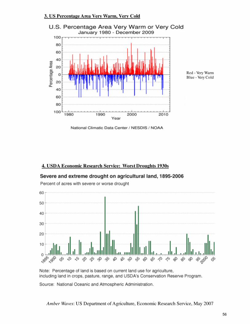
3. US Percentage Area Very Warm, Very Cold
Red - Very Warm
Blue - Very Cold
4. USDA Economic Research Service: Worst Droughts 1930s
Amber Waves: US Department of Agriculture, Economic Research Service, May 2007
56
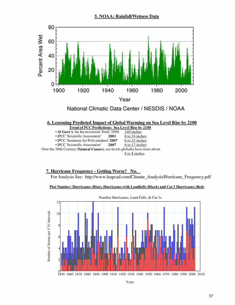
5. NOAA: Rainfall/Wetness Data
6. Lessoning Predicted Impact of Global Warming on Sea Level Rise by 2100 Trend of PCC Predictions: Sea Level Rise by 2100
• Al Gore's 'An Inconvenient Truth' 2006 240 inches
• IPCC 'Scientific Assessment' 2001 6 to 34 inches
• IPCC 'Summary for Policymakers' 2007 6 to 23 inches
• IPCC 'Scientific Assessment' 2007 6 to 17 inches
Over the 20th Century (Natural Causes), sea-levels globally have risen about
6 to 8 inches
7. Hurricane Frequency - Getting Worse? No.
For Analysis See: http://www.leapcad.com/Climate_Analysis/Hurricane_Frequency.pdf
Plot Number: Hurricanes (Blue), Hurricanes with Landfalls (Black) and Cat 3 Hurricanes (Red)
1850 1860 1870 1880 1890 1900 1910 1920 1930 1940 1950 1960 1970 1980 1990 2000 20100
2
4
6
8
10
12
Number Hurricanes, Land Falls, & Cat 3s
Years
Num
ber
of
Sto
rms
per
5 Y
r In
terv
als
57
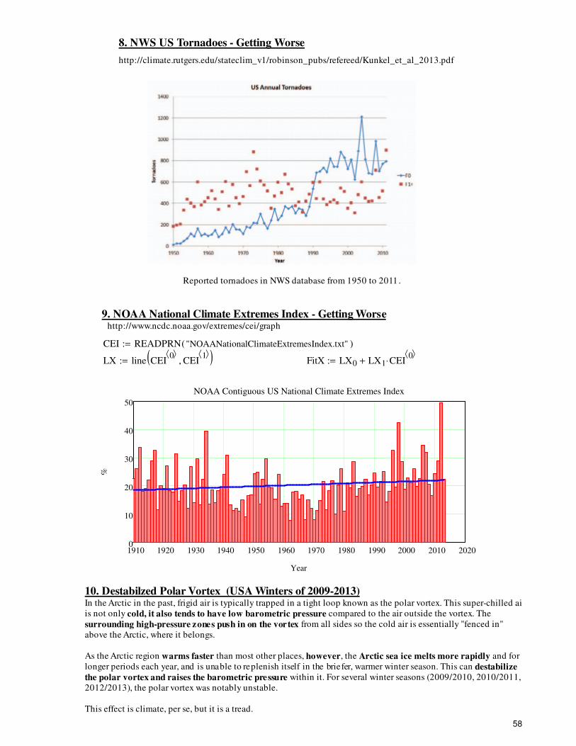
8. NWS US Tornadoes - Getting Worse
http://climate.rutgers.edu/stateclim_v1/robinson_pubs/refereed/Kunkel_et_al_2013.pdf
Reported tornadoes in NWS database from 1950 to 2011 .
9. NOAA National Climate Extremes Index - Getting Worsehttp://www.ncdc.noaa.gov/extremes/cei/graph
CEI READPRN "NOAANationalClimateExtremesIndex.txt"( ):=
LX line CEI0⟨ ⟩
CEI1⟨ ⟩
, ( ):= FitX LX0 LX1 CEI0⟨ ⟩
⋅+:=
1910 1920 1930 1940 1950 1960 1970 1980 1990 2000 2010 20200
10
20
30
40
50
NOAA Contiguous US National Climate Extremes Index
Year
%
10. Destabilzed Polar Vortex (USA Winters of 2009-2013)In the Arctic in the past, frigid air is typically trapped in a tight loop known as the polar vortex. This super-chilled air
is not only cold, it also tends to have low barometric pressure compared to the air outside the vortex. The
surrounding high-pressure zones push in on the vortex from all sides so the cold air is essentially "fenced in"
above the Arctic, where it belongs.
As the Arctic region warms faster than most other places, however, the Arctic sea ice melts more rapidly and for
longer periods each year, and is unable to replenish itself in the briefer, warmer winter season. This can destabilize
the polar vortex and raises the barometric pressure within it. For several winter seasons (2009/2010, 2010/2011, and
2012/2013), the polar vortex was notably unstable.
This effect is climate, per se, but it is a tread.
58
APPENDIX
A I. Types of GISS NASA Data Sources and New versus Old Differences:
GISTEMP Indices
Land-Ocean Temperature index (LOTI, i.e. the index that includes weather station data and sea surface
temperature data to give a global anomaly index with wide spatial coverage) (“GLB.Ts+dSST.txt”).
Met station index, which only uses weather station data (“GLB.Ts.txt”) which doesn't’t have as much coverage and
has a substantially larger trend reflecting the relative predominance of faster-warming continental data in the
average.
Old versus New differences are tiny, and mostly reflect slightly more data in the earlier years in the latest data and
the different homogenization in GHCN v3 compared to GHCN v2 (which was used up to Dec 2011). The the biggest
difference in trend (between 2006 and today), is a mere 0.05ºC/Century, and from 2008 to 2012 it is only
0.003ºC/Century.
59