CLIMATE CHANGE - CORE

Impacts of Climate Change on UK

Coastal and Estuarine Habitats: A

Critical Evaluation of the Sea Level

Affecting Marshes Model (SLAMM)

Aikaterini Pylarinou

Coastal and Estuarine Research Unit

Department of Geography

University College London

A thesis submitted for the degree of

Doctor of Philosophy

September 2014

2

To N. & D. K.

3

Declaration

I, Aikaterini Pylarinou confirm that this thesis entitled

Impacts of Climate Change on UK Coastal and Estuarine

Habitats: A Critical Evaluation of the Sea Level Affecting

Marshes Model (SLAMM) is the result of my own

research. Where information has been derived from other

sources, I confirm that this has been indicated in the thesis.

Signature ________________

Name ________________

Date ________________

4

Acknowledgements

Firstly, I would like to thank my supervisor Professor Jon French for his helpful

supervision and support. He was always willing to discuss any difficulties with great

patience. I would also like to thank my second supervisor Dr Helene Burningham for

her advice and contribution over the last four years. Thanks also to my colleagues in the

Department of Geography at University College London, especially Darryl, Miriam and

Mandy for our discussions and their encouragement. A special thanks to my wonderful

husband for his support and encouragement during these years. Finally, I acknowledge

the Environment Agency for the provided airborne LiDAR datasets and the UK

Permanent Service for Mean Sea Level for the provided sea-level data. This work was

also benefitted from support from the NERC Integrating COAstal Sediment SysTems

(iCOASST) project (NE/J005541/1).

5

Abstract

From an increasing awareness of the risks posed by climate change emerge the need to

model potential impacts on coasts at a high spatial resolution, broad spatial scales, and

time scales that correspond to the widely used IPCC sea-level rise scenarios. Little

previous work has been carried out at this scale in the UK. This thesis investigates the

potential of ‘reduced complexity’ models as a tool to represent mesoscale impacts of

sea-level rise on UK estuarine environments. The starting point for this work is the Sea

Level Affecting Marshes Model (SLAMM), which has been widely used in the USA.

The SLAMM source code is first modified to accommodate the different tidal

sedimentary environments and habitats found in the UK, and evaluated in a pilot study

of the Newtown estuary, Isle of Wight. The modified SLAMM is then applied to the

more complex environments of the Suffolk estuaries and the Norfolk barrier coast in

order to evaluate its ability to produce meaningful projections of intertidal habitat

change under the UKCP09 scenarios. Validation is also attempted against limited

known historic changes, while a comparison of the SLAMM outputs to a GIS-based

approach is also undertaken. Given sufficient sedimentation data, this approach

produces robust projections in landform and habitat change at a whole estuary scale,

with visually powerful outputs to convey possible future changes to stakeholders and

policy makers. Although the nature of the SLAMM outputs is more sophisticated than

the GIS-based approach, SLAMM is shown to have some limitations. The most serious

of them lies in the empirical nature of the various sub-models of intertidal deposition

and erosion. Whilst these can be calibrated to give meaningful results for saltmarsh, the

lack of a robust formulation for tidal flats means that SLAMM is unable to resolve key

landform and habitat transition in estuaries.

6

Table of Contents

1 INTRODUCTION .............................................................................................. 20

1.1 Overall study aim .............................................................................................................. 20

1.2 Climate Change at the Coast ............................................................................................. 20

1.3 Climate Change in the UK ................................................................................................. 28

1.4 Projecting the impacts of climate change and sea-level rise ............................................ 31

1.4.1 Need for projection at the meso or regional scale .................................................... 31

1.4.2 Mesoscale coastal responses to climate change ....................................................... 34

1.4.3 UK Coastal and Estuarine Environments and their Likely Vulnerability to Climate

Change ................................................................................................................................ 42

1.5 Modelling Approaches ...................................................................................................... 46

1.6 Aims and Objectives .......................................................................................................... 58

2 RESEARCH DESIGN ........................................................................................ 59

2.1 Overview ........................................................................................................................... 59

2.2 Processes modelled in SLAMM ......................................................................................... 61

2.2.1 Inundation .................................................................................................................. 62

2.2.2 Accretion .................................................................................................................... 64

2.2.3 Erosion ....................................................................................................................... 64

2.2.4 Overwash ................................................................................................................... 65

2.2.5 Saturation ................................................................................................................... 66

2.2.6 Salinity ........................................................................................................................ 66

2.2.7 Structures ................................................................................................................... 66

2.2.8 SLAMM data requirements and workflow ................................................................. 67

2.2.9 Climate Change Scenarios .......................................................................................... 69

2.3 SLAMM code modifications .............................................................................................. 71

2.3.1 Overview .................................................................................................................... 71

2.3.2 Implementation of a simplified habitat classification ................................................ 71

2.3.3 Modification of habitat transition rules ..................................................................... 72

2.3.4 Adjustment of Habitat Elevation Ranges ................................................................... 73

7

2.3.5 Addition of UK-specific sea level scenarios ................................................................ 74

2.4 Benchmarking the modified code ..................................................................................... 76

2.5 Model application and evaluation .................................................................................... 86

2.5.1. Newtown Estuary, Isle of Wight, UK ......................................................................... 86

2.5.2. Blyth and Deben estuaries, Suffolk, UK .................................................................... 88

2.5.3. Blakeney Point, Norfolk, UK ...................................................................................... 94

3 SLAMM SENSITIVITY ANALYSIS: APPLICATION TO NEWTOWN

ESTUARY, ISLE OF WIGHT, UK ......................................................................... 97

3.1 Previous work on the Newtown Estuary........................................................................... 97

3.1.1 Shoreline Management Plan SMP2 ........................................................................... 97

3.1.2 BRANCH Project ......................................................................................................... 99

3.2 Preliminary application of the modified SLAMM code ................................................... 102

3.3 Sensitivity Analysis .......................................................................................................... 108

3.4 Further modifications of the code .................................................................................. 126

4 APPLICATION OF THE MODIFIED SLAMM TO SUFFOLK ESTUARIES,

UK 130

4.1 Blyth Estuary ................................................................................................................... 130

4.2 Deben Estuary ................................................................................................................. 152

5 APPLICATION OF SLAMM TO COASTAL BARRIER COMPLEX OF

BLAKENEY, NORFOLK, UK ............................................................................... 167

5.1 Model parameterisation ................................................................................................. 167

5.2 Results ............................................................................................................................. 173

5.3 Indicative evaluation of the model ................................................................................. 177

6 DISCUSSION .................................................................................................... 184

6.1 Spatial models for simulation of estuarine and coastal habitat changes ....................... 184

6.2 Modification of SLAMM for application to UK estuaries ................................................ 186

6.3 Application of modified SLAMM to contrasting estuarine and barrier systems in Eastern

England.................................................................................................................................. 190

6.4 Comparison of SLAMM and GIS-based modelling .......................................................... 195

8

6.5 Ability of spatial landscape modelling to produce meaningful projections of future

habitat distribution ............................................................................................................... 201

7 CONCLUSIONS ............................................................................................... 205

REFERENCES ......................................................................................................... 207

APPENDIX ............................................................................................................... 252

9

List of Figures

Figure 1.1: Time series of relative sea level for selected stations in Northern Europe... 24

Figure 1.2: Regionalized Holocene sea-level curves resulting from contrasting

deglaciation histories. ...................................................................................................... 24

Figure 1.3: Changing estimates of the range of potential sea-level rise to 2100. ........... 25

Figure 1.4: Estimates for twenty-first century global sea-level rise from semi-empirical

models as compared to the latest IPCC Reports. ........................................................... 26

Figure 1.5: Mean sea-level trends (in mm yr-1

) from tidal stations with more than 15

years of records for the UK . ........................................................................................... 30

Figure 1.6: Relative sea-level rise projections relative to 1990 for four sample locations

around the UK and the three emissions scenarios.. ......................................................... 30

Figure 1.7: Spatial and temporal scales involved in coastal evolution . ......................... 33

Figure 1.8: Spatial and temporal scales from a coastal management perspective. ......... 33

Figure 1.9: Physical morphology encompassed by the coastal tract. . ........................... 34

Figure 1.10: Overwash: natural response of undeveloped barrier islands to sea-level rise.

......................................................................................................................................... 36

Figure 1.11: Coastal evolution through a combination of sea-level changes and sediment

availability . ..................................................................................................................... 37

Figure 1.12: Major factors that affect marsh elevation. .................................................. 38

Figure 1.13: Coastal squeeze (a) before sea wall construction; (b) after construction of a

sea wall; (c) constrained by steep terrain . ...................................................................... 40

Figure 1.14: Sharp interface and sea-level rise, based on the Ghyben – Herzberg

relationship . .................................................................................................................... 41

Figure 1.15: Relative resistance of rocks of the UK . ..................................................... 43

Figure 1.16: Modelling approaches applicable to different scales. ................................. 46

Figure 1.17: The Bruun Rule of shoreline retreat . ......................................................... 48

Figure 1.18: Schematic representation of a typical SCAPE model profile. .................... 51

Figure 1.19: Processes represented in SCAPE . .............................................................. 51

Figure 1.20: Estuary three-element schematisation used in ASMITA . ......................... 55

Figure 2.1: Basic structure of SLAMM (based on version 6.0.1). .................................. 60

Figure 2.2: Processes modelled in SLAMM. .................................................................. 61

Figure 2.3: a) Protection scenarios and b) connectivity algorithm at the SLAMM

execution table. ............................................................................................................... 67

10

Figure 2.4: SLAMM workflow. a: where LiDAR data are available; b: where only low-

quality elevation data and NWI wetland classification maps are available. ................... 69

Figure 2.5: Scaling from A1B IPCC Scenario to the 1, 1.5 and 2 m scenarios . ............ 70

Figure 2.6: SLAMM decision tree modification . ........................................................... 72

Figure 2.7: SLAMM decision tree modification, including tidal ranges. ....................... 74

Figure 2.8: UKCP09 relative sea-level rise relative to 1990.. ........................................ 75

Figure 2.9: The execution dialogue in the modified code. .............................................. 75

Figure 2.10: MATLAB script to create an idealised coastal terrain in ASCII grid format.

......................................................................................................................................... 76

Figure 2.11: The elevation input layer of the idealised coastal terrain. .......................... 77

Figure 2.12: The estuarine model layer........................................................................... 78

Figure 2.13: The Open Ocean model layer for (a) muddy and (b) sandy environments. 78

Figure 2.14: Benchmark the 2nd

modification step (TM1: 1st step; TM2: 2

nd step). ....... 81

Figure 2.15: Different responses of the ocean environment (a: sandy shore, b: muddy

shore) to sea-level rise. .................................................................................................... 84

Figure 2.16: Aerial photo of the Newtown Estuary, Isle of Wight, with overlay of

principal habitats, focusing on (a) the mouth of the estuary and (b) the saline lagoons

existing at the Newtown Quay. ....................................................................................... 87

Figure 2.17: Coastal defences. ........................................................................................ 88

Figure 2.18: Aerial photo of the Blyth estuary, Suffolk, with overlay of principal

habitats. ........................................................................................................................... 89

Figure 2.19: Flood compartments at the Blyth Estuary, focusing on the piled

breakwaters existing at the mouth of the estuary. ........................................................... 91

Figure 2.20: Aerial photo of the Deben estuary, Suffolk, with overlay of principal

habitats, focusing on (a) the extensive saltmarsh area at the middle estuary and (b) the

mouth of estuary. ............................................................................................................. 92

Figure 2.21: Flood compartments in the Deben Estuary................................................. 94

Figure 2.22: The coast of North Norfolk . ...................................................................... 95

Figure 2.23: Aerial photo of Blakeney spit, Norfolk, including its associated backbarrier

environments, and focusing on its western part. ............................................................. 96

Figure 3.1: Erosion and flood risk map for no active interaction scenario . ................... 98

Figure 3.2: Historical analysis of the western (A) and eastern (B) spit at Newtown

Estuary as part of the BRANCH project. ...................................................................... 100

Figure 3.3: Recession analysis of the spits at Newtown Estuary. ................................. 100

11

Figure 3.4: Newtown Estuary (A: current saltmarsh extent; B: saltmarsh in 2020s; C:

saltmarsh in 2050s, D: saltmarsh in 2080s; the future positions are modelled for the

Medium-High emission scenario and 2mm accretion rate as part of the BRANCH

project). ......................................................................................................................... 101

Figure 3.5: Elevation map of Newtown Estuary created using a GIS. ......................... 102

Figure 3.6: Slope map of Newtown Estuary created using a GIS. ................................ 103

Figure 3.7: Land classification (habitat) map of Newtown Estuary created using a GIS.

....................................................................................................................................... 103

Figure 3.8: Habitat distribution in Newtown Estuary under the SE Mean UKCP09 sea-

level rise scenario by the Year 2100 (Simulation ‘N_UK’). ......................................... 107

Figure 3.9: Matlab shell for execution of multiple SLAMM simulations. ................... 109

Figure 3.10: Percentage change in (A) tidal flat and (B) estuarine subtidal area relative

to the (i) initial condition and (ii) the best estimation for different DEM errors. ......... 110

Figure 3.11: Percentage change in (A) transitional marsh, (B) upper marsh and (C)

lower marsh area relative to the (i) initial condition and the (ii) best estimation for

different DEM errors. .................................................................................................... 111


lower marsh area relative to the (i) initial condition and the (ii) ‘best estimate’ 5m

resolution DEM for different resolutions. ..................................................................... 112


to the (i) initial condition and the (ii) ‘best estimate’ 5m resolution DEM for different

resolutions. .................................................................................................................... 113

Figure 3.14: Script to generate the misclassified land cover layers in Matlab. ............ 114


lower marsh area relative to the (i) initial condition and the (ii) original classification for

different habitat misclassifications. ............................................................................... 115


to the (i) initial condition and the (ii) original classification for different habitat

misclassifications. ......................................................................................................... 116



different historic and future sea-level rise scenarios. .................................................... 117


to the (i) initial condition and the (ii) best estimation for different historic and future

sea-level rise scenarios. ................................................................................................. 118

12



different upper marsh accretion rates. ........................................................................... 119

Figure 3.20: Percentage change in (A) lower marsh and (B) tidal flat area relative to the

(i) initial condition and the (ii) best estimation for different lower marsh accretion rates.

....................................................................................................................................... 120


to the (i) initial condition and the (ii) best estimation for different tidal flat accretion

rates. .............................................................................................................................. 121


to the (i) initial condition and the (ii) best estimation for different tidal flat erosion rates.

....................................................................................................................................... 122

Figure 3.23: Elevation-dependent accretion rates calculated in SLAMM. Vertical dash

lines illustrate the boundaries of each habitat, and horizontal dot lines demonstrate the

constant accretion rate used for each habitat at the previous simulation. ..................... 124

Figure 3.24: SLAMM decision tree modification including procedure of aggradation.

....................................................................................................................................... 126

Figure 3.25: Response of the (1) transitional marsh, (2) upper marsh, (3) lower marsh

and (4) tidal flat to different accretion values for the (A) upper marsh, (B) lower marsh

and (C) tidal flat before (original) and after (modified) the inclusion of aggradation.. 128

Figure 3.26: Updated SLAMM decision tree . .............................................................. 129

Figure 4.1: Topographic and bathymetric DEM of the Blyth Estuary. ......................... 131

Figure 4.2: Slope map of the Blyth Estuary. ................................................................. 132

Figure 4.3: Land classification map of the Blyth Estuary. ............................................ 132

Figure 4.4: Flood compartments of the Blyth Estuary . ................................................ 133

Figure 4.5: Tide levels (m OD) for 6 different sites in the Blyth Estuary. ................... 134

Figure 4.6: Changes in habitat distribution to 2100 for the Blyth estuary as presently

defended, modelled using different constant tidal flat accretion rates. ......................... 137

Figure 4.7: Observed shoreline change at the entrance of the Blyth estuary for the period

1991-2010 . ................................................................................................................... 138

Figure 4.8: Changes in habitat distribution to 2100 for the Blyth estuary with the

defences rendered inactive, modelled using different constant tidal flat accretion rates.

....................................................................................................................................... 139

Figure 4.9: Observed tidal flat accretion rates (a) for the Blyth estuary used to constrain

elevation-dependent accretion sub-model (b) . ............................................................. 141

13


defences rendered inactive, modelled using constant (‘RUN3’) and spatial (‘RUN5’)

tidal flat accretion rates. ................................................................................................ 142

Figure 4.11: Modelled marsh accretion rates for the Blyth estuary generated by the

MARSH-OD model and used to constrain the SLAMM sub-models. ......................... 144


defences rendered inactive, modelled using constant (‘RUN5’) and spatial (’RUN6’)

marsh accretion rates. In both simulations spatial accretion rates have been used for the

tidal flat. ........................................................................................................................ 145

Figure 4.13: D term values as a function of distance to channel for different assumptions

of proximity to channel influence. ................................................................................ 146

Figure 4.14: Sensitivity analysis for the distance to channel factor, D. ........................ 147


defences rendered inactive, modelled using spatial marsh accretion rates by including

(‘RUN8’) or not (‘RUN6’) the proximity to channel factor. ........................................ 148

Figure 4.16: Sensitivity analysis for the sedimentation sub-models: constant deposition

(RUN3); elevation dependant tidal flat deposition (RUN5); elevation dependant marsh

deposition (RUN6); elevation dependant marsh deposition with D factor (RUN8). .... 149

Figure 4.17: DEM Sensitivity analysis for the different sedimentation sub-models: (a)

constant deposition (RUN3); (b) elevation dependant tidal flat deposition (RUN5); (c)

elevation dependant marsh deposition (RUN6); (d) elevation dependant marsh

deposition with D factor (RUN8). ................................................................................. 150

Figure 4.18: Comparison of saltmarsh distribution generated by the DEM classification

SLAMM and saltmarsh extent determined by the Environment Agency. .................... 151

Figure 4.19: SLAMM Input layers for the Deben estuary: a) DEM; b) slope map; c)

land classification; d) flood compartments. .................................................................. 153

Figure 4.20: Modelled marsh accretion rates used to constrain the SLAMM sub-models

for the Deben estuary. ................................................................................................... 154

Figure 4.21: Topographic change for the Deben estuary intertidal flat for the period

2003-2010. Points visualise the rate of change in the tidal flat area. ............................ 155

Figure 4.22: Tidal flat rate of change as a function of (a) elevation and (b) distance to

channel. ......................................................................................................................... 156

Figure 4.23: Tidal flat cross-sectional profiles at six locations along the Deben Estuary.

....................................................................................................................................... 157

14

Figure 4.24: Modelled habitat distributions for the defended Deben estuary (‘RUN_A’).

....................................................................................................................................... 159

Figure 4.25: Modelled habitat distributions for the undefended Deben estuary, assuming

a quite stable tidal flat (‘RUN_B’). ............................................................................... 162


an eroding tidal flat (‘RUN_C’). ................................................................................... 163


an accreting tidal flat (‘RUN_D’). ................................................................................ 164

Figure 4.28: Historical bathymetries for the Deben inlet and ebb-tidal delta. .............. 165


in SLAMM and saltmarsh extent determined by the Environment Agency. ................ 166

Figure 5.1: SLAMM input layers for the Blakeney barrier-backbarrier complex; a)

DEM, b) Land classification, c) Slope map. ................................................................. 168

Figure 5.2: Modelled marsh accretion rates used to constrain the SLAMM marsh

accretion sub-models for the Blakeney estuary. ........................................................... 169

Figure 5.3: Coastal trend analysis for the Blakeney between 1991 and 2011, focusing on

the a) westerly migration of the Blakeney Point system and b) the shoreline retreat

along the barrier island. ................................................................................................. 170

Figure 5.4: Overwash definition sketch within SLAMM ............................................. 171

Figure 5.5: Distribution of extreme water levels in North Norfolk . ............................ 172

Figure 5.6: Overwash sub-model parameterisation. ..................................................... 172

Figure 5.7: Habitat distribution for the Blakeney complex up to 2100 (RUN_1). ....... 175

Figure 5.8: Changes in habitat distribution to 2100 for Blakeney, modelled using the

modified source code under the second (RUN_4) and third (RUN_5) scenario. ......... 176

Figure 5.9: Habitat distribution for the Blakeney complex for the year 2100 under the

second scenario, modelled at a) 5m (RUN_4) and b) 30m (RUN_6) resolution. ......... 177

Figure 5.10: Historic shoreline positions of the Blakeney coast . ................................. 178

Figure 5.11: a, b, c: Analysis of the historic shoreline position; d: Historic sea-level rise

at the two closest tide gauges, e: Habitat distribution for the year 2075, projected within

SLAMM, by assuming that the sea-level will continue to rise at a rate equal to the

historic one (2.6 mm yr-1

); f: Projected shoreline position within HTA for the years

2025, 2050, 2075. .......................................................................................................... 179

Figure 5.12: Parameterisation of the adjacent to the ocean threshold........................... 181

15


first scenario, modelled with the adjacent to the ocean threshold equal to 500m

(RUN_1) and 50m (RUN_8). ........................................................................................ 183

Figure 6.1: BRANCH (2007) modelling approach compared to SLAMM. ................. 196

Figure 6.2: Change in habitat distribution to 2100 for the Newtown estuary under the

UKCP09 SE sea-level rise scenario, modelled within the BRANCH approach without

taking into account the process of accretion (RUN0). .................................................. 197


UKCP09 SE sea-level rise scenario, modelled for different accretion scenarios using the

SLAMM and BRANCH approaches. ............................................................................ 198

Figure 6.4: Change in habitat distribution to 2100 for the Blyth estuary under the

UKCP09 SE sea-level rise scenario, modelled for different tidal flat accretion scenarios

using the SLAMM and BRANCH approaches. ............................................................ 200

Figure 6.5: Uncertainty sensitivity analysis of the modified code for the Newtown

Estuary........................................................................................................................... 203

Figure A- 0.1: Procedure of inundation. ....................................................................... 252

Figure A- 0.2: Format of each parameter. ..................................................................... 253

Figure A-0.3: Create lines for each parameter at the site parameter table. ................... 254

Figure A-0.4: Add labels for each parameter at the site parameter table. ..................... 255

Figure A-0.5: Add legend and type of value of each parameter at the site parameters

table. .............................................................................................................................. 256

Figure A-0.6: Declare variables of site parameter table. .............................................. 256

Figure A-0.7: Read the labels of the parameters from the text file. .............................. 257

Figure A-0.8: Write the labels of the parameters to the text file ................................... 258

Figure A-0.9: Read the values of the parameters from the text file. ............................ 259

Figure A-0.10: Create parameters for sub-sites. ........................................................... 260

Figure A-0.11: Determine different wetland elevation units. ....................................... 260

Figure A-0.12: Load and save elevation units from the text file. ................................. 261

Figure A-0.13: Create columns at the Elevation Input and Analysis Table.................. 262

Figure A-0.14: Write elevation units at the Elevation Input and Analysis Table. ........ 262

Figure A-0.15: Set default elevation ranges for each wetland category. ...................... 263

Figure A-0.16: Define upper and lower boundaries of the wetland categories. ........... 264

Figure A-0.17: Incorporate UKCP09 type scenarios into the IPCC ones. .................... 264

Figure A-0.18: Define labels for each scenario. ........................................................... 264

Figure A-0.19: Read each sea-level rise scenario. ........................................................ 265

16

Figure A-0.20: Write each sea-level rise scenario. ....................................................... 265

Figure A-0.21: Create checkboxes at the interface. ...................................................... 266

Figure A-0.22: Assign each scenario to the relevant checkbox. ................................... 266

Figure A-0.23: Each checkbox reads the relevant scenario. ......................................... 267

Figure A-0.24: Determine sea-level rise for each scenario (in mm). ............................ 267

Figure 0.25: Calculation of sea-level rise. .................................................................... 268

Figure A-0.26: Adjustment of elevation when different dates on DEM and Land cover

map are used. ................................................................................................................. 268

Figure A- 0.27: Procedure of aggradation..................................................................... 269

Figure A-0.28: High tide is included into the fetch calculation. ................................... 269

Figure A-0.29: Fetch threshold. .................................................................................... 270

Figure A- 0.30: Procedure of dryland erosion. ............................................................. 270

Figure A- 0.31: Procedure of overwash. ....................................................................... 271

Figure A- 0.32: Test adjacent to the ocean. .................................................................. 271

17

List of Tables

Table 1.1: Observed rate of recent historical sea-level rise and estimated contribution

from different sources. .................................................................................................... 21

Table 1.2: Synthesis of various estimates of historical global sea-level rise . ................ 22

Table 1.3: Major processes resulting in secular trend and interannual variability in Mean

Sea Level. ........................................................................................................................ 23

Table 2.1: Erosion based on the maximum fetch . .......................................................... 65

Table 2.2: Site specific parameters used in SLAMM. .................................................... 68

Table 2.3: Eustatic sea-level rise (mm) used as SLAMM inputs. ................................... 70

Table 2.4: Crosswalk between the UK and NWI wetland categories. ............................ 71

Table 2.5: SLAMM decision tree. .................................................................................. 72

Table 2.6: SLAMM default elevation ranges. ................................................................. 73

Table 2.7: UK default elevation ranges according to tidal ranges. ................................. 74

Table 2.8: SLAMM inputs based on UKCP09 sea-level rise scenarios (mm)................ 75

Table 2.9: Criteria for defining habitat position in the estuary and open ocean model . 77

Table 2.10: Site Parameters Table. ................................................................................. 79

Table 2.11: Benchmarking the code for the estuarine sub-environments. ...................... 80

Table 2.12: Habitat conversion rules in each simulation (TM1: 1st step, TM2 :2

nd step).

......................................................................................................................................... 82

Table 2.13: Open coast sub-environment model behaviour (1st modification step for (a)

sandy and (b) muddy shore). ........................................................................................... 83

Table 2.14: Benchmark the 2nd

modification step in the ocean model for a (a) sandy

shore and a (b) muddy shore. .......................................................................................... 85

Table 3.1: Erosion Rates for the Newtown Estuary . ...................................................... 98

Table 3.2: Sea-level rise for the Isle of Wight. ............................................................... 99

Table 3.3: Tidal criteria for modelling vertical zonation of inter-tidal areas.. .............. 104

Table 3.4: Site parameter table for Newtown estuary. .................................................. 104

Table 3.5: Impacts of sea-level rise at the Newton Estuary by the year 2100 (changes in

ha). ................................................................................................................................. 106

Table 3.6: Statistical distribution of SLAMM input factors for sensitivity analysis. ... 109

Table 3.7: Basis of error analysis for the land classification. ....................................... 114

Table 3.8: Accretion model parameters for the Newtown Estuary, Isle of Wight, UK.

....................................................................................................................................... 124

18

Table 3.9: Summary of the output from evaluation of the accretion sub-model for the

Newtown estuary (areas in ha). ..................................................................................... 125

Table 3.10: Impacts of sea-level rise during the modification of erosion process. ....... 129

Table 4.1: SLAMM site parameter table for the Blyth Estuary. ................................... 134

Table 4.2: Summary of modified SLAMM simulations for the Blyth estuary. ............ 135

Table 4.3: Impacts of sea-level rise at the Blyth estuary as presently defended, modelled

using different constant tidal flat accretion rates. ......................................................... 137

Table 4.4: Annual sediment demand required for each scenario simulated within

SLAMM for the Blyth Estuary. .................................................................................... 140

Table 4.5: Parameter table for the elevation dependent tidal flat accretion model. ...... 141

Table 4.6: Impacts of sea-level rise at the Blyth estuary with the defences rendered

inactive, modelled using constant (‘RUN3’) and spatial (‘RUN5’) tidal flat accretion

rates. .............................................................................................................................. 142

Table 4.7: Parameter table for the elevation dependent marsh accretion model. ......... 143


inactive, modelled using constant (‘RUN5’) and spatial (‘RUN6’) marsh accretion rates.

....................................................................................................................................... 145

Table 4.9: Site parameter table for the Deben estuary. ................................................. 152

Table 4.10:Parameters table for the SLAMM elevation and distance dependant marsh

accretion model. ............................................................................................................ 154

Table 4.11: Different simulations of the modified SLAMM in the Deben estuary. ..... 158

Table 4.12: Impacts of sea-level rise at the Deben estuary as presently defended. ...... 158

Table 4.13: Impacts of sea-level rise at the undefended Deben estuary, modelled using

different behaviour of the tidal flat area. ....................................................................... 161

Table 5.1: SLAMM site parameter table for Blakeney. ................................................ 169

Table 5.2: SLAMM overwash decision tree . ............................................................... 171

Table 5.3: SLAMM parameter table for the sensitivity analysis of the overwash model

for Blakeney. ................................................................................................................. 173

Table 5.4: Summary of the sensitivity analysis of the overwash sub-model for Blakeney.

....................................................................................................................................... 174

Table 5.5: Summary of the sensitivity analysis of the modified overwash sub-model for

Blakeney for the second (RUN_4) and third (RUN_5) scenario respectively. ............. 174

Table 5.6: Impacts of sea-level rise at the Blakeney complex under the second scenario,

modelled at 30m resolution (RUN_6). .......................................................................... 177

19

Table 5.7: Impacts of sea-level rise at the Blakeney complex for the second scenario,

assuming that sea level rises at a rate equal to the historic one (RUN_7). ................... 180

Table 5.8: Projection of future shoreline position within the HTA approach. .............. 182

Table 5.9: : Impacts of sea-level rise at the Blakeney complex for the first scenario,

modelled with the adjacent to the ocean threshold equal to 500m (RUN_1) and 50m

(RUN_8). ....................................................................................................................... 183

Table 6.1: Summary of additional simulation runs with both the SLAMM and

BRANCH approaches for the Newtown estuary. ......................................................... 196

Table 6.2: Summary of simulations runs with SLAMM and a BRANCH approach for

the Blyth estuary. .......................................................................................................... 199

Table 6.3: Range of SLAMM input factors for uncertainty sensitivity analysis. ......... 202

20

1 INTRODUCTION

1.1 Overall study aim

There is an increasing need to investigate the coastal and estuarine behaviour at time-

scales measured at decades and centuries. This is challenging though because much of

our understanding is rooted in fine-scale processes and on the other hand we have very

idealised theoretical models that apply to longer geological time-scales (French and

Burningham, 2013; Nicholls et al., 2015). This thesis focuses on the problem of sea-

level rise in UK estuarine environments and the potential of reduced complexity models

that are explicitly designed to work at high spatial resolution, broad spatial scales, and

time scales that correspond to the widely used IPCC sea-level rise scenarios (French et

al., 2015). Little previous work has been carried out at this scale in the UK. The starting

point for this work is the Sea Level Affecting Marshes Model (SLAMM), which has

been widely used in the USA (e.g. Linhoss et al., 2013, 2015), Australia (e.g. Akumu et

al., 2010) and China (e.g. Wang et al., 2014). By critically evaluating this model, after

modifying it to suit the tidal sedimentary environments typically found in the UK, the

appropriateness of reduced complexity models as a tool to represent the meso-scale

impacts of sea-level rise on UK coastal and estuarine habitats is explored.

1.2 Climate Change at the Coast

According to the latest Reports of the Intergovernmental Panel on Climate Change

(IPCC), there are many signs that the Earth’s climate at the start of the 21st century is

different from that of the 19th

century, and that important changes happened in the 20th

century (IPCC, 2007, 2013). These changes in climate, globally, are attributed a

combination of human and natural causes. Natural causes include ocean and atmosphere

interactions, the Earth’s orbital changes and the fluctuations in energy that the Earth

receives from sun and volcanic eruptions (Hulme et al., 2002; Jenkins et al., 2009). On

the other hand, the human-induced changes stem largely from emissions of greenhouse

gases (Hulme et al., 2002).

The indicator most widely used for climate change is the global-mean, annual-average,

near-surface air temperature, typically referred to as simply global temperature (Jenkins

et al., 2008). Observation records show an increase of 0.8ºC (0.76ºC ± 0.19ºC), from the

21

late 19th

century until the first years of the 21st century (Brochier and Ramieri, 2001;

Jenkins et al., 2008), with the greatest warming in the period between 1910 and 1940

and since the mid-1970s (Brochier and Ramieri, 2001). Since 1850, the more recent

years, especially 1998 and 2005, have been the warmest (IPCC, 2013). Crucially, the

warming trend for the last 50 years is twice as rapid as that for the last 100 years and

IPCC (2007) assessment concluded that “it is extremely unlikely that global climate

change of the past 50 years can be explained without external forcing, and very likely

that it is not due to known natural causes alone”. Thus, it is very likely that the main

cause of the observed temperature rise is man-made greenhouse gas emissions (Hulme

et al., 2002; IPCC, 2007; Jenkins et al, 2008). This conclusion in echoed by the recently

released IPCC AR5 assessment, which notes that the evidence for human influence as

the dominant cause of the observed warming has grown since the AR4 (IPCC, 2013).

The main consequence at the coast of increasing global temperature is sea-level rise,

primarly due to the warming of the ocean and the melting of land ice (valley glaciers,

ice caps and the major ice sheets) (Milliman and Haq, 1996; IPCC, 2001) (Table 1.1,

IPCC, 2007). Many studies have estimated the rate of sea-level rise over the last century

by combining trends at tidal stations around the world (see Table 1.2 for a summary). It

might be argued that, despite the different sampling strategies and techniques in

processing the data in these studies, the agreement between these rates is fortuitous and

reflects the use of an essentially common dataset (Gornitz et al., 1995). However, the

authoritative IPCC analyses (IPCC, 2013) report a high confidence that sea level has

risen by 0.19 [0.17 to 0.21] m over the period 1901 to 2010. In particular, the average

rate of sea-level rise globally for the same period is estimated to be 1.7 [1.5 to 1.9] mm

yr-1

, with a faster rate during the last two decades of about 3.2 [2.8 to 3.6] mm yr-1

.

Table 1.1: Observed rate of recent historical sea-level rise and estimated contribution

from different sources (IPCC, 2013).

Source of sea level rise Rate of sea-level rise (mm yr-1

)

1971-2010 1993-2010

Thermal expansion 0.8 [0.5 to 1.1] 1.1 [0.8 to 1.4]

Glaciers except Greenland and Antarcticaa

0.62 [0.25 to 0.99] 0.76 [0.39 to 1.13]

Glaciers in Greenlandb

0.06 [0.03 to 0.09] 0.10 [0.07 to 0.13]

Greenland ice sheet - 0.33 [0.25 to 0.41]

Antarctic ice sheet - 0.27 [0.16 to 0.38]

Land water storage 0.12 [0.03 to 0.22] 0.38 [0.26 to 049]

Total of contributions - 2.8 [2.3 to 3.4]

Observed total sea-level rise 2.0 [1.7 to 2.3] 3.2 [2.8 to 3.6]

a: Data for all glaciers extend to 2009, not 2010, b: This contribution is not included in

the total because is included in the observational assessment of the Greenland ice sheet.

22

Table 1.2: Synthesis of various estimates of historical global sea-level rise (from

Pirazzoli 1989; Gornitz 1995; Brochier and Ramieri, 2001; FitzGerald et al., 2008).

Author(s) Comments Rate (mm yr-1

)

Gutenberg (1941) 69 stations, 1807-1937 1.1±0.8

Valentin (1952) 253 stations, 1807-1947 1.1

Poli (1952) 110 stations, 1871-1940 1.1

Cailleux (1952) 76 stations, 1885-1951 1.3

Lisitzin (1958) (in Lisitzin, 1974) 6 stations, 1807-1943 1.1± 0.4

Fairbridge and Krebs (1962) Selected stations, 1900-1950 1.2

Kalinin and Klige (1978) 126 stations, 1900-1964 1.5

Emery (1980) 247 stations, 1935-1975 3

Gornitz et al. (1982) 195 stations, 14 reg, 1880-1980 1.2±0.1

Klige (1982) Many stations, 1900-1975 1.5

Barnett (1983) Selected stations, 1903-1969 1.5±0.15

Barnett (1984) 152 stations, 1881-1980 1.4±0.14

Gornitz and Lebedeff (1987) 130 stations, 1880-1982 1.2±0.3

130 stations, 11 reg 1880-1982 1.0±0.1

Barnett (1988) 155 stations, 1880-1986 1.15

Pirazzoli (1989) 58 stations, Europe, 1881-1986 0.9±1.2

Peltier and Tushingham (1989,

1991)

Trupin and Wahr (1990)

40 stations, 1920-1970 2.4±0.9

84 stations, 1900-1986 1.75±0.13

Wahr and Trupin (1990) 69 stations, 1900-1986 1.67±0.33

Douglas (1991)

Nakiboglu and Lambeck (1991)

21 stations, 1880-1980 1.8 ±0.1

655 stations, (100x 10

0 blocks)

1807-1990

1.15±0.38

Emery and Aubrey (1991) 517 stations, 1807-1996 Not determined

Peltier and Tushingham (1991) 1920-1970 2.4 ± 0.9

Shennan and Woodworth (1992) 33 stations, UK & North Sea

1901-1988

1.0±0.15

Groger and Plag (1993) 854 stations, 1807-1992 Not determined

Gornitz (1995) Eastern USA 1.5

Unal YS and Ghil M(1995) 1807-1988 1.62±0.38

Douglas BC(1997) 1.8±0.1

Holgate and Woodworth (2004) 177 stations 1948-2002 1.7±0.9

Cazenave and Nerem (2004);

Leuliette et al. (2004)

1993-2003 3.1±0.7

Miller and Douglas (2004) 1.5 -2

Church and White (2011) 1880-2009

1961-2009

1.7±0.2

1.9±0.4

Although climate affects the sea level globally, regional changes that include both

climate effects and those due to geological factors are also important (Titus et al., 1991;

Douglas, 1992; Lambeck, 2002; Church et al., 2004). Thus, a distinction is made

between eustatic and relative sea-level change. Eustatic changes are the changes in the

global mean sea level and result from changes in the ocean water volume and are

23

mainly associated with glacial/interglacial cycles. On the other hand, relative sea-level

changes are controlled by isostatic effects (Clark et al., 1978; Vellinga and Leatherman,

1989; Warrick and Oerlemans, 1990; Nicholls and Leatherman, 1996). These are

strongly influenced by regional and local factors (Nicholls and Leatherman, 1996;

Nicholls, 2002) and by mechanisms that vary greatly on spatial and temporal scales

(Table 1.3; French and Spencer, 2001; Douglas and Peltier, 2002). Local relative sea-

level changes are recorded by land-based tide gauges (Cazenave and Nerem, 2004; see

also Figure 1.1). The interactions of the eustatic and isostatic effects can be generalised

at a regional scale to give different characteristics of relative sea-level signatures (Clark

et al., 1978; Figure 1.2). These differences provide a crucial backdrop for future coastal

vulnerabilities (Slaymaker et al., 2009).

Table 1.3: Major processes resulting in secular trend and interannual variability in Mean

Sea Level (French and Spencer, 2001).

PROCESS

SECULAR TRENDS Rate (mm yr-1

) Timescale (yr) Eustasy

Tectono-eustasy

Glacio-eustasy

±0.001-0.1

±1-10

103-10

8

103-10

5

Regional (100-1000km) land movements

Glacio-isostasy

Lithospheric cooling and sediment loading

±1-10

0.03

104

107-10

8

Local (<100km) land movements

Neotectonic uplift/subsidence

Shelf sedimentation; delta plains

±1-10

1-5

102-10

4

10-104

Anthropogenic processes

Water impoundment (reservoirs)

Groundwater extraction (via river runoff)

Deforestation and wetland loss

Subsidence due to water, hydrocarbon, mineral

extraction (very local)

-0.5-0.75

0.4-0.7

0.2

1-5+

<100

<100

<100

<100

INTERANNUAL VARIABILITY Amplitude(cm) Period (yr)

Geostrophic currents 1-100 1-10

Low-frequency atmospheric forcing 1-4 1-10

El Nino 10-50 1-3

24

Figure 1.1: Time series of relative sea level for selected stations in Northern Europe

(data from PSMSL, 2012).

Figure 1.2: Regionalized Holocene sea-level curves resulting from contrasting

deglaciation histories (Clark et al., 1978).

25

Apart from the interest of scientists in observed sea-level rise and the processes that

force it, much effort is being devoted to the prediction of future changes. The time

horizon for these studies is generally 2100 (although later IPCC reports include longer

time frames) and the magnitude of change over this period varies considerably since the

earliest studies of the 1980s. There has been a general tendency towards lower rates of

rise (with better estimation of the uncertainty) in recent years (Figure 1.3), with the

latest IPCC report of 2013 projecting a warming of 0.3ºC to 4.8 ºC and a sea-level rise

of 0.26 to 0.98 m by 2100, depending on the chosen scenario.

Figure 1.3: Changing estimates of the range of potential sea-level rise to 2100. Vertical

bars indicate range, with best estimate also shown where available.

However, it is clear from Figure 1.3 that, against this longer-term thread, the IPCC Fifth

Assessment predictions of 2013 has increased the expected rate of sea-level rise. This

revision is founded on improved the climate models and also incorporating the effects

of changes in the large ice sheets that cover Greenland and Antarctica. This limitation of

the 4th

Assessment report was firstly pointed out by Rahmstorf (2007), who, in order to

address it, developed a new semi-empirical approach for estimating sea-level rise, based

on the idea that the rate is proportional to the amount of global warming. Later studies

have followed Rahmstorf’s (2007) semi-empirical approach (Horton et al., 2008;

Grinsted et al., 2009; Jevrejeva et al., 2010; Vermeer and Rahmstorf, 2010). This

methodology results in a predicted rise for the 21st century that is much higher than the

IPCC projections, potentially exceeding 1m by 2100 if the emissions of greenhouse gas

continue to escalate (Figure 1.4, Rahmstorf, 2010).

26

Figure 1.4: Estimates for twenty-first century global sea-level rise from semi-empirical

models as compared to the latest IPCC Reports. (modified after Rahmstorf, 2010).

If greenhouse-gas emissions were to stabilise, global mean temperature would stabilize

relatively quickly, neglecting fluctuations due to natural factors, but sea level would

continue to rise with stabilization occurring over a much longer timescale (Figure 1.5;

Wigley, 1995; Mitchell et al., 2000). This results from the so-called ‘commitment to

sea-level rise’, which includes the slow penetration of heat into the deeper ocean

(Nicholls, 2003). Thus, the rise of sea level due to thermal expansion will take centuries

or even millennia to reach equilibrium (Wigley and Raper, 1993; IPCC, 2001, 2007),

whereas the rise of sea level due to ice melting will take several millennia (IPCC, 2001,

2007). Of course, it is very difficult to stabilize the carbon dioxide concentrations,

because of the very long effective lifetime of CO2 in the atmosphere (of the order of 100

years). This would require a reduction of 60 to 70% relative to 2002 values (Hulme et

al., 2002).

Although the prospect of large sea-level rises over hundreds of years has clear

implications for the sustainability of major coastal cities (eg. Nicholls, 1995; WWF,

2009; Weiss et al., 2011), the rise in global mean and local sea levels that is expected to

happen over the 21st centrury is of most pressing significance for coastal managers.

Even the relatively modest global rises envisaged by the latest IPCC reports frequently

translate into larger relative changes on account of geological factors. Such changes

clearly have the potential to drive major changes in both coastal morphology (eg.

French G.T. et al., 1995; Han et al., 1995; Selivanov, 1996; Crooks, 2004; Garcin et al.,

2011) and ecosystems and habitats (Gornitz, 1991; Hoozemans et al., 1993; Bijilsma et

al., 1996; Mclean et al., 2001; Pethick, 2001; Reed et al., 2009).

27

The areas that will be affected the most from global warming are low-lying coastal and

estuarine margins (Boorman et al., 1989, Vellinga and Leatherman, 1989; Tooley and

Jelgersma, 1992; Galbraith et al., 2005; Nicholls et al., 2007; FitzGerald et al., 2008;

Poulos et al., 2009; Snoussi et al., 2009), where inundation will be the main result

(Gornitz, 1991; Gesch et al., 2009). Inundation-related changes are likely to be manifest

in a variety of ways, including coastal flooding, either in deltaic regions (eg. Day et al.,

1995; El-Raey, 1997; Nguen et al., 2007; Mah et al., 2011) or urban centres (eg. Han et

al., 1995; Gornitz et al., 2001; Dasgupta et al., 2009) , raised water tables and saltwater

incursion into regional coastal areas (eg. Marshall Islands, Tuvalu, etc; Roy and

Connell, 1991, Nunn and Mimura, 1997). More generally, there is also likely to be a

tendency towards more rapid and more widespread coastal erosion (Schwartz, 1965;

Gornitz, 1991; Leatherman et al., 2000; Peizen et al., 2001). All these can be expected

to impact on coastal therefore cause the ecosystem to lose area and important services

related to their wetlands (Barth and Titus, 1984 in Titus et al. 1991; Pascual and

Rodriguez-Lazaro, 2006; Gardiner et al., 2007; FitzGerald et al., 2008; Larsen et al.,

2010).

While sea-level rise is usually considered to be the main threat posed by climate change

to the coastal zone, there are other climate change aspects that will have implications for

these areas (Nicholls, 2002). A major concern is that global warming will also result in

an increase in the intensity and frequency of extreme storms (Nicholls, 2003; Wolf et

al., 2009). Storm–driven inundation and erosion may be of greater immediate concern

that a progressive rise in sea level (e.g. Henderson-Sellers et al., 1998; Nicholls, 2003).

During storms, strong winds cause high waves (USAGE, 1984) and, combined with low

atmospheric pressure, create storm surges (Hadley, 2009), which increase the water

level, and expose higher parts of the beach to wave attack (USAGE, 1984). The

situation is exacerbated when storm surges are superimposed on a progressive increase

in sea level (USAGE, 1984; FitzGerald et al., 2008; Storch and Woth, 2008). Storm

surges can be the major cause of damage to settlements and infrastructure (USAGE,

1984; Lowe and Gregory, 2005) and have been also implicated in the degradation of

coastal wetlands (Guntenspergen et al., 1995; Cahoon et al., 1995b; Nyman et al., 1995;

Cahoon, 2006, Fagherazzi and Priestas, 2010) and broader ecosystem changes that

impact on productivity and biodiversity (Day et al., 1995; Hayden et al., 1995; Christian

et al., 2000; Day et al 2008). In the longer term, changes in the intensity, distribution,

frequency and timing of storms can alter the composition of wetland species and

28

important ecosystem process rates (Twilley et al. 1999; Sherman et al. 2000; Baldwin et

al., 2001 cited in Day et al., 2008).

In light of the above observations, it is clear that estuarine and coastal landforms and

habitats are potentially vulnerable to multiple aspects of climate change in the 21st

century, including sea-level rise, changes in the intensity and frequency of storms as

well as the direct effects of increased air temperatures. These effects are evident at local,

regional and global scales (Akumu et al., 2010) and are both complicated and

exacaberated by human acivities (e.g. Pont et al., 2002; Chust et al., 2009; Restrepo,

2012).

1.3 Climate Change in the UK

The effects of climate change are already visible in the UK (Cassar, 2005). Average

temperatures have increased between 1961 and 2006 in all regions (Jenkins et al., 2008).

The Central England Temperature (CET) record, which is the longest continuous

surface air temperature record in the world, and also temperature series for Northern

Ireland, Scotland and Wales show an increase of almost 1°C since 1970s, after a period

of relative stability during the 20th

century (Jenkins et al., 2009; UKMMAS, 2010). The

air temperature over the southern North Sea shows the most rapid increase of around

0.6°C per decade. Increases in the sea surface temperature of 0.5-1°C are also evident

for the period 1870-2007 (UKMMAS, 2010), with the largest changes being in the

eastern English Channel and the Southern North Sea (MCCIP, 2011). Projections

indicate that the UK climate will become warmer, with an increase in annual

temperature across the UK of 2°C to 3.5°C by the 2080s. Warming will be greatest in

the south and east (Hulme et al., 2002; Zsamboky et al., 2011) and in summer and

autumn rather than in winter and spring (Hulme et al., 2002).

Changes in precipitation are more variable, although in some areas of the UK, an

increase can be observed in the annual total precipitation (Zsamboky et al., 2011). The

biggest change in winter precipitation has been in the western areas of UK with an

increase of 33%; the Scottish highlands show a decline of a few % (Jenkins et al., 2009;

Zsamboky et al., 2011). On the other hand, summer became drier in most areas and the

precipitation at this time of year has decreased since 1914, especially in London and

Southeast England. Indeed, in southern England summer precipitation reduced by about

29

40%, when the changes at northern Scotland were close to zero (Jenkins et al., 2009;

Zsamboky et al., 2011). Projections indicate that the winter precipitation is expected to

continue increasing by up to 23% by 2080, with a decrease in summer precipitation of

up to 28% over the same period (Zsamboky et al., 2011).

At the coast, the UK is already experiencing a rise in mean sea-level (Jenkins et al.,

2009; Zsamboky et al., 2011) with an increase in eustatic sea level of around 1mm yr-1

during the 20th

century, although the rate of rise was higher in 1990s and 2000s (Jenkins

et al., 2009; UKMMAS, 2010). However, these average trends obscure important

regional variability, mainly due to vertical land movements, which are typically

between -10 and +10 cm over a century (Jenkins et al., 2009). Notably, the trends in

Scotland are lower because of land uplift effects due to the post-glacial isostatic

adjustment (Figure 1.5; Zsamboky et al., 2011; Wahl et al., 2013). While northern

Britain is rising at 0.5 to 1 mm yr-1

, southern Britain is subsiding at around 1 to 1.5 mm

yr-1

(Hulme et al., 2009). The eustatic sea level around the UK is projected to increase

by 12-76 cm for the period 1990-2095, with slightly larger projections for the southern

part, and somewhat lower increases in relative sea level rise for the north due to land

movements (Figure 1.6; Jenkins et al., 2009).

To the effects of sea-level rise must be added the predicted increase in windiness and

storm activity, especially in winter (Hadley et al., 2009). An increase in mean wind

speed of up to 8% has been projected for northern Europe, especially during winter and

spring (Zsamboky et al., 2011). This may lead to greater coastal wave heights and

higher storm surges (Hadley et al., 2009; Zsamboky et al., 2011). Since the 1960s,

strong south and southwesterly winds occur more often in the southern UK (Pye, 2000;

Hadley, 2009). The intensity and frequency of easterly winds increased from 1973 to

1997, although the following decade saw a decrease (Van der Wal and Pye, 2004).

Although there is little evidence of secular changes in wave and storm climate in the

North Sea and most of the northeast Atlantic in the 20th

century, decadal-scale

variability is significant and there is some evidence for a more energetic wave climate in

recent decades (WASA Group, 1998). Although similar reports have been published

(Gulev and Hasse, 1999; Gulev and Grigorieva, 2004), it is not clear whether this

apparent trend is due to climate change or whether it lies within the envelope of natural

variability (Hadley, 2009). In general, the number of severe storms has increased since

30

the 1950s in the UK, but again this may lie within natural long-term variability

(Alexander et al., 2005).

Figure 1.5: Mean sea-level trends (in mm yr-1

) from tidal stations with more than 15

years of records for the UK (Zsamboky et al., 2011).

Figure 1.6: Relative sea-level rise projections relative to 1990 for four sample locations

around the UK and the three emissions scenarios. Thick lines represent the central

estimate values and the thin lines the 5th

and 95th

percentile limits of the uncertainty

range (Zsamboky et al., 2011).

31

Storm surge heights are also predicted to increase (Hulme et al., 2002; Lowe and

Gregory, 2005) due to sea-level rise and the increased storminess, along most of the UK

coast (Lowe and Gregory, 2005). The largest relative increase is expected to be in

southeast England (Hadley 2009). The UKCIP (Hulme et al., 2002) investigated this

relationship between sea-level change and storminess and predicted that the current 1:50

year storm surge events will become 1:10 year events by the end of 21st century under

low-estimate sea-level rise scenarios and will occur more than once per year under the

high-estimate scenarios. Lozano et al. (2004) suggest that, for the area west of the

British Isles under doubled CO2 concentration, the number of storms will not be

appreciably greater, but some of them will be more intense.

In conclusion, climate change driven sea-level rise is likely to be significant around

many parts of the UK, exacerbated by land movement in subsiding areas and increased

wave heights (Hadley et al., 2009; Lowe et al., 2009; Zamboky et al., 2011). While

erosion and storm inundation has long been an issue facing many coastal cities

(Shennan, 1993; Cassar, 2005), the present situation will clearly be made worse by the

anticipated changes in regional climate (Cassar, 2005). Projections of these coastal

impacts of climate change are thus very important for effective mitigation of flood and

erosion risk and management of habitats.

1.4 Projecting the impacts of climate change and sea-level rise

1.4.1 Need for projection at the meso or regional scale

Numerous attempts have been made to conceptualise and model the influence of rising

sea level on coastal morphodynamics (French and Spencer, 2001; FitzGerald et al.,

2008 for review). Both Dearing et al. (2006) and French and Burningham (2011) have

characterised this need as a major challenge in environmental science. However, there

are no universally applicable methodologies to relate coastal morphodynamic responses

to sea-level rise based on first principles of hydrodynamics and sediment transport (List

et al., 1997). Accordingly, much emphasis is placed on various forms of modelling,

both empirical and physically-based. Despite their limitations (Cooper and Pilkey,

2004), at least some of them are useful in understanding and predicting the coastal

behaviour (Murray, 2007).

32

Much of the difficulty in modelling the impacts of sea-level rise on coasts stems from

the variety of factors that determine coastal behaviour and also the range of the scales at

which these operate (French and Spencer, 2001; FitzGerald et al., 2008). There are

many alternative conceptualisations of the spatial and temporal scales relevant to the

understanding of coastal morphodynamic behaviour, reflecting the problems and

objectives that scientists have addressed in different scientific disciplines (Carter, 1988;

Kraus et al., 1991; Stive et al., 1991; Pethick and Leggett, 1993; Cowell and Thom,

1994; Pye and Blott, 2008; Whitehouse et al., 2009). All emphasise the correlation

between space and time scales, but differ in the terminology and the groupings of scales

identified. Kraus et al. (1991) defined these scales from a coastal engineering

perspective, according to which, processes like turbulence, individual waves, wind,

individual grains, beach profile change and bed or/and shoreface occur within micro

time periods (seconds to minutes) covering a micro (mm to cm) to meso (m to km)

spatial scale. Sediment pathways, tides and shoreline changes cover longer time scales,

from macro (months to years) up to mega (decade to centuries), while in term of space

range from 1 to 10 km. Finally, sub-regional and regional (mega spatial scale >10km)

occur within macro to mega time scales.

In contrast, Cowell and Thom (1994) proposed a conceptual scheme from a

geomorphological perspective, in which four distinct time scales, associated with

characteristic length scales, were identified (Figure 1.7):

i) ‘Instantaneous’ time scales: involve the morphological evolution during a

single cycle of the forces that drive morphological change, like waves and

tides.

ii) ‘Event’ time scales: are concerned with coastal evolution in response to

processes occuring in time periods that range from that of an individual

event, like a storm, through to seasonal variations in driving forces.

iii) ‘Engineering’ (or historical) time scales: involve composite evolution over

many fluctuations in boundary conditions, each of which entails many cycles

in the fundamental processes responsible for sediment transport.

iv) ‘Geological’ time scales: evolution takes place due to changes in

environmental conditions.

From a coastal management perspective, probably the most appropriate timescale is

decades to centuries (Figure 1.8), because these scales are more relevant to livelihoods

33

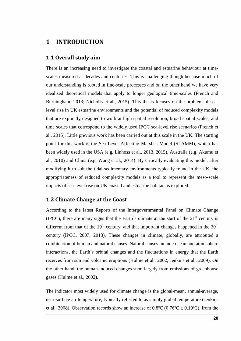
and human life and they correspond to the scale of IPCC-type scenarios (Slaymaker et

al., 2009; French and Burningham, 2011). Since sea-level rise effects on coasts vary

spatially (Gornitz, 1991), and vary with individual landform type, it is necessary to

analyze and downscale these changes down to more local scales (Dean, 1987; Fenster

and Dolan, 1993; Pilkey et al., 1993; Cooper and Pilkey, 2004). The range of relevant

spatial scales is thus quite broad, perhaps from 1 to 100 km.

Figure 1.7: Spatial and temporal scales involved in coastal evolution (Cowell and

Thom, 1994).

Figure 1.8: Spatial and temporal scales from a coastal management perspective

(Slaymaker et al., 2009).

34

Of critical importance here is the separation of variability (i.e. high order processes)

from progressive change (low order processes). The ‘coastal tract’ concept was

proposed by Cowell et al. (2003) to provide a framework for this. The tract is presented

as “a spatially contiguous set of morphological units representative of a sediment

sharing coastal cell” (Figure 1.9). A hierarchy of morphologies and processes can be

identified, in which the coastal tract constitutes the lowest order. Within the tract, meso-

scale coastal landforms and landform complexes exhibit morphological behavior

constrained by the residual effects of higher-order processes, as well as the lower-order

controls exerted by the coastal shelf and the Quaternary geology (Cowell et al., 2003).

Figure 1.9: Physical morphology encompassed by the coastal tract. The upper shoreface

may include (A) dune, washovers, flood-tide deltas, lagoonal basins and tidal flats, (B)

mainland beaches, and (C) fluvial deltas (Cowell et al., 2003).

1.4.2 Mesoscale coastal responses to climate change

Climate affects the distribution, form, functioning and dimensions of coastal and

estuarine landforms and their associated ecosystems (Woodroffe, 1993; Douglas, 2001;

Pethick, 2001; Scavia et al., 2002; Day, 2008). Morphodynamic responses to a rise in

sea level are determined by the balance between erosive forces, sediment supply and

sumbergence (Reed, 1995; Allen, 2000; French and Burningham, 2003; FitzGerald et

al., 2008) and also mediated by the influence of climate on biotic processes (Reed,

1995; McKee et al., 2007).

35

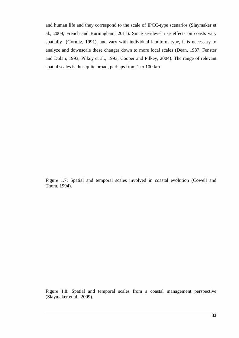
The natural long-term response of shorelines to the sea-level rise is to retreat landwards

in order to maintain their relative position (Titus, 1991; Pethick, 2001; Blott and Pye,

2004; Defeo et al., 2009), unless obstructed by cliffs or where there is sufficient

sediment supply to maintain seaward propagation (Titus, 1991; Valentin, 1952). Typical

rates of shoreline retreat along coastal plain coasts are 0.3 to 1 m per year (Pilkey and

Cooper, 2004). Conceptually, Bruun (1962) proposed that while sea level rises, erosion

of the upper part of the beach is taking place and is deposited offshore restoring the

beach profile’s shape with respect to sea level. However, the shoreline retreat due to a

sea-level rise is not continuous but episodic (SCOR Working Group 89, 1991) and also

not just a simple inundation, but a more complex reorganisation (Pilkey and Cooper,

2004).

Slow global average sea-level rise has been been associated within more-or-less

manageable coastline retreat in many areas (Ranasinghe and Stive, 2009). The

accelerated rates of rise predicted for the twenty-first century (Leuliette et al., 2004;

Beckley et al., 2007) can be expected to lead to more rapid and also more widespread

erosion and retreat (Bird, 1985; National Research Council, 1990; Leatherman, 2001),

especially on low gradient and predominantly sandy coasts (Defeo et al., 2009). An

acceleration in coastal erosion is driven by storm events superimposed upon a

background trend of rising sea level (SCOR Working Group 89, 1991). Allan and

Komar (2006) argued that increased erosion along the west coast of US since 1970s had

been associated with bigger wave heights because of sea-level rise and as well as more

intense storms. More specifically, storm surges cause large waves that can pass over the

beach without breaking, but when they finally break, the surf zone’s remaining width is

not enough to dissipate their energy (USAGE, 1984). On coastal barrier islands, this

wave erosion may transport sand landward as ‘overwash’, forcing the barrier island to

migrate and therefore to keep pace with the sea-level rise (Figure 1.10; Titus, 1990).

Changes in sea level and coastal wave climate will also influence rates of cliff erosion

(Bray and Hooke, 1997). Hard rock coasts may remain more-or-less stable as sea level

rises (National Research Council, 1987; Forbes et al., 1989), on account of their

naturally slow rates of erosion (Allison, 1989). On the other hand, soft-rock cliffs are

prone to erosion (Howe, 2002) making them much more sensitive to climate changes

and sea-level rise. Higher cliffs typically retreat more rapidly (Richards and Lorriman,

1987) and produce more sediment per unit of retreat (Dalrymple et al., 1986; Bray and

36

Hooke, 1997). More rapid erosion will increase the sediment supply (Bird, 1993) and

the eroded material will be transported in large quantities elsewhere (USAGE, 1984;

Bird, 1993), balancing the land losses that would otherwise happen through erosion and

submergence (Bird, 1993).

Figure 1.10: Overwash: natural response of undeveloped barrier islands to sea-level rise

(Titus, 1990).

Although sea-level rise has been considered as the major factor driving open coastal

erosion (Pilkey and Cooper, 2004; Stive et al., 2009), other factors may be more

important (Titus, 1990; French and Spencer, 2001). Sediment starvation, for example,

can cause coastal erosion even if the sea level is stable, while sufficient sediment supply

can cause the coastline to grow seaward even if the sea level is rising (Figure 1.11;

Marchand, 2010). Sediment delivery rates are often dominated by anthropogenic

changes (Komar, 1999; Kirwan and Murray 2007). For example, an analysis of erosion

problems at Sandy Hook (New Jersey, USA) showed that only 1% of the erosion since

1953 is due to sea-level rise, while the rest is caused by sediment starvation downdrift

of a major groyne installation, combined with an increase in the frequency and

magnitude of major storms over the period of observation (Allen, 1981).

37

Figure 1.11: Coastal evolution through a combination of sea-level changes and sediment

availability (after Valentin, 1952).

As sea-level rises, estuaries also try to maintain their relative position within the tidal

and wave energy frame by the process of transgression. This process was first suggested

by Allen (1990a) and is mainly caused due to the redistribution of sediment within the

estuarine system itself. The deeper due to the sea-level rise water in the outer estuary

increases the waves propagating in from the sea, resulting in erosion and therefore

retreat of the mudflat-saltmarsh boundary. The eroded material are moved landward and

re-deposited on the upper intertidal zone of the inner estuary, increasing the elevation of

the marshes and tidal flats. This results in a potential transgression of the landward edge

of the marsh, while the tidal flat – saltmarsh boundary continues to erode due to

increased fetch-driven waves. That means that the estuary channel moves landward as a

unit while sea-level rises (Pethick, 2001).

The vulnerability of the estuaries to the sea-level rise depends on the wetland types they

contain, on constraints on plant productivity, and also the abundance of external

sediment supply (Figure 1.12; Allen, 2000; Schwimmer and Pizzuto, 2000; French and

Spencer, 2001; Environment Agency, 2007; FitzGerald et al., 2008; Wolanski et al.,

2009). Saltmarshes for example, may respond to sea-level rise with areal reduction,

stability or even expansion, depending on the concurrent changes in sediment

availability (Philips, 1986). Increasing inundation of the saltmarsh surface translates

38

into more accommodation space available for infilling (French, 2006), which may in

turn drive both vertical and lateral accretion (Redfield, 1972; McCaffery and Thomson,

1980; Pethick, 1981; Shaw and Ceman, 1999). Under constant sea-level forcing, vertical

accretion may be sufficient to ultimately restore the marsh to a new equilibrium position

in the tidal frame (French, 1993).

Figure 1.12: Major factors that affect marsh elevation (FitzGerald et al., 2008).

Many studies have determined salt marsh vertical accretion rates and investigated the

feedback between sea-level rise and accretion (for British studies, see French, 1993;

French and Spencer, 1993; Allen and Duffy, 1998; for the Mississippi delta, see

DeLaune et al., 1983; Hatton et al., 1983; Copnner and Day 1991; Cahoon et al.,

1995a,b; for the Mediterranean, see Stanley 1988; Sestini 1992; Bondesan et al., 1995;

Ibanez et al 1997, 2010; Day et al., 1999, 2011; Pont et al., 2002). The higher the rate of

sedimentation, the bigger the rate of relative sea-level rise that can be tolerated with no

wetland loss (Day et al., 2008). In areas where the rate of sedimentation exceeds sea-

level rise, saltmarshes tend to prograde seaward (Reed, 1990; Doody, 2001). However,

vertical accretion rates of the marshes are usually limited (Baumman et al., 1984;

Walker et al., 1987; Kearny and Stevenson, 1991; Temmerman et al., 2003; FitzGerald

et al., 2008), resulting in erosion and therefore wetland loss when rates of relative sea-

39

level rise are high (Phillips, 1986; Hackney and Cleary, 1987; Kearny and Stevenson,

1991; Britsch and Dunbar, 1993; Boomans and Day, 1993; Reed and Foote, 1997; Van

der Wal and Pye, 2004).

In many saltmarshes, the production and incorporation of organic material is the

principal factor that determines the maximum rate of vertical accretion (Nyman and

Delaune, 1995; Reed, 1995; Callaway et al., 1997). Halophytic plants thus exert an

important role on the long-term sustainability of these ecosystems, because they control

their habitat elevation through the production of above- and below- ground biomass

(Morris et al., 2002). In addition to its contribution to marsh soil volume (see Figure

1.12), vegetation also creates conditions conducive for deposition (Allen and Pye, 1992;

Bartholdy, 2012) by reducing the velocity of water flow (Boorman, 1998) and

attenuating wave energy (Moller et al., 1999). However, many other systems, especially

in northwest Europe, are primarily dependent upon an external supply of inorganic

mineral sediments whether from marine or fluvial sources (French, 2006).

Tidal exchange of water and sediment occurs preferentially via channel systems (French

and Stoddart, 1992; D’Alpaos et al., 2006). The proximity to the creek network have

been also suggested in many studies as the main factor that controls the sediment

deposition rates (French and Spencer, 1993; French et al., 1995), whereas the small

creeks have a less important influence (Stoddart et al., 1989; Bartholdy et al., 2010a,

2012). As the proximity to the primary creek increases, the sediment deposition

decreases (Letzch and Frey, 1980; Carling, 1982; Reed, 1988; Stoddart et al., 1989;

French and Spencer, 1993; French et al., 1995; Bartholdy, 1997; Reed et al., 1999;

Bartholdy, 2010a). Deposition primarly takes place close to the creek margin of the

marsh edge, while it will be a minimum deposition at some distances away from the

source (Bartholdy, 2012).

Despite the effectiveness of vegetation in trapping and binding sediment (Cahoon and

Reed, 1995; Adam, 2002), wind waves also exert an important control on marsh

stability (Redfield, 1972; Pethick and Reed 1987; Allen 1989, 1997; Schwimmer,

2001). Saltmarshes typically exist in fetch-limited settings (Coward et al., 2011) in

which wave height is determined by the interplay of the wind forcing (wind speed and

duration), fetch distance and the water depth (Jackson and Nordstrom, 1992; Jackson et

al., 2002; Nordstrom and Jackson, 2012). Many estuarine and backbarrier environments

40

are effectively depth-limiting such that an increase in wind speed does not significantly

increase wave height (Jackson et al., 2002). However, the bottom depth increases when

sea level rises, resulting in larger waves that erode the upper intertidal flats, and induce

retreat of the outer salt marsh edge (Gardiner et al., 1992; Nicholls et al., 1999, 2004;

Gardiner and Porter 2001; Pethick, 2001; Simas et al., 2001; Davidson–Arnott et al.,

2002; Syvitski et al., 2005; Cahoon et al., 2006; Moller, 2006; Reed et al., 2009).

The eroded sediments will be redistributed within the marshes and the tidal flats by the

waves and may aid the vertical adjustment of the marshes, thereby aiding their landward

migration (Gardiner et al., 1992; Nicholls et al., 1999, 2004; Gardiner and Porter 2001;

Pethick, 2001; Simas et al., 2001; Davidson–Arnott et al., 2002; Syvitski et al., 2005;

Cahoon et al., 2006; Reed et al., 2009). When the inland migration is not possible, due

either to steep terrain or, often, the presence of embankments and dykes that protect the

area from the sea, ‘coastal squeeze’ can occur (Figure 1.13; Titus, 1986; Bijlsma et al.,

1996; French, 1997; Pontee, 2013).

Figure 1.13: Coastal squeeze (a) before sea wall construction; (b) after construction of a

sea wall; (c) constrained by steep terrain (Pontee, 2013).

41

Finally, sea-level rise is also associated with saltwater intrusion into rivers, coastal

aquifers and estuaries (Titus, 1990; Gornitz, 1991; Nile Delta Aquifer and Madras

Aquifer, Sherif and Singh, 1999; Douglas, 2001; Bobba, 2002; Nicholls et al., 2007;

Shellenbarger Jones et al., 2009; Werner and Simmons, 2009; Wiedenman, 2010). A

theoretical analysis of the saltwater intrusion indicates that a free water table of 1m

above the mean sea level supports 40m of freshwater below the sea level (Ghyben-

Herzberg equation). Thus, a rise in sea level of 0.5 m will cause a reduction in the

freshwater thickness of 20m (Figure 1.14; Sherif and Singh, 1999). This relationship is

based on assumptions that do not apply in all situations and is typically true away from

the sea boundary. In these areas, the water tables are more affected by pumping and

recharge activities rather than any change in sea level (Hull and Titus, 1986; Sherif and

Singh, 1999; Werner and Simmons, 2009; Ferguson and Gleeson. 2012). Higher salinity

levels will clearly affect the functioning of estuarine ecosystems and the distribution of

their habitas and species (Berry et al., 2003). In Chesapeake Bay, for example, some

islands have become so contaminated by salt that logging and farming activities are no

longer possible (Kearney and Stevenson, 1991). However, if there is space for migration

and the rate of sea-level rise is not too rapid then the animal and plant communities may

be able to adapt (Nicholls et al., 2007).

Figure 1.14: Sharp interface and sea-level rise, based on the Ghyben – Herzberg

relationship (Ghyben, 1888; Herzberg, 1901) (Sherif and Singg, 1999).

Concluding, it can be said that coastal systems adjust dynamically to a rise in sea level

and maintain a characteristic geometry, unique to each coast (FitzGerald et al., 2008).

The structure and functioning of most coastal ecosystems is closely linked to sea level;

42

if sea level increases at a rate that the ecosystem can not keep pace with, the state of the

coast will fundamentally change (Anderson et al., 2009). Given that most of the

interactions between climate change and landform and ecological responses to it are

non-linear, the effect is not just a simple innundation but a complex spatially-distributed

set of morphological and associated ecological changes. This requires appropriate

models if such changes are to be predicted with any confidence.

1.4.3 UK Coastal and Estuarine Environments and their Likely Vulnerability

to Climate Change

The coastline of the UK is naturally dynamic along much of its length on account of a

predominantly meso and macro tidal regime together with an energetic storm wave

climate (May and Hansom, 2003). Tidal ranges are very variable as a result of well-

developed amphidromic tidal systems and the indented nature of the coast (Pugh, 1987).

Western coasts are exposed to an energetic wind climate, which together with the North

Atlantic swell, results in high energy waves. On the other hand, the North Sea is

characterised by lower wind speeds and shallower waters, producing lower energy

waves along the east coast (Laurence, 1980; May and Hansom, 2003).

The UK coast can be subcategorised into low-lying soft coasts, which are often

protected by sea walls, and more resistant coasts, typically dominated by hard rock

cliffs (Boorman et al., 1989; Figure 1.15). This variation in the geology combined with

the sea-level history influences both erosion rates and the nature of the eroded material.

Much of Scotland and some parts of the Welsh coast are highly resistant and

predominantly source coarse gravel and boulders to local beaches (May and Hansom,

2003). Much of the contemporary beach sediment in these areas has derived from

glaciogenic sources (May and Hansom, 2003). On the other hand, much of eastern and

southern England are very prone to erosion because they consist of less resistant

sedimentary rocks or glacial sediments and of offshore sediment reworked during the

Holocene marine transgression (Boorman et al., 1989; Clayton and Shamoon, 1998;

May and Hansom, 2003; Zsamboky et al., 2011).

Studies show that 67% of the coast of eastern England has retreated landward over the

last century (Evans et al., 2004; Taylor et al., 2004). More generally, around 3000 km

(about 17%) of the total UK coastline is currently eroding (EUROSION, 2004). Within

43

this bigger picture, 30% of England’s coastline; 20% in Northern Ireland; 23% in

Wales; and 12% in Scotland shows active erosion (MCCIP, 2011). Continuing coastal

erosion contributes an important contemporary sediment sources that are important in

maintaining local beaches and more distant muddy intertidal environments (Boorman et

al., 1989). But these sediment feeds are reduced by coastal protection. In particular, in

UK almost 2300 km of the total coastline is artificially protected, the largest proportion

in Europe (EUROSION, 2004). This amounts to 46% of England’s coastline; 20% of

Northern Island’s; 28% Wales’ and 7% of Scotland’s (MCCIP, 2011).

Figure 1.15: Relative resistance of rocks of the UK (after May and Hansom, 2003).

44

A notable feature of the UK coast is its degree of indentation, where numerous valleys

and embayments are occupied by estuaries. These not only increase the shoreline length

but they also contain significant areas of settlement and agriculture located on land

reclaimed from the sea since medieval times (Austin et al., 2001). Such land is highly

vulnerable to inundation if the extensive flood defence infrastructure is not maintained

and upgraded to cope with higher sea level. This is especially true of southeast England,

which has some of the most extensively reclaimed estuaries (Gray, 1977; Austin et al.,

2001) and is also subject to the highest rates of relative sea-level rise (Woodworth et al.,

1999; Hulme et al., 2009; Jenkins et al., 2009, Wahl et al., 2013).

UK estuaries contain a large proportion of the tidal wetland habitats in northwest

Europe, many of which are designated as “Special Areas of Conservation” (SAC) under

the EC Habitats Directive (Council Directive 92/43/EEC of 21 May 1992). Saltmarsh is

especially well developed, primarly in meso and macro tidal areas (Allen, 2000), and

occur in four main settings; open coast, back-barrier environments, embayments and

estuaries.

Most of the saltmarshes that are actively formed today in Great Britain are characterized

as allochthonous in terms that they are formed primarily through the introduction of

externally derived clastic sediments. In general, little is known about the budgets and

the sources of British saltmarsh sediments (see, for example, French, 2006). Possible

sources of mineral matter include coastal and estuarine cliffs, offshore mud deposits and

river catchments. Mud can travel long distances from a source, and it can also be mixed

with other materials before arriving at its new deposition site (Allen and Pye, 1992).

Many studies (Eisma and Kalf, 1987; McCave, 1987; Kirby, 1987) show that small

amounts of sediment are provided by the rivers that drain into the Irish and the North

Sea, and most of the suspended mud in tidal waters is provided by eroded

unconsolidated Pleistocene glacial sediments exposed in retreating coastal cliffs.

Saltmarsh degradation and loss has been evident over the last century or so, especially

in southeast England (Boorman et al., 1989; Pye, 2000). Vertical accretion rates appear

to be sufficient to cope with relative sea-level rise, in both open coast (e.g. Dengie

peninsula, Essex; Reed, 1988) and estuarine marshes (e.g. those of the Greater Thames;

Van der Wal and Pye, 2004). However, marsh area has declined significantly over the

last few decades (Pye, 2000), with losses of 10 to 44% from 1973 to 1985/1988 (Burd,

45

1992; Cooper et al., 2001). A variety of different mechanisms of saltmarsh degradation

have been identified and it is likely the observed changes are the results of some

combination of these rather than one mechanism alone. Although increased storminess

due to sea-level rise has been reported as a cause of increased saltmarsh erosion

(Doody, 1992; Pethick, 1992), the pattern of marsh-edge erosion in south-east England

cannot support an explanation based only on the wave action (Burd, 1992; Hughes and

Paramor, 2004). Losses of subtidal seagrass (Zostera sp.) in this area have increased

vulnerability to wave action and erosion of the marsh edge, but cannot explain the loss

of marsh in sheltered locations (Hughes and Paramor, 2004).

Coastal squeeze has also been reported as a cause of saltmarsh losses that is especially

applicable to southeast England (Shennan, 1989; Burd 1992; English Nature 1992;

Covey and Laffoley, 2002; Taylor et al., 2004). Here too, the evidence is patchy.

Although there is a scarcity of plant species on the upper marshes on southeast England,

as expected under the process of coastal squeeze, this may also be a consequence of the

long history of enclosure that removed the upper marsh from the influence of the tide

(Hughes and Paramor, 2004). Covey and Laffoley (2002) argue that only 5% of recent

marsh loss is due to land claim and the constructions of flood defences.

Although many areas of the UK coastline are under threat from sea-level rise and other

aspects of climate change (Dearing et al., 2006), the vulnerability of coastal and

estuarine wetlands is of particular concern given their already high rates of loss and the

extent to which their natural response is constrained by reclamation and flood defence

structures (Wolters et al., 2005). Although hard defences still feature prominently in

coastal management and flood protection planning (DEFRA, 2002; Pethick, 2002), a

new strategy of managed realignment has become progressively favoured since the

1990s (English Nature, 1992; Doody, 2012). This approach is reflected in the Shoreline

Management Plans (SMPs) for England and Wales, which aim to set out policies to

manage coastal erosion and flood risk (Zsamboky et al., 2011; Doody, 2012). It is also

adopted by many agencies and organizations, not only in the UK but elsewhere too

(Hughes and Paramor, 2004; Morris et al., 2004) and contributes to the rationale for

improving our modelling capability, by improving our understanding on the processes

involved (Garbutt et al., 2006).

46

1.5 Modelling Approaches

From an awareness of the risks posed by climate change, emerges the need to create

robust models to provide a scientific basis for understanding, predicting and managing

the potential impacts on coasts (FitzGerald et al., 2008). This leads to the challenge of

predicting these impacts at the crucial mesoscale of 10 to 102

km and a time horizon of

10 to 102 or 10

3 years, corresponding to the ‘engineering’ scale of Cowell and Thom

(1994). A major problem with such a mesoscale is that it is situated between the small

scale processes of sediment transport, which are relatively well understood and broader

coastal evolution, which is informed by the record of Holocene stratigraphy (Figure

1.16; French and Burningham, 2009).

Figure 1.16: Modelling approaches applicable to different scales (after French and

Burningham, 2009).

An approach that has been very popular in coastal management and planning is to

estimate future shoreline retreat by extrapolating past rates of change, assuming that the

observed coastal behaviour encompasses the kind of behaviour that can be expected in

the future (National Research Council, 1990; Fenster et al., 1993; Hooke and Bray,

1996). Historical Trend Analysis (National Research Council, 1987; Leatherman, 1990)

has been used by many studies (for future shoreline position projections see: NRC 1990,

Fenster et al., 1993, Douglas et al., 1998; Futurecoast study (Defra, 2002); Pye and

Blott, 2008 and for sea-level rise effects on wetlands see: Orson et al., 1985; Vanderzee,

47

1988; Parkinson et al., 1994). It is preferred because it is site-specific and uses data that

can be acquired relatively easily. Its main assumption is that sea-level rise is the

dominant influence on recession while other parameters remain constant (Bray and

Hooke, 1997; Whitehouse et al., 2009). This assumption might be valid with rapid rates

of relative sea-level rise but is a significant limitation when other factors are important

(Bray and Hooke, 1997). Also, this method can predict behaviour only under well

represented in the historic record conditions (e.g.: Dolan et al., 1991; Hall et al., 2002;

Walkden and Hall, 2005), otherwise the reported rates will be inconsistent (Addo et al.,

2008).

Microscale processes lead to nonlinear dynamic coastal responses to environmental

change, which can be captured over short timescales by morphodynamic models based

on hydrodynamic and sediment transport principles (de Vriend et al., 1993a; Wang et

al., 1995; Nicholson et al., 1997; Cayocca , 2001; Lesser et al., 2004; Sutherland et al.,

2004; Dearing et al., 2006; Gardiner et al., 2007; Scott and Mason, 2007). Such models

are becoming increasingly sophisticated (Lesser et al., 2004) and typically incorporate

multiple modules that interact with each other to represent the hydrodynamics, residual

sediment transport patterns, and also the evolution of the bed morphology (eg.

ECOMSed (Hydroqual, 2002), ROMS (Warner et al., 2008), Delft3D (Lesser et al.,

2004), MIKE21 (Warren and Bach, 1992) (van Rijn et al., 2003; Villaret et al., 2012).

The increasing use of unstructured finite element and finite volume computational

meshes (e.g. TELEMAC) means that such models are able to handle complex

geometries, including estuaries, inlets and open coasts (Villaret et al., 2012).

However, morphodynamic models usually perform poorly in detail (de Vriend et al.,

1993a; Nicholson et al., 1997; Sutherland et al., 2004) because much of the behaviour

modelled is incompletely understood (Roelvnik and Broker, 1993). Crucially, most of

the relevant physics included in these models relates to the hydrodynamics, meaning

that they operate in time scales that are much shorter than the changes in morphology

(DeVriend et al., 1993b; Hanson et al., 2003; van Rijn et al., 2003; Scott and Mason,

2007). These short-term hydrodynamic and sediment transport problems also require a

lot of computer power (Roelvnik and Broker, 1993; Whitehouse et al., 2009) making

them unsuitable for modelling on a timescale of a century (DeVriend et al., 1993b;

Hanson et al., 2003). Even if the computer power is enough to run these small scales for

a long period of time, this may be not the best way (DeVriend et al., 1993b).

48

On the timescale of a century, the basis for most models of coastal evolution is the

Equilibrium Shoreface Profile (Larson, 1991; Pilkey et al., 1993; Thieler et al., 2000;

Kaiser and Frihy, 2009). In a two-dimensional sense, the shoreface profile refers to a

hypothetical long-term average profile achieved under a given wave climate and in a

particular set of materials (Schwartz, 1982). Many scientists have doubted its existence

due to its restrictive assumptions (Wright et al., 1991; Pilkey et al., 1993; Carter and

Woodroffe, 1994; Thieler et al., 1995, 2000). It has also been argued that it is a purely

theoretical morphology that is rarely if ever attained in practise, given that beach

morphology is always adjusting to, and lags behind, changes in wave conditions

(Moore, 1982; Kriebel et al., 1991; Pilkey et al., 1993; Wright, 1995). However it is

very useful to examine the behaviour of sandy beaches and dunes when longshore

transport gradients can be ignored (Roelvink and Broker, 1993).

Bruun (1954) was the first to describe the geometry of such an equilibrium profile

providing the basis for the so-called ‘Bruun Rule’ (Schwarts, 1967). The Bruun Rule is

a two dimensional mathematical principle founded on mass conservation that is used to

predict shoreline erosion (and therefore coastal recession) due to sea-level rise (Bruun

1962, 1983; Ranasinghe and Stive, 2009). It assumes that the shoreface profile is

developed entirely in sand, and as sea level rises, moves up and back, maintaining its

shape. The amount of sand that is removed from the upper part of the profile is equal to

the amount of deposited sand on the lower profile (Figure 1.17; Brunn, 1962). Due the

restrictive nature of these assumptions, the Bruun rule performs well only under specific

environmental circumstances (Bruun 1983, 1988; French and Spencer, 2001; Cooper

and Pilkey, 2004).

Figure 1.17: The Bruun Rule of shoreline retreat (Bruun, 1962).

49

A key limitation of the Bruun Rule comes from the the inclusion of a ‘closure depth’ in

the model. The choice of this depth is to some extent arbitary; while Bruun (1962)

assumed a depth of 18m, other studies used a depth of around 9 m (Pilkey et al. 1993).

Bruun (1988) suggested that field identification could be based on sedimentological

boundaries, while Nicholls et al. (1998) estimated closure depth based on nearshore

wave statistics. The Bruun Rule can be applied successfully in restricted fetch settings

where the depth of closure is limited (French and Spencer, 2001) and may hold for

estuarine beaches (e.g.. Rosen, 1978, Hands, 1983, Kaplin and Selivanon, 1995). Many

modifications have been proposed (Dubois, 1977; Weggel., 1979; Dean and

Maurmeyer, 1983; Hands, 1983; Dean, 1991; Davidson- Arnott, 2005) in order to

address these limitations and also many attempts have been made to test its predictive

capability (Schwartz, 1967, 1987; Rosen, 1978; Pilkey and Davis, 1987; Bruun 1988;

List et al., 1997). The results have been mixed. On one hand, fundamental objections

have been raised over the use of equilibrium profiles as a basis for shoreline change

modelling because there are more geological factors and numerous hydrodynamic

influences that condition actual profiles than the Bruun model considers (Dubois, 1992,

Pilkey et al., 1993). Many studies (Kaplin and Selivanov, 1995; List et al., 1997; Pilkey

et al., 2000; Sallenger et al., 2000; Thieler et al., 2000) have shown that the Bruun Rule

is an inadequate model of shoreline retreat (Cooper and Pilkey, 2004) and that even

under ideal conditions, the rule has never given accurate predictions (SCOR Working

Group 89,1991; List et al., 1997; Pilkey and Cooper, 2004). Thus, Cooper and Pilkey

(2004) conclude that the Bruun Rule, whilst was a useful tool for its time, has outlasted

its usefulness and it should be abandoned and replaced by other models.

On the other hand, the Bruun rule remains the most widely used contemporary method

because it is simple, it does not require field study, it can be applied by scientists with

no critical appraisal and finally due to the lack of an alternative model (Pilkey and

Cooper, 2004; Ranassinghe and Stive, 2009). Thus, it is often embedded in more

complex numerical modelling systems to represent cross-shore adjustments of the

beach. Its main assumption, for example, that the profile shape remains constant, is also

used in the ‘one-line’ GENEralized Model for Simulating Shoreline Change

(GENESIS) (Hanson and Kraus,1989) and the SBEACH numerical model (Larson and

Kraus, 1989). The first of these is empirically based and mainly used to analyse the

shoreline response to the longshore sediment transport rate and also to develop sediment

budgets in a regional scale (Kaiser and Frihy, 2009). The second examines the change

50

of the shoreline caused by the cross-shore sediment transport (Kaiser and Frihy, 2009)

and is used to predict the beach and dune erosion caused by storms (Thieler et al.,

2000). A combination of these two and CASCADE planning model (Larson et al.,

2002) emerged in a new model suitable for mesoscale prediction, the GENCADE model

(Hanson et al., 2011). The longshore sediment transport in both GENESIS and

GENCADE is calculated by using the CERC Formula (Nielsen, 1992).

More sophisticated process-based models are often preferred because they incorporate

much greater mechanistic understanding (Costanza et al., 1990; Roelvnik and Broker,

1993). In order to characterise the behaviour of the ‘whole’ system at large spatial and

temporal scales so-called ‘reduced complexity models’ have been developed, commonly

used in geomorphology (Murray and Paola, 1994; Coulthard et al., 2002). These

incorporate simplified parameterisations of the fine-scale processes that can be

considered to be ‘sub-grid’ at a mesoscale, and focus on the key linkages and feedbacks

between the major morphological components (Dickson et al., 2007). A good example

of this type of model on coastal landforms is the SCAPE (Soft Cliff and Platform

Erosion) model, which simulates the sensitivity of shore profile response, including cliff

recession rates over timescales of decades to centuries (Walkden and Hall, 2005;

Dickson et al., 2007; Addo et al., 2008; Walkden and Dickson, 2008; Walkden and

Hall, 2011). It was used initially on a specific site, the Naze Peninsula, in Essex,

southern England (Walkden and Hall, 2005) but extended later to be a general

representative of soft-rock shores overlain by a sparse beach (Figure 1.18; Dickson et

al., 2007). It can also be characterised as a hybrid model because it includes several

modules in order to describe all the different processes (wave tranformation, platform

erosion and a beach) (Figure 1.19) but also includes two feedback processes between

and within the modules that regulates their behaviour (Dickson et al., 2005; Walkden

and Hall, 2011):

Cliff retreat results in beach formation, which results in greater protection and

ultimately in a reduced rate of to cliff retreat.

More rapid cliff retreat also results in a flatter shore platform profile, which results

in greater wave dissipation, thus, less platform downwearing and therefore a

reduction in the rate of cliff retreat. (Whitehouse et al., 2009).

51

Figure 1.18: Schematic representation of a typical SCAPE model profile (Walkden and

Dickson, 2008).

Figure 1.19: Processes represented in SCAPE (Walkden and Dickson, 2008).

A comparison between the predictions of SCAPE and those made using the modified

Bruun rule showed that SCAPE predicts more complex responses and lower sensitivity

of soft rock shores to sea-level rise (Dickson et al.. 2007). However, it can not be used

in all situations or where historical sea-level rise data are not available (Walkden and

Dickson, 2008). Thus, it must be used in conjuction with other predictive models (see,

for example, Addo et al., 2008).

52

When more spatially extensive low-gradient environments are considered, vertical

changes are often as important as the horizontal shifts in a shore profile or a cliff, and

these adjustments are usually highly non-linear (Nicholls et al., 1999; Nicholls, 2004).

This is particularly true of estuarine margins dominated by extensive tidal wetlands. As

sea level increases, vertical accretion on the surface of the wetland is also increased due

to the increased organic matter (∆Sorg) and sediment input (∆Ssed) and is calculated as

the sum of these inputs (Bartholdy, 2012). However, in order to simulate the final

vertical growth (∆Ε) of marsh platforms due to sea-level change for long time periods

(50 to 103 years), the deposit thickness due to autocompaction (∆P) and the possible

isostatic and eustatic changes (∆M) must also be included. Various researchers have

investigated the interplay between these factors using a zero-dimensional approach

(equation 1.1; Krone, 1987; Allen, 1990, 1991; French, 1993, 1994; Temmerman et al.,

2003; French, 2006; Bartholdy, 2012).

∆E=∆Ssed+∆Sorg-∆M-∆P, (1.1)

This essentially a spatial formulation is justified given that the topography of the marsh

platform is nearly horizontal (Temmerman et al., 2003). The terms ∆M and ∆P are

given and the ∆Sorg is often ignored in predominantly allochthonous systems, where it is

relatively small. So, the challenge is to simulate the ∆Ssed (Bartholdy, 2012). Krone

(1987) was the first to develop a zero-dimensional mass model to calculate ∆Ssed and

used it to simulate how tidal marshes in San Francisco Bay respond to historical sea-

level change. He proposed an equation to calculate the time-dependent sedimentation on

a salt marsh unit area, which is integrated over a tidal period and then over all the tidal

periods in a year. Dividing mass deposition per unit area per year by the bulk dry

density of the material deposited yields ∆Ssed. Latter, Allen (1990) used this approach to

simulate the long-term vertical growth of salt marshes in the Severn estuary. Similar

approaches have been developed by French (1993, 2004, 2006) and Allen (1995, 1997).

More recent work has shown that this type of model can better simulate observed long-

term historical marsh growth by incorporating a relationship between suspended

sediment concentration (C0) and inundation depth. If this relationship is not included,

the observed historical growth will be underestimated, resulting to rather conservative

under-predictions of vertical marsh growth under sea-level rise scenarios (Temmerman

et al., 2003).

53

In some systems, especially those with less significant mineral sediment inputs,

vegetation growth and decomposition must also be taken into account (Friedrichs and

Perry, 2001). Morris et al. (2002) included the alterations in biological productivity with

varying levels of tidal inundation in order to show how long-term vertical accretion

rates are almost equal to sea-level rise rates on a vegetated marsh platform. In his

model, the biomass density enhance the deposition rates, reinforcing the ability of the

marsh platform adjust towards an elevation or inundation depth at which the rate of

deposition and the rate of sea-level rise will be equal. This equilibrium elevation

depends on the rate of sea-level rise, vegetation type, and also the suspended inorganic

sediment concentration.

For even more realistic results, the autocompation term (Allen, 1999) should ideally be

included. French (2006) incorporated an autocompaction term in his zero-dimensional

mass-balance model (French, 1993, 1994), although unlike the Temmerman et al.

(2003) model, this still assumes that C0 and ws (settling velocity) remain constant.

French (2006) also advocates consideration of vertical marsh adjustment in the context

of sediment supply and not solely the determination of net elevation balance.

A different approach was used more recently by Bartholdy et al. (2004, 2010a) to

determine the average deposition ∆Ssed (kg m-2

tidal period-1

) in specific time at a

specific site, by taking into account the elevation of the saltmarsh (E(t)) and the

concentration of sediment available for deposition (∆C(HWL)). Although the last term is

location-specific, it depends on the high tide level relative to the mean high water level

(MHWL) (equation 1.2; Bartholdy, 2012).

∆Ssed = ∆C(HWL) * [HWL – E(t)], (1.2)

In order to include the autocompaction, the calculated ∆Ssed must be added to the mass

depth (kg m-2

) of the saltmarsh from the surface to the lower boundary of the salt marsh

deposits, at the particular location. The result will be introduced in the mass depth

equation (equation 1.3, Bartholdy et al., 2010b, 2012) and by solving it for z, the

required salt marsh level will be given.

MSDz = A * zln(z) + z(B-A), (1.3)

where, A and B are two empirical constants.

54

Based on mean accretion measurements across the Skallingen backbarrier saltmarshes,

in western Denmark (Nielsen, 1935; Jakobsen, 1953; Bartholdy et al., 2004, 2010a), and

after their correction for autocompaction, the correlation of the calculated by the

equation 1.3 saltmarsh level to the sea level seems to depend on the distance to marsh

edge and to distance to creeks. This produces a pattern of more rapid accretion in the

outer part of the backbarrier and also along the major creeks (Bartholdy, 2012),

enhancing the importance of the spatial variations in the rate of sedimentation at all time

scales (French and Spencer, 1993; French et al., 1995; Leonard, 1997). In order for

these factors (elevation, distance to creeks and distance to marsh edge) to be modelled, a

two-dimensional approach is clearly necessary.

In order to model whole estuary evolution under different climate change scenarios,

broad-scale interactions between the tidal basin and the adjacent coastal environment

need to be included (Stive et al., 1998). Behaviour-oriented modelling (de Vriend et al.,

1993b) has been extensively used to study the evolution of tidal inlets (Van Goor et al.,

2003). These are typically based on “empirical-equilibrium assumptions” created by

applying “data-knowledge” (Dissanayake et al., 2011), meaning that this approach uses

real data to map the system behaviour onto a simple mathematical model (de Vriend et

al., 1993b). The processes considered are based on elementary physics but these are

applied to a highly idealised set of morphological sub-systems under simplified

hydrodynamic forcing (Hibma et al., 2004). Although this modelling approach has been

used in various models (Di Silvio, 1989; van Dongeren and de Vriend, 1994), the most

well known is the ASMITA (Aggregated Scale Morphological Interaction between

Tidal basin and the Adjacent coast) model (Stive et al., 1998).

In its basic form, ASMITA represents an estuary using a simple three-element

schematisation (Figure 1.20), each one of which has a tendency towards a

morphological equilibrium, when the hydrodynamic forcing is constant (van Goor et al.,

2003). These elements and their interactions are characterised by mathematical

expressions (Whitehouse et al., 2009), while the volume and area of each equilibrium

can be defined by using empirical relationships (Stive et al., 1998) and more particular

by a linear relationship with the tidal prism. That means that when the tidal prism

changes, the volume and area of each element equilibrium also change forcing the

elements to reach a new equilibrium by exchanging sediment (Whitehouse et al., 2009).

55

These empirical relationships are based on available data, and are thus different for each

estuary (Rossington and Nicholls, 2007).

Figure 1.20: Estuary three-element schematisation used in ASMITA (Whitehouse et al.,

2009).

Models such as ASMITA are limited not only by their lack of spatial detail (they are

effectively aspatial box models) but also by their assumption of equilibrium tendencies.

This limits their ability to resolve the subtleties of climate change impacts, especially

ecological changes within key landform types. In this respect, some promising

developments have occurred within the field of spatial landscape modelling. While

earlier ecological models concentrate on temporal changes with no or little spatial

articulation, a different generation of models can project cumulative impacts at many

spatial and temporal scales (Risser et al., 1984; Sklar et al. 1985; Reyes, 2009). A

typical spatial landscape model discretises the study region into a raster of cells. Each

cell contains a dynamic ecosystem simulation model, which in the case of coastal and

estuarine wetlands includes water flow and levels, tidal and river inputs, sedimentation,

subsidence and salinity, and is connected to the adjacent ones by the exchanges of the

water and suspended materials. The physical and ecological dynamics are calculated in

every cell, and any habitat change determining using a logical decision tree (Sklar et al.,

1985).

This approach is exemplified by the Coastal Ecological Landscape Spatial Simulation

(CELSS) Model (Costanza et al. 1988; Sklar et al., 1989; Costanza et al., 1990) which

was developed using 2479 cells, each representing 1 km2, to simulate large-scale

ecological habitat transitions in Atchafalaya/Terrebonne marsh/estuarine complex in

south Louisiana. Later versions of this model have taken advantages in computing

56

capability to increase the spatial resolution, making it suitable for more localised change

prediction studies at the estuary scale (e.g. Sklar et al., 1994).

The use of GIS has emerged parallel with such spatial models and is clearly a very

useful tool for coastal vulnerability assessment (McLeod et al., 2010), whether coupled

with a dynamic simulation model or not (Green and King, 2003; Rodriquez et al.,

2009). Based on an elevation analysis only, GIS can provide a crude indication of

potential inundation of coastal lowland following a rise in sea level (eg. Brooks et al.,

2006; Snoussi et al., 2009; Chust et al., 2010; Tian et al., 2010). However, GIS is more

useful when coupled with an essentially mechanistic model of some kind, and can

provide vital spatial analyses in support of the modelling (Lyon and McCarthy, 1995;

Green and King, 2003) as well as powerful visualisation tools (Green and King, 2003).

Attempts have been made to develop global databases for the coastal regions of the

world (e.g. LOICZ (Maxwell and Buddemeier, 2002), EUROSION

(http://www.eurosion.org), CoastBase (http://www.coastbase.org)). With the exception

of EUROSION, however, most of these databases have not been originally developed

for coastal applications. Accordingly, their use in coastal modelling and analyses is

limited (Vafeidis et al., 2008). A new global coastal database has been developed

specifically for vulnerability and impact analysis due to sea-level rise at regional to

global scales in the DINAS-COAST project (Dynamic and Interactive Assessment of

National, Regional and Global Vulnerability of Coastal Zones to Climate Change and

Sea-Level Rise) (DINAS-COAST Consortium, 2006). This was created in a GIS

framework (Vafeidis et al., 2008) and can be used in conjunction with the linked DIVA

model to evaluate sea-level scenarios at both regional and global scales (Hinkel, 2005;

Hinkel and Klein, 2007, 2009).

The DIVA tool neglects many of the processes that occur in conjuction with sea level

changes, such as changes in the frequency and intensity of storms, accretion and

subsidence induced by humans (Mcleod et al., 2010). However, it has been used by

many projects, notably the BRANCH project in the UK (BRANCH partnership, 2007)

to examine the impacts of climate change, and particularly sea-level rise, on coastal

habitats at a European Union - scale. BRANCH uses a set of sea-level rise scenarios (no

sea-level rise and IPCC low and high sea-level rise) and three time slices (2020s, 2050s,

2080s) compared to the baseline year of 2000. It also includes estimations for land uplift

and subsidence, so the initial global scenarios are converted to scenarios of relative sea-

http://www.coastbase.org)/

57

level rise for each impact analysis. Finally, using its ‘impact algorithm’, losses of these

habitats are estimated. A major limitation is that the DIVA model includes only two

types of coastal habitats relevant to Europe; saltmarsh and low unvegetated wetlands

(i.e. tidal flats).

Crucially, none of these approaches take account of dynamic feedbacks between

processes and coastal morphology – such as the ability of the saltmarsh to respond to

sea-level rise by increased accretion and/or the landward migration. That is why, the

DIVA software has been criticised as a basis for informing goverments and coastal

managers about adaptation, migration and also policy development (Green and King,

2003; McLeod et al., 2010). These limitations are at least partially addressed in the Sea

Level Affecting Marshes Model (SLAMM) (Park et al., 1986), providing this way a

more dynamic basis for evaluations of sea-level rise impacts at local to regional scales

(Mcleod et al., 2010).

SLAMM is a rule-based spatial model that simulates the dominant processes involved

in shoreline modifications and wetland conversions due to sea-level rise (Park et al.

1989), and the extent to which sea water inundation contributes to the conversion of one

habitat to another (based on elevation, habitat type, slope, sedimentation and accretion

and erosion rate), and also the extent to which the affected area is protected by existing

sea walls. The processes modelled include inundation, erosion and accretion, overwash,

and salinity (Clough et al., 2010). The appropriate spatial scale to use varies from local

to regional (e.g. 1 km2- 100.000 km

2), while the temporal scale also varies from a time-

step of 5 to 25 years depending on the chosen sea–level rise scenarios (McLeod et al.,

2010). Over the last 20 years it has been widely used in North America in decision-

making processes in coastal research for environmental protection and also economic

development (Park, 1991; Craft et al., 2009).

In conclusion, it is clear that models such as SLAMM, combined with the increasing

availability of high-resolution terrain datasets and GIS tools to manage both data and

model, provide a basis for a more mechanistic understanding of climate change impacts

on coastal and estuarine environments. However, much more work needs to be done to

better integrate existing models with our understanding of the dominant physical and

ecological processes in a wider range of geographical contexts.

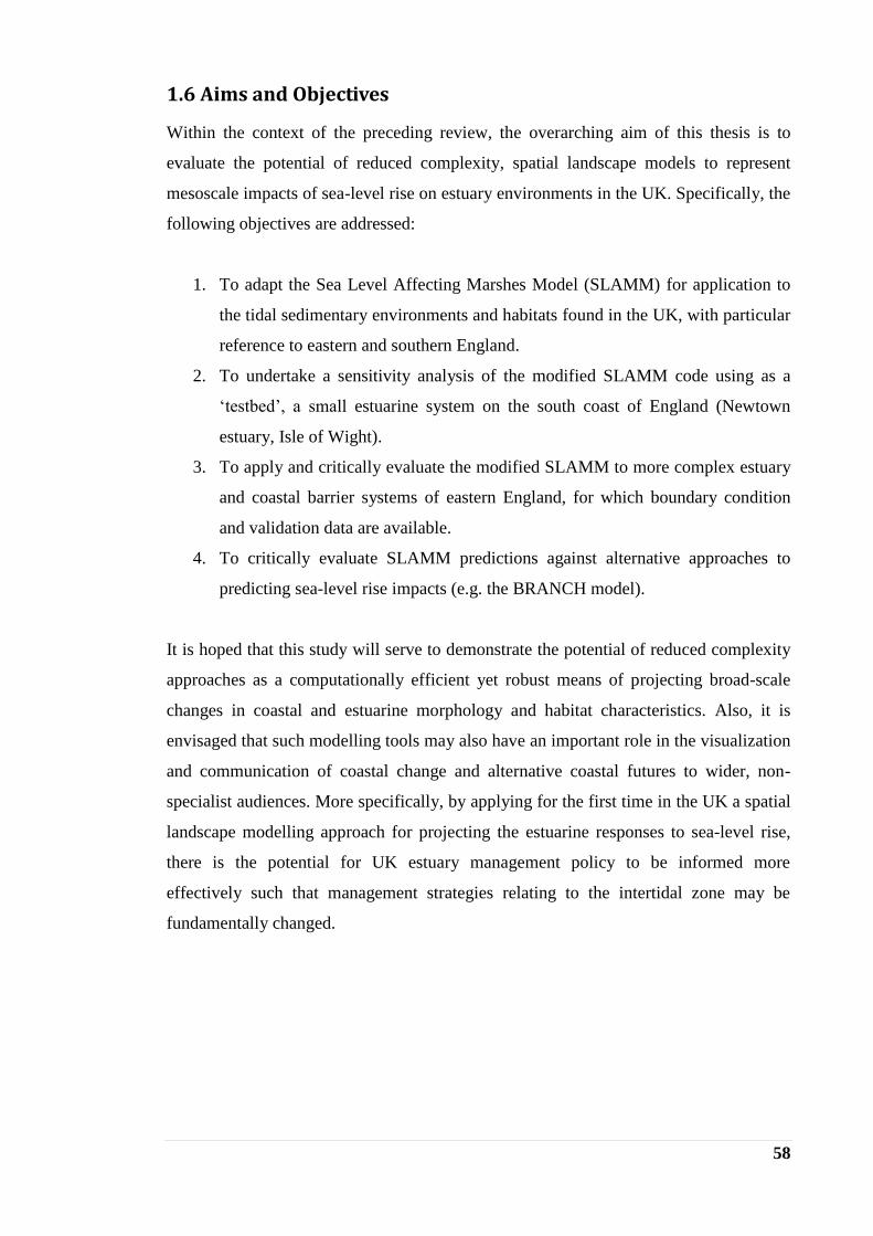
58

1.6 Aims and Objectives

Within the context of the preceding review, the overarching aim of this thesis is to

evaluate the potential of reduced complexity, spatial landscape models to represent

mesoscale impacts of sea-level rise on estuary environments in the UK. Specifically, the

following objectives are addressed:

1. To adapt the Sea Level Affecting Marshes Model (SLAMM) for application to

the tidal sedimentary environments and habitats found in the UK, with particular

reference to eastern and southern England.

2. To undertake a sensitivity analysis of the modified SLAMM code using as a

‘testbed’, a small estuarine system on the south coast of England (Newtown

estuary, Isle of Wight).

3. To apply and critically evaluate the modified SLAMM to more complex estuary

and coastal barrier systems of eastern England, for which boundary condition

and validation data are available.

4. To critically evaluate SLAMM predictions against alternative approaches to

predicting sea-level rise impacts (e.g. the BRANCH model).

It is hoped that this study will serve to demonstrate the potential of reduced complexity

approaches as a computationally efficient yet robust means of projecting broad-scale

changes in coastal and estuarine morphology and habitat characteristics. Also, it is

envisaged that such modelling tools may also have an important role in the visualization

and communication of coastal change and alternative coastal futures to wider, non-

specialist audiences. More specifically, by applying for the first time in the UK a spatial

landscape modelling approach for projecting the estuarine responses to sea-level rise,

there is the potential for UK estuary management policy to be informed more

effectively such that management strategies relating to the intertidal zone may be

fundamentally changed.

59

2 RESEARCH DESIGN

2.1 Overview

The Sea Level Affecting Marshes Model (SLAMM) is used in this thesis as a modelling

platform with which to evaluate the meso-scale impacts of sea-level rise in the kind of

estuarine and backbarrier settings that are found in the UK. SLAMM is free and open

source software, which after 20 years of development, has been characterised as an

important forecast and simulation model in coastal research (Liao et al., 2011). It has

been used at a wide range of scales, in North America (see examples at

http://www.fws.gov/refuges/planning/seaLevelRise.html), Australia (e.g. Akumu et al.,

2010) and China (e.g. Wang et al., 2014) in order to inform decision-making processes

not only for environmental protection but for economic development too (Liao et al.,

2011).

SLAMM was first developed in 1986, funded by the United States Environmental

Protection Agency (EPA) (Park et al., 1986). Since then, six versions of the model have

been released (SLAMM2: Park et al., 1989; Park, 1991; Titus et al., 1991, SLAMM3:

Lee et al., 1991; Park et al., 1991, 1993; Lee et al., 1992, SLAMM4: Galbraith et al.,

2002; Galbraith et al., 2003, SLAMM4.1: NWF, 2006, SLAMM5: Craft et al., 2009,

SLAMM6: used by many consultancy projects made by Warren Pinnacle Consulting on

behalf the U.S. Fish and Wildlife Service, National Wildlife Refuge System;

Geselbracht et al., 2011; Glick et al., 2013; Linhoss et al., 2013, 2015; Chu et al., 2014;

Wang et al., 2014). An upgrade of the latest major version will be released soon

(SLAMM 7).

SLAMM is a rule-based spatial model, which represents a domain as an array of

discrete cells, the size of which depends on data availability and the characteristics of

the study site but typically ranges from 5 to 30 m. The only required data to specify the

initial condition are the elevation, slope and land classification raster layers. These are

provided in a standard ASCII grid format, which can be generated by most GIS

packages. A complex but flexible decision tree, which consists of qualitative and

geometric relationships, is then used to determine how the habitat class within each cell

will be affected and converted to another one, given specific site parameters and rate of

sea-level rise (Figure 2.1; Clough et al., 2010).

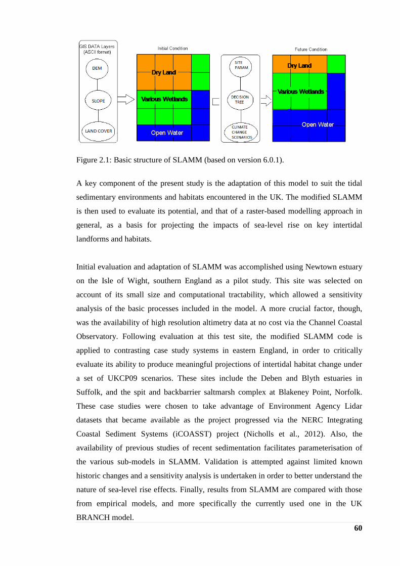
60

Figure 2.1: Basic structure of SLAMM (based on version 6.0.1).

A key component of the present study is the adaptation of this model to suit the tidal

sedimentary environments and habitats encountered in the UK. The modified SLAMM

is then used to evaluate its potential, and that of a raster-based modelling approach in

general, as a basis for projecting the impacts of sea-level rise on key intertidal

landforms and habitats.

Initial evaluation and adaptation of SLAMM was accomplished using Newtown estuary

on the Isle of Wight, southern England as a pilot study. This site was selected on

account of its small size and computational tractability, which allowed a sensitivity

analysis of the basic processes included in the model. A more crucial factor, though,

was the availability of high resolution altimetry data at no cost via the Channel Coastal

Observatory. Following evaluation at this test site, the modified SLAMM code is

applied to contrasting case study systems in eastern England, in order to critically

evaluate its ability to produce meaningful projections of intertidal habitat change under

a set of UKCP09 scenarios. These sites include the Deben and Blyth estuaries in

Suffolk, and the spit and backbarrier saltmarsh complex at Blakeney Point, Norfolk.

These case studies were chosen to take advantage of Environment Agency Lidar

datasets that became available as the project progressed via the NERC Integrating

Coastal Sediment Systems (iCOASST) project (Nicholls et al., 2012). Also, the

availability of previous studies of recent sedimentation facilitates parameterisation of

the various sub-models in SLAMM. Validation is attempted against limited known

historic changes and a sensitivity analysis is undertaken in order to better understand the

nature of sea-level rise effects. Finally, results from SLAMM are compared with those

from empirical models, and more specifically the currently used one in the UK

BRANCH model.

61

2.2 Processes modelled in SLAMM

Six primary processes are modelled within SLAMM in order to project the fate of the

habitat distribution under different sea-level rise scenarios: inundation, accretion,

erosion, overwash, saturation and salinity (Figure 2.2). The simulations are usually

executed with a time-step of 25 years by 2100, in order to correspond to the time scales

used within the IPCC sea-level rise scenarios. However, any other time-step or even

specific time-series of years can be executed. A simulation for the ‘current’ year can

also be executed in cases where the land classification layer does not match the

SLAMM conceptual model, and therefore it must be ‘corrected’ based on the DEM.

Prior to a simulation, SLAMM checks if the dates of the land cover map and that of the

digital elevation model (DEM) are the same. If they are not, then the elevations used in

the model can be adjusted to account for the effects of relative sea-level rise in the

intervening period, as specified in equation 2.1. In each time-step, the land elevation is

adjusted such that the Mean Tide Level (MTL) remains zero; this is the internal datum

within SLAMM (Clough et al., 2010).

1000

))((GlobalLocalDEMDateNWIDate

DEMdateNWIDate

HistSLRHistSLRYearYearElevElev

(2.1)

where, ElevDate = Elevation at given date (m)

NWI = US National Wetland Inventory

YearDate = Year number for given date

HistSLRLocal = Site specific historic trend of sea level rise (mm yr-1

)

HistSLRGlobal = Global historic trend (IPCC, 2007)

1000 = unit conversion constant (mm yr-1

)

Figure 2.2: Processes modelled in SLAMM.

62

2.2.1 Inundation

The response of each wetland category to sea-level rise depends on its ability to

maintain its relative elevation within the tidal frame (Reed, 1990). In that direction, the

minimum elevation of each wetland category is recalculated within SLAMM in each

time-step (equation 2.2). This is then compared to the minimum elevation of the specific

wetland category in order to determine the fate of the cell habitat under the sea-level

rise scenario being modelled (Clough et al., 2010).

SLRAccrDTMinElevMinElevcategorytCategorytCategory

*1,, (2.2)

where MinElevcategory = Minimum elevation of the relevant category (m)

DT = Time step (yr)

Accr = Accretion or sedimentation rate (m yr-1

), which is assumed to

be zero if the land is protected by a flood defence

SLR = Predicted local sea-level rise during time step (m)

If this elevation is lower than the minimum elevation for the existing wetland type and

the sea-level rise is greater than the accretion, inundation is assumed. In that case, the

habitat will undergo a transition. The fraction transformed is then computed for each

time step as a function of the minimum elevation, the lower elevation boundary of that

wetland and also the slope of the cell (equation 2.3) (Clough et al., 2010).

Cat

tCat

Cat

Width

Slope

MinElevLowBound

FracLost

)tan

(,

(2.3)

where FracLostCat = Fraction of wetland that is lost in time step (untless)

LowBound = Lower elevation boundary of the wetland class (m)

MinElevcat,t = Minimum elevation of the wetland class at time t

before the conversion (m)

Slope = Slope of the cell (degrees)

Width tCat = Width of the cell (m)

63

The sea level is calculated at any time in the future by adding the ‘local’ sea level trend

to the global projections of sea-level rise. In order the ‘local’ trend to be isolated, the

global historic sea-level rise is subtracted from the local historic trend (equation 2.4)

(Clough et al., 2010).

1000

))((0 GlobalLocalTTModel

TModelTModel

HistSLRHistSLRYearYearGlobalSLRSLR

(2.4)

where, SLRTModel = Projected local sea level rise at current model year (m)

GlobalSLRTModel = Global average slr predicted in current model year (m)

YearTModel = Current model year

YearT0 = Date when model started

HistoricSLRLocal = Site specific historic trend of sea level rise (mm yr-1

)

HistoricSLRGlobal = Global historic trend (IPCC, 2007)

1000 = unit conversion constant (mm m-1

)

Also, the model can take into account spatially explicit land movements, if a spatial

uplift or subsidence map is available (equation 2.5). In this approach the historic sea-

level rise parameter is ignored (Clough et al., 2010).

100

))((0 cellTTModel

TModelTModel

UpliftYearYearGlobalSLRSLR

(2.5)

where Upliftcell = Spatial map of land uplift (cm yr-1

).

SLAMM uses 1990 as a base year for all simulations, following the lead of IPCC sea-

level rise scenarios. If the SLAMM start date is before 1990 then the local historic trend

must be added to projected sea level rise:

1000

))(1990(0 LocalT

TModelTModel

RHistoricSLYearSLRSLR

(2.6)

If the start date is after 1990 then the projected sea level rise from 1990 to the model

start date must be subtracted from the projected global sea level rise:

0TTModelTModelGlobalSLRSLRSLR (2.7)

64

Finally, the relative sea-level rise is calculated from one time step to another using the

following equation (Clough et al., 2010):

eviousTTCurrent

SLRSLRSLRPr

(2.8)

where SLR = Sea level rise since previous time step (m)

SLRTCurrent = Sea level rise projected at current model year (m)

SLRTPrevious = Sea level rise projected at previous time-step (m)

2.2.2 Accretion

Accretion process is a fundamental component of marsh stability under sea-level rise,

since it can restore the marsh to a new equilibrium position in the tidal frame (French,

1993). SLAMM simulates the effect of sediment accretion within various classes of

intertidal wetland. The simplest option allows the user to specify constant accretion

rates for each wetland category. However, the accretion rate can also be allowed to vary

as a function of other factors, such as elevation or the distance to channel (Letzch and

Frey, 1980; Carling, 1982; Reed, 1988; Stoddart et al., 1989; French and Spencer, 1993;

French et al., 1995; Bartholdy, 1997; Reed et al., 1999; Bartholdy, 2010a; 2012). In this

case, accretion becomes a time-varying function of cell elevation, distance to channel

and salinity, described by the equation 2.9. This equation can be specified individually

for the dfferent wetland type.

Acell = Aelev * (D * S) (2.9)

where Acell = predicted accretion rate for a cell (mm yr-1

)

Aelev = accretion rate for a cell as a function of elevation

D = factor representing distance to river or tidal channel

S = salinity factor representing salinity effects (when accretion

rates cannot be described based on the elevation and distance to

channel)

2.2.3 Erosion

While marshes typically experience at least some degree of inundation due to sea-level

rise, the marsh edges may also be eroded due to exposure to wave action, resulting to

additional marsh loss (Pethick, 2001; Schwimmer, 2001; Moller, 2006). SLAMM

includes the process of lateral erosion by assuming that it depends on the maximum

65

fetch, which is calculated at the beginning of each time-step on a cell-by-cell basis, and

the proximity of the wetland to open ocean or estuarine water. A simple thresholding of

erosion rates is used, informed by the work of Knutson et al. (1981). It is assumed that

marsh edge erosion occurs when the maximum fetch exceeds 9 km, while erosion of the

tidal/ocean flat is assumed to occur at all times (Table 2.1). This process applies only to

cells adjacent to open water. The actual erosion rates are specified by the user as

constant values, except in the case of the ocean beach for which it is calculated based on

the Bruun Rule (equations 2.10, 2.11). The additional fraction lost due to erosion is

determined according to equation 2.12 (Clough et al., 2010).

Table 2.1: Erosion based on the maximum fetch (Clough et al., 2010).

Max Fetch (km) Erosion

<9 None

9-20 Heavy

>20 Severe (cell is exposed to open ocean)

Erosioncategory = Recession – Distance (2.10)

Recession = 100 * SLR (2.11)

)(Δ

Category

category

Cat

Width

ErosionTFracLost (2.12)

where, Erosioncategory = Erosion in the current cell (m yr-1

or m for the ocean beach)

Recession = width of the lost beach during the specific time step (m)

Distance = Distance from the cell’s front edge to open ocean (m)

FracLostcat = Additional fraction of wetland lost due to erosion (unitless)

Widthcategory = Class width in the specific cell (m yr-1

)

2.2.4 Overwash

The process of overwash is only simulated for beaches on an open coast. SLAMM

suggests that this occurs on barrier beaches less than 500 m in width due to storms

occurring on a frequency of 25 years. Based on observations in the USA, SLAMM

suggests that 50% of the adjacent to the beach transitional marsh and salt marsh (and

25% of any mangrove) are converted to undeveloped dryland and beach respectively

(Leatherman and Zaremba, 1986). Also it is suggested that estuarine beach within 500

m of the ocean beach migrates advancing by 60 m, while the ocean beach will recede by

66

30 m. However, the user may specify different values for each assumption. Any dryland

adjacent to the ocean beach will convert to ocean beach (Clough et al., 2010).

2.2.5 Saturation

A rise in sea level forces a water table response at the coast, which may, in turn, cause

freshwater wetlands to migrate onto adjacent uplands. If a dryland cell is within 6 km of

the open ocean and if between them a 500 m width of freshwater wetland exists,

SLAMM calculates the water table elevation for the dry land. If this is greater than the

elevation of the dryland, saturation is assumed to take place and the dryland is

converted to the nearest wetland type (Clough et al., 2010).

2.2.6 Salinity

In areas with significant freshwater flow, the type of the marsh is often more correlated

to water salinity than elevation (Higinbotham et al., 2004), resulting in overlapping of

their elevation ranges. Thus, SLAMM includes a simple salt wedge model to specify the

wetland elevation ranges based on the water salinity, where the different fresh-water

flows must be specified. SLAMM assumes that if fresh water wetlands and dry lands

fall below the “salt boundary”, they will be inundated by salt water. A connectivity

model is also used in this point in order to determine the categories based on their

connection to a saltwater source, and therefore their ability to be subjected to saline

inundation (Clough et al., 2010).

2.2.7 Structures

Areas protected from inundation by flood defences may be defined via an input raster

layer indicating the defended location and the area behind it as protected. When this

layer is not available, these areas can be assigned as dryland into the initial land

classification layer and assumed within SLAMM as protected by enabling the so-called

‘Protection Scenario’ (Figure 2.3a). Protected areas in both situations are not allowed to

change during the course of a simulation.

Another approach can also be used if the defences are very well depicted into the DEM.

In this case, the defences and the areas behind them are not assigned as protected, but

they are subjected to inundation based on their connectivity to a saltwater source. This

67

connectivity is calculated by enabling the so-called connectivity algorithm (Figure

2.3b), and it can be used to also test the efficacy of the defences (Clough et al., 2010).

Figure 2.3: a) Protection scenarios and b) connectivity algorithm at the SLAMM

execution table.

2.2.8 SLAMM data requirements and workflow

Arguably the most important data requirement is that of high vertical accuracy and high

spatial resolution elevation data (Figure 2.4a). When only low-quality elevation data are

available, a pre-processor can be used to ‘correct’ them by assigning elevations to each

wetland category, based on known relationships between tidal ranges and wetland types,

assuming that the wetland classification layer (e.g. Wetland maps as developed by the

US National Wetlands Inventory (NWI); Figure 2.4b) is correct. Even where LiDAR

data are used, an elevation analysis can optionally be run to determine if the DEM and

classification layer are consistent with the rule base within SLAMM. If not, the wetland

elevation range rules can be manually edited.

68

Although many LiDAR survey systems allow remote measurements of both topography

and shallow bathymetry (e.g. SHOALS (Lillycrop and Banic, 1993; Lillycrop et al.,

1993, 1994), LADS (Setter and Willlis, 1994; Nairn, 1994), Hawk eye (Koppari et al.,

1994; Steinvall et al., 1994)), conventional topographic LiDAR systems cannot

penetrate water bodies (Smart et al., 2009). In this case, the topographic DEM must be

supplemented by separate bathymetric data to create a composite DEM with elevations

expressed relative to MTL, as noted above. This DEM is then used to generate a slope

map layer, used to calculate the fractional loss of a cell due to inundation, and a wetland

classification layer, based on the elevation-dependence of habitat types as enclosed

within SLAMM’s rule base. Table 2.2 summarises the site specific parameters that must

be defined by the user, either for the whole area or for specific sub-areas. Finally, the

sea-level rise scenarios and the time-step must be specified (Figure 2.4).

Table 2.2: Site specific parameters used in SLAMM.

SITE-SPECIC PARAMETERS

NWI Photo Date (YYYY)

DEM Date (YYYY)

Direction Offshore [n,s,e,w]

Historic Trend (mm y-1

)

GT Great Diurnal Tide Range (m)

Salt Elevation (m above MTL)

Marsh Erosion ( m y-1

)

Tidal Flat Erosion (m y-1

)

Regularly Flood Marsh Accrettion (mm y-1

)

Irregularly Flood Marsh Accrettion (mm y-1

)

Tidal Fresh Marsh Accrettion (mm y-1

)

Beach Sedimentation Rate (mm y-1

)

Use Elevation Pre-Processor [TRUE, FALSE]

69

Figure 2.4: SLAMM workflow. a: where LiDAR data are available; b: where only low-

quality elevation data and NWI wetland classification maps are available.

2.2.9 Climate Change Scenarios

SLAMM is pre-coded with the IPCC (2001) A1B, A1T, A1F1, A2, B1, B2, sea level

scenarios, which are described in detail in the Special Report on Emissions Scenarios

(Nakicenovic et al., 2000). More particularly, the minimum, mean or maximum

estimate of each of the above scenarios can be used (Table 2.3; Clough et al., 2010).

The A1 family is usually preferred because this assumes a rapid economic growth, a

peak of global population in mid-century and a rapid introduction of new and more

efficient technologies, and more specifically, A1B, which assumes that all sources will

be balanced (Nakicenovic et al., 2000). SLAMM includes additional sea-level rise

scenarios of total eustatic sea-level rise of 1, 1.5 or 2 m (Figure 2.5), produced by

scaling up the A1B maximum scenario. Alternatively, other sea-level rise estimates for

the 21st century can be specified by the user.

70

Table 2.3: Eustatic sea-level rise (mm) used as SLAMM inputs (Clough et al., 2010).

A1B A1T A1F1 A2 B1 B2

Min

2025 28 28 30 26 27 29

2050 63 66 64 58 52 56

2075 100 125 94 103 76 85

2100 129 182 111 155 92 114

Mean

2025 76 82 76 75 76 79

2050 167 175 172 157 150 160

2075 279 278 323 277 233 255

2100 387 367 491 424 310 358

Max

2025 128 128.5 137 127 128 134

2050 284 291 299 269 259 277

2075 485 553 491 478 413 451

2100 694 859 671 743 567 646

Figure 2.5: Scaling from A1B IPCC Scenario to the 1, 1.5 and 2 m scenarios (Clough et

al., 2010).

71

2.3 SLAMM code modifications

2.3.1 Overview

SLAMM is written in Object Pascal and is open source software, distributed under a

Common Public License. It is developed in Delphi 2007 and also requires the Delphi

OpenGL libraries in order to be compiled. Its architecture is slightly unconventional in

that the land cover classification is hard coded in accordance with the US National

Wetland Inventory (NWI) scheme, which is not widely used elsewhere. Moreover, the

forcing scenarios and various aspects of the sub-model parameterisations are also

embedded in the source code rather than being read from external files. This means that

source code alterations and re-compilation are required for application to sites outside

North America. Accordingly, the first task undertaken in the present work is to modify

the SLAMM source code to include a simplified land cover classification based on

categories more suited to UK coastal and estuarine contexts. Also required, are a set of

modified habitat transition rules and amended rules specifying their relation to the tidal

frame. Support for UK-specific regional sea-level rise scenarios is also needed.

2.3.2 Implementation of a simplified habitat classification

SLAMM uses 25 wetland categories that follow the US National Wetland Inventory

(NWI) but these are not readily transferable to the UK. Accordingly, this study is

guided by a simple set of wetland categories defined by the INTERREG funded

BRANCH project (BRANCH partnership, 2007) in the direction of promoting the use

of spatial planning to help EU biodiversity to adapt to climate change. The “crosswalk”

between these two classification systems is summarised in Table 2.4.

Table 2.4: Crosswalk between the UK and NWI wetland categories.

SLAMM

code

NWI Classes UK Coastal Habitats

(BRANCH, 2007)

Modified SLAMM

Categories

Est

uary

Mod

el

1 Dev. dry land 10. Land 1. Dry Land

7 Trans.marsh 5.Transitional marsh 7. Trans.Marsh

20 Irr. Fl. marsh 4. Upper marsh 20. Upper Marsh

8 Reg.fl. marsh 3. Pioneer saltmarsh 8. Lower Marsh

11 Tidal flat 2.Mudflat 11. Tidal Flat

17 Estuarine water 1.Standing water 17. Est. subtidal

Coast

al

mod

el 12 Ocean Beach

Use of Leatherman

(2001) equation in GIS

12. Ocean beach

13 Ocean flat 13. Ocean flat

19 Open ocean 19. Open ocean

72

2.3.3 Modification of habitat transition rules

Conversion of one wetland category to another occurs in response to either inundation

or erosion. As described in section 2.2.3, erosion depends on the maximum fetch and

the proximity of the wetland to the open ocean or the estuarine water, while the critical

parameter that defines when a wetland category is inundated and therefore converted to

another wetland category is its minimum elevation. The maximum elevation of each

wetland category is only used when the Elevation Pre-Processor is utilised, in order to

assign wetland elevation on the basis of wetland type, tide range and direction offshore,

when LiDAR data are not available (Clough and Larson, 2010). All these transition

rules are described on Table 2.5, and compared to the UK rules on Figure 2.6. In order

to adapt the code to the UK, the decision tree is modified by assuming that the

transitional marsh converts to upper marsh instead of lower marsh due to inundation,

and the dryland to transitional marsh instead of estuarine beach when it is adjacent to

the subtidal (Figure A-0.1 in Appendix).

Table 2.5: SLAMM decision tree (Clough et al., 2010).

Converting from Inundation - Converts to Erosion -Converts to

Dry Land Transitional Marsh

Ocean Beach (if adj to ocean water)

Ignored

Estuarine beach (if adj to water-erosion>heavy*)

Trans.Marsh Lower Marsh Tidal Flat

Upper Marsh Lower Marsh Tidal Flat

Lower Marsh Tidal Flat Tidal Flat

Tidal Flat/Beach Estuarine Subtidal Est. Subtidal

Oc. Flat/Beach Open Ocean Open Ocean

*heavy erosion when maximum fetch > 9km (see table 2.1)

Figure 2.6: SLAMM decision tree modification (grey arrows: inundation; red arrows:

erosion).

73

2.3.4 Adjustment of Habitat Elevation Ranges

In the original SLAMM code, the default elevation ranges of each wetland category are

defined in the Elevation Inputs and Analysis Table as a function of the Salt Elevation,

the Half Tide Unit (HTU) and the Mean Tide Level (MTL) (Table 2.6). The Salt

elevation is that which is inundated by water once per month. This effectively defines

the location where the dry land and the fresh water wetland begin. The Half Tide Unit

(HTU) is defined from equation 2.13 (Clough and Larson, 2010), while the MTL is

assumed to remain constant at zero. So, the HTU is equal to MHHW, which together

with the MLLW are defined in the code from equations 2.14 and 2.15.

HTU = MHHW – MTL (2.13)

MHHW = GtideRange /2 (2.14)

MLLW = MTL – GtideRange/2 (2.15)

Table 2.6: SLAMM default elevation ranges.

SLAMM

category No

Category Name Default Min. Elev. Default Max. Elev.

1 DryLand 1 Salt Elevation

7 Transitional Marsh 1 HTU 1 Salt Elevation

20 Upper Marsh 0.5 HTU 1 Salt Elevation

8 Lower Marsh 0 HTU 1.2 HTU

11 Tidal Flat -1 HTU MTL

17 Estuarine Subtidal 0 0

12 Ocean Beach -1 HTU 1 Salt Elevation

13 Ocean Flat -1 HTU MTL

19 Open Ocean 0 0

Although these could be useful for a secondary determination of tidal datum when

primary data are not available (e.g. NOAA, 2000), they will likely vary from area to

area. Thus, the modified code determines the position of each intertidal habitat

according to their position in the tidal frame (Table 2.7; Figure 2.7), as used in the

BRANCH project (after Chapman, 1960; Pye and French, 1993; Leggett and Dixon,

1994; Blott and Pye, 2004). Firstly, the tidal range parameters are added at the ‘Site

Parameter Table’ as required input values (see Figures A-0.2 to A-0.10 in Appendix)

and their values are linked to the default wetland elevation boundaries at the ‘Elevation

Input and Analysis Table’ (see Figures A-0.11 to A-0.16 in Appendix). Thus, in each

simulation the user defines the tidal range in the ‘Site Parameter Table’, and SLAMM

automatically updates the elevation of each wetland category at the ‘Elevation Input and

Analysis Table’, adapting it to each specific area.

74

Table 2.7: UK default elevation ranges according to tidal ranges (BRANCH partnership,

2007).

SLAMM

category No

Category Name Default

Min. Elev.

Default

Max. Elev.

Estuarine

Habitats

1 DryLand HAT

7 Transitional Marsh MHWS HAT

20 Upper Marsh MHW MHWS

8 Lower Marsh MHWN MHW

11 Tidal Flat LAT MHWN

17 Estuarine Subtidal LAT

Open

Ocean

Habitats

12 Ocean Beach LAT HAT

13 Ocean Flat LAT HAT

19 Open Ocean LAT

Figure 2.7: SLAMM decision tree modification, including tidal ranges (grey arrows:

inundation; red arrows: erosion).

2.3.5 Addition of UK-specific sea level scenarios

The UKCP09 sea-level scenarios are incorporated into the modified SLAMM code

(Table 2.8; Figure 2.8). These are based on the IPCC Fourth Assessment Report (IPCC,

2007), and assume that the rates of vertical land movement remain constant over the 21st

century. Land movement uncertainty is neglected because this is likely to be small in

comparison to the eustatic sea-level rise estimates (UKCP, 2009). These new scenario

options were added to the SLAMM user interface (as illustrated in Figure 2.9).

Accordingly, the mean sea-level trend is defined as required by the user parameter (1.7

mm yr-1

for the IPCC scenarios (IPCC, 2007), 1.4 mm yr-1

for the UK (Woodworth et

al., 2009; Wahls et al., 2013)) (see Figures A-0.17 to A-0.26; update A-0.2 to A-0.4 and

A-0.6 to A-0.10).

75

Table 2.8: SLAMM inputs based on UKCP09 sea-level rise scenarios (mm).

UKCP09 sea-level rise scenarios (mm)

LONDON (SE) CARDIFF (SW) EDINBURGH (NE) BELFAST (NW)

H M L H M L H M L H M L

2025 137.5 116 98 137 115.5 98 91 69.5 52 94.5 73 66

2050 258 218 184 259 218 184 180 139 105 186 145 111

2075 402.5 337.5 284 402 336.5 284 303.5 225 171.5 298.5 233.5 180.5

2100 565 472 396 565 472 396 419 326 250 430 338 262

Figure 2.8: UKCP09 relative sea-level rise relative to 1990. Thick lines represent the

central estimate values and thin lines the 5th

and 95th

percentile limits of the ranges of

uncertainty.

Figure 2.9: The execution dialogue in the modified code.

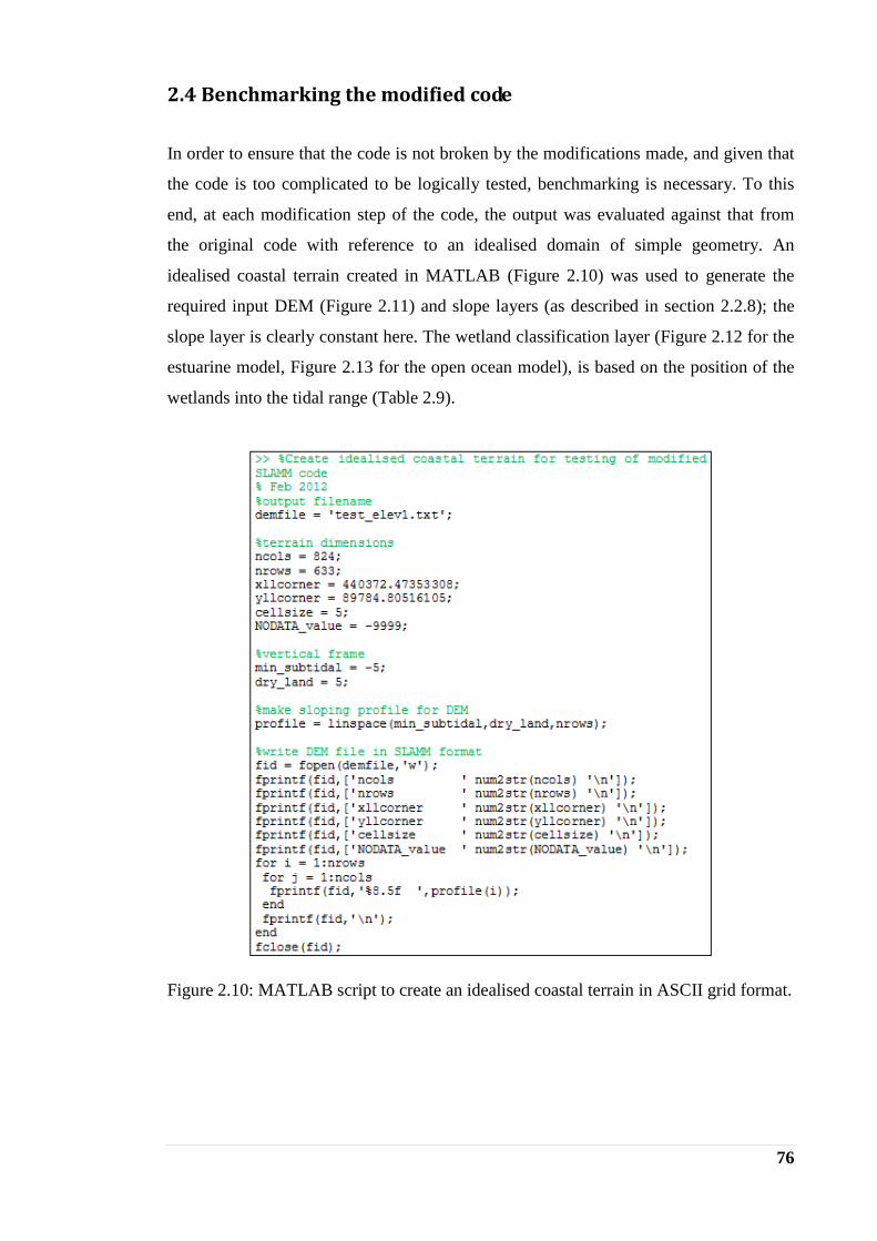
76

2.4 Benchmarking the modified code

In order to ensure that the code is not broken by the modifications made, and given that

the code is too complicated to be logically tested, benchmarking is necessary. To this

end, at each modification step of the code, the output was evaluated against that from

the original code with reference to an idealised domain of simple geometry. An

idealised coastal terrain created in MATLAB (Figure 2.10) was used to generate the

required input DEM (Figure 2.11) and slope layers (as described in section 2.2.8); the

slope layer is clearly constant here. The wetland classification layer (Figure 2.12 for the

estuarine model, Figure 2.13 for the open ocean model), is based on the position of the

wetlands into the tidal range (Table 2.9).

Figure 2.10: MATLAB script to create an idealised coastal terrain in ASCII grid format.

77

Figure 2.11: The elevation input layer of the idealised coastal terrain.

Table 2.9: Criteria for defining habitat position in the estuary and open ocean model

(note that numerical values here are purely for illustrative purposes).

Coastal Habitats

in the Estuary

Model

Coastal Habitats in the

Open Ocean Model

Criteria for defining habitat

position based on elevation and

tidal level

Dry Land DryLand >HAT >1.9

Transitional marsh

Ocean Beach

Ocean Flat

MHWS-HAT 1.5-1.9

Upper marsh MHW-MHWS 1.15-1.5

Lower marsh MHWN-MHW 0.8-1.15

Tidal Flat LAT-MHWN (-2.6)-0.8

Estuarine Subtidal Open Ocean <LAT <(-2.6)

78

Figure 2.12: The estuarine model layer.

Figure 2.13: The Open Ocean model layer for (a) muddy and (b) sandy environments.

79

Before each simulation, the site parameters (Table 2.10) are defined, where more

parameters are required in the modified code in order to describe an area, due to the

third modification step. Accordingly, the wetland boundary conditions are automatically

updated within the modified code, while they must be manually adjusted within the

original code. The simulations are executed under the A1B max IPCC sea-level rise

scenario within a time-step of 25 years.

Table 2.10: Site Parameters Table (note that numerical values are purely for illustrative

purposes).

ORIGINAL SLAMM CODE MODIFIED SLAMM CODE

Historic Trend (mm yr-1

) Historic Trend (mm yr-1) 1.5

GT Great Diurnal Tide Range (m) GT Great Diurnal Tide Range (m) 3.4

Salt Elevation (m above MTL) Salt Elevation (m above MTL) 1.9

HAT (m) 1.9

MHWS (m) 1.5

MHW (m) 1.15

MHWN (m) 0.8

LAT (m) -2.6

Marsh Erosion (m yr-1

) Marsh Erosion (m yr-1

) 0.25

T.Flat Erosion (m yr-1

) T.Flat Erosion (m yr-1

) 0.2

Reg. Flood Marsh Accr (mm yr-1

) Lower Marsh Accr (mm yr-1

) 2.0

Irreg. Flood Marsh Accr (mm yr-1

) Upper Marsh Accr (mm yr-1

) 1.8

Tidal Fresh Marsh Accr(mm yr-1

) Tidal Fresh Marsh Accr(mm yr-1

) -

Beach Sed.Rate (mm yr-1

) Beach Sed.Rate (mm yr-1

) 2.0

Firstly, the modified code is benchmarked within the estuarine environment. The first

step (“TM1”) simply adopts the UK-based wetland classification; the fact that no

quantitative changes in overall intertidal areas are predicted confirms that this

modification has no adverse effect on the model algorithm. Thus, this code is then used

to benchmark the next step with the modified transition rules (“TM2”), where different

projected areas are generated for the lower and upper marsh category without affecting

the behaviour of the other ones (Table 2.11; Figure 2.14).

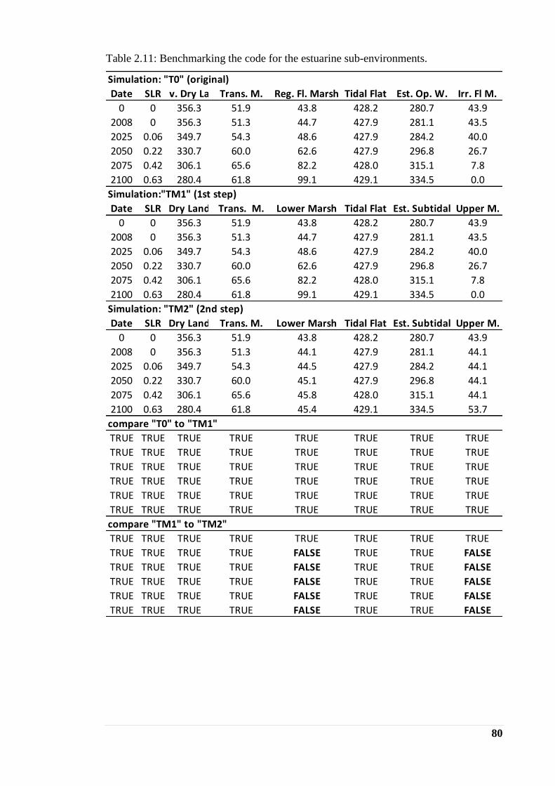
80

Table 2.11: Benchmarking the code for the estuarine sub-environments.

Simulation: "T0" (original)

Date SLRDev. Dry LandTrans. M. Reg. Fl. Marsh Tidal Flat Est. Op. W. Irr. Fl M.

0 0 356.3 51.9 43.8 428.2 280.7 43.9

2008 0 356.3 51.3 44.7 427.9 281.1 43.5

2025 0.06 349.7 54.3 48.6 427.9 284.2 40.0

2050 0.22 330.7 60.0 62.6 427.9 296.8 26.7

2075 0.42 306.1 65.6 82.2 428.0 315.1 7.8

2100 0.63 280.4 61.8 99.1 429.1 334.5 0.0

Simulation:"TM1" (1st step)

Date SLR Dry Land Trans. M. Lower Marsh Tidal Flat Est. Subtidal Upper M.

0 0 356.3 51.9 43.8 428.2 280.7 43.9

2008 0 356.3 51.3 44.7 427.9 281.1 43.5

2025 0.06 349.7 54.3 48.6 427.9 284.2 40.0

2050 0.22 330.7 60.0 62.6 427.9 296.8 26.7

2075 0.42 306.1 65.6 82.2 428.0 315.1 7.8

2100 0.63 280.4 61.8 99.1 429.1 334.5 0.0

Simulation: "TM2" (2nd step)

Date SLR Dry Land Trans. M. Lower Marsh Tidal Flat Est. Subtidal Upper M.

0 0 356.3 51.9 43.8 428.2 280.7 43.9

2008 0 356.3 51.3 44.1 427.9 281.1 44.1

2025 0.06 349.7 54.3 44.5 427.9 284.2 44.1

2050 0.22 330.7 60.0 45.1 427.9 296.8 44.1

2075 0.42 306.1 65.6 45.8 428.0 315.1 44.1

2100 0.63 280.4 61.8 45.4 429.1 334.5 53.7

compare "T0" to "TM1"

TRUE TRUE TRUE TRUE TRUE TRUE TRUE TRUE






compare "TM1" to "TM2"


TRUE TRUE TRUE TRUE FALSE TRUE TRUE FALSE





81

Figure 2.14: Benchmark the 2nd

modification step (TM1: 1st step; TM2: 2

nd step).

This change was expected, but further investigation is required in order to ensure that

nothing else is affected. Table 2.12 summarises the habitat conversion rules in each

time-step. Although, the conversion rule for the transitional marsh is modified and

converted to upper marsh instead of lower marsh, the amount of area converted is not

82

affected, as desired. This modification results in a more dynamic behaviour of the upper

marsh by assuming that this habitat also migrates upland to transitional marsh; in the

original SLAMM code it is assumed that it only loses area to lower marsh, giving rise to

a continual decrease in the area of this habitat. These changes means that, in the test

case, 20ha of upper marsh are inundated at the last time-step when using the modified

code while only 8ha according to the original one.

Table 2.12: Habitat conversion rules in each simulation (TM1: 1st step, TM2 :2

nd step).

Simulation: "TM1"

DRYLAND TRANS.M. UPPER LOWER TIDAL F. ES.SUBTIDAL0-2008 0 -0.60 -0.36 0.84 -0.24 0.36

0.60 0.96 0.12 0.36

2008-2025 -6.54 3.02 -3.52 3.95 0.01 3.08

6.54 3.52 7.04 3.09 3.08

2025-2050 -18.99 5.67 -13.32 13.96 0.02 12.66

18.99 13.32 26.64 12.67 12.66

2050-2075 -24.60 5.67 -18.93 19.59 0.02 18.25

24.60 18.93 37.86 18.28 18.25

2075-2100 -25.74 -3.86 -7.76 16.88 1.09 19.39

25.74 29.60 37.36 20.47 19.39

Simulation: "TM2"

DRYLAND TRANS.M. UPPER LOWER TIDAL F. ES.SUBTIDAL0-2008 0 -0.60 0.24 0.24 -0.24 0.36

0.60 0.36 0.12 0.36

2008-2025 -6.54 3.02 0.00 0.43 0.01 3.08

6.54 3.52 3.52 3.09 3.08

2025-2050 -18.99 5.67 0.00 0.64 0.02 12.66

18.99 13.32 13.32 12.67 12.66

2050-2075 -24.60 5.67 0.00 0.66 0.02 18.25

24.60 18.93 18.93 18.28 18.25

2075-2100 -25.74 -3.86 9.53 -0.41 1.09 19.39

25.74 29.60 20.06 20.47 19.39

DRYLAND TRANS.M. UPPER LOWER TIDAL F. ES.SUBTIDAL0-2008 TRUE TRUE FALSE FALSE TRUE TRUE

TRUE TRUE FALSE TRUE TRUE

2008-2025 TRUE TRUE FALSE FALSE TRUE TRUE








The modified code is also benchmarked for the open coast sub-environments that are

presented in SLAMM. Since the first modification step does not affect directly the

coastal model, its benchmarking is ignored but used to investigate the response of each

coastal category to the sea-level rise, by recognising two different cases depending on

the context of the shore; a sandy (“TM1o_beach”) and a muddy (“TM1o_flat”) shore

(Table 2.13; Figure 2.15). The muddy tidal flat is more capable to cope with the sea-

83

level rise, while most of the sandy beach is lost to the ocean according to the Bruun

rule. In addition, although the muddy environment presents the same transition rules to

the estuarine one, a more complex behaviour is presented on the sandy environment,

due to the different responses of the dryland to sea-level rise based on its proximity to

the open ocean (see Table 2.5). Thus, at the beginning of the simulation, inundated

dryland is converted to transitional marsh, since it is not close to the ocean, while most

of the ocean beach is eroded. Thus, the area of the open ocean is dramatically increased

considering the dryland adjacent to the ocean at the last time-steps. At these time-steps

dryland is inundated to ocean beach. Finally, it is worth mentioning here that although

the criteria for the procedure of erosion are not met (actual maximum fetch <9 km),

transitional marsh is eroded to tidal flat at year 2075. This is explained by the fact that

the fetch is assumed as infinite at locations where open water persists to the edge of the

study area (SLAMM forum).

Table 2.13: Open coast sub-environment model behaviour (1st modification step for (a)

sandy and (b) muddy shore).

84

Figure 2.15: Different responses of the ocean environment (a: sandy shore, b: muddy

shore) to sea-level rise.

85

Due to the appearance of marsh in both simulations, the second modification step needs

to be benchmarked for each case (“TM2o_beach”, “TM2o_flat” in Table 2.14).

Different results are generated only at the last time-step of both simulations, where

inundation of transitional marsh occurs. Similarly to the estuarine environment,

transitional marsh is inundated to upper marsh instead of lower marsh, but the inundated

area is the same, indicating that this conversion rule is applied correctly to the coastal

model too. Consequently, the overall benchmarking of the code can be judged to have

been successful, and therefore the modified code can be applied with confidence to

other UK estuarine environments.

Table 2.14: Benchmark the 2nd

modification step in the ocean model for a (a) sandy

shore and a (b) muddy shore.

(a) Simulation "TM1o_beach" (1st modification step)

Date SLR DRYLAND TRANS. UPPER LOWER T. FLAT ES. SUBT. OC.BEACHOC.FLAT OP.OCEAN

0 0 356.3 0 0 0 0 0 567.8 0 280.7

2008 0 356.3 0 0 0 0 0 567.4 0 281.1

2025 0.0622 349.7 6.5 0 0 0 0 467.7 0 380.8

2050 0.2182 330.7 25.5 0 0 0 0 0.0 0 848.5

2075 0.4187 306.1 23.5 0 0 2 0 16.4 0 856.7

2100 0.6282 280.4 11.4 0 12.1 0 2 15.9 0 883.0

Simulation "TM2o_beach" (2nd modification step)


0 0 356.3 0 0 0 0 0 567.8 0 280.7

2008 0 356.3 0 0 0 0 0 567.4 0 281.1

2025 0.0622 349.7 6.5 0 0 0 0 467.7 0 380.8

2050 0.2182 330.7 25.5 0 0 0 0 0.0 0 848.5

2075 0.4187 306.1 23.5 0 0 2 0 16.4 0 856.7

2100 0.6282 280.4 11.4 12.1 0 0 2 15.9 0 883.0

(b) Simulation "TM1o_flat" (1st modification step)


0 0 356.3 0 0 0 0 0 0 567.8 280.7

2008 0 356.3 0 0 0 0 0 0 567.4 281.1

2025 0.0622 349.7 6.5 0 0 0 0 0 564.3 284.2

2050 0.2182 330.7 25.5 0 0 0 0 0 551.7 296.8

2075 0.4187 306.1 50.1 0 0 0 0 0 533.4 315.1

2100 0.6282 280.4 61.8 0 14.1 0 0 0 514.0 334.5

Simulation "TM2o_flat" (2nd modification step)


0 0 356.3 0 0 0 0 0 0 567.8 280.7

2008 0 356.3 0 0 0 0 0 0 567.4 281.1

2025 0.0622 349.7 6.5 0 0 0 0 0 564.3 284.2

2050 0.2182 330.7 25.5 0 0 0 0 0 551.7 296.8

2075 0.4187 306.1 50.1 0 0 0 0 0 533.4 315.1

2100 0.6282 280.4 61.8 14.1 0 0 0 0 514.0 334.5

86

2.5 Model application and evaluation

2.5.1. Newtown Estuary, Isle of Wight, UK

Newtown estuary, on the Isle of Wight, southern England, was selected as a pilot study

on account of its small size and computational tractability. Newtown is one of five

estuaries on the Isle of Wight, UK (Figure 2.16). It is located on the north coast between

the Western Yar and Medina estuaries. More generally, it is part of the estuarine system

of Solent (Cope et al., 2008). The estuary has been under the protection of the National

Trust since 1965 and includes the only National Nature Reserve of the Isle of Wight, the

Newtown Harbour (which consists of the Newtown River and the surrounding land).

This National Nature Reserve supports important and also threatened wildlife by

providing feeding and over-wintering ground, especially for waders and other wildfowl,

like Brent goose, widgeon, teal and black-tailed godwit (Gardiner et al., 2007; Isle of

Wight SMP2, 2010). The Newtown River is also designated as an Area of Outstanding

Natural Beauty (AONB) and has been designated as a Site of Special Scientific Interest

(SSSI) since 1951.

The mouth of the estuary is dominated by intertidal sand backed by low maritime cliffs

which are then backed by agricultural land. Habitats within the estuary include

saltmarsh and mudflats, and an important saline lagoon, formed within the site of old

salt workings, exists at the Newtown Quay. The Newtown estuary coastline, much like

the rest of the north coastline of the island, is relatively undeveloped and has been

subject to long-term retreat (Gardiner et al., 2007). Although the eroding cliffs produce

a lot of sediment, most of it is transported offshore and therefore cannot protect local

beaches from retreat (Isle of Wight SMP2, 2010).

The coastline is mesotidal, with a tidal range of 3.4 m calculated based on the closest

tide gauge station at Cowes (around 8km to the northeast). Most of the marsh surfaces

lay between 0.8m and 1.9m OD, with the highest astronomical tides reaching almost 2m

OD (UK Hydrographic Office, 2000).

87

Figure 2.16: Aerial photo of the Newtown Estuary, Isle of Wight, with overlay of

principal habitats, focusing on (a) the mouth of the estuary and (b) the saline lagoons

existing at the Newtown Quay (Source: Google Earth).

In contrast to the southwest part of the island, which is exposed to storm waves within

the English Channel, its north-west coast is protected from the open ocean. Thus, the

waves generated in the West Solent are fetch-limited and do not exceed 1m in height

(SCOPAC, 2003). As a consequence, the northern part of the island is undefended with

only minor defences in limited locations.

The Newtown estuary is an undeveloped and naturally evolving inlet with only defence

localised defence walls and embankments at Shalfleet Quay, Newtown Quay due to

saltworks and on the upper part of Shalfleet Lake. These currently have a residual life

15 to 25 years (Isle of Wight SMP2, 2010; Figure 2.17). The general lack of coastal

defences will allow the habitats to migrate inland, such that coastal squeeze is not a

major concern here (Gardiner et al., 2007). The estuary entrance consists of two spits.

Although the western spit is active and has rolled back, the eastern one does not show

similar behaviour except for a landward shift between 1962 and 1995 of around 30 m

(Gardiner et al., 2007). However, the eastern spit has breached, leaving some saltmarsh

areas unprotected from the wave action (Bray and Cottle, 2003).

88

Figure 2.17: Coastal defences (Source: Isle of Wight SMP2, 2010).

The modified SLAMM code was applied in this pilot case study in order to undertake a

sensitivity analysis of the various model parameters and external forcing involved.

LIDAR data, available at no cost from the Channel Coastal Observatory

(http://www.channelcoast.org/), were used to generate the required from SLAMM input

layers, while site specific data are available from projects previously undertaken in this

case study.

2.5.2. Blyth and Deben estuaries, Suffolk, UK

The Blyth and Deben estuaries, two small estuarine systems on Suffolk, eastern

England, were selected in order to critically evaluate the ability of the model to produce

meaningful projections of intertidal habitat change under a set of UKCP09 scenarios. As

noted earlier, these sites were selected due to availability of background literature on

habitats and sedimentary processes, as well as bathymetric datasets. The latter was

supplemented the Environment Agency LiDAR data made available through the NERC

iCOASST project (Nicholls et al., 2012; 2015).

The Blyth estuary is a barrier-enclosed system in a mainly rural catchment of 214 km2

in Suffolk (Figure 2.18) with a dune-backed sand and gravel beach that extends

southwards from an elevated headland where the town of Southwold is situated (French,

2008). It contains a mosaic of coastal, wetland and heathland habitats supporting a

diverse fauna and flora, including nationally rare and scarce species. Thus, it is included

within a Special Protection Area and Ramsar Site, the Minsmere-Walberswick SSSI. It

http://www.channelcoast.org/

89

also lies within the Suffolk Coast and Heaths Area of Outstanding Natural Beauty

(AONB) (Environment Agency, 1999a, 2009).

Figure 2.18: Aerial photo of the Blyth estuary, Suffolk, with overlay of principal

habitats.

The Blyth estuary has a tidal length of 10.7 km (French, 2001), and it can be

characterised as microtidal (Fairbridge, 1980; Davidson et al., 1991) with average

ranges at Southwold of 2.0 m and 1.2 m at springs and neaps respectively. Highest

Astronomical Tide (HAT), Mean High Water Springs (MHWS) and Mean sea-level

(MSL) are approximately 1.6 m, 1.1 m and 0.2 m above Ordnance Datum (OD)

respectively. The estuary is well-mixed, with a small freshwater inflow (0.4 m3s

-1 at

Halesworth, (Institute of Hydrology, 1996)) in comparison with the tidal prism (3 x 106

m3 on a mean spring tide) (French, 2008; French and Burningham, 2003; French et al.,

2000, 2008).

Over 14 m of muddy sediment, with gravel and sand at the mouth, have been deposited

in the estuary over the last 6,500 years (Brew et al., 1992). Taking into account the

negligible sediment supply from the River Blyth itself, the sediment is derived from the

North Sea and from the continuing process of erosion of the coastline further north, and

90

transported into the estuary driven by waves (French, 2008; French and Burningham,

2003; French et al., 2008).

Extensive reclamation of agricultural land took place in the second half of the 18th

century (Lawrence, 1990), and by 1840 all tidal flat marshes were reclaimed (Beardall

et al., 1991; Buncombe, 1994), confining the estuary to a narrow channel. The defences

are primarily earth embankments, with protection at some places, and they are near the

end of their life (Environment Agency, 2009). The Sandpit Marshes were abandoned in

the 1920s, followed by the Bulcamp and Angel Marshes in the 1940s. Although the

Angel Marshes are partially reverted to salt marsh, the other two are muddy tidal flats

(Figure 2.19) (French, 2008; French and Burningham, 2003; French et al., 2000).

The narrow mouth of the estuary is maintained by two piled breakwaters, set 40m apart

(French, 2008; French and Burningham, 2003; French et al., 2008). At the south of the

mouth a narrow sand shingle beach exist, backed by dunes for the first 500 m south of

the harbour, but then giving way to a narrow maintained shingle embankement. In

contrast, the shore to the north comprises a wide sand shingle beach, backed by dunes.

The dune strip, the Denes, has grown and stabilised since the north breakwater

construction, forming the seaward flood barrier to the Havenbeach Marshes. The last

one, together with the Woodsend and Town Marshes upstream, are below mean tide

level and used as pastures (Environment Agency, 1999a).

Further upstream, the Buss Creek Marshes are located leading into Botany Marshes,

where the main sewage works of the area exist. At its northwest side, the Reydon

Marshes are located, opposite of which the Tinkers Marsh exist (Environment Agency,

1999a). At this point of the river, the defences are fronted by a 2 - 3 m plateau of

intertidal saltmarsh. These widths have been eroded in many places, especially in

response to the storm surges of 2007 (Environment Agency, 2009) and 2013 (Spencer et

al., 2014). Combined with the deep channel bed in this area, this has led to serious

problems of instability and the forward slumping failure of defences. It is worth

mentioning here, that the Tinkers Marsh embankment, especially along its western end,

is the lowest level of flood defence within the whole estuary. The Tinkers Marsh is

divided by the Robinson’s Marsh at the south by Squire’s Hill and the sewage pipe

embankment to the bridge (Environment Agency, 1999a, 2009).

91

Finally, upstream of the estuary and towards to Blyford Bridge, the narrow channel has

a width of 300-500 m and is surrounded by low farmland. Here, the low embankments

do not completely constrain the main river channel, leaving space for natural

development of the channel. Also, they are failing due to storm surges in 2006 and 2007

(Environment Agency, 1999a, 2009).

Figure 2.19: Flood compartments at the Blyth Estuary (Environment Agency, 2009),

focusing on the piled breakwaters existing at the mouth of the estuary.

In contrast, the Deben is a long and narrow estuary extending for over 20 km south-

eastwards from the town of Woodbridge to the sea north of Felixstowe (Figure 2.20).

Most of its intertidal area is occupied by tidal flats, and it also occupies extensive and

92

diverse saltmarsh communities (approximately 28% of the total saltmarsh area of

Suffolk; CHaMP, 2002), supporting overwintering waders and wildfowl. Thus, it is

designated as a SSSI and a Special Protection Area and is also Ramsar Site. It is also

included within the Suffolk AONB and its southern half is designated as Heritage Coast

(Environment Agency, 1999b).

Figure 2.20: Aerial photo of the Deben estuary, Suffolk, with overlay of principal

habitats, focusing on (a) the extensive saltmarsh area at the middle estuary and (b) the

mouth of estuary (Source: Google Earth).

The Deben estuary can be characterised as mesotidal with 3.2 m tidal range on springs

and 1.9 m on neaps at the mouth, and a higher (by about 0.3 - 0.4 m) range at

Woodbridge. The estuary is dominated by tidal processes, and the influence of fresh

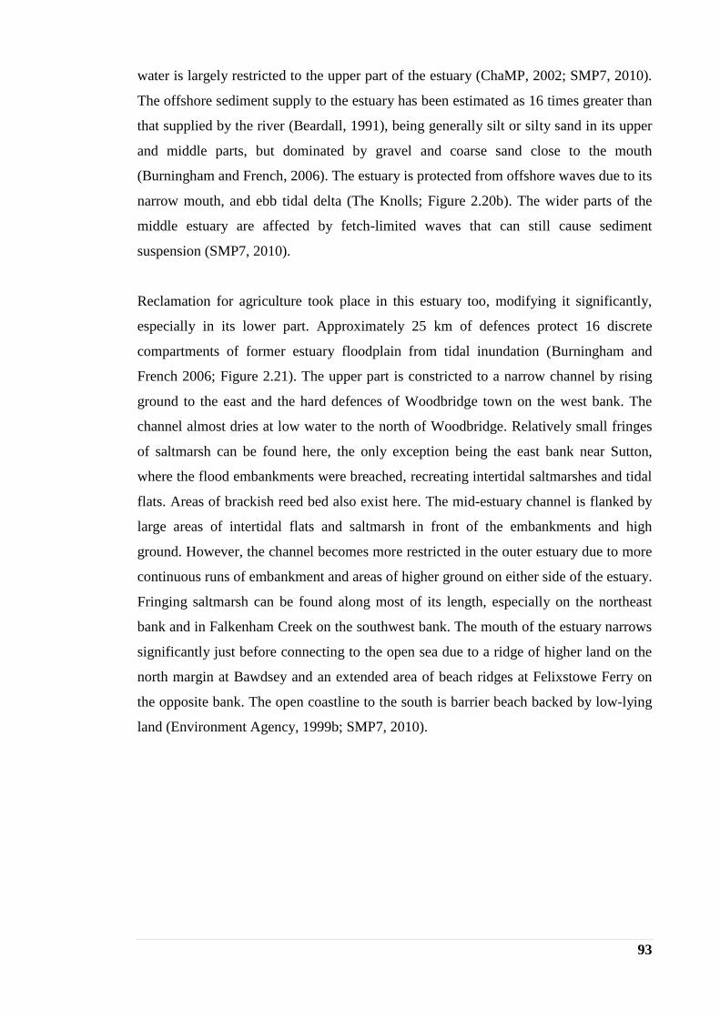
93

water is largely restricted to the upper part of the estuary (ChaMP, 2002; SMP7, 2010).

The offshore sediment supply to the estuary has been estimated as 16 times greater than

that supplied by the river (Beardall, 1991), being generally silt or silty sand in its upper

and middle parts, but dominated by gravel and coarse sand close to the mouth

(Burningham and French, 2006). The estuary is protected from offshore waves due to its

narrow mouth, and ebb tidal delta (The Knolls; Figure 2.20b). The wider parts of the

middle estuary are affected by fetch-limited waves that can still cause sediment

suspension (SMP7, 2010).

Reclamation for agriculture took place in this estuary too, modifying it significantly,

especially in its lower part. Approximately 25 km of defences protect 16 discrete

compartments of former estuary floodplain from tidal inundation (Burningham and

French 2006; Figure 2.21). The upper part is constricted to a narrow channel by rising

ground to the east and the hard defences of Woodbridge town on the west bank. The

channel almost dries at low water to the north of Woodbridge. Relatively small fringes

of saltmarsh can be found here, the only exception being the east bank near Sutton,

where the flood embankments were breached, recreating intertidal saltmarshes and tidal

flats. Areas of brackish reed bed also exist here. The mid-estuary channel is flanked by

large areas of intertidal flats and saltmarsh in front of the embankments and high

ground. However, the channel becomes more restricted in the outer estuary due to more

continuous runs of embankment and areas of higher ground on either side of the estuary.

Fringing saltmarsh can be found along most of its length, especially on the northeast

bank and in Falkenham Creek on the southwest bank. The mouth of the estuary narrows

significantly just before connecting to the open sea due to a ridge of higher land on the

north margin at Bawdsey and an extended area of beach ridges at Felixstowe Ferry on

the opposite bank. The open coastline to the south is barrier beach backed by low-lying

land (Environment Agency, 1999b; SMP7, 2010).

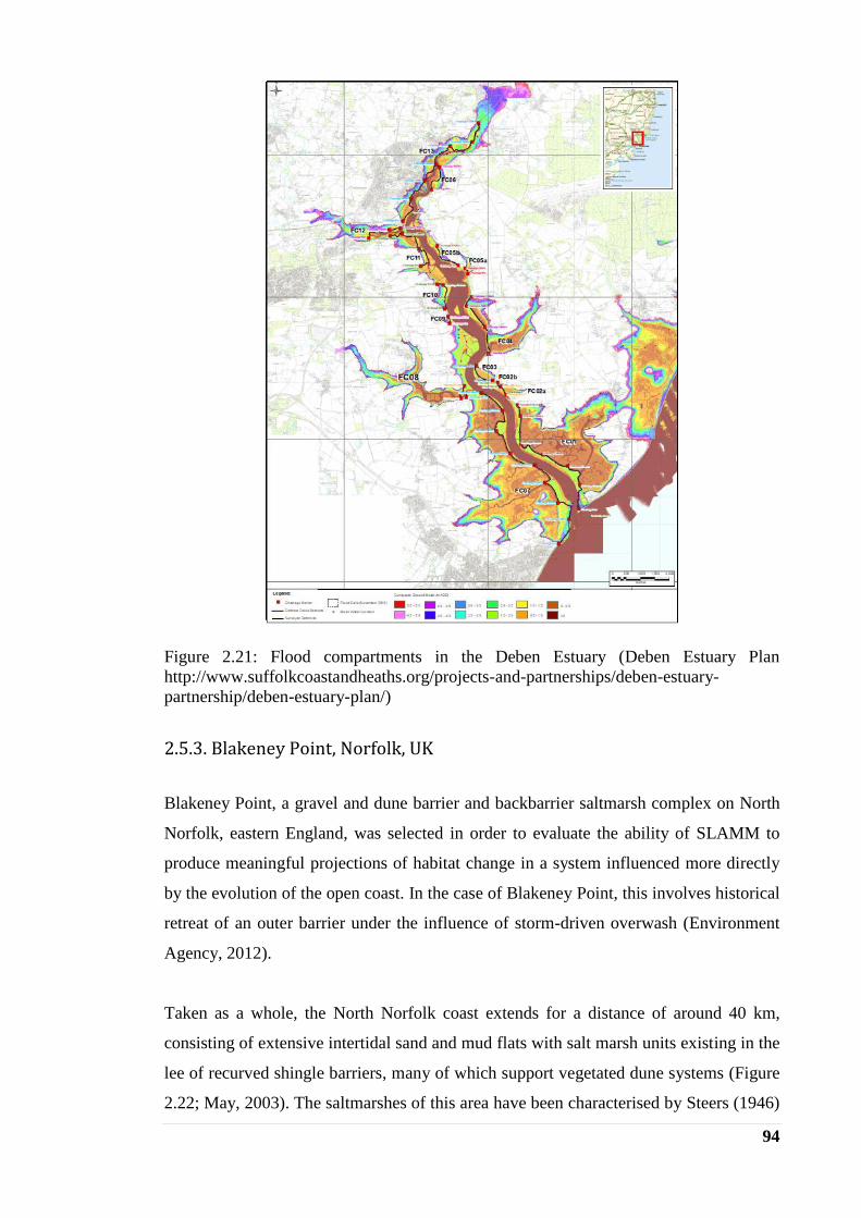
94

Figure 2.21: Flood compartments in the Deben Estuary (Deben Estuary Plan

http://www.suffolkcoastandheaths.org/projects-and-partnerships/deben-estuary-

partnership/deben-estuary-plan/)

2.5.3. Blakeney Point, Norfolk, UK

Blakeney Point, a gravel and dune barrier and backbarrier saltmarsh complex on North

Norfolk, eastern England, was selected in order to evaluate the ability of SLAMM to

produce meaningful projections of habitat change in a system influenced more directly

by the evolution of the open coast. In the case of Blakeney Point, this involves historical

retreat of an outer barrier under the influence of storm-driven overwash (Environment

Agency, 2012).

Taken as a whole, the North Norfolk coast extends for a distance of around 40 km,

consisting of extensive intertidal sand and mud flats with salt marsh units existing in the

lee of recurved shingle barriers, many of which support vegetated dune systems (Figure

2.22; May, 2003). The saltmarshes of this area have been characterised by Steers (1946)

http://www.suffolkcoastandheaths.org/projects-and-partnerships/deben-estuary-partnership/deben-estuary-plan/

http://www.suffolkcoastandheaths.org/projects-and-partnerships/deben-estuary-partnership/deben-estuary-plan/

95

as the finest coastal marshes in Great Britain. The coastline is macrotidal, subjected to a

strong tidal influence especially at the west with a mean range of 3.4 m at neaps and 6.4

m at springs, where most of the marsh surfaces lay between 2 m and 3.2 m OD; the

larger dune-covered barriers reach a height of 15 - 20 m OD. The highest astronomical

tides reach almost 4 m OD, although storm surges can increase water level to over 5m

OD (French et al., 1990, 1995; French 1993; Reed et al, 1999).

Figure 2.22: The coast of North Norfolk (May, 2003).

Blakeney Point (Figure 2.23) is a large shingle spit extending from Sheringham

westwards for over 17 km. The first 5.5 km enclose low cliffs of glacial till, while the

central part forms a ridge of about 200 m width and almost 10m height, in front of the

Salthouse Marsh and the Fresh Marsh. Finally, the western part continues for 3km as a

single ridge and develops then a series of long recurves with a south/south-westward

trend. These are the most recent members of a set of shingles, indicating the westwards

growth of the spit (May, 2003). Consequently, the age of the marshes at either side of

the Blakeney channel also increases eastwards, with the oldest one probably developed

during the 15th

century (Pethick, 1980), while lateral growth of new marsh has been

occurring at the western end of Blakeney since the 1950s (Pye and French, 1993 in May

2003). Marshes also exist at the east side of Blakeney, but most of them have been land-

claimed (May, 2003).

96

Figure 2.23: Aerial photo of Blakeney spit, Norfolk, including its associated backbarrier

environments, and focusing on its western part (Source: Google Earth).

97

3 SLAMM SENSITIVITY ANALYSIS: APPLICATION TO

NEWTOWN ESTUARY, ISLE OF WIGHT, UK

3.1 Previous work on the Newtown Estuary

3.1.1 Shoreline Management Plan SMP2

The current (phase 2) SMP for the Isle of Wight was developed by the Council of the

Isle of Wight (Isle of Wight SMP2, 2010). It covers all the coastline of the island (110

km) which is divided it into seven zones, where the Newtown Estuary is part of the

North-West Coastline (PDZ7). For each zone, future erosion and flood risk maps are

produced for two different management scenarios:

No Active Intervention (NAI) scenario: no further coastal defence work is

necessary

With Present Management (WPM) scenario: present practises are continued into

the future.

Flood risk maps for the Newtown Estuary are presented in Figure 3.1. The erosion risk

map is created by applying the future erosion rates, calculated by using the Walkden

and Dickson (2008) formula (equation 3.1; Table 3.1), to GIS maps layers, thereby

indicating the eroded zone for each year. When coastal defence structures exist, the

erosion rates are applied from the point at which this structure is predicted to fail,

otherwise it is applied from the first year (Isle of Wight SMP2, 2010).

ε2=ε1 *1

2

S

S, (3.1)

where, ε1= historic recession rate, ε2= future recession rate, S1=historic sea-level rise,

S2= future sea-level rise (produced in accordance to national government guidance

issued by DEFRA in 2006, which aimed to define the sea-level allowances to be used in

coastal management plans and schemes (DEFRA, 2006; Table 3.2)

98

Figure 3.1: Erosion and flood risk map for no active interaction scenario (a: Entrance to

Newtown Estuary, b: Southern Newtown Estuary) (after Isle of Wight SMP2, 2010).

Table 3.1: Erosion Rates for the Newtown Estuary (Isle of Wight SMP2, 2010).

Erosion Rates (m year-1

)

Historic Current

to 2025

2025

to

2055

2055

to

2085

2085

to

2105

Potential 100

year erosion

(m)

(unprotected)

Western Spit 0.6 0.69 0.91 1.06 1.15 96

Eastern Spit 0.62 0.72 0.94 1.10 1.19 99

Inside Eastern Spit 0.2 0.23 0.30 0.35 0.35 32

99

Table 3.2: Sea-level rise for the Isle of Wight.

Future Sea Level Rise (cm)

(Isle of Wight SMP2, 2010)

Sea Level Rise Allowance

(mm year-1

)

(DEFRA, 2006) From 1990 From 2009

By 2025 +14 +7 4

By 2055 +39.5 +32 8.5

By 2085 12

By 2105 +105.5 +98 15

The flood risk map created is based on the flood zones supplied by the Isle of Wight

Strategic Flood Risk Assessment (Isle of Wight SFRA, 2009). The latter are based on

ArcGIS shapefiles supplied by the Environment Agency, all taking into account sea-

level rise data supplied by DEFRA (2006; Table 3.2) and PPS25 (2006). The outline for

the SMP2 flood zones was created by using the worst case scenario supplied by Isle of

Wight Council. This outline was then combined to the ‘Tide Level map’ supplied from

the Environment Agency producing new water levels. These new water levels were

overlaid on topography in order to provide the flood risk maps (Isle of Wight SMP2,

2010).

3.1.2 BRANCH Project

The BRANCH project is a trans-national project aiming to show how spatial planning

can help biodiversity to adapt to climate change (BRANCH partnership, 2007). Its

‘coastal package’ aimed to develop and also test spatial planning tools for coastal and

estuarine systems in order to inform their management with regard to climate change

effects on biodiversity (BRANCH project partners, 2003). The Newtown Estuary is one

of the local-scale case studies of this project. Historical data were used in order to

establish the baseline information, and aerial photographs and LiDAR data to obtain the

habitat distribution, all in GIS. Four sea-level rise scenarios are developed (Low,

Medium-Low, Medium-High, High) for three time periods (2020s, 2050s, 2080s) based

on the UKCIP (Hulme et al., 2002). However, rates of sea-level rise are necessary for

modelling, thus the annual sea-level rise rates are calculated between these time-

periods. Finally, two different modelling approaches are applied to the Newtown

Estuary in order to assess the impacts of climate change; one for the intertidal habitats

and one for the spits (Gardiner et al., 2007).

100

In the case of the spits, historic shoreline positions were compiled by digitising the

mean high water (MHW) shorelines from past maps (Figure 3.2). Historic retreat rates

were computed using the Leatherman’s (1990) equation (eq. 3.2), in order to estimate

the future retreat rates under the Medium-High emission scenarios, and further model

the recession of the spits (Figure 3.3).

ε2=ε1 * 1

2

S

S (3.2)

where, ε1= Historic recession rate, ε2= future recession rate, S2= Future sea-level rise,

S1=Historic sea-level rise. This equation differs from the Walkden and Dickson (2008)

equation; it is linear with sea-level rise and results follow the Bruun Rule’s assumptions

(Gardiner et al., 2007).

Figure 3.2: Historical analysis of the western (A) and eastern (B) spit at Newtown

Estuary as part of the BRANCH project (after Gardiner et al., 2007).

Figure 3.3: Recession analysis of the spits at Newtown Estuary (under the Medium-high

emission scenario as part of the BRANCH project; Gardiner et al., 2007).

101

The distribution of intertidal habitats was generated using airborne LiDAR data,

according to their elevation within the tidal frame (Figure 3.4). In order to assess the

impacts of sea-level rise on these habitats, the new expected sea level was added onto

the tidal parameters. For more realistic results, the analysis also included the effects of

vertical accretion of 2mm/year and 4mm/year (Figures 3.4 b-d for the Medium-High

emission scenario with 2mm accretion).

Figure 3.4: Newtown Estuary (A: current saltmarsh extent; B: saltmarsh in 2020s; C:

saltmarsh in 2050s, D: saltmarsh in 2080s; the future positions are modelled for the

Medium-High emission scenario and 2mm accretion rate as part of the BRANCH

project; after Gardiner et al., 2007).

102

3.2 Preliminary application of the modified SLAMM code

In the present study, the modified SLAMM code was applied to Newtown, in order to

undertake a sensitivity analysis of the various model parameters and external forcing

involved. As noted previously, a key factor influencing the initial selection of the

Newtown estuary was the availability of LiDAR data at no cost from the Channel

Coastal Observatory (http://www.channelcoast.org/). At this stage in the project,

LiDAR were not generally available for most of the estuaries in England and Wales.

These data have a sampling interval of 1m and an indicative vertical accuracy of ±15

cm. LiDAR data combined with digitised bathymetry data in ARC-GIS 9.3 in order to

create the input DEM for SLAMM (Figure 3.5). Given the quality of the LiDAR data,

the elevation pre-processing option in SLAMM was not used. The DEM was used to

derive the slope (Figure 3.6) and the land classification map based on wetland position

in the tidal frame (Figure 3.7; Table 3.3), as described in Chapter 2. All input layers

were resampled to a 5 m horizontal interval.

Figure 3.5: Elevation map of Newtown Estuary created using a GIS.

103

Figure 3.6: Slope map of Newtown Estuary created using a GIS.

Figure 3.7: Land classification (habitat) map of Newtown Estuary created using a GIS.

104

Table 3.3: Tidal criteria for modelling vertical zonation of inter-tidal areas. Tidal levels

are derived from the Admiralty tide tables (UK Hydrographic Office, 2000).

Coastal habitats and

land classification

Criteria for defining habitat position based

on elevation and tidal level

Tidal level Elevation (m) E

stu

ary

mod

el

1. Dry land >HAT > 1.9

7. Transitional marsh MHWS-HAT 1.5 - 1.9

20. Upper marsh MHW-MHWS 1.15 - 1.5

8. Lower marsh MHWN-MHW 0.8 - 1.15

11. Tidal Flat LAT-MHWN (-2.6) - 0.8

17. Estuarine Subtidal <LAT < (-2.6)

13. Ocean Flat LAT – HAT (-2.6) - 1.9

19. Open Ocean <LAT < (-2.6)

Table 3.4 summarises the additional site-specific parameters used in the sensitivity

analysis model runs. The historic sea-level trend includes the effect of vertical land

movements and is estimated at 1.49 mm yr-1

using the closest tide gauge station at

Portsmouth (almost 25 km to the northwest). The greater diurnal tide range at this site is

calculated by the difference between MHWS and MLWS (3.4 m), while erosion and

accretion parameters are obtained from the SMP2 (Isle of Wight SMP2, 2010) and the

BRANCH project (BRANCH partnership, 2007).

Table 3.4: Site parameter table for Newtown estuary.

Parameter Newtown

DEM Date (YYYY) 2008

Direction Offshore[n,s,e,w] N

Historic Sea Level Trend (mm y-1

) 1.49

GT Great Diurnal Tide Range (m) 3.4

Salt Elevation (m above MTL) 1.9

HAT (m) 1.9

MHWS (m) 1.5

MHW (m) 1.15

MHWN (m) 0.8

LAT (m) -2.6

Marsh Erosion (m y-1

) 0.25

Tidal Flat Erosion (m y-1

) 0.2

Lower Marsh Accr (mm y-1

) 2 *

Upper Marsh Accr (mm y-1

) 1.8 *

Beach Sedimentation Rate (mm y-1

) 2

*Spatially varying accretion values for each wetland category. If the accretion model is

to be used, these parameters are left blank.

105

For the purpose of the sensitivity analysis, simulations were executed under the

UKCP09 SE mean sea-level rise scenario using a time-step of 25 years (Simulation

‘N_UK’). Under this forcing scenario, the estuarine habitats are seemingly able to adapt

to sea-level rise during the early time-steps, although changes in the lower marsh area

are significant by the last time-step (Figure 3.8). In more detail, as presented in Table

3.5, sea-level drives enlargement of the estuarine subtidal by almost 30% by the year

2100. However, the area of the tidal flat increases from about 185 ha in year 2008 to

about 208ha in year 2100, indicating that although part of it is inundated/eroded and

therefore converted to estuarine subtidal, a larger part of it migrates upland to the marsh

area. Consequently, the total area covered by marsh decreases by 2100. Most affected,

though, is the lower marsh area with a decrease of 30%, because in most cases there is

no space for upland migration. The transitional marsh remains quite stable by migrating

upland to dryland, which is also inundated to ocean beach when it is adjacent to the

ocean.

It is worth noting here that differences were not expected in the first time-step where

SLAMM corrects the land classification based on the DEM, since the land classification

is generated from the DEM based on the same conceptual model used in SLAMM.

However, the resolution used for its creation can generate them. In this study, the land

classification layer is generated by the original DEM file of 1m resolution, but they are

both then resampled to 5 m, leading to small differences in the boundaries of some

wetland categories between the two layers. SLAMM tries to correct these small

differences at the first time-step by assuming inundation of the specific cells, ignoring

the process of aggradation. Moreover, while inundation of a habitat within a specific

cell is assumed, its transition to the correct one is based on empirical calculations which

might result in bigger differences. Thus, it is wise to resample the DEM in the desired

resolution first, and based on this generate the required land classification layer. In that

case, the generated layers should have less differences and match he conceptual model

used in SLAMM and therefore the current time-step could be skipped.

106

Table 3.5: Impacts of sea-level rise at the Newton Estuary by the year 2100 (changes in ha).

Simulation name: "N_UK"

Date SLR Dry Land Trans. M. Upper M. Lower M. Tidal Flat Est. Subtidal Ocean Beach Ocean Flat Open Ocean

0 0 638.1 14.3 20.0 51.5 176.4 16.3 0.0 41.6 47.7

2008 0 628.7 19.5 15.8 49.2 185.0 17.3 0.8 41.2 48.4

2025 0.0563 627.7 14.5 15.9 51.7 187.6 17.8 0.4 40.8 49.5

2050 0.1583 625.7 14.4 14.1 49.6 192.5 18.6 0.0 39.7 51.2

2075 0.2778 623.0 14.6 13.4 46.5 197.1 20.2 0.0 37.7 53.4

2100 0.4123 619.5 14.8 13.5 36.8 208.2 21.6 0.0 35.4 56.2

0-2008 -9.4 5.3 -4.3 -2.3 8.6 1.0 0.8 -0.4 0.7

-8.3 -3.1 -7.3 -9.6 -1.0 -0.3 -0.4 -0.7

-1.1

2008-2025 -0.9 -5.1 0.1 2.5 2.6 0.5 -0.5 -0.3 1.0

-0.7 -5.8 -5.6 -3.2 -0.5 -0.7 -0.3 -1.0

-0.2

2025-2050 -2.0 0.0 -1.8 -2.07 4.93 0.80 -0.35 -1.17 1.73

-1.8 -1.8 -3.7 -5.7 -0.80 -0.6 -1.2 -1.73

-0.2

2050-2075 -2.7 0.2 -0.7 -3.2 4.6 1.5 0.0 -2.0 2.2

-2.4 -2.3 -3.0 -6.2 -1.5 -0.3 -2.0 -2.2

-0.3

2075-2100 -3.5 0.2 0.1 -9.7 11.0 1.4 0.0 -2.3 2.8

-3.0 -2.8 -2.7 -12.4 -1.4 -0.5 -2.3 -2.8

-0.5

107

Figure 3.8: Habitat distribution in Newtown Estuary under the SE Mean UKCP09 sea-

level rise scenario by the Year 2100 (Simulation ‘N_UK’).

The BRANCH project approach and SLAMM differ in that the former uses two

different modelling approaches in order to assess the impacts of sea-level rise on an

estuary; one for the open coast and one for the intertidal habitats. In contrast, SLAMM

models the whole estuary at once. More specifically, in BRANCH the spits are

modelled by using empirical relationships based on the assumption that the shoreline

behaviour is included into the previous shoreline movements. However, the spits at the

Newtown estuary have changed their shape and direction throughout the years, such that

this approach tends to overestimate spit recession. On the other hand, SLAMM treats

the open coastal flat in front of the spits exactly with the same way to the intertidal

habitats within the estuary. Here, this tends to result in a more stable estuary mouth, and

this approach therefore has its limitations.

108

Within the estuary proper, previous modelling efforts, including BRANCH, largely

evolve the progressive drowning of the existing topography under sea-level rise. This

approach does not incorporate any mechanistic modelling of habitat transitions, as

SLAMM does by incorporating a flexible decision tree and qualitative relationships. In

addition, the process of erosion is totally ignored in most previous models, and although

the accretion parameter is taken into account by the BRANCH project, it only applies to

areas colonised by saltmarsh. SLAMM introduces more sophistication in that different

accretion and erosion values can be applied for each wetland category. Moreover,

SLAMM can take into consideration the spatiality of the accretion parameter within

each habitat type by calculating it as a time-varying function of elevation, distance to

channel (and salinity, when this sub-model is activated). Given this additional

complexity, a sensitivity analysis is necessary in order to evaluate how important these

parameters are and how they affect the prediction of sea-level rise impacts on the

various parts of the estuarine intertidal.

3.3 Sensitivity Analysis

The sensitivity analysis undertaken here investigates how each input factor within

SLAMM affects the outputs of the model. This can potentially enhance our

understanding of the model. More importantly, the sensitivity analysis will determine if

the additional processes included in SLAMM generate predictions that are significantly

different to those obtained using simpler approaches (such as the BRANCH method).

To this end, an array of SLAMM input parameters is initially defined (Table 3.6), each

one of which is investigated separately. A Matlab-based shell was developed in order to

execute multiple SLAMM simulations in a Monte Carlo framework (Figure 3.9). The

results are presented as graphs showing the percentage change of each intertidal wetland

category relative to the initial condition and the best estimated value of each parameter,

i.e. the values used in Section 3.2 above.

109

Table 3.6: Statistical distribution of SLAMM input factors for sensitivity analysis.

Parameters Best estimate Range of values for

sensitivity analysis

Inp

ut

layer

s Elevation - Error in DEM 0m [-0.15:0.15:0.15]

- Resolution 5m [1, 5, 10, 20, 30]

Land Cover -Error in the classification Misclassify 15%

SL

R Historic SLR 1.49 mm yr

-1 [1:0.1:3]

Future SLR scenario UKCP09 SE

mean [min, mean, max]

Sit

e-

Sp

ecif

ic

Inp

uts

Erosion -Marsh 0.25 m yr

-1

- Tidal Flat 0.2 mm yr-1

[0:0.1:1]

Accretion

- Upper Marsh 1.8 mm yr-1

[1:0.1:8]

- Lower Marsh 2 mm yr-1

[1:0.1:10]

- Tidal flat/ Beach Sed. 2 mm yr-1

[1:0.1:10]

Figure 3.9: Matlab shell for execution of multiple SLAMM simulations.

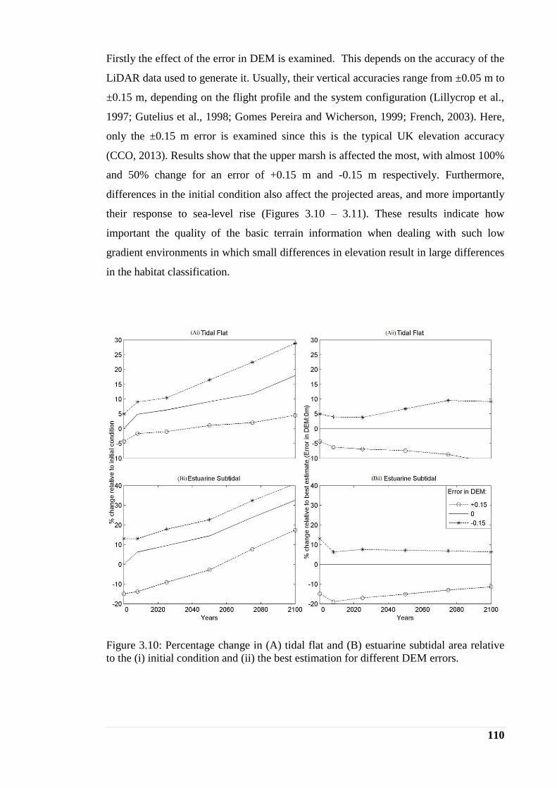
110

Firstly the effect of the error in DEM is examined. This depends on the accuracy of the

LiDAR data used to generate it. Usually, their vertical accuracies range from ±0.05 m to

±0.15 m, depending on the flight profile and the system configuration (Lillycrop et al.,

1997; Gutelius et al., 1998; Gomes Pereira and Wicherson, 1999; French, 2003). Here,

only the ±0.15 m error is examined since this is the typical UK elevation accuracy

(CCO, 2013). Results show that the upper marsh is affected the most, with almost 100%

and 50% change for an error of +0.15 m and -0.15 m respectively. Furthermore,

differences in the initial condition also affect the projected areas, and more importantly

their response to sea-level rise (Figures 3.10 – 3.11). These results indicate how

important the quality of the basic terrain information when dealing with such low

gradient environments in which small differences in elevation result in large differences

in the habitat classification.


to the (i) initial condition and (ii) the best estimation for different DEM errors.

111



different DEM errors.

Secondly, the spatial resolution of the input data is examined. SLAMM is quite flexible

with regards to cell-size, suggesting a range of 5 - 30 m sampling interval, depending on

the size of the site and the availability of the data. The higher suggested resolution is

considered here as the best estimation. Results differ from the initial simulation in a

range of ±0-10% when high resolution data have been used, while big differences are

observed for data with lower resolution, raising the question of whether SLAMM is

really suitable for very large area simulations at resolutions of 30 m or lower (Figure

3.12 - 3.13). The most affected wetland category on this scale is the estuarine subtidal,

112

especially at the last time-steps, reaching a difference of 150% (Figure 3.13d).

Significantly affected is also the lower marsh, presenting a difference of 50% for the

year 2025 (Figure 3.12f), while the upper marsh (Figure 3.12d) and tidal flat (Figure

3.13b) present a maximum change of 20%. Consequently, the lower the resolution of

the input data, less accurate the projected results are. Therefore, it is wise to use high

resolution LiDAR data.


lower marsh area relative to the (i) initial condition and the (ii) ‘best estimate’ 5m

resolution DEM for different resolutions.

113


to the (i) initial condition and the (ii) ‘best estimate’ 5m resolution DEM for different

resolutions.

The last parameter that affects the input layers is an error in the land classification.

Classification is usually dependent on the type of remotely-sensed data used, their

interpretation and also their spatial analysis (Scott et al., 1987; Arbuckle et al., 1998).

The minimum level of interpretation accuracy in the identification of land use and land

cover categories from remote sensor data is 80-85% (Anderson, 1971; Anderson et al.,

1971, 1976; Olson, 2008). Thus, in order to test the sensitivity of the model to

misclassification, new land classification layers are generated in Matlab (Figure 3.14;

Table 3.7) with 15% of each category randomly misclassified to the closest one.

114

Table 3.7: Basis of error analysis for the land classification.

15% From Misclassified To

1 Upper marsh Lower marsh

2 Upper marsh Transitional marsh

3 Transitional marsh Dryland

4 Transitional marsh Upper marsh

5 Tidal flat Estuarine subtidal

6 Tidal flat Lower marsh

7 Lower marsh Upper marsh

8 Lower marsh Tidal flat

9 Estuarine subtidal Tidal flat

Figure 3.14: Script to generate the misclassified land cover layers in Matlab.

In each simulation, only two categories are affected according to the error mapping

summarised in Table 3.7. When a category is misclassified to one with a higher

elevation, inundation is assumed leading to the transformation of this wetland category

to the correct one. This is not the case when a category is misclassified to one

characterised by a lower elevation (Figures 3.15 - 3.16). This behaviour is explained

from the fact that the process of ‘correction’ is based on the process of inundation (see

section 2.2), ignoring the process of aggradation. Thus, the need to include the

115

procedure of aggradation is a key finding of this part of the sensitivity analysis.

However, even when inundation of the misclassified category is assumed, different

habitat distribution is projected for the current time-step, since the conversions are

based on empirical calculations. These differences range between around 5- 10% from

the current time-step of the original simulation. Different habitat distribution on the

current condition therefore projects different future habitat distribution.


lower marsh area relative to the (i) initial condition and the (ii) original classification for

different habitat misclassifications.

116


to the (i) initial condition and the (ii) original classification for different habitat

misclassifications.

The sensitivity of the modelled habitat changes to both historic and projected future sea-

level rise rate was also examined. The results from this analysis are summarised in

Figures 3.17 and 3.18. The response of the wetland categories to these two forcings are

the same, because both are actually used to calculate the final sea-level rise applied at

each time-step (see eq. 2.4). As expected, the more rapid the rate of sea-level rise, the

larger the areas that are inundated. The estuarine subtidal and the tidal flat are enlarged,

whilst the area of saltmarsh invariably decreases. Most affected is the lower marsh area

reaching a difference of almost 50% from the original simulation at the last time-step

(2100) for a historic sea-level rise rate of 3 mm yr-1

.

117



different historic and future sea-level rise scenarios.

118


to the (i) initial condition and the (ii) best estimation for different historic and future

sea-level rise scenarios.

Finally, the basic processes included into the model are examined, with first one the

process of accretion. This was accomplished by applying different accretion rates for

the upper and lower saltmarsh and the tidal flat (Figures 3.19 – 3.21). Upper marsh

accretion rates below the ‘best estimate’ value affect the upper marsh by 10%, but only

at the middle time-steps (2025-2050). In contrast, lower and transitional marsh areas are

affected during the whole simulation reaching a difference of 10% and 30% respectively

at the last time-step. However, at higher accretion rates, all three zones are affected,

with the transitional marsh being more vulnerable and reaching a difference of 40%

from the best estimate by the year 2100 (Figures 3.19).

The most important outcome at this point is that the transitional marsh is affected by

this parameter, although this was not expected according to the SLAMM structure. A

further investigation into the model code indicates that this habitat is included into the

upper marsh accretion model and thus treated with the same way. Although this is

correct, it points out that the accretion module is under-documented.

119



different upper marsh accretion rates.

The results also show that the lower marsh is very sensitive to changes in the lower

marsh accretion parameter. In absence of accretion on the lower marsh, its area is very

vulnerable to the sea-level rise and is gradually decreased during the simulation; up to

half the low marsh area may be lost by 2100, with a corresponding increase in the area

of tidal flat. The higher the accretion rate, more lower marsh area is capable to keep up

with the sea-level rise, increasing its area and therefore decreasing the area of the tidal

flat (Figure 3.20).

120

Figure 3.20: Percentage change in (A) lower marsh and (B) tidal flat area relative to the

(i) initial condition and the (ii) best estimation for different lower marsh accretion rates.

The model is less sensitive to tidal flat accretion rate, with the tidal flat affected by only

2% at the last time-steps of the simulation (Figure 3.21). However, the most important

outcome here is that accretion rates higher than 4.5 mm yr-1

for all three sub-models do

not further affect the projected wetland categories, since these rates are higher than the

sea-level rise rate, demonstrating again the need to include aggradational process in the

model.

121


to the (i) initial condition and the (ii) best estimation for different tidal flat accretion

rates.

The last process examined is the process of erosion. As explained in Section 2.2, marsh

erosion is assumed to occur within SLAMM when the fetch is more than 9 km. This

criterion is not met for the small Newtown estuary, and therefore marsh erosion is not

modelled. Thus, changes in the marsh erosion parameter do not affect its habitat

distribution. However, evidence from studies at the southeast England (Burd, 1992;

Cooper et al., 2001; van der Wal and Pye, 2004; Wolters et al., 2005) indicate that

marsh erosion can be caused, even in estuaries with a smaller fetch, by a combination of

high tides, strong winds, and increased wave height, pointing out the weakness of

SLAMM to properly model the process of marsh erosion in the small UK estuaries.

Thus, the need to incorporate a threshold of a smaller fetch within SLAMM has

emerged through the sensitivity analysis.

On the other hand, the tidal flat is assumed to be eroded at each time-step with only the

requirement of its adjustment to water. Therefore, changes at the tidal flat erosion

parameter affect the vulnerability of the Newtown estuary to the sea-level rise; higher

values of tidal flat erosion increase the eroded tidal flat area. Thus, the latter decreases

122

its total area by being converted to subtidal, which therefore is increased (Figure 3.22).

It is worth noting here that values of tidal flat erosion >0.3 m yr-1

do not have a further

influence on the projected results.


to the (i) initial condition and the (ii) best estimation for different tidal flat erosion rates.

As shown in the previous chapter, more sophisticated spatial accretion routines are also

available within SLAMM. These calculate the accretion rates for each habitat as a time-

varying function of cell elevation, distance to channel and salinity. These are specified

according to the following equations:

Aelev = accretion rate for a cell as a function of elevation

= MinAccr + ShapePctile * (MaxAccr-MinAccr) (3.3)

where MaxAccr = Max. accretion rate for the specific site given optimal distance

to tidal channel, elevation and salinity (mm/year)

MinAccr = Min. accretion rate for the specific site (mm/year)

ShapePctile = (Shape(Elev)-MinShape) / (MaxShape-MinShape) (3.4)

Shape = a (1-ElevPctile)3+b (1-ElevPctile)

2 + c (1-ElevPctile) (3.5)

ElevPctile = (Elev-ElevMin) / (ElevMax – ElevMin) (3.6)

123

Elev = elevation of the cell relative to MTL (m)

ElevMax = max. elevation for the specific wetland type (m above TL)

ElevMin = min. elevation for the specific wetland type (m above MTL)

a,b,c = cubic coefficients defining the shape of the curve (unitless)

D =factor representing distance to river or tidal channel

)1(

21

minDMaxDistEffect

ChannelD

(3.7)

where D2Channel =distance to channel (m)

DistEffectMax = not additional effect beyond this distance

Dmin = min value of D factor (unitless)”

If there are no available data to parameterize this relationship, it should be

ignored by setting the DistEffectMax to 0, and Dmin to 1 (Clough et al., 2010).

S = salinity factor representing salinity effects

If cell

Salinity in )2/max(),2/max( ZoneTSalinityZoneTSalinityTMaxTMax

(3.8)

= )2//(1)(1(max

TMaxZoneSalinitySalinitySSCellTMaxNonTNonTMax

(3.9)

otherwise S = NonTMax

S (3.10)

where Salinitycell = salinity at a given cell (ppt)

SailinityTMax = salinity level at which max accretion rate occurs (ppt)

SNonTMax = accretion factor with no salinity effect (unitless)

TMaxZone = salinity range over which there is salinity effect (ppt)

The salinity factor is usually ignored because the rates of accretion can be described

based on the elevation and distance to channel (Clough et al., 2010). At this stage, the

distance to channel will also be ignored, due to lack of data availability. Therefore, the

accretion rates are calculated based on the elevation only. The hypothetical accretion

pattern is presented on Figure 3.23, based on which the accretion sub-model for each

habitat is calibrated (Table 3.8; Simulation ‘N_UK_a’).

124

Figure 3.23: Elevation-dependent accretion rates calculated in SLAMM. Vertical dash

lines illustrate the boundaries of each habitat, and horizontal dot lines demonstrate the

constant accretion rate used for each habitat at the previous simulation.

Table 3.8: Accretion model parameters for the Newtown Estuary, Isle of Wight, UK.

Accretion model Parameters Upper and Transitional

Marsh

Lower

marsh

Tidal

Flat

Max Accretion rate (mm yr-1

) 1.8 2 5

Min Accretion rate (mm yr-1

) 1.7 1.8 2

a coefficient (cubic) -0.8 -0.8 -1

b coefficient (square) 1 1 0.9

c coefficient (linear) 1 1 0.5

Compared with the previous simulation where constant accretion rates used

(‘Simulation ‘N_UK’), the tidal flat experiences higher accretion rates making it more

able to cope with sea-level rise. This tolerance of the tidal flat to sea-level rise combined

with the lower accretion rates for the lower marsh area, forces the former to migrate

landward, squeezing slightly the lower marsh (Table 3.9).

125

Table 3.9: Summary of the output from evaluation of the accretion sub-model for the Newtown estuary (areas in ha).

Simulation name: "N_UK"

Date SLR Dry Land Trans. M. Upper M. Lower M. Tidal Flat Est. Subtidal Ocean Beach Ocean Flat Ocean

0 0 638.1 14.3 20.0 51.5 176.4 16.3 0.0 41.6 47.7

2008 0 628.7 19.5 15.8 49.2 185.0 17.3 0.8 41.2 48.4

2025 0.0563 627.7 14.5 15.9 51.7 187.6 17.8 0.4 40.8 49.5

2050 0.1583 625.7 14.4 14.1 49.6 192.5 18.6 0.0 39.7 51.2

2075 0.2778 623.0 14.6 13.4 46.5 197.1 20.2 0.0 37.7 53.4

2100 0.4123 619.5 14.8 13.5 36.8 208.2 21.6 0.05 35.4 56.2

Simulation name: "N_UK_A"

Date SLR Dry Land Trans. M. Upper M. Lower M. Tidal Flat Est. Subtidal Ocean Beach Ocean Flat Ocean

0 0 638.1 14.3 20.0 51.5 176.4 16.3 0.0 41.6 47.7

2008 0 628.7 19.5 15.8 49.2 185.0 17.3 0.8 41.2 48.4

2025 0.0563 627.7 14.4 16.0 51.7 187.8 17.7 0.4 40.8 49.5

2050 0.1583 625.7 14.3 14.2 49.6 193.1 18.1 0.0 39.7 51.2

2075 0.2778 623.0 14.4 13.5 46.3 198.4 19.2 0.0 37.7 53.4

2100 0.4123 619.5 14.6 13.6 36.1 210.6 19.9 0.05 35.4 56.2

compare "N_UK" to "N_UK_A"

TRUE TRUE TRUE TRUE TRUE TRUE TRUE TRUE TRUE TRUE TRUE

TRUE TRUE TRUE TRUE TRUE TRUE TRUE TRUE TRUE TRUE TRUE

TRUE TRUE TRUE FALSE FALSE TRUE FALSE FALSE TRUE TRUE TRUE

TRUE TRUE TRUE FALSE FALSE TRUE FALSE FALSE TRUE TRUE TRUE

TRUE TRUE TRUE FALSE FALSE FALSE FALSE FALSE TRUE TRUE TRUE

TRUE TRUE TRUE FALSE FALSE FALSE FALSE FALSE TRUE TRUE TRUE

126

3.4 Further modifications of the code

The pilot application of the modified SLAMM to the Newtown estuary reveals the need

for a number of further modifications to the model code. First, it is evident that the

process of aggradation (i.e. the seaward expansion of specific intertidal wetland units)

must be included. This is accomplished by enabling the additional transitions depicted

in Figure 3.24. The source code is detailed in A-0.27. The maximum elevation of each

wetland category within a cell is computed at each time-step as a function of its

minimum one, by assuming the same accretion rate. The changes made in the code

assume that aggradation occurs when this maximum elevation is greater than the default

maximum elevation for this wetland category. In contrast to the ‘original’ code, the

modified one enables this procedure even for the current time-step, when it is necessary,

and most importantly also includes the tidal flat wetland category. Under this procedure

the wetland class then converts to one that is higher within the tidal frame. The fraction

transformed is then computed for each time-step, as a function of the maximum

elevation and the upper elevation boundary of that wetland and also the slope of that

cell (equation 3.11).

Figure 3.24: SLAMM decision tree modification including procedure of aggradation

(grey arrows: inundation; red arrows: erosion, green arrows: aggradation).

127

Cat

tCat

Cat

Width

Slope

MaxElevUpperBound

FracLost

)tan

(,

(3.11)

where FracLostCat = Fraction of wetland lost in time step (dimensionless)

MaxElev = Max elevation of the wetland class at time t (m)

UpperBound = Max elevation boundary of the wetland class (m)

Slope = Slope of the cell (degrees)

Width Cat = Width of the cell (m)

With the process of aggradation enabled, the response of the wetland categories to the

UKCP09 SE mean sea-level rise scenario is changed (Figure 3.25). First, when the

modified code is applied to the Newtown Estuary and compared to results obtained with

previous code and the initial site-specific parameters clear differences are evident for

accretion values larger than the sea-level rise; marsh areas can cope with sea-level rise

and more importantly propagate seawards. Most sensitive is the model to the lower

marsh accretion parameter where lower marsh loses more than half of its area by 2100

due to seaward propagation of the upper marsh by increasing its area by almost 200%.

(Figure 3.25B). In addition, different results are projected even for the initial accretion

values. The correction of the habitat distribution in the first time-step is not only

determined by the minimum elevation of each wetland category, resulting to inundation,

but the maximum elevation is also taken into consideration determining if the specific

wetland category is subjected to aggradation too. Therefore, more differences can be

corrected at this time-step. The fact that the projected habitat distribution for the current

time-step is very similar to the initial one indicates the success of this modification step.

Second, it is clear that the marsh erosion procedure needs to be modified. As noted in

Chapter 2, SLAMM assumes that marsh is eroded when it is adjacent to water where the

fetch is more than 9 km. Although this could be the case for some of the larger estuaries

of the US, such a long fetch is rare in UK estuarine systems where even a smaller fetch

can cause wave-driven marsh-erosion (Wolters et al., 2005). In recognition of this, the

fetch threshold within SLAMM is modified to 0.5 km as described in Figures A-0.28

and A-0.29. Marsh is thus projected to experience lateral erosion when it is adjacent to

water where the fetch exceeds 0.5 km, increasing the tidal flat area (Simulation ‘N_2’).

Finally it is notable that, although dryland should also be subjected to erosion, this

128

process is not actually implemented in the original SLAMM code. When this process is

enabled (Figure A-0.30; Simulation ‘N_3’), the results project a slight increase of the

tidal flat area (Table 3.10).

Figure 3.25: Response of the (1) transitional marsh, (2) upper marsh, (3) lower marsh

and (4) tidal flat to different accretion values for the (A) upper marsh, (B) lower marsh

and (C) tidal flat before (original) and after (modified) the inclusion of aggradation. In

both cases, initial accretion rates of 1.8 and 2 mm yr-1

are used for the upper marsh and

both the lower marsh and the tidal flat respectively, as well as accretion rates higher

than the sea-level rise equal to 6.5, 6.4 and 6.3mm yr-1

for the upper, lower marsh and

the tidal flat respectively.

129

Table 3.10: Impacts of sea-level rise during the modification of erosion process.

Simulation: "N_1": Fetch: 9 km

Date SLR Dry Land Trans. M. Upper M. Lower M. Tidal Flat Est. Subt.

0 0 638.1 14.3 20.0 51.5 176.4 16.3

2025 0.0563 633.7 19.9 17.2 53.0 173.8 17.9

2050 0.1583 631.3 14.5 14.7 53.9 181.8 18.5

2075 0.2778 629.5 13.4 13.3 46.0 192.3 19.9

2100 0.4123 626.7 13.2 12.9 35.1 204.4 21.5

Simulation:"N_2" Fetch: 0.5 km


0 0 638.1 14.3 20.0 51.5 176.4 16.3

2025 0.0563 631.5 21.8 17.2 52.3 173.6 18.9

2050 0.1583 630.8 14.0 15.1 53.6 181.5 19.1

2075 0.2778 628.1 14.5 13.2 45.3 192.1 20.5

2100 0.4123 625.4 14.2 12.8 34.3 204.2 22.1

Simulation:"N_3": Dryland erosion included


0 0 638.1 14.3 20.0 51.5 176.4 16.3

2025 0.0563 631.5 21.7 17.2 52.3 173.7 17.2

2050 0.1583 630.8 14.0 15.1 53.6 181.6 17.9

2075 0.2778 628.1 14.4 13.2 45.3 192.2 19.4

2100 0.4123 625.5 14.0 12.8 34.4 204.3 20.7

The final decision tree of the modified SLAMM is presented in Figure 3.26. This

version of the source code provides the basis for the more substantive applications to

the Suffolk estuaries and Norfolk barrier coastline summarised in the following

Chapters.

Figure 3.26: Updated SLAMM decision tree (grey arrows: inundation; red arrows:

erosion, green arrows: aggradation).

130

4 APPLICATION OF THE MODIFIED SLAMM TO SUFFOLK

ESTUARIES, UK

The modified SLAMM code is applied to selected estuaries in Suffolk, eastern England,

in order to critically evaluate more fully its ability to produce robust projections of

intertidal habitat change in more complex estuaries. A key factor influencing the initial

selection of these estuaries was the availability of Environment Agency LiDAR data

under the NERC iCOASST project (Nicholls et al., 2012; 2015). The Suffolk estuaries

are of interest on account of their varied geomorphology and long history of

reclamation. A starting point here is to use the modified SLAMM code to evaluate the

likely changes of the existing intertidal environment due to the climate-driven sea-level

rise. However, the flood defences that currently protect the extensive reclaimed areas

will require upgrading in order to cope with the projected sea-level rise (French, 2008).

In recognition of this, managed realignment has to be considered. In that case, the

evolution of the protected areas needs to be investigated by assuming the defences

inactive.

SLAMM is initially applied to the Blyth estuary in order to investigate the sensitivity of

the projected habitat distribution to the different assumptions made in the underlying

sub-models for the tidal flat and saltmarsh and the extent to which these can be tuned to

allow simulation of the effects of removal or realignment of the flood defences that

protect a large proportion of the natural estuary intertidal. A second application models

intertidal change in the larger Deben estuary. This has a less complex morphology but

fewer datasets exist with which to constrain the sedimentation sub-models in SLAMM.

4.1 Blyth Estuary

A composite LiDAR dataset (2 m resolution) produced by the Environment Agency

from surveys undertaken in 2010 and 2012 was used as the base DEM for the Blyth.

These data were integrated with subtidal bathymetry surveys undertaken by the UCL

Coastal and Estuarine Research Unit between 1998 and 2001. The resulting elevation

dataset, resampled to 5 m resolution, is presented in Figure 4.1. The derived slope and

the land cover layers used to define the model domain are shown in Figures 4.2 and 4.3

respectively. However, one more layer is necessary now indicating the areas protected

131

by defences (Figure 4.4). These figures illustrate the varied geomorphology and

reclamation patterns of the Blyth estuary. In the upper part it is enclosed by earth

embankments that protect low farmland, but is enlarged in the middle part characterised

by a large tidal prism of the abandoned Bulcamp, Sandpit and Angel marshes and by

reedbeds. Finally, its entrance is restricted by defences that protect extended low-lands.

Approximately 17 km of earth embankments protect around 67 ha of land from tidal

flooding (CHaMP, 2002; French, 2003; French and Burningham, 2003).

Figure 4.1: Topographic and bathymetric DEM of the Blyth Estuary.

132

Figure 4.2: Slope map of the Blyth Estuary.

Figure 4.3: Land classification map of the Blyth Estuary.

133

Figure 4.4: Flood compartments of the Blyth Estuary (after French 2008).

Table 4.1 summarises the required site parameters for the model runs. The historic sea-

level trend includes the vertical land movements and is estimated at 2.7 mm yr-1

using

the closest tide gauge station at Lowestoft (around 25 km to the northeast) (PSMSL,

2012). The tidal regime of the middle estuary is used to set up the model, as obtained

from the Hydrographic Survey undertaken in the Blyth estuary by the Gardline

Environmental Ltd in 2003 for the Environment Agency (Figure 4.5). A higher HAT is

taken into account, though, taken into consideration the strong surge influence to the

tides, and therefore to the habitat distribution; in 1953 the surge reached 3.6 m OD at

Southwold (French, 2001; French and Burningham, 2003). Mean marsh accretion

parameters are obtained from a survey undertaken by French and Burningham (2003)

for the period 1997 and 2001, while observed tidal flat accretion rates are obtained from

a sedimentation survey undertaken by Pye and Blott (2008b) in December 2008.

Finally, the extensive literature on the Blyth estuary indicates that some of the

abandoned defences in the Sandpit, Angel and Bulcamp marsh have been completely

eroded over the last 50 years. Thus, an erosion of 0.1 m yr-1

can be assumed

(Environment Agency, 1999a; French and Burningham, 2003; French, 2008; Pye and

Blott, 2008b).

134

Figure 4.5: Tide levels (m OD) for 6 different sites in the Blyth Estuary (reproduced

from Gardline Environmental Ltd, 2003). Data for site 4 are used at the present study.

Table 4.1: SLAMM site parameter table for the Blyth Estuary.

Parameter Blyth

DEM Date (YYYY) 2010

NWI Date (YYYY) 2010

Direction Offshore[n,s,e,w] E

Historic Sea Level Trend (mm yr-1

) 2.7


HAT (m) 1.6

MHWS (m) 0.9

MHW (m) 0.78

MHWN (m) 0.65

LAT (m) -1.3


) 0.1

Tidal Flat Erosion (m yr-1

0.1

Lower Marsh Accretion (mm yr-1

) 6

Upper Marsh Accretion (mm yr-1

) 5

Beach/Tidal flat Sedimentation Rate (mm yr-1

) 6.4 (mean for all marshes)

20.7 (max in Bulcamp Old)

135

Nine simulations were performed, as summarised in Table 4.2, under the mid-range

UKCP09 regional sea-level scenario, in order to investigate the effect of varied

sedimentation models. First, the impacts of sea-level rise at the Blyth estuary are

investigated assuming that all the present defences will continue to be maintained

protecting the reclaimed areas behind them. The constant accretion module is simulated

for the un-protected by defences estuary, based on either the mean (‘RUN1’) or max

(‘RUN2’) tidal flat accretion rate of 6.4 and 20.7 mm yr-1

respectively, in order to

investigate the response of the estuary to this parameter. In both simulations the mean

constant accretion rate of 6 and 5 mm yr-1

is used for the lower and upper marsh

respectively.

The defences are then considered inactive and the areas behind them are subjected to the

processes related to the sea-level rise. Firstly, the constant accretion module is used by

repeating the above scenarios of mean (‘RUN3’) and max (‘RUN4’) constant tidal flat

accretion. The more dynamic spatial accretion module is then incorporated in its

simplest form for the tidal flat (‘RUN5’) and the marsh area (‘RUN6’). A final

refinement is to also include the proximity to the channel influence into the marsh

spatial accretion module by investigating three different scenarios (‘RUN7’, ‘RUN8’,

‘RUN9’) to further evaluate the sensitivity of the model to this parameter.

Table 4.2: Summary of modified SLAMM simulations for the Blyth estuary.

Simulation Tidal Flat Accretion Marsh Accretion

Active

defences

RUN1 Mean Constant Mean Constant

RUN2 Max Constant Mean Constant

No

active

defences

RUN3 Mean Constant Mean Constant

RUN4 Max Constant Mean Constant

RUN5 Spatial Mean Constant

RUN6 Spatial Spatial (elevation dependence)

RUN7

Spatial

Spatial (elevation

and distance to

channel)

Dmax=50m

RUN8 Dmax=100m

RUN9 Dmax=250m

136

A. Active defences

The results of the first two simulations, modelled using the mean (‘RUN1’) and max

(‘RUN2’) constant tidal flat accretion rate are compared in Table 4.3 and Figure 4.6. In

both simulations low-lying terrain remains protected by the defences. In the first

simulation, the estuary seems to keep pace with the sea-level rise. More specifically, at

the beginning of the first scenario, the tidal flat accretion rate is enough to outstrip the

sea-level rise, forcing the lower marsh to migrate seaward over the tidal flat. However,

the extended lower marsh cannot keep pace with the increased sea-level resulting to

inundation at the next time-step. Thus, the tidal flat area is increased in 2050 but slightly

inundated at the last time-steps as sea-level continues to rise. On the other hand, the

maximum tidal flat accretion rate applied in the second simulation, always outstripping

the sea-level rise, forcing the tidal flat to be almost totally converted to lower marsh by

2050. As the lower marsh area fills in over the tidal flat, its area is extremely increased,

enhancing therefore the ability of the rest marsh area to keep up with the sea-level rise.

The coastal environment is not affected by changes in the tidal flat accretion parameter,

since this parameter is not relevant to the specific coastal environment. In both

simulations, the response of the beach at the sea-level rise is simulated within SLAMM

by using the Bruun rule, projecting total beach erosion by year 2025. This projection,

though, does not agree with the observed shoreline trend monitored by the EA (2011)

for the period 1991-2010. As it is illustrated in Figure 4.7, the open coast shoreline

presents a more complex pattern of up-drift accretion and downdrift erosion for the last

two decades, than just a simple eroded beach along the coast, pointing out the limitation

of SLAMM to include a complex shoreline response to the sea-level rise.

137

Table 4.3: Impacts of sea-level rise at the Blyth estuary as presently defended, modelled

using different constant tidal flat accretion rates. Simulation: 'RUN1'

Date SLRLow Ground

High

ground

Transitional

Marsh

Upper

MarshLower Marsh Tidal Flat Subtidal

0 0 670.3 2779.6 113.4 25.6 13.9 249.4 30.4

2025 0.0497 687.1 2756.5 119.3 18.7 26.8 235.4 35.1

2050 0.1517 693.8 2746.0 120.5 21.0 16.1 244.4 35.9

2075 0.2712 701.7 2732.3 121.9 23.5 16.2 243.9 36.6

2100 0.4057 709.9 2717.3 120.3 26.9 17.9 244.6 37.1

Simulation: 'RUN2'

Date SLRLow Ground

High

ground

Transitional

Marsh

Upper


0 0 670.3 2779.6 113.4 25.6 13.9 249.4 30.4

2025 0.0497 687.2 2756.5 126.7 21.5 41.2 211.2 34.6

2050 0.1517 699.1 2746.0 147.3 48.2 149.1 50.5 37.5

2075 0.2712 718.0 2732.3 155.2 56.1 156.3 20.0 38.2

2100 0.4057 732.0 2717.3 153.9 61.0 159.9 11.2 38.7

Figure 4.6: Changes in habitat distribution to 2100 for the Blyth estuary as presently

defended, modelled using different constant tidal flat accretion rates.

138

Figure 4.7: Observed shoreline change at the entrance of the Blyth estuary for the period 1991-2010 (Environment Agency, 2011).

139

B. Inactive defences

In order the defences to be rendered as inactive, they have been assigned as long narrow

hills of dryland, while the areas behind them as tidal flats, both subjected to the

processes related to the sea-level rise. The two scenarios of mean and max constant tidal

flat accretion simulated within the defended estuary are repeated for the undefended

estuary too (‘RUN3’ and ‘RUN4’). The results of these runs, as presented in Figure 4.8,

indicate that the behaviour of the protected areas of the estuary is very similar to the

unprotected ones, with marsh to be generated only in high elevations for a mean tidal

flat accretion rate but almost filling in the tidal flat for a maximum rate. However, even

this maximum rate is not enough to convert some very deep areas of tidal flat to lower

marsh, even in 100 years.


defences rendered inactive, modelled using different constant tidal flat accretion rates.

140

The annual tidal flat sediment demand required for each scenario is calculated at this

point in order to evaluate the projected results in the context of sediment availability.

The results are summarised in Table 4.4, and are critically compared with the potential

annual deposition for the whole estuary as this is determined by French et al. (2008).

More specifically, in this study the gross sediment flux for the whole estuary is

estimated at 92.3 t x 103 yr

-1, which could sustain the required from the tidal flat

sediment demands for all the scenarios. However, this could probably be constrained by

the local supply estimated for the whole estuary at 1.4 t x 103 yr

-1. Although this implies

all the scenarios as unrealistic, it is noted in the same study, that this residual sediment

flux is not very reliable, because it is very difficult to be calculated, especially when

bathymetric surveys and spatially representative measurements of contemporary

deposition and erosion are missing.

Table 4.4: Annual sediment demand required for each scenario simulated within

SLAMM for the Blyth Estuary.

Defended

Estuary

Undefended

Estuary

Intertidal annual

deposition

(French et al., 2008)

(t x 103 yr

-1)

Tidal Flat Area (m2) 2,493,700 7,184,375

Tidal flat annual deposition

demand (t x 103 yr

-1) Gross Residual

Mean accr.

rate (mm yr-1

) 6.4 6 16

92.3 1.4 Max accr. rate

(mm yr-1

) 20.7 18 53

However, constant accretion rates for the tidal flat cannot depict realistically its

response to the sea-level rise, since they ignore any morphodynamic feedback as the

elevation evolves within the tidal frame. Thus, the third simulation is repeated by

incorporating this time the dynamic spatial accretion model for the tidal flat (‘Run5’).

This sub-model is parameterised based on observed tidal flat accretion data, as they

obtained from the Pye and Blott (2008b) sedimentation survey. These elevation

dependent accretion data are initially fitted with various empirical models (Figure 4.9a),

which are used to constrain the relevant ones according to the SLAMM framework

(Figure 4.9b). The best fit to the real data exponential curve is better characterised by

the quadratic SLAMM curve. Thus, the last one is used to parameterise the tidal flat

accretion sub-model. Table 4.5 summarises the parameters used to constrain the

different elevation dependent tidal flat accretion models within SLAMM.

141

Figure 4.9: Observed tidal flat accretion rates (a) for the Blyth estuary used to constrain

elevation-dependent accretion sub-model (b) (Source: Pye and Blott, 2008b).

Table 4.5: Parameter table for the elevation dependent tidal flat accretion model.

SLAMM Accretion model parameters Linear Quadratic Cubic


) 19.15 23.7 36.8


) -3.55 0.9 1.16

a coefficient (cubic)* 0 0 1

b coefficient (square)* 0 1 0

c coefficient (linear)* 1 0 0

*a,b,c: coefficients defining the shape of the accretion curve within SLAMM (see

equations 3.3 to 3.6).

The response of the estuary to the specific sea-level rise scenario, modelled using the

constant (‘RUN3’) and the spatial (‘RUN5’) tidal flat accretion models is presented in

Table 4.6 and Figure 4.10. The much higher accretion rates generated by the spatial

model for the low-lying tidal flat areas, consider it more capable to cope with the sea-

level rise. Thus, less tidal flat is inundated in such low elevations in the last simulation,

decreasing the projected subtidal. Parallel, the spatial tidal flat accretion rates generated

in its higher elevations are much lower, getting very close to zero at some points. Thus,

the estuary is less capable to form saltmarsh in the higher elevations of the upper

estuary, decreasing the projected lower marsh area in the last simulation.

142


inactive, modelled using constant (‘RUN3’) and spatial (‘RUN5’) tidal flat accretion

rates.

Simulation: 'RUN3'

Date SLR

0 0 2847.9 187.3 50.8 45.3 718.4 32.4

2025 0.05 2838.5 203.3 42.7 69.3 684.1 40.0

2050 0.15 2830.9 208.7 48.7 57.9 688.0 41.3

2075 0.27 2824.5 204.6 52.0 62.8 685.9 42.7

2100 0.41 2810.9 202.5 55.0 62.2 694.4 43.9

Simulation: 'RUN5'

Date SLR

0 0.00 2847.9 187.3 50.8 45.3 718.4 32.4

2025 0.05 2838.7 204.4 41.3 58.4 697.6 37.4

2050 0.15 2833.1 210.5 46.4 38.2 708.3 38.9

2075 0.27 2828.9 206.4 50.0 38.1 709.0 40.0

2100 0.41 2815.7 204.0 54.4 44.7 709.0 41.0

High

Ground

Transitional

Marsh

Upper

Marsh

Lower

MarshTidal Flat Subtidal

High

Ground

Transitional

Marsh

Upper

Marsh

Lower

MarshTidal Flat Subtidal


defences rendered inactive, modelled using constant (‘RUN3’) and spatial (‘RUN5’)

tidal flat accretion rates.

143

Summarising it can be said that the Blyth estuary responds more dynamically to the

specific sea-level rise scenario if a spatial accretion pattern is taken into account for the

tidal flat. On the other hand, a mean constant tidal flat accretion rate overestimates the

vulnerability of the estuary, forcing it to migrate landwards, while a maximum constant

tidal flat accretion rate underestimates it, forcing it to migrate seawards.

A final refinement here is to also include a spatial accretion model for the saltmarsh

(“RUN6”). Saltmarsh sedimentation in the Blyth has been investigated (see French and

Burningham, 2003 for a study on the relationship between the marsh sedimentation and

the sea-level rise; French et al., 2008 for a sediment flux study; French et al., 2000 for a

study in the sedimentation movement within abandoned reclamations). However, the

data are too sparse to permit generalisation into a spatial model. Accordingly, the

aspatial MARSH-0D model (French, 2006) is used to compute the elevation

dependence of marsh deposition rate given appropriate local vertical tidal limits and

background sediment concentration. Modelled sedimentation as a function of time-

evolving evolution was then fitted to the exponential empirical model, which used to

constrain the SLAMM saltmarsh accretion model parameters (Figure 4.11; Table 4.7).

However, the MARSH-0D simulations used only a simplified tidal regime (only four

tidal constituents, M2, S2, O1, K1) and did not include the influence of the storm surge,

a factor that is important to be taken into account into the accretion rate (Stumpf, 1983;

Pugh, 1987; French, 2006; Schuerch et al., 2012). Therefore, it is necessary to fill in the

missing data by assuming a zero- accretion rate at the highest elevation of the marsh.

Table 4.7: Parameter table for the elevation dependent marsh accretion model.

Accretion model Parameters Lower Marsh Upper and Transitional Marsh


) 33 18


) 18 0

a coefficient (cubic)* 0 1

b coefficient (square)* 1 0

c coefficient (linear)* 1 0

*a,b,c: coefficients defining the shape of the curve (see equations 3.3 to 3.6).

144

Figure 4.11: Modelled marsh accretion rates for the Blyth estuary generated by the

MARSH-OD model and used to constrain the SLAMM sub-models.

The results of this simulation are compared to the one modelled using the constant

marsh accretion model (‘RUN5’) in Table 4.8 and Figure 4.12. The spatial accretion

rates applied to the lower and upper marsh area, even in their highest elevations, are

much higher than the constant marsh accretion rate applied in the previous simulation.

Thus, less lower marsh is inundated to tidal flat in low-lying areas, while in higher

elevations more is capable to build up to upper marsh. The last one is therefore

migrating now seawards over the lower marsh, while in higher elevations more is built

up to transitional marsh. At these low elevations, the spatial accretion rates of the

transitional marsh are still higher than the constant rate applied in the previous

simulation, making the low-lying transitional marsh more capable to keep pace with the

sea-level rise, and not be inundated to upper marsh. In higher elevations though, this

rate is much smaller than the constant one, considering the transitional marsh less

capable to build up, projecting less higher ground in the first time-steps. However, as

the upper marsh continues to be converted to transitional marsh in the next time-steps,

more of this is able to build up to higher ground.

145


inactive, modelled using constant (‘RUN5’) and spatial (‘RUN6’) marsh accretion rates.

Simulation: 'RUN5'

Date SLR

0 0.00 2847.9 187.3 50.8 45.3 718.4 32.4

2025 0.05 2838.7 204.4 41.3 58.4 697.6 37.4

2050 0.15 2833.1 210.5 46.4 38.2 708.3 38.9

2075 0.27 2828.9 206.4 50.0 38.1 709.0 40.0

2100 0.41 2815.7 204.0 54.4 44.7 709.0 41.0

Simulation: 'RUN6'

Date SLR

0 0.00 2847.9 187.3 50.8 45.3 718.4 32.4

2025 0.05 2834.6 223.5 54.9 38.8 688.6 37.4

2050 0.15 2838.0 217.1 79.5 18.2 684.1 38.9

2075 0.27 2840.5 208.1 88.1 12.6 683.8 40.0

2100 0.41 2828.2 196.9 105.1 14.2 683.2 40.9

Tidal FlatHigh

Ground

Transitional

Marsh

Upper

MarshLower Marsh Subtidal

High

Ground

Transitional

Marsh

Upper



defences rendered inactive, modelled using constant (‘RUN5’) and spatial (’RUN6’)

marsh accretion rates. In both simulations spatial accretion rates have been used for the

tidal flat.

146

In addition to the strong influence of elevation on the time-evolution of saltmarsh

sedimentation, proximity to sediment sources (marshe edges, tidal creeks) is well

documented as a driver of spatial variation in sedimentation (Reed, 1988; Stoddart et

al., 1989; French and Spencer, 1993; French et al., 1995; Bartholdy, 1997; Reed et al.,

1999; Bartholdy, 2010a, 2012). This factor is included in the SLAMM saltmarsh model

via the D term in equation 3.7. Clough et al. (2010) suggest that this term is used to

progressively reduce sedimentation over a range of 500 m (DistEffectMax), beyond

which a minimum value (Dmin) of 0.1 is used for areas of marsh that are not affected by

the proximity to channels or open water. Although this could be the case for the big

estuaries in US, in the small UK estuaries, this threshold is approximately 100 m

(French and Spencer, 1993). However, a sensitivity analysis of this threshold is

investigated in order to evaluate the sensitivity of the model to this parameter. In that

direction, three simulations are performed for ranges of 50 m (RUN7), 100 m (RUN8)

and 250 m (RUN9). Figure 4.13 presents the values of the D term used into the

equation 3.7 as a function of distance to channel for all the above simulations. It is

worth mentioned here that the definition of the main channel must be manually done via

the salinity sub-model, without activating it though.

Figure 4.13: D term values as a function of distance to channel for different assumptions

of proximity to channel influence.

Inclusion of the D term into the accretion sub-models tends to result in more extensive

lower marsh at the expense of higher marsh. This reflects the preferential reduction in

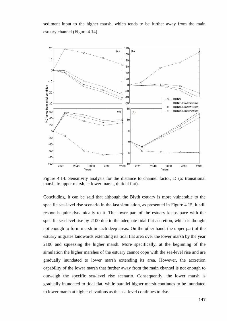
147

sediment input to the higher marsh, which tends to be further away from the main

estuary channel (Figure 4.14).

Figure 4.14: Sensitivity analysis for the distance to channel factor, D (a: transitional

marsh, b: upper marsh, c: lower marsh, d: tidal flat).

Concluding, it can be said that although the Blyth estuary is more vulnerable to the

specific sea-level rise scenario in the last simulation, as presented in Figure 4.15, it still

responds quite dynamically to it. The lower part of the estuary keeps pace with the

specific sea-level rise by 2100 due to the adequate tidal flat accretion, which is thought

not enough to form marsh in such deep areas. On the other hand, the upper part of the

estuary migrates landwards extending its tidal flat area over the lower marsh by the year

2100 and squeezing the higher marsh. More specifically, at the beginning of the

simulation the higher marshes of the estuary cannot cope with the sea-level rise and are

gradually inundated to lower marsh extending its area. However, the accretion

capability of the lower marsh that further away from the main channel is not enough to

outweigh the specific sea-level rise scenario. Consequently, the lower marsh is

gradually inundated to tidal flat, while parallel higher marsh continues to be inundated

to lower marsh at higher elevations as the sea-level continues to rise.

148


defences rendered inactive, modelled using spatial marsh accretion rates by including

(‘RUN8’) or not (‘RUN6’) the proximity to channel factor.

Summarising it can be said that the predicted intertidal habitat changes are highly

sensitive to assumptions made in the underlying sedimentation sub-models. This is

especially so in the case of the different saltmarsh sub-environments (Figure 4.16). The

higher marshes are not significantly affected from different assumptions on the tidal flat

accretion sub-model. However, their areas are increased when the elevation dependent

marsh accretion sub-model is activated, due to the more effective upland migration of

the lower marsh. In contrast, lower accretion rates are assumed for the marshes when

the distance to channel factor is also included into this model. Most affected of course

are the higher marsh areas, since they are further away from the channel, considering

them less able to cope with the sea-level rise, and therefore being inundated and

149

converted to lower marsh. Thus, the lower marsh area is increased, while some parts of

it which are not very close to the channel are inundated and converted to tidal flat.

Figure 4.16: Sensitivity analysis for the sedimentation sub-models: constant deposition

(RUN3); elevation dependant tidal flat deposition (RUN5); elevation dependant marsh

deposition (RUN6); elevation dependant marsh deposition with D factor (RUN8) (a:

transitional marsh, b: upper marsh, c: lower marsh, d: tidal flat).

As noted in Chapter 3, the elevation-dependence of the habitat decision tree means that

SLAMM remains very sensitive to the quality of the underlying terrain data. Even a

small error of ±0.15 m on the DEM may results to significant differences in habitat

extents, which need to be identified when defining initial conditions. Most sensitive is

the lower marsh. The error analysis presented in Figure 4.17 indicates that realistic

LiDAR errors of ±0.15 m give rise to up to 50% variation in its initial extent.

Interestingly, this sensitivity becomes much more apparent for the lower marsh when

more sophisticated dynamic spatial accretion model is used. An error of +0.15 m on the

DEM generates a more extended lower marsh. Thus, more lower marsh is now further

away from the channel experiencing less accretion rates, considering it less capable to

keep pace with the sea-level rise and parallel to build up to upper marsh.

150

Figure 4.17: DEM Sensitivity analysis for the different sedimentation sub-models: (a) constant deposition (RUN3); (b) elevation dependant

tidal flat deposition (RUN5); (c) elevation dependant marsh deposition (RUN6); (d) elevation dependant marsh deposition with D factor

(RUN8).

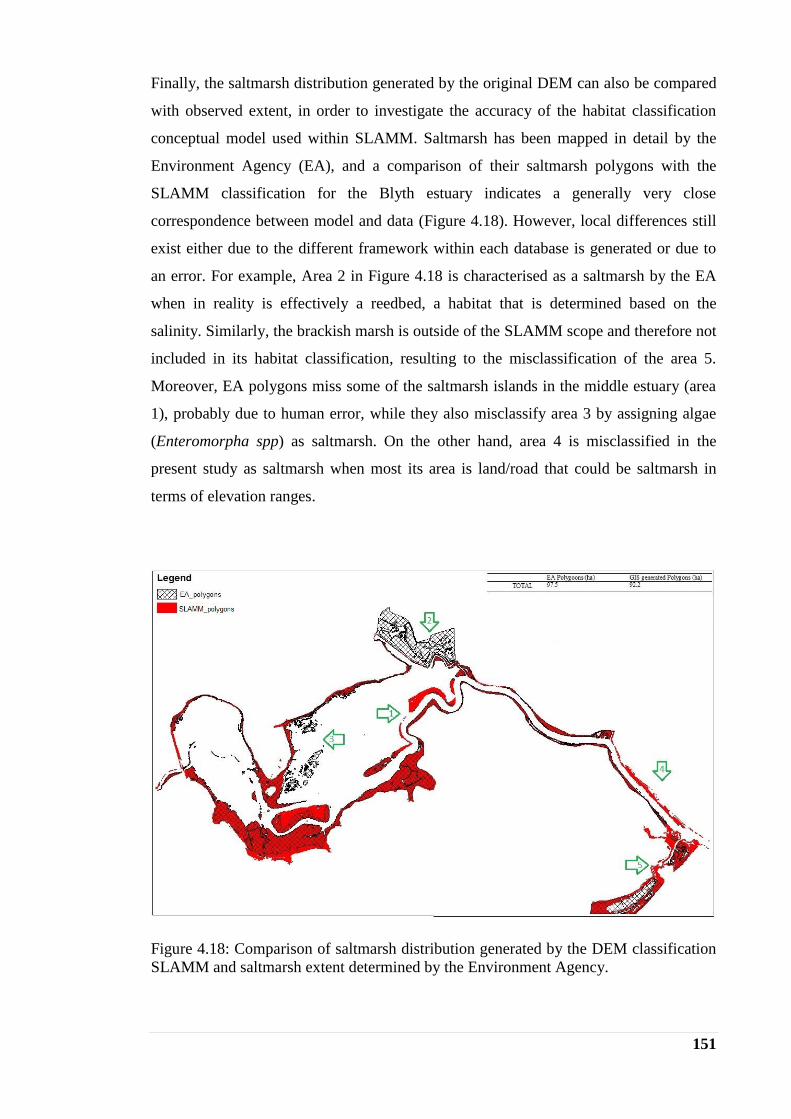
151

Finally, the saltmarsh distribution generated by the original DEM can also be compared

with observed extent, in order to investigate the accuracy of the habitat classification

conceptual model used within SLAMM. Saltmarsh has been mapped in detail by the

Environment Agency (EA), and a comparison of their saltmarsh polygons with the

SLAMM classification for the Blyth estuary indicates a generally very close

correspondence between model and data (Figure 4.18). However, local differences still

exist either due to the different framework within each database is generated or due to

an error. For example, Area 2 in Figure 4.18 is characterised as a saltmarsh by the EA

when in reality is effectively a reedbed, a habitat that is determined based on the

salinity. Similarly, the brackish marsh is outside of the SLAMM scope and therefore not

included in its habitat classification, resulting to the misclassification of the area 5.

Moreover, EA polygons miss some of the saltmarsh islands in the middle estuary (area

1), probably due to human error, while they also misclassify area 3 by assigning algae

(Enteromorpha spp) as saltmarsh. On the other hand, area 4 is misclassified in the

present study as saltmarsh when most its area is land/road that could be saltmarsh in

terms of elevation ranges.


SLAMM and saltmarsh extent determined by the Environment Agency.

152

4.2 Deben Estuary A composite LiDAR dataset (2 m resolution) produced by the Environment Agency

from surveys undertaken in 2010 and 2012 was used as the base DEM for the Deben

estuary. These data were integrated with subtidal bathymetry surveys undertaken by the

UCL Coastal and Estuarine Research Unit between 1998 and 2001. The resulting

elevation dataset is resampled to 5 m resolution and is summarised in Figure 4.19a. The

derived slope and the land cover layers used to define the model domain are shown in

Figures 4.19b and 4.19c respectively. Finally, Figure 4.19d represents the protected by

the defences area.

These figures illustrate the morphology and reclamation pattern found at the Deben

estuary. Similarly to the Blyth estuary described in Section 4.1, the Deben is

characterised by a relatively natural development of saltmarshes in its upper part, but it

is enclosed by defences at its lower part, with the mouth being its narrowest section

(CHaMP, 2002).

Table 4.9 summarises the required site parameters for the model runs. The historic sea-

level trend includes the vertical land movements and is estimated at 2.1 mm yr-1

using

the closest tide gauge station at Sherness (around 70 km to the south) (PSMSL, 2012).

The tide regime in m OD for the Bawdsey is used to set up the model. An assumption of

0.1 m yr-1

for both tidal flat and the marsh area is also included.

Table 4.9: Site parameter table for the Deben estuary.

Parameter Deben estuary

NWI and DEM Photo Date (YYYY) 2010

DEM Photo Date (YYYY) 2010

Direction Offshore[n,s,e,w] S


) 2.1


HAT (m) 2.25

MHWS (m) 1.85

MHW (m) 1.5

MHWN (m) 1.15

LAT (m) -2.15

Marsh Erosion ( m yr-1

) 0.1

Tidal flat erosion (m yr-1

) 0.1

153

Figure 4.19: SLAMM Input layers for the Deben estuary: a) DEM; b) slope map; c)

land classification; d) flood compartments.

154

Although there is a relatively large literature on management of the estuary’s flood

defences (Frostick and McCave, 1979; Environment agency, 1999b, SMP7, 2010),

accretion rates have not been systematically measured to permit generalisation into a

spatial model. To address this problem, the MARSH-0D model (French, 2006) is used

to compute the elevation dependence of marsh deposition rate given appropriate local

vertical tidal limits and background sediment concentration. Modelled sedimentation as

a function of time-evolving elevation is best fitted to the quadratic empirical model,

which is then used to constrain the SLAMM saltmarsh accretion model parameters

(Figure 4.20; Table 4.10). As with the Blyth estuary simulations, it was necessary to

constrain surge-drive sedimentation by assuming a zero deposition at the highest

elevation. Finally, the distance to channel factor is also taken into account, as described

in detail in Section 4.1.

Figure 4.20: Modelled marsh accretion rates used to constrain the SLAMM sub-models

for the Deben estuary.

Table 4.10:Parameters table for the SLAMM elevation and distance dependant marsh

accretion model.

Lower marsh Upper and transitional marsh

Max Accretion (mm yr-1

) 9.6 2.4

Min Accretion (mm yr-1

) 2.4 0

Coefficient a (cubic)* 0 1

Coefficient b (square)* 1 1

Coefficient c (linear)* 1 0

DeffectMax (m) 100 100

Dmin (unitless) 0.1 0.1

*a,b,c: coefficients defining the shape of the curve (see equations 3.3 to 3.6).

155

Meanwhile, the composite LiDAR dataset is compared with past EA LiDAR data from

2003 in order to investigate the behaviour of the tidal flat for the period 2003 and 2010.

At this point and based on French’s (2003) study where the accuracy of the LiDAR data

is investigated, the 2003 dataset is corrected for a systematic error of 10cm with respect

to the 2010 data. The accuracy of the LiDAR dataset, though, could also be degraded

from a random error which is much harder to constrain, and also by artifacts that arise in

the LiDAR data processing. In addition, differences are also expected in vegetated areas

due to the changing ground surface condition because of the different flight survey time

during the year. The resulting elevation change map is presented in Figure 4.21. The

tidal flat seems to be erosional along most of the eastern margin of the channel, but

accretional on the western margin.

Figure 4.21: Topographic change for the Deben estuary intertidal flat for the period

2003-2010. Points visualise the rate of change in the tidal flat area.

156

The rate of the tidal flat change at locations where valid LiDAR data exist for both years

is visualised in the same figure and analysed as a function of elevation and distance to

the main channel in Figure 4.22. This analysis indicates that the tidal flat change on the

Deben estuary does not depend in any simple way on these two factors. In addition, a

survey undertaken by Frostick and McCave (1979) on the sediment change of the

specific estuary over a calendar year reports a seasonal variation in accretion and

erosion. The seasonal cycle of accretion is reported to be caused by the algal growth

during summer, while the reduced wave action during the same period tends to allow

the tidal flat to build-up. These data cannot be used to permit a generalisation into a

spatial model, and therefore constant accretion rates must be applied for the tidal flat

within SLAMM in order to investigate its fate under the specific sea-level rise scenario.

Figure 4.22: Tidal flat rate of change as a function of (a) elevation and (b) distance to

channel.

Further investigation is necessary at this point in order to find a more specific pattern to

describe the behaviour of the tidal flat, maybe by dividing the estuary in zones of

different sedimentation behaviour. By applying a cross-sectional profile analysis in 6

locations along the Deben estuary, and based on Kirby’s (2000) theory that a high and

convex cross-sectional shape characterises accreting tidal flats, while a low and concave

one characterises eroding ones (Figure 4.23), it is clear that the estuary can be zoned

into a western accretional and eastern erosional side. This behaviour of the tidal flat can

be partially related to the meandering platform of the estuary.

157

Figure 4.23: Tidal flat cross-sectional profiles at six locations along the Deben Estuary.

Four simulations were performed, as summarised in Table 4.11, under the mid-range

UKCP09 regional sea-level scenario. Firstly, the impacts of sea-level rise at the Deben

estuary are investigated assuming that all the present defences will continue to be

maintained protecting the areas behind them. The area is simulated in zones of different

tidal flat behaviour; the accretional western and the erosional eastern side (‘RUN_A’).

The defences are then considered inactive. In that case the above analysis for the tidal

flat behaviour cannot describe the behaviour of the tidal flat behind the defences, and

therefore three scenarios of different tidal flat behaviour are examined; a stable

(‘RUN_B’), an eroding (‘RUN_C’) and an accreting (‘RUN_D’) tidal flat.

158

Table 4.11: Different simulations of the modified SLAMM in the Deben estuary.

Simulation Tidal flat accretion sub-model Marsh accretion

sub-model

Active

defences

Run_A Subsite 1 = 12.7 mm yr-1

Subsite 2 = -9 mm yr-1

Spatial

No

active

defences

Run_B accretion= 0 mm yr-1

Spatial

Run_C Eroding tidal flat = -11.2mm yr-1

Spatial

Run_D Accreting tidal flat = 10.8 mmyr-1

Spatial

A. Active Defences

First, the impacts of sea-level rise at the Deben estuary are investigated assuming that

all the present defences will continue to be maintained protecting the reclaimed areas

behind them. The results are presented in Table 4.12 and Figure 4.24, where the zoning

of the estuary into sub-sites of different input parameters for the tidal flat is also

depicted.

At the beginning, the estuary seems to respond quite dynamically to the specific sea-

level scenario. As the sea level continues to rise, higher marsh cannot keep pace and is

inundated to lower marsh, increasing its area. The lower elevations of the estuary,

though, respond differently within each sub-site. Along the western margin of the

estuary, the accreting tidal flat outweighs the sea-level rise and forms marsh at its higher

areas. On the other hand, the eroding tidal flat is inundated increasing the subtidal area.

This is more obvious at the upper part of the estuary where this is not constrained by

defences. In that direction, it can be said that the Deben estuary migrates eastwards by

2100 under the specific sea-level rise scenario, with the low lying terrain remaining

protected by the defences.

Table 4.12: Impacts of sea-level rise at the Deben estuary as presently defended.

Simulation: 'RUN_A' Low

Date SLR Ground

0 0.00 2017 7494 39 135 51 480 244 83 21 398

2025 0.05 2019 7489 35 129 66 472 238 52 19 444

2050 0.15 2019 7482 28 109 120 433 249 0.1 12 509

2075 0.27 2019 7475 25 61 201 393 264 0.1 7 516

2100 0.41 2020 7468 24 41 241 355 288 0.1 0 525

Transitional

Marsh

Upper

Marsh

Lower

Marsh Tidal Flat

Estuarine

Subtidal

High

Ground

Ocean

Beach

Ocean

Flat

Open

Ocean

159

Figure 4.24: Modelled habitat distributions for the defended Deben estuary (‘RUN_A’).

160

B. Inactive Defences

As mentioned in Section 4.1, in order for the defences to rendered as inactive, they have

been assigned as long narrow hills of dryland and the areas behind them as tidal flat,

both subject to the processes related to sea-level rise. Three different scenarios of tidal

flat behaviour are simulated here by assuming a more-or-less stable, an eroding and an

accreting tidal flat. The results are presented in Figures 4.25 – 4.27 respectively and

summarised in Table 4.13.

In the first scenario, the Deben estuary seems to migrate landwards under the specific

sea-level rise scenario, with the previously protected by defences areas remaining quite

stable (Figure 4.25). At the beginning, the higher marsh areas cope with the sea-level

rise being slightly inundated to lower marsh in areas further away from the main

channel where its accretion capability is very low. As the sea-level rises though at the

next time-steps, its accretional capability even closer to the channel is not enough to

keep pace with the sea-level rise, forcing it to lose half of its area by 2100.

Consequently, the lower marsh area is increased. The expanded lower marsh in higher

elevations of the estuary cannot cope with the increased sea level and therefore is

inundated to tidal flat, which although is inundated to subtidal in the lower elevations of

the estuary, its total area is increased by 10% in 2100.

Similar behaviour of saltmarsh landwards migration is observed in the next two

simulations. However, the areas in lower elevations of the estuary respond totally

different in each scenario. More specifically, in the second scenario, although the tidal

flat is expanded landwards over the lower marsh, as described in the previous scenario,

its eroding lower parts cannot cope with the sea-level rise and therefore are inundated

increasing the subtidal area by 60% in 2100. As a result, this scenario considers the

Deben estuary very vulnerable to the specific sea-level rise scenario, with the removal

of the defences inundating parts of the areas behind them by creating small creeks

within them (Figure 4.26).

On the other hand, the accretional response of the tidal flat under the third scenario is

sufficient to outweigh sea-level rise, keeping the subtidal area steady by 2100. At the

same time, it is also able to build up to lower marsh, quadrupling its area. The expanded

lower marsh in such low elevations of the estuary is also capable of accreting to higher

161

marsh. Although its total area is decreased by 2100, this is still more than in the two

previous simulations. Thus, this scenario shows the Deben estuary to be able to cope

with sea-level rise, with the removal of the defences keeping stable the tidal flat at the

deeper areas of the eastern estuary, but filling in its higher western side (Figure 4.27).

In the coastal environment, as mentioned in the previous case study, the impacts of the

sea-level rise on the ocean beach are simulated within SLAMM using a Bruun

formulation. This predicts total erosion of the beach by 2050. Particular interest presents

the feature of the Knolls. In all three simulations the Knolls are assigned as ocean flat

and therefore treated like the tidal flat in each simulation. Thus, in the first scenario the

Knolls are not very capable to cope with the sea-level rise, losing almost half of its area

by 2100. In the second scenario, the eroding Knolls are totally inundated by 2100.

Finally, their accreting behaviour on the last scenario outweighs the sea-level rise,

keeping their area steady. However, none of these simulations are able to include the

complex morphodynamic behaviour of the ebb-tidal delta. According the survey

undertaken by Burningham and French (2006), and presented in Figure 4.28, this

system first experiences a small-scale intertidal breakdown by losing intertidal volume,

followed by reconstruction and resumed growth.

Table 4.13: Impacts of sea-level rise at the undefended Deben estuary, modelled using

different behaviour of the tidal flat area.

Simulation: 'RUN_B'

Date SLR

0 0.00 7897 138 235 189 1756 244 83 21 399

2025 0.05 7879 133 225 186 1787 237 59 20 436

2050 0.15 7843 124 194 202 1838 239 0.4 19 503

2075 0.27 7800 119 138 236 1888 253 0.9 15 511

2100 0.41 7755 117 113 228 1951 265 1.0 13 519

Simulation: 'RUN_C'

Date SLR

0 0.00 7897 138 235 189 1756 244 83 21 399

2025 0.05 7879 133 225 179 1779 251 48 17 450

2050 0.15 7843 124 193 197 1801 281 0.4 11 512

2075 0.27 7800 119 137 232 1819 327 0.9 6 521

2100 0.41 7754 116 112 225 1823 397 0.9 0 533

Simulation: 'RUN_D'

Date SLR

0 0.00 7897 138 235 189 1756 244 83 21 399

2025 0.05 7879 133 226 247 1728 233 63 21 431

2050 0.15 7844 126 207 418 1615 230 0.4 21 501

2075 0.27 7802 125 161 634 1483 230 1.0 21 505

2100 0.41 7759 125 144 832 1339 232 1.0 21 510

High

Ground

Transition

al Marsh

Upper

Marsh

Lower

Marsh

Estuarine

Subtidal

Ocean

Beach

Tidal

Flat

Ocean

Flat

Open

Ocean

High

Ground

Transition

al Marsh

Upper

Marsh

Lower

Marsh

Tidal

Flat

Estuarine

Subtidal

Ocean

Beach

Ocean

Flat

Open

Ocean

High

Ground

Transition

al Marsh

Upper

Marsh

Lower

Marsh

Tidal

Flat

Estuarine

Subtidal

Ocean

Beach

Ocean

Flat

Open

Ocean

162


a quite stable tidal flat (‘RUN_B’).

163


an eroding tidal flat (‘RUN_C’).

164


an accreting tidal flat (‘RUN_D’).

165

Figure 4.28: Historical bathymetries for the Deben inlet and ebb-tidal delta (data from Burningham and French, 2006).

166

Finally, the saltmarsh distribution generated by the original DEM can also be compared

with observed extent, in order to investigate the accuracy of the habitat classification

conceptual model used within SLAMM. Similarly to the Blyth estuary in Section 4.1,

saltmarsh has been mapped in detail by the Environment Agency (EA), and a

comparison of their saltmarsh polygons with the SLAMM classification for the Deben

estuary is presented in Figure 4.29, indicating a generally very close correspondence

between model and data. Localised differences though still exist, however. For

example, Area 1 is characterised as a saltmarsh by the EA when in reality it is

effectively a reedbed (Phragmites spp), a habitat that is determined partly by salinity

rather than simple elevation. In addition, minor differences arise at the saltmarsh – tidal

flat boundaries.


in SLAMM and saltmarsh extent determined by the Environment Agency.

167

5 APPLICATION OF SLAMM TO COASTAL BARRIER

COMPLEX OF BLAKENEY, NORFOLK, UK

5.1 Model parameterisation

As a follow-up to the simulations of estuarine habitat change, the modified SLAMM

code was applied to the gravel and dune barrier and backbarrier saltmarsh complex of

Blakeney, North Norfolk, eastern England. The aim here is to critically evaluate the

ability of the modified model code to produce robust projections of habitat change in a

system influenced more directly by the evolution of the open coast. In the case of

Blakeney, this involves historic retreat of the outer barrier under the influence of storm-

driven overwash (Clymo, 1964; Funnell et al., 2000)

As with the previous case studies, a key factor influencing the selection of this site was

the availability of a composite LiDAR dataset; this was provided by the Environment

Agency from surveys undertaken mostly between 2008 and 2010 at a 2 m resolution.

These data were used as the base DEM and were integrated with subtidal bathymetry

which was manually digitised based on UKHO bathymetry chart (chart no: 0108-0).

The composite elevation dataset is resampled to 5 m resolution and visualised in Figure

5.1a. The derived land cover and slope layers used to define the model domain are

presented in Figures 5.1b and 5.1c respectively.

Table 5.1 summarises the site-specific parameters used in the model runs. The historic

sea-level trend is estimated at 2 mm yr-1

by interpolating the historic trend of the two

closest tide gauge stations at Immingham and Lowestoft (PSMSL, 2012). The tidal

reference levels for Blakeney, expressed in m OD, are obtained from the SMP2 project

(SMP2-Appendix C, 2010). Due to missing data though, the highest and lowest

astronomical levels are obtained by interpolating the relevant ones in Immingham and

Cromer (Admiralty, 2000). Deposition rates have not been systematically measured at

the backbarrier side of the island. Accordingly, the MARSH-0D model (French, 2006)

is again used to compute the dependence of saltmarsh deposition rate on elevation;

modelled sedimentation as a function of elevation was used to constrain the SLAMM

saltmarsh accretion model parameters and a zero accretion rate assumed at the highest

elevation of the marsh (Figure 5.2). In addition, the proximity to the creek network is

168

known to exert a strong control on sedimentation in the marshes of North Norfolk

(French and Spencer, 1993; French et al., 1995), and the distance to channel factor is

also used in the SLAMM marsh accretion sub-models. In the absence of both data and a

more mechanistic model of tidal flat processes, sedimentation in this environment is

simply assumed to track sea-level rise.

Figure 5.1: SLAMM input layers for the Blakeney barrier-backbarrier complex; a)

DEM, b) Land classification, c) Slope map.

169

Table 5.1: SLAMM site parameter table for Blakeney.

Parameter Value

Date (YYYY) 2010

Direction Offshore[n,s,e,w] N


) 2

Salt Elevation (m above MTL) 3

HAT (m) 3

MHWS (m) 2.6

MHW (m) 1.9

MHWN (m) 1.2

LAT (m) -2.8


) 0.1

T.Flat Erosion (m y-1

) 0.1

Beach Sedimentation Rate / Tidal Flat Accretion (mm yr-1

) 2

LOWER MARSH

ACCRETION MODEL


) 24


) 9.9

Coefficient a 0

Coefficient b 1

Coefficient c 3

DeffectMax (m) 100

Dmin (unitless) 0.1

UPPER MARSH ACCRETION

MODEL


) 9.9


) 0

Coefficient a 0

Coefficient b 1.4

Coefficient c 1

DeffectMax (m) 100

Dmin (unitless) 0.1

Figure 5.2: Modelled marsh accretion rates used to constrain the SLAMM marsh

accretion sub-models for the Blakeney estuary.

The Blakeney barrier has retreated over recent historical timescale, in parallel with

incremental westward extension of the spit through creation of sequential recurves

170

under storm conditions (Funnell et al., 2000; Environment Agency, 2012). This

behaviour is visualised in Figure 5.3 according to the coastal trend analysis undertaken

by the Environment Agency (2012) for the period 1991 to 2011; a 2 m advance in the

dune line is evident in the transect N2C1, in parallel with a foredune retreat of 20 m in

20 years in transect N2C2. To the east and along the spit length, a roll back of the

shingle ridge is occurring in response to natural processes, on average rate of 0.6 m yr-1

.

Figure 5.3: Coastal trend analysis for the Blakeney between 1991 and 2011, focusing on

the a) westerly migration of the Blakeney Point system and b) the shoreline retreat

along the barrier island (Environment Agency, 2012).

171

Overwash is an important process driving the landward rollover of a barrier over the

landward saltmarsh and tidal channel environments. SLAMM includes an overwash

module, as mentioned in Chapter 2, that applies to barrier islands less than 500 m in

width due to storms with a frequency of 25 years. During overwash, the barrier beach

rolls back by 30 m, and overwashed sediment is carried over the crest of the barrier and

deposited onto the adjacent marsh, converting it to undeveloped dryland and estuarine

beach (Table 5.2; Figure 5.4). This behaviour is based on observations from the large

sandy barrier beaches in the USA (Leatherman and Zaremba, 1986; Clough et al.,

2010).

Table 5.2: SLAMM overwash decision tree (Clough et al., 2010).

Converting from to Default values

Ocean Beach Ocean 30 m

Dryland Ocean Beach 30 m

Transitional and upper marsh Undeveloped Dryland 50%

Lower marsh Estuarine Beach 50%

Estuarine Subtidal Estuarine Beach 60m

Figure 5.4: Overwash definition sketch within SLAMM

Accordingly, the overwash sub-model must be parameterised for the specific case study.

An overwash frequency of 2 years is assumed, since the coast of North Norfolk

experience extreme water levels almost every year (Figure 5.5). The maximum

overwashed width is the width of the shingle ridge, estimated to be about 25 m, based

on present aerial photos (Figure 5.6). The barrier roll over is estimated to be

approximately 1.2 m in every overwash event, assuming that a retreat rate of 0.6 m yr-1

calculated on the coastal trend analysis undertaken by the Environment Agency (2012)

is driven by the process of overwash (see Figure 5.3). Consequently, 1.2 m of sediment

are overwashed in every event from the 25 m width shingle ridge and deposited on the

marsh area at the back side of the ridge (‘marsh loss’: approximately 5%).

172

Figure 5.5: Distribution of extreme water levels in North Norfolk (after SMP2, 2010).

Figure 5.6: Overwash sub-model parameterisation based on analysis of aerial imagery

in Google Earth: 1) marsh loss, 2) maximum overwash width.

Three different scenarios are simulated under the UKCP09 SE sea-level rise scenario, as

presented in Table 5.3, in order to investigate how this process affects the habitat

distribution of Blakeney. The overwash sub-model is not incorporated in the first

simulation (RUN_1), but a comparative evaluation in two subsequent simulations

applies an overwash of 5% (RUN_2) and 100% (RUN_3).

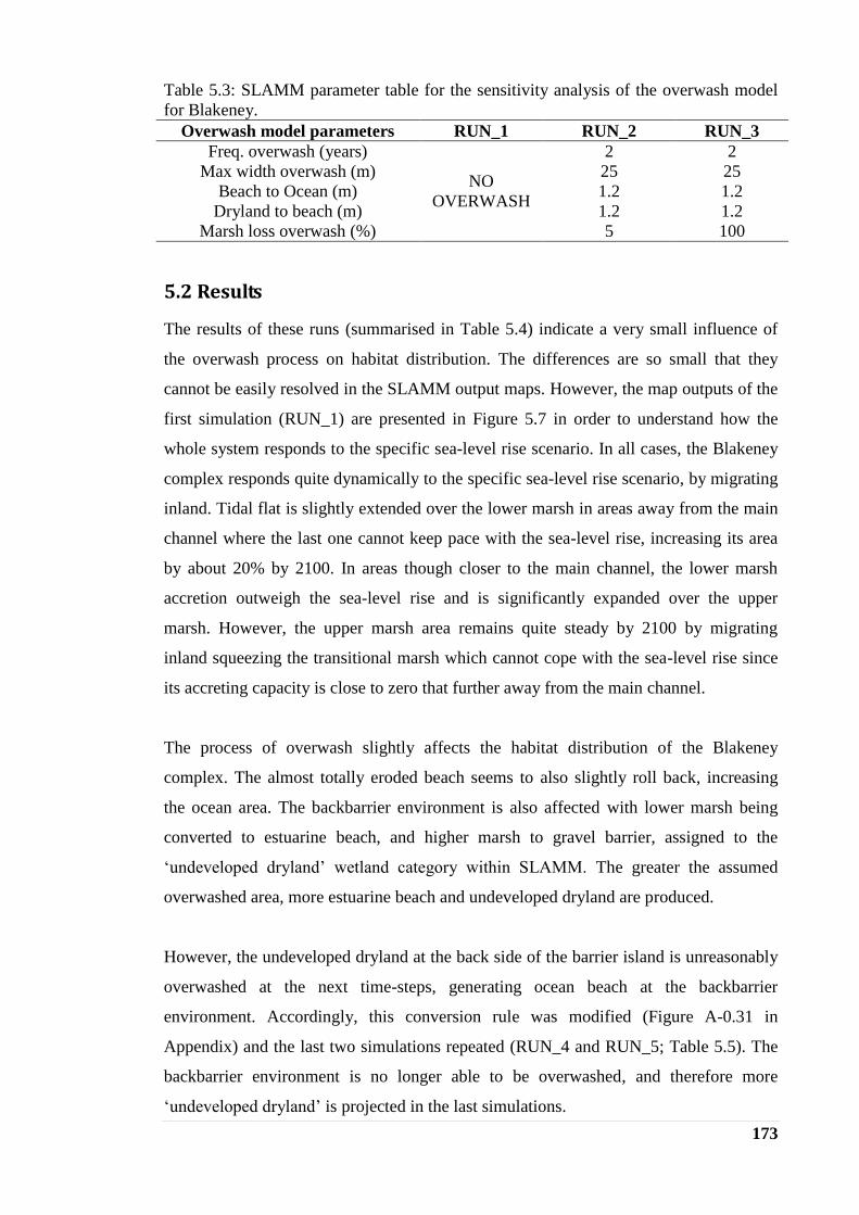
173

Table 5.3: SLAMM parameter table for the sensitivity analysis of the overwash model

for Blakeney.

Overwash model parameters RUN_1 RUN_2 RUN_3

Freq. overwash (years)

NO

OVERWASH

2 2

Max width overwash (m) 25 25

Beach to Ocean (m) 1.2 1.2

Dryland to beach (m) 1.2 1.2

Marsh loss overwash (%) 5 100

5.2 Results

The results of these runs (summarised in Table 5.4) indicate a very small influence of

the overwash process on habitat distribution. The differences are so small that they

cannot be easily resolved in the SLAMM output maps. However, the map outputs of the

first simulation (RUN_1) are presented in Figure 5.7 in order to understand how the

whole system responds to the specific sea-level rise scenario. In all cases, the Blakeney

complex responds quite dynamically to the specific sea-level rise scenario, by migrating

inland. Tidal flat is slightly extended over the lower marsh in areas away from the main

channel where the last one cannot keep pace with the sea-level rise, increasing its area

by about 20% by 2100. In areas though closer to the main channel, the lower marsh

accretion outweigh the sea-level rise and is significantly expanded over the upper

marsh. However, the upper marsh area remains quite steady by 2100 by migrating

inland squeezing the transitional marsh which cannot cope with the sea-level rise since

its accreting capacity is close to zero that further away from the main channel.

The process of overwash slightly affects the habitat distribution of the Blakeney

complex. The almost totally eroded beach seems to also slightly roll back, increasing

the ocean area. The backbarrier environment is also affected with lower marsh being

converted to estuarine beach, and higher marsh to gravel barrier, assigned to the

‘undeveloped dryland’ wetland category within SLAMM. The greater the assumed

overwashed area, more estuarine beach and undeveloped dryland are produced.

However, the undeveloped dryland at the back side of the barrier island is unreasonably

overwashed at the next time-steps, generating ocean beach at the backbarrier

environment. Accordingly, this conversion rule was modified (Figure A-0.31 in

Appendix) and the last two simulations repeated (RUN_4 and RUN_5; Table 5.5). The

backbarrier environment is no longer able to be overwashed, and therefore more

‘undeveloped dryland’ is projected in the last simulations.

174

Table 5.4: Summary of the sensitivity analysis of the overwash sub-model for Blakeney.

Simulation: 'RUN_1'

Date Dry Land

0 2377.8 0.0 333.2 507.8 405.6 0.0 284.2 103.4 296.0 473.0 3348.7

2025 2360.8 0.0 272.0 544.3 440.3 0.0 282.1 85.4 238.4 463.0 3443.5

2050 2332.4 0.0 156.2 603.2 500.3 0.0 296.0 82.7 2.1 457.9 3699.0

2075 2303.5 0.0 83.1 595.2 572.5 0.0 317.0 74.2 3.2 452.2 3729.0

2100 2276.8 0.0 48.5 544.6 624.1 0.0 360.4 70.4 3.3 446.0 3755.7

Simulation: 'RUN_2'

Date Dry Land

0 2377.8 0.0 333.2 507.8 405.6 0.0 284.2 103.4 296.0 473.0 3348.7

2025 2357.6 0.0 271.1 544.4 440.3 0.1 282.1 85.4 239.5 463.0 3446.4

2050 2330.1 0.0 153.9 603.1 500.3 0.1 296.0 82.7 2.2 457.9 3703.6

2075 2301.6 0.0 81.1 594.8 572.5 0.0 316.8 74.2 3.2 452.2 3733.3

2100 2275.3 0.0 47.0 543.8 623.9 0.1 360.4 70.4 3.2 446.0 3759.7

Simulation: 'RUN_3'

Date Dry Land

0 2377.8 0.0 333.2 507.8 405.6 0.0 284.2 103.4 296.0 473.0 3348.7

2025 2359.8 0.6 270.5 543.8 440.2 0.2 282.1 85.4 238.6 463.0 3445.8

2050 2332.0 0.2 153.2 602.0 500.0 0.3 296.0 82.7 2.3 457.9 3703.1

2075 2303.0 0.0 80.9 593.5 572.1 0.3 316.6 74.2 3.2 452.2 3733.8

2100 2276.5 0.0 47.0 542.2 623.5 0.3 360.0 70.4 3.2 446.0 3760.7

Subtidal

Ocean

Beach

Ocean

Flat Ocean

Lower

Marsh

Estuarine

Beach

Tidal

Flat

Ocean

Und.

Dryland

Transitional

Marsh

Upper

Marsh

Ocean

Und.

Dryland

Transitional

Marsh

Upper

Marsh

Lower

Marsh

Estuarine

Beach

Tidal

Flat Subtidal

Ocean

Beach

Ocean

Flat

Und.

Dryland

Transitional

Marsh

Upper

Marsh

Lower

Marsh

Estuarine

Beach

Tidal

Flat Subtidal

Ocean

Beach

Ocean

Flat

Table 5.5: Summary of the sensitivity analysis of the modified overwash sub-model for

Blakeney for the second (RUN_4) and third (RUN_5) scenario respectively.

Simulation: 'RUN_4'

Date Dry Land

0 2377.8 0.0 333.2 507.8 405.6 0.0 284.2 103.4 296.0 473.0 3348.7

2025 2357.5 0.8 271.2 544.3 440.3 0.1 282.1 85.4 239.3 463.0 3446.0

2050 2329.9 0.2 153.9 603.1 500.2 0.1 296.0 82.7 2.2 457.9 3703.6

2075 2301.3 0.1 81.2 594.9 572.5 0.1 316.9 74.2 3.2 452.2 3733.4

2100 2275.2 0.1 47.0 543.9 623.9 0.1 360.4 70.4 3.2 446.0 3759.8

Simulation: 'RUN_5'

Date

0.0 2377.8 0.0 333.2 507.8 405.6 0.0 284.2 103.4 296.0 473.0 3348.7

2025 2359.7 1.6 270.7 544.0 440.2 0.1 282.1 85.4 237.9 463.0 3445.1

2050 2331.9 0.9 153.3 602.2 500.1 0.2 296.0 82.7 2.4 457.9 3702.2

2075 2303.0 0.7 81.0 593.0 572.3 0.3 316.6 74.2 3.3 452.2 3733.2

2100 2276.5 0.5 47.0 541.7 623.4 0.5 360.0 70.4 3.2 446.0 3760.7

Ocean

Flat Ocean

Und.

Dryland

Transitional

Marsh

Upper

Marsh

Lower

Marsh

Estuarine

Beach

Tidal

Flat

Subtidal

Ocean

Beach

Ocean

Flat Ocean

Subtidal

Ocean

Beach

Und.

Dryland

Transitional

Marsh

Upper

Marsh

Lower

Marsh

Estuarine

Beach

Tidal

Flat

Dry Land

In order to investigate more deeply the effects of overwash on the habitat distribution,

the projections to 2100 are examined in more detail in Figure 5.8. Under the extreme

scenario of a completely overwashed shingle ridge (RUN_5), it is clear that the

overwash sub-module produces unreasonable results with the overwashed sediment

being deposited far away from the shingle ridge.

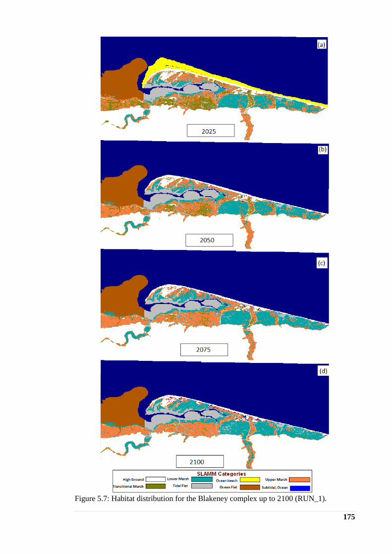
175

Figure 5.7: Habitat distribution for the Blakeney complex up to 2100 (RUN_1).

176

Figure 5.8: Changes in habitat distribution to 2100 for Blakeney, modelled using the

modified source code under the second (RUN_4) and third (RUN_5) scenario.

The weakness of SLAMM to properly simulate the process of overwash has been

acknowledged by the developers for simulations undertaken at a fine (<30m) resolution.

Following this, the second scenario (RUN_4) is repeated using 30m resolution

(RUN_6). The ocean beach responds more dynamically, by slightly rolling back instead

of being totally eroded under the Bruun Rule. In parallel, the overwashed sediment has

been deposited at the backbarrier environment affecting only the 5% of the adjacent to

the barrier island marsh, evenly distributed across the island (Table 5.6; Figure 5.9).

177

Table 5.6: Impacts of sea-level rise at the Blakeney complex under the second scenario,

modelled at 30m resolution (RUN_6).

Simulation: 'RUN_6'

Date Dry Land

0 2373.6 0.0 334.6 511.5 404.1 0.0 284.8 102.7 296.2 474.0 3346.9

2025 2366.7 0.2 274.3 519.2 436.9 0.0 289.7 88.9 296.8 462.6 3393.1

2050 2354.5 1.0 160.3 571.1 477.2 1.0 314.0 91.0 292.0 457.9 3408.4

2075 2329.3 0.8 109.1 566.6 525.3 1.4 335.9 90.3 285.9 452.4 3431.3

2100 2305.3 0.8 83.8 523.8 568.2 1.6 372.6 89.9 278.4 446.4 3457.5

Subtidal

Ocean

Beach

Ocean

Flat Ocean

Und.

Dryland

Transitional

Marsh

Upper

Marsh

Lower

Marsh

Estuarine

Beach

Tidal

Flat


second scenario, modelled at a) 5m (RUN_4) and b) 30m (RUN_6) resolution.

5.3 Indicative evaluation of the model

In both resolutions, SLAMM cannot include the tendency of the spit to develop

westwards. This westward growth of Blakeney is evident in Figure 5.10 with the growth

stages over the last century being marked by the formation of the different recurves. The

recurves are shaped by westerly and northwesterly wave action, with the most recent

extension having been added after a storm surge in 1978 (Bird, 2008). This analysis

indicates that the western end of the Blakeney system is mainly affected by storm

driven processes, considering it far more complex than SLAMM could ever handle.

Therefore, this complex part is not included within the further analysis of the model.

178

Figure 5.10: Historic shoreline positions of the Blakeney coast (generated in GIS based

on historic maps available on digimap).

A hindcast analysis could be useful at this point to validate the model performance

within the barrier and backbarrier environment. Unfortunately, this is not possible due

to lack of historic terrain information, and this is clearly a limitation of the SLAMM

approach given the short archive of LiDAR data (dating back no earlier than 1995 in the

UK). However, Historic Trend Analysis (HTA) (National Research Council, 1987;

Leatherman, 1990), widely used in coastal management and planning, is used here to

validate the projected by SLAMM shoreline behaviour. As mentioned in Chapter 1, this

approach assumes that the observed coastal behaviour encompasses the kind of

behaviour that is expected in the future (National Research Council, 1990; Fenster et al.,

1993; Hooke and Bray, 1996), with the sea-level rise being the dominant influence

(Bray and Hooke, 1997; Whitehouse et al., 2009).

The analysis is summarised in Figure 5.11. The historic behaviour of the shoreline is

analysed based on available historic OS Ordnance Survey maps, by digitising the mean

high water (MHW) line. As presented in graphs a, b and c the shoreline is quite steady,

with its western end advancing seawards, until 1950, when it starts to retreat linearly.

This behaviour, coupled with the observed in the region linear sea-level rise since 1950

(graph d), leads to the assumption that the post-1950 shoreline retreat is driven by

historic sea-level rise.

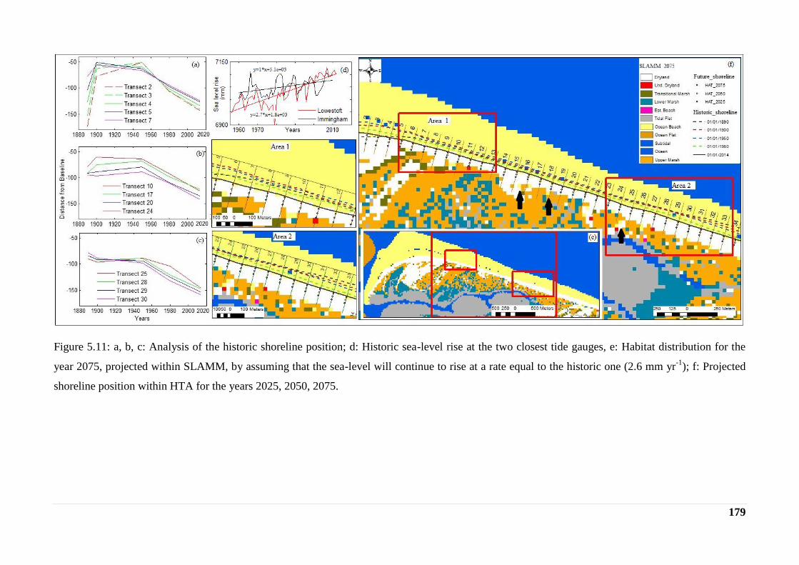
179

Figure 5.11: a, b, c: Analysis of the historic shoreline position; d: Historic sea-level rise at the two closest tide gauges, e: Habitat distribution for the

year 2075, projected within SLAMM, by assuming that the sea-level will continue to rise at a rate equal to the historic one (2.6 mm yr-1

); f: Projected

shoreline position within HTA for the years 2025, 2050, 2075.

180

In that direction, the historic rates of change calculated, based on the post-1950

behaviour by using the DSAS extension (Thieler et al., 2009) in GIS. These historic

retreat rates are then used in the equation 5.1 (Leatherman’s 1990) to extrapolate them

into the future, and therefore compute the shoreline position for the years 2025, 2050

and 2075 (Table 5.8).

1

2

12

S

SRR , ( 5.1)

where R2= future retreat rate (m yr-1

), R1= historic retreat rate (m yr-1

),

S2 = future sea-level rise (mm yr-1

), S1 = historic sea-level rise (mm yr-1

).

In order to compare the two modelling approaches, the last simulation performed within

SLAMM (RUN_6) is repeated by assuming that the sea-level will continue to rise under

the same rate in the future (RUN_7). In that direction a custom simulation is performed

by assuming a global sea-level rise equal to 0.2 m by 2100, in order an eustatic sea-level

rise of 0.13 m by 2075 to be calculated. The results are presented at the Table 5.7 up to

year 2100 and in the Figure 5.11e for the year 2075. The ocean beach converts to ocean

by about 0.1% by year 2075, while at the backbarrier environment a slight inland marsh

migration occurs squeezing the transitional marsh, which lose almost half of its area.

Table 5.7: Impacts of sea-level rise at the Blakeney complex for the second scenario,

assuming that sea level rises at a rate equal to the historic one (RUN_7).

Simulation: 'RUN_7'

Date

SLR

(eustatic) Dry Land

0.0 0 2373.6 0.0 334.6 511.5 404.1 0.0 284.8 102.7 296.2 474.0 3346.9

2025.0 0.02 2378.5 0.3 301.3 509.8 416.4 0.0 285.0 85.5 298.7 471.1 3381.8

2050.0 0.07 2382.4 0.4 226.0 558.0 426.4 0.3 293.9 86.3 300.1 470.5 3384.2

2075.0 0.13 2365.1 0.7 181.0 588.2 451.6 0.6 292.8 90.3 301.4 463.2 3393.6

2100.0 0.20 2353.0 0.6 142.5 603.5 481.0 0.9 292.7 92.2 302.9 461.5 3397.7

Subtidal

Ocean

Beach

Estuarine

Beach

Tidal

Flat

Und.

Dryland

Transitional

Marsh

Upper

Marsh

Lower

Marsh

Ocean

Flat Ocean

Focusing on the shoreline position, the projected habitat distribution generated within

SLAMM for the year 2075 is overlaid by the historic and future shoreline positions, as

the last ones are calculated within the HTA modelling approach for the years 2025,

2050 and 2075, as presented in Figure 5.11f. The fact that the 2014 shoreline position is

depicted at the seaward lower boundary of the dryland is due to the low quality input

data. Thus, the importance for high quality data is once again highlighted (see

sensitivity analysis at Section 3.3). Most importantly, though, the future shoreline

positions computed within the HTA approach, driven by the process of overwash, are

projected within the dryland wetland category of SLAMM. Consequently, this process

181

is not captured within the overwash sub-model incorporated within SLAMM, indicating

the limitation of the model to properly simulate this process without a hydrodynamic

model.

On the other hand, ocean beach is generated at the backbarrier environment, even after

the last modification of the source code (Figure 5.11f). This, coupled with the inundated

areas projected at high elevations of the backbarrier environment at high resolution

simulations (see simulations RUN_4 and Run_5 in Figure 5.7), is explained by the fact

that the adjacent to the ocean dryland, i.e. within 500 m, is inundated to ocean beach

and therefore to ocean (see Table 2.5).

Accordingly, the source code was further modified, and the adjacent to the ocean

threshold is determined as a variable parameter that must be specified by the user for

each case study (Figures A-0.32; update Figures A-0.2 to A-0.4 and A-0.6 to A-0.10 in

Appendix). For Blakeney, this threshold is estimated at approximately 50 m, based on

present aerial photos (Figure 5.12), by taking into account that the beach will be totally

eroded, and the first scenario is repeated with the modified code (RUN_ 8) in order to

simulate the impacts of sea-level rise at the Blakeney complex, ignoring the process of

overwash. The results, presented in Table 5.9 and Figure 5.13, project a different

respond of the backbarrier environment, with the dryland considered part of the

estuarine system, and being inundated to transitional marsh.

Figure 5.12: Parameterisation of the adjacent to the ocean threshold based on analysis of

aerial imagery in Google Earth.

182

Table 5.8: Projection of future shoreline position within the HTA approach.

ID in 2014 in 2025 in 2050 in 2075 StartX StartY Azimuth X Y X Y X Y

1 n/a n/a n/a n/a n/a n/a n/a n/a n/a n/a n/a n/a n/a n/a n/a n/a n/a n/a n/a n/a

2 -1.4 0.98 YES 1.44 2 2 1.44 143 159.3 195.3 231.3 600457 346759 191 600427 346603 600421 346567 600414 346532

3 -1.4 0.98 YES 1.4 2 2 1.4 141 156.4 191.4 226.4 600554 346739 194 600517 346587 600508 346553 600500 346519

4 -1.2 0.99 YES 1.17 2 2 1.17 134 147.1 176.3 205.6 600651 346715 194 600616 346572 600609 346544 600602 346515

5 -1.0 0.99 YES 1 2 2 1 127 138.2 163.2 188.2 600748 346690 194 600714 346557 600708 346532 600702 346508

6 -1.1 1.00 YES 1.05 2 2 1.05 126 137.3 163.5 189.8 600845 346664 195 600809 346532 600802 346507 600795 346481

7 -0.9 1.00 YES 0.92 2 2 0.92 125 135.0 158.0 181.0 600941 346638 195 600906 346508 600900 346485 600894 346463

8 -0.8 0.99 YES 0.79 2 2 0.79 122 130.5 150.2 170.0 601038 346611 195 601003 346485 600998 346466 600993 346447

9 -0.8 1.00 YES 0.84 2 2 0.84 122 130.9 151.9 172.9 601134 346585 196 601098 346459 601093 346438 601087 346418

10 -1.0 1.00 YES 0.97 2 2 0.97 126 136.3 160.6 184.8 601230 346557 196 601193 346426 601186 346403 601180 346379

11 -1.0 0.99 YES 1.03 2 2 1.03 128 139.2 164.9 190.7 601327 346530 196 601288 346396 601281 346371 601274 346346

12 -1.0 1.00 YES 1.02 2 2 1.02 126 137.0 162.5 188.0 601423 346502 196 601385 346370 601378 346346 601371 346321

13 -0.9 0.97 YES 0.89 2 2 0.89 117 126.8 149.0 171.3 601519 346474 196 601483 346353 601476 346331 601470 346310

14 -1.0 0.99 YES 0.96 2 2 0.96 121 131.2 155.2 179.2 601615 346446 196 601577 346320 601571 346297 601564 346274

15 -0.9 0.99 YES 0.86 2 2 0.86 116 125.5 147.0 168.5 601710 346418 196 601675 346297 601669 346277 601663 346256

16 -0.8 0.98 YES 0.78 2 2 0.78 113 121.2 140.7 160.2 601806 346389 196 601773 346273 601768 346254 601763 346235

17 -0.8 0.99 YES 0.84 2 2 0.84 122 131.6 152.6 173.6 601903 346365 194 601872 346237 601867 346217 601862 346196

18 -1.0 0.99 YES 0.96 2 2 0.96 135 145.5 169.5 193.5 602001 346341 194 601966 346200 601961 346177 601955 346153

19 -1.0 1.00 YES 0.95 2 2 0.95 140 150.8 174.5 198.3 602097 346316 197 602052 346172 602045 346150 602038 346127

20 -0.9 0.99 YES 0.87 2 2 0.87 136 145.1 166.9 188.6 602193 346286 197 602149 346148 602143 346127 602136 346106

21 -0.7 0.99 YES 0.72 2 2 0.72 128 136.4 154.4 172.4 602288 346256 197 602247 346126 602242 346109 602236 346092

22 -0.7 0.99 YES 0.73 2 2 0.73 129 137.1 155.4 173.6 602384 346226 197 602342 346095 602337 346078 602331 346061

23 -0.8 1.00 YES 0.78 2 2 0.78 135 143.1 162.6 182.1 602479 346198 195 602441 346060 602436 346041 602431 346022

24 -0.8 0.99 YES 0.84 2 2 0.84 143 152.0 173.0 194.0 602576 346171 195 602535 346025 602530 346004 602524 345984

25 -0.9 0.95 YES 0.91 2 2 0.91 146 156.5 179.3 202.0 602672 346145 195 602631 345994 602624 345972 602618 345950

26 -0.9 1.00 YES 0.85 2 2 0.85 142 151.2 172.4 193.7 602769 346118 195 602728 345972 602723 345952 602717 345931

27 -0.9 0.98 YES 0.86 2 2 0.86 142 151.6 173.1 194.6 602865 346091 195 602825 345945 602819 345924 602813 345904

28 -0.9 0.99 YES 0.92 2 2 0.92 148 158.1 181.1 204.1 602961 346065 195 602919 345912 602913 345890 602907 345868

29 -0.9 1.00 YES 0.94 2 2 0.94 154 164.1 187.6 211.1 603058 346038 196 603014 345880 603007 345857 603001 345835

30 -1.0 0.99 YES 0.95 2 2 0.95 159 169.6 193.4 217.1 603154 346011 196 603108 345848 603102 345825 603095 345802

31 -1.0 0.97 YES 0.95 2 2 0.95 162 172.7 196.5 220.2 603250 345984 196 603204 345818 603197 345795 603191 345772

32 -0.9 0.94 YES 0.91 2 2 0.91 165 174.8 197.5 220.3 603347 345957 196 603299 345789 603293 345767 603287 345745

33 -0.9 0.96 YES 0.86 2 2 0.86 167 176.7 198.2 219.7 603443 345930 196 603395 345760 603389 345739 603384 345718

34 -0.8 0.94 YES 0.84 2 2 0.84 171 180.0 201.0 222.0 603539 345903 196 603491 345730 603485 345710 603479 345689




HTA

LRR LR2

Linear

??

Historic

SLR

(mm/year)

Projected Shoreline Coordinates

2025 2050 2075

DSAS

Distance from Baseline Transect coordinates Historic

retreat

(m/yr)

Future

SLR

by 2075

Future

Retreat Rate

by 2075

183

Table 5.9: : Impacts of sea-level rise at the Blakeney complex for the first scenario,

modelled with the adjacent to the ocean threshold equal to 500m (RUN_1) and 50m

(RUN_8).

Simulation: 'RUN_1'

Date Dry Land

0 2377.8 333.2 507.8 405.6 284.2 103.4 296.0 473.0 3348.7

2025 2360.8 272.0 544.3 440.3 282.1 85.4 238.4 463.0 3443.5

2050 2332.4 156.2 603.2 500.3 296.0 82.7 2.1 457.9 3699.0

2075 2303.5 83.1 595.2 572.5 317.0 74.2 3.2 452.2 3729.0

2100 2276.8 48.5 544.6 624.1 360.4 70.4 3.3 446.0 3755.7

Simulation: 'RUN_8'

Date Dry Land

0 2377.8 333.2 507.8 405.6 284.2 103.4 296.0 473.0 3348.7

2025 2360.8 275.4 544.3 440.3 282.2 105.2 236.7 463.0 3422.1

2050 2332.4 167.6 603.4 500.1 296.2 104.1 0.0 457.9 3668.1

2075 2303.7 101.5 595.9 572.2 319.0 102.0 0.1 452.2 3683.3

2100 2277.5 74.5 547.2 624.1 362.1 100.4 0.1 446.0 3697.9

Transitional

Marsh

Upper

Marsh

Lower

Marsh

Tidal

Flat

Transitional

Marsh

Upper

Marsh

Lower

Marsh

Tidal

Flat Subtidal

Ocean

Beach

Ocean

Flat Ocean

Subtidal

Ocean

Beach

Ocean

Flat Ocean


first scenario, modelled with the adjacent to the ocean threshold equal to 500m

(RUN_1) and 50m (RUN_8).

Summarising, it can be said that the open to the ocean part of the Blakeney complex

responds differently than its inner one under the UK-CP sea-level rise scenario. The

former one is projected to be unable to cope with the sea-level rise and being totally

eroded, while the estuarine part responds very dynamically by migrating inland.

However, the more complex process of the westward development of the spit and the

process of overwash that mostly control the response of the specific case study to the

sea-level rise cannot be captured within SLAMM. Thus, the need for further

development of the model is emerged by including more robust sub-models.

184

6 DISCUSSION

6.1 Spatial models for simulation of estuarine and coastal habitat

changes

The research presented here has explored the potential of reduced complexity, spatial

landscape models to represent mesoscale impacts of sea-level rise on estuarine

environments in the UK. The Sea Level Affecting Marshes Model (SLAMM) (Clough

et al., 2010) was used as a starting point, because, after 20 years of development, it has

been characterised as an important forecast and simulation model in coastal research

(Liao et al., 2011). Notably, it has been widely used in US for the North American

estuaries and wetland environments ( SLAMM2: Park et al., 1989; Park, 1991; Titus et

al., 1991, SLAMM3: Lee et al., 1991,1992; Park et al., 1991, 1993, SLAMM4:

Galbraith et al., 2002, 2003, SLAMM4.1: NWF, 2006, SLAMM5: Craft et al., 2009,

SLAMM6: used by many consultancy projects by Warren Pinnacle Consulting on

behalf of the U.S. Fish and Wildlife Service, the National Wildlife Federation, the Gulf

of Mexico Alliance, the Nature Conservancy and the Indiana University; Chu et al.,

2014; Geselbracht et al., 2011; Glick et al., 2013; Linhoss et al., 2013, 2015; Wang et

al., 2014).

SLAMM is a rule-based spatial model, which simulates the dominant processes

involved in shoreline modifications and wetland conversions during sea-level rise. Like

other spatial models used in the past in the US (e.g. Sklar et al., 1985, 1989, 1994;

Costanza et al., 1988, 1990), the area of interest is simulated on a cell-by-cell basis, and

habitat change is determined by using a decision tree. Whilst previous spatial models

have often been based on cellular automata principles (see also Dearing et al., 2006),

SLAMM places greater reliance on global rules to determine the evolution of habitat

type according to elevation and relative position within a rasterised landscape. As a

consequence, cells are not connected to their neighbours by exchanges of water and

suspended materials, and this limits the ability of the model to represent the

constraining influence of sediment supply, which is known to be important in estuarine

and intertidal wetland systems (French, 2006; Kirwan et al., 2010). On the other hand,

SLAMM can handle a range of spatial resolutions (cell sizes), depending on the size of

the site and the availability of the data input. For example, a resolution of 10 m was

used for the Grand Bay Estuarine Research Reserve and the Southern Jefferson County

185

at the Gulf of Mexico (Warren Pinnacle Consulting Inc, 2011a,b), 15 m for the

southeastern Louisiana (Glick et al., 2013) and the Cape May National Wildlife Reserve

in New Jersey (Warren Pinnacle Consulting Inc, 2011c) and 30m resolution for the

more extended Kenai Peninsula and Anchorage in Alaska (Clough and Larson, 2009)

and the Chesapeake Bay Region in the US (Glick et al., 2008). SLAMM can also

recognise the existence of more than one land cover category within a cell and simulate

them separately. Consequently, SLAMM is suitable to simulate quite complex

environments and is capable of spatially detailed projections.

Although spatial models have been widely applied to coastal and estuarine problems in

the US, little previous work of this kind has yet been carried out in the UK. Preliminary

work on an estuary model based on cellular automata principles was carried out by

Dearing et al. (2006), including a pilot application to the Blackwater Estuary, UK.

Probably the only operational use of spatial modelling is the BRANCH project

(BRANCH partnership, 2007), which simulated the impacts of sea-level rise at six local

case studies on the south coast of the UK. This approach is GIS-based, and in contrast

to SLAMM, which simulates the whole estuary at once, divides the area of interest into

the open coast and the intertidal habitats and assesses the impacts of sea-level rise on

each one of them individually.

Modelling of the open coast in the UK has focused on the shoreline movement under

different sea-level rise scenarios, by using empirical relationships (e.g. Futurecoast

study (Defra, 2002); Pye and Blott, 2008; Isle of Wight SMP2, 2010), or more

sophisticated process-based models with representative example the SCAPE model

(Walkden and Hall, 2005, 2011; Dickson et al., 2007; Addo et al., 2008; Walkden and

Dickson, 2008). The former technique is based on the assumption that shoreline

behaviour is only driven by the sea-level rise (Bray and Hooke, 1997; Whitehouse et al.,

2009). Therefore, it is not suitable for coasts that are also affected by other factors. An

example of this type of more complex shoreline behaviour is the barrier island and spit

complex of the North Norfolk coast. These exhibit progressive landward retreat of

gravel and dune-capped barriers, in parallel with incremental westwards extension

driven by episodic storm conditions (Steers et al., 1979; Funnell et al., 2000). On the

other hand, the SCAPE model is a reduced complexity model that includes several

modules in order to describe more complex responses. However, its application is

restricted to a specific range of coastal types (cliffs, beaches and shore platforms), and

186

therefore must be used in conjunction with other predictive models (Walkden and Hall,

2005, 2011; Dickson et al., 2007; Addo et al., 2008; Walkden and Dickson, 2008).

Current estuarine modelling approaches (see also Brooks et al., 2006; Snoussi et al.,

2009; Tian et al., 2010) are largely based on the progressive drowning of the existing

topography under different sea-level rise scenarios, lacking any physically–based

modelling of habitat transition. SLAMM represents a step forward here in that it

incorporates a flexible decision tree and qualitative relationships in order to determine

the fate of each habitat. More importantly, more processes than just inundation are

included, with most important vertical accretion within intertidal marsh and flat

environments. Importantly, accretion can either be specified as a constant value for each

habitat, when insufficient data are available, or as a time-varying function of cell

elevation, wetland type, distance to channel and salinity.

SLAMM has already been used in US as a tool to help environmental managers

understand the effects of sea-level rise and consequently identify strategies to minimise

them (Glick et al., 2013). Building on this experience, this thesis has investigated the

potential for UK estuary management policy to be informed more effectively by using

models such as SLAMM. To this end, the SLAMM source code has been examined in

detail and, where appropriate, modifications made to allow its application outside the

US. Its component sub-models have also been examined and their limitations explored

in the context of case studies on the south and east coast of England. Of particular

importance is the dependence of SLAMM not only on high resolution topographic data

but also on the availability of background information on the tidal regime and on

indicative rates of intertidal sedimentation with which to constrain the operation of its

various rules. Whilst the former are now increasingly available in the form of airborne

LiDAR data (e.g. French, 2003, Brock and Purkis, 2009), observations of intertidal

sedimentation processes and rates are still lacking for many sites. Moreover, the historic

archive of airborne LiDAR data is still quite short (the earliest Environment Agency

coastal datasets are for 1995). This makes longer – term hindcast validation difficult.

6.2 Modification of SLAMM for application to UK estuaries

The architecture of SLAMM is slightly unconventional in terms of the land cover

classification. This is hard coded according to the US National Wetland Inventory

187

(NWI) scheme (U.S. Fish and Wildlife Service, 1974), which is not widely used

elsewhere. In addition, the forcing scenarios and various aspects of the sub-models are

also embedded in the source code rather being read from external files. Consequently,

changes in its source code are required in order to apply the model to sites outside North

America, and to explore changes resulting from a wider set of regional sea-level forcing

scenarios.

To this end, the SLAMM code was modified in order to suit the tidal sedimentary

environments and habitats more typical of the UK. A simpler land classification is

included as it is defined by the INTERREG funded BRANCH project (BRANCH

partnership, 2007). In parallel, the land classification conceptual model within SLAMM

was modified to automatically update the elevation range of each habitat according to

their position to the tidal frame, as used in the BRANCH project (after Chapman, 1960;

Pye and French, 1993; Leggett and Dixon, 1994; Blott and Pye, 2004). Consequently, in

contrast to the original model, the modified scheme more readily accommodates

specific case studies. In addition, the habitat transition rules were modified to include a

smoother habitat conversion due to inundation; the transitional marsh is inundated to

upper marsh instead of lower marsh, and the dryland to transitional marsh instead of

estuarine beach when it is adjacent to the subtidal. Finally, UK-specific sea-level rise

scenarios were incorporated into the modified code. Consequently, the modified code

can be used to simulate the impacts of sea-level rise in the UK estuarine systems.

The estuarine systems in the UK are generally much smaller in extent than many of the

North American systems previously investigated using SLAMM. Their intertidal

habitats are also often fragmented, with many saltmarsh units been only a few meters in

width. This necessitates application of the modified SLAMM at a higher spatial

resolution. Thus, although the highest resolution used to date in the US is 10m (see case

studies of Brand Bay NERR and Southern Jefferson County in Mexico (Warren and

Pinnacle Inc, 2011a,b)), a 5 m resolution is used in the present UK applications. This

corresponds to the upper resolution limit suggested by the original model authors

(Clough et al., 2010).

The modified code was firstly applied to a small case study estuary, on the south coast

of England, the Newtown estuary, Isle of Wight. Initial simulations indicated significant

changes in the distribution of intertidal flat and saltmarsh under the UKCP09 SE mean

188

sea-level rise scenario (UKCP, 2009).These changes were compared with results from a

previous modelling effort for the Newtown estuary carried out as part of the BRANCH

project (BRANCH partnership, 2007). As already noted above, the approach used

within the BRANCH project is based on the progressive drowning of the existing

topography lacking any mechanistic modelling of habitat transition. In particular, lateral

erosion at the tidal flat – saltmarsh transition is totally ignored, while accretion is only

taken into account for areas already colonised by saltmarsh vegetation. In contrast,

SLAMM presents a step forward by incorporating a flexible decision tree and

qualitative relationships to determine the habitat transition. It also takes into account of

more processes related to sea-level rise than just inundation, with most important being

vertical accretion within the intertidal marsh and flat environments. Importantly, this

accretion is also allowed to vary spatially.

The small size of the Newtown estuary allows a comprehensive sensitivity analysis of

the basic processes and parameters included in the model. Firstly, the effect of an error

at the DEM was investigated, by examining the typical elevation accuracy of the UK

LiDAR data, which is generally quoted as being equal to ±0.15 m (French, 2003; CCO,

2013). The results highlighted out the importance of the quality of the terrain

information, especially for such low gradient environments, by affecting the initial

condition of the habitat distribution, and therefore their further response to the sea-level

rise.

The importance of fine resolution simulations was also highlighted. The recommended

cell size range of 5 to 30m (Clough et al., 2010) was extended to include a higher

resolution of 1m. The results indicate the significant influence of this parameter to the

projected habitat distribution. The lower the resolution used, greater the differences are

to the projected habitat distribution relevant to the present condition. However, this

parameter affects the run time of the simulation, which is significantly increased for fine

resolution simulations. For the small Newtown estuary, the run time of a simulation

varied from 1 minute for a low resolution simulation (30 m) to ten minutes and six

hours for a fine resolution simulation of 5 and 1 m respectively (using a single 2.4GHz

cpu). This limits the application of fine resolution simulations in very large areas, where

resolution need to be sacrificed for a shorter simulation time.

189

A further factor that could affect the quality of the input data is the interpretation

accuracy in the identification of the habitat distribution from remote sensor data. The

smallest recommended level of accuracy equal to 85% (Anderson, 1971; Anderson et

al., 1971, 1976; Olson 2008) is examined here by randomly misclassifying 15% of each

category to the closest in terms of elevation one. This analysis highlights the capability

of SLAMM to correct errors in the habitat distribution (Clough et al., 2010) based on

their position into the tidal frame. However, this process is simulated solely in terms of

inundation, ignoring the equally important process of aggradation (i.e. the seaward

expansion of specific intertidal wetland units). Therefore the source code was further

modified to incorporate this process, enabling SLAMM to capture a more accurate

present habitat distribution. The latter considers SLAMM a valuable tool in decision

making strategies for case studies with poorly represented habitat distribution data.

Most fundamentally, the process of aggradation further affects the representation of

accretional processes into the future habitat projections. The sensitivity of the projected

habitat distribution on this extremely important factor was examined here by applying

different accretion values for the upper and lower marsh and the tidal flat. The higher

the accretion rate applied in a given habitat, the better it is able to cope with the sea-

level rise (Reed, 1990; Doody, 2001; Day et al., 2008). However, with the procedure of

aggradation disabled, the model cannot capture the process of upland migration in areas

with sufficient sediment supply. This particular modification of the source code is

therefore vital to the performance of the model.

Finally, the process of lateral erosion was investigated for the tidal flat and the marsh

area by applying different erosion rates for each one of them. Based on evidence from

studies in southeast England (Burd, 1992; Cooper et al., 2001; van der Wal and Pye,

2004; Wolters et al., 2005) that marsh edge erosion can occur even in estuaries with a

small fetch, the model code was modified to reduce the fetch threshold to 0.5 km. The

code was also edited to allow erosion of the ‘dryland’; this allows the model to

represent the erosion of inactive flood defences. This modification is mostly relevant for

estuaries where embankments have failed but continue to limit the fetch until they

eroded away (French et al., 2000).

This sensitivity analysis focuses mainly on the output uncertainty at each time-step, due

to individual input parameters. An analysis of the cumulative representation would also

190

be interesting, but this is outside the scope of this thesis. A deeper investigation of the

uncertainty factor could also explore the inter-dependencies between the different input

uncertainties and how this might propagate into model projection errors. That would

most logically involve a Monte Carlo simulation possibly involving several hundred

simulations to cover all the parameters. One of the challenges that might arise here is

the selection of appropriate estuarine state indicators (cf Van Koningsveld et al., 2005)

to match model output to management needs.

The various source code modifications reported here allow meaningful use of SLAMM

beyond the North American context for which it was designed. The modified code

accommodates a simplified classification of intertidal habitats that is better suited to

application in the UK, and potentially elsewhere in northwest Europe. It might also be

argued that a simpler classification is more commensurate with the ability of this kind

of rule-based model to resolve changes in habitat based largely on elevation as a

determining factor. The detailed floristic composition of wetland subtypes clearly

reflects not only the elevation (and its direct effect on hydroperiod) but also factors such

as soil structure and chemistry, drainage and competition that may exhibit a much

weaker dependence on elevation (Paul, 1993; Boorman et al., 1998; Callaway, 2001;

Silvestri et al., 2005).

6.3 Application of modified SLAMM to contrasting estuarine and

barrier systems in Eastern England

The variously modified SLAMM code was subsequently applied to the more complex

environments of the Suffolk estuaries and Norfolk barrier coast in eastern England in

order to critically evaluate its ability to produce meaningful projections of habitat

change under the UKCP09 sea–level rise scenarios. The choice of the sites was mainly

based on the availability of the LiDAR data from the Environment Agency, since

topographic data at high resolution and accuracy is vital for meaningful application of

the model (Clough et al., 2010). The LiDAR data were supplemented by the available

background literature on habitats and sedimentary processes within these environments

and by application of a simpler 0-dimensional model of saltmarsh sedimentation

(French, 2006) to derive the required functional dependencies between sedimentation

and elevation.

191

Initially, SLAMM was applied into two estuarine systems on the Suffolk of eastern

England; the Blyth and the Deben estuary. Both of them are of particular interest due to

extensive reclamation of their intertidal margins since the 17th

century (French and

Burningham, 2003; French et al., 2008), and large potential intertidal area that is

presently protected from inundation by earth embankments. Simulations were

performed with the assumption that these defences were maintained in situ and also for

the entirely hypothetical case that all defences are removed. Since the effect of restoring

tidal exchange to individual flood compartments is purely additive (i.e. they do not

feedback into estuary tidal prism, hydrodynamics and sedimentation; French, 2008), this

extreme scenario is also sufficient to evaluate any more incremental reduction in the

defended area.

A key focus of this work was to explore the appropriateness of the various assumptions

in the under-lying accretion sub-models. The model was empirically parameterised

based on observed historic sedimentation data (French and Burningham, 2003; Pye and

Blott, 2008b), while the MARSH-0D (French, 2006) model (essentially an aspatial box

model; Hearn, 2008) was used to further constrain saltmarsh sedimentation by

generating a functional relationship between elevation and sedimentation rate under the

local tidal regime. A limitation of the MARSH-0D (French, 2006) model as used here is

that its uses a simplification of the tidal regime (only four tidal constituents, M2, S2,

O1, K1), and in the mode used here, does not include aperiodic surge effects. The latter

can be an important contributor to marsh sedimentation, especially in micro- and meso-

tidal settings (Stumpf, 1983; Pugh, 1987; French, 2006; Schuerch et al., 2012). This was

addressed by extrapolating the computed accretion rates by assuming a zero-deposition

in the highest elevation of the marsh. A further refinement through the distance to

channel effect was also included.

This approach is reasonably effective in representing one of the major morphodynamic

feedbacks that is known to condition the adjustment of marsh elevation (which is here

the chief control of habitat type) within the tidal frame at centennial timescales (Allen,

2000; French and Reed, 2001; Friedrichs and Perry, 2001; French and Burningham,

2003; Temmerman et al., 2003; French, 2006). The analysis highlights that the

projected changes in the habitat distribution are clearly very sensitive to the various

assumptions in the accretion sub-models, and that it is often difficult to justify particular

values with reference to observations. Experimentation with constant accretion rates

192

indicated that the rule based approach is the only way forward given that SLAMM does

not keep track of sediment mass balance and cannot adjust sedimentation rate according

to local sediment supply.

Importantly, tidal flats are rather more dynamic than saltmarshes and frequently exhibit

temporal variation between accretion and erosion at seasonal, low interannual and

decadal timescales (Anderson et al., 1981; O’Brien et al., 2000; French and

Burningham, 2003). However, inferences based on historic sedimentation are

occasionally possible. The Blyth is as good example here, where measured sediment

accumulation over a dated horizon following abandonment of flood defences can be

used to generate functional relationship between sedimentation and elevation. This

approach assumes a tendency towards accretion, with any intermediate erosional

episodes clearly not resolved.

Also, in the case of the Blyth, historic sedimentation within newly created intertidal

areas seemingly leads to an equilibrium elevation that lies below that at which saltmarsh

would ordinarily establish. This can be interpreted as evolution towards a wave-

dominated equilibrium (Fagherazzi and Wiberg, 2009), which cannot be captured in

SLAMM since the influence of the waves is not incorporated into the model. This is

clearly a limitation of the model, since the upper intertidal flats are significantly affected

by the waves (Nicholls et al., 1999, 2004; Simas et al., 2001; Syvitski et al., 2005;

Gardiner et al., 1992, Gardiner and Porter 2001; Pethick, 2001; Davidson–Arnott et al.,

2002; Cahoon et al., 2006; Moller, 2006; Reed et al., 2009). Handling this kind of

situation, and the resolution of alternative divergent states (Phillips, 2014), would

clearly require a more mechanistic treatment of the interaction between intertidal

sedimentation, locally generated wind waves, and the tidal regime.

In the Deben case study, an attempt was made to resolve recent changes in tidal flat

elevation from the EA LIDAR data and also to relate these to characteristically

erosional or accretional tidal profiles, following the approach of Kirby (2000). Based on

this, the tidal profiles are classified according to the contributions of tidal currents and

wind waves to the sediment transport, and the intertidal flat within SLAMM is then

zoned accordingly. However, this approach is still very crude and highlights once again

the need for a more mechanistic treatment of the tidal flat. This is a major weakness of

SLAMM, but it is not clear that the necessary models actually exist, although progress

193

is being made with explanatory numerical models for simplified geometries (e.g.

Mariotti and Fagherazzi, 2013; Thornhill et al., 2015). Moreover, the poorly modelled

tidal flat within SLAMM also controls the evolution of the subtidal, which depends on

the surrounding environment rather than being modelled itself. In other words, SLAMM

is a model that focuses into the intertidal environment.

Particular interest presents in the case of the Deben estuary the feature of the Knolls,

which are assigned here as ocean flat and therefore treated within SLAMM similarly to

the tidal flat environment. A comparison of the projections with a survey undertaken by

Burningham and French (2006) indicates that SLAMM is not able to capture the

complex historic behaviour of the ebb-tidal delta in the absence of an effective wave

model. Morphodynamic of ebb deltas shores is complex, involving waves, tides and, in

the case of the Deben, mixed sediments. Resolving this behavirour requires a dedicated

sub-model that is presently lacking in SLAMM. Moreover, in both case studies, the

response of the beach at the sea-level rise is simulated within SLAMM by using the

Bruun rule, projecting total beach erosion. This projection though does not agree with

the observed historic shoreline trend which indicates a more complex pattern of

shoreline response. This is clearly a limitation of the model which also enhances the

idea that the Bruun rule is an inadequate model of shoreline retreat (Kaplin and

Selivanov, 1995; List et al., 1997; Pilkey et al., 2000; Sallenger et al., 2000; Thieler et

al., 2000), highlighting the need to incorporate a wave hydrodynamic model.

The fairly simple open coastal beach and barrier sub-model within SLAMM is

evaluated with reference to the complex barrier coast of Norfolk. In particular,

simulations of the Blakeney spit complex are used to test the ability of SLAMM to

reproduce coastal retreat driven by storm overwash (Clymo, 1964; Funnell et al., 2000).

The MARSH-0D (French, 2006) model was again used to parameterise the marsh

accretion sub-model, while in the absence of both data and a more mechanistic model of

tidal flat processes, this environment was assumed to simply track the sea-level rise.

The overwash sub-model is currently rather experimental in SLAMM and has been used

rather infrequently and only at low resolution. Modifications were found to be necessary

to resolve the unreasonable projection of ocean beach at the backbarrier environment.

The overwash transition rule of the backside of the ridge was de-activated, and the

threshold that considers the ‘dryland’ part of the coastal environment, and therefore

194

considers it subjected to be inundated to ocean beach, was determined as variable in

order to be specific for each case study. The latter makes the model capable of

application in a broader range of environmental contexts.

With the overwash model inactive, the beach is rapidly eroded according to the Bruun

Rule. However, the procedure of erosion is de-activated during the simulation when

overwash is assumed to be the main cause of coastal retreat. In that case, the outer

barrier seems to slightly retreat, while in parallel the overwashed sediment is deposited

in the backbarrier environment. A big limitation of the model though, in both cases, is

that it cannot include the westwards development of the spit (Clymo, 1964; Funnell et

al., 2000). It is thus unable to simulate planform evolution in systems that are influenced

by storm-driven processes.

A hindcast analysis was not possible to evaluate the performance of the model due to

the restricted terrain information with which a historic simulation could be initialised.

Although a digital elevation model could be generated by adjusting the present

elevations to account of the effects of relative sea-level rise and deposition rates for the

intervening period, this could inevitably lead to project the initial elevations.

Differences might exist, though, to the projected habitat distribution since the affected

areas are calculated based on empirical equations by taking into account only the

minimum and maximum elevation of each wetland category in each cell. At this end, an

indicative evaluation was achieved for the Blakeney spit and barrier case study by

comparing historic migration of the shoreline and outer barrier with projected future

change. The Historic Trend Analysis (National research Council, 1987; Leatherman,

1990) approach was used for the comparison, by using the same (linear) sea-level

forcing in both modelling approaches. The results showed that although SLAMM seems

to capture a slight roll back of the barrier island, this is weakly represented with such a

simple empirical model. Further development therefore is required by including a

hydrodynamic model, which can also take into account the magnitude and the extent of

the overwash deposits (Donnelly et al., 2006; Roelvink et al., 2009).

The modifications to the habitat type classification and certain elements of the decision

tree have been successfully tested in a selection of UK estuarine and backbarrier

settings. High spatial resolution of 5m is computationally tractable for the modelled

domains, allowing multiple model runs to investigate the model sensitivity and the

195

projected outcomes under a wide range of scenarios. SLAMM performs best in the

upper intertidal, where the elevational adjustment of saltmarsh surfaces is mainly

governed by patterns of sedimentation that can be expressed as relatively robust

functions of elevation and position with respect to channels or open water. Projections

under the UKCP09 sea-level rise scenario show a dynamic response of the estuaries by

migrating landwards squeezing the upper marsh zones where landward migration is

prevented by low accretion rates in higher elevations away from the main channel.

However, the tidal flat is modelled less convincingly. Tidal flat morphodynamics are

more complex and more difficult to parameterise as simple functions of elevation and

location relative to the main channel. As such, crude assumptions must necessarily be

made. The major consequence of this is that rather arbitrary changes are projected in the

tidal flat extent leading to possible mis-representation of the crucial transition between

tidal flat and lower marsh.

Finally, a key habitat in the Suffolk estuaries that is not treated directly within the

modified SLAMM is the brackish reedbed. Reedbeds dominated by Phragmites spp

occur within the upper reaches of both Deben and Blyth estuaries and function as

important habitats, especially for rare bird species (French and Burnignham 2003;

JNCC, 2008). Whilst SLAMM does incorporate a salinity sub-model, this is founded on

the assumption of a salt-wedge estuary (Clough et al., 2010). In Suffolk, the strong tidal

exchange, even in the micro-tidal Blyth (French et al., 2008) means that the estuaries

stratify only partially and intermittently in their upper reaches. Significant modification

to the salinity model would thus be required to parameterise this salinity regime and

thereby resolve the changing distribution of brackish habitats.

6.4 Comparison of SLAMM and GIS-based modelling

It is instructive to compare results generated by the modified SLAMM code with those

obtained using the methodology of the BRANCH project (BRANCH partnership,

2007). The BRANCH approach is based on the progressive drowning of the

topography, by adding the new expected sea level onto the tidal parameters, based on

which the future habitat distribution is generated for each scenario (Figure 6.1a). For

more realistic results, the effects of vertical accretion are represented by applying a

constant accretion rate to areas colonised by saltmarsh (Figure 6.1b). Spatial variation in

accretion is not represented. Thus, the present study applies different constant accretion

196

rates for each habitat, as SLAMM does in its simplest form. This was easily

accomplished within the last version of GIS (ArcGIS 10), which can integrate complex

algebraic statements within Python in order to generate the desired DEM.

Figure 6.1: BRANCH (2007) modelling approach compared to SLAMM.

Five different scenarios of accretion pattern are investigated for the Newtown estuary,

under the UKCP09 SE mean sea-level rise scenario, as described in Table 6.1. In the

first simulation, accretion is not taken into account (RUN0), while the accretion patterns

simulated using the final version of the modified SLAMM are represented by RUN1 to

RUN4.

Table 6.1: Summary of additional simulation runs with both the SLAMM and

BRANCH approaches for the Newtown estuary.

Accretion rate (mm yr-1

)

Tidal flat Lower marsh Upper and Transitional marsh

RUN0 - - -

RUN1 2.0 2.0 1.8

RUN2 6.3 2.0 1.8

RUN3 2.0 6.4 1.8

RUN4 2.0 2.0 6.5

The habitat distribution projected by 2100 under the first simulation (RUN0) is

compared to the initial condition of the estuary in Figure 6.2. A simple drowning of the

topography renders the estuary very vulnerable to the rise in sea level. Most of the

existing saltmarsh reverts to tidal flat, a rather dramatic outcome that clearly fails to

account for the sedimentary response to an increase in the frequency and depth of tidal

inundation (Redfield, 1972; McCaffery and Thomson, 1980; Pethick, 1981; Shaw and

Ceman, 1999; French, 2006).

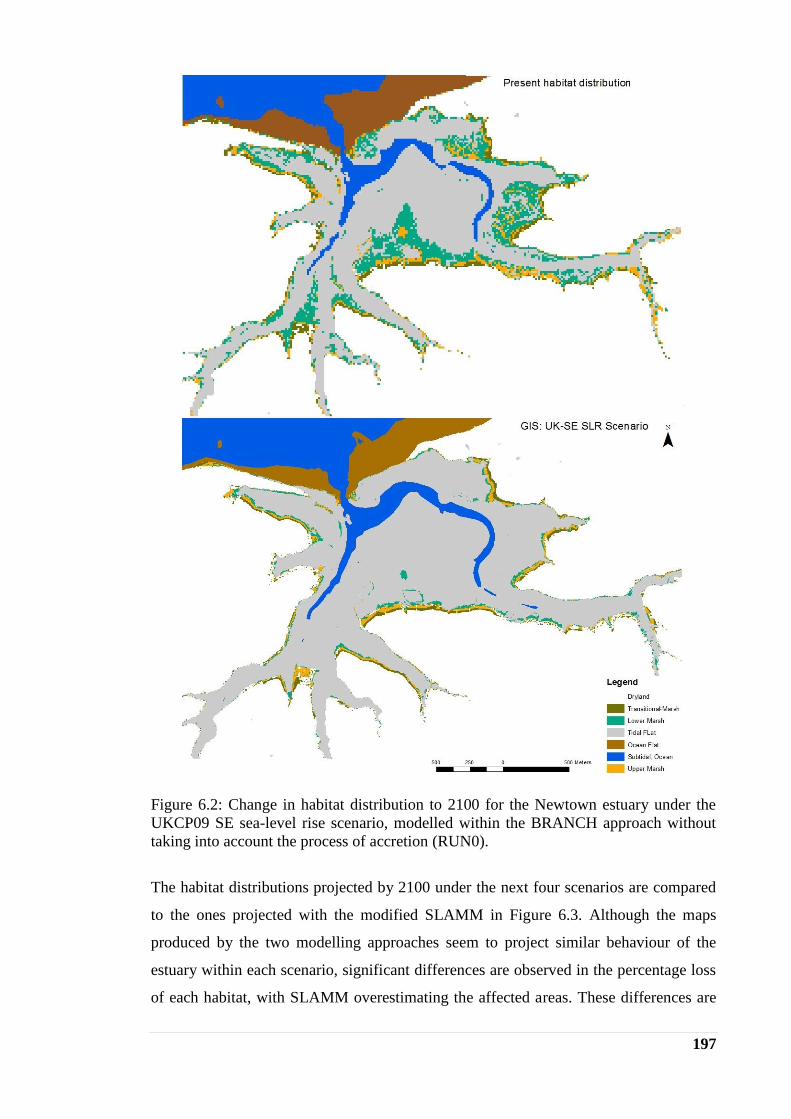
197


UKCP09 SE sea-level rise scenario, modelled within the BRANCH approach without

taking into account the process of accretion (RUN0).

The habitat distributions projected by 2100 under the next four scenarios are compared

to the ones projected with the modified SLAMM in Figure 6.3. Although the maps

produced by the two modelling approaches seem to project similar behaviour of the

estuary within each scenario, significant differences are observed in the percentage loss

of each habitat, with SLAMM overestimating the affected areas. These differences are

198

clearly explained by the different framework incorporated within each approach.

BRANCH simulates each scenario based on the DEM, while SLAMM is mainly

focused on the land cover, where in a cell-by-cell basis decides the fate of each habitat

by using empirical equations based only on the minimum and maximum elevation of the

specific cell.


UKCP09 SE sea-level rise scenario, modelled for different accretion scenarios using the

SLAMM and BRANCH approaches.

199

This difference between the two approaches is investigated more fully with reference to

the Blyth estuary. Three different scenarios of tidal flat accretion pattern are

implemented for this case study (Table 6.2). In the first one (RUN0) accretion is not

taken into account, while the two scenarios of mean (RUN1) and max (RUN2) tidal flat

accretion, as described in Chapter 4, are repeated for the two modelling approaches.

Table 6.2: Summary of simulations runs with SLAMM and a BRANCH approach for

the Blyth estuary.

Accretion rate (mm yr-1

)

Tidal flat Lower marsh Upper and Transitional marsh

RUN0 - - -

RUN1 6.4 (Mean) 6.0 5.0

RUN2 20.7 (max) 6.0 5.0

The results are compared in Figure 6.4. As with the Newtown estuary, the Blyth

intertidal cannot cope with the sea-level rise when the accretion is ignored (RUN0). The

low-lying tidal flat area at the lower part of the estuary is mostly flooded, while the rest

of the estuary intertidal migrates landwards, squeezing the marsh area. Under the second

scenario (RUN1), the estuary is more able to cope with sea-level rise. The BRANCH

produces a significant increase in the marsh area, reaching approximately 90% for the

lower marsh. This difference is attributed to its neglect of lateral edge erosion. Finally,

an unrealistic scenario of tidal flat accretion (RUN2) produces almost total loss of the

tidal flat in both cases. However, its conversion to a different habitat is treated

differently in each modelling approach. Under the BRANCH simulation the estuary

almost dries out, instead of gradually being converted to saltmarsh as is projected by

SLAMM. In the latter case, the rate of saltmarsh accretion then constrains further

progression towards a higher in terms of elevation habitat. The more sophisticated

decision tree implemented in SLAMM thus generates far more meaningful final

outcomes in situations where accretion is known to be significant.

200

Figure 6.4: Change in habitat distribution to 2100 for the Blyth estuary under the UKCP09 SE sea-level rise scenario, modelled for different tidal flat

accretion scenarios using the SLAMM and BRANCH approaches.

201

6.5 Ability of spatial landscape modelling to produce meaningful

projections of future habitat distribution

Overall, the evaluation of SLAMM presented here has demonstrated the ability of

reduced complexity models in general to simulate mesoscale impacts of sea-level rise

on estuarine and coastal environments. However, such models are often very dependent

on rather restrictive underlying assumptions. In the case of SLAMM, its performance is

dependent on the provision of accurate elevation data, since this is the crucial variable

that determines the transition between habitat types. Until very recently the availability

of high quality LiDAR and bathymetry datasets has been limited, even in the UK, where

access to datasets has often been a limited factor. Given a move towards open data

access, this should be less of an issue in the future. Even a small error in the elevation

could affect significantly the representation of the initial habitat distribution, as well as

the projected changes. The former implication further includes the uncertainty from the

interpretation accuracy in the classification of the habitat distribution from the

underlying terrain information. However, this can be partially corrected into SLAMM,

given an accurate DEM.

For a given DEM, accuracy resolution also plays an important role in the performance

of the model. The finer the resolution used, the more realistic the projected changes are

likely to be, since SLAMM simulates the area of interest in a cell-by-cell basis based on

the minimum and maximum elevation of each cell. However, the choice of the

resolution depends on the size of the area on account for the required run time of the

simulation, which is significantly increased in finer resolution simulations. For the small

Newtown estuary, for example, the run time of a simulation varied from 1 minute for a

low resolution simulation (30m) to ten minutes and six hours for a fine resolution

simulation of 5 and 1m respectively. This is a limitation of the model in comparison

with the GIS-based modelling approach used in the BRANCH project (BRANCH

partnership, 2007), whilst a 5m resolution was found to work well in the three

application domains in Suffolk and Norfolk, which were all much larger than the

Newtown estuary and a large number of model runs were required for each one.

Furthermore, accurate observation data are necessary to parameterise the embedded

sub-models for more efficient projections. Although the absence of fieldwork data can

be addressed for the saltmarsh by using the MARSH-0D (French, 2006) model to

202

constrain saltmarsh sedimentation as a function of elevation, the complex tidal flat

morphodynamics are difficult to be parameterised based on elevation and location from

the main channel, constraining its modelling to crude assumptions. However, in all

cases, the amount of area affected is computed by empirical equations, leading to

potential misrepresentation of the projected changes.

The uncertainty of the model to the factors described above is illustrated in Figure 6.5

by using the Newtown estuary as a case study due to its small size. Table 6.3 describes

the range of the model’s input factors. The parameter uncertainty effect seems to be

quite large for most environments, with the large range in the outputs occurring due to

the choice of key parameter values. Accretion is clearly a key here; only sufficient data

available to fully constrain dependence on elevation and the use of a simple

supplementary model (e.g. French, 2006) is the only way forward here. In addition, the

sensitivity of the model outputs to the quality of the DEM is quite large, since, as

already noted above, the elevation is the crucial parameter that determines the transition

between the habitat types. Finally, sea-level rise scenario uncertainty is surprisingly

small, reflecting the resilience of the saltmarsh environments to sea-level rise (Redfield,

1972; McCaffery and Thomson, 1980; Pethick, 1981; Shaw and Ceman, 1999; French,

2006).

Table 6.3: Range of SLAMM input factors for uncertainty sensitivity analysis.

SLAMM Input Factors min mean max

Ver

tica

l

Acc

reti

on

Tidal flat (mm yr-1

) 0.0 2.0 6.3

Lower marsh (mm yr-1

) 0.0 2.0 6.4

Upper marsh (mm yr-1

) 0.0 1.8 6.5

Lat

eral

Ero

sion

Tidal flat (m yr-1

) 0.0 0.2 1.0

Marsh (m yr-1

) 0.0 0.25 1.0

DE

M DEM error (m) -0.15 +0.15

Spatial resolution (cell size) (m) 1 5 30

SLR Sea-level rise scenario: SE UKCP09 min mean max

203

Figure 6.5: Uncertainty sensitivity analysis of the modified code for the Newtown

Estuary.

More importantly, though, reduced complexity models are based on simplified

parameterisations that focus on the key linkages and feedbacks between the major

morphological components (Walkden and Hall, 2005, 2011; Dickson et al., 2007;

Walkden and Dickson, 2008). In this repsect, the embedded sub-models within

SLAMM are empirically parameterised based on a simplified kinematic response to sea-

level rise, and linear erosion terms that neglect the complex processes of wave-driven

204

erosion. Although progress has been made to address this issue (e.g. Bassoulet et al.,

2000; Le Hir, 2000; Di Silvio et al., 2010; Mariotti and Fagherazzi, 2013 ), it is

important to further develop models in order to capture more complex processes

(French et al., 2015; Thornhill et al., 2015).

205

7 CONCLUSIONS

This thesis sets out to investigate the potential of reduced complexity models as a tool to

more effectively inform estuary management, with particular reference to the effects of

sea-level rise on intertidal habitat distribution. The Sea Level Affecting Marshes Model

(SLAMM), widely used in the USA, has here been adapted and evaluated for

application to UK estuarine environments.

SLAMM includes a complex habitat classification based on the US National Wetlands

Inventory, which is hard-coded, making application outside North America problematic.

Numerous other potentially user-adjustable parameter values are embedded with the

source code. Accordingly, the original code has been modified to incorporate a simpler

habitat classification that is appropriate for a UK (and broader northwest European)

context and which is, arguably, commensurate with the ability of a relatively simple

model to resolve specific habitats largely on the basis of their elevation within the tidal

frame. At the same time, numerous other changes were made to the embedded sub-

models, especially those for the tidal flat, saltmarsh and the treatment of barrier

overwash.

The modified source code was applied to different estuarine and coastal environments in

UK. The small size of the UK case studies allows the model to run at higher resolution

than has hitherto been attempted in US applications. However, accurate data are

necessary to calibrate the model for more efficient projections. In absence of field data,

this is addressed for the saltmarsh by using the MARSH-0D model (French, 2006) to

constrain saltmarsh sedimentation by generating a functional relationship between

elevation and sedimentation rate under the local tidal regime. However, the more

complex tidal flat morphodynamics are difficult to parameterise based purely on

elevation and location from the main channel, constraining its modelling to crude

assumptions that may lead to misrepresentation of its fate under specific sea-level rise

scenarios.

The analysis presented here demonstrates that reduced complexity models are more

sophisticated than the GIS-based approaches used to date in the UK (BRANCH

206

partnership, 2007), and are able to resolve a wider range of suited responses and

behaviours. In the case of SLAMM, however, the use of empirical sub-models to handle

key systems linkages means that important processes are neglected. This, in turn, makes

it very easy to generate projections that, whilst visually appealing to stakeholders and

policy makers, are actually quite misleading. A key area of weakness concerns the

representation of tidal flat processes. There is clearly a need for further work to translate

scientific understanding of hydrodynamics and morphodynamics into better mesoscale

model formulations (Di Silvio et al., 2010; Mariotti and Fagherazzi, 2013; Thornhill et

al., 2015). In addition, a sediment transport model that could take into account the

exchange of sediment between the neighbouring sections and conserve the sediment

budget would also be a major improvement in SLAMM.

207

REFERENCES Adam, P. (2002) ‘Saltmarshes in a Time of Change’ Environmental Conservation, 29,

39-61.

Addo, K.A., Walkden, M., Mills, J.P. (2008) ‘Detection, Meausurement and Prediction

of Shoreline Recession in Accra, Ghana’ ISPRS Journal of Photogrammetry &

Remote Sensing, 63, 543-558.

Admiralty (2000) Admiralty Tide Tables, Volume 1: United Kingdom and Ireland

(Including European Channel Ports). The United Kingdom Hydrographic

Office.

Akumu, C., Pathinara, S., Baban, S., and Butcher, D. (2010) ‘Examining the Potential

Impacts of Sea Level Rise on Coatsal Wetlands in North-Eastern NSW’, Journal

of Coastal Conservation, 15, 15-22.

Allan, J.C. and Komar, P.D. (2006) ‘Climate Controls on US West Coast Erosion

Processes’ Journal of Coastal Research, 22, 511-529.

Allen, J.R.L. (1981) ‘Beach Erosion as a Function of Variations in the Sediment

Budget, Sandy Hook, New Jersey, USA’ Earth Surface Processes and

Landforms, 6, 139- 150.

Allen, J.R.L. (1989) ‘Evolution of Saltmarsh Cliffs in Muddy and Sandy Systems: A

Qualitative Comparison of British West-Coast Estuaries’ Earth Surface

Processes and Landforms, 14, 85-92.

Allen, J.R.L. (1990) ‘Salt-marsh Growth and Stratification: A Numerical Model with

Special Reference to the Severn Estuary, Southwest Britain’ Marine Geology,

95, 77-96.

Allen, J.R.L. (1990a) ‘The Seven Estuary in Southwest Britain: Its retreat under Marine

Transgression and the Fine Sediment Regime’, Sedimentary Geology 66, 13.28.

Allen, J.R.L. (1991) ‘Saltmarsh Accretion and Sea-level Movement in the inner Severn

Estuary: The Archeological and Historical Contribution’ Journal of Geological

Society, 148, 485-494.

Allen, J.R.L. (2000) ‘Morphodynamics of Holocene Salt Marshes: A Review Sketch

from the Atlantic and Southern North Sea coasts of Europe’ Quaternary Science

Reviews, 19, 1155-1231.

208

Allen, J.R.L. and Duffy, M.J. (1998) ‘Medium-term Sedimentation on High Intertidal

Mudflats and Salt Marshes in the Severn Estuary, SW Britain: The Role of Wind

and Tide’ Marine Geology, 150, 1-27.

Allen, J.R.L. and Pye, K. (1992) ‘Coastal Saltmarshes: Their Nature and Importance’,

In Allen, J. and Pye, K. (eds.) Saltmasshes: Morphodynamics, Conservation and

Engineering Significance, Cambridge University Press, 1-18.

Allison, R.J. (1989) ‘Rates and Mechanisms of Change on Hard Rock Coastal Cliffs’

Zeitschriftfur Geomorphologie Supplement Band, 73, 125-138.

Alexander, L., Tett, S., & Johnsson, T. (2005) ‘Recent Observed Changes in Severe

Storms over the United Kingdom and Iceland’ Geophysical Research Letters,

32, L13704.

Anderson, J.R. (1971) ‘Land Use Classification Schemes used in Selected recent

Geographic Applications of remote Sensing’, Photogrammetric Engineering, 37,

379-387.

Anderson, J.R., Hardy, E.E., Roach, J.T. (1971) ‘A Land-use Classification System for

Use with Remote-sensor data’, U.S. Geological Survey Circular, 671, 16pp.

Anderson, J.R., Ernest, E.H., Roach, J.T., Witmer, R.E. (1976) A Land Use and Land

Cover Classification System for Use with Remote Sensor Data. Geological

Survey Professional Paper 964, United States Government Pronting Office,

Washington, 1976.

Anderson, F.E., Black, L., Watling, L.E., Mook, W., Mayer, L.M.A. (1981) ‘A

Temporal and Spatial Study of Mud Flat Erosion and Deposition’ Journal of

Sedimentary Research, 51, 726-736.

Anderson, K.E., Cahoon, D.R., Gill, S.K., Gutierrez, B.T., Thieler, E.R., Titus, J.G., and

Williams,S.J. (2009) ‘Executive Summary’ In: J.G. Titus, K.E., Anderson, D.R.,

Cahoon, D.B., Gesch, S.K., Gill, B.T., Gutierrez, E.R., Thieler, and S.J.,

Williams (ed.) Coastal Sensitivity to Sea-Level Rise:A Focus on the Mid-Atlantic

Region. A report by the U.S.Climate Change Science Programme and the

Subcommittee on Global Change Research, U.S. Environmentan Protection

Agency, Washington DC, 1-8.

Arbuckle, C.J., Huryn, A.D., Israel, S.A. (1998) ‘Applications of Remote Sensing and

GIS to Wetland Inventory: Upland Bogs’ 10th

Colloquium if the Spatial

Information Research Centre, University of Otago, New Zealand, Novemebr 16-

19 1998.

209

Austin, G.E., Rehfisch, M.M., Vilew, H.A., Berry, P.M. (2001) ‘Impacts on Coastal

Environments’ In: Harrison, P.A., Berry, P.M., Dawson, T.P. (eds) Climate

Change and Nature Conservation in Britain and Ireland: Modelling Natural

Resource Responses to Climate Change (the MONARCH project) UKCIP

Technical Report, Oxford, 177 – 228.

Baldwin, A., Egnmotovich, M., Ford, M., Platt, W. (2001) ‘Regeneration in Fringe

Mangrove Forests damaged by Hurricane Andrew’ Plant Ecology, 157, 151-

164.

Barnett, T.P. (1983) ‘Recent Changes in Sea Level and their Possible Causes’ Climate

Change, 5, 15-38.

Barnett, T.P. (1984) ‘The Estimates of Global Sea level Change: A Problem of

Uniqueness’ Journal of Geophysical Research, 89, 7980-7988.

Barnett, T.P. (1988) ‘Global Sea Level’ in NCPO, Climate Variations Over the Past

century and the Greenhouse Effect, A Report based on the First Climate Trends

Workshop, 7-9 September 1988, Washington, DC, National Climate Prorgam

Office/NOAA, Rockville, MD.

Barth, M.C. and Titus, J.G. (1984) Greenhouse Effect and Sea Level Rise, New York:

Van Nostrand Reinhold.

Bartholdy, A.T., Bartholdy, J., Kroon, A. (2010a) ‘Salt Marsh Stability and Patterns of

Sedimentation Across a Backbarrier Platform’ Marine Geology, 278, 31-42.

Bartholdy, J. (1997) ‘The Backbarrier Sediments of the Skallingen Peninsula, Denmark’

Geografisk Tidskrift-Danish Journal of Geography, 97, 11-32.

Bartholdy, J. (2012) ‘Salt Marsh Sedimentation’ In: Davis Jr., R.A. and Dalrymple,

R.W. (eds) Principles of Tidal Sedimentology, Springer Science and Business

Media, 151 – 185.

Bartholdy, J., Christiansen, C., Kunzen, H. (2004) ‘Long Term Variations in

Backbarrier Slat Marsh Deposition on the Skallingen Peninsula – The Danish

Wadden Sea, Marine Geology, 278, 31-42.

Bartholdy, J., Pedersen, J.B.T., Bartholdy, A.T. (2010b) ‘Autocompaction in Shallow

Silty Salt Marsh Clay’ Sediment Geology, 223, 310-319.

Bassoulet, P., Le Hir, P., Gouleau, D., Robert, S. (2000) ‘Sediment Transport over an

Intertidal Mudflat: Field Investigations and Estimations of Fluxes within the Bay

of Marennes-Oleron (France), Continental Shelf Research, 20, 1635 – 1653.

Baumman, R.H., Day, J.W., Miller, C.A. (1984) ‘Mississipi Deltaic Wetlands Survival:

Sedimentation versus Coastal Submergence’, Science, 224, 1093-1095.

210

Beardall, C.H., Dryden, R.C., Holzer, T.J. (1991) The Suffolk Estuaries: A Report by the

Suffolk Wildlife Trust on the Wildlife and Conservation of the Suffolk Estauries

Segment Publications, Ipswich, UK.

Beckley, B.D., Lemoine, F.G., Luthcke, S.B., Ray, R.D., Zelensky, N.P. (2007) ‘A

Reassessment of Global and Regional Mean Sea Level Trends from TOPEX and

Jason-1 Altimetry based on Revised Reference Frame and Orbits’ Geophysical

Research Letter, 34.

Bijlsma, L., Ehler, C.N., Klein, R.J.T., Kulshrestha, S.M., McLean, R.F., Mimura, N.,

Nicholls, R.J., Nurse, L.A., Perez Nieto, H., Turner, R.K., Warrick, R.A. (1996)

‘Coastal Zones and Small Islands’ In: Watson, R.T., Zinyowera, M.C., Moss,

R.H. (eds) Impacts, Adaptations and Mitigation of Climate Change: Scientific-

Technical Analyses(The Second Assessement Report of the Intergovermental

Panel on Climate Change, Working Group II), Cambridge University Press,

289-324.

Bird, E.C.F. (1985) Coastline Changes – A Global Review, New York: John Wiley and

Sons. 219pp.

Bird, E.C.F. (1993) Submerging Coasts: The Effects of a Rising Sea Level on Coastal

Environments John Wiley, Chichester, UK.

Bird, E. (2008) ‘Spits, Barriers and Bars’ in Bird, E. (ed) Coastal Geomorphology An

Introduction, John Wiley & Sons Ltd.

Blot, S.J. and Pye, K. (2004) ‘Application of LiDAR Digital Terrain Modelling to

Predict Intertidal habitat Development at a Managed Retreat Site: Abbotts Hall,

Essex, UK’ Earth Surface Processes and Landforms, 29, 893-905.

Bobba, A.G. (2002) ‘Numerical Modellling of Salt-Water Intrusion due to Human

Activities and Sea-Level Change in the Godavari Delta, India’ Hydrological

Sciences, 47 (S), S67-S80.

Bondesan, M.G., Castiglioni, G., Elmi, C., Gabbianelli, G, Marocco, R., Pirazzoli, P.,

Tomasin, A. (1995) ‘Coastal Areas at Risk from Storm Surges and Sea-Level

Rise in Northeastern Italy’ Journal of Coastal Research, 11, 1354-1379

Boomans, R.M.J., Day, J.W. Jr. (1993) ‘High Precision Measurements of Sediment

Elevation in Shallow Coastal Areas using a Sedimentation – Erosion Table’

Estuaries, 16, 375 – 380.

Boorman, L.A. (1998) ‘Salt-Marshes – Present Functioning and Future Change’

Mangroves and Salt Marshes, 3, 227-241.

211

Boorman, L.A., Goss-Custard J.D., McGrorty S. (1989) ‘Climatic Change, Rising Sea

Level and the British Coast’, LONDON, HMSO, 24pp (ITE research

publication, no. 1).

Boorman, L.A., Garbutt, A., Barratt, D. (1998) ‘The Role of Vegetation in Determining

Patterns of the Accretion of Salt Marsh Sediment’ In: Black, K.S., Paterson,

D.M., Cramp, A. (eds) Sedimentary Processes in the Intertidal Zone, Geological

Society, London, Special Publications, 139, 389-399.

Bouttier, F. and Courtier, P. (1999) ‘Data Assimilation Concepts and Methods’

Meteorological Training Course Lecture Series, ECMWF.

Brampton, A.H. (1992) ‘Engineering Significance of British Saltmarshes’ In: Allen,

J.R.L. and Pye, K. (eds) Saltmarshes, Morphodynamics, Conservation and

Engineering Significance, University Cambridge Press, Cambridge, UK, 115-

122.

BRANCH project (2003) INTERREG IIIB North-West Europe Application Form Part

A – Project Content and Management.

BRANCH partnership (2007) Planning for Biodiversity in a Changing Climate –

BRANCH Project Final Report, Natural England, UK.

Bray, M.J. and Cottle, R. (2003) Solent Coastal Habitat Management Plan. Report by

Posford Haskoning and University of Portsmouth to English Nature and

Environment Agency. Volume 1 Summary of Habitat Change, Volume 2

Technical Report.

Bray, M.J. and Hooke, J.M. (1997) ‘Prediction of Soft-cliff Retreat with Accelerating

Sea-Level Rise’ Journal of Coastal Research, 13, 453-467.

Brew, D.S., Funnell, B.M., Kreiser, A. (1992) ‘Sedimentary Environments and

Holocene Evolution of the Lower Blyth Estuary’ Proceedings of the Geologists’

Association, 103, 57-74.

Britsch, L.D. and Dunbar, J.B. (1993) ‘land Loss Rates: Louisiana Coastal Plain’

Journal of Coastal Research, 9, 324-338.

Brochier, F., and Ramieri, E. (2001) ‘Climate Change Impacts on the Mediterranean

Coastal Zones’ Nota di Lavoro, April 2001, Fondazione Eni Enrico Mattei, No

27.

Brock, J.C. and Purkis, S.J. (2009) ‘The Emerging Role of Lidar Remote Sensing in

Coastal Research and Resource Management’, Journal of Coastal Research, SI

(53), 1-5.

212

Brooks, N., Nicholls, R., Hall, J. (2006) ‘Sea Level Rise: Coastal Impacts and

Responses’ Expertise for WBGU on Oceans and Global Change, Final Draft,

Berlin, 2006.

Bruun, P. (1954) ‘Coastal Erosion and Development of Beach Profile’, U.S. Army

Beach Eros. Board Tech.Memo. No 44, U.S. Army Corps Eng., Waterw. Exr.

Stn., Vicksburg, MS.

Bruun, P. (1962) ‘Sea-level Rise as a Cause of Shore Erosion’ Proceedings of the

American Society of Civil Engineers. Journal of the Waterways and Harbors

Division, 88,117-130.

Bruun, P. (1983) ‘Review of Conditions for uses of the Bruun Rule of Erosion’ Coastal

Engineering, 7, 77-89.

Bruun, P. (1988) ‘The Bruun Rule of Erosion by Sea-Level Rise: A Discussion on

Large-Scale Two- and Three-dimensional Usages’ Journal of Coastal Research,

4, 627-648.

Bryan, B., Harvey, N., Belperio, T., Bourman, B. (2001) ‘Distributed process modeling

for regional assessment of coastal vulnerabilty to sea-level rise’ Environmental

Modeling and Assessment, 6, 57-65.

Buncombe, W. (1994) Osprey Pocket Guide to the River Blyth, Waveney Valley

Products, Beccles, Suffolk.

Burd, F. (1992) Erosion and Vegetation Change on the Saltmarshes of Essex and North

Kent Between 1973 and 1988, Research and Survey in Nature Conservation,

No42, Nature Conservancy Council, Peterborough, UK.

Burningham, H. and French, J. (2006) ‘Morphodynamic behaviour of a mixed sand-

gravel ebb-tidal delta: Deben Estuary, Suffolk, UK’, Marine Geology, 225, 23-

44.

Cahoon, D.R. (2006) ‘A Review of Major Storm Impacts on Coastal Wetland

Elevations’ Estuaries and Coasts, 29, 889-898.

Cahoon, D.R. and Reed, D.J. (1995) ‘Relationships among Marsh Surface Topography,

Hydroperiod, and Soil Accretion in a Deteriorating Louisiana Salt Marsh;

Sediment Dynamics, Deposition and Erosion in Temperate Salt Marshes’


Cahoon, D.R., Reed, D.J., Day, J.W.Jr. (1995a) ‘Estimating Shallow Subsidence in

Macrotidal Salt Marshes of the Southeastern United States: Kaye and Barghoorn

Revisited’ Marine geology, 128, 1-9.

213

Cahoon, D.R., Reed, D.J., Day Jr, J.W., Steyer, G.D., Boumans, R.M., Lynch, J.C.,

McNally, D., Latif, N. (1995b) ‘The Influence of Hurricane Andrew on

Sediment Distribution in Louisiana Coastal Marshes’ Journal of Coastal

Research, SI 21, 280-294.

Callaway, J.C. (2001) ‘Hydrology and Substrate’ In: Zedler, J.B. (ed) handbook for

Restoring Tidal Wetlands, CRC Press LLC, Chapter 3, 89-118.

Callaway, J.C., Nyman, J.A., DeLaune, R.D. (1996) ‘Sediment Accretion in Coastal

Wetlands: A Review and a Simulation Model of Processes’ Current Topics in

Wetland Biogeochemistry, 2, 2-23.

Callaway, J.C., Delaune, R.D., Patrick, W.H. (1997) ‘Sediment Accretion Rates from

four Coastal Wetlands along the Gulf of Mexico’ Journal of Copastal Research,

13, 181-191.

Carling, P.A. (1982) ‘Temporal and Spatial Variation in Intertidal Sedimentation Rates’

Sedimentology, 29, 17-23.

Carter, R.W.G. (1988) Coastal Environments: An Introduction to the Physical,

Ecological and Culutural Systems of Coastline, Academic Press, London, 199-

244.

Carter, R.W.G. and Woodroffe, C.D. (1994) ‘Coastal Evolution: An Introduction’ In:

Carter, R.W.G. and Woodroffe C.D. (eds) Coastal Evolution: Late Quaternary

Shoreline Morphodynamics. Cambridge, Cambridge University Press, 1-31.

Cassar, M. (2005) Climate Change and the Historic Environment Centre for Sustainable

Heritage, University College London.

Cailleux, A. (1952) ‘Recentes Variations du Niveau des Mers et des Terres’ Rev. gen.

Hydraul., 48, 310-315.

Cayocca, F. (2001) ‘Long Term Morphological Modelling of Tidal Inlet: The Arcachon

Basin, France, Coastal Engineering, 42, 115-142.

Cazenave, A., Nerem, R.S. (2004) ‘Present-day Sea Level Change: Observations and

Causes’ Reviews of Geophysics, 42, RG3001, doi:10.1029/2003RG000139.

CCO (2013) http://www.channelcoast.org/southwest/survey_techniques/

/airborne_remote_sensing_topo_surveys/?link=LIDAR_surveys_of_cliffs_and_s

altmarsh_systems.html

ChaMP (2002) Suffolk Coast and Estuaries Coastal Habitat Management Plan, Final

Report, 3G547201, English Nature/ Environment Agency,

3G547201/R00002/JGLG/PBor.

http://www.channelcoast.org/southwest/survey_techniques/%20/airborne_remote_sensing_topo_surveys/?link=LIDAR_surveys_of_cliffs_and_saltmarsh_systems.html



214

CHaMP (2003) North Norfolk Coastal Habitat Management Plan Final Report G5472,

English Nature, G5472/R/RS/PBor.

Channel Coastal Observatory (http://www.channelcoast.org/).

Christian, R.R., Stasavich, L., Thomas, C., Brinson, M.M. (2000) ‘Reference is a

Moving Target in Sea-Level Controlled Wetlands’ In: Weinstein, M.P., Kreeger,

D.A. (eds) Concepts and Controveries in Tidal Marsh Ecology, The

Netherlands: Kluwer Press, 805-825.

Chu, M.L., Guzman, J.A., Munoz-Carpena, R., Kiker, G.A., Linkov, I. (2014) ‘A

Simplified Approach for Simulating Changes in Beach Habitat due to the

Combined Effects of Long-Term Sea Level Rise, Storm Erosion, and

Nourishment’ Environmental Modelling and Software, 52, 111-120.

Church, J.A., and White, N.J. (2011) ‘Sea-Level Rise from the Late 19th

to the early 21st

century’, Surveys in Geophysics, 32, 585-602.

Church, J.A., White, N.J., Coleman, R., Lambeck, K., Mitrovica, J.X. (2004) ‘Estimates

of the Regional Distribution of Sea-Level Rise over the 1950-2000 Period’

Journal of Climate, 17, 2609-2625.

Chust, G., Caballero, A., Marcos, M., Liria, P., Hemandez, C., Borja, A. (2010)

‘Regional Scenarios of Sea Level Rise and Impacts on Basque (Bay of Biscay)

coastal habiats, throughout the 21st century’ Estuarine, Coastal and Science, 87,

113-124.

Chust, G., Borja, A., Liria, P., Galparsoro, I., Marcos, M., Caballero, A., Castro., R.

(2009) ‘Human Impatcs Overwhelm the Effects of Sea-Level Rise on Basque

Coastal Habitats (N Spain) between 1954 and 2004’ Estuarine, Coastal and

Shelf Science, 84, 453- 462.

Clark, J.A., Farrell, W.E., Peltier, W.R. (1978) ‘Global Changes in Postglacial Sea

Level: A Numerical Calculation’ Quaternary Research, 9, 265-287.

Clayton, K. and Shamoon, N. (1998) ‘New Approach to the Relief of Great Britain II. A

Classification of Rocks based on Relative Resistance to Denudation’

Geomorphology, 25, 155-171.

Clough, J.S. and Larson, E.C. (2009) SLAMM Analysis of Kenai Peninsula and

Anchorage, AK, Final Report, Warren Pinnacle Consulting Inc.

Clough, J.S., Larson, E.C. (2010) ‘SLAMM 6.0.1 beta, Users Manual’ Warren Pinnacle

Consultingm Inc.

Clough, J.S., Park, R.A., Fuller, R. (2010) ‘SLAMM 6 beta Technical Documentation’

Warren Pinnacle Consulting, inc.

http://www.channelcoast.org/

215

Clymo, R.S. (1964) ‘Movement of the Main Shingle Bank at Blakeney Point, Norfolk’,

Norolk and Norwich Naturalists Society Transaction, 21, 3-6.

CoastBase http://www.coastbase.org.

Conner, W.H. and Day Jr., J.W. (1991) ‘Variations in Vertical Accretion in a Louisiana

Swamp’ Journal of Coastal Research, 7, 617-622.

Cooper, J., and Pilkey, O. (2004) ‘Sea-level Rise and Shoreline Retreat: Time to

Abandon the Bruun Rule’ Global and Planetary Change, 43(3-4), 157-171.

Cooper, N., Cooper, T., Burd, F. (2001) ‘25 Years of Salt Marsh Erosion in Essex:

Implications for Coastal Defence and Nature Conservation’ Journal of Coastal

Conservation, 9, 31-40.

Cope, S.N., Bradbury, A.P., Gorcznska, M. (2008) Solent Dynamic Coast Project: Main

Report, New Forest District Council/ Channel Coastal Observatory.

Costanza, R., Farber, S.C., Maxwell, J. (1989) ‘The Valuation and Management of

Wetland Ecosystems’ Ecological Economics, 1, 335-361.

Costanza, R., Sklar, F.H., White, M.L. (1990) ‘Modeling Coastal Landscape Dynamics’

Bioscience, 40, 91-107.

Costanza, R, Sklar, F.H., White, M.L., Day, Jr., J.W. (1988) ‘A Dynamic Spatial

Simulation Model of Land Loss and Marsh Succession on Coastal Louisiana’ In:

Mitsch, W.J., Straskraba, M., Jorgensen, S.E. (eds) Wetland Modelling, Elsevier

Science Publisher, 99-114.

Coulthard, T.J., Macklin, M.G., Kirkby, M.J. (2002) ‘A Cellular Model of Holocene

Upland River Basin and Alluvial Fan Evolution’ Earth Surface Processes and

Landform, 27, 269-88.

Covey, R. and Laffoley, D. d’A. (2002) Maritime State of Nature Report for England;

Getting onto an Even Keel, English Nature, Petrborough, UK.

Coward, L., Corbett, D.R., Walsh, J.P. (2011) ‘Shoreline Change along Sheltered

Coastlines: Insights from te Neuse River Estuary, NC, USA’ Remote Sensing, 3,

1516-1534.

Cowell, P.J. and Thom, B.G. (1994) ‘Morphodynamics of Coastal Evolution’ In: Carter,

R.W.G. and Woodroffe (eds), Coastal Evolution, Late Quaternary Shoreline

Morphodynamics, Cambridge University Press, 33-86.

Cowell, P.J., Stive, M.J.F., Niederoda, A.W., de Vriend, H.J., Swift, D.J.P., Kaminsky,

G.M. and Capobianco, M. (2003) ‘The Coastal Tract (part 1): A Conceptual

Approach to Aggregated Modelling of Low Order Coastal Change’ Journal of

coastal research, 19, 812-827.

216

Craft, C., Clough, J., Ehman, J., Joye, S., Park, R., Pennings, S., Guo, H., Machmuller,

M. (2009) ‘Forecasting the Effects of Accelerated Sea-level Rise on Tidal Marsh

Ecosystem Services’ Frontiers in Ecology and the Environment, 7, 73-78.

Crooks, S. (2004) ‘The Effect of Sea-Level Rise on Coastal Geomorphology’ IBIS, 146,

18-20.

D’Alpaos, A., Lanzoni, S., Mudd, S.M., Fagherazzi, S. (2006) ‘Modeling the Influence

of Hydroperiod and Vegetation on the Cross-Sectional Formation of Tidal

Channels’ Estuarine, Coastal and Shelf Science, 69 (3-4), 311-324.

Dalrymple, R.A., Biggs, R.B., Dean, R.G, Wang, H. (1986) ‘Bluff recession Rates in

Chesapeake Bay’ Journal of Waterway, Port, Coastal and Ocean Engineering,

112, 164-169.

Dasgupta, S., Laplante, B., Meinser, C., Wheeler, D., Yan, J. (2009) ‘The Impact of Sea

Level Rise on Developing Countries: A Comparative Analysis’ Climatic

Change, 93, 379-388.

Davidson, N.C., Laffoley, D.d’A, Doody, J.P., Way, L.S., Gordon, J., Key, R., Drake,

C.M., Pienkowski, M.W., Mitchell, R., Duff, K.L. (1991) Nature Conservation

and Estuaries in Great Britain, Nature conservancy Council.

Davidson-Arnott, R.G.D., van Proosdij, D., Ollerhead, J., Schostak, L. (2002)

‘Hydrodynamics and Sedimentation in Salt Marshes: Examples from a

Macrotidal Marsh, Bay of Fundy’ Geomorphology, 48, 209-231.

Davidson-Arnott, R.G.D. (2005) ‘Conceptual Model of the Effects of Sea Level Rise on

sandy Coasts’ Journal of Coastal Research, 21(6), 1166-1172

Day, J., Ibanez, C., Scarton, F., Pont, D., Hensel, P., Day, J., Lane, R. (2011)

‘Sustainability of Mediterranean Deltaic and Lagoon Wetlands with Sea-Level

Rise: The Importance of River Input’ Estuaries and Coasts, 34, 483-493.

Day, J.W., Christian, R.R., Boesch, D.M., Yanez-Arancibia, A., Morris, J., Twilley,

R.R., Naylor, L., Schaffner, L., Stevenson, C. (2008) ‘Consequences of Climate

Change on the Ecogeomorphology of Coastal Wetlands’ Estuaries and Coasts,

31, 477-491.

Day, Jr., J.W., Pont, D., Hensel, P.F., Ibanez, C. (1995) ‘ Impacts Of Sea Level Rise on

Deltas in the Gulf of Mexico and the Mediterranean: The Importance of Pulsing

Events to Sustainability’ Estuaries, 18, 636-647.

Dean, R.G. (1977) Equilibrium Beach Profiles: U.S. Atlantic and Gulf Coasts,

Technical Report No.12, Department of Civil Engineering, University of

Delaware, 45p.

217

Dean, R.G. (1987) ‘Additional Sediment Input to the Nearshore Region’ Shore Beach,

55, 76-81.

Dean, R.G. (1991) ‘Equilibrium Beach Profiles: Characteristics and Applications’


Dean, R.G. and Maurmeyer, E.M. (1983) ‘Models for Beach Profile Response’ In:

Komar, P.D. (ed.) Handbook of Coastal Processes and Erosion, Boca Raton,

Florida: C.R.C. Press, 151-166.

Dearing, J., Richmond, N., Plater, A., Wolf, J., Prandle, D., and Coulthard, T. (2006)

‘Modelling Approaches for Coastal Simulation based on Cellullar Automata:

The Need and Potential’ Philosophical Transactions of the Royal Society A, 364,

1051-1071.

Defeo, O., McLachlan, A., Schoeman, D.S., Schlacher, T.A., Dugan, J., Jones, A.,

Lastra, M., Scapini, F. (2009) ‘Threats to Sandy Beach Ecosystems: A Review’

Estuarine, Coastal and Shelf Science, 81, 1-12.

DEFRA (2002) Managed Realignment Review, Policy research Project FD 2008,

Department for Environment, Food and Rural Affairs, London. Department of

Environment Food and Rural Affairs, London.

DEFRA (2006b) Flood and Coastal Defence Appraisal Guidance FCDPAG3 Economic

Appraisal – Supplementary note to Operating Authorities – Climate Change

Impacts Department for Environment, Food, and Rural Affairs, London.

DeLaune, R.D., Smith, C.J., Patrick Jr., W.H. (1983) ‘Relationship of Marsh Elevation,

Redox Potential, and Sulfide to Spartina Alterniflora Productivity’ Soil Science

Society of America Journal, 47, 930-935.

DeVriend, H.J., Zyserman, J., Nickolson, J., Roelvink, J.A., Pechon, P., Southgate, H.N.

(1993a) ‘Medium Term 2DH Coastal Area Modelling’ Coastal Engineering, 21,

193-224.

DeVriend, H.J., Capobianco, M., Chasher, T., De Sward, H.E., Latteux, B., Stive,

M.J.F. (1993b) ‘Approaches to Long-Term Modelling of Coastal Morphology:

A Review’ Coastal Engineering, 21, 225-269.

Dickson, M.E., Walkden, M.J.A., Hall, J.W. (2005) ‘Systematic Impacts of Climate

Change on an Eroding Coastal Region over the Twenty-First Century’ Climatic

Change, 84, 141-166.

Dickson, M., Walkden, M., Hall, J., Pearson, S., Rees, J. (2005) ‘Numerical Modelling

of Potential Climate-Change Impacts on Rates of Soft-cliff Recession, Northeast

218

Norfolk, UK’ Coastal Dynamics 2005 Proceedings of the 5th

International

Conference, 4-8 April, 2005, Barcelona, Spain.

Dijkema, K.S. (1987) ‘Geography of Saltmarshes in Europe’ Zeitschrift fur

Geomorphologie, 31, 489-499.

DINAS-COAST Consortium (2006) DIVA 1.0 Postdam Institute for Climate Impact

Research, Postdam, Germany, CR-ROM.

Di Silvio, G. (1989) ‘Modelling the Morphological Evolution of Tidal Lagoons and

their Equilibrium Configurations’ XXII Congress of the IAHR. Ottawa, Canada

Di Silvio, G., Dall’Angelo, C., Bonaldo, D, Fasolato, G. (2010) ‘Long-term Model of

Planimetric and Bathymetric Evolution of a Tidal Lagoon’, Continental Shelf

Research, 30, 894-903.

Dissanayake, D.M.P.K., Ranasinghe, R., Roelvink, J.A., Wang, Z.B. (2011) ‘Process-

based ans Semi-Empirical Modelling Approaches on Tidal Inlet Evolution’

Journal of Coastal Research, SI 64 (Processings of the 11th

International Coastal

Symposium), 1013-1017, Szezecin, Poland, ISSN 0749-0208

Dolan, R., Fenster, M., Holme, S. (1991) ‘Temporal Analysis of Shoreline Recession

and Accretion’ Journal of Coastal Research, 7, 723-744.

Doody, J.P. (1992) ‘The Conservation of British Saltmarshes’ In: Allen, J.R.L. and Pye,

K. Saltmarshes, Morphodynamics, Conservation abd Engineering Significance,

University of Cambridge Press, Cambridge, UK, 80-114.

Doody, J.P. (2001) Coastal Conservation and Management: An Ecological Perspective,

Kluwer Academic Publishers, Dordrecht, the Netherlands.

Doody, J.P. (2012) ‘Coastal Squeeze and Managed Realignment in Southeast England,

does it tell us anything about the future?’ Ocean and Coastal Management

(article in press).

Douglas, B.C. (1991) ‘Global Sea Level Rise’ Journal of Geophysical Research, 95,

6981-6992.

Douglas, B.C. (1992) ‘Global Sea Level Acceleration’ Journal of Geophysical

Research, 97 (C8), 12699-12706.

Douglas, B.C. (1997) ‘Global Sea Level Rise: A Redetmination’ Surveys in Geophysics,

18, 279-292.

Dougla, B.C. (2001) ‘An Introduction to Sea Level’ In: Douglas, B.C., Kearney, M.S.,

Leatherman, S.P. (eds) Sea Level Rise, History and Consequences, London

Academic Press.

219

Douglas, B.C. and Peltier, W.R. (2002) ‘The Puzzle of Global Sea Level Rise’ Physics

Today, 55, 35-40.

Douglas, B.C., Crowell, M., Leatherman, S.(1998) ‘Considerations for Shoreline

Position Prediction’ Journal of Coastal Research, 14, 1025-1033.

Dubois, R.N. (1977) ‘Predicting Beach Erosion as a Function of Rising Water Level’

The Journal of Geology, 85, 470-476.

Dubois, R.N. (1992) ‘A Re-evaluation of Bruun’s Rule and Supporting Evidence’


Eisma, D. and Kalf, J. (1987) ‘Dispersal, Concentration and Deposition of Suspended

Matter in the North Sea’ Journal of the Geological Society, 144, 161-178.

El-Raey, M. (1997) ‘Vulnerability Assessment of the Coastal Zone of the Nile Delta of

Egypt, to the Impacts of Sea Level Rise’ Ocean and Coastal Management, 37,

29-40.

Emery, K.O. (1980) ‘Relative Sea Levels from Tide-Gauge Record’ Proceedings of the

national Academy of Science, USA, 77,6968-72.

Emery, K.O. and Aubrey, D.G. (1991) Sea Levels, land levels, and tide gauges, New

York, Springler-Verlag.

English Nature (1992) Coastal Zone ConservationEnglish Nature’s Rationale,

Objectives and Practical Recommendations, English Nature, Peterborough, UK.

Environment Agency (1999a) Suffolk Estuarine Strategies, Phase II – Report A, Blyth

Estuary.

Environment Agency (1999b) Suffolk Estuarine Strategies, Phase II – Report C, Deben

Estuary.

Environment Agency (2007) Saltmarsh Management Manual. R&D Technical Report

PFA-076/TR, Environment Agency, Bristol, 123pp.

Environment Agency (2009) Suffolk Estuarine Strategies, Blyth, Strategy Approval

Report.

Environment Agency (2011) Coastal Trends Report – Suffolk (Lowestoft to Languard

Point, Felixstowe), RP022/S/2011, February 2011.

Environment Agency (2012) Coastal Trends Report – North Norfolk (Old Hunstanton

to Kelling), RP028/L/2011, October 2012.

Evans, E., Ashley, R., Hall, J., Penning-Rowsell, E., Saul, A., Sayers, P., Thorne, C.,

Watkinson, A. (2004) Foresight Future Flooding Scientific Summary: Volume I

Future Risks and their Drivers Office of Science and Technology, London.

220

EUROSION (2004) Living with Coastal Erosion in Europe: Sediment and Space for

Sustainability, Report to Directorate General Environment, European

Comission, http://www.eurosion.org.

Fagherazzi, S. and Wiberg, P.L. (2009) ‘Importance of Wind Conditions, Fetch, and

Water Levels on Wave-generated Shear Stress om Shallow Intertidal Basins’,

Journal of Geophysical Research, 114, F03022.

Fagherazzi, S. and Priestas, A.M. (2010) ‘Sediments and Water Fluxes in a Muddy

Coastline: Interplay Between Waves and Tidal Channel hydrodynamics’ Earth

Surface Processes and Landforms, 35, 284-293.

Fairbridge, R.W. (1980) ‘The Estuary: Its Definition and Geodynamic Cycle’ In:

Olausson, E., Cato, I. (eds) Chemistry and Biochemistry of Estuaries, Wiley,

New York, 1-35.

Fairbridge, R.W. and Krebs, O.A. (1962) ‘Sea Level and the Southern Oscillation’

Geophysical Journal, 6, 532-545.

Fenster, M.S., Dolan, R. (1993) ‘Historical Shoreline Trends Along the Outer Banks,

North Carolina: Processes and Responses’ Journal of Coastal Research, 9, 172-

188.

Fenster, M.S., Dolan, R., Elder, J.F. (1993) ‘A New Method for Predicting Shoreline

Positions from Historical Data’ Journal of Coastal Research, 91, 147-171.

Ferguson, G. and Gleeson, T. (2012) ‘Vulnerability of Coastal Aquifers to Groundwater

Use and Climate Change’ Nature Climate Change,

DOI:10.1038/NCLIMATE1413.

FitzGerald, D.M., Fenster, M.S., Argow, B.A, and Buynevich, I.V. (2008) ‘Coastal

Impacts Due to Sea-Level Rise’ Annual Review of Earth and Planetary

Sciences, 36(1), 601-647.

Forbes, D.L., Taylor, R.B., Shaw, J. (1989) ‘Shorelines and Rising Sea Levels in

Eastern Canada’ Episodes, 12, 23-28.

French, C.E., French, J.R., Clifford, N.J., Watson, C.J. (2000) ‘Sedimentation-erosion

Dynamics of Abandoned Reclamation: The Role of Waves and Tides’

Continental Shelf Research, 20, 1711-1733.

French, G.T., Awosika, L.F., Ibe, C.E. (1995) ‘Sea-Level Rise and Nigeria: Potential

Impacts and Consequences’ Journal of Coastal Research, 14, 224-242.

French, J.R. (1993) ‘Numerical Simulation of Vertical Marsh Growth and Adjustment

to Accelerated Sea-Level Rise, North Norfolk, U.K’ Earth Surface Processes

and Landforms, 18 (1), 63-81.

http://www.eurosion.org/

221

French, J.R. (1994) ‘Wetland Response to Accelerated Sea-Level Rise: A European

Perspective’ In: Finkl, C.W. (ed.) ‘Coastal Hazards: Perception, Mitigation and

Susceptibility’ Journal of Coastal Research Special Issue, 12, 94-105.

French, J.R. (2001) Hydrodynamic Modelling of the Blyth Estuary: Impast of Sea-Level

Rise, Coastal and estuarine research Unit, University College London, Report

for Environment Agency, Anglian Region.

French, J.R. (2003) ‘Airborne LiDAR in Support of Geomorphological and Hudraulic

Modelling’ Earth Surface Processes and Landfroms, 28, 321-335.

French, J.R. (2004) Critical Concepts in Coastal Geomorphology, London, Routledge.

French, J.R. (2006) ‘Tidal Marsh Sedimentation and Resilience to Environmental

Change:Exploratory modelling of Tidal, Sea-Level and Sediment Supply

Forcing in Predominantly Allocthonous Systems’ Marine Geology, 235, 119-

136.

French, J.R. (2008) ‘Hydrodynamic Modelling of Estuarine Flood Defence Realignment

as an Adaptive management Response to Sea-level Rise’ Journal of Coastal

Research, 24, 1-12.

French, J.R and Burningham, H. (2003) ‘Tidal Marsh Sedimentation Versus Sea-level

Rise: A Southeast England Estuarine Perspective’ Proceedings Coastal

Sediments ’03, Sheraton Sand Key, Vlearwater, Florida.

French, J.R. and Burningham, H. (2009) ‘Coastal Geomorphology: Trends and

Challenges’ Progress in Physical Geography, 33, 117-129.

French, J.R. and Burningham, H. (2011) ‘Qualitative Mathematical Modelling of

Coupled Coast and Estuary Morphodynamics: A Modified Boolean Network

Approach’ American Geophysical Union, Fall Meeting 2011.

French, J.R. and Burningham, H. (2013) ‘Coasts and Climate: Insights from

Geomorphology’ Progress in Physical Geography, 37, 550-561.

French, J.R. and Reed, D.J. (2001) ‘Physical Contexts for Saltmarsh Conservation’ In:

Warren, A. and French, J.R. (eds) Habitat Conservation: Managing the Physical

Environment, John Wiley & Sons, LTD, 179-228.

French, J.R. and Spencer, T. (1993) ‘Dynamics of Sedimentation in a Tide-Diminated

Backbarrier Salt Marsh, Northfolk, UK’ Marine Geology, 110, 315-331.

French, J.R. and Spencer, T. (2001) ‘Sea-level Rise’ In: Warren, A. and French, J.R.

(eds) Habitat Conservation: Managing the Physical Environment, John Wiley &

Sons, LTD, 305-349.

222

French, J.R. and Stoddart, D.R. (1992) ‘Hydrodynamis of Salt-Marsh Creek Systems –

Implications for Marsh Morphological Development and Material Exchange’

Earth Surface Processes and Landforms, 17, 235-252.

French, J.R., Spencer, T., Stoddart, D. (1990) ‘Backbarrier Salt marshes of the North

Norfolk Coast: Geomorphic Development and Response to Rising Sea-Levels’

Discussion papers in Conservation, Ecology and Conservation Unit, UCL, 54.

French, J.R., Burningham, H., Benson, T. (2008) ‘Tidal and Meteorological Forcing of

Suspended Sediment Flux in a Muddy Mesotidal Estuary’ Estuaries and Coasts,

31: 843-859.

French, J.R., Spencer, T., Murray, A.L., Arnold, N.S. (1995) ‘Geostatistical Analysis of

Sediment Deposition in Two Small Tidal Wetlands, Norfolk, UK’ Journal of

Coastal Research, 11, 308-321.

French, J., Payo, A., Murray, B., Orford, J., Elliot, M., Cowell, P. (2015) ‘Appropriate

Complexity for the Prediction of Coastal and Estuarine Geomorphic Behaviour

at Decadal to centennial Scales’ Geomorphology, In Press.

French, P.W. (1997) Coastal and Estuarine Management Routledge Environmental

Management Series, pp 251.

French, P.W. (2001) Coastal Defences. Processes, Problems and Solutions, Routledge,

London, UK.

Friedrichs, C.T. and Perry, J.E. (2001) ‘Tidal Saltmarsh Morphodynamics: A

Synthesis’, Journal of Coastal Research Special Issue, 27, 7-37.

Frostick, L.E. and McCave, I.N. (1979) ‘Seasonal Shifts of Sediment within an Estuary

Mediated by Algal Growth’ Estuarine and Coastal Marine Science, 9, 569-576.

Funnell, B.M., Boomer, I., Jones, R. (2000) ‘Holocene Evolution of the Blakeney Spit

Area of the North Norfolk coastline’, Proceedings of the Geologists’

Association, 111, 205-217.

Galbraith, H., Jones, R., Park, R., Clough, J.S. , Herrod-Julius, S., Harrington, B., Page,

G. (2002) ‘Global Climate Change and Sea Level Rise: Potential Losses of

intertidal Habitat for shorebirds’ Waterbird, 25, 173-183.

Galbraith, H., Jones, R., Park, R., Clough, J., Herrod-Julius, S., Harrington, B., Page, G.

(2003) ‘Global Climate Change and Sea Level Rise: Potential Losses of

intertidal habitat for shorebirds’ In: Valette-Silver, N.J. and Scavia, D. (eds)

Ecological Forecasting: New Tools for Coastal and marine Ecosystem

Management, NOAA, Silver Spring, Maryland, 19-22.

223

Galbraith, H., Jones, R., Park, R., Clough, J., Herrod-Julius, S., Harrington, B., Page, G.

(2005) Global Climate Change and Sea Level Rise: Potential Losses of

intertidal habitat for shorebirds. USDA Forest Service Gen. Tech. Rep. PSW-

GTR-191.2005.

Garbutt, R.A., Reading, C.J., Wolters, M., Gray, A.J., Rothery, P. (2006) ‘Monitoring

the Development of Intertidal Habitats on Former Agricultural Land after the

Managed Realignment of Coastal Defences at Tollesbury, Essex, UK’ Marine

Pollution Bulletin, 53, 155-164.

Garcin, M., Yates, M., Le Cozannet, G., Walker, P., Donato, V. (2011) ‘Sea Level Rise

and Coastal Morphological Changes on Tropical Islands: Examples from New

Caledonia and French Polynesia (SW Pacific)’ Geophysical Research Abstracts,

13EGU2011-3504.

Gardiner, L.R., Porter, D.E. (2001) ‘Stratigraphy and Geologic History of a

Southeastern Salt Marsh Basin, North Inlet, South Carolina, USA’ Wetlands

Ecology and Management, 9, 371-382.

Gardiner, L.R., Smith, B.R, Michener, W.K. (1992) ‘Soil Evolution along a Forest-

Marsh Transect under a Regime of slowly Rising Sea Level, North Inlet, South

Carolina, USA’ Geoderma, 55, 141-157.

Gardiner, S., Ingleby, A., Jude, S., Nicholls, R.J., Rauss, I., Williams, A (2007)

‘Developing Spatial Planning Tools and Guidance to Enable Coastal

Biodiversity to Adapt to Climate Change, Annex 3’ of Planning for Biodiversity

in a Changing Climate – BRANCH project Final Report,, Natural England, UK.

Gardline Environmental Ltd (2003) River Blyth Hydrographic Survey: Hydrodynamics

and Sediment Study, Data Period: April 24th

to May 27th

.

Gesch, D.B., Gutierrez, B.T., Gill, S.K. (2009) ‘Coastal Elevations’ In: J.G., Titus,

K.E., Anderson, D.R., Cahoon, D.B., Gesch, S.K., Gill, B.T., Gutierrez, E.R.,

Thieler, S.J., Williams (ed.) Coastal Sensitivity to Sea-Level Rise:A Focus on

the Mid-Atlantic Region. A report by the U.S.Climate Change Science

Programme and the Subcommittee on Global Change Research, U.S.

Environmentan Protection Agency, Washington DC, 25-42.

Geselbracht, L., Freeman, K., Kelly, E., Gordon, D.R., Putz, F.E. (2011) ‘Retrospective

and Prospective Model Simulations of Sea Level Rise Impacts on Gulf of

Mexico Coastal Marshes and Forests in Waccasassa Bay, Florida’ Climatic

Change, 107, 35-57.

224

Ghyben, B.W. (1888) ‘Nota in Verband Met de Voorgenomen putboring Nabij

Amsterdam (Notes on the Probable Results of the Proposed Well Drilling Near

Amsterdam)’ Tijdschrift van het Koninklijk Institunt van Ingeniers, The Hague,

8-22.

Glick, P., Clough, J., Nunley, B. (2008) Sea-Level Rise nas Coastal Habitats in the

Chesapeake Bay Region, Technical Report, National Wildlife Federation.

Glick, P., Clough, J., Polaczyk, A., Couvillion, B., Nunley., B. (2013) ‘Potential Effects

of Sea-Level Rise on Coastal Wetlands in Southeastern Louisiana’ Journal of


Gomes Pereira, L.M. and Wicherson, R.J. (1999) ‘Suitability of Laser Data for Deriving

geographical Information. A Case Study in the Context of Manageemnt of

Fluvial Zones’ ISPRS Journal of Photogrammetry and Remote Sensing, 54, 105-

114.

Gornitz, V. (1991) ‘Global Coastal Hazards from Future Sea Level Rise’ Global Planet

Change, 89, 379-98.

Gornitz, V. (1995) ‘Sea-level Rise:A Review of Recent past and Near – Future trends’

Earth and Surface Processes and Landfroms, 20, 7-20.

Gornitz, V., Lebedeff, S., Hansen, J. (1982) ‘Global Sea Level Trend in the Past

Century’ Science, 215, 1611-1614.

Gornitz, V. and Lebedeff, S. (1987) ‘Global Sea Level Changes during the Past

Century’ In: Nummedal, D., Pilkey, O.H., Howard, J.D. (eds), Sea Level

Fluctuation and Coastal Evolution , SEPM Spec.Publ. 41, 3-16.

Gornitz, V., Cough, S., Hartig, E. (2001) ‘Impacts of Sea Level Rise in the New York

Metropolitan Area’ Global and Planetary Change, 32, 61-88.

Gray, A.J. (1977) ‘Reclaimed Land’ In: Barnes, R.S.K. (ed) The Coastline, Wiley,

London, 253-270.

Grinsted, A., Moore, J.C., Jevrejeva, S. (2009) ‘Reconstructing Sea Level from Paleo

and Projected Temperatures 2000 to 2100 AD’ Climate Dynamics, 34, 461-472.

Green, D. and King, S. (2003) ‘Progress in Geographical Information Systems and

Coastal Modeling: An Overview’ In: Lakhan, V. (ed) Advances in Coastal

Modeling, Elsevier Science, 553-580.

Groger, M. and Plag, H.P. (1993) ‘Estimations of a Global Sea-Level Trend:

Limitations from the Structure of the PSMSL Global Sea Level Data Set’ Global

and Planetary Change, 8, 161-9.

225

Gulve, S.K., and Hasse, L. (1999) ‘Changes of Wind Waves in the North Atlantic Over

the Last 30 Years’ International Journal of Climatology, 19, 1091-1117.

Gulve, S.K., and Grigorieva, V. (2004) ‘Last Century Changes in Ocean Wind Wave

Height from Global Visual Wave Data’ Geophysical Research Letters, 31,

L24302.

Guntenspergen, G.R., Cahoon, D.R., Grace, J.B., Steyer, G.D., Fournet, S., Townson,

M.A., Foote, A.L. (1995) ‘Disturbance and Recovery of the Louisiana Coastal

Marsh Landscape from the Impacts of Hurrican Andrew’ Journal of Coastal

Research, SI 21, 324-339.

Gutelius, W., Carter, W., Shrestha, R., Medvedev, E., Gutierez, R., Gibeaut, J. (1998)

‘Engineering Applications of Airborne Scanning Lasers: Reports from the Field’

Photogrammetric Engineering & Remote Sensing, 64, 246-253.

Gutenberg, B. (1941) ‘Changes in Sea Level, Post-glacial Uplift and Mobility of the

Earth’s Interior’Bulletin of the Geological Society of America, 52, 721-72.

Hackney, C.T., Cleary, W.J. (1987) ‘Saltmarsh Loss in Southeastern North Carolina

Lagoons: Importance of Sea Level Rise and Inlet Dredging’ Journal of Coastal

Research, 3, 93-97.

Hadley, D. (2009) ‘Land Use and the Coastal Zone’ Land Use Policy, 26S, S198-S203.

Hall, J.W., Meadowcroft, I.C., Lee, E.M., Van Gelder, P.H.A.J.M (2002) ‘Stochastic

Simulation of Episodic Soft Coastal Cliff Recession’ Coastal Engineering, 46,

159-174.

Han, M., Hou, J., Wu, L. (1995) ‘Potential Impacts of Sea-Level Rise on China’s

Coastal Environment and Cities: A National Assessment’ Journal of Coastal

Research, 14, 79-95.

Hands, E.B. (1983) ‘The Greta Lakes as a Test Model for Profile Responses to Sea-

Level Change’ In: Komar, P.D. (ed.) Handbook of Coastal Processes and

erosion, Boca Raton, CRC Press, 167-189.

Hanson, H. and Kraus, N. (1989) GENESIS: Generalized Model For Simulating

Shoreline Change Technical Report CERC -89-19, 85 p, Vicksburg, Mississippi,

US Army Corps of Engineers.

Hanson, H., Connell, K.J., Larson, M., Kraus, N.C., Beck, T.M., Frey, A.E. (2011)

‘Coastal Evolution Modeling at Multiple Scales in Regional Sediment

Management Applications’ Proceedings of Coastal Sediments 2011, Miami, Fl.,

3, 1920-1932.

226

Hanson, H., Aarninkhof, S., Capobianco, M., Jimenez, J.A., Larson, M., Nicholls, R.J.,

Plant, N.G., Southgate, H.N., Steetzel, H.J., Stive, M.J.F., de Vriend, H.J. (2003)

‘Modelling of Coastal Evolution on Yearly to decadal Time Scales’ Journal of

Cooastal research, 19, 790-811.

Hatton, R.S., DeLaune, R.D., Patrick Jr., W.H. (1983) ‘Sedimentation, Accretion, and

Subsidence in Marshes of Bataria Basin, Louisiana’ Limnology and

Oceanography, 28, 494-502.

Hayden, B.P., Santos, C.F.V., Shao, G., Kochel, R.C. (1995) ‘Geomorphological

Controls on Coastal Vegetation at the Virginia Coast Reserve’ Geomorphology,

13, 283-300.

Hearn, C.J. (2008) The Dynamics of Coastal Models, Cambridge University Press.

Henderson-Sellers, A., Zhang, H., Berz, G., Emanuel, K., Gray, W., Landsea, C.,

Holland, G., Lighthill, J., Shieh, S.L., Webster, P., McGuffie, K. (1998)

‘Tropical Cyclones and Global Climate Change: A Post-IPCC Assessment’

Bulletin Americal Meteorological Society, 79, 19-38.

Herzberg, A. (1901) ‘Die Wasserversorgung einiger Nordseeb~ider (The Water Supply

on Parts of the North Sea Coast in Germany)’ Journal Gabeleucht ung und

Wasserversorg ung, 44, 815-819, 824-844.

Hibma, A., Stive, M.J.F., Wang, Z.B. (2004) ‘Estuarine Morphodynamics’ Coastal


Higinbotham, C.B., Alber, M.M., Chalmers, A.G. (2004) ‘Analysis of Tidal Marsh

Vegetation Patterns in Two Georgia Estuaries using Aerial Photography and

GIS’ Estuaries, 27, 670-683.

Hinkel, J. (2005) ‘DIVA: An Iterative Method for Building Modular Integrated Models’

Advances in Geosciences, 4, 45-50.

Hinkel, J. and Klein, R.J.T. (2007) ‘Integrating Knowledge for Assessing Coastal

Vulnerability to Climate Change’ In: McFadden, L., Nicholls, R.J., Penning-

Rowsell, E.C. (eds) Managing Coastal Vulnerability: An Integrated Approach,

Amsterdam: Elsevier Science, 61-78.

Hinkel, J., and Klein, R.J.T. (2009) ‘Integrating Knowledge to Assess Coastal

Vulnerability to Sea-Level Rise: The Development of the DIVA Tool’ Global

Environmental Change, 19, 384-395.

Hoffman, J.S., Keyes, D., Titus, J.G. (1983) ‘Projecting Future Sea Level Rise;

Methodology, Estimates to the Year 2100 and Research Needs’ Washington

DC:US Environmental Protection Agency, 121pp.

227

Hoffman J.S., Wells, J.B., Titus, J.G. (1986) ‘Future Global Warming and Sea Level

Rise. In: Sigbjarnarson, G. (ed) Proceedings Iceland Coastal and River

Symposium ’85. Reykjavik, National Energy Authority, 246-66.

Holgate, S.J., Woodworth, P.L. (2004) ‘Evience for Enhanced Coastal Sea Level Rise

during the 1990s’ Geophysic Research Letters, 31, 4.

Hooke, J.M., Bray, M.J. (1996) ‘Approaches to Analysis and Prediction of Coastal

Processes and Morphology’ In: Taussik, J., Mitchell, J. (eds) Partnership in

Coastal Zone Management, Samara Publishing, Cardigan, 167-174.

Hoozemans, F.M.J., Marchand, M., Pennekamp, H.A. (1993) ‘Sea Level Rise: A Global

Vulnerability Analysis: Vulnerability Assessments for Population, Coastal

Wetlands and Rice Production on Global Scale’ Second Revised Edition, Delft

Hydraulics and Rijkswaterstaat, Delft and The Hague, The Netherlands, 184.

Horton, R., Herweijer, C., Rosenzweig, C., Liu, J., Gornitz, V., Ruane, A.C. (2008) ‘Sea

level rise projections for current generation CGCMs based on the

semi‐empirical method’ Geophysical Research Letters, 35, L02715.

Howe, M.A. (2002) A Review of the Coastal Soft Cliff Resource in Wales, with

particular reference to its Importance for Invertebrates, CCW Natural Science

Report No. 02/5/1.

Hughes, R.G. and Paramor, O.A.L. (2004) ‘On the Loss of Saltmarshes in South-East

England and methods for their restoration’ Journal of Applied Ecology, 41, 440-

448.

Hull, C.H.J. and Titus, J.G. (1986) Greenhouse Effect, Sea Level Rise and Salinity in the

Delaware Estuary, EPA 230-50-86-010, 86pp.

Hulme, M., and Jenkins, G. (1998) Climate Change Scenarios for the United Kingdom

UKCIP Technical Report No.1. Climatic Research Unit, University of East

Anglia and Hadley Centre, Met. Office.

Hulme, M., Turnpenny, J., Jenkins, G. (2002) Climate Change Scenarios for the United

Kingdom - The UKCIP02 Briefing Report. Tyndall Centre for Climate Change

Research, School of Environmental Sciences, University of East Anglia,

Norwitch, UK.

HydroQual, Inc. (2002) A Primer for ECOMSED Users Manual, Version 1.3,

HydroQual, Inc., Mahwah, New Jersey, pp 188.

Ibanez, C.A., Canicio, A., Day, J.W., Curco, A. (1997) ‘Morphologic Evolution,

Relative Sea Level Rise and Sustainable Management of Water and Sediment in

the Ebre Delta’ Journal of Coastal Conservation, 3, 191-202.

228

Ibanez, C., Sharpe, P.J., Day, J.W., Day, J.N., Prat, N. (2010) ‘Vertical Accretion and

Relative Sea Level Rise in the Ebro Delta Wetlands (Catalonia, Spain)

Wetlands, 30, 979-988.

Institute of Hydrology (1996) UK National River Flow Archive, Station no. 035014,

Wallingford, UK.

Isle of Wight Shoreline Management Plan 2, (Isle of Wight, SMP2) (2010) Main Report

Chapter 4: Policy Development Zone 7- North West Coastline (PDZ7); &

Appendix C: Baseline Process Understanding: C1: Assessment of Shoreline

Dynamis, C2: Defence Appraisal, C3: Baseline Scenarios of Future Shoreline

Change, Appendix D: Natural and Built Environment Baseline, Coastal

Management, Isle of Wight Council.

Isle of Wight SFRA (2009) Tidal Climate Change Mapping Update Supplementary

Technical Note, Entec UK Ltd for Isle of Wight Council Planning Services.

IPCC (2001) Climate Change 2001: The Scientific Basis, Contribution of Working

Group I to the Third Assessment Report of the Intergovernmental Panel on

Climate Change. Houghton, J.T., Ding, Y., Griggs, D.J., Noguer, M., vand der

Linden, P.J., Dai, X., Maskell, K., Johnson, C.A. (eds). Cambridge University

Press.

IPCC (2007) Summary for Policy Makers. In:Climate Change 2007: The Physical

Science Basis, Contribution of Working Group I to the Fourth Assessment

Report of the Intergovernmental Panel of Climate Change. Solomon, S., Qin,

D., Manning, M., Marquis, M., Averyt, K.B., Tignor, M., and Miller, H.L.,

(eds). Cambridge University Press, Cambridge, United Kingdom and New York,

NY, USA.

IPCC (2013): Summary for Policy Makers. In: Climate Change 2013: The Physical

Science Basis, Contibution of Working Group I to the Fifth Assessment Report of

the Intergovernmental Panel of Climate Change, Stocker, T.F., Qin, D., Plattner,

G.-K., Tignor, M., Allen, S.K., Boschung, J., Nauels, A., Xia, Y., Bex, V.,

Midgley, P.M. (eds). Cambridge University Press, Cambridge, United Kingdom

and New York, NY, USA.

Jackson, N.L. and Nordstrom, K.L. (1992) ‘Site-Specific Controls on Wind and Wave

Processes and Beach Mobility on Estuarine Beaches in New Jersey, USA’


229

Jackson, N.L., Nordstrom, K.F., Eliot, I., Masselink, G. (2002) ‘Low Energy Sandy

Beaches in Marine and Estuarine Environments: A Review’ Geomorphology,

48, 147-162.

Jakobsen, B. (1953) ‘Landskabsudviklingen I Skallingmarsken’ Geogr. Tidsskr. 52,

147-158.

Jenkins, G., Perry, M., Prior, M. (2008) The Climate of UK and Recent Trends. Met

Office, Hadley Centre, Exeter, UK.

Jenkins, G., Murphy, J., Sexton, D.S., Lowe, J.A., Jones, P., Kilsby, C. (2009) UK

Climate Projections: Briefing Report. Met Office, Hadley Centre, Exeter, UK.

Jevrejeva, S., Moore, J.C., Grinsted A. (2010) ‘How will sea level respond to changes in

natural and anthropogenic forcings by 2100?’ Geophysical research Letters, 27,

5pp.

JNCC (2008) Information Sheet on Ramsar Welands, Available from URL:

http://www.jncc.gov.uk/pdf/RIS/UK11017.pdf,

Jones, L., Angus, S., Cooper, A., Doody, P., Everard, M., Garbutt, A., Gilchrist, P.,

Hansom, J., Nicholls, R., Pye, K., Ravenscroft, N., Rees, S., Rhind, P.,

Whitehouse, A. (2011) ‘Coastal Margins’ In: The UK National Ecosystem

Assessment Technical Report, UK National Ecosystem Assessment, UNEP-

WCMC, Cambridge.

Kaiser, M.F.M. and Frihy, O.E. (2009) ‘Validity of the Equilibrium Beach Profiles:Nice

Delta Coastal Zone, Egypt’ Geomorphology, 107, 25-31.

Kamphuis, J. (1987) ‘Recession Rates of Glacial Till Bluffs’ Journal of Waterway,

Port, Coastal, and Ocean Engineering, 113, 60-73.

Kaplin, P.A. and Selivanov, A.O. (1995) ‘Recent Coastal Evolution of the Caspian Sea

as a Natural Model for Coastal Responses to the Possible Acceleration of Global

Sea-Level Rise’ Marine Geology, 124, 161-175.

Kearny, M.S., Stevenson, J.C. (1991) ‘Island Land Loss and Marsh Vertical Accretion

Rate: Evidence for Historical Sea Level Changes in Chesapeake bay’ Journal of


Kirby, R. (1987) ‘Sediment Exchanges across the Coastal Margins of N.W. Europe’

Journal of the Geological society, 144, 121-126.

Kirby, R. (2000) ‘Practical Implications of Tidal Flat Shape’ Continental Shelf

Research, 20, 1061-1077.

230

Kirwan, M.L., and Murray, A.B. (2007) ‘A Coupled Geomorphic and Ecological Model

of Tidal Marsh Evolution’ Proceedings of the National Academy of Sciences of

the United States of America, 104(15), 6118-22.

Kirwan, M.L., Guntenspergen, G.R., D’Alpaos, A., Morris, J.T., Mudd, S.M.,

Temmerman, S. (2010) ‘Limits on the Adaptability of Coastal Marshes to Rising

Sea Level’ Geophysical Research Letters,37, L23401.

Klige, R.K. (1982) ‘Oceanic Level Fluctuations in the History of the Earth’, In Sea and

Oceanic Level Fluctuations for 15,000 years, Acadd.Sc. USSR, Institute of

Geography, Moscow, Nauka (in Russian), 11-22.

Knutson, P.L., Ford, J.C., Inskeep, M.R., Oyler, J. (1981) ‘National Survey of Planted

Salt Marshes (Vegetative Stabilization and Wave Stress)’ Wetlands, Journal of

the Society of Wetland Scientists.

Komar, P.D. (1999) ‘Coastal Change-scales of Processes and Dimensions of Problems’

In: Kraus, N.C. and Douglas W.G. (eds) Coastal Sediments ’99: Proceedings of

the 4th

International Symposiumon Coastal Engineering and Science of Coastal

Sediment Transport Processes, 1, 1-17.

Koppari, K., Karlsson, U., Steivall, O. (1994) ‘Airborne Laser Depth Sounding in

Sweden’ Proceedings U.S. Hydrographic Conference 1994, The Hydrographic

Society Spec., 32, 124-133.

Kraus, N.C., Larson, M., Kriebel, D.L. (1991) ‘Evaluation of Beach Erosion and

Accretion Predictors’ Coastal Sediments’91, Americal Society of Civil

Engineers, Seattle, 527-587.

Kriebel, D.L., Kraus, N.C., Larson, M. (1991) ‘Engineering Methods for Predicting

Beach Profile Response’ Coastal Sediments ’91 American Society Civil

Engineers, 557-571.

Krone, R.B. (1987) ‘A Method for Simulating Historic Marsh Elevations’ In Kraus,

N.C. (ed) Coastal Sediments ’87, Americal Society of Civil Engineers, New

York, 316-323.

Lambeck, K. (2002) ‘Sea Level Change from mid Holocene to Recent Time: An

Australian Example with Global Implications’ Ice Sheets, Sea Level and the

Dynamic Earth, Geodynamics Series, 29, American Geophysical Union,

Washington, DC, 33-50.

Larsen, L., Moseman, S., Santor, A., Hopfensperger, K., & Burgin, A. (2010) ‘A

Complex-systems approach to predicting effects of sea level rise and nitrogen

231

loading on nitrogen cycling in coastal wetland ecosystems’ Eco-DAS VIII

Chapter 5. American Society of Limnology and Oceanography,Inc, 67-92.

Larson, M. (1991) ‘Equilibrium Profile of a Beach with Varying Grain Size’ Coastal

Sediments’91, New York: ASCE, 905-919.

Larson, M., and Kraus, N.C. (1989) SBEACH: Numerical Model for Simulating Storm

Induced Beach Change, Technical Report, Vicksburg, Mississipi: U.S. Army

Corps of Engineers, 256pp.

Larson, M., Kraus, N.C., Hanson, H. (2002) ‘Simulation of Regional Longshore

Sediment Transport and Coastal Evolution – The Cascade Model’

Proceedings28th Coastal Engineering Conference, ASCE, 2612-2624.

Laurence, D. (1980) ‘Wave Climatology of the UK Continental Shelf’ In: Banner, F.T.,

Collins, M.B., Massie, K.S. (eds) The North-West European Shelf Seas: The Sea

Bed and the Sea in Motion II. Physical and Chemical Oceanography, and

Physical Resources, Elsevier Oceanography Series, chapter 10.

Lawrence, R. (1990) Southwold River: Georgian Life in the Blyth Valley, Suffolk

Books, Exeter, UK.

Le Hir, P., Roberts, W., Cazaillet, O., Christie, M., Bassoullet, P., Bacher, C. (2000)

‘Characterization of Intertidal Flat Hydrodynamics’ Continental Shelf Research,

20, 12-13.

Leatherman, S.P. (1984) ‘Coastal Geomorphic Responses to Sea-Level Rise: Galveston

Bay, Texas’ In: Bath, M.C., Titus, J.G. (eds) Greenhouse Effect and Sea Level

Rise, New York: Van Nostrand Reihhold, 151-178.

Leatherman, S.P. (1990) ‘Modeling Shore Response to Sea-Level Rise on Sedimentary

Coasts’ Progress in Physical Geography, 14, 447-464.

Leatherman, S.P. (2001) ‘Social and Economic Cost of Sea Level Rise’ In: Douglas,

B.C., Kearney, M.S., Leatherman, S.P. (eds) Sea Level Rise: History and

Consequences, San Diego: Academic Press, 181-223.

Leatherman, S.P., Zhang, K., Douglas, B.C. (2000) ‘Sea Level Rise Shown to Drive

Coastal Erosion’ EOS Transactions of the American Geological Union, 81, 55-

56

Lee, J.K., Park, R.A., Mausel, P.W. (1992) ‘Application of Geoprocessing and

Simulation Modeling to Estimate Impacts of Sea Level Rise on the Northeast

Coast of Florida’ Photogrammetric Engineering and Remote Sensing, 58, 1579-

1586.

232

Lee, J.K., Park R.A., Mausel, P.W., Howe, R.C. (1991) ‘GIS-related modelling of

Impacts of Sea Level Rise on Coastal Areas’ GIS/LIS ’91 Conference, Atlanta,

Georgia. , 356-367.

Leonard, L.A. (1997) ‘Controls of Sediment Transport and Deposition in an Incised

Mainland Marsh Basin, Southeastern North Carolina’ Wetlands, 2, 263-274.

Lesser, G.R., Roelvink, J.A., van Kester, J.A.T.M., Stelling, G.S. (2004) ‘Development

and Validation of a Three-Dimensional Morphological Model’ Coastal


Letzch, W.S., Frey, R.W. (1980) ‘Deposition and Erosion in a Holocene Salt Marsh,

Sapelo Island, Georgia’ Journal of Sedimentary Research, 50, 529-542.

Leuliette, E.W., Nerem, R.S., Mitchum, G.T. (2004) ‘Calibration of TOPEX/Poseidon

and Jason altimeter data to construct a continuous record of mean sea level

change’ Marine Geodesy, 27, 79-94.

Liao, M., Jiang, Y., Wang, Y., Gao. W. (2011) ‘Sea Level Affecting Marshes Model

and Remotely Sensed and Geo-spatial Datasets for a Large Area’ Annals of GIS,

17:2, 99-104.

Lillycrop, W.J. and Banic, J.R. (1993) ‘Advancements in the U.S. Army Corps of

Engineers Hydrographic Survey Capabilities: The SHOALS system’ Marine

Geodesy, 15, 177-185.

Lillycrop, W.J., Parson, L.E., Guenther, G.C. (1993) ‘Processing LiDAR returns to

Extract Water Depth’ Proceedings International Symposium Spectral Sens. Res.

November 1992, Maui, Hawaii.

Lillycrop, W.J., Irish, J.L.M., Parson, L.E. (1997) ‘SHOALS System: Three Years of

Operation with Airborne Lidar Bathymetry – Experiences, Capability and

Technology Advancements’ Sea Technology, 38, 17-25.

Lillycrop, W.J., Parson, L.E., Estep, L.L., LaRocque, P.E., Guenther, G.C., Reed, M.D.,

Truitt, C.L. (1994) ‘Field Testing of the U.S. Army Corps of Engineers Airborne

Lidar Hydrographic Survey System’ Proceedings U.S. Hydrographic

Conference ’94, The Hydrographic Society Spec., 32, 144-151.

Linhoss, A.C., Kiker, G., Shirley, M, Frank, K. (2015) ‘Sea-Level Rise, Inundation, and

Marsh Migration: Simulating Impacts on Developed Lands and Environmental

Systems’ Journal of Coastal Research, 31, 36-46.

Linhoss, A.C., Kiker, G.A., Aiello-Lammens, M.E., Chu-Agor, M.L., Convertino, M.,

Munoz-Carpena, R., Fischer, R., Linkov, I. (2013) ‘Decision Analysis for

Species preservation under Sea-Level Rise’ Ecological Modelling, 264-272.

233

List, J. H., Sallenger, A. H., Hansen, M. E., Jaffe, B. E. (1997) ‘Accelerated Relative

Sea-level Rise and Rapid Coastal Erosion: Testing a Causal Relationship for the

Louisiana Barrier Islands’ Marine Geology, 140, 347-365.

Lisitzin, E. (1974) ‘Sea Level Changes’ Elsevier, New York.

Lowe, J., and Gregory, J. (2005) ‘The Effects of Climate Change on Storm Surges

around the United Kingdom’ Phylosophical Transactions of Mathematical,

Physical & Engineering Science, 363, 1313-28.

Lowe, J., Howard, T., Pardaens, A., Tinker, J., Holt, J., Wakelin, S., Milne, G., Leake,

J., Wolf, J., Horsburgh, K., Reeder, T., Jenkins, G., Ridely, J., Dye, S., Bradley,

S. (2009) UK Climate Projections science Report: Marine and Coastal

Projections. Met Office, Hadley Centre, Exeter, UK.

Lozano, I., Devoy R.N.J., May, W., Andersen, U. (2004) ‘Storminess and Vulnerability

along the the Atlantic Coastlines of Europe: Analysis of Storm Records and of a

greenhouse gases induced climate scenario’ Marine Ecology 210: 205-226.

Lyon, J.G and McCarthy, J. (1995) ‘Introduction to Wetland and Environmental

Applications of GIS’ In: Lyon, J.G and McCarthy, J. (eds), Wetland and

Environmental Applications of GIS, Lewis Publishers, United States of America,

3-8.

Mah, D.Y.S., Putuhena, F.J., Lai, S.H. (2011) ‘Modelling the Flood Vulnerability of

Deltaic Kuching City, Malaysia’ Natural Hazard, 58, 865-875.

Mariotti, G. and Fagherazzi, S. (2013) ‘Critical Width of Tidal Flats Triggers Marsh

Collapse in the Absence of Sea-Level Rise’ Proceedings of the National

Academy of Sciences of the United States of America, v.110, no 14, 5353-5356.

Maxwell, B.A. and Buddemeier, R.W. (2002) ‘Coastal Typology Development with

Heterogeneous Data Sets’ Regional Environmental Change, 3, 77-87.

May, V.J. (2003) ‘Coastal assemblage GSR sites, Site: North Norfolk Coast (GCR ID:

2038)’ Chapter 11 in: May, V.J. and Hansom, J.D. (eds) Coastal

Geomorphology of Great Britain Geological Conservation Review Series,

No.28, Joint Nature Conservation Committee, Peterborough, pp 754.

May, V.J. and Hansom, J.D. (2003) Coastal Geomorphology of Great Britain

Geological Conservation Review Series, No.28, Joint Nature Conservation

Committee, Peterborough, pp 754.

McCaffery, R.J., Thomson, J. (1980) ‘A Record of the Accumulation of Sediment and

Trace Metals in a Connecticut Salt Marsh’ Advances in Geophysics, 22, 165-

236.

234

McCave, I.N. (1987) ‘Fine Sediment Sources and Sinks around the East Anglian Coast’

Journal of the Geological Society, 144, 149-152.

MCCIP (2011) Marine climate change impacts Annual Report Card 2010-2011.

McKee, K.L., Cahoon, D.R., Feller, I.C. (2007) ‘Caribbean Mangroves adjust to Rising

Sea Level Through Biotic Controls on Change in Soil Elevation’ Global

Ecology and Biogeography, Journal Compilation, Blackwell Publishing Ltd.

McLean, R.F., Tsyban, A.; Burkett, A.; Codignotto, J.O.; Forbes, D.L.; Mimura, N.;

Beamish, R.J.; Ittekkot, V. (2001) ‘Coastal zones and marine ecosystems’ In:

McCarthy, J.J., Canziani, O.F., Leary, N.A., Dokken, D.J., and White, K.S.

(eds.), Climate Change 2001: Impacts, Adaptation and Vulnerability.

Cambridge: Cambridge University Press, pp. 343–380.

Mcleod, E., Poulter, B., Hinkel, J., Reyes, E., Salm, R. (2010) ‘Sea-Level Rise Impact

Models and Enviroenmental Conservation: A Review of Models and their

Applications’ Ovean and Coastal Management, 53, 507-517.

Meadowcroft, I.C., Hall, J.W., Lee, E.M., Milheiro-Oliveira, P. (1999) Coastal Cliff

Recession: Development and Application of Prediction Method, HR Wallingford

Report SR549.

Miller, L. and Douglas, B.C. (2004) ‘Mass and volume contributions to twentieth-

century global sea level rise’ Nature, 428, 406-409.

Milliman, J.D., and Haq, B.U. (1996) ‘Sea-Level Rise and Coastal Subsidence-

Towards Meaningful Strategies’ In: Milliman, J.D., and Haq, B.U. (eds.), Sea-

Level Rise and Coastal Subsidence:Causes, Consequences, and Strategies,

Kluwer Academic Publishers, 1-11.

Mitchell, J.F.B., Johns, T.C., Ingram, W.J., Lowe, J.A. (2000) ‘The Effect of Stabilising

Atmospheric Carbon Dioxide Concentrations on Global and Regional Climate

Change’ Geophysical Research Letters, 27, 2997-3100.

Moller, I. (2006) ‘Quantifying Saltmarsh Vegetation and its Effect on Wave Height

Dissipation: Results from a UK East Coast Saltmarsh’ Estuarine, Coastal and

Shelf Science, 69, 337- 351.

Moller, I., Spencer, T., French, J.R., Leggett, G.J., Dixon, M. (1999) ‘Wave

Transormation over Salt Marshes: A Field and Numerical Modelling Studyfrom

North Norfolk, England’ Estuary, Coastal and Shelf Science, 49, 411-426.

Moore, B.D. (1982) ‘Beach Profile Evolution in Response to Changes in Water Level

and Wave Height’ M.S.Thesis, University of Delaware, Newark, Delaware,

164p.

235

Morris, J.T., Sundareshwar, P.V., Nietch, C.T., Kjerfve, B., and Cahoon, D.R. (2002)

‘Responses of Coastal Wetlands To Rising Sea Level’ Ecology, 83(10), 2869-

2877.

Morris, R.K.A., Reach, I.S., Duffy, M.J., Collins, T.S., Leafe, R.N. (2004) ‘On the Loss

of Saltmarshes in South-East England and the Relationship with Nereis

Diversicolor’ Journal of Applied Ecology, 41, 787-791.

Murray, A.B. (2003) ‘Constructing the Goals, Strategies, and Predictions Associated

with Simplified Numerical Models and detailed Simulations’ In: Iverson, R.M.

and Wilcock, P.R. (ed) Prediction in Geomorphology, AGU Geophys. Monogr.

151-165.

Murray, A.B. (2007) ‘Reducing Model Complexity for Explanation and Prediction’

Geomorphology, 90, 178-191.

Murray, A.B. and Paola, C. (1994) ‘A Cellular Model of Braided Rivers’ Nature, 371,

54-7.

Nairn, R. (1994) ‘Royal Australian Navy Laser Airborne Depth Sounder, The First Year

of Operations’ International Hydro. Rev., Monaco, LXXI(1), 109-119.

Nakiboglou, S.M. and Lambeck, K. (1991) ‘Secular sea level change’ In:Sabanidi, R.,

Lambeck, K., Boschi, E. (eds) Isostasy, Sea-Level and mantle Pheology, Kluwer

Academic, Dordrecht, 237-258.

Nakicenovic, N., Alcamo, J., Davis, G., de Vries, B., Fenhann, J., Gaffin, S., Gregory,

K., Grubler, A., Jung, T.Y., Kram, T., La Rovere, E.L., Michaelis, L., Mori, S.,

Morita, T., Pepper, W., Pitcher, H., Price, L., Riahi, K., Roehrl, A., Rogner, H.,

Sankovski, A., Schlesinger, M., Shukla, P., Smith, S., Swart, R., van Rooijen, S.,

Victor, N., Dadi, Z. (2000) ‘Emission Scenarios’ A Special Report of IPCC

Working Group III, Intergovermental Panel on Climate Change, Cambridge

University Press, Cambridge, UK, 599.

National Research Council (NRC) (1987) Response to Changes in Sea-Level

_Engineering Implications, Marine Board National Research Council,

Washington, DC: National Academic Press, 135p.

National Research Council (NRC) (1990) Managing Coastal Erosion, Washington, DC:

National Academic Press.

Nguyen, H.N., Vu, K.T., Nguyen, X.N. (2007) ‘Flooding in Mekong River Delta,

Vietnam’ Human Development Report 2007/2008, Fighting Climate Change:

Human Solidarity in a Divided World, Human Development Report Office

Occasional Paper.

236

Nicholls, R.J. (1995) ‘Coastal Megacities and Climate Change’ GeoJournal, 373, 369-

379.

Nicholls, R.J. (2002) ‘Rising Sea Levels: Potential Impacts and Responses’ In: Hester,

R. and Harrison, R.M. (eds) Global Environmental Change Issues in

Environmental Science and Technology, Royal Society of Chemistry,

Cambridge, 17, 83-107.

Nicholls, R.J. (2003) Case Study on Sea-Level Rise Impacts Workshop on the Benefits

of Climate Policy: Improving Information for Policy Makers, Organisation for

Economic Co-operation and Development.

Nicholls, R.J. (2004) ‘Coastal Flooding and Wetland Loss in the 21st century: Changes

under the SRES Climate and Socio-Economic Scenarios’ Global Environmental

Change, 14, 69-86.

Nicholls, R.J., Leatherman, S.P. (1996) ‘Adapting to Sea-Level Rise: Relative Sea

Level Trends to 2100 for the USA’ Coastal Management, 24, 301-324.

Nicholls, R.J., Birkemeier, W.A., Lee, G. (1998) ‘Evaluation of Depth of Closure Using

Data from Duck, NC, USA’ Marine Geology, 148, 179-201.

Nicholls, R.J., Hoozemans, F.M.J., Marchand, M. (1999) ‘Increasing Flood Risk and

Wetland Losses due to Global Sea-Level Rise: Regional and Global Analyses’

Global Environmental Change, 9, S69-S87.

Nicholls, R.J., Wong, P.P., Burkett, V.R., Codignotto, J.O., Hay, J.E., McLean, R.F.,

Ragoonaden, S., Woodroffe, C.D. (2007) ‘Coastal Systems and Low-lying

Areas’ In: Parry, M.L., Canzianni, O.F., Palutikof, J.P., Linden, P.J., Hanson,

C.E. (eds) Climate Change 2007: Impacts, Adaptation and Vulnerability,

Cambridge University Press, Cambridge/New York, 315-356.

Nicholls, R.J., Bradbury, A., Burningham, H., Dix, J., Ellis, M., French, J., Hall, J.W.,

Karunarathna, H.U., Lawn, J., Pan, S., Reeve, D.E., Rogers, B., Souza, A.,

Stansby, P.K., Sutherland, J., Tarrant, O., Walkden, M., Whitehouse, R. (2012)

‘iCOASST – Integrating Coastal Sediment Systems’, In: Lynett, P., McKee

Smith, J. (eds) Proceedings of the 33rd

International Conference on Coastal

Engineering 2012, Reston, US, Coastal Engineering Research Council,

Sediment, 100-15pp.

Nicholls, R.J., French, J.R., Burnhinham, H., Van Maanen, B., Payo, A., Sutherland, J.,

Walkden, M., Thornhill, G., Brown, J., Luxford, F., Simm, J., Reeve, D.E., Hall,

J.W., Souza, A., Stansby, P.K., Amoudry, L.O., Rogers, B.D., Ellis, M.,

Whitehouse, R., Horrillo-Caraballo, J.M., Karunarathna, H., Pan, S., Plater, A.,

237

Dix, J., Barnes, J. and Heron, E. (2015) ‘Improving decadal coastal geomorphic

predictions: an overview of the iCOASST project’ Proceedings Coastal

Sediments 2015, San Diego, USA.

Nicholson, J., Broken, I., Roelvink, J.A., Price, D., Tanguy, J.M., Moreno, L. (1997)

‘Intercomparison of Coastal Area Morphodynamic Models’ Coastal


Nielsen, N. (1935) ‘Eine Methode zur Exakten Sedimentations-messung’ Meddelelser

fra Skalling Laboratoriet, 1.

Nielsen, P. (1992) Coastal Bottom Boundary Layers and Sediment Transport, World

Scientific, Singapore, 324.

NOAA (2000) Tidal Datums and Their Applications NOAA Special Publication NOS

CO-OPS 1.

Nordstrom, K.F. and Jackson, N.L. (2012) ‘Physical Processes and Landforms on

Beaches in Short Fetch ENcironments in Estuaries, Small Lakes and Reservoirs;

A Review’ Earth-Science Reviews, 11, 232-247.

Nunn, P.D. and Mimura, N. (1997) ‘Vulnerability of South Pacific Island Nations to

Sea-Level Rise’ Journal of Coastal Research Special Issue, 24: 133-51.

NWF (2006) An Unfavourable Tide – Global Warming, Coastal Habitats and

Sportfishing in Florida, national Wildlife Federation, Florida, Wildlife

Federation, June 2006.

Nyman, J.A. and Delaune, R.D. (1995) ‘Organic-Matter Fluxes and Marshes Stability in

a Rapidly Submerging Estuarine Marsh’ Estuaries, 18, 207-218.

Nyman, J.A., Crozier, C.R., Delaune, R.D. (1995) ‘Roles and Patterns of Hurricane

Sedimentation in an Estuarine Marsh Landscape’ Estuarine Coastal and Shelf

Science, 40, 665-679.

O’Brien, D.J., Whitehouse, R.J.S., Cramp, A. (2000) ‘The Cyclic Development of a

Macrotidal Mudflat on Varying Timescales’, Continental Shelf Research, 20,

1593-1619.

Olson, C.E., Jr. (2008) ‘Is 80% Accuracy Good Enough?’ Conference Proceedings,

Pecora 17, The Future of Land Imaging… Going Operational, November 18-20,

2008, Denver Colorado.

Orson, R., Panageotou, W., Leatherman, S.P. (1985) ‘Response of Tidal Salt Marshes to

Rising Sea Levels Along the U.S. Atlantic and Gulf Coasts’ Journal Coastal

Research, 1, 29-37.

238

Park, R.A. (1991) Global Climate Change and Greenhouse Emissions, Washington,

DC: Subcommittee on Health and Environment, US House of Representatives,

171-182.

Park, R.A., Armentano, T.V., Cloonan, C.L. (1986) ‘Predicting the Effects of Sea Level

Rise on Coastal Wetlands’ In: Titus, J.G. (ed) Effects of Changes in

Stratospheric Ozone and Global Climate and Sea Level Rise, U.S.

Environmental Protection Agency, Washington, D.C., 129-152.

Park, R.A., Lee, J.K., Canning, D. (1993) ‘Potential Effects of Sea Level Rise on Puget

Sound Wetlands’ Ceocarto International , 8, 99-110.

Park, R.A., Cough, J.S., Jones, R., Galbraith, H. (2003) ‘Modelling the Impacts of Sea-

Level Rise’ Proceedings of the 13th

Bienial Coastal Zone Conference, July 13-

17, 2003.

Park, R.A., Lee, J.K., Mausel., P.W., Howe, R.C. (1991) ‘Using Remote Sensing for

Modelling the Impacts of sea Level Rise’World Resource Review, 3, 184-205.

Park, R.A., Trehan, M.S., Mausel, P.W., Howe, R.C. (1989) ‘The Effects of Sea Level

Rise on U.S. Coastal Wetlands’ In: Smith, J.B. and Tirpak, D.A. (eds) The

Potential Effects of Global Climate Change on the United States, Appendix B –

Sea Level Rise, U.S. Environmental Protection Agency, Washington, D.C.

Parkison, R.W., Delaune, R.D., White, G.R. (1994) ‘Historical and Geological

Mangrove Peat Accretion Rates and Their Use in Sea-Level Rise Forecasting

Models’, Journal Coastal Research, 10.

Pascual, A., and Rodriguez-Lazaro, J. (2006) ‘Marsh Development and Sea Level

Changes in the Gernika Estuary (Southern Bay of Biscay): Foraminifers as Tidal

Indicators’ Scientia Marina, 70S1, 101-117.

Paul, A. (1993) Saltmarsh Ecology, Cambridge University Press.

Peizen, Z., Molnar, P., Downs, W.R. (2001) ‘Increased Sedimentation Rates and Grain

Sizes 2-4 Myr ago due to Influence of Climate Change on Erosion Rates’

Nature, 410, 891-897.

Peltier, W.R. and Tushingham, A.M. (1989) ‘Global Sea Level Rise and the greenhouse

Effect: Might they be Connected?’ Science, 244, 806-810.

Peltier, W.R. and Tushingham, A.M. (1991) ‘Influence of Glacial Isostatic Adjustment

on Tide-gauge Measurements of Secular Sea Level Change’ Journal of

Geophysical Research, 96, 6779-6796.

239

Pethick, J. (1980) ‘Salt-marsh Initiation during the Holocene Transgression: The

Example of the North Norfolk Marshes, England’ Journal of Biogeography, 7,

1-9.

Pethick, J.S. (1981) ‘Long-term Accretion Rates on Tidal Salt Marshes’ Journal of

Sedimentary Petrology, 61, 571-577.

Pethick, J.S. (1992) ‘Saltmarsh Geomorphology’ In: Allen, J.R.L. and Pye, K. (eds)

Saltmarshes: Morphodynamics Conservation and Engineering Significance,

Cambridge University Press, Cambridge, 41-62.

Pethick, J.S. (2001) ‘Coastal Management and Sea-Level Rise’ Catena, 42, 307-322.

Pethick, J.S. (2002) ‘Estuarine and Tidal Wetland Restoration in the United Kingdom:

Policy versus Practice’ Restoration Ecology, 10, 431-437.

Pethick, J.S., Legget, D. (1993) ‘The Morphology of the Anglian Coast’ In: Hillen, R.,

Verhagen, H.D. (eds) Coastlines of the Southern North Sea, Americal Society of

Civil Engineers, New York, 52-64.

Pethick, J.S., Reed, D. (1987) ‘Coastal Protection in an Area of Saltmarsh Erosion’ In:

Krauss, N.C. (ed) Proceedings Coast Sediments ’87, New York, Americal

Society of Civil Engineers, 1094-1104.

Phillips, J.D. (1986) ‘Coastal Submergence and Marsh Fringe Erosion’ Journal of


Phillips, J.D. (2014) ‘State Transitions in Geomorphic Responses to Environmental

Change’, Geomorphology, 204, 208-216.

Pilkey, O. H., and Cooper, J. A. G. (2004) ‘Society and sea level rise’ Science (New

York, N.Y.), 303(5665), 1781-2.

Pilkey, O.H. and Davis, T.W. (1987) ‘An Analysis of Coastal Recession Models: North

Carolina Coast’ In: Nummedal, D., Pilkey, O.H., Howard, J. (eds) Sea Level

Fluctuations and Coastal Evolution. Tuscon, Arizona: SEP.M. Special

Publication 41, 59-68.

Pilkey, O.H., Young, R.S., Riggs, S.R., Sam Smith, A.W., Wu, H., Pilkey, W.D. (1993)

‘The Concept of Shoreface Profile of Equilibrium: ACritical Review’ Journal of


Pilkey, O.H., Young, R.S., Bush, D.M. (2000) ‘Comment on sea level rise by

Leatherman et al.’ EOS, 81, 436.

Pirazzoli, P.A. (1989) ‘Present and Near-future Global Sea-Level Changes’

Palaeogeography, Palaeoclimatology, Palaeoecology (Global and Planetary

Change Section), 75, 241-58.

240

Planning Policy Statement 25 (PPS25) (2006) Developement and Flood Risk.

Polli, S. (1952) ‘Gli Attualli Movimenti Verticali Delle Coste Continentali’ Ann.

Geofis., 5, 597-602.

Pont, D., Day, J., Hensel, P., Franquet, E., Torre, F., Rioual, P., Ibanez, C., Coulet, E.

(2002) ‘Response Scenarios for the Deltaic Plain of the Rhone in the face of an

Acceleration in the Rate of Sea Level Rise, with a Special Attention for

Salicornia-type Environments’ Estuaries, 25, 337-358.

Pontee, N. (2013) ‘Defining Coastal Squeeze: A Discussion’ Ocean and Coastal

Management, 84,204 - 207.

Poulos, E.S., Ghionis, G., Maroukian, H. (2009) ‘The Consequences of a Future

Eustatic Sea-Level Rise on the Deltaic Coasts of Inner Thermaikos Gulf (Aegan

Sea) and Kyparissiakos Gulf (Ionian Sea), Greece’ Geomorphology, 17, 18-24.

PSMSL (2012) Permanent Service for Mea Sea Level, http://www.psmsl.org.

Pugh, D.T. (1987) Tides, Surges and Mean Sea-Level, John Wiley and Sons Ltd

Pye, K. (2000) ‘Saltmarsh Erosion in Southeast England: Mechanisms, Causes and

Implications’ In: Sherwood, B.R., Gardiner, B.G., Harris, T. British

Saltmarshes, The Linnean Society of London, London, UK, 360-396.

Pye, K. and Blott, S.J. (2008) ‘Past and Future Shoreline Change in Alnmouth Bay’

Internal Research Report IR957, Kenneth Pye Associates Ltd, Northumberland,

UK.

Pye, K. and Blott, S.J. (2008a) Time, Space and Causality in Coastal Geomorphological

Change, Kenneth Pye Research Associates Ltd, Internal Research Report, No.

905.

Pye, K. and Blott, S. (2008b) Blyth Estuary Sedimentation Study, Draft Version 1.0, A

Report to Suffolk County Council, Suffolk Coastal District Council, Waveney

District Council, Southwold Town Council, Blyth Estuary Group, The

Environment Agency.

Pye, K. and French, P.W. (1993) ‘Erosion and Accretion Processes on British

Saltmarshes’ Database of British Saltmarshes, Cambridge Environmental

Research Consultants Ltd, London, UK.

Rahmstorf, S. (2007) ‘A Semi-Empirical Approach to Projecting Future Sea-Level

Rise’ Science,315, 368-370.

Rahmstorf, S. (2010) ‘A New Review on Sea Level Rise’ Nature Reports Climate

Change. doi:10.1038/climate.2010.29.

241

Ranasinghe, R. and Stive, M.J.F. (2009) ‘Rising Seas and Retreating Coastlines’

Climatic Change, 97, 465-468.

Raper, S.C.B, Wigley, T.M.L & Warrick, R.A. (1996) ‘Global Sea-Level Rise:Past and

Future’. In: Milliman, J.D. and Haq, B.U. (eds.) Sea-Level Rise and Coastal

Subsidence:Causes, Consequences, and Strategies, Kluwer Academic

Publishers, 11-45.

Redfield, A.C. (1972) ‘Development of a New England Salt Marsh’ Ecological

Monographs, 42(2), 201-237.

Reed, D. (1988) ‘Sediment Dynamics and Deposition in a Retreating Coastal Salt

Marsh’ Estuarine, Coastal and Shelf Science, 26, 67-79.

Reed, D. (1990) ‘The Impact of Sea Level Rise on Coastal Salt Marshes’ Progress in

Physical Geography 14, 465-481.

Reed, D. (1995) ‘The Response of Coastal Marshes to Sea-Level Rise: Survival or

Sumbergence?’ Earth Surface Process. Landforms, 20, 39-48.

Reed, D., and Foote, A. (1997) ‘Effect of Hydrologic Management on Marsh Surface

Sediment Deposition in Coastal Luisiana’ Estuaries, 20(2), 301-311.

Reed, D., Davidson-Arnott, R., Perillo, G.M.E. (2009) ‘Estuaries, Coastal marshes,

Tidal Flats and Coastal Dunes’ In: Slaymaker, O., Spencer, T., Embleton-

Hamann, C. (eds) Geomorphology and Global Environmental Change,

Cammbridge University Press, 130-157.

Reed, D.J., Spencer, T., Murray, A.L., French, J.R., Leonard, L. (1999) ‘Marsh Surface

Sediment Deposition and the Role of Tidal Creeks: Implications for Created and

Managed Coastal Marshes’ Journal of Coastal Conservation, 5, 81-90.

Restrepo, J.D. (2012) ‘Assessing the Effect of Sea-level Change and Human Activities

on a Major Delta on the Pacific Coast of Northern South America: The Patia

River’ Geomorphology 151-152, 207-223.

RESPONSE, (2006) ‘Coastal Processes and Climate Change Predictions in the Coastal

Study Areas’ LIFE Environment Project 2003-2006, LIFE 03 ENV/UK/000611

Reyes, E. (2009) ‘Wetland Landscape Spatial Models’ In: Perillo, G.M.E., Wolanski,

E., Cahoon, D.R., Brinson, M.M. (ed.) Coastal Wetlands An Integrated

Ecosystem Approach,885-902.

Richards, K.S. and Lorriman, N.R. (1987) ‘Basal Erosion and Mass Movement’ In:

Anderson, M.G. and Richards, K.S. (eds) Slope Stability, New York, 331-357.

Roelvnik, J.A. and Broker, I. (1993) ‘Cross-Shore Profile Models’ Coastal Engineering,

21, 163-191.

242

Roelvnik, J.A., Reniers, A., van Dongeren, A.R., van Thiel de Vries, J.S.M., McCall,

R.. Lescinski, J. (2009) ‘Modelling Storm Impacts on Beaches, Dunes and

Barrier Islands’ Coastal Engineering, 56, 1133-1152.

Rodríguez, I., Montoya, I., Sánchez, M., Carreño, F. (2009) ‘Geographic Information

Systems applied to Integrated Coastal Zone Management’ Geomorphology, 107,

100-105.

Rosen, P.S. (1978) ‘A Regional Test of the Bruun Rule on Shoreline Erosion’ Marine

Geology, 26, M7-M16.

Rossington, S.K., Nicholls, R.J., Knaapen, M.A.F., Wang, Z.B. (2007) ‘Morphological

Behaviour of UK Estuaries Under Conditions of Accelerating Sea Level Rise’

In: Dohmen-Janssen and Hutscher (eds) River, Coastal and Estuarine

Morphodynamics:RCEM 200.

Roy, P. and Connell, J. (1991) ‘Climate Change and the Future of Atoll States’ Journal

of Coastal Research, 7, 1057-1096.

Sallenger, A.H., Morton, R., Fletcher, C., Thieler, R., Howd , P. (2000) ‘Comment on

Sea Level Rise by Leatherman et al.’, EOS, 81, 436.

Scavia, D., Field, J.C., Boesch, D.F., Buddemeier, R.W., Burkett, V., Cayan, D.R.,

Fogarty, M., Harwell, M.A., Howarth, R.W., Mason, C., Reed, D.J., Royer,

T.C., Sallenger, A.H., Titus, J.G. (2002) ‘Climate Change Impacts on U.S.

Coastal and Marine Ecosystems’ Estuaries, 2, 149-164.

Schuerch, M., Rapaglia, J., Liebetrau, V., Vafeidis, A., Reise, K. (2012) ‘Salt Marsh

Accretion and Storm Tide Variation: An Example from a Barrier Island in the

North Sea’, Estuaries and Coasts, 35, 486-500.

Schwartz, M.L. (1965) ‘Laboratory Study of Sea Level Rise as a Cause of Shore

Erosion’ Journal of Geology, 73, 528-534.

Schwartz, M.L. (1967) ‘The Bruun Theory of Sea Level Rise as a Cause of Shore

Erosion’ Journal of Geology, 75, 76-92.

Schwartz, M.L. (1982) The Encyclopedia of Beaches and Coastal Environments.

Stroudsburg, Hutehinson Ross.

Schwartz, M.L. (1987) ‘The Bruun Rule – Twenty Years Later’ Journal of Coastal

Research,3, ii-iv.

Schwimmer, R.A. (2001) ‘Rates and Processes of Marsh Shoreline Erosion in Rehoboth

Bay, Delaware, U.S.A.’ Journal of Coastal Research, 17, 672 – 683.

Schwimmer, R.A., Pizzuto, J.E. (2000) ‘A Model for the Evolution of Marsh

Shorelines’ Journal of Sedimentary Research, 70, 1026-1035.

243

SCOPAC (2003) SCOPAC Sediment Transport Study North West Isle of Wight (Needles

to Old Castle Point).

SCOR Working Group 89 (1991) ‘The Response of Beaches to Sea Level changes: A

Review of Predictive Models’ Journal of Coastal research, 7, 895-921.

Scott, D.B. and Greenberg, D.A (1983) ‘Relative Sea Level Rise and Tidal

Development in the Fundy Tidal Systems’ Canadian Journal of Earth Sciences,

20, 1554-1564.

Scott, M.J., Csuti, B., Jacobi, J.D., Estes, J.E. (1987) ‘Species Richness. A Geographic

Approach to Protecting Future Biological Diversity’, BioScience, 37, 782 – 788.

Scott, T.R. and Mason, D.C. (2007) ‘Data assimilation for a coastal area

morphodynamic model: Morecambe Bay’ Coastal Engineering, 54, 91-109.

Selivanov, A.O. (1996) ‘Morphological Changes on Russian Coasts under Rapid Sea-

Level Changes: Examples from the Holocene History and Implications for the

Future’ Journal of Coastal Research, 12, 823-830.

Sestini, G. (1992) ‘Implications of Climatic Changes for the Po Delta and Venice

Lagoon’ In:Jeftic, L., Milliman, J., Sestini, G. (1992) Climatic Change and the

Mediterranean, Edward Arnmold, London.

Setter, C. and Willis, R.J. (1994) ‘LADS – From Development to Hydrographic

Operations’ Proceedings U.S. Hydrographic Conference 1994, The

Hydrographic Society Spec., 32, 134-139.

Shaw, J., Ceman, J. (1999) ‘Salt Marsh Aggradation in Response to Late-Holocene Sea-

Level Rise at Amberst Point, Nova Scotia, Canada’ The Holocene, 9, 439-51.

Shellenbarger Jones, A., Bosch, C, Strange, E. (2009) ‘Vulnerable Species: The Effects

of Sea-Level Rise on Coatsal Habitats’ In: J.G. Titus, K.E.Anderson,

D.R.Cahoon, D.B.Gesch, S.K.Gill, B.T. Gutierrez, E.R.Thieler, and S.J.

Williams (ed.) Coastal Sensitivity to Sea-Level Rise:A Focus on the Mid-Atlantic

Region. A report by the U.S.Climate Change Science Programme and the

Subcommittee on Global Change Research, U.S. Environmentan Protection

Agency, Washington DC, 1-8.

Shepherd, A. and Wingham, D. (2007) ‘Recent Sea-Level Contributions of the

Antarctic and Greenland Ice Sheets’, Science, 315, 1529-1532.

Shennan, I. (1989) ‘Holocene Crustal Movements and Sea Level Changes in Great

Britain’ Journal of Quaternary Science, 4, 77-89.

Shennan, I. (1993) ‘Sea-Level Changes and the Threat of Coastal Inundation’ The

Georaphical Journal, 159(2), 148-156

244

Shennan, I. and Woodworth, P. (1992) ‘A Comparison of late Holocene and twentieth-

century Sea-Level Trends from the UK and North Sea Region’ Geophysical

Journal International, 109, 96-105.

Sherif, M.M. and Singh, V.P. (1999) ‘Effect of Climate Change on Sea Water Intrusion

in Coastal Aquifers’ Hydrological Processes, 13, 1277-1287.

Sherman, R.E., Fahey, T.J., Battles, J.J. (2000) ‘Small-scale Distirbance and

Regeneration Dynamis in a Neotropical Mangrove Forest’ Journal of Ecology,

88, 165-178.

Silvestri, S., Defina, A., Marani, M. (2005) ‘Tidal Regime, Salinity and Salt Marsh

Plant Zonation’, Estuarine, Coastal and Shelf Science, 62, 119-130.

Simas, T., Nunes, J., and Ferreira, J. (2001) ‘Effects of Global Climate Change on

Coastal Salt Marshes’ Ecological Modelling, 139, 1-15.

Sklar, F.H., Costanza, R., Day, Jr., J.W. (1985) ‘Dynamic Spatial Simulation Modeling

of Coastal Wetland Habitat Succession’ Ecological Modelling, 29, 261-281.

Sklar, F.H., White, M.L., Costanza, R. (1989) ‘The Coastal Ecological Landscape

Spatial Simulation (CELSS) Model: Structure and Results for the

Atchafalaya/Terrebonne Study Area’ NWRC open file report, US Fish and

Wildlife Service, Washington, DC.

Sklar, F.H., Gopu, K.K., Maxwell, T., Costanza, R. (1994) ‘Spatially Explicit and

Implicit Dynamic Simulations of Wetland Processes’ In: Mitsch, W.J. (ed)

Global Wetlands: Old World and New, Amsterdam, Elsevier, 537-54.

Slaymaker, O., Spancer, T., Dadson, S. (2009) ‘Landscape and landscape-scale

Processes as the Unfilled Niche in the Global Environmental Change Debate:An

Introduction’ In: Slaymaker, O., Spencer, T., Embleton-Hamann, C. (eds)

Geomorphology and Global Environmental Change, Cammbridge University

Press, 1-36.

Smart, G.M., Bind, J., Duncan, M.J. (2009) ‘River Bathymatry from Vonventional

LiDAR using Water Surface Returns’ 18th

World IMACS/MODSIM Congrss,

Caims, Australia, 13-17 July 2009.

SMP2 (2010) North Norfolk SMP2, Appendix C – Baseline Processes.

SMP7 (2010) The Suffolk SMP, First Review of Shoreline Management Plan SMP7

(previously Sub-Cell 3C), Lowestoft Ness to Felixstowe Landguard Point –

Appendix I: Estuaries Assessment.

245

Snoussi, M., Ouchni, T, Khouakhi, A., Niang Diop, I. (2009) ‘Impacts of Sea-level Rise

on the Moroccan Coastal Zone; Quantifying Coastal Erosion and Flooding in the

Tangier Bay’ Geomorphology, 107, 32-40.

Spencer, T., Brooks, S.M., Moller, I., Evans, B.R. (2014) ‘Where Local Matters;

Impacts of a Major North Sea Storm Surge’, Eos, Transactions American

Geophysical Union, 95, 30, 269-270.

Stanley, D.J. (1988) ‘Subsidence in the Northeastern Nile Delta: Rapid Rates, Possible

Causes, and Consequences’ Science, 240, 497-500.

Steers, J.A. (1946) ‘Twelve Years’ Measurment of Accretion on Norfolk Salt marshes’

Geological Magazine, 85, 163 – 166.

Steer, J.A., Stoddart, D.R., Bayliss-Smith, T.P., Spencer, T., Durbidge, P.M. (1979)

‘The Storm Surge of 11 January 1978 on the East Coast of England’, The

Geographical Journal, 145, 2, 192-205.

Steinvall, O., Koppari, K., Karlsson, U. (1994) ‘Airborne Laser Depth Sounding:

System Aspects and Performance’ Proceedings SPIE Ocean Optics XII, 2258,

392-412.

Stevenson, J., Ward, L., & Kearny, M. (1986) ‘Vertical Accretion in Marshes with

Varying Rates of Sea-Level Rise’ In: Wolfe, D.A. (ed.) Estuarine Variability,

Orlando:Academic Press, 241-259.

Stive, M.J.F. (2004) ‘How Important is Global Warming for Coastal Erosion?’ Climatic

Change, 64, 27-39.

Stive, M.J.F. and Wang, Z.B. (2003) ‘Morphodynamic modelling of tidal basins and

coastal inlets. In: Lakhan V.C (ed.) Advances in coastal modeling, Elsevier

Oceanography Series, 67, 367-392. Amsterdam:Elsevier.

Stive, M.J.F., Roelvink, D.J.A., de Vriend, H.J. (1991) ‘Large-Scale Coastal evolution

Concept’ Proceedings of the 22nd

International Conference on Coastal

Engineering Delft, American Society of Civil Engineers, New York, 1962-1974.

Stive, M.J.F., Cowell, P.J., Nicholls, R.J. (2009) ‘Beaches, cliffs and deltas’. In:

Slaymaker, O., Spencer, T., Embleton-Hamann, C. (eds) Geomorphology and

Global Environmental Change, Cammbridge University Press, 158-179.

Stive, M.J.F., Capobianco, M., Wang, Z.B., Ruol, P., Buijsman, M.C. (1998)

‘Morphodynamics of a Tidal Lagoon and the Adjacent Coast’ In: Dronkers, J.

and Scheffers, M. (eds) Physics of Estuaries and Coastal Seas, Balkema,

Rotterdam, Netherlands, 397-407.

246

Stoddart, D.R., Reed, D.J., French, J.R. (1989) ‘Understanding Salt Marsh Accretion,

Scolt Head Island, Norfolk, England’ Estuaries, 12, 228-236.

Storch, H., and Woth, K. (2008) ‘Storm surges: Perspectives and Options’

Sustainability Science, 3, 33-43.

Stumpf, R.P. (1983) ‘The Process of Sedimentation on the Surface of a Salt Marsh’

Estuarine, Coastal and Shelf Science, 17, 494-508.

Sunamura, T. (1988) ‘Projection of Future Coastal Cliff Recession Under Sea Level

Rise Induced by the Greenhouse Effect: Nii-Jima Island, Japan’ Transactions,

Japanese Geomorphological Union, 9, 17-33.

Sutherland, J., Walstra, D.J.R., Chester, T.J., van Rijin, L.C., Southgate, H.N. (2004)

‘Evaluation of Coastal Area Modelling Systmes at an Estuary Mouth’ Coastal


Sylvitski, J., Harvey, N., Wolanski, E., Burnett, W., Perillo, G., and Gornits, V. (2005)

‘Dynamics of the Coastal zone’ In: C. Crossland, H. Kremer, H. Lindeboom, J.

Marshall Crossland, and M. Le Tissier (ed.) Coastal Fluxes in the Anthropocene,

40-94.

Taylor, J.A., Murdock, A.P., Pontee, N.I. (2004) ‘A Macroscale Analysis of Coastal

Steepening around the Coast of England and Wales’ Geographical Journal, 170,

179-188.

Temmerman, S., Govers, G., Meire, P., Wartel, S. (2003) ‘Modelling Long-term Marsh

Growth under Changing Tidal Conditions and Suspended Sediment

Concentrations, Scheldt Estuary, Belgium, Marine Geology, 193, 151-169.

Thieler, E.R., Himmelstoss, E.A., Zichichi, J.L., Ergul, Ayhan (2009) Digital Shoreline

Analysis System (DSAS) version 4.0 – An ArcGIS Extension for Calculating

Shoreline Change, U.S. Geological Survey Open-File report 2008-1278.

Thieler, E.R., Brill, A.L., Cleary, W.J., Hobbs III, C.H., Gammisch, R.A. (1995)

‘Geology of the Wrightsville Beach, North Carolina Shoreface: Implications for

the Concept of the Shoreface Profile of Equilibrium’ Marine Geology, 126, 271-

287.

Thieler, E.R., Pilkey, O.H., Young, R.S., Bush, D.M., Chai, F. (2000) ‘The Use of

Mathematical Models to Predict Beach Behavior for U.S. Coastal Engineering:

A Critical Review’ Journal of Coastal Research, 16(1), 48-70.

Thomas, R.H. (1986) ‘Future Sea Level Rise and its Early Detection by Satellite

Remote Sensing’ In: Titus, J.G. (Ed) Effects of Changing Stratospheric Ozone

247

and Global Climate, Volume 4: Sea Level Rise, 19- 36, Washington, U.S.,

Environmental Protection Agency.

Thornhill, G., French, J.R., and Burningham, H. (2015) ‘ESTEEM – A new ‘Hybrid

Complexity’ Model for Simulating Estuary Morphological Change at Decadal to

Centennial Scales’ Proceedings Coastal Sediments 2015, San Diego, USA.

Tian, B., Zhang, L., Wang, X., Zhou, Y., Zhang, W. (2010) ‘Forecasting the Effects of

Sea-Level Rise at Chongming Dongtan Nature Reserve in the Yangtze Delta,

Shangai, China’ Ecological Engineering 36, 1383-1388.

Titus, J.G. (1986) ‘Greenhouse Effect, Sea Level Rise and Coastal Zone Management’

Coastal Zone Management, 14, 147-171.

Titus, J.G. (1990) ‘Greenhouse Effect, Sea Level Rise and Land Use’ Land Use Policy,

7, 138-153.

Titus J.G. (1991) ‘Greenhouse Effect and Coastal Wetland Policy: How Americans

could abandon an Area the Size of Massachusetts at Minimum Cost.

Environmental Management , 15, 39-58.

Titus J.G. (2002) ‘Does sea-level rise matter to transportation along the Atlantic Coast?’

Potential Impacts of Climate Change on Transportation., U.S. Department of

Transportation, Rep.Washington,DC.

Titus, J.G. and Narrayanan, V. (1996) ‘The Risk of Sea Level Rise: Delphic Monte-

Carlo Analysis in Which twenty Researchers Specify Subjective Probability

Distributions for Model Coefficients within their Respective Areas of Expertise.

Climate Change, 33, 151-212.

Titus, J.G., Park, R.A., Leatherman, S.P., Weggel, J.R., Greene, M.S., Mausel, P.W.,

Brown, S., Gaunt, G., Trehan, M., Yohe, G. (1991) ‘Greenhouse Effect and Sea

Level Rise: The Cost of Holding Back the Sea’ Coastal Management, 19, 171-

204.

Tooley, M.J. and Jelgersma, S. (1992) Impacts of Sea-Level Rise on European Coastal

Lowlands, Oxford, Blackwell.

Trenhaile, A.S. (2000) ‘Modelling the Development of Wave-cut Shore Platforms’

Marine Geology, 166, 163-178.

Trupin, A. and Wahr, J. (1990) ‘Spectroscopic analysis of global tide-gauge sea level

data’, Geophysical Journal International , 100, 441-453.

Twilley, R.R., Rivera-Monroy, V.H., Chen, R., Botero, L. (1999) ‘Adapting an

Ecological Mangrove Model to Simulate Trajectories in Restoration Ecology’

Marine Pollution Bulletin, 37, 404-419.

248

UKCP (2009) http://www.ukcip.org.uk/resources/ukcp09-sea-level-change/

United Kingdom Marine Monitoring and Assessment Strategy (UKMMAS) (2010)

Charting Progress 2 Feeder Report: Ocean Processes (ed Huthnance, J.).

Department fro Environment Food and Rural Affairs on Behalf of UKMMAS,

279pp.

Unal, Y.S., Ghil, M. (1995) ‘Interannual and Interdecadal oscillation patterns in Sea

Level’, Climate Dynamics, 11, 255-278.

U.S. Fish and Wildlife Service (1974) The National Wetlands Inventory (NWI)

http://www.fws.gov/wetlands/NWI/index.html

USAGE (1984) Shore Protection Manual, Vicksburg, Mississipi: US Army Corps of

Engineers, 2 vols.

Vafeidis, A.T., Nicholls, R.J., McFadden L., Tol, R.S.J., Hinkel, J, Spencer, T.,

Grashoff, P.S., Boot, G., Klein, R.J.T. (2008) ‘ A New Global Ciastal Database

for Impact and Vulnerability Analysis to Sea-Level Rise’ Journal of Coastal

Research, 24, 917-924.

Valentin, H. (1952) ‘Die Kusten der Erde’ Petermans Geographische Mitteilungen,

Erganzungsband, 246.

Van der Wal, D., and Pye, K. (2004) ‘Patterns, Rates and Possible Causes of Saltmarsh

Erosion in the Greater Thames Area (UK)’Geomorphology, 61, 373-391.

Van Dongeren, A.R., de Vriend, H.J. (1994) ‘A Model of Morphological Behaviout of

Tidal Basins’ Coastal Engineering, 22, 287-310.

Van Goor, M.A., Zitman, T.J., Wang, Z.B., Stive, M.J.F. (2003) ‘Impact of Sea-Level

Rise on the Morphological Equilibrium State of Tidal Inlets’ Marine Geology,

202, 211-227.

Van Koningsveld, M., Davidson, M.A., and Huntley, D.A. (2005) ‘Matching Science

with Coastal Management Needs: The Search for Appropriate Coastal State

Indicators’ Journal of Coastal Research, 21 (3), 399-411.

Vanderzee, M.P. (1988) ‘Changes in Saltmars Vegetation as an Early Indicator of Sea-

Level Rise’ In: Pearman, G.I. (ed) Greenhouse: Planning for Climate Change,

Commonwealth Scientific and Industrial Research Organisation, 147-160.

Van Rijn, L.C., Walstra, D.J.R., Grasmeijer, B., Sutherland, J., Pan, S., Sierra, J.P.

(2003) ‘The Predictability of Cross-Shore bed Evolution of Sandy Beaches at

the time scale of Storms and Seasons using Process-based Profile Models’

Coastal Engineering, 47, 295-327.

http://www.ukcip.org.uk/resources/ukcp09-sea-level-change/

249

Vellinga, P., Leatherman, S.P. (1989) ‘Sea Level Rise, Consequences and Policies’


Vermeer, M., and Rahmstorf, R. (2009) ‘Global Sea Level Linked to Global

Temperature’, Proceedings of the National Academy of Sciences of the United

States of America, 106, 21527-32.

Villaret, C., Huybrechts, N., Davies, A.G. (2012) ‘A Large Scale Morphodynamic

Process-Based Model of the Gironde Estuary’ Jubilee Conference Proceedings,

NCK-Days 2012, doi: 10.3990/2.172.

Wahls, T, Haigh, I.D., Woodworth, P.L., Albrecht, F., Dillingh, D., Jensen, J., Nicholls,

R.J., Weisse, R., Woppelmann, G. (2013) ‘Observed Mean Sea Level Changes

Around the North Sea Coastline from 1800 to Present’ Earth Science Reviews,

124, 51-67.

Wahr, J.M. and Trupin, A.S. (1990) ‘New Computation of Global Sea Level Rise from

1990 tide-gauge data’ EOS, 71,1267.

Walkden, M., and Dickson, M. (2008) ‘Equilibrium Erosion of Soft Rock Shores with a

Shallow or Absent Beach under Increased Sea Level Rise’ Marine Geology, -

251, 75-84.

Walkden, M.J.A. and Hall, J.W. (2005) ‘A Predictive Mesoscale Model of the Erosion

and profile Development of Soft Rock Shores’Coastal Engineering, 52, 535-

563.

Walkden, M.J.A. and Hall, J.W. (2011) ‘A Mesoscale Predictive Model of the Erosion

and Management of a Soft-rock Coast’ Journal of Coastal Research, 27, 529-

543.

Walker, H.J., Coleman, J.M., Roberts, H.H., Tye, R.S. (1987) ‘Wetland Loss in

Louisiana’ Geografiska Annaler, 69, 189-200.

Wang, Z.B., Louters, T., DeVriend, H.J. (1995) ‘Morphodynamic Modelling for a Tidal

Inlet in the Wadden Sea’ Marine Geology, 126, 289-300.

Wang, H., Zhenming, G., Yuan, L., Zhang, L. (2014) ‘Evaluation of the Combined

Threat from Sea-Level Rise and Sedimentation Reduction to the Coastal

Wetlands in the Yangtze Estuary, China’ Ecological Engineering, 71, 346-354.

Warner, J.C., Sherwood, C.R., Signell, R.P., Harris, C.K., Arango, H.G. (2008)

‘Development of a three-dimensional, Regional, Coupled Wave Current and

Sediment Transport Model’ Computer and Geosciences, 34, 1284-1306.

Warren, I.R, and Bach, H.K. (1992) ‘MIKE21: A Moastal Waters and Seas’

Environmental Software, 7, 4, 229e240.

250

Warren Pinnacle Consulting Inc (2011a) SLAMM Analysis of Grand Bay NERR and

Environs, Prepared for The nature Conservancy, Gulf of Mexico Initiative.

Warren Pinnacle Consulting Inc (2011b) SLAMM Analysis of Southern Jefferson

County, TX, Prepared for Gulf of Mexico Alliance.

Warren Pinnacle Consulting Inc (2011c) Application of the Sea-Level Affecting Marshes

Model (SLAMM 6) to Cape May NWR, Prepared for U.S. Fish and Wildlife

Service National Wildlife Refuge System.

Warrick, R.H. and Oerlemans, J. (1990) ‘Sea Level Rise’ In: Houghton, J.T., Jenkins,

G.J., Ephraums (eds) Climate Change – the IPCC Scientific Assessment.

Cambridge, Cambridge University Press, 257-81.

Warrick, R.H., LeProvost, C., Meir, M. Oerlemans, J., Woodworth, P.L. (1996)

‘Changes in Sea Level’ In: Houghton, J.T., Meira Filho, L.G., Calander, B.A.,

Harris, N., Kattenberg, A., Maskell, K. (eds) Climate Change 1995: The Science

of Climate Change, Cambridge, cambridge University Press, 358-405.

WASA GROUP (1998) ‘Changing Waves and Storms in The Northeast Atlantic?’

Bulletin of the Americal Meteorological Society, 79, 741-760.

Weggel, R.J. (1979) A Method for Estimating Long-Term Erosion Rates from a Long-

Term Rise in Water Level USAGE-WES Coastal Engineering Technical Aid 79-

2.

Weiss, J.L., Overpeck, J.T., Strauss, B. (2010) ‘Implications of Recent Sea Level Rise

Science for Low-Elevation Areas in Coastal Cities of the Conterminous U.S.A’


Werner, A.D. and Simmons, C.T. (2009) ‘Impact od Sea-Level Rise on Sea Water

Intrusion in Coastal Aquifers’ Ground Water, 47, 197-204.

Whitehouse, R., Balson, P., Beech, N., Brampton, A., Blott, S., Burningham, H.,

Cooper, N., French, J., Guthrie, G., Hanson, S., Nicholls, R., Pearson, S., Pye,

K., Rossington, K., Sutherland, J., Walkden, M. (2009) Characterisation and

Prediction of large-scale, long-term Change of Coastal Geomorphological

Behaviours: Final Science Report. Science Report SC060074/SR1. Environment

Agency.

Wiedenman, R.E. (2010) Adaptive Response Planning for Sea-Level Rise and Saltwater

Intrusion in Miami-Data County, Department of Urban and Regional Planning

Florida State University.

Wigley, T.M.L. (1995) ‘Global Mean Temperature and Sea-Level Consequences of

Greenhouse Stabilization’ Geophysical Research Letters, 22 (1), 45-48.

251

Wigley, T.M.L. and Raper, S.C.B. (1992) ‘Implications for Climate and Sea Levels of

Revised IPCC emissions scenarios, Nature, 357, 293-300.

Wigley, T.M.L. and Raper, S.C.B. (1993) ‘Future Changes in Global Mean

Temperature and Sea Level’ In: Warrick, R.A., Barrow, E.M., Wigley, T.M.L.

(eds) Climate and Sea Level Change: Observations, Projections and

Implementation, Cambridge University Press, 111-113.

Wolanski, E., Brinson, M.M., Cahoon, D.R., Perillo, G.M.E (2009) ‘Coastal

Wetlands:A Synthesis’ In: Perillo, G.M.E., Wolanski, E., Cahoon, D.R.,

Brinson, M.M. (ed.) Coastal Wetlands An Integrated Ecosystem Approach, 1-57.

Wolf, J., Leake, J., Lowe, J. (2009) ‘Wave Climate Changes on the NW European shelf

from Ensemble Climate Model Downscaling’ Proudman Oceanographic

Laboratory, Royal Society Sea Level Meeting, 2-3 November 2009.

Wolters, M., Bakker, J.P., Bertness, M.D., Jefferies, R.L., Moller, I. (2005) ‘Saltmarsh

Erosion and Restoration in south-east England:Squeezing the Evidence requires

realignment’ Journal of Applied Ecology, 42, 844-851.

Woodroffe, C.D. (1993) ‘Sea Level’ Progress in Physical Geography, 17, 359-368.

Woodworth, P., Tsimplis, M., Flather, R., Shennan, I. (1999) ‘A Review of the Trends

observed in British Isles Mean Sea Level Data Measured by Tide Gauges’

Geophysical Journal International, 136, 651-670.

Woodworth, P.L., Teferle, F.N., Bingley, R.M., Shennan, I., Williams, S.D.P. (2009)

‘Trends in UK Mean Sea Level Revisited’ Geophysical Journal International,

176, 19-30.

Wright, L.D. (1995) Morphodynamics of Inner Continental Shelves, Boca Raton,

Florida: CRC Press, 241p.

Wright, L.D., Boon, J.D., Kim, S.C., List, J.H. (1991) ‘Modes of Cross-Shore Sediemnt

Transport on the Shoreface of the Middle Atlantic Bight’ Marine Geology, 96,

19-51.

WWF (2009) Mega-Stress for Mega-Cities: A Climate Vulnerability Ranking of Major

Coastal Cities in Asia

Zhang, K., Douglas, B.C., Leatherman, S.P. (2004) ‘Global Warming and Coastal

Erosion’ Climatic Change, 64, 41-58.

Zsamboky, M., Fernandez-Bilbao, A., Smith, D.E., Knight, J., Allen, J. (2011) Impacts

of Climate Change on Disadvantaged UK Coastal Communities Joseph

Rowntree Foundation, www.jrf.org.uk.

http://www.jrf.org.uk/

252

APPENDIX

Figure A- 0.1: Procedure for inundation.

253

Figure A- 0.2: Format of each parameter.

254

Figure A-0.3: Create lines for each parameter at the site parameter table.

255

Figure A-0.4: Add labels for each parameter at the site parameter table.

256

Figure A-0.5: Add legend and type of value of each parameter at the site parameters

table.

Figure A-0.6: Declare variables of site parameter table.

257

Figure A-0.7: Read the labels of the parameters from the text file.

258

Figure A-0.8: Write the labels of the parameters to the text file

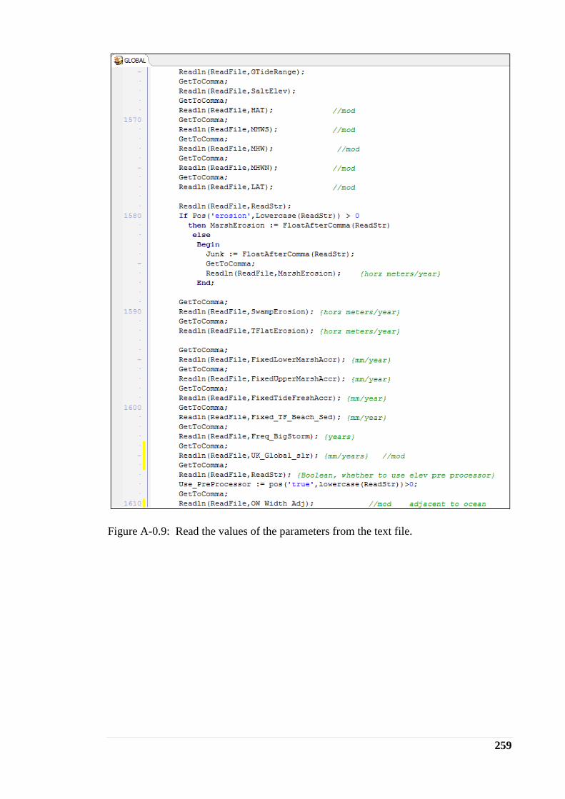
259

Figure A-0.9: Read the values of the parameters from the text file.

260

Figure A-0.10: Create parameters for sub-sites.

Figure A-0.11: Determine different wetland elevation units.

261

Figure A-0.12: Load and save elevation units from the text file.

262

Figure A-0.13: Create columns at the Elevation Input and Analysis Table.

Figure A-0.14: Write elevation units at the Elevation Input and Analysis Table.

263

Figure A-0.15: Set default elevation ranges for each wetland category.

264

Figure A-0.16: Define upper and lower boundaries of the wetland categories.

Figure A-0.17: Incorporate UKCP09 type scenarios into the IPCC ones.

Figure A-0.18: Define labels for each scenario.

265

Figure A-0.19: Read each sea-level rise scenario.

Figure A-0.20: Write each sea-level rise scenario.

266

Figure A-0.21: Create checkboxes at the interface.

Figure A-0.22: Assign each scenario to the relevant checkbox.

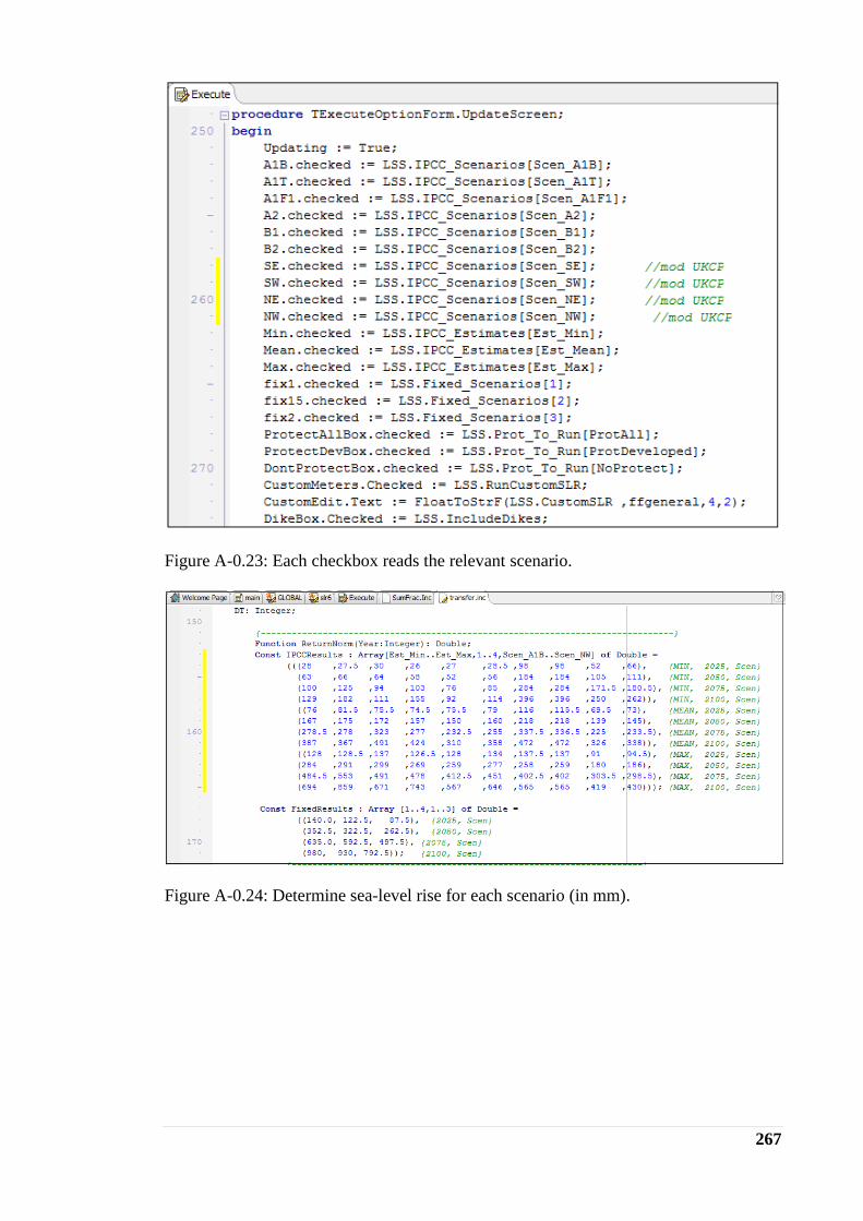
267

Figure A-0.23: Each checkbox reads the relevant scenario.

Figure A-0.24: Determine sea-level rise for each scenario (in mm).

268

Figure 0.25: Calculation of sea-level rise.

Figure A-0.26: Adjustment of elevation when different dates on DEM and Land cover

map are used.

269

Figure A- 0.27: Procedure of aggradation.

Figure A-0.28: High tide is included into the fetch calculation.

270

Figure A-0.29: Fetch threshold.

Figure A- 0.30: Procedure of dryland erosion.

271

Figure A- 0.31: Procedure of overwash.

Figure A- 0.32: Test adjacent to the ocean.

CLIMATE CHANGE - CORE

Documents

Transcript of CLIMATE CHANGE - CORE