Mesure de la production de bosons électrofaibles dans les ...

Thèse de doctorat présentée pour l’obtention du grade de

Docteur d’UniversitéSpécialité : Particules, Interactions, Univers

par

Guillaume Taillepied

Mesure de la production de bosonsélectrofaibles dans les collisions p–Pb

à √sNN = 8.16 TeV avec ALICE

soutenue le 24 septembre 2021 à Clermont-Ferrand

Jury:

Rapporteurs : M. GagliardiE. Gonzalez FerreiroM. Ploskon

Examinateurs : N. BastidJ. Castillo CastellanosS. Monteil

Directeur de thèse : X. Lopez

Contents

Acknowledgments v

Abstract vii

Résumé détaillé ix

Introduction 1

I High-energy nuclear physics 5

1 Nuclear matter in particle physics 71.1 Fundamentals of QCD . . . . . . . . . . . . . . . . . . . . . . . . . . . . . . . . . . 7

1.1.1 Quark model and the colour charge . . . . . . . . . . . . . . . . . . . . . . . 71.1.2 QCD Lagrangian . . . . . . . . . . . . . . . . . . . . . . . . . . . . . . . . . 91.1.3 Perturbative QCD and the asymptotic freedom . . . . . . . . . . . . . . . . 111.1.4 Chiral symmetry breaking . . . . . . . . . . . . . . . . . . . . . . . . . . . . 131.1.5 QCD phase diagram . . . . . . . . . . . . . . . . . . . . . . . . . . . . . . . 16

1.2 Structure of nuclei . . . . . . . . . . . . . . . . . . . . . . . . . . . . . . . . . . . . 191.2.1 The parton model . . . . . . . . . . . . . . . . . . . . . . . . . . . . . . . . . 191.2.2 QCD-improved parton model . . . . . . . . . . . . . . . . . . . . . . . . . . 221.2.3 The PDF framework . . . . . . . . . . . . . . . . . . . . . . . . . . . . . . . 271.2.4 Nuclear effects and nPDFs . . . . . . . . . . . . . . . . . . . . . . . . . . . . 31

2 Heavy-ion collisions 372.1 History of a collision . . . . . . . . . . . . . . . . . . . . . . . . . . . . . . . . . . . 372.2 Heavy-ion accelerators . . . . . . . . . . . . . . . . . . . . . . . . . . . . . . . . . . 412.3 The Glauber model . . . . . . . . . . . . . . . . . . . . . . . . . . . . . . . . . . . . 422.4 Small systems . . . . . . . . . . . . . . . . . . . . . . . . . . . . . . . . . . . . . . . 46

2.4.1 Small systems as benchmarks for heavy-ions . . . . . . . . . . . . . . . . . . 472.4.2 Collectivity in small systems(?) . . . . . . . . . . . . . . . . . . . . . . . . . 49

i

3 Weak bosons in heavy-ion collisions 533.1 Carriers of the weak force . . . . . . . . . . . . . . . . . . . . . . . . . . . . . . . . 53

3.1.1 Historical perspective . . . . . . . . . . . . . . . . . . . . . . . . . . . . . . . 533.1.2 W± and Z0 bosons in the Standard Model . . . . . . . . . . . . . . . . . . . 583.1.3 Properties of the W± and Z0 bosons . . . . . . . . . . . . . . . . . . . . . . 60

3.2 Production and decay . . . . . . . . . . . . . . . . . . . . . . . . . . . . . . . . . . . 623.2.1 The Drell-Yan process . . . . . . . . . . . . . . . . . . . . . . . . . . . . . . 623.2.2 Higher order corrections . . . . . . . . . . . . . . . . . . . . . . . . . . . . . 653.2.3 Muonic decay channel . . . . . . . . . . . . . . . . . . . . . . . . . . . . . . 663.2.4 Production and study in proton–lead collisions . . . . . . . . . . . . . . . . . 67

3.3 Measurements at the LHC . . . . . . . . . . . . . . . . . . . . . . . . . . . . . . . . 703.3.1 Production in Pb–Pb collisions at midrapidities . . . . . . . . . . . . . . . . 703.3.2 Production in Pb–Pb collisions at large rapidities . . . . . . . . . . . . . . . 723.3.3 Production in p–Pb collisions at midrapidities . . . . . . . . . . . . . . . . . 733.3.4 Production in p–Pb collisions at large rapidities . . . . . . . . . . . . . . . . 76

II A Large Ion Collider Experiment 79

4 The ALICE detector 814.1 The Large Hadron Collider . . . . . . . . . . . . . . . . . . . . . . . . . . . . . . . . 81

4.1.1 LHC at CERN . . . . . . . . . . . . . . . . . . . . . . . . . . . . . . . . . . 814.1.2 Injection and beams . . . . . . . . . . . . . . . . . . . . . . . . . . . . . . . 83

4.2 Overview of ALICE . . . . . . . . . . . . . . . . . . . . . . . . . . . . . . . . . . . . 844.3 Global detectors . . . . . . . . . . . . . . . . . . . . . . . . . . . . . . . . . . . . . . 87

4.3.1 Constituents . . . . . . . . . . . . . . . . . . . . . . . . . . . . . . . . . . . . 874.3.2 V0-based triggering and beam-gas rejection . . . . . . . . . . . . . . . . . . 894.3.3 Luminosity and visible cross sections . . . . . . . . . . . . . . . . . . . . . . 904.3.4 Centrality determination . . . . . . . . . . . . . . . . . . . . . . . . . . . . . 91

4.4 Central barrel . . . . . . . . . . . . . . . . . . . . . . . . . . . . . . . . . . . . . . . 934.4.1 Detector layout . . . . . . . . . . . . . . . . . . . . . . . . . . . . . . . . . . 954.4.2 Primary vertex reconstruction . . . . . . . . . . . . . . . . . . . . . . . . . . 964.4.3 Charged track reconstruction . . . . . . . . . . . . . . . . . . . . . . . . . . 984.4.4 Particle identification . . . . . . . . . . . . . . . . . . . . . . . . . . . . . . . 100

5 Forward muon spectrometer 1075.1 Overview . . . . . . . . . . . . . . . . . . . . . . . . . . . . . . . . . . . . . . . . . . 1075.2 Composition . . . . . . . . . . . . . . . . . . . . . . . . . . . . . . . . . . . . . . . . 110

5.2.1 Tracking system . . . . . . . . . . . . . . . . . . . . . . . . . . . . . . . . . . 1105.2.2 Trigger stations . . . . . . . . . . . . . . . . . . . . . . . . . . . . . . . . . . 1115.2.3 Absorbers . . . . . . . . . . . . . . . . . . . . . . . . . . . . . . . . . . . . . 112

5.3 Track reconstruction . . . . . . . . . . . . . . . . . . . . . . . . . . . . . . . . . . . 1135.3.1 Reconstruction algorithm . . . . . . . . . . . . . . . . . . . . . . . . . . . . . 113

ii

5.3.2 Alignment of the tracking chambers . . . . . . . . . . . . . . . . . . . . . . . 1145.3.3 Reconstruction efficiency . . . . . . . . . . . . . . . . . . . . . . . . . . . . . 115

5.4 Muon triggering . . . . . . . . . . . . . . . . . . . . . . . . . . . . . . . . . . . . . . 116

6 Data taking in ALICE 1196.1 Online Control System . . . . . . . . . . . . . . . . . . . . . . . . . . . . . . . . . . 119

6.1.1 Trigger . . . . . . . . . . . . . . . . . . . . . . . . . . . . . . . . . . . . . . . 1206.1.2 Data AcQuisition (DAQ) . . . . . . . . . . . . . . . . . . . . . . . . . . . . . 1226.1.3 High-Level Trigger (HLT) . . . . . . . . . . . . . . . . . . . . . . . . . . . . 1276.1.4 Detector and Experiment Control Systems (DCS and ECS) . . . . . . . . . . 130

6.2 ALICE Offline . . . . . . . . . . . . . . . . . . . . . . . . . . . . . . . . . . . . . . . 1326.2.1 The LHC computing grid . . . . . . . . . . . . . . . . . . . . . . . . . . . . 1326.2.2 ROOT and AliRoot . . . . . . . . . . . . . . . . . . . . . . . . . . . . . . . . 1336.2.3 Simulation and reconstruction . . . . . . . . . . . . . . . . . . . . . . . . . . 135

7 ALICE in the LHC Run 3 1377.1 Physics motivation . . . . . . . . . . . . . . . . . . . . . . . . . . . . . . . . . . . . 1377.2 Central barrel and global detectors . . . . . . . . . . . . . . . . . . . . . . . . . . . 140

7.2.1 Inner Tracking System . . . . . . . . . . . . . . . . . . . . . . . . . . . . . . 1407.2.2 Time Projection Chamber . . . . . . . . . . . . . . . . . . . . . . . . . . . . 1417.2.3 Readout and trigger . . . . . . . . . . . . . . . . . . . . . . . . . . . . . . . 142

7.3 Muon spectrometer . . . . . . . . . . . . . . . . . . . . . . . . . . . . . . . . . . . . 1477.3.1 Motivation for the upgrade . . . . . . . . . . . . . . . . . . . . . . . . . . . . 1477.3.2 Muon identifier and tracking system . . . . . . . . . . . . . . . . . . . . . . 1487.3.3 Muon Forward Tracker . . . . . . . . . . . . . . . . . . . . . . . . . . . . . . 149

7.4 Software upgrade . . . . . . . . . . . . . . . . . . . . . . . . . . . . . . . . . . . . . 1517.4.1 The Online-Offline framework . . . . . . . . . . . . . . . . . . . . . . . . . . 1517.4.2 Data Quality Control . . . . . . . . . . . . . . . . . . . . . . . . . . . . . . . 1547.4.3 MID raw data QC . . . . . . . . . . . . . . . . . . . . . . . . . . . . . . . . 157

III Z0- and W±-boson measurementsin p–Pb collisions at √

sNN = 8.16 TeV 161

8 Data analysis 1638.1 Data samples and selection . . . . . . . . . . . . . . . . . . . . . . . . . . . . . . . . 163

8.1.1 Collision system and LHC periods . . . . . . . . . . . . . . . . . . . . . . . . 1638.1.2 Event selection . . . . . . . . . . . . . . . . . . . . . . . . . . . . . . . . . . 1658.1.3 Luminosity . . . . . . . . . . . . . . . . . . . . . . . . . . . . . . . . . . . . 1678.1.4 Centrality . . . . . . . . . . . . . . . . . . . . . . . . . . . . . . . . . . . . . 1718.1.5 Track selection . . . . . . . . . . . . . . . . . . . . . . . . . . . . . . . . . . 172

8.2 Signal extraction . . . . . . . . . . . . . . . . . . . . . . . . . . . . . . . . . . . . . 1738.2.1 Overview . . . . . . . . . . . . . . . . . . . . . . . . . . . . . . . . . . . . . 173

iii

8.2.2 MC simulations . . . . . . . . . . . . . . . . . . . . . . . . . . . . . . . . . . 1758.2.3 Z0-boson signal extraction . . . . . . . . . . . . . . . . . . . . . . . . . . . . 1798.2.4 W±-boson signal extraction . . . . . . . . . . . . . . . . . . . . . . . . . . . 184

8.3 Efficiency correction . . . . . . . . . . . . . . . . . . . . . . . . . . . . . . . . . . . 1928.4 Differential studies . . . . . . . . . . . . . . . . . . . . . . . . . . . . . . . . . . . . 1938.5 Summary of systematic uncertainties . . . . . . . . . . . . . . . . . . . . . . . . . . 195

9 Results and physics interpretation 1979.1 Z0 and W± production cross sections in p–Pb collisions . . . . . . . . . . . . . . . . 197

9.1.1 Measured production . . . . . . . . . . . . . . . . . . . . . . . . . . . . . . . 1979.1.2 Comparison with measurements at √sNN = 5.02 TeV . . . . . . . . . . . . 1999.1.3 Comparison with theoretical calculations . . . . . . . . . . . . . . . . . . . . 2009.1.4 Comparison with CMS measurement at midrapidity . . . . . . . . . . . . . . 202

9.2 Lepton charge asymmetry . . . . . . . . . . . . . . . . . . . . . . . . . . . . . . . . 2049.3 Nuclear modification factor . . . . . . . . . . . . . . . . . . . . . . . . . . . . . . . 2089.4 Binary scaling . . . . . . . . . . . . . . . . . . . . . . . . . . . . . . . . . . . . . . . 211

Conclusion 213

List of figures 215

List of tables 221

Bibliography 223

iv

Acknowledgments

First and foremost I would like to deeply thank my thesis supervisor, Prof. Xavier Lopez, forthe time I shared with him during this thesis. His involvement, his scientific skills and his rigourprovided me with the perfect working environment. Thank you Xavier for your kindness and yourpatience. I would like to thank as well Nicole Bastid, Javier Castillo, Martino Gagliardi, ElenaGonzalez, Mateusz Ploskon and Stéphane Monteil for agreeing to be part of my jury. All thecomments, discussions and suggestions were very much appreciated.

The ALICE group at the LPC has been a warm and welcoming environment, making my lifein the laboratory interesting and pleasant. This naturally extends to the whole laboratory, fromthe colleagues of the other groups to the administration and IT departments.

During my work I had the pleasure to publish with very kind and competent persons. Thankyou Ophélie, Sizar, Nicolo and Mingrui for our writing and discussion sessions, I hope we will stayin touch and wish you all the best in your future endeavours. Being part of a CERN Collaborationsuch as ALICE leads one to meet way too many people for allowing me to list and thank everyonewho had a scientific and/or personal impact on me and my work.

I am very grateful to Silvia Masciocchi, Andrea Dubla and Ralf Averbeck, and all the peopleat the GSI institute, for giving me the opportunity to pursue my journey in heavy-ion physics. Iam very much looking forward to start working with you.

This experience would not have been the same without all the other students I had the chanceto meet here. Jonathan, Siyu, Boris, Yannick, Manon, Florian, Sofia, Cédric, Henri, Emmanuelle,Théo, Mélissa, Ioan, Chandan, Chun-Lu, Damien, Lina, Mark, Nazlim, Lenhart, Zhuman, Louis,Cristina, Arthur, and all the others, it was a pleasure eating, drinking, climbing, playing, discussing,and simply being with you all.

My family and friends have been more crucial for the completion of this thesis that they willprobably ever realise. I am both happy for all we gained and sorry for all we lost during thesepeculiar times.

To my mother and my sister, for their unconditional, although not always deserved, support.

v

Abstract

Electroweak-boson production in p–Pb collisions at √sNN = 8.16 TeV with ALICE.

The matter that surrounds us is made of quarks, forming bound states through the exchangeof the bosons mediating the strong nuclear force, the gluons. The interaction between quarksand gluons is described theoretically by means of quantum chromodynamics (QCD). Similarly toordinary matter, the quark matter can be found in various states that one can depict in a phasediagram. Experimentally, these phases can be created by performing heavy-ion collisions (HIC),such as the ultra-relativistic lead-lead collisions delivered at the Large Hadron Collider (LHC).Such a collision leads to the creation of a Quark-Gluon Plasma (QGP), a near-perfect fluid whichstudy sheds light on the first moments of the Universe, as the standard model of cosmology predictsthat the Universe was a QGP a few microseconds after the Planck wall. In the experimental studyof HIC, the measurements are often a sum of effects occuring at various stages of the history ofthe collision, and can be related to the initial state, the existence and evolution of the QGP phase,if any, or the hadronisation phase in which the partons that were released in the QGP form boundstates as the confinment mechanism sets in.

This thesis aims at providing information on the initial state through the measurement ofelectroweak-boson production in proton-lead (p–Pb) collisions. The parton model allows to de-scribe the internal structure of the nucleus by means of the nuclear Parton Distribution Functions(nPDFs), representing the distribution of the hadron momentum among its constituent partons ata given energy scale. The nPDFs are used as input for theoretical calculations of the productioncross section of a given process in hadronic collisions, replacing the long-distance, non-perturbativepart of the factorised expression. The nPDFs are determined from a global QCD analysis of data,which are fitted with phenomenological functional forms that can be extrapolated to all energyscales, with the DGLAP evolution equations, and to all chemical species with the A dependenceof the nPDFs themselves. Their determination thus relies on the amount of available experimentaldata.

The Z0 and W± bosons are colourless particles, produced at the very early stages of the collision,in the so-called hard scattering processes, and decaying very rapidly due to their large masses andwidths. Their production cross section is directly proportional to the momentum of the collidingparton. Moreover, they have a probability to decay into muons in the Z0 → µ+µ− and W± → µ±νprocesses, with a branching fraction of 3% and 10%, respectively. The lepton themselves are alsoinsensitive to the strong force, and their energy loss in the medium by brehmsstrahlung can be

vii

shown to be negligible. The leptonic decay of electroweak bosons thus provides medium-blindprocesses which production cross section is directly proportional to the nPDFs of the collidinghadrons, and this information will travel through the following stages of the collision history with-out being affected until their detection.

In the following, the measurements of the Z0- and W±-boson productions in p–Pb collisionsat √sNN = 8.16 TeV are measured in the muonic decay channels, using the ALICE muonspectrometer. The analysis is based on data collected in 2016 in two configurations called p-goingand Pb-going, depending on whether the proton beam moves towards the spectrometer or awayfrom it, respectively. The measurements are performed on the dimuon invariant mass spectrumfor the Z0 and through a fit of the single-muon pT distribution for the W±. The production crosssections for the three processes are reported and compared with theoretical calculations relyingon various parametrisations of the nPDF, as well as calculations performed from free-nucleonPDF as to evaluate the modification of the production from the nuclear effects themselves. Thetwo charges of the W± boson allow for the evaluation of the lepton-charge asymmetry as well,a quantity sensitive to the down-to-up ratio in the nucleus. The nuclear modification factor ispresented, computed using pQCD calculations of the reference pp cross section. Finally, theproduction of hard processes is expected to scale with the number of binary collisions, assumingan unbiased estimation of the centrality of the events. Measurements of the cross section, scaledto the average number of binary collisions in several centrality classes, are thus also shown.

The ALICE detector is currently undergoing an upgrade in preparation for the Run 3 of theLHC. Part of this upgrade aims at transforming the trigger system of the muon spectrometer intothe Muon IDentifer (MID), as to cope with the continuous readout mode and the higher collisionrate foreseen. Besides the upgrade of the detector, a new software framework, O2, has been de-velopped to replace the one used during Run 1 and 2 (AliRoot). A new software for the QualityControl of the MID, aiming at monitoring the detector status and quality of the data during datataking, is developped in this new framework and according to the new experimental conditions. Thecontribution to the MID Quality Control that constituted the service work of this thesis is detailed.

Keywords: heavy-ion collisions, quantum chromodynamics, initial state, nuclear parton dis-tribution functions, electroweak bosons, Z0, W±, ALICE, LHC.

viii

Résumé détaillé

Dans ce manuscrit, la mesure de la production des bosons électrofaibles dans les collisions proton-plomb (p–Pb) à une énergie dans le centre de masse √

sNN = 8.16 TeV avec ALICE est reportée.Ce résumé commence par une présentation du contexte théorique sous-jacent à cette analyse, enmontrant en quoi ces mesures peuvent aider à la détermination des fonctions de distributionspartoniques qui décrivent la structure interne du noyau. Il se poursuit par une description dudétecteur ALICE, centrée sur le spectromètre à muons qui a servi à collecter les données utilisées.Enfin, la stratégie d’analyse est détaillée et les résultats obtenus sont reportés et discutés.

Chromodynamique quantique et les collisions d’ions lourdsLa matière hadronique est faite de quarks, particules élémentaires de spin 1/2. Le Modèle Standardde la physique des particules [1] contient six quarks regroupés en trois doublets : up et down,charm et strange, top et bottom. Les principales caractéristiques des quarks sont indiquées dansle Tableau 1. Ces quarks portent une charge dîte de couleur pouvant prendre trois valeurs, rouge(r), bleu (b) ou verte (g). Dans le modèle des quarks, indépendamment proposé par Murray Gell-Man et Georges Zweig en 1964 [2, 3], les hadrons sont en conséquence interprétés comme étant desassemblages de quarks. Il est naturel de décrire la transformation de couleur à l’aide du groupe desymmétrie SU(3), celui-ci menant à la prédiction des états baryoniques (contenant trois quarks) etmésoniques (contenant deux quarks) observés dans la nature. Le recourt au groupe de symmétrieSU(3) entraîne également la prédiction de huit bosons médiateurs de l’interaction dîte forte, dontla couleur constitue la charge. Ces bosons de masse nulle et de spin 1 sont appelés gluons, etsont responsables du confinement des quarks en paquets d’au moins deux quarks ayant une chargetotale de couleur nulle.

La chromodynamique quantique (QCD) est la théorie de l’interaction forte. Sous sa formluationLagrangienne, elle s’exprime comme :

LQCD = ψa

iγµ∂µδab −mδab − gsγ

µtAabAAµ

ψb −

1

4FAµνF

µνA , (1)

où a = (1, 2, 3) = (r, g, b) et A = (1, ..., 8) indiquent respectivement les indices de couleur des quarkset gluons1. L’une des caractéristiques fondamentales de la QCD provient du fait que les gluonsportent une charge de couleur, et sont donc eux-mêmes sensibles à l’interaction forte (à l’inverse

1Voir la Section 1.1.2 pour une description détaillée des termes présents dans le Lagrangien.

ix

Quark Charge Isospin B S C B T Masse (MeV/c2)

d – down −13

−12

13

0 0 0 0 4.7+0.5−0.3

u – up +23

+12

13

0 0 0 0 2.2+0.5−0.4

s – strange −13

0 13

−1 0 0 0 95+9−3

c – charm +23

0 13

0 +1 0 0 (1.275+25−35)× 103

b – bottom −13

0 13

0 0 −1 0 (4.18+0.04−0.03)× 103

t – top +23

0 13

0 0 0 +1 (173.2± 0.9)× 103

Table 1: Charge, isospin, nombres quantiques et masse des quarks du Modèle Standard. Lesnombres quantiques sont le nombre baryonique B, et les nombres de saveur : étrangeté S, charmeC, beauté B and vérité T . La masse indiquée pour le quark top est celle rapportée par le Teva-tron Electroweak Working Goup, estimée d’après l’analyse des mesures au Tevatron et au LHC.Informations tirées de la Ref. [4].

par exemple du photon, de charge nulle et donc insensible à l’interaction électromagnétique). Eneffet, développer le tenseur FA

µν donne l’expression :

FAµν = ∂µAA

ν − ∂νAAµ − αs

4πfABCAB

µACν , (2)

dont le dernier terme décrit l’interaction du gluon avec lui-même.

La QCD possède deux régimes particuliers selon l’énergie à laquelle on se place. À basse énergie,l’interaction liant les particules colorées est importante et entraîne le confinement des quarks enhadrons. À haute énergie en revanche, la force de cette interaction décroît dans un régime nomméla liberté asymptotique. Cette évolution de l’interaction forte est illustrée par sa "constante" decouplage αs, comme indiquée par la Figure 1 (gauche). Un paramètre fondamental de la QCD estΛQCD, l’échelle d’énergie en dessous de laquelle la force de l’interaction empêche l’utilisation destechniques perturbatives dans les calculs.

Ces différents régimes entraînent l’apparition de phases de la matière forte, qui peuvent êtreétudiées à travers l’exploration d’un diagramme de phase tel que celui de la Figure 1 (droite).Différentes régions peuvent être isolées sur ce diagramme, correspondant aux différentes phases dela matière forte. À faible énergie, le phénomène de confinement entraîne l’apparition de la matièrenucléaire ordinaire, dans laquelle les quarks sont regroupés en hadrons, eux-mêmes formant desassemblages composites plus lourds, les noyaux atomiques. Une élevation de l’energie empêcherala formation de noyaux, sans pour autant casser les hadrons, formant de ce fait une phase de gazhadronique. À très haute température, le couplage αs devient trop faible pour entretenir l’existencedes hadrons eux-mêmes, et les quarks et gluons qui les constituent sont relachés et deviennent li-bres. Cette phase, appelées le Plasma de Quarks et Gluons (QGP), est un important objet d’étudedans le cadre de la physique des particules, donnant un accès unique à des spécificités de la QCD

x

αs(MZ2) = 0.1179 ± 0.0010

αs(

Q2 )

Q [GeV]

τ decay (N3LO)low Q2 cont. (N3LO)

DIS jets (NLO)Heavy Quarkonia (NLO)

e+e- jets/shapes (NNLO+res)pp/p-p (jets NLO)

EW precision fit (N3LO)pp (top, NNLO)

0.05

0.1

0.15

0.2

0.25

0.3

0.35

1 10 100 1000

Nuclear

matter

Tem

pera

ture

T

Baryon chemical potential μB

Quark-Gluon Plasma(QGP)

Vacuum

Hadronic

gas

Quark

matter?

LHC (CERN)

RHIC (BNL)

NICA (JINR)

FAIR (GSI)

CFL?

0

EIC (BNL)

TcCrossover

transition

Crossover

transition

First-order phase transition,

deconfinment and chiral transition

Critical point

SPS (CERN)

Figure 1: Gauche : mesures du couplage αs(Q2) en fonction de l’échelle d’énergie Q. Figure

tirée de la Ref. [4]. Droite : diagramme de phase de la matière forte dans l’espace (µB, T )correspondant respectivement au potentiel baryonique et à la température. Voir la Section 1.1.5pour une description détaillée du diagramme.

absente des autres phases.

La création d’un QGP dans le laboratoire nécessite une densité d’énergie très importante, quin’est atteinte qu’auprès des plus puissants accélérateurs de particules, tels que le Grand Collision-neur de Hadrons (LHC) au CERN [5]. Le LHC est un anneau de 27 kilomètres de circonférence,permettant d’accélérer jusqu’à des vitesses ultra-relativistes (plus de 99% de la vitesse de la lu-mière) deux faisceaux de particules circulant dans des sens opposés. Ces faisceaux se rencontrenten quatre points de collisions autour desquels sont installées les quatre principales expériences duLHC : ALICE, ATLAS, CMS et LHCb. Bien que le mode de fonctionnement ordinaire du LHCconsiste en l’accélération de faisceaux de protons, un certain temps est chaque année dédié à l’ac-célération et la collision d’ions lourds, tels que des noyaux de plomb. Dans l’histoire d’une collisiond’ions lourds, plusieurs étapes peuvent être distinguées [6] :

1. État initial : les deux noyaux sont accélérés à des vitesse proches de celle de la lumière, etsubissent en conséquence une importante contraction de Lorentz.

2. Collision : les noyaux entrent en collision, et de nombreuses collisions partoniques (entrequarks et gluons) ont lieu. Ces intéractions partoniques initiales entraînent les procédés ditsdurs, lors desquels de grandes quantités d’impulsion (> 10 GeV) sont échangées en des tempstrès courts (∼ 1/Q). Ces processus donnent naissance aux particules dures parmi lesquelleson trouve les gerbes hadroniques, des photons, paires d’electrons, quarks lourds et les bosonsvecteurs.

xi

3. Procédés semi-durs : suite à la production de particules dures, des procédés impliquantde plus faibles transferts d’énergie prennent place. Lors de cette étape, les consituants desnoyaux sont libérés, les gluons de l’état initial se fragmentent et s’hadronisent, produisant lamajeure partie de la multiplicité de l’évènement.

4. Phase hors-équilibre : la densité de particules créées lors d’une collision d’ions lourdsentraine des interactions entre celles-ci, ces interactions pouvant être détectées et étudiées àtravers des effets collectifs tels que le flux elliptique ou les phénomènes de co-déplacement.

5. Plasma de Quark et Gluons : les interactions lors de la phase hors-équilibre entraîne lathermalisation du système, qui continue cependant de s’étendre et se refroidir. Cette étapepeut être efficacement décrite par des modèles hydrodynamiques.

6. Hadronisation et gel : lorsque le refroidissement progressif du système ramène la tempera-ture sous une valeur critique, le confinement rassemble les partons dans des états hadroniques.Deux phases de gel sont par la suite distinguées : le gel thermique, après lequel les hadronspeuvent encore subir des interactions inélastiques, et le gel chimique après lequel la com-position chimique de l’etat final n’évolue plus, alors que seules des interactions elastiquespeuvent encore survenir.

Cette description schématique n’est évidemment pas fixe, et l’histoire d’une collision d’ions lourdsreste une question essentiellement ouverte, faisant l’object d’intenses efforts de recherche. Cesétapes se déroulent en un temps très courts, environ 20 fm/c, empêchant l’accès expérimentaldirect. Le produit d’une collision d’ions lourds, tel qu’il est détécté expérimentalement, est doncla somme de tous les effets intervenant aux différentes étapes de la collision. Il est donc d’uneimportance cruciale, pour les expérimentateurs, de trouver des sondes et observables spécifiques àl’étude de chaque étape, afin d’en distinguer les effets. À ce titre, les collisions proton-plomb (p–Pb)réalisées au LHC apportent un éclairage supplémentaire. Dans de telles collisions, l’apparition d’unQGP n’est en effet pas attendue, de telle sorte que seuls les effets nucléaires dits froids2 entrenten action. La comparaison des mesures faites dans les collisions p–Pb et plomb-plomb (Pb–Pb)permet donc de distinguer ces effets des effets nucléaires chauds.

Fonctions de distribution partoniquesLes fonctions de distribution partoniques (PDF) décrivent la probabilité de trouver un partonportant une fraction x, appelée x de Bjorken, de l’impulsion totale du hadron à une énergiedonnée. Elle permettent donc une description de l’état initial de la collision en terme de répartitionde l’énergie dans le noyau. Par le théorème de factorisation, il est possible d’exprimer la sectionefficace de production σ d’un état final générique H dans une collision hadronique comme :

σpp→H(s, µ2F , µ

2R) =

i,j

dx1dx2fi(x1, µ

2F , µ

2R)fj(x2, µ

2F , µ

2R)σij→X(x1, x2, s;µ

2F , µ

2R), (3)

2Par convention, on désigne comme effects nucléaires chauds les effets faisant suite à la présence d’un QGP, etcomme effets froids ceux qui n’en dépendent pas.

xii

Figure 2: Les PDF nucléaires du carbone 12C, du fer 56Fe et du plomb 208Pb à l’énergie Q2 =100 GeV2 dans le modèle nNNPDF2.0. Figure tirée de la Ref. [7].

où s représente l’énergie, x1 et x2 sont les x de Bjorken des partons 1 et 2 respectivement, etµF et µR sont les échelles de factorisation et de renormalisation. Dans cette expression, σ est lasection efficace partonique, calculable par l’application de techniques perturbatives. Les termesfi et fj représentent les PDF des partons i et j. Ces fonctions sont non-perturbatives, rendantimpossible leur détermination par le calcul, elles peuvent en revanche être estimée depuis lesmesures expérimentales. Pour cela, une paramétrisation initiale de la PDF est établie de manièrephénoménologique à une échelle d’énergie initiale arbitraire Q0. À l’aide des équations d’évolutionde DGLAP, cette paramétrisation initiale est ensuite extrapolée à l’énergie requise, correspondantà celle du jeu de donné considéré, permettant l’évaluation des observables. Cette étape est réaliséepour tous les jeux de données disponibles. Enfin, les paramètres libres du modèles à Q0 sontajustés afin de déterminer ceux qui permettent de reproduire au mieux l’ensemble des mesuresexpérimentales.

La paramétrisation typique d’une PDF se présente comme :

f(x,Q0, ai) = xa1(1− x)a2C(x, ai>2), (4)

où les termes ai sont les paramètres libres du modèle. Les termes en x et 1−x vont respectivementcontraindre la distribution dans les limites où x tend vers 0 et 1. La fonction C est la fonctiond’interpolation, qui détermine le comportement de la PDF entre ces deux limites. Dans le casd’une PDF nucléaire (nPDF), les paramètres libres porteront la dépendance en A. Les nPDF dequelques éléments dans le modèle nNNPDF2.0 [7] sont données par la Figure 2. La différence decomportement entre les quarks de valence uV et dV et ceux de mer est particulièrement visible, lesquarks de valence dominant la distribution à de grandes valeurs de x. La détermination d’une nPDFpeut également suivre une approche alternative, reposant sur la paramétrisation de la fonction demodification nucléaire. Il est en effet possible de relier une nPDF à la PDF du proton libre par :

fp/Ai (x,Q2) = RA

i (x,Q2)f p

i (x,Q2), (5)

xiii

où fp/Ai (x,Q2) est la PDF du parton i dans un proton du noyau A, f p

i celle de ce même partondans un proton libre, et RA

i est la fonction de modification nucléaire. Cette dernière peut doncégalement se définir comme le rapport entre la nPDF et la PDF. Suite à la quantité et la précisiondes données récoltées dans les collisions pp, les PDF du proton libre sont connues avec une plusgrande précision que celle du proton lié, permettant d’utiliser les premières comme réferences dansla détermination des secondes. Ces deux approches, ainsi que la variété des paramétrisations etméthodes de détermination possibles, entraine l’existence de nombreux jeux de nPDF. La Figure3 montre la forme typique d’une fonction de modification nucléaire en fonction du x de Bjorken.Plusieurs régions peuvent y être distinguées, selon les effets nucléaires entrant en action :

• l’effet de shadowing, pour des petites valeurs de x, entraîne une diminution de la PDF suiteaux interférences destructives créées par les diffusions multiples entre partons dans le noyau,

• l’effet d’antishadowing, homologue de l’effet de shadowing, entraîne une augmentation de laPDF suite aux interférences constructives,

• l’effet EMC, du nom de la European Muon Collaboration qui l’a mis en avant, est uneobservation de la diminution des PDF pour des valeurs proches de x = 1 dont l’interprétationest encore en cours.

Les paramètres xa, xe, ya et ye représentent des paramètres libres supplémentaires du modèle,permettant de déterminer pour chaque nPDF la position des extrema dans les régions d’antishad-owing et d’effet EMC.

Les résultats présentés dans cette thèse sont comparés à trois modèles récents de nPDF :nCTEQ15 [9], EPPS16 [8] et nNNPDF2.0 [7]. Ces trois modèles suivent diverses approchesphénomenologiques et methodologiques pour la détermination des distributions. Dans le modèlenCTEQ15, une paramétrisation directe des nPDF est réalisée, avec une fonction d’interpolationexprimée sous forme polynômiale. Le modèle comporte 35 paramètres libres, dont la déterminationest faite sur environ 700 points expérimentaux dans sa version initiale. En 2021, une extension dece modèle a été publiée, contenant la version nCTEQ15WZ [10]. Celle-ci se distingue du modèleinitial par l’inclusion de 120 points expérimentaux supplémentaires provenant de mesures de laproduction des bosons W± et Z0 effectuées au LHC lors du Run 1. Le modèle EPPS16 reposesur la détermination de la fonction de modification nucléaire, prenant la PDF libre CT14 commebase. Ici également, la fonction d’interpolation est un polynôme. Ce modèle contient plus de 1800points expérimentaux, permettant une paramétrisation indépendante du quark s, en conséquencede quoi le modèle contient également plus de paramètres libres (52). Le modèle nNNPDF2.0 sedistingue des deux précédents par le choix d’utiliser un réseau de neurones pour la fonction d’in-terpolation, permettant d’atteindre une précision équivalente aux modèles nCTEQ et EPPS avec256 paramètres libres. Le modèle nNNPDF connaît une évolution rapide, portée par l’inclusion denouveaux points expérimentaux. À ce jour, environ 1500 points sont utilisés pour la déterminationde la version 2.0. La Table 2 résume les principales caractéristiques des modèles utilisés dans cetravail de thèse.

xiv

Figure 3: Illustration de la fonction de modification nucléaire dans le modèle EPPS16. Figuretirée de la Ref. [8].

Bosons électrofaibles dans les collisions d’ions lourdsL’étude de la production des bosons W± et Z0 dans les collisions d’ions lourds fournit une manièreefficace de sonder l’état initial de la collision. Depuis leur découverte au Super Proton Synchrotron(SPS) dans les années 1980, ces bosons ont été largement étudiés auprès d’expériences et par descollaborations dédiées. La Table 3 donne les principales caractéristiques des bosons W± et Z0: leurmasse, largeur, et rapport d’embranchement BR hadronique et leptonique.

L’énergie atteinte par le LHC dans les collisions d’ions lourds a rendu possible l’étude desbosons électrofaibles pour la première fois. Comme ils ne portent pas de charge de couleur, ilssont insensibles à l’interaction forte, et leur propagation ne sera donc pas affectées par la présenceéventuelle de matière forte dans l’histoire de la collision. Comme indiqué dans la Table 3, ilspossèdent une certaine probabilité de se désintégrer en leptons, particules également insensiblesà l’interaction forte. Il est possible de montrer que suite à leur impulsion importante, les muonsprovenant de la désintégration des bosons électrofaibles ont des interactions électromagnétiquesnégligeables avec le plasma, de sorte que le procédé dans son ensemble n’est pas affecté par le QGP.La grande masse des bosons en fait des particules dures, dont la production lors des tous premiersinstants de la collision a été montrée comme étant proportionnelle aux nPDF des ions entrant encollision. Cette information cruciale sur l’état initial sera donc portée par les bosons, puis par leurs

xv

Modèle nCTEQ15 EPPS16 nNNPDF2.0Ordre NLO NLO NLO

Séparation des saveurs quarks de valence quarks de valence et mer quarks de valence et merPDF libre de référence CTEQ6M modifiée CT14NLO NNPDF3.1Points expérimentaux 708 1811 1467

Échelle Q0 1.30 GeV 1.30 GeV 1 GeVParamètres libres 35 52 256Paramétrisation polynôme polynôme réseau de neurones

Incertitudes Hessienne Hessienne Monte Carlo

Table 2: Caractéristiques principales des modéles nCTEQ15 [9], EPPS16 [8] et nNNPDF2.0 [7].Les informations pour le modèle nCTEQ15 valent pour sa version originale.

Boson Masse (GeV/c2) Largeur (GeV/c2) BR hadronique (%) BR leptonique (%)W± 80.379 ± 0.012 2.085 ± 0.042 67.41 ± 0.27 10.86 ± 0.09Z0 91.1876 ± 0.0021 2.4952 ± 0.0041 69.911 ± 0.056 3.3658 ± 0.0023

Table 3: Masse, largeur, et rapport d’embranchement hadronique et leptonic des bosons W± etZ0. Informations tirées de la Ref. [4].

produits de désintégration, jusqu’aux détecteur où elle pourra être collectée directement.

L’intérêt d’une telle étude est illustrée par la Figure 4, montrant des prédictions sur la pro-duction des bosons Z0, W− et W+ en collisions p–Pb à l’énergie nominale du LHC. Ces calculsthéoriques ont été réalisés avec et sans inclure les modifications nucléaires des PDF. Sans ces mod-ifications, la production du boson Z0 est symmétrique en fonction de la rapidité, alors qu’une largeasymmétrie entre les productions à rapidité positive et négative est observée lors de leur inclu-sion. Les mêmes conclusions sont dérivables des distributions pour les bosons W− et W+. Il estégalement intéressant de considerer les incertitudes sur les prédictions. Même lorsque les valeurscentrales sont significativement différentes, la taille des intervalles d’erreur entraine un recouvre-ment important des distributions avec et sans modifications nucléaires. Il est donc important defournir davantage de données précises pour la détermination des nPDF, afin d’aider à réduire lesincertitudes sur les modèles.

La Figure 4 permet d’identifier les observables d’intérêt, fournissant des informations et con-traintes importantes pour la détermination des nPDF. La section efficace de production est lapremière d’entre elles, par sa dépendance directe aux nPDF. La taille des effets nucléaires peutêtre évaluée par le facteur de modification nucléaire RpPb, défini comme le rapport entre les sec-tions efficaces de production dans les collisions p–Pb et pp, cette dernière étant corrigée pour lenombre de nucléons dans le noyau :

RpPb =1

208

dσpPb

dσpp

. (6)

xvi

Figure 4: Section efficace de production des bosons Z0 (gauche), W− (milieu) et W+ (droite)dans les collisions p–Pb à √

sNN = 8.8 TeV. La ligne en pointillés correspond aux prédictionsréalisées avec le modèle de PDF libre CTEQ6.6 [11], sans inclusion de modifications nucléaires.La ligne pleine correspond aux prédictions avec CTEQ6.6 combiné avec le modèle EPS09 [12] demodification nucléaire. Les panneaux inférieurs montrent les incertitudes relatives pour chaquedistribution. Figure tirée de la Ref. [13].

Il est important de noter que le dénominateur dans l’expression représente une somme de collisionspp. Le facteur de modification nucléaire, calculé ou mesuré pour les bosons électrofaibles, ne seradonc pas égal à 1 en l’absence d’effets nucléaires, puisque la production dans des collisions p–Pbest également impactée par l’effet d’isospin. Enfin, il est possible de bénéficier des deux chargespossibles du boson W± pour définir le ratio de charge R :

R =N

µ+←W+

Nµ−←W−

, (7)

où Nµ+←W+ et N

µ−←W− représentent le nombre de muons provenant de la désintégration de W+ et

W− respectivement. Cette observable permet de contraindre les PDF des quarks légers à travers sasensibilité au rapport entre le nombre de quarks d et u dans le noyau. Il est possible d’augmentercette sensibilité en définissant l’asymmétrie de charge Ach comme :

Ach =N

µ+←W+ −N

µ−←W−

Nµ+←W+ +N

µ−←W−

=R− 1

R + 1. (8)

Ces quantités étant des rapports, et étant calculés à partir du nombre de muons détectés, et nonde la section efficace de production, ils permettent d’enlever certaines sources d’incertitudes sur lamesure finale.

xvii

Figure 5: Illustration shématique du détecteur ALICE. La région autour du point de collision estdétaillée dans le panneau en haut à droite.

Le détecteur ALICEL’expérience ALICE (A Large Ion Collider Experiment) [14] est l’une des quatre principales ex-périences du LHC, la seule dédiée à l’étude des collisions d’ions lourds. La Collaboration ALICEcomporte 1975 membres, venant de 170 instituts répartis dans 40 pays. La Collaboration utiliseun détecteur de 10 000 tonnes, long de 26 mètres, large et haut de 16 mètres, enterré 56 mètressous terre à l’un des points d’interaction du LHC. Le détecteur a été spécialement conçu poursupporter les importantes multiplicités de particules attendues dans les collisions d’ions lourds lesplus centrales, pouvant produire jusqu’à 8 000 particules chargées par unité de rapidité, tout enconservant des capacités de trajectographie et de reconstruction de traces sur un large intervalled’impulsion.

Le détecteur est schématisé sur la Figure 5. Il contient trois principaux groupes de sous-détecteurs :

• les détecteurs dits globaux fournissent des informations générales sur les collisions, telles quela multiplicité et la centralité de chaque évènement. Ils participent au déclenchement et àl’analyse du bruit de fond,

• le tonneau central, centré autour du point de collision, est utilisé pour la reconstruction

xviii

du vertex primaire, la trajectographie des particules chargées, l’identification des électrons,photons et hadrons, ainsi que la détection des gerbes hadroniques,

• le spectromètre à muons, conçu pour la détection des produits de désintégration muoniquedes mésons légers (ρ, η, ω), quarkonia, hadrons de saveurs lourdes et bosons électrofaibles àgrande rapidité.

Plusieurs de ces détecteurs ont servi aux analyses présentées dans ce manuscrit.

Le V0 contient deux tuiles de scintillateurs, découpées en 4 cercles creux concentriques etplacées à 340 cm et -90 cm du point de collision. Les fonctions principales du V0 sont de fournirun signal de déclenchement à travers la coincidence de signaux dans les deux tuiles, ainsi que defournir des capacités de rejet du bruit de fond. L’amplitude totale du signal enregistré par lestuiles est utilisée pour l’évaluation de la centralité de l’évènement, et le V0 contribue à la mesurede la section efficace visible par balayage van der Meer [15, 16].

Le calorimètre à zero degré (Zero Degree Calorimeter, ZDC) contient deux ensemble identiquesde deux calorimètres chacun, pour la détection de protons et neutrons le long de la ligne desfaisceaux. Les deux ensembles sont placés de part et d’autre du point de collision, à 113 m decelui-ci. Le ZDC fournit un évaluateur de la centralité de l’évènement grâce à la détection desnucléons spectateurs.

Le système de trajectographie interne (Inner Tracking System, ITS) est un cylindre composé desix couches de détecteurs en silicone, placé symmétriquement autour du point de collision. Étantle détecteur le plus proche du point de collision, avec une couche interne à 3.9 cm de celui-ci, l’ITSvise à évaluer les vertex primaires et secondaires, et assiste la chambre à projection temporelle(Time Projection Chamber, TPC) dans la trajectographie des particules chargées.

Le spectromètre à muons [17, 18] constitue le principal détecteur utilisé pour réaliser les mesuresprésentées dans cette thèse. Il fournit une couverture azimuthale totale pour des angles polairescompris entre 170 et 178. La composition du spectromètre est indiquée sur la Figure 6. Ilest composé d’un système de trajectographie, d’un système de déclenchement et d’un ensembled’absorbeurs.

Le système de trajectographie contient cinq stations, chacune comprenant deux plans de cham-bres cathodiques. Les prérequis en terme de résolution ont conduit à l’utilisation de chambresproportionnelles multifils pour les stations de trajectographie, permettant d’atteindre une préci-sion spatiale de 100 µm nécessaire à la résolution des différents états d’excitation du bottomonium.La troisième station est située à l’intérieur d’un aimant dipolaire, dont les bobines résistives four-nissent un champ magnétique intégré de 3 Tm dans le plan horizontal, perpendiculairement à l’axedes faisceaux. La déviation induite par ce champ permet la mesure de la charge et de l’impulsiondes muons traversant le trajectographe.

Le déclencheur à muons est composé de quatre plans regroupés en deux stations, chaque plancontenant 18 chambres à plaques résistives (Resistive Plate Chamber, RPC). Une évaluation bidi-mensionnelle de la position d’un muon frappant le déclencheur est fournie par un système debandes de lecture orthogonales découpant les plans en 234 zones de détection. Chaque RPC estfaite de deux électrodes en Bakelite de haute résistivité séparées de 2 mm. Le signal est créé par

xix

Figure 6: Coupe transversale, dans le plan longitudinal, du spectromètre à muon d’ALICE.

l’avalanche d’électrons déclenchée par le passage d’une particule chargée à travers le gaz contenudans l’espace entre les deux électrodes. Le système fournit des signaux de déclenchement selondes configurations pré-programmées, afin par exemple de sélectionner les évènements contenant unmuon de basse ou haute impulsion transverse, une paire de muons de signes opposés, etc.

Le spectromètre est protégé du bruit de fond par la présence de plusieurs absorbeurs. Entre lepoint de collision et la première station de trajectographie se trouve l’absorbeur avant, un cône deciment et de carbone de 37 tonnes visant à absorber les particules de faible impulsion provenantdu point d’interaction. Les stations du déclencheur sont situées derrière un mur de fer d’uneépaisseur de 1,2 m, qui filtre les hadrons et les particules passant à travers l’absorbeur avant ouétant produites dans celui-ci. Le spectromètre dans son ensemble est protégé de l’important bruitde fond produit par les interactions entre le tube du faisceau et les particules émises à très faiblerapidité par l’absorbeur à petit angle, un tuyau de tungstène, de plomb et d’acier entourant letuyau du faisceau sur tout la longueur du spectromètre. Enfin, un second mur de fer protègel’arrière du déclencheur des particules produites lors des interactions entre le faisceau et le gazrémanant présent dans le tuyau du faisceau.

Upgrade d’ALICE pour le Run 3 au LHCDepuis 2018, le LHC est à l’arrêt afin de préparer les prises de données du Run 3. Cet arrêtlong, le deuxième depuis le démarrage du LHC en 2009, permet aux collaborations d’améliorerleurs détecteurs. L’amélioration du LHC lui-même vise à augmenter la luminosité délivrée par le

xx

collisioneur. Le programme d’amélioration du détecteur ALICE [19] vise à renforcer les capacitésde détection et d’analyse dans trois domaines principaux.

• Saveurs lourdes : l’amélioration de la précision et des possibilités de mesures de la pro-duction des quarks c et b constitue l’une des principales motivations pour l’amélioration dudétecteur ALICE. Ces études se feront principalement à travers les mesures de la thermal-isation des saveurs lourdes dans le QGP, par la détermination du rapport entre baryons etmésons pour chaque saveur, les anisotropies azimuthales et la possible production thermiquedu quark c à l’intérieur du QGP ; ainsi que par l’évaluation de la dépendance aux massespartoniques et charges de couleur de la perte d’énergie dans le QGP. Ces études nécessi-tent notamment une importante précision dans la détermination des vertex secondaires, etla capacité de fonctionner en lecture continue afin de pleinement bénéficier de la luminositéofferte par le LHC.

• Quarkonia : la mesure de la production des quarkonia, états liés de quark-antiquark cou b, devrait apporter une réponse définitive à la question de la production de ces saveursdans le QGP. Les données des Runs 1 et 2 ont notamment fait ressortir l’importance deréaliser de telles mesures à de très faibles impulsions transverses. Plusieurs modèles ont étéproposés pour reproduire les productions observées des mésons J/ψ et Υ, tels que l’hadroni-sation statistique, l’écrantage de Debye ou les modèles de transport. L’amélioration devraitégalement permettre des mesures précises de la production des états excités de ces mésons.

• Dileptons de basse masse invariante : ces mesures apporteront un éclairage sur l’évolu-tion spatio-temporelle de la matière forte lors des collisions d’ions lourds. Elles permettronten particulier d’étudier la brisure spontanée de la symétrie chirale, l’évolution de la tem-pérature du système, et le temps de vie des différentes phases d’évolution de la collision.Ici encore les capacités de détermination des vertex de production et les mesures à bassesimpulsions transverses sont cruciales.

À ceci s’ajoute un intérêt certain pour la mesure des gerbes hadroniques et des états exotiques.

Ces objectifs seront autant réalisés par l’amélioration des détecteurs existants que par l’ajout denouveaux détecteurs. Le spectromètre à muons se verra amélioré par l’addition du trajectographeà muons à l’avant (Muon Forward Tracker, MFT) [20]. Le MFT se situe entre le point de collisionet l’absorbeur à l’avant. Il est composé de deux demi-cônes, chacun comportant cinq demi-disquesfaits de détecteurs en silicone. Le MFT apporte des capacités de détermination de vertex au spec-tromètre et, couplé au trajectographe, améliore la reconstruction des traces. Il devrait notammentpermettre une mesure précise de la production du ψ(2S) afin de tester les modèles de dissociationet (re)combinaison.

L’électronique de lecture du trajectographe sera améliorée afin d’assumer le taux de lectureattendu dans le mode continu. Le déclencheur à muons sera transformé pour devenir l’identificateurà muons (Muon Identifier, MID). Le vieillissement des RPC sera diminué par l’utilisation de cartesà plus faible gain, couplée à des puces électroniques appelées FEERIC fournissant une amplificationdu signal. Les RPC les plus proches du faisceau, ayant soutenu une charge plus importante lorsdes Runs 1 et 2, seront remplacées.

xxi

Enfin, un nouveau logiciel d’analyse est développé afin de remplacer AliRoot, le logiciel utiliséprécedemment par la Collaboration ALICE. Ce nouveau logiciel, appelé O2 (Online-Offline) [21],vise notamment à assurer la possibilité de lire, analyser et stocker les données aux taux du Run 3,s’élevant à 50 kHz dans les collisions Pb–Pb et 200 kHz pour les collisions p–Pb et pp.

Lors de ce travail de thèse, j’ai contribué à l’amélioration du détecteur par la participationau développement du logiciel de contrôle qualité (Quality Control, QC) du MID. Le QC vise àfournir un retour instantané sur la qualité des données et le fonctionnement du détecteur lors descampagnes de prise de données. Il surveille également les premières étapes du traitement des don-nées et leur enregistrement. Un module du QC, attaché à un détecteur, comprend typiquementune série de tâches effectuées sur les données, ou un fraction d’entre elles, produisant des résultatsaffichés sous la forme d’histogrammes régulièrement mis à jour dans la salle de contrôle de l’ex-périence. Ces objets de sortie permettent de surveiller en temps réel l’état de fonctionnement, uneinformation cruciale pour les analystes lors notamment de l’évaluation de l’efficacité du détecteur.Ces objets peuvent aussi, en cas de besoin, être conservés pour référence.

Un module du QC s’organise autour de fichiers pour les tâches définies par l’utilisateur, etd’un fichier de configuration au format json. Ce dernier contient des informations telles que lesfichiers et bibliothèques devant être chargées lors du lancement du module, ou les instructionsd’échantillonnage des données lorsqu’une lecture de la totalité de celles-ci n’est pas possible ousouhaitable. Ma participation a consisté à l’inclusion de tâches de vérfication des données brutesdans le module du MID. Le module a éte testé sur des données simulées, en forçant l’apparitiond’erreurs aléatoires. Les données sont lues par le module au fil de l’eau, et une série de testsautomatisés s’assurent de leur qualité. Une erreur détectée par le module se trouve affichée sousla forme :

BCid: 0x71c Orbit: 0xf [in page: 542 (line: 277505) ]loc-reg inconsistency: fired locals (00010000) != expected from reg (00000000);Crate ID: 15 Loc ID: 4 status: 0xc0 trigger: 0x 0 firedChambers: [...]

La première ligne permet d’identifier l’évènement, la seconde fourni une description de l’erreurdétectée (ici une incohérence entre les réponses de cartes à différentes étapes de la chaîne de traite-ment). La troisième ligne permet enfin de localiser spatialement l’erreur à travers les identifiantsuniques attribués à chaque RPC du MID. Un histogramme est rempli pour chaque évènement luet chaque erreur détectée.

Mesure de la production des bosons électrofaibles dans lescollisions p–Pb à √

sNN

= 8.16 TeVLes données analysées lors de ce travail de thèse ont été collectées lors de collisions p–Pb effectuéesen 2016 à une énergie dans le centre de masse √

sNN = 8.16 TeV. Les collisions ont été effectuéesdans deux configurations différentes, l’une avec le faisceau de proton dirigé vers le spectromètre(p–Pb), l’autre avec le faisceau de proton pointant à son opposé (Pb–p). Les collisions entreprotons et noyaux de plomb etant asymétriques, la rapidité dans le centre de masse se retrouve

xxii

Système Période Nb de runs Rapidité NCMSH NCMUL

p–Pb LHC16r 57 2.03 < ycms < 3.53 18.5× 106 25.8× 106

Pb–p LHC16s 80 −4.46 < ycms < −2.96 35.1× 106 72.0× 106

Table 4: Caractéristiques des deux périodes analysées dans cette thèse, correspondant à descollisions p–Pb à √

sNN = 8.16 TeV.

décalée par rapport à la rapidité dans le référentiel du laboratoire par Δy ≈ 0.465. La couvertureen rapidité du spectromètre, −4 < ylab < −2.5, correspond donc à :

• p–Pb collisions : 2.03 < ycms < 3.53,

• Pb–p collisions : −4.46 < ycms < −2.96,avec le faisceau de protons se dirigeant vers les rapidités positives, par convention. La rapiditépeut être reliée au x de Bjorken par :

x1,2 =MZ,W√sNN

exp (−y) . (9)

Les configurations p–Pb et Pb–p correspondent donc à de faibles (∼ 10−4− ∼ 10−3) et fortes(∼ 0.1− ∼ 1) valeurs de x respectivement.

Les évènements sont dans un premier temps sélectionné par la PhysicsSelectionTask quiapplique une série de tests basiques portant sur la qualité des données, rejetant par exemple lesévènements classés comme bruit de fond par le V0. La tâche rejette également les évènementspile-up, ceux pour lesquelles deux collisions ou plus ont eu lieu lors du croisement de deux paquetsdes faisceaux. Une sélection portant sur la qualité du vertex s’assure qu’au moins une trace aitété détecté par l’ITS, et que le vertex primaire se trouve à moins de 10 cm du point d’interaction.Les classes de déclenchement permettent ensuite de sélectionner les évènements utiles à l’analyse.Pour ce travail, deux classes ont principalement été utilisées:

• Dimuon Unlike-sign low (MUL) : demandant une paire de muons de signes opposés avecun impulsion transverse (pT) d’au moins 0.5 GeV/c, servant à la mesure du boson Z0,

• Single Muon High (MSH) : demandant un muon avec pT 4.2 GeV/c pour la mesure duboson W±.

La Table 4 résume les caractéristiques des deux périodes et indiquent le nombre d’évènementssélectionnés pour les deux classes de déclenchement. Le calcul de la luminosité pour les deuxanalyses diffère, la mesure du boson Z0 ayant été effectuée avant l’inclusion de la sélection sur lepile-up dans la PhysicsSelectionTask. Les luminosités correspondant à chaque configurationsont été évaluées à :

• sans rejet du pile-up (boson Z0) :

Lint =

8.40± 0.01 (stat) ± 0.17 (syst) nb−1 collisions p–Pb,12.74± 0.01 (stat) ± 0.26 (syst) nb−1 collisions Pb–p,

(10)

xxiii

• avec rejet du pile-up (boson W±) :

Lint =

6.81± 0.01 (stat) ± 0.15 (syst) nb−1 collisions p–Pb,10.2± 0.01 (stat) ± 0.28 (syst) nb−1 collisions Pb–p.

(11)

Les évènements sélectionnés ont ensuite été lus pour en extraire les traces pouvant correspondreaux signaux des bosons Z0 et W±. Une sélection est appliquée afin de s’assurer de la qualité destraces et rejeter une partie du bruit de fond. Cette sélection comporte :

• la coincidence entre le trajectographe et le déclencheur, afin de s’assurer que la trace re-construite dans le trajectographe correspond à un segment de trace reconstruit dans le dé-clencheur,

• le rejet des traces ayant un angle polaire mesuré à l’extrémité de l’absorbeur à l’avant horsde 170 < θabs < 178 afin de ne pas conserver des traces ayant subit des diffusions multiplesdans l’absorbeur,

• une sélection sur le produit de l’impulsion de la trace avec sa distance de plus proche approche(p×DCA), c’est-à-dire la distance entre le vertex et la trace projetée dans le plan perpen-diculaire au faisceau et contenant le vertex. Cette sélection vise à réduire drastiquement lebruit de fond en ne sélectionnant que des traces provenant du vertex d’interaction.

Une région fiducielle est de plus définie pour chaque analyse, d’après les capacités du détecteur etafin de maximiser l’efficacité de l’extraction du signal. Ces régions sont définies par :

• la couverture angulaire du spectromètre, −4 < ylab < −2.5,

• une sélection sur l’impulsion transverse (pT) de la trace, avec pT > 20 GeV/c pour l’analysedu boson Z0 et pT > 10 GeV/c pour l’analyse du boson W±,

• une sélection sur la masse invariante de la paire de muons pour l’analyse du boson Z0, quidoit être dans l’intervalle 60 < mµµ < 120 GeV/c2 afin d’enlever les paires ayant une masseinvariante irréaliste avec celle du boson Z0.

L’extraction de signal du boson Z0 repose sur l’analyse de la distribution en masse invariante despaires de muons reconstruites dans les évènements et à partir des traces sélectionnés. L’applicationde ces sélections permet d’obtenir les distributions indiquées par la Figure 7, sur laquelle un pic deproduction autour d’une masse invariante d’environ 90 GeV/c2 est nettement visible. Le comptagedes candidats dans la région fiducielle donne 64± 8 candidats pour le Z0 dans les collisions p–Pbet 34± 6 dans les collisions Pb–p.

La sélection présentée précedemment vise à réduire au maximum le bruit de fond. Il peutcependant rester des contributions non négligeables, provenant de la décroissance muonique deshadrons de saveur lourde, de paires de quarks top, du procéde Z → ττ → µµ ou du bruit de fondcombinatoriel. Ces contributions potentielles ont été estimées par le biais de simulations Monte

xxiv

)2 (GeV/cµµm20 40 60 80 100 120

)2

Eve

nts

/ (

3 G

eV

/c

0

2

4

6

8

10

12

14

= 8.16 TeVNNsp-Pb,

This work

data

POWHEG

)2 (GeV/cµµm20 40 60 80 100 120

)2

Eve

nts

/ (

3 G

eV

/c

0

2

4

6

8

10 = 8.16 TeVNNsPb-p,

This work

data

POWHEG

Figure 7: Distribution en masse invariante des paires de muons reconstruites dans les collisionsp–Pb (gauche) et Pb–p (droite) à √

sNN = 8.16 TeV. Les lignes sur chaque figure correspondent àdes simulations du procédé Z0 → µ+µ− avec le générateur POWHEG, et CT10 et EPS09 commemodèles de PDF et nPDF, respectivement. Les simulations incluent la réponse du détecteur etsont normalisées au nombre d’évènements dans les données.

Carlo ou de l’analyse des paires de signes similaires pour le bruit combinatoriel. Le bruit de fondtotal a été estimé à 1% pour la configuration p–Pb, il est négligeable pour la configuration Pb–p.Ce faible niveau de bruit de fond permet de prendre le résultat du comptage comme extraction designal, avec une erreur systématique de 1% dans les collisions p–Pb.

L’extraction de signal du boson W± est compliquée par la présence d’un neutrino dans l’étatfinal du procédé W → µν. Ce neutrino ne peut pas être reconstruit à travers l’énergie manquante,ALICE n’étant pas un détecteur hermétique. L’extraction de signal repose donc sur l’étude dela distribution en pT des muons, qui est ajustée par une combinaison de gabarits obtenus parsimulations Monte Carlo. Ces gabarits visent à reproduire les contributions participant au spectreinclusif. L’ajustement est réalisé par la formule :

f(pT) = Nbkg · fbkg(pT) +Nµ±←W± ·

fµ±←W±(pT) +R · f

µ±←Z0(pT)

, (12)

où :

• fbkg, fµ±←W± et fµ±←Z0 représente les gabarits pour les muons provenant de la décroissance

des hadrons de saveur lourde, des bosons W± et des bosons Z0 respectivement,

• Nbkg et Nµ±←W± sont les paramètres libres de l’ajustement, représentant le nombre de muons

provenant de la décroissance des hadrons de saveur lourde et des bosons W± respectivement,

• R est un paramètre fixe, forçant le nombre du muons provenant de la décroissance de bosonsZ0 à être proportionnel à celui provenant de la décroissance de bosons W± suivant le rapportde leurs sections efficaces de production évalué par le générateur POWHEG [22].

xxv

Eve

nts

/ (

0.5

Ge

V/c

)

1

10

210

310

410

510

= 8.16 TeVNNsp-Pb,

Negative muons

This work

40.0± > 10 GeV/c) = 847.7 T

µ (pWN

/ ndf = 134.96 / 1082χ

Data

(POWHEG)-

From W

* (POWHEG)γFrom Z/

From c + b (FONLL)

Global fit

(GeV/c)T

µp10 20 30 40 50 60 70 80

0.2

0.4

0.6

0.8

1

1.2

1.4

1.6

1.8

Eve

nts

/ (

0.5

Ge

V/c

)

1

10

210

310

410


Negative muons

This work

44.8± > 10 GeV) = 1395.8 T

(pWN

/ ndf = 124.03 / 1082χ

Data

(POWHEG)-

From W

* (POWHEG)γFrom Z/

From c + b (FONLL)

Global fit

(GeV/c)T

µp10 20 30 40 50 60 70 80

0.2

0.4

0.6

0.8

1

1.2

1.4

1.6

1.8

Eve

nts

/ (

0.5

Ge

V/c

)

1

10

210

310

410

510 = 8.16 TeVNNsp-Pb,

Positive muonsThis work

43.6± > 10 GeV) = 1166.7 T

(pWN

/ ndf = 137.56 / 1082χ

Data

(POWHEG)+

From W

* (POWHEG)γFrom Z/

From c + b (FONLL)

Global fit

(GeV/c)T

µp10 20 30 40 50 60 70 80

0.2

0.4

0.6

0.8

1

1.2

1.4

1.6

1.8

Eve

nts

/ (

0.5

Ge

V/c

)

1

10

210

310

410



26.8± > 10 GeV) = 526.9 T

(pWN

/ ndf = 177.78 / 1082χ

Data

(POWHEG)+

From W

* (POWHEG)γFrom Z/

From c + b (FONLL)

Global fit

(GeV/c)T

µp10 20 30 40 50 60 70 80

0.2

0.4

0.6

0.8

1

1.2

1.4

1.6

1.8

Figure 8: Ajustement de la distribution en pT des muons simples dans les collisions p–Pb (haut)et Pb–p (bas) pour les muons chargés négativement (gauche) et positivement (droite). Le panneauinférieur de chaque figure montre le rapport entre les données et le résultat de l’ajustement.

Le résultat de cette procédure est illustré par la Figure 8. Pour les quatre configurations decollision et de charge considérées, le résultat de l’ajustement est en bon accord avec les données.Cette procédure repose sur l’utilisation intensive de simulations, elle est donc dépendante de laparamétrisation de celles-ci, ainsi que de celle de la méthode d’ajustement. Afin d’evaluer l’in-certitude associée, ces paramètres ont été variés afin de refaire l’ajustement dans des conditionsdifférentes. Les variations considérées comportent : l’intervalle dans lequel l’ajustement est réalisé,la valeur du couplage et l’ordre auquel les gabarits sont simulés, les modèles de PDF et nPDF util-isés pour la génération des gabarits des bosons, l’incertitude sur la section efficace de productiondes hadrons de saveur lourde, l’incertitude sur la résolution des clusters, qui doit être dégradéedans les simulations, et la reproduction d’un potentiel misalignement du spectromètre dans sonensemble. Toutes ces variations sont combinées de toutes les manières possibles, donnant 1290

xxvi

Collision NW− NW+ NZ0

p–Pb 824.1± 43.9± 72.8 1105.8± 47.3± 65.4 64± 8± 1Pb–p 1388.4± 48.5± 53.3 493.0± 28.3± 35.8 34± 6

Table 5: Nombres de muons provenant de la décroissance des bosons Z0 et W± dans les collisionsp–Pb et Pb–p à √

sNN = 8.16 TeV.

configurations utilisées pour l’ajustement. Une sélection sur la qualité de ce dernier assure quela configuration considérée est capable de reproduire les données de manière satisfaisante. Cesajustements donnent une distribution de N

µ±←W± , dont la moyenne fournit le résultat final de

l’extraction de signal et la déviation standard est prise comme erreur systématique associée. LeTableau 5 résume les extractions de signal pour les deux analyses. Ces valeurs sont finalementcorrigées pour l’efficacité du détecteur au cours de la période avec POWHEG, incluant une sim-ulation de la réponse du détecteur avec le code GEANT3 [23]. La Table 6 résume les sources etvaleurs des erreurs systématiques considérées pour les deux analyses.

in % Collisions p–Pb Collisions Pb–pW− W+ Z0 W− W+ Z0

Extraction du signal 8.8 5.9 1.0 3.8 7.3 —– vs rapidité 4.4 – 14.3 3.9 – 10.7 — 2.5 – 9.5 3.9 – 21.6 —

– vs centralité 3.6 – 12.8 3.6 – 12.8 — 3.6 – 12.8 3.6 – 12.8 —Efficacité du trajectographe 0.5 1.0 1.0 2.0

Efficacité du déclencheur 0.5 1.0 0.5 1.0Coincidence 0.5 1.0 0.5 1.0

Clusters et misalignement 0.7 0.6 7.7 0.7 0.3 5.7Facteur de normalisation 1.1 0.7 1.9 0.2

Section visible V0 1.9 1.9 2.0 2.0Nmult

coll 2.8 – 4.3 — 2.8 – 4.3 —

Table 6: Résumé des sources d’incertitudes systématiques affectant les mesures des bosons Z0 etW± dans les collisions p–Pb et Pb–p à √

sNN = 8.16 TeV. Des intervalles sont indiquées pourles études différentielles, un barre horizontale indique que la source n’est pas appliquable ou estnégligeable.

RésultatsLa section efficace de production est évaluée comme :

dσµ+µ−←Z0

dy=

Nµ+µ−←Z0

Δy × Lint × ε,

dσµ±←W±

dy=

Nµ±←W±

Δy × Lint × ε, (13)

xxvii

avec Nµ+µ−←Z0 et N

µ±←W± le nombre du muons venant de bosons Z0 et W± respectivement, Δy

la largeur de l’intervalle en rapidité, Lint la lumosité intégrée et l’efficacité du détecteur.La section efficace du boson Z0 est montrée par la Figure 9, où elle est comparée à des prédictions

théoriques obtenues avec les modèles nucléaires EPPS16 [8] et nCTEQ15 [9] et le modèle libre CT14[24]. À des rapidités négatives, on constate la faible différence qu’il existe entre les prédictionsavec et sans modifications nucléaires. En effet, cette région correspondant à des valeurs du x deBjorken entre ∼ 10−1 et ∼ 1, la production y est affectée à la fois par l’antishadowing et par l’effetEMC, les deux effets tendant à s’annuler l’un l’autre. À rapidité positive, en revanche, l’inclusiondes modifications nucléaires a un effet significatif sur les prédictions, puisqu’ici seul le shadowingentre en action et baisse la production attendue. Il est également important de noter la tailledes incertitudes sur les modèles nucléaires. Cette région correspond à de basses valeurs du x deBjorken, et à ce titre elle souffre du manque de données disponibles pour contraindre les modèlesthéoriques. En comparant ces modèles avec les points expérimentaux, on constate que les mesuressont bien reproduites par les calculs théoriques, mais qu’aucune conclusion sur les modificationsnucléaires elles-mêmes ne peut être tirée. En effet, les points expérimentaux sont en accord avecles prédictions incluant ou non les modifications nucléaires des PDF.

Figure 9: Section efficace de production du procédé Z0 → µ+µ− dans les collisions p–Pb à√sNN = 8.16 TeV, comparée avec des prédiction théoriques avec les modèles de nPDF EPPS16

et nCTEQ15, ainsi qu’avec des prédiction du modèle de PDF libre CT14, incluant l’effet d’isospinmais modifications nucléaires. Les barres et boîtes autour des points expérimentaux correspondentrespectivement aux incertitudes statistiques et systématiques. Les points théoriques ont été décalésverticalement pour assurer la lisibilité.

La section efficace de production des bosons W± est montrée par la Figure 10. Le signal duboson W± étant plus fort que celui du Z0, il a ici été possible de couper l’intervalle en rapidité enplusieurs sous-intervalles, pour une évaluation différentielle de la section efficace. Les mesures sontcomparées avec des prédictions obtenues avec les modèles EPPS16, nCTEQ15, nCTEQ15WZ [10]et nNNPDF2.0 [7]. On peut dériver les mêmes conclusions que pour la Figure 9 sur la faible ampli-tude des effects nucléaires à rapidité négative, et leur forte amplitude et incertitudes aux rapidités

xxviii

Figure 10: Section efficace de production du procédé W± → µ±νµ pour les bosons W− (haut) etW+ (bas) en fonction de la rapidité, dans les collisions p–Pb à √

sNN = 8.16 TeV. Les mesuressont comparées avec des prédictions obtenues en utilisant plusieurs modèles de nPDF, ainsi qu’avecdes prédictions obtenues avec le modèle de PDF libre CT14, incluant l’effet d’isospin mais sansmodifications nucléaires. Les panneaux inférieurs de chaque figure indiquent le rapport entre lesmesures et prédictions nucléaires, et les prédictions CT14. Les barres et boîtes autour des pointsexpérimentaux correspondent respectivement aux incertitudes statistiques et systématiques, labande grise dans les panneaux inférieurs indique l’incertitude sur les prédictions CT14. Les pointsexpérimentaux sont centrés dans les intervalles en rapidité, les points théoriques sont décaléshorizontalement pour une meilleure visibilité. xxix

positives. On observe un bon accord entre les prédictions des modèles EPPS16 et nCTEQ15. Ilest également intéressant de comparer les deux versions du modèle nCTEQ15, on constate alorsque l’inclusion de données supplémentaires pour la détermination de nCTEQ15WZ s’est traduitepar une réduction significative de l’incertitude associée à ce modèle, reflétant l’intérêt de fournir denouvelles données. Le modèle nNNPDF montre un certain désaccord avec EPPS16 et nCTEQ15pour les prédictions du boson W−, avec une section efficace plus faible à rapidité négative et uncomportement plat à rapidité positive. L’accord de nNNPDF2.0 avec les autres modèles est enrevanche plus satisfaisant dans le cas du boson W+. Les mesures de la production du boson W−

montrent une évolution plus importante de la section efficace que celle prédite par les modèles, en-trainant notamment une différence significative pour les bins les plus centraux des deux intervallesen rapidité. Ces mesures pourront donc permettre de mieux contraindre les modèles nucléaires.L’accord entre la mesure et les prédictions est meilleur dans le cas du boson W+. Dans ce secondcas, il faut particulièrement noter l’intervalle à plus grande rapidité pour une rapidité positive. Icila section efficace mesurée est bien reproduite par les modèles incluant les modifications nucléaires,mais pas par le modèle CT14 qui prédit une section efficace à 3.5 σ de celle mesurée. Ce pointconstitue la plus forte observation de modifications nucléaires des PDF dans ce travail de thèse.Pour les deux bosons, il est également important de souligner que la taille des incertitudes expéri-mentales est généralement plus faible que celle des modèles. Ainsi, même en cas d’accord entre lathéorie et l’expérience, ces mesures peuvent apporter un contrainte certaine et aider à réduire lesincertitudes accompagnant les calculs théoriques.

Les sections efficaces de production mesurées à grande rapidité avec le spectromètre à muonsd’ALICE sont complémentaires avec des mesures similaires effectuées par des détecteurs couvrantdes rapidités centrales. La Figure 11 compare les mesures du boson W± obtenues lors de ce travailde thèse avec celles obtenues par la Collaboration CMS [25] depuis les mêmes systèmes de collision.La combinaison de ces mesures permet de couvrir quasi-intégralement le domaine en pseudorapid-ité |ηµlab| < 4, correspondant à des x de Bjorken sur quatre ordres de grandeur. Les mesures dela Collaboration CMS sont effectuées dans une région fiducielle différente de celle des mesuresALICE, avec une sélection sur l’impulsion transverse à 25 GeV/c, ce qui empêche une comparaisondirecte. Il est en revanche possible de comparer les deux analyses à travers leur rapport avec desprédictions théoriques calculées dans les régions fiducielles adéquates. On note ici un bon accordentre les mesures provenant des deux analyses, le comportement observé aux bords de l’intervallecouvert par le détecteur CMS étant confirmé par les mesures à grandes rapidités. La précisionapportée par le LHC sur les mesures de bosons électrofaibles dans les collisions p–Pb est largementmise en avant par la comparaison des incertitudes des points expérimentaux et théoriques. Ainsi,même si le modèle EPPS16 montre un très bon accord avec les mesures, l’inclusion de ces dernièresfournira des contraintes importantes pour augmenter la précision des calculs.

Dans le modèle de Glauber, on s’attend à ce que la production des particules dures, tellesque les bosons électrofaibles, soit directement proportionnelle avec le nombre de collisions binaires(collisions nucléon-nucléon). Ceci peut être vérifié par l’étude de la production en fonction de lacentralité de la collision. La Figure 12 montre la section efficace de production du boson W± enfonction de la centralité exprimée par le nombre moyen de collisions binaires Nmult

coll pour quatre

xxx

Figure 11: Rapport aux prédictions CT14 des sections efficaces de production des bosons W−

(haut) et W+ (bas) mesurées par les Collaborations ALICE (cette thèse) et CMS [25] dans lescollisions p–Pb à √

sNN = 8.16 TeV. Ce rapport est comparé avec le rapport à CT14 de prédictionsobtenues avec le modèles EPPS16. Tous les calculs théoriques tiennent compte de l’effet d’isospin.La bande grises correspond à l’incertitude sur les prédiction CT14, les barres et boîtes autour despoints expérimentaux indiquent les incertitudes statistiques et systématiques, respectivement.

xxxi

classes de centralité. Afin d’augmenter la précision sur la mesure, les productions des bosons W−

et W+ sont ici combinées. On observe effectivement la mise à l’échelle attendue sur les deuxdistributions. Il est important de noter que la ligne en pointillés sur les figures n’est pas le résultatd’un ajustement des données par une fonction constante, mais le résultat de l’évaluation de lasection efficace normalisée sur l’intervalle en centralité 0–100%.

Figure 12: Section efficace de production des bosons W± en fonction de la centralité, normaliséeau nombre moyen de collisions binaires Nmult

coll , dans les collisions Pb–p (gauche) et p–Pb (droite) à√sNN = 8.16 TeV. Les barres et boîtes autour des points indiquent respectivement les incertitudes

statistiques et systématiques. La ligne en pointillés correspond à la même observable évaluée pourune centralité de 0–100%.

ConclusionLes mesures de production des bosons Z0 et W± dans les collisions p–Pb à √

sNN = 8.16 TeVont été présentées. Les bosons sont détectés à travers leur canal de désintégration muonique, enutilisant les données collectées par le spectromètre à muons du détecteur ALICE. Les mesures ontété effectuées dans les régions fiducielles :

Z0 :

−4 < ηµ < −2.5,pµT > 20 GeV/c,60 < m

µ+µ− < 120 GeV/c2,

W± :

−4 < ηµ < −2.5,pµT > 10 GeV/c.

La couverture en rapidité du spectromètre, et les deux configurations de collision disponibles, per-mettent d’accéder à de basses (∼ 10−4 − 10−3) et hautes (∼ 10−1− ∼ 1) valeurs du x de Bjorken.Les mesures expérimentales ont été comparées à celles faites par la Collaboration CMS à des ra-pidités centrales, montrant l’accord entre les deux analyses et la complémentarité des expériencesdu LHC en terme de couverture de l’espace des phases. Les mesures ont également été comparéesà des prédictions théoriques avec et sans modifications nucléaires des PDF. La section efficace deproduction du boson Z0 est bien reproduite par les mesures, mais les incertitudes théoriques etexpérimentales empêchent de conclure sur les modifications nucléaires. Des tensions sont observées

xxxii

dans le cas du boson W− pour les rapidités les plus centrales, et ce avec l’ensemble des modèlesthéoriques considérés. Ces modèles sont en revanche en bon accord avec les mesures de la produc-tion du boson W+ lorsqu’ils incluent les modifications nucléaires, alors qu’une déviation de 3.5 σd’une prédiction basée sur le modèle de PDF libre CT14 est observée à grande rapidité positive.

Cette étude apporte d’importantes contraintes pour la détermination des nPDF, particulière-ment pour des valeurs du x de Bjorken pour lesquelles les données expérimentales sont rares. Laprécision des mesures est souvent meilleure que celle des modèles, indiquant la possibilité d’utiliserles résultats pour diminuer les incertitudes théoriques même en cas d’accord entre les modèleset l’expérience. Les effets significatifs de l’inclusion de telles données dans les modèles ont puêtre observés dans la comparaison entre les deux versions disponibles du modèle nCTEQ15. Lahaute luminosité attendue après le redémarrage du LHC en 2022 entraînera une nouvelle augmen-tation de la précision de telles mesures. Celles-ci permettront de poursuivre les itérations entreles communautés théoriques et expérimentales vers une détermination toujours plus précise desnPDF.

xxxiii

Bibliography

[1] M. D. Schwartz, Quantum Field Theory and the Standard Model. Cambridge UniversityPress, Cambridge, 2014.

[2] M. Gell-Mann, “A schematic model of baryons and mesons,” Physics Letters 8 (1964)214–215.

[3] G. Zweig, “An SU3 model for strong interaction symmetry and its breaking,”.https://cds.cern.ch/record/570209. Published in: Developments in the Quark Theory ofHadrons. Vol. 1: 1964 - 1978, ed. D. Lichtenberg and S. Rosen, Hadronic Press, NonantumMA, 1980. pp. 22-101.

[4] Particle Data Group, P. Zyla, et al., “Review of Particle Physics,” Progress of Theoreticaland Experimental Physics 2020 (2020) 083C01. https://pdg.lbl.gov/. Updated in 2021.

[5] L. Evans and P. Bryant, “LHC Machine,” Journal of Instrumentation 3 (2008) S08001.

[6] W. Busza, K. Rajagopal, and W. van der Shee, “Heavy Ion Collisions: The Big Picture andthe Big Questions,” Annual Review of Nuclear and Particle Science 68 (2018) 339–376,arXiv:1802.04801 [hep-ph].

[7] R. A. Khalek, J. J. Ethier, J. Rojo, and G. van Weelden, “nNNPDF2.0: Quark FlavorSeparation in Nuclei from LHC Data,” Journal of High-Energy Physics 09 (2020) 183,arXiv:2006.14629 [hep-ph].

[8] K. J. Eskola, P. Paakkinen, H. Paukkunen, and C. A. Salgado, “EPPS16: Nuclear partondistributions with LHC data,” The European Physics Journal C 77 (2017) 163,arXiv:1612.05741 [hep-ph].

[9] K. Kovarik, A. Kusina, T. Jezo, D. B. Clark, C. Keppel, F. Lyonnet, J. G. Morfin, F. I.Olness, J. F. Owens, I. Schienbein, and J. Y. Yu, “nCTEQ15 - Global analysis of nuclearparton distributions with uncertainties in the CTEQ framework,” Physical Review D 93(2016) 085037, arXiv:1509.00792 [hep-ph].

[10] A. Kusina, T. Jezo, D. B. Clark, P. Duwentäster, E. Godat, T. J. Hobbs, J. Kent,M. Klasen, K. Kovarík, F. Lyonnet, K. F. Muzaffa, F. I. Olness, I. Schienben, and J. Y. Yu,“Impact of LHC vector boson production in heavy ion collisions on strange PDFs,” TheEuropean Physical Journal C 80 (2020) 968, arXiv:2007.09100 [hep-ph].

xxxv

[11] P. M. Nadolsky, H.-L. Lai, Q.-H. Cao, J. Huston, J. Pumplin, D. Stump, W.-K. Tung, andC.-P. Yuan, “Implications of CTEQ global analysis for collider observables,” Physical ReviewD 78 (2008) 013004, arXiv:0802.0007 [hep-ph].

[12] K. J. Eskola, H. Paukkunen, and C. A. Salgado, “EPS09 – A new generation of NLO andLO nuclear parton distribution functions,” Journal Of High Energy Physics 04 (2009) 065,arXiv:0902.4154 [hep-ph].

[13] H. Paukkunen and C. A. Salgado, “Constraints for the nuclear parton distributions from Zand W± production at the LHC,” Journal of High Energy Physics 03 (2011) 71,arXiv:1010.5392 [hep-ph].

[14] ALICE Collaboration, K. Aamodt et al., “The ALICE experiment at the CERN LHC,”Journal of Instrumentation 3 (2008) S08002. http://cds.cern.ch/record/1129812. Alsopublished by CERN Geneva in 2010.

[15] S. van der Meer, “Calibration of the effective beam height in the ISR,” Tech. Rep.CERN-ISR-PO-68-31. ISR-PO-68-31, CERN, Geneva, 1968.https://cds.cern.ch/record/296752.

[16] V. Balagura, “Notes on van der Meer Scan for Absolute Luminosity Measurement,” NuclearInstruments and Methods in Physics Research A 654 (2011) 634–638, arXiv:1103.1129[physics.ins-det].

[17] ALICE Collaboration, G. Dellacasa et al., “Technical Design Report of the DimuonForward Spectrometer,” Tech. Rep. CERN-LHCC-99-022. ALICE-TDR-5, CERN, Aug,1999. http://cds.cern.ch/record/401974.

[18] ALICE Collaboration, G. Dellacasa et al., “ALICE dimuon forward spectrometer:addendum to the Technical Design Report,” Tech. Rep. CERN-LHCC-2000-046.ALICE-TDR-5-add-1, CERN, Dec, 2000. http://cds.cern.ch/record/494265.

[19] ALICE Collaboration, B. Aabelev et al., “Upgrade of the ALICE Experiment: Letter OfIntent,” Journal of Physics G 41 (2014) 087001.

[20] ALICE Collaboration, J. Adam et al., “Technical Design Report for the Muon ForwardTracker,” Tech. Rep. CERN-LHCC-2015-001. ALICE-TDR-018, CERN, Jan, 2015.https://cds.cern.ch/record/1981898.

[21] ALICE Collaboration, J. Adam et al., “Technical Design Report for the Upgrade of theOnline-Offline Computing System,” Tech. Rep. CERN-LHCC-2015-006. ALICE-TDR-019,CERN, Apr, 2015. https://cds.cern.ch/record/2011297.

[22] S. Aioli, P. Nason, C. Oleari, and E. Re, “A general framework for implementing NLOcalculations in shower Monte Carlo programs: the POWHEG BOX,” JHEP 06 (2010) 43,arXiv:1002.2581 [hep-ph].

xxxvi

[23] R. Brun, F. Bruyant, M. Maire, A. C. McPherson, and P. Zanarini, “GEANT3: user’s guideGeant 3.10, Geant 3.11 rev. version,” 1987. https://cds.cern.ch/record/1119728.CERN-DD-EE-84-01.

[24] S. Dulat, T. J. Hou, J. Gao, M. Guzzi, J. Huston, P. Nadolsky, J. Pumplin, C. Schmidt,D. Stump, and C. P. Yuan, “New parton distribution functions from a global analysis ofquantum chromodynamics,” Physical Review D 93 (2016) 033006, arXiv:1506.07443[hep-ph].

[25] CMS Collaboration, A. M. Sirunyan et al., “Observation of nuclear modifications in W±

boson production in pPb collisions at √sNN = 8.16 TeV,” Physics Letters B 800 (2020)

135048, arXiv:1905.01486 [hep-ex].

xxxvii

xxxviii

Introduction

The study of the constituents and behaviour of nuclear matter under different thermodynamicalconditions is the quest of heavy-ion physics. It relies on the theory of quantum chromodynamics(QCD) that describes the quark sector of the Standard Model of particle physics. QCD predictsthat, similarly to normal matter, the nuclear matter can be found in various states depending onmacroscopic conditions such as the temperature and baryonic density. One of the central objectiveof heavy-ion collisions is then to enable the characterisation of the nuclear matter phase diagram.The transitions between the states of nuclear matter demand a tremendous amount of energy, suchthat their realisation requires powerful particle accelerators, the collision of heavy ions at very highrates, and sizeable experimental apparatus to collect and process the data.

A collision between two ultrarelativistic ions, such as performed at the European Organisationfor Nuclear Research (CERN) using the Large Hadron Collider (LHC), is a complex process ofhuge entropy production. It allows to bring the system up to large temperatures at low baryonicdensity, fusing the ion constituents into a strongly-coupled, near-perfect fluid called the Quark-Gluon Plasma (QGP). The study of the QGP sheds light on the first moments of the Universe,as the standard model of cosmology predicts that the Universe was a QGP a few microsecondsafter the Planck wall. The lifetime of a QGP in the evolution of a heavy-ion collision is feeble, asthe system quickly expands and cools down. The study of the QGP, arguably the main goal ofhigh-energy nuclear physics, relies on a precise knowledge of the initial state of the collision, suchthat the so-called hot nuclear effects, related to the QGP, can be disentangled from the cold effects,among which one finds the modification of the inner structure of nucleons when they are boundinside a nucleus. These nuclear modifications are theoretically reproduced by means of nuclearparton distribution functions (nPDF), describing the repartition of the nucleon total energy amongits constituents quarks and gluons by means of the Bjorken-x variable, the fraction of the totalmomentum carried by a given parton. The determination of the nPDF is based on global analysesof the available experimental data.

In this thesis, measurements of the W±- and Z0-boson production in p–Pb collisions are re-ported. Due to their large masses, these electroweak bosons are produced early during the collision,in hard processes of high momentum exchange. Their production is significantly dependent on theinner structure of the colliding hadrons, providing a valuable probe of the nPDF. Moreover, onecan detect the bosons through their leptonic decay, in order to have a full decay chain of particlesthat do not interact strongly, therefore being blind to the QGP phase. Studies in p–Pb collisionsconstitute an intermediate step in between measurements in pp and Pb–Pb collisions, and the

1

asymmetry of the collision system can be used for extracting additional information.The measurements are performed with data from p–Pb collisions at √sNN = 8.16 TeV, col-

lected using the detector of ALICE (A Large Ion Collider Experiment). ALICE is one of the fourmain experiments at the LHC, and is the only one dedicated to heavy-ion physics. The ALICECollaboration regroups 1975 members from 170 institutes over 40 countries. The detector is com-posed of a central barrel for the detection of electrons, hadrons and photons at midrapidities, anda muon spectrometer lying at large rapidities. The latter provided the data samples used for thiswork. Combining the rapidity acceptance of the spectrometer and the large centre-of-mass energydelivered by the LHC enables the access to a very low Bjorken-x region, where experimental dataare scarce and the nPDF models show large uncertainties. This study then provides specific andvaluable inputs for the determination of nPDF models.

This document is organised in nine chapters regrouped in three parts. The first part describesthe theoretical context of the analysis in three chapters.

• Chapter 1 exposes the theoretical description of nuclear matter from particle physics. Itstarts with a presentation of fundamental aspects of QCD by detailing its Lagrangian for-mulation, the running of the coupling strength αs from which originate the regimes of per-turbative QCD and asymptotic freedom, the chiral symmetry breaking mechanism, and thenuclear matter phase diagram and its various regions. In a second section, the representationof the inner structure of hadrons is described, through the improved parton model that givesrise to the PDF framework for free nucleons and nPDFs for the bound ones.

• Chapter 2 gives a selection of topics about heavy-ion collisions relevant for this thesis.The current understanding of the history of a heavy-ion collision is described, followed by apresentation of the Glauber model, the standard description of a hadronic collision used forthe determination of its geometrical parameters. The specific topic of small systems, thatis, collision systems (such as p–Pb) in which the creation of a QGP is a priori not foreseen,is discussed. Recent observations in such systems have significantly impacted the vision ofheavy-ion collisions, and constitute a strong motivation for this study.

• Chapter 3 concludes the first part with a discussion on the Z0 and W± boson production.Their prediction and discovery at the CERN SPS is recalled, followed by a presentationof their current status within the Standard Model and the most recent knowledge on theirmass, width and decay probabilities. The theoretical description of the boson productionand decay through the Drell-Yan mechanism is then presented, with an emphasis on p–Pbcollisions. The chapter ends with a state-of-the-art of Z0 and W± studies at the LHC.

The second part, containing four chapters, presents the experimental context of this work.

• Chapter 4 offers a description of the LHC at CERN, presenting the accelerator complexand detailing the generation and acceleration of the proton and ion beams. Then the ALICEdetector is described, starting with the so-called global detectors that aim at characterisingthe collision, followed by the central barrel that provides means of detection of electrons,photons and hadrons, and participates to the determination of the primary vertex.

2

• Chapter 5 introduces the muon spectrometer, with which the data samples used in thisanalysis were obtained. Its composition is presented in details. The tracking and triggeringprocedures are then described.

• Chapter 6 presents the online and offline systems of ALICE, constituting the two steps ofthe data treatment chain. The online system runs during data taking, and is composed ofthe trigger system, data acquisition, high-level trigger and detector and experiment controlsystems. The offline system performs the full reconstruction of the events, and provides theAliRoot framework used for data analysis and simulation.

• Chapter 7 summarises the ongoing upgrade of the experiment, in preparation for the LHCrestart scheduled for 2022. The physics motivations, and the foreseen physics program,are briefly recapped. The upgrade itself is then presented, starting with the ameliorationsconcerning the central barrel and global detectors, followed by that concerning the muonspectrometer, and concluding with the upgrade of the software system. In this last section,the outcome of my service task, on the software for the quality control of the muon identifier,is presented.

The two chapters of the last part present the data analyses constituting the core of my PhD work.

• Chapter 8 details the analysis procedure enabling the measurement of the Z0- and W±-boson production. The data samples are presented, with a description of how the eventsand muon tracks are selected, and how the luminosity and centrality are evaluated. Theprocedure for the signal extraction and correction for the efficiency of the detector are thendescribed. The evaluation of the systematic uncertainties is discussed.

• Chapter 9 presents the results of the Z0 and W± measurements, through the integrated anddifferential production cross sections, lepton charge asymmetry and nuclear modification fac-tor. The measurements are compared with theoretical predictions and similar measurementsperformed at the LHC. The normalised yield is also presented as a function of centrality.

A conclusion summarises the results and main outcomes of the comparison with models, anddiscusses the future potentialities offered by this study.

3

Part I

High-energy nuclear physics

5

Chapter 1

Nuclear matter in particle physics

This chapter presents the theoretical context underlying this thesis. The Standard Model ofparticle physics [1] describes the interaction between quarks and gluons by means of quantumchromodynamics (QCD), whose fundamental characteristics are briefly recalled in Section 1.1.The aim of the analyses presented in this work is to probe a subspace of the phase diagram,featuring the liquid phase. It corresponds to the "ordinary" nuclear matter, that is the one foundunder everyday thermodynamical conditions under which the quarks and gluons are confined intohadrons. This state can be described in terms of the Parton Distribution Functions (PDF) and theirnuclear counterparts, the so-called nuclear PDF (nPDF). This framework is detailed in Section1.2.

1.1 Fundamentals of QCD

1.1.1 Quark model and the colour chargeThe most fundamental tenet of QCD is that hadronic matter is made of quarks. The so-calledquark model, independently proposed by Murray Gell-Man and George Zweig in 1964 [2, 3] isan organisational scheme for hadrons in terms of their valence quarks, which underlies the SU(3)symmetry group that dictates the strong interaction. The six known quarks are listed in Table1.1 along with their quantum numbers and masses. Quarks are strongly interacting fermionsof spin 1/2, having positive parities by convention and the baryon number 1/3. The quantumnumbers are related to the charge Q (in terms of the elementary charge e) through the generalisedGell-Mann-Nishijima formula [4, 5]:

Q = I +B + S + C +B + T

2, (1.1)

where I, B, S, C, B, T correspond to the quark isospin, baryon number, strangeness, charm,bottomness and topness, respectively. To each quark is associated an antiquark by sign conjugationof the parity, charge, baryon and flavour numbers.

In the quark model, baryons such as protons and neutrons are interpreted in terms of three-quark states |q1q2q3〉. As to account for the observed spins of the low-mass baryons, quarks

7

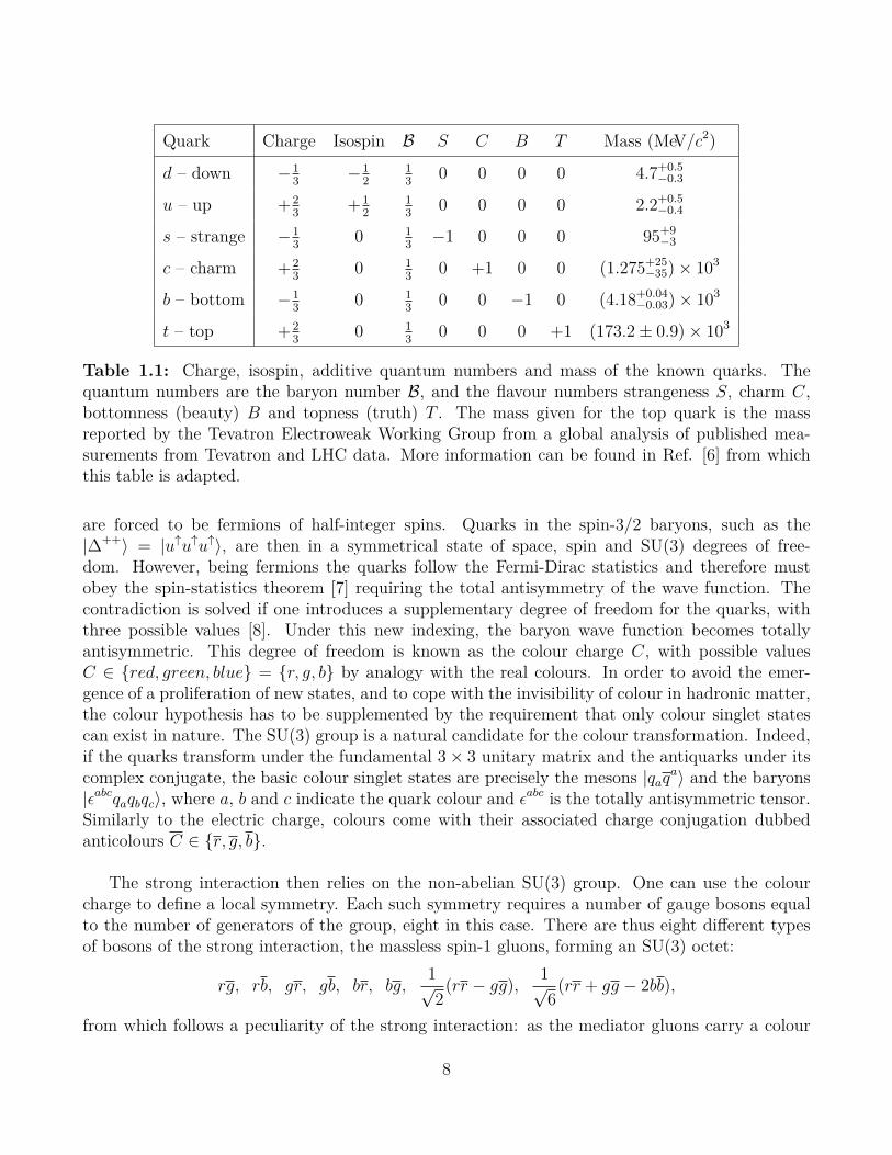
Quark Charge Isospin B S C B T Mass (MeV/c2)

d – down −13

−12

13

0 0 0 0 4.7+0.5−0.3

u – up +23

+12

13

0 0 0 0 2.2+0.5−0.4

s – strange −13

0 13−1 0 0 0 95+9

−3

c – charm +23

0 13

0 +1 0 0 (1.275+25−35)× 103

b – bottom −13

0 13

0 0 −1 0 (4.18+0.04−0.03)× 103

t – top +23

0 13

0 0 0 +1 (173.2± 0.9)× 103

Table 1.1: Charge, isospin, additive quantum numbers and mass of the known quarks. Thequantum numbers are the baryon number B, and the flavour numbers strangeness S, charm C,bottomness (beauty) B and topness (truth) T . The mass given for the top quark is the massreported by the Tevatron Electroweak Working Group from a global analysis of published mea-surements from Tevatron and LHC data. More information can be found in Ref. [6] from whichthis table is adapted.

are forced to be fermions of half-integer spins. Quarks in the spin-3/2 baryons, such as the|∆++〉 = |u↑u↑u↑〉, are then in a symmetrical state of space, spin and SU(3) degrees of free-dom. However, being fermions the quarks follow the Fermi-Dirac statistics and therefore mustobey the spin-statistics theorem [7] requiring the total antisymmetry of the wave function. Thecontradiction is solved if one introduces a supplementary degree of freedom for the quarks, withthree possible values [8]. Under this new indexing, the baryon wave function becomes totallyantisymmetric. This degree of freedom is known as the colour charge C, with possible valuesC ∈ red, green, blue = r, g, b by analogy with the real colours. In order to avoid the emer-gence of a proliferation of new states, and to cope with the invisibility of colour in hadronic matter,the colour hypothesis has to be supplemented by the requirement that only colour singlet statescan exist in nature. The SU(3) group is a natural candidate for the colour transformation. Indeed,if the quarks transform under the fundamental 3× 3 unitary matrix and the antiquarks under itscomplex conjugate, the basic colour singlet states are precisely the mesons |qaqa〉 and the baryons|εabcqaqbqc〉, where a, b and c indicate the quark colour and εabc is the totally antisymmetric tensor.Similarly to the electric charge, colours come with their associated charge conjugation dubbedanticolours C ∈ r, g, b.

The strong interaction then relies on the non-abelian SU(3) group. One can use the colourcharge to define a local symmetry. Each such symmetry requires a number of gauge bosons equalto the number of generators of the group, eight in this case. There are thus eight different typesof bosons of the strong interaction, the massless spin-1 gluons, forming an SU(3) octet:

rg, rb, gr, gb, br, bg,1√2(rr − gg), 1√

6(rr + gg − 2bb),

from which follows a peculiarity of the strong interaction: as the mediator gluons carry a colour

8

charge, they can self-interact. The symmetric single state 1√3(rr+bb+gg), corresponding the colour

(in fact colourless) singlet, does not exist. Indeed, a colour singlet gluon would be unconfined,behaving as a strongly interacting photon, thus giving the strong force an infinite range.

1.1.2 QCD LagrangianQuantum chromodynamics (QCD) is a non-abelian gauge theory based on a special unitary group(i.e. a Yang-Mills theory) [1, 9, 10] describing the interaction of coloured quarks and gluons.It forms the SU(3) components of the SU(3) ⊗ SU(2) ⊗ U(1) Standard Model [1]. Denotinga = (1, 2, 3) = (r, g, b) the quark colour indices and A = (1, ..., 8) the gluon colour indices, itsLagrangian reads1:

LQCD = ψa

(iγµ∂µδab −mδab − gsγµtAabAA

µ

)ψb −

1

4FAµνF

µνA , (1.2)

where repeated indices are summed over and δ is the Kroenecker delta. The fundamental param-eters of QCD are the quark masses m and the strong coupling gs, often expressed as αs = g2s/4π.

ψa and ψb are the quark-field spinors, dynamical functions of spacetime in the fundamentalrepresentation of the SU(3) gauge group. The γµ are the Dirac covariant matrices connecting thespinor representation to the vector representation of the Lorentz group:

γ0 =

1 0 0 00 1 0 00 0 −1 00 0 0 −1

, γ1 =

0 0 0 10 0 1 00 −1 0 0−1 0 0 0

,

γ2 =

0 0 0 −i0 0 i 00 i 0 0−i 0 0 0

, γ3 =

0 0 1 00 0 0 −1−1 0 0 00 1 0 0

.

The AAµ terms correspond to the eight gluon field. The tAab denote the fundamental representa-

tion of the SU(3) Lie algebra, the eight 3 × 3 matrices forming the generators of the group. Onehas:

tA =1

2λA, (1.3)

that is, a representation of the generators tA is given by the hermitian and traceless Gell-Mannmatrices λA:

λ1 =

0 1 01 0 00 0 0

, λ2 =

0 −i 0i 0 00 0 0

, λ3 =

1 0 00 −1 00 0 0

, λ4 =

0 0 10 0 01 0 0

,

1The Lagrangian given here is not fully complete, and so-called gauge-fixing terms and ghost fields must beintroduced in order to make the theory consistent. More details one this topic can be found in Ref. [9].

9

λ5 =

0 0 −i0 0 0i 0 0

, λ6 =

0 0 00 0 10 1 0

, λ7 =

0 0 00 0 −i0 i 0

, λ8 =1√3

1 0 00 1 00 0 −2

,

The field tensor FAµν is given by:

FAµν = ∂µAA

ν − ∂νAAµ −

αs

4πfABCAB

µACν , (1.4)

with the structure constants of the SU(3) group fABC following from the commutation relation ofthe SU(3) generators, yielding the algebra of the group:[

tA, tB]= ifABCt

C . (1.5)

The structure constant are antisymmetric in the exchange of two indices, the non-zero ones are:

f 312 = 1, (1.6)

f 714 = f 5

16 = f 624 = f 7

25 = f 534 = f 6

37 =1

2, (1.7)

f 845 = f 8

67 =1

2

√3. (1.8)

The last, non-abelian term on the right-hand side of Equation 1.4 makes a fundamental dynam-ical difference between QCD and quantum electrodynamics (QED) as it describes the gluon self-interaction, which eventually leads to the phenomenon called asymptotic freedom.

Useful colour-algebra relations include:

tAabtAbc = CF δac, CF ≡

N2C − 1

2NC

=4

3, (1.9)

fACDfBCD = CAδAB, Ca ≡ NC = 3, (1.10)

tAabtBab = TRδAB, TR =

1

2, (1.11)

which introduce the SU(3) group invariants CF and CA, the Casimir colour factors associated withthe gluon emission from a quark and a gluon, respectively, and TR the colour factor for a gluon tosplit into a qq pair.

Developing the QCD Lagrangian, and multiplying out the field tensor contraction FAµνF

A,µν ,one gets the elements of a QCD Feynman diagram:

• Quark propagator: a= ψa

(iγµ∂µ −mq

)ψa,

• Gluon propagator: A= (∂µAν

A − ∂νAµA)(∂µA

Aν − ∂νAA

µ ),

10

• Quark-gluon vertex: ab

A

= gsψaλAabψbγ

µAAµ ,

• 3-gluons vertex:A

BC = gs (∂

µAνA − ∂νAµ

A) fABCABµAC

ν ,

• 4-gluons vertex:D

CB

A= g2sfEABAµ

AAνBfECDAC

µADν .

1.1.3 Perturbative QCD and the asymptotic freedomIn field theories, the quantum corrections (loops) calculated in perturbation theory have ultravioletdivergences originating from the intermediate states with high momenta [9]. In renormalisable fieldtheories, such as QCD, these divergences can always be combined with the bare parameters of theLagrangian and are absorbed in the renormalised parameters. The renormalisation procedurerequires to introduce a mass scale µ (often denoted µR) at which the subtractions removing theultraviolet divergences are performed. The value of µ is arbitrary, and this parameter does notshow up in the QCD Lagrangian of Equation 1.2. A dimensionless observable R(Q2, xf ), where xfrepresents any dimensionless kinematic variables, must then be independent of the arbitrary valueof µ. This independence is given by the Callan-Symanzik relation for QCD [11, 12, 13]:

d

d ln(µ2)R(Q2/µ2, αs, xf ) = µ2 d

dµ2R(Q2/µ2, αs, xf ) (1.12)

=

(µ2 ∂

∂µ2 + µ2∂αs

∂µ2

∂

∂αs

)R(Q2/µ2, αs, xf ) (1.13)

= 0. (1.14)

If one defines:β(αs) = µ2∂αs

∂µ2 , t = ln

(Q2

µ2

), (1.15)

11

Equation 1.14 becomes (− ∂

∂t+ β(αs)

∂

∂αs

)= R

(et, αs, xf

)= 0. (1.16)

Expressing the observable as a perturbative series now in αs(Q2) defined by:

t =

∫ αs(Q2)

αs

dx

β(x), αs(µ

2) ≡ αs, (1.17)

one has:

R(et, αs, xf ) =

nmax∼π/αs∑n=0

rn(1, αs, xf )

(αs(µ

2)

π

)n

, (1.18)

which can be checked to be a solution of Equation 1.17. Setting et = 1, that is, setting the physicalscale Q equal to the renormalisation scale µ, makes the coefficients rn independent of Q2/µ2. Whenone takes µ close to the scale of the momentum transfer Q in a given process, then αs(µ

2 ' Q2)is indicative of the effective strength of the strong interaction for that process.

The coupling satisfies the renormalisation group equation:

Q2 ∂αs

∂Q2 = β(αs). (1.19)

In QCD, the β function has the perturbative expansion:

β(αs) = −(b0α2s + b1α

3s + b2α

4s +O(α5

s)), (1.20)

with b0, b1 and b2 being the 1-, 2- and 3-loop β-function coefficients:

b0 =11CA − 4nfTR

12π=

33− 2nf

12π,

b1 =17C2

A − nfTR(10CA + 6CF )

24π2 =153− 19nf

24π2 , (1.21)

b2 =2857− 5033

9nf +

32527n2f

128π3 ,

for the SU(3) values of CA and CF and with nf the number of active quarks (i.e. satisfyingmq µ). Starting from b2, the coefficients are renormalisation-scheme dependent and the for-mula given here is obtained in the widely-used modified minimal subtraction (MS) scheme [14].The minus sign in Equation 1.20 is the origin of the asymptotic freedom, i.e. the fact that thestrong coupling becomes weak for processes involving large momentum transfers (so-called hardprocesses). In the 100 GeV – 1 TeV range the coupling amounts to ∼ 0.1.

12

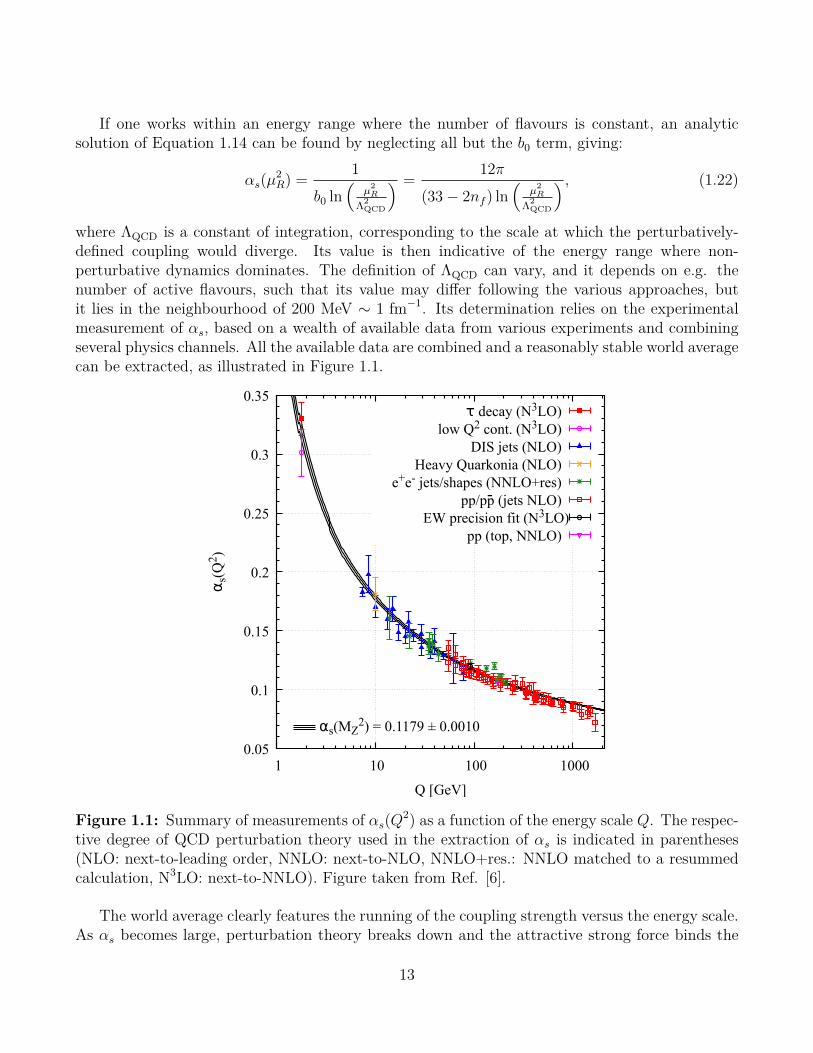
If one works within an energy range where the number of flavours is constant, an analyticsolution of Equation 1.14 can be found by neglecting all but the b0 term, giving:

αs(µ2R) =

1

b0 ln(

µ2R

Λ2QCD

) =12π

(33− 2nf ) ln(

µ2R

Λ2QCD

) , (1.22)

where ΛQCD is a constant of integration, corresponding to the scale at which the perturbatively-defined coupling would diverge. Its value is then indicative of the energy range where non-perturbative dynamics dominates. The definition of ΛQCD can vary, and it depends on e.g. thenumber of active flavours, such that its value may differ following the various approaches, butit lies in the neighbourhood of 200 MeV ∼ 1 fm−1. Its determination relies on the experimentalmeasurement of αs, based on a wealth of available data from various experiments and combiningseveral physics channels. All the available data are combined and a reasonably stable world averagecan be extracted, as illustrated in Figure 1.1.

αs(MZ2) = 0.1179 ± 0.0010

αs(

Q2 )

Q [GeV]

τ decay (N3LO)low Q2 cont. (N3LO)

DIS jets (NLO)Heavy Quarkonia (NLO)

e+e- jets/shapes (NNLO+res)pp/p-p (jets NLO)

EW precision fit (N3LO)pp (top, NNLO)

0.05

0.1

0.15

0.2

0.25

0.3

0.35

1 10 100 1000

Figure 1.1: Summary of measurements of αs(Q2) as a function of the energy scale Q. The respec-

tive degree of QCD perturbation theory used in the extraction of αs is indicated in parentheses(NLO: next-to-leading order, NNLO: next-to-NLO, NNLO+res.: NNLO matched to a resummedcalculation, N3LO: next-to-NNLO). Figure taken from Ref. [6].

The world average clearly features the running of the coupling strength versus the energy scale.As αs becomes large, perturbation theory breaks down and the attractive strong force binds the

13

quarks and gluons into confined and colourless states, whence the name of confinement for thelow-Q regime. On the contrary, for large energy scales the coupling becomes weaker, yielding theasymptotic freedom. For very large energies the weakening is so important that quarks and gluonsare not bounded anymore and start to move freely. These various regimes are at the origin of thephases of nuclear matter, which are discussed in Section 1.1.5.

1.1.4 Chiral symmetry breakingIn the Standard Model, the mass of quarks is generated via Yukawa coupling to the Higgs field.As they are the constituents of the hadrons, one would expect that in the ground state, the hadronmass should correspond to the one of its valence quarks. However, taking as an example the protonp = |uud〉 with mp ∼ 938 MeV/c2, one sees that the sum of the masses of two up quarks and onedown is far from amounting to mp: 2mu +md ∼ 9.1 MeV/c2, the mass of the valence quarks onlyaccount for about 1% of the proton mass. As it is shown below, this difference is explained bythe chiral symmetry breaking in QCD. Chirality indicates the lack of identity of a phenomenonto its mirror image. In particle physics, the so-called handedness is defined from the spin of theparticle through the helicity, the projection of the spin along the direction of motion. A particle isright-handed if the helicity points towards the direction of motion, left-handed otherwise. Helicityallows one to define the parity as the symmetry transformation between right- and left-handedparticles. Chiral symmetry is then the invariance under parity.

Considering the QCD Lagrangian of Equation 1.2, for the first two flavours, one gets:

L =∑q=u,d

ψq,a(iγµ∂µδab −mδab − gsγµtAabAA

µ )ψq,b −1

4FAµνF

µνA

= q(iγµDµ −Mδab

)q − 1

4FAµνF

µνA , (1.23)

where we introduced a notation for the gauge covariant derivative Dµ and a matrix notation forthe quark field q and the mass M as:

Dµ = ∂µδab − igstAabAAµ , q =

(ud

), M =

(mu 00 md

). (1.24)

Assuming that mu −md is much less than the hadronic mass scale, one can approximate M as amultiple of the unit matrix. This Lagrangian is then invariant under the chiral transformation:

q → exp

(3∑

i=0

αiσi

)q,

where σ0 is the unit matrix and σi, i = (1, 2, 3) are the Pauli matrices. This U(2)V symmetry (Vstanding for vector) can be decomposed into the product U(1)V ⊗ SU(2)V . The U(1)V symmetrycorresponds to the quark number symmetry, while SU(2)V is the isospin symmetry that emergeswhen considering the u and d quarks to be degenerated in mass. Note here that as the gluon fieldsare not affected by chiral transformation the gluon degrees of freedom can be neglected throughoutthis discussion [15].

14

One can furthermore take the massless limit where mu and md are negligible, and hence M ≡ 0.Considering the left- and right-handed projectors:

γL =1

2(1− γ5) , γR =

1

2(1 + γ5) , with γ5 ≡ iγ0γ1γ2γ3, (1.25)

satisfying the relations γ2L = γL, γ2R = γR and γLγR = 0, one can decompose the quark fields intoleft- and right-handed components:

qL = γLq, qR = γRq. (1.26)

The quark sector of the Lagrangian of Equation 1.23 then becomes:

L = qLiγµDµqL + qRγ

µDµqR. (1.27)

As no term connects the left- and right-handed fields, independent left and right rotations arepermitted, yielding a U(2)L ⊗ U(2)R symmetry:

qL → exp

(3∑

i=0

αiσi

)qL, qR → exp

(3∑

i=0

βiσi

)qR,

and constitutes a chiral symmetry as it acts separately on left- and right-handed fields (in this casea chiral SU(2)). According to Noether’s theorem [16], each of these symmetries has an associatedconserved current:

Liµ = qγµγLσ

iq, (1.28)Ri

µ = qγµγRσiq. (1.29)

If chiral symmetry was exact, the QCD spectrum would show that every hadron comes with apartner of same mass and opposite parity, which is not observed. Chiral symmetry is explicitelybroken by the non-zero masses of the quarks. Looking e.g. at the triplets ρ(770) and a1(1260),which are chiral partners, one sees by their masses mρ(770) ∼ 755 MeV/c2 and ma1(1260)

∼ 1230

MeV/c2 that the chiral symmetry is in fact strongly broken. This indicates that the masses ofthe u and d quarks are not as small as their current mass in the QCD vacuum2. Due to thestrong coupling between quarks, the QCD vacuum is non-vanishing, it is defined by the chiralcondensation [17]:

〈qq〉 = 〈0|qLqR + qRqL|0〉 6= 0. (1.30)

Equation 1.30 denotes the chiral spontaneous symmetry breaking in the QCD vacuum, and de-scribes the flip of chirality as for example a right-handed particle annihililates via qR, leaving qLto create a left-handed particle of same momentum. The chiral condensation 〈qq〉 explains the

2Defining the mass of the quarks is an arduous topic which comes with a lot of caveats. For the light quarks u,d and s, the so-called current mass is the one acquired through the Higgs mechanism. An extensive discussion canbe found in Ref. [6] ("Quark Masses") and references herein.

15

energy gap between the physics and QCD vacua, which generates an additional constituent massfor the quarks, even at vanishing current masses [18]:

M(p2)large−p2=

2

3π2γm

−〈qq〉(12ln p

2

Λ2QCD

)1−γm , (1.31)

where p is the quark momentum in the propagator and γm = 12/(33 − 2nf ) = π/b0. This canbe extended by also neglecting the s quark mass, yielding a chiral SU(3) symmetry spontaneouslybroken to SU(3)V , with eight pseudoscalar Goldstone bosons corresponding to the flavour SU(3)octet: π0, π±, K0, K0, K± and η. The fact that they constitute the lightest hadrons allows oneto apply chiral SU(3) perturbation theory for the three lightest quarks [19] while other techniquesare needed for the heavy quarks [10].

Figure 1.2 shows the constituent mass as a function of the squared momentum for severalflavours. One can see that about 99% of the u and d mass are generated by the chiral spontaneoussymmetry breaking, and that chiral symmetry is restored at very large momentum transfer. Asthe visible matter in the Universe is constituted by the nucleons (the proton |uud〉 and neutron|udd〉), almost all the mass of the visible Universe comes from the chiral spontaneous symmetrybreaking mechanism.

Figure 1.2: Constituent quark masses as a function of the squared momentum for the u/d, s, cand b quarks. Figure taken from Ref. [20], adapted from Ref. [21].

1.1.5 QCD phase diagramAs established above, the peculiarities of QCD lead to the existence of several phases for mattermade of quarks and gluons. At low energy, quarks and gluons are confined into colourless bound

16

states, while at high energy QCD indicates that the strongly interacting matter undergoes a phasetransition to a state where quarks and gluons are not confined anymore, the Quark-Gluon Plasma(QGP). Similarly to the standard matter, the phases of the QCD matter can be depicted andstudied through a phase diagram. A common choice is the (µB, T ) space to do so, where T is thetemperature and µB is the baryon-chemical potential. In QCD, a |qqq〉 baryon is always created orannihilated pairwise with an antibaryon |qqq〉. Said otherwise, one can define a conserved quantity,the so-called baryon number B presented in Section 1.1.1, as:

B = NB −NB, (1.32)

where NB and NB are the numbers of baryons and antibaryons respectively. For systems in whichthe baryon number is allowed to vary, the most convenient thermodynamic potential to consideris the grand potential:

Ω(T, V, µ) = E − TS − µBB. (1.33)

Reaching the thermodynamic equilibrium requires the minimisation of Ω, and for a system atequilibrium one recognises µB as the increase in E when B increases by one. When systemsare analysed using the grand canonical ensemble of statistical physics, µB is kept as a controlparameter, and the baryon density nB = B/V is a derived quantity whose value depends on thedetails of the equation of state nB = nB(T, µB). A schematic view of the QCD phase diagram inthe (µB, T ) plane is given in Figure 1.3. It must be stressed that the current knowledge of theQCD phase diagram is mostly conjectural, and as such it must be considered with care.

The QCD vacuum in which we live, having the hadrons as its excitations, lies at the bottomleft of the diagram. As established in Section 1.1.4, this region features a strong breaking of thechiral symmetry, providing the hadrons with most of their mass. The phase coined "nuclear matter"corresponds to the nuclei that we observe under Earth-like thermodynamical conditions. One of thefirst successful model at describing the baryons is the bag model developed at the MassachusettsInstitute of Technology (MIT) in 1974 [22, 23, 24]. This model visualises the hadron as a bag ofradius R in which the quarks evolve freely. In its simplest form, the quarks are massless, that isto say ultra-relativistic. The boundary condition at the surface is chosen to prevent the colourflux to leave the confining region. In the fundamental state, the size of the bag is such that thepressure applied by the quarks on the surface is equilibrated by the confinement pressure due tothe QCD vacuum, pointing inwards and counter-acting the kinetic energy of the inner quarks.The vacuum pressure is the bag constant, usually denoted B. The model has been successful inobtaining some properties of the nucleons, such as the radii and magnetic moments. In order tofit the data, however, the bag has to have a radius R ∼ 1 fm, which leaves little room for pionsand other mesons. The model was then extended into the chiral bag model [25, 26] in which pionsare coupled to the surface of the bag.

Ordinary nuclear matter is a mixed phase, consisting of droplets (the nuclei) surrounded by thevacuum. The transition between vacuum and nuclear matter is expected to take place at low T ,for µB ∼ 300 MeV. Moving along the horizontal axis of the diagram, and augmenting the baryonpotential while staying at low temperature, one moves towards matter of higher and higher densitywhich starts to correspond to the expected state inside a neutron star. At even higher densities,

17

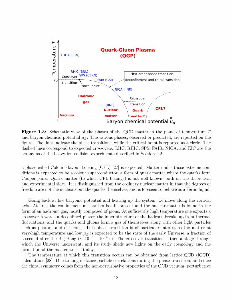
Nuclear

matter

Tem

pera

ture

T

Baryon chemical potential μB

Quark-Gluon Plasma(QGP)

Vacuum

Hadronic

gas

Quark

matter?

LHC (CERN)

RHIC (BNL)

NICA (JINR)

FAIR (GSI)

CFL?

0

EIC (BNL)

TcCrossover

transition

Crossover

transition

First-order phase transition,

deconfinment and chiral transition

Critical point

SPS (CERN)

Figure 1.3: Schematic view of the phases of the QCD matter in the plane of temperature Tand baryon-chemical potential µB. The various phases, observed or predicted, are reported on thefigure. The lines indicate the phase transitions, while the critical point is reported as a circle. Thedashed lines correspond to expected crossovers. LHC, RHIC, SPS, FAIR, NICA, and EIC are theacronyms of the heavy-ion collision experiments described in Section 2.2.

a phase called Colour-Flavour-Locking (CFL) [27] is expected. Matter under those extreme con-ditions is expected to be a colour superconductor, a form of quark matter where the quarks formCooper pairs. Quark matter (to which CFL belongs) is not well known, both on the theoreticaland experimental sides. It is distinguished from the ordinary nuclear matter in that the degrees offreedom are not the nucleons but the quarks themselves, and is foreseen to behave as a Fermi liquid.

Going back at low baryonic potential and heating up the system, we move along the verticalaxis. At first, the confinement mechanism is still present and the nuclear matter is found in theform of an hadronic gas, mostly composed of pions. At sufficiently high temperature one expects acrossover towards a deconfined phase: the inner structure of the hadrons breaks up from thermalfluctuations, and the quarks and gluons form a gas of themselves along with other light particlessuch as photons and electrons. This phase transition is of particular interest as the matter atvery-high temperature and low µB is expected to be the state of the early Universe, a fraction ofa second after the Big-Bang (∼ 10−5 − 10−4 s). The crossover transition is then a stage throughwhich the Universe underwent, and its study sheds new lights on the early cosmology and theformation of the matter we see today.

The temperature at which this transition occurs can be obtained from lattice QCD (lQCD)calculations [28]. Due to long distance particle correlations during the phase transition, and sincethe chiral symmetry comes from the non-perturbative properties of the QCD vacuum, perturbative

18

QCD (pQCD) cannot be applied in the study of the phase transition. In order to solve QCD fromfirst principles in the non-perturbative regime, one can introduce the QCD Lagrangian onto adiscrete, Euclidean space-time lattice. The lattice is a mesh in which quarks are located on thevertices, while gluons travel along the lines between them. This framework allows for applyingthe Feynman path integral technique to deal with the propagators, while the temperature of thesystem is treated by statistical physics. Varying the size of the lattice space, one can extrapolateto the infinitesimal case, i.e. the continuum limit. lQCD is a rapidly-growing field of theoreticalphysics, mostly challenged by computing power and bandwidth issues as realistic calculationsrequire a sizeable amount of numerical integrations. Nonetheless, several predictions have alreadybeen obtained under this framework for what concerns the QCD transition at high temperatureand low baryonic potential. One of the most recent evaluation of the critical temperature Tc atwhich the transition occurs is shown in Figure 1.4. The extrapolation from several values of thelattice volume Nτ up to the continuum limit yields a critical temperature at Tc = (156.5 ± 1.5)MeV [29]. A recent review of the lQCD results concerning the exploration of the phase diagramcan be found in Ref. [30].

Figure 1.4: Left: pseudo-critical temperature Tc(0) as a function of the lattice volume Nτ usingseveral parametrisation of the chiral order parameter CΣ, the disconnected chiral susceptibilityCχ and the susceptibility of the chiral order parameter χΣ. The solid grey band depicts thecontinuum extrapolated value. Right: phase boundary of 2 + 1 flavour QCD compared withthe line of constant energy density ε = (0.42 ± 0.06) GeV/fm3 and the line of constant entropys = (3.7 ± 0.5) fm−3 in the T − µB plane. It is also compared with the chemical freeze-outparameters extracted from grand canonical ensemble based fits to hadron yields within 0–10%centrality class from ALICE and 0–5% centrality class from STAR. Figures taken from Ref. [29]where more details can be found.

At the top of the diagram, at high temperature, one finds the Quark-Gluon Plasma (QGP)phase [31], a state of matter in which the elementary particles constituting the hadrons of baryonicmatter are released from their strong attraction towards one another due to the extremely highenergy density. Initially expected to be a gas of almost-free quarks and gluons, it was found tobe a strongly interacting liquid. The study of the QGP is of relevance for cosmology, as it helps

19

pinpointing the conditions underwent by the Universe shortly after the Big Bang. In this regard,a sizeable amount of resources is dedicated to QGP studies, which can be done with a colliderof sufficiently high energy such that the necessary thermodynamical conditions for a QGP to becreated are met. Reference [32] provides a recent overview of the phenomenology of the QGP.

1.2 Structure of nuclei

1.2.1 The parton modelThe parton model was originally proposed by Richard Feynman in 1969 as a way to analyse high-energy hadronic collisions [33, 34]. It was immediately applied to deep inelastic scattering (DIS)of electrons on protons by Bjorken and Paschos [35]. Later on, after the development of QCDand its experimental confirmation through the observation of the Bjorken scaling and asymptoticfreedom, partons came to be matched with the quarks and gluons constituting the hadrons.

The most convenient way to experimentally study the inner structure of hadrons is by DIS. Inthis process, illustrated in Figure 1.5, a lepton ` of very-high energy scatters off a hadron h whichbreaks apart and fragment into a final state X containing many particles of large invariant massmx mh. In the perturbative approximation, the interaction occurs by means of the exchange ofa virtual photon γ∗ emitted by the lepton and absorbed by the target hadron, transferring energyto one of its constituent quark. Historically, the process provided the first convincing evidence ofthe reality of quarks, which until that point were considered as a purely mathematical object. Inthe Target Rest Frame (TRF), the four-momentum transfer from the lepton to the hadron is:

qTRF= (E − E ′)(k − k′), (1.34)

where E (E ′) and k (k′) are respectively the energy and the three-momenta of the lepton ` (`′),and its square is given in terms of the initial- and final-state lepton energies and the scatteringangle θ of the final-state lepton `′ by:

Q2 = −q2 TRF= 2EE ′(1− cos θ). (1.35)

One can introduce the Lorentz-invariant Bjorken variables x and y:

x =Q2

2P · qTRF=

Q2

2M(E − E ′), y =

P · qP · k

TRF= 1− E ′

E, (1.36)

where P TRF= (M, 0, 0, 0) is the four-momentum of the hadron. The x variable, commonly known as

Bjorken-x, represents the fraction of the total momentum of the nucleon carried by a given parton,while the elasticity y denotes the fraction of energy lost by the lepton in the process, defining theso-called elasticity of the event. With these, the unpolarised double-differential cross section ofthe DIS process reads:

d2σ

dQ2dx=

4πα2em

Q4

y2

2Q2Lµν(k, k′)W µν(P, q), (1.37)

20

hX

p

` `′k k′

γ∗

Figure 1.5: Feynman diagram for the deep inelastic lepton-hadron scattering.

where αem = e2/4π is the electromagnetic fine-structure constant and Lµν and W µν are the leptonicand hadronic tensors, respectively. For a neutral-current electromagnetic scattering, the leptonictensor reads:

Lµν(k, k′) = 2(kµk

′ν + k′µkν − k · k′gµν), (1.38)

and the hadronic tensor can be obtained from the conservation of current as [36]:

W µν(P, q) = −(gµν − qµqν

q2

)F1(x,Q

2) +1

P · q

(P µ − P · q

q2qµ)(

P ν − P · qq2

qν)F2(x,Q

2),

(1.39)where F1 and F2 are the structure functions of the hadron. In these terms, the cross section canbe written as:

dσ

dQ2dx=

4πα2em

Q4

1

x

[xy2F1(x,Q

2) +

(1− y − x2y2M

2

Q2

)F2(x,Q

2)

]. (1.40)

One can go further by considering the infinite-momentum frame (IMF) (the Breit frame), inwhich the hadron moves at high velocity, and assuming Q2 M2 one gets:

PIMF=

(Q

2x, 0, 0,

Q

2x

), q

IMF= (0, 0, 0,−Q). (1.41)

That is to say, the hadron is highly boosted, and the interaction times between partons are dilated.One can then consider these interactions to be frozen over the timescale in which the interactionwith the lepton takes place, and the lepton can scatter incoherently from the individual partons.The parton involved in the interaction can then be considered to be effectively free. In this originalversion of the parton model, the high-energy hadron can be seen as a collection of point-likeconstituents moving colinearly. One can thus define

fi(ξ) = the probability density of finding a parton i within the hadroncarrying a fraction ξ of the hadron momentum.

The function fi(ξ) is the parton distribution function (PDF).

21

The photon couples only to electrically charged particles, the Leading Order (LO) of thehadronic tensor reads:

W µν =∑i=q,q

∫dξ

ξfi(ξ)W

µνi (p, q) +O

(1

Q2

), (1.42)

where p = ξPIMF= (ξQ/2x, 0, 0, ξQ/2x) and W µν

i denotes a so-called partonic tensor. At theperturbative scales Q2 M2 the higher orders can be neglected. In this LO approximation,called the Born approximation, the quark-initiated partonic tensor is:

W µνq,Born(p, q) =

x

2Q2

e2q2Tr [γµpγνγνnγµ] δ(ξ − x), (1.43)

where eq is the quark fractional charge, δ is the Dirac-delta function and:

n = q + xPIMF= (Q/2, 0, 0,−Q/2), n2 = 0. (1.44)

The delta function in Equation 1.43 arises from integrating over the final-state quark momentump′ and shows that, to LO perturbative accuracy, the Bjorken-x measures the momentum fractionof the parton. Using Equations 1.42 and 1.43, one rewrites the cross section as:(

dσ

dQ2dx

)LO

=∑q,q

e2qfq(x)

(dσ

dQ2dx

)Born

,

(dσ

dQ2dx

)Born

=4πα2

em

Q4

[y2

2+

(1− y − x2y2M

2

Q2

)].

(1.45)If expressed in terms of the structure functions, one has:

2xF1(x) = F2(x) = x∑q,q

e2qfq(x). (1.46)

The relation F2 = 2xF1 is known as the Callan-Gross relation [37]. Notably, it defines the F2(x)structure function as the charge-weighted sum of the parton densities xfq(x). Equation 1.46 showsthat, in the naive parton model, the structure functions depend only on x and not on the scale, aphenomenon referred to as the Bjorken scaling.

1.2.2 QCD-improved parton modelIn the naive parton model, gluons show up as missing momentum, but they are not treated asdynamical quantities. Incorporating the effects of gluon radiation by quarks leads to the definitionof the QCD-improved parton model. The diagram of such a radiation is shown in Figure 1.6. Herea quark that carries a fraction y of the proton momentum radiates a gluon with a fraction (1− z)of its momentum. After the radiation, the quark, carrying a momentum fraction yz, scatters offthe virtual photon. The momentum fraction seen by the photon is thus x = yz which impliesz = x/y.

22

hp

yP(1− z)yPzyP ≡ xP

γ∗

Q2

Pqq(z)

Figure 1.6: Feynman diagram for the deep inelastic lepton-hadron scattering, preceded by agluon radiation.

Taking the gluon radiation into account, the F2 structure function is found to be:F2(x,Q

2)

x=∑i

e2i

∫ 1

x

dy

yfi(y)

[δ

(1− x

y

)+αs

2πPqq

(x

y

)lnQ2

m2

], (1.47)

where m2 is a lower transverse momentum cut-off to regularise the divergence when the gluon iscollinear with the quark, and Pqq is the splitting function given by:

Pqq =4

3

(1 + z2

1− z

). (1.48)

The splitting function represents the probability for the parent quark to emit a gluon with thedaughter quark retaining a fraction z of the parent momentum. An infrared divergence shows upwhen (1 − z) → 0 where the gluon becomes so soft that the parent and daughter quarks cannotbe resolved anymore. In order to simplify the notation, one can set:

Iqq(x) =αs

2π

∫ 1

x

dy

yf(y)Pqq

(x

y

), (1.49)

and get:

F2(x,Q2)

x=∑i

e2i

fi(x) + Iqq(x) lnµ2

m2︸︷︷︸fi(x,µ

2)

+Iqq(x) lnQ2

µ2

︸︷︷︸

fi(x,Q2)

. (1.50)

Here are defined the renormalised quark distribution fi(x, µ2) at the factorisation scale µ where areseparated the singular factor, which depends on m but not on Q2, from the calculable factor whichdepends on Q2 but not on m. Substituting the renormalised distribution for the bare distributionin Iqq one obtains:

fi(x,Q2) = fi(x, µ

2) +αs

2π

∫ 1

x

dy

yfi(y, µ

2)Pqq

(x

y

)lnQ2

µ2 +O(α2s). (1.51)

23

The expression of F2 up to O(α2s) then becomes:

F2(x,Q2)

x=∑i

e2i

[fi(x, µ

2) +αs

2π

∫ 1

x

dy

yfi(y, µ

2)Pqq

(x

y

)lnQ2

µ2

]. (1.52)

The structure function F2 should not depend on the choice of the factorisation scale, whichleads to the renormalisation group equation:

1

2e2x

∂F2(x,Q2)

∂ lnµ2 =∂f(x, µ2)

∂ lnµ2 +αs

2π

∫ 1

x

dy

y

[∂f(y, µ2)

∂ lnµ2 ln

(Q2

µ2

)− f(y, µ2)

]Pqq

(x

y

)(1.53)

= 0. (1.54)

One sees from this equation that the term (∂f/∂ lnµ2) is of the order αs, then the first term inthe above integral is of the order of α2

s. Neglecting this term, one obtains the evolution equationfor the quark:

∂f(x, µ2)

∂ lnµ2 =αs

2π

∫ 1

x

dy

yf(y, µ2)Pqq

(x

y

)+O(α2

s), (1.55)

which is known as the Dokshitzer-Gribov-Lipatov-Altarelli-Parisi (DGLAP) equation [38, 39, 40].It can be numerically solved once f(x, µ2

0) is given as an input at some starting scale µ20.

Introducing the gluon distribution requires to consider all the splitting graphs, each yielding asplitting function:

Pqq :

z

Pqg :

z

Pgq :

z

Pgg :

z

In the Pqg and Pgq cases, no singularity develops since the daughter and parent can always bedistinguished. For the two other graphs a singularity develops in the soft limit (1− z) → 0. The

24

leading order splitting functions read:

P (0)qq (z) =

4

3

[1 + z2

(1− z)++

3

2δ(1− z)

],

P (0)qg (z) =

1

2

[z2 + (1− z)2

], (1.56)

P (0)gq (z) =

4

3

[1 + (1− z)2

z

],

P (0)gg (z) = 6

[z

(1− z)++

1− zz

+ z(1− z) +(11

12−nf

18

)δ(1− z)

].

The singularities showing up in Pqq and Pgg in the soft limit are regulated by the so-called "plus"prescription, denoted by the subscript + and defined as:

[f(x)]+ = f(x)− δ(1− x)∫ 1

0

f(z)dz, (1.57)

or equivalently: ∫ 1

x

f(z) [g(z)]+ dz =

∫ 1

x

[f(z)− f(1)] g(z)dz − f(1)∫ x

0

g(z)dz. (1.58)

The prescription guarantees that the integral from x to 1 of the splitting function multiplied bythe parton density function exists, provided that the PDF goes to zero as x goes to 1. The qq, qg,gq and gg transitions lead to a set of 2nf +1 coupled evolution equations that can be written as:

∂fi(x, µ2)

∂ lnµ2 =

nf∑j=−nf

αs

2π

∫ 1

x

dy

yPij

(x

y

)fj(y, µ

2), (1.59)

where Pij(z) is the splitting function for a daughter i with momentum fraction z of a parent j.The indexing denotes:

i, j =

−nf , ...,−1 antiquarks

0 gluon

1, ..., nf quarks

The expressions for the evolution equations can be simplified by writing the so-called Mellin con-volution in short-hand notation as:

P ⊗ f ≡∫ 1

x

dy

yP

(x

y

)f(y, µ2), (1.60)

allowing to rewrite the set of coupled equations as:

∂fi

∂ lnµ2 =

nf∑j=−nf

αs

2πPij ⊗ fj. (1.61)

25

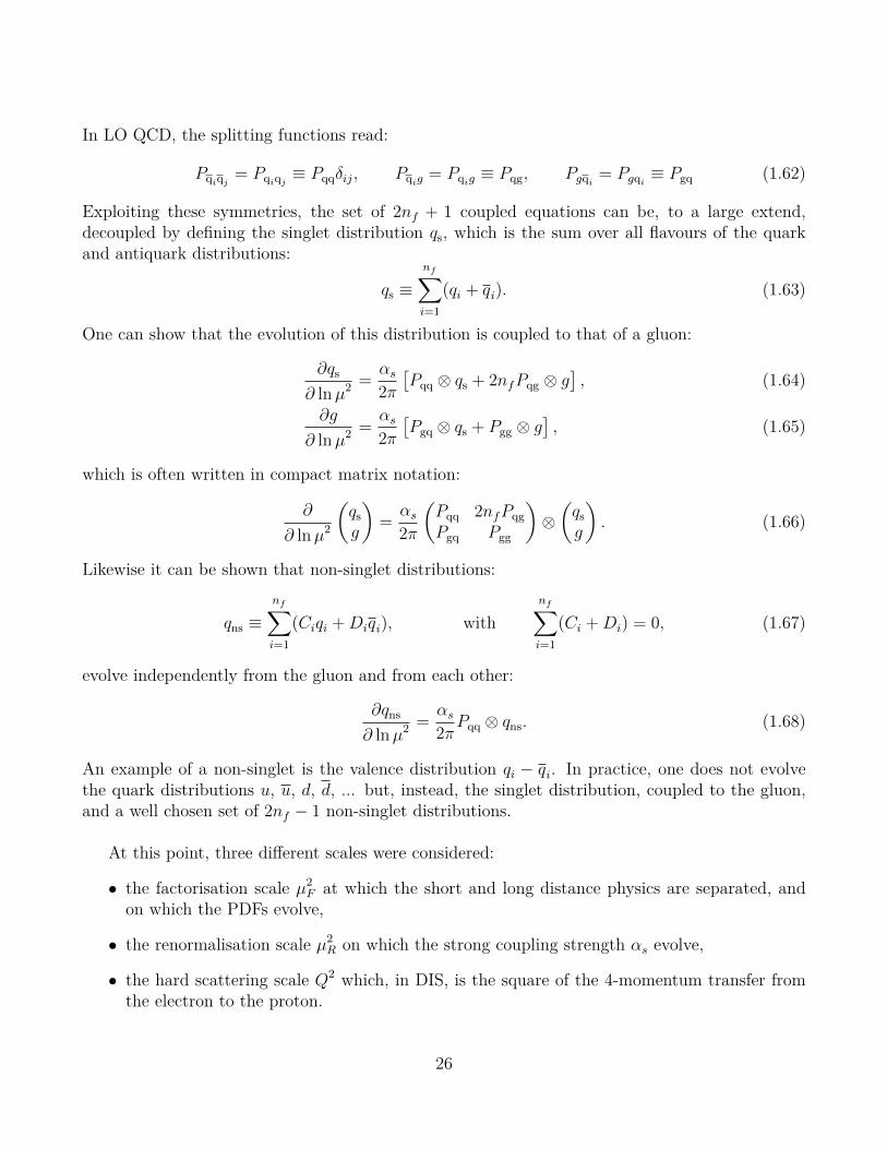
In LO QCD, the splitting functions read:

Pqiqj= Pqiqj

≡ Pqqδij, Pqig= Pqig

≡ Pqg, Pgqi= Pgqi

≡ Pgq (1.62)

Exploiting these symmetries, the set of 2nf + 1 coupled equations can be, to a large extend,decoupled by defining the singlet distribution qs, which is the sum over all flavours of the quarkand antiquark distributions:

qs ≡nf∑i=1

(qi + qi). (1.63)

One can show that the evolution of this distribution is coupled to that of a gluon:

∂qs

∂ lnµ2 =αs

2π

[Pqq ⊗ qs + 2nfPqg ⊗ g

], (1.64)

∂g

∂ lnµ2 =αs

2π

[Pgq ⊗ qs + Pgg ⊗ g

], (1.65)

which is often written in compact matrix notation:

∂

∂ lnµ2

(qsg

)=αs

2π

(Pqq 2nfPqg

Pgq Pgg

)⊗(qsg

). (1.66)

Likewise it can be shown that non-singlet distributions:

qns ≡nf∑i=1

(Ciqi +Diqi), with

nf∑i=1

(Ci +Di) = 0, (1.67)

evolve independently from the gluon and from each other:

∂qns

∂ lnµ2 =αs

2πPqq ⊗ qns. (1.68)

An example of a non-singlet is the valence distribution qi − qi. In practice, one does not evolvethe quark distributions u, u, d, d, ... but, instead, the singlet distribution, coupled to the gluon,and a well chosen set of 2nf − 1 non-singlet distributions.

At this point, three different scales were considered:

• the factorisation scale µ2F at which the short and long distance physics are separated, and

on which the PDFs evolve,

• the renormalisation scale µ2R on which the strong coupling strength αs evolve,

• the hard scattering scale Q2 which, in DIS, is the square of the 4-momentum transfer fromthe electron to the proton.

26

Exposing the different scales, one can write the (non-singlet) evolution equation and the expressionfor F2 at LO as:

∂qns(x, µ2F )

∂ lnµ2F

=αs(µ

2R)

2π

∫ 1

x

dy

yPqq

(x

y

)qns(y, µ

2F ), (1.69)

F2(x,Q2) =

nf∑i=1

e2ix[qi(x, µ

2F ) + qi(x, µ

2F )]+O(αs). (1.70)

Usually, one sets µ2F = µ2

R = Q2. This choice yields a theoretical uncertainty on the predictions,which is evaluated by varying the scales within a certain range. A typical choice for the variationsis

1

4µ2F ≤ µ2

R ≤ 4µ2F and

1

4Q2 ≤ µ2

F ≤ 4Q2. (1.71)

One should note, however, that F2(x,Q2) in Equation 1.70 depends only on µ2

F which, for a givenQ2, is arbitrary. It follows that the LO perturbative stability is poor, and that LO pQCD haslimited predictive power. This issue is remedied when higher order terms are included, as theyare functions of both Q2 and µ2

F . The scale dependence rapidly decreases as higher orders ofcorrections are added, driving a significant effort towards the evaluation of the splitting functions,and currently the knowledge of F2 goes up to NNLO.

1.2.3 The PDF frameworkThe factorisation theorem can be applied to a wide class of processes in order to separate theminto a universal long distance piece (which is non-perturbative, but process independent) and ashort distance piece that is calculable in pQCD. For the hadroproduction of a generic final stateX in unpolarised pp collisions, the corresponding factorised expression reads [41]:

σpp→X(s, µ2F , µ

2R) =

∑i,j

∫dx1, dx2fi(x1, µ

2F , µ

2R)fj(x2, µ

2F , µ

2R)σij→X(x1, x2, s;µ

2F , µ

2R), (1.72)

The unpolarised hard cross section σab→X can be calculated perturbatively as an expansion in theQCD and electroweak running couplings. A common procedure is to set the factorisation (µF ) andrenormalisation (µR) scales equal to the energy scale of the process: µF = µR ≡ µ = Q. The PDFsfi and fj are process-independent, but they are not perturbative. They can, however, be estimatedfrom measurements, and extrapolated to the necessary scales with the DGLAP equations. It isconvenient to define the valence and sea distributions by

uV = u− u, dV = v − v, sV = s− s = 0, ...

uS = 2u, dS = 2d, sS = 2s, ...

so that qi+qi = qi,V+qi,S for all flavours i. As the quantum numbers of the proton must be carriedby the surplus of quarks over antiquarks, one gets the counting rules:∫ 1

0

uV(x)dx = 2,

∫ 1

0

dV(x)dx = 1

∫ 1

0

sV(x)dx = 0, (1.73)

27

the latter holding also for c, b and t quarks. The momentum distributions xfi(x)dx give theprobability that a quark carries a momentum fraction between x and x + dx. Summing over allthe quark flavours in experimental data, leads to a deficit in the total probability, which is solvedby introducing a gluon momentum distribution xg(x). Then:

∑i

∫ 1

0

xfi(x)dx+

∫ 1

0

xg(x)dx = 1. (1.74)

The universality of the PDF is ensured by the isospin symmetry, which states that the u (anti)quarkdistribution in the proton is equal to the d (anti)quark distribution in the neutron, and vice versa.All these physics requirements are used as constraints during the PDF determination.

The PDFs are determined from a global QCD analysis (see Refs. [42, 43] for recent reviews, andreferences herein) of data from both colliders and fixed-target experiments. Various collaborationsand working groups provide PDFs and their associated error sets, as well as regular updatesfollowing from theoretical developments or the availability of new data. Several hundreds of PDFsets are now available, among which some of the most recent are ABMP163 [44], CT184 [46],JAM195 [47], MSHT206 [48] and NNPDF3.17 [49] (the given references correspond to the laststandard release of the sets, note that the names can greatly vary between versions, especially whenit is based on the authors’ names). The PDF determination usually relies on a parametrisationat an arbitrary input scale Q0, typically around 1 GeV, from which the PDF is derived at anyrelevant scale by means of DGLAP evolution. In the process, the parameters at Q0 are optimisedto fit the variety of experimental data that are used. The contribution of heavy-quark flavours ispower-suppressed at scales below their threshold production, with most models going up to fiveactive flavours.

A typical parametrisation for each flavour or flavour combination is of the form:

f(x,Q0, ai) = xa1(1− x)a2C(x, ai), (1.75)

with different parameters ai for each flavour. The a1 and a2 coefficients control the asymptoticbehaviour of f(x,Q0, ai) in the limits x → 0 and 1. For example, the (1 − x)a2 term, witha2 > 0, ensures that the PDFs vanish in the elastic limit x → 1. The C(x) function, called theinterpolating function, affects the behaviour of the PDFs outside of the asymptotic limits, and canbe parametrised in several way. A typical choice is to take a basic polynomial:

C(x) = 1 + a2y(x) + a3[y(x)]2 + ..., (1.76)

3Alekhin–Blümlein–Moch–Placakyte, the authors.4CT: CTEQ-TEA. CTEQ stands for Coordinated Theoretical-Experimental Project on QCD [45], a regroupment

of theoreticians and experimentalists around QCD-centered research projects and collaborative works. TEA refersto the Tung Et Al. group which takes care of the determination and update of the CTEQ PDF sets, with the lateWu-Ki Tung as co-founder of CTEQ and former group leader.

5JLab Angular Momentum, the name of the collaboration, based at the Jefferson Laboratory.6Martin–Stirling–Harland-Lang–Thorne, the authors.7Neural-Network PDF, from the methodology used for the determination.

28

where y can be any function of x, such as y = x, y =√x, and so on. The gluon PDF is determined

in the same manner, often with a lower order polynomial and different mapping of y in order toaccount for the fewer existing constraints on the gluonic distributions in the data. In their mostrecent releases the CT and MSHT groups respectively used a basis of Bernstein and Chebyshevpolynomials instead of basic ones, as it allows for a larger number of free parameters while stayingformally equivalent to the simple polynomial expansion.

An alternative approach to the PDF parametrisation is adopted by the NNPDF collaboration.The interpolating function C(x) is modelled using a multi-layered feed-forward neural network,which allows for a much larger number of free parameters (typically higher by one order of mag-nitude) than in the sets of the other groups. The form of Equation 1.75 is still assumed, but withC(x) = NN(x), where NN is a neural network. The xa1(1 − x)a2 term is now a preprocessingfactor that speeds up the minimisation procedure and is determined by iteration. In order to avoidoverfitting, the data are splitted into a training and a validation sets, the best fit being determinedby cross-validation.

After the choice of parametrisation, the best-fit parameters and associated uncertainties aredetermined via a fitting methodology and the minimisation of a suitable statistical estimator suchas χ2. The definition of the χ2 may vary from one group to the other and each choice is detailedin the corresponding publication. A standard choice is of the form:

χ2 =

Ndata∑i,j

[Ti(ak)−Di] (M−1cov)ij

[Tj(ak)−Dj

], (1.77)

where Ndata is the number of data points from a given experiment, Ti and Di are the correspondingtheoretical predictions and experimental measurements, and (M−1

cov)ij is the inverse of the experi-mental covariance matrix. The theoretical prediction Ti depends on the set of parameters ak viathe PDF parametrisation of Equation 1.75, such that the χ2 defined above assesses the agreementbetween data and theory.

Determining the best-fit parameters is not sufficient, it needs to be accompanied by a determi-nation of the associated uncertainty as to enable the evaluation of the uncertainty on predictionsfrom the PDFs. Two main methods are used for this, the so-called Hessian and Monte Carlo (MC)methods.

The Hessian method [50] is based on the parabolic expansion of the χ2 in the vicinity of itsminimum:

∆χ2 ≡ χ2 − χ2min =

npar∑i=1,j

Hij

(ai − a0i

) (aj − a0j

), (1.78)

where npar is the number of parameters of the PDF and a0i,j denotes the best-fit values determinedby χ2 minimisation. The Hessian matrix is defined as:

Hij ≡1

2

∂2χ2

∂ai∂aj

∣∣∣∣~a=~a0

. (1.79)

29

The diagonalisation of the Hessian matrix enables the representation of the PDF uncertainties interms of orthogonal eigenvectors within a fixed tolerance T =

√∆χ2. These eigenvectors can then

be used to estimate the PDF uncertainty for arbitrary cross sections, using the master formula ofHessian PDF sets for the uncertainty of a cross section F :

σF =1

2

(npar∑i

[F(S+

i )−F(S−i )]2)1/2

, (1.80)

where S±i corresponds to the i-th eigenvector associated with positive and negative variations withrespect to the best fit value.

The MC method relies on the construction of a representation of the probability distribution interms of a large number of replicas Nrep, encoding all the information on central values, variancesand correlations provided by the experiments. Specifically, given an experimental measurementof a hard-scattering observable F (exp)

I with total uncorrelated uncertainty σ(stat)I , a number Nsyst

of fully correlated systematic uncertainties σ(corr)I,c and a number Na (Nr) of absolute (relative)

normalisation uncertainties σ(norm)I,n , the MC replicas are constructed using the expression:

F (art)(k)I = S

(k)I,NF

(exp)I

1 +

Nsyst∑c=1

r(k)I,cσ

(corr)I,c + r

(k)I σ

(stat)I

, k = 1, ..., Nrep, (1.81)

where S(k)I,N is a normalisation prefactor. The variables r(k)I,c , r(k)I are univariate Gaussian random

numbers. The PDFs are then individually fitted on each of the MC replicas. The resulting set ofPDFs scans the probability density in the space of PDFs. The expectation function of a genericobservable F(f), depending on the fitted set of PDFs f, is estimated as the average over thereplica sample,

〈F(f)〉 = 1

Nrep

Nrep∑k=1

F(f). (1.82)

The corresponding uncertainty is determined as the variance of the MC sample:

σF =

1

Nrep − 1

Nrep∑k=1

[F(f (k))− 〈F(f)〉

]21/2

. (1.83)

The PDF sets determined by the various groups are distributed as numerical tables in thestandard Les Houches Accord PDF (LHAPDF) format [51] and can be accessed from a publicrepository [52]. An example of PDF sets, NNPDF3.1, is shown in Figure 1.7. The PDF4LHCworking group now regularly provides and updates a set of recommendations [53] for the determi-nation, publication and usage of PDF sets and the assessment of PDF and PDF+αs uncertainties,focusing on applications for the Large Hadron Collider (LHC).

30

Figure 1.7: The NNPDF3.1 NNLO PDF set evaluated at µ2 = 10 GeV2 (left) and µ2 = 104 GeV2

(right). The gluon distribution is scaled by a factor 1/10 for better visibility. Figure taken fromRef. [49].

1.2.4 Nuclear effects and nPDFsThe concepts presented up to now focused on the determination of the proton PDF and theneutron one through the isospin symmetry. What has been discussed is also relevant for studyingthe partonic content of heavier nuclei, by means of the determination of nuclear PDF (nPDF) sets.Although still limited, the amount of available data from heavy-ion collisions (HIC) is rapidlygrowing and nPDF models are becoming more and more precise. Here as well, several models areavailable, among which one can cite the recent EPPS168 [54], nCTEQ159 [55], nNNPDF2.010 [56],DSSZ11 [57], and KA1512 [58]. An interesting recent set is TUJU1913 [59], which was derived usingthe open source xFitter (formerly HERAFitter) tool [60]. In the following, we shall focus on theEPPS, nCTEQ and nNNPDF models are they are the ones to which the results presented in thisthesis are compared.

It is, in principle, possible to extract the nPDF fAi for the parton i in a nucleus of atomic

number A independently for each chemical species, without having to rely on a comprehensive8Eskola–Paakkinen–Paukkunen–Salgado, the authors.9Nuclear-CTEQ, as it based on the CTEQ framework for free-PDF determination.

10Nuclear Neural-Network PDF, from the methodology.11De Florian–Sassot–Stratmann–Zurita, the authors.12Khanpour–Atashbar Tehrani, the authors.13Tübingen–Jyvaskyla, the hosting Universities of the authors.

31

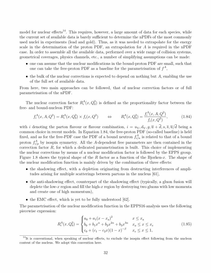
model for nuclear effects14. This requires, however, a large amount of data for each species, whilethe current set of available data is barely sufficient to determine the nPDFs of the most commonlyused nuclei in experiments (lead and gold). Thus, as it was needed to extrapolate for the energyscale in the determination of the proton PDF, an extrapolation for A is required in the nPDFcase. In order to assemble all the available data, performed over a wide range of collision systems,geometrical coverages, physics channels, etc., a number of simplifying assumptions can be made:

• one can assume that the nuclear modifications in the bound-proton PDF are small, such thatone can take the free-proton PDF as a baseline for the parametrisation of fA,

• the bulk of the nuclear corrections is expected to depend on nothing but A, enabling the useof the full set of available data.

From here, two main approaches can be followed, that of nuclear correction factors or of fullparametrisation of the nPDF.

The nuclear correction factor RAi (x,Q

20) is defined as the proportionality factor between the

free- and bound-nucleon PDF:

fAi (x,A,Q

2) = RAi (x,Q

20)× fi(x,Q2) ⇔ RA

i (x,Q20) =

fAi (x,A,Q

2)

fi(x,Q2)

, (1.84)

with i denoting the parton flavour or flavour combination, i = uV, dV, g, u + d, s, s, u/d being acommon choice in recent models. In Equation 1.84, the free-proton PDF (so-called baseline) is heldfixed, and as for the free-PDF case the PDF of a bound neutron fA

i/n is related to that of a boundproton fA

i/p by isospin symmetry. All the A-dependent free parameters are then contained in thecorrection factor R, for which a dedicated parametrisation is built. This choice of implementingthe nuclear corrections by means of a nuclear modification factor is followed by the EPPS group.Figure 1.8 shows the typical shape of the R factor as a function of the Bjorken-x. The shape ofthe nuclear modification function is mainly driven by the combination of three effects:

• the shadowing effect, with a depletion originating from destructing interferences of ampli-tudes arising for multiple scatterings between partons in the nucleus [61],

• the anti-shadowing effect, counterpart of the shadowing effect (typically, a gluon fusion willdeplete the low-x region and fill the high-x region by destroying two gluons with low momentaand create one of high momentum),

• the EMC effect, which is yet to be fully understood [62].The parametrisation of the nuclear modification function in the EPPS16 analysis uses the followingpiecewise expression:

RAi (x,Q

20) =

a0 + a1(x− xa)2 x ≤ xa

b0 + b1xα + b2x

2α + b3x3α xa ≤ x ≤ xe

c0 + (c1 − c2x)(1− x)−β xe ≤ x ≤ 1,

(1.85)

14It is conventional, when speaking of nuclear effects, to exclude the isospin effect following from the nucleoncontent of the nucleus. We adopt this convention here.

32

Figure 1.8: Illustration of the EPPS16 fit function RAi (x,Q

20). See the text for more details about

the nuclear effects and the meaning of the xk and yk. Figure taken from Ref. [54].

where α = 10xa, and all the parameters ak, bk and ck have implicit i and A dependencies. Theseparameters are fully determined by the asymptotic small-x limit y0 = RA

i (x→ 0, Q20), the antishad-

owing maximum ya = RAi (xa, Q

20) and the EMC minimum ye = RA

i (xe, Q20), as well as requirements

for continuity and vanishing first derivatives at the matching points xa and xe. The A dependencyof the yk points is parametrised as:

yk(A) = yk(Aref)

(A

Aref

)γk[yk(Aref)−1]

, (1.86)

with γk ≥ 0 and Aref = 12. In the EPPS16 model the input scale Q20 is set at the charm pole mass

Q20 = m2

c = (1.3 GeV)2 and the value of the strong coupling strength is set at the PDG value [6]by αs(MZ) = 0.118, with MZ the mass of the Z boson. The CT14 PDF set [63] serves as baseline,and the error sets are determined by means of the Hessian matrix method.

The second approach, followed in the nCTEQ global analysis [55], does not operate with anuclear correction factor. It is instead a full parametrisation of the whole nPDF for bound proton

33

fA(x,Q0)15. In the nCTEQ15 analysis the functional form mimics that of the CTEQ6 PDF [64]:

xfAi (x,Q0) = c0c

c1(1− x)c2ec3x(1 + ec4x)c5 , (1.87)

for i = uV, dV, g, u + d, s + s, s − s. A specific parametrisation of the down-to-up quark ratio ischosen as:

d(x,Q0)

u(x,Q0)= c0x

c1(1− x)c2 + (1 + c3x)(1− x)c4 . (1.88)

The A dependence is directly embedded into the ck coefficients:

ck(A) ≡ ck,0 + ck,1(1− A−ck,2

). (1.89)

The coefficient ck,0 = ck(A = 1) is the underlying proton coefficient. It is held fixed during thenCTEQ analysis, and set at the value determined in the study of Ref. [65]. Here as well the inputscale corresponds to the charm pole mass, Q0 = 1.3 GeV and the method for the determination ofthe error sets is the Hessian matrix method.

The same choice was taken for the nNNPDF2.0 analysis. The parametrisation scale is chosen asQ0 = 1 GeV, where the evolution basis (the one given by the eigenvectors of the DGLAP evolutionequations) is given by Σ, T3, T8, V, V3 and g. Expressed in terms of the elements of the flavourbasis, composed of the active flavours, the evolution basis reads:

Σ(x,Q0) = (u+ + d+ + s+)(x,Q0), total quark singlet,

T3(x,Q0) = (u+ − d+)(x,Q0), quark triplet,

T8(x,Q0) = (u+ + d+ − 2s+)(x,Q0), quark octet, (1.90)

V (x,Q0) = (u− + d−)(x,Q0), total valence quark,

V3(x,Q0) = (u− − d−)(x,Q0), valence quark triplet,

g(x,Q0) gluon,

with q± = q± q and s = s is assumed. Six PDF combinations are independently parametrised as:

xfi(x,Q0) = Bix

αi(1− x)βiNNi(x,A), (1.91)

with i = (Σ, T3, T8, V, V3, g) the flavour combination, BΣ = BT3= BT8

= 1 and the three other Bcoefficients are fixed by the sum rules. NNi(x,A) is the value yielded by the neuron of the outputlayer of the neural network associated to each specific distribution. The neural network consistsin one input layer, one hidden layer with sigmoid activation function and one output layer withlinear activation function. In the nNNPDF2.0 analysis the uncertainty on the nPDFs is estimatedwith the MC method, using a number of replicas Nrep = 1000. Figure 1.9 shows the results of thenNNPDF2.0 determination for three nucleus species, carbon, iron and lead.

Table 1.2 summarises the key specifications of the three nPDF models discussed in this section.

15It should be noted that baselines are still used here, as to help the global fits by providing e.g. reference valuesand boundary conditions.

34

Figure 1.9: The nNNPDF2.0 set of nuclear PDF for 12C, 56Fe and 208Pb at the energy scaleQ2 = 100 GeV2. The uncertainty band correspond to the 90% confidence level. Figure taken fromRef. [56].

nPDF set nCTEQ15 EPPS16 nNNPDF2.0Order NLO NLO NLO

Flavour separation valence quarks valence + sea quarks valence + sea quarksProton baseline CTEQ6M-like CT14NLO NNPDF3.1

Data points 708 1811 1467Input scale Q0 1.30 GeV 1.30 GeV 1 GeV

Free parameters 35 52 256Parametrisation polynomial polynomial neural network

Error determination Hessian Hessian MC

Table 1.2: Key specifications of the nCTEQ15 [55], EPPS16 [54] and nNNPDF2.0 [56] nPDFsets.

35

Chapter 2

Heavy-ion collisions

In this chapter, a selection of topics relevant for the analyses presented in this manuscript arebriefly reviewed. The first section sets the stage by summarising the current view of the evolutionof a heavy-ion collisions (HIC). It is followed by a short introduction to the main present andfuture heavy-ion colliders in Section 2.2. Section 2.3 describes the theoretical side of the Glaubermodel, the common picture for modelling a hadronic collision and through which key quantitiesfor the characterisation of the event can be obtained. Finally, Section 2.4 presents the motivationbehind the study of small systems as a mean to acquire more inputs for the interpretation of datafrom HIC, and provides some details on peculiar recent observations.

2.1 History of a collisionThe requirements, in terms of thermodynamical conditions, for the creation of a quark-gluonplasma (QGP) prevent its systematic study in the laboratory, outside of large scale experimentsable to bring beams of particles up to relativistic speed before colliding them. Up to now HIC arethe only known way to create a QGP, with one caveat: a hadronic collision is a complex process,in which the QGP only represents a fraction of the physics involved. Over the years, a standardmodel of ultrarelativistic HIC (URHIC) has emerged, which is depicted in Figure 2.1. Every stageof the evolution features a different form of QCD matter with specific active degrees of freedom.One can isolate several steps, described below, all defined in terms of the Lorentz-invariant propertime τ ≡

√t2 − z2, which parametrises the hyperbolic curves in the figure, and defining τ = 0 as

the collision time. The indicated times are of course not firm boundaries, but rather indicationsof our current understanding of the phenomena and their temporal evolution. More informationcan be found in Ref. [66].

1: Initial state (τ < 0 fm/c):Before the collision, setting oneself in the centre-of-mass (cms) frame, one sees the incoming

nuclei as being highly contracted, with a longitudinal extent smaller by a factor γ =√sNN/2mN ∼

103 at the LHC energies (the Lorentz boost factor) to that of the radial extent in the transverseplane. The system here is described by the QCD-improved parton model presented in Section 1.2

37

Figure 2.1: Light cone and space-time evolution of a HIC, with the typical proper times τindicated for the energies attained at the Large Hadron Collider (LHC). The overlay shows asimulation as seen in the laboratory frame. Figure taken from Ref. [67].

as a wall of partons travelling along colinear trajectories. At high energy, the nuclei are mostlycomposed of gluons as seen in the low-x gluon distribution function of Figure 1.9. The higherwe go in energies, the higher the gluon density becomes. However, the longitudinal extensionof the nucleus has a lower limit and the rapid increase of the number of gluons cannot continueforever. Having a typical transverse size of 1/Q, the gluons will eventually overlap each other andsaturate [68, 69]. The gluons form a classical coherent field configuration called the Colour GlassCondensate (CGC) [70]. The saturation scale, Qs, is proportional to the gluon distribution, theradius of the hadron and the coupling:

Qs ∼ αs(Q2s)xg(x,Q2

s)

πR2 , (2.1)

where R is the radius of the mother hadron. The saturation scale for a nucleus follows the sameexpression, with the corresponding nuclear gluon distribution and radius: g(x,Q2

s) → gA(x,Q2s)

and R→ RA1/3, meaning that the gluon saturation effect will be more significant in heavy nucleithan in protons. The CGC approach is an alternative to the nPDF framework described in Section1.2 for the description of the initial state.

2: Collision (τ ∼ 0 fm/c):At τ = 0, the two nuclei hit each other and the interactions start developing. The central

collision of ultra-relativistic heavy nuclei is a process of huge entropy production. Hard processes

38

involving large momentum transfers Q > 10 GeV are the first to occur, within a time τ ∼ 1/Q bythe uncertainty principle. These processes lead to the production of hard particles, i.e. particlescarrying transverse energies and momenta of the order of Q. The hard processes include (hadronic)jets, direct photons, dilepton pairs, heavy quarks and vector bosons. They are often used tocharacterise the event (e.g. "di-jet event").

This stage is efficiently described by the framework presented in Chapter 1, by means of theQCD-improved parton model. The nucleus is seen as a stream of partons, with partonic inter-actions being frozen over the timescale at which the collision happens. The high energy of thecollision allows one to use pQCD and the factorisation theorem to depict the interactions and cal-culate the cross sections. The non-perturbative part of the cross section is estimated from globalQCD analysis of experimental data, from which the nPDF is derived. Hard processes are thereforeof particular interest for the study of HIC, as their production is theoretically rather well known,and they experience the whole history of the system from which information on the various stagescan be obtained.

3: Semi-hard particle production (0 < τ < 0.3 fm/c):At this stage are produced the so-called semi-hard processes, with a corresponding transverse

momentum scale of about 1 GeV/c. The bulk of the partonic content of the colliding nuclei,which constituted the CGC, is now liberated by the collision. Most of the multiplicity of theevent is generated here, as most of the hadrons eventually seen in the detectors are producedvia the fragmentation and hadronisation of the initial-state gluons after their liberation. Rightafter being liberated, they form a relatively dense medium, with an average density estimated asε ∼ 15 GeV/fm3 in Pb–Pb collisions at the LHC energies. This density is about one order ofmagnitude higher than that in nuclear matter. This out-of-equilibrium state of partonic matter isknown as the glasma [71].

4: Out-of-equilibrium state (0.3 < τ < 2 fm/c):If the produced partons could not interact with each other, they would rapidly separate and

independently evolve (via fragmentation and hadronisation) towards the final state hadrons. Thissituation corresponds, roughly speaking, to what happens in pp collisions, where the density is lowenough to neglect the interaction mentioned above (although the situation is more complex andwill be addressed in Section 2.4). In URHIC, collective phenomena are observed, such as the parti-cle anisotropic flow [32] and comovers interactions [72], indicating that the particles liberated andcreated during the collision do interact. A direct consequence is that the system quickly reachesthermal equilibrium: data are consistent with a very short thermalisation time τth ∼ 1 fm/c. Itis a striking feature, as it requires a strong interaction between the partons, able to compete withthe medium expansion: these interactions have to redistribute energy and momentum among thepartons despite the fact that the latter separate quite fast from each other. Such a rapid thermal-isation is not consistent with perturbative calculations at weak coupling, driving the emergenceof a new paradigm: the dense partonic matter produced at the intermediate stages of a HIC may

39

actually be a strongly coupled, near perfect fluid.

5: Quark-Gluon Plasma (2 < τ < 6 fm/c):The outcome of the thermalisation process is the high-temperature phase of QCD matter

known as the QGP. The existence of this phase is well established from theoretical calculationson the lattice, but its production during a HIC is at best ephemeral: the partonic matter keepsexpanding and cooling down (this implies in particular that the temperature is space and timedependent, such that the thermal equilibrium is only reached locally) until the hadronisation phase,in which the coloured quarks and gluons recombined into colour-singlet hadrons. During the timeof existence of the QGP, its description can be achieved by means of relativistic hydrodynamics[31]. The fundamental equations are the conservation of the energy-momentum tensor and thebaryon number:

∂µ〈T µν〉 = 0, ∂µ〈jµB〉 = 0, (2.2)

where the expectation value is taken with respect to the time-dependent state in local thermalequilibrium. Arguably one the main objective of heavy-ion programs is the characterisation ofthe QGP through the determination of its physical properties, such as the temperature, density,or shear viscosity to entropy ratio. The precise nature of the QGP is still an open question. Ifthe system can be approximated by a perfect fluid, the expectation values are parametrised solelyby the local density ε and the local pressure P . If the fluid is not perfect, extra information arerequired, such as the viscosity or the heat conductivity. A recent review of the phenomenology ofthe QGP can be found in Ref. [32].

6: Hadronic phase and freeze-out (τ > 6 fm/c):Hadronisation occurs when the local temperature reaches the order of the critical temperature

of the phase transition Tc ' 155 MeV. This hadronic system is still relatively dense, such that thelocal thermal equilibrium is preserved during the expansion. One then speaks of hot hadron gas,with decreasing temperature and density. Inelastic interactions keep occuring until the so-calledchemical freeze-out. From this point on, the relative abundances of hadrons are fixed, and theonly interactions that still happen are elastic. The properties of the medium at this stage, as afunction of the beam energy, is shown in Figure 2.2. Around τ ∼ 20 fm, the elastic collisions stopas well, at the thermal freeze-out. The momenta of the formed particles are set, and they streamfreely towards the detectors.

It should be mentioned that this picture is not fixed, and the actual behaviour of the QCDmatter during a HIC remains an open question. Recent works on the application of hydrodynamics,for example, indicate that the system may never come close to equilibrium [74, 75, 76]. In thisalternative picture, the transition between the fourth and fifth phases should be considered in termsof hydrodynamisation instead of reach of an equilibrium state, and the boundary between the twoset at the point where hydrodynamics becomes applicable. Then the so-called "pre-equilibriumstate" is wrongly named, and one should speak of pre-hydrodynamisation instead.

40

Figure 2.2: Temperature T and baryon chemical potential µB as a function of the beam energy.The energy reach of various heavy-ion experiments is shown. Figures taken from Ref. [73].

2.2 Heavy-ion acceleratorsThe study of HIC is a vivid field in rapid expansion. It relies on the ability to perform a large varietyof collision configurations over a vast range of energies. This motivates the current existence,building and planification of several experiments fully or partially dedicated to HIC. The mainfacilities currently running or planned for the near future are:

• the Super Proton Synchrotron (SPS) and the Large Hadron Collider (LHC) [77] at theEuropean Organisation for Nuclear Research (CERN) in Geneva, Switzerland,

• the Relativistic Heavy Ion Collider (RHIC) [78] at Brookhaven National Laboratory (BNL)in Upton, New York,

• the Nuclotron-based Ion Collider fAcility (NICA) [79] at the Joint Institute for NuclearResearch (JINR) in Dubna, Russia,

• the Facility for Antiproton and Ion Research (FAIR) [80] at the GSI Helmholtz Centre forHeavy Ion Research in Darmstadt, Germany,

• the Electron-Ion Collider (EIC) [81] at BNL, as an extension of RHIC.

As depicted in Figure 1.3, these accelerators are designed to run with various energies, collisiontypes (colliders or fixed targets) and chemical species, enabling the exploration of a large regionof the phase diagram. The SPS was the first facility to observe signals in favour of the QGPformation in HIC collisions, such as the J/ψ anomalous suppression [82]. It provides now beamsfor the NA61/SHINE experiment [83] and serves as injector for the LHC (see Section 4.1). Anextension of its heavy-ion physics program has been recently proposed in Ref. [84]. RHIC and theLHC aim at exploring the low-µB, high-T region. FAIR and NICA assess the line of first order

41

phase transition, the former aiming at the critical point, the latter being designed for reaching thelargest µB accessible in a laboratory. With its peculiar e–A collision system, the EIC will provideprecise measurements of the internal structure of nuclei. The key characteristics of the acceleratorsare summarised in Table 2.1. As the measurements presented in this thesis were performed usingLHC data, the accelerator will be presented in more details in Chapter 4.

SPS RHIC LHC NICA FAIR (SIS100) EICStarting year 1976 2000 2009 2022 2025 2025

Ions O, S, In, Pb Al, Au, Cu, Pb, Xe up to Au up to U up to UZr, Ru, UEmax per nucleon 177 GeV 100 GeV 2.76 TeV 4.5 GeV 11 GeV 100 GeV

Table 2.1: Starting year, accelerated ions and maximum energy Emax per nucleon for the fivemain present and future heavy-ion accelerators. The energy per nucleon correspond to the maximalenergy attained or foreseen for the heavy-ion beams. The information for FAIR are given forSIS100, the accelerator of the complex dedicated to heavy ions.

2.3 The Glauber modelWhen studying HIC, pp collisions come as a natural reference, being the simplest hadronic colli-sion system. In order to draw the comparison, one needs to know precisely the geometry of thecollision, as to know the overlap area between the two nuclei, from which is derived the amount ofnucleons participating in the collision. Such information is of particular interest when performingmeasurements as a function of the event multiplicity, and provide information on the temperaturereached during the collision, a key point for QGP studies. In experiments, the Glauber modelling[85] of HIC has come to be the standard way to calculate geometrical quantities on the collision,typically expressed as the impact parameter b, the number of participating nucleons Npart or thenumber of binary nucleon-nucleon collisions Ncoll. At sufficiently high energies one reaches theoptical limit [86], in which nucleons have high momenta such that they will be undeflected as thenuclei pass through each other (i.e. they are transparent to each other). This is the so-calledultra-relativistic regime, in which the densities reached around the collision point are low. Besidescalculations in the optical limit, one can combine the Glauber model with Monte Carlo techniquesas an efficient framework through the use of more realistic particle production codes (see Refs.[87, 88] for early examples).

Glauber calculations start from a parametrisation of the nucleon density, for which a Fermidistribution (also known as the Wood-Saxon nucleon density) is generally used:

ρ(r) = ρ01 + w(r/R)2

1 + exp(r−Ra

) , (2.3)

where ρ0 is the nucleon density at the centre of the nucleus (ρ0 = ρ(r = 0)), and R the nucleusradius. a is the skin thickness of the nucleus, denoting how quickly the nuclear density falls off

42

near the edges. The additional parameter w is needed to describe deviations from a sphericalshape (w = 0 for Pb, in which case a 2-parameter Fermi is sufficient). The collisions are assumedto be inelastic, with a number of charged particles produced to be the same on average for eachnucleon-nucleon collision. As the cross section involves soft processes (processes of low momentumtransfer), it is not possible to calculate it in pQCD. The measured inelastic nucleon-nucleon crosssection σinel

NN is then used as an input, providing the only non-trivial dependence of the Glaubercalculation to the beam energy. Typical values for σinel

NN used by the ALICE Collaboration at theLHC energies are [89]:

σinelNN =

61.8± 0.9 mb,

√sNN = 2.76 TeV,

67.6± 0.6 mb,√sNN = 5.02 TeV,

64.8± 0.5 mb,√sNN = 5.44 TeV,

72.5± 0.5 mb,√sNN = 8.16 TeV.

The collision geometry foreseen by the Glauber model in the optical limit is depicted in Figure2.3.

Figure 2.3: Schematic representation of the optical-limit Glauber geometry in the longitudinal(left) and transverse (right) views. Figure taken from Ref. [85].

In Figure 2.3, two heavy ions, denoted as target A and projectile B1, are shown colliding atrelativistic velocities at an impact parameter ~b. One can consider two flux tubes located at adisplacement ~s with respect to the centre of the target nucleus, and hence at a distance ~s−~b fromthe centre of the projectile. During the collision, these tubes overlap. The probability, per unit oftransverse area, for a given nucleon to be located in the target flux tube is:

TA(~s) =

∫ρA(~s, zA)dzA, (2.4)

1At colliders, the choice of the nucleus considered as the target or the projectile is of course purely a matter ofconvenience or convention.

43

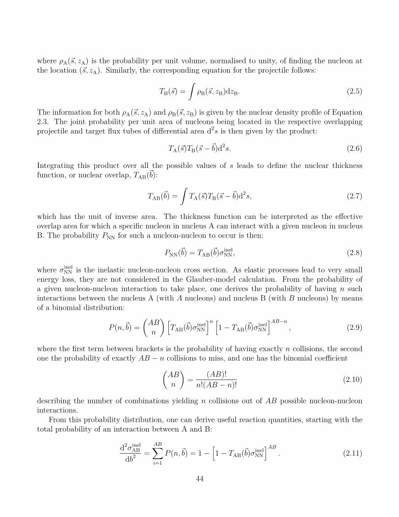
where ρA(~s, zA) is the probability per unit volume, normalised to unity, of finding the nucleon atthe location (~s, zA). Similarly, the corresponding equation for the projectile follows:

TB(~s) =

∫ρB(~s, zB)dzB. (2.5)

The information for both ρA(~s, zA) and ρB(~s, zB) is given by the nuclear density profile of Equation2.3. The joint probability per unit area of nucleons being located in the respective overlappingprojectile and target flux tubes of differential area d2s is then given by the product:

TA(~s)TB(~s−~b)d2s. (2.6)

Integrating this product over all the possible values of s leads to define the nuclear thicknessfunction, or nuclear overlap, TAB(~b):

TAB(~b) =

∫TA(~s)TB(~s−~b)d2s, (2.7)

which has the unit of inverse area. The thickness function can be interpreted as the effectiveoverlap area for which a specific nucleon in nucleus A can interact with a given nucleon in nucleusB. The probability PNN for such a nucleon-nucleon to occur is then:

PNN(~b) = TAB(~b)σinelNN , (2.8)

where σinelNN is the inelastic nucleon-nucleon cross section. As elastic processes lead to very small

energy loss, they are not considered in the Glauber-model calculation. From the probability ofa given nucleon-nucleon interaction to take place, one derives the probability of having n suchinteractions between the nucleus A (with A nucleons) and nucleus B (with B nucleons) by meansof a binomial distribution:

P (n,~b) =

(ABn

)[TAB(~b)σ

inelNN

]n [1− TAB(~b)σ

inelNN

]AB−n, (2.9)

where the first term between brackets is the probability of having exactly n collisions, the secondone the probability of exactly AB − n collisions to miss, and one has the binomial coefficient(

ABn

)=

(AB)!

n!(AB − n)!(2.10)

describing the number of combinations yielding n collisions out of AB possible nucleon-nucleoninteractions.

From this probability distribution, one can derive useful reaction quantities, starting with thetotal probability of an interaction between A and B:

d2σinelAB

db2=

AB∑i=1

P (n,~b) = 1−[1− TAB(~b)σ

inelNN

]AB

. (2.11)

44

In the case where the nuclei are not polarised, the vectorial impact parameter can be replaced bya scalar distance, and the cross section reads:

σinelAB =

∫ ∞0

2πbdb

1−

[1− TAB(b)σ

inelNN

]AB. (2.12)

The total number of nucleon-nucleon collisions is then:

Ncoll(b) =AB∑i=1

nP (n, b) = (AB)TAB(b)σinelNN , (2.13)

using the result for the mean of a binomial distribution.The number of nucleons in the target and projectile nuclei that interact is called the number

of participants Npart, also known as the number of wounded nucleons. At impact parameter b it isgiven by:

Npart(~b) =A

∫TA(~s)

1−

[1− TB(~s−~b)σinel

NN

]Bd2s+ (2.14)

B

∫TB(~s−~b)

1−

[1− TA(~s)σinel

NN

]Ad2s (2.15)

where it can be noted that the integral over the bracketed terms gives the respective inelastic crosssections for nucleon-nucleon collisions:

σinelA(B) =

∫d2s

1−

[1− TA(B)(~s)σ

inelNN

]A(B). (2.16)

The Monte Carlo approach of Glauber modelling, so-called Glauber Monte Carlo (Glauber-MC) provides an efficient and simple way to calculate geometry-related quantities such as 〈Npart〉and 〈Ncoll〉, the average numbers of participants and nucleon-nucleon binary collisions, respectively.Moreover, it enables the possibility to simulate experimentally observable quantities such as thecharged-particle multiplicity, which allows for the use of similar analysis methods (e.g. centralitycuts) to that for real data. In the Glauber-MC procedure, the two colliding nuclei are numericallyassembled by distributing A nucleons for nucleus A and B nucleons for nucleus B in a three-dimensional coordinate system, according to their respective nuclear density profiles. A randomimpact parameter b is then drawn as to parametrise the centrality of the collision. The AB collisionis then treated as a sequence of independent nucleon-nucleon collisions by having them travellingalong straight-line trajectories. An example of collision simulated with the Glauber-MC method isshown in Figure 2.4. By simulating many nucleus-nucleus collisions, one can build a distributionsimilar to that of data taking, from which the geometrical quantities can be derived.

In the optical limit approach, it is assumed that the scattering amplitude can be described byan eikonal approach, where the incoming nucleons see the target as a smooth density. It capturesmany features of the collision process, but does not feel the full physics behind the total crosssection, leading to distortions in the Npart and Ncoll distributions, while the Glauber-MC approach

45

Figure 2.4: Glauber-MC event simulated in Au–Au collisions at √sNN 200 GeV with impactparameter b = 6 fm, viewed in the transverse (left) and longitudinal (right) planes. Darker disksrepresent the participating nucleons. Figure taken from Ref. [85].

does not suffer from these flaws. The full integral to calculate the total cross section is [86]:

σAB =

∫d2b

∫d2sA1 ...d

2sAAd2sB1 ...d

2sBB

× TA(~s A1 )...TA(~s

AA )TB(~s

B1 )...TB(~s

BB ) (2.17)

×

1−

B∏j=1

A∏i=1

[1− σ(~b− ~s A

i + ~s Bj )]

,

to be compared with the formula obtained in the optical limit of Equation 2.12. Many termsare missing in the optical limit formula, which are the terms describing local density fluctuationsevent-by-event. Despite this difference, the two approaches are in very good agreement when itcomes to evaluate simple geometrical quantities such as Npart and Ncoll as a function of the impactparameter.

2.4 Small systemsIn the HIC community, small collision systems2 have long been used to study initial- and final-stateeffects in the so-called cold nuclear matter (that is, without passing through a phase of QGP), inorder to establish a baseline for the interpretation of heavy-ion (A+A) results. Subtracting these

2Broadly speaking, small systems designate all collision systems where one does not expect to see the apparitionof a QGP phase during the evolution of the system. As it is discussed in this section, recent observations ofcollectivity-like phenomena in small systems might have rendered this definition obsolete.

46

cold effects from A+A measurements leads to establish the hot effects, expected to be signaturesof the creation and evolution of the QGP, such as jet quenching, quarkonia suppression and regen-eration, strangeness enhancement or collective flow. At the starting time of the LHC, only pp andPb–Pb collisions were firmly scheduled, and operational plans for p–Pb collisions were only prelim-inary, although strongly advocated for by both theoreticians and the experimental community [90].Three of the four main LHC experiments (ALICE, ATLAS and CMS), included p+A collisions intheir performance studies and have discussed their importance. At that time, a p–Pb program atthe LHC was foreseen to satisfy two main interests, by providing benchmarks for Pb–Pb resultsand offering new scientific opportunities for studies related to e.g. saturation, ultra-peripheralcollisions or astrophysics-related processes. As it turned out, the study of small systems by theHIC community revealed one of the most striking discovery of the LHC era, namely the presenceof QGP-like behaviour (collective effects) in systems where they were not expected.

2.4.1 Small systems as benchmarks for heavy-ionsThe usage of small systems as a benchmark for A+A studies has been essential for the interpre-tation of A+A results at RHIC. A key example is the absence of suppression in the transversemomentum spectrum of the inclusive hadron production [91, 92], which proved the jet quench-ing hypothesis as the genuine final-state effect at work to explain the observed deficit of high-pThadrons in Au–Au collisions [93, 94]. A few years before, at the CERN SPS, data from severalp+A systems at different energies were already found to be fundamental for the interpretation ofresults on the J/ψ suppression in Pb–Pb collisions [82].

Equation 1.72 shows the importance of precisely knowing the PDFs such that models are ableto reproduce the data. The proton PDF is well constrained by a wealth of data, and is extractedfrom global fits performed at LO, NLO and NNLO. In the nuclear case, the precision on the PDFdetermination suffers from the lack of data available in the perturbative region, and most of thesedata are covering the range x > 0.01, above the kinematical reach of the LHC where the PDFuncertainties then remain sizeable. This situation is illustrated in Figure 2.5 showing the nuclearmodification functions uV, dV and g from the EPPS16 analysis [54], where one can observe thelarge uncertainty bands at low-x and in the EMC region. One of the central conceptual insightexpected from the heavy-ion program at the LHC is the transition from cold nuclear matter to hotpartonic matter. For all dynamical model of this evolution, a control over the initially-producedparticle density is crucial. This density, however, varies with the uncertainty on the nPDF, whosereduction is a decisive step in addressing one of the central issues in the dynamics of heavy-ioncollisions.

The medium properties in HIC is characterised through processes which couple to the mediumin a theoretically well-controlled manner, among which we find heavy flavours (HF). The descrip-tion of the heavy quark (charm and bottom) production is provided by the Fixed-Order Next-to-Leading-Log (FONLL) resummation approach [95, 96]. In the left panel of Figure 2.6, the nuclearmodification factor RpPb (i.e. the ratio of the production in p–Pb collisions to that in pp collisionsscaled by the atomic number of Pb) of charm and bottom is shown, with the nuclear modifications

47

Figure 2.5: EPPS16 nuclear modifications for Pb at the parametrisation scale Q20 = 10 GeV2, for

the uV, dV and g PDFs. The black curves correspond to the central fits, the dashed green lines tothe error sets. The total uncertainties are shown as blue bands. Figures taken from Ref. [54].

Figure 2.6: Left: nuclear modification factors for the charm and bottom quarks in p–Pb collisionsat √sNN = 8.8 TeV, and the corresponding uncertainties from the EPS09 parametrisation of thenuclear modifications. Figure taken from Ref. [90]. Right: inclusive jet nuclear modificationfactor R∗pPb as a function of the jet pT, in p–Pb collisions at √sNN = 5.02 TeV, measured bythe CMS collaboration [97]. The measurements are compared with calculations using the EPS09parametrisation of the nuclear modifications. The ∗ exponent indicates that the pp reference crosssection is not directly measured, but extrapolated (see Ref. [97] for more details).

implemented using the EPS09 [98] parametrisation. The nuclear effects tend to be small, and oneshould particularly notice that their size is of the same order as the size of the uncertainties of thepredictions, showing the importance of increasing our knowledge on the cold nuclear effects for thepurpose of understanding the hot ones.

The modification of the spectrum of particles produced at large transverse momentum, the so-called jet quenching effect, is one of the main probes of the properties of the hot and dense matter

48

formed in HIC. Here as well, it is of utmost importance to disentangle cold and hot effects in orderto interpret the results in Pb–Pb collisions. In the right panel of Figure 2.6, the measurementof the RpPb for jets in p–Pb collisions at √sNN = 5.02 TeV by the CMS collaboration [97] isreported. The ratio shows that there is little sensitivity (although non-zero) of the jet productionto cold nuclear effects, indicating that the modifications observed in Pb–Pb can majoritarily beinterpreted in terms of parton energy loss in the medium. Reference [99] gives a recent overviewof jet quenching measurements in HIC.

Electroweak bosons constitute an other important probe in p–Pb collisions. As they are themain topic of this thesis, their importance will be developed in a dedicated section in Chapter 3.

2.4.2 Collectivity in small systems(?)In the classical picture of hadronic collisions, pp, p+A and A+A collisions are well separated, thefirst providing a reference, the second probing the cold nuclear effects and the third assessing bothhot and cold effects. But recent years have witnessed a surprising development in multiparticledynamics of high multiplicity pp and p+A collisions. This started with the observation of a ridge-like structure by the CMS experiment in pp collisions [100], and has been confirmed since them.The surprise came from the fact that a few years before, a very similar effect was observed in HIC,in Au+Au collisions at √sNN = 200 GeV at RHIC [101, 102].

Measurements of azimuthal particle correlations in small collision systems have drawn a lotof interest. In HIC, the measurements of flow coefficients, through which is quantified the degreeof azimuthal anisotropy, are understood as the propagation, via the hydrodynamic expansion, ofthe initial spatial anisotropy to the final state particles. Similar observations in small collisionsystems do not necessarily have the same origin, and one must carry a careful comparison betweendata and theory in order to understand the experimental observations. The correlations are oftenparametrised via the particles relative azimuthal angle ∆φ in the transverse plane, and their relativelongitudinal pseudorapidity ∆η. The typical shape of correlations between pairs of charged particle,displayed in the ∆φ − ∆η space and for Pb–Pb collisions, is shown in the top panels of Figure2.7. The distribution shows a clear ridge-like structure in the near side (∆φ ∼ 0), considered to bethe consequence of the collective expansion of the matter during the QGP phase. In the middleleft panel of the Figure, the same two-particle correlation function is shown in low-multiplicityp–Pb collisions. Here the ridge is not seen. However, looking at high multiplicity events (middleright panel), the ridge is present, although not as pronounced as in Pb–Pb data. The situation isreproduced when looking at pp collisions, in the bottom panels of Figure 2.7. Here again, whenselecting high multiplicity events, the ridge appears. It is interesting to notice that the magnitudeof the ridge is highly dependent on the collision system. The full interpretation of this effect isyet to be derived. One has to carefully account for the non-flow background, which can create thesame pattern in the data while not being a sign of collective behaviour.

These new results triggered a global analysis, or re-analysis, of the data in small and largesystems, as well as a vast theoretical effort towards the interpretation of these observations. Arecent review of the experimental and theoretical status of this topic can be found in [106]. The

49

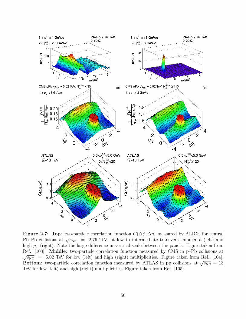
Figure 2.7: Top: two-particle correlation function C(∆φ,∆η) measured by ALICE for centralPb–Pb collisions at √sNN = 2.76 TeV, at low to intermediate transverse momenta (left) andhigh pT (right). Note the large difference in vertical scale between the panels. Figure taken fromRef. [103]. Middle: two-particle correlation function measured by CMS in p–Pb collisions at√sNN = 5.02 TeV for low (left) and high (right) multiplicities. Figure taken from Ref. [104].

Bottom: two-particle correlation function measured by ATLAS in pp collisions at √sNN = 13TeV for low (left) and high (right) multiplicities. Figure taken from Ref. [105].

50

fact that small systems is an ever-growing field of interest in the heavy-ion community, due to thenew insights it can provide for the interpretation of HIC data, is a central motivation of the workpresented in this thesis, which aims at studying reference processes in p–Pb collisions.

51

Chapter 3

Weak bosons in heavy-ion collisions

This chapter focuses on the Z0- and W±- boson production, with an emphasis on p–Pb collisionsas a context. The first section provides a quick history of the prediction and discovery of thebosons, leading to their current status within the Standard Model and the knowledge of theirproperties. Section 3.2 presents the theoretical framework for the description and understandingof the production and decay of weak bosons in hadronic collisions. The chapter ends by a reviewof the measurements performed at the Large Hadron Collider (LHC) in Section 3.3.

3.1 Carriers of the weak force

3.1.1 Historical perspectiveThe history of the Z0 and W± bosons can be traced back to 1933, when Enrico Fermi publishedhis landmark theory for beta decay [107], where he applied the principles of quantum mechanicsto matter particles, assuming that they can be created and annihilated just like light quanta inatomic transitions. Hideki Yukawa [108] introduced the idea of an intermediate massive bosonexchanged between the nucleons that would generate the nucleon interaction. It turned out laterthat Yukawa’s bosons are the Lattes, Occhialini and Powell pions [109], and that Yukawa’s intentionto describe both the strong interaction and the weak coupling did not meet with success regardingthe weak interaction. The form of the weak interaction was established as a special combinationof a vector current V and an axial-vector current A, namely V −A, in interaction with itself, afterproposals from R. Feynman and M. Gell-Mann [110], E. Sudarshan and R. Marshak [111], and J.J. Sakurai [112]. Shortly after, Brazilian physicist J. L. Lopes devised in 1958 an equation [113]showing the analogy of the weak nuclear interactions with electromagnetism, and predicted thatthe weak interaction would feature both charged and neutral currents through the exchange of verymassive bosons. A really firm prediction of the masses would be obtained with the emergence ofthe electroweak unified theory of Glashow [114], Salam and Ward [115], and Weinberg [116]. Theformula obtained by Weinberg in 1967 features a parameter θW , so-called weak mixing angle, whosevalue was not known. Weinberg could thus only establish boundaries for the masses: mW± ≥ 37

GeV/c2 and mZ0 ≥ 75 GeV/c2. In the 15 years separating the prediction of the W± and Z0 bosons

53

from their discovery, this angle was measured by a variety of experiment such that in 1982 themasses were calculated to be:

mW± = 82± 2 GeV/c2, mZ0 = 92± 2 GeV/c2.

The ideal machine to produce the weak bosons in the most convenient experimental conditions isan e+e− collider. Indeed, the Large Electron-Positron (LEP) program at CERN would demonstratethat by providing precise measurements of the W± and Z0 masses. However, the starting of theLEP collider was still in the far future, leading Rubbia, Cline and McIntyre [117] to proposethe transformation of an existing high-energy proton accelerator into a proton-antiproton collideras a fast and inexpensive way to achieve collisions above the energy threshold for weak-bosonproduction. The proposal was accepted as an evolution of the CERN super proton synchrotron(SPS) in 1978, and the first pp collisions at an energy of √sNN = 540 GeV were delivered in July1981.

The production of W± and Z0 bosons at a pp collider is expected to occur mainly as the resultsof quark-antiquark annihilation:

du →W+, du →W−, uu → Z0, dd → Z0.

In the parton model, about half of the momentum of a high-energy proton is carried, on average,by the three valence quarks, which then individually carry 1/6 of the proton momentum. Weakboson production thus requires a total centre-of-mass energy equal to about 6 times the mass ofthe bosons. The W± boson predominantly decay into quark-antiquark pairs, which appear as twohadronic jets, but this detection channel is overwhelmed by two-jet production from hard partonscatterings. It was thus chosen to detect the W± bosons by identifying their leptonic decays. Theminimal luminosity is determined by the need to detect Z0 → e+e−, with a cross section of ∼ 1nb at

√s ∼ 600 GeV. Considering the branching fraction of the process, amounting to about 3%,

one gets that a luminosity of the order 10−29 cm−2 s−1 would yield one event per day. Theserequirements drove the design of the antiproton source and beam collimation and accelerationat the SPS. Table 3.1 summarises the running conditions of the collider during its nine years ofoperation time. The collider was shut down at the end of 1990 as it was no longer competitivewith the 1.8 TeV proton-antiproton collider at Fermilab which started to run in 1987.

Two experiments, UA1 and UA21 were conceived to collect SPS data, both approved in 1978.UA1 is a general-purpose magnetic detector [118, 119], a 6-chamber cylindrical assembly of 5.8m in length and 2.3 m in diameter, making it the largest imaging drift chamber at that time.Its almost complete solid-angle coverage made it effective in the reconstruction of the undetectedneutrino in the W± → e±ν. The UA2 [120] was on the contrary optimised for the detection ofelectrons from W± and Z0 decays, relying on calorimetry of high granularity. By ignoring some ofthe physics, being for example blind to muons, UA2 was easier to design and only costed a thirdof UA1, a strong argument towards its approval. The calorimeter had 24 slices of 4 tons each,

1UA stands for Underground Area, as the SPS is built in an underground tunnel at an average depth of 100meters.

54

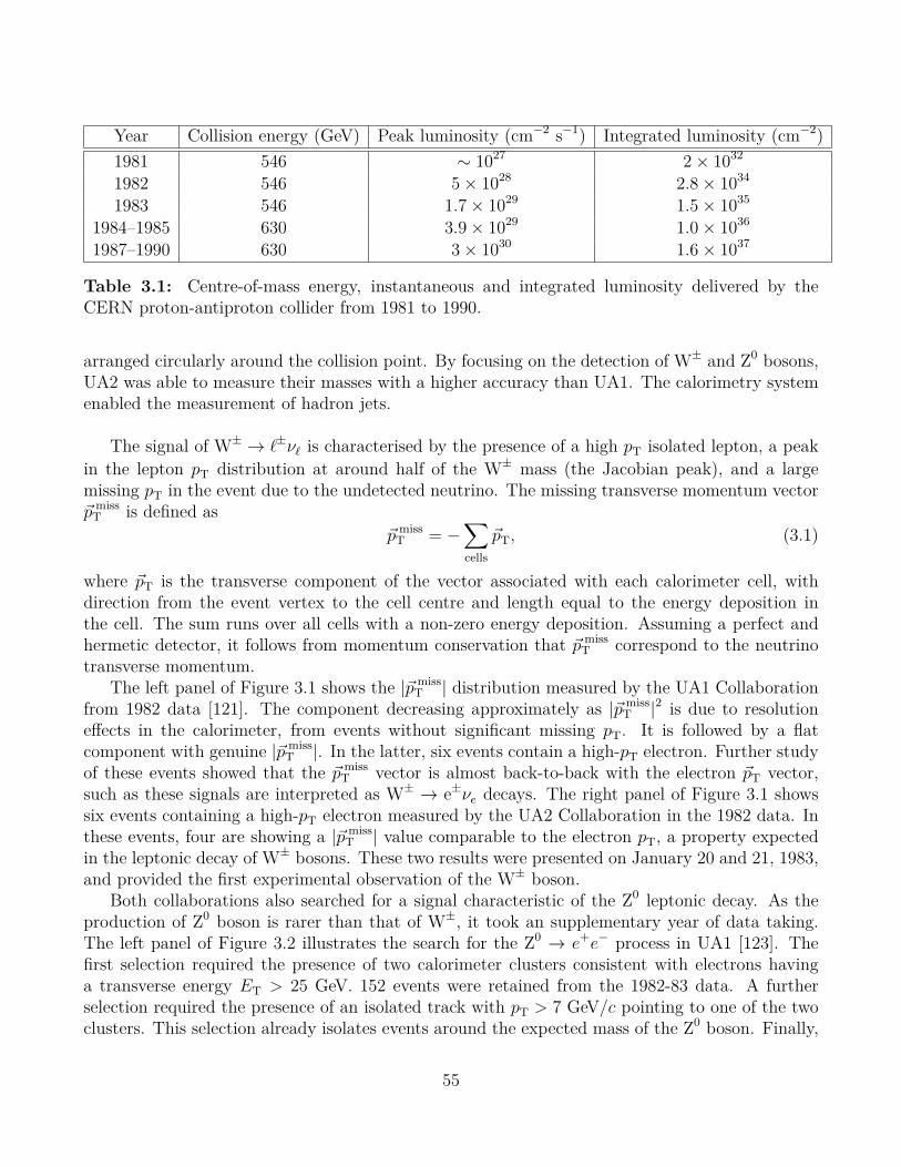
Year Collision energy (GeV) Peak luminosity (cm−2 s−1) Integrated luminosity (cm−2)1981 546 ∼ 1027 2× 1032

1982 546 5× 1028 2.8× 1034

1983 546 1.7× 1029 1.5× 1035

1984–1985 630 3.9× 1029 1.0× 1036

1987–1990 630 3× 1030 1.6× 1037

Table 3.1: Centre-of-mass energy, instantaneous and integrated luminosity delivered by theCERN proton-antiproton collider from 1981 to 1990.

arranged circularly around the collision point. By focusing on the detection of W± and Z0 bosons,UA2 was able to measure their masses with a higher accuracy than UA1. The calorimetry systemenabled the measurement of hadron jets.

The signal of W± → `±ν` is characterised by the presence of a high pT isolated lepton, a peakin the lepton pT distribution at around half of the W± mass (the Jacobian peak), and a largemissing pT in the event due to the undetected neutrino. The missing transverse momentum vector~p missT is defined as

~p missT = −

∑cells

~pT, (3.1)

where ~pT is the transverse component of the vector associated with each calorimeter cell, withdirection from the event vertex to the cell centre and length equal to the energy deposition inthe cell. The sum runs over all cells with a non-zero energy deposition. Assuming a perfect andhermetic detector, it follows from momentum conservation that ~p miss

T correspond to the neutrinotransverse momentum.

The left panel of Figure 3.1 shows the |~p missT | distribution measured by the UA1 Collaboration

from 1982 data [121]. The component decreasing approximately as |~p missT |2 is due to resolution

effects in the calorimeter, from events without significant missing pT. It is followed by a flatcomponent with genuine |~p miss

T |. In the latter, six events contain a high-pT electron. Further studyof these events showed that the ~p miss

T vector is almost back-to-back with the electron ~pT vector,such as these signals are interpreted as W± → e±νe decays. The right panel of Figure 3.1 showssix events containing a high-pT electron measured by the UA2 Collaboration in the 1982 data. Inthese events, four are showing a |~p miss

T | value comparable to the electron pT, a property expectedin the leptonic decay of W± bosons. These two results were presented on January 20 and 21, 1983,and provided the first experimental observation of the W± boson.

Both collaborations also searched for a signal characteristic of the Z0 leptonic decay. As theproduction of Z0 boson is rarer than that of W±, it took an supplementary year of data taking.The left panel of Figure 3.2 illustrates the search for the Z0 → e+e− process in UA1 [123]. Thefirst selection required the presence of two calorimeter clusters consistent with electrons havinga transverse energy ET > 25 GeV. 152 events were retained from the 1982-83 data. A furtherselection required the presence of an isolated track with pT > 7 GeV/c pointing to one of the twoclusters. This selection already isolates events around the expected mass of the Z0 boson. Finally,

55

Figure 3.1: Left: UA1 distribution of the missing transverse energy for equal bins of (EMIST )2.

The events highlighted in black contain a high-pT electron. Figure taken from Ref. [121]. Right:(a) ratio of the missing pT to the electron pT (called ET in the publication) for six UA2 eventscontaining an electron with ET > 15 GeV. (b) electron pT distribution for the four UA2 eventswith the highest |~p miss

T |/ET ratio. Figure taken from Ref. [122].

the selection is refined by extending the previous selection to both clusters, leaving four events.They are consistent with a unique value of the e+e− invariant mass, within the detector resolution.As the UA1 detector was able to detect muons, the collaboration found one extra event consistentwith the Z0 → µ+µ− process. From the same collision period, the UA2 collaboration extractedeight events containing two isolated electrons with ET > 25 GeV [124], as displayed in the rightpanel of Figure 3.2. From these studies, the two collaborations were able to estimate the mass ofthe Z0 boson as:

mUA1

Z0 = 95.2± 2.5± 3.0 GeV/c2, mUA2

Z0 = 91.9± 1.3± 1.4 GeV/c2,

providing the first experimental observation of a signal consistent with the expectations for the Z0

boson.

By 1985, before the collider shutdown in 1986 for upgrade, the two collaborations had collected asizeable amount of signal associated to W± and Z0 leptonic decays. UA1 had recorded 290 signalsfor the W± in the electronic channel and 57 in the muonic channel, as well as 33 (21) events

56

Figure 3.2: Left: search for the Z0 → e+e− decay in UA1. The events are selected by requiring(a) two hits in the calorimeter with transverse energy ET > 25 GeV with pT > 7 GeV/c for one(b) or two (c) of the associated tracks. Figure taken from Ref. [123]. Right: search for theZ0 → e+e− decay in UA2. The top panel shows the invariant mass distribution of pairs of particlereconstructed from hits in the calorimeter with ET > 25 GeV. The bottom panel shows the samedistribution after requiring that one (white area) or two tracks (shaded area) are identified asisolated electrons. Figure taken from Ref. [124].

corresponding to Z0 electronic (muonic) decays [125]. In the same years, the UA2 collaborationrecorded samples of 251 W± → e±ν and 39 Z0 → e+e− events [126]. This allowed the twocollaborations to precise their respective measurements for the masses of the weak bosons:

mUA1

W± = 82.7± 1.0± 2.7 GeV/c2, mUA2

W± = 80.2± 0.8± 1.3 GeV/c2,

mUA1

Z0 = 93.1± 1.0± 3.1 GeV/c2, mUA2

Z0 = 91.5± 1.2± 1.7 GeV/c2.

The experimental confirmation of the existence of the weak bosons was a striking confirmationof crucial aspects of the Standard Model of particle physics. The physics community was at thattime already heavily committed to the theory, and the UA1 and UA2 results were highly expected.Nonetheless, they represent an extraordinary experimental triumph, coming from experimentsdesigned, approved and built within a few years, along with the development of important exper-imental techniques that are still in use forty years later.

57

3.1.2 W± and Z0 bosons in the Standard ModelIn quantum electrodynamics (QED) [9], the Lagrangian for the photon Aµ coupled to an electronfield ψ reads:

LQED = −1

4F µνFµν + ψ

(iγµDµ −me

)ψ, (3.2)

where the adopted notations follow that of the QCD Lagrangian of Equation 1.2. This Lagrangianis invariant under independent redefinitions of the phase of the field ψ at each space-time point,

ψ′(x) = exp (iθ(x))ψ(x), (3.3)

provided that the gauge field Aµ transforms as

A′µ(x) = Aµ(x)−1

e∂µθ(x). (3.4)

The Lagrangian thus possesses a local gauge invariance under transformations of the field belongingto the U(1) gauge group. There is a single gauge coupling e corresponding to this group.

The Standard Electroweak Model known as Glashow-Weinberg-Salam (GWS) [114, 115, 116]builds up on QED, extending it to the SU(2)⊗U(1) group. Initially, the Lagrangian of this modelcontains three massless bosons W i associated with the SU(2) group, and one massless boson Bassociated with U(1), yielding the gauge boson Lagrangian:

L = −1

4W i µνW i

µν −1

4BµνBµν (3.5)

with the field strength tensors of the U(1) gauge field B and the SU(2) gauge fields W i:

W iµν = ∂µW

iν − ∂νW i

µ − gW εijkW jµW

kν , (3.6)

Bµν = ∂µBν − ∂νBµ, (3.7)

gW being the SU(2) gauge coupling. Analogously to gluons carrying colour charge in QCD, theW i vector bosons already have interactions because of the non-abelian nature of the symmetrygroup SU(2). The coupling of the gauge fields to fermionic matter fields is implemented using thecovariant derivative:

Dµ = δij∂µigW (T ·W µ)ij + iY δijg

′WB

µ (3.8)

where g′W is the U(1) gauge coupling. The matrices T are a representation of the SU(2) weakisospin algebra and the U(1) charge Y is called the weak hypercharge. The tensor εijk appearsbecause its components are the structure constants of SU(2):[

T i, T j]= iεijkT k with ε123 = 1. (3.9)

One can define W±µ =

(W 1

µ ∓ iW 2µ

)/√2 and T± = T 1 ± iT 2 to obtain:

Wµ · T = W 3µT3 +

1√2W+

µ T+ +

1√2W−

µ T− (3.10)

58

where the matrices T± and T 3 satisfy [T+, T−

]= 2T 3, (3.11)[

T 3, T±]= ±T±. (3.12)

T+ and T− are thus the weak isospin raising and lowering operators.The presence of four massless bosons in Equation 3.5 is contradicted by experimental observa-

tions, as only one massless vector boson (the photon) is found in nature. The feebleness and shortrange of the weak interaction indicates that the mediating bosons are massive. It is then necessaryto include in the theory a mechanism of spontaneous symmetry breaking that gives explicit massterms for three of the bosons and retains only one conserved charge, the electric charge. In theStandard Model of the electroweak interaction, the fundamental SU(2)⊗U(1) symmetry is brokenby the Higgs mechanism. The first implementation of this mechanism is due to P. W. Anderson in1962 [127] (published in 1963), applied solely to non-relativistic theory. The relativistic model wasdeveloped in 1964 by three different groups2: François Englert and Robert Brout [129], Peter W.Higgs [130], and Gerald Guralnik, Carl Hagen and Tom Kibble [131]. A few years later, the theorywas proved to be renormalisable even in the presence of massive bosons by Gerard ’t Hooft andMartinus Veltman [132]. The LHC era provided a striking confirmation of the Higgs mechanismthrough the discovery of a particle consistent with the expectations on the Higgs boson by theATLAS [133] and CMS [134] Collaborations in high-energy pp collisions.

The electric charge arises as a nontrivial linear combination of YW , the weak hypercharge, andthe T3 component of the weak isospin:

Q = T3 +1

2YW (3.13)

that does not couple to the Higgs boson. Said otherwise: the Higgs and electromagnetic fields haveno effect on each other, at the tree level, while any other combination of the hypercharge and weakisospin will interact with the Higgs. As a consequence, one has an apparent separation between theweak force and electromagnetism. The U(1) symmetry group of electromagnetism is then definedby the group generated by this special linear combination. This spontaneous symmetry breakingmakes the W3 and B bosons coalesce into two different physical bosons with different masses,corresponding to the neutral weak boson Z0 and the photon γ:(

γ

Z0

)=

(cos θW sin θW− sin θW cos θW

)(BW3

), (3.14)

where θW is the Weinberg or electroweak mixing angle parametrising the rotation of the axes inthe (W3, B) plane. It is fixed by the relative strength of the coupling constants:

sin2 θW =g′ 2W

g2W + g′ 2W' 0.23. (3.15)

2In 1965, two 20-year old Russian undergraduates, Alexander Migdal and Alexander Polyakov, derived themechanism independently from the other groups [128]. As their work was not supported by leading scientists oftheir time, they saw their paper delayed by the editorial office of JTEP until its publication in 1966.

59

After this rotation the quadratic terms in the vector boson fields become

L =g2Wv

2

4W+

µ W− µ +

(g2W + g′ 2W )v2

8ZµZ

µ (3.16)

where v is the Higgs vacuum expectation value. The W± and Z0 bosons have therefore acquired amass term given by:

mW± =1

2vgW , mZ0 =

1

2v

√g2W + g′ 2W =

mW±

cos θW. (3.17)

Thus, as the Higgs field acquires a non-zero vacuum expectation value, the symmetry of the SU(2)group is spontaneously broken. This does not give rise to Goldstone boson, as it was the case forthe QCD symmetry breaking, but leads to the formation of the massive vector bosons W± and Z0.

3.1.3 Properties of the W± and Z0 bosonsThe properties of the particles are listed and updated by the Particle Data Group [6] by using thefull available data. For the weak bosons, the parameters are determined from a global fit of datacoming from the LEP [135] and SLC [136] accelerators, designed in the 1980s to copiously produceZ0 bosons following their prediction and discovery at SPS. Both these experiments are lepton col-liders, enabling the study the boson properties in a very clear environment. The W± parameters(mass, width, branching fractions) are obtained by combining data from the LEP, Tevatron [137]and LHC [77] experiments.

The procedure for obtaining the Z0 mass and width follows that of the LEP ElectroweakWorking Group [138], relying on a global analysis of data through a fit using the Z0 mass, width, andhadronic cross section, the ratios of hadronic to leptonic partial widths, and the Z0 pole forward-backward lepton asymmetries. The mass and width come from the corresponding parameters ina Breit-Wigner distribution [139] in its relativistic form, commonly used to model resonances inhigh-energy physics. It has the probability density function:

f(E) =k(

E2 −M2)2

+M2Γ2, (3.18)

where M and Γ are the mass and width of the resonance, respectively, and E is the centre-of-massenergy. k is a constant of proportionality equal to:

k =2√2MΓγ

π√M2 + γ

with γ =√M2

(M2 + Γ2

). (3.19)

The Breit-Wigner distribution is also used for the determination of the W± properties, based onstudies from the LEP Electroweak working group [140], the Tevatron Working Group [141, 142] andthe ATLAS Collaboration [143]. The world average procedure done by the Particle Data Group is

60

illustrated in Figure 3.3 for the mass and the width of the W± boson. The values labelled LEP2are obtained by averaging the results obtained by the different collaborations at LEP: ALEPH,DELPHI, L3 and OPAL. The Tevatron values are averages of the CDF and D0 results. One canappreciate the progressive increase of precision of the measurements, as the top points correspondto the running years of LEP, up to 2000, followed by the Tevatron which operated until 2011, andfor the mass of the W± the additional measurement provided by the ATLAS Collaboration in 2018.

80.2 80.4 80.60

5

10

0.051±80.440 ALEPH

0.067±80.336 DELPHI

0.055±80.270 L3

0.052±80.415 OPAL

0.033±80.376 LEP2/dof = 49/412χ

0.019±80.389 CDF

0.023±80.383 D0

0.016±80.387 Tevatron/dof = 4.2/62χ

0.015±80.385 World av. (old)

0.019±80.370 ATLAS

0.012±80.379 World av. (new)

April 2017

[GeV]WM

2 2.50

2

4

6

8

0.11± 2.14 ALEPH

0.17± 2.40 DELPHI

0.14± 2.18 L3

0.14± 2.00 OPAL

0.083± 2.195 LEP2/dof = 37/332χ

0.064± 2.033 CDF

0.068± 2.061 D0

0.049± 2.046 Tevatron/dof = 1.4/42χ

0.042± 2.085 World av.

April 2017

[GeV]WΓ

Figure 3.3: World averages of the mass (left) and the width (right) of the W± bosons frommeasurements from the LEP, Tevatron and, for the mass, LHC experiments. Figures taken fromRef. [6].

Table 3.2 presents the mass, width, and hadronic and leptonic branching ratios (BR) of theW± and Z0 bosons. The electroweak sector provides several ways to test the Standard Model andlook for signs of new physics. A recent review of electroweak precision tests of the Standard Modelcan be found in Ref. [144], where an emphasis is put on new developments since the discovery ofthe Higgs boson.

61

Boson Mass (GeV/c2) Full width (GeV/c2) Hadronic BR (%) Leptonic BR (%)W± 80.379 ± 0.012 2.085 ± 0.042 67.41 ± 0.27 10.86 ± 0.09Z0 91.1876 ± 0.0021 2.4952 ± 0.0041 69.911 ± 0.056 3.3658 ± 0.0023

Table 3.2: Mass, full width, and branching fractions of the hadronic and leptonic decays of theW± and Z0 bosons. Adapted from Ref. [6].

3.2 Production and decay

3.2.1 The Drell-Yan processOne can consider the factorised expression of Equation 1.72 for the production of a lepton pairthrough quark-antiquark annihilation, and expand perturbatively the partonic cross section:

σABNN =

∑i,j

∫dx1, dx2fi(x1, Q

2)fj(x2, Q2)σqq→`` (3.20)

=∑i,j

∫dx1, dx2fi(x1, Q

2)fj(x2, Q2)×

[σLO +

αs(Q2)

2πσNLO +

(αs(Q

2)

2π

)2

σNNLO + ...

].

(3.21)

The expression is general, and applies to a wide variety of hard-scattering processes, such as jetsand heavy flavour production. Among these processes is the so-called Drell-Yan process, namedafter the suggestion of Sidney Drell and Tung-Mow Yan in 1970 [145] as a mean to describe theproduction of a lepton-antilepton pair in hadronic collisions. Experimentally, the process wasfirst observed in proton-uranium collisions at the Alternating Gradient Synchrotron (AGS) [146].Initially formulated for the creation of a lepton pair by the exchange of an off-shell photon, theDrell-Yan mechanism can be extended to the production of the Z0 and W± bosons, thus coveringthe subprocesses:

qq → γ∗ → `+`−

qq → Z0 → `+`−

qq′ → W± → `±ν

The Drell-Yan process contributes to the PDF determination in the same way as the data fromdeep inelastic scatterings (DIS). Indeed, the Feynman diagram of the Drell-Yan process is obtainedby simply rotating the diagram of DIS by 90:

DIS: X

` `

q q

⇒ Drell-Yan: X

q

q

`

`

62

with X = γ∗,Z0,W±. A time-like electromagnetic boson is produced in the s-channel in theDrell-Yan process while a space-like boson is produced in the t-channel in DIS. The lowest-orderpartonic cross section for qq annihilation creating a lepton pair via the exchange of an off-shellphoton is given by:

σ(q(p1)q(p2)→ ``

)=

4πα2

3s

1

NQ2

q, (3.22)

where s = (p1 + p2)2. In general, the incoming quark and antiquark have a spectrum of collision

energies√s, it is then more convenient to consider the differential lepton pair invariant mass

distribution. The subprocess cross section for producing a lepton pair of mass M then reads:

dσ

dM2 =4πα2

3M2

1

NQ2

qδ(s−M2

). (3.23)

In the centre-of-mass frame of the two hadrons, the 4-momenta of the incoming partons are:

p1 =

√s

2(x1, 0, 0, x1) , (3.24)

p2 =

√s

2(x2, 0, 0,−x2) . (3.25)

One can relate the qq collision energy s to the overall hadron-hadron collision energy by:

s = (p1 + p2)2 = x1x2s. (3.26)

Substituting Equation 3.23 into Equation 3.21 gives the parton-model cross section for the process:

dσ

dM2 =

∫ 1

0

dx1dx2∑q

[fq(x1)fq(x2) + fq(x1)fq(x2)

]× dσ

dM2 (qq → ``) (3.27)

=4πα2

3M2

1

N

∫ 1

0

dx1dx2δ(x1x2s−M2

)×

∑q

Q2q


]. (3.28)

In the parton model, the distribution functions fi(x) are independent of M2, the lepton paircross section multiplied by M4 thus exhibits a scaling in the variable τ =M2/s:

M4 dσ

dM2 =4πα2

3Nτ

∫ 1

0

dx1dx2δ (x1x2 − τ)×

∑q

Q2q


](3.29)

=4πα2

3NτF(τ), (3.30)

which is exactly analogous to the approximate Bjorken scaling of the DIS structure functionsFi(x,Q

2). From the 4-momenta of the incoming parton, one derives the rapidity of the lepton pairin terms of the parton momentum fractions:

y =1

2ln

(x1x2

)(3.31)

63

and thus:x1 =

√τ exp(y), x2 =

√τ exp(−y). (3.32)

The double-differential cross section therefore reads:

d2σ

dM2dy=

4πα2

3M2Ns

∑q

Q2q


]. (3.33)

By measuring the distribution as a function of the mass and rapidity of the dilepton, one can thusdirectly measure the quark and antiquark distribution functions in the colliding hadrons. Figure3.4 shows the flavour decomposition of the Z0 and W± total cross sections in pp collisions [147]from the MRST PDF set [148]. In the evolution of the decomposition as a function of the collisionenergy, one can appreciate the relevance of increasing the energy for probing the inner structureof the nucleon. The contribution from s-c scatterings reaches 23% (17%) of the total W− (W+)cross section at the LHC nominal energy of 14 TeV. This significant dependence on the strangeand charm contributions makes the weak bosons valuable probes of the sea quark distributions.

Figure 3.4: Left: parton flavour decomposition of the Z0 total cross section as a function of thecollision energy. Individual contributions are shown as percentages of the total cross section. Thevertical dashed lines, from left to right, correspond to the pp collisions at

√s = 1.8 TeV performed

at Tevatron and pp collisions at√s = 14 TeV, the nominal collision energy at the LHC. Right:

same as left, for W+ (solid lines) and W− (dashed lines). In pp collisions the decomposition is thesame for W+ and W−. Figures taken from Ref. [147].

64

3.2.2 Higher order correctionsThe usage of pQCD requires the evaluation of higher order corrections in order to determine atwhich order the contributions start to be negligible, such that the perturbative expansion can betruncated. Various studies were produced following the planification of the LHC, for the evaluationof NLO [149] and NNLO [150] corrections on the production of weak bosons. Figure 3.5 shows theZ0 and W± cross sections as a function of rapidity, evaluated for various orders of the pertubativeexpansion [150], at the foreseen LHC nominal energy of

√s = 14 TeV.

Figure 3.5: Rapidity distribution of the Z0 (left) and W± (right) cross sections at LO, NLOand NNLO in pp collisions at the LHC nominal energy

√s = 14 TeV with the MRST PDF set

[151]. Since the production is symmetric in y, only half of the range is shown for W− and W+.The uncertainty bands are obtained by varying the factorisation and renormalisation scales in theinterval mZ0

,W±/2 ≤ µR,F ≤ 2mZ0,W± . Figures taken from Ref. [150].

For the Z0 boson (left panel of Figure 3.5), the NLO corrections significantly increase theLO predictions by 15% at large rapidities up to 30% at midrapidity. One can notice as well amodification of the shape of the NLO distribution, which is more peaked at y = 0. Adding theNNLO corrections yields a very different conclusion, as the production is slightly decreased by only1–2% compared to NLO, with which it is in agreement within uncertainties. This indicates thatat NNLO, the predictions are already starting to converge and will be stable against higher-orderQCD corrections. The associated uncertainty shows very little dependence on the factorisationand renormalisation scales, allowing one to use the Z0 boson as a probe of the parton distributionsand an efficient observable for discriminating among the various available PDF sets.

The same conclusion is derived from the study of the W+ and W− bosons (right panel of Figure3.5). Here as well the addition of NLO corrections yields an enhancement of the production, espe-cially at midrapidity, while NNLO corrections bring rather small modifications to the distribution.Adding higher-order contributions drastically reduces the uncertainties, which ranges from about0.6% at midrapidity to 3% for large rapidities. The production shows large differences for the

65

two charges of the boson, such that comparative studies can be foreseen to bring supplementaryinformation and constraints on PDF models.

3.2.3 Muonic decay channelAs indicated in Table 3.2, the Z0 and W± bosons mainly decay hadronically. However, this decaymode suffers from the large background created by jets, such that the leptonic decay provides amuch cleaner environment. The dominant processes for the creation of weak bosons decaying intomuons are then:

uu(dd)→ Z0 → µ+µ−, ud→W+ → µ+νµ, du→W− → µ−νµ,

with significant contributions from s-c scatterings and higher order corrections including gluonsand photons initial and final state radiations. The detection of the Z0 boson is then straightfor-ward, as the final state consists of two muons of large transverse momenta forming a dimuon oflarge invariant mass. The detection of the W± bosons, on the contrary, is complicated by thepresence of a neutrino in the final state, which can not be directly detected, and the procedure forthe signal extraction from data depends on the experimental condition. A hermetic detector en-ables the indirect characterisation of the neutrino by means of the missing energy and momentumin the event, whereas for an non-hermetic detector the signal has to be extracted from the singlemuon spectrum. In the latter case, the so-called template fit method can be used, relying on thegeneration of MC templates accounting for the various contributions to the inclusive spectrum,which are then combined in an appropriate manner and used to fit and reproduce the data. Thespecific contribution of muons from W± decays can then be isolated.

The vector-axial vector (V − A) nature of the W± decay conserves the correlation betweenthe boson rapidity yW and the muon pseudorapidity ηµ, and the decay of the muon is thus notisotropic. At the parton level, the cross section in the rest frame of the W± is proportional to theangle θ∗ between the boson and the decay muon [10]:

dσ

d cos θ∗∝ (1± cos θ∗)

2, (3.34)

with the sign depending on the product of the W±-boson and the decay-muon helicities. Thisrelation creates a preferred angular orientation for the decay, as illustrated in Figure 3.6. Theweak interaction only couples left-handed fermions and right-handed anti-fermions. From angularmomentum conservation, the outgoing lepton ` (anti-lepton `) will preferentially follow the direc-tion of the incoming quark q (anti-quark q ). This can have a strong effect for the detection ofthe signal at large rapidities: for a process where the lepton is emitted backward with respect tothe W± boson, the detection of the lepton at large rapidity requires the emission of the boson atopposite and even larger rapidities, pushing the reach of the detection towards a kinematic regionwhere the production quickly drops.

66

Figure 3.6: W± production and decay diagrams for W− (left) and W+ (right) as seen in theboson rest frame. The small black arrows indicate the direction of motion of the particles, whilethe large grey arrows correspond to their spin, with the spin of the W± always pointing in directionof the incoming antiquark.

3.2.4 Production and study in proton–lead collisionsThe production of weak bosons has not been studied in heavy-ion collisions before the LHC era,due to limitations in energies. Copious production at the LHC was foreseen, and triggered theinterest of the theory community, for its impact on nPDF determination. As the valence quarkdistributions are rather well constrained by nuclear DIS, the production of weak bosons providesan efficient way to probe the sea quark PDF [152, 153]. The asymmetrical nature of p+A colli-sions, enabling to disentangle the measurements at forward and backward rapidities, were strongarguments in favour of the inclusion of a p–Pb program at the LHC [153, 90]. Figure 3.7 showsthe calculated cross sections, as a function of rapidity, of the Z0 and W± bosons, obtained fromthe CTEQ6.6 free-nucleon PDF [154], either used alone or paired with the EPS09 [98] nuclearmodification function. The cross sections were calculated for p–Pb collisions at √sNN = 8.8 TeV,corresponding to the nominal LHC energy for this collision system.

The relevance of the measurement of the Z0-boson production in p–Pb collisions is illustratedby the almost symmetric spectrum predicted in the absence of nuclear effects in the PDF. Theresidual asymmetry is due to the different relative content of u and d quarks in the proton andlead nuclei (the isospin effect), and can be shown to have a small effect on the Z0-boson production[153] close to the Z0 peak. The red dashed line in the left panel of Figure 3.7 illustrates this byshowing the distributions obtained by only considering QED couplings, which correspond to theremoval of the pure Z0-exchange and Z0/γ∗-interference terms in the computation, leaving onlythe virtual photon exchange. It is normalised by a factor 1100 for visibility. The large asymmetryseen for this process brings out the effects associated to the different isospin content of the twohadrons.

Applying the nuclear effects introduces a strong asymmetry in the rapidity-dependent cross

67

Figure 3.7: Production cross section of the Z0 (left), W− (middle) and W+ (right) bosons in p–Pbcollisions at √sNN = 8.8 TeV, calculated at the boson pole mass M2 = M2

Z0,W± . The dashed line

and green uncertainty band correspond to predictions with the CTEQ6.6 [154] PDF set, withoutapplication of nuclear modifications. The full line corresponds to predictions with the CTEQ6.6PDF, modified by the EPS09 [98] parametrisation of the nuclear modifications. The black verticallines indicate the uncertainty from the nPDF. The lower panels show the relative uncertaintieswith the same colour code. The red dashed curve superimposed to the Z0 distribution correspondto the cross section for virtual photon exchange only. The abscissae are labelled yR to indicatethat the rapidity is the boson one, in the absence of final state radiations. Figures taken from Ref.[153].

section. The production at negative rapidities correspond to the high-x region of the nPDF,assessing both enhancing (anti-shadowing) and suppressing (EMC) effects, while the productionat positive rapidities is modified by the suppressive shadowing. This strikingly shows the advantageof p–Pb collisions, where the two regions can be disentangled and independently probed. One canstill notice that the size of the error bars remains important, such that the predictions with andwithout nuclear modifications are often nearly, if not fully, compatible within uncertainties, evenwhen the central values show significant discrepancies. Measuring the production of weak bosonsdoes not only provide constraints for the determination of the nPDF, but also helps to shrink themodel uncertainties, which remain sizeable.

The same distributions computed for the W− and W+ bosons show drastic differences withrespect to the Z0 case, as illustrated in the middle and right panels of Figure 3.7. Here the predic-tions without nuclear modifications of the PDF are already highly asymmetrical, an effect arisingfrom the different flavours responsible for the production. Nonetheless, significant deviations for thefree-nucleon predictions can be seen, especially at positive rapidities in the interval 0 . y . 3. Themeasurement of the W± can moreover be performed independently for the two charges, enablingthe evaluation of a series of additional observables such as the charge ratio. In such ratios, partof the experimental and theoretical uncertainties can cancel, allowing for a better overall precision.

68

From this study one can derive the relevant quantities to be measured, which will providemeaningful inputs for the determination of the nuclear modifications. The first one is naturallythe production cross section itself, which has been shown in the previous chapter to be directlyproportional to the PDF of the partons in colliding hadrons:

σAB ∝∑q

[fq(x1, Q

2)fq(x2, Q2) + fq(x1, Q

2)fq(x2, Q2)]. (3.35)

The charge ratio R provides information on the quark content of nucleus, and can constrainthe PDF of the light quarks through its sensitivity to the d-to-u ratio. It is defined as:

R =N

µ+←W+

Nµ−←W−

. (3.36)

One can furthermore increase the sensitivity to the difference in production with respect to thecharge by defining the lepton charge asymmetry Ach, a function of the charge ratio:

Ach =N

µ+←W+ −N

µ−←W−

Nµ+←W+ +N

µ−←W−

=R− 1

R + 1. (3.37)

The magnitude of the nuclear effects are estimated by means of the nuclear modification factorRpPb, defined as the ratio of the cross section in p–Pb collisions to that in pp, the latter beingcorrected for the number of nucleons in a lead ion:

RpPb =1

208

dσp−Pbdσpp

. (3.38)

In order to match what is experimentally accessible, the denominator is taken as the sum ofindependent pp collisions, such that measurements of the cross section at the same or similarenergies can be used. As a consequence, in the study of weak boson production, the nuclearmodification factor must be considered with care, as it includes effects such as the isospin which cansignificantly affect the production (notably that of W± bosons). Even without nuclear modificationof the PDFs, the RpPb would deviate from unity, and this observable must not be mistaken for thenuclear modification function described in Section 1.2.4.

In the Glauber modelling of nuclear collisions, it is natural to assume that, for hard processes,the number of produced particles scales with the number of binary (nucleon–nucleon) collisionsNcoll. In this case the scattering processes are well localised and the interference effects betweendifferent collisions may be neglected. The cross section of a hard process without any strong finalstate effect, such as the leptonic decay of the Z0 and W± bosons, are then expected to show thesame dependence as Ncoll to the collision geometry. Therefore, one expects:

σAB(b)

Ncoll(b)= const., (3.39)

for all values of the impact parameter b. The experimental verification of the binary scaling requiresan unbiased estimation of the centrality of the collisions, from which is estimated the geometry ofthe collision. A recent review of the theoretical and experimental progresses in the Glauber model,including studies of the binary scaling of hard processes, can be found in Ref. [155].

69

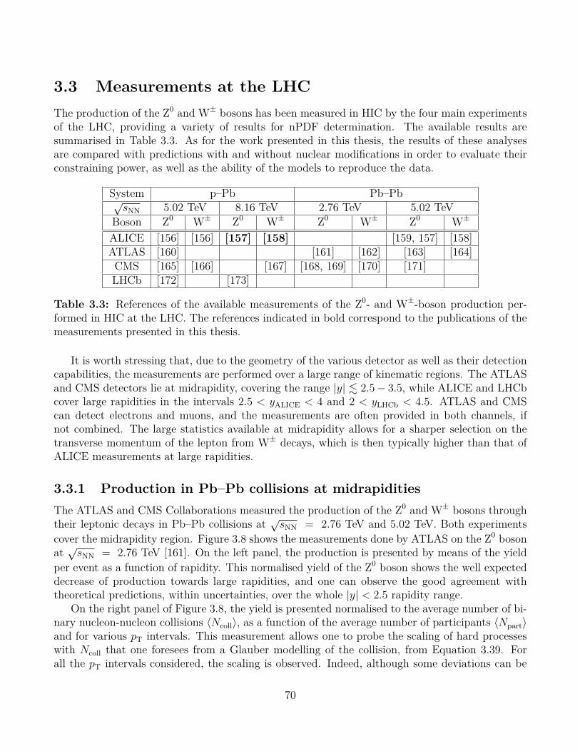
3.3 Measurements at the LHCThe production of the Z0 and W± bosons has been measured in HIC by the four main experimentsof the LHC, providing a variety of results for nPDF determination. The available results aresummarised in Table 3.3. As for the work presented in this thesis, the results of these analysesare compared with predictions with and without nuclear modifications in order to evaluate theirconstraining power, as well as the ability of the models to reproduce the data.

System p–Pb Pb–Pb√sNN 5.02 TeV 8.16 TeV 2.76 TeV 5.02 TeV

Boson Z0 W± Z0 W± Z0 W± Z0 W±

ALICE [156] [156] [157] [158] [159, 157] [158]ATLAS [160] [161] [162] [163] [164]CMS [165] [166] [167] [168, 169] [170] [171]LHCb [172] [173]

Table 3.3: References of the available measurements of the Z0- and W±-boson production per-formed in HIC at the LHC. The references indicated in bold correspond to the publications of themeasurements presented in this thesis.

It is worth stressing that, due to the geometry of the various detector as well as their detectioncapabilities, the measurements are performed over a large range of kinematic regions. The ATLASand CMS detectors lie at midrapidity, covering the range |y| . 2.5− 3.5, while ALICE and LHCbcover large rapidities in the intervals 2.5 < yALICE < 4 and 2 < yLHCb < 4.5. ATLAS and CMScan detect electrons and muons, and the measurements are often provided in both channels, ifnot combined. The large statistics available at midrapidity allows for a sharper selection on thetransverse momentum of the lepton from W± decays, which is then typically higher than that ofALICE measurements at large rapidities.

3.3.1 Production in Pb–Pb collisions at midrapiditiesThe ATLAS and CMS Collaborations measured the production of the Z0 and W± bosons throughtheir leptonic decays in Pb–Pb collisions at √sNN = 2.76 TeV and 5.02 TeV. Both experimentscover the midrapidity region. Figure 3.8 shows the measurements done by ATLAS on the Z0 bosonat √sNN = 2.76 TeV [161]. On the left panel, the production is presented by means of the yieldper event as a function of rapidity. This normalised yield of the Z0 boson shows the well expecteddecrease of production towards large rapidities, and one can observe the good agreement withtheoretical predictions, within uncertainties, over the whole |y| < 2.5 rapidity range.

On the right panel of Figure 3.8, the yield is presented normalised to the average number of bi-nary nucleon-nucleon collisions 〈Ncoll〉, as a function of the average number of participants 〈Npart〉and for various pT intervals. This measurement allows one to probe the scaling of hard processeswith Ncoll that one foresees from a Glauber modelling of the collision, from Equation 3.39. Forall the pT intervals considered, the scaling is observed. Indeed, although some deviations can be

70

Figure 3.8: Left: per-event rapidity distribution of detected Z0 bosons in Pb–Pb collisionsat √sNN = 2.76 TeV measured by the ATLAS Collaboration. The model to which the datapoints are compared correspond to Pythia-simulated events normalised to the Z0 → `` crosssection in pp collisions at the same energy taken from NNLO calculations and scaled by 〈TAA〉.The bars and boxes around the data points indicate the statistical and systematic uncertainties,respectively. Right: centrality dependence of the Z0 boson yield divided by 〈Ncoll〉 in Pb–Pbcollisions at √sNN = 2.76 TeV. Measurement for the ee and µµ channels are horizontally shiftedfor better visibility. Bars and boxes around the data points correspond to statistical and systematicuncertainties, respectively. The bracket around the combined results show the total uncertainty,including that on 〈Ncoll〉. The dashed lines are fits of the distributions with a constant. Figurestaken from Ref. [161].

seen for the independent measurements in the e+e− and µ+µ−, the combined measurements areconsistent with constants, indicated on the plots as dashed lines corresponding to fits of the data.

ATLAS also measured the production of weak bosons in Pb–Pb collisions at√sNN = 5.02 TeV.The measured yields of the Z0, W+ and W−, normalised to the average of the nuclear overlap func-tion 〈TAA〉, are reported in Figure 3.9. They are compared with theoretical predictions calculatedwith the EPPS16 [54] and nCTEQ15 [55] nPDF sets, as well as predictions from the free-nucleonCT14 [63] model, accounting for the isospin effect but without nuclear modifications. It is es-pecially interesting to note here that the measurements in Pb–Pb collisions seem to favour thepredictions without nuclear modification of the PDF. The Z0 measurements are not consistentwith predictions, although closer to free-nucleon than to nPDF models. The W± measurementsare fully consistent with the CT14-only predictions.

The most recent measurements in Pb–Pb collisions brought the uncertainties on the electroweakboson productions down to a few-percent level, and shown peculiar discrepancies with theoreticalpredictions. This triggered several theoretical studies, aiming at benefiting from the new precisionand explaining the deviation between the models and the measurements. In a study by K. Eskolaet al. [174], the standard paradigm of taking the inelastic nucleon-nucleon cross section at a value

71

Figure 3.9: Normalised yields of the Z0 (left), W+ (middle) and W− (right) bosons as afunction of the absolute rapidity (Z0) or pseudorapidity (W±) measured in Pb–Pb collisions at√sNN = 5.02 TeV by the ATLAS Collaboration. The bars and boxes correspond to the statistical

and systematic uncertainties, respectively. The measurement are compared with predictions fromthe EPPS16 [54] and nCTEQ15 [55] nPDF models, as well as prediction from the free-nucleonCT14 [63] PDF, accounting the isospin but without nuclear modifications. The bottom panelsshow the ratios of the predicted yields to the measured ones. Figures taken from Refs. [163, 164].

extrapolated from pp data is questioned as a potential source of bias. The alternative determinationthey propose leads to a nuclear-suppressed cross section that amounts to 60% of the standard value.Another study by F. Jonas and C. Loizides [175] investigates a possible effect from the centralitydetermination itself, as well as the relevance of the skin thickness in Pb which can play a significantrole at the precision level attained by the most recent experimental measurements.

3.3.2 Production in Pb–Pb collisions at large rapiditiesThe production of Z0 and W± bosons at large rapidities has been measured by the ALICE Col-laboration. The left panel of Figure 3.10 shows the Z0 invariant yield normalised to the average ofthe nuclear overlap 〈TAA〉 measured in Pb–Pb collisions at √sNN = 5.02 TeV [157]. This studyis performed on the combined data samples from the 2015 and 2018 collision periods at the LHC,improving the previous ALICE measurement done on 2015 data only [159]. Comparing the twotop points in the figure, one can appreciate the increase of precision brought by the supplementarystatistics. The measured yield is compared with predictions from the EPS09 [98], EPPS16 [54]and nCTEQ15 [55] models, with which a good agreement is found. Comparison is also drawn witha calculation using the free-nucleon CT14 [63] PDF, including the isospin effect. This calculationis clearly not consistent with the measurement, showing a deviation of 3.4 σ. This study pro-vides a significant observation of nuclear modifications. Its precision will also help reducing theuncertainties of the models.

Preliminary measurements of the W± production at large rapidities were recently released bythe ALICE Collaboration. The right panel of Figure 3.10 shows the nuclear modification factor RAA

of the W+ and W− bosons in Pb–Pb collisions at √sNN = 5.02 TeV as a function of the collisioncentrality. The factor is calculated from the invariant yield of the µ± ← W± process normalisedto the average nuclear overlap function 〈TAA〉, then divided by the centrality-independent pp cross

72

ALI-PREL-352363

Figure 3.10: Left: invariant yield of the Z0 → µ+µ− divided by 〈TAA〉 measured inPb–Pbcollisions at √sNN = 5.02 TeV. The vertical dashed band represents the statistical uncertainty onthe data while the green filled band corresponds to the quadratic sum of statistical and systematicuncertainties. The result is compared with the previous ALICE measurement in the same collisionsystem [159] as well as theoretical predictions. Figure taken from Ref. [157]. Right: preliminarymeasurement of W− and W+ nuclear modification factor in Pb–Pb collisions at √sNN = 5.02 TeV.The pp reference is taken from pQCD calculations with the CT10 PDF set [176].

section taken from pQCD calculations with the CT10 [176] free-nucleon PDF. The flat behaviourobserved for the RAA is therefore also seen for the normalised invariant yield itself, providing aconfirmation of the binary scaling expected from the Glauber model. The RAA shows an increaseof the W− production, and a decrease of that of W+, a consequence of the isospin effect whichaffects differently the bosons depending on their charge. This measurement constitutes the firstevaluation of the W± production in heavy-ion collision in this rapidity region. The finalised resultswill be published along the measurement in p–Pb collisions in Ref. [158], where they will becompared with theoretical calculations.

3.3.3 Production in p–Pb collisions at midrapiditiesThe production of Z0 measured at midrapidity by ATLAS [160] is shown in Figure 3.11. The mea-surement is made on the combination of the dielectron and dimuon channels. The measurementcover the rapidity interval |y∗| < 3.5, with y∗ denoting the rapidity in the centre-of-mass frame. Itis compared with predictions from the CT10 [176] and MSTW2008 [177] free-nucleon PDFs, theformer being NLO and the latter NNLO. Comparisons are also made with predictions includingthe nuclear modifications of the PDF by applying the EPS09 [98] modification function to theCT10 baseline. The distribution is seen to be strongly asymmetric, following the expected trendobserved in Figure 3.7. In order to evaluate the agreement between the models and data, theauthors performed a χ2 test of compatibility. The unmodified CT10 and MSTW2008 calculationshave p-values of 0.07 and 0.01, respectively, while the CT10+EPS09 combination gives a p-valueof 0.79, pointing towards a preference for the observation of nuclear correction effects from the

73

study. The same conclusion was derived from a Kolmogorov-Smirnov test [178]. It should be notedthat at midrapidity, the effect of nuclear corrections tends to be small, as the region cover severalcompeting nuclear effects.

Figure 3.11: Rapidity-differential cross section of the Z0 detected in the leptonic decay channel(e + µ) in p–Pb collisions at √sNN = 5.02 TeV with the ATLAS detector. The bars andboxes indicate the statistical and systematic uncertainties, respectively. The measurements arecompared with calculations with the CT10 [176] and MSTW2008 [177] free-nucleon PDF, andwith the EPS09 [98] nPDF set, using CT10 as baseline. The bottom panels shows the ratio of thedata to the various models. Figure taken from [160].

The production of the W± boson was measured by CMS in p–Pb collisions at√sNN = 5.02 TeVand 8.16 TeV [166, 167], in the electronic and muonic channels. As the signal is characterised by ahigh-pT lepton, a kinematic selection of pT > 25 GeV/c is applied to the data. The CMS detectorenables the evaluation of the missing transverse energy due to the final-state neutrino. The crosssections for W+ and W− are shown as a function of the lepton pseudorapidity in Figure 3.12. Theresults at √sNN = 5.02 TeV are compared with predictions from the CT10+EPS09 nuclear modeland standalone CT10 calculations. The measurement at √sNN = 8.16 TeV are compared withmore recent models, namely EPPS16 [54] and nCTEQ15 [55] for nuclear sets, and CT14 [63] forfree nucleons. The two nPDF calculations use CT14 as well, although it should be remembered

74

that EPPS16 requires a baseline for the modelisation of the Pb ion, while nCTEQ15 is a fullparametrisation of the nPDFs, and CT14 is then only used to model the incoming proton.

Figure 3.12: Production cross section of W+ (left) and W− (right), as a function of the leptonpseudorapidity, in p–Pb collisions at √sNN = 5.02 TeV (top) and 8.16 TeV (bottom) measured bythe CMS Collaboration. The error bars represent the statistical uncertainty, while brackets showthe statistical and systematic uncertainties summed in quadrature. The free-nucleon predictionsfrom CT10 [176] and CT14 [63] are shown as full bands, the predictions including the nuclearcorrections are displayed as dashed lines. They rely on the EPS09 [98], EPPS16 [54] or nCTEQ15[55] parametrisation of the nPDFs. The bottom panels show the ratio of the data and nPDFcalculations to that of the free-nucleon ones. Figures taken from [166, 167].

In the 5.02 TeV measurement, one finds the same lack of large difference between the predic-tions with and without nuclear corrections, as the size of the latter tend to be of the order ofthe corrections themselves. At 8.16 TeV, the comparison yields more meaningful results. In thenegative rapidity region, the data are compatible with all calculations within uncertainties. At

75

forward rapidities, nuclear corrections are higher and large deviations from the CT14-only predic-tions are seen. The measurement follows the trend of the nPDF by showing a depletion in thisregion. Comparing EPPS16 and nCTEQ15, one sees that the shadowing effect is more pronouncedin the latter, something which is not in agreement with the data. Over the whole rapidity range,the EPPS16 model appears to be favoured.

3.3.4 Production in p–Pb collisions at large rapiditiesThe measurements at large rapidities are possible thanks to the coverage of the LHCb detectorand the muon spectrometer of ALICE. The measurement of the Z0 boson in p–Pb collisions byLHCb is shown in Figure 3.13. The measurements are compared with NNLO predictions from theMSTW2008 [177] PDF set paired with EPS09 [98] for the nuclear corrections. Due to the shortrunning time of heavy-ion collision at the LHC, and the low production cross section of the weakboson at large rapidities, the measurement was performed from a limited number of reconstructedZ0: 4± 2 bosons at backward rapidities and 11± 3 at forward, explaining the large uncertaintiesseen in the plot. Nonetheless, one can see that the calculations at backward rapidity underestimatethe production cross section. At forward rapidity the measured production rate is fully compatiblewith calculations.

Figure 3.13: Left: Z0-boson cross section measured in p–Pb collisions at √sNN = 5.02 TeVby the LHCb Collaboration, at backward and forward rapidities. The inner bands represent thesystematic uncertainty, while the outer ones indicate the statistical and systematic uncertaintiessummed in quadrature. The measurements are compared with predictions from the MSTW2008[177] PDF set, with and without including the nuclear corrections using EPS09 [98]. The un-certainties on the theoretical predictions are negligible compared to those on the experimentalresults, they are therefore not shown. Figure taken from Ref. [172]. Right: same measurementsfrom p–Pb collisions at √sNN = 8.16 TeV. The error bars correspond to the total uncertainty.Predictions from the NNDPF3.1 [49] free-PDF set are shown, along with calculations includingthe nuclear corrections from the EPPS16 [54] and nCTEQ15 [55] models. Figure taken from Ref.[173].

76

The ALICE Collaboration measured the production of the Z0 and W± bosons in p–Pb collisionsat √sNN = 5.02 TeV and 8.16 TeV. The measured cross sections are shown in Figure 3.14. Hereas well, the limited statistics in the data leads to rather large uncertainties on the measurement,while the ability to control the detector misalignment created a significant amount of systematicuncertainty. It is interesting to note for the W± cross section the different behaviour of W+

and W−, and especially the large suppression of the W+ production at backward rapidities. Themeasurements are compared with two free-PDF models, MSTW2008 [177] and CT10 [176], bothwith and without nuclear corrections using EPS09 [98]. The usage of different baselines mayintroduce sizeable differences, although this is not the case with more recent sets that tend to becompatible with one another. As seen at the edges of the rapidity intervals probed by CMS, thenuclear modifications are rather negligible at backward rapidity while they are not at forward.Yet, the uncertainties on the measurements does not allow for drawing any strong conclusion onthe nuclear corrections, as they are generally compatible with predictions regardless of whetherthe nuclear corrections are implemented or not.

Figure 3.14: Cross sections of Z0 (left), W+ (middle) and W− (right) in the muonic decay channel,measured at forward and backward rapidities by the ALICE Collaboration in p–Pb collisions at√sNN = 8.16 TeV. The bars and boxes represent the statistical and systematic uncertainties,

respectively. The results are compared with theoretical calculations with the CT10 [176] andMSTW2008 [177] free-PDF sets, paired with the EPS09 [98] parametrisation of the nPDF. In thetop panels, the predictions are horizontally shifted for better visibility. The bottom panels showthe ratio of data and EPS09 to the free-nucleon predictions. Figures taken from Ref. [156].

The ALICE Collaboration also measured the Z0 and W± productions in p–Pb collisions at√sNN = 8.16 TeV [157, 158], which constitutes the topic of this work. The analyses and results

are described in details in Chapters 8 and 9.

77

Part II

A Large Ion Collider Experiment

79

Chapter 4

The ALICE detector

This chapter presents the ALICE detector. A brief overview of ALICE in the context of the LHCat CERN is given, followed by an overview of the detector itself and a description of its so calledglobal detectors and central barrel subsets. As the analysis presented in this thesis relies on datataken with the muon spectrometer, this part of the apparatus is described in detail in the dedicatedfollowing chapter.

4.1 The Large Hadron Collider

4.1.1 LHC at CERNThe Large Hadron Collider (LHC) is a large and powerful circular collider installed at the Eu-ropean Organization for Nuclear Research (CERN1), in the 26.7 km diameter tunnel previouslyoccupied by the Large Electron-Positron collider (LEP). It sits at the end of the CERN acceleratorcomplex, displayed in Figure 4.1. It delivered its first proton beam in 2009. The LHC is designedfor very-high energy hadronic collisions, reaching the ultra-relativistic regime. Even before theconstruction of the LHC, the CERN had a long history of scientific achievements [179], such asthe discovery of neutral currents, the first observation of the W± and Z0 bosons, the creation andmanipulation of antihydrogen atoms and the report of direct CP violation. In the LHC era, thepeak achievement is the observation of a boson consistent with the Higgs boson predicted 40 yearsearlier. A detailed description of the LHC can be found in Ref. [180].

Along the LHC sit four main experiments, each targeting different physics goals and featuringdifferent detection methods to reach them:

• A Large Ion Collider Experiment (ALICE) [181]: a multipurpose experiment optimisedfor the high-multiplicity environment created by heavy-ion collisions, and through them thestudy of the strongly interacting matter;

1The CERN acronym comes from the former name of the organisation, European Center for Nuclear Research,in french Centre Européen pour la Recherche Nucléaire.

81

Figure 4.1: The CERN facility. The arrows indicate the path taken by the various particlebeams, from their production site to the collision points.

• A Toroidal LHC ApparatuS (ATLAS) [182]: a multipurpose experiment, designed forhigh luminosity pp mode in order to search for new particles and physics beyond the StandardModel;

• Compact Muon Solenoid (CMS) [183]: another general purpose experiment, with thesame goals as ATLAS but using different technical solutions;

• LHC beauty (LHCb) [184]: a fully instrumented forward spectrometer focusing on Pviolation, heavy-flavor CP violation and the matter-antimatter asymmetry, mainly throughbeauty physics.

Although ALICE is the only detector dedicated to heavy-ion collisions, all the experiments havean heavy-ion program. Following their respective designs and physics goals, they have variousgeometrical acceptances, allowing them to cover the phase space in a complementary way. Atypical year of data taking at the LHC contains a lengthy time dedicated to pp mode, a few weeksfor heavy-ion collisions, followed by a winter shutdown. Data taking happens several years in arow, after which a Long Shutdown (LS) takes place, allowing the collaborations to repair andupgrade their detectors, and the LHC teams the accelerator. Two shutdowns have happened since

82

the starting of the LHC, LS1 from 2013 to 2015 and LS2, started in 2018 and still ongoing at thetime of writing of this thesis.

4.1.2 Injection and beamsThe CERN accelerator complex relies on using previous accelerators as injectors for the new ones.The injection chain is sketched in Figure 4.2: before reaching the LHC itself, a particle is pre-accelerated in a chain of accelerators. The proton source is a simple bottle of hydrogen gas. Thehydrogen atoms are stripped off their electron with an electric field, then injected into the LinearAccelerator 2 (LINAC2), the first accelerator of the chain, before moving to the circular ProtonSynchrotron (PS) and Super Proton Synchrotron (SPS), reaching an energy of 50 MeV, 28 GeVand 450 GeV at each stage. The lead beam is obtained by evaporating Pb atoms, removing the29 outermost electrons electrically. The resulting ions are accelerated by LINAC3, sent through a1 µm-thin layer of carbon, removing 25 more electrons, and injected into and accelerated by theLow Energy Ion Ring (LEIR) then PS, from where they follow the same chain as the protons. Theremaining 28 electrons are removed by an aluminium foil after PS. During these steps, the protonsand lead are assembled in hundreds of bunches forming a train (a proton beam typically containsabout 2 800 bunches with 1011 protons each at start). In such a train, the minimal bunch spacing,defined as the minimal time between two injections in the SPS, is about 25 ns.

LINAC3 LEIR(78 m)

PS(628m)

SPS(7 km)LINAC2

Pb29+

Pb54+4.2 MeV/nucleon

Pb54+72 MeV/nucleon

Pb82+5.9 GeV/nucleon

Pb82+177 GeV/nucleon

H+

H+

50 MeVH+

28 GeVH+

450 GeV LHC(27 km)

Figure 4.2: The LHC injection chain for proton and lead beams. The energy per nucleon attainedafter each accelerator and, for Pb, the ionisation, are indicated.

The two beams are finally sent in the two beam pipes of the LHC, one circulating clockwiseand the other anticlockwise. They are accelerated using electromagnetic resonators, kept intocircular orbits by means of dipole magnets, and brought to collision at four points where themain LHC experiments are installed. Under normal operation conditions, the beams can circulateseveral hours in the LHC, after which their intensity diminishes and the collision rate becomes toolow. As to maximise the collision probability, they are collimated before the interaction pointsusing quadrupole magnets. Table 4.1 indicates the nucleon-nucleon centre-of-mass energy √sNN,luminosity L and geometrical cross section σgeom under nominal running conditions for the threemain collision configurations: proton-proton (pp), proton-lead (p–Pb) and lead-lead (Pb–Pb).

83

Mode √sNN (TeV) L (cm-2s-1) σgeom (b)

pp 14.0 1034 0.07p–Pb 8.8 1029 1.9

Pb–Pb 5.5 1027 7.7

Table 4.1: LHC nominal nucleon-nucleon centre-of-mass energy √sNN, luminosity L and geomet-rical cross section σgeom for pp, p–Pb and Pb–Pb collisions.

4.2 Overview of ALICEAt the time of writing of this thesis, the ALICE collaboration consisted in 1,975 members from 170institutes in 40 countries. Its 300th publication came out in 2020. The collaboration uses a 26 mlong, 16 m wide and 16 m high detector, weighting 10 000 tons, buried 56 m underground at one ofthe LHC interaction points. The detector is designed to cope with the high particle multiplicitiesexpected in the most central heavy-ion collisions (dNch/dy up to 8 000) while still being able totrack and reconstruct particles from very low to fairly high transverse momentum (pT), between∼ 100 MeV/c and ∼ 100 GeV/c. Figure 4.3 shows a cross sectional view of the detector. In thischapter, the ALICE detector is presented in its configuration during the LHC Run 2, when thedata used for the measurements presented in this thesis were collected. The configuration for theRun 3, accounting for the upgrade of LS2, will be described in Chapter 7.

The ALICE subdetectors can be regrouped in three main ensembles, whose composition andusage are described in more details in the next sections:

• a set of global detectors participating in the event triggering and providing general informa-tion on the collision, such as the collision centrality and multiplicity, and the event planereconstruction;

• the central barrel, covering the mid-rapidity range, used for primary vertex reconstruc-tion, tracking of charged particles, particle identification of electrons, photons and chargedhadrons, and detection of jets;

• the muon spectrometer, aiming at detecting the muon decay products of low mass mesons(ρ, φ, ω), quarkonia, heavy-flavor hadrons and weak bosons at large rapidity.

The combination of the central barrel and muon spectrometer gives ALICE a large spatialcoverage, illustrated in Figure 4.4 in which it is compared to the acceptance of the other LHCexperiments.

The ALICE coordinate system [186] is a right-handed orthogonal Cartesian system with theorigin at the collision point. The z axis follows the beam line, with the muon spectrometer atnegative z. The positive and negative sides are conventionally referred to as A-side and C-side,respectively. Table 4.2 summarises the names, acceptances, positions and roles of the varioussubparts of the detector. Complementary to what is presented in this thesis, one can refer to the

84

Fig

ure

4.3:

Sche

mat

ics

ofth

eA

LIC

Ede

tect

oran

dits

subp

arts

.T

here

gion

arou

ndth

eco

llisio

npo

int

isde

taile

din

the

top

right

pane

l.

85

Detector Acceptance Position Main purposePolar AzimuthalGlobal detectors

ZDC: ZN |η| > 8.8 full z = ±113m forward neutronsZDC: ZP 6.5 < |η| < 7.5 |φ| < 10 z = ±113m forward protons

ZDC: ZEM 4.8 < |η| < 5.7 |2φ| < 32 z = 7.3m photonsPMD 2.3 < η < 3.9 full z = 367cm photons

FMD disc 1 3.6 < η < 5.0

full

z = 320cm

charged particlesFMD disc 2 1.7 < η < 3.7inner: z = 83cmouter: z = 75cm

FMD disc 3 −3.4 < |η| < −1.7 inner: z = −63cmouter: z = −75cm

T0 A-side: 4.6 < η < 4.9

full

z = 370cm charged particlesC-side: −3.3 < η < −3.0 z = −70cm

V0 A-side: 2.8 < η < 5.1 z = 340cm time, vertexC-Side: −3.7 < η < −1.7 z = −90cm

AD A-side: 4.8 < η < 6.3 full z = 170cm diffractive eventsC-side: −7.0 < η < −4.9 z = −195cmCentral barrel

ITS layer 1,2 (SPD) |η| < 2.0, |η| < 1.4full

r = 3.9, 7.6cm tracking, vertexITS layer 3,4 (SDD) |η| < 0.9, |η| < 0.9 r = 15.0, 23.9cm tracking, PIDITS layer 5,6 (SSD) |η| < 1.0, |η| < 1.0 r = 38, 43cm

TPC |η| < 0.9 full 85 < r < 247 tracking, PIDTRD |η| < 0.8 full 290 < r < 368cm tracking, e± identificationTOF |η| < 0.9 full 370 < r < 399cm PID

HMPID |η| < 0.6 1 < φ < 59 r = 490cm PIDPHOS |η| < 0.12 220 < φ < 320 460 < r < 478cm photons

EMCAL |η| < 0.7 80 < φ < 187

430 < r < 455cm photons, jetsDCAL 0.22 < |η| < 0.7 260 < φ < 320

|η| < 0.7 320 < φ < 327

ACORDE |η| < 1.3 30 < φ < 150 r = 850cm cosmic rays, calibrationMuon spectrometer

Tracking station 1

−4.0 < η < −2.5 full

z = −5.36m

muon trackingTracking station 2 z = −6.86mTracking station 3 z = −9.83mTracking station 4 z = −12.92mTracking station 5 z = −14.22mTrigger station 1 −4.0 < η < −2.5 full z = −16.12m muon triggeringTrigger station 2 z = −17.12m

Table 4.2: Position, geometrical coverage and main purpose of the ALICE subdetectors. Adaptedfrom [185].

86

η10− 8− 6− 4− 2− 0 2 4 6 8 10

SPD (Layer 1)

SPD (Layer 2)ZDC:ZN ZDC:ZNZDC:ZPZDC:ZP ZDC:ZEM

SDD V0AV0C

SSD T0AT0C

TPCMUON

TRD PMD

TPC FMD (disc 1)

HMPID FMD (disc 2)FMD (disc 2)

Figure 4.4: Left: Pseudorapidity coverage of the ALICE subdetectors. Right: Comparison ofthe geometrical acceptances of the main LHC experiments.

Technical Design Report [187] of the subdetectors and the various Physics Performance Reports[188, 189, 185] for more information.

4.3 Global detectorsThe event characterisation in ALICE mostly relies on a set of detectors lying at large rapidities,both in the forward and backward regions. They provide general information on the event, suchas the centrality, the reaction plane and the trigger decision. They participate as well in theevaluation of the luminosity, and the rejection of background induced by beam-gas interactions. Ashort description of these detectors is given here, along with selected examples of their usage andperformances.

4.3.1 Constituents• Zero Degree Calorimeter (ZDC) [190]: the ZDC is made of two identical sets of two

hadronic calorimeters each: one for proton (ZP) and one for neutrons (ZN). The sets arelocated along the beam pipes, on both sides of the collision point, 113 m away from it. Theyaim at measuring the energy of the spectator nucleons for an estimation of the collisioncentrality. They are made of dense material slabs, in which silica optical fibres are embeddedas active material, detecting the Cherenkov light produced by the charged particles of theshower created when a nucleon hits the calorimeter. The spectator protons are separatedfrom the beam by the LHC beam optics, while spectator neutrons fly at zero degree withoutchanging direction. The ZN have to sit in between the two beam pipes and have thereforethe tightest geometrical constraints with a transverse dimension required to be smaller than7 cm. A dense tungsten alloy was chosen as to maximise the shower containment. The ZP,sitting outside the pipes, is made of larger, less expensive brass absorbers.

87

The two sets are completed by an electromagnetic calorimeter, the ZEM, placed at largerapidity on the A-side. Made of lead and quartz fibres, it is used to remove ambiguities inthe centrality determination: in peripheral collisions many nucleons remain bound in largenuclear fragments that continue to travel in the beam pipe without being detected by theZDC, having a magnetic rigidity close to that of the beam. The ZEM helps resolving suchambiguities by providing an estimation of the number of participant nucleons. By comparingthe energy measured by the ZEM with the one measured by ZN and ZP, one is comparingthe number of participant and spectator nucleons from which the centrality of the collisioncan be evaluated.

• Photon Multiplicity Detector (PMD) [191]: the PMD is a particle shower detector,placed on the A-side at 3.6 m from the collision point. It is made of two identical planes ofclosely packed hexagonal proportional counters, filled with an Ar+CO2 mixture and encom-passing a thick lead converter. The plane behind the converter registers hits from photonsand charged particles, while the plane in front of it is used for vetoing charged particles, asto disentangle the photon signal. The PMD enables the measurement of the photon multi-plicity and spatial distribution (in the η−φ space) and helps providing an estimation of thetransverse electromagnetic energy and reaction plane of the event.

• ALICE Diffractive (AD) [192]: the AD detector was installed during the first long shut-down of the LHC, between 2013 and 2014. It is composed of two stations installed on eachside of the interaction point at very large rapidities. The stations contains two layers of 4scintillators plastics of about 18 × 21 cm2 each. The light generated by charged particleshitting the scintillators is converted by photomultipliers. The AD aims at extending theacceptance for low diffractive masses, it also improves the trigger efficiency for MinimumBias events.

• Forward detectors: Forward Multiplicity Detector (FMD), T0, V0 [193]: the con-ventional denomination of “forward detectors” actually regroups three apparatus, all sittingat large rapidities: the FMD, T0 and V0. They result from the splitting of the initiallypreferred solution of a unique device for fast triggering and multiplicity information in theforward and backward regions.

FMD The FMD consists of five rings of silicon strip detectors, each containing 10 240silicon sensors regrouped in 10 or 20 wafers. It aims at evaluating the charged particlemultiplicity at large rapidities. Together with the Inner Tracking System of the central barrel,they provide an early multiplicity measurement, fully covering the −3.4 < η < 5.1 range andfor all collision systems. The FMD also participates in the evaluation of correlations, thecollective flow and the reaction plane of the event.

T0 The T0 is made of two arrays of 12 Cherenkov counters each, asymmetrically placedon the A- and C-side at z = 375 cm and z = −72.7 cm respectively. Its time resolution ofabout 50 ps makes it useful for fast triggering, providing a wake-up signal to the Transition

88

Radiation Detector and delivering a collision time reference to the Time-Of-Flight. Themeasurement of the vertex position with a precision of ±1.5 cm yields a fast trigger byconfirming the position of the interaction point within pre-defined limits. Coupled to ameasurement of the particle multiplicity, it generates three possible trigger signals: minimumbias, semi-central and central. The T0 is also used as a reference in Van Der Meer (vdM)scans for the evaluation of the visible cross section.

V0 The V0 consists of two arrays of scintillator tiles, each segmented in 4 concentric ringsand 8 sectors of 45 in azimuth, asymmetrically placed around the collision point at z = 340cm (V0-A) and z = −90 cm (V0-C). The main goals of the V0 are to provide an onlinetrigger through the coincidence of a signal in the two arrays, as well as background-rejectioncapabilities. It is used to provide a wake-up signal to the Transition Radiation Detector(TRD) of the central barrel. The measured signal amplitude is used for the determinationof the centrality via a Glauber model fit, and the measurement of the particle time-of-flightbetween the two arrays helps to discriminate again beam-gas interactions. As for the T0,the V0 participates in the evaluation of the visible cross section by means of vdM scans.

4.3.2 V0-based triggering and beam-gas rejectionOne of the main goal of the V0 is to provide a Minimum Bias (MB) trigger for all collision systemsand centrality-based triggers in AA collisions. The V0-based triggers used throughout the ALICEoperating since 2009 are listed in Table 4.3. The measurement of the time-of-flight between thetwo arrays allows as well an efficient rejection of background signals from beam-gas interactions.

Trigger name ConditionMB-OR signals in V0 and SPD (obsolete)MB-AND signals in V0-A and V0-C

MBZ MB and signal in both ZDC

Table 4.3: Minimum Bias triggers provided by the V0.

In the 2009 and 2010 pp periods, the MB-OR trigger was used, requiring a signal in the centralbarrel Silicon Pixel Detector (SPD, corresponding to the two innermost layers of the ITS) or ineither of the two arrays of the V0. With the increase of luminosity and background after 2010,the high-efficiency MB-OR was replaced by the high-purity MB-AND, requiring hits in both arrays.The triggering on MB events can be extended with the requirement of having also a signal fromthe two arrays of the ZDC. On top of the MB triggers, the V0 provides centrality-based triggersthrough the application of thresholds on the summed-up signals. Several amplitude triggers canbe defined, corresponding to various centrality ranges of interest, among which the 0–10%, 0–50%and 30–50% ranges are commonly used. The left panel of Figure 4.5 shows the number of recordedevents, for MB and two centrality classes, in Pb–Pb collisions at√sNN = 5.02 TeV in 2015 and 2018.

89

ALI-PERF-313420

(ns)V0C

tV0At

20 10 0 10 20 30

(n

s)

V0C

+ t

V0A

t

20

10

0

10

20

30

1

10

210

310 = 7 TeVspp

ALI−PUB−70649

Figure 4.5: Left: Number of recorded events for MBZ and centrality-based triggers from theV0, as a function of time in Pb–Pb collisions at √sNN = 5.02 TeV. Right: Correlation betweenthe sum and difference of signal times in V0-A and V0-C in pp collisions at √sNN = 7 TeV. Thecollision events at (8.3 ns, 14.3 ns) can be distinguished from the background from beam 1 at(-14.3 ns, -8.3 ns) and beam 2 at (14.3 ns, 8.3 ns). Figure taken from Ref. [185].

The LHC beam pipes feature a very high, yet non-perfect vacuum which constitutes a sourceof background through the interaction between the beams and the residual gas in the pipes. Thissource can be efficiently reduced thanks to the two arrays of the V0, by measuring the time-of-flightof particles on each side and applying an offline selection. This measurement, in pp collisions at√sNN = 7 TeV, is shown in the right panel of Figure 4.5. At the front-end electronics level, a

coincidence window of 8 ns is placed around the beam-beam timing in order to select beam-beamevents and reject a great part of the beam-gas events. Since the 2012 run, this selection criterionis also partially applied at the hardware level.

4.3.3 Luminosity and visible cross sectionsIn scattering theory the luminosity L is the ratio of the number of events N detected per unit oftime (dN/dt) to the total inelastic cross section σinel. It has the dimension of events per area pertime (m-2s-1), often expressed with the non-SI units of barn: b-1s-1. The integral of L with respectto time defines the integrated luminosity Lint:

L =1

σinel

dN

dt, Lint =

∫Ldt. (4.1)

Its evaluation in ALICE for a given data sample is based on the visible cross section σvis seenby a detector. One needs to define a class of inelastic events satisfying a given trigger condition,hereafter referred to as the reference process. The visible cross section is a fraction of σinel:

σvis = ε× σinel, (4.2)

90

where ε is the fraction of inelastic events satisfying the trigger condition. Once σvis is measured,the luminosity can be evaluated as the ratio between the rate R of the reference process and thevisible cross section:

L =R

σvis. (4.3)

With this procedure one does not need to know ε, and the measurement of σvis provides an absolutenormalisation factor for indirect luminosity determination in data analysis.

The visible cross section of a chosen reference process can be measured by means of vdM scans[194, 195], in which the two beams are moved across each other in the x and y directions (inthe horizontal and vertical planes respectively). The x and y scans are performed separately, thebeams being head-on in the other direction. At a circular collider, the measurement of the rateof the reference process as a function of the beam separation ∆x and ∆y allows one to determinethe head-on luminosity for a pair of colliding bunches with particle intensities n1 and n2 as:

L =n1n2frevhxhy

, (4.4)

where frev is the collider revolution frequency and hx and hy are the effective beam widths in thex and y directions. They are measured as the area below the R(∆x, 0) and R(0,∆y) curves nor-malised to the head-on rate R(0, 0). Using the latter and the luminosity computed with Equation4.4, and solving Equation 4.3, one can evaluate σvis.

Coincidence between signals in the two arrays of the V0 (i.e. the MB-AND trigger) and the T0provide useful reference processes for the evaluation of σvis [196]. In the T0 case, an additionalcriterion requests that the longitudinal coordinate of the interaction vertex is within ± 30 cm of thenominal collision point. This criterion is applied through the time difference of the signals in T0-Aand T0-C, and aims at rejecting beam-gas and satellite background. Signal in one of the ZDCneutron calorimeters can also be used as reference, providing a sensitivity to both electromagneticdissociation events with single- or double-sided neutron emission, and hadronic events. Figure 4.6shows an example of visible cross section measurement in p–Pb collisions, using V0- and T0-basedreference processes.

4.3.4 Centrality determinationThe centrality c is defined as the percentage of the total hadronic cross section, which experimen-tally corresponds to either a particle multiplicity Nch or an energy deposition in the ZDC EZDC,as measured by the detector, above or up to a certain threshold N thr

ch or EthrZDC:

c ≈ 1

σAA

∫ ∞N

thrch

dσ

dNch

dNch ≈1

σAA

∫ EthrZDC

0

dσ

dEZDC

dEZDC. (4.5)

The procedure for the centrality estimation in ALICE is briefly summarised here. More detailscan be found in Ref. [197] and references herein.

91

Figure 4.6: Visible cross sections for the V0 (red) and T0 (blue) processes measured in vdMscans in p–Pb (left) and Pb–p (right) collisions at √sNN = 8.16 TeV, as a function of the productof the colliding bunches intensities. The top and bottom plots correspond to two different scans,the solid line is a constant fit to the data. Figure taken from [196].

The centrality related geometrical quantities, Npart and Ncoll, corresponding to the number ofparticipant nucleons and binary collisions respectively (see Section 2.3), are usually obtained bymeans of Monte Carlo implementations of the Glauber model [85]. The nucleon position ρ(r) in thenucleus is modelised stochastically using a modified Woods-Saxon (or 2-parameter Fermi) distri-bution, and the Glauber MC is coupled to a Negative Binomial Distribution (NBD) [198] to ensurean adequate reproduction of the data. The parameters of the resulting, so called NBD-Glaubermodel are determined by fitting the amplitude of the signal collected in the V0, as illustrated inFigure 4.7. The mean number of participants 〈Npart〉 and binary collisions 〈Ncoll〉 can then becalculated for centrality classes defined by sharp cuts in the simulated V0 distribution.

While this method provides an efficient evaluation of the centrality in Pb–Pb collisions, itsuffers from an important caveat in p–Pb, namely the multiplicity fluctuations [200]. For p–Pb collisions, those fluctuations are sizeable compared to the width of the Npart distribution, acentrality selection based on multiplicity may then select a sample of nucleon-nucleon collisionswhich is biased compared to a sample defined by cuts on the impact parameter b. The NBD-Glauber fit itself allows one to quantify this effect. In the left panel of Figure 4.8 is shown theratio between the average multiplicity per average participant to the average multiplicity of theNBD-Glauber fit as a function of centrality. As expected, the ratio does not deviate from unitywhen the classes are defined by a selection on b. In Pb–Pb, the ratio deviates for the most peripheralcollisions only, reflecting the fact that the width of the plateau of the Npart distribution is large withrespect to multiplicity fluctuations. On the contrary, in p–Pb collisions and for multiplicity-basedestimators, large deviations are found both in the central and peripheral regions.

This motivated the development of the so-called hybrid method, aiming at providing an unbi-

92

V0A amplitude (arb. units)0 200 400 600 800 1000

Eve

nts

(arb

. uni

ts)

5−10

4−10

3−10

2−10

= 8.16 TeVNNsPb, −ALICE, pDataNBD-Glauber fit

= 0.44)k = 21.4, µ NBD (⊗ partN

5%−0

10%

−5

20%

−10

40%

−20

60%

−40

80%

−60

0 50 100 150

3−10

60%

−40

80%

−60

100%

−80

Figure 4.7: Distribution of the sum of amplitudes in V0-A (Pb-going side) for p–Pb collisions at√sNN = 8.16 TeV. The distribution is fitted with the NBD-Glauber model, shown as a line. The

insert shows a zoom of the most peripheral region. The failure of the NBD-Glauber fit at very lowamplitude reflects the trigger inefficiencies in peripheral collisions. Figure taken from Ref. [199].

ased centrality estimator. The method, described in Ref. [200], relies on two assumptions:

• the energy deposited in the ZDC is free from the multiplicity bias,

• some observables scale linearly with Ncoll and Npart, according to the wounded nucleon model[201, 202].

Two such observables are used, either assuming that the charged-particle multiplicity at mid-rapidity is proportional to Npart, or that the target-going (here the Pb ion) charged-particle mul-tiplicity is proportional to the number of wounded target nucleon (with N target

part = Npart− 1 = Ncoll

in p–Pb). These two assumptions lead to the computation of two sets of 〈Ncoll〉: 〈Nmultcoll 〉 in the

former case and⟨NPb−side

coll

⟩in the latter. In the right panel of Figure 4.8 is shown the effect of

using the hybrid method for the centrality evaluation in p–Pb collisions. The charged-particlemultiplicity, scaled to 〈Npart〉, shows a flat trend which one can extrapolate to the pp measurement(black point). Table 4.4 reports the value of 〈Ncoll〉 obtained with the two methods for variouscentrality classes.

4.4 Central barrelThe central barrel of ALICE, sitting in the mid-rapidity region, contains three main ensembles. Thetracking system (ITS and TPC) provides a measurement of the primary vertex position and enablesthe tracking and identification of charged particles. The particle identification system (TRD, TOF

93

Centrality [%]0 10 20 30 40 50 60 70 80 90 100

µ /

⟩

ancesto

r N⟨

/

⟩ M

ultip

licity

⟨

0

0.2

0.4

0.6

0.8

1

1.2

1.4

1.6

1.8

2V0A

CL1

V0C

V0M

b (imp.par)

V0M (PbPb)

GlauberMC

= 5.02 TeVNNspPb

= 2.76 TeVNNsPbPb

ALI−PUB−100573

Figure 4.8: Left: Multiplicity fluctuation bias quantified as the mean multiplicity per averageparticipant over the average multiplicity of the NBD-Glauber fit µ as a function of centrality. Figuretaken from Ref. [200]. Right: Charged particle multiplicity normalised to the average numberof participant 〈Ncoll〉 for different centrality estimators, in p–Pb collisions at √sNN = 8.16 TeV.The same quantity measured in pp collisions at √sNN = 8 TeV is given for reference. Figure takenfrom Ref. [199].

Centrality (%) 〈Nmultcoll 〉

⟨NPb−side

coll

⟩syst. (%)

0–5 13.4 14.2 6.45–10 12.5 12.9 3.910–20 11.5 11.8 3.420–40 9.81 9.77 2.340–60 7.09 6.83 4.360–80 4.28 4.09 4.980–100 2.08 2.13 3.3

Table 4.4: Average number of collisions 〈Ncoll〉 evaluated from the multiplicity either at midra-pidity or on the Pb-side (〈Nmult

coll 〉 and⟨NPb−side

coll

⟩respectively) with the hybrid method, in p–Pb

collisions at √sNN = 8.16 TeV. Table adapted from Ref. [197].

and HMPID) supports the PID capabilities of the tracking system, notably by improving theseparation of protons, kaons, pions and electrons over a wide pT range. Finally, the calorimetrysystem (PHOS, EMCAL and DCAL) extends the measurement in the central barrel to neutralparticles. The central barrel is immersed in a low magnetic field (≤ 0.5 T) delivered by the L3magnet.

94

4.4.1 Detector layout• Inner Tracking System (ITS) [203]: the ITS consists of six layers of silicon detectors, cov-

ering |η| < 2 for the innermost layer and |η| < 1.4 for the outermost one, located at r = 3.9cm and r = 43 cm respectively. The six layers are regrouped in three subsystems, from theinside out one finds: two layers of Silicon Pixel Detectors (SPD), two layers of Silicon DriftDetectors (SDD) and two layers of Silicon Strip Detectors (SSD). The ITS aims at measuringprimary and secondary vertices, participating to the particle identification, supporting thetracking capabilities of the TPC at low momenta and providing a measurement of the multi-plicity at mid-rapidity. Combined with the FMD, it allows for a continuous measurement ofthe multiplicity in the range −3.4 < η < 5.1. While the six layers operate together at a lowfrequency (100 Hz) to match the pace of the central barrel, the SPD can run at higher rate(1 kHz) in order to provide the vertex information to the faster-paced muon spectrometer.

• Time-Projection Chamber (TPC) [204]: the TPC is a 90 m2 cylinder filled with anAr+CO2 gas mixture, divided into two drift sectors by a central electrode. The end caps arestructured into 18 trapezoidal regions on each side, equipped with multi-wire proportionalchamber with cathode pad readout. The magnetic field delivered by the L3 magnet, coupledto the size of the TPC which longitudinal extension amounts to about 500 cm, leads to a drifttime of 88 µs, limiting the recording rate in the central barrel. The TPC is the main devicefor particle identification and charged particle tracking at mid-rapidity. In combinationwith the ITS, it provides as well a precise measurement of the vertex position, even in thelarge-multiplicity environment created in heavy-ion collisions.

• Transition Radiation Detector (TRD) [205]: the TRD is composed of 540 modules,each containing a 4.8 cm thick radiator and a multiwire proportional chamber with cathodepad readout. They are regrouped in 18 sectors of 6 layers with a 5-fold segmentation alongthe beam direction. The TRD was designed for electron identification through electron-piondiscrimination, and in combination with the ITS and TPC it allows for the measurement ofvector meson resonances and open heavy flavors.

• Time-Of-Flight (TOF) [206, 207]: the TOF detector consists of multigap resistive platechambers arranged in 18 sectors in azimuth and 5 sectors along z. They feature a high anduniform electric field over the sensitive volume, such that any traversing particle immediatelytriggers an avalanche, generating signals picked-up by electrodes. With a time resolutionbetter than 40 ps and an efficiency close to 1, the TOF is able to identify protons, pions andkaons in the intermediate momentum range.

• High-Momentum Particle Identification Detector (HMPID) [208]: the HMPID iscomposed of 7 proximity-focusing ring imaging Cherenkov counters of about 1.5 × 1.5 m2

each, providing a partial azimuthal coverage of 58. The Cherenkov radiation is emitted whena charged particle crosses the 15 mm thick perfluorohexane radiators and collected by photoncounters made of multiwire pad chambers. The HMPID extends the TOF identification ofprotons, kaons and pions to higher momenta.

95

• Calorimeters: PHOton Spectrometer (PHOS), ElectroMagnetic CALorimeter(EMCAL), Di-jet CALorimeter (DCAL) [209, 210, 211]: outside of the HMPID sits aset of calorimeters with partial azimuthal coverages, extending the detection and trackingabilities of ALICE to photons and jets. Initially composed of the PHOS and EMCAL, theset was completed during the first long shutdown of the LHC (LS1) with the DCAL, installedback-to-back in azimuth with the EMCAL, to achieve correlation analysis.

PHOS The PHOS is composed of an ElectroMagnetic Calorimeter (EMC) made of highly-segmented, dense lead-tungstate crystals. The electromagnetic shower created when a parti-cle hits the EMC is detected by avalanche photodiodes. As to discriminate between chargedand neutral particles, a Charged Particle Veto (CPV), made of multiwire proportional cham-bers with cathode pad readout, is installed in front of the EMC. The 99% efficiency of theCPV allows the PHOS to measure photons and neutral mesons in their photonic decays ina large momentum range.

EMCAL and DCAL The EMCAL and DCAL (commonly referred to as EMCAL) arelayered Pb-scintillators sampling calorimeters with alternating layers of 1.44 mm of lead and1.76 mm of polystyrene scintillators, in which electromagnetic particles lose their energy via acombination of brehmsstrahlung radiation and pair creation. The EMCAL enhances ALICE’scapabilities to measure jets and high-momentum photons and electrons. The addition ofDCAL at opposite azimuth from EMCAL, thus forming a two-arm calorimeter, enables thestudy of back-to-back correlations where jets are involved. The EMCAL also serves fortriggering on high-energy jets.

• ALICE COsmic Ray DEtector (ACORDE) [212]: on top of the L3 magnet sits ACORDE,a scintillator array for triggering on cosmic rays. 60 modules are distributed on the threeupper surfaces of the magnet. Each contains two 0.2 × 2 m2 paddles of plastic scintillatorsarranger in a doublet configuration. The trigger hit is provided by a coincidence signal inthe two paddles within a time window of 40 ns. The signal can be used for the calibration,alignment and performance studies of other ALICE tracking devices (ITS, TPC and TRD),which tracking precision enables the recording of interesting cosmic events with very highmultiplicity of parallel muon tracks, the so-called muon bundles.

4.4.2 Primary vertex reconstructionThe determination of the primary vertex relies on the preliminary estimation made by the SPD,which is afterwards constrained using the tracks reconstructed by the tracking systems of the cen-tral barrel.

A first estimation is performed by looking at tracklets in the innermost layers of the ITS. Twohits in the SPD layers, having similar azimuthal angles, are assumed to come from the same sourceand define a tracklet. By linear extrapolation, a preliminary estimation of the corresponding

96

track is estimated. Due to the presence of the bending magnet, the linear extrapolation is anapproximation, but the proximity of the SPD to the nominal collision point allow for a preciseenough estimation with this procedure. For a given event, a first evaluation of the primary vertexis performed by fitting all the tracks for their crossover point. As to account for a possible pile-up,in which several collisions happen in a small enough time window such that they are mixed intoa single event, the fitting procedure is iterated, discarding at each step the tracks participating tothe determination of the previous vertex. By construction, the first vertex found has the largestnumber of contributing tracks and is taken as the primary one. As the SPD is able to operate ata rate higher than the one of the other ITS layers, its estimation of the vertex is available for themuon spectrometer. The precision of the estimation is high enough to be used as a constraint inthe first tracking pass.

The position of the vertex is more precisely determined in a second step, from the tracksreconstructed by the TPC and the full ITS. The same procedure is followed, extrapolating thetracks to the collision region and fitting the distribution of validated tracks. Figure 4.9 shows thewidth of the luminous region (the region over which the events are distributed) in the transverse (x)and longitudinal (z) directions, in pp and Pb–Pb collisions. The precision on the vertex position

x (cm)1 0.5 0 0.5 1

p(x

)

410

310

210

110

ALI−PUB−72291z (cm)

10 5 0 5 10

p(z

)

0

0.02

0.04

0.06

= 2.76 TeVNN

sPbPb

= 7 TeVspp

ALI−PUB−72295

ηdN/d

0 5 10 15 20 25 30 35 40 45

m)

µve

rte

x s

igm

a (

0

200

400

600

800 x SPD

y SPD

x TRK

y TRK

mµ 2 ± = 42 DY

σ

mµ 6 ± = 290 yα

0.04± = 1.39 y

β

mµ 2 ± = 40 DX

σ

mµ 6 ± = 297 xα

0.04± = 1.37 x

β

β)η(dN/d

α ⊕ D

σ = σ

ALICE

= 7 TeVspp

ALI−PUB−72321

Figure 4.9: Left and centre: Transverse and longitudinal profiles of the luminous region ob-tained from the reconstructed vertices in pp and p–Pb collisions. Right: Widths of the final vertexdistribution (solid points) in the transverse (x, y) plane. For comparison, the width of the verticesevaluated by the SPD is shown as open points. All the figures are taken from Ref. [185].

depends on the finite size of the luminous region σD and the resolution on the vertex determination,itself depending on the particle multiplicity (indicating the number of tracks available for thedetermination) and the fit parameters:

σvtx = σD ⊕α√

(dN/dη)β. (4.6)

The resolution, as a function of the particle multiplicity, is shown in the rightmost panel of Figure4.9. The solid points correspond to the precision of the final vertex, determined from the tracks re-constructed in the central barrel. For comparison, the widths of the preliminary vertices estimatedfrom the SPD tracklets is shown as open points.

97

4.4.3 Charged track reconstructionThe procedure for track reconstruction in the central barrel is illustrated in Figure 4.10. It relieson a three-stages inward-outward-refit sequence [213, 214], starting in the TPC and adding moreand more information at each step, up to the precise determination of the track nature, spatialcharacteristics and quality.

Figure 4.10: Event reconstruction flow in the central barrel.

The procedure starts with the clusterisation, in which the raw data of the detectors are con-verted into so-called clusters containing the position of the signal, its amplitude, time, etc. withthe associated errors. In the TPC, at large radius, clusters are associated in order to build trackseeds. A seed consists in either two points in the TPC associated to a constraint from the prelimi-nary vertex evaluation by the ITS, or three points in the TPC without the vertex constraint. Thetrack finding and fitting then employs the Kalman filter [215], starting from the outermost pads ofthe TPC and propagating the track candidate inwards by looking for hits in the nearest clustersfulfilling a proximity cut. The Kalman filter follows three steps at each stage:

1. take as input a track candidate as a state vector containing the track parameters and theircovariance matrices, which are propagated to the next pad row in the TPC;

2. add to the inverted covariance matrix, representing the current state of knowledge on thetrack parameters at this point, a noise term accounting for the loss of information due tostochastic processes (multiple scatterings, energy loss fluctuations...);

3. update the track information if the point in the new pad is compatible with the trackprolongation.

A first identification is performed at this stage thanks to the dE/dx measurement. The TPCreadout chambers contain 159 tangential pad rows, a track would ideally produce 159 hits when

98

crossing the active volume. After the first reconstruction pass, a quality selection is applied to thetracks, rejecting the ones without a minimum, pre-defined number of contributing pads (requiringtypically 20 clusters, and more than 50% of the cluster expected for a given track position). Thetracks reconstructed and validated in the TPC and then used as seeds for track reconstructionin the ITS. The procedure followed through the TPC readout pads is repeated for the 6 layersof the ITS. After all the layers have been considered, χ2-based checks are performed, aiming atresolving conflicts between tracks sharing one or several clusters, or selecting the best candidateamong several hypotheses for a given track. Finally, the highest quality candidates are added tothe reconstructed event. The left panel of Figure 4.11 shows the improvement of the resolutionfollowing the matching with ITS and application of the vertex constraint. The latter drasticallyimproves the resolution of the TPC standalone tracks, while it has no effect on the ITS-TPCmatched tracks.

((GeV/c) )T

1/p

0 0.1 0.2 0.3 0.4 0.5 0.6 0.7 0.8 0.9 1

((G

eV

/c)

)T

1/p

m

0

0.002

0.004

0.006

0.008

0.01

0.012

0.014

0.016

|<0.8d = 5.02 TeV, |NN

sp-Pb,

TPC standalone tracks

TPC tracks constrained to vertex

TPC+ITS combined tracks

TPC+ITS constrained to vertex

-1

-1

ALICE

ALI-PUB-72271ALI-PUB-72271ALI-PUB-72271 (GeV/c)T

p

110 1 10

m)

µ r

eso

lutio

n (

0,x

yd

0

50

100

150

200

250

300

ALICEcharged particles

= 7 TeVspp

= 5.02 TeVNN

spPb

= 2.76 TeVNN

sPbPb

ALI−PUB−72263

Figure 4.11: Left: pT resolution for standalone TPC and ITS-TPC matched tracks with andwithout constraint to the vertex, in p–Pb collisions at √sNN = 5.02 TeV. The ITS-TPC matchingand vertex constraint significantly improves the resolution. Right: Resolution of the transversedistance to the primary vertex for charged ITS-TPC matched tracks in pp, p–Pb and Pb–Pbcollisions. Figures taken from Ref. [185].

After completion of the ITS tracking, the tracks are propagated to their point of closest ap-proach to the preliminary interaction vertex, and the Kalman filter is reversed. Starting with muchmore precise parameters, the track are refitted in the outward direction, using the clusters foundduring the inward step. At this stage, some improperly assigned points can be discarded thanksto the precision. After reaching the TPC radius, an attempt is made to match the tracks withtracklets in the TRD and hits in the TOF and HMPID in order to refine the track identification,as well as EMCAL and PHOS. Finally, combining all the information, the tracks are propagatedinwards and refitted one last time on the previously found clusters in the TPC and ITS. The

99

track’s position, direction, inverse curvature and its associated covariance matrix are determined.The vertices are determined from this final set, the vertex producing the largest amount of tracksbeing considered as the primary vertex. The right panel of Figure 4.11 shows the final resolutionof the transverse distance to the primary vertex for charged ITS-TPC matched tracks in pp, p–Pband Pb–Pb collisions. One can notice the increase of precision in heavier systems, thanks to thehigher multiplicity allowing for a better determination of the vertex.

4.4.4 Particle identificationThe Particle IDentification (PID) in the central barrel proceeds in two steps. In the first one, thesubdetectors, considered independently, are used to assign to each particle a set of probabilities,one for each type of particle. In a second step, those individual information are combined toimprove the separation between particle species and assign a type to each track. The PID relieson different mechanism, depending on the detector and the particle species.

Hadrons

The hadron identification is performed using four subsystems, by means of three mechanisms:

• the specific energy loss dE/dx in the ITS four outmost layers (SSD and SDD) and in theTPC, compared to predictions computed with the parametrised Bethe-Block equation,

• the measurement of the arrival time in the TOF, compared with the integral of the particle’stime-of-flight computed for different mass hypotheses in the last tracking pass of the Kalmanfilter,

• the Cherenkov angle measurement in the HMPID, given by

cos θ =1

nβ, (4.7)

where θ is the Cherenkov angle, n the refractive index of the radiator and β the particlevelocity.

The PID through dE/dx measurement in the TPC is illustrated in the left panel of Figure 4.12.The PID capabilities can be furthermore improved by combining several participating subdetectors.The right panel of Figure 4.12 shows the results of combining the difference between expected andmeasured PID signals in the TPC and the TOF. The kaon / pion separation can be extended bymeans of fits of the bidimensional distribution.

The usage of several subdetectors with different technical solutions allow for extending thehadron identification over a large momentum range. Figure 4.13 shows the K/π and K/p separationpower of the four systems considered in this section, as a function of the particle pT, in Pb–Pbcollisions. The separation is expressed as the distance ∆ between the peaks divided by the Gaussianwidth σ of the pion and kaon response. The lower panel in each figure shows the pT range overwhich the detector have a separation power of more than 2σ.

100

)c (GeV/p

0.2 0.3 1 2 3 4 5 6 7 8 910 20

(a

rb.

un

its)

x/d

ET

PC

d

20

40

60

80

100

120

140

160

180

200

π

e

K p dTeV 2.76 = NNsPbPb

ALI−PUB−72357

1

10

210

310

410

(a.u.)π

⟩dE/dx⟨dE/dx

30 20 10 0 10 20

(p

s)

π⟩T

OF

t⟨

T

OF

t

400

200

0

200

400

600

800

1000

1200

1400 = 2.76 TeVNN

sPbPb

| < 0.8η010% central |

< 3.0 GeV/cT

2.5 < p

p

K

π

ALI−PUB−72494

Figure 4.12: Left: Specific energy loss dE/dx in the TPC as a function of the particle momentum,in Pb–Pb collisions at √sNN = 2.76 TeV. The lines correspond to parametrisations of the Bethe-Block equation. Right: K/π separation by combining the arrival time measurement in TOF anddE/dx in the TPC. Figures taken from Ref. [185].

πσ/

,Kπ

∆

0

2

4

6

8

10

12

14

16

18

20

|<0.5η|Kπ

TPC

|<0.8ηTPC 0.6<|

PbPb conditions

TOFHMPID

ITS

)c (GeV/T

p

0 1 2 3 4 5 6 7

ITS

TPC

TOF

HMPID

Kσ/

K,p

∆

0

2

4

6

8

10

12

14

16

18

20

|<0.5η|Kp

TPC

|<0.8ηTPC 0.6<|

PbPb conditions

TOFHMPID

ITS

)c (GeV/T

p

0 1 2 3 4 5 6 7

ITS

TPC

TOF

HMPID

ALI−PUB−72465

Figure 4.13: Kaon-pion (left) and kaon-proton (right) separation power of the ITS, TPC, TOFand HMPID systems as a function of the particle transverse momentum. The lower panels showthe pT range over which the system has a separation power higher than 2σ. Figures taken fromRef. [185].

Electrons

The detectors participating to the PID of hadrons also contribute to the identification of electrons.In addition, the EMCAL, PHOS and TRD have dedicated electron identification capabilities. The

101

electron PID in EMCAL and PHOS are based on the E/p method, exploiting the fact that theelectrons deposit their entire energy in calorimeters while hadrons only lose a small fraction of it.The ratio of the particle’s energy to its momentum is therefore close to unity for electrons andmuch lower for hadrons, allowing one to disentangle the two signals. Figure 4.14 shows the E/pdistribution of the energy E in the EMCAL clusters and the momentum p of the reconstructedtracks from pp collisions at √sNN = 7 TeV in the intermediate pT range, for electrons and pions.The measured distributions are compared to Pythia simulations of each process. As expected,the electrons signal is characterised by a peak close to 1, the lower tail expansion being due tobrehmsstrahlung in the detector material in front of the EMCAL.

E/p

0 0.5 1 1.5 2

counts

(arb

. norm

.)

0

0.05

0.1

0.15

0.2

(a) electrons

E/p

0 0.5 1 1.5 2

= 7 TeVs(b) pions pp

(GeV/c) < 3.0 T

2.5 < p

ALICE

MC

ALI−PUB−72531

Figure 4.14: E/p distribution for electrons (left) and pions (right) in the EMCAL, in pp collisionsat√s = 7 TeV. The samples of identified electrons and pions are obtained from γ conversion and

Λ/K0S decays respectively. The dotted lines correspond to Pythia simulations of each processes,

with realistic detector configuration and full reconstruction. Figure taken from Ref. [185].

The electron identification in the TRD is based on dE/dx measurement associated with theirtransition radiation, that is the emission of a radiation when a relativistic charged particle crossesthe interface of two media with different dielectric constant. The emission is proportional to therelativistic Lorentz factor γ. At 1 GeV/c, γe/γπ ≈ 2000/7, enabling e/π differentiation. Theworking principle of the TRD is illustrated in the left panel of Figure 4.15, while the right panelshows TRD signal, combining dE/dx and transition radiation, in p–Pb collisions. The electronsignal forms a bulk which is easily identified.

Photons

Photon identification in the central barrel relies on two procedures: either the reconstruction ofelectromagnetic showers in the PHOS and EMCAL calorimeters, or the reconstruction of electron-positron pairs coming from the conversion of photons in the material of the inner detectors withthe Photon Conversion Method (PCM).

102

Cathode pads

Cathode wires

Anode wires

Radiator

electronpion

Drift region

Amplification region

Transition photon )c (GeV/p

0.4 0.5 0.6 1 2 3 4 5 +

TR

(a

rb.

un

its)

x/d

ET

RD

d0

1

2

3

4

5

6

π

e

p

TeV 5.02 = NN

spPb

ALI−PUB−72539

Figure 4.15: Left: Cross sectional view, in the r − φ plane, of one of the TRD layer, withthe clusters produced by an electron and a pion track. Right: TRD signal (dE/dx + transitionradiation) as a function of the particle momentum, in p–Pb collisions at √sNN = 5.02 TeV, forprotons from Λ decays, charged pions from K0

S decays and electrons from γ conversions. Figuretaken from Ref. [185].

In the PHOS and EMCAL, the cluster finding algorithm starts from any cell measuring anenergy deposit above a certain threshold. This threshold varies depending on the collision configu-ration, as to account for the probability of overlap being higher in Pb–Pb. Cells sharing a commonedge with the first one, and measuring an energy above the noise level, are added to the cluster,until the full shower is isolated. A shower can be created either by a single electromagnetic orhadronic shower, or by an overlap of several ones. The latter case will be characterised by localmaxima, i.e. several cells with large energy separated by at least one cell with lower energy. Thepresence of such a pattern initiates the so-called cluster unfolding algorithm, aiming at separatingthe various showers. Once the shower reconstruction is done, the photon identification in thecalorimeters is performed following three criteria:

1. the shower should not match a charged-particle track reconstructed by the tracking system,

2. the shower shape parameters can be used to discriminate between photonic and hadronicshowers,

3. the time-of-flight information should correspond to a fast particle and allow for the rejectionof clusters produced by nucleons.

The application of several or all of these criteria depends on the requested purity of the sample,the procedure varies from one analysis to another.

Above 5 MeV, the interaction between photons and the detector material is dominated byconversion into electron-positron pairs, which can be precisely measured and reconstructed with

103

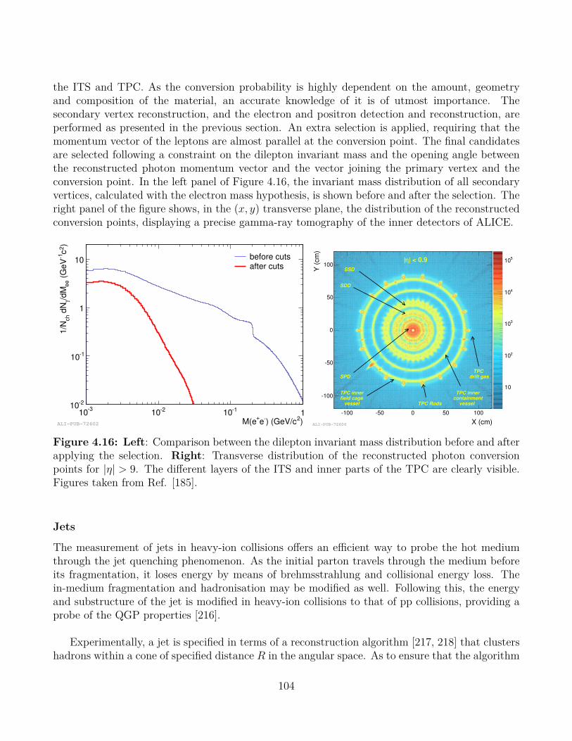
the ITS and TPC. As the conversion probability is highly dependent on the amount, geometryand composition of the material, an accurate knowledge of it is of utmost importance. Thesecondary vertex reconstruction, and the electron and positron detection and reconstruction, areperformed as presented in the previous section. An extra selection is applied, requiring that themomentum vector of the leptons are almost parallel at the conversion point. The final candidatesare selected following a constraint on the dilepton invariant mass and the opening angle betweenthe reconstructed photon momentum vector and the vector joining the primary vertex and theconversion point. In the left panel of Figure 4.16, the invariant mass distribution of all secondaryvertices, calculated with the electron mass hypothesis, is shown before and after the selection. Theright panel of the figure shows, in the (x, y) transverse plane, the distribution of the reconstructedconversion points, displaying a precise gamma-ray tomography of the inner detectors of ALICE.

)2) (GeV/ce+

M(e

310 210 110 1

)2

c1

(G

eV

ee

/dM

γ d

Nch

1/N

210

110

1

10 before cuts after cuts

ALI−PUB−72602 X (cm)

100 50 0 50 100

Y (

cm

)

100

50

0

50

100

10

210

310

410

510

SSD

SDD

SPD

TPC Rods

TPC innerfield cage

vessel

TPC innercontainment

vessel

TPCdrift gas

| < 0.9 η|

ALI−PUB−72606

Figure 4.16: Left: Comparison between the dilepton invariant mass distribution before and afterapplying the selection. Right: Transverse distribution of the reconstructed photon conversionpoints for |η| > 9. The different layers of the ITS and inner parts of the TPC are clearly visible.Figures taken from Ref. [185].

Jets

The measurement of jets in heavy-ion collisions offers an efficient way to probe the hot mediumthrough the jet quenching phenomenon. As the initial parton travels through the medium beforeits fragmentation, it loses energy by means of brehmsstrahlung and collisional energy loss. Thein-medium fragmentation and hadronisation may be modified as well. Following this, the energyand substructure of the jet is modified in heavy-ion collisions to that of pp collisions, providing aprobe of the QGP properties [216].

Experimentally, a jet is specified in terms of a reconstruction algorithm [217, 218] that clustershadrons within a cone of specified distance R in the angular space. As to ensure that the algorithm

104

is applicable to both experimental data and theoretical calculations, it is expected to be collinear-and infrared-safe (respectively meaning that the jet measurement should not be affected by collinearsplitting or soft emissions). In ALICE, the jet candidates are reconstructed using the anti-kT [219]algorithm. The reconstruction can depend solely on charged tracks measurement by the ITS andTPC (charged jets) or combine them with the energy deposition in the EMCAL to include neutralparticles (full jets). In the latter case, the energy deposition in the EMCAL by charged particlesis subtracted as to avoid double counting.

The next step consists in correcting for the background contribution to the jet candidate mea-sured energy. The standard method relies on event-by-event calculation of the average momentumdensity, which is multiplied by the jet area and the result subtracted from the measured energy.As this method leads to large residual fluctuations, an ongoing effort aims at developing new tech-niques allowing for a more precise measurement of the jet momentum, e.g. relying on machinelearning [220].

105

Chapter 5

Forward muon spectrometer

The measurements presented in this thesis are performed on data recorded using the muon spec-trometer of ALICE. The machinery is detailed in the first two sections, while the last two respec-tively describe the procedures for muon tracking and triggering. Considerations on the efficiencyare given following their relevance for the study of weak bosons. Most of the information pre-sented in this chapter is extracted from the ALICE paper [181], the spectrometer technical designreports and the ALICE performance paper [181, 221, 222, 185]. More details can be found in thesedocuments, and references herein.

5.1 OverviewThe ALICE detector is equipped with a muon spectrometer lying at large rapidities. It detectsmuons with full azimuthal coverage and polar angle 171 < θ < 178, corresponding to pseudora-pidity −4 < η < −2.5 in the ALICE convention. The spectrometer enables the measurement ofthe muon decays of light (ρ, ω, φ) and heavy (J/ψ and Υ families) vector mesons, HF hadrons(B and D), and weak bosons (W± and Z0). The large rapidity coverage is complementary to thecentral barrel and to other LHC experiments, such as ATLAS and CMS. It overlaps with therapidity coverage of the LHCb detector (−2 < ηLHCb < −4.5), but the technical conception andphysics goal of the two apparatus lead them to probe different regimes: LHCb is designed forhigh luminosity pp mode but saturates for the most central heavy-ion events, while ALICE is fullyefficient in the latter and suffers from the limitations of its recording rate in the former.

The spectrometer is composed of a set of tracking chambers assisted by a dipole magnet formomentum measurement, a triggering system, and a set of absorbers shielding the detector fromvarious background sources. A detailed layout is shown in Figure 5.1, and Table 5.1 gives the maintechnical characteristics of the muon arm.

107

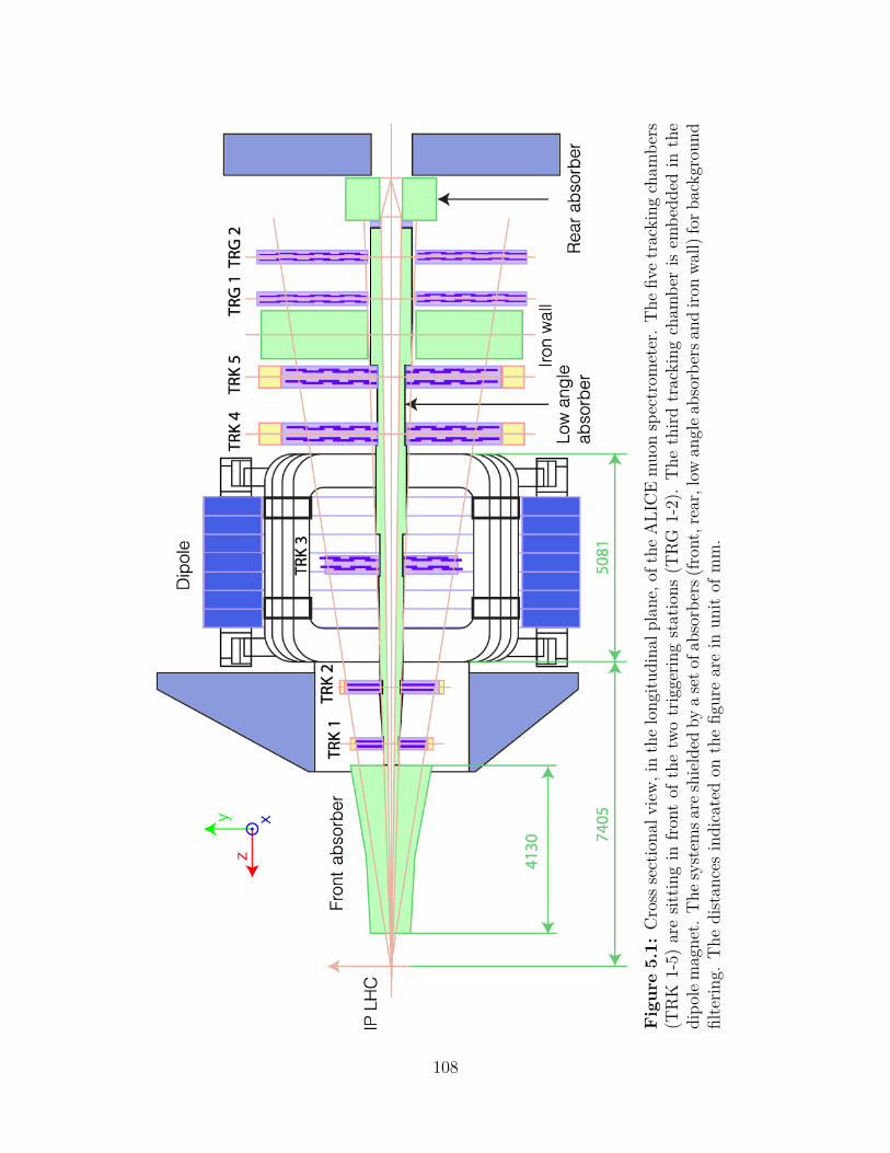
Fig

ure

5.1:

Cro

ssse

ctio

nalv

iew

,in

the

long

itudi

nalp

lane

,oft

heA

LIC

Em

uon

spec

trom

eter

.The

five

trac

king

cham

bers

(TR

K1-

5)ar

esit

ting

infro

ntof

the

two

trig

gerin

gst

atio

ns(T

RG1-

2).

The

third

trac

king

cham

ber

isem

bedd

edin

the

dipo

lem

agne

t.T

hesy

stem

sare

shie

lded

bya

seto

fabs

orbe

rs(fr

ont,

rear

,low

angl

eabs

orbe

rsan

diro

nwa

ll)fo

rbac

kgro

und

filte

ring.

The

dist

ance

sin

dica

ted

onth

efig

ure

are

inun

itof

mm

.

108

Muon detectionPolar angular coverage 171 < θ < 178

Azimuthal angular coverage fullMinimum muon momentum 4 GeV/c

Pseudorapidity coverage −4.0 < η < −2.5Front absorber

Longitudinal (from IP) −5 030 mm ≤ z ≤ −900 mmTotal thickness (material) ' 10 λint,' 60 X0 (carbon, concrete, steel)

Dipole magnetNominal magnetic field, integrated field 0.67 T, 3 Tm

Free gap between poles 2.972 - 3.956 mOverall magnet length 4.97 m

Longitudinal position (from IP) −z = 9.94 m (centre of the dipole coils)Tracking chambers

No. of stations, no. of planes per station 5, 2Longitudinal position of stations −z = 5 357, 6 860, 9 830, 12 920, 14 221 mm

Anode-cathode gap (equal to wire pitch) 2.1 mm for st. 1, 2.5 mm for st. 2-5Gas mixture 80% Ar + 20% CO2

Pad size st. 1 (bending plane) 4.2 × 6.3, 4.2 × 12.6, 4.2 × 25.2 mm2

Pad size st. 2 (bending plane) 5 × 7.5, 5 × 15, 5 × 30 mm2

Pad size st. 3-5 (bending plane) 5 × 25, 5 × 50, 5 × 100 mm2

Maximum hit density st. 1-5 (central Pb–Pb × 2) 5.0, 2.1, 0.7, 0.5, 0.6 × 10 cm-2 hits/cm2

Spatial resolution (bending plane) ' 70 µmTrigger chambers

No. of stations, no. of planes per station 2, 2Longitudinal position of stations −z = 16 120, 17 120 m

Total no. of RPCs, total active surface 72, about 140 m2

Gas gap single, 2 mmElectrode material and resistivity Bakelite, ρ = 3− 8× 109Ω cm

Gas mixture C2H2F4 / i-butane / SF6 (89.7%, 10%, 0.3%)Pitch of readout strip (bending plane) 10.6, 21.2, 42.5 mm (for trigger st.1)

Max. strip occupancy in bend. (non bend.) plane 3% (10%) in central Pb–PbMaximum hit rate on RPCs 3 Hz / cm2 in Pb–Pb

Trigger electronicsTotal no. of FEE channels 2.1× 104

No. of local trigger cards 234 + 8

Table 5.1: Summary of the main characteristics of the ALICE muon spectrometer. The infor-mation in the table are adapted from Ref. [181].

109

5.2 Composition

5.2.1 Tracking systemThe muon tracker is composed of five stations, each containing two planes of cathode pad cham-bers. The third station sits inside a 800-tons dipole magnet, delivering a integrated magnetic fieldof 3 Tm by means of resistive coils. The first two chambers have radii defined by the angularacceptance of the spectrometer (polar angle 171 < θ < 178 with the origin at the collision point,in full azimuth), while the last three chambers are larger in order to account for the deviation ofcharged tracks in the magnetic field. They are arranged in a projective geometry from 2.5 to 20m2, for a total surface of about 100 m2. The magnetic field generated by the dipole magnet liesin the horizontal plane, perpendicular to the beam line, from which one defines the bending (y, z)and non-bending (x, y) planes. Its polarity can be inverted in a short time, and Pb–Pb data arerecorded using the two configurations.

The tracking system is required to attain a spatial resolution better than 100 µm, mainlydriven by the mass resolution needed to disentangle the bottomonia states1 and constrained by theparticle multiplicity in Pb–Pb collisions. This requirement is fulfilled with Multi-Wire ProportionalChambers (MWPC) of high granularity. The chambers of the first two stations have a quadrantstructure, with the readout electronics distributed on their surface. The three other chambers havea slat architecture with electronics on the side of the slats (Figure 5.2). The first station, havingto cope with a very high particle density in the vicinity of the collision point, is composed of padsas small as 4.2 × 6.3 mm2. Larger pads are used for the stations further away from the interactionpoint.

quadrant

slat

Figure 5.2: Schematic view of the quadrant structure (left) and slat architecture (right) of thetwo innermost and three outermost tracking stations respectively.

The working principle of the MWPC is illustrated on Figure 5.3. Each MWPC is composed1Which requires a resolution of 100 MeV/c2 at 10 GeV/c2

110

of a central anode plane with equally spaced wires, sitting in-between two cathode planes whosesegmentation aims at keeping the occupancy below 5%. The wires have a high voltage, of about1650 V, while the cathode planes are grounded. This generates an electric field with increasinggradient towards the wires. The volume within the two cathodes is filled with a gaseous mixture ofAr+CO2 at a 80% / 20% ratio. As to limit multiple scatterings in the chambers, low-Z materialssuch as carbon fibres are used, resulting in a chamber thickness of 0.03 radiation length (X0).

A charged particle crossing the gaseous medium will ionise it, liberating electrons that drifttowards the nearest anode wire due to the electric field, triggering an avalanche of secondaryelectrons. The resulting ion cloud creates a charge distribution on the cathode pads nearby. Thecathode positions provide the x and y coordinates of the hit, while the z coordinate is providedby the position of the chamber itself.

Cathode pads

anode wires

x

z

incident track

1650 V

anode wire

Avalanche

y

z

Figure 5.3: Layout and working principle of the MWPC composing the tracking chambers viewedin the (x, z) and (y, z) planes.

5.2.2 Trigger stationsThe muon trigger system is composed of four ∼ 6 × 6 m2 planes regrouped in two stations, located16 and 17 m away from the nominal interaction point. Each planes contains 18 single-gap ResistivePlate Chambers (RPC) made of two high-resistivity Bakelite electrodes separated by a 2 mm gasgap (Figure 5.4). The outside faces of the plates are painted with graphite, one is kept under highvoltage while the other is grounded. The signal is created by the avalanche of electrons triggeredby a charged particle crossing the gas in-between the two electrodes.

The signal is picked-up by orthogonal readout strips, providing bi-dimensional information onthe hit position. The strips are connected to the Front-End Electronics (FEE), which gather the

111

Ground

HV

Gas

resistive electrode plate

resistive electrode plate

insulating film

Spacer

pick-upy-strips

pick-upx-strips

Figure 5.4: Schematics of a RPC composing the muon trigger planes.

signal from the four planes and pass it to the local trigger electronics. The system is divided into234 detection areas, each associated to a local trigger board. The strip segmentation is finer atvery large rapidity, where a high multiplicity is expected, and decreases when moving further awayfrom the beam line. The chamber response is fast, with a signal rising in about 2 ns, and thetrigger system attains a spatial resolution of ∼ 1 cm and time resolution of the order of 1-2 ns.

5.2.3 AbsorbersThe ALICE spectrometer design was driven by the requirement of coping with the very highmultiplicity environments created by heavy-ion collisions, applying an extra factor two to themultiplicity predicted by means of simulations with HIJING [223]. Several absorbers are meant toshield the muon chambers, reducing the detector occupancy and helping the background rejection.The filtering set is composed of four absorbers: the front absorber, between the interaction pointand the muon chambers, the low-angle absorber, also called beam shield and lying along the beampipe, the iron wall sitting between the tracking and triggering systems, and the rear absorberlocated after the trigger stations.

The front absorber is a 37-tons cone located inside the L3 magnet, before the first trackingstation and at 90 cm from the nominal interaction point. It aims at reducing the flux of chargedparticles by at least a factor two. Its length of 4.13 m correspond to about 60 X0 ' 10 λint.Besides filtering, the front absorber is required to limit multiple scatterings as to not compromisethe resolution of the spectrometer. In this regard, the region close to the interaction is made ofcarbon, a low-Z material, followed by concrete. The carbon and concrete part is surrounded byhigh-Z material (lead and polyethylene) in order to absorb low-energy photons and neutrons, aswell as secondary particles produced within the absorber itself.

The triggering stations are further protected by a 1.2 m thick iron wall filtering out hadronsand secondary particles punching through the front absorber. The whole spectrometer is protected

112

from the high background produced by the interactions with the beam pipe of particles (mainlypions and kaons) emitted at very small angle (θ < 2) by the small-angle absorber and second ironwall. The small-angle beam shield is made of high-density material (tungsten and lead) envelopedwith stainless steel. It surrounds the beam pipe throughout the muon arm in its entirety. Thesecond iron wall protects the back of the trigger stations from the particle produced in beam-gasinteractions.

5.3 Track reconstruction

5.3.1 Reconstruction algorithmFollowing the passage of charged particles in the tracking chambers, clusters are determined bymeans of the Maximum Likelihood Expectation Maximisation (MLEM) algorithm [224], whichallows one to find local maxima in a distribution for which equations are either not known orcannot be solved directly. The spatial location are determined by fitting the cathode-inducedcharged distribution with a 2D-Mathieson function [225], a single parameter function applicablefor small anode-cathode separation:

ρ(λ)

qa= K1

1− tanh2(K2λ)

1 +K3 · tanh2(K2λ), with K1 =

K2

√K3

4tanh−1√K3

, K2 =π

2

(1−√K3

2

),

(5.1)where qa is the net anode charge and λ = x/h with h the anode-cathode separation and x theposition along the x-axis, either parallel or normal to the anode wire direction. The single parame-ter K3 can be determined from the chamber geometrical configuration, allowing for the evaluationof the cluster position x with a fit. The cluster information is used as inputs for the track re-construction algorithm, which is based on the Kalman filter [215] already presented for the trackreconstruction in the central barrel (Section 4.4.3).

The algorithm builds track seeds starting from station 4 and 5, as they are less subject tobackground contamination from soft particles escaping the front absorber. In each station, a tracksegment is built by linking cluster pairs from the two planes, and joining them with a straight line.The seeds are extrapolated in the magnetic field to the preliminary vertex estimated by the ITS(usually SPD only), after which a first estimation of the track momentum can be performed usingthe standard Lorentz law:

~F =d~p

dt= q

(~E + ~v × ~B

), (5.2)

where q is the charge of the track, ~v its velocity and ~E and ~B the electric and magnetic fields ofthe magnet. From this relation the guessed track momentum p can be linked to the radius of thetrack curvature R using:

p[GeV/c] = 0.3[T]× R[cm] = 0.3[T]× L[cm]

θd(5.3)

where L is the length of the magnet and θd is the angle between the beam line and the track segmentafter the magnet. Here a first selection criterion is applied on the guessed track momentum, wheretracks with p < 3 GeV/c or p > 3 TeV/c are rejected.

113

The second step of the track reconstruction algorithm starts back from the seeds built in station4 or 5, and look for corresponding clusters in station 5 or 4. At least one cluster has to be foundin the two planes of the other station, defining the second criterion of the tracking algorithm: avalid track needs to have at least three out of the four possible clusters in stations 4 and 5. Theassociation of clusters between the two stations is based on a χ2 selection. The presence of severalclusters passing the selection leads the track seed to become a tree with several hypotheses, whichare all propagated. The Kalman algorithm reevaluates the track kinematic parameters using thenew information, and the procedure is repeated down to the first station. At each station, a trackhypothesis is discarded if no cluster can be associated to it. Additionally, at each recomputationof the track parameters a χ2-based cut aims at discarding tracks of poor quality. Therefore, theKalman filter-based algorithm for track reconstruction features three selection criteria:

• the first estimation of the track momentum should yields 3 GeV/c < p < 3 TeV/c,

• the track hypothesis has to pass χ2-based selections at both cluster and track levels,

• the track has to be built from at least one out of the two possible clusters in stations 1, 2and 3, and three out of the possible four clusters in stations 4 and 5.

After the full reconstruction of the tracks in the tracking system, one gets the so-called uncor-rected track parameters yielded by the Kalman filter. The tracks are finally extrapolated to thevertex position measured by the SPD, and their parameters are corrected for multiple scatteringsand energy loss in the front absorber.

5.3.2 Alignment of the tracking chambersThe requirement of a mass resolution of 1% at the Υ mass introduces a strong constraint on thealignment of the tracking chambers. During the installation of the chambers, they are positionedwith a spatial accuracy of a few tenth of millimetres by means of theodolite measurements andphotogrammetry. At the beginning of each data taking period, dedicated runs are performed forthe alignment, during which the dipole magnet is switched off. The ten chambers are aligned onstraight tracks. This initial positioning is disturbed when switching on the magnet and electronicspower supplies. The chamber supports suffer as well from thermal stress. Such deformations needto be accounted for, in order to correct the data and be able to reproduce the alignment conditionsin the simulations.

The misalignment is monitored by means of the Geometry Monitoring System (GMS) [226],an array of about 460 optical sensors installed on platforms located at each corner of the trackingchambers. Two different optical devices are used, both recording with CCD sensors optical signalsprojected through a lens. The long range monitoring, corresponding to measurements betweenstations, in provided by Brandeis CCD Angle Monitor (BCAM). Each BCAM contains two ormore light sources, and an electronic camera looking at light sources from other BCAM. The shortrange monitoring, measuring distance between the two planes within a station, is provided by RedAlignment System NIKHEF (RASNIK) based proximity systems, a single tube containing the lensand CCD, which focuses on a mask with coded squares attached to another layer. The informationis gathered by the Long-Wire Data Acquisition System (LWDAQ).

114

The relative position of the planes is determined using a modified version of the MILLEPEDEpackage [227]. MILLEPEDE provides a way to include both global and local parameters, respec-tively referring to parameters contributing to all data (such as a chamber position) or relative toa single track (e.g. track curvature). Data recorded with and without magnetic field, as well asmeasurements from the GMS, can then be incorporated all at once in the determination of therelative misalignment, performed by a simultaneous fit of global and local parameters with a linearleast square model. In this way, a precision of about 100 µm is reached.

While the method is sensitive to the relative misalignment of the detector elements, it doesnot account for a potential global displacement of the entire spectrometer. A data-driven methodwas hence developed, simulating the detector response with a parametrisation of the measuredresolution of the clusters associated to a track, using extended Crystal Ball (CB) functions [228]to reproduce the distribution of the differences between the cluster and the track position ineach chamber. The parameters of the Gaussian core and power law tails of the CB are tunedto data, then used to reproduce the smearing of the track parameters. A global displacementof the detector is mimicked by applying a systematic shift, in opposite direction for positivelyand negatively charged tracks, to the distribution of the angular deviation of the tracks in themagnetic field. This shift parameter is determined from simulations, reproducing the differencebetween positive and negative tracks observed in data.

5.3.3 Reconstruction efficiencyThe efficiency of the tracking stations is calculated from data, taking advantage of the detectorredundancy. The tracking algorithm requires only a subset of the chambers to be fired, enabling theevaluation of each chamber efficiency, which are then combined to determine the overall efficiencyof the tracker. Let i and j be the two chambers of a station. One can face four configurations whena track goes through the station, as illustrated in Figure 5.5: the “ij” configuration when bothchambers are fired, “i0” and “0j” if only the chamber i or j is fired, and “00” when no clusters arereconstructed in the station.

The total number of tracks Ntot is the sum of the four configurations:

Ntot = Nij +Ni0 +N0j +N00. (5.4)

Considering that the efficiency of chambers i and j (hereafter εi and εj) are independent, one canwrite:

Nij = εi · εj ·Ntot, Ni0 = εi · (1− εj) ·Ntot, N0j = (1− εi) · εj ·Ntot, (5.5)

from which follows:εi =

Nij

Nij +N0j

, and εj =Nij

Nij +Ni0

, (5.6)

the efficiency of each chamber can be evaluated without having to know N00.

The efficiency of the tracking system is also affected by the presence of fake tracks. This canbe dealt with by applying a selection on the p × DCA, the product of the track momentum toits distance of closest approach (that is, the distance to the primary vertex of the track trajectory

115

Chamber: i j

i-j

i-0

0-j

0-0

Cluster Track

Figure 5.5: Possible configurations after the passage of a charged particle through a trackingstation with chambers i and j.

projected in the plane transverse to the beam axis), ensuring that the track points to the interactionvertex. At low pT, below 1-2 GeV/c, this cut is not fully efficient, a selection on the track normalisedχ2 is then also applied (χ2 < 3.5) to further reduce the contamination. The amount of fake tracks islargely reduced by this selection, amounting to about 1.5% for the 0-10% central events in Pb–Pb.

5.4 Muon triggeringThe muon trigger system aims at reducing, thanks to the iron wall, the probability of triggering,and therefore storing, events where no valid muon candidate for light vector mesons, open andclosed HF hadrons, or weak boson is present. It provides as well muon identification through thematching of a track segment in the trigger stations to a track reconstructed in the tracking system.The trigger decision is taken by the muon chambers, at the electronics level. It is based on a fastselection (about 650 ns) of candidate muon and dimuon signals above a user-defined pT threshold.The pT-based procedure is justified by the rejection of pions and kaons, expected to be dominantat low pT. It is illustrated in Figure 5.6.

The trigger decision is performed by comparing in station 2 the track segment reconstructedfrom hits in the two stations, to a “track with infinite momentum” defined as a straight line passingthrough the interaction vertex and the cluster in the first station, and extrapolated to the second.The difference in position between the two tracks defines the deviation δy = y2 − y∞. The pTselection can then be applied by cutting on δy, which is inversely proportional to pT. The pT cutis not sharp, as the intrinsic trigger efficiency is not an ideal step function: it increases sharplybefore reaching a plateau of about 99% around 5 GeV/c. Two cuts are defined, serving differentanalysis purposes. A low-pT cut enables the analysis of particle of low transverse momentum. Asthe signal rate in this region is high, and in order to cope with the recording rate and storing

116

IP

y

z

B

y1y2

δy

µ µ if pT →∞

MT1 MT2

y∞

Figure 5.6: Sketch of the working principle of the muon trigger decision. The insert on the topright is a zoom-in of the dotted square. The MT1 and MT2 labels indicate the first and secondtrigger stations respectively.

capabilities, the low-pT triggers are downscaled. As to maximise the statistics for intermediate tohigh pT probes, a high-pT cut, without downscaling factor, is also defined. The values of thosepT threshold are period dependent, ranging from 0.5 to 4.2 TeV/c. Combined with the charge ofthe track and the single muon / dimuon label, the muon trigger can produce six different triggersignals, summarised in Table 5.2.

Trigger type Trigger name Condition

Muon-Single MSL single muon, low-pT thresholdMSH single muon, high-pT threshold

Muon-Pair

MLL same-sign muon pair, low-pT thresholdMLH same-sign muon pair, high-pT thresholdMUL opposite-sign muon pair, low-pT thresholdMUH opposite-sign muon pair, high-pT threshold

Table 5.2: Trigger types defined by the muon trigger system. For dimuon triggers, the pTthreshold is applied on individual tracks.

The efficiency of the trigger chambers is evaluated using the information redundancy, as forthe tracking chambers. The trigger efficiency can also be affected by the occupancy. The detectorcontains 234 local boards, the resulting granularity creates a sizeable probability of having twotracks that are close enough to interfere with the trigger signal. This is evaluated by embeddingtechnique. A simulated signal is embedded in real data, as to mimic the detector occupancy duringdata taking, and the trigger rate is compared to the one obtained from pure simulation, only usingas input the chamber efficiencies. The loss of trigger signal evaluated with this method can reach3.5% for the most central Pb–Pb collisions [185].

117

Chapter 6

Data taking in ALICE

This chapter introduces the online and offline systems of ALICE, constituting the two steps ofthe data treatment chain that was in place during the LHC Run 2. The online control systemimplements trigger selections and handles the flow of data from their detection in the sub-elementsof the detector to the storage of the selected events on hard drives. The offline system performsthe reconstruction of the event and encompasses the analysis and simulation frameworks, enablingdata analysis.

6.1 Online Control SystemALICE aims at taking data during hadronic collisions performed at the LHC, focusing on but notrestricting to heavy-ion collisions. It therefore operates in several running modes with significantdifferences. The Pb–Pb mode, primary focus of the experiment, features a relatively low interac-tion rate (of ≤ 10 kHz at nominal luminosity L = 1027 cm-2 s-1), relatively short running time (afew weeks per year) but very high multiplicities and thus large event sizes. This requires a ratherlow trigger selectivity, but the trigger complexity is high and needs at least the partial reconstruc-tion of the event in order to extract signals of interest. Handling and storing large-size eventsrequire sufficient bandwidth together with an efficient selection and compression of the data. Onthe contrary, in pp mode (and, to some extend, p–Pb), the interaction rate is much higher (up to500 kHz) while the event size is small. The running time, in pp mode, is of several months a year.In this case, the requirements on the trigger complexity, bandwidth and data compression are lessdrastic, whereas the trigger selectivity becomes crucial.

These requirements are met using the Online Control System, composed of the Trigger sys-tem, the High-Level Trigger (HLT), the Data Acquisition (DAQ) and the Detector Control System(DCS). The four modules are interfaced with each other by the Experiment Control System (ECS)layer, as shown in Figure 6.1. These five parts, constituting the online control system, are sum-marised in the following subsections, more information can be found in the dedicated TechnicalDesign Report [229].

119

Figure 6.1: The ALICE online control system. The Trigger system, High-Level Trigger (HLT),Data Acquisition (DAQ) and Detector Control System (DCS) are monitored and interfaced by theExperiment Control System (ECS). Figure taken from Ref. [229].

6.1.1 TriggerThe triggering in ALICE is challenging, due to the widely varying relaxation time of the varioussubdetectors, and the differences between the particle multiplicities, event sizes, and interactionrates among the various running modes. This is optimised by the Central Trigger Processor (CTP),designed to select events having specific features at a rate that can be scaled as to account for thebandwidth restrictions.

The triggering procedure is based on logic trigger signals sent by the subdetectors. They arecharacterised by a specific measurement made by the detector itself, often following from a fastcalculation, such as an evaluation of the multiplicity, a pT threshold, the presence of a muon pair,etc. An example of such calculation is the one used to apply the pT selection by the muon triggerpresented in Section 5.4. These logical signals are sent to the CTP as trigger inputs, where theyare combined using a Field-Programmable Gate Array (FPGA), an integrated circuit containingan array of programmable logic blocks. The FPGA combines the input signals following a userdefined process in order to form the different physics triggers (e.g. 10% most central MB event,single muon with high-pT threshold...). The CTP communicates independently with each detector,as they may have different triggering patterns, by means of Local Trigger Units (LTUs). Thereis one LTU per detector element, which sends the recorded signal to the CTP, receives its triggerdecision, translates it following the detector needs, and forward it to the Front-End Electronics(FEE) of the detector. The detectors providing triggering capabilities, along with their functions,are listed in Table 6.1.

Following from the low latency of some of the detectors, the trigger decision is organised inthree levels. The fastest level, L0, is delivered to the detector 1.2 µs after the collision, providing aalert to detectors whose electronics are not pipe-lined, but awaiting for a trigger decision to startprocessing signals. The L1 level arrives at the detector 6.5 µs after the interaction took place. Atthis stage, most of the trigger inputs are available, allowing for a major rate reduction to be appliedwhen needed. The last trigger level, L2, comes after the end of the drift time of the TPC (about 88µs), after which the past-future pile-up protection can be applied. In Pb–Pb mode, the past-futureprotection circuit monitors the number of interactions, characterised by their multiplicity. Pile-upof two central events will veto the trigger, while pile-up of an event with low multiplicity can be

120

Detector Functions LevelSPD hit-multiplicity and hit-topology based trigger L0TRD electron, high-pT particle, charged jet L1TOF multiplicity, topology (back-to-back), cosmic ray L0

PHOS photon L0EMCAL photon, neutral jet L0/L1

ACORDE cosmic ray (single and multiple hits) L0V0 coincidence-based MB, centrality L0T0 event vertex selection, interaction trigger L0

ZDC MB interaction, electromagnetic dissociation L1MUON single muon, dimuon L0

Table 6.1: Trigger capabilities provided by the various ALICE detectors, with their trigger level(see text). Taken from Ref. [185].

tolerated up to a programmable level. After L2, the events are furthermore filtered following thedecision of the HLT.

This organisation in terms of timing levels allows one to define and control differently parti-tions of the detector. A partition, also called a detector cluster, is a dynamically-defined subsetof detectors participating in the readout of a given event. A cluster is defined for its relevancein terms of data analysis, and the trigger decision sent to this particular cluster can be adaptedaccording to the recording rate of its constituents. For example, the muon spectrometer is able torecord data at a much higher rate than the TPC. Along with other fast detectors (including e.g.the SPD for vertex measurement, the V0 and T0 arrays for the evaluation of the multiplicity), it isregrouped in the MUON cluster, improving the statistics available for this specific physics channel.

The input data handled by the CTP is usually global, meaning that it does not correlatespecific geometrical regions in different detectors. For peculiar applications however, it might notbe required to record the whole event, and a selection defining a specific azimuthal region canallow for physics analysis while providing an efficient way to reduce the amount of data needed tobe processed and stored. This type of selection is especially fruitful when triggering on events inwhich the ALICE calorimetry system is involved, as it does not have a full azimuthal coverage.The boundaries of the azimuthal region can be imposed to the most central detectors, such as theITS and TPC.

Finally, the CTP is designed to handle the rate of the various triggers. The data acquisitiontends to saturate with high frequency triggers, leaving few to no bandwidth available for triggeringon rare processes. In order to prioritise those events, of particular physics interest, the CTP isable to downscale the non-rare triggers to a predefined rate. The data acquisition monitors theoccupancy of its buffers, sending a signal to the CTP when it exceeds a given threshold. The CTPresponds by restricting triggering on common processes, ensuring continued available bandwidthfor rare processes. When the occupancy of the buffers has lowered below a suitable threshold,another signal is sent to re-activate all the trigger types. The timing at which the non-rare triggers

121

are downscaled is precisely monitored as to be taken into account while evaluating the integratedluminosity.

A set of trigger inputs, output trigger cluster, past-future protection requirements, along witha few other control bits, define together a trigger class, the central concept for event selection inALICE. Classes are named following a generic scheme:

C<descriptor> – <BC mask> – <past-future protection> – <cluster>,

where:

• the descriptor is a logical function of the input codes,

• the BC mask code is a letter describing for which bunch crossing category the trigger is active,

• the past-future protection code defines whether the past-future protection scheme isapplied (and how) or not,

• the detector cluster code corresponds to the cluster read out in the trigger class.

For instance, the measurement of the W-boson production presented in this thesis uses as maintrigger CMSH7-B-NOPF-MUFAST. The class corresponds to MSH7 events: events where the muontrigger (M) reports the detection of a single muon (S) with a high pT threshold (H), in combinationwith a MB signal from the V0 arrays (7). The class is active for the B bunch crossing categories(two filled bunches crossing), without past-future protection (NOPF), and read out data from thedetectors of the MUFAST cluster, containing the SPD, T0, V0, AD, and the muon tracking andtrigger systems. The major ALICE triggers are summarised in Table 6.2.

6.1.2 Data AcQuisition (DAQ)The ALICE DAQ [230] is a vast computing system composed of hundreds of interconnected Per-sonal Computers (PCs) aiming at organising and controlling the flow of data from its detectionto the storage of the events. Along the chain is performed sub- and full event reconstruction, inassociation with the HLT farm. The DAQ also includes software packages for the monitoring ofdata quality and system performances. The architecture of the DAQ is shown in Figure 6.2. Itrelies on the parallelisation of the data treatment, with data streams working independently andconcurrently, followed by stages of event building where data are merged and eventually recordedas a complete event. The LHC clock, having a precision of 25 ns corresponding to at most onebunch crossing, is used to associate a time tag to each fragment in order to identify fragmentspertaining to the same event for the full reconstruction.

The chain starts at the level of the detectors read-out. The CTP forms a decision for ev-ery bunch crossing, which is sent to the LTU of each detector needed to be read out. The LTUscommunicate the positive decisions by means of Timing, Trigger and Control (TTC) systems, asso-ciating to the raw data the LHC timing reference, first level trigger decision and the correspondingbunch and event number. Data are then pushed into the system by the detectors Front-End and

122

Trigger Description ConditionMB-type triggers

MBor minimum bias signals in one of the V0s and SPDMBand minimum bias signals in V0A and V0CMBZ minimum bias MB and signals in both ZDCsSPI multiplicity n hits in SPD

Centrality triggersCENT central event V0-based centrality trigger for Pb–Pb (0–10%)SEMI semicentral event V0-based centrality trigger for Pb–Pb (0–50%)

EMCAL triggersE0 EMCAL L0 EMCAL L0 shower trigger in coincidence with MB

EJE neutral jet EMCAL L1 jet algorithm following EMCAL L0EJE2 neutral jet like EJE but with lower thresholdEGA photon/electron EMCAL L1 photon algorithm following EMCAL L0EGA2 photon/electron like EGA but with lower threshold

TRD triggersTJE charged jet n charged particles in TRD chamber in coincidence with MBTQU electron for quarkonia electron with pT > 2 GeV/c in TRD in coincidence with MBTSE electron for open beauty electron with pT > 3 GeV/c in TRD in coincidence with MB

MUON triggersMSL single muon low single muon in muon tracker in coincidence with MBMSH single muon high like MSL but with higher thresholdMUL dimuon unlike sign two muons of opposite sign above low threshold, in coinc. with MBMLL dimuon like sign two muons of same sign above low threshold, in coinc. with MB

Miscellaneous triggersHM high multiplicity high multiplicity in SPD in coincidence with MBPH photon by PHOS PHOS energy deposit in coincidence with MBEE single electron electron signal in TRD (sector 6–8) and EMCALDG diffractive charged particle in SPD and no signal in V0

CUP barrel ultraperipheral charged particle in SPD and no signal in V0, for Pb–Pb and p–PbMUP muon ultraperipheral (di)muon in muon trigger and no signal in V0A, for Pb–Pb and p–PbZED electromagnetic dissociation signal in any of the neutron ZDCsCOS cosmic event signal in ACORDE

Table 6.2: Descriptors of the major ALICE triggers. Adapted from Ref. [185].

123

Figure 6.2: Overview of the ALICE DAQ system and its interface with the HLT system. Themeaning of the acronyms is given in the text. Figure taken from Ref. [230].

Read-Out (FERO) electronics through about 500 optical Detector Data Links (DDLs). The signalsconveyed by the DDL are collected by DAQ Read-Out Receiver Cards (D-RORCs), hosted by PCscalled Local Data Concentrators (LDCs). In the LDCs the event fragments are getting assembledinto sub-events according to their tagging. Some D-RORCs also send a copy of the data to theHLT farm where it is received by Common Read-Out Receiver Cards (C-RORCs)1 and transferredto the Front-End Processor (FEP). The HLT performs a preliminary online reconstruction, fromwhich a decision about the data to be recorded is taken (see Section 6.1.3). Upon positive decision,the sub-events assembled by the LDCs are shipped to the Global Data Collectors (GDCs) wherethey are furthermore combined. The distribution of the LDCs outputs to the GDCs is monitoredby the Event Destination Manager (EDM) as to ensure an efficient repartition of the data andcomputing load. The full events are built by the GDCs, and written into data files which arestored in the Transient Data Storage (TDS), a temporary buffer big enough to store several hoursworth of continuous data taking. The files are read by the TDS Managers (TDSMs) and finallymigrated to the Permanent Data Storage (PDS) at the CERN computing centre, where they willbe accessible for offline analysis.

The Data Acquisition and Test Environment (DATE) [231] is the DAQ software framework.1During the LHC Run 1, the data were received by HLT Read-Out Receiver Cards (H-RORCs), before being

changed for C-RORCs following the need for higher link rates.

124

Its functions cover the overall control of the system, as well as the system performance and dataquality monitoring. The services needed by the DAQ system itself such as the control or thedatabase are performed by the DAQ Services Servers (DSS). Additional servers are used to runthe Detector Algorithms (DA) or the Data Quality Monitoring (DQM).

The DAs constitute a framework designed and implemented to achieve as much as possible thedetector calibration directly online. Indeed, the systems are sensitive to configuration settings,mechanical geometry, changes in the environmental conditions, ageing of the components and de-fections in the sensors. The output of the calibration tasks may be needed to configure the detectorelectronics for data taking, enabling e.g. the production of zero-suppressed data or the maskingof noisy channels, in order to reduce the volume of data. DAs are detector-specific calibrationprocedures, provided by the sub-detector teams and implemented in the global framework. EachDA collects the detector data and produces results online, which can be directly reused for exampleto configure the detector and contribute to the sub- and full event reconstruction performed by theDAQ. They can also be shipped offline, post-processed if necessary, and stored to be used in dataanalysis. Two types of DAs are defined, depending on whether they need a dedicated run (exclusivemode) or they are active during data taking (background mode). In the first case, so-called LDCDA, the data are collected during a dedicated, standalone (single detector running) and usuallyshort-duration run, and recorded on the LDCs. At the end of the run, the DA is launched onthe data and the calibration results are directly available. These runs are also used to fine-tuneor debug the DA behaviour itself. In background modes, called MON DA, dedicated monitoringmachines are used to run single DA processes. The data are then picked-up from the normal dataflow in a non-intrusive way, and processed on the fly. Each DA focuses on a given type of event(calibration, physics) and the source it uses to monitor it (a detector or set of detectors). A post-processing phase follows the end of the run as to finalise the results. A MON DA can typicallyaim at filling an histogram event by event, then compute a fit and extract some key value. MONDAs are used as well to map dead channels. The full mapping of the detector may need a largeamount of events, in which case intermediate results are saved at the end of a run and re-loadedfor the next run.

The DQM is ensured by the Automatic MOnitoRing Environment (AMORE) framework de-veloped by and used in ALICE. It is mainly written in C++ and interfaced with the ROOT [232]data analysis framework, whilst the use of AliRoot [233], the ALICE offline framework describedin section 6.2, is used when offline analysis is needed. It was designed to be flexible and modular,such that each detector team is able to develop specific code that is built into dynamic librariescalled modules.

The modules use the DATE monitoring libraries to access the raw data, collect data from theLDCs and GDCs, or read data from files. AMORE is based on a publisher-subscriber paradigm, asillustrated in Figure 6.3. On the publisher side, large number of processes, called agents, containuser-defined code to be executed depending on the DAQ environment status (start or end of run,ongoing data taking...) and producing output objects to be published. An output typically containsthe resulting quantities, often in the form of histograms (although there is no restriction on theirtype) associated to metadata allowing for a proper and coherent handling by the framework. All

125

is encapsulated into Monitor Objects (MOs) and published into a pool. Each MO has a qualityassociated to it, which is stored within the object. The quality is a flag that can take differentvalues:

• kNULLFLAG: no quality, used for transient objects or when associating a quality it not appli-cable (e.g. for the transport of error messages),

• kINFO: good quality,

• kWARNING: the object should be checked,

• kERROR: the object is clearly of bad quality,

• kFATAL: the object is so incorrect it calls for an immediate intervention.

Depending on user needs, the MOs can be discarded at the end of the running period, after adefined period of time, or stored permanently in a MySQL database for future access.

Figure 6.3: The publisher-subscriber paradigm of AMORE. On the publisher side, agents com-municate with the various part of the online system in order to produce MOs published in a pool.The pool is the accessed by clients (the subscribers) for visualisation in the control room. Figuretaken from Ref. [230].

The subscriber part uses clients to connect to the pool, retrieve the MOs and display them inthe ALICE control room through a customisable Graphical User Interface (GUI) (see the left panelof Figure 6.4). Since most of the detector teams have similar needs and requirements, a genericGUI has been developed, allowing one to choose and display MOs among the thousand of objectsproduced by the agents. Custom GUIs were also developed by the teams following their specificrequirements for commissioning, testing and monitoring purposes. Custom GUIs also allow oneto use custom object types that could not be handled properly by the generic GUI. The DQM isinterfaced with the ALICE DAQ bookkeeping facility, the Electronic Logbook (eLogbook), withwhich it communicates in both ways. The eLogbook provides the DQM with information about

126

the run, such as its type (physics, calibration...) or the detectors involved. In return, it can readthe pool and give a worldwide access to the MOs through a web client, while the subscriber clientsare only accessible from within the ALICE control room. The right panel of Figure 6.4 shows anexample of MOs retrieved and displayed through the eLogbook.

Figure 6.4: Examples of MOs visualisation, using the AMORE generic GUI (left) or accessedthrough the eLogbook (right). Figures taken from Ref. [230].

6.1.3 High-Level Trigger (HLT)The HLT [234] is a large PC farm supporting the ALICE DAQ. Its main purposes are to emit asoftware trigger decision and provide efficient data compression as to reduce the amount of spaceneeded for data storage. By performing a real-time, full-event reconstruction, the HLT enables theapplication of efficient compression algorithms. The complete reconstruction allows as well one toperform a direct, high-level evaluation of the quality of the data, immediately revealing problemsthat arise during data taking. The precise reconstruction of the event requires a calibration of thedetectors, which in turns relies on a first reconstruction as input. By performing a fast, onlinereconstruction, the HLT contributes to the calibration procedures and helps reducing the requiredoffline resources. In summary the HLT participates to triggering, online reconstruction, calibra-tion, quality monitoring and data compression. The architecture of the HLT is described in Figure6.5.

Since the TPC produces more than 90% of the data volume, it constitutes the main target fordata compression and provides the HLT with its most intensive computing tasks. The processingof the TPC data starts with the clusterisation of the raw data, which happens on-the-fly as thedata flow received by the C-RORCs is pushed into FPGAs. The cluster finder of the HLT extractsthe hits from the raw data, looks for time-separated bunches of neighbouring signals in the TPCdetection plane, and calculates the coordinates using the weighted mean of the signals (i.e. theircentre of gravity) along with the computation of other quantities such as the total charge and thecluster width. The data compression is then achieved in two ways:

127

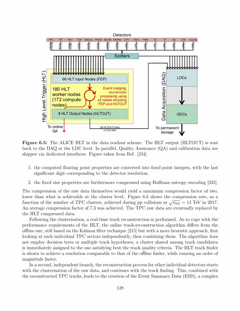
Figure 6.5: The ALICE HLT in the data readout scheme. The HLT output (HLTOUT) is sentback to the DAQ at the LDC level. In parallel, Quality Assurance (QA) and calibration data areshipper via dedicated interfaces. Figure taken from Ref. [234].

1. the computed floating point properties are converted into fixed point integers, with the lastsignificant digit corresponding to the detector resolution;

2. the fixed size properties are furthermore compressed using Huffman entropy encoding [235].

The compression of the raw data themselves would yield a maximum compression factor of two,lower than what is achievable at the cluster level. Figure 6.6 shows the compression rate, as afunction of the number of TPC clusters, achieved during pp collisions at √sNN = 13 TeV in 2017.An average compression factor of 7.3 was achieved. The TPC raw data are eventually replaced bythe HLT compressed data.

Following the clusterisation, a real-time track reconstruction is performed. As to cope with theperformance requirements of the HLT, the online track-reconstruction algorithm differs from theoffline one, still based on the Kalman filter technique [215] but with a more heuristic approach, firstlooking at each individual TPC sectors independently, then combining them. The algorithm doesnot employ decision trees or multiple track hypotheses, a cluster shared among track candidatesis immediately assigned to the one satisfying best the track quality criteria. The HLT track finderis shown to achieve a resolution comparable to that of the offline finder, while running an order ofmagnitude faster.

In a second, independent branch, the reconstruction process for other individual detectors startswith the clusterisation of the raw data, and continues with the track finding. This, combined withthe reconstructed TPC tracks, leads to the creation of the Event Summary Data (ESD), a complex

128

Figure 6.6: HLT compression factor achieved for TPC data, as a function of the input data sizeexpressed in terms of the number of TPC clusters, in pp collisions at √sNN = 13 TeV in 2017. Theaverage compression factor over the whole period amounts to 7.3. Figure taken from Ref. [234].

ROOT data structure holding all of the reconstruction information for a given event. The HLTsends its output back to the DAQ via dedicated optical links. In addition, it forms a trigger deci-sion, containing a readout list specifying the detector output to be stored or discarded. The DAQbuffers the event fragments locally, waiting for the HLT decision to arrive. Upon positive decision,the event is accepted if all the detector links are able to store data, rejected if none of them can.A negative decision can be issued for some detector links, in which case the corresponding datamay be replaced by the HLT ones.

The TPC, being a drift detector, is very sensitive to changes in the environmental conditionssuch as the pressure or the temperature, through their effects on the properties of the gas inside thedrift chamber. The tracking quality is also affected by the geometrical misalignment between theTPC and the ITS. In order to account for the latter, calibration maps are computed online fromthe received data by comparing independently fitted TPC track parameters with those found in theITS. The maps are then used to correct the clusters. As no data are available at the beginning ofthe run, the HLT starts from a default calibration. Then, after the collection of a sufficient amountof data (roughly 3 000 Pb–Pb events, which takes about two minutes), a map is established andreplaces the previous one. The calibration maps are updated every 15 minutes, corresponding tothe time window during which the drift time calibration is stable. Currently, the HLT has accessto the value of the pressure at the beginning of the run, and no access to the temperature at all2.On the contrary, pressure and temperature as a function of time is available for offline calibration.

2A fact that will change in Run 3, during which the temperature at the beginning of the run will be communicatedto the HLT.

129

On average, the difference in position along the z axis evaluated with online and offline calibrationslies around 0.5 mm, which is of the order of the intrinsic TPC space point resolution.

Finally, the access to the raw data from all the detectors, and the subsequent reconstructionof the event fragments, allow the HLT to participate in the data quality monitoring. User-definedquantities are collected or evaluated for each event and used to fill histograms on-the-fly, whichcan the be accessed at any time during the run or displayed by the monitoring stations in thecontrol room.

6.1.4 Detector and Experiment Control Systems (DCS and ECS)As shown in Figure 6.7, the ALICE control system includes all control activities of the onlinesystems: the ECS, the DCS, and the control of the DAQ, Trigger and HLT.

Figure 6.7: The ALICE control system put in context. Figure taken from Ref. [229].

The DCS is responsible for the safe and correct operation of the ALICE experiment. It aims atensuring the highest possible running efficiency by reducing downtime to a minimum and maximis-ing the number of readout channels operational at any time. It contributes as well to the efficiencyof physics analysis by storing all the necessary parameters. A strong emphasis was put on its avail-ability and reliability, as it is meant to be operational, sometimes unattended, throughout all thephases of the experiment, including shutdowns. The core of the DCS is a commercial SupervisoryControl And Data Acquisition (SCADA), which controls and monitors the detector devices (suchas the high voltage set to the muon tracking chambers, for instance), provides configuration datafrom the configuration database and archives relevant data into an archival database.

The hardware architecture relies on a 3-layers organisation. The lowest-level, so-called fieldlayer consists of devices connected to the about 150 sub-systems of ALICE, collecting information

130

from the sub-detectors and providing services to them. The intermediate-level controls layer,composed of about 100 PCs and a number of Programmable Logic Controllers (PLCs), collectsthe information sent by the field layer and send control commands to the devices. The top-levelsupervisory layer provides the user interface and the connection to the disk servers or to the ALICEexternal systems.

The software architecture is a tree-like structure mimicking the structure of the sub-detectorsand their own sub-systems and devices. The framework enables the communication with exter-nal devices and systems through a standardised set of interfaces. The basic building blocks arethe Control Units, modelling the behaviour and interactions between components, and the De-vice Units driving the equipment to which they correspond. At the end of the run, the criticalparameters for physics analysis are exported from the archival database to the Offline ConditionDataBase (OCDB), a set of files containing the alignment and calibration data.

The ECS is the top level of control in ALICE, providing a unified view of the experimentand a central point from where all the operations are initiated and controlled. It also allows forindependent, concurrent activities on parts of the experiment by different operators through asplitting of the experiment, at the detector level, into partitions. The ECS then performs theconfiguration of the partitions, manages the resources allocated to them, and handles potentialconflicts between them. The architecture of the ECS is illustrated in Figure 6.8.

Figure 6.8: Schematics of the ECS architecture. Figure taken from Ref. [229].

At the heart of the system lies the database, where all resources are described. Its manipulationis facilitated by an utility, the Experiment Control Agent (ECA). Resources are allocated by thePartition Control Agent (PCA), creating an environment in which only the allocated resources arevisible to the online systems. Within a partition, the ECS manages the specific control systems

131

active at a lower level (DCS and controls of the Trigger, DAQ and HLT) and the communicationand synchronisation with the LHC machine.

6.2 ALICE OfflineThe ALICE offline framework [236, 237] is a set of softwares used by the ALICE collaborationfor data processing. Except for some legacy FORTRAN code, it is based on the Object Oriented(OO) paradigm through the use of the C++ programming language [238]. Using ROOT [232] as abaseline framework, it provides an environment for event generation and reconstruction, detectorsimulation, as well as data acquisition and analysis. The framework has three main objectives:

• the simulation of various processes featured in hadronic collisions,

• the reconstruction of physics data from simulated and real interactions, including the detectorresponse,

• the analysis of the reconstructed data.

It is the end point of the experimental activity, in which the physics content is extracted from thedata.

6.2.1 The LHC computing gridDuring Run 2, CERN was storing around 8 Gb of data per second, while seeing global transferrates of over 60 Gb/s. This amount of data produced, processed and stored during runningtime requires massive computing and transfer capabilities. Providing the global resources forstorage, distribution and analysis of the data is the role of the Worldwide LHC Computing Grid(WLCG) [239], a network of about 900 000 computer cores from over 170 sites in 42 countries.The general layout of the grid was formalised in the hierarchical, so-called MONARC model [240]and is illustrated in Figure 6.9.

MONARC is a distributed system in which the computing centres are organised in Tiers. Tier0 is the CERN data centre itself (which is also part of the Tier 1 and 2 levels), located in Geneva,Switzerland. It represents about 20% of the total computing capacity, and is responsible for thestorage of the raw data, the running of first reconstruction passes, and the distribution of theraw and reconstructed outputs to the Tier 1 centres. The Tier 1 level regroups thirteen majorcomputing centres with high storage capacity and permanent support for the grid. Tier 1 centresoutside of CERN collectively store a copy of the raw and reconstructed data, providing a naturalbackup. They participate to the large-scale reprocessing of the data, and ensure safe-keeping anddistribution of the corresponding output to Tier 2 centres. Tier 2s are smaller regional computingcentres, typically universities and other scientific institutes. They can provide sufficient computingpower and storage capacities for specific analysis tasks. One of the major difference between theTiers is the Quality of Service (QoS) and the reliability of the computing resources, the highestlevel being offered by Tiers 0 and 1. Outside of the grid model, one can also consider Tiers 3 and

132

Figure 6.9: Schematic view of the computing grid hierarchy in the framework of the tieredMONARC model. Figure taken from Ref. [236].

4, corresponding to university departmental centres and user workstations, respectively.

The user interacts with the grid by means of the User Interface (UI) provided by the ALICEEnvironment (AliEn) system [241]. AliEn was conceived as the ALICE user entry point intothe grid, shielding him from the underlying complexity and heterogeneity. The authentication inAliEn allows the user to access the grid, retrieve data and submit jobs for simulation and analysisusing Job Agents (JAs). Users describe their jobs via the Job Description Language (JDL). Thesubmitted jobs are collected on the AliEn servers and distributed among the computing centres,taking into account the grid and centres workload and the availability of the requested files. AliEnalso provides an interface in ROOT using Application Programming Interface (API) services, aswell as the Information and Monitoring services used to check and publish the status of the gridunder the MonALISA framework [242]. Through the MonALISA interface, the user can monitorthe jobs and collect several parameters such as the job status, its running and cpu times or itsmemory consumption.

6.2.2 ROOT and AliRootAliRoot is the name of the ALICE offline framework for Run 1 and 2. It is based on ROOT, anOO program and library developed by CERN, optimised for an efficient handling of very largequantities of data. Originally dedicated to high-energy physics, and containing therefore severalfeatures specific to this field, it is now used in many other applications such as astrophysics anddata mining. Key features of ROOT include its Input/Output (I/O) subsystem, allowing one tostore and retrieve C++ objects, and its data containers called ROOT trees, with its substructuresbranches and leaves. The ROOT framework offers a number of important elements which are

133

exploited in AliRoot, including a complete data analysis framework, with a large set of utilityfunctions such as commonly used mathematical functions, random number generators, and multi-parametric and minimisation procedures. The inclusion of a C++ compiler (initially CINT, nowCling) makes it versatile, allowing one to use it to execute C++ scripts and command line inputs.The Parallel ROOT Facility (PROOF) [243] extends ROOT capabilities on parallel computing sys-tems and clusters, providing a distributed, parallel computing platform for large-scale productionand analysis.

The AliRoot framework is illustrated in Figure 6.10. The central part of the framework is theSTEER module, which provides steering of program execution for simulation, reconstruction andanalysis, general run management, creation and destruction of data structures, and base classes forsimulation, reconstruction, and detector elements. To each detector corresponds an independentmodule containing the necessary code for simulation and reconstruction. AliRoot was designedwith two basic principles in mind: modularity and re-usability, as to maximise the participationof physicists in the code development and minimise the amount of unused or rewritten code.

Figure 6.10: Schematic view of the AliRoot framework. Figure taken from Ref. [236].

Modularity allows for the replacement of part of the system with minimal to no impact onthe rest. Elements of the framework are made modular by defining an abstract interface to them.This provides, for example, the possibility to use different transport Monte Carlo’s, via a set ofvirtual interfaces that are part of the ROOT system, called Virtual Monte Carlo (Virtual MC).Several event generators can also be used, either independently or in combination, by means of

134

the EVGEN interface. The standardisation of the output through the interfaces allows one tomake such changes without affecting the user code. Re-usability protects the investment made byprogrammers, ensuring the maximum amount of backward compatibility as the system evolves.

6.2.3 Simulation and reconstructionThe role of the AliRoot framework for simulation and reconstruction is shown schematically inFigure 6.11. An event generator, by means of MC techniques, produces a set of particles withthe associated kinematic information. A kinematic tree is build following the production history,in the form of mother-daughter relationships and from the knowledge of the production vertex.The generated tracks are then transported through the detector via detector simulation packagessuch as GEANT 3 [244], GEANT 4 [245] or FLUKA [246]. The package transports the particlethrough the set of simulated detectors and produces hits, which in the terminology inherited fromGEANT3 indicates the energy deposition at a given point. At the next step, the detector responseis taken into account. The hits are dis-integrated, the generated track information is removed fromthe hits and the MC information is only kept in labels attached to the hits, as to be retrieved atthe end of the chain for comparison. In the digitisation process, hits are first transformed intoan ideal detector response, then a real detector response, accounting for the electronic manipu-lation of the signals, and replicating the running conditions taken from the OCDB. If one needsto superimpose different simulated events, an intermediate high-resolution, zero-threshold formatcalled summable digits can be used. This enables for example event merging, where a signal eventis embedded into a signal-free underlying event as to include the occupancy in the evaluation ofthe detector response. Eventually, the digits are converted into raw data, a format correspondingto the actual output of the detector during data taking. From here on the processing of simulateddata is indistinguishable from the processing of the real ones.

The data produced by the event generator contain the full information on the particles, in-cluding their identification and momentum. Along the processing chain, the information is dis-integrated and reduced to that generated by particles crossing the detector. The reconstructionalgorithms used on the real raw data are applied to the simulated ones in order to reconstructthe full event in a similar way. The presence of the labels allows one to link the reconstructedinformation with the information taken directly from the MC generation, from which the detectorperformances can be evaluated, e.g. through the so-called acceptance-times-efficiency (A×ε) factorestimated by taking the ratio of reconstructed to generated signal for a given process.

Fast simulations, indicated by the arrows in Figure 6.11, are shortcuts of the whole chain,increasing the speed of the simulation by bypassing some steps. The AliRoot framework imple-ments several algorithms for such simulations. A typical need for fast simulation comes from lowcross-section observables, for which high-statistics simulations are required, above the comput-ing resources generally available. In this case the full detector response can be replaced with ameaningful parametrisation of the acceptance, efficiency and resolution. The parameters are tobe evaluated once, through a detailed simulation, and can then be reused during analysis. Thesystematic error introduced by the fast simulation procedures is in general small compared to thereduction in statistical uncertainty. The AliRoot framework for fast simulations is highly modula-

135

Figure 6.11: Schematic depiction of the data processing framework in AliRoot. The verticaldashed line separates the simulation part (left) from the reconstruction one (right). The curvefollows the full simulation and reconstruction chain, the arrows indicate the possibilities for fastsimulations (see text for details). Figure taken from Ref. [188].

ble, allowing the user to define and implement methods specific to a given analysis task.

The output of the reconstruction procedure is the ESD, a ROOT file including all the necessaryinformation for physics studies, such as global event properties, PID, track momenta, etc. The sizeof the ESD is already about one order of magnitude smaller than that of the raw data. This can befurther reduced by a train of user-defined analysis tasks, producing Analysis Object Data (AOD)after the filtering of the ESD following the needs of specific physics objectives. After each collisionperiod, so-called scheduled analyses are planed and prioritised in order to produce general AODfor a given physics channel, following the needs of the various Physics Working Groups (PWGs).A typical example is the AOD for muon analysis, containing only events where a muon-relatedtrigger was fired and removing data of some of the central barrel detectors. This extra step offiltering reduces even more the size of the files needed to be read, ensuring a scalable economy ofcomputing time and resources.

136

Chapter 7

ALICE in the LHC Run 3

This chapter presents the upgrade of the ALICE detector that is ongoing thanks to the LHC longshutdown. The upgrade aims at providing the experimental apparatus and continuous readoutcapabilities necessary to fully benefit from the high p–Pb and Pb–Pb collision rate delivered bythe LHC after its restart, scheduled for the first semester of 2022. During Run 3, a total luminosityof ∼ 10 nb−1 is foreseen in Pb–Pb collisions. The physics motivation for the upgrade is summarisedin Section 7.1. It is followed by a description of the detector upgrades in Sections 7.2 and 7.3 for thecentral barrel and the muon spectrometer, respectively. The unprecedented collision and recordingrates that are foreseen require, in addition to the detector upgrade, a significant modification ofthe software environment, leading to the development of the Online-Offline framework describedin Section 7.4. In this last section, the module for the Quality Control of the Muon Identifier datais presented, as its development constituted the Service Task of this thesis work.

7.1 Physics motivationQCD is the established gauge theory of the strong interaction. However, several of its fundamentalaspects are not well understood, such as the parton-hadron transition, the nature of confinement,and the nature of the QCD matter at high temperature. The main objectives of ALICE are theexperimental verification of the phase transitions and the investigation of the properties of thestrongly-interacting matter. In order to fulfil its scientific program, and fully exploit the potentialof the LHC run 3, the ALICE collaboration is upgrading its hardware and software environment,aiming at extending the precision of the current measurements and enabling new ones. The mainpart of the physics program, which defines the requirements for the detector, concerns the produc-tion of heavy-flavour hadrons, quarkonia and low-mass dileptons. The upgraded ALICE detectorcan also bring significant contributions to jet measurements and searches for heavy nuclear states.A short description of the main physics motivation is given below, a detailed description can befound in the ALICE upgrade Letter of Intent [247].

137

Heavy flavours The high-precision measurement of charm and beauty production in HIC isone of the main physics motivations for the upgrade of the ALICE detector. Two topics that needhigh-precision and high-statistics measurements are foreseen:

• the study of the thermalisation of heavy quarks in the medium, through the determinationof the baryon-to-meson ratio for c and b particles, the azimuthal anisotropies, and possiblein-medium thermal production of charm quarks,

• the evaluation of the parton-mass and colour-charge dependencies of the in-medium energyloss, by measuring the pT-dependencies of the nuclear modification factors separately for Dand B mesons and comparing them with those for light-flavour particles.

The capability of studying yields and spectra of particles containing heavy quarks is given bythe performance of secondary-vertex isolation close to the primary interaction vertex. Removingthe high background affecting such measurements, especially at low pT, requires excellent particleidentification (PID) capabilities, beyond what can be achieved with the present detector.

Quarkonia Measurements of the charmonium family will be a key objective of the LHC run 3.Charmonia are the first hadrons for which a clear suppression mechanism in QGP was proposed,based on a colour-charge analogue of Debye screening [248]. Further extensions of the modelwere proposed following the difficulties or reproducing the observed suppression patterns, notablythat of ψ(2S). One of the main alternative is the statistical hadronisation model, in which thecharm quarks produced in the initial hard collisions thermalise in the QGP and are distributedinto hadrons at chemical freeze-out. The model then takes as input the charm-production crosssection, thus requiring its precise determination. Another model for charmonium production is thekinetic transport model, in which a continuous dissociation and regeneration of charmonium takesplace in the QGP over its entire lifetime. Besides the charm-production cross section, this modelrequires the knowledge of the time dependence of the temperature, as well as other relevant crosssections and assumptions on the melting scenarii of charmonium states.

The measurement of the production of different charmonium states in Pb–Pb collisions atthe LHC should provide a definitive answer on the question of the production mechanism in theQGP. The published results from the LHC runs 1 and 2 indicate the importance of measurementsdown to zero pT. Statistically significant measurements of the different charmonium states isalso mandatory, the excited ψ(2S) and ψ(3S) being prime examples calling for high statistics,and the expected integrated luminosity of run 3 will bring the measurement of the yield, nuclearmodification factor and elliptic flow up to new precision levels. Other measurements are expectedto benefit from the ALICE upgrade, such as the J/ψ polarisation and production at low pT, wherean excess, possibly coming from photo-production, has already been observed.

The upgrade will also enable a more precise measurement of the Υ family, bringing additionaland complementary information on the QCD colour force with respect to the charmonium family.The bottomonium production is sensitive to the same phenomena as the charmonium system.However, the binding energies in vacuum and the dissociation temperatures in a heat bath differsignificantly, the measurement then allows for the access of different regions of the in-mediumheavy-quark potential.

138

Low-mass dileptons The measurement of low-mass dileptons gives an insight into the bulkproperties and space-time evolution of the hot and dense QCD matter formed in ultra-relativisticHIC, and provides an access to the hadronic excitation spectrum in the medium. Such measure-ments assess:

• the spontaneous breaking of chiral symmetry, through the distortion of the vector and axial-vector spectral functions, and which is related to the masses of the light-quark particles.Such modifications, in particular for the ρ meson, should be observable in dilepton spectra,

• the temperature reached by the system, evaluated by measurements of the dilepton invariant-mass and pT spectra,

• the lifetime of the phases of the system and its overall space-time evolution, by disentanglingearly and late contributions allowing one to access the evolution of collectivity and thefundamental properties related to it, such as the transport coefficients, the viscosity, and theequation of state which become potentially accessible.

The measurement of low-mass dileptons with the upgraded ALICE detector will exploit the e+ e−channel. The detection capabilities must go down to 0.1–0.2 GeV/c in order to reach dilepton in-variant masses and transverse momenta as low as the critical temperature Tc ' 150 MeV. Measure-ments in this region are challenged by the rejection of different backgrounds, such as electrons fromDalitz decays, charm decays and photon conversion in the detector material. In order to achievethis goal, the upgrade aims at improving the tracking capabilities at very-low momenta, enhancingthe vertexing capabilities through which the photon-conversion and charm-decay background aresuppressed, and lowering the material budget for a reduction of the conversion probability. It isalso important to increase the integrated luminosity, by achieving a high-rate event detection andstorage.

Jets The study of jets enables to map out the energy loss of hard scattered partons in the QGP,giving an access to the properties of the medium. On their way out of the medium, partons interactwith the QGP, losing energy through both radiative and elastic processes. The observed energyloss, referred to as jet quenching, strongly depends on the colour-charge density in the medium. Itsoftens the fragmentation function of the jet, which results in an enhancement of low-momentumhadron multiplicity and a depletion of the high-pT region. The measurement of jet quenching opensthe probing of the medium at the hottest, densest stage of the collision. Precise measurements ofthe jet substructure and of its modification in terms of energy flow, of the modification of jet-energypatterns, and of the broadening of jets due to interactions in the hot matter promise to offer newfundamental insights into the underlying theory. ALICE provides tools for differential studies ofthe jet structure through the track reconstruction and separation down to low momentum, andthe PID including that of heavy flavours. The high-rate upgrade will also provide substantialbenefits for photon-jet correlation studies, which are typically limited by the small cross section ofelectromagnetic processes and the challenge of extracting isolated photons in HIC.

139

Heavy nuclear states Another area where the ALICE measurements are unique is the searchfor exotic objects. The PID capabilities benefit from the combination of different detectors andtechniques, which has lead for example to the successful search for the 4He antinuclei. The expectedhigh rate will enable the inspection of as many as 1010 Pb–Pb events, allowing for a systematicstudy of the production of nuclei and antinuclei, bringing within reach the detection of light multi-hyper-nuclei such as 5

ΛΛH. Other exotic objects to search for include bound states of (ΛΛ) or theH dibaryon, a possible (Λn) bound state, as well as bound states involving multi-strange baryons.The important point to note here is that, using the ALICE apparatus, in addition to search for theexistence of these states, one can also study their decay properties. The presence of strangenessin these objects, making them more flavour symmetric than ordinary matter, may increase theirstability. Such observations would give access to completely new information on hyper-nuclei andother heavy-nuclear bound states.

7.2 Central barrel and global detectors

7.2.1 Inner Tracking SystemThe present ITS [203] consists of six cylindrical layers of silicon detectors placed coaxially aroundthe beam pipe, at radii from 39 to 430 mm and covering the pseudorapidity range |η| < 0.9. Thenumber, position and segmentation of the layers were designed to achieve the highest possibleprecision in the determination of charged particles distance of closest approach (DCA) to theprimary vertex and efficient track finding in combination with the TPC. The inner radius is theminimum allowed by the beam pipe, while the outer radius is required to match tracks with thosefrom the TPC. A crucial limitation of the present ITS detector is given by its limited readoutcapabilities. Although only marginally dependent on the detector occupancy, the ITS can runup of a maximum of about 1 kHz. For the physics observables aimed at by the upgrade physicsprogram, for which selective triggers cannot be applied, this rate limitation would restrict ALICEto use only a small fraction of the full Pb–Pb collision rate.

The upgrade of the ITS [249] aims at solving these issues, by modifying the layout, the segmen-tation and the readout of the detector. The new ITS, ITS2, is fully based on the CMOS MonolithicActive Pixel Sensors (MAPS) technology, which combines sensitive volume and front-end readoutlogic in the same piece of silicon. Such a technology allows for the reduction the material budgetthanks to the thin sensors (50 to 100 µm) and limited need of cooling, in combination with light-material interconnection circuits and support structures. The ITS2 layout is shown in Figure 7.1.It includes seven cylindrical layers grouped in two sub-systems: the Inner Barrel (IB), with three27 cm-long layers with radii of 2.3, 3.1 and 3.9 cm, and the Outer Barrel (OB) composed of two84 cm-long middle layers at 24 and 30 cm from the interaction point, and two 148 cm-long outerlayers at 42 and 48 cm. The seven layers cover a total surface of about 10 m2 with 12.5 gigapixels.

The ITS2 design characteristics will lead to a sizeable improvement of the ALICE trackingperformances, especially for low-pT particles, below 1 GeV/c. The material budget of the threeinnermost layers, as low as 0.35% of a radiation length X0, combined with a spatial resolution

140

Figure 7.1: The ITS2 layout, with three inner layers close to the beam pipe, two middle layersand two outer layers.

of about 5 µm (measured in beam tests) and the 2.3 cm radius of the innermost layer, will drivethe expected track impact parameter resolution at pT ∼ 500 MeV/c down to about 40 µm, whichimproves the original tracker performance by a factor ∼ 3 in the transverse plane and ∼ 6 in thebeam direction. This will enable the separation of prompt and secondary c and b quarks. Thenew detector will also allow for an efficient track reconstruction down to very low pT. Simulations,displayed in Figure 7.2, show that the tracking efficiency at pT ∼ 0.1 GeV/c will be improved byabout a factor 6. The readout electronics will also enables the recording of events at a typical rateof 50 kHz and a few 100 kHz for minimum bias Pb–Pb and pp collisions, respectively.

7.2.2 Time Projection ChamberThe TPC [204] is the main charged-particle tracking and PID device of the ALICE detector. Itwas optimised to provide high precision momentum and dE/dx measurements in the high densityof charged particles in central Pb–Pb collisions. The current design of the readout is based onMulti-Wire Proportional Chambers (MWPC) with cathode pad readout. The size of the readoutpads is chosen to minimise the detector occupancy and optimise the position resolution and two-track separation, resulting in a total of 557,568 readout channels and an active readout area ofabout 32 m2. The readout chambers employ a commonly used scheme of wire grids, including aplane of anode wires, cathode wires and a gating grid. In the absence of a trigger, the gating gridwires are biased by a voltage that prevents electrons to enter the amplification region and ionsfrom previous events to penetrate into the drift volume. The maximum drift time of ions from theamplification region to the gating grid is about 180 µs. In order to provide efficient ion gating,the gating grid must therefore be closed for 180 µs after the end of the electron drift, Additionally,a 100 µs past protection is applied to avoid event pile-up. This sets a first limitation of about3.5 kHz to the maximum readout rate of the present TPC. Another limitation is given by the

141

(GeV/c)T

p

-110 1 10

m)

µP

oin

ting R

esolu

tion (

0

50

100

150

200

250

300

350

400ALICE

Current ITS (data)

Upgraded ITS

z

ϕr

z

ϕr

ALI-PUB-103021

(GeV/c)T

p

-110 1 10Sta

ndalo

ne tra

ckin

g e

ffic

iency (

%)

0

20

40

60

80

100

ALICE

Current ITS

Upgraded ITS

ALI-PUB-103028

Figure 7.2: Simulated performances of the ITS2 (red) compared with measured performances ofthe original ITS (blue). The track pointing resolution (left) and the tracking efficiency (right) areshown as a function of the tracked particle transverse momentum.

readout electronics that is capable of sustaining a maximum rate of minimum-bias events of 520Hz. Operating the TPC in ungated mode, i.e. leaving the gating grid continuously open, wouldresult in a severe buildup of space charge in the drift volume due to back-drifting ions.

The goal of the upgrade is to operate in an ungated mode while keeping the distortions of thedrift field induced by the ion space charge at a tolerable level. In particular, the excellent trackingand PID capabilities as provided by the present system must be preserved. The upgraded detectorwill operate continuously and triggerless without the use of a gating grid. This is achieved byusing new readout chambers based on multi-stage Gas Electron Multipliers (GEM) [250]. GEMshave been proven to operate reliably in high-rate applications and provide intrinsic ion blockingcapabilities, thus enabling the TPC to operate in a continuous, ungated readout mode at collisionrates of 50 kHz. The TPC upgrade increases the readout rate by about two orders of magnitudecompared to the present system, giving access to previously inaccessible physics observables. Asan example, the low-mass dielectron invariant mass spectrum is shown in Figure 7.3, as it wouldbe accumulated in a typical yearly heavy-ion run at an integrated luminosity of about 3 nb−1, withthe current and upgraded TPC. A detailed description of the design, construction and installationof the TPC upgrade is given in Ref. [251].

7.2.3 Readout and triggerThe ALICE upgrade aims at reaching the readout of 50 kHz Pb–Pb collisions and 200 kHz ppand p–Pb collisions at nominal performances, as well as implementing a new online system thatis capable of receiving and processing the full detector information. This requires a general mod-ification and improvement of the detector readout and trigger systems [252]. With this program,

142

Figure 7.3: Simulations of the inclusive e+ e− invariant mass spectrum for the 10% most centralevents in Pb–Pb collisions at √sNN = 5.5 TeV, assuming 2.5 × 107 events (left) and 2.5 × 109

events (right) corresponding to the collected data with the current and upgraded TPC, respectively.Figures taken from Ref. [247].

the statistics for the aforementioned physics topics will be increased by a factor ∼ 100 (10) for MBevents at mid- (large) rapidities over the numbers achievable with the ALICE detector up to LS2.The idea of reading the full detector information, either upon a MB trigger or in a continuousfashion, requires one single trigger signal based on an interaction trigger detector only. However,in order to keep flexibility and to allow trigger contributions for the elimination of possible back-ground signals as well as triggers for calibration and commissioning, a Central Trigger Processor(CTP) delivering several trigger signals will be employed.

Upgrade architecture Figure 7.4 shows the ALICE upgraded readout scheme. The on-detectorelectronics systems connect via front-end links to either the ALICE Common Readout Unit (CRU)or, when the readout electronics is not upgraded, to detector-specific readout systems. The CRU,a computing unit based on high-performance Field-Programmable Gate Array (FPGA) processors,acts as the interface between the on-detector systems, the Online-Offline (O2) computing systemand the CTP. The readout systems are connected to the Detector Control System (DCS) viastandard optical detector data links. In this scheme, three general readout configurations exist:

1. In the first configuration, the Local Trigger Unit (LTU) uses the fast serial trigger linkprotocol to transmit the timing and trigger information directly to the CRU located in thecounting room, via a trigger distribution module. The CRU modules forward the data tothe detector front-end electronics via the GBT front-end links.

2. The second configuration is used for detectors needing a minimum latency trigger path andalso uses the CRU for the readout. The LTUs connect directly to the on-detector electronics,

143

Figure 7.4: Upgraded readout scheme of ALICE. Configuration I: CRU is used as readout proces-sor and trigger distribution system. Configuration II: CRU is used as readout processor, the triggerdistribution is done from the CTP/LTU directly to the on-detector electronics. Configuration III:CRU is not used as the detectors do not upgrade their electronics and use detector-specific readoutsystems. Figure taken from Ref. [252].

144

bypassing the CRU, for trigger signals.

3. The third configuration does not use the CRU to read out the detector, and relies on thedetector-specific systems when they are not upgraded.

Fast Interaction Trigger (FIT) As part of the upgrade, the cluster of ALICE forward detectorswill be replaced by a single trigger detector, the Fast Interaction Trigger (FIT). The FIT will bethe main forward trigger, luminometer, and detector for the measurement of the collision time.It will as well determine the event multiplicity, and the collision centrality and event plane. TheFIT system is composed of three subdetectors, the FV0, FT0 and FDD, which are respectively theupgrades of the V0, T0 and AD. They are all located in the large rapidity regions, and integratedin a common front end electronics and DCS. A schematic view of the FIT sub-systems is shownin Figure 7.5, with the position, coverage and technology of each sub-detector given in Table 7.1.The diversity of the detection techniques and the scattered positions are needed in order to fulfilthe many required functionalities.

Figure 7.5: Schematics of the FIT layout, with the relative locations of the FV0, FT0 and FDDarrays (not to scale). Figure taken from Ref. [253].

Among the three components of the FIT detector, the FT0 is the fastest: comprising 208optically separated quartz radiators, its expected time resolution for high-multiplicity HIC is about7 picoseconds, ranking FIT among the fastest detectors in high-energy physics experiments. Thisprecise timing is crucial for online vertex determination and for identifying charged lepton andhadron species using time-of-flight measurement. The FV0 is the largest component, consisting infive concentrical rings for a total radius of about 68 cm. Its size provides an optimal acceptance,which is of utmost importance for extracting the centrality and determining the event plane.Finally, the FDD uses two nearly identical scintillator arrays to tag photon-induced or diffractiveprocesses by recognising the absence of activity in the forward direction. It will also provide abackground monitoring tool.

145

z position (m) Radius (mm) Pseudorapidity TechnologyFT0-A 3.3 47.5 < r < 205.6 3.5 < η < 4.9 Cherenkov quartz radiatorsFT0-C -0.819 63.3 < r < 211.1 −3.3 < η < −4.9

FV0 - ring 1

3.16

41 < r < 72.1 4.5 < η < 5.0

Segmented scintillatorFV0 - ring 2 73.9 < r < 128.1 3.9 < η < 4.5FV0 - ring 3 129.9 < r < 211.6 3.4 < η < 3.9FV0 - ring 4 213.4 < r < 386.1 2.8 < η < 3.4FV0 - ring 5 387.9 < r < 720.25 2.2 < η < 2.8

FDD-A 17 62 < r < 211.1 4.8 < η < 6.3 Scintillator arraysFDD-C -19 37 < r < 282 −7.0 < η < −4.9

Table 7.1: Position, radial and pseudorapidity coverages, and technology of the sub-systems ofFIT.

Trigger system The upgraded ALICE trigger system supports the readout of triggered andcontinuously read out detectors. Some sub-systems not upgrading their readout electronics willnot be capable of reading the full event rate. These detectors will therefore be read out wheneverthey are not busy. The information is merged with the data from the other sub-detectors in theonline system. Figure 7.6 shows how the physics and so-called heartbeat triggers will be used forthe continuous and triggered readout. As the online system supports the continuous read-out of

Figure 7.6: Illustration of the usage of physics and heartbeat triggers for the correspondingreadout modes. Figure taken from Ref. [252].

detectors, the event building is based on the assembly of data recorded during a time frame ofconfigurable length common to all detectors. The time frame boundaries are communicated to thedetector readout electronics via the transmission of non-physics heartbeat triggers, allowing for theseparation of the data stream into pieces for the event building. The heartbeat trigger is scheduledby the CTP to run with the highest possible priority and with a fixed period. The detectorreadout systems implement copies of the bunch crossing, orbit and trigger counters, The hardwarecompares these counters with the LHC counters only transmitted in full during a heartbeat event.In case of a discrepancy, the detector electronics re-aligns the counters and communicates the errorto the online system. Each readout unit generates a heartbeat event containing no physics data

146

but indicating the bunch crossing and orbit counter information at which the heartbeat triggerarrived. These events are used by the online system for data segmentation, fault finding andrecovery procedures. The electronics of the existing detectors are or will be upgraded to handlethis combination of physics and heartbeat triggers.

The CTP will manage a system of detectors with different properties. The majority of thedetectors will read out at the nominal interaction rate, dead-time free. However, in order toprovide backward compatibility to detectors not being upgraded, the trigger system must copewith detectors which will have dead-time during the readout. The strategy for the upgradedALICE system is to select and read out all interactions and apply an online data reduction in theonline computing system. Trigger inputs are collected to satisfy three different latencies, giventhree different levels denoted as LM, L0 and L1. The LM latency is suitable for generating a wake-up signal for the TRD electronics, and is provided by the FIT detector. It will not, however, bepossible to generate a trigger signal from the EMCal early enough for this trigger level, for whichreason the L0 signal is retained. The trigger levels of the various sub-systems, and correspondingreadout rate in 50 kHz Pb–Pb collisions, are summarised in Table 7.2.

Group Detector Triggered by Pb–Pb readout rate (kHz) CRU used

Global and cosmicFIT L0 or L1 100 noZDC L0 > 100 yes

ACORDE L0 or L1 100 no

Central barrel

ITS L0 100 yesTPC (L0 or L1) 50 yesTRD LM & (L0 or L1) 39 yesTOF L0 or L1 > 100 no

HMPID L0 & L1 2.5 noPHOS L0 & L1 42 noEMCal L0 & L1 42 noMFT (L0 or L1) 50 yes

MuonMCH (L0 or L1) 100 yesMID (L0 or L1) > 100 yes

Table 7.2: Readout parameter overview for Pb–Pb beam operation at 50 kHz interaction rate.Triggers in parentheses are optional. Adapted from Ref. [252].

7.3 Muon spectrometer

7.3.1 Motivation for the upgradeThe main limitation of the run 2 muon spectrometer comes from the multiple scattering effects in-duced on the muon tracks by the hadron absorber, resulting in the inability to determine preciselythe muon production vertex. This prevents the disentanglement of open charm and open beauty

147

production at forward rapidity without making assumptions relying on physics models. It is im-possible to separate prompt and displaced J/ψ mesons, thereby losing an important source for thestudy of beauty production. Additionally, there are significant statistical uncertainties, especiallyfor low masses and low pT, in single muon and dimuon analyses due to the high background comingfrom semi-muonic decays of pions and kaons. Also, there is limited mass resolution for the lightneutral resonances. Apart from these, the readout of the present system is not designed to copewith the high rates foreseen in Runs 3 and 4. The upgrade for the muon spectrometer thus includea modification of the readout electronics [247] and the addition of a new silicon pixel tracker, theMuon Forward Tracker (MFT) [254].

7.3.2 Muon identifier and tracking systemThe muon trigger system is upgraded to become the Muon Identifier (MID), which will operatein continuous readout mode. The readout rate will be more than two orders of magnitude largercompared to the previous design. To reduce ageing effects in the Resistive Plate Chambers (RPC),the charge per hit must be limited. This is realised by using the same types of RPCs at lowergain with a new front-end chip, called FEERIC, that provides signal amplification contrary to theprevious chips. The upgrade plan includes a replacement of the RPCs closest to the beam line, asthey have accumulated an already large integrated charge during Runs 1 and 2. The performanceof the RPCs with the new electronics was tested to be similar to the precedent configuration. Theefficiency of the FEERIC-equipped RPCs is displayed in Figure 7.7. In both the bending andnon-bending planes, it is typically measured to be higher that 97%.

Figure 7.7: Efficiency of the MID RPCs equipped with FEERIC cards, measured in ALICE in2015 for pp and Pb–Pb collisions.

The upgraded MID readout architecture is shown in Figure 7.8. The architecture features 16crates containing one regional board and 16 local ones. The eight half-planes of the MID aresegmented into 7 columns and 9 lines each, a column-line intersection is treated by up to 4 local

148

Figure 7.8: MID readout electronics architecture.

cards. In order to reduce the design and production effort, the hardware implementation of theregional and local boards is identical, the FPGA firmware they contain being adapted dependingon the usage. The local card receives the binary chamber signal indicating whether the corre-sponding channel has been fired for each bunch crossing. The signal is processed by the FPGAin the local card, applying e.g. a user-defined mask of noisy channels or a reduction of the datavolume through zero-suppression, providing as well a 16-bit counter for monitoring the detectorcounting rate and a trigger, clock, control and data interface to the regional card. The regionalcard receives the local information via 16 serial links, merges the raw events in their final formatand add the trigger information. The regional cards contains two GBT links to send the data tothe CRUs in the counting room, which then forward the MID data to the O2 computing system.

The muon chambers (MCH) constituting the tracking system consist of 156 MWPC withcathode pad readout, the so-called cathode pad chambers, with more than one million electronicchannels. In order to support the interaction rate of 50 kHz, the design readout rate has been setto 100 kHz as safety margin. Approximately 34,000 front-end ASICs and 17,000 front-end cardsneed to be replaced and are connected via about 500 GBT optical links to the CRU. The datatransmission between the Front-End Electronics (FEE) and the CRU is based on optical GBTlinks.

The detector implementation is not modified, thus the location, physical layout and connectionsto the chambers of the FEE boards remain unchanged. A new front-end chip called SAMPA [255]has been developed in common with the TPC upgrade project. The previous FE boards arereplaced by new Dual SAMPA (DS) boards, each hosting two SAMPA chips providing a total of64 readout channels. The data from the DS boards are shipped out through FE links implementedon printed circuit boards. New concentrator boards accumulate data from several DS boards andsend them to the CRU.

7.3.3 Muon Forward TrackerThe role of the MFT [254] is to measure charged tracks with high spatial resolution in front of themuon spectrometer and inside its acceptance. The MFT surrounds the beam pipe, being positionedinside the ITS outer barrel and between the ITS inner barrel and the front absorber of the muon

149

spectrometer. The layout and position of the MFT is shown in Figure 7.9. The MFT consists of

Figure 7.9: Left: 3-dimensional view of the MFT detector. Right: schematics of the MFTposition between the ITS and the front absorber of the muon spectrometer.

two half-cones, each containing five half-disks. Conventionally, the half-disks are denoted HD-0 toHD-4, starting from the disk closest to the interaction point. The MFT covers the pseudorapidityacceptance −3.6 < η < −2.45. In this range, the probability for a particle to hit at least four ofthe five disks is greater than 90%, considering a Gaussian distribution for the interaction vertex inthe z direction with σ ' 60 mm, a value slightly superior to what has been measured during Runs1 and 2. A half-disk consists of a disk spacer, a support, two printed circuit boards and the sensorladders. A sensor ladder consists of between one and five silicon pixel sensors soldered to a printedcircuit with aluminium strips. The geometrical parameters of the MFT and of each half-disk arereported in Table 7.3.

HD-0 HD-1 HD-2 HD-3 HD-4 Full MFTInner radius (mm) 25.0 25.0 25.0 38.2 39.2 –Outer radius (mm) 92.6 98.0 104.3 130.1 143.5 –z-position (mm) −460 −493 −531 −687 −768 –

Number of sensors 64 64 76 112 132 896

Table 7.3: Geometrical parameters of the MFT, and number of sensors per half-disk and in thefull MFT. Adapted from Ref. [254].

An example of the expected effect of the MFT is shown in Figure 7.10 for the study of theψ(2S) through the dimuon invariant mass spectra. The matching between tracks in the MFT andthe tracking chambers of the spectrometer will allow one to disentangle prompt and non-promptcharm and beauty production. It will gives access to the measurement of ψ(2S) by enhancing the

150

signal-to-background ratio by a factor 5 or 6, enabling the test of dissociation and recombinationmodels by comparing the nuclear modification factors of J/ψ and ψ(2S) down to zero pT.

Figure 7.10: Dimuon invariant mass distribution in the J/ψ family region for pµµT < 10 GeV/c,in Pb–Pb collisions, without (left) and with (right) including information from the MFT.

7.4 Software upgrade

7.4.1 The Online-Offline frameworkThe ALICE upgrade addresses the challenge of reading out and inspecting Pb–Pb collisions atrates of 50 kHz, and sampling pp and p–Pb collisions at up to 200 kHz. This results in the collec-tion and inspection of a data volume significantly higher than that of Runs 1 and 2. This requiresthe development of a new computing framework, the Online-Offline (O2) computing system [256].The computing architecture is shown in Figure 7.11. The total throughput from the detector willincrease up to 3TB/s, to be then reduced to 500 GB/s after an initial compression by a farmof about 150 parallel First Level Processors (FLP) computing nodes. Raw data are splitted inchunks, so-called uncompressed time frames, up to 23 ms long. A many-to-many network setupthen recomposes all the parts belonging to the same time frame on one of the Event ProcessingNode (EPN) in a round robin manner. Each time frame is on average 10 GB in size, and each EPNis expected to perform reconstruction on it. The derived quantities, such as the track parameters,are then used as a mean to compress raw data related information and reduce the size of eachcompressed time frame to an average of 2 GB, with an aggregate rate of 100 GB/s, to persistentstorage. A later asynchronous (relative to data taking) step then uses the EPN farm to reprocessall the data taken in the synchronous processing, using final calibrations and reconstructing thepart of the detectors that can afford late reconstruction. A major difference between Run 3 andRun 1-Run 2 data processing is therefore the blending of traditional roles of the online and offlineframeworks, which now share the same algorithms.

151

Figure 7.11: The computing architecture of ALICE in Run 3.

In order to cope with the challenges of Run 3, and in particular to ensure components reusagebetween the synchronous and asynchronous phases, the O2 framework is developed in collaborationwith the FAIR software group at the GSI institute. The ALICE O2 architecture derives fromthe current Run 1-Run 2 architecture of the High Level Trigger (HLT), and can be consideredsubdivided into three major parts:

• the transport layer, FairMQ,

• the O2 data model,

• the Data Processing Layer (DPL).

The transport layer: FairMQ

The so-called transport layer is implemented using the FairMQ [257] message passing toolkitdeveloped at GSI. It defines the core building blocks of the architecture in terms of so-calledFairMQDevices, and implements how they communicate among each other. This abstracts awayfrom the user the interaction with the network fabric itself. Moreover, for the case in whichtwo devices work on the same node, shared-memory-backed message passing is also supported.Effectively FairMQ is an implementation of the actor model [258] for concurrent processing.

The O2 data model

On top of the transport layer, ALICE builds the O2 data model, a specific description of themessages being exchanged by the various devices. The data model is designed with three key

152

features: being computer language agnostic, being extensible, and allowing for an efficient transportbetween nodes and mapping of the data objects in shared memory or the GPU memory whererequired.

Each message is expected to be composed of two parts, a header and a payload. The headercontains by default information such as the data origin (i.e. the detector or process creating it),a mnemonic data description (i.e. the type of data contained in the payload) and other ancillaryinformation like a spatial index or the serialisation method used to encode the payload. Whilea base header is required for every message, user code can attach extra headers allowing theconstruction of a veritable type system to describe the payloads.

Multiple data formats and serialisation methods are supported for the different payloads. Forall the cases where serialisation of complex objects can be afforded, for example for Quality Controland Assurance, native serialisation of C++ objects, such as histograms, is assured via native ROOTTMessage serialisation.

The Data Processing Layer

By construction, the transport layer provided by FairMQ is generic and experiment agnostic, hidinglower level implementation details of the transport but still providing very basic abstractions tothe end user who wants to write algorithms. On the other hand, the O2 data model provides asimplified type system to describe the objects being exchanged by the framework, but it does notmonitor how the data exchange concretely happens. For these two reasons, relying only on thetwo would leave a lot of standards to be written by the end user. In particular, it would be neededto take care of creating a proper configuration that connects all the devices required to performa given computation, making sure there are no pathological cases in the configuration such asmissing or circular dependencies between modules. This would require to keep track of all thein-flight parts relative to a computation, potentially coming from different sources, and dispatchthe computation only when all the inputs are available.

Thus a third layer, the DPL, is introduced, allowing one to describe the computation as a set ofdata processors implicitly organised in a logical dataflow describing how the data is transformed.The DPL configuration is expressed by the user in a declarative and implicit manner. Each dataprocessor needs to declare upfront its input types (e.g. clusters), as well as its outputs (e.g. tracks).The DPL creates a topology that connects the producer of some kind of data to all its consumers.This removes from the user the need of managing the topology, allows for the composition of smallerworkflows into larger ones, and leaves to the framework the role of optimising the logical dataflowdescription to a physical topology. Such a dataflow is implemented by providing a callback thatfills the model representing the workflow.

Once a dataflow is described, the user can run it by simply starting a single executable, calledthe DPL driver. Depending on the deployment environment, such a driver will map the dataflow toa concrete topology and from there to a set of processes running FairMQ devices. While doing so,it makes sure the configuration matches the development environment. For example, on a laptopit will use a simple debug GUI to display logs and metrics aggregated during the processing. Onthe other hand, when deployed in the online cluster, it will make sure it connects to the productionlogging and monitoring infrastructure. Once the configuration to be deployed is fully determined,

153

the driver launches the process itself or generate a configuration for third party deployment tools.

7.4.2 Data Quality ControlThe aim of data Quality Control (QC) is to provide a prompt feedback on the quality of the databeing recorded and on the processes underlying the handling and transformation of this data, suchas reconstruction and calibration. It is also of great importance to control the quality of subsequentreconstruction/calibration steps performed asynchronously to the data taking. As a consequence,the QC covers what is known as quality assurance and data quality monitoring. The output ofthe QC chain consists of an assessment of the data quality, usually computed automatically. TheQC decision is used to check the transition from uncompressed to fully compressed data. The QCsystem can be described by a workflow as in Figure 7.12.

Figure 7.12: Quality Control and assessment general design in O2.

154

QC objects production

The QC system receives data at different stages of the online data flow or from the offline datastorage. Information about the conditions under which these data were collected and the associatedcalibration, is also made available to this system. The QC provides objects (e.g. histograms, graphsor values) and a quality assessment for nearly all of them. The quality assessment is provided bythe setting of different quality flags. In order to assess or refine the quality of an object, differenttypes of monitoring can be carried out, depending on the time and information available. Inaddition, the QC output objects will require metadata to index the monitoring information andreduce the need for collecting such information from other systems.

The QC objects are produced in three different places:

1. Within other processes from the data taking pipeline. This case applies in priority to thetasks which would anyway produce QC objects during their execution. It is also used whenmonitoring the decoding, calibration or reconstruction processes themselves. It has theadvantage of saving resources by not duplicating the work, but can affect the data taking.

2. As independent processes on the EPN/FLP. Within the synchronous data flow, these pro-cesses can have shared memory access to the data going through the nodes and will processas much as they can while the data are still accessible in the buffers, without slowing downthe data taking.

3. As independent processes in dedicated QC nodes. These processes have less constraints, asthey cannot affect the data taking, at the cost of receiving less samples, possibly around 1%of the full data. This approach is favoured for QC tasks that consume many resources, interms of memory or CPU.

The system is flexible enough to manage QC object producers with different needs in terms ofresources, performance, stability and data sample quality. It can also accept objects produced innon-QC processes.

Merging

Most of the QC objects which are produced on the FLP and EPN nodes need to be merged. Asfar as the FLPs are concerned, as QC is often by detector, merging could happen for a subsetof the FLPs which serve a given detector but not all of them. The merging procedure can bedone either by embedding QC results in the data stream as separate blocks, or using a scalablemerging procedure as will be done for the QC objects of the EPNs. On the EPNs, the QC objectswill be produced while processing aggregated Time Frames. Since successive Time Frames willbe reconstructed by different EPN nodes, the merging process will have to collect the QC objectsfrom all EPNs. This merging can be executed synchronously for the fraction of data needed forfast quality assessment and asynchronously for the rest of the data. It means that the QC objectscan still be populated and produced even though the mergers might not be able to cope with theamount of data.

155

Given the high number of inputs (up to 1 per EPN, i.e. 1500) a multi-level approach, such asMap-Reduce, is used. Mergers and producers are decoupled and each is unaware of the existenceof the others. Producers populate objects and make them available whenever possible. Mergerspull the latest version of the QC objects at regular intervals and merge them.

Automatic checks

Automatic checks usually consist in the comparison of the QC data with a reference value, such as athreshold or a distribution. In general, references may change according to the run and data takingconditions, including detector hardware status, beam conditions or the collision system. For thisreason, the QC is able to set and modify the reference online. For the sake of the reproductibilityof quality assessment and for asynchronous use, the reference is stored and versioned in a database.

There is a dual interaction with the Condition and Calibration Data Base (CCDB1): the systemallows for the reference data set online to be written in the database, the previously set referenceand thresholds but also the variables related to data taking conditions are read from the database bythe QC processes. Both synchronous and asynchronous QC processes need to access the referencein the database. Separating the generation of QC objects from the quality assessment means thatthe latter can be done asynchronously and even iteratively if the reference data or the evaluationprocedure were to be modified.

Correlation and trending

Some QC processes need to take as input the merged, and often time-aggregated, output of otherQC processes. This is true for correlation and trending which can be considered as standard QCprocesses running within the QC farm. Despite the fact that they run asynchronously and shouldnot need any merging, automatic check procedures need to be done and quality rated.

Storage

Merged QC objects and their associated quality are stored for future reference and in view ofcorrelation and trending. The storage is able to handle the foreseen load which consists of anaverage of 5000 objects, peaking at 10000, updated every 60 seconds while serving the clients. Arelational database is typically capable of such performance. Moreover, the limiting factor for sucha system has been demonstrated to be bandwidth. For a pessimistic average size of 1 MB permonitoring object, a 10 GB/s input connection would be far enough even for the peaks. Finally,such a system is able to cache seamlessly the data in case of congestions.

QC results

The QC objects and their associated quality are used to check the transition from compressed tofully compressed data in the asynchronous part of the data flow. During data taking operations,the QC results are accessed by shifters and experts, inside and outside the control room, via one

1The CCDB is the ALICE O2 experiment parameter manager for Run 3. It replaces the OCDB used for thispurpose in Run 1 and 2. More information can be found in Ref. [256].

156

or several dedicated web applications. The system provides a web API to enable an individualaccess to the necessary information for tool building.

A generic application is provided which meets the needs of the shifter and the common needs ofthe users in general. This application is also web-based and allows for the display and manipulationof objects in a dynamic way. This implies the ability to transfer and display ROOT-based objectsin a web browser. It uses the recent developments in ROOT which provides the serialisation ofROOT objects and files either in binary or in a JSON format. Most of the application is doneclient-side in javascript. As the visualisation clients connect via a web server to the database, theycannot affect other QC processes. The web server can even limit the number of requests going tothe database which could indirectly impact the QC chain.

7.4.3 MID raw data QCA typical QC task contains files for the task itself, files for the checkers, and a json file for theconfiguration. The QC requires a number of configuration items in the configuration file:

• config: contains the global configuration of the QC which applies to any component, suchas the links to the required databases and paths to repositories for the output objects,

• tasks: contains the declaration of the QC tasks, with the name of the task, module anddetector, the class used for the initialisation and running of the task, and possibly a set ofuser-defined parameters that will be propagated throughout the workflow,

• externalTasks: contains the declaration of external devices which sends objects to the QCto be checked and stored,

• checks: contains the declaration of the QC checks, associated to a task and defining theuser-defined class containing the checks to be performed,

• dataSamplingPolicies: provides a way to sample the data in the DPL workflow based ongiven conditions, such as a fraction of randomly selected data or a size limit to the payload.

If needed, the configuration file can also contain the declaration of aggregators and post-processingtasks.

The QC of the MID raw data is performed by the RawQcTask of the MID module. The rawdata are organised in pages, each page containing a Raw Data Header (RDH) and the payload,constituting altogether the HeartBeat Frame (HBF). Each page corresponds to an orbit trigger.Whenever the CRU receives an orbit trigger, it closes the current page by sending an HBF withempty payload. The HBFs themselves are organised into Time Frames (TFs), containing a user-defined number of HBF. Initially, TFs were composed of 256 HBFs, which was reduced to 128 tocope with processing limitations of the TPC. TFs are sent to the QC, and used as inputs for theRawQcTask::monitorData function containing the QC algorithm. The input raw data are parsedwith DPLRawParser, allowing one to read the TF HBF per HBF. The information contained in theHBF is decoded, then read by the task.

157

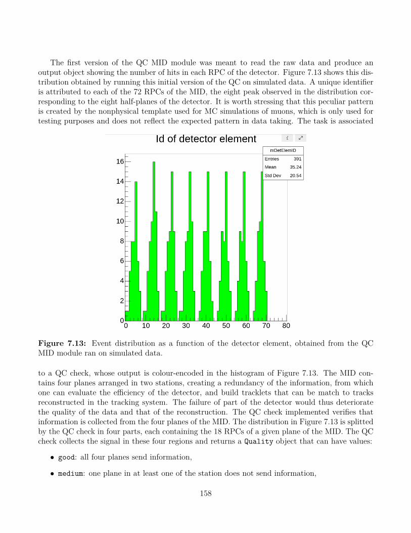
The first version of the QC MID module was meant to read the raw data and produce anoutput object showing the number of hits in each RPC of the detector. Figure 7.13 shows this dis-tribution obtained by running this initial version of the QC on simulated data. A unique identifieris attributed to each of the 72 RPCs of the MID, the eight peak observed in the distribution cor-responding to the eight half-planes of the detector. It is worth stressing that this peculiar patternis created by the nonphysical template used for MC simulations of muons, which is only used fortesting purposes and does not reflect the expected pattern in data taking. The task is associated

Figure 7.13: Event distribution as a function of the detector element, obtained from the QCMID module ran on simulated data.

to a QC check, whose output is colour-encoded in the histogram of Figure 7.13. The MID con-tains four planes arranged in two stations, creating a redundancy of the information, from whichone can evaluate the efficiency of the detector, and build tracklets that can be match to tracksreconstructed in the tracking system. The failure of part of the detector would thus deterioratethe quality of the data and that of the reconstruction. The QC check implemented verifies thatinformation is collected from the four planes of the MID. The distribution in Figure 7.13 is splittedby the QC check in four parts, each containing the 18 RPCs of a given plane of the MID. The QCcheck collects the signal in these four regions and returns a Quality object that can have values:

• good: all four planes send information,

• medium: one plane in at least one of the station does not send information,

158

• bad: the two planes in at least one station do not send information.

The module was tested as a continuous workflow by pairing it to a data producer continuouslysending raw data, mimicking real data taking. The output object of the QC task is then filledon the fly, and the histogram is regularly updated, allowing one to verify the detector status as afunction of time.

The module was further completed for extending checks of the raw data. The reading isextended in order to check each GBT link individually, and look for inconsistencies in the data.One can for example force an error by modifying the electronics delay between local and regionalcards. Manually setting this delay at a non-nominal value leads the local and regional responsesto not arrive at the same bunch crossing, producing errors. The output is a file containing a listof possible problems, if any, as well as a summary containing the number of processed and faultyevents. The list of problems is provided per interaction record. An entry in the output file typicallyreads:

BCid: 0x71c Orbit: 0xf [in page: 542 (line: 277505) ]loc-reg inconsistency: fired locals (00010000) != expected from reg (00000000);Crate ID: 15 Loc ID: 4 status: 0xc0 trigger: 0x 0 firedChambers: [...]

The event can be identified through the bunch crossing (BC) and orbit identifiers. The next lineprovides information on the origin of the error. In this example, following the nature of the errorthat was forced, the entry is tagger as loc-reg inconsistency. The last line allows to locate theerror in terms of the crate and local board identifiers, and contains the coordinates of the firedchambers, enabling the monitoring of the status of each RPC individually. The checker producesa summary of the error detection after each TF, in the form:

Fraction of faulty events: 232 / 4296

The fraction of faulty events represents the ratio of the number of processed events where an errorwas found, to the total number of processed events. This information can be sent to a standardQC output object, such as a histogram, which is then filled on-the-fly as the TFs are received andprocessed by the task. An example is shown in Figure 7.14.

For now the module was tested locally, on simulated data, and consists in the QC of raw dataonly. The next step will require its testing in the full O2 framework, and the inclusion of furtherchecks such as noisy channels, occupancy, digits and clusters.

159

Figure 7.14: Event distribution as a function of the detector element, obtained from the QCMID module ran on simulated data.

160

Part III

Z0- and W±-boson measurementsin p–Pb collisions at √

sNN = 8.16 TeV

161

Chapter 8

Data analysis

The the performance of the measurement of the weak-boson production in heavy-ion collisions(HIC) at large rapidities, with the ALICE muon spectrometer, was studied in Ref. [259]. Theirmeasurements in p–Pb collisions at √sNN = 5.02 TeV by the ALICE Collaboration [156] showedthat, although feeble, the signal can be extracted, and with the energy increase at 8.16 TeV onecan expect a significantly higher production for a precise measurement. This chapter presentsthe analysis methodology and the intermediary results that lead to the measurements presentedin the next chapter. The chapter starts with a presentation of the data sample in Section 8.1,describing the event and track selections along with the evaluation of the integrated luminosityand the event centrality. Section 8.2 focuses on the signal extractions of the Z0 and W± bosons,with considerations on the background evaluation. The procedure for the efficiency correction isdescribed in Section 8.3. The chapter ends with information on the computation for differentialstudies in Section 8.4 and a summary of the systematic uncertainties affecting the measurementsin Section 8.5.

8.1 Data samples and selection

8.1.1 Collision system and LHC periodsThe data samples analysed in this work correspond to two p–Pb collision periods and were collectedin November and December 2016 by the ALICE detector at the LHC. Because of the single magnetdesign at the LHC, the proton and Pb beams have the same magnetic rigidity. The energy pernucleon in the Pb beam is therefore smaller than that of the proton beam by a factor 82

208∼ 0.4. The

centre-of-mass energy per nucleon-nucleon collision √sNN in a HIC is related to the centre-of-massenergy of pp collisions

√s with the same accelerating conditions as:

√sNN =

√s×

√Z1Z2

A1A2

, (8.1)

where A1 (Z1) and A2 (Z2) are the atomic (charge) numbers of the first (second) colliding ion. Inthe 2016 p–Pb collision period, the equivalent centre-of-mass energy in pp collisions is

√s = 13

163

TeV, from which one gets:

Z1 = 1 Z2 = 82A1 = 1 A2 = 208

⇒ √

sNN = 13×√

82

208= 8.16 TeV. (8.2)

Since the collision system is asymmetrical, the rapidity in the centre-of-mass frame is shiftedwith respect to that of the laboratory frame by:

∆y =1

2ln

(Zp/Ap

ZPb/APb

)≈ 0.465 (8.3)

towards the proton beam. The muon spectrometer of ALICE covers the pseudorapidity interval−4 < ηlab < −2.5 in the ALICE coordinate system1, such that the angular coverage correspond todifferent values of Bjorken-x depending on whether the proton beam moves towards the spectrom-eter or away from it. For convenience, the former configuration is called the p-going configuration,or p–Pb collisions, the latter Pb-going or Pb–p. As the spectrometer does not cover both positiveand negative rapidities, the two configurations are realised by swapping the beam directions. Ifone adopts the convention that the proton beam travels towards positive rapidities, the rapidityintervals in the centre-of-mass frame are then:

• p–Pb collisions: 2.03 < ycms < 3.53,

• Pb–p collisions: −4.46 < ycms < −2.96.

The corresponding Bjorken-x intervals are given in Table 8.1. They are calculated at LO withEquation 3.32, which reads, for p–Pb collisions:

x1,2 =MZ,W√sNN

exp (−y) . (8.4)

−4.46 < ycms < −2.96 2.03 < ycms < 3.53

Z0 2.16× 10−1 < x < 9.66× 10−1 3.27× 10−4 < x < 1.47× 10−3

W± 1.90× 10−1 < x < 8.51× 10−1 2.89× 10−4 < x < 1.29× 10−3

Table 8.1: Bjorken-x intervals assessed by the measurement of Z0 and W± bosons with the ALICEmuon spectrometer in p–Pb collisions at √sNN = 8.16 TeV. The calculations are performed atLO with the masses of the bosons set at the PDG values [6].

The data taking is divided into periods, conventionally denoted as

LHC + year + sequential letters.1The ALICE coordinate system is an orthogonal right-handed basis with the origin at the collision point, the ~ex

pointing to the centre of the accelerator and ~ey pointing upwards.

164

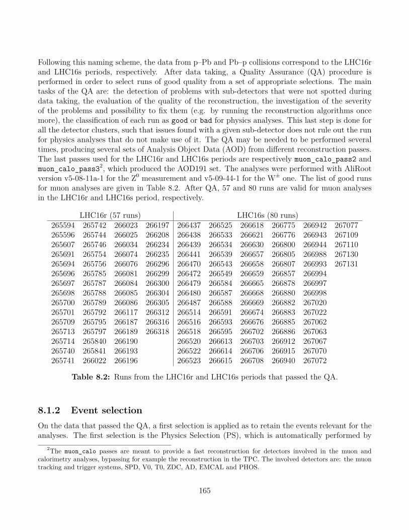
Following this naming scheme, the data from p–Pb and Pb–p collisions correspond to the LHC16rand LHC16s periods, respectively. After data taking, a Quality Assurance (QA) procedure isperformed in order to select runs of good quality from a set of appropriate selections. The maintasks of the QA are: the detection of problems with sub-detectors that were not spotted duringdata taking, the evaluation of the quality of the reconstruction, the investigation of the severityof the problems and possibility to fix them (e.g. by running the reconstruction algorithms oncemore), the classification of each run as good or bad for physics analyses. This last step is done forall the detector clusters, such that issues found with a given sub-detector does not rule out the runfor physics analyses that do not make use of it. The QA may be needed to be performed severaltimes, producing several sets of Analysis Object Data (AOD) from different reconstruction passes.The last passes used for the LHC16r and LHC16s periods are respectively muon_calo_pass2 andmuon_calo_pass32, which produced the AOD191 set. The analyses were performed with AliRootversion v5-08-11a-1 for the Z0 measurement and v5-09-44-1 for the W± one. The list of good runsfor muon analyses are given in Table 8.2. After QA, 57 and 80 runs are valid for muon analysesin the LHC16r and LHC16s period, respectively.

LHC16r (57 runs) LHC16s (80 runs)265594 265742 266023 266197 266437 266525 266618 266775 266942 267077265596 265744 266025 266208 266438 266533 266621 266776 266943 267109265607 265746 266034 266234 266439 266534 266630 266800 266944 267110265691 265754 266074 266235 266441 266539 266657 266805 266988 267130265694 265756 266076 266296 266470 266543 266658 266807 266993 267131265696 265785 266081 266299 266472 266549 266659 266857 266994265697 265787 266084 266300 266479 266584 266665 266878 266997265698 265788 266085 266304 266480 266587 266668 266880 266998265700 265789 266086 266305 266487 266588 266669 266882 267020265701 265792 266117 266312 266514 266591 266674 266883 267022265709 265795 266187 266316 266516 266593 266676 266885 267062265713 265797 266189 266318 266518 266595 266702 266886 267063265714 265840 266190 266520 266613 266703 266912 267067265740 265841 266193 266522 266614 266706 266915 267070265741 266022 266196 266523 266615 266708 266940 267072

Table 8.2: Runs from the LHC16r and LHC16s periods that passed the QA.

8.1.2 Event selectionOn the data that passed the QA, a first selection is applied as to retain the events relevant for theanalyses. The first selection is the Physics Selection (PS), which is automatically performed by

2The muon_calo passes are meant to provide a fast reconstruction for detectors involved in the muon andcalorimetry analyses, bypassing for example the reconstruction in the TPC. The involved detectors are: the muontracking and trigger systems, SPD, V0, T0, ZDC, AD, EMCAL and PHOS.

165

the AliPhysicsSelectionTask. At its lowest level, the PS performs basic checks on V0 and ZDCtimings to ensure that the event correspond to a collision at the interaction point. The task alsoenables a rejection of events affected by the bunch-crossing pile-up (corresponding to events withtwo or more collisions occurring in the same bunch crossing) and out-of-bunch pile-up (where oneor more collisions occurred in bunch crossings different from the one that trigger the acquisition).The events are furthermore required to have a good vertex reconstructed by the SPD, asking for anon-zero number of contributors in the SPD, and a longitudinal vertex position estimated within±10 cm from the nominal interaction point. For the muon analyses presented here, the rejectionof pile-up events removes about 10% of the data sample, while the selection on the vertex has avery small effect.

The last event selection relies on the trigger classes fired during data taking. In this work, fourtriggers were used:

• Minimum Bias (MB) trigger: INT, corresponding to a logical AND between signals fromV0A and V0C. The trigger used is CINT7-B-NOPF-CENT. Given the smaller downscaling factorwith respect to the CINT7-B-NOPF-MUFAST trigger class, it allows for a higher statistics forthe offline normalisation,

• Single Muon Low trigger: MSL, requiring one muon track fired in the trigger system witha pT & 0.5 GeV/c threshold in addition to the MB trigger. The trigger class used is theCMSL7-B-NOPF-MUFAST,

• Single Muon High trigger: MSH, same as MSL, with a pT threshold at ∼ 4.2 GeV/c. Thetrigger class used is CMSH7-B-NOPF-MUFAST,

• Dimuon Unlike-sign Low trigger: MUL, which requires a muon pair of opposite chargesign, each with pT & 0.5 GeV/c, in addition to the MB trigger. The trigger class used isCMUL7-B-NOPF-MUFAST.

The last two triggers are meant to provide the data samples containing dimuons and single muonsof high pT, which characterise the signal of the Z0 and W± bosons. The MSL trigger is used for analternative computation for the luminosity determination, as explained in the next section. Table8.3 summarises the main characteristics of the two analysed periods.

Period System Nb of runs Rapidity NCMSH NCMUL

LHC16r p–Pb 57 2.03 < ycms < 3.53 18.5× 106 25.8× 106

LHC16s Pb–p 80 −4.46 < ycms < −2.96 35.1× 106 72.0× 106

Table 8.3: Main characteristics of the periods analysed in this study, from p–Pb collisions at√sNN = 8.16 TeV.

166

8.1.3 LuminosityThe integrated luminosity for each period, and the associated statistical uncertainty, are calculatedas:

Lint =NMB

σV0

=FMBnorm ×NCTRIG

σV0

,

(σLintstat

Lint

)2

=∑i

(σixi

)2

, (8.5)

where TRIG is MUL for the Z0 measurement and MSH for the W± one. σV0 is the visible cross-sectionestimated by means of van-der-Meer scans of the V0-based MB trigger signal. For the LHC16rand LHC16s periods it amounts to 2.09± 0.04 b and 2.10± 0.04 b respectively, where the quotederrors are systematics, the statistical ones being negligible [196]. The xi (σi) in the formula forthe statistical uncertainty correspond to the quantities (statistical uncertainty on the quantities)used for the evaluation of the luminosity, with i = FMB

norm, NCTRIG, σMB.FMBnorm is a normalisation factor used to obtain the number of MB events NMB corresponding to

the number of CTRIG triggered events NCTRIG. It can be computed using two methods, and has tobe corrected for pile-up.

Offline method The first method to compute Fnorm is based on recorded triggers at the offlinelevel, in AODs. One can compute the offline normalisation factor for each run i with the directoffline method (off1):

F off1,inorm =

N iMB

N iMB&0TRIG

× PU i, (8.6)

where N iMB is the total number of MB events, and N i

MB&0TRIG is the total number of MB eventswhere one 0TRIG input is recorded, that is, a TRIG input at the L0 level. PU i is the pile-upcorrection (see below) that accounts for the probability to have more than one interaction in anevent.

The precision can be increased by defining an indirect offline method (off2), adding an extrastep in which an intermediate trigger with higher statistics is used. In this work the single muonCMSL trigger is used. The offline factor then becomes

F off2,inorm =

N iMB

N iMB&0MSL

× N iCMSL

N iCMSL&0TRIG

× PU i, (8.7)

where N iCMSL is the total number of MSL events and N i

MB&0MSL (N iCMSL&0TRIG) is the number of MB

(CTRIG) events where one 0MSL (0TRIG) event is recorded.

Online method The Fnorm factor can also be computed using a so-called online method, basedon the online L0b trigger scalers. It corresponds to L0 inputs sent from the trigger to the CTP.The normalisation factor is computed for each run as:

F on,inorm =

L0biMB

L0biTRIG× P i

MB

P iTRIG× PU i, (8.8)

167

where L0biMB and L0bi

TRIG are the measured trigger counts of the L0b inputs for MB and TRIGtriggers, both taken from the MUFAST3 trigger cluster, and P i

MB and P iMUL are the purity factors

computed offline in order to correct the L0b taken directly from the OCDB where the physicsselection is not yet applied.

Purity The purity factors P iMB,TRIG are corrections applied to account for MB or TRIG events

that do not pass the PS. They are defined as

P iMB,TRIG =

N iMB,TRIG(PS)

N iMB,TRIG(ALL)

, (8.9)

where N iMB,TRIG(ALL) and N i

MB,TRIG(PS) are the number of events recorded by the MB or TRIGtrigger during the run i before and after PS, respectively. The P i

MB, P iCMUL and P i

CMSH, as a functionof the run number, are displayed in Fig. 8.1.

2655

9426

5596

2656

0726

5691

2656

9426

5696

2656

9726

5698

2657

0026

5701

2657

0926

5713

2657

1426

5740

2657

4126

5742

2657

4426

5746

2657

5426

5756

2657

8526

5787

2657

8826

5789

2657

9226

5795

2657

9726

5840

2658

4126

6022

2660

2326

6025

2660

3426

6074

2660

7626

6081

2660

8426

6085

2660

8626

6117

2661

8726

6189

2661

9026

6193

2661

9626

6197

2662

0826

6234

2662

3526

6296

2662

9926

6300

2663

0426

6305

2663

1226

6316

2663

18

iP

0.95

0.96

0.97

0.98

0.99

1

1.01

1.02

1.03

1.04

1.05

= 8.16 TeVNNsp-Pb,

This workPurity CINT

Purity CMSH

Purity CMUL

2664

3726

6438

2664

3926

6441

2664

7026

6472

2664

7926

6480

2664

8726

6514

2665

1626

6518

2665

2026

6522

2665

2326

6525

2665

3326

6534

2665

3926

6543

2665

4926

6584

2665

8726

6588

2665

9126

6593

2665

9526

6613

2666

1426

6615

2666

1826

6621

2666

3026

6657

2666

5826

6659

2666

6526

6668

2666

6926

6674

2666

7626

6702

2667

0326

6706

2667

0826

6775

2667

7626

6800

2668

0526

6807

2668

5726

6878

2668

8026

6882

2668

8326

6885

2668

8626

6912

2669

1526

6940

2669

4226

6943

2669

4426

6988

2669

9326

6994

2669

9726

6998

2670

2026

7022

2670

6226

7063

2670

6726

7070

2670

7226

7077

2671

0926

7110

2671

3026

7131

iP

0.95

0.96

0.97

0.98

0.99

1

1.01

1.02

1.03

1.04

1.05

= 8.16 TeVNNsPb-p,

This workPurity CINT

Purity CMSH

Purity CMUL

2655

9426

5596

2656

0726

5691

2656

9426

5696

2656

9726

5698

2657

0026

5701

2657

0926

5713

2657

1426

5740

2657

4126

5742

2657

4426

5746

2657

5426

5756

2657

8526

5787

2657

8826

5789

2657

9226

5795

2657

9726

5840

2658

4126

6022

2660

2326

6025

2660

3426

6074

2660

7626

6081

2660

8426

6085

2660

8626

6117

2661

8726

6189

2661

9026

6193

2661

9626

6197

2662

0826

6234

2662

3526

6296

2662

9926

6300

2663

0426

6305

2663

1226

6316

2663

18

iP

U

1

1.01

1.02

1.03

1.04

1.05

1.06

= 8.16 TeVNNsp-Pb,

This work

2664

3726

6438

2664

3926

6441

2664

7026

6472

2664

7926

6480

2664

8726

6514

2665

1626

6518

2665

2026

6522

2665

2326

6525

2665

3326

6534

2665

3926

6543

2665

4926

6584

2665

8726

6588

2665

9126

6593

2665

9526

6613

2666

1426

6615

2666

1826

6621

2666

3026

6657

2666

5826

6659

2666

6526

6668

2666

6926

6674

2666

7626

6702

2667

0326

6706

2667

0826

6775

2667

7626

6800

2668

0526

6807

2668

5726

6878

2668

8026

6882

2668

8326

6885

2668

8626

6912

2669

1526

6940

2669

4226

6943

2669

4426

6988

2669

9326

6994

2669

9726

6998

2670

2026

7022

2670

6226

7063

2670

6726

7070

2670

7226

7077

2671

0926

7110

2671

3026

7131

iP

U

1

1.01

1.02

1.03

1.04

1.05

1.06

= 8.16 TeVNNsPb-p,

This work

Figure 8.1: Evolution of the purity (top) and pile-up (bottom) factors as a function of the runnumber, in p–Pb (left) and Pb–p (right) collisions.

3The MUFAST cluster contains the muon trigger and tracking systems, as well as the SPD, V0, T0 and AD.

168

Pile-up factor The pile-up factor PU i for run i is calculated using

PU i =µi

1− e−µi . (8.10)

µi is the mean number of collisions per bunch crossing, assuming a poissonian distribution, for therun i:

µi = − ln

(1− P i

MB × L0bRateiMB

nib × fLHC

), (8.11)

where P iMB is the MB purity factor for run i, L0bRateiMB is the number of MB events recorded by

the L0b counter per data taking time, nib is the number of colliding bunches and fLHC = 11245 Hz

is the revolution frequency of the LHC. The evolution of the pile-up factor as a function of the runnumber is shown in Fig. 8.1. The factor is not used in the W± analysis, as the pile-up is alreadyaccounted for at the Physics Selection level.

Luminosities For each method, the total Fnorm and its statistical uncertainty are computed asthe weighted average of the run-per-run contributions:

Fnorm =

∑Nruns

i=1 F inorm ×N i

CTRIG∑Nruns

i=1 N iCTRIG

, (8.12)

The evolution of the F inorm factors, as a function of the run number, is displayed in Fig. 8.2, and

Table 8.4 summarises the numerical values obtained with the two methods for the two periods.The direct offline method is neglected compared to the indirect one, as the latter provides a muchmore precise evaluation of the normalisation factor. The final Fnorm is taken as the average be-tween the online and indirect offline methods, the difference between the two is taken as systematicuncertainty.

CMUL trigger CMSH triggerMethod p-going Pb-going p-going Pb-goingF off1norm 679.8± 5.4 373.0± 1.0 765.9± 14.4 596.9± 2.3

F off2norm 678.7± 1.4 371.5± 0.4 755.0± 1.7 596.9± 0.8F onnorm 683.3± 0.5 372.2± 0.3 765.3± 0.6 603.4± 0.5

Total 681.0± 1.0± 4.6 371.9± 0.4± 0.7 760.2± 1.2± 10.3 600.2± 0.7± 6.5

Table 8.4: Normalisation factors obtained from the direct offline (off1), indirect offline (off2)and online (on) methods for the dimuon (CMUL) and single muon (CMSH) triggers. The quoteduncertainties in the different methods are the statistical uncertainties. The ones quoted for thetotal values are statistical and systematic uncertainties, respectively.

The integrated luminosity is then computed using Equation 8.5. At this stage, the Z0 andW± measurements followed two different approaches. At the time when the Z0 measurement

169

2655

9426

5596

2656

0726

5691

2656

9426

5696

2656

9726

5698

2657

0026

5701

2657

0926

5713

2657

1426

5740

2657

4126

5742

2657

4426

5746

2657

5426

5756

2657

8526

5787

2657

8826

5789

2657

9226

5795

2657

9726

5840

2658

4126

6022

2660

2326

6025

2660

3426

6074

2660

7626

6081

2660

8426

6085

2660

8626

6117

2661

8726

6189

2661

9026

6193

2661

9626

6197

2662

0826

6234

2662

3526

6296

2662

9926

6300

2663

0426

6305

2663

1226

6316

2663

18

norm

iF

400

500

600

700

800

900

1000

1100

1200

= 8.16 TeVNNsp-Pb, Dimuons, CMUL7 triggerThis work

Offline, direct

Offline, indirect

Online

2664

3726

6438

2664

3926

6441

2664

7026

6472

2664

7926

6480

2664

8726

6514

2665

1626

6518

2665

2026

6522

2665

2326

6525

2665

3326

6534

2665

3926

6543

2665

4926

6584

2665

8726

6588

2665

9126

6593

2665

9526

6613

2666

1426

6615

2666

1826

6621

2666

3026

6657

2666

5826

6659

2666

6526

6668

2666

6926

6674

2666

7626

6702

2667

0326

6706

2667

0826

6775

2667

7626

6800

2668

0526

6807

2668

5726

6878

2668

8026

6882

2668

8326

6885

2668

8626

6912

2669

1526

6940

2669

4226

6943

2669

4426

6988

2669

9326

6994

2669

9726

6998

2670

2026

7022

2670

6226

7063

2670

6726

7070

2670

7226

7077

2671

0926

7110

2671

3026

7131

norm

iF

340

360

380

400

420

440

460 = 8.16 TeVNNsPb-p, Dimuons, CMUL7 triggerThis work

Offline, direct

Offline, indirect

Online

2655

9426

5596

2656

0726

5691

2656

9426

5696

2656

9726

5698

2657

0026

5701

2657

0926

5713

2657

1426

5740

2657

4126

5742

2657

4426

5746

2657

5426

5756

2657

8526

5787

2657

8826

5789

2657

9226

5795

2657

9726

5840

2658

4126

6022

2660

2326

6025

2660

3426

6074

2660

7626

6081

2660

8426

6085

2660

8626

6117

2661

8726

6189

2661

9026

6193

2661

9626

6197

2662

0826

6234

2662

3526

6296

2662

9926

6300

2663

0426

6305

2663

1226

6316

2663

18

norm

iF

600

700

800

900

1000

1100

1200

= 8.16 TeVNNsp-Pb, Single muons, CMSH7 triggerThis work

Offline, direct

Offline, indirect

Online

2664

3726

6438

2664

3926

6441

2664

7026

6472

2664

7926

6480

2664

8726

6514

2665

1626

6518

2665

2026

6522

2665

2326

6525

2665

3326

6534

2665

3926

6543

2665

4926

6584

2665

8726

6588

2665

9126

6593

2665

9526

6613

2666

1426

6615

2666

1826

6621

2666

3026

6657

2666

5826

6659

2666

6526

6668

2666

6926

6674

2666

7626

6702

2667

0326

6706

2667

0826

6775

2667

7626

6800

2668

0526

6807

2668

5726

6878

2668

8026

6882

2668

8326

6885

2668

8626

6912

2669

1526

6940

2669

4226

6943

2669

4426

6988

2669

9326

6994

2669

9726

6998

2670

2026

7022

2670

6226

7063

2670

6726

7070

2670

7226

7077

2671

0926

7110

2671

3026

7131

norm

iF

500

550

600

650

700

750

800

850

900

= 8.16 TeVNNsPb-p, Single muons, CMSH7 triggerThis work

Offline, direct

Offline, indirect

Online

Figure 8.2: Fnorm as a function of the run number, for MUL (top) and MSH triggered events, inp–Pb (left) and Pb–p (right) collisions.

was performed, the AliPhysicsSelectionTask did not offer the possibility to exclude the pile-upevents, such that they were included in the data sample from which the luminosity is computed. Itwas verified afterwhile that the pile-up effect is negligible for this measurement at the cross sectionlevel, as the reduction in the luminosity comes with a reduction of the number of extracted dimuonsfrom Z0 decays, the two effects ending up cancelling each other out. For the W±, performed morerecently, the pile-up events are rejected by the PS task, leading to a lower value for the luminosityas events are rejected much earlier in the analysis flow. It was also verified that the two analyses,having the same MB condition, are consistent with one another when the same procedure isfollowed for both CMUL and CMSH triggered events. For the luminosity, one gets:

• without pile-up rejection:

Lint =

8.40± 0.01 (stat)± 0.17 (syst) nb−1 at forward,12.74± 0.01 (stat)± 0.26 (syst) nb−1 at backward,

(8.13)

170

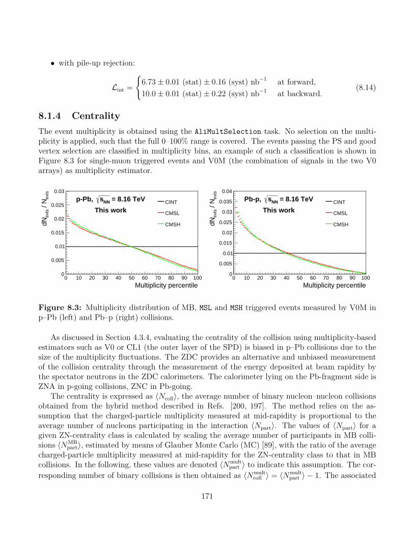
• with pile-up rejection:

Lint =

6.73± 0.01 (stat)± 0.16 (syst) nb−1 at forward,10.0± 0.01 (stat)± 0.22 (syst) nb−1 at backward.

(8.14)

8.1.4 CentralityThe event multiplicity is obtained using the AliMultSelection task. No selection on the multi-plicity is applied, such that the full 0–100% range is covered. The events passing the PS and goodvertex selection are classified in multiplicity bins, an example of such a classification is shown inFigure 8.3 for single-muon triggered events and V0M (the combination of signals in the two V0arrays) as multiplicity estimator.

Multiplicity percentile0 10 20 30 40 50 60 70 80 90 100

evts

/ N

evts

dN

0

0.005

0.01

0.015

0.02

0.025

0.03

= 8.16 TeVNNsp-Pb,

This workCINT

CMSL

CMSH

Multiplicity percentile0 10 20 30 40 50 60 70 80 90 100

evts

/ N

evts

dN

0

0.005

0.01

0.015

0.02

0.025

0.03

0.035

0.04

= 8.16 TeVNNsPb-p,

This workCINT

CMSL

CMSH

Figure 8.3: Multiplicity distribution of MB, MSL and MSH triggered events measured by V0M inp–Pb (left) and Pb–p (right) collisions.

As discussed in Section 4.3.4, evaluating the centrality of the collision using multiplicity-basedestimators such as V0 or CL1 (the outer layer of the SPD) is biased in p–Pb collisions due to thesize of the multiplicity fluctuations. The ZDC provides an alternative and unbiased measurementof the collision centrality through the measurement of the energy deposited at beam rapidity bythe spectator neutrons in the ZDC calorimeters. The calorimeter lying on the Pb-fragment side isZNA in p-going collisions, ZNC in Pb-going.

The centrality is expressed as 〈Ncoll〉, the average number of binary nucleon–nucleon collisionsobtained from the hybrid method described in Refs. [200, 197]. The method relies on the as-sumption that the charged-particle multiplicity measured at mid-rapidity is proportional to theaverage number of nucleons participating in the interaction 〈Npart〉. The values of 〈Npart〉 for agiven ZN-centrality class is calculated by scaling the average number of participants in MB colli-sions 〈NMB

part〉, estimated by means of Glauber Monte Carlo (MC) [89], with the ratio of the averagecharged-particle multiplicity measured at mid-rapidity for the ZN-centrality class to that in MBcollisions. In the following, these values are denoted 〈Nmult

part 〉 to indicate this assumption. The cor-responding number of binary collisions is then obtained as 〈Nmult

coll 〉 = 〈Nmultpart 〉 − 1. The associated

171

Centrality class 0–100% 0–20% 20–40% 40–60% 60–100%〈Nmult

coll 〉 7.09± 0.28 12.2± 0.52 9.81± 0.17 7.09± 0.29 3.17± 0.09

Table 8.5: Average number of binary collisions 〈Nmultcoll 〉 estimated with the hybrid ZN method in

p–Pb collisions at √sNN = 8.16 TeV. Table adapted from Ref. [197].

uncertainty is evaluated using different approaches as described in Ref. [197]. The resulting valuesof 〈Nmult

coll 〉 and their uncertainties are summarised in Table 8.5.

8.1.5 Track selectionThe selected events should contain at least one or two muon tracks, following the selection onthe trigger condition. In order to extract them, and select the tracks relevant for the analyses, anumber of selection criteria is applied. A first set aims at ensuring a clean sample of muon trackcandidates:

• the trigger-tracker matching requires that each track reconstructed in the muon trackingsystem matches a track segment in the trigger chambers. The selection is based on a χ2 testof the quality of the matching. The matching serves as muon identification, as the shieldingof the trigger system is expected to stop all particles but muons,

• a selection of the polar angle at the end of the front absorber θabs requires 170 < θabs <178. Equivalently, the same selection can be applied to the radial transverse positionat the end of the front absorber Rabs, asking it to be in the interval 17.5 < Rabs < 89.5cm. This aims at removing the tracks crossing the high-density region of the front absorber,where they experience significant multiple scatterings,

• the product of the track momentum to its distance of closest approach p×DCAprovides an efficient rejection of the contamination by tracks not pointing to the interactionvertex. It exploits the correlation between the track momentum p and its DCA, correspond-ing to the distance to the primary vertex of the track trajectory extrapolated to the planetransverse to the beam axis. Indeed, following the multiple scatterings in the front absorber,the DCA distribution of particles produced in the collision follows a Gaussian distribution,with a width dependent on the material crossed and which is proportional to the inverse mo-mentum of the tracks. Background tracks, on the other hand, have on average a DCA largerthan about 40 cm, independently from their momentum. A Gaussian fit of the distributionis performed, allowing one to apply the selection p × DCA < 6 σ for the rejection of thisbackground source.

Supplementary to this selection, a fiducial region is defined following the detection capabilitiesand to increase the efficiency of the signal extraction:

• a selection on the track pseudorapidity, −4 < ηlab < −2.5, ensures that the track is withinthe spectrometer acceptance and avoids edge effects,

172

• a low boundary is set on the track transverse momentum as both the Z0 and W± signalsare characterised by high-pT muons. The limit is set at pT > 10 GeV/c in the W± mea-surement, and pT > 20 GeV/c for Z0. In this second case, the selection is applied on theindividual tracks and not on the dimuon pT,

• in the Z0 analysis, the invariant mass interval over which the signal is extracted is 60 <mµµ < 120 GeV/c2 as to fully encompass the Z0 peak while excluding as much backgroundas possible.

The effects of the selections are illustrated in Figure 8.4.The top panels show the evolution of the single muon pT distribution for muon track candidates

in the MSH triggered events, as the selection criteria are sequentially applied. One sees a largedifference in the effects of the selection between p–Pb and Pb–p collisions. In the latter, thespectrometer lies on the side of the Pb fragments, and receives a large amount of supplementarybackground compared to p–Pb collisions. The number of tracks in the distributions is given inTable 8.6.

Period after PS + good vertex + η + θabs + matching + pDCALHC16r 16,691,304 15,368,669 14,211,023 14,126,091 10,283,041 10,247,955LHC16s 30,931,163 28,531,664 25,850,779 25,587,821 15,995,207 15,714,934

Table 8.6: Number of tracks after physics and vertex selection and the application of the cuts.

The middle panels of Figure 8.4 show the final distribution, after application of the full selection,of the single muon pT spectrum for positively and negatively charged tracks, as well as the combineddistribution. A bulk of production is seen around ∼ 40 GeV/c, half of the W± boson mass,corresponding to the characteristic signal of its muonic decay (the Jacobian peak). There is asignificant difference between the µ+ and µ− distribution, following from the quark content of thenucleus that affect in opposite manner the production of W+ and W− bosons. This difference isstriking when looking at the charge ratio as a function of pT, shown in the bottom panels of thefigure.

8.2 Signal extraction

8.2.1 OverviewThe evaluation of the production starts from the extraction of the number of Z0 and W± bosonsfrom the data. The former is characterised by two muons of opposite charges, each with high pT,forming a dimuon of invariant mass close to the mass of the boson itself, around 90 GeV/c2. Theinvariant mass is calculated as:

mµµ =

√(E1 + E2)

2 −(px,1 + px,2

)2 − (py,1 + py,2)2 − (pz,1 + pz,2

)2, (8.15)

173

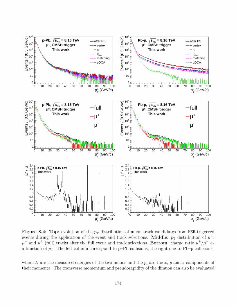
(GeV/c)T

µp0 10 20 30 40 50 60 70 80 90 100

Eve

nts

/ (0.

5 G

eV/c

)

1

10

210

310

410

510

610


, CMSH trigger±µThis work

after PS+ vertex

η+

absθ+ + matching+ pDCA

(GeV/c)T

µp0 10 20 30 40 50 60 70 80 90 100

Eve

nts

/ (0.

5 G

eV/c

)

1

10

210

310

410

510

610



after PS+ vertex

η+

absθ+ + matching+ pDCA

(GeV/c)T

µp0 10 20 30 40 50 60 70 80 90 100

Eve

nts

/ (0.

5 G

eV/c

)

1

10

210

310

410

510

610



full+µ-µ

(GeV/c)T

µp0 10 20 30 40 50 60 70 80 90 100

Eve

nts

/ (0.

5 G

eV/c

)

1

10

210

310

410

510

610



full+µ-µ

(GeV/c)T

µp0 10 20 30 40 50 60 70 80 90 100

- µ / + µ

00.20.40.60.8

11.21.41.61.8

22.22.4

This work = 8.16 TeVNNsp-Pb,

(GeV/c)T

µp0 10 20 30 40 50 60 70 80 90 100

- µ / + µ

00.20.40.60.8

11.21.41.61.8

22.22.4

This work = 8.16 TeVNNsPb-p,

Figure 8.4: Top: evolution of the pT distribution of muon track candidates from MSH-triggeredevents during the application of the event and track selections. Middle: pT distribution of µ+,µ− and µ± (full) tracks after the full event and track selections. Bottom: charge ratio µ+/µ− asa function of pT. The left column correspond to p–Pb collisions, the right one to Pb–p collisions.

where E are the measured energies of the two muons and the pi are the x, y and z components oftheir momenta. The transverse momentum and pseudorapidity of the dimuon can also be evaluated

174

following:

pµµT =

√(px,1 + px,2

)2+(py,1 + py,2

)2, ηµµ =

1

2ln

(E1 + E2 + pz,1 + pz,2E1 + E2 − (pz,1 + pz,2)

). (8.16)

The extraction of the W± boson is complicated by the presence of a neutrino in the final state.Moreover, as ALICE is not a hermetic detector, the missing energy or transverse mass in the eventcannot be estimated. The signal extraction procedure then relies on the inclusive single muon pTdistribution, in which three main contributions are expected: the large pT region is populated bymuons coming from W± and Z0 bosons, while at low pT a large number of muons coming fromthe decay of heavy-flavour hadrons (HF) is expected. The inclusive spectrum is reproduced fromsimulations with the template fit method. MC simulations are performed for each contribution,then combined with:

f(pT) = Nbkg · fbkg(pT) +Nµ±←W± ·

(fµ±←W±(pT) +R · f

µ±←Z0(pT)

), (8.17)

where:

• fbkg, fµ±←W± and fµ±←Z0 are the templates, constructed following the simulation procedure

explained below,

• Nbkg and Nµ±←W± are the numbers of muons from HF decays and W± decays respectively,

• R is the ratio of the cross section of muons from Z0 decays to that of W± decays estimatedby the MC generator.

Equation 8.17 is used to fit the single muon inclusive spectrum, with Nbkg and Nµ±←W± as free

parameters, while R is fixed. The yield of muons from W± decays is then directly given by thevalue of N

µ±←W± after the fit.

8.2.2 MC simulationsThe signal extraction for the W± relies on MC simulations of contributions from W± and Z0

bosons and HF hadrons. As these simulations are meant to reproduce the experimental spectrum,it needs to include a reproduction of the particle transport through the detector, as well as itsrunning conditions and detection capabilities. The simulations will also be used for the evaluationof the detector efficiency. All simulations are performed run-by-run, with a number of events pro-portional to the number of MSH- or MUL-triggered events in the data.

HF hadrons

The simulation of HF-hadron production and muonic decay is estimated in the Fixed-Order Next-to-Leading-Log (FONLL) framework [95, 96], from production cross sections obtained with [260].The cross sections are obtained as a function of pT and y, with the NNPDF3.0 [261] PDF set, andsumming over the various possible decay chains:

175

b→ B → `,b→ B → D → `,

c→ (0.7D0 + 0.3D+)→ `.As prediction cannot be made directly for p–Pb collisions at √sNN = 8.16 TeV from the webinterface, they were derived from pp collisions at 8 TeV, without accounting for the nuclear cor-rections. Such corrections are expected to be negligible in the region of interest of this work, asthey only affect the pT region below ∼ 5 GeV/c [262]. The rapidity shift and energy difference areaccounted for by:

• obtaining the dσ/dy distributions in 2.03 < y < 3.53 and −4.46 < y < −2.96,

• shifting the distributions from the initial ranges to −4 < y < −2.5 to manually implementthe rapidity,

• performing a bin-by-bin scaling to increase the production for the energy difference, with ascaling factor given by: √

sNN(p–Pb)√s(pp) =

8.16

8= 1.02. (8.18)

assuming that the deviation from linearity over such a small range is negligible [263].The resulting distributions are fitted with phenomenological functions:

f(pT) = p0exp

(−p1 ×

√pT)

pp2T, f(y) = p0 + p1 × y2, (8.19)

where the pi, i = 0, 1, 2 are free parameters. The results of the fits are shown in Figure 8.5.They are used for the parametrisation for MC generation of muons from HF hadron decays withPYTHIA 6 [264].

After the generation with PYTHIA 6, the events are passed to a GEANT3 [265] simulationof the detector, anchored to the corresponding files in the OCDB. The GEANT3 code reproducesthe running condition during data taking, including the misalignment, and simulates the particletransport through the material. This reproduction of the running condition is not perfect, suchthat other corrections need to be applied.

The simulations must be corrected for the cluster resolution of the muon chambers, whichhas to be degraded in order to match the resolution observed during data taking. The standardreconstruction parametrises the cluster resolution with a distribution having Gaussian tails. Amore realistic description can be achieved using Crystal Ball (CB) functions instead [266]. A CBhas a Gaussian core that models the detector resolution, and power-law tails with independentparameters on both sides. The low-mass tail accounts for energy loss effects, while the high-masstail is attributed to multiple Coulomb scatterings in the front absorber and momentum resolution.The CB function reads:

f(x;N, x, σ, t1, t2, p1, p2) = N ·

A · (B − t)−p1 , t ≤ t1,

exp(−1

2t2), t1 ≤ t ≤ t2,

C · (D + t)−p2 , t ≥ t2.

(8.20)

176

(GeV/c)T

µp0 10 20 30 40 50 60 70 80 90 100

(pb

/ G

eV)

T /

dpσd

4−10

3−10

2−10

1−101

10

210

310

410

510

610

710

810

910 / ndf 2χ 0.3714 / 95

p0 5.645e+08± 1.559e+09

p1 0.1033± 0.9243 p2 0.272± 3.464

Muons from HF (c+b), p-Pb

This work

FONLL cross section

fit

(GeV/c)T

µp0 10 20 30 40 50 60 70 80 90 100

(pb

/ G

eV)

T /

dpσd

4−10

3−10

2−10

1−101

10

210

310

410

510

610

710

810

910 / ndf 2χ 0.09372 / 95

p0 6.206e+08± 1.577e+09

p1 0.106± 1.446 p2 0.287± 3.106

Muons from HF (c+b), Pb-p

This work

FONLL cross section

fit

y4− 3.8− 3.6− 3.4− 3.2− 3− 2.8− 2.6−

/ dy

(pb

)σd

810

910

1010 / ndf 2χ 0.003948 / 48

p0 4.751e+07± 1.878e+08

p1 4.207e+06±2.381e+06 −

Muons from HF (c+b), p-Pb

This work

FONLL cross section

fit

y4− 3.8− 3.6− 3.4− 3.2− 3− 2.8− 2.6−

/ dy

(pb

)σd

810

910

1010 / ndf 2χ 0.001248 / 48

p0 4.321e+07± 1.872e+08

p1 3.75e+06±4.16e+06 −

Muons from HF (c+b), Pb-p

This work

FONLL cross section

fit

Figure 8.5: FONLL [95] cross sections for the leptonic decay of HF hadrons as a function of pT(top) and y (bottom) in p–Pb (left) and Pb–p (right) collisions. The lines correspond to fits withphenomenological functions.

where:

t =x− xσ

, A =

(p1|t1|

)p1

· exp(−|t1|

2

2

), B =

p1|t1|− |t1|, (8.21)

C =

(p2|t2|

)p2

· exp(−|t2|

2

2

), D =

p2|t2|− |t2|. (8.22)

N , x and σ are the normalisation, mean and width of the Gaussian core while pi and ti (i = 1, 2)are the parameters of the tails. The A, B, C and D terms are defined as to ensure that both thefunction and its first derivative are continuous. The parameters are tuned on data, using the CBas a fit function for various experimental observables.

The anchoring to the OCDB, and the usage of the alignment files it contains, allows for takinginto account the relative displacement of the detector elements with respect to one another. Inaddition, one may face as well a misalignment of the spectrometer in its entirety. This effect

177

is mimicked by applying a systematic shift to the track deviation in the magnetic field, shiftingthe µ+ and µ− tracks in opposite directions. The magnitude of this shift can be tuned using aninitialisation parameter of the AliTaskMuonTrackSmearing task, this parameter being the numberof σ by which the mean value of the CB function used for the cluster resolution is shifted. Itsevaluation has to be performed by comparing some variable of interest between distributions fromdata and simulation.

In this work, the global shift was tuned by looking at the single muon pT distribution. Between10 and 20 GeV/c, one can assume that the distribution is only coming from the muonic decayof HF hadrons. The FONLL-based simulations of HF hadron decays are analysed using varioustuning factors and the µ+/µ− ratio is computed and compared to the one measured in the data.Table 8.7 shows the experimentally measured ratio, and the one obtained for various values of thetuning parameter. A parameter of 2.4 is found to best reproduce the ratio in p–Pb collisions, whilethe best match is found for a tuning parameter 2.3 in Pb–p. As the tuning parameter is expectedto be the same for the two periods, which were taken one after the other and without any accessto the ALICE cavern in between, a value of 2.4 is chosen, since:

• it is computed from a higher number of muons: in the [10;20] GeV/c interval, there are about70,000 muons in the p–Pb data sample, 40,000 in Pb–p,

• the global agreement for both periods is better: the ratio in p–Pb (Pb–p) simulations is at0.2σ (1σ) from that of data with a tuning at 2.4, at 1.2σ (0.3σ) with a tuning at 2.3.

System Data 2.2 2.3 2.4 2.5 2.6p–Pb 0.781± 0.006 0.794± 0.003 0.787± 0.002 0.780± 0.002 0.772± 0.002 0.767± 0.002Pb–p 0.766± 0.007 0.774± 0.002 0.768± 0.002 0.759± 0.002 0.751± 0.001 0.745± 0.001

Table 8.7: Charge ratio µ+/µ− for pT between 10 and 20 GeV/c measured in data and FONLL-based simulations for various values of the global misalignment tuning parameter in p–Pb andPb–p collisions.

Although the value of 2.4 is taken as the central value of the shift, one can see in Table 8.7that all tuning parameters between 2.2 and 2.6 are still leading to a charge ratio in simulationsthat agrees with the experimental one within 3σ. The 2.2–2.6 range is therefore taken as theuncertainty interval on the tuning parameter of the smearing task.

Z0 and W± bosons

The generation of the weak bosons is performed using POWHEG [267] as the particle generator.POWHEG generates hard events for various processes where heavy quarks, Higgs and electroweakbosons are involved. It implements NLO calculations and includes the Z0/γ∗ interference. CT10[176] at NLO is used for the free-nucleon PDF and EPS09 [98], also at NLO, serves for the im-plementation of the nuclear corrections. As POWHEG is only a hard event generator, it needs tobe interfaced with a shower MC program such as PYTHIA6 [264]. The detector response is simu-lated using GEANT3 [265], with corrections for the cluster resolution and the global misalignment

178

parametrised in the same way as for the HF simulations. The isospin effect, which has a significanteffect on the W± bosons, is accounted for by simulating separately pp and pn binary collisions,then combining the results together with the formula:

1

NpPb

dNpPb

dpT=Z

A

1

Npp

dNpp

dpT+A− ZA

1

Npn

dNpn

dpt, (8.23)

where A = 208 and Z = 82 are the atomic and charge number of Pb, respectively. The aboveformula is valid for the W± simulations, the merging for the Z0 is done at the invariant mass levelinstead of the transverse momentum. The output of the simulations is shown in Figure 8.6. Thefigures show the MC truth distributions, i.e. the simulations at the generation level, before particletransport, for the pT distribution of single muon tracks from W± decays, and the dimuon invariantmass distribution of muon pairs from Z0 decays.

In Equation 8.17, the number of muons coming from the decays of Z0 bosons is not a freeparameter, it is set to be proportional to the number of muons from W± following the ratio oftheir respective cross sections as predicted by POWHEG (the parameter R in the equation). Theprocedure is the following:

• the dN/dpT distribution is obtained from the simulations, applying the full event and trackselections,

• the resulting distribution is scaled by a factor σ4π/Ntrials, where σ4π is the total POWHEGcross section of the process in the full phase space, and Ntrials is the total number of eventsthat were generated in order to get the required statistics after the selection. This scalingtransforms the dN/dpT distribution into dσ/dpT,

• the cross sections for the W± and Z0 bosons, are obtained by integration over the region ofinterest, which allows for the evaluation of their ratio R = σZ0/σW± .

The ratios computed for the two collision systems and both muon electrical charges are given inTable 8.8.

System p–Pb Pb–pMuon charge – + – +

R 0.34 0.22 0.21 0.48

Table 8.8: Ratio R of the µ± ← Z0 cross section to that of µ± ← W± estimated in p–Pb andPb–p collisions at √sNN = 8.16 TeV from simulations with POWHEG [267].

8.2.3 Z0-boson signal extractionThe signal extraction of the Z0 boson in its muonic decay is performed from the dimuon invariantmass distribution obtained after applying the event and track selection detailed in Section 8.1.

179

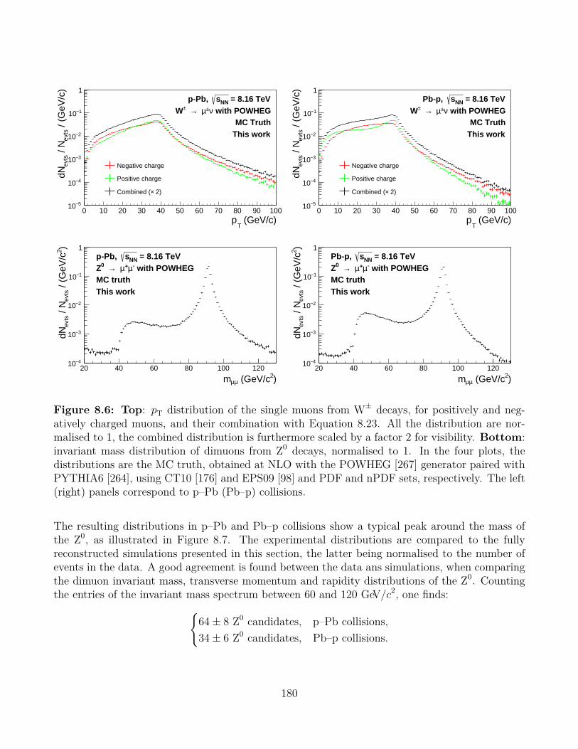
(GeV/c)T

p0 10 20 30 40 50 60 70 80 90 100

/ (G

eV/c

)ev

ts /

Nev

tsdN

5−10

4−10

3−10

2−10

1−10


with POWHEGν±µ → ±WMC Truth

This work

Negative charge

Positive charge

2)×Combined (

(GeV/c)T

p0 10 20 30 40 50 60 70 80 90 100

/ (G

eV/c

)ev

ts /

Nev

tsdN

5−10

4−10

3−10

2−10

1−10


with POWHEGν±µ → ±WMC Truth

This work

Negative charge

Positive charge

2)×Combined (

)2 (GeV/cµµm20 40 60 80 100 120

)2 /

(GeV

/cev

ts /

Nev

tsdN

4−10

3−10

2−10

1−10


with POWHEG-µ+µ → 0ZMC truthThis work

)2 (GeV/cµµm20 40 60 80 100 120

)2 /

(GeV

/cev

ts /

Nev

tsdN

4−10

3−10

2−10

1−10


with POWHEG-µ+µ → 0ZMC truthThis work

Figure 8.6: Top: pT distribution of the single muons from W± decays, for positively and neg-atively charged muons, and their combination with Equation 8.23. All the distribution are nor-malised to 1, the combined distribution is furthermore scaled by a factor 2 for visibility. Bottom:invariant mass distribution of dimuons from Z0 decays, normalised to 1. In the four plots, thedistributions are the MC truth, obtained at NLO with the POWHEG [267] generator paired withPYTHIA6 [264], using CT10 [176] and EPS09 [98] and PDF and nPDF sets, respectively. The left(right) panels correspond to p–Pb (Pb–p) collisions.

The resulting distributions in p–Pb and Pb–p collisions show a typical peak around the mass ofthe Z0, as illustrated in Figure 8.7. The experimental distributions are compared to the fullyreconstructed simulations presented in this section, the latter being normalised to the number ofevents in the data. A good agreement is found between the data ans simulations, when comparingthe dimuon invariant mass, transverse momentum and rapidity distributions of the Z0. Countingthe entries of the invariant mass spectrum between 60 and 120 GeV/c2, one finds:

64± 8 Z0 candidates, p–Pb collisions,34± 6 Z0 candidates, Pb–p collisions.

180

)2 (GeV/cµµm20 40 60 80 100 120

)2E

vent

s / (

3 G

eV/c

0

2

4

6

8

10

12


This work

data

POWHEG

)2 (GeV/cµµm20 40 60 80 100 120

)2E

vent

s / (

3 G

eV/c

0

2

4

6

8


This work

data

POWHEG

(GeV/c)T

µµp0 10 20 30 40 50 60 70 80 90

Eve

nts

/ (2

GeV

/c)

0

2

4

6

8

10

12


This work

data

POWHEG

(GeV/c)T

µµp0 10 20 30 40 50 60 70 80 90

Eve

nts

/ (2

GeV

/c)

0

2

4

6

8


This work

data

POWHEG

µµη

4− 3.8− 3.6− 3.4− 3.2− 3− 2.8− 2.6−

Eve

nts

0

2

4

6

8

10

12


This workdata

POWHEG

µµη

4− 3.8− 3.6− 3.4− 3.2− 3− 2.8− 2.6−

Eve

nts

0

2

4

6

8


This work

data

POWHEG

Figure 8.7: Invariant mass (top), pT (middle) and η (bottom) distributions of dimuons from Z0

candidates in p–Pb (left) and Pb–p (right) collisions at √sNN = 8.16 TeV. The lines correspondto fully reconstructed simulations of the Z0 → µ+µ− process at NLO, generated with POWHEG,using CT10 and EPS09 as PDF and nPDF, respectively. The particle transport and detectorresponse is accounted for using the GEANT3 code.

181

The fiducial region over which the measurement is performed,pµT > 20 GeV/c,−4 < yµ < −2.5,60 < mµµ < 120 GeV/c2,

is defined such that the signal region is isolated from background as much as possible. How-ever, several sources can create a muon pair of opposite sign and high invariant mass that willcontaminate the signal. In this study, the following sources were considered:

• the muonic decays of HF hadrons: cc→ µ+µ− and bb→ µ+µ−,

• the muonic decays of top-antitop pairs: tt→ µ+µ−,

• indirect Z0 decays through a τ pair, which then decay into two muons (and neutrinos):Z0 → τ+τ− → µ+µ−νµνµ,

• uncorrelated pairs formed from muons that do not originate from the same physics process.

The first source is estimated with POWHEG simulations of the cc(bb)→ µµ process. The MCtruth distributions are scaled to the cross section predicted by the generator, then scaled againto the luminosity of the corresponding collision period. This yields a realistic estimation of thecontribution of these processes to the experimental invariant mass spectrum. The simulationswere performed in the full phase space, the same selection as for the signal extraction is thenapplied in order to reach the same fiducial region. Figure 8.8 shows the evolution of the invariantmass distribution of dimuons from c and b decays. One can see that after the full selection isapplied, the significant amount of dimuons initially found in the region of interest is completelyremoved. It is worth reminding that the selection applied to the data contains no selection on thedimuon rapidity, the one shown in the figures is only given for reference. Following this study, thecontribution from the muonic decays of HF hadrons to the background is neglected.

The tt and τ+τ− contributions are estimated using simulations with POWHEG, applying againthe same selection as in the data. The distributions are then scaled to the Z0 → µµ distributionfollowing the ratio of their cross sections predicted by POWHEG. The comparison is shown inthe bottom panels of Figure 8.8. The contamination from each source is estimated as the ratioof the background source integrated in the region of interest, to that of the signal. These ratiosare found to be negligible, except for the tt → µ+µ− process in p–Pb collisions, which yields a1% contribution in the fiducial region. The fact that it is not contributing in Pb–p collisions canbe explained by the rapidity shift, which pushes the rapidity in the centre-of-mass towards largenegative rapidity. The rapidity distribution of dimuons from top-antitop decays being narrowerthan that of Z0 decays, the production is more suppressed.

The last source that was considered is the uncorrelated background, coming from muons pairsartificially constructed from muons that do not come from the same process. Since the probabilityto have such a pair is the same for muons of same or opposite charge, the uncorrelated backgroundcan be estimated by looking at the like-sign dimuon invariant mass distribution in the data,applying the same selection as for the signal extraction. Figure 8.9 shows the invariant mass

182

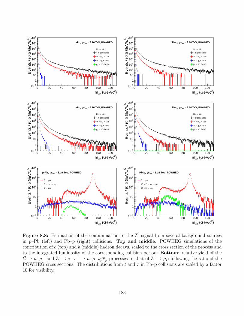
)2 (GeV/cµµm0 20 40 60 80 100 120

)2E

vent

s / (

0.5

GeV

/c

1−10

1

10

210

310

410

510

610

710

810 = 8.16 TeV, POWHEGNNsp-Pb,

µµ → cc

generatedπ4

< -2.5µµ-4 < y

< -2.5µη-4 <

> 20 GeV/cT

p

)2 (GeV/cµµm0 20 40 60 80 100 120

)2E

vent

s / (

0.5

GeV

/c

1−10

1

10

210

310

410

510

610

710

810 = 8.16 TeV, POWHEGNNsPb-p,

µµ → cc

generatedπ4

< -2.5µµ-4 < y

< -2.5µη-4 <

> 20 GeV/cT

p

)2 (GeV/cµµm0 20 40 60 80 100 120

)2E

vent

s / (

0.5

GeV

/c

1−10

1

10

210

310

410

510

610


µµ → bb

generatedπ4

< -2.5µµ-4 < y

< -2.5µη-4 <

> 20 GeV/cT

p

)2 (GeV/cµµm0 20 40 60 80 100 120

)2E

vent

s / (

0.5

GeV

/c

1−10

1

10

210

310

410

510

610


µµ → bb

generatedπ4

< -2.5µµ-4 < y

< -2.5µη-4 <

> 20 GeV/cT

p

)2 (GeV/cµµm0 20 40 60 80 100 120

)2E

vent

s / (

0.5

GeV

/c

1−10

1

10

210

310


µµ →Z

µµ → ττ →Z

µµ → tt

)2 (GeV/cµµm0 20 40 60 80 100 120

)2E

vent

s / (

0.5

GeV

/c

1−10

1

10

210

310


µµ →Z

µµ → ττ → Z ×10

µµ → t t×10

Figure 8.8: Estimation of the contamination to the Z0 signal from several background sourcesin p–Pb (left) and Pb–p (right) collisions. Top and middle: POWHEG simulations of thecontribution of c (top) and b (middle) hadron decays, scaled to the cross section of the process andto the integrated luminosity of the corresponding collision period. Bottom: relative yield of thett → µ+µ− and Z0 → τ+τ− → µ+µ−νµνµ processes to that of Z0 → µµ following the ratio of thePOWHEG cross sections. The distributions from t and τ in Pb–p collisions are scaled by a factor10 for visibility.

183

distribution of same-sign muon pairs obtained from MSH-triggered events, for various values of thepT selection. When a selection at 20 GeV/c is applied, no entry is left in the spectrum, both inp–Pb and Pb–p collisions. An upper limit to this contribution can be obtained by releasing the pTselection, fitting the distribution and extrapolate to the 60 < mµµ < 120 GeV/c2 region. Severalfunctions were tested: a single tail CB, the ATLAS function, a power law (PL) and a doubleexponential (expo):

fCB = N ·

exp

(− (x−x)2

2σ2

)if x−x

σ< p0

A ·(B − x−x

σ

)−p1 otherwise, fATLAS = p0 ·

exp(−p1√x)

xp2 ,

fexpo = p0 exp(p1x) + p2 exp(p3x), fPL = p0(1+(x/p1)

2)p2 ,

(8.24)

where the pi are free parameters and the notations for the CB follows the ones of the two-tailsversion given in Equation 8.20. The results of the fits with the CB and PL functions are shownin Figure 8.9, the CB function yielding the lowest χ2/ndf, the PL function giving the highestestimation of the contribution in the fiducial region of interest. In all the trials, the integral in theregion of interest is negligible, with a maximum of 10−3 "counts".

Combining all these considerations, the total amount of background is 1% in p–Pb collisionswhile it is negligible in Pb–p. This allows one to take the background as a systematic uncertaintyon the signal extraction, which can then be performed by simply counting the entries in the fiducialregion of interest defined by the selections on the muon pT and y, and the dimuon invariant mass.

8.2.4 W±-boson signal extractionThe signal extraction of the W± boson is done by fitting the inclusive single muon pT spectrumwith a combination of MC templates accounting for the various contributions, using Equation 8.17.Figure 8.10 shows examples of such fits for the four possible combinations of charges and collisionsystems. The templates used here were obtained with the central values of the FONLL predictionsfor HF, CT10nlo and EPS09nlo in POWHEG for weak bosons, and were corrected for the clusterresolution and global misalignment as described in Section 8.2.2. The fits are performed in the15–65 GeV/c interval, then extrapolated to the full pT > 10 GeV/c region. In the four cases, thefit is observed to well reproduce the inclusive spectrum. The number of muons coming from W±

decays is extracted as the Nµ←W parameter in Equation 8.17.Despite the agreement, one has to consider the dependence of the signal extraction procedure

on the various inputs for the fits and the parametrisation of the simulations used for generatingthe templates. This dependence can be investigated by varying these inputs, and performing thefit with an alternative set up in order to evaluate the difference it makes in the signal extraction.The variations that were considered for this study are listed here and described below:

• the interval over which the fit is performed,

• the PDF and nPDF sets used for the generation of the W± and Z0 templates, and the orderat which the simulations are performed,

184

)2 (GeV/cµµm0 10 20 30 40 50 60 70 80

)2E

vent

s / (

0.5

GeV

/c

1−10

1

10

210

310


Like-sign dimuons from MSH/ndf = 60 / 1512χCrystal Ball,

This work

cutT

no p

) > 10 GeVµ(T

p

) > 20 GeVµ(T

p

)2 (GeV/cµµm0 10 20 30 40 50 60 70 80

)2E

vent

s / (

0.5

GeV

/c

1−10

1

10

210

310


Like-sign dimuons from MSH/ndf = 45 / 1512χCrystal Ball,

This work

cutT

no p

) > 10 GeVµ(T

p

) > 20 GeVµ(T

p

)2 (GeV/cµµm0 10 20 30 40 50 60 70 80

)2E

vent

s / (

0.5

GeV

/c

1−10

1

10

210

310


Like-sign dimuons from MSH/ndf = 76 / 1532χPower law,

This work

cutT

no p

) > 10 GeVµ(T

p

) > 20 GeVµ(T

p

)2 (GeV/cµµm0 10 20 30 40 50 60 70 80

)2E

vent

s / (

0.5

GeV

/c

1−10

1

10

210

310


Like-sign dimuons from MSH/ndf = 46 / 1532χPower law,

This work

cutT

no p

) > 10 GeVµ(T

p

) > 20 GeVµ(T

p

Figure 8.9: Invariant mass distribution of same sign muon pairs in p–Pb (left) and Pb–p (right)collisions, for various values of the muon pT selection. The curves correspond to fits of distributionswithout pT selection, using a Crystal Ball (top) or power law (bottom) function.

• the FONLL predictions used for the generation of the HF template,

• the correction for the cluster resolution,

• the correction for the global misalignment of the spectrometer.

Fit range The fits shown in Figure 8.10 are performed between 15 and 65 GeV/c. Varying theboundaries of the interval will change the weight of each template in the determination of the bestfit parameter, which can impact the fit stability and the signal extraction. In order to take thiseffect into account, the low limit is varied between 10 and 20 GeV/c with steps of 2 GeV/c, andthe high limit is varied between 50 and 80 GeV/c with steps of 6 GeV/c. The two variations arenot done independently, instead each configuration of low and high boundaries is used, for a totalof 36 possibilities.

185

(GeV/c)T

µp10 20 30 40 50 60 70 80

Eve

nts

/ (0.

5 G

eV/c

)

1

10

210

310

410


Negative muonsThis work

40.0± > 10 GeV/c) = 847.7 T

µ (pWN

/ ndf = 134.96 / 1082χ

Data

(POWHEG)-

From W

* (POWHEG)γFrom Z/

From c + b (FONLL)

Global fit

(GeV/c)T

µp10 20 30 40 50 60 70 80

0.20.40.60.8

11.21.41.61.8

(GeV/c)T

µp10 20 30 40 50 60 70 80

Eve

nts

/ (0.

5 G

eV/c

)

1

10

210

310

410


Negative muonsThis work

44.8± > 10 GeV) = 1395.8 T

(pWN

/ ndf = 124.03 / 1082χ

Data

(POWHEG)-

From W

* (POWHEG)γFrom Z/

From c + b (FONLL)

Global fit

(GeV/c)T

µp10 20 30 40 50 60 70 80

0.20.40.60.8

11.21.41.61.8

(GeV/c)T

µp10 20 30 40 50 60 70 80

Eve

nts

/ (0.

5 G

eV/c

)

1

10

210

310

410



43.6± > 10 GeV) = 1166.7 T

(pWN

/ ndf = 137.56 / 1082χ

Data

(POWHEG)+From W

* (POWHEG)γFrom Z/

From c + b (FONLL)

Global fit

(GeV/c)T

µp10 20 30 40 50 60 70 80

0.20.40.60.8

11.21.41.61.8

(GeV/c)T

µp10 20 30 40 50 60 70 80

Eve

nts

/ (0.

5 G

eV/c

)

1

10

210

310

410



26.8± > 10 GeV) = 526.9 T

(pWN

/ ndf = 177.78 / 1082χ

Data

(POWHEG)+From W

* (POWHEG)γFrom Z/

From c + b (FONLL)

Global fit

(GeV/c)T

µp10 20 30 40 50 60 70 80

0.20.40.60.8

11.21.41.61.8

Figure 8.10: Global fits of the single muon pT distribution in p–Pb (top) and Pb–p (bottom)collisions for negatively (left) and positively (right) charged muons. The bottom panel in each plotshows the ratio of the data to the fit result, after extrapolation of the latter to the full pT range.

Coupling constant and perturbative order The generation of the weak boson templateswith POWHEG uses CT10 and EPS09, both at NLO, with a value of the strong coupling constanttaken as the PDG world average of αs = 0.118. The CT10 PDF set comes with several subsets,among which two are determined with the most extreme variations of αs within its uncertainty,ranging from 0.112 to 0.127. These subsets can be used by calling the CT10nlo_as_0112 andCT10nlo_as_0127 PDFs. The order at which the PDF and nPDF are determined can also betested by using the LO version of CT10 and EPS09, rather than the NLO one. The pT distributionof muons from W± decays is shown in Figure 8.11 for simulations at LO, and with the variationsof αs, compared to the nominal parametrisation with CT10nlo + EPS09nlo and αs = 0.118. Thesevariations can have a non-negligible effect on the predicted production of muons from W± decays.But since these simulations are meant to build templates, one only has to consider the shape and

186

they were then normalised to unity for comparison. The effect of these variations is found to benegligible.

(GeV/c)T

µp10 20 30 40 50 60 70 80 90 100

( c

onst

/ 0.

5 G

eV/c

)N

TdN

/ dp

4−10

3−10

2−10

1−10

1

from W-µ = 8.16 TeVNNsp-Pb, CT10nlo + EPS09nlo

CT10lo + EPS09lo

CT10nlo_as_0112 + EPS09nlo


(GeV/c)T

µp

10 20 30 40 50 60 70 80 90 1000.20.40.60.8

1

1.21.4

1.61.8

(GeV/c)T

µp10 20 30 40 50 60 70 80 90 100

( c

onst

/ 0.

5 G

eV/c

)N

TdN

/ dp

4−10

3−10

2−10

1−10

1

from W-µ = 8.16 TeVNNsPb-p, CT10nlo + EPS09nlo

CT10lo + EPS09lo



(GeV/c)T

µp

10 20 30 40 50 60 70 80 90 1000.20.40.60.8

1

1.21.4

1.61.8

(GeV/c)T

µp10 20 30 40 50 60 70 80 90 100

( c

onst

/ 0.

5 G

eV/c

)N

TdN

/ dp

4−10

3−10

2−10

1−10

1

from W+µ = 8.16 TeVNNsp-Pb, CT10nlo + EPS09nlo

CT10lo + EPS09lo



(GeV/c)T

µp

10 20 30 40 50 60 70 80 90 1000.20.40.60.8

1

1.21.4

1.61.8

(GeV/c)T

µp10 20 30 40 50 60 70 80 90 100

( c

onst

/ 0.

5 G

eV/c

)N

TdN

/ dp

4−10

3−10

2−10

1−10

1

from W+µ = 8.16 TeVNNsPb-p, CT10nlo + EPS09nlo

CT10lo + EPS09lo



(GeV/c)T

µp

10 20 30 40 50 60 70 80 90 1000.20.40.60.8

1

1.21.4

1.61.8

Figure 8.11: pT distribution of negative (top) and positive (bottom) muon from W± decaysin p–Pb (left) and Pb–p (right) collisions simulated at LO and for variations of αs, comparedto the nominal parametrisation. In each plot, the bottom panel shows the ratio of the modifieddistribution to the central one.

nPDF set The dependence on the nPDF was accounted for by replacing EPS09 with EKS98[268] in the POWHEG simulations. The distributions, once normalised to unity, are found to bein very good agreement. Yet, contrary to what was observed for αs and the perturbative order,changing the nPDF has a significant effect on the ratio R of Equation 8.17, such that this sourceis included in the pool of variations considered in this study.

FONLL predictions The predictions for the cross section of muons from HF hadron decayscome with an uncertainty emanating from the knowledge of the mass of the heavy quark, thebaseline PDF and the factorisation and renormalisation scales. The distributions taken at theedge of the uncertainty intervals show a non-negligible difference in the shape of the predicted

187

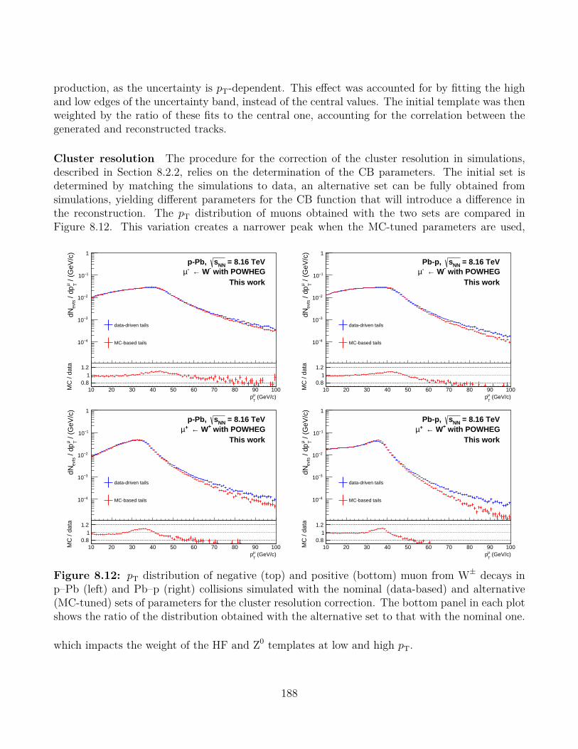
production, as the uncertainty is pT-dependent. This effect was accounted for by fitting the highand low edges of the uncertainty band, instead of the central values. The initial template was thenweighted by the ratio of these fits to the central one, accounting for the correlation between thegenerated and reconstructed tracks.

Cluster resolution The procedure for the correction of the cluster resolution in simulations,described in Section 8.2.2, relies on the determination of the CB parameters. The initial set isdetermined by matching the simulations to data, an alternative set can be fully obtained fromsimulations, yielding different parameters for the CB function that will introduce a difference inthe reconstruction. The pT distribution of muons obtained with the two sets are compared inFigure 8.12. This variation creates a narrower peak when the MC-tuned parameters are used,

(GeV/c)T

µp10 20 30 40 50 60 70 80 90 100

/ (G

eV/c

)Tµ

p /

dev

tsdN

4−10

3−10

2−10

1−10

1

= 8.16 TeVNNsp-Pb, with POWHEG- W← -µ

This work

data-driven tails

MC-based tails

(GeV/c)T

µp10 20 30 40 50 60 70 80 90 100M

C /

data

0.81

1.2 (GeV/c)

T

µp10 20 30 40 50 60 70 80 90 100

/ (G

eV/c

)Tµ

p /

dev

tsdN

4−10

3−10

2−10

1−10

1

= 8.16 TeVNNsPb-p, with POWHEG- W← -µ

This work

data-driven tails

MC-based tails

(GeV/c)T

µp10 20 30 40 50 60 70 80 90 100M

C /

data

0.81

1.2

(GeV/c)T

µp10 20 30 40 50 60 70 80 90 100

/ (G

eV/c

)Tµ

p /

dev

tsdN

4−10

3−10

2−10

1−10

1

= 8.16 TeVNNsp-Pb, with POWHEG+ W← +µ

This work

data-driven tails

MC-based tails

(GeV/c)T

µp10 20 30 40 50 60 70 80 90 100M

C /

data

0.81

1.2 (GeV/c)

T

µp10 20 30 40 50 60 70 80 90 100

/ (G

eV/c

)Tµ

p /

dev

tsdN

4−10

3−10

2−10

1−10

1

= 8.16 TeVNNsPb-p, with POWHEG+ W← +µ

This work

data-driven tails

MC-based tails

(GeV/c)T

µp10 20 30 40 50 60 70 80 90 100M

C /

data

0.81

1.2

Figure 8.12: pT distribution of negative (top) and positive (bottom) muon from W± decays inp–Pb (left) and Pb–p (right) collisions simulated with the nominal (data-based) and alternative(MC-tuned) sets of parameters for the cluster resolution correction. The bottom panel in each plotshows the ratio of the distribution obtained with the alternative set to that with the nominal one.

which impacts the weight of the HF and Z0 templates at low and high pT.

188

Global misalignment The tuning parameter of the task mimicking the global misalignment,determined by following the procedure described in Section 8.2.2, was estimated to be:

nshift = 2.4± 0.2 σCB. (8.25)

The uncertainty can have a significant effect on the simulated distributions, the fits were thenperformed with three values of the parameter: its central value, and the low and high limits if theuncertainty interval, 2.2 and 2.6. The pT distribution of single muons obtained using these threevalues are compared in Figure 8.13.Variations in nshift induce a significant shift of the distribution,and the Jacobian peak is displaced by a few GeV/c.

(GeV/c)T

µp10 20 30 40 50 60 70 80 90 100

/ (G

eV/c

)Tµ

p /

dev

tsdN

4−10

3−10

2−10

1−10

1

= 8.16 TeVNNsp-Pb, with POWHEG- W← -µ

This work

σ2.2

σ2.4

σ2.6

(GeV/c)T

µp10 20 30 40 50 60 70 80 90 1000.8

0.91

1.11.2

(GeV/c)T

µp10 20 30 40 50 60 70 80 90 100

/ (G

eV/c

)Tµ

p /

dev

tsdN

4−10

3−10

2−10

1−10

1

= 8.16 TeVNNsPb-p, with POWHEG- W← -µ

This work

σ2.2

σ2.4

σ2.6

(GeV/c)T

µp10 20 30 40 50 60 70 80 90 1000.8

0.91

1.11.2

(GeV/c)T

µp10 20 30 40 50 60 70 80 90 100

/ (G

eV/c

)Tµ

p /

dev

tsdN

4−10

3−10

2−10

1−10

1

= 8.16 TeVNNsp-Pb, with POWHEG+ W← +µ

This work

σ2.2

σ2.4

σ2.6

(GeV/c)T

µp10 20 30 40 50 60 70 80 90 1000.8

0.91

1.11.2

(GeV/c)T

µp10 20 30 40 50 60 70 80 90 100

/ (G

eV/c

)Tµ

p /

dev

tsdN

4−10

3−10

2−10

1−10

1

= 8.16 TeVNNsPb-p, with POWHEG+ W← +µ

This work

σ2.2

σ2.4

σ2.6

(GeV/c)T

µp10 20 30 40 50 60 70 80 90 1000.8

0.91

1.11.2

Figure 8.13: pT distribution of negative (top) and positive (bottom) muon from W± decays inp–Pb (left) and Pb–p (right) collisions simulated with the three values of the tuning parameteraccounting for the global misalignment of the spectrometer. In each plot, the bottom panel showsthe ratio of the modified distributions (with a tuning at 2.2 and 2.6) to the central one (tuning at2.4).

The signal extraction is finally performed by considering all these variations, combining them inevery way possible. The variations include the fit range (36 possibilities), the nPDF (2 possibilities),

189

the FONLL inputs (3 possibilities), the parameters for the cluster resolution (2 possibilities) andthe tuning parameter for the global misalignment (3 possibilities). In total, 1296 configurationsare used to construct the templates and fit the experimental spectrum. For each fit, a selection isdefined and it determines whether the configuration is kept or not:

• the fit result must be valid (TFitResult::IsValid() == kTRUE),

• the covariant matrix must be accurate (TFitResult::CovMatStatus() == 3).

As the variations are applied to both µ+ and µ− spectra, a combined χ2 test was defined as:

χ2tot

ndftot=

χ2

µ− + χ2

µ+

ndfµ− + ndf

µ+

. (8.26)

The fit result of a given configuration is kept if χ2tot/ndftot < 2, ensuring that the configuration

is able to reproduce the inclusive spectrum despite the independent analysis of negatively andpositively charged muons.

The final value for NW , and its associated statistical uncertainty, is taken as the average of allthe values obtained with different input parameters and fit ranges. Their dispersion, evaluated asthe standard deviation, is taken as the systematic uncertainty on the signal extraction:

⟨NW

⟩=

∑ni=1N

iW

n, σstat

NW=

∑ni=1 σ

stat

NiW

n, σsyst

NW=

√∑ni=1

(N i

W −⟨NW

⟩)2n− 1

, (8.27)

where n is the number of configurations that passed the fit quality selection. Figure 8.14 shows thenumber of W± extracted from each trial, with the corresponding average and associated statisticaland systematic uncertainties, along with the χ2

tot/ndftot of each trial that passed the selection.The combinations of the variations tend to be able to reproduce the data, as only 1% of theconfigurations are discarded in p–Pb collisions, and 0.5% in Pb–p. The fit results show ratherlarge fluctuations in p–Pb collisions for the W− yield, leading to a higher systematic uncertainty(about 9%) than for the other configurations. Table 8.9 shows the raw signals for muons from W±

decays extracted from the data, with the corresponding statistical and systematic uncertainties.

p–Pb Pb–pµ− ←W− 824.1± 43.9± 72.8 1388.4± 48.5± 53.3µ+ ←W+ 1105.8± 47.3± 65.4 493.0± 28.3± 35.8

Table 8.9: Raw number of muons from W± decays, extracted from a global fit of the inclusivesingle muon pT distributions for pµT > 10 GeV/c and −4 < yµlab < −2.5. The quoted errorscorrespond to the statistical and systematic uncertainties, respectively.

190

trial0 200 400 600 800 1000 1200

W y

ield

(in

tegr

ated

in 1

0-10

0 G

eV)

500

600

700

800

900

1000

1100

1200

1300

1400

1500- W← -µ = 8.16 TeV, NNsp-Pb,

72.8± 43.9 ± = 824.1 - W← -µN

= 1278trialsN

This work

trialµN

>µ<N

Stat. error

Syst. error

trial0 200 400 600 800 1000 1200

W y

ield

(in

tegr

ated

in 1

0-10

0 G

eV)

1100

1200

1300

1400

1500

1600

1700

1800

1900

2000

2100- W← -µ = 8.16 TeV, NNsPb-p,

53.3± 48.5 ± = 1388.4 - W← -µN

= 1290inputsN

This work

trialµN

>µ<N

Stat. error

Syst. error

trial0 200 400 600 800 1000 1200

W y

ield

(in

tegr

ated

in 1

0-10

0 G

eV)

800

900

1000

1100

1200

1300

1400

1500

1600

1700

1800+ W← +µ = 8.16 TeV, NNsp-Pb,

65.4± 47.3 ± = 1105.8 + W← +µN

= 1278inputsN

This work

trialµN

>µ<N

Stat. error

Syst. error

trial0 200 400 600 800 1000 1200

W y

ield

(in

tegr

ated

in 1

0-10

0 G

eV)

300

400

500

600

700

800

900

1000+ W← +µ = 8.16 TeV, NNsPb-p,

35.8± 28.3 ± = 493.0 + W← +µN

= 1290inputsN

This work

trialµN

>µ<N

Stat. error

Syst. error

trial0 200 400 600 800 1000 1200

tot

/ nd

fto

t2 χ

0.8

1

1.2

1.4

1.6

1.8

2

2.2

p-Pb, this work

trial0 200 400 600 800 1000 1200

tot

/ nd

fto

t2 χ

0.8

1

1.2

1.4

1.6

1.8

2

2.2

Pb-p, this work

Figure 8.14: Extraction of the W± signal in p–Pb (left) and Pb–p (right) collisions. Top andmiddle: raw number of muons from W± decays as a function of the trial, for negative (top) andpositive (middle) muons. The solid line represents the average of the distribution, while the long-dashed (short-dashed) line represents the statistical (systematic) uncertainty. Bottom: χ2

tot/ndftotdistributions for the fits that passed the quality selection.

191

8.3 Efficiency correctionIn order to evaluate the real production of the Z0 and W± bosons, one needs to correct theraw yield for the efficiency of the detector. The latter is evaluated by means of simulations,using the same simulations that were presented above, with POWHEG for the generation of hardevents, paired with PYTHIA6 for parton shower. The CT10 and EPS09 PDF and nPDF setsare used, both at NLO, with the isospin effect included by simulating pp and pn binary collisionscombined with Equation 8.23. The particle transport and detector response are monitored bya detector simulation with the GEANT3 transport code. The simulations are anchored to theLHC16r and LHC16s OCDB. The cluster resolution is corrected using CB functions with thedata-driven parameters, and the global misalignment is parametrised with a 2.4 σ deviation. Thesimulations are performed run-by-run, with a number of generated events proportional to thenumber of CMUL and CMSH events for the computation of the efficiency of muons from Z0 and W±

decays, respectively.The efficiency ε for each run i is calculated as the ratio of the number of reconstructed events

in the spectrometer N irec to the number of generated events in the fiducial region N i

gen taken fromthe MC truth:

εi =N i

rec

N igen

. (8.28)

The overall efficiency of the period, and associated statistical uncertainty, are computed throughan averaging over the run efficiencies, weighted by wi the fraction of MUL- or MSH-triggered eventsin run i:

〈ε〉 =∑n

i=1wi × εi∑ni=1wi

, σ〈ε〉 =

√∑ni=1wi × σεi∑n

i=1wi

. (8.29)

The systematic uncertainty on the efficiency is evaluated by varying the simulation environ-ment. Variations on the PDF and nPDF sets were considered, but the effects on the total efficiencyitself are negligible. The same conclusion was derived from variations of the transport code, replac-ing GEANT3 by GEANT4. The only significant source of systematic uncertainty on the efficiencycomes from the corrections for the cluster resolution and global misalignment. In the Z0 analysis,it was evaluated by computing the efficiency with and without the corrections. Figure 8.15 showsthe dimuon invariant mass distribution simulated with and without the corrections for clusterresolution and global misalignment. Including the corrections smears the peak in the distribution.Since the measurement is performed in a limited range in invariant mass, this smearing pushespart of the events outside of the boundaries, such that the total efficiency decreases, by 8% in p–Pbcollisions and 6% in Pb–p collisions. In the Z0 analysis this source of uncertainty is the largestcontribution to the overall systematic uncertainty on the measurements. In the W± study, as asecond alternative set of parameters for the cluster resolution became available, the uncertaintywas evaluated independently for the cluster resolution and tuning of the global misalignment, byvarying one while fixing the other at its nominal value. Computing the efficiency from simulationsparametrised with CB functions, using either the data-driven set of parameters or the MC-tunedone, yields a difference below 1% which is taken as the associated uncertainty. With a clusterresolution parametrised with CB functions with the data-driven parameters, the global misalign-

192

)2 (GeV/cµµm20 40 60 80 100 120 140

)2E

vent

s / (

0.5

GeV

/c

210

310

410

510

= 8.16 TeVNNsp-Pb,

This workno global shiftMC-tuned CB tails

σshift at 2.4 data-tuned CB tails

)2 (GeV/cµµm20 40 60 80 100 120 140

)2E

vent

s / (

0.5

GeV

/c

210

310

410

510

= 8.16 TeVNNsPb-p,

This workno global shiftMC-tuned CB tails

σshift at 2.4 data-tuned CB tails

Figure 8.15: Invariant mass distribution of dimuons from Z0 decays.

ment was varied between the boundaries of its uncertainty, at 2.2 and 2.6 σ. Even by taking thelargest estimation, that is, the full difference between the two, the effect is found to be negligiblecompared to the one from the cluster resolution.

The efficiencies of muons from W−, W+ and Z0 decays are shown in Figure 8.16. A similartrend is found for the three bosons in a given collision system, with a stable detector efficiency inLHC16r while several drops are seen in LHC16s. This feature originates from face-to-face high-voltage trips in the third and fourth stations of the tracking system, decreasing the overall trackingcapabilities of the spectrometer. The efficiency for dimuons is lower than that of single muons, dueto the need of detecting two muons instead of one, but also following from the smearing effect ofthe cluster resolution correction described above, explaining why the fraction of missed dimuonsis more that twice that of single muons. The efficiencies computed in the full fiducial region aregiven in Table 8.10, with the systematic uncertainties corresponding to the corrections for clusterresolution and global misalignment.

p–Pb Pb–pε(µ− ←W−) 0.905± 0.007 (syst) 0.878± 0.006 (syst)ε(µ+ ←W+) 0.907± 0.005 (syst) 0.886± 0.003 (syst)ε(µ+µ− ← Z0) 0.724± 0.001 (stat)± 0.057 (syst) 0.723± 0.001 (stat)± 0.041 (syst)

Table 8.10: Efficiencies of µ± from W± decays and µ+µ− from Z0 decays in p–Pb and Pb–pcollisions. The statistical uncertainties on the efficiency correction for the W± bosons are negligible.The systematic uncertainties come from the cluster resolution correction and global misalignment,the other sources being negligible.

193

8.4 Differential studiesSo far, the procedure and intermediate results have been presented from computations in the fullfiducial region. Due to the large statistics of the W± analysis, results were also obtained in severalbins of rapidity and collision centrality. It is worth stressing that the whole analysis procedurewas done for all the considered bins. In the laboratory frame, the rapidity interval was splitted inthree bins of width 0.4, 0.4 and 0.7 from central to large rapidities, yielding in the centre-of mass

2655

9426

5596

2656

0726

5691

2656

9426

5696

2656

9726

5698

2657

0026

5701

2657

0926

5713

2657

1426

5740

2657

4126

5742

2657

4426

5746

2657

5426

5756

2657

8526

5787

2657

8826

5789

2657

9226

5795

2657

9726

5840

2658

4126

6022

2660

2326

6025

2660

3426

6074

2660

7626

6081

2660

8426

6085

2660

8626

6117

2661

8726

6189

2661

9026

6193

2661

9626

6197

2662

0826

6234

2662

3526

6296

2662

9926

6300

2663

0426

6305

2663

1226

6316

2663

18

run

∈

0.8

0.85

0.9

0.95

1

1.05

= 8.16 TeVNNsp-Pb, - W← -µ

This work

run-per-run

weighted average

2664

3726

6438

2664

3926

6441

2664

7026

6472

2664

7926

6480

2664

8726

6514

2665

1626

6518

2665

2026

6522

2665

2326

6525

2665

3326

6534

2665

3926

6543

2665

4926

6584

2665

8726

6588

2665

9126

6593

2665

9526

6613

2666

1426

6615

2666

1826

6621

2666

3026

6657

2666

5826

6659

2666

6526

6668

2666

6926

6674

2666

7626

6702

2667

0326

6706

2667

0826

6775

2667

7626

6800

2668

0526

6807

2668

5726

6878

2668

8026

6882

2668

8326

6885

2668

8626

6912

2669

1526

6940

2669

4226

6943

2669

4426

6988

2669

9326

6994

2669

9726

6998

2670

2026

7022

2670

6226

7063

2670

6726

7070

2670

7226

7077

2671

0926

7110

2671

3026

7131

run

∈0.75

0.8

0.85

0.9

0.95

1

1.05

= 8.16 TeVNNsPb-p, - W← -µ

This work

run-per-run

weighted average

2655

9426

5596

2656

0726

5691

2656

9426

5696

2656

9726

5698

2657

0026

5701

2657

0926

5713

2657

1426

5740

2657

4126

5742

2657

4426

5746

2657

5426

5756

2657

8526

5787

2657

8826

5789

2657

9226

5795

2657

9726

5840

2658

4126

6022

2660

2326

6025

2660

3426

6074

2660

7626

6081

2660

8426

6085

2660

8626

6117

2661

8726

6189

2661

9026

6193

2661

9626

6197

2662

0826

6234

2662

3526

6296

2662

9926

6300

2663

0426

6305

2663

1226

6316

2663

18

run

∈

0.8

0.85

0.9

0.95

1

1.05

= 8.16 TeVNNsp-Pb, + W← +µ

This work

run-per-run

weighted average

2664

3726

6438

2664

3926

6441

2664

7026

6472

2664

7926

6480

2664

8726

6514

2665

1626

6518

2665

2026

6522

2665

2326

6525

2665

3326

6534

2665

3926

6543

2665

4926

6584

2665

8726

6588

2665

9126

6593

2665

9526

6613

2666

1426

6615

2666

1826

6621

2666

3026

6657

2666

5826

6659

2666

6526

6668

2666

6926

6674

2666

7626

6702

2667

0326

6706

2667

0826

6775

2667

7626

6800

2668

0526

6807

2668

5726

6878

2668

8026

6882

2668

8326

6885

2668

8626

6912

2669

1526

6940

2669

4226

6943

2669

4426

6988

2669

9326

6994

2669

9726

6998

2670

2026

7022

2670

6226

7063

2670

6726

7070

2670

7226

7077

2671

0926

7110

2671

3026

7131

run

∈

0.75

0.8

0.85

0.9

0.95

1

1.05

= 8.16 TeVNNsPb-p, + W← +µ

This work

run-per-run

weighted average

2655

9426

5596

2656

0726

5691

2656

9426

5696

2656

9726

5698

2657

0026

5701

2657

0926

5713

2657

1426

5740

2657

4126

5742

2657

4426

5746

2657

5426

5756

2657

8526

5787

2657

8826

5789

2657

9226

5795

2657

9726

5840

2658

4126

6022

2660

2326

6025

2660

3426

6074

2660

7626

6081

2660

8426

6085

2660

8626

6117

2661

8726

6189

2661

9026

6193

2661

9626

6197

2662

0826

6234

2662

3526

6296

2662

9926

6300

2663

0426

6305

2663

1226

6316

2663

18

run

∈

0.65

0.7

0.75

0.8

0.85

0.9

0.95

1

= 8.16 TeVNNsp-Pb, 0 Z← -µ+µ

This work

run-per-run

weighted average

2664

3726

6438

2664

3926

6441

2664

7026

6472

2664

7926

6480

2664

8726

6514

2665

1626

6518

2665

2026

6522

2665

2326

6525

2665

3326

6534

2665

3926

6543

2665

4926

6584

2665

8726

6588

2665

9126

6593

2665

9526

6613

2666

1426

6615

2666

1826

6621

2666

3026

6657

2666

5826

6659

2666

6526

6668

2666

6926

6674

2666

7626

6702

2667

0326

6706

2667

0826

6775

2667

7626

6800

2668

0526

6807

2668

5726

6878

2668

8026

6882

2668

8326

6885

2668

8626

6912

2669

1526

6940

2669

4226

6943

2669

4426

6988

2669

9326

6994

2669

9726

6998

2670

2026

7022

2670

6226

7063

2670

6726

7070

2670

7226

7077

2671

0926

7110

2671

3026

7131

run

∈

0.55

0.6

0.65

0.7

0.75

0.8

0.85

0.9

0.95

1

= 8.16 TeVNNsPb-p, 0 Z← -µ+µ

This work

run-per-run

weighted average

Figure 8.16: Run-by-run efficiencies in p–Pb (left) and Pb–p (right) collisions for single muonsfrom W− (top) and W+ (middle) decays, and dimuons from Z0 decays (bottom). The horizontallines correspond to the weighted averages of the whole periods.

194

frame:ycms ∈ [+2.03,+2.43]; [+2.43,+2.83]; [+2.83,+3.53] in p–Pb collisions,ycms ∈ [−4.46,−3.76]; [−3.76,−3.36]; [−3.36,−2.96] in Pb–p collisions.

(8.30)

These bins were considered for all the observables measured for muons from W± decays. Alongwith the rapidity-dependent measurements, an evaluation of the normalised yield as a functionof the collision centrality was performed, considering four centrality intervals: 0–20%, 20–40%,40–60% and 60–100%. The larger width of the largest rapidity and lowest centrality intervals wererequired as to have a sufficient amount of signal for the measurements. The available statisticsbeing too low in the Z0 measurement, differential studies were not considered.

8.5 Summary of systematic uncertaintiesThe systematic uncertainties on the luminosity, signal extraction and efficiency are described in thecorresponding sections of this chapter. Three supplementary sources were included. The uncer-tainty on the tracking efficiency is obtained by considering the difference between the efficienciesobtained from data and MC simulations, using the redundancy between the tracking chambers[185] as described in Section 5.3.3. The uncertainty on the muon trigger efficiency is determinedby propagating the uncertainty on the intrinsic efficiency of the individual trigger chambers, whichis evaluated in a similar manner as for the tracking system, with a data-driven method using theredundancy of the trigger chamber information. Finally, the muon identification introduces anadditional uncertainty, which reflects the differences observed between data and simulations whenapplying different values of the χ2 selection on the matching between tracks reconstructed in thetracking system with track segments in the trigger chambers. It should be noted that these lastsources were not evaluated for this work, but taken from the Υ analysis in p–Pb collisions at√sNN = 8.16 TeV [269]. The uncertainties on single muons are half that of dimuons. The sources

of systematic uncertainties, and their values, are summarised in Table 8.11. The total systematicfor an observable is obtained by summing in quadrature the relevant sources.

195

in % p–Pb collisions Pb–p collisionsW− W+ Z0 W− W+ Z0

Signal extraction 8.8 5.9 1.0 3.8 7.3 —– vs rapidity 4.4 – 14.3 3.9 – 10.7 — 2.5 – 9.5 3.9 – 21.6 —

– vs centrality 3.6 – 12.8 3.6 – 12.8 — 3.6 – 12.8 3.6 – 12.8 —Tracking efficiency 0.5 1.0 1.0 2.0Trigger efficiency 0.5 1.0 0.5 1.0

Trigger-tracker matching 0.5 1.0 0.5 1.0Cluster resolution and alignment 0.7 0.6 7.7 0.7 0.3 5.7

Normalisation factor 1.4 0.7 1.0 0.2V0 cross section 1.9 1.9 2.0 2.0〈Nmult

coll 〉 2.8 – 4.3 — 2.8 – 4.3 —

Table 8.11: Summary of the systematic uncertainties affecting the measurements of muons fromW± and Z0 decays in p–Pb and Pb–p collisions. Ranges are indicated for differential studies, cor-responding to the extrememost values. A horizontal bar indicates that the source is not applicable,either because the analysis is not concerned by the source, or it was found to be negligible.

196

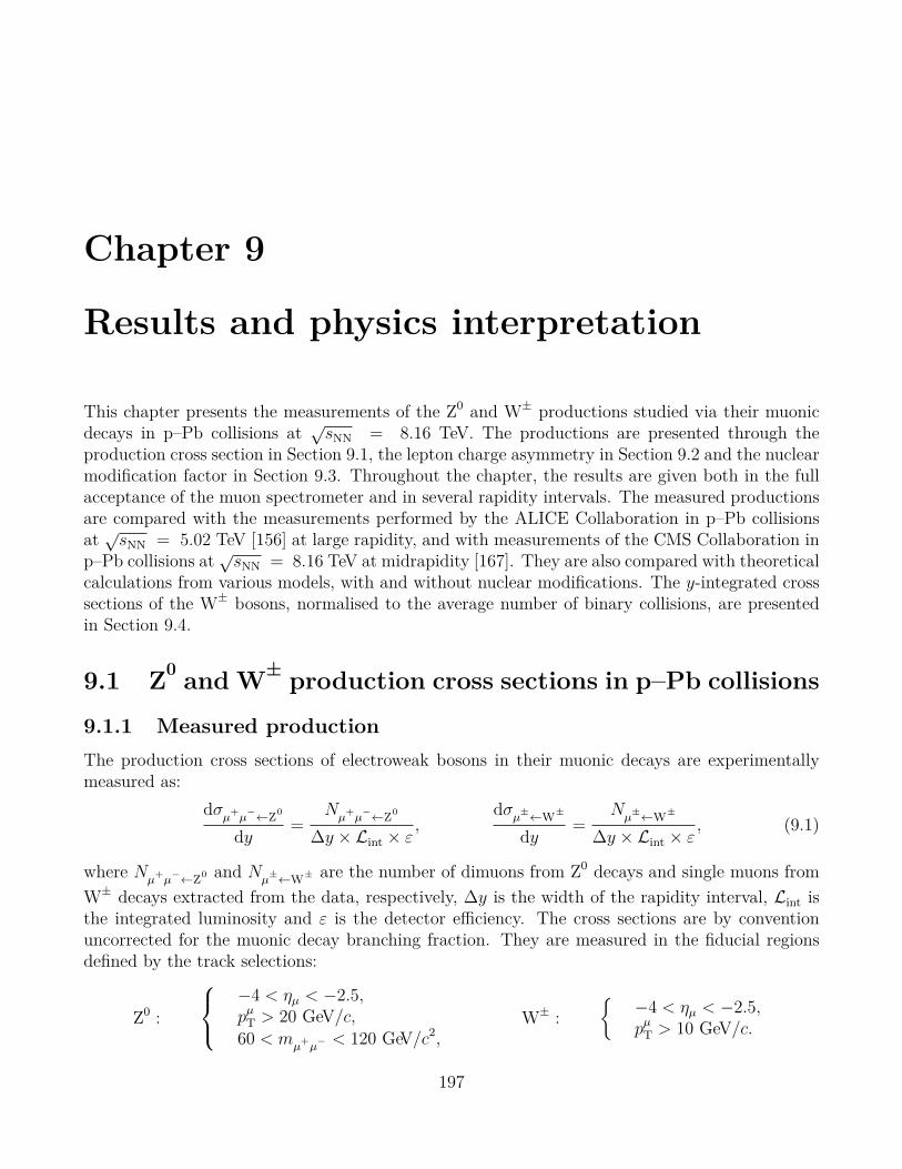
Chapter 9

Results and physics interpretation

This chapter presents the measurements of the Z0 and W± productions studied via their muonicdecays in p–Pb collisions at √sNN = 8.16 TeV. The productions are presented through theproduction cross section in Section 9.1, the lepton charge asymmetry in Section 9.2 and the nuclearmodification factor in Section 9.3. Throughout the chapter, the results are given both in the fullacceptance of the muon spectrometer and in several rapidity intervals. The measured productionsare compared with the measurements performed by the ALICE Collaboration in p–Pb collisionsat √sNN = 5.02 TeV [156] at large rapidity, and with measurements of the CMS Collaboration inp–Pb collisions at√sNN = 8.16 TeV at midrapidity [167]. They are also compared with theoreticalcalculations from various models, with and without nuclear modifications. The y-integrated crosssections of the W± bosons, normalised to the average number of binary collisions, are presentedin Section 9.4.

9.1 Z0 and W± production cross sections in p–Pb collisions

9.1.1 Measured productionThe production cross sections of electroweak bosons in their muonic decays are experimentallymeasured as:

dσµ+µ−←Z0

dy=

Nµ+µ−←Z0

∆y × Lint × ε,

dσµ±←W±

dy=

Nµ±←W±

∆y × Lint × ε, (9.1)

where Nµ+µ−←Z0 and N

µ±←W± are the number of dimuons from Z0 decays and single muons from

W± decays extracted from the data, respectively, ∆y is the width of the rapidity interval, Lint isthe integrated luminosity and ε is the detector efficiency. The cross sections are by conventionuncorrected for the muonic decay branching fraction. They are measured in the fiducial regionsdefined by the track selections:

Z0 :

−4 < ηµ < −2.5,pµT > 20 GeV/c,60 < m

µ+µ− < 120 GeV/c2,

W± :

−4 < ηµ < −2.5,pµT > 10 GeV/c.

197

The production cross sections measured in the full acceptance of the spectrometer are shown inthe top panels of Figure 9.1, and the values are summarised in Table 9.1.

cmsy

4− 2− 0 2 4

(nb

)µµ cm

sy

/ d

- µ+ µ → 0

Zσ

d

0

1

2

3

4

5

6

7

8

9

10

= 8.16 TeVNNsp-Pb collisions,

This work

-µ+µ → 0Z

c > 20 GeV/T

µp

2c < 120 GeV/−µ+µ60 < m

cmsµy

4− 2− 0 2 4

(nb

)cm

sµ

y /

d± µ

→ ±W

σd

0

20

40

60

80

100

120

140

160

180

200

= 8.16 TeVNNsPb collisions, −p

This work

± W← ±µ

c > 10 GeV/T

µp

− W← −µ+ W← +µ

cmsµy

4.4− 4.2− 4− 3.8− 3.6− 3.4− 3.2− 3−

(nb

)cm

sµ

y /

d± µ

→ ±W

σd

0

50

100

150

200

250

300

350


This work± W← ±µ

c > 10 GeV/T

µp− W← −µ+ W← +µ

cmsµy

2.2 2.4 2.6 2.8 3 3.2 3.4

(nb

)cm

sµ

y /

d± µ

→ ±W

σd

0

50

100

150

200

250

300

350


This work± W← ±µ

c > 10 GeV/T

µp− W← −µ+ W← +µ

Figure 9.1: Production cross sections of the muonic decays of Z0 and W± bosons measured inp–Pb collisions at √sNN = 8.16 TeV. The top panels show the cross sections integrated in thefull acceptance of the muon spectrometer, while the bottom panels display the cross sections ofthe µ± ←W± processes in several rapidity bins. The data points are at the centre of the intervals,their horizontal extension corresponds to the width of the rapidity ranges. The vertical bars andboxes indicate the statistical and systematic uncertainties, respectively.

The top left panel shows the cross section of the Z0 → µ+µ− process. The large differenceseen between backward and forward rapidities comes from the rapidity shift, which pushes theforward region towards higher production while moving the backward region to the tail of the bell-shaped cross section distribution. One can notice that, due to the rather low amount of signal,the measurements are dominated by the statistical uncertainties, which amount to 13% (17%) inp–Pb (Pb–p) collisions while the systematics is 8% (7%). The top right panel of Figure 9.1 showsthe same observable for the µ− ←W− and µ+ ←W+ processes. Several effects act differently forthe four combinations of rapidities and charge. The rapidity shift has the same consequence ofincreasing the production at forward rapidities and decreasing it at backward. The isospin effectsignificantly impacts the productions of W− and W+, it favours the former and suppresses thelatter. Finally, the considerations on helicities developed in Section 3.2.3 and their consequences

198

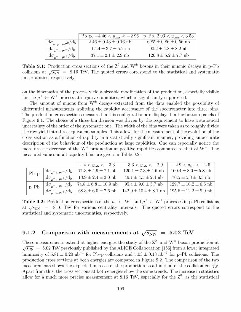
Pb–p, −4.46 < ycms < −2.96 p–Pb, 2.03 < ycms < 3.53dσ

µ+µ−←Z0/dy 2.46± 0.43± 0.16 nb 6.85± 0.86± 0.56 nb

dσµ−←W−/dy 105.4± 3.7± 5.2 nb 90.2± 4.8± 8.2 nb

dσµ+←W+/dy 37.1± 2.1± 2.9 nb 120.8± 5.2± 7.7 nb

Table 9.1: Production cross sections of the Z0 and W± bosons in their muonic decays in p–Pbcollisions at √sNN = 8.16 TeV. The quoted errors correspond to the statistical and systematicuncertainties, respectively.

on the kinematics of the process yield a sizeable modification of the production, especially visiblefor the µ+ ←W+ process at negative rapidities, which is significantly suppressed.

The amount of muons from W± decays extracted from the data enabled the possibility ofdifferential measurements, splitting the rapidity acceptance of the spectrometer into three bins.The production cross sections measured in this configuration are displayed in the bottom panels ofFigure 9.1. The choice of a three-bin division was driven by the requirement to have a statisticaluncertainty of the order of the systematic one. The width of the bins were taken as to roughly dividethe raw yield into three equivalent samples. This allows for the measurement of the evolution of thecross section as a function of rapidity in a statistically significant manner, providing an accuratedescription of the behaviour of the production at large rapidities. One can especially notice themore drastic decrease of the W+ production at positive rapidities compared to that of W−. Themeasured values in all rapidity bins are given in Table 9.2.

−4 < ylab < −3.3 −3.3 < ylab < −2.9 −2.9 < ylab < −2.5

Pb–p dσµ−←W−/dy 71.3± 4.9± 7.1 nb 120.1± 7.3± 4.6 nb 160.4± 8.0± 5.8 nb

dσµ+←W+/dy 13.9± 2.4± 3.0 nb 49.1± 4.5± 2.4 nb 70.5± 5.3± 3.3 nb

p–Pb dσµ−←W−/dy 74.8± 6.8± 10.9 nb 95.4± 9.0± 5.7 nb 129.7± 10.2± 6.6 nb

dσµ+←W+/dy 68.3± 6.0± 7.6 nb 142.9± 10.4± 8.1 nb 195.6± 12.2± 9.0 nb

Table 9.2: Production cross sections of the µ− ←W− and µ+ ←W+ processes in p–Pb collisionsat √sNN = 8.16 TeV for various centrality intervals. The quoted errors correspond to thestatistical and systematic uncertainties, respectively.

9.1.2 Comparison with measurements at √sNN = 5.02 TeV

These measurements extend at higher energies the study of the Z0- and W±-boson production at√sNN = 5.02 TeV previously published by the ALICE Collaboration [156] from a lower integrated

luminosity of 5.81 ± 0.20 nb−1 for Pb–p collisions and 5.03 ± 0.18 nb−1 for p–Pb collisions. Theproduction cross sections at both energies are compared in Figure 9.2. The comparison of the twomeasurements shows the expected increase of the production as a function of the collision energy.Apart from this, the cross sections at both energies show the same trends. The increase in statisticsallow for a much more precise measurement at 8.16 TeV, especially for the Z0, as the statistical

199

cmsy

4− 2− 0 2 4

(nb

)µµ cm

sy

/ d

− µ+ µ → 0

Zσ

d 0

1

2

3

4

5

6

7

8

9

10

p-Pb collisions−µ+µ → 0Z

c > 20 GeV/T

µp

= 8.16 TeV (this work)NNs

= 5.02 TeV (JHEP02 (2017) 077)NNs

cmsµy

4− 2− 0 2 4

(nb

)cm

sµ

y /

d−

W← − µ

σd

0

50

100

150

200

250

Pb collisions−p− W← −µ

c > 10 GeV/T

µp(this work)

= 8.16 TeVNNs

(JHEP02 (2017) 077) = 5.02 TeVNNs

cmsµy

4− 2− 0 2 4

(nb

)cm

sµ

y /

d+

W← + µ

σd

0

50

100

150

200

250

Pb collisions−p+ W← +µ

c > 10 GeV/T

µp(this work)

= 8.16 TeVNNs

(JHEP02 (2017) 077) = 5.02 TeVNNs

Figure 9.2: Production cross sections of the muonic decays of Z0 (top), W− (bottom left) andW+ (bottom right) bosons measured in p–Pb collisions at √sNN = 8.16 TeV (this work) and√sNN = 5.02 TeV from Ref. [156]. The bars and boxes indicate the statistical and systematic

uncertainties, respectively.

uncertainty at 5.02 TeV amounts to 20% in p–Pb collisions and more than 100% in Pb–p, as thecross section was estimated from two Z0 candidates. With the forthcoming increase of luminosityat the LHC, one can expect the measurements of weak bosons in heavy-ion collisions to attain avery high precision, providing strong constraints on nPDF models.

9.1.3 Comparison with theoretical calculationsThe measurements of the Z0-boson production are compared to theoretical calculations in Figure9.3. The calculations were obtained at NLO from the EPPS16 [54] and nCTEQ15 [55] nuclearmodels, using CT14 [63] as baseline PDF in the former case, and for the modelisation of theproton beam. Calculations were also obtained from standalone CT14, including the isospin effectbut no nuclear modification of the PDF. The comparison of the nuclear- and free-PDF predictionsallows one to evaluate the effect of the nuclear modifications themselves. One can see that atbackward rapidity, as the Bjorken-x region overlaps the EMC and anti-shadowing regions, the neteffect is small and predictions with and without nuclear modifications are indistinguishable. Atforward rapidity, where the Bjorken-x region is fully immersed in the suppressing shadowing region,

200

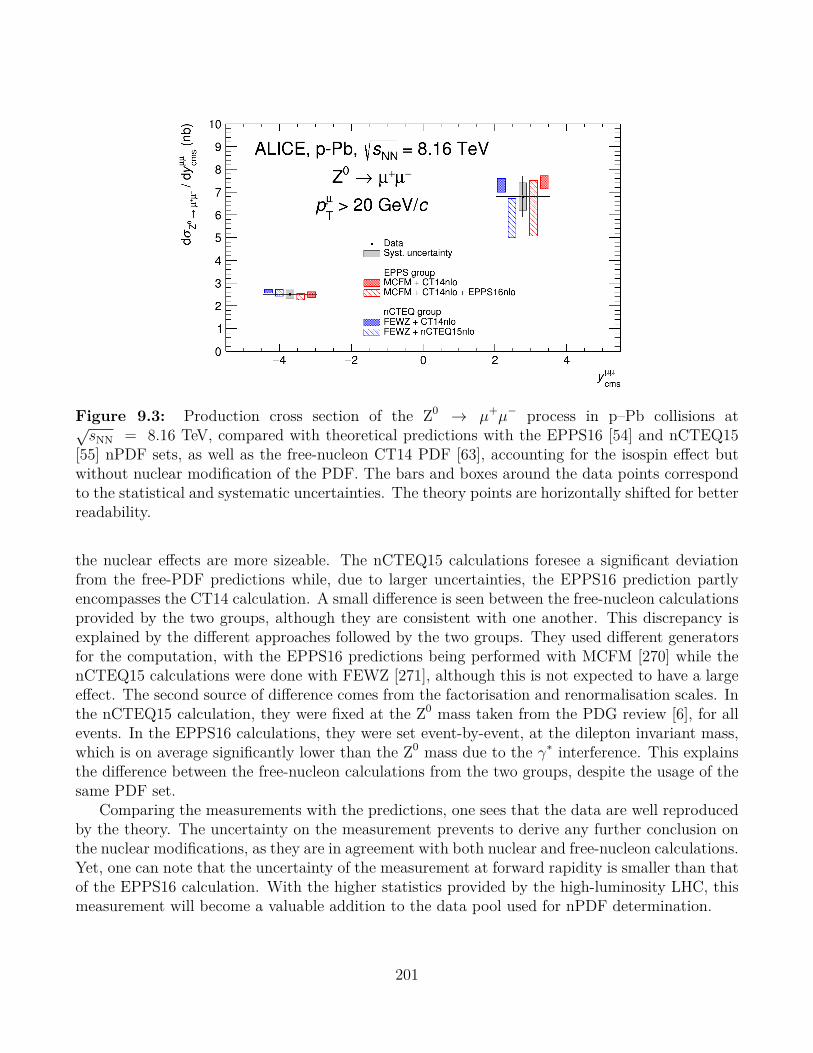
Figure 9.3: Production cross section of the Z0 → µ+µ− process in p–Pb collisions at√sNN = 8.16 TeV, compared with theoretical predictions with the EPPS16 [54] and nCTEQ15

[55] nPDF sets, as well as the free-nucleon CT14 PDF [63], accounting for the isospin effect butwithout nuclear modification of the PDF. The bars and boxes around the data points correspondto the statistical and systematic uncertainties. The theory points are horizontally shifted for betterreadability.

the nuclear effects are more sizeable. The nCTEQ15 calculations foresee a significant deviationfrom the free-PDF predictions while, due to larger uncertainties, the EPPS16 prediction partlyencompasses the CT14 calculation. A small difference is seen between the free-nucleon calculationsprovided by the two groups, although they are consistent with one another. This discrepancy isexplained by the different approaches followed by the two groups. They used different generatorsfor the computation, with the EPPS16 predictions being performed with MCFM [270] while thenCTEQ15 calculations were done with FEWZ [271], although this is not expected to have a largeeffect. The second source of difference comes from the factorisation and renormalisation scales. Inthe nCTEQ15 calculation, they were fixed at the Z0 mass taken from the PDG review [6], for allevents. In the EPPS16 calculations, they were set event-by-event, at the dilepton invariant mass,which is on average significantly lower than the Z0 mass due to the γ∗ interference. This explainsthe difference between the free-nucleon calculations from the two groups, despite the usage of thesame PDF set.

Comparing the measurements with the predictions, one sees that the data are well reproducedby the theory. The uncertainty on the measurement prevents to derive any further conclusion onthe nuclear modifications, as they are in agreement with both nuclear and free-nucleon calculations.Yet, one can note that the uncertainty of the measurement at forward rapidity is smaller than thatof the EPPS16 calculation. With the higher statistics provided by the high-luminosity LHC, thismeasurement will become a valuable addition to the data pool used for nPDF determination.

201

The W± cross sections were also compared with model calculations. By the time the analysiswas completed, two new nPDF sets became available: the nCTEQ15 model was extended by theinclusion of Z0 and W± data from the LHC, leading to the nCTEQ15WZ [272] determination. ThenNNPDF2.0 [56] model includes flavour decomposition, which enables the evaluation of electroweakboson production. The comparison of the differential cross sections with various theoretical modelsis shown in Figure 9.4. In the theory points, the same pattern is seen as for the prediction on theZ0 production, with small to no nuclear effects predicted at backward rapidities and significantsuppression due to nuclear modifications at forward. Comparing the nCTEQ15 and nCTEQ15WZmodels, one sees the benefits of including Z0 and W± data at the LHC, as the latter model featureslargely reduced uncertainties compared to the pristine version. While the EPPS16, nCTEQ15 andnCTEQ15WZ models tend to agree with each other, within uncertainties, the nNNPDF2.0 modelshows large discrepancies in the predicted production and evolution as a function of rapidity,especially for W−. Here one especially notices the predictions at positive rapidities, which followa flat behaviour. It should be stressed that the nNNPDF model is still under development, and isyet to include part of the available data which can have a significant impact on the calculation ofthe W± production. The methodology of the nNNPDF collaboration, relying on neural networksfor the determination of the interpolants, leads this model to have much smaller uncertainties.

The evolution of the measured production as a function of rapidity deviates from what ispredicted by the models in the W− analysis, especially for the most central bins where the dataare higher than the models, regardless of whether they include the nuclear modifications or not.At larger rapidities an agreement is found with the EPPS16, nCTEQ15 and nCTEQ15WZ models,while the peculiar behaviour predicted by nNNPDF2.0 does not catch the measurement. In theW+ case, the general agreement with nuclear models is better. The measured cross section in themost central positive rapidity bin seems to favour the free-nucleon PDF, although still being inagreement with several nuclear models within uncertainties. In the five other rapidity bins, themeasurements favour the inclusion of nuclear modifications in the calculations. This observationis particularly valid for the 2.83 < ycms < 3.53 bin, where the data is in agreement with nPDFcalculations while showing a 3.5 σ deviation from the CT14-only prediction. It is worth recallingthat this bin covers the lowest Bjorken-x region, around 10−4, where it is especially useful toprovide constraints to the model. Interestingly enough, one can notice that the nNNPDF2.0 modelprovides the best reproduction of the measurement in this region. Finally, the measurements atpositive rapidities, for both W− and W+, have much lower uncertainties than that of most ofthe calculations, following from the lack of constraints in the corresponding Bjorken-x interval.These measurements can therefore be particularly useful for the determination of nPDF, in helpingreducing the model uncertainties at low-x.

9.1.4 Comparison with CMS measurement at midrapidityThe CMS Collaboration has measured the production of W± boson in the muonic decay channelat midrapidity, in between the forward and backward rapidity intervals accessible from the ALICEmuon spectrometer. The measurements in p–Pb collisions at √sNN = 8.16 TeV are publishedin Ref. [167]. The data sample has a corresponding luminosity of 173.4 ± 6.1 nb−1, and the

202

Figure 9.4: Production cross section of the W± → µ±νµ process for W− (top) and W+ (bottom) asa function of rapidity for muons with pT > 10 GeV/c in p–Pb collisions at √sNN = 8.16 TeV. Themeasurements are compared with predictions from several nPDF sets, as well as with calculationsbased on the CT14 PDF [63], accounting for the isospin effect but without nuclear modificationsof the PDF. The bottom panels show the ratio to the CT14 calculations. The horizontal barscorrespond to the width of the rapidity intervals. The vertical bars and boxes indicate the statisticaland systematic uncertainties, respectively, and the grey band in the bottom panels represent theuncertainty of the CT14 predictions. The data points are centered in the rapidity intervals, whilethe theory predictions are horizontally shifted for better readability.

203

measurement is performed in the fiducial region:|ηµlab| < 2.4,pµT > 25 GeV/c.

Apart from a gap of 0.1 units of rapidity, the combination of the CMS and ALICE acceptancesare fully complementary, which leads to cover the pseudorapidity range |ηµlab| < 4, providing aexhaustive measurement of the nuclear effects over four orders of magnitude of Bjorken-x. Since thepT selection is different in the two analyses, a direct comparison can not be drawn. The contributionof the two measurements can efficiently be compared by looking at the ratio of data to theory, andtaking the free-nucleon calculation as a reference allows one to highlight the nuclear modifications.In Figure 9.5 is shown the ratio of the ALICE and CMS measurements to CT14 [63] calculationsaccounting for the isospin effect but without implementation of the nuclear modifications. Forcomparison purposes, the ratio of EPPS16 [54] to CT14 is also shown.

The ALICE measurements extend the trend seen at the edges of the CMS acceptance, with aratio close to or even at unity at negative rapidities while rather significant suppressing nucleareffects are seen at positive rapidities. The EPPS16 model seems to well reproduce the evolutionof the measurements from both collaborations. A striking feature of the ALICE measurementsat large rapidities are the size of the uncertainties compared to that of the EPPS16 calculations,pointing once more the ability of these measurement to provide further constraining inputs for thenPDF determination.

9.2 Lepton charge asymmetryThe lepton charge asymmetry Ach is measured as:

Ach =N corr

µ+←W+ −N corr

µ−←W−

N corr

µ+←W+ +N corr

µ−←W−

, (9.2)

where N corr

µ+←W+ and N corr

µ−←W− are respectively the number of muons from W+ and W− decays

extracted from the data and corrected for the efficiency of the detector. This ratio is an interestingobservable for its sensitivity to the down-to-up quark ratio in the nucleus. It also allows for thereduction of the uncertainties, as some sources such as the trigger and tracking efficiencies cancelin the calculation. The theoretical calculations have reduced uncertainties as well, due to thecancellation of sources such as the choice of the factorisation and renormalisation scales. In thiswork, the lepton charge asymmetry was measured in the full acceptance of the spectrometer, aswell as in the same rapidity bins as those considered for the evaluation of the differential crosssection. In the full acceptance, the measured Ach amounts to:

APb–pch = −0.479± 0.046± 0.056, Ap–Pb

ch = 0.145± 0.014± 0.021, (9.3)

where the quoted uncertainties are statistical and systematic, respectively. The measured valuesin the rapidity bins are given in Table 9.3.

The measured Ach are shown in Figure 9.6. In the top panel, the measurement performed in

204

Figure 9.5: Ratio to CT14 [63] predictions of the production cross section of muons from W−

(top) and W+ (bottom) decays measured by the ALICE (this work) and CMS [167] Collaborationsin p–Pb collisions at √sNN = 8.16 TeV. The measured ratio is compared to the one obtainedfrom pQCD calculations with CT14 + EPPS16 [54]. All calculations include the isospin effect.The grey band around the line at unity corresponds to the uncertainty on the free-PDF prediction,the bars and boxes around the data points indicate the statistical and systematic uncertainties,respectively.

205

−4 < ylab < −3.3 −3.3 < ylab < −2.9 −2.9 < ylab < −2.5APb–p

ch −0.647± 0.175± 0.229 −0.420± 0.066± 0.029 −0.389± 0.049± 0.025

Ap–Pbch −0.047± 0.006± 0.012 0.200± 0.034± 0.019 0.203± 0.029± 0.017

Table 9.3: Lepton charge asymmetry of muons from W± decays, measured in p–Pb collisions at√sNN = 8.16 TeV. The quoted errors are the statistical and systematic uncertainties, respectively.

the full acceptance of the spectrometer is compared with the ALICE measurement made in p–Pbcollisions at √sNN = 5.02 TeV [156]. From the comparison, one can derive the same conclusions asfor the cross sections. The increase of statistics yields a more precise result, which is not dominatedby the statistical uncertainty anymore. The measured asymmetry increases as a function of thecollision energy. At forward rapidity, the measurement at √sNN = 8.16 TeV is not consistent withzero as it was the case for the measurement at 5.02 TeV, highlighting the different evolution of the

cmsµy

4− 2− 0 2 4

chA

0.8−

0.6−

0.4−

0.2−

0

0.2

0.4

= 8.16 TeVNNsPb, −p

c > 10 GeV/T

µp

(this work) = 8.16 TeVNNs

(JHEP02 (2017) 077) = 5.02 TeVNNs

cmsy

4.4− 4.2− 4− 3.8− 3.6− 3.4− 3.2− 3−

chA

1−

0.9−

0.8−

0.7−

0.6−

0.5−

0.4−

0.3−

0.2−

0.1−

0

= 8.16 TeVNNsp, −Pbc > 10 GeV/

T

µpThis work

cmsy

2.2 2.4 2.6 2.8 3 3.2 3.4

chA

0.2−

0.1−

0

0.1

0.2

0.3

0.4

0.5

= 8.16 TeVNNsPb, −pc > 10 GeV/

T

µpThis work

Figure 9.6: Lepton charge asymmetry of muons from W± decays in p–Pb collisions at√sNN = 8.16 TeV. The top panel shows the measurement in the full acceptance of the spectrome-

ter, along with the measurement in p–Pb collisions at √sNN = 5.02 TeV from Ref. [156]. The bot-tom panel shows the differential measurement performed in p–Pb collisions at √sNN = 8.16 TeV.The bars and boxes indicate the statistical and systematic uncertainties, respectively.

206

u- and d-quark PDFs as the energy increases. The differential evaluation, shown in the bottompanels of Figure 9.6, predicts a sharp drop of the asymmetry at large rapidities, with a sign reversalat forward. At backward, the small amount of positive muons from W+ decays leads to a largeuncertainty in the bin at the largest rapidity, preventing to firmly conclude on the decrease.

Figure 9.7 shows the comparison of the Ach with various theoretical calculations. The predic-tions were obtained with the EPPS16 [54] and nNNPDF2.0 [56] nuclear models, as well as free-PDFpredictions relying on CT14 [63] for reference. It is interesting to note that at both negative andpositive rapidities, the EPPS16 model does not predict any deviation of the Ach from free-PDFcalculations, such that the observable would be more sensitive to the proton PDF than to thenuclear modifications. On the contrary, the nNNPDF2.0 model shows a very large deviation atpositive rapidity. Interestingly enough, the measurement lies between the two models, by showinga decrease of the ratio towards higher rapidities, although not as large as what is predicted bynNNPDF2.0.

Figure 9.7: Lepton charge asymmetry Ach as a function of rapidity of muons from W± decays inp–Pb collisions at √sNN = 8.16 TeV. The measurements are compared with predictions from theEPPS16 [54] and nNNPDF2.0 [56] nPDF sets, as well as CT14-only [63] predictions including theisospin effect but without nuclear modifications. The bottom panels show the ratio to the CT14calculations.The bars and boxes indicate the statistical and systematic uncertainties, respectively.The theory points are horizontally shifted for better readability.

207

9.3 Nuclear modification factorThe nuclear modification factor RpPb is calculated as:

RpPb =1

208

σp–Pbµ±←W±

σppµ±←W±

. (9.4)

σp–Pbµ±←W± corresponds to the production cross sections measured in p–Pb collisions and presented

in Section 9.1. σppµ±←W± is the reference cross section in pp collisions at the same energy. Since

such a measurement has not been made, due to the lack of pp collisions at√s = 8.16 TeV, the

reference cross section must either be extrapolated from a similar measurement, or be estimated viatheoretical calculations. The LHCb Collaboration has measured the production of W± boson in ppcollisions at

√s = 8 TeV [273]. The lower energy of the collision, the difference in acceptance, and a

pT selection set at 20 GeV/c in the LHCb study, would necessitate to perform simulations in orderto correct the measurements before using them for the evaluation of the RpPb. It was thereforedecided to adopt the second option, and obtain the reference cross section fully from simulations.The calculations were performed with the same simulation environment as the one used for thesignal extraction, using POWHEG [267] as hard event generator, paired with PYTHIA6 [264]for parton shower, and CT10 [176] as proton PDF. The LHCb study has shown that CT10 isable to well reproduce the measurement of W± bosons over the acceptance of the ALICE muonspectrometer and at similar collision energy. Two sources of uncertainties were considered:

• the uncertainty from the knowledge on the PDF was evaluated by replacing CT10 withCTEQ6.6 [154], taking as uncertainty half the difference between the cross sections computedwith the two models,

• the uncertainty from the knowledge of αs, which was varied between its boundaries at 0.112and 0.127, taking the difference between the cross sections computed with these values withthe one computed with the central value αs = 0.118, providing the lower and upper limit ofthe uncertainty interval.

The two sources are eventually combined quadratically to determine the full uncertainty on thecalculation.

The measured RpPb are shown in Figure 9.8. The values of the RpPb measured in the fullacceptance of the muon spectrometer are indicated in Table 9.4. The nuclear modification factorof weak bosons assesses the combination of the nuclear modifications and isospin effect. The neteffect is rather small at positive rapidities, where theRpPb are close to one for both W− and W+. Onthe contrary, the effect is important at backward rapidities, where the RpPb deviates significantlyfrom unity. The measured values for various rapidity bins are given in Table 9.5. When goingtowards large rapidities, the RpPb follow a decreasing trend, indicating that the production crosssection is wider in pp collisions and decreases less rapidly than the production in p–Pb collisions.The exception to this trend is the RpPb for W+ at negative rapidities, where fluctuations in themeasurement seem to suggest a flat behaviour.

208

cmsy

5− 4− 3− 2− 1− 0 1 2 3 4 5

pPb

R

0.5

1

1.5

2

2.5

3


c > 10 GeV/T

p

This work

− W← −µData with stat. uncertaintySystematic uncertaintypp reference uncertainty

+ W← +µData with stat. uncertaintySystematic uncertaintypp reference uncertainty

cmsy

5− 4− 3− 2− 1− 0 1 2 3 4 5

pPb

R

0.5

1

1.5

2

2.5

3


c > 10 GeV/T

p

This work

− W← −µData with stat. uncertaintySystematic uncertaintypp reference uncertainty

+ W← +µData with stat. uncertaintySystematic uncertaintypp reference uncertainty

Figure 9.8: Nuclear modification factor RpPb of muons from W± decays measured in p–Pbcollisions at√sNN = 8.16 TeV, in the full acceptance of the muon spectrometer (left) and in variousrapidity bins (right). The reference pp cross section is taken from calculations with the CT10 [176]proton PDF. The bars and open boxes indicate the statistical and systematic uncertainties on thecross section in p–Pb, respectively. The hashed boxes represent the uncertainty on the referencecross section. The systematic uncertainty on the luminosity is shown as a black box around theline RpPb = 1.

Pb–p, −4.46 < ycms < −2.96 p–Pb, 2.03 < ycms < 3.53

Rµ−←W−

pPb 1.620± 0.057± 0.079+0.092−0.062 0.888± 0.047± 0.080+0.060

−0.039

Rµ+←W+

pPb 0.643± 0.036± 0.051+0.046−0.031 0.793± 0.034± 0.051+0.048

−0.037

Table 9.4: Nuclear modification factor of muons from W± decays in p–Pb collisions at√sNN = 8.16 TeV in the full acceptance of the muon spectrometer. The quoted errors cor-

respond to the statistical and systematic uncertainties from the p–Pb cross section, and the upperand lower bound of the systematic uncertainty from the pp cross section, respectively.

The measured RpPb are compared with theoretical calculations in Figure 9.9 obtained withthe EPPS16 [54] and nNNPDF2.0 [56] models. The calculations show interesting behaviours as afunction of rapidity. The RpPb of muons from W− decays is predicted by both models to increaseas a function of rapidity, while the opposite trend is seen in the measurement. In the three otherconfigurations, the EPPS16 model predicts very small to no evolution of the nuclear modificationfactor, which is consistent with the measurement of W+ at negative rapidities but contradicts whatis experimentally observed at positive rapidities. Discrepancies are also seen when comparing themeasurements with nNNPDF2.0 calculations. The behaviour of the W− nuclear modificationfactor follows opposite trends than that of the measurements, increasing towards large rapiditieswhile the measured RpPb decreases. The agreement seems better for the W+ boson. At negativerapidities, the nNNPDF2.0 is in agreement with the measurement within uncertainties, althoughit predicts a slight increase at very large rapidity while the data seems to favour the opposite.

209

Figure 9.9: Nuclear modification factor RpPb of muons from W− (top) and W+ (bottom) de-cays, as a function of rapidity, in p–Pb collisions at √sNN = 8.16 TeV. The measurements arecompared with predictions from the EPPS16 [54] and nNNPDF2.0 [56] models, using CT14 [63]and NNPDF3.1 [49] proton PDF sets for the reference cross section, respectively. The bars andboxes indicate the statistical and systematic uncertainties on the cross section in p–Pb collisions,respectively. The uncertainty on the reference cross section is indicated as a grey band around thedata points. The theory points are horizontally shifted for better readability.

210

−4 < ylab < −3.3 −3.3 < ylab < −2.9 −2.9 < ylab < −2.5

Pb–p Rµ−←W−

pPb 1.566± 0.107± 0.155+0.085−0.053 1.635± 0.099± 0.062+0.098

−0.060 1.765± 0.088± 0.064+0.100−0.076

Rµ+←W+

pPb 0.606± 0.105± 0.132+0.056−0.039 0.760± 0.070± 0.036+0.054

−0.034 0.632± 0.047± 0.030+0.040−0.029

p–Pb Rµ−←W−

pPb 0.838± 0.076± 0.122+0.052−0.035 0.882± 0.083± 0.053+0.058

−0.041 1.111± 0.087± 0.057+0.086−0.049

Rµ+←W+

pPb 0.621± 0.055± 0.069+0.032−0.032 0.833± 0.061± 0.047+0.056

−0.037 0.943± 0.059± 0.043+0.058−0.041

Table 9.5: Nuclear modification factor of muons from W± decays in p–Pb collisions at√sNN = 8.16 TeV in various rapidity bins. The quoted errors correspond to the statistical

and systematic uncertainties from the p–Pb cross section, and the upper and lower bound of thesystematic uncertainty from the pp cross section, respectively.

At positive rapidities, the same decreasing tendency is seen in both the experimental data andnNNPDF2.0 calculations, although disagreeing on the gradient. One can generally conclude thatthe theory faces difficulties in reproducing the RpPb data, stressing the importance of providingnew inputs for the determination of the nuclear models.

9.4 Binary scalingThe production of W± was finally studied as a function of centrality, in order to verify the expectedscaling of hard processes with the number of binary nucleon-nucleon collisions. The study of thecentrality-dependent yield can also serve as test bench for the centrality estimation. In order tomaximise the amount of signal in each bin, the yields of W− and W+ are combined. Four centralityclasses were considered: 0–20%, 20–40%, 40–60% and 60–100%. The centrality is expressed as theaverage number of binary nucleon-nucleon collisions 〈Nmult

coll 〉, the correspondence between 〈Nmultcoll 〉

and the centrality classes was given in Table 8.5. The normalised invariant yield is evaluated as:

1

〈Nmultcoll 〉

×N i

W±

Lint × f iMB × ε

, (9.5)

where N i

W± is the number of muons from W± decays in a given centrality class i, f iMB is the fraction

of MB-triggered events in the centrality class i to that in 0–100%, Lint is the integrated luminosityand ε is the detector efficiency.

The bias of multiplicity-based estimators was observed in this study, as seen in Figure 9.10 (thecomputation of the cross section is described below). The expected scaling of the W± productionwith the average number of binary nucleon-nucleon collisions 〈Nmult

coll 〉 is realised when using theZDC as centrality estimators, but large deviations are seen when the centrality is estimated withthe multiplicity-based V0 and CL1.

The normalised cross section in the full centrality range is measured to be:

Pb–p : 30.2± 2.0± 2.8 nb, p–Pb : 44.6± 3.3± 5.1 nb.

The measured evolution of the normalised invariant yield as a function of 〈Nmultcoll 〉 is shown in Figure

9.11. The centrality-dependent yield is found to be consistent with a constant within uncertainties.

211

Centrality class0-100% 0-20% 20-40% 40-60% 60-100%

(nb

)⟩

coll

mul

t N⟨

/ ± W

← ± µσ

10

20

30

40

50

60 = 8.16 TeVNNsp, −Pb

c > 10 GeV/T

µp

< -2.96cms

µy-4.46 <

This work

ZNCV0CCL1

Figure 9.10: Production of W± boson normalised to the average number of binary collision〈Nmult

coll 〉 for various centrality estimators and centrality intervals. A dashed line is drawn at thevalue for 0–100% centrality to guide the eye.

Figure 9.11: Combined yields of muons from W± decays in p–Pb collisions at √sNN = 8.16 TeV,normalised to the average number of binary nucleon-nucleon collisions 〈Nmult

coll 〉, for Pb–p (left) andp–Pb (right) collisions. The bars and boxes correspond to the statistical and systematic uncer-tainties, respectively. The horizontal dashed lines correspond to the normalised yield measured forthe 0–100% centrality.

It should be stressed that the dashed line in the figure is not a linear fit of the distribution, butrather indicate the value measured in the 0–100% centrality range. A separate evaluation of theinvariant yield from W− and W+ was tested, leading the same conclusion. The resulting statisticaluncertainties prevent to see any charge-dependent effect on the normalised yield.

212

Conclusion

In this thesis, the measurements of the Z0- and W±-boson production in p–Pb collisions at√sNN = 8.16 TeV with ALICE are reported. The electroweak bosons are detected through

their leptonic decays, using data collected with the muon spectrometer of the experiment. Twodata samples were used, corresponding to p–Pb and Pb–p collisions, with an integrated luminosityof 6.81 ± 0.15 nb−1 and 10.2 ± 0.27 nb−1, respectively. For each analysis, a fiducial region wasdefine as to ensure a clean data sample and measurements at the highest precision:

Z0 :

−4 < ηµ < −2.5,pµT > 20 GeV/c,60 < m

µ+µ− < 120 GeV/c2,

W± :

−4 < ηµ < −2.5,pµT > 10 GeV/c.

Accounting for the rapidity shift in p–Pb collisions, the rapidity intervals in the centre-of-massframe covered by the spectrometer are −4.46 < yPb-p

cms < −2.96 and 2.03 < yp-Pbcms < 3.53, corre-

sponding to high (∼ 10−1) and low (∼ 10−3−10−4) Bjorken-x regions, respectively. The productionof the Z0 boson was presented as the production cross section at negative and positive rapidities,measured in the full acceptance of the muon spectrometer. The W± production was reportedthrough the production cross section, lepton charge asymmetry and nuclear modification factor,and was evaluated in the full acceptance and in several rapidity intervals.

The measurements were compared to similar studies at the LHC. Comparisons with the sameanalyses performed in p–Pb collisions at √sNN = 5.02 TeV by the ALICE Collaboration high-lighted the benefits of increasing the energy of the collisions and luminosity of the periods. Themeasurements at √sNN = 8.16 TeV were indeed found to be much more precise, although theZ0 yields was still facing statistical limitations. The combination of the CMS and ALICE mea-surements of the W± cross sections shown the complementarity of the LHC experiments, as thecombined measurements assess the full |ylab| < 4 interval, over eight units of rapidity.

The measurements were compared to theoretical predictions, from the EPPS16, nCTEQ15and nNNPDF2.0 nPDF models, as well as reference calculations with the free-nucleon CT14 PDF,accounting for the isospin effect but without nuclear modifications. The production cross sectionof the Z0 boson was found to be well reproduced by the models. No conclusion could be derived onthe nuclear modifications, as the measurements were consistent with all predictions, regardless ofwhether they include the nuclear corrections or not. The W± cross sections were also generally wellreproduced by the models, at the exception of W− in the most central bins at both forward andbackward rapidities where disagreements are observed. The W+ cross section at positive rapidities

213

shows a strong preference for predictions including the nuclear modifications. The deviation fromthe free-PDF calculation goes up 3.5 σ for the largest rapidity interval. The recent nNNPDF2.0model is overall less efficient at reproducing the measurements.

Comparison of the lepton charge asymmetry yielded interesting differences between the EPPS16and nNNPDF2.0 models at forward rapidity, where the EPPS16 predictions does not show anysignificant nuclear effects, while nNNPDF2.0 predicts a large drop towards larger rapidities. Themeasured asymmetry lies in between the two models, showing a decrease of the asymmetry al-though not as strong as what is foreseen by the nNNPDF2.0 calculation. The two models arealso strongly disagreeing on the nuclear modification factor. Yet, no strong preference can be seenwhen comparing with the measurements.

The normalised yield of W± bosons was also present as a function of the average numberof binary nucleon-nucleon collisions. The study shown the important bias of multiplicity-basedestimators of the centrality. With the unbiased estimation provided by the ZDC detector, thedistribution of the normalised yield is found to be consistent with a constant, as expected from aGlauber modelling of the collision.

This study provides important constraints for the nPDF determination, in a Bjorken-x regionwhere the available data are scarce. Significant tensions are observed between the measured pro-duction and the theoretical calculations. The precision of the measurements is often found to bebetter than that of the calculations, such that even when an agreement if found this study will helpfor nPDF determination by participating in the reduction of the model uncertainties. By includingall the measurements of weak boson production provided by the LHC experiments, including theones obtained in this work, nPDF determination groups will be able to provide a new generationof sets with drastically improved accuracy and precision.

The high luminosity foreseen at the LHC after its restart in 2022 will provide another increasein the precision of electroweak boson measurements. The statistics will enable differential studiesof the Z0-boson production, and a higher granularity for that of the W± bosons. It should alsoallow one to measure backward-forward asymmetries in p–Pb collisions with the ALICE muonspectrometer, despite the small overlap of the centre-of-mass rapidity intervals due to the rapidityshift, which only covers 2.96 < |ycms| < 3.53. These measurements during the LHC Runs 3 and4 will pursue the iterations between the experimental and theoretical communities towards thedetermination of nPDF.

214

List of Figures

1.1 Summary of measurements of αs(Q2) as a function of the energy scale Q. . . . . . . 13

1.2 Constituent quark masses as a function of the squared momentum for the u/d, s, cand b quarks. . . . . . . . . . . . . . . . . . . . . . . . . . . . . . . . . . . . . . . . 16

1.3 Schematic view of the phases of the QCD matter in the plane of temperature T andbaryon-chemical potential µB. . . . . . . . . . . . . . . . . . . . . . . . . . . . . . . 17

1.4 Left: pseudo-critical temperature Tc(0) as a function of the lattice volume Nτ usingseveral parametrisation of CΣ, Cχ and χΣ. Right: phase boundary of 2+ 1 flavourQCD. . . . . . . . . . . . . . . . . . . . . . . . . . . . . . . . . . . . . . . . . . . . 19

1.5 Feynman diagram for the deep inelastic lepton-hadron scattering. . . . . . . . . . . 211.6 Feynman diagram for the deep inelastic lepton-hadron scattering, preceded by a

gluon radiation. . . . . . . . . . . . . . . . . . . . . . . . . . . . . . . . . . . . . . . 221.7 The NNPDF3.1 NNLO PDF set. . . . . . . . . . . . . . . . . . . . . . . . . . . . . 301.8 Illustration of the EPPS16 fit function RA

i (x,Q20). . . . . . . . . . . . . . . . . . . . 32

1.9 The nNNPDF2.0 nPDF set. . . . . . . . . . . . . . . . . . . . . . . . . . . . . . . . 34

2.1 Light cone and space-time evolution of a HIC. . . . . . . . . . . . . . . . . . . . . . 382.2 Temperature T and baryon chemical potential µB as a function of the beam energy. 412.3 Optical limit of the Glauber model. . . . . . . . . . . . . . . . . . . . . . . . . . . . 432.4 Glauber-MC event simulated in Au–Au collisions at √sNN = 200 GeV in the trans-

verse and longitudinal planes. . . . . . . . . . . . . . . . . . . . . . . . . . . . . . . 462.5 EPPS16 nuclear modifications for Pb at the parametrisation scale Q2

0 = 10 GeV2,for the uV, dV and g PDFs. . . . . . . . . . . . . . . . . . . . . . . . . . . . . . . . . 48

2.6 Left: nuclear modification factors for the charm and bottom quarks in p–Pb col-lisions at √sNN = 8.8 TeV from the EPS09 nPDF model. Right: inclusive jetnuclear modification factor R∗pPb as a function of the jet pT, in p–Pb collisions at√sNN = 5.02 TeV, measured by the CMS collaboration. . . . . . . . . . . . . . . . 48

2.7 Near-side ridge measured in pp, p–Pb and Pb–Pb collisions at the LHC. . . . . . . 50

3.1 W± measurements by the UA1 and UA2 Collaborations. . . . . . . . . . . . . . . . 563.2 Z0 measurements by the UA1 and UA2 Collaborations. . . . . . . . . . . . . . . . . 573.3 World average of the mass and width of the W± bosons. . . . . . . . . . . . . . . . 613.4 Flavour decomposition of the Z0 and W± production cross sections as a function of

the collision energy. . . . . . . . . . . . . . . . . . . . . . . . . . . . . . . . . . . . . 64

215

3.5 Rapidity distribution of the Z0 and W± cross sections at LO, NLO and NNLO inpp collisions at the LHC nominal energy

√s = 14 TeV with the MRST PDF set. . . 65

3.6 Production and decay diagrams of the W± bosons in the rest frame. . . . . . . . . . 673.7 Production cross sections of the Z0 and W± bosons in p–Pb collisions at √sNN =

8.8 TeV from the EPS09 model. . . . . . . . . . . . . . . . . . . . . . . . . . . . . . 683.8 Measurement of Z0-boson production in Pb–Pb collisions at √sNN = 2.76 TeV by

the ATLAS Collaboration. . . . . . . . . . . . . . . . . . . . . . . . . . . . . . . . . 713.9 Measurement of Z0- and W±-boson production in Pb–Pb collisions at√sNN = 5.02 TeV

by the ATLAS Collaboration. . . . . . . . . . . . . . . . . . . . . . . . . . . . . . . 723.10 Measurement of Z0- and W±-boson production in Pb–Pb collisions at√sNN = 5.02 TeV

by the ALICE Collaboration. . . . . . . . . . . . . . . . . . . . . . . . . . . . . . . 733.11 Rapidity-differential cross section of the Z0 detected in the leptonic decay channel

(e+ µ) in p–Pb collisions at √sNN = 5.02 TeV with the ATLAS detector. . . . . . 743.12 Production cross section of W+ and W−, as a function of the lepton pseudorapidity,

in p–Pb collisions at √sNN = 5.02 TeV and 8.16 TeV measured by the CMSCollaboration. . . . . . . . . . . . . . . . . . . . . . . . . . . . . . . . . . . . . . . . 75

3.13 Z0-boson production cross section measured in p–Pb collisions at √sNN = 5.02 TeVand 8.16 TeV by the LHCb Collaboration. . . . . . . . . . . . . . . . . . . . . . . . 76

3.14 Production cross sections of the Z0 and W± bosons in p–Pb collisions at√sNN = 5.02 TeVmeasured by the ALICE Collaboration. . . . . . . . . . . . . . . . . . . . . . . . . . 77

4.1 The CERN facility. . . . . . . . . . . . . . . . . . . . . . . . . . . . . . . . . . . . . 824.2 The LHC injection chain for proton and lead beams. . . . . . . . . . . . . . . . . . 834.3 Schematics of the ALICE detector. . . . . . . . . . . . . . . . . . . . . . . . . . . . 854.4 Left: Pseudorapidity coverage of the ALICE subdetectors. Right: Comparison of

the geometrical acceptances of the main LHC experiments. . . . . . . . . . . . . . . 874.5 Left: Number of recorded events for the V0-based triggers in Pb–Pb collisions.

Right: Correlation between the sum and difference of signal times in V0-A andV0-C in pp collisions. . . . . . . . . . . . . . . . . . . . . . . . . . . . . . . . . . . . 90

4.6 Visible cross sections for the V0 and T0 processes measured in vdM scans in p–Pbcollisions. . . . . . . . . . . . . . . . . . . . . . . . . . . . . . . . . . . . . . . . . . 92

4.7 Sum of amplitudes in V0-A for p–Pb collisions. . . . . . . . . . . . . . . . . . . . . 934.8 Multiplicity bias in p–Pb collisions. . . . . . . . . . . . . . . . . . . . . . . . . . . . 944.9 Left and centre: Transverse and longitudinal profiles of the luminous region.

Right: Widths of the final vertex distribution in the transverse plane. . . . . . . . . 974.10 Event reconstruction flow in the central barrel. . . . . . . . . . . . . . . . . . . . . . 984.11 Resolution for standalone TPC and ITS-TPC matched tracks. . . . . . . . . . . . . 994.12 Left: Specific energy loss dE/dx in the TPC as a function of the particle momen-

tum, in Pb–Pb collisions. Right: K/π separation by combining the arrival timemeasurement in TOF and dE/dx in the TPC. . . . . . . . . . . . . . . . . . . . . . 101

4.13 Kaon-pion and kaon-proton separation power of the ITS, TPC, TOF and HMPIDsystems as a function of the particle transverse momentum. . . . . . . . . . . . . . . 101

216

4.14 E/p distribution for electrons and pions in the EMCAL, in pp collisions at√s = 7

TeV. . . . . . . . . . . . . . . . . . . . . . . . . . . . . . . . . . . . . . . . . . . . . 1024.15 Left: Cross sectional view of one of the TRD layer. Right: TRD signal as a function

of the particle momentum, in p–Pb collisions at √sNN = 5.02 TeV, for protonsfrom Λ decays, charged pions from K0

S decays and electrons from γ conversions. . . . 1034.16 Left: Comparison between the dilepton invariant mass distribution before and after

applying the selection. Right: Transverse distribution of the reconstructed photonconversion points for |η| > 9. . . . . . . . . . . . . . . . . . . . . . . . . . . . . . . . 104

5.1 Cross sectional view, in the longitudinal plane, of the ALICE muon spectrometer. . 1085.2 Schematic view of the quadrant structure and slat architecture of the two innermost

and three outermost tracking stations. . . . . . . . . . . . . . . . . . . . . . . . . . 1105.3 Layout and working principle of the MWPC composing the tracking chambers. . . . 1115.4 Schematics of a RPC composing the muon trigger planes. . . . . . . . . . . . . . . . 1125.5 Possible configurations after the passage of a charged particle through a tracking

station. . . . . . . . . . . . . . . . . . . . . . . . . . . . . . . . . . . . . . . . . . . . 1165.6 Sketch of the working principle of the muon trigger decision. . . . . . . . . . . . . . 117

6.1 The ALICE online control system. . . . . . . . . . . . . . . . . . . . . . . . . . . . . 1206.2 Overview of the ALICE DAQ system and its interface with the HLT system. . . . . 1246.3 The publisher-subscriber paradigm of AMORE. . . . . . . . . . . . . . . . . . . . . 1266.4 Examples of MOs visualisation, using the AMORE generic GUI or accessed through

the eLogbook. . . . . . . . . . . . . . . . . . . . . . . . . . . . . . . . . . . . . . . . 1276.5 The ALICE HLT in the data readout scheme. . . . . . . . . . . . . . . . . . . . . . 1286.6 HLT compression factor achieved for TPC data, in pp collisions. . . . . . . . . . . . 1296.7 The ALICE control system put in context. . . . . . . . . . . . . . . . . . . . . . . . 1306.8 Schematics of the ECS architecture. . . . . . . . . . . . . . . . . . . . . . . . . . . . 1316.9 Schematic view of the computing grid hierarchy in the framework of the tiered

MONARC model. . . . . . . . . . . . . . . . . . . . . . . . . . . . . . . . . . . . . . 1336.10 Schematic view of the AliRoot framework. . . . . . . . . . . . . . . . . . . . . . . . 1346.11 Schematic depiction of the data processing framework in AliRoot. . . . . . . . . . . 136

7.1 The ITS2 layout. . . . . . . . . . . . . . . . . . . . . . . . . . . . . . . . . . . . . . 1417.2 Simulated performances of the ITS2 compared with measured performances of the

original ITS. . . . . . . . . . . . . . . . . . . . . . . . . . . . . . . . . . . . . . . . . 1427.3 Simulations of the inclusive e+ e− invariant mass spectrum for the current and

upgraded TPC. . . . . . . . . . . . . . . . . . . . . . . . . . . . . . . . . . . . . . . 1437.4 Upgraded readout scheme of ALICE. . . . . . . . . . . . . . . . . . . . . . . . . . . 1447.5 Schematics of the FIT layout. . . . . . . . . . . . . . . . . . . . . . . . . . . . . . . 1457.6 Illustration of the usage of physics and heartbeat triggers for the corresponding

readout modes. . . . . . . . . . . . . . . . . . . . . . . . . . . . . . . . . . . . . . . 1467.7 Efficiency of the MID RPCs equipped with FEERIC cards. . . . . . . . . . . . . . . 1487.8 MID readout electronics architecture. . . . . . . . . . . . . . . . . . . . . . . . . . . 149

217

7.9 3-dimensional view of the MFT detector and schematics of the its position in themuon spectrometer. . . . . . . . . . . . . . . . . . . . . . . . . . . . . . . . . . . . . 150

7.10 Dimuon invariant mass distribution in the J/ψ family region, in Pb–Pb collisions,without and with including information from the MFT. . . . . . . . . . . . . . . . . 151

7.11 The computing architecture of ALICE in Run 3. . . . . . . . . . . . . . . . . . . . . 1527.12 Quality Control and assessment general design in O2. . . . . . . . . . . . . . . . . . 1547.13 Event distribution as a function of the detector element, obtained from the QC MID

module ran on simulated data. . . . . . . . . . . . . . . . . . . . . . . . . . . . . . . 1587.14 Event distribution as a function of the detector element, obtained from the QC MID

module ran on simulated data. . . . . . . . . . . . . . . . . . . . . . . . . . . . . . . 160

8.1 Evolution of the purity and pile-up factors as a function of the run number, in p–Pband Pb–p collisions. . . . . . . . . . . . . . . . . . . . . . . . . . . . . . . . . . . . . 168

8.2 Fnorm as a function of the run number in p–Pb and Pb–p collisions. . . . . . . . . . 1708.3 Multiplicity distribution of MB, MSL and MSH triggered events measured by V0M in

p–Pb and Pb–p collisions. . . . . . . . . . . . . . . . . . . . . . . . . . . . . . . . . 1718.4 Top: evolution of the pT distribution of muon track candidates from MSH-triggered

events during the application of the event and track selections. Middle: pT distri-bution of µ+, µ− and µ± tracks after the full event and track selections. Bottom:charge ratio µ+/µ− as a function of pT. . . . . . . . . . . . . . . . . . . . . . . . . . 174

8.5 FONLL cross sections for the leptonic decay of HF hadrons as a function of pT andy in p–Pb and Pb–p collisions. . . . . . . . . . . . . . . . . . . . . . . . . . . . . . . 177

8.6 Top: pT distribution of the single muons from W± decays, for positively and nega-tively charged muons, and their combination. Bottom: invariant mass distributionof dimuons from Z0 decays, normalised to 1, in p–Pb and Pb–p collisions. . . . . . . 180

8.7 Invariant mass, pT and η distributions of dimuons from Z0 candidates in p–Pb andPb–p collisions at √sNN = 8.16 TeV. . . . . . . . . . . . . . . . . . . . . . . . . . . 181

8.8 Estimation of the contamination to the Z0 signal from several background sourcesin p–Pb and Pb–p collisions. . . . . . . . . . . . . . . . . . . . . . . . . . . . . . . . 183

8.9 Invariant mass distribution of same sign muon pairs in p–Pb and Pb–p collisions,for various values of the muon pT selection. . . . . . . . . . . . . . . . . . . . . . . . 185

8.10 Global fits of the single muon pT distribution in p–Pb and Pb–p collisions for neg-atively and positively charged muons. . . . . . . . . . . . . . . . . . . . . . . . . . . 186

8.11 pT distribution of negative and positive muon from W± decays in p–Pb and Pb–p col-lisions simulated at LO and for variations of αs, compared to the nominal parametri-sation. . . . . . . . . . . . . . . . . . . . . . . . . . . . . . . . . . . . . . . . . . . . 187

8.12 pT distribution of negative and positive muon from W± decays in p–Pb and Pb–pcollisions simulated with the nominal (data-based) and alternative (MC-tuned) setsof parameters for the cluster resolution correction. . . . . . . . . . . . . . . . . . . . 188

8.13 pT distribution of negative and positive muon from W± decays in p–Pb and Pb–pcollisions simulated with the three values of the tuning parameter accounting forthe global misalignment of the spectrometer. . . . . . . . . . . . . . . . . . . . . . . 189

8.14 Extraction of the W± signal in p–Pb and Pb–p collisions. . . . . . . . . . . . . . . . 191

218

8.15 Invariant mass distribution of dimuons from Z0 decays. . . . . . . . . . . . . . . . . 1938.16 Run-by-run efficiencies in p–Pb and Pb–p collisions for single muons from W− and

W+ decays, and dimuons from Z0 decays. . . . . . . . . . . . . . . . . . . . . . . . . 194

9.1 Production cross sections of the muonic decays of Z0 and W± bosons measured inp–Pb collisions at √sNN = 8.16 TeV. . . . . . . . . . . . . . . . . . . . . . . . . . . 198

9.2 Production cross sections of the muonic decays of Z0, W− and W+ bosons measuredin p–Pb collisions at √sNN = 8.16 TeV and √sNN = 5.02 TeV. . . . . . . . . . . . 200

9.3 Production cross section of the Z0 → µ+µ− process in p–Pb collisions at√sNN = 8.16 TeV,compared with theoretical predictions. . . . . . . . . . . . . . . . . . . . . . . . . . 201

9.4 Production cross section of the W± → µ±νµ process for W− and W+, in p–Pbcollisions at √sNN = 8.16 TeV, compared with theoretical predictions. . . . . . . . 203

9.5 Ratio to CT14 predictions of the production cross section of muons from W− andW+ decays measured by the ALICE and CMS Collaborations in p–Pb collisions at√sNN = 8.16 TeV. . . . . . . . . . . . . . . . . . . . . . . . . . . . . . . . . . . . . 205

9.6 Lepton charge asymmetry of muons from W± decays in p–Pb collisions at√sNN = 8.16 TeV.2069.7 Lepton charge asymmetry Ach as a function of rapidity of muons from W± decays

in p–Pb collisions at √sNN = 8.16 TeV. . . . . . . . . . . . . . . . . . . . . . . . . 2079.8 Nuclear modification factor RpPb of muons from W± decays measured in p–Pb

collisions at √sNN = 8.16 TeV. . . . . . . . . . . . . . . . . . . . . . . . . . . . . . 2099.9 Nuclear modification factor RpPb of muons from W− and W+ decays, as a function

of rapidity, in p–Pb collisions at √sNN = 8.16 TeV. . . . . . . . . . . . . . . . . . . 2109.10 Production of W± boson normalised to the average number of binary collision

〈Nmultcoll 〉 for various centrality estimators and centrality intervals. . . . . . . . . . . . 212

9.11 Combined yields of muons from W± decays in p–Pb collisions at √sNN = 8.16 TeV,normalised to the average number of binary nucleon-nucleon collisions 〈Nmult

coll 〉, forPb–p and p–Pb collisions. . . . . . . . . . . . . . . . . . . . . . . . . . . . . . . . . 212

219

List of Tables

1.1 Charge, isospin, additive quantum numbers and mass of the known quarks. . . . . . 81.2 Key specifications of the nCTEQ15, EPPS16 and nNNPDF2.0 nPDF sets. . . . . . 35

2.1 Heavy-ion accelerators. . . . . . . . . . . . . . . . . . . . . . . . . . . . . . . . . . . 42

3.1 Centre-of-mass energy, instantaneous and integrated luminosity delivered by theCERN proton-antiproton collider from 1981 to 1990. . . . . . . . . . . . . . . . . . 55

3.2 Mass, full width, and branching fractions of the hadronic and leptonic decays of theW± and Z0 bosons. . . . . . . . . . . . . . . . . . . . . . . . . . . . . . . . . . . . . 62

3.3 References of the available measurements of the Z0- and W±-boson production per-formed in HIC at the LHC. . . . . . . . . . . . . . . . . . . . . . . . . . . . . . . . 70

4.1 LHC nominal nucleon-nucleon centre-of-mass energy, luminosity and geometricalcross section for pp, p–Pb and Pb–Pb collisions. . . . . . . . . . . . . . . . . . . . . 84

4.2 Position, geometrical coverage and main purpose of the ALICE subdetectors. . . . . 864.3 Minimum Bias triggers provided by the V0. . . . . . . . . . . . . . . . . . . . . . . 894.4 Average number of collisions 〈Ncoll〉 evaluated in p–Pb collisions. . . . . . . . . . . . 94

5.1 Summary of the main characteristics of the ALICE muon spectrometer. . . . . . . . 1095.2 Trigger types defined by the muon trigger system. . . . . . . . . . . . . . . . . . . . 117

6.1 Trigger capabilities provided by the various ALICE detectors. . . . . . . . . . . . . 1216.2 Descriptors of the major ALICE triggers. . . . . . . . . . . . . . . . . . . . . . . . . 123

7.1 Position, radial and pseudorapidity coverages, and technology of the sub-systems ofFIT. . . . . . . . . . . . . . . . . . . . . . . . . . . . . . . . . . . . . . . . . . . . . 146

7.2 Readout parameter overview for Pb–Pb beam operation at 50 kHz interaction rate. 1477.3 Geometrical parameters of the MFT, and number of sensors per half-disk and in

the full MFT. . . . . . . . . . . . . . . . . . . . . . . . . . . . . . . . . . . . . . . . 150

8.1 Bjorken-x intervals assessed by the measurement of Z0 and W± bosons with theALICE muon spectrometer in p–Pb collisions at √sNN = 8.16 TeV. . . . . . . . . . 164

8.2 Runs from the LHC16r and LHC16s periods that passed the QA. . . . . . . . . . . 1658.3 Main characteristics of the periods analysed in this study, from p–Pb collisions at√

sNN = 8.16 TeV. . . . . . . . . . . . . . . . . . . . . . . . . . . . . . . . . . . . . 166

221

8.4 Normalisation factors obtained from the direct offline, indirect offline and onlinemethods for the dimuon and single muon triggers. . . . . . . . . . . . . . . . . . . . 169

8.5 Average number of binary collisions 〈Nmultcoll 〉 estimated with the hybrid ZN method

in p–Pb collisions at √sNN = 8.16 TeV. . . . . . . . . . . . . . . . . . . . . . . . . 1728.6 Number of tracks after physics and vertex selection and the application of the cuts. 1738.7 Charge ratio µ+/µ− for pT between 10 and 20 GeV/c measured in data and FONLL-

based simulations for various values of the global misalignment tuning parameter inp–Pb and Pb–p collisions. . . . . . . . . . . . . . . . . . . . . . . . . . . . . . . . . 178

8.8 Ratio R of the µ± ← Z0 cross section to that of µ± ← W± estimated in p–Pb andPb–p collisions at √sNN = 8.16 TeV from simulations with POWHEG. . . . . . . . 179

8.9 Raw number of muons from W± decays, extracted from a global fit of the inclusivesingle muon pT distributions for pµT > 10 GeV/c and −4 < yµlab < −2.5. . . . . . . . 190

8.10 Efficiencies of µ± from W± decays and µ+µ− from Z0 decays in p–Pb and Pb–pcollisions. . . . . . . . . . . . . . . . . . . . . . . . . . . . . . . . . . . . . . . . . . 193

8.11 Summary of the systematic uncertainties affecting the measurements of muons fromW± and Z0 decays in p–Pb and Pb–p collisions. . . . . . . . . . . . . . . . . . . . . 195

9.1 Production cross sections of the Z0 and W± bosons in their muonic decays in p–Pbcollisions at √sNN = 8.16 TeV. . . . . . . . . . . . . . . . . . . . . . . . . . . . . . 199

9.2 Production cross sections of the µ− ← W− and µ+ ← W+ processes in p–Pbcollisions at √sNN = 8.16 TeV for various centrality intervals. . . . . . . . . . . . . 199

9.3 Lepton charge asymmetry of muons from W± decays, measured in p–Pb collisionsat √sNN = 8.16 TeV. . . . . . . . . . . . . . . . . . . . . . . . . . . . . . . . . . . 206

9.4 Nuclear modification factor of muons from W± decays in p–Pb collisions at√sNN = 8.16 TeVin the full acceptance of the spectrometer. . . . . . . . . . . . . . . . . . . . . . . . 209

9.5 Nuclear modification factor of muons from W± decays in p–Pb collisions at√sNN = 8.16 TeVin various rapidity bins. . . . . . . . . . . . . . . . . . . . . . . . . . . . . . . . . . 211

222

Bibliography

[1] M. D. Schwartz, Quantum Field Theory and the Standard Model. Cambridge UniversityPress, Cambridge, 2014.

[2] M. Gell-Mann, “A schematic model of baryons and mesons,” Physics Letters 8 (1964)214–215.

[3] G. Zweig, “An SU3 model for strong interaction symmetry and its breaking,”.https://cds.cern.ch/record/570209. Published in: Developments in the Quark Theoryof Hadrons. Vol. 1: 1964 - 1978, ed. D. Lichtenberg and S. Rosen, Hadronic Press,Nonantum MA, 1980. pp. 22-101.

[4] T. Nakano and K. Nishijima, “Charge Independence for V - particles,” Progress ofTheoretical Physics 10 (1953) 581–582.

[5] M. Gell-Mann, “The interpretation of the new particles as displaced charge multiplets,” IlNuovo Cimento (1995-1965) 4 (1956) 848–866.

[6] Particle Data Group, P. Zyla, et al., “Review of Particle Physics,” Progress ofTheoretical and Experimental Physics 2020 (2020) 083C01. https://pdg.lbl.gov/.Updated in 2021.

[7] M. Fierz, “Über die relativische Theorie kräftefreier Teilchen mit beliebigem Spin,”Helvetica Physica Acta 12 (1939) 3–37.

[8] O. W. Greenberg, “Spin and Unitary-Spin Independence in a Paraquark Model of Baryonsand Mesons,” Physical Review Letters 13 (1964) 598.

[9] M. E. Peskin and D. V. Schroeder, An Introduction to Quantum Field Theory. AdvancedBook Program, Boudler, CO, 1995.

[10] R. Ellis, W. Stirling, and B. Webber, QCD and Collider Physics. Cambridge Monographson Particle Physics, Nuclear Physics and Cosmology. Cambridge University Press,Cambridge, 1996.

[11] C. G. Callan, “Broken Scale Invariance in Scalar Field Theory,” Physical Review D 2(1970) 1541.

223

http://dx.doi.org/10.1016/S0031-9163(64)92001-3

http://dx.doi.org/10.1016/S0031-9163(64)92001-3

https://cds.cern.ch/record/570209

http://dx.doi.org/10.1143/PTP.10.581

http://dx.doi.org/10.1143/PTP.10.581

http://dx.doi.org/10.1007/BF02748000

http://dx.doi.org/10.1007/BF02748000

http://dx.doi.org/10.1093/ptep/ptaa104

http://dx.doi.org/10.1093/ptep/ptaa104

https://pdg.lbl.gov/

http://dx.doi.org/10.5169/seals-110930

http://dx.doi.org/10.1103/PhysRevLett.13.598

http://dx.doi.org/10.1103/PhysRevD.2.1541


[12] K. Symanzik, “Small distance behaviour in field theory and power counting,”Communications in Mathematical Physics 18 (1970) 227–246.

[13] K. Symanzik, “Small-distance-behaviour analysis and Wilson expansion,” Communicationsin Mathematical Physics 23 (1971) 49–86.

[14] W. A. Baarden, A. J. Buras, D. Duke, and T. Muta, “Deep-inelastic scattering beyong theleading order in asymptotically free gauge theories,” Physical Review D 18 (1978) 3998.

[15] G. Altarelli, The Development of Perturbative QCD. World Scientific Publishing Company,Singapore, 1994. Ch. 6: Polarized Electroproduction and the Spin of the Quarks inside theProton. pp. 294-307.

[16] E. Noether, “Invariante Variationprobleme,” Nachrichten der Königlichen Gesellschaft derWissenschaften zu Göttingen 2 (1918) 235–257.

[17] S. Hands, “The phase diagram of QCD,” Contemporary Physics 42 (2001) 209–225,arXiv:physics/0105022 [phys.ed-ph].

[18] K. Langfeld, H. Markum, R. Pullirsch, C. Robers, and S. Schmidt, “Concerning the quarkcondensate,” Physical Review C 67 (2003) 065206, arXiv:nucl-th/0301024 [nucl-th].

[19] G. Ecker, “Chiral perturbation theory,” Progress in Particle and Nuclear Physics 35 (1995)1–80, arXiv:hep-ph/9501357 [hep-ph].

[20] X. Zhang, Study of Heavy Flavours from Muons Measured with the ALICE Detector inProton-Proton and Heavy-Ion Collisions at the CERN-LHC. PhD thesis, Université BlaisePascal – Clermont-Ferrand II, 2012. tel-00786269.

[21] C. Fischer and R. Alkofer, “Nonperturbative propagators, running coupling, and thedynamical quark mass of Landau gauge QCD,” Physical Review D 67 (2003) 094020,arXiv:hep-ph/0301094 [hep-ph].

[22] A. Chodos, R. Jaffe, K. Johnson, C. Thorn, and V. Weisskopf, “New extended model ofhadrons,” Physical Review D 9 (1974) 3471.

[23] T. DeGrand, R. L. Jaffe, K. Johnson, and J. Kiskis, “Masses and other parameters of thelight hadrons,” Physical Review D 12 (1975) 2060.

[24] K. Johnson, “The M.I.T. bag model,” Acta Physica Polonica B 6 (1975) 865–892.

[25] G. E. Brown and M. Rho, “The little bag,” Physics Letters B 82 (1979) 177–180.

[26] L. Vepstas, A. D. Jackson, and A. S. Goldhaber, “Two-phase model of baryons and thechiral Casimir effect,” Physics Letters B 140 (1984) 280–284.

[27] M. G. Alford, A. Schmitt, K. Rajagopal, and T. Schäfer, “Color superconductivity in densequark matter,” Reviews of Modern Physics 80 (2008) 1455, arXiv:0709.4635 [hep-ph].

224

http://dx.doi.org/10.1007/BF01649434

http://dx.doi.org/10.1007/BF01877596

http://dx.doi.org/10.1007/BF01877596


http://dx.doi.org/10.1142/2300

http://dx.doi.org/10.1080/00107510110063843

http://arxiv.org/abs/physics/0105022

http://dx.doi.org/10.1103/PhysRevC.67.065206

http://arxiv.org/abs/nucl-th/0301024

http://dx.doi.org/10.1016/0146-6410(95)00041-G

http://dx.doi.org/10.1016/0146-6410(95)00041-G

http://arxiv.org/abs/hep-ph/9501357

https://tel.archives-ouvertes.fr/tel-00786269





http://dx.doi.org/10.1016/0370-2693(79)90729-9

http://dx.doi.org/10.1016/0370-2693(84)90753-6

http://dx.doi.org/10.1103/RevModPhys.80.1455

http://arxiv.org/abs/0709.4635

[28] J. B. Kogut, “The lattice gauge theory approach to quantum chromodynamics,” Reviews ofModern Physics 55 (1983) 775.

[29] HotQCD Collaboration, A. Bazavov et al., “Chiral crossover in QCD at zero and non-zerochemical potentials,” Physics Letters B 795 (2019) 15–21, arXiv:1812.08235 [hep-lat].

[30] J. N. Guenther, “Overview of the QCD phase diagram. Recent progress from the lattice,”The European Physical Journal A 57 (2021) 136, arXiv:2010.15503 [hep-lat].

[31] K. Yagi, T. Hatsuda, and Y. Miake, Quark-Gluon Plasma. Cambridge Monographs onParticle Physics, Nuclear Physics and Cosmology. Cambridge University Press, Cambridge,2005.

[32] R. Pasechnik and M. Sumbera, “Phenomenological Review on Quark-Gluon Plasma:Concepts vs. Observations,” Universe 3 (2017) 7, arXiv:1611.01533 [hep-ph].

[33] R. P. Feynman, “Very High-Energy Collisions of Hadrons,” Physical Review Letters 23(1969) 1415.

[34] R. P. Feynman, “The behavior of hadron collisions at extreme energies,” ConferenceProceedings C 690905 (1969) 237–258. First usage of the term parton.

[35] J. D. Bjorken and E. A. Paschos, “Inelastic Electron-Proton and γ-Proton Scattering andthe Structure of the Nucleon,” Physical Review 185 (1969) 1975.

[36] J. Collins, Foundations of Perturbative QCD. Cambridge Monographs on Particle Physics,Nuclear Physics and Cosmology. Cambridge University Press, Geneva, 2011.

[37] C. G. Callan and D. J. Gross, “High-Energy Electroproduction and the Constitution of theElectric Current,” Physical Review Letters 22 (1969) 156.

[38] V. N. Gribov and L. N. Lipatov, “Deep inelastic e p scattering in perturbation theory,”Soviet Journal of Nuclear Physics 15 (1972) 438–450.

[39] H. D. Politzer, “Reliable Perturbative Results for Strong Interactions?,” Physical ReviewLetters 30 (1973) 1346.

[40] G. Altarelli and G. Parisi, “Asymptotic freedom in parton language,” Nuclear Physics B126 (1977) 298–318.

[41] J. C. Collins, D. E. Soper, and G. Sterman, Perturbative Quantum Chromodynamics,ch. Factorization of Hard Processes in QCD, pp. 1–91. World Scientific PublishingCompany, Singapore, 1989. arXiv:hep-ph/0409313 [hep-ph].

[42] K. Kovarik, P. M. Nadolsky, and D. E. Soper, “Hadron structure in high-energy collisions,”Reviews of Modern Physics 92 (2020) 045003, arXiv:1905.06957 [hep-ph].

225



http://dx.doi.org/10.1016/j.physletb.2019.05.013


http://dx.doi.org/10.1140/epja/s10050-021-00354-6


http://dx.doi.org/10.3390/universe3010007




http://dx.doi.org/10.1103/PhysRev.185.1975

http://dx.doi.org/10.1017/CBO9780511975592




http://dx.doi.org/10.1016/0550-3213(77)90384-4

http://dx.doi.org/10.1016/0550-3213(77)90384-4

http://dx.doi.org/10.1142/9789814503266_0001




[43] J. J. Ethier and E. R. Nocera, “Parton Distributions in Nucleons and Nuclei,” AnnualReview of Nuclear and Particle Science 70 (2020) 43–76, arXiv:2001.07722 [hep-ph].

[44] S. Alekhin, J. Blümlein, S. Moch, and R. Placakyte, “Parton Distribution Functions, αs

and Heavy-Quark Masses for LHC Run II,” Physical Review D 96 (2017) 014011,arXiv:1701.05838 [hep-ph].

[45] CTEQ Collaboration, “The Coordinated Theoretical-Experimental Project on QCD.”https://www.physics.smu.edu/scalise/cteq/.

[46] T.-J. Hou et al., “New CTEQ global analysis of quantum chromodynamics withhigh-precision data from the LHC,” Physical Review D 103 (2021) 014013,arXiv:1912.10053 [hep-ph].

[47] JAM Collaboration, N. Sato, C. Andres, E. J. Ethier, and W. Melnitchouk, “Strangequark suppression from a simultaneous Monte Carlo analysis of parton distributions andfragmentation functions,” Physical Review D 101 (2020) 074020, arXiv:1905.03788[hep-ph].

[48] S. Bailey, T. Cridge, L. A. Harland-Lang, A. D. Martin, and R. S. Thorne, “Partondistributions from LHC, HERA, Tevatron and fixed target data: MSHT20 PDFs,” TheEuropean Physical Journal C 81 (2020) 341, arXiv:2012.04684 [hep-ph].

[49] NNPDF Collaboration, R. D. Ball et al., “Parton distributions from high-precision colliderdata,” The European Physical Journal C 77 (2017) 663, arXiv:1706.00428 [hep-ph].

[50] J. Pumplin, D. Stump, R. Brock, D. Casey, J. Huston, J. Kalk, H. L. Lai, and W. K. Tung,“Uncertainties of predictions from parton distribution functions II: the Hessian method,”Physical Review D 65 (2001) 014013, arXiv:hep-ph/0101032 [hep-ph].

[51] A. Buckley, J. Ferrando, S. Lloyd, K. Nordstrom, B. Page, M. Ruefenacht, M. Schoenherr,and G. Watt, “LHAPDF6: parton density access in the LHC precision era,” The EuropeanPhysical Journal C 75 (2015) 132, arXiv:1412.7420 [hep-ph].

[52] “LHAPDF 6.3.0.” https://lhapdf.hepforge.org/.

[53] PDF4LHC Collaboration, J. Butterworth et al., “PDF4LHC recommendations for LHCRun II,” Journal of Physics G 43 (2015) 023001, arXiv:1510.03865 [hep-ph].

[54] K. J. Eskola, P. Paakkinen, H. Paukkunen, and C. A. Salgado, “EPPS16: Nuclear partondistributions with LHC data,” The European Physics Journal C 77 (2017) 163,arXiv:1612.05741 [hep-ph].

[55] K. Kovarik, A. Kusina, T. Jezo, D. B. Clark, C. Keppel, F. Lyonnet, J. G. Morfin, F. I.Olness, J. F. Owens, I. Schienbein, and J. Y. Yu, “nCTEQ15 - Global analysis of nuclearparton distributions with uncertainties in the CTEQ framework,” Physical Review D 93(2016) 085037, arXiv:1509.00792 [hep-ph].

226

http://dx.doi.org/10.1146/annurev-nucl-011720-042725





https://www.physics.smu.edu/scalise/cteq/

http://dx.doi.org/10.1103/physrevd.103.014013





http://dx.doi.org/10.1140/epjc/s10052-021-09057-0










https://lhapdf.hepforge.org/

http://dx.doi.org/10.1088/0954-3899/43/2/023001







[56] R. A. Khalek, J. J. Ethier, J. Rojo, and G. van Weelden, “nNNPDF2.0: Quark FlavorSeparation in Nuclei from LHC Data,” Journal of High-Energy Physics 09 (2020) 183,arXiv:2006.14629 [hep-ph].

[57] D. de Florian, R. Sassot, M. Stratmann, and P. Zurita, “Global Analysis of Nuclear PartonDistributions,” Physical Review D 85 (2011) 074028, arXiv:1112.6324 [hep-ph].

[58] H. Khapour and S. Atashbar Tehrani, “Global analysis of nuclear parton distributionfunctions and their uncertainties at next-to-next-to-leading order,” Physical Review D 93(2016) 014026, arXiv:1601.00939 [hep-ph].

[59] M. Walt, I. Helenius, and W. Vogelsang, “Open-source QCD analysis of nuclear partondistribution functions at NLO and NNLO,” Physical Review D 100 (2019) 096015,arXiv:1908.03355 [hep-ph].

[60] S. Alekhin et al., “HERAFitter - Open Source QCD Fit Project,” The European PhysicalJournal C 75 (2015) 304, arXiv:1410.4412 [hep-ph].

[61] N. Armesto, “Nuclear shadowing,” Journal of Physics G 32 (2006) R367–R394,arXiv:hep-ph/0604108 [hep-ph].

[62] S. Malace, D. Gaskell, D. W. Higinbotham, and I. Cloet, “The Challenge of the EMCEffect: existing data and future directions,” International Journal of Modern Physics E 23(2014) 1430013, arXiv:1405.1270 [nucl-ex].

[63] S. Dulat, T. J. Hou, J. Gao, M. Guzzi, J. Huston, P. Nadolsky, J. Pumplin, C. Schmidt,D. Stump, and C. P. Yuan, “New parton distribution functions from a global analysis ofquantum chromodynamics,” Physical Review D 93 (2016) 033006, arXiv:1506.07443[hep-ph].

[64] H.-L. Lai, J. Huston, Z. Li, P. Nadolsky, J. Pumplin, D. Stump, and C.-P. Yuan,“Uncertainty induced by QCD coupling in the CTEQ global analysis of partondistributions,” Physical Review D 82 (2010) 054021, arXiv:1004.4624 [hep-ph].

[65] J. F. Owens, J. Huston, C. E. Keppel, S. Kuhlmann, J. G. Morfin, F. Olness, J. Pumplin,and D. Stump, “The impact of new neutrino DIS and Drell-Yan data on large-x partondistributions,” Physical Review D 75 (2007) 054030, arXiv:hep-ph/0702159 [hep-ph].

[66] W. Busza, K. Rajagopal, and W. van der Shee, “Heavy Ion Collisions: The Big Picture andthe Big Questions,” Annual Review of Nuclear and Particle Science 68 (2018) 339–376,arXiv:1802.04801 [hep-ph].

[67] M. Strickland, “Anisotropic Hydrodynamics: Three Lectures,” Acta Physica Polonica B 45(2014) 2355, arXiv:1410.5786 [nucl-th].

[68] L. V. Gribov, E. M. Levin, and M. G. Ryskin, “Semihard processes in QCD,” PhysicsReports 100 (1983) 1–150.

227

http://dx.doi.org/10.1007/JHEP09(2020)183









http://dx.doi.org/10.1140/epjc/s10052-015-3480-z

http://dx.doi.org/10.1140/epjc/s10052-015-3480-z


http://dx.doi.org/10.1088/0954-3899/32/11/R01


http://dx.doi.org/10.1142/S0218301314300136

http://dx.doi.org/10.1142/S0218301314300136











http://dx.doi.org/10.5506/APhysPolB.45.2355

http://dx.doi.org/10.5506/APhysPolB.45.2355


http://dx.doi.org/10.1016/0370-1573(83)90022-4

http://dx.doi.org/10.1016/0370-1573(83)90022-4

[69] A. H. Mueller and J. Qiu, “Gluon recombination and shadowing at small values of x,”Nuclear Physics B 268 (1986) 427–452.

[70] F. Gelis, E. Iancu, J. Jalilian-Marian, and R. Venugoplan, “The Color Glass Condensate,”Annual Review of Nuclear and Particle Science 60 (2010) 463–489, arXiv:1002.0333[hep-ph].

[71] X.-G. Huang and J. Liao, “Kinetic evolution of the glasma and thermalization in heavy-ioncollisions,” International Journal of Modern Physics E 23 (2014) 1430003,arXiv:1402.5578 [nucl-th].

[72] E. G. Ferreiro, “Excited charmonium suppression in proton-nucleus collisions as aconsequence of comovers,” Physics Letters B 749 (2015) 98–103.

[73] J. Cleymans, “Status of the thermal model and chemical freeze-out,” EPJ Web ofConferences 95 (2015) 03004.

[74] W. Florkowski, M. P. Heller, and M. Spalinski, “New theories of relativistic hydrodynamicsin the LHC era,” Reports on Progress in Physics 81 (2017) 046001, arXiv:1707.02282[hep-ph].

[75] P. Romatschke, “Do nuclear collisions create a locally equilibrated quark-gluon plasma?,”The European Physical Journal C 77 (2017) 21, arXiv:1609.02820 [nucl-th].

[76] P. Romatschke, “Relativistic Fluid Dynamics Far From Local Equilibrium,” PhysicalReview letters 120 (2018) 012301, arXiv:1704.08699 [hep-th].

[77] L. Evans and P. Bryant, “LHC Machine,” Journal of Instrumentation 3 (2008) S08001.

[78] M. Harrison, S. Peggs, and T. Roser, “The RHIC Accelerator,” Annual Review of Nuclearand Particle Science 52 (2002) 425–469.

[79] E. Syresin et al., “NICA Accelerator Complex at JINR,” in Proceedings of the 10thInternational Particle Accelerator Conference (IPAC’19), Melbourne, Australia, 19-24 May2019, pp. 452–454. Jun., 2019.

[80] P. Spiller et al., “The FAIR Heavy Ion Synchrotron SIS100,” Journal of Instrumentation15 (2020) T12013.

[81] A. Accardi et al., “Electron Ion Collider: The Next QCD Frontier - Understanding the gluethat binds us all,” 2014.

[82] NA50 Collaboration, M. C. Abreu et al., “Evidence for deconfinement of quarks andgluons from the J/ψ suppression pattern measured in Pb–Pb collisions at the CERN-SPS,”Physics Letters B 477 (2000) 28–36.

228

http://dx.doi.org/10.1016/0550-3213(86)90164-1

http://dx.doi.org/10.1146/annurev.nucl.010909.083629



http://dx.doi.org/10.1142/S0218301314300033



http://dx.doi.org/10.1051/epjconf/20159503004

http://dx.doi.org/10.1051/epjconf/20159503004

http://dx.doi.org/10.1088/1361-6633/aaa091



http://dx.doi.org/10.1140/epjc/s10052-016-4567-x





http://dx.doi.org/10.1088/1748-0221/3/08/s08001

http://dx.doi.org/10.1146/annurev.nucl.52.050102.090650


http://dx.doi.org/doi:10.18429/JACoW-IPAC2019-MOPMP014

http://dx.doi.org/10.1088/1748-0221/15/12/T12013

http://dx.doi.org/10.1088/1748-0221/15/12/T12013

http://dx.doi.org/10.1016/S0370-2693(00)00237-9

[83] NA61/SHINE Collaboration, N. Abgrall et al., “NA61/SHINE facility at the CERNSPS: beams and detector systems,” Journal of Instrumentation 9 (2014) P06005,arXiv:1401.4399 [physics.ins-det].

[84] NA60+ Collaboration Collaboration, T. Dahms, E. Scomparin, and G. Usai,“Expression of Interest for a new experiment at the CERN SPS: NA60+,” tech. rep.,CERN, Geneva, May, 2019. https://cds.cern.ch/record/2673280.

[85] M. L. Miller, K. Reygers, S. J. Sanders, and P. Steinberg, “Glauber Modeling in HighEnergy Nuclear Collisions,” Annual Review of Nuclear and Particle Science 57 (2007)205–243, arXiv:nucl-ex/0701025 [nucl-ex].

[86] A. Bialas, M. Bleszynski, and W. Czyz, “Multiplicity distributions in nucleus-nucleuscollisions at high energies,” Nuclear Physics B 111 (1976) 461–476.

[87] T. Ludlam, A. Pfoh, and A. Shor, “HIJET: a Monte Carlo event generator for p-nucleusand nucleus-nucleus collisions,” 1985. https://www.osti.gov/biblio/6195452.BNL-51921.

[88] A. Shor and R. Longacre, “Effects of secondary interactions in proton-nucleus andnucleus-nucleus collisions using the hijet event generator,” Physics Letters B 218 (1989)100–104.

[89] C. Loizides, J. Kamin, and D. d’Enterria, “Improved Monte Carlo Glauber predictions atpresent and future nuclear colliders,” Physical Review C 97 (2018) 054910,arXiv:1710.07098 [nucl-ex]. Erratum: Phys.Rev.C99(2019)019901.

[90] C. A. Salgado and other, “Proton-Nucleus Collisions at the LHC: Scientific Opportunitiesand Requirements,” Journal of Physics G 39 (2012) 015010, arXiv:1105.3919 [hep-ph].

[91] STAR Collaboration, J. Adams, “Evidence from d + Au Measurements for Final-StateSuppression of High-pT Hadrons in Au+Au Collisions at RHIC,” Physical Review Letters91 (2003) 072304, arXiv:nucl-ex/0306024 [nucl-ex].

[92] PHENIX Collaboration, S. S. Adler et al., “Absence of Suppression in Particle Productionat Large Transverse Momentum in √sNN = 200 GeV d + Au Collisions,” Physical ReviewLetters 91 (2003) 072303, arXiv:nucl-ex/0306021 [nucl-ex].

[93] STAR Collaboration, C. Adler et al., “Centrality dependence of high pT hadronsuppression in Au+Au collisions at √sNN = 130 GeV,” Physical Review Letters 89 (2002)202301, arXiv:nucl-ex/0206011 [nucl-ex].

[94] PHENIX Collaboration, S. S. Adler et al., “Suppressed π0 Production at LargeTransverse Momentum in Central Au+Au Collisions at √sNN = 200 GeV,” Physical ReviewLetters 91 (2003) 072301, arXiv:nucl-ex/0304022 [nucl-ex].

229

http://dx.doi.org/10.1088/1748-0221/9/06/p06005





http://arxiv.org/abs/nucl-ex/0701025

http://dx.doi.org/10.1016/0550-3213(76)90329-1

https://www.osti.gov/biblio/6195452

http://dx.doi.org/10.1016/0370-2693(89)90483-8

http://dx.doi.org/10.1016/0370-2693(89)90483-8



https://doi.org/10.1103/PhysRevC.99.019901

http://dx.doi.org/10.1088/0954-3899/39/1/015010














[95] M. Cacciari, M. Greco, and P. Nason, “The pT spectrum in heavy-flavourhadroproduction,” Journal of High Energy Physics 05 (1998) 007, arXiv:hep-ph/9803400[hep-ph].

[96] M. Cacciari, S. Frixione, and P. Nason, “The pT spectrum in heavy-flavourphotoproduction,” Journal of High Energy Physics 03 (2001) 006, arXiv:hep-ph/0102134[hep-ph].

[97] CMS Collaboration, V. Khachatryan et al., “Measurement of inclusive jet production andnuclear modifications in pPb collisions at √sNN = 5.02 TeV,” The European PhysicalJournal C 76 (2016) 372, arXiv:1601.02001 [nucl-ex].

[98] K. J. Eskola, H. Paukkunen, and C. A. Salgado, “EPS09 – A new generation of NLO andLO nuclear parton distribution functions,” Journal Of High Energy Physics 04 (2009) 065,arXiv:0902.4154 [hep-ph].

[99] S. Cao and X.-N. Wang, “Jet quenching and medium response in high-energy heavy-ioncollisions: a review,” Reports on Progress in Physics 84 (2021) 024301, arXiv:2002.04028[hep-ph].

[100] V. Khachatryan et al., “Observation of long-range, near-side angular correlations inproton-proton collisions at the LHC,” Journal of High Energy Physics 09 (2010) 91,arXiv:1009.4122 [hep-ex].

[101] STAR Collaboration, B. I. Abelev et al., “Long range rapidity correlations and jetproduction in high energy nuclear collisions,” Physical Review C 80 (2009) 064912,arXiv:0909.0191 [nucl-ex].

[102] PHOBOS Collaboration, B. Alver et al., “High Transverse Momentum TriggeredCorrelations over a Large Pseudorapidity Acceptance in Au + Au Collisions at √sNN = 200GeV,” Physical Review Letters 104 (2010) 062301, arXiv:0903.2811 [nucl-ex].

[103] ALICE Collaboration, K. Aamodt et al., “Harmonic decomposition of two particle angularcorrelations in Pb–Pb collisions at √sNN = 2.76 TeV,” Physics Letters B 708 (2012)249–264, arXiv:1109.2501 [nucl-ex].

[104] CMS Collaboration, S. Chatrchyan et al., “Observation of long-range, near-side angularcorrelations in pPb collisions at the LHC,” Physics Letters B 718 (2013) 795–814,arXiv:1210.5482 [nucl-ex].

[105] ATLAS Collaboration, G. Aad et al., “Observation of Long-Range Elliptic AzimuthalAnisotropies in

√s = 13 and 2.76 TeV pp Collisions with the ATLAS Detector,” Physical

Review Letters 116 (2016) 172301, arXiv:1509.04776 [hep-ex].

[106] J. L. Nagle and W. A. Zajc, “Small System Collectivity in Relativistic Hadronic andNuclear Collisions,” Annual Review of Nuclear and Particle Science 68 (2018) 1–36,arXiv:1801.03477 [nucl-ex].

230

http://dx.doi.org/10.1088/1126-6708/1998/05/007



http://dx.doi.org/10.1088/1126-6708/2001/03/006






http://dx.doi.org/10.1088/1126-6708/2009/04/065


http://dx.doi.org/10.1088/1361-6633/abc22b



















[107] E. Fermi, “Versuch einer Theorie der β-Strahlen,” Zeitschrift für Physik 88 (1934) 161–177.Preliminary notes: La ricerca scientifica 2 (1933) 12.

[108] H. Yukawa, “On the Interaction of Elementary Particles,” Progress of Theoretical PhysicsSupplement 1 (1955) 1–10.

[109] C. M. G. Lattes, G. P. S. Occhialini, and C. F. Powell, “Observations of the Tracks of SlowMesons in Photographic Emulsions,” Nature 160 (1947) 453–456.

[110] R. P. Feynman and M. Gell-mann, “Theory of the Fermi Interaction,” Physical Review 109(1958) 193.

[111] E. C. G. Sudarshan and R. E. Marshak, “The nature of the four-fermion interaction,” inProceedings of the Padua-Venice Conference on Mesons and Newly-Discovered Particles,pp. 22–27. 1957. https://web2.ph.utexas.edu/~gsudama/pub/1958_005.pdf. Reprintedin: P.K. Kabir, The Development of Weak Interaction Theory, Gordon and Breach, NewYork 1963, pp. 118-128.

[112] J. J. Sakurai, “Mass reversal and weak interactions,” Il Nuovo Cimento (1955-1965) 7(1958) 649–660.

[113] J. Leite Lopes, “A model of the universal fermi interaction,” Nuclear Physics 8 (1958)234–236.

[114] S. L. Glashow, “The renormalizability of vector meson interactions,” Nuclear Physics 10(1959) 107–117.

[115] A. Salam and J. C. Ward, “Weak and electromagnetic interactions,” Il Nuovo Cimento(1955-1965) 11 (1959) 568–577.

[116] S. Weinberg, “A Model of Leptons,” Physical Review Letters 19 (1967) 1264.

[117] C. Rubbia, P. McIntyre, and D. Cline, “Producing Massive Neutral Intermediate VectorBosons with Existing Accelerators,” in Proceedings of the International NeutrinoConference, Aachen 1976, pp. 683–687. 1976.

[118] UA1 Collaboration, A. Astbury et al., “A 4π solid angle detector for the SPS used as aproton-antiproton collider at a centre of mass energy of 540 GeV,” Tech. Rep.CERN-SPSC-78-06. SPSC-P-92, CERN, Geneva, 1978.https://cds.cern.ch/record/319371.

[119] UA1 Collaboration, M. Barranco Lunque et al., “The construction of the central detectorfor an experiment at the CERN p-p collider,” Nuclear Instruments and Methods 176 (1980)175–180.

[120] UA2 Collaboration, M. Banner et al., “Proposal to study antiproton-proton interactions at540 GeV cm energy,” Tech. Rep. CERN-SPSC-78-8. SPSC-P-93, CERN, Geneva, 1978.https://cds.cern.ch/record/596804.

231

http://dx.doi.org/10.1007/BF01351864

http://dx.doi.org/10.1143/PTPS.1.1

http://dx.doi.org/10.1143/PTPS.1.1

http://dx.doi.org/10.1038/160453a0



https://web2.ph.utexas.edu/~gsudama/pub/1958_005.pdf

http://dx.doi.org/10.1007/BF02781569

http://dx.doi.org/10.1007/BF02781569

http://dx.doi.org/10.1016/0029-5582(58)90152-4

http://dx.doi.org/10.1016/0029-5582(58)90152-4

http://dx.doi.org/10.1016/0029-5582(59)90196-8

http://dx.doi.org/10.1016/0029-5582(59)90196-8

http://dx.doi.org/10.1007/BF02726525

http://dx.doi.org/10.1007/BF02726525


http://dx.doi.org/10.1007/978-3-322-90614-4_67

http://dx.doi.org/10.1007/978-3-322-90614-4_67


http://dx.doi.org/10.1016/0029-554X(80)90699-0

http://dx.doi.org/10.1016/0029-554X(80)90699-0


[121] UA1 Collaboration, G. Arnison et al., “Experimental observation of isolated largetransverse energy electrons with associated missing energy at s=540 GeV,” Physics LettersB 122 (1983) 103–116.

[122] UA2 Collaboration, M. Banner et al., “Observation of single isolated electrons of hightransverse momentum in events with missing transverse energe at the CERN pp collider,”Physics Letters B 122 (1983) 476–485.

[123] UA1 Collaboration, G. Arnison et al., “Experimental observation of lepton pairs ofinvariant mass around 95 GeV/c2 at the CERN SPS collider,” Physics Letters B 126 (1983)398–410.

[124] UA2 Collaboration, P. Bagnaia et al., “Evidence for Z0 → e+e− at the CERN pp collider,”Physics Letters B 129 (1983) 130–140.

[125] UA1 Collaboration, C. Albajar et al., “Studies of intermediate vector boson productionand decay in UA1 at the CERN proton-antiproton collider,” Zeitschrift für Physik C 44(1989) 15–61. https://cds.cern.ch/record/193391.

[126] UA2 Collaboration, B. Adeva et al., “A determination of the properties of the neutralintermediate vector boson Z0,” Physics Letters B 231 (1989) 509–518.

[127] P. W. Anderson, “Plasmons, Gauge Inveriance, and Mass,” Physical Review 130 (1963) 439.

[128] A. A. Migdal and A. M. Polyakov, “Spontaneous Breakdown of Strong InteractionSymmetry and Absence of Massless Particles,” Soviet Physics - Journal of Experimentaland Theoretical Physics 51 (1966) 135–146.http://jetp.ac.ru/cgi-bin/dn/e_024_01_0091.pdf.

[129] F. Englert and R. Brout, “Broken Symmetry and the Mass of Gauge Vector Mesons,”Physical Review Letters 13 (1964) 321.

[130] P. W. Higgs, “Broken Symmetries and the Masses of Gauge Bosons,” Physical ReviewLetters 13 (1964) 508.

[131] G. S. Guralnik, C. R. Hagen, and T. Kibble, “Global Conservation Laws and MasslessParticles,” Physical Review Letters 13 (1964) 585.

[132] G. ’t Hooft and M. Veltman, “Regularization and renormalization of gauge fields,” NuclearPhysics B 44 (1972) 189–213.

[133] ATLAS Collaboration, G. Aad et al., “Observation of a new particle in the search for theStandard Model Higgs boson with the ATLAS detector at the LHC,” Physics Letters B716 (2012) 1–29, arXiv:1207.7214 [hep-ex].

[134] CMS Collaboration, S. Chatrchyan et al., “Observation of a new boson at a mass of 125GeV with the CMS experiment at the LHC,” Physics Letters B 716 (2012) 30–61,arXiv:1207.7235 [hep-ex].

232

http://dx.doi.org/10.1016/0370-2693(83)91177-2

http://dx.doi.org/10.1016/0370-2693(83)91177-2

http://dx.doi.org/10.1016/0370-2693(83)91605-2

http://dx.doi.org/10.1016/0370-2693(83)90188-0

http://dx.doi.org/10.1016/0370-2693(83)90188-0

http://dx.doi.org/10.1016/0370-2693(83)90744-X

http://dx.doi.org/10.1007/BF01548582

http://dx.doi.org/10.1007/BF01548582


http://dx.doi.org/10.1016/0370-2693(89)90703-X


http://jetp.ac.ru/cgi-bin/dn/e_024_01_0091.pdf





http://dx.doi.org/10.1016/0550-3213(72)90279-9

http://dx.doi.org/10.1016/0550-3213(72)90279-9






[135] S. Myers and E. Picasso, “The design, construction and commissioning of the CERN largeElectron-Positron collider,” Contemporary Physics 31 (1990) 387–403.

[136] “SLAC Linear Collider Conceptual Design Report,” Tech. Rep. SLAC-229, Stanford LinearAccelerator Center, Jun, 1980.

[137] S. Holmes, R. S. Moore, and V. Shiltsev, “Overview of the Tevatron collider complex:goals, operations and performance,” Journal of Instrumentation 6 (2011) T08001,arXiv:1106.0909 [physics.acc-ph].

[138] ALEPH Collaboration, DELPHI Collaboration, L3 Collaboration, OPAL Collaboration,SLD Collaboration, LEP Electroweak Working Group, SLD Electroweak and HeavyFlavour groups, “Precision electroweak measurements on the Z resonance,” PhysicsReports 427 (2006) 257–454, arXiv:hep-ex/0509008 [hep-ex].

[139] G. Breit and E. Wigner, “Capture of Slow Neutrons,” Physical Review 49 (1936) 519.

[140] ALEPH Collaboration, DELPHI Collaboration, L3 Collaboration, OPAL Collaboration,SLD Collaboration, LEP Electroweak Working Group, SLD Electroweak and HeavyFlavour groups, “Electroweak measurements in electron-positron collisions atW-boson-pair at LEP,” Physics Reports 532 (2013) 119–244, arXiv:1302.3415 [hep-ex].

[141] CDF, D0 Collaboration, T. A. Aaltonen et al., “Combination of CDF and D0 W -BosonMass Measurements,” Physical Review D 88 no. 5, (2013) 052018, arXiv:1307.7627[hep-ex].

[142] The Tevatron Electroweak Working Group, “Combination of CDF and D0 Results onthe Width of the W boson,” arXiv:1003.2826 [hep-ex]. FERMILAB-TM-2460-E.

[143] ATLAS Collaboration, M. Aaboud et al., “Measurement of the W -boson mass in ppcollisions at

√s = 7 TeV with the ATLAS detector,” The European Physical Journal C 78

(2018) 110, arXiv:1701.07240 [hep-ex]. Erratum: EPJC 78(2018)898.

[144] J. Erler and M. Schott, “Electroweak Precision Tests of the Standard Model after theDiscovery of the Higgs Boson,” Progress in Particle and Nuclear Physics 106 (2019)68–119, arXiv:1902.05142 [hep-ph].

[145] S. D. Drell and T.-M. Yan, “Massive Lepton-Pair Production in Hadron-Hadron Collisionsat High Energies,” Physical Review Letters 25 (1970) 316. Erratum: PRL 25(1970)902.

[146] J. H. Christenson et al., “Observation of Massive Muon Pairs in Hadron Collisions,”Physical Review Letters 25 (1970) 1523.

[147] A. D. Martin, R. G. Roberts, W. J. Stirling, and R. S. Thorne, “Parton Distributions andthe LHC: W and Z Production,” The European Physical Journal C 14 (2000) 133–145,arXiv:hep-ph/9907231 [hep-ph].

233

http://dx.doi.org/10.1080/00107519008213789

http://dx.doi.org/10.1088/1748-0221/6/08/T08001


http://dx.doi.org/10.1016/j.physrep.2005.12.006


http://arxiv.org/abs/hep-ex/0509008











https://doi.org/10.1140/epjc/s10052-018-6354-3

http://dx.doi.org/10.1016/j.ppnp.2019.02.007




https://doi.org/10.1103/PhysRevLett.25.902.2


http://dx.doi.org/10.1007/s100520050740


[148] A. D. Martin, R. G. Roberts, W. J. Stirling, and R. S. Thorne, “Parton distributions: anew global analysis,” The European Physical Journal C 4 (1998) 463–496,arXiv:hep-ph/9803445 [hep-ph].

[149] S. Frixione and M. L. Mangano, “How accurately can we measure the W cross section?,”Journal of High Energy Physics 05 (2005) 056, arXiv:hep-ph/0405130 [hep-ph].

[150] C. Anastasiou, L. Dixon, K. Melnikov, and F. Petriello, “High-precision QCD at hadroncolliders: electroweak gauge boson rapidity distributions at NNLO,” Physical Review D 69(2004) 094008, arXiv:hep-ph/0312266 [hep-ph].

[151] A. D. Martin, R. G. Roberts, W. J. Stirling, and R. S. Thorne, “NNLO global partonanalysis,” Physics Letters B 531 (2002) 216–224, arXiv:hep-ph/0201127 [hep-ph].

[152] R. Vogt, “Shadowing effects on vector boson production,” Physical Review C 64 (2001)044901, arXiv:hep-ph/0011242 [hep-ph].

[153] H. Paukkunen and C. A. Salgado, “Constraints for the nuclear parton distributions from Zand W± production at the LHC,” Journal of High Energy Physics 03 (2011) 71,arXiv:1010.5392 [hep-ph].

[154] P. M. Nadolsky, H.-L. Lai, Q.-H. Cao, J. Huston, J. Pumplin, D. Stump, W.-K. Tung, andC.-P. Yuan, “Implications of CTEQ global analysis for collider observables,” PhysicalReview D 78 (2008) 013004, arXiv:0802.0007 [hep-ph].

[155] D. d’Enterria and C. Loizides, “Progress in the Glauber model at collider energies.”. Toappear in Annual Review of Nuclear and Particle Science. arXiv:2011.14909 [hep-ph].

[156] ALICE Collaboration, J. Adam et al., “W and Z boson production in p-Pb collisions at√sNN = 5.02 TeV,” Journal of High Energy Physics 02 (2017) 077, arXiv:1611.03002

[nucl-ex].

[157] ALICE Collaboration, S. Acharya et al., “Z-boson production in p–Pb collisions√sNN = 8.16 TeV and Pb–Pb collisions at √sNN = 5.02 TeV,” Journal of High Energy

Physics 09 (2020) 076, arXiv:2005.11126 [nucl-ex].

[158] ALICE Collaboration, S. Acharya et al., “W±-boson production in p–Pb collisions√sNN = 8.16 TeV and Pb–Pb collisions at √sNN = 5.02 TeV.”. To be published.

[159] ALICE Collaboration, S. Acharya et al., “Measurement of Z0-boson production at largerapidities in Pb-Pb collisions at √sNN = 5.02 TeV,” Physics Letters B 780 (2018) 372–383,arXiv:1711.10753 [nucl-ex].

[160] ATLAS Collaboration, G. Aad et al., “Z boson production in p+Pb collisions at√sNN = 5.02 TeV measured with the ATLAS detector,” Physical Review C 92 (2015)

044915, arXiv:1507.06232 [hep-ex].

234

http://dx.doi.org/10.1007/s100529800904


http://dx.doi.org/10.1088/1126-6708/2004/05/056





http://dx.doi.org/10.1016/S0370-2693(02)01483-1










https://arxiv.org/abs/2011.14909












[161] ATLAS Collaboration, G. Aad et al., “Measurement of Z boson Production in Pb+PbCollisions at √sNN = 2.76 TeV with the ATLAS Detector,” Physical Review Letters 110(2013) 022301, arXiv:1210.6486 [hep-ex].

[162] ATLAS Collaboration, G. Aad et al., “Measurement of the production and lepton chargeasymmetry of W bosons in Pb+Pb collisions at √sNN = 2.76 with the ATLAS detector,”European Physics Journal C 75 (2015) 23, arXiv:1408.4674 [hep-ex].

[163] ATLAS Collaboration, G. Aad et al., “Z boson production in Pb+Pb collisions at √sNN=5.02 TeV measured by the ATLAS experiment,” Physics Letters B802 (2020) 135262,arXiv:1910.13396 [nucl-ex].

[164] ATLAS Collaboration, G. Aad et al., “Measurement of W± boson production in Pb+Pbcollisions at √sNN = 5.02 TeV with the ATLAS detector,” European Physical Journal C79 (2019) 935, arXiv:1907.10414 [nucl-ex].

[165] CMS Collaboration, V. Khachatryan et al., “Study of Z boson production in pPb collisionsat √sNN = 5.02 TeV,” Physics Letters B 759 (2016) 36, arXiv:1512.06461 [hep-ex].

[166] CMS Collaboration, V. Khachatryan et al., “Study of W boson production in pPbcollisions at √sNN = 5.02 TeV,” Physics Letters B 750 (2015) 565, arXiv:1503.05825[nucl-ex].

[167] CMS Collaboration, A. M. Sirunyan et al., “Observation of nuclear modifications in W±

boson production in pPb collisions at √sNN = 8.16 TeV,” Physics Letters B 800 (2020)135048, arXiv:1905.01486 [hep-ex].

[168] CMS Collaboration, S. Chatrchyan et al., “Study of Z boson production in PbPb collisionsat √sNN = 2.76 TeV,” Physical Review Letters 106 (2011) 212301, arXiv:1102.5435[nucl-ex].

[169] CMS Collaboration, S. Chatrchyan et al., “Study of Z production in PbPb and ppcollisions at √sNN = 2.76 TeV in the dimuon and dielectron decay channels,” Journal ofHigh Energy Physics 03 (2015) 022, arXiv:1410.4825 [nucl-ex].

[170] CMS Collaboration, S. Chatrchyan et al., “Study of W boson production in PbPb and ppcollisions at √sNN = 2.76 TeV,” Physics Letters B 715 (2012) 66, arXiv:1205.6334[nucl-ex].

[171] CMS Collaboration, A. M. Sirunyan et al., “High precision measurements of Z bosonproduction in PbPb collisions at √sNN = 5.02 TeV,” 2021. CMS-HIN-19-003,CERN-EP-2021-039. To be published.

[172] LHCb Collaboration, R. Aaij et al., “Observation of Z production in proton-lead collisionsat LHCb,” Journal of High Energy Physics 09 (2014) 030, arXiv:1406.2885 [hep-ex].

235






http://dx.doi.org/10.1016/j.physletb.2020.135262
























[173] LHCb Collaboration, R. Aaij et al., “Measurement of Z production cross-sections inproton-lead collisions at √sNN = 8.16 TeV,” 2019.https://cds.cern.ch/record/2700245. LHCb-CONF-2019-003.

[174] K. J. Eskola, I. Helenius, M. Kuha, and H. Paukkunen, “Shadowing in InelasticNucleon-Nucleon Cross Section?,” Physical Review Letters 125 (2020) 212301,arXiv:2003.11856 [hep-ph].

[175] F. Jonas and C. Loizides, “Centrality dependence of electroweak boson production in PbPbcollisions at the LHC.”. To be published. arXiv:2104.14903 [nucl-ex].

[176] H.-L. Lai, M. Guzzi, J. Huston, Z. Li, P. Nadolsky, J. Pumplin, and C.-P. Yuan, “Newparton distributions for collider physics,” Physical Review D 82 (2010) 074024,arXiv:1007.2241 [hep-ph].

[177] A. D. Martin, W. J. Stirling, R. S. Thorne, and G. Watt, “Parton distributions for theLHC,” The European Physical Journal C 63 (2009) 189–285, arXiv:0901.0002 [hep-ph].

[178] C. A. Pruneau, Data Analysis Technique for Physical Scientists. Cambridge UniversityPress, Cambridge, 2014.

[179] H. Schopper and L. Di Lella, 60 Years of CERN Experiments and Discoveries, vol. 23 ofAdvanced Series on Directions in High Energy Physics. World Scientific, 2015.https://www.worldscientific.com/doi/abs/10.1142/9441.

[180] O. S. Brüning, P. Collier, P. Lebrun, S. Myers, R. Ostojic, J. Poole, and P. Proudlock, LHCDesign Report. CERN Yellow Reports: Monographs. CERN, Geneva, 2004.http://cds.cern.ch/record/782076.

[181] ALICE Collaboration, K. Aamodt et al., “The ALICE experiment at the CERN LHC,”Journal of Instrumentation 3 (2008) S08002. http://cds.cern.ch/record/1129812. Alsopublished by CERN Geneva in 2010.

[182] ATLAS Collaboration, G. Aad et al., “The ATLAS Experiment at the CERN LargeHadron Collider,” Journal of Instrumentation 3 (2008) S08003.https://cds.cern.ch/record/1129811. Also published by CERN Geneva in 2010.

[183] CMS Collaboration, S. Chatrchyan et al., “The CMS experiment at the CERN LHC,”Journal of Instrumentation 3 (2008) S08004. https://cds.cern.ch/record/1129810.Also published by CERN Geneva in 2010.

[184] LHCb Collaboration, A. A. Alves et al., “The LHCb Detector at the LHC,” Journal ofInstrumentation 3 (2008) S08005. https://cds.cern.ch/record/1129809. Also publishedby CERN Geneva in 2010.

[185] ALICE Collaboration, B. B. Abelev et al., “Performance of the ALICE Experiment at theCERN LHC,” International Journal of Modern Physics A29 (2014) 1430044,arXiv:1402.4476 [nucl-ex].

236



https://arxiv.org/abs/2104.14903





http://dx.doi.org/10.1142/9441

https://www.worldscientific.com/doi/abs/10.1142/9441

http://dx.doi.org/10.5170/CERN-2004-003-V-1

http://dx.doi.org/10.5170/CERN-2004-003-V-1

http://cds.cern.ch/record/782076

http://dx.doi.org/10.1088/1748-0221/3/08/S08002


http://dx.doi.org/10.1088/1748-0221/3/08/S08003


http://dx.doi.org/10.1088/1748-0221/3/08/S08004


http://dx.doi.org/10.1088/1748-0221/3/08/S08005

http://dx.doi.org/10.1088/1748-0221/3/08/S08005


http://dx.doi.org/10.1142/S0217751X14300440


[186] ALICE Collaboration, L. Betev and P. Chochula, “Definition of the ALICE coordinateSystem and Basic Rules for Subdetector Components Numbering,” 2003.https://edms.cern.ch/document/406391/2. ALICE-INT-2003-038.

[187] ALICE Collaboration, “Technical design reports.”https://alice-collaboration.web.cern.ch/documents/tdr/index.html.

[188] ALICE Collaboration, P. Cortese et al., “ALICE: Physics performance report, volume I,”Journal of Physics G 30 (2004) 1517–1763. https://cds.cern.ch/record/643556.

[189] ALICE Collaboration, C. W. Fabjan et al., “ALICE: Physics performance report, volumeII,” Journal of Physics G 32 (2006) 1295–2040. https://cds.cern.ch/record/879894.

[190] ALICE Collaboration, G. Dellacasa et al., “ALICE Zero-Degree Calorimeter (ZDC):Technical Design Report,” Tech. Rep. CERN-LHCC-99-005. ALICE-TDR-3, CERN, Mar,1999. https://cds.cern.ch/record/381433.

[191] ALICE Collaboration, G. Dellacasa et al., “ALICE Photon Multiplicity Detector (PMD):Technical Design Report,” Tech. Rep. CERN-LHCC-99-032. ALICE-TDR-6, CERN, Sep,1999. https://cds.cern.ch/record/451099.

[192] A. V. Tello, “AD, the ALICE diffractive detector,” in Proceedings of the 9th InternationalWorkshop on Diffraction in High Energy Physics (Diffraction 2016), vol. 1, p. 04002. 2017.

[193] ALICE Collaboration, P. Cortese et al., “ALICE forward detectors: FMD, T0 and V0:Technical Design Report,” Tech. Rep. CERN-LHCC-2004-025. ALICE-TDR-11, CERN,Sep, 2004. https://cds.cern.ch/record/781854.

[194] S. van der Meer, “Calibration of the effective beam height in the ISR,” Tech. Rep.CERN-ISR-PO-68-31. ISR-PO-68-31, CERN, Geneva, 1968.https://cds.cern.ch/record/296752.

[195] V. Balagura, “Notes on van der Meer Scan for Absolute Luminosity Measurement,”Nuclear Instruments and Methods in Physics Research A 654 (2011) 634–638,arXiv:1103.1129 [physics.ins-det].

[196] ALICE Collaboration, A. Acharya et al., “ALICE luminosity determination for p-Pbcollisions at √sNN = 8.16 TeV,” Tech. Rep. ALICE-PUBLIC-2018-002, CERN, Apr, 2018.https://cds.cern.ch/record/2314660.

[197] ALICE Collaboration, A. Acharya et al., “Centrality determination in heavy ioncollisions,” Tech. Rep. ALICE-PUBLIC-2018-011, CERN, Aug, 2018.https://cds.cern.ch/record/2636623.

[198] UA5 Collaboration Collaboration, G. J. Alner et al., “Multiplicity distributions indifferent pseudorapidity intervals at a CMS energy of 540 GeV,” Physics Letters B 160(Apr, 1985) 193–198. 25 p. https://cds.cern.ch/record/159457.

237

https://edms.cern.ch/document/406391/2

https://alice-collaboration.web.cern.ch/documents/tdr/index.html

http://dx.doi.org/10.1088/0954-3899/30/11/001


http://dx.doi.org/10.1088/0954-3899/32/10/001




http://dx.doi.org/10.1063/1.4977150



http://dx.doi.org/10.1016/j.nima.2011.06.007




http://dx.doi.org/10.1016/0370-2693(85)91491-1

http://dx.doi.org/10.1016/0370-2693(85)91491-1


[199] ALICE Collaboration, S. Acharya et al., “Charged-particle pseudorapidity density atmid-rapidity in p–Pb collisions at √sNN = 8.16 TeV,” The European Physical Journal C79 (2019) 307, arXiv:1812.01312 [nucl-ex].

[200] ALICE Collaboration, J. Adam et al., “Centrality dependence of particle production inp–Pb collisions at fivenn,” Physical Review C 91 (2015) 064905, arXiv:1412.6828[nucl-ex].

[201] A. Bialas, M. Bleszynski, and W. Czyz, “Multiplicity Distributions in Nucleus-NucleusCollisions at High-Energies,” Nuclear Physyics B 111 (1976) 461–476.

[202] A. Bialas and A. Bzdak, “Wounded quarks and diquarks in high energy collisions,”Physical Review C 77 no. 3, (Mar, 2008) 034908.

[203] ALICE Collaboration, G. Dellacasa et al., “ALICE Inner Tracking System (ITS):Technical Design Report,” Tech. Rep. CERN-LHCC-99-012. ALICE-TDR-4, CERN, Jun,1999. http://cds.cern.ch/record/391175.

[204] ALICE Collaboration, G. Dellacasa et al., “ALICE time projection chamber: TechnicalDesign Report,” Tech. Rep. CERN-LHCC-2000-001. ALICE-TDR-7, CERN, Jan, 2000.https://cds.cern.ch/record/451098.

[205] ALICE Collaboration, P. Cortese et al., “ALICE transition-radiation detector: TechnicalDesign Report,” Tech. Rep. CERN-LHCC-2001-021. ALICE-TDR-9, CERN, Oct, 2001.https://cds.cern.ch/record/519145.

[206] ALICE Collaboration, G. Dellacasa et al., “ALICE Time-Of-Flight system (TOF):Technical Design Report,” Tech. Rep. CERN-LHCC-2000-012. ALICE-TDR-8, CERN, Feb,2000. https://cds.cern.ch/record/430132.

[207] ALICE Collaboration, P. Cortese et al., “ALICE Time-Of Flight system (TOF):addendum to the Technical Design Report,” Tech. Rep. CERN-LHCC-2002-016.ALICE-TDR-8-add-1, CERN, Apr, 2002. https://cds.cern.ch/record/545834.

[208] ALICE Collaboration, S. Beole et al., “ALICE high-momentum particle identification:Technical Design Report,” Tech. Rep. CERN-LHCC-98-019. ALICE-TDR-1, CERN, Aug,1998. https://cds.cern.ch/record/381431.

[209] ALICE Collaboration, G. Dellacasa et al., “ALICE Photon Spectrometer (PHOS):Technical Design Report,” Tech. Rep. CERN-LHCC-99-004. ALICE-TDR-2, CERN, Mar,1999. https://cds.cern.ch/record/381432.

[210] ALICE Collaboration, P. Cortese et al., “ALICE Electromagnetic Calorimeter TechnicalDesign Report,” Tech. Rep. CERN-LHCC-2008-014. ALICE-TDR-14, CERN, Aug, 2008.http://cds.cern.ch/record/1121574.

238







http://dx.doi.org/10.1016/0550-3213(76)90329-1

http://dx.doi.org/10.1103/physrevc.77.034908









[211] ALICE Collaboration, J. Allen et al., “ALICE DCal: An Addendum to the EMCalTechnical Design Report Di-Jet and Hadron-Jet correlation measurements in ALICE,”Tech. Rep. CERN-LHCC-2010-011. ALICE-TDR-14-add-1, CERN, Jun, 2010.http://cds.cern.ch/record/1272952.

[212] ACORDE Collaboration, A. Fernández et al., “ACORDE a Cosmic Ray Detector forALICE,” Nuclear Instruments and Methods in Physics Research A 572 (2006) 102–103.https://cds.cern.ch/record/957722.

[213] M. Ivanov, I. Belikov, P. Hristov, T. Kuhr, and K. Safarik, “Track reconstruction in highdensity environment,” Nuclear Instrumentation and Methods in Physics Research A 566(2006) 70.

[214] Y. Belikov, M. Ivanov, K. Safarik, and B. J, “TPC tracking and particle identification inhigh density environment,” eConf C0303241 (2003) TULT011, arXiv:physics/0306108[physics].

[215] R. Fruhwirth, “Application of Kalman filtering to track and vertex finding,” NuclearInstrumentation and Methods in Physics Research A 262 (1987) 444.

[216] A. Majumder and M. Van Leeuwen, “The Theory and Phenomenology of PerturbativeQCD Based Jet Quenching,” Progress in Particle and Nuclear Physics 66 (2011) 41,arXiv:1002.2206 [hep-ph].

[217] M. Connors, C. Nattrass, R. Reed, and S. Salur, “Jet measurements in heavy ion physics,”Reviews of Modern Physics 90 (2018) 025005, arXiv:1705.01974 [nucl-ex].

[218] M. Cacciari, G. P. Salam, and G. Soyez, “FastJet user manual,” The European PhysicalJournal C 72 no. 3, (2012) 1896, arXiv:1111.6097 [hep-ph].

[219] M. Cacciari, G. P. Salam, and G. Soyez, “The anti-kt jet clustering algorithm,” Journal ofHigh Energy Physics 2008 no. 04, (2008) 063, arXiv:0802.1189 [hep-ph].

[220] R. Haake, “Machine Learning based jet momentum reconstruction in Pb-Pb collisionsmeasured with the ALICE detector,” in Proceedings of European Physical SocietyConference on High Energy Physics — PoS(EPS-HEP2019), vol. 364, p. 312. 2020.arXiv:1909.01639 [nucl-ex].

[221] ALICE Collaboration, G. Dellacasa et al., “Technical Design Report of the DimuonForward Spectrometer,” Tech. Rep. CERN-LHCC-99-022. ALICE-TDR-5, CERN, Aug,1999. http://cds.cern.ch/record/401974.

[222] ALICE Collaboration, G. Dellacasa et al., “ALICE dimuon forward spectrometer:addendum to the Technical Design Report,” Tech. Rep. CERN-LHCC-2000-046.ALICE-TDR-5-add-1, CERN, Dec, 2000. http://cds.cern.ch/record/494265.

239








http://dx.doi.org/10.1016/0168-9002(87)90887-4

http://dx.doi.org/10.1016/0168-9002(87)90887-4








http://dx.doi.org/10.1088/1126-6708/2008/04/063

http://dx.doi.org/10.1088/1126-6708/2008/04/063


http://dx.doi.org/10.22323/1.364.0312

http://dx.doi.org/10.22323/1.364.0312




[223] X.-N. Wang and M. Gyulassy, “HIJING 1.0: A Monte Carlo Program and ParticleProduction in High Energy Hadronic and Nuclear Collisions,” Computer PhysicsCommunications 83 (1994) 307–331, arXiv:nucl-th/9502021 [nucl-th].

[224] A. Zinchenko and G. Chabratova, “A new approach to cluster finding and hitreconstruction in cathode pad chambers and its development for the forward muonspectrometer of ALICE,” Nuclear Instrumentation and Methods in Physics Research A 502(2003) 778–780.

[225] E. Mathieson, “Cathode charge distributions in multiwire chambers: 4. Empirical formulafor small anode-cathode separation,” Nuclear Instrumentation and Methods in PhysicsResearch A 270 (1988) 602–603.

[226] A. Grigoryan et al., “The Geometry Monitoring System of the ALICE Dimuonspectrometer - Overview,” 2005. http://cds.cern.ch/record/960453.ALICE-INT-2005-009.

[227] V. Blobel and C. Kleinwort, “A New Method for the High-Precision Alignment of TrackDetectors,” in Contribution to the Conference on Advanced Statistical Techniques inParticle Physics, Durham, 18-22 March 2002. 2002. arXiv:hep-ex/0208021 [hep-ex].

[228] J. E. Gaiser, Charmonium Spectroscopy from Radiative Decays of the J/Psi and Psi-Prime.PhD thesis, SLAC - Stanford University, 1982.www.slac.stanford.edu/cgi-bin/getdoc/slac-r-255.pdf.

[229] ALICE Collaboration, P. Cortese et al., “Technical Design Report of the Trigger, DataAcquisition, High-Level Trigger and Control System,” Tech. Rep. CERN-LHCC-2003-062.ALICE-TDR-10, CERN, Nov, 2003. http://cds.cern.ch/record/684651.

[230] ALICE Collaboration, F. Carena et al., “The ALICE data acquisition system,” NuclearInstruments and Methods in Physics Research A 741 (2014) 130–162.

[231] ALICE Collaboration, W. Carena et al., “ALICE DAQ and ECS User’s guide,” Tech. Rep.ALICE-INT-2005-015, CERN, Jun, 2006. http://edms.cern.ch/document/616039/2.

[232] R. Brun and F. Rademakers, “ROOT – An object oriented data analysis framework,”Nuclear Instruments and Methods in Physics Research A 389 (1997) 81–86.

[233] ALICE Collaboration, “AliRoot, ALICE Off-line framework for simulation, reconstructionand analysis.” http://aliceinfo.cern.ch/Offline.

[234] ALICE Collaboration, S. Acharya et al., “Real-time data processing in the ALICE HighLevel Trigger at the LHC,” Computer Physics Communications 242 (2019) 25–48,arXiv:1812.08036 [physics.ins-det].

[235] D. A. Huffman, “A Method for the Construction of Minimum-Redundancy Codes,” inProceedings of the IRE, vol. 40, pp. 1098–1101. 1952.

240

http://dx.doi.org/10.1016/0010-4655(94)90057-4

http://dx.doi.org/10.1016/0010-4655(94)90057-4

http://arxiv.org/abs/nucl-th/9502021

http://dx.doi.org/10.1016/S0168-9002(03)00580-1

http://dx.doi.org/10.1016/S0168-9002(03)00580-1

http://dx.doi.org/10.1016/0168-9002(88)90736-X

http://dx.doi.org/10.1016/0168-9002(88)90736-X


http://arxiv.org/abs/hep-ex/0208021

www.slac.stanford.edu/cgi-bin/getdoc/slac-r-255.pdf




http://edms.cern.ch/document/616039/2

http://dx.doi.org/10.1016/S0168-9002(97)00048-X

http://aliceinfo.cern.ch/Offline

http://dx.doi.org/10.1016/j.cpc.2019.04.011


http://dx.doi.org/10.1109/JRPROC.1952.273898

[236] ALICE Collaboration, P. Cortese et al., “Technical Design Report of the Computing,”Tech. Rep. CERN-LHCC-2005-018. ALICE-TDR-12, CERN, Jun, 2005.http://cds.cern.ch/record/832753.

[237] ALICE Collaboration, “Alice offline.” http://alice-offline.web.cern.ch.

[238] ISO/IEC, “ISO/IEC 14882:1998: Programming languages — C++,” 1998.https://isocpp.org/std/the-standard.

[239] CERN, “WLCG — Worlwide LHC Computing Grid.” https://wlcg.web.cern.ch.

[240] CERN, “The MONARC Project: Models Of Networked Analysis at Regional Centers forLHC Experiments.” https://monarc.web.cern.ch/MONARC/.

[241] ALICE Collaboration, P. Saiz, L. Aphecetche, P. Buncic, R. Piskac, J.-E. Revsbech, andV. Sego, “AliEn — ALICE environment on the GRID,” Nuclear Instruments and methodsin Physics Research A 502 (2003) 437–440.

[242] I. Legrand et al., “MonALISA: An agent based dynamic system to monitor, control andoptimize distributed systems,” Computer Physics Communications 180 (2009) 2472–2498.

[243] M. Ballintjin, R. Brun, F. Rademakers, and G. Roland, “The PROOF Distributed ParallelAnalysis Framework based on ROOT,” in Proceedings of the 13th International Conferenceon Computing in High-Energy and Nuclear Physics, La Jolla, March 2003, vol. C0303241,p. TUCT004. 2003. arXiv:physics/0306110 [physics].

[244] R. Brun, F. Bruyant, M. Maire, A. C. McPherson, and P. Zanarini, “GEANT3: user’sguide Geant 3.10, Geant 3.11 rev. version,” 1987. https://cds.cern.ch/record/1119728.CERN-DD-EE-84-01.

[245] GEANT4 Collaboration, S. Agostinelli et al., “Geant4 — a simulation toolkit,” NuclearInstruments and Methods in Physics Research A 506 (2003) 250–303.

[246] A. Ferrari, P. R. Sala, A. Fasso, and J. Ranft, “FLUKA: a multi-particle transport code(program version 2005),” 2005. https://cds.cern.ch/record/898301. CERN-2005-010;INFN-TC-2005-11; SLAC-R-773.

[247] ALICE Collaboration, B. Aabelev et al., “Upgrade of the ALICE Experiment: Letter OfIntent,” Journal of Physics G 41 (2014) 087001.

[248] T. Matsui and H. Satz, “J/ψ suppression by quark-gluon plasma formation,” PhysicsLetters B 178 (1986) 416–422.

[249] ALICE Collaboration, B. Abelev et al., “Technical Design report for the Upgrade of theALICE Inner Tracking System,” Tech. Rep. CERN-LHCC-2013-024. ALICE-TDR-017,CERN, Nov, 2013. https://cds.cern.ch/record/1625842.

241


http://alice-offline.web.cern.ch

https://isocpp.org/std/the-standard

https://wlcg.web.cern.ch

https://monarc.web.cern.ch/MONARC/

http://dx.doi.org/10.1016/S0168-9002(03)00462-5

http://dx.doi.org/10.1016/S0168-9002(03)00462-5




http://dx.doi.org/10.1016/S0168-9002(03)01368-8

http://dx.doi.org/10.1016/S0168-9002(03)01368-8


http://dx.doi.org/10.1088/0954-3899/41/8/087001

http://dx.doi.org/10.1016/0370-2693(86)91404-8

http://dx.doi.org/10.1016/0370-2693(86)91404-8


[250] F. Sauli, “GEM: A new concept for electron amplification in gas detectors,” NuclearInstruments and Methods in Physics Research A 386 (1997) 531–534.

[251] ALICE TPC Collaboration, J. Adolfsson et al., “The upgrade of the ALICE TPC withGEMs and continuous readout,” Journal of Instrumentation 16 (2021) P03022,arXiv:2012.09518 [physics.ins-det].

[252] ALICE Collaboration, B. Abelev et al., “Upgrade of the ALICE Readout & TriggerSystem,” Tech. Rep. CERN-LHCC-2013-019. ALICE-TDR-015, CERN, Sep, 2015.https://cds.cern.ch/record/1603472.

[253] S. Rojas-Torres, “The Forward Diffractive Detector for ALICE,” in Proceedings of the 8thAnnual Conference on Large Hadron Collider Physics — PoS(LHCP2020), vol. 382, p. 221.2020.

[254] ALICE Collaboration, J. Adam et al., “Technical Design Report for the Muon ForwardTracker,” Tech. Rep. CERN-LHCC-2015-001. ALICE-TDR-018, CERN, Jan, 2015.https://cds.cern.ch/record/1981898.

[255] S. H. I. Barboza et al., “SAMPA chip: a new ASIC for the ALICE TPC and MCHupgrades,” Journal of Instrumentation 11 (2016) C02088.

[256] ALICE Collaboration, J. Adam et al., “Technical Design Report for the Upgrade of theOnline-Offline Computing System,” Tech. Rep. CERN-LHCC-2015-006. ALICE-TDR-019,CERN, Apr, 2015. https://cds.cern.ch/record/2011297.

[257] M. Al-Turany, D. Klein, A. Manafov, A. Rybalchenko, and F. Uhlig, “Extending theFairRoot framework to allow for simulation and reconstruction of free streaming data,”Journal of Physics: Conference Series 513 (2014) 022001.

[258] C. Hewitt, P. Bishop, and R. Steiger, “A Universal Modular ACTOR Formalism forArtificial Intelligence,” in Proceedings of the 3rd Internation Joint Conference on ArtificialIntelligence IJCAI’73, pp. 235–245. 1973.

[259] Z. Conesa del Valle, Performance of the ALICE muon spectrometer. Weak boson productionand measurement in heavy-ion collisions at LHC. PhD thesis, Université de Nantes,Universitat Autónoma de Barcelona, 2007. tel-00198703.

[260] “FONLL Heavy Quark Production,” 2007.http://www.lpthe.jussieu.fr/~cacciari/fonll/fonllform.html.

[261] NNPDF Collaboration, R. D. Ball et al., “Parton distributions for the LHC Run II,”Journal of High Energy Physics 04 (2015) 040, arXiv:1410.8849 [hep-ph].

[262] S. Acharya et al., “Production of muons from heavy-flavour hadron decays in p–Pbcollisions at √sNN = 5.02 TeV,” Physics Letters B 770 (2017) 459–472,arXiv:1702.01479 [nucl-ex].

242

http://dx.doi.org/10.1016/S0168-9002(96)01172-2

http://dx.doi.org/10.1016/S0168-9002(96)01172-2

http://dx.doi.org/10.1088/1748-0221/16/03/P03022



http://dx.doi.org/10.22323/1.382.0221


http://dx.doi.org/10.1088/1748-0221/11/02/c02088


http://dx.doi.org/10.1088/1742-6596/513/2/022001

https://tel.archives-ouvertes.fr/tel-00198703/document

http://www.lpthe.jussieu.fr/~cacciari/fonll/fonllform.html





[263] M. Cacciari. Private communication.

[264] T. Sjostran, S. Mrenna, and P. Skands, “PYTHIA 6.4 physics and manual,” Journal ofHigh Energy Physics 05 (2006) 026, arXiv:hep-ph/0603175 [hep-ph].

[265] R. Brun, F. Bruyant, F. Carminati, S. Giani, M. Maire, A. McPherson, G. Patrick, andL. Urban, “GEANT: Detector Description and Simulation Tool,” 1994.https://cds.cern.ch/record/1082634. CERN-W-5013.

[266] ALICE Collaboration, J. Adam et al., “Quarkonium signal extraction in ALICE,” Tech.Rep. ALICE-PUBLIC-2015-006, CERN, Oct, 2015.https://cds.cern.ch/record/2060096.

[267] S. Aioli, P. Nason, C. Oleari, and E. Re, “A general framework for implementing NLOcalculations in shower Monte Carlo programs: the POWHEG BOX,” JHEP 06 (2010) 43,arXiv:1002.2581 [hep-ph].

[268] K. J. Eskola, V. J. Kolhinen, and C. A. Salgado, “The scale dependent nuclear effects inparton distributions for practical applications,” The European Physical Journal C 9 (1999)61–68, arXiv:hep-ph/9807297 [hep-ph].

[269] ALICE Collaboration, S. Acharya et al., “Υ production in p–Pb collisions at√sNN = 8.16 TeV,” Physics Letters B 806 (2020) 135486, arXiv:1910.14405 [nucl-ex].

[270] R. Boughezal, J. M. Campbell, K. Ellis, C. Focke, W. Giele, X. Liu, F. Petriello, andC. Williams, “Color-singlet production at NNLO in MCFM,” The European PhysicalJournal C 77 (2017) 7, arXiv:1605.08011 [hep-ph].

[271] R. Gavin, F. Petriello, and S. Quackenbush, “FEWZ 2.0: A code for hadronic Z productionat next-to-next-to-leading order,” Computer Physics Communications 182 (2011)2388–2403, arXiv:1011.3540 [hep-ph].

[272] A. Kusina, T. Jezo, D. B. Clark, P. Duwentäster, E. Godat, T. J. Hobbs, J. Kent,M. Klasen, K. Kovarík, F. Lyonnet, K. F. Muzaffa, F. I. Olness, I. Schienben, and J. Y. Yu,“Impact of LHC vector boson production in heavy ion collisions on strange PDFs,” TheEuropean Physical Journal C 80 (2020) 968, arXiv:2007.09100 [hep-ph].

[273] LHCb Collaboration, R. Aaij et al., “Measurement of forward W and Z boson productionin pp collisions at

√s = 8 TeV,” Journal of High-Energy Physics 01 (2016) 155,

arXiv:1511.08039 [hep-ex].

243

http://dx.doi.org/10.1088/1126-6708/2006/05/026

http://dx.doi.org/10.1088/1126-6708/2006/05/026






http://dx.doi.org/10.1007/s100529900005

http://dx.doi.org/10.1007/s100529900005




http://dx.doi.org/10.1140/epjc/s10052-016-4558-y

http://dx.doi.org/10.1140/epjc/s10052-016-4558-y










Mesure de la production de bosons électrofaibles dans les ...

Documents

Transcript of Mesure de la production de bosons électrofaibles dans les ...