Mesogranulation and the solar surface magnetic field distribution

L. Yelles Chaouche1,2, F. Moreno-Insertis1,2, V. Martınez Pillet1, T. Wiegelmann3, J. A.

Bonet 1,2, M. Knolker4,5, L. R. Bellot Rubio6, J.C. del Toro Iniesta6, P. Barthol3, A.

Gandorfer3, W. Schmidt5, S.K. Solanki3,7

ABSTRACT

The relation of the solar surface magnetic field with mesogranular cells is

studied using high spatial (≈ 100 km) and temporal (≈ 30 sec) resolution data

obtained with the IMaX instrument aboard SUNRISE. First, mesogranular cells

are identified using Lagrange tracers (corks) based on horizontal velocity fields

obtained through Local Correlation Tracking. After ≈ 20 min of integration, the

tracers delineate a sharp mesogranular network with lanes of width below about

280 km. The preferential location of magnetic elements in mesogranular cells is

tested quantitatively. Roughly 85% of pixels with magnetic field higher than 100

G are located in the near neighborhood of mesogranular lanes. Magnetic flux is

therefore concentrated in mesogranular lanes rather than intergranular ones.

Secondly, magnetic field extrapolations are performed to obtain field lines

anchored in the observed flux elements. This analysis, therefore, is independent

of the horizontal flows determined in the first part. A probability density function

(PDF) is calculated for the distribution of distances between the footpoints of

individual magnetic field lines. The PDF has an exponential shape at scales

between 1 and 10 Mm, with a constant characteristic decay distance, indicating

the absence of preferred convection scales in the mesogranular range. Our results

support the view that mesogranulation is not an intrinsic convective scale (in

the sense that it is not a primary energy-injection scale of solar convection), but

1Instituto de Astrofisica de Canarias, Via Lactea, s/n, 38205 La Laguna (Tenerife), Spain

2 Dept. of Astrophysics, Universidad de La Laguna, 38200 La Laguna (Tenerife), Spain

3Max-Planck-Institut fur Sonnensystemforschung, Max-Planck-Strasse 2, 37191 Katlenburg-Lindau, Ger-

many

4High Altitude Observatory (NCAR), Boulder, CO 80307, USA

5Kiepenheuer-Institut fur Sonnenphysik, 79104, Freiburg, Germany

6Instituto de Astrofisica de Andalucia (CSIC), Glorieta de la Astronomia, s/n 18008 Granada, Spain

7School of Space Research, Kyung Hee University, Yongin, Gyeonggi, 446-701, Korea

arX

iv:1

012.

4481

v1 [

astr

o-ph

.SR

] 2

0 D

ec 2

010

– 2 –

also give quantitative confirmation that, nevertheless, the magnetic elements are

preferentially found along mesogranular lanes.

Subject headings: quiet Sun — Sun: activity — solar convection.

1. Introduction

Mesogranulation was historically introduced as a prominent scale imprinted on the hor-

izontal photospheric flows calculated through local correlation tracking (LCT) of intensity

images (November et al. 1981; Simon et al. 1988; Brandt et al. 1988, 1991; Muller et al.

1992; Roudier et al. 1998, 1999; Shine et al. 2000; Leitzinger et al. 2005): both the pattern of

positive and negative divergence of that flow as well as the time evolution of Lagrange tracers

moving in it revealed cells with sizes between, say, 5 and 10 arcsec. Much debate ensued

concerning whether the mesogranular flow patterns correspond to actual convection cells in

that range of sizes rather than, e.g., to simple granule associations which persist in time

(see, e.g. Cattaneo et al. 2001; Roudier et al. 2003; Roudier & Muller 2004; Nordlund et al.

2009; Matloch et al. 2009, 2010). Independent hints for the existence of a convective flow

operating on those scales are therefore of importance. The study of the surface distribution

of magnetic elements can provide such hints; as a minimum, it can constitute an alternative

avenue, independent of the inaccuracies of LCT methods, to determine the properties of

the mesogranular patterns. Such an approach has been employed by Domınguez Cerdena

et al. (2003); Domınguez Cerdena (2003); Sanchez Almeida (2003) using ground-based data

and by Roudier et al. (2009) and Ishikawa & Tsuneta (2010) using satellite observations. In

those papers, visual evidence was obtained that there is an association between magnetic flux

structures (flux elements, transient horizontal fields) and the mesogranular pattern obtained

through the study of horizontal flows. Yet, detailed quantitative studies and statistics that

could put such an association on a firmer basis are still missing.

The aim of this letter is to obtain quantitative information of the relation between

photospheric magnetic flux distributions and mesogranular scales by using the observations of

unprecedented quality provided by the Imaging Magnetograph eXperiment (IMaX; Martinez

Pillet et al. 2010) aboard the SUNRISE balloon-borne observatory (Barthol et al. 2010;

Solanki et al. 2010). IMaX provides time series of virtually seeing-free high spatial resolution

(0.15 arcsec) images and magnetograms that constitute an ideal data set for the study of

photospheric magnetism. Using the Sunrise/IMaX data, we combine information from (a)

the velocity field gained through Local Correlation Tracking of intensity images; (b) the

spatial patterns provided by the magnetograms; and (c) the field line structure obtained

through extrapolation of the magnetogram data, to gain quantitative information concerning

– 3 –

patterns at intermediate scales between granulation and supergranulation.

2. Data

For this study we use sequences of images recorded with IMaX near the solar disk center

on 2009 June 9. Images were taken at five wavelengths along the profile of the magnetic-

sensitive FeI 5250.2 A line located at ±80 mA, ±40 mA from line center, and continuum at

+227 mA. The estimated circular polarization noise is 5 × 10−4 in units of the continuum

wavelength for non-reconstructed data and 3 times larger for the reconstructed one. IMaX

has a spectral resolution of 85 mA and a spatial resolution of ∼ 100 km (Martinez Pillet

et al. 2010). The reduction procedure produces time series of images with a cadence of 33.25

s, spatial sampling of 39.9 km and a field-of-view (FOV) of 32× 32 Mm2. We use two time

series, the first one comprising 42 snapshots (23 minutes) and the second one 58 snapshots

(32 minutes). Magnetograms are derived from inversions of the observed Stokes parameters

using the SIR code (Ruiz Cobo & del Toro Iniesta 1992). We call these magnetograms

the reconstructed data. In this letter we mainly use the reconstructed data except in the

last section (Sec. 5) where, in addition, we use so-called calibrated data, i.e., magnetograms

obtained using a proportionality law between Stokes-V (from non-reconstructed data) and

Bz (for details of this method, see Martinez Pillet et al. 2010). The intensity maps are taken

from the reconstructed data.

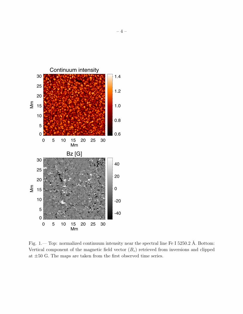
Figure 1 displays a map of normalized continuum intensity (top) and the corresponding

longitudinal magnetogram (bottom), the latter showing many internetwork flux concentra-

tions alongside stronger flux elements probably belonging to the network.

3. Mesogranulation and horizontal flows

Following the traditional method, mesogranular patterns are outlined by using Lagrange

tracers (popularly known as corks) arranged at time t = 0 uniformly in a 2D grid that co-

incides with the observational pixel matrix. Then, the corks are advected following the

instantaneous horizontal velocity field along the whole duration of the time series (here we

use the second time series: 32 minutes). The horizontal velocity field is determined using

the local correlation tracking (LCT) algorithm by Welsh et al. (2004) applied to consecutive

continuum intensity images. The correlation is performed in local windows weighted by a

Gaussian function with FWHM=320 km. Often, in the literature, the velocity field deter-

mined through LCT and used to advect corks is a time average of the noisy determinations

– 4 –

0.6

0.8

1.0

1.2

1.4Continuum intensity

0 5 10 15 20 25 30Mm

0

5

10

15

20

25

30

Mm

-40

-20

0

20

40

Bz [G]

0 5 10 15 20 25 30Mm

0

5

10

15

20

25

30

Mm

Fig. 1.— Top: normalized continuum intensity near the spectral line Fe I 5250.2 A. Bottom:

Vertical component of the magnetic field vector (Bz) retrieved from inversions and clipped

at ±50 G. The maps are taken from the first observed time series.

– 5 –

of the instantaneous velocity fields for consecutive snapshots (for a discussion about the

effect of time averaging see e.g. Rieutord et al. 2000, 2001). The high signal-to-noise ratio,

the high spatial and temporal resolution and the absence of atmospheric distortion in the

IMaX data make it possible to evaluate clean velocity fields and consequently to compute

cork advection without time averaging.

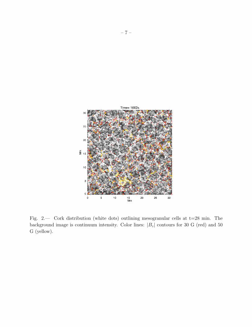
In Fig. 2 we show (white dots) the distribution of corks at t = 28 min, i.e., toward the

end of the series, on the background of the continuum intensity image at that time. The

corks clearly delineate cells of mesogranular size containing several granules. In fact, the

vast majority of corks are located in the lanes between those cells (which we will call here

mesogranular lanes or mesolanes for short). A clear mesogranular pattern with the majority

of the corks concentrated in mesolanes is already visible after only some 20 minutes from

t = 0. This is less than the time (2-4 hours) reported by Roudier et al. (2009) using the

Hinode/SOT NarrowBand Filter Imager.

In order to obtain quantitative measures for the mesogranular network we define a cork

density function, ρcork, by counting the number of corks in each pixel in the image. To

provide an upper bound for the width of the mesolanes, we scan the image vertically using

whole horizontal lines and calculate the width (1/e of the maximum) of the peaks of the

ρcork function in each line. We then derive an average peak width for the whole scan. If we

use all peaks above ρcork = 10, then the resulting upper bound for the lane width is 285 km.

The largest concentrations of corks are located in narrow mesolanes: using all peaks above

ρcork = 30, for instance, yields a width of 180 km (4.5 pixels). Given the random orientation

of the mesolanes, their actual width is certainly below those numbers. Using a horizontal

scan instead of a vertical one yields basically the same numbers (the maximum deviation is

7%).

4. Correlation between mesogranular lanes and field concentrations

A first test of the relation between mesogranules and the surface magnetic field can

be obtained by studying the spatial association between mesogranular cells and magnetic

flux concentrations. Through visual inspection, various researchers have obtained indica-

tions that the magnetic field concentrations with higher flux density are distributed at the

boundaries of cells of mesogranular size (5 to 10 arc sec; see Domınguez Cerdena et al. 2003

and Sanchez Almeida 2003); in fact, Domınguez Cerdena (2003) shows the preference of

elements with flux density above 60 G to be located in regions of high negative divergence

of the horizontal vlocity. Further visual evidence is provided by Roudier et al. (2009) who

plot Stokes-V images obtained with Hinode/NFI on top of cork distributions showing a rela-

– 6 –

tionship between magnetic field concentrations and cork lanes (see also de Wijn et al. 2005;

Solanki et al. 2010).

The conclusions at that level can be reinforced through our high-resolution maps by

drawing contours of |Bz| down to small values, like 30 G. The red and yellow contours in

Fig. 2 correspond to flux density values of 30 and 50 Gauss, respectively. The figure exhibits

flux concentrations mostly located at mesolanes. One can notice that flux concentrations

with higher flux density (yellow contours: 50 G) correlate better with mesolanes.

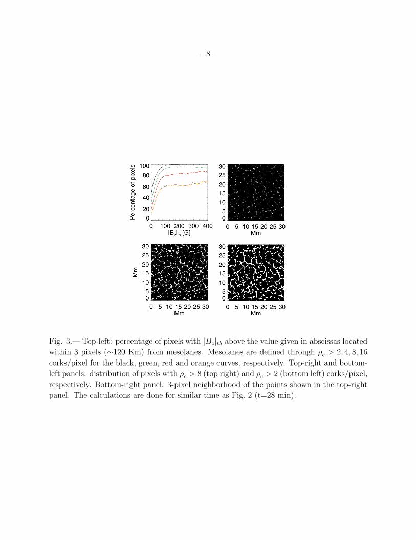
Going one step further, we can obtain quantitative estimates to test the visual impression

gained by combining cork images and magnetograms. We use as a proxy for the mesolanes

the locations with cork density above a threshold, ρc > ρc0, and use the values ρc0 = 2, 4, 8, 16

corks / pixel. All of those values yield clear mesogranular lanes, as apparent, e.g., in the

top-right and bottom-left panel of Fig. 3, drawn for ρc0 = 8 and 2, respectively. Increasing

ρc0 decreases the level of connectivity of the lanes. We then focus on the mesolanes defined

by ρc > ρc0 = 8 and study which fraction of the magnetic elements are really in (or near)

them. To obtain a quantitative estimate, for each fixed threshold intensity |Bz|th in the range

(0, 400) G, we consider the set of pixels with B > |Bz|th and calculate which fraction of the

set is located in 3-pixel neighborhoods of the mesolanes. The result is shown in the top left

panel of Fig. 3, red curve. The curve reaches an approximate horizontal asymptote at the

85% level for |Bz|th above 100 G. The other curves in the figure contain the same results

but using ρc0 = 2 (black curve), 4 (green) and 16 (orange). We see approximate horizontal

asymptotes in all cases, and all are reached for |Bz|th between 80 to 100 G. We conclude

that the vast majority of pixel elements with B & 100 G is located in the near neighborhood

of locations with high cork density. For the least restrictive case (ρc0 = 2), virtually all

magnetic elements with B & 100G are located in the neighborhood of the mesolanes. For

large ρc0 (e.g., ρc0 = 16 c/p, orange curve), the resulting areas have less connectivity and

do not delineate so clearly the mesogranular network. Correspondingly, the asymptotic

percentage values for B & 100 G become smaller. The width of the 3-pixel neighborhoods

of the mesolanes is shown in the bottom-right panel for the ρc0 = 8 corks/pixel case. The

panel shows a fully developed network of mesolanes covering only 17% of the whole surface

(which, of course, coincides with the |Bz|th → 0 limit of the red curve). As an aside note,

all curves remain basically the same if we remove the prominent network element located in

the lower part of Fig. 2.

– 7 –

Fig. 2.— Cork distribution (white dots) outlining mesogranular cells at t=28 min. The

background image is continuum intensity. Color lines: |Bz| contours for 30 G (red) and 50

G (yellow).

– 8 –

Fig. 3.— Top-left: percentage of pixels with |Bz|th above the value given in abscissas located

within 3 pixels (∼120 Km) from mesolanes. Mesolanes are defined through ρc > 2, 4, 8, 16

corks/pixel for the black, green, red and orange curves, respectively. Top-right and bottom-

left panels: distribution of pixels with ρc > 8 (top right) and ρc > 2 (bottom left) corks/pixel,

respectively. Bottom-right panel: 3-pixel neighborhood of the points shown in the top-right

panel. The calculations are done for similar time as Fig. 2 (t=28 min).

– 9 –

5. The separation between the footpoints of extrapolated field lines

5.1. Method

As a further test of the relation between surface fields and convection at different scales,

in this section we study the statistics of footpoint separation between field lines linking the

magnetic elements observed with IMaX. To that end, we calculate the magnetic field vector

in the atmosphere using force-free field extrapolations (FFF) from the IMaX data. We use

a code with weighted optimization method (Wiegelmann 2004; see also Seehafer 1978). The

force-free assumption is equivalent to assuming that the electrical current j and the magnetic

field B are parallel, or, using Ampere’s law:

∇×B =4 π

cj = αB ; (1)

α in Eq. 1 measures the level of field line twist. The field values obtained with the IMaX data

correspond to the height where the Fe I 5250.2 A line is formed. Although the photosphere

is not a small-β plasma (with β the ratio of gas to magnetic pressures), there are theoretical

and observational indications (Wiegelmann et al. 2010a,b; Martınez Gonzalez et al. 2010)

that the force-free assumption is acceptable when calculating extrapolations starting from

those heights. We will be using α = 0.1/L, with L×L being the IMaX field of view. In any

case, Wiegelmann et al. (2010b), using the same IMaX data, show that values of α in the

range (−4/L, 4/L) lead to similar values in the statistical properties they analyzed for the

extrapolated field lines.

For computational reasons, we have calculated the extrapolations in a box of 389 × 389

× 389 equally spaced grid points, keeping the original horizontal dimensions, leading to a

cell size of ≈ 80 km. Yet, test calculations with the original number of grid points (778 in

each direction) yield essentially the same results.

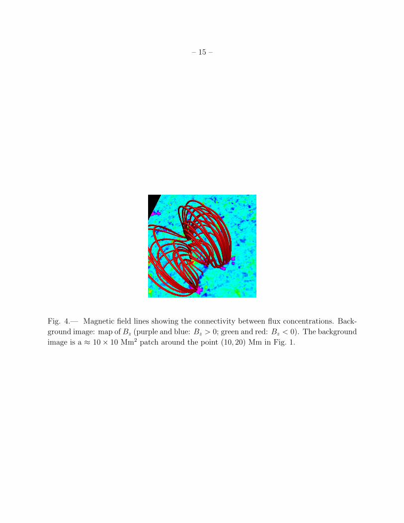
An example of magnetic field lines is shown in Fig. 4. A map of the vertical magnetic

field component is shown at the bottom of the box corresponding to a region of about 10×10

Mm2 centered on the point (x, y) = (10, 20) Mm in Fig. 1. The field line footpoints are seen

to cluster on field concentrations in the domain. In agreement with the conclusions of

Wiegelmann et al. (2010b), this figure shows a rough proportionality between the footpoint

distance and the height reached by the field lines.

– 10 –

5.2. Statistics of footpoint separation

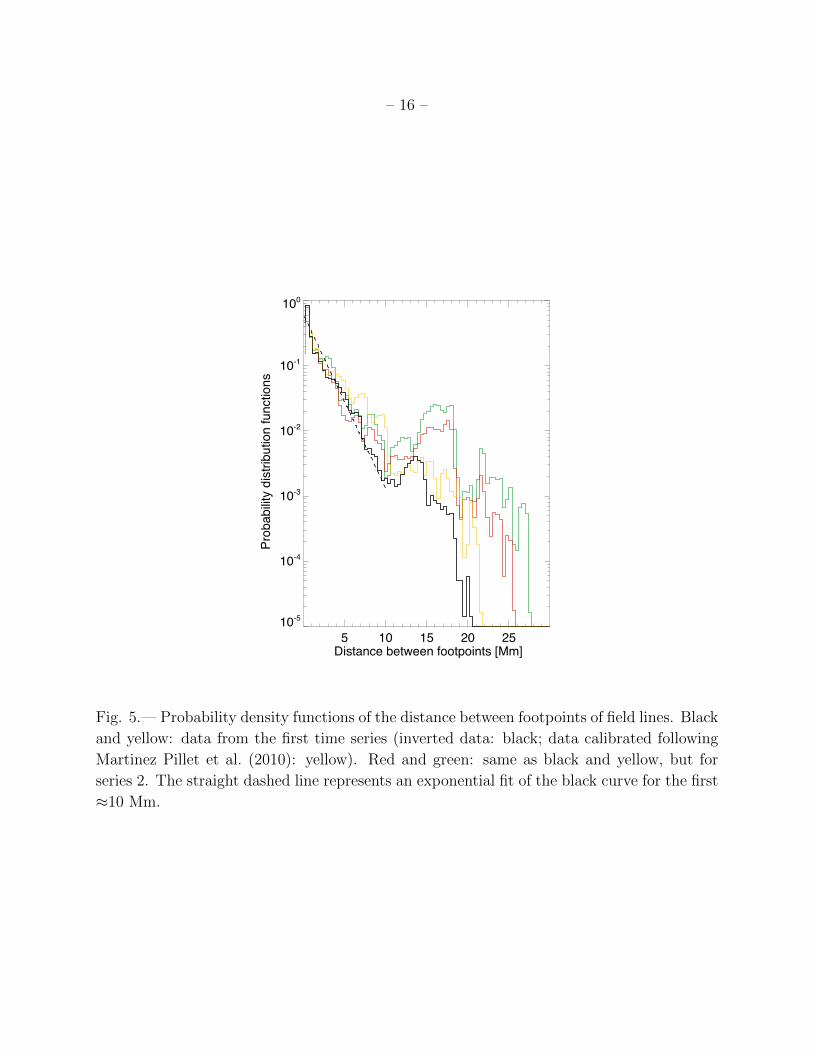
Calling x the distance between footpoints, we calculate the probability density function

(PDF) for x using as statistical ensemble for each time series the field lines in each snapshot

and the whole collection of snapshots in the series. To include a field line in the study,

we request a flux density above 15 G on both footpoints. The resulting PDFs are shown

in Fig. 5. The black and red lines correspond to the first and second time series, respec-

tively. Additionally, we plot PDFs for distances between field line footpoints calculated by

extrapolating calibrated data following Martinez Pillet et al. (2010), as explained in Sec. 2,

which involves no inversion procedure (yellow and green curves, for the first and second time

series, respectively). All the curves approximately fit an exponential distribution at scales

between 1 and 10 Mm, i.e., at granular and mesogranular scales; the slope is d log (PDF)/dx

≈ −0.6 Mm−1. Beyond 10 Mm, at supergranular scales, the curves show a deviation from

the exponential. This bump most probably corresponds to the presence in that time series

of strong network elements. Anyway, given the size of the IMaX field of view (≈ 30 Mm)

and the long duration of the largest convection cells, we cannot draw statistical inferences

from the PDF for scales above, say, 10 Mm. On the other hand, we have carried out a

Kolmogorov-Smirnov test of the goodness of fit of the footpoint distance data in the 1-10

Mm range to a lognormal distribution, additionally to the exponential distribution; a log-

normal distribution is found to fit well magnetogram data or, more generally, data resulting

from the fragmentation of magnetic elements (Abramenko & Longcope 2005; see also Bog-

dan et al. 1988). In our case, the test, carried out for individual snapshots in the given

distance range, favors the exponential distribution. Details of this analysis will be given in

a publication in preparation.

We note the constancy of the slope of the PDF at scales between 1 and 10 Mm and that

the characteristic decay distance is approximately 1.7 Mm. This is probably a consequence

of the fact that there are no intrinsic horizontal scales in that range other than granulation,

e.g., because mesogranulation is the direct result of other convection scales, rather than

representing a primary scale in which energy is being injected into the convective flows.

6. Discussion and Conclusions

An important open question in solar physics is the precise nature of the convection scales

with size and duration above the granular values. While both granulation and supergranula-

tion yield velocity field patterns that have been observed at the surface, mesogranules have

been detected only through indirect proxies, like tracking of intensity patterns, which do not

provide reliable evidence of underlying convection cells in that range of sizes and durations.

– 11 –

There is an ongoing debate on whether there is a continuum of sizes for the convection cells

on scales above granular, possibly with self-similar properties and with no particular scale

being singled out within that range (Nordlund et al. 2009), or whether the mesogranular

scales are just the result of a collective interaction between families of granules. The mag-

netic field can provide an alternative and more direct avenue to explore convective patterns

since the magnetic flux can be measured directly using Stokes polarimetry techniques. The

magnetic elements appear with a broad spectrum of flux densities (Orozco Suarez et al. 2007;

Khomenko et al. 2003) and can also be detected through G-Band or Ca-II bright points (see

de Wijn et al. 2005; Sanchez Almeida et al. 2010) and therefore can provide important clues

concerning the nature of the flows underlying the mesogranular scales as well as about the

magnetic elements themselves.

The high spatial and temporal cadences of the IMaX data allow us to try a few differ-

ent, complementary studies of the relation between magnetic field and mesogranular flows.

First, we have carried out Lagrange tracing of mass elements following horizontal flow fields

obtained through LCT of intensity maps; we have obtained a number of improvements com-

pared with traditional cork maps (faster development of the mesogranular lanes, no need for

time averages). We have also obtained an upper bound for the width of the mesogranular

lanes of some 280 km. Second, we have provided quantitative measures for the associa-

tion between magnetic elements and mesogranular lanes. The large majority (85 %) of the

magnetic elements with flux density above ∼ 100 G are found in 120-km neighborhoods of

mesogranular lanes with ρc > 8 and about 80 % of flux elements above 30 G are located near

mesogranular lanes with ρc > 2. Our results indicate a good coupling between the flow field

and the magnetic elements, suggesting that the evolution of the latter is mostly kinematic.

Third, we have considered the connectivity between magnetic elements and, in particular,

the distance between footpoints of field lines anchored in the photosphere. The probability

density function of such distances shows that there is abundant connectivity on mesogranular

scales; it also shows that the distribution is basically featureless in those scales, with only

one characteristic value, the slope of the distribution, equal to (1.7 Mm)−1.

Our results concerning statistics of separations of field line footpoints suggest that there

is no intrinsic scale of convection in the mesogranular range. This may only mean that

there is no mechanism for direct injection of energy into convection on those scales, but

does not rule out the existence of convection cells with those sizes, e.g., through nonlinear

interactions of cells at other scales (as in a turbulent cascade) or through the interaction of

thermal downflows (Rast 2003).

Financial support by the European Commission through the SOLAIRE Network (MTRN-

– 12 –

CT-2006-035484) and by the Spanish Ministry of Research and Innovation through projects

AYA2007-66502, CSD2007-00050 and AYA2007-63881 is gratefully acknowledged, as are

the computer resources, technical expertise and assistance provided by the MareNostrum

(BSC/CNS, Spain) supercomputer installation. L.Y.C. and F.M-I. are grateful to V. Abra-

menko for advice concerning the Kolmogorov-Smirnov test of statistical distributions. The

German contribution to Sunrise is funded by the Bundesministerium fur Wirtschaft und

Technologie through DLR Grant 50 OU 0401, and by the Innovationsfond of the Presi-

dent of the Max Planck Society (MPG). The Spanish contribution has been funded by the

Spanish MICINN under projects ESP2006-13030-C06 and AYA2009-14105-C06. The HAO

contribution was partly funded through NASA grant number NNX08AH38G. This work has

been partially supported by WCU grant No. R31-10016 funded by the Korean Ministry of

Education, Science and Technology.

REFERENCES

Abramenko, V. I., & Longcope, D. W. 2005, ApJ, 619, 1160

Barthol, P., et al. 2010, ArXiv e-prints

Bogdan, T. J., Gilman, P. A., Lerche, I., & Howard, R. 1988, ApJ, 327, 451

Brandt, P. N., Ferguson, S., Shine, R. A., Tarbell, T. D., & Scharmer, G. B. 1991, A&A,

241, 219

Brandt, P. N., Scharmer, G. B., Ferguson, S., Shine, R. A., & Tarbell, T. D. 1988, Nature,

335, 238

Cattaneo, F., Lenz, D., & Weiss, N. 2001, ApJ, 563, L91

de Wijn, A. G., Rutten, R. J., Haverkamp, E. M. W. P., & Sutterlin, P. 2005, A&A, 441,

1183

Domınguez Cerdena, I. 2003, A&A, 412, L65

Domınguez Cerdena, I., Sanchez Almeida, J., & Kneer, F. 2003, A&A, 407, 741

Ishikawa, R., & Tsuneta, S. 2010, ApJ, 718, L171

Khomenko, E. V., Collados, M., Solanki, S. K., Lagg, A., & Trujillo Bueno, J. 2003, A&A,

408, 1115

– 13 –

Leitzinger, M., Brandt, P. N., Hanslmeier, A., Potzi, W., & Hirzberger, J. 2005, A&A, 444,

245

Martınez Gonzalez, M. J., Manso Sainz, R., Asensio Ramos, A., & Bellot Rubio, L. R. 2010,

ApJ, 714, L94

Martinez Pillet, V., et al. 2010, ArXiv e-prints

Matloch, L., Cameron, R., Schmitt, D., & Schussler, M. 2009, A&A, 504, 1041

Matloch, L., Cameron, R., Shelyag, S., Schmitt, D., & Schussler, M. 2010, A&A, 519, A52

Muller, R., Auffret, H., Roudier, T., Vigneau, J., Simon, G. W., Frank, Z., Shine, R. A., &

Title, A. M. 1992, Nature, 356, 322

Nordlund, A., Stein, R. F., & Asplund, M. 2009, Living Reviews in Solar Physics, 6, 2

November, L. J., Toomre, J., Gebbie, K. B., & Simon, G. W. 1981, ApJ, 245, L123

Orozco Suarez, D., et al. 2007, ApJ, 670, L61

Rast, M. P. 2003, ApJ, 597, 1200

Rieutord, M., Roudier, T., Ludwig, H., Nordlund, A., & Stein, R. 2001, A&A, 377, L14

Rieutord, M., Roudier, T., Malherbe, J. M., & Rincon, F. 2000, A&A, 357, 1063

Roudier, T., Lignieres, F., Rieutord, M., Brandt, P. N., & Malherbe, J. M. 2003, A&A, 409,

299

Roudier, T., Malherbe, J. M., Vigneau, J., & Pfeiffer, B. 1998, A&A, 330, 1136

Roudier, T., & Muller, R. 2004, A&A, 419, 757

Roudier, T., Rieutord, M., Brito, D., Rincon, F., Malherbe, J. M., Meunier, N., Berger, T.,

& Frank, Z. 2009, A&A, 495, 945

Roudier, T., Rieutord, M., Malherbe, J. M., & Vigneau, J. 1999, A&A, 349, 301

Ruiz Cobo, B., & del Toro Iniesta, J. C. 1992, ApJ, 398, 375

Sanchez Almeida, J. 2003, A&A, 411, 615

Sanchez Almeida, J., Bonet, J. A., Viticchie, B., & Del Moro, D. 2010, ApJ, 715, L26

Seehafer, N. 1978, Sol. Phys., 58, 215

– 14 –

Shine, R. A., Simon, G. W., & Hurlburt, N. E. 2000, Sol. Phys., 193, 313

Simon, G. W., Title, A. M., Topka, K. P., Tarbell, T. D., Shine, R. A., Ferguson, S. H.,

Zirin, H., & SOUP Team. 1988, ApJ, 327, 964

Solanki, S. K., et al. 2010, ApJ, 723, L127

Welsh, B. T., Fisher, G. H., Abbett, W. P., & Regnier, S. 2004, ApJ, 610, 1148

Wiegelmann, T. 2004, Sol. Phys., 219, 87

Wiegelmann, T., Yelles Chaouche, L., Solanki, S. K., & Lagg, A. 2010a, A&A, 511, A4

Wiegelmann, T., et al. 2010b, ApJ, 723, L185

This preprint was prepared with the AAS LATEX macros v5.2.

– 15 –

Fig. 4.— Magnetic field lines showing the connectivity between flux concentrations. Back-

ground image: map of Bz (purple and blue: Bz > 0; green and red: Bz < 0). The background

image is a ≈ 10× 10 Mm2 patch around the point (10, 20) Mm in Fig. 1.

– 16 –

5 10 15 20 25 Distance between footpoints [Mm]

10-5

10-4

10-3

10-2

10-1

100

Pro

babi

lity

dist

ribut

ion

func

tions

Fig. 5.— Probability density functions of the distance between footpoints of field lines. Black

and yellow: data from the first time series (inverted data: black; data calibrated following

Martinez Pillet et al. (2010): yellow). Red and green: same as black and yellow, but for

series 2. The straight dashed line represents an exponential fit of the black curve for the first

≈10 Mm.